arX

iv:1

408.

2598

v1 [

astr

o-ph

.SR

] 1

2 A

ug 2

014

Kelvin-Helmholtz instability driven by coronal mass ejections in

the turbulent corona

Daniel O. Gomez1 and Edward E. DeLuca

Harvard-Smithsonian Center for Astrophysics, 60 Garden St, Cambridge, MA 02138

and

Pablo D. Mininni

Departamento de Fısica, Facultad de Ciencias Exactas y Naturales, Universidad de Buenos

Aires & Instituto de Fısica de Buenos Aires, Ciudad Universitaria, 1428 Buenos Aires,

Argentina.

Received ; accepted

To appear in Astrophys. J.

1On sabbatical leave from Departamento de Fısica, Facultad de Ciencias Exactas y Nat-

urales, Universidad de Buenos Aires & Instituto de Astronomıa y Fısica del Espacio, Ciudad

Universitaria, 1428 Buenos Aires, Argentina.

– 2 –

ABSTRACT

Recent high resolution AIA/SDO images show evidence of the development of

the Kelvin-Helmholtz instability, as coronal mass ejections (CMEs) expand in the

ambient corona. A large-scale magnetic field mostly tangential to the interface is

observed, both on the CME and on the background sides. However, this magnetic

field is not intense enough to quench the instability. There is also observational

evidence that the ambient corona is in a turbulent regime, and therefore the

development of the instability can differ significantly from the laminar case.

To study the evolution of the Kelvin-Helmholtz instability with a turbulent

background, we perform three-dimensional simulations of the magnetohydrody-

namic equations. The instability is driven by a velocity profile tangential to the

CME-corona interface, which we simulate through a hyperbolic tangent profile.

The turbulent background is obtained by the application of a stationary stir-

ring force. The main result from these simulations is the computation of the

instability growth-rate for different values of the intensity of the turbulence.

Subject headings: instabilities, magnetohydrodynamics, Sun: coronal mass ejections,

turbulence

– 3 –

1. Introduction

The presence of shear flows is ubiquitous in astrophysical problems, such as

jet propagation in the interstellar medium (Ferrari, Trussoni & Zaninetti 1980;

Begelman, Blandford & Rees 1984; Bodo et al. 1994), the dynamics of spiral arms in

galaxies (Dwarkadas & Balbus 1996), cometary tails (Brandt & Mendis 1979) or differential

rotation in accretion disks (Balbus & Hawley 1998). It is also relevant in a variety of

space physics problems, such as zonal flows in the atmospheres of rotating planets like

Jupiter (Hasegawa 1985), the solar wind (Poedts, Rogava & Mahajan 1998) or the Earth’s

magnetopause (Parker 1958).

Shear flows often give rise to the well-known Kelvin-Helmholtz (KH) instability

(Helmholtz 1868; Kelvin 1871), which has been extensively studied by Chandrasekhar

(1961). It is an ideal hydrodynamic instability, that converts the energy of the large-scale

velocity gradients into kinetic and/or magnetic energy at much smaller scales. The presence

of a magnetic field parallel to the shear flow has a stabilizing effect, and can even stall

the instability if the Alfven speed becomes larger than one half of the shear velocity jump

(Lau & Liu 1980; Miura & Pritchett 1982). On the other hand, an external magnetic field

perpendicular to the shear flow has no effect on the linear regime of the instability, and it is

simply advected by the flow.

Foullon et al. (2011) reported observations of a KH pattern obtained by the

Atmospheric Imaging Assembly (AIA) on board the Solar Dynamics Observatory (SDO),

which produces high spatial resolution (pixel size of 0.6 arcsec) and high temporal cadence

(10-20 sec) images of the Sun in several bandpasses covering white light, ultraviolet and

extreme ultraviolet. The observed pattern of the Kelvin-Helmholtz instability extends from

about 70 Mm up to about 180 Mm above the solar surface (1 Mm = 103 km). When

a coronal mass ejection (CME) expands supersonically upwards from the solar surface,

– 4 –

a bow shock is formed ahead of the CME and a strong shear flow develops across the

contact discontinuity separating the shocked ambient plasma from the ejected material.

A similar configuration arises at the flanks of the Earth magnetopause, where the KH

instability has also been observed and studied (Fujimoto & Teresawa 1995; Fairfield et al.

2000; Nykyri & Otto 2001). More recently it was observed as well in connection to

the magnetopause of other planets, such as Saturn (Masters et al. 2010) and Mercury

(Sundberg et al. 2011). When the supersonic solar wind impinges on these magnetized

planets, it first crosses a bow shock (and becomes subsonic in the the reference frame of

the planet) and then circumvents the planet slipping through the outer part of a surface of

tangential discontinuity known as the magnetopause, where a strong shear flow is generated.

The ambient corona is expected to be turbulent, as evidenced by measurments of

non-thermal broadenings of highly ionized spectral lines. Most recent observations of

nonthermal broadenings obtained by the Extreme-ultraviolet Imaging Spectrometer (EIS)

on board Hinode, correspond to nonthermal motions in the range of 20 − 60 km.s−1

(Doschek et al. 2014). The typical sizes of these nonthermal motions are sufficiently small to

remain unresolved by EIS, whose pixel size is 2 arcsec, and therefore its only manifestation

is an excess in the Doppler broadening of spectral lines (i.e. beyond the thermal Doppler

broadening).

The goal of the present paper is to study the interaction between these two rather

dissimilar features: the large-scale laminar pattern generated by the ongoing KH instability,

and the small-scale nonthermal motions presumably corresponding to a well developed

turbulence. With this goal in mind, we set up three-dimensional simulations of the MHD

equations, to study the evolution of the KH instability in the presence of a turbulent

ambient background. A priori, the expected role of a small-scale turbulence on a large-scale

flow, is to produce the effect of an enhanced diffusivity which can be characterized through

– 5 –

an effective or turbulent viscosity. The effect of this extra diffusivity on an ongoing

instability for the large-scale flow, as it is currently the case for KH, is to reduce its growth

rate or even to switch-off the instability completely. We test and basically confirm this

theoretical picture with a series of simulations of a KH-unstable shear flow superimposed

on a small-scale turbulent background with different turbulence intensities. The AIA

observations showing a KH pattern are described in §2. We introduce the MHD equations in

§ 3 and describe the basic features of the Kelvin-Helmholtz instability in §4. The observed

features of small-scale turbulence are discussed in § 5 and our numerical results are shown

in § 6. The potential consequences of the results presented in this paper are discussed in §7,

and our conclusions are listed in §8.

2. AIA observations

The coronal mass ejection (CME) occurred on 2010 November 3 near the southeast

solar limb, showed the characteristic pattern of the KH instability on AIA images. This

pattern has only been observed at the highest temperature channel, centered at the 131A

bandpass at 1.1 107 K. The sequence of AIA images show a regular array of three to

four vortex-like structures on the northern flank of the CME, that were interpreted by

Foullon et al. (2011) as the manifestation of an ongoing KH instability. The geometrical

setup of a CME expanding upwards from the solar surface is similar to the one corresponding

to the one taking place at the Earth’s magnetopause (Foullon et al. 2011). In view of this

similarity, these authors termed CME-pause to the surface of tangential discontinuity that

separates the plasma of the ejecta from the shocked plasma of the ambient corona.

From these observations, Foullon et al. (2013) were able to estimate several of the

relevant physical parameters for this instability, while the values of other parameters were

inferred under different assumptions discussed in their subsection 5.3. The observational

– 6 –

values for these various parameters are listed in Table 2 of Foullon et al. (2013). Among

the most important parameters, they estimated a wavelength for observed the KH pattern

of λ = 18.5± 0.5 Mm and an instability growth rate of γKH = 0.033± 0.012 s−1, which was

driven by the velocity jump accross the shear layer of 680± 92 km.s−1. These numbers are

in good agreement with the dispersion relationship of the KH instability (see § 4 below).

Even though they estimated the magnetic field at both sides of the CME-pause to be strong

enough to correspond to Alfven speeds in excess of the velocity jump accross the shear

layer, they argue that the orientation is largely tangential to the surface but perpendicular

to the direction of the KH pattern, and therefore it does not play any significant role in the

development of the instability.

Ofman & Thompson (2011) also reported observational evidence of the occurrence

of the KH instability at the interface between a CME and the surrounding corona. This

particular event took place on 2010 April 8, it was the first to be detected in EUV in the

solar corona and was clearly observed by six out of the seven wave bands of AIA/SDO.

The velocity jump accross the shear layer for this event was estimated in the range of

6 − 20 km.s−1, while the wavelength of the observed KH pattern was λ ≃ 7 Mm, based

on the size of the initial ripples. From the dispersion relationship, an instability growth

rate of γKH ≃ 0.005 s−1 can be obtained, which shows a reasonable agreement with the

approximately 14 min over which the KH pattern was observed to propagate, grow and

saturate (Ofman & Thompson 2011).

– 7 –

3. Magnetohydrodynamic description

The incompressible MHD equations for a fully ionized hydrogen plasma are the

Navier-Stokes equation and the induction equation

∂U

∂t= − (U ·∇)U + v2A (∇×B)×B −∇P + ν∇2U + F (1)

∂B

∂t= ∇× (U×B) + η∇2B . (2)

The velocity U is expressed in units of a characteristic speed U0, the magnetic field B is

in units of B0, and we also assume a characteristic length scale L0 and a spatially uniform

particle density n0. The assumption of incompressibility is valid provided that the plasma

velocity associated with the instabilities being considered, remains significantly smaller

than both the Alfven velocity and the speed of sound. Because of quasi-neutrality, the

electron and the proton particle densities are equal, i.e., ne = ni = n0. The (dimensionless)

Alfven speed is then vA = B0/√4πmin0U0, while η and ν are respectively the dimensionless

magnetic diffusivity and kinematic viscosity. These equations are complemented by the

solenoidal conditions for both vector fields, i.e.,

∇ ·B = 0 = ∇ ·U . (3)

4. Kelvin-Helmholtz instability

Let us assume that the plasma is subjected to an externally applied shear flow given by

U 0 = U0y(x)y, (4)

so that the total velocity field is now U 0 + u, where

U0y(x) = U0

[

tanh

(

x− π2

∆

)

− tanh

(

x− 3π2

∆

)

− 1

]

, (5)

– 8 –

The velocity profile given in Eqn. (5) simulates the encounter of largely uniform flows of

intensities +U0y and −U0y through an interface of thickness 2∆ parallel to the flows.

The numerical setup is sketched in Figure 1, where the jump provided by the hyperbolic

tangent is duplicated to satisfy periodic boundary conditions throughout the numerical

box. Also, we assume the presence of an external and uniform magnetic field B0 = B0y,

so that the total magnetic field is B0 + b. The assumption of a hyperbolic tangent profile

is often adopted (Drazin 1958; Chandrasekhar 1961; Miura 1992) as a way to model

shear flows with a finite thickness. The velocity profile given in Eqn. (5) is an exact

equilibrium of Eqs. (1)-(2) obtained through the application of the stationary external

force F 0 = −ν∇2U0y(x)y (see also Gomez et al. (2014)), and therefore it is numerically

implemented simply by the application of the volume force F 0.

A shear flow such as the one given by Eqn. (5) is subjected to the well known

Kelvin-Helmholtz instability, which is of a purely hydrodynamic nature, i.e. it occurs

even in the absence of any magnetic field. Within the framework of MHD, the stability

of a tangential velocity discontinuity (i.e. in the limit of ∆ = 0) was first studied by

Chandrasekhar (1961). For the case of an external magnetic field aligned with the shear

flow, the mode is stabilized by the magnetic field, unless the velocity jump exceeds twice the

Alfven speed. For the case at hand, we assume the external magnetic field to be sufficiently

weak (i.e. vA < 1), since otherwise the instability pattern would not have been observed in

AIA images. A stability analysis of a sheared MHD flow of finite thickness (i.e., ∆ 6= 0) in

a compressible plasma has also been performed (Miura & Pritchett 1982), confirming the

result of the purely hydrodynamic case. If we approximate the hyperbolic tangent profile

given in Eqn. (5) by piecewise linear functions, the instability growth rate γKH arising from

the linearized version of Eqs. (1)-(2) is (for details, see Drazin & Reid (1981))

(

γKH∆

U0

)2

=1

4

(

e−4ky∆ − (2ky∆− 1)2)

, (6)

– 9 –

which attains its maximum at λmax ≈ 15.7 ∆ and γmax ≈ 0.2U0/∆, as shown in Figure 2.

More importantly, Figure 2 also shows that the KH instability only arises for large-scale

modes, i.e. such that ky∆ ≤ 0.64, corresponding to λ ≥ 9.82∆.

We perform numerical integrations of Eqs. (1)-(2) subjected to the external force

F 0 = −ν∇2U0y(x)y (where U0y(x) is given in Eqn. (5)) on the cubic box of linear size 2π

sketched in Figure 1, assuming periodic boundary conditions in all three directions. The

number of gridpoints is 2563 and the dimensionless Alfven speed was set at vA = 0.2 in

all our simulations, indicating that the external magnetic field intensity B0 is such that

its Alfven velocity remains smaller than the maximum velocity U0 of the shear profile.

We use a pseudospectral strategy to perform the spatial derivatives and a second order

Runge-Kutta scheme for the time integration (see a detailed description of the code in

Gomez et al. (2005)). For the viscosity and resistivity coefficients we chose ν = η = 2.10−3,

which are small enough to produce energy dissipation only at very small scales, comparable

to the Nyquist wavenumber. The values of all the dimensionless parameters adopted

for our simulations are summarized in Table 1. In all simulations, the pressure in

Eqn. (1) is obtained self-consistently by taking the divergence of the equation, using the

incompressibility condition, and solving at each time step the resulting Poisson equation for

the pressure.

The evolution of the z-component of vorticity is shown in Figure 3 at three different

times, displaying the characteristic pattern of the KH instability. The observed frame

corresponds to the right half of the numerical box displayed in Figure 1, which covers the

shear layer centered at x0 = 3π/2, and has been rotated for better viewing. The observed

pattern is dominated by Fourier mode ky = 1, whose growth rate according to Eqn. (6) is

γKH(ky = 1) ≃ 0.87.

To estimate the instability growth rate, we use the component ux(x0, y, z) evaluated

– 10 –

at x0 = π/2, 3π/2 (i.e., in the central part of the shear flows) as a proxy (see Figure 4).

Since the KH flow is a two-dimensional flow taking place at z = constant planes, we take

the maximum velocity of the profile ux(x0, y, z) at any given value of z, and then average in

the z-direction, i.e.

Ux,max =

∫ 2π

0

dz

2πmax [ux(x0, y, z), 0 ≤ y < 2π] . (7)

In Figure 5 we show the maximum value of the ux(x0, y, z) profile (averaged with

respect to the z-direction) for both x0 = π/2 and x0 = 3π/2, although as expected the

two curves are undistinguishable. The straight gray line corresponds to the theoretically

predicted growth rate γKH ≃ 0.87 for the Fourier mode ky = 1 (using Eqn. (5)), which is

the one observed in the time sequence shown in Fig. 3.

5. The turbulent corona

Spectroscopic studies of coronal spectral lines show quantitative evidence of the

existence of spatially unresolved fluid motions through the nonthermal broadening effect on

these lines. Doschek et al. (2014) report nonthermal motions with velocities between 20 and

60 km.s−1 obtained by EIS on Hinode, corresponding to regions at the loop tops and above

the loop tops during several flares. EIS obtains images at the following two wavelength

bands: 170 − 213 A and 250 − 290 A. The angular resolution for the flare observations

performed by Doschek et al. (2014) is about 2 arcsec. The line-of-sight motions responsible

for these nonthermal broadenings correspond to plasma at temperatures in the range of

11− 15 MK, and they increase with the height above the flare loops.

These fluid motions have also been observed with EIS/Hinode in non-flaring active

region loops (Doschek et al. 2008). These fluid motions are being carried out by plasma

at temperatures of about 1.2 − 1.4 MK with particle densities spanning the range of

– 11 –

5 108−1010 cm−3. The rms values for the fluid velocities were in the range of 20−90 km.s−1.

Outflow velocities in the range of 20 − 50 km.s−1 have also been detected through net

blueshifts of the same spectral lines. The magnitude of the outflow velocities was found

to be positively correlated with the rms velocity. Brooks and Warren (2011) performed a

detailed study on active region AR 10978 using EIS/Hinode during a time span of five days

in 2007 December. Persistent outflows were observed to take place at the edges of this active

region, with an average speed of 22 km.s−1 and average rms velocities of 43 km.s−1. More

recently, Tian et al. (2012) studied upflows in connection to dimming regions generated by

CMEs, and reported velocities of up to 100 km.s−1. It is speculated that these persistent

outflows can be a significant source for the slow solar wind.

To generate a turbulent background in our simulations, we apply a stationary force to

all modes within a thin spherical shell of radius kturb = 1/lturb in Fourier space, consisting

of a superposition of harmonic modes with random phases. The nonlinear interactions

between these Fourier modes that are being externally driven with a force of intensity fturb,

will develop a stationary turbulent regime with its associated energy cascade involving all

wavenumbers k ≥ kturb. To make sure that it is a small-scale turbulence, we chose lturb to

be much smaller than the wavelength observed for the KH pattern, and even somewhat

smaller than the thickness ∆ of the shear layer (i.e. lturb < ∆).

The pattern of vorticity obtained when only the turbulent forcing is applied (i.e. a

simulation with no KH driving), is shown in Figure 7. The observed pattern corresponds

to a turbulent regime which is statistically stationary, homogeneous and isotropic. Even

though all spatial scales from lturb down to the smallest scales available in the simulation

participate in the dynamics and in the ensuing energy cascade, only those vortices of

sizes comparable to lturb can be identified, which is to be expected for a power law power

spectrum with a negative index such as Kolmogorov’s. Therefore, these concentrations of

– 12 –

vorticity can safely be associated to the energy-containing eddies of the turbulence. As

mentioned in § 1, the expected effect of this small-scale turbulence on a larger scale flow, is

an effective or enhanced diffusivity. In the case at hand, its effect on the instability growth

rate is expected to be

γ(k) = γKH(k)− νturbk2 , (8)

where γKH(k) is given in Eqn. (6) and νturb is the aforementioned effective or turbulent

viscosity. We performed simulations applying both the large-scale force F 0 to drive the

KH instability and the small-scale force of intensity fturb to drive the turbulent regime.

In Figure 8 we show the resulting distribution of the vorticity component ωz(x, y), which

can be compared with the one shown in Figure 3 for the KH instability on a laminar

background, and the one shown in Figure 7 for the purely turbulent run, with no KH

pattern. We can qualitatively see that the role of turbulence is in fact an attenuation in the

growth of the instability.

One of the observable consequences of this turbulent regime is the nonthermal

broadening of coronal spectral lines caused by the turbulent motion of the fluid elements

emitting these (optically thin) spectral lines. Once this turbulence reaches a Kolmogorov

stationary regime, the rms value of the turbulent velocity uturb is

Eturb =u2turb

2=

∫

1/lturb

dk ǫ2/3 k−5/3 ∝ (ǫ lturb)2/3 , (9)

where Eturb is the (dimensionless) kinetic energy density of the turbulence and ǫ is its energy

dissipation rate. Note that neither ǫ or Eturb are known a priori, since they arise as a result

of the stationary regime attained by the turbulence. However, using heuristic arguments we

can find how these quantities scale with the input parameters of this turbulence: namely

lturb and fturb. The fluid is energized by the work done per unit time by the external force of

intensity fturb at scale lturb, energy then cascades down to smaller scales and it is dissipated

by viscosity at the rate ǫ at dissipative scales. In a stationary regime, the power delivered

– 13 –

by the external force should match the energy dissipation rate, i.e.

ǫ ∝ fturb uturb . (10)

Equations (9)-(10) can be combined to obtain both uturb and ǫ in terms of fturb and lturb,

ǫ ∝ f3/2turb l

1/2turb , (11)

uturb ∝ (fturb lturb)1/2 . (12)

On dimensional arguments, the turbulent viscosity introduced in Eqn. (8) has to be

proportional to the turbulent velocity uturb times the typical scale lturb, i.e. νturb ∝ uturb lturb,

which considering Eqn. (12)

νturb = Cf1/2turb l

3/2turb . (13)

6. Numerical results

To quantify the role of turbulence in the evolution of the KH instability, we performed

a sequence of simulations for which the only parameter being changed is the turbulent

forcing fturb. As the parameter fturb is gradually increased, the corresponding turbulent

velocity uturb (observationally perceived as nonthermal broadening of spectral lines) is also

increased, which in turn raises the turbulent viscosity νturb. As a result, the instability

growth rate (see Eqn. (8)) is expected to be reduced. To estimate the instability growth

rate from our simulations, we follow the same procedure described in § 4, which amounts

to follow the temporal evolution of the profile ux(y) for the gridpoints centered at the

shear layer. Note however, that now the velocity at each grid point can be split into a

part corresponding to the large-scale KH evolution plus another part corresponding to the

turbulence.

Because of the geometrical setup of our simulations, the large-scale part of the flow at

each z = constant plane is an exact replica of one another (KH is a two-dimensional flow)

– 14 –

while the turbulent part is not, since it is a fully three-dimensional flow. The averaging

procedure in the z-direction described in Eqn. (7) gets rid of the turbulent part of the flow,

since the mean velocity of this turbulence is exactly zero. We can also compute the rms

deviation of the velocity when averaging in the z-direction, which should exactly correspond

to uturb, since the KH part of the flow is identical for all z = constant planes. Therefore,

this statistical strategy allows us to obtain the main features of both the large-scale (i.e.

the KH instability) and small-scale (the turbulence) components of this complex flow.

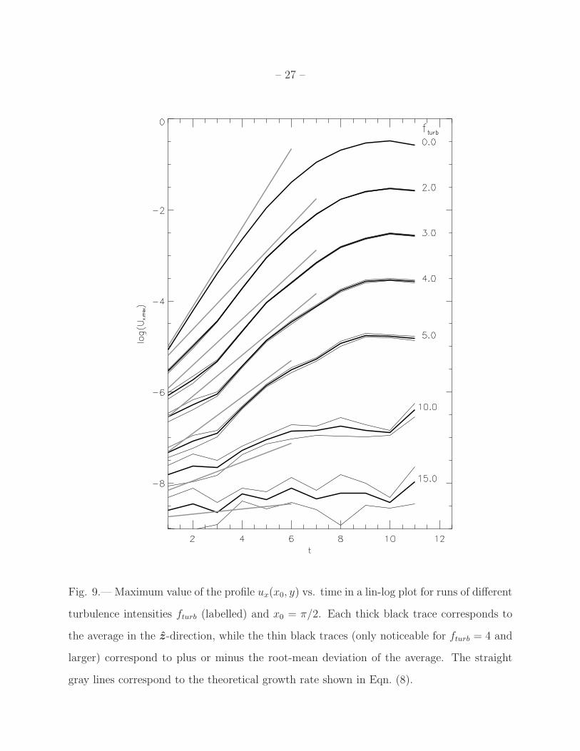
Figure 9 shows the main result of the present study, which is the value of Ux,max

(defined in Eqn. (7)) as a function of time in a lin-log plot, for runs corresponding to

different turbulent intensities. The thick black lines corresponds to Ux,max(t) for each

simulation, the thin black lines indicate one standard deviation with respect to the average

(i.e. Ux,max ± uturb), and the straight gray lines are the theoretical predictions for each case,

as emerges from Eqn. (8). Note that the theoretical slopes (i.e. the gray lines in Figure 9)

are not best fits to each of the simulations, but the result arising from Eqn. (8), which

contains only one free parameter for the whole set of simulations, namely the constant

C. This constant is the only dimensionless parameter that remains undetermined by the

dimensional analysis described above. We find that the value of C that best fits all our

simulations is C ≈ 18.8.

7. Discussion

In the previous section, we presented results from numerical simulations showing the

role of a background turbulence in reducing the growth rate of an ongoing KH instability.

These numerical results are intended to simulate the KH instability being developed at the

interface between some CMEs and the ambient corona, which have been recently reported

in the literature. There is also mounting evidence reported in the literature about the

– 15 –

turbulent nature of the solar corona, mostly related with spatially unresolved motions

leading to measurable nonthermal broadenings in coronal spectral lines.

To numerically model this turbulent background, we made a number of simplifying

assumptions. For instance, we assume the turbulent regime to be spatially homogeneous

and isotropic and also stationary. We maintain this turbulent state throughout the whole

simulation by applying a stationary stirring force of intensity fturb at a well defined

lengthscale lturb. We deliberately chose this lengthscale to be much smaller than the

wavelength of the KH unstable mode, since the AIA images reporting the KH pattern do not

show any observable evidence of a turbulent background. Also, the rotation period of the

energy-containing vortices is of the order of τturb ≃ lturb/uturb, which remains shorter than

the instability growth time for all the cases considered. The properties of this turbulent

regime are therefore determined by only two input parameters: lturb which is kept fixed

throughout the whole study, and fturb which is varied to give rise to cases with different

turbulent velocities (uturb) and effective viscosities (νturb).

We can use Eqs. (12)-(13) to express the effective viscosity νturb in terms of two

measurable quantities such as uturb and lturb. A crude estimate of the dimensionless constant

in Eqn. (12) leads to uturb ≈ 0.22 (fturb lturb)1/2 and therefore

νturb ≈ 85.4 uturb lturb . (14)

Given the fact that the turbulence did not completely suppress the KH instability, we

can therefore in principle use this equation to estimate an upper bound for lturb for

any observed value of uturb. For instance, if we refer to the KH event occurred on 2010

November 3 and reported by Foullon et al. (2011), they estimate a velocity jump at the

interface of U0 = 340 km.s−1 and a wavelength for the KH pattern of λ = 2πL0 = 18.5 Mm

(corresponding to a length unit of L0 = 3 Mm and ky = 1 in our simulations). For

ky = 1, the dispersion relation reduces to γ ≈ 0.87 − νturb, as shown in Eqn. (8). For the

– 16 –

turbulent attenuation to be negligible (i.e. νturb ≪ 0.87) and assuming a turbulent velocity

of 60 km.s−1 (see Doschek et al. (2014)), we obtain for lturb an upper bound of 166 km. In

general,

lturb ≪ 166 km(uturb

60 km.s−1)−1 (15)

In summary, in order for the invoked turbulent state to produce nonthermal broadening

of spectral lines of the order of uturb and at the same time not to affect the observed KH

event in any appreciable manner, the typical size lturb of its energy-containing eddies should

satisfy Eqn. (15).

8. Conclusions

The study presented in this paper was motivated by two relatively recent observational

findings on the nature of the solar corona. One of them is the apparent development of the

Kelvin-Helmholtz instability as some CMEs expand in the ambient corona, as shown by

AIA/SDO images (Foullon et al. 2011, 2013; Ofman & Thompson 2011). The second one is

that the coronal plasma seems to be in a turbulent state, as evidenced by the nonthermal

broadening of coronal spectral lines measured from EIS/Hinode data (Doschek et al. 2008;

Brooks and Warren 2011; Tian et al. 2012; Doschek et al. 2014).

Our main goal has been to study the feasibility for these two apparently dissimilar

features to coexist. Namely, the large-scale laminar pattern observed for the KH instability,

and the small-scale spatially unresolved turbulent motions leading to the observed

nonthermal broadenings. We therefore performed three-dimensional simulations of the

MHD equations, to study the evolution of the KH instability in the presence of a turbulent

ambient background for different intensities of this turbulence.

Theoretically, the effect of a small-scale turbulence on a large-scale flow would be to

– 17 –

produce an enhanced diffusivity which can be modeled by an effective or turbulent viscosity.

The impact of this small-scale turbulence on an ongoing large-scale instability such as

KH, would then be a reduction of its growth rate, as emerges from Eqn. (8). The degree

of this reduction is controlled by the turbulent viscosity νturb which we obtained from a

dimensional analysis to be νturb = Cf1/2turb l

3/2turb (see Eqn. (13)), leaving only the dimensionless

constant C undetermined.

The comparison between the instability growth rates obtained from our simulations

with the ones arising from Eqn. (8) esentially confirms this theoretical scenario, while

providing an empirical determination for the dimensionless constant C, which amounts to

C ≈ 18.8. Perhaps more importantly, since νturb ∝ uturb lturb and given the fact that the

instability has not been completely quenched by the turbulence (otherwise it would not have

been observed), observational determinations of uturb from nonthermal broadenings pose

an upper limit to the correlation length of the turbulence lturb. For observational values of

uturb ≈ 20− 60 km.s−1, the correlation length of turbulence is expected to be smaller than

about lturb ≈ 100 km, which is consistent with not having been spatially resolved by current

coronal imaging spectrometers such as EIS aboard Hinode.

DG and EED acknowledge financial support from grant SP02H1701R from Lockheed-

Martin to SAO. DG also acknowledges support from PICT grant 0454/2011 from ANPCyT

to IAFE and PDM acknowledges support from PICTs 2011-1529 and 2011-1626 from

ANPCyT to IFIBA (Argentina).

– 18 –

REFERENCES

Balbus, S.A., & Hawley, J.F. 1998, Rev. Mod. Phys., 70, 1

Begelman, M.C., Blandford, R.D., & Rees, M.J. 1984, Rev. Mod. Phys., 56, 255

Bodo, G., Massaglia, S., Ferrari, A., & Trussoni, E. 1994, A&A, 283, 655

Brandt, J.C., & Mendis, D.A. 1979, “Solar System Plasma Physics”, Eds. C.F. Kennel et

al. (North Holland: Amsterdam), 2, 253

Brooks, D.H., & Warren, H.P. 2011, ApJ, 727, L13

Chandrasekhar, S. 1961, “Hydrodynamic and Hidromagnetic Stability”, Oxford University

Press: New York.

Doschek, G.A., Warren, H.P., Mariska, J.T., Muglach, K., Culhane, J.L., Hara, H., &

Watanabe, T. 2008, ApJ, 686, 1362

Doschek, G.A., McKenzie, D.E., & Warren, H.P. 2014, ApJ, 788, 26

Drazin, P.G. 1958, J. Fluid Mech., 4, 214

Drazin, P.G., & Reid, W.H. 1981, “Hydrodynamic Stability”, Cambridge University Press:

Cambridge.

Dwarkadas, V.V., & Balbus, S.A. 1996, ApJ, 467, 87

Fairfield, D.H., Otto, A., Mukai, T., Kokubun, S., Lepping, R.P., Steinberg, J.T., Lazarus,

A.J., Yamamoto, T. 2000, J. Geophys. Res., 105, 21159

Ferrari, A., Trussoni, E., & Zaninetti, L. 1980, MNRAS, 193, 469

Foullon, C., Verwichte, E.,Nakariakov, V.M., Nykyri, K., & Farrugia, C.J. 2011, ApJ, 729,

L8

– 19 –

Foullon, C., Verwichte, E., Nykyri, K., Aschwanden, M.J., & Hannah, I.G. 2013, ApJ, 767,

170

Fujimoto, M., & Teresawa, T. 1995, J. Geophys. Res., 100, 12025

Gomez, D.O., Mininni, P.D., & Dmitruk, P. 2005, Phys. Scripta, T116, 123

Gomez, D.O., Bejarano, C., & Mininni, P.D. 2014, Phys. Rev. E, 89, 053105

Hasegawa, A. 1985, Adv. Phys., 34, 1

Helmholtz, H.L.F. 1868, Monthly Rep. Royal Prussian Acad. Phil. Berlin, 23, 215

Lau, Y.Y., & Liu, C.S. 1980, Phys. Fluids, 23, 939

Masters, A., and 10 co-authors 2010, J. Geophys. Res., 115, A07225

Miura, A., & Pritchett, P.L. 1982, J. Geophys. Res., 87, 7431

Miura, A. 1992, J. Geophys. Res., 97, 10655

Nykyri, K., & Otto, A. 2001, Geophys. Res. Lett., 28, 3565

Ofman, L., & Thompson, B.J. 2011, ApJ, 734, L11

Parker, E.N. 1958, ApJ, 128, 6640

Poedts, S., Rogava, A.D., & Mahajan, S.M. 1998, ApJ, 505, 369

Sundberg, T., and 7 co-authors 2011, Planetary & Space Sci., 59, 2051

Tian, H., McIntosh, S.W., Xia, L., He, J., & Wang. X. 2012, ApJ, 748, 106

Thomson, W.(Lord Kelvin) 1871, Phil. Mag., 42, 362

This manuscript was prepared with the AAS LATEX macros v5.2.

– 20 –

Table 1. Values of dimensionless parameters for the simulations: N is the linear size, U0 is

the velocity at each side of the shear layer, ∆ is the thickness of the shear layer, vA is the

Alfven speed, η is the magnetic diffusivity, ν is the kinematic viscosity, lturb is the the

length scale of the turbulence and fturb is the strength of the turbulent forcing.

N U0 ∆ vA η ν lturb fturb

256 1 0.1 0.2 2.10−3 2.10−3 0.05 0, 2, 3, 4, 5, 10, 15

Fig. 1.— Numerical box displaying the imposed velocity profile U0(x) in the y-direction and

the external homogeneous magnetic field B0y. The shaded patches correspond to regions

with intense shear. Each axis ranges from 0 to 2π.

– 21 –

Fig. 2.— Growth rate for the Kelvin-Helmholtz instability of a shear layer with a velocity

jump from +U0 to −U0 over a half-width ∆ as a function of wavenumber.

– 22 –

Fig. 3.— Time sequence (as labelled) of the vorticity component ωz(x, y) at the plane

z = 2π for the right half of the numerical box shown in Fig. 1 (rotated 90◦) for a purely

shear-driven simulation. Gray corresponds to ωz = 0 while black (white) corresponds to

negative (positive) concentrations of vorticity.

– 23 –

Fig. 4.— Numerical box (see also Fig. 1) displaying the velocity profile ux(y) for the slice

located at the center of the shear layer. This velocity profile obtained for a sequence of times

is used to estimate the instability growth rate.

– 24 –

Fig. 5.— Maximum value of the profile ux(x0, y) vs. time in a lin-log plot. The two black

traces are indistinguishable from one another and correspond to x0 = π/2 and x0 = 3π/2.

The straight gray line corresponds to the theoretical growth rate.

– 25 –

Fig. 6.— Instability growth rates vs. wavenumber. Black trace corresponds to Kelvin-

Helmholtz in a non-turbulent medium, as shown in Fig. 2. Gray traces correspond to cases

with different values of the turbulent viscosity νturb (labelled).

– 26 –

Fig. 7.— Vorticity component ωz(x, y) at the plane z = 2π for the right half of the numerical

box shown in Fig. 1 (rotated 90◦) for a purely turbulence-driven simulation at t = 10. Gray

corresponds to ωz = 0 while black (white) corresponds to negative (positive) concentrations

of vorticity.

Fig. 8.— Vorticity component ωz(x, y) at the plane z = 2π for the right half of the numerical

box shown in Fig. 1 (rotated 90◦) for a shear and turbulence-driven simulation at t =

10. Gray corresponds to ωz = 0 while black (white) corresponds to negative (positive)

concentrations of vorticity.

– 27 –

Fig. 9.— Maximum value of the profile ux(x0, y) vs. time in a lin-log plot for runs of different

turbulence intensities fturb (labelled) and x0 = π/2. Each thick black trace corresponds to

the average in the z-direction, while the thin black traces (only noticeable for fturb = 4 and

larger) correspond to plus or minus the root-mean deviation of the average. The straight

gray lines correspond to the theoretical growth rate shown in Eqn. (8).