A comparison of NRBCs for PUFEM in 2D

Helmholtz problems at high wave numbers

O. Laghrouche∗, A. El-Kacimi∗ and J. Trevelyan†

∗School of the Built Environment, Heriot-Watt University, Edinburgh EH14 4AS,

UK†School of Engineering, Durham University, Durham DH1 3LE, UK

Abstract

In this work, exact and approximate Non-Reflecting Boundary Conditions (NRBCs)are implemented with the Partition of Unity Finite Element Method (PUFEM) tosolve short wave scattering problems governed by the Helmholtz equation in twodimensions. By short wave problems, we mean situations in which the wavelengthis a small fraction of the characteristic dimension of the scatterer. Various NRBCsare implemented and a comparison of their performance is carried out based on theaccuracy of the results, ease of implementation and computational cost. The aim isto accurately model such problems in a reduced computational domain around thescatterer with fewer elements and without refining the mesh at each wave number.

Key words: Helmholtz equation, finite elements, plane wave basis, non-reflectingboundary conditions, wave scatteringPACS:

1 Introduction

To solve wave scattering problems in unbounded media using the finite ele-ment method, it is necessary to truncate the domain at some boundaries, toform the computational domain, and to apply a suitable boundary conditionallowing the outgoing waves to radiate away towards infinity. If approximateboundary conditions are used, these should be placed at a sufficiently largedistance from the scatterer, which leads to solutions in large computationaldomains. If, however, accurate boundary conditions are used, the computa-tional domain can be reduced so that the truncation boundary is very close tothe scatterer and hence fewer finite elements may be used. But exact NRBCsare non local and, as a consequence, the global system becomes dense nearthe outer boundary.

Preprint submitted to Elsevier 11 April 2008

Another problem arises from the fact that polynomial based finite elementshave limited ability to deal with short wave problems due to the require-ment of around ten nodal points per wavelength, or even higher resolutionfor short wave problems. To overcome this difficulty, various finite elementswhich incorporate knowledge about the problem to be solved were developed.The approach is based on the enrichment of the solution space by analyti-cal solutions. In the case of the Helmholtz equation, plane waves were usedwith finite elements in the Partition of Unity Method [1–5], Least-SquaresMethod [6], Ultra-Weak Variational Method [7,8] and Discontinuous Enrich-ment method [9,10]. The reader is directed to reference [11] for a survey of theactivity which took place up to 2004. More recent work could be found, forexample, in [12,13]. The developed plane wave basis finite elements have beenvery successful in reducing the computing effort by up to 90% [14,15] and it isdemonstrated that a discretization level of about 2.5 degrees of freedom perwavelength is sufficient to achieve engineering accuracy [12,16].In this work, plane wave basis finite elements are combined with exact andapproximate models of NRBCs to solve wave scattering problems. The prob-lem of interest is a simple model of an acoustic plane wave scattered by a rigidcircular cylinder, for which the exact solution is known. Various numericaltests are carried out with a fixed mesh and for a wide range of wave numbers.Three approximate boundary conditions are used. Those are of Bayliss, Gun-zburger and Turkel (BGT) [17,18], Engquist and Majda (EM) [19,20], andFeng (F) [21]. Different orders of these boundary conditions are also consid-ered. The DtN map is used as an exact NRBC whereas an inhomogeneousRobin condition, through which the analytical solution of the scattering prob-lem is imposed on the outer boundary of the domain, is used as a reference.Note that approximate NRBCs have been developed since the late 1970s anda huge literature is available in this field. Regarding the DtN method, it goesback to Keller and Givoli [22] who developed it for the Helmholtz equationwhen the outer boundary is a circle or a sphere. It is a non-local condition andit involves an infinite trigonometric or spherical harmonic series. DtN condi-tions were derived for various equations and geometries, and also for singleor multiple disjoint computational domains [23]. So much activity has beentaking place in this area and the reader is directed to references [24–28].

2 Formulation of the problem and finite element model

The problem of a horizontal plane wave of potential uI = eikx scattered bya rigid object ΩS of boundary ΓN in an infinite two dimensional medium isconsidered. The diffracted potential u satisfies the Helmholtz equation

∇2u + k2u = 0 outside ΩS , (1)

2

with the Neumann boundary condition

∇u · n = −∇uI · n on ΓN , (2)

and the Sommerfeld radiation condition

limr→∞

r1

2 (∂u

∂r− iku) = 0, (3)

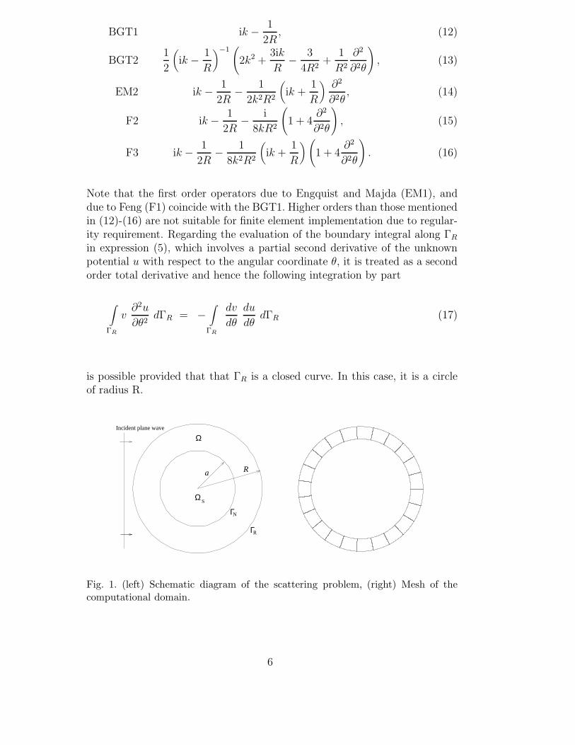
where ∇2 denotes the Laplacian operator, ∇ is the gradient vector operator,k is the wave number, n is the outward normal vector to the line boundaryΓN and i is the complex imaginary such that i2 = −1. The time variable isremoved by considering a harmonic steady state. For computational purpose,the region of interest Ω around the scatterer is bounded by an artificial circularboundary ΓR of radius R at which special conditions must be imposed toappear transparent to the propagating waves (Figure 1 (left)). The solutionof the original scattering problem is approximated by the solution u of theproblem defined by the Helmholtz equation (1) in Ω, the Neumann boundarycondition (2) and the boundary condition

∇u · n − Bu = 0 on ΓR, (4)

where B is an operator corresponding to a NRBC.Multiplying the Helmholtz equation (1) by a test function v and integratingby parts, we obtain a weak formulation of the problem where it is required tofind the scattered potential u ∈ H1(Ω) such that

∫

Ω

(

∇u · ∇v − k2uv)

dΩ −∫

ΓR

vBu dΓR = −∫

ΓN

v∇ui · n dΓ, (5)

for all v ∈ H1(Ω), where H1(Ω) is the usual Sobolev space [29]. An exis-tence and uniqueness results for (5) can be established, under appropriateassumptions, by virtue of Fredholm’s alternative theorem [30] and continua-tion arguments [31].The computational domain Ω is meshed into n-noded finite elements and thepotential field u is written as combination of m plane waves as follows

u =n∑

p=1

m∑

q=1

Np exp(ikr · dq)Ap,q, (6)

where Np are the usual polynomial shape functions. The coefficients Ap,q arethe amplitudes of the set of plane waves associated with each node p. Theplane waves are chosen to be evenly distributed such that dq = (cos αq, sin αq)

3

with αq = 2πq/m. The geometry of each finite element is described by the co-ordinate transformation r = T (ξ) between the global coordinates r = (x, y)and the local coordinates ξ = (ξ, η) ∈ [−1, 1]2. In this work, Galerkin weight-ing is used and hence the test functions v take the form of the plane waveenriched shape functions. For the evaluation of element matrices, high orderGauss-Legendre integration scheme is used in all computations. Let us recallthat semi-analytical integration rules were developed for finite elements withstraight edges [32] but were not used in this work because the mesh of thecomputational domain contains elements with curved edges (Figure 1 (right)).

3 Non-reflecting boundary conditions considered

All considered NRBCs are briefly presented in this section. Their explanationis beyond the scope of this paper and the reader is directed to the corre-sponding literature. Note that, through the Robin type boundary condition,the analytical solution of the scattering problem is explicitly imposed on theouter boundary ΓR. Therefore the corresponding numerical solution will beconsidered as a reference solution and will provide information on the PUFEMdiscretization error. It will, therefore, allow to distinguish the contribution ofthe considered NRBCs to the global error.

3.1 Robin type boundary condition - reference solution

The considered scattering problem by a rigid circular cylinder of radius a hasan analytical solution. It is given by [33]

u = −∞∑

n=0

inεn

J ′n(ka)

H ′n(ka)

Hn(kr) cosnθ, (7)

where r and θ are the polar coordinates of a considered point. Hn and Jn are,respectively, the Hankel function and the Bessel function of the first kind andorder n. The prime in H ′

n and J ′n denotes differentiation with respect to the

argument. The sequence εn is defined by ε0 = 1, εn = 2 for all n ≥ 1. Thesolution (7) is imposed on the outer boundary ΓR through the Robin boundarycondition

∇u · n + iku = g, (8)

where g is the boundary condition such that the exact solution of the problemcorresponds to the diffracted potential u. In this case the weak formulation of

4

the scattering problem becomes

∫

Ω

(

∇u · ∇v − k2uv)

dΩ +∫

ΓR

ikuv dΓ = −∫

ΓN

v∇uI · n dΓ +∫

ΓR

vg dΓ.(9)

3.2 Exact boundary condition: DtN

Outside the outer boundary ΓR the solution u of the scattered potential isexpressed as a series sum of harmonics [22]

u(r, θ) =1

π

∞∑

n=0

εn

Hn(kr)

Hn(kR)

2π∫

0

u(R, θ′) cos n(θ − θ′)dθ′. (10)

This time, the sequence εn is defined by ε0 = 12, εn = 1 for all n ≥ 1 and

θ′ is a reference angle . Considering the normal derivative of expression (10)along the outer boundary ΓR it is possible to establish the following relation

Bu =k

π

N∑

n=0

εn

H ′n(kR)

Hn(kR)

2π∫

0

u(R, θ′) cos n(θ − θ′)dθ′, (11)

which is the DtN boundary condition. The infinite series of the DtN boundarycondition is truncated at N and is then no longer exact. In this case, the DtNmap will represent the wave harmonics exactly up to the truncation number.Harari and Hughes [27] derived a simple relation between the number N ofterms retained in the series and the non-dimensional wave number kR to en-sure the uniqueness of the solution, that is N ≥ kR. It is also possible touse the modified DtN operator introduced by Grote and Keller [26], which re-moves the difficulties due to the truncation of the infinite series and improvesthe accuracy regardless of kR and N . In this work, the rule proposed by Harariand Hughes [27] is used to truncate both expressions (7) and (10).

3.3 Approximate NRBCs

As mentioned earlier, the three approximate NRBCs considered are of Bayliss,Gunzburger and Turkel of order 1 and 2 (BGT1 and BGT2), Engquist andMajda of order 2 (EM2), and Feng of order 2 and 3 (F2 and F3). The corre-sponding operator B for each boundary condition and for a considered orderis given by

5

BGT1 ik −1

2R, (12)

BGT21

2

(

ik −1

R

)−1(

2k2 +3ik

R−

3

4R2+

1

R2

∂2

∂2θ

)

, (13)

EM2 ik −1

2R−

1

2k2R2

(

ik +1

R

)

∂2

∂2θ, (14)

F2 ik −1

2R−

i

8kR2

(

1 + 4∂2

∂2θ

)

, (15)

F3 ik −1

2R−

1

8k2R2

(

ik +1

R

)

(

1 + 4∂2

∂2θ

)

. (16)

Note that the first order operators due to Engquist and Majda (EM1), anddue to Feng (F1) coincide with the BGT1. Higher orders than those mentionedin (12)-(16) are not suitable for finite element implementation due to regular-ity requirement. Regarding the evaluation of the boundary integral along ΓR

in expression (5), which involves a partial second derivative of the unknownpotential u with respect to the angular coordinate θ, it is treated as a secondorder total derivative and hence the following integration by part

∫

ΓR

v∂2u

∂θ2dΓR = −

∫

ΓR

dv

dθ

du

dθdΓR (17)

is possible provided that that ΓR is a closed curve. In this case, it is a circleof radius R.

R

Incident plane wave

Ω

Γ

ΓS

R

a

Ω

N

Fig. 1. (left) Schematic diagram of the scattering problem, (right) Mesh of thecomputational domain.

6

4 Numerical results and discussion

The computational domain Ω is meshed into a single layer of 23 finite elementsaround the scattering cylinder (Figure 1 (right)). The finite elements are 9-noded and their geometry is interpolated using Lagrange polynomials. At eachnodal point we use 30 plane waves to approximate the scattered potential.We define the parameter τ as the number of degrees of freedom (DOF) perwavelength in the problem. It is given by

τ =2

k

√

π ntot m

R2 − a2, (18)

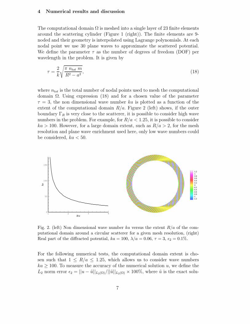
where ntot is the total number of nodal points used to mesh the computationaldomain Ω. Using expression (18) and for a chosen value of the parameterτ = 3, the non dimensional wave number ka is plotted as a function of theextent of the computational domain R/a. Figure 2 (left) shows, if the outerboundary ΓR is very close to the scatterer, it is possible to consider high wavenumbers in the problem. For example, for R/a < 1.25, it is possible to considerka > 100. However, for a large domain extent, such as R/a > 2, for the meshresolution and plane wave enrichment used here, only low wave numbers couldbe considered, ka < 50.

R/a

ka

1 2 3 40

50

100

150

1.210.80.60.40.20

-0.2-0.4-0.6-0.8-1-1.2

Fig. 2. (left) Non dimensional wave number ka versus the extent R/a of the com-putational domain around a circular scatterer for a given mesh resolution, (right)Real part of the diffracted potential, ka = 100, λ/a = 0.06, τ = 3, ǫ2 = 0.1%.

For the following numerical tests, the computational domain extent is cho-sen such that 1 ≤ R/a ≤ 1.25, which allows us to consider wave numberska ≥ 100. To measure the accuracy of the numerical solution u, we define theL2 norm error ǫ2 = ||u − u||L2(Ω)/||u||L2(Ω) × 100%, where u is the exact solu-

7

tion. Figure 2 (right) shows an example of contour plots of the real part of thescattered potential around the cylinder for ka=100 when the DtN boundarycondition is imposed on the outer boundary ΓR. In this case, 60 integrationpoints are employed per element, in each spatial direction, for the evaluationof the element matrices. The L2 error is very satisfactory, ǫ2 = 0.1%.Now, the same scattering problem is considered with the parameters takenabove and for a range of wave numbers extending from ka = 1 to ka = 120.The accuracy of the numerical results is estimated for different boundary con-ditions applied on ΓR and the results are summarised in Table 1. First, it isobvious that the DtN boundary condition performs well for all wave numbers.Its performance is very similar to that of the Robin boundary condition, inwhich the analytical solution is imposed on ΓR. This proves that the errorgenerated by the DtN boundary condition is negligible and that the L2 erroris due only to the PUFEM discretization. However, L2 errors generated by allapproximate NRBCs show that their contribution to the error, as boundaryconditions, is significant compared to the discretization error.It is worth mentioning that at low wave numbers, the parameter τ indicatesthat the number of DOF per wavelength is very high, which leads to a highcondition number. Despite this fact, the L2 error stays very low [15]. Also, atlow wave numbers, the diameter d of the scattering cylinder is only a fractionof the wavelength λ (d = 0.32λ for ka = 1). But as the wave number increases,the scatterer’s diameter becomes multi-wavelength sized (d = 3.2λ for ka = 10and d = 32λ for ka = 100) and the problem becomes a short wave scatteringone. As the finite elements span many wavelengths, for the numerical evalua-tion of the element matrices, the number of integration points was increasedto accommodate the oscillatory behaviour of the integrand. For ka = 10, only10 integration points were used. However, this number was increases to 70 forka = 120.Regarding the approximate NRBCs, it is clear that BGT1 performs poorlyfor all wave numbers as the L2 error remains higher than 15% all the timewhile using BGT2 leads to a significant drop in ǫ2. Up to ka = 20, BGT2leads to a better accuracy compared to other approximate NRBCs (EM2, F2and F3). However, for ka > 20, their performances are very similar. At lowwave numbers, the distance between the inner boundary ΓN and the outerboundary ΓR is very small, in term of the wavelength. But for increasing wavenumber, this distance becomes very large in term of λ. This is obvious fromthe simple relationship (R−a)/λ = k/8π. Despite the fact that ΓR is very farfrom the scatterer in term of λ, at high wave numbers, the L2 error remainsaround 3%. This is due to ΓR which is not at an asymptotic distance from thescatterer.Let us recall that Shirron [34] compared the approximate NRBCs consid-

ered here for polynomial based finite elements. Canonical problems for rigidscattering were solved where each component of the Anger-Jacobi expansionof the incident plane wave was considered separately. In a different work,Shirron et al. [35] compared these approximate NRBCs and infinite elements

8

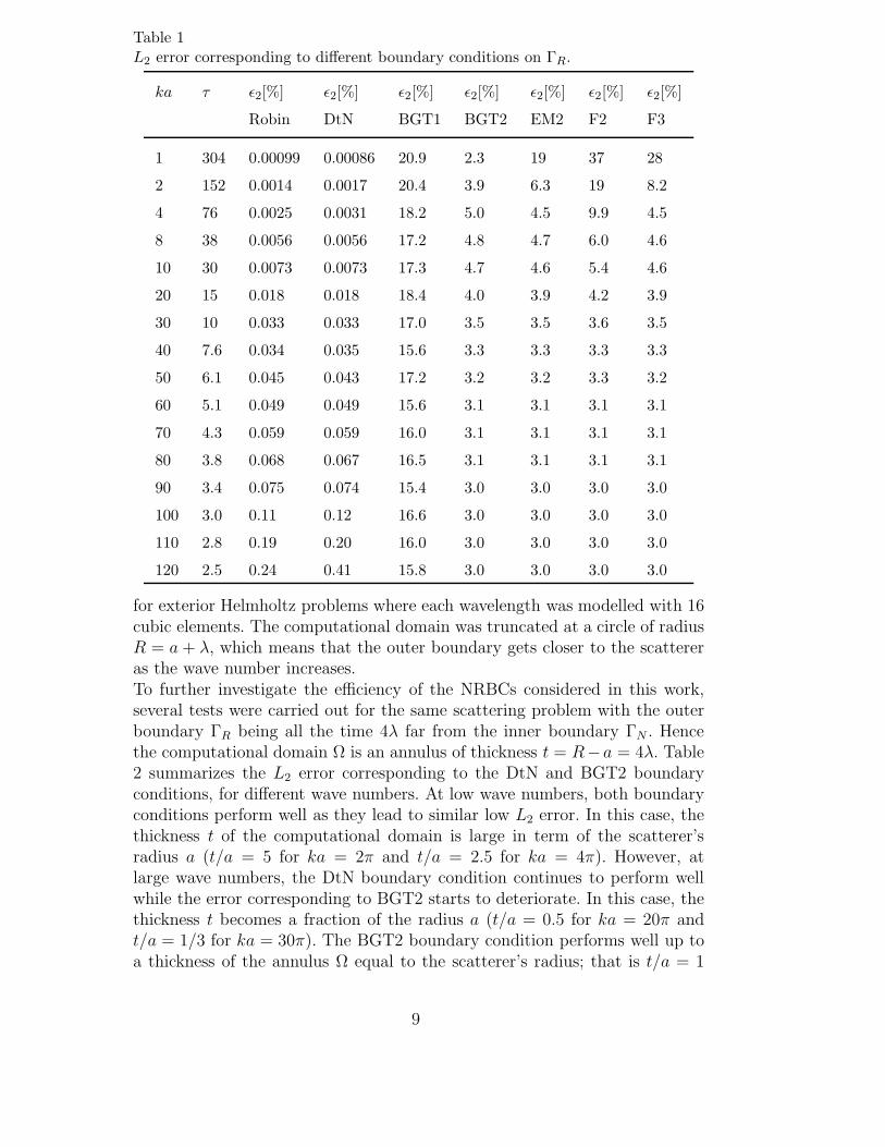
Table 1L2 error corresponding to different boundary conditions on ΓR.

ka τ ǫ2[%] ǫ2[%] ǫ2[%] ǫ2[%] ǫ2[%] ǫ2[%] ǫ2[%]

Robin DtN BGT1 BGT2 EM2 F2 F3

1 304 0.00099 0.00086 20.9 2.3 19 37 28

2 152 0.0014 0.0017 20.4 3.9 6.3 19 8.2

4 76 0.0025 0.0031 18.2 5.0 4.5 9.9 4.5

8 38 0.0056 0.0056 17.2 4.8 4.7 6.0 4.6

10 30 0.0073 0.0073 17.3 4.7 4.6 5.4 4.6

20 15 0.018 0.018 18.4 4.0 3.9 4.2 3.9

30 10 0.033 0.033 17.0 3.5 3.5 3.6 3.5

40 7.6 0.034 0.035 15.6 3.3 3.3 3.3 3.3

50 6.1 0.045 0.043 17.2 3.2 3.2 3.3 3.2

60 5.1 0.049 0.049 15.6 3.1 3.1 3.1 3.1

70 4.3 0.059 0.059 16.0 3.1 3.1 3.1 3.1

80 3.8 0.068 0.067 16.5 3.1 3.1 3.1 3.1

90 3.4 0.075 0.074 15.4 3.0 3.0 3.0 3.0

100 3.0 0.11 0.12 16.6 3.0 3.0 3.0 3.0

110 2.8 0.19 0.20 16.0 3.0 3.0 3.0 3.0

120 2.5 0.24 0.41 15.8 3.0 3.0 3.0 3.0

for exterior Helmholtz problems where each wavelength was modelled with 16cubic elements. The computational domain was truncated at a circle of radiusR = a + λ, which means that the outer boundary gets closer to the scattereras the wave number increases.To further investigate the efficiency of the NRBCs considered in this work,several tests were carried out for the same scattering problem with the outerboundary ΓR being all the time 4λ far from the inner boundary ΓN . Hencethe computational domain Ω is an annulus of thickness t = R−a = 4λ. Table2 summarizes the L2 error corresponding to the DtN and BGT2 boundaryconditions, for different wave numbers. At low wave numbers, both boundaryconditions perform well as they lead to similar low L2 error. In this case, thethickness t of the computational domain is large in term of the scatterer’sradius a (t/a = 5 for ka = 2π and t/a = 2.5 for ka = 4π). However, atlarge wave numbers, the DtN boundary condition continues to perform wellwhile the error corresponding to BGT2 starts to deteriorate. In this case, thethickness t becomes a fraction of the radius a (t/a = 0.5 for ka = 20π andt/a = 1/3 for ka = 30π). The BGT2 boundary condition performs well up toa thickness of the annulus Ω equal to the scatterer’s radius; that is t/a = 1

9

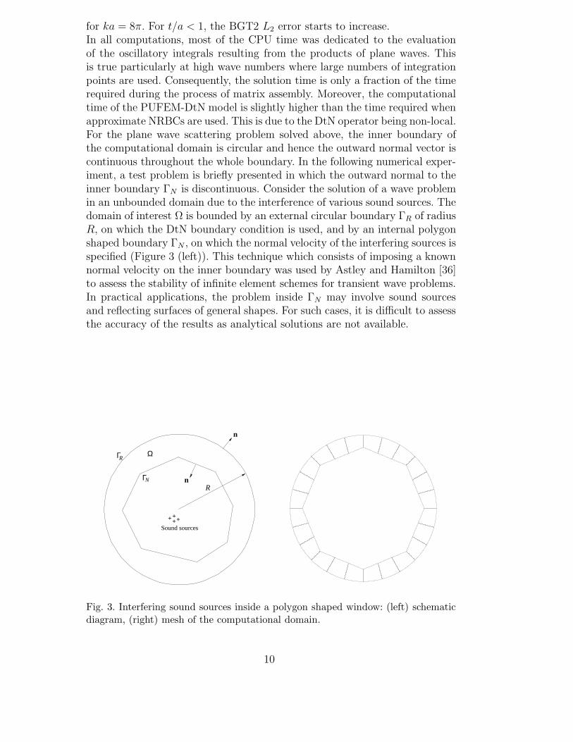
for ka = 8π. For t/a < 1, the BGT2 L2 error starts to increase.In all computations, most of the CPU time was dedicated to the evaluationof the oscillatory integrals resulting from the products of plane waves. Thisis true particularly at high wave numbers where large numbers of integrationpoints are used. Consequently, the solution time is only a fraction of the timerequired during the process of matrix assembly. Moreover, the computationaltime of the PUFEM-DtN model is slightly higher than the time required whenapproximate NRBCs are used. This is due to the DtN operator being non-local.For the plane wave scattering problem solved above, the inner boundary ofthe computational domain is circular and hence the outward normal vector iscontinuous throughout the whole boundary. In the following numerical exper-iment, a test problem is briefly presented in which the outward normal to theinner boundary ΓN is discontinuous. Consider the solution of a wave problemin an unbounded domain due to the interference of various sound sources. Thedomain of interest Ω is bounded by an external circular boundary ΓR of radiusR, on which the DtN boundary condition is used, and by an internal polygonshaped boundary ΓN , on which the normal velocity of the interfering sources isspecified (Figure 3 (left)). This technique which consists of imposing a knownnormal velocity on the inner boundary was used by Astley and Hamilton [36]to assess the stability of infinite element schemes for transient wave problems.In practical applications, the problem inside ΓN may involve sound sourcesand reflecting surfaces of general shapes. For such cases, it is difficult to assessthe accuracy of the results as analytical solutions are not available.

Ω

ΓN

R

ΓR

n

n

++++

Sound sources

Fig. 3. Interfering sound sources inside a polygon shaped window: (left) schematicdiagram, (right) mesh of the computational domain.

10

For the interference test problem considered here, the equivalent variationalformulation to (5) is given by

∫

Ω

(

∇u · ∇v − k2uv)

dΩ −∫

ΓR

vBu dΓR =∫

ΓN

v∇w · n dΓ, (19)

where w is representing the sound sources inside ΓN . As an example, 4 ra-dial sound sources placed at different locations are considered to interfere.The computational domain Ω is limited by an inner boundary in the shapeof a regular octagon and an outer circular boundary. It is meshed into 24 el-ements with 9 nodes each (Figure 3 (right)). The function w is given by thesum of Hankel functions of first kind and order zero with sources located atradii rj . That is w =

∑4j=1 H0(k|r − rj|), with rj = (0.3, 0.3)T , (−0.3, 0.3)T ,

(−0.3,−0.3)T and (0.3,−0.3)T for j = 1, 2, 3 and 4, respectively. The L2 errorof the solution is obtained from the expression previously defined where u isreplaced by w. This test example is run for two extreme cases of the wavenumber ka = 10 and ka = 120, and under similar conditions of the scatter-ing problem solved earlier regarding the number of plane waves attached ateach node, the number of integration points and the number of components inthe DtN series. The only difference lies in the geometry of the computationaldomain which is bounded by an inner octagonal boundary ΓN with cornersplaced at a unit distance a from the center and the outer circular boundary ΓR

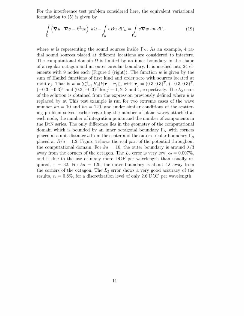
placed at R/a = 1.2. Figure 4 shows the real part of the potential throughoutthe computational domain. For ka = 10, the outer boundary is around λ/3away from the corners of the octagon. The L2 error is very low, ǫ2 = 0.007%,and is due to the use of many more DOF per wavelength than usually re-quired, τ = 32. For ka = 120, the outer boundary is about 4λ away fromthe corners of the octagon. The L2 error shows a very good accuracy of theresults, ǫ2 = 0.8%, for a discretization level of only 2.6 DOF per wavelength.

11

0.250.20.150.10.050

-0.05-0.1-0.15-0.2-0.25

0.30.240.180.120.060

-0.06-0.12-0.18-0.24-0.3

Fig. 4. Sound sources inside a polygon shaped window, real part of the potential:(left) ka = 10, τ = 32, ǫ2 = 0.007%, (right) ka = 120, τ = 2.6, ǫ2 = 0.8%.

5 Conclusion

In this work, a wave scattering problem is solved with a fixed mesh for a widerange of wave numbers. The used PUFEM model allows to compute manywavelengths per nodal spacing provided that enough integration points areused in the evaluation of the element matrices. The numerical results showthat the combined model PUFEM-DtN provides accurate results even whenthe outer boundary of the computational domain is very close to the scatterer.Regarding approximate NRBCs, it is found that, at low wave numbers, BGT2is more accurate than EM2, F2 and F3. However, at high wave numbers, theyall lead to similar accuracy. Moreover, at high wave numbers, when the outerboundary is very close to the scatterer in term of the absolute distance, butmany wavelengths away from it, approximate NRBCs perform poorly. This isdue to the fact that approximate radiation conditions are based on asymp-totic expansions and hence are not valid in the immediate surrounding of thescattering object. It seems that approximate NRBCs lead to optimal resultswhen the outer boundary is placed at a distance equal to the radius of thescattering object.The DtN operator, compared with the approximate NRBCs for identical com-putational domains, leads to better accuracy results. However, it is more de-manding at the implementation level because of its non-local nature. As aconsequence, it leads to higher computational effort during the integrationalong the outer boundary and during the solution process. But this does notmean that the DtN model is computationally more expensive. In fact, a modelusing approximate NRBCs would be computationally more expensive than amodel using the DtN if the same accuracy is sought, because the former wouldrequire a much larger domain. Therefore, the choice of the best option between

12

PUFEM-DtN and PUFEM-approximate NRBCs must be based on practicalconsiderations; either go for a reduced computational domain with a globalmatrix dense near the outer boundary, for PUFEM-DtN, or choose a largercomputational domain with a sparse global matrix, for PUFEM-approximateNRBCs.Last, it should be possible to extend the combined model of PUFEM-DtN tothree dimensions, in which case many real problems could be solved with asignificantly reduced computational domain. It is believed that by meshingthe computational domain with a single layer of multi-wavelength sized finiteelements around the scatterer, this will reduce the size of the global matrixand lead to solutions of 3D problems for a wide range of wave numbers witha reasonable computing effort.

ACKNOWLEDGEMENTS

The first author is grateful to the Royal Society and the Nuffield Foundationfor funding the research computing facilities. The Carnegie Trust for the Uni-versities of Scotland is acknowledged for supporting travel and subsistence forcollaboration. We are also grateful to Professor Jeremy Astley for very usefuldiscussions.

References

[1] Melenk JM, Babuska I. The Partition of Unity Finite Element Method. BasicTheory and Applications. Comput. Meths. Appl. Mech. Engrg. 1996; 139:289–314.

[2] Babuska I, Melenk JM. The Partition of Unity Method. Int. Jour. Num. Meth.

Eng. 1997; 40:727–758.

[3] Laghrouche O, Bettess P. Short wave modelling using special finite elements.Jour. Comput. Acous. 2000; 8(1):189–210.

[4] Ortiz P, Sanchez E. An improved partition of unity finite element model fordiffraction problems. Int. Jour. Num. Meth. Eng., 2001; 50:2727–2740.

[5] Astley RJ, Gamallo P. Special short wave elements for flow acoustics Comp.

Meth. Appl. Mech. Engng. 2005; 194:341–353.

[6] Monk P, Wang DQ. A least-squares mtehod for the Helmholtz equation.Comput. Meth. Appl. Mech. Engng. 1999; 175:121–136.

[7] Cessenat O, Despres B. Application of an ultra weak variational formulationof elliptic PDEs to the two-dimensional Helmholtz problem. SIAM J. Numer.

Anal. 1998; 35(1):255–299.

[8] Huttunen T, Monk P, Kaipio JP. Computation aspects of the ultra weakvariational formulation. J. Comput. Phys. 2002; 182:27–46.

13

[9] Farhat C, Harari I, Franca L. The discontinuous enrichment method. Comp.

Meth. Appl. Mech. Engng. 2001; 190:6455–6479.

[10] Farhat C, Harari I, Hetmanuk U. A discontinuous Galerkin method withLagrange multipliers for the solution of Helmholtz problems in the mid-frequency regime. Comp. Meth. Appl. Mech. Engng. 2003; 192:1389–1419.

[11] Bettess P, Laghrouche O, Perrey-Debain E (Eds.). Theme Issue on Short WaveScattering. Phil. Trans. R. Soc. Lond. A 2004; 362.

[12] Laghrouche O, Bettess P, Perrey-Debain E, Trevelyan J. Wave interpolationfinite elements for Helmholtz problems with jumps in the wave speed. Comput.

Meth. Appl. Mech. Engng. 2005; 194:367–381.

[13] Strouboulis T, Babuska I, Hidajat R. The generalized finite element methodfor Helmholtz equation: Theory, computation, and open problems. Comput.

Methods Appl. Mech. Engrg. 2006; 195:4711–4731.

[14] Laghrouche O, Bettess P. Short wave modelling using special finiteelements Towards an adaptive approach. Mathematics of Finite Elements and

Applications 2000; JR Whiteman (Ed.), Elsevier, Chapter 10:181–194.

[15] Laghrouche O, Bettess P, Astley RJ. Modelling of short wave diffractionproblems using approximating systems of plane waves. Int. Jour. Num. Meth.

Eng. 2002; 54:1501–1533.

[16] Perrey-Debain E, Laghrouche O, Bettess P, Trevelyan J. Plane wave basis finitelements and boundary elements for three dimensional wave scattering. Phil.

Trans. R. Soc. Lond. A 2004; 362:561–577.

[17] Bayliss A, Turkel E. Radiation boundary conditions for wave-like equations.Comm. Pure Appl. Math. 1980; 33:707–725.

[18] Bayliss A, Gunzburger M, Turkel E. Boundary Conditions for the NumericalSolution of Elliptic Equations in Exterior Regions. J. Appl. Math. 1982; 42:430–451.

[19] Engquist B, Majda A. Absorbing boundary conditions for the numricalsimulation of waves. Math. Comput. 1977; 31:629–651.

[20] Engquist B, Majda A. Radiation boundary conditions for acoustic and elasticwave calculations. Comm. Pure Appl. Math. 1979; 32:313–357.

[21] Kang F, Finite element method and natural boundary reduction. Proceddings

of the International Congress of Mathematics, Warsaw, 1983, 1439–1453.

[22] Keller JB, Givoli D. Exact non-reflecting boundary conditions. J. Comput.

Phys. 1989; 82:172–192.

[23] Grote MJ, Kirsch C. Dirichlet-to-Neumann boundary conditions for multiplescattering problems. Journal of Computational Physics 2004; 201:630–650.

[24] Givoli D. Numerical methods for problems in infinite domains. 1992;Amsterdam, Elsevier Science Publishers.

14

[25] Givoli D. Recent advances in the DtN F E Method. Archives of Computational

Methods in Engineering 1999; 6:71–116.

[26] Grote MJ, Keller JB. On Nonreflecting Boundary Conditions. J. Comput. Phys.

1995; 122:231–243.

[27] Harari I, Hughes TJR. Analysis of continuous formulations underlying thecomputation of time-harmonic acoustics in exterior domains. Comput. Meth.

Appl. Mech. Engng. 1992; 97:103–124.

[28] Harari I, Grosh K, Hughes TJR, Malhotra M, Pinsky PM, Stewart JR,Thompson LL. Recent developments in finite element methods for structuralacoustics. Archives of Computational Methods in Engineering 1996; 3:131–311.

[29] Adams RA. Sobolev Spaces, Academic Press, New York, 1975.

[30] Gilbarg D, Trudinger NS. Elliptic partial differential equations of second order.Springer-Verlag, 1983.

[31] Leis R. Boundary value problems in mathematical physics. Teubner, Wiley, 1989.

[32] Bettess P, Shirron J, Laghrouche O, Peseux B, Sugimoto R, Trevelyan J. Anumerical integration scheme for special finite elements for Helmholtz equation.Int. Jour. Num. Meth. Eng., 2003; 56:531–552.

[33] Morse PM, Feshbach H. Methods of Theoretical Physics. McGraw-Hill BookCompany, USA, 1953.

[34] Shirron JJ. Numerical Solution of Exterior Helmholtz Problems Using Finite

and Infinite Elements, PhD thesis, College Park, MD, 1995.

[35] Shirron JJ and Babuska I. A comparison of approximate boundary conditionsand infinite element for exterior Helmholtz problems. Comput. Methods Appl.

Mech. Engrg. 1998; 164, pp.121–139.

[36] Astley RJ, Hamilton JA. The stability of infinite element schemes for transientwave problems. Comput. Methods Appl. Mech. Engrg. 2006; 195: 3553-3571.

15

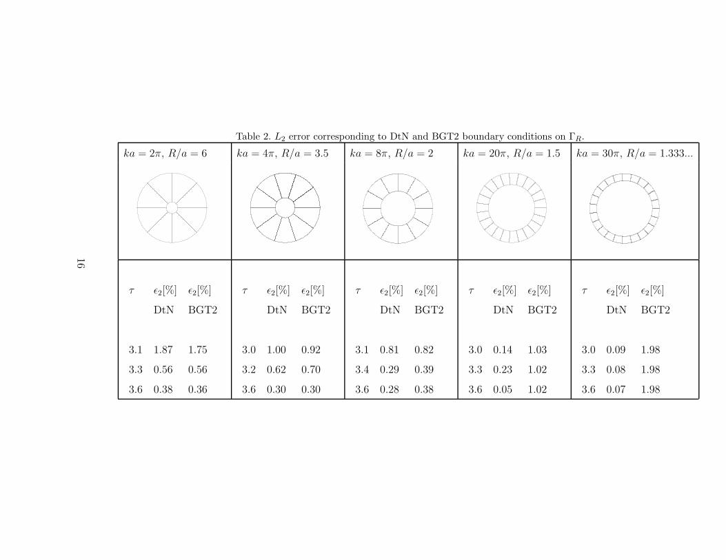
Table 2. L2 error corresponding to DtN and BGT2 boundary conditions on ΓR.

ka = 2π, R/a = 6 ka = 4π, R/a = 3.5 ka = 8π, R/a = 2 ka = 20π, R/a = 1.5 ka = 30π, R/a = 1.333...

τ ǫ2[%] ǫ2[%]

DtN BGT2

3.1 1.87 1.75

3.3 0.56 0.56

3.6 0.38 0.36

τ ǫ2[%] ǫ2[%]

DtN BGT2

3.0 1.00 0.92

3.2 0.62 0.70

3.6 0.30 0.30

τ ǫ2[%] ǫ2[%]

DtN BGT2

3.1 0.81 0.82

3.4 0.29 0.39

3.6 0.28 0.38

τ ǫ2[%] ǫ2[%]

DtN BGT2

3.0 0.14 1.03

3.3 0.23 1.02

3.6 0.05 1.02

τ ǫ2[%] ǫ2[%]

DtN BGT2

3.0 0.09 1.98

3.3 0.08 1.98

3.6 0.07 1.98

16