Real Numbers - Rajur College

1

CHAPTER 1

Real Numbers

1.1 Introduction

In this chapter, we shall study some basic properties of Real Numbers. Weshall assume the familarity of the students with the sets of Natural Numbers,Integers and Rational Numbers. The set of real numbers can be constructedfrom the set of rational numbers or can also be defined axiomatically. However,the rigourous definition, in either of these two ways, is beyond the scopeof this book. Here, we shall state the properties of real numbers that areused in the sequel. These properties can be classified in three catergories:Alegebraic Properties, Order Properties and the property of ’Completeness’.The algebraic and order properties have been used in high school mathematics.However, the completeness property is not studied before. The completenessproperty of real number system is most crucial in Calculus. In fact, the theoryof calculus is founded on the completeness property of the real number system.Thus the emphasis of the present discussion is on the completeness propertyand its consequences. The students are advised to focus on the completenessproperty and urged to understand its fundametal role in the theory of calculus.

We now state the algebraic and order properties of real numbers.

(Algebraic Properties) : There are defined on R two binary operations,namely addition (+) and multiplication (.) which satisfy the following prop-erties:

(i) Commutativity : For all a, b ∈ R, a+ b = b+ a and ab = ba.

(ii) Associativity : For all a, b, c ∈ R, a+(b+c) = (a+b)+c, a·(b·c) = (a·b)·c.(iii) There exist in R, two elements 0 and 1 such that 0 6= 1 and for alla ∈ R, a+ 0 = a and a · 1 = a.

(iv) For every a ∈ R, there is an element −a in R such that a+ (−a) = 0.

(v) For every a ∈ R with a 6= 0, there is an element a−1 in R such thata · a−1 = 1.

(vi) Distributive Law : For all a, b, c ∈ R, a · (b+ c) = a · b+ a · c.

Note : We write ab in place of a · b. The operations of subtraction and division

2

are defined as follows: for a, b ∈ R,

a− b = a+ (−b) and if a 6= 0, thena

b= ab−1.

As R possesses the above algebraic properties, R is called a field.

(Order Properties) : There is defined on R a relation, called an orderrelation and denoted by <, which satisfies the following properties:

(vii) For all a, b ∈ R, exactly one of the following statements is true:a < b, a = b, b < a.

(viii) Transitivity: For all a, b, c ∈ R, if a < b and b < c then a < c.

(ix) For all a, b, c ∈ R,(α) a < b ⇒ a+ c < b+ c and

(β) a a to mean a < b.

Statements such as a < b, a ≤ c are called inequalities. We say that a realnumber a is positive or negative according as a > 0 or a < 0.

The following are basic properties of inequalities:

1) a > b ⇔ a− b > 0.

2) a > 0 ⇔ − a < 0.

3) [a > 0 and b > 0] ⇒ ab > 0.

4) If a bc if c is negative.

This latter result says that multiplication by a negative number reverses thedirection of inequality. For example,

2 < 5 ⇒ 2(−3) > 5(−3) ⇒ − 6 > −15.

5) a < b and c < d ⇒ a = c < b+ d.

This says that, like equations, we may add inequalities (in the proper order).

6) [0 ≤ a < b and 0 ≤ c < d] ⇒ ac < bd.

This says that we may multiply inequalities when no negative numbers areinvolved. But this is false if negative numbers are involved. For example, it istrue that 2 < 5 and −3 < −2. But it is not true that −6 < −10.

7) [0 ≤ a 0. In particular, 1 > 0 since 1 6= 0 and 1 = 12.

9) a > 0 ⇒ 1/a > 0. Also, a > b > 0 ⇒ 1/a < 1/b.

3

10) a > 1 ⇒ a2 > a and 0 < a < 1 ⇒ a2 < a.

11) Let b > 0, y > 0. Then

a

b<x

y⇒ a

b<a+ x

b+ y<x

y.

12) Let a < b+ ε for every positive number ε. Then a ≤ b.This result is often useful. To prove it, let a > b, if possible. Then a− b > 0.Hence taking ε = a− b we get a < b+ (a− b) or a < a. This is a contradiction.Hence a ≤ b.

Definition: Suppose S is a non-empty subset of R. A real number a is calleda minimum element of S and we write a = minS if (i) a ∈ S and (ii) a ≤ xfor all x in S.

A real number b is called a maximum element of S and we write b = maxSif (i) b ∈ S and (ii) x ≤ b for all x in S.

A minimum element of S is unique (if it exists). To see this, let a, a′ beboth minimum elements of S. Then by definition, we must have a ≤ a′anda′ ≤ a. Hence a = a′. Similarly, a maximum element of S is unique (if itexists).

1.3 Rational Numbers

We denote by N, Z and Q the set of all Natural numbers, Integers and Rationalnumbers respectively.

The following property of N is equivalent to the Principle of MathematicalInduction:

Well-odering principle : Every non-empty subset of N contains a minimumelement.

Also note that

(i) 1 = minN and if n ∈ N and x ∈ R are such that n < x < n+1, then x 6∈ N.(ii) The set of all rational numbers is an ordered field (like R).

(iii) Q is a dense set. That is, between any two distinct rational numbers thereis a rational number.

For, if a, b ∈ Q, and a < b, then c = (a+ b)/2 ∈ Q and a < c < b.

1.5 Absolute Value

Definition: For every x ∈ R, the absolute value of x is denoted by |x| and is

4

defined as follows:

|x| ={x if x > 0−x if x ≤ 0.

In other words, |x| = max{x,−x}.For example, |2| = 2, | − 3| = 3, |0| = 0.

Also, if real numbers a, b correspond to points A,B on the real line, thenwe define the number |a− b| to be the (non-negative) distance between A andB.

Let x, y, a, b be any real numbers. We now list properties of absolutevalue. Most of them can be proved by considering cases. The results 8,9,10are particularly important.

1. |x| ≥ 0. Also, |x| = 0 if and only if x = 0.

2. | − x| = |x|. Hence |x− y| = |y − x|.

3. |xy| = |x||y|.

4. |x2| = |x|2 = x2.

Hence |x| is the non-negative square-root of x2.

5. |x/y| = |x|/|y|, if y 6= 0.

6. Let a ≥ 0. Then |x| ≤ a if and only if −a ≤ x ≤ a.To prove |x| ≤ a⇒ −a ≤ x ≤ a, let |x| ≤ a. Then

x ≥ 0⇒ [−x ≤ 0 ≤ a and x = |x| ≤ a] so that −a ≤ x ≤ a.x < 0⇒ x < 0 ≤ a and −x = |x| ≤ a and so −a ≤ x ≤ a again.

The converse can be proved similarly.

7. −|x| ≤ x ≤ |x|.

8. |x± y| ≤ |x|+ |y|.For, by 7, −|x| ≤ x ≤ |x|, − |y| ≤ y ≤ |y|.Hence adding we get −(|x|+ |y|) ≤ x+ y ≤ |x|+ |y|.So by 6, |x+ y| ≤ |x|+ |y|.

5

Alternatively, it is easy to see that |x + y| = |x| + |y| if x, y have thesame sign and |x+ y| < |x|+ |y| if x and y are of opposite signs.

Replacing y by −y in the last result we get

|x− y| ≤ |x|+ | − y| = |x|+ |y|.

9. ||x| − |y|| ≤ |x± y|.For, |x| = |(x− y) + y| ≤ |x+ y|+ |y|.Hence |x| − |y| ≤ |x+ y|.Also, −(|x| − |y|) = |y| − |x| ≤ |y + x| = |x+ y|.So by 6, ||x| − |y|| ≤ |x+ y|. Finally, replacing y by −y,

|x− y| ≥ ||x| − | − y|| = ||x| − |y||.

10. Let |a| 6= |b|. Then ∣∣∣x+ y

a+ b

∣∣∣ ≤ |x|+ |y||a| − |b|.

For by 8 and 9,

0 ≤ |x+ y| ≤ |x|+ |y| and 0 < ||a| − |b|| ≤ |a+ b|.Hence by 5 above and 7 of §1.2 we get∣∣∣x+ y

a+ b

∣∣∣ =|x+ y||a+ b|

≤ |x|+ |y||a| − |b|

.

11. Let a > 0. Then |x− y| < a ⇔ y − a < x < y + a.

12. Let a > 0. Then |x| ≤ a ⇔ x2 ≤ a2

and |x| > a ⇔ x < −a or x > a.

13. If a1, a2, . . . , an are any finitely many real numbers, then

|a1 + a2 + · · ·+ an| ≤ |a1|+ |a2|+ · · ·+ |an|.

Notation: Given a, b ∈ R, a < b, we define the following sets:

[a, b] = {x ∈ R | a ≤ x ≤ b},

(a, b) = {x ∈ R | a < x < b},

6

[a, b) = {x ∈ R | a ≤ x < b},

(a, b] = {x ∈ R | a < x ≤ b}.

The set [a, b] is called a closed interval with end points a,b and length b−a.The set (a, b) is called an open interval and [a, b) and (a, b] are called halfopen/half closed intervals.

In calculus many times we need to consider a set of those points which arenear a given point. Such a set is called a neighbourhood of the given point.Thus given a number a and a positive number δ, we write

N(a, δ) = (a− δ, a+ δ)

and call this open interval the δ-neighbourhood (briefly, δ-nhd) of a. In otherwords, N(a, δ) is the set of those points which are distance less than δ froma :

N(a, δ) = {x | |x− a| < δ}.

Also, omitting the point a from N(a, δ) we obtain the deleted δ-nhd of a, whichis denoted as N ′(a, δ). Thus

N ′(a, δ) = N(a, δ)− {a}= (a− δ, a) ∪ (a, a+ δ)

= {x | 0 < |x− a| < δ}.

1.6 Supremum and Infimum

Definition : Let S be a non-empty set of real numbers. Then Fig.1

7

(i) S is said to be bounded above if there is a real number a such that x ≤ afor all x ∈ S. Also, then a is called a rough upper bound or just an upper boundfor S. See Fig.1(i).

(ii) S is said to be bounded below if there is a real number b such that b ≤ xfor all x ∈ S. Also, then b is called a rough lower bound or just a lower boundfor S. See Fig.1(ii).

(iii) S is said to be bounded if S is bounded above and also bounded below.See Fig.1(iii).

Examples : 1) The set S = {1, 3, 4, 6} is bounded above and for example, 8is a rough upper bound for S since all elements of S are less than 8. Similarly,6, 8.52, 15

√7 are also upper bounds for S. In fact, every number ≥ 6 is an

upper bound for S. Also, S is bounded below and every number le1 is a lowerbound for S. Hence by (iii) of the above definition the set S is a bounded set.

2) Consider the interval T = [3, 7.4). By definition, we know that T is the setof all numbers x such that 3 ≤ x < 7.4. Hence T is bounded above and everynumber ≥ 7.4 is an upper bound for T. Also T is bounded below and everynumber ≤ 3 is a lower bound for T. Hence T is a bounded set.

3) Let S be a non-empty set of real numbers. Then

S is a bounded set

⇔ There are real numbers a, b such that a ≤ x ≤ b for all x ∈ S⇔ S ⊆ [a, b] for some real numbers a, b.

4) The set R is not bounded above. To prove thissuppose that R is boundedabove and let a be an upper bound for R. Then every number in R must beless than or equal to a. But this is not true. for example, a+ 1 is an elementof R and a + 1 > a. This contradiction proves that R is not bounded above.Similarly, it can be shown that R is not bounded below.

Consider the above set S = {1, 3, 4, 6} again. Clearly, 6 is an upper boundfor S. But the number 6 has the following additional property: No numbersmaller than 6 is an upper bound for S. To see this let a be any number < 6.Then it is not true that every element of S is ≤ a. For example, 6 is in S and6 > a. Hence a is not an upper bound for S. The above two properties of 6,taken together, mean that 6 is the smallest among all the upper bounds for S.We say that 6 is the least upper bound for S. Similarly, 1 is a lower bound for

8

S and moreover, no number greater than 1 is a lower bound for S. Thus 1 isthe greatest lower bound for S.

Definition : Let S be a no-empty set of real numbers. A real number M iscalled the least upper bound or the supremum for S, and we write M = supS,if

(i) M is an upper bound for S and

(ii) no number less than M is an upper bound for S. See Fig.1(iii).

Note that property (ii) can be stated equivalently as follows:

(ii)′ For every number ε > 0, the number M − ε is not an upper bound

for S. That is,

(ii)′′ For every number ε > 0, there is at least one element x0 of S

such that x0 > M − ε. See Fig.1(iv).

Definition : Let S be a no-empty set of real numbers. A real number m iscalled the greatest lower bound or the infimum for S, and we write m = inf S,if

(i) m is a lower bound for S and

(ii) no number greater m is a lower bound for S. See Fig.1(iii).

Note that property (ii) can be stated equivalently as follows:

(ii)′ For every number ε > 0, the number m+ ε is not a lower bound

for S. That is,

(ii)′′ For every number ε > 0, there is at least one element y0 of S

such that y0 < m+ ε. See Fig.1(iv).

The numbers inf S and supS are also sometimes called the exact bounds ofS.

Examples : 5) For the set S = {1, 3, 4, 6}, we have supS = 6 and inf S = 1.

6) For T = [3.7.4), supT = 7.4 and inf T = 3.

To prove this observe that 7.4 is an upper bound for T as x < 7.4 for allx ∈ T. Secondly, take any number a < 7.4. Then if a < 3, take x0 = 3, andif 3 ≤ a < 7.4, take x0 = (a + 7.4)/2. In either case we see that x0 ∈ T andx0 > a. Hence a is not an upper bound for T and so supT = 7.4.

Next, 3 is clearly a lower bound for T. Also if c is any number greater than3, then y0 = 3 is an element of T such that y0 < c. So c is not a lower boundfor T. Hence inf T = 3.

7) Let S be a no-empty set of real numbers. Then the supremum of S isunique, if it exists. Similarly, inf S is unique, if it exists.

9

To prove this, suppose that S has two suprema, say M and M ′. If theseare unequal then either M < M ′ or M > M ′. First suppose M < M ′. Thensince M ′ is a supremum of S, M is not an upper bound of S. This contradictsour assuption that M is a supremum of S. We get a similar contradition ifM > M ′. Hence M = M ′ and so S can have at most one supremum. Similarly,it can be shown that inf S is unique, when it exists.

8) The supremum of a set S ⊆ R, if it exists, may or may not be an elementof S. A similar remark is true for the infimum of S.

Thus in Ex. 6 above, supT = 7.4 is not in T = [3, 7.4) while in Ex. 5,supS = 6 actually is an element of S = {1, 3, 4, 6}. Similarly, it is easy to seethat inf T = 3 and 3 ∈ T while inf(4, 9] = 4 and 4 is not in the half-openinterval (4, 9].

But if supS exists and belongs to S, then supS is clearly the maximumelement of S.

Conversely, if maxS exists then supS exists and maxS = supS. Thus inEx. 5, supS = maxS = 6. But the set T in Ex. 6 has no maximum elementbecause supT exists but is not in T.

Similarly, inf S exists and belongs to S if and only if minS exists; and ineither case, inf S = minS. Thus inf[3, 7.4) = min[3, 7.4) = 3.

Finally, the open interval A = (4, 9) has no minimum element becauseinf A exists and is 4 but 4 /∈ A.9) Suppose S is a non-empty finite set of real numbers. Then by the property6 of §1.4, S possesses the maximum element and the minimum element. Hencein this case, supS and inf S both exist and are respectively equal to maxSand minS.

This is not true for infinite sets of real numbers: for example, the infiniteset N has no maximum element.

Therefore the distinction between supS and maxS (and also between inf Sand minS) appears only when we consider infinite sets.

10) By Ex. 8 and 9, we see that T = [3, 7.4) is a bounded infinite set.

Note: Clearly, if inf S and supS both exist, then we have

inf S ≤ x ≤ supS, for all x ∈ S.

We now state the Completeness Property of real numbers.

10

The Completeness Property: For every non-empty subset S of R, if S isbounded above, then supS exists in R. (This is expressed by saying that theordered field R is complete.)

This property gaurantees the existence of the supremum of a non-emptysubset of R which is bounded above. From it a similar result for infimum canbe deduced; see property 2 below.

The ordered field Q of rational numbers is not complete in the above sense.To prove this consider the set

A = {x ∈ Q | x2 < 2}.

Then A is non-empty because for example, 1 ∈ S. Next, 2 is an upper boundfor A because 2 ∈ Q and

x ≥ 2 ⇒ x2 ≥ 4 > 2 ⇒ x2 > 2 ⇒ x /∈ A,

so that x < 2 for all x in A.Hence A is bounded above. But supA does not exist in Q. To see this

take any rational number a. Then by 5 of §1.3,a2 6= 2. Hence either a2 < 2 ora2 > 2.

If a ≤ 0, then a < 1 and 1 ∈ A. Hence a is not an upper bound of A.Let a > 0 and a2 < 2. Consider the number b = (2a + 2)/(a + 2). Then

b ∈ Q, b > 0 and

(i) b2 − 2 =2(a2 − 2)

(a+ 2)2(ii) b− a =

2− a2

a+ 2.

By (i), b2 < 2. Hence b ∈ A. Also by (ii), b > a. Hence a is not an upper boundof A.

Finally, let a > 0 and a2 > 2. Then a is an upper bound of A. (Why ?).But taking b as before we see that b ∈ Q, b > 0 and by (i), b2 > 2. Hence bis an upper bound of A. Also, by (ii), b < a. Hence b is an upper bound of Aand b is smaller than a. Hence a is not the smallest upper bound for A, i.e.a 6= supA.

Thus we see that the subset A of Q is non-empty and is bounded abovebut supA does not exist in Q.

The following properties of real numbers can be deduced from the com-pleteness property.

11

1) Existence of irrational numbers : Consider the set

B = {x ∈ R | x2 < 2.}.

Then, as seen for the set A above, we can show that B is a non-empty subsetof R and B is bounded above. Hence by completeness property, supB (= a,say) exists in R. Clearly, a > 0. Also, as seen above,

a2 < 2 ⇒ a 6= supB and a2 > 2 ⇒ a 6= supB.

Hence a2 = 2. This number a is a real irrational number. It is clled the positivesquare root of 2 and is denoted by

√2.

Note : Suppose a, b ∈ R and a is irrational and b is rational. Then thenumbers a + b,−a, a − b and a−1 are irrational. If b 6= 0, then the numbersab, ab−1, ba−1 are irrational.

2) Let S be a non-empty set of real numbers. If S is bounded below, theninf S exists in R.

To prove this, consider the set

S1 = {−x | x ∈ S}.

Then S1 is non-empty as S is non-empty. Also,

a is a lower bound for S ⇔ a ≤ x, for all x ∈ S⇔ −a ≥ −x, for all x ∈ S⇔ −a ≥ y, for all y ∈ S1⇔ −a is an upper bound for S1.

Now suppose that S is bounded below. Then by the above, S1 is boundedabove and so, by completeness property , supS1(= M , say) exists in R. Thenagain by the above, −M is a lower bound for S. Also, given ε > 0, there isx0 ∈ S1 such that x0 > M − ε. Hence y0 = −x0 < −M + ε and y0 ∈ S. Hence−M = inf S.

3) Archimedean property : If x, y ∈ R, then there is a natural number nsuch that nx > y.

To prove this, note first that if x ≥ y then the result holds with n = 1.Next, let 0 < x < y. Suppose that there is no natural number n such that

12

nx > y. Then for all n ∈ N, we have nx < y. Hence the set S = {nx | n ∈ N} isnon-empty and bounded above. Hence by completeness property supS(= M,say) exists. Then

For all n ∈ N nx ≤M⇒ For all n ∈ N, (n+ 1)x ≤M⇒ For all n ∈ N, nx ≤M − x.

Now M−x < M as x > 0. So M−x is an upper bound of S and M−x < supS.This is a contradiction. Hence nx ≥ y for some n ∈ N.

4) For every y ∈ R, then there is a natural number n such that n > y.

With x = 1, the Archimedean property implies that there is a naturalnumber m such that m = mx > y. So n = m+ 1 is as required.

5) If x ∈ R and x > 0, then there is a natural number n such that 0 < 1/n > x.

Here if x > 1, take n = 1. If 0 < x ≤ 1, the Archimedean property impliesthat there is a natural number m such that mx ≥ 1. Now let n = m+ 1. Thennx > mx ≥ 1 and so nx > 1 as required.

6) Given x ∈ R, there is a unique integer m such that m ≤ x < m + 1. Thisinteger is called the integral part of x and is denoted as [x].

To prove uniqueness of [x], let m,n be two integers such that

m ≤ x < m+ 1 and n ≤ x < n+ 1.

Then m < n+ 1 and n < m+ 1. hence m ≤ n and n ≤ m; so m = n.

To prove the existence of [x], we consider various cases:

(i) Observe that [x] = 0 if 0 ≤ x < 1 and [x] = −1 if −1 ≤ x < 0.

(ii) If x ≥ 1, by 4) there is a natural number such that n > x. of all suchnatural numbers n, let m + 1 be the least, which exists by the well-orderingprinciple. Then m ≤ x. Thus m ≤ x < m+ 1 and so [x] = m.

(iii) If x < −1, then −x > 1 and so by 4) there is a natural number suchthat n ≥ x. of all such natural numbers n, let p+ 1 be the least, which existsby the well-ordering principle. Then p < −x ≤ p+ 1 so that −p− 1 ≤ x < pand so [x] = −p− 1.

7) The set Q is dense in R. That is, between any two distinct real numbersthere is a rational number.

13

Suppose a, b ∈ R and a < b. Then b−a > 0 and so by 5), there is a naturalnumber n such that 1/n < b− a. By 6), there is an integer m such that

m− 1 ≤ an+m

or an < m ≤ an+ 1

or a <m

n≤ a+

1

n.

Thus m/n is a rational number between a and b.

8) The set all irrational numbers is dense in R. That is, between any twodistinct real numbers there is an irrational number.

Suppose a, b ∈ R and a < b. If a > 0 or b < 0, by 7), choose a rationalnumber r such that a

√2 < r 0, we get on dividing by√2, a < r/

√2 < b and c = r/

√2 is an irrational number as r is a non-zero

rational and√

2 is irrational. Thus c is an irrational number between a and b.

Examples : 1) Consider the set

S = {1, 1

2,1

3, . . . ,

1

n, . . .}.

Here every element x of S is of the form x =1

nfor some n ∈ N. Now 1 is

the maximum element of S because 1 ∈ S and 1/n ≤ 1 for all n ∈ N. Hence

supS = 1. Next, inf S = 0. For, first1

n> 0. Secondly, given any ε > 0, by 5),

there is a natural number m such that1

m< ε. Hence if x0 =

1

m, then x0 ∈ S

and x0 < 0 + ε. So inf S = 0. Finally, S has no minimum element becauseinf S = 0 /∈ S.2) Let S, T be non-empty sets of real numbers and S ⊆ T. Then

(i) supS ≤ supT if T is bounded above.

(ii) inf T ≤ inf S if T is bounded below.

To prove (i), suppose that T is bounded above. Then there is a number ksuch that x ≤ k for all x ∈ T. In particular, x ≤ k for all x ∈ S since S ⊆ T.Hence S is also bounded above. So by the completeness property, supT andsupS both exist. Now x ∈ S ⇒ x ∈ T ⇒ x ≤ supT. Hence supT is an upper

14

bound of S. Therefore supS ≤ supT since supS is the least upper bound ofS. This proves (i). The reader can similarly prove (ii).

EXERCISE 1

1. Solve the inequalities:

(i) 3− 5x < 2x− 11 (ii) −1 <3x+ 4

x− 7.

2. Let a > 0 and f(x) = ax2 + bx+ c. Prove that

(i) f(x) ≥ 0 for all x ∈ R, ⇔ b2 ≥ ac.(ii) If f(x) = 0 has distinct real roots α, β and α < β, then for a givennumber t,

f(t) > 0 ⇔ t < α or x > β,f(t) < 0 ⇔ α < t < β.

3. Solve the inequalities:

(i) |3x+ 4| < |x+ 2| (ii)2 + x

3− x(iii) |2x2 − 11x+ 14| < 2.

4. Prove that a set of real numbrs is bounded if and only if there is aconstant a > 0 such that |x| ≤ a for all x ∈ S.

5. Find the supremum and infimum of the following sets:

(i) (a, b) (ii) (a,∞) (iii) (−∞, a) (iv) {(−1)n1

n: n ∈ N}

(v) {n− 1

n: n ∈ N} (vi){(−1)n +

n+ 1

n+ 2: n ∈ N}

6. If a, b ∈ R, show that

(i) max{a, b} =1

2

[a+ b+ |a− b|

],

(ii) min{a, b} =1

2

[a+ b− |a− b|

].

7. Find a rational number between√

6 and√

7.

ANSWERS

15

1. (i) x > 2 (ii) x <3

4or x > 7.

2. (i) Use the identity f(x) = a[(x+

b

a

)2+ac− b2

a2

)].

(ii) Here f(x) = a(x− α)(x− β).

3. (i) By §1.5 12), the inequality is equivalent to

(3x+ 4)2 < (x+ 2)2

i.e. to (2x+ 3)(x+ 1) < 0 or − 3

2< x < −1.

(ii) x <1

2(iii)

3

2< x < 4.

4. Suppose that the number a exists as stated. Then for all x ∈ S, we have−a ≤ x ≤ a. Hence S is bounded. Conversely, suppose S is bounded.Then there exist constants c, d such that c ≤ x ≤ d for all x ∈ S. Leta ≥ max{−c, d}. Then for all x ∈ S,

−a ≤ c ≤ x ≤ d ≤ a or |x| ≤ a.

5. (i) sup = b, inf = a (ii) sup does not exist, inf = a(iii) sup = a, inf does not exist (iv) sup = 1

2 , inf = −1(v) sup = 1, inf = 0 (vi) sup = 2, inf = −1

3

6. Since 600 < 625 < 700, we have

10√

6 < 25 < 10√

7

or√

6 < 2.5 <√

7.

So we may take r = 2.5.

16

CHAPTER 2

Limits

Introduction :

Limit is the fundamental concept of Calculus. It describes the behaviour ofa function as its input value approaches a particular value. We will introducethe concept of limit in this chapter and study its basic properties.

Suppose a man wants to compute the speed of a vehicle passing through apoint P. He can determine the instantaneous speed by computing the averagespeed from point P to points which are close to P. If these average speedsover small distances approach a certain value, then that value is known asthe instantaneous speed at P. This is exactly how the speed of a vehicle isdetermined in real-world models.

Neighbourhood of a point: Let c ∈ R and δ > 0 be any positive realnumber, then the neighbourhood of the point c of radius δ is denoted byNδ(c) and is defined as

Nδ(c) = {x ∈ R | |x− c| < δ} = {x ∈ R | −δ < x− c < δ}= {x ∈ R | c− δ < x < c+ δ} = (c− δ, c+ δ)

= the open interval from c− δ to c+ δ.

Example : N0·2(3) = (3− 0 · 2, 3 + 0 · 2) = (2 · 8, 3 · 2).

Example : N5(2) = (2− 5, 2 + 5) = (−3, 7).

Deleted Neighbourhood of a point: Let c ∈ R and δ > 0 be any positivereal number, then the deleted neighbourhood of the point c of radius δ is

17

denoted by N ′δ(c) and is defined as

N ′δ(c) = {x ∈ R | 0 < |x− c| < δ}= {x ∈ R | −δ < x− c < δ} − {c}= {x ∈ R | −δ < x− c < δ, x 6= c}= {x ∈ R | c− δ < x < c+ δ, x 6= c}= (c− δ, c+ δ)− {c} = (c− δ, c) ∪ (c, c+ δ).

Example : N ′3(1) = (1− 3, 1) ∪ (1, 1 + 3) = (−2, 1) ∪ (1, 4).

Example : Suppose a particle falls freely experiencing no air resistance, andits velocity v(t) at time t is given by v(t) = 32t. Consider the following tableof values of v(t) :

t 1 · 9 1 · 99 1 · 999 2 · 0001 2 · 001 2 · 01

v(t) 60 · 8 63 · 68 63 · 968 64 · 0032 64 · 032 64 · 32

From the bottom row of the above table we see that the velocity v(t) seems tobe approaching the value 64 as the time t approaches 2. Observe that t canapproach 2 from the right side of 2 or from its left side; but v(t) approaches64 in both cases.

We express the above observation mathematically as

limt→2

v(t) = 64,

and say that “the limit of v(t) as t approaches 2 is 64”.

18

Formal Definition of Limit: Let f be a function defined in a deleted neigh-bourhood of a point a ∈ R. We say that L ∈ R is the limit of the function fat a and write lim

x→af(x) = L if

for any ε > 0, ∃ a δ > 0 such thatif 0 < |x− a| < δ then |f(x)− L |< ε

i.e. in terms of neighbourhoods,if x ∈ N ′δ(a) then f(x) ∈ Nε(L).

Note: We sometimes use the following notation: ‘∃’ is read as ‘there exist’ or‘there exists’. Also, ‘∀’ is read as ‘for every’ or ‘for all’.

Example: Let f(x) = b ,∀x ∈ R, be a constant function. Let a ∈ R. Showthat lim

x→af(x) = b.

Solution: Let ε > 0 be given, we have to find δ > 0, such that,if 0 < |x− a| < δ then |f(x)− b| < ε.

Note that in this case, |f(x) − b| = |b − b| = 0 < ε ∀x ∈ R. Hence we cantake δ to be any positive number and then we can say that

0 < |x− a| < δ ⇒ |f(x)− b| < ε.∴ limx→a

f(x) = b i.e. limx→a

b = b.

Example: Let f(x) = x, ∀x ∈ R, be the identity function. Let a ∈ R. Showthat lim

x→af(x) = a.

Solution: Let ε > 0 be given, we have to find δ > 0, such that,if 0 < |x− a| < δ then |f(x)− a| < ε.

Note that in this case, |f(x)−a| = |x−a|. So we take δ = ε. Then 0 < |x−a| <δ ⇒ |f(x)− a| < ε.∴ limx→a

f(x) = a i.e. limx→a

x = a.

Example: Using the definition of limit, show that limx→a

x2 = a2 for any a ∈ R.

Solution: Let ε > 0 be given, we have to find δ > 0, such that0 < |x− a| < δ ⇒ |x2 − a2| < ε.

19

Note that

|x2 − a2| = |(x− a)(x+ a)|= |x− a| |x+ a|≤ |x− a|(|x|+ |a|) [ by triangle inequality]

< |x− a|(|a|+ 1 + |a|) ∀x ∈ N1(a)

= |x− a|(2|a|+ 1) ∀x ∈ N1(a)

< ε,

if |x− a| <ε

2|a|+ 1.

So we choose δ = min{

ε2|a|+1 , 1

}. Then by the above,

0 < |x− a| < δ ⇒ |x2 − a2| < ε.∴ limx→a

x2 = a2.

Example: Using the defintion of limit show that limx→0

2x2 + 3

x+ 5=

3

5.

Solution: Let ε > 0 be given, we have to find δ > 0, such that

0 < |x− 0| < δ ⇒∣∣∣2x2+3x+5 −

35

∣∣∣ < ε.

Note that ∣∣∣∣2x2 + 3

x+ 5− 3

5

∣∣∣∣ =

∣∣∣∣10x2 + 15− 3x− 15

5(x+ 5)

∣∣∣∣ =

∣∣∣∣10x2 − 3x

5(x+ 5)

∣∣∣∣=

∣∣∣∣x(10x− 3)

5(x+ 5)

∣∣∣∣ = |x| |10x− 3|5|x+ 5|

≤ |x| |10x+ 50|5|x+ 5|

∀x ∈ N1(0)

= |x|10|x+ 5|5|x+ 5|

∀x ∈ N1(0)

= 2|x− 0| ∀x ∈ N1(0)

< ε,

if |x− 0| < ε/2. Hence choose δ = min{ε2 , 1}. Then

0 < |x− 0| < δ ⇒∣∣∣2x2+3x+5 −

35

∣∣∣ < ε.

∴ limx→0

2x2 + 3

x+ 5=

3

5.

20

Exercises:Using the definition of limit show that

a) limx→2

x2 = 4 b) limx→3

(x2 − x) = 6 c) limx→9

√x = 3

d) limx→−6

x+ 4

2− x=−1

4e) lim

x→3

x

4x− 9= 1 f) lim

x→0

√x = 0.

Non-existence of limit: Sometimes it so happens that a given function fdoes not have a limit at a given point a. That is, there exists no number L forwhich the definition of limit is satisfied. But how can we prove this fact in agiven case?

For this purpose we first derive a necessary condition for the existence ofthe limit of f(x) as x→ a.

Thus suppose that limx→a

f(x) = L for a certain number L. Then, by def-

inition, given any ε > 0, there exists δ > 0 such that for all x the deletedneighbourhood (a− δ, a+ δ)− {a}, we have

|f(x)− L| < ε/2. (A)

Hence, if x1, x2 are any two points in (a− δ, a+ δ)− {a}, we have

|f(x1)− f(x2)| = |f(x1)− L+ L− f(x2)|≤ |f(x1)− L|+ |f(x2)− L| < ε/2 + ε/2 = ε. (B)

In other words, condition (A) says that the number L is such that the valuesof f are close to the same number L for all values of x sufficiently close toa. This implies condition (B) namely, the values f(x1), f(x2) of f are close toeach other for all values x1, x2 of x sufficiently close to a.

Hence the condition (B) necessarily holds if the condition (A) holds forsome number L. Therefore, if condition (B) is not satisfied, then no numberL can exist for which condition (A) is satisfied.

Hence to prove the non-existence of the limit of f at a, it is enough to dothe following:

Find a particular number ε > 0, with the following property: Given anyδ > 0, two numbers x1 and x2 in ∈ N ′δ(a) can be found such that

|f(x1)− f(x2)| ≥ ε.

Example : Show that limx→0

sin

(1

x

)does not exist.

21

Solution: To see this, take ε = 1, and given any δ > 0, choose a positiveinteger n such that 1/(2nπ − (π/2)) < δ. Let

x1 = 1/(2nπ + (π/2)) and x2 = 1/(2nπ − (π/2)). Then clearly,

x1, x2 ∈ (−δ, δ)− {0} and

|f(x1)− f(x2)| = | sin(2nπ + (π/2))− sin(2nπ − (π/2))|= |1− (−1)| = 2 > 1 = ε.

Hence the limit limx→0

sin(1/x) does not exist.

Actually, we see from the figure below that, as x gets close to 0 from theright or from the left, f(x) does not approach any particular number. But f(x)oscillates between 1 and −1 infinitely often. Hence we choose ε and x1, x2 asin the above.

Right Hand Limit:Suppose function f(x) is defined for all x such that a < x < a + δ1 for

some δ1 > 0. We say that right hand limit of f at point a ∈ R is L1 ∈ R if, forany ε > 0, there exists δ > 0 such thata < x < a+ δ ⇒ |f(x)− L1| < ε.

We write this fact as limx→a+

f(x) = L1 = limx→ax>a

f(x).

22

Left Hand Limit:

Suppose function f(x) is defined for all x such that a − δ2 < x < a forsome δ2 > 0. We say that left hand limit of f at point a ∈ R is L2 ∈ R if, forany ε > 0, there exists δ > 0 such thata− δ < x < a⇒ |f(x)− L2| < ε.

We write this fact as limx→a−

f(x) = L2 = limx→ax<a

f(x).

Remark : Observe that limx→a

f(x) = L if and only if

limx→a+

f(x) = L = limx→a−

f(x).

Example : Let f(x) = |x|x , x 6= 0. Find lim

x→0f(x), if it exists.

Solution: Note that limx→0+

f(x) = limx→0x>0

|x|x

= limx→0x>0

x

x= lim

x→0x>0

1 = 1,

and limx→0−

f(x) = limx→0x<0

|x|x

= limx→0x<0

−xx

= limx→0x<0

(−1) = −1.

∴ limx→0+

f(x) 6= limx→0−

f(x). Hence limx→0

f(x) does not exist.

Properties of Limits:

Theorem : Let f be a function defined in some deleted neighbourhood of apoint a. If lim

x→af(x) exists then it is unique.

Proof: Let limx→a

f(x) = L1 and limx→a

f(x) = L2, where L1, L2 ∈ R. We have to

prove that L1 = L2. On the contrary, suppose L1 6= L2.

∴ L1 − L2 6= 0. ∴ |L1 − L2| > 0.

Since limx→a

f(x) = L1, we know that

for ε = |L1 − L2| > 0, ∃ δ1 > 0 such that0 < |x− a| < δ1 ⇒ |f(x)− L1| < ε

2 . (1)

Since limx→a

f(x) = L2, we know that

for ε = |L1 − L2| > 0, ∃ δ2 > 0 such that0 < |x− a| < δ2 ⇒ |f(x)− L2| < ε

2 . (2)Let δ = min{δ1, δ2}.∴ by (1) and (2) we get0 < |x− a| < δ ⇒ |f(x)− L1| < ε

2 , |f(x)− L2| < ε2 . (3)

Now ε = |L1 − L2| = |L1 − f(x) + f(x)− L2|

23

≤ |L1 − f(x)|+ |f(x)− L2| [by triangle inequality]= |f(x)− L1|+ |f(x)− L2| [since |a− b| = |b− a|]< ε

2 + ε2 = ε, if 0 < |x− a| < δ, by (3).

∴ ε < ε,

which is a contradiction. So L1 6= L2 is not possible. Thus L1 = L2.∴ limx→a

f(x) is unique, if it exists.

Theorem: Let f and g be two functions such that limx→a

f(x) = K and

limx→a

g(x) = L. Then

a) limx→a

α f(x) = α limx→a

f(x) = αK where α is a constant.

b) limx→a

(f ± g)(x) = limx→a

f(x)± limx→a

g(x) = K ± L.

c) limx→a

(f · g)(x) = limx→a

f(x) · limx→a

g(x) = K · L.

d) limx→a

f

g(x) =

limx→a

f(x)

limx→a

g(x)=K

L, provided L 6= 0.

Proof: a) If α = 0 then αf(x) = 0, ∀x.∴ limx→a

α f(x) = limx→a

0 = 0 = 0 · limx→a

f(x) = 0 K.

Suppose α 6= 0.Let ε > 0, we have to find δ > 0, such that0 < |x− a| < δ ⇒ |αf(x)− αK| < ε.

Note that |αf(x)− αK| = |α| |f(x)−K|. (1)

Since limx→a

f(x) = K, we know that for ε|α| > 0, ∃ δ1 > 0 such that

0 < |x− a| < δ1 ⇒ |f(x)−K| < ε|α| .

Let δ = δ1. Then by (1) we get

0 < |x− a| < δ ⇒ |αf(x)− αK| = |α||f(x)−K|

< |α| ε|α|

= ε.

∴ 0 < |x− a| < δ ⇒ |αf(x)− αK| < ε.

∴ limx→a

α f(x) = αK = α limx→a

f(x).

b) Let ε > 0, we have to find δ > 0 such that0 < |x− a| < δ ⇒ |(f + g)(x)− (K + L)| < ε.

24

Consider

|(f + g)(x)− (K + L)| = |f(x) + g(x)−K − L|= |f(x)−K + g(x)− L|≤ |f(x)−K|+ |g(x)− L|, (1)

by triangle inequality.

Since limx→a

f(x) = K, we know that for ε2 > 0, ∃ δ1 > 0 such that

0 < |x− a| < δ1 ⇒ |f(x)−K| < ε2 . (2)

Since limx→a

g(x) = L, we know that for ε2 > 0, ∃ δ2 > 0 such that

0 < |x− a| < δ2 ⇒ |g(x)− L| < ε2 . (3)

Let δ = min{δ1, δ2}.∴ by (2) and (3), (1) gives0 < |x− a| < δ ⇒ |(f + g)(x)− (K + L)| < ε

2 + ε2 = ε.

∴ limx→a

(f + g)(x) = K + L = limx→a

f(x) + limx→a

g(x).

Similarly,limx→a

(f − g)(x) = K − L = limx→a

f(x)− limx→a

g(x).

c) First we prove that if limx→a

g(x) = L then the function g is bounded in some

deleted neighbourhood of the point a.Since lim

x→ag(x) = L, we know that

for ε = 1 > 0, ∃ δ > 0 such that0 < |x− a| < δ ⇒ |g(x)− L| < ε = 1i.e. −1 < g(x)− L < 1i.e. L− 1 < g(x) < 1 + LLet M = max{|L− 1|, |1 + L|}.∴ |g(x)| < M, ∀x ∈ N ′δ(a).∴ g(x) is bounded in the deleted neighbourhood N ′δ(a).

Now we prove c).Let ε > 0, we have to find δ > 0 such that0 < |x− a| < δ ⇒ |(fg)(x)−KL| < ε.

25

Note that, using the triangle inequality, we have

|(fg)(x)−KL| = |f(x)g(x)− g(x)K + g(x)K −KL|= |g(x)(f(x)−K) +K(g(x)− L)|≤ |g(x)(f(x)−K)|+ |K(g(x)− L)|= |g(x)| |f(x)−K|+ |K| |g(x)− L|≤ |g(x)| |f(x)−K|+ (|K|+ 1)|g(x)− L|. (1)

Since limx→a

g(x) = L, we know that

g(x) is bounded in some deleted neighbourhood of the point a.∴ ∃ δ1 > 0 and M ∈ R,M > 0 such that|g(x)| < M, ∀x ∈ N ′δ1(a). (2)Since lim

x→af(x) = K, we know that

for ε2M > 0, ∃ δ2 > 0 such that

0 < |x− a| < δ2 ⇒ |f(x)−K| < ε2M . (3)

Since limx→a


for ε2(|K|+1) > 0, ∃ δ3 > 0 such that

0 < |x− a| < δ3 ⇒ |g(x)− L| < ε2(|K|+1) . (4)

Let δ = min{δ1, δ2, δ3}.∴ by using (2), (3) and (4), (1) gives

0 < |x− a| < δ ⇒ |(fg)(x)−KL| < ε2 + (|K|+1)ε

2(|K|+1) = ε2 + ε

2 = ε.

∴ 0 < |x− a| < δ ⇒ |(fg)(x)−KL| < ε.∴ limx→a

(fg)(x) = KL = limx→a

f(x) · limx→a

g(x).

A second proof of part c): Let ε > 0, we have to find δ > 0 such that0 < |x− a| < δ ⇒ |(fg)(x)−KL| < ε.

26

Note that

|(fg)(x)−KL| = |f(x)g(x)−KL|= |f(x)g(x)−K g(x)− Lf(x) + LK

+ Lf(x)− LK +K g(x)− LK|= |g(x)(f(x)−K)− L(f(x)−K) + L(f(x)−K)

+K(g(x)− L)|= |(f(x)−K)(g(x)− L) + L(f(x)−K) +K(g(x)− L)|≤ |f(x)−K| |g(x)− L|+ |L| |f(x)−K|+ |K| |g(x)− L|≤ |f(x)−K| |g(x)− L|+ (|L|+ 1)|f(x)−K|

+ (|K|+ 1)|g(x)− L|. (1)

Since limx→a

f(x) = K, we know that

for√ε3 > 0, ∃ δ1 > 0 such that

0 < |x− a| < δ1 ⇒ |f(x)−K| <√ε3 . (2)

Since limx→a


for√ε > 0, ∃ δ2 > 0 such that

0 < |x− a| < δ2 ⇒ |g(x)− L| <√ε. (3)

Since limx→a

f(x) = K, we know that

for ε3(|L|+1) > 0, ∃ δ3 > 0 such that

0 < |x− a| < δ3 ⇒ |f(x)−K| < ε3(|L|+1) . (4)

Since limx→a


for ε3(|K|+1) > 0, ∃ δ4 > 0 such that

0 < |x− a| < δ4 ⇒ |g(x)− L| < ε3(|K|+1) . (5)

Let δ = min{δ1, δ2, δ3, δ4}.Then using (2), (3), (4) and (5), (1) gives

0 < |x− a| < δ ⇒ |(fg)(x)−KL| <√ε

3

√ε

+ (|L|+ 1)ε

3(|L|+ 1)+

(|K|+ 1)ε

3(|K|+ 1)= ε.

∴ 0 < |x− a| < δ ⇒ |(fg)(x)−KL| < ε.

∴ limx→a

(fg)(x) = KL.

27

d) First we prove that limx→a

1

g(x)=

1

L.

Let ε > 0, we have to find δ > 0 such that

0 < |x− a| < δ ⇒∣∣∣ 1g(x) −

1L

∣∣∣ < ε.

Note that∣∣∣ 1g(x) −

1L

∣∣∣ =∣∣∣L−g(x)g(x)L

∣∣∣ = |L−g(x)||g(x)| |L| = |g(x)−L|

|g(x)| |L| . (1)

Since limx→a


for ε = |L|2 > 0, ∃ δ1 > 0 such that

0 < |x− a| < δ1 ⇒ ||g(x)| − |L|| ≤ |g(x)− L| < |L|2 .

∴ 0 < |x− a| < δ1 ⇒ −|L|2 < |g(x)| − |L| < |L|

2

i.e. |L| − |L|2 < |g(x)| < |L|+ |L|2

i.e. |L|2 < |g(x)| < 32 |L|.

∴ 2|L| >

1|g(x)| >

23|L| .

∴ 1|g(x)| <

2|L| . (2)

Since limx→a


for |L|2ε2 > 0, ∃ δ2 > 0 such that

0 < |x− a| < δ2 ⇒ |g(x)− L| < |L|22 ε. (3)

Let δ = min{δ1, δ2}.∴ using (2) and (3), (1) gives

0 < |x− a| < δ ⇒∣∣∣ 1g(x) −

1L

∣∣∣ < 2|L| |L|

|L|2ε2 = ε.

∴ limx→a

1

g(x)=

1

L.

∴ by part c),

limx→a

f(x)

g(x)= lim

x→a

(f(x)× 1

g(x)

)= lim

x→af(x) · lim

x→a

1

g(x)= K

1

L=K

L.

Example: If limx→a

f(x) = K, then limx→a|f(x)| = |K|.

Solution: Since limx→a

f(x) = K, we know that given ε > 0, ∃ δ > 0 such that

0 < |x− a| < δ ⇒ |f(x)−K| < ε. (1)

Now we have the inequality ||f(x)| − |K|| ≤ |f(x)−K|. Hence by (1),

28

0 < |x− a| < δ ⇒ ||f(x)| − |K|| ≤ |f(x)−K| < ε.So, lim

x→a|f(x)| = |K|.

Example: Evaluate limx→2

(2x2 + 3x− 6).

Solution: Using the above properties of limits, we get

limx→2

(2x2 + 3x− 6) = 2 limx→2

x2 + 3 limx→2

x− limx→2

6

= 2× 22 + 3× 2− 6 = 8.

Example: Evaluate the following limits:a) lim

x→2(2x3 − 3x+ 4).

Solution: Consider limx→2

(2x3 − 3x+ 4) = 2 limx→2

(x3)− 3 limx→2

(x) + limx→2

(4)

= 2(23)− 3(2) + (4) = 16− 6 + 4 = 14.

b) limx→1

x3 + 4x− 3

x2 − 12.


x3 + 4x− 3

x2 − 12

=limx→1

(x3 + 4x− 3)

limx→1

(x2 − 12)[ since lim

x→1(x2 − 12) = −11 6= 0 ]

=13 + 4(1)− 3

12 − 12=

2

−11=−2

11.

c) limx→1

x3 − 1

x2 − 1.


x3 − 1

x2 − 1= lim

x→1

(x− 1)(x2 + x+ 1)

(x− 1)(x+ 1)

= limx→1

(x2 + x+ 1)

(x+ 1)

=(12 + 1 + 1)

(1 + 1)=

3

2.

Note: In above example we cannot substitute x = 1 in numerator anddenominator at the first step, since we are considering the values of x near1 but different from 1. Also, for this reason, we can cancel out the commonfactor (x− 1).

Example: Use limt→0

sin t

t= 1 and find lim

x→0

sin ax

sin bx, a 6= 0, b 6= 0.

29

Solution: We have

limx→0

sin ax

sin bx= lim

x→0

(sin ax

ax× bx

sin bx× a

b

)= lim

x→0

sin ax

ax× 1

limx→0sin bxbx

× limx→0

a

b= 1× 1

1× a

b=a

b.

Example: Evaluate limx→4

4−√x+ 12

x− 4.

Solution: We have

limx→4

4−√x+ 12

x− 4= lim

x→4

4−√x+ 12

x− 4× 4 +

√x+ 12

4 +√x+ 12

= limx→4

16− (x+ 12)

(x− 4)(4 +√x+ 12)

= limx→4

4− x(x− 4)(4 +

√x+ 12)

= limx→4

−1

4 +√x+ 12

=−1

4 +√

4 + 12=−1

8.

Theorem: The “Sandwich” Theorem. Suppose g(x) ≤ f(x) ≤ h(x) for all xin some deleted neighbourhood of a point a.

If limx→a

g(x) = limx→a

h(x) = L then limx→a

f(x) = L.

Proof: Let ε > 0, we have to find δ > 0 such that0 < |x− a| < δ ⇒ |f(x)− L| < ε. (1)

Since limx→a


for ε > 0, ∃ δ1 > 0 such that0 < |x− a| < δ1 ⇒ |g(x)− L| < εi.e. L− ε < g(x) < L+ ε. (2)

Since limx→a

h(x) = L, we know that

for ε > 0, ∃ δ2 > 0 such that0 < |x− a| < δ2 ⇒ |h(x)− 2| < εi.e. L− ε < h(x) < L+ ε. (3)

Since g(x) ≤ f(x) ≤ h(x) for all x in some deleted neighbourhood of a,∃ δ3 > 0 such that

30

0 < |x− a| < δ3 ⇒ g(x) ≤ f(x) ≤ h(x). (4)Let δ = min{δ1, δ2, δ3}.By (2), (3) and (4) we get0 < |x− a| < δ ⇒ L− ε < g(x) ≤ f(x) ≤ h(x) < L+ εi.e. L− ε < f(x) < L+ εi.e. |f(x)− L| < ε.∴ limx→a

f(x) = L.

Example: By using sandwich theorem show that limx→a

√x =√a for any a > 0.

Solution: For any x > 0, we have

|√x−√a| =

∣∣∣∣(√x−√a)(√x+√a)√

x+√a

∣∣∣∣ =|x− a|√x+√a

<|x− a|√

a[as√x > 0].

∴ −|x− a|√a

≤√x−√a ≤ |x− a|√

a.

Therefore since limx→a

−|x− a|√a

= limx→a

|x− a|√a

= 0, by sandwich theorem we get

limx→a

(√x−√a) = 0.

∴ limx→a

√x− lim

x→a

√a = 0.

∴ limx→a

√x =√a.

Example : Evaluate limx→0

x2 cos(1/x).

Solution: We know that for all x 6= 0, −1 ≤ cos(1/x) ≤ 1.∴ −x2 ≤ x2 cos(1/x) ≤ x2, as x2 > 0.

Since limx→0

(−x2) = limx→0

x2 = 0, by sandwich theorem we get

limx→0

x2 cos(1/x) = 0.

Some Extensions of the Limit Concept:Infinite Limit: Let f be defined in some deleted neighbourhood of a pointa, then lim

x→af(x) =∞ if for any K ∈ R, ∃ δ > 0 such that

0 < |x− a| < δ ⇒ f(x) > K.Also, lim

x→af(x) = −∞ if for any K ∈ R, ∃ δ > 0 such that

0 < |x− a| < δ ⇒ f(x) < K.

31

Limit at Infinity: Let A ⊆ R, f : A → R. Suppose (a,∞) ⊆ A for somea ∈ R.

We say that limx→∞

f(x) = L if for every ε > 0,∃ K ∈ R such that

x > K ⇒ |f(x)− L| < ε.

Suppose (−∞, b) ⊆ A for some b ∈ R. We say that limx→−∞

f(x) = L if for every

ε > 0, ∃ K ∈ R, such that,x < K ⇒ |f(x)− L| < ε.

Note: We have introduced the symbols ∞ and −∞ in the above definitions.They are not real numbers.

Note: We will make use of the following results:

1. limx→∞

1

x= 0.

Proof: In fact, given any ε > 0, choose K > 1/ε. Thenx > K ⇒ x > 1/ε ⇒ ε > 1/x ⇒ 0 < 1/x < ε.

2. limx→−∞

1

x= 0.

Proof: In fact, given any ε > 0, choose K < −1/ε. Then x is negative and sox < K ⇒ x < −1/ε ⇒ ε > −1/x ⇒ −ε < 1/x < 0.

3. limx→∞

ex =∞.

Proof: Note that e = 2.7182... > 1. Hence ex increases as x increases. So, lete = 1 + t where t > 1. Given any K > 0, choose a positive integer n such thatn > K/t. Then

x > n⇒ ex > (1 + t)n = 1 + tn+ · · ·+ tn > tn > K ⇒ ex > K.

Hence ex →∞ as x→∞.

4. limx→−∞

ex = 0.

Proof: Let any ε > 0 be given. In the last result, taking K = 1/ε, we canchoose a positive integer n such that

−x > n⇒ e−x > 1/ε⇒ 0 < ex < ε.

Hence ex → 0 as x→ −∞.

32

5. limx→0+

ex = limx→0x>0

ex = 1. 6. limx→0−

ex = limx→0x<0

ex = 1

7. limx→0+

e1x = lim

x→0x>0

e1x = e∞ =∞

8. limx→0−

e1x = lim

x→0x<0

e1x =

1

e∞=

1

∞= 0.

Example: Evaluate limx→∞

5x2 + 3x+ 20

3x2 − 2x.

Solution: We have

limx→∞

5x2 + 3x+ 20

3x2 − 2x= lim

x→∞

(5 + 3x + 20

x2)

(3− 2x)

=5 + 0 + 0

3− 0=

5

3.

Example : If limx→a

f(x) > 0 then show that there exists a δ > 0 such that

0 < |x− a| < δ ⇒ f(x) > 0.

Solution: Let limx→a

f(x) = L > 0.

∴ for ε = L2 > 0, ∃ δ > 0 such that

0 < |x− a| < δ ⇒ |f(x)− L| < εi.e. |f(x)− L| < L

2i.e. −L

2 < f(x)− L < L2

i.e. L− L2 < f(x) < L+ L

2i.e. L

2 < f(x) < 3L2 .

∴ f(x) > L2 > 0.

∴ 0 < |x− a| < δ ⇒ f(x) > 0.

Exercises:

1. Evaluate following limits, if they exist.

(a) limx→1+

1

x− 1(b) lim

x→∞

x+ 2√x

(x > 0)

(c) limx→∞

√x− 5√x+ 3

(x > 0) (d) limx→∞

√x− x√x+ x

(x > 0)

2. If limx→a

f(x) < 0 then show that there exists a δ > 0 such that

0 < |x− a| < δ ⇒ f(x) < 0.

33

Continuity

The idea of continuity may be thought of informally as the quality of havingparts that are in immediate connection with one another. The idea evolvedfrom the intuitive notion of a curve without breaks or jumps.

Defintion: Let f be a function defined in some neighbourhood of a point a.We say that the function f is continuous at the point a if

limx→a

f(x) = f(a).

That is, f is continuous at a if for every ε > 0, ∃ δ > 0 such that

|x− a| < δ ⇒ |f(x)− f(a)| < ε.

That is, f is continuous at a if following conditions holds:

(i) f(a) exists, i.e. f is defined at the point a and

(ii) limx→a

f(x) exists and

(iii) limx→a

f(x) = f(a).

If any one of the above conditions is not satisfied then f is not continuous (oris discontinuous) at the point a.

If conditions (i) and (ii) are satisfied but (iii) is not satisfied then we saythat f has a removable discontinuity at the point a. This discontinuity can beremoved by defining f(a) to be the value of the limit of f at a.

If condition (ii) is not satisfied then we say that f has a non-removablediscontinuity or an essential discontinuity at the point a.

Example: Let f(x) = (x2 − 1)/(x− 1), x 6= 1. This function is not definedat 1, and is therefore discontinuous at 1. But the limit of f at 1 exists and infact, lim

x→1f(x) = lim

x→1(x+ 1) = 2. So, if we define f(1) to be 2, then f becomes

continuous at 1. So f has a removable discontinuity at 1.

Example: f : R→ R,f(x) = 1

x , x 6= 0= 0, x = 0.

Here f(0) = 0, but limx→0

f(x) = limx→0

1

xdoes not exist. Hence f has a

non-removable discontinuity at x = 0.

34

If a ∈ R, a 6= 0 then limx→a

f(x) = limx→a

1

x=

1

a= f(a). So f is continuous at

x = a. Thus f is continuous everywhere except at 0.

Example: Let f : R→ R,f(x) = |x|

x , x 6= 0= 0, x = 0.

Here f(0) = 0. Now limx→0+

f(x) = limx→0x>0

|x|x

= limx→0

x

x= lim

x→01 = 1,

and limx→0−

f(x) = limx→0x<0

|x|x

= limx→0x<0

−xx

= limx→0

(−1) = −1.

∴ limx→0+

f(x) 6= limx→0−

f(x).

∴ limx→0


∴ f is discontinuous at x = 0.‘0’ is a point of essential discontinuity of f.Note that f can also be defined as

f(x) =

1 , x > 00 , x = 0−1 , x < 0

Example: Let f : R→ R,f(x) = sinx

x , x 6= 0= 0, x = 0.

Here f(0) = 0.

Also, we know that limx→0

sinx

x= 1. So lim

x→0f(x) = 1 6= 0 = f(0).

∴ f is discontinuous at x = 0.It is a removable discontinuity. We can remove this discontinuity by redefiningf(0) to be 1.

Example: Let f : R→ R,f(x) = sin

(1x

), x 6= 0

= 0, x = 0.

We know limx→0

f(x) = limx→0

sin

(1

x

)does not exist.

∴ f has an essential discontinuity at x = 0.

Example: Let f : R→ R,

35

f(x) = x sin 1x , x 6= 0

= 0, x = 0.

Note that 0 ≤ |x sin 1x | = |x| · | sin

1x | ≤ |x| because | sin 1

x | ≤ 1. Therefore, since

limx→0

(0) = limx→0|x| = 0, by sandwich theorem it follows that lim

x→0x sin

1

x= 0.

Since f(0) = 0, we see that f is continuous at x = 0.

Example : Discuss continuity of f at x = 0, where

f(x) = e1x−1e1x+1

, x 6= 0

= 0, x = 0.

Solution: Here f(0) = 0. Note that

limx→0+

f(x) = limx→0x>0

e1x − 1

e1x + 1

= limx→0x>0

e1x

(1− 1

e1x

)e

1x

(1 + 1

e1x

) = limx→0x>0

1− 1

e1x

1 + 1

e1x

=1− 0

1 + 0= 1.

Next, limx→0−

f(x) = limx→0x<0

e1x − 1

e1x + 1

=0− 1

0 + 1= −1.

Thus limx→0+

f(x) 6= limx→0−

f(x). Hence limx→0

f(x) does not exist. So, f is

discontinuous at x = 0.

Example : f(x) = xe1x

1+e1x, x 6= 0, f(0) = 0.

Discuss continuity of f at x = 0.

Solution: Here f(0) = 0. Note that

limx→0+

f(x) = limx→0x>0

x e1x

1 + e1x

= limx→0x>0

e1xx

e1x

(1 + 1

e1x

) = limx→0x>0

x1

e1x

+ 1=

0

0 + 1= 0,

and limx→0−

f(x) = limx→0x<0

x e1x

1 + e1x

=0× 0

1 + 0= 0.

36

∴ limx→0

f(x) = 0 = f(0).

∴ the function f is continuous at x = 0.

Example : Discuss continuity of f at the points 1, 2 and 4 where

f(x) =

2x− 1 , x ≤ 1x2 , 1 < x < 2

3x− 4 , 2 ≤ x < 4

x3/2 , x ≥ 4

Solution: (i) Here f(1) = 2(1)− 1 = 2− 1 = 1. Nowlimx→1+

f(x) = limx→1x>1

f(x) = limx→1x>1

x2 = (1)2 = 1

andlimx→1−

f(x) = limx→1x<1

f(x) = limx→1x<1

(2x− 1) = 2(1)− 1 = 2− 1 = 1.

∴ limx→1

f(x) = 1 = f(1).

∴ the function f is continuous at x = 1.(ii) Here f(2) = 3(2)− 4 = 6− 4 = 2.Also, lim

x→2+f(x) = lim

x→2x>2

f(x) = limx→2x>2

(3x− 4) = 3(2)− 4 = 6− 4 = 2

and limx→2−

f(x) = limx→2x<2

f(x) = limx→2x<2

x2 = 22 = 4.

∴ limx→2


∴ f is not continuous at x = 2.

(iii) Here f(4) = 432 =

(4

12

)3= 23 = 8.

Note that limx→4+

f(x) = limx→4x>4

f(x) = limx→4x>4

x32 = 4

32 = 8

and limx→4−

f(x) = limx→4x<4

f(x) = limx→4x<4

(3x− 4) = 3(4)− 4 = 12− 4 = 8.

∴ limx→4

f(x) = 8 = f(4).

∴ the function f is continuous at x = 4.

Example: Find numbers α and β if the function f is continuous at everypoint of (−3, 5), where

37

f(x) =

x+ α , −3 < x < 13x+ 2 , 1 ≤ x < 3β + x , 3 ≤ x < 5

Solution: Here f(1) = 3(1) + 2 = 3 + 2 = 5.Now lim

x→1−f(x) = lim

x→1x<1

f(x) = limx→1x<1

(x+ α) = 1 + α.

Since f is continuous at x = 1, we havelimx→1−

f(x) = limx→1+

f(x) = limx→1

f(x) = f(1).

∴ 1 + α = 5. ∴ α = 5− 1 = 4.Also, f(3) = β + 3, andlimx→3−

f(x) = limx→3x<3

f(x) = limx→3x<3

(3x+ 2) = 3(3) + 2 = 9 + 2 = 11.

Since f is continuous at x = 3, we havelimx→3−

f(x) = limx→3+

f(x) = limx→3

f(x) = f(3).

∴ β + 3 = 11. ∴ β = 11− 3 = 8.∴ α = 4, β = 8.

Example: Let f : R→ R, and K > 0 be such that|f(x)− f(y)| ≤ K|x− y| ∀x, y ∈ R.Show that f is continuous at every point c ∈ R.Solution: Let c ∈ R. By data,|f(x)− f(y)| ≤ K|x− y|, ∀x, y ∈ R. (1)Let ε > 0, we have to find δ > 0 such that|x− c| < δ ⇒ |f(x)− f(c)| < ε.

Let δ = εK . Then by (1),

|x− c| < δ ⇒ |f(x)− f(c)| ≤ K|x− c| < Kδ = ε.∴ limx→c

f(x) = f(x).

∴ f is continuous at c ∈ R. So, f is continuous on R.Exercises:

1. Discuss continuity of the function f at x = 0 :

(i) f(x) = e1x2

1+x x 6= −1

(ii) f(x) = 1x sin 1

x , x 6= 0, f(0) = 0

(iii) f(x) = x−|x|x , x 6= 0, f(0) = 0.

2. Discuss continuity of f at x = 12 , where

38

f(x) =

x , 0 ≤ x < 1

21 , x = 1

21− x , 1

2 < x < 1.

3. Find numbers α and β if the function f is continuous at every point in(−2, 2), where

f(x) =

x+ α , −2 < x < 02x+ 1 , 0 ≤ x < 1β − x , 1 ≤ x < 2.

4. Discuss continuity of the function f at x = 4, where

f(x) =

x2

4 − 4 , 0 < x < 40 , x = 4

4− 64x2

, x > 4.

Theorem: If f and g are continuous functions at point c then(i) αf is continuous at c, for any number α.(ii) f ± g is continuous at c.(iii) f · g is continuous at c.(iv) f/g is continuous at c, if g(c) 6= 0.

Proof: (ii) Since f and g are continuous at point c, we havelimx→c

f(x) = f(c), limx→c

g(x) = g(c). Hence

limx→c

(f + g)(x) = limx→c

f(x) + limx→c

g(x) = f(c) + g(c) = (f + g)(c).

∴ f + g is continuous at point c. Similar proofs for (i), (iii) and (iv) hold.

Theorem: If f is continuous at x = c and g is continuous at f(c) then thecomposite function gof is continuous at c.

Proof: Since g is continuous at f(c), given ε > 0, ∃ δ1 > 0 such that|f(x)− f(c)| < δ1 ⇒ |(gof)(x)− (gof)(c)| < ε (1)

Since f is continuous at c,for δ1 > 0, ∃ δ > 0 such that|x− c| < δ ⇒ |f(x)− f(c)| < δ1. (2)

By (1) and (2) we get|x− c| < δ ⇒ |(gof)(x)− (gof)(c)| < ε.∴ gof is continuous at c.

Example: If a function f is continuous at point c then function |f | is also

39

continuous at point c.

Solution: Let ε > 0, we have to find δ > 0 such that|x− c| < δ ⇒ ||f |(x)− |f |(c)| < ε.Since f is continuous at c, we know thatgiven ε > 0, ∃ δ1 > 0 such that|x− c| < δ1 ⇒ |f(x)− f(c)| < ε.Let δ = δ1.Then, since ||f(x)| − |f(c)|| ≤ |f(x)− f(c)|, it follows that|x− c| < δ ⇒ ||f(x)| − |f(x)|| < ε.∴ |f | is continuous at point c.

Example: Determine the points of continuity of the function h : R−{0} → R,

defined by h(x) = 1+| sinx|x .

Solution: Let f1(x) = 1, for all x ∈ R, f2(x) = sinx, for all x ∈ R, f3(x) =|x|, for all x ∈ R, f4(x) = x, for all x ∈ R. We know all these functions are

continuous on R. We can write function h as h = f1+(f3of2)f4

. Since addition ofcontinuous functions, division of continuous functions (non-zero denominator)and composition of continuous functions yield a continuous function, we seethat h is continuous function on R− {0}.Example: If f is continuous at a point c and f(x) ≥ 0 in some neighbourhoodof c then

√f(x) is also continuous at c.

Solution: Let ε > 0, we have to find δ > 0 such that|x− c| < δ ⇒ |

√f(x)−

√f(c)| < ε.

Suppose f(c) > 0. Then

|√f(x)−

√f(c)| =

∣∣∣∣∣(√f(x)−√f(c))×

(√f(x) +

√f(c))√

f(x) +√f(c)

∣∣∣∣∣=

|f(x)− f(c)|√f(x) +

√f(c)

≤ |f(x)− f(c)|√f(c)

. (1)

Since limx→c

f(x) = f(c) (as f is continuous at x = c), we know that

for√f(c)ε > 0, ∃ δ1 > 0 such that

|x− c| < δ1 ⇒ |f(x)− f(c)| < ε ·√f(c). (2)

Let δ = δ1.∴ by (1) and (2) we get

40

|x− c| < δ ⇒ |√f(x)−

√f(c)| < ε

√f(c)√f(c)

= ε

i.e. |√f(x)−

√f(c)| < ε.

∴√f(x) is continuous at c.

Suppose f(c) = 0.Let ε > 0, we have to find δ > 0 such that|x− c| < δ ⇒ |

√f(x)− 0| < ε

i.e.√f(x) < ε.

Since f is continuous at c, we know thatfor ε2 > 0, ∃ δ1 > 0 such that|x− c| < δ1 ⇒ |f(x)− 0| < ε2.i.e. f(x) < ε2

∴√f(x) < ε.

Let δ = δ1.∴ |x− c| < δ ⇒

√f(x) < ε.

∴√f(x) is continuous at c.

Example: Let f : R → R, f(x) = xn, n ∈ N, then f is continuous at anya ∈ R.Example: Polynomial function p(x) = anx

n + an−1xn−1 + · · ·+ a1x+ a0,

ai ∈ R, n non-negative integer, is continuous at any a ∈ R.Example: Rational function r(x) = p(x)

q(x) where p(x) and q(x) are polynomialfunctions, is continuous at all points where it is defined i.e. at all points xsuch that q(x) 6= 0.

Example: f(x) = sinxcosx = tanx is continuous everywhere in R except on the

set {±π2 ,±

3π2 , · · · } i.e. on the set of zeros of cosx.

Example: Discuss continuity of√

(x− 2)(x− 4).

Solution: (x − 2)(x − 4) is a polynomial function and hence is continuouseverywhere on R.∴√

(x− 2)(x− 4) is continuous ∀x ∈ R such that (x− 2)(x− 4) ≥ 0i.e. x− 2 ≥ 0 and x− 4 ≥ 0 or x− 2 ≤ 0 and x− 4 ≤ 0i.e. x ≥ 2 and x ≥ 4 or x ≤ 2 and x ≤ 4i.e. x ≥ 4 or x ≤ 2.∴√

(x− 2)(x− 4) is continuous ∀x ∈ (−∞, 2] ∪ [4,∞).

Example: Let u(x) = x and

41

f(x) =

{0 , x 6= 01 , x = 0.

Show that limx→0

f(u(x)) 6= f( limx→0

u(x)).

Solution: Observe that f(u(x)) = f(x).∴ limx→0

f(u(x)) = limx→0

f(x) = 0 [since limx→0+

f(x) = 0 = limx→0−

f(x).]

Now limx→0

u(x) = limx→0

x = 0.

∴ f(

limx→0

u(x))

= f(0) = 1.

∴ limx→0

f(u(x)) 6= f(

limx→0

u(x)).

Example: Let f(x) = x|x| , x 6= 0, f(0) = 0 then f is continuous everywhere in

R except x = 0.

Example: Let

f(x) =

{1 , x ∈ [−1, 1]0 , x ∈ (−∞,−1) ∪ (1,∞)

then f is continuous everywhere in R except two points x = −1 and x = 1.

Example: Let

f(x) =

1 , x ∈ (−1, 1) ∪ (2, 3) = A

4− x , x ∈ (3, 4) = B0 , x ∈ (A ∪B)c = R− (A ∪B),

then f is continuous everywhere in R except three points x = −1, 1, 2.

Example: Let

f(x) =

n− 1 , n− 1 < x < nn , x = nn , n < x < n+ 1, n ∈ Z

then f is continuous at every point in Zc. That is, f is continuous everywhereexcept integer points.

Exercises:

1. Discuss the continuity of the following functions:i) f(x) = x2+2x+1

x2+1(x ∈ R)

ii) f(x) =√x+√x (x ∈ R, x ≥ 0)

iii) f(x) = cos(√

1 + x2), (x ∈ R)iv) f(x) = x− [x], (x ∈ R)

where [x] denotes the greatest integer function.

42

2. Find two functions f and g such that f is discontinuous at x = 1 butf · g is continuous at x = 1.

3. Give examples of functions f and g both of which are discontinuous atpoint a ∈ R but for which f + g is continuous at a.

4. Give an example of a function f : [0, 1] → R that is discontinuous atevery point of [0, 1] but for which |f | is continuous on [0, 1].

Example: Discuss continuity of the function f on R where,f(x) = 1 if x is rational and,

= −1 if x is irrational.Solution: Let c ∈ R. We show that function f is discontinuous at the pointc, by showing that lim

x→cf(x) does not exist.

Let ε = 1 > 0 and δ > 0 be any real number. By density theorem,there is a rational number x1 and an irrational number x2 in N ′δ(c). Hence,|f(x1)− f(x2)| = |1− (−1)| = 2 > 1.

Hence limx→c

f(x) does not exist. Therefore function f is not continuous at

point c. Since c be arbitrary real number, f is discontinuous on R.

Example: Let f : R → R be a continuous function such that f(x) = 0 forevery rational number x. Show that f(x) = 0 for any real number x.Solution: Let c be any real number. If c is rational number we are through.Suppose c is an irrational number. We will prove that f(c) = 0. On the

contrary suppose f(c) 6= 0. Therefore |f(c)| > 0. Let ε = |f(c)|2 . Since f is

continuous at point c, there is δ > 0 such that |f(x) − f(c)| < |f(c)|2 for all

x ∈ Nδ(c).By density theorem there is a rational number x1 ∈ Nδ(c). Hence, |f(x1) −f(c)| < |f(c)|

2 , that is |0− f(c)| < |f(c)|2 .

By canceling |f(c)| from both sides we get, 1 < 12 , which is contradiction.

Hence our assumption f(c) 6= 0 is wrong. Therefore f(c) = 0.

Example: Let f, g : R → R be continuous functions such that f(x) = g(x)for every rational number x. Show that f(x) = g(x) for any real number x.Solution: Since f(x) = g(x) for every rational number x, therefore f(x) −g(x) = 0 for every rational number x.Therefore (f−g)(x) = 0 for every rational number x. Since f, g are continuousfunctions on R, therefore f−g is continuous on R. Hence by previous example

43

(f − g)(x) = 0 for any real number x. Therefore f(x) = g(x) for any realnumber x.

Note: 1) Let f, g : R→ R be continuous functions such that f(x) = g(x) forevery irrational number x. Show that f(x) = g(x) for any real number x.

2)Let f, g : R → R are functions such that f(x) = g(x) for every rationalnumber x. If f and g are continuous at a point c then f(c) = g(c).

3)Let f, g : R → R are functions such that f(x) = g(x) for every irrationalnumber x. If f and g are continuous at a point c then f(c) = g(c).

Example: Let g : R→ R be a function defined as,g(x) = 2x, if x is rational andg(x) = x+ 3, if x is irrational.Find all points at which g is continuous.

Solution: Let g be continuous at a point c.Case1) c is a rational number.Let h(x) = x + 3 for all x ∈ R. Clearly h is continuous function at point c.Also h(x) = g(x) for all irrational numbers x, therefore by note 3) h(c) = g(c).That is c+ 3 = 2c, hence c = 3.Case 2) c is an irrational number.Let f(x) = 2x for all x ∈ R. Clearly f is continuous function at point c. Alsof(x) = g(x) for all rational numbers x, therefore by note 2) f(c) = g(c). Thatis 2c = c + 3, hence c = 3, which is a contradiction since c is an irrationalnumber.Therefore function g is continuous only at c = 3.

Example: Find all possible continuous functions f on R such that, f(x+y) =f(x)f(y), ∀x, y ∈ R.Solution: Since f(0) = f(0 + 0) = f(0)f(0) = (f(0))2, therefore f(0) =0 or f(0) = 1.Case 1) f(0) = 1.Since f(0) = f(1 + (−1)) = f(1)f(−1), therefore f(−1) = 1

f(1) = (f(1))−1.

Let pq be a rational number where p, q are integers, q > 0.

Consider f(pq ) = f(1q + 1q + 1

q + ...+ 1q (|p| times) )

= f(1q ) f(1q ) f(1q ) ... f(1q ) (|p| times )

= [f(1q )]p = [(f(1q ))q]pq = [f(1q · q)]

pq = (f(1))

pq .

Therefore f(x) = (f(1))x for every rational number x.

44

Hence by previous example f(x) = (f(1))x for any real number x.Case 2) f(0) = 0.For any real number x, f(x) = f(x+ 0) = f(x)f(0) = 0.

Example: Discuss the continuity of the functionh(x) = max {f(x), g(x)} , ∀ x ∈ R, where f and g are continuous functionson R.Solution: We know for any two real numbers a, b, max{a, b} = a+b+|a−b|

2 .Therefore for any real number x,h(x) = max{f(x), g(x)} = f(x)+g(x)+|f(x)−g(x)|

2

= (f+g)(x)+|(f−g)(x)|2 .

Since f, g are continuous on R, f + g, |f − g| are continuous on R.Hence h is continuous on R.

Example: Discuss continuity of the function f at x = 0 where,f(x) = sin( 1x), x 6= 0, and f(0) = 0.

Solution: Let ε = 0.5 > 0 and δ > 0 be any real number. By Archimedianproperty choose n,m ∈ N such that, x1 = 1

(2n+1)π2< δ and x2 = 1

mπ < δ.

Then, |f(x1)− f(x2)| = |(−1)n − 0| = 1 > 0.5.So lim

x→0f(x) does not exist. Therefore f is discontinuous at the point 0.

Exercises:

1. Discuss the continuity of following functions.1) For x ∈ R, f(x) = x if x is rational; f(x) = 1− x if x is irrational.2) h = min {f, g}, where f and g are continuous functions on R.

2. Find all possible continuous functions f on R in each case:1)f(xy) = f(x)f(y), ∀x, y ∈ R.2)f(x+ y) = f(x) + f(y), ∀x, y ∈ R.3)f(xy) = f(x) + f(y), ∀x, y ∈ R.

Continuous Functions on Intervals

Let A ⊆ R, f : R→ R. We say that f is continuous on set A if f is continuousat every point of A.

Definition: A function f : A→ R (A ⊆ R) is said to be bounded on the setA if these exists M > 0 such that |f(x)| ≤M ∀x ∈ A.Note: Let A ⊆ R, f : A→ R, then the Range of f or the image of A under

45

f is the set {f(x) ∈ R | x ∈ A}. Thus a function f is bounded if and only ifits range is a bounded set.

Example: Let f : (0, 1)→ R, f(x) = 1x , then f is not bounded on (0, 1).

To see this, let M > 1 be any given number. Let x = 1/2M. Then clearly,x ∈ (0, 1) and 1/x = 2M > M so that |f(x)| = 1/x > M .

Example: Let f : (1, 2) → R, f(x) = 1x , then f is bounded on (1, 2), since

|f(x)| ≤ 1, ∀x ∈ (1, 2).

Example: Let f : (1,∞)→ R, f(x) = 1x , then f is bounded on (1,∞) since

|f(x)| ≤ 1, ∀x ∈ (1,∞).

Example: Let f : (0, 1]→ R, f(x) = e1x , then f is not bounded on (0, 1].

Example: Let f : [1,∞)→ R, f(x) = e1x , then f is bounded on [1,∞) since

|f(x)| ≤ e, ∀x ∈ [1,∞).

Definition : Let f be a real-valued function defined on a set S ⊆ R. Thefunction f is said to have an absolute maximum value on the set S if there isat least one point c in S such that f(x) ≤ f(c), ∀x ∈ S. The number f(c) iscalled the absolute maximum value of f on S.

We say that f has an absolute minimum value on S if there is a pointd ∈ S such that f(x) ≥ f(d), ∀x ∈ S, and then f(d) is called the absoluteminimum value of f on S.

Theorem: Boundedness Theorem For Continuous Functions.Let a function f be continuous on a closed and bounded interval [a, b]. Thenf is bounded on [a, b].

Proof: We prove the result by contradiction. Assume that f is unbounded(i.e. not bounded) on [a, b].

Since [a, b] = [a, c]∪ [c, b] where b+a2 = c is the midpoint of [a, b], and since

f is unbounded on [a, b], we see that f is unbounded on [a, c] or [c, b]. Denoteby [a1, b1] the subinterval on which f is unbounded; if f is unbounded on boththe subintervals, let [c, b] = [a1, b1].

Since [a1, b1] = [a1, c1]∪ [c1, b1] where b1+a12 = c1 is the midpoint of [a1, b1],

and since f is unbounded on [a1, b1], we see that f is unbounded on [a1, c1]or [c1, b1]. Denote by [a2, b2] the subinterval on which f is unbounded; if f isunbounded on both the subintervals, let [c1, b1] = [a2, b2].

Continuing in this way, let, for each n, [an+1, bn+1] denote that half of

46

[an, bn] on which f is unbounded. Note that the length of [an, bn] = b−a2n , and

a ≤ a1 ≤ a2 ≤ · · · ≤ an ≤ bn ≤ · · · ≤ b2 ≤ b1 ≤ b, for all n.

Let A = {a, a1, a2, · · · }. Then A ⊆ [a, b], so that A is a non-empty boundedset of real numbers. Hence the supremum of A exists. Let α = supA. Clearly,a ≤ α ≤ b.

(i) Let a < α < b.

Since f is continuous at α, for ε = 1, ∃ δ > 0 such that|x− α| < δ ⇒ |f(x)− f(α)| < 1.

Now |f(x)| = |f(x)− f(α) + f(α)| ≤ |f(x)− f(α)|+ |f(α)|.Hence |x− α| < δ ⇒ |f(x)| < 1 + |f(α)|.So, f is bounded on I = (α− δ, α+ δ).

Here a ≤ a1 ≤ a2 ≤ · · · ≤ an ≤ · · · . Since α = supA, corresponding tothe above δ, there exists m such that am > α − δ. Now choose n ≥ m suchthat bn − an = b−a

2n < δ. Then α− δ < am ≤ an < bn < an + δ ≤ α+ δ. Hence[an, bn] ⊆ (α− δ, α+ δ) = I. Hence f is bounded on [an, bn], which contradictsthe choice of [an, bn].

(ii) Let α = b.

Then clearly, α = bn = b for all n. Then since f is continuous at α, forε = 1, ∃ δ > 0 such thatx ∈ I = (α− δ, α]⇒ |f(x)− f(α)| < 1.So, as before, f is bounded on I, also there exists n such that [an, bn] ⊆ I.Hence f is bounded on [an, bn], which is a contradiction.

(iii) Let a = α.

Then clearly, a = an = α for all n. Then since f is continuous at α, forε = 1, ∃ δ > 0 such thatx ∈ I = [α, α+ δ)⇒ |f(x)− f(α)| < 1.Hence, as before, f is bounded on I. Choose n such that bn − an = b−a

2n < δ.Then α = an < bn < an + δ = α+ δ. Hence [an, bn] ⊆ [α, α+ δ) = I. Hence fis bounded on [an, bn], which is a contradiction.

Hence our assumption gives a contradiction in all cases. Hence f is boundedon [a, b].

Example: The function f(x) = x2 + 1 is continuous and bounded on (0, 1)but does not attain infimum or supremum on (0, 1).Here supremum of f = 2 and infimum f = 1. If there is c ∈ (0, 1) such thatf(c) = 2, then c2 + 1 = 2 that is, c2 = 1, therefore c = ±1 which is not in(0, 1). A contradiction to c ∈ (0, 1). Therefore f does not attains its supre-

47

mum. Similarly f does not attain its infimum.

Example: The function f(x) = sin( 1x), x 6= 0 and f(0) = 0 is discontinuousat 0 ∈ [−1, 1]. Also it attains its infimum −1 and supremum 1 on [−1, 1].

Example: Let f(x) = 2x, ∀ x ∈ [0, 1); f(x) = −x + 2, ∀ x ∈ [1, 2) andf(x) = 1, ∀ ∈ [2, 3] be a function on [0, 3].The function f is discontinuous at points 1, 2 ∈ [0, 3], bounded on [0, 3] and itdoes not attain its supremum 2 on [0, 3].

Example: If every continuous function on a non-empty interval I is boundedthen show that I is a closed bounded interval.Solution: If I is unbounded then the function f(x) = x is continuous andunbounded on I. Therefore I must be bounded.Since I is bounded in R, by completeness property of R, a = inf(I) andb = sup(I) exists in R.If I is not closed then either a or b does not belong to I. Without loss ofgenerality, suppose a /∈ I. Therefore the function g(x) = 1

x−a is continuousand unbounded on I,a contradiction.Therefore I must be closed.

Theorem: Extreme - Value Theorem For Continuous Functions.If f is a continuous function on a closed and bounded interval [a, b], then thereexist points c and d in [a, b] such that f(c) = sup f and f(d) = inf f.

(Here sup f = supS and inf f = inf S, where S = {f(x)|x ∈ [a, b]}.)Proof: We know that since f is a continuous function on the closed andbounded interval [a, b], f is bounded on [a, b]. Hence M = supS and m = inf Sboth exist on [a, b].

We will prove that f attains its supremum in [a, b]. The result for theinfimum will follow as a consequence because inf f = sup(−f) and −f iscontinuous on [a, b] since f is so.

Let M = sup f. If possible, suppose that there is no x in [a, b] such thatf(x) = M.Let g(x) = M − f(x). Then g(x) > 0, ∀x ∈ [a, b]. Also, g is continuous on[a, b]. Hence 1

g is continuous on [a, b]. Hence 1g is bounded on [a, b]. So, ∃K > 0

such that ∀x ∈ [a, b], 1g(x) < K,

i.e. 1M−f(x) < K or M − f(x) > 1

K .

∴ ∀x ∈ [a, b], f(x) < M − 1K ,

48

which is contradiction since M is the least upper bound (supremum) of f on[a, b] and M − 1

K < M.∴ ∃ c ∈ [a, b] such that f(c) = sup f.

Theorem: Bolzano’s Theorem (Location of roots theorem).Let f be a continuous function on a closed and bounded interval [a, b] andassume that f(a) and f(b) have opposite sings. Then there is at least one c inthe open interval (a, b) such that f(c) = 0.

Proof: Assume f(a) < 0 and f(b) > 0. Let S = {x ∈ [a, b] | f(x) ≤ 0}. Thena ∈ S. Also, S ⊆ [a, b] so that S is a non-empty bounded set of real numbers.Hence the supremum of S exists, say c.

Now the possibilities are: f(c) < 0 or f(c) > 0 or f(c) = 0.

Let f(c) < 0. As f is continuous at c ∈ [a, b], limx→c

f(x) = f(c). Hence taking

ε = −12 f(c), ∃ δ > 0 such that

x ∈ (c− δ, c+ δ)⇒ f(c)− ε < f(x) < f(c) + ε,so x ∈ [c, c+ δ)⇒ f(x) < 1

2f(c) < 0.Hence [c, c+ δ) ⊆ S. In particular, c+ 1

2δ ∈ S. This is a contradiction becausec = supS and c+ 1

2δ > c. Hence f(c) < 0 is not possible.

Let f(c) > 0. As f is continuous at c ∈ [a, b], limx→c

f(x) = f(c). Hence taking

ε = 12f(c), ∃ δ > 0 such that

x ∈ (c− δ, c+ δ)⇒ f(c)− ε < f(x) < f(c) + ε,so x ∈ (c− δ, c)⇒ 0 < 1

2f(c) < f(x).

But c = supS. Hence corresponding to the above δ, there exists a pointx0 ∈ S such that c > x0 > c − δ. Then f(x0) ≤ 0 as x0 is in S. This is acontradiction since as shown above, f(x) > 0 in (c− δ, c).

Hence we must have f(c) = 0, as required.

Note: The above theorem says that if f is a continuous function on a closedand bounded interval [a, b] with f(a) < 0 < f(b) or f(b) < 0 < f(a), thengraph of the function f intersects X axis at a point between a and b.

Theorem: The Intermediate - Value Theorem for Continuous Functions.Let f be a continuous function on a closed and bounded interval [a, b]. Letx1, x2 ∈ [a, b] such that x1 < x2 and f(x1) 6= f(x2). Then f takes on everyvalue between f(x1) and f(x2) somewhere in the interval (x1, x2).

Proof: Since f(x1) 6= f(x2), suppose f(x1) < f(x2) and let K be such thatf(x1) < K < f(x2).

49

Let g(x) = f(x)−K, x ∈ [x1, x2].As f is continuous on [x1, x2] ⊆ [a, b], g is continuous on [x1, x2]. Note that

g(x1) = f(x1)−K < 0 and

g(x2) = f(x2)−K > 0.

∴ by Bozano’s Theorem ∃ c ∈ (x1, x2) such that g(c) = 0 i.e. f(c) −K = 0i.e. f(c) = K.

Note: Converse of the intermediate value theorem is not true.For example the function f(x) = sin( 1x), x 6= 0 ; f(0) = 0 satisfies theintermediate value property on [−1, 1], but f is not continuous at 0 ∈ [−1, 1].

Example: Given a real-valued function f which is continuous on the closedinterval [0, 1]. Assume that 0 ≤ f(x) ≤ 1 for each x ∈ [0, 1]. Prove that thereis at least one point c in [0, 1] for which f(c) = c. Such a point is called a fixedpoint of f.

Solution: Let g(x) = f(x)− x, x ∈ [0, 1]. Then g is continuous in [0, 1] and

g(0) = f(0)− 0 = f(0) ≥ 0,

and g(1) = f(1)− 1 ≤ 0.

∴ by Bolzano’s theorem ∃ c ∈ [0, 1] such that g(c) = 0 i.e. f(c) − c = 0 i.e.f(c) = c.

Example: Let f be a continuous function on a closed and bounded interval[a, b]. Show that the image of [a, b] under f, namely

f([a, b]) = {f(x) | x ∈ [a, b]},is a closed and bounded interval.

Solution: By Boundedness theorem, the supremum and infimum of f([a, b])both exist.Let m = inf f([a, b]),M = sup f([a, b]).By extreme value theorem, ∃ c, d ∈ [a, b] such that m = f(c) and M = f(d).Hence by intermediate value theorem, f([a, b]) = [m,M ] = [f(c), f(d)], as wasto be shown.

Example: Show that the equation 2xx− 1 = 0 has at least one root in (0, 1).

Solution: Let f(x) = 2xx− 1. Clearly, f is continuous in [0, 1].Since f(0) = 20 × 0− 1 = −1 < 0

50

and f(1) = 21 × 1− 1 = 2− 1 = 1 > 0,by Bolzano’s theorem it follows that ∃ c ∈ (0, 1) such that f(c) = 0 i.e.2c × c− 1 = 0.∴ c ∈ (0, 1) is a root of 2x × x− 1 = 0.

Exercises:

1. Show that the equation x = cosx has a solution in the interval[0, π2

].

2. Show that the polynomial p(x) = x4+7x3−9 has at least two real roots.

3. Does there exist a function which is bounded on [a, b] but does not attainmaximum or minimum on [a, b]? Justify your answer.

4. Let f be a polynomial of degree n, say f(x) =n∑k=0

akxk, such that the

first and last coefficients a0 and an have opposite signs. Show thatf(x) = 0 for at least one positive x.

5. Let f(x) = tanx. Although f(π4

)= 1 and f

(3π4

)= −1, there is no x

in the interval(π4 ,

3π4

)such that f(x) = 0. Explain why this does not

contradict Bolzano’s theorem.

Exercises on Limits and Continuity

1. Prove the following by using the definition of limit:

(a) limx→1

(x2 + 9) = 10 (b) limx→3

2

x+ 9=

1

6

(c) limx→−6

x+ 4

x− 2=

1

4(d) lim

x→1

x+ 3

3 +√x

= 1.

2. Compute the following limits:

(a) limx→3

x4 − 81

2x2 − 5x− 3(b) lim

x→0

x3 − 7x4

x3

(c) limx→2

1

x2(d) lim

x→a

x2 − a2

x2 + 2ax+ a2, a 6= 0.

3. Use limx→0

sinx

x= 1 to evaluate the following limits:

(a) limx→0

sin 2x

x(b) lim

x→0

sin 5x− sin 3x

x

51

(c) limx→0

sinx− sin a

x− a(d) lim

x→0

1− cosx

x2.

4. Compute following limits using sandwich theorem:

(a) limx→∞

5− cosx

x+ 9(b) lim

x→0−x3 cos

(3

x

)(c) lim

x→−∞

3x2 − sin 4x

x2 + 10(d) lim

x→1

x2

x2 + 1.

5. Compute following limits:

(a) limx→∞

x6 − 10

x6 + 10(b) lim

x→−∞

ex

2 + 3e3x

(c) limx→∞

7x

5x + 3x.

6. Find the number A which makes the function

f(x) =

{x2 − 2 , x < 1Ax− 4 , 1 ≤ x continuous at x = 1.

7. Discuss the continuity of the function f defined on R thus:

f(x) =

{1, if x is rational,0, if x is irrational.

8. Discuss the continuity of

f(x) =

x−6x−3 , x < 0

2 , x = 0√x2 + 4 , x > 0.

9. Discuss the continuity of f(x) = x3+1x2+1

at x = −1.

10. Determine the set of points at which f(x) = x2+3x+5x2+3x−7 is continuous.

11. Determine the points at which f(x) =√x2 − 2x is continuous.

12. Examine the continuity of the following functions at x = 0 :

(a) f(x) =

{(1 + x)1/x , x 6= 0

1 , x = 0

(b) f(x) =

{(1 + 2x)1/x , x 6= 0

e2 , x = 0

52

(c) f(x) =

{e−1/x

2, x 6= 0

1 , x = 0.

(d) f(x) =

{ex

2

e1/x2−1

, x 6= 0

1 , x = 0.

13. Let

f(x) =

{sinx , x ≤ cax+ b , x > c

where a, b and c are constants. If b and c are given, find all values of a(if any exist) for which f is continuous at the point x = c.

14. (a) Use the inequality | sinx| < |x|, for 0 < |x| < π2 , to prove that the

sine function is continuous at 0.(b) Use part (a) to prove that the cosine function is continuous at 0.(c) Use parts (a) and (b) to prove that the sine and cosine functions arecontinuous at any real x.

15. Use the inequality 0 < cosx < sinxx < 1

cosx for 0 < x < π2 , to prove that

limx→0

sinx

x= 1.

16. Given a real-valued function f which is continuous on a closed andbounded interval [a, b]. Assume that f(a) ≤ a and that f(b) ≥ b. Provethat f has a fixed point in [a, b].

17. Show that every polynomial of odd degree with real coefficients has atleast one real root.

18. Let f be a continuous function on interval [0, 1] such thatf(0) = f(1). Show that there exists a point c ∈ [0, 12 ] such that f(c) =f(c+ 1

2).(Hint: Consider g(x) = f(x)− f(x+ 1

2), x ∈ [0, 1/2]).

19. Suppose f : [0, 1] → R is continuous and takes on only rational values.Show that f is a constant function.

53

CHAPTER 3

Differentiation

The derivative is a central concept of differential calculus. The deriative is ameasure of how a function changes as its input changes. It can be thoughtas how much one quantity is changing in response to changes in some otherquantity. The process of finding the derivative is called differentiation.

The Derivative:

Definition: Suppose a function f is defined on an open interval containing a

point a. If the limit, limx→a

f(x)− f(a)

x− aexists, then we say that f is differentiable

(or derivable) at a and the derivative of f at a is denoted by f ′(a).

So, f ′(a) = limx→a

f(x)− f(a)

x− a.

If we take x = a+ h, then

f ′(a) = limh→0

f(a+ h)− f(a)

h.

Right hand and left hand derivatives:

If limh→0+

f(a+ h)− f(a)

hexists, then it is called the right hand derivative of f

at a, and is denoted by f ′+(a). Similarly, if limh→0−

f(a+ h)− f(a)

hexists, then

it is called the left hand derivative of f at a, and is denoted by f ′−(a). Clearly,f ′(a) exists iff f ′+(a) and f ′−(a) both exist and are equal.

Examples:

1. The derivative of a constant function is 0 (zero) at any real number a.

2. Let f(x) = x2.To find the derivative of f(x) at point a.

Consider limh→0

f(a+ h)− f(a)

h

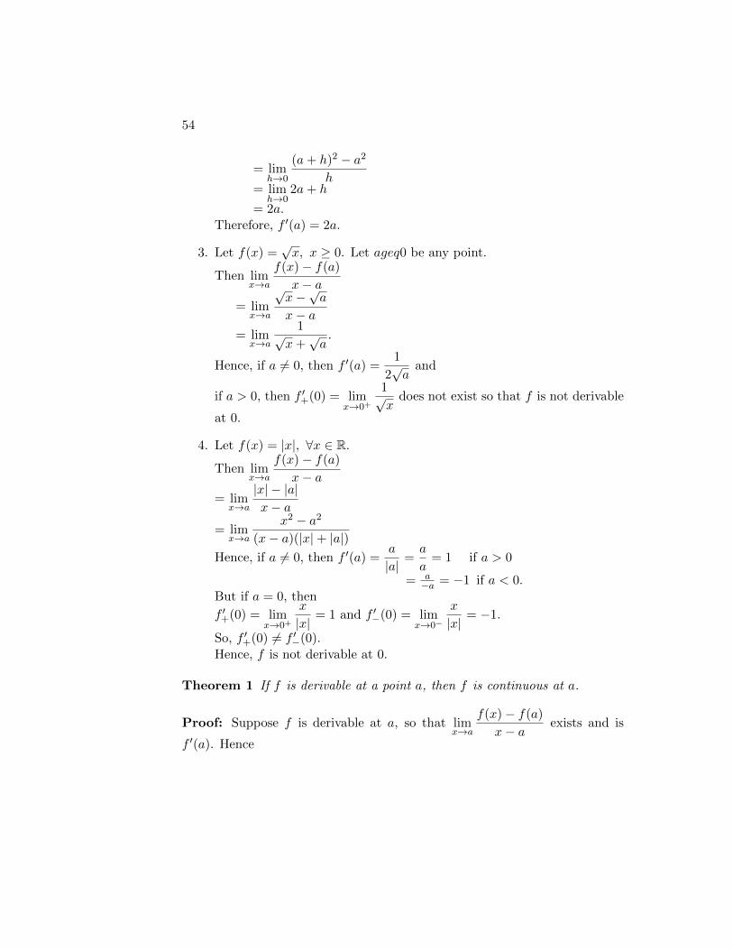
54

= limh→0

(a+ h)2 − a2

h= lim

h→02a+ h

= 2a.Therefore, f ′(a) = 2a.

3. Let f(x) =√x, x ≥ 0. Let ageq0 be any point.

Then limx→a

f(x)− f(a)

x− a= lim

x→a

√x−√a

x− a= lim

x→a

1√x+√a

.

Hence, if a 6= 0, then f ′(a) =1

2√a

and

if a > 0, then f ′+(0) = limx→0+

1√x

does not exist so that f is not derivable

at 0.

4. Let f(x) = |x|, ∀x ∈ R.

Then limx→a

f(x)− f(a)

x− a= lim

x→a

|x| − |a|x− a

= limx→a

x2 − a2

(x− a)(|x|+ |a|)Hence, if a 6= 0, then f ′(a) =

a

|a|=a

a= 1 if a > 0

= a−a = −1 if a < 0.

But if a = 0, then

f ′+(0) = limx→0+

x

|x|= 1 and f ′−(0) = lim

x→0−

x

|x|= −1.

So, f ′+(0) 6= f ′−(0).Hence, f is not derivable at 0.

Theorem 1 If f is derivable at a point a, then f is continuous at a.

Proof: Suppose f is derivable at a, so that limx→a

f(x)− f(a)

x− aexists and is

f ′(a). Hence

55

limx→a

f(x) = limx→a

[f(x)− f(a)

x− a(x− a) + f(a)

]= f ′(a) · 0 + f(a)= f(a).

Therefore f is continuous at a.

Note: The converse of the above theorem is not true.For example, let f(x) = |x|, ∀x ∈ R.Then f is continuous at 0, but as shown in example 4 above, f is not derivableat 0.

Example: Determine whether the function h(x) = x|x|, x ∈ R, is differen-tiable and find the derivative if it exists.Solution: Here, h(x) = x|x| = x2 if x > 0

= 0 if x = 0= −x2 if x < 0.

Clearly, h′(x) = 2x if x > 0= −2x if x < 0.

Let us check whether h is differentiable at 0.

h′+(0) = limx→0+

h(x)− h(0)

x− 0

= limx→0

x2

x= lim

x→0x

= 0,

h′−(0) = limx→0−

h(x)− h(0)

x− 0

= limx→0

−x2

x= lim

x→0−x

= 0.Therefore, h′+(0) = h′−(0) = 0.Therefore, h is differentiable at 0 and h′(0) = 0.Hence, h is differentiable at each x ∈ R.

Geometrical interpretation of derivative:Consider two points A[a, f(a)] and B[b, f(b)] on the graph of the curve y =

56

f(x). Let the chord BA meet X− axis at C so that ∠XCB is its inclination.Draw ordinates AP , BQ and draw AR ⊥ QB.

We have AR = PQ = h and RB = QB − PA = f(a+ h)− f(a).

Therefore, tan(∠XCB) = tan(∠RAB) =RB

AR=f(a+ h)− f(a)

h. (1)

As h approaches 0, the point B moving along the curve approaches the pointA, the chord AB approaches tangent line TA and ∠XCB approaches ∠XTAwhich is the inclination, say θ, of the tangent at A.On taking limits as h→ 0, the equation (1) gives

tan θ = f ′(a).

Thus, f ′(a) is the slope of the tangent to the curve y = f(x) at the pointA[a, f(a)].

Note: The slope of the tangent at a point of a curve is also known as theGradient of the curve at that point.

Example: Check whether the function f(x) = | log(x)| is differentiable atx = 1.

57

Solution: At x = 1,f(x+ h)− f(x) = f(1 + h)− f(1)

= | log(1 + h)| − | log 1|= | log(1 + h)|

Therefore,f(x+ h)− f(x)

h=

log(1 + h)

hif h > 0

=− log(1 + h)

hif −1 < h < 0.

So, f ′+(1) = limh→0+

f(1 + h)− f(1)

h

= limh→0

log(1 + h)

h= 1,

and f ′−(1) = limh→0+

f(1 + h)− f(1)

h

= limh→0

− log(1 + h)

h= −1.

Therefore, f ′+(1) 6= f ′−(1).So, f ′(1) does not exist.Therefore, f is not differentiable at x = 1.

Example: If f(x) = x sin(1x

)when x 6= 0 and f(0) = 0, show that f is

continuous but not derivable for x = 0.Solution: We have

|f(x)− f(0)| = |x sin

(1

x

)| = |x|| sin

(1

x

)| ≤ |x|.

Given any ε > 0 taking δ = ε, we have |f(x) − f(0)| ≤ |x| < ε whenever|x− 0| < δ.Therefore, lim

x→0f(x) = 0 = f(0).

Therefore, f is continuous at 0. Next,

limx→0

f(x)− f(0)

x− 0= lim

x→0

x sin(1x

)x

= limx→0

sin

(1

x

).

58

But, limx→0

sin

(1

x

)does not exist.

Therefore, f ′(0) does not exist.Therefore, f is not derivable at x = 0.

Exercises:

1. Using the definition of derivative, find the derivative of the followingfunctions:

(a) f(x) =1

x, ∀x ∈ R, x 6= 0

(b) f(x) = x3

(c) f(x) = xn, n ∈ N(d) f(x) = 3x

(e) f(x) = cosx.

2. The motion of a particle moving in a straight line is specified by theformula S = t2 + 2t+ 3. Find the velocity of motion (i) initially, (ii) atthe end of 3 seconds.

3. Discuss the derivability of the function f given byf(x) = x2, x < 1

= 2− x, 1 ≤ x ≤ 2= −x2 + 3x− 2, x > 2,

at x = 1, 2.

4. Give an example to show that the derivative of a continuous function isnot always a continuous function.

5. Check whether the function f defined by f(x) = |x−2|+ |x| is derivableat x = 0, 2.

6. If a function f is defined by f(x) =xe

1x

1 + e1x

, x 6= 0

= 0, x = 0,show that f is continuous but not derivable at x = 0.

7. Show that the function f(x) = |x − a|φ(x) where φ(x) is a continuousfunction and φ(a) 6= 0, has no derivative at the point x = a.

59

8. Find the coefficients c and d so that the functionf(x) = x2, if x ≤ a

= cx+ d, if x > ais continuous and derivable at a.

Differentiability of a function over an interval:A function f is said to be differentiable on an open interval I if it is differen-tiable at each a ∈ I. If I = [c, d] then f is differentiable on I if

(i) f ′+(c) exists and(ii) f ′−(d) exists and

(iii) f ′+(a) = f ′−(a) for each a such that c < a < d.

Example: Define f : [−1, 2]→ R as follows:f(x) = x if −1 ≤ x < 0

= sinx if 0 ≤ x < 1= x2 if 1 ≤ x ≤ 2.

Solution: f ′(−1) = f ′+(−1) = limx→−1+

f(x)− f(−1)

x− (−1)= lim

x→−1

x+ 1

x+ 1= 1.

Also, f ′(2) = f ′−(2) = limx→2−

f(x)− f(2)

x− 2= lim

x→2

x2 − 4

x− 2= 4.

At x = 0, f ′+(0) = limx→0+

f(x)− f(0)

x− 0= lim

x→0

sinx− sin 0

x− 0= 1

and f ′−(0) = limx→0−

f(x)− f(0)

x− 0= lim

x→0

x− sin 0

x− 0= 1.

Therefore, f ′+(0) = f ′−(0) = 1⇒ f ′(0) = 1.

At x = 1, f ′+(1) = limx→1+

f(x)− f(1)

x− 1= lim

x→1

x2 − 1

x− 1= 2

and f ′−(1) = limx→1−

f(x)− f(1)

x− 1= lim

x→1

sinx− 1

x− 1which does not exist ⇒

f ′(1) does not exist.Therefore, f is differentiable on [−1, 1) ∪ (1, 2].

Basic Rules of Differentiation:There are a number of basic properties of derivatives that are very useful in

60

the calculation of derivatives of various combinations of functions. We nowgive a brief statement of some of these properties, which will be familiar tothe reader from earlier courses.

Theorem 2 Let f, g be functions defined on an interval containing point aand f, g be differentiable at a. Then

1. If c ∈ R, then the function (cf) is differentiable at a and(cf)′(a) = cf ′(a).

2. The function f + g is differentiable at a and(f + g)′(a) = f ′(a) + g′(a).

3. Product Rule:The function f · g is differentiable at a and(f · g)′(a) = f ′(a) · g(a) + f(a) · g′(a).

4. Quotient Rule:If g(a) 6= 0, then the function f/g is differentiable at a and(f

g

)′(a) =

f ′(a)g(a)− f(a)g′(a)

(g(a))2.

Theorem 3 Chain Rule:Suppose I, J are open intervals and f : I → R, f(I) ⊂ J and g : J → R.Suppose f is differntiable at a ∈ I and g is differentiable at f(a). Then thecomposite function (g ◦ f) is differentiable at a and

(g ◦ f)′(a) = g′(f(a)) · f ′(a).

Derivative of an inverse function: Suppose (i) f is a derivable function ona closed and bounded interval [a, b] with a < b. Suppose (ii) f ′(x) 6= 0 ∀ x ∈[a, b].

Now, (i) implies that f is continuous on [a, b] and so the range of f is alsoa closed and bounded interval, say [c, d]. Further, by (ii), it can be shown thatf is actually either strictly increasing or strictly decreasing on [a, b]. Hence fis, in particular, a one-one function on [a, b]. Hence the inverse function, f−1,of f exists and its domain is [c, d]. Also, to describe the relation between f andf−1, conveniently, let us write g = f−1. Then for every x in [a, b], y = f(x)

61

is a unique number in [c, d]. Conversely, for every y in [c, d], there is a uniquenumber x in [a, b] such that y = f(x) i.e. such that x = g(y).

Thus for x in [a, b] and y in [c, d], we have

y = f(x) ⇔ x = g(y).

Now it can be shown that, under the conditions (i) and (ii) above,(a) g is also continuous on [c, d],(b) the inverse function, g of f is differentiable on [c, d] and for every y ∈ [c, d],(

f−1)′

(y) =1

f ′(x), where y = f(x),

i.e. g′(y) =1

f ′(x), where y = f(x). (∗)

Examples:

1. Every polynomial function p(x) = a0 + a1x+ a2x2 + . . .+ anx

n is differ-entiable at any x ∈ R.

2. Let f(x) = tanx =sinx

cosx, ∀x ∈ R for which cosx 6= 0. Then

f ′(x) =cosx d

dx sinx− sinx ddx cosx

(cosx)2

=cos2 x+ sin2 x

cos2 x

=1

cos2 x= sec2 x.

3. Let f = R → R be defined by f(x) = x5 + 4x + 3 and g = f−1. Findg′(8).Solution: f is continuous and one-one function on R and f ′(x) =5x4 + 4 6= 0 for any x ∈ R. Therefore, the inverse function g = f−1

is differentiable at every x ∈ R.Let x0 = 1⇒ f(x0) = f(1) = 8.

Thererfore, g′(8) =1

f ′(1)= 9.

4. Let f : (−π/2, π/2)→ (−1, 1) be defined as f(x) = sinx.Clearly, f(x) is continuous and one-one function on (−π/2, π/2) and

62

f ′(x) = cosx 6= 0, ∀x ∈ (−π/2, π/2).So, the inverse function g(y) = f−1(y) = sin−1 y is differentiable at everyy ∈ (−1, 1) and

g′(y) =1

f ′(x)=

1

cosx=

1√1− sin2 x

=1√

1− y2, y ∈ (−1, 1).

5. Find the derivatives of the following functions:

(a) f(x) = (2x2 + 5x+ 3)4

(b) f(x) = 3sinx

(c)

√x+

√x+√x

(d) f(x) = sinh 3x cosh(x/5)

Solution:

(a) f ′(x) = 4(2x2 + 5x+ 3)3(4x+ 5)

(b) f ′(x) = 3sinx log 3(cosx) = 3sinx cosx log 3

(c) f ′(x) =1

2

√x+

√x+√x

[1 +

1

2√x+√x

(1 +

1

2√x

)]

(d) f ′(x) = 3 cosh 3x cosh(x/5) +1

5sinh 3x sinh(x/5).

6. Show that the function y = xe−x satisfies the equation xy′ = (1 − x)y.Solution: y′ = e−x − xe−x = (1− x)e−x.Therefore, xy′ = (1− x)y.

Exercises:

1. Find the derivatives of the following functions:

(a) y = (sinx)cosx

(b) y = 3

√sin 2x

1− sin 2x

(c) f(x) = coth(tanx)− tanh(cotx)

(d) f(x) =ex + sinx

xex

63

(e) f(x) = | sinx|

(f) f(x) =x

1 + x2.

2. Determine whether each of the following functions is differentiable andfind the derivative wherever it exists:

(a) f(x) = x+ |x|(b) f(x) = |x|+ |x+ 1|(c) f(x) = | sinx|

(d) f(x) =√

1−√

1− x2.

3. Show that the function y =−e−x2

2x2satisfies the differential equation

xy′ + 2y = e−x2.

4. Given that the function h(x) = x3 + 2x + 1 for x ∈ R, has an inverseh−1 on R, find the value of h−1

′(y) at the points corresponding to x =

0, 1,−1.

5. Prove that the derivative of a differentiable even function is an oddfunction and the derivative of an odd function is an even function.

6. Prove that the derivative of a periodic function with period T is a peri-odic function with period T .

7. Find f ′(x) if f(x) =

∣∣∣∣∣∣x 1 0x2 2x 2x3 3x2 6x

∣∣∣∣∣∣ .8. For u =

1

2log

(1 + v

1− v

). Check the relation

du

dv

dv

du= 1.

Mean Value Theorems:In this section we are going to study the mean value theorems, which relatethe values of a function to values of its derivative.We begin by studing the relationship between the relative extrema of a functionand the values of its derivative.

Let I be an interval. A function f : I → R is said to have:

64

1. a relative maximum at point a ∈ I if there exists a neighborhood V ofa such that f(x) ≤ f(a) for all x ∈ V ∩ I.

2. a relative minimum at point a ∈ I if there exists a neighborhood V of asuch that f(a) ≤ f(x) for all x ∈ V ∩ I.

We say, f has a relative exremum at a ∈ I if it has either a relative maximumor a relative minimum at a.

Theorem 4 : Let a be an interior point of I and f : I → R have a relativeextremum at a. If f ′(a) exists then f ′(a) = 0.

Proof: We prove the result for the case that f has a relative maximum at a.The proof for the case of a relative minimum is similar.Now, f ′(a) exists and f ′(a) ∈ R.So exactly one of the following is true:

1. f ′(a) > 0,

2. f ′(a) < 0,

3. f ′(a) = 0

First, suppose f ′(a) > 0.By definition of derivative, there exists a neighborhood V ⊆ I of a such thatf(x)− f(a)

x− a> 0 for x ∈ V, x 6= a.

If x ∈ V ⊆ I and x > a, then

f(x)− f(a) = (x− a)f(x)− f(a)

x− a> 0.

So, f(x) > f(a) which contradicts to the hypothesis thatf has relative maxi-mum at a.Therefore f ′(a) > 0 is impossible.Similarly, we cannot have f ′(a) < 0.Therefore, we must have f ′(a) = 0.

Note:

1. Let f : I → R and c ∈ I. If f ′(c) = 0 or f ′(c) is undefined ,then c iscalled as a critical point for f .

65

2. The only domain points where a function can assume extreme values arecritical points and end points.

Theorem 5 : (Rolle’s Theorem)Suppose a < b and f : [a, b]→ R is

1. continuous on [a, b],

2. derivable on (a, b) and

3. f(a) = f(b).

Then there exists a point c ∈ (a, b) such that f ′(c) = 0.

Proof: f is continuous on [a, b]. So, f is bounded on [a, b] and attains itsmaximum value M and minimum value m on [a, b].Hence, ∃ c, d ∈ [a, b] such that f(c) = M and f(d) = m. Clearly, m ≤M .If m = M , then f is constant on [a, b]. Therefore, f ′(x) = 0, ∀x ∈ (a, b).If, m < M , then the numbers m and M cannot both be equal to the equalvalues f(a) and f(b).So, first let M = f(c) 6= f(a).Then c ∈ (a, b). Hence, by (2), f ′(c) exists.We now show that f ′(c) = 0.Since f(x) ≤ f(c), ∀x ∈ [a, b], we have

f(x)− f(c)

x− c≥ 0 for x < c

andf(x)− f(c)

x− c≤ 0 for x > c.

Hence, as x→ c−, we get f ′−(c) ≤ 0and as x→ c+, we get f ′+(c) ≥ 0.Since f ′(c) = f ′−(c) = f ′+(c), we thereforeget f ′(c) = 0.So, c is the required point.A similar proof shows that if m = f(d) 6= f(a), then d is the required point.

Geometrical interpretation of Rolle’s theorem:Geometrically, Rolle’s theorem says that, if f is continuous function on [a, b]and if the graph of f has a tangent at each point between the points (a, f(a))and (b, f(b)), which are on the same level, then there is a point c (a < c < b)such that the tangent to the graph of f at point (c, f(c)) is parallel to the

66

X−axis, that is, f reaches its maximum or minimum value at an interiorpoint of [a, b].

Examples:

1. Let p be a polynomial of degree n ≥ 2. Show that between any twodistinct roots of p there is a root of p′.Solution: Let p(x) = a0x

n + a1xn−1 + . . .+ an−1x+ an, a0 6= 0

be a polynomial of degree n and let a and b be distinct roots of p(x)with a < b.So, p(a) = p(b) = 0. Clearly, p is continuous on [a, b] and derivable on(a, b).All conditions of Rolle’s theorem are satisfied.So, there exists c ∈ (a, b) such that p′(c) = 0.Therefore, a root of p′ lies between the roots a, b of p.

2. Verify Rolle’s theorem for the function

f(x) = ex(sinx− cosx) on

[π

4,5π

4

].

Solution: Here, f(x) = ex(sinx− cosx).f(π/4) = eπ/4(sin(π/4)− cos(π/4))

67

= eπ/4((1/√

2)− 1/√

2)= 0.

f(5π/4) = e5π/4(sin(5π/4)− cos(5π/4))= eπ/4((−1/

√2) + 1/

√2)

= 0.

Therefore, f(π

4

)= f

(5π

4

).

Clearly, f is continuous on

[π

4,5π

4

]. Also, f is differentiable and

f ′(x) = ex(sinx− cosx) + ex(cosx+ sinx) ∀x ∈(π

4,5π

4

).

So, all conditions of Rolle’s theorem are satisfied.

Hence, there must exist c ∈(π

4,5π

4

)such that f ′(c) = 0.

To verify this, let f ′(c) = 0.i.e. ec(sin c− cos c) + ec(cos c+ sin c) = 0i.e. 2ec sin c = 0i.e. sin c = 0 (∵ 2ec 6= 0)i.e. c = nπ, n ∈ Z.

So, c = π ∈(π

4,5π

4

)satisfies f ′(c) = 0.

Hence, Rolle’s theorem is verified.

3. If f(x) = (x − 3) log x then show that the equation x log x = 3 − x forsome x ∈ (1, 3).Solution: Here, f(x) = (x− 3) log x.f(1) = (1− 3) log 1 = 0, f(3) = (3− 3) log 3 = 0.∴ f(1) = f(3).Clearly, f is continuous on [1, 3] and differentiable on (1, 3).∴ By Rolle’s theorem, ∃c ∈ (1, 3) such that f ′(c) = 0.Here, f(x) = (x− 3) log x.

Therefore, f ′(x) = (x− 3)1

x+ log x, x > 0.

∴ f ′(c) = 0 givesc− 3

c+ log c = 0.

∴ (c− 3) + c log c = 0.∴ c log c = 3− c.∴ c ∈ (1, 3) satisfies the equation x log x = 3− x.

68

Theorem 6 : (Lagrange’s Mean Value Theorem)Suppose a < b and f : [a, b]→ R is

1. continuous on [a, b],

2. derivable on (a, b).

Then there exists a point c ∈ (a, b) such that

f ′(c) =f(b)− f(a)

b− a.

Proof: For a ≤ x ≤ b, we define

φ(x) = f(x)− kx

where k is chosen such that φ(a) = φ(b).

For this, we require f(a)− ka = f(b)− kb or k =f(b)− f(a)

b− a. [I]

Now f is continuous on [a, b] and differentiable on (a, b). So, φ is continuouson [a, b] and differentiable on (a, b). Also, φ(a) = φ(b).Therefore, by Rolle’s theorem there exists c ∈ (a, b) such that φ′(c) = 0 i.e.f ′(c) = k i.e.

f ′(c) =f(b)− f(a)

b− a, using [I]

Geometrical Interpretation of LMVT:

69

Geometrically, LMVT states that there exists a point c ∈ (a, b), such that thetangent at point (c, f(c)) is parallel to the chord joining points (a, f(a)) and(b, f(b)).

Note:

1. The expressionf(b)− f(a)

b− agives the ’mean value’ of the slope of f on

[a, b] and LMVT says that f ′ must attain this mean value somewhere on(a, b).

2. If we write b − a = h andc− ah

= θ, then 0 < θ < 1 and c = a + θh.

Hence, LMVT can be stated as: If f = [a, a+ h]→ R is

(a) continuous on [a, a+ h],

(b) derivable on (a, a+ h),

then there exists θ ∈ (0, 1) such that

f(a+ h)− f(a) = hf ′(a+ θh).

Examples:

1. Verify LMVT forf(x) = log x on [1, e].Solution: Here f(x) = log x, x ∈ [1, e].Clearly, f is continuous on [1, e] and differentiable on (1, e). Also, f ′(x) =1

x.

To verify LMVT we have to find c ∈ (1, e) such that f ′(c) =f(e)− f(1)

e− 1

i.e.1

c=

log(e)− log(1)

e− 1

i.e.1

c=

1

e− 1Therefore, c = e− 1 ∈ (1, e) since e = 2.718 . . ..Hence LMVT is verified.

70

2. If 0 < a < b < 1 then prove that

b− a√1− a2

< sin−1 b− sin−1 a <b− a√1− b2

.

Solution: Consider f(x) = sin−1 x, x ∈ [a, b].Clearly, f is continuous on [a, b]. Also,

f ′(x) =1√

1− x2, ∀x ∈ (a, b).

Therefore, f is derivable on (a, b).

So, by LMVT, ∃c ∈ (a, b) such that f ′(c) =f(b)− f(a)

b− ai.e.

1√1− c2

=sin−1 b− sin−1 a

b− a[I]

Here, 0 < a < c −c2 > −b2 > −1.∴√

1− a2 >√

1− c2 >√

1− b2.∴ 1√

1−a2 <1√1−c2 <

1√1−b2 .

Using [I], we therefore get 1√1−a2 <

sin−1 b−sin−1 ab−a < 1√

1−b2 .

∴ b−a√1−a2 < sin−1 b− sin−1 a < b−a√

1−b2 .

3. Prove that | sinx− sin y| ≤ |x− y|, ∀x, y ∈ R.Solution: Let x, y ∈ R and f(t) = sin t, t ∈ [x, y].Clearly, f is continuous on [x, y].Also f is derivable and f ′(t) = cos t, t ∈ (x, y).

So, by LMVT ∃c ∈ (x, y) such that f ′(c) =f(y)− f(x)

y − xi.e. cos c =

sin y − sinx

y − x

so that | cos c| = | sin y − sinx||y − x|

.

We know that | cos c| ≤ 1, ∴ | sin y−sinx||y−x| ≤ 1.

∴ | sinx− sin y| ≤ |x− y|, ∀x, y ∈ R.

Recall that a function f : I → R is said to be strictly increasing on an intervalI if for any points x1, x2 ∈ I such that x1 < x2, we have f(x1) < f(x2).

71

Similarly, f is strictly decreasing on I if for any points x1, x2 ∈ I such thatx1 < x2, we have f(x1) > f(x2).

Theorem 7 : Suppose a 0, ∀x ∈ (a, b)⇒ f is a strictly increasing function on (a, b).

4. f ′(x) < 0, ∀x ∈ (a, b)⇒ f is a strictly decreasing function on (a, b).

Proof: Let a < x < y < b, then by LMVT ∃c ∈ (x, y) such that f(y)−f(x) =f ′(c)(y − x), [I]

1. Suppose f ′(x) 6= 0 ∀x ∈ (a, b).To show: f is a one-one function on (a, b).On the contrary, suppose f is not a one-one function on (a, b). Thenthere exist x, y ∈ (a, b) such that x < y and f(x) = f(y). But then by[I], ∃c ∈ (x, y) such that f ′(c) = 0i.e. ∃c ∈ (a, b) such that f ′(c) = 0, which is a contradiction.So, f must be one-one on (a, b).

2. Suppose f ′(x) = 0 ∀x ∈ (a, b).To show: f is a constant function on (a, b).On the contrary, suppose f is not constant on (a, b).Then ∃x, y ∈ (a, b) such that x < y and f(x) 6= f(y), so by [I], we have,

∃c ∈ (x, y) such that f ′(c) =f(y)− f(x)

y − x6= 0.

Hence, ∃c ∈ (a, b) such that f ′(c) = 0 which is a contradiction.So, f must be constant on (a, b).

3. Suppose f ′(x) > 0, ∀x ∈ (a, b).

Using [I], we have f ′(c) =f(y)− f(x)

y − x> 0.

Here, x < y ⇒ y − x > 0.So, f(y)− f(x) > 0⇒ f(x) < f(y).So, for any x, y ∈ (a, b) with x < y, we have f(x) < f(y).Therefore, f is strictly increasing on (a, b).

72

4. Similarly, we can prove if f ′(x) < 0, ∀x ∈ (a, b), then f is strictlydecreasing on (a, b).

Note: f is increasing on an interval I, if for any x, y ∈ I with x < y, we havef(x) ≤ f(y).Similarly, f is decreasing on I if for any x, y ∈ I with x < y, we have f(x) ≥f(y).So, by above theorem, if f ′(x) ≥ 0, ∀x ∈ I, then f is increasing on I and iff ′(x) ≤ 0, ∀x ∈ I, then f is decreasing on I.

Thus if the derivative f ′ has a fixed sign on an interval, the f is monotonicon that interval. This fact leads us to a test, given below, for obtaining thelocal extreme points of f on [a, b].

For example, in the above figure, consider values of f near the pointsc1, c2, c3. Here f is continuous on [a, b] and also derivable on [a, b] except at c3.

Now at points to the left of c1, the tangent to the graph of f makes anacute angle with the positive x−axis, i.e. f ′(x) ≥ 0 at all these points. So fincreases on the left of c1. Also, at points to the right of c1, the tangent to thegraph of f makes an obtuse angle with the positive x−axis, i.e. f ′(x) ≤ 0 at all

73

these points. So f decreases on the right of c1. Hence f is locally maximum atc1. Similarly, the reader should check that f is locally minimum at c2. Finally,since f is continuous at c3 and derivable in a deleted neighbourhood of c3, itcan be similarly seen that f is locally maximum at c3.These observations lead to following test for existence of local extreme values.

Theorem 8 : (The First Derivative Test for Local Extreme Values)Let f be continuous on an interval I = [a, b] and let c be an interior point ofI. Assume that f is differentiable on (a, c) and (c, b). Then

1. If there is a neighborhood (c − δ, c + δ) ⊆ I such that f ′(x) ≥ 0 forc − δ < x < c and f ′(x) ≤ 0 for c < x < c + δ, then f has a localmaximum at c.

2. If there is a neighborhood (c − δ, c + δ) ⊆ I such that f ′(x) ≤ 0 forc − δ < x < c and f ′(x) ≥ 0 for c < x < c + δ, then f has a localminimum at c.

Proof:

1. If x ∈ (c − δ, c) then by Lagrange’s mean value theorem, there exists apoint cx ∈ (x, c) such that

f(c)− f(x) = (c− x)f ′(cx)

Since, f ′(cx) ≥ 0, we have f(c)− f(x) ≥ 0.∴ f(c) ≥ f(x) for x ∈ (c− δ, c).Similarly, if x ∈ (c, c+ δ) then by Lagrange’s mean value theorem, thereexists a point cx ∈ (c, x) such that

f(c)− f(x) = (c− x)f ′(cx)

But here f ′(cx) ≤ 0, also (c− x) ≤ 0.∴ f(c)− f(x) ≥ 0∴ f(c) ≥ f(x) for x ∈ (c, c+ δ).Therefore, c is a point of local maximum for f .

2. Proof is similar.

74

Note: Suppose I = [a, b] and f : I → R is a derivable function. If c is a pointof local extremum for f then c is either a critical point for f or an endpoint.

Examples:

1. Find the intervals on which f(x) = −x3 + 12x + 5, x ∈ (−3, 3), is in-creasing or decreasing. Where does the function assume extreme valuesand what are these values?Solution: The function f is continuous on (−3, 3). Also, f ′ is definedfor all x ∈ (−3, 3) andf ′(x) = −3x2 + 12 = −3(x2 − 4)

= −3(x+ 2)(x− 2).∴ f ′(x) = 0 for x = 2,−2.∴ x = −2, 2 are critical points for f .These critical points subdivide (−3, 3) into subintervals (−3,−2), (−2, 2), (2, 3).

subintervals (-3, -2) (-2, 2) (2, 3)

sign of f ′(x) − + −

∴ f is increasing on (−2, 2) and decreasing on (−3,−2), (2, 3).So, by first derivative test, we conclude that x = −2 is a point of localminimum for f and x = 2 is a point of local maximum for f .∴ f(−2) = −11 is minimum value for f and f(2) = 21 is maximum valuefor f .

2. Show that x− x2

2< log(1 + x) < x− x2

2(1 + x)for x > 0.

Solution: Consider f(x) = log(1 + x)−(x− x2

2

), x ≥ 0.

∴ f ′(x) =1

1 + x− (1− x) =

x2

1 + x> 0, ∀x > 0.

So, f(x) is strictly increasing on (0,∞)⇒ f(0) < f(x), ∀x > 0.

∴ log(1 + 0) < log(1 + x)−(x− x2

2

)∴ 0 < log(1 + x)−

(x− x2

2

)

75

∴ x− x2

2< log(1 + x). [I]

Now consider g(x) = x− x2

2(1 + x)− log(1 + x), x ≥ 0.

∴ g′(x) =x2

2(1 + x)2> 0, ∀x > 0.

∴ g(x) is strictly increasing on (0,∞).∴ g(0) < g(x) for 0 < x.

∴ 0 < x− x2

2(1 + x)− log(1 + x).

∴ log(1 + x) < x− x2

2(1 + x). [II]

Using [I] and [II], we get

x− x2

2< log(1 + x) < x− x2

2(1 + x)for x > 0.

Theorem 9 : (Cauchy’s Mean Value Theorem)Let a < b. Suppose the functions f, g : [a, b]→ R are

1. continuous on [a, b]

2. derivable on (a, b) and

3. g′(x) 6= 0 ∀x ∈ (a, b).

Then there exists a point c ∈ (a, b) such that

f ′(c)

g′(c)=f(b)− f(a)

g(b)− g(a).

Proof: If g(a) = g(b), then g satisfies all conditions of Rolle’s theorem, sothere exists c ∈ (a, b) such that g′(c) = 0. But it is given that g′(x) 6= 0, ∀x ∈(a, b).∴ g(a) 6= g(b).For a ≤ x ≤ b, we define φ(x) = f(x)− kg(x)where k is a constant chosen such that φ(a) = φ(b)i.e. f(a)− kg(a) = f(b)− kg(b)

i.e. k =f(b)− f(a)

g(b)− g(a). [I]

Since, f, g are

76

1. continuous on [a, b] and

2. derivable on (a, b),

φ is also

1. continuous on [a, b] and

2. derivable on (a, b).

Also, φ(a) = φ(b).∴ φ satisfies all conditions of Rolle’s theorem.Hence, there exists a point c ∈ (a, b) such that φ′(c) = 0.∴ f ′(c)− kg′(c) = 0.

∴f ′(c)

g′(c)= k. (∵ g′(c) 6= 0)

∴f ′(c)

g′(c)=f(b)− f(a)

g(b)− g(a)using [I]

Examples:

1. Verify Cauchy’s mean value theorem for the functions f(x) = ex andg(x) = e−x in [0, 1]. Show that c is the arithmetic mean of a and b.Solution: f, g are continuous on [0, 1]. Also, f, g are differentiable on(0, 1). Furtherg′(x) = −e−x 6= 0 ∀x ∈ (0, 1).Thus, all conditions of CMVT are satisfied.So, there must exist c ∈ (a, b) such that

f ′(c)

g′(c)=f(b)− f(a)

g(b)− g(a).

∴ec

−e−c=

eb − ea

e−b − e−a.

−e2c = −ea+b.∴ 2c = a+ b.

∴ c =a+ b

2∈ (a, b).

Hence, CMVT is verified and c is the arithmetic mean of a and b.

77

2. Find c of Cauchy’s mean value theorem for the functions cosx and sinxin [0, π/2].Solution: Let f(x) = cosx, g(x) = sinx.Then both f, g are continuous on [0, π/2] and derivable on (0, π/2).Also, g′(x) = cosx 6= 0, ∀x ∈ (0, π/2).So all conditions of CMVT are satisfied.By Cauchy’s mean value theorem there exists a real number c ∈ (0, π/2)such that

f ′(c)

g′(c)=f(b)− f(a)

g(b)− g(a). [I]

∴sin c

− cos c=

cos(π/2)− cos 0

sin(π/2)− sin 0∴ − tan c = −1∴ tan c = 1∴ c = π/4 ∈ (0, π/2).So, c = π/4 is the point satisfying [I].

3. Verify CMVT for the functions f(x) =1

x2and g(x) =

1

xon [a, b], a > 0.

Show that the point c of Cauchy’s mean value theorem is the harmonic

mean of a and b. Solution: Here f(x) =1

x2and g(x) =

1

x.

Clearly, both f, g are continuous on [a, b] and derivable on (a, b), wherea > 0.∴ By CMVT, ∃c ∈ (a, b) such that

f ′(c)

g′(c)=f(b)− f(a)

g(b)− g(a).

∴−2/c3

−1/c2=

1/b2 − 1/a2

1/b− 1/a

∴2c2

c3=

1

b+

1

a

∴2

c=a+ b

ab

∴ c =2ab

a+ b∈ (a, b).

Hence, CMVT is verified and c is the harmonic mean of a and b.

78

4. Show that for 0 < x < π/2,

(a) sinx < x < tanx

(b)2

π<

sinx

x< 1.

Solution:

(a) For 0 ≤ x < π/2, let f(x) = x− sinx, g(x) = tanx− x.Then for all x ∈ (0, π/2), f ′(x) = 1 − cosx > 0 and g′(x) =sec2 x− 1 > 0.So, f, g are strictly increasing on [0, π/2).Hence, for 0 < x, f(0) < f(x) and g(0) < g(x)i.e. 0 < x− sinx and 0 < tanx− xi.e. sinx < x and x < tanx∴ sinx < x < tanx.

(b) For 0 < x ≤ π/2, let F (x) =sinx

xand F (0) = 1.

Then F is continuous on [0, π/2].

Also, on (0, π/2), F ′(x) =x cosx− sinx

x2< 0 since x < tanx by

(a).Hence, F is strictly decreasing on [0, π/2) and so for x ∈ (0, π/2),we have F (π/2) < F (x) < F (0).

Therefore,2

π<

sinx

x< 1.

Exercises:

1. Verify Rolle’s theorem, if applicable, for the given function.

(a) f(x) = |x|, x ∈ [−1, 1]

(b) f(x) = x(x− 2)e−x, x ∈ [0, 2]

(c) f(x) = 9x3 − 4x, x ∈ [−2/3, 2/3]

(d) f(x) = cos2 x, x ∈ [−π/4, π/4].

2. Verify LMVT if applicable, for the given function.

(a) f(x) = ex, x ∈ [−1, 1]

79

(b) f(x) = 3x2 − 5x+ 1, x ∈ [2, 5]

(c) f(x) = sinx+ cosx, x ∈ [0, 2π]

(d) f(x) =√x2 − 4, x ∈ [2, 3].

3. Verify CMVT if applicable, for the given function.

(a) f(x) = ex, g(x) =x2

1 + x2, x ∈ [−3, 3]

(b) f(x) = x2 + 2, g(x) = x3 − 1, x ∈ [1, 2].

4. Show thatx

1 + x< log(1 + x) < x, x > 0.

5. Show thatb− a1 + b2

< tan−1 b− tan−1 a <b− a1 + a2

, ∀ 0 < a < b.

6. Verify Cauchy’s mean value theorem for functions f(x) =√x and g(x) =

1√x

in [a, b], a > 0. Show that the number c of CMVT is the geometric

mean of a and b.

7. Separate the intervals in which the polynomial 2x3 − 15x2 + 36x + 1 isincreasing or decreasing.

8. Ifa0

n+ 1+a1n

+ . . .+an−1

2+an1

= 0, show that the equation

a0xn + a1x

n−1 + . . .+ an−1x+ an = 0 has a root in (0, 1).

9. If f(x) = x(x + 1)(x + 2)(x + 3), show that the equation f ′(x) = 0 hasthree real roots.

10. Using f(x) = (4−x) log x, show that x log x = 4−x for some x ∈ (1, 4).

11. Find the points of local extrema, the intervals on which functions areincreasing or decreasing for

(a) f(x) = x+1

x, x 6= 0

(b) f(x) = x3, x ∈ [−1, 1]

(c) f(x) = x5 − 5x4 + 5x3 − 1, x ∈ R(d) f(x) = xe−x, x ∈ (0, 2)

80

(e) f(x) = x2 + 3x+ 5, x ∈ R

(f) f(x) =x

x2 + 1, x ∈ R.

12. Show that the equation tanx = 1 − x has at least one solution for0 < x < 1.

13. Show that there is no k ∈ R such that the equation x3 + 12x + k = 0has two distinct roots in [0, 2].

14. Let I be an interval and f : I → R be differentiable on I. Show that ifthe derivative f ′ is never 0 on I, then either f ′(x) > 0 for all x ∈ I orf ′(x) < 0 for all x ∈ I.

15. Let p be a polynomial of degree n ≥ 2. Show that between any twodistinct roots of p there lies a root of p′.

L’ Hospital’s Rules:

In calculus, we frequently come across limits of the form limx→a

f(x)

g(x). We note

that the limit exists and is equal tolimx→a f(x)

limx→a g(x)provided lim

x→af(x), lim

x→ag(x)

both exist and limx→a

g(x) 6= 0.

But if limx→a f(x) = 0 and limx→a g(x) = 0, then as x → a,f(x)

g(x)may tend

to a finite limit or to ∞ or to −∞ or it may oscillate.

In this case, we say that limx→a

f(x)

g(x)is of indeterminate form

0

0.

Similarly, if limx→a

f(x) = ∞ and limx→a

g(x) = ∞, then limx→a

f(x)

g(x)is said to be of

the indeterminate form∞∞

.

We state below a collection of theorems called L’ Hospital’s rule which are

useful in evaluating limits of the form0

0and

∞∞

. Other indeterminate forms

like 0 ·∞, 00, 1∞, ∞−∞ can be reduced either to0

0or∞∞

form by algebraic

manipulations and by taking logarithms or exponentials.

81

Theorem 10 : (L’ Hospital’s Rule I)Suppose a < b and functions f, g are derivable on (a, b) and g′(x) 6= 0 ∀x ∈

(a, b). Suppose that limx→a+

f(x) = 0 = limx→a+

g(x) and limx→a+

f ′(x)

g′(x)= L, then

limx→a+

f(x)

g(x)= L.

Here, L can be a real number or ∞ or −∞.

Remarks:

1. L’ Hospital’s rule for0

0indeterminate form is also valid for left land

limits. There we replace (a, b) by (c, a) where c < a and x → a+ byx→ a−.Combining the versions of left hand limits and right hand limits, we ob-

tain L’ Hospital’s rule for (two sided) limits of0

0indeterminate form as

follows:Let f, g be functions which are differentiable in some deleted neigh-borhood of a where g′(x) 6= 0 and let lim

x→af(x) = 0 = lim

x→ag(x) and

limx→a

f ′(x)

g′(x)= L, then lim

x→a

f(x)

g(x)= L.

2. L’ Hospital’s rule I is also valid if instead of considering limits as x→ awhere a is a real number, we consider limits as x→∞ or x→ −∞.

3. If limx→a+

f ′(x)

g′(x)is also indeterminate of the form

0

0, then it may be possible

to apply the above theorem again to conclude that if limx→a+

f ′′(x)

g′′(x)exists,

then it is equal to limx→a+

f ′(x)

g′(x).

Theorem 11 : (L’ Hospital’s Rule II)Suppose a < b and functions f, g are derivable on (a, b) and g′(x) 6= 0 ∀x ∈

(a, b). Suppose that limx→a+

f(x) = ±∞ = limx→a+

g(x) and limx→a+

f ′(x)

g′(x)= L, then

limx→a+

f(x)

g(x)= L.

82

Remarks:

1. Above L’ Hospital’s rule can be stated for x→ a− or x→ a with suitablemodifications in the hypothesis of the theorem.

2. L’ Hospital’s rule II is also valid if instead of considering limits as x→ awhere a is a real number, we consider limits as x→∞ or x→ −∞.

3. If limx→a+

f ′(x)

g′(x)is again indeterminate of the form

∞∞

, then by applying

the above theorem again, we conclude that, if limx→a+

f ′′(x)

g′′(x)exists, then it

is equal to limx→a+

f ′(x)

g′(x).

Examples:

1. Find limx→0

sinx

x.

Solution: f(x) = sinx, g(x) = x are differentiable everywhere on thereal line and f ′(x) = cosx, g′(x) = 1.Further, g′(x) 6= 0 for all x ∈ R.limx→0

f(x) = 0 = limx→0

g(x)

and limx→0

f ′(x)

g′(x)= lim

x→0cosx = 1.

Therefore, by L’ Hospital’s rule I, we have

limx→0

sinx

x= lim

x→0

f ′(x)

g′(x)= 1.

2. Show that limx→∞

x2

e2x= 0.

Solution: Note that limx→∞

x2

e2xis of the indeterminate form

∞∞

. Also,

f(x) = x2, g(x) = e2x satisfy all hypotheses of L’ Hospital’s rule II, so

limx→∞

x2

e2xexists provided lim

x→∞

2x

2e2xexists. and again by L’ Hospital’s

rule, this limit exists provided limx→∞

2

4e2xexists.

Now limx→∞

2

4e2x= 0 and hence lim

x→∞

x2

e2x= 0.

83

3. Evaluate limx→∞

2x2 + 5x+ 7

x2 − x+ 1.

Solution: limx→∞

2x2 + 5x+ 7

x2 − x+ 1

(∞∞

form)

= limx→∞

4x+ 5

2x− 1

(∞∞

form)

= limx→∞

4

2= 2.

4. Find limx→0

1− cosx

x2.

Solution: Let f(x) = 1− cosx and g(x) = x2.Both f, g are differentiable in every deleted neighborhood of 0 and g′(x) =2x 6= 0 in that deleted neighborhood.Also, lim

x→0f(x) = 0 = lim

x→0g(x).

So, we can apply L’ Hospital’s rule I,

limx→0

1− cosx

x2= lim

x→0

sinx

2x

(0

0form

)= lim

x→0

cosx

2= 2.

Sometimes L’ Hospital’s rule does not help us to evaluate a given limitas illustrated in the following example.

5. Find limx→∞

√1 + x2

x.

Solution: Here, f(x) =√

1 + x2 and g(x) = x.Note that, lim

x→∞f(x) =∞ = lim

x→∞g(x).

If we try to apply, L’ Hospital’s rule, we get a loop.

limx→∞

√1 + x2

x= lim

x→∞

(2x

2√1+x2

)1

= limx→∞

x√1 + x2

.

= limx→∞

1(2x

2√1+x2

) .

= limx→∞

√1 + x2

x.

84

However, the limit can be found directly as,

limx→∞

√1 + x2

x= lim

x→∞

√1 + x2

x2= lim

x→∞

√1 +

1

x2= 1.

6. Find limx→∞

log x

x.

Solution: Here f(x) = log x and g(x) = x are differentiable on (0,∞)and g′(x) = 1 6= 0, ∀x ∈ (0,∞).

By L’ Hospital’s rule, we have limx→∞

log x

x= lim

x→∞

(1x

)1

= 0.

7. Find limx→0

ex − cosx− xx sinx

.

Solution: limx→0

ex − cosx− xx sinx

(0

0form

)= lim

x→0

ex − cosx− xx2

x

sinx

= limx→0

ex − cosx− xx2

(0

0form

)= lim

x→0

ex + sinx− 1

2x

(0

0form

)= lim

x→0

ex + cosx

2= 1.

Now, we see how to evaluate limits for other indeterminate forms suchas∞−∞, 0 ·∞, 1∞, 00, ∞0. Here, the first two forms can be converted

into0

0or∞∞

. For the remaining forms we need to use the continuity of

the logarithmic and exponential functions.

8. Evaluate limx→0

(1

x− 1

ex − 1

).

Solution: limx→0+

(1

x− 1

ex − 1

)has indeterminate form ∞−∞.

limx→0

(1

x− 1

ex − 1

)=ex − 1− xx(ex − 1)

(0

0form

)=

ex − 1

ex − 1 + xex

(0

0form

)

85

=ex

2ex + xex

=1

2.

9. Evaluate limx→π/2

(secx− tanx).

Solution: limx→π/2

(secx− tanx) (∞−∞ form)

= limx→π/2

(1

cosx− sinx

cosx

)= lim

x→π/2

(1− sinx

cosx

) (0

0form

)= lim

x→π/2

cosx

− sinx= 0.

10. Evaluate limx→0+

x2 log x.

Solution: limx→0

x2 log x (0 · ∞ form)

= limx→0

log x

1/x2

(∞∞

form)

= limx→0

1/x

−2/x3

= limx→0

−x2

2= 0.


(2− x) tan(πx

4

).

Solution: limx→2

(2− x) tan(πx

4

)(0 · ∞ form)

= limx→2

2− xcot(πx4

) (0

0form

)= lim

x→2

−1

−π4 cosec2

(πx4

)= lim

x→2

4

πsin2

(πx4

)=

4

π.


xx (00 form)

86

Solution: Put y = xx.∴ log y = x log x → 0 as x→ 0+.Hence, lim

x→0+y = lim

x→0+elog y

= elimx→0+

log y(using continuity of et)

= e0 = 1.∴ limx→0+

xx = 1.


(1 +mx)1/x (1∞ form)

Solution: Put y = (1 +mx)1/x.

∴ log y =1

xlog(1 +mx).

limx→0+

log y = limx→0+

1

xlog(1 +mx) (0 · ∞ form)

= limx→0+

log(1 +mx)

x

= limx→0+

m

1 +mx= m.

∴ limx→0+

y = limx→0+

elog y

= elimx→0+

log y= em.

∴ limx→0+

(1 +mx)1/x = em.


xsinx (00 form)

Solution: Let y = xsinx.∴ log y = sinx log x.limx→0+

log y = limx→0+

sinx log x (0 · ∞ form)

= limx→0+

log x

cosec x

(∞∞

form)

= limx→0+

1/x

cosec x cotx

= limx→0+

sin2 x

x cosx

(0

0form

)= lim

x→0+

2 sinx cosx

cosx− x sinx= 0.

87

∴ limx→0+

y = limx→0+

elog y

= elimx→0+

log y

= e0 = 1.∴ limx→0+

xsinx = 1.


(cosecx)1/ log x (∞0 form)

Solution: Let y = (cosecx)1/ log x.

∴ log y =1

log xlog(cosecx).

∴ limx→0

log y = limx→0

log(cosecx)

log x

(∞∞

form)

= limx→0

−1cosecxcosecx · cotx

1x

= − limx→0

x cotx

= − limx→0

cosx · x

sinx= −1 · 1 = −1.

∴ limx→0

y = limx→0

elog y

= elimx→0

log y

= e−1 =1

e.

∴ limx→0

(cosecx)1/ log x =1

e.


(ax + x)1/x (1∞ form)

Solution: Let y = (ax + x)1/x.

∴ log y =1

xlog(ax + x)

∴ limx→0

log y = limx→0

1

xlog(ax + x) (∞ · 0 form)

= limx→0

log(ax + x)

x

(0

0form

)= lim

x→0

1ax+x(ax log a+ 1)

1

= limx→0

ax log a+ 1

ax + x

88

= log a+ 1.∴ limx→0

y = limx→0

elog y

= elimx→0

log y

= elog a+1

= elog a · e1 = a · e.∴ limx→0

(ax + x)1/x = a · e.

Exercises:

1. Evaluate the following limits, if they exist.

(a) limx→∞

x2

e2x

(b) limx→0

e2x − cosx

x

(c) limx→0

tanx− xx− sinx

(d) limx→0

1 + x

x

(e) limx→0

x

tanx

(f) limx→0

2x2 − 3x+ 1

x2 − x

(g) limx→0

ex − 1 + log(1− x)

tanx− x(h) lim

x→∞x

1x

(i) limx→0+

tan 5x

tanx

(j) limx→0

ax − 1

bx − 1

(k) limx→∞

x sin

(1

x

)(l) lim

x→1(1− x)

tanπx

2

89

(m) limx→0

(1

x− cotx

)(n) lim

x→0

(1

x− log(1 + x)

x2

)(o) lim

x→0

(1

sinx− 1

x

)(p) lim

x→0(cosx)

1x2

(q) limx→0

(1

ex − 1− 1

x

)(r) lim

x→∞

(1 +

3

x

)x(s) lim

x→1

(x2 − 1

)log x(t) lim

x→π/4(tanx)tan 2x

(u) limx→a

(x− a)x−a

(v) limx→π/2

(secx)cotx

(w) limx→0+

(1

x

)2 sinx

(x) limx→∞

(ex + x)1x

2. Show that

(a) limx→a

xn − an

x− a= nan−1.

(b) limx→a

ax − bx

x= log a− log b for a, b > 0.

(c) limx→0

(ax + bx

2

) 1x

=√ab.

(d) limx→∞

(1 +mx)1x = e for m > 0.

90

3. Find the value of a, b such that

limx→0

x(1 + a cosx)− b sinx

x3= 1.

Successive Differentiation:Derivatives of order greater than one are obtained by a natural extension of thedifferentiation process, called successive differentiation. If the derivative f ′(x)of a function f exists at every point x in an interval I containing a point c,then we can consider existence of the derivative of the function f ′ at the pointc. In case f ′ has a derivative at the point c, we refer to the resulting numberas the second derivative of f at c, and we denote this number by f ′′(c) or byf (2)(c). In similar fashion, we define the third derivative f ′′′(x) = f (3)(c), . . . ,and the nth derivative f (n)(c), whenever these derivatives exist. Note that theexistence of the nth derivative presumes the existence of the (n−1)th derivativein an interval containing c.If y = f(x), we denote the nth derivative of f at x as f (n)(x) or yn(x) or

Dnf(x) ordny

dxn.

Examples:

1. If y = sin−1 x, prove that (1− x2)y2 − xy1 = 0.Solution: y = sin−1 x.

∴ y1 =1√

1− x2

∴ y21 =1

1− x2∴ (1− x2)y21 − 1 = 0.Differentiating both sides w.r.t. x, we get

(1− x2)2y1y2 + y21(−2x) = 0

∴ (1− x2)y2 − xy1 = 0

.

2. If y = log(log x), prove that xy2 + y1 + xy21 = 0.Solution: y = log(log x).

91

∴ y1 =1

log x

1

x

∴ xy1 =1

log xDifferentiating both sides w.r.t. x, we get

xy2 + y1 = − 1

(log x)21

x

= − x

x2(log x)2

= −xy21.∴ xy2 + y1 + xy21 = 0.

The nth derivative of some standard functions:

1. If y = (ax+ b)m, m ∈ R,then y1 = ma(ax+ b)m−1,y2 = m(m− 1)a2(ax+ b)m−2,y3 = m(m− 1)(m− 2)a3(ax+ b)m−3 andin general, yn = m(m− 1)(m− 2) . . . (m− n+ 1)an(ax+ b)m−n.If m is a positive integer, then

yn =m!

(m− n)!an(ax+ b)m−n if n < m

= m!am if n = m= 0 if n > m.

2. If y =1

ax+ b.

Put m = −1 in (1), we getyn = (−1)(−2) . . . (−n)an(ax+ b)−1−n

=(−1)nn!an

(ax+ b)n+1.

3. If y = log(ax+ b).

We have, y1 =1

ax+ b· a.

By above result (2), we have

yn =(−1)n−1(n− 1)!an

(ax+ b)n.

4. If y = amx.We have y1 = mamx log a

92

y2 = m2amx(log a)2

y3 = m3amx(log a)3.In general,yn = mnamx(log a)n.

5. If y = emx.Put a = e in (4), we getyn = mnemx(log e)n

= mnemx.

6. If y = sin(ax+ b), then we havey1 = a cos(ax+ b) = a sin(ax+ b+ π/2)y2 = a2 cos(ax+ b+ π/2) = a2 sin(ax+ b+ 2π/2)y3 = a3 cos(ax+ b+ 2π/2) = a3 sin(ax+ b+ 3π/2)In general,yn = an sin(ax+ b+ nπ/2).

7. Similar to (6), if y = cos(ax+ b), thenyn = an cos(ax+ b+ nπ/2).

8. If y = eax sin(bx+ c), we havey1 = aeax sin(bx+ c) + beax cos(bx+ c).Put a = r cos θ, b = r sin θ

where r =√a2 + b2, θ = tan−1

b

a.

∴ y1 = reax cos θ sin(bx+ c) + reax sin θ cos(bx+ c)= reax sin(bx+ c+ θ)

∴ y2 = r2eax sin(bx+ c+ 2θ)In general,yn = rneax sin(bx+ c+ nθ).

9. Similarly, if y = eax cos(bx+ c), thenyn = rneax cos(bx+ c+ nθ)

where r =√a2 + b2, θ = tan−1

b

a.

Examples:

93

1. If y =16x+ 18

2x2 + 5x+ 3, find yn.

Solution: Here y =16x+ 18

2x2 + 5x+ 3=

16x+ 18

(x+ 1)(2x+ 3)

∴ y =2

x+ 1+

12

2x+ 3

∴ yn =2(−1)nn!1n

(x+ 1)n+1+

12(−1)nn!2n

(2x+ 3)n+1.

2. If y = e2x cos2 x sinx, find the nth derivative of y.Solution: We have y = e2x cos2 x sinx

= e2x1

2(1 + cos 2x) sinx

= e2x(

1

2sinx+

1

2cos 2x sinx

)= e2x

(1

2sinx+

1

4sin 3x− 1

4sinx

)= e2x

(1

4sinx+

1

4sin 3x

)∴ y =

1

4e2x sinx+

1

4e2x sin 3x.

∴ yn =1

4

√5ne2x sin

(x+ n tan−1

1

2

)+

1

4

√13ne2x sin

(3x+ n tan−1

3

2

).

Theorem 12 : (Leibnitz’s Theorem)If y = uv, where u and v are functions of x possessing derivatives of nth order,then

yn = (uv)n

=n C0unv +n C1un−1v1 + . . .+n Cr−1un−r+1vr−1

+n Crun−rvr + . . .+n Cnuvn [I]

where nCr =n!

(n− r)!r!.

Proof: We prove the theorem using mathematical induction.Step 1: y1 = (uv)1

= u1v + uv1

94

= 1C0u1v + 1C1uv1Thus, the result is true for n = 1.

Step 2: Assume that the result is true for n = m. Therefore

ym = (uv)m

=m C0umv +m C1um−1v1 + . . .+m Cr−1um−r+1vr−1

+m Crum−rvr + . . .+m Cm−1u1vm−1 +m Cmuvm.

Differentiating both sides, we get

y(m+1) = (uv)m+1

=m C0um+1v +m C0umv1 +m C1umv1 +m C1um−1v2

+ . . .+m Cr−1um−r+2vr−1 +m Cr−1um−r+1vr

+m Crum−r+1vr +m Crum−rvr+1

+ . . .+m Cmu1vm +m Cmuvm+1

=m C0um+1v + (mC0 +m C1)umv1 + (mC1 +m C1)um−1v2

+ . . .+ (mCr−1 +m Cr)um−rvr + . . .+m Cmuvm+1.

We have the results,

mCr−1 +m Cr =m+1 Cr and mCm =m+1 Cm+1,mC0 =m+1 C0.

Therefore

ym+1 = (uv)m+1

=m+1 C0um+1v +m+1 C1umv1 +m+1 C2um−1v2

+ . . .+m+1 Crum−r+1vr + . . .+m+1 Cm+1uvm+1.

Therefore, the result is true for n = m+ 1.Hence, by the principle of mathematical induction the theorem is true for allpositive integers n.

Examples:

1. If y = (sin−1 x)2, prove that(1− x2)yn+2 − (2n+ 1)xyn+1 − n2yn = 0.

95

Solution: We have y = (sin−1 x)2.Differentiating both sides w.r.t. x, we get

y1 = 2 sin−1 x · 1√1− x2

∴ y1√

1− x2 = 2 sin−1 x.Squaring and simplifying, we get(1− x2)y21 − 4y = 0.Differentiating once again, we get(1− x2)2y1y2 − 2xy21 − 4y1 = 0∴ 2y1

[(1− x2)y2 − xy1 − 2

]= 0

∴ (1− x2)y2 − xy1 − 2 = 0 [I]Differentiating [I] n times using Leibnitz’s theorem, we get[

nC0(1− x2)yn+2 +n C1(−2x)yn+1 +n C2(−2)yn]

− [nC0xyn+1 +n C1yn] = 0

∴ (1− x2)yn+2 − 2nxyn+1 − n(n− 1)yn − xyn+1 − nyn = 0∴ (1− x2)yn+2 − (2n+ 1)xyn+1 − n2yn = 0.

2. If y1m + y

−1m = 2x, show that

(x2 − 1)yn+2 + (2n+ 1)xyn+1 + (n2 −m2)yn = 0.

Solution: We have y1m +

1

y1m

= 2x.

Put y1m = t.

∴ t+1

t= 2x.

∴ t2 − 2xt + 1 = 0 which is a quadratic equation in t. Solving it for t,we gett = x±

√x2 − 1.

We ignore the negative sign.

∴ t = x+√x2 − 1 = y

1m

∴ y = (x+√x2 − 1)m [I]

Differentiating [I] w.r.t. to x, we get

y1 = m(x+√x2 − 1)m−1

(1 + x√

x2−1

)∴ y1 =

m(x+√x2 − 1)m√

x2 − 1

∴√x2 − 1y1 = my

96

Differentiating once again, we get√x2 − 1y2 +

x√x2 − 1

y1 = my1

= m my√x2−1

∴ (x2 − 1)y2 + xy1 −m2y = 0 [II]Differentiating [II] n times using Leibnitz’s theorem, we get(x2 − 1)yn+2 + n(2x)yn+1 + n(n− 1)yn + xyn+1 + nyn −m2yn = 0∴ (x2 − 1)yn+2 + (2n+ 1)xyn+1 + (n2 −m2)yn = 0.

3. If x = tan(log y), prove that(1 + x2)yn+1 + (2nx− 1)yn + n(n− 1)yn−1 = 0.Solution: We have x = tan(log y)∴ log y = tan−1 x∴ y = etan

−1 x [I]Differentiating [I] w.r.t. x, we get

y1 = etan−1 x · 1

1 + x2

∴ (1 + x2)y1 = etan−1 x = y

∴ (1 + x2)y1 − y = 0 [II]Differentiating [II] n times using Leibnitz’s theorem, we get(1 + x2)yn+1 + n(2x)yn + n(n− 1)yn−1 − yn = 0∴ (1 + x2)yn+1 + (2nx− 1)yn + n(n− 1)yn−1 = 0

Exercises:

1. Find the nth derivative of

(a) xnex

(b) x3 cosx

2. Let f(x) = x sin

(1

x

)for x 6= 0 and f(0) = 0. Show that f is continuous

at 0 but f ′(0) does not exist.

3. Let f(x) = x2 sin

(1

x

)for x 6= 0 and f(0) = 0. Show that f ′(0) exists

but f ′ is not continuous at 0.

4. Prove that

97

(a)dn

dxn

(1

a2 − x2

)=n!

2a

[(−1)n+1

(a− x)n+1+

(−1)n

(a+ x)n+1

].

(b) If y = sin2 x sin 2x, then

yn =1

4

[2n+1 sin(2x+ nπ/2)− 4n−1 sin(4x+ nπ/2)

].

(c) If y = eax cosx sinx then

yn =1

2eax(a2 + 4)n/2 sin(2x+ n tan−1

(2

a

)).

5. If y = ea sin−1 x cosx sinx then prove that

(1− x2)yn+2 − (2n+ 1)xyn+1 − (n2 + a2)yn = 0.

6. If y = sin(m sin−1 x), then show that(1− x2)yn+2 − (2n+ 1)xyn+1 + (n2 −m2)yn = 0.

7. If y = (x2 − 1)n, prove that(x2 − 1)yn+2 + 2xyn+1 − n(n+ 1)yn = 0.

8. If y = log(x+√

1 + x2), prove that

(a) (1 + x2)y2 + xy1 = 0

(b) (1 + x2)yn+2 + (2n+ 1)xyn+1 + n2yn = 0

(c) yn+2(0) = −n2yn(0).

Taylor’s Theorem:Taylor’s theorem can be regarded as an extension of the mean value theoremto higher order derivatives. Whereas the mean value theorem relates thedifference of values of a function and its first derivative, Taylor’s theoremprovides a relation between the difference of values of the function and itshigher order derivatives.It is useful to be able to approximate a function by an infinite series. Taylor’stheorem can be used to represent a function as an infinite series.

Theorem 13 : (Taylor’s Theorem with Lagrange’s form of remain-der)Let n ∈ N, let I = [a, b] and let f : I → R be such that f and its derivatives

98

f ′, f ′′, . . . f (n) are continuous on I and that f (n+1) exists on (a, b). If x0 ∈ I,then for any x ∈ I, there exists a point c between x and x0 such that

f(x) = f(x0) + f ′(x0)(x− x0) +f ′′(x0)

2!(x− x0)2

+ . . .+f (n)(x0)

n!(x− x0)n +

f (n+1)(c)

(n+ 1)!(x− x0)n+1.

Note: We may write the conclusion of Taylor’s theorem asf(x) = Pn(x) +Rn(x) where

Pn(x) = f(x0) + f ′(x0)(x− x0) +f ′′(x0)

2!(x− x0)2 + . . .+

f (n)(x0)

n!(x− x0)n is

the Taylor polynomial for f at x0 and Rn(x) =f (n+1)(c)

(n+ 1)!(x−x0)n+1 for some

point c between x and x0, is the Lagrange’s form of remainder of order n.Suppose f possesses derivatives of all orders on I. If Rn(x)→ 0 as n→∞ forall x in I, then we say that the Taylor series generated by f at x0 convergesto f on I and we write

f(x) =∞∑k=0

f (k)(x0)

k!(x− x0)k.

This series is known as Taylor’s series expansion of f at x0.

With x0 = a and x = a+h, we have the following version of Taylor’s theorem.

Theorem 14 : (Taylor’s Theorem - Second form)Let f be a function defined on [a, a+ h] such that

1. the nth derivative f (n) is continuous on [a, a+ h]

2. the (n+ 1)th derivative f (n+1) exists on (a, a+ h).

Then there exists a point c in (a, a+ h) such that

f(a+ h) = f(a) + f ′(a)h+f ′′(a)

2!h2 + . . .+

f (n)(a)

n!hn +

f (n+1)(c)

(n+ 1)!hn+1.

We have another form of Taylor’s theorem known as Maclaurin’s theorem.

99

Theorem 15 : (Maclaurin’s Theorem)Let f be a function defined on [0, x] such that

1. the nth derivative f (n) is continuous on [0, x]

2. the (n+ 1)th derivative f (n+1) exists on (0, x).

Then there exists at least one real number c in (0, x) such that

f(x) = f(0) + f ′(0)x+f ′′(0)

2!x2 + . . .+

f (n)(0)

n!xn +Rn(x)

where Rn(x) =f (n+1)(c)

(n+ 1)!xn+1 is called the Lagrange’s form of remainder.

Note: Suppose f possesses derivatives of all orders on I. If Rn(x) → 0 asn → ∞ for all x in I, then the Maclaurin series generated by f converges tof and we write

f(x) =∞∑k=0

f (k)(0)

k!xk.

This series is known as Maclaurin’s series expansion of f .

We are not proving any of these theorems. Assuming their validity we solveexamples.

Maclaurin’s series expansions of some basic functions:

1. Expansion of ex

Let f(x) = ex ∴ f(0) = e0 = 1f ′(x) = ex ∴ f ′(0) = 1f ′′(x) = ex ∴ f ′′(0) = 1...f (n)(x) = ex ∴ f (n)(0) = 1By Maclaurin’s theorem, we have

100

f(x) = f(0) + f ′(0)x+f ′′(0)

2!x2 + . . .+

f (n)(0)

n!xn + . . .

f(x) = ex = 1 + x+x2

2!+x3

3!+ . . .+

xn

n!+ . . .

2. Expansion of sinxLet f(x) = sinx ∴ f(0) = 0f ′(x) = cosx ∴ f ′(0) = 1f ′′(x) = − sinx ∴ f ′′(0) = 0f (3)(x) = − cosx ∴ f (3)(0) = −1f (4)(x) = sinx ∴ f (4)(0) = 0...By Maclaurin’s theorem, we have

f(x) = f(0) + f ′(0)x+f ′′(0)

2!x2 + . . .+

f (n)(0)

n!xn + . . .

f(x) = sinx = x− x3

3!+x5

5!− x7

7!+ . . .

3. Expansion of cosxLet f(x) = cosx ∴ f(0) = 1f ′(x) = − sinx ∴ f ′(0) = 0f ′′(x) = − cosx ∴ f ′′(0) = −1f (3)(x) = sinx ∴ f (3)(0) = 0f (4)(x) = cosx ∴ f (4)(0) = 1...By Maclaurin’s theorem, we have

f(x) = f(0) + f ′(0)x+f ′′(0)

2!x2 + . . .+

f (n)(0)

n!xn + . . .

f(x) = cosx = 1− x2

2!+x4

4!− x6

6!+ . . .

4. Expansion of log(1 + x)Let f(x) = log(1 + x) ∴ f(0) = log 1 = 0

f ′(x) =1

1 + x∴ f ′(0) = 1

f ′′(x) =−1

(1 + x)2∴ f ′′(0) = −1

101

f (3)(x) =2

(1 + x)3∴ f (3)(0) = 2

f (4)(x) =−6

(1 + x)4∴ f (4)(0) = −6

...By Maclaurin’s theorem, we have

f(x) = f(0) + f ′(0)x+f ′′(0)

2!x2 + . . .+

f (n)(0)

n!xn + . . .

f(x) = log(1 + x) = x− x2

2!+

2x3

3!− 6x4

4!+ . . .

= x− x2

2+x3

3− x4

4+ . . .

Examples:

1. Obtain Maclaurin’s series expansion of tanx.Solution: Let y = f(x) = tanx ∴ y(0) = 0f ′(x) = sec2 x = 1 + tan2 x∴ y1 = 1 + y2 ∴ y1(0) = 1y2 = 2yy1 ∴ y2(0) = 0y3 = 2y21 + 2yy2 ∴ y3(0) = 2y4 = 4y1y2 + 2y1y2 + 2yy3 ∴ y4(0) = 0y5 = 8y1y3 + 6y22 + 2yy4 ∴ y5(0) = 16...By Maclaurin’s theorem, we have

f(x) = y(0) + y1(0)x+y2(0)

2!x2 + . . .+

y(n)(0)

n!xn + . . .

f(x) = tanx = x+2x3

3!+

16x5

5!+ . . .

= x+1

3x3 +

2

15x5 + . . .

2. Verify the Taylor’s series expansion

tan−1 x = x− x3

3+x5

5− x7

7+ . . .

102

Hence find the value ofπ

4as an infinite series.

Solution: Here y = f(x) = tan−1 x ∴ y(0) = 0.

y1 = f ′(x) =1

1 + x2∴ y1(0) = 1.

Now (1 + x2)y1 = 1.Differentiating n times using Leibnitz theorem this gives

(1 + x2)yn+1 + 2nxyn + n(n− 1)yn−1 = 0.

Hence at x = 0,

yn+1(0) = −n(n− 1)yn−1(0).

Thus,y2m(0) = −(2m− 1)(2m− 2)y2m−2(0) (1)

andy2m+1(0) = −(2m)(2m− 1)y2m−1(0) (2).

Since y0(0) = y(0) = 0, by induction (1) shows that y2m(0) = 0 for allm.Since y1(0) = 1, (2) gives successively y3(0) = −2, y5(0) = 24, y7(0) =−720 and so on.By Maclaurin’s series, we have

f(x) = f(0) + f ′(0)x+f ′′(0)

2!x2 + . . .+

f (n)(0)

n!xn + . . .

f(x) = tan−1 x = x− 2x3

3!+

24x5

5!− 720x7

7!+ . . .

= x− x3

3+x5

5− x7

7+ . . .

Putting x = 1, we have

tan−1 1 = 1− 1

3+

1

5− 1

7+ . . .

∴π

4= 1− 1

3+

1

5− 1

7+ . . ..

3. Assuming the validity of expansion prove that

ex cosx = 1 + x− x3

3− x4

4− x5

5− . . .

103

Solution: Let f(x) = ex cosx ∴ f(0) = 1f (n)(x) = 2n/2ex cos

(x+ nπ

4

)∴ f ′(0) =

√2 cos

(π4

)=√

2(

1√2

)= 1

f ′′(0) = 2 cos(π2

)= 0

f (3)(0) = 2√

2 cos(3π4

)= 2√

2(−1√2

)= −2

f (4)(0) = 4 cosπ = −4By Maclaurin’s series expansion, we have

f(x) = f(0) + f ′(0)x+f ′′(0)

2!x2 + . . .+

f (n)(0)

n!xn + . . .

f(x) = ex cosx = 1 + x− x3

3− x4

6+ . . .

4. Find series expansion of log

√1 + x

1− x.

Solution: We have log

√1 + x

1− x=

1

2[log(1 + x)− log(1− x)].

log(1 + x) = x− x2

2+x3

3− x4

4+ . . . and

log(1− x) = −x− x2

2− x3

3− x4

4+ . . .

Thus, log

√1 + x

1− x=

1

2[log(1 + x)− log(1− x)]

=1

2

[(x− x2

2+x3

3− x4

4+ . . .

)−(−x− x2

2− x3

3− x4

4+ . . .

)]=

1

2

[2x+

2x3

3+

2x5

5+

2x7

7+ . . .

]= x+

x3

3+x5

5+x7

7+ . . .

5. Use Taylor’s theorem to express the polynomial 2x3 + 7x2 + x − 6 inpowers of (x− 2).Solution: Let f(x) = 2x3 + 7x2 + x− 6 ∴ f(2) = 40f ′(x) = 6x2 + 14x+ 1 ∴ f ′(2) = 53f ′′(x) = 12x+ 14 ∴ f ′′(2) = 38f (3)(x) = 12 ∴ f (3)(2) = 12.

104

Hence f (3) is a constant function. So f (4)(x) ≡ 0, for n ≥ 4.By Taylor’s theorem,

f(x) = f(2) + f ′(2)(x− 2) +f ′′(2)

2!(x− 2)2 +

f (3)(2)

3!(x− 2)3 + . . .

= 40 + 53(x− 2) + 19(x− 2)2 + 2(x− 2)3.

6. Expand sinx in ascending powers of(x− π

2

).

Solution: Let f(x) = sinx ∴ f(π/2) = sin(π/2) = 1f ′(x) = cosx ∴ f ′(π/2) = 0f ′′(x) = − sinx ∴ f ′′(π/2) = −1f (3)(x) = − cosx ∴ f (3)(π/2) = 0f (4)(x) = sinx ∴ f (4)(π/2) = 1...Using Taylor’s theorem, we have

f(x) = f(π/2)+f ′(π/2)(x−π/2)+f ′′(π/2)

2!(x−π/2)2+

f (3)(π/2)

3!(x−π/2)3+. . .

= 1− 1

2!(x− π/2)2 +

1

4!(x− π/2)4 + . . .

Exercises:

1. Expand tanx in powers of(x− π

4

).

2. Expand 5 + x2 − 4x4 + 3x7 in powers of (x− 1).

3. Find series expansion of sin−1 x.

4. Use Taylor’s theorem to expand the functionlog(1 + x)

1 + xin ascending

powers of x upto first 4 terms.

5. Use Maclaurin’s series to expand the function log(1 + sinx).

6. Verify the Maclaurin’s series expansion

sinhx = x+x3

3!+x5

5!+ . . .

105

7. Prove the Maclaurin’s series expansion

esinx = 1 + x+x2

2− x4

8+ . . .

8. Expand ex in powers of (x− 1).

9. Find the Taylor’s series generated by f(x) = 2x at x0 = 1.

10. Find series expansion of (1 + x)n on [0, x].

Real Numbers - Rajur College

Documents

Transcript of Real Numbers - Rajur College