Dispersion analysis of Discontinuous GalerkinSchemes applied to Poincaré, Kelvin and Rossby

waves

P.-E. Bernardc, E. Deleersnijderb,c, V. Legatc, J.-F. Remaclea,c

aDepartment of Civil Engineering, Université catholique de Louvain, Placedu Levant 1,1348 Louvain-la-Neuve, Belgium

bInstitut d’Astronomie et de Géophysique Georges Lemaître, Université catholique deLouvain, Chemin du cyclotron 2, 1348 Louvain-la-Neuve, Belgium

cCenter for Systems Engineering and Applied Mechanics (CESAME), Universitécatholique de Louvain, Avenue Georges Lemaître 4, 1348 Louvain-la-Neuve, Belgium.

Abstract

A technique for analyzing dispersion properties of numerical schemes is proposed. Themethod is able to deal with both non dispersive or dispersive waves, i.e. waves for whichthe phase speed varies with wavenumber. It can be applied to unstructured grids and tofinite domains with or without periodic boundary conditions.

We consider the discrete versionL of a linear differential operatorL. An eigenvalueanalysis ofL gives eigenfunctions and eigenvalues(li, λi). The spatially resolved modesare found out using a standarda posteriorierror estimation procedure applied to eigen-modes. Resolved eigenfunctionsli’s are used to determine numerical wavenumberski’s.Eigenvalues’ imaginary parts are the wave frequenciesωi and a discrete dispersion relationωi = f(ki) is constructed and compared with the exact dispersion relation of the contin-uous operatorL. Real parts of eigenvaluesλi’s allow to compute dissipation errors of thescheme for each given class of wave.

The method is applied to the discontinuous Galerkin discretization of shallow waterequations in a rotating framework with a variable Coriolis force. Such a modelexhibitsthree families of dispersive waves, including the slow Rossby waves that are usually dif-ficult to analyze. In this paper, we present dissipation and dispersion errors for Rossby,Poincaré and Kelvin waves. We exhibit the strong superconvergence of numerical wavenumbers issued of discontinuous Galerkin discretizations for all families of waves. In par-ticular, the theoretical superconvergent rates, demonstrated for a onedimensional lineartransport equation, for dissipation and dispersion errors are obtainedin this two dimen-sional model with a variable Coriolis parameter for the Kelvin and Poincaré waves.

Key words: Dispersion analysis, Discontinuous Galerkin Method, Geophysical Flows,Hyperbolic systems

Accepted for publication in Journal of Scientific Computing 31 August 2007

1 Introduction

Ocean phenomena exhibits a wide range of time and space scales. Most types of motion areunsteady and some of them lead occasionally to quasi-discontinuities. Complex bathymetryand topology have to be considered since they generate smallscales features containinga significant part of the ocean energy. Those constraints justify the shift from traditionalstructured grids models to unstructured meshes using finiteelements or finite volumes [e.g.Hanert et al., 2004, Pietrzak et al., 2005].

It is necessary for an ocean model to propagate waves in a satisfactory way. This is whypropagation properties of the numerical schemes used in ocean modelling have been in-vestigated in details in many studies. For regular structured grids, a space Fourier mode isgenerally introduced into the discretized dispersion relation, leading after some analyticalcalculations to the dispersion relation, that is a relationbetween the wavenumber and thefrequency, depending on the grid and on the numerical scheme[e.g. Beckers and Deleer-snijder, 1993, Gavrilov and Tosic, 1998, Mesinger and Arakawa, 1976]. Such a method isunlikely to be applicable to unstructured mesh models. Thisis why an alternative approachis presented herein, which is valid for any type of space discretization and allows for dis-crete dispersion relations to be established and for the space dependency of every mode tobe determined.

High-order methods such as high-order continuous finite elements [e.g. Ihlenburg and Babuska,1997, Thompson and Pinsky, 1994] or spectral elements [e.g.Iskandarani et al., 1995, Got-tlieb and Hesthaven, 2001] have been developed and applied to several domains that areconsidered to be of high relevance. The Discontinuous Galerkin (DG) method has been re-cently applied to many fields of practical engineering such as computational fluid dynamics,aeroacoustics or electromagnetics [e.g. Bassi and Rebay, 1997a, Chevaugeon et al., 2005,Remacle et al., 2005, Warburton and Karniadakis, 1999], and has become a very attractivemethod especially for advection-dominated problems [e.g.Cockburn et al., 2000, Adjeridet al., 2002, Bassi and Rebay, 1997b]. The use of high-order elements, especially when cou-pled with a quadrature-free formulation, makes the DG method a very competitive methodin terms of computational efficiency. One of the advantages of the DG method is its super-convergence properties and its ability to propagate waves without excessive dissipation ordispersion. Hu and Atkins studied the dispersion properties of the DG method applied to aone-dimensional scalar advection equation [e.g. Hu and Atkins, 2002]. By using a compu-tational approach it has been shown that the DG method of polynomial orderp exhibits forthis simple problem a superconvergence of order2p + 3 for the dispersion errors, and oforder2p+2 for the dissipation ones. Those superconvergence rates, proven by Ainsworth in[e.g. Ainsworth, 2004], exceed the orders of accuracy obtained for the traditional continuousfinite element methods [e.g. Thompson and Pinsky, 1994].

2

In this paper we investigate the superconvergence properties of the DG method applied tothe linearized shallow water equations. In a first step, we analyze the different waves inthis model and derive a reference numerical dispersion relation with a variable Coriolis pa-rameter. Then we discretize the equations with the DG methodand find discrete dispersionrelations by developing a general grid-independent modal analysis. We finally compare thisdiscrete dispersion relation with the reference solution and analyze the dispersion and dissi-pation errors.

2 Waves in the shallow water equations

The shallow water equations describe the flow of a thin layer of incompressible fluid underthe influence of a gravitational force without stratification. Those equations can be consid-ered as the long wave limit of Euler’s equations of inviscid fluid dynamics where the wavelengths are much larger than the water depth. They form a system of quasi-linear hyperbolic

0

ez

H H0

η

Fig. 1. Definition of the water depthH, bathymetryH0 and elevationη

equations which reads:

∂H

∂t+ ∇ · (Hv) = 0 , (1)

∂Hv

∂t+ ∇ · (Hvv) + gH∇η + fez × v =

τs − τ

b

ρ(2)

wheret is time,f is the Coriolis parameter,v is the depth-averaged horizontal velocity,gis the gravitational acceleration,τ

s andτb denote the surface and bottom stresses, respec-

tively. The depth of the fluid layer is denoted byH = H0 + η, whereH0 andη are thebathymetry and the relative surface elevation respectively, as shown in Figure 1. If the nonlinear transport terms and all dissipation mechanisms are neglected and if the bathymetryH0 is assumed to be constant, the shallow water equations (1) and (2) reads:

3

∂η

∂t+ H0

(

∂u

∂x+

∂v

∂y

)

= 0, (3)

∂u

∂t+ g

∂η

∂x− fv = 0, (4)

∂v

∂t+ g

∂η

∂y+ fu = 0. (5)

where the classicalβ-plane approximationf = f0 + βy is used. Note that such an assump-tion does not limit the generality of this paper. Extension to the general Coriolis expressionis straightforward.

In order to analyze the performances of a numerical technique in terms of dispersion errors,we derive continuous dispersion relationships in a simplified geometry for all the typicalwaves of the shallow water equations and compare it to the numerical relationships obtainedfrom a modal analysis of the numerical scheme. To observe thewaves in the shallow waterequations (3), (4) and (5), we consider the simplified squaredomain of sizeL at midlatitudesas depicted in Figure 2. Reflecting boundary conditions are assumed on the northern andsouthern parts of this local domain while periodic boundaryconditions are used in the east-west direction:

η(0, y) = η(L, y),

u(0, y) = u(L, y),

v(0, y) = v(L, y),

v(x,−L/2) = 0 = v(x, L/2).

The linearized shallow water model in a rotating framework at midlatitudes exhibits severalkinds of waves, mainly the Poincaré, Kelvin and Rossby waves:

– the Poincaré waves are long and slow gravity waves becomingdispersive because of theEarth rotation.

– the Rossby waves are very slow waves created by the variability of the Coriolis parameterin they direction. Those waves are very important in ocean dynamicssince they propagateonly westward in the northern hemisphere, intensifying thewestern boundary currents.Those currents are responsible for huge heat and energy transfer. Even a minor shift inthe location of those currents may affect the climate and weather over large areas of theglobe. In the case of a constant Coriolis parameter and a flat bathymetry, the potentialvorticity becomes zero and we observe steady geostrophic waves characterized by a zerofrequency.

– the Kelvin waves are created by the tides and the wind. They propagate only along thecoasts or along the equator and exhibit an exponential decayaway from those coast-lines. Kelvin waves move at gravity wave speed along the coastline, while they exhibit a

4

y

xL

η = η(x = 0)

u = u(x = 0)

v = v(x = 0)

ΩΩ = Ω(y)

v = 0

v = 0

Fig. 2. Definition of the local cartesian domain of sizeL at midlatitudes. The northern and southernboundaries are assumed closed while periodicity is used in the east-west direction.

geostrophic balance in the other direction. In order to observe such waves in the simpli-fied geometry, it was mandatory to introduce reflecting boundary conditions as shown inFigure 2.

Geostrophic and Kelvin waves are called non dispersive waves because the speed of thewaves is independent of the wave number. An analytical Coriolis independent expressionis then available, which is not the case for the dispersive Rossby and Poincare waves.

Analytical dispersion analysis

As proposed by [Longuet-Higgins, 1965], we derive a third order equation inv for theshallow water equations. By substituting mass equation (3) into the momentum equations(4) and (5), we obtain:

∂2u

∂t2− gH0

(

∂2u

∂x2+

∂2v

∂x∂y

)

− f∂v

∂t= 0 ,

∂2v

∂t2− gH0

(

∂2v

∂y2+

∂2v

∂x∂y

)

+ f∂u

∂t= 0 .

Then we differentiate both those equations in a tricky way and we deduce the third orderequation:

5

+

(

∂2

∂t2− gH0

∂2

∂x2

)(

∂2v

∂t2− gH0

(

∂2v

∂y2+

∂2v

∂x∂y

)

+ f∂u

∂t

)

−(

f∂2

∂t2− gH0

∂2

∂x2y

)(

∂2u

∂t2− gH0

(

∂2u

∂x2+

∂2v

∂x∂y

)

− f∂v

∂t

)

= 0

∣∣∣∣

(

∂3

∂t3− gH0

∂

∂t

(

∂2

∂x2+

∂2

∂y2

)

+ f 2∂

∂t− gH0

∂f

∂y

∂

∂x

)

∂v

∂t= 0 . (6)

Finally, regrouping the terms, we obtain:(

∂

∂t

(

− ∂2

∂y2+

1

gH0

(

∂2

∂t2+ f 2

))

− ∂

∂x

(

β +∂

∂x

∂

∂t

))

∂v

∂t= 0 . (7)

Since the Coriolis parameter is assumed to be a linear function of y, we cannot assume aplane wave solution. The solution exhibits a generaly-dependence and has to be written asthe real part of the following expression:

v(x, y, t) = Y (y) exp (i(kxx − ωt)) (8)

with the unknown functionY (y) and the wave number in thex directionkx.By substituting equation (8) in equation (7), we then obtain atypical Sturm-Liouville rela-tion:

d2Y

dy2−[

2f0β

gH0

y +β2

gH0

y2

]

︸ ︷︷ ︸

g(y)

Y +

[

1

gH0

(

ω2 − f 2

0

)

− βkx

ω− k2

x

]

︸ ︷︷ ︸

k2

y

Y = 0 . (9)

For each value ofkx, we obtain a one-dimensional eigenvalue problem which can be nu-merically solved withY (−L/2) = 0 = Y (L/2) as boundary conditions. The eigenvaluesarek2

y while the eigenvectors are the modes in they-directionY (y). For each given couple(kx, ky), the frequencies are obtained as the roots of the third orderequation:

ω3 −(

gH0k2 + f 2

0

)

ω − gH0βkx = 0 (10)

with k2 = k2

x+k2

y. The smallest root in norm is the Rossby frequency associatedto the givencouple(kx, ky), while the two others are the Poincaré frequencies representing the westwardand the eastward Poincaré waves. This approach yields exactdispersion relations with avariable Coriolis parameter for the Poincaré and Rossby waves, as illustrated in Figure 3.

6

0 0.2 0.4 0.6 0.8 1x 10

−5

−1

−0.8

−0.6

−0.4

−0.2

0

0.2

0.4

0.6

0.8

1

x 10−3

kx

ω Eastward Poincare wave

Westward Poincare wave

Rossby wave

Fig. 3. Dispersion relations of the Poincaré and Rossby waves computed with H0 = 1000 m,g = 10 ms−2, f0 = 10−4 s−1 andβ = 1.05 10−9 m−1s−1. Continuous lines are the exact fre-quencies from the Sturm-Louvilleapproach while the dashed lines are the classical approximationsof a constant Coriolis parameter for Poincaré waves and the WKB approximation for Rossby waves.Those relations are computed on a large domain of sizeL = 106 m. Only the first mode in theydirection was considered:ky = π/L.

The Wentzel-Kramers-Brillouin approximation

Our results are in good agreement with the Wentzel-Kramers-Brillouin (WKB) approxi-mation [e.g. Wentzel, 1926] widely used to obtain an analytical expression for the Rossbywaves. This approximation consists in neglecting small terms under the assumption of slowlyvarying coefficients, as in theβ-plane approximation. By neglecting the third order timederivative in equation (6), we obtain the WKB dispersion relation:

ω =gH0βkx

f 20 + gH0k2

. (11)

Note that the terms depending ony are usually neglected as well with the WKB approxima-tion, which leads to a different definition of theky’s in (11) than in (10) : the eigenfunctionsbecome sines,Yn = sin(nπ(x − L/2)), and the wave numbers readk2

yn = nπ/L in thesimplified cartesian domain.In Figure 3, we clearly observe that such an approximation isnot accurate enough to per-form a convergence study, since the errors are beyond the numerical scheme accuracy. Wethen need to use the Sturm-Liouville formulation (9) and (10) to obtain reference solutions

7

for such a study.

Constant Coriolis coefficientf = f0

Let us now assume the Coriolis coefficient to be constant. Thisapproximation leads to asimple analytical expression for the dispersion relations. With β = 0, the Sturm-Liouvillerelation (9) and the frequencies relation (10) become respectively:

d2Y

dy2+

[

1

gH0

(

ω2 − f 2

0

)

− k2

x

]

︸ ︷︷ ︸

k2

y

Y = 0 (12)

andω2 = gH0k

2 + f 2

0. (13)

Note that the Sturm-Liouville relation (9), withβ = 0, becomes a classical wave equation,the modesY (y) becoming sines functions, while the frequencies relation gives the usualPoincaré dispersion relation:

ω = ±√

gH0k2 + f 20 . (14)

A second consequence of theβ = 0 approximation is the transformation of the Rossbywaves into steady-state geostrophic waves, which can be considered as a degenerated solu-tion of the Rossby waves with a zero potential vorticity. The steady-state solution consistsin an equilibrium state between the Coriolis effect and the pressure force:fv = gez ×∇η.The streamlines of the velocity coincide with the isobaths of the relative elevation. Thosesteady waves exhibit a null frequencyω = 0, only valid for a constant Coriolis parameter.

The case of a null velocity componentv = 0

For a coastline oriented along the east-west direction, letus assume the velocity componentv to be zero. The shallow water equations (3), (4) and (5) reads:

∂η

∂t+ H0

∂u

∂x= 0, (15)

∂u

∂t+ g

∂η

∂x= 0, (16)

g∂η

∂y=−fu. (17)

The v component of the momentum equation yields the geostrophic balance in they di-rection. By cross differentiation, the first two equations can be written as a simple wave

8

equation:∂2u

∂t2− gH0

∂2u

∂x2= 0 .

The solution is the real part of:

u(x, y, t) = Y (y) exp (i(kxx − ωt))

with the generaly-dependenceY (y) and the dispersion relation for the Kelvin waves reads:

ω = ±√

gH0kx . (18)

Frequencies are independent of the functionY (y): this expression corresponds to a non-dispersive wave and is therefore a valid analytical relation for any value of the Coriolisparameterf . Moreover, the general solution can be written as:

u(x, y, t) = exp

(

− y√gH0

(

f0 +β

2y

))

exp (i(kxx − ωt)) (19)

According to [Majda, 2003], in mid-latitudes, a good approximation is to takef = f0. Inthis case, the structure of theu is of the form:

u(x, y, t) = exp(

−yf0/√

gH0

)

exp (i(kxx − ωt)) (20)

characterized by the Rossby radiusLR = f0/√

gH0. Near the equator, the Coriolis forcemay be approximated byf = βy and the equatorial Kelvin modes are of the form:

u(x, y, t) = exp

(

−y2β

2√

gH0

)

)

exp (i(kxx − ωt)) (21)

characterized by the equatorial deformation radiusL2

E =√

gH0/β. Westward Kelvin wavescannot exist in the northern hemisphere because this solution violates finite energy principlewith an exponential growth iny.

3 Discontinuous Galerkin Method for the linearized shallow water equations

To solve the boundary value problem defined by (3)-(4)-(5), we use the DG method in orderto analyze its numerical dispersion and dissipation properties. The two-dimensional domainis defined asΩ with its boundary denoted by∂Ω. We seek to determine the vector of un-knownsU = (η, u, v) as the solution of a system of conservation laws:

∂U

∂t+ ∇ · F(U) + S(U) = 0 (22)

9

where the flux matrix and the source vector are defined respectively as:

F =

H0u H0v

gη 0

0 gη

and S =

0

−fv

fu

. (23)

To obtain the weak formulation, we multiply (22) by a test functionw and integrate on thedomainΩ:

∫

Ω

∂U

∂t· wdΩ +

∫

Ω

∇ · F(U) · wdΩ −∫

Ω

S(U) · wdΩ = 0 (24)

To derive the discrete equations, the computational domainis divided into a set of elementsΩe called a mesh. The unknown fields in the DG method are approximated by piecewisediscontinuous polynomials: in elementΩe, the fieldsU are approximated using the space ofpolynomials of order at mostp. The size of this space is equal to(p+1)(p+2)/2. Noa prioriinter-element continuity is required. The total number of degrees of freedom for a triangularmesh ofn elements is therefore equal to3n(p+1)(p+2)/2. By selecting discontinuous testfunctions and integrating by parts, the elementwise weak formulation is directly obtained:

∫

Ωe

∂U

∂t·wdΩe −

∫

Ωe

F(U) ·∇wdΩe +∫

∂Ωe

F(U) ·n ·wds−∫

Ωe

S(U) ·wdΩe = 0. (25)

A numerical flux function has to be supplied to this formulation because unknownsU aremulti-valued at element interfaces∂Ωe. Two neighboring elements in the continuous finiteelement method share common nodes that ensure the continuity of the finite element ap-proximation. With the DG method, fields are discontinuous through element edges. Jumpsat element interfaces have to be controlled by a numerical flux function. For meshes of tri-angles, the boundary∂Ωe of an elementΩe is composed of three edges∂Ωe1

, ∂Ωe2and

∂Ωe3. The flux function is computed on those edges using a combination of the fields on

both sides of each edge, i.e. using the unknown fieldsU inside elementΩe and using theunknown fieldsUk in the neighboring triangle across each edge:

∫

∂Ωe

F(U) · n · wds =3∑

k=1

∫

∂Ωek

Fn(U,Uk) · wds.

Though producing no spatial dissipation, the use of a centered scheme for computingFn

may cause oscillations when the discretization is not able to resolve a certain range of wavenumbers [e.g. Marchandise et al., 2006] because nothing is provided to dissipate unresolvedoscillatory modes. Upwind schemes allow to filter unresolved modes and remove unaccept-able oscillations. Moreover, upwind schemes provide a moreaccurate numerical dispersionrelation than centered schemes.

In order to obtain an efficient upwinding scheme, the system of equations (22) has to be de-

10

coupled by projecting the system (22) without source term onthe normal directionn = (nx, ny):

∂U

∂t+ A

∂U

∂nx

= 0 , (26)

where

A =∂Fn

∂U=

0 H0nx H0ny

gnx 0 0

gny 0 0

is the jacobian matrix of the flux vector in this normal direction Fn. The Jacobian matrixA has 3 eigenvalues:λi = (0, c,−c) with c =

√gH0 the speed of gravity waves and the

eigenvector matrix whose columns are made up of the corresponding eigenvectors is:

R =

0 c/g −c/g

−ny nx nx

nx ny ny

.

Note that we do not consider the source termsS since they have no influence on the signof the eigenvalues. Writing equations in the directionn using characteristic variablesU =R

−1U allows us to obtain a set of uncoupled equations:

∂U

∂n+ Λ

∂U

∂n= 0 ,

with Λ the diagonal matrix of the eigenvalues and the characteristic variables are given by:

U =

vt

gη/(2c) + vn

−gη/(2c) + vn

,

with the normal and tangential components of the velocityvn = unx + vny and vt =−uny + vnx respectively.

To obtain the less dissipative flux function stabilizing theadvection scheme, a Riemannsolver is then applied. The Riemann problem consists in finding the self similar solution ofan hyperbolic problem with discontinuous initial data. We consider an interface that sep-arates two constant statesUl = (ηl, vnl, vtl) and Ur = (ηr, vnr, vtr). If we impulsivelyremove the interface at timet = 0, the Riemann solution can be written as a superpositionof 3 waves, the first one moving at positive speedc, one moving at negative speed−c and thelast one moving at zero speed. The solutionU

∗ = (η∗, u∗, v∗) for all timest at−ct < x < ctcan be obtained by the superposition of the characteristic variables:

11

gηl

2c+ vnl =

gη∗

2c+ v∗

n

gηr

2c− vnr =

gη∗

2c− v∗

n

The solution of the Riemann problem finally reads:

U∗ =

η + 2cgJvnK

vn + g

2cJηK

vt

= U +

0 2c/gnx 2c/gny

(2c/g)−1nx 0 0

(2c/g)−1ny 0 0

︸ ︷︷ ︸

D

JUK

where andJK denote the mean value and the jump between the left and right fields re-spectively. Therefore, the flux between elements is:

F(U) · n = A

(

U + DJUK)

.

Finally, we have to define a spatial piecewise discontinuouspolynomial approximation ofU, denoted byUh, in the weak formulation (25). The semi-discrete DG formulation canthen be summarized by the expression:

∂Uh

∂t= LU

h (27)

whereL is the DG discretization of the linear shallow water space operatorsL for the squaredomain with semi-periodic boundary conditions.

4 Discrete modal analysis of the shallow water waves

To compare the numerical dispersion relation with the exactrelations obtained in Section2,we perform a discrete modal analysis of the DG solutionU

h.

Let us assume the discrete solutions to be the real part of:

Uh(x, y, t) = X

h(x, y) exp (iωt) . (28)

Incorporating (28) into (27) leads to the following eigenvalue problem:

[L − λI]Xh = 0. (29)

12

−0.005 0 0.005 0.01 0.015 0.02 0.025 0.03 0.035 0.04 0.045

−0.02

−0.015

−0.01

−0.005

0

0.005

0.01

0.015

0.02

ℜ(λ)

ℑ(λ)

Fig. 4. Spectrum of eigenvaluesλ [s−1] of the DG discretizationL of the spatial operatorsL. Thewave frequencyω is the imaginary part and is used to compute the dispersion error while the realpart is the dissipation error of the numerical scheme.

To each eigenvectorXj, we can associate an elevation modeηj(x, y) and a velocity mode(uj(x, y), vj(x, y)) corresponding to the real part of this eigenvector. On the one hand, by ap-plying a two dimensional Fast Fourier Transform to the elevation modeηi, the Fourier powerspectrum of the mode is obtained and the associated wavenumber vectorkj = (kx,j, ky,j)can be derived. This Fourier analysis is only applied to the resolved modes of the discrete op-erator. The distinction between resolved and unresolved numerical modes is done by meansof thea posteriorierror estimation procedure described in [Bernard et al., 2006]. Typically,a mode is considered to be resolved if the relative spatial error is below a threshold, e.g.5%.The Fourier spectrum of the elevation modeηj is given by:

Apq =∫ L

0

∫ L

0

ηj(x, y) exp(

2iπ(px

L+

qy

L))

dxdy .

TheL2 norm of the field can then be obtained by taking advantage of the Parseval’s theorem:

‖ ηj ‖2=∫ L

0

∫ L

0

η2

j (x, y)dxdy = L2∑

p

∑

q

|Apq|2 .

This analysis gives us, as result, a single numerical wave number vectorkj. Because of theperiodicity of the domain, only even wavenumberskx = 2pπ/L have to be considered andwe can writekx,j = 2pπ/L, ky,j = qπ/L wherep andq are the values corresponding to thedominant wave number. The spatial error of this mode, denoted byej, can then be identified

13

as the remainder in the Fourier spectrum, i.e. theL2 norm of the difference between theexact mode and the numerical mode:

e2

j = L2∑

p 6=p

∑

q 6=q

|Apq|2 .

On the other hand, the numerical frequenciesωj are defined as the imaginary part of thecomplex eigenvaluesλj while the real part of the eigenvalues are denoted byµj:

λj = µj + iωj

Since the spatial operators were computed with a Riemann solver, introducing some dissi-pation in the numerical scheme, the eigenvalue spectrum depicted in Figure 4 exhibits a realpart different from zero. The dissipation error of modej is then given by the absolute valueof µj while the dispersion error of modej can be defined as:

κj = |ωj − ω(kj)|

wherekj =√

k2x,j + k2

y,j. The discrete dispersion analysis finally consists in analyzing thenumerical relationωj(kj), and comparing it to the exact, or reference, dispersion relationω(kj) .

5 Results

In a first step, we consider structured meshes using the DG method with a Riemann solverfor the flux computation and a constant Coriolis parameter, tocompare the analytical andnumerical dispersion relations and to observe steady geostrophic modes. The dissipation anddispersion errors and their convergence rates are analyzedfor several polynomial orders. In asecond step, the same computation is then performed on theβ-plane, where the Coriolis fac-tor is a linear function ofy, i.e.f = f0+βy. The reference solutions for comparison are thenprovided by the Sturm-Liouville approach. Finally, the same method is applied to unstruc-tured meshes with the same numerical techniques. For all computations, the geometrical andphysical parameters areL = 106 m, g = 10 ms−2, H0 = 103 m andf0 = 3 10−4 s−1. Forthose values, the typical non dimensional numbers are givenby:

Ro =1

3,

βL

f0

= 1 .

Moreover, in order to obtain a better numerical accuracy, the non dimensional version ofthe shallow water equations is solved and the results will bepresented in a non dimensionalform: all frequencies are presented asω′ = ω 104 and the prime upperscript will be omittedfor sake of simplicity. The structured and unstructured meshes used in our computations aredefined in Figure 5.

14

Structured meshes with constant Coriolis parameter

p = 2, h = L/12 p = 3, h = L/10 p = 4, h = L/8

p = 2 p = 3 p = 4

Fig. 5. Definition of the structured and unstructured meshes used for computing discrete dispersionrelations with the DG method. The size fields of the unstructured grids have been computed to reachapproximately the same number of degrees of freedom than for the structured grids.

Let us consider structured grids andβ = 0. As an example, the total number of degrees offreedom for the mesh of128 fourth order elements is given by128 × 3 × 15 = 5760. Withthe help ofMATLAB, the computation of the whole spectrum ofL, involving 5760 eigenval-ues and eigenfunctions, lasts approximately30 minutes on a desktop computer and requiredabout500 MB of RAM. In order to observe the convergent behavior, the same computationis also performed with polynomial orderp = 3 andp = 2. The reference dispersion curvesand the numerical dispersion relations are presented in Figure 6. Only the positive frequen-cies are considered. Figures 7 and 8 are Poincaré and Kelvin modes, respectively, for aconstant Coriolis coefficient. The color levels represent the elevationη while super-imposedvectors represent the velocities. We obtain as expected Poincaré modes composed of sinesand cosines functions, while the Kelvin modes are a combination of sines and cosines in thex-direction and exhibit the expected exponential decay of equation (19) in they-direction.Finally, geostrophic modes are depicted in Figure 9. They correspond to the null eigenvaluesof the discrete operator. Thus, any combination of two modesin geostrophic balance is ingeostrophic balance and correspond to a null eigenvalue of the operator. Those modes arenot separated by the numerical process so that their Fourierspectrum may contain a varietyof normal modes. The velocity vectors are aligned with the lines of iso-elevation and thedivergence of the velocity is zero, which is clearly not the case for Poincaré waves.

15

0 1 2 3 4 5 6 7 80

5

10

15

20

25

k

ω

Fig. 6. Poincaré and Kelvin numerical and analytical dispersion relations for a constant Coriolisfactor, with the fourth order polynomials elements and the parametersL = 106 m, g = 10 ms−2,H0 = 103 m andf0 = 3 10−4 s−1. Analytical Poincaré and Kelvin relations correspond to thecontinuous and dashed line respectively while the dots are the numerical fourth order DG results.

kx = 2, ky = 1 kx = 4, ky = 2 kx = 4, ky = 3 kx = 8, ky = 8

Fig. 7. Some Poincare modes for a constant Coriolis coefficient.

kx = 2 kx = 4 kx = 6 kx = 8

Fig. 8. Some Kelvin modes corresponding to a Rossby radius of3 10−6.

Dispersion errors for the Poincaré and Kelvin waves are shown in the left part of Figure 10

16

Fig. 9. Modes in geostrophic balance.

100

101

10−7

10−6

10−5

10−4

10−3

10−2

100

101

102

10−10

10−8

10−6

10−4

10−2

100

100

101

10−7

10−6

10−5

10−4

10−3

10−2

100

101

102

10−10

10−8

10−6

10−4

10−2

100

Poincare

dispersion

Poincare

dissipation

6.9

8.6 11.3

5.9

7.4 9.8

Kelvin

dispersion

Kelvin

dissipation

6.7

8.2

9.7

5.5

7.4

9.2

k k

k k

κ µ

κ µ

Fig. 10. Convergence of the dispersionκ and dissipationµ errors for the Poincaré (top row) andKelvin (bottom row) waves with a constant Coriolis coefficient. The dots represent the numericalresults while the lines are theirL2 approximation to obtain the convergence rate. The second, thirdand fourth order elements correspond to the green, blue and red lines respectively. Both the dispersionand dissipation errors exhibit the superconvergence of order2p + 3 and2p + 2 respectively.

while we see dissipation errors on the right part. Hu and Atkins showed that one of the DGmethod properties is the superconvergent behaviour of the dispersion and dissipation errors

17

[e.g. Hu and Atkins, 2002]. In particular, it was demonstrated [e.g. Ainsworth, 2004] forthe 1D transport equation that the DG method superconvergesat a rate of2p + 3 for everypolynomial orderp, if a Riemann solver is used for the flux computation. This2p + 3 rate isreached for centered schemes only for even polynomial orders, while a2p+1 rate is obtainedfor odd orders. Same kind of results were demonstrated for the dissipation introduced by aRiemann solver, which superconverges at a rate of2p + 2.

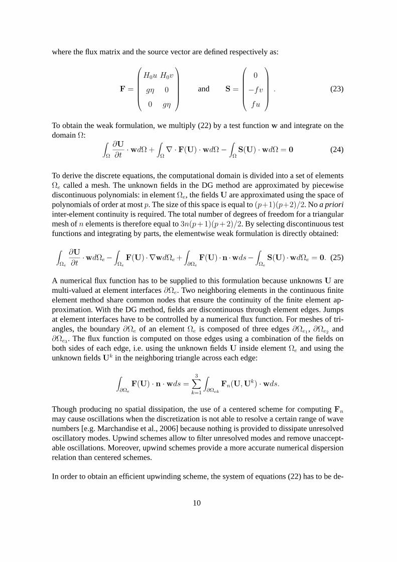
kx = 2, ky = 1 kx = 4, ky = 2 kx = 4, ky = 3 kx = 4, ky = 4

Fig. 11. Shape of some Poincare modes for a variable Coriolis coefficientwith β = 3 10−10 m−1s−1

andf0 = 3 10−4 s−1. Note that the shape of the modes in they-directions is now exactly the samethan for the Rossby modes.

kx = 2, ky = 1 kx = 2, ky = 2 kx = 2, ky = 3 kx = 2, ky = 4

Fig. 12. Shape of some Rossby modes withβ = 3 10−10 m−1s−1 andf0 = 3 10−4 s−1.

A least square fit of the dispersion error curves in the left part of Figure 10 shows that theerror is converging at rateO(kh)7, O(kh)9 andO(kh)11 for p = 2, 3 and4 respectively, i.e.a super convergence of order2p+3. Using the same fit, a super convergence of order2p+2is reached in the right part of Figure 10 for the dissipation errors. We see on those figuresthat the use of upwind fluxes introduces some numerical dissipation, but the resulting erroris very low for resolved modes and superconverges to zero.

Finally, the theoretical rates of convergence for DG with a Riemann solver and a 1D trans-port equation are also observed for the 2D shallow water equations with a constant Corioliscoefficientf .

18

0 1 2 3 4 5 6 7 8 9 100

5

10

15

20

25

30

k

ω

k1y

k2y k3

y

β = 0approximation

Fig. 13. Reference and numerical dispersion relations. The continuouslines are the exact Poincarédispersion relations for different values ofky, the dashed line is the analytical Kelvin dispersionrelation and the dots are the DG results. We see on the close up view the different dispersion curvesfor the three first wavenumberskn

y , n = 1, 2, 3, and the lack of accuracy of the constant Coriolisparameter approximation with those parameters, compared to the Sturm-Liouville approach.

Structured and unstructured meshes with variable Coriolisparameter

Let us now perform the same computation with a variable Coriolis parameter, i.e. with theβ-plane approximation andβ = 3 10−10 m−1s−1, on both structured and unstructured meshes.The analytical dispersion relation for the non-dispersiveKelvin waves (18) is still valid, butthe Sturm-Liouville approach has to be used in order to obtain a reference dispersion relation

19

j 1 2 3 4 5 6

ky,j 3.1331 6.3411 9.4651 12.5966 15.7321 18.8696

jπ/L 3.1416 6.2832 9.4248 12.5664 15.7080 18.8496Table 1Wavenumbersky,j of the Sturm-Liouville problem (9) compared to their approximationjπ/L.

for the Rossby and Poincaré waves. In table 1, we give some of the first exact eigenvaluesky,j computed with the Sturm-Liouville approach. These are compared with the approxi-mated wavenumberjπ/L. The frequenciesω are then obtained by using the relation (10).

The dispersion relations for Rossby and Poincaré are shown inFigure 13. Only the posi-tive part of the frequencies is considered, even if the two Poincaré waves lose their exactsymmetry because of theβ-effect. We see on the close up view the lack of accuracy of theapproximated analytical expression with those parameters. We may also point out that thesingle dispersion curve of the constant Coriolis case has been replaced by a set of dispersioncurves, one for everyky, since the wavenumbers are not the same in thex andy directions.It means that modes with very similar wavenumbersk may exhibit different frequencies.

−0.5 −0.4 −0.3 −0.2 −0.1 0 0.1 0.2 0.3 0.4 0.5−1.5

−1

−0.5

0

0.5

1

1.5

y

Yn(y)

Fig. 14. Shape of the first three eigenmodes in they directionY (y) computed with the one dimen-sional Sturm-Liouville problem (9) (continuous lines) and with the DG modal analysis (dots) forβ = 3 10−10 m−1s−1.

We see in Figures 11 and 12 the Poincaré and Rossby modes respectively. The Kelvin modesremain unchanged since they are not modified by the variability of the Coriolis parameter.As expected, the sines and cosines dependence of those modesin the y-direction with a

20

constant Coriolis coefficient has been replaced, leading to ageneraly-dependenceY (y)depending on the value ofβ. Note that both Rossby and Poincaré modes exhibits this samey-dependence for a same wave numberky. In Figure 14 we see those functionsY (y) forβ = 3 10−10 m−1s−1, computed with the one dimensional Sturm-Liouville problem (9) incontinuous lines while the dots represents the DG modal analysis.

Figures 15 presents the Poincaré Kelvin and Rossby dispersion and dissipation errors. Thesame theoretical convergence rates as for theβ = 0 case are obtained for the Poincaré andKelvin waves, for both dispersion and dissipation errors. The reference numerical dispersionrelation from the Sturm-Liouville approach was computed with a6000 points 1D continu-ous FEM. This solution is accurate enough, compared to the DGdispersion relation, until anabsolute error of about10−7. Below this threshold, the numerical accuracy of the referencesolution becomes insufficient as for the dispersion rate computation on the Rossby waveswith p = 4. For the other Rossby rates, the dispersion and dissipation errors do not seemto fit as well the theoretical predictions, an order2 seems to be missing. This result can beexplained as follows: in the analytical development [Ainsworth, 2004], Ainsworth has con-sidered a 1D transport equation with constant coefficients,leading to non dispersive waves.The first theoretical convergence rates obtained in this study were2p + 2 and2p + 1 forthe dispersion and dissipation respectively, in terms of relative errors. Those rates are thenextended to2p+3 and2p+2 for the absolute errors. This extension to absolute values is notvalid for the Rossby waves, since those waves experience a strong dispersive behaviour. Thecorrespondence between relative and absolute error is thenno more relevant. We observe onFigure 17 that the theoretical convergence rates are reached in terms of relative dispersionand dissipation errors, even for the dispersive Rossby waves. Notice that the relative dissi-pation error was computed by dividing the absolute error by the norm of the correspondingeigenvalue, since the analytical dissipation in the systemis zero. The theoretical conver-gence rate is then reached for the three shallow water waves,provided that the relative erroris considered instead of the absolute one in the case of strongly dispersive waves.

Finally, the same modal analysis provides in Figure 16 the Poincaré, Kelvin and Rossby dis-persion and dissipation errors for unstructured meshes. Inthose convergence plots, unstruc-tured meshes do not affect the DG method superconvergence rates obtained on structuredgrids. This general grid-independent modal analysis is thus a promising tool to comparedifferent numerical schemes in terms of dispersion and dissipation.

6 Conclusions

Starting from an implementation of the two-dimensional linearized shallow water with theDG method, we developed a modal analysis of the scheme by computing the eigenvalues andeigenvectors of the discretization of the space operators.Even if used with a DG scheme,this analysis is fully independent of the numerical scheme and of the mesh. It is a very use-

21

full tool to compare in an accurate way different numerical methods or to investigate someconvergence properties of one scheme and thus to help ranking numerical methods on thebasis of dissipation and dispersion errors.

Only periodic boundary conditions on the eastern and western boundaries were consideredin order to simplify algebra and to reduce the computationalcosts while keeping the threekind of waves in the system. The extension of this test case tonon periodic conditions isstraightforward and would not affect the efficiency of the method but the convergence studywould then become prohibitive in terms of computational costs, since we would have to per-form the convergences on several meshes instead of simply considering the wavenumbers.

The theoretical rates of convergence for the absolute dispersion and dissipation errors, es-tablished for the one dimensional transport equation, havebeen obtained for the two dimen-sional non dispersive Poincaré and Kelvin waves. The computation of the dispersion errorsfor dispersive waves required to compute a reference solution without the WKB approxi-mation, by means of the numerical resolution of a Sturm-Liouville problem. The theoreticalrates were also obtained for the very dispersive Rossby waves, provided that the rate com-putation is based on the relative errors. Note that in the framework of an ocean model whichaims to capture small scale processes, say between1 and25 km, the very large Rossby wave-lengths will always be resolved in a very accurate way. Moreover, the Rossby frequenciesare significantly different from zero and have to be resolvedonly for the smaller wavenum-bers. Because of its dissipation and dispersion properties,it is clear that the high-order DGmethod is a very accurate technique to simulate wave propagation, and is thus a good can-didate for ocean applications.

Acknowledgements

Paul-Emile Bernard is supported by theFonds pour la formation à la Recherche dansl’Industrie et dans l’Agriculture(FRIA, Belgium). Eric Deleersnijder is a Research asso-ciate with the Belgian National Fund for Scientific Research (FNRS). The present study wascarried out within the scope of the project “A second-generation model of the ocean system"funded by theCommunauté Française de Belgique, asActions de Recherche Concertées,under contract ARC 04/09-316. This work is a contribution to the SLIM 1 project.

1 SLIM, Second-Generation Louvain-la-Neuve Ice-ocean Model,www.climate.be/SLIM

22

References

S. Adjerid, K. D. Devine, J. E. Flaherty, and L. Krivodonova.A posteriori error estima-tion for discontinuous Galerkin solutions of hyperbolic problems.Computer Methods inApplied Mechanics and Engineering, 191:1097–1112, 2002.

M. Ainsworth. Dispersive and dissipative behavior of high order Discontinuous Galerkinfinite element methods.Journal of Computational Physics, 198(1):106–130, 2004.

F. Bassi and S. Rebay. A high-order accurate discontinuous finite element method for thenumerical solution of the compressible navier-stokes equations.Journal of ComputationalPhysics, 130:267–279, 1997a.

F. Bassi and S. Rebay. A high-order accurate discontinuous finite element solution of the 2dEuler equations.Journal of Computational Physics, 138:251–285, 1997b.

J.-M. Beckers and E. Deleersnijder. Stability of a fbtcs scheme applied to the propagationof shallow-water inertia-gravity waves on various space grids. Journal of ComputationalPhysics, 108:95–104, 1993.

P.-E. Bernard, N. Chevaugeon, V. Legat, E. Deleersnijder, andJ.-F. Remacle. High-order h-adaptive discontinuous Galerkin methods for ocean modeling. Ocean Dynamics (acceptedfor publication), 2006.

N. Chevaugeon, J.-F. Remacle, Gallez, P. Ploumans, and S. Caro.Efficient discontinuousgalerkin methods for solving acoustic problems. In11th AIAA/CEAS Aeroacoustics Con-ference, 2005.

B. Cockburn, G.E. Karniadakis, and C.-W. Shu.Discontinuous galerkin Methods. LectureNotes in Computational Science and Engineering. Springer Verlag, 2000.

M.B. Gavrilov and I.A. Tosic. Propagation of the rossby waveson two dimensional rectan-gular grids.Meteorology and Atmospheric Physics, 68:119–125, 1998.

D. Gottlieb and J. Hesthaven. Spectral methods for hyperbolic problems.Journal of Com-putational and Applied Mathematics, 128:83–131, 2001.

E. Hanert, D.Y. Le Roux, V. Legat, and E. Deleersnijder. Advection schemes for unstruc-tured grid ocean modelling.Ocean Modelling, 7:39–58, 2004.

F. Hu and H. Atkins. Eigensolution analysis of the Discontinuous Galerkin Method withNonuniform Grids i One Space Dimension.Journal of Computational Physics, 182(2):516–545, 2002.

F. Ihlenburg and I. Babuska. Finite element solution of the helmholtz equation with highwave number. part 2. the h-p version of the finite element method. SIAM Journal onNumerical Analysis, 34:315–358, 1997.

M. Iskandarani, D.B. Haidvogel, and J.P. Boyd. A staggered spectral element model withapplication to the oceanic shallow water equations.International Journal for NumericalMethods in Fluids, 20:393–414, 1995.

M.S. Longuet-Higgins. Planetary waves on a rotating sphere, ii. Proceedings of the RoyalSociety of London, 284:40–68, 1965.

A. Majda. Introduction to PDE’s and waves for the atmosphere and ocean. AmericanMathematical Society, 2003.

E. Marchandise, N. Chevaugeon, and J.-F. Remacle. Spatial andspectral superconvergenceof discontinuous galerkin method for hyperbolic problems.Journal of Computational andApplied Mathematics (accepted for publication), 2006.

23

F. Mesinger and A. Arakawa. Numerical methods used in athmospheric models.GlobalAtmospheric Research Programme (GARP) Publications Series No.17, 1, 1976.

J. Pietrzak, E. Deleersnijder, and J. Schroeter (Editors).The second international workshopon unstructured mesh numerical modelling of coastal, shelfand ocean flows (delft, thenetherlands, september 23-25, 2003).Ocean Modelling (special issue), 10:1–252, 2005.

J.-F. Remacle, X. Li, M.S. Shephard, and J.E. Flaherty. Anisotropic adaptive simulation oftransient flows using discontinuous galerkin methods.International Journal for Numeri-cal Methods in Engineering, 62(7):899–923, 2005.

L. Thompson and P. Pinsky. Complex wavenumber fourier analysis of the p-version finiteelement method.Computational Mechanics, 13:255–275, 1994.

T. Warburton and G.E. Karniadakis. A discontinuous galerkin method for the viscous mhdequations.Journal of Computational Physics, 152:608–641, 1999.

G. Wentzel. A generalization of quantum conditions for the purposes of wave mechanics.Zeits. F. Phys., pages 38–518, 1926.

24

100

101

10−6

10−4

10−2

100

101

10−8

10−6

10−4

100

101

102

10−10

10−5

100

100

101

10−6

10−4

10−2

100

101

10−8

10−6

10−4

100

101

102

10−10

10−5

100

Poincare

dispersion

Poincare

dissipation

6.5

8.6 11

5.6

7.5 9.5

Kelvin

dispersion

Kelvin

dissipation

7.4

9.3

10.7

6.5

8.1

9.3

Rossby

dispersion

Rossby

dissipation

4.8

6.3

5.7

3.7

5.37.8

k k

k k

k k

κ µ

κ µ

κ µ

Fig. 15. Convergence of the absolute dispersionκ and dissipationµ errors for the Poincaré, Kelvinand Rossby waves with a variable Coriolis coefficient. The second, third and fourth order elementscorrespond to the green, blue and red lines respectively. Both the dispersion and dissipation errorsexhibit the superconvergence of order2p + 3 and2p + 2 respectively for the Poincaré and Kelvinwaves. The rate computation for the dispersive Rossby waves has to be performed on relative errorsto reach the expected superconvergence.

25

100

101

10−6

10−4

10−2

100

101

10−8

10−6

10−4

100

101

102

10−10

10−5

100

100

101

10−6

10−4

10−2

100

101

10−8

10−6

10−4

100

101

102

10−10

10−5

100

Poincare

dispersion

Poincare

dissipation

6.7

8.9

11.1

5.8

7.79.5

Kelvin

dispersion

Kelvin

dissipation

7.1

9

10.6

6.8

8.7

9.7

Rossby

dispersion

Rossby

dissipation

5

6.8

3.8

5.8

7.4

k k

k k

k k

κ µ

κ µ

κ µ

Fig. 16. Convergence of the absolute dispersionκ and dissipationµ errors for the Poincaré, Kelvinand Rossby waves with a variable Coriolis coefficient on unstructured meshes. The second, third andfourth order elements correspond to the green, blue and red lines respectively. Both the dispersionand dissipation errors exhibit the superconvergence of order2p + 3 and2p + 2 respectively for thePoincaré and Kelvin waves, just as for the structured meshes. The rate computation for the dispersiveRossby waves has to be performed on relative errors to reach the expected superconvergence.

26

100

101

10−8

10−6

10−4

100

101

10−8

10−6

10−4

100

101

10−8

10−6

10−4

100

101

10−8

10−6

10−4

Absolute

dispersion

error

Relative

dispersion

error

5

6.8

6

7.6

Absolute

dissipation

error

Relative

dissipation

error

3.8

5.8 7.4

4.8

6.5 9.2

k k

µ µrel

κ κrel

Fig. 17. Comparison between convergence rates for the absolute (left) and the relative (right) dis-persion and dissipation errors for the Rossby waves on unstructured grids. The theoretical rates ofconvergence of2p + 2 and2p + 1 for the relative dispersion and dissipation errors respectively arereached for the Rossby wave. The rates of2p + 3 and2p + 2 for the absolute errors are not reachedsince the correspondence between absolute and relative errors are based on the assumption of a nondispersive wave and the Rossby waves precisely experience a strongdispersive behaviour.

27