Contribution of equatorial Pacific winds to southern tropical Indian Ocean Rossby waves

JOURNAL OF GEOPHYSICAL RESEARCH, VOL. 106, NO. C2, PAGES 2407-2422, FEBRUARY 15, 2001

Contribution of equatorial Pacific winds to southern tropical Indian Ocean Rossby waves

James T. Potemra •

International Pacific Research Center, School of Ocean and Earth Science and Technology, University of Hawaii at Manoa, Honolulu, Hawaii

Abstract. Westward propagating features, identified as Rossby waves, have been observed and modeled in the southern tropical Indian Ocean (STIO) between 10 ø and 30øS. These STIO Rossby waves, which have broad zonal and meridional extents, could interact with the westward flowing South Equatorial Current (SEC) as well as coastal currents on the south shore of Java (the South Java Current) and along the western shore of Australia (the Leeuwin Current). Previous work has attributed these waves to variations in wind stress along the west coast of Australia, Ekman pumping in the STIO interior, and a combination of both. This study investigates the importance of a third factor: remotely forced coastal Kelvin waves. Observations show that changes in wind stress curl in the eastern equatorial Pacific create annual upwelling and downwelling Rossby waves. Numerical model results confirm previous studies that demonstrate these waves, upon reaching the western boundary of the Pacific, create poleward propagating coastal Kelvin waves along the western shore of the Irian Jaya/Australia land mass. Direct observations of annual sea level variations along the northwest coast of Australia show a phase lag from the northernmost station to the southernmost that is not explained by direct wind forcing, suggesting that this signal is propagating from the Indonesian seas. It is shown in this work that when these waves reach the Indian Ocean, they are in phase with the local Ekman forcing and enhance the STIO Rossby waves. In the model the signal from the equatorial Pacific accounts for almost 80% of the energy of the STIO Rossby wave near the coast of Australia and 10% of the energy offshore.

1o Introduction

The large-scale circulation in the southern tropical Indian Ocean (STIO), shown schematically in Figure 1, is dominated by the South Equatorial Current (SEC) that flows from east to west between about 10 ø and 30øS (although the boundaries of this current are not exactly known). The SEC terminates at the western boundary and splits at Madagascar into the northward flowing Zanzibar Current (ZC) and the southward flowing Mozambique Current (MC) and East Madagascar Current (EMC). The origin of the SEC is the South In- dian Ocean Current (SIOC; also referred to as the East- ern Gyral Current (EGC)) that flows to the east just north of the Antarctic Circumpolar Current (ACC). As the SIOC approaches the west coast of Australia,

• Now at School of Oceanography, University of Washing- ton, Seattle, Washington.

Copyright 2001 by the American Geophysical Union.

Paper number 1999JC000031. 0148-0227/01 / 1999J C000031 $09.00

it turns northward to form the SEC. Along the coast, however, the flow is toward the pole, against the pre- vailing winds. This current, called the Leeuwin Current (LC), is thought to be driven by an alongshore pressure gradient that is established by a density gradient from the warm, fresh throughflow water [see, e.g., Church et al., 1989; Clarke, 1991; Godfrey a•d Weaver, 1991; Cresswell and Peterson, 1993].

The dominant variability in the STIO region on the annual timescale is due to westward propagating Rossby waves [e.g., P•rigaud and Delecluse, 1992; Morrow and Birol, 1998; Yang et al., 1998]. These Rossby waves are evident in both numerical models [Woodberry et al., 1989; Pdrigaud a•d Delecluse, 1992; Masumoto a•d Meyers, 1998] and remote observations [Pgrigaud and Delecluse, 1992; Yang et al., 1998; Masumoto and Mey- ers, 1998; Morrow and Birol, 1998]. The dynamics of these waves, particularly their forcing, and the effect of these waves on the large-scale circulation are still not clear.

Rossby waves in the STIO were first investigated by Woodberry et al. [1989] using a one-and-a-half-layer, reduced gravity model (forced by Hellerman and Rosen-

2407

2408 POTEMRA: EQUATORIAL PACIFIC CONTRIBUTION TO STIO ROSSBY WAVES

10N

EQ

10S

20S

30S

40S

40E 50E 60E 70E 80E 90E 100E 110E 120E 130E ß

Figure 1. Schematic representation of surface flows in the southern tropical Indian Ocean (STIO). Abbreviations for the western boundary currents are defined in the text.

stein [1983] climatological wind stress). The model produced annual Rossby waves, formed just to the east of 100øE (maximum signal from 20 ø to 15øS). It was postulated that variations in the Southern Hemisphere trade winds were the cause of these waves and the ef-

fects of these waves were seen in the transport of the SEC and in the currents off the west coast of Australia

[Woodberry et al., 1989]. It is important to note that the model used in this study did not include a Pacific basin, and the throughflow was included only as an open boundary cordition.

In a subsequent study, Pdrigaud and Delecluse [1992] used a one-and-one-half-layer reduced gravity model (forced by Florida State University (FSU) winds) to investigate Rossby waves in the STIO. Their model, which compared favorably with remote Geosat observations, showed upwelling Rossby waves in the eastern part of the basin during March through October (along 90øE). Minimum sea level variations of 12 cm (depar- ture from the long-term mean) were noted at 90øE during July. A downwelling wave was evident during the rest of the year, with peak sea level variations of 12 cm at 90øE during December. P6rigaud and Delecluse pointed out that the wind stress curl is weak in the interior of the basin, where the waves reach maximum amplitude (at 90øE), and suggested the waves are produced from coastal winds along the western shore of Australia and then propagate offshore. Again, similar to Woodberry et al. [1989], the model geometry only included the Indian Ocean.

Finally, STIO Rossby waves were the focus of a re- cent study by Masumoto and Meyers [1998]. They used

a multilevel, z coordinate model (forced with Heller- man and Rosenstein [1983] climatological wind stress) and compared the results to expendable bathythermo- graph (XBT) and TOPEX/Poseidon (T/P) data. They determined that STIO Rossby waves were largely forced in the eastern Indian Ocean by Ekman pumping along the wave characteristic but that Ekman pumping affected the signal throughout the ocean interior. While the model they used was global and therefore included remote Pacific effects, remote Pacific forcing was not specifically addressed.

The present study examines a new possibility that remotely forced Rossby waves in the equatorial Pa- cific contribute to STIO Rossby waves. Annual Rossby waves are formed in the equatorial Pacific from changes in Ekman pumping near the eastern boundary [Meyers, 1979; Lukas and Firing, 1985; Kessler, 1990]. When these Rossby waves reach the western boundary of the Pacific, they induce poleward propagating Kelvin waves along the west side of Irian Jaya and Australia. As these Kelvin waves travel along the western coast of Australia, they excite Rossby waves.

The idea of energy "leakage" from the Pacific to the Indian Ocean was first described by Clarke [1991]. In that study the effects of the gappy western boundary of the equatorial Pacific on large-scale wave reflection were theorized. Clarke [1991] determined that 10% of the energy flux that reaches the western equatorial Pacific due to propagating long Rossby waves makes it into the In- dian Ocean. Reflected equatorial Kelvin waves account for 34% of the energy flux, and the remainder gets dissipated in the boundary layers of the various islands that

POTEMRA: EQUATORIAL PACIFIC CONTRIBUTION TO STIO ROSSBY WAVES 2409

make up the westerr, boundary of the Pacific [Clarke, 1991].

Vetscheil •! al. [199•], as par• of a modeling study, showed numerically that a first-mode Rossby wave (generated in •he eastern equatorial Pacific) would provide energy to the Indian Ocean. In •he model a free Rossby wave impinged on the western boundary, and energy en- tered •he Indian Ocean (presumably by a coastal Kelvin wave), as is eviden• by upper layer thickness anomalies along •he northwes• Australian coast at 10øS.

Other studies have also demonstrated the importance of equatorial Pacific forcing on sea level variations on the northwest Australian coast [e.g., Clarke and Liu, 1994; Wajsowicz, 1996; Murtugudde et al., 1998]. All of these studies, however, focused on interannual variability. In addition, these studies were involved primarily with variations along the northwest coast of Australia and did not directly address the affect these variations would have on STIO Rossby waves.

Here the Pacific to Indian Ocean connection will be

investigated with respect to its effect on STIO Rossby waves. Since these waves have been observed annually (one upwelling and one downwelling wave per year), the present study will focus on monthly timescales, un- like the previous studies of the Pacific to Indian Ocean connection that focused on interannual variability (and therefore relatively low frequency Rossby waves).

The key issues that will be addressed include (1) Can sea level variability in the equatorial Pacific propagate to the Indian Ocean on annual timescales; (2) What is the phase relationship of the forcing in the equatorial Pacific and the observed STIO Rossby wave variations (Do remotely forced sea level variations act to enhance or diminish STIO Rossby waves); and (3) How much of the observed variability in STIO sea level is explained by remote Pacific forcing. A theoretical discussion aimed at the first issue is given in section 2 followed by some observational evidence and some results from large-scale general circulation models (GCMs) to address the second and third issues.

2. Theoretical Considerations

Previous studies of STIO Rossby waves have ne- glected remote effects from the Pacific; however, it has been shown that equatorial Rossby waves in the Pacific could provide energy to the Indian Ocean via coastal Kelvin waves. Clarke [1991] showed that when first- mode, long Rossby waves (interannual period) impinge on the western boundary of the Pacific, 10% of the energy makes it into the Indian Ocean. That work focused on the interannual waves that are created during E1 Nifio-Southern Oscillation (ENSO) events. As part of the derivation, a limit is placed on the horizontal scale and period of the wave_ Following Clarke [1991], it is assumed that motion is independent of the zonal extent of the western boundary region, Ax, which, through expansion, requires

kAx <<1. (1)

a,• where co is the fre- The wave number k is given by -•-, quency of the Rossby wave (-• years -• for the interannual waves described by Clarke [1991]) and c is the first baroclinic mode phase speed (given as 3 m s -• by Clarke [1991]). Ax represents the width of the Pacific boundary region, from Kalimantan to the Solomon Is- lands, and is approximately 4900 km). In the case of interannual Rossby waves, co is about 6.6 x 10 -8 s -•, and the left side of (1) is 0.16. Therefore low-frequency Pacific Rossby waves (periods of years) have motions mainly independent of x and leak some energy (10% by Clarke [1991]) into the Indian Ocean, and in fact, it has been shown that interannual variations in north-

west Australian sea level are correlated to variations in

the equatorial Pacific [e.g., Clarke and Liu, 1994; Waj- sowicz, 1996; Murtu#udde et al., 1998].

For higher frequencies, however, the left side of (1) is closer to 1. For example, at semiannual periods (co _ 2• days-•) kax is 1 13. Therefore it must first be 180

demonstrated that variations in sea level in the equatorial Pacific due to annual Rossby waves will propagate into the Indian Ocean as coastal waves.

Once these waves reach the west coast of Australia

and propagate southward, a high-frequency limit is placed on their ability to supply energy to the STIO region. Coastal Kelvin waves along an eastern boundary will generate offshore Rossby waves into the ocean interior only within certain latitudes (so-called turning latitudes; see, for example, McCreary and Kundu [1987]

50

40

(• 35 .e

•.• 30

-o 25

--J 20

:•- 15

lo

5

o

c = 2.62 m/s

0 30 60 90 120 150 180 210 240 270 300 330 360

Forcing Period (days)

Figure 2. Equation (2) was used to compute the critical latitude, given a certain periodic forcing and c. The solid line is for the first baroclinic mode (c - 2.62 m s -•), and the dashed line is for the second baroclinic mode (c = 1.07 m s -•). The curve shows, for example, for semiannual forcing, first mode coastal Kelvin waves will only generate offshore Rossby waves equatorward of 27 ø latitudeø

2410 POTEMRA: EQUATORIAL PACIFIC CONTRIBUTION TO STIO ROSSBY ¾VAVES

0.20

0.15 0.10

0.05

0.00

......... ! ......... ! ......... i ......... • .........

a

160E

10N

5N

EQ

lOS o.oo

170E 180 170w 160w 150w

.... o.•5 .... o.•o .... o.•5 .... o.•o Zonal Wind Stress along 170W (N/m2)

Figure 3. The idealized forcing for the rectangular basin model was purely zonal (periodic in time), centered at the equator, 170øW: (a) wind stress along the equator and (b) variations with latitude at 170 øW.

for a derivation). The turning latitude is determined as a function of frequency, given by

c

tan(0c)- 2coREart h (2) Again, co is the frequency of the wave, and c is the

phase speed. REart h is the radius of the Earth, and 0c is the critical latitude. When the latitude is equatorward of 0c, the wavenumber is real, and the waves are westward (offshore) propagating Rossby waves. Pole- ward of this latitude, the wavenumber is complex, and only coastal Kelvin waves are permitted. Figure 2 shows the critical latitude for values of co up to i year for two values of c (approximating the first and second baroclinic modes).

To demonstrate this limit, a simple reduced gravity model was run with idealized forcing. A rectangular

1ø by 1ø grid (• • ) representing 50 ø longitude and 60 ø latitude (from 30øS to 30øN) was used. To generate poleward propagating coastal Kelvin waves along the eastern boundary (as would be found along the west coast of Australia), the model was forced by zonal, periodic wind stress centered on the equator, 20 ø west of the eastern boundary (in the STIO case the coastal Kelvin waves would be formed as Pacific Rossby waves interact with the western boundary of the Pacific). The wind stress magnitude (shown in Figure 3) was tapered in both the zonal and meridional directions as follows:

x-xo y- yo

r• - Aosin(cot)exp - L• - Ly (3)

where

Ao= 0.2 N m•; co = 2•r/30 and 2•r/180 Xo 20 ø W of the boundary

(170øW for this example); Yo equator;

L•= 2 Ly;

The model's initial upper layer was set to 300 m thick and a density of 1024 kg m -3. The resulting first baroclinic mode phase speed c is 2.62 m s-•. The model was run with monthly and semiannual periodic forcing.

Figure 4 shows how the period of the forcing affects the solution. Periodic forcing was used to generate poleward propagating coastal Kelvin waves. The equatorially centered forcing actually creates westward equatorial Rossby waves as well as eastward propagating equatorial Kelvin waves. It is the latter that impinge on the eastern boundary and generate the coastal Kelvin waves.

Energy (per unit volume) was computed at each grid point (i,j) from

t=T

P v? ß P• = [ i,j -1 t' ,,,1 -It' i,j] At, (4) t--0

with the pressure P computed from the model upper layer thickness h as

- - ho). Pi,j c The initial upper thickness ho was 300 m, and the period T was 30 days for •he first experiment (Figure 4a) and 180 days for the second (Figure 4b). In each case, coastal Kelvin waves appear on the eastern boundary. Consistent with Figme 2, however, these coastal waves only shed energy into the basin interior within 5 ø of the equator for the case wi[h 30 day forcing. For lower- frequency coastal waves (180 day forcing), Rossby wave energy is evident within about 30 ø of the equator. The experiment by Versehell et al. [1995] was forced by an equatorial Pacific Rossby wave with a period of 20 days, which limited the amount of energy that would be generated in the midlatitude Indian Ocean.

3, Application to the STIO Region The theory outlined in section 2 is now applied to the

STIO region. Observations have shown the existence of long Rossby waves in the equatorial Pacific, formed by Ekman pumping near the eastern boundary [Meyers, 1979; Lukas and Firing, 1985; Kessler, 1990]. Further, P•rigaud and Delecluse [1992] showed, using remote ob-


3ON ............................................ •

25N

20N

15N

1ON

5N

EQ

5S

10S

(3

20S

15S

30S : w 80 17'5W 170W 1

11 ' 15SJ 20S 1 25S 1 ß

.........

2 4 6 8 10

150W

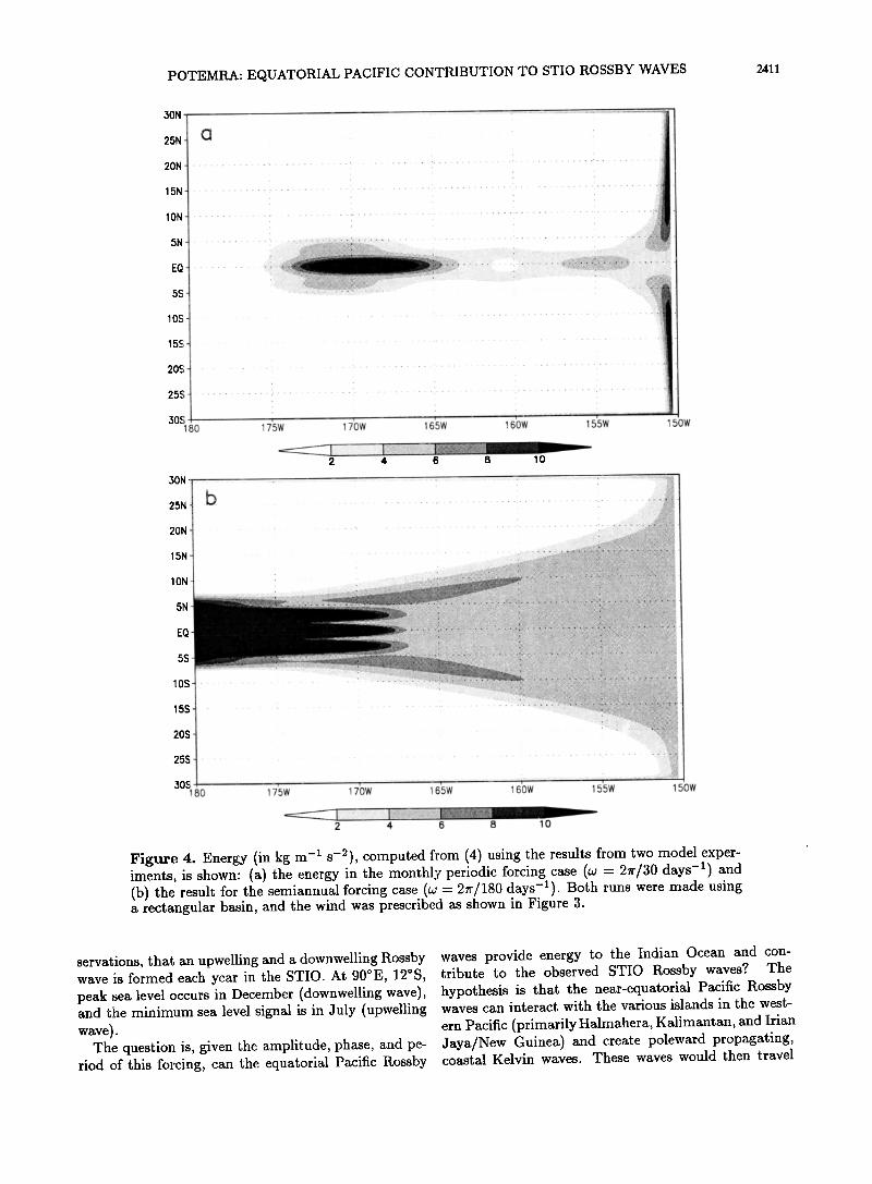
Figure 4. Energy (in kg m -1 s-a), computed kom (4) using the results from two model experiments, is •hown: (•) th• energy in th• monthly periodic forcing case (•o - 2•r/30 and (b) th• r•ult for th• semiannual forcing case (v• - 2•r/180 Uoth runs were made using a rectangular basin, and the wind was prescribed as shown in Figure 3.

setvarious, that an upwelling and a downwelling Rossby wave is formed each year in the STIO. At 90øE, 12øS, peak sea level occurs in December (downwelling wave), and the minimum sea level signal is in July (upwelling wave).

The question is, given •he amplitude, phase, and period of •his forcing, can the equatorial Pacific Rossby

waves provide energy to the Indian Ocean and contribute to the observed STIO Rossby waves7 The hypothesis is that the near-equatorial Pacific Rossby waves can interact with the various islands in the western Pacific (primarily Halmahera, Kalimantan, and Irian J aya/New Guinea) and create poleward propagating, coastal Kelvin waves. These waves would then travel


along the western shores of Irian Jaya and Australia into the Indian Ocean. The resulting sea level variations would then contribute to STIO Rossby waves.

As outlined above, the period of the forcing is critical to whether equatorial Pacific Rossby waves will provide energy (in the form of coastal Kelvin waves) to the In- dian Ocean and at what latitude these Kelvin waves will

generate Rossby waves (if at all). Further, the coastline configuration of the eastern boundary of the Indian Ocean plays a role. The Malay Archipelago stretches from west to east along 10øS (see Figure 1), thus plac- ing a northern boundary on STIO waves formed along the eastern boundary. As discussed previously, the period of the forcing in the eastern Pacific will determine the period of the coastal Kelvin waves and the critical latitude of Ross[;y wave formation. Thus, for waves with periods less than 60 days, the critical latitude is 10 ø within the equator, and the Lesser Sunda Islands prevent these waves from entering the Indian Ocean.

Finally, remotely formed coastal Kelvin waves along western Australia will be affected by local wind stress

(Ekman pumping). The relative phase of the local wind an('. the remotely forced waxres need to be compared to the phase of the observed STIO Rossby waves. In other words, given a certain phase to the Pacific forcing and a certain phase speed of the generated waves, the remotely forced coastal waves will either enhance or diminish locally forced sea level variations.

The approach taken here is to employ the same one- and-one-half-layer reduced gravity model described previously. Realistic boundaries are used, and both the Pacific a)•d l_ndian Ocean basins are included. To in-

vestigate propagation paths, the same simplified wind forcing is used (see (3)). Wind forcing of monthly, semiannual, annual, and 4 year periods was applied in a region in the eastern equatorial Pacific (see Figure 5). The model was run for 5 years to remove the initial response (15 years in the case of the 4 year period forcing), and results were computed from the final year of integration.

In the model the wind patch excites a westward Kelvin wave that reflects off the eastern boundary of

1

0.9

0.8

0.7

0.6

0.5

0.4

0.3

0.2

o. 1

o

-o.1

1

1•o 2•)o 2'•o 2•,o 2•io 2•o 300 1 2 5 4 5 6 7 8 9 lO 11 12

20N ' /(/ • • 15N .C 15N d ' '

5s 5s .

15S - • , - - - - 15S 20S 20S

I•OE 120E 140E 160E 180 160W 140W 120W 10bW 8dW 60W -0.1 0 0.1 0.2 0.3 0.4 0.5 0.6 0.7 0.8 0.9 1

Figure 5. The wind stress used to forced the idealized model experiments was purely zonal. At its peak, the wind stress attains 0.2 N m '-2. (a) The meridional modulation of the wind stress amplitude (in N m -2) along the equator. (b) The time-varying modulation of the wind stress amplitude for the four experiments: four-year, annual, semiannual, and monthly. (c) Wind stress amplitude (the 0.05 and 0.1 N m -2 levels are contoured). (d) The zonal modulation of the wind stress amplitude (in N m -2) along 140øW.


-15

-20 Jan

' x..,, / ,, ,'

X - ,' ,,• ,' -X• ', -' , •

_,,,' ,,,,

• / '• / ,,, Monthly • ,

--- Semiannual •, • Annual

•-- Combination (30+180+365 days) Four-year

.... i .... i .... i .... i .... i .... I .... I , , , i I .... i .... i .... i , , ,

Feb Mar Apr May Jun Jul Aug Sep Oct Nov Dec

Figure 6, Sea level deviations at 15øS, 115øE are shown for the five model experiments. The legend refers to the period of the wind forcing in the eastern Pacific. The wind forcing varies in time as shown in Figure 5.

the equatorial Pacific. The reflected first-mode Rossby wave (symmetric sea level deviations along 5øN and 5øS) takes about 5 months to reach the western boundary of the Pacific. The theoretical phase speed, ap- proximated as gx/•/3 for the equator, is 0.873 m s -•. Upon reaching the western boundary, a complex inter- action of wave reflection occurs between islands in the

Celebes Sea. The result is a coastal Kelvin wave that

propagates south along the west coast of Australia. The coastal Kelvin wave travels much faster than the Rossby wave and takes about 2 weeks to go from the equator to 25øS along the west coast of Australia, so the signal reaches the STIO about 180 days after the disturbance was forced in the eastern Pacific.

Figure 6 shows the model sea level deviations at 15øS, 115øE (in the eastern Indian Ocean). In the experiment when the winds vary with an annual period (again, only imposed in the eastern equatorial Pacific), STIO Rossby waves have their largest amplitude (9 cm). Semiannual forcing generates a somewhat smaller amplitude wave (6 cm), and the winds with a 4 year period produce STIO Rossby waves with a 3 cm amplitude. When the model was forced by winds with monthly, semiannual, and annual variability, the result is smaller-amplitude Rossby waves in the first part of the year (about 8 cm amplitude) when the semiannual and annual signals are out of phase and a larger amplitude (about 16 cm) later in the year when the annual and semiannual signals are in phase.

It appears from these rnodel results that annual forced equatorial Rossby waves in the Pacific can produce, via coastal Kelvin waves, Rossby waves in the STIO region. The next issue is the phase of these Rossby waves generated in the Pacific compared to the phase of those generated locally in the STIO region. To investigate this, the simple model was run with realistic seasonal wind stress of Hellerman and Rosenstein [1983].

The relatively simple reduced gravity model forced with realistic winds [Hellerman and Rosenstein, 1983] and realistic coastlines produces STIO Rossby waves similar to observations and more complex global models (this is presented in section 4). The maximum signal in the STIO region near Australia as seen in the T/P data is at about 15øS [Yang et al.• 1998]. For the model in this study the maximum is farther south. However, for the following analysis, comparisons will be made along 15øS in the STIO, unless otherwise noted.

Sea level was computed from the model upper layer thickness (long-term mean removed) along 15øS from the eastern Indian Ocean (90øE) to the west coast of Australia (120øE), and the results from three experiments will be discussed (see Figure 7).

For the baseline run (Figure 7d), when climatological wind forcing is applied, annual STIO Rossby waves are evident as high (in March through mid-August) and low (in August through April) sea level deviations along the Australian coast that propagate offshore. The peak values are at 110øE (8 cm in September and-8 cm in March).

Also shown in Figure 7 are sea level perturbations from two additional experiments. In the first experiment, the model was run with wind stress fixed to the mean December values everywhere from 10øS to 10øN. Seasonally varying winds were used everywhere outside the equatorial region. This was intended to eliminate the equatorial Pacific Rossby waves (i.e., to highlight just the locally forced component of the STIO waves). In the second experiment, seasonally varying winds were applied only in the equatorial Pacific (10øS-10øN, 135øE to the eastern boundary of the Pacific). December mean winds were applied everywhere else. In this way the model-produced STIO Rossby waves were purely a result of equatorial Pacific winds. Both results are compared with the baseline model results (seasonally varying wind everywhere) in Figure 7.

It should be noted that a more traditional method

of closing the throughflow to eliminate remote Pacific effects was not used here. By closing the throughflow the coastline of the Malay Archipelago gets connected to Australia/New Guinea. Coastal Kelvin waves generated in the Indian Ocean can propagate from Indonesia to Australia and then south along the coast. In reality the gap between Indonesia and Australia is too large for coastal waves to cross. Therefore a regional wind approach was chosen to isolate the effects of the equatorial Pacific from the higher-latitude STIO. Similarly, effects from the equatorial Indian Ocean are not considered for this study and are assumed to be small [see Poretara, 1•]o

The two experiments demonstrate that the model STIO signal is a superposition of remotely forced Pa- cific waves and locally forced waves. For the Hellerman and Rosenstein [1983] wind stress forcing and the model vertical parameterization (which results in a first baroclinic phase speed of 2.62 m s-•), the equatorial Pa- cific forcing produces high sea level along the model

Off-Eq Wind ß . .

ß .

FEB1 Q ' '

APR1

t,IAY1

JUN1

FEB1

MAR1 -• .............. ß

APR1

MAY1

JUN1

Eq-Pac Wind '- '•-='.'.•-s•:•'•' '•'.-•.:

.:

JUL1 :. - ß

ß

....

AUG1 ....

SEPI .......

OCT1

NOV1

0œCl .... 90E 9•E 96E 991[ 102E 105E tO8E 111E 114E ! 17E 1201[

--6 --4 --2 0

Off-Eq •ind plus Eq-Pac •ind

ß FEB1

APR1

MAY1

JUN1

JUL1

kU01

SEP1

OCT1

NOV1

DEC1

90œ 95[ 96œ 99œ 102œ 105œ 108œ 111œ 114œ 117œ 120œ

--6 --4 --2 0

dULl

AU01

SEP1

oc'rl

NOV1

DEC1

90E 93E •:6E 99E 102E 105E 108 E ..... 111E 114.E 117E 120E

-6 -4 -2 0

All Wind (Baseline)

Figure 7. Model sea level deviations (in centimeters) in the Indian Ocean along 15øS are contoured (negative values shaded). The model was forced with time-varying wind in specific regions' (a) the result when only off-equator wi•.•ds (outside 10øS-10øN) are allowed to vary, (b) the result when only equatorial Pacific winds (e•:tst of 135øE, 10øS-10øN) are allowed to vary, (c) the sum of the results of these two cases, and (d) the baseline model run (winds time-varying everywhere).

POTEMRA: EQUATORIAL PACIFIC CONTRIBUTION TO STIO ROSSBY ¾VAVES 2415

lOO

8o

• 60 o

20

Ind•n Oce• foming - - - Pacif• Ocean forcing

ß

0 , , , , I i , i 105E 110E 115E 120E

Figure 8. Energy was computed from the model velocity and upper layer thickness as the integral of (4) from 20 ø to 10 ø S. The solid line is the ratio (in percentage) of the off-equatorial wind case to the total, and the dashed line is the ratio of the equatorial Pacific wind case to the total.

eastern boundary (at 15øS) from early March through August. The maximum signal (7 cm) occurs right at the boundary in May. Lower than average sea level is from September through February, with a peak along the boundary in mid-November of-6 cm. The effects of local wind forcing (no equatorial winds) result in a maximum along the boundary from early May through October, almost 2 months after the Pacific signal, and the maximum signal is offshore at 110øE. This maximum (5 cm) is slightly less than that formed by the equatorial winds, and it does not occur right on the boundary. Negative sea level perturbations prevail the rest of the year along the coast, with a peak of-5 cm at 110øE.

When these results are added, the result is very similar to the baseline model run, with positive sea level perturbations at the coast from mid-March through mid- September and the maxima occurring offshore at 110øE. The sum of the two experiments does not exactly match the baseline run for several reasons, including nonlinear- ities in the model, equatorial Indian Ocean, and local Indonesian winds and coastal waves that may propagate entirely around Australia.

Figure 8 shows the relative contribution of each signal. Energy (per unit area) was computed as the integral of (4) from 20 ø to 10øS using the model results from the experiment with only Indian Ocean winds (locally forced waves) and from the experiment with equatorial Pacific winds. The relative energy f. crn each (compared to the sum of the two experiments) is given ir Figure 8. As stated, the Pacific effects have the largest effect at the coast, while the local forcing has a large effect in the interior (at 108 øE).

As a measure of energy, the model velocity and upper layer thickness fields were integrated over one forcing period (see (4)) for the four experiments (monthly, semiannual, annual, and 4 year forcing). The results, given in Figure 9, show how the maximum STIO Rossby wave energy is produced by the annual forcing. In the case of monthly forcing, almost all of the energy is along the eastern boundary of the Pacific in the fcrm of coastal Kelvin waves. Interestingly, in the semiannualy forced case, little energy is seen in the eastern Pacific because

of reflected waves canceling the forceJ waves (because of the location and period of the forcing). This, however, is beyond the scope of the present investigation.

4. Observational and Numerical Evidence

Section 3 demonstrated in a reduced gravity model that equatorially forced waves in the Pacific have a con- structive effect on STIO Rossby waves. The question remains whether this connection can be observed in the lyea] ocean.

Direct observations of the connection between the Pa-

cific and Indian Oceans is challenging, however, since the propagation speed is relatively fast while the dis- tance is short. First-mode coastal Kelvin waves that

start near the equator (along the west coast of Irian Jaya) would take less than 2 weeks to propagate to 25øS (assuming a phase speed of 3 m s-•).

The repeat orbit of the T/P satellite is not sufficient to discern this signal, but the apparent continuation of a signal from the Pacific to the Indian Ocean can be seen. Sea level deviations (long-term mean removed) from T/P are plotted along 15øS in the Indian Ocean (from 100 ø to 120øE) and then along 5øN in the Pacific from 120 ø to 160øE (see Figure 10). For comparison, sea level deviations from the model used in this study (referred to as the University of Hawaii Layered Model (UHLM)) and from two more complex GCMs (the Navy Layered Ocean Model (NLOM)[Walleraft, 1991], and the Parallel Ocean Ciimate Model (POCM) [$emtner and Chevyin, i 992] are also shown along the same lines).

The models have different grids (specifically, the def- inition of land points ;_s different in each), and sea level can only be computed from the models to a certain point offshore from the real coastline. The T/P data and the UHLM show high sea level along the Australian coast (at 15øS) during the first half of the year and low sea level during the second half, suggesting that the more simple UHLM is getting the correct phase of the STIO waves.

Propagation from the Pacific is also suggested in the remote observations and model results. Rossby waves in the Pacific are evident along 5øN, and the signal at the western boundary of the Pacific is in phase with the signal at 15øS at the eastern boundary of the Indian Ocean.

While the GCMs and altimeter agree and seem to suggest a link between the Pacific and Indian Oceans, the only direct in situ measurement comes from tide gauges. Daily measurements of sea level are available at five stations along the northwest shore of Australia (a map is given in Figure 11) from 1984-1996 (although some data are missing for the first 2 years at certain locations). Annual and semiannual harmonics were computed for the I0 year period 1987-1996 at each location. The sums of the two harmonics at each location

are given in Figure 11. There is an apparent phase lag between each station,


4 Year forcing

10N

•ø -•<•'•'•••i•i,i•i-•••i:-..i•':"':'""'•'"'i ................................. ............::.....•.:.•.:...•....:.::.:.:.....:..........•....:....::.:..•...:..:.. .................. '"'"'•'-'•:-:'• ....... • .... • -"--' . , .

20S T ....... •'-•"-'"•"'•"•'•"••'•••••••':• ..... • "'m ........................ • • t .............. •'""'"*""••-'•'•••••••;½•f X ................

100E 120E 140E 160E 180 160W 140W 120W 100W SOW 60W

3ON

20N

1ON

EQ

10S

20S

3OS

30N

20N

1ON

EQ

10S

20S

30S

30N

20N

1ON

EQ

10S

20S

50S

365 Day forcing

100E 120E 140E 160E 180 160W 140W 120W 100W 80W 60W

180 Day forcing

..:•..._,••'...i ...... :: ..... i ..... i..,•.. i i•',, : -•

_ .. !.::.-.. :. .. , .... .... .... ,.., ........ ..... 100E 120E 140E 160E 180 160W 140W 120W 100W 80W 60W

30 Day forcing

• - --•--•- '-- .-?•- -- -:-- -,-- - -j- -: .... : ........ ! ........ ! ........ '- - - ••':.-.:,.•.-.- ..... I

100E 120E 140E 160E 180 160W 140W 120W 100W 80W 60W

4 8 16 20

Figure 9. Energy (in kg m -• s-U; computed from (4) from four model experiments with different period forcing.

lO

11

12 100E

10

11

12 100E

110E 120E

TOPEX

, • •!i:•.-:.:i • :. j ::J.-'q'.:.-"-!.:i•i-':::-.-'.:•½! ....

•&-:•:...,,..--.-. E4•."'•?:t . .

., :- ;.•;...•,• ....

8' . _

150E 140E 150E

NLOY

13'OE 140E

160E

1

2

::.....-•.::-- :--6 :!:.....;:•? ..,. ? ..... , ""

4 , ',:':" .:'"';-;4..:•:- . •.•::::

.... -',:•?" 5 :.':;;•i'; !• ....

:.-' : :- .:;-{.--it::•:--

ß

6 !::->•"- - - ß {i'?•? ' s.:--.:• :.-:....•..-%: ;:'"i'L '•"::'•"

7 :½•:'""•}:':"::"'"':½h• ' •,. ,.:-. ,;t..•½:..-

':'::---';-- -•:•..•. "•.. ,.,•':•- :

9 :ii,- ...... .

10 - '

.... '-'½...'•'.i:':!:.",,

100E 110E 120E

10

11

'• 12 110E 120E 150E 160E 100E 110E 120E

UHL1/

130E 140E 150E 160E

-6 -4 -2 0

Figure 10. Sea level (long-term mean removed) is given (in centimeters) along 5øN in the Pacific and along 15øS in the Indian Ocean from: (a) TC PEX/Poseidon (computed as a climatology from 1993-1998); (b) the model used in this study;-(c) the NLOM; and (d) the POCM. Negative values are shaded.

2418 POTEMRA: EQUATORIAL PACIFIC CONTRIBUTION TO STIO ROSSBY VVAVES

90øE 100øE 110øE 120øE 130øE 140øE

5øN • 5øN .• -.•.

O

5'S

10øS

15øS

20øS

25øS ] 30øS .

90øE 100øE

•arw,

- .

,•:,r..'• e. " Port

Carnarv

ii

110øE 120øE 130øE

O

5'S

10øS

.. 15øS

20øS

25øS

.... 30øS 140øE

lO

5

õ o

' Darwin 15 Wyndham Broom '

.. -• Pt. Hedland / '% Carnarvon

• '. • x ••/- ..• --

--5 -lO

-15

--20 0 .... 3'0 60 Day of the year

Figure 11. Annual plus semiannual harmonics were computed-from daily in situ tide gauge records (for 1987-1996). The map shows the relative locations along the western coast of Aus- tralia.

again suggestive of a southward propagating feature. The annual cycle at Darwin shows maximum (minimum) sea level in late February (late July). At the next location (traveling south), Wyndham, the peak is in early March. Continuing south, the annual cycle maximum is early April for Broome and Port Hedland and early June for Carnarvon. The peak in the annual

,

cycle then appears to propagate at about 0.37 m s -z. Interestingly, the minima in the annual cycle propagates at a slightly faster speed, about 0.61 m s -z. Both are considerably slower than the predicted speed of a first- mode Kelvin wave but could be continental shelf waves

[Robinson, 1964; Mysak, 1967; Smith, 1972]. Nevertheless, there seenas to be a propagation of an-

nual sea level variability southward along the west coast of Australia that is in phase with the sea level variabil-

ity of the STIO Rossby waves. To determine if this is actually a propagating signal, or merely local wind forcing, local Ekman pumping was also examined.

Ekman pumping driven by alongshore winds will also create changes in sea level along the coast, and it is important to determine what the local wind effects are to separate them from the freely propagating wave (e.g., the apparent propagation of the signal from Darwin. to Carnarvon may be explained in part by a propagation of the alongshore winds).

To investigate the local wind effects, daily wind data were obtained at each tide gauge location for 1993 (from the NCEP reanalysis). The annual cycle from the tide gauges during 1993 is similar to the annual cycle from 1984 through 1996 (compare Figures 11 and 12). Ap- proximating the slope of the shoreline, the NCEP wind


20 [__ D•rv•n 5 õ o o

-40 "•'" •'" • .... •'" •"' •"' ''" •" '-• -10 4O

2O

E 0

-20

-40

40

20

E 0

-20

-40

40

20

E 0

-20

-40

I_, , , i , ,[•,1 , , , i , , , i , , , i , , , i ,W-rl , , , i , , , i , , , i , , , i , , ,

F,,,I,,,I,,,I,,,i,,,I,,,I,,,I,,,I,,,I,,,I,,,

! •;•'o;'e'"'""'"""'""'"'"' "'""• I-,,, I,•,1 •,,1,,, I,,,I,,,I

•,•''' I'''1' '' I''' I'' ' I'''1''' I' '' I ' '' I ''' I''' I'' '-I

Hedland • ,

40 L'''!'''I'''I'''!'''I'''I'''I'''I'''t'''I'''I'''J

20 •- Carnarvon • •.'1.

l --40 •,,,•,,,I,,,I,,,I,,,I,,,I,,,I,,,I,,,I,,,I,,,1•'1

Jan Feb Mar Apr May Jun Jul Aug Sep Oct Nov Dec

1

lO

5

o

-5

-lO

LCarnawon . /

o b / i II,rl/llt[.11111111-[I i1111, 0 . ,! , Jan Feb Mar Apr May Jun Jul Aug Sep Oct Nov Dec

Figure 12. (left) The 1993 sea level deviations (in centimeters) a; five locations and (right) alongshore wind speed (in m s -•) from the sat' •e locations (from the National Centers for Evi- tonmental Prediction (NCEP)). The wind spee(l is plotted such that positive is alongshore with the coast on the left (downwelling favorable). The annual and semiannual harmonics are shown with the heavy line.

speeds were converted to alongshore and offshore com- ponents. The alongshore component, along with the tide gauge data, is shown in Figure 12. The annual cycle (annual and semiannual harmonics) is also given.

There is an apparent propagation of the alongshore wind speed (excluding the record at Broome). Down- welling favorable winds occur at Darwin and Wynd- ham almost simultaneously, with a peak in early June. Three weeks later the peak occurs at Port Hedland, and 2 weeks after that (mid-July) the peak downwelling occurs at Carnarvon. The propagation of the annual cycle in alongshore wind speed (time of maximum downwelling) is about 1.0 m s -• when the data at Broome are not included (0.93 otherwise). Similar to the tide gauge data, the apparent propagation of the time of maximum upwelling is faster at about 3.7 m s -•.

Figure 13 shows the extrema in the annual cycle of sea level and alongshore wind speed (from Figure 12). The apparent phase speed of the downwelling signal is

0.37 m s -z , and it is 0.61 m s -1 for the upwelling signal. It is perhaps interesting that the alongshore winds are not in the same sense as the tide gauge sea level. The tide gauges record positive sea level deviations early in the year and negative in the middle and end of the year. The alongshore wind speed indicates the beginning of the year (with the exception of Broome) to be upwelling favorable (low sea level) and the middle of the year to be downwelling favorable (high sea level).

,5. Discussion

Theoretical constraints place an upper and lower frequency limit on waves that can propagate from the equatorial Pacific through the Indonesian seas and into the interior Indian Ocean as Rossby waves. Interannual Rossby waves in the Pacific (such as those generated during ENSO events) mostly get reflected at the western boundary. Higher-frequency Rossby waves form

2420 POTEMRA' EQUATORIAL PACIFIC CONTRIBUTION TO STIO ROSSBY WAVES

Darwin

s00 I I

I I

I I - -"-I' o- el,

I . .................... ......... 35oo 0 Max sea level -

r• Min sea level

• • Max along-shore wind (downwelling)

4000 t ..... , .... l.,Mir•,alqng•-sho, re wind,(up•eliing), • ..... • ..... , ..... Jan 1 Feb 1 Mar 1 Apr 1 May 1 Jun 1 Jul 1 Aug 1 Sep 1

1000

1500

2000

2500

3000

Wyndham

Broome

PT Hedland

Carnarvon

Figure 13. The maxima in the annual cycle of sea level deviations and alongshore winds (from 1993; see Figure 12) are shown. The alongshore location is given at the right. The time of maximum sea level deviations (downwelling wi.tds) is given with the squares, and the time of minimum sea level dev;_ations (upwelling winds) is given with the circles (the symbols are solid ibr wind speed). Note that the winds at Broome are out of phase with the other locations and were not taken into account for the linear regression fit. Also, the winds at Carnarvon are upwelling favorable all year, so the solid circle at, this location represents the time when the upwelling winds are weakest.

coastal Kelvin waves in the Indonesian seas. In the

model geometry these coastal Kelvin waves propagate counterclockwise around Australia (until dissipated by friction). If the frequency is too high, offshore Rossby wave solutions are not permitted. For typical stratification, Rossby waves are limited to within 27 ø of the equator when the forcing is semiannual and to within 10 ø of the equator when the forcing has a 60 day period. The

1 Indonesian archipelago stretches roughly west to east along 10øS, thus blocking the Rossby waves generated by higher frequencies. Forcing within these two ranges, i.e., of order several months to a year, will leak energy into the Indian Ocean and generate offshore Rossby waves.

Numerical model experiments show that STIO Rossby wave solutions are possible for annual forcing in the Pa- cific. In the model this remote forcing accounts for a sig- nificant fraction (up to 80%) of the STIO Rossby wave, particularly near the coast. Since forcing in the Pacific, in a climatological sense, produces sea level changes along the northwest coast of Australia that are in phase with the local STIO Ekman pumping, it is hypothesized

that the equatorial Pacific winds act to enhance STIO Rossby waves and that this adds a third factor (along with local coastal wind fluctuations and Ekman pumping in the STIO interior) to be considered in the forcing of STIO Rossby waves.

Forcing in the Pacific, in a climatological sense, produces sea level changes along the northwest coast of Australia that are in phase with the local STIO Ekman pumping. It is therefore hypothesized that the equatorial Pacific winds act to enhance STIO Rossby waves.

Observational evidence of wave propagation from the Pacific to the Indian Ocean is not available. The typical sampling frequency of altimeters is too low to capture the coastal waves (which take about 2 weeks to propagate from the equator to 25øS off the west coast of Australia). Tide gauge data, available at five locations along the west coast of Australia, does show a propagating feature that is not fully explained by changes in alongshore winds.

Phase differences in the tide gauge records along the northwest coast of Australia support the idea that a signal is propagating from north to south along the coast.


This phase difference in the sea level record was discussed by Godfrey and Golding [1981]. Godfrey and Ridgway [1985] also discuss this propagating signal as originating in the Indonesian seas. They explain that the signal at Darwin could originate from upwelling in the Banda and Arafura Seas during the northwest mon- soon, which is maximum in February and March.

The observed phase speed is lower than a first-mode coastal Kelvin wave. While the simple reduced gravity model can only support. this type of wave, this region could support a continental shelf wave [e.g., Mysak, 1967• Mysak, 1968a; 1968b]o These were first observed in this region by Hamon [1966]. The phase speed for a shelf wave depends, among other things, on the slope and width of the shelf. Hamon [1966] got a phase speed close to the first-mode Kelvin wave but used data from the southwestern and eastern coasts where the shelf is much more narrow. On the northwestern coast the shelf

extends for a over 100 km, and the phase speed for shelf waves is inversely related to the shelf width. The model, however, does not resolve the shelf, and the only allow- able solution is the Kelvin wave. The exact mechanism, however, is for future studies. In any case the observed annual sea level variability propagates south and is in phase with the STIO Rossby waves.

The change in phase speed from 0.4 m s -• for the downwelling wave (in February through May) to 0.6 m s -1 for the upwelling wave (in mid-July through September) is also interesting. This could be explained by a seasonal change in the stratification off the northwest Australian shelf. The slow downwelling signal occurs in mid-February (at Darwin) to late May (at Carnarvon). During this time the density gradient setup by the flow from the Indonesian seas is weak (maximum throughflow occurs in northern summer). Levitus data [Levitus, 1982] show a gradient of 1.5 kg m -3 between the surface waters at Darwin and Carnar-

yon in November and about 0.6 kg m -3 in March. In addition, the mixed layer deepens from a minimum in January through March to a maximum in June. The relatively shallow mixed layer early in the year could also cause the wave to slow.

More observations, particularly higher temporal res- olution data, are required to explain fully the coastal signal off northwest Australia. Nevertheless, the observations and model experiments suggest that energy does propagate from the Pacific to the Indian Ocean and that this represents an important consideration for the formation of STIO Rossby waves.

Acknowledgments. The author most gratefully ac- knowledges the assistance of Dennis Moore, Mark Merrifield, and Bo Qiu for many helpful discussions and comments to the draft. Jay McCreary and the rest of the IPRC staff were instrumental throughout this research effort. The tide gauge data were provided by the Pacific Sea Level Center at the University of Hawaii. Funding was provided by JAM- STEC grant 434957 and NSF grant OCE 9819511. The International Pacific Research Center is partly sponsored

by Frontier Research System for Global Change. SOEST contribution number 5269 and IPRC contribution number IPRC-60.

References

Church, J. A., G. R. Cresswe]I, and J. S. Godfrey, The Leeuwin Current, in Poleward Flows Along Eastern Ocean Boundaries, edited by S. Neshyba, N. K. Mooers, and R. L. Smith, pp. 230-252, Springer Verlag, New York, 1989.

Clarke, A. J., On the reflection and transmission of low- frequency energy at the irregular western Pacific Ocean boundary, J. Geophys. Res., 96, 3289-3305, 1991.

Clarke, A. J., and X. Liu, Interannual sea level in the noy:,n- ern and eastern Indian Ocean, J. Phys. Oceanogr., 24, 1224-1235, 19940

Cresswell, G. R., The Leeuwin Current, J. R. Soc. West. Aust., 74, 1-14, 1991.

Cresswell, G. R., and J. L. Peterson, The Leeuwin Current south of western Australia, Y. Aust. Mar. Fresh. Res., 4{4{, 285-303, 1993.

Godfrey, J. S., and T. J. Golding, The sverdmp relation in the Indian Ocean and the effect of Pacific-Indian Ocean

tkroughfiow on Indian Ocean circulation and on the East Australian Current, J. Phys. Oceanogr., 11, 771-779, 1981.

Godfrey, J. S., and K. R. Ridgway, The large-scale envi- ronment of the poleward-flowing Leeuwin Current, western Australia: Longshore steric height gradients, wind stresses and geostrophic flow, J. Phys. Oceanogr., 15, 481-495, 19850

Godfrey, J. S., and A. J. Weaver, Is the Leeuwin Current driven by Pacific heating and winds?, Prog. Oceanogr., 27, 225-272, 1991.

Hamon, B V., Continental shelf waves and the effects of at- mospheric pressure and wind stress on sea level, J. Geo- phys. Res., 71, 2883-2893, 1966.

Hellerman, S., and M. Rosenstein, Normal monthly wind stress over the world ocean with error estimates, J. Phys. Oceanogr., lo ø, 1093-1104, 1983.

Kessler, W. S., Observations of long Rossby waves in the northern tropical Pacific, J. Geophys. Res., 95, 5183-5217, 1990.

Levitus, S., Climatological atlas of the world ocean, NOAA Prof. Pap. lo ø, 173 pp., Natl. Oceanic and Atmos. Ad- min., Silver Spring, Md., 1982.

Luk_as, R., and E. Firing, The annual Rossby wave in the central equatorial Pacific Ocean, J. Phys. Oceanogr., 15, 55-67, 1985.

Masumoto, Y., and G. Meyers, Forced Rossby waves in the southern tropical Indian Ocean, J. Geophys. Res., 103, 27,589-27,602, 1998.

McCreary, J., and P. Kundu, Thermohaline forcing of eastern boundary currents with application to the circulation off the west coast of Australia, J. Mar. Res., d•6, 25-58, 1987.

Meyers, G., On the am•ual Rossby wave in the tropical North Pacific, J. Phys. Oceanogr., 9, 663-674, 1979.

Morrow, R., and F. Birol, Variability in the southeast In- dian Ocean from altimetry: Forcing mechanisms for the Leeuwin Current, J. Geophys. Res., 103, i•.529-18,544, 1998.

Murtugudde, R., A. J. Busalacchi, and J. Beauchamp, Sea- sonal to interannual effect• of the Indonesian Throughflow on the tropical Indo-Fa::f,c basin, J. Geophys. Res., 10o ø, 21,425-21,441, 1998.

Mysak, L. A., On the theory of continental shell' waves, J. .,i4cr. Res., 25, 205-227, 1967.

2422 POTEMRA: EQUATORIAL PACIFIC CONTRIBUTION TO STiO ROSSBY WAVES

Mysak, L. A., Edgewaves on a gently sloping continental shelf of finite width, J. Mar. Res., 26, 24-33, 1968a.

Mysak, L. A., Effects of deep-sea stratification and current on edgewaves, J. Mar. Res., 26, 34-42, 1968b.

P6rigaud, C., and Po Delecluse, Annual sea level variations in the southern tropical Indian Ocean from GEOSAT and shallow-water simulations, Jo Geophys. Res., 97, 20,169- 20,178, 1992•

Potemra, Jo T., Seasonal variations of the Pacific to Indian Ocean tluoughfiow, J. Phys. Oceanogr., 29, 2930-2944, 1999.

Robinson, A. R., Continental shelf waves and the response of sea level to weather systems, J. Geophys. Res., 69, 367-368, 1964.

Semtner, A. J., and R. M. Chervin, Ocean general circulation from a global eddy-resolving model, J. Geophys. Res., 97, 5493-5550, 1992.

Smith, R., Nonlinear Kelvin and continental-shelf waves,J. Fluid Mech., 52, 379-391, 1972.

Verschell, M. A., J. C. Kindle, and J. J. O'Bricn, Effects of Indo-Pacific throughflow on the upper tropical Pacific and Indian Oceans, Jo Geophys. Res., 100, 18,409-18,420, 1995o

Wajsowicz, R. C., The response of the Indo-Pacific throughflow to interannual variations in the Pacific wind siress, part II, Realistic geometry and ECMWF wind stress anomalies for 1985-89, J. Phys. Oceanogr., 26, 2589-2610, 19960

Wallcraft, A. J., The navy layered ocean model user's guide, NOARL Rep. 35, 21 pp., Stennis Space Center, Miss., 19910

Woodberry, K. E., M. E. Luther, and J. J. O'Brien, The wind-driven circulation in the southern tropical Indian Ocean, Jo Geophyso Res., 9J, 17,985-18,002, 1989.

¾ang, Jo, Lo Yu, Co Koblinsky, and D. Adamec, Dynam- ics of the seasonal variations in the Indian Ocean from

TOPEX/Poseidon sea surface height and an ocean model, Geophyso Res. Left., 25, 1915-1918, 1998.

J. T. Potemra, School of Oceanography, Univer- sity of Washington, Box 357940, Seattle, WA 98195. (jimp@ o c ean. washingt on. edu)

(Received August 2, 1999; revised September 19, 2000; accepted October 13, 2000.)

Contribution of equatorial Pacific winds to southern tropical Indian Ocean Rossby waves

Documents

Transcript of Contribution of equatorial Pacific winds to southern tropical Indian Ocean Rossby waves