A new approximation for the dynamics of topographic Rossby waves

A new approximation for the dynamics of topographic

Rossby waves

By YOSEF ASHKENAZY1*, NATHAN PALDOR2 and YAIR ZARMI1, 1Solar Energy and

Environmental Physics, BIDR, Ben-Gurion University, Midreshet Ben-Gurion 84990, Israel; 2Institute of Earth

Sciences, The Hebrew University of Jerusalem, Jerusalem 91904, Israel

(Manuscript received 14 September 2011; in final form 7 March 2012)

ABSTRACT

A new theory of non-harmonic topographic Rossby waves over a slowly varying bottom depth of arbitrary,

1-D, profile is developed based on the linearised shallow water equations on the f-plane. The theory yields

explicit approximate expressions for the phase speed and non-harmonic cross-slope structure of waves.

Analytical expressions are derived in both Cartesian and Polar coordinates by letting the frequency vary in the

cross-shelf direction and are verified by comparing them with the numerical results obtained by running an

ocean general circulation model (the MITgcm). The proposed approximation may be suitable for studying

open ocean and coastal shelf wave dynamics.

Keywords: topographic waves, perturbation method, lake dynamics, linearised shallow water equations, polar

coordinates

1. Introduction

Variations in bottom topography may result in second-class

(low-frequency) waves, similar to planetary Rossby waves

(e.g. Rhines, 1969a,b, 1989; Csanady, 1982; Pedlosky,

2003). The similarity between the two wave types becomes

evident upon considering the general case in which pot-

ential vorticity varies with both the Coriolis parameter and

water depth. Due to this similarity, rotating tank experi-

ments with varying bottom topography are often used

in the study of many aspects of the two types of (Rossby)

waves. The potential vorticity considerations make it

clear that in the Northern Hemisphere, shallower depths

correspond to higher latitudes and thus topographic

Rossby waves propagate with the shallower depths on their

right, similar to the westward propagation of planetary

Rossby waves under the influence of varying Coriolis

parameter.

Topographic Rossby waves are of great importance in

coastal ocean and lake dynamics. There are numerous

observational indications for their existence (e.g. Csanady,

1973, 1976; Saylor et al., 1980; Raudsepp et al., 2003), and

their unique dynamics have provided explanation of

observed features throughout the world ocean (e.g. Ball,

1963, 1965; Shilo et al., 2007, 2008). Most theories of

topographic Rossby waves have concentrated on a parti-

cular depth profile (mostly linear and rarely quadratic or

exponential) that are amenable to analytical solutions,

while general depth profiles received little attention. Here,

we propose a simple approximation for topographic wave

dynamics in an arbitrary bottom profile in one direction,

assuming only that the bottom topography is slowly

varying. With this approximation it is possible to estimate

the evolution of an initial perturbation, even when the

eigenstates of the system are not known. The approxima-

tion may be used to study more general coastal, and open

ocean, topographic wave dynamics.

The paper is organised as follows: in Section 2.1, we

develop the new approximation in Cartesian coordinates

and then compare the analytical approximation to numer-

ical simulation results obtained by the MITgcm (Section

2.2). In Section 3, we propose a similar approximation for a

polar (cylindrical) coordinate system and a similar compar-

ison to the numerical simulation. We conclude the study

with a short discussion in Section 4.*Corresponding author.

email: [email protected]

Tellus A 2012. # 2012 Y. Ashkenazy et al. This is an Open Access article distributed under the terms of the Creative Commons Attribution-Noncommercial 3.0

Unported License (http://creativecommons.org/licenses/by-nc/3.0/), permitting all non-commercial use, distribution, and reproduction in any medium, provided

the original work is properly cited.

1

Citation: Tellus A 2012, 64, 18160, DOI: 10.3402/tellusa.v64i0.18160

P U B L I S H E D B Y T H E I N T E R N A T I O N A L M E T E O R O L O G I C A L I N S T I T U T E I N S T O C K H O L M

SERIES ADYNAMICMETEOROLOGYAND OCEANOGRAPHY

(page number not for citation purpose)

http://www.tellusa.net/index.php/tellusa/article/view/18160

2. A new approximation for topographic Rossby

waves in a channel

2.1. Analytical approximation

2.1.1. Zero-order approximation. We start from the

linearised shallow water equations (LSWEs) in a channel

of varying depth H0 � bðyÞ (see Fig. 1) on the f-plane (see

Gill, 1982):

@u

@t� f0v ¼ �g

@g

@x(1)

@v

@tþ f0u ¼ �g

@g

@y(2)

@g

@tþ ½H0 � bðyÞ� @u

@xþ @v

@y

� �� v

db

dy¼ 0; (3)

where u and v are the zonal and meridional velocities, h is

the free surface, f0 is the Coriolis parameter, g is the

gravitation constant, H0 is the unperturbed mean water

level and b(y) is the (arbitrary) bottom topography profile.

We will see below that, in order to be handled by our

proposed perturbation expansion, b(y) has to be slowly

varying. We assume periodic boundary conditions in the

zonal direction and vanishing meridional velocity at the

zonally aligned channel walls. We note that an alternative

setting is a channel that is bounded by a wall along the

y direction, where the zonal velocity has to vanish. How-

ever, such a setting may result in reflecting topographic

waves and fast Kelvin waves that propagate along one of

the walls of the channel, which complicates the analytical

and numerical treatment.

By differentiating eqs. (1) and (2) with respect to t, it is

possible to express the zonal and meridional velocities, u, v,

as functions of h:

<u ¼ � g

f0

1

f0

@xt þ @y

!g; (4)

<v ¼ g

f0

� 1

f0

@yt þ @x

!g; (5)

where the operator < is defined by:

< ¼ 1þ 1

f 20

@tt: (6)

It is possible to obtain a single equation for h by

multiplying eq. (3) by < and using eqs. (4) and (5):

@t �g

f 20

ðH0 � bÞ@xxt �g

f0

b0@x

(

þ 1

f 20

@t @tt � gðH0 � bÞ@yy þ gb0@y

h i)g ¼ 0;

(7)

where b0 ¼ db=dy. This equation is equivalent to eqs.

(1)�(3) and is similar to the one derived in Pedlosky

(2003). Gill (1982) developed an equation similar to eq. 7,

but this equation is not applicable in our case, since the

underlying assumption in its development was the rigid lid

approximation, in which h is time-independent.

We non-dimensionalise the equation by scaling the

variables as follows: x ¼ ðffiffiffiffiffiffiffiffiffigH0

p=f0Þx, y ¼

ffiffiffiffiffiffiffiffiffigH0

p=f0a

� �y,

t ¼ t=ðaf0Þ and b ¼ H0b, where the ‘hat’ indicates non-

dimensional variables andffiffiffiffiffiffiffiffiffigH0

p=f0 is the Rossby radius of

deformation. To complete the scaling, we also use g ¼ H0g,although this scaling is not necessary for the mathematical

treatment presented below. a is a parameter that charac-

terises the bottom slope and can be chosen to be the

maximum of jb?(y)j. Note that the proposed scaling is

invalid in the absence of bottom slope, in which case one

expects to find only Kelvin and Poincare waves. a is a small

parameter and thus the above scaling of y and t implies

‘shrinking’ of these variables; this indicates that the under-

lying assumption of this scaling is long meridional wave-

length (either compared with the zonal wavelength or

compared with the Rossby radius of deformation) and

slow wave frequency (compared with f0). The idea behind

the different scaling of the zonal and meridional coordi-

nates is the asymmetry of the system, in which the bottom

topography is constant in x but varies with y. As it is well

known and consistent with the numerical results presented

below, topographic waves propagate mainly along isobaths

and hardly across bathymetry lines.

For convenience, we now drop the ‘hat’ sign and,

unless indicated, the variables are non-dimensional.

Fig. 1. Linear (solid) and quadratic (dashed) topographies used

for the simulation of topographic Rossby waves. Both profiles

span the same height variation over the same latitudinal extent.

Here, H0�170m.

2 Y. ASHKENAZY ET AL.

Under the above scaling, the non-dimensional form of

eq. (7) is:

n@t � ð1� bÞ@xxt � b0@x

þ e@t @tt � ð1� bÞ@yy þ b0@y

h iog ¼ 0;

(8)

where:

e ¼ a2: (9)

The high-order time derivative (fast waves) and the

derivatives with respect to y (short meridional waves)

are multiplied by o, in accordance with the rational behind

the above scaling as explained earlier. If one also assumes,

in addition, that the zonal wavelength is also long, then

the second term in eq. (8) is also smaller than the first

and third terms by order o, which leads at zeroth-

order approximation, to an equation equivalent to the

planetary geostrophy equation (e.g. Primeau, 2002; Vallis,

2006).

Next, we assume that the solution to eq. (8) is of the

form:

gðx; y; tÞ ¼ ~gðy; tÞeikx: (10)

Equation (8) then becomes:

@t þ ixðyÞ � exðyÞkb0

@t @tt � ð1� bÞ@yy þ b0@y

h i� �~g ¼ 0; (11)

where xðyÞ is defined as:

xðyÞ ¼ � kb0

1þ ð1� bÞk2: (12)

We will shortly show that v is associated with the

zeroth-order approximation of the frequency of the

waves.

To allow for a perturbation series expansion, ~g is

assumed to be of the form:

~gðy; tÞ ¼ �gðyÞei½X0ðy;tÞþeX1ðy;tÞþe2X2ðy;tÞþ��: (13)

[An expansion of �gðyÞ itself instead of the expansion in the

exponential yields equivalent results.] The zeroth-order

approximation (in o) is obtained by using eq. (13) in eq.

(11), leading to the following differential equation for

X0ðy; tÞ:

@tX0 þ x ¼ 0; (14)

so that:

X0ðy; tÞ ¼ �xðyÞt: (15)

It is thus clear that v(y) may be regarded as the zeroth-

order frequency. The zeroth-order approximation for the

free surface g0ðx; y; tÞ is thus:

g0ðx; y; tÞ ¼ �gðyÞei½kx�xðyÞt�; (16)

where �gðyÞ is an arbitrary function that should be selected

so as to guarantee that the meridional velocity vanishes at

the channel walls. We note, however, that since the

underlying assumption is that the y-derivatives are small,

�gðyÞ is a slowly varying function. Below, we present the

first-order approximation g1ðx; y; tÞ for gðx; y; tÞ.To evaluate the velocities we first apply the above scaling

in eqs. (4) and (5) and scale the velocity components onffiffiffiffiffiffiffiffiffigH0

p, the speed of gravity waves, that is u ¼ a


pu and

v ¼ffiffiffiffiffiffiffiffiffigH0

pv. The non-dimensional counterparts of eqs. (4)

and (5) are:

<u ¼ � @xt þ @y

g; (17)

<v ¼ � e@yt � @x

g; (18)

where < [the non-dimensional counterpart of the dimen-

sional operator defined in eq. (6)] is given by:

< ¼ 1þ e@tt: (19)

Thus, from eq. (18) it is clear that the zeroth-order

approximation for the meridional velocity v0 is determined

by the geostrophic balance, unlike the zeroth-order

approximation for the zonal velocity u0 [see eq. (17)]. In

addition, u0 also contains a secular term (i.e. a term that

grows with time), which results from the appearance of

y-derivatives on the right-hand side of eq. (17) and since v

is a function of y; see Ashkenazy et al. (2011) for further

discussion regarding the appearance of secular terms in

the approximation of planetary Rossby waves. Thus, the

approximation is valid for limited times such that

X0ðy; tÞ � eX1ðy; tÞ. It is possible to show that the energy

of the system is preserved for each order of approxima-

tion, despite the secular terms, and is actually expected

owing to the fact that the LSWEs conserve energy

(e.g. Vallis, 2006) and from the nature of perturbation

theory. We note that secular terms also arise from the

classical planetary geostrophic approximation (Ashkenazy

et al., 2011).

It follows from the fact that v depends on y that the

phase speed, xðyÞ=k, varies with y, depending on the local

slope, b?(y), and on the water depth, H0 � bðyÞ; this is trueregardless of the specific bottom topography profile, b(y).

Thus, different parts of an initial perturbation will propa-

gate with different phase speeds. This behaviour will be

demonstrated and explained below.

DYNAMICS OF TOPOGRAPHIC ROSSBY WAVES 3

It is possible to find the specific bottom topography for

which the (zeroth-order) phase speed is constant, that is

x ¼ const. Consistent with previous studies (Buchwald

and Adams, 1968; Gill, 1982), this specific profile is an

exponential profile.

For future reference we note that the dimensional

frequency associated with the dispersion relation (12) is

given by:

xðyÞ ¼ � gf0b0ðyÞkf 2

0 þ gðH0 � bÞk2; (20)

and the zonal phase speed is found by dividing v by k. The

dimensional-free surface h0 can be easily calculated by

multiplying eq. (16) by H0; the zeroth-order velocities u0,

v0, may be found using eqs. (17) and (18), after neglecting

terms of order o and using the scaling factors given above

(i.e. multiplying these relations by affiffiffiffiffiffiffiffiffigH0

pand


p,

respectively).

The LSWEs (1)�(3) can be rescaled using the above

scaling. Then, the small parameter e ¼ a2 multiplies only

the time derivative of the zonal momentum equation. Thus,

the proposed scaling is relevant when the time derivative in

eq. (1) is small compared with the other term in this

equation. Such a situation occurs when the wave frequency

is small. According to eq. (20), the wave frequency is small

when the bottom topography is slowly varying; we thus

associate the small parameter a with the bottom slope. In

addition, when both the zonal and meridional wavelengths

are long compared with the Rossby radius of deforma-

tion, or when the water depth approaches zero (i.e.

bðyÞ ! H0), the dispersion relation can be approximated

as xðyÞ � �gb0ðyÞk=f0. In this limit, the wave is non-

dispersive in the zonal direction and long zonal wavelength

(small k) results in a smaller frequency and, hence, more

accurate perturbation expansion. This limit is the analogue

of the extratropical planetary Rossby waves frequency

under the long-wave approximation, for which the wave

frequency is x � �bgH0k=f 20 . Lastly, when the Rossby

radius of deformation is much greater than the zonal and

meridional wavelengths and the water depth is sufficiently

large, the dispersion relation [eq. (20)] can be approximated

as xðyÞ � �f0b0ðyÞ=½ðH0 � bÞk�. In this limit, short zonal

waves (large k) result in smaller wave frequency and hence

better perturbation expansion. This limit is the analogue of

equatorial planetary Rossby wave frequency, where

x � �b=k.

2.1.2. First- and high-order approximations. Using eqs.

(11) and (13) and writing a differential equation for each

order of approximation, we obtain the following general

form for Xnðy; tÞ:

@tXn �X2n

j¼0

ijan;jðyÞtj ¼ 0; (21)

where the coefficients an;jðyÞ are real and may be found

based on an�1; jðyÞ using eq. (11); see Adem (1956) for a

similar expansion. It is clear that a0;0ðyÞ ¼ �xðyÞ, so that

starting from the zeroth-order approximation it is possible

to find the first-order coefficients, which, in turn, yield

the second-order approximation coefficients, and so on.

The general solution to eq. (21) is trivial:

Xnðy; tÞ ¼X2n

j¼0

ijan;jðyÞtjþ1

j þ 1: (22)

The first-order approximation coefficients are:

a1;0 ¼x

k�gb0

�2ð1� bÞ�g0x0 þ x½�g00ð1� bÞ � b0�g0�

þ �g½x3 � b0x0 þ ð1� bÞx00��;

a1;1 ¼x

k�gb0

��2ð1� bÞ�g0xx0 þ �g½xx0b0

� 1� bÞð2x02 þ xx00Þ��

;

a1;2 ¼ð1� bÞx2x02

kb0;

(23)

where v(y) is given in eq. (12). For the special case of

x ¼ const, we get a1;1 ¼ a1;2 ¼ 0 and a1;0 takes a simpler

form.

2.1.3. Some remarks. A few comments regarding the

approximations presented above are worth noting.

First, the different Vn’s contain both real and imaginary

terms. The imaginary terms (an; j where j is odd) will lead

to exponential growth or decay with time, depending on the

sign of an; j . Even if the infinite sum in eq. (13) converges,

each order of approximation may contain secular terms

and, thus, the approximation is valid for times such that the

highest order term is smaller than its preceding term, that is

Xn�1ðy; tÞBeXnðy; tÞ.Second, the coefficients an;j depend on �g, b and v that

are functions of y. In addition, in an;j the derivatives of �gare divided by �g, such that singular points may occur when

�g decays to zero slower than exponential (while for an

exponential decay, the ratio between the derivative of �g and

�g is constant). This limitation does not affect the solution

outside the vicinity of the singularity. Such singular points

can be seen in the numerical example discussed below, yet,

as expected, other regions are not affected by these

singularities.


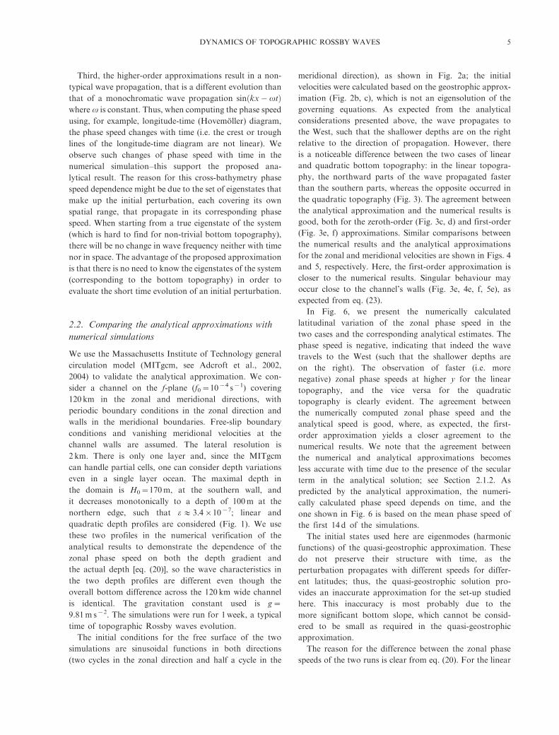
Third, the higher-order approximations result in a non-

typical wave propagation, that is a different evolution than

that of a monochromatic wave propagation sinðkx� xtÞwherev is constant. Thus, when computing the phase speed

using, for example, longitude-time (Hovemoller) diagram,

the phase speed changes with time (i.e. the crest or trough

lines of the longitude-time diagram are not linear). We

observe such changes of phase speed with time in the

numerical simulation�this support the proposed ana-

lytical result. The reason for this cross-bathymetry phase

speed dependence might be due to the set of eigenstates that

make up the initial perturbation, each covering its own

spatial range, that propagate in its corresponding phase

speed. When starting from a true eigenstate of the system

(which is hard to find for non-trivial bottom topography),

there will be no change in wave frequency neither with time

nor in space. The advantage of the proposed approximation

is that there is no need to know the eigenstates of the system

(corresponding to the bottom topography) in order to

evaluate the short time evolution of an initial perturbation.

2.2. Comparing the analytical approximations with

numerical simulations

We use the Massachusetts Institute of Technology general

circulation model (MITgcm, see Adcroft et al., 2002,

2004) to validate the analytical approximation. We con-

sider a channel on the f-plane (f0�10�4 s�1) covering

120 km in the zonal and meridional directions, with

periodic boundary conditions in the zonal direction and

walls in the meridional boundaries. Free-slip boundary

conditions and vanishing meridional velocities at the

channel walls are assumed. The lateral resolution is

2 km. There is only one layer and, since the MITgcm

can handle partial cells, one can consider depth variations

even in a single layer ocean. The maximal depth in

the domain is H0�170m, at the southern wall, and

it decreases monotonically to a depth of 100m at the

northern edge, such that o : 3.4�10�7; linear and

quadratic depth profiles are considered (Fig. 1). We use

these two profiles in the numerical verification of the

analytical results to demonstrate the dependence of the

zonal phase speed on both the depth gradient and

the actual depth [eq. (20)], so the wave characteristics in

the two depth profiles are different even though the

overall bottom difference across the 120 km wide channel

is identical. The gravitation constant used is g�9.81m s�2. The simulations were run for 1week, a typical

time of topographic Rossby waves evolution.

The initial conditions for the free surface of the two

simulations are sinusoidal functions in both directions

(two cycles in the zonal direction and half a cycle in the

meridional direction), as shown in Fig. 2a; the initial

velocities were calculated based on the geostrophic approx-

imation (Fig. 2b, c), which is not an eigensolution of the

governing equations. As expected from the analytical

considerations presented above, the wave propagates to

the West, such that the shallower depths are on the right

relative to the direction of propagation. However, there

is a noticeable difference between the two cases of linear

and quadratic bottom topography: in the linear topogra-

phy, the northward parts of the wave propagated faster

than the southern parts, whereas the opposite occurred in

the quadratic topography (Fig. 3). The agreement between

the analytical approximation and the numerical results is

good, both for the zeroth-order (Fig. 3c, d) and first-order

(Fig. 3e, f) approximations. Similar comparisons between

the numerical results and the analytical approximations

for the zonal and meridional velocities are shown in Figs. 4

and 5, respectively. Here, the first-order approximation is

closer to the numerical results. Singular behaviour may

occur close to the channel’s walls (Fig. 3e, 4e, f, 5e), as

expected from eq. (23).

In Fig. 6, we present the numerically calculated

latitudinal variation of the zonal phase speed in the

two cases and the corresponding analytical estimates. The

phase speed is negative, indicating that indeed the wave

travels to the West (such that the shallower depths are

on the right). The observation of faster (i.e. more

negative) zonal phase speeds at higher y for the linear

topography, and the vice versa for the quadratic

topography is clearly evident. The agreement between

the numerically computed zonal phase speed and the

analytical speed is good, where, as expected, the first-

order approximation yields a closer agreement to the

numerical results. We note that the agreement between

the numerical and analytical approximations becomes

less accurate with time due to the presence of the secular

term in the analytical solution; see Section 2.1.2. As

predicted by the analytical approximation, the numeri-

cally calculated phase speed depends on time, and the

one shown in Fig. 6 is based on the mean phase speed of

the first 14 d of the simulations.

The initial states used here are eigenmodes (harmonic

functions) of the quasi-geostrophic approximation. These

do not preserve their structure with time, as the

perturbation propagates with different speeds for differ-

ent latitudes; thus, the quasi-geostrophic solution pro-

vides an inaccurate approximation for the set-up studied

here. This inaccuracy is most probably due to the

more significant bottom slope, which cannot be consid-

ered to be small as required in the quasi-geostrophic

approximation.

The reason for the difference between the zonal phase

speeds of the two runs is clear from eq. (20). For the linear


topography case, only the local water depth affects the zonal

phase speed and thus, as the depth decreases, the denomi-

nator becomes smaller and hence the phase speed increases.

In contrast, for the quadratic topography, the local bottom

slope appears in the numerator and as it decreases towards

higher y, so does the phase speed. In this case, the effect of

the local bottom slope in reducing the zonal phase speed

towards larger y outweighs the effect of local depth that

tends to increasing the zonal phase speed at larger y.

It is possible to approximate the eigenstates of LSWEs in

the case of a linear depth profile using Airy Functions and

Parabolic Cylinder Functions [Cohen et al. (2010); see also

the planetary counterpart in Paldor and Sigalov (2008)].

These functions oscillate at large depths and decay (faster

than exponential) at shallower depths. Higher eigenmodes

extend farther into shallower depths, where each of them

propagates with its own phase speed. These straightfor-

ward considerations can explain the different phase speeds

for different y’s by viewing an arbitrary initial perturbation

as a collection of eigenstates, each propagating with its own

speed in a different subregime of the domain, leading to

different phase speeds at different latitudes.

Although we consider here the case of topographic wave

within a channel, our approximation is also relevant for

coastal shelf and open ocean topographic wave dynamics.

The reason is that the problem that we solve is essentially

an initial value problem in the meridional direction. Thus,

the channel width can be as large as desired*it is possible

to approximate the dynamics of initially meridionally

concentrated perturbation within the channel. The pertur-

bation can be located far from the channel walls, to mimic

open ocean dynamics, or close to the shallow boundary to

mimic coastal shelf dynamics. We have verified these claims

by performing additional numerical simulations (results

not shown) with a channel that is four times wider than the

one considered in the numerical simulations discussed

Fig. 2. The initial (a) free surface h, (b) zonal velocity u and (c) meridional velocity v for the linear bottom topography case. The

corresponding fields of the quadratic bottom topography are very similar to the linear topography ones. Note that the proportion of the

figure does not reflect the same zonal and meridional extent. Also note that the meridional wavelength is four times larger than the zonal one.


above. We found similar agreement between the analytical

approximation and the numerical results, with better

performance for the perturbation that is located far from

the channel walls. As expected, the first-order approxima-

tion was more accurate than the zeroth-order one.

We performed an additional numerical simulation with a

sinusoidal (two waves in the y-direction) bottom topogra-

phy. Here, only the zeroth-order approximation exhibited a

reasonable agreement with the numerical simulations. We

speculate that the secular terms of the approximation

diverge faster for rough topography profile.

It is unlikely to find exact analytical solutions of the

LSWEs for arbitrary bottom topography. The analytical

approximation presented here provides the wave structure

and zonal phase speed for bottom topography that is

uniform in the zonal direction (i.e. the long-shelf direction),

but is arbitrary in the meridional (cross-shelf) direction,

and the approximation is valid for small o values. Note that

the time of validity of the approximate solution becomes

shorter as o increases. In addition, the details of the wave’s

meridional structure are not required for calculating the

(zeroth-order) dispersion relation.

3. An approximation for topographic Rossby

waves in circular basins

3.1. Analytical approximation

3.1.1. Zero-order approximation. The derivations of the

previous section can be straightforwardly extended to

basins other than the channel studied above. Since circular

basins seem to be closer to the geometry of a typical lake

geometry, we find it useful to discuss this geometry in

details.

Fig. 3. The numerical (upper panels), zeroth-order approximation (middle panels) and first-order approximation (lower panels) free

surface h after 7 d of simulation, for the linear (left panels) and quadratic (right panels) bottom topographies. The agreement between the

numerical and analytical results is good. In all cases, the wave propagates westward (such that the shallower depths are on the right), where

for the linear bathymetry case, faster wave propagation is observed at higher latitudes.


The LSWEs in polar coordinates on the f-plane and with

varying depth H0 � b(r) are given by:

@vr

@t� f0vh ¼ �g

@g

@r;

@vh

@tþ f0vr ¼ �

g

r

@g

@h;

@g

@tþH0 � bðrÞ

r

@ðrvrÞ@rþ @vh

@h

� �� vr

db

dr¼ 0;

(24)

where vr and vu are the radial and azimuthal velocities,

h is the free surface displacement, f0 is the constant

Coriolis parameter, g is the gravitation constant, H0 is

the unperturbed water depth and b(r) is the (radial) bottom

topography. The independent variables are the radial,

azimuthal and time coordinates (r, u and t, respectively).

Note that we assume here, similar to the previous section,

that the depth changes only in the radial direction, r.

The velocities may be expressed in terms of the free

surface:

<vr ¼ �g

f0

1

f0

@rt þ1

r@h

!g; (25)

Fig. 4. As Fig. 3 for the zonal velocity u. Note the large amplitude close to the boundary of the channel (small and large y). The first-

order approximation (lower panels) is more similar to the numerical results (upper panels) compared to the zero-order approximation

(middle panels).


<vh ¼g

f0

� 1

f0

1

r@ht þ @r

!g; (26)

where the time operator < is given by eq. (6). From the

set eq. (24) it is possible to obtain a single equation for the

free surface by applying the operator < to the continuity

(i.e. the third) equation and using eqs. (25) and (26) to

eliminate the velocity components from this equation. The

result is:

@t �g

f 20

H0 � b

r2@hht þ

g

f0

b0

r@h

(

þ 1

f 20

@t @tt � gH0 � b

r@r � gðH0 � bÞ@rr þ gb0@r

�)g ¼ 0:

(27)

Note that the equation is singular at r�0.

We now perform the following scaling to switch to

non-dimensional (or scaled) variables: h ¼ ah,

r ¼ ðffiffiffiffiffiffiffiffiffigH0

p=f0aÞr, t ¼ t=ðaf0Þ, b ¼ H0b and g ¼ H0g, where

the ‘hat’ indicates non-dimensional (scaled) variable.

a is a parameter that characterises the mean bottom

slope. We now omit the ‘hat’ sign and, unless otherwise

indicated, the different variables designate non-dimen-

sional variables.

Using the above scaling, eq. (27) transforms to:

@t �1� b

r2@hht þ

b0

r@h

�

þ e@t @tt �1� b

r@r � ð1� bÞ@rr þ b0@r

��g ¼ 0;

(28)

where e ¼ a2. Using eq. (25), the boundary condition of

vanishing radial velocity at the basin periphery is:

e@rt þ1

r@h

� �g ¼ 0: (29)

The solution to eq. (28) is assumed to be of the form:

gðh; r; tÞ ¼ ~gðr; tÞeikh; (30)

Fig. 5. As Fig. 3 for the meridional velocity v.


and substituting this form in eq. (28) leads to:

�@t þ ixðrÞ

þ erxðrÞkb0

@t @tt �1� b

r@r � ð1� bÞ@rr þ b0@r

��~g ¼ 0;

(31)

where v(r) is:

xðrÞ ¼ kb0r

r2 þ ð1� bÞk2: (32)

v(r) is associated below with the zeroth-order approxima-

tion for the frequency.

We next assume that ~g is of the form:

~gðr; tÞ ¼ �gðrÞei½X0ðr;tÞþeX1ðr;tÞþe2X2ðr;tÞþ��: (33)

To zeroth-order approximation in o one obtains:

X0ðr; tÞ ¼ �xðrÞt; (34)

such that xðrÞ may be regarded as the zeroth-order term

in the power series of the frequency. g0ðx; y; tÞ is then

given by:

g0ðh; r; tÞ ¼ �gðrÞei½kh�xðrÞt�; (35)

where �gðrÞ should satisfy the boundary conditions of zero

radial velocity at the basin periphery. Since the radial

derivatives are assumed to be small (following the scaling

given above), �gðrÞ should be a slowly varying function.

Below we present the first-order approximation for h

(i.e. h1).

It is possible to find the zero-order velocities vh;0, vr;0

using the scaling vh ¼ affiffiffiffiffiffiffiffiffigH0

pvh and vr ¼


pvr and

using eqs. (25) and (26).

Since v is a function of r, the phase speed varies as

a function of r, depending on the local slope b?(r) and

local water depth H0 � bðrÞ. There exists a bottom topo-

graphy profile for which the (zero-order) phase speed

is constant, that is x ¼ const. This particular profile is

given by:

bðrÞ ¼ 1þ xr2

kð2þ kxÞþ C1r�kx; (36)

Fig. 6. Zonal phase speed as a function of latitude for the numerical (solid), zero-order (long dashed) and first-order (short dashed)

results, for the (a) linear and (b) quadratic bottom topographies. The wave propagates westward as the phase speed is negative but for the

linear topography the wave propagation speed increases northwards and the opposite occurs for the quadratic topography. The phase

speed calculated based on the first-order approximation is closer to the numerical one compared to the phase speed calculated based on the

zero-order approximation. The phase speed was calculated based on the mean of the first 14 d of simulation.


where C1 is an arbitrary constant. v must be negative since

for positive v the constant C1 must vanish (or else b(r)

tends infinity at r�0), and for such positive v, b(r) � 1

implying the impossible scenario where the depth profile is

larger than the total thickness of water. Thus, to zeroth-

order approximation, the constant rotation of the topo-

graphic wave is clockwise (anti-cyclonic). When C1�0 (or

when jkxjBB1), the profile is parabolic with the max-

imum/minimum b(r) located at the centre of the basin.

The dimensional zeroth-order frequency is given by:

xðrÞ ¼ gf0b0ðrÞkr

f 20 r2 þ gðH0 � bÞk2

; (37)

and the dimensional depth profile that yields a constant

v is:

bðrÞ ¼ H0 þf 2

0 xr2

gkð2f0 þ kxÞþ C1r�kx=f0 : (38)

The zeroth-order dimensional velocities and free surface

may be found straightforwardly using the above scaling,

and by neglecting terms of order o.

3.1.2. First- and high-order approximations. In polar

coordinates, the higher-order approximation is essentially

the same as that in Cartesian coordinates given in eqs. (21)

and (22), with the trivial replacement of y by r, and using

eqs. (31) and (33).

The coefficients of the first-order approximations for

V are:

a1;0 ¼x

k�gb0�2rð1� bÞ�g0x0 þ x½rb0�g0 � ðr�g00 þ �g0Þð1� bÞ�f

� �g½rx3 � rb0x0 þ ð1� bÞðx0 þ rx00Þ��;

a1;1 ¼x

k�gb02rð1� bÞ�g0xx0f

� �g½rxx0b0 � ð1� bÞðxx0 þ 2rx02 þ rxx00Þ��;

a1;2 ¼ �ð1� bÞrx2x02

kb0;

(39)

where v(r) is given in eq. (32). Also here, for constant v the

coefficients a1,1 and a1,2 are zero while a1,0 takes a simpler

form.

3.2. Comparison between the analytical

approximation and numerical simulations

As in Section 2.2, we used the MITgcm for the numerical

verification of our analytical approximations. The spatial

dimensions of the square used in the simulation are

120�120m with a resolution of 2 km. The Coriolis

parameter is f0�10�4 s�1, the gravitation constant is

g�9.81m s�2 and H0�90m. The (dimensional) b(r) is

shown in Fig. 7, and it follows eq. (38) so that the zeroth-

order frequency is constant and corresponds to a topo-

graphic wave rotation of one cycle per 10 d.

In Fig. 8, we present a comparison between the

numerical simulation and the zeroth-order approximation

of the free surface. The simulation is initiated with a

Gaussian profile in the radial direction, multiplied by a

sinusoidal function in the azimuthal direction, with a wave

number, k�2 (see Fig. 8a). The initial velocities were

chosen to be in geostrophic balance with the free surface

and the initial perturbation rotated clockwise. The numeri-

cally calculated free surface for t�3 and 8 d is shown in

Fig. 8b, c. It is evident that the initial perturbation rotates

with constant angular velocity for different values of r,

confirming the analytical prediction of constant v for the

profile given in eq. (38). In Fig. 8d, the zeroth-order

approximation free surface for t�8 d is depicted. The

orientation of the numerical and analytical free surface for

t�8 d (Fig. 8c, d) is similar; yet, while the zeroth-order

approximation exhibits only rotation of the initial pertur-

bation, the numerically calculated free surface exhibits also

radial propagation. This difference may be attributed to

viscosity and non-linear terms that are included in the

numerical model. We note that the first-order approxima-

tion exhibits dependence of wave frequency on the radial

coordinate; this difference between the analytical first-

order approximation and the numerical results may be

linked to higher wave frequency close to the periphery of

the basin, making the perturbation expansion less accurate.

Fig. 7. Bottom topography b(r) as a function of the radius r of

the circular basin. The dashed line indicates the unperturbed free

surface, H0�90m. This depth profile yields a constant frequency

v for the zeroth-order approximation [eq. (36)]. We choose C1�0.


We have also compared numerical simulations (results

not shown) to the zeroth-order approximation for other

bottom topography profiles. As expected, the numerical

simulations of these cases indicated different angular

rotations at different values of r, that is v does vary

with r. The remarks listed in Section 2.1.3 for a periodic

zonal channel are also relevant to the current case of

a circular basin.

4. Discussion and summary

We have studied topographic Rossby waves dynamics on

the f-plane using the LSWEs. A slowly varying arbitrary

bottom topography profile in one of the directions was

assumed. We propose a new approximation, according to

which the time and cross-bathymetry directions are con-

sidered to be slow and long, that is changes in the cross-

bathymetry direction are small. The small non-dimensional

parameter is the square of a number representing the slope

of the bottom topography (which we choose to be the

maximum of the absolute value of the slope). It then

follows that the cross-bathymetry coordinate appears as a

parameter, that is the underlying differential equation, for

each order of approximation, does not contain derivatives

with respect to the cross-bathymetry coordinate. This

equation leads to a wave frequency (and hence phase

speed) that explicitly depends on the cross-bathymetry

coordinate where the wave propagation depends on the

local slope of the bottom topography and on the local

water depth. [We note that it is possible to apply an

alternative expansion in which the wave number depends

on y (i.e. k(y)) instead of the v(y) dependence. We however

find the latter easier to interpret and implement as an initial

value problem.] The analytical approximation is valid for

slowly varying arbitrary initial conditions in the cross-

bathymetry direction that satisfy the boundary conditions;

the analytical approximation exhibits close similarity

with the numerical simulations carried out using the

MITgcm. The proposed approximation may be relevant

to coastal shelf and open ocean wave dynamics since the

Fig. 8. (a) Initial free surface h(u, r). (b) The free surface of the numerical simulations for t�3 d. (c) As (b) for t�8 d. (d) As (c) but for

the zero-order approximation. Note that the initial perturbation rotates clockwise and completes one full cycle in approximately 10 d. Also

note that angular frequency v(r) is almost constant as a function of radius r, as predicted by the theory.


channel can be very wide and the evolution of a meridion-

ally localised perturbation is very well approximated by the

analytical theory. Both linear and quadratic bottom

topographies were used in the simulations, both spanning

the same overall height difference. Yet, the linear bottom

topography yielded faster wave propagation towards

shallower depths, while the quadratic bottom topography

exhibited the opposite behaviour, due to the smaller local

slope at shallower depths.

We have developed a similar approximation for a

circular basin using the LSWEs in polar coordinates on

the f-plane and a general bottom topography profile in the

radial direction. The approximation may be found useful in

the study of lakes with (nearly) circular symmetry. This

case shares similar characteristics with a channel of

periodic boundary conditions. We have found a specific

form of the bottom topography that yields the same

angular rotation as a function of the radial dimension;

constant (zeroth-order) topographic wave rotation may be

just clockwise rotation.

It had been shown previously that when changes in

bottom topography are very moderate with respect to the

changes in the wavelength, it is possible to replace the

mean water depth by the local water depth (e.g. Pedlosky,

2003). In essence, our proposed approximation is based

on similar arguments, formulating the approximation

rigorously and developing also the first-order approxima-

tion. The main advantage of the proposed approximation

over existing ones is the ability to find the dispersion

relation for arbitrary bottom topography. Extension

of the present work to basins with elliptical shape is

possible, which may be more relevant to lake dynamics in

some cases.

References

Adcroft, A., Campin, J.-M., Heimbach, P., Hill, C. and Marshall,

J. 2002.MITgcm Release Manual. MIT/EAPS, Cambridge, MA.

Online at: http://mitgcm.org/sealion/online_documents/manual.

html

Adcroft, A., Campin, J.-M., Hill, C. and Marshall, J. 2004.

Implementation of an atmosphere-ocean general circulation

model on the expanded spherical cube. Mon. Weather Rev.

132(12), 2845�2863.Adem, J. 1956. A series solution for the barotropic vorticity

equation and its application in the study of atmospheric

vortices. Tellus 8(3), 364�372.

Ashkenazy, Y., Paldor, N. and Zarmi, Y. 2011. On the meridional

structure of extra-tropical Rossby waves. Tellus A 63(4),

817�827. DOI: 10.1111/j.1600-0870.2011.00516.x.

Ball, F. K. 1963. The effect of rotation on the simpler modes of

motion of a liquid in an elliptic paraboloid. J. Fluid Mech. 22,

529�545.Ball, F. K. 1965. Second-class motions of a shallow liquid. J. Fluid

Mech. 23, 545�561.Buchwald, V. T. and Adams, J. K. 1968. Propagation of con-

tinental shelf waves. Proc. R. Soc. Lond. A 305(1481), 235�250.Cohen, Y., Paldor, N. and Sommeria, J. 2010. Laboratory

experiments and a non-harmonic theory for topographic Rossby

waves over a linearly sloping bottom on the f-plane. J. Fluid

Mech. 645, 479�496.Csanady, G. T. 1973. Wind-induced barotropic motions in long

lakes. J. Phys. Oceanogr. 3, 429�438.Csanady, G. T. 1976. Topographic waves in Lake Ontario. J.

Phys. Oceanogr. 6, 93�103.Csanady, G. T. 1982. Circulation in the Coastal Ocean. Reidel,

Dordrecht.

Gill, A. E. 1982. Atmosphere�Ocean Dynamics. Academic Press,

London.

Paldor, N. and Sigalov, A. 2008. Trapped waves on the mid-

latitude beta-plane. Tellus 60A, 742�748.Pedlosky, J. 2003. Waves in the Ocean and Atmosphere. Springer-

Verlag, Berlin, Heidelberg, New York.

Primeau, F. 2002. Long Rossby wave basin-crossing time and the

resonance of low-frequency basin modes. J. Phys. Oceanogr. 32,

2652�2665.Raudsepp, U., Beletsky, D. and Schwab, D. 2003. Basin-scale

topographic waves in the Gulf of Riga. J. Phys. Oceanogr. 33,

1129�1140.Rhines, P. B. 1969a. Slow oscillations in an ocean of varying

depth. 1. Abrupt topography. J. Fluid Mech. 37, 161�189.Rhines, P. B. 1969b. Slow oscillations in an ocean of varying

depth. 2. Islands and seamounts. J. Fluid Mech. 37, 191�205.Rhines, P. B. 1989. Deep planetary circulation and topography:

simple models of midocean flows. J. Phys. Oceanogr. 19,

1449�1470.Saylor, J. H., Huang, C. K. and Reid, R. 1980. Vortex modes in

southern Lake Michigan. J. Phys. Oceanogr. 10, 1814�1823.Shilo, E., Ashkenazy, Y., Rimmer, A., Assouline, S., Katsafados,

P. and co-authors. 2007. The effect of wind variability on

topographic waves: Lake Kinneret case. J. Geophys. Res. 112,

C12024.

Shilo, E., Ashkenazy, Y., Rimmer, A., Assouline, S. and Mahrer,

Y. 2008. Wind spatial variability and topographic wave

frequency. J. Phys. Oceanogr. 38, 2085�2096.Vallis, G. K. 2006. Atmospheric and Oceanic Fluid Dynamics.

Cambridge University Press, Cambridge.


http://mitgcm.org/sealion/online_documents/manual.html

http://mitgcm.org/sealion/online_documents/manual.html

A new approximation for the dynamics of topographic Rossby waves

Documents

Transcript of A new approximation for the dynamics of topographic Rossby waves