Topographic uncertainty quantification for flow-like landslide ...

Nat. Hazards Earth Syst. Sci., 20, 1441–1461, 2020https://doi.org/10.5194/nhess-20-1441-2020© Author(s) 2020. This work is distributed underthe Creative Commons Attribution 4.0 License.

Topographic uncertainty quantification for flow-like landslidemodels via stochastic simulationsHu Zhao1 and Julia Kowalski1,2

1AICES Graduate School, RWTH Aachen University, Schinkelstr. 2, 52062 Aachen, Germany2Computational Geoscience, Geowissenschaftliches Zentrum, Universität Göttingen,Goldschmidtstr. 1, 37077 Göttingen, Germany

Correspondence: Hu Zhao ([email protected])

Received: 24 October 2019 – Discussion started: 2 January 2020Revised: 30 March 2020 – Accepted: 7 April 2020 – Published: 26 May 2020

Abstract. Digital elevation models (DEMs) representing to-pography are an essential input for computational modelscapable of simulating the run-out of flow-like landslides.Yet, DEMs are often subject to error, a fact that is mostlyoverlooked in landslide modeling. We address this researchgap and investigate the impact of topographic uncertaintyon landslide run-out models. In particular, we will describetwo different approaches to account for DEM uncertainty,namely unconditional and conditional stochastic simulationmethods. We investigate and discuss their feasibility, as wellas whether DEM uncertainty represented by stochastic simu-lations critically affects landslide run-out simulations. Basedupon a historic flow-like landslide event in Hong Kong, wepresent a series of computational scenarios to compare bothmethods using our modular Python-based workflow. Our re-sults show that DEM uncertainty can significantly affectsimulation-based landslide run-out analyses, depending onhow well the underlying flow path is captured by the DEM, aswell as on further topographic characteristics and the DEMerror’s variability. We further find that, in the absence of sys-tematic bias in the DEM, a performant root-mean-square-error-based unconditional stochastic simulation yields simi-lar results to a computationally intensive conditional stochas-tic simulation that takes actual DEM error values at refer-ence locations into account. In all other cases the uncondi-tional stochastic simulation overestimates the variability inthe DEM error, which leads to an increase in the potentialhazard area as well as extreme values of dynamic flow prop-erties.

1 Introduction

Landslides are natural hazards that occur frequently allaround the world causing casualties, economic devastation,and environmental destruction. Most often, they are natu-rally driven, e.g., by means of long-lasting and/or intensiveprecipitation events or induced by earthquakes. Yet, land-slides might also be triggered or an area’s susceptibility tothem increased as a result of human activities, e.g., deforesta-tion and construction. According to the United Nations Of-fice for Disaster Risk Reduction and the Centre for Researchon the Epidemiology of Disasters, 378 recorded landslidesfrom 1998 to 2017 affected 4.8 million people and caused18 414 deaths as well as several billion US dollars of eco-nomic losses (Wallemacq et al., 2018). Froude and Petley(2018) reported that in total 55 997 people were killed during4862 fatal nonseismic landslide events from January 2004to December 2016. Still, it has to be assumed that the dam-age potential of landslides is underestimated as (1) eventshave been underreported for decades, especially in develop-ing countries, and (2) losses caused by coseismic landslideevents tend to be classified as secondary losses due to earth-quakes.

Rapid flow-like landslides, such as rock avalanches anddebris flows, show a particularly high hazard potential dueto their high mobility, long travel distance, and fast prop-agation speed. In recent years, the geohazard communityhas put a lot of effort into developing computational run-out models in order to assess and predict risks associatedwith rapid landslides and to develop mitigation strategies.Most of the models in practical use are based on a (compu-tationally efficient) “shallow-flow-type” process description

Published by Copernicus Publications on behalf of the European Geosciences Union.

1442 H. Zhao and J. Kowalski: Topographic uncertainty quantification for flow-like landslide models

and depth-averaging techniques (e.g., Pitman et al., 2003;Hungr, 2009; Pastor et al., 2009; Christen et al., 2010; Xiaand Liang, 2018). In these, the flowing material is treated asan “equivalent fluid” and governed by idealized internal andbasal rheologies (Hungr, 2009). Alternative (computation-ally demanding) models aim to directly describe fully three-dimensional flow behavior. They hence offer a higher processcomplexity level (e.g., Mast et al., 2014; Teufelsbauer et al.,2011) yet are typically not feasible for practical hazard mit-igation purposes. Detailed reviews of computational run-outmodels for rapid, flow-like landslides have been published byMcDougall (2017) and Pastor et al. (2018).

An indispensable input to any of these computational land-slide run-out models is data that represent the terrain in whichthe slide is likely to occur. Pioneered by Miller and Laflamme(1958), digital elevation models (DEMs) have become themost popular form of representing topographies in the scien-tific community. Methods for generating DEMs have evolvedrapidly over decades from conventional approaches, like fieldsurveying and topographic-map digitizing, to passive and ac-tive remote sensing, such as stereoscopic photogrammetry,interferometric synthetic aperture radar (InSAR), and lightdetection and ranging (lidar); see Wilson (2012) for a com-prehensive review. Differences between these methods ex-ist in terms of their footprint, cost, resolution, and accuracyof the resulting DEM. Whatever method used, however, theresulting DEM will inevitably contain errors that are intro-duced either during source data acquisition or during dataprocessing. The so-called DEM error hence refers to thedifference between the true real-world elevations and theirDEM representation. Typically, there is a lack of informationon the DEM error, which has led to the notion of “DEM un-certainty”, which refers to what we do not know about theerror; see Wechsler (2007).

Nowadays, several global DEM databases, e.g., SRTM(Rodriguez et al., 2006), AW3D30 (Courty et al., 2019),and TanDEM-X (Wessel et al., 2018), as well as some re-gional DEM databases (Pakoksung and Takagi, 2016) arepublicly available. Commercial DEM databases that are as-sociated with significant costs also exist (Hawker et al.,2018). Online initiatives such as OpenTopography facilitatecommunity access and aim to democratize online availabilityof high-resolution topography data acquired with lidar andother technologies (Krishnan et al., 2011). Despite a broadvariety of existing DEM sources, however, we are still facing(and will continue to face in the near future) a very limitedavailability of high-accuracy DEMs for some regions that areparticularly prone to landslide hazards, e.g., in Asia (Froudeand Petley, 2018). Whenever using DEM data for simulation-based landslide hazard analysis, it is hence important to beaware of DEM error and uncertainty and to consider their po-tential impact on computational run-out analyses and relatedcomputational risk assessments.

DEM error has had the attention of researchers for a longtime. Many efforts have for instance been put into quanti-

fying the error associated with specific DEM sources basedon data of higher accuracy, e.g., acquired by satellite mea-surements (Berry et al., 2007; Mouratidis and Ampatzidis,2019), medium-footprint lidar (Hofton et al., 2006), or GPSsurvey (Rodriguez et al., 2006; Bolkas et al., 2016; Patelet al., 2016; Wessel et al., 2018; Elkhrachy, 2018). Mean-while, a variety of methods have been devised to classifyDEM error into various categories (Oksanen, 2003; Henglet al., 2004; Fisher and Tate, 2006). Due to the complexityof potential influencing factors (sensor technology, retrievalalgorithms, data processing, land cover and surface morphol-ogy, terrain attributes; Wilson, 2012; Fisher and Tate, 2006;Gonga-Saholiariliva et al., 2011), these methods can onlyconstrain the DEM error and will not deterministically cor-rect for it at all grid points. Hence, DEM uncertainty remainsand has to be accounted for in any subsequent analysis thatrelies on the DEM data.

In this circumstance, a stochastic simulation is an effectivecomputational approach to deal with the situation (Holmeset al., 2000). Instead of considering a single (assumed as ac-curate) DEM, the fundamental idea of a stochastic simulationin the context of DEM uncertainty propagation is to separatethe DEM into a known deterministic contribution and an un-known DEM error. DEM uncertainty is then accounted forby treating the DEM error as a random field consisting of acollection of random variables defined at selected grid points.An ensemble of equiprobable realizations of the random fieldis then generated based on certain assumptions and availableinformation about DEM error. This could for instance be theso-called root mean square error (RMSE), a minimalist in-dicator for the overall error magnitude, or a semivariogramthat provides information about the spatial autocorrelationof the DEM error. Adding the DEM error realizations to theknown deterministic DEM contribution results in an ensem-ble of equiprobable DEM realizations, which can finally beused for a DEM uncertainty propagation analysis.

Stochastic simulation methods for DEM uncertainty prop-agation analyses have been developed since the 1990s andare by now widely applied in many fields, including terrainanalysis (Holmes et al., 2000; Raaflaub and Collins, 2006;Moawad and EI Aziz, 2018), flood modeling (Watson et al.,2015; Hawker et al., 2018; Kiczko and Miroslaw-Swiatek,2018), soil erosion modeling (Aziz et al., 2012), landslidesusceptibility mapping (Qin et al., 2013), and dry-block-and-ash-flow modeling (Stefanescu et al., 2012). With respect torapid, flow-like landslide run-out modeling, very little workhas been done to assess the potential impact of DEM uncer-tainty, most likely due to the complexity, and hence level ofsophistication, of the associated process models. Meanwhile,however, advances in computing technology have led to com-putationally feasible and well-developed landslide run-outsimulation tools. As one of the most important inputs forthese tools, a DEM determines the landslide’s flow path. Anatural next step is hence to consider the impact of DEM un-certainty in these models, as overlooking DEM uncertainty

Nat. Hazards Earth Syst. Sci., 20, 1441–1461, 2020 https://doi.org/10.5194/nhess-20-1441-2020

H. Zhao and J. Kowalski: Topographic uncertainty quantification for flow-like landslide models 1443

may lead to a bias in risk management decisions. The majoraim of this study is therefore to describe two different ap-proaches in order to incorporate DEM uncertainty into com-putational landslide run-out analyses and to investigate anddiscuss the feasibility of the approaches, as well as whetherDEM uncertainty is critical to landslide run-out modelingand affects the modeling’s results.

This paper is organized as follows: in Sect. 2, we brieflydescribe the landslide run-out model used in this study, whichis a continuum-mechanical shallow-flow model based onthe Voellmy–Salm rheology. In Sect. 3, we call on variousmethods to account for DEM uncertainty with a major fo-cus on two approaches, namely an unconditional and a con-ditional stochastic simulation method. The rest of the pa-per is devoted to investigating DEM uncertainty propagationfor rapid, flow-like landslides based on an integrated work-flow that combines the aforementioned computational pro-cess model (Sect. 2) with the stochastic DEM simulations(Sect. 3). Note that, while in our particular study we choseto use a continuum-mechanical shallow-flow process modelbased on the Voellmy–Salm rheology, the workflow itselfis modular and nonintrusive. It would hence also be possi-ble to couple the stochastic DEM simulation with any other(DEM-based) computational landslide model. Section 4 de-scribes the modular Python-based workflow that we devel-oped in order to set up and manage the workflow and tointerpret its simulation results. We present a series of com-putational scenarios based upon a historic landslide event inSect. 5. All scenarios compare the unconditional and con-ditional stochastic DEM simulation. Finally, Sect. 6 is de-voted to a discussion of our results. Important conclusionsare drawn in Sect. 7.

2 Landslide process model

As detailed in the introduction, a variety of process-basedcomputational landslide run-out models have been devel-oped in recent decades. Among these is a family of depth-integrated shallow-flow-type landslide models that we choseas the basis for our work. Shallow-flow-type landslide mod-els can be further classified based on their applied basalrheology, e.g., Voellmy, Bingham, and quadratic resistancemodel (Naef et al., 2006; Hungr and McDougall, 2009). Ourstudy uses the Voellmy–Salm (VS) process model, which is adepth-averaged continuum-mechanical model incorporatingthe Voellmy basal rheology. Note that the stochastic work-flow presented later is modular and does not depend on thischoice. Hence, the Voellmy model can straightforwardly besubstituted by other computational process models.

2.1 Reference frame and relation to topographic error

Let {X,Y,Z} denote a fixed Cartesian coordinate system, inwhich X and Y are the horizontal axes and Z is the vertical

axis. The coordinates of a point in the Cartesian coordinatesystem are denoted by (X,Y,Z). A topography can then beexpressed as a surface mapping of horizontal X and Y co-ordinates and represents the elevation at each point, namelyZ(X,Y ). The mapped topography induces a surface coordi-nate system {x,y,z}, in which x and y denote tangential di-rections and z points in the direction of the surface normal.Hence any vector that is constant with respect to the fixedCartesian coordinates system, e.g., gravitational accelerationg= (gX,gY ,gZ)T = (0,0,−g)T , spatially varies when in-terpreted in terms of the surface-mapped coordinated systemg= (gx,gy,gz)T . Error or uncertainty in the topography rep-resentation Z(X,Y ) hence directly translates into error anduncertainty in that vector representation.

2.2 Voellmy rheology computational process model

The Voellmy process model along with its computational im-plementation is described in Bartelt et al. (1999) and Christenet al. (2010). It assesses the slide’s dynamics in terms of flowheight H(x,y, t) and depth-averaged velocity U(x,y, t) :=(Ux(x,y, t),Uy(x,y, t))

T , both of which depend on time tand spatial coordinates x and y. The governing system reads

∂tH + ∂x(HUx)+ ∂y(HUy)= Q̇(x,y, t) (1a)

∂t (HUx)+ ∂x

(HU2

x + gzH 2

2

)+ ∂y

(HUxUy

)= gxH − nx(µgzH + g‖U‖2/ξ) (1b)

∂t (HUy)+ ∂x(HUxUy)+ ∂y

(HU2

y + gzH 2

2

)= gyH − ny(µgzH + g‖U‖2/ξ). (1c)

Here, Eq. (1a) denotes the mass balance, in whichH ,Ux , andUy stand for height and surface tangential velocity compo-nents and Q̇(x,y, t) stands for a mass production source termthat accounts for erosion of material along the way. Equa-tions (1b) and (1c) denote the x and y momentum balance, inwhich gx , gy, and gz are the three local components of grav-itational acceleration vector g. Furthermore, nx and ny are xand y components of the unit vector n that opposes the localvelocity, and µ and ξ are two friction parameters that standfor dry Coulomb and turbulent friction coefficients, respec-tively. The friction parameters are determined by back anal-ysis based on historic events. Note that additional model pa-rameters introduced in the original publications, such as ve-locity shape factors and nonhydrostatic pressure corrections,are not taken into account as they are hard to constrain andhave been shown to not critically affect the slide’s dynamics(e.g., Hungr et al., 2005; Christen et al., 2010).

The topographic surface Z(X,Y ) enters the governingequations of the process model implicitly in terms ofthe spatially varying gravitational acceleration vector g=(gx,gy,gz)

T . Any error and uncertainty present in the topog-

https://doi.org/10.5194/nhess-20-1441-2020 Nat. Hazards Earth Syst. Sci., 20, 1441–1461, 2020


raphy representation hence also enters the landslide run-outsimulation results.

The VS model was first proposed to model snow avalanche(Salm, 1993). Recently it has been widely applied to othertypes of gravity-driven rapid mass movements includingflow-like landslides (Pastor et al., 2018; Frank et al., 2015;Hussin et al., 2012; Kumar et al., 2019). In this study, theproprietary mass flow simulation platform RAMMS (Chris-ten et al., 2010) which provides a GIS-integrated implemen-tation of the VS model is used for landslide run-out model-ing. It is integrated as a module of our workflow (see Sect. 4)that is developed for the purpose of DEM uncertainty propa-gation analysis.

3 Methods to represent DEM uncertainty

Again, the topographic surface is expressed as a functionZ(X,Y ) parameterized in horizontal coordinates X and Y .In practice, the function Z(X,Y ) is often constructed fromdiscrete gridded raster data. We hence assume that a domainof interestD is discretized into the horizontalX and Y direc-tion, which results in a spatial grid defined as

Dmn = {Dij = (Xi,Yj ) | (Xi,Yj ) ∈D; i = 1,2,

. . .,m; j = 1,2, . . .,n}. (2)

The elevation data associated with each grid point Dij aredefined as

Zmn = {Zij = Z(Xi,Yj ) | ∀ Dij ∈Dmn}. (3)

The elevation Zmn of a common DEM data product might beerroneous with respect to the true values as discussed in theintroduction. If we denote the true elevation as

Z∗mn = {Z∗

ij = Z∗(Xi,Yj ) | ∀ Dij ∈Dmn}, (4)

the DEM error can be expressed as

εmn = {εij = Z∗

ij −Zij | ∀ Dij ∈Dmn}. (5)

If we knew the error εmn, we would be able to recover thereal-world topographic surface Z∗mn. The fact, however, thatthe error is unknown or we only have limited informationabout it implies an uncertainty in the input to our landslideprocess simulation. Within this study, we will refer to the un-certainty associated with the unknown DEM error as DEMuncertainty. In this circumstance, each εij is treated as a ran-dom variable and εmn is accordingly treated as a randomfield, which consists of a collection of random variables εij .By generating multiple realizations of the random field εmn,DEM uncertainty can be represented. This process is widelyknown as stochastic simulation. It requires a suitable modelto describe the jointed uncertainty in all εij based on limitedavailable information about DEM error. The task can be fur-ther divided into determining (1) the probability distribution

function (pdf) of each εij which quantifies local uncertaintyat each grid point and (2) the correlation between differentεij which is usually termed spatial autocorrelation of DEMerror.

According to available information on the DEM error, ex-isting approaches that could be used to solve the two issuescan be generally classified into two groups:

a. unconditional stochastic simulation (USS),

b. conditional stochastic simulation (CSS).

More specifically, USS is only informed of properties ofDEM error, e.g., the RMSE, and thus does not honor anyactual DEM error values. CSS is informed of a certain num-ber of actual DEM error values at reference locations withinthe DEM, e.g., obtained from higher-accuracy reference data,and thus could directly honor the actual DEM error values atreference locations (Fisher and Tate, 2006).

3.1 Unconditional stochastic simulation (USS) based onthe RMSE

Typically available information about the DEM error pro-vided by DEM vendors is the root mean square error(RMSE). For a set of K reference locations, it is defined as

RMSE=

√√√√ 1K

K∑k=1(Z∗kk −Zkk)

2. (6)

Here, Z∗KK = {Z∗

kk = Z∗(Xk,Yk) | (Xk,Yk) ∈D; k =

1,2, . . .,K} denotes higher-accuracy elevation valuesmeasured at the reference locations and ZKK = {Zkk =Z(Xk,Yk) | (Xk,Yk) ∈D; k = 1,2, . . .,K} denotes corre-sponding elevation values based on the DEM.

It should be noted that, while the RMSE is typically avail-able, this is not true for the reference elevation values Z∗KKthemselves. As stated numerous times in the literature, it iscritical that the RMSE only provides a global indication ofDEM error magnitude without any information about its spa-tial autocorrelation. Still, it is by far the most widely usedDEM error indicator for many DEM databases and mostlythe only available information that are included with DEMproducts. In this circumstance, USS could be used to repre-sent DEM uncertainty and study its propagation into land-slide run-out analyses.

Modeling DEM uncertainty based on USS assumes thatall local error values εij are independent and fulfill the sameunivariate Gaussian distribution with a mean (µ) of zero anda standard deviation (σ ) equivalent to the given RMSE. Un-der this assumption, an ensemble of spatially uncorrelatedrealizations of the random field εmn can be generated by ran-domly assigning error values to each εij according to its localGaussian probability distribution.

In the next step, we have to account for the (unknown) spa-tial autocorrelation of εmn. Potential methods that could be



applied are simulated annealing, spatial autoregressive mod-eling, spatial moving averages, etc.; see Wechsler (2007).Simulated annealing is generally computationally intensive,and spatial autoregressive modeling becomes impractical forthe simulation of large areas (Oksanen, 2006). In this study,we use the spatial moving-averages method that increases thespatial autocorrelation by filtering spatially uncorrelated re-alizations with a distance-weighted filter proposed by Wech-sler and Kroll (2006). For εij at one grid point of an uncorre-lated realization, its value is replaced by the weighted aver-age of εij at all grid points within the filter kernel. The weightdecreases with increasing distance to the grid point, which issimilar to semivariogram trends (Wechsler and Kroll, 2006).The size of the filter denoted as d depends on the maximumautocorrelation length of εmn which again is unknown if theRMSE is the only available information. In practice, d is of-ten determined based on the maximum autocorrelation lengthof the original DEM (Wechsler, 2007; Aziz et al., 2012).

Though it relies on some assumptions, such as an appro-priate choice of correlation length d , the sketched approachis generally applicable if the RMSE is the only available in-formation. It may become critical if a DEM contains a sys-tematic bias which means that the mean of Z∗kk−Zkk deviateslargely from zero. More specifically, if we follow Fisher andTate (2006) and Wessel et al. (2018) in defining mean µ andstandard deviation σ as

µ=1K

K∑k=1(Z∗kk −Zkk) and

σ =

√√√√ 1K − 1

K∑k=1((Z∗kk −Zkk)−µ)

2, (7)

we can express the RMSE in terms of µ and σ as

RMSE=

√µ2+

K − 1K

σ 2. (8)

If the number of reference points K is relatively large,√(K − 1)/K is close to 1. Equation (8) then indicates that

the RMSE is larger than the standard deviation σ if the meanµ deviates from zero. The difference between the RMSE andσ increases with increasing µ. For example, the µ, σ , andRMSE of the global TanDEM-X DEM based on about 3 mil-lion reference points are 0.17, 1.28, and 1.29 m (Wessel et al.,2018). Those of the EU-DEM of Central Macedonia based on12 943 reference points are 1.8, 3.6, and 4.0 m, while thoseof the ASTER GDEM of the same area based on the samereference points are 6.8, 7.6, and 10.2 m (Mouratidis andAmpatzidis, 2019). This means that assuming the standarddeviation of the DEM error to be given as the RMSE conse-quently overestimates the variability in the DEM error if themean deviates largely from zero.

The implications of both issues, namely the fact that thefilter size d is unknown and has to be subjectively chosen

and that the RMSE provides an insufficient representation ofthe DEM error, are investigated in the following study. Forconvenience, the two issues are referred to as

– unrepresentative RMSE and

– subjective d.

3.2 Conditional stochastic simulation (CSS) based onhigher-accuracy reference data

This approach requires the availability of higher-accuracyreference data at certain reference locations, e.g., fromhigher-accuracy DEM products or GPS surveys. Note that,although these data might be subject to error themselves, itis fair to assume this error to be much smaller. This justifiesthe use of the higher-accuracy reference data as true eleva-tion values Z∗KK . Based on Z∗KK , we could determine thestatistics of the DEM error, e.g., the RMSE, the µ, and theσ as discussed in Sect. 3.1. Likewise, we can assess the spa-tial autocorrelation of the DEM error, e.g., in the form of asemivariogram model (see Sect. 5.2.1). In addition, we knowthe DEM error at the reference locations exactly, denoted asε∗KK = { ε

∗

kk | k = 1,2, . . .,K}. Yet, we still lack knowledgeabout the DEM error away from the K reference locations,hence the complete random field εmn.

In that situation, conditional stochastic simulation (CSS)can be used to simulate, i.e., generate, realizations of therandom field εmn. Many geostatistical methods of condi-tional simulation could be applied, including sequential sim-ulation algorithms, the p-field approach, and simulated an-nealing (Goovaerts, 1997). In this study, we apply a sequen-tial Gaussian simulation. It is the most attractive techniquefor stochastic spatial simulation according to Temme et al.(2009) and has been widely utilized in DEM uncertaintypropagation analysis (Holmes et al., 2000; Aziz et al., 2012).

The sequential Gaussian simulation sequentially sampleseach local error εij along a random path that consists of allgrid points Dij under the multi-Gaussian assumption. Thismeans that, assuming the random field εmn satisfies a mul-tivariate Gaussian distribution, each εij fulfills a univariateGaussian distribution denoted as N(µij ,σij ). The essentialidea now is that the mean µij and standard deviation σij aredetermined sequentially by means of simple kriging basedon the semivariogram model of DEM error that provides co-variances in simple kriging equations and the conditioninginformation including ε∗KK and previously sampled εij . Bymaking each univariate Gaussian distribution conditional notonly on ε∗KK but also on all previously sampled εij , the semi-variogram model of DEM error is reproduced in realizationsof εmn (Goovaerts, 1997). The process to generate one real-ization of εmn is as follows:

1. Determine a semivariogram model to represent the spa-tial autocorrelation of DEM error based on normal scoretransformed ε∗KK .



2. Define a random path visiting each Dij once.

3. At each Dij , determine N(µij ,σij ) using simple krig-ing based on the semivariogram model and normal scoretransformed ε∗KK .

4. Sample a value from N(µij ,σij ), assign it to εij , andadd εij into normal score transformed ε∗KK .

5. Repeat steps (3) and (4) until all Dij along the path arevisited.

6. Back-transform all sampled εij to the original distribu-tion of ε∗KK .

Multiple realizations can be generated by defining differentrandom paths.

4 Implementation

Studying the impact of DEM uncertainty on landslide run-outmodeling is computationally intensive and technically de-manding. It includes representing DEM uncertainty in termsof a large number of DEM realizations, conducting numer-ous landslide run-out modeling based on the DEM realiza-tions, and postprocessing extensive output data. In addition,understanding how DEM uncertainty affects terrain attributesmay facilitate us in interpreting its impact on landslide run-out modeling. This requires the ability to calculate terrainattributes, e.g., slope and roughness, of the original DEM aswell as of the generated DEM realizations.

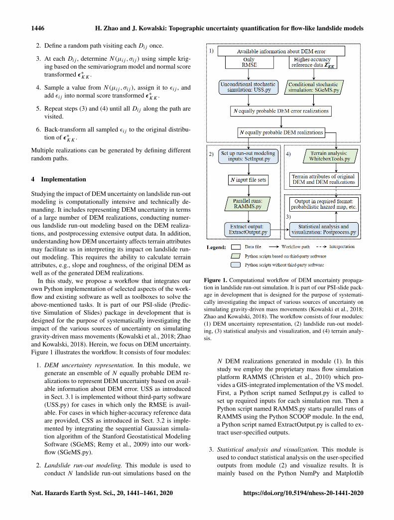
In this study, we propose a workflow that integrates ourown Python implementation of selected aspects of the work-flow and existing software as well as toolboxes to solve theabove-mentioned tasks. It is part of our PSI-slide (Predic-tive Simulation of Slides) package in development that isdesigned for the purpose of systematically investigating theimpact of the various sources of uncertainty on simulatinggravity-driven mass movements (Kowalski et al., 2018; Zhaoand Kowalski, 2018). Herein, we focus on DEM uncertainty.Figure 1 illustrates the workflow. It consists of four modules:

1. DEM uncertainty representation. In this module, wegenerate an ensemble of N equally probable DEM re-alizations to represent DEM uncertainty based on avail-able information about DEM error. USS as introducedin Sect. 3.1 is implemented without third-party software(USS.py) for cases in which only the RMSE is avail-able. For cases in which higher-accuracy reference dataare provided, CSS as introduced in Sect. 3.2 is imple-mented by integrating the sequential Gaussian simula-tion algorithm of the Stanford Geostatistical ModelingSoftware (SGeMS; Remy et al., 2009) into our work-flow (SGeMS.py).

2. Landslide run-out modeling. This module is used toconduct N landslide run-out simulations based on the

Figure 1. Computational workflow of DEM uncertainty propaga-tion in landslide run-out simulation. It is part of our PSI-slide pack-age in development that is designed for the purpose of systemati-cally investigating the impact of various sources of uncertainty onsimulating gravity-driven mass movements (Kowalski et al., 2018;Zhao and Kowalski, 2018). The workflow consists of four modules:(1) DEM uncertainty representation, (2) landslide run-out model-ing, (3) statistical analysis and visualization, and (4) terrain analy-sis.

N DEM realizations generated in module (1). In thisstudy we employ the proprietary mass flow simulationplatform RAMMS (Christen et al., 2010) which pro-vides a GIS-integrated implementation of the VS model.First, a Python script named SetInput.py is called toset up required inputs for each simulation run. Then aPython script named RAMMS.py starts parallel runs ofRAMMS using the Python SCOOP module. In the end,a Python script named ExtractOutput.py is called to ex-tract user-specified outputs.

3. Statistical analysis and visualization. This module isused to conduct statistical analysis on the user-specifiedoutputs from module (2) and visualize results. It ismainly based on the Python NumPy and Matplotlib



modules. For example, a probabilistic hazard map canbe produced to indicate potential hazard area.

4. Terrain analysis. This module is used to analyze terraincharacteristics of the original DEM and DEM realiza-tions from module (1), which may help us to interpretoutputs from module (3). This is achieved by integrat-ing several terrain analysis tools from WhiteboxTools(Lindsay, 2018) like calculating slope, aspect, rough-ness index, etc. into our workflow (WhiteboxTools.py).

5 Case study

This study is based upon a historic landslide and two DEMsources. For the purpose of DEM uncertainty propagationanalysis, we assume one DEM source to be more accuratethan the other and then obtain higher-accuracy reference datafrom the more accurate DEM source to assess elevation er-ror in the less accurate DEM source. We design a series ofcomputational scenarios based on the higher-accuracy refer-ence data to study the impact of DEM uncertainty on land-slide process simulation for both the case where only theRMSE is available and the case where higher-accuracy refer-ence data are available. Additional computational scenariosare designed to study the unrepresentative RMSE and sub-jective d issues as detailed in Sect. 3.1 in the form of a sen-sitivity analysis.

5.1 Scenario background and DEM sources

A historic landslide happened on 7 June 2008 on the hill-side above Yu Tung Road in Hong Kong due to an intenserainfall event; see Fig. 2. It was the largest flow-like land-slide out of 19 landslides during that event. Around 3400 m3

of material was mobilized and traveled about 600 m until itwas deposited. The landslide event had a severe infrastruc-tural impact, as it led to closure of the westbound lanes of YuTung Road for more than 2 months (AECOM Asia CompanyLimited, 2012). The Yu Tung Road landslide also served asa benchmark case for predictive landslide run-out analysis atthe second Joint Technical Committee on Natural Slopes andLandslides (JTC1) workshop on Triggering and Propagationof Rapid Flow-like Landslides in Hong Kong 2018 (Pastoret al., 2018). Two types of DEM data of the Yu Tung Roadarea were the basis for this study:

– A public 5 m resolution digital terrain model coveringthe whole area of Hong Kong (HK-DTM). It can bedownloaded from the website of the Survey and Map-ping Office of Hong Kong. The HK-DTM is generatedfrom a series of digital orthophotos, which are derivedfrom aerial photographs taken in 2014 and 2015. Thereported accuracy is ±5 m at a 90% confidence level.(DATA.GOV.HK, 2020)

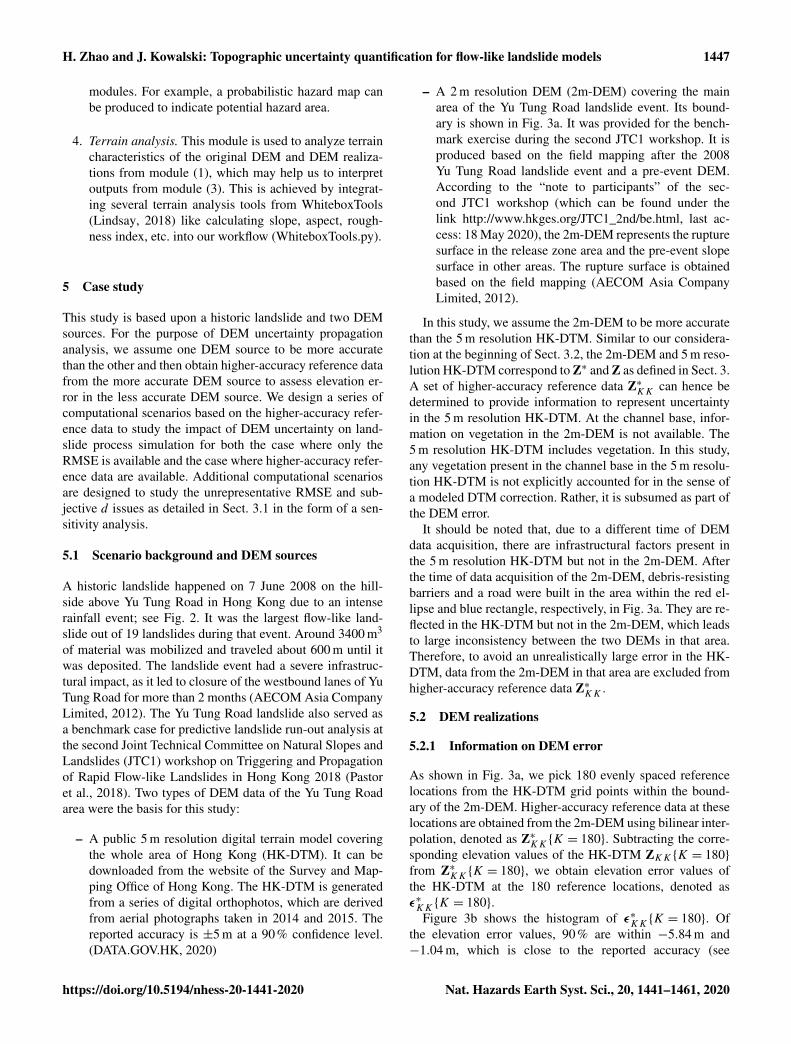
– A 2 m resolution DEM (2m-DEM) covering the mainarea of the Yu Tung Road landslide event. Its bound-ary is shown in Fig. 3a. It was provided for the bench-mark exercise during the second JTC1 workshop. It isproduced based on the field mapping after the 2008Yu Tung Road landslide event and a pre-event DEM.According to the “note to participants” of the sec-ond JTC1 workshop (which can be found under thelink http://www.hkges.org/JTC1_2nd/be.html, last ac-cess: 18 May 2020), the 2m-DEM represents the rupturesurface in the release zone area and the pre-event slopesurface in other areas. The rupture surface is obtainedbased on the field mapping (AECOM Asia CompanyLimited, 2012).

In this study, we assume the 2m-DEM to be more accuratethan the 5 m resolution HK-DTM. Similar to our considera-tion at the beginning of Sect. 3.2, the 2m-DEM and 5 m reso-lution HK-DTM correspond to Z∗ and Z as defined in Sect. 3.A set of higher-accuracy reference data Z∗KK can hence bedetermined to provide information to represent uncertaintyin the 5 m resolution HK-DTM. At the channel base, infor-mation on vegetation in the 2m-DEM is not available. The5 m resolution HK-DTM includes vegetation. In this study,any vegetation present in the channel base in the 5 m resolu-tion HK-DTM is not explicitly accounted for in the sense ofa modeled DTM correction. Rather, it is subsumed as part ofthe DEM error.

It should be noted that, due to a different time of DEMdata acquisition, there are infrastructural factors present inthe 5 m resolution HK-DTM but not in the 2m-DEM. Afterthe time of data acquisition of the 2m-DEM, debris-resistingbarriers and a road were built in the area within the red el-lipse and blue rectangle, respectively, in Fig. 3a. They are re-flected in the HK-DTM but not in the 2m-DEM, which leadsto large inconsistency between the two DEMs in that area.Therefore, to avoid an unrealistically large error in the HK-DTM, data from the 2m-DEM in that area are excluded fromhigher-accuracy reference data Z∗KK .

5.2 DEM realizations

5.2.1 Information on DEM error

As shown in Fig. 3a, we pick 180 evenly spaced referencelocations from the HK-DTM grid points within the bound-ary of the 2m-DEM. Higher-accuracy reference data at theselocations are obtained from the 2m-DEM using bilinear inter-polation, denoted as Z∗KK{K = 180}. Subtracting the corre-sponding elevation values of the HK-DTM ZKK{K = 180}from Z∗KK{K = 180}, we obtain elevation error values ofthe HK-DTM at the 180 reference locations, denoted asε∗KK{K = 180}.

Figure 3b shows the histogram of ε∗KK{K = 180}. Ofthe elevation error values, 90% are within −5.84 m and−1.04 m, which is close to the reported accuracy (see


http://www.hkges.org/JTC1_2nd/be.html


Figure 2. The 2008 Yu Tung Road landslide. Left: Google map of Hong Kong (map data © 2019). Right: aerial photograph of Yu Tung Roadsite after the 2008 landslide. It corresponds to the No. L25 landslide in the GEO Report (AECOM Asia Company Limited, 2012).

Sect. 5.1). The µ, σ , and RMSE according to Eqs. (7) and(6) are −3.0, 1.5, and 3.3 m, respectively. Here, it shouldbe noted that the RMSE is larger than the σ since the µ isnot zero, which indicates a systematic bias. As discussed inSect. 3.1, this also indicates that assuming the standard de-viation of the HK-DTM error to be equivalent to the RMSEin USS would overestimate the variability in the HK-DTMerror.

Based on ε∗KK{K = 180}, we can determine an isotropicsemivariogram model which describes the spatial autocorre-lation of the HK-DTM error. It results in

γ (h)= 0.1×Sph(h

180

)+ 0.9×Exp

(h

50

). (9)

Here, Sph(·) and Exp(·) denote the basic spherical and ex-ponential semivariogram models (Goovaerts, 1997) and hdenotes the horizontal distance between any two locations.A comparison between the experimental semivariance val-ues based on ε∗KK{K = 180} and the parameterized semivar-iogram model given by Eq. (9) can be seen in Fig. 4. Semi-variance is a measure of spatial dependence between DEMerror values at two different locations. The continuous semi-variogram model is fitted to the experimental semivariancevalues so as to deduce semivariance values for any possibledistance h required by simple kriging (Goovaerts, 1997). Therange of the semivariogram model is 180 m. It indicates themaximum autocorrelation length of the HK-DTM error, onwhich the size of the spatial moving filter d depends (seeSect. 3.1).

5.2.2 DEM uncertainty scenarios

As mentioned in Sect. 3, DEM users are often restricted toDEM error information in the form of a single RMSE valueper data product. Rarely, they have higher-accuracy referencedata. In order to account for both situations, two correspond-ing information levels are considered in the following study.

a. Rudimentary error information – the RMSE only. In thissituation, the RMSE is assumed to be the only availableerror information for the 5 m resolution HK-DTM. Inorder to compare results to (b), we employ the RMSE3.3 m as generated based on Z∗KK{K = 180} as well asthe size of the spatial moving filter d of 180 m to matchthe range of the fitted semivariogram model in Fig. 4.USS introduced in Sect. 3.1 is used to generate N re-alizations of the HK-DTM, denoted as USSN{RMSE=3.3, d = 180}.

b. Highly informed – higher-accuracy reference data. Inthis situation, Z∗KK{K = 180} is assumed to be avail-able. That means we know the error ε∗KK{K = 180} atthe reference locations exactly and the fitted semivari-ogram model based on ε∗KK{K = 180}. CSS introducedin Sect. 3.2 is used to generateN realizations of the HK-DTM, denoted as CSSN .

Following the two nominal scenarios (a) and (b) that arebased on specific error ε∗KK{K = 180} at reference locationsdetermined from the available data sources, we also want toanalyze the impact of unrepresentative RMSE and subjectived issues of USS as introduced in Sect. 3.1 in the form of asensitivity analysis. Hence, to what extent can we trust theresults of USS if only a single RMSE value per data prod-uct is available. Three additional values of the RMSE thatare 0.5, 1.5, and 2.5 m with a fixed d of 180 m are used asinputs for USS to study the unrepresentative RMSE issue. Itshould be noted that the RMSE 1.5 m corresponds to the truestandard deviation σ based on ε∗KK{K = 180}; see Fig. 3b.Another three additional values of d that are 0, 90, and 270 mwith a fixed RMSE of 3.3 m are used to consider the subjec-tive d issue. The corresponding realizations of the HK-DTMare denoted as USSN{RMSE= 0.5, 1.5, 2.5, d = 180} andUSSN{RMSE= 3.3, d = 0, 90, 270}. To sum up, all the sce-narios for stochastic simulation are listed in Table 1.



Figure 3. (a) Elevation error ε∗KK{K = 180} of the HK-DTM at 180 reference locations. The background is the hillshade plot of the HK-

DTM. Debris-resisting barriers and a road in the area indicated by the red ellipse and blue rectangle constructed after the 2008 landslide eventare represented in the HK-DTM but not in the 2m-DEM. It causes inconsistency between the two DEMs in that area. To avoid an unrealis-tically large error in the HK-DTM, data from the 2m-DEM in that area are excluded from higher-accuracy reference data. (b) Histogram ofε∗KK{K = 180}. The RMSE is larger than the standard deviation (σ ) since the mean (µ) is not zero. As discussed in Sect. 3.1, this indicates

that assuming the standard deviation of the HK-DTM error to be equivalent to the RMSE in USS would overestimate the variability in theHK-DTM error.

Table 1. Scenarios for stochastic simulation.

Method to generate Input to generateDEM realizations DEM realizations

Scenario (a) USS RMSE= 3.3; d = 180

Scenario (b) CSS semivariogram; ε∗KK{K = 180}

Scenarios forUSS RMSE= 0.5, 1.5, 2.5; d = 180

unrepresentative RMSE

Scenarios forUSS RMSE= 3.3; d = 0, 90, 270

subjective d

Note that, in scenario (a) and (b), the inputs to generate DEM realizations are obtained from higher-accuracyreference data at the 180 reference locations.

Figure 4. Experimental semivariances based on ε∗KK{K = 180}

and fitted parameterized semivariogram model given by Eq. (9). Therange of the semivariogram model is 180 m. It indicates the maxi-mum autocorrelation length of DEM error, on which the size of thespatial moving filter d depends (see Sect. 3.1).

5.2.3 Number of DEM realizations

The integrity of a stochastic simulation requires a largenumber of DEM realizations, and more realizations natu-rally require many computational resources. Thus one hasto find a reasonable compromise. Typically, this can befound through a representative convergence study. Sincein our study we address the impact of topographic uncer-tainty on landslide run-out simulation, we analyze the rel-ative change in topographic attributes with an increasingnumber of HK-DTM realizations in a preliminary study.In this study, 1000 HK-DTM realizations are generated forthe two information levels (a) and (b) as introduced inSect. 5.2.2, namely USSN=1000{RMSE= 3.3, d = 180} andCSSN=1000, respectively. Topographic attributes includingslope, aspect, and roughness at all HK-DTM grid points arecalculated for each realization.



We define an indicator of the relative change similarly toRaaflaub and Collins (2006) to investigate the converging be-havior. Taking slope as an example, for a given number n ofHK-DTM realizations, we first calculate the standard devi-ation of slope at each HK-DTM grid point over the n real-izations. The calculated standard deviation values at all gridpoints constitute a grid of standard deviation values. Thenwe calculate the standard deviation of the grid of standarddeviation values, which leads to a single standard deviationvalue for the given number n. For each n from 1 to 1000,we can correspondingly calculate a standard deviation value.The same procedure is applied to aspect, roughness, and ele-vation.

Figure 5 shows plots of normalized standard deviation ofthe grid of standard deviation values with respect to the num-ber of HK-DTM realizations for the two situations (a) and(b). It can be seen that for situation (a), aspect levels out first,followed by slope, roughness, and elevation. Beyond 500 re-alizations, there is little change in normalized standard de-viations. This indicates that adding more realizations has lit-tle impact on topographic attributes. For situation (b), aspectalso levels out first while the other three attributes show lessdifference. Compared to (a), (b) converges faster, which indi-cates CSS requires fewer DEM realizations than USS does.Nevertheless, we set N = 500 for the remainder of this studyboth for USS and CSS. Namely, we generate 500 HK-DTMrealizations for each scenario input set as listed in Table 1.

5.2.4 Statistics of DEM error realizations

In order to conduct a further quality check of our implemen-tation of both USS and CSS, we investigate the correspond-ing DEM error realizations of the USSN=500{RMSE= 3.3,d = 180} and CSSN=500 scenarios, denoted as USSError

N=500{RMSE= 3.3, d = 180} and CSSError

N=500, respectively. Ide-ally, the local mean µij and standard deviation σij of DEMerror realizations at each grid pointDij should match the un-derlying assumptions as introduced in Sect. 3 if the numberof DEM error realizations is sufficiently large.

Figure 6a and c show the mean and standard deviation gridof the USSError

N=500{RMSE= 3.3, d = 180}. It can be seen thatthe mean values at all grid points are centered around 0 m.The standard deviation values are centered around 3.3 m.This corresponds to the assumption underlying USS that allεij fulfill the same univariate Gaussian distribution with amean (µ) of zero and a standard deviation (σ ) given by theRMSE (see Sect. 3.1).

Figure 6b and d show the mean and standard deviationgrid of the CSSError

N=500. The mean values at grid points awayfrom the reference locations are centered around the mean(µ) −3.0 m based on ε∗KK{K = 180}. They become close toε∗KK{K = 180} with the decrease in distance between gridpoints and the reference locations and are equal to ε∗KK{K =180} at the reference locations. Similarly, the standard de-viation values at grid points away from the reference loca-

tions are centered around the standard deviation (σ ) 1.5 mbased on ε∗KK{K = 180}. They vanish at the reference lo-cations. This also corresponds to the assumption underlyingCSS that each εij fulfills a univariate Gaussian distributionwith a mean µij and standard deviation σij given by the sim-ple kriging estimate and simple kriging standard deviation atDij (see Sect. 3.2).

5.3 Landslide process simulation setup

With the DEM realizations generated in Sect. 5.2, we canstudy the impact of DEM uncertainty on landslide processsimulation. Here, we introduce the key inputs and our setupfor the process simulation.

5.3.1 Model input

Release zone area and fracture height, friction parameters,and a DEM are three key inputs for performing a determinis-tic landslide process simulation based on the VS model andutilizing the mass movement simulation platform RAMMS(Christen et al., 2010). For all scenarios, we consistently usethe release zone area as provided for the benchmark exer-cise during the second JTC1 workshop, which matches thatof the 2008 Yu Tung Road landslide (Pastor et al., 2018) asshown in Fig. 7b. The fracture height is assumed to be 1.2 m,leading to a release volume of around 2900 m3, based onthe 5 m resolution HK-DTM. The friction parameters µ andξ used in this study are 0.105 and 300 m s−2, respectively.They are suggested in the GEO Report issued by the CivilEngineering and Development Department of Hong Kongand are obtained using back analysis with information froma video capturing the lower portion of the landslide and de-tailed field mapping after the landslide (AECOM Asia Com-pany Limited, 2012). The HK-DTM and all HK-DTM real-izations generated in Sect. 5.2 are used as DEM inputs. En-trainment is not considered in this study.

It should be noted that release zone area and fractureheight, as well as friction parameters, may also be subjectto uncertainty in landslide modeling practice. In this studywe keep them fixed and focus only on the DEM uncertaintywhich is mostly overlooked in landslide run-out modeling.Future work should therefore continue to focus on system-atically quantifying all the uncertainty factors and evaluat-ing their relative importance and interaction. Researcherscarrying out this work should notice that increasing the di-mension of uncertainty factors instantly requires a muchlarger number of simulation runs for stochastic simulationand computational-resource consumption may become pro-hibitively expensive. One promising solution to this chal-lenge is to employ emulator techniques.

5.3.2 Simulation ensembles

We denote a deterministic landslide process simulation basedon a DEM as a simulation run and N deterministic landslide



Figure 5. The relative change in topographic attributes with respect to the number of HK-DTM realizations. The realizations are generatedwith (a) USSN{RMSE= 3.3, d = 180}; (b) CSSN . Beyond N = 500, adding more realizations has little impact on topographic attributes.Therefore, we set N = 500 for all computational scenarios in Table 1.

Figure 6. Statistics of HK-DTM error realizations. (a) Mean and (c) standard deviation grid of USSErrorN=500{RMSE= 3.3, d = 180}. The

mean and standard deviation values are centered around 0 and 3.3 m. (b) Mean and (d) standard deviation grid of CSSErrorN=500. The mean

values at grid points away from the reference locations are centered around the mean (µ) −3.0 m of ε∗KK{K = 180} and are equal to

ε∗KK{K = 180} at the reference locations. The standard deviation values at grid points away from the reference locations are centered around

the standard deviation (σ ) 1.5 m of ε∗KK{K = 180} and vanish at the reference locations. This matches the assumptions underlying USS and

CSS as introduced in Sect. 3.

process simulations based on N DEM realizations as a simu-lation ensemble. The following deterministic simulation andsimulation ensembles are conducted based on the originalHK-DTM and the aforementioned computational scenarios;see Table 1. They are named after the corresponding DEMand DEM realizations.

1. Deterministic simulation HK-DTM. One landslide pro-cess simulation run is conducted based on the origi-nal HK-DTM. This one time simulation corresponds towhat is traditionally performed in a simulation-based

hazard assessment study. The results serve as the basisto assess the impact of DEM uncertainty.

2. USSN=500{RMSE= 3.3, d = 180} ensemble. A total of500 landslide process simulations are conducted basedon the USSN=500{RMSE= 3.3, d = 180} DEM real-izations as introduced in Sect. 5.2. Each of them is re-ferred to as USSnN=500{RMSE= 3.3, d = 180}, withn= 1,2, . . .,500. This ensemble allows us to access the



impact of DEM uncertainty if only the RMSE is avail-able.

3. CSSN=500 ensemble. A total of 500 landslide pro-cess simulations are conducted based on the CSSN=500DEM realizations. Similar to (2), each of them is re-ferred to as CSSnN=500, with n= 1,2, . . .,500. This en-semble allows us to assess the impact of DEM uncer-tainty if higher-accuracy reference data are available.

4. USSN=500{RMSE= 0.5, 1.5, 2.5, d = 180} ensembles.For each of the three different RMSE values, 500 land-slide process simulations are conducted, while keepingthe maximum autocorrelation length d constant. Theylead to 1500 process simulations. The results allow usto discuss the unrepresentative RMSE issue as detailedin Sect. 3.1. They can be also used to discuss the rela-tionship between the degree of DEM uncertainty and itsimpact.

5. USSN=500{RMSE= 3.3, d = 0, 90, 270} ensembles.For each of the three maximum autocorrelation lengthvalues, 500 landslide process simulations are con-ducted, while keeping the RMSE constant. They leadto 1500 process simulations. The results allow us to dis-cuss the subjective d issue as detailed in Sect. 3.1.

All in all this adds up to one deterministic simulation runHK-DTM, as well as to simulation ensembles of 500 processsimulations of both the USSN=500 {RMSE= 3.3, d = 180}ensemble and the CSSN=500 ensemble, which is constructedfrom higher-accuracy reference data based on the 2m-DEM,and 3000 additional process simulations to result in six en-sembles of USSN=500{RMSE= 0.5, 1.5, 2.5, d = 180} andUSSN=500{RMSE= 3.3, d = 0, 90, 270} to test sensitivi-ties. Each process simulation takes around 1 min on a laptopwith Intel Core i7-9750H CPU, adding up to around 67 h ofsimulation time.

6 Results and discussions

This section is organized according to the simulation ensem-bles introduced in Sect. 5.3.2. Section 6.1 presents the re-sults of the deterministic simulation HK-DTM which servesas the basis for all following discussions. Section 6.2 is de-voted to analyzing the impact of DEM uncertainty on land-slide process simulation in the cases of only the RMSE beingavailable (USSN=500{RMSE= 3.3, d = 180} ensemble) andhigher-accuracy reference data being available (CSSN=500ensemble). In Sect. 6.3, the unrepresentative RMSE and sub-jective d issues are discussed based on the ensembles de-scribed in Sect. 5.3.2 (labeled 4 and 5).

6.1 Deterministic simulation HK-DTM

In a continuum-mechanical landslide process model such asthat used for this study and introduced in Sect. 2, the land-

Figure 7. Results of the deterministic simulation HK-DTM.(a) Hmax(x,y) above a cutoff threshold of 0.1 m. The black out-line is the 0.1 m contour ofHmax(x,y). The area within this outlineis regarded as the hazard area. Area 1–3 are denoted for later discus-sions (see Sect. 6.2.1). (b) ‖Umax(x,y)‖ above a cutoff threshold of0.01 m s−1. The relatively high elevation area within the red circledecelerates and holds back the flow material. The channel bottomand cross section are denoted for later discussions (see Sect. 6.2.2).

slide flow behavior is characterized by its spatially vary-ing height and velocity distribution over time, denoted asH(x,y, t) and U(x,y, t). Hence, for the purpose of land-slide hazard assessment and mitigation measure develop-ment, maximum height and velocity data over the durationof the landslide are most informative. Thus, we focus on themaximum values of H(x,y, t) and U(x,y, t) over the wholetime, denoted as Hmax(x,y) and ‖Umax(x,y)‖.

Figure 7a and b show Hmax(x,y) and ‖Umax(x,y)‖ asgiven by the deterministic simulation HK-DTM. It shouldbe noted that there is a relatively high elevation area at theend part of the channel in the HK-DTM as denoted withinthe red circle in Fig. 7b. It corresponds to the construction ofdebris-resisting barriers after the 2008 Yu Tung Road land-slide as introduced in Sect. 5.1. The flow material is decel-erated and held back here. We will come back to this pointlater in Sect. 6.2.1.

Landslide run-out distance is often characterized in termsof its apparent friction angle. The tangent of the apparentfriction angle is equal to the ratio of the landslide fall heightand the run-out distance (DeBlasio and Elverhoi, 2008). Theapparent friction angle evaluated from the deterministic sim-ulation is 16.80◦. This result is used as a reference to assessthe impact of DEM uncertainty in the following discussions.



6.2 USSN=500{RMSE = 3.3, d = 180} ensemble andCSSN=500 ensemble

While it is straightforward to present the results of a deter-ministic simulation run as shown in Sect. 6.1, a stochasticsimulation-based ensemble ofN simulation runs calls for tai-lored statistics to manage and interpret the extensive outputdata. First, we define the hazard probability P(xl ,yl) at one lo-cation (xl,yl) as the frequency of Hmax(xl,yl) exceeding acertain predefined height threshold value; hence

P(xl ,yl) =

∑Nn=1P

n(xl ,yl)

N, P n(xl ,yl)

=

{1, if H n

max(xl,yl)≥ threshold

0, otherwise,(10)

where H nmax(xl,yl) denotes the maximum flow height at lo-

cation (xl,yl) for the nth simulation run of the correspondingensemble. Hence P n(xl ,yl) indicates whether location (xl,yl) iswithin the hazard area of the nth simulation run for a giventhreshold, and P(xl ,yl) indicates the resulting hazard proba-bility at location (xl,yl) considering the complete ensemble.Here, the threshold is set as 0.1 m, which matches the cut-off threshold of the deterministic simulation HK-DTM inFig. 7a. Evaluation of hazard probabilities at all locationsthen gives rise to a probabilistic hazard map (Stefanescuet al., 2012), which provides an overall view of the DEMuncertainty impact.

Besides assessing the overall impact of DEM uncertaintyin terms of the probabilistic hazard map, we will also dis-cuss the local impact of DEM uncertainty on dynamic flowproperties, focusing onHmax(x,y) and ‖Umax(x,y)‖ at loca-tions along the channel bottom and the channel cross sectiondenoted in Fig. 7b.

6.2.1 Probabilistic hazard maps

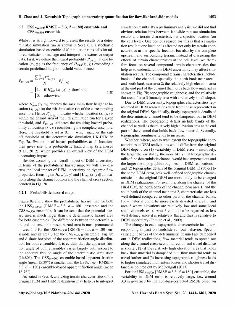
Figure 8a and c show the probabilistic hazard map for boththe USSN=500 {RMSE= 3.3, d = 180} ensemble and theCSSN=500 ensemble. It can be seen that the potential haz-ard area is much larger than the deterministic hazard areafor both ensembles. The difference between the determinis-tic and the ensemble-based hazard area is most pronouncedin area 1–3 for the USSN=500 {RMSE= 3.3, d = 180} en-semble and in area 3 for the CSSN=500 ensemble. Fig. 8band d show boxplots of the apparent friction angle distribu-tion for both ensembles. It is evident that the apparent fric-tion angle of both ensembles varies largely with respect tothe apparent friction angle of the deterministic simulation(16.80◦). The CSSN=500 ensemble-based apparent frictionangle (mean 15.39◦) is smaller than the USSN=500 {RMSE=3.3, d = 180} ensemble-based apparent friction angle (mean16.76◦).

As stated in Sect. 4, analyzing terrain characteristics of theoriginal DEM and DEM realizations may help us to interpret

simulation results. By a preliminary analysis, we did not findobvious relationships between landslide run-out simulationresults and terrain characteristics at a specific location (onthe cell level). One obvious reason for this is that a simula-tion result at one location is affected not only by terrain char-acteristics at the specific location but also by the completeupstream and surrounding terrain. Instead of discussing theeffects of terrain characteristics at the cell level, we there-fore focus on several compound terrain characteristics thathelp us to understand how DEM uncertainty may affect sim-ulation results. The compound terrain characteristics includebanks of the channel, especially the north bank near area 1and south bank near area 2; the relatively high elevation areaat the end part of the channel that holds back flow material asshown in Fig. 7b; topographic roughness; and the relativelyflat area of area 3 (namely area with a relatively small slope).

Due to DEM uncertainty, topographic characteristics rep-resented in DEM realizations vary from those represented inthe original DEM. Specifically, firstly, topographic details ofthe deterministic channel tend to be dampened out in DEMrealizations. The topographic details include banks of thechannel as well as the relatively high elevation area at the endpart of the channel that holds back flow material. Secondly,topographic roughness tends to increase.

Whether, where, and to what extent the topographic char-acteristics in DEM realizations would differ from the originalDEM depend on (1) variability in DEM error – intuitively,the larger the variability, the more likely that topographic de-tails of the deterministic channel would be dampened out andthe larger the topographic roughness in DEM realizations –and (2) topographic details of the original DEM. If subject tothe same DEM error, less well defined topographic charac-teristics in the original DEM are more likely to be changedin DEM realizations. For example, along the channel of theHK-DTM, the north bank of the channel near area 1, and thesouth bank of the channel near area 2, characteristics are lesswell defined compared to other parts of the channel banks.Flow material could be more easily diverted to area 1 andarea 2 where elevations are relatively low and some localsmall channels exist. Area 3 could also be regarded as lesswell defined since it is relatively flat and thus is sensitive toDEM uncertainty (Temme et al., 2009).

The change in each topographic characteristic has a cor-responding impact on landslide run-out behavior. Specifi-cally (1) if banks of the deterministic channel are dampenedout in DEM realizations, flow material tends to spread outalong the channel cross-section direction and travel distanceis shorter; (2) if the relatively high elevation area that holdsback flow material is dampened out, flow material tends totravel further; and (3) increasing topographic roughness leadsto higher simulated momentum losses and shorter travel dis-tance as pointed out by McDougall (2017).

For the USSN=500 {RMSE= 3.3, d = 180} ensemble, thevariability in DEM error is relatively large, i.e., around3.3 m governed by the non-bias-corrected RMSE based on



Figure 8. (a) Probabilistic hazard map and (b) corresponding apparent friction angle distribution of the USSN=500 {RMSE= 3.3, d = 180}ensemble; (c) probabilistic hazard map and (d) corresponding apparent friction angle distribution of the CSSN=500 ensemble. The blackoutline plotted on the hazard maps represents the deterministic hazard area (see Fig. 7a). In the boxplots, the blue star denotes the apparentfriction angle of the deterministic simulation HK-DTM (see Sect. 6.1). The difference between the deterministic and the ensemble-basedhazard area is most pronounced in area 1–3 for the USSN=500 {RMSE= 3.3, d = 180} ensemble and in area 3 for the CSSN=500 ensemble.

ε∗KK{K = 180} (see Fig. 6c). In this situation, both the northbank near area 1 and south bank near area 2 as well as therelatively high elevation area at the end part of the chan-nel can be dampened out in HK-DTM realizations. For theCSSN=500 ensemble, the variability in DEM error is rela-tively small, i.e., around 1.5 m governed by the standard de-viation (σ ) based on ε∗KK{K = 180} (see Fig. 6d). In thissituation, the banks tend to remain well defined, while therelatively high elevation area can be dampened out in HK-DTM realizations. Thus, area 1 and area 2 are possibly sub-ject to hazard in the USSN=500 {RMSE= 3.3, d = 180} en-semble but less likely to be so in the CSSN=500 ensemble.As mentioned above, area 3 is a flat area which is sensitive toDEM uncertainty. Furthermore, it is located near the deposi-tion, around which the impact of upstream DEM uncertaintyseems to accumulate. Thus, it is highly affected in both en-sembles.

The apparent friction angle distribution is determinedby a combined effect of change in channel banks, changein the relatively high elevation area at the end part ofthe channel, and increasing topographic roughness. Forthe USSN=500 {RMSE= 3.3, d = 180} ensemble, a dete-riorated channel bank representation and increasing topo-graphic roughness make flow material travel a shorter dis-tance, i.e., larger apparent friction angle, while a deterioratedrelatively high elevation area representation allows flow ma-terial to travel further, i.e., smaller apparent friction angle.

For the CSSN=500 ensemble, channel banks are likely toremain well defined and the degree of topographic rough-ness increase is lower due to its relatively small variabil-ity in DEM error compared to the USSN=500 {RMSE= 3.3,d = 180} ensemble. Thus, flow material in the CSSN=500ensemble tends to travel a longer distance, i.e., smaller ap-parent friction angle, compared to the flow material in theUSSN=500 {RMSE= 3.3, d = 180} ensemble.

In summary, we can conclude from the probabilistic haz-ard maps and boxplots of apparent friction angle distributionthat (1) accounting for DEM uncertainty may significantlyincrease the potential hazard area, (2) the potential hazardarea is highly related to the variability in DEM error and to-pographic characteristics of the original DEM, and (3) USSbased on the RMSE only may overestimate the spread of po-tential hazard area and underestimate travel distance due to anon-bias-corrected RMSE that overestimates the variabilityin DEM error.

It should be noted that the probabilistic hazard map hereis constructed based on maximum height and a predefinedthreshold. In simulation-based hazard assessment practice,one may indicate potential hazard using other indicators,e.g., the maximum momentum that reflects the impact pres-sure, and correspondingly modify the threshold value. In thiscase, our workflow is easily extendible to account for otherindicators.



6.2.2 Dynamic flow properties

Figure 9a, c, and e show elevation, maximum height, andmaximum velocity at locations along the channel bottombased on the USSN=500 {RMSE= 3.3, d = 180} ensemble.It is evident that both maximum height and maximum veloc-ity at these locations largely vary from those of the determin-istic simulation. Specifically, the mean of maximum height(maximum velocity) values at all the locations based on thedeterministic simulation is 1.28 m (7.17 m s−1). The mean ofthe ensemble-based 90 % confidence interval of maximumheight (maximum velocity) is [0.18 m, 2.17 m] ([0.99 m s−1,7.89 m s−1]; the range between the mean of the ensemble-based 5th percentile and the mean of the ensemble-based95th percentile). Another observation is that the ensemble-based mean of flow dynamic properties is generally smallerthan the mean of flow dynamic properties of the determin-istic simulation (as seen by the dashed red line being gener-ally under the black line in both Fig. 9c and e). The meanof the ensemble-based mean of maximum height (maximumvelocity) is 0.85 m (4.57 m s−1), around 66 % (64 %) of themean of the deterministic simulation at 1.28 m (7.17 m s−1;see Fig. 9c and e).

Figure 9b, d, and f show corresponding results basedon the CSSN=500 ensemble. Similar trends to those in theUSSN=500 {RMSE= 3.3, d = 180} ensemble can also beobserved. Namely, both maximum height and maximum ve-locity at these locations largely vary from those of the de-terministic simulation, and the ensemble-based mean of flowdynamic properties is generally smaller than that of the de-terministic results. The main differences are that the varia-tion range of CSSN=500 ensemble-based flow dynamic prop-erties is smaller and the CSSN=500 ensemble-based mean offlow dynamic properties is larger compared to those of theUSSN=500 {RMSE= 3.3, d = 180} ensemble. More specif-ically, the mean of the CSSN=500 ensemble-based 90 % con-fidence interval of maximum height (maximum velocity) is[0.5 m, 2.03 m] ([3.56 m s−1, 7.99 m s−1]). The mean of theCSSN=500 ensemble-based mean of maximum height (max-imum velocity) is 1.1 m (6.01 m s−1), around 86 % (84 %) ofthe mean of the deterministic simulation 1.28 m (7.17 m s−1;see Fig. 9d and f).

The above observations result from similar factors to thosediscussed in Sect. 6.2.1. Due to DEM uncertainty, the follow-ing statements can be made:

– Ensemble-based flow dynamic properties are likely tovary from those of the deterministic simulation. Largervariability in DEM error is likely to result in moreextreme results. As discussed in Sect. 6.2.1, the vari-ability in DEM error for the USSN=500 {RMSE= 3.3,d = 180} ensemble is larger than that for the CSSN=500ensemble due to the unrepresentative RMSE issue. Thusthe variation range of USSN=500 {RMSE= 3.3, d =180} ensemble-based flow dynamic properties is gen-

erally larger than that of CSSN=500 ensemble-basedflow dynamic properties, giving a larger mean of theensemble-based 90 % confidence interval (the trendwould be more clear if we also consider outliers outsidethe 90 % confidence interval).

– Banks of the deterministic channel may be dampenedout in DEM realizations. Deteriorated channel bankrepresentation makes flow material more spread outalong the channel cross-section direction. This couldlead to a smaller ensemble-based mean of flow dy-namic properties at channel bottom locations comparedto flow dynamic properties of the deterministic simula-tion. This can be directly seen in Fig. 10, which dis-plays results of one channel cross section. Also, dueto larger variability in DEM error, flow material in theUSSN=500 {RMSE= 3.3, d = 180} ensemble is morespread along the channel cross-section direction, result-ing in a smaller ensemble-based mean of flow dynamicproperties at channel bottom locations compared to thatof the CSSN=500 ensemble. This can also be seen inFig. 10.

– Topographic roughness in DEM realizations tends toincrease. As pointed out in Sect. 6.2.1, increasing to-pographic roughness results in higher simulated mo-mentum losses and thus smaller flow dynamic proper-ties on average. The higher the degree of topographicroughness increase, the higher the simulated momen-tum losses and the smaller the flow dynamic proper-ties. This also contributes to a smaller ensemble-basedmean of flow dynamic properties at channel bottom lo-cations compared to flow dynamic properties of the de-terministic simulation, as well as to a smaller USSN=500{RMSE= 3.3, d = 180} ensemble-based mean of flowdynamic properties at channel bottom locations com-pared to the CSSN=500 ensemble.

Based on the ensembles’ dynamic flow properties we canconclude that (1) accounting for DEM uncertainty may sig-nificantly affect dynamic flow properties, e.g., maximumheight and maximum velocity, and hence any hazard assess-ment that is based on landslide dynamics and (2) USS basedonly on the RMSE may overestimate the range of dynamicflow properties and underestimate the ensemble-based meanof dynamic flow properties due to an unrepresentative RMSEthat overestimates the variability in DEM error.

6.3 Additional ensembles to investigate USSsensitivities in RMSE and d

Here, we discuss the unrepresentative RMSE and subjectived issues as introduced in Sect. 3.1 based on six additionalensembles, USSN=500 {RMSE= 0.5, 1.5, 2.5, d = 180} and{RMSE= 3.3, d = 0, 90, 270} (refer to Sect. 5.3.2), as wellas the USSN=500 {RMSE= 3.3, d = 180} ensemble. Results



Figure 9. Elevation, maximum height, and maximum velocity at locations along the channel bottom (see Fig. 7b). Panels (a), (c), and(e) correspond to the USSN=500 {RMSE= 3.3, d = 180} ensemble and panels (b), (d), and (f) to the CSSN=500 ensemble. In each panel,dash-dotted blue lines represent the ensemble-based 5th and 95th percentiles of the quantity. The dashed red line represents the ensemble-based mean of the quantity. The black line denotes corresponding results of the deterministic simulation. Annotated mean values are anaverage of all the locations. Ensemble-based flow dynamic properties largely vary from deterministic simulation results. The variation rangeof the USSN=500 {RMSE= 3.3, d = 180} ensemble is larger, while its ensemble-based mean is smaller, compared to counterparts of theCSSN=500 ensemble.

of the CSSN=500 ensemble are used as a reference sinceCSSN=500 incorporated more information on the DEM er-ror. It is thus reasonable to assume that its results reflect thereality better.

Figure 11 shows the consolidated results of the ensembles.The left, middle, and right column correspond to the set ofUSSN=500 {RMSE= 0.5, 1.5, 2.5, 3.3, d = 180} ensembles,set of USSN=500 {RMSE= 3.3, d = 0, 90, 180, 270} en-sembles, and CSSN=500 ensemble, respectively. The first rowshows stacked bar plots of the potential hazard area’s magni-tude based on the probabilistic hazard map for each ensemble

(see Fig. 8a and c). The second row shows the apparent fric-tion angle distribution. The last two rows show statistics ofmaximum height and maximum velocity at channel bottomlocations (see Fig. 9c–f). Also, deterministic simulation re-sults are included.

Focusing on the left column, it can be seen that with in-creasing RMSE (1) low-probability (0–0.2) hazard area sig-nificantly increases and high-probability (0.8–1) hazard areagradually decreases, leading to increase in overall potentialhazard area if we keep the same threshold value; (2) exceptfor the RMSE= 0.5 m ensemble, the apparent friction an-



Figure 10. Elevation, maximum height, and maximum velocity at locations along the channel cross section (see Fig. 7b). Panels (a), (c), and(e) correspond to the USSN=500 {RMSE= 3.3, d = 180} ensemble and panels (b), (d), and (f) to the CSSN=500 ensemble. In each panel,dash-dotted blue lines represent ensemble-based 5th and 95th percentiles of the quantity. The dashed red line represents the ensemble-basedmean of the quantity. The black line denotes corresponding results of the deterministic simulation. Annotated mean values are an averageof all the locations. Due to DEM uncertainty, flow material of both ensembles tends to spread out along the channel cross-section direction.The ensemble-based mean of flow dynamic properties at the channel bottom location is smaller than flow dynamic properties at the channelbottom location of the deterministic simulation (compare peak value of dashed red line with peak value of black line). The more the flowmaterial spreads out, the smaller the ensemble-based mean of flow dynamic properties at the channel bottom location (compare results of theUSSN=500 {RMSE= 3.3, d = 180} ensemble with those of the CSSN=500 ensemble).

gle steadily increases; and (3) the range of extreme valuesof maximum height (maximum velocity) at channel bottomlocations increases while the average of maximum height(maximum velocity) at channel bottom locations decreases.

For purely RMSE-based USS, the standard deviation ofDEM error is assumed to be determined by the RMSE. Hencelarger RMSE indicates larger variability in DEM error inDEM realizations. The larger the variability in DEM error,the more likely topographic details of the deterministic chan-

nel would be dampened out and the larger the topographicroughness in DEM realizations. As discussed in Sect. 6.2.1,this would make flow material more spread out along thechannel cross-section direction (namely larger potential haz-ard area) and travel a shorter distance (namely larger appar-ent friction angle). As discussed in Sect. 6.2.2, larger vari-ability in DEM error is likely to result in more extreme valuesof flow dynamic properties (namely larger range of extremevalues), while spreading of flow material along the channel



Figure 11. Consolidated results of all ensembles. The left, middle,and right columns correspond to the set of USSN=500 {RMSE=0.5, 1.5, 2.5, 3.3, d = 180} ensembles, set of USSN=500 {RMSE=3.3, d = 0, 90, 180, 270} ensembles, and CSSN=500 ensemble, re-spectively. The first row shows stacked bar plots of the potentialhazard area’s magnitude based on the probabilistic hazard map foreach ensemble (see Fig. 8a and c). The second row shows appar-ent friction angle distribution. The last two rows show statistics ofmaximum height and maximum velocity at channel bottom loca-tions (see Fig. 9c–f).

cross-section direction and larger topographic roughness leadto a smaller ensemble-based mean of flow dynamic proper-ties at channel bottom locations.

As discussed in Sect. 6.2.1, the apparent friction angledistribution is determined by a combined effect of changein channel banks, change in the relatively high elevationarea at the end part of the channel, and increasing topo-graphic roughness. It naturally follows that for a small vari-ability in DEM error (here RMSE= 0.5 m), all the changesare less significant in DEM realizations, and thus the appar-ent friction angle of the USSN=500{RMSE= 0.5, d = 180}ensemble closely matches the deterministic simulation re-sult. For an intermediate variability in DEM error (hereRMSE = 1.5 m), the relatively high elevation area at the endpart of the channel is subject to change, while channel bankstend to remain well defined in DEM realizations. This leadsto a longer travel distance of the USSN=500{RMSE=1.5,d = 180} ensemble (namely smaller apparent friction angle)in comparison to that of the deterministic simulation result.

From the middle column of Fig. 11, we find that the re-sults for a USS ensemble of vanishing spatial autocorrelationUSSN=500 {RMSE= 3.3, d = 0} consistently differ signif-icantly from USS ensembles that include spatial autocorre-lation, namely USSN=500{RMSE= 3.3, d = 90, 180, 270}ensembles. This indicates that whether spatial autocorrela-tion is considered or not may make a difference but the extentof spatial autocorrelation has less influence on simulation re-sults. As we know spatial autocorrelation to be present intopographic data but often lack information on its exact au-tocorrelation length, this is actually good news for practicalhazard assessment studies.

Comparing the left column of Fig. 11 with the right col-umn, it can furthermore be seen that the results of theUSSN=500 {RMSE= 1.5, d = 180} ensemble are quite closeto the results of the CSSN=500 ensemble. The USSN=500{RMSE= 1.5, d = 180} ensemble is informed of the bias-corrected RMSE (namely the true standard deviation, in ourcase 1.5 m; see Fig. 3b). It indicates that if a bias-correctedRMSE is given, USS is able to provide reasonable resultsconsidering that the extent of spatial autocorrelation has lessinfluence on simulation results.

All in all, we find that (1) the results of USS are in generalmore sensitive to values of the RMSE and less sensitive tovalues of d; (2) an unrepresentative RMSE that overestimatesthe variability in DEM error may overestimate the potentialhazard area and extreme values of dynamic flow properties;(3) whether or not spatial autocorrelation of DEM error isconsidered can make a difference in ensemble-based simu-lation results; and (4) if a bias-corrected RMSE is given, itis possible to obtain reasonable ensemble-based simulationresults using USS.



7 Conclusions

In this paper, we investigated different approaches to study-ing the impact of topographic uncertainty on simulation-based flow-like landslide run-out analyses. Based upon a his-toric landslide event for which two DEM data sets of differ-ent accuracy were available, we presented a series of compu-tational scenarios. Unconditional and conditional stochasticsimulation are conducted to generate DEM realizations, bothfor the case in which only the RMSE is available and for thecase in which reference data of higher accuracy are available.The computational workflow including the stochastic sim-ulation to generate the DEM realizations and the landsliderun-out simulation is implemented as a modular Python-based package. How topographic uncertainty propagates inthe results of landslide run-out analysis is discussed in de-tail. In addition, we addressed the two major issues of purelyRMSE-based unconditional stochastic simulation, i.e., thefact that non-bias-corrected RMSE overestimates the vari-ability in DEM error (referred to as unrepresentative RMSEin our study) and the fact that determining the size of the spa-tially moving filter in the absence of further information onthe spatial DEM error structure is often subjective (referredto as subjective d in our study). Our main conclusions are asfollows:

– DEM uncertainty significantly affects simulation-basedlandslide run-out modeling depending on how well theunderlying flow path is represented, which is deter-mined by topographic characteristics of the originalDEM and the variability in DEM error. For the samedegree of variability in DEM error, the less well definedparts of the flow path in the original DEM are morelikely to be affected and thus lead to change in flow be-havior at these parts. Also, an increasing variability inDEM error leads to an increased impact. More specifi-cally, with increasing variability in the DEM error, thepotential hazard area and extreme values of dynamicflow properties are likely to increase. This shows theimportance of considering topography-induced uncer-tainty for simulation-based landslide hazard assessmentrather than simply trusting the results of a determinis-tic simulation if a high accuracy of the DEM source isnot guaranteed. Also, a preliminary terrain analysis maygive some hints on areas that will potentially be affectedby a topographic uncertainty study.

– Both unconditional and conditional stochastic simu-lation methods can be applied to study DEM uncer-tainty propagation in landslide run-out modeling. Theirmain difference is that the computationally performantunconditional stochastic simulation can be conductedbased on RMSE information only, while the compu-tationally costly conditional stochastic simulation re-quires the availability of higher-accuracy reference dataand is thus more accurate. The higher-accuracy refer-

ence data provide additional information on the DEMerror structure, i.e., its spatial autocorrelation. If theDEM does not contain systematic bias or alternativelya bias-corrected RMSE is provided, the unconditionalstochastic simulation yields reasonable results. Oth-erwise, the assumptions underlying the unconditionalstochastic simulation lead to an overestimation of theDEM error variability, which leads to an increased po-tential impact of DEM uncertainty on the potential haz-ard area and to extreme values of dynamic flow prop-erties. In particular, our study shows that if no higher-accuracy reference data are available or if computa-tional costs of a conditional stochastic simulation aretoo large, the results of a RMSE-based unconditionalstochastic simulation can still be used to provide an up-per bound on the potential hazard area as well as ex-treme values of flow dynamic properties for a hazard as-sessment to take topographic uncertainties into account.

– Results of an unconditional stochastic simulation are ingeneral sensitive to the RMSE value as well as sensitiveto whether or not the DEM error’s spatial autocorrela-tion is considered. If the latter is taken into account, re-sults are less sensitive to the actual value of the DEMerror’s maximum autocorrelation length. This indicatesthat determining a representative RMSE may be moreimportant than finding a correct maximum autocorrela-tion length, while the DEM error’s spatial autocorrela-tion should not be ignored for simulation-based land-slide hazard assessment.

Data availability. The 5 m resolution HK-DTM used in thisstudy is available as a free download on the website of theSurvey and Mapping Office of Hong Kong under the fol-lowing link: https://www.landsd.gov.hk/mapping/en/download/psi/opendata.htm (DATA.GOV.HK, 2020). The 2 m resolution DEMwas provided by the organizers of the second JTC1 workshop onTriggering and Propagation of Rapid Flow-like Landslides held inHong Kong in 2018 to conduct a benchmark exercise. Readers canapproach the Civil Engineering and Development Department ofHong Kong to obtain these DEM data for research purposes.

Author contributions. JK and HZ conceived the idea and designedthe case study. HZ performed the implementation, simulations, anddata analyses with contributions from JK. HZ wrote the manuscript.JK reviewed and revised the manuscript.

Competing interests. The authors declare that they have no conflictof interest.

Acknowledgements. We thank the Civil Engineering and Develop-ment Department of Hong Kong for provision of the 2 m resolution


https://www.landsd.gov.hk/mapping/en/download/psi/opendata.htm



DEM. We also thank DATA.GOV.HK for the public 5 m resolutionDTM.

Financial support. This research has been supported by the ChinaScholarship Council (grant no. 201706260262) and the RWTH Ex-ploratory Research Space (Prep Fund PFSDS025).

Review statement. This paper was edited by Paola Reichenbachand reviewed by two anonymous referees.

References

AECOM Asia Company Limited: Detailed study of the 7 June 2008landslides on the hillshade above Yu Tung Road, Tung Chung,Tech. rep., 2012.

Aziz, S., Steward, B., Kaleita, A., and Karkee, M.: Assess-ing the effects of DEM uncertainty on erosion rate esti-mation in an agricultural field, T. ASABE, 55, 785–798,https://doi.org/10.13031/2013.41514, 2012.

Bartelt, P., Salm, B., and Gruber, U.: Calculating dense-snowavalanche runout using a Voellmy-fluid model with ac-tive/passive longitudinal straining, J. Glaciol., 45, 242–254,https://doi.org/10.3189/002214399793377301, 1999.

Berry, P., Garlick, J., and RG, S.: Near-global validation ofthe SRTM DEM using satellite radar altimetry, Remote Sens.Environ., 106, 17–27, https://doi.org/10.1016/j.rse.2006.07.011,2007.

Bolkas, D., Fotopoulos, G., Braun, A., and Tziavos,I.: Assessing digital elevation model uncertainty us-ing GPS survey data, J. Surv. Eng., 142, 04016001,https://doi.org/10.1061/(ASCE)SU.1943-5428.0000169, 2016.

Christen, M., Kowalski, J., and Bartelt, P.: RAMMS: nu-merical simulation of dense snow avalanches in three-dimensional terrain, Cold Reg. Sci. Technol., 63, 1–14,https://doi.org/10.1016/j.coldregions.2010.04.005, 2010.

Courty, L., Soriano-Monzalvo, J., and Pedrozo-Acuna, A.: Evalu-ation of open-access global digital elevation models (AW3D30,SRTM, and ASTER) for flood modelling purposes, J. Flood RiskManag., 12, e12550, https://doi.org/10.1111/jfr3.12550, 2019.

DATA.GOV.HK: 5 m resolution digital terrain model of the HongKong Special Administrative Region, available at: https://www.landsd.gov.hk/mapping/en/download/psi/opendata.htm, last ac-cess: 18 May 2020.

DeBlasio, F. and Elverhoi, A.: A model for frictional melt produc-tion beneath large rock avalanches, J. Geophys. Res.-Earth, 113,F02014, https://doi.org/10.1029/2007JF000867, 2008.

Elkhrachy, I.: Vertical accuracy assessment for SRTM andASTER digital elevation models: a case study of Najrancity, Saudi Arabia, Ain Shams Eng. J., 9, 1807–1817,https://doi.org/10.1016/j.asej.2017.01.007, 2018.

Fisher, P. and Tate, N.: Causes and consequences of error in digitalelevation models, Prog. Phys. Geogr.-Earth Environ., 30, 467–489, https://doi.org/10.1191/0309133306pp492ra, 2006.

Frank, F., McArdell, B. W., Huggel, C., and Vieli, A.: The im-portance of entrainment and bulking on debris flow runoutmodeling: examples from the Swiss Alps, Nat. Hazards Earth

Syst. Sci., 15, 2569–2583, https://doi.org/10.5194/nhess-15-2569-2015, 2015.

Froude, M. J. and Petley, D. N.: Global fatal landslide occurrencefrom 2004 to 2016, Nat. Hazards Earth Syst. Sci., 18, 2161–2181,https://doi.org/10.5194/nhess-18-2161-2018, 2018.

Gonga-Saholiariliva, N., Gunnell, Y., Petit, C., and Mering,C.: Techniques for quantifying the accuracy of gridded el-evation models and for mapping uncertainty in digital ter-rain analysis, Prog. Phys. Geogr.-Earth Environ., 35, 739–764,https://doi.org/10.1177/0309133311409086, 2011.

Goovaerts, P.: Geostatistics for natural resources evaluation, OxfordUniversity Press, New York, USA, 1997.

Hawker, L., Bates, P., Neal, J., and Rougier, J.: Perspectives on dig-ital elevation model (DEM) simulation for flood modeling in theabsence of a high-accuracy open assess global DEM, Front. EarthSci., 6, 233, https://doi.org/10.3389/feart.2018.00233, 2018.

Hengl, T., Gruber, S., and Shrestha, D.: Reduction of er-rors in digital terrain parameters used in soil-landscapemodeling, Int. J. Appl. Earth Observ., 5, 97–112,https://doi.org/10.1016/j.jag.2004.01.006, 2004.

Hofton, M., Dubayah, R., Blair, J., and Rabine, D.: Validation ofSRTM elevations over vegetated and non-vegetated terrain usingmedium footprint LiDAR, Photogramm. Eng. Rem. S., 72, 279–285, https://doi.org/10.14358/PERS.72.3.279, 2006.

Holmes, K., Chadwick, O., and Kyriakidis, P.: Error in a USGS30-meter digital elevation model and its impact on terrain mod-eling, J. Hydrol., 233, 154–173, https://doi.org/10.1016/S0022-1694(00)00229-8, 2000.

Hungr, O.: Numerical modelling of the motion of rapid, flow-likelandslides for hazard assessment, KSCE J. Civil Eng., 13, 281–287, https://doi.org/10.1007/s12205-009-0281-7, 2009.

Hungr, O. and McDougall, S.: Two numerical models forlandslide dynamic analysis, Comput. Geosci., 35, 978–992,https://doi.org/10.1016/j.cageo.2007.12.003, 2009.

Hungr, O., Corominas, J., and Eberhardt, E.: Estimating landslidemotion mechanism, travel distance and velocity, in: Landsliderisk management, edited by: Hungr, O., Fell, R., Couture, R., andEberhardt, E., 99–128, https://doi.org/10.1201/9781439833711,2005.

Hussin, H. Y., Quan Luna, B., van Westen, C. J., Christen, M.,Malet, J.-P., and van Asch, Th. W. J.: Parameterization of a nu-merical 2-D debris flow model with entrainment: a case studyof the Faucon catchment, Southern French Alps, Nat. HazardsEarth Syst. Sci., 12, 3075–3090, https://doi.org/10.5194/nhess-12-3075-2012, 2012.

Kiczko, A. and Miroslaw-Swiatek, D.: Impact of uncertainty offloodplain digital terrain model on 1D hydrodynamic flow cal-culation, Water, 10, 1308, https://doi.org/10.3390/w10101308,2018.

Kowalski, J., Zhao, H., and Cai, Y.: Topographic uncertainty inavalanche simulations, in: International Snow Science WorkshopProceedings 2018, 690–695, 2018.

Krishnan, S., Crosby, C., Nandigam, V., Phan, M., Cowart, C.,Baru, C., and Arrowsmith, R.: OpenTopography: a services ori-ented architecture for community access to LiDAR topogra-phy, in: ACM International Conference Proceeding Series, p. 7,https://doi.org/10.1145/1999320.1999327, 2011.

Kumar, V., Gupta, V., Jamir, I., and Chattoraj, S.: Evaluationof potential landslide damming: Case study of Urni land-


https://doi.org/10.13031/2013.41514

https://doi.org/10.3189/002214399793377301

https://doi.org/10.1016/j.rse.2006.07.011

https://doi.org/10.1061/(ASCE)SU.1943-5428.0000169

https://doi.org/10.1016/j.coldregions.2010.04.005

https://doi.org/10.1111/jfr3.12550



https://doi.org/10.1029/2007JF000867

https://doi.org/10.1016/j.asej.2017.01.007

https://doi.org/10.1191/0309133306pp492ra

https://doi.org/10.5194/nhess-15-2569-2015



https://doi.org/10.1177/0309133311409086

https://doi.org/10.3389/feart.2018.00233

https://doi.org/10.1016/j.jag.2004.01.006

https://doi.org/10.14358/PERS.72.3.279

https://doi.org/10.1016/S0022-1694(00)00229-8

https://doi.org/10.1016/S0022-1694(00)00229-8

https://doi.org/10.1007/s12205-009-0281-7

https://doi.org/10.1016/j.cageo.2007.12.003

https://doi.org/10.1201/9781439833711



https://doi.org/10.3390/w10101308

https://doi.org/10.1145/1999320.1999327


slide, Kinnaur, Satluj valley, India, Geosci. Front., 10, 753–767,https://doi.org/10.1016/j.gsf.2018.05.004, 2019.

Lindsay, J.: WhiteboxTools user manual, Geomorphometry and Hy-drogeomatics Research Group, University of Guelph, Guelph,Canada, 20 November 2018.

Mast, C., Arduino, P., Miller, G., and Mackenzie-Helnwein, P.:Avalanche and landslide simulation using the material pointmethod: flow dynamics and force interaction with structures,Comput. Geosci., 18, 817–830, https://doi.org/10.1007/s10596-014-9428-9, 2014.

McDougall, S.: 2014 Canadian Geotechnical Colloquium: landsliderunout analysis – current practice and challenges, Can. Geotech.J., 54, 605–620, https://doi.org/10.1139/cgj-2016-0104, 2017.

Miller, C. and Laflamme, R.: The digital terrain model – theory &application, Photogramm. Eng., 24, 433–442, 1958.

Moawad, M. and EI Aziz, A.: Assessment of remotely sensed digitalelevation models (DEMs) compared with DGPS elevation dataand its influence on topographic attributes, Adv. Remote Sens.,7, 144–162, https://doi.org/10.4236/ars.2018.72010, 2018.

Mouratidis, A. and Ampatzidis, D.: European digital elevationmodel validation against extensive global navigation satellitesystems data and comparison with SRTM DEM and ASTERGDEM in central Macedonia (Greece), ISPRS J. Geo-Inf., 8,108, https://doi.org/10.3390/ijgi8030108, 2019.

Naef, D., Rickenmann, D., Rutschmann, P., and McArdell, B. W.:Comparison of flow resistance relations for debris flows usinga one-dimensional finite element simulation model, Nat. Haz-ards Earth Syst. Sci., 6, 155–165, https://doi.org/10.5194/nhess-6-155-2006, 2006.

Oksanen, J.: Tracing the gross errors of DEM-visualization tech-niques for preliminary quality analysis, in: Proceedings of the21st International Cartographic Conference “Cartographic Re-naissance”, 2410–2416, 2003.

Oksanen, J.: Digital elevation model error in terrain analysis, PhDthesis, University of Helsinki, Helsinki, 2006.

Pakoksung, K. and Takagi, M.: Digital elevation models on ac-curacy validation and bias correction in vertical, Model. EarthSyst. Environ., 2, 11, https://doi.org/10.1007/s40808-015-0069-3, 2016.

Pastor, M., Haddad, B., Sorbino, G., Cuomo, S., and Drempetic, V.:A depth-integrated, coupled SPH model for flow-like landslidesand related phenomena, Int. J. Numer. Anal. Meth. Geomechan.,33, 143–172, https://doi.org/10.1002/nag.705, 2009.

Pastor, M., Soga, K., McDougall, S., and Kwan, J.: Review ofbenchmarking exercise on landslide runout analysis 2018, in:Proceedings of the Second JTC1 Workshop on Triggering andPropagation of Rapid Flow-like Landslides, edited by: Ho, K.,Leung, A., Kwan, J., Koo, R., and Law, R., 281–323, The HongKong Geotechnical Society, 2018.

Patel, A., Katiyar, S., and Prasad, V.: Performances evaluation ofdifferent open source DEM using differential global positioningsystem (DGPS), Egypt. J. Remote Sens. Space Sci., 19, 7–16,https://doi.org/10.1016/j.ejrs.2015.12.004, 2016.

Pitman, E., Nichita, C., Patra, A., Bauer, A., Sheridan, M., and Bur-sik, M.: Computing granular avalanches and landslides, Phys.Fluid., 15, 3638–3646, https://doi.org/10.1063/1.1614253, 2003.

Qin, C., Bao, L., Zhu, A., Wang, R., and Hu, X.: Un-certainty due to DEM error in landslide susceptibil-

ity mapping, Int. J. Geogr. Inf. Sci., 27, 1364–1380,https://doi.org/10.1080/13658816.2013.770515, 2013.

Raaflaub, L. and Collins, M.: The effect of error in grid-ded digital elevation models on the estimation of topo-graphic parameters, Environ. Modell. Softw., 21, 710–732,https://doi.org/10.1016/j.envsoft.2005.02.003, 2006.

Remy, N., Boucher, A., and Wu, J.: Applied Geostatistics withSGeMS, Cambridge University Press, Cambridge, UK, 2009.

Rodriguez, E., Morris, C., and Belz, J.: A global assessment of theSRTM performance, Photogramm. Eng. Rem. S., 72, 249–260,https://doi.org/10.14358/PERS.72.3.249, 2006.

Salm, B.: Flow, flow transition and runout distancesof flowing avalanches, Ann. Glaciol., 18, 221–226,https://doi.org/10.3189/S0260305500011551, 1993.

Stefanescu, E., Bursik, M., Cordoba, G., Dalbey, K., Jones, M.,Patra, A., Pieri, D., Pitman, E., and Sheridan, M.: Digital ele-vation model uncertainty and hazard analysis using a geophys-ical flow model, P. Roy. Meteorol. Soc. A, 468, 1543–1563,https://doi.org/10.1098/rspa.2011.0711, 2012.

Temme, A., Heuvelink, G., Schoorl, J., and Claessens, L.: Chapter5 Geostatistical Simulation and Error Propagation in Geomor-phometry, in: Geomorphometry, edited by: Hengl, T. and Reuter,H., 33, 121–140, https://doi.org/10.1016/S0166-2481(08)00005-6, 2009.

Teufelsbauer, H., Wang, Y., Pudasaini, S., Borja, R., and Wu,W.: DEM simulation of impact force exerted by granu-lar flow on rigid structures, Ac. Geotechn., 6, 119–133,https://doi.org/10.1007/s11440-011-0140-9, 2011.

Wallemacq, P., UNISDR, and CRED: Economiclosses, poverty & disasters 1998–2017, Tech. rep.,https://doi.org/10.13140/RG.2.2.35610.08643, 2018.

Watson, C., Carrivick, J., and Quincey, D.: An improved method torepresent DEM uncertainty in glacial lake outburst flood propa-gation using stochastic simulations, J. Hydrol., 529, 1373–1389,https://doi.org/10.1016/j.jhydrol.2015.08.046, 2015.

Wechsler, S. P.: Uncertainties associated with digital elevation mod-els for hydrologic applications: a review, Hydrol. Earth Syst.Sci., 11, 1481–1500, https://doi.org/10.5194/hess-11-1481-2007,2007.

Wechsler, S. and Kroll, C.: Quantifying DEM uncertainty and itseffect on topographic parameters, Photogramm. Eng. Rem. S.,72, 1081–1090, https://doi.org/10.14358/PERS.72.9.1081, 2006.

Wessel, B., Huber, M., Wohlfart, C., Marschalk, U., Kosmann, D.,and Roth, A.: Accuracy assessment of the global TanDEM-Xdigital elevation model with GPS data, ISPRS J. Photogramm.,139, 171–182, https://doi.org/10.1016/j.isprsjprs.2018.02.017,2018.

Wilson, J.: Digital terrain modeling, Geomorphology, 137, 107–121, https://doi.org/10.1016/j.geomorph.2011.03.012, 2012.

Xia, X. and Liang, Q.: A new depth-averaged model forflow-like landslides over complex terrains with cur-vatures and steep slopes, Eng. Geol., 234, 174–191,https://doi.org/10.1016/j.enggeo.2018.01.011, 2018.

Zhao, H. and Kowalski, J.: DEM uncertainty propagation in rapidflow-like landslide simulations, in: Proceedings of the SecondJTC1 Workshop on Triggering and Propagation of Rapid Flow-like Landslides, edited by: Ho, K., Leung, A., Kwan, J., Koo, R.,and Law, R., 191–194, The Hong Kong Geotechnical Society,2018.


https://doi.org/10.1016/j.gsf.2018.05.004

https://doi.org/10.1007/s10596-014-9428-9

https://doi.org/10.1007/s10596-014-9428-9

https://doi.org/10.1139/cgj-2016-0104

https://doi.org/10.4236/ars.2018.72010

https://doi.org/10.3390/ijgi8030108



https://doi.org/10.1007/s40808-015-0069-3

https://doi.org/10.1007/s40808-015-0069-3

https://doi.org/10.1002/nag.705

https://doi.org/10.1016/j.ejrs.2015.12.004

https://doi.org/10.1063/1.1614253

https://doi.org/10.1080/13658816.2013.770515

https://doi.org/10.1016/j.envsoft.2005.02.003


https://doi.org/10.3189/S0260305500011551

https://doi.org/10.1098/rspa.2011.0711

https://doi.org/10.1016/S0166-2481(08)00005-6

https://doi.org/10.1016/S0166-2481(08)00005-6

https://doi.org/10.1007/s11440-011-0140-9

https://doi.org/10.13140/RG.2.2.35610.08643

https://doi.org/10.1016/j.jhydrol.2015.08.046

https://doi.org/10.5194/hess-11-1481-2007


https://doi.org/10.1016/j.isprsjprs.2018.02.017

https://doi.org/10.1016/j.geomorph.2011.03.012

https://doi.org/10.1016/j.enggeo.2018.01.011

Topographic uncertainty quantification for flow-like landslide ...

Documents

Transcript of Topographic uncertainty quantification for flow-like landslide ...