Quantification of brain PET studies

vrije universiteit

Quantification of brain PET studies

academisch proefschrift

ter verkrijging van de graad Doctor aande Vrije Universiteit Amsterdam,op gezag van de rector magnificus

prof.dr. L.M. Bouter,in het openbaar te verdedigen

ten overstaan van de promotiecommissievan de faculteit der Geneeskunde

op maandag 21 september 2009 om 10.45 uurin de aula van de universiteit,

De Boelelaan 1105

door

Mohammed Maqsood Yaqub

geboren te Amsterdam

promotor: prof.dr. A.A. Lammertsmacopromotoren: dr. R. Boellaard

dr. B.N.M. van Berckel

The printing of this thesis was financially supported byBV Cyclotron VU,Internationale Stichting Alzheimer Onderzoek,Veenstra Instruments BV.

Copyright © 2009, M.M. YaqubAll rights reservedPrinted by Ipskamp Drukkers, EnschedeISBN: 978 90 8659 358 3

Contents

1 Introduction 111.1 Positron emission tomography . . . . . . . . . . . . . . . . . 111.2 PET Tracers . . . . . . . . . . . . . . . . . . . . . . . . . . 121.3 Pharmacokinetic models . . . . . . . . . . . . . . . . . . . . 141.4 Aim of the thesis . . . . . . . . . . . . . . . . . . . . . . . . 161.5 Outline of the thesis . . . . . . . . . . . . . . . . . . . . . . 18

2 Optimization algorithms and weighting factors for PET 192.1 Introduction . . . . . . . . . . . . . . . . . . . . . . . . . . . 212.2 Methods . . . . . . . . . . . . . . . . . . . . . . . . . . . . . 22

2.2.1 Theoretical background . . . . . . . . . . . . . . . . 222.2.2 Optimisation algorithms used . . . . . . . . . . . . . 242.2.3 Weighting factors . . . . . . . . . . . . . . . . . . . . 262.2.4 Experiments . . . . . . . . . . . . . . . . . . . . . . 28

2.3 Results . . . . . . . . . . . . . . . . . . . . . . . . . . . . . . 322.3.1 Optimisation of algorithm settings . . . . . . . . . . 322.3.2 Performance of optimisation algorithms . . . . . . . 352.3.3 Effect of weighting factors . . . . . . . . . . . . . . . 36

2.4 Discussion . . . . . . . . . . . . . . . . . . . . . . . . . . . 392.4.1 Evaluation of optimisation algorithms . . . . . . . . 392.4.2 Weighting factors . . . . . . . . . . . . . . . . . . . 40

2.5 Conclusion . . . . . . . . . . . . . . . . . . . . . . . . . . . 41

3 Wavelet based denoising for PET 433.1 Introduction . . . . . . . . . . . . . . . . . . . . . . . . . . . 443.2 Methods . . . . . . . . . . . . . . . . . . . . . . . . . . . . . 46

3.2.1 Time activity curves . . . . . . . . . . . . . . . . . . 463.2.2 Lifting Wavelets . . . . . . . . . . . . . . . . . . . . 483.2.3 TAC denoising . . . . . . . . . . . . . . . . . . . . . 50

7

Contents

3.2.4 Evaluations . . . . . . . . . . . . . . . . . . . . . . . 543.3 Results . . . . . . . . . . . . . . . . . . . . . . . . . . . . . . 56

3.3.1 Simulations . . . . . . . . . . . . . . . . . . . . . . . 563.3.2 Clinical evaluations . . . . . . . . . . . . . . . . . . . 61

3.4 Discussion . . . . . . . . . . . . . . . . . . . . . . . . . . . . 613.4.1 Optimisation of filters . . . . . . . . . . . . . . . . . 613.4.2 Analysis of simulated TACs . . . . . . . . . . . . . . 643.4.3 Kinetic analysis of clinical TACs . . . . . . . . . . . 65

3.5 Conclusion . . . . . . . . . . . . . . . . . . . . . . . . . . . 65

4 Quantification of [18F ]FP-β-CIT studies 674.1 Introduction . . . . . . . . . . . . . . . . . . . . . . . . . . . 684.2 Methods . . . . . . . . . . . . . . . . . . . . . . . . . . . . . 70

4.2.1 Scanning protocol . . . . . . . . . . . . . . . . . . . 704.2.2 Image analysis . . . . . . . . . . . . . . . . . . . . . 714.2.3 Kinetic analysis . . . . . . . . . . . . . . . . . . . . . 71

4.3 Results . . . . . . . . . . . . . . . . . . . . . . . . . . . . . . 744.3.1 Time activity curves . . . . . . . . . . . . . . . . . . 744.3.2 Simulations . . . . . . . . . . . . . . . . . . . . . . . 754.3.3 Clinical data . . . . . . . . . . . . . . . . . . . . . . 79

4.4 Discussion . . . . . . . . . . . . . . . . . . . . . . . . . . . . 824.4.1 Simulations . . . . . . . . . . . . . . . . . . . . . . . 824.4.2 Clinical data . . . . . . . . . . . . . . . . . . . . . . 834.4.3 General considerations . . . . . . . . . . . . . . . . . 84

4.5 Conclusion . . . . . . . . . . . . . . . . . . . . . . . . . . . 85

5 Quantification of [18F ]FDDNP studies 875.1 Introduction . . . . . . . . . . . . . . . . . . . . . . . . . . . 885.2 Methods . . . . . . . . . . . . . . . . . . . . . . . . . . . . . 89

5.2.1 Scanning protocol . . . . . . . . . . . . . . . . . . . 895.2.2 Image analysis . . . . . . . . . . . . . . . . . . . . . 915.2.3 Kinetic analyses of clinical data . . . . . . . . . . . . 915.2.4 Clinical studies . . . . . . . . . . . . . . . . . . . . . 925.2.5 Simulation studies . . . . . . . . . . . . . . . . . . . 925.2.6 Metabolite model . . . . . . . . . . . . . . . . . . . . 94

5.3 Results . . . . . . . . . . . . . . . . . . . . . . . . . . . . . . 965.3.1 Time activity curves . . . . . . . . . . . . . . . . . . 96

8

Contents

5.3.2 Clinical studies . . . . . . . . . . . . . . . . . . . . . 965.3.3 Simulations Studies . . . . . . . . . . . . . . . . . . 100

5.4 Discussion . . . . . . . . . . . . . . . . . . . . . . . . . . . . 1075.4.1 Clinical studies . . . . . . . . . . . . . . . . . . . . . 1075.4.2 Simulation studies . . . . . . . . . . . . . . . . . . . 1115.4.3 General considerations . . . . . . . . . . . . . . . . . 113

5.5 Conclusion . . . . . . . . . . . . . . . . . . . . . . . . . . . 114

6 Simplified parametric methods for [11C]PIB 1156.1 Introduction . . . . . . . . . . . . . . . . . . . . . . . . . . . 1166.2 Methods . . . . . . . . . . . . . . . . . . . . . . . . . . . . . 117

6.2.1 Scanning protocol . . . . . . . . . . . . . . . . . . . 1176.2.2 Image analysis . . . . . . . . . . . . . . . . . . . . . 1196.2.3 Kinetic analysis of clinical data . . . . . . . . . . . . 1196.2.4 Clinical evaluations . . . . . . . . . . . . . . . . . . . 1206.2.5 Simulations . . . . . . . . . . . . . . . . . . . . . . . 121

6.3 Results . . . . . . . . . . . . . . . . . . . . . . . . . . . . . . 1226.3.1 Clinical studies . . . . . . . . . . . . . . . . . . . . . 1226.3.2 Simulation studies . . . . . . . . . . . . . . . . . . . 132

6.4 Discussion . . . . . . . . . . . . . . . . . . . . . . . . . . . . 1346.4.1 Plasma input versus SRTM . . . . . . . . . . . . . . 1366.4.2 Comparison of parametric methods using clinical data1366.4.3 Comparison of parametric methods using simulations 1376.4.4 General considerations . . . . . . . . . . . . . . . . . 138

6.5 Conclusion . . . . . . . . . . . . . . . . . . . . . . . . . . . 139

7 Simplified parametric methods for [18F ]FDDNP 1417.1 Introduction . . . . . . . . . . . . . . . . . . . . . . . . . . . 1427.2 Methods . . . . . . . . . . . . . . . . . . . . . . . . . . . . . 144

7.2.1 Scanning protocol . . . . . . . . . . . . . . . . . . . 1447.2.2 Image analysis . . . . . . . . . . . . . . . . . . . . . 1447.2.3 Kinetic analysis . . . . . . . . . . . . . . . . . . . . . 1457.2.4 Simulations . . . . . . . . . . . . . . . . . . . . . . . 146

7.3 Results . . . . . . . . . . . . . . . . . . . . . . . . . . . . . . 1467.3.1 Human studies . . . . . . . . . . . . . . . . . . . . . 1467.3.2 Simulations . . . . . . . . . . . . . . . . . . . . . . . 153

9

Contents

7.4 Discussion . . . . . . . . . . . . . . . . . . . . . . . . . . . . 1587.4.1 Clinical assessment of parametric methods . . . . . . 1587.4.2 Assessment of parametric methods using simulations 159

7.5 Conclusion . . . . . . . . . . . . . . . . . . . . . . . . . . . 160

8 Summary, general discussion and future perspectives 1618.1 Summary . . . . . . . . . . . . . . . . . . . . . . . . . . . . 1618.2 General discussions and future perspectives . . . . . . . . . 165

9 Samenvatting, kwantificatie van PET hersenstudies 1699.1 Inleiding . . . . . . . . . . . . . . . . . . . . . . . . . . . . . 1699.2 Resultaten en conclusies van het onderzoek . . . . . . . . . 171

10 Appendix 17510.1 Overview of non-lineair compartment models . . . . . . . . 17510.2 Inplementation of simulated annealing . . . . . . . . . . . . 17710.3 Overview of parametric algorithms . . . . . . . . . . . . . . 178

10.3.1 Reference Logan . . . . . . . . . . . . . . . . . . . . 17910.3.2 MRTMo . . . . . . . . . . . . . . . . . . . . . . . . . 17910.3.3 MRTM . . . . . . . . . . . . . . . . . . . . . . . . . 18010.3.4 MRTM2 . . . . . . . . . . . . . . . . . . . . . . . . . 18010.3.5 MRTM3 . . . . . . . . . . . . . . . . . . . . . . . . . 18010.3.6 MRTM4 . . . . . . . . . . . . . . . . . . . . . . . . . 18110.3.7 RPM1 . . . . . . . . . . . . . . . . . . . . . . . . . . 18110.3.8 RPM2 . . . . . . . . . . . . . . . . . . . . . . . . . . 181

Bibliography 183

Publicatielijst 193

Dankwoord 195

Curriculum Vitae 197

10

1 Introduction

1.1 Positron emission tomographyPositron emission tomography (PET) allows for in vivo imaging and quan-tification of tissue function.[1] PET is based on the detection of two char-acteristic γ-rays, originating from the annihilation of a positron that isemitted by a radioactive nuclide. A positron emitting radionuclide can beincorporated into a molecule of interest, such as the glucose analogue FDG(2-fluoro-2-deoxy-D-glucose), and subsequently be injected into a subject.A labelled molecule is called a tracer and its distribution in a subjectcan be measured accurately using PET. The measured time course of theradioactivity concentration in tissue can be analysed using PET pharma-cokinetic models to extract tissue function. The specific function dependson the tracer being used. For example, in case of [18F ]FDG, the tissuefunction of interest is glucose metabolism.Accurate quantification of activity using PET is due to the specific char-

acteristics of positron decay. First, a radionuclide decays by emitting apositron. Next, after travelling ~1-2 mm in tissue, the positron combineswith an electron. The combined particles annihilate immediately, trans-forming the total mass into two photons according to E = MeC

2.[2, 3, 4]Here Me is the mass of an annihilating particle, c is the speed of light andE is the resulting energy. The photons are emitted in almost oppositedirections and each photon has an energy of 511 keV . The PET scanneruses fast electronics and a ring of detectors (1.1a) to detect emitted pho-tons. If two detectors are triggered almost simultaneously (coincidencedetection, i.e. within nanoseconds), then it is assumed that an annihi-lation has taken place along the line connecting these detectors (line ofresponse). After all data have been collected and stored in sinograms, adedicated algorithm is used to reconstruct these measured coincidences,into images, giving the distribution of activity concentration within thesubject being scanned.

11

1 Introduction

For quantification, various corrections are needed. Photons originatingfrom deeper parts are attenuated more than those from superficial partsof the subject. Attenuation correction factors can be derived from a trans-mission scan. Transmission scans are performed by rotating one or morepositron emitting line sources around the subject (1.1b) or, more recently,from dedicated low dose CT scans in case of combined PET/CT scanners.These transmission scans provide a measure of the total attenuation (oractually transmission) along each line of response. There are several otherPET specific errors that can be corrected for, while others are inherentto the technique used. Examples of the latter are, first, that positronstravel a few mm from the site of the decaying molecule of interest (i.e.the tracer) before annihilating and, second, that photons do not travel inexactly opposite directions. Both phenomena result in a slight misposi-tioning of the line of coincidence and, therefore, set a theoretical limit tothe spatial resolution that can be achieved with PET. Examples of errorsthat can be corrected are, first, random coincidences where two photonsfrom different annihilation events are detected simultaneously (1.1c) and,second, scattered coincidences where one of the photons is scattered beforedetection (1.1d), both potentially resulting in mispositioning of the lineof coincidence. The most common method to correct for randoms is toestimate the number of randoms per line of response by acquiring them ina delayed coincidence time window. Scatter can be corrected for by eithersimulating a scatter profile of the subject or by excluding photons withlower energies, as the energy of scattered photons is reduced. Appropriatecorrections for attenuation, randoms and scatter during acquisition and/orreconstruction means that accurate quantification of tracer distribution ispossible using PET.

1.2 PET Tracers

PET is widely known for [18F ]FDG imaging in oncology.[5] The successof [18F ]FDG is based on its widespread availability, a consequence of therelatively long half-live of 18F , and on its high uptake in tumours (i.e.providing high contrast images), which is based on the high metabolic rateof glucose seen in most tumours in combination with the unidirectionaluptake (trapping) of FDG.

12

1.2 PET Tracers

(a) (b)

(c) (d)

Figure 1.1: Schematic diagram of a PET scanner, showing a single ring of detectors.Figure 1.1a represents the detection of a true annihilation event in a sub-ject. Figure 1.1b illustrates the method used for measuring attenuationcorrection factors using a rotating line source around the subject. Fig-ures 1.1c and 1.1d show possible mispositioning errors due to random andscatter coincidences, respectively.

13

1 Introduction

The flexibility of PET, however, allows for development of tracers forimaging of various molecular processes. Several positron emitting radio-nuclides are available (e.g. 11C, 13N , 15O and 18F ) and any molecule thatcan be labelled with one of these radionuclides can be used for imaging thetime course of that molecule in tissue. Especially 11C allows for labellingof many molecules of interest, as substitution of a natural carbon atom by11C does not change the chemical properties of that molecule. Many PETtracers have been developed for in vivo imaging of different functional andmolecular processes in various types of tissue. Examples of tracers usedin brain studies are [15O]H2O, [15O]O2, [18F ]FP-β-CIT, [11C]PIB, (R)-[11C]PK11195 and [11C]flumazenil for imaging flow, oxygen consumption,dopamine transporter receptors, amyloid burden, activated microglia andbenzodiazepine receptors, respectively. The success of a PET tracer de-pends on its metabolic profile, and its selectivity and affinity for the targetbeing studied (e.g. a receptor), or on its ability to act as a substrate for acertain metabolic pathway. A high rate of (peripheral) metabolism of thetracer and non-specific binding, however, can hamper quantification.This thesis focuses on brain PET studies using tracers that are neurore-

ceptor ligands. In those studies, tracers usually are injected in nearly neg-ligible (tracer) amounts in order to measure the natural state without dis-turbing underlying physiological processes and molecular interactions.[6]The latter is one of the fundamental properties of PET tracer studies. Ifthe tissue is (and remains) in a physiological steady state during a scan, ap-propriate tracer pharmacokinetic models can be used to translate the timeactivity course of that tracer into quantitative values of relevant pharma-cokinetic parameters. Differences in specific parameters between healthycontrols and patients can often be related to severity of disease, such as forAlzheimer’s (AD) and Parkinson’s (PD) disease. Consequently, quantifi-cation of these parameters can potentially be used for diagnosing disease,monitoring disease progression and/or evaluating response to therapy.

1.3 Pharmacokinetic models

To quantify a physiological process, it sometimes is sufficient to performa simple static PET scan during (tracer) equilibrium conditions. In mostcases, however, full kinetic analysis is needed and multiple consecutive

14

1.3 Pharmacokinetic models

PET frames (i.e. dynamic scan) need to be acquired over time. Thetotal scan time needs to be long enough to measure both uptake andclearance of the tracer. Next, anatomical regions of interest (ROI) aredefined directly on the PET image or, alternatively, a co-registered MRIscan or the summed image obtained from adding several PET frames. Theaverage activity concentration in each ROI as function of time is called atime activity curve (TAC). Finally, such a TAC is used in combination witha pharmacokinetic model, providing quantitative measures of associatedpharmacokinetic parameters.Most PET pharmacokinetic models are based on the assumption that

the PET tracer is distributed homogenously in distinct compartments.Consequently, a TAC is the (volume weighted) sum of the contributionsfrom all compartments present in the ROI.As an example, three compartments are used with the (reversible) two

tissue compartment model [7] (Figure 1.2, also see appendix 10.1): (1) thetracer can be in the plasma compartment (P), the activity of which canbe measured using a separate arterial blood sampling device, this activitycurve is called the input function, (2) the tracer can move relatively ‘freely’in tissue (F), and (3) the tracer can be bound to a specific target in tissue(S), e.g. a receptor for which the tracer (= ligand) has high affinity.Although the tracer can also be bound non-specifically (NS), it usually isassumed that this type of binding will have fast kinetics, and therefore willnot be distinguishable from the free compartment (Figure 1.2). In general,to further simplify quantification, only tracers are considered that arenot metabolised in the brain, and for which labelled metabolites formedoutside the brain will not cross the blood brain barrier. The input functionand the mathematical description of this compartmental model are thenused to fit the data using non-linear regression algorithms, in order tofind the optimal values for the various parameters, e.g. rate constantsK1 (ml ∗ cm−3min−1), k2(min−1), k3(min−1) and k4(min−1). Finally,several parameters of interest for the three compartment model can becalculated, such as volume of distribution (VT = K1/k2 ∗ (1 + k3/k4)) andbinding potential (BPND = k3/k4). VT is a measure of the concentrationof tracer in tissue relative to that in blood at equilibrium and BPND is aquantitative measure of ligand-receptor binding.Depending on kinetics of the tracer modifications of the reversible two

15

1 Introduction

tissue model may be needed. If the kinetic behaviour of the tracer is veryslow or if the tracer is trapped in the tissue (e.g. [18F ]FDG), then anirreversible two tissue model should be used instead. In this irreversiblemodel k4 is set to 0. On the other hand, if the exchange of tracer betweenbound and free compartments is very fast, so that compartments cannotbe distinguished from each other (e.g. [11C]flumazenil), then a singletissue model should be used instead. In this model free and the boundcompartments are lumped together.One drawback of all models mentioned above is that they require arte-

rial blood sampling to determine the input function. The use of arterialblood sampling can be avoided, however, if a reference region [8, 9] isavailable. This reference region should be comparable to the region un-der study, except that it should be devoid of the receptor of interest. Inreference tissue models the plasma concentration is substituted out, byincorporating equations describing the relationship between plasma andthe reference tissue compartment.Finally, for most compartment models, also linearised versions are avail-

able [10, 11, 12, 13, 14, 15, 16], which are much faster and less sensitive fornoise than non-linear models. Linearised methods are therefore used forrapid generation of parametric maps, i.e. full three-dimensional images ofthe parameter of interest. Parametric maps are especially valuable whenlarge heterogeneity in tracer uptake is expected across or within anatom-ical regions. Linearised models, however, are often biased in comparisonwith their non-linear counterparts.

1.4 Aim of the thesis

PET is an accurate method for measuring activity concentrations and sev-eral successful pharmacokinetic models are available for analysing PETdata. For each new tracer, however, it should be evaluated which modelis optimal. When developing such a model for a new tracer, the startingpoint should be the most general model that can describe the underlyingphysiology. As it is only possible to fit a limited number of parametersfrom a single PET study, it may be necessary to lump compartments to-gether. Again, this should be based on the underlying physiology and,if available, information from preclinical studies. For example, when ex-

16

1.4 Aim of the thesis

Figure 1.2: Reversible two tissue compartment model, where P represents (tracer)radioactivity concentration in plasma (Bq/ml) and TISSUE radioactiv-ity concentration in tissue; F + NS represents free and non-specificallybound parent in tissue and S specifically bound parent in tissue; K1

(ml∗cm−3min−1) and k2(min−1) are rate constants, describing exchangeof parent between plasma and tissue; k3 and k4 are rate constants (min−1),describing exchange of parent between free and bound compartments.

change between compartments is very fast, they can be lumped together.Next, the model may be simplified even further in order to improve pre-cision of estimated parameters, as this increases with decreasing numberof parameters, i.e. with decreasing complexity of the model. Simplifica-tion, however, may also result in reduced accuracy and it depends on theprocess under study whether this is acceptable. In general, finding theoptimal model means finding the optimal trade-off between precision andaccuracy for the parameter of interest. Finally, there is ongoing research indeveloping new pharmacokinetic models and more stable implementationsof existing models (e.g. new linearisations).The aim of this thesis was to find optimal methods (or models) for

quantification of several new PET tracers used in human brain studies,and, additionally, to improve tracer parameter estimation in general byevaluating new approaches. Different pharmacokinetic models were eval-uated to optimise quantification of several new ligands used in humanstudies of neuro-degenerative diseases ([18F ]FP-β-CIT, [18F ]FDDNP and[11C]PIB). Furthermore, various algorithms to improve parameter esti-

17

1 Introduction

mation in general were evaluated, such as filtering techniques, weightingfactors, parameter coupling/fixing for parametric methods and non-linearregression optimisation algorithms.

1.5 Outline of the thesisChapter 2 describes several non-linear regression optimisation algorithmsand the effects of using incorrect weighting factors. These methods wereevaluated in terms of both accuracy and reproducibility of fitted PETpharmacokinetic parameters.Chapter 3 discusses improvements in quantification of simulated and

clinical (R)-[11C]PK11195 data by denoising TACs using several waveletsbased filtering techniques.In chapter 4 the performance of several kinetic and semi-quantitative

methods for analysing human [18F ]FP-β-CIT studies is discussed. Bothsimulations and human studies were performed to determine effects ofnoise, scan duration and blood volume on the parameters of interest.In chapter 5 the evaluation of several conventional kinetic methods for

analysing human [18F ]FDDNP is described. In addition, the performanceof a so-called metabolite model (i.e. a model that includes an addi-tional compartment for labelled metabolites) was investigated, as therehas been some concern that labelled [18F ]FDDNP metabolites might crossthe blood-brain barrier.[17, 18]Finally, in chapters 6 and 7 the performance of methods to generate

parametric images of [11C]PIB and [18F ]FDDNP binding, respectively, ispresented.

18

2 Optimization algorithms andweighting factors for PET

ARTICLE: Optimization algorithms and weightingfactors for analysis of dynamic PET studies

AUTHORS: Maqsood Yaqub, Ronald Boellaard, Marc A.Kropholler, and Adriaan A. Lammertsma

INSTITUTES: Department of Nuclear Medicine & PET Research,VU University Medical Centre, Amsterdam, The

Netherlands

JOURNAL: Physics in Medicine and Biology, 2006, 51:4217-4232

19

2 Optimization algorithms and weighting factors for PET

AbstractPET pharmacokinetic analysis involves fitting of measured PET data to aPET pharmacokinetic model. The fitted parameters may, however, sufferfrom bias or be unrealistic, especially in case of noisy data. There aremany optimisation algorithms, each having different characteristics. Thepurpose of the present study was to evaluate (1) the performance of differ-ent optimisation algorithms and (2) the effects of using incorrect weightingfactors during optimisation in terms of both accuracy and reproducibilityof fitted PET pharmacokinetic parameters.In this study, the performance of commonly used optimisation algo-

rithms (i.e. interior-reflective Newton methods) and a simulated anneal-ing (SA) method were evaluated. This SA algorithm, known as basin-hopping, was modified for the present application. In addition, optimi-sation was performed using various weighting factors. Algorithms andeffects of using incorrect weighting factors were studied using both sim-ulated and clinical time activity curves (TACs). Input data, taken from[15O]H2O, [11C]Flumazenil and (R)-[11C]PK11195 studies, were used tosimulate time activity curves at various variance levels (0 - 15% COV ).Clinical evaluation was based on studies with the same three tracers.SA was able to produce accurate results without the need for selecting

appropriate starting values for (kinetic) parameters, in contrast to theinterior-reflective Newton method. The latter gave biased results unlessit was modified to allow for a range of starting values for the differentparameters. For patient studies, where large variability is expected, bothSA and the extended Newton method provided accurate results.Simulations and clinical assessment showed similar results for the eval-

uation of different weighting models in that small to intermediate mis-matches between data variance and weighting factors did not significantlyaffect the outcome of the fits. Large errors were only observed when themismatch between weighting model and data variance was large.It is concluded that selection of specific optimisation algorithms and

weighting factors can have a large effect on the accuracy and precision ofPET pharmacokinetic analysis. Apart from carefully selecting appropriatealgorithms and variance models, further improvement in accuracy mightbe obtained by using noise reducing strategies, such as wavelet filtering,provided that these methods do not introduce significant bias.

20

2.1 Introduction

2.1 IntroductionPositron emission tomography (PET) is a medical imaging technique thatallows for measuring the distribution of radiotracers in vivo. Typically,dynamic scans are performed to measure the time course of a radiotracerin tissue. Parameters of interest, such as flow (F ), volume of distribution(VT ), or binding potential (BPND), are then derived by fitting the timeactivity curves (TACs) to an appropriate kinetic model. Accuracy of fittedparameters depends on the accuracy of the kinetic model, the level ofnoise, performance of the optimisation algorithm and use of appropriateweighting models.Although many optimisation algorithms are available, such as simulated

annealing [19], the Marquardt algorithm [20] and the interior reflectiveNewton method [21], evaluation of the use of different optimisation al-gorithms for PET pharmacokinetic analysis is limited. Accuracy of fitparameters depends on the ability of an optimisation algorithm to locatethe global minimum. For example, Wong and Meikle [22] have successfullyapplied a simulated annealing algorithm to fit PET data and concludedthat it showed less bias in the estimation of physiological parameters ascompared with the Marquardt algorithm.Another important issue relates to the variance in the PET data. A

kinetic model might not fit all data points equally well, because of noisein the measured data [23] or as a result of approximations in the model.Consequently, data need to be filtered and/or fitted using an appropriatevariance model, weighting each point of the TAC according to its variance.Estimating the correct variance in a TAC can be time consuming, suchas in the case of bootstrap methods [24, 25], or it can provide only anapproximate estimate of the local variance.[26, 27, 28] However, a numberof methods to derive the variance in TACs have been described [29, 30],which are reasonably accurate and computationally efficient. Nevertheless,in practice, whole scanner count rates are frequently used to estimatevariance.[31] Therefore, it is important to evaluate whether approximatevariance models are sufficiently accurate to derive weighting factors forthe purpose of kinetic modelling.In summary, the purpose of the present study was to evaluate: (1) the

performance of a number of optimisation algorithm, including simulatedannealing, and (2) the effects of various different weighting factor schemes

21


on accuracy and reproducibility of fitted parameters. To this end, bothsimulations and clinical evaluations were performed.

2.2 Methods

2.2.1 Theoretical background

Weighted non-linear least squares algorithms iteratively locate the lowestweighted residual sum of squares (WRSS) using a built-in optimisationroutine. In this study, WRSS is defined as the squared residual errorbetween measured and fitted TACs, weighted according to an approximatevariance model, as will be discussed later. The equation forWRSS is givenby:

WRSS =N∑i=1

Wi (Yi − Fi (x))2 (2.1)

where N is the number of frames, i the frame number, and Wi the weightfor frame i (section 2.3). Yi and Fi are both activity concentrations forframe i. Yi is the measured activity concentration and Fi the correspond-ing value fitted to a kinetic model. Finally, vector x consists of the kineticmodel parameters to be optimised. A function evaluation is defined as asingle calculation of this WRSS cost function. More details about PETpharmacokinetic models can be found in [7]. In general, a pharmacoki-netic model describes the exchange of a radioactive tracer between bloodor plasma (input function) and one or more tissue compartments (Figure2.1). The total tissue concentration is measured using a PET scanner, theplasma concentration by arterial sampling. The model parameters to befitted are the rate constants k (or combinations thereof), describing therate of exchange between compartments.In general, the task for an optimisation routine is to find the lowest value

of the cost function (i.e. WRSS). Cost functions can have a multidimen-sional configurational (or parameter) space, which can be seen as a spacewith many hills and valleys, where the fit parameters are its coordinatesand the value of the cost function corresponds with its height.There are different types of optimisation algorithms, such as derivative

methods, direct search algorithms and heuristic algorithms, such as sim-ulated annealing, which was developed for describing the thermodynamic

22

2.2 Methods

cooling process of liquids.[19] Derivative based optimisation methods arefrequently used and are effective if the cost function is smooth and thecurvature (or gradient) information points towards the global minimum.Derivative based methods, such as the first (e.g. Steepest Decent, Conju-gate Gradient, Powell, etc) and second (e.g. Broyden-Fletcher-Goldfarb-Shanno, Davidson-Fletcher-Powell) derivative methods, use the local cur-vature (or gradient) information to move towards the global minimum.[19]Other approaches such as the Nelder-Mead method [32] only use functionevaluations to find the global minimum, thereby avoiding the use of pos-sibly misleading curvature or gradient information.Simulated annealing (SA, [33]) is based on the observation that slow

cooling of a liquid leads to a nearly defect-free solid state, i.e. a global min-imum. Slow cooling can be simulated using the Metropolis Monte Carloalgorithm (MMC, [34]). The MMC algorithm randomly steps through thecost function landscape. Moreover, MMC includes an acceptance proba-bility for each step: downhill steps are always accepted, whilst uphill stepsare accepted only at a finite temperature. This acceptance rate decreaseswith decreasing temperature. Thus, within MCC, temperature is a con-trol parameter, indirectly controlling the acceptance probability of eachmove (see appendix A for an example of the SA algorithm). The mainadvantage of SA is that uphill steps are allowed, making it possible to stepout of a local minimum.In general, performance of an optimisation algorithm differs for various

types of cost functions, variance levels and weighting models. All thesefactors may affect accuracy and reproducibility of the outcome. Further-more, the algorithm itself, its implementation and its initialisation set-tings, such as parameter starting values, termination tolerances and pos-sible constraints, also affect outcome.Optimisation algorithms search for the lowest values of the cost func-

tion with an accuracy that depends on the given termination tolerance.Increasing tolerance increases speed, whilst lower tolerances may providemore accurate results. If the tolerance is set too low, however, accuracyof the results will be limited by (machine) round-off errors.[19]Fit parameters can be constrained within a specified range. This re-

duces fitting time, as the configurational space is smaller. Constrainedoptimisation is also very effective if, due to noise, the global minimum

23


(a) (b)

Figure 2.1: Pharmacokinetic compartment models. Figure 2.1a: Single tissue com-partment model, where CP is the tracer plasma radioactivity concentra-tion (Bq/ml) and CT the radioactivity concentration in tissue (Bq/ml), asmeasured with PET. K1 and k2 are rate constants (min−1), describingexchange of tracer between plasma and tissue. Figure 2.1b: Two tissuecompartment model, where CFreeT is the radioactivity concentration offree tracer in tissue (Bq/ml) and CBoundT the radioactivity concentrationof bound tracer in tissue (Bq/ml). k3 and k4 are rate constants (min−1),describing exchange between free and bound tracer compartments.

of the unconstrained function is located outside a physiologically accept-able range. In this case, the algorithm focuses on the best local minimumwithin these boundaries.

2.2.2 Optimisation algorithms used

Standard optimisation routines, lsqnonlin

Standard optimisation routines were investigated, as implemented in themathematical software package MATLAB (Optimisation toolbox R11.1,Mathworks, Natick, Massachusetts). Preliminary results obtained in aprevious feasibility study [35] were in favour of (large scale) “lsqnonlin”

24

2.2 Methods

compared with other MATLAB optimisation routines. Therefore, in thepresent study only lsqnonlin was investigated. This function was initialisedwith the option “large scale”, which is recommended if the cost functioncontains many different minima. Note that this setting is specific for theMATLAB implementation of the optimisation routines. The lsqnonlinroutine is designed for non-linear least squares optimisation. Large-scalelsqnonlin is a derivative based trust region method, based on the interiorreflective Newton method.[21] Moreover, lsqnonlin uses approximations ofquadratic functions.

Simulated Annealing

Basin-hopping [36] is based on the simulated annealing recipe, with a fewdifferences. The main difference with regular SA is that, within each iter-ation, the current configuration is also minimized locally using the PolakRibiera variant of the conjugate gradient algorithm (CG; [19]). The latteraddition combines the ability of SA to climb barriers and find new lowerlocal minima with the speed and accuracy in local minimisation of thederivative-based methods. Basin-hopping performed well in finding manyknown lowest energy configurations of the Lennard-Jones clusters.[36]For the present study, the basin-hopping algorithm was slightly modified

(see appendix 10.2). First, after every 10 iterations, the lowest configu-ration found during these iterations was re-used, so that the algorithmfocuses on the best configuration at that stage. The second modificationwas to keep the acceptance rate at 50% by adjusting the control parameter‘temperature’ accordingly during iterations. The final modification was alinear reduction of the maximum step size with the number of functionevaluations, ensuring that the algorithm increasingly focuses on a smallerregion in the configurational space. The initial maximum step size shouldbe calibrated. If the initial maximum step size is set too large, then manyfunction evaluations are needed for effective minimisation. In contrast,trapping within a local minimum may occur when the step size is settoo small. Calibration of these parameters was performed empirically asexplained later.

25


Extended lsqnonlin

Lsqnonlin uses the given termination tolerances to stop further optimi-sation. In the present study, lsqnonlin was modified so that each TACwas fitted multiple times using randomly generated starting parameters.This modified version of lsqnonlin will be referred to as ‘extended lsqnon-lin’. By using a range of starting values of the fit parameters it wasattempted to avoid trapping in a local minimum. New starting parame-ters were selected until the predefined total number of function evaluationswas reached. Starting parameter values were uniformly distributed within±100% around the simulated kinetic parameter value. The optimal ini-tial distortions of the starting parameters were found by trial and errorusing simulated TACs. The parameter set which provided the lowest costfunction value will be used.

Boundaries/constraints

Lower kinetic parameter boundaries were set to 0.1% of the simulated pa-rameter values and upper boundaries were set to 10000% of the simulatedparameter values to avoid negative values, extreme values or divisions byzero. For SA a simple penalty function was used, which increases the costfunction with a penalty proportional to the distance from the boundary.Lsqnonlin uses the Kuhn-Tucker method.[21]

2.2.3 Weighting factors

Curves fitted to measured or simulated TAC data will not fit all pointsequally well due to noise in the measured data [23] and because any modelwill only provide an approximate description of the underlying physiol-ogy (model simplifications). Therefore each point of the TAC should beweighted according to its variance. Frequently, the whole scanner countrate is used to estimate the variance as function of time, although thisapproach is not the most accurate method. It is therefore important toevaluate the impact of using incorrect variance models on the estimationof kinetic parameters. In the present study five different variance modelswere used (equations are used separately for each frame):

1. σ21 = α ▪dcf ▪dcf T

L▪L , where the variance for each frame (σ21) is calcu-

26

2.2 Methods

lated using the whole scanner trues counts (T ); L represents framelength, dcf the decay correction factor, and α is a proportionalityconstant signifying variance level,

2. σ22 = α ▪ dcf ▪ dcf T+2▪R

L▪L , which is essentially equal to variance model1, except for the inclusion of the whole scanner randoms (R) rate(according to the Noise Equivalent Counts Rate [31]),

3. σ23 = α, i.e. with constant variance over time,

4. σ24 = α ▪ dcf ▪ dcf , where the variance consists only of the decay

correction,

5. σ25 = α ▪ TAC ▪L ▪ dcf , i.e. variance is based on the TAC count rate

itself.

The decay correction factor (for each frame) is given by dcf = λ (Te−Ts){e(−λ▪Ts)−e(−λ▪Te)} ,

where λ is the decay constant, and Ts and Te are frame start and end time,respectively. Note that the TAC depicts the average decay corrected ra-dioactivity concentration per frame, while scanner rates are not decaycorrected.Weights were normalized and calculated for each frame using Wj = 1

σ2j

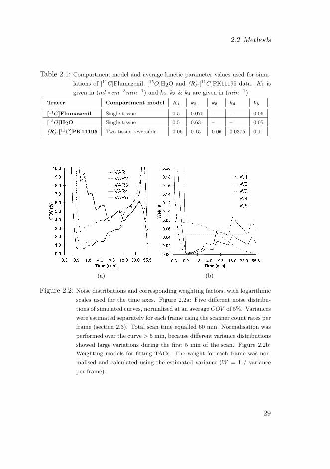
, where j is the weighting model used. Weights are only correct if theweighting model is equal to the variance model used to impose noise ontothe simulated TACs. Variance models 1, 2 and 4 are relatively similar,model 3 represents unweighted fitting and model 5 is included to analysethe impact of a large mismatch between applied variance and weightingmodel on the outcome of pharmacokinetic analysis. Differences betweenthe various models are illustrated in Figure 2. In this study a frequentlyused model (i.e. model 1) was chosen as reference model for simulatingnoise distributions, although it may not be the most accurate method toestimate (local and temporal) noise distributions. The primary aim ofthis paper was, however, to study the impact of mismatch between noisemodel and weighting factors on accuracy and precision of pharmacokineticanalysis rather than to assess the most accurate weighting model.

27


2.2.4 Experiments

Data sets

Data derived from clinical studies were used to generate simulated TACs.Simulated noiseless TACs were generated using measured (human) inputfunctions, an appropriate compartment model and typical kinetic para-meters. ‘Typical’ or average kinetic parameter values and the pharma-cokinetic compartment model used for simulating TACs are summarisedin Table 2.1. Simulations were performed for each tracer ([11C]Flumazenil(FMZ), [15O]H2O and (R)-[11C]PK11195) separately.

Variance model 1 was chosen to add noise to noiseless TACs. The addednoise was normalised so that the average coefficient of variation (COV)over the last 60% of the frames (i.e. for the curve > 5 min) was set topredefined levels of 5, 10 and 15%, respectively (Figure 2.2). For eachvariance level and each tracer 100 noisy TACs were generated, which wereused for all optimisation algorithms tested.

Clinical evaluation was based on a total of 15 studies. Clinical studieswere part of ongoing research, which had been approved by the MedicalEthics Committee of the VU University Medical Centre. For each tracer(FMZ, H2O and PK11195) data from 5 patients were used. For each pa-tient study 10 regions of interest (ROIs) were defined. In case of flumazeniland H2O studies, these ROIs were randomly chosen in grey and white mat-ter with ROI sizes ~ 1 cm3. The PK11195 data consisted of anatomicallydefined ROIs using MRI coregistration (ROI sizes ~ 3-5 cm3). Input func-tions were measured with an online continuous blood sampling device.[37]At discrete times additional manual samples were obtained for online cal-ibration of the measured whole blood input function, plasma/whole bloodratios, and metabolite corrections.[38] The whole blood and metabolitecorrected plasma input functions were then used within the kinetic anal-yses.

Each of the 900 simulated and 150 clinical TACs were fitted separatelywith the five different weighting models, creating 5 different cost functionsfor each TAC. The performance of the optimisation algorithms was alsoevaluated for these 5 different weighting models.

28

2.2 Methods

Table 2.1: Compartment model and average kinetic parameter values used for simu-lations of [11C]Flumazenil, [15O]H2O and (R)-[11C]PK11195 data. K1 isgiven in (ml ∗ cm−3min−1) and k2, k3 & k4 are given in (min−1).

Tracer Compartment model K1 k2 k3 k4 Vb

[11C]Flumazenil Single tissue 0.5 0.075 – – 0.06[15O]H2O Single tissue 0.5 0.63 – – 0.05(R)-[11C]PK11195 Two tissue reversible 0.06 0.15 0.06 0.0375 0.1

(a) (b)

Figure 2.2: Noise distributions and corresponding weighting factors, with logarithmicscales used for the time axes. Figure 2.2a: Five different noise distribu-tions of simulated curves, normalised at an average COV of 5%. Varianceswere estimated separately for each frame using the scanner count rates perframe (section 2.3). Total scan time equalled 60 min. Normalisation wasperformed over the curve > 5 min, because different variance distributionsshowed large variations during the first 5 min of the scan. Figure 2.2b:Weighting models for fitting TACs. The weight for each frame was nor-malised and calculated using the estimated variance (W = 1 / varianceper frame).

29


Peformance criteria

Three performance criteria (A, B and C) were used to analyse the results.Criterion A is based on the lowest value of the cost function (WRSS).WRSS values obtained after fitting a TAC by two different optimisationalgorithms were directly compared using a relative tolerance of 10−6 toexclude rounding off effects in the stored data. For each comparison oneof the algorithms used was defined as ‘reference’. A comparison resulted inthe following classifications: a ‘win’, ‘equal’ or ‘loss’. A ‘win’ correspondsto a lower WRSS value, an ‘equal’ to a difference in WRSS value smallerthan the tolerance value and a ‘loss’ to a higher WRSS value than thatobtained with the reference algorithm, respectively.Criterion B is also based on the lowest fitted WRSS value, but now

by taking the uncertainty of the fitted kinetic parameters into account.Criterion A determines which algorithm is a better optimiser. However,it is also important to know whether an algorithm returns significantlydifferent or incorrect kinetic fit parameters. In other words, does a lowercost function value always provide more accurate values for the kineticfit parameters? An arbitrary threshold of 5% of the observed kineticparameters was used for the latter purpose (i.e. a difference smaller then5% was defined as an ‘equal’ result).Criterion C is based on observed accuracy and reproducibility in average

kinetic (macro-) parameters. Although values for each of the fit parame-ters or rate constants (Figure 1) are obtained, usually macro-parameters,such as flow (F ), volume of distribution (VT ) and binding potential(BPND) are of interest in PET studies. For a single-tissue compartmentmodel (Figure 2.1a) VT is given by the ratio K1/k2. For a reversible two-tissue compartment model (see Figure 2.1b) VT equals K1/k2 ∗ (1 + k3/k4)and BPND equals k3/k4. The focus of the present study was on F (= K1) for H2O, VT for FMZ, and BPND for PK11195.The average value and the coefficient of variation (COV ) of the fitted

kinetic parameters over a specified number of fitted TACs were calculatedto determine accuracy and reproducibility. Kinetic parameters, which felloutside a predefined physiological range (Table 2.2), were excluded. Forsimulations, accuracy per TAC was assessed using the ‘relative accuracy’,which is defined as ‘observed kinetic parameter value’ divided by ‘true(=simulated) kinetic parameter value’. For clinical studies, ‘relative accu-

30

2.2 Methods

Table 2.2: Physiological boundaries for [11C]Flumazenil, [15O]H2O and (R)-[11C]PK11195 analyses. LB is the lower parameter boundary and UB theupper parameter boundary.

Tracer K1 (LB; UB) BP (LB; UB) VT (LB; UB)

[11C]Flumazenil (0.000001; 0.9) – (0.000001; 12)[15O]H2O (0.000001; 1.5) – (0.000001; 1.5)(R)-[11C]PK11195 (0.000001; 0.3) (0.000001; 4.5) (0.000001; 2.1)

racy’ was defined as ‘observed kinetic parameter’ divided by ‘kinetic pa-rameter obtained with extended lsqnonlin and weighting model 1’, whichwas used as default. In the latter case only changes in outcome relative tothese default settings could be assessed. Reproducibility of a parameterwas defined as ‘coefficient of variation’.

Optimisation of algorithm settings

Optimal settings for SA and extended lsqnonlin were derived empiricallyusing simulated data and criterion A. Since optimal settings for extendedlsqnonlin are equal to those for lsqnonlin, only optimal settings for ex-tended lsqnonlin needed to be determined.Settings that needed to be optimised were the relative termination tol-

erance of the cost function value, Ftol (10−4, 10−6, 10−8, 10−10 and10−12), and the total number of function evaluations (1000, 20000 and80000 fevalfs). The relative termination tolerance on the input parame-ter was fixed to 10−8. One iteration of extended lsqnonlin is equal to oneminimisation using lsqnonlin and one iteration of SA is equal to one localminimisation using CG.For SA some additional settings needed to be optimised, i.e. the initial

maximum step size and the final maximum step size (tested in the rangeof 5% - 0.00001% of the expected value of each kinetic parameter). Op-timal settings in terms of speed and accuracy were then used for furtherevaluation of algorithms and weighting factors.

31


Evaluation of optimisation algorithms

First, algorithm performance was assessed using simulated TACs withcriteria A and B. Extended lsqnonlin was compared with SA at differentnumbers of function evaluations (1000, 20000 and 80000 fevalfs) usingcriterion A. For criterion B only comparisons with simulated data and80000 function evaluations were used. Finally criterion C was used forsimulated and clinical TACs to confirm results found with criterion B andto assess the effects of different algorithms and weighting factors on theestimation of kinetic parameters.

2.3 Results

2.3.1 Optimisation of algorithm settings

Optimising SA settings

SA yielded good results for all three tracers with an initial maximum stepsize of the same order of the value of the kinetic parameter. Thereforethis setting was used throughout the remainder of this study. The finalmaximum step size did not significantly affect results, but needed to besmall enough, i.e. lower then 10−3% of the expected value of the kineticparameter.

Optimising tolerance settings

Figure 2.3 depicts results for both SA and extended lsqnonlin at differentvalues of the relative termination tolerance of the cost function value. BothSA and extended lsqnonlin gave best results when Ftol was set to 10−12,but differences were small compared with Ftol equal to 10−8. At thislower tolerance setting only 6-7% of the total number of TACs (i.e. 4500)were fitted with a lower WRSS (criterion A). Both algorithms performedmuch better for Ftol set to 10−8 than to 10−4. Lower tolerance settingresulted in larger computation times with only minimal improvement inobserved cost function minimisation. Thus Ftol = 10−8 was consideredoptimal in terms of speed and accuracy.

32

2.3 Results

(a) (b)

Figure 2.3: Assessment of optimal relative termination tolerance on the function value(Ftol) setting by fitting 4500 simulated TACs with fixed number of func-tion evaluations (=1000). Each pair of grey and white bars depict theperformance of the algorithm at a certain Ftol setting: grey bars depictthe number of TACs with better fits, in terms of the WRSS, and whitebars depict the number of TACs with poorer fits compared with those us-ing Ftol equal to 10−8. Figure 2.3a: results for simulated annealing (SA),Figure 2.3b: results for extended lsqnonlin.

33


(a) (b)

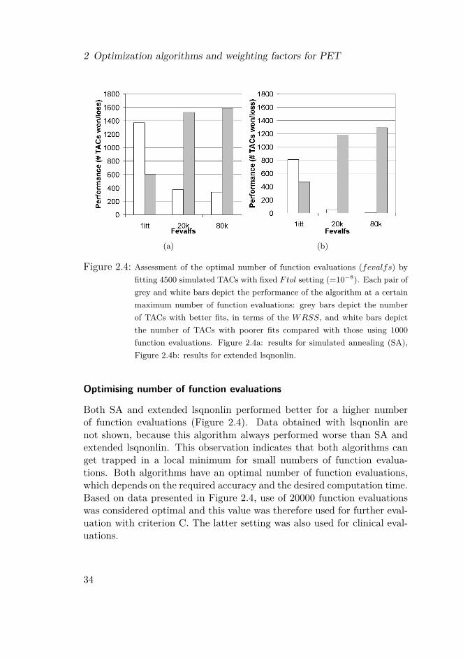
Figure 2.4: Assessment of the optimal number of function evaluations (fevalfs) byfitting 4500 simulated TACs with fixed Ftol setting (=10−8). Each pair ofgrey and white bars depict the performance of the algorithm at a certainmaximum number of function evaluations: grey bars depict the numberof TACs with better fits, in terms of the WRSS, and white bars depictthe number of TACs with poorer fits compared with those using 1000function evaluations. Figure 2.4a: results for simulated annealing (SA),Figure 2.4b: results for extended lsqnonlin.

Optimising number of function evaluations

Both SA and extended lsqnonlin performed better for a higher numberof function evaluations (Figure 2.4). Data obtained with lsqnonlin arenot shown, because this algorithm always performed worse than SA andextended lsqnonlin. This observation indicates that both algorithms canget trapped in a local minimum for small numbers of function evalua-tions. Both algorithms have an optimal number of function evaluations,which depends on the required accuracy and the desired computation time.Based on data presented in Figure 2.4, use of 20000 function evaluationswas considered optimal and this value was therefore used for further eval-uation with criterion C. The latter setting was also used for clinical eval-uations.

34

2.3 Results

Figure 2.5: Extended lsqnonlin fits compared with simulated annealing (SA) at dif-ferent number of function evaluations (fevalfs). On the vertical axis thenumber of better (white bars) and poorer (grey bars) fits using SA areindicated. A total of 4500 TACs were fitted using Ftol = 10−8. For the80k* columns, fits were better by also taking into account criterion B,i.e. not just a lower WRSS but also a difference of more than 5% in theresulting parameters.

2.3.2 Performance of optimisation algorithmsCriterion A, evaluation based on cost function minimisation

In Figure 2.5 comparisons based on criterion A between SA and extendedlsqnonlin are shown for various numbers of function evaluations using sim-ulated TACs. More often, a lower WRSS was obtained with extendedlsqnonlin than with SA. More function evaluations resulted in smallerdifferences between extended lsqnonlin and SA, i.e. at 80k function eval-uations ~70% of the TACs were equally well fitted in terms of WRSS.Lsqnonlin (data not shown) always performed worse than both SA andextended lsqnonlin.

Criterion B, evaluation based on differences in parameter estimation

Comparison of WRSS between SA and extended lsqnonlin for simulatedTACs, based on criterion B, is also given in Figure 2.5. Differences between

35


SA and extended lsqnonlin using criterion B were less pronounced thanfor criterion A, i.e. 80% of all 4500 fitted TACs were classified as identicalfor both algorithms.

Criterion C, accuracy and reproducibility of kinetic parameters

Results obtained using simulations are shown in Figure 2.6. Kinetic pa-rameter estimates with lsqnonlin showed larger bias then those obtainedwith extended lsqnonlin and SA. However, for FMZ all three algorithmsperformed similarly. Differences between extended lsqnonlin and SA werenegligible in case of single-tissue (1T) compartment models (H2O andFMZ) and small for the reversible two-tissue (2T) compartment model(PK11195).Clinical data (Figure 2.7) yielded similar results. Lsqnonlin provided

more bias and worse reproducibility than SA and extended lsqnonlin. Dif-ferences between SA and extended lsqnonlin were lower for clinical datathan for simulated TACs at a variance level of 5% using variance model 1.

2.3.3 Effect of weighting factors

Simulations

Differences in accuracy and reproducibility amongst weighting models 1 to4 were almost negligible for 1T compartment models (Figure 2.6a-f). Forthe 2T compartment model (Figure 2.6g-i) increase of bias due to noisewas larger than the effect of using incorrect weighting factors (models 1-4).However, weighting model 5 provided poor results for all simulations dueto the large mismatch between weighting and applied variance model, i.e.model 1.Results for PK11195 obtained at a 15% variance level are not shown,

because of the high number of rejected fits. The numbers of rejected fitswere ~15, 36 and 45% for variance levels equal to 5, 10 and 15%, respec-tively (pooled over all weighting models). The numbers of rejected fitswere ~0, 17 and 24% at variance levels equal to 5, 10 and 15%, respec-tively, using results obtained with weighting model 1 only. The highestnumber of rejected fits was found when weighting model 5 was used bothfor 1T and 2T compartment models (~5, 5, 7, 13 and 33% rejected TACs

36

2.3 Results

(a) (b) (c)

(d) (e) (f)

(g) (h) (i)

Figure 2.6: Average fitted kinetic parameters for simulated TACs (Ftol = 10−8 and20k function evaluations). The relative accuracy is defined as the ratioof the fitted parameter value over simulated parameter value. On thehorizontal axis the different weighting models are indicated. Differentfilling colours indicate different variance levels, i.e. COV = 5% (whitebars), COV = 10% (grey bars), and COV = 15% (black bars).

37


(a) (b) (c)

Figure 2.7: Average fitted kinetic parameters for clinical TACs (Ftol = 10−8 and 20kfunction evaluations). The relative accuracy is defined as the ratio ofthe fitted parameter value over the fitted value obtained with extendedlsqnonlin with weight type 1. On the horizontal axis the different weight-ing models are indicated. Lsqnonlin (light grey bars), extended lsqnonlin(dark grey bars), and SA (black bars). Note that accuracies and precisionsof the binding potential (BPND) for (R)-[11C]PK11195 (Figure 2.7c) falloutside the figure scale for weighting model 5.

38

2.4 Discussion

for weighting models 1-5 respectively, pooled over all tracers and variancelevels).

Clinical evaluation

Differences in accuracy and reproducibility of kinetic parameters amongstthe weighting models tested were more pronounced for the 2T compart-ment model than for 1T compartment models. The differences in accuracywere, however, relatively small amongst weighting models 1 to 4, less than~7% for 1T compartment models and less than ~20% for the 2T com-partment model (Figure 2.7) compared with the differences found usingweighting model 5. Weighting model 5 showed largest bias and poor-est reproducibility of estimated kinetic parameters amongst the weightingmodels tested.

2.4 Discussion

2.4.1 Evaluation of optimisation algorithms

The present study indicates that performance of the three algorithms stud-ied depended on algorithm settings such as the termination tolerance (Fig-ure 2.3) and number of function evaluations (Figure 2.4 & 2.5). Figures2.3, 2.4 and 2.5 demonstrate that optimal settings should be estimatedbeforehand using (simulated) TAC to determine the optimal trade-off be-tween accuracy and computation time.In general, simulations of both 1T and 2T compartment models showed

that lsqnonlin showed larger bias of the fitted kinetic parameters than ex-tended lsqnonlin and SA (Figure 2.6). Only small differences in the clinicalresults between extended lsqnonlin and SA were observed, but lsqnonlinagain yielded substantially deviating results (Figure 2.7). Use of a range ofstarting parameters to fit each TAC as implemented by extended lsqnon-lin is therefore preferred. This strategy is automatically incorporated inSA. Although SA only requires one set of starting parameters, it generatesnew starting values using the Metropolis Monte Carlo algorithm.Extended lsqnonlin was the best optimiser amongst the three algo-

rithms tested here, because it most frequently provided fits with the lowest

39


WRSS values (Figure 2.5). However, according to criterion B, SA pro-vided almost identical fits for ~80% of the TACs. Criterion B was usedwith an arbitrary threshold of 5% of the observed kinetic parameter. Thisthreshold can be increased to comply with the uncertainties of pharma-cokinetic parameters found in clinical data resulting in lower differencesbetween SA and extended lsqnonlin. Differences between SA and extendedlsqnonlin were even smaller when criterion C instead of B was used. Forclinical data better reproducibility of kinetic parameters was obtained withSA and extended lsqnonlin than with lsqnonlin (Figure 2.7). It can there-fore be concluded that extended lsqnonlin and SA are equally suitable forPET pharmacokinetic analysis.An advantage of SA over extended lsqnonlin is that each TAC is fitted

with just one set of starting values for the kinetic parameters, while usingthe same number of function evaluations. SA can be seen as a method toproduce random starting points by the Metropolis Monte Carlo methodfollowed by local minimisation at each newly generated starting pointusing the CG algorithm.

2.4.2 Weighting factors

Simulations for single tissue compartment models (Figure 2.6a-f) indicatedthat differences in (relative) accuracy amongst different weighting factorswere almost negligible (<2%). Significant differences only occurred forweighting model 5, representing an extreme mismatch between estimatedand true (simulated) variance of the data. This result indicates that ap-proximate estimation of the variance may be justified in case of 1T models.On the other hand, differences in accuracy amongst weighting models 1to 4 for 2T kinetic simulations were not negligible (from 1 up to 20%).Note, however, that the increase in bias with noise (from 8 up to 35%)was larger than that caused by using non-matched weighting factors.Clinical results are difficult to interpret, because the real kinetic param-

eter values are not known. Therefore in this study results using extendedlsqnonlin with weighting model 1 were used as reference. Weighting mod-els 2 and 3 provided comparable results as those obtained with weightingmodel 1. Differences amongst model 1 to 4 were less than ~7% for 1Tcompartment models and less than ~20% for 2T compartment models(Figure 2.7), whilst use of weighting model 5 resulted in much larger bi-

40

2.5 Conclusion

ases. Therefore, use of weighting models, which differ substantially fromthe true variance of the measured data, may result in large biases of 20%or more. In general, more accurate results are obtained when weightingmodels more accurately correspond with the true variance of the data andthat careful selection of a weighting model can improve accuracy of PETpharmacokinetic results.[29, 30]Overall, however, this study indicates that small to intermediate mis-

matches between (real) variance and applied weighting model may notsignificantly affect accuracy and reproducibility of estimated kinetic para-meters. It may therefore be justified to use approximate variance estima-tions to derive the weighting factors for PET kinetic analysis. Clearly, acorrect match between applied weighting factors and (real) variance wouldprovide the best fits and should be preferred. Accurate estimation of thevariance is, however, difficult and/or time consuming [24, 25, 26, 27, 28]and may even not be possible for dynamic studies acquired without listmode acquisition.[24, 25] The latter is also hampered by the introductionof new iterative reconstruction algorithms, such as RAMLA [39], weightedleast squares [40, 41] and various types of OSEM algorithms [42], for whichthere are no local variance estimators yet.It is important to note, that effects of noise on accuracy and repro-

ducibility are large (up to 50% at a 10% noise level), especially for thetracer PK11195, as can be deduced from Figures 2.6g, 2.6h and 2.6i.Therefore, strategies to reduce TAC noise, such as wavelets [43, 44, 45],are promising methods for improving accuracy and reproducibility of PETkinetic analysis. However, noise reduction strategies may also introducesome bias and the benefits by improving the signal to noise ratio usingthese techniques should thus be larger than the possible bias being intro-duced.

2.5 Conclusion

In this study effects of using various optimisation algorithms and weightingfactors on accuracy and reproducibility of PET derived kinetic parameterswere investigated. A commonly used optimisation algorithm, such as theMATLAB function ‘lsqnonlin’, was not able to produce unbiased results.Algorithms that use a range of starting parameters, such as simulated

41


annealing or an extended version of lsqnonlin (multiple starting values),provided more accurate results. In addition, it was demonstrated that useof incorrect weighting models may result in poor accuracy and precision.However, when these weighting models are only approximately correct,effects of noise on accuracy and precision are likely to be larger. Therefore,apart from careful selection of the optimisation algorithm and weightingmodel being applied, especially noise reduction strategies are required tofurther improve accuracy and precision of PET pharmacokinetic analyses.

AcknowledgementsThe authors would like to thank the personnel of the Department of Nu-clear Medicine & PET Research for tracer production and data acquisition.

42

3 Wavelet based denoising for PET

ARTICLE: Impact of wavelet based denoising of(R)-[11C]PK11195 time activity curves on

accuracy and precision of kineticanalysisOptimization algorithms and

weighting factors for analysis of dynamicPET studies

AUTHORS: Maqsood Yaqub1, Ronald Boellaard1, AlieSchuitemaker2, Bart N.M. van Berckel1 and

Adriaan A. Lammertsma1

INSTITUTES: (1) Department of Nuclear Medicine & PETResearch, VU University Medical Centre,

Amsterdam, The Netherlands; (2) Department ofNeurology, VU University Medical Centre,

Amsterdam, The Netherlands

JOURNAL: Medical Physics, 2008, 35: 5069-5078

43


Abstract

The purpose of the present study was to investigate the use of variouswavelets based techniques for denoising of (R)-[11C]PK11195 time activitycurves (TACs) in order to improve accuracy and precision of PET kineticparameters, such as volume of distribution (VT ) and distribution volumeratio with reference region (DV R). Simulated and clinical TACs werefiltered using two different categories of wavelet filters: (1) wave shrinkingthresholds using a constant or a newly developed time varying threshold;(2) ‘statistical’ filters, which filter extreme wavelet coefficients using a setof ‘calibration’ TACs. PET pharmacokinetic parameters were estimatedusing linear models (plasma Logan and reference Logan analyses).For simulated noisy TACs, optimised wavelet based filters improved the

residual sum of squared errors with the original noise free TACs. Further-more, both clinical results and simulations were in agreement. PlasmaLogan VT values increased after filtering, but no differences were seen inreference Logan DV R values. This increase in plasma Logan VT sug-gests a reduction of noise induced bias by wavelet based denoising, as wasseen in the simulations. Wavelet denoising of TACs for (R)-[11C]PK11195PET studies is therefore useful when parametric Logan based VT is theparameter of interest.

3.1 Introduction

The regional distribution of a positron-emitting tracer can be measuredin vivo using positron emission tomography (PET). By performing serialscans, following injection, the time course of the tracer in tissue can bedetermined. Important parameters, such as volume of distribution (VT )or volume of distribution ratio with a reference region (DV R), can thenbe derived by fitting these measured time activity curves (TACs) to ap-propriate kinetic models. The quality of the estimates obtained, however,not only depends on the correctness of the kinetic model used, but alsoon the level of noise. Note that throughout this manuscript the consensusnomenclature as published by Innis et al. [46] is used.The latest generation of PET scanners, such as the High Resolution Re-

search Tomograph (HRRT), can acquire dynamic scans with high spatial

44

3.1 Introduction

resolution.[47, 48] Despite increased sensitivity, (short) individual framessuffer from noise, complicating accurate quantification of kinetic parame-ters, especially in smaller regions of interest. In general, some sort of spa-tial smoothing (e.g. reconstruction filter) is used to improve signal to noiseratios, but clearly this approach reduces spatial resolution. Various otherfiltering techniques are available and in recent years filtering techniquesbased on wavelets, which can denoise spatial and temporal (i.e. TAC)signals without smoothing, have been introduced in PET.[49, 50, 45, 51]The two main advantages of wavelets based filtering are, firstly, the

availability of various different wavelet functions and filters for processingsignals, and, secondly, the fact that wavelet functions are localized in bothtime and frequency domains. Localization in time and frequency domainsmakes it possible to filter certain frequency components at selected timepoints. For example, one could choose to remove high frequency compo-nents only at later time points of the TAC, thereby keeping the initialhigh frequency ‘peak’ signal of the TAC intact. Time localized filtering inconventional Fourier based filtering techniques is almost impossible, be-cause if filtered than the frequency component will be removed from alltime points.In contrast to wavelet based spatial image filtering techniques [45, 51],

little attention has been paid to the use of wavelet based methods specifi-cally for denoising TACs.[49, 50] Filtering of individual voxels or regionalTACs may help retain spatial resolution, whilst reducing noise, therebyreducing the number of fit outliers and improving (parametric) pharma-cokinetic images, such as those obtained with Logan plot analysis.[15]In general, it may improve precision of estimated parameters of inter-est (e.g. VT or DV R), especially in case of parametric (voxel) analysesand/or for tracers showing low uptake such as in the case of cerebral (R)-[11C]PK11195 studies.[52]In the present study existing denoising techniques based on different

lifting-wavelets [53, 54] were assessed by filtering simulated and measured(R)-[11C]PK11195 TACs. First, performances of different wavelet basedTAC filtering approaches were evaluated, and then the optimal filteringtechnique was used to assess improvements in quantifying clinical data.Performance of the filters was evaluated by measuring changes, beforeand after filtering, of (parametric) pharmacokinetic parameters of inter-

45


est. These were derived using plasma Logan [15] and reference Logan[16] analyses, as these methods are commonly used for parametric kineticanalysis of brain PET studies. Wavelet denoising of TACs is of specificinterest for these methods, because they suffer from noise induced bias inthe pharmacokinetic parameters.[55]

3.2 Methods

3.2.1 Time activity curves

Clinical TACs

Voxel TACs were extracted from a dynamic (R)-[11C]PK11195 scan ofan elderly healthy subject. The scan was acquired as part of an ongoingclinical study.[52] This study had been approved by the Medical EthicsCommittee of the VU University Medical Centre and the subject hadgiven written informed consent prior to inclusion in the study protocol.The dynamic (R)-[11C]PK11195 scan (ECAT EXACT HR+, CTI /

Siemens, Knoxville, USA) was acquired in 3D mode, following bolus injec-tion of 369 MBq [11C](R)-PK11195, and corrected for tissue attenuationusing a 10 minutes 2D transmission scan. The dynamic emission scanconsisted of 22 frames with a total scan duration of 60.5 minutes (1x30,1x15, 1x5, 1x10, 2x15, 2x30, 3x60, 4x150, 5x300 and 2x600 s). Frameswere reconstructed using FORE19 + 2D Filtered Back Projection with aHanning filter at a cut-off of 0.5 times the Nyquist frequency. A matrixsize of 256x256 and a zoom factor of 2 were applied during reconstruction,resulting in an image pixel size of 1.2x1.2 mm and a slice thickness of 2.5mm. The reconstruction settings resulted in an image resolution of 7 mmfull width at half maximum (FWHM). Reconstructions included all usualcorrections, such as normalization, and decay, dead time, attenuation,randoms and scatter corrections.The arterial input function was measured using an online continuous

blood sampling device.[37] At discrete times (~3, 6, 10, 20, 30, 40 and60 minutes post injection), additional manual samples were obtained foronline calibration of the measured whole blood input function, and deter-mination of plasma/whole blood ratios and metabolite fractions.The PET scan was co-registered with a T1-weighted MRI scan (1T

46

3.2 Methods

IMPACT, Siemens Medical Solutions, Erlangen, Germany), which wasused to segment the brain into grey matter, white matter and cerebrospinalfluid.[56, 57, 58] Parametric image evaluations were constrained to a singleaxial plane through the brain, resulting in a total of 5740 grey and 2895white matter voxel TACs for filtering and kinetic analyses. In addition, ananatomically defined ROI of the whole cerebellum was used for generationof the reference TAC, used in the reference tissue models [16], as describedbelow.

Simulated TACs

Simulated TACs were generated using a typical metabolite corrected (mea-sured) (R)-[11C]PK11195 plasma curve as input function and the reversibletwo-tissue compartment model [7] (Figure 3.1) with kinetic parametersbased on human (R)-[11C]PK11195 studies (Table 3.1). Identical to clini-cal studies, these TACs consisted of 22 frames with a total scan durationof 60.5 minutes. In simulations the variations in binding, delivery andTAC noise level were investigated.Kinetic parameters for simulations were derived from clinical data. The

reference tissue parameters were kept fixed to reference tissue as given inTable 3.1. The default parameters used for the target region are givenby target tissue 3 in Table 3.1. During simulations, two pharmacokineticentities of the target region were varied within physiologically expectedranges: delivery K1 (target tissues 3, 6 & 7; Table 3.1) and binding poten-tial BPND (target tissues 1, 2, 4 & 5). 100 TACs were generated for eachparameter combination (target tissues 1-7) and, in addition, all TACs weresimulated at several noise levels ranging from 0-25% coefficient of variation(COV), in increments of 5%.The noise model was based on the total scanner trues counts, frame

lengths and decay correction factors [31, 59]:

σ2i = α ▪ dcfi ▪ dcfi

TiLi ▪ Li

(3.1)

where σ2i is the variance, Ti the scanner total trues, Li the frame length,

and dcfi the decay correction factor per frame (i). Finally, α is a propor-tionality constant for scaling COV . COVi is given for a group of simulatedTACs by calculating σi

averagei. COV is then the average of all COVi calcu-

47


Figure 3.1: Reversible two tissue compartment model: P is the tracer plasma con-centration (Bq/ml), TISSUE is the measured tissue concentration (Bq/ml),F +NS is the concentration of free tracer in tissue (Bq/ml), S is the con-centration of tracer bound to binding sites in tissue (Bq/ml), K1 is a rateconstant (ml ∗ cm−3min−1), and k2, k3 and k4 are the rate constants(min−1) describing exchange between the various compartments. Para-meters of interest are volume of distribution, VT = K1/k2 ∗ (1 + k3/k4), andbinding potential, BPND = k3/k4. For clarity, the fractional blood volumeVb is not shown.

lated for frames after 2.5 min.

3.2.2 Lifting WaveletsA theoretically detailed explanation of lifting wavelets can be found else-where. [53, 54, 60, 61] The purpose of the present study is the applicationof these algorithms to filtering TACs. In short, a TAC can be decomposedinto its wavelet coefficients using a wavelet transform, just as a Fouriertransform decomposes the signal into its frequency components. A Fouriertransform uses sinuses and cosines as basis, whereas, the wavelet basis iscomposed of the wavelet functions. Wavelet functions are localized in bothtime and frequency, and are therefore better in representing signals withsharp edges and peaks, which is important for time activity curves. In ad-dition, different useful wavelet function coefficients have been constructedfor various types of data such as the Daubechies wavelets [62], which canbe used for transformation and approximation of polynomials.

48

3.2 Methods

Table 3.1: Kinetic parameters used to generate simulated reference and target tissuetime activity curves for (R)-[11C]PK11195. K1, k2, k3 and k4 are rateconstants, Vb fractional blood volume, VT volume of distribution, DV Rvolume of distribution ratio with reference tissue, and BPND binding po-tential. K1 is given in (ml ∗ cm−3min−1) and k2, k3 & k4 are given in(min−1). Curves were generated using a two tissue reversible plasma inputmodel. During all simulation Vb(0.071), k4 (0.04 min−1) and K1/k2 (0.35)were kept constant.TAC K1 k3 BPND VT DV R

Reference tissue 0.056 0.040 1.00 0.700 –Target tissue 1 0.056 0.030 0.78 0.623 0.890Target tissue 2 0.056 0.045 1.17 0.760 1.086Target tissue 3 0.056 0.060 1.56 0.896 1.280Target tissue 4 0.056 0.075 1.95 1.033 1.476Target tissue 5 0.056 0.090 2.34 1.169 1.670Target tissue 6 0.039 0.060 1.56 0.896 1.280Target tissue 7 0.073 0.060 1.56 0.896 1.280

The first application of the wavelet transformation yields wavelet coef-ficients, which are grouped into two bands: a low and a high frequencyband, with the total number of coefficients equalling the number of framesin the TAC. The wavelet coefficients in each band can easily be related totheir corresponding time points in the original temporal TAC, i.e. mod-ifying a coefficient will result in a change of TAC at the correspondingtemporal location. The forward transform can be reapplied to the lowfrequency band, which again splits this band into two frequency bands.The number of times a transform can be reapplied depends on the lengthof the initial signal. The wavelet coefficients from all frequency bands,except from the lowest frequency band, are called detail coefficients. Theoriginal signal can be reconstructed by reversing the whole process.Different types of wavelet transform algorithms are available. In the

present study lifting wavelets are used. The lifting scheme is an inter-esting method for denoising TACs because the number of frames doesnot have to be a power of 2. Here only the currently available CDF(Cohen-Daubechies-Feauveau) biorthogonal wavelet functions [54, 63] will

49


be evaluated. Each CDF biorthogonal wavelet function is defined by twoparameters, which are the number of vanishing moments of the dual andprimal wavelets. The exact meaning of these 2 parameters is not rele-vant for the present study, except that the number of times a TAC canbe forward transformed (Ftrmax ) is related to the largest value of thespecified vanishing moments (mmax) and the number of frames in a TAC(nf ) through the following equation:

Ftrmax = floor

ln(

nf−1mmax−1

)ln (2)

(3.2)

Consequently, in the present study only the first 16 CDF wavelets areevaluated, i.e. with up to 8 vanishing moments (Table 3.2). This allowsfor 1, 2, & 4 times forward transformations in case of TACs with 22frames, giving wavelet coefficients grouped into 2, 3 & 5 frequency bands,respectively.

3.2.3 TAC denoising

In many cases, a large proportion of the detail coefficients of a wavelettransformed signal can be assumed to be due to noise and set to zero,resulting in a more sparse representation of the same data in the waveletdomain. This property is often used for data compression and removalof noise. Similar wavelet based denoising techniques are also available forimproving PET data.[49, 50, 45, 51] In the present study, TACs were fil-tered using the following three filtering strategies: soft-thresholding basedfilters; soft-thresholding filters adapted to account for changes in varianceover time; and ‘statistical’ filters. These filters can be applied separatelyfor each of the frequency bands and several bands can be excluded fromfiltering.

Soft-thresholding filters

Wavelet coefficients were filtered using soft-thresholding [64], i.e. waveletcoefficients of selected frequency bands were reduced with a certain thresh-old value, and if the coefficient values were smaller than the threshold, theywere set to zero. The equation for the threshold used is given by:

50

3.2 Methods

Table 3.2: Details of the Cohen-Daubechies-Feauveau (CDF) biorthogonal waveletfunctions used. The function number is an arbitrary number used for iden-tification in the text. CDF biorthogonal wavelet functions are defined bythe number of vanishing moments for both dual and primal wavelets. Thelast column gives the number of forward transformations that are allowedfor lifting TACs with 22 frames.

Function number Number of vanishing moments Transformations allowedDual wavelet Primal wavelet

1 2 2 42 2 4 23 4 2 24 4 4 25 2 6 26 6 2 27 8 2 18 2 8 19 8 4 110 4 8 111 8 6 112 6 8 113 8 8 114 6 4 215 4 6 216 6 6 2

51


T Tj = n ▪ Tj ▪ Facj (3.3)

This T Tj threshold is a constant value for all wavelet coefficients of a fre-quency band j. n is the normalisation factor, which needs to be calculatedfor each TAC. Normalization was performed using wavelet coefficients fromthe highest frequency band and calculating the median value of the abso-lute deviates from 0.[45, 64] Tj is a threshold factor, estimated for eachfrequency band j, using visually calibrated adaptive smoothing (VISU)[64] or Stein’s unbiased risk estimate (SURE).[65] Equations and detailedinformation on the thresholds Tj can be found elsewhere.[65, 64] The re-sulting filters were also called VISU ( Tj is estimated using VISU) orSURE (Tj is estimated using SURE). In this way the filter is fully derivedfrom the data themselves. Thresholds may be multiplied with additionalfactors Facj (0.05, 0.10, 0.25, 0.50, 1, 1.5, 3, 3.5, 4, 5, 6, 7, 8, and 10)in order to further fine-tune the strength of the filter for each frequencyband individually. The resulting thresholds (T Tj ) were then applied usingsoft-thresholding. Finally, the resulting filtered wavelet coefficients wereused to reconstruct the filtered signal.

Soft-thresholding filters adapted to account for changes in varianceover time

Basic wavelet thresholding techniques assume white noise, i.e. equal con-tribution of all frequencies. Temporal noise in emission tomography, how-ever, usually is not white, but consists of different time dependent factorsdue to e.g. varying activity levels and distributions, detector dead time,and decay over time. Therefore the soft-thresholding filters were adaptedto account for changes in variance over time according to the noise modelgiven in Eq. 3.1. These filters were derived from the original (soft) VISUand SURE filters, but instead of using a constant threshold for all waveletcoefficients of a frequency band, they were varied within the band. Theequation for this threshold is given by:

T pj = n ▪ Tj ▪ wtp ▪ Facj (3.4)

Here T pj is the threshold applied to the wavelet coefficient p of frequencyband number j. Note, that each wavelet coefficient p corresponds to a

52

3.2 Methods

temporal position of the original TAC. However, the frequency band hasa lower number of wavelet coefficients than the number of frames in theoriginal TAC. Therefore, interpolation is needed. wtp is an additional fil-tering factor for wavelet coefficient p, which varies according to the noisemodel described above (Eq. 3.1), i.e. higher variance needs more filter-ing. If the corresponding temporal position for wavelet coefficient p isexactly given by i, then wtp = 1

σ2i, otherwise interpolation is needed as

explained above. The meaning of n and Tj is the same as above. Thesenew weighted thresholding filters were called wVISU (Tj estimated usingVISU) or wSURE (Tj estimated using SURE). Again, thresholds weremultiplied with additional factors Facj (0.05 to 10) in order to furtherfine-tune the strength of each filter across the frequency bands.

Statistical filters

‘Statistical’ filters, closely related to those described by Millet et al. [50],were designed to estimate and exclude statistical outliers in the waveletdomain. The statistical filter uses a given number of ‘calibration’ TACsfor estimating averages and standard deviations of each wavelet coefficient.Next, each measured TAC is filtered by correcting its wavelet coefficientsfor significant deviations from these averages. The statistical filter ‘thresh-olds’ are therefore specified as the number of standard deviations (2, 1.5,1, 0.5 and 0.25 times SD), which a wavelet coefficient may deviate fromthe (expected) average value, as derived from the “calibration” TACs.Wavelet coefficients, which deviate more than the specified number of SDfrom the average, are set to the maximum allowed deviation.

Calibration TACs were derived as follows. During simulations the pre-estimated wavelet coefficient averages and SDs were obtained from sim-ulated noisy grey matter TACs (target tissue 3; Table 3.1). In case ofclinical data, the pre-estimated wavelet coefficient averages needed for thestatistical filter were calculated separately for grey and white matter re-gions using all voxel TACs from those regions.

53


3.2.4 Evaluations

Filter optimisation

All filters were first optimised using simulations in order to find optimalsettings applicable to clinical TACs. Optimisation of these settings is,however, complex due to the use of various parameters, noise levels andphysiologically different TACs (Table 3.1). Therefore, several assumptionsand simplifications were used.

1. TACs simulated at 15% COV noise levels were optimisation, as thislevel is representative for noise seen at voxel level in (R)-[11C]PK11195studies.

2. The estimated weighted sum of squared differences (WRSS) be-tween filtered (noisy) and corresponding noise free TACs was usedas the parameter to be optimised. WRSS was defined as:

WRSS =N∑i=1

Wi

(FCi − FNFi

)2(3.5)

where Wi(= 1σ2i, see Eq. 3.1) are the weights for frame i, FCi is

the filtered (noisy) activity concentration in frame i and FNFi isthe noise free (true) activity concentration in frame i. WRSS waschosen in order to optimise filters with respect to reducing noise,while conserving the average signal, i.e. shape of the TAC. Thisis highly relevant, because noise gives the largest contribution tobias in Logan plot analysis[55], a method that commonly is used forgenerating parametric images using a plasma input function.

3. Different types of simulated TACs (Table 3.1) were analysed. Anoptimised filter should be optimal for all types of simulated TACs,because all of these types of TACs can be expected in clinical data.

4. Finally, for each of the filters (VISU, SURE, wVISU, wSURE andstatistical) optimisation of settings was performed in several steps:

a) Default starting values were used for the strength of filtering.As mentioned above, for VISU, SURE, wVISU and wSURE,

54

3.2 Methods

this strength is given by the factors Facj and for the statisticalfilter by the maximally allowed deviation (number of SDs). Thedefault filtering factor in case of thresholding filters was set to1 and for the statistical filter the lowest frequency band was ex-cluded from filtering, whilst the maximally permitted deviationfor the other frequency bands was set to 1 SD. These defaultparameters provided a starting point and were fine-tuned in thefollowing steps (b-d).

b) Using above default settings, filtering using each wavelet func-tion was evaluated. The highest frequency band was alwaysfiltered and the filtering of additional frequency bands was alsoevaluated. The combinations that did not result in an improve-ment in WRSS for all types of simulated TACs were not usedin optimal settings.

c) Both optimal wavelet function and number of frequency bandsto be filtered were selected from the remaining settings.

d) Using this selection, the ideal filtering factors were determined.In case of the statistical filter the best wavelet coefficient filter-ing SD for the lowest frequency bands was evaluated.

Kinetic analysis

Simulated TACs and TACs derived from a human (R)-[11C]PK11195 scanwere filtered using filters optimised according to the procedure given above.Individually filtered and unfiltered TACs were then analysed using plasmaLogan and reference Logan methods.[15, 16] The outcome parameters forthe plasma input and reference tissue Logan plot analyses were VT andDV R, respectively. Logan plot analysis with arterial plasma input or ref-erence tissue input functions were chosen, as these methods are frequentlyused for parametric analysis of PET brain studies. Yet these methodspotentially suffer from noise induced bias and therefore wavelet based de-noising of TACs should be of specific interest for these linearised kineticmethods.

55


(a) (b)

Figure 3.2: Time activity curves. Figure 3.2a: Measured decay corrected time activitycurves of (R)-[11C]PK11195 for total grey matter (open circles) and arandomly chosen grey matter voxel (filled circles). Data were taken froman elderly healthy control. Figure 3.2b: Simulated time activity curvesof (R)-[11C]PK11195 for grey matter (Table 3.1, Target tissue 3) at threedifferent noise levels (“line”, “open circles”, and “filled circles” for COV= 0, 7.5 and 15%, respectively).

3.3 Results

Figure 3.2 shows examples of clinical (R)-[11C]PK11195 TACs for differentROI sizes (Figure 3.2a; grey matter voxel and total grey matter ROI) andsimulated (R)-[11C]PK11195 grey matter TACs (Table 3.1, target tissue3) at several noise levels (Figure 3.2b; 0, 7.5 and 15% COV).

3.3.1 Simulations

Filter optimisations

For VISU, SURE, wVISU and wSURE filters the largest improvementswere seen when only wavelet coefficients of the highest frequency bandwere filtered. In case of VISU, only functions 1, 2, 5, 7, and functionsfrom 9 to 16 (Table 3.2) showed improved WRSS after filtering. Overall,best filtering results for VISU were obtained using wavelet function 12.

56

3.3 Results

However, the performance differences for VISU in wavelets functions 7,9, 11, 12, 13, 14, and 16 were small. Wavelet function 12 also showedbest filtering results for SURE, wVISU and wSURE filters. In case ofthe statistical filter overall best WRSS was found when filtering the twohighest frequency bands using wavelet function 16.

After having determined optimal wavelet function & number of fre-quency bands to be filtered, the optimal filtering strength was fine-tuned.In case of VISU, the optimal factor ranged from 0.5 to 3.5, with lowerfactors for TACs simulated with lower K1 and BPND. In clinical practicethe type of TAC is unknown and therefore one intermediate filtering factor(=1) was chosen. Similarly, filtering factors of 0.5, 0.5 and 0.1 were chosenfor SURE, wVISU and wSURE, respectively. The optimal filtering factorfor the statistical filter was set to wavelet coefficient average ± 0.5xSD forthe two highest frequency bands.

Figure 3.3 shows examples of filtering simulated grey matter TACs (Ta-ble 3.1, target tissue 3) at 15% COV, using the optimal VISU filter, in-dicating improvement in COV. Similar results were found for the otheroptimal filters. These optimal filter settings were used to filter simulatedgrey matter TACs at various noise levels (0-25% COV). Figure 3.4 showsimproved WRSS for filtered TACs, with larger improvements for TACswith higher noise levels.

Kinetic analysis.

Table 3.3 summarizes kinetic results before and after filtering the sevendifferent types of TACs investigated (see Table 3.1). Overall, best resultswere obtained with the VISU and statistical filters. Therefore, the follow-ing results will focus on results obtained using these two filters. In general,using these filters, reference Logan DV R did not change compared withthose derived from unfiltered data. In addition, standard deviations ofplasma Logan VT did not improve after filtering (Table 3.3 and Figure3.5a. However, an improvement in accuracy (i.e. less bias) was found forplasma Logan VT (Table III and Figure 3.5b), which was independent ofvariations in K1 (Figure 3.6a). In addition, this improvement was morepronounced for higher simulated specific binding levels, as shown in Fig-ure 3.6b by comparing results with those from noise free (thus unfiltered)TACs.

57


(a) (b)

Figure 3.3: Average (solid lines) and standard deviation (dashed lines) of 100 filtered(black lines) and unfiltered (grey lines) simulated grey matter time activitycurves (Table 3.1, Target tissue 3) at 15% noise levels. Dashed lines areset at one standard deviation from the average. The optimised VISU filterwas used for filtering. Figure 3.3a shows the entire 60 min curves, whilstFigure 3.3b represents the early phase (0-10 min) only.

Figure 3.4: Average weighted residual sum of squares (WRSS) of 100 filtered (dashedlines) and unfiltered (solid line) simulated grey matter time activity curves(Table 3.1, Target tissue 3) at noise levels from 0-25%. Optimised VISU(grey dashed line) and statistical (black dashed line) filters were used forfiltering data.

58

3.3 Results

(a) (b)

Figure 3.5: SD (figure 3.5a) and average (figure 3.5b) of plasma Logan VT of 100filtered (dashed lines) and unfiltered (solid line) simulated grey mattertime activity curves (Table 3.1, Target tissue 3) at noise levels from 0-25%. Optimised VISU (grey dashed line) and statistical (black dashedline) filters were used for filtering data.

Table 3.3: Weighted residual sum of squares (WRSS), plasma Logan VT andreference Logan DV R for optimised filters. Seven different TACs(Table 3.1) were generated at a fixed noise level of 15% COV . Resultsare shown for thresholding (VISU and SURE), weighted thresholding(wVISU and wSURE) and statistical filters. Results are comparedwith noise free (true) values and with unfiltered data.TAC Filter WRSS VT (±SD) DV R (±SD)

Target tissue 1 Noise free 0 0.62 0.89No filtering 25.09 0.62 +- 0.06 0.99 +- 0.05

VISU 21.78 0.63 +- 0.06 0.99 +- 0.05SURE 21.47 0.63 +- 0.06 0.99 +- 0.05wVISU 20.81 0.62 +- 0.06 0.99 +- 0.05wSURE 21.01 0.62 +- 0.06 0.99 +- 0.05Statistical 7.00 0.64 +- 0.05 0.98 +- 0.05


VISU 25.08 0.74 +- 0.09 1.10 +- 0.07

59


TAC Filter WRSS VT (±SD) DV R (±SD)SURE 25.55 0.73 +- 0.09 1.10 +- 0.07wVISU 24.24 0.73 +- 0.08 1.10 +- 0.07wSURE 25.38 0.73 +- 0.08 1.10 +- 0.07Statistical 8.26 0.76 +- 0.08 1.10 +- 0.07










VISU 28.59 0.84 +- 0.11 1.23 +- 0.08

60

3.4 Discussion

TAC Filter WRSS VT (±SD) DV R (±SD)SURE 31.30 0.83 +- 0.11 1.23 +- 0.08wVISU 27.72 0.82 +- 0.11 1.23 +- 0.08wSURE 32.48 0.82 +- 0.11 1.23 +- 0.08Statistical 9.86 0.87 +- 0.10 1.23 +- 0.08

3.3.2 Clinical evaluationsClinical TACs (at pixel level) were filtered using both optimised VISU andstatistical filters. Figure 3.7 depicts histograms for the plasma Logan VTdistribution in grey (Figure 3.7a) and white matter (Figure 3.7b). In bothregions and for both filters, filtering shifted the peak of this distributiontowards higher values. In contrast, reference Logan DV R distributionsderived from filtered TACs almost completely overlapped those from un-filtered TACs.

3.4 DiscussionThe aim of the present study was to improve accuracy and precision of esti-mates of distribution volume ratios (DV R) and volume of distribution (VT) of (R)-[11C]PK11195 studies by denoising time activity curves (TACs)without affecting spatial resolution. Wavelet based filters were used, whichhave the advantage of frequency filtering localized in time domain. Threedifferent categories of wavelet based filtering techniques were applied toboth simulated and clinical (R)-[11C]PK11195 TACs: (1) wave shrinkingtechniques, which estimate a threshold for each TAC separately, assumingwhite noise; (2) wave shrinking techniques, with thresholds adapted toaccount for changes in variance over time, and (3) statistical filters whichcorrect for statistically defined outliers in the wavelet domain using a setof ‘calibration’ TACs.

3.4.1 Optimisation of filtersOptimisation was performed in several steps in order to simplify selectionof the optimal parameters for each of the filters. (R)-[11C]PK11195 TACs,

61


(a) (b)

Figure 3.6: Average plasma Logan VT of 100 filtered (dashed lines) and unfiltered(thick solid line) simulated grey matter time activity curves (Table 3.1)at a noise level of 15% COV versus (3.6a) simulated delivery K1 and(3.6b) plasma Logan VT at 0% noise level (true VT ). Optimised VISU(grey dashed line) and statistical (black dashed line) filters were used forfiltering data. The thin solid lines (line of identity in 3.6b) indicate truevalues.

62

3.4 Discussion

(a) (b)

Figure 3.7: Histograms of the distribution of VT from plasma Logan, before (solid line)and after (dashed lines) filtering different human (R)-[11C]PK11195 greymatter (3.7a) and white matter (3.7b) TACs at voxel level. OptimisedVISU (grey dashed line) and statistical (black dashed line) filters wereused for filtering data.

needed for the calibration step, were simulated at clinically expected pixelnoise levels (15% COV ) and pharmacokinetic parameters spanned theclinically expected physiological range. Optimal calibration parametersfor each of the filters were selected to achieve the lowest WRSS withoutintroducing bias in any of the simulated TACs. In general, lower WRSSmeans that noise has been reduced and a poorer WRSS means a largerdeviation from the simulated (noise free) TAC, either due to noise ordue to distortion of the true signal. Figure 3.3 clearly shows that filters,which were optimised in terms of WRSS, did not introduce bias in theshape of the TAC, i.e. the average shapes of the TACs before and afterfiltering were not significantly different. In contrast, optimisation based ona kinetic parameter does not guarantee that the obtained filter is correct.For example, a filter that is optimised based on a kinetic parameter mayintroduce bias in the signal such that it compensates for the bias causedby noise. Consequently, such a filter may work well in one case, but wouldfail for other TACs with different underlying kinetics. As noise is one ofthe main causes of bias in the plasma input Logan analysis [55], it is a

63


valid approach to optimise wavelet filters with respect to WRSS, therebyattempting to optimise filters for reducing noise, whilst avoiding bias inthe signal, represented by the shape of the TAC.

3.4.2 Analysis of simulated TACs

In general, filtering using the thresholding filters VISU, SURE, wVISUand wSURE improved WRSS of the curves at higher noise levels (COV> 10%; Figure 3.4). The statistical filter, which is related to the work ofMillet et al. [50], seemed to improve WRSS even at lower noise levels,but this is only true when the TACs to be filtered are all based on thesame underlying curve and when statistics of the wavelet coefficients usedin the filter are from the same TACs. However, this is hardly the case inclinical practice, where the true underlying kinetic curves are unknown andstatistics are derived from a large region, such as total grey matter. Thelatter approach was simulated by taking wavelet coefficient statistics fromgrey matter TACs (Table 3.1, target tissue 3) and then using them to filterTACs with other physiological parameters expected for (R)-[11C]PK11195.For the current setting this proved to work well for the statistical filter interms of better WRSS.The effects of wavelet filtering on kinetic analysis were also evaluated.

Reference Logan DV R results did not improve. This may be due to thefact that after filtering smoother TACs are obtained, but the reference Lo-gan analysis is already capable of putting a smooth line through the data.In contrast, filtering significantly improved accuracy of plasma Logan VTresults (Table 3.3 , Figures 3.5b and 3.6). Improvements were larger forTACs with higher noise levels and at higher binding levels. The observedimprovement of Logan VT is expected, as noise is one of the main causesof bias for this method.[55, 13]Finally, a comparison of the overall performance of the filters showed

best results for VISU and statistical filters (Table 3.3 ), with the statisticalfilter always performing slightly better. No additional gain was seen inusing weighting factors (Eq. 3.1) to fine-tune the thresholds (Eq. 3.4), asin wVISU and wSURE. Therefore, in practice, the additional correctionof thresholds to account for changes in variance over time may not benecessary for these thresholding filters.

64

3.5 Conclusion

3.4.3 Kinetic analysis of clinical TACsClinical results for calibrated VISU and statistical filters were in agreementwith the simulations. Plasma Logan VT values increased after filtering, butno changes were seen in reference Logan DV R values. This increase inplasma Logan VT suggests a reduction of noise induced bias by waveletbased denoising. Therefore, a reduction of bias in plasma Logan VT ispossible using wavelet based TAC denoising, which improves quantificationof (R)-[11C]PK11195 studies when Logan VT is the parameter of choice.[52]

3.5 ConclusionIn the present study effects of various wavelet based time activity curve fil-tering algorithms on accuracy and reproducibility of kinetic (R)-[11C]PK11195parameters were assessed. Optimised wavelet based filters improved boththe residual sum of squared errors of noisy TACs and results of the plasmaLogan VT analysis. However, no improvement was seen in reference Lo-gan DV R. Wavelet denoising of TACs for (R)-[11C]PK11195 PET studiesis therefore useful when parametric Logan based VT is the parameter ofinterest.

AcknowledgementsThe authors would like to thank the personnel of the Department of Nu-clear Medicine & PET Research for tracer production and data acquisition.

65

4 Quantification of [18F ]FP-β-CITstudies

ARTICLE: Quantification of dopamine transporterbinding using [18F ]FP-β-CIT and positron

emission tomography

AUTHORS: Maqsood Yaqub1, Ronald Boellaard1, Bart N.M.van Berckel1 , Mirthe M. Ponsen2, Mark

Lubberink1, Albert D. Windhorst1, Henk W.Berendse2 and Adriaan A. Lammertsma1


Amsterdam, The Netherlands; (2) Department ofNeurology, VU University Medical Centre,

Amsterdam, The Netherlands

JOURNAL: Journal of Cerebral Blood Flow & Metabolism,2007, 27: 1397-1406

67

4 Quantification of [18F ]FP-β-CIT studies

Abstract

The purpose of this study was to compare different kinetic and semi-quantitative methods for analysing human [18F ]FP-β-CIT studies: plasmainput models, simplified (SRTM) and full (FRTM) reference tissue mod-els, standard uptake values (SUV ) and SUV ratios (SUVr). Both simu-lations and clinical evaluations were performed to determine the effects ofnoise, scan duration and blood volume on Akaike model selection, and onprecision and accuracy of estimated parameters.For typical noise levels (COV ~ 2.5%) and scan durations (< 90 min),

simulations provided poor fits (Akaike criterion) in case of reversible plasmainput models showing a relatively high number of outliers compared withthe two-tissue irreversible model. Reference tissue models provided morereliable fits, which were nearly independent of noise and scan duration. Forclinical data, two tissue irreversible and reversible plasma input modelsfitted striatum curves equally well (Akaike criterion). BPND with plasmainput models were less precise and contained more outliers than BPNDobtained with SRTM or FRTM . Amongst all methods tested, SRTMshowed the highest contrast between patients and controls. When differ-entiating between patients and controls, SUVr performed almost equallywell as SRTM , although contrast between striatum and background waslower.In conclusion, SRTM provided BPND estimates with the highest pre-

cision and accuracy. Moreover, SRTM provided good contrast betweenpatients and controls, and between striatum and background. SRTM istherefore the method of choice for quantitative [18F ]FP-β-CIT studies.SUVr might be an alternative for larger clinical trials.

4.1 Introduction

The dopamine reuptake transporter (DAT) is frequently used to assess theintegrity of dopamine neurons. Indeed, reduced uptake of DAT ligands hasconsistently been demonstrated in the striatum of patients with Parkin-son’s disease (PD), where degeneration of dopamine neurons is known tooccur.[66, 67, 68, 69, 70] DAT abnormalities might also be present in otherdisorders, such as obsessive-compulsive disorder [71], attention deficit dis-

68

4.1 Introduction

order [72] and schizophrenia.[73]

The most common DAT ligand is β-CIT, a cocaine analogue, which hasbeen labelled with radionuclides for both PET (124I; [74]) and SPECT,(123I; [75, 76, 74, 77]). Especially SPECT tracers often have been usedfor clinical purposes. In these studies quantification of specific bindinghas been performed with both kinetic and equilibrium methods and closeagreement between the results was found.[76, 74] However, kinetics of thistracer, are extremely slow, taking up to ~24h to reach maximum uptakein the striatum, thus making an equilibrium analysis problematic (scanneeds to take place one day after injection; [74]).

Therefore, other analogues of β-CIT have been developed as DAT trac-ers, for example FP-β-CIT and FE-β-CIT [78], with much faster kineticsin striatum [79]. For both these tracers only a limited number of studieshave been performed. In case of FP-β-CIT studies, results have been re-ported for in vitro autoradiography examinations, plasma metabolites andclinical PET scans.[80, 81, 82, 70] Results indicated high specific and re-versible binding in striatum in contrast with low non-displaceable uptakein cerebellum.

To date, FP-β-CIT studies with PET have only been analysed usingsimple radioactivity ratios at a fixed time interval after bolus injection [81,82, 70], or using plasma and reference tissue input Logan based linearizedmethods.[83, 15, 16] Although more comprehensive tracer kinetic modelsare available [7], they have not been evaluated for quantification of FP-β-CIT data. Clearly, this type of evaluation is particularly important whenaccurate quantification of DAT is essential, for example when monitoringdisease progression or when evaluating the effects of (neuro-protective)treatment strategies.

The purpose of the present study was to identify which tracer kineticmodel should be used for quantitative analysis of [18F ]FP-β-CIT studies.To this end both simulated and clinical [18F ]FP-β-CIT data were used.The data were analysed using various compartmental models based onplasma [7] or reference tissue [8, 84, 9] input data. In addition, for com-parison, standard uptake values (SUV ) and regional SUV to cerebellumSUV ratios (SUVr) at set times were investigated because of their frequentuse in clinical diagnostic studies.

69


4.2 Methods

4.2.1 Scanning protocol

Clinical data were derived from ongoing patient studies, approved by themedical ethics committee of the VU University Medical Centre, and con-sisted of twelve subjects (5 healthy male controls, 1 healthy female control,2 female and 4 male PD patients, Hoehn & Yahr 2-3) with age rangingfrom 55 to 71 years (PD =64±7.6 and healthy controls 65±3.7). Eachsubject gave written informed consent prior to inclusion in the study pro-tocol. Clinical results are beyond the scope of the present study and willbe reported elsewhere.As part of the study protocol, each subject first underwent a T1-weighted

MRI scan using a 1T IMPACT scanner (Siemens Medical Solutions, Er-langen, Germany). This scan was performed to exclude anatomical ab-normalities and for co-registration and segmentation purposes.PET studies were performed using an ECAT EXACT HR+ scanner

(CTI / Siemens, Knoxville, USA). The characteristics of this scanner havebeen described previously.[85, 86] First, a 10 min transmission scan in 2Dacquisition mode was performed, which was used to correct the subsequentemission scan for tissue attenuation. Next, a dynamic emission scan in3D acquisition mode was performed following bolus injection of 185 MBq[18F ]FP-β-CIT.[87] The dynamic emission scans consisted of 23 frames(1x15, 3x5, 3x10, 2x30, 3x60, 2x150, 2x300, 7x600 s) with a total scanduration of 90 min. These frames were reconstructed using FORE + 2Dfiltered back projection [88] and a Hanning filter with a cut-off of 0.5 timesthe Nyquist frequency. Reconstructions included all usual corrections,such as normalization, decay, dead time, attenuation, randoms and scatter[89] corrections.The protocol also included continuous arterial sampling, starting 2 min

prior to injection and continuing throughout the entire emission scan,using a dedicated on-line detection system.[37] In addition, at set times(5, 10, 20, 40, 60, 75 and 90 min post injection), arterial sampling wasinterrupted briefly for the withdrawal of discrete arterial samples. Aftereach sample, this arterial line was flushed with heparinised saline in orderto avoid clotting of blood within the line. An arterial whole blood curvewas obtained by correcting the on-line sampler curve for decay, removing

70

4.2 Methods

the flushing periods, and finally calibrating against the discrete bloodsample data, measured in a cross-calibrated well counter.[90] Finally, ametabolite corrected plasma curve was derived from the whole blood curveusing the plasma to whole blood ratios and metabolite fractions obtainedfrom the manual blood samples. Arterial blood sampling failed in foursubjects due to technical problems. Data from these subjects were onlyused for investigating the reference tissue models.

4.2.2 Image analysisThe de-sculled T1-weighted MRI scans [91] were co-registered [56, 57]with a summed PET image (frames 3-12: 25 s – 5 min post injection,thereby resembling a flow image, which is useful for maximizing corticalinformation). Time radioactivity curves (TACs) were then generated, byusing MR-based automatic delineation of regions of interest (ROI, [92]).For the purpose of the present study only grey matter TACs for cerebel-lum, cortical grey matter, caudate, putamen and striatum regions wereanalysed.

4.2.3 Kinetic analysisSimulations

Simulated [18F ]FP-β-CIT data were used to assess accuracy and precisionof various compartmental models in a controlled fashion. Simulated TACswere generated for cerebellum and striatum using a typical [18F ]FP-β-CITinput function and reversible two-tissue compartmental model parametersbased on healthy control and PD patient data (Table 4.1). Additionally,three entities were varied during simulation and hundred TACs were gen-erated at each different parameter combination: fractional blood volume(Vb = 0, 0.02, 0.04, 0.06 and 0.08), TAC noise levels (coefficient of vari-ation COV = 0, 2.5 and 5%) and scan duration (60, 90 and 120 min).Simulated noise was based on total scanner true counts, frame lengthsand decay correction factors.[59]Data were analysed using five different compartmental models: single-

tissue plasma input (1T2k), two-tissue reversible plasma input (2T4k),two-tissue irreversible plasma input (2T3k), simplified reference tissue(SRTM ; [9]) and full reference tissue model (FRTM; [8, 84]). Plasma

71


input models contained one further fit parameter for blood volume. Forreference tissue models (SRTM and FRTM) the cerebellum was used asreference tissue. For all models the kinetic parameters were constrained topositive values and multiple initial parameter estimates were used duringthe non-linear least squares fitting procedure.[59]Simulation data were evaluated in two ways: (1) by determining the

preferred model according to the Akaike criterion [93] and (2) by com-paring bias and COV of estimated binding potential (BPND) for thevarious models after removing physiologically extreme outliers. For theAkaike comparison, plasma input and reference tissue models were evalu-ated separately. BPND was calculated both directly (BP 2T4k

ND , BPSRTMND

and BPFRTMND model), and indirectly using volume of distribution ratios(BP 1T2ki

ND and BP 2T4kiND , [84]):

• BP 2T4kND = k3/k4 obtained using 2T4k,

• BP 1T2kiND = V striatum

T /V cerebellumT − 1, with VT obtained using 1T2k

for both striatum and reference region,

• BP 2T4kiND = V striatum

T /V cerebellumT − 1, with VT obtained using 2T4k

for both striatum and reference region,

• BPSRTMND = BPND obtained using SRTM ,

• BPFRTMND = BPND obtained using FRTM .Theoretically, the fitted BPND is dependent on the model used: for plasmainput models the directly fitted BPND (BP 2T4k

ND ) = BPNSND +BPSPND; andfor reference tissue models (including the indirect plasma input methodsusing VT ) the fitted BPND = BPSPND

1+BPNSND

. In these formulas BPND is thefitted binding potential for the target region, BPSPND corresponds to specificbinding and BPNSND corresponds to slow kinetic non-specific binding. Notethat non-specific binding with fast kinetics (high rate constants) cannot beassessed with PET and are ‘seen’ as part of the compartment representingfree tracer in tissue.

Clinical data

Clinical [18F ]FP-β-CIT data were evaluated using a number of techniques.First, Akaike values were calculated for all models and compared. Second,

72

4.2 Methods

Table 4.1: Kinetic parameters used for creating simulated [18F ]FP-β-CIT time acti-vity curves using the two-tissue reversible compartmental model. K1 isgiven in (ml ∗ cm−3min−1) and k2, k3 & k4 are given in (min−1).

ROI K1 k2 k3 k4 BPND Vb

Striatum healthy control 0.37 0.04 0.090 0.0196 4.60 0.05Striatum PD patient 0.37 0.04 0.066 0.0196 3.36 0.05Cerebellum 0.48 0.05 0.020 0.0267 0.75 0.05

where possible, BPND values were estimated and compared. These twocomparisons were based on the following models:

• SRTM , providing BPSRTMND ,• FRTM , providing BPFRTMND ,• 1T2k, providing BP 1T2ki

ND indirectly from VT ’s as described above,• 2T3k; this irreversible model does not provide a direct parameter of

interest that can be compared with the other models and was only usedfor Akaike assessment,

• 2T4k, providing both BP 2T4kND and BP 2T4ki

ND as described above.In addition, specific binding potential (BPSPND) was assessed usingBPND

obtained from a two-tissue reversible model fit to the cerebellum (BP 2T4k,CerebellumND )

as a measure of relatively slow non-specific binding [84]:• BP 2T4k,SP

ND = BP 2T4k,StriatumND −BP 2T4k,Cerebellum

ND ,• BP 2T4ki,SP

ND = BP 2T4kiND ▪

(1 +BP 2T4k,Cerebellum

ND

),

• BPSRTM,SPND = BPSRTMND ▪


ND

),

• BPFRTM,SPND = BPFRTMND ▪


ND

).

Comparison of BPND values was performed after discarding all spuri-ous data. First, scans with incomplete plasma and metabolite data werenot used to evaluate plasma input models (2 scans). Second, in an at-tempt to avoid the use of data compromised by patient motion, TACswith abnormal shapes due to (partial) movement were removed prior tokinetic analysis. Finally, physiologically incorrect BPND estimates, ob-tained from kinetic analyses for each applied model, were discarded. Thephysiological boundaries were derived by visually inspecting histograms ofthe BPND distribution and the boundary was set to exclude fits that fell

73


Table 4.2: Percentages of rejected estimates for the various models used to fit clinical[18F ]FP-β-CIT TACs from striatum, caudate, putamen and grey matterregions.

Model Striatum (%) Grey matter (%) Caudate (%) Putamen (%)

BP 1T2kiND 18 0 43 15

BP 2T4kND 27 0 43 15

BP 2T4kiND 36 0 86 46

BPSRTMND 0 17 0 0BPFRTMND 0 8 7 0BP 2T4k,SP

ND 27 0 43 15BP 2T4ki,SP

ND 36 0 86 46BPSRTM,SPND 27 19 43 15BPFRTM,SPND 27 9 43 15

outside the range of normally distributed values. The maximum BPNDvalues were set to 16 and 14 for the direct BPND (2T4k) and the referencetissue models respectively (indirect, SRTM and FRTM). The number ofphysiologically incorrect BPND estimates were used to estimate the capa-bility of a model to overcome fit inaccuracies due to noise and short scandurations (see Table 4.2).In addition to BPND values also standard uptake value (SUV ) ratios

(SUVr, striatum to cerebellum SUV ratio over 40-60, 60-90 and 80-90min) were investigated as they have been used routinely in clinical stu-dies. These SUV ratios were compared with BPSRTMND . Finally, averageBPND, SUV and SUVr for patients and controls were calculated to assessdiscriminative power of the various methods.

4.3 Results

4.3.1 Time activity curves

Typical TACs of [18F ]FP-β-CIT in striatum, cerebellum and a grey mat-ter (positioned in the frontal cortex) ROI are shown in Figure 4.1a, to-gether with the metabolite-corrected plasma curve. The fractions of [18F ]-labelled metabolites in plasma as function of time for 8 subjects are shown

74

4.3 Results

(a) (b)

Figure 4.1: (4.1a) Decay corrected TAC of [18F ]FP-β-CIT in striatum, cerebellumand a frontal cortex grey matter ROI together with a metabolite correctedplasma curve. Data were taken from a control subject. (4.1b) Fractionsof [18F ]-labelled metabolites in plasma as function of time, averaged overdata from 8 subjects (dark grey line) together with standard deviationsfor average fraction (light grey lines at one SD from average) at each timepoint.

in Figure 4.1b.

4.3.2 Simulations

In general, low numbers of outliers (2-4%) in the outcome parameterswere found for all simulations. In addition, both Akaike criterion and ki-netic analyses indicated similar model preferences for both healthy controland PD patient data. Therefore, here, only results for simulated healthycontrol data are presented.

75


Fit accuracy

Akaike analyses of plasma input models indicated that both increasingTAC noise level (from COV = 0 to 5%, Figure 4.2a) and decreasing totalscan time (from 120 to 60 min, Figure 4.2b) resulted in increasing prefer-ence for the irreversible model (2T3k) at the cost of the reversible model(2T4k). Changing Vb (from 0 to 0.08) did not have a noticeable effect onthese Akaike results of any plasma input model.Akaike analyses of the reference tissue models indicated that an increase

in TAC noise level (from COV = 0 to 5%, Figure 4.2c) shifted the prefer-ence from FRTM to SRTM . Decreasing scan duration (from 120 to 60min, Figure 4.2d), however, showed the reverse pattern. Finally, SRTMwas more affected by increasing Vb (from 0 to 0.08) than FRTM (Figure4.2e).

Bias and precision of outcome parameter

Although the two tissue reversible model (BP 2T4kND ) was used to simulate

data, direct estimates of total binding potential using this model only pro-vided the lowest bias and highest precision for TACs without any noise(COV = 0%, Figure 4.3a). Increasing scan duration also improved biasand accuracy of this model (Figure 4.3b). BP 2T4k

ND , however, rapidly de-teriorated compared with other methods if simulations were performed atnoise levels seen in clinical practice (COV ≥ 2.5%, Figure 4.3a). In addi-tion, for increasing Vb (from 0 to 0.08) some changes in uncertainty andbias of the direct BPND estimate were visible (BP 2T4k

ND : bias increasingfrom 1.15±0.32 to 1.31±0.51). In contrast, for all other models tested (in-direct plasma input models, SRTM and FRTM) no noticeable differencesin BPND estimates were seen over a range of simulated Vb values (Bias:BP 1T2ki

ND , 0.60±0.03; BP 2T4kiND , 0.59±0.05; BPSRTMND , 0.40±0.01;BPFRTMND ,

0.38±0.02).BPND estimates from reference tissue models (for both BPSRTMND and

BPFRTMND bias average of 0.40±0.02) showed bias, even at Vb = 0, but thisbias was almost constant with low standard errors of the estimates forvarious noise levels, different Vb fractions and intermediate to large scandurations (> 60 min).Indirect BPND estimates using VT from 2T4k fits of striatum and refer-

76

4.3 Results

(a) (b)

(c) (d) (e)

Figure 4.2: Preferred compartment model according to Akaike criterion for simulated[18F ]FP-β-CIT data at default settings (Vb = 0.06, scan time = 90 minand COV = 2.5 %) with different TAC noise levels (Figure 4.2a & 4.2c),scan times (Figure 4.2b & 4.2d) and fractional blood volumes (Vb, Figure4.2e). Preference was calculated separately for plasma input (1T2k, 2T4kand 2T3k for single-tissue, two-tissue reversible and two tissue irreversiblemodel, respectively) and reference tissue models (SRTM and FRTM forsimplified and full reference tissue model, respectively). Simulated datawere based on typical two tissue compartmental model parameters forhuman controls.

77


(a) (b)

Figure 4.3: Bias and precision of BPND estimated with different compartment mod-els for simulated [18F ]FP-β-CIT data at default settings (Vb = 0.06, scantime = 90 min and COV = 2.5 %) with different TAC noise levels (Figure4.3a) and scan times (Figure 4.3b). Error bars show the standard devia-tions in the bias. Bias is defined as the ratio of estimated over simulatedBPND with BP 2T4k,SP

ND (= BP 2T4k,StriatumND − BP 2T4k,Cerebellum

ND = 3.85)for healthy humans.

ence regions (BP 2T4kiND ) had lower bias than both BPSRTMND and BPFRTMND ,

probably due to the fact that a two tissue reversible model was used to sim-ulate the cerebellum. Furthermore, standard errors of BP 2T4ki

ND estimateswere much lower than those of total BP 2T4k

ND (Figure 4.3a&b). IndirectBPND values using VT from 1T2k fits of striatum and reference regions(BP 1T2ki

ND ) were similar to those of BP 2T4kiND for longer scan durations (≥

90 min, Figure 4.3b). Surprisingly, indirect BPND measures using the1T2k method (BP 1T2ki

ND ) also showed less bias than SRTM and FRTM .The 1T2k plasma input model was, however, not able to correctly fit stria-tum nor cerebellum TACs and therefore provided a systematic bias in VTfor both striatum and cerebellum. When using these VT in the indirectapproaches these biases might have partially cancelled out.

78

4.3 Results

(a) (b)

Figure 4.4: Average compartmental model preferences according to the Akaike crite-rion for clinical [18F ]FP-β-CIT data of striatum, caudate, putamen andfrontal grey matter. Plasma input (1T2k, 2T4k and 2T3k; Figure 4.4a)and reference tissue (SRTM and FRTM ; Figure 4.4b) models are shownseparately.

4.3.3 Clinical data

Fit accuracy

The two-tissue irreversible model yielded slightly better fits for striatum,caudate and putamen than the two-tissue reversible model, according tothe Akaike criterion (Figure 4.4a). In addition, the 2T4k model clearlywas the preferred model for fitting cortical grey matter TACs (Figure4.4a). The Akaike criterion indicated higher preference for the simplified(SRTM) than for the full reference tissue model (FRTM) for striatum,caudate, putamen and cortical grey matter (Figure 4.4b).

BPND estimates

BPND estimates for caudate, putamen and striatum based on plasmainput models contained a large number of outliers (for striatum 1T2k =18% and 2T4k = 27%, Table 4.2) especially for the caudate region (1T2k =43% and 2T4k = 43%, Table 4.2). In contrast, SRTM and FRTM showedno outliers for striatum and putamen. BPND estimates for a cortical grey

79


matter region contained no outliers for conventional plasma input models,and in this case the number of outliers were somewhat higher for referencetissue models (SRTM=17% and FRTM=8%, Table 4.2).The reference tissue models yielded the most stable results for striatum

fits, in terms of numbers of outliers and accuracy of the model outcome.Therefore, other model outcomes were compared with those of SRTM .Table 4.3 summarises linear regression parameters obtained from correla-tion plots of different BPND estimation approaches versus the BPND es-timate obtained with SRTM (for striatum). In striatum (and for caudateand putamen) the best correlation with BPSRTMND was found for BPFRTMND

(R2=0.97, striatum, Table 4.3), which could be expected, as they bothare reference tissue models. The next best correlation with BPSRTMND

was found for the indirect single-tissue model and corrected BPSRTM,SPND

(both R2=0.91, striatum, Table 4.3). The results from the direct two-tissue reversible model (R2=0.08, striatum, Table 4.3) yielded very poorcorrelations with BPSRTMND . Similar trends were found for caudate andputamen.

SUV and SUV ratios

The correlation of SUVr (over 60-90 and 80-90 min) with BPSRTMND forstriatum showed good agreement between both methods (R2=0.74 andR2=0.79 respectively, Table 4.3). SUV values themselves showed a muchlower correlation with SRTM for both striatum (SUV over 80-90 min:R2= 0.15) and other grey matter regions (R2= 0.58). Trends were similarfor striatum, caudate and putamen showing that SUVr80−90 show bestcorrelation with SRTM compared with other SUVr studied.

Discrimination between patients and normal controls

Figure 4.5 depicts rescaled averages of patient and control BPND esti-mates. Rescaling was performed such that striatum values of controlswere equal to 1. The model averages of ‘striatum patients’, ‘grey mat-ter patients’ and ‘grey matter controls’ are thus normalized to averagestriatum value of the controls. SUV and SUVr showed a similar patternas most other methods, with only the direct two-tissue reversible modelshowing a different pattern. The largest difference between patients and

80

4.3 Results

Table4.3:

Line

arregressio

npa

rameters(slope

,intercept

andthePe

arsonprod

uctmom

entcorrelationcoeffi

cientR

2 )for

BPND

ofstria

tum,c

auda

tean

dpu

tamen

usingdiffe

rent

approaches

versus

BPSRTM

ND

.Fo

rsomecorrelations

noda

tawas

availabledu

eto

outliers(in

dicatedwith

NA).

Mod

elStriatum

Cau

date

Putam

enIntercep

tSlop

eR

2Intercep

tSlop

eR

2Intercep

tSlop

eR

2

BP

1T2ki

ND

0.91

-0.96

1.72

0.44

1.33

1.69

0.96

-0.54

1.64

BP

2T4k

ND

0.08

4.23

0.54

0.00

9.16

0.12

0.10

3.58

0.38

BP

2T4ki

ND

0.79

-2.52

2.89

NA

NA

NA

0.87

-0.22

1.44

BPFRTM

ND

0.97

-0.14

0.99

0.84

-0.13

1.07

1.00

-0.07

1.00

BP

2T4k,SP

ND

0.10

3.42

0.57

0.00

8.31

0.07

0.13

2.59

0.42

BP

2T4ki,SP

ND

0.81

-2.12

3.85

NA

NA

NA

0.76

0.92

1.59

BPSRTM,SP

ND

0.91

-0.22

1.77

0.93

0.31

2.10

0.87

0.18

1.76

BPFRTM,SP

ND

0.84

-0.33

1.70

0.61

2.29

2.30

0.87

0.10

1.76

SUVr

40−

600.58

2.01

0.15

0.31

2.28

0.06

0.75

1.81

0.22

SUVr

60−

900.74

2.27

0.32

0.49

2.95

0.13

0.84

1.96

0.41

SUVr

80−

900.79

2.28

0.42

0.69

3.07

0.20

0.86

1.98

0.50

81


(a) (b)

Figure 4.5: Clinical [18F ]FP-β-CIT averages of SUV , SUVr = ROI-to-cerebellum ra-tio (ROI=striatum or frontal grey matter), binding potential (BPND )estimates from simplified reference tissue model (SUV80−90, SUVr80−90,BPSRTMND and BPSRTM,SPND : Figure 4.5a) and BP estimates from plasmainput models (BP 1T2k,i

ND , BP 2T4kND , BP 2T4ki

ND and BP 2T4k,SPND : Figure 4.5b).

All averages are normalised to the average value of striatum data of thecontrols. Error bars show the rescaled standard deviations. Significancevalues (p) using the two-tailed Student’s t-distribution between patientsand controls are shown for striatum.

control subjects was achieved using the indirect two-tissue reversible model(Figure 4.5b). However, this method resulted in a large number of outliers(Table 4.2), making its clinical use not feasible.

4.4 Discussion

4.4.1 Simulations

As expected, for perfect data, the two-tissue reversible model providedoptimal fits, as this model was used to simulate the data. As soon as datacontained noise (> 2.5% COV) in combination with shorter scan durations(< 120 min), better fits were obtained with the two-tissue irreversiblemodel according to the Akaike criterion. This indicates that informationon reversible kinetics is rapidly lost in the noise, especially for shorter scan

82

4.4 Discussion

durations.For reference tissue models, FRTM provided the best fits at both in-

creasing fractional blood volumes (Vb = 0 to 0.08) and at decreasing scandurations (< 120 min, Figure 4.2d). FRTM fitted the TAC from 0 to60 slightly better than SRTM , while both FRTM and SRTM providedsimilar accurate fits over 90 to 120 min. Average residual sum of squareddifferences between simulated and fitted data with FRTM was 22% lower(better) than that of SRTM for scans of 60 min, while this differencedecreased to 7% for scans of 120 min. This decreasing difference betweenFRTM and SRTM at increasing scan durations consequently increasesthe Akaike preference for SRTM at longer scan durations (Figure 4.2d),i.e. preference for models with less parameters. SRTM , however, was thepreferred model for higher variance levels (> 2.5%). In general, FRTMperformed only slightly better than SRTM , according to the Akaike sim-ulations.Direct BPND estimates using the two-tissue reversible plasma input

model (BP 2T4kND ) showed the highest level of bias and the largest errors,

indicating relatively high dependency on scan statistics and duration. Al-though reference tissue models (SRTM and FRTM) resulted in biasedBPND estimates (due to e.g. non-specific binding), they showed the loweststandard errors at higher noise levels and at shorter scan durations. More-over, bias obtained with reference tissue models seemed to be relativelyindependent of noise and scan duration.

4.4.2 Clinical data

According to the Akaike criterion, irreversible models fitted the striatal(putamen and caudate) TACs only slightly better than reversible models,which is in agreement with the simulations for short scan duration (< 90min) and average variance level (~2.5%).Large numbers of outliers in BPND estimates obtained with plasma

input models needed to be excluded (Table 4.2). The large numbers ofoutliers are explained by the short scan time (90 min) relative to the slowclearance of [18F ]FP-β-CIT. This is in agreement with the simulations,where scan durations of at least 120 min were required to obtain reliablefits using plasma input models. For striatum regions there is no clearpreference for reversible versus irreversible models (figure 4.4a) due to

83


high binding and ‘slow’ kinetics. Consequently, fitting a TAC showingirreversible kinetics using a reversible model will result in an unrealistichigh BPND , as the model tries to set k4 equal to 0 and thus BPND tovery high values (Table4.2). Similarly, TAC showing reversible kineticswill be fit poorly using the irreversible model. Cortical areas show muchless binding, so that in all cases a reversible model was able to fit the data(Figure 4.4a). The poorer results of the reference tissue models for thecortical areas are, in this case, caused by the low binding (Table 4.2). Ingeneral SRTM and FRTM provide less stable fit results when a TACcontains low binding.SRTM and FRTM performed equally well with results that were highly

correlated, as expected from the simulations. Therefore, further evalua-tions were confined to the SRTM model due to the lower number of fitparameters. SRTM yielded better BPND estimates than direct estimatesof BPND using plasma input models in terms of parameter sensitivityand standard errors. On the other hand, BPND estimates obtained fromplasma input based volume of distribution ratios had high correlation withSRTM . The difference between the direct and the indirect methods isprobably due to the high uncertainty in the direct estimate of BPND inwhich it is difficult to separate specific from non-specific binding (in addi-tion to the high correlation between fit parameters).

4.4.3 General considerations

In both simulations and clinical evaluations, the most reliable results withrelatively high precision were found with reference tissue models as op-posed to other (plasma input) kinetic methods. In addition, plasma inputmodels were unable to determine the kinetics correctly, because data couldbe described equally well by reversible and irreversible plasma input mod-els for clinical scans of 90 min duration. Furthermore, reference tissuemodels provided a clear distinction between patients and healthy controlsand they are less invasive because no arterial sampling is required. SUVstriatum-to-cerebellum ratios also provided good distinction between pa-tients and healthy controls. In fact, the difference between both subjectgroups using SUVr (over 80-90 min) was smaller, but with higher precisionthan SRTM . Therefore both SUVr and reference tissue models are suit-able methods for analysing [18F ]FP-β-CIT studies. An obvious drawback

84

4.5 Conclusion

of using SRTM is the need for a dynamic scan with a duration of at least90 and preferably 120 minutes. This results in reduced patient comfort,increased scanner occupation and thus lower patient throughput. SRTM ,however, does provide higher contrast between striatum and cortical ROI.SUV and SUVr can be biased by the uncertainty in the exact scan time,flow differences and pathological TAC differences. Further clinical evalua-tions are needed to assess if these potential drawbacks would hamper theuse of SUVr for clinical [18F ]FP-β-CIT studies.

4.5 ConclusionSimulations showed that reference tissue models outperformed plasma in-put models with respect to precision and accuracy under clinically relevantconditions. For scan durations of 90 minutes or less, plasma input modelswere unable to determine whether kinetics in striatum were reversible orirreversible. Similar observations were made using clinical [18F ]FP-β-CITstriatum (caudate and putamen) data. SUV ratios performed almostequally well as SRTM in distinguishing between patients and controls.SRTM , however, provided better contrast between striatum and corticalregions than the SUV based methods.In summary, SRTM with a minimum scan duration of 90 minutes is

the method of choice for quantitative analysis of [18F ]FP-β-CIT studies.For diagnostic studies SUVr could be an interesting alternative, but fur-ther studies are required to investigate its behaviour under abnormal flowconditions.

AcknowledgementsThe authors would like to thank the personnel of the Department of Nu-clear Medicine & PET Research for tracer production and data acqui-sition and Janssen Research Foundation (Belgium) for kindly donating2β − carbo−methoxy − 3β − (4− idophenyl)nortropane.

85

5 Quantification of [18F ]FDDNPstudies

ARTICLE: Evaluation of tracer kinetic models foranalysis of [18F ]FDDNP studies

AUTHORS: Maqsood Yaqub1, Ronald Boellaard1, Bart N.M.van Berckel1 , Nelleke Tolboom2, Gert

Luurtsema1, Anke A. Dijkstra1, Mark Lubberink1,Albert D. Windhorst1, Philip Scheltens2 and



Amsterdam, The Netherlands; (2) Department ofNeurology & Alzheimer Centre, VU UniversityMedical Centre, Amsterdam, The Netherlands

JOURNAL: Molecular Imaging and Biology, 2009 (in press)

87

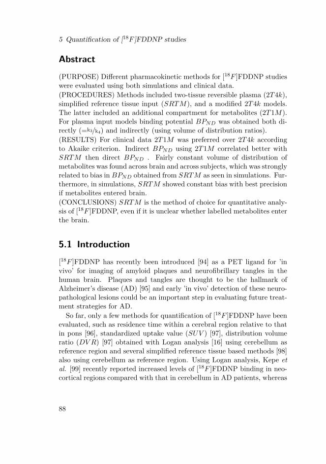
5 Quantification of [18F ]FDDNP studies

Abstract

(PURPOSE) Different pharmacokinetic methods for [18F ]FDDNP studieswere evaluated using both simulations and clinical data.(PROCEDURES) Methods included two-tissue reversible plasma (2T4k),simplified reference tissue input (SRTM), and a modified 2T4k models.The latter included an additional compartment for metabolites (2T1M).For plasma input models binding potential BPND was obtained both di-rectly (=k3/k4) and indirectly (using volume of distribution ratios).(RESULTS) For clinical data 2T1M was preferred over 2T4k accordingto Akaike criterion. Indirect BPND using 2T1M correlated better withSRTM then direct BPND . Fairly constant volume of distribution ofmetabolites was found across brain and across subjects, which was stronglyrelated to bias in BPND obtained from SRTM as seen in simulations. Fur-thermore, in simulations, SRTM showed constant bias with best precisionif metabolites entered brain.(CONCLUSIONS) SRTM is the method of choice for quantitative analy-sis of [18F ]FDDNP, even if it is unclear whether labelled metabolites enterthe brain.

5.1 Introduction

[18F ]FDDNP has recently been introduced [94] as a PET ligand for ’invivo’ for imaging of amyloid plaques and neurofibrillary tangles in thehuman brain. Plaques and tangles are thought to be the hallmark ofAlzheimer’s disease (AD) [95] and early ’in vivo’ detection of these neuro-pathological lesions could be an important step in evaluating future treat-ment strategies for AD.So far, only a few methods for quantification of [18F ]FDDNP have been

evaluated, such as residence time within a cerebral region relative to thatin pons [96], standardized uptake value (SUV ) [97], distribution volumeratio (DV R) [97] obtained with Logan analysis [16] using cerebellum asreference region and several simplified reference tissue based methods [98]also using cerebellum as reference region. Using Logan analysis, Kepe etal. [99] recently reported increased levels of [18F ]FDDNP binding in neo-cortical regions compared with that in cerebellum in AD patients, whereas

88

5.2 Methods

no difference in uptake between cerebellum and other regions was foundin healthy controls (HC). In addition, Small et al. [100] found that globalDV R values in HC were lower than in patients with mild cognitive im-pairment (MCI), which in turn were lower than in AD subjects. However,arterial sampling was not used in any of these studies. Arterial samplingis considered to be the gold standard, especially if pathological changesmay also affect reference regions.The purpose of the present study was to investigate which pharmacoki-

netic model could best be used for quantitative analysis of [18F ]FDDNPstudies. To this end both simulated and clinical [18F ]FDDNP data wereused. Data were analysed using various compartmental models based onplasma [7] and reference tissue [8, 84, 9] input data. In addition, a plasmainput model was evaluated, which accounted for uptake of labelled metabo-lites in the brain. Finally, standard uptake value ratios with cerebellum(SUVr) were investigated.

5.2 Methods


Clinical data were derived from ongoing patient studies consisting of 12subjects (6 HC, 3 MCI [101], and 3 AD) with ages ranging from 58 to72 years. Mean age (±SD) was 66±5, 68±4 and 63±6 for HC, MCI andAD, respectively. AD patients were diagnosed with probable AD meetingNINCDS-ADRDA criteria.[102] The study was approved by the MedicalEthics Committee of the VU University Medical Centre and each subjectgave written informed consent prior to inclusion in the study. Clinicalresults are beyond the scope of the present study and will be reportedelsewhere.As part of the study protocol, each subject first underwent a T1-weighted

MRI scan using a 1.5T SONATA scanner (Siemens Medical Solutions, Er-langen, Germany). This MRI scan was performed to exclude anatomicalabnormalities and for co-registration and segmentation purposes.PET studies were performed using an ECAT EXACT HR+ scanner

(CTI / Siemens, Knoxville, USA). The characteristics of this scanner havebeen described previously.[86] First, a 10 minutes transmission scan in

89


2D acquisition mode was performed. This scan was used to correct thesubsequent emission scan for tissue attenuation. Next, a dynamic emissionscan in 3D acquisition mode was performed following bolus injection of168±8 MBq [18F ]FDDNP.[103] This dynamic emission scan consisted of23 frames (1x15, 3x5, 3x10, 2x30, 3x60, 2x150, 2x300, 7x600 s) with a totalscan duration of 90 minutes. All frames were reconstructed using FORE+ 2D filtered back projection [88] and a Hanning filter with a cut-off of0.5 times the Nyquist frequency. Reconstructions included all standardcorrections, such as normalization, and decay, dead time, attenuation,randoms and scatter [89] corrections.

The protocol also included continuous arterial sampling, starting 2 minprior to injection and continuing up to 60 minutes, using a dedicatedon-line detection system.[37] In addition, at set times (5, 10, 20, 40, 60min post injection), arterial sampling was interrupted briefly for the with-drawal of discrete arterial samples. After each sample, the arterial linewas flushed with heparinised saline in order to avoid clotting within theline. Finally, two manual samples were withdrawn at 75 and 90 minutespost injection.

Arterial blood samples were used to determine plasma and whole bloodradioactivity concentrations using a well counter cross calibrated againstthe PET scanner.[90] In addition, plasma parent tracer and metaboliteconcentrations were determined using solid phase extraction combinedwith HPLC technology and equipped with off-line radioactivity detection.[104]An arterial whole blood curve was obtained by correcting the on-line sam-pler curve for decay, removing the flushing periods, and calibrating againstthe discrete (whole blood) sample data. Finally, a metabolite correctedplasma curve was derived from this whole blood curve using both plasmato whole blood ratios and metabolite fractions obtained from the manualblood samples. To this end, the total fraction of labelled metabolites asfunction of time was fitted to a Hill-type function.[105] This function pro-vided more accurate fits than other functions such as multi-exponentials.Arterial blood sampling was not available for 6 subjects (3 HC and 3 MCI).Data from these subjects were only used for investigating reference tissuemodels.

90

5.2 Methods

5.2.2 Image analysis

De-skulled T1-weighted MRI scans [91] were co-registered [56, 57] witha summed PET image (frames 3-12: 25 s – 5 min post injection). Thissummed PET image resembles a flow image, thereby maximizing corticalinformation. Time activity curves were then generated using MR-basedautomatic delineation of regions of interest (ROI), as described by Svareret al..[92] For the purpose of the present study only TACs from 17 regions(cerebellum, orbital frontal cortex, medial inferior frontal cortex, anteriorcingulate cortex, thalamus, insula, caudate, putamen, superior temporalcortex, parietal cortex, medial inferior temporal cortex, superior frontalcortex, occipital cortex, sensory motor cortex, posterior cingulate cortex,enthorinal cortex, hippocampus), all averaged over left and right hemi-spheres, were analysed. These anatomical regions were small and definedin grey matter only, thereby minimizing signal dilution due to partial vol-ume effects as much as possible.

5.2.3 Kinetic analyses of clinical data

Clinical data were analysed using conventional plasma input and refer-ence tissue based algorithms.[7] As there is some concern that labelled[18F ]FDDNP metabolites might cross the blood-brain barrier [18, 17], ad-ditional analyses were performed using a plasma input model accountingfor metabolites entering the brain. In addition, average regional activityconcentration ratios with the reference region (SUVr) were derived overthe time intervals of 40-60, 60-90 and 80-90 minutes after injection. Forall reference tissue models and SUVr cerebellar grey matter was used asreference region, based on its relatively low levels of amyloid and neurofib-rillary tangles.[95]Five different conventional compartmental models were evaluated: single-

tissue (1T2k), two-tissue irreversible (2T3k) and two-tissue reversible (2T4k)plasma input models, and simplified (SRTM ; [9]) and full (FRTM ; [8,84]) reference tissue models. Plasma input models contained one addi-tional fit parameter for blood volume. The SRTM was used to estimatebinding potential directly (BPSRTMND ). The 2T4k plasma input modelwas used to estimate binding potential both directly ( BP 2T4k

ND = k3/k4)and indirectly using volume of distribution ratios ( BP 2T4ki

ND = DV R−1 =

91


V targetT /V reference

T −1).[84] The latter approach will be indicated by 2T4ki.Based on the possibility of metabolites entering the brain [18, 17], also

a modified 2T4k model was used. This model included an additional (par-allel) single-tissue compartment for labelled metabolites (2T1M , Figure5.1). The metabolite input curve was based only on polar metabolites andignoring the minor fraction of other metabolites. The direct binding poten-tial (BP 2T1M

ND ) for this model was defined as k3/k4 (Figure 5.1), and the vol-umes of distributions, VT and VTm , were defined as K1/k2 ∗

(1 +BP 2T1M

ND

)and K1m/k2m, respectively. Similar to 2T4ki, the binding potential wasalso estimated indirectly using the volume of distribution ratios with thecerebellum as reference region (BP 2T1Mi

ND ). All 2T1M fits were repeated,after fixing VTm to the cerebellum value (=2T1Mfvtm). This model wasalso used to estimate binding potential both directly (BP 2T1Mfvtm

ND ) andindirectly using DVR-1 (BP 2T1Mfvtmi

ND ). The indirect methods for estimat-ing BPND using 2T1M and 2T1Mfvtm will be indicated by 2T1M i and2T1M i

fvtm, respectively.

5.2.4 Clinical studies

Clinical results were evaluated in several ways. First, for all compartmen-tal models (SRTM , FRTM , 1T2k, 2T3k, 2T4k, 2T1M and 2T1Mfvtm),fitted TACs were evaluated using the Akaike criterion. Next, where pos-sible, BPND values were estimated both directly and indirectly using VTratios with cerebellum (i.e. 2T4ki, 2T1M i and 2T1M i

fvtm). In addition,estimates of BPND were compared with BPSRTMND . Finally, SUVr − 1values were estimated and compared with BPSRTMND , given that at trueequilibrium SUVr corresponds with DV R.

5.2.5 Simulation studies

Conventional simulations. Simulated time activity curves (TACs) for tar-get and reference regions were generated using a typical [18F ]FDDNPplasma input function in combination with the two-tissue reversible plasmainput model (2T4k). In the simulations variations in binding, delivery andfractional blood volume were investigated.Kinetic parameters were based on typical 2T4k parameters obtained

92

5.2 Methods

Figure 5.1: Schematic diagram of the model that includes a tissue metabolite com-partment. BBB represents the blood-brain-barrier; PParent and PMet aretracer plasma radioactivity concentrations (Bq/ml) of parent and labelledmetabolites, respectively; T is the radioactivity concentration in tissue,F + NSParent that of free and non-specifically bound parent in tissue,SParent that of bound parent in tissue and F + NSMet that of labelledmetabolites in tissue (Bq/ml); K1 (ml ∗ cm−3min−1) and k2 (min−1) arerate constants, describing exchange of parent between plasma and tissue;k3 and k4 are rate constants (min−1), describing exchange of parent be-tween free and bound compartments; K1m (ml ∗ cm−3min−1) and k2m

(min−1) are rate constants, describing exchange of labelled metabolitesbetween plasma and tissue.

93


from clinical data. Default parameters for simulated reference and targettissue TACs are given by R1 and T1, respectively, as listed in Table 5.1.Target tissue parameters were varied with respect to binding potential(BP 2T4k

ND and BP 2T4kiND : T2-T5), fractional blood volume (Vb: T6, T7) and

delivery (K1: T8-T15). 100 TACs were generated for each run and noisewas added to simulate an average noise level of 7.5% COV (coefficient ofvariation). Noise simulation was based on clinically derived typical valuesof total scanner true counts, frame lengths and decay correction factors.A detailed description of the noise simulation used is given in [59].Simulated data were analysed using conventional models as described

above (1T2k, 2T3k, 2T4k, SRTM , FRTM and 2T4ki) and SUVr meth-ods over the time intervals 40-60, 60-90 and 80-90 minutes. Fits wereevaluated by comparing goodness of fit according to the Akaike crite-rion. Next, models were evaluated by comparing bias and COV of esti-mated binding potential (where appropriate also the indirect estimationthrough volumes of distribution). Bias was estimated in relative termsusing 100

(BPmodelND

BP simulatedND

− 1), where BPmodelND represents BPND estimated

using the method of analysis under investigation, and BP simulatedND simu-lated BPND, which was set to either BP 2T4k

ND or BP 2T4kiND for direct and

indirect methods, respectively.

5.2.6 Metabolite model

To simulate the effects of cerebral uptake of labelled metabolites, sim-ulated TACs were generated using a typical [18F ]FDDNP plasma inputfunction in combination with the 2T1M model. Kinetic parameters werebased on typical 2T1M parameters obtained from clinical data. Defaultparameters for simulated reference and target tissue TACs are given byR1 and T1, respectively, as listed in Table 5.2. Target tissue parameterswere varied, including binding potential (BP 2T1M

ND and BP 2T1MiND : T2-T9),

delivery of metabolites (K1m : T10-T13) and volume of distribution ofmetabolites (VTm: T14-T21). 100 TACs were generated for each run andnoise was added to simulate an average noise level of 7.5% COV (coefficientof variation), as described above.Simulated data were analysed using 2T4k, 2T4ki, 2T1Mfvtm (i.e. 2T1M

with VTm fixed to the simulated value), 2T1M ifvtm (i.e. indirect estimation

94

5.2 Methods

Table 5.1: Kinetic parameters used to generate reference (R) and target (T) tis-sue time activity curves (TAC). K1(ml ∗ cm−3min−1), k2(min−1) andk3(min−1) are rate constants, Vb is fractional blood volume, VT is volume ofdistribution, and BP 2T4k

ND and BP 2T4kiND are binding potentials estimated di-

rectly (2T4k) and indirectly (2T4ki) using the reversible two tissue model,respectively. The indirect calculation of BPND was performed using targetto reference volumes of distribution ratios. During all simulations k4 (0.032min−1) and K1/k2 (3.3) were fixed.

TAC K1 BP 2T4kND Vb VT BP 2T4ki

ND

R 1 0.35 1.63 0.050 8.7 –T 1 0.35 2.3 0.050 11 0.25T 2 0.35 1.7 0.050 8.9 0.03T 3 0.35 2.0 0.050 9.9 0.14T 4 0.35 2.6 0.050 12 0.37T 5 0.35 2.9 0.050 13 0.48T 6 0.35 2.3 0.025 11 0.25T 7 0.35 2.3 0.075 11 0.25T 8 0.21 2.3 0.050 11 0.25T 9 0.25 2.3 0.050 11 0.25T 10 0.28 2.3 0.050 11 0.25T 11 0.32 2.3 0.050 11 0.25T 12 0.39 2.3 0.050 11 0.25T 13 0.43 2.3 0.050 11 0.25T 14 0.46 2.3 0.050 11 0.25T 15 0.50 2.3 0.050 11 0.25

95


through volumes of distribution), and SRTM . Bias and COV of bindingpotential obtained were compared between the various models. Bias fordirect and indirect 2T1M models was defined in a similar way as for thestandard models, i.e. using 100

(BPmodelND

BP simulatedND

− 1), where BPmodelND repre-

sents BPND estimated using the method of analysis under investigation,and BP simulatedND simulated BPND, set to either BP 2T1M

ND or BP 2T1MiND for

direct and indirect models, respectively.In addition to BPND, in metabolite simulations, also VT values were

estimated using 2T4k and the 2T1Mfvtm models. Bias in estimated

VT for the 2T4k model was defined as 100(

VmodelT

V total,simulatedT

− 1), where

V total,simulatedT is K1/k2 ∗ (1 +BPND) + K1m/k2m. Bias in estimated VT for

the 2T1Mfvtm model was defined as 100(

VmodelT

V simulatedT

− 1), where V simulated

T

is K1/k2 ∗ (1 +BPND).

5.3 Results5.3.1 Time activity curvesTypical parent [18F ]FDDNP and polar metabolite plasma curves are shownin Figure 5.2a, and typical time activity curves for cerebellum and frontalcortex in Figure 5.2b. The average (N=5) fractions of [18F ]-labelledmetabolites in plasma as function of time are shown in Figure 5.3, fittedusing a Hill type function. Very rapid metabolism of [18F ]FDDNP can beseen, with metabolite related [18F ]-activity primarily due to polar metabo-lites (Figure 5.3). The polar metabolites are composed of N-dealkylatedfragments with similar chromatogram retention times as primarily fluo-roethanal and with a smaller fractions of fluoroacetic acids.[17]

5.3.2 Clinical studiesFigures 5.4 show typical fits using various compartmental models. Ingeneral, poor fits were seen for the 1T2k model (Figure 5.4a). Metabo-lite models showed slightly better fits (Figure 5.4b) than all conventionalmodels (Figure 5.4a). Good fits were seen for the reference tissue mod-els (Figure 5.4c). Similarly, the Akaike criterion gave preference to 2T1M

96

5.3 Results

Table 5.2: Kinetic parameters used to generate reference (R) and target (T) tissuetime activity curves (TAC). A two-tissue reversible compartmental modelwith an additional single-tissue compartment for metabolites was used.K1(ml ∗ cm−3min−1), k2(min−1) and k3(min−1) are rate constants, Vbis fractional blood volume, VT is volume of distribution for [18F ]FDDNP.BP 2T1M

ND and BP 2T1MiND are binding potentials estimated directly and in-

directly using the metabolite model, respectively. The indirect calculationof BPND was performed using target to reference volumes of distributionratios. K1m (ml ∗ cm−3min−1) is a rate constant and VTm the volume ofdistribution for the metabolites. During all simulations k4 (0.099 min−1)and K1/k2 (2.4) were fixed, and same the K1m and k2m were used in refer-ence and target tissues.

TAC K1 BP 2T1MND Vb VT BP 2T1Mi

ND K1m VTm

R 1 0.34 0.65 0.05 4 – – –T 1 0.34 1.3 0.05 5.59 0.39 0.50 0.59T 2 0.34 0.8 0.05 4.37 0.09 0.50 0.6T 3 0.34 1.0 0.05 4.86 0.21 0.50 0.6T 4 0.34 1.2 0.05 5.34 0.33 0.50 0.6T 5 0.34 1.4 0.05 5.83 0.45 0.50 0.6T 6 0.34 1.6 0.05 6.31 0.58 0.50 0.6T 7 0.34 1.8 0.05 6.80 0.70 0.50 0.6T 8 0.34 2.1 0.05 7.53 0.88 0.50 0.6T 9 0.34 2.3 0.05 8.01 1.00 0.50 0.6T 10 0.34 1.3 0.05 5.59 0.39 0.00 0.6T 11 0.34 1.3 0.05 5.59 0.39 0.01 0.6T 12 0.34 1.3 0.05 5.59 0.39 0.03 0.6T 13 0.34 1.3 0.05 5.59 0.39 0.05 0.6T 14 0.34 1.3 0.05 5.59 0.39 0.50 0.1T 15 0.34 1.3 0.05 5.59 0.39 0.50 0.2T 16 0.34 1.3 0.05 5.59 0.39 0.50 0.3T 17 0.34 1.3 0.05 5.59 0.39 0.50 0.4T 18 0.34 1.3 0.05 5.59 0.39 0.50 0.5T 19 0.34 1.3 0.05 5.59 0.39 0.50 0.7T 20 0.34 1.3 0.05 5.59 0.39 0.50 0.8T 21 0.34 1.3 0.05 5.59 0.39 0.50 0.9

97


(a) (b)

Figure 5.2: Typical [18F ]FDDNP decay corrected time activity curves from an ADsubject for (5.2a) metabolite corrected parent compound and polarmetabolites in plasma, and (5.2b) cerebellum and frontal cortex (ctx)grey matter.

98

5.3 Results

Figure 5.3: Fraction of [18F ]-labelled polar metabolites (dark dashed line) and par-ent compound (dark line) in plasma as function of time, averaged over 7subjects, together with standard deviations (dashed light grey lines at oneSD from average).

models above other plasma input models (2T1Mfvtm 37.3%, 2T1M 31.7%,2T4k 26.2%, 2T3k 4.8% and 1T2k 0% preference, respectively). With re-spect to reference tissue models, the Akaike criterion had strong preferencefor SRTM (88%).Average values of the various parameters, together with observed range,

for 2T4k, 2T1M and SRTM models are given in Table 5.3 for typicalAD regions, i.e. for regions previously shown to be involved in AD[100].These regions were used in order to accurately estimate typical kineticparameters for AD subjects, as the latter parameter estimates were usedin the simulations.Figure 5.5 shows high correlation (R2=0.95) between K1m and k2m val-

ues from the 2T1M model over all regions and subjects, indicating analmost constant VT for metabolites. Table 5.4 shows correlation coeffi-cients obtained from linear regression analyses of various outcome mea-sures with BPSRTMND . As expected, high correlation was found betweenBPND estimates of SRTM and FRTM (R2=0.99). In addition, goodcorrelation was obtained for SUVr over 40-60 minutes (R2=0.93). Note

99


that the 2T1M i models, i.e. including a compartment for metabolitesentering the brain, correlated better with SRTM than the conventional2T4ki model (Table 5.4 and Figure 5.6)

5.3.3 Simulations Studies

Conventional simulations

In general, SRTM produced better fits than FRTM according to theAkaike criterion (~85% preference). According to the same criterion, 2T4kshowed better fits than both 1T2k and 2T3k in all simulations (~96%preference). At lower K1 values, however, preference for 2T4k reduced infavour of 2T3k (max. 33% preference for 2T3k). Visual inspection showedpoor fits for the 1T2k model, similar to what was seen in clinical fits, andtherefore it was excluded from further evaluation.When simulating different levels of binding the 2T4k model (direct es-

timation of BPND) showed good overall accuracy (5% bias BPND), butmediocre precision (24% COV BPND). Results for reference tissue basedmodels, including SUVr, are summarized in table 5.5. In general, all refer-ence tissue based methods showed increased bias at lower levels of binding,but results were more stable at higher levels. Therefore, bias estimateswere averaged only over the stable part, i.e. for BP 2T4ki

ND > 0.14. In con-trast, absolute differences with simulated BP 2T4ki

ND values were more sta-ble and are shown over the full range of simulated BP 2T4ki

ND values (Table5.5). Average bias (Table 5.5) over the stable range of BP 2T4ki

ND (> 0.14)was lowest for indirect 2T4k (2T4ki). 2T4ki and SRTM both showedrelatively constant bias and high precision for higher simulated BPNDlevels. Finally, best accuracy and precision for SUVr was obtained withSUVr40−60.All models were less sensitive to changes in Vb. At a fixed level of binding

(BPND=2.3, BP 2T4kiND =0.25), variations in derived BPND due to changes

in simulated Vb were smaller than 5% for all compartmental models. ForSUVr methods bias (±COV ) in approximated BPND (i.e. SUVr − 1)depended on the actual time interval used and changed from 21±16%to 10±18%, from 30±22% to 28±21% and from 31±41% to 34±45% forSUVr40−60, SUVr60−90 and SUVr80−90, respectively, when varying Vb ofthe target region from 0.025 to 0.075.

100

5.3 Results

(a)

(b) (c)

Figure 5.4: Decay corrected frontal cortex grey matter time activity curve from anAD subject (= data) with fits using (5.4a) conventional plasma input,(5.4b) metabolite and (5.4c) reference tissue models.

101


Table5.3:

Average(±

SD)values

ofthe

kineticparam

eters,together

with

theirrange

givenbetw

eenbrackets,

for(a)

thereversible

two-tissue

compartm

entmodel(2

T4k),(b)

the2T

1M

metabolite

modeland

(c)the

simplified

referencetissue

model(S

RTM

),derivedfrom

clinicaldata.These

consistedofseveraltypicalA

Dcortical(ctx)

andcerebellar

(cer)grey

matter

regionsfrom

healthycontrols

(HC)and

AD

subjects.

Data

K1

k2

k3

BP

2T

4k

ND

VT

BP

2T

4ki

ND

Vb

HC

ctx0.25±

0.030.06±

0.010.02±

0.012.14±

0.7114±

60.22±

0.180.03±

0.01

(0.2–0.3)

(0.04–0.08)

(0.01–0.05)

(1–4)

(7–25)

(-0.04-0.7)

(0.01–0.05)

AD

ctx0.36±

0.080.06±

0.010.02±

0.011.76±

0.7117±

50.23±

0.200.05±

0.03

(0.3–0.5)

(0.04–0.08)

(0.01–0.04)

(1–3)

(9–26)

(-0.03-0.6)

(0.02–0.11)

AD

+H

Ccer

0.35±0.09

0.07±0.01

0.02±0.02

1.67±0.56

13±5

–0.03±

0.02

(0.3–0.5)

(0.06–0.09)

(0.01–0.06)

(1–3)

(6–20)

(0.01–0.07)

(a)

Data

K1

k2

k3

BP

2T

1M

ND

VT

BP

2T

1Mi

ND

Vb

K1

mVTm

HC

ctx0.28±

0.050.33±

0.301.06±

0.753.07±

2.893.70±

0.620.03±

0.140.03±

0.010.08±

0.100.66±

0.07

(0.2–0.4)

(0.09–0.68)

(0.01–2.43)

(0.4–11)

(3–5)

(-0.18-0.44)

(0.01–0.05)

(0.01–0.5)

(0.49–0.76)

AD

ctx0.41±

0.100.24±

0.150.54±

0.502.06±

1.655.19±

0.860.06±

0.110.04±

0.020.16±

0.270.65±

0.06

(0.3–0.6)

(0.09–0.73)

(0.05–1.84)

(0.6–8)

(4–7)

(-0.2-0.3)

(0.01–0.09)

(0.03–0.93)

(0.55–0.78)

AD

+H

Ccer

0.39±0.13

0.28±0.16

0.49±0.47

1.89±1.42

4.24±1.07

–0.02±

0.020.34±

0.460.60±

0.04

(0.3–0.6)

(0.10–0.53)

(0.04–1.30)

(0.5–4)

(3–6)

(0.01–0.05)

(0.02–1.00)

(0.53–0.67)

(b)

Data

R1

k2

BPSRTM

ND

HC

ctx0.89

±0.06

0.08±

0.020.06

±0.04

(0.7–1.0)

(0.03–0.11)

(-0.07–0.12)

AD

ctx0.87

±0.08

0.06±

0.020.07

±0.04

(0.7–1.0)

(0.03–0.11)

(0.00–0.14)

(c)

102

5.3 Results

Figure 5.5: Correlation between metabolite influx (K1m) and efflux (k2m ) rate con-stants for clinical [18F ]FDDNP data from several regions of interests andsubjects. These rate constants were obtained using a modified two-tissuereversible model, including an additional single-tissue compartment formetabolites.

Table 5.4: Outcome parameters (slope, intercept and Pearson product moment cor-relation coefficient R2) for linear regression of different models versusBPSRTMND . In case of SUVr methods, SUVr − 1 was taken as an estimateof BPND. NA indicates poor correlation, i.e. R2<0.10.

Model Slope Intercept R2

FRTM 0.97 0.01 0.992T4k -4.11 2.21 0.152T4ki NA NA NA2T1M NA NA NA2T1M i 2.66 -0.11 0.68

2T1Mfvtm NA NA NA2T1M i

fvtm 2.59 -0.09 0.58SUVr40−60 1.14 0.03 0.93SUVr60−90 0.64 0.06 0.69SUVr80−90 0.46 0.06 0.43

103


Figure 5.6: Correlation of BPND from 2T1M ifvtmand 2T4ki, respectively, with

BPSRTMND for clinical [18F ]FDDNP data obtained from several regions ofinterest and subjects. 2T4ki represents the reversible two-tissue plasma in-put model and 2T1M i

fvtm the modified reversible two-tissue model, whichincludes an additional parallel single-tissue compartment for metabolites.For both models BPND was estimated indirectly through calculation ofdistribution volume ratios.

104

5.3 Results

Table 5.5: Average bias and absolute difference (diff.) with simulated BPND over arange of simulated BP 2T4ki

ND for various reference tissue models. In addition,corresponding SD are given. In case of SUVr methods, SUVr−1 was takenas an estimate of BPND. For bias the range was set from 0.25 to 0.48, dueto the large relative biases at lower specific binding. For absolute differencethe range was set from 0.03 to 0.48.Model Bias (%) SD in bias (%) Diff. SD in diff.

2T4ki 1 17 0.041 0.033SRTM -12 16 0.053 0.062FRTM -13 23 0.094 0.175SUVr40−60 -1 14 0.034 0.026SUVr60−90 16 15 0.054 0.037SUVr80−90 22 33 0.095 0.072

Delivery differences affected all compartmental methods, including plasmainput models. For the direct 2T4k model bias in BPND varied from 10to -2%, when varying K1 of the target region from 0.212 to 0.496. Re-sults for indirect 2T4k and SRTM are shown in Figure 5.7. Results fromFRTM are not included, as BPND bias was as high as 250%. Bias inBPND (±COV ), based on SUVr − 1, ranged from -27±18% to 3±17%,from 25±20% to -3±18% and from 48±36% to -7±39% for SUVr40−60,SUVr60−90 and SUVr80−90, respectively, when varying K1 of the targetregion from 0.212 to 0.496.

Metabolite simulations

Metabolite simulations were limited to 2T4k, 2T1Mfvtm and SRTM .SRTM provided the most precise estimation of BPND over the rangeof simulated K1m with a COV of 4.0±0.4%. Although there was a strongnegative bias (-42±7%) for SRTM , it was very constant (Figure 5.8a).2T1M i

fvtm provided a more accurate estimate of BPND (5±7% bias), butprecision (COV of 37±20%) was much poorer than for SRTM (Figure5.8a). 2T1Mfvtm, 2T4k and 2T4ki provided lower precision and higherbias in estimated BPND over the range of simulated K1m (Figures 5.8band 5.8c. However, VT estimates with the 2T1Mfvtm model were much

105


Figure 5.7: Bias of BPND for different compartment models for simulated[18F ]FDDNP data (obtained using 2T4k) as function of variable targetinflux rates (K1 Target). Error bars represent SD in bias. K1 in referenceregion was fixed to 0.35, and K1/k2 was fixed to 3.3 for both target andreference regions. 2T4ki and SRTM represent indirect (using volumes ofdistribution) two-tissue reversible and simplified reference tissue models,respectively.

106

5.4 Discussion

more accurate and had higher precision (Figure 5.8c).Simulations over a range of different binding levels showed strong neg-

ative bias (-46±4% with COV of 7±6%) for SRTM , but again resultingBPND estimates were the most stable amongst all models tested (Fig-ure 5.9a). Similarly, most accurate results were obtained with indirect2T1Mfvtm (Figure 5.9a). Precision of both SRTM and 2T1M i

fvtm im-proved with increasing BPND. BPND estimates obtained with 2T1Mfvtm,2T4k and 2T4ki were not precise and strongly biased (Figure 5.9). Finally,Figure 5.10a shows nearly linearly increasing (negative) bias in BPND ob-tained with SRTM for increasing VTm. In contrast, Figure 5.10b illus-trates that this bias was independent of K1m for K1m>0.1.

5.4 Discussion

5.4.1 Clinical studies

Due to rapid plasma clearance and metabolism [18F ]FDDNP scans itproved to be difficult to obtain reliable measurements of metabolite frac-tions at later time points. As a result, only incomplete plasma data wereavailable for 6 of the subjects and data from these subjects were only usedfor evaluation of reference tissue models. Although only 6 subjects withcomplete plasma input data remained, this seems to be sufficient for thisinitial evaluation of quantitative (plasma input) models. Clearly, how-ever, the difficulties in obtaining reliable plasma metabolite data shouldbe taken into account when selecting a method for routine clinical studies.Clinical [18F ]FDDNP data were analysed using conventional models,

models correcting for possible metabolites entering the brain, and activityratios. Clearly, due to the very nature of clinical data, absolute statementsabout accuracy and precision cannot be given. Therefore, the variousmethods were compared using the Akaike criterion. In addition, resultingBPND values were compared with SRTM , as this model showed stableresults during simulations.On the basis of the Akaike criterion plasma input models with a com-

partment for metabolites were preferred over conventional plasma inputmodels, and SRTM was preferred over FRTM . Good correlations withSRTM were obtained only for FRTM , SUVr40−60, and plasma input

107


(a)

(b) (c)

Figure 5.8: Bias of (5.8a) indirect and reference tissue model BPND, (5.8b) directBPND, and (5.8c) VT estimates from different compartment models. Errorbars represent SD in bias. Simulated [18F ]FDDNP data were generatedusing the metabolite plasma input model (2T1M) with variable metaboliteinflux rates (K1m ).

108

5.4 Discussion

(a) (b)

Figure 5.9: Bias of (5.9a) indirect (and reference tissue) and (5.9b) direct BPND es-timates from different compartment models for simulated [18F ]FDDNPdata generated using the metabolite plasma input model (2T1M) withvarious target tissue binding potentials. Error bars represent SD in bias.

109


(a) (b)

Figure 5.10: Bias of BPND estimated with the simplified reference tissue model(SRTM) for simulated [18F ]FDDNP data generated using the metabo-lite plasma input model (2T1M) as function of (5.10a) various VTmvalues and (5.10b) various metabolite influx rates (K1m ). Error barsrepresent SD in bias.

110

5.4 Discussion

models that included a compartment for metabolites entering the brain,such as 2T1M i and 2T1M i

fvtm (Figure 5.6). For most other methodscorrelations with SRTM were poor (R2<0.1).Specifically, in case of the metabolite models, somewhat large values

were seen for the micro parameters K1m and k2m (Figure 5.5). However,the majority of observed K1m values are below 0.5 (many overlapping dataat lower K1m) and K1m and k2m are well correlated. The higher K1m andk2m values are possibly the result of noise, as the higher values forK1m andk2m were generally seen for the smallest ROIs used. Moreover, the relativeslow in-grow of metabolites, i.e. the metabolite input function shows aslow increase rather than a sharp peak, makes estimation of individualmicro-parameters less precise. Note, however, that the macro-parameterVTm is reasonably stable across anatomical regions and subjects.Observed improvements in fits and correlations for models that incor-

porate a labelled metabolite compartment, together with the reasonablyconstant VTm, suggest that metabolites enter the brain. This is in linewith a previous assessment using multi-input spectral analysis [18] andinitial animal studies where labelled metabolites of [18F ]FDDNP wereinjected.[17] Additional studies are, however, needed to confirm whetherthis is indeed the case.

5.4.2 Simulation studiesThe standard 2T4k plasma input model was not a good model for esti-mating the level of specific [18F ]FDDNP binding directly (i.e. as definedby k3/k4). Firstly, although BPND bias calculated relative to total bindingpotential showed good accuracy, it only had mediocre precision. Secondly,at lower regional delivery (=K1 ) levels, its bias was sensitive to the actualvalue of K1 . This increased sensitivity to K1 is related to the kineticsof [18F ]FDDNP, which for a normal level of binding in regions with lowdelivery are relatively slow. Under those conditions, within the time frameof a scan, tracer kinetics are best described by an irreversible compart-ment model, which is illustrated by the increased preference for the 2T3kmodel according to the Akaike criterion.The 2T1Mfvtm model did not provide accurate estimates of (direct)

BPND in the metabolite simulations (Figures 5.8b and 5.9b). Although,data were simulated using the same model, BPND was very sensitive to

111


noise, as a result of the large number of fit parameters. However, VTestimates obtained with the 2T1Mfvtm model were less sensitive to noiseand provided highly accurate and precise VT values (Figure 5.8c).For plasma input models, more accurate and precise results were ob-

tained with indirect estimates of BPND (2T4ki and 2T1M ifvtm) than

with their direct counterparts (2T4k and 2T1Mfvtm), especially in caseof metabolite simulations. In most cases these indirect methods showedlower bias than BPSRTMND . This higher accuracy of 2T4ki (in conventionalsimulations) and 2T1M i

fvtm (in metabolite simulations) was, however, ac-companied with lower precision compared with BPSRTMND .SRTM was better than FRTM , both in terms of bias and COV . In

addition, in the majority of the simulations, it was preferred by the Akaikecriterion. SRTM results were comparable in conventional and metabolitesimulations. If no metabolites entered the brain, SRTM derived BPNDshowed a constant negative bias, although it was affected by changes indelivery. On the other hand, when polar metabolites entered the brain,SRTM showed increasing negative bias with increasing VTm. However,clinical data showed an overall constant VTm (Figure 5.5). This indicatesthat variable bias in SRTM derived BPND due to variability in VTmwill be limited. Simulations showed that, for VTm fixed to the clinicalestimated value (VTm =0.6), this bias also was not sensitive to metabo-lite influx (Figure 5.10b, K1m >0.01, BPND bias ~-46%). Furthermore,the bias found in these simulations could be related to the slope betweenBPSRTMND versus BP 2T1Mfvtmi

ND (slope=2.59, Table 5.4; 100%*(1/2.59) =39%) for the clinical studies, indicating a relatively constant metabolitecontribution in practice. Thus SRTM seems to be a useful method, irre-spective whether labelled metabolites enter the brain, provided that VTmis relatively constant across the brain and between subjects, as actuallysuggested by the clinical results.Among SUVr methods, over the range of simulated binding levels, only

SUVr40-60 showed acceptable results, with much better accuracy (-1%)than SRTM (-12%). However, apart from a strong dependency on varia-tions in delivery, SUVr results were also highly dependent on differencesin blood volume fractions with only an acceptable accuracy for a specifictime interval (SUVr60−90). In general, SUVr results varied widely be-tween different time intervals which, together with the large uncertainties,

112

5.4 Discussion

indicates that this might not be the ideal method for clinical studies.In general, SRTM showed best overall performance, although it showed

some sensitivity to regional flow/delivery differences. As expected, SRTM ,like all other reference tissue based models, showed larger biases at lowerregional binding levels. Important advantages of SRTM were its overallhigh precision and a relatively constant bias in BPND, even in the pres-ence of labelled metabolites. Although this bias was dependent on theactual value of VTm, clinical data indicated that this was constant acrossthe brain and among subjects.


Amyloid plaques (and neurofibrillary tangles) do not behave like neurore-ceptors. They have complex structures with multiple affinity sites for[18F ]FDDNP. In addition, it is likely that access to amyloid sites will be-come more difficult with increasing plaque size.[106] Consequently, use ofreceptor-ligand models to assess amyloid load might provide an increasingunderestimation with increasing load. In addition, quantification might becompromised by the possibility of labelled metabolites entering the brain,especially since the fraction of labelled (polar) metabolites in blood is highdue to rapid metabolism of [18F ]FDDNP.Nevertheless, [18F ]FDDNP may still be of value if a difference between

MCI and healthy controls can be demonstrated, and it might be used tostudy pathological effects as a function of disease severity/progression.[100]In addition, at early stages, a stable receptor-ligand model is likely toprovide a reasonable quantitative estimate of the pathological changes as-sociated with AD and could therefore be an important tool in evaluatingeffects of therapy. Clearly, given its relatively small specific signal, thevalue of [18F ]FDDNP can only be determined by large comparative clin-ical studies, such as the one by Small and collaborators.[100] From thepresent study it follows that such a comparison should preferably be per-formed using SRTM as method of analysis, as it showed high precisionand constant bias across the brain and among subjects even when metabo-lites enter the brain.

113


5.5 ConclusionSRTM outperformed other models, providing BPND estimates with highprecision. As clinical data indicated that the volume of distribution of la-belled metabolites VTm was constant across the brain and among subjects,bias in SRTM derived BPND will be constant and predictable. The mainpotential drawback is its sensitivity to variations in regional K1, althoughthis did not appear to be a problem in the clinical studies.

AcknowledgementsThe authors would like to thank the personnel of the Department of Nu-clear Medicine & PET Research for tracer production and data acquisition.The authors would also like to thank the ‘American Health AssistanceFoundation’ (grant A2005-026), the ‘Internationale Stichting AlzheimerResearch’ (grant #05512) and the Netherlands Foundation of Scientificresearch (VIDI grant 016.066.309) for financial support.

114

6 Simplified parametric methods for[11C]PIB

ARTICLE: Simplified parametric methods for [11C]PIBstudies

AUTHORS: Maqsood Yaqub1, Nelleke Tolboom2, RonaldBoellaard1, Bart N.M. van Berckel1 , Erica W. vanTilburg1, Gert Luurtsema1, Philip Scheltens2 and




JOURNAL: NeuroImage, 2008, 42: 76-86

115

6 Simplified parametric methods for [11C]PIB

Abstract

The purpose of the present study was to evaluate the performance ofvarious parametric reference tissue models for quantification of [11C]PIBstudies. Several models with and without fixing the reference tissue ef-flux rate constant (k′2) were investigated using both simulations and clin-ical data. The following parametric methods were evaluated: receptorparametric mapping (basis function implementation of the simplified ref-erence tissue model with and without fixed k′2), reference Logan, and sev-eral multi-linear reference tissue methods (again with and without fixedk′2). In addition, standardised uptake value ratios with cerebellum (SUVr)

were evaluated. Simulations were used to assess the effects of variationin flow (R1), fractional blood volume (Vb) and binding potential (BPND)itself on precision and accuracy of parametric BPND. For clinical studies,most parametric methods showed comparable performance, with poorestresults for SUVr. Best performance was obtained for receptor paramet-ric mapping (RPM2) and one of the multi-linear reference tissue models(MRTM2), both with fixed k′2: BPND outcome was less affected by noiseand the images showed better contrast than other tested methods. RPM2and MRTM2 also provided best accuracy and precision in the simulationstudies and are therefore the methods of choice for parametric analysis ofclinical [11C]PIB studies.

6.1 Introduction

N-methyl[11C]2-(4’-methylaminophenyl)-6-hydroxy-benzothiazole ([11C]PIB)is a ligand for in-vivo imaging of amyloid plaques in the human brain usingpositron emission tomography (PET). Presence of these amyloid plaquesis a key feature of Alzheimer’s disease (AD, [95])and their detection maypotentially allow for early diagnosis of AD.To date, several [11C]PIB studies have been published, in which various

kinetic models have been evaluated. Initially, standardized uptake values(SUV ) were used to quantify PIB uptake.[107] Later, a more extensivestudy was performed by Price et al. [108], evaluating SUV , SUV nor-malized to SUV of cerebellum (SUVr), spectral analysis, compartmentalmodels with plasma input, Logan with arterial input, and Ichise multi-

116

6.2 Methods

linear analysis. Next, Lopresti et al. [109] evaluated simplified referencetissue model (SRTM, [9]), SUVr, invasive Logan with arterial sampling,Logan using a population averaged arterial input and reference Loganusing cerebellum as reference region. Next, Ziolko et al. [110] evaluateddifferent statistical methods for analysing reference Logan data (with cere-bellum as reference region). The main conclusion from the studies listedabove was that Logan with arterial input was the most reliable method,followed by SRTM and Logan using a population averaged arterial in-put. In all these studies the distribution volume ratio (DV R) was theparameter of interest. DV R was calculated either by estimating the dis-tribution volume (VT ) (for nomenclature see [46]) ratio with that of thereference region (cerebellum) or by adding one to the binding potential(i.e. DV R = BPND + 1). Finally, in a recent study, Zhou et al. [111]showed that improvements in SRTM fits can be made by using addi-tional parameter coupling at a region of interest level or by constrainingat a pixel level. Clinical [11C]PIB studies may benefit of such improvedquantification methods with higher accuracy and precision for quantifyingamyloid binding.The aim of the present study was to further investigate the performance

of various reference tissue based parametric methods, including those inwhich the reference tissue efflux rate constant (k′2) is fixed to improvequantification, the latter in line with findings from Zhou et al..[111] Theperformances of these parametric methods were compared using clinicaldata from healthy controls, and AD patients (probable AD, NINCDS-ADRDA criteria [102]). In addition simulations were performed usingclinically derived kinetic parameters. The purpose of these simulationstudies was to assess the effects of blood volume and flow differences, andimportance of noise on accuracy and precision of the binding potentials ofthe various parametric methods.

6.2 Methods


Clinical data were obtained from ongoing patient studies, which had beenapproved by the Medical Ethics Committee of VU University Medical

117


Centre, and consisted of 11 subjects (6 healthy controls, and 5 AD) withage ranging from 60 to 72 years (average 64±5). Each subject gave writteninformed consent prior to inclusion in the study protocol. Clinical resultsare beyond the scope of the present study and will be reported elsewhere.As part of the study protocol, each subject first underwent a T1-weighted

MRI scan using a 1.5T SONATA scanner (Siemens Medical Solutions, Er-langen, Germany). This MRI scan was performed to exclude anatomicalabnormalities and for co-registration and segmentation purposes.Test-retest PET studies, with two scans on one day, were performed

using an ECAT EXACT HR+ scanner (CTI / Siemens, Knoxville, USA).The characteristics of this scanner have been described previously.[85, 86]For each scan, first, a 10 min transmission scan in 2D acquisition modewas performed, which was used to correct the subsequent emission scan fortissue attenuation. Next, a dynamic emission scan in 3D acquisition modewas performed following bolus injection of 370 MBq [11C]PIB. The dy-namic emission scans consisted of 23 frames (1x15, 3x5, 3x10, 2x30, 3x60,2x150, 2x300, 7x600 s) with a total scan duration of 90 minutes. Theseframes were reconstructed using FORE + 2D filtered back projection [88]and a Hanning filter with a cut-off of 0.5 times the Nyquist frequency.Reconstructions included all usual corrections, such as normalization, anddecay, dead time, attenuation, randoms and scatter [89] corrections.The protocol also included continuous arterial sampling, starting 2 min

prior to injection and continuing up to 60 min of the emission scan, using adedicated on-line detection system.[37] In addition, at set times (5, 10, 20,40, 60) minutes post injection, arterial sampling was interrupted brieflyfor the withdrawal of discrete arterial samples. After each sample, thearterial line was flushed with heparinised saline in order to avoid clottingof blood. In addition, two manual samples were withdrawn at 75 and90 minutes post injection. An arterial whole blood curve was obtainedby correcting the on-line sampler curve for decay, removing the flushingperiods, and finally calibrating against the discrete blood sample data,measured in a cross-calibrated well counter.[90] Next, plasma to wholeblood ratios and metabolite fractions obtained from the blood sampleswere fitted using a multi-exponential and a Hill-type function, respectively.Finally, a metabolite corrected plasma curve was derived from the wholeblood curve using the fitted plasma to whole blood ratios and metabolite

118

6.2 Methods

fractions.[38] Arterial blood sampling failed in 5 subjects (2 controls and 3AD) due to technical problems. Data from these subjects were only usedfor investigating various reference tissue parametric methods.


The de-sculled T1-weighted MRI scans [91] were co-registered [56, 57] witha summed PET image (frames 3-12: 25 s – 5 min post injection). Thissummed image resembles a flow image, thereby maximizing cortical infor-mation. Regions of interest (ROIs) were defined using an MRI templatebased procedure.[92] For the purpose of the present study only grey mat-ter ROIs from 18 regions (all averaged over left and right hemispheres:cerebellum, orbital frontal cortex, medial inferior frontal cortex, anteriorcingulate cortex, thalamus, insula, caudate, putamen, superior temporalcortex, parietal cortex, medial inferior temporal cortex, superior frontalcortex, occipital cortex, sensory motor cortex, posterior cingulate cortex,enthorinal cortex, hippocampus; [92]) were analysed.

6.2.3 Kinetic analysis of clinical data

Clinical data were analysed on a pixel-by-pixel level using reference para-metric mapping [10, 112], reference Logan [16] and several multi-linearreference tissue models [14]. Grey matter of cerebellum was used as refer-ence tissue because of its low levels of fibrillar amyloid [108]. Short algo-rithm descriptions of the various models, together with optimal settingsfor [11C]PIB, are given in appendix 10.3. In brief, RPM1 and RPM2are implementations of SRTM [9] and SRTM2 [112], respectively, us-ing the basis function approach, thereby improving speed and avoidingconvergence problems. Reference Logan is based on integration of thedifferential equations of the two-tissue compartment model together withan appropriate reference region. MRTMo to MRTM4 are variations ofthe multi-linear reference tissue model, originally proposed by Ichise etal. [14], in which the solution is obtained by multi-linear least squares.RPM1, Reference Logan, MRTMo and MRTM are all fitted in a sin-gle run, whereas RPM2, MRTM2, MRTM3 and MRTM4 are fittedusing two consecutive runs. In the latter methods, in the first run a corre-sponding method (RPM1, MRTM , MRTMo and MRTM for RPM2,

119


MRTM2, MRTM3 and MRTM4, respectively) is used to obtain an av-erage or median estimate of the reference tissue efflux rate constant, k′2,which subsequently is fixed in the second run to reduce quantificationerrors due to noise.By defining regions of interest on the parametric images, regionally av-

eraged BPND values were obtained for comparison with both SRTM andthe two-tissue reversible plasma input model (2T4k) [7]. Using standardnon-linear regression techniques, the latter two models (2T4k and SRTM)were only applied to regionally averaged TACs. In the present studySRTM and 2T4k were primarily used for evaluating parametric meth-ods and for estimating average kinetic parameters needed for the simu-lations. Using the 2T4k model, BPND can be estimated both directlyand indirectly. In case of direct estimation BPND is obtained as the k3/k4

ratio of the target region. For the indirect approach VT estimates (using2T4k) of both target and reference regions are used to calculate BPNDas DV R − 1 [84]. Data were fitted using an optimised non-linear least-squares procedure.[59] According to this procedure, parameter boundaries(Table 6.1) were estimated using several runs, each TAC was refitted mul-tiple times using different starting parameters and the fit was visuallyinspected afterwards. Although binding cannot be negative, the lowerlimit of BPSRTMND was set to a negative value (Table 6.1) to avoid noiseinduced positive bias in case of (normal) negligible binding.Finally, the use of standardised uptake value (SUV ) ratios (SUVr, tar-

get to grey matter cerebellum SUV ratio over 40-60, 60-90 and 80-90 min)was investigated.

6.2.4 Clinical evaluations

To check whether a reference tissue approach is valid at all, SRTM derivedBPND (BPSRTMND ) for clinical data was compared with BPND obtainedindirectly (through VT ) from the two tissue compartment plasma inputmodel (BP 2T4k

ND = DV R − 1). The 2T4k model was also used to deriveclinically relevant kinetic parameters to be used in the simulations.Several approaches were used to assess the parametric reference tis-

sue methods for clinical data. First, average ROI values of the variousparametric BPND were compared with both BPSRTMND and BP 2T4k

ND . Inaddition, SUVr − 1 values were compared with BPSRTMND and BP 2T4k

ND .

120

6.2 Methods

Table 6.1: Parameter boundaries used during non-linear regression analysis. K1

(ml ∗ cm−3min−1), k2(min−1) and k3(min−1) are rate constants, Vb thefractional blood volume, and R1 is the K1 ratio with the reference tissue.BP 2T4k

ND and BPSRTMND are binding potentials estimated using the two tissuereversible plasma input model (2T4k) and the simplified reference tissuemodel (SRTM), respectively.

Kinetic 2T4k SRTM

Parameter lower bound Upper bound lower bound Upper bound

K1 0.01 1.6 – –k2 0.02 1.6 0.006 Infinitek3 0.005 1.5 – –BP 2T4k

ND 0.001 15 – –Vb 0 1 – –R1 – – 0.4 2.3BPSRTMND – – -0.5 9

Next, reproducibility of the outcome measure for each method was as-sessed by estimating relative test-retest variability. This was quantified as100% ∗ ABS(T−R)

12ABS(T+R) , where T and R are estimates of apparent BPND or

DV R for test and retest scans, respectively, and ABS represents absolutevalue. Variability in BPND was also calculated in absolute terms, i.e. asABS (T −R). The latter analysis was performed because for very lowbinding levels even minor absolute differences can result in large relativedifferences. Finally, for parametric methods, the effects of a shorter scantime (60 min) on BPND were assessed.

6.2.5 Simulations

Simulated time activity curves (TACs) for target and reference regionswere generated using a typical [11C]PIB plasma input curve in combina-tion with a two-tissue reversible plasma input model. In the simulationsvariations in binding, delivery and fractional blood volume were investi-gated.Kinetic parameters for simulation were derived from clinical data (Ta-

ble 6.2). The default parameters used in the simulations were those given

121


for reference tissue 1 and target tissue 1 in Table 6.3. First, only defaultreference tissue parameters (Table 6.3, reference tissue 1) were used, andtarget tissue parameters for binding potential (target tissues 1-4), frac-tional blood volume Vb (target tissues 1, 5 & 6) and delivery K1 (targettissues 1, 7-10) were varied. Then, to assess global changes in fractionalblood volume and delivery, also corresponding reference tissue parameterswere varied (reference tissues 1-7) with each parameter being varied tothe same degree for both target and reference regions. 400 TACs weregenerated for each run and each run was repeated at different noise levelsranging from 0 to 27% COV (coefficient of variation), with incrementsof 3%. Noise simulation was based on total scanner true counts, framelengths and decay correction factors.[59]Simulated data were analysed using the various parametric methods. In

addition, for comparison, corresponding TACs without noise were anal-ysed using SRTM and the optimised non-linear least-squares procedurementioned above.First, bias in BPSRTMND was determined as 100%∗

(BPSRTMND

BP 1T2kiND

− 1), where

BP 1T2kiND is the simulated BPND and the fitted value according to SRTM .

Next, accuracy and precision of apparent BPND for each parametric me-thod were evaluated for all simulated parameter sets and noise levels. Bias(accuracy) was defined as 100% ∗

(BP ∗ND

BPSRTMND

− 1), where BP ∗ND is the ap-

parent BPND from a parametric method and BPSRTMND the correspondingSRTM value for the same TAC without noise. For the simulations, thecoefficient of variation (COV ) was defined as the standard deviation ofthe average bias (n=400).

6.3 Results6.3.1 Clinical studiesTime activity curves

Typical [11C]PIB TACs for both cerebellum and frontal cortex are shownin Figure 6.1a, together with the metabolite corrected plasma curve. Theaverage fraction of [11C]-labelled plasma metabolites as function of timeis shown in Figure 6.1b.

122

6.3 Results

Table6.2:

Clin

ical

averagevalues

(±SD

)of

kine

ticpa

rameters,

asob

tained

with

thetw

otis

suereversible

plasmainpu

tmod

el.Dataconsist

edof

severalc

ortic

alan

dcerebe

llum

grey

matterregion

sfrom

healthycontrols

(HC)an

dAD

subjects.BP

2T4k

ND

andBP

2T4ki

ND

arebind

ingpo

tentials

estim

ated

directly

andindirectly

usingtw

otis

sue

reversible

plasmainpu

tmod

el,respe

ctively.

The

indirect

calculationofBPND

was

performed

usingvolumes

ofdistrib

utionratio

swith

thecerebe

llum

asreferencetis

sue.

Data

K1

k2

k3

BP

2T4k

ND

BP

2T4ki

ND

Vb

HC,cortical

region

s0.25

±0.03

0.14

±0.03

0.02

±0.05

1.10

±0.35

0.11

±0.12

0.03

±0.01

AD,cortical

region

s0.22

±0.03

0.11

±0.02

0.05

±0.02

1.99

±0.78

0.61

±0.41

0.05

±0.01

HC,cerebellum

0.27

±0.01

0.14

±0.01

0.02

±0.01

0.78

±0.21

–0.03

±0.01

AD,cerebellum

0.26

±0.01

0.13

±0.01

0.02

±0.01

0.79

±0.14

–0.04

±0.01

123


Table 6.3: Kinetic parameters used in simulations to generate reference and targettissue time activity curves. K1, k2 and k3 are rate constants, Vb fractionalblood volume, and VT volume of distribution. BP 2T4k

ND and BP 2T4kiND are

binding potentials estimated directly and indirectly using two tissue re-versible plasma input model, respectively. During all simulations k4 (0.015min−1) and K1/k2 ratio (2) were kept constant.

TAC K1 k2 k3 BP 2T4kND Vb VT BP 2T4ki

ND

Reference tissue 1 0.270 0.135 0.010 1.00 0.050 4 –Reference tissue 2 0.270 0.135 0.010 1.00 0.025 4 –Reference tissue 3 0.270 0.135 0.010 1.00 0.075 4 –Reference tissue 4 0.162 0.081 0.010 1.00 0.050 4 –Reference tissue 5 0.216 0.108 0.010 1.00 0.050 4 –Reference tissue 6 0.324 0.162 0.010 1.00 0.050 4 –Reference tissue 7 0.378 0.189 0.010 1.00 0.050 4 –Target tissue 1 0.270 0.135 0.030 2.00 0.050 6.0 0.5Target tissue 2 0.270 0.135 0.018 1.20 0.050 4.4 0.1Target tissue 3 0.270 0.135 0.023 1.50 0.050 5.0 0.25Target tissue 4 0.270 0.135 0.045 3.00 0.050 8.0 1.0Target tissue 5 0.270 0.135 0.030 2.00 0.025 6.0 0.5Target tissue 6 0.270 0.135 0.030 2.00 0.075 6.0 0.5Target tissue 7 0.162 0.081 0.030 2.00 0.050 6.0 0.5Target tissue 8 0.216 0.108 0.030 2.00 0.050 6.0 0.5Target tissue 9 0.324 0.162 0.030 2.00 0.050 6.0 0.5Target tissue 10 0.378 0.189 0.030 2.00 0.050 6.0 0.5

124

6.3 Results

(a) (b)

Figure 6.1: (6.1a) Decay corrected TAC of [11C]PIB in cerebellum and a frontal greymatter ROI, together with a metabolite corrected plasma curve. Datawere taken from an AD subject. (6.1b) Fractions of [11C]-labelled metabo-lites in plasma as function of time, averaged over data from 6 subjectstogether with standard deviations (error bars).

125


(a) (b)

Figure 6.2: Scatter plots of (6.2a) BPND and (6.2b) R1 between SRTM and indi-rect 2T4k model, with data taken from several cortical regions from ADpatients (filled triangle) and healthy controls (open triangle). For plotsthe Pearson’s product moment correlation coefficient (R2), the linear fitequation and regression line (line) are given.

Plasma input versus SRTM

Both BPND and R1 obtained from SRTM were highly correlated withcorresponding parameters from 2T4ki (i.e. indirect calculation of BPNDusing a 2T4k plasma input model), as illustrated in Figures 6.2a and 6.2b.In addition, there was no correlation of with either R1 or target region Vbfrom 2T4ki, confirming the validity of a reference tissue approach. Averagevalues of kinetic parameters from 2T4k fits are given in Table 6.2.

Parametric methods

The correlation between BPND obtained with the various parametricmethods and that of both SRTM and 2T4ki is summarized in Table6.4. In general, these correlations were high with only slight differencesbetween methods. All parametric methods, except SUVr, showed bet-

126

6.3 Results

ter correspondence (i.e. better R2 and slope) with SRTM than with2T4ki. Overall best correspondence, i.e. in terms of best regression slope,with BPSRTMND was found for MRTM2, RPM2, RPM1, MRTM4 andMRTM . Scatter plots show that, compared with both 2T4ki (Figure 6.3a)and SRTM (Figure 6.3b), reference Logan was slightly more ‘biased’ thanRPM2. Furthermore, it can be seen that, as data (Figures 6.3a and 6.3b)are located on straight lines, (relative) bias was independent of level ofbinding.Tables 6.5 gives relative test-retest variabilities of BPND and DV R,

together with the absolute test-retest variability of BPND. Clearly, rela-tive test-retest variability of BPND was high, whereas that of DV R andabsolute variability of BPND were very acceptable. As expected, relativetest-retest variability of BPND was much larger for healthy controls thanfor AD patients. Absolute test-retest variability was poorest for SUVrmethods. For example, the best SUVr method (SUVr40−60) showed a sig-nificantly poorer absolute variability than RPM2 for both healthy control(two tailed t-test significance p < 10−2) and AD data (p < 10−8).Typical BPND parametric maps for an AD patient are shown in Fig-

ure 6.4. MRTMo, MRTM , MRTM3, MRTM4 and reference Loganshowed large numbers of ‘dot’-artefacts inside the brain due to extremevalues. Furthermore, MRTM , reference Logan, RPM1, SUVr60−90 andSUVr80−90 produced noisy images. Amongst all parametric methods,parametric images obtained with RPM2 showed best contrast and leastnoise closely followed by those generated by MRTM2. MRTM2 stillshowed some (small) artefacts in parametric images (Figure 6.4). Amongstthe SUVr methods, the (visually) best images were seen for the interval40-60 minutes and the best contrast for 60-90 minutes.When reducing analysis time from 90 to 60 minutes, results of reference

Logan became unreliable. In contrast, for all other parametric meth-ods, regionally averaged data of 60 and 90 minutes scans were highlycorrelated (R2 > 0.96), with smallest relative difference in BPND forMRTM2(0.1%), followed byMRTM4(-0.5%), RPM2(3.8%),MRTM(4.4%),MRTMo(-6%), RPM1(6.5%), and MRTM3(-7.2%). Visual inspectionof parametric maps with shorter “acquisition” time (60 min), however,showed larger numbers of artefacts and unexpected clusters with highBPND than for 90 min acquisition times.

127


Table 6.4: Clinical linear regression parameters (slope, intercept and Pearson’s prod-uct moment correlation coefficient R2) for several cortical regions in allsubjects, including AD patients. BPND and SUVr − 1 from parametricmethods were correlated with BPSRTMND and BP 2T4ki

ND .Parametric BPSRTMND BP 2T4ki

ND

outcome R2 Intercept slope R2 Intercept slope

SUVr40−60 0.96 0.05 1.22 0.91 0.03 0.96SUVr60−90 0.94 0.02 1.25 0.96 0.02 1.11SUVr80−90 0.90 0.01 1.24 0.95 0.02 1.18BPND MRTMo 0.96 -0.04 0.83 0.87 -0.05 0.66BPND MRTM 0.98 -0.01 1.05 0.90 -0.03 0.91BPND MRTM2 0.97 0.00 1.00 0.91 -0.01 0.84BPND MRTM3 0.96 -0.04 0.81 0.87 -0.05 0.64BPND MRTM4 0.98 -0.06 0.98 0.92 -0.07 0.81BPND ref. Logan 0.97 -0.04 0.86 0.89 -0.04 0.71BPND RPM1 0.99 0.02 1.02 0.93 0.01 0.87BPND RPM2 0.96 0.00 0.98 0.86 -0.02 0.82

128

6.3 Results

(a) (b)

Figure 6.3: Scatter plots of BPND obtained with RPM2 (circles) and reference Lo-gan (triangles) versus (6.3a) BPND using 2T4ki and (6.3b) BPND usingSRTM . The solid line represents the line of identity. Data were takenfrom several cortical regions from AD patients (filled symbols) and healthycontrols (open symbols).

129


Table 6.5: Average (± SD) test-retest (TrT) variability of BPND and DV R for severalparametric methods, SUV ratios and SRTM . Data from healthy controls(a) and AD patients (b) are presented separately. For SUVr, BPND wasapproximated by SUVr − 1.

Parametric Relative TrT variability Absolute TrT variabilitymethod BPND(%) DV R(%) BPND

SUVr40−60 − 1 84 ± 279 3.9 ± 4.2 0.048 ± 0.051SUVr60−90 − 1 47 ± 72 5.2 ± 5.1 0.061 ± 0.056SUVr80−90 − 1 97 ± 380 6.1 ± 6.9 0.070 ± 0.076MRTMo 205 ± 804 2.3 ± 2.5 0.026 ± 0.029MRTM 238 ± 790 3.5 ± 3.8 0.039 ± 0.044MRTM2 50 ± 67 3.0 ± 3.5 0.035 ± 0.042MRTM3 102 ± 189 2.4 ± 2.5 0.026 ± 0.029MRTM4 118 ± 253 2.8 ± 3.3 0.031 ± 0.036Reference Logan 134 ± 420 2.6 ± 2.8 0.030 ± 0.032RPM1 63 ± 187 3.2 ± 4.3 0.038 ± 0.050RPM2 103 ± 289 2.8 ± 2.8 0.033 ± 0.034SRTM 700 ± 4000 2.8 ± 2.9 0.034 ± 0.036

(a)

Parametric Relative TrT variability Absolute TrT variabilitymethod BPND(%) DV R(%) BPND

SUVr40−60 18 ± 29 5.8 ± 5.1 0.103 ± 0.083SUVr60−90 28 ± 59 7.9 ± 7.1 0.135 ± 0.109SUVr80−90 34 ± 62 10.1 ± 7.9 0.176 ± 0.118MRTMo 18 ± 30 3.1 ± 2.6 0.044 ± 0.035MRTM 18 ± 27 4.5 ± 4.7 0.070 ± 0.065MRTM2 20 ± 54 3.6 ± 3.9 0.056 ± 0.057MRTM3 20 ± 36 3.1 ± 2.5 0.045 ± 0.033MRTM4 22 ± 46 3.4 ± 3.6 0.050 ± 0.049Reference Logan 24 ± 68 3.3 ± 2.9 0.047 ± 0.038RPM1 16 ± 29 4.1 ± 3.9 0.064 ± 0.057RPM2 20 ± 60 3.2 ± 3.2 0.048 ± 0.047SRTM 20 ± 43 4.4 ± 4.7 0.068 ± 0.065

(b)

130

6.3 Results

Figure 6.4: [11C]PIB parametric BPND images of an axial plane through the mid-dle of the brain from a typical AD subject. Eleven different parametricmethods were used. For Reference Logan and SUVr methods, BPND wasapproximated by subtracting 1.

131


(a) (b)

Figure 6.5: Comparison of SRTM and 2T4ki using simulated noise free data: (6.5a)scatter plot of BPSRTMND versus BP 2T4ki

ND ; (6.5b) bias in BPSRTMND as func-tion of BP 2T4ki

ND .

6.3.2 Simulation studies

Validity of SRTM

For noiseless TACs, BPSRTMND was strongly correlated (R2=1.00, Figure6.5a) with simulated BP 2T4ki

ND . Although relative bias of BPSRTMND waslarger at lower simulated specific binding levels (Figure 6.5b), the absolutedifference between BPSRTMND andBP 2T4ki

ND was constant (~0.072). Varyingfractional blood volume in the target region from 2.5 to 7.5% resultedin a change in BPSRTMND bias of less than 0.2%. A similar variation inglobal Vb had a bigger effect. For example, changing global Vb from 2.5 to7.5% resulted in a change in BPSRTMND bias from 19 to 11%. Variations inlocal Vb (i.e. target region) had the biggest impact on BPSRTMND bias. Achange in target K1 from 0.16 to 0.38 ml ∗ cm−3min−1 changed BPSRTMND

bias from –2 to +26%. In contrast, the effect of global K1 variations onBPSRTMND bias was less than 2%.

132

6.3 Results

(a) (b)

Figure 6.6: Bias and COV of (6.6a) BPND and (6.6b) SUVr − 1 for increasing simu-lated BPND in the target region. All other parameters were fixed at de-fault settings (Table 6.2) and TAC noise levels were 9% COV . Estimatedbias is relative to BPSRTMND and error bars indicate standard deviation inbias (i.e. COV ).

Variation in BPND

To assess the accuracy of the various parametric methods for differentBPND values, results were compared with those of SRTM using TACssimulated at a noise level of 9% COV , corresponding to noise at a pixellevel. In Figure 6.6a bias in obtained BPND relative to BPSRTMND isshown for all parametric methods. On average, best accuracies were seenfor RPM2 (0.4%), MRTM2, MRTM and RPM1 (2%), with overallbest COV for RPM2 (6%), followed by MRTM3, MRTM2, MRTM4,MRTMo and reference Logan and RPM1 (9%, Figure 6.6a). Poorestperformance, in terms of accuracy, was seen for MRTM3 (-6%), followedby MRTMo, reference Logan and MRTM4 (-2.5%). Compared with thekinetic methods, all SUVr based methods showed larger biases (46-52%)and COV (>10%) relative to BPSRTMND (Figure 6.6b).

133


Variation in fractional blood volume

Fractional blood volume simulations were performed at noise levels of 9%COV with BPND fixed at 2, i.e. with a specific binding potential of 1.For all methods, the effects on bias relative to BPSRTMND were small (<5%)when increasing target or global Vb from 2.5 to 7.5%.

Variation in delivery

Delivery differences in the target region were simulated at noise levelsof 9% COV with BPND fixed to 2. For all kinetic parametric methods,local and global delivery changes had only a small effect on bias relative toSRTM (<9%). In contrast, bias in all SUVr methods was very dependenton both global and local delivery differences. For example, bias in SUVrover 60-90 minutes decreased from 83 to 36% when target K1 increasedfrom 0.16 to 0.38ml∗cm−3min−1. In contrast, the same increase in globalK1 resulted in an increase in bias from 39 to 55%

TAC noise levels

Table 6.6 summarizes biases and COV of BPND , relative to BPSRTMND , forthe various parametric methods, at several simulated noise levels. Overall noise levels, best accuracies and precisions were found for RPM2 andMRTM2. Although RPM1 accuracy was similar to that of RPM2 atlower noise levels, it became poorer at higher noise levels.

6.4 Discussion

In this study the performance of different parametric methods for measur-ing BPND of [11C]PIB was assessed, including those in which the referencetissue efflux rate constant (k′2) is fixed. The performance of these referencetissue based parametric methods was evaluated using both simulations andclinical data, and results were compared with those of SRTM . Validity ofusing a reference tissue approach was investigated by comparing SRTMresults with those using a plasma input model.

134

6.4 Discussion

Table6.6:

Biasan

dCOV

ofBPND

fordiffe

rent

parametric

metho

dsan

dseveralsim

ulated

noise

levels.

Simulations

were

performed

usingde

faultp

aram

eters(

Table6.3)

with

target

tissueBPNDfix

edto

2.Biasw

ascalculated

relativ

etoBPSRTM

ND

.Param

eters

Noise

level

3%COV

6%COV

12%

COV

24%

COV

bias

SUVr

40−

60−

140

.9±

3.3%

40.8

±6.4%

40.2

±13.5%

39.3

±27.3%

bias

SUVr

60−

90−

152

.9±

2.6%

52.7

±5.0%

52.5

±9.6%

54.9

±19.5%

bias

SUVr

80−

90−

151

.7±

3.9%

51.8

±7.9%

50.6

±14.7%

51.9

±29.0%

bias

BPND

MRTMo

-3.3

±2.0%

-4.5

±3.8%

-7.5

±6.4%

-14.7

±11.7%

bias

BPND

MRTM

-1.4

±1.9%

-0.9

±4.1%

1.4

±10.1%

-0.3

±145.1%

bias

BPND

MRTM2

-1.4

±1.4%

-1.0

±2.7%

-0.5

±5.6%

-2.3

±12.1%

bias

BPND

MRTM3

-3.4

±1.5%

-4.8

±2.9%

-7.7

±5.4%

-19.1

±11.8%

bias

BPND

MRTM4

-1.9

±1.6%

-1.9

±3.1%

-2.2

±6.0%

-8.0

±13.8%

bias

BPND

RPM1

0.0

±2.1%

0.5

±4.2%

3.0

±9.8%

5.8

±21.8%

bias

BPND

RPM2

0.1

±1.4%

0.0

±2.7%

1.1

±5.5%

-0.1

±11.4%

bias

BPND

ref.

Log

an-4.4

±1.7%

-4.5

±3.4%

-4.3

±6.8%

-8.1

±14.7%

135


6.4.1 Plasma input versus SRTM

SRTM has been evaluated previously by Price et al..[108] Results ofthe present clinical studies confirmed the validity of SRTM for quantify-ing [11C]PIB uptake, showing a strong correlation between BP 2T4ki

ND andBPSRTMND , although BPND is somewhat underestimated using SRTM (seeslope in Figure 6.2a). This underestimation of BPND seen with SRTMhas also been observed with various other tracers [10, 52] and may be dueto different sensitivities to the contribution of non-specific binding or todifferences in flow and blood volume fraction between target and referenceregions. The latter can easily be understood, as SRTM does not includea correction term for blood volume (differences).[10]In contrast with previous studies [108], in the present study simula-

tions were also used to evaluate the differences between plasma inputand SRTM . These simulations showed similar high correlations betweenBPSRTMND and BP 2T4ki

ND . SRTM only showed large bias at relatively lowBPND levels and for large regional variations in delivery. The large biasat low BPND was primarily due to division by the relatively low simulatedvalue for specific binding (BPND ~ 0.2). The actual standard deviationsand the absolute differences with BP 2T4ki

ND were acceptable. In addition,although in the simulations actual bias in BPSRTMND was very sensitive toregional differences in delivery, it should be noted that the range in K1values was large, whereas clinical data indicated that in the actual rangeacross regions and subjects was much smaller (Table 6.2). Nevertheless,reference tissue models should be used with care when large flow deficitsare expected.

6.4.2 Comparison of parametric methods using clinical data

Evaluation using clinical data was based on a number of approaches. Thefirst approach was to assess correlation with BPSRTMND . Note that in allthese comparisons data from AD patients and healthy controls were pooledtogether in order to assess correlation over a large range of possible levelsof binding. Strong correlations were found between BPSRTMND and all para-metric methods in terms of R2 (R2>0.9, Table 6.4). The correspondingslopes were best for MRTM2 followed by RPM2, RPM1, MRTM4 andMRTM . Although reference Logan showed good correlation (R2=0.97)

136

6.4 Discussion

with SRTM , it showed underestimation at higher BPND levels due to alower correlation slope (Figure 6.3b).Next, test-retest variability for clinical data was evaluated. This analy-

sis was performed separately for healthy controls and for AD. As expected,test-retest variability of BPND was larger in healthy controls than for ADdue to the lower BPND values. In addition, the variability in BPND wasonly acceptable in absolute terms, but very large when expressed in rela-tive terms. This was due to the very low BPND levels, which are commonfor healthy controls and for relatively ‘healthy’ regions in AD subjects.It should be noted that relative test-retest variability is much better forDV R than for BPND and the presented results should be compared withprevious reports on DV R [108]. In general, when excluding the relativevariability in BPND, there were no large differences in test-retest perfor-mance between the various kinetic parametric methods (Table 6.5). Non-kinetic methods, i.e. SUVr, however, showed two-fold poorer variabilitythan the kinetic parametric methods.Next, parametric maps were also evaluated visually. Visual inspection

of typical clinical [11C]PIB parametric maps (Figure 6.4) indicated thatMRTM2 and RPM2 may be the best methods for generating parametricimages, especially with respect to overall contrast and image noise.Finally, effects of reducing scan duration to 60 minutes were investi-

gated. All quantitative parametric methods, except reference Logan, onlyshowed minor to small changes in BPND (<7%) for these shorter scansdurations. Reference Logan analysis, however, did not produce acceptableresults for 60 minutes scans. This could be related to the fact that linearregression was performed only for data beyond t∗ = 50 minutes, whichwas the optimal setting for the original 90 minutes clinical data. For 60minutes data, t∗ could be reduced, but this would result in additional bias.It should be mentioned that, for all methods, more artefacts and reducedimage quality were seen. Further clinical studies are needed to determinethe best trade-off between logistics, patient discomfort, artefacts and bias.

6.4.3 Comparison of parametric methods using simulations

In the simulations, BPND results for all parametric methods were com-pared with BPSRTMND at various noise levels and for various kinetic para-meters (Table 6.3).

137


In general, at fixed noise levels (9% COV ), accuracy and precision werebest for RPM2 (0.4±6%) and worst for SUVr based methods (49±10%).However, differences in accuracy and precision between the kinetic meth-ods were relatively small. The slightly better performance of RPM2 com-pared with other kinetic methods is due to the fixed k

′2 value and the

use of basis functions. In contrast to the kinetic methods, bias in SUVrmethods was very sensitive to local and global delivery changes.

Finally, simulations at higher noise levels showed best accuracy andprecision for MRTM2 and RPM2 (Table 6.6), indicating that bias inparametric maps as a result of noise can be reduced by fixing k′2 (appendixB). The slightly better accuracy for RPM2 than for MRTM2 may bedue to the fact that the actual solution of the differential model equationsis used rather than a simple (linearized) integration, which is known tointroduce bias with higher noise levels.[13, 55]


Consistent with Price et al. [108], both clinical data and simulations con-firmed the validity of SRTM for [11C]PIB studies, based on high correla-tions with BPND estimated using 2T4k DV R− 1. Difference in quantita-tive performance between various kinetic parametric methods was small,although there was slightly more difference in image quality. Overall, per-formance was best for MRTM2 and RPM2 and worst for SUVr. Asmight be expected, SUVr was very sensitive to variations in both localand global delivery. SUVr seems of limited value in quantifying amyloidload. However, due to acceptable clinical correlations, SUVr can still beuseful for qualitative analysis of the amyloid load using [11C]PIB.

In summary, RPM2 and MRTM2 are the best methods for generatingparametric data. Both RPM2 and MRTM2 provide better accuracy andprecision by fixing k′2. This finding is in line with a previous study [111],which showed that [11C]PIB quantification improvements can be madeusing parameter coupling.

138

6.5 Conclusion

6.5 ConclusionIn both simulated and clinical data a high correlation was found betweenBPSRTMND and BP 2T4ki

ND . Amongst various parametric methods, best ac-curacy and precision was achieved with RPM2 and MRTM2, i.e. whenfixing k

′2 during the analysis. RPM2 and MRTM2 are therefore the

methods of choice for parametric analysis of clinical [11C]PIB studies.

AcknowledgmentsThe authors would like to thank the personnel of the Department of Nu-clear Medicine & PET Research for tracer production and data acquisi-tion. The authors would also like to thank the American Health Assis-tance Foundation (grant A2005-026), Internationale Stichting AlzheimerResearch (grant #05512) and the Netherlands Foundation of ScientificResearch (VIDI grant 016.066.309) for their financial support.

139

7 Simplified parametric methods for[18F ]FDDNP

ARTICLE: Simplified parametric methods for[18F ]FDDNP studies

AUTHORS: Maqsood Yaqub1, Nelleke Tolboom2, Bart N.M.van Berckel1 , Philip Scheltens2, Adriaan A.

Lammertsma1 and Ronald Boellaard1



JOURNAL: NeuroImage, (accepted, 2009)

141

7 Simplified parametric methods for [18F ]FDDNP

Abstract

The purpose of the present study was to evaluate the performance of var-ious parametric methods for quantification of [18F ]FDDNP studies. Allparametric methods tested were based on the use of a reference tissue andthey were compared with the simplified reference tissue model (SRTM),as previously it has been shown that SRTM is the method of choicefor analysing [18F ]FDDNP studies, even when an arterial plasma inputfunction is available. The following parametric methods were evaluated:receptor parametric mapping (basis function implementation of SRTM ;with and without fixing the reference tissue efflux rate constant k′2), refer-ence Logan and several multi-linear reference tissue methods (again withand without fixing k

′2). Simulations were used to assess the effects of

variation in relative flow (R1), fractional blood volume (Vb) and bindingpotential (BPND) on precision and accuracy of estimated BPND. Forclinical data, best performance was obtained using receptor parametricmapping (RPM2) and one of the multi-linear reference tissue models(MRTM2), with k′2 being fixed in both methods. These models showedgood correlation with SRTM , their BPND results were less affected bynoise and images showed good contrast. Furthermore, in simulations,RPM2 and MRTM2 provided the most accurate and precise BPND es-timates. RPM2 and MRTM2 are the methods of choice for parametricanalysis of [18F ]FDDNP studies.

7.1 Introduction

[18F ]FDDNP is a ligand, that has been developed for imaging amyloidplaques and neurofibrillary tangles in the human brain in vivo using PET.[94]These plaques and tangles are present in the brain of patients with Alzheimer’sdisease (AD; [95]).To date, use of parametric methods for analysing [18F ]FDDNP data

has been limited to residence time within a cerebral region relative to thatin pons [96], standardized uptake value (SUV ) and distribution volumeratio (DV R; [97]) using Logan analysis with cerebellum as reference region(Logan et al., 1996). Recent studies, using reference Logan analysis, havereported increased levels of [18F ]FDDNP uptake (i.e. DV R) in neocortical

142

7.1 Introduction

regions of AD patients compared with both patient’s own cerebellum [97]and corresponding neocortical regions in healthy controls.[100]

Although, reference Logan analysis is an accepted parametric method,there are alternative parametric approaches, such as the use of basis func-tions [10] and multi-linear analyses.[14] In addition, the impact of noisemay be reduced by imposing additional parameter constraints.[112] Fur-thermore, for the related tracer [11C]PIB, it was shown by Zhou et al. [111]that improvements in quantification could be achieved by coupling of pa-rameters in the simplified reference tissue model (SRTM ; [9]). A study[113], evaluating different reference tissue based parametric methods inorder to optimise quantification of [11C]PIB studies, confirmed these im-provements and showed several methods outperforming reference Logan.

In a recent validation study [114] using plasma input data, it was shownthat SRTM is the method of choice for quantifying human [18F ]FDDNPdata, providing more reproducible results than conventional plasma in-put methods. In addition, it was shown that, in contrast to other meth-ods, SRTM gave a relatively constant bias in the presence of labelled[18F ]FDDNP metabolites. These metabolites are a concern as severalstudies have shown that they may enter the brain.[18, 17]

The purpose of the present study was to investigate the accuracy andprecision of various parametric methods for quantifying [18F ]FDDNP stu-dies. These parametric methods would allow for the generation of fully3D images of binding potential (BPND). A parametric method should becomputationally fast and robust with respect to noise, which can be highat a voxel level. Based on the fact that SRTM was the method of choice ata region of interest (ROI) level [114], all parametric methods tested werereference tissue based and they were compared with SRTM . Methodsincluded different approaches for reducing noise induced bias, such as theuse of basis functions, multi-linear analyses and fixing the reference tissueefflux rate constant (k′2). Performance of these parametric methods wasevaluated using data from healthy controls, subjects with minimal cogni-tive impairment (MCI, [101]) and AD patients. In addition, simulationswere performed based on clinically relevant kinetic parameters. In thesesimulations, effects of blood volume, blood flow and noise on accuracy andprecision of derived BPND values were studied.

143


7.2 Methods


Clinical data were derived from ongoing patient studies, approved by theMedical Ethics Review Committee of VU University Medical Centre, andconsisted of 12 subjects (6 healthy controls, 3 MCI, and 3 AD) with an ageranging from 57 to 72 years (average 65±5). Each subject gave writteninformed consent prior to inclusion in the study protocol. Clinical resultsare beyond the scope of the present study and will be reported elsewhere.As part of the study protocol, each subject first underwent a T1-weighted

MRI scan using a 1.5T SONATA scanner (Siemens Medical Solutions, Er-langen, Germany). This MRI scan was performed to exclude anatomicalabnormalities and for co-registration and segmentation purposes.PET studies were performed using an ECAT EXACT HR+ scanner

(CTI / Siemens, Knoxville, USA). The characteristics of this scanner havebeen described previously.[85, 86] For each study, first a 10 min transmis-sion scan in 2D acquisition mode was performed, which was used to cor-rect the subsequent emission scan for tissue attenuation. Next, a dynamicemission scan in 3D acquisition mode was performed following bolus injec-tion of 168±8 MBq [18F ]FDDNP. This scan consisted of 23 frames (1x15,3x5, 3x10, 2x30, 3x60, 2x150, 2x300, 7x600 s) with a total scan durationof 90 minutes. Frames were reconstructed using FORE + 2D filtered backprojection [88] and a Hanning filter with a cut-off of 0.5 times the Nyquistfrequency. Reconstructions included all usual corrections, such as nor-malization, and decay, dead time, attenuation, randoms and scatter [89]corrections.


The de-sculled T1-weighted MRI scans [91] were co-registered [56, 57]with a summed PET image (frames 3-12: 25 s – 5 min post injection).This summed image resembled a flow image, thereby maximizing corticalinformation. ROI were defined using an MR-based template.[92] For thepurpose of the present study, grey matter ROI from 18 (cerebellum, orbitalfrontal cortex, medial inferior frontal cortex, anterior cingulate cortex,thalamus, insula, caudate, putamen, superior temporal cortex, parietal

144

7.2 Methods

cortex, medial inferior temporal cortex, superior frontal cortex, occipitalcortex, sensory motor cortex, posterior cingulate cortex, enthorinal cortex,hippocampus), all averaged over left and right hemispheres, were analysed.

7.2.3 Kinetic analysis

Clinical data were analysed at a pixel-by-pixel level using reference para-metric mapping without and with fixing the reference tissue efflux rateconstant k′2 (RPM1 and RPM2; [10, 112]), reference Logan ([16]) and sev-eral multi-linear reference tissue models (MRTMo, MRTM , MRTM2,MRTM3 and MRTM4; [14]). For all these reference tissue based para-metric methods cerebellum grey matter was used as reference tissue, asit is known to have low levels of amyloid plaques and neurofibrillarytangles.[95, 115]A detailed description of the methods, together with the settings used,

can be found in appendix 10.3. In short, RPM1 and RPM2 are basisfunction implementations of SRTM . Reference Logan is a reference tis-sue adaptation of the (linear) Logan plot.[15] MRTMo to MRTM4 areall variations of the reference Logan model, but with somewhat differ-ent assumptions, ordering of terms and use of multi-linear least squares.RPM1, reference Logan, MRTMo and MRTM are all fitted in a sin-gle run, whereas, RPM2, MRTM2, MRTM3 (MRTMo in second run)and MRTM4 (MRTM in second run) are fitted using two consecutiveruns. After an initial run using a separate method (RPM1, MRTM ,MRTMo and MRTMo for RPM2, MRTM2, MRTM3 and MRTM4,respectively), the median efflux rate constant k′2 of the reference tissueis fixed in the second run to reduce the number of fit parameters. Thepharmacokinetic parameter of interest estimated with all these methodsis the binding potential BPND. For reference Logan BPND was estimatedusing DV R− 1.For comparison, ROI time activity curves (TAC) data were also analysed

using SRTM . Parametric methods were evaluated by calculating averageBPND values over these anatomical ROI and comparing them with BPNDobtained with SRTM (= BPSRTMND ) using linear regression analysis andBland-Altman plots.[116]

145


7.2.4 Simulations

Clinical studies were analysed first to obtain estimates of the kinetic para-meters. Based on these clinical results, simulated TAC were generated us-ing a typical [18F ]FDDNP plasma input curve [114] in combination with astandard reversible two tissue compartment model (2T4k). In the simula-tions, variations in blood flow, blood volume and BPND were investigatedfor different noise levels.Default parameters used for reference (R1) and target (T1) regions are

listed in Table 7.1. First, only default parameters for reference tissue (R1)were used and parameters for target tissue BPND (T1-T5), fractionalblood volume (Vb: T1, T6, T7) and delivery (K1: T1, T8-T11), respec-tively, were varied. Next, to assess global changes in fractional bloodvolume and delivery, corresponding reference tissue TAC parameters werealso varied (R1-R7). In these simulations each parameter was varied to thesame degree in both target and reference regions. For each run 400 TACwere generated and each run was repeated at different noise levels rangingfrom 0 to 27% COV (coefficient of variation) in increments of 3%. Thisrange was chosen to cover the entire range of clinically observed noise lev-els of ~5% (ROI averages) to ~15% (voxel values). Yet some higher noiselevels were also included to be sure that the full clinical range was covered.Noise simulations were based on total scanner true counts, frame lengthsand decay correction factors.[59]Simulated data were analysed using all parametric methods listed above.

In addition, for comparison, corresponding noise free TAC were analysedusing SRTM . For all parametric methods, bias (%) in derived BPND wasassessed using 100 ∗

(BPxND

BPSRTMND

− 1), where BP xND is the apparent BPND

from the parametric method.

7.3 Results

7.3.1 Human studies

Comparison with SRTM

Typical TAC of [18F ]FDDNP in cerebellum and a frontal ROI are shownin Figure 7.1. Table 7.2 lists correlation coefficients obtained from linear

146

7.3 Results

Table 7.1: Kinetic parameters used to generate reference (R) and target tissue (T)time activity curves (TAC). K1 (ml ∗ cm−3min−1) is a rate constant,Vb fractional blood volume, VT volume of distribution, and BP 2T4k

ND orBP 2T4ki

ND are binding potentials estimated using the two tissue reversiblemodel and either direct (2T4k) and indirect (2T4ki) approaches, respec-tively. In the indirect approach the volume of distribution ratios are usedto estimate binding potential. During all simulations k4 (0.032 min−1)and K1/k2 (3.3) were kept constant.Note that k3 values used can be derivedfrom k3 = BP 2T4k

ND ∗ k4.TAC K1 BP 2T4k

ND Vb VT BP 2T4kiND

R 1 0.35 1.63 0.050 8.7 –R 2 0.35 1.63 0.025 8.7 –R 3 0.35 1.63 0.075 8.7 –R 4 0.21 1.63 0.050 8.7 –R 5 0.28 1.63 0.050 8.7 –R 6 0.43 1.63 0.050 8.7 –R 7 0.50 1.63 0.050 8.7 –T 1 0.35 2.0 0.050 9.9 0.14T 2 0.35 1.7 0.050 8.9 0.03T 3 0.35 2.3 0.050 11 0.25T 4 0.35 2.6 0.050 12 0.37T 5 0.35 2.9 0.050 13 0.48T 6 0.35 2.0 0.025 9.9 0.14T 7 0.35 2.0 0.075 9.9 0.14T 8 0.21 2.0 0.050 9.9 0.14T 9 0.28 2.0 0.050 9.9 0.14T 10 0.43 2.0 0.050 9.9 0.14T 11 0.50 2.0 0.050 9.9 0.14

147


Figure 7.1: Decay corrected TAC of [18F ]FDDNP in cerebellum and a frontal greymatter ROI. Data were taken from an AD subject.

regression analyses of the various parametric methods against BPSRTMND .In general, all parametric methods showed high correlation with SRTM(R2 > 0.96). The differences between the slopes were assessed using anal-ysis of variance (ANOVA) with post-hoc Bonferroni test. The slope ofMRTM3 versus those of all other methods, exceptMRTM andMRTM2,were significantly different at p=0.05 level. The slope of MRTM2 isshowing the smallest difference (-0.0159) and that of MRTM the largestdifference (-0.1613) with MRTM3. However, although MRTM showedthe largest difference with MRTM3 it was not significantly different dueto the large variability of the MRTM data. Detailed analysis of thesecorrelations was furthermore performed using scatter (Figure 7.2) andBland-Altman (Figure 7.3) plots. MRTM shows the poorest limits ofagreement (i.e. 95% confidence interval equals 0.12, Figure 7.3b) and thelargest change in bias with binding (Slope = 0.19 & R2=0.37, Figure 7.3b).All other methods showed better limits of agreement (<=0.08). Table7.3 gives averages (±SD) of the differences plotted in Figure 3 for threedifferent ranges of BPSRTMND . Reference tissue algorithms are known toperform worse at lower binding levels. Therefore the following analysis isrestricted to higher levels of binding (BPSRTMND > 0.12, Table 7.3). Again,the noisiest results were obtained for MRTM (Table 7.3). Comparableperformance was seen for all other methods in terms of linear regression(Figure 7.2) and Bland-Altman (Figure 7.3, Table 7.3) plots.

148

7.3 Results

(a) (b)

(c) (d)

Figure 7.2: Correlation of various parametric BPND with BPSRTMND for human[18F ]FDDNP data, obtained from several subjects including AD patients.

149


(a)(b)

(c)(d)

(e)(f)

(g)(h)

Figure7.3:

Bland-A

ltman

plotsof

thehum

an[ 18F]FD

DNP

data.The

differencesare

plottedversus

theaverages

ofparam

etricBPND

andBPSRTM

ND

.Dashed

linesshow

thelim

itsof

agreement

(±2*SD

fromaverage).

Foreach

plotalinear

regressionline

isgiven

togetherwith

itsequation

andPearson

productmom

entcorrelation

coefficient

(R2).

150

7.3 Results

Table 7.2: Linear regression parameters (slope, intercept and Pearson product mo-ment correlation coefficient R2) for several cortical regions in different sub-jects, including AD patients. BPND results from parametric methods werecorrelated against BPSRTMND . Regression parameters were estimated foreach subject. The table gives the averages (± SD) regression parameters.Parametric BPSRTMND

Method R2 Intercept slope

MRTMo 0.98 (0.02) -0.02 (0.01) 1.07 (0.08)MRTM 0.96 (0.04) -0.01 (0.01) 1.18 (0.12)MRTM2 0.98 (0.02) 0.01 (0.01) 1.03 (0.05)MRTM3 0.98 (0.02) -0.01 (0.01) 1.01 (0.06)MRTM4 0.98 (0.02) 0.00 (0.01) 0.91 (0.05)Reference Logan 0.98 (0.02) 0.01 (0.01) 0.88 (0.05)RPM1 0.96 (0.08) 0.03 (0.01) 0.88 (0.10)RPM2 0.98 (0.01) 0.00 (0.01) 1.11 (0.06)

Parametric images

Figure 7.4 shows typical parametric maps for an AD patient. In general,MRTMo, MRTM , MRTM3 and MRTM4 suffered from ‘dot’-artefactsinside the brain due to extreme values. In addition,MRTM , reference Lo-gan and RPM1 produced noisier BPND images than the other methods.The number of these artefacts, i.e. outcomes with BPND > 2 or BPND <1, was highest for MRTM and consisted of 5.5% of the brain voxels.The number of these artefacts was less than 1.7% for MRTM , MRTMo,MRTM3 and MRTM4 and was 0% for reference Logan, RPM1 andRPM2. In addition,MRTM , reference Logan and RPM1 produced nois-ier BPND images than the other methods. Both RPM2 and MRTM2showed low noise and no artefacts. Although MRTM2 and RPM2 pro-vided similar contrast, RPM2 images showed somewhat higher BPNDvalues than corresponding RPM1 and MRTM2 images.

151


Table 7.3: Averages differences (± SD) derived from Bland-Altman plots(Figure 7.3) for several intervals of BPSRTMND values.

Parametric Average (±SD) of difference with BPSRTMND

Method BPSRTMND -0.2 to 0.12 BPSRTMND 0.12 to 0.2 BPSRTMND 0.2 to 0.4

MRTMo -0.016 (0.017) -0.003 (0.022) -0.002 (0.016)MRTM 0.002 (0.024) 0.031 (0.037) 0.045 (0.024)MRTM2 0.011 (0.016) 0.025 (0.015) 0.011 (0.016)MRTM3 -0.014 (0.015) -0.001 (0.018) -0.013 (0.015)MRTM4 -0.008 (0.016) -0.002 (0.011) -0.032 (0.017)Reference Logan 0.004 (0.016) 0.003 (0.011) -0.024 (0.013)RPM1 0.026 (0.020) 0.019 (0.013) 0.006 (0.016)RPM2 0.006 (0.018) 0.031 (0.019) 0.026 (0.013)

Figure 7.4: Parametric [18F ]FDDNP BPND images for an axial plane through themiddle of the brain in a typical AD subject. Eight different paramet-ric methods were used. The same greyscale applies to all images and isrestricted to the interval from –0.1 to 0.5.

152

7.3 Results

7.3.2 Simulations

Without noise

First, different levels of binding for the target region were simulated. Ac-curacy of BPND obtained from each parametric method was evaluatedrelative to BPSRTMND . In general, bias in parametric BPND was constantover the simulated range of binding levels (i.e. true BPND ranging from0.03 to 0.48). Best BPND accuracy was achieved using both RPM meth-ods (on average 0% bias, data not shown) and the highest bias was seenfor reference Logan (on average -6% bias).Next, changes in fractional blood volume were simulated. All paramet-

ric methods, except the two RPM methods, showed additional variationin accuracy due to changes in target Vb. All MRTM based algorithmsshowed the same behaviour, i.e. increasing Vb from 0.025 to 0.075 in-creased bias from 7 to 18% (data not shown). The largest variation inbias was seen for reference Logan, where for the same range in Vb, biaschanged from 4 to -24% (data not shown). In contrast to variations intarget Vb , variations in global Vb had no effect on the accuracy of anyparametric method.Finally, effects of changes in regional delivery on BPND accuracy were

evaluated. These changes resulted in additional bias for all parametricmethods (Table 7.4). Overall, the lowest bias was seen for RPM1, RPM2and MRTM2. Changes in global delivery only affected accuracy of ref-erence Logan. In this case, when K1 decreased from 0.50 to 0.21, BPNDbias increased from –2 to –39%.

Noise at voxel level

For these simulations the TAC noise level was set at 9% COV , whichis comparable to noise at a voxel level seen in human studies. Again,accuracy of BPND was assessed by comparison with BPSRTMND .First, effects of different levels of binding were assessed. Table 7.5 sum-

marizes bias in and precision of BPND for all parametric methods over therange of true BPND from(0.03 to 0.48. In general, compared with simula-tions without noise, for all parametric methods increased bias and poorerprecision were seen, especially at lower levels of binding (Table 7.5). Inaddition, larger differences between methods were seen. The largest errors

153


Table 7.4: Bias of parametric BPND for TACs generated with several different targetK1 values. Reference region K1 was fixed to 0.35 ml ∗ cm−3min−1. TACswere simulated without noise. Bias is relative to BPSRTMND .

Parametric K1 (ml ∗ cm−3min−1)Method 0.21 0.28 0.35 0.43 0.50

MRTMo 12% 5% -1% -3% 1%MRTM 33% 9% -1% -3% 12%MRTM2 2% 1% -2% -2% -11%MRTM3 12% 5% -1% -3% 1%MRTM4 5% 2% -1% -3% -12%Reference Logan -39% -13% -6% -3% -2%RPM1 6% -2% 0% 2% 0%RPM2 6% -2% 0% 2% 0%

were seen forMRTM . Overall, best accuracy and precision were obtainedfor RPM2, followed by MRTM2, MRTM4 and reference Logan (Table7.5).Next, effects of variations in fractional blood volume were evaluated.

Compared with simulations without noise no additional bias was observedfor MRTM2, MRTM4, reference Logan and RPM2 (Table 7.6).Finally, for all parametric methods, bias in BPND due to regional vari-

ations in delivery increased as a result of noise (Table 7.7). Similar tothe simulations without noise, only reference Logan was affected by varia-tions in global delivery. Overall, best accuracy of BPND was obtained forRPM2 and MRTM2.

Variable noise levels

Figure 7.5 depicts accuracy and precision of several parametric methodsas function of TAC noise level. Amongst all methods tested, RPM2 andMRTM2 showed best accuracy. RPM2 showed slightly better precisionat higher noise levels (Figure 7.5).

154

7.3 Results

Table7.5:

Biasof

parametric

BPND

forTA

Csgene

ratedwith

diffe

rent

targetBPND

values,a

sgivenby

BP

2T4ki

ND

.TA

Cs

weresim

ulated

at9%

COV

noise

levels.

Bias

±SD

isrelativ

etoBPSRTM

ND

.Param

etric

BP

2T4ki

ND

Metho

d1.7

22.3

2.6

2.9

MRTMo

-16

±98

%-15

±19

%-14

±13

%-14

±9%

-13

±9%

MRTM

-8±

693%

-35

±58

8%

4±

116%

22±

267%

-2±

215%

MRTM2

28±

153%

2±

22%

-2±

13%

-1±

10%

0±

8%

MRTM3

-17

±98

%-12

±18

%-13

±12

%-13

±8%

-12

±7%

MRTM4

-50

±16

7%

-3±

24%

-5±

13%

-3±

11%

-1±

8%

Referen

ceLog

an-8

±10

8%

-6±

22%

-7±

14%

-7±

11%

-6±

8%

RPM1

21±

158%

18±

40%

9±

27%

5±

20%

5±

17%

RPM2

-9±

98%

2±

22%

0±

14%

-2±

10%

0±

8%

155


Table 7.6: Bias of parametric BPND for TACs generated with different target frac-tional blood volume (Vb) values. Reference region Vb was fixed to 5%.TACs were simulated at 9% COV noise levels. Bias ± SD is relative toBPSRTMND .Parametric Vb(%)Method 2.5 5 7.5

MRTMo -4 ± 21 % -15 ± 19 % -33 ± 17 %MRTM -11 ± 360 % -35 ± 588 % -25 ± 584 %MRTM2 13 ± 24 % 2 ± 22 % -15 ± 20 %MRTM3 -1 ± 21 % -12 ± 18 % -30 ± 17 %MRTM4 6 ± 27 % -3 ± 24 % -20 ± 21 %Reference Logan 3 ± 23 % -6 ± 22 % -24 ± 20 %RPM1 12 ± 37 % 18 ± 40 % 9 ± 39 %RPM2 -1 ± 21 % 2 ± 22 % -1 ± 25 %

(a) (b)

Figure 7.5: Bias and COV of parametric BPND as function of (simulated) TAC noiselevel (% COV ). Bias is relative to BPSRTMND . COV reflects coefficient ofvariation of the bias.

156

7.3 Results

Table7.7:

Biasof

parametric

BPND

forTA

Csgene

ratedwith

diffe

rent

targetK

1values.Referen

ceregion

K1was

fixed

to0.35

ml∗cm−

3 min−

1 .TA

Csweresim

ulated

at9%

COV

noise

levels.

Bias

±SD

isrelativ

etoBPSRTM

ND

.Param

etric

K1(m

l∗cm−

3 min−

1 )Metho

d0.21

0.28

0.35

0.43

0.50

MRTMo

-83

±48

%-34

±26

%-15

±19

%-6

±18

%1

±18

%MRTM

97±

1187

%-10

±45

6%

-35

±588%

-1±

100%

-1±

301%

MRTM2

12±

40%

2±

26%

2±

22%

1±

24%

-9±

25%

MRTM3

-63

±33

%-30

±23

%-12

±18

%-6

±17

%1

±17

%MRTM4

1±

43%

-3±

28%

-3±

24%

-11

±26

%-20

±28

%Referen

ceLog

an-43

±45

%-13

±29

%-6

±22

%-5

±19

%-1

±19

%RPM1

20±

84%

19±

53%

18±

40%

-3±

27%

-11

±28

%RPM2

2±

39%

2±

27%

2±

22%

-7±

17%

-1±

17%

157


7.4 Discussion

In this study, the performance of various parametric methods for gener-ating quantitative [18F ]FDDNP BPND images was evaluated, includingmethods in which the reference tissue efflux rate (k′2) is fixed to a me-dian value derived from all voxels. In a previous study it was shown thatSRTM is the method of choice for analysing [18F ]FDDNP data. Indeed,SRTM provided more reproducible results than conventional plasma in-put models , even if labelled metabolites enter the brain.[114] Therefore,SRTM was used as the standard with which all parametric methods werecompared. Consequently, these parametric methods were all based on theuse of a reference tissue. Performance was evaluated using both clinicaland simulated data, focusing on BPND, as this is the parameter of in-terest. Simulated TAC data were generated using the standard reversibletwo tissue compartment plasma input model with kinetic parameters de-rived from clinical studies (Table 7.1). As mentioned above, however, allparametric methods were compared with SRTM applied to these TACwithout adding noise.

7.4.1 Clinical assessment of parametric methods

BPNDobtained with all parametric methods correlated strongly withBPSRTMND

(Figure 7.2; R2 > 0.9). These correlation graphs showed more bias athigher BPND levels for most methods.Closer analysis revealed a number of differences between the paramet-

ric methods evaluated. Firstly, MRTM produced noisier results thanall other methods (Figure 7.3b & Table 7.3). Secondly, qualitative assess-ment of parametric images showed thatMRTMo,MRTM ,MRTM3 andMRTM4 suffered from ‘dot’-artefacts inside the brain due to outliers (Fig-ure 7.4). Thirdly, MRTM , reference Logan and RPM1 produced noisierBPND images than all other methods (Figure 7.4). RPM1, MRTM andMRTMo do not make use of a fixed k

′2, a parameter that itself is sen-

sitive to noise. As k′2 should be the same for all tissue voxels, fixing itto an appropriate value should, at least in theory, result in more stableestimates.[112, 14] Finally, MRTM4 and reference Logan slightly under-estimated BPND for higher levels of binding (Figure 7.2). This may be dueto noise, as several studies have shown that noise may result in additional

158

7.4 Discussion

parameter bias in linearized methods.[55, 13] Note, however, that otherparametric methods studied show some positive and/or negative bias aswell.In the present study, all parametric methods were compared with SRTM .

As SRTM is based on non-linear regression, it is sensitive to noise, makingit less suitable for calculations at the voxel level. Therefore, comparisonswere performed at a ROI level. These comparisons could be compromisedby heterogeneity within the ROI. To minimize the latter effects, ROI con-tained grey matter voxels only and were relatively small (5-20 cc). Adisadvantage of comparing parametric images at a ROI level is that differ-ences in noise levels between parametric images are reduced (smoothingeffect). For example, differences in noise level in Table 7.3 (ROI level) aremuch smaller than those seen in the actual parametric images themselves(Figure 7.4).In summary, amongst all parametric methods evaluated, RPM2 and

MRTM2 provided the best overall results for clinical data. These methodsfix k′2 to the median value estimated in an initial run, thereby effectivelyreducing noise induced bias and/or improving image quality, i.e. paramet-ric maps produced by RPM2 and MRTM2, showed BPND images withgood contrast, less noise and no ‘dot’-artefacts.

7.4.2 Assessment of parametric methods using simulations

First, simulations were performed without noise in order to assess bias inthe methods unrelated to noise. Overall best BPND accuracy was seen forRPM1 and RPM2, most likely because these algorithms are based on abasis function implementation of SRTM itself. There were no differencesbetween RPM1 and RPM2 results. As expected, fixing k′2 in case of noisefree (perfect) data does not have an advantage. However, MRTM2, inwhich k′2 is also fixed, performed better than MRTM . In the second run,MRTM2 has a fit term less than MRTM and therefore the overall fitequation is slightly different.[14]The present simulations showed that each of the parametric methods is

affected differently by regional variations in Vb and K1. The largest biaswas seen for reference Logan and overall best accuracy was observed forMRTM2, RPM1 and RPM2 (Table 7.4). Global changes in Vb and K1(i.e. similar changes in target and reference tissues) did not affect accuracy

159


of the parametric methods, except for reference Logan.More noise increased bias in BPND for all methods. Overall, poor

accuracy and precision were seen for MRTM and best for RPM2 andMRTM2. Both RPM2 and MRTM2 performed better as a result of fix-ing k′2, thereby reducing the number of fit parameters. Reference Loganalso showed good performance. However, as mentioned above, this modelwas affected by variations in global K1.In summary, also in the simulations, best performance was seen for

RPM2 and MRTM2.

7.5 ConclusionRPM2 and MRTM2 outperformed other parametric methods in bothsimulations and analysis of human data. These methods provided bestaccuracy and precision of estimated BPND, because of a reduction innumber of fit parameters by estimating k′2 in a first run and subsequentlyfixing to the median voxel value in the second. RPM2 and MRTM2 aretherefore the methods of choice for parametric analysis of [18F ]FDDNPstudies.

AcknowledgmentsThe authors would like to thank personnel of the Department of Nu-clear Medicine & PET Research for tracer production and data acquisi-tion. The authors would also like to thank the Netherlands Foundationof Scientific research (VIDI grant 016.066.309), the ‘American Health As-sistance Foundation’ (grant A2005-026) and the ‘Internationale StichtingAlzheimer Research’ (grant #05512) for financial support.

160

8 Summary, general discussion andfuture perspectives

8.1 SummaryPositron emission tomography (PET) is an accurate technique for in vivoquantification of tissue function. PET tracers are molecules that are la-belled with positron emitting radionuclides. The annihilation photonsresulting from these decaying radionuclides can be detected accurately us-ing PET and various physiological and pharmacokinetic parameters canbe derived from the acquired data using tracer kinetic models. To date,various PET tracers are available for studying different tissue functionsand there is an ongoing search for new tracers.This thesis describes various methods for improving parameter estima-

tion during pharmacokinetic analysis, such as various filtering techniques,the use of weighting factors and non-linear regression optimisation algo-rithms. Furthermore, in this thesis applicability of various pharmacoki-netic models, together with simplified methods, was evaluated for tracersthat play a role in the study of Parkinson’s disease ([18F ]FP-β-CIT) andAlzheimer’s disease ([18F ]FDDNP and [11C]PIB).Brain studies using PET are often concerned with detecting differences

in neuroreceptor binding between subjects. Neuroreceptor binding is de-termined using a PET tracer which shows high affinity for that neurore-ceptor. First, a dynamic PET scan is made, which are a series of consec-utive PET scans, in order to accurately measure the tracer uptake andclearance. Next, for each anatomical region of interest, the average timeactivity curve is determined (TAC). Finally, TACs are analyzed usingpharmacokinetic models in order to determine the pharmacokinetic para-meters. During analysis, pharmacokinetic models are fitted to the TACsusing non-linear regression. Non-linear regression algorithm adjusts iter-atively the pharmacokinetic parameters until a best fit is found.

161

8 Summary, general discussion and future perspectives

Pharmacokinetic models used in PET (brain) studies describe the tracerbinding in mathematical terms. Pharmacokinetic models are highly sim-plified versions of reality and different simplifications are used for eachtracer. The parameters of interest in these studies are the volume of dis-tribution (VT ) and the binding potential (BPND). VT is the ratio of thetracer concentration in tissue relative to that in blood at equilibrium andBPND is a measure of binding that takes into account both neuroreceptordensity and affinity of the ligand for the receptor. In general, two maintypes of PET pharmacokinetic models can be identified: plasma inputand reference tissue models. Plasma input models require accurate arte-rial blood sampling during a PET scan. Arterial plasma data are thenused as input function for kinetic analysis. Reference tissue models do notrequire arterial sampling, but rather a reference region is used as inputfor the regions under study. A suitable reference tissue should be similarto the region under study, but be devoid of the receptors of interest. Ref-erence tissue models avoid the need for arterial sampling and, therefore,are more patient friendly and better suited for routine clinical studies.However, the accuracy of reference tissue models for a new tracer needs tobe evaluated by comparison with plasma input models. In this thesis themost common pharmacokinetic models were evaluated such as: single tis-sue (reversible) (1T2k), irreversible two-tissue (2T3k) and reversible twotissue (2T4k) plasma input models, together with simplified (SRTM) andfull (FRTM) reference tissue models. BPND is the pharmacokinetic pa-rameter of interest for SRTM , FRTM and (sometimes) 2T4k, and VT for1T2k and (usually) 2T4k. The plasma input models can also be used to es-timate BPND indirectly, i.e. from the volume of distribution ratio (DV R),according to BPND = DV R − 1, where DV R = V target

T /V referenceT . This

indirectly estimated BPND is comparable with BPND obtained with thereference tissue models and requires the same assumptions for the refer-ence tissue.

Most pharmacokinetic models are also available in linearised versions.Linearised models may be less accurate, but are much faster and more ro-bust with respect to noise than their non-linear counterparts. Linearisedmodels are therefore ideal for rapid evaluation of kinetic parameters acrossthe brain (i.e. at the voxel level), in particular if it is not known whereabnormalities in binding can be found or when tracer binding is so hetero-

162

8.1 Summary

geneous that abnormalities might be missed in an ROI analysis. For eachapplication, however, accuracy of these linearised or simplified methodsneeds to be evaluated.Finally, very simple semi-quantitative methods are available that can

give a measure of the binding if tracer uptake has reached equilibrium.Although suffering from bias, these methods can also be useful for examplein larger clinical trials or for routine clinical (e.g. diagnostic) use. Inthis thesis semi-quantitative methods, such as standardised uptake value(SUV ) and SUV normalized to that of the reference region (SUVr), wereevaluated.All studies included simulations in order to evaluate pharmacokinetic

models under fully controlled conditions, such as effects of variation in rela-tive flow (R1 = Ktarget

1 /Kreference1 ), fractional blood volume (Vb), binding

potential (BPND ), and TAC noise. These simulation studies are also im-portant because it is the only way to determine accuracy and precision,as the true pharmacokinetic parameters in clinical data are unknown.Chapter 2 describes the evaluation of the effects of pharmacokinetic

analysis using incorrect weighting factors, the performance of optimisa-tion algorithms commonly used in PET (i.e. interior-reflective Newtonmethods), and a newly developed simulated annealing (SA) based me-thod. Only reversible plasma input models (i.e. 1T2k and 2T4k) wereinvestigated and data were taken from [15O]H2O, [11C]Flumazenil and(R)-[11C]PK11195 studies. SA is a method that automatically producesappropriate new starting parameters for repeated optimisation. There-fore, in contrast to the commonly used interior-reflective Newton method,SA was able to produce accurate results without the need for selectingappropriate starting values for (kinetic) parameters. The Newton methodyielded biased results, unless it was modified to restart over a range ofinitial parameter estimates. For patient studies, where large variabilitycan be expected, both SA and the extended Newton method providedaccurate results. Small to intermediate mismatches between variance indata and weighting factors used did not significantly affect the outcome ofthe fits. Therefore approximately correct weighting models are requiredfor good accuracy. It was concluded that selection of specific optimisationalgorithms and weighting factors can have a large effect on the accuracyand precision of PET pharmacokinetic analyses.

163


In chapter 3, improvements by wavelets based denoising of (R)-[11C]PK11195TACs are discussed. Wavelets allow for filtering frequency components atselected time intervals and could therefore be ideal for filtering TACs, be-cause TAC noise levels are time dependent. In simulations, when usingoptimised settings, all wavelet filters tested reduced noise without biasingTACs. Furthermore, for both clinical and simulated data, plasma LoganVT values increased after filtering. This increase in plasma Logan VT sug-gests a reduction of noise-induced bias by wavelet based denoising, as wasseen during simulations. However, after filtering, no improvements wereseen for reference Logan DV R outcomes. Wavelet denoising of TACs for(R)-[11C]PK11195 PET studies might therefore be especially useful whenparametric Logan based VT is the parameter of interest.

Chapter 4 describes a study on the quantification of [18F ]FP-β-CIT, atracer of the dopamine transporter used for human PET studies. Simula-tion studies showed poor fits (Akaike criterion) for plasma input models attypical noise levels (COV ~ 2.5%) and scan durations (< 90 min). Thesepoor fits are due to the relatively slow kinetics of [18F ]FP-β-CIT, whichapproaches irreversible kinetics for short scan times. However, referencetissue models provided more reliable fits, which were nearly independentof noise and scan duration. Similar results were obtained in clinical stu-dies. SRTM provided best discrimination between patients and controls.When differentiating between patients and controls, SUVr performed al-most equally well as SRTM , although contrast between striatum andbackground was lower. Therefore, SRTM is the method of choice forquantitative [18F ]FP-β-CIT studies. SUVr, however, might be an alter-native for larger clinical trials.

Chapter 5 describes a study on the quantification of [18F ]FDDNP,a tracer of amyloid deposition. Blood data showed rapid metabolism of[18F ]FDDNP, with a large number of polar metabolites being formed.Recently, it has been demonstrated that the latter metabolites may enterthe brain and, therefore, they should be accounted for. To do so, evalua-tion of analytical methods included a modified 2T4k plasma input modelwith an additional compartment for metabolites (2T1M). In clinical stu-dies, based on the Akaike criterion, the 2T1M model was preferred overthe standard 2T4k model. SRTM showed better correlation with 2T1Mthen with 2T4k. Furthermore, in simulations, SRTM showed relatively

164

8.2 General discussions and future perspectives

constant bias with best precision, even when it was assumed that metabo-lites could enter the brain. It was concluded that SRTM is the methodof choice for quantitative analysis of [18F ]FDDNP studies, even if it isunclear whether labelled metabolites enter the brain.In chapter 6 various reference tissue based parametric methods for

improving quantification of [11C]PIB studies are evaluated. The follow-ing parametric methods were evaluated: receptor parametric mapping(basis function implementation of the simplified reference tissue modelwith and without fixed k′2), reference Logan, and several multi-linear ref-erence tissue methods (again with and without fixed k

′2). In addition

a semi-quantitative method, SUVr, was evaluated. For clinical studies,most parametric methods showed comparable performance, with poorestresults for SUVr. Best performance was obtained for receptor paramet-ric mapping (RPM2) and one of the multi-linear reference tissue mod-els (MRTM2), both with fixed (reference tissue clearance constant) k′2.BPND was least affected by noise and generated images showed bettercontrast than with other methods. In addition, RPM2 andMRTM2 pro-vided the most accurate and precise BPND estimates. Therefore, RPM2and MRTM2 are the methods of choice for parametric analysis of clinical[11C]PIB studies.Finally, in chapter 7 the evaluation of several parametric methods for

improving quantification of [18F ]FDDNP studies is described. This studywas similar in design to the [11C]PIB study of the previous chapter. Inclinical studies, again best performance was obtained using RPM2 andMRTM2. Both methods showed good correlation with SRTM , BPNDwas least affected by noise and parametric images showed good contrast.Similar results were found in the simulations. Therefore, RPM2 andMRTM2 also are the methods of choice for parametric analysis of clinical[18F ]FDDNP studies.


This thesis describes two studies in which various algorithms were eval-uated for improving parameter estimation in general and that are of rel-evance for any PET tracer. The first study, evaluated various optimisa-tion algorithms and schemes for weighting data. This study showed that

165


weighting factors and optimisation algorithms need to be selected carefullyto obtain the highest possible accuracy for the derived pharmacokineticparameters. Furthermore, a procedure for finding optimal non-linear TACfits was defined. Subsequently, this procedure was used in all quantifica-tion studies described in this thesis and future studies should use similarmethods to avoid poor quality fits. The second study evaluated differ-ent wavelet based filtering algorithms for denoising TAC. Only recentlywavelet based filtering has been introduced into PET. In practice, waveletbased filtering may be difficult due to the many parameters that need tobe optimized for each tracer. For example, in evaluating various availablewavelet functions, large differences in the outcome were seen. In futurestudies an extensive evaluation of different existing wavelet functions to-gether with novel wavelet functions to be designed specifically for PETTACs is needed, in order to achieve optimal separation of noise from thespecific signal in the wavelet domain. As a specific example, it was shownthat wavelet denoising of (R)-[11C]PK11195 TACs is useful when Loganbased VT is the parameter of interest. Logan analysis is one of the fastestmethods for generating parametric VT images, but it can suffer from noiseinduced bias. In this particular case, wavelet filtering reduce bias andimproved accuracy. This type of filtering could also be useful for othertracers with relatively low cerebral uptake, because noise induced bias isa general problem of the plasma Logan method.[13, 55]

In previous [18F ]FP-β-CIT and [18F ]FDDNP studies, analyses were per-formed using either simple measures such as SUV or (parametric) refer-ence tissue models without properly validating against a plasma inputmodel. However, for new tracers such a validation is required to guaran-tee accurate quantification. This thesis describes a general approach fordetermining the most appropriate model, which was applied to [18F ]FP-β-CIT, [11C]PIB and [18F ]FDDNP studies. This approach can be subdi-vided into the following steps: (1) assessment of pharmacokinetic modelsthat describe the underlying kinetic behaviour best, i.e. reversible models,irreversible models and the number of pharmacokinetic compartments andparameters to describe; (2) use of both clinical and simulated data to as-sess of accuracy and precision; (3) evaluation of accuracy and precision ofreference tissue models against the optimal plasma input method in orderto avoid arterial sampling; (4) assessment whether even simpler methods,

166


such as SUVr, can be used. In addition to this general approach, sometracer specific analyses might be required, such as the analysis of the ef-fects of the slow kinetics of [18F ]FP-β-CIT on outcome accuracy, and theeffects of metabolites entering the brain for [18F ]FDDNP. Using this ap-proach the most appropriate model for clinical use could be determinedfor all 3 ligands. Furthermore, simulations provided estimates of accuracyand precision under various conditions, such as metabolite levels in braintissue, tracer delivery, level of binding, noise levels and scan duration. Inthe future, these procedures could be combined into an even more gen-eralised approach by including linearised methods for irreversible bindingand spectral analysis based methods.

In the study on quantification of [18F ]FP-β-CIT, both SRTM and SUVrwere validated for use in larger future clinical trials in Parkinson’s disease.Both methods do not require arterial sampling, making studies less in-vasive. In addition, due to the longer half-life of 18F , [18F ]FP-β-CITcould be produced centrally and delivered to scanners in hospitals with-out an on-site cyclotron. To improve future studies, a more sensitive anda higher resolution scanner (such as the HRRT) is needed for better delin-eation of sub regions in the striatum. Furthermore, due to disease relatedmovements, patient motion monitoring and correction techniques shouldbe evaluated and implemented. Finally, [18F ]FP-β-CIT suffers from veryslow tissue kinetics and a related tracer with faster kinetics would be ad-vantageous for reducing scanning time.

Both [11C]PIB and [18F ]FDDNP are rapidly metabolised in the humanbody. Consequently, a more extensive study is needed to investigatingwhether labelled metabolites enter brain tissue. If the metabolites doenter the brain than the increased number kinetic parameters would de-grade the quantification, therefore new amyloid binding tracers would benecessary. Furthermore, so far receptor-ligand models have been used toanalyse data. These models, however, have some limitations when used toquantify amyloid binding. A receptor ligand can bind to receptors with-out physical restrictions, only its selectivity to the receptor or competitionwith endogenous ligands can reduce its specific binding. However, in caseof amyloid tracers, binding to the outer surface of the amyloid plaques ismuch easier than binding sites in the inner (shielded) core, reducing theeffective binding seen with PET[106]. Further evaluation of this potential

167


underestimation in binding is needed.Overall, SRTM is the best kinetic method for analysing both [11C]PIB

and [18F ]FDDNP scans and should be used in future studies. [18F ]FDDNPis less suited for diagnosing Alzheimer’s disease, but may be better forfollowing disease progression, as shown elsewhere.[100] [11C]PIB, on theother hand, is better suited for diagnosing AD.[108] Labelling with 11Cmakes distribution of PIB to remote scanners impossible. On the otherhand, 11C labelled tracers are better suited for response studies than 18Flabelled tracers, because of the lower radiation dose to the patient. Futureamyloid tracers preferably should have low levels of non-specific binding,and limited peripheral metabolism with labelled metabolites not enter-ing the brain. Ideally, such a tracer should be useful both for diagnosingAlzheimer’s disease at its earliest stage and for following disease progres-sion, enabling monitoring the effects of novel treatment strategies.Further optimisation of quantifying [11C]PIB and [18F ]FDDNP studies

focussed on parametric imaging. Most parametric methods are ‘linearisedversions’ of the corresponding (non-linear) compartment model. Thesemethods are much faster and less sensitive to noise than methods that arebased on non-linear regression, usually at the cost of additional bias in theparameters of interest. Although most previous studies have used refer-ence Logan to generate parametric images of [11C]PIB and [18F ]FDDNPbinding, this thesis has shown that this is not the optimal parametric me-thod for these two tracers. For both tracers best accuracy and precisionwas obtained using RPM2 and MRTM2, in which the efflux rate con-stant k′2 of the reference tissue is fixed to the median value obtained froma first run with free k′2.

168

9 Samenvatting, kwantificatie vanPET hersenstudies

9.1 InleidingPositron emission tomography (PET) is een medische afbeeldingtechniekwaarmee het mogelijk is om verschillende farmacokinetische parameters invivo te kwantificeren. Deze parameters worden bepaald uit nauwkeurigemeting van de verdeling van geïnjecteerde radioactief gemerkte stoffen(=radiotracers). Nauwkeurige meting van de farmacokinetische parame-ters is mogelijk door de hoge sensitiviteit en een goede spatiele resolutie(~2.5-7 mm FWHM) van de PET camera. PET studies worden gebruiktvoor het kwantitatief bepalen van weefsel functies en voor het onderzoeknaar de effecten van nieuwe medicijnen.Dit proefschrift beschrijft diverse methoden voor verbetering van de

kwantificatie van humane PET hersenstudies. Daarbij werden de effectenvan verschillende filters, wegingsfactoren en optimalisatie-algoritmen opde nauwkeurigheid van niet-lineaire regressie fits van tijds-activiteits cur-ven (TACs) uitvoerig onderzocht. Dit proefschrift beschrijft ook enkelevalidatiestudies van nieuwe tracers die gebruikt worden bij onderzoeknaar de ziekte van Parkinson ([18F ]FP-β-CIT en de ziekte van Alzheimer([18F ]FDDNP and [11C]PIB).In PET studies van de hersenen wordt in vele gevallen gekeken naar

verschillen in neuroreceptorbinding tussen de subjecten. Receptorbind-ing wordt bepaald door gebruik te maken van radiotracers met een hogeaffiniteit voor die receptor. Daarbij wordt eerst een dynamische PET scanuitgevoerd waarbij een serie opeenvolgende afbeeldingen wordt gemaakt,zodat opname, retentie en klaring van de tracer per regio nauwkeurigkunnen worden vastgelegd in TACs. Daarna worden de farmacokinetischeparameters bepaald door de TACs te analyseren met behulp van een far-macokinetische model, waarbij over het algemeen gebruik wordt gemaakt

169

9 Samenvatting, kwantificatie van PET hersenstudies

van niet-lineaire regressie. Tijdens niet-lineaire regressie worden, met be-hulp van een optimalisatie algoritme, de fysiologische parameters gewijzigdtotdat een optimale fit met de gemeten data is gevonden.

Een PET farmacokinetische model is gebaseerd op receptor-ligand bind-ing en beschrijft de kinetiek van het ligand in bloed en weefsel, waarbijin het laatste geval het ligand zowel vrij kan voorkomen als gebondenaan neuroreceptoren. De belangrijkste farmacokinetische parameters bijneuroreceptor studies zijn het distributie volume (VT ) en de bindingspo-tentiaal (BPND). VT is een relatieve maat voor de (totale) opname vande radiotracer in weefsel ten opzichte van die in plasma, terwijl BPND eendirecte maat voor ligand-receptor binding is. In de literatuur wordt onder-scheid gemaakt tussen twee soorten farmacokinetische modellen, namelijk’plasma input’ en ’reference tissue’ modellen. Plasma input modellen zijntheoretisch gezien nauwkeuriger, maar ze zijn tegelijk ook invasiever voorde patiënt omdat daarbij arterieel bloed continu moet worden afgenomentijdens de gehele PET scan. Tevens moeten de tracer- en metabolietac-tiviteitsconcentraties in het arterieel bloed nauwkeurig worden gemetenvoor goede kwantificatie. Bij de reference tissue modellen zijn geen metin-gen en/of afname van arterieel bloed nodig, maar in plaats daarvan wordteen referentie gebied gebruikt. Het referentiegebied moet vergelijkbaarzijn met het te onderzoeken weefsel, maar de receptor waar de tracer aanbindt mag er niet in voorkomen. De toepasbaarheid van reference tissuemodellen moet voor iedere nieuwe tracer worden gevalideerd, bijvoorbeelddoor vergelijking met plasma input modellen. In dit proefschrift wer-den de meest gangbare niet-lineaire farmacokinetische modellen gebruikt,zoals de ‘single-tissue’ (1T2k), ‘two-tissue irreversible’ (2T3k), ‘two-tissuereversible’ (2T4k), ‘simplified reference tissue’ (SRTM) en ‘full referencetissue’ (FRTM) modellen. BPND werd bepaald met de modellen 2T4k,SRTM en FRTM , terwijl VT werd bepaald met de modellen 1T2k en2T4k. BPND werd ook indirect met behulp van de distributie volume ra-tio (= DV R = V target

T /V referenceT = BPND − 1) uitgerekend. De indirect

bepaalde BPND is daarmee vergelijkbaar met de BPND gevonden met dereference tissue modellen (SRTM en FRTM).

Naast de niet-lineaire farmacokinetische modellen zijn er ook gelin-eariseerde methoden. Deze lineaire methoden zijn soms minder nauwkeurig,maar wel veel sneller en minder gevoelig voor ruis, dan de niet-lineaire

170

9.2 Resultaten en conclusies van het onderzoek

modellen. Ruis is vooral hoog bij kleinere regio’s. Lineaire methodenzijn daardoor geschikt voor snelle kinetische analyse van alle voxels vaneen brein of bij kwantificatie van zeer heterogeen verdeelde tracerbinding,waarbij door gebruik van grotere regio’s mogelijke afwijkingen verlorengaan. Methoden, waarbij analyses op voxel niveau worden uitgevoerdgeven daarbij afbeelding van de onderliggende kinetische parameters enworden daarom ook wel parametrische methoden genoemd. De nauwkeu-righeid van parametrische methoden moet bij iedere nieuwe tracer eerstworden gevalideerd gebruikmakend van niet-lineaire modellen en zowelsimulaties als klinische data.Tot slot zijn er ook nog semi-kwantitatieve methoden zoals de standard-

ised uptake value (SUV ) ratio met de reference tissue (SUVr) geëvalueerd.Deze methoden geven een schatting van de tracer binding als de tracer op-name een equilibrium heeft bereikt. Ondanks de grote afwijking wordendeze methoden vooral toegepast bij grote klinische studies of bij routinegebruik voor diagnose.Bij alle evaluaties werden naast klinische data ook gesimuleerde data

gebruikt. Met gesimuleerde data is het mogelijk om de invloeden vandiverse parameters, zoals bijvoorbeeld perfusie en receptordichtheid, op denauwkeurigheid en precisie van farmacokinetische modellen te bestuderen.


Hoofdstuk 2 beschrijft de invloeden van verschillende wegingsfactoren enoptimalisatiealgoritmen op kwantificatie van de fysiologische parameters.Dit onderzoek introduceert voor PET een nieuw op ’simulated anneal-ing’ gebaseerd optimalisatiealgoritme (SA). De algoritmen werden getestop data verkregen met de tracers [15O]H2O, [11C]Flumazenil, en (R)-[11C]PK11195. SA is een algoritme dat tijdens optimalisatie automatischnieuwe betere (start-) parameters genereert en dan de optimalisatie op-nieuw uitvoert. Met SA is het daardoor mogelijk om nauwkeurig te fitten,en de resultaten zijn onafhankelijk van de gegeven startwaarden van de fit-parameters. Het interior-reflective Newton algoritme is de meest gebruikteoptimalisatietechniek binnen PET. Dit algoritme gaf tijdens de experi-menten onnauwkeurige resultaten, maar de resultaten werden beter nadatook dit algoritme werd aangepast om automatisch een aantal keren te her-

171


starten met nieuwe startparameters. Tijdens regressie worden, afhankelijkvan de mate van ruis, wegingsfactoren gebruikt om onderscheid te makenin de nauwkeurigheid van de verschillende TAC datapunten. De invloedvan variaties in wegingsfactoren waren klein, mits het verschil tussen hetgesimuleerde ruismodel en de ruis in de data klein was. Daarom zijn cor-recte wegingsfactoren noodzakelijk voor een goede nauwkeurigheid. Metdeze studie is hiermee aangetoond dat de keuze van een goed optimal-isatiealgoritme en de juiste wegingsfactoren een groot effect kan hebbenop de nauwkeurigheid en precisie van de kinetische parameters.

Hoofdstuk 3 beschrijft de effecten van enkele op ’wavelets’ gebaseerdefiltertechnieken voor het filteren van TACs, om daarmee de kwantifi-cering van (R)-[11C]PK11195, een tracer voor geactiveerd microglia, teverbeteren. Wavelets filtering is een recent ontwikkelde techniek. Metwavelets kan men frequenties filteren bij zelf gekozen tijdsintervallen. Hi-erdoor kan men bijvoorbeeld latere frames van TACs sterker filteren om-dat het signaal daar laagfrequent is. In gesimuleerde data was na filter-ing een verbetering te zien in de TACs, omdat de ruis verminderde, devorm behouden bleef en de TACs meer gingen lijken op de gesimuleerderuisvrije curves. Plasma Logan VT van de gefilterde TACs nam signifi-cant toe bij gesimuleerde en klinische data. De toename in VT suggereerteen vermindering van de door ruis geïnduceerde afwijking na toepassingvan wavelet filtering. Er was, in tegenstelling tot de plasma Logan meth-ode, geen verbetering te zien in de farmacokinetische parameters van dereference tissue Logan methode. Geconcludeerd kan worden dat gebruikvan wavelet-filters de analyse van (R)-[11C]PK11195 studies met plasmaLogan VT aanzienlijk kan verbeteren.

Hoofdstuk 4 beschrijft een humane validatiestudie voor de tracer [18F ]FP-β-CIT. Dit is een tracer voor de dopaminetransporter en kan gebruikt wor-den bij onderzoek naar de ziekte van Parkinson. Reversible plasma inputmodellen (1T2k en 2T4k) gaven slechte fits bij gebruikelijke ruis niveaus(COV ~ 2.5%) en scantijden (<90 min). Slechte fits zijn het gevolg van detrage kinetiek van [18F ]FP-β-CIT, waardoor er bij korte scantijden geengoed onderscheid mogelijk is tussen reversibele en irreversibele binding.De reference tissue modellen (SRTM en FRTM) lieten veel stabielere re-sultaten zien, die minder afhankelijk waren van ruis of kortere scantijden.SRTM liet het grootste verschil tussen gemiddelde BPND van patiënten

172


en gezonde vrijwilligers zien. SUVr liet een vergelijkbaar verschil zien,maar het contrast tussen striatum en achtergrond was voor SUVr lager.Geconcludeerd kan worden dat met SRTM de hoogste nauwkeurigheid enprecisie gehaald wordt. SRTM verdient daarom de voorkeur voor kwanti-tatieve analyse van [18F ]FP-β-CIT studies. SUVr zou een goed alternatiefkunnen zijn bij grotere klinische studies.

Hoofdstuk 5 beschrijft een humane kwantificatiestudie van de tracer[18F ]FDDNP. Dit is een tracer die gebruikt wordt voor het afbeelden vande stapeling van amyloid en ‘neurofibrillary tangles’ in de hersenen vanpatiënten met de ziekte van Alzheimer. In bloedmonsters is te zien dat[18F ]FDDNP snel wordt afgebroken, waarbij een relatief grote hoeveelheidpolaire metabolieten ontstaat. Deze polaire metabolieten zouden mogelijkin de hersenen opgenomen kunnen worden. Om het effect hiervan te on-derzoeken werd naast de gangbare farmacokinetische modellen ook eenaangepast 2T4k model gebruikt met een extra parallel compartiment voormetabolieten in weefsel (2T1M). Het 2T1M model, kreeg volgens hetAkaike criterium, de voorkeur boven het 2T4k model voor analyse vanklinische data. Bovendien correleerde het 2T1M model voor klinischedata veel beter met SRTM dan het gebruikelijke 2T4k model. In sim-ulaties had SRTM voor het bepalen van BPND de hoogste precisie meteen relatief constante bias. SRTM heeft daarom de voorkeur voor kwan-titatieve analyse van [18F ]FDDNP studies. Zelfs als metabolieten in dehersenen opgenomen worden geeft SRTM nog steeds goede resultaten.

Hoofdstuk 6 beschrijft verschillende op reference tissue gebaseerdeparametrische methoden met het doel om de kwantificatie van [11C]PIBstudies te verbeteren. [11C]PIB is eveneens een tracer die gebruikt wordtvoor het afbeelden van amyloid stapeling in de hersenen bij de ziekte vanAlzheimer. De in dit studie geëvalueerde parametrische methoden zijn‘receptor parametric mapping’, ‘reference Logan’ en enkele multi-lineairereference tissue methoden. Daarnaast ook de semi-kwantitatieve methode,SUVr, geëvalueerd. De meeste methoden lieten een onderling vergelijk-baar resultaat zien bij klinische evaluaties met minder goede resultatenvoor SUVr. De beste resultaten werden echter verkregen met ‘receptorparametric mapping’ (RPM2) en een van de multi-lineaire reference tissuemethoden (MRTM2), allebei met een gefixeerde (reference tissue clear-ance constant) k′2. RPM2 enMRTM2 hadden minder last van ruis en de

173


parametrisch beelden toonden meer contrast dan parametrische beeldengegenereerd met de andere geteste methoden. Ook waren bij de simulatiesnauwkeurigheid en precisie van de gefitte BPND het beste voor RPM2 enMRTM2. Deze methoden zijn daarom het meest geschikt voor [11C]PIBstudies.Hoofdstuk 7 beschrijft de evaluatie van verschillende op reference tis-

sue gebaseerde parametrische methoden met als doel de kwantificatie van[18F ]FDDNP studies te verbeteren. De uitvoering van deze studie isvergelijkbaar met de hier boven beschreven [11C]PIB studie. In een voor-gaande studie (hoofdstuk 6) was al aangetoond dat SRTM het meest pre-cieze model is voor gebruik bij analyse van [18F ]FDDNP studies. In dezestudie, lieten RPM2 en MRTM2 bij klinische data een goede correlatiezien met SRTM , de BPND verkregen met deze methoden werd het minstbeïnvloed door ruis en de parametrische beelden lieten het beste contrastzien. Vergelijkbare resultaten werden gevonden tijdens simulaties. RPM2enMRTM2 zijn daarom ook de meest geschikte parametrische methodenvoor [18F ]FDDNP studies.De in dit proefschrift ontwikkelde methoden en kinetische modellen

stellen ons in staat om kwantitatieve gegevens van binding van de ver-schillende genoemde tracers nauwkeurig in vivo af te beelden. Hiermeekan op een nauwkeurige wijze inzicht verkregen worden in (het verloopvan) pathofysiologische processen in de hersenen bij diverse neurologischeaandoeningen.

174

10 Appendix

10.1 Overview of non-lineair compartment models

Below is given a table with all non-lineair pharmacokinetic compartmentmodels used in this thesis. The plasma input models were also used toestimate the fractional blood volume Vb. Furthermore, reversible plasmainput models can be used to estimate the binding potential indirectly(BPND = DV R− 1 = V target

T /V referenceT − 1).

175

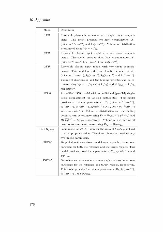
10 Appendix

Model Description

1T2k Reversible plasma input model with single tissue compart-ment. This model provides two kinetic parameters: K1

(ml ∗ cm−3min−1) and k2(min−1). Volume of distributionis estimated using VT = K1/k2.

2T3k Irreversible plasma input model with two tissue compart-ments. This model provides three kinetic parameters: K1

(ml ∗ cm−3min−1), k2(min−1) and k3(min−1) .2T4k Reversible plasma input model with two tissue compart-

ments. This model provides four kinetic parameters: K1

(ml ∗ cm−3min−1), k2(min−1), k3(min−1) and k4(min−1).Volume of distribution and the binding potential can be es-timate using VT = K1/k2 ∗ (1 + k3/k4) and BPND = k3/k4,respectively.

2T1M A modified 2T4k model with an additional (parallel) single-tissue compartment for labelled metabolites. This modelprovides six kinetic parameters: K1 (ml ∗ cm−3min−1),k2(min−1), k3(min−1), k4(min−1), K1m (ml ∗ cm−3min−1)and k2m (min−1). Volume of distribution and the bindingpotential can be estimate using VT = K1/k2 ∗ (1 + k3/k4) andBP 2T1M

ND = k3/k4, respectively. Volume of distribution ofmetabolites can be estimates using VTm = K1m/k2m.

2T1Mfvtm Same model as 2T1M , however the ratio of K1m/k2m is fixedto an appropriate value. Therefore this model provides onlyfive kinetic parameters.

SRTM Simplified reference tissue model uses a single tissue com-partment for both the reference and the target regions. Thismodel provides three kinetic parameters: R1, k2(min−1), andBPND.

FRTM Full reference tissue model assumes single and two tissue com-partments for the reference and target regions, respectively.This model provides four kinetic parameters: R1, k2(min−1),k3(min−1) , and BPND.

176

10.2 Inplementation of simulated annealing

10.2 Inplementation of simulated annealing1. Initialising

a) User given starting parameters (start parameter, Xstart; initial max-imum step size, IMS; final maximum step size, FMS; maximumnumber of function evaluations, fevalfsMAX; cost function,F (x))

b) Control parameters (step size (SS); reduced temperature ß, ß is thereduced temperature, ß = 1

kT , T is the control parameter ‘temper-ature’ and k is the Boltzmann constant. For more information see[34]. Start values are set as follows:i. SS = IMS

ii. ß = 1c) Minimize F {x} with starting parameter Xstart, using the non-linear

conjugate gradient method (CG, [19], pp 343-52) and store the resultin Xmin,currenti. Xmin,current = CG {F (Xstart)}

2. Calculate the next parameter (Xnext) by adding a random generated value(uniformly distributed within ±SS) to each parameter of Xmin,current:

a) Xnext = Xmin,current+SS ▪ (2 ▪ random− 1), random is a routine forgenerating uniformly distributed random numbers between 0 and 1

3. Minimize F (x) with starting parameter Xnext and store the result inXmin,next:

a) Xmin,next = CG {F (Xnext)}

4. Reduce step size, SS, linearly with the total number of function evaluationsalready used (fevalfs):

a) SS =(FMS−IMSfevalfsMAX

)▪ fevalfs+ IMS

5. Check if Metropolis Monte Carlo criterion accepts the next configuration(step) or keeps the current configuration (For more information see [34]):

a) If e−(F (Xmin,next)−F (Xmin,current))▪ß > random, then accept next con-figuration (Xmin,current = Xnext)i. If F (Xmin,current) has a lower value then best known lowest cost

function value, then remember this as the new best known lowestcost function value

177

10 Appendix

b) Or else reject next configuration (Xmin,current stays the same)

6. After e.g. 10 iterations

a) Calculate the acceptance chance of last 10 iterations, i.e. percent-age of accepted parameters during iterations and adjust ß to keepacceptance chance constant at 50%:i. ß If acceptance chance > 60 % then increase ßii. ß If acceptance chance < 40 % then decrease ß

b) Put current position back to the lowest found local minimum, so thealgorithm can focus its search around the best local minimum foundso far

7. If maximum function evaluations are reached then stop, otherwise back to2

10.3 Overview of parametric algorithmsThe parametric methods evaluated in the present study are all based ona reference tissue approach, thereby avoiding the need for arterial cannu-lation. The reference region consists of a single tissue compartment forthe (free) tracer, with K

′1 and k

′2 giving influx (ml ∗ cm−3min−1) and

efflux (min−1) rate constants, respectively. These rate constants describethe exchange between plasma and reference region. In general, the targetregion consists of two tissue compartments, for free and bound tracer, re-spectively. K1 (ml ∗ cm−3min−1), k2(min−1), k3(min−1) and k4(min−1)are rate constants describing exchange between the various compartmentsfor the target region. In case of methods based on the simplified referencetissue model (SRTM , [9]) the target consists of only one compartmentcontaining both free and bound tracer. For SRTM , K1 (ml∗cm−3min−1)and k2a (min−1) are rate constants, describing exchange between plasmaand target tissue. Here k2a equals k2

1+k3/k4from the two-tissue compart-

ment model mentioned above.The reference tissue model is based on a number of assumptions. First,

the contribution by fractional blood volume in tissue (Vb) is assumed to benegligible, which may be true after a time point (= t∗) measured beyondthe initial peak. In the present study the optimal t∗ was estimated foreach parametric method using several test runs and clinical data. This

178

10.3 Overview of parametric algorithms

was required, as the same t∗ is not necessarily optimal for all methods. Inparticular, a difference between reference Logan and the various MRTMmethods was expected, as the first requires a fit to the (later) linear partof the plot only, whilst the latter are multi-linear approaches that allowfor the inclusion of more data points. Next, influx and efflux ratios forreference and target tissues are assumed to be the same, i.e. K′1/k′2 = K1/k2.Finally, it is assumed that Vb▪CP (t)

CND(t) ≈ 0 in reference Logan based methods.Here, CP (t) is the concentration of the radioligand in plasma, and CND (t)is the concentration of the radioligand in the non-displaceable tissue, i.e.the reference tissue.

10.3.1 Reference Logan

The reference Logan method [16] is based on solving the compartmentaldifferential equations by integration and linearization, thereby reducingcomputation time and avoiding convergence problems as seen for non-linear methods. The equation for the reference Logan method is givenby:

Y1 = r1X1 + term1 (10.1)

with Y1 =´ t

0 CT (t)dtCT (t) , X1 =

´ t0 CND(t)dtCT (t) , r1 = a

a′ , term1 = −ab′

a′CND(t)CT (t) + b,

b = − 1k2, b′ = − 1

k′2, a′ = K

′1

k′2, a = K1/k2 + K1k3

k2k4and CT (t) is the concen-

tration of radioligand in tissue. term1 is constant, because in this modelCT (t)CND(t) is assumed to be constant, which may be true during equilibriumfor certain tracers. For both [18F ]FDDNP and [11C]PIB linear regressionwas performed only on data beyond t∗ = 50 minutes. The distributionvolume ratio (DV R = r1) and the binding potential (BPND = r1− 1) arethen obtained from the resulting regression parameters.

10.3.2 MRTMo

The original Multi-linear Reference Tissue Method (MRTMo, [14]) isbased on the reference Logan method. However, in MRTMo, CT (t)

CND(t) isnot assumed to be constant, and thus multi-linear regression is needed foranalysis:

Y1 = r1X1 − r2X2 + b (10.2)

179

10 Appendix

with X2 = CND(t)CT (t) and r2 = ab′

a′ . For both [18F ]FDDNP and [11C]PIB,linear regression was performed only using data beyond t∗ = 5 minutes.R1 (= r2

b ), DV R (= r1) and BPND (= r1 − 1) are then estimated fromthe fit parameters.

10.3.3 MRTM

Rearrangement of equation 10.2 leads to MRTM [14], which is given bythe following equation:

Y2 = γ1Z1 + γ2Z2 + γ3Z3 (10.3)

with Y2 = CT (t), Z1 =´ t

0 CND (t) dt, Z2 =´ t

0 CT (t) dt, Z3 = CND (t),γ1 = − a

a′b , γ2 = 1b and γ2 = ab′

a′b . For both [18F ]FDDNP and [11C]PIB, lin-ear regression was performed only using data beyond t∗ = 5 minutes. Aftermulti-linear regression BPND is estimated using BPND = −

(γ1γ2

+ 1), k′2

is estimated using γ1γ3.

10.3.4 MRTM2

Rearrangement of MRTM leads to MRTM2 [14]:

Y2 = γ1Z4 + γ2Z2 (10.4)

with Z4 =´ t

0 CND (t) dt+ b′CND (t) dt, b′ is fixed to the median b′ (= − 1k′2

) from all pixels with BPND > 0 taken from a first run using MRTM .For both [18F ]FDDNP and [11C]PIB, linear regression was performed onlyusing data beyond t∗ = 5 minutes. After multi-linear regression BPND isestimated using BPND = −

(γ1γ2

+ 1)and in case of single tissue R1 and

k2 can be found using R1 = γ1k′2and k2 = −γ2.

10.3.5 MRTM3

MRTM3 equals MRTMo with fixed k′2 to the median k

′2 for all pixels

with BPND >0 from an initial run of MRTMo. For both [18F ]FDDNPand [11C]PIB, linear regression was performed only using data beyond t∗= 5 minutes.

180

10.3 Overview of parametric algorithms

10.3.6 MRTM4MRTM4 equals MRTMo with fixed k

′2 to the median k

′2 for all pixels

with BPND >0 from an initial run of MRTM . For both [18F ]FDDNPand [11C]PIB, linear regression was performed only using data beyond t∗= 5 minutes.

10.3.7 RPM1Reference parametric mapping (RPM1, [10]) is an implementation ofSRTM using basis functions [10] in order to improve speed and avoidconvergence problems. In this method, 40 basis functions were used. Forboth [18F ]FDDNP and [11C]PIB, θmin3 = kmin2

1+BPmaxNDand θmax3 = kmax2 were

set to 0.01 and 0.3 min−1, respectively.[10]

10.3.8 RPM2RPM2 is preformed using RPM1 in two consecutive runs, as describedby Wu and Carson [112] for SRTM , in order to improve signal to noiseratio. In a first run of RPM1 the median k′2 is estimated for all pixels withBPND >0. This is then fixed during a second run. In this method, again40 basis functions were used. For both [18F ]FDDNP and [11C]PIB, θmin3 =

kmin21+BPmaxND

and θmax3 = kmax2 were set to 0.01 and 0.3 min−1, respectively.

181

Bibliography[1] Ter Pogossian, M.M., Phelps, M.E., Hoffman, E.J., and Mullani, N.A., “A positron-

emission transaxial tomograph for nuclear imaging (PETT),” Radiology, volume 114,no. 1, pp. 89–98, January 1975

[2] Anderson, C.D., “The positive electron,” Physical Review, volume 43, no. 6, pp. 491–494,March 1933

[3] Dirac, P.A.M., “The Quantum Theory of the Electron. Part II,” The Royal Society,volume 118, no. 779, pp. 351–361, March 1928

[4] Dirac, P.A.M., “The Quantum Theory of the Electron,” The Royal Society, volume 117,no. 778, pp. 610–624, February 1928

[5] Lewis, P., Griffin, S., Marsden, P., Gee, T., Nunan, T., Malsey, M., and Dussek, J.,“Whole-Body F-18 Fluorodeoxyglucose Positron Emission Tomography in PreoperativeEvaluation of Lung-Cancer,” Lancet, volume 344, no. 8932, pp. 1265–1266, November1994

[6] Lammertsma, A.A., “Radioligand studies: imaging and quantitative analysis,” Eur Neu-ropsychopharmacol, volume 12, no. 6, pp. 513–516, December 2002

[7] Gunn, R.N., Gunn, S.R., and Cunningham, V.J., “Positron emission tomography com-partmental models,” J Cereb Blood Flow Metab, volume 21, no. 6, pp. 635–652, June2001

[8] Hume, S.P., Myers, R., Bloomfield, P.M., Opackajuffry, J., Cremer, J.E., Ahier, R.G.,Luthra, S.K., Brooks, D.J., and Lammertsma, A.A., “Quantitation of Carbon-11-LabeledRaclopride in Rat Striatum Using Positron Emission Tomography,” Synapse, volume 12,no. 1, pp. 47–54, September 1992

[9] Lammertsma, A.A. and Hume, S.P., “Simplified reference tissue model for PET receptorstudies,” Neuroimage, volume 4, no. 3 Pt 1, pp. 153–158, December 1996

[10] Gunn, R.N., Lammertsma, A.A., Hume, S.P., and Cunningham, V.J., “Parametric imag-ing of ligand-receptor binding in PET using a simplified reference region model,” Neu-roimage, volume 6, no. 4, pp. 279–287, November 1997

[11] Blomqvist, G., Pauli, S., Farde, L., Eriksson, L., Persson, A., and Halldin, C., “Mapsof Receptor-Binding Parameters in the Human Brain - A Kinetic-Analysis of Pet Mea-surements,” Eur J Nucl Med, volume 16, no. 4-6, pp. 257–265, ISSN 0340-6997, April1990

[12] Patlak, C.S., Blasberg, R.G., and Fenstermacher, J.D., “Graphical Evaluation of Blood-To-Brain Transfer Constants from Multiple-Time Uptake Data,” J Cereb Blood FlowMetab, volume 3, no. 1, pp. 1–7, ISSN 0271-678X, 1983

183

Bibliography

[13] Ichise, M., Toyama, H., Innis, R.B., and Carson, R.E., “Strategies to improve neurore-ceptor parameter estimation by linear regression analysis,” J Cereb Blood Flow Metab,volume 22, no. 10, pp. 1271–1281, October 2002

[14] Ichise, M., Liow, J.S., Lu, J.Q., Takano, T., Model, K., Toyama, H., Suhara, T., Suzuki,T., Innis, R.B., and Carson, T.E., “Linearized reference tissue parametric Imaging meth-ods: Application to [C-11]DASB positron emission tomography studies of the serotonintransporter in human brain,” J Cereb Blood Flow Metab, volume 23, no. 9, pp. 1096–1112,September 2003

[15] Logan, J., Fowler, J.S., Volkow, N.D., Wolf, A.P., Dewey, S.L., Schlyer, D.J., Macgre-gor, R.R., Hitzemann, R., Bendriem, B., Gatley, S.J., and Christman, D.R., “GraphicalAnalysis of Reversible Radioligand Binding from Time Activity Measurements Appliedto [N-C-11-Methyl]-(-)-Cocaine Pet Studies in Human-Subjects,” J Cereb Blood FlowMetab, volume 10, no. 5, pp. 740–747, September 1990

[16] Logan, J., Fowler, J.S., Volkow, N.D., Wang, G.J., Ding, Y.S., and Alexoff, D.L., “Dis-tribution volume ratios without blood sampling from graphical analysis of PET data,” JCereb Blood Flow Metab, volume 16, no. 5, pp. 834–840, September 1996

[17] Luurtsema, G., Schuit, R.C, Takkenkamp, K., Lubberink, M., Hendrikse, N.H., Wind-horst, A.D., Molthoff, C.F.M, Tolboom, N., van Berckel, B.N.M., and Lammertsma, A.A.,“Peripheral metabolism of [18F]FDDNP and cerebral uptake of its labelled metabolites,”Nucl Med Biol, volume in press, pp. –, 2008

[18] Lubberink, M., van Berckel, B.N.M., Luurtsema, G., Takkenkamp, K., Tolboom, N.,Yaqub, M., and Lammertsma, A.A., “Multi-input spectral analysis for assessing cerebraluptake of labelled metabolites: validation and application to [11C]PIB and [18F]FDDNPstudies,” , 2007

[19] Press, W.H., Flannery, B.P., Teukolsky, S.A., and Vetterling, W.T., Numerical Recipesin C, Cambridge University Press, 1990

[20] Marquardt, D.W., “An Algorithm for Least-Squares Estimation of Nonlinear Parame-ters,” J Soc Ind Appl Math, volume 11, no. 2, pp. 431–441, 1963

[21] Coleman, T.F. and Li, Y.Y., “An interior trust region approach for nonlinear minimiza-tion subject to bounds,” Siam Journal on Optimization, volume 6, no. 2, pp. 418–445,May 1996

[22] Wong, K.P., Meikle, S.R., Feng, D., and Fulham, M.J., “Estimation of input functionand kinetic parameters using simulated annealing: Application in a flow model,” IEEET Nucl Sci, volume 49, no. 3, pp. 707–713, June 2002

[23] Carson, R.E., “Precision and Accuracy Considerations of Physiological Quantitation inPet,” J Cereb Blood Flow Metab, volume 11, no. 2, pp. A45–A50, March 1991

[24] Buvat, I., “A non-parametric bootstrap approach for analysing the statistical propertiesof SPECT and PET images,” Phys Med Biol, volume 47, no. 10, pp. 1761–1775, May2002

[25] Dahlbom, M., “Estimation of image noise in PET using the bootstrap method,” IEEE TNucl Sci, volume 49, no. 5, pp. 2062–2066, October 2002

184

Bibliography

[26] Alpert, N.M., Chesler, D.A., Correia, J.A., Ackerman, R.H., Chang, J.Y., Finklestein, S.,Davis, S.M., Brownell, G.L., and Taveras, J.M., “Estimation of the local Statistical Noisein Emission Computed Tomography,” IEEE T Med Imaging, volume 1, pp. 142–146, 1982

[27] Huesman, R.H., “A New Fast Algorithm for the Evaluation of Regions of Interest andStatistical Uncertainty in Computed-Tomography,” Phys Med Biol, volume 29, no. 5,pp. 543–552, 1984

[28] Mesina, C.T., Boellaard, R., Jongbloed, G., van der Vaart, A.W., and Lammertsma,A.A., “Experimental evaluation of iterative reconstruction versus filtered back projectionfor 3D [O-15]water PET activation studies using statistical parametric mapping analysis,”Neuroimage, volume 19, no. 3, pp. 1170–1179, July 2003

[29] Fessler, J.A., “Mean and variance of implicitly defined biased estimators (such as pe-nalized maximum likelihood): Applications to tomography,” IEEE T Image Process,volume 5, no. 3, pp. 493–506, March 1996

[30] Qi, J.Y. and Leahy, R.M., “A theoretical study of the contrast recovery and variance ofMAP reconstructions from PET data,” IEEE T Med Imaging, volume 18, no. 4, pp. 293–305, April 1999

[31] Strother, S.C., Casey, M.E., and Hoffman, E.J., “Measuring Pet Scanner Sensitivity -Relating Countrates to Image Signal-To-Noise Ratios Using Noise Equivalent Counts,”IEEE T Nucl Sci, volume 37, no. 2, pp. 783–788, April 1990

[32] Nelder, J.A. and Mead, R., “A Simplex-Method for Function Minimization,” Comput J,volume 7, no. 4, pp. 308–313, 1965

[33] Kirkpatrick, S., Gelatt, C.D., and Vecchi, M.P., “Optimization by Simulated Annealing,”Science, volume 220, no. 4598, pp. 671–680, 1983

[34] Thijssen, J.M., Computational Physics, Cambridge University Press, 1999

[35] Yaqub, M., Boellaard, R., Kropholler, M.A., Lubberink, M., and Lammertsma, A.A.,“Simulated annealing in pharmacokinetic modelling of PET neuroreceptor studies: accu-racy and precision compared with other optimisation algorithms,” , 2004

[36] Wales, D.J. and Doye, J.P.K., “Global optimization by basin-hopping and the lowestenergy structures of Lennard-Jones clusters containing up to 110 atoms,” J Phys ChemA, volume 101, no. 28, pp. 5111–5116, July 1997

[37] Boellaard, R., van Lingen, A., van Balen, S.C.M., Hoving, B.G., and Lammertsma, A.A.,“Characteristics of a new fully programmable blood sampling device for monitoring bloodradioactivity during PET,” Eur J Nucl Med, volume 28, no. 1, pp. 81–89, January 2001

[38] Lubberink, M., Boellaard, R., Greuter, H.N.J.M., and Lammertsma, A.A., “Effect of un-certainty in plasma metabolite levels on kinetic analysis of [11C] flumazenil and [11C](R)-PK11195 PET studies,” , 2004

[39] De Pierro, A.R. and Yamagishi, M.E.B., “Fast EM-like methods for maximum "a pos-teriori" estimates in emission tomography,” IEEE T Med Imaging, volume 20, no. 4,pp. 280–288, April 2001

185

Bibliography

[40] Yavuz, M. and Fessler, J.A., “New statistical models for randoms-precorrected PETscans,” Inform Proc Med Imaging, volume 1230, pp. 190–203, 1997

[41] Anderson, J.M., Mair, B.A., Rao, M., and Wu, C.H., “Weighted Least-Squares Recon-struction Methods for Positron Emission Tomography,” IEEE T Med Imaging, volume 16,pp. 159–165, 1997

[42] Boellaard, R., Lubberink, M., De Jong, H.W.A.M., Kropholler, M.A., and Lammertsma,A., “Application of various iterative reconstruction methods for quantitative 3D dynamicbrain PET studies,” , 2004

[43] Donoho, D.L., “De-Noising by Soft-Thresholding,” IEEE Transactions on InformationTheory, volume 41, no. 3, pp. 613–627, May 1995

[44] Lin, J.W., Laine, A.F., Akinboboye, O., and Bergmann, S.R., “Use of wavelet transformsin analysis of time-activity data from cardiac PET,” J Nucl Med, volume 42, no. 2,pp. 194–200, February 2001

[45] Turkheimer, F.E., Brett, M., Visvikis, D., and Cunningham, V.J., “Multiresolution anal-ysis of emission tomography images in the wavelet domain,” J Cereb Blood Flow Metab,volume 19, no. 11, pp. 1189–1208, November 1999

[46] Innis, R.B., Cunningham, V.J., Delforge, J., Fujita, M., Giedde, A., Gunn, R.N., Holden,J., Houle, S., Huang, S.C., Ichise, M., Lida, H., Ito, H., Kimura, Y., Koeppe, R.A.,Knudsen, G.M., Knuuti, J., Lammertsma, A.A., Laruelle, M., Logan, J., Maguire, R.P.,Mintun, M.A., Morris, E.D., Parsey, R., Price, J.C., Slifstein, M., Sossi, V., Suhara,T., Votaw, J.R., Wong, D.F., and Carson, R.E., “Consensus nomenclature for in vivoimaging of reversibly binding radioligands,” J Cereb Blood Flow Metab, volume 27, no. 9,pp. 1533–1539, September 2007

[47] De Jong, H.W.A.M., Boellaard, R., Lenox, M., Michel, C., and Lammertsma, A.A.,“Correction for emission contamination in transmission scans for the High ResolutionResearch Tomograph,” IEEE T Nucl Sci, volume 51, no. 3, pp. 673–676, June 2004

[48] Wienhard, K., Schmand, M., Casey, M.E., Baker, K., Bao, J., Eriksson, L., Jones, W.F.,Knoess, C., Lenox, M., Lercher, M., Luk, P., Michel, C., Reed, J.H., Richerzhagen, N.,Treffert, J., Vollmar, S., Young, J.W., Heiss, W.D., and Nutt, R., “The ECAT HRRT:Performance and first clinical application of the new high resolution research tomograph,”IEEE T Nucl Sci, volume 49, no. 1, pp. 104–110, February 2002

[49] Alpert, N.M., Reilhac, A., Chio, T.C., and Selesnick, I., “Optimization of dynamicmeasurement of receptor kinetics by wavelet denoising,” Neuroimage, volume 30, no. 2,pp. 444–451, April 2006

[50] Millet, P., Ibanez, V., Delforge, J., Pappata, S., and Guimon, J., “Wavelet analysis ofdynamic PET data: Application to the parametric imaging of benzodiazepine receptorconcentration,” Neuroimage, volume 11, no. 5, pp. 458–472, May 2000

[51] Turkheimer, F.E., Banati, R.B., Visvikis, D., Aston, J.A.D., Gunn, R.N., and Cunning-ham, V.J., “Modeling dynamic PET-SPECT studies in the wavelet domain,” J CerebBlood Flow Metab, volume 20, no. 5, pp. 879–893, May 2000

186

Bibliography

[52] Schuitemaker, A., van Berckel, B.N.M., Kropholler, M.A., Veltman, D.J., Scheltens, P.,Jonker, C., Lammertsma, A.A., and Boellaard, R., “SPM analysis of parametric (R)-[C-11]PK11195 binding images: Plasma input versus reference tissue parametric methods,”Neuroimage, volume 35, no. 4, pp. 1473–1479, May 2007

[53] Fernandez, G., Periaswamy, S., and Sweldens, W., “LIFTPACK: A Software Packagefor Wavelet Transformationa and Lifting Wavelet,” Appl Sign Image Proc, volume IV,pp. 396–408, 1996

[54] Sweldens, W., “The lifting scheme: A construction of second generation wavelets,” SiamJournal on Mathematical Analysis, volume 29, no. 2, pp. 511–546, March 1998

[55] Slifstein, M. and Laruelle, M., “Effects of statistical noise on graphic analysis of PETneuroreceptor studies,” J Nucl Med, volume 41, no. 12, pp. 2083–2088, December 2000

[56] Maes, F., Collignon, A., Vandermeulen, D., Marchal, G., and Suetens, P., “Multimodal-ity image registration by maximization of mutual information,” IEEE T Med Imaging,volume 16, no. 2, pp. 187–198, April 1997

[57] West, J., Fitzpatrick, J.M., Wang, M.Y., Dawant, B.M., Maurer, C.R., Kessler, R.M.,Maciunas, R.J., Barillot, C., Lemoine, D., Collignon, A., Maes, F., Suetens, P., Van-dermeulen, D., vandenElsen, P.A., Napel, S., Sumanaweera, T.S., Harkness, B., Hemler,P.F., Hill, D.L.G., Hawkes, D.J., Studholme, C., Maintz, J.B.A., Viergever, M.A., Ma-landain, G., Pennec, X., Noz, M.E., Maguire, G.Q., Pollack, M., Pelizzari, C.A., Robb,R.A., Hanson, D., and Woods, R.P., “Comparison and evaluation of retrospective in-termodality brain image registration techniques,” J Comput Assist Tomogr, volume 21,no. 4, pp. 554–566, July 1997

[58] Zhang, Y.Y., Brady, M., and Smith, S., “Segmentation of brain MR images through ahidden Markov random field model and the expectation-maximization algorithm,” IEEET Med Imaging, volume 20, no. 1, pp. 45–57, January 2001

[59] Yaqub, M., Boellaard, R., Kropholler, M.A., and Lammertsma, A.A., “Optimizationalgorithms and weighting factors for analysis of dynamic PET studies,” Phys Med Biol,volume 51, no. 17, pp. 4217–4232, September 2006

[60] Graps, A., “An Introduction to Wavelets,” IEEE Comput Sci Eng, volume 2, no. 2,pp. 50–61, 1995

[61] Strang, G., “Wavelets and Dilation Equations - A Brief Introduction,” Siam Review,volume 31, no. 4, pp. 614–627, December 1989

[62] Daubechies, I., “Orthonormal Bases of Compactly Supported Wavelets,” Comm Pur ApplMath, volume 41, no. 7, pp. 909–996, October 1988

[63] Cohen, A., Daubechies, I., and Feauveau, J.C., “Biorthogonal Bases of Compactly Sup-ported Wavelets,” Comm Pur Appl Math, volume 45, no. 5, pp. 485–560, June 1992

[64] Donoho, D.L. and Johnstone, I.M., “Adapting to unknown smoothness via wavelet shrink-age,” J Am Stat Assoc, volume 90, no. 432, pp. 1200–1224, December 1995

[65] Stein, C.M., “Estimation of the Mean of A Multivariate Normal-Distribution,” Ann Stat,volume 9, no. 6, pp. 1135–1151, 1981

187

Bibliography

[66] Tissingh, G., Bergmans, P., Booij, J., Winogrodzka, A., van Royen, E.A., Stoof, J.C.,and Wolters, E.C., “Drug-naive patients with Parkinson’s disease in Hoehn and Yahrstages I and II show a bilateral decrease in striatal dopamine transporters as revealed by[I-123]beta-CIT SPECT,” J Neurology, volume 245, no. 1, pp. 14–20, January 1998

[67] Ichise, M., Kim, Y.J., Ballinger, J.R., Vines, D., Erami, S.S., Tanaka, F., and Lang, A.E.,“SPECT imaging of pre- and postsynaptic dopaminergic alterations in L-dopa-untreatedPD,” Neurology, volume 52, no. 6, pp. 1206–1214, April 1999

[68] Kim, S.E., Lee, W.Y., Choe, Y.S., and Kim, J.H., “SPECT measurement of iodine-123-beta-CIT binding to dopamine and serotonin transporters in Parkinson’s disease:Correlation with symptom severity,” Neurological Research, volume 21, no. 3, pp. 255–261, April 1999

[69] Benamer, H.T.S., Patterson, J., Wyper, D.J., Hadley, D.M., Macphee, G.J.A., and Gros-set, D.G., “Correlation of Parkinson’s disease severity and duration with I-123-FP-CITSPECT striatal uptake,” Movement Disorders, volume 15, no. 4, pp. 692–698, July 2000

[70] Ma, Y., Dhawan, V., Mentis, M., Chaly, T., Spetsieris, P.G., and Eidelberg, D., “Para-metric mapping of [F-18]FPCIT binding in early stage Parkinson’s disease: a PET study,”Synapse, volume 45, no. 2, pp. 125–133, August 2002

[71] Hesse, S., Mulller, U., Lincke, T., Barthel, H., Villmann, T., Angermeyer, M.C., Sabri, O.,and Stengler-Wenzke, K., “Serotonin and dopamine transporter imaging in patients withobsessive-compulsive disorder,” Psychiatry Research Neuroimaging, volume 140, no. 1,pp. 63–72, October 2005

[72] Volkow, N.D., Wang, G.J., Fowler, J.S., and Ding, Y.S., “Imaging the effect ofmethylphenidate on brain dopamine: New model on its therapeutic actions for attention-deficit/hyperactivity disorder,” Biol Psychiat, volume 57, no. 11, pp. 1410–1415, June2005

[73] Hsiao, M.C., Lin, K.J., Liu, C.Y., Tzen, K.Y., and Yen, T.C., “Dopamine trans-porter change in drug-naive schizophrenia: an imaging study with Tc-99m-TRODAT-1,”Schizophrenia Research, volume 65, no. 1, pp. 39–46, December 2003

[74] Coenen, H.H., Dutschka, K., Muller, S.P., Geworski, L., Farahati, J., and Reiners, C.,“N.C.A. Radiosynthesis of [I-123,I-124]Beta-Cit, Plasma Analysis and PharmacokineticStudies with Spect and Pet,” Nucl Med Biol, volume 22, no. 8, pp. 977–984, November1995

[75] Neumeyer, J.L., Wang, S.Y., Milius, R.A., Baldwin, R.M., ZeaPonce, Y., Hoffer, P.B.,Sybirska, E., Altikriti, M., Charney, D.S., Malison, R.T., Laruelle, M., and Innis, R.B.,“[I-123] 2-Beta-Carbomethoxy-3-Beta-(4-Iodophenyl)Tropane - High-Affinity Spect Ra-diotracer of Monoamine Reuptake Sites in Brain,” J Med Chem, volume 34, no. 10,pp. 3144–3146, October 1991

[76] Laruelle, M., Wallace, E., Seibyl, J.P., Baldwin, R.M., ZeaPonce, Y., Zoghbi, S.S.,Neumeyer, J.L., Charney, D.S., Hoffer, P.B., and Innis, R.B., “Graphical, Kinetic, andEquilibrium Analyses of In-Vivo [I-123] Beta-Cit Binding to Dopamine Transporters inHealthy-Human Subjects,” J Cereb Blood Flow Metab, volume 14, no. 6, pp. 982–994,November 1994

188

Bibliography

[77] Marshall, V. and Grosset, D.G., “Role of dopamine transporter imaging in the diagnosisof atypical tremor disorders,” Movement Disorders, volume 18, pp. S22–S27, 2003

[78] Halldin, C., Farde, L., Lundkvist, C., Ginovart, N., Nakashima, Y., Karlsson, P., andSwahn, C.G., “[C-11] beta-CIT-FE, a radioligand for quantitation of the dopamine trans-porter in the living brain using positron emission tomography,” Synapse, volume 22, no. 4,pp. 386–390, April 1996

[79] AbiDargham, A., Gandelman, M.S., DeErausquin, G.A., ZeaPonce, Y., Zoghbi, S.S.,Baldwin, R.M., Laruelle, M., Charney, D.S., Hoffer, P.B., Neumeyer, J.L., and In-nis, R.B., “SPECT imaging of dopamine transporters in human brain with iodine-123-fluoroalkyl analogs of beta-CIT,” J Nucl Med, volume 37, no. 7, pp. 1129–1133, July1996

[80] Neumeyer, J.L., Tamagnan, G., Wang, S.Y., Gao, Y.G., Milius, R.A., Kula, N.S.,and Baldessarini, R.J., “N-substituted analogs of 2 beta-carbomethoxy-3 beta-(4’-iodophenyl)tropane (beta-CIT) with selective affinity to dopamine or serotonin trans-porters in rat forebrain,” J Med Chem, volume 39, no. 2, pp. 543–548, January 1996

[81] Lundkvist, C., Halldin, C., Swahn, C.G., Hall, H., Karlsson, P., Nakashima, Y., Wang,S.Y., Milius, R.A., Neumeyer, J.L., and Farde, L., “[O-Methyl-C-11]Beta-Cit-Fp, A Po-tential Radioligand for Quantitation of the Dopamine Transporter - Preparation, Autora-diography, Metabolite Studies, and Positron Emission Tomography Examinations,” NuclMed Biol, volume 22, no. 7, pp. 905–913, October 1995

[82] Lundkvist, C., Halldin, C., Ginovart, N., Swahn, C.G., and Farde, L., “[F-18]beta-CIT-FP is superior to [C-11]beta-CIT-FP for quantitation of the dopamine transporter,” NuclMed Biol, volume 24, no. 7, pp. 621–627, October 1997

[83] Kazumata, K., Dhawan, V., Chaly, T., Antonini, A., Margouleff, C., Belakhlef, A.,Neumeyer, J., and Eidelberg, D., “Dopamine transporter imaging with fluorine-18-FPCITand PET,” J Nucl Med, volume 39, no. 9, pp. 1521–1530, September 1998

[84] Lammertsma, A.A., Bench, C.J., Hume, S.P., Osman, S., Gunn, K., Brooks, D.J., andFrackowiak, R.S.J., “Comparison of methods for analysis of clinical [C-11]raclopride stu-dies,” J Cereb Blood Flow Metab, volume 16, no. 1, pp. 42–52, January 1996

[85] Adam, L.E., Zaers, J., Ostertag, H., Trojan, H., Bellemann, M.E., and Brix, G., “Per-formance evaluation of the whole-body PET scanner ECAT EXACT HR+ following theIEC standard,” IEEE T Nucl Sci, volume 44, no. 3, pp. 1172–1179, June 1997

[86] Brix, G., Zaers, J., Adam, L.E., Bellemann, M.E., Ostertag, H., Trojan, H., Haberkorn,U., Doll, J., Oberdorfer, F., and Lorenz, W.J., “Performance evaluation of a whole-bodyPET scanner using the NEMA protocol,” J Nucl Med, volume 38, no. 10, pp. 1614–1623,October 1997

[87] Klok, R.P., Klein, P.J., Herscheid, J.D.M., and Windhorst, A.D., “High yielding andGMP compliant synthesis of the dopamine transporter ligand FP-beta-CIT,” J LabelledCompd Rad, volume 49, pp. 77–89, 2006

[88] Defrise, M., Kinahan, P.E., Townsend, D.W., Michel, C., Sibomana, M., and Newport,D.F., “Exact and approximate rebinning algorithms for 3-D PET data,” IEEE T MedImaging, volume 16, no. 2, pp. 145–158, April 1997

189

Bibliography

[89] Watson, C.C., “New, faster, image-based scatter correction for 3D PET,” IEEE T NuclSci, volume 47, no. 4, pp. 1587–1594, August 2000

[90] Greuter, H.N.J.M., van Ophemert, P.L.B., Luurtsema, G., Franssen, E.J.F., Boellaard,R., and Lammertsma, A.A., “Validation of a multiwell gamma-counter for measuringhigh-pressure liquid chromatography metabolite profiles,” J Nucl Med Technol, vol-ume 32, no. 1, pp. 28–32, March 2004

[91] Smith, S.M., “Fast robust automated brain extraction,” Hum Brain Map, volume 17,no. 3, pp. 143–155, November 2002

[92] Svarer, C., Madsen, K., Hasselbalch, S.G., Pinborg, L.H., Haugbol, S., Frokjaer, V.G.,Holm, S., Paulson, O.B., and Knudsen, G.M., “MR-based automatic delineation of vol-umes of interest in human brain PET images using probability maps,” Neuroimage,volume 24, no. 4, pp. 969–979, February 2005

[93] Akaike, H., “Fitting Autoregressive Models for Prediction,” Ann I Stat Math, volume 21,no. 2, pp. 243–247, 1969

[94] Barrio, J.R., Huang, S.C., Cole, G.M., Satyamurthy, N.M., Petric, A., Phelps, M.E., andSmall, G.W., “PET imaging of tangles and plaques in Alzheimer disease,” , May 1999

[95] Braak, H. and Braak, E., “Frequency of stages of Alzheimer-related lesions in differentage categories,” Neurobiol Aging, volume 18, no. 4, pp. 351–357, July 1997

[96] Shoghi Jadid, K., Small, G.W., Agdeppa, E.D., Kepe, V., Ercoli, L.M., Siddarth, P.,Read, S., Satyamurthy, N., Petric, A., Huang, S.C., and Barrio, J.R., “Localization ofneurofibrillary tangles and beta-amyloid plaques in the brains of living patients withAlzheimer disease,” Am J Geriatr Psychiatry, volume 10, no. 1, pp. 24–35, January 2002

[97] Kepe, V., Shoghi-Jadid, K., Wu, H.M., Huang, S.C., Small, G.W., Satyamurthy, N., Pet-ric, A., Phelps, M.E., and Barrio, J.R., “Global and and regional [F-18]FDDNP bindingas in vivo measure of Alzheimers disease,” J Nucl Med, volume 45 (Suppl.), pp. 126–126,2004

[98] Comparison of Simplified Methods for Quantitative Analysis of [18F]FDDNP PET Data,volume IEEE NSS-MIC; 4, 2007

[99] Kepe, V., Huang, S.C., Small, G.W., Satyamurthy, N., and Barrio, J.R., “Visualizingpathology deposits in the living brain of patients with Alzheimer’s disease,” MethodsEnzymol, volume 412, pp. 144–160, 2006

[100] Small, G.W., Kepe, V., Ercoli, L.M., Siddarth, P., Bookheimer, S.Y., Miller, K.J., Lavret-sky, H., Burggren, A.C., Cole, G.M., Vinters, H.V., Thompson, P.M., Huang, S.C.,Satyamurthy, N., Phelps, M.E., and Barrio, J.R., “PET of brain amyloid and tau in mildcognitive impairment,” N Engl J Med, volume 355, no. 25, pp. 2652–2663, December2006

[101] Petersen, R.C., Doody, R., Kurz, A., Mohs, R.C., Morris, J.C., Rabins, P.V., Ritchie, K.,Rossor, M., Thal, L., and Winblad, B., “Current concepts in mild cognitive impairment,”Arch Neurol, volume 58, no. 12, pp. 1985–1992, December 2001

190

Bibliography

[102] Mckhann, G., Drachman, D., Folstein, M., Katzman, R., Price, D., and Stadlan,E.M., “Clinical-Diagnosis of Alzheimers-Disease - Report of the Nincds-Adrda WorkGroup Under the Auspices of Department-Of-Health-And-Human-Services Task-Forceon Alzheimers-Disease,” Neurology, volume 34, no. 7, pp. 939–944, 1984

[103] Klok, R.P., Klein, P.J., van Berckel, B.N., Tolboom, N., Lammertsma, A.A.,and Windhorst, A.D., “Synthesis of 2-(1,1-dicyanopropen-2-yl)-6-(2-[18F]-fluoroethyl)-methylamino-naphthalene ([18F]FDDNP),” Appl Radiat Isot, volume 66, no. 2, pp. 203–207, February 2008

[104] Takkenkamp, K., Luurtsema, G., Greuter, H.N., Schuit, R.C, Hendrikse, N.H., Tol-boom, N., van Berckel, B.N., and Lammertsma, A., “Plasma metabolites of [11C]PIBand [18F]FDDNP,” , 2007

[105] Gunn, R.N., Sargent, P.A., Bench, C.J., Rabiner, E.A., Osman, S., Pike, V.W., Hume,S.P., Grasby, P.M., and Lammertsma, A.A., “Tracer kinetic modeling of the 5-HT1Areceptor ligand [carbonyl-11C]WAY-100635 for PET,” Neuroimage, volume 8, no. 4,pp. 426–440, November 1998

[106] Shoghi Jadid, K., Barrio, J.R., Kepe, V., and Huang, S.C., “Exploring a mathemati-cal model for the kinetics of beta-amyloid molecular imaging probes through a criticalanalysis of plaque pathology,” Mol Imaging Biol, volume 8, no. 3, pp. 151–162, May 2006

[107] Klunk, W.E., Engler, H., Nordberg, A., Wang, Y.M., Blomqvist, G., Holt, D.P.,Bergstrom, M., Savitcheva, I., Huang, G.F., Estrada, S., Ausen, B., Debnath, M.L.,Barletta, J., Price, J.C., Sandell, J., Lopresti, B.J., Wall, A., Koivisto, P., Antoni, G.,Mathis, C.A., and Langstrom, B., “Imaging brain amyloid in Alzheimer’s disease withPittsburgh Compound-B,” Ann Neurol, volume 55, no. 3, pp. 306–319, March 2004

[108] Price, J.C., Klunk, W.E., Lopresti, B.J., Lu, X.L., Hoge, J.A., Ziolko, S.K., Holt, D.P.,Meltzer, C.C., DeKosky, S.T., and Mathis, C.A., “Kinetic modeling of amyloid binding inhumans using PET imaging and Pittsburgh Compound-B,” J Cereb Blood Flow Metab,volume 25, no. 11, pp. 1528–1547, November 2005

[109] Lopresti, B.J., Klunk, W.E., Mathis, C.A., Hoge, J.A., Ziolko, S.K., Lu, X.L., Meltzer,C.C., Schimmel, K., Tsopelas, N.D., DeKosky, S.T., and Price, J.C., “Simplified quantifi-cation of Pittsburgh compound B amyloid imaging PET studies: A comparative analysis,”J Nucl Med, volume 46, no. 12, pp. 1959–1972, December 2005

[110] Ziolko, S.K., Weissfeld, L.A., Klunk, W.E., Mathis, C.A., Hoge, J.A., Lopresti, B.J.,DeKosky, S.T., and Price, J.C., “Evaluation of voxel-based methods for the statisticalanalysis of PIBPET amyloid imaging studies in Alzheimer’s disease,” Neuroimage, vol-ume 33, no. 1, pp. 94–102, October 2006

[111] Zhou, Y., Resnick, S.M., Ye, W.G., Fan, H., Holt, D.P., Klunk, W.E., Mathis, C.A.,Dannals, R., and Wong, D.F., “Using a reference tissue model with spatial constraint toquantify [C-11]Pittsburgh compound BPET for early diagnosis of Alzheimer’s disease,”Neuroimage, volume 36, no. 2, pp. 298–312, June 2007

[112] Wu, Y. and Carson, R.E., “Noise reduction in the simplified reference tissue modelfor neuroreceptor functional imaging,” J Cereb Blood Flow Metab, volume 22, no. 12,pp. 1440–1452, December 2002

191

Bibliography

[113] Yaqub, M., Tolboom, N., Boellaard, R., van Berckel, B.N.M., van Tilburg, E.W., Lu-urtsema, G., Scheltens, P., and Lammertsma, A.A., “Simplified parametric methods for[C-11]PIB studies,” Neuroimage, volume 42, no. 1, pp. 76–86, ISSN 1053-8119, August2008

[114] Yaqub, M., Boellaard, R., van Berckel, B.N.M., Tolboom, N., Luurtsema, G., Dijkstra,A.A., Lubberink, M., Windhorst, A.D., Scheltens, P., and Lammertsma, A., “Evalua-tion of tracer kinetic models for analysis of [18F]FDDNP studies,” Mol Imaging Biol,volume (ahead of print, DOI: 10.1007/s11307-009-0208-1), pp. –, 2009

[115] Joachim, C.L., Morris, J.H., and Selkoe, D.J., “Diffuse senile plaques occur commonlyin the cerebellum in Alzheimer’s disease,” Am J Pathol, volume 135, no. 2, pp. 309–319,August 1989

[116] Bland, J. M. and Altman, D. G., “Statistical methods for assessing agreement betweentwo methods of clinical measurement.” Lancet, volume 1, no. 8476, pp. 307–310, Feb 1986

192

Publicatielijst

• Yaqub, M., Boellaard, R., Kropholler, M.A., and Lammertsma,A.A., “Optimization algorithms and weighting factors for analysisof dynamic PET studies,” Phys Med Biol, volume 51, no. 17, pp.4217–4232, September 2006

• Yaqub, M., Boellaard, R., van Berckel, B.N.M., Ponsen, M.M., Lub-berink, M., Windhorst, A.D., Berendse, H.W., Lammertsma, A.A.,“Quantification of dopamine transporter binding using [18F]FP-beta-CIT and positron emission tomography,” J Cereb Blood Flow Metab,volume 27, no. 7, pp. 1397-1406, July 2007

• Yaqub, M., Tolboom, N., Boellaard, R., van Berckel, B.N.M., vanTilburg, E.W., Luurtsema, G., Scheltens, P., and Lammertsma,A.A., “Simplified parametric methods for [C-11]PIB studies,” Neu-roimage, volume 42, no. 1, pp. 76–86, ISSN 1053-8119, August2008

• Yaqub, M., Boellaard, R., Schuitemaker, A., van Berckel, B.N.M.,Lammertsma, A.A., “Impact of wavelet based denoising of [11C](R)-PK11195 time activity curves on accuracy and precision of kineticanalysis,” Med Phys, volume 35, no. 11, pp. 5069-5078, November2008

• Yaqub, M., Boellaard, R., van Berckel, B.N.M., Tolboom, N., Luurt-sema, G., Dijkstra, A.A., Lubberink, M., Windhorst, A.D., Schel-tens, P., and Lammertsma, A., “Evaluation of tracer kinetic modelsfor analysis of [18F]FDDNP studies,” Mol Imaging Biol, (ahead ofprint, 2009)

• Yaqub M, Tolboom N, van Berckel BN, Scheltens P, LammertsmaAA, Boellaard R., “Simplified parametric methods for [18F]FDDNPstudies,” Neuroimage, (accepted, 2009)

193

Publicatielijst

• Tolboom, N., Yaqub, M., Boellaard, R., Luurtsema, G., Windhorst,A.D., Scheltens, P., Lammertsma, A.A., van Berckel, B.N.M., “Test-retest variability of quantitative [(11)C]PIB studies in Alzheimer’sdisease,” Eur J Nucl Med Mol Imaging, (ahead of print, 2009)

• Tolboom, N., Yaqub, M., van der Flier, W.M., Boellaard, R., Luurt-sema, G., Windhorst, A.D., Barkhof, F., Scheltens, P., Lammertsma,A.A., van Berckel, B.N.M., “Detection of Alzheimer pathology invivo using both 11C-PIB and 18F-FDDNP PET” J Nucl Med, vol-ume 50, no. 2, 191-207, Februari 2009

• Tolboom, N., van der Flier, W.M., Yaqub, M., Boellaard, R., Ver-wey, N.A., Blankenstein, M.A., Luurtsema, G., Windhorst, A.D.,Scheltens, P., Lammertsma, A.A., Van Berckel, B.N.M., “Relation-ship of cerebrospinal fluid markers with [11C]PIB and [18F]FDDNPbinding,” J Nucl Med, (ahead of print, 2009)

• Klumpers, U.M., Veltman, D.J., Boellaard, R., Comans, E.F., Zuketto,C., Yaqub, M., Mourik, J.E., Lubberink, M., Hoogendijk, W.J.,Lammertsma, A.A.., “Comparison of plasma input and reference tis-sue models for analysing [(11)C]flumazenil studies,” J Cereb BloodFlow Metab, volume 28, no. 3,579-587, Oct 2007

194

Dankwoord

De studies in dit proefschrift zijn tot stand gekomen door een goede samen-werking tussen vele mensen uit verschillende disciplines. Een aantal vanhen wil ik in het bijzonder bedanken.

Prof. dr. A.A. Lammertsma, beste Adriaan, bedankt, het is een eer omte kunnen promoveren in de groep van een internationaal gerenommeerdfysicus die belangrijke bijdragen heeft geleverd op het gebied van PET.Door jouw kritisch maar constructief commentaar zijn alle stukken in ditproefschrift inhoudelijk consistent en ook taalkundig correct.

Dr. R. Boellaard, beste Ronald, bedankt voor jouw supervisie en ookvoor de uitvoerige discussies tijdens het onderzoek. Samen met jou heb ikmeegewerkt in verschillende projecten, met als resultaat dit proefschrift.Een goede begeleiding van jou kant was daarbij essentieel. Zonder jouwbijdragen zou dit proefschrift er niet zijn.

Dr. B.N.M. van Berckel, beste Bart bedankt, door jouw bijdrage is er eengoede samenwerking tussen fysici en neurologie onderzoekers. Ik heb alsfysicus wat geleerd van de klinische kant van onderzoek doen.

De leden van de leescommissie: Prof. dr. R.M. Heethaar, Prof. dr.P. Scheltens, Prof. dr. P. Dupont, dr. A.T.M. Willemsen, dr. H.W.Berendse, en dr. C. Svarer. Allen bedankt voor het bestuderen van mijnproefschrift. Thank you very much for studying my thesis.

Drs. N. Tolboom, beste Nelleke, bedankt voor het selecteren en scannenvan de subjecten voor de Alzheimer studies. Daarnaast ook bedankt voorde vele discussies die voor mij hebben bijgedragen tot een beter inzicht inPET modeling.

195

Dankwoord

Dr. M. Lubberink en dr. M. Huisman, beste Mark en Marc, bedankt voorde discussies en ook voor het grondig nakijken van de inleiding, samenvat-ting en discussie van dit proefschrift.

Drs. M. Ponsen. Beste Mirthe, bedankt voor het selecteren en scannenvan de subjecten bij de Parkinson studie.

Sectie J-vleugel en Meander: F. van Velden, N. Hoetjes, J.E.M. Mourik,M. Kropholler, P. Cheebsumon, en R. Kloet. Allen bedankt voor de gezel-lige momenten tijdens de promotie.

Sectie chemie: H.N.J.M. Greuter, G. Luurtsema, R.C. Schuit, K. Takkenkampen P.L.B. van Ophemert. Dank voor onder andere metingen aan bloed-samples en radioactiviteit.

Laboranten van afdeling PET. Beste laboranten, bedankt voor het scan-nen en de ondersteuning bij het uitvoeren van de studies.

Radionucliden centrum. Bedankt voor leveren van de radionucliden envoor het commentaar op studies die in dit proefschrift zijn beschreven.

R. Schmeits, A. Kroonenberg-Kalwij, J. van der Kuij, A. van Lingen enN.M. Bock, bedankt voor de ondersteuning op de afdeling.

Alle andere medewerkers van de afdeling Nucleaire Geneeskunde & PETonderzoek bedankt voor de prettige samenwerking.

Best familie en vrienden bedankt voor de hulp en steun.

Mohammed Maqsood Yaqub.

196

Curriculum Vitae

Mohammed Maqsood Yaqub werd op 13 juli 1976 in Amsterdam geboren.In 1996 behaalde hij het VWO diploma aan het Johan de Witt Collegein Den Haag. Daarna begon hij aan de studie technische natuurkundeaan de technische universiteit Delft, waar hij in 2003 slaagde voor hetmasteropleiding. Vanaf 2004 is hij werkzaam op de afdeling NucleaireGeneeskunde & PET onderzoek van het VU medisch centrum in Amster-dam. Daar deed hij zijn promotie onderzoek en is hij sinds eind 2008 inopleiding tot Klinisch Fysicus Nucleaire Geneeskunde.

197

Quantification of brain PET studies

Documents

Transcript of Quantification of brain PET studies