Normal approximation under local dependence
42
arXiv:math/0410104v1 [math.PR] 5 Oct 2004 The Annals of Probability 2004, Vol. 32, No. 3A, 1985–2028 DOI: 10.1214/009117904000000450 c Institute of Mathematical Statistics, 2004 NORMAL APPROXIMATION UNDER LOCAL DEPENDENCE By Louis H. Y. Chen 1 and Qi-Man Shao 2 National University of Singapore and University of Oregon We establish both uniform and nonuniform error bounds of the Berry–Esseen type in normal approximation under local dependence. These results are of an order close to the best possible if not best possible. They are more general or sharper than many existing ones in the literature. The proofs couple Stein’s method with the concen- tration inequality approach. 1. Introduction. Since the work of Berry and Esseen in the 1940s, much has been done in the normal approximation for independent random vari- ables. The standard tool has been the Fourier analytic method as devel- oped by Esseen (1945). However, without independence, the Fourier analytic method becomes difficult to apply and bounds on the accuracy of approx- imation correspondingly difficult to find. In such situations, a method of Stein (1972) provides a much more viable alternative to the Fourier analytic method. Corresponding to calculating a Fourier transform and applying the inversion formula, it involves deriving a direct identity and solving a dif- ferential equation. As dependence is the rule rather than the exception in applications, Stein’s method has become increasingly useful and important. A crucial step in the Fourier analytic method for normal approximation is the use of a smoothing inequality originally due to Esseen (1945). The smoothing inequality is used to overcome the difficulty resulting from the nonsmoothness of the indicator function whose expectation is the distribu- tion function. There is a correspondence of this in Stein’s method, which is called the concentration inequality. It is originally due to Stein. Its simplest Received May 2002; revised August 2003. 1 Supported in part by Grant R-146-000-013-112 at National University of Singapore. 2 Supported in part by NSF Grant DMS-01-03487, and Grants R-146-000-038-101 and R-1555-000-035-112 at National University of Singapore. AMS 2000 subject classifications. Primary 60F05; secondary 60G60. Key words and phrases. Stein’s method, normal approximation, local dependence, con- centration inequality, uniform Berry–Esseen bound, nonuniform Berry–Esseen bound, ran- dom field. This is an electronic reprint of the original article published by the Institute of Mathematical Statistics in The Annals of Probability, 2004, Vol. 32, No. 3A, 1985–2028 . This reprint differs from the original in pagination and typographic detail. 1
-
Upload
independent -
Category
Documents
-
view
0 -
download
0
Transcript of Normal approximation under local dependence

arX
iv:m
ath/
0410
104v
1 [
mat
h.PR
] 5
Oct
200
4
The Annals of Probability
2004, Vol. 32, No. 3A, 1985–2028DOI: 10.1214/009117904000000450c© Institute of Mathematical Statistics, 2004
NORMAL APPROXIMATION UNDER LOCAL DEPENDENCE
By Louis H. Y. Chen1 and Qi-Man Shao2
National University of Singapore and University of Oregon
We establish both uniform and nonuniform error bounds of theBerry–Esseen type in normal approximation under local dependence.These results are of an order close to the best possible if not bestpossible. They are more general or sharper than many existing onesin the literature. The proofs couple Stein’s method with the concen-tration inequality approach.
1. Introduction. Since the work of Berry and Esseen in the 1940s, muchhas been done in the normal approximation for independent random vari-ables. The standard tool has been the Fourier analytic method as devel-oped by Esseen (1945). However, without independence, the Fourier analyticmethod becomes difficult to apply and bounds on the accuracy of approx-imation correspondingly difficult to find. In such situations, a method ofStein (1972) provides a much more viable alternative to the Fourier analyticmethod. Corresponding to calculating a Fourier transform and applying theinversion formula, it involves deriving a direct identity and solving a dif-ferential equation. As dependence is the rule rather than the exception inapplications, Stein’s method has become increasingly useful and important.
A crucial step in the Fourier analytic method for normal approximationis the use of a smoothing inequality originally due to Esseen (1945). Thesmoothing inequality is used to overcome the difficulty resulting from thenonsmoothness of the indicator function whose expectation is the distribu-tion function. There is a correspondence of this in Stein’s method, which iscalled the concentration inequality. It is originally due to Stein. Its simplest
Received May 2002; revised August 2003.1Supported in part by Grant R-146-000-013-112 at National University of Singapore.2Supported in part by NSF Grant DMS-01-03487, and Grants R-146-000-038-101 and
R-1555-000-035-112 at National University of Singapore.AMS 2000 subject classifications. Primary 60F05; secondary 60G60.Key words and phrases. Stein’s method, normal approximation, local dependence, con-
centration inequality, uniform Berry–Esseen bound, nonuniform Berry–Esseen bound, ran-dom field.
This is an electronic reprint of the original article published by theInstitute of Mathematical Statistics in The Annals of Probability,2004, Vol. 32, No. 3A, 1985–2028. This reprint differs from the original inpagination and typographic detail.
1

2 L. H. Y. CHEN AND Q.-M. SHAO
form is used in Ho and Chen (1978). More elaborate versions are proved inChen (1986, 1998) and Chen and Shao (2001). In Chen and Shao (2001), itis developed also for obtaining nonuniform error bounds.
This paper is concerned with normal approximation under local depen-dence using Stein’s method. Local dependence roughly means that certainsubsets of the random variables are independent of those outside their re-spective “neighborhoods.” No structure on the index set is assumed. Bothuniform and nonuniform error bounds of the Berry–Esseen type are obtainedand shown to be more general or sharper than many existing results in theliterature. These include those of Shergin (1979), Prakasa Rao (1981), Baldiand Rinott (1989), Baldi, Rinott and Stein (1989), Rinott (1994) and Demboand Rinott (1996).
The approach used in the paper is that of the concentration inequality.It is based on the ideas of Chen (1986) where the concentration inequalityis derived differently from those in Chen and Shao (2001), due to the non-positivity of the “covariance function.” The uniform bounds obtained areimprovements of those in Chen (1986), and the nonuniform bounds, whichare proved by following the techniques in Chen and Shao (2001), are newin the literature. In proving the bounds, an attempt is made to achieve thebest possible order for them. For example, the nonuniform bounds obtainedare best possible as functions of the variables.
The forms of the bounds obtained are inspired by the results in Chen(1978), where necessary and sufficient conditions are proved for asymptoticnormality of locally dependent random variables (termed finitely dependentin that paper). Such bounds deal successfully with those cases where thevariance of a sum of n random variables grows at a different rate from n.An example due to Erickson (1974) is used to illustrate this point.
This paper is organized as follows. The main results and their applica-tions are given in Section 2. Two uniform and one nonuniform conditionalconcentration inequalities are proved in Section 3. The proofs of the uniformbounds are given in Section 4 and those of the nonuniform bounds in Section5.
2. Main results. Throughout this paper let J be an index set and let{Xi, i ∈ J } be a random field with zero means and finite variances. DefineW =
∑
i∈J Xi and assume that Var(W ) = 1. Let n be the cardinality of J ,let F be the distribution function of W and let Φ be the standard normaldistribution function.
For A ⊂ J , let XA denote {Xi, i ∈ A}, Ac = {j ∈ J : j /∈ A}, and let |A|denote the cardinality of A. Adopt the notation: a∧b = min(a, b) and a∨b =max(a, b).
We first introduce dependence assumptions and define notation that willbe used throughout the paper.

NORMAL APPROXIMATION UNDER LOCAL DEPENDENCE 3
(LD1) For each i ∈ J , there exists Ai ⊂ J such that Xi and XAci
areindependent.
(LD2) For each i ∈ J , there exist Ai ⊂ Bi ⊂J such that Xi is independentof XAc
iand XAi is independent of XBc
i.
(LD3) For each i ∈ J , there exist Ai ⊂ Bi ⊂ Ci ⊂ J such that Xi is inde-pendent of XAc
i, XAi is independent of XBc
iand XBi is independent
of XCci.
(LD4∗) For each i ∈ J , there exist Ai ⊂ Bi ⊂ B∗i ⊂ C∗
i ⊂ D∗i ⊂ J such
that Xi is independent of XAci, XAi is independent of XBc
i, XAi
is independent of {XAj , j ∈ B∗ci }, {XAl
, l ∈ B∗i } is independent of
{XAj , j ∈ C∗ci } and {XAl
, l ∈C∗i } is independent of {XAj , j ∈D∗c
i }.It is clear that (LD4∗) implies (LD3), (LD3) yields (LD2) and (LD1) is
the weakest assumption. Roughly speaking, (LD4∗) is a version of (LD3)for {XAi , i ∈ J }. On the other hand, in many cases (LD1) implies (LD2),(LD3) and (LD4*) with Bi,Ci,B
∗i ,C
∗i and D∗
i defined as: Bi =⋃
j∈AiAj ,
Ci =⋃
j∈BiAj , B∗
i =⋃
j∈AiBj , C∗
i =⋃
j∈B∗iBj and D∗
i =⋃
j∈C∗iBj . Other
forms of local dependence have also been used in the literature, such asdependency neighborhoods in Rinott and Rotar (1996), where convergencerates of multivariate central limit theorem were obtained. Some of theirresults may not be covered by our theorems.
For each i ∈ J , let Yi =∑
j∈AiXj . We define
Ki(t) = Xi{I(−Yi ≤ t < 0)− I(0 ≤ t ≤−Yi)}, Ki(t) = EKi(t),
K(t) =∑
i∈J
Ki(t), K(t) = EK(t) =∑
i∈J
Ki(t).(2.1)
Since Var(W ) = 1, we have∫ ∞
−∞K(t)dt = EW 2 = 1.(2.2)
2.1. Uniform Berry–Esseen bounds. The Berry–Esseen theorem [Berry(1941) and Esseen (1945); see, e.g., Petrov (1995)] states that if {Xi, i ∈ J }are independent with finite third moments, then there exists an absoluteconstant C such that
supz∈R
|F (z)−Φ(z)| ≤ C∑
i∈J
E|Xi|3.
Here and throughout the paper, C denotes an absolute constant which mayhave different values at different places. If, in addition, Xi, i ∈ J , are iden-tically distributed, then the bound is of the order n−1/2, which is known tobe the best possible.
The main objective of this section is to obtain general uniform Berry–Esseen bounds under various dependence assumptions with an aim to achievethe best possible orders. We first present a result under assumption (LD1).

4 L. H. Y. CHEN AND Q.-M. SHAO
Theorem 2.1. Under (LD1), we have
supz
|F (z)−Φ(z)| ≤ r1 + 4r2 + 8r3 + r4 + 4.5r5 + 1.5r6,(2.3)
where
r1 = E
∣
∣
∣
∣
∣
∑
i∈J
(XiYi −EXiYi)
∣
∣
∣
∣
∣
, r2 =∑
i∈J
E|XiYi|I(|Yi|> 1),
r3 =∑
i∈J
E|Xi|(Y 2i ∧ 1), r4 =
∑
i∈J
E{|WXi|(Y 2i ∧ 1)},
r5 =
∫
|t|≤1Var(K(t))dt, r6 =
(∫
|t|≤1|t|Var(K(t))dt
)1/2
.
(2.4)
Since r1, r2, r3 and r4 depend on the moments of {Xi, Yi,W}, they can beeasily estimated (see Remark 2.1). The following alternative formulas of r5
and r6 may be useful. Let {X∗i , i ∈ J } be an independent copy of {Xi, i ∈ J }
and define Y ∗i =
∑
j∈AiX∗
j . Then
Var(K(t)) =∑
i,j∈J
E{XiXj{I(−Yi ≤ t < 0)− I(0 ≤ t ≤−Yi)}
× {I(−Yj ≤ t < 0)− I(0 ≤ t≤−Yj)}
−XiX∗j {I(−Yi ≤ t < 0)− I(0 ≤ t≤−Yi)}
× {I(−Y ∗j ≤ t < 0)− I(0≤ t ≤−Y ∗
j )}},and hence
r5 =∑
i,j∈J
E{XiXjI(YiYj ≥ 0)(|Yi| ∧ |Yj| ∧ 1)
−XiX∗j I(YiY
∗j ≥ 0)(|Yi| ∧ |Y ∗
j | ∧ 1)}.Similarly, we have
r26 = 1
2
∑
i,j∈J
E{XiXjI(YiYj ≥ 0)(|Yi|2 ∧ |Yj |2 ∧ 1)
−XiX∗j I(YiY
∗j ≥ 0)(|Yi|2 ∧ |Y ∗
j |2 ∧ 1)}.In particular, under assumption (LD2),
r5 ≤∑
i,j∈J ,BiBj 6=∅
E{|XiXj |(|Yi| ∧ |Yj| ∧ 1) + |XiX∗j |(|Yi| ∧ |Y ∗
j | ∧ 1)}
and
r26 ≤ 1
2
∑
i,j∈J ,BiBj 6=∅
E{|XiXj |(|Yi|2 ∧ |Yj |2 ∧ 1) + |XiX∗j |(|Yi|2 ∧ |Y ∗
j |2 ∧ 1)}.
Thus, we have a much neater result under (LD2).

NORMAL APPROXIMATION UNDER LOCAL DEPENDENCE 5
Theorem 2.2. Let N(Bi) = {j ∈ J :BjBi 6= ∅} and 2 < p ≤ 4. Assume
that (LD2) is satisfied with |N(Bi)| ≤ κ. Then
supz
|F (z)−Φ(z)| ≤ (13 + 11κ)∑
i∈J
(E|Xi|3∧p + E|Yi|3∧p)
+ 2.5
(
κ∑
i∈J
(E|Xi|p + E|Yi|p))1/2
.(2.5)
In particular, if E|Xi|p + E|Yi|p ≤ θp for some θ > 0 and for each i ∈ J ,
then
supz
|F (z)−Φ(z)| ≤ (13 + 11κ)nθ3∧p + 2.5θp/2√κn,(2.6)
where n = |J |.
Note that in many cases κ is bounded and θ is of order of n−1/2. In thosecases κnθ3∧p + θp/2√κn = O(n−(p−2)/4), which is of the best possible orderof n−1/2 when p = 4. However, the cost is the existence of fourth moments.To reduce the assumption on moments, we need a stronger condition.
Theorem 2.3. Suppose that (LD3) is satisfied. Let N(Ci) = {j ∈ J :CiBj 6= ∅},
Wi =∑
j∈N(Ci)c
Xj , σ2i = Var(Wi) and λ = 1∨max
i∈J(1/σi).
Then
supz
|F (z)−Φ(z)| ≤ 4λ3/2(r2 + r3 + r7 + r8 + r9 + r10 + r11 + r12),(2.7)
where Zi =∑
j∈BiXj ,
r7 =∑
i∈J
E{|XiYi|I(|Xi|> 1)},
r8 =∑
i∈J
E{|Xi|I(|Xi| ≤ 1)(|Yi| ∧ 1)|Zi|},
r9 =∑
i∈J
E{|WXi|I(|Xi| ≤ 1)(|Yi| ∧ 1)(|Zi| ∧ 1)},
r10 =∑
i,j∈J ,BiBj 6=∅
E{|XiXj |(|Yi| ∧ |Yj| ∧ 1) + |XiX∗j |(|Yi| ∧ |Y ∗
j | ∧ 1)},
r11 =∑
i∈J
P (|Xi|> 1)E|Xi|(|Yi| ∧ 1),
r12 =∑
i∈J
E{(|W |+ 1)(|Zi| ∧ 1)}E|Xi|(|Yi| ∧ 1),
(2.8)
and (X∗i , Y ∗
i ) is an independent copy of (Xi, Yi).

6 L. H. Y. CHEN AND Q.-M. SHAO
In particular, we have:
Theorem 2.4. Let 2 < p≤ 3. Assume that (LD3) is satisfied with max(|N(Ci)|, |{j : i ∈Cj}|) ≤ κ. Then
supz
|F (z)−Φ(z)| ≤ 75κp−1∑
i∈J
E|Xi|p.(2.9)
Rinott (1994) and Dembo and Rinott (1996) obtained uniform bounds oforder n−1/2 when Xi is bounded with order of n−1/2 under a different localdependence assumption which appears to be weaker than (LD2). However,their approach does not seem to be extendable to random variables whichare not necessarily bounded.
Remark 2.1. Although r4 involves W , there are several ways to boundit. When there is no additional assumption besides (LD1), we can use thefollowing estimate:
E|WXi|(Y 2i ∧ 1)
≤E|WXi|(
|Ai|∑
j∈Ai
(X2j ∧ 1)
)
≤ |Ai|∑
j∈Ai
E|WXi|(X2j ∧ 1)I(|Xi| ≤ |Xj |)
+ |Ai|∑
j∈Ai
E|WXi|(X2j ∧ 1)I(|Xi|> |Xj |)
≤ |Ai|∑
j∈Ai
E|W ||Xj |(X2j ∧ 1) + |Ai|
∑
j∈Ai
E|W ||Xi|(X2i ∧ 1)
≤ |Ai|∑
j∈Ai
E|W − Yj|E|Xj |(X2j ∧ 1) + |Ai|
∑
j∈Ai
E|YjXj |(|Xj | ∧ 1)
+ |Ai|2E|W − Yi|E|Xi|(X2i ∧ 1) + |Ai|2E|YiXi|(|Xi| ∧ 1)
≤ |Ai|∑
j∈Ai
(1 + E|Yj |)E|Xj |(X2j ∧ 1) + |Ai|
∑
j∈Ai
E|YjXj |(|Xj | ∧ 1)
+ |Ai|2(1 + E|Yi|)E|Xi|(X2i ∧ 1) + |Ai|2E|YiXi|(|Xi| ∧ 1).
2.2. Nonuniform Berry–Esseen bound. Nonuniform bounds were firstobtained by Esseen (1945) for independent and identically distributed ran-dom variables {Xi, i ∈ J }. These were improved to CnE|X1|3/(1 + |x|3) byNagaev (1965). Bikelis (1966) generalized Nagaev’s result to
|F (z)−Φ(z)| ≤ C∑
i∈J E|Xi|31 + |z|3

NORMAL APPROXIMATION UNDER LOCAL DEPENDENCE 7
for independent and not necessarily identically distributed random variables.In this section we present a general nonuniform bound for locally depen-
dent random fields {Xi, i ∈ J } under (LD4∗).
Theorem 2.5. Assume that E|Xi|p <∞ for 2 < p ≤ 3 and that (LD4∗)is satisfied. Let κ = maxi∈J max(|D∗
i |, |{j : i ∈ D∗j}|). Then
|F (z)−Φ(z)| ≤Cκp(1 + |z|)−p∑
i∈J
E|Xi|p.(2.10)
2.3. m-dependent random fields. Let d ≥ 1 and let Zd denote the d-dimensional space of positive integers. The distance between two points i =(i1, . . . , id) and j = (j1, . . . , jd) in Zd is defined by |i− j| = max1≤l≤d |il − jl|and the distance between two subsets A and B of Zd is defined by ρ(A,B) =inf{|i−j| : i ∈ A, j ∈ B}. For a given subset J of Zd, a set of random variables{Xi, i ∈ J } is said to be an m-dependent random field if {Xi, i ∈ A} and{Xj , j ∈ B} are independent whenever ρ(A,B) > m, for any subsets A andB of J .
Thus choosing Ai = {j : |j − i| ≤ m} ∩ J ,Bi = {j : |j − i| ≤ 2m} ∩ J ,Ci ={j : |j − i| ≤ 3m} ∩ J ,B∗
i = {j : |j − i| ≤ 3m} ∩ J ,C∗i = {j : |j − i| ≤ 6m} ∩
J and D∗i = {j : |j − i| ≤ 9m} ∩J in Theorems 2.4 and 2.5 yields a uniform
and a nonuniform bound.
Theorem 2.6. Let {Xi, i ∈ J } be an m-dependent random field with
zero means and finite E|Xi|p <∞ for 2 < p≤ 3. Then
supz
|F (z)−Φ(z)| ≤ 75(10m + 1)(p−1)d∑
i∈J
E|Xi|p(2.11)
and
|F (z)−Φ(z)| ≤ C(1 + |z|)−p(19)pd(m + 1)(p−1)d∑
i∈J
E|Xi|p.(2.12)
Here we have reduced the m-dependent random field to a one-dependentrandom field by taking blocks and then applied (2.10) to get (2.12). Theresult (2.11) was previously obtained by Shergin (1979) without specifyingthe absolute constant. For nonuniform bounds, results weaker than (2.12)have been obtained in the literature. See, for example, Prakasa Rao (1981)and Heinrich (1984). However, the result in Prakasa Rao (1981) is far frombest possible even for independent random fields, while Heinrich (1984) isthe best possible only for the i.i.d. case. For other uniform and nonuni-form Berry–Esseen bounds for m-dependent and weakly dependent randomvariables, see Tihomirov (1980), Dasgupta (1992) and Sunklodas (1999). InSunklodas (1999) a lower bound is also given.

8 L. H. Y. CHEN AND Q.-M. SHAO
2.4. Examples. In this section we give three examples discussed in liter-ature to illustrate the usefulness of our general results.
2.4.1. Graph dependency. This example was discussed in Baldi and Rinott(1989) and Rinott (1994), where some results on uniform bound were ob-tained.
Consider a set of random variables {Xi, i ∈ V} indexed by the verticesof a graph G = (V,E). G is said to be a dependency graph if, for anypair of disjoint sets Γ1 and Γ2 in V such that no edge in E has one end-point in Γ1 and the other in Γ2, the sets of random variables {Xi, i ∈ Γ1}and {Xi, i ∈ Γ2} are independent. Let D denote the maximal degree of G,that is, the maximal number of edges incident to a single vertex. Let Ai ={j ∈ V : there is an edge connecting j and i}, Bi =
⋃
j∈AiAj , Ci =
⋃
j∈BiAj ,
B∗i =
⋃
j∈AiBj , C∗
i =⋃
j∈B∗iBj and D∗
i =⋃
j∈C∗iBj . An application of The-
orems 2.4 and 2.5 yields the following theorem.
Theorem 2.7. Let {Xi, i ∈ V} be random variables indexed by the ver-
tices of a dependency graph. Put W =∑
i∈V Xi. Assume that EW 2 = 1,EXi = 0 and E|Xi|p ≤ θp for i ∈ V and for some θ > 0. Then
supz
|P (W ≤ z)−Φ(z)| ≤ 75D5(p−1)|V|θp(2.13)
and for z ∈ R,
|P (W ≤ z)−Φ(z)| ≤C(1 + |z|)−pD5p|V|θp.(2.14)
While (2.13) compares favorably with those of Baldi and Rinott (1989),(2.14) is new.
2.4.2. The number of local maxima on a graph. Consider a graph G =(V,E) (which is not necessarily a dependency graph) and independentlyidentically distributed continuous random variables {Yi, i ∈ V}. For i ∈ V ,define the 0–1 indicator variable
Xi =
{
1, if Yi > Yj for all j ∈ Ni,0, otherwise,
where Ni = {j ∈ V :d(i, j) = 1} and d(i, j) denotes the shortest path distancebetween the vertices i and j. Note that d(i, j) = 1 iff i and j are neighbors,so Xi = 1 indicates that Yi is a local maximum. Let W =
∑
i∈V Xi be thenumber of local maxima. If (V,E) is a regular graph, that is, all vertices havethe same degree d, then by Baldi, Rinott and Stein (1989), EW = |V|/(d+1),
σ2 = Var(W ) =∑
i,j∈V ,d(i,j)=2
s(i, j)(2d + 2− s(i, j))−1(d + 1)−2

NORMAL APPROXIMATION UNDER LOCAL DEPENDENCE 9
and
supz|P (W ≤ z)−Φ((z −EW )/σ)| ≤Cσ−1/2,
where s(i, j) = |Ni ∩Nj |.Theorem 2.8 is obtained by applying Theorem 2.2. The uniform bound,
which improves σ−1/2 of Baldi, Rinott and Stein (1989) to σ−1, is similar tothat of Dembo and Rinott (1996). However, the nonuniform bound is new.
Theorem 2.8. We have
supz|P (W ≤ z)−Φ((z −EW )/σ)| ≤ Cd2|V|/σ3(2.15)
and
|P (W ≤ z)−Φ((z −EW )/σ)| ≤ C(1 + |z|)−3d5|V|/σ3.(2.16)
Theorem 2.9. We have
|P (W ≤ z)−Φ((z − np)/σ)| ≤ Cr2
(1 + |z|3)√
np(1− p).(2.17)
2.4.3. One-dependence with o(n) variance. This example was discussedin Erickson (1974). Define a sequence of bounded, symmetric and identi-cally distributed random variables X1, . . . ,Xn with EX2
i = 1 as follows. LetX1 and X2 be independent bounded and symmetric random variables withvariance 1 and put B2
k = Var(∑k
i=1 Xi). For k ≥ 2, define Xk+1 = −Xk if
B2k > k1/2 and define Xk+1 to be independent of X1, . . . ,Xk if B2
k ≤ k1/2. It
is clear that X1, . . . ,Xn is a one-dependent sequence, |B2n − n1/2| ≤ 2 and
∑ni=1 Xi is a sum of B2
n ∼ n1/2 terms of independent and identically dis-tributed random variables. By the Berry–Esseen theorem,
supz
|P (W ≤ z)−Φ(z/Bn)| ≤ Cn−1/4E|X1|3
and the order n−1/4 is correct. While the bound in (2.11) generalizes andimproves many others, it is asymptotically Cn1/4E|X1|3, which goes to ∞.On the other hand, Theorem 2.3 gives the correct order n−1/4. To see this,we observe that if Xi is independent of all other random variables, then wecan choose Ai = Bi = Ci = {i} and Xi = Yi = Zi. On the other hand, if Xi =−Xi−1 or −Xi+1, then Ai = Bi = Ci = {i− 1, i} or {i, i+1}, respectively. Inthis case Yi = Zi = 0 identically. Consequently, the right-hand side of (2.7)is bounded by
CE|X1/Bn|3 × number of Xi which is independent
of all the other random variables
≤ CE|X1/Bn|3B2n = CE|X1|3B−1
n ≤Cn−1/4E|X1|3,as desired.

10 L. H. Y. CHEN AND Q.-M. SHAO
3. Concentration inequalities. The concentration inequality in normalapproximation using Stein’s method plays a role corresponding to that ofthe smoothing inequality of Esseen (1945) in the Fourier analytic method. Itis used to overcome the difficulty caused by the nonsmoothness of the indi-cator function whose expectation is the distribution function. In this sectionwe establish two uniform and one nonuniform conditional concentration in-equalities. We first prove Propositions 3.1, 3.2 and 3.3, which will be used inthe proofs of Theorems 2.1, 2.2 and 2.5, respectively. Esseen (1968), Petrov(1995) and others have obtained many uniform concentration inequalitiesfor sums of independent random variables. Our uniform concentration in-equalities are different from theirs except in the i.i.d. case.
Let {Xi, i ∈ J } be a random field with EXi = 0 and EX2i < ∞. Put
W =∑
i∈J Xi. Assume that EW 2 = 1.
Proposition 3.1. Assume (LD1). Then for any real numbers a < b,
P (a≤ W ≤ b)≤ 0.625(b − a) + 4r2 + 2.125r3 + 4r5,(3.1)
where r2, r3 and r5 are as defined in (2.4).
Proof. Let α = r3 and define
f(w) =
−b− a + α
2, for w ≤ a−α,
1
2α(w − a + α)2 − b− a + α
2, for a−α < w ≤ a,
w − a + b
2, for a < w ≤ b,
− 1
2α(w − b−α)2 +
b− a + α
2, for b < w ≤ b + α,
b− a + α
2, for w > b + α.
(3.2)
Then f ′ is a continuous function given by
f ′(w) =
1, for a≤ w ≤ b,0, for w ≤ a−α or w ≥ b + α,linear, for a−α≤ w ≤ a or b ≤w ≤ b + α.
Clearly, |f(w)| ≤ (b−a+α)/2. With this f , Yi, and K(t) and K(t) as definedin (2.1), we have
(b− a + α)/2 ≥ EWf(W ) =∑
i∈J
E{Xi(f(W )− f(W − Yi))}
=∑
i∈J
E
{
Xi
∫ 0
−Yi
f ′(W + t)dt
}

NORMAL APPROXIMATION UNDER LOCAL DEPENDENCE 11
(3.3)
=∑
i∈J
E
{∫ ∞
−∞f ′(W + t)Ki(t)dt
}
= E
∫ ∞
−∞f ′(W + t)K(t)dt := H1 + H2 + H3 + H4,
where
H1 = Ef ′(W )
∫
|t|≤1K(t)dt,
H2 = E
{∫
|t|≤1(f ′(W + t)− f ′(W ))K(t)dt
}
,
H3 = E
{∫
|t|>1f ′(W + t)K(t)dt
}
,
H4 = E
{∫
|t|≤1f ′(W + t)(K(t)−K(t))dt
}
.
Clearly, by (2.2),
H1 = Ef ′(W )
{
1−∫
|t|>1K(t)dt
}
≥ Ef ′(W )(1− r2)≥ P (a≤ W ≤ b)− r2
(3.4)
and
|H3| ≤∑
i∈J
E|XiYi|I(|Yi|> 1) = r2.(3.5)
By the Cauchy inequality,
|H4| ≤1
8E
∫
|t|≤1[f ′(W + t)]2 dt + 2E
∫
|t|≤1(K(t)−K(t))2 dt
≤ b− a + 2α
8+ 2r5.
(3.6)
To bound H2, let
L(α) = supx∈R
P (x ≤W ≤ x + α).
Then by writing
H2 = E
∫ 1
0
∫ t
0f ′′(W + s)dsK(t)dt−E
∫ 0
−1
∫ 0
tf ′′(W + s)dsK(t)dt
= α−1∫ 1
0
∫ t
0{P (a−α ≤W + s≤ a)− P (b ≤W + s ≤ b + α)}dsK(t)dt
−α−1∫ 0
−1
∫ 0
t{P (a−α ≤W + s≤ a)
−P (b ≤W + s ≤ b + α)}dsK(t)dt,

12 L. H. Y. CHEN AND Q.-M. SHAO
we have
|H2| ≤ α−1∫ 1
0
∫ t
0L(α)ds |K(t)|dt + α−1
∫ 0
−1
∫ 0
tL(α)ds |K(t)|dt
= α−1L(α)
∫
|t|≤1|tK(t)|dt ≤ 0.5α−1L(α)r3 = 0.5L(α).
(3.7)
It follows from (3.3)–(3.7) that
P (a ≤W ≤ b) ≤ 0.625(b − a) + 0.75α + 2r2 + 2r5 + 0.5L(α).(3.8)
Substituting a = x and b = x + α in (3.8), we obtain
L(α) ≤ 1.375α + 2r2 + 2r5 + 0.5L(α)
and hence
L(α) ≤ 2.75α + 4r2 + 4r5.(3.9)
Finally, combining (3.8) and (3.9), we obtain (3.1). �
Proposition 3.2. Assume (LD3). Let ξ = ξi = (Xi, Yi,Zi), where Yi =∑
j∈AiXj and Zi =
∑
j∈BiXj . For Borel measurable functions aξ and bξ of
ξ such that aξ ≤ bξ, we have
P ξ(aξ ≤ W ≤ bξ)≤ 0.625σ−1
i (bξ − aξ) + 4σ−2i r2 + 2.125σ−3
i r3 + 4σ−3i r10 a.s.,
(3.10)
where σi and r10 are as defined in Theorem 2.3, and P ξ(·) denotes the
conditional probability given ξ.
Proof. We use the same notation as in Theorem 2.3 and follow thesame line of the proof as that of Proposition 3.1. Let fξ be defined similarlyas in (3.2) such that fξ((aξ +bξ)/2) = 0 and f ′
ξ is a continuous function givenby
f ′ξ(w) =
1, for aξ ≤ w ≤ bξ,0, for w ≤ aξ − α or w ≥ bξ + α,linear, for aξ − α≤ w ≤ aξ or bξ ≤ w ≤ bξ + α,
where α = σ−2i r3. Then, |fξ(w)| ≤ (bξ − aξ + α)/2. Put
M(t) =∑
j∈N(Ci)c
Kj(t) and M(t) =∑
j∈N(Ci)c
Kj(t).
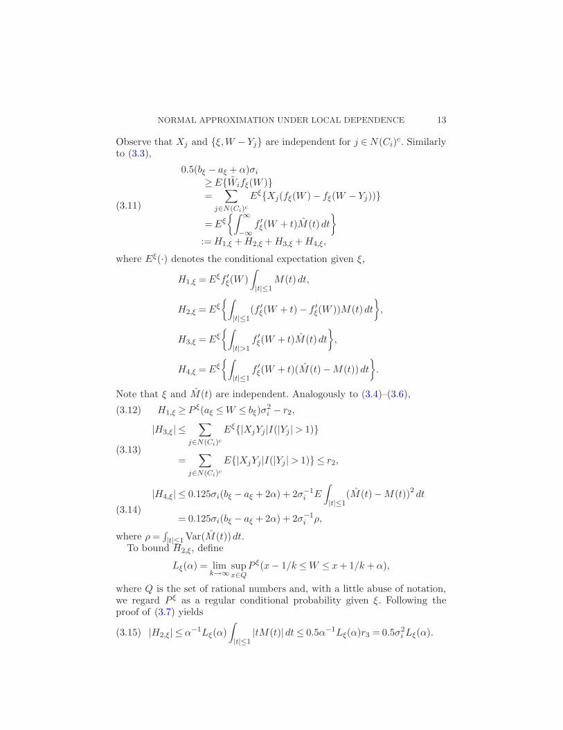
NORMAL APPROXIMATION UNDER LOCAL DEPENDENCE 13
Observe that Xj and {ξ,W − Yj} are independent for j ∈ N(Ci)c. Similarly
to (3.3),
0.5(bξ − aξ + α)σi
≥E{Wifξ(W )}=
∑
j∈N(Ci)c
Eξ{Xj(fξ(W )− fξ(W − Yj))}
= Eξ{∫ ∞
−∞f ′
ξ(W + t)M (t)dt
}
:= H1,ξ + H2,ξ + H3,ξ + H4,ξ,
(3.11)
where Eξ(·) denotes the conditional expectation given ξ,
H1,ξ = Eξf ′ξ(W )
∫
|t|≤1M(t)dt,
H2,ξ = Eξ{∫
|t|≤1(f ′
ξ(W + t)− f ′ξ(W ))M(t)dt
}
,
H3,ξ = Eξ{∫
|t|>1f ′
ξ(W + t)M(t)dt
}
,
H4,ξ = Eξ{∫
|t|≤1f ′
ξ(W + t)(M(t)−M(t))dt
}
.
Note that ξ and M(t) are independent. Analogously to (3.4)–(3.6),
H1,ξ ≥ P ξ(aξ ≤ W ≤ bξ)σ2i − r2,(3.12)
|H3,ξ| ≤∑
j∈N(Ci)c
Eξ{|XjYj |I(|Yj |> 1)}
(3.13)=
∑
j∈N(Ci)c
E{|XjYj|I(|Yj |> 1)} ≤ r2,
|H4,ξ| ≤ 0.125σi(bξ − aξ + 2α) + 2σ−1i E
∫
|t|≤1(M(t)−M(t))2 dt
(3.14)= 0.125σi(bξ − aξ + 2α) + 2σ−1
i ρ,
where ρ =∫
|t|≤1 Var(M (t))dt.To bound H2,ξ, define
Lξ(α) = limk→∞
supx∈Q
P ξ(x− 1/k ≤W ≤ x + 1/k + α),
where Q is the set of rational numbers and, with a little abuse of notation,we regard P ξ as a regular conditional probability given ξ. Following theproof of (3.7) yields
|H2,ξ| ≤ α−1Lξ(α)
∫
|t|≤1|tM(t)|dt ≤ 0.5α−1Lξ(α)r3 = 0.5σ2
i Lξ(α).(3.15)

14 L. H. Y. CHEN AND Q.-M. SHAO
Thus by (3.12)–(3.15),
P ξ(aξ ≤ W ≤ bξ)≤ 0.625σ−1
i (bξ − aξ) + 0.75ασ−1i + 2σ−2
i r2 + 2σ−3i ρ + 0.5Lξ(α).
(3.16)
Now substitute aξ = x − 1/k and bξ = x + 1/k + α in (3.16). By taking thesupremum over x∈ Q and then letting k →∞, we obtain
Lξ(α) ≤ 1.375ασ−1i + 2σ−2
i r2 + 2σ−3i ρ + 0.5Lξ(α)
and hence
Lξ(α) ≤ 2.75ασ−1i + 4σ−2
i r2 + 4σ−3i ρ.(3.17)
Combining (3.16) and (3.17), we obtain
P ξ(aξ ≤ W ≤ bξ)≤ 0.625σ−1
i (bξ − aξ) + 4σ−2i r2 + 2.125σ−3
i r3 + 4σ−3i ρ.
(3.18)
It remains to prove that ρ ≤ r10. Let (X∗j , Y ∗
j ) be an independent copy of
(Xj , Yj). Note that Kj(t) and Kl(t) are independent for l ∈ N(Bj)c. Direct
computations yield
ρ =∑
j∈N(Ci)c
∑
l∈N(Ci)c
∫
|t|≤1Cov(Kj(t), Kl(t))dt
=∑
j∈N(Ci)c
∑
l∈N(Bj )N(Ci)c
∫
|t|≤1Cov(Kj(t), Kl(t))dt
=∑
j∈N(Ci)c
∑
l∈N(Bj)N(Ci)c
E{XlXjI(YlYj ≥ 0)(|Yl| ∧ |Yj | ∧ 1)
−XlX∗j I(YlY
∗j ≥ 0)(|Yl| ∧ |Y ∗
j | ∧ 1)}
≤∑
j∈J
∑
l∈N(Bj)
E{|XlXj|(|Yl| ∧ |Yj | ∧ 1) + |XlX∗j |(|Yl| ∧ |Y ∗
j | ∧ 1)}
= r10.
This completes the proof of the proposition. �
For obtaining a nonuniform conditional concentration inequality, we needtwo lemmas on moment inequalities for locally dependent random fields.
Lemma 3.1. Let {Xi, i ∈ J } be a random field satisfying (LD3) and let
ξi be a measurable function of Xi with Eξi = 0 and Eξ4i < ∞ for each i ∈ J .
Let T =∑
i∈J ξi and σ2 = E(T 2). Then
σ2 =∑
i∈J
∑
j∈Ai
Eξiξj(3.19)

NORMAL APPROXIMATION UNDER LOCAL DEPENDENCE 15
and, for a > 0,
ET 4 = 3σ4 − 6∑
i∈J
E(ξiξAi)E(ξBiξCi) + 3∑
i∈J
E(ξiξAi)Eξ2Bi
(3.20)
− 3∑
i∈J
E(ξiξ2Ai
ξBi) +∑
i∈J
E(ξiξ3Ai
)
+ 6∑
i∈J
E(ξiξAiξBiξCi)− 3∑
i∈J
E(ξiξAiξ2Bi
)
≤ 3σ4 + 5.5∑
i∈J
{a3Eξ4i + a−1Eξ4
Ai+ a−1Eξ4
Bi+ a−1Eξ4
Ci},(3.21)
where
ξAi =∑
j∈Ai
ξj, ξBi =∑
j∈Bi
ξj , ξCi =∑
j∈Ci
ξj .
In particular, we have
σ2 ≤ κ1
∑
i∈J
Eξ2i(3.22)
and
ET 4 ≤ 3σ4 + 22κ31
∑
i∈J
Eξ4i ,(3.23)
where κ1 = maxi∈J max(|Ci|, |{j ∈ J : i ∈ Cj}|).
Proof. By (LD3), ξi and {ξj , j ∈ Aci} are independent and this implies
(3.19). Note that for each i ∈ J , ξi and T − ξAi are independent, {ξi, ξAi}and T − ξBi are independent and {ξi, ξAi , ξBi} and T − ξCi are independent.Therefore
ET 4 =∑
i∈J
E{ξi(T3 − (T − ξAi)
3)}
=∑
i∈J
3E{ξiξAiT2} − 3E{ξiξ
2Ai
T}+ E{ξiξ3Ai}
= 3∑
i∈J
E{ξiξAi}E(T − ξBi)2 + 3
∑
i∈J
E{ξiξAi(T2 − (T − ξBi)
2)}(3.24)
− 3∑
i∈J
E{ξiξ2Ai
ξBi}+∑
i∈J
E{ξiξ3Ai}
= 3∑
i∈J
E{ξiξAi}(σ2 − 2EξBiξCi + Eξ2Bi
)
+ 3∑
i∈J
E{ξiξAi(2ξBiξCi − ξ2Bi
)}

16 L. H. Y. CHEN AND Q.-M. SHAO
− 3∑
i∈J
E{ξiξ2Ai
ξBi}+∑
i∈J
E{ξiξ3Ai}
= 3σ4 − 6∑
i∈J
E(ξiξAi)E(ξBiξCi) + 3∑
i∈J
E(ξiξAi)Eξ2Bi
− 3∑
i∈J
E(ξiξ2Ai
ξBi) +∑
i∈J
E(ξiξ3Ai
)
+ 6∑
i∈J
E(ξiξAiξBiξCi)− 3∑
i∈J
E(ξiξAiξ2Bi
).
Now the Cauchy inequality implies that, for any a > 0 and any randomvariables u1, u2, u3, u4,
E|u1u2u3u4|≤ 1
4{a3E|u1|4 + a−1E|u2|4 + a−1E|u3|4 + a−1E|u4|4}.
(3.25)
It follows that the right-hand side of (3.24) is bounded by 5.5∑
i∈J {a3Eξ4i +
a−1Eξ4Ai
+ a−1Eξ4Bi
+ a−1Eξ4Ci}. This proves (3.21).
To prove (3.22) and (3.23), put A−1i = {j ∈ J : i ∈Aj} and C−1
i = {j ∈ J :i ∈Cj}. Then κ1 = maxi∈J (|Ci| ∨ |C−1
i |). By the Cr inequality and (3.19),
σ2 ≤∑
i∈J
∑
j∈Ai
0.5{Eξ2i + Eξ2
j }
≤ 0.5κ1
∑
i∈J
Eξ2i + 0.5
∑
j∈J
∑
i∈C−1j
Eξ2j ≤ κ1
∑
i∈J
Eξ2i .
Similarly, by (3.21) with a = κ1,
ET 4 ≤ 3σ4 + 5.5∑
i∈J
{
κ31Eξ4
i + κ−11 κ3
1
∑
j∈Ai
E|ξj |4
+ κ−11 κ3
1
∑
j∈Bi
E|ξj |4 + κ−11 κ3
1
∑
j∈Ci
E|ξj |4}
≤ 3σ4 + 22κ31
∑
i∈J
E|ξi|4.
This completes the proof of Lemma 3.1. �
Lemma 3.2. Let {Xi, i ∈ J } be a random field satisfying (LD4∗). Let
ξi be a measurable function of Xi with Eξi = 0 and Eξ4i < ∞ and let ηi be
a measurable function of XAi with Eηi = 0 and Eη4i < ∞. Let T =
∑
i∈J ξi
and S =∑
i∈J ηi. Then, for any a > 0,
E(T 2S2) ≤ 3ET 2ES2 + 4∑
i∈J
{a3Eξ4i + a−1Eξ4
C∗i
+ a−1Eξ4D∗
i
+ a−1Eη4B∗
i+ a−1Eη4
C∗i
+ a−1Eη4D∗
i},
(3.26)

NORMAL APPROXIMATION UNDER LOCAL DEPENDENCE 17
where
ξC∗i
=∑
j∈C∗i
ξj, ξD∗i=∑
j∈D∗i
ξj,
ηB∗i
=∑
j∈B∗i
ηj, ηC∗i
=∑
j∈C∗i
ηj, ηD∗i
=∑
j∈D∗i
ηj.
In particular, we have
E(T 2S2)≤ 3ET 2ES2 + 12κ32
∑
i∈J
{E|ξi|4 + E|ηi|4},(3.27)
where κ2 = maxi∈J max(|D∗i |, |{j ∈ J : i ∈D∗
j}|).
Proof. By (LD4∗), the following pairs of random variables are inde-pendent: (i) ξi and (T − ξAi)(S − ηB∗
i)2; (ii) ξiξAi and (S − ηB∗
i)2; (iii) ξiηB∗
i
and (T − ξC∗i)(S − ηC∗
i). Thus we have
E(T 2S2) =∑
i∈J
E(ξiTS2)
=∑
i∈J
E(ξi{TS2 − T (S − ηB∗i)2 + ξAi(S − ηB∗
i)2})
=∑
i∈J
2E(ξiηB∗iTS)−
∑
i∈J
E(ξiη2B∗
iT ) +
∑
i∈J
E(ξiξAi)E(S − ηB∗i)2
= 2∑
i∈J
E{ξiηB∗i(TS − (T − ξC∗
i)(S − ηC∗
i))}
+ 2∑
i∈J
E(ξiηB∗i)E(T − ξC∗
i)(S − ηC∗
i)
−∑
i∈J
E(ξiη2B∗
iξC∗
i) +
∑
i∈J
E(ξiξAi){E(S2)− 2EηB∗iS + Eη2
B∗i}
= 2∑
i∈J
E{ξiηB∗i(ξC∗
iS + ηC∗
iT − ξC∗
iηC∗
i)}
+ 2∑
i∈J
E(ξiηB∗i){E(TS)−E(ξC∗
iS)−E(ηC∗
iT ) + E(ξC∗
iηC∗
i)}
−∑
i∈J
E(ξiη2B∗
iξC∗
i) + ET 2E(S2)
− 2∑
i∈J
E(ξiξAi)EηB∗iηC∗
i+∑
i∈J
E(ξiξAi)Eη2B∗
i
= 2(E(TS))2 + ET 2ES2 + 2∑
i∈J
E{ξiηB∗iξC∗
iηD∗
i}

18 L. H. Y. CHEN AND Q.-M. SHAO
+ 2∑
i∈J
E{ξiηB∗iηC∗
iξD∗
i} − 2
∑
i∈J
E{ξiηB∗iξC∗
iηC∗
i}
+ 2∑
i∈J
E(ξiηB∗i){−E(ξC∗
iηD∗
i)−E(ηC∗
iξD∗
i) + E(ξC∗
iηC∗
i)}
−∑
i∈J
E(ξiη2B∗
iξC∗
i)− 2
∑
i∈J
E(ξiξAi)EηB∗iηC∗
i+∑
i∈J
E(ξiξAi)Eη2B∗
i
≤ 3ET 2ES2 + 4∑
i∈J
{a3Eξ4i + a−1Eξ4
C∗i
+ a−1Eξ4D∗
i
+ a−1Eη4B∗
i+ a−1Eη4
C∗i
+ a−1Eη4D∗
i},
where (3.25) was used to obtain the last inequality. By the Cr inequality,(3.27) follows directly from (3.26). �
We are now ready to state and prove a nonuniform concentration inequal-ity.
Proposition 3.3. Let {Xi, i ∈ J } be a random field satisfying (LD4∗)and put κ = maxi∈J max(|D∗
i |, |{j ∈ J : i ∈ D∗j}|). Let ξi be a measurable
function of Xi satisfying Eξi = 0 and |ξi| ≤ 1/(4κ). Define
ξAj =∑
l∈Aj
ξl, ξBj =∑
l∈Bj
ξl, T =∑
j∈J
ξj.
Assume that 1/2 ≤ ET 2 ≤ 2 and let ζ = ζi = (ξi, ξAi , ξBi). Then, for Borel
measurable functions aζ and bζ of ζ such that bζ ≥ aζ ≥ 0,
Eζ{(1 + T )3I(aζ ≤ T ≤ bζ)} ≤ C(bζ − aζ + α) a.s.,(3.28)
where α = 16κ2∑
j∈J E|ξj |3. In particular, if aζ ≥ x > −1, then
P ζ(aζ ≤ T ≤ bζ)≤ C(1 + x)−3(bζ − aζ + α) a.s.(3.29)
Proof. Let C∗ci = J −C∗
i and let
Kj,ξ(t) = ξj{I(−ξAj ≤ t < 0)− I(0≤ t≤−ξAj)},
Mξ(t) =∑
j∈C∗ci
Kj,ξ(t), Mξ(t) = EMξ(t), Ti =∑
j∈C∗ci
ξj = T − ξC∗i.
Since |ξj| ≤ 1/(4κ) and 1/2 ≤ ET 2 ≤ 2, we have
|ξC∗j| ≤ 1
4 , E|T − ξC∗j|2 ≤ 6,(3.30)
and by (3.23),
E|T − ξC∗j|4 ≤ 108 + 22κ2
∑
j∈J
E|ξj |3 ≤ 108 + 2α.(3.31)

NORMAL APPROXIMATION UNDER LOCAL DEPENDENCE 19
Consider two cases.
Case I (α > 1). By (3.23),
Eζ{(1 + T )3I(aζ ≤ T ≤ bζ)}
≤ (Eζ |1 + T |4)3/4 ≤ {Eζ(2 + |T − ξC∗i|)4}3/4
≤ E(2 + |T − ξC∗i|)4
≤ 8(16 + E|T − ξC∗i|4)
≤ 8
(
16 + 3(E|T − ξC∗i|2)2 + 22κ3
∑
j∈J
E|ξj |4)
≤ 216
(
1 + κ2∑
j∈J
E|ξj |3)
≤ 217α.
This proves (3.28).
Case II (0 < α < 1). Define
hζ(w) =
0, for w ≤ aζ − α,1
2α(w − aζ + α)2, for aζ − α < w ≤ aζ ,
w − aζ +α
2, for aζ < w ≤ bζ ,
− 1
2α(w − bζ −α)2 + bζ − aζ + α, for bζ < w ≤ bζ + α,
bζ − aζ + α, for w > bζ + α,
and fζ(w) = (1 + w)3hζ(w). Clearly, h′ζ is a continuous function given by
h′ζ(w) =
1, for aζ ≤ w ≤ bζ ,0, for w ≤ aζ − α or w ≥ bζ + α,linear, for aζ − α≤ w ≤ aζ or bζ ≤w ≤ bζ + α,
(3.32)
and 0 ≤ hζ(w) ≤ bζ − aζ + α. With this fζ , and by the fact that for everyj ∈C∗c
i , ξj and (ζ,T − ξAj) are independent,
Eζ{Tifζ(T )} =∑
j∈C∗ci
Eζ(ξj{fζ(T )− fζ(T − ξAj)})
=∑
j∈C∗ci
Eζ(ξj{(1 + T )3 − (1 + T − ξAj)3}hζ(T − ξAj))
+∑
j∈C∗ci
Eζ{ξj(1 + T )3(hζ(T )− hζ(T − ξAj ))}
:= G1 + G2.(3.33)

20 L. H. Y. CHEN AND Q.-M. SHAO
Write G1 = 3G1,1 − 3G1,2 + G1,3, where
G1,1 =∑
j∈C∗ci
Eζ(ξjξAj (1 + T )2hζ(T − ξAj )),
G1,2 =∑
j∈C∗ci
Eζ(ξjξ2Aj
(1 + T )hζ(T − ξAj)),
G1,3 =∑
j∈C∗ci
Eζ(ξjξ3Aj
hζ(T − ξAj)).
Then (ξj, ξAj , T − ξC∗i) and ζ are independent for each j ∈ C∗c
i . Hence, by(3.30),
|G1,2| ≤ (bζ − aζ + α)∑
j∈C∗ci
Eζ{|ξj |ξ2Aj
(1 + |T |)}
≤ (bζ − aζ + α)∑
j∈C∗ci
E{|ξj |ξ2Aj
(3 + |T − ξC∗i|)}
≤ C(bζ − aζ + α)∑
j∈C∗ci
E{|ξj|ξ2Aj
(1 + |T − ξC∗j|)}
≤ C(bζ − aζ + α)∑
j∈C∗ci
E{|ξj|ξ2Aj}E(1 + |T − ξC∗
j|)
≤ C(bζ − aζ + α)∑
j∈J
E{|ξj |ξ2Aj}
≤ C(bζ − aζ + α)κ2∑
j∈J
E|ξj |3
≤ C(bζ − aζ + α).
Similarly, by (3.30), |G1,3| ≤ C(bζ − aζ + α). To bound G1,1 write
G1,1 =∑
j∈C∗ci
E(ξjξAj)Eζ((1 + T − ξC∗
j)2hζ(T − ξC∗
j))
+∑
j∈C∗ci
Eζ(ξjξAj{(1 + T )2hζ(T − ξAj)− (1 + T − ξC∗j)2hζ(T − ξC∗
j)})
= E
(
∑
j∈C∗ci
ξjξAj
)
Eζ((1 + T )2hζ(T ))
+∑
j∈C∗ci
E(ξjξAj)Eζ((1 + T − ξC∗
j)2hζ(T − ξC∗
j)− (1 + T )2hζ(T ))
+∑
j∈C∗ci
Eζ(ξjξAj{(1 + T )2hζ(T − ξAj)− (1 + T − ξC∗j)2hζ(T − ξC∗
j)})

NORMAL APPROXIMATION UNDER LOCAL DEPENDENCE 21
:= G1,1,1 + G1,1,2 + G1,1,3.
First we have
|G1,1,1| = E(T − ξC∗i)2Eζ((1 + T )2hζ(T ))
≤ C(bζ − aζ + α)Eζ(1 + T )2
≤ C(bζ − aζ + α)(1 + E(1 + T − ξC∗i)2)
≤ C(bζ − aζ + α).
Next, as in bounding G1,2, we obtain
|G1,1,3| ≤∣
∣
∣
∣
∣
∑
j∈C∗ci
Eζ(ξjξAj(1 + T )2{hζ(T − ξAj )− hζ(T − ξC∗j)})∣
∣
∣
∣
∣
+
∣
∣
∣
∣
∣
∑
j∈C∗ci
Eζ(ξjξAj{(1 + T )2 − (1 + T − ξC∗j)2}hζ(T − ξC∗
j))
∣
∣
∣
∣
∣
≤∑
j∈C∗ci
Eζ(|ξjξAj |(1 + T )2|ξAj − ξC∗j|)
+ C(bζ − aζ + α)∑
j∈C∗ci
Eζ(|ξjξAjξC∗j|(1 + |T |))
≤ C∑
j∈J
(E|ξj |ξ2Aj
+ E|ξjξAjξC∗j|) + C(bζ − aζ + α)
∑
j∈J
E|ξjξAjξC∗j|
≤ C(bζ − aζ + α).
Finally, in a similar way, |G1,1,2| ≤ C(bζ − aζ + α). Combining the aboveinequalities yields
|G1| ≤C(bζ − aζ + α).(3.34)
Now we bound G2. Using the definition of Kj,ξ(t), we write
G2 =∑
j∈C∗ci
Eζ(
ξj(1 + T )3∫ 0
−ξAj
h′ζ(T + t)dt
)
=∑
j∈C∗ci
Eζ(
(1 + T )3∫
|t|≤1h′
ζ(T + t)Kj,ξ(t)dt
)
= Eζ(
(1 + T )3∫
|t|≤1h′
ζ(T + t)Mξ(t)dt
)
= Eζ(
(1 + T )3∫
|t|≤1h′
ζ(T )Mξ(t)dt
)

22 L. H. Y. CHEN AND Q.-M. SHAO
+ Eζ(
(1 + T )3∫
|t|≤1(h′
ζ(T + t)− h′ζ(T ))Mξ(t)dt
)
+ Eζ(
(1 + T )3∫
|t|≤1h′
ζ(T + t)(Mξ(t)−Mξ(t))dt
)
:= G2,1 + G2,2 + G2,3.
Note that
ET 2i = E(T − ξC∗
i)2≥1
2ET 2 −Eξ2C∗
i≥ 1
4 − 18 = 1
8
and hence
G2,1 = ET 2i Eζ{(1 + T )3h′
ζ(T )} ≥ 18Eζ{(1 + T )3I(aζ ≤ T ≤ bζ)}.(3.35)
By the Cauchy inequality, (3.26) and (3.31),
|G2,3| ≤ Eζ(
(1 + T )4∫
|t|≤1[h′
ζ(T + t)]2 dt
)
+ Eζ(∫
|t|≤1(1 + T )2(Mξ(t)−Mξ(t))
2 dt
)
≤ (bζ − aζ + 2α)Eζ(1 + T )4
+ CEζ{
(1 + (T − ξC∗i)2)
∫
|t|≤1(Mξ(t)−Mξ(t))
2 dt
}
≤ C(bζ − aζ + α)(1 + E(T − ξC∗i)4) + G2,3,1
≤ C(bζ − aζ + α) + G2,3,1,
where
G2,3,1 =
∫
|t|≤1E{(1 + (T − ξC∗
i)2)(Mξ(t)−Mξ(t))
2}dt.
By (3.22) and (3.27) we have
E{(1 + (T − ξC∗i)2)(Mξ(t)−Mξ(t))
2}
≤ Cκ∑
j∈J
E|Kj,ξ(t)|2 + Cκ3∑
j∈J
E|ξj |4 + Cκ3∑
j∈J
E|Kj,ξ(t)|4
and hence
G2,3,1 ≤ Cκ∑
j∈J
E|ξj |2|ξAj |+ Cκ3∑
j∈J
E|ξj |4 + Cκ3∑
j∈J
E|ξj |4|ξAj |
≤ Cκ∑
j∈J
E|ξj |2|ξAj |+ Cκ2∑
j∈J
E|ξj |3

NORMAL APPROXIMATION UNDER LOCAL DEPENDENCE 23
≤ Cκ∑
j∈J
∑
l∈Aj
E|ξj |2|ξl|+ Cκ2∑
j∈J
E|ξj |3
≤ Cκ2∑
j∈J
E|ξj |3 ≤Cα.
To bound G2,2, define
Lζ(α) = limk→∞
supx≥0,x∈Q
Eζ{(1 + T )3I(x− 1/k ≤ T ≤ x + 1/k + α)},
where Q is the set of rational numbers and Eζ is regarded as a regularconditional expectation given ζ . Then, for aζ > 1, so that aζ − α > 0, wehave
G2,2 = Eζ(
(1 + T )3∫ 1
0
∫ t
0h′′
ζ (T + s)dsMξ(t)dt
)
+ Eζ(
(1 + T )3∫ 0
−1
∫ 0
th′′
ζ (T + s)dsMξ(t)dt
)
= α−1∫ 1
0
∫ t
0Eζ{(1 + T )3(I(aζ −α ≤ T + s ≤ aζ)
− I(bζ ≤ T + s ≤ bζ + α))}dsMξ(t)dt
+ α−1∫ 0
−1
∫ 0
tEζ{(1 + T )3(I(aζ −α≤ T + s ≤ aζ)
− I(bζ ≤ T + s≤ bζ + α))}dsMξ(t)dt
and
|G2,2| ≤ α−1∫ 1
0
∫ t
0Lζ(α)ds |Mξ(t)|dt
+ α−1∫ 0
−1
∫ 0
tLζ(α)ds |Mξ(t)|dt
= α−1Lζ(α)
∫
|t|≤1|tMξ(t)|dt
≤ 12α−1Lζ(α)
∑
j∈J
E|ξjξ2Aj|
≤ 12κ2α−1Lζ(α)
∑
j∈J
E|ξj |3
≤ 116Lζ(α).
(3.36)
Therefore,
G2 ≥ 18Eζ{(1 + T )3I(aζ ≤ T ≤ bζ)}−C(bζ − aζ + α)− 1
16Lζ(α).(3.37)

24 L. H. Y. CHEN AND Q.-M. SHAO
Now by (3.31)
Eζ{Tifζ(T )} ≤ (bζ − aζ + α)Eζ |Ti(1 + T )3|≤ C(bζ − aζ + α)E(|Ti|(1 + |Ti|3))≤ C(bζ − aζ + α).
(3.38)
So combining (3.33), (3.34), (3.37) and (3.38), we have for aζ > 1,
Eζ{(1 + T )3I(aζ ≤ T ≤ bζ)} ≤ C(bζ − aζ + α) + 12Lζ(α).(3.39)
For 0 < aζ ≤ 1, it suffices to consider bζ − aζ ≤ 1. Applying Proposition 3.2
to {ξi, i ∈ J }, we obtain
Eζ{(1 + T )3I(aζ < T < bζ + α)}≤CP ζ(aζ < T < bζ + α) ≤ C(bζ − aζ + α).
(3.40)
Now take aζ = x− 1/k and bζ = x + 1/k + α. By taking the supremum over
x ∈ Q and then letting k →∞, (3.39) and (3.40) imply
Lζ(α) ≤ Cα + 12Lζ(α).
Hence
Lζ(α) ≤ Cα.(3.41)
This together with (3.39) and (3.40) proves (3.28) and hence Proposition
3.3. �
4. Proofs of Theorems 2.1–2.4. We first derive a Stein identity for W .
Let f be a bounded absolutely continuous function. Then
E{Wf(W )}=∑
i∈J
E{Xi(f(W )− f(W − Yi))}
=∑
i∈J
E
{
Xi
∫ 0
−Yi
f ′(W + t)dt
}
=∑
i∈J
E
{∫ ∞
−∞f ′(W + t)Ki(t)dt
}
= E
∫ ∞
−∞f ′(W + t)K(t)dt
(4.1)

NORMAL APPROXIMATION UNDER LOCAL DEPENDENCE 25
and hence by the fact that∫∞−∞ K(t)dt = EW 2 = 1,
Ef ′(W )−EWf(W )
= E
∫ ∞
−∞f ′(W )K(t)dt−E
∫ ∞
−∞f ′(W + t)K(t)dt
= E
∫ ∞
−∞f ′(W )(K(t)− K(t))dt
+ E
∫
|t|>1(f ′(W )− f ′(W + t))K(t)dt
+ E
∫
|t|≤1(f ′(W )− f ′(W + t))(K(t)−K(t))dt
+ E
∫
|t|≤1(f ′(W )− f ′(W + t))K(t)dt
:= R1 + R2 + R3 + R4.
(4.2)
Now choose f to be fz,α, the unique bounded solution of the differentialequation
f ′(w)−wf(w) = hz,α(w)−Nhz,α,(4.3)
where α > 0 is to be determined later,
hz,α(w) =
1, for w ≤ z,1 + (z −w)/α, for z ≤ w ≤ z + α,0, for w ≥ z + α,
(4.4)
and Nhzα = (2π)−1/2∫∞−∞ hz,α(x)e−x2/2 dx. The solution of (4.3) is given by
fz,α(w) = ew2/2∫ w
−∞[hz,α(x)−Nhz,α]e−x2/2 dx
= −ew2/2∫ ∞
w[hz,α(x)−Nhz,α]e−x2/2 dx.
From Lemma 2 and arguments on pages 23 and 24 in Stein (1986), we have,for all w and v,
0≤ fz,α(w) ≤ 1,(4.5)
|f ′z,α(w)| ≤ 1, |f ′
z,α(w)− f ′z,α(v)| ≤ 1(4.6)
and
|f ′z,α(w + s)− f ′
z,α(w + t)|
≤ (|w|+ 1)min(|s|+ |t|,1) + α−1
∣
∣
∣
∣
∫ t
sI(z ≤ w + u ≤ z + α)du
∣
∣
∣
∣
(4.7)
≤ (|w|+ 1)min(|s|+ |t|,1) + I(z − s∨ t ≤ w ≤ z − s∧ t + α).(4.8)

26 L. H. Y. CHEN AND Q.-M. SHAO
Proof of Theorem 2.1. By (4.6),
|R1|=∣
∣
∣
∣
∣
Ef ′(W )∑
i∈J
(XiYi −EXiYi)
∣
∣
∣
∣
∣
≤ r1(4.9)
and
|R2| ≤∑
i∈J
E|XiYi|I(|Yi|> 1) = r2.(4.10)
By (4.8),
|R3| ≤ E
∫
|t|≤1(|W |+ 1)|t||K(t)−K(t)|dt
+ E
∫ 1
0I(z − t ≤ W ≤ z + α)|K(t)−K(t)|dt
+ E
∫ 0
−1I(z ≤ W ≤ z − t + α)|K(t)−K(t)|dt
≤ r3 + r4 + R3,1 + R3,2,
(4.11)
where
R3,1 = E
∫ 1
0I(z − t ≤ W ≤ z + α)|K(t)−K(t)|dt,
R3,2 = E
∫ 0
−1I(z ≤ W ≤ z − t + α)|K(t)−K(t)|dt.
Let δ = 0.625α + 4r2 + 2.125r3 + 4r5. Then by Proposition 3.1
P (z − t≤ W ≤ z + α) ≤ δ + 0.625t
for t > 0. Hence by the Cauchy inequality,
R3,1 ≤ E
{∫ 1
0(0.5α(δ + 0.625t)−1I(z − t ≤W ≤ z + α)
+ 0.5α−1(δ + 0.625t)|K(t)−K(t)|2)dt
}
≤ 0.5α + 0.5α−1δ
∫ 1
0Var(K(t))dt + 0.32α−1
∫ 1
0tVar(K(t))dt.
A similar inequality holds for R3,2. Thus we arrive at
R3 ≤ α + 0.5α−1δr5 + 0.32α−1r26 + r3 + r4.(4.12)
By (4.7) and Proposition 3.1 again, we have
|R4| ≤ E
∫
|t|≤1(|W |+ 1)|tK(t)|dt
+ α−1∫
|t|≤1
∣
∣
∣
∣
∫ t
0P (z ≤ W + u ≤ z + α)du
∣
∣
∣
∣
|K(t)|dt
≤ 2r3 + α−1∫
|t|≤1tδ|K(t)|dt ≤ 2r3 + α−1δr3.
(4.13)

NORMAL APPROXIMATION UNDER LOCAL DEPENDENCE 27
Combining the above inequalities yields
|Ehz,α(W )−Nhz,α|≤ r1 + r2 + 3r3 + r4 + α + α−1{δ(0.5r5 + r3) + 0.32r2
6}≤ r1 + r2 + 3.625r3 + r4 + 0.32r5 + α
+ α−1{(4r2 + 2.125r3 + 4r5)(0.5r5 + r3) + 0.32r26}.
Using the fact that Ehz−α,α(W ) ≤ P (W ≤ z) ≤ Ehz,α(W ) and that |Φ(z +
α)−Φ(z)| ≤ (2π)−1/2α, we have
supz
|P (W ≤ z)−Φ(z)| ≤ supz
|Ehz,α(W )−Nhz,α|+ 0.5α.(4.14)
Letting α =√
2/3((4r2 + 2.125r3 + 4r5)(0.5r5 + r3) + 0.32r26)1/2 yields
supz
|P (W ≤ z)−Φ(z)|
≤ r1 + r2 + 3.625r3 + r4 + 0.32r5
+√
6((4r2 + 2.125r3 + 4r5)(0.5r5 + r3) + 0.32r26)1/2
(4.15)≤ r1 + r2 + 3.625r3 + r4 + 0.32r5 + 1.5r6
+ 0.5(1.5(4r2 + 2.125r3 + 4r5) + 4(0.5r5 + r3))
≤ r1 + 4r2 + 8r3 + r4 + 4.5r5 + 1.5r6.
This proves Theorem 2.1. �
Proof of Theorem 2.2. Let p3 = 3∧p. Using the following well-knowninequality: ∀xi ≥ 0, αi ≥ 0 with
∑
αi = 1,∏
xαii ≤
∑
αixi,(4.16)
we have
r2 ≤∑
i∈J
E|Xi||Yi|p3−1
≤∑
i∈J
{
1
p3E|Xi|p3 +
p3 − 1
p3E|Yi|p3
}
and
r3 ≤∑
i∈J
E|Xi||Yi|p3−1
≤∑
i∈J
{
1
p3E|Xi|p3 +
p3 − 1
p3E|Yi|p3
}
.

28 L. H. Y. CHEN AND Q.-M. SHAO
Similarly we have
r5 ≤∑
i,j∈J ,BiBj 6=∅
{E|XiXj||Yi|p3−2 + E|XiX∗j ||Yi|p3−2}
≤ 2∑
i,j∈J ,BiBj 6=∅
{
1
p3E|Xi|p3 +
1
p3E|Xj |p3 +
p3 − 2
p3E|Yi|p3
}
≤ 2κ∑
i∈J
{
2
p3E|Xi|p3 +
p3 − 2
p3E|Yi|p3
}
and
r26 ≤
1
2
∑
i,j∈J ,BiBj 6=∅
{E|XiXj ||Yi|p−2 + E|XiX∗j ||Yi|p−2}
≤ κ∑
i∈J
{
2
pE|Xi|p +
p− 2
pE|Yi|p
}
.
Now we estimate r4. Recall that
Zi =∑
j∈Bi
Xj
and that (Xi, Yi) and W −Zi are independent.We have
r4 ≤∑
i∈J
{E|W −Zi|E|Xi|(Y 2i ∧ 1) + E|ZiXi|(Y 2
i ∧ 1)}
≤∑
i∈J
{(1 + E|Zi|)E|Xi|(Y 2i ∧ 1) + E|ZiXi||Yi|p3−2}
≤∑
i∈J
E|Xi||Yi|p3−1 +∑
i∈J
∑
j∈Bi
E|Xj |E|Xi||Yi|p3−2
+∑
i∈J
∑
j∈Bi
E|XjXi||Yi|p3−2
≤∑
i∈J
{
1
p3E|Xi|p3 +
p3 − 1
p3E|Yi|p3
}
+ 2κ∑
i∈J
{
2
p3E|Xi|p3 +
p3 − 2
p3E|Yi|p3
}
.
To estimate r1, let ξi = XiYiI(|XiYi| ≤ 1). We have
r1 ≤ E
∣
∣
∣
∣
∣
∑
i∈J
(ξi −Eξi)
∣
∣
∣
∣
∣
+ 2∑
i∈J
E|XiYi|I(|XiYi|> 1)

NORMAL APPROXIMATION UNDER LOCAL DEPENDENCE 29
≤ Var
(
∑
i∈J
ξi
)1/2
+ 2∑
i∈J
E|XiYi|p3/2
≤ Var
(
∑
i∈J
ξi
)1/2
+∑
i∈J
{E|Xi|p3 + E|Yi|p3}.
Similarly to bounding r6,
Var
(
∑
i∈J
ξi
)
≤∑
i,j∈J ,BiBj 6=∅
(E|ξiξj|+ E|ξi|E|ξj |)
≤∑
i,j∈J ,BiBj 6=∅
(E|XiYi|p/4|XjYj|p/4 + E|XiYi|p/4E|XjYj|p/4)
≤ κ∑
i∈J
(E|Xi|p + E|Yi|p).
Combining the inequalities above yields (2.5). �
Proof of Theorem 2.3. The idea of the proof is similar to that ofTheorem 2.1. Noting that Ki and W −Zi are independent, we rewrite (4.2)as
Ef ′(W )−EWf(W )
=∑
i∈J
{
E
∫ ∞
−∞f ′(W )Ki(t)dt−E
∫ ∞
−∞f ′(W + t)Ki(t)dt
}
=∑
i∈J
E
∫ ∞
−∞(f ′(W )− f ′(W −Zi + t))Ki(t)dt
+∑
i∈J
E
∫ ∞
−∞(f ′(W −Zi + t)− f ′(W + t))Ki(t)dt
= Q1 + Q2 + Q3 + Q4,
(4.17)
where
Q1 =∑
i∈J
E
∫
|t|≤1(f ′(W )− f ′(W −Zi + t))Ki(t)dt,
Q2 =∑
i∈J
E
∫
|t|>1(f ′(W )− f ′(W −Zi + t))Ki(t)dt,
Q3 =∑
i∈J
E
∫
|t|>1(f ′(W −Zi + t)− f ′(W + t))Ki(t)dt,
Q4 =∑
i∈J
E
∫
|t|≤1(f ′(W −Zi + t)− f ′(W + t))Ki(t)dt.

30 L. H. Y. CHEN AND Q.-M. SHAO
By (4.6), similarly to (4.10),
|Q2|+ |Q3| ≤ 2∑
i∈J
E|XiYi|I(|Yi|> 1) = 2r2.(4.18)
To bound Q4, write Q4 = Q4,1 + Q4,2, where
Q4,1 =∑
i∈J
EI(|Xi|> 1)
∫
|t|≤1(f ′(W −Zi + t)− f ′(W + t))Ki(t)dt,
Q4,2 =∑
i∈J
EI(|Xi| ≤ 1)
∫
|t|≤1(f ′(W −Zi + t)− f ′(W + t))Ki(t)dt.
Then by (4.6),
|Q4,1| ≤∑
i∈J
E|XiYi|I(|Xi| > 1) = r7.(4.19)
From (4.7), we obtain
|Q4,2| ≤∑
i∈J
EI(|Xi| ≤ 1)
∫
|t|≤1(|W |+ |t|+ 1)(|Zi| ∧ 1)|Ki(t)|dt
+ α−1∑
i∈J
EI(|Xi| ≤ 1)
×∫
|t|≤1I(Zi ≥ 0)
×∫ 0
−Zi
I(z ≤W + t + u ≤ z + α)du |Ki(t)|dt
+ α−1∑
i∈J
EI(|Xi| ≤ 1)
×∫
|t|≤1I(Zi < 0)
×∫ −Zi
0I(z ≤ W + t + u ≤ z + α)du|Ki(t)|dt
≤∑
i∈J
E(|W |+ 1)|Xi|I(|Xi| ≤ 1)(|Zi| ∧ 1)(|Yi| ∧ 1)
+ 0.5∑
i∈J
E|Xi|(|Yi|2 ∧ 1) + Q4,3
≤ r8 + r9 + 0.5r3 + Q4,3,(4.20)where
Q4,3 = α−1∑
i∈J
E
{
I(|Xi| ≤ 1)
×∫
|t|≤1I(Zi ≥ 0)

NORMAL APPROXIMATION UNDER LOCAL DEPENDENCE 31
×∫ 0
−Zi
P ξi(z ≤ W + t + u ≤ z + α)du |Ki(t)|dt
}
+ α−1∑
i∈J
E
{
I(|Xi| ≤ 1)
×∫
|t|≤1I(Zi < 0)
×∫ −Zi
0P ξi(z ≤ W + t + u ≤ z + α)du |Ki(t)|dt
}
and ξi = (Xi, Yi,Zi). By Proposition 3.2,
Q4,3 ≤ α−1∑
i∈J
E
{
I(|Xi| ≤ 1)
×∫
|t|≤1(0.625σ−1
i α + 4σ−2i r2
+ 2.125σ−3i r3 + 4σ−3
i r10)|Zi||Ki(t)|dt
}
(4.21)
≤ 0.625λ∑
i∈J
E{|Xi|I(|Xi| ≤ 1)(|Yi| ∧ 1)|Zi|}
+ α−1{4λ2r2 + 2.125λ3r3 + 4λ3r10}r8
= 0.625λr8 + α−1{4λ2r2 + 2.125λ3r3 + 4λ3r10}r8.
Combining (4.19)–(4.21) yields
|Q4| ≤ r7 + r9 + 1.625λr8 + 0.5r3
+ α−1{4λ2r2 + 2.125λ3r3 + 4λ3r10}r8.(4.22)
Similarly we have
|Q1| ≤∑
i∈J
P (|Xi|> 1)E|Xi|(|Yi| ∧ 1)
+∑
i∈J
E{(|W |+ 1)(|Zi| ∧ 1)}E|Xi|(|Yi| ∧ 1) + r3
+ α−1{0.625λα + 4λ2r2 + 2.125λ3r3 + 4λ3r10}
×{
0.5r3 +∑
i∈J
E{(|W |+ 1)(|Zi| ∧ 1)}E|Xi|(|Yi| ∧ 1)
}
= r11 + r12 + r3
+ α−1{0.625λα + 4λ2r2 + 2.125λ3r3 + 4λ3r10}(0.5r3 + r12).
(4.23)

32 L. H. Y. CHEN AND Q.-M. SHAO
Combining (4.17), (4.18), (4.22), (4.23) and (4.14), we obtain
supz
|F (z)−Φ(z)|≤ 0.5α + 2r2 + 2λr3 + r7 + 1.625λr8 + r9 + r11 + 1.625λr12
+ α−1{4λ2r2 + 2.125λ3r3 + 4λ3r10}(r8 + 0.5r3 + r12).
(4.24)
Let
α = (2(4λ2r2 + 2.125λ3r3 + 4λ3r10)(r8 + 0.5r3 + r12))1/2.
Then the right-hand side of (4.24) is
= 2r2 + 2λr3 + r7 + 1.625λr8 + r9 + r11 + 1.625λr12
+ {2(4λ2r2 + 2.125λ3r3 + 4λ3r10)(r8 + 0.5r3 + r12)}1/2
≤ 2r2 + 2λr3 + r7 + 1.625λr8 + r9 + r11 + 1.625λr12
+ 0.5λ−3/2(4λ2r2 + 2.125λ3r3 + 4λ3r10) + λ3/2(r8 + 0.5r3 + r12)
≤ 4λ3/2(r2 + r3 + r7 + r8 + r9 + r10 + r11 + r12).
This proves Theorem 2.3. �
Proof of Theorem 2.4. We can assume that
κp−1∑
i∈J
E|Xi|p ≤ 175 .(4.25)
Otherwise (2.9) is trivial. Let ξi =∑
j∈N(Ci) Xj . Then by (4.25)
√
Eξ2i ≤ (E|ξi|p)1/p ≤
(
|N(Ci)|p−1∑
j∈N(Ci)
E|Xj |p)1/p
≤(
κp−1∑
j∈J
E|Xj |p)1/p
≤ ( 175)1/p ≤ ( 1
75)1/3 < 0.2372
(4.26)
and
σi ≥√
EW 2 −√
Eξ2i ≥ 1− 0.2372 = 0.7628.
Thus 4λ3/2 ≤ 6.01. By (4.16) and the Minkowski inequality
r8 ≤∑
i∈J
E|XiZi||Yi|p−2
=∑
i∈J
E(κ(p−1)/p|Xi|(|Zi|/κ1/p)(|Yi|/κ1/p)p−2)
≤∑
i∈J
1
pκp−1E|Xi|p +
∑
i∈J
(
1
pκE|Zi|p +
(p− 2)
pκE|Yi|p
)

NORMAL APPROXIMATION UNDER LOCAL DEPENDENCE 33
≤ κp−1
p
∑
i∈J
E|Xi|p +∑
i∈J
|Ci|p−1(p− 1)
pκ
∑
j∈Ci
E|Xj |p
≤ κp−1∑
i∈J
E|Xi|p.
Similarly we have
r2 + r3 + r7 + r11 ≤ 2κp−1∑
i∈J
E|Xi|p.
Note that |N(Bi)| ≤ |N(Ci)|. Following the proof for r26 yields
r10 ≤∑
i,j∈J ,BiBj 6=∅
{E(κ(p−2)/p|Xi|κ(p−2)/p|Xj |(|Yi|/κ2/p)p−2)
+ E(κ(p−2)/p|Xi|κ(p−2)/p|X∗j |(|Yi|/κ2/p)p−2)}
≤ 2∑
i,j∈J ,BiBj 6=∅
{
κp−2
p(E|Xi|p + E|Xj |p) +
p− 2
pκ2E|Yi|p
}
≤ 2κp−1∑
i∈J
E|Xi|p.
The r9 can be bounded as r8 and r4. By (4.26),
r9 ≤∑
i∈J
E|W − ξi|E|Xi|(|Yi| ∧ 1)(|Zi| ∧ 1) +∑
i∈J
E|ξi||Xi||Yi|p−2
≤ 1.2372∑
i∈J
E|Xi||Yi||Zi|p−2 +∑
i∈J
E|Xi||ξi||Yi|p−2
≤ 2.2372κp−1∑
i∈J
E|Xi|p.
Similarly,
r12 ≤ 3.2372κp−1∑
i∈J
E|Xi|p.
Theorem 2.4 follows from (2.7) and the above inequalities. �
5. Proof of Theorem 2.5. The basic idea of the proof of Theorem 2.5 issimilar to that of Theorem 2.3. We use the same notation as in Section 2.2and remind the reader that {Xi, i ∈ J } satisfies (LD4∗) and that E|Xi|p <∞for 2 < p ≤ 3.
First we need a few preliminary lemmas. Let
τ = 1/(8κ), Xi = XiI(|Xi| ≤ τ), Xi = XiI(|Xi|> τ),
W =∑
i∈J
Xi, Yi =∑
j∈Ai
Xj ,(5.1)

34 L. H. Y. CHEN AND Q.-M. SHAO
and
β1 =∑
i∈J
E|XiYi|I(|Xi|> τ), β2 =∑
i∈J
EX2i I(|Xi|> τ),
β3 =∑
i∈J
E|Xi|3I(|Xi| ≤ τ).(5.2)
Our first lemma shows that W is close to W .
Lemma 5.1. Assume β2 ≤ τ/16. Then there exists an absolute constant
C such that, for z ≥ 0,
|P (W > z)−P (W > z)|≤∑
i∈J
P (|Yi|> (z + 1)/4) + C(z + 1)−3κ3β3
+ 64κ2β2{(1 + z)−3 + P (W > (z − 1)/2)}.(5.3)
Proof. Observe that
P (W > z) = P
(
W > z,maxi∈J
|Xi| ≤ τ
)
+ P
(
W > z,maxi∈J
|Xi|> τ
)
≤ P (W > z) +∑
i∈J
P (W > z, |Xi| > τ)
≤ P (W > z) +∑
i∈J
{P (W − Yi > 3(z − 1/3)/4, |Xi|> τ)
+ P (Yi > (z + 1)/4, |Xi|> τ)}≤ P (W > z) +
∑
i∈J
{P (W − Yi > 3(z − 1/3)/4)P (|Xi|> τ)
+ P (Yi > (z + 1)/4)}≤ P (W > z) +
∑
i∈J
{P (W > (z − 1)/2)P (|Xi|> τ)
+ P (−Yi > (z + 1)/4) + P (Yi > (z + 1)/4)}≤ P (W > z) + P (W > (z − 1)/2)τ−2
∑
i∈J
E|X2i |I(|Xi|> τ)
+∑
i∈J
P (|Yi| > (z + 1)/4)
= P (W > z) + 64κ2β2P (W > (z − 1)/2)
+∑
i∈J
P (|Yi| > (z + 1)/4).
(5.4)
Similarly, noting that |∑j∈AiXj | ≤ 1, we have
P (W > z)≤ P (W > z) + κ2β2P (W > z − 2).(5.5)

NORMAL APPROXIMATION UNDER LOCAL DEPENDENCE 35
Note that β2 ≤ τ/16 implies |EW | ≤ 1/16 and by (3.22),
|Var(W )− 1| = |Var(W )−Var(W )|
≤ 2(EW 2)1/2
(
Var
(
∑
i∈J
Xi
))1/2
+ Var
(
∑
i∈J
Xi
)
≤ 2(κβ2)1/2 + κβ2 ≤ 2/3.
(5.6)
Applying (3.23) to W −EW yields
P (W > z − 2) ≤ E|W −EW + 4|4(z + 2−EW )4
≤ C(z + 1)−4
(
1 + κ3∑
i∈J
E|Xi|4I(|Xi| ≤ τ)
)
≤ C(z + 1)−4
(
1 + κ3τ∑
i∈J
E|Xi|3I(|Xi| ≤ τ)
)
≤ C(z + 1)−4(1 + κ2β3).
(5.7)
By (5.4)–(5.7) and the assumption that κβ2 ≤ 1, (5.3) is proved and hencethe lemma. �
Lemma 5.2. Assume E|Xi|p <∞ for some 2 < p ≤ 3. Then there exists
an absolute constant C such that, for z ≥ 0,
P (W > (z − 1)/2) ≤ C(1 + z)−p(1 + κp−1γ)(5.8)
and∑
i∈J
P (|Yi| > (z + 1)/4) + κ3(1 + z)−3β3
+ (1 + z)−3β1 + κ2β2{(1 + z)−3 + P (W ≥ (z − 1)/2)}≤ Cκp(1 + z)−pγ + C(1 + z)−3κ2p−1γ2,
(5.9)
where γ =∑
i∈J E|Xi|p.
Proof. If κp−1γ > (1 + z)p−2, then (5.8) is trivial because P (W > (z −1)/2) ≤ 4(z + 1)−2E(W + 1)2 = 8(z + 1)−2. To prove (5.8) for κp−1γ ≤ (1 +z)p−2, let
Xi = XiI(|Xi| ≤ (1 + z)τ)−EXiI(|Xi| ≤ (1 + z)τ),
X∗i = XiI(|Xi|> (1 + z)τ)−EXiI(|Xi|> (1 + z)τ),
W =∑
i∈J
Xi, W ∗ =∑
i∈J
X∗i .

36 L. H. Y. CHEN AND Q.-M. SHAO
Then
P (W > (z − 1)/2)
≤ P (W > (z − 3)/4) + P (W ∗ > (z + 1)/4)
≤ C(1 + z)−4E|W + 1|4 + 4(1 + z)−1E|W ∗|≤ C(1 + z)−4(1 + E|W |4) + C(1 + z)−1((1 + z)τ)−p+1γ.
Similarly to (5.6), κp−1γ ≤ (1 + z)p−2 implies Var(W ) ≤ 4. Hence by (3.23),
E|W |4 ≤ C
(
1 + κ3∑
i∈J
E|Xi|4I(|Xi| ≤ (1 + z)τ)
)
≤ C(1 + κp−1(1 + z)4−pγ).
By combining the above inequalities, (5.8) is proved.We now prove (5.9). From (5.8), the Chebyshev inequality and the Holder
inequality, the left-hand side of (5.9) is bounded by
((z + 1)/4)−p∑
i∈J
E|Yi|p + κ3(1 + z)−3τ3−pγ
+ (1 + z)−3τ−p+2∑
i∈J
E|Xi|p−1|Yi|+ C(1 + z)−3κ2τ−p+2γ(1 + κp−1γ)
≤ C(1 + z)−pκpγ + C(1 + z)−3κ2p−1γ2.
This completes the proof of the lemma. �
Proof of Theorem 2.5. Without loss of generality, assume z ≥ 0.When κp−1γ > 1, (2.10) follows directly from (5.8). When κp−1γ ≤ 1, then(2.10) is a consequence of (5.9) and the following inequality:
|F (z)−Φ(z)| ≤∑
i∈J
P (|Yi| > (z + 1)/4) + C(1 + z)−3β1
+ Cκ2β2{(1 + z)−3 + P (W ≥ (z − 1)/2)}+ Cκ2(1 + z)−3β3.
(5.10)
So it suffices to prove (5.10). It is clear, that for z ≥ 0,
|P (W > z)− (1−Φ(z))| ≤ P (W > (z − 1)/2) + 16(1 + z)−3.
So (5.10) holds if κ2β2 > 128 . It remains to consider the case that
κ2β2 ≤ 116 .(5.11)
Let W be defined as in (5.1). By Lemma 5.1, it suffices to show that
|P (W ≤ z)−Φ(z)|≤ C(1 + z)−3β1 + Cκ(1 + z)−3β2 + Cκ2(1 + z)−3β3.
(5.12)

NORMAL APPROXIMATION UNDER LOCAL DEPENDENCE 37
Let σ2 = Var(W ), T = (W −EW )/σ. Then
|P (W ≤ z)−Φ(z)|= |P (T ≤ (z −EW )/σ)−Φ(z)|≤ |P (T ≤ (z −EW )/σ)−Φ((z −EW )/σ)|
+ |Φ((z −EW )/σ)−Φ(z)|.(5.13)
By the Chebyshev inequality,
|EW | ≤ τ−1∑
i∈J
EX2i I(|Xi|> τ)≤ 1
16 .(5.14)
By (5.6), we have 1/3 < σ2 < 2, and moreover, similarly to (5.6),
|σ2 − 1| = 2
∣
∣
∣
∣
∣
∑
i∈J
E(XiW )
∣
∣
∣
∣
∣
+ Var
(
∑
i∈J
Xi
)
≤ 2∑
i∈J
E|XiYi|I(|Xi|> τ) + κ∑
i∈J
EX2i I(|Xi|> τ)
= 2β1 + κβ2.
(5.15)
Thus by (5.14) and (5.15),
|Φ((z −EW )/σ)−Φ(z)|≤ |Φ((z −EW )/σ)−Φ(z/σ)|+ |Φ(z/σ)−Φ(z)|≤ C(1 + z)−3|EW |+ C(1 + z)−3|σ2 − 1|≤ C(1 + z)−3κβ2 + C(1 + z)−3β1.
(5.16)
With x = (z −EW )/σ (> −1/2), we only need to show that
|P (T ≤ x)−Φ(x)| ≤Cκ2(1 + x)−3β3.(5.17)
Put
ξi = (Xi −E(Xi))/σ, ξAi =∑
j∈Ai
ξj , ξBi =∑
j∈Bi
ξj,
Ki(t) = ξi(I(−ξAi < t ≤ 0)− I(0 < t <−ξAi)), Ki(t) = EKi(t).
By the definition of τ , we have |ξAi | ≤ 12 and |ξBi | ≤ 1
2 . If (1 + x)κ2β3 > 1,then by (3.23),
|P (T > x)− (1−Φ(x))|≤ (1 + x)−4E|1 + T |4 + (1 + x)−4
≤ C(1 + x)−4
(
1 + κ3∑
i∈J
E|ξi|4)
≤ C(1 + x)−4
(
1 + κ3τ∑
i∈J
E|ξi|3)
≤ C(1 + x)−4(1 + κ2β3) ≤C(1 + x)−3κ2β3,

38 L. H. Y. CHEN AND Q.-M. SHAO
which proves (5.17).If (1 + x)κ2β3 ≤ 1, let α = 64κ2β3. Also let hx,α(w) be as in (4.4) and let
f(w) = fx,α(w) be the unique bounded solution of the Stein equation (4.3)with x replacing z. Then by (4.1) and similarly to (4.2),
Ef ′(T )−ETf(T )
=∑
i∈J
E
∫
|t|≤1(f ′(T − ξBi + t)− f ′(T + t))Ki(t)dt
+∑
i∈J
E
∫
|t|≤1(f ′(T )− f ′(T − ξBi + t))Ki(t)dt
:= R1 + R2.
(5.18)
Let g(w) = (wf(w))′ and let
R1,1 =∑
i∈J
E
∣
∣
∣
∣
∫
|t|≤1
∫ −ξBi
0g(T + u)duKi(t)dt
∣
∣
∣
∣
,
R1,2 = α−1∑
i∈J
E
∣
∣
∣
∣
∫
|t|≤1
∫ −ξBi
0I(x ≤ T + u ≤ x + α)duKi(t)dt
∣
∣
∣
∣
.
Noting that∣
∣
∣
∣
f ′x,α(w + t)− f ′
x,α(w + s)−∫ t
sg(w + u)du
∣
∣
∣
∣
≤ α−1
∣
∣
∣
∣
∫ t
sI(x ≤ w + u ≤ x + α)du
∣
∣
∣
∣
,(5.19)
we have
|R1| ≤R1,1 + R1,2.
Let ζi = (ξi, ξAi , ξBi). By Lemma 5.3,
R1,1 ≤∑
i∈J
E
∫
|t|≤1
∣
∣
∣
∣
∫ −ξBi
0Eζig(T + u)du
∣
∣
∣
∣
|Ki(t)|dt
≤ C(1 + x)−3∑
i∈J
E
∫
|t|≤1|ξBi ||Ki(t)|dt
≤ C(1 + x)−3∑
i∈J
E|ξiξAiξBi |
≤ Cκ2(1 + x)−3β3,
and by Proposition 3.3,
R1,2 ≤ α−1∑
i∈J
E
∫
|t|≤1
∣
∣
∣
∣
∫ −ξBi
0P ζi(x ≤ T + u ≤ x + α)du
∣
∣
∣
∣
Ki(t)|dt

NORMAL APPROXIMATION UNDER LOCAL DEPENDENCE 39
≤ Cα−1(1 + x)−3∑
i∈J
E
∫
|t|≤1(κ2β3 + α)|ξBi ||Ki(t)|dt
≤ Cα−1(1 + x)−3(κ2β3 + α)∑
i∈J
E|ξiξAiξBi |
≤ Cκ2(1 + x)−3β3.
This proves
|R1| ≤ Cκ2(1 + x)−3β3.
Similarly we have
|R2| ≤ Cκ2(1 + x)−3β3.
Hence we have
|Ehx,α(T )−Nhx,α| ≤Cκ2(1 + x)−3β3.(5.20)
Finally, using the fact that Ehx−α,α(T ) ≤ P (T ≤ x) ≤ Ehx,α(T ) and that|Φ(x + α) − Φ(x)| ≤ C(1 + x)−3α for x > −1/2, we have (5.17). This com-pletes the proof of Theorem 2.5. �
It remains to prove Lemma 5.3 which was used above.
Lemma 5.3. Let ζ = ζi = (ξi, ξAi , ξBi) and
g(w) = gx,α(w) = (wfx,α(w))′.(5.21)
Then for x > −1/2 and |u| ≤ 4, we have
Eζg(T + u)≤ C(1 + x)−3(1 + κ2β3).(5.22)
Proof. From the definitions of Nhx,α, fx,α and g, we have
Nhx,α = Φ(x) +α√2π
∫ 1
0se−(x+α−αs)2/2 ds,
fx,α(w) =
√2πew2/2Φ(w)(1−Nhx,α), w ≤ x,√2πew2/2(1−Φ(w))Nhx,α
−αew2/2∫ 1+(z−w)/α
0se−(z+α−αs)2/2 ds, x < w ≤ x + α,
√2πew2/2(1−Φ(w))Nhx,α, w > x + α,
g(w) =
(√
2π(1 + w2)ew2/2Φ(w) + w)(1−Nhx,α), w < x,
(√
2π(1 + w2)ew2/2(1−Φ(w))−w)Nhx,α + rx,α(w),x ≤ w ≤ x + α,
(√
2π(1 + w2)ew2/2(1−Φ(w))−w)Nhx,α, w > x + α,

40 L. H. Y. CHEN AND Q.-M. SHAO
where
rx,α(w) = −wew2/2∫ x+α
w
(
1 +x− s
α
)
e−s2/2 ds +
(
1 +x−w
α
)
.
For x < w < x + α, we have, by integration by parts,
rx,α ≥−ew2/2∫ x+α
ws
(
1 +x− s
α
)
e−s2/2 ds +
(
1 +x−w
α
)
= ew2/2∫ x+α
we−s2/2 ds≥ 0.
So 0≤ rx,α ≤ 1 for x < w < x+α. It can be verified that 0 < g(w) ≤C(1+ |x|)for all x. Therefore, (5.22) holds when −1 < x ≤ 6.
When x > 6, the proof of (5.22) is very similar to that of Lemma 5.2 of
Chen and Shao (2001).
A direct calculation shows that, for w ≥ 0,
0≤√
2π(1 + w2)ew2/2(1−Φ(w))−w ≤ 2
1 + w3.(5.23)
This implies that g ≥ 0, g(w) ≤ 2(1 − Φ(x)) for w ≤ 0 and g(w) ≤ 21+w3 +
I(x < w < x+α) for w ≥ x; furthermore, g is clearly increasing for 0≤ w < x.
Therefore,
Eζg(T + u) = Eζg(T + u)I(T + u ≤ x− 1)
+ Eζg(T + u)I(T + u ≥ x)
+ Eζg(T + u)I(x − 1 < T + u < x)≤ 2(1−Φ(x)) + g(x − 1) + 2(1 + x3)−1
+ P ζ(x ≤ T + u ≤ x + α)
+ Eζg(T + u)I(x − 1 < T + u < x)
≤ C((1 + x)−3 + x2e(x−1)2/2(1−Φ(x))) + C(1 + x)−3α
+ Eζg(T + u)I(x − 1 < T + u < x)
≤ C(1 + x)−3(1 + α) + Eζg(T + u)I(x− 1 < T + u < x).
(5.24)
NORMAL APPROXIMATION UNDER LOCAL DEPENDENCE 41
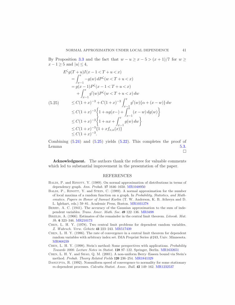
By Proposition 3.3 and the fact that w − u ≥ x − 5 > (x + 1)/7 for w ≥x− 1 ≥ 5 and |u| ≤ 4,
Eζg(T + u)I(x − 1 < T + u < x)
=
∫ x
x−1−g(w)dP ζ(w < T + u < x)
= g(x − 1)P ζ(x− 1 < T + u < x)
+
∫ x
x−1g′(w)P ζ(w < T + u < x)dw
≤ C(1 + x)−3 + C(1 + x)−3∫ x
x−1g′(w){α + (x−w)}dw
≤ C(1 + x)−3{
1 + αg(x−) +
∫ x
x−1(x−w)dg(w)
}
≤ C(1 + x)−3{
1 + αx +
∫ x
x−1g(w)dw
}
≤ C(1 + x)−3{1 + xfx,α(x)}≤ C(1 + x)−3.
(5.25)
Combining (5.24) and (5.25) yields (5.22). This completes the proof ofLemma 5.3.
�
Acknowledgment. The authors thank the referee for valuable commentswhich led to substantial improvement in the presentation of the paper.
REFERENCES
Baldi, P. and Rinott, Y. (1989). On normal approximation of distributions in terms ofdependency graph. Ann. Probab. 17 1646–1650. MR1048950
Baldi, P., Rinott, Y. and Stein, C. (1989). A normal approximation for the numberof local maxima of a random function on a graph. In Probability, Statistics, and Math-
ematics. Papers in Honor of Samuel Karlin (T. W. Anderson, K. B. Athreya and D.L. Iglehart, eds.) 59–81. Academic Press, Boston. MR1031278
Berry, A. C. (1941). The accuracy of the Gaussian approximation to the sum of inde-pendent variables. Trans. Amer. Math. Soc. 49 122–136. MR3498
Bikelis, A. (1966). Estimates of the remainder in the central limit theorem. Litovsk. Mat.
Sb. 6 323–346. MR210173Chen, L. H. Y. (1978). Two central limit problems for dependent random variables.
Z. Wahrsch. Verw. Gebiete 43 223–243. MR517439Chen, L. H. Y. (1986). The rate of convergence in a central limit theorem for dependent
random variables with arbitrary index set. IMA Preprint Series #243, Univ. Minnesota.MR868239
Chen, L. H. Y. (1998). Stein’s method: Some perspectives with applications. Probability
Towards 2000. Lecture Notes in Statist. 128 97–122. Springer, Berlin. MR1632651Chen, L. H. Y. and Shao, Q. M. (2001). A non-uniform Berry–Esseen bound via Stein’s
method. Probab. Theory Related Fields 120 236–254. MR1841329Dasgupta, R. (1992). Nonuniform speed of convergence to normality for some stationary
m-dependent processes. Calcutta Statist. Assoc. Bull. 42 149–162. MR1232537

42 L. H. Y. CHEN AND Q.-M. SHAO
Dembo, A. and Rinott, Y. (1996). Some examples of normal approximations by Stein’smethod. In Random Discrete Structures (D. Aldous and R. Pemantle, eds.) 25–44.Springer, New York. MR1395606
Erickson, R. V. (1974). L1 bounds for asymptotic normality of m-dependent sums usingStein’s technique. Ann. Probab. 2 522–529. MR383503
Esseen, C. G. (1945). Fourier analysis of distribution functions: A mathematical studyof the Laplace–Gaussian law. Acta Math. 77 1–125. MR14626
Esseen, C. G. (1968). On the concentration function of a sum of independent randomvariables. Z. Wahrsch. Verw. Gebiete 9 290–308. MR231419
Heinrich, L. (1984). Nonuniform estimates and asymptotic expansions of the remainderin the central limit theorem for m-dependent random variables. Math. Nachr. 115 7–20.MR755264
Ho, S.-T. and Chen, L. H. Y. (1978). An Lp bound for the remainder in a combinatorialcentral limit theorem. Ann. Probab. 6 231–249. MR478291
Nagaev, S. V. (1965). Some limit theorems for large deviations. Theory Probab. Appl.
10 214–235. MR185644Petrov, V. V. (1995). Limit Theorems of Probability Theory : Sequences of Independent
Random Varaibles. Clarendon Press, Oxford. MR1353441Prakasa Rao, B. L. S. (1981). A nonuniform estimate of the rate of convergence in the
central limit theorem for m-dependent random fields. Z. Wahrsch. Verw. Gebiete 58
247–256. MR637054Rinott, Y. (1994). On normal approximation rates for certain sums of dependent random
variables. J. Comput. Appl. Math. 55 135–143. MR1327369Rinott, Y. and Rotar, V. (1996). A multivariate CLT for local dependence with
n−1/2 log n rate and applications to multivariate graph related statistics. J. Multivariate
Anal. 56 333–350. MR1379533Shergin, V. V. (1979). On the convergence rate in the central limit theorem for m-
dependent random variables. Theory Probab. Appl. 24 782–796. MR550533Stein, C. (1972). A bound for the error in the normal approximation to the distribution
of a sum of dependent random variables. Proc. Sixth Berkeley Symp. Math. Statist.
Probab. 2 583–602. Univ. California Press, Berkeley. MR402873Stein, C. (1986). Approximation Computation of Expectations. IMS, Hayward, CA.Sunklodas, J. (1999). A lower bound for the rate of convergence in the central limit
theorem for m-dependent random fields. Theory Probab. Appl. 43 162–169. MR1669963Tihomirov, A. N. (1980). Convergence rate in the central limit theorem for weakly de-
pendent random variables. Theory Probab. Appl. 25 800–818. MR595140
Institute for Mathematical Sciences
National University of Singapore
3 Prince George’s Park
Singapore 118402
Singapore
and
Department of Mathematics
Department of Statistics and
Applied Probability
National University of Singapore
Singapore 117543
Singapore
e-mail: [email protected]
Department of Mathematics
University of Oregon
Eugene, Oregon 97403
USA
and
Department of Mathematics
Department of Statistics and
Applied Probability
National University of Singapore
Singapore 117543
Singapore
e-mail: [email protected]