Tight Approximation of Image Matching

Simon KormanSchool of EE

Tel-Aviv UniversityRamat Aviv, Israel

simon.korman@gmail.com

Daniel ReichmanFaculty of Math and CS

Weizmann Institute of ScienceRehovot, Israel

daniel.reichman@gmail.com

Gilad TsurFaculty of Math and CS

Weizmann Institute of ScienceRehovot, Israel

gilad.tsur@gmail.com

November 9, 2011

Abstract

In this work we consider the image matching problem for two grayscale n × n images, M1

and M2 (where pixel values range from 0 to 1). Our goal is to find an affine transformation Tthat maps pixels from M1 to pixels in M2 so that the differences over pixels p between M1(p)and M2(T (p)) is minimized. Our focus here is on sublinear algorithms that give an approximateresult for this problem, that is, we wish to perform this task while querying as few pixels fromboth images as possible, and give a transformation that comes close to minimizing the difference.

We give an algorithm for the image matching problem that returns a transformation T whichminimizes the sum of differences (normalized by n2) up to an additive error of ε and performsO(n/ε2) queries. We give a corresponding lower bound of Ω(n) queries showing that this is thebest possible result in the general case (with respect to n and up to low order terms).

In addition, we give a significantly better algorithm for a natural family of images, namely,smooth images. We consider an image smooth when the total difference between neighboringpixels is O(n). For such images we provide an approximation of the distance between the imagesto within an additive error of ε using a number of queries depending polynomially on 1/ε andnot on n. To do this we first consider the image matching problem for 2 and 3-dimensionalbinary images, and then reduce the grayscale image matching problem to the 3-dimensionalbinary case.

1

arX

iv:1

111.

1713

v1 [

cs.D

S] 7

Nov

201

1

1 Introduction

Similarity plays a central part in perception and categorization of visual stimuli. It is no wonder thatsimilarity has been intensely studied, among others, by cognitive psychologists [16, 6] and computervision and pattern recognition researchers. Much of the work on computer vision, including that onimage matching, involves algorithms that require a significant amount of processing time, whereasmany of the uses of these algorithms would typically require real-time performance.

A motivating example is that of image registration [19, 14]. Here we are given two images of aparticular scene or object (e.g., two pictures taken from a video sequence) and wish to match oneimage to the other, for tasks such as motion detection, extraction of 3-dimensional information,noise-reduction and super-resolution. Many advances were made in dealing with this task and itcan now be performed in a wide variety of situations. However, image registration algorithms aregenerally time consuming.

Image registration is an application of a more abstract computational problem - the imagematching problem [8, 9, 11]. In this problem we are given two digital n × n images M1 and M2

and wish to find a transformation that changes M1 so that it best resembles M2. In this work weconsider the distance between two n×n images M1 and M2 when we perform affine transformationson their pixels. Namely, given an affine transformation T , we sum over all pixels p the absolute valueof the difference between M1(p) and M2(T (p)), where the difference is considered to be 1 for pixelsmapped outside M2. The distance between M1 and M2 is defined as the minimum such distancetaken over all affine transformations. Our focus is on affine transformations as such transformationsare often used when considering similarity between images. We limit ourselves to trasformationswith a bounded scaling factor. This is congruent with applications, and prevents situations suchas one image mapping to very few pixels in another. Exact algorithms for this problem generallyenumerate all possible different transformations, fully checking how well each transformation fitsthe images. Hundt and Liskiewicz [8] give such an algorithm for the set of affine transformationson images with n × n pixels (transformations on which we focus in this paper), that runs in timeΘ(n18). They also prove a lower bound of Ω(n12) on the number of such transformations (whichimplies a Ω(n12) lower bound on algorithms using this technique).

As known exact algorithms have prohibitive running times, image registration algorithms usedin practice are typically heuristic. These algorithms often reduce the complexity of the problem byroughly matching “feature points” [19, 14] - points in the images that have relatively distinct char-acteristics. Such heuristic algorithms are not analyzed rigorously, but rather evaluated empirically.

Two related problems are those of shape matching and of point set matching, or point patternmatching. In shape matching [18] the goal is to find a mapping T between two planar shapes S1and S2, minimizing a variety of distance measures between the shapes T (S1) and S2. A problemof similar flavor is that of point set matching [5], where we are given two (finite) sets of points Aand B in a Euclidean space and seek to map A to a set T (A) that minimizes the distance betweenT (A) and B under some distance metric. Algorithms for these exact problems were give by Altet al’ [2] and by Chew et al’ [4] both require prohibitive running times. Recent research [5] hasfocused on finding transformations that are close to the optimal one requiring less time. It shouldbe noted that the running times the algorithms in [5] are superlinear in the number of points inA and B. We emphasize that these works are concerned with planar shapes and point sets ratherthan digital images.

Our main contribution is devising sublinear algorithms for the image matching problem. Sub-linear algorithms are extremely fast (and typically randomized) algorithms that use techniques

2

such as random sampling to asses properties of objects with arbitrarily small error. The numberof queries made by such algorithms is sublinear in the input size, and generally depends on theerror parameter. The use of sublinear algorithms in image processing was advocated by Rashkod-nikova [13] who pioneered their study for visual properties. She gave algorithms for binary (0− 1)images, testing the properties of connectivity, convexity and being a half-plane. In her work, animage is considered far from having such a property if it has a large hamming distance from everyimage with the property. Ron and Tsur [15] introduced a different model that allowed testing ofsparse images (where there are o(n2) different 1-pixels) for similar properties. Kleiner et al. [10]give results on testing images for a partitioning that roughly respects a certain template. Unlike theaforementioned works we do not deal only with binary images, but also consider grayscale images,where every pixel gets a value in the range [0, 1].

1.1 Our Results

In this work we prove both general results and results for smooth images.

1. General Upper Bound: We present an algorithm that when given access to any two n × ngrayscale images M1 and M2 and a precision parameter ε returns a transformation T suchthat the distance between M1 and M2 using T is at most ε greater than the minimum distancebetween them (taken over all affine transformations). The query complexity of this algorithmis Θ(n/ε2), which is sublinear in n2, the size of the matrices.

2. Lower Bound: We show that every algorithm estimating matching between images withinadditive error smaller than 1/4 must make an expected Ω(n) number of queries.

3. Upper Bound For Smooth Images: We show that if the images M1 and M2 are smooth, thatis, for both images the total difference between neighboring pixels is O(n), then for everypositive ε we can find a transformation T such that the distance between M1 and M2 usingT is at most ε greater than the minimum distance between them. This can be done using anumber of queries that is polynomial in 1/ε and does not depend on n.

Being smooth is a property of many natural images - research has shown a power-law distributionof spatial frequencies in images [17, 12], translating to very few fast changes in pixel intensity. Whilewe show that our algorithm works well with smooth images, we note that distinguishing betweenimages that have a total difference between neighboring pixels of O(n) and those with a total ofO(n) + k requires Ω(n2/k) queries.

An unusual property of the way distance between images is defined in this work is that it isnot symmetric. In fact, an image M1 may have a mapping that maps all its pixels to only half thepixels in M2, so that each pixels is mapped to a pixels with the same value, while any mappingfrom M2 to M1 leaves a constant fraction of the pixels in M2 mapped either outside M1 or to pixelsthat do not have the same color (To see this consider an image M1 that has only black points, andan image M2 that is black on one the left side and white on the other). We note that one can usethe algorithms presented here also to measure symmetric types of distances by considering inversemappings.

Techniques

3

The Algorithm for the General Case: Imagine that sampling a pair of pixels, p ∈ M1

and q ∈ M2, would let us know how well each affine transformation T did with respect to thepixel p, that is, what the difference is between M1(p) and M2(T (p)). The way we define grayscalevalues (as ranging from 0 to 1), we could sample Θ(ε2) random pairs of points and have, for everytransformation, an approximation of the average difference between points up to an additive errorof ε with constant probability. As there are polynomially many different affine transformationsif we increased the number of samples to amplify the probability of correctness, we could useO(log(n)/ε2) queries and return a transformation that was ε-close to the best1. However, when wesample p ∈M1 and q ∈M2 uniformly at random we get a random pixel and its image under only afew of the different transformations. We show that O(n/ε2) queries suffice to get a good estimationof the error for all interesting transformations (that is, transformations that map a sufficiently largeportion of pixels from M1 to pixels in M2). Using these pixels we can return a transformation thatis close to optimal as required.

The Lower Bound: We prove the lower bound by giving two distributions of pairs of images.In the first, the images are random 0− 1 images and far from each other. In the second, one imageis partially created from a translation of the other. We show that any algorithm distinguishingbetween these families must perform Ω(n) expected queries. The proof of the lower bound issomewhat similar to the lower bound given by Batu et al. [3] on the number of queries required toapproximate edit distance. Here we have a two-dimensional version of roughly the same argument.Note that a random 0 − 1 image is far from being smooth, that is, many pixels have a valuesignificantly different from that of their neighbors.

The Algorithm For Smooth Images: Our analysis of the algorithm for smooth imagesbegins by considering binary images. The boundary of a 0−1 image M is the set of pixels that havea neighboring pixel with a different value. We consider two affine transformations T, T ′ close if forevery pixel p the distance in the plane between T (p) and T ′(p) is small. Only points that are closeto the boundary might be mapped to different values by close transformations T and T ′ (meaningthat the pixel will be mapped correctly by one and not by the other - see Figure 1). It followsthat if there is a big difference in the distance between M1 and M2 when mapped by T and theirdistance when mapped by T ′, then the perimeter, the size of the boundary, is large. This impliesthat when the perimeter is small, one can sample a transformation T and know a lot about thedistance between images for transformations that are “close” to T . This idea can be generalizedto 3-dimensional binary images. Such 0− 1 images are a natural object in 3 dimensions as color isnot a feature typically attributed to areas within a body. More importantly, however, one can use3-dimensional binary images to model 2-dimensional grayscale images. Smooth grayscale images,i.e., images where the sum of difference (in absolute value) between neighboring pixels is O(n),translate to 3-dimensional binary images that have a small perimeter. An appropriate version ofthe 3-dimensional algorithm can be used to get a good approximation for the mapping betweentwo grayscale images.

OrganizationWe begin by giving some preliminaries in Section 2. We then describe and prove the correctness

of the algorithm for the general case (with a query complexity of O(n/ε2)). We give the lower

1The O symbol hides logarithmic factors

4

bound in the next section. Following that we give the algorithm for smooth binary images inSection 4.1. In Section 4.2 we give an explicit construction of an ε-net of transformations suchthat any transformation is close to one of the those in the net. In Section 4.3 we give the three-dimensional version of our algrithm, and in Section 4.4 we show how to use this version to workwith grayscale images.

2 Preliminaries

We are given two images represented by n× n matrices. For grayscale images the values of entriesin the matrix are in the range [0, 1] and for binary images they are either 0 or 1.

Definition 2.1 A pixel p in an n × n image M is a pair of coordinates, namely a pair (i, j) ∈1, . . . , n2. We denote this as p ∈M .

Definition 2.2 The value of a pixel p = (i, j) in an image M is M [i, j], or M(p).

Definition 2.3 For r ∈ R2 we denote by brc the pixel p that the point r falls in.

Definition 2.4 A transformation T has a scaling factor in the range [1/c, c] (for a positive constantc) if for all vectors v it holds that ||v||/c ≤ ||Tv|| ≤ c||v||.

Here we are particularly interested in affine transformations in the plane that are used to mapone pixel to another, when these transformations have a scaling factor in the range [1/c, c] for a fixedpositive constant c. Such a transformation T can be seen as multiplying the pixel vector by a 2× 2non-singular matrix and adding a ”translation” vector, then rounding down the resulting numbers.When comparing two images, requiring the matrix to be non-singular prevents the transformationfrom mapping the image plane in one image onto a line or a point in the other.

Given an affine transformation in the form of a matrix A and a translation vector t, there isa corresponding transformation T (p) = bAp+ tc. We call T an image-affine transformation andwe say that T is based on A and t. Generally speaking, when we discuss algorithms getting animage-affine transformation as input, or enumerating such transformations, we assume that thesetransformations are represented in matrix format.

Definition 2.5 The distance between two n×n images (M1,M2) with respect to a transformationT , which we denote ∆T (M1,M2), is defined as

1

n2

[|p ∈M1 | T (p) /∈M2|+

∑p∈M1|T (p)∈M2

|M1(p)−M2(T (p))|]

Note that the distance ∆T (M1,M2) ranges from 0 to 1.

Definition 2.6 We define the Distance between two images (M1,M2) (which we denote ∆(M1,M2))as the minimum over all image-affine transformations T of ∆T (M1,M2).

Definition 2.7 Two different pixels p = (i, j) and q = (i′, j′) are adjacent if |i − i′| ≤ 1 and|j − j′| ≤ 1.

5

The following definitions relate to binary (0− 1) images:

Definition 2.8 A pixel p = (x, y) is a boundary pixel in an image M if there is an adjacent pixelq such that M(p) 6= M(q).

Definition 2.9 The perimeter of an image M is the set of boundary pixels in M as well as the4n− 4 outermost pixels in the square image. We denote the size of the perimeter of M by PM .

Note that PM is always Ω(n) and O(n2).

3 The General Case

We now present the algorithm for general images. The lower bound we will prove in Section 3.2demonstrates that this algorithm has optimal query complexity, despite having a prohibitive runningtime. The main signficance of the algorithm is in showing that one can achieve query complexityof O(n). It is an open question if one can achieve this query complexity in sublinear time or evensignificantly faster than our running tme.

3.1 The Algorithm

Algorithm 1 Input: Oracle access to n× n images M1,M2, and a precision parameter ε.

1. Sample k = Θ(n/ε2) pixels P = p1, . . . , pk uniformly at random (with replacement) from M1.

2. Sample k pixels Q = q1, . . . , qk uniformly at random (with replacement) from M2.

3. Enumerate all image-affine transformations T1, . . . , Tm (Recall that m, the number of image-affine transformations, is in O(n18)).

4. For each transformation T` denote by Out` the number of pixel coordinates that are mappedby T` out of the region [1, n]2.

5. For each transformation T` denote by Hit` the number of pairs pi, qj such that T`(pi) = qj,and denote by Bad` the value 1

|p∈P,q∈Q|T`(pi)=qj|∑

pi,qj∈p∈P,q∈Q|T`(pi)=qj |M1(pi)−M2(qj)|

6. Return T` that minimizes (n2−Out`)·Bad` (discarding transformations T` such that Hit` < ε).

Theorem 3.1 With probability at least 2/3 Algorithm 1 returns a transformation T such that|∆T (M1,M2)−∆(M1,M2)| < ε.

We prove Theorem 3.1 by showing that for any fixed transformation T` (where Hit` ≥ ε)the sample we take from both images gives us a value Bad` that is a good approximation of thevalue 1

|p∈M1,q∈M2|T`(pi)=qj|∑

pi,qj∈p∈M1,q∈M2|T`(pi)=qj |M1(pi)−M2(qj)| with high probability, and

applying a union bound. To show this we give several definitions and claims. For these we fix animage-affine transformation T and two images M1 and M2, so that T maps at least ε/2 of thepoints in M1 to points in M2 (note that transformations that do not map such an ε/2 portion ofpixels are discarded by the algorithm with very high probability).

6

1. Let T (M1) be the set of pixels q ∈M2 such that there exist pixels p ∈M1 so that T (p) = q.

2. For a set of pixels Q ∈M2 let T−1(Q) denote the set p ∈M1|T (p) ∈ Q.

3. We denote by Q′ the points that are in Q (the sample of points taken from M2) and in T (M1).

4. We denote by P ′ the points p ∈ P such that T (p) ∈ Q′.

5. For a pixel q ∈M2 we denote by |q| the number of pixels p ∈M1 such that T (p) = q.

6. For a pixel q ∈ M2 we denote by q the sum over pixels p ∈ M1 such that T (p) = q of|M1(p)−M2(T (p))|.

7. Denote by pbad the average over pixels p from those mapped from M1 to T (M1) of |M1(p)−M2(T (p))|.

8. Denote by pbad the value (∑

q∈Q′ q)/(∑

q∈Q′ |q|).

Claim 3.1 With probability at least 1/(8n18) over the choice of P and Q the size of Q′ is Ω(n/ε)and the size of P ′ is Ω(log(n)/ε3).

Proof: The probability of any particular pixel in Q belonging to Q′ is at least ε/2, and Q is ofsize θ(n/ε2) (where pixels are chosen independently). Hence the expected number of points in Q′ isΩ(n/ε). An additional factor of Θ(log(n)) hidden in the Θ notation of k assures us (using Chernoffbounds) that the probability Q′ not being large enough is at most 1/(8n18) as required.

Assume the first part of the claim holds. Recall that no more than a constant number of pixelsfrom M1 are mapped to any pixel in M2, and therefore |T−1(Q′)| = Ω(n/ε). As the pixels of Pare chosen independently and uniformly at random from the n2 pixels of M1, each pixel in P ismapped to a pixel in Q′ with a probability of Ω(1/(nε)). Hence, the expected size of P ′ is Ω(1/ε3)and the second part of the claim follows (via a similar argument).

Claim 3.2 With probability at least 1/(8n18) over the choice of P and Q it holds that |pbad−pbad| <ε/4.

Proof: Note that pbad equals (∑

q∈T (M1)q)/(

∑q∈T (M1)

|q|). Now, consider the value pbad =

(∑

q∈Q′ q)/(∑

q∈Q′ |q|). Each pixel q ∈ Q′ is chosen uniformly at random and independently from

the pixels in T (M1). To see that the claim holds we note that with probability at least 1−1/(8n18)(using Hoeffding bounds and the fact that with high probability P ′ is Ω(log(n)/ε3)) we have that|(∑

q∈Q′ q/|Q′|)−(∑

q∈T (M1)q/|T (M1)|)| = Ø(ε) and that |(

∑q∈Q′ |q|/|Q′|)−(

∑q∈T (M1)

|q|/|T (M1)|)| =Ø(ε). The claim follows.

Claim 3.3 With probability at least 1/(8n18) over the choice of P and Q it holds that |Bad`−pbad| <ε/2

Proof: We have that pbad =∑q∈Q′ q∑q∈Q′ |q|

. It follows that pbad equals Ep∈T−1(Q′)[M1(p) = M2(T (p))]

where p is chosen uniformly at random from T−1(Q′). The pixels in P ′ are chosen uniformly atrandom from T−1(Q′) and (with sufficiently high probability), by Claim 3.1 there are Ω(log(n)/ε3)such pixels. The claim follows using Hoeffding bounds.

We thus see that Bad` is ε-close to the average difference between M1(p) and M2(T`(p)) forpixels p ∈M1 mapped by T` to M2. As Out` is exactly the number of pixels mapped by T` out ofM2, the claim follows from the definition of distance.

7

3.2 Lower Bound

We build a lower bound using binay images, and parameterize the lower bound with the imageperimeter (see Theorem 3.2). Note that for an image M having a perimeter of size k implies thatthe total difference between pixels and their neighbors in M is Θ(k). We use a bound on this totaldifference to discuss the smoothness of grayscale images later in this work.

Theorem 3.2 Fix k > 0 such that k = o(n) (k may depend on n). Let A be an algorithm that isgiven access to pairs of images M1,M2 where max(PM1 , PM2) = Ω(n2/k). In order to distinguishwith high probability between the following two cases:

1. ∆(M1,M2) < 4/16

2. ∆(M1,M2) > 7/16

A must perform Ω(n/k) queries.

In order to prove Theorem 3.2 we will first focus on the case where k = 1. Namely, weshow that any algorithm that satisfies the conditions as stated in the theorem for all images withmax(PM1 , PM2) = Θ(n2) must perform Ω(n) queries. Following this we will explain how the proofextends to the case of a general k.

We use Yao’s principle - we give two distributions D1,D2 over pairs of images such that thefollowing holds:

1. Pr(M1,M2)˜D1[∆(M1,M2) > 7/16] > 1− o(1)

2. Pr(M1,M2)˜D2[∆(M1,M2) < 4/16] = 1

and show that any deterministic algorithm that distinguishes with high probability between pairsdrawn from D1 and those drawn from D2 must perform Ω(n) expected queries. We now turn todescribe the distributions.

The distribution D1 is the distribution of pairs of images where every pixel in M1 and every pixelin M2 is assigned the value 1 with probability 0.5 and the value 0 otherwise, independently. Pairsin the distribution D2 are constructed as follows. M1 is chosen as in D1. We now choose uniformlyat random two values sh, sv ranging each from 0 to n/8. Pixels (i, j) in M2 where i < sh or j < svare chosen at random as in D1. The remaining pixels (i, j) satisfy M2(i, j) = M1(i − sh, j − sv).Intuitively, the image M2 is created by taking M1 and shifting it both horizontally and vertically,and filling in the remaining space with random pixels.

Both distributions D1 and D2 possess the required limitation on the size of the boundaries(i.e. max(PM1 , PM2) = Θ(n2)). It suffices to show this with respect to the image M1, whichis constructed in the same way in both distributions. It is easy to see (since M1’s pixels are

independently taken to be 0 or 1 uniformly at random) that Pr[PM1 ≥ n2

4 ] = 1− o(1).We now proceed to prove the properties of D1 and D2. Starting with D2, given the transfor-

mation T that shifts points by sv and sh, all but a 15/64’th fraction (which is smaller than 1/4) ofM1’s area matches exactly with a corresponding area in M2 and the following claim holds.

Claim 3.4 Pr(M1,M2)˜D2[∆(M1,M2) < 4/16] = 1

In order to prove that pairs of images drawn from D1 typically have a distance of at least 7/16we first state the following claim [8]:

8

Claim 3.5 The number of image-affine transformations T between n× n images M1 and M2 thatmap at least one of M1’s pixels into M2 is polynomial in n.

Claim 3.6 Pr(M1,M2)˜D1[∆(M1,M2) > 7/16] > 1− o(1)

Proof: Consider two images M1,M2 that are sampled from D1. The value ∆T (M1,M2) for anarbitrary transformation T is ∆T (M1,M2) ≤ Prp∈M1 [T (p) ∈ M2 ∧M1(p) = M2(T (p))]. For anypixel p, over the choice of M1 and M2, it holds that Pr[T (p) ∈ M2 ∧M1(p) = M2(T (p))] ≤ 1/2 (ifT (p) ∈ M2 the probability is 1/2). The random (over the choice of M1,M2) variable ∆T (M1,M2)has an expectation of at most n2/2. As it is bounded by the sum of n2 independent 0− 1 randomvariables with this expectation, the probability that ∆T (M1,M2) < (1/2 − ε)n2 for any positivefixed ε is Θ(e−n

2). As ∆(M1,M2) = minT ∆T (M1,M2), and as there are at most a polynomial

number of transformations T , the claim follows using a union bound.The proof of Theorem 3.2 for the case k = 1 is a consequence of the following claim.

Claim 3.7 Any algorithm that given a pair of n× n images M1,M2 acts as follows:

1. Returns 1 with probability at least 2/3 if ∆(M1,M2) ≤ 4/16.

2. Returns 0 with probability at least 2/3 if ∆(M1,M2) ≥ 7/16.

must perform Ω(n) expected queries.

Proof: To show this we consider any deterministic algorithm that can distinguish with probabilitygreater than 1/2+ ε (for a constant ε > 0) between the distributions D1 and D2. Assume (toward acontradiction) such an algorithm A that performs m = o(n) queries exists. We will show that withvery high probability over the choice of images, any new queryA performs is answered independentlywith probability 0.5 by 0 and with probability 0.5 by 1. This implies the Theorem.

The fact that any new query A performs is answered in this way is obvious for D1 - here thepixels are indeed chosen uniformly at random.

We now describe a process P that answers a series of m queries performed by A in a way thatproduces the same distribution of answers to these queries as that produced by pairs of imagesdrawn from D2. This will complete the proof. The process P works as follows (we assume withoutloss of generality that A never queries the same pixel twice):

1. Select m bits r1, . . . , rm uniformly and independently at random. These will (typically) serveas the answers to A’s queries.

2. Select uniformly at random two values sh, sv ranging each from 0 to n/8.

3. For qk = (i, j) - the k’th pixel queried by A, return the following:

(a) If qk is queried in M1, and M2(i+ sh, j + sv) was sampled, return M2(i+ sh, j + sv).

(b) If qk is queried in M2, and M1(i− sh, j − sv) was sampled, return M1(i− sh, j − sv).(c) Else, return rk.

9

Obviously, P has the same distribution of answers to queries as that of images drawn fromD2 - the choice of sh, sv is exactly as that done when selecting images from D2, and the values ofpixels are chosen in a way that respects the constraints in this distribution. We now show that theprobability of reaching Steps 3a and 3b is o(1). If P does not reach these steps it returns r1, . . . , rmand A sees answers that were selected uniformly at random. Hence, the claim follows.

Having fixed r1, . . . , rm in Step 1, consider the queries q′1, . . . , q′m that A performs when answered

r1, . . . , rm−1 (that is, the query q′1 is the first query A performs. If it is answered by r1 it performsthe query q′2, etc.). In fact, we will ignore the image each query is performed in, and consider onlythe set of pixel locations pk = (ik, jk). Step 3a or 3b can only be reached if a pair of pixels pk, p`satisfies |ik− i`| = sv and |jk− j`| = sh. There are Θ(m2) such pairs, and as m = o(n) we have thatm2 = o(n2). As the number of choices of sv, sh is in Θ(n2), the probability of sv, sh being selectedso that such an event occurs is o(1) as required.

Proving Theorem 3.2 for the Case k > 1 (sketch). We construct distributions similar tothose above, except that instead of considering single pixels we partition each image to roughlyn2/k2 blocks of size k × k, organized in a grid. The distributions D1,D2 are similar, except thatnow we assign the same value to all the pixels in each block. For the distribution D2 we selectsv, sh to shift the image by multiples of k. The remainder of the proof is similar to the case wherek = 1, but the number of queries that an algorithm must perform decreases from Ω(n) to Ω(n/k),while the boundary size decreases from Θ(n2) to Θ(n2/k).

4 The Smooth Image Case

4.1 The Algorithm for Binary Images with Bounded Perimeter

Given a pair of binary images M1,M2 with PM1 = O(n) and PM2 = O(n) our approach to findingan image-affine transformation T such that ∆T (M1,M2) ≤ ∆(M1,M2) + ε is as follows. Weiterate through a set of image affine transformations that contain a transformation that is close tooptimal (for all images with a perimeter bounded as above), approximating the quality of everytransformation in this set. We return the transformation that yields the best result.

We first show (in Claim 4.1) how to approximate the value ∆T (M1,M2) given a transformationT . We then show that for two affine transformations T , T ′ that are close in the sense that forevery point p in the range 1, . . . , n2 the values T (p) and T ′(p) are not too far (in Euclideandistance), the following holds. For the image affine transformations T, T ′ based on T and T ′ thevalues ∆T (M1,M2) and ∆T ′(M1,M2) are close. This is formalized in Theorem 4.1 and Corollary ??.Finally we claim that given a set T of affine transformations such that for every affine transformationthere exists a transformation close to it in T , it suffices for our purposes to check all image affinetransformations based on transformations in T . In Section 4.2 we give the construction of such aset.

The following claims and proofs are given in terms of approximating the distance (a numer-ical quantity) between the images. However, the algorithm is constructive in the sense that itfinds a transformation that has the same additive approximation bounds as those of the distanceapproximation.

Claim 4.1 Given images M1 and M2 of size n × n and an image-affine transformation T , letd = ∆T (M1,M2). Algorithm 2 returns a value d′ such that |d′ − d| ≤ ε with probability 2/3 and

10

performs Θ(1/ε2) queries.

Algorithm 2 Input: Oracle access to n×n images M1,M2, precision parameter ε and a transfor-mation T (given as a matrix and translation vector).

1. Sample Θ(1/ε2) values p ∈M1. Check for each p whether T (p) ∈M2, and if so check whetherM1(p) = M2(T (p)).

2. Return the proportion of values that match the criteria T (p) ∈M2 and M1(p) = M2(T (p)).

The approximation is correct to within ε using an additive Chernoff bound.We now define a notion of distance between affine transformations (which relates to points in

the plane):

Definition 4.1 Let T and T ′ be affine transformations. The ln∞ distance between T and T ′ isdefined as max

p∈[1,n+1)2‖T (p)− T ′(p)‖2.

The notion of ln∞ distance simply quantifies how far the mapping of a point in an image accordingto T may be from its mapping by T ′. Note that this definition doesn’t depend on the pixel valuesof the images, but only on the mappings T and T ′, and on the image dimension n.

The following fact will be needed for the proof of Theorem 4.1.

Claim 4.2 Given a square subsection M of a binary image and an integer b, let PM denote thenumber of boundary pixels in M . If M contains at least b 0-pixels and at least b 1-pixels, thenPM ≥

√b.

Proof: Let M be a square of d× d pixels. Note that d >√b. To see the claim holds we consider

three cases. In the first case, all rows and all columns of M contain both 0 and 1 pixels. In such acase each row contains at least one boundary pixel, PM ≥ d >

√b, and we are done. In the second

case there exists, without loss of generality, a row that does not contain the value 0, and all columnscontain the value 0. Again this means there are at least d boundary pixels (one for each column),PM ≥ d >

√b, and we are done. Finally, consider the case that there are both rows and columns

that do not contain the value 0. This means that there is a boundary pixel for each row and foreach column that do contain the value 0. If there were fewer than

√b boundary pixels this would

mean there are fewer than√b rows and columns that contain 0 pixels, and M could not contain b

different 0 pixels. This would lead to a contradiction, and thus PM ≥√b, and we are done.

We now turn to a theorem that leads directly to our main upper-bound results.

Theorem 4.1 Let M1,M2 be n × n images and let δ be a constant in (0,√

2). Let T and T ′ beimage affine transformations based on the affine transformations T , T ′, such that ln∞(T , T ′) < δn.It holds that

∆T ′(M1,M2) ≤ ∆T (M1,M2) +O(δPM2

n

)

11

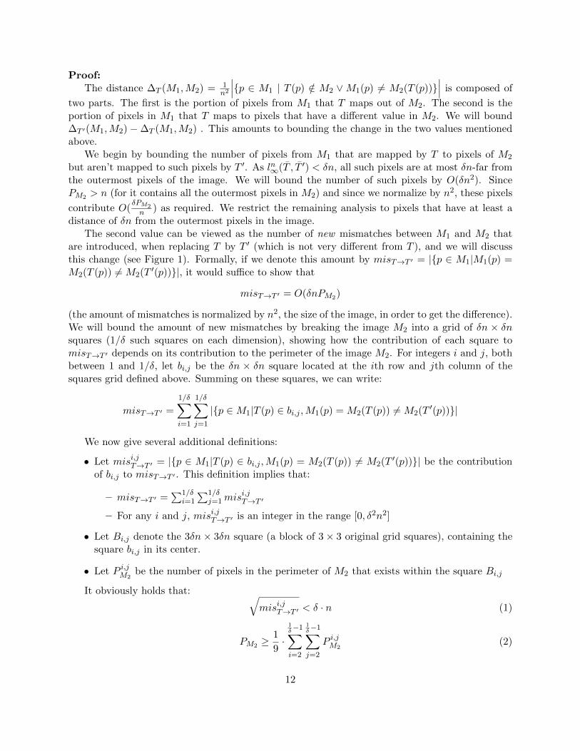
Proof:The distance ∆T (M1,M2) = 1

n2

∣∣∣p ∈ M1 | T (p) /∈ M2 ∨M1(p) 6= M2(T (p))∣∣∣ is composed of

two parts. The first is the portion of pixels from M1 that T maps out of M2. The second is theportion of pixels in M1 that T maps to pixels that have a different value in M2. We will bound∆T ′(M1,M2)−∆T (M1,M2) . This amounts to bounding the change in the two values mentionedabove.

We begin by bounding the number of pixels from M1 that are mapped by T to pixels of M2

but aren’t mapped to such pixels by T ′. As ln∞(T , T ′) < δn, all such pixels are at most δn-far fromthe outermost pixels of the image. We will bound the number of such pixels by O(δn2). SincePM2 > n (for it contains all the outermost pixels in M2) and since we normalize by n2, these pixels

contribute O(δPM2n ) as required. We restrict the remaining analysis to pixels that have at least a

distance of δn from the outermost pixels in the image.The second value can be viewed as the number of new mismatches between M1 and M2 that

are introduced, when replacing T by T ′ (which is not very different from T ), and we will discussthis change (see Figure 1). Formally, if we denote this amount by misT→T ′ = |p ∈ M1|M1(p) =M2(T (p)) 6= M2(T

′(p))|, it would suffice to show that

misT→T ′ = O(δnPM2)

(the amount of mismatches is normalized by n2, the size of the image, in order to get the difference).We will bound the amount of new mismatches by breaking the image M2 into a grid of δn × δnsquares (1/δ such squares on each dimension), showing how the contribution of each square tomisT→T ′ depends on its contribution to the perimeter of the image M2. For integers i and j, bothbetween 1 and 1/δ, let bi,j be the δn × δn square located at the ith row and jth column of thesquares grid defined above. Summing on these squares, we can write:

misT→T ′ =

1/δ∑i=1

1/δ∑j=1

|p ∈M1|T (p) ∈ bi,j ,M1(p) = M2(T (p)) 6= M2(T′(p))|

We now give several additional definitions:

• Let misi,jT→T ′ = |p ∈ M1|T (p) ∈ bi,j ,M1(p) = M2(T (p)) 6= M2(T′(p))| be the contribution

of bi,j to misT→T ′ . This definition implies that:

– misT→T ′ =∑1/δ

i=1

∑1/δj=1mis

i,jT→T ′

– For any i and j, misi,jT→T ′ is an integer in the range [0, δ2n2]

• Let Bi,j denote the 3δn× 3δn square (a block of 3× 3 original grid squares), containing thesquare bi,j in its center.

• Let P i,jM2be the number of pixels in the perimeter of M2 that exists within the square Bi,j

It obviously holds that: √misi,jT→T ′ < δ · n (1)

PM2 ≥1

9·

1δ−1∑i=2

1δ−1∑j=2

P i,jM2(2)

12

Since ln∞(T , T ′) < δn, each pixel p ∈ M1 that is mapped by T into bi,j is certainly mapped byT ′ into Bi,j . It follows that

misi,jT→T ′ = |p ∈M1|T (p) ∈ bi,j , T ′(p) ∈ Bi,j ,M1(p) = M2(T (p)) 6= M2(T′(p))|

misi,jT→T ′ is the sum of pixels p ∈ M1, which are either 0-pixels or 1-pixels. Assume, with outloss of generality, that there are more such 0-pixels. These pixels account for at least half theamount:

misi,jT→T ′ ≤ 2 · |p ∈M1|T (p) ∈ bi,j , T ′(p) ∈ Bi,j , 0 = M1(p) = M2(T (p)) 6= M2(T′(p))|

This implies that there are at least 0.5f(c) ·mis

i,jT→T ′ 0-pixels in bi,j and at least 0.5

f(c) ·misi,jT→T ′

1-pixels in Bi,j where f(c) is a constant depending only on c (since our scaling factors are withinthe range [1c , c], f(c) = O(c2) pixels from M1 are mapped to the same pixel in M2). In particular,

the larger square Bi,j contains at least 0.5f(c) · mis

i,jT→T ′ 0-pixels as well as at least 0.5

f(c) · misi,jT→T ′

1-pixels.Using Claim 4.2, we can conclude that:

P i,jM2≥

√0.5

f(c)·misi,jT→T ′ (3)

and using the bounds of equations (1) and then (2) and (3), we can conclude that:

misT→T ′ =

1δ−1∑i=2

1δ−1∑j=2

misi,jT→T ′ ≤ δ · n ·1/δ∑i=1

1/δ∑j=1

√misi,jT→T ′ ≤ 9

√2f(c)δnPM2

Definition 4.2 Let A be the set of Image-Affine transformations. For a positive α, the set oftransformations T = Tili=1 is an α-cover of A if for every A in A, there exists some Tj in T ,such that ln∞(A, Tj) ≤ α.

We are going to show that for any given n and δ > 0 there’s a δn-cover of A with size thatdoes not depend on n but only on δ. Using this fact, given two images M1 and M2 , we will runAlgorithm 2 on every member of the cover, and get an approximation of ∆(M1,M2). In fact, wefind a transformation T ∈ A that realizes this bound.

Claim 4.3 Let T = Ti`i=1 be a δn-cover of A and let M1,M2 be two n× n images. A transfor-mation T ∈ T such that

|∆T (M1,M2)−∆(M1,M2)| ≤ O(δ

n·max(PM1 , PM2) + ε)

can be found with high probability using O(`/ε2) queries.

13

Figure 1: Consider two δn−close transformations between binary images M1 and M2 (the white/grayareas in the images correspond to 0/1 pixels). The solid and dotted arrows describe the action of the twotransformations on the pixels p1, . . . , p5. The areas between the dashed lines in M2 contain the pixels that areδn−close to boundary pixels. The only pixels in M1 that are possibly mapped correctly by one transformationbut not by the other are those that are mapped into the ’dashed’ area by one of the transformations. In thisexample, only p1 and p5 are mapped correctly by one, but not by the other.

Proof: To find such a transformation T we will run Algorithm 2 for m = Θ(log `) times on eachof the ` transformations Ti with precision parameter ε, and set si as the median of the resultsgiven for Ti. By the correctness of Claim 4.1 and standard amplification techniques, for each i thevalue si will differ from ∆Ti(M1,M2) by at most ε with probability at least 1

3` (we will say such avalue si is correct). Using a union bound we get that the probability of any si not being correct isat most 1/3. This will bound our probability of error, and from here on we assume all the valuessi are indeed correct and show that we will get a transformation as required.

We now consider an image affine transformation A such that ∆(M1,M2) = ∆A(M1,M2). Bythe fact that T is a δn-cover, there exists a transformation Ti such that ln∞(A, Ti) ≤ δn. GivenTheorem 4.1 the value ∆Ti(M1,M2) ≤ ∆(M1,M2) +O( δn ·max(PM1 , PM2)) and thus the minimum

value sj will not exceed ∆(M1,M2) +O( δn ·max(PM1 , PM2) + ε). Choosing the transformation Tjthat this value is associated with, we get that

|∆Tj (M1,M2)−∆(M1,M2)| ≤ O(δ

n·max(PM1 , PM2) + ε)

as required.

In section 4.2 we show the existence of a δn-cover of A whose size is Θ(1/δ6). We can thereforeconclude with the following corollaries:

Corollary 4.2 Given images M1,M2 and constants δ, ε, we have that ∆(M1,M2) can be approxi-mated, using O(1/ε2δ6) queries, with an additive error of O( δn ·max(PM1 , PM2) + ε).

Corollary 4.3 Given images M1,M2 and constants δ, ε such that PM1 = O(n) and PM2 = O(n),∆(M1,M2) can be approximated, using O(1/ε2δ6) queries, with an additive error of O(δ + ε).

14

4.2 Construction of a δn-cover of A

In this section we construct a δn-cover of A, which will be a product of several 1-dimensionaland 2-dimensional grids of transformations, each covering one of the constituting components of astandard decomposition of Affine transformations [7], which is given in the following claim.

Claim 4.4 Every (orientation-preserving) affine transformation matrix A can be decomposed intoA = TR2SR1, where T,Ri, S are translation, rotation and non-uniform scaling matrices 2.

We now describe a 6-dimensional grid, which we will soon prove to be a δn-cover of A, as needed.According to claim 4.4, every affine transformation can be composed of a rotation, scale, rotationand translation. These primitive transformations correspondingly have 1, 2, 1 and 2 degrees offreedom. These are: rotation angle, x and y scales, rotation angle and x and y translations. Itis elementary, for instance, that if we impose a 2-dimensional grid of x and y translations, spacedin each direction by an interval of

√2δn, then for any two neighboring translations T1 and T2 on

this grid it holds that ln∞(T1, T2) < δn. Since the range of possible translations is limited to theinterval [−n, n], the size of the 2-dimensional grid is Θ(1/δ2). Similarly for scaling, we are limitedto the interval [1c , c] and in order to have ln∞(S1, S2) < δn for neighboring scalings we use spacingsof Θ(δ). Likewise, we cover the 1-dimensional space of rotations, with angles in the interval [0, 2π]with spacings of Θ(δ). Finally, by taking the cartesian product of these grids, we end up with asingle grid of size Θ(1/δ6).

It remains to be shown that the grid we defined above, which we denote by G, imposes a δn-coverof A.

Claim 4.5 For every n, for every δ′, there exists a δ′n-cover of A of size Θ(1/δ′6).

Proof: Given the grid G and any image-affine transformation A, if we denote by A′ the nearesttransformation to A on the grid G, we need to show that ln∞(A,A′) < δn. According to claim4.4, A and A′ can be written in the form A = TR2SR1 and A′ = T ′R′2S

′R′1, such that ln∞(T, T ′),ln∞(R1, R

′1), l

n∞(S, S′) and ln∞(R2, R

′2) are all at most δn.

We now measure how differently A and A′ might act on a pixel p, in order to obtain a bound onln∞(A,A′). At each stage we use the triangle inequality, accumulating additional distance introducedby each transformation as well as the ln∞ bounds on the constituting transformations.

‖SR1(p)− S′R′1(p)‖ ≤ ‖S(R1p)− S′(R1p)‖+ ‖S′(R1p)− S′(R′1p)‖= ‖(S − S′)(R1p)‖+ ‖S′(R1p−R′1p)‖≤ δn+ c‖R1p−R′1p‖ = δn+ cδn = (c+ 1)δn

‖R2SR1(p)−R′2S′R′1(p)‖ ≤ ‖R2(SR1p)−R′2(SR1p)‖+ ‖R2(SR1p)−R′2(S′R′1p)‖= ‖(R2 −R′2)(SR1p)‖+ ‖R′2(SR1p− S′R′1p)‖≤ δn+ ‖SR1p− S′R′1p‖ = (c+ 2)δn

2arguments are similar for orientation-reversing transformations (which include reflection)

15

‖A(p)−A′(p)‖ = ‖TR2SR1(p)− T ′R′2S′R′1(p)‖≤ ‖T (R2SR1p)− T ′(R2SR1p)‖+ ‖T ′(R2SR1p)− T ′(R′2S′R′1p)‖= ‖(T − T ′)(R2SR1p)‖+ ‖T ′(R2SR1p−R′2S′R′1p)‖≤ δn+ ‖R2SR1(p)−R′2S′R′1(p)‖ = (c+ 3)δn

The construction follows by setting δ = δ′/(c+ 3).

4.3 3-Dimensional Images

In this section we generalize our techniques and results to 3-dimensional images. One importantapplication of the 3-dimensional (0 − 1) setting is to the problem of aligning 3 dimensional solidobjects, which are represented by 3-dimensional 0− 1 matrices, where the objects are representedby the 1s. The other motivation is the need to handle 2-dimensional grayscale images. This is donein section 4.4, where our algorithm is based on a reduction from grayscale images to 3-dimensional0− 1 images.

In this setting, we are given two images represented by n × n × n 0 − 1 matrices. The imageentries are indexed by voxels, which are triplets in 1, . . . , n3 and the affine transformations inthe 3-d space act on a voxel by first multiplying it with a non-singular 3 × 3 matrix A (whichaccounts for rotation and anisotropic scale), then adding a ’translation’ vector and finally roundingdown to get a new voxel. The distance under a fixed affine transformation T between two imagesM1,M2 is defined in an analogous way to the 2-dimensional case (definition 2.5) and is denotedby d = ∆T (M1,M2). So is the distance between two images with respect to affine transformations(that is ∆(M1,M2)). Voxels are considered adjacent if they differ in each of their coordinates byat most 1 and a voxel is a boundary voxel if it is adjacent to different valued voxels. Finally, theperimeter of the image is the set of its boundary voxels together with its outer 6n2−12n+8 voxels(and it is always Ω(n2) and O(n3)).

Given two images M1,M2 and an affine transformation T we can approximate ∆T (M1,M2)using the same methods as those used in Algorithm 2. The only difference is that we sample voxelsrather than pixels. Thus we have:

Claim 4.6 Given 3-dimensional binary images M1 and M2 of size n× n× n and an image-affinetransformation T , let d = ∆T (M1,M2). There is an algorithm that returns a value d′ such that|d′ − d| ≤ ε with probability 2/3 and performs Θ(1/ε2) queries.

Claim 4.2 generalizes to the following:

Claim 4.7 Given a cubic subsection M of a binary 3-dimensional image with dimensions h×h×h,and an integer b, let PM denote the number of boundary voxels in M . If M contains at least b0-voxels and at least b 1-voxels, then PM = O(b2/3).

Proof: Assume without loss of generality that there are fewer 0-voxels than 1-voxels. We indexthe voxels in M as M(i, j, k). Let us denote by M(i, j, ·) the sum

∑hk=1M(i, j, k), and use M(i, ·, k)

and M(·, j, k) in a similar manner. We first note several facts:

1. h ≥ (2b)1/3

16

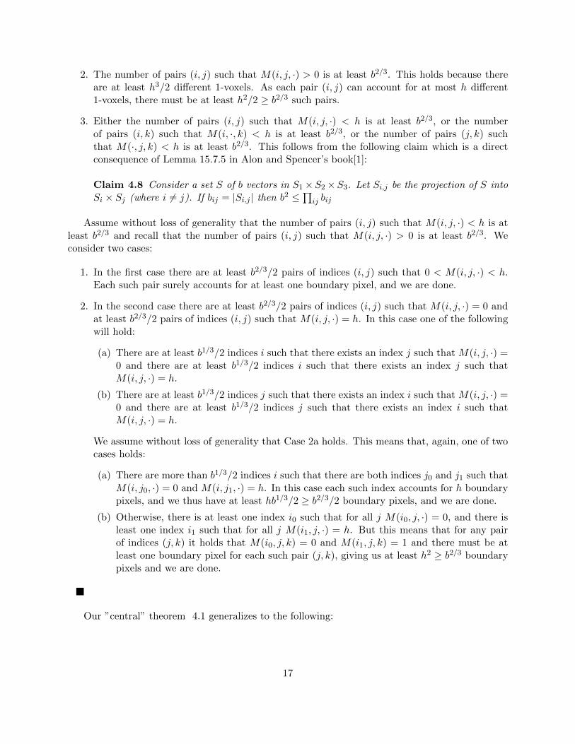
2. The number of pairs (i, j) such that M(i, j, ·) > 0 is at least b2/3. This holds because thereare at least h3/2 different 1-voxels. As each pair (i, j) can account for at most h different1-voxels, there must be at least h2/2 ≥ b2/3 such pairs.

3. Either the number of pairs (i, j) such that M(i, j, ·) < h is at least b2/3, or the numberof pairs (i, k) such that M(i, ·, k) < h is at least b2/3, or the number of pairs (j, k) suchthat M(·, j, k) < h is at least b2/3. This follows from the following claim which is a directconsequence of Lemma 15.7.5 in Alon and Spencer’s book[1]:

Claim 4.8 Consider a set S of b vectors in S1×S2×S3. Let Si,j be the projection of S intoSi × Sj (where i 6= j). If bij = |Si,j | then b2 ≤

∏ij bij

Assume without loss of generality that the number of pairs (i, j) such that M(i, j, ·) < h is atleast b2/3 and recall that the number of pairs (i, j) such that M(i, j, ·) > 0 is at least b2/3. Weconsider two cases:

1. In the first case there are at least b2/3/2 pairs of indices (i, j) such that 0 < M(i, j, ·) < h.Each such pair surely accounts for at least one boundary pixel, and we are done.

2. In the second case there are at least b2/3/2 pairs of indices (i, j) such that M(i, j, ·) = 0 andat least b2/3/2 pairs of indices (i, j) such that M(i, j, ·) = h. In this case one of the followingwill hold:

(a) There are at least b1/3/2 indices i such that there exists an index j such that M(i, j, ·) =0 and there are at least b1/3/2 indices i such that there exists an index j such thatM(i, j, ·) = h.

(b) There are at least b1/3/2 indices j such that there exists an index i such that M(i, j, ·) =0 and there are at least b1/3/2 indices j such that there exists an index i such thatM(i, j, ·) = h.

We assume without loss of generality that Case 2a holds. This means that, again, one of twocases holds:

(a) There are more than b1/3/2 indices i such that there are both indices j0 and j1 such thatM(i, j0, ·) = 0 and M(i, j1, ·) = h. In this case each such index accounts for h boundarypixels, and we thus have at least hb1/3/2 ≥ b2/3/2 boundary pixels, and we are done.

(b) Otherwise, there is at least one index i0 such that for all j M(i0, j, ·) = 0, and there isleast one index i1 such that for all j M(i1, j, ·) = h. But this means that for any pairof indices (j, k) it holds that M(i0, j, k) = 0 and M(i1, j, k) = 1 and there must be atleast one boundary pixel for each such pair (j, k), giving us at least h2 ≥ b2/3 boundarypixels and we are done.

Our ”central” theorem 4.1 generalizes to the following:

17

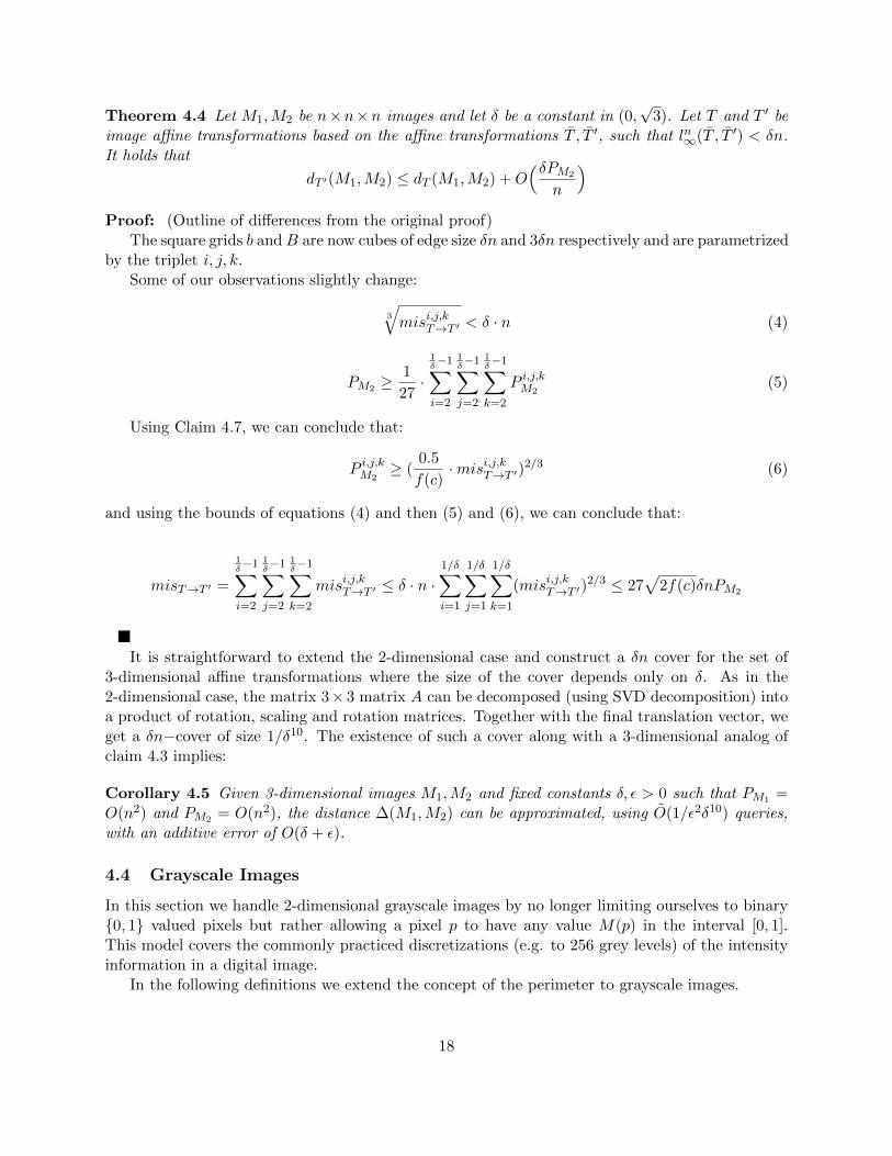
Theorem 4.4 Let M1,M2 be n×n×n images and let δ be a constant in (0,√

3). Let T and T ′ beimage affine transformations based on the affine transformations T , T ′, such that ln∞(T , T ′) < δn.It holds that

dT ′(M1,M2) ≤ dT (M1,M2) +O(δPM2

n

)Proof: (Outline of differences from the original proof)

The square grids b andB are now cubes of edge size δn and 3δn respectively and are parametrizedby the triplet i, j, k.

Some of our observations slightly change:

3

√misi,j,kT→T ′ < δ · n (4)

PM2 ≥1

27·

1δ−1∑i=2

1δ−1∑j=2

1δ−1∑k=2

P i,j,kM2(5)

Using Claim 4.7, we can conclude that:

P i,j,kM2≥ (

0.5

f(c)·misi,j,kT→T ′)

2/3 (6)

and using the bounds of equations (4) and then (5) and (6), we can conclude that:

misT→T ′ =

1δ−1∑i=2

1δ−1∑j=2

1δ−1∑k=2

misi,j,kT→T ′ ≤ δ · n ·1/δ∑i=1

1/δ∑j=1

1/δ∑k=1

(misi,j,kT→T ′)2/3 ≤ 27

√2f(c)δnPM2

It is straightforward to extend the 2-dimensional case and construct a δn cover for the set of3-dimensional affine transformations where the size of the cover depends only on δ. As in the2-dimensional case, the matrix 3× 3 matrix A can be decomposed (using SVD decomposition) intoa product of rotation, scaling and rotation matrices. Together with the final translation vector, weget a δn−cover of size 1/δ10. The existence of such a cover along with a 3-dimensional analog ofclaim 4.3 implies:

Corollary 4.5 Given 3-dimensional images M1,M2 and fixed constants δ, ε > 0 such that PM1 =O(n2) and PM2 = O(n2), the distance ∆(M1,M2) can be approximated, using O(1/ε2δ10) queries,with an additive error of O(δ + ε).

4.4 Grayscale Images

In this section we handle 2-dimensional grayscale images by no longer limiting ourselves to binary0, 1 valued pixels but rather allowing a pixel p to have any value M(p) in the interval [0, 1].This model covers the commonly practiced discretizations (e.g. to 256 grey levels) of the intensityinformation in a digital image.

In the following definitions we extend the concept of the perimeter to grayscale images.

18

Definition 4.3 The gradient of a pixel in a grayscale image M is the maximal absolute differencebetween the pixel value and the pixel values of its adjacent pixels.

Definition 4.4 The perimeter size PM of a grayscale image M is defined as the sum of its pixels’gradients (where the gradient of each of the 4n− 4 outermost pixels of the image is counted as 1).

Notice, that the gradient of a pixel is a real valued number in [0, 1] and that if we consider abinary 0-1 image, its boundary pixels are exactly those with gradient one. Also, the perimeter sizeis Ω(n) and O(n2).

When dealing with binary 0−1 images, our similarity measure between images was defined to bethe maximal similarity between the images with respect to any Affine transformation on the imagepixels. In the grayscale extension we would like to introduce further transformations, allowing ourdistance metric to capture (or be invariant to) illumination changes. That is, we would like toconsider images that differ by a global linear change in pixel values to be similar. Such a linearchange first multiplies all image pixels values by a ’contrast’ factor con and then adds to them a’brightness’ factor bri. As is custom in the field, pixel values that deviate from the [0, 1] interval asa result of such a transformation will be truncated so that they stay within the interval. Also, welimit con to the interval [1/c, c] for some positive constant c and therefore bright can be limited to[−c, 1] (since con maps a pixel value into the range [0, c]). We denote the family of such intensitytransformations by BC.

Definition 4.5 Let T1 and T2 be any two functions from BC. The ln∞ distance between T1 andT2 is defined as the maximum over pixel values v ∈ [0, 1] of max‖T1(v) − T2(v)‖2 (which equalsmax |T1(v)− T2(v)|).

We can now define the distance between grayscale images under a combination of an affine andan intensity transformation.

Definition 4.6 Let T ∈ A be an Affine transformation and let L ∈ BC be and intensity transfor-mation. The distance between grayscale images M1,M2, with respect to T and L is:

∆T,L(M1,M2) =1

n2

∑p∈M1

(1T (p)/∈M2

+ 1T (p)∈M2· |M1(p)− L(M2(T (p)))|

)We can now state our main result:

Claim 4.9 Given n × n grayscale images M1,M2 and positive constants δ and ε, we can findtransformations T ∈ T and L ∈ BC such that with high probability

|∆T,L(M1,M2)−∆(M1,M2)| ≤ O( δn·max(PM1 , PM2) + ε

)using O(1/ε2δ8) queries.

Proof: We will show Claim 4.9 holds by reducing the problem of approximating the distancebetween two 2-dimensional grayscale images to that of approximating the distance between two3-dimensional 0− 1-images. In particular, we will map an n×n grayscale image M to an n×n×nbinary image M ′ defined as follows: M ′(i, j, k) = 1 if and only if M(i, j) ≥ k/n.

19

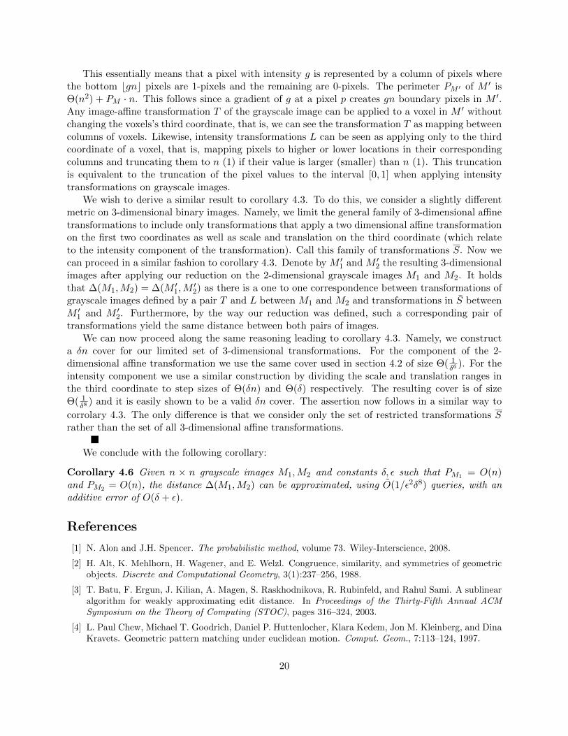
This essentially means that a pixel with intensity g is represented by a column of pixels wherethe bottom bgnc pixels are 1-pixels and the remaining are 0-pixels. The perimeter PM ′ of M ′ isΘ(n2) + PM · n. This follows since a gradient of g at a pixel p creates gn boundary pixels in M ′.Any image-affine transformation T of the grayscale image can be applied to a voxel in M ′ withoutchanging the voxels’s third coordinate, that is, we can see the transformation T as mapping betweencolumns of voxels. Likewise, intensity transformations L can be seen as applying only to the thirdcoordinate of a voxel, that is, mapping pixels to higher or lower locations in their correspondingcolumns and truncating them to n (1) if their value is larger (smaller) than n (1). This truncationis equivalent to the truncation of the pixel values to the interval [0, 1] when applying intensitytransformations on grayscale images.

We wish to derive a similar result to corollary 4.3. To do this, we consider a slightly differentmetric on 3-dimensional binary images. Namely, we limit the general family of 3-dimensional affinetransformations to include only transformations that apply a two dimensional affine transformationon the first two coordinates as well as scale and translation on the third coordinate (which relateto the intensity component of the transformation). Call this family of transformations S. Now wecan proceed in a similar fashion to corollary 4.3. Denote by M ′1 and M ′2 the resulting 3-dimensionalimages after applying our reduction on the 2-dimensional grayscale images M1 and M2. It holdsthat ∆(M1,M2) = ∆(M ′1,M

′2) as there is a one to one correspondence between transformations of

grayscale images defined by a pair T and L between M1 and M2 and transformations in S betweenM ′1 and M ′2. Furthermore, by the way our reduction was defined, such a corresponding pair oftransformations yield the same distance between both pairs of images.

We can now proceed along the same reasoning leading to corollary 4.3. Namely, we constructa δn cover for our limited set of 3-dimensional transformations. For the component of the 2-dimensional affine transformation we use the same cover used in section 4.2 of size Θ( 1

δ6). For the

intensity component we use a similar construction by dividing the scale and translation ranges inthe third coordinate to step sizes of Θ(δn) and Θ(δ) respectively. The resulting cover is of sizeΘ( 1

δ8) and it is easily shown to be a valid δn cover. The assertion now follows in a similar way to

corrolary 4.3. The only difference is that we consider only the set of restricted transformations Srather than the set of all 3-dimensional affine transformations.

We conclude with the following corollary:

Corollary 4.6 Given n × n grayscale images M1,M2 and constants δ, ε such that PM1 = O(n)and PM2 = O(n), the distance ∆(M1,M2) can be approximated, using O(1/ε2δ8) queries, with anadditive error of O(δ + ε).

References

[1] N. Alon and J.H. Spencer. The probabilistic method, volume 73. Wiley-Interscience, 2008.

[2] H. Alt, K. Mehlhorn, H. Wagener, and E. Welzl. Congruence, similarity, and symmetries of geometricobjects. Discrete and Computational Geometry, 3(1):237–256, 1988.

[3] T. Batu, F. Ergun, J. Kilian, A. Magen, S. Raskhodnikova, R. Rubinfeld, and Rahul Sami. A sublinearalgorithm for weakly approximating edit distance. In Proceedings of the Thirty-Fifth Annual ACMSymposium on the Theory of Computing (STOC), pages 316–324, 2003.

[4] L. Paul Chew, Michael T. Goodrich, Daniel P. Huttenlocher, Klara Kedem, Jon M. Kleinberg, and DinaKravets. Geometric pattern matching under euclidean motion. Comput. Geom., 7:113–124, 1997.

20

[5] M. Gavrilov, P. Indyk, R. Motwani, and S. Venkatasubramanian. Combinatorial and experimentalmethods for approximate point pattern matching. Algorithmica, 38(1):59–90, 2003.

[6] U. Hahn, N. Chater, and L.B. Richardson. Similarity as transformation. Cognition, 87(1):1–32, 2003.

[7] R. Hartley and A. Zisserman. Multiple view geometry in computer vision. Cambridge university press,2008.

[8] C. Hundt and M. Liskiewicz. Combinatorial bounds and algorithmic aspects of image matching underprojective transformations. Mathematical Foundations of Computer Science 2008, pages 395–406, 2008.

[9] C. Hundt and M. Liskiewicz. New complexity bounds for image matching under rotation and scaling.Journal of Discrete Algorithms, 2010.

[10] I. Kleiner, D. Keren, I. Newman, and O. Ben-Zwi. Applying property testing to an image partitioningproblem. IEEE Trans. Pattern Anal. Mach. Intell., 33(2):256–265, 2011.

[11] G.M. Landau and U. Vishkin. Pattern matching in a digitized image. Algorithmica, 12(4):375–408,1994.

[12] R.P. Millane, S. Alzaidi, and W.H. Hsiao. Scaling and power spectra of natural images. In Proceedingsof Image and Vision Computing New Zealand, pages 148–153, 2003.

[13] S. Raskhodnikova. Approximate testing of visual properties. In Proceedings of the Seventh InternationalWorkshop on Randomization and Approximation Techniques in Computer Science (RANDOM), pages370–381, 2003.

[14] R. Szeliski. Image alignment and stitching: A tutorial. Foundations and Trends® in Computer Graphicsand Vision, 2(1):1–104, 2006.

[15] G. Tsur and D. Ron. Testing properties of sparse images. In FOCS, pages 468–477. IEEE ComputerSociety, 2010.

[16] A. Tversky. Features of similarity. Psychological review, 84(4):327, 1977.

[17] A. van der Schaaf and J.H. van Hateren. Modelling the power spectra of natural images: statistics andinformation. Vision Research, 36(17):2759–2770, 1996.

[18] R.C. Veltkamp. Shape matching: Similarity measures and algorithms. In smi, page 0188. Published bythe IEEE Computer Society, 2001.

[19] B. Zitova and J. Flusser. Image registration methods: a survey. Image and vision computing, 21(11):977–1000, 2003.

21