Convergence Analysis of Tight Framelet Approach for Missing Data

Recovery

Jian-Feng Cai∗, Raymond H. Chan†, Lixin Shen‡, and Zuowei Shen§

Abstract

How to recover missing data from an incomplete samples is a fundamental problem in math-ematics and it has wide range of applications in image analysis and processing. Although manyexisting methods, e.g. various data smoothing methods and PDE approaches, are availablein the literature, there is always a need to find new methods leading to the best solution ac-cording to various cost functionals. In this paper, we propose an iterative algorithm based ontight framelets for image recovery from incomplete observed data. The algorithm is motivatedfrom our framelet algorithm used in high-resolution image reconstruction and it exploits theredundance in tight framelet systems. We prove the convergence of the algorithm and also giveits convergence factor. Furthermore, we derive the minimization properties of the algorithmand explore the roles of the redundancy of tight framelet systems. As an illustration of theeffectiveness of the algorithm, we give an application of it in impulse noise removal.

1 Introduction

The recovery of missing data from incomplete data is an essential part of any image processingprocedures whether the final image is to be utilized for visual interpretation or for automaticanalysis. The problem can be formulated as follows. Let f be the original image defined on animage domain Ω and (f+ǫ)|Λ be the observable data on Λ ⊂ Ω. Here ǫ is the noise. The task of themissing data recovery is to find or approximate f on Ω\Λ from the available data (f+ǫ)|Λ such thatthe restored image retains as many important image features of (f + ǫ)|Λ as possible. The problemarises, for examples, in image inpainting and impulse noise removal. A number of approaches forsolving the problem has been proposed in recent years, see, for examples, [2, 4, 10, 11, 19, 20, 25].

In our previous work [4, 10], we proposed iterative algorithms based on tight frames for recov-ering images from missing data. In each iteration of these algorithms, we modify the tight framecoefficients of each iterate via some thresholding operators. This has a built-in regularization effectin the sense that the tight frame coefficients minimize a functional which penalizes a weightedℓ1 norm of the tight frame coefficients as well as the distance between these coefficients and therange of the underlying tight frame system. The effect allows the tight frame coefficients from Λ

∗Temasek Laboratories and Department of Mathematics, National University of Singapore, 2 Science Drive 2,

Singapore 117543. Email:tslcaij@nus.edu.sg†Department of Mathematics, The Chinese University of Hong Kong, Shatin, N.T., Hong Kong, P. R. China.

Email:rchan@math.cuhk.edu.hk. The research was supported in part by HKRGC Grant 400505 and CUHK DAG

2060257.‡Department of Mathematics, Syracuse University, Syracuse, NY 13244. Email: lshen03@syr.edu. The research

was supported by the US National Science Foundation under grant DMS-0712827.§Department of Mathematics, National University of Singapore, 2 Science Drive 2, Singapore 117543. Email:

matzuows@nus.edu.sg. The research was supported in part by Grant R-146-000-060-112 at the National University

of Singapore.

1

to affect the tight frame coefficients in Ω \ Λ in a smooth way. By interpreting the algorithm as aproximal forward-backward splitting [13] iteration for a minimization problem, we proved in [4] theconvergence of the algorithm and found the minimization properties that the limit of the algorithmsatisfies. However, there is no result on the rate of the convergence of the algorithm.

To obtain an algorithm with a convergence factor, in this paper we modify the algorithms in[4, 10] by fixing the scaling (i.e., low-frequency) coefficients of each iteration to be those of the initialguess. We prove that the modified algorithm converges provided that a low-pass filtering matrixassociated with the low-pass filter of the tight frame system is nonsingular. We then show that theconvergence factor of the new algorithm depends on the smallest singular value of this low-passfiltering matrix. We also prove that the non-singularity of the matrix can always be satisfied byadjusting the size of the images. Furthermore, we present the minimization properties of the limitof the new algorithm, and explore the roles of the redundancy of tight frame systems. We thenshow the efficiency of our algorithm by applying it to impulse noise removal.

The outline of this paper is as follows: In Section 2, we briefly introduce the tight frame theory.In Section 3, we review the framelet-based missing data recovery algorithms in [4, 10], and proposeour new modified algorithm. In Section 4, we prove the convergence of the new algorithm andgive the minimization properties of the solution (i.e., the limit) of the algorithm. In Section 5, weintroduce the impulse noise models and adapt our new algorithm to impulse noise removal. Thenumerical tests are presented in Section 6 and conclusions are given in Section 7.

2 Tight Frames

In this section, we review some basics of tight frames that are sufficient to present our algorithmin this paper. More detailed theory can be found, for example, in [14, 16, 27].

Let A be a K-by-N (K ≥ N) matrix whose rows are vectors in RN . The system, also denoted

by A, consisting of all the rows of A, is a tight frame for RN if for an arbitrary f ∈ R

N ,

‖f‖2 =∑

g∈A

|〈f, g〉|2.

The associated analysis operator is defined again as A : RN → R

K with

Af = 〈f, g〉g∈A, ∀f ∈ RN .

Its adjoint operator, the synthesis operator, is A∗ : RK → R

N with

A∗c =∑

g∈A

cgg, c = cgg∈A.

Hence, A is a tight frame if and only if A∗A = I. When kerA∗ 6= 0, the system A is redundantand AA∗ 6= I. If a tight frame satisfies kerA∗ = 0, then it becomes an orthogonal basis.

The tight frame A used in our algorithm are generated from the spline wavelet frame filters byusing the unitary extension principle given in [27]. Let us mention how they are generated. Let

h0(ω) = cos2m(ω/2). (2.1)

Note that the trigonometric polynomial h0 is the refinement symbol of the B-spline

φ(ω) =sin2m(ω/2)

(ω/2)2m

2

of order 2m. The wavelets corresponding to φ are given by

ψn(ω) = hn(ω/2)φ(ω/2)

with wavelet masks

hn(ω) =

√(2mn

)sinn(ω/4) cos2m−n(ω/4), (2.2)

for 1 ≤ n ≤ 2m. The low-pass filter (scaling mask) h0 and the high-pass filters (wavelet masks) hn,1 ≤ n ≤ 2m satisfy the condition of the unitary extension principle (see [27])

2m∑

k=0

|hk(ω)|2 = 1 and2m∑

k=0

hk(ω)hk(ω + π) = 0 (2.3)

for ω ∈ [−π, π]. It is shown in [27] that the system X = 2k/2ψn(2k · −j) : k, j ∈ Z;n = 1, . . . , 2mis a tight framelet system. The choices of m = 1 and m = 2 give the so-called piecewise linearand piecewise cubic tight framelet systems, respectively. Specifically, the filters associated with thepiecewise cubic tight framelet systems are

h0 =1

16[1, 4, 6, 4, 1]; h1 =

1

8[1, 2, 0,−2,−1];

h2 =

√6

16[−1, 0, 2, 0,−1]; h3 =

1

8[−1, 2, 0,−2, 1]; h4 =

1

16[1,−4, 6,−4, 1].

where h0 is the low-pass filter while hk, 1 ≤ k ≤ 2m, are the high-pass filters. The filters h0, h2,h4 are symmetric while h1, h3 are antisymmetric.

From the given spline tight framelet filters hk, 0 ≤ k ≤ 2m, we can design a tight frame systemA associated with these filters. Let h be a filter with length 2m+ 1, i.e.,

h = [h(−m), h(−m + 1), . . . , h(−1), h(0), h(1), . . . , h(m− 1), h(m)]. (2.4)

If Neumann boundary condition is used, then the matrix representation of h will be an N -by-Nmatrix H given by

[H]i,j =

h(i− j) + h(i+ j − 1), if i+ j ≤ (m+ 1),h(i− j) + h(−1 − (2n − i− j)) if i+ j ≥ 2N −m+ 1,h(i− j) otherwise.

(2.5)

When the filter h is symmetric, the resulting matrix H will have a Hankel-plus-Toeplitz structureand its spectra can be computed easily, see [24]. We note that Neumann boundary conditionsusually produce restored images having less artifacts near the boundary, see [6, 24] for instances.

Next we define the matrices Lk and Hk:

Lk = H(k)0 H

(k−1)0 · · ·H(1)

0 and Hk =

H

(k)1 Lk−1

...

H(k)2mLk−1

, k > 0, (2.6)

where H(ℓ)k are the matrix representations of the filters formed from hk by inserting 2ℓ−1 − 1 zeros

between every two adjacent components of hk. With Lk and Hk in hand, for any given integer

3

L > 0, a matrix A induced from the spline tight framelets is given as follows

A :=

LL

HL

HL−1...

H1

≡

LL

AL

. (2.7)

Applying (2.3), one obtains

L∗kLk + H∗

kHk = L∗k−1Lk−1, 0 < k ≤ L,

which leads toA∗A = I, and L∗

LLL + A∗LAL = I.

Hence, A is a tight frame in RN , and ‖Av‖ = ‖v‖ for all v ∈ R

N .So far we have only considered tight framelet systems in 1-D. Since images are 2-D objects, when

we handle images, we use tensor product tight framelet system generated by the corresponding

univariate tight framelet system. Let H(ℓ)k , 0 ≤ k ≤ 2m and 1 ≤ ℓ < L, be matrices used in (2.6).

DefineG

(ℓ)(2m+1)i+j := H

(ℓ)i ⊗H

(ℓ)j (2.8)

where 0 ≤ i, j ≤ 2m. Clearly(2m+1)2−1∑

k=0

(G(ℓ)k )∗G

(ℓ)k = I.

We then define

Lk := G(k)0 G

(k−1)0 · · ·G(1)

0 and Hk :=

G(k)1 Lk−1

...

G(k)(2m+1)2−1

Lk−1

. (2.9)

With these notations, we can similarly form the matrices A and AL using (2.7).

3 Algorithms for Recovering Missing Data

In the first part of this section, we give a brief review of the framelet-based algorithm proposed in[4, 10] for the recovery of missing data. The algorithm is motivated by the redundant nature of thetight frame system and it has been applied to high-resolution image reconstruction [9]. The ideawas first mentioned in [6] for frames generated by bi-orthogonal wavelet systems. In the secondpart of the section, we propose a new algorithm by modifying the algorithm proposed in [4, 10].

Recall that we are given g = f + ǫ on Λ and like to recover f in Ω \ Λ. Define the projectionoperator

PΛg(i) =

g(i), i ∈ Λ,

0, i ∈ Ω\Λ,(3.1)

where g(i) is the grey-level of the pixel i. Here we are raster scanning images column by column toobtain the vector representations of the images. Starting with the identities f = PΛf + (I − PΛ)fand f = A∗Af , we have

f = PΛf + (I − PΛ)A∗Af. (3.2)

4

Given a non-negative vector u and a vector w, we define the thresholding operator Du as follows

Duw :=[tu(0)(w(0)), tu(1)(w(1)), . . .

]t, (3.3)

where tλ(x) := sgn(x)max(|x| − λ, 0) is the soft thresholding function [15]. The framelet-basedalgorithm in [4, 10] is as follows:

fk+1 = PΛf0 + (I − PΛ)A∗DuAfk, k = 0, 1, · · · , (3.4)

where f0 := g. We remark that a similar algorithm was also proposed in [19, 20] when A isorthonormal or a union of wavelet systems.

The thresholding operator Du plays two roles. On the one hand, it removes noise. On theother hand, it gives a small perturbation of the frame coefficients Afk, which makes it possibleto permeate information contained in the given data to those places where the data is missing.As we know, in the identity fk = A∗Afk, Afk is not only the vector of frame coefficients of fk

under the system A, but it also has the smallest ℓ2 norm among those vectors which can perfectlyrepresent fk (see e.g. [14]). In this sense, at each iteration, the algorithm automatically has abuilt-in regularization effect which minimizes the ℓ2 norm of the frame coefficients of fk among allthe choices. We make the claim more precise below.

Let αk := DuAfk. In [4], we proved that (3.4) can be viewed as a proximal forward-backwardsplitting (PFBS) iteration on αk. Moreover, using the convergence theory for PFBS in [13], wehave shown that (3.4) converges, and the sequence αk converges to a minimizer of

minα

1

2‖PΛ(f0 −A∗α)‖2 +

1

2‖(I −AA∗)α‖2 + ‖diag(u)α‖1

. (3.5)

Note that

• the term ‖PΛ(f0 −A∗α)‖2 measures the closeness of the recovered image to the given data,

• the term ‖(I −AA∗)α‖2 is the distance of α to the range of A, and

• the term ‖diag(u)α‖1 is related to the sparsity of the solution α.

Thus we see that αk is in fact minimizing a regularized functional.As shown in [4, 10], the algorithm in (3.4) performs well in our numerical experiments. However,

the convergence rate of the algorithm is not available and cannot be derived using the convergencetheory for PFBS in [13]. The goal of this paper is to modify this algorithm to a new algorithm thathas a convergence rate.

For this, we first rewrite (3.4). We partition the non-negative vector u in (3.4) as

u =

[u1

u2

], (3.6)

where u1 is a zero vector with size the same as the number of rows of LL, and the size of u2 equalsthe number of rows of AL. If we define the thresholding operator T as

T ALv := Du2(ALv), (3.7)

(i.e., we do not threshold the low-frequency coefficients), then (3.4) becomes

fk+1 = PΛf0 + (I − PΛ)A∗

[LLf

k

T (ALfk)

], k = 0, 1, · · · . (3.8)

5

In [4], we proved that the sequence αk =

[LLf

k

T (ALfk)

]converges to a minimizer for (3.5).

The main change in our new algorithm is that we fix the low-frequency coefficients of eachiteration in (3.8) to be those of the initial guess. This leads to the following new algorithm.

Algorithm 1 (Missing Data Recovering Algorithm)Let f|Λ be given and f0 be the initial guess satisfying PΛf

0 = f|Λ. Define

fk+1 = PΛf0 + (I − PΛ)A∗

[LLf

0

T (ALfk)

], k = 0, 1, · · · . (3.9)

The initial seed f0 is normally chosen by spline interpolation, e.g., cubic spline interpolation oras the given data for the simplicity. Since spline interpolation provides a good approximation forsmooth functions, the low frequency component LLf

0 of f0 approximates well to the low frequencycontent of the original image. Iterative algorithm (3.9) is essentially the same as (3.8). The onlydifference is that the term LLf

k in (3.8) is replaced by LLf0 in (3.9). When L is sufficiently large,

LL is a long low-pass filter. Hence, both the difference between LLf0 and LLf

k contains mainlylow frequency content of the original image. In the next section, we will see that by fixing LLf

0, wecan prove the convergence of the new algorithm and obtain its convergence rate. Our convergenceproof here is different from that given in [4] for (3.8). In fact, we will prove that the framelet

coefficient β =

[LLf

0

T ALv

], where v is the limit of fk of (3.9), is a minimizer of

minα1=LLf0

1

2‖PΛ(f0 −A∗α)‖2 +

1

2‖(I −AA∗)α‖2 + ‖diag(u)α‖1

, (3.10)

where α1 denotes the partition of α according to LL. Clearly (3.10) is a constrained version of(3.5), and hence (3.9) is actually solving a constrained minimization problem. A different initialseed f0 leads to a different constraint in the above minimization problem, hence, gives a differentsolution.

4 Analysis of Algorithm 1

This section consists of three parts. In the first part, we prove that Algorithm 1 converges, andthen we obtain its convergence factor. In the second part, we derive the minimization propertiessatisfied by the limit of Algorithm 1. In the last part, we explain the role of the redundance of thetight frame system in the algorithm.

4.1 Convergence

To prove the convergence of Algorithm 1, we need the contracting property of the thresholdingoperator defined in (3.7). This contracting property as stated in the following lemma is crucial inthe proof of the convergence and in deriving the optimal properties of the algorithm.

Lemma 4.1 For any two vectors v1 and v2, we have

‖T AL(v1) − T AL(v2)‖ ≤ ‖v1 − v2‖.

In particular, T AL is a continuous map.

6

Proof: Due to |tλ(x) − tλ(y)| ≤ |x − y| for arbitrary real numbers x and y, and ‖ALv‖ ≤ ‖v‖ forany vector v, we have, for any two vectors v1 and v2,

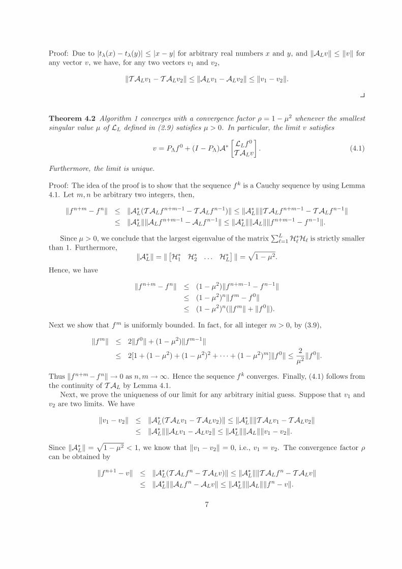
‖T ALv1 − T ALv2‖ ≤ ‖ALv1 −ALv2‖ ≤ ‖v1 − v2‖. 2Theorem 4.2 Algorithm 1 converges with a convergence factor ρ = 1 − µ2 whenever the smallestsingular value µ of LL defined in (2.9) satisfies µ > 0. In particular, the limit v satisfies

v = PΛf0 + (I − PΛ)A∗

[LLf

0

T ALv

]. (4.1)

Furthermore, the limit is unique.

Proof: The idea of the proof is to show that the sequence fk is a Cauchy sequence by using Lemma4.1. Let m,n be arbitrary two integers, then,

‖fn+m − fn‖ ≤ ‖A∗L(T ALf

n+m−1 − T ALfn−1)‖ ≤ ‖A∗

L‖‖T ALfn+m−1 − T ALf

n−1‖≤ ‖A∗

L‖‖ALfn+m−1 −ALf

n−1‖ ≤ ‖A∗L‖‖AL‖‖fn+m−1 − fn−1‖.

Since µ > 0, we conclude that the largest eigenvalue of the matrix∑L

ℓ=1 H∗ℓHℓ is strictly smaller

than 1. Furthermore,‖A∗

L‖ = ‖[H∗

1 H∗2 . . . H∗

L

]‖ =

√1 − µ2.

Hence, we have

‖fn+m − fn‖ ≤ (1 − µ2)‖fn+m−1 − fn−1‖≤ (1 − µ2)n‖fm − f0‖≤ (1 − µ2)n(‖fm‖ + ‖f0‖).

Next we show that fm is uniformly bounded. In fact, for all integer m > 0, by (3.9),

‖fm‖ ≤ 2‖f0‖ + (1 − µ2)‖fm−1‖≤ 2[1 + (1 − µ2) + (1 − µ2)2 + · · · + (1 − µ2)m]‖f0‖ ≤ 2

µ2‖f0‖.

Thus ‖fn+m−fn‖ → 0 as n,m→ ∞. Hence the sequence fk converges. Finally, (4.1) follows fromthe continuity of T AL by Lemma 4.1.

Next, we prove the uniqueness of our limit for any arbitrary initial guess. Suppose that v1 andv2 are two limits. We have

‖v1 − v2‖ ≤ ‖A∗L(T ALv1 − T ALv2)‖ ≤ ‖A∗

L‖‖T ALv1 − T ALv2‖≤ ‖A∗

L‖‖ALv1 −ALv2‖ ≤ ‖A∗L‖‖AL‖‖v1 − v2‖.

Since ‖A∗L‖ =

√1 − µ2 < 1, we know that ‖v1 − v2‖ = 0, i.e., v1 = v2. The convergence factor ρ

can be obtained by

‖fn+1 − v‖ ≤ ‖A∗L(T ALf

n − T ALv)‖ ≤ ‖A∗L‖‖T ALf

n − T ALv‖≤ ‖A∗

L‖‖ALfn −ALv‖ ≤ ‖A∗

L‖‖AL‖‖fn − v‖.

7

Therefore, ρ = ‖A∗L‖‖AL‖ = 1 − µ2. 2

Next we show that the smallest singular value µ of LL is indeed greater than zero if we choose Nproperly. To do this, we review a remarkable property of the matrix H in (2.5) if the sequence h issymmetric, i.e., h(j) = h(−j), j = 0, 1, . . . ,m. It was stated in [24] that the matrix H in (2.5) canalways be diagonalized by the discrete cosine transform (DCT) and the corresponding eigenvectorsof H are simply the DCT of the first column of the matrix H if the sequence h is symmetric. Moreprecisely, let C be the N -by-N discrete cosine transform matrix. Its entries are

[C]p,q =

√2 − δp1

Ncos

((p − 1)(2q − 1)π

2N

), 1 ≤ p, q ≤ N, (4.2)

where δpq is the Kronecker delta. We note that C is orthogonal, i.e., CtC = CCt = I. It isproven in [24] that H = CtΓC, where Γ is the diagonal matrix containing the eigenvalues of H. Bymultiplying e1 = (1, 0, . . . , 0)t to both sides of CH = ΓC, we see that the eigenvalues γp of H aregiven by

γp =[C(He1)]p+1

[Ce1]p+1, 0 ≤ p < N. (4.3)

Using (4.2), (4.3) reduces to:

γp =

∑Nq=1[He1]q cos[(2q − 1)θp]

cos θp, 0 ≤ p < N, (4.4)

where θp = pπ/(2N), i.e. 0 ≤ θp < π/2.For the symmetric sequence h given in (2.4), the first column of H is given by:

[h(0) + h(1), h(1) + h(2), . . . , h(m − 1) + h(m), h(m), 0, . . . , 0]t.

Hence,

N∑

q=1

[He1]q cos[(2q − 1)θ] =m+1∑

q=1

h(q − 1) cos[(2q − 1)θ] +m∑

q=1

h(q) cos[(2q − 1)θ]

= cos θ

m∑

q=−m

h(q)e−i2qθ.

Therefore,

γp =m∑

q=−m

h(q)e−i2qθp , 0 ≤ p < N.

Immediately, we have the following result:

Proposition 4.3 Let H(ℓ)0 be the matrix representation of the filter formed from the low-pass filter

h0 of the 2m-th spline by inserting 2ℓ−1 − 1 zeros between every two adjacent components of h0.

Then the matrix H(ℓ)0 has eigenvalues γ

(ℓ)p = cos2m(2ℓ−1θp), where θp = pπ

2N for 0 ≤ p < N . Inparticular, for LL defined in (2.9), the smallest eigenvalue µ2 of L∗

LLL is positive if 2L−1p is notdivisible by N for all 1 ≤ p < N .

8

Proof: Since h0 is the low-pass filter of the 2m-th spline whose symbol h0 is given in (2.1), wehave

m∑

q=−m

h0(q)e−iqω = cos2m

(ω2

).

It follows that the symmetric matrix H(ℓ)0 has eigenvalues γℓ,p = cos2m(2ℓ−1θp), 0 ≤ p < N . Since

H(ℓ)0 , 1 ≤ ℓ ≤ L, can be diagonalized the DCT, so does the matrix LL in (2.6). Furthermore, the

matrix LL has eigenvalues

γp := γL,pγL−1,p · · · γ1,p = cos2m(2L−1θp) cos2m(2L−2θp) · · · cos2m(20θp) =

(sin(2Lθp)

2L sin θp

)2m

,

where 0 ≤ p < N . Clearly, γ0 = 1. Note that sin θp 6= 0 for all 1 ≤ p ≤ N − 1. Hence, for a giveninteger p between 1 and N − 1, γp being zero happens only when sin(2Lθp) = 0. If so, 2Lθp is a

multiple of π, that is, 2Lp2N must be an integer since θp = pπ

2N . In other words, 2L−1p is divisibleby N . Thus, sin(2Lθp) 6= 0 if 2L−1p are not divisible by N for all 1 ≤ p ≤ N − 1. Therefore γp,0 ≤ p < N , are all positive. For LL defined in (2.9), because of its tensor product definition, all itseigenvalues are of the form γpγq with 0 ≤ p, q < N . Hence they are all positive too under the sameassumption. In particular, the smallest eigenvalue of L∗

LLL is positive too. 2Thus we see that by choosing the size of the image N appropriately, the assumption of Theorem

4.2 can be satisfied and Algorithm 1 converges. For example, we will use N = 255 and N = 511in our experiments. Finally, we note that one can always enlarge the image size N by using, forexample, symmetric extension such that N satisfies the assumption in Proposition 4.3.

4.2 Minimization

Next we study the minimization properties of the limit of Algorithm 1. Define a new sequence αk

in the framelet domain by

αk :=

[LLf

0

T ALfk

], k = 1, 2, · · · . (4.5)

In terms of αk, Algorithm 1 can be rewritten as

αk+1 =

[LLf

0

T AL

(PΛf

0 + (I − PΛ)A∗αk)], k = 0, 1, · · · . (4.6)

By Lemma 4.1, the mapping from fk to αk is continuous. It, together with Theorem 4.2 whichstates that fk converges, implies that αk converges. Denote the limit

β := limk→∞

αk. (4.7)

Due to Lemma 4.1, the mapping from αk to αk+1 is also continuous. Therefore, the limit β satisfies

β =

[LLf

0

T AL

(PΛf

0 + (I − PΛ)A∗β)]. (4.8)

Moreover, the limit is unique.For any framelet coefficient vector α ∈ R

K , we partition it as follows

α =

[α1

α2

],

9

where α1 is the framelet coefficients corresponding to LL, and α2 is those corresponding to AL. Wewill show in the following that β is a minimizer of the minimization problem

minα1=LLf0

F (α), (4.9)

where

F (α) =1

2‖PΛ(f0 −A∗α)‖2 +

1

2‖(I −AA∗)α‖2 + ‖diag(u)α‖1 (4.10)

with u being defined in (3.6). Comparing (4.9) with (3.5), the latter is an unconstrained version ofthe former.

In order to prove that β is a minimizer for (4.9), we need some notations in convex analysis.We only consider the case of finite dimensional Euclidean space R

K having the Euclidean innerproduct. For any proper, lower semi-continuous and convex function ϕ(x), where x ∈ R

K , itssubdifferential is defined by

∂ϕ(x) :=w ∈ R

K | ∀y ∈ RK , 〈y − x,w〉 + ϕ(x) ≤ ϕ(y)

.

When ϕ(x) is differentiable, the subdifferential is the ordinary gradient. According to the Fermat’srule,

ϕ(x) = infy∈RK

ϕ(y) ⇐⇒ 0 ∈ ∂ϕ(x). (4.11)

The proximity operator of ϕ is defined by

proxϕ(x) := arg miny∈RK

1

2‖x− y‖2 + ϕ(y)

.

For any convex set Γ ⊂ RK , the indicator function is defined by

ιΓ(x) :=

0, if x ∈ Γ,

+∞, otherwise.(4.12)

It is shown (see (2.8) in [13]) that

∂ιΓ(x) =

w ∈ R

K | ∀y ∈ Γ, 〈y − x,w〉 ≤ 0, if x ∈ Γ,

∅, otherwise.(4.13)

We need the following lemmas.

Lemma 4.4 For any y ∈ RK , the thresholding operator T satisfies

y2 − T (y2) ∈ ∂‖diag(u2)T (y2)‖1.

Proof: It follows, for example, from [13] that

tλ(a) = arg minb∈R

1

2(a− b)2 + λ|b|

.

Therefore, by the definition of T (y2) and (3.3), we obtain

T (y2) = arg minx∈R

K2

1

2‖y2 − x‖2 + ‖diag(u2)x‖1

,

10

where K2 is the number of rows in AL. By (4.11), the above equality is equivalent to

0 ∈ ∂

1

2‖y2 − x‖2 + ‖diag(u)x‖1

∣∣∣x=T (y2)

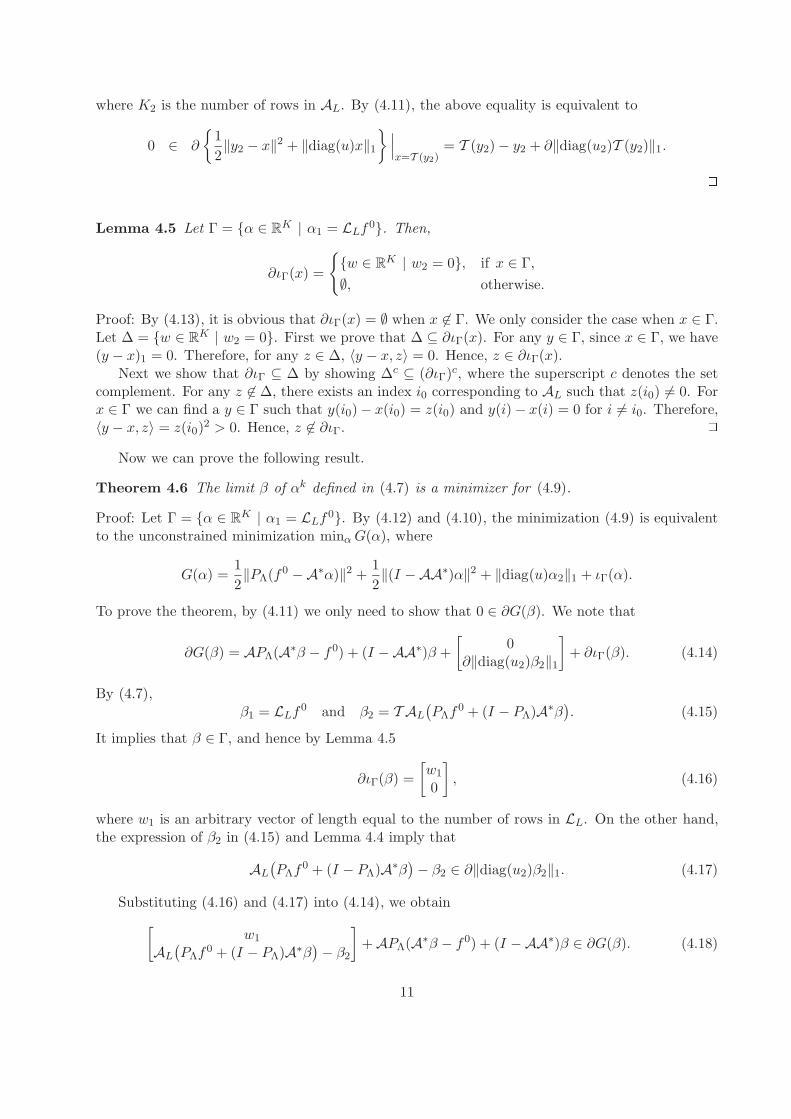
= T (y2) − y2 + ∂‖diag(u2)T (y2)‖1. 2Lemma 4.5 Let Γ = α ∈ R

K | α1 = LLf0. Then,

∂ιΓ(x) =

w ∈ R

K | w2 = 0, if x ∈ Γ,

∅, otherwise.

Proof: By (4.13), it is obvious that ∂ιΓ(x) = ∅ when x 6∈ Γ. We only consider the case when x ∈ Γ.Let ∆ = w ∈ R

K | w2 = 0. First we prove that ∆ ⊆ ∂ιΓ(x). For any y ∈ Γ, since x ∈ Γ, we have(y − x)1 = 0. Therefore, for any z ∈ ∆, 〈y − x, z〉 = 0. Hence, z ∈ ∂ιΓ(x).

Next we show that ∂ιΓ ⊆ ∆ by showing ∆c ⊆ (∂ιΓ)c, where the superscript c denotes the setcomplement. For any z 6∈ ∆, there exists an index i0 corresponding to AL such that z(i0) 6= 0. Forx ∈ Γ we can find a y ∈ Γ such that y(i0)− x(i0) = z(i0) and y(i) − x(i) = 0 for i 6= i0. Therefore,〈y − x, z〉 = z(i0)

2 > 0. Hence, z 6∈ ∂ιΓ. 2Now we can prove the following result.

Theorem 4.6 The limit β of αk defined in (4.7) is a minimizer for (4.9).

Proof: Let Γ = α ∈ RK | α1 = LLf

0. By (4.12) and (4.10), the minimization (4.9) is equivalentto the unconstrained minimization minαG(α), where

G(α) =1

2‖PΛ(f0 −A∗α)‖2 +

1

2‖(I −AA∗)α‖2 + ‖diag(u)α2‖1 + ιΓ(α).

To prove the theorem, by (4.11) we only need to show that 0 ∈ ∂G(β). We note that

∂G(β) = APΛ(A∗β − f0) + (I −AA∗)β +

[0

∂‖diag(u2)β2‖1

]+ ∂ιΓ(β). (4.14)

By (4.7),β1 = LLf

0 and β2 = T AL

(PΛf

0 + (I − PΛ)A∗β). (4.15)

It implies that β ∈ Γ, and hence by Lemma 4.5

∂ιΓ(β) =

[w1

0

], (4.16)

where w1 is an arbitrary vector of length equal to the number of rows in LL. On the other hand,the expression of β2 in (4.15) and Lemma 4.4 imply that

AL

(PΛf

0 + (I − PΛ)A∗β)− β2 ∈ ∂‖diag(u2)β2‖1. (4.17)

Substituting (4.16) and (4.17) into (4.14), we obtain

[w1

AL

(PΛf

0 + (I − PΛ)A∗β)− β2

]+ APΛ(A∗β − f0) + (I −AA∗)β ∈ ∂G(β). (4.18)

11

Since w1 can be arbitrary, we let

w1 = LL

(PΛf

0 + (I − PΛ)A∗β)− β1.

Then the left hand side of (4.18) is

[LL

(PΛf

0 + (I − PΛ)A∗β)− β1

AL

(PΛf

0 + (I − PΛ)A∗β)− β2

]+ APΛ(A∗β − f0) + (I −AA∗)β

= A(PΛf

0 + (I − PΛ)A∗β)− β + APΛ(A∗β − f0) + (I −AA∗)β = 0,

i.e., we have proved 0 ∈ ∂G(β). 24.3 A Role of Redundance

Finally, we discuss what roles the redundance of the tight frames play in reducing the jumps aroundthe boundary of Λ of the algorithm. Notice that the limiting vector v satisfies

PΛv = PΛf0 = f|Λ

and

(I − PΛ)A∗

[LLvALv

]= (I − PΛ)A∗Av = (I − PΛ)v = (I − PΛ)A∗

[LLf

0

T ALv

]. (4.19)

Since v is obtained by replacing PΛA∗

[LLf

0

T ALv

]by PΛA∗

[LLvALv

]= PΛf

0 = f|Λ as shown in (4.1),

to reduce the jumps around the the boundary of Λ, we require that the norm of

PΛA∗

[LLvALv

]− PΛA∗

[LLf

0

T ALv

]= PΛf

0 − PΛA∗

[LLf

0

T ALv

]

to be small. The larger difference in the norm will lead to bigger jumps around the boundary of Λ.This, together with (4.19), means that the norm of

A∗

[LLvALv

]−A∗

[LLf

0

T ALv

]= v −A∗

[LLf

0

T ALv

]

should be small. However, this is determined by

e =

[LLvALv

]−

[LLf

0

T ALv

]= Av −

[LLf

0

T ALv

].

What does the redundancy bring us here? Apparently, e 6= 0 and

A∗

[LLvALv

]−A∗

[LLf

0

T ALv

]= v −A∗

[LLf

0

T ALv

]= A∗e.

Since A∗ projects the sequence down to the orthogonal complement of kerA∗ which is the rangeof A, the component of e in the kernel of A∗ does not contribute. The redundant system reducesthe errors as long as the component of e in the kernel of A∗ is not zero. Since larger the kernelof A∗ is, the more redundant the frame is; and the higher the redundancy is, the more the errorsreduces in general. The smaller norm of A∗e implies smaller jumps around the boundary of Λ. Incontrast, if A is not a redundant system but an orthonormal system, then kerA∗ is 0. In thiscase, ‖A∗e‖ = ‖e‖.

12

5 Framelets-based Impulse Noise Removal

In this section, we apply Algorithm 1 to the problem of impulse noise removal. First, we brieflyreview impulse noise models. Then we give our impulse noise removal algorithms.

Let f be the original image defined on the set Ω and g the noisy image corrupted by impulsenoise. Impulse noise can be modeled as

g(i, j) =

s(i, j) with probability r,

f(i, j), with probability 1 − r,

where s(i, j) = 0 or 255 for the salt-pepper noise, and s(i, j) is a uniformly-distributed randomnumber in [0, 255] for the random-valued impulse noise, see [18]. The number r is called the noiselevel. There are two popular types of filtering methods for impulse noise removal. One is themedian filter and its variants (see [1, 12, 17, 21, 22, 26, 28, 29, 30]); another one is the variationalapproach (see [7, 25]).

By the very nature of impulse noise, many existing techniques for impulse noise removal havetwo stages. The first stage is to detect the pixels that are corrupted by impulse noises and labelthem, and the second stage is to replace those labeled by some schemes while leaving the unlabeledpixels unchanged, see [12, 18, 22]. Two methods, namely, adaptive median filter (AMF) [21] andadaptive center-weighted median filter (ACWMF) [12], will be used in this paper for detecting andlabeling the salt-pepper impulse noise and the random-valued impulse noise, respectively. Theyprovide a good tradeoff between computational complexity and robust noise detection even for highnoise levels. For completeness, the algorithms of AMF and ACWMF are reviewed in the appendix.For more details, the interested readers should consult [21, 22].

Recently, a powerful two-phase scheme for impulse noise removal was developed in [7, 8]. In thefirst phase, a noise detector, such as AMF or ACWMF method, are applied to g to determine aset N which contains the indices of the noise candidates. In the second phase, variational methodsconstrained on N are performed to restore pixels on N . We note that once N is obtained in thefirst stage, the second stage is like doing an inpainting on the set Λ = Ω \ N . Hence we can applyAlgorithm 1 to solve this problem.

To use Algorithm 1, we have to define the non-negative vector u2 in (3.6), whose entries are thethresholding parameters. They are defined as follows. All entries of u2 corresponding to the matrix

G(k)i Lk−1 in (2.9) are the same and equal to a factor of 21−kT , where T is a parameter independent

of k. Specifically, for the cubic tight frame (m = 2), we define

[κ0, κ1, κ2, κ3, κ4] = [1,3

4,

√6

4,3

4, 1].

Every entry of u2 corresponding to the matrix G(k)5i+jLk−1 is κiκj2

1−kT for all possible i, j, and k.The strategy of selecting the parameter T is as follows. It is well known that the large framelet

coefficients keep the edges and details of the underlying image. The amplitudes of the frameletcoefficients in the neighborhood of N are relatively large, partially because it contains the infor-mation of the missing data and it is also due to the artifacts created by the missing data. If theparameter T is too small, most of these coefficients will remain unchanged and the artifacts willnot be removed. If the parameter T is too large, many small features of the image will disappear.To resolve this, we apply Algorithm 1 several times with decreasing T ’s. We propose the followingtwo algorithms for the two different noise models.

13

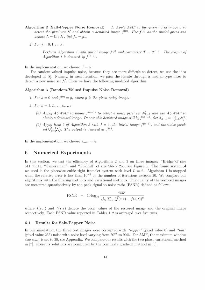
Algorithm 2 (Salt-Pepper Noise Removal) 1. Apply AMF to the given noisy image g todetect the pixel set N and obtain a denoised image f (0). Use f (0) as the initial guess anddenote Λ = Ω \ N . Set fΛ = gΛ.

2. For j = 0, 1, . . . J :

Perform Algorithm 1 with initial image f (j) and parameter T = 2J−j . The output ofAlgorithm 1 is denoted by f (j+1).

In the implementation, we choose J = 5.For random-valued impulse noise, because they are more difficult to detect, we use the idea

developed in [8]. Namely, in each iteration, we pass the iterate through a median-type filter todetect a new noise set N . Then we have the following modified algorithm.

Algorithm 3 (Random-Valued Impulse Noise Removal)

1. For k = 0 and f (0) = g, where g is the given noisy image.

2. For k = 1, 2, . . . , kmax:

(a) Apply ACWMF to image f (k−1) to detect a noisy pixel set Nk−1 and use ACWMF toobtain a denoised image. Denote this denoised image still by f (k−1). Set Λk−1 = ∩k−1

j=0N cj .

(b) Apply Item 2 of Algorithm 2 with J = 4, the initial image f (k−1), and the noise pixelsset ∪k−1

j=0Nj . The output is denoted as f (k).

In the implementation, we choose kmax = 4.

6 Numerical Experiments

In this section, we test the efficiency of Algorithms 2 and 3 on three images: “Bridge”of size511 × 511, “Cameraman”, and “Goldhill” of size 255 × 255, see Figure 1. The frame system Awe used is the piecewise cubic tight framelet system with level L = 6. Algorithm 1 is stoppedwhen the relative error is less than 10−4 or the number of iterations exceeds 30. We compare ouralgorithms with the filtering methods and variational methods. The quality of the restored imagesare measured quantitatively by the peak signal-to-noise ratio (PSNR) defined as follows:

PSNR = 10 log102552

1MN

∑s,t(f(s, t) − f(s, t))2

where f(s, t) and f(s, t) denote the pixel values of the restored image and the original imagerespectively. Each PSNR value reported in Tables 1–2 is averaged over five runs.

6.1 Results for Salt-Pepper Noise

In our simulation, the three test images were corrupted with “pepper” (pixel value 0) and “salt”(pixel value 255) noise with noise level varying from 50% to 90%. For AMF, the maximum windowsize wmax is set to 39, see Appendix. We compare our results with the two-phase variational methodin [7], where its solutions are computed by the conjugate gradient method in [3].

14

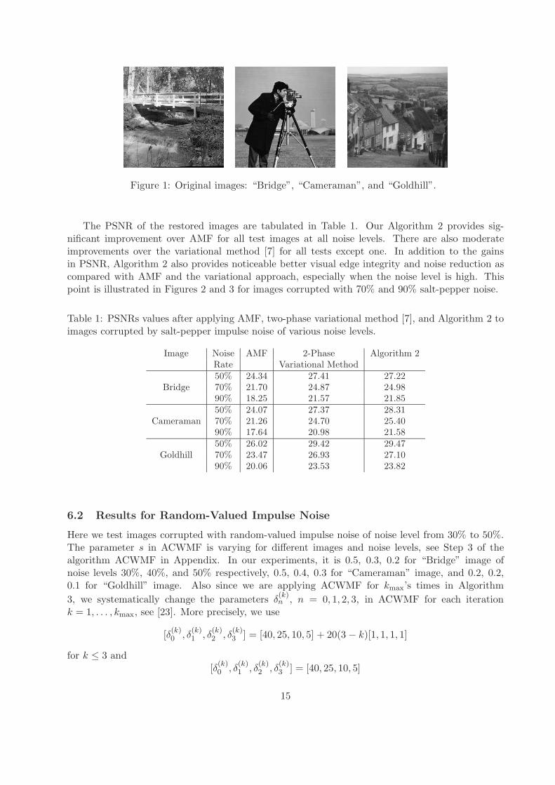
Figure 1: Original images: “Bridge”, “Cameraman”, and “Goldhill”.

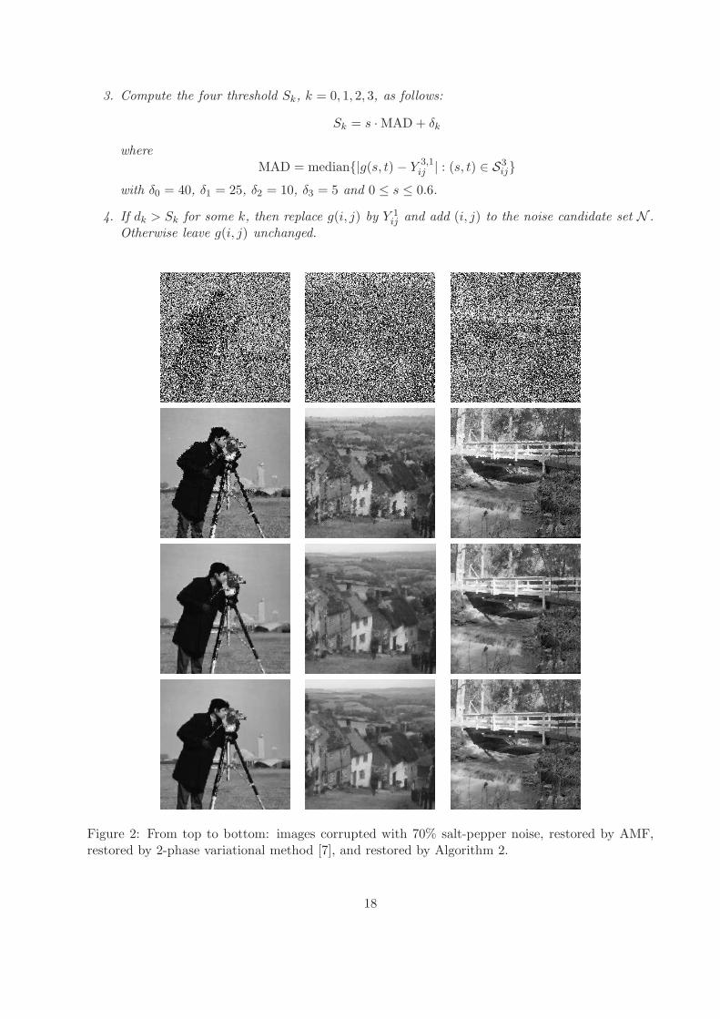
The PSNR of the restored images are tabulated in Table 1. Our Algorithm 2 provides sig-nificant improvement over AMF for all test images at all noise levels. There are also moderateimprovements over the variational method [7] for all tests except one. In addition to the gainsin PSNR, Algorithm 2 also provides noticeable better visual edge integrity and noise reduction ascompared with AMF and the variational approach, especially when the noise level is high. Thispoint is illustrated in Figures 2 and 3 for images corrupted with 70% and 90% salt-pepper noise.

Table 1: PSNRs values after applying AMF, two-phase variational method [7], and Algorithm 2 toimages corrupted by salt-pepper impulse noise of various noise levels.

Image Noise AMF 2-Phase Algorithm 2Rate Variational Method50% 24.34 27.41 27.22

Bridge 70% 21.70 24.87 24.9890% 18.25 21.57 21.8550% 24.07 27.37 28.31

Cameraman 70% 21.26 24.70 25.4090% 17.64 20.98 21.5850% 26.02 29.42 29.47

Goldhill 70% 23.47 26.93 27.1090% 20.06 23.53 23.82

6.2 Results for Random-Valued Impulse Noise

Here we test images corrupted with random-valued impulse noise of noise level from 30% to 50%.The parameter s in ACWMF is varying for different images and noise levels, see Step 3 of thealgorithm ACWMF in Appendix. In our experiments, it is 0.5, 0.3, 0.2 for “Bridge” image ofnoise levels 30%, 40%, and 50% respectively, 0.5, 0.4, 0.3 for “Cameraman” image, and 0.2, 0.2,0.1 for “Goldhill” image. Also since we are applying ACWMF for kmax’s times in Algorithm

3, we systematically change the parameters δ(k)n , n = 0, 1, 2, 3, in ACWMF for each iteration

k = 1, . . . , kmax, see [23]. More precisely, we use

[δ(k)0 , δ

(k)1 , δ

(k)2 , δ

(k)3 ] = [40, 25, 10, 5] + 20(3 − k)[1, 1, 1, 1]

for k ≤ 3 and[δ

(k)0 , δ

(k)1 , δ

(k)2 , δ

(k)3 ] = [40, 25, 10, 5]

15

for k > 3. Table 2 gives the PSNR of the restored images. We can see from it that our Algorithm 3performs much better than ACWMF. It is also better than the two-phase variational method [8].Moreover, noise patches produced by ACWMF are significantly reduced by our algorithm as shownin Figures 4 and 5.

Table 2: PSNR values after applying ACWMF, two-phase variational method in [8] and Algorithm3 to images corrupted by random-valued impulse noise of various noise levels.

Image Noise ACWMF 2-phase Algorithm 3Rate Variational Method30% 25.16 26.06 26.07

Bridge 40% 23.36 24.81 24.8750% 21.47 23.40 23.6030% 24.36 24.88 24.95

Cameraman 40% 22.57 23.66 23.8750% 20.61 22.35 22.6530% 26.88 27.65 27.70

Goldhill 40% 25.10 26.54 26.7150% 23.21 25.29 25.58

6.3 Results for Image Inpainting

To further demonstrate the efficiency of the proposed algorithm, we end the paper by presentingone more example of image inpainting. Image inpainting refers to the filling-in of missing datain digital images based on the information available in the observed region. Applications of thistechnique include film restoration, text or scratch removal, and digital zooming.

Let N be the set where original image data is missing. In the left images in the first and thirdrows of Figure 6, the set N is the location of the text imposed in the “Cameraman” and “Goldhill”images. We remove those text by using Algorithm 2 with J = 6. We present inpainted images forthree different initial guess f (0). For the “Cameraman” image, the first chosen f (0) is the image tobe inpainted itself which is the left image in the first row of Figure 6. The second chosen f (0) shownin the middle of the first row of Figure 6 is obtained by the cubic spline interpolation from theavailable information. The third chosen f (0) shown in the right of the first row of Figure 6 is theone whose pixel values in N are randomly between 0 and 255. The corresponding inpainted images(from left to right) are presented in the second row of Figure 6 with values of PSNR 30.64dB,30.52dB, and 30.50dB, respectively. Similarly, for the three different initial guesses f (0) (from leftto right) shown in the third row of Figure 6, the corresponding inpainted “Goldhill” images (fromleft to right) are presented in the last row with values of PSNR 32.62dB, 32.67dB, and 32.61dB,respectively. From above results, we can see that the proposed algorithm produces comparableresults for different initial guesses in terms of the PSNR values and the visual quality. We notethat the initial guesses generated by the cubic spline in the middle of the first row and the thirdrow in Figure 6 have PSNR values 29.43dB and 31.24dB, respectively.

7 Conclusion

In this paper, we have modified the framelet-based algorithm in [4] to obtain a new algorithmwhich we can prove convergence and can derive its convergence rate. In addition, we showed that

16

the solution of the new algorithm is minimizing a constrained problem, where the unconstrainedone was minimized by the framelet-based algorithm in [4]. Application of the algorithm in impulsenoise removal shows that it is effective when compared to median-type filters [21, 22] and variationalapproaches in [3, 7, 8].

Appendix

We first introduce the adaptive median filter (AMF) method given in [21]. It is used to detectsalt-pepper noise in our tests. Let Sw

ij be a window of size w × w centered at pixel location (i, j),i.e.,

Swij = (k, ℓ) : |k − ℓ| ≤ w and |j − ℓ| ≤ w

and let wmax-by-wmax be the maximum window size. The algorithm tries to identify the noisecandidates g(i, j) and then replace each g(i, j) by the median of the pixels in Sw

ij . AMF consists ofthe following five steps:

Algorithm 4 (AMF)

1. Initialize w = 3 and N = ∅.

2. Compute smin,wij , smed,w

ij , and smax,wij , which are the minimum, median, and maximum of the

pixel values in Swij , respectively.

3. If smin,wij < smed,w

ij < smax,wij , then go to Step 5. Otherwise, set w = w + 2.

4. If w ≤ wmax, go to Step 2. Otherwise, we replace g(i, j) by smed,wmax

ij and add the location(i, j) into the noise set N .

5. If smin,wij < g(i, j) < smax,w

ij , then g(i, j) is not a noise candidate. Otherwise we replace g(i, j)

by smed,wmax

ij and add the location (i, j) to the noise set N .

The only required parameter in AMF is the maximum window size wmax. The AMF starts withan initial window size w = 3 with a step of 2 to wmax and detects the impulse noise in an adaptiveway. In this respect, maximum window size wmax should increase with the noise level. In ourexperiments, we set wmax = 39.

Next we briefly describe the adaptive center-weight median filter (ACWMF) method in [22]. Itis used to detect random-valued impulse noise in our tests. Let

Y w,ri,j = mediang(s, t), r ⋄ g(i, j)|(s, t) ∈ Sw

ij

where the operator ⋄ denotes the repetition operation. In other words, r ⋄ g(i, j) means r copiesof g(i, j) in total. Clearly, Y w,1

ij is the output of the standard median filter. ACWMF has thefollowing four steps:

Algorithm 5 (ACWMF)

1. Calculate Y 3,1ij , Y 3,3

ij , Y 3,5ij , and Y 3,7

ij .

2. Compute the differences dk = |Y 3,2k+1ij − g(i, j)|, where k = 0, 1, 2, 3. It was shown in [12]

that dk ≤ dk+1 for k ≥ 1.

17

3. Compute the four threshold Sk, k = 0, 1, 2, 3, as follows:

Sk = s · MAD + δk

whereMAD = median|g(s, t) − Y 3,1

ij | : (s, t) ∈ S3ij

with δ0 = 40, δ1 = 25, δ2 = 10, δ3 = 5 and 0 ≤ s ≤ 0.6.

4. If dk > Sk for some k, then replace g(i, j) by Y 1ij and add (i, j) to the noise candidate set N .

Otherwise leave g(i, j) unchanged.

Figure 2: From top to bottom: images corrupted with 70% salt-pepper noise, restored by AMF,restored by 2-phase variational method [7], and restored by Algorithm 2.

18

References

[1] E. Abreu, M. Lightstone, S. Mitra, and K. Arakawa. A new efficient approach for the removalof impulse noise from highly corrupted images. IEEE Trans. Image Process., 5(3):1012–1025,1996.

[2] M. Bertalmio, G. Sapiro, V. Caselles, and C. Ballester. Image inpainting. In Proceedings ofSIGGRAPH, pages 417–424, New Orleans, LA, 2000.

[3] J.-F. Cai, R. Chan, and C. Di Fiore. Minimization of a detail-preserving regularization func-tional for impulse noise removal. Journal of Mathematical Imaging and Vision, 29(1):79–91,2007.

[4] J.-F. Cai, R. Chan, and Z. Shen. A framelet-based image inpainting algorithm. Applied andComputational Harmonic Analysis, 24(2):131–149, 2008.

[5] A. Chai and Z. Shen. Deconvolution: A wavelet frame approach. Numerische Mathematik,106:529–587, 2007.

[6] R. Chan, T. Chan, L. Shen, and Z. Shen. Wavelet algorithms for high-resolution image recon-struction. SIAM Journal on Scientific Computing, 24(4):1408–1432, 2003.

[7] R. Chan, C.-W. Ho, and M. Nikolova. Salt-and-pepper noise removal by median-type noise de-tectors and detail-preserving regularization. IEEE Transactions on Image Procssing, 14:1479–1485, 2005.

[8] R. Chan, C. Hu, and M. Nikolova. An iterative procedure for removing random-valued impulsenoise. IEEE Signal Procssing Letters, 11:921–924, 2004.

[9] R. Chan, S. D. Riemenschneider, L. Shen, and Z. Shen. Tight frame: The efficient way for high-resolution image reconstruction. Applied and Computational Harmonic Analysis, 17(1):91–115,2004.

[10] R. Chan, L. Shen, and Z. Shen. A framelet-based approach for image inpainting. TechnicalReport 2005-4, The Chinese University of Hong Kong, Feb. 2005.

[11] T. Chan and J. Shen. Nontexture inpainting by curvature driven diffusion (CDD). J. VisulComm. Image Rep., 12:436–449, 2001.

[12] T. Chen and H. Wu. Space variant median filters for the restoration of impulse noise corruptedimages. IEEE Trans. Circuits and Systems II, 48:784–789, 2001.

[13] P. Combettes and V. Wajs. Signal recovery by proximal forward-backward splitting. MultiscaleModeling and Simulation: A SIAM Interdisciplinary Journal, 4:1168–1200, 2005.

[14] I. Daubechies. Ten Lectures on Wavelets, volume 61 of CBMS Conference Series in AppliedMathematics. SIAM, Philadelphia, 1992.

[15] D. Donoho and I. Johnstone. Ideal spatial adaptation by wavelet shrinkage. Biometrika,81:425–455, 1994.

[16] R. Duffin and A. Schaeffer. A class of nonharmonic Fourier series. Transactions on AmericanMathematics Society, 72:341–366, 1952.

19

[17] A. Flaig, G. Arce, and K. Barner. Affine order statistics filters: “medianization” of linear FIRfilters. IEEE Trans. Signal Processing, 46:2101–2112, 1998.

[18] R. Gonzalez and R. Woods. Digital Image Processing. Addison-Wesley, Boston, MA, 1993.

[19] O. G. Guleryuz. Nonlinear approximation based image recovery using adaptive sparse recon-struction and iterated denoising: Part I - theory. IEEE Transaction on Image Processing,2006.

[20] O. G. Guleryuz. Nonlinear approximation based image recovery using adaptive sparse recon-struction and iterated denoising: Part II - adaptive algorithms. IEEE Transaction on ImageProcessing, 2006.

[21] H. Hwang and R. Haddad. Adaptive median filters: new algorithms and results. IEEE Trans.Image Processing, 4:499–502, 1995.

[22] S. Ko and Y. Lee. Adaptive center weighted median filter. IEEE Trans. Circuits and SystemsII, 38:984–993, 1998.

[23] S. Ko and Y. Lee. Adaptive center weighted median filter. IEEE Transactions on Circuits andSystems II, 38:984–993, 1998.

[24] M. Ng, R. Chan, and W. Tang. A fast algorithm for deblurring models with Neumann boundaryconditions. SIAM Journal on Scientific Computing, 21:851–866, 2000.

[25] M. Nikolova. A variational approach to remove outliers and impulse noise. J. Math. ImagingVision, 20:99–120, 2004.

[26] G. Pok, J.-C. Liu, and A. S. Nair. Selective removal of impulse noise based on homogeneitylevel information. IEEE Trans. Image Processing, 12:85–92, 2003.

[27] A. Ron and Z. Shen. Affine system in L2(Rd): the analysis of the analysis operator. Journal

of Functional Analysis, 148:408–447, 1997.

[28] T. Sun and Y. Neuvo. etail-preserving based filters in image processing. Pattern-RecognitionLetters, 15:341–347, 1994.

[29] Windyga. Fast impulsive noise removal. IEEE Trans. Image Processing, 10:173–179, 2001.

[30] L. Yin, R. Yang, M. Gabbouj, and Y. Neuvo. Weighted median filters: a tutorial. IEEE Trans.Circuit Theory, 41:157–192, 1996.

20

Figure 3: From top to bottom: images corrupted with 90% salt-pepper noise, restored by AMF,restored by 2-phase variational method [7], and restored by Algorithm 2.

21

Figure 4: From top to bottom: images corrupted with 30% random-valued impulse noise, restoredby ACWMF, restored by 2-phase variational method [8], and restored by Algorithm 3.

22

Figure 5: From top to bottom: images corrupted with 50% random-valued impulse noise, restoredby ACWMF, restored by 2-phase variational method [8], and restored by Algorithm 3.

23

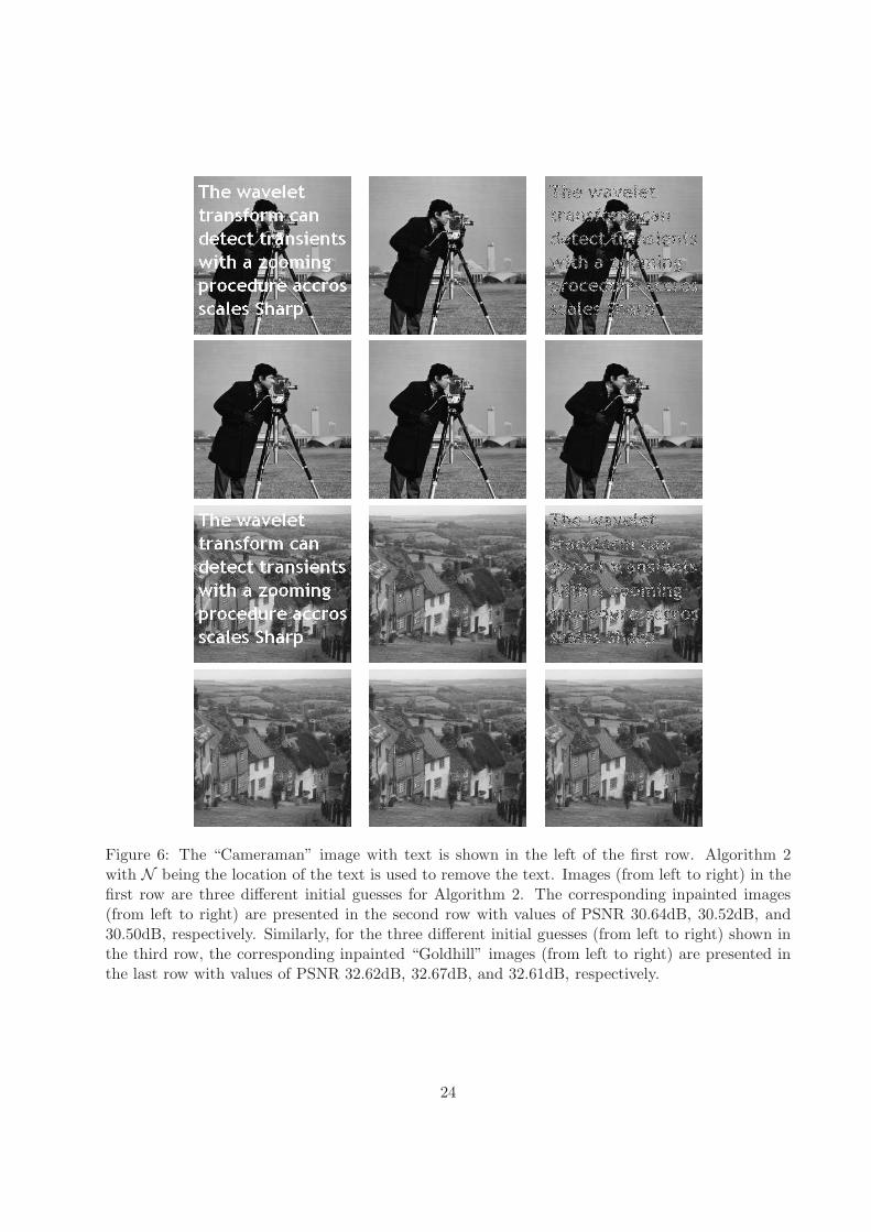
Figure 6: The “Cameraman” image with text is shown in the left of the first row. Algorithm 2with N being the location of the text is used to remove the text. Images (from left to right) in thefirst row are three different initial guesses for Algorithm 2. The corresponding inpainted images(from left to right) are presented in the second row with values of PSNR 30.64dB, 30.52dB, and30.50dB, respectively. Similarly, for the three different initial guesses (from left to right) shown inthe third row, the corresponding inpainted “Goldhill” images (from left to right) are presented inthe last row with values of PSNR 32.62dB, 32.67dB, and 32.61dB, respectively.

24