production data analysis of tight hydrocarbon reservoirs - ERA
107
University of Alberta PRODUCTION DATA ANALYSIS OF TIGHT HYDROCARBON RESERVOIRS by Shahab Kafeel Siddiqui A thesis submitted to the Faculty of Graduate Studies and Research in partial fulfillment of the requirements for the degree of Master of Science in Petroleum Engineering Department of Civil and Environmental Engineering ©Shahab Kafeel Siddiqui Fall 2012 Edmonton, Alberta Permission is hereby granted to the University of Alberta Libraries to reproduce single copies of this thesis and to lend or sell such copies for private, scholarly or scientific research purposes only. Where the thesis is converted to, or otherwise made available in digital form, the University of Alberta will advise potential users of the thesis of these terms. The author reserves all other publication and other rights in association with the copyright in the thesis and, except as herein before provided, neither the thesis nor any substantial portion thereof may be printed or otherwise reproduced in any material form whatsoever without the author's prior written permission.
-
Upload
khangminh22 -
Category
Documents
-
view
0 -
download
0
Transcript of production data analysis of tight hydrocarbon reservoirs - ERA

University of Alberta
PRODUCTION DATA ANALYSIS OF TIGHT HYDROCARBON RESERVOIRS
by
Shahab Kafeel Siddiqui
A thesis submitted to the Faculty of Graduate Studies and Research in partial fulfillment of the requirements for the degree of
Master of Science in
Petroleum Engineering
Department of Civil and Environmental Engineering
©Shahab Kafeel Siddiqui Fall 2012
Edmonton, Alberta
Permission is hereby granted to the University of Alberta Libraries to reproduce single copies of this thesis and to lend or sell such copies for private, scholarly or scientific research purposes only. Where the thesis is
converted to, or otherwise made available in digital form, the University of Alberta will advise potential users of the thesis of these terms.
The author reserves all other publication and other rights in association with the copyright in the thesis and,
except as herein before provided, neither the thesis nor any substantial portion thereof may be printed or otherwise reproduced in any material form whatsoever without the author's prior written permission.

Dedication
I dedicate my work to all those who have lovingly supported me throughout life
and all its travails.

Abstract
Tight reservoirs stimulated by multistage hydraulic fracturing are commonly described by
a dual porosity model. This work hypothesizes that the production data of some fractured
horizontal wells (which contain reactivated natural fractures) may also be described by a
triple porosity model. We test this hypothesis by extending the existing triple porosity
models to develop an analytical procedure for determining the reservoir parameters. We
derive the simplified equations for different regions of the rate-time plot including linear
and bilinear flow regions.
The second part of this work focuses on analyzing production data of tight oil
reservoirs. We plot rate-normalized pressure (RNP) versus material balance time (MBT)
of two wells drilled in Cardium and Bakken formations. We observe a half-slope
followed by a unit-slope in both cases. We hypothesize that the unit slope reflects the
linear pseudosteady state (PSS) flow and develop a new model to analyze this boundary-
dominated flow.

Acknowledgements
First, I want to give praises to Almighty Allah for sparing my life, continuously
granting me His blessings and allowing me to successfully conclude this phase of my life.
I want to acknowledge my supervisor, Dr. Hassan Dehghanpour for being a mentor,
supervisor and friend to me. I am honored to have worked with him. I am also eternally
grateful to him.
I would also like to thank Dr. Juliana Leung and Dr. Ahmed Bouferguene for
serving on my advisory committee and for their constructive feedback that helps making
this work better.
I want to acknowledge the eternal support of my parents, Kafeel Alam and Farzana
Kafeel, and my beloved wife, Zubaria.
I also would like to acknowledge the help of my friend, Afsar Ali for the
informative discussion and contributions to this work.
In addition, I would like to express my gratitude to my friends, colleagues and the
Petroleum Engineering department faculty and staff for making my time at University of
Alberta a great experience.

Table of Contents
List of Tables ....................................................................................................... viii
List of Figures ........................................................................................................ ix
CHAPTER I INTRODUCTION ..............................................................................1
1.1. Problem Definition...................................................................................2
1.2 Objectives .................................................................................................2
1.3 Outline.......................................................................................................3
CHAPTER II LITERATURE REVIEW .................................................................5
2.1 Introduction ...............................................................................................5
2.2 Dual Porosity Models ...............................................................................5
2.2.1 Pseudosteady state models ............................................................5
2.2.2 Transient Models ..........................................................................7
2.3 Triple-porosity Models .............................................................................7
2.4 Linear Flow in Hydraulically Fractured Horizontal Wells .......................9
2.5 Boundary Dominated (Pseudosteady state) Flow ...................................11
CHAPTER III DEVELOPMENT OF ANALYSIS EQUATIONS FOR SEQUENTIAL TRIPLE POROSITY SYSTEM ..........................................13
3.1 Introduction .............................................................................................13
3.2 Triple-Porosity Model for Sequential Linear Flow ................................13
3.3 Flow Regions Based on the Analytical Solution ....................................16
3.4 Development of Analysis Equation for Flow Regions Observed During Production ............................................................................................17
3.4.1 Region 1 ......................................................................................18
3.4.2 Region 2 ......................................................................................18
3.4.3 Region 3 ......................................................................................19
3.4.4 Region 4 ......................................................................................20
3.4.5 Region 5 ......................................................................................21
3.4.6 Region 6 ......................................................................................23

CHAPTER IV DEVELOPMENT OF ANALYSIS EQUATION OF BOUNDARY DOMINATED FLOW ..................................................................................26
4.1 Introduction .............................................................................................26
4.2 Modeling Boundary Dominated Flow in Fractured Horizontal Wells ...26
4.2.1 Model Assumptions ....................................................................26
4.3.2 Development of a New Solution for the Boundary Dominated Linear Flow in Horizontally Fractured Tight Reservoirs .......................28
4.3.2.1 Material balance equation ...............................................29
4.3.2.2 Linear Diffusivity Equation ............................................30
4.3.2.3 Average matrix pressure from the pressure solution ......31
4.3.2.4 Average matrix pressure based on Pseudo-steady state flow............................................................................................32
4.3.2.5 Final Solution ..................................................................33
CHAPTER V PRODUCTION DATA ANALYSIS OF GAS RESERVOIRS IN BARNET SHALE .........................................................................................36
5.1 Introduction .............................................................................................36
5.2 Procedure For Production Data Analysis for Tight Gas Wells ...............37
5.2.1 Region 4 (Bilinear Flow in Micro-fractures and Matrix) ...........37
5.2.2 Region 5 (Rate Transient Flow from Matrix) .............................38
5.3 Application of analysis Procedure to Production Data ...........................39
5.3.1 Production Data Analysis of Well 73 .........................................40
5.3.1.1 Analysis of bilinear transient region ...............................40
5.3.1.2 Analysis of Linear Transient Region (Matrix)................42
5.3.2 Regression Results for Well 73...................................................44
5.3.2.1 Comparison of Results ....................................................45
5.3.3 Production Data Analysis of Well 314 .......................................45
5.3.4 Regression Results for Well 314.................................................47
5.3.4.1 Comparison of Results ....................................................48
5.3.5 Summary and Discussion of Results...........................................48

CHAPTER VI PRODUCTION DATA ANALYSIS OF TIGHT OIL RESERVOIRS.......................................................................................................................49
6.1 Introduction .............................................................................................49
6.1.1 Pembina Cardium (Halo Oil) ......................................................49
6.1.2 Saskatchewan Bakken (Tight Oil) ..............................................50
6.2 Procedure for Production Data Analysis of Tight Oil Reservoirs ..........51
6.2.1 Analysis of Transient Matrix Depletion (Dual porosity systems)51
6.2.2 Analysis of boundary dominated flow (PSS flow) .....................52
6.3 Production Data Analysis of Cardium Wells ..........................................52
6.3.1 Observing behavior of Cardium Wells .......................................52
6.3.2 Example Application for Characterizing a Fractured Well in Cardium Formation .....................................................................54
6.3.2.1 Analysis of Linear Transient Region ..............................57
6.3.2.2 Analysis Of Boundary Dominated Flow Region ............58
6.3.3 Summary of Results ....................................................................60
6.4 Example Application for Characterizing a Fractured Well in Bakken Formation .............................................................................................61
6.4.1 Analysis of Linear Transient Region ..........................................62
6.4.2 Analysis Of Boundary Dominated Flow.....................................64
6.4.3 Summary of Results ....................................................................65
CHAPTER VII CONCLUSION AND RECOMMENDATIONS .........................67
7.1 Conclusions .............................................................................................67
7.2 Recommendations ...................................................................................68
REFERENCES ......................................................................................................69
NOMENCLATURE ..............................................................................................74
APPENDIX A ........................................................................................................76
APPENDIX B ........................................................................................................83

List of Tables
Table 3.1 Summary of analysis equations developed for constant Pwf of rate transient
solution for triple porosity system for highly compressible fluid (gas) 24
Table 3.2 Summary of analysis equations developed for constant Pwf of rate transient
solution for triple porosity system for slightly compressible fluid (oil)25
Table 5.1 Reservoir and fluid properties obtained from well tests of Well 73 ......40
Table 5.2 Values of Assumed Parameters for Regression for Well 73 .................44
Table 5.3 Regression results for Well 73 (Assuming no adsorption) ....................44
Table 5.4 Reservoir and fluid properties obtained from well tests of Well 314 ....45
Table 5.5 Values of Assumed Parameters for Regression for Well 314 ...............47
Table 5.6 Regression results for Well 314 (Assuming no adsorption) ..................48
Table 6.1 Reservoir and fluid properties of Well in Cardium Formation ..............54
Table 6.2 Unknown reservoir parameters obtained by analyzing matrix transient
region and boundary dominated region of production data of the well
completed in Cardium Formation..........................................................60
Table 6.3 Reservoir and fluid properties of well in Bakken Formation ................61
Table 6.4 Unknown reservoir parameters obtained from the analysis of the matrix
transient region and boundary dominated region of production data of the
well completed in Bakken Formation ...................................................65

List of Figures
Fig. 2.1 – Idealization of the NFR system (Warren and Root, 1963). .....................6
Fig. 2.2 – Schematic illustration of triple porosity model (Dehghanpour and Shirdel,
2011) ......................................................................................................11
Fig. 3.1 – Top view of a horizontal well in a triple porosity system. Red dotted lines
indicated virtual no flow boundaries. Arrows indicate direction of the flow
(Al-Ahmadi 2010). ................................................................................14
Fig. 3.2 – Log-log plot of dimensionless rate versus dimensionless time for a triple
porosity system. Bi-linear flow indicated by a slope of 0.25 and linear flow
is indicated by slope of 0.5 (Al Ahmadi 2010). ....................................17
Fig. 4.1 – Plan view of hydraulic fractures connected to the horizontal well. The
direction of flow is from the matrix to the fractures and from the fractures
to the well. This figure also shows fracture half-length ye. Arrows indicate
the flow direction...................................................................................27
Fig. 4.2 – Front view of hydraulic fractures connected to the horizontal well. .....28
Fig. 4.3 – Schematic of the selected control volume showing a hydraulic fracture
surrounded by the matrix blocks. Two no-flow boundaries are virtually
created at the center of adjacent fractures at distance of 0.5 Lf from the
fracture...................................................................................................29
Fig. 4.4 – The pressure profile in the matrix during the boundary dominated flow.
The rate of pressure drop with respect to time remains constant at
pseudosteady state conditions. ..............................................................32
Fig. 5.1 – Log-log plot of gas rate versus time for two horizontal shale gas wells.
Well 73 exhibits bi-linear flow between micro fracture and matrix followed
by matrix linear flow as it gives negative quarter-slope for some time and
then negative half-slope. Well 314 shows negative half-slope for almost
two log cycles and indicates matrix linear flow. ...................................39
Fig. 5.2 – Log-log plot of gas rate versus MBT that shows a negative quarter slope.
...............................................................................................................41
Fig. 5.3 – Plot of fourth root MBT versus RNP that gives slopes equal to 136370
psi/cp2/Mscf/day/day0.25 ........................................................................41
Fig. 5.4 – Log-log plot of gas rate versus MBT shows a negative half slope. ......42
Fig. 5.5 – Plot of square root MBT versus RNP that gives slopes equal to 54961
psi/cp2/Mscf/day/day0.5 ..........................................................................43
Fig. 5.6 – Log-log plot of gas rate versus MBT shows a negative half slope. ......46
Fig. 5.7 – Plot of square root MBT versus RNP that gives slopes equal to 20701
psi/cp2/Mscf/day/day0.5 ..........................................................................46
Fig. 6.1 – Plots of cumulative oil production versus time for five fractured horizontal
wells completed in Cardium formation. The log-log plots show a slope of
0.6 - 0.75 for early time scales and a slope of approximately 0.5 for late
time scales. The length of horizontal wells and number of stages of
hydraulic fractures are different in these wells. The consistent behavior of
cumulative plots shows that the flow regime is relatively similar for all the
wells.......................................................................................................53
Fig. 6.2 – Log-log plot of daily oil rate versus time for a Well in Cardium Formation
...............................................................................................................55

Fig. 6.3 – Log-log plot of daily oil rate versus calculated material balance time of the
well in Cardium Formation. ..................................................................56
Fig. 6.4 – Specialized plot of Rate Normalized Pressure versus square root of
Material Balance Time for analyzing flow from matrix to fracture ......57
Fig. 6.5 – Specialized plot of RNP versus MBT for analyzing boundary dominated
flow of the well completed in Cardium Formation. ..............................58
Fig. 6.6 – Log-log plot of daily oil rate versus calculated MBT of a Well in Bakken
Formation. .............................................................................................62
Fig. 6.7 – Plot of RNP versus square root of MBT of only transient region of the well
completed in Bakken Formation ...........................................................63
Fig. 6.8 – Specialized plot of RNP versus MBT for analyzing boundary dominated
flow in Bakken Formation .....................................................................64
Fig. A-4 – Top View of a horizontal Well in a triple porosity system. Red dotted lines
indicated virtual no flow boundaries. Arrows indicate direction of the flow
(Al-Ahmadi 2010). ................................................................................77
1
CHAPTER I
INTRODUCTION
Tight oil and shale gas reservoirs are considered “unconventional”
resources, requiring horizontal wells and massive hydraulic fracturing for
economic production. Tight hydrocarbon production is emerging as an important
source of energy supply in the United States and Canada. Some of these
unconventional resources are naturally fractured. A naturally fractured reservoir
(NFR) can be defined as a reservoir that contains fractures (planar discontinuities)
created by natural processes like diastrophism and volume shrinkage, distributed
as a consistent connected network throughout the reservoir (Ordonez et al., 2001).
Fractured petroleum reservoirs represent over 20% of the world's oil and gas
reserves (Saidi, 1983).
Horizontal drilling and multi-stage fracture stimulation is a successful
technique in allowing shale gas production. It has proved to work equally well for
producing light crude oil trapped in low permeability (e.g., tight) shale, sandstone,
or carbonate rock formations. Characterization and modeling of naturally
fractured tight reservoirs stimulated by hydraulic fractures present unique
challenges that differentiate them from conventional reservoirs.
Traditionally, dual-porosity models have been used to model NFRs where
all fractures are assumed to have identical properties. Different dual-porosity
models have been proposed such as Warren & Root (1963) sugar cube model in
which matrix provides the storage while fractures provide the flow medium. The
model assumed pseudosteady state fluid transfer between matrix and fractures.
Since then, several models were developed mainly as variation of the Warren &
Root model assuming different matrix- fracture fluid transfer conditions (Kazemi
1969 and Liu 1981).
Characterizing and modeling NFRs is challenging due to the highly
heterogeneous and anisotropic nature of the fracture system (Ordonez et al.,

2
2001). It is more realistic to assume fractures having different properties. This is
more apparent in case of hydraulically fractured wells. Thus, triple-porosity
model have been developed and is more realistic models to capture reservoir
heterogeneity in hydraulically fractured NFRs. Triple porosity model developed
for linear flow that considers transient fluid transfer (between media) is available
in the literature (Al-Ahmadi, 2010). In this work we further extend this model to
develop analysis equations of each flow regime observed during hydrocarbon
production.
Furthermore, the existing models available in the literature are useful in
analyzing matrix flow in hydraulically fractured reservoir. No appropriate models
are available to analyze the boundary dominated linear flow. Boundary dominated
flow in the hydraulically fractured reservoirs occurs when the pressure
interference reaches the virtual no flow boundaries developed at the center of two
adjacent fractures. New analysis equations are developed to model this flow
occurring under pseudosteady state flow conditions.
1.1. PROBLEM DEFINITION
Horizontal wells with multistage hydraulic fracturing are used to produce
economically from NFRs. It has been documented that hydraulic fractures growth
could re-open the pre-existing natural fractures (Gale et al. 2007). Therefore, for
any model to be used to analyze such wells, it has to account for both natural and
hydraulic fractures to be practical. Under these conditions, the reservoir should be
described by a triple porosity model.
1.2 OBJECTIVES
The objective of this research is to develop analysis equations to model each flow
regime occurring during production from a horizontal well in a triple-porosity
reservoir. The system consists of matrix and two sets of orthogonal fractures that
have different properties. These fractures are the more permeable macro-fractures

3
and the less permeable micro-fractures. Existing triple porosity model for linear
systems will be extended. New analytical equations will also be derived to model
boundary dominated flow in dual porosity reservoirs.
1.3 OUTLINE
This dissertation is divided into seven chapters. It is organized in a manner
that follows a gradual process of developing a conceptual and logical
understanding of the basic dual and triple porosity model and its limitations. It
progresses through by developing the analysis equations of different flow regimes
observed during production from a triple porosity system. This dissertation also
includes the modeling of boundary dominated (pseudosteady state) flow for linear
dual porosity reservoirs.
Chapter II presents a literature review of existing dual and triple porosity
models and its extensions for linear flow. This chapter also includes review of
existing models to analyze boundary dominated flow.
Chapter III discusses the new analysis equations developed for linear flow
towards a horizontal well in triple porosity reservoirs. The new equations are
developed to analyze each individual flow regime observed during hydrocarbon
production. The solutions are presented for slightly compressible (oil) and highly
compressible (gas) fluids.
Chapter IV presents the new equations are developed to model the boundary
dominated (pseudosteady state) flow for slightly compressible fluids in a dual
porosity system.
Chapter V presents the application of the newly developed triple porosity
model for two shale gas wells.
Chapter VI presents the application of new equations developed in Chapter
V for modeling boundary dominated flow for tight oil reservoirs. The transient
linear matrix flow of tight oil reservoirs is also analyzed using previously

4
developed dual porosity equations. The analysis results obtained from both
models are compared.
Chapter VII presents conclusions and recommendations.
5
CHAPTER II
LITERATURE REVIEW
2.1 INTRODUCTION
This chapter provides the literature review of naturally fractured reservoirs.
Some of available dual and triple porosity models will be reviewed. In addition,
linear flow solutions for the fractured reservoirs will be discussed.
2.2 DUAL POROSITY MODELS
Dual porosity models are usually used to analyze naturally fractured
reservoirs. These models assume fractures to have identical properties. Barenblatt
et al. (1960) introduced the first dual porosity model. Warren and Root (1963)
extended Barenblatt model for well test analysis. The model presented by Warren
and Root forms the basis of modern day analysis of naturally fractured reservoirs
(NFRs). The model assumes that the fluid transfer between matrix and fractures is
under pseudosteady state. The fractures provide flow medium and matrix provide
storage of fluid. They introduced two dimensionless parameters, storativity (ω)
and interporosity flow parameter (λ).
Dual porosity models can be further categorized based on the interporosity
fluid transfer assumptions:
i) Pseudosteady state models
ii) Transient models
2.2.1 Pseudosteady state models
Warren and Root (1963) analyzed NFRs by idealizing matrix blocks as
sugar cubes and assumed a continuous uniform fracture network oriented parallel
to the principal axes of permeability (Fig 2.1). They assumed pseudosteady flow
between matrix and fracture system. In their model, two differential forms (one
for matrix and one for fracture were solved simultaneously at a mathematical

6
point. An equation for interporosity flow from the matrix to the fractures was
presented:
𝑞 = 𝛼 𝑘𝑚𝜇
�𝑃𝑚 − 𝑃𝑓� (2.1)
Where, 𝑞 is the fluid transfer rate, 𝛼 is the Warren and Root shape factor, 𝑃𝑚 is
the matrix pressure, 𝑃𝑓 is the pressure of fractures, 𝜇 is the viscosity of fluid and
𝑘𝑚 is the matrix permeability.
Warren and Root applied the Laplace transformation to obtain transfer
function "𝑓(𝑠)" and presented a method to analyze pressure build up data for
infinite radial reservoirs. Kazemi et al (1968) extended his model to interference
testing.
Fig. 2.1 – Idealization of the NFR system (Warren and Root, 1963).

7
Da Prat et al. (1981) extended the Warren and Root (1963) solutions to
constant pressure inner boundary conditions and bounded outer boundary cases
for radial reservoir and presented type curves for declined curve analysis.
2.2.2 Transient Models
Kazemi (1969) proposed a slab matrix model with horizontal fractures
based on transient flow condition between matrix and fracture systems. The
solutions were developed for single-phase flow in radial reservoirs. He solved the
problem using numerical techniques. It was concluded that the results are similar
to that of Warren and Root. Thus this model is also appropriate for analyzing
NFRs.
2.3 TRIPLE-POROSITY MODELS
The induced hydraulic fractures can create new fractures or reactivate the
pre-existing natural fractures that may transform the reservoir into a triple
porosity media (Gale et al 2007).
Liu (1981) introduced the first triple porosity model. The system consists of two
matrix systems flowing into one fracture. The model was developed for radial
flow of slightly compressible fluids. The interporosity flow in the reservoir is
considered under pseudosteady state. This model was not published in petroleum
literature.
Abdassah and Ershagi (1986) developed the first triple porosity model for
petroleum literature. They developed an improved model for pressure transient
tests of naturally fractured reservoirs. Geometrical configuration studied include,
both the strata model and uniformly distributed blocks. Both models considered
two matrix systems with different properties flowing under transient interporosity
flow. It was concluded that the triple-porosity systems are characterized by
anomalous slope changes during the matrix-flow controlled region. The slope
change is the result of the contribution of matrix blocks that have the lowest

8
interporosity flow.
Al-Ghamdi and Ershaghi (1996) introduced the concept of dual fracture
triple porosity model. Dual fracture model consist of highly permeable macro
fractures and less permeable micro fractures. They proposed two sub models to
represent the dual fracture system. The first model is similar to the triple porosity
system (two matrix systems and one fracture) where one of the matrix systems is
replaced by micro-fractures. This model assumes no interporosity flow between
the micro-fracture and the matrix systems, yet both support flow in the macro-
fracture system. The second model assumes pressure support from the matrix to
the micro-fractures, which in turns feed the macro-fractures. The macro-fractures
and the micro-fractures both contribute to the production at the test well.
Liu et al. (2003) presented a mathematical model for analysis of pressure
behavior in a tri-continuum medium. The medium consists of fractures, rock
matrices and cavities. Fractures are considered to have homogeneous properties
whereas matrix and cavities have different permeability and porosity. The matrix
and cavities provide fluid storage and feeds the fractures and the fractures feeds
the well. The interporosity flow occurs under pseudosteady state condition. The
Warren–Root approach was used in developing the solution. The analytical model
was applied to a published field-buildup test and was able to match the pressure
buildup data.
Wu et al. (2004) proposed a triple-continuum model to study the effect of
micro-fractures on flow and transport processes in fractured rocks to simulate the
transport of tracers and nuclear waste of Yucca Mountain. They developed a
triple-continuum system (consisting of large fractures, small fractures and matrix)
for estimating reservoir parameters. They investigated the behavior of flow and
transport processes in fractured rocks and verified the validity of analytical
solutions with numerical modeling results. They concluded that the micro-
fractures have a significant effect on the radionuclide transport in the system.
All the models previously described were developed for the radial reservoir

9
cases.
2.4 LINEAR FLOW IN HYDRAULICALLY FRACTURED HORIZONTAL WELLS
Linear reservoirs are those reservoirs that show predominately linear flow
because of the shape of reservoirs. These reservoirs would impose one-
dimensional linear flow (El-Banbi 1998). Tight oil and gas reservoirs are
hydraulically fractured through horizontal wells for economic production.
Horizontal wells and hydraulically fractured horizontal wells may develop several
linear flow periods depending on the type of well and shape of reservoirs. The
duration of linear flow periods is governed by reservoir properties. Linear flow
occurs at early times when the flow is perpendicular to any flow surface. Many
wells have been observed to show long-term linear flow. Linear flow may be
present for years before any boundary effects are reached. Several causes of linear
transient flow may include draining of adjacent tight layers into high permeability
layers, early-time constant pressure drainage and hydraulic fracture draining a
square geometry (Wattenbarger, 2007).
Several authors (Miller, 1962 and Nabor and Barham, 1964) considered a
linear reservoir model of rectangular geometry and presented constant rate and
constant pressure solutions for linear aquifers.
El-Banbi (1998) was the first to present the analytical solution to model
fluid flow in linear fractured reservoirs. New solutions were presented for
naturally fractured reservoir using a linear reservoir model for dual porosity
systems. Solutions are derived in Laplace domain for different inner boundary
(constant pressure and constant rate) and outer boundary (infinite, closed and
constant pressures). The effects of skin and wellbore storage effects have also
been included.
Bello (2009) used El-Banbi solutions to model linear flow in dual porosity
models. Horizontal well performance in tight fractured reservoirs was analyzed.
El-Banbi’s solution for constant pressure solution was applied to analyze rate

10
transient in horizontal multi-stage fractured wells. He considered a bounded
rectangular reservoir with slab matrix blocks draining into adjoining fractures and
subsequently to a horizontal well in the center. Five flow regions were identified.
New analytical equations for transient flow conditions were presented. Skin effect
for the constant rate and constant pressure was also studied. His analytical
equations for dual porosity transient linear will be used in this work to analyze
wells exhibiting dual porosity behavior. Bello (2009) and Bello and Wattenbarger
(2008, 2009, 2010) used the dual porosity linear flow model to analyze shale gas
wells.
Al-Ahmadi (2010) extended Bello’s (2009) dual porosity model and
proposed a triple porosity model for horizontal fractured wells. This model
assumes that micro fractures are perpendicular to the hydraulic fractures and
parallel to the horizontal well. The model was developed based on the assumption
that the flow is sequential from the matrix to the micro fractures and from the
micro fractures to the hydraulic fractures and no flow occurs between matrix and
hydraulic fractures. Four sub-models were developed based on the interporosity
flow assumptions for transient and pseudosteady state flow conditions. He
presented fracture transfer function "𝑓(𝑠)" for all four models. Non-linear
regression analysis technique was used to calculate the unknown reservoir
parameters for hydraulically fractured shale gas horizontal well.
Dehghanpour and Shirdel (2011) developed the triple porosity model for
inner shale reservoir (Fig 2.2). The system consists of macro fractures with higher
permeability, matrix blocks with intermediate permeability and porosity and
matrix blocks with low permeability and porosity. They extended the existing
dual porosity models and studied the pressure response under transient and
pseudosteady state condition. They also performed sensitivity analysis to study
the effect of properties of each medium on the pressure response.

11
Fig. 2.2 – Schematic illustration of triple porosity model (Dehghanpour and Shirdel,
2011)
In this work Al-Ahmadi’s transfer function is further simplified for the
transient case only and analytical equations are developed and presented to
characterize triple porosity reservoirs.
2.5 BOUNDARY DOMINATED (PSEUDOSTEADY STATE) FLOW
After the transient matrix flow in linear reservoirs, boundary dominated
flow occurs. This flow is under pseudosteady state flow condition. This flow
occurs as the pressure transient response reaches the virtual no flow boundaries
developed between two adjacent hydraulic fractures.
Blasingame and Lee (1986) introduced the original analysis equation for
boundary-dominated flow (i.e. pseudo steady state flow) for radial reservoirs.

12
Placio and Blasingame (1993) later modified their analysis equation for any
instantaneous production time, flow regime or production scenario.
A new model for boundary dominated flow occurring in linear dual porosity
reservoirs is developed in this work.

13
CHAPTER III
DEVELOPMENT OF ANALYSIS EQUATIONS FOR SEQUENTIAL
TRIPLE POROSITY SYSTEM
3.1 INTRODUCTION
In this chapter, we develop the new analytical equations to analyze different
flow regions observed on a rate-time plot of triple porosity system. This work is
an extension of Al-Ahmadi’s (2010) triple porosity model for transient linear
flow. The triple porosity system consists of macro-fractures (higher permeability),
micro fractures (intermediate permeability) and matrix (low permeability). The
matrix feeds only the micro-fractures and micro-fractures feeds the macro-
fractures. The macro-fractures are connected to horizontal well. The model and
analysis equation are developed based on the assumption that the flow is
sequential from one medium to another.
3.2 TRIPLE-POROSITY MODEL FOR SEQUENTIAL LINEAR FLOW
Al-Ahmadi (2010) proposed a new triple porosity model to analyze linear
flow in a triple porosity system. A schematic of the triple porosity model is shown
in Fig 3.1. The arrows indicate the flow direction. The fluid flows from the matrix
to the micro-fractures and then to the macro-fractures and finally to the horizontal
well. This model is an extension to the transient dual porosity model proposed by
Kazemi (1969). Al-Ahmadi made the following assumptions to develop the
analytical solutions.
1. The closed rectangular reservoir is producing at a constant rate through a
horizontal well centrally placed in the reservoir
2. Triple porosity system consists of three contiguous media i.e. matrix, micro-
fractures and macro fractures
3. Each media in the reservoir is assumed to be homogenous and isotropic
4. Matrix blocks are idealized as slabs

14
5. Flow direction is sequential
6. Fluid is slightly compressible
Fig. 3.1 – Top view of a horizontal well in a triple porosity system. Red dotted lines
indicated virtual no flow boundaries. Arrows indicate direction of the flow (Al-
Ahmadi 2010).
El-Banbi (1998) presented the constant rate and constant pressure solutions
for linear fluid flow in fractured reservoirs. The analytical solution in Laplace
domain for the constant rate is given by
1𝑞𝐷𝑙����
=2𝜋𝑠
�𝑠𝑓(𝑠)�1 + 𝑒−2�𝑠𝑓(𝑠)𝑦𝐷𝑒
1 − 𝑒−2�𝑠𝑓(𝑠)𝑦𝐷𝑒� (3.1)

15
Al-Ahmadi (2010) derived the new transfer functions that can be used in
Eq. 3.1 to model triple porosity systems. He proposed four sub-models of the
triple porosity system for pseudosteady state and transient flow conditions. The
fracture functions 𝑓(𝑠) for the fully transient triple porosity model in Laplace
domain are given by
𝑓(𝑠) = 𝜔𝐹 +𝜆𝐴𝑐𝐹𝑓
3𝑠 �𝑠𝑓𝑓(𝑠) 𝑡𝑎𝑛ℎ�𝑠𝑓𝑓(𝑠) (3.2)
Where 𝑓𝑓(𝑠) is given by
𝑓𝑓(𝑠) = 3𝜔𝑓𝜆𝐴𝑐𝐹𝑓
+ 𝜆𝐴𝑐𝑓𝑚𝑠𝜆𝐴𝑐𝐹𝑓
�3𝑠𝜔𝑚𝜆𝐴𝑐𝑓𝑚
𝑡𝑎𝑛ℎ�3𝑠𝜔𝑚𝜆𝐴𝑐𝑓𝑚
(3.3)
The dimensionless variables is Eq. 3.1, 3.2 and 3.3 are defined as
1𝑞𝐷𝑙
=𝑘𝐹�𝐴𝑐𝑤�𝑚(𝑝𝑖) −𝑚�𝑝𝑤𝑓��
1422𝑞𝑔𝑇 (3.4)
𝑡𝑑𝑎𝑐 = 0.00633𝑘𝐹𝑡(∅𝜇𝑐𝑡)𝑡𝐴𝑐𝑤
(3.5)
𝜆𝐴𝑐𝐹𝑓 =12𝐿𝐹2
𝑘𝑓𝑘𝐹𝐴𝑐𝑤 (3.6)
𝜆𝐴𝑐𝑓𝑚 =12𝐿𝑓2
𝑘𝑚𝑘𝐹
𝐴𝑐𝑤 (3.7)
𝜔𝑖 = (∅𝜇𝑐𝑡)𝑖(∅𝜇𝑐𝑡)𝑡
(3.8)

16
Where i= F, f and m,
(∅𝜇𝑐𝑡)𝑡 = (∅𝜇𝑐𝑡)𝐹 + (∅𝜇𝑐𝑡)𝑓 + (∅𝜇𝑐𝑡)𝑚 (3.9)
𝑦𝐷𝑒 =𝑦
�𝐴𝑐𝑤 (3.10)
𝑧𝐷 =𝑧
𝐿𝑓2�
(3.11)
𝑥𝐷 =𝑥
𝐿𝐹2�
(3.12)
Refer to Appendix A for a detailed derivation of this linear triple porosity
model.
3.3 FLOW REGIONS BASED ON THE ANALYTICAL SOLUTION
There are six different region identified by Al-Ahmadi (2010) for the
constant pressure solution as the pressure propagates through the triple porosity
system. The solutions are obtained by replacing Eq. 3.2 and 3.3 in Eq. 3.1. These
solutions are inverted to real (time) domain using inverting algorithms like
Stehfest Algorithm (Stehfest 1970). The solutions are then plotted on a log-log
plot of dimensionless flow rate versus dimensionless time. Figure 3.2 shows
different flow regimes observed during production.
A negative quarter-slope identifies the bi-linear transient flow region and a
negative half-slope identifies the linear transient flow region. Region 1 represents
the linear flow through the hydraulic fractures. Region 2 represents the bi-linear
flow due to simultaneous depletion of macro fractures and micro fractures.

17
Region 3 represents the linear flow through micro fractures. Region 4 represents
bi-linear flow due to simultaneous depletion of the micro- fractures and the matrix
blocks. Region 5 is the linear flow from matrix blocks. Region 6 represents the
boundary dominated flow.
Fig. 3.2 – Log-log plot of dimensionless rate versus dimensionless time for a triple
porosity system. Bi-linear flow indicated by a slope of 0.25 and linear flow is
indicated by slope of 0.5 (Al Ahmadi 2010).
3.4 DEVELOPMENT OF ANALYSIS EQUATION FOR FLOW REGIONS OBSERVED
DURING PRODUCTION
In this work we further simplify Eq. 3.2 and Eq. 3.3 to develop the new
equations to analyze each flow region observed during production. We develop
the analysis equation for the triple porosity system for transient case only. Bello
(2009) developed similar analytical equations to analyze rate transient in
horizontal multi-stage fractured shale gas wells for dual porosity system.
The details of the derivation are shown in Appendix B.

18
3.4.1 Region 1
We observe this region when transient linear flow occurs in macro-fractures. This
occurs at early time scales when the drainage of micro-fractures and matrix is
negligible. A negative half-slope on the log-log plot characterizes this region. We
simplify Eq. 3.2 and 3.3 to obtain a dimensionless equation to analyze this region.
The mathematical details are given in Appendix B-1. The equation for Region 1 is
given by
𝑞𝐷𝑙 = 1
2𝜋�𝜋𝑡𝑑𝑎𝑐�𝜔𝑓 (3.13)
Equation 3.13 can be converted into dimensional form by substituting
dimensionless parameters defined by Eq. 3.4 to Eq. 3.12:
�𝑘𝐹𝐴𝑐𝑤 =1262𝑇�(∅𝜇𝑐𝑡)𝑓
1𝑚1
(3.14)
Where m1 is the slope obtained by plotting m(pi)−m(pwf)qg
versus √t. We can
calculate the permeability of macro-fractures using Eq. 3.14 if the other
parameters are known.
Acw is the total drainage area of the reservoir and can be calculated by
𝐴𝑐𝑤= 2 × 𝑋𝑒 × ℎ (3.15)
3.4.2 Region 2
We observe this region during simultaneous depletion of both macro-fracture and
micro-fracture (bi-linear flow). This region is characterized by a negative quarter-

19
slope on the log-log plot. We simplify Eq. 3.2 and 3.3 to obtain a dimensionless
equation to analyze this region. The mathematical details are given in Appendix
B-2. The dimensionless equation for Region 2 is given by
𝑞𝐷𝑙 =1
10.1332�𝜆𝐴𝑐𝐹𝑓𝜔𝑓𝑡𝑑𝑎𝑐
4 (3.16)
Equation 3.16 can be converted into dimensional form by substituting
dimensionless parameters defined by Eq. 3.4 to Eq. 3.12:
�𝑘𝐹𝐴𝑐𝑤 =4070𝑇
�𝜎𝐹𝑘𝑓(Ø𝜇𝑐𝑡)𝑓4
1𝑚2
(3.17)
Where m2 is the slope obtained by plotting m(pi) − m(pwf)qg
versus √t4 . If Region 2 is
observed and other parameters are known, Eq. 3.17 can be used to determine
𝑘𝐹�𝑘𝑓.
3.4.3 Region 3
We observe this region when transient linear flow occurs in micro-fracture. A
negative half-slope on the log-log plot characterizes this region. We simplify Eq.
3.2 and 3.3 to obtain a dimensionless equation to analyze this region. The
mathematical details are given in Appendix B-3. The dimensionless equation for
Region 3 is given by
𝑞𝐷𝑙 =1
2𝜋�𝜋𝑡𝑑𝑎𝑐�𝜆𝐴𝑐𝐹𝑓𝜔𝑓
3𝑦𝐷𝑒 (3.18)

20
Equation 3.18 can be converted into dimensional form by substituting
dimensionless parameters defined by Eq. 3.4 to Eq. 3.12:
�𝜎𝐹𝑦𝑒�𝑘𝑓𝐴𝑐𝑤 =2182𝑇
�(Ø𝜇𝑐𝑡)𝑓
1𝑚3
(3.19)
Where 𝜎𝐹 = 12𝐿𝐹2
(3.20)
Where m3 is the slope obtained by plotting m(pi)−m(pwf)qg
versus √t . If Region 3 is
observed and other parameters are known, Eq. 3.19 can be used to determine 𝑘𝑓
or 𝑦𝑒 if one is known from other sources.
3.4.4 Region 4
We observe this region when both matrix and micro-fracture deplete at the same
time. A negative quarter slope on the log-log plot characterizes this region. We
simplify Eq. 3.2 and 3.3 to obtain a dimensionless equation to analyze this region.
The mathematical details are given in Appendix B-4. The dimensionless equation
for Region 4 is given by
𝑞𝐷𝑙 =1
17.31�𝜆𝐴𝑐𝐹𝑓�
𝜆𝐴𝑐𝑓𝑚𝜔𝑚𝑡𝑑𝑎𝑐
4𝑦𝐷𝑒 (3.21)
Equation 3.21 can be converted into dimensional form by substituting
dimensionless parameters defined by Eq. 3.4 to Eq. 3.12:

21
�𝜎𝐹𝑦𝑒�𝑘𝑓𝐴𝑐𝑤 =6943𝑇
�𝜎𝑓𝑘𝑚(Ø𝜇𝑐𝑡)𝑚4
1𝑚4
(3.22)
Where 𝜎𝑓 = 12𝐿𝑓2
(3.23)
Substituting shape factor σf in Equation 3.22
�𝜎𝐹𝑦𝑒�𝑘𝑓𝐿𝑓𝐴𝑐𝑤 =
2004𝑇�𝑘𝑚(Ø𝜇𝑐𝑡)𝑚4
1𝑚4
(3.24)
Where m4 is the slope obtained by plotting 𝑚(𝑝𝑖)−𝑚�𝑝𝑤𝑓�
𝑞𝑔 versus √𝑡4 . If Region 4 is
observed and other parameters are known, Eq. 3.24 can be used to determine the
ratio 𝑘𝑓𝐿𝑓
, if ye is known from other sources.
3.4.5 Region 5
We observe this region when transient linear flow occurs in matrix. This is the
longest region we observe before reaching the boundary effect. A negative half-
slope on the log-log plot characterizes this region. Analysis of this region gives
the total matrix drainage area that determines the effectiveness of stimulation job.
We simplify Eq. 3.2 and 3.3 to obtain a dimensionless equation to analyze this
region. The mathematical details are given in Appendix B-5. The dimensionless
equation for Region 5 is given by
𝑞𝐷𝑙 =1
2𝜋�𝜋𝑡𝑑𝑎𝑐�𝜆𝐴𝑐𝑓𝑚𝜔𝑚
3 𝑦𝐷𝐸 (3.25)
22
Equation 3.25 can be converted into dimensional form by substituting
dimensionless parameters defined by Eq. 3.4 to Eq. 3.12:
�𝜎𝐹𝑦𝑒�𝑘𝑚𝐴𝑐𝑤 =2182𝑇
�(Ø𝜇𝑐𝑡)𝑚
1𝑚5
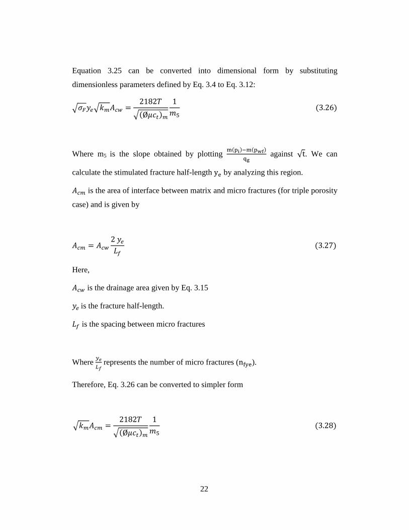
(3.26)
Where m5 is the slope obtained by plotting m(pi)−m(pwf)qg
against √t. We can
calculate the stimulated fracture half-length ye by analyzing this region.
𝐴𝑐𝑚 is the area of interface between matrix and micro fractures (for triple porosity
case) and is given by
𝐴𝑐𝑚 = 𝐴𝑐𝑤2 𝑦𝑒𝐿𝑓
(3.27)
Here,
𝐴𝑐𝑤 is the drainage area given by Eq. 3.15
𝑦𝑒 is the fracture half-length.
𝐿𝑓 is the spacing between micro fractures
Where 𝑦𝑒𝐿𝑓
represents the number of micro fractures (nfye).
Therefore, Eq. 3.26 can be converted to simpler form
�𝑘𝑚𝐴𝑐𝑚 =2182𝑇
�(Ø𝜇𝑐𝑡)𝑚
1𝑚5
(3.28)

23
If Region 5 is observed and other parameters are known, Eq. 3.28 can be used to
determine the matrix drainage area 𝐴𝑐𝑚.
3.4.6 Region 6
We observe this region when the reservoir boundary begins to influence the
transient response. In other words, the pressure transient response in the matrix
blocks has reached the virtual no flow boundaries developed between two
adjacent fractures. This region is also defined in the petroleum literature as
boundary dominated flow. We can calculate the stimulated reservoir volume SRV
by analyzing this region to estimate the OOIP and OGIP. We will derive an
equation for boundary-dominated flow of slightly compressible fluid in linear
dual porosity system.
The summary of the results for the highly compressible fluids (gas) and
slightly compressible fluid (oil) is presented in Table 3.1 and Table 3.2
respectively.

24
Table 3.1 Summary of analysis equations developed for constant Pwf of rate
transient solution for triple porosity system for highly compressible fluid
(gas)
Region Inverse Laplace Solution Analysis Equation
Region 1
(Macro-Fracture Flow)
𝑞𝐷𝐿 = 1
2𝜋�𝜋𝑡𝑑𝑎𝑐�𝜔𝑓 �𝑘𝐹𝐴𝑐𝑤 =
1262𝑇
�(∅𝜇𝑐𝑡)𝐹
1𝑚1
Region 2
(Bilinear flow b/w macro &
micro-fractures)
𝑞𝐷𝐿 =1
10.133�𝜆𝐴𝑐𝐹𝑓𝜔𝑓𝑡𝑑𝑎𝑐
4 �𝑘𝐹𝐴𝑐𝑤 =
4070𝑇
�𝜎𝐹𝑘𝑓(Ø𝜇𝑐𝑡)𝑓4
1𝑚2
Region 3
(Micro-fracture flow)
𝑞𝐷𝐿 =1
2𝜋�𝜋𝑡𝑑𝑎𝑐�𝜆𝐴𝑐𝐹𝑓𝜔𝑓
3𝑦𝐷𝑒 �𝜎𝐹𝑦𝑒�𝑘𝑓𝐴𝑐𝑤 =
2182𝑇
�(Ø𝜇𝑐𝑡)𝑓
1𝑚3
Region 4
(Bilinear flow b/w matrix &
micro-fractures)
𝑞𝐷𝐿 =1
17.54�𝜆𝐴𝑐𝐹𝑓 �
𝜆𝐴𝑐𝑓𝑚𝜔𝑚𝑡𝑑𝑎𝑐
4𝑦𝐷𝑒 �𝜎𝐹𝑦𝑒�
𝑘𝑓𝐿𝑓𝐴𝑐𝑤 =
2004𝑇
�𝑘𝑚(Ø𝜇𝑐𝑡)𝑚4
1𝑚4
Region 5
(Matrix flow) 𝑞𝐷𝐿 =1
2𝜋�𝜋𝑡𝑑𝑎𝑐�𝜆𝐴𝑐𝑓𝑚𝜔𝑚
3𝑦𝐷𝑒 �𝑘𝑚𝐴𝑐𝑚 =
1262𝑇
�(Ø𝜇𝑐𝑡)𝑚
1𝑚5

25
Table 3.2 Summary of analysis equations developed for constant Pwf of rate
transient solution for triple porosity system for slightly compressible fluid (oil)
Region Inverse Laplace Solution Analysis Equation
Region 1
(Macro-fracture flow)
𝑞𝐷𝐿 = 1
2𝜋�𝜋𝑡𝑑𝑎𝑐�𝜔𝑓 �𝑘𝐹𝐴𝑐𝑤 =
125.11𝐵𝑜𝜇
�(∅𝜇𝑐𝑡)𝐹
1𝑚1
Region 2
(Bilinear flow b/w macro & micro-
fractures)
𝑞𝐷𝐿 =1
10.133�𝜆𝐴𝑐𝐹𝑓𝜔𝑓𝑡𝑑𝑎𝑐
4 �𝑘𝐹𝐴𝑐𝑤 =
403.5𝐵𝑜𝜇
�𝜎𝐹𝑘𝑓(Ø𝜇𝑐𝑡)𝑓4
1𝑚2
Region 3
(Micro-fracture flow) 𝑞𝐷𝐿 =1
2𝜋�𝜋𝑡𝑑𝑎𝑐�𝜆𝐴𝑐𝐹𝑓𝜔𝑓
3𝑦𝐷𝑒
𝐿𝑓𝐿𝐹�𝑘𝑓𝐴𝑐𝑚 =
125.11𝐵𝑜𝜇
�(Ø𝜇𝑐𝑡)𝑓
1𝑚3
Region 4
(Bilinear flow b/w matrix & micro-
fractures)
𝑞𝐷𝐿 =1
17.54�𝜆𝐴𝑐𝐹𝑓 �
𝜆𝐴𝑐𝑓𝑚𝜔𝑚𝑡𝑑𝑎𝑐
4𝑦𝐷𝑒
𝐿𝑓𝐿𝐹�𝑘𝑓𝐴𝑐𝑚 =
403.5𝐵𝑜𝜇
�𝛼𝑚𝑘𝑚(Ø𝜇𝑐𝑡)𝑚4
1𝑚4
Region 5
(Matrix flow) 𝑞𝐷𝐿 =1
2𝜋�𝜋𝑡𝑑𝑎𝑐�𝜆𝐴𝑐𝑓𝑚𝜔𝑚
3𝑦𝐷𝑒 �𝑘𝑚𝐴𝑐𝑚 =
125.11 𝐵𝑜𝜇
�(Ø𝜇𝑐𝑡)𝑚
1𝑚5

26
CHAPTER IV
DEVELOPMENT OF ANALYSIS EQUATION OF BOUNDARY
DOMINATED FLOW
4.1 INTRODUCTION
In this chapter, we develop a new model for analyzing boundary dominated
flow in fractured tight oil wells. In Chapter VI we use this model to analyze the
boundary dominated flow in fractured tight oil reservoirs. The boundary
dominated flow occurs under pseudosteady state flow conditions.
4.2 MODELING BOUNDARY DOMINATED FLOW IN FRACTURED HORIZONTAL
WELLS
Pseudosteady state flow is observed when pressure interference occurs
between two adjacent transverse fractures. A no flow imaginary boundary is
formed at the middle of two adjacent fractures. We develop the equations to
analyze this pseudosteady behavior identified by a unit-slope on the plot of rate-
normalized pressure (RNP) versus material balance time (MBT). Fig. 4.1 shows
the no flow boundaries developed at the center of the matrix blocks separated by
two adjacent fractures. A 3D view of the horizontal well placed in the center of
reservoir is shown in Fig. 4.2.
4.2.1 Model Assumptions
In order to develop the analysis equations, we make the following assumptions:
1. The system is a dual porosity and no micro fractures (natural fractures) exist
2. The fluid flow is only from the matrix blocks to the hydraulic fractures and
only hydraulic fractures feed the well bore
3. The fluid is slightly compressible and single phase
4. The no flow boundary is assumed to be in the middle of the matrix blocks
separating two adjacent fractures
5. Spacing between the hydraulic fractures is uniform

27
6. When the pseudo steady state is reached, the pressure drop in the fractures is
negligible
7. The contribution of the matrix blocks beyond the fracture half-length is
ignored
8. Horizontal permeability is higher than vertical permeability
Fig. 4.1 – Plan view of hydraulic fractures connected to the horizontal well. The direction of flow is from the matrix to the fractures and from the fractures to the well. This figure also shows fracture half-length ye. Arrows indicate the flow direction.
x
Lf 2
Lf 2
y
Lf
Lf
ye
Xe
𝒅𝒅𝒅𝒅
= 𝟎
No Flow Boundary

28
Fig. 4.2 – Front view of hydraulic fractures connected to the horizontal well.
4.3.2 Development of a New Solution for the Boundary Dominated Linear
Flow in Horizontally Fractured Tight Reservoirs
Starting from the material balance equation and using the linear diffusivity
equation, we model the boundary dominated linear flow in fractured tight
reservoirs. To develop the analysis equation we consider, a control volume, 𝑉𝑚,
shown in Fig 4.3. It represents the volume of reservoir feeding one fracture. The
no-flow boundary is established at a distance of 0.5 𝐿𝑓from the fracture where 𝐿𝑓
is the spacing between the fractures.
z
x
Lf L
f
Lf 2
Lf 2
h
Xe
2ye

29
Fig. 4.3 – Schematic of the selected control volume showing a hydraulic fracture
surrounded by the matrix blocks. Two no-flow boundaries are virtually created at
the center of adjacent fractures at distance of 0.5 Lf from the fracture
We apply mass balance for control volume 𝑉𝑚 as shown in Fig. 4.3,
4.3.2.1 Material balance equation
Mass in – Mass out = Accumulation in the matrix (4.1)
0 − 𝑞𝑜𝜌𝑜𝛥𝑡│𝑥 = 𝜌𝑜 𝜙𝑚𝑉𝑚│𝑡 +𝛥𝑡 − 𝜌𝑚𝜙𝑚𝑉𝑚|𝑡 (4.2)
0 − 𝑞𝑜𝜌𝑜 = 𝜌𝑜 𝜙𝑚𝑉𝑚│𝑡 +𝛥𝑡 − 𝜌𝑚𝜙𝑚𝑉𝑚|𝑡
∆𝑡 (4.3)
Taking limits as Δt approaches to zero
Lf
2 ye
h
Lf 2
Lf 2
𝒅𝒅𝒅𝒅
= 𝟎
No Flow Boundary
𝒅𝒅𝒅𝒅
= 𝟎
No Flow Boundary

30
− 𝑞𝑜𝜌𝑜 = 𝑑𝑑𝑡
(𝜌𝑜 𝜙𝑚𝑉𝑚) (4.4)
− 𝑞𝑜𝜌𝑜𝑉𝑚
= 𝑑𝑑𝑡
(𝜌𝑜 𝜙𝑚) (4.5)
Using chain rule
− 𝑞𝑜𝜌𝑜𝑉𝑚
= 𝑑𝑃𝑑𝑡
� 𝜙𝑚𝑑𝑑𝑃
𝜌𝑜+𝜌𝑜 𝑑𝑑𝑃
𝜙𝑚� (4.6)
Dividing both sides by 𝜙𝑚 and 𝜌𝑜
− 𝑞𝑜𝑉𝑚 𝜙𝑚
= 𝑑𝑃𝑑𝑡
� 1𝜌𝑜
𝑑𝑑𝑃𝑚
𝜌𝑜 + 1
𝜙𝑚𝑑𝑑𝑃
𝜙𝑚� (4.7)
− 𝑞𝑜𝑉𝑚 𝜙𝑚
= 𝑑𝑃𝑑𝑡
� 𝑐𝑤 + 𝑐𝑓 � (4.8)
− 𝑞𝑜𝑉𝑚𝜙𝑚
= 𝑑𝑃𝑑𝑡
( 𝑐𝑡 ) (4.9)
𝑑𝑃𝑑𝑡
= −𝑞𝑜
𝑉𝑚𝜙𝑚 𝑐𝑡 (4.10)
Where 𝑉𝑚 is the controlled volume given by
𝑉𝑚 = 𝐿𝑓 .ℎ . 2𝑦𝑒 (4.11)
4.3.2.2 Linear Diffusivity Equation
Diffusivity equation for linear flow is given as
𝑑2𝑃𝑑𝑥2
= �𝜙𝑚 𝜇𝑜 𝑐𝑡𝑘𝑚
� 𝑑𝑃𝑑𝑡
(4.12)
Replacing 𝑑𝑃𝑑𝑡
from Eq. 4.9
𝑑2𝑃𝑑𝑥2
= �𝜙𝑚 𝜇𝑜 𝑐𝑡𝑘𝑚
� �−𝑞𝑜
𝑉𝑚𝜙𝑚 𝑐𝑡� (4.13)
Integrating both sides gives

31
𝑑𝑃𝑑𝑥
= � 𝜇𝑜 𝑘𝑚
� �−𝑞𝑜𝑉𝑚
𝑥� + 𝐶1 (4.14)
Applying the first boundary condition
At 𝑥 = 𝐿𝑓2
, 𝑑𝑃𝑑𝑥
= 0
C1 is given by
𝐶1 = � 𝜇𝑜 𝑘𝑚
𝑞𝑜𝑉𝑚� 𝐿𝑓2
(4.15)
Replacing C1 from Eq. 4.15 into Eq. 4.14, we obtain
𝑑𝑃𝑑𝑥
= � 𝜇𝑜 𝑘𝑚
��−𝑞𝑜𝑉𝑚
� 𝑥 + � 𝜇𝑜 𝑘𝑚
𝑞𝑜𝑉𝑚� 𝐿𝑓2
(4.16)
Integrating both sides of Eq. 4.16
�𝑑𝑃 = �� 𝜇𝑜 𝑘𝑚
� �−𝑞𝑜𝑉𝑚
� 𝑥 𝑑𝑥 + �� 𝜇𝑜 𝑘𝑚
𝑞𝑜𝑉𝑚� 𝐿𝑓2
𝑑𝑥 (4.17)
𝑃𝑚 = � 𝜇𝑜 𝑘𝑚
� �−𝑞𝑜
2 𝑉𝑚 𝑥2� + �
𝜇𝑜 𝑘𝑚
𝑞𝑜𝑉𝑚� 𝐿𝑓2𝑥 + 𝐶2 (4.18)
Applying the second boundary condition
At 𝑥 = 0, 𝑃𝑚 = 𝑃𝑓
Eq. 4.18 becomes
C2 = 𝑃𝑓 (4.19)
Replacing C2 from Eq. 4.19 into Eq.4.18
𝑃𝑚 = � 𝜇𝑜 𝑘𝑚
��−𝑞𝑜
2 𝑉𝑚 𝑥2� + �
𝜇𝑜 𝑘𝑚
𝑞𝑜𝑉𝑚� 𝐿𝑓2𝑥 + 𝑃𝑓 (4.20)
Eq. 4.20 represents pressure profile in the matrix block.
4.3.2.3 Average matrix pressure from the pressure solution
Average pressure of the control volume 𝑉𝑚 is given by

32
x
z
Lf 2
Lf 2
h
𝝏𝒅𝝏𝝏
= 𝒄𝒄𝒄𝒄𝝏
No Flow Boundary
𝒅𝒅𝒅𝒅
= 𝟎
Matrix Blocks
Fracture
𝑃𝑚���� =∫ 𝑃𝑚𝑑𝑉𝑚𝐿𝑓20
∫ 𝑑𝑉𝑚𝐿𝑓20
(4.21)
Fig. 4.4 – The pressure profile in the matrix during the boundary dominated flow.
The rate of pressure drop with respect to time remains constant at pseudosteady
state conditions.
Replacing 𝑃𝑚 from Eq. 4.20 and
𝑑𝑉𝑚 = 2 𝑦𝑒 × ℎ
× 𝑑𝑥 (4.22)
On solving Eq. 4.21, the average matrix pressure is given by
𝑃𝑚���� − 𝑃𝑓 = 𝜇 𝐵𝑜 𝑞𝑜 𝐿𝑓2
12 𝑘𝑚 𝑉𝑚 (4.23)
4.3.2.4 Average matrix pressure based on Pseudo-steady state flow
Expressing Pf as a function of time,
𝝏𝒅𝝏𝝏
= 𝒄𝒄𝒄𝒄𝝏
𝒅𝒅𝒅𝒅
= 𝟎
No Flow Boundary

33
𝑐𝑡 = −1
𝜙𝑚𝑉𝑚∆𝑉𝑜∆𝑃𝑚
(4.24)
𝐶𝑡 𝑉𝑚 𝑑𝑃𝑚 = −𝑑𝑉𝑚 (4.25)
Here,
∆𝑃𝑚 = 𝑃𝑖 − 𝑃𝑚���� 𝑎𝑛𝑑 ∆𝑉𝑜 = 𝐵𝑜 𝑞𝑜 𝑡 (4.26)
𝜙𝑚𝑉𝑚 = 𝜙𝑚 𝐿𝑓 ℎ 2𝑦𝑒 (4.27)
Substituting Eq. 4.26 and 4.27 in Eq. 4.24,
𝑃𝑚����−𝑃𝑖 = 𝐵𝑜 𝑞𝑜 𝑡
𝐿𝑓ℎ 2𝑦𝑒 𝜙𝑚 𝑐𝑡 (4.28)
4.3.2.5 Final Solution
Replacing 𝑃𝑚���� from Eq. 4.23
𝑃𝑖 − 𝑃𝑓 = 𝐵𝑜𝑞𝑜 𝑡
𝐿𝑓 ℎ 2𝑦𝑒 𝜙𝑚 𝑐𝑡 + 𝜇 𝐵𝑜 𝑞𝑜 𝐿𝑓2
12 𝑘𝑚 𝑉𝑚 (4.29)
We know 𝑁𝑝 = 𝑞𝑜 𝑡 (4.30)
Replacing Eq. 4.30 in Eq. 4.29 and dividing by 𝑞𝑜 we obtain
𝑃𝑖 − 𝑃𝑓𝑞𝑜
= 𝐵𝑜 𝑁𝑝
𝐿𝑓 ℎ 2𝑦𝑒 𝜙𝑚 𝑐𝑡 𝑞𝑜 + 𝜇 𝐵𝑜 𝑞𝑜 𝐿𝑓2
12 𝑘𝑚 𝑉𝑚 (4.31)
Replacing 𝑁𝑝𝑞𝑜
= 𝑡̅ (4.32)
𝑃𝑖 − 𝑃𝑤𝑓𝑞𝑜
= 𝐵𝑜 𝑡̅
𝐿𝑓 ℎ 2𝑦𝑒 𝜙𝑚 𝑐𝑡 +
𝜇 𝐵𝑜 𝐿𝑓2
12 𝑘𝑚 𝑉𝑚 (4.33)
𝑡 ̅ is the material balance time (MBT)
Np is the cumulative oil production
Qo is the daily oil rate

34
Blasingame and Lee (1986) introduced the original material balance approach for
boundary-dominated flow (i.e. pseudo steady state flow), which is later modified
by Placio and Blasingame (1993) for any instantaneous production time, flow
regime or production scenario.
When the boundary effects are observed after the transient flow regime, we
assume Pf = Pwf, this means that the pressure drop in the fracture is negligible.
𝑃𝑖 − 𝑃𝑤𝑓𝑞𝑜
= 𝐵𝑜 𝑡̅
𝐿𝑓 ℎ 2𝑦𝑒 𝜙𝑚 𝑐𝑡 +
𝜇 𝐵𝑜 𝐿𝑓2
12 𝑘𝑚 𝑉𝑚 (4.33)
Eq. 4.33 is developed for one producing fracture; to incorporate the effect of
multiple numbers of fractures we multiply 𝑞𝑜 and 𝑉𝑚 by number of fractures Nf to
obtain total flow rate 𝑄𝑜 and total reservoir volume.
𝑃𝑖 − 𝑃𝑤𝑓𝑄𝑜
= 𝐵𝑜 𝑡̅
𝐴𝑐𝑤 𝑦𝑒 𝜙𝑚 𝑐𝑡 +
𝜇 𝐵𝑜 𝐿𝑓2
12 𝑘𝑚 𝑁𝑓 𝑉𝑚 (4.34)
𝑃𝑖−𝑃𝑤𝑓𝑞𝑜
is defined in the petroleum literature as Rate-Normalized Pressure (RNP).
To analyze the boundary dominated flow we plot RNP versus MBT.
𝑃𝑖 − 𝑃𝑤𝑓𝑄𝑜
= 𝑚𝑠𝑠 𝑡̅ + 𝑏𝑠𝑠 (4.35)
Here 𝑚𝑠𝑠 and 𝑏𝑠𝑠 are the slope and intercept of the line on the plot of RNP versus
MBT given by:
𝑚𝑠𝑠 = 5.615 𝐵𝑜
𝐴𝑐𝑤 𝑦𝑒 𝜙𝑚 𝑐𝑡 (4.36)
By replacing 𝑆𝑅𝑉 = 𝐴𝑐𝑤 × 𝑦𝑒 × 𝜑𝑚 in Eq. 4.36 we obtain
𝑚𝑠𝑠 = 5.615 𝐵𝑜𝑆𝑅𝑉 𝑐𝑡
(4.37)
The intercept is given by

35
𝑏𝑠𝑠 =𝜇 𝐵𝑜 𝐿𝑓2
12 𝑘𝑚 𝑁𝑓 𝑉𝑚 (4.38)
Replacing 𝑉𝑚 from Eq. 4.11 and converting to field units
𝑏𝑠𝑠 =36.96 𝜇 𝐵𝑜 𝐿𝑓 𝑘𝑚 𝑁𝑓 𝑦𝑒 ℎ
(4.39)
Using 𝑚𝑠𝑠 we calculate the stimulated reservoir volume 𝑆𝑅𝑉. Comparing with
𝑆𝑅𝑉 calculated from transient region, we identify whether the pressure
interference has occurred not. If the value of 𝑆𝑅𝑉 obtained from matrix analysis is
very high as compared to the value obtained from analysis of the boundary-
dominated flow, we can say that the reservoir has not been depleted completely.
Another explanation is that the fracture half-length 𝑦𝑒 is over estimated. Similarly
we can identify if the number of fracture is optimum for efficient reservoir
depletion or not.
By analyzing the intercept of the line (𝑏𝑠𝑠) we can estimate the minimum
permeability of the reservoir (Song and Economides 2011). For homogenous
reservoirs, the value calculated from this analysis should be approximately equal
to the permeability obtained by well testing.
36
CHAPTER V
PRODUCTION DATA ANALYSIS OF GAS RESERVOIRS IN BARNET
SHALE
5.1 INTRODUCTION
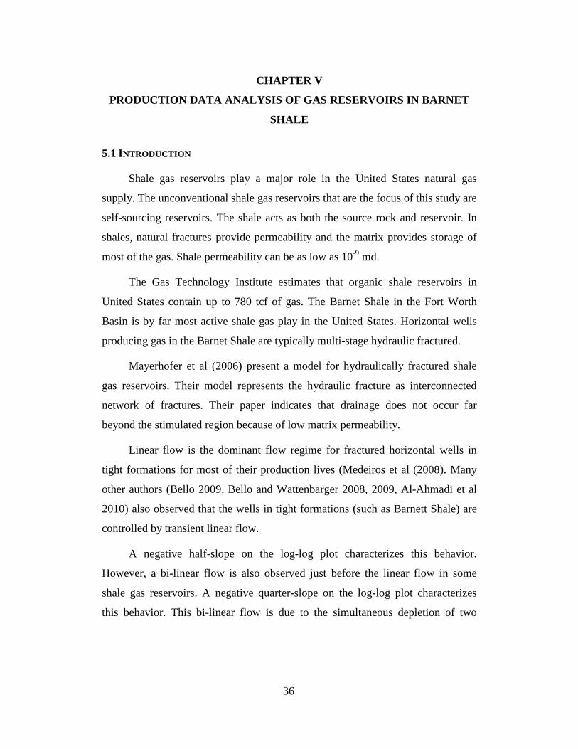
Shale gas reservoirs play a major role in the United States natural gas
supply. The unconventional shale gas reservoirs that are the focus of this study are
self-sourcing reservoirs. The shale acts as both the source rock and reservoir. In
shales, natural fractures provide permeability and the matrix provides storage of
most of the gas. Shale permeability can be as low as 10-9 md.
The Gas Technology Institute estimates that organic shale reservoirs in
United States contain up to 780 tcf of gas. The Barnet Shale in the Fort Worth
Basin is by far most active shale gas play in the United States. Horizontal wells
producing gas in the Barnet Shale are typically multi-stage hydraulic fractured.
Mayerhofer et al (2006) present a model for hydraulically fractured shale
gas reservoirs. Their model represents the hydraulic fracture as interconnected
network of fractures. Their paper indicates that drainage does not occur far
beyond the stimulated region because of low matrix permeability.
Linear flow is the dominant flow regime for fractured horizontal wells in
tight formations for most of their production lives (Medeiros et al (2008). Many
other authors (Bello 2009, Bello and Wattenbarger 2008, 2009, Al-Ahmadi et al
2010) also observed that the wells in tight formations (such as Barnett Shale) are
controlled by transient linear flow.
A negative half-slope on the log-log plot characterizes this behavior.
However, a bi-linear flow is also observed just before the linear flow in some
shale gas reservoirs. A negative quarter-slope on the log-log plot characterizes
this behavior. This bi-linear flow is due to the simultaneous depletion of two

37
connected media. The two media could be micro-fractures and matrix or micro-
fractures and macro-fractures.
Shale gas wells have been modeled using linear dual-porosity models. Some
of the horizontal wells drilled in shale gas reservoirs are hydraulically fractured.
According to Gate et al (2007), propagation of these hydraulic fractures re-
activate the pre-existing natural fractures resulting in the two perpendicular
fractures systems with different properties. Therefore, dual porosity models
(which assume homogeneous matrix properties) are not sufficient to characterize
these reservoirs, as the matrix permeability will be enhanced by reactivated
natural fractures. A triple porosity model is thus required to model horizontal
shale gas wells containing reactivated (or pre-existing) natural fractures.
This chapter deals with analysis of Region 4 and Region 5 in detail. A
preliminary procedure is also presented for analyzing field data.
5.2 PROCEDURE FOR PRODUCTION DATA ANALYSIS FOR TIGHT GAS WELLS
In this section we present the procedure to analyze the production data of
tight gas reservoir using triple porosity equations developed in Chapter III of this
dissertation. After obtaining the field data, we identify different flow regions by
constructing a specialized plot of flow rate versus material balance time. The
procedure for analyzing Region 4 and Region 5 as define in Chapter III is
presented below.
5.2.1 Region 4 (Bilinear Flow in Micro-fractures and Matrix)
Region 4 can be analyzed by following the steps presented below:
1. Identify the transient flow region indicated by quarter slope on the log-log
plot of flow rate against material balance time.
2. Plot Rate Normalized pseudo-pressure (RNP) 𝑚(𝑃𝑖)−𝑚(𝑃𝑤𝑓)𝑄𝑔
versus √𝑡̅4

38
3. Use the slope of the line (m4) to calculate either 𝑘𝑓 or 𝐿𝑓 if one of them is
known, or if 𝑘𝑓 and 𝐿𝑓 are not known we can calculate the ratio of 𝑘𝑓𝐿𝑓
using
𝐿𝑓𝐿𝐹�𝑘𝑓𝐴𝑐𝑚 =
2004𝑇�𝑘𝑚(Ø𝜇𝑐𝑡)𝑚4
1𝑚4
5.2.2 Region 5 (Rate Transient Flow from Matrix)
Region 5 can be analyzed by following the steps presented below:
1. Identify the transient flow region indicated by a half slope on the log-log plot
of flow rate against material balance time.
2. Plot Rate Normalized Pressure (RNP) 𝑚(𝑃𝑖)−𝑚(𝑃𝑤𝑓)𝑄𝑔
versus √𝑡 ̅for gas wells.
3. Use the slope of the line (m5) to calculate area of interface between matrix and
hydraulic fractures 𝐴𝑐𝑚 from
�𝑘𝑚𝐴𝑐𝑚 =2182𝑇
�(Ø𝜇𝑐𝑡)𝑚
1𝑚5
(5.2)
4. The number of micro fractures (𝑛𝑓𝑦𝑒) can be calculated using
𝑛𝑓𝑦𝑒 =𝐴𝑐𝑚
2 𝐴𝑐𝑤 (5.3)

39
5.3 APPLICATION OF ANALYSIS PROCEDURE TO PRODUCTION DATA
In this section we use the developed triple porosity model to analyze the field data
of two wells from Barnett Shale i.e. well 314 and well 73. Gas rate history of
these well is shown in Fig. 5.1 (Al-Ahmadi 2010).
Fig. 5.1 – Log-log plot of gas rate versus time for two horizontal shale gas wells. Well 73 exhibits bi-linear flow between micro fracture and matrix followed by matrix linear flow as it gives negative quarter-slope for some time and then negative half-slope. Well 314 shows negative half-slope for almost two log cycles and indicates matrix linear flow.
1
10
100
1000
10000
100000
1 10 100 1000 10000
Gas
Rat
e, M
Scf/d
ay
MBT, days
Well 73
Qg = MBT-0.25
Qg= MBT -0.5
Qg = MBT -0.50
1
10
100
1000
10000
100000
1 10 100 1000 10000
Gas
Rat
e, M
Scf/d
ay
MBT, days
Well 314

40
5.3.1 Production Data Analysis of Well 73
Table 5.1 summarizes the petro-physical and completion data of Well 73.
Table 5.1 Reservoir and fluid properties obtained from well tests of Well 73
Reservoir Type Homogeneous Permeability – Horizontal
(k) 1.50E-04 md
Dominant Flow Gas Reservoir thickness (h) 300 ft.
Multiphase flow in
reservoir No Matrix Porosity (ϕm) 0.06
Reservoir Pseudo
pressure m(Pi)
5.97E+08
psi2/cp Fracture Spacing (L) 79 ft.
Flowing BHP m(Pwf) 2.03E+07
psi2/cp Gas viscosity (μgi) 0.0201 cp
Number of stages of
fractures 18 Temperature (T) 610 0R
Length of horizontal well
(Χe) 1420 ft. Total Compressibility (ct) 3.00E-04 psi-1
5.3.1.1 Analysis of bilinear transient region
We consider the production data of well 73 till the point it exhibits a negative
quarter slope as shown in Fig.5.2. In Fig. 5.3 we plot RNP versus fourth root of
time.

41
Fig. 5.2 – Log-log plot of gas rate versus MBT that shows a negative quarter slope.
Fig. 5.3 – Plot of fourth root MBT versus RNP that gives slopes equal to 136370
psi/cp2/Mscf/day/day0.25
Now we use Eq.5.1 for analysis of Region 4 to obtain the ratio 𝑘𝑓
𝐿𝑓. Slope m4 is
found to be 136370 psi/cp2/Mscf/day/day0.25. If we assume stimulated fracture
half-length ye = 150 ft then 𝑘𝑓𝐿𝑓
is calculated by,
qg= 4243.4 MBT-0.252 R² = 0.9793
1
10
100
1000
10000
100000
1 10 100
Gas
Rat
e, M
Scf/d
ay
MBT, days
RNP = 136370 MBT0.25
0
50000
100000
150000
200000
250000
300000
1 1.2 1.4 1.6 1.8 2
∆m(p
)/qg (
psi/c
p2 /MSc
f/day
)
MBT0.25 , (days)0.25

42
�σFye�kfLf
Acw =2004T
�km(صct)m4
1m4
� 12792
× 150 × �kfLf
× 85200 =2004x610
�(1.5x10−4x3.62x10−7)4 ×1
136370
kfLf
= 0.000626 mdft �
5.3.1.2 Analysis of Linear Transient Region (Matrix)
We consider the part of production data that shows linear flow i.e. Region 5. We
plot RNP versus square root of MBT as shown in Fig. 5.4. In Fig. 5.5 we plot
RNP versus fourth root of time. Reservoir data and other parameters used are
same as in Table 5.1.
Fig. 5.4 – Log-log plot of gas rate versus MBT shows a negative half slope.
qg = 10390MBT-0.498
100
1000
10000
10 100 1000
Gas
rat
e, M
Scf/d
ay
MBT, days

43
Fig. 5.5 – Plot of square root MBT versus RNP that gives slopes equal to 54961
psi/cp2/Mscf/day/day0.5
From Fig-5.5 slope is found to be 54961 psi2/cp/MScf/day/day0.5. We use Eq.
5.2 to calculate the drainage area Acm.
�𝑘𝑚𝐴𝑐𝑚 =1262𝑇
�(Ø𝜇𝑐𝑡 )𝑚 1𝑚5
Replacing the corresponding values,
Acm =(1262)(610)
�(1.5x10⁻⁷)(3.62x10⁻⁷ )×
154961
= 1,900,000 ft2
Now we calculate the number of micro-fractures nfye using Eq. 5.3,
Acm = �2nfyeAcw�
nfye =Acm
2Acw=
19000002 × 852000
= 1
RNP = 54961 MBT0.5
0
200000
400000
600000
800000
1000000
1200000
1400000
0 5 10 15 20 25
∆m(p
)/qg,
psi/
cp2 /M
Scf/d
ay
MBT0.5, days0.5
44
5.3.2 Regression Results for Well 73
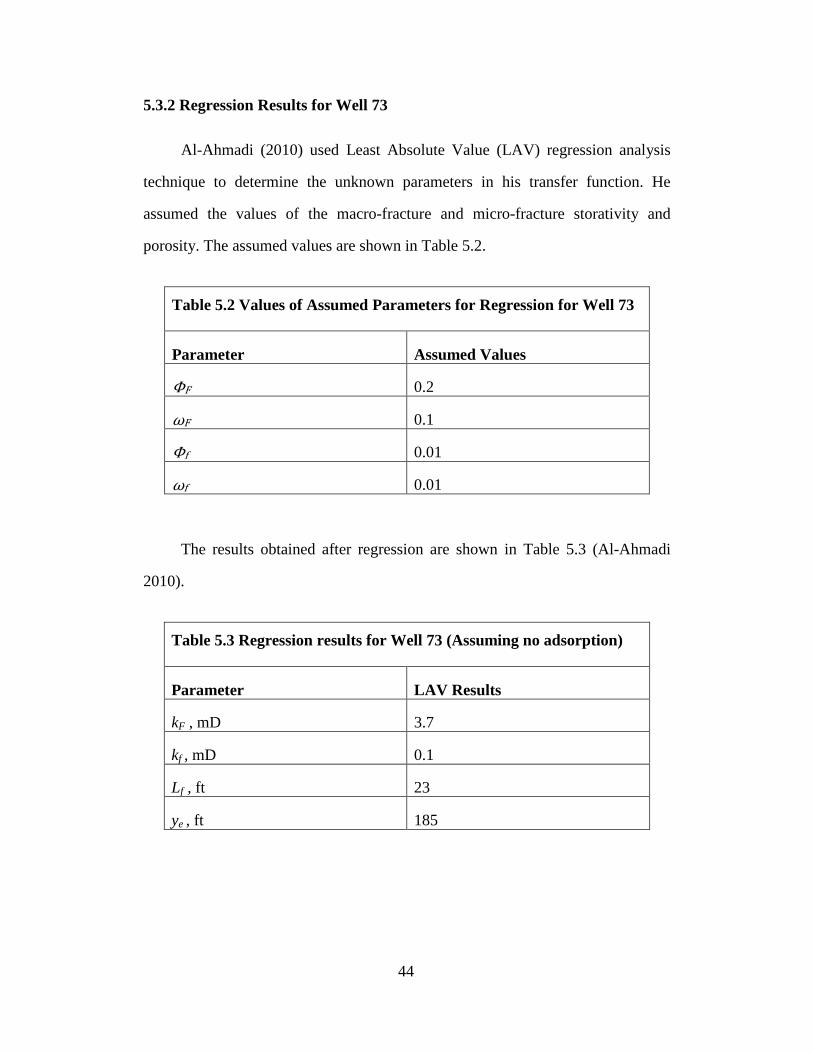
Al-Ahmadi (2010) used Least Absolute Value (LAV) regression analysis
technique to determine the unknown parameters in his transfer function. He
assumed the values of the macro-fracture and micro-fracture storativity and
porosity. The assumed values are shown in Table 5.2.
Table 5.2 Values of Assumed Parameters for Regression for Well 73
Parameter Assumed Values
ΦF 0.2
ωF 0.1
Φf 0.01
ωf 0.01
The results obtained after regression are shown in Table 5.3 (Al-Ahmadi
2010).
Table 5.3 Regression results for Well 73 (Assuming no adsorption)
Parameter LAV Results
kF , mD 3.7
kf , mD 0.1
Lf , ft 23
ye , ft 185

45
5.3.2.1 Comparison of Results
The results obtained from analytical equations vary significantly from results
obtained from regression analysis. The production data doesn’t usually contain
flow data from early time scales (fluid production from macro fractures and
micro-fractures). If the fracture properties are assumed, the regression results will
be affected. The regression results depend on the initial assumed value and can
vary if the initial guess made is not close.
5.3.3 Production Data Analysis of Well 314
The production data for this well only exhibits linear flow that reflects the matrix
depletion. Reservoir data is summarized in Table 5.4. The production data plot is
shown in Fig. 5.6.
Table 5.4 Reservoir and fluid properties obtained from well tests of Well 314
Reservoir Type Homogeneous Permeability – Horizontal (k) 1.50E-04 md
Dominant Flow Gas Reservoir thickness (h) 300 ft.
Multiphase flow in
reservoir No Matrix Porosity (ϕ) 0.06
Reservoir Pseudo
pressure m(Pi) 5.97E+08 psi2/cp Fracture Spacing (L) 106 ft.
Flowing BHP m(Pwf) 2.03E+07 psi2/cp Gas viscosity (μgi) 0.0201 cp
Number of stages of
fractures 28 Temperature (T) 610 0R
Length of horizontal
well (Χe) 2968 ft. Total Compressibility (ct) 3.00E-04 psi-1

46
Fig. 5.6 – Log-log plot of gas rate versus MBT shows a negative half slope.
Fig. 5.7 – Plot of square root MBT versus RNP that gives slopes equal to 20701
psi/cp2/Mscf/day/day0.5
Figure 5.7 shows the square root time plot slope is equal to 20701
psi2/cp/MScf/day/day0.5. Using Eq. 5.2 to calculate Acm.
q = 29134MBT0.503 R² = 0.9829
100
1000
10000
1 10 100 1000 10000
Gas
Rat
e, M
Scf/d
ay
MBT, days
RNP= 20701MBT0.5
0
100000
200000
300000
400000
500000
600000
700000
800000
0 10 20 30 40
∆m(p
)/qg,
psi/
cp2 /M
Scf/d
ay
MBT0.5, days0.5

47
�kmAcm =1262T
�(صct )m 1
m5
Replacing the corresponding values in Eq. 5.2
Acm =(1262)(610)
�(1.5x10⁻⁴)(3.62x10⁻⁷ ) ×
120701
= 5,050,000 ft2
Using Eq. 5.3 to calculate the number of micro-fractures.
nfye = Acm
2Acw=
50500002 × 1780800
≅ 1
5.3.4 Regression Results for Well 314
The assumed values are for regression is shown in Table 5.5.
Table 5.5 Values of Assumed Parameters for Regression for Well 314
Parameter Assumed Values
ΦF 0.2
ωF 0.1
Φf 0.01
ωf 0.01
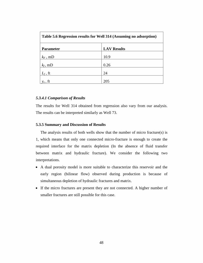
The results obtained after regression are shown in Table 5.6.
48
Table 5.6 Regression results for Well 314 (Assuming no adsorption)
Parameter LAV Results
kF , mD 10.9
kf , mD 0.26
Lf , ft 24
ye , ft 205
5.3.4.1 Comparison of Results
The results for Well 314 obtained from regression also vary from our analysis.
The results can be interpreted similarly as Well 73.
5.3.5 Summary and Discussion of Results
The analysis results of both wells show that the number of micro fracture(s) is
1, which means that only one connected micro-fracture is enough to create the
required interface for the matrix depletion (In the absence of fluid transfer
between matrix and hydraulic fracture). We consider the following two
interpretations.
• A dual porosity model is more suitable to characterize this reservoir and the
early region (bilinear flow) observed during production is because of
simultaneous depletion of hydraulic fractures and matrix.
• If the micro fractures are present they are not connected. A higher number of
smaller fractures are still possible for this case.

49
CHAPTER VI
PRODUCTION DATA ANALYSIS OF TIGHT OIL RESERVOIRS
6.1 INTRODUCTION
Recent advances in horizontal drilling and multi-stage hydraulic fracturing
have led to the successful exploitation of tight oil and shale gas reservoirs.
Clarkson and Pedersen (2011) proposed the term “Unconventional Light Oil”
(ULO) and proposed further categories of ULO on the basis of play types and
matrix permeability. Reservoir properties that could distinguish ULO plays from
conventional light oil plays also include low matrix permeability (<0.1 md). A
classification for the ULO plays in Western Canada is as follows:
1. Halo Oil – High matrix permeability (e.g. Cardium and Viking Pools of
Alberta)
2. Tight Oil – Low matrix permeability (e.g. Saskatchewan Bakken Formation)
3. Shale Oil – Very low matrix permeability (e.g. Duvernay and Muskwa
Formations)
This chapter deals with the analysis of tight oil wells from Cardium and
Bakken formations. The production data of tight oil wells exhibit linear transient
behavior that is analyzed using the dual porosity models. The linear transient flow
from matrix depletion is analyzed using dual porosity model presented by Bello
(2009). The boundary dominated flow (that occurs under pseudosteady state flow
conditions) is analyzed by the model developed in Chapter IV of this work.
6.1.1 Pembina Cardium (Halo Oil)
Cardium Formation is the largest conventional oil reserves in the Western
Canada Sedimentary Basin. The oil production initiated in the early 1950s, and
only approximately 20% of the reserve is recovered. The Cardium Formation
(deposited in the Late Cretaceous, approximately 88 million years ago) consists of

50
interbedded sandstone and shale, and some local conglomerate, spread over much
of western Alberta. Over the past fifty years, conglomerates and porous
sandstones have been targeted for conventional production of oil, mainly from the
Pembina Field. The Cardium Formation in Alberta is estimated to have contained
1,678 million m³ (10.6 billion barrels) of oil originally in place, 1,490 million m³
(9.4 billion barrels) of which was in the Pembina Field. Since its discovery in
the 1950s, 234 million m³ (1.5 billion barrels) of Cardium oil has been produced.
Production of oil in the Cardium Formation rebounded in 2009, when horizontal
drilling and multi-stage fracturing technology increased the oil recovery factor.
6.1.2 Saskatchewan Bakken (Tight Oil)
The Bakken Formation in Saskatchewan and Manitoba is a part of a relatively
thin accumulation of siltstone and sandstone sandwiched between organic-rich
shales extending over much of western Canada. It was deposited as the Devonian
Period transitioned into the Mississippian Period, approximately 360 million years
ago. The Bakken tight oil play is about 25 meters thick and consists of lower
organic-rich shale, a middle siltstone and sandstone unit, and overlying organic-
rich shale.
So far, companies have publicly reported 36 million m³ (225 million barrels)
of proved and probable reserves from the Bakken. No reserves from the Exshaw
have been publicly reported. Where the Bakken extends into North Dakota and
Montana, the United States Geological Survey estimates that there are
580 million m³ (3.65 billion barrels) of recoverable oil. The areal extent of oil-
prone Bakken in the United States is far more extensive than in Saskatchewan.
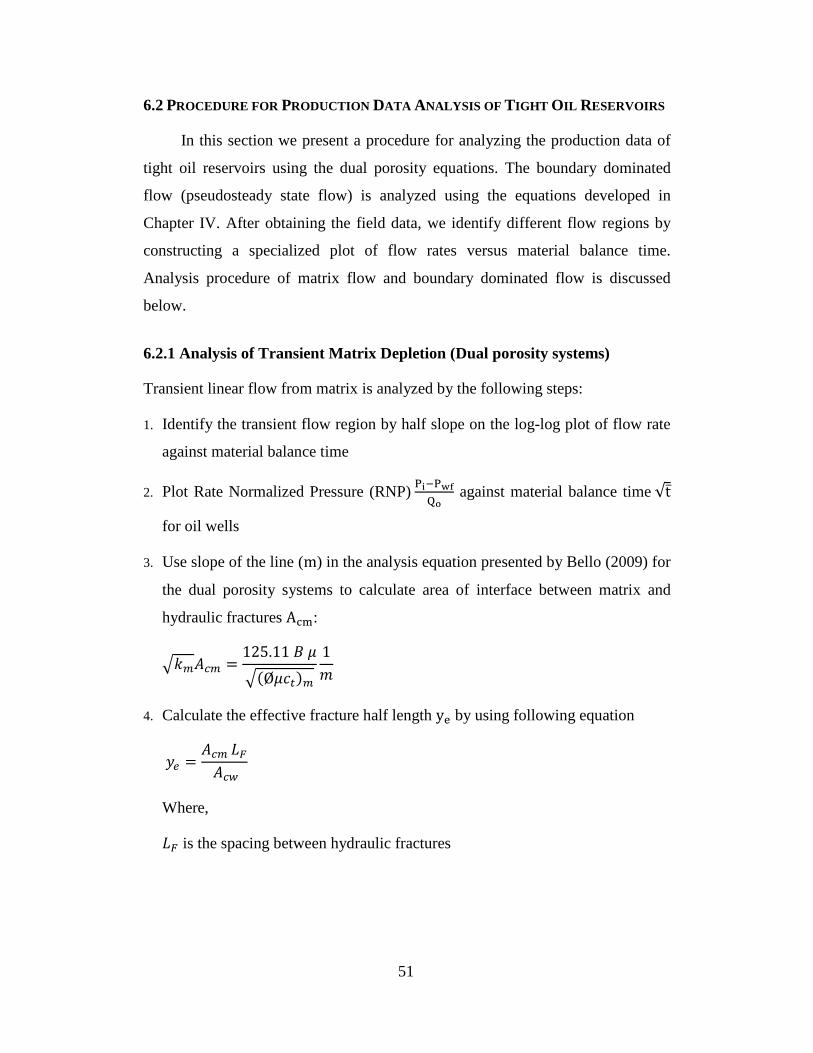
51
6.2 PROCEDURE FOR PRODUCTION DATA ANALYSIS OF TIGHT OIL RESERVOIRS
In this section we present a procedure for analyzing the production data of
tight oil reservoirs using the dual porosity equations. The boundary dominated
flow (pseudosteady state flow) is analyzed using the equations developed in
Chapter IV. After obtaining the field data, we identify different flow regions by
constructing a specialized plot of flow rates versus material balance time.
Analysis procedure of matrix flow and boundary dominated flow is discussed
below.
6.2.1 Analysis of Transient Matrix Depletion (Dual porosity systems)
Transient linear flow from matrix is analyzed by the following steps:
1. Identify the transient flow region by half slope on the log-log plot of flow rate
against material balance time
2. Plot Rate Normalized Pressure (RNP) Pi−PwfQo
against material balance time √t ̅
for oil wells
3. Use slope of the line (m) in the analysis equation presented by Bello (2009) for
the dual porosity systems to calculate area of interface between matrix and
hydraulic fractures Acm:
�𝑘𝑚𝐴𝑐𝑚 =125.11 𝐵 𝜇�(Ø𝜇𝑐𝑡)𝑚
1𝑚
4. Calculate the effective fracture half length ye by using following equation
𝑦𝑒 =𝐴𝑐𝑚 𝐿𝐹
𝐴𝑐𝑤
Where,
𝐿𝐹 is the spacing between hydraulic fractures

52
6.2.2 Analysis of boundary dominated flow (PSS flow)
Boundary dominated flow can be analyzed by the following steps:
1. Construct a log-log plot between rate-normalized pressure (RNP) and material
balance time (MBT) for the complete production data.
2. The region for the pseudo steady flow is recognized by a constant slope of one
on a log-log plot of flow rate versus MBT.
3. Plot RNP versus MBT of data points of pseudo steady state flow region on a
linear scale.
4. Record the line slope, mss, and the line intercept, bss
5. Calculate the stimulated reservoir volume SRV by substituting mss in
𝑚𝑠𝑠 = 5.615 𝐵𝑜𝑆𝑅𝑉 𝑐𝑡
6. Calculate the minimum permeability of the reservoir by substituting bss in
𝑏𝑠𝑠 =36.96 𝜇 𝐵𝑜 𝐿𝑓 𝑘𝑚 𝑁𝑓 𝑦𝑒 ℎ
6.3 PRODUCTION DATA ANALYSIS OF CARDIUM WELLS
In this section, we analyze the production data of tight oil wells drilled in Cardium
formation.
6.3.1 Observing behavior of Cardium Wells
We analyze production data from several oil wells drilled in Cardium formation to
identify different flow regimes. Figure 6.1 shows log-log plot of cumulative oil
production versus time. The advantage of such plots is the insensitivity to shut-ins
and fluctuations in production rate. The slope of this plot may indicate the
dominant flow regimes (El Banbi 1998).

53
Fig. 6.1 – Plots of cumulative oil production versus time for five fractured horizontal wells completed in Cardium formation. The log-log plots show a slope of 0.6 - 0.75 for early time scales and a slope of approximately 0.5 for late time scales. The length of horizontal wells and number of stages of hydraulic fractures are different in these wells. The consistent behavior of cumulative plots shows that the flow regime is relatively similar for all the wells.
Np = 25.348 t0.5376
Np = 5.3403 t0.7324
100
1000
10000
100 1000 10000 100000Cum
ulat
ive
Prod
uctio
n (m
3 )
Time (hrs)
Np = 46.784 t0.4854
Np = 7.0931 t0.7414
100
1000
10000
100 1000 10000 100000
Cum
ulat
ive
Prod
uctio
n (m
3 )
Time (hrs)
Np = 54.487 t0.4547
Np = 16.676 t0.6062
100
1000
10000
100 1000 10000 100000Cum
ulat
ive
Prod
uctio
n (m
3 )
Time (hrs)
Np = 77.207 t0.4221
Np = 8.2857 t0.7312 100
1000
10000
100 1000 10000 100000Cum
ulat
ive
Prod
uctio
n (m
3 )
Time (hrs)
(a) (b)
(c) (d)
Np = 26.427 t0.5399
Np = 7.6873 t0.6957
100
1000
10000
100 1000 10000 100000
Cum
ulat
ive
Prod
uctio
n (m
3 )
Time hrs (e)

54
Da Prat el al (1981) recognized that for linear flow regime, dimensionless
cumulative production QD versus dimensionless time on a log-log plot gives a
slope of 0.5. They observed this linear flow behavior for transient dual porosity
case. Therefore it can be interpreted from the second part of these plots that the
dominant flow regime in Cardium wells is also linear transient. The first region
can be interpreted as bi-linear flow. Therefore, the analysis equation developed
for linear flow for slightly compressible fluid can be applied here.
6.3.2 Example Application for Characterizing a Fractured Well in Cardium
Formation
We select a tight oil well in a Pembina field. The well is hydraulically fractured
(18 multi stages) and has been producing for nearly 2 years. The fluctuation in
production rate were caused by shut-ins. Unfortunately, complete information
about those shut-in periods is not available. Table 6.1 presents the available fluid
and reservoir properties.
Table 6.1 Reservoir and fluid properties of Well in Cardium Formation
Reservoir Type Homogeneous Permeability–
Horizontal(khor) 0.640 mD
Dominant Flow Oil Phase Permeability–Vertical (kver) 9.03 x 10⁻⁴ mD
Multiphase flow in
reservoir No Reservoir thickness (h) 7 m
Reservoir Pressure
(Pi) 15,575 KPaa Matrix Porosity (𝛟𝐦) 0.120
Flowing BHP (Pwf) 7,413 KPaa Oil Formation Volume factor
(Bo) 1.221 Rm3 / m3
Number of stages of
fractures 18 Oil Viscosity (μo) 1.13 cp
Length of horizontal
well (Χe) 1370 m
Total Compressibility (ct)
(Assumed) 1.54 x 10⁻⁴ psi-1

55
We assume that the oil flows directly into the hydraulic fractures since the vertical
permeability is very low as compared to the horizontal permeability. Figure 6.2
shows the daily oil rate versus time on a log-log plot. The data indicates that the
production rates are variable and therefore it is difficult to distinguish any flow
regimes from this plot.
Fig. 6.2 – Log-log plot of daily oil rate versus time for a Well in Cardium Formation
In order to identify different flow regimes, we plot the production rate versus
material balance time. Figure 6.3 shows the log-log plot of oil rate versus
material balance time for the same well in which three distinctive flow regions
can easily be identified. Region 1 shows of negative half-slope during maximum
life of production and Region 2 shows a negative slope of one.
We assume that Region 1 (transient matrix flow) represents linear transient
flow from the matrix into the hydraulic fractures. This assumption is supported by
low vertical permeability in Cardium formation. We apply the dual porosity
model of Bello (2009) to analyze this region. Furthermore we assume that Region
1
10
100
100 1000
Dai
ly O
il R
ate
(m3 /
day)
Time (Days)
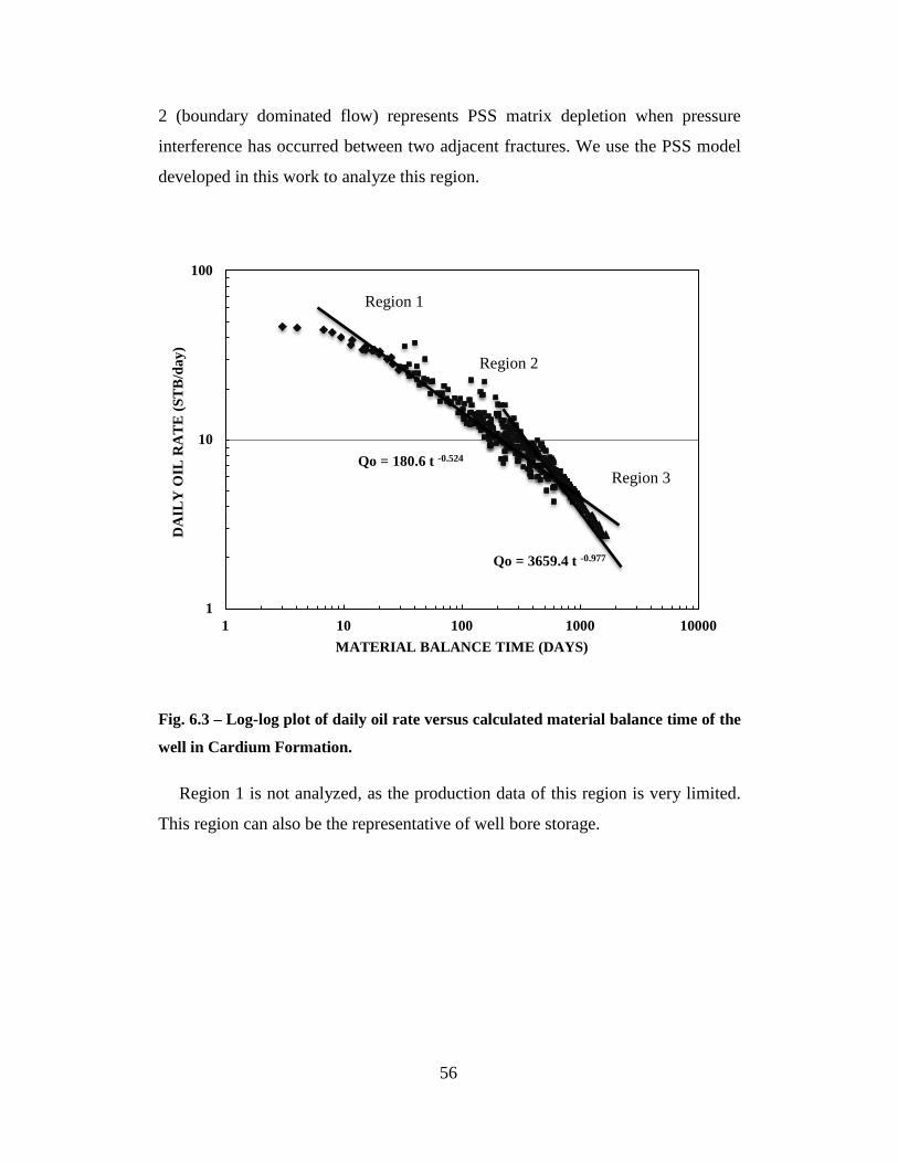
56
2 (boundary dominated flow) represents PSS matrix depletion when pressure
interference has occurred between two adjacent fractures. We use the PSS model
developed in this work to analyze this region.
Fig. 6.3 – Log-log plot of daily oil rate versus calculated material balance time of the
well in Cardium Formation.
Region 1 is not analyzed, as the production data of this region is very limited.
This region can also be the representative of well bore storage.
Qo = 180.6 t -0.524
Qo = 3659.4 t -0.977
1
10
100
1 10 100 1000 10000
DA
ILY
OIL
RA
TE (S
TB/d
ay)
MATERIAL BALANCE TIME (DAYS)
Region 1
Region 2
Region 3

57
6.3.2.1 Analysis of Linear Transient Region
In Fig. 6.4 we plot RNP versus MBT.
Fig. 6.4 – Specialized plot of Rate Normalized Pressure versus square root of
Material Balance Time for analyzing flow from matrix to fracture
We substitute the value of m, determined in Fig. 6.4, in the analysis equation of
dual porosity model and calculate the fracture-matrix interface area 𝐴𝑐𝑚:
�𝑘𝑚𝐴𝑐𝑚 =125.11 𝐵 𝜇�(Ø𝜇𝑐𝑡)𝑚
1𝑚
Slope of the line m = 56.946 KPaa / R m3 / day / day0.5 or 1.313 psi / res bbl / day
/ day0.5
𝐴𝑐𝑚 =125.11 × 1.221 × 1.13
√0.640�(0.12 × 1.13 × 1.52 × 10−4)1
1.313
𝐴𝑐𝑚 = 36,197.60 ft2
Using Eq. 3.11 to determine 𝐴𝑐𝑤
𝐴𝑐𝑤 = 2 × 𝑋𝑒 × ℎ
Slope of the line m = 56.946KPaa / R m3 / day / day0.5
0
200
400
600
800
1000
1200
1400
1600
1800
2000
0 5 10 15 20 25 30 35
RA
TE
NO
RM
AL
IZE
D P
RE
SSU
RE
(K
Paa
/ R m
3 / d
ay)
√ material balance time (days)

58
𝐴𝑐𝑤 = 2 × 1370 × 7 × 3.282 = 206,346.11 ft2
Stimulated fracture half-length 𝑦𝑒 is calculated using 𝑦𝑒 = 𝐴𝑐𝑚𝐴𝑐𝑤
× 𝐿𝑓
𝑦𝑒 =36,197.60 × 76 × 3.28
206,346.11
𝑦𝑒 = 43.73 ft or 13.33 m
The stimulated reservoir volume (𝑆𝑅𝑉 = 2 × 𝑋𝑒 × ℎ × 𝜙𝑚 × 𝑦𝑒) is
calculated to be 1,082,800 ft3 or 30,685.05 m3.
6.3.2.2 Analysis Of Boundary Dominated Flow Region
In Fig. 14, we plot RNP versus MBT
Fig. 6.5 – Specialized plot of RNP versus MBT for analyzing boundary dominated
flow of the well completed in Cardium Formation.
RNP = 1.8503 MBT + 49.118
0
500
1000
1500
2000
2500
3000
3500
0 500 1000 1500 2000
RA
TE N
OR
MA
LIZE
D P
RES
SUR
E (K
Paa
/ R m
3 / d
ay)
MATERIAL BALANCE TIME (DAYS)

59
Slope of the line mss = 1.8503 KPaa / R m3 / day / day or 0.0427 psi / STB / day /
day
and bss = 49.118 KPaa / Rm3 / day or 1.134 psi / STB / day
Using Eq. 6.2
𝑚𝑠𝑠 = 5.615 𝐵𝑜
𝐴𝑐𝑤 𝑦𝑒 𝜙𝑚 𝑐𝑡
We also know that Stimulated Reservoir Volume (𝑆𝑅𝑉) = 𝐴𝑐𝑤 𝑦𝑒 𝜙𝑚.
Therefore,
𝑆𝑅𝑉 = 5.615 𝐵𝑜 𝑐𝑡
1𝑚𝑠𝑠
SRV = 5.615 1.221
1.52 × 10⁻⁴
10.0427
SRV = 1,056,316.2 ft3 or SRV = 29,934.53 m3
Now, we use the intercept equation to determine the matrix permeability:
𝑏𝑠𝑠 =36.96 𝜇 𝐵𝑜 𝐿𝑓 𝑘𝑚 𝑁𝑓 𝑦𝑒 ℎ
𝑘𝑚 =36.96 𝜇 𝐵𝑜 𝐿𝑓 𝑏𝑠𝑠 𝑁𝑓 𝑦𝑒 ℎ
𝑘𝑚 =36.96 × 1.13 × 1.221 × 76 × 3.28
1.134 × 18 × 43.73 × 7 × 3.28
𝑘𝑚 = 0.620 mD
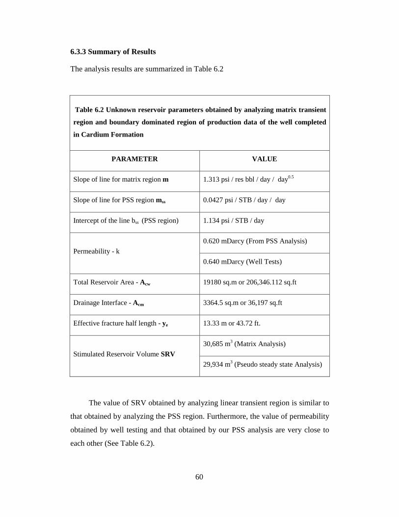
60
6.3.3 Summary of Results
The analysis results are summarized in Table 6.2
Table 6.2 Unknown reservoir parameters obtained by analyzing matrix transient
region and boundary dominated region of production data of the well completed
in Cardium Formation
PARAMETER VALUE
Slope of line for matrix region m 1.313 psi / res bbl / day / day0.5
Slope of line for PSS region mss 0.0427 psi / STB / day / day
Intercept of the line bss (PSS region) 1.134 psi / STB / day
Permeability - k 0.620 mDarcy (From PSS Analysis)
0.640 mDarcy (Well Tests)
Total Reservoir Area - Acw 19180 sq.m or 206,346.112 sq.ft
Drainage Interface - Acm 3364.5 sq.m or 36,197 sq.ft
Effective fracture half length - ye 13.33 m or 43.72 ft.
Stimulated Reservoir Volume SRV 30,685 m3 (Matrix Analysis)
29,934 m3 (Pseudo steady state Analysis)
The value of SRV obtained by analyzing linear transient region is similar to
that obtained by analyzing the PSS region. Furthermore, the value of permeability
obtained by well testing and that obtained by our PSS analysis are very close to
each other (See Table 6.2).

61
6.4 EXAMPLE APPLICATION FOR CHARACTERIZING A FRACTURED WELL IN
BAKKEN FORMATION
In this section we analyze the production data of a tight oil well completed in
Bakken formation. The well is hydraulically fractured consisting of 16 fracture
stages and has been producing for nearly 3 years. Table 6.3 summarizes the
available fluid and reservoir properties.
Table 6.3 Reservoir and fluid properties of well in Bakken Formation
Reservoir Type Unknown Permeability –
Horizontal (k hor) 0.026 mD
Dominant Flow Oil Phase API Gravity 40 API
Multiphase flow in
reservoir No Reservoir thickness (h) 19 ft.
Reservoir Pressure (Pi) 6800 psia Matrix Porosity (𝛟𝐦) 0.09
Flowing BHP (Pwf) Varying Total Compressibility
(ct) 1.726 x 10⁻⁵ psi-1
Number of stages of
fractures 16
Oil Formation Volume
factor (Bo) 1.329
Length of horizontal well
(Χe) 5600 ft. Oil Viscosity (μo) 0.5643 cp
We make the same specialized plot of oil flow rate versus material balance time
as shown in Fig. 6.6 to identify different flow regions.

62
Fig. 6.6 – Log-log plot of daily oil rate versus calculated MBT of a Well in Bakken
Formation.
In Fig. 6.6, we clearly see the linear transient flow region identified by a negative
half-slope followed by a pseudosteady state regime identified by negative one
slope. We analyze these two regions separately.
6.4.1 Analysis of Linear Transient Region
In Fig. 6.7, we make the plot of RNP versus square root of MBT of matrix
transient region.
We substitute the value of m, determined in Fig. 6.7, in the analysis equation of
dual porosity model and calculate the fracture-matrix interface area 𝐴𝑐𝑚:
�𝑘𝑚𝐴𝑐𝑚 =125.11 𝐵 𝜇�(Ø𝜇𝑐𝑡)𝑚
1𝑚
Q = 3981.5 t-0.5 R² = 0.95481
Q = 148892 t-1.0 R² = 0.94314
1
10
100
1000
1 10 100 1000 10000 100000
Oil
Rat
e (s
tb/d
ay)
Material Balance Time (days)
Region 1
Region 2
Region 3

63
Fig. 6.7 – Plot of RNP versus square root of MBT of only transient region of the well
completed in Bakken Formation
Slope of the line m = 2.96 psi / res bbl / day / day0.5
𝐴𝑐𝑚 =125.11 × 1.329 × 0.5643
√0.013�(0.09 × 0.5643 × 1.726 × 10−5)1
2.9616
𝐴𝑐𝑚 = 296,778.41 ft2
Using Eq. 3.11 to determine 𝐴𝑐𝑤
𝐴𝑐𝑤 = 2 × 𝑋𝑒 × ℎ
𝐴𝑐𝑤 = 2 × 5600 × 19 = 212,800 ft2
Stimulated fracture half-length ye is calculated to be
𝑦𝑒 =296,778.41 × 312.5
212,800
RNP = 2.9616 MBT0.5 R² = 0.9506
0
50
100
150
200
250
0 10 20 30 40 50 60 70
Rat
e N
orm
aliz
ed P
ress
ures
(psi/
stb/
day)
MBT 0.5 (days)0.5

64
𝑦𝑒 = 435.82 ft
The stimulated reservoir volume (SRV) = 2 × Xe × h × ϕm × ye is
calculated to be 8,346,824.6 ft3 .
6.4.2 Analysis Of Boundary Dominated Flow
In Fig. 6.8, we plot the RNP versus MBT of the boundary-dominated flow region.
Fig. 6.8 – Specialized plot of RNP versus MBT for analyzing boundary dominated
flow in Bakken Formation
Slope of the line mss = 0.0521 psi / STB / day / day
And bss = 8.0981 psi / STB / day
Using Eq.6.2
𝑚𝑠𝑠 = 5.615 𝐵𝑜
𝐴𝑐𝑤 𝑦𝑒 𝜙𝑚 𝑐𝑡
We also know that Stimulated Reservoir Volume (𝑆𝑅𝑉) = 𝐴𝑐𝑤 𝑦𝑒 𝜙𝑚
Therefore,
RNP = 0.0521 MBT + 8.0981 R² = 0.92405
0
200
400
600
800
1000
1200
1400
1600
0 5000 10000 15000 20000 25000 30000
Rat
e N
orm
aliz
ed P
ress
ures
(psi/
stb/
day)
Material Balance Time (days)

65
𝑆𝑅𝑉 = 5.615 𝐵𝑜 𝑐𝑡
1𝑚
= 5.615 1.329
1.726 × 10⁻⁵
10.0521
= 8,298,435.6 ft3
Now we use the intercept equation to determine the matrix permeability:
𝑏𝑠𝑠 =36.96 𝜇 𝐵𝑜 𝐿𝑓 𝑘𝑚 𝑁𝑓 𝑦𝑒 ℎ
𝑘𝑚 =36.96 𝜇 𝐵𝑜 𝐿𝑓 𝑏𝑠𝑠 𝑁𝑓 𝑦𝑒 ℎ
=36.96 × 0.5643 × 1.329 × 312.5
8.098 × 16 × 435.82 × 19 = 0.008 mD
6.4.3 Summary of Results
The analysis results are summarized in Table 6.4.
Table 6.4 Unknown reservoir parameters obtained from the analysis of the
matrix transient region and boundary dominated region of production data of
the well completed in Bakken Formation
PARAMETER VALUE
Slope of line for matrix region m 2.96 psi / res bbl / day / day0.5
Slope of line for PSS region mss 0.0521 psi / STB / day / day
Intercept of the line bss for PSS 8.0981 psi / STB / day
Permeability k 0.008 mDarcy (PSS Analysis)
0.026 mDarcy (Well Tests)
Total Reservoir Area - Acw 212,800 sq.ft
Drainage Interface - Acm 309,502 sq.ft
Effective fracture half length - ye 454.5 ft.
Stimulated Reservoir Volume SRV
8,346,824.64 ft3 (Matrix Analysis)
8,298,435.6 ft3 (Pseudo steady state
Analysis)

66
The value of SRV obtained by analyzing the linear transient region is
similar to that obtained by analyzing the PSS region. The value of permeability
obtained by well testing and that obtained from our PSS analysis are different
(See Table 6.4). This difference can be due to the heterogeneity of the reservoir.

67
CHAPTER VII
CONCLUSION AND RECOMMENDATIONS
7.1 CONCLUSIONS
The major findings of this work can be summarized as follows:
1. New equations have been developed for analyzing different regions of
production data from tight reservoirs with induced hydraulic and
reactivated natural fractures.
2. A procedure is proposed for determining the reservoir properties by using
the hydrocarbon production data and the proposed equations.
3. We used the proposed equations to analyze the production data of two
wells from Barnett shale. The results show that a dual porosity model is
more appropriate than a triple porosity data for describing Barnett well
data. Even if the micro-fractures are present in Barnett shale, their length
scale should be less than the spacing between the hydraulic fractures.
4. New equations are developed to analyze boundary dominated
(pseudosteady state) flow of a slightly compressible fluid in linear dual-
porosity systems.
5. The pseudosteady state model proposed for boundary-dominated flow can
be used in determining stimulated reservoir volume, minimum reservoir
permeability. The proposed linear pseudo-steady state analysis
complements the previously developed linear transient analysis.
6. We used the proposed PSS model to analyze the production data of two
tight oil wells from Cardium and Bakken reservoirs. The results show that
values of stimulated reservoir volume obtained from analysis of transient
matrix flow and boundary dominated flow are very close for selected wells
in both formations. The values of permeability are very close in Cardium
well and relatively close for Bakken Well.

68
7.2 RECOMMENDATIONS
The following subjects remain the subject of future study:
1. The analysis equations were developed for the fully transient triple
porosity model. Similar equations can be developed by considering the
assumption of pseudosteady state matrix-fracture interflow assumption.
2. The analysis equations can be extended to include the skin effect.
3. The analysis equations for boundary dominated flow in triple porosity
reservoirs can be developed.

69
REFERENCES
1. Abdassah, D. and Ershaghi, I. 1986. Triple-Porosity Systems for
Representing Naturally Fractured Reservoirs. SPE Form Eval (April): 113
– 127. SPE-13409-PA.
2. Al-Ahmadi, H. A. 2010, A triple porosity model for fractured horizontal
well. MSc. Dissertation, Texas A&M U., College Station, Texas.
3. Al-Ahmadi, H. A., Almarzooq, A. M. and Wattenbarger, R. A. 2010.
Application of Linear Flow Analysis to Shale Gas Wells – Field Cases.
Paper SPE 130370 presented at the 2010 Unconventional Gas Conference,
Pittsburgh, Pennsylvania, 23 – 25 February.
4. Al-Ghamdi, A. and Ershaghi, I. 1996. Pressure Transient Analysis of
Dually Fractured Reservoirs. SPE J. (March): 93 – 100. SPE-26959-PA.
5. Al-Hussainy, R., Ramey, H. J., Jr., and Crawford, P. B. 1966. The Flow of
Real Gas Through Porous Media. J. Pet Tech (May): 624 – 636. SPE-
1243A-PA
6. Anderson, D. M., Nobakht, M., Moghadam, S. and Mattar, L. 2010.
Analysis of Production Data from Fractured Shale Gas Wells. Paper SPE
131787 presented at the SPE Unconventional Gas Conference, Pittsburgh,
Pennsylvania, 23 – 25 February.
7. Barenblatt, G. I., Zhelto, I. P. and Kochina, I. N. 1960. Basic Concepts of
the Theory of Seepage of Homogeneous Liquids in Fissured Rocks.
Journal of Applied Mathematical Mechanics (USSR) 24 (5): 852 – 864.
8. Barrodale, I. and Roberts, F. D. K. 1974. Solution of an Overdetermined
System of Equations in the l1 Norm. Communication of the ACM 17 (6):
319 – 320.
9. Beckner, B.L., 1990, "Improved Modeling of Imbibition Matrix/Fracture
Fluid Transfer in Double Porosity Simulators", PhD Dissertation at
Stanford University.

70
10. Bello, R.O. 2009. Rate Transient Analysis in Shale Gas Reservoirs with
Transient Linear Behavior. Ph.D. Dissertation, Texas A&M U., College
Station, Texas.
11. Bello, R. O. and Wattenbarger, R. A. 2008. Rate Transient Analysis in
Naturally Fractured Shale Gas Reservoirs. Paper SPE 114591 presented at
the CIPC/SPE Gas Technology Symposium 2008 Joint Conference,
Calgary, Alberta, Canada, 16 – 19 June.
12. Bello, R. O. and Wattenbarger, R. A. 2009. Modeling and Analysis of
Shale Gas Production with a Skin Effect. Paper CIPC 2009-082 presented
at the Canadian International Petroleum Conference, Calgary, Alberta,
Canada, 16 – 18 June.
13. Bello, R. O. and Wattenbarger, R. A. 2010. Multi-stage Hydraulically
Fractured Shale Gas Rate Transient Analysis. Paper SPE 126754
presented at the SPE North Africa Technical Conference and Exhibition
held in Cairo, Egypt, 14 – 17 February.
14. Blasingame, T.A and Lee, W.J : “The Variable-Rate Reservoir Limits
Testing”, paper SPE 15028 presented at SPE Permian basin Oil & Gas
Recovery Conference, Midland, March 13-14, 1986
15. Brown, M., Ozkan, E., Raghavan, R. and Kazemi, H. 2009. Practical
Solutions for Pressure Transient Responses of Fractured Horizontal Wells
in Unconventional Reservoirs. Paper SPE 125043 presented at the Annual
Technical Conference and Exhibition, New Orleans, Louisiana, 4 – 7
October.
16. Bumb, A. C and McKee, C. R. 1988. Gas-Well Testing in the Pressure of
Desorption for Coalbed Methane and Devonian Shale. SPE Form Eval
(March): 179 - 185. SPE- 15227-P A.
17. Cheney, E.W. and Kincaid, R. D. 1985. Numerical Mathematics and
Computing, 2nd edition. Monterey, California: Brooks/Cole Publishing
Company.
18. de Swaan, O. A. 1976. Analytic Solutions for Determining Naturally

71
Fractured Reservoir Properties by Well Testing. SPE J. (June): 117 – 122.
SPE-5346-PA.
19. Dreier, J. 2004. Pressure-Transient Analysis of Wells in Reservoirs with a
Multiple Fracture Network. M.Sc. Thesis, Colorado School of Mines,
Golden, Colorado.
20. Dreier, J., Ozkan, E. and Kazemi, H. 2004. New Analytical Pressure-
Transient Models to Detect and Characterize Reservoirs with Multiple
Fracture Systems. Paper SPE 92039 presented at the SPE International
Petroleum Conference in Mexico, Puebla, Mexico, 8 – 9 November.
21. El-Banbi, A.H. 1998. Analysis of Tight Gas Wells. Ph.D. Dissertation,
Texas A &M U., College Station, Texas.
22. Gale, J. F., Reed, R. M. and Holder, J. 2007. Natural Fractures in the
Barnett Shale and Their Importance for Hydraulic Fracture Treatments.
AAPG Bulletin. 91 (4): 603 – 622.
23. Jalali, Y. and Ershaghi, I. 1987. Pressure Transient Analysis of
Heterogeneous Naturally Fractured Reservoirs. Paper SPE 16341
presented at the SPE California Regional Meeting, Ventura, California, 8 –
10 April.
24. Kazemi, H. 1969. Pressure Transient of Naturally Fractured Reservoirs
with Uniform Fracture Distribution. SPE J. (December):451– 462. SPE-
2156A-PA.
25. Liu, C. Q. 1981. Exact Solution for the Compressible Flow Equations
through a Medium with Triple-Porosity. Applied Mathematics and
Mechanics 2 (4): 457 – 462.
26. Liu, C. Q. 1983. Exact Solution of Unsteady Axisymmetrical Two-
Dimensional Flow through Triple Porous Media. Applied Mathematics
and Mechanics 4 (5): 717 – 724.
27. Liu, J. C., Bodvarsson, G. S. and Wu, Y. S. 2003. Analysis of Flow
Behavior in Fractured Lithophysal Reservoirs. Journal of Contaminant
Hydrology 62-63: 189 – 211.
72
28. Mayerhofer, M. J., Lolon, E. P., Youngblood, J. E. and Heinze, J. R. 2006.
Integration of Microseismic Fracture Mapping Results with Numerical
Fracture Network Production Modeling in the Barnett Shale. Paper SPE
102103 presented at the Annual Technical Conference and Exhibition, San
Antonio, Texas, 24 – 27 September.
29. Medeiros, F., Ozkan, E. and Kazemi, H. 2008. Productivity and Drainage
Area of Fractured Horizontal Wells in Tight Gas Reservoirs. SPE Res Eval
& Eng (October): 902 – 911. SPE-108110-PA.
30. Nelson, R. A. 2001. Geologic Analysis of Naturally Fractured Reservoirs,
2nd
edition. Woburn, Massachusetts: Butterworth-Heinemann.
31. Ordonez, A., Penuela, G. et al., Dec. 2001, “Recent Advances in Naturally
Fractured Reservoir Modeling”, published in CT&F, Vol. 2.
32. Ozkan, E., Brown, M., Raghavan, R. and Kazemi, H. 2009. Comparison of
Fractured Horizontal-Well Performance in Conventional and
Unconventional Reservoirs. Paper SPE 121290 presented at the SPE
Western Regional Meeting, San Jose, California, 24 – 26 March.
33. Ozkan, E., Ohaeri, U. and Raghavan, R. 1987. Unsteady Flow to a Well
Produced at a Constant Pressure in Fractured Reservoir. SPE Form Eval
(June): 186 - 200. SPE- 9902-P A.
34. Palacio, J.C., and Blasingame, T.A. Decline-Curve Analysis With Type
Curves – Analysis of Gas Well Production Data. Paper SPE 25909
presented at the 1993 SPE Rocky Mountain Regional/Low Permeability
Reservoir Symposium, Denver, Colorabo, 12 - 14 April.
35. Saidi, A.M., Nov. 1983, “Simulation of Naturally Fractured Reservoirs”,
paper SPE 12270 presented at the Seventh SPE Symposium on Reservoir
Simulation held in San Francisco, CA.
36. Song, B., Economides, M.J., and Ehlig-Economides, C.A. 2009. Design of
Multiple Transverse Fracture Horizontal Wells in Shale Gas Reservoirs.
Paper SPE 140555 presented at the 2011 SPE Hydraulic Fracturing

73
Technology Conference, Woodlands, TX, 24 - 26 January.
37. Stehfest, H. 1970. Algorithm 358 – Numerical Inversion of Laplace
Transforms. Communication of the ACM 13 (1): 47 – 49.
38. Warren, J. E. and Root, P. J. 1963. The Behavior of Naturally Fractured
Reservoirs. SPE J. (September): 245 – 255. SPE-426-PA.
39. Wattenbarger, R.A. 2007. Some Reservoir Performance Aspects of
Unconventional Gas Production. Private Conference Presentation, Lake
Louise, Alberta, Canada.
40. Wu, Y. S., Liu, H. H. and Bodvarsson, G. S. 2004. A Triple-Continuum
Approach for Modeling Flow and Transport Processes in Fractured Rock.
Journal of Contaminant Hydrology 73: 145 – 179.

74
NOMENCLATURE
Acm = Total matrix/micro-fracture surface drainage area, ft2
Acw = well-face cross-sectional area to flow, ft2
ct = total compressibility, psi-1
ff(s) = fracture function for matrix-micro-fracture fluid transfer
f(s) = fracture function for micro-fracture-macro-fracture fluid transfer
h = matrix block thickness, ft.
kf = permeability of micro-fracture, md
kF = permeability of macro-fracture, md
km = permeability of matrix block, md
ℒ−1= inverse Laplace operator
Lf = micro fracture spacing, ft.
LF = macro fracture spacing, ft.
mr = slope of region
m(pi)= gas pseudo pressure at initial conditions, psi2 /cp
m(pwf)= gas pseudo pressure at well-bore, psi2 /cp
Np = cumulative oil production
nfxe = number of micro fractures in the direction of well length
nfye = number of macro fractures in the direction of macro-fracture length
Pi = pressure of reservoir at initial conditions, psi
Pwf = pressure of reservoir at well-bore, psi
qDL = dimensionless flow rate
qg = gas rate, MScf/day
qo = oil rate produced from one fracture, m3/s
Qo = daily oil rate, STB/day
s = laplace space variable
t = time, days
t ̅ = material balance time, days

75
tdac =dimensionless time
T = absolute temperature, 0R
xD = dimensionless distance along micro-fracture spacing
Xe = length of horizontal well, ft.
yDe = dimensioless length of reservoir
ye = macro-fracture half-length , ft.
zD = dimensionless distance along macro-fracture spacing
Greek Symbols
Ø = porosity, fraction
μ = viscosity of a gas , cp
σi = shape factor, 1/ft2
ωi = storativity ratio
λAc = dimensionless interporosity flow
Subscript
f = micro-fracture
F = macro-fracture
m = matrix
i = f,F, &m
ss = Pseudo steady state
o = oil
g = gas

76
APPENDIX A
TRANSIENT LINEAR TRIPLE POROSITY ANALYTICAL SOLUTIONS
The rate solutions in fractured linear reservoirs is derived by Laplace
transformation which enables us to reduce the second-order partial differential
flow equations to a second order ordinary differential equation in Laplace domain.
Stehfest algorithm (Stehfest 1970) is then used to easily invert the Laplace
domain solution to time domain.
The differential equation in Laplace domain that describes the main flow in
linear reservoir system is given by
𝜕2𝑝𝐷𝐿𝐹𝜕𝑦𝐷2
− 𝑠𝑓(𝑠)𝑝𝐷𝐿𝐹������ = 0 (A − 1)
A-1 Linear Flow Solutions for Fractured Linear Reservoirs (Dual Porosity
System)
El-Banbi (1998) developed the first linear flow solutions for dual porosity
system in fractured linear reservoirs. In Laplace domain, Eq. A-2 relates the
constant rate and constant pressure solutions at the well bore
𝑝𝑤𝐷𝐿������ × 𝑞𝐷𝐿����� =1𝑠2
(A − 2)
Therefore, the solution for constant pressure case (El-Banbi 1998) is
1𝑞𝐷𝑙����
=2𝜋𝑠
�𝑠𝑓(𝑠)�1 + 𝑒−2�𝑠𝑓(𝑠)𝑦𝐷𝑒
1 − 𝑒−2�𝑠𝑓(𝑠)𝑦𝐷𝑒� (A − 3)
A-2 Analytical Solutions for Triple Porosity System in Linear Reservoirs
Al-Ahmadi (2010) developed the analytical solutions for triple porosity
system in linear reservoirs. The three contagious media include: macro-fractures,
micro-fractures and matrix. The fluid flow is assumed to be sequential i.e. matrix

77
to micro-fractures and micro-fractures to macro-fractures. The schematic of the
Al-Ahmadi (2010) triple porosity model is shown in Fig. A-1.
Fig. A-4 – Top View of a horizontal Well in a triple porosity system. Red dotted lines
indicated virtual no flow boundaries. Arrows indicate direction of the flow (Al-
Ahmadi 2010).

78
A-3 Summary of Equations used in developing Analytical Solutions
This section presents the summary of analytical equations used by Al-
Ahmadi to develop the analytical solutions. For details of the derivation of the
solutions, refer to Al-Ahmadi dissertation (2010).
A-3.1 Matrix Equation
Matrix equation under transient condition is given by
𝑘𝑚𝜇𝜕2𝑝𝑚𝜕𝑧2
= (𝜑𝑉𝑐𝑡)𝑚𝜕𝑝𝑚𝜕𝑡
(A − 4)
𝜕2𝑝𝑚𝜕𝑧2
=(𝜑𝑉𝜇𝑐𝑡)𝑚
𝑘𝑚𝜕𝑝𝑚𝜕𝑡
(A − 5)
A-3.2 Micro-fracture Equation
Micro-fracture equation under transient condition is given by
𝑘𝑓𝜇𝜕2𝑝𝑓𝜕𝑥2
+ 𝑞𝑠𝑜𝑢𝑟𝑐𝑒,𝑚 = (𝜑𝑉𝑐𝑡)𝑓𝜕𝑝𝑓𝜕𝑡
(A − 6)
Where 𝑞𝑠𝑜𝑢𝑟𝑐𝑒,𝑚 is a source term of flow term from matrix to micro-fracture,
given by
𝑞𝑠𝑜𝑢𝑟𝑐𝑒,𝑚 = −1𝐿𝑓�𝑘𝑚𝜇𝜕𝑝𝑚𝜕𝑧
�𝑧=
𝐿𝑓2�
(A − 7)
Thus, the final form of micro-fractures equation is
𝜕2𝑝𝑓𝜕𝑥2
=(𝜑𝑉𝜇𝑐𝑡)𝑓
𝑘𝑓𝜕𝑝𝑓𝜕𝑡
+ 1𝐿𝑓�𝑘𝑚𝑘𝑓
𝜕𝑝𝑚𝜕𝑧
�𝑧=
𝐿𝑓2�
(A − 8)

79
A-3.3 Macro-fracture Equation
Macro-fracture equation under transient condition is given by
𝑘𝐹𝜇𝜕2𝑝𝐹𝜕𝑦2
+ 𝑞𝑠𝑜𝑢𝑟𝑐𝑒,𝑓 = (𝜑𝑉𝑐𝑡)𝐹𝜕𝑝𝐹𝜕𝑡
(A − 9)
Where 𝑞𝑠𝑜𝑢𝑟𝑐𝑒,𝑚 is a source term of flow term from micro-fractures to macro-
fracture, given by
𝑞𝑠𝑜𝑢𝑟𝑐𝑒,𝑓 = −1𝐿𝐹�𝑘𝑓𝜇𝜕𝑝𝑓𝜕𝑥
�𝑥= 𝐿𝐹 2�
(A − 10)
A-3.4 Initial and Boundary conditions
Matrix
Initial Condition:
𝑝𝑚(𝑧, 0) = 𝑝𝑖
Inner Boundary:
𝜕𝑝𝑚
𝜕𝑧= 0 @ 𝑧 = 0
Outer boundary
𝑝𝑚 = 𝑝𝑓 @ 𝑧 =𝐿𝑓2
Micro-fracture
Initial Condition:
𝑝𝑓(𝑥, 0) = 𝑝𝑖
Inner Boundary:
𝜕𝑝𝑓
𝜕𝑥= 0 @ 𝑥 = 0
Outer Boundary:

80
𝑝𝑓 = 𝑝𝐹 @ 𝑥 =𝐿𝐹2
Macro-fracture
Initial Condition:
𝑝𝐹(𝑦, 0) = 𝑝𝑖
Inner Boundary:
𝑞 = −𝑘𝐹𝐴𝑐𝑤𝜇
𝜕𝑝𝐹𝜕𝑦
�𝑦=0
Outer Boundary:
𝜕𝑝𝐹𝜕𝑦
= 0 @ 𝑦 = 𝑦𝑒
A-3.5 System Dimensionless Equations
Equations presented in Appendix A-3.3 can be converted to dimensionless
equations using dimensional variables defined in Chapter 3 and dimensionless
boundary conditions.
Matrix:
𝜕2𝑝𝐷𝐿𝑚𝜕𝑧𝐷2
=3𝜔𝑚𝜆𝐴𝑐,𝑓𝑚
𝜕𝑝𝐷𝐿𝑚𝜕𝑡𝐷𝐴𝑐
(A − 11)
Micro-fracture:
𝜕2𝑝𝐷𝐿𝑓𝜕𝑥𝐷2
=3𝜔𝑓𝜆𝐴𝑐,𝐹𝑓
𝜕𝑝𝐷𝐿𝑓𝜕𝑡𝐷𝐴𝑐
+𝜆𝐴𝑐,𝑓𝑚
𝜆𝐴𝑐,𝐹𝑓
𝜕𝑝𝐷𝐿𝑚𝜕𝑧𝐷
�𝑧𝐷=1
(A − 12)
Macro-fracture:
𝜕2𝑝𝐷𝐿𝐹𝜕𝑦𝐷2
= 𝜔𝐹𝜕𝑝𝐷𝐿𝐹𝜕𝑡𝐷𝐴𝑐
+𝜆𝐴𝑐,𝐹𝑓
3𝜕𝑝𝐷𝐿𝑓𝜕𝑥𝐷
�𝑥𝐷=1
(A − 13)

81
A-3.6 Laplace Transformation
The differential equations presented in Appendix A-3.5 are transformed into
Laplace domain.
Matrix Equation
𝑝𝐷𝐿𝑚������� =𝑝𝐷𝐿𝑓������
𝑐𝑜𝑠ℎ ��3𝑠𝜔𝑚𝜆𝐴𝑐,𝑓𝑚
�𝑐𝑜𝑠ℎ ��
3𝑠𝜔𝑚𝜆𝐴𝑐,𝑓𝑚
𝑧𝐷� (A − 14)
Micro-fracture Equation
𝑝𝐷𝐿𝑓������ =𝑝𝐷𝐿𝐹������
𝑐𝑜𝑠ℎ��𝑠𝑓𝑓(𝑠)�𝑐𝑜𝑠ℎ ��𝑠𝑓𝑓(𝑠)𝑥𝐷� (A − 15)
Macro-fracture Equation
𝜕𝑝𝐷𝐿𝐹������𝜕𝑦𝐷2
= 𝜔𝐹 𝑠 𝑝𝐷𝐿𝐹������� + 𝜆𝐴𝑐,𝐹𝑓
3 𝜕𝑝𝐷𝐿𝑓������𝜕𝑥𝐷2
�𝑥𝐷=1
(A − 16)
Differentiating Eq. A-15 and Replacing in Eq. A-16, the solution becomes
𝜕2𝑝𝐷𝐿𝐹������𝜕𝑦𝐷2
− 𝑠𝑝𝐷𝐿𝐹������ �𝜔𝐹 +𝜆𝐴𝑐,𝐹𝑓�𝑠𝑓𝑓(𝑠)𝑡𝑎𝑛ℎ��𝑠𝑓𝑓(𝑠)�
3𝑠� = 0 (A − 17)
In short form
𝜕2𝑝𝐷𝐿𝐹������𝜕𝑦𝐷2
− 𝑠𝑓(𝑠)𝑝𝐷𝐿𝐹������ = 0 (A − 18)
Where 𝑓(𝑠) is Al-Ahmadi’s transfer function for the fully transient case is given
by
𝑓(𝑠) = 𝜔𝐹 +𝜆𝐴𝑐𝐹𝑓
3𝑠 �𝑠𝑓𝑓(𝑠) tanh�𝑠𝑓𝑓(𝑠) (A − 19)
Where 𝑓𝑓(𝑠) is given as

82
𝑓𝑓(𝑠) = 3𝜔𝑓𝜆𝐴𝑐𝐹𝑓
+ 𝜆𝐴𝑐𝑓𝑚𝑠𝜆𝐴𝑐𝐹𝑓
�3𝑠𝜔𝑚𝜆𝐴𝑐𝑓𝑚
tanh�3𝑠𝜔𝑚𝜆𝐴𝑐𝑓𝑚
(A − 20)

83
APPENDIX B
DEVELOPMENT OF ANALYSIS EQUATIONS
In this section, the analysis equations for the linear triple porosity model are
derived. Al-Ahmadi’s transfer function “𝑓(𝑠)” is further simplified to develop
analysis equation for each region. The fluid transfer is assumed to be under
transient flow. Al-Ahmadi’s transfer function 𝑓(𝑠) for the transient case is given
by
𝑓(𝑠) = 𝜔𝐹 +𝜆𝐴𝑐𝐹𝑓
3𝑠 �𝑠𝑓𝑓(𝑠) tanh�𝑠𝑓𝑓(𝑠) (B − 1)
Where 𝑓𝑓(𝑠) is given as
𝑓𝑓(𝑠) = 3𝜔𝑓𝜆𝐴𝑐𝐹𝑓
+ 𝜆𝐴𝑐𝑓𝑚𝑠𝜆𝐴𝑐𝐹𝑓
�3𝑠𝜔𝑚𝜆𝐴𝑐𝑓𝑚
tanh�3𝑠𝜔𝑚𝜆𝐴𝑐𝑓𝑚
(B − 2)
Eq. B-1 and B-2 are replaced in El-Banbi (1998) Laplace solution developed for
linear reservoirs. The equation for constant pressure inner boundary, closed outer
boundary (slab matrix) developed by El-Banbi is given as
1𝑞𝐷𝑙����
=2𝜋𝑠
�𝑠𝑓(𝑠)�1 + 𝑒−2�𝑠𝑓(𝑠)𝑦𝐷𝑒
1 − 𝑒−2�𝑠𝑓(𝑠)𝑦𝐷𝑒� (B − 3)
Using
coth (x) = 𝑒2𝑥 + 1𝑒2𝑥 − 1
(B − 4)
Eq. B-3 can be written as
1𝑞𝐷𝑙����
=2𝜋𝑠
�𝑠𝑓(𝑠) coth ��𝑠𝑓(𝑠)𝑦𝐷𝑒� (B − 5)
Further simplifying the Eq. B-1, B-2 and B-5, we obtain the analysis equation for
each individual regions observed on the log-log plot of dimensionless flow rate
versus dimensionless time.

84
B-1 REGION 1 This region represents flow at early time scale in the macro-fractures only. Using
Eq. B-5
1𝑞𝐷𝑙����
=2𝜋𝑠
�𝑠𝑓(𝑠) coth ��𝑠𝑓(𝑠)𝑦𝐷𝑒� (B − 5)
For early time, the value is s is larger (Since t and s are inversely related)
Approximately for x > 3, coth (𝑥) = 1
Therefore for
coth ��𝑠𝑓(𝑠)𝑦𝐷𝑒� = 1 When �𝑠𝑓(𝑠)𝑦𝐷𝑒 > 3
Eq. B-5 can be written as
1𝑞𝐷𝑙����
= 2𝜋𝑠
�𝑠𝑓(𝑠) (B − 6)
Here 𝑓(𝑠) is given as
𝑓(𝑠) = 𝜔𝐹 +𝜆𝐴𝑐𝐹𝑓
3𝑠 �𝑠𝑓𝑓(𝑠) tanh�𝑠𝑓𝑓(𝑠) (B − 1)
Where 𝑓𝑓(𝑠) is given as
𝑓𝑓(𝑠) = 3𝜔𝑓𝜆𝐴𝑐𝐹𝑓
+ 𝜆𝐴𝑐𝑓𝑚𝑠𝜆𝐴𝑐𝐹𝑓
�3𝑠𝜔𝑚𝜆𝐴𝑐𝑓𝑚
tanh�3𝑠𝜔𝑚𝜆𝐴𝑐𝑓𝑚
(B − 2)
For early time scales (higher values of s) considering fracture depletion only, we
can assume in Eq. B-1
𝜔𝐹 ≫≫ 𝜆𝐴𝑐𝐹𝑓
3𝑠 �𝑠𝑓𝑓(𝑠) tanh�𝑠𝑓𝑓(𝑠)
Therefore Eq. B-1 can be simplified into
𝑓(𝑠) = 𝜔𝐹 (B − 7)
Replacing B-7 in Eq. B-6 we obtain,

85
1𝑞𝐷𝑙����
= 2𝜋𝑠√𝑠𝜔𝐹
(B − 8)
or
𝑞𝐷𝑙���� =1
2𝜋√𝑠�𝜔𝐹 (B − 9)
Eq. B-9 can be converted from Laplace space to time domain by applying inverse
Laplace on both sides. The inverted equation is given as
𝑞𝐷𝑙 =1
2𝜋�𝜋𝑡𝑑𝑎𝑐�𝜔𝐹 (B − 10)
Using definition of dimensionless parameters defined, Eq. B-10 is converted to
obtain the analysis equation for Region 1,
�𝑘𝐹𝐴𝑐𝑤 =1262𝑇�(∅𝜇𝑐𝑡)𝑓
1𝑚1
(B − 11)
Where 𝑚1 is the slope obtained by plotting 𝑚(𝑝𝑖)−𝑚(𝑝𝑤𝑓)
𝑞𝑔 against √𝑡
B-2 Region 2
This region is observed during when bilinear flow occurs between macro fracture
and micro fracture. Using Eq. B-5
1𝑞𝐷𝑙����
=2𝜋𝑠
�𝑠𝑓(𝑠) coth ��𝑠𝑓(𝑠)𝑦𝐷𝑒� (B − 5)
This region also occurs at early time scale, as the permeability of macro-fractures
is very high. For early time, the value is s is larger (Since t and s are inversely
related)
Approximately for x > 3, coth (𝑥) = 1
Therefore,
coth ��𝑠𝑓(𝑠)𝑦𝐷𝑒� = 1 When �𝑠𝑓(𝑠)𝑦𝐷𝑒 > 3
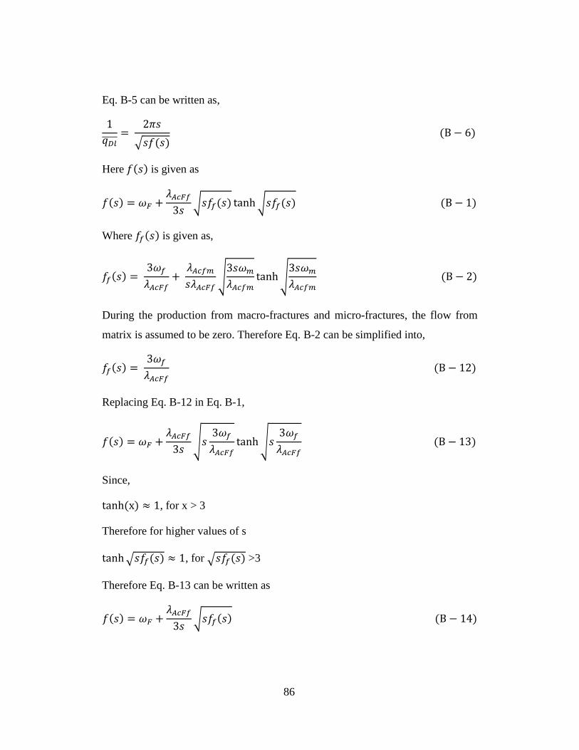
86
Eq. B-5 can be written as,
1𝑞𝐷𝑙����
= 2𝜋𝑠
�𝑠𝑓(𝑠) (B − 6)
Here 𝑓(𝑠) is given as
𝑓(𝑠) = 𝜔𝐹 +𝜆𝐴𝑐𝐹𝑓
3𝑠 �𝑠𝑓𝑓(𝑠) tanh�𝑠𝑓𝑓(𝑠) (B − 1)
Where 𝑓𝑓(𝑠) is given as,
𝑓𝑓(𝑠) = 3𝜔𝑓𝜆𝐴𝑐𝐹𝑓
+ 𝜆𝐴𝑐𝑓𝑚𝑠𝜆𝐴𝑐𝐹𝑓
�3𝑠𝜔𝑚𝜆𝐴𝑐𝑓𝑚
tanh�3𝑠𝜔𝑚𝜆𝐴𝑐𝑓𝑚
(B − 2)
During the production from macro-fractures and micro-fractures, the flow from
matrix is assumed to be zero. Therefore Eq. B-2 can be simplified into,
𝑓𝑓(𝑠) = 3𝜔𝑓𝜆𝐴𝑐𝐹𝑓
(B − 12)
Replacing Eq. B-12 in Eq. B-1,
𝑓(𝑠) = 𝜔𝐹 +𝜆𝐴𝑐𝐹𝑓
3𝑠 �𝑠3𝜔𝑓𝜆𝐴𝑐𝐹𝑓
tanh�𝑠3𝜔𝑓𝜆𝐴𝑐𝐹𝑓
(B − 13)
Since,
tanh (x) ≈ 1, for x > 3
Therefore for higher values of s
tanh�𝑠𝑓𝑓(𝑠) ≈ 1, for �𝑠𝑓𝑓(𝑠) >3
Therefore Eq. B-13 can be written as
𝑓(𝑠) = 𝜔𝐹 +𝜆𝐴𝑐𝐹𝑓
3𝑠 �𝑠𝑓𝑓(𝑠) (B − 14)

87
For bilinear flow from micro-fractures and macro-fractures, we can assume
storativity of macro-fractures doesn’t play a significant role. Therefore,
𝜔𝐹 ≪≪≪𝜆𝐴𝑐𝐹𝑓
3𝑠 �𝑠𝑓𝑓(𝑠)
Eq. B-14 can be written as
𝑓(𝑠) =𝜆𝐴𝑐𝐹𝑓
3𝑠 �𝑠𝑓𝑓(𝑠) (B − 15)
Replacing Eq. B-15 in B-6
1𝑞𝐷𝑙����
= 2𝜋𝑠
�𝑠 𝜆𝐴𝑐𝐹𝑓3𝑠 �𝑠𝑓𝑓(𝑠)
(B − 16)
Substituting the value of Eq. B-12 in Eq. B-16
1𝑞𝐷𝑙����
= 2𝜋𝑠
�𝑠 𝜆𝐴𝑐𝐹𝑓3𝑠 �𝑠
3𝜔𝑓
𝜆𝐴𝑐𝐹𝑓
(B − 17)
Simplifying B-17 to obtain analytical solution for Region 2 in Laplace space
𝑞𝐷𝑙���� =1
2𝜋�𝜆𝐴𝑐𝐹𝑓𝜔𝑓
34
𝑠−0.75 (B− 18)
Inverting Eq. B-18 in real time, using Laplace inversion. The analytical solution
for Region 2 is obtained as
𝑞𝐷𝑙 =1
10.1332�𝜆𝐴𝑐𝐹𝑓𝜔𝑓𝑡𝑑𝑎𝑐
4 (B − 19)
Using definition of dimensionless parameters defined, Eq. B-19 is converted to
obtain the analysis equation for Region 2,
�𝑘𝐹𝐴𝑐𝑤 =4070𝑇
�𝜎𝐹𝑘𝑓(Ø𝜇𝑐𝑡)𝑓4
1𝑚2
(B − 20)

88
Where 𝑚2 is the slope obtained by plotting 𝑚(𝑝𝑖)−𝑚(𝑝𝑤𝑓)
𝑞𝑔 against √𝑡4 .
B-3 Region 3
This region represents the transient linear flow occurring in the micro-fracture
only. Using Eq. B-5
1𝑞𝐷𝑙����
=2𝜋𝑠
�𝑠𝑓(𝑠) coth ��𝑠𝑓(𝑠)𝑦𝐷𝑒� (B − 5)
Here 𝑓(𝑠) is given as
𝑓(𝑠) = 𝜔𝐹 +𝜆𝐴𝑐𝐹𝑓
3𝑠 �𝑠𝑓𝑓(𝑠) tanh�𝑠𝑓𝑓(𝑠) (B − 1)
Where 𝑓𝑓(𝑠) is given as
𝑓𝑓(𝑠) = 3𝜔𝑓𝜆𝐴𝑐𝐹𝑓
+ 𝜆𝐴𝑐𝑓𝑚𝑠𝜆𝐴𝑐𝐹𝑓
�3𝑠𝜔𝑚𝜆𝐴𝑐𝑓𝑚
tanh�3𝑠𝜔𝑚𝜆𝐴𝑐𝑓𝑚
(B − 2)
In Region 3 flow is from micro-fractures only, therefore storativity and
interporosity of matrix blocks can be neglected.
𝜔𝑓 ≫≫≫≫≫ 𝜆𝐴𝑐𝑓𝑚
3𝑠 �3𝑠𝜔𝑚𝜆𝐴𝑐𝑓𝑚
tanh�3𝑠𝜔𝑚𝜆𝐴𝑐𝑓𝑚
Eq. B-2 can be written as
𝑓𝑓(𝑠) =3𝜔𝑓𝜆𝐴𝑐𝐹𝑓
(B− 21)
Since,
tanh (x) ≈ 1, for x > 3
Therefore for higher values of s
tanh�𝑠𝑓𝑓(𝑠) ≈ 1, for �𝑠𝑓𝑓(𝑠) >3

89
Eq. B-1 becomes,
𝑓(𝑠) = 𝜔𝐹 +𝜆𝐴𝑐𝐹𝑓
3𝑠 �𝑠𝑓𝑓(𝑠) (B − 22)
Similarly for Region 3, storativity of macro-fracture is also neglected.
𝜔𝐹 ≪≪≪<𝜆𝐴𝑐𝐹𝑓
3𝑠 �𝑠𝑓𝑓(𝑠)
Eq. B-22 becomes
𝑓(𝑠) =𝜆𝐴𝑐𝐹𝑓
3𝑠 �𝑠𝑓𝑓(𝑠) (B− 23)
Consider Eq. B-5
1𝑞𝐷𝑙����
=2𝜋𝑠
�𝑠𝑓(𝑠) coth ��𝑠𝑓(𝑠)𝑦𝐷𝑒� (B − 5)
Taylor series expansion of coth (x) is given as
coth 𝑥 =1𝑥
+𝑥3−𝑥3
45+ ⋯… … … … … … ..
Assume
coth 𝑥 ≈1𝑥
coth�𝑠𝑓(𝑠)𝑦𝐷𝑒 ≈1
�𝑠𝑓(𝑠)𝑦𝐷𝑒
Replacing in Eq. B-5
1𝑞𝐷𝑙����
= 2𝜋𝑠
𝑠𝑓(𝑠)𝑦𝐷𝑒 (B− 24)
Substituting Eq. B-23 in Eq. B-24, we obtain,

90
1𝑞𝐷𝑙����
= 2𝜋𝑠
𝑠 𝜆𝐴𝑐𝐹𝑓3𝑠 �𝑠𝑓𝑓(𝑠)𝑦𝐷𝑒
(B − 25)
Substituting Eq. B-21 in Eq. B-25
1𝑞𝐷𝑙����
= 2𝜋𝑠
𝑠 𝜆𝐴𝑐𝐹𝑓3𝑠 �𝑠
3𝜔𝑓
𝜆𝐴𝑐𝐹𝑓𝑦𝐷𝑒
(B − 26)
Simplifying Eq. B-26, we obtain the analytical solution in Laplace space,
𝑞𝐷𝑙���� =1
2𝜋�𝜆𝐴𝑐𝐹𝑓𝜔𝑓
3𝑠𝑦𝐷𝑒 (B − 27)
Inverting Eq. B-27 to real time, we obtain
𝑞𝐷𝐿 =1
2𝜋�𝜋𝑡𝑑𝑎𝑐�𝜆𝐴𝑐𝐹𝑓𝜔𝑓
3𝑦𝐷𝑒 (B− 28)
Using definition of dimensionless parameters defined, Eq. B-28 is converted to
obtain the analysis equation for Region 3,
�𝜎𝐹𝑦𝑒�𝑘𝑓𝐴𝑐𝑤 =2182𝑇
�(Ø𝜇𝑐𝑡)𝑓
1𝑚3
(B − 29)
Where 𝑚3 is the slope obtained if we plot 𝑚(𝑝𝑖)−𝑚�𝑝𝑤𝑓�
𝑞𝑔 against √𝑡
B-4 Region 4
This region represents transient bi-linear flow between micro-fractures and
macro-fractures. Using Eq. B-5
1𝑞𝐷𝑙����
=2𝜋𝑠
�𝑠𝑓(𝑠) coth ��𝑠𝑓(𝑠)𝑦𝐷𝑒� (B − 5)
Here 𝑓(𝑠) is given as
𝑓(𝑠) = 𝜔𝐹 +𝜆𝐴𝑐𝐹𝑓
3𝑠 �𝑠𝑓𝑓(𝑠) tanh�𝑠𝑓𝑓(𝑠) (B − 1)
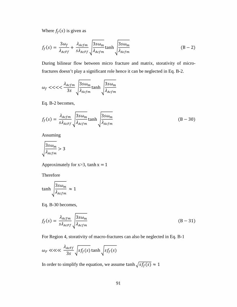
91
Where 𝑓𝑓(𝑠) is given as
𝑓𝑓(𝑠) = 3𝜔𝑓𝜆𝐴𝑐𝐹𝑓
+ 𝜆𝐴𝑐𝑓𝑚𝑠𝜆𝐴𝑐𝐹𝑓
�3𝑠𝜔𝑚𝜆𝐴𝑐𝑓𝑚
tanh�3𝑠𝜔𝑚𝜆𝐴𝑐𝑓𝑚
(B − 2)
During bilinear flow between micro fracture and matrix, storativity of micro-
fractures doesn’t play a significant role hence it can be neglected in Eq. B-2.
𝜔𝑓 <<<<𝜆𝐴𝑐𝑓𝑚
3𝑠 �3𝑠𝜔𝑚𝜆𝐴𝑐𝑓𝑚
tanh�3𝑠𝜔𝑚𝜆𝐴𝑐𝑓𝑚
Eq. B-2 becomes,
𝑓𝑓(𝑠) = 𝜆𝐴𝑐𝑓𝑚𝑠𝜆𝐴𝑐𝐹𝑓
�3𝑠𝜔𝑚𝜆𝐴𝑐𝑓𝑚
tanh�3𝑠𝜔𝑚𝜆𝐴𝑐𝑓𝑚
(B − 30)
Assuming
�3𝑠𝜔𝑚𝜆𝐴𝑐𝑓𝑚
> 3
Approximately for x>3, tanh x = 1
Therefore
tanh�3𝑠𝜔𝑚𝜆𝐴𝑐𝑓𝑚
≈ 1
Eq. B-30 becomes,
𝑓𝑓(𝑠) = 𝜆𝐴𝑐𝑓𝑚𝑠𝜆𝐴𝑐𝐹𝑓
�3𝑠𝜔𝑚𝜆𝐴𝑐𝑓𝑚
(B − 31)
For Region 4, storativity of macro-fractures can also be neglected in Eq. B-1
𝜔𝐹 ≪≪≪ 𝜆𝐴𝑐𝐹𝑓
3𝑠 �𝑠𝑓𝑓(𝑠) tanh�𝑠𝑓𝑓(𝑠)
In order to simplify the equation, we assume tanh�𝑠𝑓𝑓(𝑠) ≈ 1

92
Eq. B-31 can be written as,
𝑓(𝑠) = 𝜆𝐴𝑐𝐹𝑓
3𝑠 �𝑠𝑓𝑓(𝑠) (B− 32)
Now consider equation B-5
1𝑞𝐷𝑙����
=2𝜋𝑠
�𝑠𝑓(𝑠) coth ��𝑠𝑓(𝑠)𝑦𝐷𝑒� (B− 5)
Taylor series expansion of coth (x) is given as
coth 𝑥 =1𝑥
+𝑥3−𝑥3
45+ ⋯… … … … … … ..
Assume
coth 𝑥 ≈1𝑥
coth�𝑠𝑓(𝑠)𝑦𝐷𝑒 ≈1
�𝑠𝑓(𝑠)𝑦𝐷𝑒
Eq. B-5 becomes,
1𝑞𝐷𝑙����
= 2𝜋𝑠
𝑠𝑓(𝑠)𝑦𝐷𝑒 (B− 36)
Replacing 𝑓(𝑠) from Eq. B-32 in Eq. B-36,
1𝑞𝐷𝑙����
= 2𝜋𝑠
𝑠 𝜆𝐴𝑐𝐹𝑓3𝑠 �𝑠𝑓𝑓(𝑠)𝑦𝐷𝑒
(B − 37)
Replacing 𝑓𝑓(𝑠) from Eq. B-31 in Eq. B-37,
1𝑞𝐷𝑙����
= 2𝜋𝑠
𝑠 𝜆𝐴𝑐𝐹𝑓3𝑠
�𝑠 3𝜆𝐴𝑐𝐹𝑓
� 𝜆𝐴𝑐𝑓𝑚3𝑠 �
3𝑠𝜔𝑚𝜆𝐴𝑐𝑓𝑚
�𝑦𝐷𝑒
(B − 38)
Simplifying Eq. B-38,

93
𝑞𝐷𝑙���� =1
2𝜋�𝜆𝐴𝑐𝐹𝑓�𝜆𝐴𝑐𝑓𝑚𝜔𝑚4
√3𝑠3 𝑦𝐷𝑒 (B − 39)
Inverting Eq. B-39 to real time using Laplace inversion,
𝑞𝐷𝑙 =1
2𝜋�𝜆𝐴𝑐𝐹𝑓�𝜆𝐴𝑐𝑓𝑚𝜔𝑚4
√33 𝑦𝐷𝑒Γ(0.75)𝑡𝑑𝑎𝑐 0.25 (B− 40)
Further simplifying Eq. B-40, we obtain the analytical solution for Region 4
𝑞𝐷𝑙 =1
17.31�𝜆𝐴𝑐𝐹𝑓�
𝜆𝐴𝑐𝑓𝑚𝜔𝑚𝑡𝑑𝑎𝑐
4𝑦𝐷𝑒 (B − 41)
Using definition of dimensionless parameters defined, Eq. B-41 is converted to
obtain the analysis equation for Region 4,
�𝜎𝐹𝑦𝑒�𝑘𝑓𝐴𝑐𝑤 =6943𝑇
�𝜎𝑓𝑘𝑚(Ø𝜇𝑐𝑡)𝑚4
1𝑚4
(B − 42)
Where 𝑚4 is the slope obtained if we plot 𝑚(𝑝𝑖)−𝑚�𝑝𝑤𝑓�
𝑞𝑔 against √𝑡4
B-5 Region 5
This region represents the transient linear case when the transient linear response
is primarily from the drainage of the matrix. Using Eq. B-5
1𝑞𝐷𝑙����
=2𝜋𝑠
�𝑠𝑓(𝑠) coth ��𝑠𝑓(𝑠)𝑦𝐷𝑒� (B − 5)
Here 𝑓(𝑠) is given as
𝑓(𝑠) = 𝜔𝐹 +𝜆𝐴𝑐𝐹𝑓
3𝑠 �𝑠𝑓𝑓(𝑠) tanh�𝑠𝑓𝑓(𝑠) (B − 1)
Where 𝑓𝑓(𝑠) is given as
𝑓𝑓(𝑠) = 3𝜔𝑓𝜆𝐴𝑐𝐹𝑓
+ 𝜆𝐴𝑐𝑓𝑚𝑠𝜆𝐴𝑐𝐹𝑓
�3𝑠𝜔𝑚𝜆𝐴𝑐𝑓𝑚
tanh�3𝑠𝜔𝑚𝜆𝐴𝑐𝑓𝑚
(B − 2)

94
Consider Eq. B-2, during linear flow in the matrix
𝜔𝑓 <<<<<<<𝜆𝐴𝑐𝑓𝑚
3𝑠 �3𝑠𝜔𝑚𝜆𝐴𝑐𝑓𝑚
tanh�3𝑠𝜔𝑚𝜆𝐴𝑐𝑓𝑚
Eq. B-2 can be reduced to
𝑓𝑓(𝑠) = 𝜆𝐴𝑐𝑓𝑚𝑠𝜆𝐴𝑐𝐹𝑓
�3𝑠𝜔𝑚𝜆𝐴𝑐𝑓𝑚
tanh�3𝑠𝜔𝑚𝜆𝐴𝑐𝑓𝑚
(B− 43)
In order to simplify Eq. B-43, we assume that 𝜔𝑚 > 𝜆𝐴𝑐𝑓𝑚 as the storativity of
matrix is very high as compared to the interporosity flow parameter. Hence,
�3𝑠𝜔𝑚𝜆𝐴𝑐𝑓𝑚
> 3
Therefore,
tanh�3𝑠𝜔𝑚𝜆𝐴𝑐𝑓𝑚
≈ 1
Eq. B-43 can be written as
𝑓𝑓(𝑠) = 𝜆𝐴𝑐𝑓𝑚𝑠𝜆𝐴𝑐𝐹𝑓
�3𝑠𝜔𝑚𝜆𝐴𝑐𝑓𝑚
(B − 44)
Substituting Eq. B-44 in Eq. B-1 and neglecting 𝜔𝐹,
𝑓(𝑠) =𝜆𝐴𝑐𝐹𝑓
3𝑠�𝑠
𝜆𝐴𝑐𝑓𝑚𝑠𝜆𝐴𝑐𝐹𝑓
�3𝑠𝜔𝑚𝜆𝐴𝑐𝑓𝑚
tanh�𝑠𝜆𝐴𝑐𝑓𝑚𝑠𝜆𝐴𝑐𝐹𝑓
�3𝑠𝜔𝑚𝜆𝐴𝑐𝑓𝑚
(B− 45)
Or
𝑓(𝑠) =𝜆𝐴𝑐𝐹𝑓
3𝑠 �3𝑠 𝜆𝐴𝑐𝑓𝑚𝜆𝐴𝑐𝐹𝑓
2 𝜔𝑚4
tanh �3𝑠 𝜆𝐴𝑐𝑓𝑚𝜆𝐴𝑐𝐹𝑓
2 𝜔𝑚4
(B − 46)

95
Since 𝑘𝑓 ≫ 𝑘𝑚, therefore 𝜆𝐴𝑐𝐹𝑓 >> 𝜆𝐴𝑐𝑓𝑚 , the assumption of 3𝑠 𝜆𝐴𝑐𝑓𝑚𝜆𝐴𝑐𝐹𝑓
2 𝜔𝑚 > 3
is not valid.
Using Taylor approximation
tanh(𝑥) ≈ 𝑥
Eq. B-46 can be simplified as
𝑓(𝑠) =𝜆𝐴𝑐𝐹𝑓
3𝑠 �3𝑠 𝜆𝐴𝑐𝑓𝑚𝜆𝐴𝑐𝐹𝑓
2 𝜔𝑚 (B − 47)
Or
𝑓(𝑠) = � 𝜆𝐴𝑐𝑓𝑚3 𝑠
𝜔𝑚 (B− 48)
Now consider equation B-5
1𝑞𝐷𝑙����
=2𝜋𝑠
�𝑠𝑓(𝑠) coth ��𝑠𝑓(𝑠)𝑦𝐷𝑒� (B− 5)
Taylor series expansion of coth (x) is given as
coth 𝑥 =1𝑥
+𝑥3−𝑥3
45+ ⋯… … … … … … ..
Assume
coth 𝑥 ≈1𝑥
coth�𝑠𝑓(𝑠)𝑦𝐷𝑒 ≈1
�𝑠𝑓(𝑠)𝑦𝐷𝑒
Eq. B-5 becomes,
1𝑞𝐷𝑙����
= 2𝜋𝑠
𝑠𝑓(𝑠)𝑦𝐷𝑒 (B− 49)
Substituting Eq. B-48 in Eq. B-49

96
1𝑞𝐷𝑙����
= 2𝜋𝑠
𝑠� 𝜆𝐴𝑐𝑓𝑚3 𝑠
𝜔𝑚𝑦𝐷𝑒 (B − 50)
Or
𝑞𝐷𝑙 =1
2𝜋√𝑠�𝜆𝐴𝑐𝑓𝑚𝜔𝑚
3𝑦𝐷𝑒 (B− 51)
Inverting Eq. B-51 to real time using Laplace inversion,
𝑞𝐷𝑙 =1
2𝜋�𝜋𝑡𝑑𝑎𝑐�𝜆𝐴𝑐𝑓𝑚𝜔𝑚
3𝑦𝐷𝑒 (B − 52)
Using definition of dimensionless parameters defined, Eq. B-52 is converted to
obtain the analysis equation for Region 5,
�𝜎𝑓𝑦𝑒�𝑘𝑚𝐴𝑐𝑤 =2182𝑇
�(Ø𝜇𝑐𝑡)𝑚
1𝑚5
(B − 53)
Where 𝑚5 is the slope obtained if we plot 𝑚(𝑝𝑖)−𝑚�𝑝𝑤𝑓�
𝑞𝑔 against √𝑡