The Quasilocalized Charge Approximation

G J Kalman 1, K I Golden2, Z Donko3 and P Hartmann3 1Department of Physics, Boston College, Chestnut Hill, Massachusetts 02467, USA

2Department of Mathematics and Statistics and Department of Physics, University of Vermont, Burlington, Vermont 05401, USA

3Research Institute for Solid State Physics and Optics of the Hungarian Academy of Sciences,

P.O. Box 49, H-1525 Budapest, Hungary

kalman@bc.edu

Abstract. The quasilocalized charge approximation (QLCA) has been used for some time as a formalism for the calculation of the dielectric response and for determining the collective mode dispersion in strongly coupled Coulomb and Yukawa liquids. The approach is based on a microscopic model in which the charges are quasilocalized on a short-time scale in local potential fluctuations. We review the conceptual basis and theoretical structure of the QLC approach and together with recent results from molecular dynamics simulations that corroborate and quantify the theoretical concepts. We also summarize the major applications of the QLCA to various physical systems, combined with the corresponding results of the molecular dynamics simulations and point out the general agreement and instances of disagreement between the two.

Preamble Perhaps no other theoretical idea has played a more important role in the evolution of theoretical plasma physics and in the many body physics of charged particle systems than that of the linear response theory and the concomitant applications of the Fluctuation-Dissipation Theorem. Both of them have created the very foundation for most of our works presented here and elsewhere. A somewhat less popular, but equally powerful concept, upon which the central idea expounded in this article is based, is the notion of collective variables. Yuri Klimontovich’s central role in the development of the use of the Fluctuation-Dissipation Theorem in plasma physics is widely known. The role that his seminal work on the microscopic phase space distribution function played in the development of the technique of collective variables, by emphasizing the focus on the time evolution of microscopic dynamical variables in the analysis of collective phenomena, although less appreciated, is not less important. We are mindful of our indebtedness to his ideas as we dedicate this work to the memory of Yuri Klimontovich.

1. Introduction

In strongly coupled plasma physics, the classical coupling parameter Γ = q2 aT is the customary measure of the ratio of the average potential energy to the average kinetic energy per particle; a is the interparticle distance or Wigner–Seitz radius and T is the temperature in energy units. In strongly coupled classical plasma systems, Γ >>1. Examples are numerous: laboratory dusty plasmas; charged particles in

Institute of Physics Publishing Journal of Physics: Conference Series 11 (2005) 254–267doi:10.1088/1742-6596/11/1/025 Kinetic Theory of Nonideal Plasmas

254© 2005 IOP Publishing Ltd

cryogenic traps; condensed matter systems such as molten salts, ions in liquid metals, classical electrons trapped on the free surface of liquid helium; astrophysical systems -such a as the ion liquid in white dwarf interiors, neutron star crusts, supernova cores, and giant planetary interiors. A similar strong coupling situation arises in degenerate electron or hole liquids in solid or liquid metals and two-dimensional and layered semiconductor nanostructures. In these latter systems the source of the kinetic energy is the Fermi energy rather than the temperature and the conventional coupling parameter accordingly is given by

rs= a / a

BOHR.

Our main concern in this paper is the analysis of the collective behavior in strongly coupled Coulomb

and Yukawa systems. The formal tools for this are the dielectric function εµνAB kω( ) [having a tensor

character (subscripts) in real space and a matrix character (superscripts) in species space] and the

dynamical structure function S AB kω( ), or more generally, the dynamical current-current correlation

function Tµν

AB kω( ).

It is well known that many body Coulomb systems can be treated with relative ease in the extreme limits of weak interaction and very strong interaction, respectively. In the first case, one is faced with a gaseous system, or a Vlasov plasma (Γ=0), where correlation effects can be treated perturbatively ( Γ<1). In the second case, the system crystallizes (into a Wigner crystal, if it is a single component plasma or electron gas) where particles are completely localized ( (Γ → ∞) and phonons are the principal excitations. The strongly coupled plasma is technically in the liquid state, where both free motion and localization intervene and there is a strong interaction between individual particle motion and collective excitations. All this was recognized in the early works of Klimontovich [1] and Bohm, Gross and Pines [2]. Our principal observation is that from the point of view of collective behavior it is the localization—even though imperfect localization, or quasilocalization—of particles that plays the principal role. In contrast to the Vlasov plasma where the collective modes arise from the fluid-like continuum behavior, in the strongly coupled liquid they are more related to the normal modes of the interacting quasilocalized particles. This, of course, suggests a link with the harmonic phonon theory of crystal lattices. At the same time, one has to allow for the randomness of the distribution of the particles and for the finite lifetime of the localization in the constantly changing potential landscape. This latter process is expected to be primarily responsible for the damping of the collective modes, in contrast both to Vlasov plasmas, where Landau damping dominates and to weakly correlated plasmas where collisional damping is the principal damping mechanism. This physical picture suggests a microscopic equation-of-motion model where the particles are trapped in local potential fluctuations. The particles occupy randomly located sites and undergo oscillations around them. At the same time, however, the site positions also change and a continuous rearrangement of the underlying quasi-equilibrium configuration takes place. Inherent in this description is the assumption that the two time scales are well separated and that for the description of the fast oscillating motion, the time average (converted into ensemble average) of the drifting quasi-equilibrium configuration is sufficient. Here the distinction between the "direct" and "indirect" thermal effects should be emphasized: The former are responsible for the actual motion and migration of the particles and give rise, e.g., to the 3k2<v2> Bohm-Gross [2] term in the third-frequency-moment sum rule coefficient. The latter refer to the accessibility of the possible configurations of the random sites and to the temperature dependence of the probability of a particular configuration; this aspect is well represented in the QLCA through the Γ dependence of the equilibrium pair correlation and static structure functions.

The Quasilocalized Charge Approximation (QLCA) is based upon the above observations. In this paper we review the formal structure of the theory (Section II). We introduce collective coordinates in terms of which the Hamiltonian can be rewritten. The resulting equation of motion for the collective coordinates ultimately translates into an expression for the dielectric function and dispersion relations for collective excitations This “primitive” stage of the theory well represents the”indirect”thermal effects, insofar as the random distribution of the particles is concerned, but ignores the “direct” effect of the migrational-diffusional delocalization of the particles. A further, more recent development of the theory (the “extended” QLCA) (Section III) allows one to include the effect in the dispersion but not in the damping of the modes.

255

The QLCA, both the primitive and the extended version, has thus far been applied to a variety of Coulomb liquids: (i) the three-dimensional (3D) one-component plasma (OCP)[3], (ii) the 2D OCP[4], (iii) charged particle classical layered structures[5], (iv) the binary ionic mixture (BIM) in a neutralizing uniform background [6], (v,vi) 3D and 2D Yukawa plasmas [7,8]. (vii) degenerate 2D electron liquid [9] (viiii) charged particle bilayer of a degenerate electron liquid [10]). A review is given in [11]. A more up to date summary is a part of Section V.

The inputs required in the calculations are the static pair correlation functions (PCF). In earlier works [4,5b,7b] we relied on HNC generated PCF-s. With the advent of computer simulation techniques it turned out to be both more expedient and more accurate to import simulation generated PCF-s in the calculations. Our works [5c, 5d, 8] used PCF-s derived from classical molecular dynamics (MD) computations, while the calculations of [9, 10] were based on PCF-s computed by quantum Diffusion Monte Carlo (DMC) methods.

Over the past half decade or so, numerous MD simulations have been generated on many of these strongly coupled plasma systems. One of the goals of these works was to examine in detail the validity of the conceptual basis of the theory [12,13,14] (discussed in Section IV); another line of studies was directed at generating independent data on the dynamics of strongly coupled Coulomb and Yukawa systems. A review of the combined assessment of the QLCA theoretical and MD simulation data is given in Section V.

2. Collective coordinates Consider now a multi-component system (species A,B,C…) with the interaction potential

ϕ

ABx

i− x

j( )⇒ϕAB

k( )

Assume that the particles are quasilocalized (i.e. localized for the duration of the dynamics of interest) at quasi-equilibrium positions xi; the dynamical coordinates are the ξi, the deviations from these quasi-

equilibrium positions. Then the interaction part of the Hamiltonian becomes

U =

1

2Kµν

AB

i, j∑ x i - x j( )ξi,µ

A ξ j,νB (1)

where the effective interaction K is related to the dipole potential M associated with ϕ (in the following we omit species indices-they can be restored fairly routinely when needed):

Mij,µν = ∂µ∂νϕ x i - x j( )Kij,µν = Mij,µν 1− δ ij

⎡⎣

⎤⎦ −δ ij Mim,µν

m∑

(2)

In Eq. (2) the first term represents the effect of the displacements of the other particles on a selected particle, while the second term represents the restoring force due to the fixed environment of the other particles.

We now introduce collective coordinates ξk (t) defined by

ξi,µ (t) =

1

Nmξk ,µ (t)eik ⋅x

i

k∑ (3)

and its conjugate momentum

256

, , ,1

( ) ( ) iii it m t e

Nm⋅

µ µ µπ ≡ ξ = π∑ k xk

k (4)

IInn tteerrmmss ooff tthhee ccoolllleeccttiivvee ccoooorrddiinnaatteess tthhee HHaammiillttoonniiaann nnooww hhaass tthhee ssttrruuccttuurree

H = T + U

T =1

2π q,µ

q, ′q∑ π − ′q ,µρ ′q −q

(5)

U =N

2mMµν (k) ρ ′q −k

ρk −q

− ρ ′q −k −qρ

k+ nδ

kρ ′q −q

⎡⎣ ⎤⎦ξ− ′q ,µξq,ν

p,q,k∑

ρk =1

Neik ⋅x i

i∑

((66))

The ρ-s represent the fluctuating background density and they are not dynamical variables. It is interesting to note though that, similarity notwithstanding, the collective coordinates we use are substantially different from the collective coordinates originally introduced by Bohm and Gross and Bohm and Pines [2], which, if adapted to the in the present scenario, would be

η

k ,µ =1

mNξ

i ,µeik ⋅x i

i∑ (7)

Our collective coordinates allow for the description of correlational effects beyond the RPA in U. In contrast, using an Eq. (7) description generates an RPA type U-term in the Hamiltonian and attributes deviations from RPA behavior to nonlinear wave-wave interaction (originating from T) and to wave-particle interaction generated by an additional wave-particle interaction piece in the Hamiltonian.

The principal approximation of the QLC method is to replace the fluctuating microscopic densities and their products by their ensemble averages. This leads to the following prescription (S(k) is the static structure function):

{ }( )S N′ ′ ′− − − − − −⇒ = +q k k q q k k q q k q qq - kρ ρ ρ ρ δ δ (8)

n⇒ =k k kρ ρ δ (9)

Thhee rreessuulltt iiss tthhee QQLLCCAA HHaammiillttoonniiaann ffoorr tthhee ccoolllleeccttiivvee ccoooorrddiinnaatteess

1 1( ) ( )

2 2

nH

m⎡ ⎤= + +∑ ∑ ⎢ ⎥⎣ ⎦

k -k k -kk kπ π k kk k ξ ξD ϕ (10)

The central role is played by the Dynamical Matrix DD which plays a role similar to that of the eponymous quantity in the description of lattice phonons, but here it is the functional of the equilibrium pair correlation function:

DAB (k) =n

An

B

mAm

B

qqϕAB

q( )q∑ S AB k - q( )− δ AB n

C

nA

ϕAC

q( )S AC q( )C∑

⎡

⎣⎢⎢

⎤

⎦⎥⎥ (11)

257

Straightforward algebra (see e.g. [11]) leads from this Hamiltonian both to equations of motion for the collective coordinates of the type

{ }20 ( ) ( )= ω +k kξ k k ξD (12)

and, more interestingly, to the dielectric tensor:

( ) ( )( )

20

2= −

−k

kk

ωε 1

Dω

ω (13)

The frequency matrix ω

0AB k( )represents the RPA frequencies of the system,

ω

02 k( )⎡⎣ ⎤⎦

AB

=n

B

mB

ϕAB

k( )k 2 (14)

while the dynamical matrix D is responsible for all the correlational effects,

DAB (k) =n

An

B

mAm

B

qqϕAB

q( )q∑ S AB k - q( )− δ AB n

C

nA

ϕAC

q( )S AC q( )C∑

⎡

⎣⎢⎢

⎤

⎦⎥⎥ (15)

The dielectric tensor of Eq. (13) leads to the dispersion relations for the collective modes along the standard procedure, through its longitudinal (L) and transverse (T) matrices. With the neglect of retardation effects, one finds

( ) ( )( ) ( )1

0

0

L L

-T T

= →

= →

ε k k

ε k k

ω ω

ω ω (16)

Insofar as the longitudinal modes are concerned, correlations affect the RPA mode structure in a number of ways: changing the character of the dispersion (OCP), removing the degeneracy of modes (BIM), generating an “energy (finite frequency) gap” at k=0 (bilayer), etc. Transverse shear modes are, of course, purely correlational phenomena and would not appear in any perturbative (weak coupling) description of the liquid state.

The theoretical structure described so far represents the “primitive” QLCA. It has been applied with considerable success to a number of physical systems, both with Coulomb and Yukawa interaction, as it will be elaborated in Section V. The primitive QLCA, however, by ignoring the random motion, either due to temperature (”direct thermal effect” ), or to the Fermi energy in the degenerate electron gas, is deficient in two important ways: first, the thermal dispersion (that is responsible for the positive slope of the plasmons dispersion in a Vlasov plasma, as first pointed out by Bohm and Gross [2] and by Klimontovich [1], and also for the development of the ion-acoustic mode in a two component plasma) is not accounted for, and, second, all mechanisms leading to damping are absent in the description. In the strongly coupled phase, where particles are quasi-localized, both Landau and collisional damping are suppressed and one expects that the migrational-diffusional delocalization of the charges is the main source of the finite lifetime and thus of the damping of the oscillations. While the precise description of this scenario is still to be worked out, a technique to include some aspects the random motion is discussed in the next Section.

258

3. Extended QLCA In the foregoing derivations it was implied that the base densityρ

k is time independent. This is a good

approximation from the point of view of high-frequency oscillations, but becomes less so at lower frequencies. This random motion will affect the evolution of correlations between a selected pair of charges and will also give rise to a direct wave-particle interaction. It is this latter that we address in the following. We follow a one component longitudinal formalism whose results, however, can be easily generalized to include other than longitudinal polarization and multi-component scenarios.

Consider the system as now being a combination of subsystems: in each subsystem the base density is made up of particles having a velocity v. We can define collective coordinates for each subsystem as before:

ξ

i ,µ (v) =1

mNξ

k ,µ (v)k∑ eik ⋅xi (t ) (17)

Then

( ) ( ), ,

1( ) ( ) ii t

i i emN

⋅µ µξ = − ω− ⋅ ξ∑ k x

kk

v k v v (18)

i is now to be understood to be an index labeling a particle within the group for a given v; summation over the particles now involves summation both over i and v. The force acting on a particle is determined by the totality of the other particles; thus the equation of motion becomes

ω − k ⋅ v( )2

ξk(v) = ω

02(k) + D(k;v ′v ){ }

′v∑ ξ

k( ′v ) (19)

In this notation we have emphasized that the instantaneous correlations are, in fact, velocity dependent. Ignoring this aspect however, one finds

ω − k ⋅ v( )2

ξk (v) = ω02 (k) + D(k){ } ξk ( ′v )

′v∑ (20)

Dividing by ω − k ⋅ v( )2

, summing over v and rearranging leads to the dispersion relation

1−ω

02(k) + D(k)

ω − k ⋅ v( )2

⎧⎨⎪

⎩⎪

⎫⎬⎪

⎭⎪v∑ = 0 (21)

We now replace the summation over velocity groups by integration over the D-dimensional equilibrium velocity distribution function:

1

ω − k ⋅ v( )2v∑ ⇒ dDv

f v( )ω − k ⋅ v( )2∫ = − dDv

k ⋅∂f v( )

∂vω − k ⋅ v∫ (22)

259

The integral now can be identified as the ingredient of the classical RPA “screened” density response function. Indeed

χ0

kω( )=n

mk 2 d dv

f v( )ω − k ⋅ v( )2∫ = −

n

md dv

k ⋅∂f v( )

∂vω − k ⋅ v( )∫ (23)

To make further contact with the language customary in many-body theory, we introduce

G(k) = −

D(k)

ω02(k)

(24)

Combining these results we find that the dispersion relation of Eq. (21.) is identical to the usual mean field dispersion relation

1− ϕ k( )χ

0kω( ) 1− G k( )⎡⎣ ⎤⎦ = 0 (25)

The response function can be derived along similar lines. Consider the perturbation by an external potential Φ:

ω − k ⋅ v( )2

ξk(v) = ω

02(k) + D(k){ }

′v∑ ξ

k( ′v ) − i

n

mΦ kω( ) (26)

The perturbed density ρ becomes

ρ kω( )= ik ⋅ ξk

v∑ v( ) (27)

Recalling that

ρ kω( )= χ kω( )Φ kω( ) (28)

a summation over v and a rearrangement immediately provides

χ kω( )=χ

0kω( )

1− ϕ k( )χ0kω( ) 1− G k( )⎡⎣ ⎤⎦

(29)

for the density response function and

ε(kω) = 1−ϕ k( )χ

0kω( )

1+ ϕ k( )χ0

kω( )G k( ) (30)

for the dielectric response function.

The formal result of Eq (30), with χ

0kω( ) being the Lindhard function, has been well known in the

theory of the electron gas for a long time, where G(k) is referred to as the mean field or static local field

260

correction. There have been countless efforts to calculate G(k) by perturbation approaches, ad hoc methods and through the application of the non-perturbative Singwi-Tosi-Land-Sjolander (15) theory: none of these approaches is especially adaptable to the problem of strong coupling dynamics. It should be realized that the structural similarity notwithstanding, here G(k) is a pure product of the QLCA, and neither in its domain of applicability, nor in its physical justification is the same as the conventional mean field.

In publications [4, 9, 10] we used what amounts to the extended QLCA, although the derivation of Eq. (30) in those works was based on a heuristic formal argument. The results obtained will be elaborated upon in Section V.

Figure 1. Potential landscape of a 2D segment of a 3D OCP at Γ=80. Light (red) shading indicates high, dark (green) shading indicates low values of the potential energy.

Figure 2. Trajectory segments in a 2D Yukawa system at Γ=120 and κ=1, recorded for 6.5 plasma oscillation periods. The circled area shows a characteristic region with strong caging ( κ = a / λDEBYE ) .

4.Particle localization The conceptual basis for the QLCA has been a model that implies the following assumptions about the behavior of a strongly coupled Coulomb or Yukawa liquid:

i. in the potential landscape, deep potential minima form that are capable of trapping (caging) charged particles;

ii. a caged charge oscillates with a frequency that is determined both by the local potential well and the interaction with the other (caged) particles in their instantaneously frozen positions;

iii. the potential landscape changes slowly to allow the charges to execute a fair number of oscillations;

iv. the uncaging of particles is caused by the gradual disintegration of the caging environment; the time scale of this process is determined by the coupling strength;

v. the (time- and velocity-dependent) correlation between a selected pair of particles is well approximated by the (time- and velocity-independent) equilibrium pair correlation functions;

vi. the frequency spectrum calculated from the averaged (correlated) distribution of particles represents, in a good approximation, the average of the distribution of frequencies originating from the actual ensemble.

Hypotheses (i), through (iv) have undergone careful testing by a series of MD simulation experiments for both Coulomb and Yukawa systems and for both 2D and 3D configurations by Donko and collaborators [12,13,14]. We refer to the publications for details, but a brief summary of the conclusions follows.

261

With increasing Γ values, a visual inspection of the potential landscape clearly indicates the formation of potential wells (Figure 1). Examination of the phase space trajectories reveals a clear morphological difference between low Γ and high Γ situations: in the first case, the trajectories are open, interrupted by propagating oscillatory portions, while in the second case the trajectories are mostly closed and exhibit a loop structure characteristic of localized oscillatory motion (Figure 2) [12]. An accompanying inspection of the particle trajectories in a 2D system shows the existence of regions both with closed localized and with open trajectories (Figure3) [13].

The quantification of the relationship between localization and the strength of the coupling has been done by invoking a technique due to Rabani et al [16]. Here a “cage correlation function” was introduced to characterize the gradual disintegration of the cage created by the nearest neighbors, and to render the description of the process of escape of the caged particle quantifiable. The main result, shown in Figure 4 for a 3D Coulomb system [12], illustrates the duration (in terms of oscillation cycles) of the caging (decorrelation time, Tdecorr) as a function of Γ; Tdecorr exhibits an exponential dependence on Γ and it is revealed that localization becomes significant for Γ>10. Further studies [13] verified that this picture remains qualitatively valid for 2D configurations and Yukawa interaction as well.

Figure 4. Number of oscillation cycles (cage decorrelation time in units of the plasma period) over which the cage disintegrates and the particle gets uncaged. The sharp Γ -dependence can be fitted to an exponential. The D1 and D2 labeling refers to two different definitions of the nearest neighbors, to which the process is clearly insensitive.

The analysis of the frequency spectrum is a more involved issue and is part of an ongoing program in

collaboration with P Bakshi [14,17]. Preliminary results for the frequency spectrum of a single particle trapped in a cage show a distribution ranging largely between the plasma frequency and the Einstein frequency of the system, as expected [12, 13, 14]. A more careful analysis of the measured spectrum and its comparison with the one expected on the basis of the QLCA dispersion should reveal the extent to which hypothesis (vi) is valid.

Figure 3. Phase space trajectories of a 3D OCP (a) at strong coupling (Γ=160) and (b) at relatively weak coupling (Γ=2.5). Note the quasilocalized, drifting harmonic oscillator-like behavior at strong coupling.

262

In general, one can conclude that computer simulations have placed the conceptual foundations of the QLCA on a solid basis.

5. Results and comparisons Over the years the QLCA has been applied to obtain collective mode dispersion for various strongly coupled Coulomb and Yukawa systems. The results, in most cases, have been compared with the corresponding outcomes of MD simulations.The following physical systems have been studied:

i. the 3D OCP; ii. the 2D OCP; iii. the classical charged particle bilayer; iv. the 3D BIM; v. the 3D Yukawa system; vi. the 2D Yukawa system; vii. the 2D degenerate electron gas; viii. the degenerate electronic bilayer

Figure 5. Comparison of the QLCA and MD of Ref. [19] dispersion curves for a 2D OCP at Γ=50: (a) longitudinal plasmon mode; (b) transverse shear mode – the MFT label represents the result of an extended QLCA calculation (ω = ω / ωo , k = ka, ω0

2 = 2πe2n / ma, nπa2 = 1) .

Figure 6. Comparison of RPA, QLCA and MD dispersion curves for a charged particle classical bilayer at Γ=40; (a) the four (L=longitudinal T=transverse, + =in-phase, – =out-of-phase) modes at d/a=0.3; (b) L– mode only at d/a= 0.8-5.0. Note that the QLCA data for the L– mode are not shown in (a), but they would be about 25% below the MD curve. Observe the gap formation for small layer separation in the L– mode and that for large layer separation (weakened interlayer correlations) the

mode reverts to an acoustic behavior. (k = ka, ω02 = 2πe2n / ma, nπa2 = 1)

263

In the following we give a brief summary with some illustrative results and point out where the QLCA predictions have been corroborated and where discrepancies between theoretical predictions and simulation findings have arisen.

In the MD computer simulations the peaks of S(kω), TL(kω) and TT(kω) were identified as the mode frequencies. In one case the widths and heights of the peaks were also analyzed: since no prediction on these quantities ensue from the QLCA, the findings were compared with a more ad hoc model, discussed in [18].

In two early papers [4] the longitudinal and transverse (shear) excitations of a 2D OCP were analyzed within the framework both of the primitive and extended QLCA and compared with the MD simulations of Totsuji and Kakeya [19] (Figure 5). Clearly, the extended QLCA points provide a superior agreement.

A great deal of attention has been paid, both theoretically and in terms of simulations to the behavior of a classical charged particle bilayer system, where two 2D layers of charged particles are separated from each other by a distance d, comparable to the average interparticle separation a within the layers. Such a classical model is expected to well represent the collective mode behavior of semiconductor bilayers, even though the electron gas in these systems is degenerate (see below).The most dramatic prediction of the QLCA emerged from the analysis of the bilayer system: it was found that the longitudinal and transverse out-of-phase modes develop an energy gap (frequency gap) at k=0 [5a, 5b]; this is in contrast to the prediction of the RPA analysis (for the longitudinal mode, which is

Figure 7. Comparison of the QLCA and MD of Ref. [23] dispersion curves for a 3D Yukawa plasma at Γ=395 and κ=2. (q = ka, ω p

2 = 4πe2n / m, 4 3nπa3 = 1, κ = a / λDEBYE )

Figure 8. Comparison of the RPA, QLCA and MD dispersion curves for 2D Coulomb (Γ=120 and κ=0) and Yukawa plasmas at Γ=160 and κ=1, Γ=360 and κ=2, Γ=1050 and κ=3 values. Dashed lines: RPA; continuous line: QLCA; symbols: MD. (a) longitudinal mode, (b) transverse shear mode.

(k = ka, ω p2 = 2πe2n / ma, nπa2 = 1, κ = a / λDEBYE ) . Note the finite k cut-off of the shear mode.

264

the only one accessible to the RPA), where the out-of-phase mode has an acoustic dispersion. While this prediction sounded controversial, subsequent MD simulation unambiguously verified its correctness [5c, 5d, 20]. The comparison of the theoretical and simulation data is shown in Figure 6. There is one remarkable difference between the two sets of results for the out-of-phase mode: for small layer separation (d/a<1) the MD data are systematically higher (maximum 30%) and for larger layer separation (d/a>1) systematically lower than the corresponding QLCA data. The origin of this discrepancy is not well understood.

QLCA analysis of the two component BIM system led to the identification of the expected four (two longitudinal and two transverse) modes [6]. This should be contrasted with the single longitudinal mode resulting from a “cold” RPA calculation (the ion acoustic type mode is a thermal effect). Thus correlations remove the degeneracy of modes, but one would expect a substantial modification of the primitive QLCA results when thermal effects are included. Computer simulation work on this system is in progress [21] without definitive results at this time.

The application of the QLCA to Yukawa plasmas [7, 8] (as a model for dusty plasmas or charged colloidal systems) has reproduced the MD results both for 3D [22] (see Figure 7) and for 2D [8] ( see Figure 8), with the applicable proviso noted below.

A general feature that emerges from all the QLCA theory vs. MD simulation analyses is that there are two major areas of discrepancy. One relates to the behavior of the dispersion for relatively high k (ka>3) values: in this domain the QLCA generates an oscillatory ω(k) behavior (see e.g. Figure 5). On the one hand, this domain is not accessible to current MD simulations and thus no real comparison seems to be possible. On the other hand, from the trend discernible from the available data, it seems questionable whether the ocillatory dispersion is a realistic feature of the liquid state. The other discrepancy concerns the k->0 behavior of the transverse shear modes. It is well known that the liquid state cannot support shear in this limit: this can be regarded as the direct consequence of the diffusional-migrational behavior, whose characteristic time certainly becomes shorter than the acoustic ω->0 period of the shear mode. Since the primitive QLCA does not account for this process, it is not surprising that it provides an incorrect acoustic (ω->0 as k->0) shear dispersion. In fact, simulation results converge to confirming the existence of a finite kc cut-off (ω->0 as k-> kc) in all the systems investigated.

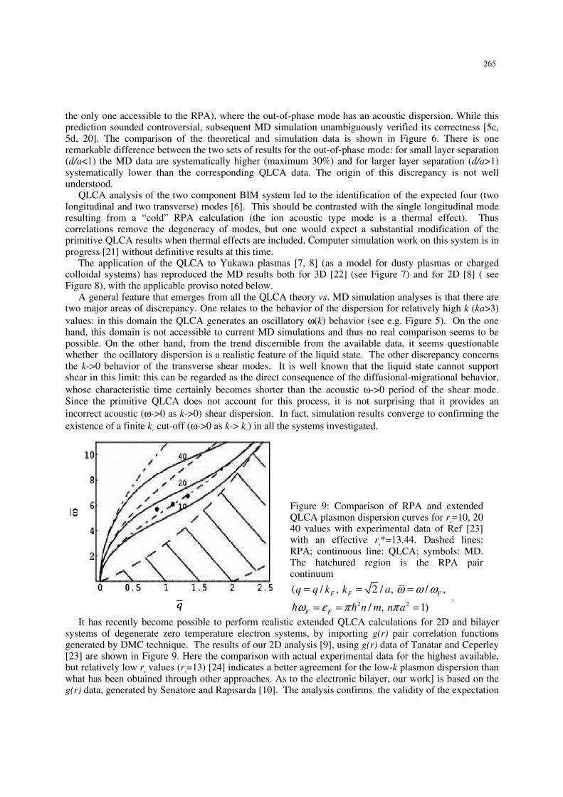
Figure 9: Comparison of RPA and extended QLCA plasmon dispersion curves for rs=10, 20 40 values with experimental data of Ref [23] with an effective r

s*=13.44. Dashed lines:

RPA; continuous line: QLCA; symbols: MD. The hatchured region is the RPA pair continuum

2 2

( / , 2 / , / ,

/ , 1)F F F

F F

q q k k a

n m n a

= = =

= = =

ω ω ωω ε π π

.

It has recently become possible to perform realistic extended QLCA calculations for 2D and bilayer systems of degenerate zero temperature electron systems, by importing g(r) pair correlation functions generated by DMC technique. The results of our 2D analysis [9], using g(r) data of Tanatar and Ceperley [23] are shown in Figure 9. Here the comparison with actual experimental data for the highest available, but relatively low r

s values (r

s=13) [24] indicates a better agreement for the low-k plasmon dispersion than

what has been obtained through other approaches. As to the electronic bilayer, our work] is based on the g(r) data, generated by Senatore and Rapisarda [10]. The analysis confirms the validity of the expectation

265

that the degenerate system would have the same qualitative behavior—in particular would develop an energy gap—as the more thoroughly analyzed classical one. To date though, there is no well analyzed experimental confirmation of the energy gap [see, however [25]).

Acknowledgements This material was based upon work supported by NSF Grant No. PHY-0206695 and DOE Grant DE-FG02-03ER5471 (GJK), by NSF Grant No PHY-0206554 (KIG), by the Hungarian Fund for Scientific Research Grants OTKA-T-34156, T-48389 (ZD and PH), the European Commission Grant MERG-CT-2004-502887 (PH) and MTA-OTKA-NSF Grant 28 (ZD, PH and GJK). GJK thanks Stamatios Kyrkos for help in the preparation of the manuscript and Pradip Bakshi for discussions relating to the frequency spectrum.

References [1] Klimontovich Yu L 1994 Statistical theory of open systems, (Dordrecht: Kluwer Academic

Publishers) and papers quoted therein. Klimontovich Yu L 1982 Kinetic theory of nonideal gases and nonideal plasmas (Oxford, New

York: Pergamon Press) [2] Pines D and Bohm D 1952 Phys. Rev. 85 338; 1953 Phys. Rev. 92 609

Bohm D and Gross E P 1949 Phys. Rev. 75 1851; 1949 Phys. Rev. 75 1864 [3] (a) Kalman G and Golden K I 1990 Phys Rev. A 41 5516

(b) Golden K I, Kalman G and Wyns P 1992 Phys. Rev. A 46 3454 [4] (a) Golden K I, Kalman G and Wyns P 1990 Phys. Rev. A 41 6940

(b) Golden K I, Kalman G and Wyns P 1992 Phys. Rev. A 46 3463 [5] (a) Golden K I and Kalman G 1993 Phys. Status Solidi B 180 533

(b) Kalman G, Valtchinov V and Golden K I 1999 Phys. Rev. Lett. 82 3124 (c) Donkó Z, Kalman G J, Hartmann P, Golden K I and Kutasi K 2003 Phys. Rev. Lett. 90 226804 (d) Donkó Z, Hartmann P, Kalman G J and Golden K I 2003 J. Phys. A: Math. Gen. 36 5877–5885

[6] (a) Kalman G and Golden K I 1990 Phys Rev. A 41 5516 (b) Golden K I and Kalman G J 2000 Phys. Plasmas 7, 14

[7] (a) Rosenberg M and Kalman G 1997 Phys. Rev. E 56 7166 (b) Kalman G, Rosenberg M and DeWitt H E 2000 Phys. Rev. Lett. 84 6030

[8] (a) Kalman G J, Hartmann P, Donkó Z and Rosenberg M 2004 Phys. Rev. Lett. 92 065001 (b) Donkó Z, Hartmann P, Kalman G J and Rosenberg M 2003 Contrib. Plasma Phys. 43, No. 5-6,

282-284 [9] Golden K I, Mahassen H and Kalman G J 2004 Phys. Rev. E 70 026406 [10] Golden K I, Mahassen H, Kalman G J, Senatore G and Rapisarda F 2005 Phys. Rev. E 71 036401 [11] v.s. 3(a), 6(b) [12] Donkó Z, Kalman G J and Golden K I 2002 Phys. Rev. Lett. 88 225001 [13] Donkó Z, Hartmann P and Kalman G J 2003 Phys. Plasmas 10 1563 [14] Bakshi P, Donkó Z and Kalman G J 2003 Contrib. Plasma Phys. 43, No. 5-6, 261-263 [15] Singwi K S, Tosi M P, Land R H and Sjolander A 1968 Phys. Rev. 176 589

Singwi K S, Sjolander A, Tosi M P and Land R H 1969 Solid State Commun. 7 1503 1970 Phys. Rev. B 1 1044; Sjolander A and Stott J 1972 Phys. Rev. B 5 2109

[16] Rabani E, Gezelter J D and Berne B J 1997 J. Chem. Phys. 107 6867 Rabani E, Gezelter J D and Berne B J 1999 Phys. Rev. Lett. 82 3649

[17] Bakshi P, Donkó Z and Kalman G J, unpublished [18] Golden K I and Kalman G J 2003 J. Phys. A: Math. Gen. 36 5865-5875 [19] Totsuji H and Kakeya N 1980 Phys. Rev. A 22 1220 [20] Ranganathan S and Johnson R E 2002 Phys. Rev. B 69 085310 [21] Szalay F, Donkó Z and Kalman G J, unpublished [22] Ohta H and Hamaguchi S 2000 Phys. Rev. Lett. 84 6026 [23] Tanatar B and Ceperley D M 1989 Phys. Rev. B 39 5005

266

[24] Hirjibehedin C F, Pinczuk A, Dennis B S, Pfeiffer L N and West K W 2002 Phys. Rev. B 65 161309

[25] (a) Popov V V, Polischuk O V, Teperik T V, Peralta X G, Allen S J, Horing N J M and Wanke M C 2003 J. Appl. Phys. 94 3556

(b) Peralta X G, Allen S J, Wanke M C, Harff N E, Simmons J A, Lilly M P, Reno J L, Burke P J and Eisenstein J P 2002 Appl. Phys. Lett. 81 1627

267