Space Charge Modeling at the Integer Resonance for the ...
269
Humboldt-Universitat zu Berlin Doctoral Thesis Space Charge Modeling at the Integer Resonance for the CERN PS and SPS Author: Dipl.-Phys. Malte Titze Supervisors: Prof. Dr. Atoosa Meseck Dr. Frank Schmidt Referees: Prof. Dr. Shinji Machida Prof. Dr. Atoosa Meseck Prof. Dr. Volker Ziemann Date of the defense: 29.01.2020 Dissertation zur Erlangung des akademischen Grades doctor rerum naturalium (Dr. rer. nat.) im Promotionsfach 00 q o Experimentelle Physik Mathematisch-Naturwissenschaftliche Fakultat Prasidentin der Humboldt-Universitat zu Berlin: Prof. Dr.-Ing. Dr. Sabine Kunst Dekan der Mathematisch-Naturwissenschaftlichen Fakultat: Prof. Dr. Elmar Kulke April 25, 2019
-
Upload
khangminh22 -
Category
Documents
-
view
4 -
download
0
Transcript of Space Charge Modeling at the Integer Resonance for the ...

Humboldt-Universitat zu Berlin
Doctoral Thesis
Space Charge Modeling at the Integer Resonance for the CERN PS and SPS
Author:Dipl.-Phys. Malte Titze
Supervisors:Prof. Dr. Atoosa Meseck
Dr. Frank Schmidt
Referees:Prof. Dr. Shinji Machida Prof. Dr. Atoosa Meseck Prof. Dr. Volker Ziemann
Date of the defense: 29.01.2020
Dissertation zur Erlangung des akademischen Grades doctor rerum naturalium
(Dr. rer. nat.)
im Promotionsfach
00
q o
Experimentelle PhysikMathematisch-Naturwissenschaftliche Fakultat
Prasidentin der Humboldt-Universitat zu Berlin: Prof. Dr.-Ing. Dr. Sabine KunstDekan der Mathematisch-Naturwissenschaftlichen Fakultat: Prof. Dr. Elmar KulkeApril 25, 2019


iii
Declaration of Authorship
Ich erklare, dass ich die Dissertation selbstandig und nur unter Verwendung der von mir gemaB § 7 Abs. 3 der Promotionsordnung der Mathematisch-Naturwissenschaftlichen Fakultat, veroffentlicht im Amtlichen Mitteilungsblatt der Humboldt-Universitat zu Berlin Nr. 42/2018 am 11.07.2018, angegebenen Hilfsmittel angefertigt habe.
Datum:
Unterschrift:


v
AbstractIn the design and operation of a particle storage ring the numerical simulation is an essential tool to understand and optimize its beam dynamics. These simulations are necessary to describe both the single particle behavior, but also the more complex processes of the interaction of charged particles between each other, including the external guiding fields. A deep theoretical understanding of the underlying mechanisms is always required, however, the beam dynamics is often too complex for quantitative analytic calculations. Dependent on the complexity of the physical problem, even the simulation tools may not be sufficiently fast enough on today’s computing facilities to take all effects into account, and so they require reasonable assumptions and simplifications to obtain results within practical time spans.
One of the simplifications in many codes based on a particle model is to alternate the computing of the interaction between the individual particles and the interaction between the particles and the guiding fields. Another simplification usually applied in such codes is the introduction of so-called macro particles, each representing an entire group of similarly behaving particles. These macro particles are then computed in the effective mean field of all particles, the so-called space charge field. Depending on the type of simulation code, this mean field can either be determined by the momentary distribution of macro particles or be given by an analytic formula. The purpose in introducing macro particles is a heuristic way to reduce the number of degrees of freedom involved, because a realistic beam consists of e.g. 1012 particles, but - depending on the application - only some 5 • 105 may be simulated reasonably fast. Of course, by performing such a reduction one must guarantee that it does not affect the physics of the beam significantly. To this end a precondition is to ensure that the number of macro particles is still large enough to avoid an artificial emittance blow-up. This can be provided by a so-called convergence test.
The topic of this work is the important question whether the different approaches in the description of space charge will lead to the same predictions - in comparison to each other, but even more importantly how well their results agree with the outcome of beam experiments. In particular, we will be dealing with two different groups of space charge models. The first group is related to an analytic description of space charge in form of Bassetti and Erskine’s formula of the electrostatic field of a Gaussian charge distribution. The other group is related to a finite-element-method approach, by solving the Poisson-equation on a grid. Both groups are hereby realized in various space charge solvers of the well-established tracking codes MAD-X (Group 1) and PyOrbit (Groups 1 and 2).
In order to prepare our studies, a common analysis framework had to be established beforehand to minimize any effects of the different data processing and handling of the codes on the results. But also an important code improvement in MAD-X had to be done prior to the actual simulations in order to obtain the correct natural chromaticity of the PS, by properly handling its combined- function magnets in the thin-lens approach.
From the experimental point of view we have chosen a scenario in which we studied the behavior of the beam near a horizontal integer resonance, in both the CERN Proton Synchrotron (PS) and the Super Proton Synchrotron (SPS). By carefully setting up the experiments and measuring the optics functions of both machines, we were able to find a scenario which could also be well described in simulations. Hereby we changed the respective machine working point in a controlled manner from a nominal working point towards the corresponding resonance - and back again. In this regard we will present all experimental results in several tables and discuss a possible explanation of the differences between the various simulation codes and the experiment for working points near the integer resonance.

vi

ZusammenfassungUm die Strahldynamik eines Speicherrings wahrend der Planung und des Betriebs zu verstehen und zu optimieren, ist die numerische Simulation ein essentielles Werkzeug. Solche Simulationen werden benotigt, um sowohl das Verhalten des einzelnen Teilchens, als auch das komplexere Zusam- menspiel mehrerer geladener Teilchen untereinander, inklusive ihrer externen Fuhrungsfelder, zu beschreiben. Hierbei ist ein tiefes theoretisches Verstandnis der zugrundeliegenden Mechanismen erforderlich, allerdings ist die Strahlphysik i.d.R. zu komplex fur eine quantitative analytische Rech- nung. Selbst Computersimulationen sind auf aktuellen Rechenclustern oftmals nicht schnell genug, um alle Effekte eines gegebenen Problems zu berucksichtigen, und deswegen machen solche Codes plausible Annahmen und Vereinfachungen um Resultate in praktikabler Zeit zu erhalten.
Eine Vereinfachung in vielen Codes, die auf einem Teilchenkonzept basieren, ist es, die Berech- nung der Wechselwirkung zwischen den einzelnen Teilchen und der Wechselwirkung zwischen den Teilchen und den Strahlfuhrungsfeldern abwechselnd zu behandeln. Eine weitere oft in solchen Codes gemachte Vereinfachung ist die Einfuhrung sogenannter Makroteilchen, die jeweils fur sich eine ganze Gruppe von sich ahnlich verhaltenden Teilchen reprasentieren. Diese Makroteilchen werden dann im effektiven mittleren Ladungsfeld aller Teilchen berechnet, dem sogenannten Raum- ladungsfeld. Je nach Code kann hierbei das Raumladungsfeld bestimmt sein durch die momentane Anordnung der Makroteilchen oder durch eine analytische Formel. Der Zweck der Einfuhrung von Makroteilchen besteht insbesondere darin, die Zahl der vorhandenen Freiheitsgrade auf heuristische Art und Weise zu reduzieren, da sich in einem realistischen Strahl z.B. rund 1012 Teilchen aufhal- ten, aber - je nach Programm - eventuell nur rund 5 • 105 in angemessener Zeit simuliert werden konnen. Naturlich muss im Falle einer solchen Reduktion dann dafur Sorge getragen werden, dass diese die Strahlphysik nicht nennenswert abandert. Insbesondere ist es wichtig zu gewahrleisten, dass die Zahl der Makroteilchen noch ausreichend grofi ist, um einen etwaigen kunstlichen Anstieg in der Emittanz zu verhindern. Dies kann durch einen sogenannten Konvergenztest sichergestellt werden.
Das Thema dieser Arbeit ist die wichtige Fragestellung, ob die verschiedenen Ansatze in der Beschreibung der Raumladung zu den gleichen Vorhersagen fuhren - hierbei im Vergleich zueinan- der, aber insbesondere auch bezuglich experimenteller Resultate. Dabei werden wir uns mit zwei verschiedenen Gruppen von Raumladungsmodellen beschaftigen: Die erste Gruppe basiert auf einer analytischen Beschreibung der Raumladung in der Form der Bassetti und Erskine Formel des elek- trostatischen Feldes einer Gaussverteilung. Die zweite Gruppe basiert auf einem Finite-Elemente Ansatz, in dem die Poisson-Gleichung auf einem Gitter gelost wird. Beide Gruppen sind hierbei in verschiedenen Raumladungsalgorithmen der etablierten Trackingcodes MAD-X (Gruppe 1) und PyOrbit (Gruppen 1 und 2) implementiert.
In der Vorbereitung unserer Studien musste ein gemeinsamer Rahmen erstellt werden, um etwaige Effekte durch die unterschiedliche Datenverarbeitung und Handhabung der Codes auf die Endresul- tate zu minimieren. Auch bedurfte es einer wichtigen Verbesserung im MAD-X Code im Vorfeld der eigentlichen Simulationen, um, vermoge einer getreuen Darstellung der Combined-Function Mag- nete im dunne-Linsen Ansatz, die korrekte naturliche Chromatizitat des PS zu erhalten.
Von experimenteller Seite her haben wir ein Szenario ausgewahlt, in dem wir das Verhalten desStrahls nahe einer horizontalen Integer-Resonanz studieren konnen - sowohl im CERN ProtonSynchrotron (PS) als auch im Super Proton Synchrotron (SPS). Durch sorgfaltiges Aufsetzender Experimente und Messung der Optikfunktionen beider Maschinen waren wir in der Lage, einSzenario zu finden, das auch gut durch Simulationen beschrieben werden kann. Hierbei haben wir

viii
die entsprechenden Arbeitspunkte in kontrollierter Art und Weise von einem nominellen Arbeit- spunkt zu der jeweiligen Resonanz geandert - und wieder zuruckgestellt. Wir werden diesbezuglich alle experimentellen Resultate in mehreren Tabellen darstellen und im Anschluss eine mogliche Erklarung der Differenzen zwischen den verschiedenen Simulationscodes und dem Experiment fur Arbeitspunkte nahe der Resonanz diskutieren.

ix
AcknowledgementsIn the process of writing this thesis - but also in the years before reaching this goal -1 have incurreda debt far too large to repay to all of those who have supported me. I will attempt a list of thanks,which is certainly incomplete.
First and foremost I want to express my deep gratitude to Prof. Dr. A. Meseck for being my thesis director, the person officially responsible from the University of Berlin’s site, for her many comments and critical discussions. I want to express the same gratitude to Dr. F. Schmidt for his role as my supervisor at CERN, his unrestricted support in all matters, assistance with the MAD-X/PTC/SC code, counterchecks, hard work and many critical discussions which resulted in great improvements of this thesis. I also want to thank Dr. B. Holzer for his role as a student adviser and mentor over the years, but also - and in particular - for establishing the connection to Frank in the first place. Furthermore I want to thank my group leader at CERN, Dr. G. Arduini, for accepting my application to work in his ABP group, as well as my former and current section leaders, Dr. E. Metral, Dr. Y. Papaphilippou and Dr. M. Giovannozzi for their unrestricted and enduring support in the course of writing this thesis. Last but not least I want to thank Prof. Dr. T. Lohse for his unreserved support near the end of this work. Without you all, this work would have never been realized.
Along the way to complete this thesis, many colleagues provided me with invaluable support and feedback. In particular I want to express my deep gratitude to Dr. H. Bartosik for his assistance in setting up the experiments, help concerning cluster computations and the PyOrbit code, as well as many productive discussions regarding the results of the simulations and the experiments. I also want to thank Dr. A. Huschauer for his assistance in setting up the PS experiments, introducing me to the CALS and many helpful discussions. For encouraging me to use (I)Python, introducing me to collective effects and countless open-minded discussions I wholeheartedly want to thank Dr. A. Oeftiger. I want to extend this gratitude to the entire operations team. It was an awesome time to work with you in countless nights in the course of this thesis, and I would have never been able to achieve its results without your great assistance.
Furthermore I want to thank especially Dr. I. Tecker for awesome discussions, help with MAD-X and your assistance regarding organizational matters. You were the best office mate I ever had! Much thanks goes also to Ms. F. Asvesta for her assistance in PyOrbit and many constructive discussions and to Dr. M. Carla’, who helped me to resolve a crucial problem in the PS simulations. I also want to thank Dr. G. Sterbini for using his PyTimber toolbox and having several productive discussions, Mr. R. Wasef for introducing me to initial scripts for the PS optics and Mr. P. Zisopoulos for his discussions concerning the beta-beating in the PS. For reading the appended manuscript I want to express my gratitude to Dr. M. Schwarz, Dr. M. Haj Tahar and Dr. F. van der Veken. Many thanks goes also to Ms. D. Rivoiron, Ms. A. Valenza, Ms. E. Dumeaux-Kurzen, Ms. J. Kotzian and Ms. I. Haug for their great assistance regarding organizational matters. There are many other colleagues who indirectly helped me with their work and discussions in larger or smaller amounts in completing this thesis, which I can not mention all. You know what you have done and it was a pleasure to work with you and had you as my colleagues!
This thesis would also not have been made possible without the history before and those whotaught me, guided me and supported me in the first place. I therefore want to express my deepgratitude to the people from HZB, in particular to Dr. J. Bahrdt, Dr. G. Wustefeld, Dr. M. Scheerand Dr. A. Gaupp. Without you all, I would never have been able to work at CERN. FurthermoreI want to thank the teachers of Humboldt-University of Berlin for their excellent courses, in particular Prof. Dr. J. Bruning and Prof. Dr. T. Friedrich of which I am proud to have heared one

x
of his lectures. Also my thanks goes to those teachers of Ruprecht-Karls University of Heidelberg, in particular Prof. Dr. R. Weissauer, my former mentor, as well as Prof. Dr. M. Kreck, Prof. Dr. E. Freitag and Prof. Dr. S. Hunklinger. My thanks goes further to the teachers of University of Konstanz for the awesome time I spent there, in particular Prof. Dr. D. Hoffmann and Prof. Dr. L. Kaup, for their exemplary well prepared courses, as well as Prof. Dr. U. Friedrichsdorf. Lastly I want to thank my former teachers at the Carl von Ossietzky Gymnasium in Hamburg, in particular Ms. Rahmke, Mr. Trinkel and Dr. Appel, hereby Dr. Appel also for bringing my attention to the course ’Faszination Physik’ at DESY.
And so from the scientific part there is one person whom I want to express my deepest gratitude. At DESY he teached me and other enthusiastic students during my free time, as I still went to school in Hamburg, on every Saturday topics in quantum mechanics, general relativity and mathematics, of how to write proper scientific texts and with whom I had great conversations overall: Dr. W. Tausendfreund. I wish you all the best and that ’Faszination Physik’ will continue to run for many years, encouranging students to start a career in the sciences.
Finally I want to thank my parents, family and friends for their support and patience. But in particular my mother for supporting me over all the years and encouraging me to never give up. It is not even in the slightest way possible to express my gratitude in words for all what you have done!
Overall it was a great experience to be able to work in the inspiring atmosphere at CERN and be part of the community. I thank CERN and the Bundesministerium fur Bildung und Forschung to made this dream come true.

xi
Contents
Declaration of Authorship iii
Abstract v
Acknowledgements ix
1 Introduction 11.1 Background........................................................................................................................... 1
1.1.1 The CERN LIU and HL-LHC program................................................................. 11.1.2 Motivation ............................................................................................................... 4
1.2 Structure of this work......................................................................................................... 51.3 Basic accelerator theory....................................................................................................... 6
1.3.1 Single-particle dynamics......................................................................................... 7Introduction ............................................................................................................ 7Beam stability......................................................................................................... 9Courant-Snyder parameterization, phase advance and Floquet-transformation 13Resonances, dynamic aperture, emittance and chromaticity ............................ 17
1.3.2 Many-particle dynamics ......................................................................................... 25Overview .................................................................................................................. 25Envelope equations with space charge ................................................................. 26Coherent motion and tune shift............................................................................. 28Incoherent tune shift ................................................................................................ 31
1.4 Appendix .............................................................................................................................. 321.4.1 Derivation of the Hamiltonian (1.6) .................................................................... 321.4.2 Lie calculus ............................................................................................................... 331.4.3 Proof of Birkhoff’s normal form............................................................................. 371.4.4 Proofs of statements concerning moment equations........................................... 401.4.5 Details regarding the derivation of the envelope equation ............................... 41
Preliminaries ............................................................................................................ 41The envelope equation ............................................................................................. 43
2 Symplectic maps for combined-function magnets 492.1 Introduction........................................................................................................................... 492.2 Preliminaries ........................................................................................................................ 51
2.2.1 Constructing the vector potential ....................................................................... 512.3 The Hamiltonian.................................................................................................................. 53
2.3.1 General considerations ......................................................................................... 552.4 Symplectic approach............................................................................................................ 57
2.4.1 First-order symplectic slice map .......................................................................... 572.4.2 Symplectic kick ...................................................................................................... 582.4.3 First-order drift-kick map...................................................................................... 59
2.5 MAD-X implementation ................................................................................................... 602.5.1 The magnetic field and its vector potential coefficients..................................... 60

xii
2.5.2 Thin-lens kick map................................................................................................... 622.5.3 First- and second order coefficients of the drift-kick map for TWISS......... 622.5.4 Explicit combined-function potential for normally aligned fields..........................642.5.5 Numerical tests......................................................................................................... 64
2.6 Appendix ............................................................................................................................... 662.6.1 On the Hamiltonian in Frenet-Serret coordinates.............................................. 662.6.2 Supplemental material............................................................................................. 692.6.3 Notations in MAD-X ............................................................................................. 70
3 Space charge codes 733.1 MAD-X .................................................................................................................................. 73
3.1.1 Introduction ............................................................................................................ 733.1.2 Beam emittance calculation ................................................................................... 753.1.3 Macros and post-analysis improvements.............................................................. 78
3.2 PTC-PyOrbit........................................................................................................................ 813.2.1 Introduction ............................................................................................................ 813.2.2 PIC node action ...................................................................................................... 82
3.3 Symplecticity checks ............................................................................................................ 863.3.1 Introduction ............................................................................................................ 863.3.2 Methods ..................................................................................................................... 87
Numeric differentiation method............................................................................. 872D-Fit method ......................................................................................................... 87
3.3.3 Benchmarking results ............................................................................................. 88Symplecticity errors ................................................................................................ 88Emittance growth in the sandbox model .............................................................. 89
3.4 Performance........................................................................................................................... 923.4.1 Convergence check................................................................................................... 923.4.2 Run time.................................................................................................................. 93
3.5 Appendix............................................................................................................................... 99
4 Integer resonance experiments 1014.1 Preparations ...........................................................................................................................101
4.1.1 Introduction ............................................................................................................ 1014.1.2 PS setup .................................................................................................................. 1044.1.3 SPS setup .................................................................................................................. 107
4.2 Analysis of the measured data ............................................................................................. 1094.2.1 Tune and intensity ................................................................................................... 1094.2.2 Beam sizes ............................................................................................................... 1154.2.3 Dispersion and chromaticity ................................................................................... 1184.2.4 Beta-beating ............................................................................................................ 122
4.3 Appendix ............................................................................................................................... 131
5 Distribution generation 1375.1 Introduction..............................................................................................................................1375.2 Linear matching ................................................................................................................... 140
5.2.1 Invariant tori..............................................................................................................1405.2.2 A numeric test...........................................................................................................146
5.3 Discussion ............................................................................................................................... 1495.3.1 Conclusions ............................................................................................................... 1495.3.2 Consequences..............................................................................................................150
5.4 Appendix ............................................................................................................................... 151

xiii
6 Simulation results 1536.1 Preliminaries...........................................................................................................................153
6.1.1 Lattice preparations..................................................................................................1536.1.2 Distribution matching...............................................................................................1546.1.3 Space charge and linear optics ............................................................................... 156
6.2 PS integer experiment...........................................................................................................1586.2.1 Emittance evolution..................................................................................................1586.2.2 Beam size .................................................................................................................. 162
6.3 SPS integer experiment ........................................................................................................1816.3.1 Emittance and optics evolution............................................................................... 181
6.4 Appendix.................................................................................................................................1896.4.1 Initial and final beam profiles in the PS simulations .......................................... 1896.4.2 Initial and final beam profiles in the SPS simulations.......................................... 196
7 Conclusions 203
A Error propagation 205A.1 Introduction............................................................................................................................205
A.1.1 Examples....................................................................................................................206A.1.2 Bessel’s correction....................................................................................................207
A.2 Regression analysis .............................................................................................................. 208A.2.1 Linear least square fit ............................................................................................ 208A.2.2 Formulation of the problem ................................................................................... 209A.2.3 First-order fit error .................................................................................................. 209
B Article 213
Bibliography 241


xv
List of Figures
1.1 CERN aerial view ............................................................................................................... 21.2 CERN accelerator complex ................................................................................................ 31.3 Standard model..................................................................................................................... 41.4 Multipoles.............................................................................................................................. 91.5 Weak focusing ..................................................................................................................... 131.6 Beam envelope in a drift section ...................................................................................... 171.7 Resonances induced by a sextupole................................................................................... 201.8 First-order correction of resonances................................................................................... 241.9 Coherent motion with space charge................................................................................... 301.10 Electric field of bi-Gauss-distribution................................................................................ 32
2.1 Combined function magnet ................................................................................................ 492.2 Residuals of thin CF maps................................................................................................... 652.3 Convergence behavior of thin CF maps............................................................................. 652.4 PS tracking example............................................................................................................ 66
3.1 PS energy-profile vs. long. profile...................................................................................... 763.2 Form factor for (dp/p0)rms in the analytical space charge models ............................... 773.3 Post-analysis scheme in 2015 ............................................................................................. 793.4 New post-analysis scheme................................................................................................... 793.5 PFW effect on the PS optics ............................................................................................. 803.6 space charge node distances................................................................................................ 823.7 Concept of slice-by-clice space charge solver.................................................................... 833.8 PIC node action in (z, dp/po)................................................................................................................................... 833.9 (x, 5p/po)-correlation of a central z-slice.......................................................................... 843.10 PIC phase space ellipse ...................................................................................................... 843.11 5p/p0-space charge kick correlation due to dispersion.................................................... 853.12 Runge-Kutta methods ......................................................................................................... 863.13 Drift PIC error matrix example ......................................................................................... 893.14 Principle of ND and 2D-fit method ................................................................................... 893.15 Error matrix examples of analytical and 2.5D code ......................................................... 903.16 Emittance growth of small-scale PIC test ....................................................................... 913.17 Emittance growth versus symplecticity error .................................................................... 913.18 Convergence campaign principle ...................................................................................... 923.19 e^-convergence for 2.5D and slice-by-slice PIC solvers...................................................... 943.20 e^-convergence for 2.5D and slice-by-slice in 3D.............................................................. 953.21 ey-convergence for 2.5D and slice-by-slice PIC solvers...................................................... 963.22 Run times of the slice-by-slice and the 2.5D PIC codes................................................. 973.23 Performance of the 2.5D and slice-by-slice code.............................................................. 98
4.1 Motivation for the integer experiments............................................................................... 1014.2 Mismatch problem.................................................................................................................1024.3 Integer experiment working point diagrams......................................................................103

xvi
4.4 Head-tail instability ..............................................................................................................1064.5 SPS supercycle....................................................................................................................... 1074.6 Coupling check in the SPS.....................................................................................................1084.7 PS tune measurements at Qx = 6.118 ............................................................................... 1094.8 PS tune measurements at Qx = 6.053 ............................................................................. 1114.9 PS cycle with tune-step........................................................................................................1114.10 SPS tune measurements at Qx = 20.144 .......................................................................... 1114.11 SPS cycle with tune-step........................................................................................................1124.12 SPS tune measurements at Qx = 20.036 .......................................................................... 1124.13 PS long-term intensity recording.........................................................................................1134.14 PS intensity measurement.....................................................................................................1154.15 SPS intensity measurement..................................................................................................1154.16 PS tomoscope ........................................................................................................................ 1164.17 PS beam profile measurements ............................................................................................1184.18 SPS beam profile measurements............................................................................................1214.19 PS mountain range profile correction.................................................................................. 1214.20 5p/p0 measurements..............................................................................................................1224.21 PS dispersion measurement at BPM 07.H................................... 1234.22 SPS dispersion measurement at BPM 32808.H...............................1234.23 PS dispersion along the ring ................................................................................................ 1244.24 SPS dispersion along the ring ............................................................................................. 1254.25 PS horizontal and vertical chromaticity .......................................................................... 1254.26 SPS horizontal and vertical chromaticity .......................................................................... 1264.27 BPM signal treatment for beta-beating measurements ................................................. 1274.28 Relation between BPM signal and phase advance ........................................................... 1274.29 Beta-beating in the PS at Qx = 6.118 ............................................................................... 1284.30 Beta-beating in the PS at Qx = 6.053 ............................................................................. 1294.31 Beta-beating in the SPS at Qx = 20.144 .......................................................................... 1304.32 Dispersion of beta-beating corrected lattice......................................................................1314.33 Baseline fit example for beta-beating measurement..........................................................1334.34 Zero-crossings of BPM signals for phase-differences measurement.................................1344.35 Zero-crossing distances for beta-beating measurement ....................................................1344.36 Phase-advance covariance entries along the PS ................................................................1354.37 Covariance spectra along the PS .........................................................................................136
5.1 Motivation: Initial mismatch PS .........................................................................................1375.2 Motivation: Initial mismatch SPS.........................................................................................1385.3 Example of particle generation............................................................................................1385.4 SPS long. profile higher-order...............................................................................................1395.5 Example of convoluting f^’s ...............................................................................................1425.6 Particles generated on an invariant torus............................................................................ 1425.7 Histograms of an invariant torus .........................................................................................1435.8 Profiles and their Fourier-spectra.........................................................................................1455.9 Bias effect in numeric approximation.................................................................................. 1475.10 Bias-correction by step-size recognition............................................................................... 1475.11 Numeric approximation of measured profiles......................................................................1485.12 Floquet-space occupation comparison.................................................................................. 149
6.1 Closed-orbit correction in the simulations.........................................................................1546.2 Closed-orbit correction in the simulations II......................................................................1556.3 Adiabatic tune-ramping in the PS ......................................................................................158

xvii
6.4 x-emittance evolution in the PS, up-ramp, method 1........................................................1596.5 x-emittance evolution in the PS, up-ramp, method 2........................................................1596.6 x-emittance evolution in the PS, de-ramp, method 1........................................................1606.7 x-emittance evolution in the PS, de-ramp, method 2........................................................1606.8 Effect of non-linearities in the emittance calculation .......................................................1616.9 Zero-run in the PS at Qx = 6.118.........................................................................................1626.10 Space charge node action at Qx = 6.053 .......................................................................... 1636.11 Beam size evolution in the PS...............................................................................................1636.12 Final beam sizes after ramp..................................................................................................1646.13 Dispersion evolution in the PS ............................................................................................1666.14 ^-evolution in the PS...........................................................................................................1676.15 Beam size along the PS ring..................................................................................................1686.16 Dispersion evolution in the PS ............................................................................................1696.17 Space charge node kick strengths at Qx = 6.053 near ±5rms.......................................... 1706.18 Space charge kicks around the PS.........................................................................................1716.19 Frequency analysis of the analytical code............................................................................1736.20 Frequency analysis of the sbs and the 2.5D code .............................................................1746.21 Tunes near the integer in the analytical and the slice-by-slice codes................................1746.22 Error estimate due to space charge dipole-components....................................................1756.23 Tracking example in the analytical model.........................................................................1766.24 Tracking example on the integer resonance.........................................................................1776.25 Beam endoscopy in the PS simulations............................................................................... 1786.26 Beam centroid movement during the tune-ramp................................................................1786.27 Centroid kicks by space charge nodes.................................................................................. 1796.28 FFT of (x) in the PS simulations.........................................................................................1796.29 Losses in the PS simulations..................................................................................................1806.30 Emittance evolution example in the SPS............................................................................1826.31 Emittance evolution example in the SPS part II............................................................... 1836.32 SPS emittance evolution prolongated.................................................................................. 1846.33 Halo ........................................................................................................................................ 1856.34 Intensity at Qx = 20.036 ...................................................................................................... 1866.35 Emittance at zero-ramp in the SPS..................................................................................... 1866.36 Optics functions in the SPS simulations............................................................................1876.37 Optics functions in the SPS simulations, part II...............................................................1886.38 Nominal horizontal profiles in the PS.................................................................................. 1896.39 Final horizontal profiles in the PS ..................................................................................... 1906.40 Horizontal profiles in the PS after back ramp...................................................................1916.41 Nominal vertical profiles in the PS..................................................................................... 1926.42 Final vertical profiles in the PS............................................................................................1936.43 Initial longitudinal profiles in the PS.................................................................................. 1946.44 Final longitudinal profiles in the PS .................................................................................. 1956.45 Nominal horizontal profiles in the SPS............................................................................... 1966.46 Final horizontal profiles in the SPS..................................................................................... 1976.47 Nominal vertical profiles in the SPS .................................................................................. 1986.48 Final vertical profiles in the SPS.........................................................................................1996.49 Nominal longitudinal profiles in the SPS .......................................................................... 2006.50 Final longitudinal profiles in the SPS ................................................................................ 201


xix
List of Tables
2.1 Chromaticity in the PS versus slice numbers.................................................................... 65
3.1 Change of covariance matrix in PIC node....................................................................... 853.2 Emittance change by space charge nodes.......................................................................... 863.3 Symplecticity error in a FODO cell with space charge ................................................. 883.4 Symplecticity error versus particle number....................................................................... 90
4.1 PS and SPS integer experiment parameters......................................................................1054.2 PS tune measurements...........................................................................................................1104.3 SPS tune measurements........................................................................................................1104.4 PS intensities and losses........................................................................................................1144.5 SPS intensities and losses.....................................................................................................1144.6 PS wirescanner and longitudinal rms values......................................................................1194.7 SPS wirescanner and longitudinal rms values ...................................................................1204.8 Covariance matrix entries of phase-differences at BPM BPM10.H................. 1354.9 Covariance matrix entries of phase-differences at BPM BPH.41608.H.............135
5.1 Coefficients Cik............................................................................................................................................144
6.1 PS tunes in the simulation ................................................................................................... 1586.2 Dispersion values in the simulations ................................................................................ 1646.3 Breakdown of beam size calculations ................................................................................ 1656.4 Average beam sizes along the PS ring ................................................................................ 1656.5 Average dispersion along the PS ring ................................................................................ 1706.6 Centroid kicks by space charge nodes ................................................................................ 1766.7 SPS tunes in the simulation ................................................................................................ 182


xxi
For Felix


1
Chapter 1
Introduction
1.1 Background
1.1.1 The CERN LIU and HL-LHC program
In the effort to an understanding of nature’s underlying principles, advances in modern scientific theories have been pushing the collision energy scale of particles further and further into terrains which are difficult, if not impossible, to study. The reason seems to be nature itself, as there are indications that, on the one hand, from a cosmological point of view the universe likely did evolve out of a state of very high energy-density and, on the other hand, from a microscopic point of view, that the coupling constants of the electromagnetic, the weak and the strong force are expected to be almost merging at collision energies of around 1013 TeV [Kaz01]. Unfortunately (or maybe fortunately), such energies are beyond the capabilities of any particle collider.
On the frontier of the highest possible particle collision energies mankind can currently produce lays the European Organization for Nuclear Research (CERN), as host of its Large Hadron Collider (LHC). CERN, founded in 1954, has currently 22 member states with around 2500 staff members and over 12200 users from 110 nationalities [CER19]. The LHC, as being the largest part in the CERN accelerator complex, is a 27 km circular particle collider, built for the purpose of achieving the highest technically possible energies for fundamental high-energy physics research.
The ring was approved and built from around 1994 onwards in the tunnel of its predecessor, the Large-Electron-Positron Collider (LEP), and assembled in two stages. In its current second stage it can produce proton-proton collisions in four collision points with a center of mass energy of around 13 TeV. Two beams of particles are hereby circulating in two separated tubes inside a superconducting magnet system, and brought into collision at the interaction points. The scale of the entire complex is shown in Fig. 1.1, while a schematic view is given in Fig. 1.2.
The LHC was operated with success over the recent years, including the celebrated discovery of the Higgs-boson [Aad+12; Cha+12], the last sought piece of the standard model depicted in Fig. 1.3. This was a major milestone in an understanding of nature’s fundamental principles. In order to further improve the performance of the LHC, major upgrades are scheduled within the coming years, starting from 2019 onwards, in which all injectors1 - as well as the main ring - will receive improvements and element replacements.
1 Rings through which the beam will be accelerated into the LHC are called injectors.
The upgrade of the pre-accelerator complex is summarized under the name LHC Injectors Upgrade (LIU). LIU is required prior to an upgrade of the LHC, the High-Luminosity LHC (HL-LHC). The HL-LHC has the primary purpose to fully exploit the capabilities of the ring, using cutting-edge technology, with the goal to increase the luminosity (i.e. the number of collisions per second and per transverse area) by a factor of around ten [Apo+17].

2 Chapter 1. Introduction
Figure 1.1: Aerial view of the CERN accelerator complex. ©CERNIncreasing the luminosity is highly desired, as it will lead to better statistics, in particular in regards of the detection of rare processes, and which will therefore improve our understanding of nature. Besides of exploring the properties of the Higgs boson, another goal of the scientific program will be the search for weakly interacting massive particles, in order to detect possible hints to physics beyond the standard model.
In order to reach high luminosities in the LHC, the pre-accelerator complex plays a crucial role, because in the chain of pre-accelerators the bunch characteristics of the LHC are determined: A high luminosity goal in the LHC collision points requires high-intensity beams in all involved machines. However, the higher the intensity of the beam is set to, the stronger the repulsive forces of the individual particles will be due to the fact that they have the same electric charge. At some point these space charge forces are sufficiently strong enough to drive undesired beam instabilities
2This figure is a derivative of "Standard model of physics", http://texample.net/ @ C. Burgard under the Creative Commons attribution license.

1.1. Background 3
Figure 1.2: Schematic view of the CERN accelerator complex. ©CERNand other phenomena, which turn out to be major limitations for the operation of the machines. Space charge is always present, but it is in particular dominant in the low-energy pre-accelerators, because its repulsive action takes place in the beam rest frame, i.e. under the effect of time dilation if observed from the laboratory frame of reference.
The CERN pre-accelerators consists of the linear accelerators LINAC3 for ions and LINAC43
for protons, the Low Energy Ion Ring (LEIR) for ions, the Proton-Synchrotron-Booster (PSB) for protons, the Proton Synchrotron (PS) and finally the Super-Proton-Synchrotron (SPS), see Fig.
3LINAC4 is the replacement of LINAC2. LINAC2 was in operation at the time of this work.
1.2. In all of those machines, simulations with high-intensity beams are necessary to determine the behavior of the beam due to the additional self-interaction of the particles.
For the purpose of simulating space charge effects, various simulation codes are at our disposal. These codes are intended to solve the complex scenarios of interacting particles inside an accelerator over a reasonably long period of time. However, although they are sophisticated, they too have to rely on certain simplifications, and it is therefore important to determine whether the different models of the codes yield correct and consistent results. This is the point where this work comes into play. In particular we are going to analyze two specific space charge codes, which are called MAD-X and PyOrbit.

4 Chapter 1. Introduction
standard matter unstable matter force carriersoutside
standard model
1st 2nd 3rd generation
12 fermions 5 bosons(+12 anti-fermions) (+1 opposite charge W)increasing mass ^
Figure 1.3: The standard model of particle physics.2
4We will introduce some notions in this chapter later on.
1.1.2 MotivationThe simulation of a large number of interacting charged particles inside a storage ring is a challenging task mainly because of two reasons: The first reason is the sheer amount of particles (at CERN usually in the order of 1011 to 1013) which require the invention of suitable models to reduce the amount of parameters to be processed, and usually to parallelize computations as much as possible. The second reason is the time span of the physical processes simulated versus the time step of the integrator. Formulated for a reader who is familiar with the subject:4 If the equations of motion are integrated in a straightforward manner, codes which are based on a non-Liouvillean model may lead to unphysical phenomena. A well-known example is the development of noise as a contribution to the beam entropy, which will affect the evolution of the beam emittances [Str96; Str00; BF+15; KF15].
In accelerators, phenomena related to the interaction between charged particles or charged particles and the vacuum chamber walls are commonly abbreviated as collective effects. The interaction of the particles fall mainly into two categories: direct and indirect effects. Direct effects are primarily caused by the Coulomb interaction between the particles inside the beam (usually described by an effective space charge field). Indirect effects are caused by the influence of image charges on the beam, which are induced in the wall of the beam pipe.
Codes dealing with space charge can be categorized in so-called adaptive codes and non-adaptive

1.2. Structure of this work 5
or ’frozen’ codes. Frozen codes consider the space charge forces as being fixed once determined, regardless of any changes on the distribution in the process of the simulation. In these frozen models, the interaction of individual particles does not have to be computed, essentially making these codes relatively fast single-particle tracker. They often assume a bi-Gaussian elliptic shape of the distribution in the transverse direction and a uniformly shape of infinite length in longitudinal direction (such beams are called ’coasting’), since in this case there exist a well-known analytic description of the electromagnetic field [BE80; Zie91]. The handling of the longitudinal charge density in case of bunched beams are then included separately. In case of a transversely circular bi-Gaussian distribution, the situation is a bit simpler, see e.g. Ref. [Sch10].
In contrast to frozen codes, adaptive codes ’adapt’ - after a given time span or length - the electromagnetic force field to the actual distribution of simulated particles. In the two codes this work is concerned with, such a length is controlled by the user to a certain extend. In addition, codes can be self-consistent, in which we understand the capability of computing the interaction between particles and the external force fields simultaneously. Examples of such codes are Vlasov solvers as in Ref. [Ume+12], and certain moment codes like BEDLAM [Cha83b; CHL85; BL85; Lys90] and V-Code [AW04]. Last but not least there is the important class of symplectic codes, in which every integration step can be characterized as coming from a canonical transformation, i.e. codes satisfying the Liouville-theorem on its parameter space.
In this work we are dealing with a benchmark of the two space charge codes MAD-X and PTC- PyOrbit against each other and against experimental results, focusing on direct space charge effects. Both codes come along with several space charge solvers, which are based on different models to simulate the propagation of interacting charged particles through the respective machine. These codes will be discussed in Chapter 3.
1.2 Structure of this work
After this introductory chapter, we will first continue in single-particle dynamics and describe in Chapter 2 in detail how we modified the MAD-X code in order to use thin-lens combined-function magnets.5 As this work is dealing with a benchmarking of MAD-X and PyOrbit, and the main building blocks in the PS are combined-function magnets, this preparation step was required prior to our space charge studies in order to correct an error of around 20% in the natural chromaticity against the thick-lens result. A thin-lens description of machine elements is essential for the MAD- X tracking procedures.
5The definition of ’thin-lens’ will be made precise in Chapter 2.6The word stems from the fact that in a simulation we can usually work only with much less particles than in the
experiment. These simulation particles therefore represent a certain number of realistic particles.
In Chapter 3 we will introduce the two space charge codes this work is concerned with, MAD-X and PyOrbit, and discuss how these codes model space charge effects. While some of the underlying space charge solvers are utilizing an analytic field description, others are based on a Particle In Cell (PIC) model in order to solve space charge on a grid, similar to a finite-element method. Because reasonable numbers for grid points and macroparticles6 used in the simulation needs to be determined, we will present results of a convergence study regarding the PIC codes. Hereby we will analyze the evolution and growth of noise and the required CPU speed. In this chapter we will also discuss results of symplecticity checks for the codes.
The next chapter, Chapter 4, is dedicated to a detailed presentation of the experimental setup and measurement results of both the PS and SPS studies. In particular we will provide tables of

6 Chapter 1. Introduction
wirescanner7 and intensity measurements, the measured dispersion around the machines as well as measurements of the so-called beta-beating in close vicinity of the integer resonance, together with an error analysis. The beta-beating is hereby the relative error of the measured ^-function (see later) towards the model.
7The principle of a wirescanner is to move a thin wire through the beam to measure its profile by the induced secondary charges in nearby scintillators.
8The reason is that computing twiss parameters requires the search of a closed-orbit, which may not be found near a resonance.
In what follows is Chapter 5, where we present a study in which we will address one aspect of the problem of generating a particle distribution so that its profiles are in good agreement with the measurements. Hereby we will derive an interesting result regarding the occupation of the particles in phase space and present a numeric test confirming our findings.
In Chapter 6 we will present the outcome ouf our two simulation studies for both the PS and the SPS and compare them against our measurements. We will hereby utilize methods discussed in Ref. [Tit19] to obtain statements regarding the emittance growth and the dispersion under the effect of space charge in the simulation. Our main emphasis lays hereby on the PS where we will find a surprising result and provide an explanation.
The last two parts of the work consists of Chapter 7, which contains our concluding remarks, as well as an appendix: As it turned out in the course of our studies, a central problem in setting up simulations near the integer resonance stems from implementing a sufficient particle generation procedure. Formulated in an exaggerated manner: If one could construct a method in order to generate particles so that in the course of the simulation their distribution is in perfect agreement with the measurements, one has already understood a great deal of the entire simulation.
In Appendix B we have therefore included work where we examined the interplay between linear normal form and matched covariance matrices, as we encountered issues related to these subjects while setting up the simulations. The main result of this work is a description of the parameterization for linear (coupled) optics, which is purely based on the tracking data, and where knowledge of the underlying optics is not required.
The results were then used in our analysis of the simulation data in Chapter 6. Besides of providing a common analysis framework, the procedure can also be used in order to provide approximations for the so-called twiss parameters (i.e. optics parameters like a, ft, y discussed later) close to the integer resonance, where conventional twiss commands can break down, even if the tracking still might work.8
1.3 Basic accelerator theory
Our goal of this section is, on the one hand, to conveniently introduce some of the concepts in accelerator theory which seem to be the most relevant for the presented studies. And on the other hand to provide (or perhaps better: to sketch) a small toolbox which is general enough to serve as a starting point for further studies.
There are many different subjects in accelerator theory which we can not cover in this small introduction. For example, we will not discuss the physics of synchrotron radiation, primarily also because this work is concerned with the physics of proton beams, which radiate a negligible amount of synchrotron light in our experiments, and generally much less than electrons due to the dependency of the mass in the radiation equation. Therefore, the beam can be understood

1.3. Basic accelerator theory 7
as a closed system under the influence of external guiding fields, whose borders are given by the vacuum chamber walls. The motion of individual particles can be described by means of conserved quantities, and thus in the foundation of accelerator theory in this work lays Hamiltonian mechanics.
We will hence begin this introduction with Hamiltonian mechanics describing the physics in the accelerator. Although we attempt to introduce several concepts in a self-contained fashion, the topic is vast and due to the limited amount of space we still have to drastically restrict ourselves and must assume some familiarity with classical mechanics and also some mathematical background.
There is an additional difficulty coming from the transition from a single-particle description of motion to concepts which involve the physics of many interacting particles: Some of the concepts of single-particle dynamics can be transported to many-particle dynamics, but it depends on how this is done; for example if one just increases the number of degrees of freedom, many concepts (and equations) become unpractical. Instead one should attempt a different description, by properly including macroscopic quantities and mean fields. In many circumstances one can arrive at far reaching results and useful equations of the evolution for these macroscopic quantities, which may once again be cast into a suitable Hamiltonian form. Some concepts of many-particle dynamics which are important for this work will be governed in part two of this introduction.
1.3.1 Single-particle dynamicsIntroduction
In order to guide and focus a beam of particles inside a beam pipe, many aspects regarding the motion of charged particles in electromagnetic fields have to be taken into consideration. In this subsection we will focus on principles which are fundamental in every situation. If radiation of accelerated charged particles can be neglected, as it is the case for the proton beams in PS and SPS experiments, the underlying equations governing the motion of the particles are Newton’s law of motion and the Lorentz force
.P = F, (1.1)
F = e(E + v x B), (1.2)
while the external electric and magnetic fields E and B are satisfying Maxwell’s vacuum equations9
9We will use SI units throughout the thesis work.
VE = 0, (1.3a)
V x E = -dtB, (1.3b)
VB = 0, (1.3c)
V x B = c~2dtE. (1.3d)
As we are dealing in this paragraph with the dynamics of individual particles under the effect of external guiding fields, it is assumed that these fields are not influenced by the particles themselves. This is no longer the case in multi-particle systems, of which we discuss some aspects in Subs. 1.3.2.
Since a storage ring or beam line consists of elements aligned along a reference trajectory, parameterized by a longitudinal position s, it is usually more convenient to determine the physicswith respect to s rather than the time. Often it is also required to switch between different coordinate systems, for example from a Cartesian one to a comoving coordinate system, which might

8 Chapter 1. Introduction
be better suited to describe the physics along a curved beam line. Aside from the need to switch between coordinate systems, it is often desired to use a first-order differential equation instead of a second-order one.
A powerful tool to fulfill the above requirements is provided by Hamilton mechanics. In this setting, equations (1.1) reads as follows
dq dHds dp , dp dHds dq ’
(1.4a)
(1.4b)
where H is a function depending on q explicit parameter s. By introducing
= (x,y,t), canonical10 momenta p = (px,py,Pt) and the
10They should not be confused with the kinematic momentum p in Eq. (1.1). The relation is pk = pxk — eAk, where Ak are the components of the vector potential of B. For this purpose we will sometimes use the subscript ’kin’ for the kinematic momentum.
nThe subscript t on At means tangent.
0_1 n
1n
0 (1.5)2nx2n
and w := (q,p)tr, the above set of equations (1.4a), (1.4b) can be recast conveniently as w' = J3VH(w). Eq. (1.2) can now be reformulated, for example by using a Hamiltonian of the following form, which is derived in Appendix 1.4.1:
H(x,y,z,px,py,n; s) =
nPo2 - KV p^ - (px - Ax)2 — (py — Ay)2 + 1 - ~B2 - KAt,
v \ Po / po
where k(x, y, s) := 1 + Kx(s)x + Ky(s)y,
Ymvx,y + eAx,y po
eAx,y,t,po
Px,y : =A + — x,y,t := p := ep
, poc
(1.6)
(1.7a)
(1.7b)
z :=(s - cpot) p2,
and n := (K-Eo)/Eo the relative energy deviation. K is total energy of the particle, Po, p0 and Eo
are, respectively, the relativistic P-function, 3-momentum and energy of a reference particle and A and p are the vector- and scalar potentials of the magnetic and electric fields11, i.e. they satisfy V x A = B and Vp + dtA = -E. The s-dependent functions Kx, Ky describe a possible curvature of the reference trajectory. We remark that the Hamiltonian (1.6) is based on a version found in Ref. [Rip85] (see also the references in the appendix and in Chapter 2). For a general introduction to Hamilton mechanics we refer the reader to Refs. [Poi93; GPS02].
As the beam line consists of many individual elements, it would be very difficult to glue them all together into Eq. (1.6) and attempt a solution. The next stage in describing the physics of the beam is therefore to look at special cases (i.e. individual elements) in which Eq. (1.6) can be solved. This yield maps of individual elements which can be composed together to yield maps for entire sections or even the entire beam line itself. In the case of a storage ring one would call such a map a one-turn-map. In the next paragraph we will discuss important examples of such cell-maps.

1.3. Basic accelerator theory 9
Beam stability
The focusing and bending of the beam trajectory is usually provided by magnetic fields. Roughly speaking the reason to use magnetic fields instead of electric ones is the velocity dependency in Eq. (1.2), which makes the magnetic forces much more effective on particles having speeds close to the speed of light. In a storage ring the bending of the beam is therefore provided by magnetic dipole fields. As their name suggests, dipole fields are produced by parallel magnetic poles which provide a constant magnetic field in between. But also the focusing of the beam is done by magnetic elements. As we shall see, an overall focusing can be performed by magnets which are transversely generated by four poles, so-called quadrupoles. Higher-order multipoles are used to compensate other effects. The transverse field lines of these multipoles in the first three orders are shown in Fig. 1.4.
Figure 1.4: Transverse magnetic field lines of normal (top) and skew (bottom) dipoles, quadrupoles and sextupoles used respectively for bending, focusing and correcting chromatic effects in the beam line. The colored lines are perpendicular to the field lines, and therefore reflect possible shapes of the polefaces for generating these fields.
e
Since the polefaces generating these fields have finite proportions and the magnetic field lines have to be closed, they will at some point no longer follow the shapes in Fig. 1.4. In the jargon of accelerator physics, fields at the pole edges are lumped together under the name fringe fields. They can become important in particular with respect to the longitudinal position s, as transverse fringe fields can always be made small enough by sufficiently large elements. For the given multipole fields in Fig. 1.4 we restricted ourselves to a description of their interior, without fringe fields.
As one can verify, the following fields satisfy Maxwell’s equations (1.3a) - (1.3d) for every n G N:
B™ + iB™ = Cn(x + y , (1.8)

10 Chapter 1. Introduction
where cn G C determines whether the multipole is normally aligned or skew, which means rotated by an angle of 90°/n. In lowest order n we obtain the dipole, quadrupole and sextupole fields shown in Fig. 1.4. From Eq. (1.8) we see that for example a quadrupole (n = 2) generates a field which depend linearly along the horizontal and vertical axis, where the dependency for both directions are of opposite sign.
In some circumstances it can happen that a single element in the beam line includes a combination of several different multipole components. As Maxwell’s equations are linear, every superposition of the fields in Eq. (1.8) is in principle possible. In Chapter 2 we will discuss so-called combined function magnets, which constitute the main building blocks of the PS, and whose proper description is therefore essential in every simulation regarding this machine.
We will now briefly demonstrate how quadrupoles can be combined to an effective focusing element in the machine. The first step is to perform a replacement of the full Hamiltonian (1.6) in order to deal with the square root. This procedure is called paraxial approximation. Observe that for the slope x' = dx/ds it holds12
12Note that p2kin = c~2(K — ep)2 — m2<?.
, dH x = .
dpxpkin,x
K —pkin,z (1.9)
and similarly y' = Kpkin,y/pkinz. If the longitudinal momentum pkin,z is large in comparison to pkin,x and pkin,y, then we can expand the square root in Eq. (1.6) in terms of these slopes by extracting the full momentum p := |p|. Expanding up and including third order in the slopes yields an approximated Hamiltonian H2:
h2 := n - K(1 + p) po
/1 _ 1 (px — Ax)2 _ 1 (py Ay)2 \ _ A1 2 (1 + p)2 2 (1 + p)2 A (1.10)
with the relative momentum deviation p := (p —p0)/p0 with respect to a constant reference momentum p0. The relation between p and p is hereby given as
?+1=j (^+1-* y+1—^2 • (1.11)Po Po
In the case of the multipole fields above, we can set <p = 0, Ax = 0 = Ay, Kx = 0 = Ky and
At^ = -1(cn(x + iy)n + Cn(x - iy)n) • (1.12)
If we consider an on-momentum particle in such a ^-independent scenario, then p = 0 = p, as the energy and momentum will not be changed in pure magnetic fields. In the case of normally aligned quadrupoles we thus have (by dropping the tilde in the notations and by dropping any constants in H2, as they will not affect the equations of motion)
H2(x,y,px,py) = ^(pl + p2y) + 1 g(x2 - y2), (1.13)

1.3. Basic accelerator theory 11
where g G R determines the focusing of the quadrupole. The corresponding equations of motion in ^-direction reads x" = — gx. Depending on the sign of g, its solution is:
x(s) = cos(7gs)x0 + — s.n(—gs)pxp, if g > 0,
x(s) = Px,0S + X0, if g = 0,
x(s) = cosh^/|g|s)x0 + -j= sinh^/|g|s)px,0, if g < 0,
(1.14a)
(1.14b)
(1.14c)
where Xi and px,i are the initial coordinates at s = 0, which we may assume to be the element entrance. There is a convention to label quadrupoles by their effect in horizontal direction as (de)focusing. Together with the solution for px we see that quadrupoles and drifts produce linear maps from initial coordinates to final coordinates Xf, px,f, after the particle traversed a distance of length L, the length of the element:
Xf \ = / cos(—gL) sin(—gL)/—g \ / Xi \Px,f ——g sin(—gL) cos(^—gL) px,i ’pf ) = ( 0 1 ) ( X) ’
Xf \ f cosh(y/|g|L) smh(y/|g|L)/y/|g| W Xi Px,f \g\ sinh(y/|g|L) cosh(y/|g|L) Px,i
(1.15a)
(1.15b)
(1.15c)
Of course, such a linear relation between initial and final coordinates is a special case. In general these maps can be rather complicated.
If the quadrupole has a small length L, its map for a given focusing can be approximated in the thin-lens approximation. This approximation is obtained here by performing the limit ^L ^ 1/f if L ^ 0, where f > 0 is the desired focal strength of the quadrupole. The approximation is useful in the case of a particular sequence of elements, which constitute the basic building block in most modern accelerators: An arrangement of a focusing quadrupole (F), a drift (O), a defocusing quadrupole (D) and another drift (O), in short: a FODO-cell.
More symmetrical, the first focusing quadrupole is often split in two halves and its first half is attached at the end of the sequence. Combining the five linear maps C := F1/2 o O o D o O o F1/2, we obtain the following map in thin-lens approximation:13
13In vertical direction, f has to be replaced by — f in the resulting expressions.
L(2 + f )c= ( L—fL
— f (1 — 2f ) 1 L2f 2
(1.16)
The eigenvalues of C are
Al,2 = 1 — ± —L2 — 4f2. (1.17)ff
Since C was given as the product of matrices with unit determinant, it holds A1A2 = 1. If we imagine that our lattice consists of many such FODO cells, stability requires |Ai| = 1. This is ensured if Ai G U(1) with L/2 < f. If this condition is fulfilled, particles remain stable around the zero reference orbit, while the phase ^ of the eigenvectors advances every cell by cos(^) = 1 — L2/(2f2).
The physical reason for stability is that the defocusing part of the first quadrupole is more than compensated in the focusing part in the second quadrupole, as the field is much stronger in the
12 Chapter 1. Introduction
outer regions of the quadrupole. Since a particle is never perfectly injected on its design trajectory, but may have a small offset, we see that quadrupoles are essential components to keep a beam of particles stable around the design trajectory.
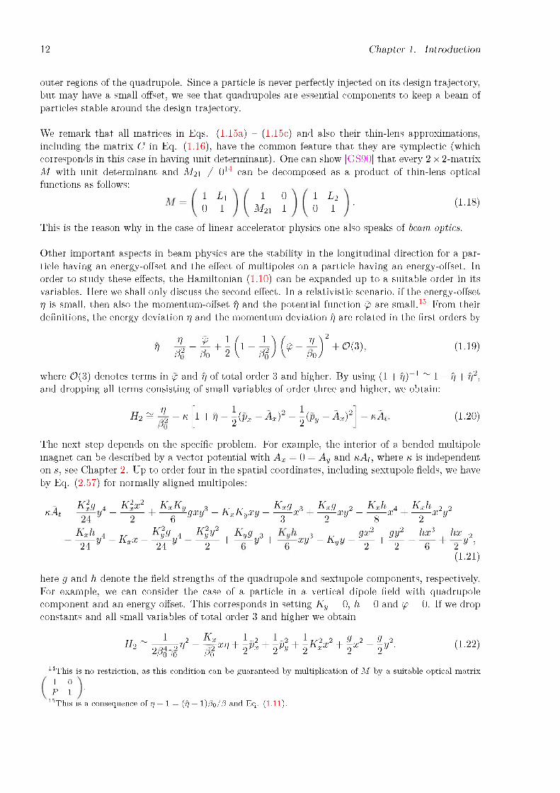
We remark that all matrices in Eqs. (1.15a) - (1.15c) and also their thin-lens approximations,including the matrix C in Eq. (1.16), have the common feature that they are symplectic (whichcorresponds in this case in having unit determinant). One can show [GS90] that every 2 x 2-matrix M with unit determinant and M21 = 014 can be decomposed as a product of thin-lens optical
14This is no restriction, as this condition can be guaranteed by multiplication of M by a suitable optical matrix 1 0 P 1 •
15This is a consequence of n + 1 = (n + 1)^o/d and Eq. (1.11).
functions as follows:1 L1 10 1 L2
0 1 M2i 1 0 1 ' (1.18)
This is the reason why in the case of linear accelerator physics one also speaks of beam optics.
Other important aspects in beam physics are the stability in the longitudinal direction for a particle having an energy-offset and the effect of multipoles on a particle having an energy-offset. In order to study these effects, the Hamiltonian (1.10) can be expanded up to a suitable order in its variables. Here we shall only discuss the second effect. In a relativistic scenario, if the energy-offset n is small, then also the momentum-offset ) and the potential function <p are small.15 From their definitions, the energy deviation n and the momentum deviation ) are related in the first orders by
nn=no P0+U1 - py)
C- nj2 + o(3),
P0/(1.19)
where 0(3) denotes terms in <p and ) of total order 3 and higher. By using (1 + )) 1 = 1 — ) + )2, and dropping all terms consisting of small variables of order three and higher, we obtain:
__ n . 1 , ~ . o 1 , ~ ■„ o ~H2 = y., - K 1 + n - 2(px - Ax) - 2(py — Ax) - KAt. (1.20)
The next step depends on the specific problem. For example, the interior of a bended multipole magnet can be described by a vector potential with Ax = 0 = Ay and KAt, where k is independent on s, see Chapter 2. Up to order four in the spatial coordinates, including sextupole fields, we have by Eq. (2.57) for normally aligned multipoles:
KAt = Kygy4 - KXx2 + KxKygxy3 - KxKyxy - K^x3 +6 3
Kxh 4
IT y - Kx x - Ky2g 4 —— y4 24 yK2y2
2+ K. y3 + xy3
K^xy2 - K^x4 + K^x2y2
2 y 8 2 ygx2 gy2 hx3 hx 2
- K,y--^ + -2 - . 2 y'(1.21)
here g and h denote the field strengths of the quadrupole and sextupole components, respectively. For example, we can consider the case of a particle in a vertical dipole field with quadrupole component and an energy offset. This corresponds in setting Ky = 0, h = 0 and <p = 0. If we drop constants and all small variables of total order 3 and higher we obtain
TT ~ 1 2 Kx . 1 ~ 2 I 1 ~ 2 I 1 2 2. g 2 g 2h2 = 2; U 2 n - -~y- xn + 2Px + 2Py + 2 Kxx +2x - 2 y ■ 2p0 10 p0 2 2 2 2 2 (1.22)

1.3. Basic accelerator theory 13
This leads to
/ 9H2x = ~df~ = pX, (1.23a)
px = -d2 = Kxxn - KX2x - gx (1.23b)ox P0
and therefore with n = n/fie (see Eq. (1.19)) to the equation of an inhomogeneous harmonicoscillator
x" + (K2 + g)x = Kxn. (1.24)
Equation (1.24) describes the so-called betatron-motion of the particle inside the magnet, relative to a curved design trajectory at x = 0, and with respect to a momentum-offset. If we neglect the fringing fields of the magnet, we can append several such bended multipoles together, which in effect corresponds in letting Kx and g vary with s along the machine.
If we set g = 0 in Eq. (1.24), we obtain a focusing of the pure bending magnet towards the design trajectory, called weak focusing. Its interpretation is given in Fig. 1.5. The general solution of Eq. (1.24) is a particular solution of the inhomogeneous equation and the general solution of the homogeneous equation. The inhomogeneous part qualitatively enlarges or shrinks the radius by which the particles traverses through the machine, depending on the dipole strength Kx. Although there is a natural focusing aspect of the bending magnets, it is necessary to focus the beam in both directions, which can be achieved with quadrupoles, as discussed earlier.
Figure 1.5: Principle of the weak focusing due to dipoles. Left: A particle (orange) having an offset with respect to a reference trajectory (blue) is circulating in a constant dipole field. Right: This circulation corresponds to an oscillation relative to the reference trajectory.The s-dependent version of Eq. (1.24) plays a central role in the description of transverse motion in storage rings. In its periodic version it is called Hill equation in honor of G. W. Hill, who first studied such an equation in 1886 in the context of celestial mechanics [Hil86]. In the next paragraph we are concerned with its solution in the setting of accelerator physics.
Courant-Snyder parameterization, phase advance and Floquet-transformation
In this paragraph we will examine the homogeneous s-dependent Hill equation x" + gx(s)x = 0,describing on-momentum transverse betatron motion, and construct a parameterization which iscentral in accelerator physics, not only in regards of transverse motion. Solutions of Hill’s equationand parametric resonances can be rather involved, see Ref. [Arn89] or Refs. [Ran16; KRS18],

14 Chapter 1. Introduction
where the special case of Mathieu’s equation is discussed.
As one can verify, Hill’s equation are obtained from a Hamiltonian of the following form: H = 1/2pX + 1/2gxx2. Slightly more general than above, and in the context of the Hamiltonians with mixed variables which we considered in the previous paragraph, we will consider a Hamiltonian of
H(q,p; s) = jHnq2 + H12qp + 1 H22p2, (1.25)
where Hij are some s-dependent functions. Before we proceed, we require the introduction of an important notion.
For a given function f on phase space, possibly depending on the independent parameter s, we can ask how f evolves under a solution w of Hamilton’s equations (1.4a), (1.4b), i.e. the evolution of f o w. This evolution is governed by Liouville’s equation of motion:
d(f o w) df—- ----- = — o w + {f,H}o w, (1.26)
ds ds
where {, } denotes the Lie bracket
>’-} YiX tp
Usually the solution w is not shown explicitly in Eq. (1.26) and we will follow this practice. The observable f is said to be a constant of the motion if, with respect to every solution of Hamilton’s equations, it holds
(df = 0. (1.27)ds
If one can find a constant of the motion, this implies that all curves satisfying Hamilton’s equations remain on surfaces f = const., regardless of how complicated the Hamiltonian or its solution might be. The art of finding proper coordinate systems is therefore centered around finding suitable (in- volutive) constants of the motion.
Due to the s-dependency in Eq. (1.25), H is generally not conserved: dH/ds = dH/ds. The concept of the parametrization by Courant and Snyder [CS57] is now to construct a quadratic form e which is a constant of the motion in this s-dependent scenario:
e = Yd2 + 2aqp + /3p2. (1.28)
The functions a, (3 and y will hereby depend on s. e is a constant of the motion if and only if
dlri2 + 2d* + d^2 = de = = d_Hdj_ dHdedsq + dsqp + dsp ds { ’ } dq dp dp dq = 2(Hna - Hi2Y)q2 + 2(Hn£ - H22Y)qp + 2(Hi20 - H22a)p2, (1.29)
so if and only if
^Y = 2(Hna - H12Y), ds
(1.30a)
da— = Hii3 - H22Y, ds
(1.30b)
d0= 2(Hi2/3 - H22a).
ds(1.30c)

1.3. Basic accelerator theory 15
From these equations it follows ?y — o? = det^cje)/4 = const., so only two of these are independent. In fact, Eqs. (1.30a) - (1.30c) are still fulfilled if we multiply a, ? and y by a constant. The next step is to assume that the motion on the invariant e is bounded, which corresponds to the assumption that its quadratic form Ge is positive definite.16 In this case we can consider a Cholesky decomposition Ge = PtrP for some (not unique) P. As we want P to be symplectic, Ge must have unit determinant, i.e. ?y = o? + 1. We can then write e = wtrw with (e.g.)
1/-? 0 qa/—? V? P '
(1.31)
It follows by construction 0 = de/ds = d(wtrw)/ds, so w must reside on the circle of radius —e:
w = \/e cos(^)— sin(^) (1.32)
where ^ is a function of s.17 We are interested in the equation of motion for the phase ^. The map P constitute a s-dependent canonical transformation. To obtain the Hamiltonian K for w =: (a, b)tr, we consider H as dependent on a, b and compute
da _ d(K — H) ds = db ’ db _ d(K — H) ~— —--------- --------------ds da
(1.33a)
(1.33b)
After some steps we find for K 'K(a,b; s) = H^e. (1.34)
2?With the help of K we can now determine the equation of motion for a/b = — cot(^), which leads us to an expression for the phase advance
d^ H22(1.35)
The last step is to use Eq. (1.31) to write the solution of Eq. (1.25) in the form
y? cos(^)— — cos(^) + — sin(^) (1.36)
Eqs. (1.30a) - (1.30c) together with Eq. (1.36) is called Courant-Snyder parameterization. Note that we have used H in its general form of Eq. (1.25) and, besides of the motion being bounded, have not made any periodicity assumption or other assumptions to arrive at Eq. (1.36).
The physical interpretation of the solution (1.36) is that the particle in the lattice moves along the machine in form of an oscillation with an s-dependent amplitude v?e. This amplitude is hereby determined by the external forces. In the case of H11 = g, H12 = 0 and H22 = 1, Eqs. (1.30a) - (1.30c) yield familiar relations central for the transversal physics in the accelerator:
7' = 2ga, a' = g? — Y, ?' = —2a.
(1.37a)(1.37b)(1.37c)
qP
16In the other case, the determinant of Ge would be negative and particles can move unbounded on a hyperbolic.17The sign on p is somewhat arbitrary. The choice here is made so that p will increase if s increases, see later.
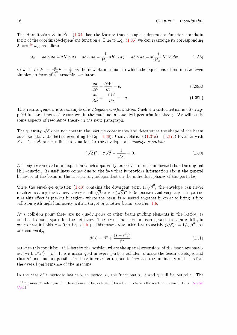
16 Chapter 1. Introduction
The Hamiltonian K in Eq. (1.34) has the feature that a single s-dependent function stands in front of the coordinate-dependent function e. Due to Eq. (1.35) we can rearrange its corresponding 2-form18 wK as follows
uK = db A da — dK A ds = db A da — -^dK A d^ = db A da — d(-=K) A d^, (1.38)H22 h22
so we have W := Hl~K = 2e as the new Hamiltonian in which the equations of motion are evensimpler, in form of a harmonic oscillator:
da dW ,d^ = b, db
(1.39a)
db _ dWd^ ----q— = —ada
(1.39b)
This rearrangement is an example of a Floquet-transformation. Such a transformation is often applied in a treatment of resonances in the machine in canonical perturbation theory. We will study some aspects of resonance theory in the next paragraph.
The quantity ^= does not contain the particle coordinates and determines the shape of the beam envelope along the lattice according to Eq. (1.36). Using relations (1.37a) - (1.37c) together with =Y = 1 + a2, one can find an equation for the envelope, an envelope equation:
(V=)" + gV= — ^ =0. (1.40)
Although we arrived at an equation which apparently looks even more complicated than the original Hill equation, its usefulness comes due to the fact that it provides information about the general behavior of the beam in the accelerator, independent on the individual phases of the particles:
3Since the envelope equation (1.40) contains the divergent term 1^f= , the envelope can never reach zero along the lattice; a very small yf= causes (\f=')" to be positive and very large. In particular this effect is present in regions where the beam is squeezed together in order to bring it into collision with high luminosity with a target or another beam, see Fig. 1.6.
At a collision point there are no quadrupoles or other beam guiding elements in the lattice, as one has to make space for the detectors. The beam line therefore corresponds to a pure drift, in which case it holds g = 0 in Eq. (1.40). This means a solution has to satisfy (^=)" = 1/^=3. As one can verify,
=(s)= =* (1.41)=
satisfies this condition. s* is hereby the position where the spatial extensions of the beam are smallest, with = (s*) = = *. It is a major goal in every particle collider to make the beam envelope, and thus =*, as small as possible in these interaction regions to increase the luminosity and therefore the overall performance of the machine.
In the case of a periodic lattice with period L, the functions a, = and y will be periodic. The
18For more details regarding these forms in the context of Hamilton mechanics the reader can consult Refs. [Arn89;Cas11].

1.3. Basic accelerator theory 17
Figure 1.6: Beam envelope in a drift section according to Eq. (1.41). In the interaction points 1 and 5 of the LHC the current P*-values are around 55 cm. The value has to be multiplied by the emittance to obtain the spatial area (squared) of the beam at the respective positions. This lead to minimal beam sizes between 16 and 70 pm [Br04]. The emittance in a linear setting is discussed in e.g. Ref. [Tit19].solution (1.36) will then yield a map from one period to the next. If ^(s + L) =: ^(s) + ^o, then
^
q(s + L) p(s + L)
q(s + L) p(s + L)
= P -1w(s + L) = P-1
cos(^o) + a sin(^o) -Y sin(^o)
cos(^o)- sin(^o)
sin(^o)cos(^o)
PP-1w(s),
P sin(^o) cos(^o) — a sin(^o)
(1.42)
The matrix in Eq. (1.42) is an example of a one-turn-map of the motion with respect to the given phase space pair (q,p). The name comes from its application in case of circular machines. The phase ^o is the total phase advance of the periodic lattice, i.e. it is given by Eq. (1.35) by
fs+L H22Po = ~Tds. (1.43)
J s P
The tune Q with respect to the pair (q,p) is defined as the integer part Q := po/(2n) of the total phase advance.
We arrived at the linear map (1.42) by starting with a quadratic Hamiltonian. In general the Hamiltonian describing the physics will be much more complicated, leading to non-linear canonical maps.19 Instead of attempting a solution for the full s-dependent Hamiltonian, an adequate approach in more general cases is to study the physics by examining the resulting maps given by products of elementary maps, as it was done in the FODO cell example above. This requires a certain machinery which we will discuss in the next paragraph.
19 A map is called canonical, if its derivative is symplectic at every point.
Resonances, dynamic aperture, emittance and chromaticity
In this work the behavior of the beam near a resonance is studied. This makes it necessary to say a few words about resonances in storage rings, how they emerge and why they are important for operation. As the name ’resonance’ implies, the particle is assumed to move under the influence of a periodic lattice in which small periodic perturbations from an otherwise ideal beam optics may influence its path. In particular for storage rings the long-term stability of the beam under such perturbations is of fundamental importance. Since the perturbations are considered to be small, the motion can be assumed to obey equations which correspond to a nearly integrable system.

18 Chapter 1. Introduction
The motion of particles in nearly integrable systems is a very rich and actively researched subject. In this short introduction it is literally an impossible task to give an adequate introduction, so we can only scratch on the surface, outline the concepts and provide further references to the interested reader.
Often the physics of the particle motion under the influence of small perturbations is studied by examining the resulting phase space distortion at a certain position s0 in the ring: Every revolution20 the particle position and momentum can be plotted in phase space, and over time this will produce a certain portrait, a Poincare surface of section or shortly Poincare section, of the phase space with respect to the initial conditions [Poi93]. In this context the the corresponding one-turn-map from one period to the next is called Poincare map, also in honor of H. Poincare who considered these maps for the first time.
20In the following we will assume that the underlying structure is a ring, but the same reasoning can be applied for a periodic section in a linear accelerator.
The Poincare map is itself a canonical transformation (see Ref. [Dra18] for a proof - or Rmk. 1.4.9). Poincare also made pioneering advances in studied certain invariants in phase space which today turned out to be central in accelerator physics. For example, more general than the Courant- Snyder invariant e discussed in the previous paragraph, one can consider a surface in phase space. Since the surface is an invariant under the effect of a canonical transformation, one can apply Stokes lemma to obtain an action as the integral along its border, which is therefore also an invariant:
? iq.=fz v.iq.=
If this is viewed in extended phase space, the action with respect to the spatial coordinate is therefore a constant of the motion, if the Hamiltonian does not depend explicitly on the independent variable, see Refs. [LL83; GPS02; Arn89] for details.
A difficulty in studying resonances via Poincare sections is that the trajectories may depend discontinuously on the initial parameters under the Poincare map. They can reside on a toroidal surface of constant action, they can appear periodic with respect to a certain integer number or even completely stochastic in nature and so it is not in general possible to obtain a global invariant.
A translation between the complicated s-dependent Hamiltonian describing the motion around the machine and some rule to conveniently describe the propagation of points under the one-turn map at a given position is therefore not obvious and essentially one has to integrate, concatenate or transform the ring-Hamiltonian of the lattice by some technique.
In this introduction we find it suitable to introduce the concepts along a basic example. For this example we consider the Hamiltonian (1.20) in case of a straight normally aligned sextupole field for a particle on-energy (n = 0). If the sextupole is approximated as thin element and located at a particular position in the lattice, this will produce an effective kick on the beam. The map from initial to final coordinates along a section of length As containing the sextupole is derived in

1.3. Basic accelerator theory 19
Chapter 2, Eq. (2.37a) - (2.37d). Its effect on the transverse coordinates are given here as:
x f — xi ,
Px,f — Px,i + ^sf2(y2 - x2),
yf — yi,
Py,f — Py,i + ^shxiyi
(1.44a)
(1.44b)
(1.44c)(1.44d)
If we assume that the remaining part of the ring is given by a linear one-turn map as in Eq. (1.42) for a given tune Q, and only consider the horizontal motion (i.e. yi — 0), then repetitive operations of this rather simple looking map already induces a rich structure for various tunes. This is shown in Fig. 1.7, where we assumed for simplicity a — 0 and ft — 1 — y near the position of the sextupole. Probably the first who studied a map of the form (1.44a) - (1.44b) was M. Henon in [H69].

20 Chapter 1. Introduction
Figure 1.7: Examples of Poincare sections induced by a single sextupole, given by Eqs. (1.44a), (1.44b) (with yt = 0), together with the one-turn map of Eq. (1.42) for various tunes Q. The integrated sextupole strength A.sh/2 was set to 1 in these examples. We have adjusted the start coordinates of each case up to values beyond which the particle motion is no longer bounded.
Q = 0.611

1.3. Basic accelerator theory 21
Similar as in the linear case of the previous paragraph, the goal is now to find invariants on which the particle trajectories remain constant. These invariants correspond to the various layers in Fig. 1.7. Apparently, these layers are no longer in the form of an ellipse (or circle in our example), but have a more complicated structure, can be disconnected or even break down outside of a diffuse border which is called the dynamic aperture. We also see that the accumulated points can vary in density along an individual invariant.
Let us denote the combination of the maps (1.44a), (1.44b) and (1.42) by M, which is the one-turn map we are interested in, and the phase advance ^0 = 2nQ of its rotation part by fi. In order to analyze the behavior of M, we will now make use of Lie operators and Hamiltonian vector fields. A detailed development of Lie operators would go far beyond the scope of this introduction. However we have included a small toolbox, some proofs and references in Appendix 1.4.2 for the interested reader.
In a first step note that the Lie operator regarding the rotation part of M, given by Eq. (1.42) (top), can be described by exp(-fi : e :) with e = (q2 + p2)/2. Secondly, note that powers of the functions ^k := (qk + ipk)/^2, fik := (qk — ipk)/a/2, where (qk,pk) for k = 1, ...,n, are canonical pairs, constitute an eigensystem of :£2£=1 ek : (see Appendix 1.4.3). Third, by introducing angleaction variables21 (fik,ek) via £k =: /eke~i^k and pk =: /keVk the reader may verify that for every differentiable F and G it holds:
21The new momenta are denoted by the same symbol as ek, since £kyk = ek.22According to Rmk. 1.4.9, Lie operators are canonical.
{F, G}m = —i{F, G}(m = {F, G}(qp). (1.45)
This means that the equations of motion are unchanged if we substitute angle-action coordinates into our Hamiltonians:
dH . dHq k = , pk = — o—,dpk dqk
dH . dH^ fi k A , e k = — w .dek dfik
(1.46a)
(1.46b)
The importance of this substitution will become clear by the following consideration: By Cor. 1.4.5 the Lie operator M* of M has the form M* = exp(: — H:) for some Hamiltonian H. Similar as in the previous paragraph, our goal is then to seek a transformation P so that M preferably goes over into a canonical map R depending only on the actions ek. To be more precise: We are looking for a transformation22 P* = exp(: x:) so that R* = (PMP-1)* = P~*M *P * holds, where R* = exp(: —H1 :) and H1 depends only on the actions ek. In this case the equations of motion with respect to H1 will be very simple:
dH1e k = — a— = 0 ^ ek — const. dfik
, -dH dHi „fik — — const. ^ fik(s) — s + fik,0.
U€k O€k
(1.47a)
(1.47b)
This means that n iterates of the associated one-turn map R with respect to H1 can be written as fik,f = nLdH1/dek + fik,i, where fik,i is the initial phase and fik,f the final phase after n passages through the periodic lattice of length L. Accordingly, iterates of M can be computed as soon as P

22 Chapter 1. Introduction
is known. With respect to the angle-action variables, the above reads:
: -Hi: ^n® = -i^n® Efa ~ bk)(1.48)
^ R*t(a)n(b) = exp(-i(a - b)dH1 )^n(b). (1.49)zJ z~
Eq. (1.49) can be extended to Rk* for continuous k. This is the link to what was described earlier in smoothing out the discontinuous motion in the Poincare section of interest, and can now be used, analogous to what was shown in Ref. [For98], to determine invariant expressions for the macroscopic beam quantities in a long-term tracking scenario, generalizing the Courant-Snyder invariant e introduced in the previous paragraph:
Let f be an analytic function on phase space, so this function transforms after one revolution to M* f. If P~* (f) = f o P— 1 =: £}a,b F,(f^(a)n(b), then, by using Eq. (1.49):
M* k(f) = E Pa?P* exp(: -kHi :)^n(b\ (1.50)
= E Pf exp(-ki(a - b)^Hh o p)(p*(^))(a)p(n))(b). (1.51)a,b
Integrating the iterates with respect to the phase advance, an action-dependent M -invariant function remains
(f (a :=2f T M*(f )dk = E Patfa o P)(a), (1.52)2n — ra nCv
similar to what was demonstrated in Ref. [For98]. (f )a is itself a fixed point of this operation, as by construction we have ((f)a)a = (f)a. In the (2D) linear case in which P is given by Eq. (1.31) and, for example, f = x2 it follows P—*(x2) = (x o P—1)2 = (dq2 = £(£2 + 2£q + n2), so P(f = (d and therefore (x2)a = (de, which yield a relation between the emittance e, the d-function and the rms value of the beam (squared), a familiar expression to the accelerator physicist.
After this motivation we will continue with our sextupole-example and write the sextupole map (1.44a), (1.44b) together with (1.42) into its equivalent form as a product of Lie operators
M* = exp(: -pe:) exp(W :x3:), (1.53)3
where w := -hAs/2. In the next step, we accumulate the two operators into a single one by making use of Thm. 1.4.12:
M * = exp(: -pe + ^31-^: x3 + O(w2):). (1.54)
The term O(w2) contains further denominators of the form 1 - e:ae: [DF76]. As we will see, such terms are responsible for the degeneracy of P (with respect to the given order) at certain tune values, and therefore indicate a degeneracy of the stable region of phase space. If we set H as the first-order expansion with respect to w in Eq. (1.54), this means a degeneracy at the integer and third-order resonance, as can readily be seen if moving to the eigenbasis of : e:
: —p€:1 - e: ae:
x3-t3 - t2n , tn2 , n3
1 - e3m 1 - eh1 1 - e—w 1 - e—3ia (1.55)3ip

1.3. Basic accelerator theory 23
The Hamiltonian H in Eq. (1.54) is now prepared for transformation to Birkhoff’s normal form 1.4.17 with respect to its first iteration at k = 3. In the notation of this theorem, this leads to a canonical transformation <p3 with H3 = H o ^3 = exp(: — x3 :)H, i.e. in the light of Eq. (1.99),
exp(: X3 :)exp(: —H3:) exp(: — X3:) = exp(: — H:) = M*, (1.56)
23A driving term strength corresponds to a factor like w in our sextupole example.
where x3 is the following homogeneous polynomial of degree 3:
_ ( 1 e3 , e2n \
X3 x/2R ^3 1 — e3^ + 1 — ef^j ' (1.57)Note that if applied to coordinate functions, the leftmost operator P3 := exp(: x3:) in Eq. (1.56) has to be applied first by Rmk. 1.4.8. This operator will thus transform the Poincare sections in Fig. 1.7 to their first-order normal-form iterate. The results are shown in Fig. 1.8. We remark that from Thm. 1.4.17 it follows that the action-dependent part of the new Hamiltonian is the same as the old one, since Q3 = 0, and so it will be a rotation.
The above procedure can be extended to more complicated situations and multiple dimensions with the help of the toolbox given in Appendices 1.4.2 and 1.4.3. The iterative construction of integrals of motion is the basic procedure to reach Birkhoff’s normal form. The argument with the denominator is similar in higher dimensions, where it leads to resonance conditions of the form (p., a — b) G 2nZ, which is discussed in connection with Prop. 1.4.14. In two dimensions this resonance condition induces various resonance lines, which are shown later in Fig. 4.3, Chapter 4, and which can be dangerous if operating the beam in its vicinity, due to degeneration and collapse of the dynamic aperture. The dynamic aperture will generally depend not only on the tunes but also on the order |a| + |b| and the strength of the driving terms.23
The one-turn map was assumed to be in a form suitable for Thm. 1.4.17. In the presence of coupling between different directions, as it is the case for example in the Hamiltonian (1.22), in which the energy is coupled to the horizontal motion, a linear diagonalization prior to the above operations therefore has to be performed (this diagonalization procedure is discussed in detail in e.g. Ref. [Tit19]). In such a coupled case, the phase advance in Eq. (1.47b) with respect to e.g. the horizontal direction will now depend on the actions related to the other directions. As the phase advance p,k is related to the k-tune, the factors in front of the various actions will have special names. The factors in front of the transverse actions are amplitude detuning factors, while those in front of the longitudinal action chromaticities. In the case of the longitudinal phase advance, the terms in front of the pure longitudinal action are called momentum compaction factors.
If the energy-offset is approximately constant, then these factors translate into factors describing the respective energy-offset-dependency of the tunes. For example, the physical interpretation in the case of the chromaticity is that particles having a larger energy-offset will experience a weaker focusing from quadrupoles, so they perform oscillations around the reference trajectory with a larger oscillation period, and therefore their overall tunes will be shifted to smaller values.

24 Chapter 1. Introduction
Figure 1.8: First normal form iterate of the Poincare sections shown in Fig. 1.7 obtained by application of P3* (here up and including third-order on the coordinates). The green points indicate the original shapes. Note that the top-left plot is taken near Q = 1/3 where the dynamic aperture of the Poincare section goes to zero, and therefore require higher-order iterations in the outer regions.

1.3. Basic accelerator theory 25
1.3.2 Many-particle dynamicsOverview
As the intensity of a beam is increased, the interaction of the particles with their neighbours becomes more and more important for the behavior of the whole beam, and one has to take collective beam dynamics into account. Collective effects come in many facets and often impose limits for the operation of an accelerator at high intensities. The evolution of macroscopic quantities like the mean (x) or the centralized rms beam size ^7{(x — (x))2) of a particle distribution, in particular due to additional space charge contributions, fall into the category of coherent motion. Incoherent motion is related to the motion of the individual particle.
All effects related to the interaction of particles with respect to an average electromagnetic mean field, which one can think of as an effective force field caused by the momentary particle distribution, are direct space charge effects. All other effects due to space charge, in particular a possible interaction between the beam and image charges in the vacuum chamber, are indirect space charge effects. As we shall see, direct space charge effects alter the coherent motion of the beam envelope. In this introduction we will focus our attention on two fundamental features regarding the dynamics of the beam in the presence of direct space charge, and which might be helpful in following some arguments in this work: The envelope equations and the tune shift due to direct space charge.
Indirect space charge effects due to an interaction of the beam with the vacuum chamber walls in form of image charges can have an effect on the incoherent motion, but can also lead to a change of the tune of the beam centroid itself [Wol14]. The magnitude and quality of this effect will depend on the chamber wall geometry and the material used.
In this work we will be dealing with experiments regarding the horizontal motion of the beam (see Chapter 4). Studies indicate that indirect effects are unlikely to have a significant effect in our specific experiments with the intensities used: The chamber walls in the PS and the SPS machines are relatively large in horizontal direction; in Ref. [Hus16], a study regarding the maximal vertical tune-shift in dependency on the intensity was performed, indicating that at our intensities the resulting shift is around two orders of magnitude below the tune-shift we estimate due to direct space charge (see Tab. 4.1). As the horizontal beam pipe walls are even further separated, we can well assume that in the PS case the effect is negligible.
Regarding the SPS case, in which the vertical plates are also much closer together, the horizontal and vertical tune shift due to impedance (i.e. interaction with the wall chamber) in dependency on the intensity was studied in Ref. [Zan13]. It was found that while in vertical direction a considerable effect was visible, there is literally no effect present in horizontal direction. Since we will be leaving the vertical tune unchanged, and the machine is well decoupled in our experiment, we will therefore assume again that only direct space charge will be relevant in our simulations.
Before we begin with the examples, let us make some general remarks regarding the analytic treatment of the dynamics involving many particles. In the presence of space charge we can not hope that our original Hamiltonian (1.6), which describes the single-particles dynamics, will remain conserved. This makes an analytic treatment of the beam dynamics with space charge much more involved. In fact, even the most simplest ’many-particle’ case, the electromagnetic two-body problem, is yet not fully resolved and remains an area of active research (see e.g. Ref. [DL05] and the references therein).
The starting point in treatments regarding space charge is often Newton’s equation of motion(1.1) in the rest frame of the beam, taking into account the electromagnetic fields generated by the

26 Chapter 1. Introduction
particles. Such an approach usually involves averaging over the number of particles. At some point one may then consider an average space charge field. In a self-consistent analytic treatment this field will change according to the momentary beam shape and according to the Maxwell-equations (1.3a) - (1.3d). If intrabeam scattering can be neglected, a suitable framework to describe this entire process are the Vlasov-Maxwell equations.
A feature of these equations is that one can recast them into a Hamiltonian system, now including the electric and magnetic field as a canonical pair of variables in a suitable (infinite-dimensional) phase space [MW82]. The importance of such a reformulation is that one can hope that, if properly discretized by taking into account the symplectic structure, to build a symplectic self-consistent multi-particle tracking code, i.e. a code which can self-consistently solve the equations of motion for the particle distribution and the fields at the same time. As we shall discuss in Chapter 3, symplecticity is very important for long-term tracking studies, because such studies are prone to unphysical round-off errors coming from e.g. truncating maps in the model, and which can accumulate over time. In this regard, progress has already been made [Qin+15; Qia16]. See also Ref. [Web15] and the references therein.
Envelope equations with space charge
In this paragraph we will discuss the equations governing the evolution of the beam envelope under the additional effect of space charge. Such a scenario was studied in Refs. [Har66; Sac68; Sac71] (and the references therein). More recent texts about this subject are e.g. Refs. [Baa98; VKR98; Hof+03; LB04; Ng06; YBFH17].
Even though we have initially stated that we can not expect that an original single-particle Hamiltonian will be conserved in the scenario of many interacting particles, one can approximate the motion using an average space charge force field, which can be derived from an effective Hamiltonian. We will therefore begin with a general observation regarding the moments of a distribution of non-interacting24 particles in phase space, whose motions are described by a Hamiltonian which may - in addition - depend on a parameter t. Let f be any (well-behaving) probability distribution function on 2n + 1 phase space, which is stable in the course of the tracking (i.e. a constant of the motion) and h differentiable. Its h-moment h is given by
h(T) := {h)(T) := J h(q,p,T)f (q,p,T)dqdp. (1.58)
Theorem 1.3.1. If the motion of the particles can be described by a Hamiltonian H, Lionville’s theorem yield .
h = dfh + {h.H}. (1.59)
For a proof the reader can consult Appendix 1.4.4. The next equations hold componentwise, but can also be read as vector equations due to the linearity of the averaging process and the derivatives. This is the reason why we will omit the indices. A consequence of Thm. 1.3.1 are moment equations, which are in the first orders:
H = Lt H, (1.60a)
q = dpH and p = — dqH, (1.60b)
q2 = 2qdpH, qp = pdpH — qdqH, p2 = —2pdqH. (1.60c)
24The interaction between particles will be modeled here as a contribution in the effective Hamiltonian.

1.3. Basic accelerator theory 27
These moment equations provide envelope equations, completely similar to Eq. (1.40), as follows: Denote by hc the ’centralized’ moment h — h. Using this notation, introduce
X := T^y = ̂<q2> — (q)2.
I := \ MH)2) — (qc(dpH)c)2•
(1.61a)
(1.61b)
Then we deduce (see Appendix 1.4.4):
Theorem 1.3.2. With the definitions (1.61a) and (1.61b) it holds
qq = {qcdph}, (1.62a)
.. x2 , ,,q q = q + {qcfidpH') ). (1.62b)
XX = q 2{(dpH)c(dpH)') — q q (qc(dpH)'), (1.62c)
with the Lionville operator on functions u, given by u' := dTu + {u, H}. Alternatively, Eq. (1.62c) can be written in the following form25
j = ^(qc. (SpW^ qdH )-1 / _ \\dpH \\
(dPHfi J / • (1.63)
Equation (1.62b) has the form of an envelope equation for the centralized rms size q. Our next goal is to connect this result to our scenario of particle motion with space charge. For this purpose, we consider a Hamiltonian H2 of the form given in Eq. (1.20), including an additional external quadrupole potential and a space charge contribution from an elliptic coasting beam:
H2(x,y,z,px,Py,n; s) = | (pl + p^ + |g(x2 — y2} + ' / v'(x, y, s; (s — filz)/vo), Po Pocyo
(1.64)
where the arguments in the space charge potential p are written here in Frenet-Serret notation. Inserting this Hamiltonian into Eq. (1.62b) yields the following envelope equation for the transverse beam sizes X and y:
d2x el K ads2 X3 gX + 2 X(a + b) ’
d2q I Kb+ + gy +ds2 y3 9y 2 y(a + b) ’
(1.65a)
(1.65b)
with xl = (x2')((pl)2') — (xc(Px)c)2, which corresponds to Lapostolle’s definition of emittance,26 andthe space charge perveance
e2AK := 2neofi2Y3mc2 ' (h66)
The variables a and b describe the transverse shape of the beam ellipse. They depend in general on the time in the beam rest frame, hence on s for fixed z. The quantity A denotes the line density of the beam with respect to the laboratory frame. The details of the calculations leading to the above results are provided in Appendix 1.4.5.
Due to the Yo 3-dependency in K, direct space charge effects are more suppressed the higher the
25The matrix has to be understood as a 2n x 2n matrix in the case of vector notation, where its four blocks containn x n diagonal matrices.
26A detailed discussion of the emittance in a linear setting can be found in e.g. Ref. [Tit19].

28 Chapter 1. Introduction
energy of the beam is set to. The physical picture is that, from the laboratory point of view, the repulsive movement of the particles relative to each other is time-dilated, which in effect corresponds to a smaller observed force.27
The Hamiltonian (1.64) can be used, optionally together with additional multipole ’driving’ terms as external force fields, as the starting point for several considerations regarding space charge and resonances. The envelope equations are general enough to hold for the important special cases of transverse Gaussian-like distributions and uniform distributions (see also Chapter 3). Further details can be found in Refs. [Sac68; Baa94; Ng06]. Alternatively, one can also start with a more general Hamiltonian involving an energy-offset, and derive similar envelope equations, now including dispersion and the energy-spread of the beam, as has been started in [VKR98].
In the next paragraph we will consider the most basic application of the envelope equations (1.65a), (1.65b) in periodic lattices, namely the description of coherent motion and the tune shift of the envelope due to direct space charge, which is a source of coherent tune shift. We will later also discuss the notion of incoherent tune-shift due to direct space charge.
Coherent motion and tune shift
Let us discuss the effect of small perturbations of the envelope equations (1.65a) and (1.65b) from an otherwise matched solution. The next procedure is well known in the literature and will serve here as a demonstration of the principles. We will assume that the beam is shaped elliptical and so that x rc a and y rc b. To simplify the notation we will now drop the tilde on the symbols and focus our discussion exemplary on the x-direction.
In the following considerations we will assume that a change in the emittance is very small. This can be understood as analogy to the case without space charge in a linear scenario, in which the emittances are constant. Furthermore, we will make one additional approximation: Namely that the Courant-Snyder parameters (dx and (dy of the underlying bare lattice can be considered as producing a constant average focusing over many periods. This assumption is known in the literature under the name smooth ring approximation.
From Eq. (1.37c) it follows ax = 0, and by the symplecticity condition therefore Yx = 1/fix, thus gx = 1/0X = const, by Eq. (1.37b). Furthermore, from Eq. (1.43) it follows in this case for the tunes 2nQx = L/fix, therefore the tune Qx of the underlying lattice is related to the focusing gx by Qx = R^gx with 2nR := L, an effective radius of the machine. Let us denote by x0 and y0
matched solutions of the envelope. This means x0 satisfies
ex = Kx0 gx 2x0 (x0 + yo) ’ (1.67)
and a similar equation must hold for y0. Consider small perturbations x = x0 + 8x and y = y0 + 8y and an s-independent line density A. By linear extension of Eqs. (1.65a) and (1.65b) this leads to
6x” + anhx + a12hy = 0,
Sy" + a2ihx + a22§y = 0,
(1.68a)(1.68b)
27An equivalent picture is an additional magnetic component in the force field, appearing in the laboratory frameof reference, which is counteracting the repulsive electric force.

1.3. Basic accelerator theory 29
where
3^ +__K___ + „x = ia, - k 2x0+3y°x4 2(xo + yo)2 2xo(xo + yo)2,
K2(xo + yo)2,
(1.69a)
(1.69b)
a2i :— ai2,
a22 4dy K 2y0(xo + yo? '
(1.69c)
(1.69d)
where we used Eq. (1.67) in Eq. (1.69a).
In order to obtain the formulae for the shifted tune, we diagonalize (1.68a) and (1.68b). Write this system as 6w" + A6w — 0, 6w :— (6x,6y), with stability matrix A — (aj). If S is the matrix of eigenvectors of A and D its corresponding diagonal matrix of eigenvalues, A — SDS-1, then (S~16w')" + DS-15w — 0, by which we see that S-15w constitute the sought eigenmodes w± of the beam. Its eigenvalues R~2Q± determine the oscillation frequencies. A small computation yields (a :— xo, b :— yo)
R2 t I—\Q± :— -y (an + a22 ± y 4a22 + (an - am)2] ,
_2 3 KR2 KR2
— 2(Qx + Qy) - ^ ' 2 -± (4(n2 _ n2.2 . 3KR2(a - b)(Ql - Qy) , K2R4(9a4 - 14a2b2 + 9b4) \ 1/2
± 4(Qx Qy) +3 ab(a + b) + 16a2b2(a + b)4
In the limit of no space charge interaction, these tunes go over in
Q± — 2(QX + Q2y) ± 2|QX - Q2y|,
(1.70)
(1.71)
so in this case 2Qx,y2Qy,x
if Qx > Qy,else,
(1.72)
which tells us that the envelope oscillates with twice the single-particle bare28 tunes. With space charge (K — 0), we can write
28 Bare means in this context ’without space charge’.
q± — 2(QX+Qy) - (KRh (i + £+ D ± ^(KRAyr+D2, (1.73)
where we introduced for brevity an inverse coupling parameter D as [Tit15]
D:— - (a+b)2+2 (a - a). (1.74)
In the context of Eq. (1.72), the coherent tune shift of the beam envelope oscillation, now in the presence of space charge, can be understood as the difference 2QX,y - Q± in the case Qx > Qy, and 2Qy,X - Q± otherwise.

30 Chapter 1. Introduction
The eigenmodes are given up to multiplication by a constant; we set
Sw- := 2aI2Sx + ̂ a22 — an — y 4a22 + (an — a22)2J Sy, (1.75a)
Sw+ := 2aI2Sx + ̂ a22 — an + y4a22 + (an —a22)2^ Sy. (1.75b)
Note that (Sw-,Sw+) = 0, i.e. the eigenmodes are orthogonal to each other. With respect to the (Sx, Sy)-coordinate system S-1 therefore corresponds to a rotation matrix with angle
tan(a) = —^ (a® — aii + y/4a22 + (aii — a22)2) = D + -\/1 + D2, (1.76)2a12
see Fig. 1.9 (left). If K is sufficiently large, then we are fully space charge dominated with D = 0. In this case tan(a) = 1, so Sw+ is oriented n/4 relative to Sx and Sy, while Sw- points in — n/4 direction. If the beam starts to oscillate, the Sx and Sy components of the Sw+ eigenmode therefore both move simultaneously in the same positive (or negative) direction, while the Sx and Sy components of the Sw- eigenmode are moving in opposite directions. In the first case, this corresponds to a breathing of the beam, while in the second case the beam is shrinking in one direction, while expanding in the other direction, as illustrated in Fig. 1.9. For a more detailed discussion of these modes the reader can consult Refs. [Sac68; LB04; Oef16]. The quantities Q± can be measured, for
Figure 1.9: Sketch of coherent motion in a space charge dominated scenario. For simplicity the beam is assumed to have an originally round cross section (blue dashed lines) as its matched solution. A small mismatch will cause the beam envelope to oscillate around this stable configuration in form of a sum of two modes, a breathing mode (center) and a betatron mode (right). In both cases the envelope is oscillating between the orange and the green state in the extreme case of a = 45°. The two modes by which the beam is oscillating correspond to the two eigenmodes Sw± described in the text.
example, by a quadrupolar pick-up system [Sin+14; Oef18].
We will close this paragraph with an interesting remark, namely that Eq. (1.73) constitute two equations for two unknowns: The beam aspect ratio a/b and a term KR2/(a + b)2 containing the space charge perveance. This makes it in principle possible to express these in terms of the measurable quantities Q±, Qx,y. We have
Q2 Q2 — 4(q2 q2 ) KR (2 3b — 4(Q2 q2 ) \h (177)Q+ + Q- = 4(Qx + Qy) (a + b)2 2 + 2a + 2b = 4(Qx + Qy) + Ah’ (1.‘‘)

1.3. Basic accelerator theory 31
with A := -KR2/(4(a + ft)2) and h := 2(4 + 3b/a + 3a/b). So A can entirely be expressed in terms of the tunes and the aspect ratio. On the other hand:
Q2+ - Q- = -4A^1 + D2, (1.78)
with D = A 1(Ql — Qy) + 3/2(b/a — a/b) (Eq. (1.74)). For abbreviation set s := 3/2(b/a — a/b).Then
222 2 2 22 22 222(Q+ - Q-) = 16A (1 + D ) = 16 (J1 + s )A + 2sA(Qx - Qy) + (Qx - Qy) j
_ A — 1 (eto2 O2t I . /(I -I- a^KO2 z)2 \2 /I C 7772 C)2\2\ fl 7(p^ A = 1 + s2 s(Qy - Qx) ' \ ' ' s )(Q+ - Q-) I 16 - (Qx - Qy) ) , I1-'9)
where we determined the sign in front of the square root by the condition A > 0 in case of round beams (s = 0). If we now use Eq. (1.77) on the left-hand side of Eq. (1.79), we obtain an implicit equation for the beam aspect ratio a/b in dependency on Q± and Qx,y. Optionally we can solve for the two unknown quantities numerically.
Incoherent tune shift
If one models the space charge force field as being generated by a stable distribution acting on an individual ’test’ particle, then this corresponds to the treatment of space charge as an additional external force field in the single-particle dynamics. However, care has to be taken, as such a model can lead to inconsistent predictions if extrapolating its results to the whole of the beam, see e.g. [Baa98] for a discussion. The reason is that, roughly speaking, Newton’s third law is violated. This topic is further discussed in Chapter 6.
Having these cautious remark in mind, we can write down an equation for the motion of a single particle in a lattice with a stationary space charge field, symmetrically to zero. We will discuss the simplest case: In Chapter 3, in connection with the frozen space charge models which rely on such a model, we require the kick of an elliptic, transversely uniformly distributed space charge distribution. Considered here as a contribution to the linear term in Hill’s equation, it will lead to
d2x . . e?X x . . Kxds2 = + nimc2lfY ax(ax. + ay) = ~gMx + 2a(a + b)'
(1.80)
where ax , ay corresponds to the two axis of the ellipse and define the aspect ratio of the charge distribution. Note that in the second line we have used their relation to the rms values 2a = ax and 2b = ay , in the notation of the previous paragraph. For the next steps we will proceed, once again, in the smooth ring approximation for the bare lattice. So gx will be a constant and, as it was shown in the previous paragraph, is related to the bare tune by Qx = R^gX In this case the solution of Eq. (1.80) yield the eigenvalue Q2x inch R-2 where
Q2 ^x, inch. = Q2x - KR2
2a(a + b)(1.81)
Expanding the square root to first order leads to an approximation for the incoherent tune-shift:
AQx,inch. Qx,inch. - Qx KR2
4Qxa(a + b)(1.82)
It is an interesting observation that from the previous paragraph it is in principle possible to determine the aspect ratio a/b and A by measuring Q± and Qx,y alone, and inserting the results ineither Eq. (1.82) or the exact equation (1.81).

32 Chapter 1. Introduction
The reason why we restricted ourselves to the simple model of a transversely elliptic homogeneous charge distribution is that in a more realistic distribution the situation near the center is linear in very good approximation, as depicted in Fig. 1.10 in the bi-Gaussian case, although attention has to be made: Due to the higher charge density in the central regions, a Gaussian distribution having the same rms value as a homogeneous distribution will have twice its slope in the center.
In this more realistic scenario particles near the center are expected to have a tune-shift as discussed above, while particles further outward will admit a tune in between the above maximal incoherently shifted tune and the bare tune (for bunched beams, their longitudinal position is also crucial). In Chapter 6 we will see examples of tune spreads in a simulation scenario.
Figure 1.10: Ex-component of the electric field (brown) in horizontal direction for y = 0 of a bi-Gaussian field with N = 1010 charges and rms beam sizes of ax = 5 • 10-3 [m] and <jy =3 • 10-3[m], according to Eq. (3.6). The corresponding horizontal probability density is displayed in blue. The grey vertical dashed lines indicate the rms values ±ax. We see that within this region the field is in very good approximation linear.
1.4 Appendix
1.4.1 Derivation of the Hamiltonian (1.6)
In this section we will derive the Hamiltonian of Eq. (1.6) in a rather similar fashion as in Ref. [Wol14]. Note that there is also an alternative route leading to this Hamiltonian29, see Eq. (2.15d) in Chapter 2. We will start with a Hamiltonian H(x,y,t,px,py, —K; s) in the following form:
29The only differences is a do factor in the third canonical pair.
H = —k^~2 (K — e^>)2 — (px — eAx)2 — (py — eAy)2 — m2c2 — neAt, (1.83)
where k = 1 + Kxx + Kyy. A derivation of this Hamiltonian is given in Chapter 2, Appendix 2.6.1.
As the reader can convince himself, the equations of motion will be unchanged if the Hamiltonian is divided by a constant, and all canonical momenta are divided by this constant. Dividing H by a nominal momentum po thus yield a new Hamiltonian H := H/p0 with respect to new

1.4. Appendix 33
canonical momenta px := px/po and potentials Aj := eAj/po, p := ep/(poc):
H = ~K\ (-K- P] - (px - Ax) - (py - Ay)2 - "P - KAt. (1.84)
Now consider an s-dependent generating function F of type 2:
F(x, y, t, Px, Py, n; s) := xPx + yPy + (s - cpot) (n + i) ji, (1.85)
where po is the relativistic P-function related to p0. It follows for the new coordinates, which we shall denote by Qx, Qy, z, and the new momenta Px, Py, p:
px =dF dx
= Px , py =dF dy
=P= y, (1.86a)
Qx =dF dPx
= x, Qy =dF
dPy= y, (1.86b)
K ---—po
dF~dt = -c(n + 1) Jr, z=
dF dn
= (s - cpot) -pi. (1.86c)
From Eq. (1.86c) it follows
and for the new Hamiltonian30
K , K - Eo n = — Po -1 = —g— cpo Eo
G = H + dsF:
G(x,y,z, px, py ,n; s) =
n tn +1 \2 ~ ~ _ m2c2
,z - K\ p) - (px - A x) - (py - Ay)2 2 kAi, (1.87)Po \ \ Po / po
where functions depending on t are now depending on s and z via t = (s - P2z)/(Poc).
1.4.2 Lie calculusIn this subsection of the appendix we will collect important properties related to Lie operators. We will not discuss convergence and domain issues and consider only functions which behave sufficiently nice. For further details the reader can consult Refs. [Dra18] and [For98].
Definition 1.4.1 (Hamiltonian vector field). For g G C^(R2n) define
:g ::= Xg := {g, •} : C^(R2n) ^ C^(R2n),
in coordinates: n: g: = E
j=idg d dg d
dqy dpy dpy dqy
where the derivatives are taken at a given point zo G R2n.
Remark 1.4.2. For every f G C^(R2n) with the symplectic structure J of (1.5) we have:
(f/(z))trJd\z = ( dqkf(z),dpkf(z) ) ( dpk|Z ) = :f: \z-dqk\z J
30We will drop all constant terms in G.

34 Chapter 1. Introduction
Remark 1.4.3. If Zj G C"rx(R2n) denotes a coordinate function, then we have:
2n {Zj,g} = 52 Jjkdkd- (1.88)
k=1
Lemma 1.4.4. Let g: M ^ R analytic and ps: R2n ^ R2n the flow of a function H G C^(R2n),i.e. dsps(q,p) = JVH(ps(q,p)). Then
dd~(g ◦ Ps) = {g,H}o ps. (1.89)
Proof.
d(g o Ps)(q,p) = g'(Ps(q,p)) o dPs(q,p) ds ds
= g' (ps(q,p))JVH (ps(q,p))
= {g,H}o ps(q,p)-
□
Corollary 1.4.5 (Lie operator). With the notation of Lem. 1.4.4 it holds for n > 0:
JL 1 , , rs (s - a)ng o Ps = 52 k. sk : -H :k g +/0 ---- n. :-H: 9 ◦ P"da. (1.90)
If we can let n go to infinity, then Eq. (1.90) is expressed as
g o ps = exp(: -sH :)g. (1.91)
In this case we call the map exp(:-sH:) the Lie operator associated to the canonical map ps: R2n ^ R2n and due to its pull-back property we write p*.
Proof. Application of Taylor’s expansion with Lagrange reminder on Lem. 1.4.4. □
Equation (1.91) is the reason why one can use the Hamiltonian in the exponential if calculating the effect of sector maps or one-turn maps in time-independent cases.
Proposition 1.4.6. 1. If a G R denotes a constant function, then
: f: a = 0, (1.92a)^ exp(: f :)(a) = a, (1.92b)
: af: = a : f: . (1.92c)
2. If g G C™(R2n), then : f + g: = : f: + :g:.
3. If g,h G C™(R2n), then
: f :(gh) = (: f: g)h + g(: f: h), (1.93a)^ exp(: f :)(gh) = (exp(: f :)g)(exp(: f :)h), (1.93b)
where the left-hand side is evaluated at g(Z)h(Z), while the Lie brackets on the right-hand sideare evaluated at g(Z) and h(Z) respectively.

1.4. Appendix 35
4. Similarly as above we have from the Jacobi-Identity:
: f: {g,h} = {: f: g,h} + {g,: f: h}, (1.94a)^ exp(: f :){g,h} = {exp(: f :)cg, exp(: f ^h}, (1.94b)
and (by direct calculation of the derivatives)
[: f:,: g:] = : {f,g} : • (1.94c)
5. In particular, with Eq. it follows(1.94c)
{f,g} = 0 ^ exp(: f :)exp(: g:) = exp(: g :)exp(: f:) = exp(: f: + : g:), (1.95a)^ exp(: f :)-i = exp(- : f :)• (1.95b)
n (: f :k g)(: f :n~k h), k
6. Let m G N and G: Rm ^ R analytical, inducing a corresponding function (C°(R'2n))m ^ C0 (R2n) by insertion, which we will denote with the same symbol.Furthermore, denote by
X := {D: Co(R2n) ^ Co(R2n); f G Co(R2n): D(fg) = D(f )g + fD(g)} (1.96)
the set of vector fields on R2n and let G: Xm ^ X induced by G. Then
exp(: f :)(G(hi, •••,hm)) = G(exp(: f :)(hi),..., exp(: f :)(hm)), (1.97a)exp(: f :)G(: gi :,•••,: gm:) exp(- : f:) = G(:exp(: f :)gi :,•••, :exp(: f :)gm :)• (1.97b)
Proof. (sketch) Eq. (1.93a) comes from the product rule of derivatives and Eq. (1.94a) from theJacobi-Identity. Eq. (1.93b) is derived from Eq. (1.93a) as in the usual real-valued case:
n : f :n (gh) = £
k=000 n
^ exp(:f:)(gh) = ^13 k.fn - k)\(:f:k g)(:f:n~k h) = (exp(:f:)g)(exp(:f:)h)Eq. (1.94b) is proven completely analogous to Eq. (1.93b).Eq. (1.93b) shows that exp(: f :) preserves the product between functions. Therefore Eq. (1.97a) follows together with the linearity of the Lie-Operator for every function G as given above. Eq. (1.97b) follows similarly by reformulation of Eq. (1.94b) in the form
exp(: f:) : g: = :exp(: f :)g: exp(: f:),
therefore we obtain a version of Hadamards lemma:
exp(: f:) : g: exp(- : f:) =:exp(: f :)g: • (1.98)
Now fix f, consider the equation for g1, ...,gm and apply G. □
Corollary 1.4.7. From Eq. (1.97b) we obtain in particular
exp(: f :)exp(:g :)exp(- : f:) = exp(:exp(: f :)g :)• (1.99)
Remark 1.4.8. Let g G C^(R2n) be analytical and extend g to a function G: Co(R2n)2n ^ Co(R2n)by insertion:
G(hi, •••,h2n)(z) := g(hi(z), •••, h2n(z)), z G R2n

36 Chapter 1. Introduction
Applying property 6 in Prop. 1.4.6 on G we obtain for f E C^(R2n):
exp(: f :)(G(hi, ...,h2n)')(z) = G(exp(: f :)(hi),..., exp(: f :)(h2n)')(z)= g(exp(: f :)(hi)(z),..., exp(: f :)(h2n)(z)).
Denote by zj : R2n ^ R, j = 1,..., 2n, the coordinate functions. Then
G(zi, ...,z2n)(z) = g(zi(z), ..., z2n(z)), y - - '=z
^ G(zi, ..., z2n) — 9.
It follows(exp(: f :)g)(z) = g(exp(: f :)(zi)(z),..., exp(: f :)(z2n)(z)). (1.100)
This equation can now be used to evaluate successive expressions of Lie operators (see also Ref. [BI90]). Define
fj :=exp(: f :)zj (1.101)
and f: R2n ^ R2n by f(z) := (fi(z),..., f 2n(z)). Then Eq. (1.100) can be rewritten as
exp(: f :)g = f (g), (1.102)
and consequentlyexp(: fi:) ••• exp(: fa :)g = (fa ◦•••◦ f f)* g.
What has been done is expressing the chain of Lie operators on the left-hand side, which have to be evaluated at the corresponding (and possibly complicated) intermediate positions, by a composition of maps which can be computed by their action on the basic coordinate functions via Eq. (1.101).
Remark 1.4.9. The Lie operator associated to a Hamiltonian flow ps is a canonical map; by Eqs. (1.94b) and (1.91) it holds
{fa*gi,V* sg2} = {exp(: -sH :)gi, exp(: -sH f)g2} = exp(: -sH :){gi,g2} = fa*{gi,g2}. (1.103)
Without proof we quote three very useful theorems
Theorem 1.4.10 (Dragt & Finn [DF76]). Let M be an analytic canonical map which can be joined by a path to the identity. Then there exist homogeneous polynomials fk of degree k so that:
M * = exp(: fi:) exp(: fa :) exp(: fa:) ••• . (1.104)
Proof. A proof of this theorem can be found in e.g. [Dra18]. □
Theorem 1.4.10 can be used, for example, to cast the properties (1.97a) and (1.97b) in a more general form. Note that fi can be set to zero in case the map M does not shift the origin.
Theorem 1.4.11 (Factored product expansion). Let hk be homogeneous polynomials of degree k E N>2. Then there exist homogeneous polynomials gk of degree k such that
exp(: h2 + ha + h3 +----- :) = exp(: g2 :)exp(: g3:) exp(: g3 :) ••• , (1.105)

1.4. Appendix 37
where gk can be computed recursively in terms of the hk. In lowest order they are
92 = h2,1 - e-: h2:,
93 =-----r------- h3,: h2:
94 = / e-1x2: [h4 - 1 { —hsh}] dr.0 2 :h2:
Proof. A proof of this theorem can be found in Ref. [Ste86]. An alternative version in [Dou82]. □
Theorem 1.4.12 (Factored product combination). Let gk be homogeneous polynomials of degree k G N>2. Then there exist homogeneous polynomials hk such that
exp(:92 :) exp(:93:) exp(:94:) • • • = exp(: h2 + h3 + h4 +----- :), (1.106)
where in lowest orders
h2 =h3 =
h4 =with : 92 :
f3 := 1 - e-:92 :93.
Proof. See Refs. [Ste86; Dou82; DF76]. □
Note that general methods to expand and combine Lie operators are given by the formulae of Zassenhaus and Baker-Campbell-Hausdorff-Dynkin, respectively.
92, : 92 :
1 - e-: 92 : 93
:92: (94 - 1 f e-T:92:{ eT:92: - 1 f3, f3}dT1 - e-:92: 4 2 0 1 : Oo: J3,J }
1.4.3 Proof of Birkhoff’s normal form
As in the previous subsection we assume that all functions behave sufficiently nice. We will prove Birkhoff’s Theorem of normal form 1.4.17 by summarizing the steps in Ref. [Gre06]. On the way we obtain important properties which we used in connection with Lie calculus for the one-turn map. The first proposition is left to the reader:
Proposition 1.4.13. Introduce fk := (qk + ipk) and pk := (qk - ipk) for k G {1,...,n}. Withrespect to these coordinates the Poisson-bracket has the following form
{f,9}v (d£dy_ M dfk dpk
d£dy\ dnk dfk .
(1.107)
Now set ek := fkpk = |(qk + pk) for k G {1,...,n}. Note the similarity to the Courant-Snyder invariant discussed in Subs. 1.3.1 with respect to the coordinates w. Of course, we can not expect that in general the ek are invariants. However they satisfy an important property:
Proposition 1.4.14. For a,b G Nq set f(a) := f^1 • • • A' and p(b') := rfr1 • • • pbrn . Then it holds
n ............. .............
{£ Pk Ck, f (a)n(b)} = iQ(a, b)f (a)n(b), (1.108)k=1
with Q(a, b) := (p, (a - bf) = a1p1 + • • • + anpn - b1p1 - • • • - bnpn.

38 Chapter 1. Introduction
Proof.
E p {«,t(aXb)} = -i E Vk E !(f^k=1 k=1 l=1 fl nl
d(£knk) d(f(a)n(b))dpi dfi
n z . . . . -= -i E »k (n^nb • • • bknk-1 ••• nn - • • • -■-&k-1 fan fn
n .............
= —i E Vk(bk - ak)f(a)n(b)- k=1
□
We have to show one additional Lemma:
Lemma 1.4.15. Let Z be a homogeneous real-valued polynomial of degree k and Ho :=Y1 n=1 Pk£k• Then there exist homogeneous real-valued polynomials x and Q of degree k so that the homologicalequation
{Ho,x} + Z = Q (1.109)holds, where
{Ho,Q} = 0. (1.110)
Proof. Let Z = y^a,b&™,\a\+\b\=k Za,bf(a)n(b) • With Q introduced in Prop. 1.4.14 define with respect to the indices of Z:
xa,b :=Qa,b :=
0Q(a,b) 1 Za,b^ if Q(a,b) = 0,
xa,b :=Qa,b :=
0, 1 ,else.
Za,b
It follows with x := Ea,b xa,bf(a)n(b), Q := Ea,b Qa,bf(a)n(b) and Eq. (1.108):
.......... n ..........Q - {Ho,x} = J2Qa,bf(a)n(b) -J2xa,b{E Vkk,f(a)n(b)}
a,b a,b k=1
= E Zabf(a)n(b) - E iQ(a,b)-1Za>biQ(a,b)f(1)n(b)a,b,Q(a,b)=O
= Z.a,b,Q(a,b)=O
The second property {Ho, Q} = 0 follows by definition of Q, as it is only non-zero if Q(a, b) = 0. In this case {Ho,f(a)n(b)} <x Q(a,b) = 0 by Eq. (1.108). By construction, Q and x are homogeneous polynomials of degree k. Z is real if and only if Za,b = Zb,a. This propagates to Q and x since Q(a, b) = -Q(b, a). □
Definition 1.4.16. A vector p G Zn is called non-resonant up to order r, if 'dz G Zn\{0} with |z| < r it holds: {p, z} = 0. p is non-resonant, if it is non-resonant up to order r for all r G N.
We will now proceed by proving Birkhoff’s theorem of normal form 1.4.17, as it was done in Ref. [Gre06]. The statement is
Theorem 1.4.17 (Birkhoff normal form). Let H = Ho + P be a decomposition of a HamiltonianH, where Ho = En=1 Pk£k and P is an analytic function having a zero of order 3 at the origin.Then for every integer r > 3 there exist a canonical transformation f: U ^ V, where U and V are

1.4. Appendix 39
neighbourhoods of the origin, so that
f *H = Ho + Z + R, (1.111)
and the following properties hold
1. Z G Pr(R2n), a polynomial of order r, with {Z, H0} = 0,
2. R G C™(U)2O(r + 1),
3. f - 1 G O(2).
Furthermore, if p is non-resonant up to order r, then Z depends only on the actions ek.
Proof. The proof is done by inductively constructing a canonical transformation Tk for k = 2, ...,r and real functions Zk, Pk+i, Rk+2 so that
Hk := H o Tk = H0 + Zk + Pk+1 + Rk+2 (1-112)holds with the following properties:
1. Zk is a polynomial of degree < k, having a zero of degree 3 at the origin with {Zk, H0} = 0.
2. Pk+1 is a homogeneous polynomial of degree k + 1.
3. Rk+2 is an analytic Hamiltonian having a zero of order k + 2 at the origin.
In this case the claim of Thm. 1.4.17 can be obtained with Z := Zr, R := Pr+1 + Rr+2. For the start of the induction at k = 2 we set t2 := id, Z2 := 0, P3 the Taylor expansion of P and R4 := P — P3. Now the claim is assumed to hold for k and we will prove the case k + 1. We will construct the canonical transformation Tk+1 as Tk+1 := Tk o ^k+1, where ^k is a Lie transform of the form given in Cor. 1.4.5 with respect to a suitable Hamiltonian Xk in form of a homogeneous polynomial of order k. I.e. recall Eq. (1.91) for g G C^(R2n):
g o ^k = exp(: — Xk :)g. (1.113)
Composing Eq. (1.112) with pk+1 and inserting zeros yields:
Hk+1 = H o Tk o Vk+1 = H0 + Zk + {H0, Xk+1} + Pk+1 (1.114a)+ Rk+2 o Vk+1 + H0 o Vk+1 — Ho — {Ho,Xk+1} (1.114b)+ Zk o Pk+1 — Zk + Pk+1 o Pk+1 — Pk+1- (1.114c)
By Eq. (1.113), the expression in Eq. (1.114b) can be rewritten as Rk+2 o ^k+1 + r=2 1 : — Xk+1 :lH0, where {xk+1, {xk+1 ,H0}} is homogeneous of order 2k > k + 2, so the entire expression is oforder k + 2 at the origin. The last expression (1.114c) can be reformulated similarly, where the first summands are {Zk,xk+1} + {Pk+1,Xk+1}. Since Zk has a zero of degree 3 or greater at the origin, the first term is of the order greater or equal k + 2. Overall the sum of (1.114b) and (1.114c) serves as Pk+2 + Rk+3, where Pk+2 is its homogeneous part of degree k + 2.
What remains is to construct Zk+1. This polynomial can be found via Lem. 1.4.15 with Z := Pk+1. We obtain homogeneous polynomials xk+1 and Qk+1 of order k + 1 with {H0,xk+1} + Pk+1 = Qk+1. and {H0, Qk+1} = 0. Define Zk+1 := Zk + Qk+1, a polynomial of degree < k + 1, having a zero of degree 3 at the origin and satisfying {Zk+1,H0} = 0.
Last claim: Let p be non-resonant up to order r. By induction assumption, Zk depends only

40 Chapter 1. Introduction
on the actions ek. So in order to show that Zk+1 depends only on the actions ek, it remains to show this for Qk+i. This homogeneous polynomial was constructed via the (a, ^-coefficients of the homogeneous polynomial Pk+1 of degree k +1 in case Q(a, b) =0. As p is non-resonant up to order r, this can only be the case if a = b holds, so Qk+1 depends only on f(a)D) = ef1 • • • • □
1.4.4 Proofs of statements concerning moment equationsWe will begin to prove Thm. 1.3.1.
Proof. Let (q(r),p(t),t) be a trajectory in phase space satisfying the Hamilton-equations q = dpH and p = —dqH. Liouville’s Theorem states that the particle probability function f is constant along the path: f (q(t),p(t),t) = const, i.e. we have 0 = f = dqfq + dpfp + dTf for every such trajectory. Since the trajectory satisfying the Hamilton-equations was arbitrary, we have for every q and p in phase space
dr f (q,P,T) = —dqi f (q,p,T )dpi H(q,p,T) + dpi f (q,p,T )dqi H(q,p,T),
.We have h = f dT h(q,p,T)f (q,p,T)dqdp + J h(q,p,T)dT f (q,p,T)dqdp. The second expression can hereby be transformed using integration by parts:
y h(q,p,T)0tf (q,P,T)dqdp = j h(q,p,T)[—dqi f (q,p,T)dp.H(q,p, t) + dpi f (q,p,T)dqiH(q,p,T)]dqdp
= — j dqi [h(q,p,T)f (q,p,T)]dpi H(q,p,T)dqdp + j dqi h(q,p,T)dpi H(q,p,T)f (q,p,T)dqdp+
+ j dpi [h(q,p,T)f (q,p,T)]dqiH(q,p,T)dqdp — j dpih(q,p,T)dqiH(q,p,T)f (q,p,T)dqdp,
The second and the fourth summand of the last expression already give the sought right-hand side {h, H}. For the first and the third summand we have:
—dqi (hf )dpi H = —dqi (hfdpi H) + hfdqi dpi H, dpi (hf )dqi H = dpi (hfdqi H) — hfdqi dpi H,
The second summands on the right-hand sides of these equations cancel each other, while the first summands give zero, by first evaluating the integration over q* (respectively p*) and then using the fact that the probability function f is zero at infinity. □
Remark 1.4.18. Let f and g be differentiable functions on phase space. Since (fc) = 0 = (gc) holds, we have
(fgc) = (fcgc) = (fcg),
This means that we can drop one ’c’ whenever a product of them occurs inside a moment-bracket. The statement follows by (fcgc) = (fcg) — (fcg) = (fcg), since g only depends on t.
Remark 1.4.19. As an immediate consequence from its definition, the Liouville-operator introduced in Thm. 1.3.2 satisfies the following properties31
1. d(f> = fn,
2. (f-g)' = f'g + fg',
3. (fc) = (Dc.
We will now prove Thm. 1.3.2.
31These rules propagate to the vector-notation due to the linearity of the operations involved.

1.4. Appendix 41
Proof. Using Rmks. 1.4.18 and 1.4.19 we have
. d . — .2qq = dT (q)2 = q2 = @qc(q = 2(qc(dpHy),
proving (1.62a). Furthermore, by differentiating the above equation, we get:
q2 + qq = {(q' )c(dpH) + qc(dpH')') = (fdpHc)2) + (qc(9pH)')
Since e2 = q2 (fdpH)2} — q2q2 holds, Eq. (1.62b) follows. It remains to show that e, given in Eq. (1.61b), changes according to
ee = Q2((dpH)c(dpH)') — qq {qc(dpH)1')
or, respectively,
, . , -i . ..
i- J(n (d H)) <q2> <qc9pH 9pH\(qc,(dpH)c) (qcdpH) {(dpH)2) (dpH)' )/ '
Differentiating the above equation for e2 we obtain, using Eq. (1.62a), Thms. 1.3.1, 1.3.2 and Rmks. 1.4.18 and 1.4.19:
fl „ fl. . . .077 72 ^rtrt/(rl 7-M2 2 2 Z\ ____(rtrt\2" d,T^ 2qq\(dpH)c) + q \((dpH)c) ) 2qqdr \qq)
= 2qq {(dpH)2c) + 2~q2((dpH)'(dpH)c) — 2qq {(qc9pH)'}= 2qq {(dpH)2) + 2q2{(dpH)'(dpH)c') — 2qq (fdpH)cdpH + qc(9pH)h),
which proves Eq. (1.62c). In order to obtain Eq. (1.63), we add a zero in Eq. (1.62c):
ei = {q2c){(dpH)c(dPH)') — (qcdpH)(qc(dpH)') + {(9pH)2}{qc(9pH) f) — {qc(9pH) c}{(9pH)2}= /(n (d H))( <(dpH)2)dpH — (qcdpH}(dpH)' \\
X^ (dpH)c) —{qc(9pH)c)9pH + {q2c}(9pH)' )/
(d H <(QpH)2> —<qc(9pH)c> \( dpH U\(qc’(dpH)c) —{qc(9pH)c) {q2c> (dpH) J /'
□
1.4.5 Details regarding the derivation of the envelope equation
This section contains details in the derivation of Eqs. (1.65a) and (1.65b) from Eqs. (1.62a) and (1.62b). For the sake of completeness we begin with some preliminary remarks regarding Lorentz transformations and the transformation of the electromagnetic field towards a moving frame.
Preliminaries
Consider a particle in its rest frame S', moving with velocity v relative to the laboratory frame S:
The corresponding Lorentz-transformation from the unprimed to the primed coordinates is given

42 Chapter 1. Introduction
by
t' = y(t — (1.115a)\ c2 J
r' = r + (y — 1)(-^ — ytv, (1.115b)
with y := (1 — fi2)-1/2, fi := v/c. A transformation of this type is also called Lorentz-boost. Let us remark the following properties:
1. The inverse transform to Eqs. and is obtained by replacing v by — v and exchanging the primes on the symbols.
(1.115a) (1.115b)
2. The origin r' = 0 is moving according tor = tv: Multiply Eq. by v to obtain vr = tv2 and insert this into Eq. . Furthermore, by Eq. , we get t' = y-1t in this case.
(1.115b)(1.115b) (1.115a)
3. It holds c2t'2 — r'2 = c2t2 — r2: If n := v/v is the unit vector in direction of v, then the boost above yield the relation
1ct' nr'
—fi ct—fi nr
(1.116)= y 1
which gives rise to the introduction of the parameter fi via sinh(fi) := — fiy, and so cosh(fi) = y.
Consider the orthogonal decomposition r = (nr)n + r — (nr)n. We have nr' = y(nr — fict) and from this together with Eq. (1.115b) it follows r — (nr)n = r' — (nr ')n, i.e. the Lorentz-boost does not affect the orthogonal part of r with respect to v. The corresponding tensor notation of Eqs. (1.115a) and (1.115b) on the 4-vector q := (ct, r) with q'a = K°fiq3 has the form
/ y —yvx/c —yvy /c —yvz/c
A“A 3 = —yvx/c 1 + (y — 1)vX/v2 (y — 1)vxvy/v2 (y — 1)vxvz/v2
—yvy/c (y — 1)vxvy /v2 1 + (y — 1)vy/v2 (y — 1)vy vz/v2
—yvz/c (y — 1)vxvz/v2 (y — 1)vy vz/v2 1 + (y — 1)vz2/v2 )(1.117)
which leaves the metric g := diag(1, —1, —1, —1) invariant: AtrgA = g or with indices A^A^ = ga3.
Proposition 1.4.20. By using Eqs. (1.115a), (1.115b) and the chain rule we get for the derivatives
dt = ydt' — yv V , (1.118a)
V = V' + (y — 1) fi (<" V') — fi v-fi, (1.118b)
where the left-hand side is evaluated at q, while the right-hand side at q' = Aq.
Proof. Let f be a function expressed in terms of the primed coordinates. Application of the chain rule yields
d(f o A) _ df dt' df drj _ ~df ~ ^ df dt = dt ~dt + dfit ~dt = ydt — yv dtf ’
d(f o A) = dfdf + fdrj = _ y k df + df k j df_drk dt' drk drj drk c2 dt' dr'k y v^ drj
□

1.4. Appendix 43
We remark that Eqs. (1.118a) and (1.118b) are completely analogous to Eqs. (1.115a) and (1.115b) if we replace ct with c-1dt, r with V and exchange the prime on the symbols.
In the presence of an electromagnetic field, a charged particle is observed in S to experience a Lorentz-force dua/dt' = e/mFaau^ with 4-velocity u := dq/dt' = y(c,v) and
F a :=
( 0 Ex/c Ey/c Ez/cEx/c 0 Bz —ByEy/c ——z 0 Bx
\ Ez/c By —Bx 0
(1.119)
where the fields are taken at q.
Remark 1.4.21. The field strength (curvature) F0/3
q'a = A0^qa, if it transforms according tois invariant against Lorentz-transformations
F'a (q') = A^A^ F»v (q) = A J-'^' (q)(A~ly)va (1.120)
Proof. du'a/dt' = Aa^du^/dt' = e/mAa^F^vuv = e/mAa^F^vAavA^uT = e/mAa^F^vAavu'^. □
By Rmk. 1.4.21 we are now in the position to obtain the electric and magnetic field F^v(q) in the laboratory frame in dependency on the expressions in the rest frame, by using representation (1.119) and the inverse of the transformation (1.120) (the calculation is left to the reader):
/ /'Ex = Y \Fx — v x BBx = y [Bj_ + c 2v x E ) ,
E || = E\\,
BII = BII-
(1.121a)
(1.121b)
From these transformation rules we deduce a well-known relation:
Corollary 1.4.22. Consider a particle at rest in S' at coordinates q' = Aq, where A denotes a Lorentz-transformation in direction v. Then the Lorentz-force F = e(E + v x B) on that particle can be expressed in terms of the primed quantities as
F(q) = e (EJ(q')+ Y~1E'±(q')) - (1.122)
Proof. Straightforward application of Eqs. (1.121a) and (1.121b):
F = e (E|| + Ex + v x Bx) = e (Ey + y (El — v x BX) + Yv x (BX + c 2v x EX
= e (E|| + yEx + Yc 2v x (y x ExYj = e (E|| + yEx + Yc 2 (v(v Ex) — Exv2
The envelope equation
We will now consider the situation in the rest frame S' of the particle beam. For this purpose we will drop for a moment the primes on all symbols. In paragraph 1.3.2 we will consider the case that the beam density has an elliptical shape with respect to orthogonal transverse coordinates x and y (and relative to the momentary beam center), and is constant with respect to the longitudinal z-axis. This can be made precise as follows:
Let n(q,t) := N f f (q,p,t)dp denote the spatial particle density distribution, obtained by integrating the normed particle phase space density f over the three canonical momenta, and where

44 Chapter 1. Introduction
N is the total number of particles. Our assumptions on the beam shape correspond to expressing n in terms of a function n which depends only on a single spatial argument:
n(x,y,z,t)J (x — x(t))2
” O2^, (y— ^(t))2 A + b2(t) , ’ (1.123)
where a(t) and b(t) define the aspect ratio of the elliptical beam cross section at time t, so that 2na(t)b(t) J0O n(r2,t)rdr = A with constant longitudinal line density A = N/L, L a unit of (beam) length.32 Considering the situation at a specific time t, we will drop the t-dependency in the notation for brevity - until we say otherwise. Using these notions, the averaging of a p and z- independent function h reads
{h) = j h(x,y) y f (x,y,z,p)dpdq = -1 h(x,y)n(q)dq
= N // h(x,y) y h(x,y, z)dzdxdy. (1.124)
Because both transverse directions can be treated in a similar fashion, we will now focus on the x-direction. Redefine x := x — x and y := y — y. Using the results in e.g. Ref. [Kel67], we can make the following Ansatz: Ez = 0 and
Exab 0
2^0 ex Jo«(&-. + 5^)
(a2 + u)3/2(b2 + u)1/2(1.125)
In the first step we must verify that such a field is satisfying Maxwell’s equations. Ex and Ey
can clearly be seen as the derivatives of a common potential function (assuming that n admits a differentiable integral). Because this potential function does not have to depend on z, we have V x E = 0. So if we set B := 0 and J := —e0dtE, then three of the four Maxwell equations are satisfied. It remains to show VE = p/e0 with p := en. For this purpose we will follow the steps in Refs. [Sac71; Ng06]. Introduce the functions £(u) := (a2 + u)1/2(b2 + u)1/2 and t(u) := x2/(a2 + u) + y2/(b2 + u). Then for x and y fixed
d ln(C) = j (
dT =
1 , 1a2 + u + b2 + J d''
(a2 + u)2 + (b2 + u)2) du.
Therefore
dxEx
^ dxEx + dy Ey
J-e. I 2e0 Jo ab f ™ 2eo o
n(T (u)) 2x2dn/dT (t (u))(a2 + u)£(u) + 1
(a2 + u)2£(u)
dln(£) ,C> ,2n(T (u)) du
du
2 '. (T (u)) V\ du.dT dudT
0
In the first term of the last integrand, the following expression can be transformed by assuming £ as a function of T :
dln(£) 1 d£ dTdu £ dT du,
32 A is independent on t by conservation of the particle number: N = JJJ ndxdydz = L2na(t)b(t) J^ n(r2 ,t)rdr.

1.4. Appendix 45
and hence
abVE = e
£0 .ab
£0
r g 1 in(T(u)) di■J0 i(u) [ i(u) dT
n(T (u)) dTi(u) du
fdn(t(u)^ fdTdu dT du
/ 2 2e x y£0 a2 b2
where we have used u(t(u y to)) ^ n(0), £(u y <x>) ^ to and ^(0) = ab for the last equation. This means that the above field is satisfying Maxwell’s equations.
Next, we will compute the integral (xEx). For this purpose we write the previously defined function t explicitly as a function of x and y. Using Eq. (1.124) with the longitudinal line density A = N/L we have
(xEx) = yy f tl v12 ,—c I x2 ( n(T (xyu))n(T (x’y’ 0))dydxdu 2t0A 0 ^(u)(a2 + u) - g —g (1.126)
Following [Sac71; Ng06], the interior double integral can be transformed by (xpy) ^ (r0) via
r cos(0) •= . 2x ’y a2 + u r sin(0) •= 1' ’Vb2 + u
(1.127)
so dx A dy = i(u)rdr A dO and r2 = t:
abe c^g p^g /* 2n(xEx) = 2—Ay J J r3 cos2 (0)n(r2)n(T (xy 0))dOdrdu
= J^. [ r3 cos2 (O)n(r2) [ n(r (x’y’ 0))dudOdr.2^0 A J0 Jo Jo
The interior u-integration can now be transformed via
(r)2 •= X- + y- r > 0(r) • a2 + ft2 ’ > 0’
so that 2rdr = r2 (cos2 (0)/a2 + sin2($)/b2)du. From u = 0 ^ r = r and u ^ <x ^ r y <x we get
n(r2)(xEx) = (abe [ [ r cos2(0)n(r2)[ 2 . rdrdOdreoA 00 r a2 sin2(0) + b2 cos2(0)
= ‘2neabi /“ rnr) “ rnip'jdrdr.(1.128)
in whichcos2($)f2n cos2(0) do “2n
Jo a2 sin2(0) + b2 cos2(0) b(a + b)
has been used. Note that in the calculation of the integral in Eq. (1.129) care has to be taken at the poles of the tangens. In fact, the integral can be carried out from 0 to n, utilizing that tan(0 + n) = tan(0), then splitting the integral further into two parts according to [0,n] = [0,n/2] U [n/2’X\ and using tan(0 + n/2) = — cot(0) together with the general formulae (see e.g. [GR07])
(1.129)
dx 1a + f3n2(x) a — ft
(1.130)

46 Chapter 1. Introduction
for k G {tan, cot}. Eq. (1.128) can be further treated by introducing
Q(r) := 2nab / n(w2)wdw, Jo
(1.131)
with Q(<x) = A. Then we obtain
(xEx) =-g2^r T- (A - Q(r»dr = Z-EA - f “ d (A - QXtfdr e0A(a + b) 2nab Jo dr 2ne0Aa + b 2 Jo dr
e Aa4ne0 a + b’
(1.132)
in which a and b can depend on t.
We are now in the position to transform the potential to the laboratory frame S. For this purpose we shall denote all of the above quantities in the beam rest frame S' with primes on the symbols. Application of a Lorentz-transformation with respect to — v0 onto the vector potential (^'/c, 0, 0, 0) yields
p(x,y,z; t) = Yo^/(x/,y/,z/; t!),
Az(x, y, z; t) = yoPop'(x', y', Z; t'^/c,
(1.133a)(1.133b)
where a hat on the spatial coordinates indicates that they belong to a cartesian coordinate system in which the z-axis coincides with the momentary direction of travel of a reference particle at time t.
A suitable t-dependent spatial rotation will then lead to a vector potential of the form (<p/c, A1, A2, A3) in S. It should be clear that the first canonical transformation applied on this potential, which is the transformation to Frenet-Serret coordinates, will just revert this rotation, so that for the resulting components we have: Ax = 0 = Ay and At(x,y,s; t) = A2(x,y,z; t), where the subscript ’t’ denotes the tangential component of the vector potential in the direction of travel, in accordance with the notation of Subs. 1.3.1.
Therefore, starting from the cartesian coordinates in the laboratory frame S, we can apply the chain of canonical transformations leading to the Hamiltonian (1.6), formulated in comoving coordinates. In effect, these transformations dictate that we have to take p and At at the Frenet-Serret coordinates (x,y,s;(s — P0z)/v0).
In the following we shall consider a Hamiltonian H2 of the form given in Eq. (1.20), with respect to a first-order expansion of y (see Eq. (1.19)), and including an additional external magnetic field At = At,SC + At, ext:
/ ~ \n n P k C~2 2
H = P2—k—Hu—+ 2 Z+A — 1e 1 ,
Po Pocyo^ ^ 'n
= ~X2 (1 — K) — K — po
.. ~AKAt,ext2
Px2
+ Py) (1.134)+
The last summand in Eq. (1.134) is the contribution from the space charge potential tp' described above. In particular we are interested in applying Eq. (1.62b) with respect to the transverse coordinate x on H2 in the special case of k = 1 and an external quadrupole potential of the form At,ext = —gx2/2 + gy2/2. Using lr.H2)' = (Px) = {Px,H} = —dxH2 and dxP* = dx>p' = —E'x

1.4. Appendix 47
this will lead to
d2x ds2
x2 1 , e 1 n e. -~{xc,gx 4----- -- ------dxp }
x3 x po PoCYo
I2 x e2X aX3 gX 4xeo^‘22mc2Yo x(a + b), (1.135)
with the line density A = y0Az in the laboratory frame.


49
Chapter 2
Symplectic maps for combined-function magnets
The following text, as well as Figs. 2.2, 2.3, 2.4 and Tab. 2.1, have been published in Ref. [Tit16].
2.1 Introduction
A combined-function magnet (CFM) is a magnetic structure consisting of the superposition of a bending magnet with multipoles of higher order. Hereby, the higher-order multipoles follow a curved reference orbit, given by the field strength of the bending magnet and the nominal energy. CFMs are used, for example, in the Proton Synchrotron (PS) at CERN, for the purpose to save space for other instruments along the ring. In Fig. 2.1 a typical combined-function magnet in the PS is shown. More details and schematics of these magnets can be found in Refs. [IM67; Hus16; Zol17].
Figure 2.1: Picture of the combined-function magnet PR.BHR32 installed in the PS. There is a total number of 100 such magnets around the ring. Each magnet is normally conducting and water-cooled, having a bending radius of around 70 m and therefore generating a field of around 1.18 T at the extraction energy of 26 GeV. The length of each device is 4.9 m and its weight around 33000 kg.
In simulation studies, numeric stability must be guaranteed in order to track particles over reasonable long periods in a storage ring. For example considering the PS, where a period of a few seconds

50 Chapter 2. Symplectic maps for combined-function magnets
corresponds to over one million revolutions, and taking into account that in every revolution the particles will pass a large number of CFMs, it becomes clear that errors in simulation may sum up dramatically.
The idea of symplectic tracking is that, roughly speaking, instead of attempting to solve the exact equations of motion by an approximation, which introduces errors in the phase space path, one solves exactly (and locally) an approximated equation of motion. This avoids the problem of self-enhanced errors during many repetitions and, instead, introduces systematic errors which are independent on the number of steps.
Commonly this is achieved by slicing the ring into small pieces, in which every step constitute a small symplectic operation. In this section we describe, in an explicit fashion, a possible way of slicing a CFM.
Let us briefly outline the structure of this section: In Subs. 2.2.1 we follow Ref. [For98] and construct the vector potential of general CFMs (excluding solenoids), so that they satisfy the vacuum Maxwell-equations. Hereby we consider only the interior of these magnets and no fringe fields. Using the technique of expansion series for the vector potential, we explicitly show how the gauge freedom is fixed by the constraints on the shape of the field: We obtain two recursion equations which determine the potential uniquely up to any order. Other approaches can be found in Refs. [For98; Bro82; Far97]. In Ref. [Ise85] such an expansion was used in order to determine the symplectic Lie-transformation maps for CFMs, while in Ref. [Zol17] an approach using cylindrical coordinates is considered.
We will complement this picture by providing particular symplectic maps which describe the transport of particles through a small section of a CFM in Frenet-Serret coordinates, and which we have implemented in the MAD-X code in particular to correct the error between the PS chromaticity before and after the makethin command. For brevity we call these maps ’slice maps’, since they emerge from a low-order expansion of a generating function (GF) with respect to the longitudinal coordinate, and to distinguish them from plain ’kick’ maps, which do not affect the transverse coordinates. It turns out that a first-order expansion of such a slice map is suitable for computing chromaticities in a ’drift-kick’ scenario for CFMs. We finally arrive at a Python code to construct the vector potential for any order in the transverse coordinates and any multipole order and to automatically obtain Fortran code of the corresponding first-order slice maps ready for inclusion into the program MAD-X [Tit].
Next, we will recall in Subs. 2.3 the construction of the Hamiltonian which describes, in comoving coordinates, the motion of the particle through the CFM. This is meant as an introduction to necessary formulae used later on, and similar to what was described in Refs. [Rip85] and [BRS87].
In Subs. 2.3.1 we turn our attention to the question of how to obtain symplectic transformation maps for general Hamiltonians: We follow the idea of expanding a GF by its time parameter, a concept already formulated in two articles in 1983 by Channell and Ruth respectively [Cha83a; Rut83]. Ruth considered the case of Hamiltonians which split into a kinetic- and a potential part, while Channell described the method for general Hamiltonians. Later on, Channel and Scovel presented an explicit expansion of a series for time-independent Hamiltonians [CS89]. Such an expansion was also described, using a different approach, by Feng and Qin [FQ10].
Here we derive a set of recursion equations describing this series for general Hamiltonians (whichmight be time-dependent) by using a particular type of GFs. This way, we do not require further comparison of orders and obtain an algorithm for the coefficients which can straightforwardly
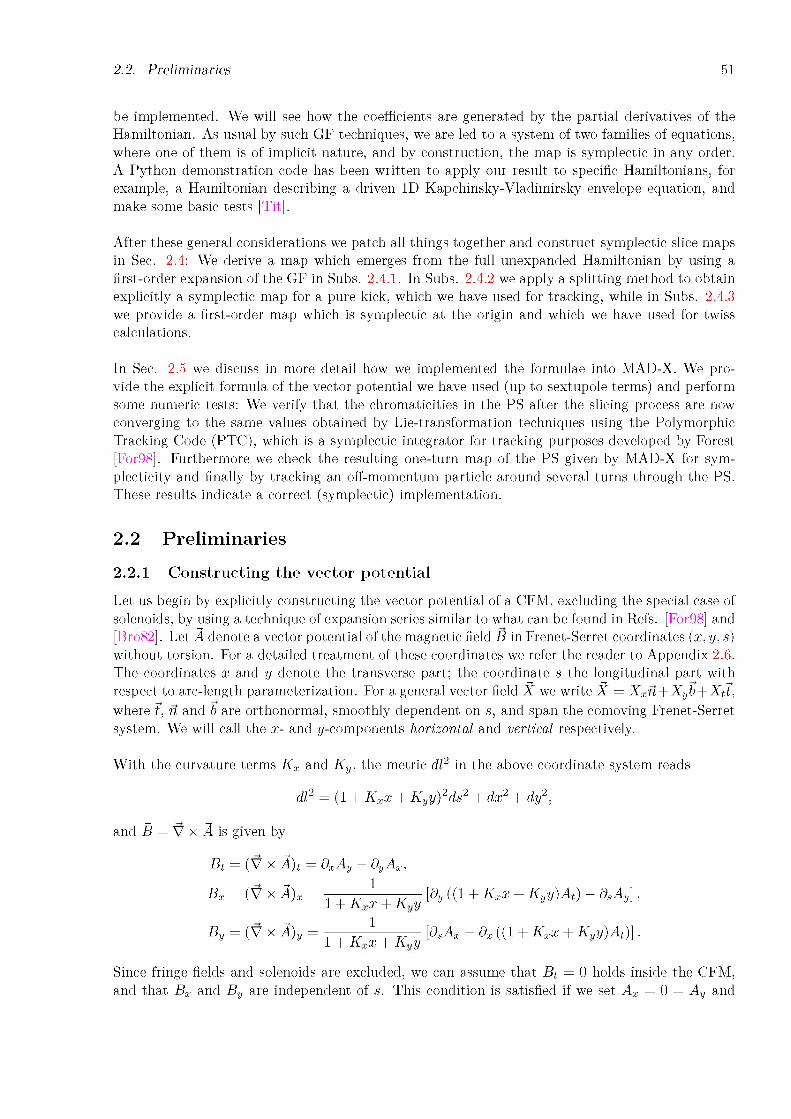
2.2. Preliminaries 51
be implemented. We will see how the coefficients are generated by the partial derivatives of the Hamiltonian. As usual by such GF techniques, we are led to a system of two families of equations, where one of them is of implicit nature, and by construction, the map is symplectic in any order. A Python demonstration code has been written to apply our result to specific Hamiltonians, for example, a Hamiltonian describing a driven 1D Kapchinsky-Vladimirsky envelope equation, and make some basic tests [Tit].
After these general considerations we patch all things together and construct symplectic slice maps in Sec. 2.4: We derive a map which emerges from the full unexpanded Hamiltonian by using a first-order expansion of the GF in Subs. 2.4.1. In Subs. 2.4.2 we apply a splitting method to obtain explicitly a symplectic map for a pure kick, which we have used for tracking, while in Subs. 2.4.3 we provide a first-order map which is symplectic at the origin and which we have used for twiss calculations.
In Sec. 2.5 we discuss in more detail how we implemented the formulae into MAD-X. We provide the explicit formula of the vector potential we have used (up to sextupole terms) and perform some numeric tests: We verify that the chromaticities in the PS after the slicing process are now converging to the same values obtained by Lie-transformation techniques using the Polymorphic Tracking Code (PTC), which is a symplectic integrator for tracking purposes developed by Forest [For98]. Furthermore we check the resulting one-turn map of the PS given by MAD-X for symplecticity and finally by tracking an off-momentum particle around several turns through the PS. These results indicate a correct (symplectic) implementation.
2.2 Preliminaries
2.2.1 Constructing the vector potentialLet us begin by explicitly constructing the vector potential of a CFM, excluding the special case of solenoids, by using a technique of expansion series similar to what can be found in Refs. [For98] and [Bro82]. Let A denote a vector potential of the magnetic field B in Frenet-Serret coordinates (x, y, s) without torsion. For a detailed treatment of these coordinates we refer the reader to Appendix 2.6. The coordinates x and y denote the transverse part; the coordinate s the longitudinal part with respect to arc-length parameterization. For a general vector field XX we write XX = Xxn + Xyb + Xtt, where t, n and b are orthonormal, smoothly dependent on s, and span the comoving Frenet-Serret system. We will call the x- and y-components horizontal and vertical respectively.
With the curvature terms Kx and Ky, the metric dl2 in the above coordinate system reads
dl2 = (1 + Kxx + Ky y)2ds2 + dx2 + dy2,
and B = V x A is given by
Bt = (V x A )t = dxAy - dy Ax,
Bx = (V x A)x = 1 + K 1 + K y [dy ((1 + Kxx + Kyy)At) - dSAy],
By = (V x A)y = 1 + K1 + K y [dsAx - dx ((1 + Kxx + Kyy)At)] .
Since fringe fields and solenoids are excluded, we can assume that Bt = 0 holds inside the CFM,and that Bx and By are independent of s. This condition is satisfied if we set Ax = 0 = Ay and

52 Chapter 2. Symplectic maps for combined-function magnets
At, Kx and Ky to be independent of s, from which Lorenz-gauge VA = 0 follows. We obtain
Bx = ^ „ dy ((f+ KXX + Ky y)At) , (2.1a)1 + Kx X + Ky y
-1 zz. „ ..... _ .By i i dx ((1 + KxX + Kyy')At) ■ (2.1b)1 + Kx X + Ky y
Because VB = 0 is automatically satisfied, the only requirement on A in order to be Maxwell- conform is the condition V x B = 0 (we consider the vacuum case), which means by Lorenz-gauge that AA = 0 has to be fulfilled. Since the B-components are independent of s and Bt is zero, the only equation which has to be fulfilled is
1 10 dx 1 + KxX + Ky ydxG + 9y 1 + KxX + Ky ydy G
with G := (1 + Kxx + Kyy)At. Equation (2.2) is equivalent to
0 = (1 + KxX + Ky!Ji (dx + dy^ G — KxdxG — KydyG,
(2.2)
(2.3)
i.e. Aj_G = —KxBy + KyBx = (B x K)t with Ai := dx + d^ and K := (Kx,Ky, 0). Now letG = Ek=0 Gk be a decomposition of G into homogeneous polynomials Gk of (total) order k in x and y. Making a coefficient comparison with respect to k, we obtain [For98]
A±Gk+1 = [— (KxX + Kyy)A± + Kxdx + Kydy] Gk■ (2.4)
Observe that A^ = (dx + idy)(dx — idy), so if we introduce the quantities r± := (x ± iy)/2 and define d± := dr±, similar as in Ref. [For98], the chain rule yields d± = dx ^ idy and thus A^ = d-d+. Now according to Lemma 2.6.3 (see Appendix 2.6) we can define the quantities gkj e C via Gk =: Ej=o gkjrk+—jrj_ and so we get
k k k , . . .k 1 j j 1 K k1 j j K k j j 1A±Gk+1 = — gkj(k — j)j [nr+ + kt—] r+ Jr— ' 2Xgkj(k — j)r+ r— ' 2Xgkj3r+ r—
k—1
= 52 [Rgk,j+1(j + 1)(j — k + 3/2) + Kgkj(k — j)(1/2 — j)] rk+—1—jr—
j=o
with k := Kx + iKy. On the other hand, the last expression must be equal to
k+1 k—1A i G , — V /i7 (k + 1 — j)jrk—j/-j—l^^/ii (k — j)( j + 1)rk—1—jrj (2 5)A± Gk+1 — / j gk+1,j(k + 1 j)jT+ t — — / j gk+1,j + 1(k j)(j + 1)t+ t — , (2.5)
j=0 j=0
so for all 0 < j < k — 1, again by Lemma 2.6.3,
(k — j)(j + 1)gk+1,j+1 = Kgk,j+1(j + 1)(j — k + 3/2) + ng^ (k — j )(1/2 — j )■ (2.6)
Equation (2.6) was derived by using the rather general symmetry assumptions above. In order to determine gk,k and gk,0, which span the kernel of A^ on the space of homogeneous polynomials of degree k , and thus completely determine the gauge, we require additional conditions. Note that because Gk = Gk, we have gkj = gk,k—j, so only half of the equations in (2.6) are necessary and only gk,0 needs to be determined.
Consider a decomposition of B into (complex) homogeneous polynomials wk of (total) order k

2.3. The Hamiltonian 53
in x and y: By + iBx = J2k==0 wk. Since (1 + nr+ + Kr-)(By + iBx) = —dxG + idyG = —d+ G, this is equivalent to the claim that in order k > 1 we have
k+1
^2(k + 1 — f)9k+i,j rk+-j r- = d+Gk+i = —wk — (kr+ + Kr-)wk-1 (2.7)j=0
and g1,0 = —w0. Let us assume that wk |r+=r_ = Xkxk, where Xk G C are known; i.e., the expansion of Bx and By are given with respect to the midplane y = 0. These conditions are fulfilled if and only if, using Eq. (2.7),
k
(k + 1)gk+1,0 = — 52(k + 1 — j)gk+1,j — 2 (Xk + KxXk-1)- (2.8)
Equations (2.6) and (2.8) completely determine the vector potential At of the CFM.
Remark 2.2.1. If we define wk =: ^k=0 wkjr+~jr-, then there is a one-to-one map between the sets {gk0; k > 1} and {wk0; k > 0}: By Eq. (2.7) we see immediately that for k > 1 we have
(k + 1)gk+1,0 = — Wk,0 — kWk-1,0. (2.9a)
Conversely, from this equation it follows by induction that
k , .Vk > 0: 52(j + 1)(—K)k jgj+1,0 = —Wk,0- (2.9b)
2.3 The Hamiltonian
Let us briefly recall the derivation of the Hamiltonian we require. We begin with the well-known Hamiltonian — ps which describes the motion of a particle in a general electromagnetic field in (torsion-free) Frenet-Serret coordinates. This Hamiltonian is derived in Appendix 2.6 and can also be found for example in Refs. [Rip85] or [Wie07]. As usual, we are using SI units and the same notation conventions as in Subs. 2.2.1.
Ps(x,y,t,Px,Py, —K; s) =
(1 + KxX + Kyy) [c-2(K — ep)2 — (px — eAx)2 — (py — eAy)2 — m2c2^ + (1 + Kxx + Kyy)eAt.
(2.10)
The parameter K denotes the total energy of the particle, i.e. with the kinetic momentum pkin := Ymv = p — eA it holds that
pkin 2 = c-2(K — ep)2 — m2c2. (2.11)
Let p := |pkin| the momentum and p0 a corresponding nominal value. As in Ref. [BRS87] we introduce the variable ] := (p — p0)/p0. Dividing by p0, we obtain the following (dimensionless) expression
ps/p0 = (1+KxX+Ky y)(1+ i)2 — (px — 'Af (py — eAy)
p0— +(1+Kxx + Kyy) At. (2.12)p0

54 Chapter 2. Symplectic maps for combined-function magnets
Let Eo be the energy corresponding to the nominal momentum po, i.e. Eo = mfi = poc/fio, and set n := (K — Eo)/Eo. Then
and
dx _ d(—Ps)_ d(—Ps/Po) d(Px/Po) _ d(—ps/po) , >ds dpx d(px/po) ’ ds dx , (. )dy = d(—ps) = d(—ps/po) d(py /po) =_ d (—ps/po) (2i3b)ds dpy d(py/po) ’ ds dy ’ '
d(—ct)_ _ d(—ps)_ d(—ps/po) d(n/fio) _ d(—ps/po) ( )ds d(—K) Po d(n/fio) d(—K) d(n/fio) ’ (.)
d(n/fio) = —1 d(—K) = 1 d(—ps) = d (—Ps/po) (2l3d)ds Eofio ds Eofio dt d (—ct) ' '
Therefore, — ps/po corresponds to a Hamiltonian with x, y, —ct,px/po,py/po and n/fio =: n as generalized coordinates. Let us denote the normalized momenta px/po and py/po again with px and py respectively. The coordinate — ct still changes without limit compared to the other (transverse) coordinates x and y. Following Ref. [BRS87], this leads us to the introduction of the variable a := s — vot, which can be introduced by performing an s-dependent canonical transformation, induced by the GF F of type 3:
F(£,C,a,Px,Py,n; s) := — pxt — PyZ + h(s — a)/fio- (2.14)
We obtain
x
y
—ct
dF dpxdF _
— Wy = Z
— ̂ = (a — s)/fio,
dFPi = — d^ = Px,
dFpz = — dz = py,
dFPa = — da = n/fio = n/fio
(2.15a)
(2.15b)
(2.15c)
and so
H(^,Z,a,Px,Py, n/fio; s) + Ps/po(Z,Z, (a — s)/fio,Px,Py,n; s)dfi^
= x (^,Z,a,Px,Py,n;s) = n/fio(2.15d)
for the new Hamiltonian H. The six equations (2.15a) - (2.15c) also prove that F is in fact a GF, since they constitute a bijection between the old and the new coordinates for every s. Up to this point, all considerations in this subsection hold for general electromagnetic fields. For our CFM with the special gauge Ax = 0 = Ay discussed in Subs. 2.2.1, we arrive at the following Hamiltonian H with
H(x, y, a,Px,Pyp; s) = Pa — (1 + Kx + Kyy) (^(1 + n)2 — Px — Py + —At (2.16)
Since we do not have any electric fields, we set p = 0. Then p is related to the coordinate n by
(1 + P)2 = fiPo
K2 f mc\2 _ K2
c2P2 \Po J fi2E2 fifi = fi [(1+ n)2 — 1+ fi2] ’ fi0 10 Po(2.17)
i.e. n is only dependent on pa, via the velocity fio of the reference particle.
The factor e/po in front of the potential At in Eq. (2.16) can be absorbed in the coefficients Xk of

2.3. The Hamiltonian 55
the B-field, which were introduced in Subs. 2.2.1, and therefore we may drop this factor later. In fact, it is already included in the curvatures Kx and Ky: Because there are no electric fields, let the reference motion with respect to the Frenet-Serret coordinates be produced by a particle having just the constant nominal momentum po above. Since our frame of reference was parameterized by arclength, it holds vo = ds/dt. The curvature terms are produced under the influence of the magnetic field B = Bxn + Byb. This reference particle remains at x = 0 = y by construction, so it will experience only the constant dipole-terms Bx,o, By,o. We have d2r/dt2 = v2dt/ds = —v2(Kxn + Kyb) and therefore
—Yomv2(Kxn + Kyb) = Yomd^ = evot x Bo = evo(Bx,ob — By,on),
so we obtain
Kx = By,o,Po
Ky =----Bx,0-Po ,
(2.18a)
(2.18b)
Note that for the reference particle, vo ± B, so we have Yomv2/p = evo\Bo|, thus e/po = 1/(Bp), where p is the radius of curvature and B2 = B2.oi + By,o.
2.3.1 General considerations
Let H be a Hamiltonian dependent on the generalized canonical variables q and p and a parameter s. Denote by As = sf — s a small section of the parameter space we are considering, where sf
denotes the ’final’ position. In order to obtain a symplectic map from the initial coordinates at s to the final ones, we assume the existence of an s-dependent GF F of type 2 to a Hamiltonian which is zero, i.e. we provide a transformation to a complete set of cyclic coordinates, identify the cyclic coordinates with the final coordinates and attempt to represent them in terms of the initial coordinates. The Hamilton-Jacobi equations for F are
q = dpF, p = dq F. (2.19)
As a first necessary condition for such an F we have
dsF(q,p; s) = —H(q,p; s). (2.20)
Note the important fact that in this equation the variables p are considered to be functions of q, p and s. To emphasize this fact, let f(q,p; s) := (q,p; s), so Eq. (2.20) can be written in the form
dsF = —H o f.
For brevity let us write Sij := dqipj o f-1. Then Lemma 2.6.4 yields
ds(Sij o f = [—dplSij • dq!h — dplSij • slk • dpkh + dsSj] ◦ f
and ds(Sij o f) = ds(dqipj) = dsdqidjF = —dqidqi (H o f)
= —dqi ([dqi H + dpi H • Sjl ] o f
= — (dqi [dqi H + dpi H • Sjl ] + dpk [dqi H + dpi H • Sjl] • Sik) o f
Consequently,
dsSij = —dqi[dqih+dpih-Sjl] — dpk[dqih+dpihSjl]• Sxk+dpiSij• dqih+dpkSij• Skl• dpih. (2.21)

56 Chapter 2. Symplectic maps for combined-function magnets
This equation shows that the s-derivatives of Sj of any order can entirely be expressed by spatial derivatives of itself and of the Hamiltonian. Secondly, in order to be able to parameterize the cyclic coordinates by the final coordinates, F|sy =: Fo must provide the identity transformation. This is guaranteed by setting
Fo = qp,
which can be verified by looking at the Hamilton-Jacobi equations for Fo. Now let us assume that we can write F in form of a Taylor-expansion around sf (with K E No U {x}) as
K+1 1 K 1F = Fo + £ -(-As)^F(q,p; sf) = Fo -J2 -+1y(-As)^+1’’ H o Y)(q, p; sf). (2.22)
By inserting this expansion (2.22) into the right-hand side of Eq. (2.19) we obtain
* 1 ......................................p = dq F = p - ^ (—. |T AsY 'd dY(H o Y)(q, p; sf), (2.23)
so all derivatives of dqipj with respect to q and p vanish at s = sf. This implies that Sj |sy = 0 andall its higher spatial derivatives vanish at sf. The derivatives d^(H o Y) in Eq. (2.22) are given by Eq. (2.72c), taken at sf. Denote for brevity
H.G := dpiG • dqiH + dpiG • Sj • dpjH = (dqH + SdpH, dpG), (2.24)
where the summation goes over repeated indices. Hence
dY(G o Y) = 9Y~1((-H. + ds)G o Y) = • • • = (-H. + ds)^G o Y,
and therefore we obtain
« 1F (q,p; s) = qp \( — + 1)! (-As)^+1((-H. + ds)^H)(Y(q, p; sf)). (2.25)
Since dqi(G o Y)(q,p; sf) = (dqiG o Y)(q, p; sf) and dpi(G o Y)(q,p; sf) = (dpjG o Y)(q,p; sf) dpipj |sy
X. - °ij by Lemma 2.6.4, we obtain the expressions
« 1q = q - 52 — + 1y(-As')^+1(dp(-H. + ds')^H')(q,p; sf), (2.26a)
* 1p = p + 52 — + 1)!(-As)^+1(dq(-H. + ds)^H)(q,p; sf), (2.26b)
using that Y(q,p; sf) = (q,p(q,p; sf); sf) = (q,p; sf). These equations describe implicitly a symplectic transformation for every K: Equation (2.26b) constitutes an implicit expression for p. Once its solution is determined, one can insert it into Eq. (2.26a) to obtain the overall symplectic solution. In Ref. [Cha83a] such a series was described and made explicit for low orders.

2.4. Symplectic approach 57
2.4 Symplectic approach
2.4.1 First-order symplectic slice map
At this point let us apply the results of Subs. 2.3.1 to our particular Hamiltonian (2.16). Since this Hamiltonian does not depend on a, and all derivatives of the Sij - especially with respect to a - vanish at the final position, it holds in every order
Pa = p ■ (2.27)
This is expected, because pure magnetic fields can not change the energy of the particle.
For a pure drift, this equation holds for all momenta: In this case, H does only depend on the canonical momenta. Let W be a sufficiently continuously differentiable function, dependent on p and s, and independent on q. Then
dqk(-H. + ds)W = -dpiW • dqkSj • dpH,
and this expression vanishes at s = sf according to our considerations in Subs. 2.3.1. Especially we conclude that p = p holds, by taking W = (-H. + dsY~1H for p > 1 inductively.
For the cyclic coordinates q in case of a pure drift, a bit more subtle but similar argument applies in this setting of GFs: Let F be a function of q,p and s, and which can be written as a linear combination of terms in which every summand contains at least one factor of the Sij or a partial derivative of these functions with respect to one of the qk or pk. Again from our considerations in Subs. 2.3.1 it should be clear that F and its partial derivatives with respect to qk and pk vanish at s = sf. By Eq. (2.21) we see that dsF is of the same form as F, because the spatial Hesse-Matrix dqidqjH in the expression for dsSij vanishes. We conclude that
dpk (-H. + ds)F = dpk (-dpiF • Sij • dpH + dsF)
vanishes at s = sf. Now observe that (-H. + ds)H = -H.H = -dpH • Sij • dpH is of the form of F. Consequently, dpk (-H. + ds)^H vanishes at s = sf for p > 1. Summarizing these results we obtain in the case of pure drift the explicit equations
q = q + AsdpH(p), (2.28a)p = p. (2.28b)
For a general CFM, let us consider Eqs. (2.26a) and (2.26b) for the simplest case K = 0, which corresponds to a first-order expansion of the GF. In Ref. [Bar+96] this was discussed for the case of pure bending magnets. Equation (2.26b) yields for px:
px = px + As (Kxh + dxG) = ux + AsKxh, (2.29)
with the abbreviations h := ^(1 + j)2 - pX - py, ux := px + AsdxG and G = (1 + Kxx + Kyy)At
(see Subs. 2.2.1). Similarly we have such an equation for py. Then we conclude
h2 2 2 2 2 / J-AcR' h\2 (ti -J-Ae/C h\2h = (1 + P) - px - py = (1 + P) - (ux + AsKxh) - (uy + AsKyh)= (1 + j)2 - ux - uy - 2Ash(uxKx + UyKy) - As2/F/<2 + K^),

58 Chapter 2. Symplectic maps for combined-function magnets
and therefore obtain the quadratic equation h2 + Ah + Z = 0, with the abbreviations
A •= 2As UxKx + UyKyA 8 1 + As2(K2 + K2) ’ui+uy - (i+n)1 + As2(KX + Ky2) •
(2.30)
Consequently, h = —A/2 + VA2/4 — Z, where we have determined the sign in front of the square root by the condition that in case As = 0 we have px = px = ux and py = py = uy. The now determined h yields an explicit symplectic map for the momenta when inserted into Eq. (2.29). For the coordinate y, Eq. (2.26a) yields, together with Eq. (2.29),
y = x + As(1 + Kxx + Ky y)px/h = x + As(1 + Kxx + Ky y)(ux/h + AsKx), (2.31)
and similarly we can drive such an equation for y. For x we first note that, by implicit differentiation of Eq. (2.17), we obtain
(1 + fi) dr- = 1 + ■, (2.32)dp.
thusX = x + AsdPa H = x + As — As(1 + Kxx + Ky y)(1 + >;pi. )/h
In summary, we obtain the following symplectic map:
xf = x + As(1 + Kx x + Ky y%')(ufx/h + AsKx), (2.33a)
pl = ux + AsKxh, (2.33b)
yf = yx + As(1 + Kxx1 + Ky yi)(uiy/h + AsKy), (2.33c)
py = uy + AsKy h, (2.33d)
xf = X + As — As(1 + Kxx1 + Ky yi)(1 + jp )/h, (2.33e)
pl = p., (2.33f)
where h (and G) are taken at the initial coordinates. Note that dx,yG = ^(1 + Kxx + Kyy)Byx, which can be inserted into these expressions in order to obtain the field-dependency of the transformation.
2.4.2 Symplectic kick
For a ’drift-kick’ scenario, the slice map (2.33a) - (2.33f) is, however, not used. For example after the slicing process in MAD-X, the tracking through the CFM is performed via consecutive drifts and kicks. To obtain the ’kick’ part of this procedure, the inverse of a ’drift’ would have to be applied in either the slice map or the thick map in Ref. [Ise85]. Because this would lead to an unnecessary blow-up of code, we follow an alternative technique which is described in Ref. [Bar+96]. For a discussion of various splitting techniques the reader can consult Ref. [For98].
Equation (2.16) in case of no fields gives the drift part with respect to vacuum
Hdrift(px,py,p.) := p. — y(1 + i)2 — px — py• (2.34)
Now, inside the magnet, this Hamiltonian would change towards the full Hamiltonian H. However,in the case of a drift-kick decomposition, this change is assumed to take place infinitesimally at acertain point so with a particular strength. At this point, only those parts of H' := H — Hdrift
which produce a kick in the spatial momenta px and py have to be taken into consideration. Thuswhat we have to do is to sort out those parts of H' which contain the momenta (since offsets arecomputed via dH/dpx etc.).

2.4. Symplectic approach 59
Since the physical kicks remain very small with respect to the reference trajectory, we can take a look at the expansion of the square root
. /fl _|_ £p2 Xp Xp — 1 -I- n -Px + Pz 2 35fV(1 + h) — Px — pz = 1 + n — 2 - + fj + • (2.35)Then we see that
H'kick := — [(Kxx + Kyy)(1 + j) + G(X, y)] Asd(s — So) (2.36)is the Hamiltonian we are interested in, where we have accounted for the fact that it acts instantaneous by the factor As5(s — so). Integration of the corresponding Hamilton-equations for H'kick
yields the following symplectic kick map:
f — ppi^x ^x , (2.37a)
pfx = PX + As(Kx(1 + j) + dxG), (2.37b)
yf = y\ (2.37c)
Pfy = Py + As(Ky (1 + j) + dy G), (2.37d)af = ' — As(KxX' + Ky yi)(1 + ■-)/(- + j), (2.37e)
pa p& • (2.37f)
2.4.3 First-order drift-kick mapThe map described in Subs. 2.4.2 constitutes a pure kick and can be used for tracking, but for chromaticity calculations it lacks any information about the dependency of the transverse coordinates with respect to the other coordinates. This information is generated indirectly during the slicing process by composition of the drifts and kicks, but if it cannot be obtained by automatic (or numeric) differentiation, we have to use a different approach.
Fortunately, the slice map (2.33a) - (2.33f) can be used in order to obtain a map which is first- order in As, contains the necessary information and is symplectic at the origin. Symplecticity at the origin is sufficient for twiss calculations, as long as the reference trajectory inside the CFM can be assumed to be located at zero. Besides of converging to the correct values (shown later in this chapter), the advantage in using such a map in comparison to the possibilities described in Subs. 2.4.2 is especially that it does not lead to a large blow-up of code [Tit].
Let T constitute a slice map according to Eqs. (2.33a) - (2.33f) with respect to length As := sf — s0, in which we drop all higher orders in As. This means that the function h in this transformation is replaced by h0 := ^/(1 + j)2 — pX — py. Let s0 < si < sf, As1 := si — s0 and As2 := sf — si, i.e. As = As1 + As2. Let Di be drifts with respect to As' for i = 1,2. Then we would like to compute the composition D-1 oToD-1, since this map constitute the kick map in a ’drift-kick-drift’ scenario within As, where the kick appears at si.
Let T(v) =: v + Asf (v), i.e. f is given according to Eqs. (2.33a) - (2.33f) in which h is replaced by h0. By Eqs. (2.28a) and (2.28b) we have D~1(v) = v — Astf0(v), where f0 is the map f

60 Chapter 2. Symplectic maps for combined-function magnets
without any field terms. Using f (v + Asw) = f (v) + O(As) we get
D-1 o T o D-i(v) = D-1 o T(v - Asi fo(v))
= D—(v - Asifo(v) + Asf (v - Asifo(v)))
= D-1(v - Asifo(v) + Asf (v) + AsO(Asi))O(As2)
= v - Asfo(v) + Asf (v) + O(As2).
This means that the first-order term of D-1 o T o D-1 with respect to As corresponds to f - f0. In addition we see that in first-order it does not matter where the kick is located between the two drifts; especially one drift of length As is sufficient. Using this result, we obtain a drift-kick map in first-order As:
xf = X + As(Kxx% + Ky yi)p\/ho,
pf = PX + As(Kxho + dxG), yf = y + As(KxX% + Ky yl)py/ho,
Py = Py + As(Ky ho + dy G), af = K - As(KxX + Kyy*)(1 + i/y.,)/ho,
p/ p/.
(2.38a)
(2.38b)
(2.38c)
(2.38d)
(2.38e)
(2.38f)
It turns out that this map is symplectic at the design trajectory (the ’closed orbit’) at zero, but not symplectic in general. However it is well-suited for MAD-X for computation of the twiss parameters, since these parameters require the knowledge of the transport map only around the closed orbit, which we assume to be at (or very close to) zero inside the CFM. The symplecticity at zero is crucial in order to remain in the symplectic group during composition.
2.5 MAD-X implementation
The following describes the implementation of combined-function magnets into MAD-X, having a tilt, skew- and normal components, in a preliminary test code using MAD-X version 5.02.12 [Tit]. In an earlier tested version of MAD-X (version 5.02.07), only the case without tilt and skew components is implemented. This older modified version is used in all of our MAD-X tracking studies.
2.5.1 The magnetic field and its vector potential coefficients
Let By + iBx = Y/k wk an expansion of the magnetic field into complex homogeneous polynomials wk G PC[x,y] of total order k in x and y. In the light of Lemma 2.6.3, wk can be represented as wk = Hj=o Wkjr-r— with wkj G C and r± := (x ± iy)/2. With x + iy =: r exp(ip) we thus obtain
kWk = 2-k rk exp(ikp)^2 wkj exp(-2ijp), (2.39)
ro
(By + iBx)\^=p0 ^krk ,k=o
representing By + iBx as a function of r and p. Let us assume that we know the expansion ofBy + iBx with respect to a given reference cone at p = po, i.e.
(2.40)

2.5. MAD-X implementation 61
with known values Xk G C, i.e. by coefficient comparison we know the left-hand side of
k
Xk = 2 k exp(ik^0)^2 Wkj exp(-2ij(po), (2.41)
or expressed in another wayWk |ra = Xk rk. (2.42)
The special case k = 0 leads immediately to
X0 = w00 = —51,0, (2.43)cf. Eq. (2.9b). If we could determine all wkj’s, we would have determined the field everywhere. In view of Eq. (2.41) this task is similar to a discrete Fourier-transform, with the difference that we have some angle p0 in the exponentials which may also be zero. However, the Vacuum MaxwellEquations will provide us with enough information to carry out this task.
From Eq. (2.7), taken at p = p0, we obtain for k > 1:
k
(k + 1)gk+i,02 krk exp(ik^0) = — ^(k + 1 — j')9k+i,j2 krk exp(ik^0) exp(—2ijip0~) +
— Xkrk — |(kexp(i^0) + k exp(—ip0))Xk-irk.
k
^ (k + 1)gk+i,0 = — (k + 1 — j)9k+i,j exp(—2j0)+
— 2k exp(—ikp0) [Xk + Re(k exp(i^>0))Xk-1]. (2.44)
Eq. (2.6) will remain unchanged. Together with Eq. (2.44), which can be considered as a generalized version of Eq. (2.8) for arbitrarily tilted magnets, we have the tools to determine the vector potential completely. It remains to discuss the filling of the Xk’s.
By Eqs. (2.18a) and (2.18b) (we can drop the normalizing factors e/p0, as explained in Subs. 2.3), and Eq. (2.40) we see that
Ky = — Bx(0, P0) = —Im(X0), (2.45a)Kx = By (0, ^0) = Re(X0), (2.45b)
must hold and in general, by considering the Taylor-expansions of Bx(r,p0) and By(r,p0) around r=0
~ 1 dk B JL 1 dk BBx(r, J0) = E k~dT^(0, ^0)r, By(r, = £ k! ~dr^(0, ^0)r. (2.46)
we receive, using Eq. (2.42), the identifications
1 dk Bpirk (0,^0) = Im(Xk), (2.47a)1 dk B„,
jp_ ~B(0^0) = Re(Xk). (2.47b)

62 Chapter 2. Symplectic maps for combined-function magnets
The left-hand sides of Eqs. (2.47a) and (2.47b), without the factorial, are denoted as the skew- and normal components of the B-field respectively, since they individually determine a normal- orientated - respectively skew-orientated - field, i.e. fields with pure vertical or pure horizontal components in case of <pQ = 0.
With Eqs. (2.6), (2.44), (2.47a) and (2.47b) we completely determined the magnetic field of a general tilted combined-function magnet.
2.5.2 Thin-lens kick mapBy combining Eqs. (2.37b) and (2.37d) we obtain with pf := pX — ipf and p1 correspondingly:
pf = p% + As(k(1 + n) + d+G). (2.48)
Hereby, d+G is given by Eq. (2.7) from the known coefficients determined in Subs. 2.5.1. The corresponding kicks in x and y direction are then determined by the positive real and negative imaginary part, respectively. The remaining formulae in Eqs. (2.37a) - (2.37f) do not depend onG. Note that in MAD-X we use orbit(5) = ct/^q, while orbit(6) = Giiw, see Appendix 2.6.3.
2.5.3 First- and second order coefficients of the drift-kick map for TWISS
Before we discuss the derivatives of the drift-kick map, let us begin with a useful Proposition.
Proposition 2.5.1. Let k G NQ, m G N and for j G {1,..., k}: akj G C. Then we have
m k m— 1 kd^^'yT'm rk~jrj = \'ld' ct .)rk—jrj
■’■ 2^-kj<+ i— = / ,, 2-^(U+akJ)r+ r — ,
m k m— 1 kd m -rk—jrj = V(d m -)rk—jrj2-^akj r+ I— = / „ ZG' k) P+ I — ,
with
d+^kl := (k + 1 — j iT+V),d—CTki := (j + 1)CTk+i,j+i.
(2.49a)
(2.49b)
(2.50a)(2.50b)
Proof. The proof is left to the reader. □
By looking at the drift-kick map given by Eqs. (2.38a) - (2.38f), we see that only Eqs. (2.38b) and (2.38d) involve the vector potential G. So let us discuss these equations. As in Subs. 2.5.2 we combine them to a single equation, which reads
pf = pz + As(nhQ + d+G), (2.51)
where, using Eq. (2.50a),oo k
d+G = Pjyk + 1 — j )hk+i,j r+—) r—. (2.52)
The terms pz and hQ in Eq. (2.51) drop out during the derivation process with respect to thespatial coordinates, so by setting akj := As(k + 1 — j)gk+1,j and noting that dx = (d+ + d— )/2 anddy = i(d+ — d—)/2, we can determine the higher-order derivatives of pf by successive application

2.5. MAD-X implementation 63
of Eqs. (2.50a) and (2.50b) as follows:
dxakj = 2 [(k + 1 - j)ak+i,j + (j + 1)ak+i,j+i] , (2.53a)
dyakj = ^i[(k + 1 - j)ak+i,j - (j + 1)ak+i,j+i] ■ (2.53b)
and
dXokj = 1 [(k + 1 - j)dxak+i,j + (j + 1)dx^k+i,j+i],
= 4 [(k + 1 - j) [(k + 2 - j')ak+2,j + (j + 1)ak+2,j+i] ++ (j + 1) [(k + 1 - j')ak+2,j + i + (j + 2)ak+2,j+2]] ,
= 4 [(k + 1 - j) [(k + 2 - f)ak+2,j + 2(j + 1)ak+2,j+i] + (j + 1)(j + 2)ak+2,j+2] , (2.54a)
dx9yakj = 2 [(k + 1 - j)dyak+i,j + (j + 1)dyak+i,j+i] ,
= 4i [(k + 1 - j) [(k + 2 - j)ak+2,j - (j + 1)ak+2,j+i] ++ (j + 1) [(k + 1 - j)ak+2,j + i - (j + 2)ak+2,j+2]] ,
= 4i [(k + 1 - j)(k + 2 - f)ak+2,j - (j + 1)(j + 2)ak+2,j+2] , (2.54b)
dyakj = 2i [(k + 1 - j')dyak+ij - (j + 1)dyak+i,j+i] ,
= -4 [(k + 1 - j) [(k + 2 - f)ak+2,j - (j + 1)ak+2,j+i] +- (j + 1) [(k + 1 - j)ak+2,j+i - (j + 2)ak+2,j+2]] ,
= -4 [(k + 1 - j) [(k + 2 - j)ak+2,j - 2(j + 1)ak+2,j+i] + (j + 1)(j + 2)ak+2,j+2] ■ (2.54c)
The derivatives are evaluated at x = 0 = y, therefore only the terms for k = 0 = j survive. They are
dxa00 = ^ (ai,0 + ai,i) = ^As (2g2,0 + g2,i), (2.55a)
dyaoo = 2i (ai,0 - ai,i) = ^iAs (2g2,0 - g2,i), (2.55b)
dXaoo = 1 (2a2,0 + 2a2,i + 2a2,2) = 1As (3gs,0 + 2g3,i + 53,2) , (2.55c)
dxdya00 = 4i (2a2,0 - 2a2,2) = 4iAs (3g3,0 - 53,2), (2.55d)
dya00 = -4 (2a2,0 - 2a2,i + 202,2) = -^As (3g3,0 - 2g3,i + 53,2) ■ (2.55e)
Eqs. (2.55a) - (2.55e) are implemented in the code for the determination of the re and te coefficients. Note that the te coefficients receive an additional factor 1/2 due to the usual relation tothe second derivative in the Taylor-series.

64 Chapter 2. Symplectic maps for combined-function magnets
2.5.4 Explicit combined-function potential for normally aligned fieldsThe higher-order terms (the order here is understood to be with respect to the transverse coordinates) of the transformation map can be obtained by deriving the corresponding transformation maps and evaluating them at zero, as was shown in the previous section. In this subsection we provide an explicit version for G which describes the case of normally aligned fields up and including sextupole components. In this case, the field components are given as coefficients Bx,k, By,k (times the normalization e/p0) for k = 0,1, etc. of the Taylor-expansion around x = 0 as
OO 1Bx(x, 0) = ^ — Bx,kxk,
OO 1By (x, 0) = 12 —! By,kXk, (2.56)
where the dipole terms (k = 0) are related to the curvatures Kx and Ky as before, according to Eqs. (2.18a) and (2.18b). By using an expansion of up to total order 4 we then get
G = K2g 4 KXx224 y
- Kx x -K2yg 4 —— y4 24 y
+ ^-gxy3 - KxKyxy -
K2yy2
2+ K- y3 + Kh xy3
K -x' + K^xy2 - K^x4 + K Vx-.x3 2 y 8 2 y
gx2 gy2 hx3 hx 2
- K,y - + -J- - ~t + t y'
Kxh 4
24 y
(2.57)
2
where g denotes the strength of the quadrupole and h the strength of the sextupole component. This potential yields the following expansion
Bx |y=0 = -Ky,
By |y=0 = Kx + gx + 2hx2,
(2.58a)
(2.58b)
as one can verify straightforwardly.
2.5.5 Numerical tests1. We have tested our first-order drift-kick map against the Lie-transformation formulae of Ref.
(which are implemented in MAD-X and yield the same results as PTC) for a single CFM. The formulae were implemented in a modified version of MAD-X (v.5.02.07) and compared to the unmodified one. The magnet was invoked without fringe fields, and the corresponding sectorfiles, which contain the Lie-transformation coeffcients, were compared. The first-order coefficients are denoted by re; the second-order coefficients by te.
[Ise85]
As an example, we have listed in Fig. 2.2 the relative error in the re-entries in case of 4 slices for a CFM against the results of the Lie-transformation. The magnet had a total length of 3.92 m and bends a 100 GeV proton by an angle of n/8. On top of its dipole field, it had a quadrupole and a sextupole field of strengths k1 = -0.03644 [m]-2 and k2 = -4 • 10-2 m-3
respectively. It turns out that the skyline of error bars looks similar for other slice numbers, while the error bar of R56 is somewhat standing out relative to the others: These relative errors, including the ones of the te-entries (not shown), follow an expected linear convergence behavior in dependency of the slice number, see Fig. 2.2.
2. As a second test of the first-order drift-kick map, we have computed the twiss parameters for the PS after thin slicing and obtained chromaticity results listed in Tab. . The tunes were at Qx = 6.450 and Qy = 6.462. Note that in MAD-X the horizontal chromaticity Q'x is defined as dQx/d(fi0pv) (and correspondingly the vertical one Q'y). For comparison, the result of the unmodified MAD-X 5.02.07 code gives Q'x = -7.333 and Q'y = -7.331 (with 128 slices) which is over 20% off in horizontal and 5% off in vertical direction from the PTC reference
2.1

2.5. MAD-X implementation 65
Rel
. erro
r0.08
0.06
0.04
0.02
0.00
Rll R21 R51 R12 R22 R52 R33 R43 R34 R44 R16 R26 R56
Figure 2.2: Left: Relative errors for various re-entries for 4 slices of a single CFM with quadrupole and sextupole component against the Lie-transformation coefficients. Those errors which are zero are not shown. Right: Counter-check with convergence behavior of the relative errors for the re-coefficients of the right-hand side.values at Q'x,0 = -6.080 and Q'y0 = -6.969. The fringe fields of the bending magnets were again switched off for comparison; otherwise the convergence of the chromaticities towards the PTC values would retain a small offset of about 0.01% in both directions. The table shows that with just 4 slices we already obtain a precision lower than 0.2%. In Fig. 2.3 the convergence behavior of the chromaticities against the PTC results is shown. Furthermore, the symplecticity of the linear part M of the PS one-turn-map with the new CF maps were confirmed by computing |Mtr JM — J|. This value was found to be in the region of the machine precision.
Table 2.1: Simulated chromaticity in the PS for various slice numbers.
Slice number QX Q'y QX/QX, 0[%] QQ 0[%]128 —6.080 —6.970 3.274 x 10⁻³ 3.797 x 10⁻³
64 —6.079 —6.970 6.468 x 10 3 7.633 x 10⁻³
32 —6.079 —6.970 1.262 x 10⁻² 1.543 x 10-216 —6.078 —6.971 2.395 x 10⁻² 3.149 x 10⁻²
8 —6.077 —6.974 4.276 x 10⁻² 6.547 x 10⁻²⁴ —6.076 —6.979 6.514 x 10⁻² 1.405 x 10⁻¹
2 —6.076 —6.991 5.305 x 10⁻² 3.120 x 10⁻¹
Figure 2.3: Convergence behavior of the horizontal- and vertical chromaticities in the PS against the PTC results (red).3. To check our symplectic kick map for tracking purposes, described in Subs. 2.4.2, we have
simulated 1024 turns of a test particle through the PS, which was given small offsets in all

66 Chapter 2. Symplectic maps for combined-function magnets
coordinates. We observe that the particle remains on its action torus with the new code, see Fig. 2.4. Every CFM was sliced 4 times (and fringe fields were switched on).
Figure 2.4: Tracking example with the new code over 1024 turns in the PS lattice, having small initial offsets in all directions.2.6 Appendix
2.6.1 On the Hamiltonian in Frenet-Serret coordinatesLet us begin with the Hamiltonian (in SI units) describing the motion of a charged particle in an electromagnetic field, formulated in cartesian coordinates. This Hamiltonian can be found for example in Ref. [Wie07], p. 24 Eqn. (1.92) or in Ref. [GPS02], p. 351 Eqn. (8.56)
H = c\J (p — eA )2 + m2c2 + ep. (2.59)
where p = (px,py,pz) denotes the canonical momenta of the particle.
In the situation of circular accelerators it is often more convenient to change the cartesian coordinate system, in which the Hamiltonian (2.59) is formulated, towards a comoving coordinate system with respect to a reference trajectory. In the original cartesian coordinates let us denote this reference trajectory by r(s) = (x(s),y(s), z(s)). We will assume that it is parameterized by arc length, i.e. t(s) := dsr(s) has norm |t(s)| = 1 for all s.
Let n(s), b(s) be unit vectors which are smoothly dependent on s and so that (t,n,b) constitute a right-handed-oriented orthonormal basis. For example, if t(s) and dst(s) are linearly independent for every s, one can choose n to be the normalized — fsn and take the cross product t x n to define b.
Assume that the map f: (£,n,s) ^ r(s) + £n(s) + pb(s) = (x,y,z) is injective on an open domain U containing a curve at £ = 0 = n, i.e. it provides a map around a section of the reference trajectory. We call the map f a Frenet-Serret coordinate system. Let us denote the tuple of new coordinates (£,n, s) with Q and consider the real-valued function F3, given by
F3(Q,p) := — p(r(s) + £n(s) + yb(s)).
Remark 2.6.1. F3 is a GF of type 3.
Proof.

2.6. Appendix 67
i) For the spatial coordinates x, y and z we have the (local) bijection
(x, y, z) = -VpF3 = f (f, p, s). (2.60)
ii) The map F3 is, by construction, differentiable with respect to the new coordinates Q. Let us denote the corresponding negative partial derivatives of F3 with respect to these coordinates by p^, pn and ps respectively. For p^ and pn we have
dF3 _pi := : = = pn
dF3pn := —= pb.op
(2.61)
The expression for ps is slightly more complicated. Since -£-n A n and similarly for the other vectors, we can deduce that there must exist differentiable functions a1, a2 and a3, which are in general dependent on s, with
dt ds
d _ ~d~n ds
d>• ds
a1n + a2b, (2.62a)
(2.62b)
—«2? — a3n. (2.62c)
—ait + a3&,
(If a3 is zero we say that the comoving frame is torsion free. It is not hard to see in this case that if ai or a2 is also zero, then the reference curve must lay in a plane.) These functions are usually given by the reference trajectory itself (see above) and therefore are assumed to be known. With equations (2.62a) - (2.62c) we get
ps := “w3 = pt + fp-^n + ppdb = (1 — aif — a2p)pt + a3fpb — a3ppn. ds ds ds
(2.63)
By Eqn. (2.60) and our assumption on f, we have a local bijective relation between the spatial coordinates x,y and z and the new coordinates f,p and s. Together with Eqs. (2.61) and (2.63) for the new momenta this proves that F3 generates a local bijection between all new and old variables, while satisfying the equations for a GF of type 3. This means that it generates a canonical transformation between the cartesian- and the Frenet-Serret coordinates. □
Before we proceed with the Hamiltonian, let us analyze the parameterization f a bit further. Again using (2.62a) - (2.62c), and taking the exterior differential componentwise, we get
(dx, dy, dz) = df = ((1 — a1f — a2p)t + a3fb — a3pn)ds + ndf + bdp. (2.64)
With the standard metric in R3, g = dx2 + dy2 + dz2, we therefore obtain in the new coodinates
dl2 := f*g = [(1 — a1 f — a2p)2 + a2f2 + a2p2j ds2—a3p(dsdf+dfds)+a3f(dsdp+dpds)+df2+dp2.
(2.65) From now on we will assume that the given Frenet-Serret system is torsion free, i.e. describes an orthogonal curvilinear coordinate system with metric
dl2 = (1 — a1f — a2p)2ds2 + df2 + dp2.

68 Chapter 2. Symplectic maps for combined-function magnets
Let us recall the coordinate-independent definition of the curl of a vector field X. If m is an arbitrary vector, the m-component of the curl V x X is given by
(V x X) • m := lim XdrV 7 A--" \A\ JdA (2.66)
where the integration goes along the boundary of a surface A of area \A\ which is orthogonal to m (orthogonal with respect to the standard scalar product). The vectors t, n and b constitute an orthonormal basis of our Frenet-Serret system: They are given as the normalized vectors of the push-forward of the basis vectors ds, d^ and dn via f, i.e. by df (ds) = dsf, df (d^) = d^f and df (dn) = dn f and normalization. By inserting for m in Eq. (2.66) this basis, the curvilinear version of the curl becomes (see Ref. [Foa07])
(V x X )t = d^ Xb - dv Xn,
(V x X)n = -------- 1--------- ((1 - aib - a2n)Xt) - dsXb],1 - aib - «2n
(V X X)b = --------- 1----- [dsXn - d^ ((1 - aib - a2n)Xt)}.1 - aib - ®2n
(2.67a)
(2.67b)
(2.67c)
Note that, by using the coordinate-independent formulation (2.66), all components emerging in Eqs. (2.67a) - (2.67c) are taken with respect to the comoving basis t, n and 6 respectively, i.e. with respect to the representation X = Xtt + Xnn + Xb6.
Remark 2.6.2. The components of the local representation X = Xsds + X^d^ + Xndn of X are related to the previous representation via the push-forward with f:
f '(X) = df, dnf, dsf )(X) = Xsdsf + X$d(f + Xndnf— (1 - aib - a2p)Xst + Xgn + Xnb, (2.68)
i.e.
Xt = (1 - aib - a2n)Xs, (2.69a)Xn = Xt, (2.69b)Xb = Xn. (2.69c)
Let us now turn our attention to the Hamiltonian (2.59). Since F3 is independent of the time, the new Hamiltonian, which we shall denote by K, is related to H by expressing the old coordinates in terms of the new coordinates as follows: K(Q,P) = H(q,p) with P := (p^,pn,ps), q := (x,y,z) = q(Q,P) and p = p(Q,P). Note that the expression (p - eA)2 is invariant against orthogonal transformations in momentum space
(p - eA)2 = (pt - eAt)2 + (pn - eAn)2 + (pb - eAb)2.
Using Eqs. (2.61), (2.63), (2.69b) and (2.69c) we then conclude for the Hamiltonian K in the new coordinates (b,n,sp,pn,ps; t):
K = c [((1 - aib - a2n)-ips - eAt)2 + p - eA^)2 + (pn - eAn)2 + m2c2] / + ep (2.70)
^ ps = (1 - aib - a2p)\Jc~2(K - ep)2 - p - eA$)2 - (pn - eAn)2 - m2c2 + (1 - aib - a2n)eAt, (2.71)
where we have left At in its form, since we will make use of the curl formulae (2.67a) - (2.67c)later on anyways, in which At is of importance instead of As . The potential functions are taken at

2.6. Appendix 69
the point (x,y,z) = f (£,p,s). With Eqs. (2.70) and (2.71) we have made two steps: We derived a Hamiltonian (2.70) in terms of Frenet-Serret coordinates out of the Hamiltonian (2.59), formulated in cartesian coordinates. And we have rearranged the expression towards ps, which will later play the role as the negative of a new Hamiltonian in which the (negative) energy and time play the role as two conjugate generalized coordinates.
At this point let us list a few references where the form of the Hamiltonian (2.70) is derived. The Hamiltonian (2.70) can be found in Wolski’s book by a different approach [Wol14], p. 74 Eq. (2.72), and in Wiedemann’s book [Wie07], p. 30 Eq. (1.116). In Ripken’s paper [Rip85], p. 10 Eq. (2.21) the final form of Eq. (2.71) can be found. Wiedemann’s derivation differs only slightly than ours: In contrast to his derivation we used here a potential-independent GF in order to provide a clear picture what role the coefficients of the vector potential play with respect to the embedding f and the curl formulae (2.67a) - (2.67c) in curvilinear orthogonal coordinates.
The change from K to — ps as the new Hamiltonian, depending on the coordinates (£, p, tp,pn, —K; s), is left to the reader; we just mention at this point that this basically stems from the fact that the 2-Form w, which leads to the Hamilton-equations ixw = 0, X(t) = 1, has the form
w = dp^ A d£ + dpn A dp + dps A ds — dK A dt.
Note that apart of this subsection we have adopted a more common notation for the rest of this work: £ ^ x, p ^ y, —a1 ^ Kx, — a2 ^ Ky.
2.6.2 Supplemental material
Let us denote with Pk C Pc[x, y] the set of complex homogeneous polynomials of degree k. We will show a small Lemma:
Lemma 2.6.3. Let v: P1 ^ P1 be a complex isomorphism. Then this map induces a bijection v* on the entire Pc[x, y] via v*g (x,y) := g(v(x),v(y)).
Proof. By construction, v*( Pk) C Pk. Therefore it is sufficient to restrict to those kind of polynomials. Surjectivity: If g G Pk is given, then g with g(x,y) := g(v-1(x),v-1(y)) is a polynomial in Pk with v*(g) = g. Injectivity: Denote r+ := v(x) =: v11x + v21y, r- := v(y) =: v12x + v22y and let gj G C for j = 0,...,k. Then the following holds for all k > 0:
k0 = Ys gjr+-jr- ^ Vj : gj = 0.
This assertion can be proven by induction over k. If k = 0 then nothing must be proven. If k = 1, then we have
0 = gor+ + g1r- = (vnx + v21y,v12 x + vny) 90 = (x,y) v11g1 v21
v12 go
v22 g1
Since this equation holds for all x and y, it follows that (v)2x2(g0,g1)tr = 0, thus g0 = 0 = g1. Note that this property holds even if g0 and g1 are polynomials. Now assume that the claim holds for some k — 1 with k > 1. Then
k
^gj r+-j r-
j=o
k-1 k-1-j j k-1gj r+ Jr- r+ + gk r_ r-.j=0

70 Chapter 2. Symplectic maps for combined-function magnets
By the case for k = 1 we have y*L0 g-rk 1 -r- = 0 and eikrk 1 = 0, thus qk = 0 and by assumption j =0Vj G {0,..., k — 1}: g- = 0. This proves the claim above. Since v* is linear by definition, the claim implies that v* is injective. □
We further prove an important Lemma by which we were able to determine the implicit map (2.26a) and (2.26b):
Lemma 2.6.4. Let G be a differentiable function of (q,p; s) and assume that there exist a GF F of type 2, providing a transformation into a complete set of cyclic coordinates. Then
dqi (G o ^) = [dqiG + (dpjG) • (dqip- o f-1) o f, (2.72a)
dp (G o f) = [(dpj G) • (dpi p- o f-1)] o f, (2.72b)
ds (G o f) = [—dpi G • dqi H — dpi G • (dqi p- o f-1) • dp H + dsG] o f. (2.72c)
Proof.
dqi (G o f)(q, p; s) = (dqj G)(f(q, p; s))dqi q- + (dpj G)(f(q, p; s))dqi p- + (dsG)(f(q, p; s))dqi s
= [(dqiG) + (dpjG) • (dqip- o f-1)] (f(q,p; s)).
dpi (G o f)(q, p; s) = (dqj G)(f(q, p; s))dpi q- + (dpj G)(f(q,p; s))dpi p- + (dsG)(f(q, p; s))dpi s
= (dpjG)(f(q,p; s))dpip-,
and
ds(G o f)(q, p; s) =(dqi G)(f(q, p; s)) dsq% +(dpi G)(f(q, p; s)) dsp% +(ds G)(f(q, p; s))
0 dsdqiF with Eq. (2.19)= — (dpiG)(f(q,p; s))(dqi(H o f))(q,p; s) + (d.sG)(f (q,p; s))
= [—9piG • dqiH — dpiG • (dqip- o f-1) • dpjH + dsG] (f (q,p; s)),
where we have used Eq. (2.72a) to obtain the last equation. □
2.6.3 Notations in MAD-XThe program MAD-X uses the following notation [Den+17]
orbit(1) = x
orbit(2) = pxorbit(3) = y,orbit(4) = py,orbit(5) = ffo a,
orbit(6) AE AE 1= = a F = a n = pop? ,poc poEo po
deltap = Ap= n, po
elrad = As,
dipr dipi
= KxAs,= Ky As.

2.6. Appendix 71
We remark that the parameter deltap in MAD-X is used in case of particle tracking as a global correction for the orbit(6) components of the particles, via Eq. (2.17).
Regarding orbit(5) we recall thata = s — vot. (2.73)
The coordinate orbit(5) corresponds to — c times the difference of the particle time minus the time of the reference particle [Den+17]. A positive orbit(5) means that the particle arrives ahead of the reference particle. This definition has to be taken with respect to a given position in the ring, which makes the conversion more involved: As above, at time t, let the particle of question be at position s. Let us say that at time t' < t the reference particle was at s' < s and the reference particle crosses s at time tr > t'. So during the time tr — t the reference particle travels the distance v0(tr — t'), which must be equal to s — s', so tr = t' + (s — s')/v0. From the definition we get
orbit(5) = —c(t—tr) = c(t'—t)+j3-\s—s') = — ct+^-1s+ct/—(3-1s/ = (3-1a+c(t/—s//v0). (2.74)
According to Ref. [Den+17] p.12, the values (t',s') are set to (0,0) unless otherwise specified by the user. In this case, tr = s/v0 and orbit(5) = 3-la. These user-dependent values must be included in the orbit transformations if this feature is required. Fortunately, this problem does not play a role for derivatives, since the constants drop out.


73
Chapter 3
Space charge codes
In this work the following six codes are considered:
1. MAD-X (Bassetti-Erskine) frozen, abbreviated as frozen,
2. MAD-X (Bassetti-Erskine) adaptive, abbreviated as adaptive,
3. PyOrbit (Bassetti-Erskine), abbreviated as analytical,
4. PyOrbit (PIC) 2.5D, abbreviated as 2p5d,
5. PyOrbit (PIC) slice-by-slice, abbreviated as sbs,
6. PyOrbit plain tracking without space charge, abbreviated as nosc.
In this chapter we will present these codes in detail and preliminary studies related to them.
3.1 MAD-X
3.1.1 IntroductionThe MAD (Methodical Accelerator Design) code is intended as a general-purpose tool for charged- particle optics design and studies in alternating-gradient accelerators and beam lines [Den+17]. It is originally designed as a single-particle tracker, whose development at CERN goes back to the 80’s of the 20th century, inspired by the publication of K. L. Brown’s SLAC report [Bro82] and the TRANSPORT code [Bro+73]. Version 3 and 4 of MAD were still developed in the 80’s, while later versions 8 and 9 in the 90’s. Its space charge capabilities were added to its latest distribution ’MAD-X’ in 2010 and 2011 [KA10; Kap10]. Additional improvements were made, leading to a direct inclusion of parts of the previous space charge code into the MAD-X source code in 2012 [KS13].
At the present state, the handling of space charge in MAD-X is implemented inside the tracking module trrun.f90, using the shared memory parallelization API OpenMP (Open Multi-processing) [D’I+14]. Additionally the tracking requires external scripts and macros in order to prepare the optics with space charge elements. These scripts are operating in the following order:
1. In a first step, a given MAD-X lattice is modified in such a way that for a selectable space charge interaction range, space charge kick matrix elements are included into the lattice. In order to include the kick elements, the original optics elements are split into several parts. The space charge kicks are implemented using the following frozen space charge model:
In the beam rest frame we consider a charge density u which is uniform elliptic in transversal direction, satisfying the vacuum Poisson equation
1 eX1(dx + dy + dz )u = “~ ’ (3-1)^0 naxay

74 Chapter 3. Space charge codes
where X' is the line charge density, only dependent on z. If X' is constant, then we can verify that
u(x,y,z) — -------1— (— + —(3.2)
2. In a next step, the charge density X is simultaneously increased in all matrix elements. Atevery step, the new optics functions and the closed orbit is determined to update the matrix space charge kicks: This is necessary since the quantities ax and ay are related to the beam sizes ax and ay according to ax — 2ax and ay — 2ay, and ax is determined from the optics beta-function /x and the dispersion Dx via
2ne0 ax + ay ax ay
is a solution of Eq. (3.1), where x2/a/% + y2/a2y < 1. Let us consider the x-coordinate. In the beam rest frame we have for the corresponding stationary electric field E’x
Ex — —dxU —eX' xne0 ax(ax + ay)'
(3.3)
In the previous equations the coordinates x, y and z were expressed relative to the rest frame of the beam. We want to express them in the laboratory frame, but keep a simple notation. For this purpose let us change the notation of the previous coordinates to (t1, x', y', z') —: q' and the new coordinates in the laboratory frame to (t, x, y, z) :— A(q') —: q, where A denotes the corresponding Lorentz-boost in z-direction. Using Cor. 1.4.22 we have for the force field in the laboratory frame: Fx — e/gE'x.
We now assume that the force is applied at a certain position z0 in the ring, acting over an effective length Az. This can be quantified by multiplication of the force field with Az5(z — z0). It follows with dz — dtc/ and the line density X :— gX' in the laboratory frame for the change on the momenta:
— 1 k — 1 Fx — A^Ex $(z — zo), dz c/ dt c/ c/g
Aze2X x0=> pkm,x,0 neoc^g2 ax(ax + ay)'
For the kick dx/dz it holds1 dx/dz — Pk^x/Pk^ — Pkin,x/p0, with total momentum p0 :— flgmc. We therefore obtain an expression for the space charge kick with respect to the given charge distribution u at z — z0 :
dx Aze2X 1 x0 dz ne0mc2 /Pg3 ax(ax + ay)'
(3.4)
These kicks are inserted in form of thin matrix kicks relative to the ’closed orbit’ of the machine, at this first stage without space charge. The closed orbit is a path through the machine which closes after one revolution. Its existence is guaranteed by the assumption that we have stable optics. Due to technical reasons of the MAD-X space charge macros, prior to this process all element names had to be renamed to new ones having at most 8 characters.
ax — fixt-x + DxAp
P0
2
rms(3.5)
The emittance ex and the energy-spread (Ap/p0)rms are hereby fixed and had to be providedby the user. Note that in the MAD-X code the dispersion Dx has to be modified by the
1See e.g. [TBW16]

3.1. MAD-X 75
relativistic ^-factor in order to take into account the particular definition of the energy component in MAD-X (see Ref. [Den+17] or Subs. 2.6.3). The step size to control the rate by which the intensity is switched on is given by the parameter delta_nu_min inside the script spcharge_matrix.madx.
3. After the new closed-orbit, the beta-functions and the dispersion of the ring with space charge were determined, all space charge matrix elements are replaced by modified MAD-X beambeam elements with proper strengths. The underlying idea behind using beam-beam elements is their implementation of Bassetti and Erskines analytic field description of the space charge force of transversely normally distributed coasting beams in form of Eq. , and thereby giving the space charge force a more realistic shape, see Fig. . The electric field of Eq. , where p is set to be a bi-Gaussian charge distribution, was hereby transformed into an expression utilizing the complex error function
[BE80](3.6)
1.10(1.125)
Ey + iEXeN w ( x + iy | exn { x2 + y2 y w ( x al +iy J |
2en. I2n(a2 - a2) /2(^2 -~a^ I \ 2aX 2a2 / L /2(^2 -~a^ I ’2t0y 2n(l'x- 11 y) \y2(ux 11 y>) V x yy \y2(<Jx 11 y)/(3.6)
w(z) := exp(-z2) 1+~n io exp(c 2')dc
where N is the number of involved particles.
All preparation steps are performed by MAD-X macros and external scripts written in FORTRAN. Additionally, MAD-X internal space charge flags are required which are described in detail in Ref. [KS13]. These flags have to be set in every step, since they influence twiss as well as tracking calculations.
After the preparation phase, the actual tracking can be performed with a thin-lens version of the new lattice. ’Thin-lens’ means in short that all non-drift elements of the lattice having a finite length, and which are described by transport maps dependent in a non-linear fashion on said length, are split into small parts of successive ’drifts’ and ’kicks’. The ’kicks’ are hereby not changing the transversal offsets and represent a symplectic approximation of the individual map, which is now first-order with respect to this length (see Ref. [Tit16] or Chapter 2 for an example of this procedure). A composition in drifts and kicks then effectively produces the higher-order terms. This is the integration process in MAD-X to solve the underlying equations of motion numerically, i.e. the step size of the simulation is controlled indirectly by changing the number of slices in which the elements are represented, and every such step thereby consists of a symplectic map.
3.1.2 Beam emittance calculationThe analytic formula of Bassetti and Erskine (3.6) requires the beam to be transversely bi-normally distributed [BE80]. Since ax is determined by Eq. (3.5) as the sum of two independent random distributions with rms values2 ex and (Xp/p0)rms, coming from the betatron motion and the dispersive motion, both of these two independent distributions must be normally distributed according to the following Theorem:
Theorem 3.1.1 (Cramer’s decomposition theorem [Cra36]). Let a random variable Z be normally distributed and written as the sum Z = X + Y of two independent random variables which are not constant. Then both X and Y must be normally distributed.
2In Ref. [Tit19] we present in detail the relation of ex to the rms value of a random distribution. The sum ofboth motions is a result of writing the solution of Eq. (1.24) in the form of a general solution of the homogeneousequation and of a particular solution of the energy-dependent inhomogeneous equation.

76 Chapter 3. Space charge codes
This is the converse of the well-known fact that the probability distribution of the sum of two normally distributed random variables is again normally distributed. Therefore, the analytical space charge models using Bassetti and Erskines formula together with Eq. (3.5) always make the indirect assumption that the distributions for the betatron motion and the dispersive motion, producing the two rms quantities on the right-hand side of Eq. (3.5), are normally distributed. As a consequence we require a form factor to modify the rms values in the case that our measured profiles are significantly different from a Gaussian shape.
In our situation of the PS experiment, the distribution in the longitudinal plane is nearly circular (see Fig. 4.16 later): The bucket is not completely filled, hence the beam is not near the separatrix. As a result, the energy-profiles and the longitudinal profiles are in very good agreement to each other, see Fig. 3.1. Therefore we can equally well take the longitudinal profiles as reference to determine the form factor. The computation of this factor is described in Fig. 3.2, where we successively increased a fit region and computed the differences to the goal - until we arrived at a minimum.
Figure 3.1: Energy-profile (orange) versus a longitudinal profile (blue) in the PS, where we scaled the longitudinal profile nz to compare it with the energy profile, using the dispersion at the horizontal wirescanner. The energy profile was determined by a tomoscope application, see Chapter 4 for the reference.The line density A in a typical scenario with a bunched beam is not constant. MAD-X takes this into account by assuming a longitudinal Gaussian shape:
A(z) « exp (-li*-^). (3.7)
2 ^Z
The longitudinal beam size cz must be given by the user in the MAD-X RUN command in form of the variable sigma_z.
Of particular importance is that prior to the tracking, the user can set the MAD-X option emittance_update in true or false to set the code to track in either adaptive or in frozen mode. The adaptive mode determines, as often as every turn, the beam emittance and updates the beambeam elements accordingly [KS13]. This computation is required in particular for the adaptive mode, but can also be printed to file in form of the variables EX_RMS and EY_RMS. Let us describe the computation of these emittances (for MAD-X version 5.02.07, which we were using here).
In a first step, MAD-X determines the twiss parameters ax,y, fix,y and gx,y, the coordinates xco,(px)co, yco and (py)co of the closed orbit, the momentum deviation n := Ap/p0 and the dispersion

3.1. MAD-X 77
Figure 3.2: Determination of the form-factor for longitudinal parabolic profiles in the PS due to Thm. 3.1.1. Left: A given profile (blue) is fitted by a Gaussian curve (green) within the region indicated by the black dashed vertical lines. These lines correspond to a scaling of the rms value (indicated by the red dashed vertical lines) of the given measured profile by a cutting factor. For comparison a fitted parabolic profile is also shown (orange). Right: Due to the importance of the space charge tune shift in the region of maximal intensity, the fit difference to the measured profiles were weighted by the intensity. The plot shows the weighted error in dependency on various cutting factors. We have choosen the first minimum for this factor, indicated by the red vertical line.terms Dx, DPx, Dy and DPy at the respective position of the current space charge node. Then the actions Jx and Jy of every particle, having transverse coordinates x, px, y and py, are determined by inserting the coordinates into the respective expressions for the phase space ellipses:
Va e{x,px,y,py}: ad := a - am - Da], (3.8a)
2Jx(x,px) = Yxxd + 2«xXd(Px )d + Px(px')d, (3.8b)
2Jy (y, Py) = Yyyd + 2ayyd(Py)d + fiy (Py?d- (3-8c)Note that the closed-orbit aco above consists of its own dispersive and betatron part. As in Bassetti and Erskine’s work, one now assumes that the particle distribution is having a bi-Gaussian form with respect to the (x,px) and (y,py)-planes. Following the considerations in Ref. [Ale13], the density distributions for each direction is treated independently and hence one can focus, without loss of generality, on the x-direction:
f(x,Px) =1 / Jx(x,Px)
2 S eXP C ) ' (3.9)
Hereby, the emittance eCS can be understood as a volume measure so that the integral over the entire (x,px)-region is equal to the total number of particles: Using the transformation to angleaction variables (x,px) ^ (px, Jx), f can be pulled back to a density distribution on Floquet-space, where the number of particles inside the region [0, 2n[x [0, Jx[ is given by the cumulative distribution function .O_ A2n J x
F(Jx) := / / f (px,Jx)dJxd^x = 1 - exp(-JX/€%C). (3.10)Jo Jo

78 Chapter 3. Space charge codes
On the other hand, the particles of the simulation correspond to a discrete distribution h with respect to Jx, which is given by a sum of Dirac-5’s:
h(Jx) = -1 E J - JXk) ^ G(Jx):= [JX h(Jx)dJx = -1 E °(Jx - JXky), (3.11)N k=i Jo N k=i
where J^ denotes the action of the particle k and 0 the Heaviside-function. If these actions are ordered from smallest to largest values, the cumulative function G evaluated at J1 can be
simplified to gJ^1) = l/N. Since we have only N particles in the simulation, we can not equate\ i r ■ r 1 1 (fr^T* t'vufniJ;' JT( Aiyonlrl licivv. l/i lo. 11 TneCoorl wo 0111 ooti^i/loo(t/ x ) wt ij x ) recty (or exampe, ij x ) wou ave to e ). nstea, we can conser
eCS as being dependent on the particle number l and obtain
l/N = 1 - exp(-J(l)/eCS,(l)), (3.12)
with eCS,(N^ := 0. Then one may average over all eCS,(l^ to obtain
cav := — v1 fcs,(l) = j(ifiwtl - l/Nfi"1 (3 13)ex : N ex N Jx [log(1 l/N)] ’ (3.13)
N l=1 N l=1
In MAD-X version 5.02.07 used in this work, this averaging procedure is implemented in a slightly different manner via the harmonic mean:
1 JN 1 ........................EXRMS := -_^ j) log(1 - (l - a)/N), (3.14)
in which a parameter a g]0, 1[ was introduced to deal with the case l = N. For further details we refer the reader to Ref. [Ale13].
3.1.3 Macros and post-analysis improvementsThe space charge module of MAD-X can not track on its own on a bare lattice, but requires a number of preparation scripts. These scripts were originally executed in the 2015 state manually, but for large-scale simulations on different machines several changes were necessary, mainly for the purpose of automation of the lattice creation, the handling of input and output files during the tracking procedure on the clusters and in order to reduce the amount of possible error sources when changing the input or the machine. The details of these changes can be found in Appendix 3.5.
In order to be able to compare MAD-X and PyOrbit (see below) outputs in a common environment, analysis schemes in form of several Python toolboxes were created. These scripts can load the input from the bare tracksumm files for proper post-analyzing. For example, the emittance calculation via covariance matrices within the common framework in [Tit19], using tune-ramp tables, had been implemented. In Figs. 3.3 and 3.4 we show an overview over these changes. Due to the large ASCII tracksumm output files MAD-X is producing, it was in addition necessary to store the data into the HDF5 format, which has much faster loading times. These files also stored the PyOrbit data.Besides of these external changes, also important source code changes were made:
1. The checkpnt_restart option of the MAD-X version 5.02.07 RUN command did not stored the end-coordinates properly. This issue was resolved by F. Schmidt.
2. The thin-lens combined-function magnets were properly included into MAD-X version 5.02.07 and proposed to the MAD-X team for inclusion into its latest MAD-X development
version, see Chapter .[Tit16]
2

3.1. MAD-X 79
MAD-X moments, emittances
Input ParticleParticle
MAD-X Lattice
genera-tor withDALIE
PTC flatfileMAD-X SC
PyOrbit moments, emittances
Twiss or built-in emittance
generator withPythonscripts
PyOrbit
2D Lapostolle
3. In cooperation with F. Schmidt and our colleague from Fermilab we modified the space charge kick matrices to include dispersive effects, which were not present in the 2015 code, in spcharge_matrix.madx. Furthermore, we fixed an issue in the computation of the field of a homogeneous distribution, which also affected spcharge_bbkick.madx.
s3
4. The bunching factor Bf is given as the average current over the peak current of the bunch. In accordance with Eq. (3.40) resp. (3.41) in Ref. , the bunching factor is moved to the denominator in spcharge_bbkick.madx.
[Ng06]
3J. Alexahin, V. Kapin and T. Zolkin

80 Chapter 3. Space charge codes
5. As it turned out in the post-analysis after our experiments in the PS, switching off the so-called poleface windings (PFWs) in the model induced a significant change in the beta-functions, shown in Fig. . The PFWs are additional windings on the pole faces of the combined- function magnets in the PS, in order to have a certain control of the multipole-components of the magnets during operation. However, they are not easy to handle in simulations, because they do not drive individual multipole-components separately. Since we are measuring near the integer resonance Qx = 6 (see Chapter , and such multipole-components can contribute to the driving of this resonance in a complicated manner, we decided to not use these windings.
3.5
4)
As a consequence, the optics calculation via twiss and with space charge was found to be more unstable in the vicinity of the integer resonance. This problem required the generation of the space charge optics at a working point further away from the integer and the use of external tables to be read as input for the quadrupole field strengths. Scripts to produce these ramp tables as well as a modification of the tracking script had to be created accordingly.
Figure 3.5: Top: Impact of switching off the poleface windings (orange) on the .'^-function (left) and the dispersion (right) along the PS ring at a specific working point close to the integer resonance. Both functions oscillate with much higher amplitudes. Bottom: The same situation in vertical direction. The dispersion in vertical direction comes from small coupling terms to the horizontal direction by kickers in the lattice in order to correct towards the observed closed-orbit (see Subs.6.1.1)

3.2. PTC-PyOrbit 81
3.2 PTC-PyOrbit
3.2.1 Introduction
PyOrbit is an open source Python/C++ implementation of the ORBIT (Objective Ring Beam Injection and Tracking) code. The original code ORBIT is a Particle-In-Cell (PIC) tracking code that transports bunches of interacting particles through a series of nodes, which represent the different elements, effects, or diagnostics that are installed in the accelerator lattice [Gal+99; Hol+02]. ORBIT and PyOrbit were developed mainly at the Oak Ridge National Laboratory (ORNL). PyOrbit is meant to take advantage of the original ORBIT capabilities, but with its Super Code driver shell replaced by Python. This replacement led to a code which is on its fundamental level C++, wrapped into Python. It compiles into a Python-like binary which at CERN presently uses Python in version 2.6.6.
PyOrbit supports a variety of space charge solvers, while utilizing the distributed memory parallelization API OpenMPI (Open Message Passing Interface). In our work we were dealing with an ’analytical’ solver, based on Bassetti and Erskine which we already mentioned, and the PIC solvers 2.5D and slice-by-slice.
As in the MAD-X case, the particle interaction and the lattice tracking are performed in an alternating fashion. The original ORBIT 6D tracker Teapot was replaced by PTC, which originated in an SNS-KEK collaboration in 2007 [For+15]. It resulted in a collection of Python scripts together with a PTC-to-Python wrapper, written in C++. This collection is called PTC-PyOrbit, but for brevity we will simply write PyOrbit instead of PTC-PyOrbit. In this work we were using PyOrbit in Revision 1291.
The simulation procedure begins with the creation of a so-called PTC flatfile from a given MAD-X lattice. This file contains all the necessary magnet cutting information of the lattice which is used in the internal PTC integrator scheme. Before its creation, the user has the option to set various parameters, for example the cutting length which is used to have some control over the splitting of the elements in the lattice. This flatfile is then loaded into PyOrbit in form of a lattice class. According to the specified magnet cutting, the number of tracking nodes are fixed in PyOrbit. The space charge interactions are hereby included as child nodes inside the body part of the PTC tracking nodes. Every node has its own tracking routine which is called when the particles are passing the node. The space charge node depends on the individual space charge solver and configurations given by the user.
The space charge nodes are not uniformly distributed around the lattice. They depend on the position of their parent PTC-tracking nodes, which themselves depend on the underlying cutting given by PTC. An example is shown in Fig. 3.6 for the PS case. By changing the cutting parameters slightly, and cycling the MAD-X lattices, we found nodes which are close to the position of the wirescanners of our experiments4. In all PyOrbit space charge codes, the space charge kick is weighted by its distance to its next neighbour, in order to guarantee that the physics does not depend on the number of kicks placed inside the lattice for a sufficiently large number of nodes.
4This is necessary in order to display the data at those positions.
Besides of two PIC codes, the third PyOrbit space charge solver which we are testing in this work is called analytical due to the fact that it implements the space charge force by the analytical model of Eq. (3.6). The method can be considered as similar to what is used in the MAD-X case. The difference to MAD-X is that its space charge nodes take the beta-function and the dispersion from the bare machine model in order to estimate the beam size at the space charge node position,

82 Chapter 3. Space charge codes
Figure 3.6: Distances of all 864 space charge nodes against a uniformly distributed grid along the PS.while in the MAD-X case the optics is updated during the process of the space charge lattice generation in a more self-consistent way, as described in Subs. 3.1.1.
Upon other features, PyOrbit provides the user with a built-in turn-by-turn emittance calculation via the centralized second-order moments as follows (inside BunchTwissAnalysis.cc): If a and b denote real valued functions on phase space, dE the energy coordinate in PyOrbit and a := (a) the averaging process, then
ac :— a — a, (3.15a)
^ (acbc) — ((a — a)(b — b)) — (ab) — ab, (3.15b)
(ab)d :— (acbc) — (acdEc)(bcdEc)/(dE2), (3.15c)2 rp2 2 2-x xd(px)d (xpx)d, (3.15d)
€2 — z2 (dEc)2 — (zcdEc)2. (3.15e)
Note that this version of PyOrbit (revision 1291) works only for lattices having a single RF cavity [For+15], which was taken into account in the underlying MAD-X lattice, in accordance with Fig. 3.4. In order to find reasonable grid sizes and macroparticle numbers for the two PIC codes, we have performed convergence checks whose results are given in detail in Sec. 3.4.
3.2.2 PIC node action
The concept of the slice-by-slice solver is illustrated in Fig. 3.7. Upon entering a space charge node, the particle beam is longitudinally split into a number of slices. Every particle is projected onto the slice closest to its z-position, interpolated on the grid of the slice, and the 2D Poisson- equation is solved on every such slice-grid to compute a resulting transverse kick. The grid size themselve can be specified by the user. In our case we were using 30 longitudinal slices and transversally a quadratic grid of 64 x 64 grid points, see Subs. 3.4.1 for more details regarding these choices.
The 2.5D solver operates in a similar fashion as the slice-by-slice solver, but has some differences: Here the entire distribution is projected onto a single slice where the 2D Poisson-equation is solved. After this operation, the code recalls the original longitudinal position of the particle and weights the resulting transverse kick with the local longitudinal charge density at that position. In Fig. 3.8 we have shown an example of the z-dependency of the final px and py momenta for a typical beam in the PS after passing through a single slice-by-slice space charge solver.

3.2. PTC-PyOrbit 83
Figure 3.7: Concept of the slice-by-slice solver. The particle beam is longitudinally split into a number of slices, indicated by the black vertical lines, and on every slice the space charge interaction is computed. Shown here is a typical example from a simulation in the PS, using 105 macroparticles which are sliced into 30 parts. In our case we had around 860 such space charge interaction nodes around the PS lattice.
Figure 3.8: Effect of the longitudinal charge density and the dispersion in the lattice on the space charge kick in horizontal (left) and vertical (right) direction. Shown are the differences between the final and initial transverse kicks in dependency on the initial longitudinal positions after the beam depicted in Fig. 3.7 passed through a single slice-by-slice space charge node. We see how the head and the tail of the beam get a smaller kick due to the smaller longitudinal charge density. But also the effect of dispersion is visible in the left-hand figure, where the kicks look more confined in larger amplitudes. An explanation is given in the text.In Fig. 3.8 (left) we observe some sort of confinement in the distribution of the horizontal kickdifferences. As the space charge PIC node does not use any underlying optics function for its kick calculation, this confinement can only be explained by the initial correlations of the distribution upon entering the node. In a first step, let us significantly reduce the (z, 5p/p0)-correlation of the space charge force by considering only those particles in the central slice.
Due to dispersion in the ring there is an initial correlation between the x-values and the energyoffsets frp/p0 upon entering the space charge node, as shown in Fig. 3.9. In the next step we will take a look at the correlation between the initial transversal offsets and the kick changes of the reduced distribution. These correlations are shown in Fig. 3.10. From these figures we can see the dependency of Ap^C := px,f — pxi and ApySC := py,f — py>i on x»: While the first one has an antisymmetric shape, the second one is symmetric. The reason is that the inner and outer particles are pushed away from the central core in opposite horizontal direction, while the force in vertical direction depends on the vertical position and is therefore symmetrically on average, for every x-offset. The converse holds for the y-cases.

84 Chapter 3. Space charge codes
Figure 3.9: Initial correlations between the energy and the transverse coordinates of the central slice of the realistic distribution shown in Fig. 3.7 before entering the first space charge node. The asymmetry in the (x, 4p/p0)-plane stems from the fact that the distribution stabilized under the effect of dispersion, so that particles with larger energy offset are primarily found outside, while particles with smaller energy offset are found more inside.
Figure 3.10: Correlations between the initial transverse coordinates and the kick differences of the central macroparticles of the distribution in Fig. 3.7 due to space charge. From the top left or bottom right picture we can clearly see how the space charge force is linear in the center and goes over into a non-linear pattern.Due to the initial (x, 5p/p0)-correlation shown in Fig. 3.9, and the (x, ApXC)-correlation shownin Fig. 3.10, the space charge kick ApSC is correlated to the energy-offset. This is shown inFig. 3.11, together with the corresponding correlation for Ap^C as comparison. We thus see howdispersion can affect the horizontal space charge kicks even if the node does not a priori know

3.2. PTC-PyOrbit 85
0.06.926 x 10-100.05.076 x 10-120.01.559 x 10-14
6.926 x 10⁻¹⁰-2.078 x 10⁻¹²
4.664 x 10⁻¹²-3.197 x 10⁻¹³
7.539 x 10-101.229 x 10⁻¹⁰
0.04.664 x 10-12 0.03.183 x 10-10 0.0
-1.164 x 10⁻¹⁴
5.076 x 10⁻¹² -3.197 x 10⁻¹³
3.183 x 10⁻¹⁰ -6.611 x 10⁻¹² -1.004 x 10⁻⁹
3.639 x 10⁻¹²
0.07.539 x 10-100.0
-1.004 x 10-90.02.539 x 10-11
1.559 x 10-141.229 x 10⁻¹⁰
-1.164 x 10-143.639 x 10-122.539 x 10-116.624 x 10⁻¹⁵
Table 3.1: Difference G2 - G1 of the covariance matrices before (1) and after (2) passage through a single slice-by-slice PIC node. The covariance matrices are hereby belonging to the particles in the central z-slice of Fig. 3.7. One can see that the space charge node does not affect the spatial coordinates, as it is expected from a kick operation; the ordering here is (x,px,y,py,z,pz).anything about the underlying optics. The reason is the interplay between the dispersion and the space charge force, under which the beam is stabilizing over many turns. Hence, the non-vanishing (Jp/p0, Ap^C)-correlation is the reason for the observed differences in Fig. 3.8, where the central region of the distribtion also admits the largest (Jp/p0)-offsets.
Figure 3.11: Dependency of the transverse space charge kicks on the initial energy offset if entering the node with a distribution having a non-trivial dispersive correlation. The left-hand plot shows how the dispersion drives the particles with larger Jp/p0-offset further away from the center.We can also investigate the emittance change after passage of the beam through a single PIC node by means of the symplectic diagonalization procedure discussed in [Tit19]. An underlying linear model is hereby assumed in which the beam goes from one matched state to another matched state by passage through the node. To get an idea for the involved resolution, we have listed in Tab. 3.1 an example of the differences of the covariance matrices before and after passage through the space charge node. Tab. 3.2 contains a summary for the slice-by-slice case and the analytical case in regards of the respective emittance changes. In the next section we examine the question of emittance change from a different point of view, namely by only considering a small number of macroparticles.

86 Chapter 3. Space charge codes
13
13
A'..- [m] Aey [m] Aez [m] E [m]sbs 6.042 x 10⁻¹⁴ 4.753 x 10⁻¹³ — 1.507 x 10⁻¹³ 3.850 x 10-analytical 3.525 x 10⁻¹⁴ 3.025 x 10⁻¹³ 2.220 x 10⁻¹⁴ 3.599 x 10-
Table 3.2: Summary of emittance changes of the slice-by-slice and the analytical space charge solvers after passing through a single space charge node, now for the case of the entire distribution of Fig. 3.7. The total changes are in the same order. The differences are given by Aex := exj — ex,i etc.3.3 Symplecticity checks
To guarantee long-term reliability in the predictions of a numeric integrator, it is a well-known requirement that the underlying map has to be symplectic. It is therefore important to examine the impact on emittance growth and noise generation in case this condition is violated. In this section we present results from examining this question in the case of small numbers of macroparticles for the PyOrbit 2.5D and the analytical space charge solver.
3.3.1 IntroductionA typical application of a space charge solver is to simulate the behavior of a beam of charged particles over a reasonably long period of time inside a storage ring. In particular this is the case when studying emittance growth near resonance lines for various working points, as e.g. in Ref.[Bar13].
On the one hand, it is a well-known fact that the simulation of a system admitting a Hamiltonian has to be symplectic in order to remain on the energy shell [GPS02]. On the other hand, this basic condition is usually violated numerically if one integrates the underlying equations of motion in a straightforward manner. Probably the simplest example when this happens is the explicit- Euler method in the solution of the harmonic oscillator, depicted in Fig. 3.12. But also in the sophisticated case of a space charge solver, now acting on the set of bunches in a large dimensional phase space, symplecticity is not necessarily be guaranteed.
Figure 3.12: Arnold cats under the effect of various Runge-Kutta solvers for the harmonic oscillator, using the same step sizes (which was choosen very rough). From left to right: Explicit euler, implicit Euler, explicit midpoint and Gauss-Legendre. Only the last solver is symplectic [HLW06].In this section we discuss some results in which we tested the symplecticity of the analytical space charge solver and the 2.5D PIC solver. Our reference cases will be the plain tracking with PyOrbit and MAD-X.
The symplecticity checks were performed by using two different (but closely related) methods of

3.3. Symplecticity checks 87
numeric differentiation. As PyOrbit is a rather sophisticated code involving Python wrapped C++ code and external libraries, these symplecticity checks had to rely on external calls and therefore can be applied to any tracking code. Two drawbacks are that one can only test the code with a limited number of particles and is limited to the resolution given by the output format. We are mainly considering a test ring of 1km circumference with 416 space charge nodes, but also use a FODO map with just 4 nodes.
As we shall see, up to the precision of these methods, the 2.5D solver violates symplecticity, while the analytic solver has a better performance - within the finite precision of the methods. We expect that this violation might also have an influence on long-term studies involving PIC solvers with many particles and the generation of noise in the transverse emittances. In this regard, Refs. [Str96; KF15] outline the importance in an understanding of the underlying mechanisms of noise generation in PIC solvers. A natural question thus arises if and how a possible symplecticity violation contributes to this behavior.
To obtain a first answer within the scope of this work, we performed several tracking studies, using a low number of macroparticles, on a FODO cell and a small test ring. We have chosen a low number of macroparticles for the main reason that we require to compute the Jacobi-matrix.
3.3.2 Methods
Let us remark that PyOrbit is not recording the beam in canonical coordinates, a fact one has to take into account before applying the following methods.
Numeric differentiation method
A straightforward way of how to check the symplecticity of a numeric integrator at a given point x (here x corresponds to a beam distribution) is to approximate its Jacobi-matrix by 1D fits for every pair of directions. Namely, if M: P ^ P denotes the given map from 2k-dimensional phase space P c K2fc to itself, we specify a step size5 e and approximate djMit(x) for a given beam distribution x by the slope of a linear fit of the values Mi(x + kebj), k G Z, where the bj denotes a basis and Mi the zth component with respect to this basis.
5In general this step size has to be chosen separately for every direction and component.
Then the symplecticity condition is straightforwardly checked by computing R := (M')tr JM' — J, where M' = (djMi(x))ij is the now determined Jacobi-matrix of M at x and J the matrix representation of the given symplectic structure in the above basis. In the following we will understand the (Frobenius) norm of R as the distance of M at a given point x G P towards symplecticity.
In the case that in every direction bj we vary the amount of bunch configurations x + kebj, k G Z, by the same number K, and if we denote the number of particles by N, we effectively have to track 36N2K times through the ring to compute the entire Jacobi-matrix. It is therefore not feasible to perform this computation for a large number of particles - but for a numeric confirmation of non-symplecticity this is also not necessary.
2D-Fit method
An alternative way to check the symplecticity condition is based on the observation that around x we can write M in form of a Taylor series as
M (x + a) = M (x) + M'(x)a + o(| a|2).

88 Chapter 3. Space charge codes
Table 3.3: Symplecticity error for various codes for a FODO cell having 4 space charge nodes, using 16 macroparticles. The 2.5D code differs by two orders of magnitude.
Code \R2D1
PyOrbit (pure tracking) 1.4966 • 10-5
Bassetti-Erskine 2.2518 • 10-5
2.5D 3.5421 • 10-3
Inserting for a the quantities ebj and ebk, in which e and e are sufficiently small, we obtain for a given symplectic structure (•, •')j:
ee{M'(x)bj, M'(x)bk)j = {M(x + ebj) — M(x),M(x + ebk) — M(x))J + O(ee2) + O(e2e).
This means that M is symplectic at x if, in the limit e,e ^ 0, for every pair (j, k) of directions the coefficient in front of the e e-polynomial, given by the 2D-fit of the values
(M(x + pebj) — M(x), M(x + vebk) — M(x))J, p,v G Z,
equals (bj, bkJ. By construction this method works for any basis.
3.3.3 Benchmarking resultsSymplecticity errors
Before we are going to benchmark the codes on our test ring, let us address the question about which of the codes we can regard as ’symplectic’, in the sense that its approximated derivative, given by one of the methods in the previous subsection, has an error which is so small that the no-space charge case leads to a similar error.
For this purpose we considered the case of a basic FODO cell having just 4 space charge nodes. Table3.3 summarizes our findings: It shows that the symplecticity error with respect to 16 macroparticles is nearly the same for the Bassetti-Erskine model and the plain tracking. On the other hand, we see a rather significant error for the 2.5D case, which means that the code can hardly be symplectic. Note that we were working in ’ordinary’ phase space, in which the proportions of the spatial and the momentum are different. For this reason we used two different families of step sizes: one for the spatial directions and one for the momentum directions of the canonical coordinates (here eq = 4 • 10-4, ep = 1 • 10-5).
We will now turn to our model of a 1km ring with several space charge nodes. First we switched off space charge. In this case we found, again by using 16 macroparticles, a deviation of \R2D| = 8.9790 • 10-5 for the 2D-fit method and a deviation of \Rnd| = 3 • 10-4 in case of the ND-method, so the 2D-fit method gives slightly better results. In case of pure MAD-X tracking, we obtained for both modes |R2d| = 2.4907 • 10-6 and |Rnd| = 3.0440 • 10-6 respectively, so both methods have almost the same precision here. As we expect PyOrbit to have the same performance than MAD-X in regards of pure tracking, we conclude that it was worthwhile to introduce the 2D-fit method. Fig. 3.13 shows a typical example of the error matrix R2d obtained with PyOrbit for the case without space charge, by using the 2D-fit method.
If we switch on space charge, the situation will change: Fig. 3.14 shows fits for both methodsfor pairs of directions in which the residuals (the entries of R) towards symplecticity were largest,

3.3. Symplecticity checks 89
12.87 X 10“5
7.11 X 10 6
1.76 X 10“6
4.35 X 10“7
-1.08 X 10 7
-2.67 X 10-B
6.60 X 10“9
-1.63 X 10 7
4.04 X IO"10
-1.00 X 1O“10
Figure 3.13: Visualization of the individual entries belonging to R2D, by tracking around the 1km ring using PyOrbit without space charge, as described in the main text. Since we were using 16 macroparticles, we have 96 x 96 entries, where the horizontal and vertical axis are given with respect to the ordering(xx, yi,zi,X2,y2, Z2, ■■■ ,Px,i,Py,i,Pz,i,Px,2,Py,2,Pz,2 • • •). The enumeration of the components start at zero. Red areas indicate regions with large error towards symplecticity.and by which we were able to check if the step sizes were chosen appropriately. As before, we have used 16 macroparticles, the 2.5D space charge solver and K = 5 different values to determine the slopes at the midpoint. The outcome of the corresponding symplecticity checks with space charge
Figure 3.14: Principle of the fit methods with respect to the 1km test ring in the 2.5D case. Left: Third-order fit of the ND method to obtain the derivative at specific bunch coordinates. Shown here is the outcome if varying component 17 in direction 90, which translates to looking at the final y-component of particle 6 if varying the initial pz-component of particle 14. Right: 2D-fit method which fits a polynomial of the form p0 + p^ ee to the given 2D grid of data points from the code, here shown with respect to the (i, j) = (92, 89)-plane. The vectors Vj correspond to the directional vectors pbj described in the main text (for varying p G Z), hence the fit coefficient p^j provides an approximation of the value (M'(x')vi, M'(x)vj J.are shown in Fig. 3.15 for the analytical- and the 2.5D solver.
Emittance growth in the sandbox model
While starting some tracking simulations for 104 turns, we observed that our sandbox ring mimicsroughly the behavior of the ’large scale’ scenario, if parameters are adjusted properly. This means

90 Chapter 3. Space charge codes
Figure 3.15: Left: Bassetti-Erskine model with |R2p| = 0.0118. Right: 2.5D solver with |R2pI = 0.14461. Both symplecticity residuals have grid sizes of 96 x 96, belonging to 16 particles. The ordering of the axis were described in Fig. 3.13.
Table 3.4: Mean values of initial error matrices with space charge.
Number of particles IRnd I |R2D1
8 3.1370 1.462912 0.8866 0.471116 0.3293 0.195020 0.2100 0.106324 0.1673 0.0877
that the growth in the mean of the horizontal and vertical emittances increases as in the large-scale case, and slows down when adding more particles.
However there is also a drawback: Namely, a small number of macroparticles leads to a larger fluctuation of the outcome in dependence on the initially generated distributions. This means that we had to perform tracking experiments repetitively for different start-seeds to improve the reliability of the results. This was especially the case for particle numbers below approximately 25.
Our first goal was to determine, in dependency of randomly chosen initial coordinates, a possible correlation between the symplecticity error and the number of macroparticles. The result can be found in Tab. 3.4. As one can see from this table, the error reduces by adding more macroparticles.
Furthermore, we were looking at how the error in symplecticity evolves with the number of turns. Our results are summarized in Figure 3.16, in which we were tracking a system of particles over 104
turns in the 2.5D case. The green curves depict the general evolution of the transverse emittances. At every 500 turns we wrote the coordinates of the beam to a file and determined the error of the derivative of the ’one-turn map’ at the current point (i.e. beam) towards symplecticity (blue curves). The straight lines indicate regression fits of the green and blue data points, respectively.
These benchmarking results indicate that there might be a correlation between the slopes of theemittance growth and the symplecticity errors. Our current explanation is that the more the particles are spread out in phase space, the less interaction happens in between them, and so over timethe reference point start to move more and more into (symplectic) single-particle tracking. In Fig.3.17 we have plotted the slopes against each other, using 95% confidence intervals of the regression

3.3. Symplecticity checks 91
Figure 3.16: Clockwise from top left: Mean emittance growth with 8, 12, 20 and 16 particles in the 2.5D case. The quantity (green) e2. + e^ on the left-hand axis is motivated in Example II.13, Ref. [Tit19]. The right-hand axis shows the momentary error towards symplecticity (blue) which decreases in the course of the tracking, whereas the emittance grows. The orange and brown lines indicate first-order regression fits.fits as error bars.
Figure 3.17: Slopes of the regression fits of Fig. 3.16, namely those related to eX + ey, versus those of the respective symplecticity-error regression fits, all with respect to the 2D-fit method. The data indicates that larger growth rates of the emittances come along with a trend towards symplecticity.
Overall we conclude that, by using numeric differentiation methods, we were able to obtain indications regarding the symplectic - respectively - non-symplectic nature of two of our space charge

92 Chapter 3. Space charge codes
solvers. The 2.5D solver seems to be non-symplectic, while the analytical solver has a much better performance. If we assume that the resolution of the symplecticity check is sufficient in case of the FODO cell, then the analytic model seems to be fairly symplectic, see Tab. 3.3. However, there might still be some small deviations, for example a possible non-symplectic treatment in regards of the longitudinal coordinate, because the kick-strengths are weighted with respect to the line charge density. Furthermore we found numeric indication of correlations between the error towards symplecticity of the 2.5D ring-map and the emittance evolution of the beam.
3.4 Performance
In this section we are addressing two questions. i) What is the emittance evolution of the two PIC codes in a long-term tracking scenario in dependency on the number of macroparticles and grid sizes? ii) what is their performance in regards of required CPU time in dependency on these two parameters?
3.4.1 Convergence check
We have started a large benchmarking effort with the goal to obtain a better understanding of the emittance growth of the two PIC space charge codes dependent on the particle numbers and grid sizes. Fig. 3.18 gives an impression of the campaign, where the various emittance evolutions are shown for the 2.5D code in comparison to the analytical solver (which do not admit this growth) over 104 turns, if varying both numbers.
While the analytical cases seem to be better matched to the optics, the cases for the 2.5D code start to grow rather significantly immediately at the start. As the underlying physics is the same, and the initial distributions were the same, the hope is that the initial growth can be catched in an experiment. Such an experiment will be the subject of Chapter 4.
Figure 3.18: Left: Overview of the various x-emittance evolutions at the working point Qx = 6.045 in the PS in dependency on macroparticle and grid numbers. The lines for the 2.5D solver are the upper ones, while for comparison we also show those of the analytical space charge solver. They correspond to the more horizontal lines in the bottom region. The beam intensity was set to 3 • 1011 here. The grey areas within the vertical dashed lines indicate the turn windows of the convergence averaging process. The initial emittance jump for the 2.5D cases, in comparison to the analytical cases, is qualitatively independent on these parameters. As the bare optics is identical in both codes, this indicates that the emittance jump is caused from the different handling of space charge between the two models. Right: The same situation within the first turns, showing the emittance jump of the 2.5D cases in more detail.

3.4. Performance 93
In order to determine the emittance growth rate of the different cases, we have selected two time windows of 500 turns each, which are indicated by the vertical dashed lines in Fig. 3.18. The first window begins at turn 1500, at which the beam seems to have gone into a stable state, while the second window begins at turn 9500. Averaging over the emittances yield initial and final values, whose quotients can be displayed against the initial configurations, as shown in Figs. 3.19 and 3.20.
Hereby we have started with default rectangle grid sizes of 64 x 64 x 20 for the 2.5D solver and 64 x 64 x 30 for the slice-by-slice solver, and changed their fineness simultaneously for all directions so that the total number of grid points is increased (or reduced) for each step by 50% with respect to the default fineness. What is shown in Figs. 3.19, 3.20 and 3.21 are the reference values for the two transverse axis, and a variation of 32, 40, 50, 64, 73, 84 and 96 grid points in each direction. From the figures we see a small trend of decrease in the ^-emittance in the slice-by-slice case in the limit of large macroparticle numbers - in contrast to a rather stationary behavior in the 2.5D case for this specific PS scenario.
The number of macroparticles were varied in units of 103 from 6, 12, 25, 50, 100, 150, 225 and 337. From the figures we conclude that our nominal setting with 104 macroparticles and the default fineness of 64 grid points seems to be well suited for our simulations.
3.4.2 Run timeWe have also kept record of the run time in all of the above simulations. The run time is hereby determined by the HEPSPEC06 benchmarking seconds of the individual machine, determined by their setup in the CERN cluster system, and multiplied by the CPU time of the job on the node. All space charge jobs were managed by the CERN LSF job system, where each job had a dedicated node assigned with 15 crates for parallel CPU computing. In this fashion we expect to get in good approximation a machine-independent measure of the performance of the space charge algorithms in question. The results are reported in Fig. 3.22.
Because the run times constitute a natural limitation for the convergence checks of the previous subsection in those regions with many macroparticles and high grid resolutions, and jobs with those large parameters do not show significant changes in their emittance evolution, one can relate their emittance evolution to the run time in order to obtain performance plots of the form shown in Fig. 3.23. One can then identify specific configurations which may provide an optimal performance.

94 Chapter 3. Space charge codes
Figure 3.19: Convergence results for the two PIC solvers 2.5D (top) and slice-by-slice (bottom) in dependency on the grid fineness (left) and the number of macroparticles (right, in units of 103). The vertical axis correspond to the observed x-emittance evolution over 104 turns. The emittance evolution is clearly converging by increasing the number of macroparticles and, for cases of small numbers of macroparticles, also by reducing the grid fineness. The crossing of the dashed lines indicate the nominal settings we have choosen in all PIC simulations.

3.4. Performance 95
Figure 3.20: 3D view of the situation depicted in Fig. 3.19. The blue line in these plots indicate our reference grid fineness. Of particular interest in regards of performance are those configurations which do not admit strong emittance growth and belong to small macroparticle numbers.

96 Chapter 3. Space charge codes
Figure 3.21: The convergence situation for both codes with respect to the y-emittances, similar to Fig. 3.20. In contrast to the x-emittances (and for this specific scenario in the PS) the convergence is slower for smaller numbers of macroparticles if reducing the number of grid points. For larger values, the growth rates in both codes tend to zero.

3.4. Performance 97
Figure 3.22: Run times of the slice-by-slice code (top) and the 2.5D code (bottom) in dependency of the various macroparticle numbers and grid sizes discussed in Subs. 3.4.1. As expected, the grid size has a significant influence on the run time, in particular for those cases with large numbers of macroparticles, and so it creates a limitation of the convergence check.

98 Chapter 3. Space charge codes
Figure 3.23: Convergence and performance of the 2.5D (left) and slice-by-slice (right) space charge codes. Top: One can clearly see how the various cases accumulate towards specific emittance growth rates. Bottom: Run time of the configurations shown in the top figures, now in dependency to their distance |A(e^/e(,, ef /ely )| towards the respective accumulation points. The red points are showing our nominal configuration. Some configurations yield better results than others for this specific PS scenario, but the spread indicates that this may differ in other circumstances.

3.5. Appendix 99
3.5 Appendix
We list important script modifications done regarding MAD-X SC:
1. In their 2015 state, various input parameters were contained in at least three different places:
spcharge_input_parameters.madx , spcharge_constants_and_formulae.madx , run_input_parameters.madx ,which would have to be checked every time the setup is changing, in particular if switching between the PS and the SPS. These input parameters were bundled in individual design folders for every machine, which contain, upon other machine-dependent MAD-X scripts, its lattice (or links to its lattice) and an input template.
2. The first step of the original scripts required the lattice to be stripped to 8 characters. This was done for the SPS using stream editor, but for the PS, other machines and lattices with more sophisticated element names, a Python script to automatically do this job was created.
3. The process of going through all three preparatory steps in the original scripts have been automated by a bash script (1_create_madx_sc), which also copies all necessary files from the space charge script location to the local working folder, in order to store the currently used lattice and input files.
4. The cleaning of the lattice of elements which are not essential for the optics (like markers, monitors and instruments) depend on the individual machine and were originally contained in the general space charge script collection. This cleaning-up process was bundled in form of an individual MAD-X script for every machine, also residing in the design folder, and called by the bash script of point . 3
5. The matching of the tune and other custom operations (like chromaticity matching, switching on a multipole, etc.) is now performed with the unmodified lattice just before the space charge scripts are executed, not as it was originally done after the space charge convergence process in the tracking script.
6. MAD-X tracking scripts executed on the cluster required total paths in order to read and store files. To deal with this issue, to copy the current input template into the local input folder and to store the tracking data into the current job subfolder, a bash script was created (3_cluster_track) together with a MAD-X tracking template (3_track.madx). In this template, the user can set up in particular the turns printed to file and the space charge solver (adaptive/frozen). The bash script also determines the number of start particles and set the values accordingly inside the tracking script.
MAD-X produces for every job a file tracksumm containing the pure tracking data and also certain space charge related output. Since in our long-term studies the tracking has to be performed over several thousands of turns, two issues were addressed: On the one hand the RUN command in MAD-X does not go well with larger turn numbers, on the other hand we also do not want to store tracking data for every turn, since it would produce a large amount of data. These issues were addressed in the tracking script 3_track.madx by making use of several loops.
7. In order to create a start distribution, two possibilities were created. The first option produces a map seen by the particles inside the tracking command TRACK, for example under the effect of optics change due to space charge. Here the bash script 2_cluster_sectorfile executes a small cluster job, creating a sectorfile (which contains the first derivative of the

100 Chapter 3. Space charge codes
one-turn map at the closed orbit) and additional output. The data can then be used by the Python script 2_make_distribution_ptc.py which generates, in several automated steps, a user-defined Gaussian-like start distribution with respect to the current lattice, using DALIE [For86].
The second option is an independent generator (generator.py) which attempts to find a matched distribution, given either pre-defined emittances or the three beam sizes. It is based on the considerations in [Tit19] and, as in the previous case, also requires as input the derivative of the one-turn map at the observation point, evaluated at the closed orbit.

101
Chapter 4
Integer resonance experiments
4.1 Preparations
4.1.1 Introduction
Our initial motivation to perform experiments near the integer resonances originated from results reported by G. Franchetti et. al. [Fra+16; Fra+17] during the 2016 High-Brightness conference in Malmo. Experimental and numeric results regarding the emittance evolution in the PS while crossing a third-order coupled resonance were shown, see Fig. 4.1. It was found that the two space charge codes MAD-X and MICROMAP predicted some different behavior at the working point Qx = 6.039 closest to the integer (Fig. 5 in Ref. [Fra+17]). In the community the question was
Figure 4.1: Measured emittance growth in horizontal (red) and vertical (blue) direction after around 1.1 seconds, while crossing the third-order resonance Qx + 2Qy = 19. The black line shows the change in intensity. These results were obtained in Ref. [Fra+16] for the PS in the scenario of crossing a third-order coupled resonance.
discussed whether the integer resonance can serve as a test-bed to decide which space charge model gives a correct prediction of the physics.
As we started to perform preliminary numeric studies near the resonance in the PS, it soon turnedout that one major difficulty in setting up the simulation with different codes is a rather largeemittance blow-up immediately after a couple of turns, see Fig. 4.2. The magnitude of these blowups depend on the code and can happen even if ensuring that the initial distribution includes theexpected closed-orbit and other relevant optics terms. The explanation is that this effect is likely

102 Chapter 4. Integer resonance experiments
caused due to further optic mismatches under the influence of space charge and the resonance. Under this assumption, several follow-up questions arose:
1. How can we generate a matched particle distribution which is, at least in the beginning of the simulation, in agreement with our experiment? The closed-orbit can change due to dispersion, and so we should include all information of the one-turn map in this process. But also the contribution from space charge changes the optics.
2. The frozen space charge code requires heuristic assumptions for the energy-spread and the emittances of the beam. What values do we set here to approach self-consistency? Both quantities are only indirectly measureable by assuming an underlying model, which can change significantly under the influence of space charge and the integer resonance (it even can change by using a different order of the analytic maps to Floquet-space in the case without space charge). The emittances and (5p/p0)rms-values given to the analytic models as parameters are not necessarily the same as those of the stabilized distribution in the course of the tracking, determined by statistics, because the space charge kicks are changing the optics once again.
Figure 4.2: A typical mismatch problem encountered in simulations with space charge at the working point Qx = 6.118 in the PS. Shown are the beam size evolutions in vertical and horizontal direction for all considered PyOrbit codes (see Chapter 3) at the position of the horizontal wirescanner. All simulations belong to an identical start distribution and the data is recorded after the first revolution.The solid black horizontal lines indicate the measured rms values, while the dashed lines the rms spread of the measurement. The larger oscillations of twice the synchrotron period can be well understood due to an imperfectly filled bucket in longitudinal direction, which induces ripples in horizontal direction due to dispersion. Since the dispersion is neglectible in vertical direction, these ripples are not present. The initial differences in the blow-up is induced by the slightly different space charge optics for the codes.3. Which part of the initial blow-up is caused from an optics mismatch, from the resonance
itself, from a numeric effect - or perhaps a problem in the code?
4. The codes MAD-X and PyOrbit compute emittances differently, as was discussed in Chapter . If non-linearities and space charge effects start to become relevant, do they all lead to the
same results? (it turns out that there are in fact differences)3
Since the analytic models simplify space charge as additional ring elements in the lattice(i.e. as external forces), they can provide optics parameters with space charge included (in

4.1. Preparations 103
the MAD-X case) and thus may provide some insights into the situation. Unfortunately it turns out that such optics-function calculations break down in the vicinity of the integer resonance. In the case of the PIC codes there exist no effective map for the space charge kick nodes naturally. Therefore methods have to be implemented to compare the outcome of the tracking results of all codes within a common framework. This framework is systematically developed in e.g. Ref. [Tit19].
In order to overcome a part of these difficulties, we decided in the experiments to not inject too close to the integer, but instead carefully set up the beam on stable conditions sufficiently far away and then ramp the tune adiabatically1 down towards the integer in a controlled manner. After letting the beam evolve a while in this setting, we ramp the tune back to the original working point. At four steps in this process, which are shown in Figs. 4.9 and 4.11 (right), we will measure the three beam profiles.
In this chapter we will focus on a description of how we set up and analyzed the experiments, while in Chapter 6 we will examine the situation from the simulation point of view. In Fig. 4.3 we show an overview of the experiments in their respective working point diagrams, as they were set up. Hereby we were measuring 8 different working points in the PS case, while in the SPS
Figure 4.3: Overview of the working points used in the two measurement campaigns. The situation for the PS is shown on the left, while the one for the SPS is shown on the right. The nominal working point from where we started is indicated by the black arrow. The red dot indicate the maximal incoherent space charge tune-shift for the optics at this nominal working point. In the PS case the shift was modified by a form factor of around 1.125, see the discussion related to Fig. 3.2, Chapter 3. The blue lines indicate resonances up and including order 4.case these were 10. For every point we measured at least 5 profiles in each direction, at all four steps of interest in the cycle. Hereby we performed the scans separately from each other to avoid any influence on the beam. Furthermore, at each working point we excited the beam to obtain a clean tune signal (which can also be used to obtain the beta-functions, see later) and performed dispersion and chromaticity measurements. Overall we had around one thousand profiles to analyze for each machine.
Before we discuss the individual machine setups, let us briefly mention how the data was handled. The large amount of data required tools to automatically sort out bad data, find the correct regions of interest, correct baselines and deal with noise. In most cases also perform proper error estimates. Additionally, we had to deal with the different data sets of the machines, which themselves can differ from the descriptions in the optics files of the simulations.
1The time spans of the tune-ramps are listed in Tab. 4.1. See also Fig. 6.3, Chapter 6.

104 Chapter 4. Integer resonance experiments
Although there are standard tools and libraries available which can extract data from the low-level systems, most of the subsequent analysis had to be tailored to our experiments. While performing the measurements, data was stored in the CERN Automatic Logging System (CALS). To access the data, we were using a Python toolbox written by G. Sterbini, and which is utilizing PyTimber, a Python API for querying data out of the CALS. To extract the data, handles have to be provided which depend on the specific machine in question, the Machine Development (MD)-tag used during the time of the measurements and the corresponding instrument. Additionally, important data was stored in form of MATLAB scripts during operation, which were using machine interface tools maintained by D. Gamba.
All of these scripts were courtesy provided to us by H. Bartosik and A. Huschauer [BH16]. The MATLAB scripts can listen to user-defined instruments during operation and were modified according to our needs. For example, in the SPS case some instruments took longer to read out data, leading to the necessity to combine the data sets by their appropriate time stamps.
In Tab. 4.1 we list the main parameters of the two experiments. The emittances were hereby obtained from the experimental beam size values under the assumption of linear optics without space charge, by the method presented in Sec. III.B, Ref. [Tit19].
4.1.2 PS setup
At CERN many different users are often working at the same time on a single machine. In order to share the beam time equally between them, a so-called supercycle is being traversed, where every user is assigned a specific cycle. These cycles constitute sets of pre-defined machine settings, here for the two involved storage rings PS Booster (PSB) and PS.
Our PS beam was set up in single-bunch operation with the following injector scheme:PSB: MD2262_LHCINDIV_IntegerCPS: MD2262_Integer
We have hereby modified our booster cycle slightly during its energy-ramp in order to achieve our original emittance goals in the PS. First preparations began at around 15.06.2017 with beams of intensities 3 • 1011 and 4 • 1011 particles. In order to enhance the effect of space charge further, we decided to use a final intensity of 6 • 1011 particles and transverse emittances according to Tab. 4.1. The measurements concluded at around 22.10.2017.
While looking for a nominal working point suitable for our experiment, we found that we were rather confined within three resonance lines: The first one was the Montague-resonance [Mon68] 2Qx = 2Qy, which induced the development of tails disturbing the beam shape if we approach equal tunes too closely. The second one was the vertical fourth-order resonance 4Qy = 25, which we could not cross but had to remain below to avoid losses. The last one was the integer resonance Qx = 6. After several tests with different tune settings, while watching the beam shape evolution for possible changes on its initial Gaussian-like profile with the wirescanners, we were led to nominal tunes of around Qx = 6.118 and Qy = 6.227. The situation together with the resonance lines are sketched on the left side of Fig. 4.3.
However, our high-intensity setup was slightly below a threshold at which so-called head-tail instabilities can occur, see Fig. 4.4. In fact, the beam was observed to behave unstable withoutthe so-called transverse feed-back (TFB) switched on at the beginning of the cycle. Because wewanted to keep the bare machine chromaticity, and also avoid influence of the TFB on our measurements, we used the TFB only during the first part of the cycle up to around 930 ms cycle

4.1. Preparations 105
Table 4.1: Main parameters of the PS and the SPS integer experiments. The quantities marked with a (*) can change slightly for different tunes and are therefore given for our nominal tunes. The emittances were determined at the nominal tunes. (**) The tune shift due to chromaticity is estimated here linearly for the case of a single particle in the bare machine, having an energy-offset in the order of the respective (Sp/p)rTOS-value. (***) The tune-ramp duration in turns.
PS SPSCircumference [m] 628.319 6911.5Energy [GeV] 2.130 25.82970 2.480 27.547^0 0.915111 0.999 3427tr (*) 5.992 17.975frev. [kHZ] 436.584 43.347Intensity 6.163 x 10¹¹ 1.238 x 10¹¹
ex [m rad] 9.195 x 10 7 7.242 x 10⁻⁸
ex,n [m rad] 2.087 x 10 6 1.994 x 10⁻⁶
ey [m rad] 7.859 x 10 7 5.707 x 10⁻⁸
€y,n [m rad] 1.784 x 10⁶ 1.581 x 10⁻⁶
ez [m rad] 7.204 x 10 3 2.281 x 10⁻⁴
zrms [^] 9.221 0.177(Sp/p)rms 8.519 x 10 1 1.327 x 10⁻³
ac (*) 2.785 x 10⁻² 3.100 x 10⁻³
Vrf, max [MV] 20.3 x 10⁻³ 4.5h 8 4620Qx 6.118 to 6.043 20.144 to 20.031Qy 6.225 20.274Qz 1.336 x 10⁻³ -1.512 x 10⁻²
1/IQz I 748.352 66.16dQx/d(Sp/p) (*) -5.180 3.801dQy/d(Sp/p) (*) -7.155 1.315(AQx')chrom (**) -4.413 x 10⁻³ 5.044 x 10⁻³
(AQy)chrom (**) -6.095 x 10⁻³ 1.745 x 10⁻³
(AQx)sc (*) -0.102 -0.042(AQy)SC (*) -0.132 -0.109Bf 4.338 x 10⁻² 6.324 x 10⁻⁵
Qx,0 ^ Qx,i [turns] (***) 12 000 434

106 Chapter 4. Integer resonance experiments
8000
6000
4000
2000
0-2000
-4000
200 300 400 500 600time [ns]
Figure 4.4: A horizontal head-tail instability developing in the PS at high intensities without TFB. The instability manifests itself in form of coherent excitations of small fluctuations in the beam density. Left: Signals on a wide-band pick-up at a specific revolution, belonging to the difference-signals in vertical (orange) and horizontal (black) direction. The blue curve is the sum signal, which is position-independent and proportional to the total current. The signals are shifted vertically for a better view. Right: Horizontal signals of 40 consecutive turns, indicating the envelope oscillations induced by the head-tail instability.time, shortly before the tune-step and the wirescanner measurements. With this setup we have observed no instabilities over the entire cycle. Further information on the TFB, which is specifi- cially designed to damp injection coherent oscillations as well as inter- and intra-bunch transverse instabilities, and their use to cure the head-tail instabilities in the PS, can be found in Ref. [SBG14].
The beam was injected at 2.14 GeV and no further energy-ramping was performed, thus the beam was in a ’flat-bottom’ state during the entire time of the cycle. Injection oscillations were difficult to control, as correcting attempts by least-square methods (MICADO) to find the corrector magnet strengths initially did not produce satisfying results. After adjusting alternative knobs in the transfer line between the PS Booster and the PS, and further MICADO corrections, we found a setup in which the amplitudes were reasonably small.
We checked the beam in regards of possible transverse coupling by a standard procedure [Ste09] to program the tunes to cross each other. In this way, coupling between the transverse directions can be identified if e.g. the horizontal betatron motion of the beam includes a part coming from the vertical motion when the tunes are crossing, similar to Fig. 4.6 in the SPS case. Minimal coupling was observed and corrected accordingly.
The tune-step, as well as all other movements of the tune, were manually programmed using a table to power the horizontal and vertical components of the PS low-energy quadrupoles, while the poleface windings (PFWs), which are primarily used for such purposes, were switched off in all of our measurements. The reason behind this decision was to avoid additional excitations of the higher-order multipole-components induced by the PFWs, which would introduce an extra compli- fication to the situation.
While programming the tune-step, we had to take care that for tunes very close to the integerthe low-energy quadrupoles were not tripped.2 By carefully respecting the security thresholds wecould reach tunes as close as around Qx = 6.035. Furthermore, we had to ensure that the low-energy quadrupoles did not produce a too high integrated field strength along the entire cycle, to
2I.e. switched off due to security reasons.

4.1. Preparations 107
avoid inducing too large remanent fields in the succeeding cycle.
The machine was being operated with harmonic number 8, which is the nominal LHC setup for the PS at injection.3 The Beam Position Monitors (BPMs) were configured such that their gain remained below saturation levels. Regarding the vertical wirescanner 64.V we had to overcome an issue: Whenever we attempted to measure at cycle-times greater than around 1200ms with the IN-scan, it got stuck. In order to be able to measure the profiles in our last step, we therefore decided to use the OUT-scans systematically for all four measurement points in the vertical case.4
4.1.3 SPS setupThe SPS beam was set up in the so-called Q20-optics5 in single-bunch operation with the following injector scheme:
PSB: MD766_INDIV_PSB_MalteCPS: MD766_LHC_INDIV_MHS_CloneSPS: MD_26_L7200_Q20_North_Extraction_2017_V1
In this way, the SPS was in a stable operation mode filled with a high-intensity bunch of about 12.5 • 1010 protons, while maintaining nearly Gaussian transversal profiles and small emittances. First preparations began at 01.08.2017 and the measurements concluded at 18.11.2017.
During our measurement campaign the SPS supercycle remained at a rather low energy, lacking the high energy ramps which usually provide beams to serve the SPS experiments at the North Area. A side-effect of this setup seems to be that no transverse coupling correction was required, as it was necessary in previous sessions, see Figs. 4.5 and 4.6.
Figure 4.5: SPS supercycle during our measurement campaign. The intensity in the machine corresponds to the red curve, while the current time is indicated by the black vertical line. This line is moving from left to right within around 30-45s. The field strength of the magnets (which correspond to the energy of the beam) is shown as black landscape. Our SPS MD study is marked by the blue rectangle.A MATLAB script was set up and modified to conveniently keep track and group together various important machine parameters, in particular the BPM data and the wall current monitor (WCM) data [BAN16] for the longitudinal beam profiles. The WCM data recording was taken of all the supercycle. Therefore temporarily the WCM data taking was restricted to our cycle only. Remaining data, like wirescanner measurements and the tune signal at the so-called Base-BandQ (BBQ), were extracted via PyTimber from the CALS in the post-processing, as it was done in the PS
3The harmonic number is related to the frequency of the RF cavity, by which one controls the number of bucketsin the ring. In our case there would theoretically be 8 slots available, but we are using only a single bunch.
4The wirescanners operate by moving the wire twice through the beam and rest in one specific position.5The main feature of the Q20-optics is that the integer part of both tunes is 20.

108 Chapter 4. Integer resonance experiments
case. The BBQ is a device based on a beam position pick-up and specificially designed to measure the tune during beam operation [Gas]. They are usually more sensitive than BPMs due to their sophisticated peak current detection.
Figure 4.6: Coupling check via the BBQ while setting up the SPS experiment. Hereby the tunes were programmed to cross each other. If the optics is coupled, the horizontal (top figures) and vertical (bottom figures) beam centroid oscillations will be present in the respective other direction and become more present if the tunes are close together. The coupling can then be corrected by a skew-quadrupole until only two clean lines are visible, similar to the right-hand side of this figure. In our case the situation was somehow reversed in such a way that no such correction was necessary (right), while on the left-hand side the skew-quadrupole, which usually did correct for such couplings, was swiched on. The reason for this behavior is likely due to the absence of remanent fields which were originally present in our earlier studies and which were induced by the preceeding cycle.The SPS has 120 BPMs along the ring which are combined into 6 groups controlled by independent server crates. Several of these groups (in particular group 1 and 3) were found to be more unreliable; often they had to be restarted in the course of our experiment. Even if we received data, various data shots6 sometimes contained malformed data (very large spikes in between normal data points) which had to be dealt with. This issue was not limited to the above groups. Lastly, the BPM servers for the individual groups were observed to be unstable for turn numbers larger than 2048. We therefore decided to record 1024 turns per shot in all BPMs, while watching the data recording constantly.
6In this context a shot is understood the period of time where we had beam in the supercycle.
After correcting the closed-orbit at injection and small RF phase mismatches between the transfer line from the PS and the SPS, we were ready to start the measurements.

4.2. Analysis of the measured data 109
4.2 Analysis of the measured data
4.2.1 Tune and intensity
We have measured the tunes for each of our working points, using two different methods on both machines. The first method is by examining the signals of the BPMs around the machine, primarily by Fourier-transform analysis on the individual BPMs, but also by a more sophisticated method of concatenating the signals of all BPMs around the ring, turn by turn, to a long array which can then be analyzed by a frequency analysis tool, as was demonstrated in Refs. [Zis+15; Zis+17].
The advantages in comparison to analyzing a single BPM are that one has a very high resolution of the tune from turn to turn, and, while being able to keep the integer part of the tune, one can avoid the noise in the low frequency band of the spectra and the synchrotron frequency. To analyze the data we have used the program SUSSIX [BMS13]. The principle of this program is that it subtracts, in an iterative fashion, modes in the FFT spectrum from the original motion, always by subtracting the largest amplitude. The program can be embedded into Python via PySussix [Li+13].
The second method consists in evaluating the outputs of the respective BBQ systems. In Fig. 4.7 we show FFT spectra of a specific BPM signal and the BBQ signal for the PS at the nominal working point Qx = 6.118. The vertical tune was measured in a similar way with the exception that a vertical kick was applied. In Fig. 4.8 these signals are displayed for the exemplary point Qx = 6.053 close to the integer, and Figs. 4.10 to 4.12 show the situation for the SPS case.
Figure 4.7: PS horizontal tune measurements at the nominal working pointQx = 6.118. The beam was excited horizontally by a single kick at around 1100 ms beam time. Left: The results at the horizontal BPM 10.H. Right: The results at the BBQ. The red vertical lines indicate the tune search window for the peak.
These measurements were repeated several times for each working point (recorded at 1100 ms beam time, within the tune-step) in order to obtain an idea for the spread of the measured tunes from shot to shot. We occasionally observed small differences between the BPMs and the BBQ in particular for the horizontal case in the SPS. In Tabs. 4.2 and 4.3 we have listed the outcome of all of these measurements and their rms spread for the PS and the SPS systematically. In addition, we have determined in the PS case the horizontal excited BPM signals with SUSSIX over a range of 32 turns at 1100 ms with respect to a moving FFT window of 1024 turns. We hereby focused our SUSSIX analysis on the PS case only, since the SPS had often failed BPM groups, which made an FFT analysis with respect to the individual BPM positions difficult. In the SPS case we used a time-FFT of the BPM signals and the BBQ signal.

110 Chapter 4. Integer resonance experiments
Table 4.2: Tune measurement for the PS, using an FFT analysis of the BPMs and the pick-up system. The Fourier transforms were performed over a period of 5000 turns and its results averaged over the entire ring. Averages over all shots at the respective working point yield the tunes and errors displayed. In the BBQ case the error comes from the spread over all shots. The leftmost column shows the results of the SUSSIX analysis regarding the horizontal motion.
SUS-H BPM-H (av.) BBQ-H BPM-V (av.) BBQ-V6.043598(395) 0.043561(843) 0.043650(1070) 0.226145(462) 0.226534(525)6.052495(847) 0.053429(116) 0.052842(752) 0.224760(1010) 0.223905(685)
6.061516(286) 0.061552(261) 0.061456(370) 0.224505(385) 0.224328(328)
6.065153(694) 0.065246(833) 0.065220(1120) 0.224478(231) 0.223820(1590)6.069699(357) 0.070194(179) 0.070005(328) 0.224781(323) 0.225159(401)6.076580(396) 0.076693(422) 0.076698(335) 0.224430(333) 0.223091(781)
6.081292(407) 0.081383(416) 0.081583(423) 0.224145(346) 0.223823(785)
6.118200(188) 0.118415(102) 0.118222(457) 0.225380(214) 0.224963(244)
Table 4.3: Tune measurement for the SPS, using an FFT analysis of the BPMs and the pick-up system. The Fourier transforms were performed over a period of 1024 turns and its results averaged over the entire ring. In contrast to the PS case, the horizontal tune values of the BBQ seem to be systematically lower than what we would expect from the BPM data.
BPM-H (av.) BBQ-H BPM-V (av.) BBQ-V0.03234(128) 0.02944(174) 0.27646(159) 0.27479(483)0.03685(120) 0.03317(263) 0.27474(49) 0.27378(494)
0.04252(93) 0.04101(189) 0.27509(77) 0.27642(211)
0.04527(63) 0.04344(168) 0.27478(82) 0.27436(324)
0.04851(236) 0.04697(409) 0.28460(2850) 0.27642(138)
0.05474(52) 0.05029(293) 0.27462(61) 0.27583(308)
0.06688(107) 0.06372(133) 0.27456(51) 0.27520(146)
0.07520(121) 0.07387(233) 0.27468(56) 0.27495(366)
0.09156(104) 0.09063(272) 0.27456(50) 0.27483(302)
0.14492(101) 0.14452(253) 0.27521(84) 0.27564(173)

4.2. Analysis of the measured data 111
0.175 -
0.150 -
0.125 -
iS o.ioo - sm 0.075 -k
0.050 -
0.025 -
0.000 -
PR.BPM10.H
O.C 0.1 0.2 0.3 0.4 0.5
Qx = 0.051539, 2017/10/21 23:19:29.075238 le7 @ 1109 [ms]
ao 0.1 0.2 0.3 0.4 0.5
Qx
Figure 4.8: Similar to in Fig. 4.7, now at the working point Qx = 6.053. In this shot both instruments show peak maxima at slightly different tune values.
Figure 4.9: Example of a PS tune measurement, showing the tunes along the entire cycle. The tune-step in this figure corresponds in moving the horizontal tune from Qx = 6.118 towards Qx = 6.036 and back again. The green dashed vertical lines indicate the times at which we performed wirescanner measurements.2017/11/18 04:40:38.354422 @ 1102 [ms]
Figure 4.10: SPS horizontal tune measurements at the nominal working point Qx = 20.144. As in the PS case the beam was excited horizontally by a kick. Left: The results of the horizontal BPM 22208.H. Right: The results of the BBQ. Throughout our experiment we observed a rather large noise peak in the low frequency spectrum.

112 Chapter 4. Integer resonance experiments
Figure 4.11: Left: Result of kicking vertically in the SPS at the nominal working point. Sidebands of this kind in the lower frequency spectrum were often visible during our measurements in both directions. Right: Tune measurements along our SPS cycle, corresponding to a tune-step towards Qx = 20.045, with the same color code as in Fig. 4.9.
Figure 4.12: Same situation as in Fig. 4.10, this time at the working point Qx = 20.036.
The PS has a total number of 43 BPMs around the ring which we found in rather good working condition: Nearly every device provided useful data over a period of 5000 turns. The situation was a bit more difficult for the SPS, as already mentioned in the introduction: The SPS has 6 BPM groups according to its 6-fold superstructure with a total of 120 BPMs. These groups tended to fail from time to time, in particular group 1 and 3, and had to be monitored steadily during the experiment. A MATLAB script was implemented in order to store the data of the BPM signals and conveniently analyze it for missing shots or bad data during operation. In our post-analysis of the SPS BPM signals we found that the horizontal BPMs have systematically higher tunes than what was measured at the BBQ, see Tab. 4.3.
The intensity was measured during operation by the Beam Loss Monitor (BLM) of the respective machine. Our nominal intensity can vary slightly from shot to shot. In the PS case it was quite challenging to obtain a stable intensity over a long period with the emittance and beam profile goals, as head-tail instabilities were observed without the use of the TFB, as discussed above. In Fig. 4.13 we show a long-term series of PS intensities during our measurement campaign. Although the intensity stability primarily depends on the LINAC source, it may happen that in the succeeding PSB cycle the crossing of resonances induce instabilities and therefore fluctuations in the intensity in the PS cycle. One can control these fluctuations - and also the shape and the

4.2. Analysis of the measured data 113
emittance of the beam at PS injection - by scraping the beam, modifying the PSB working point movement during the PSB cycle, and by controlling the amount of intensity injected into the PS by the four rings. We hereby found a stable configuration in accordance with our intensity, beam shape and emittance goals.
Figure 4.13: Example of a long-term recording of intensities in our PS measurement campaign during operation (at 170 ms). The black horizontal lines indicate the mean and the spread of the intensities measured within the specific period.In Fig. 4.14 we show the intensity for the PS at two exemplary working points. The intensities each have a small noise ripple, independent from shot to shot, while the intensities themselves are variing by a larger margin. In contrast to the SPS case, shown in Fig. 4.15, the PS had a small but still recognizable beam intensity degradation along the cycle. In order to determine this degradation for both machines, we took the average intensities of the two green time frames in front of the tune-step, which correspond to 350 to 550 ms and 750 to 950 ms, and linearly extrapolate as approximation, giving rise to a rate Rj. The actual intensity measurements are taken with respect to the grey and pink regions which correspond to intervals of 965 to 990 ms and 1015 to 1040 ms respectively, and which are choosen to be larger than the noise ripple but small enough to reduce any influence of continuous beam intensity degradation.
In order to find the intensity for our simulations, we have averaged the observed beam intensity at our nominal working points in front of the tune-step over a large number of shots. The results for both machines and every working point are summarized in Tabs. 4.4 and 4.5. Note that the errors of the losses are smaller than the intensity errors over all shots, because these differences were determined by first taking the differences of the individual shots, whose errors depend on the BLM noise level, before averaging. From a visible examination of the PS data we found that only a tune around Qx = 6.036 (not shown in Tab. 4.4 but in Fig. 4.14), closest to the integer, show small losses. On the other hand, in contrast to the PS case, the losses in the SPS case are more present after the tune-step and the beam intensities continue to decrease even after going back to the nominal working point again, while there is almost no intensity degradation at the nominal working point in front of the step (besides of a drop immediately after injection).

114 Chapter 4. Integer resonance experiments
Table 4.4: Summary of the intensities and losses of the PS integer experiment in dependency of the various working points of Tab. 4.2, in units of 1010. The intensity I1 is taken at the nominal working point Qx = 6.118 and with respect to the grey interval [965 ms, 990 ms] in Fig. 4.14, while the intensity I2 is taken with respect to the pink interval of [1015 ms, 1040 ms]. The losses, corrected by the estimated beam intensity degradation rate Rf at the nominal working point within 50 ms is shown in the rightmost column.
Qx (BBQ) Ii I2 Ri (50ms) I1 — I2 — RI (50ms)0.043650(1070) 62.2(39) 62.1(34) -0.02379(73) 0.1838(5)0.052842(752) 61.1(30) 61.1(31) -0.02411(55) 0.0741(4)
0.061456(370) 64.0(14) 64.0(14) -0.02109(62) 0.0811(4)
0.065220(1120) 61.2(17) 61.1(17) -0.02969(64) 0.0977(5)
0.070005(328) 58.0(15) 57.9(15) -0.01801(71) 0.0480(5)
0.076698(335) 61.9(27) 61.8(27) -0.02330(71) 0.1133(5)
0.081583(423) 60.0(15) 59.9(15) -0.01990(65) 0.0799(5)
0.118222(457) 61.5(23) 61.4(23) -0.01871(61) 0.0387(4)
av. 61.2(9) -0.02233(23)
Table 4.5: Summary of the intensities and losses of the SPS integer experiment similar to Tab. 4.4.
Qx(BBQ) Ii I2 Ri (50ms) I1 — I2 — RI (50ms)0.02944(174) 12.39(46) 11.60(49) -0.00049(11) 0.785590(78)0.03317(263) 12.45(40) 12.38(38) -0.00049(16) 0.074290(113)0.04101(189) 12.40(33) 12.40(33) -0.00063(11) -0.001070(78)0.04344(168) 12.36(38) 12.36(38) -0.00063(15) 0.001730(106)0.04697(409) 12.43(53) 12.43(52) -0.00027(13) 0.005370(92)0.05029(293) 12.64(34) 12.64(34) -0.00078(15) -0.000620(106)0.06372(133) 11.96(62) 11.96(62) -0.00037(13) 0.003070(92)
0.07387(233) 12.22(49) 12.21(49) -0.00047(14) 0.001770(99)
0.09063(272) 12.29(28) 12.29(27) -0.00023(14) 0.002230(99)
0.14452(253) 12.32(48) 12.32(48) -0.00017(13) 0.002570(92)
av. 12.35(14) -0.000453(43)

4.2. Analysis of the measured data 115
Figure 4.14: Example of PS intensity measurements during our tune-step experiment with an intensity of around 60 • 1010 particles. The left plot shows 8 shots at the nominal working point Qx = 6.118, while the right plot shows 8 shots at the working point around Qx = 6.038 very close to the integer resonance, where losses became visible. The colored time frames are described in the main text. The legends show the averages without degradation correction, while the extrapolated intensity degradations from the center of the grey interval to the center of the pink interval are shown in the titles. The mean and rms spead at the grey interval are indicated by the black horizontal lines.
Figure 4.15: SPS intensity measurement examples with similar color coding and time intervals as in Fig. 4.14. The left-hand plot shows the situation for the nominal working point Qx = 20.144, while the right-hand plot shows the situation for the working point Qx = 20.033 (on the BBQ).
SPS, Qx = 20.144 SPS, Qx = 20.033
4.2.2 Beam sizes
According to our experimental setup, we have measured the beam profiles at four time-steps. The first time immediately in front of the tune-step, two measurements inside the step, one at the beginning and the other one at the end, and the last one immediately after the tune-step, as the optics is moved back to the original nominal settings, indicated by the green vertical lines in Fig. 4.9 for the PS case.
The transverse profiles are measured by horizontal and vertical wirescanners. The basic principle of these devices is to move a thin carbon wire through the beam and measure the cascading

116 Chapter 4. Integer resonance experiments
secondary charges by a scintillator [Kou13]. In the PS case the wires are rotational and are set up to move with around 15 ms-1 through the beam. This yields a resolution of around 300 turns per centimeter for the PS. In the SPS case the scanners can move at a maximum speed of around 6 ms-1, which corresponds to a resolution of at most 70 turns per centimeter.
While the transverse profiles are measured by horizontal and vertical wirescanners, the longitudinal profiles are measured by respective wall current monitors. In the PS it is possible to display the longitudinal phase space during operation by means of a tomoscope application [HSA01]. This tool can provide additional information, in particular an estimate for the energy-spread7 (dp/po)rms
and the effective total RF voltage of the cavity system, see Fig. 4.16. The SPS had no such tool implemented and so we must work with the bare profiles instead.
Figure 4.16: PS tomoscope application showing a typical example of the longitudinal phase space of our integer experiment. The frequencies fs0 and fs1 are estimates of the synchrotron frequency at the center and along the contour of the bucket. The bunching factor BF differs by the one given in Tab. 4.1 by the harmonic number.The standard procedure to determine the emittances from the measured beam profiles is to assume an underlying linear optics model in which either the Courant-Snyder beta-function and the dispersion at the location of the respective wirescanner is taken into account, or the full 6D optics is used from a given lattice model, as discussed in Sec. III.B, Ref. [Tit19]. In any case, these calculations require a precise determination of the rms beam sizes derived from the given beam profiles. The preparation of the raw data, which had to be done automatically due to the large amount of measurements, is described in the next steps:
0
1.41E12
[A]
-100 -75 -50 -25 0 25 50 75 1-00
[ns]
RMS Emitt. = 0.137 eVs 90% Emitt. = 0.549 eVs Mtchd Area = 0.714 eVs RMS dp/p = 7.51E-4
BF = 0.304Ne = 6.42E11Duration = 139 ns fs0;1 = 591;507 Hz
7In the ultra-relativistic limit it is often common to speak of an energy-offset instead of a momentum-offset,because in the absence of an electric potential both quantities differ only by factors containing do, see Chapter 1.

4.2. Analysis of the measured data 117
1. All profiles were cut at the edges by around 10% to avoid that noise at the far ends of the scan region enter the algorithm. The profiles were centered according to their maxima, determined by suitable averaging. Next, one additional profile was created for every series of shots belonging to the same optics: Namely, all profiles of such a series were combined into a single profile, including the resulting error, for further analysis.
The combination was performed by first determining the mutual baseline resolution, interpolating every contour with respect to the common baseline, computing the average of all interpolated contours and finally interpolating the result back to the original resolution. The combined profiles were added to the entire list of profiles, so that we treat all individual profiles and their combinations simultaneously for the succeeding steps.
2. Next, proper start and end values are determined at which the profiles differ from the underlying noise level. In the PS case this task is particularly important in regards of the longitudinal profiles, which show different ’baselines’ infront and behind the beam due to saturation, see Fig. . To find the start and end regions of a given profile, the procedure goes in several steps. First, the profile is split into two parts according to its maximum, and each of its parts is dealt separately:
4.19
Denote by yk, k = 0,1,2,..., the values of the first part of the profile, starting on the zero-side. Further, denote by (k,l) the average of yk, ...,yl and by (k,l)e its rms error. As k increases, we obtain an average baseline value (of that first part) (0, k) whose error (0,k)e reduces accordingly. Additionally, by a given sample rate s we obtain a local mean and error (k, k + s), (k, k + s)e. The condition is now that if the local mean difference |(k, k + s) — (0, k)| is larger than given multiples of the sample error (k, k + s)e and baseline error (0, k)e, we have found a value at which the curve differs from zero. Of course, such multiples depend in general on the underlying noise level of each instrument in each machine. By properly adjusting the thresholds, we were able to find meaningful parameters for all sort of profiles, while a sample rate of around 10 was found to be sufficient. All steps had to be done for the remaining half of the profile accordingly.
3. In the longitudinal case, the profiles were treated according to the respective machine: As already mentioned, the PS longitudinal profiles appear to have different end-levels due to saturation effects of charges in the wall current monitor. In order to correct these shapes and find the proper baselines, we implemented a simple saturation model as follows:
For a time step k G {1, ...,M} denote by wk the measured (averaged) charge in the monitor and fk the unknown charge of the beam. Assume that the charge in the monitor is given by the following linear saturation model:
k-1Wk = fk + u^Wj, (4.1)
j=i
where u is an unknown constant. If I is the total intensity of the beam, then
M M / k-1 \ / M \ M k-1I = Yf = ^2 I Wk — U^Wj i ^ U ^2jWk — l)/^J2wj. (4.2)
By plugging Eq. (4.2) into Eq. (4.1), we can determine the actual beam profile fk in dependence of I. We determined I by an optimization routine using the condition fo = fM withinitial intensity-guess Io, given by the sum of the wk’s. In Fig. 4.19 we have shown how thisprocedure can correct the baseline.

118 Chapter 4. Integer resonance experiments
In the SPS case we were also confronted with a kind of saturation effect: Here the far ends are equal but the profile is slightly asymmetric. To correct for it, we decided to symmetrize according to its short part. Hereby care had to be taken to deal with the coarser resolution of the profile, in particular to split the peak accordingly, in order to avoid an artificial effect on the resulting rms value.
Examples of profiles for the PS with respect to the horizontal and vertical direction are depicted in Fig. 4.17 at our nominal working point and near the integer. These figures hereby display the resulting error in the rms value, obtained by the combination of the various profiles, as well as red vertical lines, which show the outcome of the procedure of step 2 applied to the combined profiles. Also, the red lines appearing in Fig. 4.19 were determined in this way. Fig. 4.18 shows the similar situation for the SPS case. In Tabs. 4.6 and 4.7 we summarize our results for the PS and the SPS, respectively.
Figure 4.17: Example of combined PS profiles in horizontal (left) and vertical (right) direction at the nominal working point Qx = 6.118 (top) and at the working point Qx = 6.043 (bottom) at the first measurement point inside the tune-step, close to the integer. The red vertical lines were determined by the procedure described in the text and the black vertical lines indicate the initial cutting. While the beam size increases in x-direction if approaching the integer, it remains the same in y-direction.4.2.3 Dispersion and chromaticityIn order to measure the dispersion and the chromaticity of both machines, we followed a commonprocedure [Wen09] to change the radial steering (i.e. the mean radial position of the beam), while

4.2. Analysis of the measured data 119
Table 4.6: Results of the PS wirescanner and wall current monitor measurements outside and inside the tune-step for all measured working points. The first column shows the horizontal tune Qx inside the tune-step as reference, while the four remaining columns display the rms values of the four measurement points along the cycle in [m], see Fig. 4.9. Each transverse profile were measured 6 times with the respective wirescanner (65.H horizontal and 64.V vertical). These measurements were performed separately from shot to shot to avoid mutual interference. The repetitions yield the error speads.
Qx(BBQ) 950 ms 1030 ms 1180 ms 1250 ms^x [m] ^x [m] ^x [m] ^x [m]
0.043650(1070) 0.00573(41) 0.00692(12) 0.00732(19) 0.00614(36)0.052842(752) 0.00554(20) 0.00672(15) 0.00672(17) 0.00617(17)0.061465(370) 0.00563(11) 0.00631(14) 0.00621(9) 0.00589(28)0.065220(1120) 0.00553(11) 0.00630(17) 0.00622(10) 0.00587(17)0.070005(328) 0.00558(21) 0.00606(23) 0.00626(24) 0.00584(28)0.076698(335) 0.00558(10) 0.00602(12) 0.00600(18) 0.00574(9)0.081583(423) 0.00557(22) 0.00594(19) 0.00592(30) 0.00571(20)0.118222(457) 0.00554(20) 0.00573(41) 0.00546(18) 0.00554(16)
av. 0.00559(1)
°y [m] °y [m] °y [m] °y [m]0.043650(1070) 0.00426(14) 0.00445(19) 0.00433(17) 0.00431(18)0.052842(752) 0.00440(15) 0.00443(15) 0.00455(13) 0.00443(21)0.061465(370) 0.00452(14) 0.00495(26) 0.00454(12) 0.00460(24)0.065220(1120) 0.00433(14) 0.00441(21) 0.00444(17) 0.00441(13)0.070005(328) 0.00442(15) 0.00455(12) 0.00455(15) 0.00439(11)0.076698(335) 0.00445(15) 0.00429(16) 0.00438(9) 0.00437(16)0.081583(423) 0.00437(10) 0.00440(13) 0.00443(16) 0.00419(14)0.118222(457) 0.00440(15) 0.00426(14) 0.00422(25) 0.00426(13)
av. 0.00439(1)
°z [m] °z [m] °z [m] °z [m]0.043650(1070) 9.163(92) 9.181(154) 9.110(195) 9.159(115)0.052842(752) 9.255(180) 9.233(282) 9.068(164) 9.115(111)0.061465(370) 9.210(189) 9.290(123) 9.267(227) 9.221(231)0.065220(1120) 9.340(153) 9.619(122) 9.077(83) 9.188(124)0.070005(328) 9.084(67) 9.342(258) 9.155(250) 9.071(78)0.076698(335) 9.206(169) 9.107(93) 9.084(86) 9.135(99)0.081583(423) 9.254(157) 9.237(233) 9.207(150) 9.101(51)0.118222(457) 9.255(180) 9.163(92) 9.395(140) 9.043(60)
av. 9.221(3)

120 Chapter 4. Integer resonance experiments
Table 4.7: Results of the SPS wirescanner and wall current monitor measurements similar to Tab. 4.6. The wirescanners were 51995.H (horizontal) and 41677.V (vertical).
Qx(BBQ) 1965 ms 2045 ms 2195 ms 2265 ms&x [m] &x [m] &x [m] &x [m]
0.02944(174) 0.002573(148) 0.006665(977) 0.003910(1746) 0.007672(428)0.03317(263) 0.002496(94) 0.004692(632) 0.006570(470) 0.006175(402)0.04101(189) 0.002484(83) 0.003479(88) 0.004913(147) 0.005146(116)0.04344(168) 0.002507(81) 0.003227(187) 0.003872(179) 0.004061(94)0.04697(409) 0.002520(207) 0.002962(145) 0.003731(148) 0.003851(164)0.05029(293) 0.002586(96) 0.002793(114) 0.003493(135) 0.003597(195)0.06372(133) 0.002496(80) 0.002609(97) 0.002954(51) 0.002964(63)0.07387(233) 0.002570(90) 0.002565(83) 0.002670(47) 0.002746(105)0.09063(272) 0.002609(117) 0.002558(65) 0.002615(89) 0.002694(73)0.14452(253) 0.002485(86) 0.002522(75) 0.002540(87) 0.002513(78)
av. 0.002533(32)
&y [m] &y [m] &y [m] &y [m]0.02944(174) 0.002021(54) 0.001997(33) 0.001994(60) 0.002296(126)0.03317(263) 0.001982(76) 0.002051(45) 0.001993(61) 0.002142(51)0.04101(189) 0.002052(61) 0.002053(50) 0.002022(29) 0.002095(104)0.04344(168) 0.001986(67) 0.002031(44) 0.001999(75) 0.002077(74)0.04697(409) 0.001994(66) 0.002002(58) 0.002048(37) 0.002156(139)0.05029(293) 0.002040(60) 0.001992(71) 0.002006(70) 0.002046(49)0.06372(133) 0.002005(70) 0.002038(71) 0.002046(47) 0.002077(104)0.07387(233) 0.001976(63) 0.002069(64) 0.001995(60) 0.002066(102)0.09063(272) 0.002034(61) 0.002039(58) 0.002018(47) 0.001977(65)0.14452(253) 0.002021(35) 0.002002(39) 0.002013(52) 0.001996(60)
av. 0.002011(25)
&z [m] &z [m] &z [m] &z [m]0.02944(174) 0.1602(235) 0.1703(161) 0.1571(179) 0.1695(138)0.03317(263) 0.1908(127) 0.1767(259) 0.1674(183) 0.1724(69)0.04101(189) 0.1820(138) 0.1889(177) 0.1737(134) 0.1813(160)0.04344(168) 0.1768(224) 0.1703(216) 0.1748(171) 0.1755(125)0.04697(409) 0.1724(175) 0.1643(353) 0.1833(105) 0.1640(196)0.05029(293) 0.1858(272) 0.1828(196) 0.1729(152) 0.1779(235)0.06372(133) 0.1787(150) 0.1687(186) 0.1839(141) 0.1719(218)0.07387(233) 0.1852(252) 0.1774(178) 0.1737(179) 0.1718(261)0.09063(272) 0.1740(115) 0.1484(378) 0.1744(167) 0.1814(130)0.14452(253) 0.1601(197) 0.1581(168) 0.1741(96) 0.1722(357)
av. 0.1766(43)

4.2. Analysis of the measured data 121
Figure 4.18: Similar to Fig. 4.17 the situation for the SPS case, here at the nominal working point Qx = 20.144 (top) and at the working point Qx = 20.029 (bottom) closest to the integer, where we observe a significant increase of the horizontal beam size due to the development of tails. Note that the times displayed here correspond to those in the PS minus 1015 ms.
Figure 4.19: Signal of the PS wall current monitor before (blue) and after (red) correction, using the baseline (green) determined by the procedure described in the text. On the right a closer view around the baseline is shown.recording the beam position and the tune inside and outside of the tune-step. In both machines theradial steering is controlled via a feedback loop to the RF system, which monitors the mean radialposition and provides a small energy-offset to the beam, depending on the user-specified goal. Theenergy-offset dp/p0 is related to the measured revolution frequency offset df := f — f0 via the slipfactor n := 1/Y2r — 1/Y2, where ytr denotes the transition energy given by the underlying model

122 Chapter 4. Integer resonance experiments
and 70 the reference beam energy, by (see e.g. Ref. [Ste09])
tp = f\o fo' (4.3)
The reference energy y0 was taken immediately after the end of the steering program by averaging. Fig. 4.20 shows examples of two measurement series of the mean radial position of the beam at our nominal working points for specific BPMs in both machines. Together with the respective 5p/p0-values they yield plots shown in Figs. 4.21 and 4.22.
Figure 4.20: Raw data of a beam position measurement series, following the procedure described in Subs. 4.2.3. In the PS case (left), every point is the average over 5000 turns at around 1100 ms cycle-time, while in the SPS case (right) we took averages over 1024 turns at around 1100 ms beam-time.In order to extract the dispersion (or chromaticity) out of the data, we were fitting the respective data points to curves of a suitable order. We also kept track of the error due to the three consecutive shots at each steering level. The result of this procedure is shown in Figs. 4.21 and4.22 for the PS and the SPS, respectively. At some positions in the ring, the dispersion is changing in a non-linear fashion and it turned out that a polynomial fit of order 3 in the PS case is required. For the SPS case, we found that a polynomial fit of order 2 is already sufficient; a fit of order 3 introduced artifacts in particular for the error calculation. In Figs. 4.23 and 4.24 we report the results of the dispersion measurement for the two machines. Figs. 4.25 and 4.26 show the results for the respective chromaticity measurements.
4.2.4 Beta-beatingThe two main ingredients for the rms beam size, which also enter the analytic space charge model, are the betatron motion and the dispersive motion.8 Contributions from both quantities may have the same order near the integer resonance (in the SPS case, see Chapter 6 later), and thus it is of importance to know how well our model is in agreement with the actual beta-function of the machine. In this subsection we present how we determined the betatron function in particular for cases close to the integer resonances. Together with the results of Subsec. 4.2.3 this will complement our picture about the main beam optics parameters of the two machines.
Our technique in reconstructing the beta-function from experimental data is utilizing the results presented in Ref. [CG96]. In this work it was shown how to reconstruct the beta-function using the
8See e.g. [Lee12] or Eq. 1.24, Chapter 1, in its s-dependent version, where the betatron motion corresponds to thegeneral solution of the homogeneous equation and the dispersive motion to the special solution of the inhomogeneousequation with periodic boundary conditions.

4.2. Analysis of the measured data 123
Figure 4.21: Example of the dispersion measurement at a specific BPM in the PS. The left plot shows the steering-amplitude in horizontal direction as a function of <5p/po at the nominal tune Qx = 6.118. Every point corresponds to an average of the beam center position over 5000 turns. At the nominal working point, the dependency of the position with respect to dp/p0 is nearly linear around dp/p0 = 0. The plot on the right shows the dispersion for the same BPM, but now at the working point Qx = 6.053 close to the integer, at which the optics is clearly more non-linear. The errors were obtained by consecutive measurements with the same configuration; the green band indicates a region outside which the error of the 3rd order fit is larger than one sigma, see Appendix A.2. The black tangents indicate the slopes at dp/p0 = 0 which correspond to the respective dispersions. The pink region indicates one sigma of the energy-spread of the beam. In the case of the PS, the energy-spread was found to be (3p/p0)rms = 8.519 • 10-4.
Figure 4.22: Similar to Fig. 4.21 we show the situation in the SPS case at a specific BPM for the tunes Qx = 20.144 (left) and Qx = 20.036 (right). Here the averaging was performed over 1024 turns. Note that we have used a smaller Jp/p0-range in comparison to the PS case. The energy-spread in the SPS case was found to be at around (dp/p0)rms = 1.327 • 10-3. In contrast to the PS case, it turned out that it is better to use a fit-order of 2 to avoid artifacts.
phase differences between successive BPMs. Let us summarize the main results of this work which we are going to use here. Measured quantities will be denoted by a prime, while quantities coming from a model will be denoted without prime. An index on a variable will refer to the corresponding BPM of the lattice, unless otherwise stated.
A situation of three BPMs is considered which reside at positions s1, s2 and s3 in the lattice.The main idea is that effects which lead to an error in the beta-function at s1 and s2 are generatedby lattice errors outside of the intervall [s1, s2] somewhere else in the ring, and so the tracking from

124 Chapter 4. Integer resonance experiments
Figure 4.23: Top: Measured dispersion in the PS (blue) at tunes Qx = 6.118 (left) and Qx = 6.053 (right) versus the prediction from the MAD-X model (orange). A single point on the blue curve was determined by the procedure described in Fig. 4.21. Bottom: The differences between the measurement and the model are shown for both working points (left). The situation around the horizontal wirescanner, indicated by the black vertical line, is shown in more detail (right).Si to s2 is exact and given by the underlying model. By appropriate transformations, utilizing the linear transfer maps of the model, one can then obtain an expression for the beta-function at the respective positions. Let fyj = fy — fa denote the phase advance between BPMs i and j at positions Si and Sj. Then, under the above assumption, the measured beta-functions at the positions Sj, j = 1, 2, 3, are given by [CG96]:
o= o sin(^23) sin(^i2) sin(^is)1 '1 sin(^2s) sin(^12) sin^)’
o= o sin(^13) sin(^i2) sin^s)2 12 sin(^is) sin(^'i2) sin^)’
o= o sin(#i2) sin(^23) sin(^is)3 Pz sin(^i2) sin( '̂23) sin(^i3) ’
(4.4a)
(4.4b)
(4.4c)
Furthermore, based on the above assumption and Eqs. (4.4a) - (4.4c), it is possible to interpolate the beta-function between successive BPMs: Namely, if s is a value between si and s3 and ^'(s)

4.2. Analysis of the measured data 125
Figure 4.24: Top: Measured dispersion in the SPS (blue) at tunes Qx = 20.144 (left) and Qx = 20.031 (right) versus the prediction from the MAD-X model (orange). In contrast to the PS case shown in Fig. 4.23, there is almost no change in the dispersion curve. At around position 3900 m some BPMs failed and no data was available there. Bottom: The differences between the model and the measurement are depicted. On the right the situation at the lattice start is shown (the position of the horizontal wire scanner is s = 0 m).
Figure 4.25: Horizontal (left) and vertical (right) chromaticity measurements of the PS at the nominal working point Qx = 6.118 between 400 ms and 600 ms cycle time. Since the chromaticity was not changing too much, a fit-order of 2 was sufficient. We chose the start of the time-window in such a way that the optics were not significantly affected by the remanent fields of the previous cycle.the phase advance between si and s, then the next two equations provide an interpolation [CG96]:
. ,,,, n _ (cot(^(s)) - cot(^i3)) cot(^12) - (cot(^(s)) - cot(^i2>) cot(^13)(0 (s)) cot(^i2) - cot(^ia).,z ) = B( ) ^i(cot2(^/(s))+1)p (s) = P(s) ft(cotW)) + 1) .
(4.5)
(4.6)

126 Chapter 4. Integer resonance experiments
Figure 4.26: Horizontal (left) and vertical (right) chromaticity measurements of the SPS at the nominal working point Qx = 20.144 between 600 ms and 1700 ms beam time. As in the PS case, a fit-order of 2 was sufficient. The larger relative error in comparison to the PS case comes from the smaller SPS Jp/p0-stepsize.According to these equations, while passing over the entire lattice (which means: changing the indices), there are three measurements for the value of the beta-function at every BPM position, and two measurements for the interpolation of the beta-function between two BPMs. In order to compute the resulting beta-function, we will therefore use the average over the respective measurements, as in Ref. [CG96]. This means that each of our resulting beta-function value at a specific BPM is a result which involves 7 phase differences of 5 neighbouring BPMs in total and, in the case of interpolating the measurement within a specific interval, involves 5 phase differences of 4 neighbouring BPMs, according to Eqs. (4.5) and (4.6).
The phase differences between the various BPMs can be measured by exciting the beam and looking at the timed differences of the resulting oscillations (these differences are manifesting themselves in small turn differences in the signals). In our case we have used a single kick at time 1100 ms in the center of our tune-step for both machines. Near the integer resonance, the beam center will not perform many oscillations until it is damped back to zero.9 In the PS case it was only possible to excite the beam horizontally, and we have done so for the SPS as well. Therefore we were focussing on the horizontal beta-function only.
Fig. 4.27 shows an example including the raw data at working points close to the integer for both machines. The low amount of oscillations prevent an analysis via Fourier-transformation. In addition, the frequency of the oscillations are shifting slightly. This may come from a detuning effect due to the change in amplitude, but may also depend on the gain and calibration of the individual BPM. Therefore we have focused on implementing a routine which will determine the phase differences by examining the zero-passages of these oscillations. Hereby, the translation between a fractional turn difference nj and a phase difference ^ij is given by
nij = , (4.7)2nVxwhere vx is the fractional part of the tune Qx. The concept of this equation is illustrated in Fig. 4.28. For example, in the PS at tune Qx = 6.043, the turn advances between the three neighbouring horizontal BPMs PR.BPM23.H, PR.BPM25.H and PR.BPM27.H are n12 = 2.7986 and n23 = 1.1108 respectively. Note that extra care has to be taken at the lattice start and end positions due to the
9The damping of the oscillation amplitude of the beam center can be explained by dephasing due to the individualparticle motion after the coherent excitation [Ste09].

4.2. Analysis of the measured data 127
Figure 4.27: Raw (green), averaged (orange) and windowed (blue) data for BPM examples in the PS (left) and the SPS (right). The tunes were Qx = 6.053 in the PS case and Qx = 20.032 in the SPS case, both close to the integer resonance. The data is taken around 1100 ms in which we excited the beam by a kick. We have shifted the orange and the blue curve in their vertical positions slightly so that they are better visible and do not overlap. From these figures it is apparent that the two machines provide us with rather different qualities of signals, which have to be treated by properly adjusting several thresholds to find good oscillation windows. Further details are explained in Appendix 4.3.
^122nvx
<P
sBPM 1 BPM 2
Figure 4.28: Relation between the fractional tune vx, the turn advance and the phase advance y12 between two BPMs. The lower dashed line indicates the trajectory of the beam at turn 1, while the upper dashed line indicates the trajectory at turn 2. If n12 is the observed fractional turn advance between BPM 1 and BPM 2 in one turn, then 2nvx/y12 = 1/n12.
jump from the total phase advance 2nQx back to zero.
Since the data sets are small, it is important to know the error. If the measurements of the phase advances ^j would be the result of mutually independent phase measurements ^', then their errors (fij)2 would be given by the sum of (^')2 and ($j)2 for (i,j) G {(1,2), (2,3), (1,3)}. Such a linear relation between 3 known and 3 unknown quantities can be inverted. However, the phase differences are correlated. This made it necessary to compute the measurement errors by means of the respective 7 x 7 and 5 x 5 covariance matrices. As we shall see, these covariance matrices will have non-zero off-diagonal elements.
The preparation of the BPM signals has been done in several steps, all automatically in order to deal with the large amount of data (shots, working points, machines and BPMs). For the sake of better readability, the details of this mandatory data-preparation process is described in Appendix4.3.
In Figs. 4.29 and 4.30 we show the outcome of all steps in Appendix 4.3 at the PS for our

128 Chapter 4. Integer resonance experiments
nominal working point and exemplary of a working point close to the integer. From Fig. 4.30 we see that the beta-beating increases significantly if approaching the integer, where lattice errors in the machine begin to influence the beam optics more and more. The same procedure can be applied to the SPS, in which we show the beta-beating at the nominal working point and close to the resonance in Fig. 4.31.
Figure 4.29: Measured horizontal beta-function and beta-beating (/3 — /3o)/^o relative to the model of the PS for our nominal working point Qx = 6.118, based on the phase differences of the BPMs after kicking the beam. The black and red vertical lines show the position of the horizontal wirescanner where we took our beamsize measurements. The light red and blue areas indicate the error. The reason for the bump near s = 250 m is currently not known.For the purpose of correcting the beta-beating we have implemented an external optimization routine by means of Python libraries. The routine introduces small quadrupole errors into the lattice in order to match the beta-function towards a goal, while maintaining the tune. Hereby, the goal consisting of the measured beta-function values was weighted by the respective measurement errors, so that points with large error do not have much influence on the fit, while those which smallest error have the most influence.
It was found that a SciPy [JOP+01] optimization routine which uses the simplex method of Nelder- Mead [NM65; GH12] converges in the PS case, while we were using repetitive starts to minimize the possibility of running into a local minimum. In the SPS case, however, it turned out that the parameter space was too large to converge to any meaningful configuration. Instead of calling MAD-X externally (within the previously mentioned optimization algorithm), an internal method with access to e.g. derivatives would be more suitable - or alternative methods. So far we have only attempted a correction for the PS case. In Fig. 4.30 (bottom) the result of such a correction

4.2. Analysis of the measured data 129
Figure 4.30: Measured horizontal beta-function (top) and beta-beating relative to the model of the PS (center) for the working point Qx = 6.053 close to the integer. Color codes as in Fig. 4.29. The bottom plot shows the result if correcting the beta-beating using quadrupole errors.is shown for the beta-beating close to the integer. At the position of the horizontal wirescanner the beating was already relatively small and the correction does not significantly change the situation within the given error ranges. Correcting the beta-beating introduces a small effect on the chromaticity. This problem can be overcome by an additional matching afterwards. It was observed that the beta-function is not affected in any significant way by this post-matching. However, a more serious problem emerged in regards of the dispersion, since changing the focussing of the lattice by quadrupole errors will also affect any closed solution with respect to an energy offset (i.e. the dispersion). The issue is shown in Fig. 4.32, where the measured dispersion is compared with the dispersion of the model after the beta-beating correction, with respect to the working point Qx = 6.053.

130 Chapter 4. Integer resonance experiments
Figure 4.31: Measured horizontal beta-beating relative to the model of the SPS for the nominal working point Qx = 20.144 (top) and for the working point Qx = 20.031 (bottom). The point Qx = 20.031 was the closest working point we were able to measure. Color codes as in Fig. 4.29. In the SPS case the position of the wirescanner is near the start, because we have cycled the lattice. The BPM groups were found to be more unreliable than in the PS case, which explains the gaps.Because in our PS case it turned out that the contribution of the dispersion to the beam size evolution is more relevant than the contribution from the beta-function (see the discussion related to Tab. 6.3, Chapter 6), we decided to leave the lattice in its original state. So we will perform the simulations without beta-beating correction, and discuss contributions of errors in the final outcome.

4.3. Appendix 131
Figure 4.32: Impact on the dispersion of the PS lattice if correcting its beta-beating at the working point Qx = 6.053 by quadrupole errors. The model is shown orange while the measurement is shown blue. More sophisticated methods would have to be used in the correction process in order to maintain the original dispersion, which was already in good agreement with the measurements (see Fig. 4.23).4.3 Appendix
In this section we will provide a detailed description of the analysis of the BPM signals to determine the beta-beating of the two machines PS and SPS. This analysis was done in several steps:
1. Sort out bad or missing data and identify remaining data by their BPM names (they often differ in PyTimber and in the MAD-X lattice). In particular in the SPS case there were some BPMs which tend to produce faulty signals or no signal at all. In that case the respective BPMs were dropped.
2. Perform a proper average to reduce noise. For this step we decided to average over 1/(4vx) turns with respect to an initial fractional tune guess vx coming from the underlying lattice model. Such averaging is necessary in order to avoid additional crossings of the baseline (determined below) due to noise. It does not affect the frequency.
3. Find a proper window within we determine baseline passages: We need to implement a method to detect the regions of interest where the beam oscillates sufficiently. In order to accomplish this task, the idea is to pass over the entire set of data points, which are 5000 turns in the PS case and 1024 turns in the SPS case, by a given turn window, and perform an FFT on the windowed data. Let us assume for a moment that we perform this task by shifting the window from ’left’ (small turn numbers) to ’right’ (large turn numbers). As soon as the oscillations become present within the window, which means that they lay above a certain threshold in the FFT spectrum, we note the start of the region of interest by the right border of the window. By further shifting the window, the FFT peak will, at some point, begin to fade again. If the signal is below the given FFT threshold, we note the end of the region of interest by the left border of the window.
However, the signals are often not regular enough so that we obtain a single data windowby this method. Dependent on the given threshold, we can obtain several windows whichare either in close vicinity to each other or further away. If the threshold is too high, theresulting regions will be too small, and if the threshold is too low, we might obtain too manywindows. This happened in particular in the SPS case: Sometimes the oscillations becamebetter visible again after a certain number of turns, as can be seen for the green raw data

132 Chapter 4. Integer resonance experiments
curve in the SPS case in Fig. 4.27. In order to deal with this issue, we have implemented a method to combine the various windows if they are not too far away, starting with the window containing the most sample points. The outcome of this automatic averaging and combining-procedure at a specific BPM is depicted by the blue curves in Fig. 4.27 for both machines.
The thresholds in the FFT spectra, the upper and lower bounds where we search for maxima and the FFT search windows are different for both machines and had to be adjusted by hand. In the PS case we found that an FFT window of 256 turns provided good results, while in the SPS case we used a window of 128 turns.
4. Find a proper baseline for the window of interest and determine the baseline passages: After having extracted the regions of interest in step , the next step is to correct these signals by their baseline movements. From Fig. we see that this movement can be rather significant. In order to accomplish this task, we have implemented an iterative fit algorithm. The idea is as follows: The given fractional tune estimate vx by the model translates to an oscillation period of n = 1/vx turns in the BPM signals. Let us denote for a moment by f the given curve of interest at a specific BPM. We remark that the BPM signal is not in general oscillating with a fixed frequency, but this frequency is observed to vary slightly. The algorithm starts with a point a = (x, f (x)) on the curve and a point b = (x + n, f (x + n)) which is n turns ahead of a. Then it checks whether the difference f (x) — f (x+n) changes sign while x traverses the entire domain, and remembers the respective point a when this happens. Then it performs a fit through all of such points as a first approximation of the baseline. In Fig. this process is visualized for the PS case. We found that fits of order four generally produced good results. After correcting the signal, one can repeat this process until sufficient convergence is reached. The residuals of three successive fits are also shown in Fig.
3 4.27
4.33
4.33.
After correcting the signal by their baseline movement, the baseline crossings (which are now zero crossings) are then determined algebraically by looking at two neighboring signal points with opposite sign in their y-coordinate, and assuming a linear dependency between these points.
5. Find a way to compare mutual zero passages of a family of BPMs effectively: Our goal is to determine the phase differences between various BPMs in order to compute the beta-function and the error of this procedure. In order to compute the phase differences of two BPMs, their signals must have the same number of zero crossings to compare with each other. And in order to compute the error, we require the covariance matrices involving sample sets of 5 or 7 phase differences by the discussion in Subs. . For example, the covariance between the phase differences of BPM 1 and BPM 2 and the phase differences between BPM 3 and BPM 4 requires a mutual sample set involving these four BPMs, which means we have to look at a mutual set of zero crossings of four BPMs to compare with each other.
4.2.4
If one has around 30 zero crossings per BPM and would start a point-to-point comparison between 7 BPMs, as they appear in the covariance matrices to compute the error, this would lead to around 307 = 21.87 • 109 comparisons for every BPM position. This, of course, is not practical in any circumstances. Therefore it was necessary to implement a method to obtain a mutual set of zero crossings for a given family of BPMs in an efficient way.
To accomplish this task, we first transported the different sets of zeros by means of theirexpected turn shifts according to Eq. (4.7) close to each other. Then we assigned to everyzero of a given data set an interval of interest. This interval is determined by ±1/4 of thedistance to its next neighbours, so they are always disjoint. Next, the set of intervals for a

4.3. Appendix 133
Figure 4.33: Top: First iteration of the baseline fit procedure for the PS at tune Qx = 6.053 (at a specific BPM). The green points are the points ’a’ described in the text. Bottom: Residuals if iterating the correction several times for this data set. The curves are belonging to the differences between the baselines of steps i and i — 1, for i = 2,3, 4, using fits of order 4, and show how the method converges after three steps.
given data set is transformed into a characteristic function, which is zero for points outside of all intervals and one for points inside. For a given family of k such functions (i.e. zero crossings of BPM signals we want to compare with each other) all these characteristic functions are summed up to a function n which, by construction, takes discrete values ranging from 0 to k. All those zero crossings x with n(x) = k lay within the common interval and can therefore be compared with each other: By symmetry of distance and the disjoint nature of these intervals, every zero has precisely one other counterpart in such a neighbourhood, for every BPM data set. In Fig. 4.34 we show the result of comparing three BPMs in this way.
6. Compute the phase differences, the covariance matrices and the errors: After having determined equivalent sets of zero crossings, we are now in the position to compute their turn differences and translate them into phase differences. In Fig. we show two examples of such measurements in comparison to the prediction by the model. The covariance matrices were determined by utilizing the technique of step which lets us determine the mutual groups of zero-passages of 5 and 7 BPMs, for every BPM in the lattice.
4.35
5,
In Tables 4.8 and 4.9 we have listed examples of covariance matrices at specific BPMs inthe PS and the SPS, showing that the various measurements can be correlated with eachother and thereby confirming the necessity to compute these matrices to obtain the errors.In Fig. 4.36 we show the correlation between <^12 and <p23 as well as the correlation between^12 and <p13 along the entire PS ring for the working point Qx = 6.053. We conclude fromthe figure that there is almost no difference between the 5 and the 7 dimensional cases, which

134 Chapter 4. Integer resonance experiments
Figure 4.34: Top: Comparison of the zero crossings between the corrected signals of three neighbouring BPMs in the PS for the working point Qx = 6.053. The signals are shifted by their expected turn-shift given by the model. Bottom: The same situation for the SPS at the working point Qx = 20.032 closest to the integer.PR.BPM23.H to PR.BPM25.H SPS.BPH.53008.H to SPS.BPH.53208.H
dist
ance
s [tur
ns]
Figure 4.35: Example of turn differences between the zero crossings of two neighbouring BPMs in the PS for the working point Qx = 6.053 (left) and for the SPS at the working point Qx = 20.032 (right). The dashed line indicates the average of the measurements (green), while the red line indicates the expectation from the model. The data shown here belongs to the curves in Fig. 4.34.indicates that our method is rather stable. Furthermore, the correlation curves are by themselves correlated, as expected, since a measurement of <^12 and <p23 yield <p13.
Since the covariance matrices can be diagonalized by means of orthogonal matrices, we alsotook a look at linear combinations of phase differences. Because the phase differences are (by

4.3. Appendix 135
0.0336520.0020580.0346110.0001320.000163 -0.010433 -0.010735
0.002058 0.029438 0.024098 -0.013206 0.005021 0.007188 -0.009693
0.034611 0.024098 0.058149 -0.010709 0.003140 -0.008561 -0.019527
0.000132 -0.013206 -0.010709 0.020844 0.009641 -0.012115 0.009030
0.000163 0.005021 0.0031400.0096410.012327 -0.004800 0.003890
-0.010433 0.007188 -0.008561 -0.012115 -0.004800 0.031816 0.012904
-0.010735 -0.009693 -0.019527 0.009030 0.0038900.012904 0.024357
Table 4.8: Covariance matrix at BPM PR.BPM10.H in the PS at Qx = 6.053. The components are (ipj, ipki) with respect to the following order: ^12, ^23, ^13, <p34, ^24, ^45 and ^35.
0.025577 0.009544 0.030073 -0.006512 -0.004614 -0.004365 -0.004058
0.0095440.0306180.0324540.0106210.0196180.0043640.011646
0.030073 0.032454 0.057013 -0.001904 0.015526 0.0009240.004191
-0.006512 0.010621 -0.001904 0.039165 0.027820 0.006931 0.034919
-0.004614 0.019618 0.015526 0.027820 0.042188 0.008911 0.029056
-0.004365 0.004364 0.000924 0.006931 0.008911 0.011012 0.006998
-0.004058 0.011646 0.004191 0.034919 0.029056 0.006998 0.043866
Table 4.9: Covariance matrix at BPM SPS.BPH.41608.H in the SPS atQx = 20.032. The components are in the same order as in Tab. 4.8. Although in this case the matrix is positive definite, we remark that in the SPS case the data often yield matrices which were only positive semidefinite.
Cor
rela
tion
BPM nr.
Figure 4.36: Covariance between the phase difference measurements <p12, <p23 and ip13 along all PS BPMs for a specific shot at Qx = 6.053. The differences between the 5 x 5 and the 7 x 7 covariance entries are marginal, showing that the method is stable if increasing the number of phase difference sets. Runaways like those at BPM 17/18 and BPM 24/25 can happen from shot to shot.
definition) differences of BPM phases, they correspond to an equivalent set of linear combinations of uncorrelated phase measurements. The spectra of the covariance matrices along the ring are shown in Fig. 4.37 for the PS case.
The measurement errors obtained from those covariance matrices were computed as follows:As discussed earlier, Eqs. (4.4a) - (4.4c) and (4.6) constitute a measurement of Pj and P'(s)

136 Chapter 4. Integer resonance experimentsIn
(eig
enva
lue)
Figure 4.37: Spectra of the 7 x 7 phase difference covariance matrices around the PS ring at Qx = 6.053 for the same shot as in Fig 4.36. The lines are in accordance with the ordering of the values.which is repeated three and two times, respectively, while passing over the entire lattice. The corresponding averaging expressions f3j and f3 (s) therefore involve 7 and 5 different phase differences, respectively. For example, if we consider the beta-measurement at BPM 3, then this measurement involves BPM 1 to BPM 5. In this case, the averaging expression has the dependency f33(^12, ^23, ^13, ^34, p24, ^45, ^35). And if we consider the interpolated betafunction between BPM 2 and BPM 3, then the averaging expression for the interpolation has the form /3 (s)(^i2, ^23, C13, ^34, ^24).
According to a standard procedure in stochastics (see e.g. Appendix A, Eq. (A.5)), these expressions had to be derived with respect to the individual phase differences which yield, together with the previously determined covariance matrices, the error of the measurement at every BPM position in the lattice.
7. Combine the lattice sections of every shot in order to reduce gaps or large errors due to missing or bad data: As it turned out, the signal of an individual shot were sometimes noisy in certain regions of the ring. This can vary from shot to shot and therefore made it necessary to combine the data and their respective errors of all shots for the specific working point appropriately.

137
Chapter 5
Distribution generation
5.1 Introduction
During our simulation campaigns we often observed mismatch effects immediately at the start of the simulation, see Fig. 5.1 and the discussion at the beginning of Chapter 4. This happened in particular in the PS case, and although we suspected that one part of this effect might be caused by a non-recognized dispersive contribution1 or caused due to the vicinity of the integer resonance, the underlying reason of this behavior was not a priori clear. Of course, there is always some sort of fluctuation to be expected due to the finite number of macroparticles involved. However, the noise due to this finite number should not immediately be dependent on the optics - and the SPS fluctuations were much smaller, see Fig. 5.2.
Figure 5.1: Example of an initial mismatch in our PS simulations at the nominal working point Qx = 6.118. The graph belongs to the no-space charge curve in Fig. 4.2. Left: Evolution of the horizontal emittance ex. Right: Evolution of the beam size at the horizontal wirescanner 65.H. The black horizontal lines indicate the measurement (solid) and error spread (dashed). The large oscillation can be explained by an unequally filled longitudinal bucket, oscillating with twice the synchrotron frequency, and coupling to the horizontal motion due to dispersion.In Figs. 5.3 and 5.4 (right) typical beam profiles used in these simulations are shown. The particle generator was hereby given heuristic profiles, so that the resulting distribution is in fairly good agreement with the experiment.
Since the situation around the closed-orbit is in good approximation linear, we investigated whether - in a linear scenario - the random generation of particles using differently shaped initial profiles provides a contribution to this effect. As a second goal we also wanted to improve our particle generator, in order to directly use the measured profiles instead of some heuristic assumptions. This was
1The dispersion is behaving differently in both machines, see Chapter 4.

138 Chapter 5. Distribution generation
Figure 5.2: Similar to Fig. 5.1 the situation in the SPS case at the nominal working point Qx = 20.144 and the horizontal wirescanner 51995.H (right). The fluctuations are significantly smaller than in the PS case. Furthermore, the start of the simulation was found to be more stable. However, care has to be taken if comparing both machines with their different optics, as the distances towards the respective integer resonances are differently.in particular desired to assist in the matching process of the simulations with space charge, because it turned out that matching by hand was rather cumbersome. Some other reasons are listed below.
Figure 5.3: Result of a particle generation for the PS simulations, using a heuristic approach to obtain profiles (blue) in agreement to the measurement. In the PS case, we found that a parabolic profile of order 3 in Floquet-space produced satisfying results. The black vertical lines in the figure for the longitudinal distribution indicate the location of the unstable fixed points of the separatrix. The orange curves display the measurements.

5.1. Introduction 139
Figure 5.4: Result in z-direction of generating the particles for the SPS case by using Gaussian profiles in all Floquet-planes and a longitudinal cutting at 2.4 rms, together with a 6th order PTC-map. The cutting and the rms values had to be adjusted several times until we obtained satisfying agreement. The orange curve in the right-hand plot corresponds to the measurement.In this chapter we henceforth examine the question of how the action-occupation of a particle distribution can be found, so that the generated particles will remain stable in the course of the tracking and in agreement with the three spatial profiles we measured at specific locations in the ring.
A particle generator usually requires shapes for the action-occupation distributions as input in order to generate the coordinates of the particles in the individual Floquet-spaces, which should be uncorrelated to each other in accordance with Thm. II.3, Ref. [Tit19], and maps these particles to ’ordinary’ phase space where the tracking takes place. In the simplest version, the generator requires as input certain emittance values and assumes Gaussian distributions in the respective planes, while mapping the particles using linear normal form. From experience we found that this procedure did not resolve the following issues:
i) From the discussion in Chapter 3 concerning the case of a Gaussian approximation for the PS profiles, it was found to be necessary to modify the Gaussian longitudinal fit by a suitable form factor, in order to not overvalue the charge density in the central core of the beam. This form factor, concerning the energy-projection (1D) of the distribution, would have to be obtained after generating the distribution with bi-Gaussian shapes (2D) in each Floquet-plane and mapping it to ordinary phase space.
ii) A longitudinal Gaussian distribution can lead to lost particles if they are generated outside the finite bucket area. This issue appeared in particular in the SPS case, where the bucket in the experiment was rather full. The problem might be resolved if one uses a non-linear map from Floquet-space to ordinary space, but still the required action-occupation might differ from a Gaussian profile and had to be determined. The attempt to cure this problem in a linear scenario by cutting the profiles at a certain distance induced two additional issues:
a) The original rms value is altered: For example, a cutting at 2.5a, 3a or 3.5a of a Gaussian profile will lead to a change in its rms value of 8.87%, 2.67% or 0.61% respectively. A cutting below around 2.7a was found to produce too much of an error in our scenario.
b) Concerning the situation for the PS, any such z-cutting (for example to remove tails of a Gaussian profile) with a few percentage difference had a visible effect in the horizontal

140 Chapter 5. Distribution generation
beam size evolution, because both the horizontal and the longitudinal emittance determine the stable horizontal beam size due to coupling by dispersion.
In order to simplify the situation, we will examine the initial generation process without space charge and in a linear situation. We shall see that in the case of coupling between a parabolic profile and a Gaussian profile, the action occupation might be filamented. We provide an indication of this result by a numeric example and discuss the results.
5.2 Linear matching
5.2.1 Invariant toriLet us assume that the coordinates are arranged in the form x, y, z,px,py,pz. Denote for i = 1,2,3 Mi: R6 ^ R6 the symplectic transport maps to the two wirescanners (for the transverse directions) and the wall current monitor. In this chapter we will denote all three devices for brevity as ’scanners’. Denote further by V: R6 ^ R6 the map from Floquet-space to ordinary phase space, which diagonalize the one-turn map M by R = V-1MV according to Thm. II.3, [Tit19].
We recall how to obtain rms emittances from the experimental data in this linear setting (see Ref. [Tit19], Sec. III.B): Assume that G is the covariance matrix belonging to a matched distribution. By Thm. II.5, [Tit19] we have G = VDVtr with D = diag(A, A) and A = diag(A1, A2, A3), i.e. G can be interpreted as the image of a covariance matrix of a distribution in Floquet-space, in which the individual planes are uncorrelated, transported by the map V to ordinary phase space. For i = 1,2,3 consider the maps Ti := e^MV, where ei denotes the unit vector, having a one in the ith position, so the Ti project onto the spaces belonging to the x, y and z directions at the corresponding monitor locations. Now consider the linear map E: R3 ^ R3 given by (A1, A2, A3) ^ (T1DT^r,T2DT2r,T3DT3r), so its matrix entries are Ejk = Tjeke^Tjr + Tje3+ket^+kTjr. Since covariance matrices transport under linear maps in form of matrix congruence, the image of this map can be identified with the second moments of the distribution G at the corresponding scanner positions: (x2), (y2) and (z2). They are known from our experiments, thus E-1 provides us with the rms emittances of the distribution. In order to respect any first-order coupling effects of the machine close to the integer, this is how we determined all rms values prior to our simulations.
However, this procedure does not provide further insight about how the actions are actually occupied in Floquet-space. To be more precise: For a := (a1,a2, a3) G R>0 let T3(a) C R6 be the 3-torus with radii (actions) a. From the considerations in e.g. [Tit19], Sec. II.B, we know that R leaves this 3-torus invariant and all three Floquet-planes are uncorrelated. This means that a matched distribution can be characterized by three distributions hj: R>0 ^ R>0 which yield a probability distribution on Floquet-space R6; namely the probability to find a particle at coordinate z G R6 is given as the probability h1(a1)h2(a2)h3(a3), where a1,a2,a3 belong to the unique 3-torus T3 with z G T3. Since many probability distributions hj can yield the same rms value, it is of much interest to determine their precise shape.
In the case of our PS experiments we observed stable longitudinal distributions which were more parabolic than Gaussian, and nearly rotation-symmetric in the longitudinal plane, shown in Fig. 4.19. This non-Gaussian profile and the nearly Gaussian distributions in the other directions should belong to a distribution which occupies the action variables in a specific way, so that these shapes remain in their form even in the presence of coupling.
In the course of the tracking, an individual particle on T3 will follow a discontinuous path, givenby the three different tunes and its initial phases. If the motion is non-resonant, the tunes will
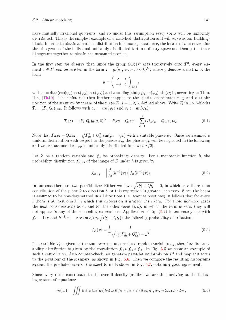
5.2. Linear matching 141
have mutually irrational quotients, and so under this assumption every torus will be uniformly distributed. This is the simplest example of a ’matched’ distribution and will serve as our buildingblock. In order to obtain a matched distribution in a more general case, the idea is now to determine the histograms of the individual uniformly distributed tori in ordinary space and then patch these histograms together to obtain the measured profiles.
In the first step we observe that, since the group SO(1)3 acts transitively onto T3, every element z G T3 can be written in the form z = g.(a1_, a2, a3,0,0,0)tr, where g denotes a matrix of the form
c s g= ,-S C 6X6
with c := diag(cos(^i), cos(^2), cos(^3)) and s := diag(sin(^1), sin(^2), sin(^>3)), according to Thm.II.3, . The point z is then further mapped to the spatial coordinates x, y and z at the position of the scanners by means of the maps Tg i = 1,2,3, defined above. Write T in 1 x 3-blocks Ti = (Pi,Qi)ix6. It follows with Ck := cos(^fc) and Sk := sin(^fc):
[Tit19]
3Ti(z) = (Pi, Qi)g(a, 0)tr = Pica - Qisa = ^(Pikck - Qiksk)ak. (5.1)
k=1
Note that PikCk - QikSk = \JP2k + Q2k sin(^k + ifk) with a suitable phase ifk. Since we assumed a uniform distribution with respect to the phases ^k, the phases ^k will be neglected in the following and we can assume that ^k is uniformly distributed in [—n/2,n/2].
Let Z be a random variable and fz its probability density. For a monotonic function h, the probability distribution fh(Z) of the image of Z under h is given by
dfh(-z) = dX(h (x)) fz(h (x)). (5.2)
In our case there are two possibilities: Either we have y P2k + Q2k = 0, in which case there is no contribution of the plane k to direction i, or this expression is greater than zero. Since the beam is assumed to be non-degenerated in all directions (i.e. scanner positions), it follows that for every i there is at least one k in which this expression is greater than zero. For these non-zero cases the next considerations hold, and for the other cases (i, k), in which the term is zero, they will not appear in any of the succeeding expressions. Application of Eq. (5.2) to our case yields with fz = 1/n and h-1(x) = arcsin(x/(akv/P?k + Qjk)) the following probability distribution:
fik (x) = -n
1
\!ak(Pik + Qik) - x2(5.3)
The variable Ti is given as the sum over the uncorrelated random variables ak , therefore its probability distribution is given by the convolution fi1 * fi2 * fi3. In Fig. 5.5 we show an example of such a convolution. As a counter-check, we generate particles uniformly on T3 and map this torus to the positions of the scanners, as shown in Fig. 5.6. Then we compare the resulting histograms against the predicted ones of the exact formula shown in Fig. 5.7, obtaining good agreement.
«i(Xi) = h1(a1 )h2(a2)h3(a3)(fi1 * fi2 * fi3')(xi, a1,a2, a3)da1da2da3, (5.4)
Since every torus contributes to the overall density profiles, we are thus arriving at the following system of equations:

142 Chapter 5. Distribution generation
Figure 5.5: Example of convoluting the two elementary distribution functions f11 and fi3, given by Eq. (5.3), with respect to a torus T3(a) with radiia = (4 • 10-3, 2 • 10-3, 0.1). The functions were determined by using the normal form map of our PS lattice at the nominal working point Qx = 6.118, and normalizing the result afterwards. All histograms have poles in the regions where the peaks are visible, but in this picture they are not fully resolved due to the finite resolution.
Figure 5.6: Top: Uniformly distributed particles (blue), generated in a shell enclosing the torus T3(a) of Fig. 5.5 in Floquet-space. The red points belong to a net of 1003 uniformly distributed points residing exactly on T3(a). Bottom: Result of mapping the top coordinates to ordinary phase space and transporting them via sectormaps to the positions of the three scanners in the PS. The wall current monitor measuring the longitudinal profile was hereby assumed to reside at the lattice start (rightmost picture).
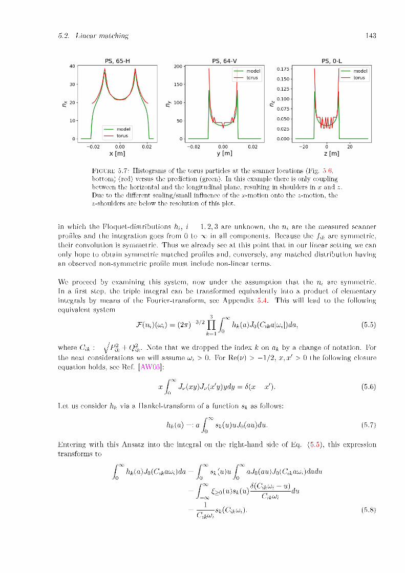
5.2. Linear matching 143
Figure 5.7: Histograms of the torus particles at the scanner locations (Fig. 5.6, bottom) (red) versus the prediction (green). In this example there is only coupling between the horizontal and the longitudinal plane, resulting in shoulders in x and z. Due to the different scaling/small influence of the x-motion onto the z-motion, the z-shoulders are below the resolution of this plot.
in which the Floquet-distributions hi, i = 1, 2, 3 are unknown, the ni are the measured scanner profiles and the integration goes from 0 to to in all components. Because the fik are symmetric, their convolution is symmetric. Thus we already see at this point that in our linear setting we can only hope to obtain symmetric matched profiles and, conversely, any matched distribution having an observed non-symmetric profile must include non-linear terms.
We proceed by examining this system, now under the assumption that the ni are symmetric. In a first step, the triple integral can be transformed equivalently into a product of elementary integrals by means of the Fourier-transform, see Appendix 5.4. This will lead to the following equivalent system
3 r raF(ni)(^i) = (2n)—3/2 JJ hk(a)J0(Cika|^i|)da, (5.5)
where Cik ■= \JP?k + Q2k• Note that we dropped the index k on ak by a change of notation. For
the next considerations we will assume ^i > 0. For Re(u) > -1/2, x,x' > 0 the following closure equation holds, see Ref. [AW05]:
x / Jv(xy)Jv(x'y)ydy = 5(x — x'). (5.6)J0
Let us consider hk via a Hankel-transform of a function sk as follows:ra
hk(a) =■ a / sk(u)uJ0(au)du. (5.7)0
Entering with this Ansatz into the integral on the right-hand side of Eq. (5.5), this expression transforms to
/ hk(a)J0(Cikawi)da = sk(u)u I aJ0(au)J0(Cikaxgdadu-J0 J0 0
= [ £>0(u)sk (u) $(<Ck '^—u) duJ—<x Cik Mi
— sk (Cik Mi). (5.8)Cik Mi

144 Chapter 5. Distribution generation
Table 5.1: Coefficients Cik determined from our PS lattice at the nominal working point Qx = 6.118 with respect to the three scanner positions. Coefficients with values smaller than 1 • 10-12 were dropped. As expected, the y-direction is decoupled from both the x- and z-direction, which are coupled themselves.
(i,k) Cik(1.1)(1, 3)(2, 2)(3.1)(3, 3)
4.1168265.050 328 x 10-2
4.998 4811.229 670
109.684 474
Plugging these functions into Eq. (5.5) and rearranging, we obtain the following equations:
Li(^i) := (2n)3/2ufCi1Ci2Ci3F(ni)(wf) = s1(Cil^i)s2(Ci2^i)s3(Ci3^i). (5.9)
Remember that we have mentioned in the beginning that, if any Cik is zero, the corresponding Sk function does not appear in the respective expression. Conversely, if they are greater than zero, sk
must appear (if we assume sk and hk are of bounded variation). In Tab. 5.1 we show examples of the Cik determined from our PS lattice at the nominal working point Qx = 6.118.
Since by assumption the ni are symmetric, the Li are real valued antisymmetric functions which approach zero if wi approaches zero. From Eq. (5.9) and the involutive nature of the Hankel transform, we can conclude that this problem can not in general be solved without further restrictions to the ni: In any reasonable scenario we are looking at three positions where each plane k contributes to the beam profile in a more or less independent fashion (i.e. we can well exclude degenerated scenarios where all scanners coincide etc.). This means that at least one of the Cik’s for k = 1,2,3 will not be zero. But if for a given direction i there are two Cik = 0, as it is the case for our PS example in Tab. 5.1, then both Sk must appear on the right-hand side of Eq. (5.9) and so if two Li ’s share the same set of sk ’s, they must have the same number of zero passages, and these passages must be related by the coefficients Cik.
In particular, it is impossible to find, in a linear setting, a matched distribution so that it projects into a Gaussian-like form onto one direction and into a parabolic form onto another direction, and where both directions are coupled: The parabolic profile is a compactly supported function, hence its Fourier-transform is an entire function of exponential type by a theorem of Paley-Wiener2 and therefore, if it would have no zeros, it would have the form exp(az + b), which is not possible.
2See e.g. Ref. [Str93]
In this context let us mention a result from [Hal14] regarding the number of expected zeros.
Lemma 5.2.1. If f is the Fourier-transform of a kernel n with
n(x) rc O(e-|x|“)
for a > 2, then f must have infinitely many zeros.
Applied to our case, this means that if the longitudinal direction is coupled at least with one of thetransverse directions, and the longitudinal profile fulfills the requirements of Lemma 5.2.1, thenthe transverse profile must differ from a Gaussian. Moreover, the zeros of their Fourier-spectra arerelated by the (coupling) constants Cik in a specific manner. Under these additional restrictions

5.2. Linear matching 145
one can proceed in examining solutions of Eq. (5.9).
In Fig. 5.8 we show the situation in the case of measured PS profiles and their corresponding Fourier-transforms. One can see how the Fourier-transform of the longitudinal profile has rather clear oscillations around its central core due to the parabolic nature of the original function, until the shape is damped towards zero, while the Fourier-spectra of the other profiles have much less visible zeros due to their Gaussian-like shape. So if we would attempt to find a Floquet-distribution in this linear coupled setting, we can expect, due to the near-Gaussian nature of the transverse horizontal profile, that some sort of irregularity start to appear.
Figure 5.8: From top to bottom: Measured profiles at the two wirescanners and the wall current monitor in the PS (left) - with respect to the nominal working point Qx = 6.118 - and their respective Fourier-spectra (right). The longitudinal profile has several clear zero passages, while the transverse profiles, as being more Gaussian-like, have literally no significant zeros.

146 Chapter 5. Distribution generation
5.2.2 A numeric testWe have analyzed what happens if attempting a solution of Eq. (5.4) numerically. Hereby we adapted the following strategy:
1. First we determine, for the three given profiles in Fig. (left), the maximal values in Floquet-space which might be occupied. Namely, the border values for direction i of the elementary histograms fik in Eq. , ak^P^. + Q2k, are summed up in the resulting con
volution (cf. Fig. due to the symmetry of these functions, and hence yield the following border for the ith direction, depending on given radii a. :
5.8
(5.3)
5.5)
x := £"k\P2k + Q2■ (5.10).
This system of equations can be inverted and, by inserting the maximal extends of the given profiles for xk, we obtain radii for the maximal expected Floquet-occupation.
2. In the next step we generated a set of ’atomic’ histograms based on a given resolution. We have chosen an initial Floquet-resolution of 60 steps from zero to the maximal a.’s of step
in every direction, leading to the number of 216 • 103 different histograms. As it turned out, care had to be taken in order to resolve the sharp peaks of these histograms in ordinary phase space: The resolution of these histograms in ordinary phase space must be sufficiently large so that the optimization routine in the next step can properly attempt to find a solution.
1
Moreover, the integration of the convolutions should be performed with the same step size as those by which the functions are passing through each other in order to avoid bias effects. An example of this problem is shown in Figs. 5.9 and 5.10: In Fig. 5.9 the histograms in the top left plot were not corrected at the poles and therefore show different spike heights. In the top right the corrected histograms with higher resolution belonging to the same Floquet-radii are shown. However, also this approach has limitations: The heights of the spikes are sensitive from histogram to histogram, and so to reduce further bias effects our next step was to choose for the spatial resolution twice the given Floquet-resolution.
In the bottom pictures of Fig. 5.9 the situation is shown for the x-direction. The left-hand plot shows an example without any a3-offset, while the right-hand plot shows the situation with offset. While the left-hand histograms look fine, the picture on the bottom right shows that there are still some small errors in the spikes due to the finite resolution of the grid, which becomes ’mismatched’ during convolution. To cure such effects, a more sophisticated method was implemented, in which we have chosen a vectorized simpson integration, together with a proper adjustment of the step sizes, leading to the results in Fig. 5.10.
After the convolutions were computed, the histograms can be safely interpolated on the final grid size for the optimization routine. Hereby we have chosen a resolution of 240 grid points for every histogram.
3. In the last step we have set the condition for a profile to be minimized: Namely we have set up a histogram-map, which maps the given (60 • 3)-dimensional ’occupation’ vector (h1,h2, h3) to its respective histogram in ordinary phase space, given as the normalized sum over all elementary histograms (l,m,n) with probability \h1(ai')h2(am)h3(an)|. The condition that the histogram is ’near’ its goal is given by the sum of the relative errors of the 240 individual entries. Hereby, the three different directions had to be weighted by the respective profileranges in order to approximate all three profiles equally. The histogram map, together with the condition function, is then ready to be minimized.

5.2. Linear matching 147
Figure 5.9: Bias effect caused by the histogram poles. On the top left we show three y-histograms using a resolution of 60 grid points in ordinary phase space, belonging to successive increases with respect to the «2-Floquet radius in three steps, from smaller (0) to larger (2) values, and a Floquet-resolution of 60 grid points. The remaining plots belong to a finer grid size, improving the spikes and which are described in the main text.
Figure 5.10: Correcting the remaining bias effect (shown exemplary in Fig. 5.9 bottom right) by convoluting with properly adjusted integration step sizes. This new case was done with a lower resolution of 30 grid points in Floquet-space and 120 grid points in ordinary phase space.Initially we have started in parallel two optimization routines to approximate the profiles.They are conveniently implemented within the Python Scipy optimization libraries: The

148 Chapter 5. Distribution generation
Nelder-Mead simplex algorithm and the Broyden-Fletcher-Goldfarb-Shanno (BFGS) quasiNewton method [JOP+01; NM65; Bro70; Fle70; Gol70; Sha70]. It was found that the quasiNewton method was more suitable for this task and we therefore switched entirely to this routine. We have then approximated the goal profiles either in an unmodified ’raw’ version or in a symmetrized version with the hope to improve accuracy.
Figure 5.11: Top: Measured beam profiles (orange) versus approximated solutions (blue) found by the steps described in the text. Because of the pronounced shoulders often seen in the x-direction due to coupling (e.g. in Fig. 5.9 bottom right), the x-approximation looks smoother. The measured profiles in this figure are symmetrized. Bottom: Similar to the top figures the situation for a Floquet-resolution of 30, by using a vectorized simpson integration with a corrected step-size.In Fig. 5.11 we show the result of the above steps and in Fig. 5.12 the situation in the respective Floquet-planes, where we clearly see the importance in removing bias effects. Due to the large parameter space, the optimizations converged rather slowly over several days of run time, while we performed several restarts in order to avoid converging into a local minimum. Although the resulting histograms tend to converge to the measurements, the corresponding occupation in the Floquet-space belonging to the horizontal tune tend to a solution which seems to be not any longer of bounded variation.
Because we found the development of some spikes in the vertical de-coupled Floquet-plane, weused this direction as a cross-check to find pure bias effects in the uncoupled case. The spikes inx and z in the top plots of Fig. 5.12 were caused by remaining bias effects due to coupling, asdescribed in point 2 above. The occurrence of these larger variations indicate a high sensitivity atthe poles and therefore emphasize that in coupled solutions with differently shaped goal profilesthe Floquet-occupation may become irregular.

5.3. Discussion 149
Figure 5.12: Top: Comparison of the action occupation determined by the BFGS algorithm of the raw (orange) and the symmetrized (blue) case for all three planes with respect to a Floquet-resolution of 60 grid points, up to a maximal action extension of «max = (3.023 • 10-3, 5.053 • 10-3, 0.321). As both cases had rather similarly looking profiles, so is their solution, because the machine precision of the optimization routine is much smaller than the used histogram resolutions. Bottom: The Floquet-occupation belonging to the improved integration procedure in Fig. 5.11, bottom. Remarkably, only a single peak was obtained in the x-plane. The reason is that due to coupling (convolution), the ’horns’ of the horizontal histograms are moving towards larger values for larger longitudinal radii, leading to the rather smooth profile in Fig. 5.11. These horns were not well resolved in the top figures under the effect of additional bias effects.5.3 Discussion
5.3.1 Conclusions
We have found evidence that in the case of differently shaped spatial (1D) profiles in a lattice with significant coupling, one can not in general expect to find well-shaped profiles for a random generator belonging to a matched distribution in Floquet-space - on the basis of linear considerations alone. On the other hand, this may be possible for profiles which do satisfy Eq. (5.9) in good approximation.
Because our result is obtained indirectly, namely in form of a contradiction, it is difficult to deduceconclusions for the case of tracking in a lattice with non-linear elements. Although in the linearcase a numeric test in form of Figs. 5.11 and 5.12 indicate that a lattice can admit two differentprofiles which are connected by coupling, with an irregularly shaped Floquet-occupation, the matter is still not fully resolved in our opinion. Under the assumption that this is indeed possible, and

150 Chapter 5. Distribution generation
that non-linear contributions can be neglected, we can proceed and attempt to draw conclusions. We will, however, emphasize that such conclusions have to be taken with care and further studies are recommended.
Going back to our PS case in Sec. 5.2.1, let us assume a coupling between the longitudinal (z) and the transverse (x) direction. We shall denote by nx, nz the spatial (1D) probability distributions, and by h1, h3 the respective (1D) Floquet-distributions. By construction, there is no correlation between the longitudinal and transverse plane, which is a consequence of Thm. II.3, Ref. [Tit19]. A particle generator will mimic this fact and thus we can expect to obtain particles having e.g. a small x-action and large z-action (depending on the shapes hi and h3).
Having a large z-action means that the corresponding particle will contribute to a histogram having large shoulders in horizontal direction, as shown in Fig. 5.10. In the course of the tracking, this particle will move further out of the beam center than a particle without significant z-action. This is similar to the contribution of dispersion to the transverse beam size. In the case of a wide h3-profile it should be clear that regardless of how thin one chooses h1, one will always get a wide nx-profile within a few betatron revolutions as an immediate consequence of coupling. This was apparently encountered during our distribution matching in the PS.
Any possible irregularity in the action-occupation, belonging to a matched distribution of goal profiles nx, nz, will certainly not be recognized by a particle generator using heuristic shapes for h1 and h3. The random generation does not recognize such fine structures and thus an immediate emittance increase in the succeeding tracking process seems to be a natural consequence.
We remark that under the assumption of h3 being entirely determined by the measured longitudinal profile, it is possible to reconstruct hi by least square inversion of the convolution process. This has been done successfully in e.g. [Oef16] in the case of hollow bunches.
To shed further light on the case of mismatch effects in coupled lattices, we suggest a followup study to determine the magnitude of the initial mismatch in dependency on either Gaussian or non-Gaussian profiles in a linear and non-linear scenario - preferably with many seeds to reduce the effect of the randomness by the generator. A complete answer to this issue will certainly include non-linear maps and probably more than three scanners.
5.3.2 ConsequencesDue to the irregular shapes found in the Floquet-profiles, and also due to space charge, we followed a more conventional approach: We generated the particles by reasonable profiles, so that their shape (and hence their rms values) at the scanner positions is close to the measurements. Then we track the particles and wait for the beam to accommodate into a stable situation, taking into account some emittance blow-up. Unless we were examining the case without space charge, we let the distribution stabilize under the additional effect of space charge. This procedure of generating particles and adjusting the emittances was done several times until everything was in satisfying agreement.
In some cases we used a refined approximation to obtain profiles whose shapes are closer to themeasurements (for the non-Gaussian cases). Specifically we generated the particles according to themeasured profiles, but now in Floquet-space, and then mapped the result to the scanner positionsto verify agreement with the measurements. Although the procedure is inaccurate, it producedfairly good results, as shown in Fig. 5.3. This was done in particular for the horizontal profile inthe SPS case and the vertical and longitudinal profiles in the PS case.

5.4. Appendix 151
The SPS case had a more Gaussian-like profile in longitudinal direction, but on the other hand there was the additional challenge that the bucket was almost completely filled. As stated in the introduction, the difficulty here was to avoid that particles were generated outside of the bucket area and then start to diverge from the main bulk in the course of the tracking, while still maintaining agreement with the measurements.
For this purpose we used higher-order map terms in the generator, which can be obtained by the PTC module of MAD-X [For16; Sch05; Abe11]. In order to make use of these higher-order terms, PTC_twiss was invoked up and including order 6 and its output was read into a Python script. Inside the script we implemented a function to map the coordinates, by going from the lowest-order map coefficients to the highest-order ones in an efficient search tree, therefore conveniently using the PTC map inside Python, where we also generated the particles and did the remaining analysis.
Fig. 5.4 shows the longitudinal phase space of a particle distribution generated for the SPS in this way, by using 6th order normal form. The edges of the separatrix can hereby be regained to a certain level. If the edges are not taken into account, the beam will tend to filament longitudinally with twice the synchrotron frequency, while simultaneously affecting the horizontal beam size due to the presence of dispersion terms, as it was discussed for the PS case in Fig. 5.1. Fortunately, these oscillations are damped due to decoherence within the first couple of synchrotron periods.
5.4 Appendix
We will derive the steps from Eq. (5.4) to (5.5). First we show a small lemma.
Lemma 5.4.1. Denote by J0 the Bessel-function of the first kind, which is extended to negative values via x ^ J0(|x|). Then this function satisfies
^,. 2 C[-i,i](y)FiJ")iy:' \ n vr=y2■ (5.11)
where F(f )(y) := —= f™ f (x)e tyxdx denotes the Fourier-transform of a function f and fD the y 2ncharacteristic function of a domain D.
Proof. By Bessel’s integral representation [MOS66]
J0(x) = — I cos(x sin(z))dz nJ o (5.12)
we get, using arcsin(u) := z and n — arcsin(v) := z for u, v G [0,1] and x > 0:
1 r/2 cos(x sin(z))dz + 1 n Jo nJ n/2
— [ cos(xu) 1 du + —nJ o V1 — u2
1 r1 MM iu = 1 f1
1- [ cos(xv) 1 dvnJ-i V1 — v2
eixu. du
fi\ u2
2n J-^ n
Since the right-hand side can be extended, and is identical, for x < 0, the claim follows.
nJ-i v 1 — u2 nJ-i1 f~ [2 „ , ,
Jo(x)n
cos(x sin(z))dzJ n/2

152 Chapter 5. Distribution generation
Denote by F the Fourier-transform, Cj the characteristic function of a domain D and by J the Bessel-function of the first kind, which is extended to negative values via x ^ Jo(|x|). If we now consider for a > 0 the map g(ix) := Jg(aw), then from F(g)(x) = F(Jg)(x/a)/|a| it follows withLemma 5.4.1
FIMx) = F fr-yllx)., (5.13)n Ca2 — x2
^ f(( 1 \ 1 1-= F (g)) (u) = -= F2(g)(u) = -= Jo (a|W|). (5.14)
2n y2n 2n
The left-hand side in the first Fourier argument of Eq. (5.14) is precisely the form of fik, if wechoose a accordingly:
F(fik)(u) = ~^Jo (akCik|w|), (5.15)V 2n
where Cik := Jp2 + Q2k. Now we are in the position to apply the Fourier-transform on Eq. (5.4).

153
Chapter 6
Simulation results
6.1 Preliminaries
In this chapter we present and discuss the main results of the simulations of all codes regarding the integer experiments. We begin with a description of how we set up the codes.1
6.1.1 Lattice preparationsBefore we began our simulations, some additional adjustments to the lattices had to be done for both machines. As already mentioned in Chapter 3, due to PyOrbit requirements we had to replace all cavities by a single generic cavity. Furthermore in the PS case we had to remove the poleface windings as they were switched off in the experiment. After the experiments were performed, it turned out that the removal of the poleface windings had a rather dramatic effect on the horizontal beta-function and the dispersion, as shown in Fig. 3.5. This caused MAD-X to quit during the process of the space charge optics generation, much earlier than expected: even at our nominal working point (!).
Nonetheless, this removal was recommended in order to avoid the not well-known higher-order components in the poleface windings. These higher-order components may change every time we set a different current in order to change the tune [Ste18; Hus16].
Furthermore, we modeled the closed-orbit in the lattice by means of small dipole kick errors. These adjustments were done for both machines at the nominal working points and shown in Fig. 6.1. These kick corrections were obtained in MAD-X by utilizing a Singular Value Decomposition (SVD) optimization routine and additional custom scripts.
Note that this procedure requires the start distributions to be generated around the new closed- orbits in order to avoid artificial initial emittance blow-up due to filamentation effects. We have therefore placed all optics matching scripts after the kick corrections were set. Hereby we used always the same kicker correction file, independent on the tune. A check for the situation at other working points revealed that we are still in a satisfying agreement, see Fig. 6.2.
In order to overcome the early exit of the MAD-X SC module at our working points, we first determined the field strengths for the quadrupoles to ramp the bare tune without space charge to those values observed in the experiment. In this way we generated the tune-ramp tables. After generation of these ramp-tables, we created the space charge optics at a tune of Qx = 6.140 (the Qy-tune was kept). The tracking script was then initiated with the respective optics, together with the previously determined ramp-tables, and inside the TRACK loops the proper quadrupole field strengths were set. The command twiss was not called afterwards. Thus we were not able to run MAD-X in full adaptive mode where the optics is recomputed by a twiss. Therefore in the
1They are listed in the beginning of Chapter 3.

154 Chapter 6. Simulation results
Figure 6.1: Closed-orbit modeled in the MAD-X lattice at the nominal working points. Top: PS case at Qx = 6.118 in horizontal (right) and vertical (left) direction. The script found a slightly better solution in vertical direction than in horizontal. Bottom: The SPS case at the working point Qx = 20.144.MAD-X adaptive mode presented in this chapter, only the emittances based on the actual action occupations are recomputed turn-by-turn.
6.1.2 Distribution matching
According to the results of Chapter 3, Subs. 3.4.1, we have chosen grid sizes of 64 x 64 x 30 in the slice-by-slice model and 64 x 64 in the 2.5D case with a longitudinal binning of 20 slots. It was found that around 105 macroparticles in these setups gave good results in regards of convergence. For the MAD-X cases we had to make a compromise between better statistics and speed (and also disk usage), so we have chosen 4000 macroparticles.
As discussed in Chapters 4 and 5, and indicated in Chapter 3, Fig. 3.18, it was difficult to find a suitable initial distribution in the codes which remains stable under the effect of space charge and - in particular in the PS case - also stable under the effect of the dispersive part coming from the vicinity of the integer resonance. For the PIC codes we had to vary the three emittances as well as the initial shape of the profiles during the particle generation process. The profiles were mostly Gaussian, but also non-Gaussian with respect to some directions.
The analytic codes MAD-X frozen, adaptive and PyOrbit analytical have additional ’degrees offreedom’: In these cases one also has to set initial values for the two emittances related to thetransverse components and the energy-spread. In the MAD-X case this has to be done already atthe stage when the space charge optics is generated, as described in Chapter 3. In the MAD-Xadaptive mode the emittances have to be defined at least in the beginning.

6.1. Preliminaries 155
Figure 6.2: Closed-orbit in the PS and the SPS, now at Qx = 6.053 (top) and Qx = 20.036 (bottom), closer to the integer in comparison to Fig. 6.1, but using the same quadrupole error strength table.
There are some constrains in choosing the model emittance values, since the space charge tuneshift is derived from those values, so we have chosen to insert the initial emittances determined from a lattice without space charge. The general problem with this freedom is that it does not naturally lead to a self-consistent model, which we require at least for the start situation: The Bassetti-Erskine space charge elements inside the lattice, which require initial emittance values, are changing the optics once again, but the observed beam size and energy-spread values of the distribution during the tracking process should stabilize near the same values as they were originally observed.
In summary, the three emittances used to generate the macroparticle distributions had to be adjusted in an iterative fashion for all six tracking codes by hand in rather time consuming tracking tests each over at least one synchrotron period. Hereby, the pronounced coupling between the horizontal and longitudinal motion due to dispersion present in the PS prevented us to adjust the two emittances ex and ez independently.
Instead of focusing on the emittances, which depend on the underlying optics model (e.g. with our without a space charge model, higher orders, etc.), and on the shape of the measured profiles, we have primarily used the three measured beam profiles as a reference, taken at the two transverse wirescanners and the wall current monitor. To obtain initial values, we generated the distributions in Floquet-space and mapped them by the linear normal form of the bare lattices to the locations of the scanners for comparison. An example of this procedure was shown in Chapter 5.

156 Chapter 6. Simulation results
Note that at this early generation stage it is not possible to use a normal map determined from a covariance matrix (see Ref. [Tit19]) under the influence of space charge, because these maps already require a stabilized distribution.
In Figs. 6.38 to 6.44 and 6.45 to 6.49, Appendix 6.4, the outcome of the above iterative procedures for all codes and both machines at the nominal working points are shown. For the next discussion of the two machines, we split the discussion into two parts, as both machines will behave differently. Hereby we will focus our main attention to the PS case, where we also describe our methods in detail. Later on we apply these methods to the SPS case, where we will report the outcome of the same analysis.
6.1.3 Space charge and linear optics
We emphasize that emittance in the context of our simulations is not a phase space volume. Here it is the outcome of a linear consideration and, furthermore, based on the finite number of particles. Therefore it is a model-dependent indication of how the single-particle phase space volume may change under the influence of non-linear effects and particle interactions. In the following we will present two different methods to compute the emittance. Both methods are discussed in detail in Ref. [Tit19].
The first method is a conventional approach by using the linear normal form from the underlying bare lattice. In principle this method corresponds to the standard way of using the Courant-Snyder optics functions and the dispersion of the bare lattice, but, moreover, includes all linear coupling terms of the bare lattice. Although the emittances computed in this way will remain stable if the tune is changing (as we shall see below), the normal form is computed from the bare lattice and therefore can not take into account any additional effect which is not included in the lattice. In particular the method can not take into account a possible tune-dependent space-charge-induced change in the dispersion. In this case the emittances of this method will in general be changing.
The second method computes the symplectic spectra of the covariance matrices under the assumption of a linear effective optics and a stabilized distribution with respect to this optics. This method therefore includes contributions from all sources, including space charge. As we shall see, this second method is more adequate in our case, although it too relies on the assumption of an underlying linear model, which is of course only an approximation.
The emittances of both methods are invariant in a linear scenario where only the tune is changing and the underlying optics parameters remain constant: Assume that we are changing the tunes of a given one-turn map from pk to pk, k = 1,2, 3, where the new tunes are also mutually distinguishable, and G is a matched distribution of M1. By the initial assumption, the respective linear one-turn maps M1 and M2 can be written, according to Thm. II.3, [Tit19] (and Thm. II.7 ibid. in the case of the second method), as Mi = SRiS-1, i = 1,2, where S denotes the mutual linear map from Floquet-space and Ri are block-diagonal matrices containing the old and new tunes. According to Thm. II.5 ibid., we can write G = SD1Str with respect to M1, where D1 is the diagonal matrix containing the emittances of G. Then by Lemma VI.8 ibid.,
M2GMtr = SR2 S-1SD1Str S-tr R Str = SD1Str = G,
so G is also conserved under the new map M2 and again by Thm. II.5 ibid, it must hold G = SD2Str
with respect to M2 . It follows D1 = D2 . The interesting part in this calculation is that in thecase of the second method it holds for the linear part of any optics, in particular in a space-chargedistorted optics. Therefore, if we see a change in the emittance evolution computed by the second

6.2. PS integer experiment 157
method, then there must be a non-trivial change in the effective normal form S, outside of the discussed freedom in conclusion II.11, [Tit19].
The importance of the linear part of the space charge force is outlined in e.g. [Sac71; VKR98]. Even without any knowledge on the effective space charge force field, one can find properties regarding the incoherent and coherent motion.
In particular, the beam center is not expected to see any direct space charge effects and, furthermore, the motion of an individual particle relative to the beam center does not see any dipole errors from the underlying lattice. This can be made plausible by the following argument, outlined in Ref. [Baa98]: For a particle i with coordinate xi let
N _xi + Kxxi = Fx,ij + Fx,ext. (6-1)
be the equation of motion, where FSCj denotes the x-component of the force of particle j on particle i, Fx,ext. additional external forces and the prime the derivative with respect to s2 By Newton’s third law, averaging over the particles i yield:
x + Kxx — Fx,ext., (6.2)and the relative motion of the particle coordinate xi with respect to the beam center is given by the difference equation
N(xi — X)" + Kx(xi — ;ri Fx,Cj + (Fx,ext. — Fx,ext.)- (6.3)
j=1In the case that the external force does not contain any higher-order driving term (i.e. is only s- dependent, as in the case of a localized dipole kick), the expression containing the external forces on the right-hand side of Eq. (6.3) vanish and only the pure space charge force remains. Furthermore, if the particle in question resides near the center of the beam, the space charge force is in good approximation linear3 and relative to the center: ^2j F^C ~ kx(xi — X). In this case, Eq. (6.3) goes over in
(xi — x)" + (Kx — kx)(xi — x) — 0. (6.4)
In a simple model with constant focusing kx, the space-charge constant kx induces a tune-shift of the particle motion relative to the beam center. This shifted tune is called the incoherent tune, as it concerns the motion of the individual particle (notice the similarity to the model discussed in paragraph 1.3.2, here, however, relative to the non-stationary beam center X). Eq. (6.4) or, more generally, Eq. (6.3) does not contain any external zero-order driving term, so if there are no other driving terms for the integer resonance (and if there is no parametrically driven resonance), the incoherent tune can be integer without any consequences. The individual tunes can be extracted by means of frequency analysis tools, which can remove the motion of the center xx from xi . The same reasoning can be applied to the other coordinates.

158 Chapter 6. Simulation results
Table 6.1: Tune-ramp goals set in the PS simulations. The Qy tunes are hold constant.
Qx Qy6.0435 6.22656.0533 6.22396.0610 6.22426.0652 6.22376.0702 6.22506.0767 6.22306.0814 6.22396.1883 6.2250
6.2 PS integer experiment
6.2.1 Emittance evolutionThe PS simulations were set up over a period of 15 • 103 turns, where the ramp towards the tunegoal spans a period of 12 • 103 turns, starting at turn 1000. This period of time corresponds to the settings in the experiment in which the ramp took place within around 2.75 ms. The tune-goals were set as bare lattice tunes according to Tab. 6.1 and close to the ones measured at the BPMs. The ramp tables were generated for both codes according to their respective input format.
A check that we are ramping in an adiabatic fashion is depicted in Fig. 6.3, were the beam size evolution is compared between ramps within 5 • 103 and 12 • 103 turns4, so that we can conclude that this condition is fulfilled.
Figure 6.3: Beam size evolution in the PS towards the Qx = 6.053 working point within the two different turn frames 1000 ^ 13000 and 5000 ^ 10000. The dashed horizontal lines indicate the measurement and their spread. This issue will be discussed in Subs. 6.2.2.A comparison of the two emittance calculation methods, which we mentioned in Subs. 6.1.3, is shown in Figs. 6.4 and 6.5 for the ramp from the nominal tune at Qx = 6.118 towards Qx = 6.053
2The necessary constants between the time and the s-coordinate are neglected here.3 See also the discussion in Chapter 1 regarding the space charge kicks in MAD-X and the discussion in Chapter
3, Subs. 3.2.2 concerning the transverse kick differences after passage through a single PIC node.4The larger time span corresponds to the settings in the experiment.

6.2. PS integer experiment 159
for all codes. From the emittance evolutions in these figures we can make a first observation that
Figure 6.4: x-emittance evolution of all space charge codes by using linear normal form for tunes ramping from Qx = 6.118 to Qx = 6.053 in the PS (method 1). The black vertical dashed lines indicate the tune-ramp start and stop at turns 1000 and 13000 respectively. Not all emittances start at the same value, because they were found after a preliminary matching procedure in which the beam stabilized in the respective space charge optics of the model. In addition there is a small spread coming from the random generator. The normal form maps were hereby computed turn-by-turn along the ramp to ensure correct application of the method and the inclusion of the change in the dispersion of the bare lattice.
Figure 6.5: Emittances computed from the symplectic spectra of the covariance matrices, in which the linear part of a tune-dependent space-charge-induced dispersion change is recognized (method 2). In contrast to the result in Fig. 6.4, the two PIC codes are now nearly flat, while the codes based on the Bassetti-Erskine model are still growing.the analytical PyOrbit model and the MAD-X codes generally predict a much stronger emittance blow-up than the PIC codes. This emittance blow-up is in parts irreversible, as shown in the respective de-ramp plots in Figs. 6.6 and 6.7.
We remark that a conserved emittance in a scenario of linear space charge with dispersion isin agreement to the established model in Ref. [VKR98]. Only the two PIC codes in Figs. 6.5 and6.7 and - expectedly - the no-space charge case are satisfying this condition fairly well, while thecodes based on a Bassetti-Erskine model do not. This implies, by the considerations done in Subs.6.1.3, that the effective optics in these codes is changing significantly if approaching the integerand must be induced from non-linear contributions of the space charge optics. From the figures

160 Chapter 6. Simulation results
Figure 6.6: Emittances computed by method 1 for the de-ramp situation from Qx = 6.053 to Qx = 6.118.
Figure 6.7: Emittances computed by method 2 for the same de-ramp as in Fig.6.6.it is apparent that it also comes in parts from reversible processes and in parts from irreversible processes. Due to its recognition of space charge, we will consider the emittances computed by the second method for the remaining part of this chapter, unless otherwise stated.
Fig. 6.8 shows the result of ramping towards the integer and back again in the case without space charge, in order to display the magnitude of non-linear effects of the bare lattice. We see from the figure that at the bare working points the effect of these non-linearities on the otherwise conserved emittances is relatively small. As these non-linearities are distortions in the Poincare section and can therefore depend on the position in the ring, we remark that our calculations are with respect to the lattice start, unless we explicitly say otherwise. Similarly, the effect of non-linear contributions of the space charge optics is visible in the two PIC cases (yellow and black) in Figs. 6.5 and 6.7 in form of the small increase and partially decrease in the emittance.
The remaining emittance offsets for the PIC codes after the de-ramp to the nominal working point can only come from non-reversible effects. These effects are caused by an interplay between particle interactions and the chaotic regimes near the integer resonance. Qualitatively speaking, the relation between the probability that particles are kicked into chaotic regions and the converse probability, that they are kicked back into non-chaotic regions, is changing the closer we get to the integer resonance. Whenever a particle is residing in a chaotic region, the finite numeric resolution, together with its frequently updated interaction with the other particles, is generating emittance

6.2. PS integer experiment 161
Figure 6.8: Effect of non-linearities on the emittance calculation during ramp and de-ramp for the no-space charge reference scenario. In a perfectly linear situation, the emittances are conserved as discussed in the text. The reversible effect can therefore be explained by small non-linearities in the Poincare section, which start to appear in the vicinity of the integer and disappear again if moving the tune back. These non-linearities affect the beam shape which is then causing a non-linear change in the entries of the underlying centralized covariance matrix of the distribution. The emittances shown here correspond to the green curves in Fig. 6.5 and 6.7.growth. In addition, the code may be non-symplectic on its own, which can produce an additional contribution to this growth, see Chapter 3 for a discussion.
In this regard Fig. 6.9 shows the situation without any tune ramp. We observe a small increase in the horizontal emittance, which is erratic and seems to be of irreversible nature. The difference in comparison to the vertical direction is likely due to the proximity to the integer resonance, which is already present to some extend at the nominal working point.
As already stated, the codes based on the Bassetti-Erskine model show a significantly larger irreversible emittance increase if approaching the integer resonance. The different performance of the analytical MAD-X codes (frozen and adaptive) in comparison to the PyOrbit analytical code is likely caused by the effort done prior to the tracking to obtain a more self-consistent space charge optics, see Chapter 3: Instead of using the beta-functions and the dispersion of the bare lattice, as it is the case in PyOrbit analytical, the MAD-X space charge nodes are using the optics functions in a more self-consistent manner, i.e. recognizing their own contribution.
The qualitative differences between PyOrbit analytic and the PIC codes can not be explained

162 Chapter 6. Simulation results
Figure 6.9: Emittance growth and noise related to the transverse Floquet-planes for all codes over the entire ramp period at the nominal working point Qx = 6.118. The start distributions are identical to those of Fig. 6.5entirely by irreversible processes: In the analytical PyOrbit code, a larger part of the emittance is again decreasing in the de-ramp in Fig. 6.7. This effect has to come from the different modeling of space charge and its effect on the beam moments.
An example of the differences between stable space charge force fields of the analytical and the slice-by-slice model are shown in Fig. 6.10. Although these pictures are taken at an individual node, they represent typical space charge kick actions which are applied on stabilized distributions in the simulation near the integer. We see how the more self-consistent slice-by-slice model produces a more linear space charge force field. This observation is supported by the previous finding, where the emittances were not increasing as strong as in the analytical case if the force remains linear (Fig. 6.5).
6.2.2 Beam sizeBy our lattice modifications we were also able to display the predicted beam size evolution for all codes at the location of the wirescanners for the same ramp situation as considered in Figs. 6.5 and 6.7. To our surprise the experimental values were in very good agreement with the case without space charge, which is shown in Fig. 6.11. This subsection is therefore dedicated to an examination of this result. Because this result was the same for every other working point, as depicted in Fig. 6.12, we will focus on the Qx = 6.053 case.
In a first step, we computed the change in the dispersion seen by the individual particles fromthe linear part of the effective space charge optics. This can be done under the assumption of a

6.2. PS integer experiment 163
Figure 6.10: Example of a space charge node kick action in the analytical code (left) and the slice-by-slice code (right) at Qx = 6.053 (at the same position in the lattice). Shown are the central particles of the bunch with respect to the longitudinal beam position. The distributions belong to stabilized distributions at this working point. The figure indicates a different behavior between the codes after the tune-ramp towards the integer.
Figure 6.11: Beam size evolution in the PS simulations for the ramp toQx = 6.053 (top) and back to the nominal working point (bottom) in the situation of Figs. 6.5 and 6.7 at the location of the horizontal wire-scanner H.65. The black horizontal dashed lines indicate the measurement results (central line) and their error spread (top and bottom lines) at the nominal working point before the ramp and at the integer.
matched distribution using the centralized covariance matrices, discussed in e.g. [Tit19]. At thelocation of the horizontal wire-scanner H.65 this yields a dispersion evolution depicted in Fig. 6.13.

164 Chapter 6. Simulation results
Figure 6.12: Final beam sizes at the end of the tune-ramps for all working points. We have hereby averaged over the last 800 turns. The plain tracking case is in good agreement to the experiment. The dips at the working point Qx = 6.043 closest to the integer are caused by losses.From this figure it is apparent that the additional contribution from the space charge nodes is tune-dependent, increases if approaching the integer and decreases after moving back again. The dispersion and beta-values at the start and at the end of the tune-ramp for the various codes are given in Tab. 6.2.
Table 6.2: Statistical dispersion and beta-function (see e.g. [Tit19], Subs. II.C) at the nominal working point and at the end of the ramp towards Qx = 6.053 for various space charge codes, at the location of the horizontal wirescanner 65.H. Note that for the analytical and the 2.5D code the ^-values are fluctuating at the start of the simulation, as visible in Fig. 6.14.
Code Dx [6.118][m] Dx [6.053][m] (5x [6.118][m] $x [6.053][m]no-sc 5.361 7.761 15.525 11.5422.5D 6.079 10.541 8.226 10.173
sbs 5.975 10.505 14.008 10.202analytical 6.017 10.888 8.439 10.859
frozen 6.320 9.911 13.456 10.948adaptive 6.207 10.509 13.702 10.730
Near the integer resonance the largest contribution to the beam size apparently comes from such dispersive contributions: For example, if we assume a given energy-spread (dp/po)rms, then we can - in a first step - compute the emittances ex from the observed beam sizes at the nominal working point Qx = 6.118 by inserting the dispersion and beta-function values, which were extracted from simulations shown in Figs. 6.13 and 6.14. In a second step, we can then compute the beam sizes at the point Qx = 6.053 with the approximation that these emittances are unchanged, and using again the dispersion values shown in Fig. 6.13.
This will yield in fairly good agreement the simulated beam sizes of Fig. 6.11 with certain contributions coming from the betatron part and the dispersive part, summarized in Tab. 6.3. The beam sizes ax at the working point Qx = 6.053 were thus computed under the assumption of a constant energy-spread of (dp/po)rms = 8.519 • 10-4 and constant emittances ex, by using the optics from the tracking data. Note that in the estimate of Tab. 6.3, the emittances were computed by using the basic formula ax = flxex + D2(dp/po)2.

6.2. PS integer experiment 165
The numbers in Tab. 6.3 should provide sufficient evidence that the main source of the beam size increase near the integer resonance is the dispersion. If we would have used the emittances determined near the integer resonance, this will qualitatively not make much difference to the fact that the dispersion plays the dominant role: For example in the analytical case, if using an emittance of ex = 2 • 10-6, we would get ax = 9.683 • 10-3 m and a breakdown of this value (squared) between the betatron part and the dispersion part of around 23.16% + 76.84% at Qx = 6.053.
Even if we include an error of 1m in the dispersion, which is in the range of what we measured on the beam centroid, the issue of a discrepancy between simulation and experiment remains. For example, in the slice-by-slice case we would arrive, using such an error, at a beam size ax of around ax = 8.187 • 10-3 m, which is still significantly away from the measurement, and a breakdown of 18.1% to 81.9%.
Table 6.3: Breakdown of beam size calculations near the integer resonance in the simulations, at the location of the horizontal wirescanner H.65.
Code ex[m] ax [6.053][m] [^x£x + Dl (6p/p0}lms]°%no-sc 9.154 x 10⁻⁷ 6.868 x 10⁻³ 22.40%+77.60%2.5D 1.121 x 10⁻⁶ 8.885 x 10⁻³ 14.45%+85.55%
sbs 7.125 x 10⁻⁷ 8.622 x 10⁻³ 9.78%+90.22%analytical 1.146 x 10⁻⁶ 9.192 x 10⁻³ 14.73%+85.27%
frozen 5.505 x 10⁻⁷ 8.107 x 10⁻³ 9.17%+90.83%adaptive 6.034 x 10⁻⁷ 8.578 x 10⁻³ 8.80%+91.20%
The situation at the nominal working point and at the working point Qx = 6.053 after the tuneramp are displayed along the entire ring in Figs. 6.15 and 6.16 for the beam-sizes and the dispersion, respectively.
We have examined the situation for the analytical and the slice-by-slice code in more detail. As already observed, near the integer the distribution in both codes are stabilizing into rather different shapes. While in the analytical code the particles are stabilizing in the outer regions of the nonlinear space charge force field, the slice-by-slice particles are spread over a larger and more linear region, while also maintaining a significant population in the central region, see Fig. 6.10.
In all considered space charge codes, space charge kicks are applied at fixed positions in the ring. In order to obtain an estimate of the ’first-order’ or ’average’ kick strengths of these nodes for particles having an energy-offset in the order of 5rms := (Sp/p0')rms, we determined the rms value of the positive and negative parts of the space charge kicks for every node, as shown exemplary in Fig. 6.17. Hereby we considered those particles near ±5rms, within regions of ±4.7 • 10-5. These
Table 6.4: Average beam sizes along the ring for the two working points of Fig.6.16.
^x,av.[6.118][m] ax, av. [6.053] [m]2p5d
analytical sbs
4.785 x 10⁻³ 9.969 x 10⁻³
4.779 x 10⁻³ 1.248 x 10⁻²
5.012 x 10⁻³ 9.562 x 10⁻³
nosc model
4.849 x 10⁻³ 6.509 x 10⁻³
4.860 x 10⁻³ 6.288 x 10⁻³

166 Chapter 6. Simulation results
Figure 6.13: Dispersion evolution in the PS simulations for the ramp toQx = 6.053 (top) and back to the nominal working point (bottom) at the location of the horizontal wirescanner H.65. The cyan horizontal lines show the result of a MAD-X twiss command without space charge. As expected, the twiss values agree fairly well with the no-sc case. Since we have adjusted the initial distributions of all codes according to the measurements at the wirescanners until we reached stable solutions, and the space charge nodes in these codes are changing the optics, also in the beginning there is an offset relative to the no-sc case.
positive and negative parts do not differ too much around the ring (the differences were found to be in the order of 10%). Computing the averages of both kick-values provides us with kick strengths along the ring which are depicted in Fig. 6.18 (we had 869 space charge nodes overall). From this figure we make the observation that space charge is apparently not smoothly treated in the simulations.
We will now outline an explanation of the differences to the experimental beam sizes. Since we are dealing with a complex simulation scenario, we have undertaken careful investigations to find reasons in the code or the setup which might explain the differences, but so far did not found any other alternative explanation. Nonetheless we emphasize that what will now follow is a possible explanation which certainly require further investigations. However, it might explain i) why the beam sizes are going back towards near their original values ii) why this phenomenon is not observed in the SPS (see later) and iii) why it is present in all considered space charge codes. We begin with an examination of the PyOrbit analytical space charge model.
As described in Chapter 3, the PyOrbit analytical code takes a lattice as the underlying tracking model and, on top of this lattice, space charge nodes are inserted at specific locations. In orderto compute the local space charge force in the machine, these space charge nodes hereby take the

6.2. PS integer experiment 167
Figure 6.14: Evolution of the horizontal beta-function in the PS simulations belonging to Fig. 6.13 for the ramp to Qx = 6.053 (top) and de-ramp (bottom) at the location of the horizontal wirescanner H.65. The analytical and the 2.5D code show an erratic behavior at the beginning of the simulation.position-dependent optics functions (in this case: the beta-function and the dispersion) of the bare lattice as reference: They enter the space charge kick maps via the local beam size, together with the given (and fixed) emittances and the energy-spread.
For the moment we shall assume that the design orbit of the bare lattice resides transversely at zero, causing the analytical model to assume that the beam center resides at zero, and hence the space charge kicks are computed relative to zero. Furthermore that, besides of the space charge nodes, there are no additional sources of errors in the original bare lattice. Since the space charge field is stable (frozen here, or stable in the sense of the adiabatic tune-ramping) and the space charge nodes are always at fixed positions in the ring, tracking with such space charge nodes therefore corresponds to tracking particles in a lattice with certain error sources, given by the multipole components of these nodes.
By examination of the stable space charge force fields of these nodes (or alternatively from the formula of Bassetti and Erskine) in Fig. 6.10, these error sources should be of quadrupole type near their center and of other orders in those regions where the shape of the force field is not linear anymore and where it finally goes over into zero. As indicated in the figure, many macroparticles can in fact reside in these non-linear force-field regions.
In the course of the tracking, the particles will thus experience certain error sources, which areinduced by the stable space charge potentials, and which will not change in repetitive revolutions

168 Chapter 6. Simulation results
Figure 6.15: Beam sizes along the PS ring at the nominal working point (top) and at the working point Qx = 6.053 near the integer (bottom), after the ramp stopped, for all PyOrbit simulations. The average values along the ring belonging to these curves are provided in Tab. 6.4. The black vertical lines denote the position of the horizontal wirescanner 65.H in the lattice. Since we have set up all simulations so that their matched horizontal profiles are in agreement with the measured horizontal profile at the nominal working point, the curves in the top plot are all in agreement at this position. We observe a significant beam size increase for the various space charge codes in those regions where the dispersion (squared) is largest (see Fig. 6.16, bottom).by definition of stability. From Fig. 6.10 (and by the nature of space charge), these space charge error sources are primarily of antisymmetric shape relative to the beam center. Because space charge is a repulsive action, the off-center components will hereby kick any off-center particle further away from the beam center.
To continue our examination of the behavior of these errors we make (temporarily) one additional simplification: Namely, that the energy change is slow in comparison to the transverse motion, so that within a certain range of turns the energy offset of the individual particle can be considered as constant. Particles having an energy-offset, and therefore moving around its non-zero dispersive orbit, will thus see steady space charge kicks similar to what is shown in Fig. 6.17.
If we consider a fixed space charge node at a positive dispersion value, then particles with apositive energy offset relative to the beam center will experience on average the main bulk of thespace charge field in form of its dipole-component, primarily kicking outwards, while particles witha negative energy offset - and hence on an orbit which is on average smaller than the beam center- will experience a similar kick, but now in a direction primarily inside, towards the ring center(and away from the beam center). It will depend on the energy offset of the individual particle and

6.2. PS integer experiment 169
Figure 6.16: Dispersion along the PS ring belonging to the same cases as in Fig.6.15. The no-sc case and the bare model are literally on top of each other, while all cases with space charge show a similar amplitude offset, which increases if approaching the integer. The average dispersion values along the ring belonging to these curves are provided in Tab. 6.5.also on its phase of how it will be affected by these fields, see Fig. 6.17.
Because the errors in the off-center region, of which we are interested in, are suppressed near the beam center (where the space charge force goes through zero), we have to consider primarily those particles which have an additional non-zero dispersive closed-orbit, given by a suitable energy offset relative to the beam.
Any quadrupole gradient error will shift the tune of the individual particle motion, while the errors induced by the energy-dependent dipole-components will lead to a tune-dependent change in its dispersive offset, if the original dispersive offset (i.e. without space charge nodes) of the particle would go through these regions. Let us assume that the motion of the particle in such a scenario can be approximated - with the energy-offset 6 as additional parameter - by the inhomogeneous Hill equation
x" + K (s)x = F (s,6). (6.5)
The term K expresses the effective focusing of the lattice, giving rise to a tune Q. We want to distinguish two components of F. The first component G describes the contribution of the unperturbed lattice. The second component G constitute the errors coming from the space charge nodes, so we have F = G + G. Overall, the general solution x of Eq. (6.5) is the sum of the general solution x^ of the homogeneous equation and a particular solution xF for the inhomogeneous equation. As the inhomogeneous term F splits into the two previously mentioned components, by linearity of Eq. (6.5) so does the particular solution xF = xq + xe. The first component x q,

170 Chapter 6. Simulation results
Table 6.5: Average values of the dispersion along the ring for the two working points of Fig. 6.16.
Dx,av.[6.118][m] Dx, av. [6.053][m]2p5d 3.094 3.189
analytical 3.090 3.194sbs 3.091 3.189
nosc 3.042 3.132model 3.043 3.134
Figure 6.17: Average kick strengths (red) for particles near ±drms for both space charge codes at Qx = 6.053. Top: analytical code, bottom: slice-by-slice code. Left: particles within drms ± 4.7 • 10-5, right: particles within — <5rms ± 4.7 • 10-5. The dispersion values shown are those at the position of the space charge node of Fig. 6.10 and belong to the respective optics with space charge, see Fig. 6.16. The kick strengths are hereby determined from the (non-centralized) rms values of the particles within the central z-slices, indicated by the black vertical lines. The different colors, which indicate the x-values, correspond to the different shapes of the matched analytical and slice-by-slice distributions near the integer, see Fig. 6.10.belonging to G, is related to the usual dispersion Dx of the bare lattice: xq = DxS. The second component xe is the part of which we are interested in. So xe will have to satisfy the following equation
x'e + K (s)xe = G(s,5). (6.6)
Hereby we expect an additional 5-dependency in the driving term G, because - as discussed -the kicks from the dipole-components are off-center, energy-offset-dependent and antisymmetric innature. By a Floquet-transformation we will now remove the s-dependent term K in front of xe.

6.2. PS integer experiment 171
Figure 6.18: Slopes of the averaged space charge kicks, applied to the particles at the space charge nodes around the PS. The kick strengths were determined by choosing particles having energy offsets near ±6rms, according to Fig. 6.17, from the matched distributions at Qx = 6.053. Several spikes are visible in both the analytical code (top) and in the slice-by-slice code (bottom). Both graphs belong to different distributions which were ramped towards the integer using the two codes. The black vertical lines indicate the position of the node which was shown in Fig. 6.10.Define:
1 fs 1 , , _V(s) :=n ~Mg\ds- (6-7)Q Jo P(s)
By periodicity of the machine it holds <p(s + nC) = p(s) I 2nn, where C denotes the circumference and n G Z.
Since the integration is performed over a smooth positive function, Eq. (6.7) can be inverted to express s in dependency of ^. In particular, all expressions in Eq. (6.6) can be understood as depending on ^. By the above relation, an increase of <p by 2n corresponds to an increase of s by C and so all optics functions are periodic in <p with period 2n.
For convenience we will drop the parameter 6 in the next lines. Set p(^) := xe(<p)/y/ft(g>). By making repeated use of ds/d<p = QP we arrive at
+ Q2n = Q2p3/2G. (6.8)dg>2
As both sides of Eq. (6.8) are periodic in ^, we can make the following Ansatz:
00d(^) =: 12 nkeikv, (6.9a)
ooP3/2(p)G(V)=: £ Gk<PkG (6.9b)
k=-tt

172 Chapter 6. Simulation results
The backwards-transformation to obtain e.g. the coefficients Gk reads
Gk = 71 / p3/2(<p)G(<p)e-ik^d<p, (6.10)2n
where the integration goes around the origin in the complex plane. The 5-dependent coefficients Gk £ C are called integer stopband integrals [Lee12]. Inserting the expressions (6.9a) and (6.9b) into Eq. (6.8) and comparing coefficients yields
_ Q2Gknk Q2 - k2 ’ (6.11)
^ xe(s,5) = JJ(s) Q^jW). (6.12)
k=-tt
Now consider an expansion of G in terms of 5: G(s,5) ='^Lp=1 (j(s)5j. Hereby we have used the fact that for 5 = 0 the dispersive orbit will be zero and hence no resulting space charge kick is applied.5 Inserting this expansion into Eq. (6.10) yields Gk(5) =: ZkA (kj5j with certain gkj £ C. It follows with
,--- _2L Q2ADj (s) := %% £ QQ-j<ekW (6.13)
k=-<x
that AD1(s) = dxe(s)/d6\§=o, i.e. AD1 corresponds to the dispersion of a periodic lattice containing the space charge energy-dependent dipole-components. This term, together with the higher- order terms, is a candidate to describe the gap between the dispersion of the bare lattice and what we see in the simulations, as we shall see in a moment.
To obtain an estimate for the effect of the space charge kicks, we consider the first-order contribution of the above series on a matched distribution of particles. This means that at a given position s, let xi = x^ + Dx6i + AD1 5i be the position of particle i, where the betatron motion x^ contains a particle-dependent phase-offset and an amplitude, while the dispersion terms are dependent on the individual energy offset 5i . The betatron motion and the dispersive motion are two independent contributions to the solution of the underlying inhomogenous Hill-equations, and thus are uncorrelated:
(x2) = {x2̂) + (Dx + ADi)2 (J2). (6.14)
In order to make use of Eq. (6.13) in Eq. (6.14), we also have to include the signs of the individual space-charge kicks applied around the machine on a particle having a dispersive orbit with respect to a given energy-offset. For our numeric estimations we will assume that these signs coincide with those of the bare dispersion values. Taking this consideration into account, while using the kick strenghts of Fig. 6.18 in Eq. (6.10), Fig. 6.22 show the outcome of our estimations.
We remark that, due to the contribution of the space charge nodes, the individual tunes exhibit a certain spread. This spread can be determined by a frequency-analysis tool. In Figs. 6.19, 6.20 and 6.21 we show examples of the outcome of such a tune analysis far and near the integer. From these frequency maps we see that the macroparticles begin to line up mainly in two narrow bands near the integer once the bare tune is moved to Qx = 6.053. It turned out that at Qx = 6.053 in the analytical case 93.6% of all selected macroparticles have tunes close to the integer, while in the slice-by-slice case these are 47.8%.
5This expansion can be motivated by inserting the dispersive offset DxS into the space charge force. In fact, Gshould be antisymmetric with respect to S, because space charge is antisymmetric with respect to x = DxS.

6.2. PS integer experiment 173
In Fig. 6.22 we were using emittances of ex = 1 • 10-6m and ex = 2 • 10-6m for the slice-by- slice and the analytical code respectively, which correspond to those values found at Qx = 6.053. The order of magnitude of the effect on the dispersion and the beam size seems to be in fairly good agreement with those found in the simulation, shown for the Qx = 6.053 cases in Figs. 6.15 and 6.16, although we made heavy use of linear approximations.
0.2250.2000.175
° 0.1500.1250.100
analytical at Qx = 6.118
0-amplitude (0.118, 0.225) max. inc. ts.
Figure 6.19: Result of an analysis by SUSSIX to determine the main frequency of every particle, for the analytical code at the nominal working point Qx = 6.118 (left) and at the working point Qx = 6.053 (right). Hereby we have selected 2000 random particles out of the total number 105 over a period of 1024 turns, and used the linear normal form of the bare lattice prior to this analysis in order to improve the data. We observe the population of two frequency bands if approaching the resonance. The point of the predicted maximal incoherent tune shift is marked by an orange point in the nominal case (left), while the bare tunes are indicated by the black points. At the nominal working point we have also tracked an individual particle with a small initial amplitude relative to zero, marked by a cyan dot. In the calculation of the tune shift, as well as in the simulations, we have used a form factor of f = 1.1289, which is discussed in Chapter 3.We are now discussing in steps what may change if moving from this simplified model back to the case of the simulations. Let us first discuss the effect of a cavity in this model. Clearly, the previously mentioned dispersive orbits of the individual particles are no longer closed but, instead, will start to slowly move according to the momentary energy-offset of the particle, from e.g. positive to negative values relative to the beam center in a periodic fashion. The particle motion itself will oscillate around this moving reference offset with a shifting tune. Such a movement is depicted in Fig. 6.23 (left) or, in the extreme case of a particle with small initial amplitude, in Fig. 6.24.
Because we are in a matched situation, a particle will roughly see a similar space charge kick for varying 6 and z values, as visible in Fig. 6.23 (right). Such a z-dependency can in principle be included into the Ansatz. We have tested both variations and found no significant differences between a pure 6-dependency and a z-action dependency. By taking into account that the synchrotron oscillation takes place at much larger time scales than a typical revolution around the ring, we expect that the momentary situation will be close to the energy-independent case.
From the tune-analysis of the two bands in Fig. 6.21 (right) we found that the macroparticlesin the right-hand band are residing mainly in the regions with larger 6-offset (positive as well asnegative), while those particles in the left-hand band reside mainly in the transition regions where6 changes sign. However, this ’mirroring’ result of the tunes should be taken with care, as ourtune-analysis was performed over 1024 turns - which are not much longer than a full synchrotronperiod of around 750 turns. It is therefore possible that this is an artifact of the relatively short

174 Chapter 6. Simulation results
Figure 6.20: Frequency analysis on the tracking data of the slice-by-slice code (top) and the 2.5D code (bottom) with the same color code as in Fig. 6.19. While there is almost no difference visible between the codes at the nominal working point, at Qx = 6.053 there are more particles with tunes not on the two frequency bands in the PIC cases than in the analytical case.0.220.20
O 0.180.160.14
Qx= 6.053
0.00 0.02 0.04 0.06Qx
Figure 6.21: The left-hand plot shows the same situation as in Figs. 6.19 and 6.20 for the case Qx = 6.053, while the right-hand plot shows a close-up of the situation around the integer. The particles near the integer were found in two narrow bands at around Qx = 6 ± 0.00119, indicated by the cyan vertical lines.turn span in combination with the non-linearities near the integer. For example, by looking at themotion of a particle starting with a small initial amplitude (see Fig. 6.24), we see that this particlecan move from an eye-shaped region of phase space into another one as the energy is changing.During the transit near 6 = 0 the particle can follow a larger trajectory which essentially coversboth eyes in double time.

6.2. PS integer experiment 175
Figure 6.22: Estimation of the magnitude of the change in dispersion (top) and rms beam size (bottom) due to the errors induced by the energy-dependent dipole-components in the space charge nodes. These errors were determined around the ring for every space charge node according to Fig. 6.18. These results should be compared with those from the simulation, depicted in Figs. 6.15 and 6.16.To visualize how particles with an energy-offset are contributing the most to the observed increase in beam size in the simulation, we have performed an ’endoscope’ on the beam near the integer over a period of 75 turns (which corresponds to around 1/10 of the synchrotron period of the PS). We have marked all particles which are outside of a certain ^-value during that time. Then we have tracked these particles over around one synchrotron period. Fig. 6.25 shows a snapshot during this tracking process at turn 38, where the main bulk of the particles fulfill the condition. As discussed, the maximal extend of the eye around which these outer particles are rotating is determined not only by the bare lattice dispersion, but also by the contribution from the space charge nodes.
In the previous considerations we have also assumed that the beam center resides at zero. This was intended in order to disentangle the position of the beam center from the argumentation. We will now drop this assumption. As initially described, we have included some kicker correctors in the lattice to obtain a single-particle closed-orbit, similar to what is seen in the experiment. Due to the effective changes in the optics by the space charge nodes, this single-particle closed-orbit is not completely identical to the one by which the beam center of the macroparticles will stabilize. This is shown in Fig. 6.26 where we see how different space charge codes lead to different stable beam centers, while the same underlying bare optics is ramped adiabatically. Regardless where the new center resides, by assumption of stability it has to be closed in good approximation. Due to such changes there is often an unavoidable small initial mismatch, causing betatron oscillations of

176 Chapter 6. Simulation results
Figure 6.23: Left: Example of tracking a particle over 1024 turns in the analytical model at Qx = 6.053, having an initial energy-offset. The situation is shown for the lattice start and the space charge kicks of the first space charge node, applied to the longitudinally central particles of a stable distribution, are superimposed (orange). This node resides also at the lattice start. Over time, the particle moves from one side of positive kick strength to the other side of negative strength, according to its energy offset 3. Right: The same situation now with respect to the x-z-plane. The space charge kick strengths for the stable distribution were linearly interpolated, showing that over time this particle will experience roughly the same kick strengths of the node (besides of the signum), even if 3 and z are changing. The resulting space charge force fields which are stabilizing near the resonance are generally found to be distorted from those at the nominal working point.
Table 6.6: Spread and mean of the centroid kicks depicted in Fig. 6.27 in horizontal and vertical direction along the PS ring. The rms values of the horizontal kicks in the analytical case are just one order of magnitude lower than the space charge kicks on the individual particles.
(APx)rms (ApC (.^Py)rms (APy)
sbs 4.887 x 10⁻¹² 2.166 x 10⁻¹³ 7.292 x 10⁻¹² -5.881 x 10⁻¹⁴
analytical 4.250 x 10⁻⁸ 7.728 x 10⁻⁹ 4.452 x 10⁻¹⁰ -1.126 x 10⁻¹¹
the beam center.
It will depend on the code whether or not the space charge kicks are computed relative to the beam center. In the analytical case kicks on the center due to space charge can be an additional source of error: By analyzing the net-kick on the beam center around the machine at the space charge nodes, we observe that in this code the net-kicks are around one magnitude smaller than the space charge kick differences themselves, as shown in Fig. 6.27. Kicks on the beam center due to direct space charge are unphysical, since they violate Newton’s third law.
For brevity let us call error sources which affect the beam as a whole external, and the space charge kicks on the individual particles, minus the previously mentioned external kicks, internal. I.e. the internal kicks in the codes do not affect the beam center by definition. Hence, the previous considerations should be applied for the internal kicks on the particle motion relative to the closed-orbit of the beam center.
If external kicks (in the above sense) are present, they can influence the orbit of the beam. Becausethese particular kicks may depend on the space charge force of the beam, they are hardly predictable during particle generation. This was also one reason for our heuristic particle generationapproach and the tune-ramping experiment, in order to minimize a possible closed-orbit mismatch

6.2. PS integer experiment 177
0.00020
0.00015
0.00010
0.00005
0.00000
-0.00005
-0.00010
qi
Figure 6.24: Trace in the analytical space charge model of a particle starting initially with a small amplitude over 1024 turns. The bare tune was set at Qx = 6.053, and the largest spike in the tune-spectrum of the particle was found to be at Qx = -7.455 • 10-4 + 6, Qy = 6.185. Over time, its dispersive orbit will change from the outer region to the inner region and back again, in dependency on its energy offset 5 (bottom). Such undistorted phase space plots were only visible in the analytical codes. Note that all but the bottom right plot are drawn in the linear normal form of the bare lattice. In the bottom right plot the situation in the tracking coordinate system is shown and the space charge field strength kicks are superimposed (orange), similar to Fig. 6.23. We see how the x-extension of this particle reaches outward in the x-range of [-3.385 cm, 3.585 cm] in the course of the tracking.
due to this effect. In the course of the tune-ramping, such errors will contribute to the change in the closed-orbit of the beam centroid, similarly as we have discussed for the individual particles. In Fig. 6.26 we show the situation at the lattice start, where in the analytical case the beam center wanders off from the others, while in the MAD-X codes it remains near the bare lattice case, and only show some fluctuations in the order of the synchrotron period. The effect of the net-influence on the beam center due to the space charge nodes can also be made visible in a Fourier spectrum, shown in Fig. 6.28.
Let us now discuss the situation for the PIC codes. As in the analytical model, the kick is applied at fixed positions in the ring. Since we are in a matched situation, the space charge field will be stable and affect the individual particle in the same manner in every revolution. The difference to the analytical model is that the shape of the space charge force field generated by the macroparticles is different, qualitatively because the force field has to ’uphold’ itself, which leads to a larger population of particles in the central regions, as indicated in Fig. 6.10 (right). If too many particles would reside on the outer regions, space charge will be reduced again and so this situation apparently

178 Chapter 6. Simulation results
Figure 6.25: Beam endoscopy for the analytical code (top) and the slice-by-slice code (bottom) with respect to 75 turns at Qx = 6.053 and with respect to the lattice start. The red vertical lines indicate the borders we have set for the two codes to colorize those particles (dark blue) which are outside of the border within 75 turns. These borders were set to x = -0.035 m and x = -0.03 m for the two codes, respectively. The maximal extension of the eyes around which these particles are oscillating depends not only on the bare lattice, but also on the contribution to the dispersion from the errors apparently induced by energy-dependent dipole-components of the space charge nodes.
Figure 6.26: Movement of the beam centroid during the tune-ramp towards Qx = 6.053 at the lattice start. As in all of our simulations, the underlying bare lattice is identical.
cannot stay stable. Of course, also the optics near the integer will contribute to the shape.

6.2. PS integer experiment 179
Figure 6.27: Differences between the mean horizontal (left) and vertical (right) momenta of the matched distributions at the working point Qx = 6.053 after passage through all space charge nodes around the ring, for the analytical (orange) and the slice-by-slice (blue) case. The vertical kick differences are around two orders of magnitude smaller. The slice-by-slice kick differences are also much smaller in comparison to the analytical case and were scaled according to the values shown in the legend. The average and spread of these kicks are summarized in Tab. 6.6.0.0200 ■0.01750.0150
— 0.01250.0100
— 0.00750.00500.00250.0000-
Figure 6.28: Fourier spectra of the x-coordinate of the beam centroid motion of Fig. 6.26 in the PyOrbit simulations at the nominal working point Qx = 6.118 (left) and at Qx = 6.053 near the integer resonance (right). The bare model tunes are indicated by the brown vertical dashed lines. Since the space charge kicks in the analytical model are transversally fixed, the spectrum of the beam center is the result of all incoherent motions in the non-linear optics and thus spread out over the maximal incoherent shifted tune, indicated by the blue vertical dashed line. In contrast, the PIC codes predict a movement of the beam center as a single-particle, in agreement with Eq. (6.2) (and no further external driving terms). A similar effect propagates also to the second moments (not shown).
FFT PS @ Qx= 6.053
model
------ 2p5d------ analytical------ nose
sbs
0.000 0.025 0.050 0.075 0.100 0.125 0.150
In the PIC codes there is also the possibility that small fluctuations are causing the shape of the force field to differ from an exact stable situation from one revolution to the next: The beam center and additional changes in the beam size can vary slightly. At the nominal working point and at the lattice start fluctuations of the center were found to be usually in the order of 10-4
m - and below, at Qx = 6.053. These are more than one hundred times smaller than the beam extensions. Since the beam extensions determine the space charge zeroth-order kicks, and there is usually an additional damping of the center due to decoherence, the effect in the PIC codes due to such fluctuations can therefore be neglected. Our numeric estimate in Fig. 6.22 confirms this picture.

180 Chapter 6. Simulation results
Regarding the intensities in the simulations we will show exemplary two graphs in Fig. 6.29. Hereby we have taken the two working points Qx = 6.053 and Qx = 6.043 closest to the integer, where the losses in the simulation were strongest. The losses of the experimental data were reported in Chapter 4 and included here. Again we observe the best agreement to the case without space charge.
Figure 6.29: Predicted losses in the PS simulations against the experimental data, indicated by the dashed horizontal black line. The left-hand plot shows the situation for the working point Qx = 6.043, while the right-hand plot the situation for the working point Qx = 6.053. The error spread of the experimental data, which was determined by the intensity differences from shot to shot, is rather small and not visible in this graph.Together with the experimental facts we conclude that there is indication that the observed tunedependent dispersion contribution in the simulations is a consequence of the fact that the individual macroparticles with sufficient energy-offset are under the effect of regular transverse kick errors, induced by the energy-dependent dipole-components of the space charge nodes. It seems that they lead, in combination with the adiabatic tune-ramping towards the resonance, to an artificial resonance effect in the codes. The strength of this effect hereby depends on the total phase advance. There is no such additional increase found in the experimental results.
Once again we want to emphasize that this explanation seems to be plausible in our opinion, since it might explain the consistent outcome of the different codes (they all have the same underlying principle in common) and the de-ramp results (i.e. that the dispersion due to the space charge nodes is reversible), but due to the complexity of the simulation codes it is difficult to exclude alternative reasons.
The dependency of the additional dispersive terms in Eq. (6.13) on the optics parameters (the bare ^-function and the lattice phase advance <^) can not only explain the observed reversibility of the beam size, see Fig. 6.11 (besides of irreversible contributions due to emittance blow-up), but also explain why such a phenomenon is not observed in the SPS: Since the SPS has a 6-fold symmetry, it is expected that tunes which are multiples of 6 exhibit a similar dispersion blow-up as the PS. This is not the case in our studies near Qx = 20, and also confirmed by the results of Chapter 4 related to the bare lattice: The dispersion of the bare lattice was determined by measuring the behavior of the beam center, which is unaffected by direct space charge. The bare SPS dispersion does not blow up (in the code and in the measurements) and, consequently, it is also not expected in the additional dispersion contribution in Eq. (6.13) due to the space charge nodes near Qx = 20. In the next section this will be presented.

6.3. SPS integer experiment 181
Follow-up studies to investigate this matter further are encouraged. We suggest the benchmarking of this scenario with a 3D space charge code and a rearrangement of the space charge kick nodes, either by changing the number of nodes or alternating their positions on a turn-by-turn basis. Also, the dependency of the beam sizes near the integer on the initial choices of emittances away from the integer during the process of particle generation may be worthwhile to consider. From our experience there might be a small tolerance in the initial choices of ex and ez due to coupling by dispersion. The dependency of the final outcome on these initial choices is an important task which should be taken into account in future studies.
6.3 SPS integer experiment
6.3.1 Emittance and optics evolutionIn the SPS case we have simulated 10 working points in a tune range given in Tab. 6.7, using the settings for the Q-20 optics. These working points correspond to those shown in Fig. 4.3 in the SPS tune diagram. The tune-ramp was programmed according to the settings during the experiment over a range of 434 turns (corresponding to around 10 ms), and the simulations were set each over 1234 turns overall.
In contrast to the PS case, the SPS behaved rather differently near the integer. While it turned out that the dispersion in the PS played the dominant role for the beam size evolution, the dispersion in the SPS changes only slightly, see Chapter 4. Since the effect of the space charge nodes on the dispersion is primarily caused by the underlying optics functions, as it was discussed in Subs. 6.2.2, this mild behavior of the bare lattice apparently propagates to a corresponding non-divergent behavior of the space charge nodes.
If we make a similar breakdown as in Tab. 6.3 of the beam size into its betatron and dispersive part, we see that the spread from the betatron motion now becomes important: If we take e.g. the no-space charge and the analytical case, then by assuming an initial (measured) beam size of 2.5 • 10-3 m and a constant energy-spread of 6 = 1.327 • 10-3, then we will arrive for Qx = 20.036, by the same calculation as in the PS case, at a beam size decomposition of 54.9% + 45.1% for the no-space charge case and an even higher betatron contribution of 66.0% + 34.0% for the analytical case. Therefore the evolution of the beam emittances and betatron functions (including the betabeating) plays now the prominent role in regards of the beam size.
In the experiment we observed the development of rather large tails at tunes in the vicinity of the resonance, see e.g. Fig. 4.18. Such tails also persisted after moving the tune back to the nominal working point. In the simulations we were not able to reproduce these tails. This might be due to an unknown driving term of the resonance in the underlying lattice. To determine such driving terms, one would have to perform detailed investigations of the beam signals around the machine and, in a second step, include these terms into the lattice. Refs. [Ben88; BS97; HSR02; Fra+14; Per14] give an impression that this task would go far beyond the scope of this work.
Because of this reason we will focus on a qualitative presentation of the emittance evolution between the various codes in dependency on the working points and show how the simulations start to diverge from each other. Later in this section we discuss how the simulated beam sizes differ from the measurements due to the tail development.
In analogy to the PS case we begin by examining the emittance evolution for a specific working

182 Chapter 6. Simulation results
Qx Qy20.0310 20.276020.0368 20.274220.0425 20.274920.0453 20.274320.0485 20.277220.0546 20.273620.0670 20.273620.0749 20.273520.0915 20.273820.1440 20.2743
Table 6.7: Tune-ramp goals set in the SPS simulations. For the simulations we have chosen the tunes close to those measured at the BPMs - after we observed the systematic offset to the BBQ in the post analysis, see Chapter 4. As in the PS case, the Qy tunes are not changed.point close to the integer resonance. Here we will choose Qx = 20.036. The emittance evolution6
by ramping towards this working point is depicted in Fig. 6.30. From that figure we see a rather different behavior in comparison to the PS case: While all emittances remain rather constant over nearly the entire tune-ramp duration, they start to evolve further after the ramp ended. The codes based on a Bassetti-Erskine model hereby predict a larger emittance growth than the PIC codes. However the two PIC codes are now spread out more than in the PS case. The slice-by-slice code is now much closer to the case without space charge. Both of these codes predict a steady emittance increase after the ramp ended.
6Given by the second method discussed in Subs. 6.1.3.
Figure 6.30: Emittance evolution in the SPS if changing the tune from Qx = 20.144 to 20.036. The dashed black vertical lines indicate the tune-ramp duration (starting at turn 400), within which the quadrupole strengths were linearly ramped, similar as in the PS case. The offset to the MAD-X runs comes from fluctuations in the particle random generator if using a different number of macroparticles.
The situation looks rather similar at other working points, as shown exemplary in Fig. 6.31.It seems as if the tune is moving faster than the system can adapt to, i.e. non-adiabatically. Because the first wirescanner measurements inside the tune-step were taken - similar to the PS case

6.3. SPS integer experiment 183
Figure 6.31: Emittance evolution in the SPS for two other working points: Qx = 20.045 (top) and Qx = 20.054 (bottom).
- at around 30 ms after the tune-ramp ended7 (so at around turn 2150 from the simulation start), over an estimated period of at least 400 turns, we have continued to track at several working points near the resonance (in the PyOrbit cases), in order to see if and how these values will saturate. This is shown in Fig. 6.32.
7There is a 15 ms notation difference between the PS and the SPS.
From this figure we see an increase and then decrease of the no-space charge case at around turn 2250. In fact, what happened is that a thin halo developed which grows constantly and finally lead to beam degradation, see Figs. 6.33 and 6.34. The halo is rather thin and hardly visible in a histogram. We have investigated whether there are other halos for the space charge cases at the three simulated working points closest to the resonance, but did not found any other occurrence. This is likely due to the fact, as stated in the beginning, that we might be missing certain driving terms in the lattice. Besides of this case, no other simulated working point showed drops in intensity.
Similar to the PS case we show the evolution of the emittances at the nominal working point to get an estimation of the noise and the influence of the resonance at this point in Fig. 6.35. As already stated, the main contribution to the beam size in the SPS simulations is apparently the spread due to the betatron motion, which involves the emittances.
It is also of interest to take a look at how the optics functions evolve near the integer resonance, at the position of the horizontal wirescanner, in Fig. 6.36. At this position in the lattice, the optics functions in the analytical codes - and in parts also the 2.5D code - tend into opposite directions around the time where the tune-ramp ended (i.e. 3,. goes down while Dx goes up). This behavior

184 Chapter 6. Simulation resultsE
y [m
]
Figure 6.32: Extended tracking run of Fig. 6.30, now over three times its original time span, in all three Floquet-planes. The no-space charge case shows a dip in both ex and ez around turn 2250, together with a drop in intensity, see 6.34.
can also be observed at the lattice start, see Fig. 6.37.

6.3. SPS integer experiment 185
Figure 6.33: Development of a thin halo in the no-space charge case which lead to beam degradation at around turn 2250 in Fig. 6.32.

186 Chapter 6. Simulation results
Figure 6.34: Drop in the intensity at Qx = 20.036 for the no-space charge case due to the halo visible in Fig. 6.33. The horizontal black dashed line indicates the magnitude of what we would expect from the measurement.
[LU] Z3
Turn
Figure 6.35: Noise in the emittance evolution for the case without tune-ramp at the nominal working point Qx = 20.144. Because the MAD-X cases are using a different distribution, they are not shown here. In the MAD-X cases no increase in both transverse emittances is visible.

6.3. SPS integer experiment 187
Figure 6.36: Behavior of the optics functions ■■'!,■ (top) and Dx (bottom) at the location of the wirescanner 51995.H if ramping towards Qx = 20.036. The horizontal cyan lines were determined from the bare lattice model.

188 Chapter 6. Simulation results
Figure 6.37: The betatron function (top) and the dispersion (bottom) along the extended simulation period at Qx = 20.036, now with respect to the lattice start.

6.4. Appendix 189
6.4 Appendix
This appendix contains additional figures of profiles for the exemplary tune-ramps Qx = 6.118 ^ 6.053 in the PS case and Qx = 20.144 ^ 20.036 in the SPS case, related to the simulations of Chapter 6.
6.4.1 Initial and final beam profiles in the PS simulations
Figure 6.38: Measured (blue) and simulated (orange) horizontal beam profiles in all six cases for the PS simulations at the location of the horizontal wirescanner 65.H and at the nominal working point Qx = 6.118, as they stabilized during tracking and under the influence of the various space charge models. As described in the text, it was rather difficult to obtain shapes close those observed in the experiment. The legend shows the respective rms values.

190 Chapter 6. Simulation results
Figure 6.39: Final horizontal profiles at Qx = 6.053 belonging to Fig. 6.38.

6.4. Appendix 191
Figure 6.40: Final horizontal profiles in the PS of the experiment and the simulation, belonging to the run in Fig. 6.38, after ramping back towards the nominal working point Qx = 6.118. As we have only simulated a short period of time of around 2000 turns on the integer, this comparison has to be taken with care.

192 Chapter 6. Simulation results
Figure 6.41: Similar to Fig. 6.38 the situation for the vertical beam profiles in all six cases for the PS simulations at the location of the vertical wirescanner 64.V and at the nominal working point Qx = 6.118, as they stabilized during tracking and under the influence of the various space charge models. Although the rms values are very similar, the larger differences in the shapes are likely caused by the more non-Gaussian profiles of the experimental data, which apparently is not recognized in the lattice.

6.4. Appendix 193
Figure 6.42: Final vertical profiles at Qx = 6.053 belonging to Fig. 6.41.

194 Chapter 6. Simulation results
Figure 6.43: Initial longitudinal beam profiles in all six cases for the PS simulations at the lattice start and at the nominal working point Qx = 6.118, as they stabilized in the course of the tracking.

6.4. Appendix 195
Figure 6.44: Final longitudinal profiles at Qx = 6.053 belonging to Fig. 6.43.

196 Chapter 6. Simulation results
6.4.2 Initial and final beam profiles in the SPS simulations
Figure 6.45: Measured and simulated beam profiles at the horizontal wirescanner 51995.H and at the nominal working point Qx = 20.144.

6.4. Appendix 197
Figure 6.46: Horizontal beam profiles at turn 1234 towards Qx = 20.036 belonging to Fig. 6.45. Note that these figures have to be taken with care, as the SPS simulation is not in a stable state at the end of the ramp.

198 Chapter 6. Simulation results
Figure 6.47: Measured and simulated beam profiles at the vertical wirescanner 41677.V and at the nominal working point Qx = 20.144.

6.4. Appendix 199
Figure 6.48: Vertical beam profiles at the end of the tune-ramp towards Qx = 20.036 belonging to Fig. 6.47.

200 Chapter 6. Simulation results
Figure 6.49: Measured and simulated beam profiles at the wall current monitor and at the nominal working point Qx = 20.144. Note that we did use an identical start distribution in the MAD-X cases here.

6.4. Appendix 201
Figure 6.50: Longitudinal beam profiles at the end of the tune-ramp towards Qx = 20.036 belonging to Fig. 6.49.


203
Chapter 7
Conclusions
In this work two different space charge codes were tested on validity in special scenarios. These codes include different approaches in the modeling of direct space charge, which can primarily be divided in analytic models and PIC models. All models are commonly used to describe the physics of high-intensity beams in cases where the interaction between particles can not be neglected. Since direct space charge is an internal force of the system, there was e.g. concern whether a modeling of direct space charge in terms of an external force field, as it is done in the analytic models, is adequate.
Our approach to test the various models was threefold: i) we began carefully prepared experiments to measure the behavior of the beam near the integer resonances in the CERN PS and SPS storage rings. This involved measurements of the beam profiles as well as measurements of optics parameters of both machines. To provide a scenario which is as simple as possible for the simulations, we injected the beams in stable configurations away from the integer, and then moved the working point in a controlled manner close to the resonances. ii) we followed this procedure in the simulations, where we carefully set up the beam away from the integer, let the simulations evolve into stable configurations, taking care that these stable beams are in agreement with the experiment, and then ramp the tune in a controlled manner towards the integer resonance by means of tune-tables. The main reason for this strategy was that optics mismatches at the simulation start can cause significant effects on the beam, which will consequently add to any effects coming from the resonance itself, and which therefore would be difficult to disentangle. iii) we implemented analysis tools to describe the tracking results of all codes within a common framework.
The main results of these efforts were presented and discussed in Chapter 6: First, that all analytic space charge codes predict a clear non-reversible emittance blow-up, while the PIC codes predict only a mildly blow-up, if at all. Secondly, both machines were following a different behavior if approaching the integer from both the experimental and the simulation point of view: In the simulation the beam size evolution in the PS case is dominated by the dispersive part, while in the SPS case it is in equal parts determined by the betatron part and the dispersive part. In the experiment we also observed a trend to develop tails in the SPS case, while we did not observed such tails in the PS case, likely due to missing driving terms in the model.
Thirdly, because all PS simulations predicted a much stronger beam size increase as was measured in the experiment, we have studied a possible explanation of this effect in Chapter 6: Space charge in all of our considered simulation codes were modeled in form of transverse kicks at specific fixed positions in the lattice, turn by turn, where the space charge force field responsible for these kicks was either coming from a frozen model or produced by a distribution which was kept in a matched state. We have investigated whether this scenario could lead to an additional computerresonance effect. It seems that this effect apparently is not present in the experiment, because in nature space charge does not happen in form of such discrete kicks at specific fixed positions.

204 Chapter 7. Conclusions
Further investigations in this matter are highly encouraged, as we reached the scope of this work. Because of this rather exceptional result encountered on the PS, our main focus in the course of this work was indeed the PS. However, we also provided measurements and simulation results for the SPS case in a similar study, which helped us to find peculiarities of the two machines. We can conclude that in the SPS case a measurement and correction of the beta-beating near the integer resonance should be performed, since the contribution of the beta-function is rather important here. Also, that the beam size evolution near the integer resonance in the SPS is generally of a more irreversible nature than in the PS case, in both simulation and experiment.

205
Appendix A
Error propagation
This subsection is intended to summarize certain useful formulae related to error propagation which we used in our scripts and in other places.
A.1 Introduction
Let h: R” ^ R>0 be integrable and for every other integrable function g: R” ^ R set
g := {g) := y g(z)h(z)dz. (A.1)
We say h is a distribution on R” if it satisfies 1 = (1), (g) is the expectation value of g with respect to h and g a random variable. In the following we will assume that an underlying distribution h is given. For g as given as above, we set gc := g — g. Whenever we have an expression of the form g2 we mean (gc)2 and not (g2)c, i.e. we always understand in the notation that the ’c’ binds stronger than the power. For n = 1 the standard deviation or rms error a of h is given by v/{z2).
Remember that two random variables f: R” ^ R and g: R” ^ R are said to be uncorrelated, iff {fg) = (f ){g) holds. Two families of component functions {xk; k G A}, {xk; k G B} for A U B = {1,...,n}, A n B = 0, are said to be independent, iff there exist functions hi and h2
so that the distribution h can be written as a product: h(z1, ...,zn) = h1(ziA )h2(ziB )•
Remark A.1.1. Let f, g: R” ^ R be integrable. Then the reader may verify
1. f = const. ^ fc = 0.
2. {gc) = 0 and (f + g)c = fc + gc.
3. {gO = {g2) — g2.
4. fg) = {fcgc) = {fgc).
5. {fg) = fg ^ (fcg) = 0. In particular, if f and g are uncorrelated, so are fc and gc.
Definition A.1.2. For x G R” fixed and an integrable function f: R” ^ R, the function Axf: z ^ f (x + z) — f (x) is integrable and so we can consider the quantity
af := {(Axf)2). (A.2)
af is called the propagated rms error of h through f at position x.
Example A.1.3. If f is linear, then Axf = f. Especially, let xi: R” ^ R denote the projectiononto the z’th component. Then the standard deviation ai of h with respect to the z’th componentis given by ai = v'((Axxi)2) = \/((xi)2) (in particular independent of any x G R”).

206 Appendix A. Error propagation
For e > 0 and x G R” assume that f: Ue(x) C R” ^ R is analytic, where Ue(x) denotes the open neighbourhood of x with radius e (with respect to the euclidean norm), and so that its Taylor expansion around x exists:
Vz G U€(0): f (x + z) = [ezdf](x) = £-(zkdk)f (x). (A.3)^0 ^!
Hereby (zkdk)^ is expanded as it is done with ordinary numbers. Then we have for the error propagated through f
(2, oo
^^.(zkdk)f(x)J / ’ (A-4)
where the averaging process goes over the z-variables.
A.1.1 Examples1. First-order error
If we consider Eq. (A.4) to first order, we obtain a dependency of the error on the second centralized moments of the distribution:
rf = {(zkdk f (x))2c) = {((zk)cdkf (x))2) = ^ dkf (x)di f (x){(zk)c(zi)c) = (Vf (x))tr£cVf (x),Kl (A.5)
with the covariance matrix £c given by (^c)kl := ((zk)c(zl)c).
2. Summation (Bienayme formula):Let f: R2 ^ R, f (zi, z2) := zi + z2 and assume that zi and z2 are uncorrelated. Using Rmk.A.1.1 and the notation introduced in Example A.1.3 we obtain for the rms value of the sum
x . ,2 = {((zidi + z2d2)(xi + x2))2 = {(zi + z2)2> = rf + rf (A.6a)
^ X + ... = 7rf + ^2 (A.6b)3. Product:
The preliminaries are the same as in point 2 with f (zi, z2) := ziz2. Again using Rmk. A.1.1 it follows
2 2 2 2 2 2 2 °z| Z2 — \((zidi + Z2U2)XiX2) c 1 — \(xiz2 + x2zi)c — xiO2 + x2Oi1——2—
@. .2 @i @2------- = + .x1x2 x1 x2
(A.7a)
(A.7b)
4. Division:The preliminaries are the same as in point 2 with f: R x (R\{0}) ^ R, f (zi,z2) := zi/z2. It follows up to first order, using Rmk. A.1.1,
2°'zi/z2
2 x1 zy>2 x2
z2x2 c/
az1/z2
xi/x2(A.8)

A.1. Introduction 207
5. Exponentiation:The preliminaries are the same as in point 2 with f (z1, z2) := zf2. Then we obtain up to first order
af = (((z1dx + z2dy)xy)2\ = / fziyxy-1 + z2 ln(x)x^ \ = x2(y-1) (afy2 + a2 ln(x)2x^ . cc
(A.9)
If z2 is fixed (i.e. h2(z2) = 5(z2) and thus a2 = 0), this equation yields at the point (x,y)\
af = |y|xy-1 a1. (A.10)
6. Mean:Let f: Rn ^ R denote the averaging function
f(zi,...,zn) := 1 zj,
1 im.with n := (x) = — V Uk.
m k=1
n j=1
where all components are uncorrelated. From Eq. (A.6a) we know that in this case computing the variances of the sum is the sum of the variances, therefore
1 naf = n^j2 (A.11)
In particular, if all components have the same rms size a , then
a(A.12)
A.1.2 Bessel’s correction
Let n G N and h: Rn ^ R>0 integrable as in Subs. A.1, and assume all component functions x1, ...,xn are pairwise uncorrelated with the same rms size a, i.e. with Uk := {xk) we have
ik G{1,...,n}: a2 = a2 = J (zk — Uk)2h(z)dz.
Now consider for some fixed m < n the following functions on Rm:
1 mx(z1,...,zm) := — y^zk,
m k=1
s2(z1, ...,zm) := — y2(zk — x(z1, ..., zm))2,m k=11 m
r2(z1, ...,zm) := m I2(zk — U)2,
r2 and s2 can be understood as rms-valued functions with respect to a discrete measure on Rm,where r2 contains the precise expectation value (x) with respect to to the distribution h, while s2
contains the average of the m sample points. In practice, only the latter is usually determined andthe former is not known. The question thus arises how the expectation values of these functions,

208 Appendix A. Error propagation
(r2) and (s2), are related to each other and to the unerlying standard deviation a2.
We have zk — E = zk — Ek + Ek — E and therefore
m<r> = — 12<(zk — E) ),
m k=11 ™
= — ^2^(zk — pk) + 2(zk — pk)(pk — e) + (pk — E) ), m k=11mt ak + m £ (Ek k=1 m k=1
— E)2,
m
=a + m (pk—e) '
1(r2 s2) m
1
If all components are equally distributed, then pk = E and so (r2) = a2. Furthermore:
m jn \lt(zk— E — m^t(zk— x) ym z \
[zk — 2zkE + E2 — zk + 2zkx — x2))k=1 /
1 m \— x2 + — '^2(2zk(x — e)) \
m k=1
m
2
= ^e2 — x2 + 2(x — e)x^
= ((E — x)2)a2
m
where we used Eq. (A.12) for the last equation. It follows
(s2) = m—1 a2. m
(A.13)
A.2 Regression analysis
A.2.1 Linear least square fit
Let ^1, ^2, ...^n be R-valued test functions (for example monomials) on Rk and f: Rk ^ R a given function which we want to approximate. For some vectors x1, x2, ..., xm G Rk we have computed the values yi := f (xi). Then we are looking for a1,..., an G R so that the m values
01^1 (X1) + fl2^2(X1) +------+ an^n(X1) — y1,
01^1 (X2) + 02^2(X2) +------+ 0n^n(X2) — y2,. ..
°1^1 (xm) + a2^2(xm) + ' ' ' + an^n(xm) — ym,
(A.14)

A.2. Regression analysis 209
are as close to zero as possible. With the introduction of y := (y1, ...,ym)tr, a := (ai, ...,an)tr and the m x n-matrix $, given by
/ pi(xi) ••• Pn(xi) \
$ := . . ,
\ ^i(Xm) • • • ^n(Xm) )
the above problem is equivalent to minimizing a ^ |$a — y|. By setting the first derivative of |ia — y|2 = (atritr — ytr)($a — y) to zero, we obtain as a necessary condition that itr(ia — y) = 0, which is equivalent to itr$a = itry. If itr$ is invertible, the solution of the least square fit is
a = ($tr $)-i$tr y. (A.15)
The matrix $+ := ($tr$)-i$tr is called the Moore-Penrose pseudoinverse of $.
A.2.2 Formulation of the problemWe now consider the task of computing the error propagated by the least square fit of Eq. (A.15), if we assume that every measurement point (x.,yf), i = 1, ...,m, comes along with a given pair of rms errors (a.,a.). In other words, we assume that for every i G {1,...,m} there exist a family ((x^, y^fg G {1,...,Mi}) of sample points minimizing Eqs. (A.14) and distributed according to distribution functions having rms error (a.,af). We want to compute the rms errors in the components of the solution vector a as well as the rms error of the fit at a given position x.1 The rms errors a. are hereby taken with respect to given distributions hi on Rk, while the rms errors d. are taken with respect to given distributions g. on R.
1Note that we are not considering any (weighted) y2 function here.
So for every j G {1,..., n} we want to compute the rms error propagated by the function fj : Rkm+m ^ R, given by
aj = fj (xi, ...,Xm,yi, ...,ym) := (($tr (xi, ...,Xm)$(xi, .....x: )) 'i^ (xi, ...,Xm)(yi, ...^m)^j , (A.16)
as well as the rms error of the fit np(x):^2 aJ pj (x) (A.17)
j=ifor every x G Rk , where all variables xi and yi are assumed to be pairwise uncorrelated.
A.2.3 First-order fit error
We have i.j = pj (x.) for i = 1,...,m and j = 1,...,n. Let x. G Rk and y G Rm. For r G {1,..., k+1} denote
R^ . J (xfR if r<k + 1,R 3 : ■- 1 y. else,
and correspondingly d.^ := d/dCy^ Furthermore, set Aa/3 := ($tr$)a/3 = $ia$i,y = pa(xf)p^(x.). From da/3 = Aay(A-i)7^ we obtain
0 = (d.^Aay )(A-1)yp + Aay (d,^(A-i)yp)
^ d.^(A-i)yp = —(A-i)yA(d.^AAa)(A-i)a^.

210 Appendix A. Error propagation
Consequently, we have
dt,fj = di,p. ((A~1')ja<pa(xp )yp)= -(A-1 ^(dt^Ax/i )(A-1)papa(x7 )y7 + 5^ (A~1')ja(da<pa )(xp 'y + 6a,k+1(A-1)japa(xt),
(A.18)
where the middle summand of the last expression can also be written as (A-1)jadapa(xt)yt, where no summation over i is taken.
Since all variables Zt,a are assumed to be stochastically independent, we get, again by using Rmk. A.1.1,
al = ((Ctn dt. fj )2\ = ((ftu )2^ (dt. fj )2 (A.19)Jj \\^V,^ ,^ J c X^'Or c ,^ j
= 52a2 52 [-(A~Y)jx(di^Axi)(A-1)Sapa(x7)y7 + (A-1)j„d^a(xt)yt] + t=1 a=1
+ £ at [(A"~1)jaPa (xt/| 2 (A.20)t=1
Observe that for 1 < p < k it holds
mdt^Ax/i = di,^2 Px(xa)pp(xa) = d^x^tf^(xt)+ ^x(xi)d^i3(Xi) = d^^x(xi)^ti + ^txdk^l(xt).
a=1(A.21)
Again, no summation over i is performed in Eq. (A.21), although the index appears twice in the expressions on the right-hand side. The first summand of Eq. (A.21) yields, when multiplied by the terms in Eq. (A.20), together with the second summand in the first bracked of Eq. (A.20),
-(A~v')jxdk^x(xt')^ti(A-lpopaX)y7 + (A-1)jxd^^x(xt)yt = (A-1d^^tr)jt((1 - $A-1$tr)y)t.
The second summand of Eq. (A.21), if multiplied by the expressions in Eq. (A.20), yields
-(A-1)jx$txdMpp (xt)(A-1)papa(x7 )y7 = -(A-1$tr )jt((d^^)A-1^tr y)t
and therefore, using the previously defined notation $+ = A-1$tr,
m k 2 m
af =y a2y h+t((d^^)^+y)t - (A-1d^tr)jt((1 - ^+)y)tl + Vd2(<b+)2t. (A.22)fj t=1 jM^ a Jj^ t=1 a j
Remark A.2.1. K := 1 - $$+ projects onto ker($tr) (= ker($+)): It satisfies K2 = K, K$ = 0 and Ktr = K.
Finally, let us consider the fit
nP(x) =52 ajPj (x) e R, x G Rk,
j=1
according to Eq. (A.15). Following the definition, we obtain an equation similar to Eq. (A.19) in which the summation over j remains inside the square:
a2(x) = ((zt,a)2) (Pj(x)dt,afj)2. (A.23)

A.2. Regression analysis 211
The next steps can be done similar as in the derivation of Eq. (A.22), where the summation over j remains:
m fc _ f 2 map(x) = 12 ^1 [pj(x) (jX9*ty$+y)i - (A~ld^trj((1 - $$+)y)^| + 12^2(Pj(x)(^+)j»)2•
i=1 ^=1 i=1
(A.24)The curves x ^ p(x) ± ap(x) define a region which is called an rms confidence band of the fit.


213
Appendix B
Article

On emittance and optics calculation from the tracking data in periodic latticesMalte TitzeCERN, Geneva, Switzerland
In this work we examine the interplay between normal form and matched particle distributions in a linear setting. We first outline the connection between the established E-matrix method and Williamson’s Theorem. Then we show that the Iwasawa decomposition provides a natural framework for a description of beam optics parameters. Along the way we will apply these methods to a realistic tracking example, as well as provide additional examples, including the connection to the parameterization of Courant-Synder.
I. INTRODUCTION
In a particle simulation involving a periodic lattice, it is usually desired to generate particles in a matched state, which means that the shape of the distribution should not change after one passage through the lattice. In fact, if a matched distribution can be found, one often has already accomplished a great deal in the understanding of the simulation. Additionally, there are circumstances in which the knowledge of the effective emittance and optics parameters is required but difficult to compute, for example in the case of the MAD-X space charge module for the CERN PS lattice (without poleface windings) near the integer resonance Qx = 6, where the search for a closed-orbit can break down.In recent years, efforts have been made with success in using covariance matrices to compute emittances and beam optics parameters. This was demonstrated in Ref. [1] in the 4D case and in [2, 3] for the 6D case. In a later published version of [1], i.e. in Ref. [4], it was used to examine the relation between the Edwards-Teng [5] (see also Ref. [6] for a summary) and the Mais-Ripken [7] parameterization in a 4D situation with coupled optics. The results were picked up in [8] in order to compute the emittances from the covariance matrices of 6D tracking data and, in regards of code implementation, recent progress has been made to include some of these techniques into the MAD-X space charge module [9]. In Refs. [10-12] generalizations of the Courant-Snyder parameterization to 4D were examined.The aim of this work is to continue in this spirit by systematically exploring the connection to linear normal form and established theorems regarding symplectic matrices: By utilizing Williamson’s Theorem we obtain a proof of the remarkable result to obtain emittances by symplectic diagonalization of the given covariance matrix. Such diagonalizations are not unique but, as we shall see in Sec. II, by knowledge of how the underlying freedom enters into the equations we outline how to obtain faithful optics information out of the tracking data.In particular we found that the Iwasawa decomposition provides a natural framework: Two of their three factors always remain the same, while the third factor can be determined under one additional condition: Namely, that the emittances have to be mutually distinguishable. We are thus led, rather naturally, to a characterization of e.g. the optics ^-functions. We also discuss an alternative route to obtain ^-functions by a statistical argument, which was proposed in Ref. [2], and which we connect and apply to our situation.Along the way we will provide several tables from a realistic tracking scenario and three examples which illustrate the results of the technical steps. The first example establishes the connection to the well-known (2D) Courant-Snyder parameterization. The second example contains a short way of how to obtain the emittances from a 4D covariance matrix, without the necessity to compute the eigenvectors. The last example also deals with a 4D situation, now with a single coupling parameter. By means of this last example we will demonstrate certain properties of the general decomposition.For practical purposes we will summarize in Sec. III the techniques of how emittance calculations can be performed in a linear scenario, establish the connection to the familiar emittance of Lapostolle and the single-particle action. For completeness we also discuss the situation of measuring beam sizes at three different locations in the lattice.

2II. ON INVARIANT COVARIANCE MATRICES
A. Motivation and preliminaries
We consider a tracking simulation which produces, at every turn, a distribution of particles depending on an initial set of coordinates. We can compute the moments of these distributions in phase space and obtain some sort of measure of the phase space volume occupied. It is of great interest to understand how to set up a distribution in which certain functions of these macroscopic quantities remain unchanged or vary only very slowly in the course of the simulation. In the following we will understand our lattice to be in the form of a ring, but the same reasoning can be applied to a straight periodic lattice.Let F: P ^ P be a canonical transformation from phase space P C R2" onto itself, which describes the physics of the storage ring in form of a single turn around the machine at a given fixed position in the ring. Such a one-turn or Poincare map is usually the result of a composition of many elementary maps, which describe the individual elements of the machine.In this work we will examine the situation in the vicinity of an assumed closed orbit, where linear effects play the dominant role. Therefore we will be focusing on the first derivative M of the one-turn map F at the closed orbit and do not consider any higher-order effects of the full map F. Because of this restriction - and for brevity - we will also call M the one-turn map. This map is symplectic since F is canonical[30].If g: P ^ [0,1] denotes the phase space density of a particle distribution, its covariance matrix G, consisting of the second-order moments, is given by
G := ZL^XkXleket = (xxtr), (1)where, for any integrable function h: P ^ R, the mean (h) is given by (h) := f g(x)h(x)dx. We see that M acts by matrix congruence on G, where the new covariance matrix G' is given by
G' = (Mx(Mxf} = (Mxxtr Mtr} = MGMtr. (2)Such covariance matrices are important, because their entries are the ingredients to compute the emittances of the beam; in the 2D case: det f /x \ 'xP2xM = (x2)(p2) — (xpx)2 = e2. (3)\ \xpx/ \px/ JMoreover, by means of Eq. (2), we have a way to follow the evolution of the moments in the course of the tracking. Because det(M) = 1 for symplectic maps, the emittance in Eq. (3) is conserved. Note that the emittance is just one example of an invariant. In Ref. [13] functions of higher-order moments which remain invariant with respect to symplectic matrices were studied.Here we are focusing on second-order moments and address as our first goal the following question: Given M, how can we classifying all ’matched’ cases in which G = G holds? As we shall see in the course of this section, the answer will connect a property used in e.g. Ref. [3] to linear normal form.
Definition II.1. We say a matrix G G R2"x2" is M-congruent invariant or, for brevity, M-invariant, if MGMtr = G holds.To begin with, we recall an important fact which we will frequently use to identify covariance matrices.Theorem II.2. G G Rmxm is a covariance matrix if and only if G is symmetric and positive semidefinite.
Proof. A proof for convenient reference is included in Appendix VIA. □This means we are interested in M -invariant symmetric and positive semidefinite matrices G, having in mind that M is the symplectic one-turn map of a lattice in a particle accelerator. In particular this means that we can assume that the complexification MC of M can be diagonalized with mutually distinguishable eigenvalues (tunes).We will now systematically develop important properties of M -invariant symmetric matrices G. Throughoutthis section convention VI.1 will hold and all matrices are given with respect to the ordering x, y, z,px,py,pzunless otherwise stated.

3B. Invariance and linear normal form
In this paragraph we outline the interplay between the technique of transforming a given linear symplectic map M with mutually distinguishable eigenvalues into a normal form and invariant covariance matrices. We will use an important lemma which not only helps us to describe the connection, but also in the next paragraph II C where we examine the degree of freedom involved in the matrices. For a procedure of how to construct the normal version of a general (higher-order) one-turn map we refer the reader to Refs. [14, 15]. Preliminary tools are given in Appendix VI A.Theorem II.3 (Linear normal form). Let M G Sp(2n;R) diagonalizable with mutually distinguishable eigenvalues on the unit circle. Then there exists V G Sp(2n; R), so that R := V— 1MV is orthogonal, leaving the plane Ek := span{ek, en+k} for k G n invariant:
vk^. di _ ( cos(Tk) sinG?k) A Vk G n ■ Re =1, - sin(^fe) cos(^ J ’
where the phases ipk G [0, 2n[ are related to the eigenvalues Xk of M by Xjk = exp(i^k), and where the jk’s correspond to a representation introduced in Dfn. VI.3, so that for the corresponding eigenvectors ajk of M, lfljk, Jajk) has positive imaginary part.With the operator o introduced in Def. VI.6 we can conveniently write R = R1 o • • • oRn. In the acceleratorphysics terminology the phase space in which the one-turn map has the above normal form is also called Floquet-space.
Proof. A proof can be found in Ref. [16] or in Appendix VIA. □The matrix V in Thm. II.3 is not unique, as can readily be seen if composing the map by additional rotations (which are symplectic) leaving the individual planes invariant:Remark II.4. By Lemma VI.8 we can conclude that the linear normal form map V of Thm. II.3 is determined up to an orthosymplectic transformation on the left; namely, if V—1MV = R = V MV, i.e. VRV— 1 = VRV , then V V = D1 + J®nD2. Because V and V are symplectic, it follows that D2 + D2 = 1 and so ~ — 1V V has the same form as R.Theorem II.5. Let M G Sp(2n; R) diagonalizable with mutually distinguishable eigenvalues on the unit circle and G symmetric. Then MGMtr = G if and only if there exists a diagonal matrix D = diag(A, A) with A = diag(&i, ...,bn) so that G = VDVtr, where V G Sp(2n;R) is given according to Thm. II.3.
Proof. Let T be the orthogonal operator discussed in Rmk. VI.7 and R = V— 1MV according to Thm.II.3. Then we have R := R1 ® • • • ® Rn = TtrRT = TtrV—1MVT, and G is M-invariant if and only if D0 := TtrV —1GV—trT is R-invariant:
RD0R = Ttr V —1MVTTtr V—1GV—tr TTtr Vtr Mtr V—tr T = Ttr V —1MGMtr V—tr T = D0,and by Lemma VI.8 this the case if and only if D0 has the form D0 = diag(b1, b1, b2, b2,..., bn, bn), which is equivalent to D := TD0Ttr = V —1GV—tr has the form D = diag(A, A) with A = diag(b1,b2, ...,bn). □This result can be connected to a statement used in Ref. [3], and to obtain a familiar expression in the form of eigenvector decompositions, as follows:Theorem II.6. Every real-valued symmetric invariant G of M, where M is diagonalizable with mutually distinguishable eigenvalues, can be represented as a sum G = ^2n=1 9kZk of n elementary matrices with gk G R, where the Zk are given by Zk = ajkajk + ajkajrk, and where {j1,j2,..., jn} C 2n is a representation system according to Conv. VI.1.
Proof. The statement can be found in e.g. Ref. [3] in a slightly different version. A proof was included in Appendix VIB. In VIB - and only there - we have changed our notation to Mtr. This means, by Conv. VI.1, that the eigenvectors ajk appearing there are proportional to the vectors Jajk here. □
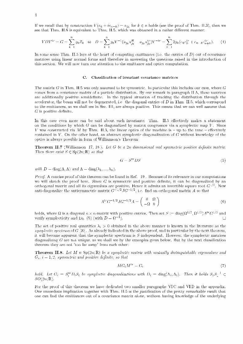
4If we recall that by construction V(ek + ien+k) = ajk for k G n holds (see the proof of Thm. II.3), then wesee that Thm. II.6 is equivalent to Thm. II.5, which was obtained in a rather different manner:
n n n
VDVtr = G = J2 9kZk O D = V gkV-1(ajka* + ajkaj)V-tr = k= (eke^ + en+ke^+k). (4)In some sense Thm. II.5 lays at the heart of computing emittances (i.e. the entries of D) out of covariance matrices using linear normal forms and therefore in answering the questions raised in the introduction of this section. We will now turn our attention to the emittance and optics computation.
C. Classification of invariant covariance matrices
The matrix G in Thm. II.5 was only assumed to be symmetric. In particular this includes our case, where G comes from a covariance matrix of a particle distribution. By our remark in paragraph II A, these matrices are additionally positive semidefinite. In the typical situation of tracking the distribution through the accelerator, the beam will not be degenerated, i.e. the diagonal entries of D in Thm. II.5, which correspond to the emittances, as we shall see in Sec. III, are always positive. This means that we can well assume that G is positive definite.In this case even more can be said about such invariants: Thm. II.5 effectively makes a statement on the conditions by which G can be diagonalized by matrix congruence via a symplectic map V. Since V was constructed via M by Thm. II.3, the linear optics of the machine is - up to the tune - effectively contained in V. On the other hand, an abstract symplectic diagonalization of G without knowledge of the optics is always possible in form of Williamson’s Theorem:Theorem II.7 (Williamson [17, 18]). Let G be a 2n-dimensional real symmetric positive definite matrix. Then there exist S G Sp(2n; R) so that
G = Str DS (5)with D = diag(A, A) and A = diag(Ai,..., Xn).
Proof. A concise proof of this theorem can be found in Ref. [19]. Because of its relevance in our computations we will sketch the proof here. Since G is symmetric and positive definite, it can be diagonalized by an orthogonal matrix and all its eigenvalues are positive. Hence it admits an invertible square root G1/2. Now anti-diagonalize the antisymmetric matrix G-1/2 JG-1/2, i.e. find an orthogonal matrix A so thatAtrG-1I2JG-1I2A = ( 0n Q (6)\ —Q U jholds, where Q is a diagonal n x n-matrix with positive entries. Then set S := diag(Q1/2, Q1/2)AtrG1/2 and verify symplecticity and Eq. (5) (with D = Q-1). □The set of positive real quantities Xi > U obtained in the above manner is known in the literature as the
symplectic spectrum of G [2U]. As already indicated in the above proof, and in particular by the next theorem, it will become apparent that the symplectic spectrum is S -independent. However, the symplectic matrices diagonalizing G are not unique, as we shall see by the examples given below. But by the next classification theorem they are not ’too far away’ from each other:Theorem II.8. Let M G Sp(2n; R) be a symplectic matrix with mutually distinguishable eigenvalues and Gi, i = 1, 2, symmetric and positive definite, so that
MGiMtr = Gi (7)hold. Let Gi = S'/'DiSi be symplectic diagonalizations with Di = diag(Ai, Ai). Then it holds S2S-1 G SO(2n; R).For the proof of this theorem we have dedicated two smaller paragraphs VIC and VID in the appendix.One immediate implication together with Thm. II.5 is the justification of the pretty remarkable result thatone can find the emittances out of a covariance matrix alone, without having knowledge of the underlying

5optics given by the one-turn map. The only assumption on the covariance matrix is that it belongs to amatched distribution with respect to the unknown linear optics: Namely, if G is given with a decompositionG = VDVtr according to Thm. II.5 and another decomposition G = StrD1S has been found, for examplefrom Thm. II.7, then we obtain with the orthogonal W := VtrS-1:
D1 = S-tr GS-1 = S-tr VDVtr S-1 = Wtr DWand since the eigenvalues can not be changed by orthogonal matrix congruence, D1 and D must contain the same entries up to a suitable permutation. In Sec. III we will see how the diagonal entries of D are connected to the classical emittances by Lapostolle (in the 2D case).6.179 x 10-61.536 x 10-81.329 x 10-51.138 x 10⁻⁷ -8.148 x 10⁻¹¹ -4.819 x 10⁻⁷
1.536 x 10-82.342 x 10-68.767 x 10-84.230 x 10-10-4.951 x 10⁻⁸-1.188 x 10⁻⁸
1.329 x 10-58.767 x 10-82.922 x 10-21.713 x 10-75.298 x 10-91.791 x 10-6
1.138 x 10-74.230 x 10-101.713 x 10-73.084 x 10-9 -7.580 x 10-135.042 x 10⁻⁹
-8.148 x 10⁻¹¹-4.951 x 10-85.298 x 10-9 -7.580 x 10-132.480 x 10-93.380 x 10-10
-4.819 x 10⁻⁷-1.188 x 10-81.791 x 10-65.042 x 10-93.380 x 10-101.371 x 10⁻⁶
TABLE I: Example of a covariance matrix belonging to a stable particle beam in the SPS at Qx = 20.144.
7.121 x 10⁻⁸ -2.906 x 10⁻¹¹ 4.643 x 10⁻⁸ -1.405 x 10⁻¹⁰ -1.657 x 10⁻¹¹ 2.463 x 10-82.906 x 10-11 5.826 x 10⁻⁸ -9.649 x 10⁻¹⁰ 8.306 x 10⁻¹¹ -1.520 x 10⁻¹⁰ 1.535 x 10-84.643 x 10-8 -9.649 x 10⁻¹⁰ 2.236 x 10⁻⁴ -6.934 x 10⁻⁹ -2.722 x 10⁻⁹ -8.960 x 10-61.405 x 10-10 8.306 x 10⁻¹¹ -6.934 x 10⁻⁹ 7.090 x 10⁻⁸ -2.198 x 10⁻¹⁰ -4.618 x 10-81.657 x 10-11 -1.520 x 10⁻¹⁰ -2.722 x 10⁻⁹ -2.198 x 10⁻¹⁰ 5.762 x 10⁻⁸ 1.440 x 10-82.463 x 10-8 1.535 x 10⁻⁸ -8.960 x 10⁻⁶ -4.618 x 10⁻⁸ 1.440 x 10⁻⁸ 1.795 x 10⁻⁴
TABLE II: Matrix V-1GV-tr according to Thm. II.5, where G is the matrix of Tab. I. The matrix is not perfectly diagonal because the full lattice contains additional effects like non-linearities, small mismatches and numeric noise which are not considered here.
In Tab. I we show an example of a covariance matrix G coming from a PyOrbit tracking simulation (without space charge) in the CERN SPS. Since G is determined under the effect of small imperfections in the lattice, V is not perfectly diagonalizing G, see Tab. II. Let us denote by |G — G*| the error between G and an ideally matched covariance matrix G* of the lattice (see Sec. III). We then see that the diagonal entries after diagonalizing G by a symplectic matrix S according to Thm. II.7 belong to such a G*, see Tab. III. Remaining small errors stem from the fact that S and V are determined by - and involved in - two different procedures.The check whether the matrix VtrS 1 is orthogonal is depicted in Tab. IV, which would be the unit matrix if V would perfectly diagonalize G. Let us summarize this finding in the following corollary.5.793 521 x 10-8 7.104 235 x 10-8 2.001317 x 10⁻⁴
TABLE III: Symplectic spectrum of G according to Thm. II.7 with respect to the horizontal, vertical and longitudinal direction. If following the procedure in Sec. III by computing the emittances using the linear lattice optics (contained in the linear normal form V), the emittances are 5.793903 • 10-8, 7.105457 • 10-8 and 2.015400 • 10-4, respectively. The agreement is remarkable.
Conclusion II.9 (Emittance from covariance matrix by symplectic diagonalization). Let G be the covariance matrix of a linearly matched particle distribution, then the emittances are given by its symplectic spectrum.Moreover, by means of Thm. II.8 and the help of the Iwasawa decomposition, we can regain optics functions out of a covariance matrix, by utilizing this natural parameterization. The Iwasawa decomposition reads [21]:

61.0021.446 x 10-3
4.914 x 10⁻⁴
-1.860 x 10⁻³
5.269 x 10⁻⁴
8.191 x 10⁻⁵
1.446 x 10⁻³
1.006-8.477 x 10⁻⁵
5.298 x 10⁻⁴
-2.643 x 10⁻³
6.747 x 10⁻⁵
4.914 x 10⁻⁴
-8.477 x 10⁻⁵
1.1171.122 x 10-4
7.149 x 10⁻⁵
-4.477 x 10⁻²
-1.860 x 10⁻³
5.298 x 10⁻⁴
1.122 x 10⁻⁴
9.978 x 10⁻¹
-1.437 x 10⁻³
-4.437 x 10⁻⁴
5.269 x 10⁻⁴
-2.643 x 10⁻³
7.149 x 10⁻⁵
-1.437 x 10⁻³
9.945 x 10⁻¹
7.311 x 10⁻⁵
8.191 x 10⁻⁵
6.747 x 10⁻⁵
-4.477 x 10⁻²
-4.437 x 10⁻⁴
7.311 x 10⁻⁵
8.970 x 10⁻¹
TABLE IV: Counter-check whether W := VtrS~1 is orthogonal, i.e. what is shown here is the matrix WtrW. Hereby the symplectic S was determined following the procedure in the proof of Thm. II.7. The error |WtrW -1| = 0.168653 can be explained by imperfections induced from the full lattice during the tracking process, resulting in divergences of G towards a perfectly linearly matched solution.
Theorem II.10 (Iwasawa decomposition of symplectic matrices). Let S C Sp(2n;R). Then there exist unique symplectic matrices K, A and N with S = KAN and the following properties:
K C Sp(2n; R) Cl O(2n; R),A = diag(D, D-1), D = diag(b1,..., bn) with bj > 0,
N ( ^tr ] , E real unit upper triangular, EFtr = FEtr.\ 0 E iIn Thm. II.15 we summarize a result in [22] of how to compute such a decomposition. If we have found a symplectic diagonalization G = StrDS of an invariant covariance matrix G, we can proceed and determine its decomposition: S = KAN. On the other hand, a linear normal form V, block-diagonalizing M, can also be decomposed as Vtr = K'A'N'. By Thm. II.8 we have S = XVtr with an orthosymplectic X, and by uniqueness of the Iwasawa decomposition it therefore follows K = XK', A = A' and N = N'. So we already found two optics factors A' and N' only by examination of the covariance matrix G.Our next goal is to understand the nature of the remaining orthosymplectic factor X. As a first step note that by VRV-1 = M, MGMtr = G and VD'Vtr := G we have
VRV-1GV-tr Rtr Vtr = MGMtr = G,^ RV-1StrDSV-trRtr = V-1GV-tr = D',and since R commutes with D' it follows
V-1 Str DSV-tr = D' (8)For the symplectic spectrum we could have used any (positive definite) covariance matrix, but for a determination of the optics functions we will now have to make one additional assumption: Namely, that the symplectic spectrum (respectively emittances) is not degenerate, which means that all emittances are mutually distinguishable. By suitable orthosymplectic permutations (their construction is given in Prop. VI.16) on K and K' let us arrange them so that without loss of generality D' = D and the 2n entries of D are in the following order:d1 = dn+1 <d2 = dn+2 <...<dn = ^2n. (9)It follows from Eq. (8), which now reads DX = XD, that diXj = Xydj or, on other words, if di = dj then
Xj = 0, and, by exchanging symbols, also Xji = 0 in that case. If we now take a look at the indices k and k + n, then we see that for all l C {k, k + n} it holds Xk,i = 0 = Xpk and Xi,k+n = 0 = Xk+n,i, so concerning

7these rows and columns X must have the following form:
^ k
f 0. 0...0 ..00 • • 0 * 0 • •• 0 * 0 ••• 00 0X = ... ...0 00 • • 0 * 0 • •• 0 * 0 ••• 00. 0...0 ..0 J
k t t k + n^ k + n
By our assumption on the mutually distinguishable pairs, and because every such group of four entries must be orthosymplectic on its own, we must have X = D1 + JD2 as in Lemma VI.8 with D2 + D22 = 1. By Rmk. II.4 this was the freedom in the choice of V, which leaves the individual Floquet-planes invariant. So without loss of generally K can be considered as equal to K' up to a symplectic permutation matrix which is exchanging the order of the symplectic spectrum and up to this freedom. Let us summarize this result:Conclusion II.11. If G is the covariance matrix of a linearly matched particle distribution, and StrGS = D a symplectic diagonalization with mutually distinguishable emittances, then the optics functions are contained in the terms K, A and N of the Iwasawa decomposition S = KAN. In particular we can regain the linear map to Floquet-space from S, block-diagonalizing M. Hereby, the factor K may contain a freedom of the form Di + JD2 with D2 + D2 = 1, i.e. of the form SO(2)n, and a suitable symplectic permutation of the components.[31]In analogy to what happens in the 2D case (see Example II.12 below), the term N can be understood as a lens- or drift factor and the term A can be described as a magnification or squeezing factor. As we shall see in Example II.16, the term K may also contain coupling and optic terms in a non-trivial fashion. Under the condition in conclusion II.11, all those three factors, and therefore the linear parameterization to normal form, are thus dependent on the n(2n + 1) parameters of the covariance matrix G only, which are 3, 10 and 21 in the 2, 4 and 6 dimensional cases respectively. The freedom in the coupling term reduces these numbers by n, so we can expect to have 2, 8 and 18 independent optics parameters in these cases.This freedom represents our inability to extract the tunes out of the covariance matrix alone and so we can expect that in repetitive measurements the additional SO(2)n-freedom enters into the covariance matrices statistically. As we will see in Example II.16, K is not in general of the form D1 + JD2. In cases one wants to obtain the exact coupling terms of an underlying model, this will require a careful analysis in order to disentangle the freedom from these coupling terms. In any case, if the emittances of the given covariance matrix are mutually distinguishable, we obtain a linear normal form map from it which block-diagonalizes M (with a certain error), as demonstrated in Tabs. V and VI.
TABLE V: Block-diagonal one-turn map M of the SPS at the tune Qx = 20.144 for the same optics as in Tab. II. Note that in this example the entries are ordered with respect to x,y, z,px ,py ,pz.
0.619812 0.0 0.0 0.784 750 0.0 0.00.0 -0.149110 0.0 0.0 0.988 821 0.00.0 0.0 0.995494 0.0 0.0 -0.094 8290.784 750 0.0 0.0 0.619812 0.0 0.00.0 -0.988 821 0.0 0.0 -0.149 110 0.00.0 0.0 0.094 829 0.0 0.0 0.995 494
As we shall see in examples II.12 and II.16, the three diagonal terms of A are directly related tothe three classical optics beta functions of the Courant-Snyder parameterization in the uncoupled case. Butas they are also appearing in a general coupled situation and are determined by a natural procedure - and

8
TABLE VI: Block-diagonal form of M now reconstructed entirely on the information of the particle distribution ofTab. I. I.e. what is shown here is S-trMStr where S was extracted from the covariance matrix using Thm. II.7.The agreement to Tab. V is very good. Note that we had to conjugate this matrix by the symplectic transpositionT12 which are discussed in Prop. VI.16.
0.6178870.003 6700.000 208
-0.786 018-0.005 988-0.000136
-0.000 045-0.145196
0.000 1600.007 309
-0.984 0760.000 050
-0.000 1090.000 0330.996 339
-0.000 1170.000 0100.106 734
0.783 5350.006 804
-0.0001440.621 5750.006 479
-0.000 040
-0.008 8430.993 562
-0.000 0190.002 528
-0.152 8630.000 014
-0.000 242-0.000 162-0.084 259-0.000 006
0.000 0420.994 648
also to distinguish them from alternative ’generalized’ ^-functions discussed below - we call these ’natural’ beta functions. In Tab. VII we show the matrices A determined from the normal form map Vtr and the symplectic map S (coming from the covariance matrix G of our SPS example) and check their relation to a twiss output from MAD-X.
TABLE VII: Iwasawa factors A determined from either the linear normal form map Vtr (top) or the symplectic map S coming from the covariance matrix G (bottom) of our SPS tracking example of Tab. I. Small differences occur because the covariance matrix G comes from a real tracking example with small lattice non-linearities, mismatches and numeric noise. From a MAD-X twiss command we compare the 1-1 and 2-2 entries (exemplary for the bottom matrix) and obtain good agreement: BETX = 84.404930, 9.1923192 = 84.498729 and BETY = 40.178387, 6.3581512 = 40.426084.
9.187 210 0.0 0.0 0.0 0.0 0.00.0 6.338 581 0.0 0.0 0.0 0.00.0 0.0 11.389 408 0.0 0.0 0.00.0 0.0 0.0 0.108 847 0.0 0.00.0 0.0 0.0 0.0 0.157 764 0.00.0 0.0 0.0 0.0 0.0 0.087 801
9.192 319 0.0 0.0 0.0 0.0 0.00.0 6.358 151 0.0 0.0 0.0 0.00.0 0.0 12.082 668 0.0 0.0 0.00.0 0.0 0.0 0.108 786 0.0 0.00.0 0.0 0.0 0.0 0.157 278 0.00.0 0.0 0.0 0.0 0.0 0.082 763
Independently on the problem of finding a faithful parameterization for the optics, one can also introduce ’generalized’ ^-functions, as proposed in Ref. [2]. The main idea is to use the analogy of the two-dimensional case, in which the ^-function appears as coefficient in the well-known relation between the emittance and the rms beam size, e.g. (x2) x /3xtx. Since the optics functions K, A and N are always the same for beams with non-degenerated spectrum, one can use the symplectic S (or Vtr of the linear normal form) in order to obtain such relations between the second moments of the matched distribution and the emittances:n n
(xixj) = etrGej = efStrDSej = ^SSjl + Si,n+lSj,n+l)h =: ^pijlAl. (10)l=i i=iAlgebraically speaking they correspond to the coefficients of the parameterization Rn ^ Sym(R2n) C
R2n ® R2n of the M-invariant covariance matrices and are by definition related to the Zl in Thm. II.6 via 2flijl = (Zl)ij. From the analogy to the 2D case (cf. G in example II.12), in which the situation goes over without coupling, one can identify /3x and 3y with 3111 and /3222, ax and ay with — 3141 and — fl22 and yx and Yy with 3441 and 352 respectively.As was shown in Refs. [2, 8, 23], these coefficients have the feature that one can also find expressions for the dispersions. The idea is that in the classical 2D theory the betatron motion and the dispersive part are uncorrelated: Let n = 3 and /y, for k = 1, 2, 4, 5 denote the dispersion function with respect to direction k, where the 6th component x6 corresponds to the energy offset 3p/p0. Then from xk = xk,^ + i/kx6

9it follows (xkX6} = yk(Xe), which translates to
w 3 3 , 3, 3/M 3k,6 Xl = n^3 36,6 Xl ^ nk = n ’ 3 , l=1 l = 1 36,6
(11)hereby the last equation was assuming a decoupled case, similar to what was previously done to relate the 3fjl to the classical optics functions. In Tab. VIII we show the general R-functions for our SPS example and their agreement with those coming from a MAD-X twiss command. It should therefore be clear how useful these statistical definitions are when it comes to situations where one can not easily determine effective optics functions otherwise, for example in the scenario of a PIC code with space charge.
84.476 949 0.774 801 -0.882 5950.774801 0.010 308 -0.010 263
-0.882 595 -0.010 263 0.010 6901.626 052 0.021 069 -0.021157
-0.023 067 -0.000164 0.000 209-0.000 297 -0.000 006 0.000 005
0.020 908 -0.757 982 -0.000 262-0.757 982 40.415 782 0.006499-0.000 262 0.006 499 0.000 004
0.000 344 -0.017 789 -0.000 0030.028 889 -0.854 362 -0.0004060.000 000 0.000 014 0.000 000
0.000 880 0.000 021 0.066 7260.000 021 0.000 001 0.0004400.066 726 0.000 440 145.988 045
-0.000 008 0.000 000 0.000 864-0.000 001 0.000 000 0.000 027-0.002 408 -0.000 059 0.008 947
1.626 052 -0.023 067 -0.000 2970.021069 -0.000164 -0.000 006
-0.021157 0.000 209 0.000 0050.043 131 -0.000 352 -0.000 011
-0.000 352 0.000 007 0.000 000-0.000 011 0.000 000 0.000 000
0.000 344 0.028 889 0.000 000-0.017 789 -0.854 362 0.000 014-0.000 003 -0.000 406 0.000 000
0.000 008 0.000 397 0.000 0000.000 397 0.042 793 0.000 0000.000 000 0.000 000 0.000 000
-0.000 008 -0.000 001 -0.002 4080.000 000 0.000 000 -0.000 0590.000 864 0.000 027 0.008 9470.000 000 0.000 000 0.000 0250.000 000 0.000 000 0.000 0020.000 025 0.000 002 0.006 850
TABLE VIII: Components of the d-tensor of Eq. (10) for our SPS example (at the working point Qx = 20.144). The following entries are going over into the classical linear lattice parameters in case of no coupling, and are given as follows in form of the output of a MAD-X twiss command: 111: BETX = 84.404930, 222: BETY = 40.178387, 141: ALFX = -1.627366, 252: ALFY = 0.850149. y-check: 441: - = 0.043224, 552: Yy = 0.042878. Dispersion: DX = -0.343296, 163/663: -0.351470, DY = -0.004177, 263/663: -0.008667. DPX = 0.003525, 463/663: 0.003678. DPY = 0.000319, 563/663: 0.000247. Note that the signs of the entries to the a’s are reversed, as expected.
Having the dispersion parameters at hand, which were determined by including assumptions of the origin of the one-turn map M, one can attempt to recover the tunes of the unknown optics - in principle. However, as we shall see, the sensitivity with respect to the dispersion terms is very high. This indicates that such an undertaking, by purely examining covariance matrices, might require more elaborate methods (and probably also better statistics by including more particles):For the next considerations we change to the ordering x,px,y,py,z,pz and write the one-turn-map M into 4 and 2-blocks
M= M4 A AB C ) ' (12)
Let Xtr = (Xi, 0,pz) for X1 e R4 describe a 4D closed-orbit solution of M, i.e. M4X1 + A(0,pz)tr = X1, which translates to X1 = (1 — M4)-1A(0,pz)tr and so D := (1 — M4)-1A contains the 4 known dispersion terms DX, DPX, DY and DPY in the second column. Although the terms in all columns of D can be approximated in an analog fashion as the left-hand side of Eq. (11) if correlations between z and the other spatial coordinates are small, and by taking into account only correlations between z and pz, let us assume that the first column is unknown. The relation V-1MV = R (V any symplectic map block-diagonalizing M, in

10Dj-1 inexact D/2 inexact Dj1 exact Dj2 exact
-3.440 703 x 10-1
3.518 960 x 10-3
-4.235 338 x 10-3
3.195 229 x 10-4
6.235 119 x 10-4 -3.400 830 x 10-1 1.143 900 x 10-3
8.110 447 x 10-6 3.533 734 x 10-3 2.491066 x 10⁻⁵
8.043 134 x 10-7 -4.242 339 x 10-3 7.223 080 x 10-6
1.321050 x 10⁻⁷ 3.187 020 x 10-4 -5.912169 x 10⁻⁸
Dj2 inexact Dj2 exactDj1 inexact False TrueDj1 exact False True
TABLE IX: Convergence successes of the Nelder-Mead simplex algorithm [24, 25] applied to Eq. (15), assuming a tune Qz = -1.511528 • 10-2 of our SPS example, in dependency of the four combinations of exact and inexact initial parameter columns. We have used 6 iteration restarts of the optimization routine. The inexact values are determined from the tracking example, in which the values of the first column were estimated by using the assumption that the z-motion is uncorrelated to the first four coordinates. As can be seen, the success depends on the precision of the dispersion terms which are in the second column of D.
particular having in mind a map coming from a covariance matrix) reads in this contextm4 A W V11 V12 \B C )\V2i V22 J
r4 0 A0 R2 )[ M4V11 + AV21
^ I BVii + CV21M4V12 + AV22 A BV12 + CV22 J
V11R4 V12R2
V21R4 V22R2 (13)hereby R4 is a 4 x 4 block-diagonal rotation matrix, as discussed in Thm. II.3. We can now use the first row to express the unknown M4 by D and the rotation matrices R2 and R4 which contain the unknown tunes:M4(Vii - DV21) + DV21 = M4V11 + (1 - M4)DV2i = V11R4, (14a)M4(V12 — DV22) + DV22 = M4 V12 + (1 — M4)DV22 = V12R2- (14b)If we assume that the 4 x 4-map V11 — DV21 is invertible (which is the case in our SPS example), we can eliminate M4 to obtain(V11R4 — DV21)(VU — DV21) 1(V12 — DV22) + DV22 — V12R2 = 0- (15)This corresponds to a system of 8 equations for 7 unknown parameters (3 tunes and the 4 entries of the first column of D). For the given data of our SPS example it turned out, however, that the sensitivity of this problem on the dispersion terms is too high, even if assuming a known z-tune, as is summarized in Tab. IX.We conclude this section with three examples.
Example II.12 (2D). For a, p e R and R 9 (3, 7 > 0 with 3y = 1 + a2 consider a linear transport map M, see Ref. [26], and a positive definite symmetric GG :=
cos(p) + a sin(p) 3 sin(p) \—7 sin(p) cos(p) — a sin(p) I ’
3—a
—aY
(16a)(16b)Then one can show that M is symplectic and it holds MGMtr = G. Furthermore, the symplectic matrices
51 :=52 :=
73 —a/73\0 1/73 ) ’
1/7Y 0 3—a/7Y 7y J
(17a)(17b)are satisfying G = SirSi (in particular, G is positive definite). This means that we have all requirements of Thm. II.8 and S2 S1-1 must be orthogonal. Indeed, we have the following Iwasawa decompositions:
S A N ( 73 0 W 151 A N 0 1/73 J 052 = A N = 7 . — a a )1
—a/3 A1 )'73 0 \ /1V 0 1/73 ) v —a/31,
(18a)(18b)

11and we see A1 = A2 and N1 = N2 and S2S-1 = K2 is orthogonal, as claimed by Thm. II.8. The two independent optics parameters a and (3 can be regained by comparison of the above Iwasawa factors with the ones obtained by any matched particle distribution according to conclusion II.11. Since MGMtr = G holds, we have M-trG-1M-1 = G-1 and therefore G-1 = MtrG-1M, which means that the associated quadratic form g(z) := ztrG-1z is M-invariant. We have g(z) = ztrN-1A-1A-trN-trz = ((AN)-tr)*12(z) or, reversely, (Atr)*(Ntr)*g = 12. The effects of these two operations are illustrated in Fig. 1 and appear frequently in elementary particle accelerator textbooks.
FIG. 1: Effect of the two operations (Ntr)* and A* on a phase space ellipse given by the quadratic form g in Example II.12, using a > 0.
Example II.13 (4D). Let G ^tr B) be the covariance matrix of a linearly matched particle distributionin a 4D tracking routine. Then its symplectic spectrum, which are the two emittances, are given bye1j2 = —=^AG ± \ AG2 - 4det(G), (19)where AG := det(A) + det(B) + 2det(C). This formula for the spectrum of a 4D covariance matrix can be found in Ref. [27] in a different context. From Eq. (19) we regain two familiar symplectic invariants:det(G) = elei,
AG = e2 + e22.(20a)(20b)The first one appears for example in Ref. [4].For the next example we need some more machinery.
Lemma II.14. Let A G K2x2 be symmetric with g > 0 so that
A = ( g 1 .\ a b
Then the LDL-Cholesky factorization A = QtrHQ of A is given by
H = diag(g, det(A)/g), Q 1 a/gQ= 0 1 .
Proof. The proof is left to the reader. Note that this equation holds also for g < 0.Theorem II.15 (T. Y. Tam). Let K G {R, C} and X G Sp(2n; K) with
□
X H X =: A1
bHB1D1 ■

12Let Ai = QhHQ be the LDL-Cholesky factorization of the positive definite Ai, where Q is unit uppertriangular and H positive diagonal. Then the Iwasawa factors A and N of X = KAN can be computed by
( H1/2 0A = ^ 0 H-1/2
N = ( Q qa-1 BiN I 0 Q-tr
Q H-1Q-trBi0 Q-tr
(21a)(21b)
Proof. See Ref. [22]. □
Example II.16 (4D optics with a single coupling term). Similar as in Example II.12 consider for i = 1, 2: ai,^i G R and R 9 fii,Yi > 0 with fiiYi = 1 + a2 and ^1 = y2 the matrices M1, M2,G1,G2 G R2x2. Let o be the operator defined in Prop. VI.6. From the properties we have J4 = J2 o J2. Let~ _ _ _ _ _
M := M1 o M2,G := G1 o G2.It follows from Prop. VI.6 with the symplecticity of Mi that M is symplectic and furthermore that G is symmetric and MGM = GG. From Prop. VI.6 it also follows that M has four complex eigenvalues of the form exp(±iyj) and by assumption it is guaranteed that no eigenvalue equals ±1. Moreover it follows that
G is positive definite. M can be interpreted as an uncoupled lattice. Let us now introduce a basic coupling term; for fi G R set c := cos(^), s := sin(^) and Sj G R2x2 as in Example II.12, Eqs. (17a), (17b), with A2)Sij using aj, fij and Yj•
U := ( C / ) G R2x2,
V := diag(U,U) G R4x4, c — s(2W Q(2) Si] := Si1 ° Sj2 .By the properties of the operator o, all four Sij are symplectic. V is clearly orthogonal and also symplectic:Vtr J4V = diag(U-1, U-1) ( -U U ) = J4
The symplectic M := VtrMV satisfies MGMtr = G with symmetric and positive definite G := VtrGV:mgm tr = v tr M VVtr G vv trMtr V = Vtr G V = G.The interpretation of G is that it describes the covariance matrix of a linearly matched particle distribution in this coupled optics. From Example II.12 we know that S^Sij = <G must hold. Therefore the symplectic
trSij := S jV are diagonalizing G as in Williamson’s Theorem: SiJSij = VtrSijS j V = VtrGV = G. Let us now use Lemma II.14 and Thm. II.15 to compute the Iwasawa decomposition exemplary in the case of S11. By construction:S11 00
0 - a 1 / yffi! 0 ^. 0 -a2/yfife0 1/VF1 00 0 1/VF2 /
s12s22 (22)
with diagonal block-matrices Sj G R2x2. It follows^ St_r1S11 =
S11 = S 11V = S12 US22 U
U -1s11U -1s12
0 s11U s12UU -1s22 0 s22U
U-1s211UU-1S12S11U
U-1snS12U \U 1(s22 + S22)U f

13Thm. II.15 tells us that we have to compute the LDL-Cholesky factorization of the positive definite
c @1c@2 SA1 := U-1S111U =
—sP1C2 + @2S2 cs(@2 — @1) A cs(@2 — @1) @1S2 + @2c\) 'By Lemma II.14, using det(A1) = @1@2, we obtain A1 = QtrHQ with
H1/2 = diag V@1c2 + @2 S2 J. 2@1@2 2@1c2 + @2S2
cs(@2 — @1)/(@1c2 + @2S2)1(23a)(23b)
In order to determine the remaining entry in the Iwasawa factor N, we compute (the details are left to the reader)X := H-1Q-trB1 = aic^+g^s2
P1C2+02S'2cs(ai-02) ^1C2+^2S2 2 2 _ 2 ai
c P2 s Pi
(23c)By Eq. (23a) we see that the determinant of the A-factor of a given covariance matrix yields @1@2. Moreover, we can recover the term y/@1c2 + @2s2 and by Eq. (23b) the cs(@2 — @1). Eq. (23a) - (23c) constitute a system of equations for the five parameters a1, a2, @1, @2 and ^ of this model and more such equations may be obtained by computing the other decompositions of Sij. In this way we can attempt to recover the entire set of parameters of this model from a given covariance matrix.Since N is symplectic, we have N 1 = —JNtr J, i.e.
N-Q-1 —Xtr
Qtr(24)1 0Using this equation, we can then compute the orthosymplectic K via K = S11N 1A 1. After some steps we find the block-diagonal form
K11 = , / oy/@1 c2 + @2S2(25)
Hereby we attached the indices on K to indicate that it emerges out of the map S11. Note that J4 = J®2, so if ^ = 0, then this term is not in the form D1 + J4D2. This example therefore completes the statement in Conclusion II.11. What happens for the other cases S12, S21 and S22? Since we expect a symmetric result for S22 let us investigate the S12 case. As we have already computed the Iwasawa factors A and N, we do not need to recompute them again. S12 has the form:^@1 0 —*1/^1 0 \0 1//Y 0 00 0 1/VF1 00 — a2//Y2 0 /Y2 J (26)
After further computations we arrive at the following orthosymplectic K12 :K12 = , J „y/@1c2 + @2S2
\ — a2 s//Y2 —ocJWi. Qf@2Y~2
0 0 \O.2s/^Yi U2c^W1 /V@272
cv@1 — s\ @s/Vr2 c/@1//@2Y2 /
(27)We see that also K12 turns into the standard form if we have no coupling. Moreover, there has to be a term D1 + J4D2 with D12 + D22 = 1 which transforms K11 into K12 . In fact, we find K12K1tr1 = D1 + J4D2 with D1 = diag(1,1/V@272,1,1//@2Y2) and D2 = diag(0, 02//@272,0, l2/V@2Y2). This corresponds to a rotation in the second plane by an angle of arctan(—a2). In general, any rotation in these planes can lead to valid K’s. Therefore it requires a careful analysis of the covariance matrices involved in order to disentangle the sought coupling terms from that freedom.

14III. EMITTANCES FROM SIMULATION AND EXPERIMENT
For large-scale simulations with many particles, the particle positions are usually not stored turn by turn, because this will generate an enormous amount of data. What can be stored without generating too much data, however, are the turn-by-turn covariance matrices of the distribution. In this section we will outline the connection to the well-established formula of Lapostolle. For completeness we will also include practical formulae to obtain emittances from experimental data.A. Simulation case
By means of the map V, given by Thm. II.3 or II.11 (from a covariance matrix) and utilized in Thm. II.5, we can parameterize all symmetric invariants G of M. As motivated in paragraph IIC, one may have the task to find, for a given covariance matrix G an M-invariant covariance matrix G* which is closest to G, so that we can apply Thm. II.5. Hereby we understand the distance between G* and G as given by the Frobenius norm. This can be formulated in a precise fashion as follows:
22A1 = (Gv,E1 }f = tr«V-1xxtrV-tr)E1) ^^tr((etTz(ekrz)tr)) = (z?) + (z22). (32)k=1 k
Let {ej; j G 2n} be the canonical basis of R2n. Introduce for k G n the matricesEk := ekekr + en+ke^ G R2"x2", (28)i.e. Ek consists of zeros besides its (k, k) and (n + k, n + k) components, which are one. Denote for brevity
Wk := VEkVtr with the notations of Thm. II.5. Then the problem stated above corresponds to the task of finding Ak G R>0 so thatf (A):= |G - AkWk|f (29)
k=iis minimized. The Ak’s then correspond to the emittances, because the covariance matrix in Floquet-space has zero off-diagonal elements for independent variables and the determinant in the individual Floquet- planes are therefore just Ak (see also example III.1 below). We remark that an expression as the sum in Eq. (29) also appears in Ref. [2]. Since h(G) := G — ^2k AkWk is extremal at a given point if and only if V-1h(G)V-tr is extremal at that point, we obtain, by using the the symmetry of (A, l>)F := tr(AtrB) and GV := V-1GV-tr:
f (A)2 = |gv IF — 2^2Ak G ,Ek ')f + Ak Ai (Ek, Ei) fk=‘ k,,=. ==:^Sk.
= |GV |F + 2 ^~^(Ak — Ak (GV, Ek)f)k=1. " 1. . „ 1 "= |Gv|F + 2 J2(Ak — 2Gv,EkP)2 — 2 YG,Ek)F■ (30)
Hence, f2 is minimal if and only if Ak :=|(V-1GV-tr,EkP■ (31)This process provides us with a closest symmetric invariant G* := Pk AkWk. Since G was assumed to be positive (semi)definite, there exist P so that G = PPtr, i.e. 2Ak = tr(V-1GV-trEk) = tr(V-1pptrV-trEk) = Aek|2 + \Aen+k|2 > 0 with A := PtrV-tr, so G* is again positive (semi)definite.Example III.1. In the 2-dimensional case n = 1 we obtain the classical emittance definition by Lapostolle (cf. [28]) as follows: Assume that G = (xxtr) is given and set Ak according to Eq. (31). With z := V-1x we get

15On the other hand, by Eq. (30) and GV = V 1GV tr = (zztr) we have
|G* — G|? = |Gv |? — 2A2, (33)hereby|GV |? = tr((zztr )(zztr)) = (ziZj )2 = (z2)2 + 2lz1z2)2 + (z2 )2. (34)| v|? (^ » j2z z) 2 1) 2 1 z 1 22 ()Now combining Eqs. (32), (33) and (34) we obtain
9A2 IA2 9A2 OlG\lG\ VE •..? -I- \G G I2 BM2A1 — 4A1 — 2A1 — 2\z1 )\z2 / — 2\z1z2l + |G — G* |_p, (35)and since det(V)2 = 1 we have det(G) = det((zztr)), therefore we regain the emittance of Lapostolle up to the Frobenius distance between G and the M-invariant G*:A2 — lAl-r2\ 1IG G I2 i36iA1 = \x1)\x2) — \x1x2) +2 |G — G* |?. (36)Example III.2. In the special case of a single particle, i.e. if G has the form G = xxtr with x G R2", then ztre2 := Aek = xtrV-tre2 (compare above) and so we get with z := V-1x the action as a ’single-particle emittance’:
2Ak = z2 + z2n+k. (37)We recall the standard 2D example of a linear transport map M of Example II.12 (or found e.g. in Ref. [26]):M = ( cos(^) + a sin(y>) 3 sin(y>) \
) —Y sin(y>) cos(y>) — a sin(y>)/ ’where 3, Y G R>o, E, a G R and 1 + a2 = 3y- Then one can show that withV ,= ( ^/VY —a/VY\ ' :\ 0 VY Jwe have Vtr J2V = J2 and
V-1MV-( cos(E) sin(E) A— sin(y>) cos(p) J ’and with x = (x1,x2)tr, z = V-1x, we obtain for the action (37):2A1 = z2 + z2 = Yx2 + 2ax1x2 + 3x2.
(38)(39)(40)(41)
B. Measurement case
In this last paragraph we will summarize of how to obtain emittances from measured profile data in this general linear setting. We assume here that the coordinates are arranged in the form x,y, z,px,py,pz. Denote for i = 1, 2, 3 M^: R6 ^ R6 the symplectic transport maps to the location of the scanners which measure our profiles (which are usually two wirescanners and a wall-current monitor) and by V: R6 ^ R6 the map from Floquet-space to ordinary phase space, which diagonalize the one-turn map M by R = V-1MV according to Thm. II.3.Assume that G is the covariance matrix belonging to a matched distribution. By Thm. II.5 we have G = VDVtr with D = diag(A, A) and A = diag(A1,A2,A3), i.e. G can be interpreted as the image of a covariance matrix of a distribution in Floquet-space, in which the individual planes are uncorrelated, transported by the map V to ordinary phase space. For i = 1, 2,3 consider the maps Ti := etM:fV, where e^ denotes the unit vector having a one in the ith position, so they project onto the spaces belonging to the x, y and z directions at the corresponding scanner locations. Now consider the linear map E: R3 ^ R3 given
tr tr tr tr tr tr trby (Ai, A2, A3) ^ (T1DT1 ,12DI2 ,13DI3 ), so its matrix entries are Ejk — T je^e^ Tj + Tje3+ke3+kTj .Since covariance matrices transport under linear maps in form of matrix congruence (see paragraph II A),the image of this map can be identified with the second moments of the distribution G at the correspondingscanner positions: (x2), (y2) and (z2). They are known from our experiments, hence E-1 provides us withthe emittances of the distribution.

16IV. CONCLUSION
We have examined in detail the close connection between linear normal form and covariance matrices belonging to a matched particle distribution. In fact, a linear normal form is contained in such a matrix: If the emittances are mutually distinguishable, then up to an SO(2)n-freedom (which can be understood as a rotation part related to the tunes) the entries of the normal form are uniquely determined. Furthermore, by means of the Iwasawa decomposition, we obtain a natural generalization of the optics ^-functions and coupling terms, which complement, together with their relation (10) to the embedding coefficients dj, our picture in this linear scenario. In addition, we have provided the connection to the Courant-Snyder parameterization and the Lapostolle-emittance and summarized useful formulae for practical applications regarding simulations and experiments.V. ACKNOWLEDGMENTS
The author want to thank Prof. Dr. M. de Gosson and Dr. F. Schmidt for inspiring comments. This work has been sponsored by the Wolfgang Gentner Programme of the German Federal Ministry of Education and Research (grant no. 05E15CHA)VI. APPENDIX
A. Preliminaries
This part of the appendix is intended as a convenient reference of properties and notations which we used in the main text. Some of these facts are known in the literature but often scattered or not easy to find in a concise and self-contained fashion. We will begin with the proof of Thm. II.2.G G Rmxm is a covariance matrix if and only if G is symmetric and positive semidefinite.
Proof. ’^’ Symmetry is a consequence of (xixj') = (xjxf). Positive semidefiniteness follows with utrGu = utr(xxtr')u = (utrxxtru) = (futrx)2) > 0. ’^’ Since G is symmetric, we can find, by Sylvester’s law of inertia, an orthogonal matrix Q and a diagonal matrix D so that D = QtrGQ hold. Since G is positive semidefinite, the diagonal entries Dk are non-negative. Set y/D by taking the square root of these diagonal elements, so that we obtain a Cholesky decomposition of G by G = QVDVDtrQtr = PPtr with P := QVD. Now take m independent random variables Zj, i.e. ^zizj') = dij for i,j = 1, ...,m. Set x := Pz. It follows G = PPtr = (Pz(Pz)tr') = (xxtr'), so G is a covariance matrix. □Let us make a notation convention:Convention VI.1. The Symbol K means either R or C. J denotes the symplectic structure
J : Jn : 1 n
0G K2n x 2n
where 1n denotes the identity matrix in Knxn. The upper letter ’H’ on a matrix means transposition and complex conjugation. For x, y G C2n we understand (■, •) as the sesquilinear form (x, y) :— xHy if nothing else is stated. We will sometimes use the abbreviation n :— {1, ...,n} for n G N. If V is a vector space, we denote its complexification by Vc and for M: V ^ V, we sometimes denote its action onto Vc by MC. However, this notion will be dropped whenever the context is clear.Let M G Sp(2n; R) be diagonalizable with mutually distinguishable eigenvalues. We denote by {aj; j G 2n} a fixed basis of eigenvectors, where aj G C2n belongs to the eigenvalue Xj G C. Because M is real, Aj is the eigenvalue of the eigenvector aj of M. We have for all i, j G 2n:
Xi(ai,Jaj) - (Mai,Jaj) - (ai,Mtr Jaj) - (aCJM-1 aj) - 1/Xj (ai,Jaj) - Xj (ai,Jaj}, (42) so we conclude, since all eigenvalues are mutually distinguishable, that if i - j, then ai and Jaj areorthogonal. Because of this orthogonality, the fact that {Jai} is a basis of C2n and (•, f is non-degenerate,

17it must hold that Vi: (a,, Jaf) = 0, and these values are purely imaginary, which follows by (x, y) = (y,x)with Jtr = —J. Set iaj := (aj,Jag') with aj G R\{0}. Since —iaj = (ag,Jag') = (dj,Jag), we can choosea representation system {j1, j2,.., jn} C 2n of the equivalence relation introduced in Dfn. VI.3, so thatVk G n: <jjk = 1 hold.The eigenvalues of Mtr coincide with M, and if we set bi := Ja,, then
Mtr bi = — JM-1Jbi = JM-1ai = XJa, = d b,,i.e. b, is an eigenvector or Mtr with respect to X,. Let us summarize:1. If we speak of an eigenvector b, of Mtr we will always understand b, := J a, for a given (and fixed) system of eigenvectors {a,, i G 2n} of M.2. From the properties of M we always have i = j ^ (a,, Jaj) =0.3. There is a subset {j1, ...,jn} C 2n so that Vk G n: (ajk, Jajk) = iak with R 9 ak > 0 holds.Proofs of the next statements are straightforward. They are required in the proof of the linear normal form Thm. II.3.Proposition VI.2. Let V be a K-vector space and M: V ^ V linear. Then all eigenvectors of M belonging to mutually distinguishable eigenvalues are linearly independent.
Definition VI.3. Let V be an R-vector space and M: V ^ V linear. Assume that MC has mutually distinguishable eigenvalues {Xj G C; j G I0}. Since M is real, it also admits the complex conjugate eigenvalues. So we can introduce on I0 the equivalence relation i ~ j :O X, = Xj. We denote the equivalence class of j G I0 by [j]. They constitute of pairs of indices.Proposition VI.4. Let V be a real vector space and M: V ^ V linear. Assume that MC has mutually distinguishable eigenvalues {Xj G C; j G I0} with corresponding eigenvectors aj = Xj + iyj G Vc so that Xj ,yj G V. Then {xj1 ,yj1 ,Xj2 ,yj2,...} are linearly independent in Vc for every representation system {ji,j2,...} of the equivalence relation introduced in Dfn. VI.3.
Proposition VI.5. Let V be a real vector space and M: V ^ V linear. Let X G C, be an eigenvalue of Me
with eigenvector a = x + iy G Vc so that x,y G V. Then the C-vector space spanned by x and y in VC is M -invariant and it holds
Va, 3 G C: M(ax + /3y) = (aXR + /3Xf )x + (3Xr — aXi)y, (43)where Xr := Re(X) and Xi := Im(X) are the real and imaginary parts of X.The next map emerged rather often in our programs as well as in some formulae, so that we found it useful to write it down as reference. It appears whenever we had to switch between the (x,px,y,py,..) phasespace notation to a block notation of the form (x, y, ...,px,py,...). But we also used this (non-symplectic) isomorphism in Thm. II.5 to transport a statement regarding 2 x 2 matrices to a statement regarding block matrices and where it is useful to keep track that changing the notation does not have any effect on the symplecticity of the result.Definition and Proposition VI. 6. Let A G K2nx2n and B G K2mx2m be two block-matrices of the form
( A11 A12 AV A21 A22 J ’
B11 B12B21 B22
with A,j G Knxn and B,j G Kmxm respectively. Define A o B G K2(n+m)x2(n+m) as
AoB := A11 0 A12 00 B11 0 B12
A21 0 A22 00 B21 0 B22
It holds

181. '> is bilinear.
2. If A,C G K2nx2n and B,D G K2mx2m, then (A o B)(C o D) = (ACo BD).
3. For A G K2nx2n, B G K2mx2m and C G K2kx2k associativity holds: A o (B o C) = (A o B) o C.
4. (A e B)tr = Atr e Btr.
5. det(A o B) = det(A) det(B).
m.6. Jn O Jm = Jn+
Remark VI.7. For convenience we may want to recast A1 o • • • o An for Ak G K2x2, k G n, in block-diagonal form, which we will denote by the symbol ® as A1 ® • • • ® An = diag(Ai,..., An). For this purpose we introduce the following orthogonal operator T G K2nx2n (and also provide its inverse) on the canonical basis {ej; j G 2n} of K2n:
T(ej) := | e(j + 1)/2
en+j /2
if j is odd, else, rr— 1/ \ f e2j-1 if j G n,1 j)~ I e2(j—n) else.Then it holds Ttr(A1 o ••• o An)T = A1 ® ••• ® An.A proof of Thm. II.3 can be found for example in Ref. [16], but because of its importance and also because of certain details in the construction of the map we will recall it here:
Proof. Let us rescale the aj’s by y/2/\aj |, where aj is given according to Conv. VI.1. So without loss of generality we consider eigenvectors so that aj = ±2 hold. By Conv. VI.1 there is a representation system {j1,j2, ■■■,jn} C 2n so that Vk G n: ajk = 2 holds. According to Prop. VI.4, we obtain a corresponding real basis {x1, x2,..., xn, y1, y2,..., yn} of C2n with ajk = xk + iyk. We thus have by construction Vk, l G n:
i26ki = (ajk, Jaji) = (xk + iyk, Jxi + iJyi) = (xk, Jxi) + (yk,Jyf) - i(yk, Jxi) + i(xk,Jyi), (44a)0 = (ajk, Jajl) = (xk + iyk, Jxi - iJyi) = (xk, Jxi) - (yk,Jyi) - i{yk, Jxi) - i(xk,Jyi). (44b)Therefore Vk, l G n:
(xk, Jxi) = 0, (yk ,Jyi) = 0, (xk ,Jyi) = 3ki,
(45a)(45b)(45c)and so the linear map V: R2n ^ R2n defined on the canonical basis {ej ,j G 2n} of R2n viaV (ej) xj
yj—n
if j G n, else, (46)is symplectic. By Prop. VI.5 we know that for k G n the planes Ek := span™{V(ek),V(en+k)} C R2n are M-invariant; i.e. if (a, (3)tr G R2 denote the vector aV(ek) + (3V(en+k) G Ek, then with A := Xjk G R:
m i e (aIEM. 3aAR + (3Xt3Ar - aAI
AR AI a-Ai aE U (47)
□By assumption M has eigenvalues on the unit circle, X2R + AI = 1, so V 1 MV has the properties as claimed.Lemma VI.8. Let R = R1 ® • • • ® Rn G K2nx2n be block diagonal with
r f cos(y-i) - sin(^i) i I sin(^i) cos(y-i)
with mutually disjoint ^i, where ^i g]0, ^[. Let B G K2nx2n be given. Then
RB = BR o B = D1 + J2nD2, (48)where Dj are diagonal matrices and of the form diag(&1, b1, b2, b2,..., bn, bn).

19Proof. Since the Rfs are orthogonal and commute with J2, the ’^’ direction is clear, so let us prove the ’^’direction. Decompose B into a symmetric and an antisymmetric part B = 1 (B + Btr) +1 (B — Btr) =: S + A.Since R is antisymmetric, it follows
RS + RA = R(S + A) = (S + A)R = SR + AR,tr ^ —SR + AR = —RS + RA.(49a)(49b)By adding and subtracting Eqs. (49a) and (49b) we obtain the equivalent conditions RS = SR and
AR = RA. So let us assume for a moment that B is (anti)symmetric.Condition BR = RB in block indices reads: Yi,j G n: BijRj = Iflf,. In particular, by exchanging indices, we can write down the following two equations for every i and j:Bij Rj = RiBij, (50a)BjiRi = Rj Bji. (50b)From these two equations we obtain
Rj BjiBij = BjiRiBij = BjiBij Rj. (51)Since B is (anti)symmetric, Bij = ±Bjr, and therefore with the positive semidefinite symmetric Lij := BjBij, Eq. (51) reads
Rj Lij = Lij Rj. (52)Now write Lij in terms of a 2 x 2 symmetric matrixL-=(rd)•
For brevity denote Cj := cos(^j) and Sj := sin(^j). Then Eq. (52) reads( rcj — dsj dcj — fsj\ ( Cj — Sj \ ( r d \ [ r d \ [ Cj — Sj \ ( rcj + dsj —rsj + dcjI rsj + dcj dsj + fcj I I Sj cj I I d fl I d fl I Sj cj I I dcj + fsj —dsj + f cjSince Sj = 0 it follows from the (1,1) or (2,2)-component that d = 0. Inserting this into e.g. the(1, 2)-component we see that r = f must hold and from Lij > 0, it follows that r > 0. We now attachthe indices i and j on r. We conclude that rij 12 = Bj Bij, so if Bij = 0, Cij := Bij / jrff must be orthogonal.In the case that Bj = 0 there are now two options: Either det(C\j) = 1 or det(C\j) = —1. In the first case, Cij and therefore Bij commutes with Rj and we get together with Eq. (50a)
Rj Bij = Bij Rj = RiBij. (53)Now the second case. By multiplication of BR = RB with the inverse of R, also BR(—^) = R(—^)B hold. In this version, Eq. (50a) readsBij Rj ( — Pj ) = Ri(— Pi)Bij . (54)Let W := ^ 1 0 ^. Then Cij W and therefore R^ W commutes with Rj, so we get
Rj Bij = Rj Bij WW = Bij W Rj W = Bij Rj (—^j) = Ri(—<pjBij. (55)Hence in both cases a equation of the form Rj = Ri(±^i) follows, so ^i = ±if>j and therefore, by construction, this is only possible if ^i = + 'j and so i = j. Conversely we have shown that if i = j, then Bij = 0, so B must be block-diagonal and its diagonal blocks must have positive determinant.Recall that we assumed that B was (anti)symmetric. In the symmetric case, since Bitir = Bii, andat the same time Bufori is orthogonal (if Bii = 0), the individual off-diagonal elements must vanish andtherefore B has a diagonal form as claimed. In the antisymmetric case Bitir = —Bii , so its diagonal entriesvanish and it has the form J2diag(b, b). □

20B. A basis for symmetric invariant matrices
Symmetric matrices which are M-congruent invariant, where M is diagonalizable with mutually distinguishable eigenvalues, can be given a basis built out of the eigenvalues of M itself. This very useful result, as stated in Cor. II.6, is used in Ref. [3] in order to find matched distributions near coupled synchrobetatron resonances. As we shall see at the end of the next paragraph, this decomposition is linked to the diagonalization of invariant covariance matrices by linear normal form, which is used in some of the other references mentioned in the introduction. For convenience, we change our notation to Mtr only in this paragraph VIB, as otherwise we would have to attach many minus signs on the maps. Assume that G is a symmetric invariant and define X := JG. Since Mtr is symplectic, MJMtr = J, condition II.1 can be recast as
X = JG = JMtr GM = M -JGM = M -1XM,and soX = M-1XM. (56)Denote by g the Lie-algebra of Sp(2n; R). One can show that g can be characterized as g = {X G
R2nx2«; jx + Xtr J = 0}. The elements of this semisimple Lie-algebra are called Hamiltonian matrices. Now observe that since G is symmetric,J(JG) + (JG)tr J = —G - Gtr J2 = 0, (57)so together with Eq. (56) we have the characterization X G g with Ad(M)X = X. If X G g, then conversely
JX is symmetric: (JX)tr = -XtrJ = JX. Let h := {X G g;Ad(M)X = X} = {X G g; [M,X] = 0}. h is a Lie-subalgebra of g since Ad(M) enters [•, •] in both entries. Condition II.1 therefore essentially means that we are considering elements X = JG of the Lie-subalgebra h of g and so that G may in addition be positive semidefinite.Lemma VI.9. Let A be a diagonalizable real or complex N x N-matrix with eigenvalues vi, ...,vn G C. Then ad(A) = [A, •] has the N2 eigenvalues Tj := vi — Vj G C for 1 < i,j < N and the corresponding eigenmatrices Vij G Cnxn to Tj have the form
Vij = uivj ,
where ui and Vj are eigenvectors of A and AH with respect to vi and Vj.
Proof. Since AH has the eigenvalues V1,..., VN, let Aui = viui and AHvi = Vivi. It follows[ A '\/r. . "I — All ■ QIH _ '?/-'?! H A — 11 - q I .aiH _ QI ■ ( A H QI ■ *1 H — i > ■ a i - Q)H _ 1 > -Qi ■ Q)H — '~T- ■ 1Z- -[A, V ij ] — Auivj uivj A — viuivj ui (A vj ) — viuivj vj uivj — T ij V ij .
□
Proposition VI.10. Let M G Sp(2n; R) be diagonalizable with mutually distinguishable eigenvalues and denote by g the Lie-algebra of Sp(2n; R) and h :— {X G g; [M, X] — 0}. Then h is abelian.
Proof. By application of Lemma VI.9 to the real matrix M we obtain the (2n)2 eigenmatrices Vij — aibH of ad(M). By Conv. VI.1, the entry bjfVijal is zero if k — i or j — l and otherwise not, and so these eigenmatrices are linearly independent. Therefore m :— {X G C2nx2n; [M, X] — 0} is spanned by the matrices Bi :— Vii — aibH, which are the eigenmatrices belonging to the eigenvalue 0. By Conv. VI.1 we have, since the eigenvalues are mutually distinguishable, for i — j: la^bj) — 0. It follows BiBj — aibHajbj1 — 0 if i — j, showing that m is abelian, especially its sub Lie-algebras h C he C m. □Proposition VI.11. There exist a basis {Ck; k G ±n} of linearly independent and J-unitary vectors of m with respect to the hermitian bilinear form fX,YJ :— —tr( JXH JY), i.e.
Vk,l G ±n: fCk,Cifj — 6kl. (58)Proof. Let {j1, ...,jn} C 2n be a representation system according to Conv. VI.1 and rescale the ajk’s so that(ajk, Jajk) — i holds. Set Ck :— ajkbHk and use the notation — jk for the other element in the equivalence

21class [jk]. Correspondingly let C-k := a-jkbHjk = Ck ■ By the proof of Prop. VI.10 {Ck; k G ±n} constitutea basis of m. We have
(Ck,C±l)j = -tr( Jbjk afk Ja±jt bj) = -tr(bj Jbjk a“ Ja±jt) = -2n{b±jl ,Jbjk }(ajk ,Ja±jt)= — 2n{Ja±jl ,J ajk }(,ajk ,Ja±ji') = 2n\(ajk ,Ja±ji )l ■ (59)We see that by an additional rescaling by -\/2n of the Ck’s we obtain J -unitarity. □
Corollary VI.12 (See Ref. [3]). The set of all real symmetric invariants of M, where M is diagonalizable with mutually distinguishable eigenvalues, is spanned by the n linearly independent matrices J(ajk j + «jkaj)J, where {ji,j2■,■■■■, jn} C 2n is a representation system according to Conv. VI.1.
Proof. From Prop. VI.11 we saw that m admits a J -unitary basis {Ck; k G ±n}. Let X = ^2 k XkCk G m be given with real- and imaginary parts Xk = XR + iXk, Ck = CR + iCl. ThenX = £ X k C k = 52 k C-k,
k
XR = XRX = X and J-unitarity of Ck ^ Xk = X-k O < vi _ -RII Yk = -Y-k■It follows if X is realY_ YRCR w- CRy NT YI(CI CI 2YRCR 5T 2YICIY y Yk (Ck + C-k) y Yk (Ck - C-k) = / y2Yk Ck y 2Yk Ck,
k=1 k=1 k=1 k=1
(60)(61)
and so X is real if and only if it can be represented as a sum of the real matrices CR and CI Now observe that 2JCR = -J (ajk aR + ajk aj )J is symmetric, while 2iJCI = -J (ajk aj - ajk aj )J is antisymmetric. So X G h if and only if X is represented as a sum of the J -orthogonal CR for k G n. □As we shall see, the result II.6 can equivalent be obtained by means of linear normal form, which will be discussed now.C. Proof of Thm. II.8 Part 1
For the proof Thm. II.8 it is more convenient to change the notation in its claim to Mtr (as otherwise we get many minus signs in the exponents). A similar assertion can be found in Ref. [20], however the proof unfortunately contained a mistake [29]. We did not found an alternative proof. For the next part we will drop the indices 1 and 2 for convenience.Since G is positive definite, there exist a Cholesky-decomposition of G in the form G = PHP, with invertible P G C2nx2n (in fact, P is real but for convenience we keep the complex notation). Then the invariance condition II.1 can be rewritten as(PMP-1)H PMP-1 = 1,i.e. U := PMP-1 is unitary. Since det(M - A) = det(PMP-1 - A), U must have the same eigenvalues as M. Let {vi G C2n; i G 2n} be a basis of eigenvectors of U with respect to the eigenvalue Ai G C, i.e.
Uvi = AiVi.We have UHvi = U-1vi = A-1vi and therefore for every i and j:
ARvi,Vj} = (AiVi,Vj') = {Uvi,Vj} = (vi,UH Vj} = A-1(vi,Vj}. (62)in particular (i = j) it follows that \Ai \2 = 1 for every i, i.e. all eigenvalues lay on the unit circle. Furthermore if i = j, then by assumption Ai = Aj. Consequently we must have fvi, Vj( = 0 in this case.

22Let ai be the eigenvectors of M with respect to Xj and bj = Jaj the eigenvectors of Mtr with respect to Aj. Since the eigenvalues are mutually distinguishable by our assumption, they are connected tothe orthogonal eigenvectors vj of U (see above) as follows:
Xjvj = Uvj = PMP-yvi ^ P-1vi = ajaj, (63a)XjVi = X-1Vi = UHVj = (PMP-1)HVj = P-HMtrPHVj ^ PHVj = pibj, (63b)with aj, (3j G C\{0} dependent on vj (and therefore unspecified yet). It follows
(vj,Vj) = a ja.j (Paj)H Paj = a jaj aH PH Paj = a jaj aH Gaj, (64a)a jflj (aj,bj} = (P-1Vj)H PH Vj = vh P-H P h Vj = (vj,Vj}. (64b)If we fix an index i, then for every j: fj(aj, bj) = aj(aj, Gaj), thus
Gaj = (3j/aj bj,and so JGaj = — fj/ajaj, i.e. — j/aj =: Yj are the eigenvalues of X := JG with respect to the eigenvectors aj. Hence we make the followingConvention VI.13.1. Let {aj, i G 2n} be a basis of eigenvectors of M. We will assume that this system is fixed and relabeled in such a way that for i G n it holds Xj = Xn+j with Im(Xj) > 0.2. The eigenvalue of Xk = JGk for k = 1, 2 with respect to the eigenvector aj of M (labeled according to point 1) is denoted by Y(k).Since bj = Jaj, Eq. (64b) provides us with the following relation between the norm of vj, aj and aj:
(vj,Vj') = —\aj\2Yj(aj, Jaj). (65)Remark VI.14. By Eq. (65) it follows in particular, since (aj ,Jaj) = atr Jaj = —aH Jaj = — (aj, Jaj), that the eigenvalues Yj must be purely imaginary.By assumption it holds G = StrDS, so X = JG = JStrDS = S-1JDS and therefore JD has the same eigenvalues y/ as X. A unitary basis {fj; j G 2n} of eigenvectors of JD is given as follows:Definition and Proposition VI.15. Denote by {ej,j G 2n} the canonical basis of C2n. For j G 2n define
^2f / ej + ien+j if j G n, J j ' |ej — ien+j else.
Then it holds:
1. {fj}jF2n span a unitary basis of C2n.
2. Let D = diag(A, A) G C2nx2n block-diagonal with diagonal n x n-matrices A := diag(Ai,..., An). Then
7Df. = l iAjfj if j G nj —iAj fj else.
3. Jfj = ifj for j G n and Jfj = —ifj else.
4. Dfj = Ajfj.
Proof. 1. If j, k G n,_then 2f,fk") = (ej + ie^+j,ek + ien+k") = (ej, ek) + (en+j, en+k") = 2<jk; similarly is the case j, k G 2n\n. If j G n and k G 2n\n, then 2(fj, fk) = (ej + ien+j, ek — ien+k) = (ej, ek) — (en+j, en+k) 0.2.
JDfj = —A A ) fj = 72(—Aj en+j ± iAj ej) = ±iAj fj. (66)

233. This follows from Eq. (66) by setting A = 1n.4. Dfj = -J2Dfj = ^AjJfj = Ajfj.
□
Definition and Proposition VI.16. For a,b G n define an orthosymplectic transposition Tab G C2n as follows:
Tab(ej) := en+b if j = a,eb if j = n + a,en+a if j = b,ea if j = n + b,ej else.
Then it holds
1. Tab is orthogonal and symplectic.
2. If D' := Tt,DTab then D' has the same form of D where Aa is exchanged with Ab.
Proof. Tab is orthogonal, since Tab is a combination of permutation and a reflection which are orthogonal. The symplecticity and the second property can be seen as follows: Without loss of generality we consider only indices j G {a, b, n + a, n + b}. Since Tab is orthogonal, TOf = T-1. ThenTar JTab(ej) =Tar DTab(ej) =
m— 1 T/„ X rri—1/ \ _ T ( _ X-Tab J (en+b) = -Tab (eb) = -en+a = J (ea)—1 —1
Tab J (eb) = T ab (en+b) = ea = J (en+a)—1 —1-Tab J(en+a) = -Tab (ea) = -en+b = J(eb)—1 —1
Tab J (ea) = ' ab (en+a) = eb = J (en+b)if j = a, jif j = n + a, I = .( ) if j = b, 1 = J j)' if j = n + b.
-T—b1D(en+b) = Abea
Tab1D(eb) = Aben+a
-Tab D(en+a) = Aaeb
T—bD(ea) = Aaen+b
if j = a,if j = n + a, if j = b, if j = n + b.
□Now attach on the matrices the index 1 and 2. Since the eigenvalues of JDk are the yjk ’s and the Ajk)’s are positive, there must exist, by Conv. VI.13, a permutation nk: n ^ n so that yjk = iA^(')(j) for j G n .ill'll I lllc III I 1 I • I I I I ll I I I • I I I I I I I’ ' ‘ A C/l I" I I I, CIIII'LI CTlO I'l.lll I 1 I 1'1. I, 11 I I |L I I I I IiIiI/lIIIiCNote inai Lilis implies automatically Y n | j — t^^n (j) ^or j G n, since tne complex conjugated y j ueiongs to the eigenvector Saj of JDk, which in turn equals San+j by our Conv. VI.13 and therefore it is related to the eigenvalue rjl.By Prop. VI.16, we can assign to nk a suitable composition Tk of symplectic permutation matrices so that the indices of the diagonal entries of D'k := T^f DkTk now coincide with the indices j of yj), with respect to our fixed eigensystem {aiy i G 2n}. These diagonal matrices D'k belong to a similar problem than the original one, now formulated with the symplectic matrices S k := T—1Sk (and Prop. VI.15 holds also for these new block-diagonal matrices). Since Tk is orthogonal, S2S—1 is orthogonal iff S2S1 1 is orthogonal. The important fact of this consideration is that we treat both cases k = 1, 2 simultaneously (if we would have looked at only one case, we could have simply relabeled the a ’s). So we conclude:
Corollary VI.17. Without loss of generality we can assume that for all j G n it holds yjk) = iAjk) and ( k) ■*( k)
Yn+j = -iAj ,
Vk G{1, 2}: Vj G 2n: JD f = yjk) fj, (67)in particular fj G E(k), by which we denote the eigenspace of JDk with respect to yjk), and {fj; j G 2n} isa unitary basis of eigenvectors of JD .

24Proposition VI.18. By assumption we have G = StrDS = (D1/2S)trD1/2S, therefore we can apply theresults of paragraph VIC, using in particular P = D1/2S. Then the corresponding orthogonal eigenvectorsCj of PMP-1 (with this particular P) are also eigenvectors of JD and satisfy:
D. Proof of Thm. II.8 Part 2
Yj JD cj = cj ^ JDcj = yj cj. (68)Proof. By Eq. (64b), using bj = Jaj, we have with corresponding ai and fii values (they are not yet specified)
(ci,Cj) = afi {ai,Jaj) = afi {Sai, J Sag)= (piSaijPj JSaj} = (D-1/2^, fij/aj JD-1/2Cj)= fij/aj[ci, JD-1Cj}.Since the ci’s constitute a basis, the claim follows. □By Prop. VI.18 and paragraph VIC we thus have for each k an orthogonal basis {cjk')}je2n of eigenvectors /if T /) . cI l c l ri n fiE I i ' ' '2 Q, („ C/.l" l./.l ci vii'l (in. I .''..inl'J.,'.' ri I I in ki.fc r (T*\ JTlt T nl lie II..II’o i 'J J-Mk, saLisjyiiig cj — aj k c k (aj) ior not yet specineu complex nuinueis aj z __ \{o}. i^ei us nowchoose ajk) so that cjk) are normalized to one, i.e. they describe a unitary basis. By Eq. (65) this is fulfilled if and only if
W'z- Tl O d I (k) 12 (k) I j \ -iVi Z {1,..., 2n}: - |ai '\ Yi a J at) = 1, (69)leaving an SU(2) freedom in the choice of the a(k)’s. In particular we obtain
Vi Z {1,..., 2n} : a(1) ai
a(2) ai Yi(1).(70)
Now let Uk Z C2nx2n be the unitary transformation sending cjk) to fj. Let us drop the index k for the next lemma.Lemma VI.19. The unitary map U satisfies
1. UJDUH = JD.
2. UD±1/2Uh = D±1/2.
3. UD± UH = D± .1 1
4. UJUH = J.
Proof. 1. Since JDcj = YjCj by Eq. (68), we have by Eq. (67): UJDUH(fj) = Yjfj = JDfj•2. Let Ej be the eigenspace of JD with respect to Yj and [j] the equivalence class of indices k Z 2n with k ~ j :^ Yk = Yj. Since Vi Z [j]: UH(fi) = ci Z Ej, and {fi Z Ej; i Z [j]} is a basis of Ej, it follows that there exist uii Z C so that
UH(fi)= £ un fi.it[j]Then
D±1/2UH(fi) = £ un\Yi\±1/2fi = Yj|±1/2 E uf = Yj\±1/2UH(fi),
^ UD±1/2Uh = D±1/2.3. Follows immediately from 2.4. By 1 and 3: JD = UJUHUDUH = UJUHD ^ J = UJUH.□

25We are ready to prove the original claim. Set Pk := UkD1/2Sk, i.e. fj = ajk) Pk(aj). It follows
a(1) TT T~)1/2 Q—1 D— 1/2TjH r p p—1 r _,(1) p „ j r /7-1 \u2D2 S2S1 D1 U1 fj '2'1 fj aj P2aj (2) fj ■ (71)
a aj
T~> T T TT 1 A 'j. 1 11 TT T'l 1/2 t~\ 1 / 2 t t i t~\ — 1/ 2rr H T T H TA — 1/2 1x1 £ -xl TT' /,'7A\By Lemma VI.19 it holds U2D^ = D^ U2 and D1 7 UH = UH D1 1 , and therefore with Eq. (70)d1/2U2S2S— 1UH D—1/2fj
^ - - H (|7j1}|—1/2 fj)
^ U2S2S—U (fj)
a(j1) ““(2) fj, aja(1)jh(2)|—1/2 f-(2) |Yj 1 f,aja(1) aj
a(2) aj
(2) aj
a(1) ajfj ■
Since multiplication of a unitary basis with complex phases is a unitary operation, S2S—1 can entirely be described on C2n as a unitary operation. And because S1 and S2 itself are real, we conclude that S2S—1 must be orthogonal. □
[1] V. A. Lebedev and S. A. Bogacz. Betatron motion with coupling of horizontal and vertical degrees of freedom. In Proc. of. PAC 99, 1999.
[2] A. Wolksi. Alternative approach to general coupled linear optics. Phys. Rev. STAB, 9(024001), February 2006.[3] B. Nash, J. Wu, and A. W. Chao. Equilibrium beam distribution in an electron storage ring near linear
synchrobetatron coupling resonances. Phys. Rev. STAB, 9(032801), 2006.[4] V. A. Lebedev and S. A. Bogacz. Betatron motion with coupling of horizontal and vertical degrees of freedom.
JINST, 5, October 2010.[5] D. A. Edwards and L. C. Teng. Parameterization of linear coupled motion in periodic systems. IEEE, 1973.[6] D. Sagan and D. Rubin. Linear analysis of coupled lattices. Phys. Rev. STAB, 2(074001), July 1999.[7] F. Willeke and G. Ripken. Methods of Beam Optics. Technical Report 88-114, DESY, December 1987.[8] Y. Alexahin. Computing Eigen-Emittances from Tracking Data, 2013. Online.[9] Y. Alexahin and F. Schmidt. New SC Algorithm for MAD-X. Technical Report ACC-2018-0036, CERN, October
2018.[10] Y. Luo. Linear coupling parameterization in the action-angle frame. Phys. Rev. STAB, 7(124001), December
2004.[11] H. Qin and C. Davidson. Generalized Courant-Snyder theory for coupled transverse dynamics of charged particles
in electromagnetic focusing lattices. Phys. Rev. STAB, 12(064001), June 2009.[12] Hong Qin, Ronald C. Davidson, Moses Chung, and Joshua W. Burby. Generalized courant-snyder theory for
charged-particle dynamics in general focusing lattices. Phys. Rev. Lett., 111:104801, Sep 2013.[13] G. Rangarajan, F. Neri, and A. J. Dragt. Generalized Emittance Invariants. In IEEE PAC Proceedings, pages
1280 - 1282, 1989.[14] E. Forest. A hamiltonian-free description of single particle dynamics for hopelessly complex periodic systems. J.
Math. Phys., 31(5):1133 - 1144, May 1990.[15] J. Bengtsson and J. Irwin. The Superconducting Super Collider - Analytical Calculations of Smear and Tune
Shift. Technical report, SSC Laboratory, Dallas, TX, 75237, February 1990.[16] A. J. Dragt. Lie Methods for Nonlinear Dynamics with Applications to Accelerator Physics. University of
Maryland, College Park, Maryland 20742, January 2018.[17] J. Williamson. On the algebraic problem concerning the normal forms of linear dynamical systems. Am. J.
Math., 58(1):141 - 163, January 1936.[18] J. Williamson. On the normal forms of linear canonical transformations in dynamics. Am. J. Math., 59(3):599
- 617, July 1937.[19] R. Simon, S. Chaturvedi, and V. Srinivasan. Congruences and Canonical Forms for a Positive Matrix: Application
to the Schweinler-Wigner Extremum Principle. In eprint arXiv:math-ph/9811003v1, November 1998.[20] M. A. de Gosson. Symplectic Geometry and Quantum Mechanics. Birkhauser Basel, 2006.[21] A. Terras. Harmonic analysis on symmetric spaces and applications, volume 2. Springer, 1988.[22] T. Y. Tam. Computing the Iwasawa decomposition of a symplectic matrix by Cholesky factorization. Appl.
Math. Lett., 19:1421 - 1424, 2006.

26[23] T. Ohkawa and M. Ikegami. Dispersion matching at the injection from a high-intensity linac to a circular
accelerator. Nucl. Instrum. Methods Phys. Res., A(576):274 - 286, March 2007.[24] J. A. Nelder and R. Mead. A simplex method for function minimization. Comput. J., 7(4):308 - 313, January
1965.[25] F. Gao and L. Han. Implementing the Nelder-Mead simplex-algorithm with adaptive parameters. Comput.
Optim. Appl., 51(1):259 - 277, 2012.[26] S. Y. Lee. Accelerator Physics. World Scientific, 3 edition, 2012.[27] S. Pirandola, A. Serafini, and S. Lloyd. Correlation matrices of two-mode bosonic systems, May 2009.[28] J. D. Lawson, P. M. Lapostolle, and R. L. Gluckstern. Emittance, Entropy and Information. Particle Accelerators,
5:61 - 65, 1973.[29] M. A. de Gosson. personal communication, February 2017.[30] Here ’canonical’ means a symplectomorphism.[31] In other words: The freedom is a block-rotation as in Thm. II.3.


241
Bibliography
[Aad+12] G. Aad et al. “Observation of a new particle in the search for the Standard ModelHiggs boson with the ATLAS detector at the LHC”. In: Phys. Lett. B 716 (2012),pp. 1 -29.
[Abe11] D. T. Abell. PTC Library User Guide. Tech-X Corporation, 2011.
[Ale13] Y. Alexahin. “Computing Eigen-Emittances from Tracking Data”. In: arXiv.org (2013). eprint: https://arxiv.org/pdf/1409.5483.pdf.
[Apo+17] High-Luminosity Large Hadron Collider (HL-LHC). Tech. rep. 007-M. Geneva, Switzerland: CERN, 2017.
[Arn89] V. I. Arnold. Mathematical Methods of Classical Mechanics. 2nd ed. Springer-Verlag New York, 1989.
[AW04] W. Ackermann and T. Weiland. “Implementation of higher order moments for beam dynamics simulation with the V-code”. In: Proc. of EPAC. Lucerne, Switzerland, 2004.
[AW05] G. B. Arfken and H. J. Weber. Mathematical Methods for Physicists. 6th ed. Elsevier Academic Press, 2005.
[Baa94] R. Baartman. “Betatron Resonances with Space Charge”. In: Proceedings of the International Workshop on Particle Dynamics in Accelerators. Tsukuba, Japan, 1994, pp. 273 -281.
[Baa98] R. Baartman. “Betatron Resonances with Space Charge”. In: AIP Conference Proceedings. 448. 1998, pp. 56 -72.
[BAN16] J. M. Belleman, W. Andreazza, and A. A. Nosych. “A new wall current monitor for the CERN Proton Synchrotron”. In: Proceedings of IBIC2016. Barcelona, Spain, 2016.
[Bar13] H. Bartosik. “Beam dynamics and optics studies for the LHC injectors upgrade”. PhD thesis. Geneva, Switzerland: CERN, 2013.
[Bar+96] D. P. Barber et al. Symplectic Thin-Lens Transfer Maps for SIXTRACK: Treatment of Bending Magnets in Terms of the Exact Hamiltonian. Tech. rep. 96-156. Notkestrasse 85, 22607 Hamburg, Germany: DESY, 1996.
[BE80] M. Bassetti and G. A. Erskine. “Closed expression for the electrical field of a twodimensional Gaussian charge”. In: ISR-TH/80-06 (1980).
[Ben88] J. Bengtsson. Non-linear transverse dynamics for storage rings with applications to the Low-Energy Antiproton Ring (LEAR) at CERN. Tech. rep. 88-05. 1988.
[BF+15] O. Boine-Frankenheim et al. “Artificial collisions, entropy and emittance growth in computer simulations of intense beams”. In: Nucl. Instrum. Methods Phys. Res. A 770 (2015), pp. 164-168.
[BH16] H. Bartosik and A. Huschauer. personal communication. 2016.
[BI90] J. Bengtsson and J. Irwin. The Superconducting Super Col lider - Analytical Calculations of Smear and Tune Shift. Tech. rep. Dallas, TX, 75237: SSC Laboratory, 1990.
[BL85] M. M. Berz and W. P. Lysenko. “Moments in Particle-In-Cell Simulations”. In: Trans.Nucl. Sci. NS-32.5 (1985), 2559ff.

242 Bibliography
[BMS13]
[Br04]
[Bro70]
[Bro+73]
[Bro82]
[BRS87]
[BS97]
[Cas11]
[CER19]
[CG96]
[Cha+12]
[Cha83a]
[Cha83b]
[CHL85]
[Cra36]
[CS57]
[CS89]
[Den+17]
[DF76]
[D’I+14]
[DL05]
[Dou82]
R. Bartolini, E. Maclean, and F. Schmidt. SUSSIX: A Computer Code for Frequency Analysis of Non-Linear Betatron Motion. 98-017. CERN, 2013.
LHC Design Report. Tech. rep. Geneva, Switzerland: CERN, 2004.
C. G. Broyden. “The Convergence of a Class of Double-rank Minimization AlgorithmsI. General Considerations”. In: IMA Journal of Applied Mathematics 6.1 (Mar. 1970), pp. 76-90.
K. L. Brown et al. TRANSPORT: A computer program for designing charged particle beam transport systems. Tech. rep. 73-16. CERN, 1973.
K. L. Brown. A First- and Second-Order Matrix Theory for the Design of Beam Transport Systems and Charged Particle Spectrometers. Research report 75. Stanford University, California: SLAC, 1982.
D. P. Barber, G. Ripken, and F. Schmidt. A non-linear canonical formalism for the coupled synchro-betatron motion of protons with arbitrary energy. Tech. rep. 87-036. Notkestrasse 85, 22607 Hamburg, Germany: DESY, 1987.
R. Bartolini and F. Schmidt. “Normal form via tracking or beam data”. In: Part. Accel. 59 (1997), pp. 93 -106.
G. F. Torres del Castillo. “The generating function of a canonical transformation”. In: Rev. Mex. Fis. E 57 (2011), pp. 158 -163.
CERN. https://home.cern. 2019.
P. Castro-Garcia. “Luminosity and beta function measurement at the electron-positron collider ring LEP”. PhD thesis. Geneva, Switzerland: CERN, 1996.
S. Chatrchyan et al. “Observation of a new boson at a mass of 125 GeV with the CMS experiment at the LHC”. In: Phys. Lett. B 716 (2012), pp. 30 -61.
P. J. Channell. Symplectic integration algorithms. Tech. rep. AT-6:ATN-83-9. Los Alamos National Laboratory, 1983.
P. J. Channell. “The moment approach to charged particle beam dynamics”. In: Trans. Nucl. Sci. NS-30.4 (1983), 2607ff.
P. J. Channell, L. M. Healy, and W. P. Lysenko. “The Moment Code BEDLAM”. In: Transactions on Nuclear Science NS-32.5 (1985), 2565f.
H. Cramer. “Uber eine Eigenschaft der normalen Verteilungsfunktion”. In: Mathema- tische Zeitschrift 41.1 (1936), pp. 405-414.
E. D. Courant and H. S. Snyder. “Theory of the Alternating-Gradient Synchrotron”. In: Ann. Phys. 281 (1957), pp. 360 -408.
P. J. Channell and C. Scovel. “Symplectic Integration of Hamiltonian Systems”. In: Nonlinearity 3 (1989), pp. 231 -259.
L. Deniau et al. The MAD-X Program: User’s Reference Manual. Geneva, Switzerland, 2017. URL: . http://madx.web.cern.ch/madx/releases/last-dev/madxuguide.pdfA. J. Dragt and J. M. Finn. “Lie series and invariant functions for analytic symplectic maps”. In: J. Math. Phys. 17.12 (1976), pp. 2215 -2227.
D’Imperio et al. Experience with OpenMP for MADX-SC. Tech. rep. ACC-2014-0075. CERN and BNL, 2014.
J. De Luca. “Covariant Hamiltonian for the electromagnetic two-body problem”. In: Chaos 15.033107 (2005).
D. R. Douglas. “Lie Algebraic Methods for Particle Accelerator Theory”. PhD thesis. University of Maryland, 1982.

Bibliography 243
[Dra18] A. J. Dragt. Lie Methods for Nonlinear Dynamics with Applications to Accelerator Physics. College Park, Maryland 20742: University of Maryland, 2018.
[Far97] S. Fartoukh. “Methods d’Analyse d’une Ligne de Focalisation Finale Dans le Cadre du Projet du Collisionneur Lineaire TESLA”. PhD thesis. Universite Paris VI, 1997.
[Fle70] R. Fletcher. “A new approach to variable metric algorithms”. In: The Computer Journal 13.3 (Jan. 1970), pp. 317-322.
[Foa07] J. Foadi. “Gradient, Divergence and Curl in Curvilinear Coordinates”. In: Researchgate. Mathematical Physics Lesson (2007). url: https://www.researchgate.net/ publication/259991333_Mathematical_Physics_Lessons_-_Gradient_Divergence and_Curl_in_Curvilinear_Coordinates.
[For+15] E. Forest et al. Synopsis of the PTC and ORBIT Integration. 2015. url: https : //www . researchgate . net/publication/265202894_Synopsis_of_the_PTC_and_ ORBIT_Integration.
[For16] E. Forest. From Tracking Code to Analysis: Generalised Courant-Snyder Theory for Any Accelerator Model. Springer, 2016.
[For86] E. Forest. “The DALIE Code”. Unpublished. 1986.
[For98] E. Forest. Beam Dynamics. Physics and technology of particle and photon beams. Harwood Academic Publishers, 1998.
[FQ10] K. Feng and M. Qin. Symplectic Geometric Algorithms for Hamiltonian Systems. Springer Berlin Heidelberg, 2010. doi: 10.1007/978-3-642-01777-3.
[Fra+14] A. Franchi et al. “First simultaneous measurement of sextupolar and octupolar resonance driving terms in a circular accelerator from turn-by-turn beam position monitor data”. In: Phys. Rev. STAB 17.074001 (2014).
[Fra+16] G. Franchetti et al. “First analysis of the space charge effects on a third order coupled resonance”. In: Proceedings of HB2016. 2016, pp. 278 -282.
[Fra+17] G. Franchetti et al. “Space charge effects on the third order coupled resonance”. In: Phys. Rev. STAB 20.081006 (2017).
[Gal+99] J. Galambos et al. “ORBIT - A ring injection code with space charge”. In: Proc. of 1999 PAC. New York, 1999.
[Gas] M. Gasior. Base-Band Q (BBQ) Measurement with Direct Diode Detection (3D). url: http://mgasior.web.cern.ch/mgasior/pro/bbq/index.html.
[GH12] F. Gao and L. Han. “Implementing the Nelder-Mead simplex-algorithm with adaptive parameters”. In: Comput. Optim. Appl. 51.1 (2012), pp. 259 -277.
[Gol70] D. Goldfarb. “A family of variable-metric methods derived by variational means”. In: Math. Comp. 24 (1970), pp. 23 -26.
[GPS02] H. Goldstein, C.P. Poole, and J.L. Safko. Classical Mechanics. 3rd ed. Addison Wesley, 2002.
[GR07] I. S. Gradshteyn and I. M. Ryzhik. Table of Integrals, Series, and Products. Ed. by Jeffrey A. and D. Zwillinger. 7th ed. Elsevier, 2007.
[Gre06] B. Grebert. “Birkhoff normal form and Hamiltonian PDEs”. In: arXiv.org (2006). eprint: https://arxiv.org/abs/math/0604132.
[GS90] V. Guillemin and S. Sternberg. Symplectic techniques in physics. Cambridge University Press, 1990.
[H69] M. Henon. “Numerical study of quadratic area-preserving mappings”. In: Quarterly of Applied Mathematics 27.3 (1969), pp. 291-312.

244 Bibliography
[Hal14]
[Har66]
[Hil86]
[HLW06]
[Hof+03]
[Hol+02]
[HSA01]
[HSR02]
[Hus16]
[IM67]
[Ise85]
[JOP+01]
[KA10]
[Kap10]
[Kaz01]
[Kel67]
[KF15]
[Kou13]
[KRS18]
[KS13]
[LB04]
P. M. Hallum. “Zeros of entire functions represented by Fourier transforms”. MA thesis. University of Hawai’i at Manoa, 2014.
W. Hardt. On the incoherent space charge limit for elliptic beams. Tech. rep. ISR/Int 300 GS/66.2. 1966.
G. W. Hill. “On the part of the motion of the lunar perigee which is a function of the mean motions of the sun and moon”. In: Acta Math. 8.1 (1886), pp. 1 -36.
E. Hairer, C. Lubich, and G. Wanner. Geometric Numerical Integration: StructurePreserving Algorithms for Ordinary Differential Equations. Springer Series in Computational Mathematics. Springer Berlin Heidelberg, 2006. isbn: 9783540306665.
I. Hofmann et al. “Space charge resonances in two and three dimensional anisotropic beams”. In: Phys. Rev. STAB 6.024202 (2003).
J. A. Holmes et al. “ORBIT: Beam Dynamics Calculations for High-Intensity Rings”. In: Proc. of EPAC 2002. Paris, France, 2002.
S. Hancock and J. L. Sanchez Alvarez. A pedestrian guide to online phase space tomography in the CERN PS complex. Tech. rep. 010. CERN, 2001.
M. Hayes, F. Schmidt, and Tomas R. “Direct measurement of resonance driving terms at SPS at 26 GeV”. In: Proc. of EPAC. Paris, France, 2002.
A. Huschauer. “Beam Dynamics Studies for High-Intensity Beams in the CERN Proton Synchrotron”. PhD thesis. TU Wien, 2016.
I-5206/MPS. Specifications for Poleface Windings. Tech. rep. MA 67-15. Technical Specification 127. CERN, 1967.
F. C. Iselin. “Lie Transformations and Transport Equations for Combined-Function Dipoles”. In: Particle Accelerators 17 (1985), pp. 143 -155.
E. Jones, T. Oliphant, P. Peterson, et al. SciPy: Open source scientific tools for Python. 2001-. URL: . http://www.scipy.org/V. Kapin and Yu. Alexahin. “Space Charge Simulation Using MADX with Account of Synchrotron Oscillations”. In: Proc. XXII Russian Particle Accelerator Conference. Protvino: RuPAC 2010, 2010, pp. 204 -206.
V. Kapin. Space charge simulation using MADX with account of longitudinal motion. 2010.
D. I. Kazakov. “Beyond the standard model (In search of supersymmetry)”. In: arXiv.org (2001). eprint: https://arxiv.org/pdf/hep-ph/0012288.pdf.
O. D. Kellog. Foundations of Potential Theory. Ed. by R. Courant et al. Vol. 31. Die Grundlehren der mathematischen Wissenschaften in Einzeldarstellung. Springer, 1967.
F. Kesting and G. Franchetti. “Propagation of numerical noise in particle-in-cell tracking”. In: Phys. Rev. AB 18.114201 (2015).
M. Koujili. “Design and construction of a new actuator for the LHC Wire Scanner”. PhD thesis. CERN, 2013.
I. Kovacic, R. Rand, and M. S. Sah. “Mathieu’s Equation and Its Generalizations: Overview of Stability Charts and Their Features”. In: Appl. Mech. Rev. 70.020802 (2018).
V. Kapin and F. Schmidt. MADX-SC Flag Description. ACC-NOTE-0036. 2013.
S. M. Lund and B. Bukh. “Stability properties of the transverse envelope equations describing intense ion beam transport”. In: Phys. Rev. STAB 7.024801 (2004).

Bibliography 245
[Lee12]
[Li+13]
[LL83]
[Lys90]
[Mon68]
[MOS66]
[MW82]
[Ng06]
[NM65]
[Oef16]
[Oef18]
[Per14]
[Poi93]
[Qia16]
[Qin+15]
[Ran16]
[Rip85]
[Rut83]
[Sac68]
[Sac71]
[SBG14]
S. Y. Lee. Accelerator Physics. 3rd ed. World Scientific, 2012.
K. S. B. Li et al. PySussix. 2013. url: . https://github.com/PyCOMPLETE/PySUSSIXA. J. Lichtenberg and M. A. Lieberman. Regular and Stochastic Motion. SpringerVerlag New York, 1983.
W. P. Lysenko. “Moment Methods for Simulation and Design”. In: Proc. of LINAC. Albuquerque, New Mexico, USA, 1990.
B. W. Montague. Fourth-order coupling resonance excited by space-charge forces in a synchrotron. Tech. rep. 68-38. CERN, 1968.
W. Magnus, F. Oberhettinger, and R. P. Soni. Formulas and Theorems for the Special Functions of Mathematical Physics. 3rd ed. Vol. 52. Die Grundlehren der mathematis- chen Wissenschaften in Einzeldarstellungen. Springer-Verlag Berlin Heidelberg GmbH, 1966.
J. E. Marsden and A. Weinstein. “The Hamiltonian Structure of the Maxwell-Vlasov equations”. In: Physica 4D (1982), pp. 394-406.
K. Y. Ng. Physics of Intensity Dependent Beam Instabilities. World Scientific Publishing Co. Pte. Ltd., 2006.
J. A. Nelder and R. Mead. “A simplex method for function minimization”. In: Comput. J. 7.4 (1965), pp. 308 -313.
A. Oeftiger. “Space Charge Effects and Advanced Modelling for CERN Low Energy Machines”. PhD thesis. Ecole Polytechnique Federale de Lausanne, 2016.
A. Oeftiger. “Requirements and results for quadrupolar mode measurements”. In: Proc. of 61. ICFA ABDW (HB2018). Daejeon, Korea, 2018, pp. 393 -398.
T. Persson. “Beam-Based Error Identification and Correction Methods for Particle Accelerators”. PhD thesis. Goteborg, Sweden: Chalmers University of Technology, 2014.
H. Poincare. Methodes nouvelles de la mecanique celeste. Ed. by D. L. Goroff. 3 volumes (1892 - 1899). English: New methods of celestial mechanics. 1993.
J. Qiang. “A Symplectic Multi-Particle Tracking Model for Self-Consistent SpaceCharge Simulation”. In: arXiv.org (2016). eprint: https://arxiv.org/pdf/1610. 04763.pdf.
H. Qin et al. “Canonical symplectic particle-in-cell method for long-term large-scale simulations of the Vlasov-Maxwell system”. In: arXiv.org (2015). eprint: http:// arxiv.org/abs/1503.08334v2.
R. H. Rand. CISM Course: Time-Periodic Systems. Udine, Italy, 2016.
G. Ripken. Non-linear canonical equations of coupled synchro-betatron motion and their solution within the framework of a non-linear 6-dimensional (symplectic) tracking program for ultra-relativistic protons. Tech. rep. 85-084. Notkestrasse 85, 22607 Hamburg, Germany: DESY, 1985.
R. D. Ruth. “A Canonical integration technique”. In: Transactions on Nuclear Science NS-30.4 (1983), pp. 2669 -2671.
F. J. Sacherer. “Transverse Space-Charge Effects in Circular Accelerators”. PhD thesis. University of California, 1968.
F. J. Sacherer. “RMS Envelope Equations with Space Charge”. In: IEEE (1971), pp. 1105 -1107.
G. Sterbini, A. Blas, and S. Gilardoni. “Beam-based performance of the CERN PS Transverse Feedback”. In: Proc. of HB2014. East-Lansing, MI, USA, 2014, pp. 40-44.

246 Bibliography
[Sch05]
[Sch10]
[Sha70]
[Sin+14]
[Ste09]
[Ste18]
[Ste86]
[Str00]
[Str93]
[Str96]
[TBW16]
[Tit]
[Tit15]
[Tit16]
[Tit19]
[Ume+12]
[VKR98]
[Web15]
[Wen09]
[Wie07]
[Wol14]
[YBFH17]
F. Schmidt. “MAD-X PTC Integration”. In: Proc. of 2005 PAC. 2005, pp. 1272 -1274.
K. Schindl. “Space Charge”. CERN. 2010. URL: https://acceleratorinstitute. web.cern.ch/acceleratorinstitute/ACINST89/Schindl_Space_Charge.pdf.
D. F. Shanno. “Conditioning of quasi-Newton methods for function minimization”. In: Math. Comp. 24.111 (1970), pp. 647 -656.
R. Singh et al. “Observations of the quadrupolar oscillations at GSI SIS-18”. In: Proc. of IBIC2014. Monterey, CA, USA, 2014, pp. 629 -633.
R. J. Steinhagen. “Tune and chromaticity diagnostics”. In: CERN Accelerator School: Beam Diagnostics. Ed. by D. Brandt. 005. 2009, pp. 317 -360.
G. Sterbini. personal communication. 2018.
S. Steinberg. “Lie series, Lie transformations, and their applications”. In: Lie Methods in Optics. Vol. 250. Springer, Berlin, Heidelberg, 1986, pp. 45 -103.
J. Struckmeier. “Stochastic effects in real and simulated charged particle beams”. In: Phys. Rev. STAB 3.034202 (2000).
R. Strichartz. A guide to distribution theory and Fourier transforms. CRC Press, 1993.
J. Struckmeier. “Concept of entropy in the realm of charged particle beams”. In: Phys. Rev. E 54.1 (1996), pp. 830 -837.
M. Titze, J. Bahrdt, and G. Wustefeld. “Symplectic tracking through straight three dimensional fields by a method of generating functions”. In: Phys. Rev. STAB 19.014001 (2016).
M. Titze. https://github.com/mtitze/madx-cf. URL: https://github.com/mtitze/ madx-cf.
M. Titze. Measurement of Space Charge Induced Envelope Tune Shift with a Quadrupo- lar Pick-Up. Seminar talk at HZB Berlin. Sept. 2015. DOI: 10.13140/RG.2.1.1259. 7364.
M. Titze. “Approach to combined-function magnets via symplectic slicing”. In: Phys. Rev. STAB 19.054002 (2016).
M. Titze. “On emittance and optics calculation from the tracking data in periodic lattices”. In: arXiv.org (2019). eprint: https://arxiv.org/abs/1901.09742.
T. Umeda et al. “A Scalable Full-Electromagnetic Vlasov Solver for Cross-Scale Coupling in Space Plasma”. In: Trans. Plasma Sci. 40.5 (2012), pp. 1421 -1428.
M. Venturini, R. A. Kishek, and M. Reiser. “Dispersion and space charge”. In: AIP Conference Proceedings. 448. 1998, pp. 278 -285.
S. D. Webb. “A Spectral Canonical Electrostatic Algorithm”. In: arXiv.org (2015). eprint: https://arxiv.org/pdf/1508.07344.pdf.
J. Wenninger. “Lattice measurements”. In: CERN Accelerator School: Beam Diagnostics. Ed. by D. Brandt. 005. 2009, pp. 361 -375.
H. Wiedemann. Particle Accelerator Physics. 3. Springer Berlin Heidelberg, 2007.
A. Wolski. Beam Dynamics in High Energy Particle Accelerators. Imperial College Press, 2014.
Y.-S. Yuan, O. Boine-Frankenheim, and I. Hofmann. “Modeling of second order space charge driven coherent sum and difference instabilities”. In: Phys. Rev. AB 20.104201 (2017).

Bibliography 247
[Zan13] C. Zannini. “Electromagnetic Simulation of CERN Accelerator Components and Experimental Applications”. PhD thesis. Ecole Polytechnique Federale de Lausanne, 2013.
[Zie91] V. Ziemann. “Beyond Basetti and Erskine: Beam-Beam Deflections for Non-Gaussian Beams”. In: PUB-5582 (1991).
[Zis+15] P. Zisopoulos et al. “Transverse tunes determination from mixed BPM data”. In: Proceedings of IPAC15. Richmond, VA, USA, 2015, pp. 1709 -1712.
[Zis+17] P. Zisopoulos et al. “Fast bunch by bunch tune measurements at the CERN PS”. In: Proceedings of IPAC17. Copenhagen, Denmark, 2017, pp. 415 -418.
[Zol17] T. Zolkin. “Sector magnets or transverse electromagnetic fields in cylindrical coordinates”. In: Phys. Rev. AB 20.043501 (2017).