00 (2015) 1–20

JournalLogo

Integer Programming as Projection

H. P. Williamsa, J. N. Hookerb

aLondon School of EconomicsbCarnegie Mellon University

Abstract

We generalise polyhedral projection (Fourier-Motzkin elimination) to integer programming (IP) and derive from this an alternativeperspective on IP that parallels the classical theory. We first observe that projection of an IP yields an IP augmented with linearcongruence relations and finite-domain variables, which we term a generalised IP. The projection algorithm can be convertedto a branch-and-bound algorithm for generalised IP in which the search tree has bounded depth (as opposed to conventionalbranching, in which there is no bound). It also leads to valid inequalities that are analogous to Chvatal-Gomory cuts but are derivedfrom congruences rather than rounding, and whose rank is bounded by the number of variables. Finally, projection provides analternative approach to IP duality. It yields a value function that consists of nested roundings as in the classical case, but in whichordinary rounding is replaced by rounding to the nearest multiple of an appropriate modulus, and the depth of nesting is againbounded by the number of variables. For large perturbations in right-hand sides, the value function is shift periodic and can beinterpreted economically as yielding “average” shadow prices.

Keywords:integer programming, projection, duality, value function

1. Introduction

We propose an alternative perspective on integer programming that is based on projection. It begins with theobservation that the projection of an integerprogramming (IP) problem is not an IP problem. More precisely, theprojection of an IP problem’s feasible set onto a subset of variables is not the feasible set of an IP. It is the feasible setof a system of linear integer inequalities and congruence relations, where the congruence relations define sublatticesof the integer lattice. This suggests that an IP problem can be viewed more generally as an inequality constrainedproblem over sublattices of the integer lattice, rather than exclusively over the entire integer lattice as in conventionalIP. We will call this a generalised IP problem.

The projection problem for generalised IPs can be solved by introducing integer auxiliary variables with finitedomains, and taking advantage of a generalised Chinese Remainder Theorem. The function of the auxiliary variablesis to help define sublattices. Projecting out all the original variables transforms the optimization problem to one thatminimises over a system of congruence relations that involve only the auxiliary variables. A problem of optimisingover possibly infinite domains is therefore transformed to one of optimising over finite domains.

This perspective leads to an alternative theory of cutting planes, branching algorithms, and IP duality. Weintroduce “congruence cuts,” which are analogous to Chvatal-Gomory cuts, except that they are derived from a linearcombination strengthed by a congruence relation, rather than a linear combination strengthened by rounding. We

Email addresses: H.P.Williams@lse.ac.uk (H. P. Williams), jh38@andrew.cmu.edu (J. N. Hooker)1

/ 00 (2015) 1–20 2

use the projection algorithm to show that their rank is bounded by the number of variables. This contrasts with theclassical classical Chvatal rank, which has no bound related only to the number of variables [11].

In addition, we show that the projection algorithm can be converted to a branching algorithm that branches oninteger auxiliary variables rather than the original integer variables, and in which the possible branches are definedby congruence relations. The depth of the tree is again bounded by the number of variables, whereas a conventionalbranching tree has unbounded depth.

Finally, by applying the projection algorithm to an IP problem with general right-hand sides, we obtain a valuefunction that is analogous to a Gomory function [1, 2] in that it contains nested rounding operations. However, ratherthan rounding to the nearest integer, one rounds to the nearest multiple of an appropriate modulus. In contrast toa value function obtained by Gomory’s method, the depth of nesting (which is analogous to cutting plane rank) isbounded by the number of variables, and the function can be obtained by one pass through the model. We showthat this value function is shift-periodic for large perturbations of the right-hand sides, which leads to an economicinterpretation and “average” shadow prices.

We begin with brief discussion of previous work. We then review projection and duality in linear programming(LP), to clarify how it is generalised for the IP case. At this point we proceeed to establish the results just described.

2. Previous Work

The idea of extending Fourier-Motzkin elimination to project the feasible set of an IP, so as to produce congruencerelations as well as inequalities, originally appeared in [12]. Here we formally state the procedure and prove itscorrectness. We also show how it forms the basis for an alternative theory of IP that includes cutting planes, branchingand duality, as well as suggesting a generalization of IP to sublattices of the integer lattice.

The concept of the value function of a mathematical programme is due to Blair and Jeroslow [1]. Here we showthat the value function can be expressed in a different form with bounded nesting depth. A forerunner of this formappears in an unpublished manuscript [14]. We state the procedure in general, show how it can be expressed as aminimum over certain Gomory functions, and prove its correctness.

The idea of carrying out the projection procedure in [12] for perturbed inequalities was suggested by Ryan [10],who showed in this fashion that a finitely generated integer monoid can be described with finitely many “disjunctiveChvatal-Gomory constraints.” This result can be seen as a corollary of our analysis. In addition, we reveal the structureof the value function and how it provides economic information.

Some related results for the more general case of mixed integer/linear programming (MILP) appear in [17]. Theseresults lead to an analytic solution of the MILP when applied only to the constraints binding in the LP relaxation; thatis, when applied to an MILP over a cone.

The economic interpretation of shadow prices in integer programming has been discussed for some time, as forexample in [5]; see [8] for a survey. Our results differ in that we exhibit a value function of bounded depth and useproperties of shift-periodic functions derived in [9] to show that the value function is eventually shift-periodic andyields “average” shadow prices.

3. LP Projection

A polyhedron can be projected onto a subspace using Fourier-Motzkin elimination [3, 13]. We will suppose thepolyhedron is described by the constraint set of an LP in the following form, where A is an m × n integral matrix andb is integral:

min zsubject to −cx ≥ −z

Ax ≥ bx ∈ Rn

(1)

We assume that any nonnegativity constraints on the variables are represented in the above constraints. Fourier-Motzkin elimination relies on the following elementary lemma, which we prove to allow comparison with a parallelresult (Theorem 2) that we will prove for IP projection.

2

/ 00 (2015) 1–20 3

...........................................................................................................................................................................................................................................................................................................................................................................................................................................................................................................................................................................................................................................................................

.......

.......

.......

.......

.......

.......

.......

.......

.......

.......

.......

.......

.......

.......

.......

.......

.......

.......

.......

.......

.......

.......

.......

.......

.......

.......

.......

.......

.......

.......

.......

.......

.......

.......

.......

.......

.......

.......

.......

.......

.......

.......

.......

.......

.......

.......

.......

.......

.......

.......

.......

.......

.......

.......

.......

.......

.......

.......

.......

.......

.......

.......

.......

.......

.......

.......

.......

.......

.......

.......

.......

.......

.......

.......

.......

.......

.......

.......

.......

.......

.......

.......

.......

.......

.......

.......

.......

.......

.......

.......

.......

.......

.......

.......

.......

.......

.......

.......

.......

.......

.......

.......

.......

.......

.......

.......

.......

.......

.......

.......

.......

.......

.......

.......

.......

.......

.......

.......

.......

.......

.......

.......

.......

.......

.......

.......

.......

.......

.......

.......

.......

.......

..

x1

x2

.....................................................................................................................................................................................................................................................................................................................................................................................................................................................................................................................................................................................................................................................................................................................................................................................................................................................................................................................................................................................................................................

...............................................................................................................................................................................................................................................................................................................................................................................................................................................................................................................................................................................................................................................................................................................................................................................................................................................................................................................................................................................................................................................

...............................................................................................................................................................................................................................................................................................................................................................................................................................................................................................................

ttt

ttt

tt

tt❞

(2,9) ..................................................................................................................................................................... ...................

(223, 72

3)..............................................................................................................................................................................

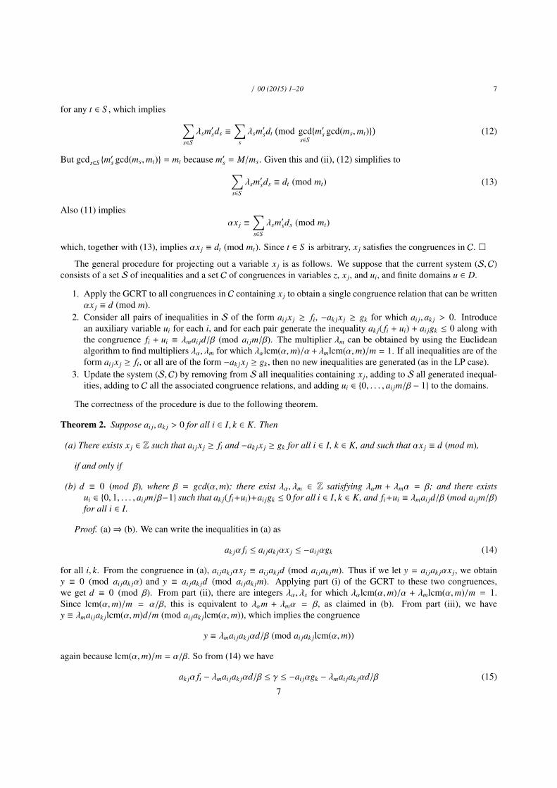
Figure 1. Illustration of a linear (integer) programming problem. Black dots are integer feasible solutions, with (x1, x2) = (2, 9) optimal. The smallopen circle is the optimal solution of the LP.

Lemma 1. Suppose ai j, ak j > 0 for all i ∈ I, k ∈ K. Then

(a) There exists x j ∈ R such that ai jx j ≥ fi and −ak jx j ≥ gk for all i ∈ I, k ∈ K

if and only if .

(b) ak j fi + ai jgk ≤ 0 for all i ∈ I, k ∈ K.

Proof. (a)⇒ (b). This is obtained by taking a linear combination of each pair of inequalities ai jxi ≥ fi, −ak jxi ≥ gk,using multipliers 1/ai j and 1/ak j, respectively.

(a) ⇐ (b). The inequalities in (a) can be written fi/ai j ≤ x j ≤ −gk/ak j for all i, k. But from (b) we have thatfi/ai j ≤ −gk/ak j for all i, k. We can therefore let x j = maxi{ fi/ai j} (or mink{−gk/ak j}), and the inequalities in (a) aresatisfied. �

Note that if I or K is empty then (b) is vacuous (they cannot both be empty, since variable x j would then not be inthe model).

The lemma implies that any variable x j can be eliminated from (1) by removing each pair of inequalities that havethe form ai jx j ≥ fi, −ak jx j ≥ gk with ai j, ak j > 0, and replacing each pair with the inequality ak j fi + ai jgk ≤ 0. (If Ior K is empty, i.e. (b) is vacuous, then x j and all the inequalities in which it occurs can be removed.) The variablesx j can be successively eliminated, in any order, until the constraints of (1) are replaced by inequalities of the formz ≥ `. The minimum value of z can be immediately read from these. If the final inequalities contain no lower boundon z, then the model is unbounded. If z is eliminated from the final inequalities (by the above method) and at leastone “false” inequality (e.g., 0 ≥ 1) results, then the original model is infeasible. It can be shown [6, 15] that afterthe elimination of r variables, any resulting inequality that depends on more than r + 1 of the original inequalities isredundant (implied by the other inequalities).

3

/ 00 (2015) 1–20 4

We can illustrate projection with a small example (Fig. 1).

min zsubject to −x2 ≥ −z C0

2x1 + x2 ≥ 13 C1−5x1 − 2x2 ≥ −30 C2−x1 + x2 ≥ 5 C3x1, x2 ∈ R

(2)

The optimal solution is (x1, x2, z) = (2 23 , 7

23 , 7

23 ), with binding constraints C1 and C3. Eliminating x1 yields z ≥ x2,

x2 ≥ 5, and x2 ≥ 7 23 . Eliminating x2 from this yields z ≥ 5 and z ≥ 7 2

3 . This confirms the optimal value 7 23 .

Suppose now that we perturb the right-hand sides of (2) as follows:

min z−x2 ≥ −z C02x1 + x2 ≥ 13 + ∆1 C1∆

−5x1 − 2x2 ≥ −30 + ∆2 C2∆

−x1 + x2 ≥ 5 + ∆3 C3∆

x1, x2 ∈ Z

(3)

We can perform the same projection operations while carrying through the perturbations. This yields z ≥ 5+5∆1 +2∆2and z ≥ 7 2

3 + 13 ∆1 + 10

3 ∆3. From this we can write a value function

v(∆1,∆2,∆3) = max{5 + 5∆1 + 2∆2, 7 2

3 + 13 ∆1 + 2

3 ∆3

}(4)

that gives the optimal value as a function of the perturbations, provided the problem remains feasible after pertur-bation. In general, Fourier-Motzkin elimination yields inequalities that contain perturbations ∆i but not z, and theperturbations yield a feasible problem if and only if these inequalities are feasible. In the present case, there are nosuch inequalities, and the problem is feasible for any perturbation.

The value function provides the basis for what might be called marginal and eventual shadow prices. The bestknown are marginal shadow prices, which indicate the sensitivity of cost to small perturbations in the right-hand side.The marginal shadow price for constraint i is the coefficient of ∆i in the largest argument of the max when each ∆i isset to zero. In the example, the second term is larger when (∆1,∆2,∆3) = (0, 0, 0), and so the shadow prices are 1

3 , 0,and 2

3 for the three constraints, respectively.As a given right-hand side is increased, one of the terms of the max eventually dominates, and its coefficient can

be regarded as an eventual shadow price in the positive direction. An eventual shadow price in the negative directionis similarly obtained. In the example, the first term of the max dominates as ∆1 increases, and so the eventual shadowprice in the positive direction is 5. The eventual shadow price in the negative direction is 1/3. Economically, theeventual shadow price can be used to compute the approximate cost of large perturbations in a right-hand side.

We will find that eventual shadow prices can be derived for generalized IP problems, although the concept of amarginal shadow price does not extend to IP in an obvious way.

4. IP Projection

In analogy with the LP case, we consider an IP in the following form:

min zsubject to −cx ≥ −z

Ax ≥ bx ∈ Zn

(5)

4

/ 00 (2015) 1–20 5

A generalised IP can be written

min zsubject to −cx − hu ≥ −z

Ax + Bu ≥ brix + siu ≡ ρi (mod mi), i ∈ Ix ∈ Zn

u j ∈ D j ⊂ Z≥0, j = 1, . . . , p

(6)

where u = (u1, . . . , up) are auxiliary variables restricted to finite domains D1, . . . ,Dp.When projecting out an integer variable x j, we can no longer infer fi/ai j ≤ x j ≤ −gk/ak j as in the proof of

Lemma 1. However, we can project out integer variables by strengthening the resultant inequalities. The idea can beillustrated using the example (2) with integer variables x1, x2. This is a classical IP with no congruence relations, butwe will see that the same method applies to generalised IPs.

Step 1. We first project out x1. We obtain the following from the constraint pairs shown:

5(−x2 + 13) ≤ 5 · 2x1 ≤ 2(−2x2 + 30) from C1,C2−x2 + 13 ≤ 2x1 ≤ 2(x2 − 5) from C1,C3

(7)

Because the middle term of the first line is divisible by 5 · 2, we can increase the term −x2 + 13 on the left to thenearest multiple of 2 (unless it is already a multiple of 2) without violating the inequality. We do this by introducingan integer auxiliary variable u1 ∈ {0, 1}. This yields the system on the left below, which implies the system on theright:

5(−x2 + 13 + u1) ≤ 5 · 2x1 ≤ 2(−2x2 + 30) ⇒ x2 ≥ 5 + 5u1

−x2 + 13 + u1 ≡ 0 (mod 2), u1 ∈ {0, 1} x2 ≡ u1 + 1 (mod 2), u1 ∈ {0, 1}

The congruence relation −x2 + 13 + u1 ≡ 0 (mod 2) reflects the fact that −x2 + 13 + u1 is a multiple of 2. (We couldhave just as well have introduced a surplus variable on the right.) We similarly strengthen the second line of (7) toobtain:

−x2 + 13 + u1 ≤ 2x1 ≤ 2(x2 − 5) ⇒ 3x2 ≥ 23 + u1

−x2 + 13 + u1 ≡ 0 (mod 2), u1 ∈ {0, 1} x2 ≡ u1 + 1 (mod 2), u1 ∈ {0, 1}

Putting these together, we have the projected system

−x2 ≥ −z C0x2 ≥ 5 + 5u1 C123x2 ≥ 23 + u1 C13x2 ≡ u1 + 1 (mod 2), u1 ∈ {0, 1}

(8)

Note that the problem of minimising z subject to this projected constraint set is a generalised IP. Its feasible set isthe union of two regions, each of which is described by a linear system applied to a sublattice of Z2 defined by thecongruences x2 ≡ u1 + 1 (mod 2) and z ≡ 0 (mod 1). The two regions correspond to the two values of u1 (namely,u1 = 0, 1) that are feasible in the congruence. In general, we will refer to the feasible values of the uis as definingscenarios. A generalised IP can be solved by solving the problem in each scenario, and taking the best solution acrossthe scenarios. In this case, the optimal solution is (x2, z) = (9, 9) in scenario u1 = 0 and (x2, z) = (10, 10) in scenariou1 = 1, with an overall optimum of (x2, z) = (9, 9).

Step 2. We now wish to project out x2 from the system (8). Because the system is now a generalised IP, we mustextend the above elimination procedure. We first obtain the following by pairing inequalities, as before:

5 + 5u1 ≤ x2 ≤ z from C0, C1223 + u1 ≤ 3x2 ≤ 3z from C0, C13

(9)

5

/ 00 (2015) 1–20 6

Table 1. Solution of the projected system.

u1 u13 5 + 5u113 (23 + u1 + u13)

0 4 5 91 0 10 8

Because x2 ≡ u1 + 1 (mod 2), we can increase the left-hand term in the first line until it is congruent to u1 + 1 (mod 2).Introducing an auxiliary variable u12, we obtain the system on the left below:

5 + 5u1 + u12 ≤ x2 ≤ z ⇒ z ≥ 5 + 5u1 + u12

5 + 5u1 + u12 ≡ u1 + 1 (mod 2), u12 ∈ {0, 1} u12 ≡ 0 (mod 2), u12 ∈ {0, 1}

It is clearly desirable that only one congruence in the system (8) contain x2, so that we can use this kind of reasoning.We indicate below how this can be achieved in general. The second line of (9) gives

23 + u1 + u13 ≤ 3x2 ≤ 3z ⇒ z ≥ 13 (23 + u1 + u13)

23 + u1 + u13 ≡ 3u1 + 3 (mod 6) 4u1 + u13 ≡ 4 (mod 6), u13 ∈ {0, . . . , 5}

Note that u12 can be fixed to zero and dropped from the problem. We therefore have the projected system

z ≥ 5 + 5u1

z ≥ 13 (23 + u1 + u13)

4u1 + u13 ≡ 4 (mod 6), u1 ∈ {0, 1}, u13 ∈ {0, . . . , 5}(10)

Step 3. We have reduced the original IP to the problem of minimising z subject to a system (10) of inequalitiesand congruences that involve only z and the auxiliary variables u1, u13. As before, we can solve the problem bytaking note of the optimal value of z in the two scenarios corresponding to the solutions (u1, u13) = (0, 4), (1, 0) ofthe congruences. Because x1, x2 are eliminated, computing the optimal value in each scenario is now trivial. The twoscenarios are listed in Table 1, where the tightest bound on z in each scenario is shown in boldface. The minimumof these is the optimal value of z, namely z = 9, corresponding to (u1, u13) = (0, 4). Since the bound of 9 comesfrom C0 and C13, we have 23 + u1 + u13 = 3x2 from C13, or x2 = 9. Since C13 comes from C1 and C3, we have5(−x2 + 13 + u1) = 5 · 2x1 from C1, or x1 = 2. The optimal solution is therefore (x1, x2, z) = (2, 9, 9).

When the variable x j to be projected out, occurs in several congruences, we wish to replace the congruences withan equivalent single congruence containing x j. This can be accomplished as follows using a generalised ChineseRemainder Theorem (GCRT). Without loss of generality, suppose the congruences have the form αx j ≡ ds (mod ms)for s ∈ S . The GCRT can then be stated as follows.

Theorem 1 (Generalised Chinese Remainder). Let C = {αx j ≡ ds (mod ms) | s ∈ S } be a system of congruences,and let M = lcm{ms | s ∈ S } and m′s = M/ms. Then we have: (i) ds ≡ dt (mod gcd(ms,mt)) for all s, t ∈ S when C isfeasible, (ii) there is a set of integers λs satisfying

∑s λsm′s = 1, and (iii) integer x j solves C if and only if it solves

αx j ≡∑s∈S

λsm′sds (mod M) (11)

The multipliers λs can be obtained using the well-known Euclidean algorithm.

Proof. Claim (i) can be obtained by subtracting the congruences of C in pairs. Claim (ii) is a well-knownconsequence of the Euclidean algorithhm. To show (iii), suppose first that integer x j satisfies the congruences inC. Taking a linear combination of the congruences in C with multipliers λsm′s, we obtain (11). Conversely, supposex j satisfies (11). Because ds ≡ dt (mod gcd(ms,mt)) for all s, t ∈ S , we have∑

s∈S

λsm′sds ≡∑

s

λsm′sdt(mod gcd

s∈S{λsm′s gcd(ms,mt)}

)6

/ 00 (2015) 1–20 7

for any t ∈ S , which implies ∑s∈S

λsm′sds ≡∑

s

λsm′sdt(mod gcd

s∈S{m′s gcd(ms,mt)}

)(12)

But gcds∈S {m′s gcd(ms,mt)} = mt because m′s = M/ms. Given this and (ii), (12) simplifies to∑

s∈S

λsm′sds ≡ dt (mod mt) (13)

Also (11) impliesαx j ≡

∑s∈S

λsm′sds (mod mt)

which, together with (13), implies αx j ≡ dt (mod mt). Since t ∈ S is arbitrary, x j satisfies the congruences in C. �

The general procedure for projecting out a variable x j is as follows. We suppose that the current system (S,C)consists of a set S of inequalities and a set C of congruences in variables z, x j, and ui, and finite domains u ∈ D.

1. Apply the GCRT to all congruences in C containing x j to obtain a single congruence relation that can be writtenαx j ≡ d (mod m).

2. Consider all pairs of inequalities in S of the form ai jx j ≥ fi, −ak jx j ≥ gk for which ai j, ak j > 0. Introducean auxiliary variable ui for each i, and for each pair generate the inequality ak j( fi + ui) + ai jgk ≤ 0 along withthe congruence fi + ui ≡ λmai jd/β (mod ai jm/β). The multiplier λm can be obtained by using the Euclideanalgorithm to find multipliers λα, λm for which λαlcm(α,m)/α+ λmlcm(α,m)/m = 1. If all inequalities are of theform ai jx j ≥ fi, or all are of the form −ak jx j ≥ gk, then no new inequalities are generated (as in the LP case).

3. Update the system (S,C) by removing from S all inequalities containing x j, adding to S all generated inequal-ities, adding to C all the associated congruence relations, and adding ui ∈ {0, . . . , ai jm/β − 1} to the domains.

The correctness of the procedure is due to the following theorem.

Theorem 2. Suppose ai j, ak j > 0 for all i ∈ I, k ∈ K. Then

(a) There exists x j ∈ Z such that ai jx j ≥ fi and −ak jx j ≥ gk for all i ∈ I, k ∈ K, and such that αx j ≡ d (mod m),

if and only if

(b) d ≡ 0 (mod β), where β = gcd(α,m); there exist λα, λm ∈ Z satisfying λαm + λmα = β; and there existsui ∈ {0, 1, . . . , ai jm/β−1} such that ak j( fi+ui)+ai jgk ≤ 0 for all i ∈ I, k ∈ K, and fi+ui ≡ λmai jd/β (mod ai jm/β)for all i ∈ I.

Proof. (a)⇒ (b). We can write the inequalities in (a) as

ak jα fi ≤ ai jak jαx j ≤ −ai jαgk (14)

for all i, k. From the congruence in (a), ai jak jαx j ≡ ai jak jd (mod ai jak jm). Thus if we let y = ai jak jαx j, we obtainy ≡ 0 (mod ai jak jα) and y ≡ ai jak jd (mod ai jak jm). Applying part (i) of the GCRT to these two congruences,we get d ≡ 0 (mod β). From part (ii), there are integers λα, λs for which λαlcm(α,m)/α + λmlcm(α,m)/m = 1.Since lcm(α,m)/m = α/β, this is equivalent to λαm + λmα = β, as claimed in (b). From part (iii), we havey ≡ λmai jak jlcm(α,m)d/m (mod ai jak jlcm(α,m)), which implies the congruence

y ≡ λmai jak jαd/β (mod ai jak jlcm(α,m))

again because lcm(α,m)/m = α/β. So from (14) we have

ak jα fi − λmai jak jαd/β ≤ γ ≤ −ai jαgk − λmai jak jαd/β (15)

7

/ 00 (2015) 1–20 8

where γ is an integer multiple of ai jak jlcm(α,m). Since d ≡ 0 (mod β), β divides d, and the leftmost expression in(15) is an integer multiple of ak jα. So we can add ak jαui to the left-hand side of (15), and we have

ak jα( fi + ui) ≤ γ + λmai jak jαd/β ≤ −ai jαgk (16)

andak jα( fi + ui) − λmai jak jαd/β ≡ 0 (mod ai jak jlcm(α,m)) (17)

Inequality (16) implies the inequality in (b). Congruence (17) simplifies to

fi + ui − λmai jd/β ≡ 0 (mod ai jm/β)

which implies the congruence in (b). We can also restrict ui to {0, 1, . . . , ai jm/β − 1}. For if ui were greater thanai jm/β − 1 then the original inequalities and congruences would still be valid if ai jm/β − 1 were subtraced from ui.

(a)⇐ (b). The inequalities in (b) can be written

−gk

ak j≥

fi + ui

ai j(18)

for all i, k. From (b) we have that d ≡ 0 (mod β), so that d/β is integral. Also from (b),

fi + ui ≡ λmai jd/β (mod ai jak jm/β) (19)

Because d/β and m/β are integral, this implies fi + ui is an integer multiple of ai j. We can therefore let

x j = maxi

{fi + ui

ai j

}(20)

and x j is integral. This and (18) imply −gk/ak j ≥ x j, or −gk ≥ ak jx j. To show ai jx j ≥ fi, we note that

ai jx j ≥ ai jfi + ui

ai j≥ fi

because ui ≥ 0. Finally, we show αx j ≡ d (mod m). From (20), we have that x j = ( fi + ui)/ai j for some i. So (19)implies that x j ≡ λmd/β (mod m/β), and therefore αx j ≡ λmαd/β (mod αm/β). This implies the following due toλαm + λmα = β in (b):

αx j ≡ (d − λαmd/β) (mod αm/β)

which implies αx j ≡ d (mod αm/β), or αx j ≡ d (mod lcm(α,m)). But this implies αx j ≡ d (mod m). �

To solve a generalised IP problem, we suppose the problem is given in the form (S,C) with domains u ∈ D, asabove. It can be viewed as an optimization problem subject to the inequalities S in variables x j, over the integersublattices defined by the congruence relations in C. In a conventional IP problem, the congruences in C are simplyx j ≡ 0 (mod 1), which require integrality, and there are no variables ui. We sequentially project out variablesx1, . . . , xn, which yields a system (S′,C′) in which S′ contains only z and variables ui, and C′ contains only uis. Theinequalities in S′ have the form z ≥ vt(u), and the optimal value of the problem is minu {maxt{vt(u)} | C′, u ∈ D}. Theoriginal problem is therefore transformed to one in which the variables ui have finite domains.

Note that unboundedness is revealed by the final inequalities in the same way as for the LP case. Infeasibilityis revealed through either false final inequalities, as in the LP case, or final inequalites that have no solution in theauxiliary variables which satisfy the generated congruences. These cases correspond, respectively, to the case of anIP which is infeasible because its LP relaxation is infeasible and an IP which has a feasible LP relaxation.

8

/ 00 (2015) 1–20 9

5. Congruence Cuts

Given a generalized IP, one can define valid congruence cuts that consist of an inequality and a congruencerelation. Congruence cuts are analogous to Chvatal-Gomory cuts in that they are derived by a linear combination andstrengthening operation. However, whereas Chvatal-Gomory cuts are strengtened by rounding, congruence cuts arestrengthened by adding an auxiliary variable to the right-hand side and imposing an additional congruence relationon the expression that results. The inequality portion of a congruence cut can be interpreted as a separating cut in thesense that it cuts off infeasible solutions in one or more scenarios defined by the current auxiliary variables.

As with Chvatal–Gomory cuts, one can generate a finite sequence of separating congruence cuts that solve a givenoptimization problem. The cuts are surrogates that are strengthened by congruences, rather than by rounding as inGomory’s method. We use projection to show that cuts of rank at most n can deduce the optimal value, while no suchbound is available for Gomory cuts. As in the case of Gomory cuts, these cuts allow one to obtain the optimal solution(in addition to the optimal value) by solving the linear relaxation, provided the relaxation is dual nondegenerate. Thecuts may not remove all fractional values, however, when the relaxation is dual degenerate.

To define a congruence cut, let S be a system of linear inequalities in variables x = (x1, . . . , xn) ∈ Zn, and let Cbe a system of congruences in variables x and u = (u1, . . . , ut) ∈ D ⊂ Zt

≥0. A rank 1 congruence cut for (S,C) isany nonnegative linear combination of ai jx j ≥ fi + ui and an inequality in S, where ai jx j ≥ fi belongs to S and acongruence of the form αx j ≡ d (mod m) belongs to C. The rank 1 cut is associated with the congruence relation

α( fi + ui) ≡ ai jd (mod ai jm) (21)

and domain ui ∈ Di = {0, . . . , ai jm − 1}. The cut is valid when all (x, u) satisfying (S,C), congruence (21), u ∈ D, andui ∈ {0, . . . , ai jm − 1} also satisfy the cut.

A rank k congruence cut for (S,C) is a rank 1 cut for some system (S′,C′) consisting of cuts of rank k − 1 or lessfor (S,C) and their associated congruences and domains, provided it is not a rank 1 cut for any such system of cutswith rank less than k − 1. A congruence cut is any rank k projection cut for finite k.

Theorem 3. Any congruence cut for (S,C) is valid for (S,C).

Proof. It is enough to show that any rank 1 cut for (S,C) is valid, because then it follows by induction thanany rank k cut is valid. Because a nonnegative linear combination of valid inequalities is valid, we can show that arank 1 cut is valid by showing that ai jx j ≥ fi + ui is valid for (S,C) when ai jx j ≥ fi is in S, (21) holds, u ∈ D, andui ∈ {0, . . . , ai jm − 1}. Equivalently, we wish to show

αai jxi j − ai jd ≥ α( fi + ui) − ai jd (22)

is valid under these conditions. However, we know that αai jxi j − ai jd ≥ α fi − ai jd is valid, because ai jxi j ≥ fi belongsto S. Also the congruence αx j ≡ d (mod m) implies that the left-hand side of (22) is a multiple of ai jm. The inequality(22) is therefore valid if ui is the smallest nonnegative integer for which the right-hand side is a multiple of ai jm. Forthis, it suffices that (21) hold and ui ∈ {0, . . . , ai jm − 1}. �

As an example, we will generate a congruence cut from inequalities C1 and C3 and the congruence x1 ≡ 0 (mod 1).We first strengthen C1 by adding an auxiliary variable u1 ∈ {0, 1}, to obtain

2x1 ≥ 13 − x2 + u1 (C1′)

We now take a linear combination of C1′ with C3 using unit multipliers (for example) to obtain the cut

x1 ≥ 18 − 2x2 + u1 (C13′)

Because α = 1, ai j = 2, and m = 1, the associated congruence (21) is

13 − x2 + u1 ≡ 0 (mod 2), or x2 ≡ u1 + 1 (mod 2)

The auxiliary variable u1 defines two scenarios, corresponding to u1 = 0, 1. The cut C1′ cuts off the solution(x1, x2, z) = (2 2

3 , 723 , 7

23 ) of the linear relaxation (2) in the second scenario, where C13′ is x1 ≥ 19 − 2x2. It can

9

/ 00 (2015) 1–20 10

therefore be regarded as a separating cut in the sense that it cuts off the solution of the current relaxation in at leastone scenario.

Projection steps provide one means of generating congruence cuts. As an example, consider again (2). In step 1of the projection, C1 and C3 were combined to yield C13 and the congruence x2 ≡ u1 + 1 (mod 2). But C13 is thelinear combination of C1′ and C3 using the same multipliers (given on the left below) that were used to combine C1and C3 in the projection step (7).

(1) 2x1 ≥ 13 − x2 + u1 C1′

(2) −x1 ≥ 5 − x2 C30 ≥ 23 − 3x2 + u1 C13

C13 and the associated relation 13 − x2 + u1 ≡ 0 (mod 2) therefore comprise a congruence cut that is obtained fromC1, C3, and x1 ≡ 0 (mod 1). The congruence relation can be simplified to x2 ≡ u1 + 1 (mod 2), as before. In general,we have the following.

Theorem 4. Each step of the integer projection method produces rank 1 projection cuts for the system (S,C) fromwhich the cuts are derived.

Proof. Each inequality generated by projection has the form

ak j( fi + ui) + ai jgk ≤ 0 (23)

and is derived from ai jx j ≥ fi, −ak jx j ≥ gk ∈ S. We wish to show that (23) is a rank 1 projection cut for (S,C). Wefirst note that (23) is a linear combination of ai jx j ≥ fi +ui and −ak jx j ≥ gk, using multipliers ak j, ai j > 0, respectively.Because αx j ≡ d (mod m) is in C, it remains only to show that ui ∈ {0, . . . , ai jm−1} and that (21) holds. The projectionstep yields the congruence relation

α( fi + ui) ≡ αλmai jd/β (mod ai jαm/β) (24)

where λαm + λmα = β. Substituting β − λαm for λmα, this becomes

α( fi + ui) ≡ ai jd (mod ai jαm/β)

This implies (21) because αm/β = lcm(α,m). Also, the projection step yields ui ∈ {0, . . . , ai jm/β − 1}, which impliesui ∈ {0, . . . , ai jm − 1}. �

One can deduce the optimal value of a problem by generating a series of congruence cuts corresponding to integerprojection steps. The projection steps illustrated in the previous section generate the following congruence cuts:

x2 ≥ 5 + 5u1 C123x2 ≥ 23 + u1 C13z ≥ 5 + 5u1 C0123z ≥ 23 + u1 + u13 C013

x1 ≡ 0 (mod 1)x2 ≡ u1 + 1 (mod 2), u1 ∈ {0, 1}4u1 + u13 ≡ 4 (mod 6), u13 ∈ {0, . . . , 5}

(25)

There are again two scenarios, corresponding to (u1, u13) = (1, 0), (0, 4). In the first scenario, the minimum of z subjectto the inequalities in (25) is (x1, x2, z) = (2, 10, 10), which satisfies all congruences. (The optimal value z = 10 can beimmediately deduced from inequalities C012 and C013.) In the second scenario, the linear system is dual degenerate,and there are two minima: (x1, x2, z) = (2, 9, 9), (2 2

5 , 9, 9). The optimal value of the IP is the minimum value of z inthe two scenarios, namely z = 9.

In general, the congruence cuts generated by projecting a generalised IP onto z prove optimality. Since each of then projection steps obtains congruence cuts by combining inequalities from previous steps, the necessary congruencecuts have rank at most n. The congruence cuts prove optimality in the following sense. Let S′ be the set of cutinequalities of the form z ≥ vt(u) and C′ the set of associated congruences containing only the variables ui, whereu ∈ D. Then as noted in the previous section, the optimal value of the problem is minu{maxt{vt(u)} | C′, u ∈ D}. Wetherefore have the following.

10

/ 00 (2015) 1–20 11

Problem (2)Project out x1

...............................................................................................................................................................................................................................................................................

u1 = 0

...............................................................................................................................................................................................................................................................................

u1 = 1

Problem (25)Project out x2

.......................................................................................................................................................

(u12, u13) = (0, 4)

Problem (26)Project out x2

.......................................................................................................................................................

(u12, u13) = (0, 0)

Feasible solutionz = 9

Feasible solutionz = 10

Figure 2. Projection-based branching tree for example (2).

Corollary 1. Some system of congruence cuts for the IP problem (5) with rank at most n proves the optimal value of(5).

Unlike Chvatal-Gomory cuts, congruence cuts do not necessarily allow one to identify an optimal solution (asopposed to the optimal value) by solving linear relaxations. Consider again the above example. If solving the linearrelaxation in scenario (u1, u13) = (0, 4) yields (x1, x2, z) = (2, 9, 9), then we know it is an optimal solution of theIP because it satisfies the congruences. However, if we obtain the alternate optimal solution (x1, x2, z) = (2 2

5 , 9, 9),we do not have an optimal solution of the IP because x1 = 2 2

5 violates the congruence x1 ≡ 0 (mod 1). Sinceno congruence cut excludes this solution, we cannot identify an optimal solution by solving a linear relaxation withcuts. This problem does not arise if the linear relaxation is dual nondegenerate, but otherwise it may be necessary toconstruct an optimal solution from a sequence of projection-based cuts as in the previous section.

6. Solution by Branching

The above analysis of integer projection leads to a branching algorithm for the generalised IP problem (S,C),u ∈ D. Each time a variable x j is projected out, we branch on the possible values of auxiliary variables ui createdduring the projection step. This means that auxiliary variables do not appear in the branches. If the original problemcontains variables ui, we branch on them as well at the root node. Branching continues until all the variables x j areeliminated.

We therefore branch on scenarios, or equivalently, on disjunctions of constraint sets that result from projection.This was the original way that the method was presented in [12].

An advantage of branching is that auxiliary variables do not accumulate as in sequential projection. In addition, thebranching tree has depth of at most n, although the width can grow exponentially. A bounding mechanism, explainedbelow, may limit the width.

Branching can be illustrated using the example (2), for which the branching tree appears in Fig. 2. At the rootnode of the tree, we carry out step 1 above, which yields the projected system (8). Now, rather than branch on x1, webranch on u1 ∈ {0, 1}.

Left branch, u1 = 0. Here (8) simplifies to

−x2 ≥ −zx2 ≥ 53x2 ≥ 23x2 ≡ 1 mod 2

(26)

11

/ 00 (2015) 1–20 12

Problem (2)

LP: (x1, x2, z) = (223, 72

3, 72

3)

Project out x1...............................................................................................................................................................................................................................................................................

u1 = 0

...............................................................................................................................................................................................................................................................................

u1 = 1

Problem (25)

LP: (x2, z) = (723, 72

3)

Project out x2.......................................................................................................................................................

(u12, u13) = (0, 4)

Problem (26)

LP: (x2, z) = (10, 10)

Prune

Feasible solutionz = 9

Figure 3. Projection-based branch-and-bound tree for example (2).

We now project out x2, which yields

5 + u12 ≤ x2 ≤ z ⇒ z ≥ 5 + u12

23 + u13 ≤ 3x2 ≤ 3z z ≥ 13 (23 + u13)

5 + u12 ≡ 1 (mod 2), u12 ∈ {0, 1} u12 ≡ 0 (mod 2), u12 ∈ {0, 1}23 + u13 ≡ 3 (mod 6), u13 ∈ {0, . . . , 5} u13 ≡ 4 (mod 6), u13 ∈ {0, . . . , 5}

Only one branch (u12, u13) = (0, 4) satifies the congruence. In this branch, the problem is to minimise z subject toz ≥ 5 and z ≥ 9, yielding the bound z ≥ 9.

Right branch, u1 = 1. Here (8) simplifies to

−x2 ≥ −zx2 ≥ 103x2 ≥ 24x2 ≡ 0 mod 2

(27)

Projecting out x2, we get

10 + u12 ≤ x2 ≤ z ⇒ z ≥ 10 + u12

24 + u13 ≤ 3x2 ≤ 3z z ≥ 8 + 13 u13

10 + u12 ≡ 0 (mod 2), u12 ∈ {0, 1} u12 ≡ 0 (mod 2), u12 ∈ {0, 1}24 + u13 ≡ 0 (mod 6), u13 ∈ {0, . . . , 5} u13 ≡ 0 (mod 6), u13 ∈ {0, . . . , 5}

Only one branch (u12, u13) = (0, 0) is possible, at which the problem is to minimise z subject to z ≥ 10 and z ≥ 8,yielding the bound z ≥ 10.

The optimal solution occurs at the left leaf node, with z = 9 and (u1, u12, u13) = (0, 0, 4).

We can introduce a branch-and-bound mechanism by solving a relaxation at each node. The solution of therelaxation can also indicate how to branch, as in traditional branch and bound, because we can branch on a variablex j that violates its associated congruence x j ≡ d (mod m). The simplest relaxation is an LP relaxation obtained bydropping the congruences.

For example, the LP relaxation of (2) at the root node has solution (x1, x2, z) = (2 23 , 7

23 , 7

23 ) (Fig. 3). Because x1

and x2 must satisfy the implicit congruence x j ≡ 0 (mod 1) for j = 1, 2, we can project out either variable and branch12

/ 00 (2015) 1–20 13

on the corresponding auxiliary variable. We choose to project out x1 and branch on u1. Solving the LP relaxation of(26) in the left branch yields (x2, z) = (7 2

3 , 723 ). Because x2 violates x2 ≡ 1 (mod 2), we must project out x2. The LP

relaxation of (27) in the right branch has solution (x2, z) = (10, 10). Because 10 is greater than the incumbent valueof 9, it is unnecessary to project out x2 and branch further. In addition, x2 satisfies x2 ≡ 0 (mod 2), which in itselfobviates the necessity of further branching.

Note that it may be necessary to branch even when all the variables x j are integral in the LP solution. The relevantcriterion is whether they satisfy their respective congruences.

7. A Value Function and Dual Solution

We can obtain a value function by applying the projection algorithm to inequalities with perturbed right-handsides. It can be regarded as a dual solution of the generalised IP.

To illustrate the idea, consider the constraint C1 in example (2), which is 2x1 + x2 ≥ 13. While projecting out x1we used the strengthened inequality

−x2 + 13 + u1 ≤ 2x1 (28)

where−x2 + 13 + u1 ≡ 0 (mod 2) (29)

and u ∈ {0, 1}. Suppose we now perturb the right-hand side of C1 to obtain the constraint 2x1 + x2 ≥ 13 + ∆, so that(28) becomes −x2 + 13 + ∆ + u1 ≤ 2x1. This inequality is not generally valid, given congruence (29). However, wecan strengthen C1 in a different way by adding ∆ + mod2(u1 − ∆) rather than u1:

−x2 + 13 + ∆ + mod2(u1 − ∆) ≤ 2x1 (30)

where modm(a) is the remainder after dividing a by m. This has the same effect as (28) when ∆ = 0. To ensurevalidity, we need the congruence

−x2 + 13 + ∆ + mod2(u1 − ∆) ≡ 0 (mod 2) (31)

However, this is equivalent to congruence (29), because u1 ≡ ∆ + modm(u1 − ∆) (mod m) due to the obvious fact thatu1 − ∆ ≡ modm(u1 − ∆) (mod m). It is easy to show that

∆ + modm(u1 − ∆) = u1 + d∆ − u1em (32)

where daem = mda/me is a rounded up to the nearest multiple of m. So (30) can be written

−x2 + 13 + u1 + d∆ − u1e2 ≤ 2x1

By incorporating this idea into the projection algorithm, we can derive a value function. Consider again theperturbed example (3).

Step 1. To project out x1, we combine C1∆ and C2∆ to obtain

5(−x2 + 13 + u1 + d∆1 − u1e2) ≤ 5 · 2x1 ≤ 2(−2x2 + 30)

This yieldsx2 ≥ 5 + 5u1 + 5d∆1 − u1e2 + 2∆2 C12∆

where x2 ≡ u1 + 1 (mod 2) as before. We combine C∆1 and C∆3 to obtain

3x2 ≥ 23 + u1 + d∆1 − u1e2 + 2∆3 C13∆

Step 2. To eliminate x2, we combine C0 and C12∆ to obtain

5 + 5u1 + u12 + 5 dd∆1 − u1e2 + 2∆2 − u12e2 ≤ x2 ≤ z13

/ 00 (2015) 1–20 14

Table 2. Lower bounds for perturbations in individual constraints i.

Bound from C012∆ Bound from C013∆

u1 u13 i = 1 2 3 i = 1 2 3

0 4 5 + 5d∆1e2 5 + d2∆2e2 5 9 + 13 d∆1 − 4e6 9 9 + 2

3 d∆3 − 2e31 0 10 + 5d∆1 − 1e2 10 + d2∆2e2 10 8 + 1

3 d∆1 − 1e6 8 8 + 23 d∆3e3

This yieldsz ≥ 5 + 5u1 + u12 + d5d∆1 − u1e2 + 2∆2 − u12e2 (33)

where u12 ≡ 0 (mod 2) and u12 ∈ {0, 1}. Note the nesting of functions d·em, which is analogous to the nesting ofrounding operations in a Chvatal function. Because u12 = 0 and d∆1 − u1e2 is even, the bound (33) simplifies to

z ≥ 5 + 5u1 + 5d∆1 − u1e2 + d2∆2e2 C012∆

We similarly combine C0 and C13∆ to obtain

3z ≥ 23 + u1 + u13 + dd∆1 − u1e2 + 2∆3 − u13e6 C013∆

where 4u1 + u13 ≡ 4 (mod 6) and u13 ∈ {0, . . . , 5}.

Step 3. We now have a value function from C012∆ and C013∆:

v(∆1,∆2,∆3) = minu1,u13

{max

{5 + 5u1 + 5d∆1 − u1e2 + d2∆2e2,13(23 + u1 + u13 + dd∆1 − u1e2 + 2∆3 − u13e6

) }}(34)

where the minimum is taken over u1, u13 satisfying u12 ≡ 0 (mod 2), 4u1 + u13 ≡ 4 (mod 6), u1 ∈ {0, 1}, andu13 ∈ {0, . . . , 5}. In this case, the congruences have only two solutions (u1, u13) = (0, 4), (1, 0).

The value function can be regarded as a function of each perturbation ∆i individually. The functions v(∆1, 0, 0),v(0,∆2, 0) and v(0, 0,∆3) for this problem instance are graphed in Figs. 4–6. As in the case of LP, the value functionis valid only for feasible perturbations. A perturbation is infeasible if the congruences, together with the inequalitiescontaining only ∆i’s, have no feasible solution.

Because daem can be replaced by mda/me, the maximum in the value function can be viewed as a maximumover Chvatal functions and is therefore a Gomory function, as is the value function generated by Gomory’s method.However, expressions of the form daem reveal the structure of the value function more clearly. The value functionpresented here differs from that obtained from Gomory’s method in two additional ways: it takes a minimum overmultiple Gomory functions, each corresponding to a scenario, and the nesting depth of rounding in the Chvatalfunctions is bounded by n.

We now describe the general procedure for projecting out a variable x j in a perturbed system. The expressions ∆i

are defined when the previous variable is eliminated. If x j is the first variable to be eliminated, then ∆i = ∆i for each i.

1. Apply the GCRT to the congruences in C containing x j to obtain a single congruence αx j ≡ d (mod m).2. Consider all pairs of inequalities in S of the form ai jx j ≥ fi + ∆i, −ak jx j ≥ gk + ∆k for which ai j, ak j > 0.

Generate the inequality (35) and associate it with the congruence fi + ui ≡ λmai jd/β (mod ai jm/β) and thedomain ui ∈ {0, . . . , ai jm/d − 1}. The multiplier λm can be obtained by using the Euclidean algorithm as before.

3. Update the system (S,C) by removing from S all inequalities containing x j, adding to S all generated inequal-ities, adding to C all the associated congruence relations, and adding ui ∈ {0, . . . , ai jm/β − 1} to the domains.

4. If x` is the next variable to be eliminated, write (35) as ai jx` ≥ f` + ∆`, where ∆` = ak jd∆i − uieai jm/β + ai j∆k.

When all variables x j have been eliminated, the result is a system (S′,C′) and domains u ∈ D such that S containsonly z and uis, and C contains only uis. The inequalities in S provide bounds of the form z ≥ vt(u,∆). Due toTheorem 5, this describes the projection onto z, and the function

v(∆) = minu

{max

t{vt(u,∆)}

∣∣∣∣∣ C′, u ∈ D}

14

/ 00 (2015) 1–20 15

0

10

20

30

40

50

60

-10 -5 0 5 10

∆∆∆∆1

Figure 4. Value function v(∆1) for constraint 1.

is therefore the optimal value of the perturbed IP problem (5). In other words, v(∆) is a value function for (5). It isclear from the form of (35) that v(∆) contains nested roundings d·em. Because n variables are eliminated, the depth ofthe nesting is at most n.

To show that projection creates a value function for an general IP problem, we must extend Theorem 2 to deal withperturbed right-hand sides. Interestingly, the perturbations do not affect the congruences, and the perturbation terms∆i appear only in the generated inequalities. The inequalities ai jx j ≥ fi and −ak jx j ≥ gk in Theorem 2 are replacedwith ai jx j ≥ fi + ∆i and −ak jx j ≥ gk + ∆k to account for the effect of perturbations on generated inequalities. Thus∆i = ∆k = 0 when all the perturbations are zero.

Theorem 5. Suppose ai j, ak j > 0 for all i ∈ I, k ∈ K. Then

(a) There exists x j ∈ Z such that ai jx j ≥ fi + ∆i and −ak jx j ≥ gk + ∆k for all i ∈ I, k ∈ K, and such thatαx j ≡ d (mod m),

if and only if

(b) d ≡ 0 (mod β), where β = gcd(α,m); there exist λα, λm ∈ Z satisfying λαm + λmα = β; and there existsui ∈ {0, 1, . . . , ai jm/β − 1} such that

ak j( fi + ui + d∆i − uieai jm/β) + ai j(gk + ∆k) ≤ 0 (35)

for all i ∈ I, k ∈ K, and fi + ui ≡ λmai jd/β (mod ai jm/β) for all i ∈ I.

Furthermore, if ∆i = ∆k = 0, then inequality (35) reduces to ak j( fi + ui) + ai jgk ≤ 0.

Proof. We first note that if ∆i = ∆k = 0, then in (35) we round −ui up to the nearest multiple of ai jm/β, which iszero because 0 ≤ ui < ai jm/β. Thus (35) reduces to ak j( fi + ui) + ai jgk ≤ 0.

(a)⇒ (b). We can write the inequalities in (a) as

ak jα( fi + ∆i) ≤ ai jak jαx j ≤ −ai jα(gk + ∆k) (36)

15

/ 00 (2015) 1–20 16

0

5

10

15

20

25

30

-10 -5 0 5 10

∆∆∆∆2

Figure 5. Value function v(∆2) for constraint 2.

for all i, k. If we let y = ai jak jαx j, then we can show as in the proof of Theorem 2 that d ≡ 0 (mod β), λαm+λmα = β forsome λα, λm ∈ Z, and the congruence relation y ≡ λmai jak jαd/β (mod ai jak jlcm(α,m)) holds. From the congruencerelation and (36), we have

ak jα( fi + ∆i) − λmai jak jαd/β ≤ γ ≤ −ai jα(gk + ∆k) − λmai jak jαd/β (37)

where γ is an integer multiple of ai jak jlcm(α,m). Since β divides d, the leftmost expression in (37) is an integermultiple of ak jα. So we can add the term

ak jα(−∆i + ui + d∆i − uieai jm/β) (38)

to the left-hand side of (37), where the expression si = −∆i + ui + d∆i − uieai jm/β takes a value in

{0, . . . , ai jak jlcm(α,m)/(ak jα) − 1} = {0, . . . , ai jm/β − 1}

We therefore haveak jα( fi + ui + d∆i − uieai jm/β) ≤ γ + λmai jak jαd/β ≤ −ai jα(gk + ∆k) (39)

whereak jα( fi + ui + d∆i − uieai jm/β) − λmai jak jαd/β ≡ 0 (mod ai jak jlcm(α,m)) (40)

Inequality (39) implies (35). Congruence (40) simplifies to

fi + ui + d∆i − uieai jm/β − λmai jd/β ≡ 0 (mod ai jm/β)

which implies the congruence in (b) because d∆i−uieai jm/β is a multiple of ai jm/β. Finally, si = mod ai jm/β(ui− ∆i) dueto (32). Because we need only consider values 0, . . . , ai jm/β − 1 for si, we generate the required values by restrictingui to {0, . . . , ai jm/β − 1}.

(a)⇐ (b). The inequalities in (b) can be written

−gk + ∆k

ak j≥

fi + ui + d∆i − uieai jm/β

ai j(41)

for all i, k. From (b) we have that d ≡ 0 (mod β), so that d/β is integral. Also from (b),

fi + ui ≡ λmai jd/β (mod ai jak jm/β)16

/ 00 (2015) 1–20 17

0

5

10

15

20

-10 -5 0 5 10

∆∆∆∆3

Figure 6. Value function v(∆3) for constraint 3.

Because d/β and m/β are integral, this implies fi + ui is an integer multiple of ai j. We also have that d∆i − uieai jm/β isa multiple of ai jm/β and therefore ai j. So we can let

x j = maxi

fi + ui + d∆i − uieai jm/β

ai j

and x j is integral. This and (41) imply −(gk + ∆k)/ak j ≥ x j, or −gk ≥ ak jx j + ∆k. To show that ai jx j ≥ fi + ∆i, we notethat

ai jx j ≥ ai jfi + ui + d∆i − uieai jm/β

ai j≥ fi + ∆i

because ui + d∆i − uieai jm/β = ∆i + modai jm/β(ui − ∆i) ≥ ∆i due to (32). Finally, it can be shown as in the proof ofTheorem 2 that αx j ≡ d (mod m). �

We note that the above procedure for computing an IP value function computes an LP value function for the sameset of inequalities when the uis and roundings are removed. For example, the IP value function (34) becomes the LPvalue function (4).

8. Economic Interpretation

It is unclear how to derive marginal shadow prices from an IP value function, because it is a step function.However, the value function assumes a regular pattern for sufficiently large perturbations in a given right-hand side.In particular, it becomes a shift periodic function whose “average” slope can be interpreted as an eventual shadowprice. In fact, this price is equal to the eventual shadow price in the linear relaxation. Fortunately, the periodicity ofthe value function is the same in all scenarios and can therefore be obtained without solving congruence relations toidentify the possible scenarios.

This analysis begins with the fact that Chvatal functions are shift-periodic functions [9]. A function f : Q → Qis (p, q)-shift-periodic on a domain D ⊆ Q, where p and q are positive integers, if for each x ∈ D and each integer λ,f (x + λp) = f (x) + λq. The pair (p, q) is the periodicity of f . Thus one might view q/p as the “average slope” of f indomain D. It is shown in [9] that Chvatal functions are shift-periodic on Q in each argument.

17

/ 00 (2015) 1–20 18

The periodicity of a Chvatal function can be computed using a few simple rules. Let a and b (, 0) be integers.It is easy to show that if f is (p, q)-shift-periodic, then (a/b) f is (bp, aq)-shift-periodic, and d f em is (mp,mq)-shift-periodic. Obviously, f +α is (p, q)-shift-periodic for any constant α. It is shown in [9] that if f1 and f2 are shift-periodicwith periodicities (p1, q1) and (p2, q2), respectively, then the rational linear combination (a1/b1) f1 + (a2/b2) f2 is shift-periodic with periodicity (b1b2 p1 p2, a1b2 p2q1 + a2b1 p1q2). Finally, note that if f has periodicity (p, q), then it alsohas periodicity (mp,mq) for any integer m > 0. So a shift-periodic function has infinitely many periodicities with thesame average slope.

Gomory functions are not shift periodic in general but become shift-periodic for sufficiently large arguments. Afunction f : Q → Q is eventually (p, q)-shift-periodic in a positive direction on domain D if there exists positiveinteger r such that for each x ∈ D and each integer λ, f (x + rp + λp) = f (x + rp) + λq. It is eventually (p, q)-shift-periodic in a negative direction if there exists positive integer r such that for each x ∈ D and each integer λ,f (x − rp − λp) = f (x − rp) − λq.

It is also shown in [9] that if a finite family of functions fi are (pi, qi)-shift-periodic on D for i ∈ I, then maxi∈I{ fi}is eventually (p j, q j)-shift-periodic in a positive direction on [d,∞) ∩ D for any finite d, where p j/q j = maxi∈I{pi/qi}.In addition, maxi∈I{ fi} is eventually (p j′ , q j′ )-shift-periodic in a negative direction on (−∞, d′] ∩ D for any d′, wherep j′/q j′ = mini∈I{pi/qi}. It follows that if the functions fi are Chvatal functions, then the Gomory function maxi∈I{ fi}is eventually (p j, q j)-shift-periodic on [d,∞) in a positive direction, and eventually (p j′ , q j′ )-shift-period on (−∞, d′]in a negative direction.

As an example, we can use these rules to deduce the periodicity of the value function (34) for any scenario(u1, u13). We first note that the periodicity is the same for any scenario, because u1 and u13 appear only as additiveconstants in the Chvatal functions. Consider first the value function v(∆1, 0, 0) for constraint C1. For any givenscenario, it is a Gomory function equal to the maximum of two Chvatal functions, which have periodicities (2, 10) and(12, 4), respectively. This Gomory function is eventually (2, 10)-shift-periodic in the positive direction and (12, 4)-shift-periodic in the negative direction. This means that the “average” shadow price is 10/2 = 5 for sufficiently largeright-hand side, and 4/12 = 1/3 for sufficiently small right-hand side. Similarly, the average shadow price for C2 is2/1 = 2 in the positive direction and 0/1 = 1 in the negative direction, and for C3 is 2/3 in the positive direction and0 in the negative direction.

Finally, we show that the minimum of finitely many Gomory functions with the same periodicity is eventuallyshift periodic, which implies that the value function v is eventually shift periodic.

Lemma 2. Let fi be eventually (p, q)-shift-periodic in the positive direction on [d,∞) for i ∈ I and finite set I, andeventually (p′, q′)-shift-periodic in the negative direction on (−∞, d′] for i ∈ I. Then mini∈I{ fi} is eventually (p, q)-shift-periodic in the positive direction on [d,∞) and eventually (p′, q′)-shift-periodic in the negative direction on(−∞, d′].

Proof. Because fi is eventually (p, q)-shift periodic on [d,∞) in the positive direction, there exists a positiveinteger ri such that for any x ∈ [d,∞),

fi(x + λri + λp) = f (x + λri) + λq (42)

Let rmax = maxi∈I{ri}. To show that mini∈I{ fi} is eventually (p, q)-shift-periodic on [d,∞) in the positive direction, itsuffices to show that for any x ∈ [d,∞),

mini∈I{ fi(x + rmax p + λp)} = min

i∈I{ fi(x + rmax p)} + λq

For this it suffices to show that for any i ∈ I and any x ∈ [d,∞),

fi(x + rmax p + λp) = fi(x + rmax p) + λq (43)

But we havefi(x + rmax p + λp) = fi(x + ri p + (rmax − ri)p + λp)= fi(x + ri p) + (rmax − ri)q + λq = fi(x + ri p + (rmax − ri)p) + λq

where the second and third equations are due to (42). This implies (43), as desired. One can show similarly thatmini∈I{ fi} is eventually (p′, q′)-shift-periodic in the negative direction. �

18

/ 00 (2015) 1–20 19

Thus the value function v(∆1, 0, 0) is (2, 10)-shift-periodic in the positive direction and (12, 4)-shift-periodic inthe negative direction. The “average” slope eventually becomes 5 in the positive direction and 1/3 in the negativedirection, as one can verify by examining Fig. 4. The situation is similar for value functions v(0,∆2, 0) and v(0, 0,∆3).

These eventual shadow prices are the same as those derived earlier for the linear case. This follows from the factthat the LP value function has a shift-periodicity equal to that of the IP value function for each perturbation ∆i. To seethis, recall that the LP value function can be obtained from the IP value function by removing uis and roundings. Thuswe can compute a periodicity of the LP value function following the same steps as for the IP value function, exceptthat constants ui are not added, and roundings d f em are not taken. But additive constants do not affect periodicity.Also, d f em is (mp,mq)-shift-periodic if f is (p, q)-shift-periodic. But f is also (mp,mq)-shift-periodic and thereforehas a shift-periodicity equal to that of d f em. The Chvatal functions that make up the IP value function therefore haveshift-periodicities equal to those of the corresponding components of the LP value function. But the Chvatal functionthat dominates as ∆i increases (or decreases) depends only on the coefficients of ∆i, and these coefficients are notaffected by removing uis and roundings. The LP value function therefore has an eventual shift-periodicity equal tothat of the IP value function, resulting in the same eventual shadow prices.

The equivalence of IP and LP eventual shadow prices also follows from the analyses in [4, 5]. For sufficientlylarge right-hand sides, one of the component Chvatal functions in the classical IP value function becomes dominant,and the relaxation of this same Chvatal function becomes dominant in the LP value function. The IP becomes an IPover the cone defined by the binding constraints in the LP relaxation. This is sometimes referred to as an “asymptoticIP.” As a consequence, the eventual shadow prices for the IP are the same as those for the LP relaxation.

9. Conclusion

We presented an alternative perspective on integer programming (IP) that is suggested by projection and parallelsthe classical theory. We showed that if IP is generalised to include optimisation over sublattices of the integer lattice,then the projection of a generalised IP is itself a generalised IP. This perspective inspires the definition of a familyof congruence cuts that are parallel to Chvatal-Gomory cuts in some respects, but whose maximum rank is boundedby the number of variables in the original IP. It also leads to a new branching algorithm in which the depth of thetree is likewise bounded by the number of variables, in contrast to conventional IP branch-and-bound methods, wherethere is no bound. Finally, it produces a value function for generalised IP that differs in structure from value functionsgenerated by Gomory’s method, and in which the maximum nesting depth of rounding is bounded by the number ofvariables. The value function becomes shift periodic and provides “average” shadow prices for large perturbations inthe right-hand sides.

References

[1] Blair, C. E. and R. G. Jeroslow, The value function of an integer program, Mathematical Programming 23 (1982) 237-273.[2] Chvatal, V., Edmonds polytopes and a heirarchy of combinatorial problems, Discrete Mathematics 4 (1973) 305–337.[3] Fourier, J. B. J., Solution d’une question particuliere du calcul des inegalites, Oeuvres II, Paris (1826) 317–328.[4] Gomory, R. E., On the relation between integer and non-integer solutions to linear programs, Proceedings of the National Academy of Sciences

53 (1965) 260–265.[5] Gomory, R. E., and W. J. Baumol, Integer programming and pricing, Econometrica 28 (1960) 521–550.[6] Kohler, D. A., Projections of convex polyhedral sets, Operations Research Center, University of California, Berkeley (1967).[7] Martin, R. K., Large Scale Linear and Integer Programming: A Unified Approach, Kluwer, Boston (1999).[8] O’Neill, R. P., P. M. Sotkiewicz, B. F. Hobbs, M. H. Rothkopf, and W. R. Stewart, Efficient market-clearing prices in markets with

nonconvexities, European Journal of Operational Research 164 (2005) 269–285.[9] Rhodes, F., and H. P. Williams, Discrete subadditive functions as Gomory functions, Mathematical Proceeedings of the Cambridge

Philosophical Society 117 (1995) 559–574.[10] Ryan, J., Decomposing finitely generated integral monoids by elimination, Linear Algebra and Its Applications 153 (1991) 209-217.[11] Schriver, A., Theory of Integer and Linear Programming, Wiley, Chichester, UK (1986).[12] Williams, H. P., Fourier-Motzkin elimination extended to integer programming problems, Journal of Combinatorial Theory 21 (1976) 118–

123.[13] Williams, H. P., Fourier’s method of linear programming and its dual, American Mathematical Monthly 93 (1986) 681–695.[14] Williams, H. P., An alternative form of the value function of an integer programme, Working paper OR22, University of Southampton (1999)[15] Williams, H. P., The dependency diagram of a linear programme, Working paper LSEOR 13.138, Management Science Group, London

School of Economics (2013).

19

/ 00 (2015) 1–20 20

[16] Williams, H. P, The general solution of a mixed integer linear programme over a cone, Working paper LSEOR 13.139, Management ScienceGroup, London School of Economics (2013).

[17] Williams, H. P., The dependency diagram of a mixed integer programme, Working paper LSEOR 13.137, Management Science Group,London School of Economics (2013).

20