
Mining Value-Based Item Packages - An Integer Programming Approach
141
Transcript of Mining Value-Based Item Packages - An Integer Programming Approach


Lecture Notes in Artificial Intelligence 3755Edited by J. G. Carbonell and J. Siekmann
Subseries of Lecture Notes in Computer Science

Graham J. Williams Simeon J. Simoff (Eds.)
Data Mining
Theory, Methodology, Techniques,and Applications
1 3

Series Editors
Jaime G. Carbonell, Carnegie Mellon University, Pittsburgh, PA, USAJörg Siekmann, University of Saarland, Saarbrücken, Germany
Volume Editors
Graham J. WilliamsTogaware Data MiningCanberra, AustraliaE-mail: [email protected]
Simeon J. SimoffUniversity of Technology, Faculty of Information TechnologySydney Broadway PO Box 123, NSW 2007, AustraliaE-mail: [email protected]
Library of Congress Control Number: 2006920576
CR Subject Classification (1998): I.2, H.2.8, H.2-3, D.3.3, F.1
LNCS Sublibrary: SL 7 – Artificial Intelligence
ISSN 0302-9743ISBN-10 3-540-32547-6 Springer Berlin Heidelberg New YorkISBN-13 978-3-540-32547-5 Springer Berlin Heidelberg New York
This work is subject to copyright. All rights are reserved, whether the whole or part of the material isconcerned, specifically the rights of translation, reprinting, re-use of illustrations, recitation, broadcasting,reproduction on microfilms or in any other way, and storage in data banks. Duplication of this publicationor parts thereof is permitted only under the provisions of the German Copyright Law of September 9, 1965,in its current version, and permission for use must always be obtained from Springer. Violations are liableto prosecution under the German Copyright Law.
Springer is a part of Springer Science+Business Media
springer.com
© Springer-Verlag Berlin Heidelberg 2006Printed in Germany
Typesetting: Camera-ready by author, data conversion by Scientific Publishing Services, Chennai, IndiaPrinted on acid-free paper SPIN: 11677437 06/3142 5 4 3 2 1 0

Preface
Data mining has been an area of considerable research and application inAustralia and the region for many years. This has resulted in the establish-ment of a strong tradition of academic and industry scholarship, blended withthe pragmatics of practice in the field of data mining and analytics. ID3, See5,RuleQuest.com, MagnumOpus, and WEKA is but a short list of the data min-ing tools and technologies that have been developed in Australasia. Data miningconferences held in Australia have attracted considerable international interestand involvement.
This book brings together a unique collection of chapters that cover thebreadth and depth of data mining today. This volume provides a snapshot of thecurrent state of the art in data mining, presenting it both in terms of technicaldevelopments and industry applications. Authors include some of Australia’sleading researchers and practitioners in data mining, together with chaptersfrom regional and international authors.
The collection of chapters is based on works presented at the AustralasianData Mining conference series and industry forums. The original papers wereinitially reviewed for the workshops, conferences and forums. Presenting authorswere provided with substantial feedback, both through this initial review processand through editorial feedback from their presentations. A final internationalpeer review process was conducted to include input from potential users of theresearch, and in particular analytics experts from industry, looking at the impactof reviewed works.
Many people contribute to an effort such as this, starting with the authors!We thank all authors for their contributions, and particularly for making theeffort to address two rounds of reviewer comments. Our workshop and conferencereviewers provided the first round of helpful feedback for the presentation ofthe papers to their respective conferences. The authors from a selection of thebest papers were then invited to update their contributions for inclusion in thisvolume. Each submission was then reviewed by at least another two reviewersfrom our international panel of experts in data mining.
A considerable amount of effort goes into reviewing papers, and reviewersperform an essential task. Reviewers receive no remuneration for all their efforts,but are happy to provide their time and expertise for the benefit of the wholecommunity. We owe a considerable debt to them all and thank them for theirenthusiasm and critical efforts.
Bringing this collection together has been quite an effort. We also acknowl-edge the support of our respective institutions and colleagues who have con-tributed in many different ways. In particular, Graham would like to thankTogaware (Data Mining and GNU/Linux consultancy) for their ongoing infras-tructural support over the years, and the Australian Taxation Office for its

VI Preface
support of data mining and related local conferences through the participationof its staff. Simeon acknowledges the support of the University of Technology,Sydney. The Australian Research Council’s Research Network on Data Min-ing and Knowledge Discovery, under the leadership of Professor John Roddick,Flinders University, has also provided support for the associated conferences, inparticular providing financial support to assist student participation in the con-ferences. Professor Geoffrey Webb, Monash University, has played a supportiverole in the development of data mining in Australia and the AusDM series ofconferences, and continues to contribute extensively to the conference series.
The book is divided into two parts: (i) state-of-art research and (ii) state-of-art industry applications. The chapters are further grouped around commonsub-themes. We are sure you will find that the book provides an interesting andbroad update on current research and development in data mining.
November 2005 Graham Williams and Simeon Simoff

Organization
Many colleagues have contributed to the success of the series of data miningworkshops and conferences over the years. We list here the primary reviewerswho now make up the International Panel of Expert Reviewers.
AusDM Conference Chairs
Simeon J. Simoff, University of Technology, Sydney, AustraliaGraham J. Williams, Australian National University, Canberra
PAKDD Industry Chair
Graham J. Williams, Australian National University, Canberra
International Panel of Expert Reviewers
Mihael Ankerst Boeing Corp., USAMichael Bain University of New South Wales, AustraliaRohan Baxter Australian Taxation OfficeHelmut Berger University of Technology, Sydney, AustraliaMichael Bohlen Free University Bolzano-Bozen, ItalyJie Chen CSIRO, Canberra, AustraliaPeter Christen Australian National UniversityThanh-Nghi Do Can Tho University, VietnamVladimir Estivill-Castro Giffith University, AustraliaHongjian Fan University of Melbourne, AustraliaEibe Frank Waikato University, New ZealandMohamed Medhat Gaber Monash University, AustraliaRaj Gopalan Curtin University, AustraliaWarwick Graco Australian Taxation OfficeLifang Gu Australian Taxation OfficeHongxing He CSIRO, Canberra, AustraliaRobert Hilderman University of Regina, CanadaJoshua Zhexue Huang University of Hong Kong, ChinaHuidong Jin CSIRO, Canberra, AustraliaPaul Kennedy University of Technology, Sydney, AustraliaWeiqiang Lin Australian Taxation OfficeJohn Maindonald Australian National UniversityMark Norrie Teradata, NCR, AustraliaPeter O’Hanlon Westpac, Australia

VIII Preface
Mehmet Orgun Macquarie University, AustraliaTom Osborn Wunderman, NUIX Pty Ltd, AustraliaRobert Pearson Health Insurance Commission, AustraliaFrancois Poulet ESIEA-Pole ECD, Laval, FranceJohn Roddick Flinders University, AustraliaGreg Saunders University of Ballarat, AustraliaDavid Skillicorn Queen’s University, CanadaGeoffrey Webb Monash University, AustraliaJohn Yearwood University of Ballarat, AustraliaOsmar Zaiane University of Alberta, Canada

Table of Contents
Part 1: State-of-the-Art in Research
Methodological Advances
Generality Is Predictive of Prediction AccuracyGeoffrey I. Webb, Damien Brain . . . . . . . . . . . . . . . . . . . . . . . . . . . . . . . . . 1
Visualisation and Exploration of Scientific Data Using GraphsBen Raymond, Lee Belbin . . . . . . . . . . . . . . . . . . . . . . . . . . . . . . . . . . . . . . . 14
A Case-Based Data Mining PlatformXingwen Wang, Joshua Zhexue Huang . . . . . . . . . . . . . . . . . . . . . . . . . . . . 28
Consolidated Trees: An Analysis of Structural ConvergenceJesus M. Perez, Javier Muguerza, Olatz Arbelaitz, Ibai Gurrutxaga,Jose I. Martın . . . . . . . . . . . . . . . . . . . . . . . . . . . . . . . . . . . . . . . . . . . . . . . . . 39
K Nearest Neighbor Edition to Guide Classification Tree Learning:Motivation and Experimental Results
J.M. Martınez-Otzeta, B. Sierra, E. Lazkano, A. Astigarraga . . . . . . . . 53
Efficiently Identifying Exploratory Rules’ SignificanceShiying Huang, Geoffrey I. Webb . . . . . . . . . . . . . . . . . . . . . . . . . . . . . . . . 64
Mining Value-Based Item Packages – An Integer ProgrammingApproach
N.R. Achuthan, Raj P. Gopalan, Amit Rudra . . . . . . . . . . . . . . . . . . . . . . 78
Decision Theoretic Fusion Framework for Actionability Using DataMining on an Embedded System
Heungkyu Lee, Sunmee Kang, Hanseok Ko . . . . . . . . . . . . . . . . . . . . . . . . 90
Use of Data Mining in System Development Life CycleRichi Nayak, Tian Qiu . . . . . . . . . . . . . . . . . . . . . . . . . . . . . . . . . . . . . . . . . 105
Mining MOUCLAS Patterns and Jumping MOUCLAS Patterns toConstruct Classifiers
Yalei Hao, Gerald Quirchmayr, Markus Stumptner . . . . . . . . . . . . . . . . . 118

X Table of Contents
Data Linkage
A Probabilistic Geocoding System Utilising a Parcel Based Address FilePeter Christen, Alan Willmore, Tim Churches . . . . . . . . . . . . . . . . . . . . . 130
Decision Models for Record LinkageLifang Gu, Rohan Baxter . . . . . . . . . . . . . . . . . . . . . . . . . . . . . . . . . . . . . . . 146
Text Mining
Intelligent Document Filter for the InternetDeepani B. Guruge, Russel J. Stonier . . . . . . . . . . . . . . . . . . . . . . . . . . . . 161
Informing the Curious Negotiator: Automatic News Extraction fromthe Internet
Debbie Zhang, Simeon J. Simoff . . . . . . . . . . . . . . . . . . . . . . . . . . . . . . . . . 176
Text Mining for Insurance Claim Cost PredictionInna Kolyshkina, Marcel van Rooyen . . . . . . . . . . . . . . . . . . . . . . . . . . . . . 192
Temporal and Sequence Mining
An Application of Time-Changing Feature SelectionYihao Zhang, Mehmet A. Orgun, Weiqiang Lin, Warwick Graco . . . . . 203
A Data Mining Approach to Analyze the Effect of Cognitive Style andSubjective Emotion on the Accuracy of Time-Series Forecasting
Hung Kook Park, Byoungho Song, Hyeon-Joong Yoo,Dae Woong Rhee, Kang Ryoung Park, Juno Chang . . . . . . . . . . . . . . . . 218
A Multi-level Framework for the Analysis of Sequential DataCarl H. Mooney, Denise de Vries, John F. Roddick . . . . . . . . . . . . . . . . 229
Part 2: State-of-the-Art in Applications
Health
Hierarchical Hidden Markov Models: An Application to HealthInsurance Data
Ah Chung Tsoi, Shu Zhang, Markus Hagenbuchner . . . . . . . . . . . . . . . . . 244

Table of Contents XI
Identifying Risk Groups Associated with Colorectal CancerJie Chen, Hongxing He, Huidong Jin, Damien McAullay,Graham Williams, Chris Kelman . . . . . . . . . . . . . . . . . . . . . . . . . . . . . . . . 260
Mining Quantitative Association Rules in Protein SequencesNitin Gupta, Nitin Mangal, Kamal Tiwari, Pabitra Mitra . . . . . . . . . . . 273
Mining X-Ray Images of SARS PatientsXuanyang Xie, Xi Li, Shouhong Wan, Yuchang Gong . . . . . . . . . . . . . . 282
Finance and Retail
The Scamseek Project – Text Mining for Financial Scams on the InternetJon Patrick . . . . . . . . . . . . . . . . . . . . . . . . . . . . . . . . . . . . . . . . . . . . . . . . . . . 295
A Data Mining Approach for Branch and ATM Site EvaluationSimon C.K. Shiu, James N.K. Liu, Jennie L.C. Lam, Bo Feng . . . . . . 303
The Effectiveness of Positive Data Sharing in Controlling the Growthof Indebtedness in Hong Kong Credit Card Industry
Vincent To-Yee Ng, Wai Tak Yim, Stephen Chi-Fai Chan . . . . . . . . . . . 319
Author Index . . . . . . . . . . . . . . . . . . . . . . . . . . . . . . . . . . . . . . . . . . . . . . . . . . . 331

Generality Is Predictive of Prediction Accuracy
Geoffrey I. Webb1 and Damien Brain2
1 Faculty of Information Technology,Monash University, Clayton, Vic 3800, Australia
[email protected] UTelco Systems,
Level 50/120 Collins St Melbourne, Vic 3001, [email protected]
Abstract. During knowledge acquisition it frequently occurs that mul-tiple alternative potential rules all appear equally credible. This paperaddresses the dearth of formal analysis about how to select betweensuch alternatives. It presents two hypotheses about the expected impactof selecting between classification rules of differing levels of generality inthe absence of other evidence about their likely relative performance onunseen data. We argue that the accuracy on unseen data of the moregeneral rule will tend to be closer to that of a default rule for the classthan will that of the more specific rule. We also argue that in comparisonto the more general rule, the accuracy of the more specific rule on unseencases will tend to be closer to the accuracy obtained on training data.Experimental evidence is provided in support of these hypotheses. Thesehypotheses can be useful for selecting between rules in order to achievespecific knowledge acquisition objectives.
1 Introduction
In many knowledge acquisition contexts there will be many classification rulesthat perform equally well on the training data. For example, as illustrated bythe version space [1], there will often be alternative rules of differing degreesof generality all of which agree with the training data. However, even when wemove away from a situation in which we are expecting to find rules that arestrictly consistent with the training data, in other words, when we allow rules tomisclassify some training cases, there will often be many rules all of which coverexactly the same training cases. If we are selecting rules to use for some decisionmaking task, we must select between such rules with identical performance on thetraining data. To do so requires a learning bias [2], a means of selecting betweencompeting hypotheses that utilizes criteria beyond those strictly encapsulatedin the training data.
All learning algorithms confront this problem. This is starkly illustrated bythe large numbers of rules with very high values for any given interestingnessmeasure that are typically discovered during association rule discovery. Manysystems that learn rule sets for the purpose of prediction mask this problemby making arbitrary choices between rules with equivalent performance on the
G.J. Williams and S.J. Simoff (Eds.): Data Mining, LNAI 3755, pp. 1–13, 2006.c© Springer-Verlag Berlin Heidelberg 2006

2 G.I. Webb and D. Brain
training data. This masking of the problem is so successful that many researchersappear oblivious to the problem. Our previous work has clearly identified that itis frequently the case that there exist many variants of the rules typically derivedin machine learning, all of which cover exactly the same training data. Indeed,one of our previous systems, The Knowledge Factory [3, 4] provides support foridentification and selection between such rule variants.
This paper examines the implications of selecting between such rules on thebasis of their relative generality. We contend that learning biases based on rel-ative generality can usefully manipulate the expected performance of classifierslearned from data. The insight that we provide into this issue may assist knowl-edge engineers make more appropriate selections between alternative rules whenthose alternatives derive equal support from the available training data.
We present specific hypotheses relating to reasonable expectations aboutclassification error for classification rules. We discuss classification rules of theform Z → y, which should be interpreted as all cases that satisfy conditionsZ belong to class y. We are interested in learning rules from data. We al-low that evidence about the likely classification performance of a rule mightcome from many sources, including prior knowledge, but, in the machine learn-ing tradition, are particularly concerned with empirical evidence—evidenceobtained from the performance of the rule on sample (training) data. We con-sider the learning context in which a rule Z → y is learned from a training setD′=(x′
1, y′1), (x′
2, y′2), . . . , (x′
n, y′n) and is to be applied to a set of previously un-
seen data called a test set D=(x1, y1), (x2, y2), . . . , (xm, ym). For this enterpriseto be successful, D′ and D should be drawn from the same or from related dis-tributions. For the purposes of the current paper we assume that D′ and D aredrawn independently at random from the same distribution and acknowledgethat violations of this assumption may affect the effects that we predict.
We utilize the following notation.
• Z(I) represents the set of instances in instance set I covered by condition Z.• E(Z → y, I) represents the number of instances in instance set I that Z → y
misclassifies (the absolute error).• ε(Z → y, I) represents the proportion of instance set I that Z → y misclas-
sifies (the error) = E(Z→y,I)|I| .
• W � Z denotes that the condition W is a proper generalization of conditionZ. W � Z if and only if the set of descriptions for which W is true is a propersuperset of the set of descriptions for which Z is true.
• NODE(W → y, Z → y) denotes that there is no other distinguishing ev-idence between W → y and Z → y. This means that there is no avail-able evidence, other than the relative generality of W and Z, indicating thelikely direction (negative, zero, or positive) of ε(W → y, D) − ε(Z → y, D).In particular, we require that the empirical evidence be identical. In thecurrent research the learning systems have access only to empirical evidenceand we assume that W (D′)=Z(D′) → NODE(W → y, Z → y). Note thatW (D′)=Z(D′) does not preclude W and Z from covering different test casesat classification time and hence having different test set error. We utilize the

Generality Is Predictive of Prediction Accuracy 3
notion of other distinguishing evidence to allow for the real-world knowledgeacquisition context in which evidence other than that contained in the datamay be brought to bear upon the rule selection problem.
We present two hypotheses relating to classification rules W → y and Z → ylearned from real-world data such that W � Z and NODE(W → y, Z → y).
1. Pr(|ε(W → y, D) − ε(true → y, D)| < |ε(Z → y, D) − ε(true → y, D)|) >Pr(|ε(W → y, D)−ε(true → y, D)| > |ε(Z → y, D)−ε(true → y, D)|). Thatis, the error of the more general rule, W → y, on unseen data will tend to becloser to the proportion of cases in the domain that do not belong to class ythan will the error of the more specific rule, Z → y.
2. Pr(|ε(W → y, D) − ε(W → y, D′)| > |ε(Z → y, D) − ε(Z → y, D′)|) >Pr(|ε(W → y, D) − ε(W → y, D′)| < |ε(Z → y, D) − ε(Z → y, D′)|). Thatis, the error of the more specific rule, Z → y, on unseen data will tend to becloser to the proportion of negative training cases covered by the two rules1
than will the error of the more general rule, W → y.
Another way of stating these two hypotheses is that of two rules with identicalempirical and other support,
1. the more general can be expected to exhibit classification error closer to thatof a default rule, true → y, or, in other words, of assuming all cases belongto the class, and
2. the more specific can be expected to exhibit classification error closer to thatobserved on the training data.
It is important to clarify at the outset that we are not claiming that the moregeneral rule will invariably have closer generalization error to the default ruleand the more specific rule will invariably have closer generalization error to theobserved error on the training data. Rather, we are claiming that relative gener-ality provides a source of evidence that, in the absence of alternative evidence,provides reasonable grounds for believing that each of these effects is more likelythan the contrary.
Observation. With simple assumptions, hypotheses (1) and (2) can be shownto be trivially true given that D′ and D are idd samples from a single finitedistribution D.
Proof.
1. For any rule X → y and test set D, ε(X → y, D) = ε(X → y, X(D)), asX → y only covers instances X(D) of D.
2. ε(Z → y, D) = E(Z→y,Z(D∩D′))+E(Z→y,Z(D−D′))|Z(D)|
3. ε(W → y, D) = E(W→y,W (D∩D′))+E(W→y,W (D−D′))|W (D)|
4. Z(D) ⊆ W (D) because Z is a specialization of W .1 Recall that both rules have identical empirical support and hence cover the same
training cases.

4 G.I. Webb and D. Brain
5. Z(D ∩ D′) = W (D ∩ D′) because Z(D′) = W (D′).6. Z(D − D′) ⊆ W (D − D′) because Z(D) ⊆ W (D).7. from 2-6, E(Z → y, Z(D ∩ D′)) is a larger proportion of the error of Z → y
than is E(W → y, W (D ∩ D′)) of W → y and hence performance on D′ is alarger component of the performance of Z → y and performance on D − D′
is a larger component of the performance of W → y. ��
However, in most domains of interest the dimensionality of the instance space willbe very high. In consequence, for realistic training and test sets the proportionof the training set that appears in the test set, |D∩D′|
|D| , will be small. Hence thiseffect will be negligible, as performance on the training set will be a negligibleportion of total performance. What we are more interested in is off-training-set error. We contend that the force of these hypotheses will be stronger thanaccounted for by the difference made by the overlap between training and testsets, and hence that they do apply to off-training-set error. We note, however,that it is trivial to construct no-free-lunch proofs, such as those of Wolpert [5]and Schaffer [6], that this is not, in general, true. Rather, we contend that thehypotheses will in general be true for ‘real-world’ learning tasks. We justifythis contention by recourse to the similarity assumption [7], that in the absenceof other information, the greater the similarity between two objects in otherrespects, the greater the probability of their both belonging to the same class. Webelieve that most machine learning algorithms depend upon this assumption, andthat this assumption is reasonable for real-world knowledge acquisition tasks.Test set cases covered by a more general but not a more specific rule are likelyto be less similar to training cases covered by both rules than are test set casescovered by the more specific rule. Hence satisfying the left-hand-side of the morespecific rule provides stronger evidence of likely class membership.
A final point that should be noted is that these hypotheses apply to individualclassification rules — structures that associate an identified region of an instancespace with a single class. However, as will be discussed in more detail below, webelieve that the principle is nonetheless highly relevant to ‘complete classifiers,’such as decision trees, that assign different regions of the instance space to differ-ent classes. This is because each individual region within a ‘complete classifier’(such as a decision tree leaf) satisfies our definition of a classification rule, andhence the hypotheses can cast light on the likely consequences of relabeling sub-regions of the instance space within such a classifier (for example, generalizingone leaf of a decision tree at the expense of another, as proposed elsewhere [8]).
2 Evaluation
To evaluate these hypotheses we sought to generate rules of varying generalitybut identical empirical evidence (no other evidence source being considered inthe research), and to test the hypotheses’ predictions with respect to these rules.
We wished to provide some evaluation both of whether the predicted effectsare general (with respect to rules with the relevant properties selected at random)

Generality Is Predictive of Prediction Accuracy 5
Table 1. Algorithm for generating a random rule
1. Randomly select an example x from the training set.2. Randomly select an attribute a for which the value of a for x (ax) is not unknown.3. If a is categorical, form the rule IF a = ax THEN c, where c is the most frequent
class in the cases covered by a = ax.4. Otherwise (if a is ordinal), form the rule IF a#ax THEN c, where # is a random
selection between ≤ and ≥ and c is the most frequent class in the cases coveredby a#ax.
as well as whether they apply to the type of rule generated in standard machinelearning applications. We used rules generated by C4.5rules (release 8) [9], as anexemplar of a machine learning system for classification rule generation.
One difficulty with employing rules formed by C4.5rules is that the systemuses a complex resolution system to determine which of several rules should beemployed to classify a case covered by more than one rule. As this is taken intoaccount during the induction process, taking a rule at random and consideringit in isolation may not be representative of its application in practice. We de-termined that the first listed rule was least affected by this process, and henceemployed it. However, this caused a difficulty in that the first listed rule usuallycovers few training cases and hence estimates of its likely test error can be ex-pected to have low accuracy, reducing the likely strength of the effect predictedby Hypothesis 2.
For this reason we also employed the C4.5rules rule with the highest cover onthe training set. We recognized that this would be unrepresentative of the rule’sactual deployment, as in practice cases that it covered would frequently be clas-sified by the ruleset as belonging to other classes. Nonetheless, we believed thatit provided an interesting exemplar of a form of rule employed in data mining.
To explore the wider scope of the hypotheses we also generated random rulesusing the algorithm in Table 1.
From the initial rule, formed by one of these three processes, we developed amost specific rule. The most specific rule was created by collecting all trainingcases covered by the initial rule and then forming the most specific rule thatcovered those cases. For a categorical attribute a this rule included a clausea ∈ X , where X is the set of values for the attribute of cases in the randomselection. For ordinal attributes, the rule included a clause of the form x ≤ a ≤ z,where x is the lowest value and z the highest value for the attribute in the randomsample.
Next we found the set of all most general rules—those rules R formed bydeleting clauses from the most specific rule S such that cover(R) = cover(S)and there is no rule T that can be formed by deleting a clause from R such thatcover(T ) = cover(R). The search for the set of most general rules was performedusing the OPUS complete search algorithm [10].
Then we formed the:
Random Most General Rule: a single rule selected at random from the mostgeneral rules.

6 G.I. Webb and D. Brain
Combined Rule: a rule for which the condition was the conjunction of allconditions for rules in the set of most general rules.
Default Rule: a rule with the antecedent true.
For all rules, the class was set to the class with the greatest number of in-stances covered by the initial rule. All rules other than the default rule coveredexactly the same training cases. Hence all rules other than the default rule hadidentical empirical support.
We present an example to illustrate these concepts. We utilize a two dimen-sional instance space, defined by two attributes, A and B, and populated bytraining examples belonging to two classes denoted by the shapes • and �. Thisis illustrated in Fig. 1. Fig. 1(a) presents the hypothetical initial rule, derivedfrom some external source. Fig. 1(b) shows the most specific rule, the rule thatmost tightly bounds the cases covered by the initial rule. Note that while we havepresented the initial rule as covering only cases of a single class, when developingthe rules at differing levels of generality we do not consider class information.Fig. 1(c) and (d) shows the two most general rules that can be formed by deleting
2 4 6 8 10A
2
4
6
8
10
B.......
..
..
..
.
..
..
..
.
..
..
..
.
..
..
..
.
..
..
..
.
..
..
..
.
..
..
..
.
..
..
..
.
..
..
..
.
..
..
..
.
..
..
..
..
..
..
..
..
..
..
..
..
..
..
..
..
..
..
..
..
..
..
..
..
..
..
..
..
..
..
..
..
..
..
..
..
..
..
..
..
..
..
..
..
..
..
..
..
•••
••
•
•••
�
���
a) Initial rule:IF A ≤ 6 ∧ 3 ≤ B ≤ 7
THEN •
2 4 6 8 10A
2
4
6
8
10
B .........
..
..
..
..
..
..
..
..
•••
••
•
•••
�
���
b) Most specific rule:IF 3 ≤ A ≤ 5 ∧ 4 ≤B ≤ 6
THEN •
2 4 6 8 10A
2
4
6
8
10
B .........................................................
..
..
..
..
..
..
..
..
..
..
..
..
..
..
..
..
..
..
..
..
..
..
..
..
..
..
..
..
..
..
..
..
..
..
..
..
..
..
..
..
•••
••
•
•••
�
���
c) Most General Rule 1:IF 4 ≤ B ≤ 6
THEN •
2 4 6 8 10A
2
4
6
8
10
B
..
..
..
..
..
..
..
..
..
.
..
..
..
..
..
..
..
..
..
.
..
..
..
..
..
..
..
..
..
.
..
..
..
..
..
..
..
..
..
.
..
..
..
..
..
..
..
..
..
.
..
..
..
..
..
..
..
..
..
.
..
..
..
..
..
..
..
..
..
.
..
..
..
..
..
..
..
..
..
.
..
..
..
..
..
..
..
..
..
.
..
..
..
..
..
..
..
..
..
..
..
..
..
..
..
..
..
..
..
..
..
..
..
..
..
..
..
..
..
..
..
..
..
..
..
..
..
..
..
..
..
..
..
..
..
..
..
..
..
..
..
..
..
..
..
..
..
..
..
..
..
..
..
..
..
..
..
..
..
..
..
..
..
..
..
..
..
..
..
..
..
..
..
..
..
..
..
..
..
..
..
..
..
..
..
..
..
..
..
..
•••
••
•
•••
�
���
d) Most General Rule 2: IF A ≤ 5THEN •
2 4 6 8 10A
2
4
6
8
10
B ...........................
..
......................................
•••
••
•
•••
�
���
e) Combined Rule:IF A ≤ 5 ∧ 4 ≤ B ≤ 6
THEN •
Fig. 1. Types of rule generated

Generality Is Predictive of Prediction Accuracy 7
Table 2. Generality relationships between rules
More Specific More Generalmost specific rule combined rulemost specific rule random most general rulemost specific rule initial rulecombined rule random most general rule
different combinations of boundaries from the most specific rule. Fig. 1(d) showsthe combined rule, formed from the conjunction of all most general rules. Thegenerality relationships between these rules are presented in Table 2.
Note that it could not be guaranteed that any pair of these rules were strictlymore general or more specific than each other as it was possible for the mostspecific and random most general rules to be identical (in which case the set ofmost general rules would contain only a single rule and the initial and combinedrules would also both be identical to the most specific and random most generalrules. It was also possible for the initial rule to equal the most specific rule evenwhen there were multiple most general rules. Also, it was possible for no gen-erality relationship to hold between an initial and the combined or the randommost general rule developed therefrom.
We wished to evaluate whether the predicted effects held between the rules ofdiffering levels of generality so formed. It was not appropriate to use the normalmachine learning experimental method of averaging over multiple runs for eachof several data sets, as our prediction is not about relationships between averageoutcomes, but rather relationships between specific outcomes. Further, it wouldnot be appropriate to perform multiple runs on each of several data sets andthen compare the relative frequencies with which the predicted effects held anddid not hold, as this would violate the assumption of independence between ob-servations relied on by most statistical tools for assessing such outcomes. Rather,we applied the process once only to each of the following 50 data sets from theUCI repository [11]:
abalone, anneal, audiology, imports-85, balance-scale, breast-cancer,breast-cancer-wisconsin, bupa, chess, cleveland, crx, dermatology, dis,echocardiogram, german, glass, heart, hepatitis, horse-colic,house-votes-84, hungarian, allhypo, ionosphere, iris, kr-vs-kp,labor-negotiations, lenses, long-beach-va, lung-cancer, lymphography,new-thyroid, optdigits, page-blocks, pendigits, pima-indians-diabetes,post-operative, promoters, primary-tumor, sat, segmentation, shuttle,sick, sonar, soybean-large, splice, switzerland, tic-tac-toe, vehicle,waveform, wine.
These were all appropriate data sets from the repository to which we had readyaccess and to which we were able to apply the combination of software toolsemployed in the research. Note that there is no averaging of results. Statisticalanalysis of the outcomes over the large number of data sets is used to compensatefor random effects in individual results due to the use of a single run.

8 G.I. Webb and D. Brain
3 Results
Results are presented in Tables 3 to 5. Each table row represents one of thecombinations of a more specific and more general rule. The right-most columnspresent win/draw/loss summaries of the number of times the relevant differ-ence between values is respectively positive, equal, or negative. The first ofthese columns relates to Hypothesis 1. The second relates to Hypothesis 2. Eachwin/draw/loss record is followed by the outcome of a one-tailed sign test repre-senting the probability of obtaining those results by chance. Where rules x andy are identical for a data set, or where one of the rules made no decisions on theunseen data, no result has been recorded. Hence not all win/draw/loss recordssum to 50.
Table 3. Results for initial rule is C4.5rules rule with most coverage
|α − x| > |α − y| |β − x| < |β − y|x y w:d:l p w:d:l p
Most Specific Combined 27:15: 5 < 0.001 21:15:11 0.055Most Specific Random MG 29:14: 4 < 0.001 23:14:10 0.017Most Specific Initial 33:10: 4 < 0.001 28:10: 9 0.001
Combined Random MG 8: 9: 0 0.004 8: 9: 0 0.004
Note: x represents the accuracy of rule x on the test data. y represents the accuracyof rule y on the test data. β represents the accuracy of rules x and y on the trainingdata (both rules cover the same training cases and hence have identical accuracyon the training data). α represents the accuracy of the default rule on the test data.
Table 4. Results for initial rule is C4.5rules first rule
|α − x| > |α − y| |β − x| < |β − y|x y w:d:l p w:d:l p
Most Specific Combined 16:13: 9 0.115 17:13: 8 0.054Most Specific Random MG 19:10: 9 0.044 20:10: 8 0.018Most Specific Initial 20: 9: 9 0.031 21: 9: 8 0.012
Combined Random MG 5: 5: 1 0.109 5: 5: 1 0.109
See Table 3 for abbreviations.
Table 5. Results for initial rule is random rule
|α − x| > |α − y| |β − x| < |β − y|x y w:d:l p w:d:l p
Most Specific Combined 26: 5:12 0.017 21: 5:17 0.314Most Specific Random MG 26: 5:12 0.017 21: 5:17 0.314Most Specific Initial 26: 5:12 0.017 21: 5:17 0.314
Combined Random MG 0: 2: 1 1.000 1: 2: 0 1.000
See Table 3 for abbreviations.

Generality Is Predictive of Prediction Accuracy 9
As can be seen from Table 3, with respect to the conditions formed by creatingan initial rule from the C4.5rules rule with the greatest cover, all win/draw/losscomparisons but one significantly (at the 0.05 level) support the hypotheses. Theone exception is marginally significant (p = 0.055).
Where the initial rule is the first rule from a C4.5rules rule list (Table 4),all win/draw/loss records favor the hypotheses, but some results are not sig-nificant at the 0.05 level. It is plausible to attribute this outcome to greaterunpredictability in the estimates obtained from the performance of the rules onthe training data when the rules cover fewer training cases, and due to the lowernumbers of differences in rules formed in this condition.
Where the initial rule is a random rule (Table 5), all of the results favor thehypotheses, except for one comparison between the combined and random mostgeneral rules for which a difference in prediction accuracy was only obtainedon one of the fifty data sets. Where more than one difference in predictionaccuracy was obtained, the results are significant at the 0.05 level with respectto Hypothesis 1, but not Hypothesis 2.
These results appear to lend substantial support to Hypothesis 1. For all butone comparison (for which only one domain resulted in a variation in performancebetween treatments) the win/draw/loss record favors this hypothesis. Of theseeleven positive results, nine are statistically significant at the 0.05 level. Thereappears to be good evidence that of two rules with equal empirical and othersupport, the more general can be expected to obtain prediction accuracy onunseen data that is closer to the frequency with which the class is representedin the data.
The evidence with respect to Hypothesis 2 is slightly less strong, however. Allconditions result in the predicted effect occurring more often than the reverse.However, only five of these results are statistically significant at the 0.05 level.The results are consistent with an effect that is weak where the accuracy of therules on the training data differs substantially from the accuracy of the rules onunseen data. An alternative interpretation is that they are manifestations of aneffect that only applies under specific constraints that are yet to be identified.
4 Discussion
We believe that our findings have important implications for knowledge acquisi-tion. We have demonstrated that in the absence of other suitable biases to selectbetween alternative hypotheses, biases based on generality can manipulate ex-pected classification performance. Where a rule is able to achieve high accuracyon the training data, our results suggest that very specific versions of the rulewill tend to deliver higher accuracy on unseen cases than will more general al-ternatives with identical empirical support. However, there is another trade-offthat will also be inherent in selecting between two such alternatives. The morespecific rule will make fewer predictions on unseen cases.
Clearly this trade-off between expected accuracy and cover will be difficult tomanage in many applications and we do not provide general advice as to how

10 G.I. Webb and D. Brain
this should be handled. However, we contend that practitioners are better offaware of this trade-off than making decisions in ignorance of their consequences.
Pazzani, Murphy, Ali, and Schulenburg [12] have argued with empirical sup-port that where a classifier has an option of not making predictions (such aswhen used for identification of market trading opportunities), selection of morespecific rules can be expected to create a system that makes fewer decisions ofhigher expected quality. Our hypotheses provide an explanation of this result.When the accuracy of the rules on the training data is high, specializing the rulescan be expected to raise their accuracy on unseen data towards that obtainedon the training data.
Where a classifier must always make decisions and maximization of predictionaccuracy is desired, our results suggest that rules for the class that occurs mostfrequently should be generalized at the expense of rules for alternative classes.This is because as each rule is generalized it will trend towards the accuracy of adefault rule for that class, which will be highest for rules of the most frequentlyoccurring class.
Another point that should be considered, however, is alternative sources ofinformation that might be brought to bear upon such decisions. We have em-phasized that our hypotheses relate only to contexts in which there is no otherevidence available to distinguish between the expected accuracy of two rulesother than their relative generality. In many cases we believe it may be possibleto derive such evidence from training data. For example, we are likely to havediffering expectations about the likely accuracy of the two alternative general-izations depicted in Fig. 2. This figure depicts a two dimensional instance space,defined by two attributes, A and B, and populated by training examples belong-ing to two classes denoted by the shapes • and �. Three alternative rules arepresented together with the region of the instance space that each covers. In thisexample it appears reasonable to expect better accuracy from the rule depictedin Fig. 2b than that depicted in Fig. 2c as the former generalizes toward a regionof the instance space dominated by the same class as the rule whereas the lattergeneralizes toward a region of the instance space dominated by a different class.
2 4 6 8 10A
2
4
6
8
10
B .........................................................
..
..............................................................................
•••
•
••
•
•••
• •
�� �
���
���
a) Initial rule:IF 4 ≤ B ≤ 6
THEN •
2 4 6 8 10A
2
4
6
8
10
B .....
..
..
.
..
..
.
..
..
.
..
..
.
..
..
.
..
..
.
..
..
.
..
..
.
..
..
.
..
..
.
..
..
.
..
..
.
..
..
.
..
..
.
..
..
.
..
..
.
..
..
.
..
..
.
..
..
..
..
..
..
..
..
..
..
..
..
..
..
..
..
..
..
..
..
..
..
..
..
..
..
..
..
..
..
..
..
..
..
..
..
..
..
..
..
..
..
..
..
..
..
..
..
..
..
..
..
..
..
..
..
..
..
..
..
•••
•
••
•
•••
• •
�� �
���
���
b) First generalization:IF 4 ≤ B ≤ 7
THEN •
2 4 6 8 10A
2
4
6
8
10
B.....
..
..
.
..
..
.
..
..
.
..
..
.
..
..
.
..
..
.
..
..
.
..
..
.
..
..
.
..
..
.
..
..
.
..
..
.
..
..
.
..
..
.
..
..
.
..
..
.
..
..
.
..
..
.
..
..
..
..
..
..
..
..
..
..
..
..
..
..
..
..
..
..
..
..
..
..
..
..
..
..
..
..
..
..
..
..
..
..
..
..
..
..
..
..
..
..
..
..
..
..
..
..
..
..
..
..
..
..
..
..
..
..
..
..
•••
•
••
•
•••
• •
�� �
���
���
c) Second generalization:IF 3 ≤ B ≤ 6
THEN •
Fig. 2. Alternative generalizations to a rule

Generality Is Predictive of Prediction Accuracy 11
While our experiments have been performed in a machine learning context,the results are applicable in wider knowledge acquisition contexts. For example,interactive knowledge acquisition environments [3, 13] present users with alter-native rules all of which perform equally well on example data. Where the useris unable to bring external knowledge to bear to make an informed judgementabout the relative merits of those rules, the system is able to offer no furtheradvice. Our experiments suggest that relative generality is a factor that an in-teractive knowledge acquisition system might profitably utilize.
Our experiments also demonstrate that the effect that we discuss is one thatapplies frequently in real-world knowledge acquisition tasks. The alternativerules used in our experiments were all rules of varying levels of generality thatcovered exactly the same training instances. In other words, it was not possi-ble to distinguish between these rules using traditional measures of rule qualitybased on performance on a training set, such as information measures. Theonly exception was the data sets for which the rules at differing levels of gen-erality were all identical. In all such cases the results were excluded from thewin/draw/loss record reported in Tables 3 to 5. Hence the sum of the valuesin each win/draw/loss record places a lower bound on the number of data setsfor which there were variants of the initial rule all of which covered the sametraining instances. Thus, for at least 47 out of 50 data sets, there are variants ofthe C4.5rules rule with the greatest cover that cover exactly the same trainingcases. For at least 38 out of 50 data sets, there are variants of the first rulegenerated by C4.5rules that cover exactly the same training cases. This effect isnot a hypothetical abstraction, it is a frequent occurrence of immediate practicalimport.
In such circumstances, when it is necessary to select between alternative ruleswith equal performance on the training data, one approach has been to selectthe least complex rule [14]. However, some recent authors have argued thatcomplexity is not an effective rule quality metric [8, 15]. We argue here thatgenerality provides an alternative criterion on which to select between such rules,one that allows for reasoning about the trade-offs inherent in the choice of onerule over the other, rather than providing a blanket prescription.
5 On the Difficulty of Measuring Degree of Generalization
It might be tempting to believe that our hypotheses could be extended by in-troducing a measure of magnitude of generalization together with predictionsabout the magnitude of the effects on prediction accuracy that may be expectedfrom generalizations of different magnitude.
However, we believe that it is not feasible to develop meaningful measures ofmagnitude of generalization suitable for such a purpose. Consider, for example,the possibility of generalizing a rule with conditions age < 40 and income <50000 by deleting either condition. Which is the greater generalization? It mightbe thought that the greater generalization is the one that covers the greaternumber of cases. However, if one rule covers more cases than another then there

12 G.I. Webb and D. Brain
will be differing evidence in support of each. Our hypotheses do not relate tothis situation. We are interested only in how to select between alternative ruleswhen the only source of evidence about their relative prediction performance istheir relative generality.
If it is not possible to develop measures of magnitude of generalization thenit appears to follow that it will never be possible to extend our hypotheses toprovide more specific predictions about the magnitude of the effects that maybe expected from a given generalization or specialization to a rule.
6 Conclusion
We have presented two hypotheses relating to expectations regarding the ac-curacy of two alternative classification rules with identical supporting evidenceother than their relative generality. The first hypothesis is that the accuracyon unseen data of the more general rule will be more likely to be closer to theaccuracy on unseen data of a default rule for the class than will the accuracy onunseen data of the more specific rule. The second hypothesis is that the accu-racy on previously unseen data of the more specific rule will be more likely tobe closer to the accuracy of the rules on the training data than will the accuracyof the more general rule on unseen data.
We have provided experimental support for those hypotheses, both with re-spect to classification rules formed by C4.5rules and random classification rules.However, the results with respect to the second hypothesis were not statisticallysignificant in the case of random rules. These results are consistent with thetwo hypotheses, albeit with the effect of the second being weak when there islow accuracy for the error estimate for a rule derived from performance on thetraining data. They are also consistent with the second hypothesis only applyingto a limited class of rule types. Further research into this issue is warranted.
These results may provide a first step towards the development of useful learn-ing biases based on rule generality that do not rely upon prior domain knowl-edge, and may be sensitive to alternative knowledge acquisition objectives, suchas trading-off accuracy for cover. Our experiments demonstrated the frequentexistence of rule variants between which traditional rule quality metrics, suchas an information measures, could not distinguish. This shows that the effectthat we discuss is not an abstract curiosity but rather is an issue of immediatepractical concern.
Acknowledgements
We are grateful to the UCI repository donors and librarians for providing thedata sets used in this research. The breast-cancer, lymphography and primary-tumor data sets were donated by M. Zwitter and M. Soklic of the UniversityMedical Centre, Institute of Oncology, Ljubljana, Yugoslavia.

Generality Is Predictive of Prediction Accuracy 13
References
1. Mitchell, T.M.: Version spaces: A candidate elimination approach to rule learning.In: Proceedings of the Fifth International Joint Conference on Artificial Intelli-gence. (1977) 305–310
2. Mitchell, T.M.: The need for biases in learning generalizations. Technical Re-port CBM-TR-117, Rutgers University, Department of Computer Science, NewBrunswick, NJ (1980)
3. Webb, G.I.: Integrating machine learning with knowledge acquisition through di-rect interaction with domain experts. Knowledge-Based Systems 9 (1996) 253–266
4. Webb, G.I., Wells, J., Zheng, Z.: An experimental evaluation of integrating machinelearning with knowledge acquisition. Machine Learning 35 (1999) 5–24
5. Wolpert, D.H.: On the connection between in-sample testing and generalizationerror. Complex Systems 6 (1992) 47–94
6. Schaffer, C.: A conservation law for generalization performance. In: Proceedings ofthe 1994 International Conference on Machine Learning, Morgan Kaufmann (1994)
7. Rendell, L., Seshu, R.: Learning hard concepts through constructive induction:Framework and rationale. Computational Intelligence 6 (1990) 247–270
8. Webb, G.I.: Further experimental evidence against the utility of Occam’s razor.Journal of Artificial Intelligence Research 4 (1996) 397–417
9. Quinlan, J.R.: C4.5: Programs for Machine Learning. Morgan Kaufmann, SanMateo, CA (1993)
10. Webb, G.I.: OPUS: An efficient admissible algorithm for unordered search. Journalof Artificial Intelligence Research 3 (1995) 431–465
11. Blake, C., Merz, C.J.: UCI repository of machine learning databases. [Machine-readable data repository]. University of California, Department of Information andComputer Science, Irvine, CA. (2004)
12. Pazzani, M.J., Murphy, P., Ali, K., Schulenburg, D.: Trading off coverage foraccuracy in forecasts: Applications to clinical data analysis. In: Proceedings of theAAAI Symposium on Artificial Intelligence in Medicine. (1994) 106–110
13. Compton, P., Edwards, G., Srinivasan, A., Malor, R., Preston, P., Kang, B.,Lazarus, L.: Ripple down rules: Turning knowledge acquisition into knowledgemaintenance. Artificial Intelligence in Medicine 4 (1992) 47–59
14. Blumer, A., Ehrenfeucht, A., Haussler, D., Warmuth, M.K.: Occam’s Razor. In-formation Processing Letters 24 (1987) 377–380
15. Domingos, P.: The role of Occam’s razor in knowledge discovery. Data Mining andKnowledge Discovery 3 (1999) 409–425

Visualisation and Exploration of Scientific Data
Using Graphs
Ben Raymond and Lee Belbin
Australian Government, Department of the Environment and Heritage,Australian Antarctic Division, Channel Highway,
Kingston 7050, [email protected]
Abstract. We present a prototype application for graph-based explo-ration and mining of online databases, with particular emphasis on sci-entific data. The application builds structured graphs that allow the userto explore patterns in a data set, including clusters, trends, outliers, andrelationships. A number of different graphs can be rapidly generated,giving complementary insights into a given data set. The application hasa Flash-based graphical interface and uses semantic information from thedata sources to keep this interface as intuitive as possible. Data can beaccessed from local and remote databases and files. Graphs can be ex-plored using an interactive visual browser, or graph-analytic algorithms.We demonstrate the approach using marine sediment data, and showthat differences in benthic species compositions in two Antarctic baysare related to heavy metal contamination.
1 Introduction
Structured graphs have been recognised as an effective framework for scientificdata mining — e.g. [1, 2]. A graph consists of a set of nodes connected by edges. Inthe simplest case, each node represents an entity of interest, and edges betweennodes represent relationships between entities. Graphs thus provide a naturalframework for investigating relational, spatial, temporal, and geometric data [2],and give insights into clusters, trends, outliers, and other structures. Graphshave also seen a recent explosion in popularity in science, as network structureshave been found in a variety of fields, including social networks [3, 4], trophicwebs [5], and the structures of chemical compounds [6, 7]. Networks in thesefields provide both a natural representation of data, as well as analytical toolsthat give insights not easily gained from other perspectives.
The Australian Antarctic Data Centre (AADC) sought a graph-based visual-isation and exploration tool that could be used both as a component of in-housemining activities, as well as by clients undertaking scientific analyses.
The broad requirements of this tool were:
1. Provide functionality to construct, view, and explore graph structures, andapply graph-theoretic algorithms.
G.J. Williams and S.J. Simoff (Eds.): Data Mining, LNAI 3755, pp. 14–27, 2006.c© Springer-Verlag Berlin Heidelberg 2006

Visualisation and Exploration of Scientific Data Using Graphs 15
2. Able to access and integrate data from a number of sources. Data of interesttypically fall into one of three categories:– databases within the AADC (e.g. biodiversity, automatic weather sta-
tions, and state of the environment reporting databases). Thesedatabases are developed and maintained by the AADC, and so havea consistent structure and are directly accessible.
– flat data files (including external remote sensed environmental data suchas sea ice concentration [8], data collected and held by individual scien-tists, and data files held in the AADC that have not yet been migratedinto actively-maintained databases).
– web-accessible (external) databases. Several initiatives are under waythat will enable scientists to share data across the web (e.g. GBIF [9]).
3. Be web browser-based. A browser-based solution would allow the tool to beintegrated with the AADC’s existing web pages, and thus allow clients toexplore the data sets before downloading. It would also allow any bandwidth-intensive activities to be carried out at the server end, an important consid-eration for scientists on Antarctic bases wishing to use the tool.
4. Have an intuitive graphical interface (suitable for a general audience) thatwould also provide sufficient flexibility for more advanced users (expected tobe mostly internal scientists).
5. Integrated with the existing AADC database structure. To allow the interfaceto be as simple as possible, we needed to make use of the existing datastructures and environments in the AADC. For example, the AADC keeps adata dictionary, which provides limited semantic information about AADCdata, including the measurement scale type (nominal, ordinal, interval, orratio) of a variable. This information would allow the application to makeinformed processing decisions (such as which dissimilarity metric or measureof central tendency to use for a particular variable) and thus minimise thecomplexity of the interface.
A large number of software packages and algorithms for graph-based datavisualisation have been published, and a summary of a selection of graph softwareis presented in Table 1 (an exhaustive review of all available graph software isbeyond the scope of this paper). Existing software that we were aware of metsome but not all of our requirements. The key feature that seemed to be missingfrom available packages was the ability to construct a graph directly from adata source (i.e. to create a graph that provides a graphical portrayal of theinformation contained in a data source). Two notable exceptions are GGobi[10] and Zoomgraph [11]. However, GGobi is intended as a general-purpose datavisualisation, and has relatively limited support for structured (nodes and edges)graphs. Zoomgraph’s graph construction is driven by scripting commands. Forour general audience, we desired that the graph construction be driven by agraphical interface, and not require the user to have any knowledge of scriptingor database (e.g. SQL) commands.
This paper describes a prototype tool that implements the requirements listedabove. The key novelty of this tool is the ability to rapidly generate a graph

16 B. Raymond and L. Belbin
Table 1. A functional summary of a selection of graph software. BG: the packageprovides functionality for constructing graphs from tabular or other data (manual graphconstruction excluded); DB,WS: direct access to data from databases/web services;L&D: provides tools for the layout and display of graphs; A: provides algorithms forthe statistical analysis of graphs; Int.: interface type; BB: is web browser-based. †Smallgraphs only. ‡Designed for large graphs. *Limited functionality when run as an applet.
Package BG DB WS L&D A Int. BB Summary
GGobi[10] ✓ ✓ ✗ ✓† ✗ GUI ✗ General data visualisation system withsome graph capabilities
Zoomgraph[11] ✓ ✓ ✗ ✓‡ ✓ Text ✓* Zoomable viewer with database-drivenback end
UCINET[29] ✓ ✓ ✓ GUI ✗ Popular social network analysis pack-age
Pajek[28] ✗ ✓‡ ✓ GUI ✗ Analysis and visualization of large net-works
Tulip[32] ✗ ✓‡ ✓ GUI ✗ Large graph layout and visualisationLGL[33] ✗ ✓‡ ✗ GUI ✓ Large graph layoutGraphViz [34] ✗ ✓ ✗ Text ✗ Popular layout packageSUBDUE[14] ✗ ✗ ✓ Text ✗ Subgraph analysis package
structure from a set of data, without requiring SQL or other scripting com-mands. The tool can be used to create and explore graph structures from avariety of data sources. The graphical interface has been written as a Flash ap-plication; the server-side code is written in ColdFusion (our primary applicationdevelopment environment). The interface can also accept text-based commandsfor users wishing additional flexibility.
2 Methods
The exploratory analysis process can be divided into three main stages — graphconstruction; visual, interactive exploration; and the application of specific ana-lytical algorithms. In practice, these components would be used in an interactive,cyclical exploratory process. We discuss each of these aspects in turn.
2.1 Graph Construction
Currently, data can be accessed from one or more local or remote databases(local in this context means “within the AADC”) or user files. Accessing mul-tiple data sources allows a user to integrate their data with other databases,but is predictably made difficult by heterogeneity across sources. We extractdata from local databases using SQL statements; either directly or mediated bygraphical widgets. Local files can be uploaded using http/get and are expectedto be in comma-separated text format. Users are encouraged to use standardisedcolumn names (as defined by the AADC data dictionary), allowing the semantic

Visualisation and Exploration of Scientific Data Using Graphs 17
advantages of the data dictionary to be realised for file data. Remote databasescan be accessed using web services. Initially we have provided access only toGBIF data [9] through the DiGIR protocol. Data from web service sources aredescribed by XML schema, which can be used in a similar manner to the datadictionary to provide limited semantic information.
To construct a graph representation of these data, the user must specify whichvariables are to be used to form the nodes, and a means of forming edges betweennodes. Nodes are formed from the discrete values (or n-tuples) of one or morevariables in the database. The graphical interface provides a list of available datasources, and once a data source is selected, a list of all variables provided bythat data source. This information comes from the column names in a userfile or database table, or from the “concepts” list of a DiGIR XML resourcefile. Available semantic information is used to decide how to discretise the nodevariables. Continuous variables need to be discretised to form individual nodes.A simple equal-interval binning option is provided for this purpose. Categoricalor ordinal (i.e. discrete) variables need no discretisation, and so this dialogue isnot shown unless necessary.
Once defined, each node is assigned a set of attribute data. These data arepotentially drawn from all other columns in the database. The graphical interfaceallows attribute data to be drawn from a different data source provided that thesources can be joined using a single variable. More complex joins can be achievedusing text commands. Attribute data are used to create the connectivity of thegraph. Nodes that share attribute values are connected by edges, which areoptionally weighted to reflect the strength of the linkage between the nodes. Theapplication automatically chooses a weighting scheme that is appropriate to theattribute data type; this choice can be overridden by the user if desired.
Once data sources and variables have been defined, the application parsesthe node attributes to create edges, and builds an XML (in fact GXL, [12])document that describes the graph. The graph can be either visually explored,or processed with one of many graph-based analytic algorithms.
2.2 Graph Visualisation
Graph structures are displayed to the user in an interactive graph browser. Thebrowser is a modified version of the Touchgraph LinkBrowser [13], which is anopen-source Java tool for graph layout and interaction. Layout is accomplishedusing a spring-model method, in which each edge is considered to be a spring,and the node positions are chosen to minimise the global energy of the springsystem. Nodes also have mutual repulsion in order to avoid overlap in the layout.
While small graphs can reasonably be displayed in their entirety, large graphsoften cannot be displayed in a comprehensible form on limited screen real estate.We solve this problem by allowing large graphs to be explored as a dynamicseries of smaller graphs (see below). We discuss alternative approaches, such ashierarchical views with varying level of detail, in the discussion.
Interaction with the user is achieved through three main processes: node se-lection, neighbourhood adjustment, and edge manipulation. The displayed graph

18 B. Raymond and L. Belbin
is focused on a selected node. The neighbourhood setting determines how muchof the surrounding graph is displayed at any one time. This mechanism allowslocal regions of a graph to be displayed. Edge manipulation can be done using aslider that sets the weight threshold below which edges are not displayed. It isdifficult to judge a priori which edges to filter out, as weak edges can obscure thegraph structure in some cases but may be crucial in others. A practical solutionis to create a graph with relatively high connectivity (many weak links), andthen allow the user to remove links in an interactive manner.
The graph layout is done dynamically, and changes smoothly as the uservaries the interactive settings. The graph layout uses various visual propertiesof the nodes and edges to convey information, including colour, shape, label,and mouse-over popup windows. We also allow attributes of the nodes to set thegraph layout. This is particularly useful with spatial and temporal data.
An alternative visualisation option is to save the XML document and importit into the user’s preferred graph software. This might be appropriate with ex-tremely large graphs, since this visualisation tool does not work well with suchgraphs.
2.3 Analytical Tools
The fields of graph theory and data mining have developed a range of algo-rithms that assess specific properties of graph structures, including subgraphanalyses (e.g. [14, 15, 16, 17, 18]), connectivity and flow [7], graph simplifica-tion [5, 19], clustering, and outlier detection [20, 21]. Many of the propertiesassessed by these tools have interpretations in terms of real-world phenomena(e.g. [22, 23, 24]) that are not easily assessed from non-graph representations ofthe data. These provide useful analytical information to complement existingscientific analyses, and also the possibility of building graphs based on analysesof other graphs.
A simple but very useful example is an operator that allows the similaritybetween two graphs to be calculated. We use an edge-matching metric, equal tothe number of edges that appear in both graphs, as a fraction of the total numberof unique edges in the two graphs (an edge is considered to appear in both graphsif the same two nodes appear in both graphs, and they are joined by an edgein both graphs). This provides a simple method for exploring the relationshipsbetween graphs, and also a mechanism for creating graphs of graphs: given aset of graphs, one can construct another graph G in which each graph in the setis represented by a node. Using a graph similarity operator, one can calculatethe similarity between each pair of graphs in the set, and use this similarityinformation to create weighted edges between the nodes in G. The visualisationtool allows a node in a graph to be hyperlinked to another graph, so that eachnode in a graph of graphs can be explored in its own right. We demonstratethese ideas in the Results section, below.
We have chosen not to implement other algorithms at this stage, concentratinginstead on the graph construction and visual exploratory aspects. We raise futurealgorithm development options in the Discussion section, below.

Visualisation and Exploration of Scientific Data Using Graphs 19
3 Results
We use a small Antarctic data set to demonstrate the graph construction andvisualisation tools in the context of an exploratory scientific investigation.
Australia has an on-going research programme into the environmental im-pacts of human occupation in Antarctica (see http://www.aad.gov.au/default.asp?casid=13955). A recent component of this programme was aninvestigation into the relationships between benthic species assemblages andpollution near Australia’s Casey station [25]. Marine sediment samples werecollected from two sites in Brown Bay, which is adjacent to a disused rubbish tipand is known to have high levels of many contaminants. Samples were collectedat approximately 30m and 150m from the tip. Control samples were collectedfrom two sites in nearby, uncontaminated O’Brien Bay. Four replicate sampleswere collected from two plots at each site, giving a total of 32 samples. Sedimentsamples were collected by divers using plastic corers and analysed for fauna (gen-erally identified to species or genus level) and heavy metal concentrations (Pb,Cd, Zn, As, Cr, Cu, Fe, Ni, Ag, Sn, Sb). These metals are found in man-madeproducts (e.g. batteries and steel alloys) and can be used as indicators of anthro-pogenic contamination. Details of the experimental methods are given in [25].
This data set has a very simple structure, comprising a total of 14 variables:site name, species id, species abundance, and measured concentrations ofthe 11 metals listed above. Site latitude and longitude were not recorded butthe site name string provides information to the site/plot/replicate level (seeFig. 1 caption). All of the above information appears in one database table. Thespecies id identifier links to the AADC’s central biodiversity database, whichprovides additional information about each species (although we do not use thisadditional information in the example presented here). Standard practice wouldnormally also see a separate table for the sample site details, but in this casethere are only a small number of sample sites that are specific to this data set.
Fig. 1. A graph of Antarctic marine sample sites, linked by their species attributedata. Sites can be separated into two clusters on the basis of their species, indicatingtwo distinct types of species assemblage. The white node is the “focus” node (seetext); other colours indicate the number of distinct species within a site, ranging fromgrey (low) to black (high). Sites from contaminated Brown Bay (right cluster) have lessspecies (less diversity) than sites from uncontaminated O’Brien Bay (left cluster). Nodelabels are of the form XBySsPpr and denote the position of the sample in the nestedexperimental hierarchy. BBy denotes samples from one of two locations in Brown Bayand OBy denotes O’Brien Bay; s denotes the site number within location; p denotesthe plot number within site; and r denotes the core replicate number within plot.

20 B. Raymond and L. Belbin
Despite the simplicity of the data set, there are a large number of graphs thatcan be generated. The key questions to be answered during the original investi-gation related to spatial patterns in species assemblages, and the relationshipsof any such patterns to contamination (heavy metal concentrations).
Spatial patterns in species assemblages can be explored using sites as nodes,and edges generated on the basis of species attribute data. To create this graph,we needed only to select site name as entities, and species id as attributesin the graphical interface. Both of these variables were recognised by the datadictionary as categorical, and so no discretisation was needed. An edge weightingfunction suitable for species data was selected. This function is based on theBray-Curtis dissimilarity, which is commonly used with ecological data:
wij = 1 −∑
k
|xik − xjk|(xik + xjk)
, (1)
where wij denotes the weight of the edge from node i to node j, and xik denotesthe kth attribute of node i.
The resultant graph is shown in Fig. 1. Weak edges have been pruned, leavinga core structure of two distinct clusters of sites: the left-hand cluster correspondsto sites from O’Brien Bay; the right-hand cluster Brown Bay. This strong clus-tering suggests that the species assemblages of the two bays are distinct. As wellas this broad two-cluster structure, the graph provides other information aboutthe species composition of the sites. Each cluster shows spatial autocorrelation— that is, samples from a given site in a given bay are most similar to othersamples from the same site (e.g. BB3 nodes are generally linked to other BB3nodes). The colouring of the nodes reflects the number of species within a site(grey=low, black=high), and indicates that the contaminated Brown Bay siteshave less species diversity than the uncontaminated O’Brien Bay sites.
An alternative view of the data can be generated by swapping the definitionsfor entity and attribute, giving a graph of species id nodes with edges cal-culated on the basis of site id attribute data. Fig. 2 shows four snapshots ofthis graph. These were captured during an interactive exploration of the graph,during which weak edges were progressively removed from the graph. The se-quence of graphs shows the emergence of two clusters of nodes within the graph,and confirms the presence of two broad species assemblages. However, the mostcommonly-observed species (darkest node colours) lie in the centre of the graph,with two sets of less-commonly observed species on the left and right peripheriesof the graph. This indicates that the central species are seen across a range ofsites (and hence have links to the majority of species) whereas the species onthe peripheries of the graph are seen at restricted sets of sites. This may haveimplications if we wish to characterise the environmental niches of species. Wecan investigate further by interactively adjusting the visible neighbourhood ofthe graph. Fig. 3a shows the same graph as Fig. 2b but focused on the Gam-mIIA species node, and with only the immediate neighbours of that node madevisible. This species has direct links to only four other species, and was seen atrelatively few sites. This suggests that GammIIA might only be present in certain

Visualisation and Exploration of Scientific Data Using Graphs 21
(a)
(b)
(c)
(d)
Fig
.2.A
gra
ph
ofA
nta
rctic
marine
spec
ies,
linked
by
thei
rsite
att
ribute
data
.T
he
gra
ph
in(a
)co
nta
insth
efu
llse
tofed
ges
,w
hic
hare
pro
gre
ssiv
ely
filter
edout
ingra
phs
(b)
–(d
).A
sw
eak
edges
are
pru
ned
,th
etw
ocl
ust
ers
emer
ge.
Thes
egra
phs
pro
vid
eco
mple
men
tary
info
rmation
toth
at
show
nin
Fig
.1
and
confirm
that
the
spec
ies
can
be
div
ided
into
two
bro
ad
ass
embla
ges
.T
he
whit
enode
isth
e“fo
cus
node”
(see
text)
;oth
erco
lours
indic
ate
the
num
ber
ofsite
sat
whic
ha
part
icula
rsp
ecie
sw
as
obse
rved
,ra
ngin
gfr
om
gre
y(low
)to
bla
ck(h
igh).

22 B. Raymond and L. Belbin
(a) (b)
(c)
Fig. 3. Three different views of the species graph shown in Fig. 2b, each showing onlythe immediate neighbours of the focus node. (a) and (b) are focused on GammIIAand cirratul, species from the periphery of the original graph, while (c) is focused onthe more central OstII. The white node is the “focus node” (see text); other coloursindicate the number of sites at which a particular species was observed, ranging fromgrey (low) to black (high). GammIIA and cirratul have fewer neighbours and wereseen at fewer sites than OstII, indicating that OstII is less specialised in its preferredenvironment than GammIIA and cirratul.
environmental conditions. A similar argument applies to cirratul (Fig. 3b). How-ever, those species that are more central in the graph (e.g. OstII ) are connectedto many other species and were seen at many sites and are therefore less spe-cialised in terms of their preferred environment.
Having established some patterns in species assemblages, we wish to explorethe relationships between these patterns and measured metal contamination.A convenient method for this is through the graph similarity operator. Wegenerated a second graph of sites, using chromium as attribute data (graphnot shown), and made an edge-wise weight comparison between the site-speciesgraph and the site-chromium graph. The result is shown in Fig. 4. The struc-ture of this graph is identical to that in Fig. 1, but the colouring of the edgesindicates the weight similarity. Darker grey indicates edges that have similarweights in both the site-species and site-chromium graphs. Edges within theO’Brien Bay and Brown Bay clusters are generally well explained by chromium(i.e. similar within-cluster chromium values). More notably, the edges linkingthe O’Brien Bay cluster to the Brown Bay cluster are not well explained interms of chromium. Similar results were obtained using the other metal variables,

Visualisation and Exploration of Scientific Data Using Graphs 23
Fig
.4.T
he
sam
egra
ph
as
Fig
.1,but
with
edge
colo
uri
ng
changes
toin
dic
ate
sim
ilari
tyofch
rom
ium
bet
wee
nsite
s.D
ark
ered
ges
are
those
thatare
bet
ter“ex
pla
ined
”by
chro
miu
mpatt
erns(s
eete
xtfo
rdet
ails)
.E
dges
within
clust
ersare
gen
erally
wel
lex
pla
ined
(sim
ilar
within
-clu
ster
chro
miu
mva
lues
),w
her
eas
the
inte
r-cl
ust
ered
ges
indic
ate
dissim
ilar
chro
miu
mva
lues
.T
hes
ere
sults,
and
sim
ilar
resu
lts
with
oth
erm
etalva
riable
s,su
gges
tth
at
spec
ies
diff
eren
ces
bet
wee
nth
etw
obay
sm
aybe
rela
ted
tohea
vy
met
alco
nce
ntr
ations.

24 B. Raymond and L. Belbin
Fig. 5. A graph of graphs. Each node represents an entire subgraph — in this case,a graph of sites linked by a metal attribute. This graph of graphs indicates that thespatial distributions of copper, lead, iron, and tin are similar, and different to those ofnickel, chromium, and the other metals.
supporting the notion that the differences in the benthic species assemblages ofthese bays is related to heavy metal contamination.
Finally, we use a graph of graphs to explore the similarities between the spatialpatterns of the various heavy metals. We generated 11 graphs, one for each metal,using sites as entities and the metal as attribute data. The pairwise similaritiesbetween each of these graphs were calculated. Fig. 5 shows the resultant graph,in which each node represents an entire site-metal graph, and the edges indicatethe similarities between those graphs. The graph suggests that copper, lead, iron,and tin are distributed similarly, and that their distribution is different to thatof nickel, chromium, and the other metals. This was confirmed by inspectinghistograms of metal values at each location: values of copper, lead, iron, and tinwere higher at one of the Brown Bay locations (the one closest to the tip) thanthe other, whereas the remaining metals showed similar levels at each of the twoBrown Bay locations.
4 Discussion
Graphs have been previously been recognised for their value in data mining andexploratory analyses. However, existing software tools for such analyses (thatwe were aware of) did not meet our requirements. We have outlined a prototypeweb-based tool that builds graph structures from data contained in databasesor files, and presents the graphs for visual exploration or algorithmic analysis.
The construction phase requires the user to define the variables that will beused to form the graph nodes. While there may be certain definitions that arelogical or intuitive in the context of a particular database (for example, it isprobably intuitive to think of species as nodes when exploring a database ofwildlife observations), the nodes can in fact be an arbitrary combination of anyof the available variables. This is a powerful avenue for interaction and flexibility,as allows the user to interpret the data from a variety of viewpoints, a key tosuccessful data mining.
Our interest in graph-based data mining is focused on relatively small graphs(tens to hundreds of nodes). This is somewhat unusual for graph-based datamining, which often looks to accomodate graphs of thousands or even millions

Visualisation and Exploration of Scientific Data Using Graphs 25
of nodes. Our focus on small graphs is driven by our application to Antarcticscientific data. Such data are extremely costly to acquire and so many of thedata sets that are of interest to us are of relatively small size (generally, tensto thousands of observations). Our goal is to obtain maximum insight into theinformation provided by these data. This is facilitated by the ability to rapidlygenerate a number of graphs and interpret a given dataset from a variety ofviewpoints,as noted above. Furthermore, the visualisation tool that we havechosen to use provides a high degree of interactivity in terms of the layout ofthe graph, which further enhances the user’s insight into the data. However,this visualisation tool is best suited to relatively small graphs, as the dynamiclayout algorithm becomes too slow for more than about a hundred nodes on astandard PC. Other visualisation tools, specifically designed for large graphs (e.g.[19, 26, 27]) might be useful for visualising such graphs. FADE [19] and MGV [26]use hierarchical views that can range from global structure of a graph with littlelocal detail, through to local views with full detail. We note that the constrainton graph size lies with the visualisation tool and not the algorithm that we useto generate the graph from the underlying data. We have successfully used ourgraph generation procedures on a database of wildlife observations comprisingapproximately 150000 observations of 30 variables — quite a large data set byAntarctic scientific standards!
One of the notable limitations of our current implementation is the requirementthat attribute data be discrete. (Edges are only formed between nodes that have anexact match in one or more attributes). Continuous attributes must be discretised,which is both wasteful of information and can lead to different graph structureswith different choices of discretisation method. Discretisation is potentially par-ticularly problematic for Antarctic scientific data sets, which tend not only to berelatively small but also sparse. Sparsity will lead to few exact matches in discre-tised data, and to graphs thatmay have too few edges to conveyuseful information.Future development will therefore focus on continuous attribute data.
Many other packages for graph-based data exploration exist, and we haveincorporated the features of some of these into our design. The GGobi pack-age [10] has a plugin that allows users to work directly with databases. GGobialso ties into the open-source statistical package R to provide graph algorithms.Zoomgraph [11] takes the same approach. This is one method of providing graphalgorithms without the cost of re-implementation. Another is simply to pass thegraph to the user, who can then use one of the many freely-available graph soft-ware packages (e.g. [28, 29, 30, 31]). Yet another approach, which we are currentlyinvestigating, is the use of analytical web services. Our development has beendone in Coldfusion, which can make use of Java and can also expose any functionas a web service. This may allow us to deploy functions from an existing Javagraph library such as Jung [31] as a set of web services. This approach wouldhave the advantage that external users could also make use of the algorithms,by passing their GXL files via web service calls.
The software discussed in this paper is available from http://aadc-maps.aad.gov.au/analysis/gb.cfm.

26 B. Raymond and L. Belbin
References
1. Washio, T., Motoda, H.: State of the art graph-based data mining. SIGKDD Ex-plorations: Newsletter of the ACM Special Interest Group on Knowledge Discovery& Data Mining 5(1) (2003) 59–68
2. Kuramochi, M., Desphande, M., Karypis, G.: Mining Scientific Datasets UsingGraphs. In: Kargupta, H., Joshi, A., Sivakumar, K., and Yesha, Y. (eds): NextGeneration Data Mining. MIT/AAAI Press (2003) 315–334
3. Brieger, R.L.: The analysis of social networks. In: Hardy, M., Bryman, A. (eds):Handbook of Data Analysis. SAGE Publications, London (2004) 505–526
4. Lusseau, D., Newman, M.E.J.: Identifying the role that individual animals play intheir social networks. Proceedings of the Royal Society of London B 271 (2004)S477–S481
5. Luczkovich, J.J., Borgatti, S.P., Johnson, J.C., and Everett, M.G.: Defining andmeasuring trophic role similarity in food webs using regular equivalence. Journalof Theoretical Biology 220(3) (2003) 303–321
6. Yook, S.-H., Oltavai, Z.N., and Barabasi, A.-L.: Functional and topological char-acterization of protein interaction networks. Proteomics 4 (2004) 928–942
7. De Raedt, L., Kramer, S.: The level wise version space algorithm and its applicationto molecular fragment finding. In: Proceedings of the Seventeenth InternationalJoint Conference on Articial Intelligence. Morgan Kaufmann, San Francisco (2001)853–862
8. Comiso, J.: Bootstrap sea ice concentrations for NIMBUS-7, SMMR and DMSPSSM/I. Boulder, CO, USA: National Snow and Ice Data Center (1999, updated2002)
9. Global Biodiversity Information Facility, http://www.gbif.net10. Swayne, D.F., Buja, A., Temple Lang, D.: Exploratory visual analysis of graphs in
GGobi. In: Proceedings of the 3rd International Workshop on Distributed Statis-tical Computing, Vienna (2003)
11. Adar, E., Tyler, J.R.: Zoomgraph. http://www.hpl.hp.com/research/idl/projects/graphs/
12. Winter, A., Kullbach, B., Riediger, V.: An overview of the GXL graph exchangelanguage. In Diehl, S. (ed.): Software Visualization. Lecture Notes in ComputerScience, Vol. 2269. Springer-Verlag, Berlin Heidelberg New York (2002) 324–336
13. Shapiro, A.: Touchgraph. http://www.touchgraph.com14. Cook, D.J., Holder, L.B.: Graph-based data mining. IEEE Intelligent Systems
15(2) (2000) 32–41
15. Kuramochi, M., Karypis, G.: Finding frequent patterns in a large sparse graph.In: Berry, M.W., Dayal, U., Kamath, C., Skillicorn, D.B. (eds.): Proceedings ofthe Fourth SIAM International Conference on Data Mining, Florida, USA. SIAM(2004)
16. Cortes, C., Pregibon, D., Volinsky, C.: Computational methods for dynamic graphs.J. Computational and Graphical Statistics 12 (2003) 950–970
17. Inokuchi, A., Washio, T., Motoda, H.: Complete mining of frequent patterns fromgraphs: mining graph data. Machine Learning 50 (2003) 321–354
18. Yan, X., Han, J.: CloseGraph: Mining closed frequent graph patterns. In: Getoor,L., Senator, T.E., Domingos, P., Faloutsos, C. (eds.): Proceedings of the NinthACM SIGKDD International Conference on Knowledge Discovery and Data Min-ing, Washington, DC, USA. ACM (2003) 286–295

Visualisation and Exploration of Scientific Data Using Graphs 27
19. Quigley, A., Eades, P.: FADE: graph drawing, clustering, and visual abstraction.In: Marks, J. (ed.): Proceedings of the 8th International Symposium on GraphDrawing. Lecture Notes in Computer Science, Vol. 1984. Springer-Verlag, BerlinHeidelberg New York (2000) 197–210
20. Shekhar, S., Lu, C.T., Zhang, P.: Detecting graph-based spatial outliers: algorithmsand applications (a summary of results). In: Provost, F., Srikant, R. (eds.): Pro-ceedings of the Seventh ACM SIGKDD International Conference on KnowledgeDiscovery and Data Mining (2001) 371–376
21. Noble, C.C., Cook, D.J.: Graph-based anomaly detection. In: Getoor, L., Senator,T.E., Domingos, P., Faloutsos, C. (eds.): Proceedings of the Ninth ACM SIGKDDInternational Conference on Knowledge Discovery and Data Mining, Washington,DC, USA. ACM (2003) 631–636
22. Girvan, M., Newman, M.E.J.: Community structure in social and biological net-works. Proc. Natl. Acad. Sci. USA 99 (2002) 7821–7826
23. Drossel, B., McKane, A.J.: Modelling food webs. In: Bornholdt, S., Schuster, H.G.(eds.) Handbook of Graphs and Networks: From the Genome to the Internet.Wiley-VCH, Berlin (2003) 218–247
24. Moody, J.: Peer influence groups: identifying dense clusters in large networks. SocialNetworks 23 (2001) 216–283
25. Stark, J.S., Riddle, M.J., Snape, I., Scouller, R.C.: Human impacts in Antarcticmarine soft-sediment assemblages: correlations between multivariate biological pat-terns and environmental variables at Casey Station. Estuarine, Coastal and ShelfScience 56 (2003) 717–734
26. Abello, J., Korn, J.: MGV: a system for visualizing massive multi-digraphs. IEEETransactions on Visualization and Computer Graphics 8 (2002) 21–38
27. Wills, G.J.: NicheWorks — interactive visualization of very large graphs. J. Com-putational and Graphical Statistics 8(2) (1999) 190–212
28. Batagelj, V., Mrvar, A.: Pajek - Program for Large Network Analysis.http://vlado.fmf.uni-lj.si/pub/networks/pajek/
29. Borgatti, S., Chase, R.: UCINET: social network analysis software.http://www.analytictech.com/ucinet.htm
30. Bongiovanni, B., Choplin, S., Lalande, J.F., Syska, M., Verhoeven, Y.: MascotteOptimization project. http://www-sop.inria.fr/mascotte/mascopt/index.html
31. White, S., O’Madadhain, J., Fisher, D., Boey, Y.-B.: Java Universal Net-work/Graph Framework. http://jung.sourceforge.net
32. Auber, D.: Tulip — A Huge Graph Visualization Framework.http://www.tulip-software.org/
33. Adai, A.T., Date, S.V., Wieland, S., Marcotte, E.M.: LGL: creating a map ofprotein function with an algorithm for visualizing very large biological networks.Journal of Molecular Biology 340(1) (2004) 179–190
34. Ellson, J., North, S.: Graphviz - Graph Visualization Software. http://www.graphviz.org/

G.J. Williams and S.J. Simoff (Eds.): Data Mining, LNAI 3755, pp. 28 – 38, 2006. © Springer-Verlag Berlin Heidelberg 2006
A Case-Based Data Mining Platform
Xingwen Wang and Joshua Zhexue Huang
E-Business Technology Institute, The University of Hong Kong, Pokfulam Road, Hong Kong
{xwwang, jhuang}@eti.hku.hk
Abstract. Data mining practice in industry heavily depends on experienced data mining professionals to provide solutions. Normal business users cannot easily use data mining tools to solve their business problems, because of the complexity of data mining process and data mining tools. In this paper, we propose a case-based data mining platform, which reuses the knowledge captured in past data mining cases to semi-automatically solve new similar problems. We first extend generic data mining model for knowledge reuse. Then we define data mining case. And then we introduce this platform in detail from its storage bases, functional modules, user interface, and application scenario. Theoretically, this platform can simplify data mining process, reduce the dependency on data mining professional, and shorten business decision time.
Keywords: Data Mining, Knowledge Reuse, Case-Based Reasoning, Case- Based Data Mining Platform.
1 Introduction
Data mining is a technique of extracting useful but implicit knowledge from large amounts of data. It has been widely used to solve business problems, such as, customer segmentation, customer retention, credit scoring, product recommendation, direct marketing campaigns, cross selling, fraud detection, and so on [2]. These problems are ubiquitous in most companies regardless of their size. Data mining has been an important technique applied in current business decision.
Data mining process is not trivial. It consists of many steps, such as, business problem definition, data collection, data preprocessing, modelling, and model deployment [4]. In each step, different techniques may be applied. For example, during the modelling, techniques such as association analysis, decision trees, neural networks, regression, clustering, and time sequence analysis can be used. On the other hand, many commercial data mining tools, such as, Clementine, Enterprise Miner, and Intelligent Miner, have been widely used to solve data mining problems. Even though they have provided user-friendly graphical interfaces to drag-and-drop algorithms to form a processing flow, the prerequisite to successfully conduct a data mining process is that the user should know what those algorithms can do, how to make use of them sequentially, and how to set the parameters.
Because of the complexity of data mining process and data mining tools, normal business users cannot easily use data mining tools to solve their business problems.

A Case-Based Data Mining Platform 29
Data mining practice in industry heavily depends on experienced data mining professionals to provide solutions. For the rarity of data mining professionals, data mining practice has become quite expensive and time-consuming.
In this paper, we propose a case-based data mining platform. It makes use of the knowledge captured in past data mining cases to formulate semi-automatic data mining solutions for typical business problems. Knowledge reuse is the key to this case-based data mining platform. In order for knowledge reuse, we should concern the issues, such as, what is the reusable knowledge in data mining process, how to represent the reusable knowledge, and how to take the reusable knowledge into use. In the remainder of this paper, we will first discuss the extensions of generic data mining model for knowledge reuse in Section 2. We will define data mining case in Section 3. In Section 4, we will have a look on this case based data mining platform on its storage base, functional modules, user interface, and application scenario. In the last section, we will give a brief conclusion.
2 Extending Data Mining Model for Knowledge Reuse
Data mining, as a technique, has been investigated for several decades. The generic data mining model can be simply described as using historical data to generate useful model. This generic model has often been extended for certain purposes or in certain application domains. For example, Kotasek and Zendulka [6] have taken domain knowledge into consideration in their data mining model, the MSMiner [11] has integrated ETL and data warehouse into its data mining model, and the CWM [8] has treated data mining as one of its analysis functions. Here, in order for knowledge reuse, we also need to extend this generic data mining model.
The first extension is to relax the algorithms resided in data mining system. That is, data mining algorithms can be externally implemented and can be called by a data mining system. Actually, this kind of extension has been widely implemented in data mining library such as visual basic data mining library [12] and WEKA [14]. The purpose that we recall it here is to show the roadmap of our model’s extensions. Meanwhile, in order to relax the dependence of data mining system with its input and output, we use a data base to externally store its input data, and a model base to externally store its output models. Thus, a data mining system has associated a data storage base, an algorithm storage base, and a model storage base.
The second extension is to use processing flows generated in past data mining solutions to solve new similar problems. Even though data mining, as a whole, has its well-understood processing steps, a concrete data mining’s processing flow may vary with others when they belong to different industry types, or they have different data mining tasks, or they have different expectations on output model. For example, the process of building a customer classification model for automobile industry may be quite different with the process of building a prediction model for telecommunication industry. This kind of processing flow shows the information, such as, what data have been used in the process, what operators have been involved, what model(s) has been generated, and most importantly, how these data, operators, and model(s) are connected in a sequence. On the contrary, to the applications which have the same industry type, the same data mining task, and the same expectation on output model,

30 X. Wang and J.Z. Huang
the processing flows will be quite similar. Based on these facts, when we deal with a new problem, we can use a similar case’s processing flow as template to solve it.
At this time, it is not ready yet to take a past case’s processing flow to reuse, because the issue about how to get a right case at right time is not concerned. This issue is a problem of similarity-based retrieval. That is, we compare the similarity scores of new problem with the past cases, and then we select the most similar case as the right one to help solve the new problem. For this requirement on similarity-based retrieval, we need further to define some meaningful and comparable attributes to calculate similarity scores. Generally, these attributes include industry type, problem type, business objective, data mining goal, and other, which can determine a data mining case’s processing flow at a general level. For simplifying the description, we use the term of data mining task to enclose these meaningful and comparable attributes. Data mining task is attached on the data mining system to retrieve similar data mining cases. It is also the third extension to generic data mining model.
Now, we can illustrate the data mining model that we have extended. As shown in Figure 1, the central part of this data mining model is a process builder. It retrieves similar cases based on data mining task, loads data from the data base, calls operators from operator base, reuses processing flows to generate model(s) for new data mining problem, and outputs model(s) to model base.
Data Base
ModelBase
ProcessBuilder
OperatorBase
ProcessingFlow
Task
Fig. 1. Extended Data Mining Model for Knowledge Reuse
This data mining model has used the concept of case-based reasoning (CBR). Case-based reasoning [1] is a sub-field of Artificial Intelligence (AI). It has been widely used to solve the problems such as configuration, classification, planning, prediction, and so on [13]. From the perspective of case-based reasoning, this data mining model has taken knowledge retrieval and knowledge reuse into consideration, it has also figured out the content of data mining cases. In the next section, we will have a close look on data mining case.
3 Data Mining Case
From case-based reasoning perspective, a case is a knowledge container [9]. A case should be defined and represented at an operable level. In this section, we will introduce data mining case definition and representation.

A Case-Based Data Mining Platform 31
From above discussion, we can see that a data mining case consists of five parts: the task, the data, the operator, the model, and the processing flow. Here, we will further define the detailed contents of every part. As shown in Figure 2, data mining case is defined with tree structure in several levels. The first level has included the task, the data, the operator, the model and the processing flow part. In the following, we will concern other levels’ contents.
To data mining task, as mentioned before, it includes the elements of industry type, problem type, business objective, data mining goal, company name, and department name. Among them, the first four elements are used for similarity assessment, while the later two elements are used for case grouping.
To the data in this data mining case, what we include is the information about data storage and metadata. The general situation about data storage is that the data are stored in a database or a data warehouse, whereas the data contain many tables, and a table contains many fields. Based on this situation, we describe the data with more three levels: the first level corresponds to the data (a set of tables), the second level corresponds to the table, and the third level corresponds to the field. At each level, there are many other elements, such as, the name, the type, and so on. In a data mining case, the original data and the intermediate data generated in the data mining process all are stored. So, in a data mining case, there are several data description parts.
To the operator in data mining case, it has the elements such as its path, name, category, function, input, parameters, output, and guideline. Here, the operator guideline is used to record the reusable knowledge concerned with the context of an operator on such question as why this operator is required. Furthermore, different operator has different parameters. Thus, we separate operator parameter from operator itself and define it as next level elements. Operator parameter includes the elements such as its name, type, value type, and so on. Among them, the parameter guideline is an important part. It is used to record the reusable knowledge concerned with the internal issues of an operator on such questions as what parameters are required, and how to set their values under certain conditions.
To the model generated in data mining process, we will not define the model’s representation format. We just use PMML [5] language to represent model. PMML has become an industry standard. So, in data mining case, the model includes the elements of model type, model parameter, PMML code path, and PMML code name.
Finally, the processing flow describes connective relations of the data, the operators, and the model(s). So, the numbers of the data, operators, and models have been included as the elements of processing flow. The most important part of the processing flow is connections. A connection has an input ID, an operator ID, and an output ID. A data mining case only has one processing flow, and correspondingly, a processing flow corresponds to a data mining case.
As to case representation, we use XML to represent our data mining case. XML is easy to extend and exchange. In our work, the corresponding data mining case representation language (DMCRL) has been defined. The XML-based DMCRL is easy to extend to represent all kinds of data mining cases and easy to integrate with PMML.

32 X. Wang and J.Z. Huang
Operator
Operator Path
Operator Name
Opeator Function
Operator Category
Operator Input ID
Operator Parameter
Operator Output ID Parameter Name
Parameter Type
Parameter Default Value
Parameter Value Type
Parameter Min Value
Operator Guideline
Parameter Max Value
Parameter Guideline
Task
Industry Type
Problem Type
Data Mining Goal
Business Objective
Company Name
Department Name
Data
Data Location
Data Name
Table
Data Type
Number of Tables
Operating Status
Next Operation
Parent Data ID
Table Name
Field
Table Type
Number of Fields Field Name
Field Type
Statistical Info
Value Info
Model
Model Type
Model Parameter
PMML Code Name
PMML Code Path
Processing Flow
Number of Data
Number of Operators
Number of Models
Connections Input ID
Operator ID
Output ID
Data M ning Case
Fig. 2. Date Mining Case Model
i

A Case-Based Data Mining Platform 33
4 Case-Based Data Mining Platform
4.1 Storage Bases and Functional Modules
After defining data mining case, we would like to modify the extended data mining model, which has been shown in Figure 1, to draw the architecture of this case-based data mining platform, as shown in Figure 3. Compared with the extended data mining model, the task part and processing flow part have been obliterated and they have been enclosed into data mining case, while data mining case is represented with DMCRL and stored in DMCRL repository. At the same time, the process builder has also changed as a case builder.
DataConnector
Operator BaseOperatorAdapter
ModelBase
Data Base
ModelTranslator
Case Builder
CaseRetriever
DMCRLRepository
Fig. 3. Architecture of Knowledge Based Data Mining Platform
In this platform, there are four storage bases and five functional modules. The four storage bases are data base, operator base, model base, and DMCRL repository. Among them, the data base, the operator base, and the model base are respectively used to store the data, the operator, and the model. Even though the descriptive parts of the data, the operator, and the model have been encoded in DMCRL, their physical parts are still stored in these storage bases. The DMCRL repository is used to store the data mining cases, which have been represented with DMCRL. The DMCRL repository is also the knowledge base to this platform, because the reusable knowledge of data mining process has been encoded in data mining case, represented with DMCRL, and stored in DMCRL repository.
The five functional modules are case builder, case retriever, data connector, operator adaptor, and model translator. Among them, the case builder is the central functional module. It is used to conduct the data mining process with the supports of other functional modules. The case retriever is used to retrieve the similar case(s) from the DMCRL repository after setting the data mining task. The data connector is

34 X. Wang and J.Z. Huang
used to connect the data base with the case builder. The connector can be the commonly used ODBC or JDBC. The operator adaptor is used to interface the operators with the case builder. Because the operators may be implemented by third parts, we should design the corresponding adaptors to all the operators from different providers. Lastly, the model translator is used to translate the model into the PMML-represented format.
Fig. 4. Main User Interface

A Case-Based Data Mining Platform 35
4.2 User Interface
The main user interface of this platform is illustrated as Figure 4. Here, the main user interface is the one of case builder, while the other four functional models are dialog-based interface. On its upper part, we can see there are three functional sub-windows. From left to right, and from top to bottom, the three windows respectively are case management window, case exploring window, and similar case management window. Coupled with these three windows, there are three tabbed windows. As shown in the lower part, they are respectively operator management window, case building window, and message window. Thus, there are totally six functional windows.
The case management window is used to organize the cases. The cases can be grouped from different aspects, such as, industry type, business objective, data mining goal, as well as company name and department name. The operator management window is used to organize and register operators. The operators can be the data mining libraries from third parts. The case exploring window is used to explore the case’s content in detail. The case will be displayed with graphical flow in case exploring window. The user can view these aspects, such as, what data have been used, what operators have been involved, and what model(s) has been generated. The case building window is used to build the new case. Besides exploring a concrete case, we can modify the processing flow or build a new processing flow from scratch in case building window. The similar case management window is used to manage the similar cases. We assume we can get more than one similar case at similar case retrieval. The similar case management window is used to navigate all the similar cases to view. Meanwhile, there is a threshold to set the criterion of similarity and control the number of retrieved similar cases. The last window is the message window, which is used to log the messages generated in the data mining process.
These six windows can communicate one and another. For example, from the case management window, we can select a specific case to explore its content in case exploring window, to retrieve its similar cases and display in similar case management window, or to be used as template to modify in case building window. From the similar case management window, we can select a specific case to explore in the case exploring window or modify in the case building window.
4.3 Application Scenario
Basically, the application scenarios of this platform include case exploring, model building, and model deployment. Among them, the model building is the main application scenario and will be explained here. As shown in figure 5, the activity diagram of model building is illustrated. Suppose a new data mining case is needed to conduct on this platform, the user needs to do the steps:
1. Click “Retrieve Similar Case” button, which is located at the bottom of case management window, to open “Case Retriever” dialog.

36 X. Wang and J.Z. Huang
Input data mining task
Retrieve similar cases
having similar cases?
View similar cases and select a proper one as template
Open the template case in case builder window
Connect input data
Check the followed operator nodes in the processing flow
proper?
Connect it and execute this node
Yes
final step?
Get the final model
Delete or inset a new operator node
No
On case builder window, generate DM model by expert
Click button to open 'Case Retriever' Dialogue
No
Yes
Yes No
Fig. 5. Activity Diagram of Model Building
2. Input data mining task on case retriever. The elements of data mining task have been listed on case retriever. The user needs to set the values of these elements by directly inputting or selecting from combo boxes.
3. Click “Retrieve” button on case retriever to retrieve similar case from DMCRL repository. We assume there are enough cases stored in DMCRL repository. The number of retrieved similar case depends on the threshold value of similarity. The threshold value can be adjusted on the bottom of similar case management window.
4. If there is no similar case, an expert is required to conduct the data mining process on case builder window. Under this situation, this platform is worked as a common data mining platform. On the other hand, if several similar cases have been

A Case-Based Data Mining Platform 37
retrieved, they will be display in similar case management window. The user can view them one by one and select a proper one as template to solve the new problem. About the proper case, the general situation is that the most similar case is the proper one.
5. When a proper similar case is selected as template, it will be opened in case builder window. For the convenience in further description, the processing flow displayed in case building window of Figure 5 will be used as example to describe from now on.
6. In case building window, right-click on Data_1 node to invoke data connector. With data connector, we connect current problem’s input data to this platform. On data connector, the user can set input data’s location, name, type, and other information.
7. Right-click the followed Oper_1 node to invoke operator adapter. From operator adaptor, the user can first check this operator’s usability by viewing its category, function, and guidelines. If it is not a proper operator, the user needs to delete it or insert a new operator ahead of it. If it is a proper operator, the user needs to connect it by setting its path, name, input ID, parameters, and output ID. At setting the operator’s parameters, we can refer the parameter’s guideline to see how to set its value. After setting all the required values of the operator, the user can execute it.
8. Do in the same way to check and execute the rest operator nodes. A note is that, between two successive operators, there is a data node. This data node is the output of former operator and is also the input of successive operator. The user can view, or save, or export this intermediate data. At the rear part, some intermediate model will be generated. The user can view it first and then decide to accept or discard it. When the final model has been generated, the application scenario of model building is end.
From this application scenario, we can see that the reusable knowledge, either the whole processing flow, the operator guideline, or the parameter guideline, are very helpful to solve a new data mining problem. These knowledge are worked as a supervisor aside of the user. They can eliminate many perplexities for user, such as, what steps should be taken, what operators should be used, how the parameters should be set, and so on.
5 Conclusion
Data mining is a complex and time-consuming process. Data mining practice in industry heavily depends on data mining professionals to provide solutions. In this paper, we have proposed a case-based data mining platform, which reuses the knowledge captured in the past data mining cases to solve new similar problems. This platform is under developing. The XML-based data mining case representation language has been defined, and the storage bases, the functional modules and the user interface have been designed. From its application scenario, we can see that this platform can eliminate many perplexities, such as, what steps should be taken, what

38 X. Wang and J.Z. Huang
operators should be used, how the parameters should be set, and so on. A normal business user can easily and quickly use the knowledge encoded in data mining cases to conduct their data mining practice on this platform. Compared with other systems, this case-based data mining platform will simplify data mining process, reduce the dependency on data mining professional, and shorten business decision time.
Acknowledgement
This work is conducted with the support of Innovation and Technology Fund (ITS/110/002), Innovative Technology Commission, Hong Kong SAR.
References
1. Aamodt, A. and Plaza, E. (1994), “Case-Based Reasoning: Foundational Issues, Methodological Variations, and System Approaches”, AI Communications, Vol. 7(1), pp.39-59.
2. Berson, A., Simith, S., and Thearling, K., (1999), Building Data Mining Applications for CRM, McGraw-Hill, Inc., New York.
3. Cox, E., (2002), “A Protocycling Methodology For Knowledge-Based Data Mining Projects”, PC AI Magazine, Vol. 16(3), pp. 21-31.
4. CRISP-DM Group (2000), Cross Industry Standard Process for Data Mining (CRISP-DM) Version 1.0, http://www.crisp-dm.org/.
5. Data Mining Group (2001), Predictive Model Markup Language (PMML) Version 2.0, http://www.dmg.org/pmml-v2-0.htm
6. Kotasek P. and Zendulka J. (2002), “Describing the Data Mining Process with DMSL”, in: Manolopoulos, Y. and N´avrat, P. (Eds), Proceedings of the ADBIS 2002 Communications, Bratislava, Slovak Republic, September 2002, pp.131-140.
7. Krishnaswamy, S., and Zaslavasky, A., (2001), “Towards Data Mining Service on the Internet with a Multiple Service Provider Model: An XML Based Approach”, Journal of Electronic Commerce Research, Vol. 2(3), pp. 103 –130.
8. Object Management Group (2000), Common Warehouse Metamodel (CWM), http://www.omg.org/cwm/
9. Richter, M. M. (1995), “The Knowledge Contained in Similarity Measures”, invited talk at the International Conference on Case-based Reasoning (ICCBR’95).
10. SAS whitepaper (1999), SAS Enterprise Miner 4.3, http://www.sas.com/ 11. Shi Zhongzhi, You Xiangtao, Ye Shiren, and Gong Xiujun, (2000), “General Multi-
Strategy Data Mining Platform – MSMiner”, Smart Engineering System Design: Neural Networks, Fuzzy Logic, Evolutionary Programming, Data Mining and Complex Systems, ASME Press, New York.
12. VBDM.Net Consultant (2002), Visual Basic Data Mining .Net, http://www.visual-basic-data-mining.net/
13. Watson, I. (1997), Applying Case-Based Reasoning: Technical for Enterprise Systems, Morgan Kaufmann Publishers, Inc.
14. Witten, I. H. and Frank, E. (2000), Data mining: Practical machine learning tools and techniques with Java implementations, Morgan Kaufmann, San Francisco.

G.J. Williams and S.J. Simoff (Eds.): Data Mining, LNAI 3755, pp. 39 – 52, 2006. © Springer-Verlag Berlin Heidelberg 2006
Consolidated Trees: An Analysis of Structural Convergence
Jesús M. Pérez, Javier Muguerza, Olatz Arbelaitz, Ibai Gurrutxaga, and José I. Martín
Dept. of Computer Architecture and Technology, University of the Basque Country, M. Lardizabal, 1, 20018 Donostia, Spain
{txus.perez, j.muguerza, olatz.arbelaitz, ibai.gurrutxaga, j.martin}@ehu.es
http://www.sc.ehu.es/aldapa
Abstract. When different subsamples of the same data set are used to induce classification trees, the structure of the built classifiers is very different. The stability of the structure of the tree is of capital importance in many domains, such as illness diagnosis, fraud detection in different fields, customer’s behaviour analysis (marketing), etc, where comprehensibility of the classifier is necessary. We have developed a methodology for building classification trees from multiple samples where the final classifier is a single decision tree (Consolidated Trees). The paper presents an analysis of the structural stability of our algorithm versus C4.5 algorithm. The classification trees generated with our algorithm, achieve smaller error rates and structurally more steady trees than C4.5 when using resampling techniques. The main focus on this paper is showing how Consolidated Trees built with different sets of subsamples tend to converge to the same tree when the number of used subsamples is increased.
1 Introduction
Many examples of the use of resampling techniques ⎯oversampling or undersampling⎯ with different objectives can be found in bibliography. A very important application of resampling is to use it in order to equilibrate the class distribution in databases with class imbalance [12],[18]. In many areas, such as medicine, fraud detection, etc; cases of one of the classes can be difficult to obtain. This leads very often to class imbalance in the data set which, in general, does not even coincide with the distribution expected in reality. A similar case is the one of databases with non-uniform cost, where the misclassification cost is not the same for the whole confusion matrix. In these cases, if the algorithm does not take into account the cost-matrix in the induction process, the use of resampling techniques to make some errors become more important than others can be a way of introducing such a cost in the learning algorithm [9]. On the other hand, for some databases the use of machine learning algorithms is computationally too expensive due to their memory requirements. In these cases resampling can be used for size reduction [4],[16]. We can not forget one of the most extended uses of resampling techniques: the

40 J.M. Pérez et al.
construction of multiple classifiers such as bagging, boosting, etc; able to obtain larger accuracy in the classification [1],[3],[6],[10].
In all the mentioned cases, subsamples obtained by resampling the original data set will be given to the learning algorithm in order to build a classifier. This resampling affects severely the behaviour of the classification algorithms [12]. Classification trees are not an exception. Classification trees induced from slightly different subsamples of the same data set are very different in accuracy and structure [8]. This weakness is called unsteadiness or instability. The stability is of capital importance in many domains, such as illness diagnosis, fraud detection in different fields, customer’s behaviour analysis (marketing), etc, where comprehensibility of the classifier is necessary [7]. As Turney found working on industrial applications of decision tree learning, “the engineers are disturbed when different batches of data from the same process result in radically different decision trees. The engineers lose confidence in the decision trees even when we can demonstrate that the trees have high predictive accuracy” [17]. Some authors [7],[17] have measured the stability of a classifier observing if different instances agree in the prediction made for each case of the test set (logical stability or variance). However, since the explanation of a tree comes from its structure we need a way of building structurally steady classifiers in order to obtain a convincing explanation (physical stability or structural stability).
This paper presents an analysis of the structural stability of decision trees built using the Consolidated Trees’ Construction algorithm (CTC). The CTC algorithm, opposite to other algorithms that work with many subsamples (bagging, boosting), induces a single tree, therefore it does not lose the comprehensibility of the base classifier. A measure of similarity between two induced classifiers (tree’s structures) will be used in order to evaluate the structural stability of the algorithm. The structural analysis done shows that the algorithm has a steadier behaviour than C4.5 [15], obtaining this way a steadier explanation. In this paper the main focus is done in showing how the trees built with the proposed algorithm tend to become more similar when the number of subsamples used to build them increases. In some domains, they converge to the same instance of tree even if different subsamples are used.
The discriminating capacity of the CTC algorithm has already been evaluated in previous works [13],[14]. These works show that the classification trees generated using the CTC algorithm achieve smaller error rates than the ones built with C4.5, giving this way a better quality to the explanation.
The paper proceeds with a description of our methodology for building classification trees, Section 2. In Section 3, the description of the data set and the experimental set-up is presented. This paper includes a summary of the results of our previous work in Section 4. Section 5 presents the analysis of the structural stability and convergence of the structure of trees built with CTC algorithm. Finally, Section 6 is devoted to summarise the conclusions and further work.
2 Consolidated Trees’ Construction Algorithm
Consolidated Trees’ Construction algorithm (CTC) uses several subsamples to build a single tree. This technique is radically different from bagging, boosting, etc. The con-sensus is achieved at each step of the tree’s building process and only one tree is built.

Consolidated Trees: An Analysis of Structural Convergence 41
The different subsamples are used to make proposals about the feature that should be used to split in the current node. The split function used in this work is the gain ratio criterion (the same used by Quinlan in C4.5). The decision about which feature will be used to make the split in a node of the Consolidated Tree (CT) is accorded among the different proposals. The decision is made by a voting process node by node. Based on this decision, all the subsamples are divided using the same feature. The iterative process is described in Algorithm 1.
The algorithm starts extracting a set of subsamples (Number_Samples) from the original training set. The subsamples can be obtained based on the desired resampling technique (Resampling_Mode).
Decision tree’s construction algorithms, usually divide the initial sample in several data partitions. In our algorithm, LSi contains the data partitions created from each subsample Si.
Algorithm 1. Consolidated Trees’ Construction Algorithm (CTC) Generate Number_Samples subsamples (Si) from S with Resampling_Mode method.
CurrentNode := RootNode for i := 1 to Number_Samples LSi := {Si} end for repeat
for i := 1 to Number_Samples CurrentSi := First(LSi)
LSi := LSi - CurrentSi Induce the best split (X,B)i for CurrentSi end for
Obtain the consolidated pair (Xc,Bc), based on (X,B)i, 1 ≤ i ≤ Number_Samplesif (Xc,Bc) ≠ Not_Split
Split CurrentNode based on (Xc,Bc)for i := 1 to Number_Samples
Divide CurrentSi based on (Xc,Bc) to obtain n subsamples {S1i, … Sn
i}LSi := {S1
i, … Sni} + LSi
end for else consolidate CurrentNode as a leaf
end if
Force in all subsamples(Consolidate)
CurrentNode := NextNode until ∀i, LSi is empty
In the algorithm, the consolidation of a node is divided in two main parts. The first one where a separate analysis is done in each of the subsamples, and the second one, where based on all the proposals, a decision to consolidate the node is made. At this point, all the subsamples are forced to make the same split.
The pair (X,B)i is the split proposal for the first partition in LSi. X is the feature selected to split and B indicates the proposed branches or criteria to divide the data in the current node. Xc is the feature obtained by a voting process among all the
Decision in each subsample

42 J.M. Pérez et al.
proposed X. Whereas Bc is the median of the proposed Cut values when Xc is continuous and all the possible values of the feature when Xc is discrete.
When a node is consolidated as a leaf node, the a posteriori probabilities associated to it are calculated by averaging the a posteriori obtained from the data partitions related to that node in all the subsamples.
The used resampling technique and the number of subsamples used in the tree’s building process are important aspects of the algorithm [16]. There are many possible combinations for the Resampling_Mode: size of the subsamples ⎯100%, 75%, 50%, etc; of the original training set ⎯, with replacement or without replacement, stratified or not, etc. In previous works stratified subsamples of 75% and 50% of the original training set and bootstrap samples have been used for experimentation and we have observed that CTC algorithm behaves in a similar manner for all of them. We present in this paper results for stratified subsamples of 75% because the quality of the achieved results is slightly better than it is with other combinations.
Once the consolidated tree has been built, it works the same way a decision tree does.
C4.5sex:{m,f} age:cut=33 sex:{m,f}
C4.5 C4.5
Consolidated Tree’s
Progress
• • •
sexC:{m,f} sexC:{m,f} sexC:{m,f}sex
m
age: cut=28 age:cut=30 color:{r,g,b}C4.5 C4.5 C4.5
ageC:cutC ageC:cutC30
ageC:cutC
age
color:{r,g,b} not-split not-splitC4.5 C4.5 C4.5
not-split not-splitnot-split
Finish Finish Finish
≤30 >30≤30 >30 ≤30 >30 ≤30 >30f f f
fffm m m f
sexm f
sexm f
age≤30 >30
• • •
• • •
• • •
• • •
• • •
• • •
• • •
• • •
• • •
•••
•••
•••
Decision
Decision
Decision
Fig. 1. Example of a Consolidated Tree’s (CT) building process based on C4.5 (gain ratio)
We present an example of how a CT tree is built in Fig.1. In the first step, “sex” (X) variable with branches “m” and “f” (B) is proposed by two of the samples and “age” (X ) with cut value “33” (B) by another one. Whereas in the second step, the proposed variables are “age” for two of the samples and “color” for a third one. If the

Consolidated Trees: An Analysis of Structural Convergence 43
proportions appearing in the figure are representative of the proportions happening in each step of the CT’s building process, Xc will be “sex” in the first step with branches “m” and “f”, and “age” in the second one with 30 selected as cut value.
In the last step of the example in Fig. 1, the proposal is not to split the node in two of the partitions and in another one the proposal is to split it using “color” variable. If this proportion is maintained, the final decision will be to consolidate the node as a leaf.
3 Experimental Methodology
Twenty databases of real applications have been used for the experimentation. Most of them belong to the well known UCI Repository benchmark [2]. The Segment domain has been used for experimentation in two different ways: taking into account the whole set of data (segment2310) and conserving the training/test division of the original data set (Segment210). The Faithful database is a real data application from our environment, centred in the electrical appliance’s sector. Table 1 shows the wide range of characteristics of the used domains: the number of patterns (N. of patterns) goes from 148 to 24,507, the number of features (N. of features) from 4 to 57 and the number of classes of the dependent variable (N. of classes) from 2 to 15.
Table 1. Description of experimental domains
Domain N. of patterns N. of features N. of classes Breast-W 699 10 2 Heart-C 303 13 2 Hypo 3163 25 2 Lymph 148 18 4 Credit-G 1000 20 2 Segment210 210 19 7 Iris 150 4 3 Glass 214 9 7 Voting 435 16 2 Hepatitis 155 19 2 Soybean-L 290 35 15 Sick-E 3163 25 2 Liver 345 6 2 Credit-A 690 14 2 Vehicle 846 18 4 Breast-Y 286 9 2 Heart-H 294 13 2 Segment2310 2310 19 7 Spam 4601 57 2 Faithful 24507 49 2
The CTC methodology has been compared to the C4.5 tree building algorithm Release 8 of Quinlan, using the default parameter settings. Both kinds of trees have been pruned, using the pruning algorithm of the C4.5 R8 software, to situate both

44 J.M. Pérez et al.
systems in a similar zone in the learning curve [11],[19]. We can not forget that developing too much a classification tree leads to a greater probability of overtraining. The validation methodology used in this experimentation has been to execute 5 times a 10-fold stratified cross validation [11]. In each of the folds of the cross-validation 100 stratified subsamples have been extracted, always without replacement and with size of 75% of the training sample in the corresponding fold. These subsamples have been used to build both kinds of trees, CT and C4.5.
For CTC algorithm the subsamples have been used disjointedly to build the trees, which has led to different number of instances of CTs when varying the Number_Samples (N_S) parameter: N_S = 5 (20 trees), N_S = 10 (10 trees), N_S = 20 (5 trees), N_S = 30 (3 trees), N_S = 40 (2 trees) and N_S = 50 (2 trees). This means that for each fold, 42 Consolidated Trees have been built.
For C4.5 algorithm different options have been tried:
• C4.5100 consists on building a tree with each one of the 100 subsamples mentioned before, generated undersampling the training set (fold). The amount of information of the original training set used by each algortihm is different in this case: a CT sees more information than a C4.5 tree, which can lead to differences in accuracy. This has led us to design another comparison, where both algorithms use the same information (C4.5union).
• The sample used to induce each one of the C4.5union trees will be the union of the subsamples used to build the corresponding CT. So, in this experimentation the information handled by both algorithms is the same. In this case as many C4.5 trees as CTs are built.
• Related to the previous one we made a third comparison among C4.5 and CTC algorithm where the C4.5 trees have been built directly from the training data belonging to each fold of the 10-fold cross-validation (C4.5not resampling). We can not forget that this case can not be used when resampling is required. However we think the comparison is interesting to appreciate correctly the achieved error rates.
The number of C4.5 trees generated is larger than the number of CT trees. We have generated 100 C4.5100 trees, 42 C4.5union trees (same amount that CT trees) and one C4.5not resampling in each fold.
With this information we can quantify the number of trees generated for the wide experimentation described in this section. For each of the 20 databases, 5 runs of 10 folds have been generated, so, for CTC algorithm, 42,000 trees have been built, and for C4.5 algorithm, 100,000 (C4.5100) + 42,000 (C4.5union) + 100 (C4.5not resampling).= 142,100 trees.
4 Summary of Previous Work
This section is devoted to present the results of different comparisons made among the two algorithms (C4.5 and CTC).
The analysis has been made from two points of view: error and structural stability. In order to evaluate the structural stability, a structural distance among the trees that are being compared has been defined: Common. This structural measure is based on a pair to pair comparison, Similarity, among all the trees of the set. This function

Consolidated Trees: An Analysis of Structural Convergence 45
(Similarity) counts the common nodes among two trees. It is calculated starting from the root and covering the tree, level by level. If two nodes coincide in the feature used to make the split, the proposed branches or stratification and the position in the tree, they will be counted as common nodes. When a different node is found the subtree under that node is not taken into account. For a set of trees Tset, with m trees the Common value is calculated as the average value of all the possible pair to pair comparisons (Equation 1):
∑−
<=−
=1
0,
),()1(
2)(
m
lklk
lkset TTSimilaritymm
TCommon (1)
From a practical point of view, Common quantifies structural stability of the classification algorithm, whereas the error would quantify the quality of the explanation given by the tree. Evidently an improvement in structural stability must be supported with a reasonable error rate. Our main goal has been to increase stability with no loss in accuracy.
As a summary of previous work we can say that the behaviour of the CTC algorithm improves when the value of Number_Samples increases. When this value is 20 or greater, the results for CTC are better in average than results for any of the versions of C4.5. Table 2 shows the results of the comparison of CTC (with N_S = 30), C4.5100, C4.5union, and C4.5not_resampling.
Values related to Error and Common are given (column R.Dif is always calculated as the relative difference among the CTC results and the results of C4.5). The table shows that in 16 (C4.5100), 17 (C4.5union) and 9 (C4.5not_resampling) domains out of 20,
Table 2. Average results of Error and Common for every domain. CTC (N_S = 30), C4.5100
(C4.51), C4.5union (C4.5u) and C4.5not_resampling (C4.5n_r) are shown.
Error Common CTC C4.51 R.Dif C4.5u R.Dif C4.5n_r R.Dif CTC C4.51 C4.5u C4.5n_r
Breast-W 5.58 6.06 -7.99 6.26 -10.87 5.63 -0.99 2.94 1.67 19.47 2.38 Heart-C 23.12 24.57 -5.88 27.94 -17.23 23.96 -3.48 7.36 1.46 16.11 3.18 Hypo 0.72 0.78 -7.30 1.23 -41.13 0.71 1.31 3.97 2.63 24.34 3.39 Lymph 20.01 22.02 -9.11 24.83 -19.42 20.44 -2.09 7.95 2.10 17.71 3.23 Credit-G 28.03 28.28 -0.89 32.71 -14.29 28.50 -1.64 12.25 2.33 42.97 4.42 Segment210 12.72 13.71 -7.20 12.75 -0.26 13.61 -6.52 5.38 1.96 8.19 1.95 Iris 4.63 6.29 -26.35 6.63 -30.14 5.75 -19.39 2.80 2.06 5.87 3.20 Glass 30.26 32.48 -6.83 30.28 -0.07 31.55 -4.08 6.62 2.65 17.27 6.01 Voting 3.42 4.17 -17.87 5.47 -37.49 3.41 0.41 4.45 2.19 22.21 4.21 Hepatitis 20.70 20.68 0.11 22.03 -6.03 20.29 2.01 4.06 0.85 12.23 3.25 Soybean-L 11.18 13.53 -17.37 10.92 2.34 11.02 1.46 15.54 6.18 22.95 12.14 Sick-E 2.32 2.21 4.93 2.91 -20.22 1.96 18.54 7.73 4.75 16.74 8.13 Liver 33.94 35.90 -5.46 35.15 -3.44 35.31 -3.88 7.06 1.19 13.57 3.17 Credit-A 14.82 14.81 0.03 18.42 -19.58 14.51 2.11 6.04 2.14 26.19 3.92 Vehicle 27.82 28.30 -1.70 26.55 4.80 27.61 0.76 18.30 7.11 32.97 13.57 Breast-Y 26.78 28.35 -5.52 34.47 -22.30 25.81 3.78 2.23 0.75 34.99 1.16 Heart-H 21.38 20.89 2.35 22.45 -4.75 21.02 1.69 4.50 1.41 25.05 1.66 Segment2310 3.39 3.96 -14.49 3.20 5.74 3.24 4.46 22.54 10.20 29.31 14.84 Spam 7.31 7.73 -5.46 7.96 -8.17 7.25 0.74 16.69 4.55 27.87 9.97 Faithful 1.48 1.50 -1.61 2.42 -38.92 1.48 -0.18 10.76 6.54 52.86 8.18 Average 75% 14.98 15.81 -6.68 16.73 -14.07 15.15 -0.25 8.46 3.24 23.44 5.60

46 J.M. Pérez et al.
the error is smaller for CTC than for C4.5. The statistically significant differences (paired t-test [5],[6]), with 95% confidence level, have been marked in italics. The differences are statistically significant in 11 databases for C4.5100, and 10 databases for C4.5union. In the databases where results for C4.5100 or C4.5union are better, the differences are not statistically significant. The differences with results of C4.5not_resampling are never statistically significant being the behaviour of CTC better in average. So we can ensure that the discriminating capacity of CTC algorithm is at least as good or better than the one of C4.5. In this situation, it is worth the comparison of the structural stability of the different classifiers. Achieving greater structural stability will mean that CT trees have better explaining capacity. The data show that CTs achieve higher structural stability than C4.5100 (in average 8.46 compared to 3.24) and C4.5not_resampling (in average 8.46 compared to 5.60).
Looking to the values of Common obtained for C4.5union we could say that they achieve higher structural stability than CTC (Common is in average 23.44 compared to 8.46) but this happens because complexity of C4.5union trees is an order of magnitude larger than the complexity of CTs. In environments where explanation and therefore stability is important so complex trees are not useful. Moreover, being the error smaller for CTC, the principle of parsimony of the model makes worse the C4.5union option. More information about this experimentation can be found in [14].
Therefore, we can say that in average, classification trees induced with CTC algorithm have lower error rate than those induced with C4.5, and they are structurally steadier. As a consequence they provide a wider and steadier explanation, that allows to deal with the problem of the excessive sensitivity classification trees have to resampling methods.
5 Analysis of Convergence
We have observed that the value of Common for CT trees increases with the number of used subsamples. This means that the CT trees tend to have a larger common structure when Number_Samples increases. This is a desirable behaviour but it could be due to the higher complexity of the trees (this was the case of C4.5union in previous section). In order to take into account the parsimony principle we have normalised the Common value in respect to the trees’ size (number of internal nodes). We will denominate this measure %Common and it will quantify the identical fraction of two or more trees.
The information in Fig 2. belongs to one run of the 10 fold cross-validation for Breast-W database. The curves represent the values of %Common in each one of the folds when the Number_Samples parameter varies. We will give some clues for better understanding the figure: obtaining a value of 100% for %Common in a set of trees means that all the compared trees are equal; obtaining a value of 90% means that in average the compared trees have 90% of the structure identical.
Each line in Fig. 2 represents for CTC algorithm (left side) and C4.5 algorithm (right side), the evolution of %Common when the number of samples used to build the trees increases in one fold. The number of trees compared in each fold varies with Number_Samples parameter. For N_S = 5, 20 trees are compared in each fold and it

Consolidated Trees: An Analysis of Structural Convergence 47
Fig. 2. Structural convergence of CTC and C4.5union for the Breast-W domain
can be observed that the CTs have in average 90% or more of the structure common in 6 folds out of 10; and in the fold with worst results the compared trees have 50% of the structure equal. As the number of samples used to build the CTs increases, the percentage of the trees that is equal increases in most of the folds. Concretely, when the number of samples used is 40 or greater, all the trees in the 10 folds are identical. We can say in this case that the CT trees converge structurally in N_S = 40. This means that for N_S = 40 or greater, the tree built with CTC will be always the same independently of the used subsamples. For C4.5union trees (right side), we can not observe any convergence when increasing the number of samples used to build them.
After this analysis we could say that Fig. 2 shows the structural convergence of CTC algorithm in Breast-W domain (There is not convergence for C4.5union).
As a summary, we can say that for Breast-W database, CTs converge to an unique tree after a certain value of Number_Samples, whereas C4.5 trees show a greater structural variation.
If we analyse the results of the 20 databases (see Table 3 where averages of the 5 runs and 10 folds for %Common are presented), for most of them (15 databases for N_S = 50, and similar values for the rest) CT trees have larger common structure than C4.5 trees, that is to say, the behaviour of CTC is better than the behaviour of C4.5union, For some values of Number_Samples parameter, relative improvements up to 50% are achieved.
After studying the results in Fig. 2 and Table 3, it seems that from a certain value of Number_Samples parameter the tree obtained with CTC algorithm will be always the same.
In the previous analysis all the comparisons have been done among trees with the same value of Number_Samples parameter and we have observed that the value of %Common increases with this parameter. This suggests us a new question: will also the structure of CTs built with different values of Number_Samples be similar? In this case, we could say that CT trees are gradually changing towards a specific tree while Number_Samples increases. To answer this question we present the study of Fig. 3.
Fig. 3 shows the values %Common for CTC (continuos lines), C4.5union (dashed lines) and C4.5100 (triangles, Number_Samples parameter does not make any sense in this case), so that, for each case an idea of the percentage of the tree that remains common is given.
CTC
30,00
40,00
50,00
60,00
70,00
80,00
90,00
100,00
5 10 20 30 40 50
Number_Samples
%C
om
mo
nC4.5union
30,00
40,00
50,00
60,00
70,00
80,00
90,00
100,00
5 10 20 30 40 50
Number_Samples
%C
om
mo
n

48 J.M. Pérez et al.
Table 3. Results of %Common for every domain. C4.5100, CTC and C4.5union.
%Common C4.5100 CTC C4.5union 5 10 20 30 40 50 5 10 20 30 40 50
Breast-W 60 87 95 97 98 99 99 73 78 86 89 89 89 Heart-C 13 26 36 47 52 55 64 14 19 28 34 36 39 Hypo 56 70 74 80 89 94 92 42 51 52 57 57 57 Lymph 30 59 72 80 86 84 91 59 67 76 76 78 80 Credit-G 8 15 20 29 32 37 44 12 16 22 26 30 30 Segment210 19 25 31 37 39 35 45 26 33 41 45 56 47 Iris 69 82 84 87 90 87 92 64 70 77 74 76 81 Glass 15 22 25 27 28 26 28 24 31 41 44 43 46 Voting 53 72 84 91 92 90 92 51 58 67 69 72 70 Hepatitis 16 33 43 50 55 61 58 20 26 35 41 45 50 Soybean-L 31 46 53 64 70 69 72 52 60 66 69 72 74 Sick-E 46 53 56 59 63 65 67 18 17 18 18 22 21 Liver 7 9 13 17 21 24 27 6 9 17 19 23 24 Credit-A 23 30 36 48 53 58 55 20 24 30 35 38 39 Vehicle 14 15 17 20 21 23 23 18 21 24 25 29 32 Breast-Y 21 39 50 57 70 76 81 26 38 52 58 61 66 Heart-H 24 34 40 52 60 63 68 31 28 34 35 40 43 Segment2310 29 35 40 44 49 49 50 31 36 43 46 51 56 Spam 5 9 11 13 15 16 16 6 9 10 10 15 15 Faithful 18 29 30 31 36 39 31 7 7 9 10 11 11 Average 28 40 45 51 56 57 60 30 35 41 44 47 48
25
30
35
40
45
50
55
60
65
70
5 10 20 30 40 50
Number_Samples
%C
om
mo
n
C4.5unionC4.5union(range)CTCCTC(range)C4.5100
Fig. 3. Averages of %Common for CTC, C4.5100 and C4.5union (5 times 10 folds, 20 databases)
For each database, average %Common values of the 5 runs and 10 folds are calculated and every point in the graphic represents the average of the 20 databases. For CTC and C4.5union two studies are presented. In the first one, trees built with identical values for Number_Samples parameter are compared (diamonds). In the second one, called “range” in Fig. 3, trees with different values of Number_Samples are compared (squares). In this case the point corresponding to N_S = 20 represents the %Common value obtained from the comparison of every tree built with N_S ≥ 20. Being this value (59) larger than %Common (51) means that there are trees built with 30, 40 or 50

Consolidated Trees: An Analysis of Structural Convergence 49
subsamples that when compared to the trees built with 20 subsamples all together, they are even more similar than the trees built with 20 subsamples among them.
On the other hand, it can be observed that the trees built using CTC have a larger common structure than the rest. In average we can say that for any value of Number_Samples, CTC results are better than C4.5union results in at least 10%. In the case of C4.5100, the behaviour is much worse. Besides, being the values of CTC “range” larger than values of CTC, we can assert that independently of the value used for Number_Samples parameter, similar structures are reached, so, we can say that even if different subsamples are used to build trees, the obtained structures are similar. This makes the explanation of the classification steady when varying the Number_Samples parameter. If we look to the graphics in Fig. 2 it seems that for Breast-W database, when Number_Samples is greater than 40 all the trees are identical. This does not happen in all databases but looking to the tendencies of the average (Fig. 3), we could think that it will exist for each database a value of Number_Samples with the same properties.
The data in Table 3 has given us the idea of studying the number of folds (#folds) where all the trees converge exactly to the same tree for the different values of Number_Samples. Centring the analysis in CTC, we can differentiate three kinds of behaviours (clusters) among the analysed databases: domains where for the majority of folds (#folds ≥ 25, since the total number of folds is 50) all the trees converge to the same one (Cluster1: Breast-W, Hypo, Lymph, Iris, Voting, Breast-Y), domains with an intermediate number of folds that converge to the same tree (Cluster2: Heart-C, Hepatitis, Soybean-L, Heart-H, Sick-E, Credit-A), and domains where for the analysed values of Number_Samples this situation never happens (Cluster3: Credit-G, Segment210, Glass, Liver, Vehicle, Segment2310, Spam, Faithful). This division shows that even if CTC algorithm seems to converge for all the databases, the number of samples needed to converge is domain dependent.
Table 4 shows the results of the mentioned analysis for CTC and C4.5union.
Table 4. Analysis of converging folds (#folds) and %Common (%Com) for CTC and C4.5union for different values of Number_Samples (N_S)
CTC C4.5union
N_S 5 10 20 30 40 50 5 10 20 30 40 50
Cluster1 1.83 8.00 21.00 31.00 36.00 38.00 0.00 0.00 0.50 1.00 4.67 4.83
Cluster2 0.00 0.00 0.50 1.67 5.17 5.50 0.00 0.00 0.00 0.00 0.50 0.83
#fol
ds
Cluster3 0.00 0.00 0.00 0.00 0.00 0.00 0.00 0.00 0.00 0.00 0.00 0.00
Cluster1 68.33 76.36 82.01 87.44 88.16 91.08 52.61 60.37 68.37 70.39 72.10 73.87
Cluster2 36.94 44.06 52.99 58.63 61.70 64.08 25.68 28.96 35.29 38.64 42.14 44.28
%C
om
Cluster3 19.81 23.36 27.38 30.16 31.16 33.14 16.21 20.31 25.79 28.37 32.08 32.59
When trying to understand the values in the upper part of Table 4 (#folds), it has to be taken into account that we use very hard conditions to count an unity: all the trees built for a certain value of Number_Samples have to be identical. For example, if we look to the data for Breast-W database in Fig.2, (results belong to 1 run 10 folds), when N_S = 20 the values of %Common in the 10 folds are: 35.71; 80.00; 90.91; and for the remaining seven 100.00. This means that in seven folds all the compared trees

50 J.M. Pérez et al.
are identical. In this case the value of #folds would be 7. The values shown in the table are averages of the databases belonging to the corresponding cluster but taking into account the 50 folds of the 5 runs. Notice that even if the number of converging folds is sometimes very small, this does not mean that the trees are completely different; the average common part of the compared trees (lower part of the table: %Com) is still important.
Table 4 shows that the number of converging folds increases with the parameter Number_Samples for both algorithms. On the other hand, values obtained for CTC are always much better than values for C4.5union in the 3 clusters. Besides, in every database the error of the CT trees is smaller than error of C4.5union or C4.5100 trees and, as it can be observed in Table 2, most of the domains in Cluster1 are among the databases where the differences are statistically significant.
The same kind of analysis has been done for trees built with C4.5100 option. The number of folds where all the trees converge to the same one is in this case 0 for every database. The percentage of average common structure (%Common) is 28% (See Table 3); even lower than the values obtained for CT trees with Number_Samples=5 (40%).
Therefore the CTC algorithm provides a wider and steadier explanation with smaller error rates.
6 Conclusions and Further Work
In order to afford the unsteadiness classification trees suffer when small changes in the training set happen, we have developed a methodology for building classification trees: Consolidated Trees’ Construction Algorithm (CTC), being the objective to maintain the explanation without losing accuracy. This paper focuses on the study of the structural convergence of the algorithm.
The behaviour of the CTC algorithm has been compared to C4.5 for twenty databases, 19 from the UCI Repository and one database from a real data application from our environment.
The results show that CT trees tend to converge to a single tree when Number_Samples is increased and the obtained classification trees achieve besides, smaller error rates than C4.5. So we can say that this methodology builds structurally more steady trees, giving stability to the explanation and with smaller error rate, so, with higher quality in the explanation. This is essential for some specific domains: medical diagnosis, fraud detection, etc.
Observing the results in structural stability we can conclude that the number of samples required to achieve the structural convergence varies depending on the database. We are analysing the convergence for larger values of the parameter Number_Samples in order to find the needed number of samples to achieve the convergence in each database. In this sense, the use of different parallelisation techniques (shared memory and distributed memory computers) will be considered due to the increase of computational cost.
Analysis of the results obtained for both algorithms with other instantiations of Resampling_Mode parameter can also be interesting.

Consolidated Trees: An Analysis of Structural Convergence 51
The reasons that lead to three different clusters of domains in convergence need to be analysed. The analysis of the influence of the pruning in the error and the bias/variance decomposition can be interesting in this study.
The CTC algorithm provides a way to deal with the need of resampling the training set. Anyway, we are working in quantifying the influence that changes in the class distribution can have in the CTC algorithm. It would also be interesting the comparison of the results obtained with other techniques that use resampling in order to improve the accuracy of the classifier, such as bagging, boosting, etc., although they completely miss the explaining capacity.
Acknowledgments
The work described in this paper was partly done under the University of Basque Country (UPV/EHU) project: 1/UPV 00139.226-T-15920/2004. It was also funded by the Diputación Foral de Guipuzcoa and the European Union.
We would like to thank the company Fagor Electrodomesticos, S. COOP. for permitting us the use of their data (Faithful) obtained through the project BETIKO. The lymphography domain was obtained from the University Medical Centre, Institute of Oncology, Ljubljana, Yugoslavia. Thanks go to M. Zwitter and M. Soklic for providing the data.
References
1. Bauer E., Kohavi R.: An Empirical Comparison of Voting Classification Algorithms: Bagging, Boosting, and Variants, Machine Learning, Vol. 36, (1999) 105-139.
2. Blake, C.L., Merz, C.J.: UCI Repository of Machine Learning Databases, University of California, Irvine, Dept. of Information and Computer Sciences. http://www.ics.uci. edu/~mlearn/MLRepository.html (1998).
3. Breiman L.: Bagging Predictors. Machine Learning, Vol. 24, (1996) 123-140. 4. Chan P.K., Stolfo S.J.: Toward Scalable Learning with Non-uniform Class and Cost
Distributions: A Case Study in Credit Card Fraud Detection, Proceedings of the 4th International Conference on Knowledge Discovery and Data Mining, (1998) 164-168.
5. Dietterich T.G.: Approximate Statistical Tests for Comparing Supervised Classification Learning Algorithms, Neural Computation, Vol. 10, No. 7, (1998) 1895-1924.
6. Dietterich T.G.: An Experimental Comparison of Three Methods for Constructing Ensembles of Decision Trees: Bagging, Boosting, and Randomization, Machine Learning, Vol. 40, (2000) 139-157.
7. Domingos P.: Knowledge acquisition from examples via multiple models. Proc. 14th International Conference on Machine Learning Nashville, TN (1997) 98-106.
8. Drummond C., Holte R.C.: Exploiting the Cost (In)sensitivity of Decision Tree Splitting Criteria, Proceedings of the 17th International Conference on Machine Learning, (2000) 239-246.
9. Elkan C.: The Foundations of Cost-Sensitive Learning, Proceedings of the 17th International Joint Conference on Artificial Intelligence, (2001) 973-978.
10. Freund, Y., Schapire, R. E.: Experiments with a New Boosting Algorithm, Proceedings of the 13th International Conference on Machine Learning, (1996) 148-156.

52 J.M. Pérez et al.
11. Hastie T., Tibshirani R. Friedman J.: The Elements of Statistical Learning. Springer-Verlang (es). ISBN: 0-387-95284-5, (2001).
12. Japkowicz N.: Learning from Imbalanced Data Sets: A Comparison of Various Strategies, Proceedings of the AAAI Workshop on Learning from Imbalanced Data Sets, Menlo Park, CA, (2000).
13. Pérez J.M., Muguerza J., Arbelaitz O., Gurrutxaga I.: A new algorithm to build consolidated trees: study of the error rate and steadiness, Proceedings of the conference on Intelligent Information Systems, Zakopane, Poland, (2004).
14. Pérez J.M., Muguerza J., Arbelaitz O., Gurrutxaga I., Martín J.I.: Behaviour of Consolidated Trees when using Resampling Techniques, Proceedings of the 4th International Workshop on Pattern Recognition in Information Systems, PRIS, Porto, Portugal, (2004).
15. Quinlan J.R.: C4.5: Programs for Machine Learning, Morgan Kaufmann Publishers Inc.(eds), San Mateo, California (1993).
16. Skurichina M., Kuncheva L.I., Duin R.P.W. Bagging and Boosting for the Nearest Mean Classifier: Effects of Sample Size on Diversity and Accuracy, LNCS Vol. 2364. Multiple Classifier Systems: Proc. 3th Inter. Workshop, MCS , Cagliari, Italy, (2002) 62-71.
17. Turney P. Bias and the quantification of stability. Machine Learning, 20 (1995), 23-33. 18. Weiss G.M., Provost F.: Learning when Training Data are Costly: The Effect of Class
Distribution on Tree Induction, Journal of Artificial Intelligence Research, Vol. 19, (2003) 315-354.
19. Windeatt T., Ardeshir G.: Boosted Tree Ensembles for Solving Multiclass Problems, LNCS Vol. 2364. Multiple Classifier Systems: Proc. 3th Inter. Workshop, MCS , Cagliari, Italy, (2002) 42-51.

K Nearest Neighbor Edition to Guide
Classification Tree Learning: Motivation andExperimental Results
J.M. Martınez-Otzeta, B. Sierra, E. Lazkano, and A. Astigarraga
Department of Computer Science and Artificial Intelligence,University of the Basque Country, P. Manuel Lardizabal 1,
20018 Donostia-San Sebastian, Basque Country, [email protected]
http://www.sc.ehu.es/ccwrobot
Abstract. This paper presents a new hybrid classifier that combines theNearest Neighbor distance based algorithm with the Classification Treeparadigm. The Nearest Neighbor algorithm is used as a preprocessing al-gorithm in order to obtain a modified training database for the posteriorlearning of the classification tree structure; experimental section showsthe results obtained by the new algorithm; comparing these results withthose obtained by the classification trees when induced from the originaltraining data we obtain that the new approach performs better or equalaccording to the Wilcoxon signed rank statistical test.
Keywords: Machine Learning, Supervised Classification, ClassifierCombination, Classification Trees.
1 Introduction
Classifier Combination is an extended terminology used in the Machine Learning[20], more specifically in the Supervised Pattern Recognition area, to point outthe supervised classification approaches in which several classifiers are broughtto contribute to the same task of recognition [7]. Combining the predictions ofa set of component classifiers has been shown to yield accuracy higher than themost accurate component on a long variety of supervised classification problems.To do the combinations, various strategies of decisions, implying these classifiersin different ways are possible [32, 15, 7, 27]. Good introductions to the area canbe found in [9] and [10].
Classifier combination can fuse together different information sources to uti-lize their complementary information. The sources can be multi-modal, such asspeech and vision, but can also be transformations [14] or partitions [5, 2, 22] ofthe same signal.
The combination, mixture, or ensemble of classification models could be per-formed mainly by means of two approaches:
G.J. Williams and S.J. Simoff (Eds.): Data Mining, LNAI 3755, pp. 53–63, 2006.c© Springer-Verlag Berlin Heidelberg 2006

54 J.M. Martınez-Otzeta et al.
– Concurrent execution of some paradigms with a posterior combination ofthe individual decision each model has given to the case to classify [31]. Thecombination can be done by a voting approach or by means of more complexapproaches [11].
– Hybrid approaches, in which the foundations of two or more different clas-sification systems are implemented together in one classifier [14]. In the hy-brid approach lies the concept of reductionism, where complex problems aresolved through stepwise decomposition [28].
In this paper, we present a new hybrid classifier based on two families ofwell known classification methods; the first one is a distance based classifier [6]and the second one is the classification tree paradigm [3] which is combinedwith the former in the classification process. The k-NN algorithm is used as apreprocessing algorithm in order to obtain a modified training database for theposterior learning of the classification tree structure. This modified database canlead to the induction of a tree different from the one induced according to theoriginal database. The two major differences are the choice of a different splitvariable at some point in the tree, and the different decision about pruning atsome depth. We show the results obtained by the new approach and comparethem with the results obtained by the classification tree induction algorithm(ID3 [23]).
The rest of the paper is organized as follows. Section 2 reviews the decisiontree paradigm, while section 3 presents the K-NN method. The new proposedapproach is presented in section 4 and results obtained are shown in section 5.Final section is dedicated to conclusions and points out the future work.
2 Decision Trees
A decision tree consists of nodes and branches to partition a set of samples intoa set of covering decision rules. In each node, a single test or decision is madeto obtain a partition. The starting node is usually referred as the root node.An illustration of this appears in Figure 1. In the terminal nodes or leaves adecision is made on the class assignment. Figure 2 shows an illustrative exampleof a Classification Tree obtained by the mineset software from SGI.
In each node, the main task is to select an attribute that makes the bestpartition between the classes of the samples in the training set. There are manydifferent measures to select the best attribute in a node of the decision trees:two works gathering these measures are [19] and [16]. In more complex workslike [21] these tests are made applying the linear discriminant approach in eachnode. In the induction of a decision tree, an usual problem is the overfitting ofthe tree to the training dataset, producing an excessive expansion of the treeand consequently losing predictive accuracy to classify new unseen cases. Thisproblem is overcome in two ways:
– weighing the discriminant capability of the attribute selected, and thus dis-carding a possible successive splitting of the dataset. This technique is knownas ”prepruning”.

K Nearest Neighbor Edition to Guide Classification Tree Learning 55
Fig. 1. Single classifier construction. Induction of a Classification Tree.
Fig. 2. Example of a Classification Tree
– after allowing a huge expansion of the tree, we could revise a splitting modein a node removing branches and leaves, and only maintaining the node.This technique is known as ”postpruning”.
The works that have inspired a lot of successive papers in the task of thedecision trees are [3] and [23]. In our experiments, we use the well-known decisiontree induction algorithm, ID3 [23].
3 The K-NN Classification Method
A set of pairs (x1, θ1), (x2, θ2), . . . , (xn, θn) is given, where the xi’s take values ina metric space X upon which is defined a metric d and the θi’s take values in the

56 J.M. Martınez-Otzeta et al.
set {1, 2, . . . , M} of possible classes. Each θi is considered to be the index of thecategory to which the ith individual belongs, and each xi is the outcome of theset of measurements made upon that individual. We use to say that ”xi belongsto θi” when we mean precisely that the ith individual, upon which measurementsxi have been observed, belongs to category θi.
A new pair (x, θ) is given, where only the measurement x is observable, and itis desired to estimate θ by using the information contained in the set of correctlyclassified points. We shall call
x′n ∈ x1, x2, . . . , xn
the nearest neighbor of x if
min d(xi, x) = d(x′n, x), i = 1, 2, . . . , n
The NN classification decision method gives to x the category θ′n of its nearestneighbor x′
n. In case of tie for the nearest neighbor, the decision rule has to bemodified in order to break it. A mistake is made if θ′n �= θ.
An immediate extension to this decision rule is the so called k-NN approach[4], which assigns to the candidate x the class which is most frequently rep-resented in the k nearest neighbors to x. In Figure 3 , for example, the 3-NNdecision rule would decide x as belonging to class θo because two of the threenearest neighbors of x belongs to class θo.
Much research has been devoted to the K-NN rule [6]. One of the most im-portant results is that K-NN has asymptotically very good performance. Looselyspeaking, for a very large design set, the expected probability of incorrect clas-sifications (error) R achievable with K-NN is bounded as follows:
+
+
+
+
+
+Candidate
0 Class Case
+ Class case
Fig. 3. 3-NN classification method. A voting method has to be implemented to takethe final decision. The classification given in this example by simple voting would beclass=circle.

K Nearest Neighbor Edition to Guide Classification Tree Learning 57
R∗ < R < 2R∗
where R∗ is the optimal (minimal) error rate for the underlying distributionspi, i = 1, 2, . . . , M .
This performance, however, is demonstrated for the training set size tendingto infinity, and thus, is not really applicable to real world problems, in whichwe usually have a training set of about hundreds or thousands cases, too little,anyway, for the number of probability estimations to be done.
More extensions to the k-NN approach could be seen in [6, 1, 25, 17]. Moreeffort has to be done in the K-NN paradigm in order to reduce the number ofcases of the training database to obtain faster classifications [6, 26].
4 Proposed Approach
In boosting techniques, a distribution or set of weights over the training set ismaintained. On each execution, the weights of incorrectly classified examples areincreased so that the base learner is forced to focus on the hard examples in thetraining set. A good description of boosting can be found in [8].
Following the idea of focusing in the hard examples, we wanted to know if onealgorithm could be used to boost a different one, in a simple way. We have chosentwo well-known algorithms, k-NN and ID3, and our approach (in the followingwe will refer to it as k-NN-boosting) works as follows:
– Find the incorrectly classified instances in the training set using k-NN overthe training set but the instance to be classified
– Duplicate the instances incorrectly classified in the previous step– Apply ID3 to the augmented training set
Let us note that this approach is equivalent to duplicate the weight of incor-rectly classified instances, according to k-NN.
In this manner, the core of this new approach consists of inflating the trainingdatabase adding the cases misclassified by the k-NN algorithm, and then learnthe classification tree from the new database obtained. It has to be said that thisapproach increases the computational cost only in the model induction phase,while the classification costs are the same as in the original ID3 paradigm.
Modifying the instance distribution in the training dataset, two major effectscan be obtained:
– Election of a different variable to split at some node– Change in the decision about pruning the tree at some point
4.1 Change in the Variable to Split
Let us suppose the training set is formed by twelve cases, six of them belongingto class A and the remaining six to class B.
In figure 4 is depicted an example on the change of information gain after theedition of the training set. The number in parentheses are in the form (#instances

58 J.M. Martınez-Otzeta et al.
(1,4) (4,1)
Split based on X
(1,1)
Initial distribution: (6,6)
Split based on Y
(4,2)(2,4)
(3,4) (4,3)
Split based on X
(1,1)
New distribution: (8,8)
Split based on Y
(6,2)(2,6)
a) Before edition of the training set b)After edition of the training set
Fig. 4. Effects on split variable
−+ +
++
+
+
−
−−−
−
−
−−− −
+−
Instance misclassified according to KNN
(a) Before training set editing
−+ +
++
+
+
−
−−−
−
−
−−− −
+−−
New decision borderDuplicated instance
(b) After training set editing
Fig. 5. Effects on pruning
belonging to A,#instances belonging to B). In the left side it is shown the originaltraining set, along with the partitions induced by the variables X and Y. The in-formation gain if X is chosen is (1 − 0.7683) = 0.2317, and if Y is chosen instead is(1−0.9183) = 0.0817. So, X would be chosen as variable to split. After the trainingset edition, as showed in the right side of the figure, four instances are duplicated,two of them belonging to class A, and the remaining two to class B. Now, the in-formation gain if X is chosen is (1 − 0.9871) = 0.0129, and if Y is chosen instead is(1 − 0.8113) = 0.1887. Variable Y would be chosen, leading to a different tree.
4.2 Change in the Pruning Decision
In figure 5 is shown an example where a change in the pruning decision couldbe taken into account. In the left subfigure, before the edition of the training setwith duplication of cases misclasified by k-NN, the density of examples belonging

K Nearest Neighbor Edition to Guide Classification Tree Learning 59
to class “-” is very low, so a new split in the tree is not considered. But, after theduplication of the lonely instance, the density of examples belonging to its classgrows, making possible a further split of the tree and the building of differentdecision borders.
If the two sources of instability above mentioned were generated at random,no improvement in the final accuracy might be expected. We wanted to test ifinstability generated according to the cases misclasified by other algorithm (k-NN) could lead to a improvement over the accuracy yielded by the original ID3.In the next section are the experimental results we obtained.
5 Experimental Results
Ten databases are used to test our hypothesis. All of them are obtained from theUCI Machine Learning Repository [2]. These domains are public at the Statlogproject WEB page [18]. The characteristics of the databases are given in Table 1.As it can be seen, we have chosen different types of databases, selecting someof them with a large number of predictor variables, or with a large number ofcases and some multi-class problems.
Table 1. Details of databases
Database Number of Number of Number ofcases classes attributes
Diabetes 768 2 8Australian 690 2 14Heart 270 2 13Monk2 432 2 6Wine 178 3 13Zoo 101 7 16Waveform-21 5000 3 21Nettalk 14471 324 203Letter 20000 26 16Shuttle 58000 7 9
In order to give a real perspective of applied methods, we use 10-Fold Cross-validation [29] in all experiments. All databases have been randomly separatedinto ten sets of training data and its corresponding test data. Obviously all thevalidation files used have been always the same for the two algorithms: ID3and our approach, k-NN-boosting. Ten executions for every 10-fold set havebeen carried out using k-NN-boosting, one for each different K ranging from1 to 10. In Table 2 a comparative of ID3 error rate, as well as the best andworst performance of k-NN-boosting, along with the average error rate amongthe ten first values of K, used in the experiment, is shown. The cases when k-NN-boosting outperforms ID3 are drawn in boldface. Let us note that in six out of tendatabases the average of the ten sets of executions of k-NN-boosting outperformsID3 and in two of the remaining four cases the performance is similar.

60 J.M. Martınez-Otzeta et al.
Table 2. Rates of experimental errors of ID3 and k-NN-boosting
Database ID3 error k-NN-boosting K value k-NN-boosting K value Average(best) (worst) (over all K)
Diabetes 29.43 29.04 5 32.68 10 31.26± 0.40 ±1.78 ±0.87 ± 1.37
Australian 18.26 17.97 6 19.42 1 18.55± 1.31 ±0.78 ± 1.26 ± 0.32
Heart 27.78 21.85 1 27.78 6 25.48± 0.77 ±0.66 ± 3.10 ±3.29
Monk2 53.95 43.74 4 46.75 5 45.09±5.58 ±5.30 ± 0.73 ±1.03
Wine 7.29 5.03 2 5.59 1 5.04±0.53 ±1.69 ±1.87 ±0.06
Zoo 3.91 2.91 4 3.91 1 3.41±1.36 ±1.03 ±1.36 ±0.25
Waveform-21 24.84 23.02 5 25.26 8 24.22±0.25 ±0.27 ± 0.38 ± 0.45
Nettalk 25.96 25.81 7 26.09 10 25.95± 0.27 ±0.50 ± 0.44 ±0.01
Letter 11.66 11.47 2 11.86 9 11.66± 0.20 ±0.25 ± 0.21 ± 0.02
Shuttle 0.02 0.02 any 0.02 any 0.02±0.11 ±0.11 ± 0.11 ±0.00
In nine out of ten databases there exists a value of K for which k-NN-boostingoutperforms ID3. In the remaining case the performance is similar. In two out often databases even in the case of the worst K value with respect to accuracy, k-NN-boosting outperforms ID3, and in other three they behave in a similar way.In Table 3 the results of applying the Wilcoxon signed rank test [30] to comparethe relative performance of ID3 and k-NN-boosting for the ten databases testedare shown. It can be seen that in three out of ten databases (Heart, Monk2 andWaveform-21) there are significance improvements under a confidence level of 95%,while no significantly worse performance is found in any database for any K value.
Let us observe that in several cases where no significant difference can befound, the mean value obtained by the new proposed approach outperformsID3, as explained above.
In order to give an idea about the increment in the number of instances thatthis approach implies, in Table 4 the size of the augmented databases is drawn.The values appearing in the column labeled K = n corresponds to the size ofthe database generated from the entire original database when applying the firststep of k-NN-boosting. As it can be seen, the size increase is not very high, and soit does not really affect to the computation load of the classification tree modelinduction performed by the ID3 algorithm.
K-NN-boosting is a model induction algorithm belonging to the classificationtree family, in which the k-NN paradigm is just used to modify the database thetree structure is learned from. Due to this characteristic of the algorithm, the

K Nearest Neighbor Edition to Guide Classification Tree Learning 61
Table 3. K-NN-boosting vs. ID3 for every K. A ↑ sign means that k-NN-boostingoutperforms ID3 with a significance level of 95% (Wilcoxon test).
Database K=1 K=2 K=3 K=4 K=5 K=6 K=7 K=8 K=9 K=10Diabetes = = = = = = = = = =Australian = = = = = = = = = =Heart ↑ = = = = = = = = =Monk2 ↑ ↑ ↑ ↑ = = ↑ ↑ ↑ ↑Wine = = = = = = = = = =Zoo = = = = = = = = = =Waveform-21 = = = = ↑ = = = ↑ =Nettalk = = = = = = = = = =Letter = = = = = = = = = =Shuttle = = = = = = = = = =
Table 4. Sizes of the augmented databases
Database Original K=1 K=2 K=3 K=4 K=5 K=6 K=7 K=8 K=9 K=10size
Diabetes 768 1014 990 1003 987 987 976 977 973 972 969Australian 690 928 916 916 909 905 895 893 894 897 890Heart 270 385 375 365 360 360 364 359 360 363 366Monk2 432 552 580 580 588 604 590 575 565 564 565Wine 178 219 236 227 238 232 234 238 236 229 237Zoo 101 103 123 108 106 109 111 113 117 120 122Wavef.-21 5000 6098 6129 5930 5964 5907 5891 5851 5848 5824 5824Nettalk 14471 15318 15059 15103 15065 15085 15069 15077 15056 15059 15061Letter 20000 20746 20993 20799 20889 20828 20857 20862 20920 20922 20991Shuttle 58000 58098 58111 58096 58108 58111 58112 58111 58120 58129 58133
performance comparison is done between the ID3 paradigm and our proposedone, as they work in a similar manner.
6 Conclusions and Further Work
In this paper a new hybrid classifier that combines Classification Trees (ID3)with distance-based algorithms is presented. The main idea is to augment thetraining test duplicating the badly classified cases according to k-NN algorithm.The underlying idea is to test if one algorithm (k-NN) could be used to boosta different one (ID3), acting over the distribution of the training examples andthen causing two effects: the choice of a different variable to split at some node,and the change in the decision about pruning or not a subtree.
The experimental results support the idea that such boosting is possible anddeserve further research. A more complete experimental work on more databasesas well as another weight changing schemas (let us remember that our approach

62 J.M. Martınez-Otzeta et al.
is equivalent to double the weight of misclassified instances) could be subject ofexhaustive research.
Further work could focus on other classification trees construction methods,as C4.5 [24] or Oc1 [21].
An extension of the presented approach is to select among the feature subsetthat better performance presents by the classification point of view. A FeatureSubset Selection [12, 13, 26] technique can be applied in order to select which ofthe predictor variables should be used. This could take advantage in the hybridclassifier construction, as well as in the accuracy.
Acknowledgments
This work has been supported by the University of the Basque Country undergrant 1/UPV00140.226-E-15412/2003 and by the Gipuzkoako Foru AldundiaOF-761/2003.
References
1. D. Aha, D. Kibler, and M. K. Albert. Instance-based learning algorithms. MachineLearning, 6:37–66, 1991.
2. C. L. Blake and C. J. Merz. UCI repository of machine learning databases, 1998.
3. L. Breiman, J. Friedman, R. Olshen, and C. Stone. Classification and RegressionTrees. Monterey, CA: Wadsworth, 1984.
4. T. M. Cover and P. E. Hart. Nearest neighbor pattern classification. IEEE Trans.IT-13, 1:21–27, 1967.
5. R. G. Cowell, A. Ph. Dawid, S. L. Lauritzen, and D. J. Spiegelharter. ProbabilisticNetworks and Expert Systems. Springer, 1999.
6. B. V. Dasarathy. Nearest neighbor (nn) norms: Nn pattern recognition classifica-tion techniques. IEEE Computer Society Press, 1991.
7. T. G. Dietterich. Machine learning research: four current directions. AI Magazine,18(4):97–136, 1997.
8. Y. Freund and R. E. Schapire. A short introduction to boosting. Journal ofJapanese Society for Artificial Intelligence, 14(5):771–780, 1999.
9. J. Gama. Combining Classification Algorithms. Phd Thesis. University of Porto,2000.
10. V. Gunes, M. Menard, and P. Loonis. Combination, cooperation and selectionof classifiers: A state of the art. International Journal of Pattern Recognition,17:1303–1324, 2003.
11. T. K. Ho and S. N. Srihati. Decision combination in multiple classifier systems.IEEE Transactions on Pattern Analysis and Machine Intelligence, 16:66–75, 1994.
12. I. Inza, P. Larranaga, R. Etxeberria, and B. Sierra. Feature subset selection bybayesian networks based optimization. Artificial Intelligence, 123(1-2):157–184,2000.
13. I. Inza, P. Larranaga, and B. Sierra. Feature subset selection by bayesian networks:a comparison with genetic and sequential algorithms. International Journal ofApproximate Reasoning, 27(2):143–164, 2001.

K Nearest Neighbor Edition to Guide Classification Tree Learning 63
14. R. Kohavi. Scaling up the accuracy of naive-bayes classifiers: a decision-tree hybrid.In Proceedings of the Second International Conference on Knowledge Discovery andData Mining, 1996.
15. Y. Lu. Knowledge integration in a multiple classifier system. Applied Intelligence,6:75–86, 1996.
16. J. K. Martin. An exact probability metric for decision tree splitting and stopping.Machine Learning, 28, 1997.
17. J. M. Martınez-Otzeta and B. Sierra. Analysis of the iterated probabilistic weightedk-nearest neighbor method, a new distance-based algorithm. In 6th InternationalConference on Enterprise Information Systems (ICEIS), volume 2, pages 233–240,2004.
18. D. Michie, D. J. Spiegelhalter, and C. C. (eds) Taylor. Machine learning, neuraland statistical classification, 1995.
19. J. Mingers. A comparison of methods of pruning induced rule trees. Technical Re-port. Coventry, England: University of Warwick, School of Industrial and BusinessStudies, 1, 1988.
20. T. Mitchell. Machine Learning. McGraw-Hill, 1997.21. S. K. Murthy, S. Kasif, and S. Salzberg. A system for the induction of oblique
decision trees. Journal of Artificial Intelligence Research, 2:1–33, 1994.22. J. Pearl. Evidential reasoning using stochastic simulation of causal models. Arti-
ficial Intelligence, 32(2):245–257, 1987.23. J. R. Quinlan. Induction of decision trees. Machine Learning, 1:81–106, 1986.24. J. R. Quinlan. C4.5: Programs for Machine Learning. Morgan Kaufmann Publish-
ers, Los Altos, California, 1993.25. B. Sierra and E. Lazkano. Probabilistic-weighted k nearest neighbor algorithm: a
new approach for gene expression based classification. In KES02 proceedings, pages932–939. IOS press, 2002.
26. B. Sierra, E. Lazkano, I. Inza, M. Merino, P. Larranaga, and J. Quiroga. Prototypeselection and feature subset selection by estimation of distribution algorithms.a case study in the survival of cirrhotic patients treated with TIPS. ArtificialIntelligence in Medicine, pages 20–29, 2001.
27. B. Sierra, N. Serrano, P. Larranaga, E. J. Plasencia, I. Inza, J. J. Jimenez, P. Re-vuelta, and M. L. Mora. Using bayesian networks in the construction of a bi-levelmulti-classifier. Artificial Intelligence in Medicine, 22:233–248, 2001.
28. B. Sierra, N. Serrano, P. Larranaga, E. J. Plasencia, I. Inza, J. J. Jimenez, P. Re-vuelta, and M. L. Mora. Machine learning inspired approaches to combine standardmedical measures at an intensive care unit. Lecture Notes in Artificial Intelligence,1620:366–371, 1999.
29. M. Stone. Cross-validation choice and assessment of statistical procedures. JournalRoyal of Statistical Society, 36:111–147, 1974.
30. F. Wilcoxon. Individual comparisons by ranking methods. Biometrics, 1:80–83,1945.
31. D. Wolpert. Stacked generalization. Neural Networks, 5:241–259, 1992.32. L. Xu, A. Kryzak, and C. Y. Suen. Methods for combining multiple classifiers
and their applications to handwriting recognition. IEEE Transactions on SMC,22:418–435, 1992.

Efficiently Identifying Exploratory Rules’
Significance
Shiying Huang and Geoffrey I. Webb
School of Computer Science and Software Engineering,Monash University, Melbourne VIC 3800, Australia
{Shiying.Huang, Geoff.Webb}@infotech.monash.edu.au
Abstract. How to efficiently discard potentially uninteresting rules inexploratory rule discovery is one of the important research foci in datamining. Many researchers have presented algorithms to automaticallyremove potentially uninteresting rules utilizing background knowledgeand user-specified constraints. Identifying the significance of exploratoryrules using a significance test is desirable for removing rules that mayappear interesting by chance, hence providing the users with a more com-pact set of resulting rules. However, applying statistical tests to identifysignificant rules requires considerable computation and data access inorder to obtain the necessary statistics. The situation gets worse as thesize of the database increases. In this paper, we propose two approachesfor improving the efficiency of significant exploratory rule discovery. Wealso evaluate the experimental effect in impact rule discovery which issuitable for discovering exploratory rules in very large, dense databases.
Keywords: Exploratory rule discovery, impact rule, rule significance,interestingness measure.
1 Introduction
Exploratory rule discovery techniques seek multiple models which are able to ef-ficiently describe the potentially interesting inter-relationships among attributesin a database. Searching for multiple models instead of a single model oftenresults in numerous spurious or uninteresting rules.
How to automatically discard statistically insignificant rules has been an im-portant issue in research of exploratory rule discovery. Several papers have beendevoted to this topic. Bay and Pazzani [4], Liu et. al [10] and Webb [15], devel-oped techniques for identifying insignificant rules with qualitative attributes only(or descretized quantitative attributes). Aumann and Lindell [2] and Huang andWebb [8] both did research on exploratory rule significance with undescretizedquantitative attributes as consequent.
When filtering insignificant exploratory rules regarding quantitativeattributes, the rule discovery systems have to go through the database severaltimes so as to collect the necessary parameters for the significance test. More-over, considerable CPU time has to be spent on data access and looking for
G.J. Williams and S.J. Simoff (Eds.): Data Mining, LNAI 3755, pp. 64–77, 2006.c© Springer-Verlag Berlin Heidelberg 2006

Efficiently Identifying Exploratory Rules’ Significance 65
the set of records which is covered by the antecedent of a rule. For example, ithas been shown by Huang and Webb [8] that the time spent for discovering thetop 1000 significant impact rules is on the whole much more than that spent ondiscovering the top 1000 impact rules without using any filter, especially whenmost of the top 1000 impact rules are insignificant. A technique for improvingthe efficiency of the insignificance filter is presented in the same paper by in-troducing the triviality filter. The anti-monotonicity of triviality was utilized toeffectively prune the search space.
There is an immediate need for improving the efficiency of the insignificancefilter for distributional-consequent exploratory rule discovery, even after the in-troduction of the triviality filter. In this paper, we propose two approaches forefficiency improving in exploratory rule discovery, which can result in substan-tial reduction of the computation for discovering significant rules. Although thedemonstration is done on impact rule discovery, these techniques can also berecast for other exploratory rule discovery tasks.
The paper is organized as follows: In section 2, we introduce the conceptand notations of exploratory rule discovery. Existing techniques for discardinginsignificant exploratory rules are introduced in section 3, followed by the briefdescription of impact rule discovery in section 4. The techniques for improvingthe efficiency are presented in section 5. In section 6, we provide experimentalresults and evaluations. Conclusions are drawn in section 7.
2 Exploratory Rule Discovery
Traditional machine learning systems discover a single model from the availabledata that is expected to maximize the accuracy or some other specific measuresof performance on unknown future data. Predictions or classifications are thendone on the basis of this single model [15]. Examples include the decision tree[12], the decision rules [11], and the Naive-Bayes classifier. However, alternativemodels exist that perform equally well as those which are selected by the systems.Thus, it is not always sensible to choose only one of the“best” models in somecases. The criteria for deciding whether a model is best or not also varies withthe context of application. Exploratory rule discovery techniques are proposedto overcome this problem by searching for multiple models which satisfy certainconstraints and presenting all these models to the user. Thus, the users areprovided with alternative choices. Better flexibility is achieved herewith.
Exploratory rule discovery techniques [8] are classified into propositional rulediscovery which seeks rules with qualitative attributes or discretized quantitativeattributes only and distributional-consequent rule discovery which seeks ruleswith quantitative attributes as consequent. The status of performance suchquantitative attributes are described with their distributions. Association rulediscovery [1], contrast sets discovery [4] are examples of propositional exploratoryrule discovery, while impact rule discovery [13] and quantitative associationrule discovery [2] both belong to the class of distributional-consequent rule dis-covery. It is argued that distributional-consequent rules are able to provide better

66 S. Huang and G.I. Webb
descriptions of the interrelationship between quantitative attributes and quali-tative attributes.
Here are some notions of exploratory rule discovery that we are to use in thispaper:
1. A dataset is a finite set of records2. For propositional rule discovery, a record is an element to which we apply
Boolean predicates called conditions, while for distributional-consequent rulediscovery, a record is a pair < c, v >, where c is the nonempty set of Booleanconditions, and v is a set of values for the quantitative variables in whosedistribution the users are interested.
3. A rule is in the form of A → C. For propositional rules, both A and C areconjunctions of Boolean conditions. The status of such rule is described byinterestingness measures like the support and the confidence. Contrarily, fordistributional-consequent rule discovery, A is a conjunction of Boolean con-ditions while C is a nonempty set of target quantitative variables in whichthe users are interested. The quantitative variables are described by distri-butional statistics. We prefer using A → target to denote a distributional-consequent rule instead, for the purpose of avoiding confusion.
4. Rule A → C is a parent of B → C if A ⊂ B. If |A| = |B| − 1, then thesecond rule is a direct parent of the first one, otherwise, it is a grandparentof the first rule.
5. We use the notion coverset(A), where A is a conjunction of conditions, torepresent the set of records that satisfy the condition (or set of conditions)A. If a record x is in coverset(A), we say that x is covered by A. If A is ∅,coverset(A) includes all the records in the database.
6. Coverage(A) is the number of records covered by A. coverage(A) =|coverset(A)|.
3 Insignificant Exploratory Rules
As is mentioned before, exploratory rule discovery searches for multiple modelsin a database, and may lead to discovering spurious or uninteresting rules. Howto decrease the number of resulting rules becomes a problem of concern. Oneapproach is up to the users to define a suitable set of constraints which maybe utilized so that the algorithm can automatically discard some potentiallyuninteresting rules. Another approach is to perform comparison within resultingrules, so as to present the users with a more compact set of models. Techniquesregarding automatically removing potentially uninteresting rules are summarizedby Huang and Webb [8].
3.1 Improvement
Filtering insignificant rules using statistical tests is one of the interestingtopics of research. By using this technique we perform significance tests amongrules and discard those which happen to appear interesting only by chance. To

Efficiently Identifying Exploratory Rules’ Significance 67
provide a clear idea of insignificant rules, we will at first introduce the concept ofrule improvement defined by Bayardo et al. [5]. Confidence improvement whichis used as an example, defined a minimum improvement in confidence that apropositional rule must exhibit in order to be regarded as potentially interesting:
imp(A → C) = min(∀A′ ⊂ A, confidence(A → C)− confidence(A′ → C))
It is argued that setting a minimum improvement is desirable in discardingpotentially uninteresting exploratory rules. However, the values used for com-parison are derived from samples instead of from the total population. Thereis the problem that the observed improvement provides only an estimate of thetrue improvement, and if no account is taken of the quality of that estimate, soit is likely to result in poor decisions.
Rule filtering techniques regarding the significance of rules concern about thestatistically significance of the improvement, rather than the values of interest-ingness measures. Statistical tests are done with resulting rules and those withinexpectation (or without enough surprisingness) are automatically removed. Suchtechniques may lead to type-1 error, which result in accepting spurious or un-interesting rules and type-2 error, which result in rejecting rules that are notspurious. A technique for statistically sound exploratory rule discovery is pro-posed by Webb [15] using a holdout set to validate the resulting rules.
3.2 Statistical Significance of Rules
Chi-square test is a widely used test for identifying propositional rule indepen-dence. Liu et al. [10] did research on association rules with a fixed attribute asconsequent. They used a chi-square test to decide whether the antecedent of arule is independent from its consequent or not, accepting only rules whose an-tecedent and consequent are positively correlated, thus, discarding rules whichhappen to appear interesting by chance. The rules discarded by using an inde-pendent test are referred to as insignificant rules.
Consider the following Boolean-consequent rules:
A → C[support = 60%, confidence = 90%]A&B → C[support = 45%, confidence = 91%]A&D → C[support = 46%, confidence = 70%]
There is a high possibility that the conditions B and C are conditionally in-dependent given A, thus the second rule provides little interesting information.According to Liu et al., the third rule does not bear interesting information,either. It should also be discarded, because the condition D is negatively corre-lated to condition C, given A. Bay and Pazzani [4] also made use of Chi-squaretest to decide the significance of contrast sets. Webb [15] proposed a statisticallysound technique for filtering insignificant rules, using the Fisher exact test anda hold out set.

68 S. Huang and G.I. Webb
Aumann and Lindell [2] and Huang and Webb [8] both proposed ideas forfiltering insignificant distributional-consequent exploratory rules. In this paper,we use the definition proposed by the latter.
Definition 1. significant impact rule An impact rule A → target is signifi-cant if the distribution of its target is significantly improved in comparison withthe target distribution of any of its direct parents’. The measure for the targetdistribution can be the mean, the variance etc.
significant(A → target) = ∀x ∈ A, dist(coverset(A))� dist(coverset(A − x) − coverset(A))1
An impact rule is insignificant if it is not significant.
Definitions of insignificant propositional exploratory rules are provided by Liuet al. [10] and Bay and Pazzani [4].
In this paper, the mean of the target attribute over coverset(A) is used as theinterestingness measure to be compared for the impact rule. Statistical test isdone to decide whether the target means of two samples are significantly differentfrom each other.
4 K-Most-Interesting Impact Rule Discovery andNotations
The impact rule discovery algorithm we adopt is based on the OPUS [14] al-gorithm, which enable the successfully discovery of the top k impact rules thatsatisfy a certain set of constraints.
We characterized the terminology of k-most-interesting impact rule discoveryto be used in this paper as follows:
1. An impact rule is in form of A → target, while the target is describe by thefollowing measures: coverage, mean, variance, maximum, minimum, sumand impact.
2. Impact is an interestingness measure suggested by Webb [13]2: impact(A →target) = (mean(A → target) − targ) × coverage(A)).
3. A k-most-interesting impact rule discovery task is a 7-tuple:KMIIRD(C, T , D, M, λ, I, k).C: is a nonempty set of Boolean conditions, which are the set of available
conditions for impact rule antecedents.T : is a nonempty set of the variables in whose distribution we are interested.D: is a nonempty set of records, which is called the database. A record is a
pair < c, v >, c ⊆ C and v is a set of values for T .1 The token “�” is used to denote significantly improved, and dist(R) is used to
represent the distribution of the target variable over the set of records R.2 In this formula, mean(A → target) denotes the mean of the targets covered by A,
and coverage(A) is the number of the records covered by A.

Efficiently Identifying Exploratory Rules’ Significance 69
Table 1. OPUS IR Filter
Algorithm: OPUS IR Filter(Current, Available, M)
1. SoFar := ∅2. FOR EACH P in Available
2.1 New := Current ∪ P2.2 IF New satisfies all the prunable constraints in M except the nontrivial [8]
constraint THEN2.2.1 IF any direct subset of New has the same coverage as New THEN
New → relevant stats is a trivial ruleAny superset of New is trivial, so do not access any children of this node,go to step 2.
2.2.2 ELSE IF the mean of New → relevant stats is significantly higher than all itsdirect parents THEN
IF the rule satisfies all the other non-prunable constraints in MTHEN record Rule to the ordered rule list
OPUS IR Filter(New, SoFar, M)SoFar := SoFar ∪ P
2.2.3 END IF2.3 END IF
3. END FOR
M: is a set of constraints. There are two types of constraints prunable andunprunable constraints. Prunable constraints are constraints that youcan derive useful bounds for search space pruning and still ensures thecompleteness of information. Examples include the anti-monotone, thesuccinct constraints [7], or the convertible constraints [9]. Constraintswhich are not prunable are unprunable constraints
λ: {X → Y }×{D} → R is a function from rules and databases to value anddefine a interestingness metric such that the greater the value of λ(X →Y, D) the greater the interestingness of this rule given the database.
I: is the set of impact rules that can be derived from D, whose antecedentsare conjunctions of one or more conditions in C, whose targets are mem-bers of T , and which satisfy the constraints in M.
k: is a user specified integer number denoting the number of rules in theultimate solution for this task.
The original algorithm for impact rule discovery with filters are describedin table 1. In this table, current is the set of conditions, whose supersets arecurrently being explored. Available is the set of conditions that may be addedto current. By adding every condition in available to current one by one, weform the antecedent of the current rule: New → target, which will be referred tolater as current rules. Rule list is an ordered list of the top-k interesting ruleswe have encountered.
5 Efficient Identification of Exploratory Rule Significance
5.1 Deriving Difference Set Statistics Without Data Access
According to the algorithm in table 1 and definition 1, we have to compare themean of current rule with the means of all its direct parents’ in order to decidewhether a rule is significant or not. The set difference operations necessary for

70 S. Huang and G.I. Webb
this purpose requires excessive data access and computation. However with thestatus of current rule and all its parent rules known, we will be able to derivethe statistics of the difference sets for performing the significance test, withoutadditional access to the database. The following lemma validates this statement.
Lemma 1. Suppose we are searching for impact rules from a database D. IfA ⊂ B, and coverset(A)−coverset(B) = R, where A and B are both conjunctionof conditions, R is a set of records from D. If the mean and variance of thetarget attribute over coverset(A) and coverset(B) are known, as well as thecardinality of both record sets, the mean and variance of the target attributeover set R can be derived without additional data access.
Proof. Since coverset(A) − coverset(B) = R, it is obvious that
|R| = coverage(A) − coverage(B) (1)
mean(R) =coverage(A) × mean(A → target) − coverage(B) × mean(B → target)
|R|(2)
variance(A → target) =
�x∈coverset(A) (target(x) − mean(A → target))2
coverage(A) − 1(3)
variance(B → target) =
�x∈coverset(B) (target(x) − mean(B → target))2
coverage(B) − 1(4)
�
x∈coverset(A)
target(x) = mean(A → target) × coverage(A) (5)
�
x∈coverset(B)
target(x) = mean(B → target) × coverage(B) (6)
From 3, 4, 5 and 6 it is feasible to derive the following equation:�
x∈Rtarget(x)2 =
�
x∈coverset(A)
target(x)2 −�
x∈coverset(B)
target(x)2
= variance(A → target) × (coverage(A) − 1)
+mean(A → target)2 × coverage(A)
− variance(B → target) × (coverage(B) − 1)
−mean(B → target)2 × coverage(B) (7)�
x∈Rtarget(x) =
�
x∈coverset(A)
target(x) −�
x∈coverset(B)
target(x) (8)
Thus,
variance(R) =
�x∈R (target(x) − mean(R))2
|R| − 1
=
�x∈R target(x)2
|R| − 1−
2mean(R)�
x∈R target(x)
|R| − 1+
|R|mean(R)2
|R| − 1
Since all the parameters in the right hand side of the equation are already known, weare able to derive all the necessary statistics for doing significance test without accessingthe records in R. The lemma is proved.

Efficiently Identifying Exploratory Rules’ Significance 71
Fig. 1. The parallel intersection Approach for ABCDE
Note: in this proof, mean(A → target) denotes the target mean of the records coveredby rule A → target, variance(A → target) denotes the target variance of the recordscovered by rule A → target, while mean(R) denotes the target mean of the records inrecord set R, and variance(R) represents the target variance of the records in R.
By deriving the difference set statistics from the statistics of the parent ruleand New → target in table 1, we are able to save data access and computationfor collecting the statistics for performing the significance test, thus improve theefficiency of the search algorithm.
5.2 The Circular Intersection Approach
Parallel Intersection Approach. According to the definition of significantimpact rules, we compare the current rule with all its direct parents to identify itssignificance. In the original OPUS IR Filter algorithm, the procedure describedin figure 1 is employed to find the coverset of every direct parent of the currentrule which is being explored. Each arrow in figure 1 represents an intersectionoperation. When deciding whether a rule with 5 conditions, namely A, B, C, Dand E on the antecedent is significant or not, the algorithm has to go through16 intersection operations! We refer to this approach as the parallel intersectionapproach.
By examining figure 1, we notice that there are considerable overlaps inthe parallel intersection approach. For example, by using the parallel inter-section approach, we have to do the same intersection of coverset(A) andcoverset(B) three times, when searching for coverset(ABCD), coverset(ABCE)and coverset(ABDE). There must be a way in which two of these operationscan be omitted.
Circular Intersection Approach. we propose the approach of circular inter-section which is shown in figure 23. In this approach, intersections are done intwo stages. Firstly, in the forward stage, intersections are done from conditionA to condition E one at a time, and the results are kept in memory. Then we3 Each dashed arrow in figure 2 and figure 3 points to the outcome of that specific
intersection operation and does not represent an actual operation.

72 S. Huang and G.I. Webb
Fig. 2. The circular intersection approach flow for ABCDE
Fig. 3. The circular intersection approach for ABCDE when current is ABCD
do intersections from the last condition E back to the second one B, which isreferred to as the backward stage. During the backward stage, the coverset ofeach direct parent of the current rule is found. By introducing the circular inter-section approach, the number of intersection operations required for identifyingthe significance of current rule is reduced to only 10.
Complexity. Using the parallel intersection approach, the number of intersec-tion operations for iterating through all the subsets is:
(n − 2) × n + 1,
where n is the maximum number of conditions on the rule antecedent. Thecomplexity is O(n2).
After introducing the circular intersection approach, the intersection opera-tions for iterating through all the subsets are:
3n − 5.
The complexity is O(n). However, practically the difference in running time willnot be so dramatic, since we have introduced the triviality filter, which enablesthe pruning of the search space. Both the parallel intersection procedure and thecircular intersection procedure will probably stop at anytime when it is identifiedthat the current rule is a trivial rule.
The two approaches (the difference set statistics derivation approach and thecircular intersection approach) mentioned above can combine with each otherso as to achieve higher efficiency. We can save one more intersection operationby introducing the difference set statistics derivation technique in section 5.1.Suppose that we are deciding whether the rule A&B&C&D&E → target issignificant or not. Now that the statistics of one of its parent A&B&C&D →target is known, thus we don’t have to derive the statistics of coverset(ABCD)once again. Hereby, one intersection operation can also be saved by followingthe procedure shown in figure 3 according to lemma 1. The number of necessaryintersection operations is reduced to
3n − 6.

Efficiently Identifying Exploratory Rules’ Significance 73
Table 2. Improved OPUS IR Filter
Algorithm: OPUS IR Filter(Current, Available, parent rule, M)
1 SoFar := ∅;2 FOR EACH P in Available
2.1 New := Current ∪ P2.2 IF New satisfies all the prunable constraints in M except the nontrivial
constraint THEN2.2.1 Derive the statistics of coverset(Current)− coverset(New), according to lemma
1.2.2.2 IF the mean of New → target is not significantly improved comparing to
coverset(Current) − coverset(New) THENgo to step 2.2.4;
2.2.3 ELSE use the circular intersection to comparing the mean of New → target withthe mean of its direct parents other than parent rule
2.2.3.1 IF the mean New → target is significantly improved comparing to all itsdirect parents THENrecord New → target to rule list;OPUS IR Filter(New, SoFar, New → target);SoFar := SoFar ∪ P ;
2.2.3.2 END IF;2.2.4 END IF;
2.3 END IF;3 END FOR
The new algorithm for impact rule discovery with filters is shown in table 2. Inthis table, the parent rule is the corresponding rule for the node whose childrenwe are currently exploring. The antecedent of parent rule is current.
6 Experimental Evaluations
In order to explain how the techniques introduced in this paper can practicallyimprove the efficiency of rule discovery, we did our experiments by applying thenew algorithm to 10 databases chosen from the UCI Machine Learning reposi-tory [6] and the UCI KDD archives [3]. The databases are described in table 3.We applied 3-bin equal-frequency discretization to map all the quantitative at-tributes, except the target attribute, into qualitative ones. The significance level
Table 3. Basic information of the databases
database records attributes conditions TargetAbalone 4117 9 24 ShuckedweightHeart 270 13 40 Max heart rate
Housing 506 14 49 MEDVGerman credit 1000 20 77 Credit amountIpums.la.97 70187 61 1693 Total incomeIpums.la.98 74954 61 1610 Total incomeIpums.la.99 88443 61 1889 Total incomeTicdata2000 5822 86 771 Ave. income
Census income 199523 42 522 Wage per hourCovtype 581012 55 131 Elevation

74 S. Huang and G.I. Webb
we chose to decide the significance of impact rules is 0.05. The minimum coveragefor discovered impact rules is set to 0.01, which is very low. The running timeshown in the figures and tables are CPU time spent for the algorithms to searchfor top 1000 significant impact rules with the highest impact on a computer withtwo PIII 933MHz processors, 1.5G memory, and 4G virtual memory.
We ran our original algorithm without the two efficiency improving tech-niques. For databases abalone, heart, housing, German credit and ipmus.la.97,which are relatively smaller, we set the maximum number of conditions on
(a) (b)
(c) (d)
(e)
Fig. 4. Comparison of Running Time before and after applying data access savingtechniques for (a) abalone, (b) heart, (c) housing, (d) German credit, and (e) ipums.la.97with maximum number of conditions allowed on rule antecedent set to 3-8, and withno restriction on maximum number of conditions allowed on rule antecedent

Efficiently Identifying Exploratory Rules’ Significance 75
the rule antecedents from 3 to 8, and then run the program with no limit on themaximum number of conditions allowed on rule antecedents. After this, the dif-ference set statistics derivation approach and the circular intersection approachare introduced respectively, before the efficient algorithm in table 2 is ran fol-lowing the same procedure. For ipmus.la.98, ipmus.la.99, ticdata2000, censusincome and covtype, which are relatively larger databases, we only ran the pro-grams with maximum number of conditions allowed on rule antecedents set to3, 4, and 5. We plot the allowed number of maximum conditions on antecedents
(a) (b)
(c) (d)
(e)
Fig. 5. Comparison of Running Time before and after applying data access savingtechniques for (a) Ipums.la.98, (b) ipums.la.99, (c) Ticdata2000, (d) Census income,and (e) covtype with maximum number of conditions allowed on rule antecedent set to3, 4 and 5

76 S. Huang and G.I. Webb
against required running time for these programs to discover the top 1000 sig-nificant impact rules in figure 4 and 5. The lines with square dots show thechanges in CPU time for algorithms with neither of these efficiency improvingtechniques. The lines with round dots show the results for algorithm with differ-ence set statistics derivation only, while the lines with triangular dots denote thetrends brought by the algorithms with the circular intersection approach only.The results for algorithm with both techniques introduced are plotted using thelines with diamond dots.
Almost every database undergoes considerable reduction in running time afterthe introduction of these two efficiency improving approaches. The differencesin efficiency increases with the maximum number of conditions allowed on ruleantecedent. When there is no limit on the maximum number of conditions onrule antecedent, CPU time spent for the OPUS IR Filter algorithm with the twoefficiency improving techniques applied to search for top 1000 significant impactrules in ipums.la.97 is less than one sixth of that necessary for OPUS IR Filterwithout introducing the techniques. However, necessary running time is alsoinfluenced by other factors including the size of the databases, the proportion oftrivial rules in the top 1000 impact rules, and the proportion of significant rules.
After examining the effects of these two efficiency improving techniques in-dependently, we come to the conclusion that the difference statistics derivationtechnique works better in some databases like census income; while the circularintersection approach has a greater effect on databases including ipums.la.98.However, the differences in effect are associated with several subtle factors in-cluding the order in which the available conditions are ranked as the input ofalgorithm, and the order in which different parent rules are compared with thecurrent rule to be assessed.
7 Conclusion
The large number of resulting rules has long been a handicap for exploratoryrule discovery. Many techniques have been proposed to reduce the set of re-sulting rules to a manageable size. Removing statistically insignificant rulesis one of those techniques that are popular. Such techniques lead to con-siderable decrease in the resulting number of exploratory rules. However,performing statistical tests to identify the significance of a rule requires con-siderable data access and computation. We proposed two techniques in thispaper, which can improve the efficiency of rule discovery by deriving differ-ence set statistics without additional references to the data, and by reducingthe redundancy of intersection operations. We implemented the techniques ink-most-interesting impact rule discovery, which is suitable for distributional-consequent exploratory rule discovery in very large, dense databases. Exper-imental results show a substantial improvement in efficiency after applyingthese techniques.

Efficiently Identifying Exploratory Rules’ Significance 77
References
1. Rakesh Agrawal, Tomasz Imielinski, and Arun N. Swami. Mining association rulesbetween sets of items in large databases. In Peter Buneman and Sushil Jajodia,editors, Proceedings of the 1993 ACM SIGMOD International Conference on Man-agement of Data, pages 207–216, Washington, D.C., 26–28 1993.
2. Y. Aumann and Y. Lindell. A statistical theory for quantitative association rules.In Knowledge Discovery and Data Mining, pages 261–270, 1999.
3. S. D. Bay. The uci kdd archive [http://kdd.ics.uci.edu], 1999.4. S. D. Bay and M. J. Pazzani. Detecting group differences: Mining contrast sets.
In Data Mining and Knowledge Discovery, pages 213–246, 2001.5. Roberto J. Bayardo, Jr., Rakesh Agrawal, and Dimitrios Gunopulos. Constraint-
based rule mining in large, dense databases. Data Min. Knowl. Discov., 4(2-3):217–240, 2000.
6. C. L. Blake and C. J. Merz. UCI repository of machine learning databases, 1998.7. J. Han and M. Kamber. Data mining : concepts and techniques. Morgan Kaufmann,
2001.8. Shiying Huang and Geoffrey I. Webb. Discarding insignificant rules during impact
rule discovery in large database. In SIAM Data Mining Conference, 2005, NewportBeach, USA.
9. Jiawei han Jian Pei and Laks V.S. Lakshmanan. Mining frequent itemsets withconvertible constraints. In Proceedings of the 17th International Conference onData Engineering, page 433. IEEE Computer Society, 2001.
10. B. Liu, W. Hsu, and Y. Ma. Pruning and summarizing the discovered associations.In Knowledge Discovery and Data Mining, pages 125–134, 1999.
11. R. S. Michalski. A theory and methodology of inductive learning. In R. S. Michal-ski, J. G. Carbonell, and T. M. Mitchell, editors, Machine Learning: An ArtificialIntelligence Approach, pages 83–134. Springer, Berlin, Heidelberg, 1984.
12. J. R. Quinlan. C4.5: programs for machine learning. Morgan Kaufmann PublishersInc., 1993.
13. G. I. Webb. Discovering associations with numeric variables. In Proceedings of theseventh ACM SIGKDD international conference on Knowledge discovery and datamining, pages 383–388. ACM Press, 2001.
14. Geoffrey I. Webb. OPUS: An efficient admissible algorithm for unordered search.Journal of Artificial Intelligence Research, 3:431–465, 1995.
15. G. I. Webb. Statistically sound exploratory rule discovery, 2004. To be published.

G.J. Williams and S.J. Simoff (Eds.): Data Mining, LNAI 3755, pp. 78 – 89, 2006. © Springer-Verlag Berlin Heidelberg 2006
Mining Value-Based Item Packages – An Integer Programming Approach
N.R. Achuthan1, Raj P. Gopalan2, and Amit Rudra3
1 Department of Mathematics and Statistics, Curtin University of Technology, Kent St, Bentley WA 6102, Australia
[email protected] 2 Department of Computing, Curtin University of Technology,
Kent St, Bentley WA 6102, Australia [email protected] 3 School of Information Systems,
Curtin University of Technology, Kent St, Bentley WA 6102, Australia [email protected]
Abstract. Traditional methods for discovering frequent patterns from large databases assume equal weights for all items of the database. In the real world, managerial decisions are based on economic values attached to the item sets. In this paper, we first introduce the concept of the value based frequent item packages problems. Then we provide an integer linear programming (ILP) model for value based optimization problems in the context of transaction data. The specific problem discussed in this paper is to find an optimal set of item packages (or item sets making up the whole transaction) that returns maximum profit to the organization under some limited resources. The specification of this problem allows us to solve a number of practical decision problems, by applying the existing and new ILP solution techniques. The model has been implemented and tested with real life retail data. The test results are reported in the paper.
1 Introduction
As organizations accumulate vast amounts of data from day to day operations, the prospect of finding hidden nuggets of knowledge has greatly increased [19]. Traditional inventory systems help a retailer keep track of items in stock and to replenish specific items as they fall below certain levels. The issue these days is not just replenishing the stock on the shelves but also grouping them according to their perceived association with items that attract the attention of customers. Using past sales data, the associations among frequent items can be determined efficiently by current algorithms. The methods for finding the frequent patterns involve different types of partial enumeration schemes where all items are given equal importance. However, in most business environments, items are associated with varying values of price, cost, and profit. So, the relative importance of items differs significantly. Kleinberg et al. [1] noted that frequent patterns and association rules extracted from real life data would be of use to business organizations only if they solve problems in the microeconomic context of the business. Brijs et al. [2] suggest that patterns in the data are interesting only to the extent to which

Mining Value-Based Item Packages – An Integer Programming Approach 79
they can be used in the decision making process of the enterprise. For example, the management of a supermarket could be interested in identifying combinations of items that generate the maximum profit and requires physical storage space within certain limits. Another example is finding association rules where the items are most profitable or have the lowest margin.
Many such real-world problems can be expressed as optimization problems that maximize or minimize a real valued function. In this paper, we will focus on one such optimization problem in the context of transaction data and refer to it as value based frequent item packages problem. A package consists of items that are usually sold together. The aim is to find a set of items that can be sold as part of various packages to realize the maximum profit overall for the business.
Data mining research in the last decade has produced several efficient algorithms for association rule mining [3] [4] [5], with potential applications in financial data analysis, retail industry, telecommunications industry, and biomedical data analysis. However, literature on the use of these algorithms to solve real-world problems is limited [2]. Ali et al [6] reported the application of association rules to reducing fall-out in the processing of telecommunication service orders. They also used the technique to study associations between medical tests on patients. Viveros et al [7] applied data mining to health insurance data to discover unexpected relationships between services provided by physicians and to detect overpayments.
Most of the data mining algorithms developed for transaction data give equal importance for all the items. However, in a real business, not all the items are of equal value and many management decisions are made based on the money value associated with the items. The value may be in terms of the profit made or cost incurred or any other utility function defined on the items. Recent works by Aumann and Lindel [18] and Webb [17] discuss the quantitative aspects of association rules and tackle the problem using a rule based approach. More recently, Brij et al [2] developed a zero-one mathematical programming model for determining a subset of frequent item sets that account for total maximum profit from a pre-specified collection of frequent item sets with certain restrictions on the items selected. They used this model for the market basket analysis of a supermarket. Demiriz and Bennett [8] have successfully used similar optimization approaches for semi-supervised learning.
Mathematical programming has been applied as the basis for developing some of the traditional techniques of data mining such as classification, feature selection, support vector machines, and regression [9] [8]. However, these techniques do not address the value based business decision problems arising in the context of data mining and knowledge discovery. To the best of our knowledge, except for [2], mathematical modeling approach to classes of real world decision problems that integrate patterns discovered by data mining has not been reported so far. In this paper, we address this relatively unexplored research area and propose a new mathematical model for some classes of the value based frequent item packages problem. We contend that frequently occurring and profitable baskets are of greater importance to the retailer than just frequent subsets of transactions. The items that occur in a transaction can be packaged together or alternatively sold as individual items. We consider the expected minimum revenue, minimum and maximum number of items in the optimal item packages, and storage constraint pertinent to a real life retailer.

80 N.R. Achuthan, R.P. Gopalan, and A. Rudra
The structure of the rest of this paper is as follows: In Section 2, we define relevant terms used in transaction data, frequent item sets and association rule mining. In Section 3, we consider a general version of the optimal item packages problem and present an integer linear programming formulation for the same. In Section 4, we illustrate the model by a sample profit optimal item packages problem, provide its ILP formulation and the result of processing it using the commercial mathematical programming software (CPLEX). Finally, we conclude our paper in Section 5 providing pointers for further work.
2 Transaction Data – Notations and Definitions
Transaction data refers to information about transactions such as the purchases in a store, each purchase described by a transaction ID, customer ID, date of purchase, and a list of items and their prices. A web transaction log is another example in which each transaction may denote a user id, web page and time of access.
Let T denote the total number of transactions. Let I = {1, 2, …, N} denote the set of all potential items that may be included in any transaction and more precisely the items included in the tth transaction may be denoted by It, a subset of I, where t ranges from 1 to T.
The support s of a subset X of the set I of items, is the percentage of transactions in which X occurs. A set of items X is a frequent item set if its support s is greater than or equal to a minimum support threshold specified by the user. An association rule is of the form X ⇒ Y, where X and Y are frequent item sets that do not have any item in common. We say that X ⇒ Y has support s if s% of transactions includes all the items in X and Y, and confidence c if c% of transactions containing the items of X also contains the items of Y. A valid association rule is one where the support s and the confidence c are above user-defined thresholds for support and confidence respectively. Association rules [10] [11] [12] identify the presence of any significant correlation in a given data set.
3 Optimal Item Packages Problem
Brijs et al [2] considered a market basket analysis problem for finding an optimal set of frequent item sets that returns the maximum profit and proposed a mixed integer linear programming (MILP) formulation of their problem. Their model proposed maximizing the profit function of frequent item set X, i.e.
∑∈LX
XP* M(X)max – ∑∈Ni
ii Q* Cost ,
where N is the set of all items and L is the set of all frequent item sets X; M(X) is gross sales margin generated by X; and PX, Qi ∈ {0,1} are decision variables; subject to ∑
∈=
NiItemMax iQ , where i is a basic item and ItemMax is the maximum threshold
set for the number of items in X.

Mining Value-Based Item Packages – An Integer Programming Approach 81
We generalize their problem specification to include different types of resource restrictions and develop an integer linear programming formulation for the same. The Optimal Item Packages Problem (OIPP) is to choose a set of frequent item sets that we term as item packages, so as to maximize the total net profit subject to conditions on maximum storage space for selected items and minimum total revenue from the selected frequent item sets. Our formulation of the problem is much more flexible compared to Brij et al’s [2], as the model can adapt to not only different resource restrictions but also to various bounds on the number of items to be included in the final selection. For example, it can specify the minimum and maximum number of elements in the final solution.
3.1 Motivation for OIPP
In many real-life businesses, a transaction may consist of a specific set of items forming a package. For example, while buying a car, a customer’s choice may be made easier by having a number of fixed packages offered by the supplier. In some other businesses, it may not make sense to separate any item from a given package; e.g. medical procedures, travel packages etc.
Alternatively, a vendor may be interested in finding out from previous sales as to which, if any, set of items exist that could be offered as a package. This packaging of items (or products) could potentially offer him certain amount of profit under a number of resource constraints. For instance, the resource constraints could be available stocking space, budget (minimum cost or maximum profit), quantity (that needs to be sold) etc. He may be further interested in doing a sensitivity analysis as to how far the resources can be stretched while the given solution remains optimal. Again, in another instance, the vendor may like to see how a change in a certain resource affects his profitability (for example, if he is able to organize a little more space for storage or invest a little more money). For a travel bureau, a constraint could be time-oriented resources (like, a travel consultant’s time),
OIPP: For a given database {It ⊂ I : 1≤ t ≤ T}, let {Xj : 1 ≤ j ≤ k} be a pre-specified list of k frequent item sets. Let fj and nj respectively denote the number of transactions that exactly include Xj (i.e. fj = |{t: It = Xj}| ) and the number of items in Xj , 1≤ j ≤ k. The constant bij assumes the value 1 whenever item i is a member of the frequent item set Xj , i∈ I, 1≤ j ≤ k. Let pj denote the revenue made by the frequent item set Xj whenever Xj forms a transaction. Let ci denote the cost incurred (per unit) while selecting item i, 1≤ i ≤ N. Let si denote the storage space (in appropriate units) required per unit for item i whenever the item is selected. Furthermore, let S denote
the total available storage space. Find, a subset I of {i: 1≤ i ≤ N} and a subset F of the set of frequent item sets {Xj : 1 ≤ j ≤ k} such that they satisfy the following properties:
1. The number of items in I is bounded below and above by positive integers NL and NU respectively;
2. A frequent item set Xj is selected in F if and only if Xj is covered by I , that
is, Xj ⊆ I ;

82 N.R. Achuthan, R.P. Gopalan, and A. Rudra
3. The total storage space required for the selected items of I does not exceed the available space of S units;
4. The total revenue made by frequent item sets of F is at least Minrev ; 5. The net profit (total revenue – the total cost) is maximized.
We now provide an ILP model for the OIPP described above. Let yi denote the 0-1 decision variable that assumes value 1 whenever item i is chosen. Let zj denote the 0-1 decision variable that assumes value 1 whenever the frequent item set Xj is covered by the set of selected items, that is, by the set of items { i: yi = 1}.
Lower and upper bound constraints: NL ≤ ∑=
N
1iiy ≤ NU (1)
Occurrence constraint of Xj: ∑∈
≥jXi
jji , 0 z n - y 1≤ j ≤ k (2)
Item storage space constraint: S≤∑ ∑= =
k
1jjjiij
N
1i
zf )s b ( (3)
Lower bound constraint on revenue: ∑=
k
1jjjj zfp ≥ Minrev (4)
Restrictions on variables: yi = 0 or 1, zj = 0 or 1 (5)
Objective function: Maximize ∑=
k
1jjjj zfp -∑ ∑
= =
k
1jjjiij
N
1i
zf )c b ( (6)
In this value based frequent item set problem the input information regarding X1, …, Xk , pj, fj , si and ci must be extracted through data mining of frequent item sets. For the above model (1) – (6), the constraints and the objective function may be validated as follows:
Let the set of selected items to cover all the selected frequent item sets be denoted
by I = { i: yi = 1}. It is easy to see that | I | = ∑=
N
1iiy and the constraint (1) provides
the lower and upper bound restrictions on this number. The number of items common
to the set I and the frequent item set Xj is given by ∑∈ jXi
iy . Whenever ∑∈ jXi
iy = |Xj|
= nj , the set I covers the frequent item set Xj . The constraint (2) ensures that the
decision variable zj is 1 if and only if the frequent item set Xj is covered by I . In this case note that F={ Xj : zj = 1} is the collection of frequent item sets selected. The
storage space required by an item i of the selected item sets in F is ∑=
k
1jjjiij zf s b ,

Mining Value-Based Item Packages – An Integer Programming Approach 83
for 1 ≤ i ≤ N. The constraint (3) expresses the upper bound restriction on the available storage space viz. S. The contribution made by the frequent item set Xj to the profit may be expressed as pjfj zj where zj =1 if and only if Xj is covered by the set
I . The constraint (4) ensures a minimum revenue contribution from the set of all covered frequent item sets. The constraints of (5) express the 0-1 restrictions of the decision variables yi and zj. The objective function in (6) maximizes the total profit contribution expressed as the total net revenue.
4 Experimental Results
To verify our ILP formulation of the OIPP, we implemented and experimentally tested our model with real life market transaction data obtained from a Belgian retail store [16]. The dataset (retail.txt) stores five months of transaction data collected over four separate periods.
Retail data characteristics:
Total number of transactions 88,163 Item ID range 1- 16470 Number of items (N) 3,151 Total number of customers 5,133 Average basket size 13 Data collection period 5 months total (in four separate periods)
For further details of the data refer to [16]. Since not all characteristics of the data are publicly available (presumed to be confidential), we supplemented them with values for such fields as storage space required per item (si), revenue from selling item package Xj (pj) and cost attributed to item i (ci).
4.1 Data Preparation Stages
As discussed in section 3, before building the ILP model of the market data we need to know the data characteristics. Therefore, the data is preprocessed using the following steps to prepare it for input to the mathematical programming software:
1. Each transaction record is organized as an ascending sequence of item Ids; 2. A count of the number of items (nj) in each transaction is inserted as the first
field of the record; 3. The records in the database are then sorted in ascending order according to the
count of items and then by the item Ids as minor keys; 4. Finally, the distinct frequent transactions are listed with their frequencies (fj).
In the present context, a transaction is frequent if its frequency is greater than or equal to 2. Note that the total number of distinct frequent transactions (item sets) is denoted by k.
5. This final dataset is fed to a program (createLP) which builds the ILP model corresponding to the current problem.
This model is then submitted to a mathematical programming application to be solved as an ILP with binary integer variables (yi’s and zj’s).

84 N.R. Achuthan, R.P. Gopalan, and A. Rudra
[We used C++ programs (for steps 1 – 5 above) to process the input retail market basket dataset and produced the output in appropriate format. As our ILP formulation assumes data mining activities as a pre-step, discussions regarding the preprocessing done by these programs are unnecessary.]
4.2 Sample Optimal Package Selection Problem
To help explain our methodology, we use an example problem and work it through the different stages of finding the optimal profit from the given dataset. Consider the following dataset consisting of 5 sales transactions involving 7 items.
X1 = {7}, X2 = { 1, 2}, X3 = {5, 6}, X4 = {12, 13} and X5 = {2, 6, 12, 13}
Table 1 below, shows the characteristics of various items (spi – selling price, profi – profit per unit); while Table 2 presents the details of each item package.
Table 1. Characteristics of items in the sample dataset
Item
1
2
5
6
7
12
13
si 0.2 0.3 0.25 0.3 0.15 0.3 0.2
ci 2.5 3.1 4.5 3.7 2.1 3.5 2.5
s.p.i 3.2 3.9 6.7 4.9 2.6 4.0 3.1
profi 0.7 0.8 2.2 1.2 0.5 0.5 0.6
Table 2. Processed sample dataset for creating the ILP model
Count of items (nj)
Number of transactions (fj)
Item package (Xj)
Package revenue (pj* fj)
Package storage (∑si* fj)
Package cost
(∑ci* fj)
1 200 7 520 30 420 2 231 1 2 1640.1 115.5 1293.6 2 34 5 6 394.4 18.7 278.8 2 341 12 13 2421 170.5 2046 4 11 2 6 12 13 174.9 12.1 140.8
The first column shows the number of items in the packages viz. nj; the second shows the frequency (fj); while the third shows the individual items that make up each item package. The last three columns show the computed aggregates for each package.
The createLP program, outlined in step 5 above, processes the formatted dataset (steps 1-4) and produces the corresponding ILP model (Fig. 1) to the sample dataset. This model is then solved using CPLEX, a commercial package for solving all kind of linear programs. Fig. 2 presents the output from the package.
We notice (Fig. 2) that the optimal value i.e. the maximal profit, obtained under the given constraints of 100 units of storage space and satisfying the minimum revenue of

Mining Value-Based Item Packages – An Integer Programming Approach 85
\Problem name: sample.lp Maximize
100z1 + 346.5z2 + 115.6z3 + 375.1z4 + 34.1z5
Subject To -1z1 +y7 >= 0 -2z2 +y1 +y2 >= 0 -2z3 +y5 +y6 >= 0 -2z4 +y13 +y12 >= 0 -4z5 +y2 +y6 +y12 +y13 >= 0 30z1 + 115.5z2 + 18.7z3 + 170.5z4 + 12.1z5 <= 100 520z1 + 1640.1z2 + 394.4z3 + 2421.1z4 + 174.9z5 > = 600 y1 +y2 +y5 +y6 +y7 +y12 +y13 >= 5 y1 +y2 +y5 +y6 +y7 +y12 +y13 <= 10 Binaries z1 z2 z3 z4 z5 y1 y2 y5 y6 y7 y12 y13
End
Fig. 1. Sample problem sample.lp
Integer optimal solution: Objective = 2.4970000000e+002 Solution time = 0.03 sec. Iterations = 0 Nodes = 0 CPLEX> dis sol var - Variable Name Solution Value z1 1.000000 z3 1.000000 z5 1.000000 y7 1.000000 y2 1.000000 y5 1.000000 y6 1.000000 y13 1.000000 y12 1.000000
All other variables in the range 1-12 are zero.
Fig. 2. Solution of sample ILP using CPLEX
$600 is $249.70. The three best item packages to stock are X1, X3 and X5 which correspond to the binary decision variables z1, z3 and z5 respectively. Further, the particular items in the optimal set to store are 7, 2, 5, 6, 12 and 13 (corresponding to the decision variables y7 y2 y5 y6 y12 y13. The remaining item packages and items do not participate in the optimal solution.
We now present the results from the retail dataset as described at the beginning of the section. We note that the number of distinct frequent item sets, namely k = 929. To build the model, for each item i, we have randomly generated the corresponding selling price (spi), cost price (ci) and storage space (si) with its profit around 25%.
Min. revenue constraint
lower & upper bounds
Max.storage constraint

86 N.R. Achuthan, R.P. Gopalan, and A. Rudra
Given a certain maximum storage space, the retailer might like to find out the optimum profit (and item packages) against a maximum number of items to be put on the shelves. He might also be curious as to how the profit varies if he is able to acquire more storage space. To show how easily this can be achieved using our ILP formulation, we varied the values for S, the maximum storage space parameter, from 1000 to 4000 and varied the upper limit for the number of items to be shelved i.e. NU from 20 to 500. The resulting ILP was then submitted to CPLEX 9.0 to calculate the value of the net profit function (z). Table 3 shows the effect of changing the maximum number of items (NU) has on the objective.
Table 3. Profit function and time (in seconds) for varying storage space (S) and number of items (NU)
NU 20 50 100 150 200 300 400 450 500
S=4000 Profit 22,697 27,996 32,323 34,646 36,320 39,281 39,384 39,381 39,384
Time 0.24 0.24 0.23 0.26 0.23 0.24 0.22 0.12 0.11
S=3000 Profit 22,697 27,996 32,323 34,646 36,320 39,281 39,281 39,328 39,328
Time 0.25 0.22 0.23 0.26 0.22 0.24 0.22 0.35 0.34
S=2000 Profit 22,697 27,996 32,323 34,646 36,320 38,315 38,423 38,423 38,423
Time 0.25 0.22 0.23 0.26 0.21 0.22 0.23 0.23 0.23
S=1000 Profit 22,697 27,996 32,323 34,556 35,564 35,636 35,636 35,636 35,636
Time 0.25 0.22 0.23 0.38 0.41 0.23 0.23 0.23 0.23
We then chart (Figure 3) the observations to visualize the effects of max. storage and Nu on the value of the objective, z. We observe that while increasing the number of items does increase the net profit quite substantially, after a certain stage the rate or amount of change in the same is not significant, eventually peaking and remaining so in spite of increasing resources (storage space or number of items stored). This observation could be of value to the retailer as he can clearly visualize the expected changes in profit by changing certain parameters as need be. Similarly, one can study the effect of varying the limits of other resources and study their effects on the profitability function.
For our experiments, we used an AMD Athlon XP2100 PC with a CPU clock of 2.1 GHz having 512 MB of RAM running Windows 2000. Our experiments show very encouraging results as all of them are achieved in a sub-second response time. This proves that our method of solving such problems is very much viable.
Limitations. The model presented in the previous sections has been tested with a reasonable size dataset. However, it is not without its limitations. While the number of transactions (T) could be very large (limited by how large an integer can be on a specific system), for the given data varying the minimum number of items (NL) could increase the number of possible combinations of items and thereby could affect the solving time. This is dependant on environmental factors like available memory, storage and CPU speed. CPLEX could not solve this problem, using the above PC configuration, when all non-frequent transactions were included within a reasonable time viz. 8 hours.

Mining Value-Based Item Packages – An Integer Programming Approach 87
Fig. 3. Effect of varying max storage and max number of items on the objective
5 Conclusions
In this paper, we have introduced a general class of problems called the value based optimal item package problem that can support real world business decisions using data mining. The solutions to these problems require the combination of mathematical modeling with data mining and knowledge discovery from large transaction data. We formulated a generic problem using the mixed integer linear programming model and implemented it using real life transactional data from a retail store. Our specification provides scope for using a large number of methodologies available in the literature to solve the value based frequent item set problems.
It is well known that the general integer linear programming problem is NP hard. In addition, in many practical applications of the frequent item set problem, the parameters like N, the number of items and T, the number of transactions in the data base may be very large. When N and T are not very large, we can use some of the
Total Profit for MaxStorage 4000
0
5,000
10,000
15,000
20,000
25,000
30,000
35,000
40,000
45,000
20 50 100 150 200 300 400 450 500
NU
pro
fit
0
0.1
0.2
0.3
0.4
0.5
0.6
0.7
0.8
profit time
Total Profit for MaxStorage 3000
0
5,000
10,000
15,000
20,000
25,000
30,000
35,000
40,000
45,000
20 50 100 150 200 300 400 450 500
NU
pro
fit
0
0.1
0.2
0.3
0.4
0.5
0.6
0.7
0.8
profit time
Total Profit for MaxStorage 2000
0
5,000
10,000
15,000
20,000
25,000
30,000
35,000
40,000
45,000
20 50 100 150 200 300 400 450 500
NU
pro
fit
0
0.1
0.2
0.3
0.4
0.5
0.6
0.7
0.8
profit time
Total Profit for MaxStorage 1000
0
5,000
10,000
15,000
20,000
25,000
30,000
35,000
40,000
45,000
20 50 100 150 200 300 400 450 500
NU
pro
fit
0
0.1
0.2
0.3
0.4
0.5
0.6
0.7
0.8
profit time

88 N.R. Achuthan, R.P. Gopalan, and A. Rudra
standard commercial software products such as CPLEX to solve the model proposed in this paper. Furthermore, future research can be focused on developing specially designed branch and cut algorithms [13] [14] [15], branch and price algorithms and/or efficient heuristics and probabilistic methods to solve our ILP formulations of these models. When N and T are large, the future research can explore the possibility of solving these models restricted to some random samples drawn from the database and developing methods of estimating the required information.
References
1. Kleinberg, J., Papadimitriou, C., Raghavan, P.: A Microeconomic View of Data Mining. Data Mining and Knowledge Discovery. Vol. 2 (1998) 311-324
2. Brijs, T., Swinnen, G., Vanhoof, K, Wets, G.: Building an Association Rules Framework to Improve Product Assortment Decisions. Data Mining and Knowledge Discovery. Vol. 8 (2004) 7-23
3. Gopalan, R.P., Sucahyo, Y.G.: High Performance Frequent Patterns Extraction using Compressed FP-Tree. Proceedings of SIAM International Workshop on High Performance and Distributed Mining (HPDM04), Orlando, USA (2004)
4. Han, J., Pei, J., Yin, Y.: Mining Frequent Patterns without Candidate Generation. Proceedings of ACM SIGMOD, Dallas, TX (2000)
5. Liu, J., Pan, Y., Wang, K., Han, J.: Mining Frequent Item Sets by Opportunistic Projection. Proceedings of ACM SIGKDD, Edmonton, Alberta, Canada (2002)
6. Ali, K., Manganaris, S., Srikant, R.: Partial Classification using Association Rules. Proceedings of KDD-97, Newport Beach, California (1997)
7. Viveros, M.S., Nearhos, J.P., Rothman, M.J.: Applying Data Mining Techniques to a Health Insurance Information System. Proceedings of VLDB-96, Bombay, India, (1996)
8. Demiriz, A., Bennett, K.P.: Optimization Approaches to Semi-Supervised Learning. In Complementarity: Applications, Algorithms and Extensions. Kluwer Academic Publishers, Boston (2001) 121-141
9. Bradley, P., Gehrke, J., Ramakrishnan, R., Srikant, R.: Scaling Mining Algorithms to Large Databases. Communications of the ACM. Vol. 45 (2002) 38-43
10. Fayyad, U.M., Piatetsky-Shapiro, G., Smyth, P., Uthurusamy, R.: Advances in Knowledge Discovery and Data Mining. MIT Press, Cambridge, MA (1996)
11. Han, J., Kamber, M.: Data Mining: Concepts and Techniques. Morgan Kaufmann Publishers, San Francisco (2001)
12. Hand, D., Mannila, H., Smyth, P.: Principles of Data Mining. MIT Press, Cambridge, MA (2001)
13. Achuthan, N.R., Caccetta, L., Hill, S.P.: A New Subtour Elimination Constraint for the Vehicle Routing Problem. E.J.O.R. Vol. 91 (1996) 573-586
14. Achuthan, N.R., Caccetta, L., Hill, S.P.: Capacitated Vehicle Routing Problem: Some New Cutting Planes. Asia-Pacific Journal of Operational Research. Vol. 15 (1998) 109-123
15. Achuthan, N.R., Caccetta, L., Hill, S.P.: An Improved Branch and Cut Algorithm for the Capacitated Vehicle Routing Problem. Transportation Science. Vol. 37 (2003) 153-169
16. Brijs T., Swinnen G., Vanhoof K., and Wets G. The Use of Association Rules for Product Assortment Decisions: A Case Study, in: Proceedings of the Fifth International Conference on Knowledge Discovery and Data Mining, San Diego (USA), August 15-18, (1999) 254-260

Mining Value-Based Item Packages – An Integer Programming Approach 89
17. Webb, G. Discovering Associations with Numeric Variables. Proceedings of the Knowledge Discovery in Databases (KDD 01), San Francisco (USA), (2001) 383-388.
18. Aumann, Y., Lindell, Y. A Statistical Theory for Quantitative Association Rules. Proceedings of the Knowledge Discovery in Databases (KDD 99), San Francisco (USA), (1999) 262-270
19. Marakas, G. M. Modern Data Warehousing, Mining and Visualization. Prentice Hall, Upper Saddle River, New Jersey (USA). (2003).

G.J. Williams and S.J. Simoff (Eds.): Data Mining, LNAI 3755, pp. 90 – 104, 2006. © Springer-Verlag Berlin Heidelberg 2006
Decision Theoretic Fusion Framework for Actionability Using Data Mining on an Embedded System
Heungkyu Lee1, Sunmee Kang2, and Hanseok Ko3
1 Dept. of Visual Information Processing, Korea University, Seoul, Korea 2 Dept. of Computer Science, Seokyeong University
3 Dept. of Electronics and Computer Engineering, Korea University, Seoul, Korea [email protected], [email protected],
Abstract. This paper proposes a decision theoretic fusion framework for ac-tionability using data mining techniques in an embedded car navigation system. An embedded system having limited resources is not easy to manage the abun-dant information in the database. Thus, the proposed system stores and man-ages only multiple level-of-abstraction in the database to resolve the problem of resource limitations, and then represents the information received from the Web via the wireless network after connecting a communication channel with the data mining server. To do this, we propose a decision theoretic fusion framework that includes the multiple level-of-abstraction approach combining multiple-level association rules and the summary table, as well as an active interaction rule generation algorithm for actionability in an embedded car navi-gation system. In addition, it includes the sensory and data fusion level rule extraction algorithm to cope with simultaneous events occurring from multi-modal interface. The proposed framework can make interactive data mining flexible, effective, and instantaneous in extracting the proper action item.
Keywords: Data mining, Embedded data mining, and Speech interactive approach.
1 Introduction
As detailed and accurate data are accumulated and stored in databases at various stages, the large amounts of data in databases makes it almost impractical to manually analyze them for valuable information. Thus, the need for automated analysis and discovery tools to extract useful knowledge from huge amounts of raw data has been urgent. To cope with this problem, data mining methodologies are emerging as effi-cient tools in realizing the above objectives. Data mining [1][15][11] is the process of extracting previously unknown information in the form of patterns, trends, and struc-tures from large quantities of data. These methodologies are being used in many fields, such as financial, business, medical, manufacturing and production, scientific domains, and the World Wide Web (WWW). Especially, autonomous decision-making process using a data mining approach has been useful in various fields for sourcing efficient and reliable information [3][20].

Decision Theoretic Fusion Framework for Actionability 91
In addition, as computer and scientific technologies have improved recently, small size handheld mobile devices such as PDAs, mobile phones, and Auto PCs have been used in various fields of mobile computing and Telexistence technologies more and more. The need to utilize a variety of service applications such as car navigation, MP3/WAV player, car maintenance program, and information center solution con-necting to server, on these devices is increasing. However, an embedded hardware system has limited resources that are not enough to handle the large amounts of data, and analyze them. Thus, an embedded technique to resolve this problem is required.
To cope with this problem, we propose a decision theoretic fusion framework that includes the multiple level-of-abstraction approach which combines multiple-level association rules and a summary table as well as active interaction rule generation algorithm for actionability in an embedded car navigation system. In addition, it includes the sensory and data fusion level rule extraction algorithm to cope with si-multaneous events occurring from multi-modal interfacing. This embedded system is connected to the data mining server based on the web in order to extract and access the rules and data. This is because the Web not only contains a huge amount of in-formation, but also can provide a powerful infrastructure for communication and information sharing [6][8]. With this data mining server, the proposed system can provide an efficient data representative service as well as actionability to present interactive methods without processing the raw data.
The proposed system is applied to command, control, communication, and intelli-gent car navigation systems. This provides an efficient speech interactive agent (SIA) rendering smooth car navigation by employing a conversational tool; embedded automatic speech recognition, embedded text-to-speech, and distributed speech rec-ognition modules, all the while enabling safe driving. The embedded car navigation system is extended to provide a user-friendly service and interactive capability by using the conversational tools. The system can reveal the status of the system and its scheduled jobs by actively using the active interaction rule generation algorithm. This is due to the fact that the driver has an access pattern about specific applications that are frequently used. In addition, the information about traffic, weather, news, daily schedules, and car management can provide valuable information to the driver as well as decision-making advice on what action the proposed system should take. Using such information, the speech interactive agent provides efficient interactive methods to operate for the required events.
First, this system uses sensory fusion rules in order to combine multiple events simultaneously occurring from multi-modal sensors such as push-to-talk, remote controller, touch screen, mute, hands-free, external buttons, and application events received from multimedia service applications in the embedded client system. Sec-ond, the data fusion framework is provided by using the features extracted from sensory fusion rules. At this time, user access patterns occurring by user driven events operate a specific service application, and are mined and stored in databases on an embedded system for certain periods. This feature provides the means to decide a specific action. The proposed system can connect the Internet server using a CDMA 200 terminal to represent large amounts of information. However, an embedded sys-tem has a small sized memory that has not enough space to store a lot of information. To resolve this problem, the multiple level-of-abstraction approach for the multiple-level association rules is applied.

92 H. Lee, S. Kang, and H. Ko
The content of this paper is as follows. The design concept of the proposed sys-tem is presented in Section 2. In Section 3, we describe the data mining method-ologies based on the decision theoretic fusion framework for actionability. Finally, in Section 4, we provide discussions and conclusive remarks.
2 Architecture of Embedded Car Navigation System
This Section describes the introduction of embedded system on a real car for Telemat-ics service. In addition, speech interactive agent is described as a effective speech interaction tools for safeguard driving and service guide as well as information gath-ering and generation tools.
2.1 System Overview
The embedded car navigation system provides the various embedded service applica-tions on a car as well as networked service applications via a wireless network using the CDMA 2000 terminal as shown in Figure 1. In our proposed system, we include the interactive techniques using speech interactive agent to provide a speech interac-tion method as an intelligent interface between human and machine. The speech interactive agent plays a role in combining and processing the information from inter-face modalities as well as in communicating with the data mining server to provide useful information to the user. This system needs a database to store some valuable information and manage some information. Such an embedded system has limited resources. To resolve this problem, this system stores and manages the multiple
Fig. 1. System architecture overview
Decision Theoretic Fusion Framework for Actionability 93
level-of-abstraction in the database. The multiple level-of-abstraction information is downloaded, and updated from the data mining server using HTTP (Hyper-Text Transfer Protocol). In addition, this system can manage the user’s access patterns providing the user used the service for a certain period. By using this information, the speech interactive agent can speak to the user when the system is first switched on at the start of the day, and the scheduled job should be executed. This information is also managed in the database by using multiple level-of-abstraction.
2.2 Speech Interactive Agent
Conversation is one of the most important factors that facilitate dynamic knowledge interaction. People can have a conversation with a conversational agent that talks with people by using the eASR and eTTS [19] as a combined unit. The speech interaction agent, as a conversational agent [10][16], carries out command and control tasks while interacting with the driver according to the given scenarios on the car navigation system.
As a problem-solving paradigm, the fusion process model using the functional evaluation stage is employed [12]. Although the car navigation system is determinis-tic, the use of multiple input sensors makes the system complex to cope with various situations. The proposed speech agent is decomposed into three separate processes; composition process of sensory sources, speech signal processing process and deci-sion-making process. As shown in Figure 2, the composition process of sensory sources plays a role in combining input requests and guiding the next-step. The speech signal processing process provides a means of speech interaction using speech recognition and text-to-speech functions. The decision-making process provides a user-friendly interfacing mode using a speech interaction helper function as well as a self-diagnosis function using a speech interaction watch-dog module.
Fig. 2. Speech Interactive Agent (SIA) block diagram
The speech recognition system is classified into the embedded ASR and distributed speech recognition (DSR) system that is used via the wireless network, using a CDMA 2000 terminal. Thus, the feature extractor based on ETSI v1.1.2 has the front-end role of passing the mel-cepstral features to eASR or DSR according to the scenarios without communicating between the speech agent and the application proc-ess. The eTTS utters the information when the event is requested by the user and application programs. The ‘‘speech interaction helper’’ provides helper scenarios to

94 H. Lee, S. Kang, and H. Ko
the user when a recognition error occurs or an out-of-vocabulary is encountered. The ‘‘watch-dog’’ function monitors the service situation and status of the eASR/eTTS in order to cope with the exception-handling error which can occur when a user pushes the external buttons during the service interval.
Through the use of the speech interactive agent on embedded car navigation sys-tem, next Section describes the interactive information generation method using sen-sor and data fusion on the embedded system and then, the information gathering and generation method via the Web.
3 Decision Theoretic Fusion Framework
This Section provides the base framework for embedded data mining from the raw data to highly processed information. First, raw data is generalized by using the sen-sor fusion method and then data fusion rules and active interaction rule generation is employed. Finally, the embedded system is connected to the Web for effective data processing and service and user satisfaction.
3.1 Sensory Fusion Rule
To perform the requests for speech interaction, firstly the sensory fusion model can be expressed by
( )1,/ −= ii YKOfY (1)
where i is a number of processing results, O is a observable sensory input, K is a domain knowledge, Yi-1 is status information being processed from a previous time and f() is the sensory fusion function to combine the sensory inputs and then control the current re-quests given the previous situation. The observable sensor input, O is expressed by
( ) ( ) ( ) ( ) ( )∏=
⋅⋅⋅⋅=k
iiEgPttgRgHFgMutegO
054321
(2)
where M is a mute, HF is a hands-free, R is a remote controller, Ptt is a push-to-talk, E is a event created by service applications, and k is a number of applications being run simultaneously. Each input is independent each other as well as processed parallelly. The variable, g() is a function to observe and detect the sensor input. While a sensory input between g1 and g4 is a direct input from a sensor, g5 is a transmitted input from application programs via the inter-process communication. The sensory inputs can hap-pen simultaneously. However, for the action to be performed promptly it is always one function that is most suitable in a given situation. This is due to the fact that the hard-ware resource has limitations, and the system can provide the robustness, consistency and efficiency in using a service. Thus, the fusing function, f() should be considered with respect to service quality and usability. In this paper, we apply the rule based deci-sion function as a fusion function of respective inputs. In equation (1), K is a domain specific knowledge to provide combing rules as shown in Table 1. The given rule is decided by considering the service capability, priority and resource limitations, etc. Decision categories are composed of five decision rules. By using this sensory fused rule, data fusion rule is generalized for effective speech interaction in next subsection.

Decision Theoretic Fusion Framework for Actionability 95
Table 1. The negotiation rule table according to the priority control
Current State
Previous State
eASR is requested
Application TTS is requested
CNS TTS is requested
Hands-Free But-
ton pushed
Mute Button pushed
Hands-Free button enable
Disabled Disabled Enabled Not appli-cable
Not appli-cable
Mute button enable
Enabled Disabled Enabled Not appli-cable
Not appli-cable
eASR run-ning
Previous eASR exits and new eASR runs
Previous eASR exits and eTTS
starts
eASR runs continuously
and CNS TTS starts
eASR exits
eASR exits
Application eTTS run-
ning
Previous eTTS stops and eASR runs
Previous eTTS stops and new
eTTS starts
Application eTTS pauses
and CNS TTS starts
eTTS stops
eTTS stops
CNS eTTS running
CNS eTTS starts and
eASR runs
Previous CNS eTTS finishs
and then appli-cation eTTS
starts
Previous CNS eTTS stops
and new CNS eTTS starts
Don’t care Don’t care
3.2 Data Fusion Rules from Interface Modalities
When given the sensory fusion result, the speech agent can decide the action to be performed. Next, the data fusion model for speech interaction can be expressed by
( ) ( ) ( ) 3 ..., ,1 , YJ =⋅⋅= iPIOHZ ii (3)
( ) ( ) 3,...,1 ,/ == iMOhOH iiiii (4)
where i is the number of speech interaction tools and Hi(Oi) is a speech interaction tool; 1)embedded speech recognition, 2)distributed speech recognition 3)text-to-speech. Thus, the variable, O1 and O2 are speech sampling data and O3 is text data. Thus, Hi(Oi) is decomposed as follows.
j
j
k WOLW
MOhOH
/
/
maxarg11111
(5)
where h1(O1) is a pattern recognizer using the maximum a posteriori (MAP) decision rule to find the most likely sequence of words.
( ) )()/( 2222222 OhMOhOH == (6)
where h2(O2) is a front-end feature extractor to pass the speech features into the back-end distributed speech recognition server.

96 H. Lee, S. Kang, and H. Ko
( ) )/( 33333 MOhOH = (7)
where h3(O3) is a speech synthesizer function to read the sentences. J(Y) is a selecting function to choose a speech interaction tool. The currently se-
lected speech module is just enabled. The variable, Mi is a given specific domain knowledge. M1 is an acoustic model to recognize the word, M2 is not used and M3 is TTS DB. The variable, P is procedural knowledge to provide a user-friendly service such as a helper function. I(P) is a function to guide the service scenario according to the results of the speech interaction tool.
As a result, Z is an action to be performed sequentially. The final decision-making, Z(t) represents the user’s history to be processed when the decision is stored for a long period of time. This can provide the statistical information when the user frequently utilizes a specific function.
Sensory fused rules and data fusion rules can be a fusion framework for generation of gathered information. In addition, extension of application service and integration can be easily employed based on this framework. From this information, the genera-tion method of user action statistics is described in next subsection.
3.3 Active Interaction Rule Generation
Users may interact at various service stages and domain knowledge may be used in the form of a higher-level specification of the model, or at a more detailed level. In our system, the speech interactive agent interacts with users using a conversational tool. This user interaction information is applied to data mining which is inherently an interactive and iterative process. This is due to the fact that the user has repeated patterns that he or she frequently uses on specific applications with the car navigation system. By using this information, the speech interactive agent asks the user whether the user wants to perform a specific task, which is the statistical information to be stored and estimated for a period of time according to the procedure in Figure 3. In addition, the speech interactive agent can start a music player automatically according to the days’ weather broadcasts if the system has not been used for a long time. This function can be set on or off manually on an application by a user. To obtain some information for specific tasks, the speech interactive agent downloads and updates the mined data from the data mining server via the wireless internet.
Fig. 3. Active interaction procedure using the user’s frequency rule

Decision Theoretic Fusion Framework for Actionability 97
To extract the features for data mining, the rough set theory [1] is applied. By us-ing the rough set theory, a decision rule induction from an attribute value table is done. The feature extraction algorithm can generate multiple feature sets (reducts). These feature sets are used for predicting the user’s action with the primary decision-making algorithm and confirmation algorithm. The primary decision-making algorithm compares the feature values of objects with decision rules. If a matching criterion is found, the decision rule for action of the speech interactive agent is as-signed to the specific job. However, the user may not require the specific task to be performed because of lack of confidence if the user is distracted at that time. Thus, the confirmation algorithm is applied using speech interaction tools; speech recogni-tion and text-to-speech. When the user just says ‘‘yes”, the action is performed ac-cording to the rule of the decision-making algorithm.
Table 2. Decision rules for the action
Decision rule 1. IF (F1 = 0) THEN (D = 0) Decision rule 2. IF (F2 = 1) AND (F3 = NOW) THEN (D = N) Decision rule 3. IF (F4 = 1) AND (F5 = 1) THEN (D = N)
Table 3. Test sample data
Object No. F1 F2 F3 F4 F5 D 1,2,3,4,5,6,7 0 X X X X 0
1 1 1 Time 24% 2 1
2 1 1 Time 10% 3 2 3 1 0 X 4% 5 3 4 1 0 X 10% 4 4 5 1 0 X 50% 1 5 6 1 0 X 1% 7 6 7 1 0 X 1% 6 7
We select five features, F1-F5. F1 is the indicator to notify whether the system is in the sleep mode or not. F2 is the indicator to notify whether the object (application ID) is one reserved at the scheduled time or not. F3 is the reserved time if the F2 is set to 1. F4 is the frequency rate when the object is used for some time. F5 is the priority of that application. Table 2 includes 3 decision rules generated with the rule extraction algorithm. The decision rules are followed continually when the F1 is just set to 1. If the matching criterion is met in the next decision rules, decision rule is set to N, which is the object number to be performed by the speech interactive agent. Table 3 depicts a sample data set. When F1 is 1, F2 is 1, and F3 of the object 2 is on time to be executed, the decision rule, D is set to 2. Thus, the object 2 is selected as the one that can be executed. If F3 does not notify by a scheduled time, the decision rule, D is set to 5 because the object number 5 has the highest priority, F5=1.
This proposed method gives the intelligence and automation for user satisfaction. In addition, sensory fused rules and data fusion rules can be employed easily on the

98 H. Lee, S. Kang, and H. Ko
embedded system, but the amount of this information for user satisfaction is limited. Thus, the previously constructed information on the Web can give the efficient and satisfactory ones to the users. So, the next subsection describes the embedded data mining method using the Web.
3.4 The Association of the Web
An embedded hardware system has not enough memory devices to manage the data because it has a resource limitation problem and low performance capability. Actu-ally, our system has a 512Mbyte working memory (NOR flash memory) and a 256Mbyte Compact Flash (CF) memory. The working memory includes operating system and some files to boot. It cannot store some information permanently. The CF memory includes 200Mbyte map data for car navigation, and 30Mbyte TTS DB. This is due to the cost of car navigation product. However, the user wants to utilize various information and services from a lot of different information sources. To re-solve this problem, this system stores and manages only multiple level-of-abstraction. This mined data for multiple-level association rules are performed on the server-side. The data mining server plays a role in performing the Web mining. Mining typical user profiles and URL associations from the vast amount of access logs is an impor-tant feature. It deals with tailoring the interaction with Web information space based on information about the users.
The multiple level-of-abstraction is composed of multiple-level association rules and a summary table. The methods for mining associations at a generalized abstrac-tion level by extension of the Apriori algorithm is applied as in [14]. The summary table forms the topic based indexing scheme. It stores basic information about groups of tuples of the underlying relations. This summary table is incrementally updateable and is able to support a variety of data mining and statistical analysis tasks. The summary table forming the indexed file is downloaded from the data mining server when the system is first switched on at the start of the day and the information is changed in the data mining server. The generalization process using attribute-oriented induction approach [14] for summary tables is performed on the server-side. It extracts a large set of relevant data in a database from a low concept level to a rela-tively high one. Thus, the system does not spend extra calculation time for data min-ing on an embedded system.
The sample structure of the multiple level-of-abstraction is as shown in Figure 4. It has a hierarchy form to index the data. We use two kinds of mined data; news and traffic information. (a) of Figure 4 depicts the news information. (b) of Figure 4 de-picts the traffic information. The summary table basically includes the primary key, data, title, associated URL, and comments. Embedded applications that represent the news and traffic information just display the multiple level-of-abstraction informa-tion. If the user wants to see the specific information, that information is downloaded and displayed on the screen by selecting the specific button, or speaking the title. The speech interactive agent requests the URL for information to be sent to the data min-ing server, then the server sends the requested information in a form of HTML type text using HTTP protocol. The received text information is parsed and passed to the TTS, then the TTS reads this texts.

Decision Theoretic Fusion Framework for Actionability 99
Fig. 4. Multiple level-of-abstraction to manage the news and traffic information
4 Experimental Evaluation
Multimedia Service applications, the Main daemon and the speech interactive agent together are implemented and tested on X-scale 400 Mhz, WindowsCE.NET AutoPC system. 11 Khz speech sampling rate for input and output is used for the speech in-teractive agent. Each application program and daemon processes communicate be-tween them using IPC method respectively according to the negotiated protocols. On the first time, to test the application programs respectively, the speech interactive agent and simulator are developed. After integrating works are finished, the real car test is evaluated on integrated working environment.
For experimental evaluation of speech based user inter interface such as speech recognition and text-to-speech, respective algorithms are evaluated respectively. First, noise preprocessing algorithm with 2-channel microphone array is applied and implemented for suppressing car noises. The experiments were conducted using the CAR01 corpus from the Speech Information Technology & Industry Promotion Cen-ter (SITEC) [23]. This corpus consists of car control and navigation related com-mands words, isolated digit and connected four digits. As the baseline experiment without any noise reduction method and a single channel noise reduction method using spectral subtraction algorithm (SS) is conducted to compare the performance improvement of the dual-channel noise reduction method.
In 2-channel noise reduction methods, we evaluated some methods using the delay-and-sum beamformer (DS), Griffiths-Jim beamformer (GJ) [4] and eigen-decomposition (EVD) [21]. In addition, we applied the high-pass filter (HP) to cancel the low fre-quency component of the car environment. But the performance of the EVD method combined with the HP and E-EVD (new two reconstructed signals) method is highly improved. From the results as shown in Table 4 and 5, it is shown that the best per-formance is obtained when E-EVD method is combined with HP.

100 H. Lee, S. Kang, and H. Ko
Table 4. Word accuracy of various noise reduction methods (%)
Method Channel
Baseline SS HP+GJ HP+DS HP+ E-EVD
Ch 3 + Ch 5 38.32 57.66 80.66 87.23 89.14 Ch 4 + Ch 7 83.94 85.77 88.50 90.51 91.88
Table 5. PESQ score of various noise reduction methods
Method Channel
Baseline SS HP+GJ HP+DS HP+ E-EVD
Ch 3 + Ch 5 2.68 2.74 2.74 2.93 2.91 Ch 4 + Ch 7 3.23 3.23 3.19 3.17 3.28
Table 6. Driving tests on a real car
office Low-speed high-speed average Car Off-line 99.69 94.44% 92.10% - Avante (1800CC)
Men - 95.4% 96% 95.7% EF Sonata, SM5(2000CC) Women - 92.5% 93.42% 92.96% EF Sonata, SM5(2000CC) Average - 93.95% 94.71% 94.33% EF Sonata, SM5(2000CC)
Next, speech recognition experiment is performed. The speech recognition func-tion for the speech interactive agent is classified into embedded ASR and DSR front-end. The total number of recognizable words on embedded ASR is more than about 5,000 words. However, the tree-based dynamic word recognition approach is applied according to the operational scenarios on each multimedia service application. The case of DSR is about 10,000 words for each city. The embedded speech recognition engine is developed and optimized in car noises, and we implemented DSR by using the third-party DSR Software Development Kit (SDK).
For embedded ASR, an isolated word recognizer with dynamic vocabularies to re-duce computing time and optimized memory size [15][22] is applied, and speech signals are analyzed within 125ms frame with 10ms lapped into 26th order feature vector that has 13th order MFCCs including log energy and their 1st derivatives. To cope with the car noises, we applied feature compensation scheme based on multivariate Gaussian-Based Cepstral normalization (RATZ) [18], and the hidden Markov model (HMM) based on tied mixture is applied [7][17]. Driving test is performed on a real car as de-lineated in Table 6. The driving speed was done at a low speed between 20 and 60 Km/H while high speed was between 70 and 110 Km/H. A total of 40 men and women are tested on a Hyundai EF-Sonata and Samsung SM5 car respectively. The number of recognizable words is 100 words on each given scenario respectively.
Finally, text-to-speech experiment is performed. The speech interactive agent has two TTS child-processes. One is related with the CNS, and the other is related with application services. For fast speed on embedded system, the execution time and code sizes of the TTS are also optimized. However, the access time of storage to get the specific tri-phone wave takes a lot of time. It is dependent on the used flash memory.

Decision Theoretic Fusion Framework for Actionability 101
The sound quality test is evaluated as in Table 7 for men and women in terms of mean-opinion score. The output sampling rate of each version is 16Khz. The TTS 1, 2, 4 and 5 are the various versions of the engines developed for embedded environments. The TTS 1 is 32M in size with a man’s voice while the TTS 2 is 64M in size also of a man’s voice. The TTS 4 is 32M with a woman’s voice. The TTS 5 is 64M with a woman’s voice. The TTS 3 is 32M with a woman’s voice developed by a benchmark developer. Finally, We applied 16KHz, 40M DB (TTS6) with a woman’s voice by compressing 16 KHz, 64M DB. Even if the sampling rate is down and the memory required is more than 8MByte, the sound quality is much better than 16Kz, 32M DB. That is why TTS system has dependency on TTS database for sound quality.
Table 7. MOS(Mean Opinion Score) test for TTS
TTS1 (32M)
TTS2 (64M)
TTS3 (32M)
TTS4 (32M)
TTS5 (64M)
TTS6 (40M)
Men 2.93125 3.41675 4.00625 3.65625 4.01875 3.95421 Women 2.66875 3.04375 3.25 3.0625 3.44375 3.3478
Avg. 2.8 3.23025 3.628125 3.359375 3.73125 3.651005
Respective modules are integrated based on the behavior of the speech interactive agent. The speech interactive agent is not a best solution for human and machine inter-face if the usage is not easy. Thus, to provide the efficient tool for speech interaction and improve the performance of speech recognition rate, usability issues are considered. These issues include start button to notify speech recognition, undo function, command mode, verification function, out-of-vocabulary rejection, speech guidance and so on. In our proposed system, following consideration is implemented. Speech recognition start button by pushing the external push to talk (PTT) button is provided. Disabling func-tion of speech recognition is automatically done if the user does not speak any word for 3 seconds after pushing the PTT button. Verification function is applied using TTS to notify the recognition result. Undo function provides the feedback to the previous state by pushing the PTT button again within 1 seconds if the recognition result is failed. Command mode is classified into a global and local command. The user can choose the command mode; expand mode and local mode. Expand mode includes a global and local commands, and local mode includes only a local command. Out-Of-Vocabulary (OOV) rejection is applied to reject the word if there is no one in a given recognition list. Lastly, Speech guidance using the TTS in order to notify the guideline information for the easy use is applied. On this situation, a lot of people used this system for some periods. Mostly used application was road navigation, MP3 player, Radio, and TV in order.
5 Discussions and Conclusions
5.1 Discussions
As the quality of automatic speech recognition (ASR) and text-to-speech (TTS) stead-ily improves, a variety of multimedia application services using embedded ASR
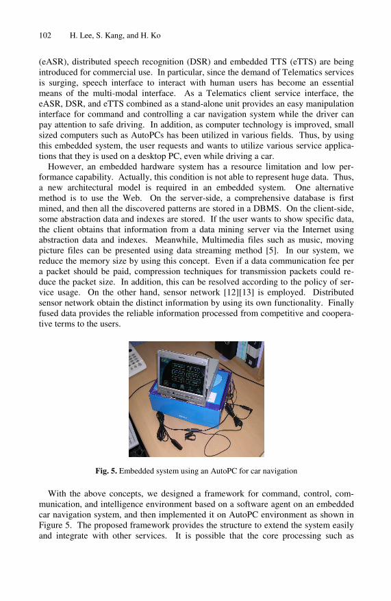
102 H. Lee, S. Kang, and H. Ko
(eASR), distributed speech recognition (DSR) and embedded TTS (eTTS) are being introduced for commercial use. In particular, since the demand of Telematics services is surging, speech interface to interact with human users has become an essential means of the multi-modal interface. As a Telematics client service interface, the eASR, DSR, and eTTS combined as a stand-alone unit provides an easy manipulation interface for command and controlling a car navigation system while the driver can pay attention to safe driving. In addition, as computer technology is improved, small sized computers such as AutoPCs has been utilized in various fields. Thus, by using this embedded system, the user requests and wants to utilize various service applica-tions that they is used on a desktop PC, even while driving a car.
However, an embedded hardware system has a resource limitation and low per-formance capability. Actually, this condition is not able to represent huge data. Thus, a new architectural model is required in an embedded system. One alternative method is to use the Web. On the server-side, a comprehensive database is first mined, and then all the discovered patterns are stored in a DBMS. On the client-side, some abstraction data and indexes are stored. If the user wants to show specific data, the client obtains that information from a data mining server via the Internet using abstraction data and indexes. Meanwhile, Multimedia files such as music, moving picture files can be presented using data streaming method [5]. In our system, we reduce the memory size by using this concept. Even if a data communication fee per a packet should be paid, compression techniques for transmission packets could re-duce the packet size. In addition, this can be resolved according to the policy of ser-vice usage. On the other hand, sensor network [12][13] is employed. Distributed sensor network obtain the distinct information by using its own functionality. Finally fused data provides the reliable information processed from competitive and coopera-tive terms to the users.
Fig. 5. Embedded system using an AutoPC for car navigation
With the above concepts, we designed a framework for command, control, com-munication, and intelligence environment based on a software agent on an embedded car navigation system, and then implemented it on AutoPC environment as shown in Figure 5. The proposed framework provides the structure to extend the system easily and integrate with other services. It is possible that the core processing such as

Decision Theoretic Fusion Framework for Actionability 103
combining rules from interface modalities, data fusion rules, DBMS processing, and communication tasks are done by the speech interactive agent. In this system, a con-versational tool provides advantages in confirming the final decision to use human interactive data mining [3].
5.2 Conclusions
In this paper, we proposed a decision theoretic fusion framework that includes the multiple level-of-abstraction approach combining multiple-level association rules and the summary table, as well as the active interaction rule generation algorithm using the rough set theory for actionability on an embedded car navigation system. In addi-tion, it included the sensory and data fusion level rule extraction algorithm to cope with simultaneous events occurring from multi-modal interface. Using such a deci-sion theoretic fusion framework, a variety of applications can be applied easily to this system in the form of flexible, extensible and transparent ones. We expect that this fusion framework will be able to meet the user’s demands and desires.
Acknowledgements
This work was supported by grant No. A17-11-02 from the Korea Institute of Indus-trial Technology Evaluation & Planning Foundation.
References
[1] A. Kusiak, and et al., “Autonomous Decision-Making: A Data Mining Approach,” IEEE Trans. on Information Technology in Biomedicine, Vol. 4, No. 4, December 2000.
[2] B. Delaney, and et al., ‘‘A Low-Power, Fixed-Point Front-End Feature Extraction for a Distributed Speech Recognition System,’’ HP Technical Report, HPL-2001-252, 2001.
[3] C. C. Aggarwal, “A Human-Computer Interactive Method for Projected Clustering,” IEEE Trans. On Knowledge and Data Engineering, Vol. 16, No. 4, April 2004.
[4] D. R. Campbell, and P. W. Shields, “Speech enhancement using sub-band adaptive Grif-fiths-Jim signal processing,” Speech Communication 39, pp. 97-110, 2003.
[5] G. Brettlecker, H. Schuldt, and R. Schatz. ‘‘Hyperdatabases for Peer-to-Peer Data Stream Processing,’’ IEEE International Conference on Web Service, pp.358-366, July 2004.
[6] H. Ashida, and T. Morita, ‘‘Architecture of data mining server: DATAFRONT/Server,’’ IEEE SMC '99 Conference Proceedings., Volume: 5 , 12-15 Oct. 1999.
[7] J. Beh and H. Ko, ‘‘A Novel Spectral Subtraction Scheme For Robust Speech Recogni-tion: Spectral Subtraction using Spectral Harmonics of Speech,’’ ICME, pp. 633-636, Jul. 2003.
[8] J. Han and et al. ‘‘Data mining for Web intelligence,’’ Computer , Volume: 35, Issue: 11, Nov. 2002.
[9] J. Han, Y. Cai, and N. Cercone, “Data-Driven Discovery of Quantitative Rules in Rela-tional Databases,” IEEE Trans. on Knowledge and Data Eng., vol. 5, pp.29-40, 1993.
[10] M. Aakay, and et al., ‘‘A system for medical consultation and education using multimodal human/machine communication,’’ IEEE Trans. On Information Technology in Biomedi-cine, Vol 2 , Issue: 4 , Dec. 1998.

104 H. Lee, S. Kang, and H. Ko
[11] M. Chen, and et al., “Data Mining: An Overview from a Database Perspective,” IEEE Trans. on knowledge and Data Engineering, Vol. 8, No. 6, December 1996.
[12] R. T. Antony, Principles of Data Fusion Automation, Artech house, 1995. [13] R. R. Brooks and S. S. Iyengar, MultiSensor Fusion: Fundamentals and Applications
with Software, Prentice Hall, 1998. [14] R. Srikant and R. Agrawal, “Mining Generalized Association Rules,” Proc. 21th Int’l
Conf. Very Large Data Bases, pp. 407-419, Sept. 1995. [15] S. Mitra, and et al., “Data Mining in Soft Computing Framework: A Survey,” IEEE
Trans. on Neural Networks, Vol. 13, No. 13, January 2002. [16] S. Takata, S. Kawato, and M Mase, ‘‘Conversational agent who achieves tasks while in-
teracting with humans based on scenarios,’’ Robot and Human Interactive Communica-tion Proceedings:11th IEEE International Workshop, 25-27 Sept. 2002.
[17] T. Kim and H. Ko, ‘‘Uttrance Verification Under Distributed Detection and Fusion Framework’’, Eurospeech, pp. 889~892, Sep. 2003.
[18] W. Kim, S. Ahn and H. Ko, ‘‘Feature Compensation Scheme Based on Parallel Combined Mixture Model’’, Eurospeech, pp. 677~680, Sep, 2003.
[19] X. Huang, A. Acero and H. Hon, Spoken Language Processing, Prentice Hall PTR, 2001.
[20] Y. Elovici and D. Braha, “A Decision-Theoretic Approach to Data Mining,” IEEE Trans on Systems, Man, and Cybernetics – PART A:Systems and Humans, Vol. 33, No. 1, January 2003.
[21] Y. Cao, S. Sridharan, and M. Moody, “Multichannel speech separation by Eigendecom-position and its application to co-talker interference removal,” IEEE Transactions on Speech and Audio Processing, vol. 5, no. 3, pp. 209-219, May 1997.
[22] Y. Gong, and Y. Kao, ‘‘Implementing a high accuracy speaker-independent continuous speech recognizer on a fixed-point DSP,’’ Proc. of ICASSP, Vol. 6, June 2000.
[23] http://www.sitec.or.kr.

G.J. Williams and S.J. Simoff (Eds.): Data Mining, LNAI 3755, pp. 105 – 117, 2006. © Springer-Verlag Berlin Heidelberg 2006
Use of Data Mining in System Development Life Cycle
Richi Nayak1 and Tian Qiu2
1 School of Information Systems, QUT, Brisbane, QLD 4001, Australia [email protected]
2 EDS Credit Services, Adelaide, Australia [email protected]
Abstract. During the life cycle of a software development project, many problems arise. Resolutions to these problems are time consuming and expensive. This paper discusses the use of data mining in solving some of these problems to improve the system development life cycle process. A case study of applying data mining to the software Problem Report management data is also presented. The empirical results demonstrate the capability and benefit of data mining analysis in systems development life cycle.
1 Introduction
The System Development Life Cycle (SDLC) includes various phases during which the defined software products are created or modified [22]. These phases include planning, definition, requirement analysis, design, development, testing and integration, implementation, operation and maintenance. During the SDLC process, huge repositories for configuration management, risk management, project metric report and problem report management are maintained in addition to source code.
These repositories are potential sources of useful information that can be used in improving the SDLC process. Researchers have started using data mining (DM) [5,9,10,11,16,18,21] techniques in this process. Some examples of DM usage are in (1) software maintenance by summarizing and augmenting software changes, (2) software development process by automatically generating test cases and checking their outputs, (3) software reuse by predicting success or failure of components beforehand, and matching and discovering reusable patterns, and (4) project planning and estimation by identifying relationships between human resources and product types.
This paper discusses the capability and benefit of data mining analysis in systems development life cycle. The paper is organised into two parts. The first part includes the discussion on various DM applications in SDLC. The second part presents a case study of applying DM to the software problem report management data.
2 Data Mining Applications in SDLC
Figure 1 illustrates a general framework of applying DM techniques to aid the SDLC process. We have summarised the use of DM in SDLC into two areas: (1) software development process that includes management rule generation, risk assessment and

106 R. Nayak and T. Qiu
software component testing and (2) software reuse and maintenance that includes component discovery, reuse and maintenance.
There are also examples of complementing DM with the use of software engineering (SE) principles. [7] utilised SE principles for the development of clustering architecture implemented on the multi-stage DM process to reduce the processing time. A SE methodology is also used to combine the application of deductive logic for generating intelligence from a collection of SE data [13].
Software Modules(Source code,
Libraries)
Pre-processing
Project Documentation (Electronicand Paper based), Problem
Reports, Conceptual Models (UML)
Project ManagementDatbases (Risk
Management, ConfigurationMangement)
Data MiningClustering
Post-Processing
Decision & Rgression trees
Neural networks Association
Data Integration & Selection
Other machine learningtechniques
Manamgement RulesGeneration
SoftwareComponent testing
Software ComponentDiscovery
SoftwareComponent Reuse
Software ComponentMaintenance
Fig. 1. A general framework showing steps of DM process in SDLC
2.1 Software Development Process
There exist several software development methodologies such as waterfall, incremental, rapid, agile and object-oriented [18]. Usually developers choose a methodology based on their previous experience or according to the managerial decisions. Every organisation collects a meta-data about the applications being developed. A data set can be created based on the methodology used, human resources involved, nature of the application, etc, and finally whether the project has been successful or not. Results of the DM analysis can be used in advising developers on the usage of a methodology according to the nature of the future application, to warn developers about failure stories, and to inform project mangers on human resources planning and scheduling.

Use of Data Mining in System Development Life Cycle 107
DM has been used in detecting error-patterns linked to a certain software component(s). The error patterns in combination with the associated component(s) can give an overview of the problem, and whether this problem in the component is associated with other failures elsewhere in the component hierarchy. [9] used the classification and regression trees algorithm to predict which software modules likely to have faults discovered during operations. They derived the variables from various SDLC repositories and used them as useful predictors of software quality. Software developers need such predictions early in development to enhance software quality.
[16] successfully used regression tree analysis to determine the project size based on the size of individual software components. The size estimation helps in resource planning. [5] used the classification and association data mining to model the complex behaviour of the software development process and created different scenarios for the same project. The generated management rules make the decision-taking process easy for project managers in a similar situation.
Researchers have also used DM in automatic testing of systems. [10] used info-fuzzy network based method to recover the system requirements, to automatically design a minimal set of test cases and to evaluate the correctness of outputs.
2.2 Software Reuse and Maintenance
The use of object oriented analysis and design has skyrocketed in the last decade and contributes greatly to both organizational and commercially available software components. However finding the right component at the right time can be a complex task. Choosing the right library or (module) component can result in an efficient project, but selecting the wrong components can cause unnecessary project delays due to possible software failure and debugging.
Nakkrasae et al. [15] used a neural network technique to classify software components for effective archival and retrieval purposes. This work enables software components details to be stored, classified, and subsequently retrieved for reuse. In the same line, Miller et al [12] utilised DM techniques to discover structural information about legacy programs and constructed a warehouse of program-analysis data to provide support in software reuse and maintenance.
Morisio et al. [14] identified success or failure factors in components by using predictive DM which is aimed at two factors namely human factors and product type. This leads to recommending possible successful components for reuse. Michail [11] used link analysis to find association between library classes and program functions that are typically reused in combination with application classes. Specific rules of how components are associated with library functions through usage are created.
Many software projects fail because components fail and huge resources is wasted in debugging and fixing faulty code. This becomes worse when changes in one part of the program code make other components faulty and unusable based on relationships between the components. Ying et al. [20] applied association mining to determine change patterns – set of files that were changed together frequently in the past – from the change history of the programming codes. The mined change patterns (a set of files) are used as recommendation (to check for correctness) whenever a developer modifies the linked existing code. Shirabad et al [17] investigated decision tree learning to find out the relevant files that are affected by the changes applied to a

108 R. Nayak and T. Qiu
particular file or a set of files. They used the software maintenance records to provide the training data set in a DM process.
2.3 Data Mining Tools in SDLC
The most commonly used DM techniques in SDLC are decision trees, neural networks and association analysis. A DM tool used in SDLC should be effective to utilise these techniques, easy to use, support data preparation and most importantly, be able to present results in a succinct manner. The general-purpose DM tools such as SAS ‘Enterprise Miner’ and Statsofts’s ‘Statistica Data Miner’ (known for the user-friendly drag-and-drop workspace and good reporting functions) can be used. There also exits DM tools especially built to assist in SDLC process. An example is EMERALD [4], Enhanced Measurement for Early Risk Assessment of Latent Defects, for assessing reliability risk for software developers and managers. This tool has been used in number of studies, e.g., [19] used EMERALD for predicting fault ranges of software modules with Fuzzy Nonlinear Regression.
2.4 Major Issues Arising with Applications of Data Mining in SDLC
General problems encountered with data such as over-fitting/poor-fitting, missing and noisy values, large size and dimensionality, still remain the same for this domain as others. Some of the issues listed below can be considered as major requirements and challenges for the further evolution of DM technology in SDLC.
Diversity of the Data Types: Large software projects often keep huge amounts of data spread over different non-consolidated repositories such as source code repositories e.g., CVS*; conceptual models of software e.g., UML†; modelling tools e.g., Rational Rose‡; project management tools and documentation tools. Additionally, data collected during a SDLC process reside in many sources such as flat files, relational databases, data warehouses, transactional databases, advance database systems (including object-oriented, object-relational, multimedia and specific application-oriented databases) and the Web. While DM is applicable to any kind of data, the challenges and techniques may vary depending on the repository type.
A DM system must be able to deal with data drawn from different sources and formats. Without proper pre-processing, analysis of data to uncover patterns will be difficult since bad quality data ultimately leads to useless discoveries. The pre-processing module should include the use of simple query languages to extract data from various repositories, integrate, select, assess for quality and convert to the format suitable to the analysis tool.
Mining Methodology and User Interaction Issues: Data residing in many sources also poses a problem in mining of knowledge at multiple levels [8]. This raises the problem of finding associations among these various sets of extracted knowledge. The integration of extracted relationships from various sources is an unresolved issue [18].
* CVS is a common method to store source code of a project in a centralized repository. † Unified Modelling Language is a popular modelling language in SDLC. ‡ An industry standard multi-purpose modelling tool (by IBM) for software projects.

Use of Data Mining in System Development Life Cycle 109
Additionally, a large portion of the SDLC process is based on background knowledge of personnel involved. A DM technique should learn to incorporate the priori knowledge in its process.
Another aspect of DM that can be a problem is the presentation and visualization of the complex results. Output of a mining process is usually a large number of meaningful rules. However the representation of these rules to assist a project manager in making strategic directions requires significant post-processing.
Performance Issues: These include efficiency, scalability, and user effectiveness of data mining algorithms and tools. The performance metrics assessing the appropriateness of DM methods to SDLC includes robustness, scalability, automatic pre-processing capability, reliability, noise tolerance and sensitivity analysis [6]. A DM tool should be able to include all (or majority) of these to get the user satisfaction.
3 A Case Study: Analysis of Problem Report Data
This section describes the application of DM techniques to the software Problem Report (PR) management data of a large global telecommunication company. When a problem is reported, the responsible team can only approximately suggest the efforts (time) to fix the problem based on their previous experience. If the current project is not within their familiar topics, the accuracy of the estimation becomes worse.
The goal of this mining process is to provide estimation of effort to fix when a problem is raised. The results will reveal the hidden relationships in data, such as:
• How long does it take to fix a problem when a particular type of PR is raised? • What type of project documents needs significant efforts to fix the associated bug?
This will bring great cost savings and benefits to the organisation by the improved control over the PR fixing and an accurate project planing, estimation and progress control. The results will especially be useful to developers in problem reasoning. When a programmer is struggling with a bug, a resolution can be suggested from the knowledge inferred from the previous similar problems stored in PRs.
3.1 Data Pre-processing
The first task in the process is to prepare the data set according to the DM techniques.
Field Selection: The PR data consists of textual information, categorical and numerical fields. Several fields such as confidential, submitter-ID, environment, fix, release note, audit trail, the associated project name and the PR number are ignored during mining. These are used in pre-processing and post-processing stages to assist in the selection of data and a better understanding of the rules being found.
Whenever a PR is raised, a project leader will have to find answers for the following questions before taking any action:
• How severe the problem is (customer impact)? • What is the impact of the problem on project schedule (Cost & Team priority)? • What type of the problem it is (a Software bug or a design flaw)?

110 R. Nayak and T. Qiu
• How long it will take to fix? • How many people were involved? • What is the problem description?
Accordingly, attributes such as Severity (serious, critical or non-critical), Priority (high, medium or low), Class (sw-bug, doc-bug, change-request, duplicate, mistaken, or support), Arrival-Date, Closed-Date, Responsible, and Synopsis are considered for mining.
The attribute ‘Class’ is chosen as the target attribute in order to find out any valuable knowledge of the type of the problem with the rest of the PR attributes. Knowing the relationship between the fix effort and the PR class, a project leader can analyse the fix effort versus the human resources available. This knowledge can now be used in the scheduling and resource planning.
Every PR has an attribute, State (open, active, analysed, suspended, feedback, resolved and closed), to indicate the current stage of the PR. Since, the aim of this mining exercise is to find useful knowledge from existing projects, the PRs with a closed value in their State field are only considered.
The first five fields have fixed input values. Responsible attribute is used to calculate how many people were involved to fix the problem. Association or classification rules are generated by applying DM techniques on these fields. The Synopsis field has text information. It may contain what type of a project document (a piece of code or a support document) that the PR is concerned with. It can be used as a text index. Text Mining is considered to analyse this qualitative information.
Data Cleaning: The data set has some noise due to evolution of the data acquisition system and human involvement with the process. An example is the use of different terminologies over the time such as SW-bug or sw-bug as an input value for Class field (Example a, d in Figure 2). A Time-Zone field and other new input values have been added later in the system on management request based on the feedback of users after several years of system running.
To handle with the erroneous PRs, attempts are made to recover errors in PRs manually or automatically. If successful, the modified PRs are included in the mining process. For example, SW-bug in Class field is replaced by sw-bug throughout the data. The Completed-Date field (that was obsolete after some year of usage) is deleted, and the value (if any) is copied into the Closed-Date field.
The PRs, in which an error cannot be recovered precisely, are either discarded or replaced by a ‘?’ if a software can handle the missing values. For example, the instance a in Figure 2 has its closed time earlier than the time being raised. Some PRs do not have all the values stored; such as Example c in Figure 2 has no closed date. An example of inconsistent values is shown in Figure 2 - there is no input for the Time-Zone field in a PR recorded before 1998, as the Time-Zone field is added in 1998.
Data Transformation: The attributes Arrival-Date and Closed-Date are transformed to a time-period - identifying the time spent to fix a PR – by taking account the additional information Time-Zone and Responsible. This transformation resulted in the Time-to-fix attribute with continuous values (figure 3). The Responsible attribute has the information about personnel engaged in rectifying the problem. We assume that the derived attribute Time-to-fix is total time spent to fix a problem if there is only

Use of Data Mining in System Development Life Cycle 111
one person involved. The calculated time period from Arrival-Date and Closed-Date is than multiplied by the number of people yield from the Responsible attribute. We have also experimented with discretizing this attribute with cutting points be one day (1), half week (3 days), one week (7), two weeks (14), one month (30) and one quarter (90 days), half year (180 days) and more than one year (360 days). The main reason behind this exercise is to give an approximate estimate. It allows for a minor change in human resource, and being not highly dependent on the exact human resource involved.
Fig. 2. Data examples from the original PR data set
Fig. 3. Data examples ready for mining
3.2 Data Modelling and Mining
We have chosen three data mining techniques to analyse the PR data:
• Predictive modelling on the PR data to make estimation on the time spent to fix a PR according to the PR properties.
• Link analysis to discover association among various PR characteristics. • Text mining to analyse Synopsis field to find out most representative words in the
problem-discussion, showing the major cause of a problem, along with the relationship of each frequent word with other words to show how are they related.
PR_ID|Category|Severity|Priority|Class|Arrival-Date|Close-Date|Synopsis
a. 17358|bambam|serious|high|sw-bug|20:50 May 25 CST 1999|11:35 Mar 24 CST 1999| STI STR register not being reset at POR
b. 17436|bambam|serious|high|support|18:10 Mar 30 CST 1999|12:00 May 24 CST 1999| sequence_reg varable in the RDR_CHL task is not defined
c. 580 |bingarra|serious|low|doc-bug|10:10 May 31 May 1996| | In URDRT2 of design doc, the word 'last' should be 'first'
d. 6205 |gali|serious|medium|SW-bug|14:30 Nov 5 1997|13:14 Dec 1 1997| grouping of options in dialog box
Severity |Priority| Time-to-fix| Class |Synopsis
a. serious, high, 61, sw-bug, STI STR register not being reset at POR b. serious, high, 56, support, sequence_reg varable in the RDR_CHL task is not
defined c. serious, low, ?, doc-bug, In URDRT2 of design doc, the word 'last' should be
'first' d. serious, medium, 24, sw-bug, grouping of options in dialog box

112 R. Nayak and T. Qiu
The predictive modelling or classification task builds a model by recognising distinct characteristics of the data set. We have chosen tree induction or decision tree (DT) due to their simplicity, efficiency and capability of dealing with noise and large data. The size of a DT depends on the number of attributes used to construct it. Because the number of attributes in our problem is small, the resulting DT is relatively simple and thus its structure is understood easily by a human analyst.
The link analysis operation exposes samples and trends by predicting correlation of variables in a given data set. We have used the Apriori algorithm [6] to reveal hidden affinity among the variables if a PR report is being raised.
We have used the C5 [2], CBA [1] and the TextAnalyst [3] tools for classification, both classification and association, and text mining respectively.
3.3 Assimilation and Analysis of Outputs
Classification and Association Rule Mining: In order to get better rules and to decrease the error rate, several approaches are used. One approach is to stratify the data on the target using the choice-based sampling instead of using random samples. Equal numbers of samples representing each possible value of the target attribute (Class) are chosen for training. This improves the possibility of finding rules that are associated with the small groups of values during training. Another approach is to choose different amounts of PR data as training sets.
We used different training data sets. The first data set (Case 1, Table 1) contains 1224 PRs belonging to a specific software project out of total 11,000 PRs. The second data set (Case 2) contains the equal distributed target values for a medium size of 3400 PRs (about 900 PRs from each value of ‘Class’) from all software projects. The third data set (Case 3) contains a large size of 5381 PRs from all software projects. We also performed the randomly selected PRs in 10-fold cross-validation experiments. The cross validation technique splits the whole data set into several subsets (called folds). Let each fold to be the test case and the rest as training sets in turn during training.
Experiments were conducted to test both type of time attribute – manually discretised or continuous values (labelled D or C in Table 1). Table 1 reports the classification mining results on all three cases, the associative rule mining results as Case 4, and (average) 10-fold cross-validation results.
We used two learning engines to discover rules from the PR data set– single support CBA (labelled SS in the Table 1 e.g., Case1-SS) and multiple support CBA (labelled b in the Table 1 e.g., Case1-MS). Constraints, support and confidence, are included in rules to control the quality of results. Confidence is the measure of the strength of a rule that indicates the probability of having consequence(s) in the rules provided that the rule contains certain antecedent(s). Support indicates the number of input data supporting the rule.
Some of the attributes in the data do not have uniform distributions, and many attributes are of very low frequency. Therefore a single support for all attributes is not able to discover important rules. This problem is relieved by setting multiple supports that allow user to choose different minimum supports to different attributes.
In general, all classification results in CBA achieve around 46% error rate in training data set (the lowest is 43.51%, the highest is above 59.10%). Above 51%

Use of Data Mining in System Development Life Cycle 113
correct prediction rate is achieved in testing data set (the lowest has 43.51%, the highest has 58.25%). Another interesting point is that the attempt to improve the accurate prediction in the way of equal-distributed target-value samples does not lead much change; there is only roughly 3% improvement over the final result. The error rates from using multiple supports are higher and the number of extracted rules is lower than those from using single support mining engine.
The continuous time values result better than manually discretized values. This indicates that the discretized values may have resulted in some information loss.
Table 1. CBA Mining Results Summary. Rules are ranked by confidence.
Error rate (%) Time cost (seconds) #Rules
Training Testing Training Testing
Case1-SS-D 15 46.16 52.94 1.00 0.08
Case1-SS-C 10 45.180 47.56 1.01 0.07
Case1-MS-D 11 47.059 47.49 1.01 0.10
Case1-MS-C 9 45.180 47.56 1.04 0.09
Case2-SS-D 41 57.04 59.95 0.41 1.1
Case2-SS-C 18 57.39 58.09 0.44 1.3
Case2-MS-D 21 59.10 58.25 0.44 1.0
Case2-MS-C 12 58.45 58.91 0.45 1.2
Case3-SS-D 20 43.61 44.5 2.2 2.0
Case3-SS-C 15 43.5 43.8 2.2 2.0
Case3-MS-D 15 46.5 45.1 1.6 1.9
Case3-MS-C 15 46.5 46.9 1.6 1.6
10-CV-SS-D 22 50.5 52.5 25
10-CV-SS-C 18 46.05 46.89 25.4
10-CV-MS-D 17 48.87 49.1 28.9
10-CV-MS-C 16 45.02 45.98 25.3
Case4-SS-D 15 46.16 N/A 0.60 N/A
Case4-SS-C 10 45.180 N/A 0.66 N/A
Case4-MS-D 11 47.059 N/A 0.77 N/A
Case4-MS-C 9 45.180 N/A 1.04 N/A
There is no rule that has confidence value larger than 80%, however they do describe some characters of the PR fixing process. Therefore they are useful for the project management in estimating bug fixing related time issues.
Followings are examples of generated classification rules with CBA:
Rule 1: If severity= non-critical and Time-to-fix = 3 to 30 days and priority= medium Then class = doc-bug. Confidence = 82.7%, Support = 2.7%

114 R. Nayak and T. Qiu
Rule 2: If severity= critical and Time-to-fix = less than 3 days and priority = high Then class = sw-bug. Confidence = 75.2%, Support = 2.3%
Overall, the extracted rules infer that the software related bugs can be fixed within 3 days with above 75% confidence if they have high priority and are in critical condition. It may take 3 months to fix the problem if the corresponding priority and severity are graded as medium and serious.
The software C5 was also used to perform classification data mining. We also utilised boosting and cross validation (Table 2). Boosting is a technique for generating and combining multiple classifiers to give improved predictive accuracy. After a number of trials, several different decision trees or rule sets are combined to reduce error rate for prediction. Boosting takes a longer time to produce the final classifier, and may not always achieve better results than a single classifier approach does, especially when the training data set has noise. Boosting and cross validation techniques do not generate a new rule, but try to find a better rule from the existing results. They only produce better results than the individual trees if the individual trees disagree with one another.
Table 2. C5 Mining Results Summary
Normal mining Mining with Boosting Mining with cross-validation (10-fold)
Training Testing Training Testing Training Testing
#Rules 51 N/A N/A. N/A 57.7 N/A
Error Rate (%) (Rules)
41.5 42.6 41.3 42.6 43.9 42.8
Error Rate (%) (Trees)
40.3 42.5 39.4 42.6 44.1 43.1
Size of tree 141 N/A. N/A. N/A 121.9 N/A.
Process Time (seconds)
5.6 0.2 37.7 0.4 41.1 1.1
Some example extracted classification rules with C5 are:
Rule 1: When a PR is in low priority and the time spent is around half a day (0.5 day) Then the rule has a high probability (87.5% Confidence) to classify a bug to be a document related bug.
Rule 2: When a PR is in medium priority with non-critical severity and the time spent is around 1.1 day Then the rule has 84.6% Confidence to classify a bug to be a document related bug.
Rule 3: When a PR is in low priority and the time spent for fixing is around 1 week Then the rule has 83.3% Confidence to classify a bug to be a software bug.
In general, all the rule sets achieve around 42% training error rate (the lowest is 40.3%, the highest is 43.9%) and 42.5% test error rate (the lowest is 39.4%, the

Use of Data Mining in System Development Life Cycle 115
highest is 44.1%). Both of the rates are better than CBA results. The time efficiency of C5 is also better than CBA.
Text Mining in PR Data: In order to find valuable knowledge from thousands of text, we categorise the pure text into several document types based on specific background knowledge. The result of the text mining together with the rules obtained from classification and association can more accurately predict the time and cost of fixing PRs. The TextAnalyst [3] tool automatically provides a concise and accurate summary of the analysed text and extracts some valuable rules. It builds up a semantic network for the investigation over the PR data.
The semantic network tree of the PR data contains a set of the most important words or word combinations, called concepts. Each concept of the semantic network is characterised by a weight value and a set of relationship of this concept to other concepts in the network. Every relationship between concepts is also assigned a weight value. The values of the weights range from 0 to 100, which correspond to the probability that the associated concept is characteristic for the whole PR data.
An interesting result is obtained for SCMP, Software Configuration Management Plan, a support document in every project. Since SCMP is not a main design document for a project with just about tens pages, it has never been considered as a trouble making item. However, the result showed that SCMP has 71% probability of appearing in test related PRs, and 58% probability of appearing in Code related PRs. This result is higher than the result associated with SRS (“Software Requirements Specification”, a main development document directly related to software). This indicates that the attention should be paid in designing the SCMP document, and hence reducing the total cost of fixing SCMP related PRs.
Another analysis shows that a test related PR also has a higher weight (36, 100) in document related bugs than a SRS related PR (35, 99) does. This suggests that designers should also focus on the quality of the support and testing related documents along with the product related documents.
3.4 Problems in Performing Mining
The error rates in both CBA and C5 are higher than expected. Although several approaches are attempted to reduce the error such as uniform distribution of values, cross validation, boosting, different size of training set, etc. Unfortunately, the average error rate is only fallen down by 5% from 47% to 42%. The best result is 9% improvement from 46% to 37%. These results indicate that some amount of noise is still existent in data even after dealing with the noise during pre-processing.
The relationships between PRs and human resources within a particular project play a major role. The time needed to fix a bug is different for each project depending upon the actual human resources available. We have used only the ‘Responsible’ attribute to indicate the human resource available. Truly, the relationship with the human resources available for past projects is needed to help project leaders to predict time consummations more accurately. The integration of the ‘Change Request’ data set that records all customer request process may rectify this problem.
Another reason is a non-uniform value distribution in the data set. For example, there are only 342 PRs with change-request value in the data set, compared to more than

116 R. Nayak and T. Qiu
5900 PRs related to sw-bug. Any potential rule associated to change-request can be heavily affected due to the presence of large size group with other values. Again the use of additional data sources together with the PR data set can rectify this problem.
We also attempted to use neural networks, there was no significant improvement in accuracy. In addition, it was difficult to interpret the outputs without the use of rule extraction techniques.
4 Conclusion
This paper attempts to show the use of data mining as one of the efficient methods to improve the SDLC process. Data mining can assist software developers by automating some of the development tasks. For example, the fundamental idea behind object-oriented programming is the re-use of components and linkage of objects through class instantiation, polymorphism and abstraction calls. Data mining can help to realise this concept more efficiently.
This paper also explored the use of data mining on a set of data collected during the SDLC process under a real software business environment. Some useful rules are inferred on the time consumption to fix a Problem Report and the relationship between the content and the type of the PR. These rules are in the form of associations, decision trees and semantic trees. The result may help developers in problem reasoning, and project leaders in estimation and planning.
Results of this application indicate that DM has capacity to improve the quality and efficiency of the software development process, even though the scale of this DM task was limited. It will be interesting to apply data mining to different phases of software development such as software quality data and integration of various data and knowledge at multiple levels.
As in many other domains, the benefits and capabilities brought by data mining in SDLC are worth of further investigations.
Acknowledgment
We will sincerely like to thank Mihir Shah, Parita Choksi and Magnus Haugaasen (ITB239: Enterprise Data Mining students at QUT) for conducting a short literature review on DM in SE domain. We will also like to show our gratitude to Dr Anurag Nayak a Senior IT Consultant for providing answers to SDLC related questions.
References
1. CBA, http://www.comp.nus.edu.sg/~dm2/ 2. C5.0, http://www.rulequest.com/see5-info.html 3. TextMiner, http://www.megaputer.com/company/index.html 4. EMERALD, http://www.graphicsillustrated.com/reliametrics/products/tools.html 5. Alvarez-Macias J., J. Mata-Vazquez and J. Riquelme-Santos, Data Mining for the
Management of Software Development Process, IJSEKE, Vol. 14, Issue 6 (2004) 665-695.

Use of Data Mining in System Development Life Cycle 117
6. Chung H and P. Gray, Current Issues in Data Mining Journal of Management Information Systems, forthcoming
7. Gerardo B., J. Lee, Y. Choi and M. Lee, “The K-Means Clustering Architecture in the Multi-Stage Data Mining Process” , ICCSA 2005, LNCS 3481, pg 71-81,2005.
8. Han J., and M. Kamber, “Data mining: concepts and techniques”, Morgan Kaufmann Publishers, 2001.
9. Khoshgoftar T. and E. Allen, “Predicting Fault-Prone Software Modules in Embedded Systems with Classification Trees”, International Journal of Reliability, Quality and Safety Engineering, 7(4), 2004.
10. Last M., M. Friedman and A. Kendal, Using Data Mining for Automated Software Testing, IJSEKE, Vol 14. Issue 4., 2004.
11. Michail A Data mining library reuse patterns using generalized association rules In International Conference on Software Engineering (2000), pp. 167–176.
12. Miller R. and A Gujarathi Mining for program structure IJSEKE, vol 9, No 5 (1999) 499-517 13. Mitkas P., “Knowledge Discovery for Training Intelligent Agents: Methodology, Tools
and Applications”, AIS-ADM 2005, LNAI 3505, pp 2-18, 2005. 14. Morisio M., M. Ezran and C. Tully (2003) Comments on ‘More Success and Failure
Factors in Software Reuse” , IEEE trans on SE, Vol 29, Issue 5. pg 478, 2003. 15. Nakkrasae S.and P. Sophatsathit, An Rpcl-Based Indexing Approach for SoftwareComponent
Classification, IJSEKE, Vol 14, Issue 5. pg.497-518, 2004 16. Pendharkar P. An exploratory study of object-oriented software component size determinants
and the application of regression tree forecasting models. Information & Management 42 (2004) 61-73.
17. Shirabad J., T. Lethbridge and S Matwin Applying data mining to software maintenance records In Proceedings of the 2003 conference of the Centre for Advanced Studies on Collaborative research.
18. Sunderhaft, N and Medonca. M. Mining Software Engineering Data: A Survey, A DACS state of the art report prepared for air-force Research Laboratory - Rome, NY, 1999.
19. Xu Z., Allen E.B., Prediction of Software Faults using Fuzzy Nonlinear Regression Modeling, In 5th IEEE International Symposium on High Assurance Systems Engineering, Nov, 2000, NewMaxico, pp 281-290.
20. Ying A., G. Murphy, R. Ng and C. Carroll. Predicting Source Code Changes by Mining Change History, IJSEKE, Vol 30. Issue 9. pg. 574-590, 2004.
21. (eds) Dia H and Webb G. IJSEKE, special issue: Best Papers from SEKE 2003 Workshop on Data Mining for Software Engineering and Knowledge Engineering, Vol 14, No 4, August 2004.
22. The Systems Development Life Cycle Guidance Document. [Accessed 21/6/2005] Available online at: http://www.usdoj.gov/jmd/irm/lifecycle/table.htm

G.J. Williams and S.J. Simoff (Eds.): Data Mining, LNAI 3755, pp. 118 – 129, 2006. © Springer-Verlag Berlin Heidelberg 2006
Mining MOUCLAS Patterns and Jumping MOUCLAS Patterns to Construct Classifiers
Yalei Hao1, Gerald Quirchmayr1,2, and Markus Stumptner1
1 Advanced Computing Research Centre, University of South Australia, SA5095, Australia
2 Institut für Informatik und Wirtschaftsinformatik, Universität Wien, Liebiggasse 4, A-1010 Wien, Austria
[email protected], [email protected], [email protected]
Abstract. This paper proposes a mining novel approach which consists of two new data mining algorithms for the classification over quantitative data, based on two new pattern called MOUCLAS (MOUntain function based CLASsification) Patterns and Jumping MOUCLAS Patterns. The motivation of the study is to develop two classifiers for quantitative attributes by the concepts of the association rule and the clustering. An illustration of using petroleum well logging data for oil/gas formation identification is presented in the paper. MPs and JMPs are ideally suitable to derive the implicit relationship between measured values (well logging data) and properties to be predicted (oil/gas formation or not). As a hybrid of classification and clustering and association rules mining, our approach have several advantages which are (1) it has a solid mathematical foundation and compact mathematical description of classifiers, (2) it does not require discretization, (3) it is robust when handling noisy or incomplete data in high dimensional data space.
1 Introduction
Data mining based classification aims to build accurate and efficient classifiers not only on small data sets but more importantly also on large and high dimensional data sets, while the widely used traditional statistical data analysis techniques are not sufficiently powerful for this task1, 2. With the development of new data mining techniques on association rules, new classification approaches based on concepts from association rule mining are emerging. These include such classifiers as ARCS3, CBA4, LB5, JEP6, etc., which are different from the classic decision tree based classifier C4.57 and k-nearest neighbor8 in both the learning and testing phases. To improve ARCS3, A non-grid-based technique9 has been further proposed to find quantitative association rules that can have more than two predicates in the antecedent. All the above algorithms are constrained by the framework of binning. Though several excellent discretization algorithms10, 11 are proposed, a standard approach to discretization has not yet been developed.

Mining MOUCLAS Patterns and Jumping MOUCLAS Patterns 119
Therefore, all the above research issues establish a challenge, which is whether it is possible that an association rule based classifier with any number of predicates in the antecedent can be developed for quantitative attributes by the concepts of clustering which can overcome the limitation caused by the discretization method. In this paper, to resolve the problem, we present a new approach to the classification over quantitative data in high dimensional databases, called MOUCLAS (MOUntain function based CLASsification), based on the concept of the fuzzy set membership function. It aims at integrating the advantages of classification, clustering and association rules mining to identify interesting patterns in selected sample data sets.
2 Problem Statement
We now give a formal statement of the problem of MOUCLAS Patterns (called MPs) and introduce some definitions.
The MOUCLAS algorithm, similar to ARCS, assumes that the initial association rules can be agglomerated into clustering regions, while obeying the anti-monotone rule constraint. Our proposed framework assumes that the training dataset D is a normal relational set, where transaction d ∈ D. Each transaction d is described by attributes Aj, j = 1 to l. The dimension of D is l, the number of attributes used in D. This allows us to describe a database in terms of volume and dimension. D can be classified into a set of known classes Y, y ∈ Y. The value of an attribute must be quantitative. In this work, we treat all the attributes uniformly. We can treat a transaction as a set of (attributes, value) pairs and a class label. We call each (attribute, value) pair an item. A set of items is simply called an itemset.
In this paper, we propose two novel classifiers, called the De-MP and J-MP, which exploit the discriminationg ability of MOUCLAS Patterns (MPs) and Jumping MOUCLAS Patterns (JMPs).
The MOUCLAS Pattern (so called MP) has an implication of the form:
Cluster(D)t → y,
where Cluster(D)t is a cluster of D, t = 1 to m, and y is a class label. The definitions of frequency and accuracy of MOUCLAS Patterns are defined as
following: The MP satisfying minimum support is frequent, where MP has support s if s% of the transactions in D belong to Cluster(D)t and are labeled with class y. The MP that satisfies a pre-specified minimum confidence is called accurate, where MP has confidence c if c% of the transactions belonging to Cluster(D)t are labeled with class y.
We also adopt the concept of reliability12 to describe the correlation. The measure of reliability of the association rule A⇒B can be defined as:
reliability R(A⇒B) = )(
)(
AP
BAP ∧ − ( )BP
Since R is the difference between the conditional probability of B given A and the unconditional of B, it measures the effect of available information of A on the

120 Y. Hao, G. Quirchmayr, and M. Stumptner
probability of the association rule. Correspondingly, the greater R is, the stronger MOUCLAS patterns are, which means the occurrence of Cluster(D)t more strongly implies the occurrence of y. Therefore, we can utilize reliability to further prune the selected frequent and accurate and reliable MOUCLAS patterns (MPs) to identify the truly interesting MPs and make the discovered MPs more understandable. The MP satisfying minimum reliability is reliable, where MP has reliability defined by the above formula.
Given a set of transactions, D, the problems of De-MP are to discover MPs that have support and confidence greater than the user-specified minimum support threshold (called minsup)13, and minimum confidence threshold (called minconf)13 and minimum reliability threshold (called minR) respectively, and to construct a classifier based upon MPs.
A Jumping MOUCLAS Pattern (JMP) can be further defined based on the notion of the Jumping Emerging Pattern6 (JEP) and MP. A JEP is an itemset whose support increases significantly from 0 in a class (say poisonous class in mushroom data from the UCI repository) to a user-specified value in another class (say edible class). We can then use JEP as an index for dimensionality reduction. For each JEP in a certain class y, only the attributes of the JEP will be kept for all the transactions in the class y. We then perform the clustering on those transactions.
Let C denote the dataset of transaction d labeled with class y after dimensionality reduction processing by JEPs. A JMP can be defined as a cluster_rule , namely a rule:
cluset → y,
where cluset is a set of itemsets from a cluster Cluster(C)t, which is obtained from the clustering on the same class of transactions after dimensionality reduction via JEP, y is a class label, y ∈ Y. Let JMPset denote a set of JMPs which coresponds to the same JEP.
Suppose the number of transactions of C in cluset is cluCount, the number of tansactions in C is clasCount, the support of transaction d belong to cluset in C, denoted as subsup, can be defined by the formula:
subsup = clasCount
cluCount
Given a set of transactions, D, the problems of J-MP is to discover all JMPs and calculate their subsup and construct a classifier based upon JMPs.
3 The MOUCLAS-1 Algorithm
The classification technique, MOUCLAS-1, consists of two steps:
1. Discovery of frequent, accurate and reliable MPs. 2. Construction of a classifier, called De-MP, based on MPs.
The core of the first step in the MOUCLAS-1 algorithm is to find all cluster_rules that have support above minsup. Let C denote the dataset D after dimensionality reduction processing. A cluster_rule represents a MP, namely a rule:

Mining MOUCLAS Patterns and Jumping MOUCLAS Patterns 121
cluset → y,
where cluset is a set of itemsets from a cluster Cluster(C)t, y is a class label, y ∈ Y. The support count of the cluset (called clusupCount) is the number of transactions in C that belong to the cluset. The support count of the cluster_rule (called cisupCount) is the number of transactions in D that belong to the cluset and are labeled with class y. The confidence of a cluster_rule is (cisupCount / clusupCount) × 100%. The support count of the class y (called clasupCount) is the number of transactions in C that belong to the class y. The support of a class (called clasup) is (clasupCount / |C |) × 100%, where | C | is the size of the dataset C.
Given a MP, the reliability R can be defined as:
R(cluset → y) = (cisupCount / clusupCount) - (clasupCount / |C |) × 100%
The traditional association rule mining only uses a single minsup in rule generation, which is inadequate for many practical datasets with uneven class frequency distributions. As a result, it may happen that the rules found for infrequent classes are insufficient and too many may be found for frequent classes, inducing useless or over-fitting rules, if the single minsup value is too high or too low. To overcome this drawback, we apply the theory of mining with multiple minimum supports14 in the step of discovering the frequent MPs as following.
Suppose the total support is t-minsup, the different minimum class support for each class y, denoted as minsupi can be defined by the formula:
minsupi = t-minsup × freqDistr(y)
where, freqDistr(y) is the function of class distributions. Cluster_rules that satisfy minsupi are called frequent cluster_rules, while the rest are called infrequent cluster_rules. If the confidence is greater than minconf, we say the MP is accurate.
The first step of MOUCLAS-1 algorithm works in three sub-steps, by which the problem of discovering a set of MPs is solved:
Algorithm: Mining frequent and accurate and reliable MOUCLAS patterns (MPs) Input: A training transaction database, D; minimum support threshold (minsupi);
minimum confidence threshold (minconf); minimum reliability threshold (minR) Output: A set of frequent, accurate and reliable MOUCLAS patterns (MPs) Methods:
(1) Reduce the dimensionality of transactions d, which efficiently reduces the data size by removing irrelevant or redundant attributes (or dimensions) from the training data, and
(2) Identify the clusters of database C for all transactions d after dimensionality reduction on attributes Aj in database C, based on the Mountain function, which is a fuzzy set membership function, and specially capable of transforming quantitative values of attributes in transactions into linguistic terms, and
(3) Generate a set of MPs that are both frequent, accurate and reliable, namely, which satisfy the user-specified minimum support (called minsupi), minimum confidence (called minconf) and minimum reliability (called minR) constraints.

122 Y. Hao, G. Quirchmayr, and M. Stumptner
In the first sub-step, we reduce the dimensionality of transactions in order to enhance the quality of data mining and decrease the computational cost of the MOUCLAS algorithm. Since, for attributes Aj, j = 1 to l in database, D, an exhaustive search for the optimal subset of attributes within 2l possible subsets can be prohibitively expensive, especially in high dimensional databases, we use heuristic methods to reduce the search space. Such greedy methods are effective in practice, and include such techniques as stepwise forward selection, stepwise backward elimination, combination of forwards selection and backward elimination, etc. The first sub-step is particularly important when dealing with raw data sets. Detailed methods concerning dimensionality reduction can be found in some papers15-18.
Fuzzy based clustering is performed in the second sub-step to find the clusters of quantitative data. The Mountain-climb technique proposed by R. R. Yager and D. P. Filev19 employed the concept of a mountain function, a fuzzy set membership function, in determining cluster centers used to initialize a Neuro-Fuzzy system. The substractive clustering technique20 was defined as an improvement of Mountain-climb clustering. A similar approach is provided by the DENCLUE algorithm21, which is especially efficient for clustering on high dimensional databases with noise. The techniques of Mountain-climb clustering, Substractive clustering and Denclue provide an effective way of dealing with quantitative attributes by mountain functions (or influence functions), which has a solid mathematical foundation and compact mathematical description and is totally different from the traditional processing method of binning. It offers us an opportunity of mining the patterns of data from an innovative angle. As a result, part of the research task presented in the introduction can now be favorably answered.
The observation that, a region which is dense in a particular subspace must create dense regions when projected onto lower dimensional subspaces, has been proved by R. Agrawal and his research cooperators in CLIQUE22. In other words, the observation follows the concepts of the apriori property. Hence, we may employ prior knowledge of items in the search space based on the property so that portions of the space can be pruned. The successful performance of CLIQUE has again proved the feasibility of applying the concept of apriori property to clustering. It brings us a step further towards the solution of the rest part of the research task, that is, if the initial association rules can be agglomerated into clustering regions, just like the condition in ARCS, we may be able to design a new classifier for the purpose of classification, which confines its search for the classifier to the cluster of dense units of high dimensional space. The answer to the rest research task can contribute to the third sub-step of the MOUCLAS algorithm to the forming of the antecedent of cluster_rules, with any number of predicates in the antecedent. In the third sub-step, we identify the candidate cluster_rules which are actually frequent and accurate and reliable. From this set of frequent and accurate and reliable cluster_rules, we produce a set of MPs.
Let I be the set of all items in D, C be the dataset D after dimensionality reduction, where transaction d ∈ C contains X ⊆ I, a k-itemset. Let E denote the set of candidates

Mining MOUCLAS Patterns and Jumping MOUCLAS Patterns 123
of cluster_rules, where e ∈ E, and F denote the set of frequent cluster_rules. The first step of the MOUCLAS algorithm is given in Figure 1 as follows.
The task of the second step in MOUCLAS-1 algorithm is to use a heuristic method to generate a classifier, named De-MP, where the discovered MPs can cover D and are organized according to a decreasing precedence based on their confidence and support. Suppose R be the set of frequent, accurate and reliable MPs which are generated in the past step, and MPdefault_class denotes the default class, which has the lowest precedence. We can then present the De-MP classifier in the form of
<MP1, MP2, …, MPn, MPdefault_class>,
where MPi ∈ R, i = 1 to n, MPa ≻MPb if n ≥ b > a ≥ 1 and a, b∈ i, C ⊆ ∪ cluset of MPi,.
1 X = reduceDim (I); // reduce the dimensionality on the set of all items I of in D 2 Cluster(C)t = genCluster (C); // identify the complete clusters of C 3 for each Cluster(C)t do E = genClusterrules(cluset, class); // generate a set of candidate cluster_rules 4 for each transaction d ∈ C do 5 Ed = genSubClusterrules (E, d); // find all the cluster_rules in E whose cluset are
supported by d 6 for each e ∈ Ed do 7 e. clusupCount++; // accumulate the clusupCount of the cluset of cluster_rule e 8 if d.class = e.class then e.cisupCount++ // accumulate the cisupCount of cluster_rule e supported by d 9 end 10 end 11 F = {e ∈ E | e.cisupCount ≥ minsupi }; // construct the set of frequent cluster_rules 12 MP = genRules (F); //generate MP using the genRules function by minconf and minR 13 end
14 MPs = ∪ MP; // discover the final set of MPs
Fig. 1. The First Step of the MOUCLAS-1 Algorithm
The second step of the MOUCLAS-1 algorithm also consists of three sub-steps, by which the De-MP classifier is formed:
Algorithm: Constructing De-MP Classifier Input: A training database after dimensionality reduction, C; The set of frequent
and accurate and reliable MOUCLAS patterns (MPs) Output: De-MP Classifier Methods: (1) Identify the order of all discovered MPs based on the definition of precedence
and sequence them according to decreasing precedence order. (2) Determine possible MPs for De-MP classifier from R following the
descending sequence of MPs. (3) Discard the MPs which cannot contribute to the improvement of the accuracy
of the De-MP classifier and keep the final set of MPs to construct the De-MP classifier.

124 Y. Hao, G. Quirchmayr, and M. Stumptner
In the first sub-step, the MPs are sorted in descending order, which has the training transactions surely covered by the MPs with the highest precedence when possible in the next sub-step. The sort of the whole set of MPs is performed following the definition of precedence:
Given two MPs, we say that MPa has a higher precedence than MPb, denoted as
MPa ≻ MPb,
if ∀ MPa, MPb ∈ MPs, it holds that: the confidence of MPa is greater than that of MPb, or if their confidences are the same, but the support of MPa is greater than that of MPb, or if both the confidences and supports of MPa and MPb are the same, but MPa is generated earlier than MPb.
In the second sub-step, we test the MPs following decreasing precedence and stop the sub-step when there is no rule or no training transaction. For each MP, we scan C to find those transactions satisfying the cluset of the MP. If the MP can correctly classify one transaction, we store it in a set denoted as L. Those transactions satisfying the cluset of the MP will be removed from C at each pass. Each transaction can be identified by a unique ID. The next pass will be performed on the remaining data. A default class is defined at each scan, which is the majority class in the remaining data. At the end of each pass, the total number of errors that are made by the current L and the default class are also stored. When there is no rule or no training transaction left, we terminate this sub-step. After this sub-step, every MP in L can correctly classify at least one training transaction in C.
In the third sub-step, though we would like to find as many MPs as possible to give good coverage of the training transactions in the second sub-step, we prefer strong MPs which have relatively high support and confidence, due to their characteristics of corresponding to larger coverage and stronger differentiating power. Meanwhile, we hope that the De-MP classifier, consisting of a combination of strong MPs, has a
1 R = sort(R); // sort MPs based on their precedence 2 for each MP R in sequence do3 temp = ;4 for each transaction d C do5 if d satisfies the cluset of MP then6 store d.ID in temp;7 if MP correctly classifies d then8 insert MP at the end of L;9 delete the transaction who has ID in temp from C;10 selecting a default class for the current L; // determine the default class based on majority class of remaining transactions in C11 end12 compute the total number of errors of L; // compute the total number of errors that are made by the current L and the default class 13 end14 Find the first MP in L with the lowest total number of errors and discard all the MPs after the MP in L;15 Add the default class associated with the above mentioned first MP to end of L;16 De-MP classifier = L
Fig. 2. The Second Step of the MOUCLAS Algorithm

Mining MOUCLAS Patterns and Jumping MOUCLAS Patterns 125
relatively smaller number of classification errors, because of greedy strategy. In addition, the reduction of MPs can increase the understandability of the classifier. Therefore, in this sub-step, we identify the first MP with the least number of errors in L and discard all the MPs after it because these MPs produce more errors. The undiscarded MPs and the default class corresponding to the first MP with the least number of errors in L form our De-MP classifier.
The second step of the MOUCLAS algorithm is shown in Figure 2. In the testing phase, when we classify a new transaction, the first MP in De-MP
satisfying the transaction is used to classify it. In De-MP classifier, default_class, having the lowest precedence, is used to specify a default class for any new sample that is not satisfied by any other MPs as in C4.57, CBA4.
4 The MOUCLAS-2 Algorithm
The classification technique, MOUCLAS-2, consists of two main processes:
1. Discovering of all JMPs for each class. 2. Calculating their subsup and building a classifier, called J-MP, based on JMPs.
The core of the MOUCLAS-2 algorithm is to find all cluster_rules, namely the JMPs. The MOUCLAS-2 algorithm works in three sub-steps, by which the problem of discovering JMPsets and construction of a classifier is solved:
Algorithm: Mining Jumping MOUCLAS Patterns (JMPs) and building J-MP Classifier
Input: A training transaction database, D; Output: J-MP Classifier Methods:
(1) Reduce the dimensionality of transactions d in each class y by the information of the attributes in corresponding JEPs, and
(2) Identify all the clusters of database based on the Mountain function, which is a fuzzy set membership function, and specially capable of transforming quantitative values of attributes in transactions into linguistic terms, and
(3) Generate JMPsets for each class y and calculate their subsup.
In the first sub-step, detailed method concerning JEP can be found in this paper6. The third sub-step of the MOUCLAS-2 algorithm form the cluster_rules, with any
number of predicates in the antecedent. It brings us a step further towards the solution of our research challenge. From this set of cluster_rules of a class y, we produce a set of JMPs for the class y.
Let I be the set of all items in D labeled with class y, C be the dataset of transaction d labeled with class y after dimensionality reduction processing by a JEP, where transaction d ∈ C contains Xi ⊆ I, a k-itemset, and i be the number of JEPs in the class y. Let E denote a set of cluster_rules (JMPset) of a class y, corresponding to a JEP, where e ∈ E.

126 Y. Hao, G. Quirchmayr, and M. Stumptner
The first step of the MOUCLAS-2 algorithm is given in Figure 3 as follows.
1 X = genJEP (I); // generate all the JEPs of all the class y in D 2 for each class y do 3 for each JEP of a same class y do 4 Xi = reduceDim (I); // reduce the dimensionality on the set of all items I in D
labeled with class y based on the attributes of the JEP 5 Ei = genClusterrules(cluset, class); // generate a set of cluster_rules, namely
JMPset, based on Xi 6 for each transaction d ∈ C do 7 if one e ∈ Ei can be supported by d then e.cluCount++; // accumulate the
cluCount of cluster_rule e supported by d 8 end 9 subsupi =
C
e.cluCount ; //calculate the subsup of each JMPset
10 end 11 end
12 JMPs = ∪ Ei; // discover the final set of JMP
Fig. 3. The Training Phase of the MOUCLAS-2 Algorithm
1 for each transaction d ∈ D do 2 for each class y do 3 for each JMPset of a same class y do 4 if d satisfies a JMPset then e.subsupt++ ; // accumulate the subsup of JMPsets
supported by d 5 end 6 the subsupy of d in class y = e.subsupt ; // calculate the total subsup of d in class y 7 end 8 if subsupy is the maximum then d is labeled as y 9 if the subsup in two or more classes are the same then d is labeled as the class,
whose JMPs are generated earlier than the others. 10 if the subsup = 0 then d is labeled as a default class 11 end
Fig. 4. The Testing Phase of the MOUCLAS Algorithm
In the testing phase, The MOUCLAS-2 algorithm also consists of two sub-steps, by which the J-MP classifier can classify test data:
Algorithm: Classification Process of J-MP Classifier Input: A test database, D; The set of Jumping MOUCLAS patterns (JMPs); The
support of transaction d belong to JMPs in C (subsup) Output: classification result of test database Methods:
(1) Determine the subsup of each transaction d in D in each class. (2) Classify the test data.

Mining MOUCLAS Patterns and Jumping MOUCLAS Patterns 127
In the first sub-step, we firstly determine whether a JMPset can be supported by a transaction d ∈ D. If so, we then sum up the total subsup of the transaction d in one class. In this way, the subsupy of the transaction d in the class y can be obtained, where y ∈ Y. In the second step, the testing transaction d can be labeled as the class y, where the subsupy is greater than all the others. If the transaction d has the same maximum subsupy in two classes, then it is labeled as the class, whose JMPs are generated earlier than the other.
The classification process of the MOUCLAS algorithm is shown in Figure 4.
5 Example of MOUCLAS Application in Reservoir Characterization
Oil/gas formation identification is a vital task of reservoir characterization in the petroleum industry, where the petroleum database contains such records (or attributes) as seismic data, various types of well logging data and petrophysical property data whose values are all quantitative.
An illustration of using well logging date for purpose of oil/gas formation identification is illustrated in Figure 5. The well logging data sets include attributes (well logging curves) of GR (gamma ray), RDEV (deep resistivity), RMEV (shallow resistivity), RXO (flushed zone resistivity), RHOB (bulk density), NPHI (neutron porosity), PEF (photoelectric factor) and DT (sonic travel time). Since most of the reservoirs are horizontally and vertically heterogeneous, no depth information is used for training.
Fig. 5. Quantitative Petroleum Data for MOUCLAS Mining (note: the dashed indicate the location of oil formation )
One transaction of the database can be treated as a set of the items corresponding to the same depth and a class label (oil/gas formation or not). A hypothetically useful MP or JMP may suggest a relation between well logging data and the class label of

128 Y. Hao, G. Quirchmayr, and M. Stumptner
oil/gas formation since. In this sense, a selected set of such MPs or JMPs can be a useful guide to petroleum engineers to identify possible drilling targets and their depth and thickness at the stage of exploration and exploitation.
MPs and JMPs aim at deriving an explicit or implicit heuristic relationship between measured values (well logging data) and properties to be predicted (oil/gas formation or not). The MOUCLAS based method is ideally suitable to establish such implicit relationships through proper training. The notable advantage of MOUCLAS based algorithms over more traditional processing techniques such as model based well logging analysis is that a physical model to describe the relationship between the well logging data and the property of interest is not needed; nor is an very precise understanding of the physical phenomena of the well logging data. From this point of view, MOUCLAS based algorithms provides a complementary and useful technical approach towards the interpretation of petroleum data and benefits petroleum discovery.
6 Conclusions
Two novel classification patterns, the MOUCLAS Pattern (MP) and the Jumping MOUCLAS Pattern (JMP) for quantitative data in high dimensional databases, are investigated in this paper. We also propose the algorithm for the discovery of the interesting MPs and JMPs and construct two new classifiers called De-MP and J-MP. As a hybrid of classification and clustering and association rules mining, our approach may have several advantages which are (1) it has a solid mathematical foundation and compact mathematical description of classifiers, (2) it does not require discretization, as opposed to other, otherwise quite similar methods such as ARCS are strongly related to, (3) it is robust when handling noisy or incomplete data in high dimensional data space, regardless of the database size, due to its grid-based characteristic. An illustration of application of MPs and JMPs is presented for the cost effective and intelligent well logging data analysis for reservoir characterization. In the future research, we attempt to carry out experiments on petroleum datasets to establish a relationship between different well logs, seismic attributes, laboratory measurements and other reservoir properties to evaluate performance of the MOUCLAS algorithms proposed in this paper.
Acknowledgement
This work was partially supported by the Australia-China Special Fund for Scientific and Technological Cooperation under grant CH030086.
References
1. Fayyad, U. M., Piatetsky-Shapiro, G., & Smyth, P. From data mining to knowledge discovery: An overview. Advances in knowledge discovery and data mining. AAAI/MIT Press. (1996) 1-34
2. Han, J., & M. Kamber. Data mining: concepts and techniques. Morgan Kaufmann Publishers. (2000)

Mining MOUCLAS Patterns and Jumping MOUCLAS Patterns 129
3. B. Lent, A. Swami, and J. Widom. Clustering association rules. ICDE'97, (1997) 220-231 4. B. Liu, W.Hsu, and Y.Ma. Integrating classification and association rule mining. KDD’98.
(1998) 80-86 5. Meretakis, D., & Wuthrich, B. Extending naive Bayes classifiers using long itemsets. Proc.
of the Fifth ACM SIGKDD. ACM Press. (1999) 165-174 6. Jinyan Li, Guozhu Dong, Kotagiri Ramamohanarao. Making Use of the Most Expressive
Jumping Emerging Patterns for Classification. Knowledge and Information Systems, 3(2):131--145, 2001.
7. Quinlan, J. R. C4.5: Programs for machine learning. San Mateo, CA: Morgan Kaufmann. (1993)
8. Cover, T. M., & Hart, P. E. Nearest neighbor pattern classification. IEEE Transactions on Information Theory, 13. (1967) 21-27
9. R. Skikant and R. Agrawal. Mining quantitative association rules in large relational tables. SIG-MOD’96, (1996) 1-12.
10. Fayyad, U., & Irani, K. Multi-interval discretization of continuous-valued attributes for classification learning. Proc. of the 13th Int’l Conf. on Artificial Intelligence. Morgan Kaufmann. (1993) 1022--1029
11. Dougherty, J., Kohavi, R., & Sahami, M. Supervised and unsupervised discretization of continuous features. Proc. of the Twelfth Int’l Conf. on Machine Learning pp. 94--202. Morgan Kaufmann. (1995)
12. Khalil M. Ahmed, Nagwa M. El-Makky, Yousry Taha: A note on "Beyond Market Baskets: Generalizing Association Rules to Correlations". In The Proceedings of SIGKDD Explorations Volume1, Issue 2, (2000) 46-48
13. Agrawal, R., Srikant, R. Fast algorithms for mining association rules. Proc. of the 20th VLDB (1994) 487- 499
14. Bing Liu, Wynne Hsu, Yiming Ma, "Mining Association Rules with Multiple Minimum Supports" Proceedings of the ACM SIGKDD International Conference on Knowledge Discovery & Data Mining (KDD-99), August 15-18, San Diego, CA, USA (1999)
15. Dong, G., & Li, J. Feature selection methods for classification. Intelligent Data Analysis: An International Journal, 1, (1997)
16. H. Liu and H. Motoda, editors. Feature Selection for Knowledge Discovery and Data Mining. Boston: Kluwer Academic Publishers, (1998)
17. W.Sarawagi and M. Stonebraker. On automatic feature selection. Int’l J. of Pattern Recognition and Artificial Intelligence, 2, (1988) 197-220.
18. R. Kohavi and G. John. Wrappers for feature subset selection. Artificial Intelligence, (1997) 273-324
19. Yager, R. and D. Filev, "Generation of Fuzzy Rules by Mountain Clustering," Journal of Intelligent & Fuzzy Systems, Vol. 2, No. 3, (1994) 209-219
20. Chiu, S. L. Fuzzy model identification based on cluster estimation. Journal of Intelligent and Fuzzy System, 2(3), (1994)
21. A. Hinneburg and D. Keim. An efficient approach to clustering in large Multimedia dataset with noise. KDD’98, (1998) 58-65
22. R. Agrawal, J. Gehrke, D. Gunopulos, and P. Raghavan. Automatic subspace clustering of high dimensional data for data mining applications. SIGMOD'98. (1998)

Author Index
Achuthan, N.R. 78Arbelaitz, Olatz 39Astigarraga, A. 53
Baxter, Rohan 146Belbin, Lee 14Brain, Damien 1
Chan, Stephen Chi-Fai 319Chang, Juno 218Chen, Jie 260Christen, Peter 130Churches, Tim 130
de Vries, Denise 229
Feng, Bo 303
Gong, Yuchang 282Gopalan, Raj P. 78Graco, Warwick 203Gu, Lifang 146Gupta, Nitin 273Gurrutxaga, Ibai 39Guruge, Deepani B. 161
Hagenbuchner, Markus 244Hao, Yalei 118He, Hongxing 260Huang, Joshua Zhexue 28Huang, Shiying 64
Jin, Huidong 260
Kang, Sunmee 90Kelman, Chris 260Ko, Hanseok 90Kolyshkina, Inna 192
Lam, Jennie L.C. 303Lazkano, E. 53Lee, Heungkyu 90Li, Xi 282Lin, Weiqiang 203Liu, James N.K. 303
Mangal, Nitin 273Martın, Jose I. 39Martınez-Otzeta, J.M. 53
McAullay, Damien 260Mitra, Pabitra 273Mooney, Carl H. 229Muguerza, Javier 39
Nayak, Richi 105Ng, Vincent To-Yee 319
Orgun, Mehmet A. 203
Park, Hung Kook 218Park, Kang Ryoung 218Patrick, Jon 295Perez, Jesus M. 39
Qiu, Tian 105Quirchmayr, Gerald 118
Raymond, Ben 14Rhee, Dae Woong 218Roddick, John F. 229Rudra, Amit 78
Shiu, Simon C.K. 303Sierra, B. 53Simoff, Simeon J. 176Song, Byoungho 218Stonier, Russel J. 161Stumptner, Markus 118
Tiwari, Kamal 273Tsoi, Ah Chung 244
van Rooyen, Marcel 192
Wan, Shouhong 282Wang, Xingwen 28Webb, Geoffrey I. 1, 64Williams, Graham 260Willmore, Alan 130
Xie, Xuanyang 282
Yim, Wai Tak 319Yoo, Hyeon-Joong 218
Zhang, Debbie 176Zhang, Shu 244Zhang, Yihao 203