Chapter 3 INTEGER PROGRAMMING - CiteSeerX

Chapter 3

INTEGER PROGRAMMING

Robert Bosch Oberlin College Oberlin OH, USA

Michael Trick Carnegie Mellon University Pittsburgh PA, USA

3.1 INTRODUCTION Over the last 20 years, the combination of faster computers, more reliable

data, and improved algorithms has resulted in the near-routine solution of many integer programs of practical interest. Integer programming models are used in a wide variety of apphcations, including scheduling, resource assignment, planning, supply chain design, auction design, and many, many others. In this tutorial, we outline some of the major themes involved in creating and solving integer programming models.

The foundation of much of analytical decision making is linear programming. In a linear program, there are variables, constraints, and an objective function. The variables, or decisions, take on numerical values. Constraints are used to limit the values to a feasible region. These constraints must be linear in the decision variables. The objective function then defines which particular assignment of feasible values to the variables is optimal: it is the one that maximizes (or minimizes, depending on the type of the objective) the objective function. The objective function must also be linear in the variables. See Chapter 2 for more details about Linear Programming.

Linear programs can model many problems of practical interest, and modem linear programming optimization codes can find optimal solutions to problems with hundreds of thousands of constraints and variables. It is this combination of modeling strength and solvabiHty that makes Hnear programming so important.

70 BOSCH AND TRICK

Integer programming adds additional constraints to linear programming. An integer program begins with a linear program, and adds the requirement that some or all of the variables take on integer values. This seemingly innocuous change greatly increases the number of problems that can be modeled, but also makes the models more difficult to solve. In fact, one frustrating aspect of integer programming is that two seemingly similar formulations for the same problem can lead to radically different computational experience: one formulation may quickly lead to optimal solutions, while the other may take an excessively long time to solve.

There are many keys to successfully developing and solving integer programming models. We consider the following aspects:

• be creative in formulations,

• find integer programming formulations with a strong relaxation,

• avoid symmetry,

• consider formulations with many constraints,

• consider formulations with many variables,

• modify branch-and-bound search parameters.

To fix ideas, we will introduce a particular integer programming model, and show how the main integer programming algorithm, branch-and-bound, operates on that model. We will then use this model to illustrate the key ideas to successful integer programming.

3.1.1 Facility Location

We consider a facihty location problem. A chemical company owns four factories that manufacture a certain chemical in raw form. The company would like to get in the business of refining the chemical. It is interested in building refining facilities, and it has identified three possible sites. Table 3.1 contains variable costs, fixed costs, and weekly capacities for the three possible refining facility sites, and weekly production amounts for each factory. The variable costs are in dollars per week and include transportation costs. The fixed costs are in dollars per year. The production amounts and capacities are in tons per week.

The decision maker who faces this problem must answer two very different types of questions: questions that require numerical answers (for example, how many tons of chemical should factory / send to the site-y refining facility each week?) and questions that require yes-no answers (for example, should the site-y facility be constructed?). While we can easily model the first type of question by using continuous decision variables (by letting Xij equal the

INTEGER PROGRAMMING 71

Table 3.1. Facility location problem.

Variable cost

Fixed cost Capacity

factory 1 factory 2 factory 3 factory 4

1

25 15 20 25

500 000 1500

S i t e 2

20 25 15 15

500000 1500

3

15 20 25 15

500000 1500

Production

1000 1000 500 500

number of tons of chemical sent from factory / to site j each week), we cannot do this with the second. We need to use integer variables. If we let yj equal 1 if the site-y refining facihty is constructed and 0 if it is not, we quickly arrive at an IP formulation of the problem:

minimize 52 • 25xii + 52 • 20xi2 + 52 • 15xi3 + 52 . 15x21 + 52 • 25x22 + 52 • 20x23 + 52 • 20x31 + 52 • 15x32 + 52 • 25x33 + 52 • 25x41 + 52 • 15x42 + 52 • 15x43 + 500000^1 + 500 000^2 +500 000>'3

subject to 11 + x\2 + Xi3 = 1000 X2\ +X22 +JC23 = 1000 • 31 +-^32+ - 33 = 500 X41 + X42 + X43 = 500

• 11 +-^21 +-^31 +M\ < 1500)^1 x\2 + X22 + X32 + X42 < 1500_y2 • 13 + - 23 + - 33 + - 43 < 1500^3

Xij > 0 for all / and j

>^y€{0, 1} for all 7

The objective is to minimize the yearly cost, the sum of the variable costs (which are measured in dollars per week) and the fixed costs (which are measured in dollars per year). The first set of constraints ensures that each factory's weekly chemical production is sent somewhere for refining. Since factory 1 produces 1000 tons of chemical per week, factory 1 must ship a total of 1000 tons of chemical to the various refining facilities each week. The second set of constraints guarantees two things: (1) if a facihty is open, it will operate at or below its capacity, and (2) if a facility is not open, it will not operate at all. If the site-1 facility is open (yi = 1) then the factories can send it up to 1500^1 = 1500 • 1 = 1500 tons of chemical per week. If it is not open

72 BOSCH AND TRICK

(_yj =: 0), then the factories can send it up to 1500};i = 1500 0 = 0 tons per week.

This introductory example demonstrates the need for integer variables. It also shows that with integer variables, one can model simple logical requirements (if a facility is open, it can refine up to a certain amount of chemical; if not, it cannot do any refining at all). It turns out that with integer variables, one can model a whole host of logical requirements. One can also model fixed costs, sequencing and scheduling requirements, and many other problem aspects.

3.1.2 Solving the Facility Location IP Given an integer program (IP), there is an associated Hnear program (LR)

called the linear relaxation. It is formed by dropping (relaxing) the integrality restrictions. Since (LR) is less constrained than (IP), the following are immediate:

• If (IP) is a minimization problem, the optimal objective value of (LR) is less than or equal to the optimal objective value of (IP).

If (IP) is a maximization problem, the optimal objective value of (LR) is greater than or equal to the optimal objective value of (IP),

If (LR) is infeasible, then so is (IP).

If all the variables in an optimal solution of (LR) are integer-valued, then that solution is optimal for (IP) too.

• If the objective function coefficients are integer-valued, then for minimization problems, the optimal objective value of (IP) is greater than or equal to the ceiling of the optimal objective value of (LR). For maximization problems, the optimal objective value of (IP) is less than or equal to the floor of the optimal objective value of (LR).

In summary, solving (LR) can be quite useful: it provides a bound on the optimal value of (IP), and may (if we are lucky) give an optimal solution to (IP).

For the remainder of this section, we will let (IP) stand for the Facility Location integer program and (LR) for its linear programming relaxation. When


we solve (LR), we obtain

Objective •^11 X.\2 Xi3

X2\ X22 -^23

• 31 -^32 -^33

X41 X^2 -^43

y \ yi 3 3

3340000 • • 1000

1000 • • • 500 • • 500 • 2 2 2 3 3 3

This solution has factory 1 send all 1000 tons of its chemical to site 3, factory 2 send all 1000 tons of its chemical to site 1, factory 3 send all 500 tons to site 2, and factory 4 send all 500 tons to site 2. It constructs two-thirds of a refining facility at each site. Although it costs only 3340 000 dollars per year, it cannot be implemented; all three of its integer variables take on fractional values.

It is tempting to try to produce a feasible solution by rounding. Here, if we round y\, yi, and ^3 from 2/3 to 1, we get lucky (this is certainly not always the case!) and get an integer feasible solution. Although we can state that this is a good solution—its objective value of 3840000 is within 15% of the objective value of (LR) and hence within 15% of optimal—we cannot be sure that it is optimal.

So how can we find an optimal solution to (IP)? Examining the optimal solution to (LR), we see that >'], yi, and _y3 are fractional. We want to force y\, yi, and y2, to be integer valued. We start by branching on _yi, creating two new integer programming problems. In one, we add the constraint y\ = 0. In the other, we will add the constraint 'i = 1. Note that any optimal solution to (IP) must be feasible for one of the two subproblems.

After we solve the hnear programming relaxations of the two subproblems, we can display what we know in a tree, as shown in Figure 3.1.

Note that the optimal solution to the left subproblem's LP relaxation is integer valued. It is therefore an optimal solution to the left subproblem. Since there is no point in doing anything more with the left subproblem, we mark it with an "x" and focus our attention on the right subproblem.

Both y2 and y^ are fractional in the optimal solution to the right subproblem's LP relaxation. We want to force both variables to be integer valued. Although we could branch on either variable, we will branch on ^2- That is, we will create two more subproblems, one with y2 = 0 and the other with j2 = 1 • After we solve the LP relaxations, we can update our tree, as in Figure 3.2.

Note that we can immediately "x out" the left subproblem; the optimal solution to its LP relaxation is integer valued. In addition, by employing a bounding argument, we can also x out the right subproblem. The argument goes like this: Since the objective value of its LP relaxation (3636666|) is greater than the objective value of our newly found integer feasible solution

74 BOSCH AND TRICK

j ] = 0

1 3340000

1 • -1000 1000 • •

• 500 •

• 500 • 2 2 2 3 3 3 > ' 1 = 1

3730000

• 1000

500 500

500 •

500 •

1 1

3470000

1000 •

500 •

• 500

1 \

1000

2

3 1

Figure 3.1. Intermediate branch and bound tree.

(3470000), the optimal value of the right subproblem must be higher than (worse than) the objective value of our newly found integer feasible solution. So there is no point in expending any more effort on the right subproblem.

Since there are no active subproblems (subproblems that require branching), we are done. We have found an optimal solution to (IP). The optimal solution has factories 2 and 3 use the site-1 refining facility and factories 1 and 4 use the site-3 facility. The site-1 and site-3 facihties are constructed. The site-2 facility is not. The optimal solution costs 3470000 dollars per year, 370000 dollars per year less than the solution obtained by rounding the solution to (LR).

This method is called branch and bound, and is the most common method for finding solutions to integer programming formulations.

3.1.3 Difficulties with Integer Programs While we were able to get the optimal solution to the example integer pro

gram relatively quickly, it is not always the case that branch and bound quickly solves integer programs. In particular, it is possible that the bounding aspects of branch and bound are not invoked, and the branch and bound algorithm can then generate a huge number of subproblems. In the worst case, a problem with n binary variables (variables that have to take on the value 0 or 1) can have 2^ subproblems. This exponential growth is inherent in any algorithm for integer programming, unless P = NP (see Chapter 11 for more details), due to the range of problems that can be formulated within integer programming.


Ji=0

3340000

• -1000

1000 • •

• 500 •

• 500 • 2 2 2 3 3 3 y,=l

3730000

• 1000

500 500

500 •

500 •

1 1 ^2=0

3470000

• • 1000

1000 • •

500 • •

• 500 •

1 ^ 2 '• 3 3

} ^ 2 = 1

3470000

1000

500

1

1000

500 1

3636 666f

1000 500 500

I

500 •

500 •

1 1

Figure 3,2. Final branch and bound tree.

Despite the possibility of extreme computation time, there are a number of techniques that have been developed to increase the likelihood of finding optimal solutions quickly. After we discuss creativity in formulations, we will discuss some of these techniques.

3.2 BE CREATIVE IN FORMULATIONS At first, it may seem that integer programming does not offer much over lin

ear programming: both require linear objectives and constraints, and both have numerical variables. Can requiring some of the variables to take on integer values significantly expand the capabiHty of the models? Absolutely: integer programming models go far beyond the power of Hnear programming models. The key is the creative use of integrality to model a wide range of common

76 BOSCH AND TRICK

structures in models. Here we outline some of the major uses of integer variables.

3.2.1 Integer Quantities The most obvious use of integer variables is when an integer quantity is

required. For instance, in a production model involving television sets, an integral number of television sets might be required. Or, in a personnel assignment problem, an integer number of workers might be assigned to a shift.

This use of integer variables is the most obvious, and the most over-used. For many applications, the added ''accuracy" in requiring integer variables is far outweighed by the greater difficulty in finding the optimal solution. For instance, in the production example, if the number of televisions produced is in the hundreds (say the fractional optimal solution is 202.7) then having a plan with the rounded off value (203 in this example) is likely to be appropriate in practice. The uncertainty of the data almost certainly means that no production plan is accurate to four figures! Similarly, if the personnel assignment problem is for a large enterprise over a year, and the linear programming model suggests 154.5 people are required, it is probably not worthwhile to invoke an integer programming model in order to handle the fractional parts.

However, there are times when integer quantities are required. A production system that can produce either two or three aircraft carriers and a personnel assignment problem for small teams of five or six people are examples. In these cases, the addition of the integrality constraint can mean the difference between useful models and irrelevant models.

3.2.2 Binary Decisions Perhaps the most used type of integer variable is the binary variable: an

integer variable restricted to take on the values 0 or 1. We will see a number of uses of these variables. Our first example is in modeling binary decisions.

Many practical decisions can be seen as ''yes" or ''no" decisions: Should we construct a chemical refining facifity in site j (as in the introduction)? Should we invest in project B? Should we start producing new product Y? For many of these decisions, a binary integer programming model is appropriate. In such a model, each decision is modeled with a binary variable: setting the variable equal to 1 corresponds to making the "yes" decision, while setting it to 0 corresponds to going with the "no" decision. Constraints are then formed to correspond to the effects of the decision.

As an example, suppose we need to choose among projects A, B, C, and D. Each project has a capital requirement ($1 milHon, $2.5 million, $4 milhon, and $5 million respectively) and an expected return (say, $3 million, $6 million,


$13 million, and $16 million). If we have $7 million to invest, which projects should we take on in order to maximize our expected return?

We can formulate this problem with binary variables XA, A:B, XQ, and XD representing the decision to take on the corresponding project. The effect of taking on a project is to use up some of the funds we have available to invest. Therefore, we have a constraint:

JCA + 2.5. 3 + 4xc + 5XD < 7

Our objective is to maximize the expected profit:

Maximize 3xi + 6x2 + 13^3 + 15x4

In this case, binary variables let us make the yes-no decision on whether to invest in each fund, with a constraint ensuring that our overall decisions are consistent with our budget. Without integer variables, the solution to our model would have fractional parts of projects, which may not be in keeping with the needs of the model.

3.2.3 Fixed Charge Requirements In many production applications, the cost of producing x of an item is

roughly linear except for the special case of producing no items. In that case, there are additional savings since no equipment or other items need be procured for the production. This leads to o. fixed charge structure. The cost for producing x of an item is

• 0, ifx = 0

• C] + C2X, if X > 0 for constants c\, C2

This type of cost structure is impossible to embed in a linear program. With integer programming, however, we can introduce a new binary variable y. The value _y = 1 is interpreted as having non-zero production, while >' = 0 means no production. The objective function for these variables then becomes

c\y + C2X

which is appropriately linear in the variables. It is necessary, however, to add constraints that link the x and y variables. Otherwise, the solution might be y = Q and x = 10, which we do not want. If there is an upper bound M on how large x can be (perhaps derived from other constraints), then the constraint

X < My

correctly links the two variables. If _y = 0 then x must equal 0; if >' = 1 then x can take on any value. Technically, it is possible to have the values x = 0 and

78 BOSCH AND TRICK

y = \ with this formulation, but as long as this is modeling a fixed cost (rather than a fixed profit), this will not be an optimal (cost minimizing) solution.

This use of "M" values is common in integer programming, and the result is called a "Big-M model". Big-M models are often difficult to solve, for reasons we will see.

We saw this fixed-charge modeling approach in our initial facility location example. There, the y variables corresponded to opening a refining facility (incurring a fixed cost). The x variables correspond to assigning a factory to the refining facility, and there was an upper bound on the volume of raw material a refinery could handle.

3.2.4 Logical Constraints Binary variables can also be used to model complicated logical constraints,

a capability not available in linear programming. In a facility location problem with binary variables y\, yi, y^, y^, and ys corresponding to the decisions to open warehouses at locations 1, 2, 3, 4 and 5 respectively, complicated relationships between the warehouses can be modeled with linear functions of the y variables. Here are a few examples:

• At most one of locations 1 and 2 can be opened: y\+ yi <\.

• Location 3 can only be opened if location 1 is _y3 < >'i.

• Location 4 cannot be opened if locations 2 or 3 are such that y^ + yi S^ or>'4 + >'3 < 1-

• If location 1 is open, either locations 2 or 5 must be y2 + y5>y\-

Much more complicated logical constraints can be formulated with the addition of new binary variables. Consider a constraint of the form: ?>x\ +Ax2 < 10 OR Ax\ -f 2x2 > 12. As written, this is not a linear constraint. However, if we let M be the largest either \'ix\ +4jC2| or |4x] -f 2x21 can be, then we can define a new binary variable z which is 1 only if the first constraint is satisfied and 0 only if the second constraint is satisfied. Then we get the constraints

3x1 -h 4x2 < 10 -h (M - 10)(1 - z)

4x] -f- 2x2 > 12 - (M -f \2)z

When z = 1, we obtain

3x] 4-4x2 < 10

4x] + 2x2 > -M

When z = 0, we obtain

3xi -f- 4x2 < M

4xi -f-2x2 > 12


This correctly models the original nonlinear constraint. As we can see, logical requirements often lead to Big-M-type formulations.

3.2.5 Sequencing Problems Many problems in sequencing and scheduling require the modeling of the

order in which items appear in the sequence. For instance, suppose we have a model in which there are items, where each item / has a processing time on a machine pt. If the machine can only handle one item at a time and we let ti be a (continuous) variable representing the start time of item / on the machine, then we can ensure that items / and j are not on the machine at the same time with the constraints

tj > ti + Pi IF tj > ti

ti > tj + pj IF tj < ti

This can be handled with a new binary variable j/y which is 1 if ti < tj and 0 otherwise. This gives the constraints

tj >ti+pi-Mil -y)

ti > tj + Pj - My

for sufficiently large M. If j is 1 then the second constraint is automatically satisfied (so only the first is relevant) while the reverse happens for y = 0.

3.3 FIND FORMULATIONS WITH STRONG RELAXATIONS

As the previous section made clear, integer programming formulations can be used for many problems of practical interest. In fact, for many problems, there are many alternative integer programming formulations. Finding a ''good" formulation is key to the successful use of integer programming. The definition of a good formulation is primarily computational: a good formulation is one for which branch and bound (or another integer programming algorithm) will find and prove the optimal solution quickly. Despite this empirical aspect of the definition, there are some guidelines to help in the search for good formulations. The key to success is to find formulations whose linear relaxation is not too different from the underlying integer program.

We saw in our first example that solving hnear relaxations was key to the basic integer programming algorithm. If the solution to the initial hnear relaxation is integer, then no branching need be done and integer programming is no harder than linear programming. Unfortunately, finding formulations with this property is very hard to do. But some formulations can be better than other formulations in this regard.

80 BOSCH AND TRICK

Let us modify our facility location problem by requiring that every factory be assigned to exactly one refinery (incidentally, the optimal solution to our original formulation happened to meet this requirement). Now, instead of having Xij be the tons sent from factory / to refinery j , we define X/j to be 1 if factory / is serviced by refinery j . Our formulation becomes

Minimize 1000 • 52 • 25xii + 1000 • 52 • 20xi2 + 1000 • 52 • \5xu + 1000 • 52 • 15x21 + 1000 • 52 • 25x22 + 1000 • 52 • 20x23 + 500 • 52 • 20x31 + 500 • 52 • 15x32 + 500 • 52 • 25x33 + 500 • 52 • 25x41 + 500 • 52 • 15x42 + 500 • 52 • 15x43 + 500000^1 + 500000);2 + 500000};3

Subjectto x i i+xi2 + xi3 = l Xl\ + X22 + ^23 = 1 • 31 +-^32+-^33 = 1 X41 + X42 + X43 = 1

1000x11 + 1000x21 +500x31 +500x41 < 1500>'i 1000x12 + 1000x22 + 500x32 + 500x42 < \5my2 1000X13 + 1000X23 + 500X33 + 500X43 < 1500^3

Xij €{0,1} for all / and j

>',€{0, 1} for ally.

Let us call this formulation the base formulation. This is a correct formulation to our problem. There are alternative formulations, however. Suppose we add to the base formulation the set of constraints

Xij < yj for all / and j

Call the resulting formulation the expanded formulation. Note that it too is an appropriate formulation for our problem. At the simplest level, it appears that we have simply made the formulation larger: there are more constraints so the linear programs solved within branch-and-bound will likely take longer to solve. Is there any advantage to the expanded formulation?

The key is to look at non-integer solutions to linear relaxations of the two formulations: we know the two formulations have the same integer solutions (since they are formulations of the same problem), but they can differ in non-integer solutions. Consider the solution xi3 = 1,X2] = l,-^32 = l,-^42 = 1, >'! = 2/3, y2 = 2/3, _y3 = 2/3. This solution is feasible to the Hnear relaxation of the base formulation but is not feasible to the linear relaxation of the expanded formulation. If the branch-and-bound algorithm works on the base formulation, it may have to consider this solution; with the expanded formulation, this solution can never be examined. If there are fewer fractional solutions to explore (technically, fractional extreme point solutions), branch and bound will typically terminate more quickly.


Since we have added constraints to get the expanded formulation, there is no non-integer solution to the hnear relaxation of the expanded formulation that is not also feasible for the linear relaxation of the base formulation. We say that the expanded formulation is tighter than the base formulation.

In general, tighter formulations are to be preferred for integer programming formulations even if the resulting formulations are larger. Of course, there are exceptions: if the size of the formulation is much larger, the gain from the tighter formulation may not be sufficient to offset the increased linear programming times. Such cases are definitely the exception, however: almost invariably, tighter formulations are better formulations. For this particular instance, the Expanded Formulation happens to provide an integer solution without branching.

There has been a tremendous amount of work done on finding tighter formulations for different integer programming models. For many types of problems, classes of constraints (or cuts) to be added are known. These constraints can be added in one of two ways: they can be included in the original formulation or they can be added as needed to remove fractional values. The latter case leads to a branch and cut approach, which is the subject of Section 3.6.

A cut relative to a formulation has to satisfy two properties: first, every feasible integer solution must also satisfy the cut; second, some fractional solution that is feasible to the linear relaxation of the formulation must not satisfy the cut. For instance, consider the single constraint

3;ci + 5JC2 + 8;c3 + 10x4 < 16

where the Xi are binary variables. Then the constraint x^ -\- X4 < 1 is a cut (every integer solution satisfies it and, for instance x = (0, 0, .5, 1) does not) but X] + ^2 + - 3 + ^4 < 4 is not a cut (no fractional solutions removed) nor is - 1 + ^2 + ^3 £ 2 (which incorrectly removes ;c = (1, 1, 1, 0).

Given a formulation, finding cuts to add to it to strengthen the formulation is not a routine task. It can take deep understanding, and a bit of luck, to find improving constraints.

One generally useful approach is called the Chvatal (or Gomory-Chvatal) procedure. Here is how the procedure works for ' '<" constraints where all the variables are non-negative integers:

1 Take one or more constraints, multiply each by a non-negative constant (the constant can be different for different constraints). Add the resulting constraints into a single constraint.

2 Round down each coefficient on the left-hand side of the constraint.

3 Round down the right-hand side of the constraint.

82 BOSCH AND TRICK

The result is a constraint that does not cut off any feasible integer solutions. It may be a cut if the effect of rounding down the right-hand side of the constraint is more than the effect of rounding down the coefficients.

This is best seen through an example. Taking the constraint above, let us take the two constraints

2>xx + 5;c2 + 8;c3 + 10;c4 < 16 x^<\

If we multiply each constraint by 1/9 and add them we obtain

3/9JC1 + 5/9x2 + 9/9JC3 + \0/9x^ < 17/9

Now, round down the left-hand coefficients (this is valid since the x variables are non-negative and it is a "<" constraint):

^3+^4 < 17/9

Finally, round down the right-hand side (this is vahd since the x variables are integer) to obtain

^3 + ^4 :£ 1

which turns out to be a cut. Notice that the three steps have differing effects on feasibihty. The first step, since it is just taking a linear combination of constraints, neither adds nor removes feasible values; the second step weakens the constraint, and may add additional fractional values; the third step strengthens the constraint, ideally removing fractional values.

This approach is particularly useful when the constants are chosen so that no rounding down is done in the second step. For instance, consider the following set of constraints (where the xt are binary variables):

• 1 + - 2 : 1 ^2 + - 3 : 1 x\ -^ X3 < I

These types of constraints often appear in formulations where there are lists of mutually exclusive variables. Here, we can multiply each constraint by 1/2 and add them to obtain

^1 + 2 + 3 < 3/2

There is no rounding down on the left-hand side, so we can move on to rounding down the right-hand side to obtain

^1 +^2 +-^3 < 1

which, for instance, cuts off the solution x = (1/2, 1/2, 1/2). In cases where no rounding down is needed on the left-hand side but there

is rounding down on the right-hand side, the result has to be a cut (relative to the included constraints). Conversely, if no rounding down is done on the right-hand side, the result cannot be a cut.


In the formulation section, we mentioned that "Big-M" formulations often lead to poor formulations. This is because the linear relaxation of such a formulation often allows for many fractional values. For instance, consider the constraint (all variables are binary)

xi +A;2 + X3 < 1000};

Such constraints often occur in facility location and related problems. This constraint correctly models a requirement that the x variables can be 1 only if y is also 1, but does so in a very weak way. Even if the x values of the linear relaxation are integer, y can take on a very small value (instead of the required 1). Here, even forx = (1,1,1), y need only be 3/1000 to make the constraint feasible. This typically leads to very bad branch-and-bound trees: the linear relaxation gives little guidance as to the "true" values of the variables.

The following constraint would be better:

• 1 + ^2 + ^3 < 'iy

which forces _y to take on larger values. This is the concept of making the M in Big-M as small as possible. Better still would be the three constraints

^1 < ^ X2<y X2 <y

which force y to be integer as soon as the x values are. Finding improved formulations is a key concept to the successful use of in

teger programming. Such formulations typically revolve around the strength of the linear relaxation: does the relaxation well-represent the underlying integer program? Finding classes of cuts can improve formulations. Finding such classes can be difficult, but without good formulations, integer programming models are unlikely to be successful except for very small instances.

3.4 AVOID SYMMETRY Symmetry often causes integer programming models to fail. Branch-and-

bound can become an extremely inefficient algorithm when the model being solved displays many symmetries.

Consider again our facility location model. Suppose instead of having just one refinery at a site, we were permitted to have up to three refineries at a site. We could modify our model by having variables yj, Zj and Wj for each site (representing the three refineries). In this formulation, the cost and other coefficients for yj are the same as for Zj and Wj. The formulation is straightforward, but branch and bound does very poorly on the result.

The reason for this is symmetry: for every solution in the branch-and-bound tree with a given y, z, and w, there is an equivalent solution with z taking on y's values, w taking on z's and _y taking on w. This greatly increases the number

84 BOSCH AND TRICK

of solutions that the branch-and-bound algorithm must consider in order to find and prove the optimality of a solution.

It is very important to remove as many symmetries in a formulation as possible. Depending on the problem and the symmetry, this removal can be done by adding constraints, fixing variables, or modifying the formulation.

For our facihty location problem, the easiest thing to do is to add the constraints

yj ^ Zj > Wj for all j

Now, at a refinery site, Zj can be non-zero only if yj is non-zero, and Wj is non-zero only if both yj and Zj are. This partially breaks the symmetry of this formulation, though other symmetries (particularly in the x variables) remain.

This formulation can be modified in another way by redefining the variables. Instead of using binary variables, let yj be the number of refineries put in location j . This removes all of the symmetries at the cost of a weaker linear relaxation (since some of the strengthenings we have explored require binary variables).

Finally, to illustrate the use of variable fixing, consider the problem of coloring a graph with K colors: we are given a graph with node set V and edge set E and wish to determine if we can assign a value v{i) to each node / such that v(i) e {I,,.., K} and vii) # v(j) for all (/, ; ) e E.

We can formulate this problem as an integer programming by defining a binary variable xtk to be 1 if / is given color k and 0 otherwise. This leads to the constraints

Y j Xik = 1 for all / (every node gets a color) k

Xik + Xjk = 1 for all k, (i, j) e E (no adjacent get the same)

Xik € {0. 1) for all /, k

The graph coloring problem is equivalent to determining if the above set of constraints is feasible. This can be done by using branch-and-bound with an arbitrary objective value.

Unfortunately, this formulation is highly symmetric. For any coloring of graph, there is an equivalent coloring that arises by permuting the coloring (that is, permuting the set { 1 , . . . , A:} in this formulation). This makes branch and bound very ineffective for this formulation. Note also that the formulation is very weak, since setting xik = 1//: for all i,k is a feasible solution to the linear relaxation no matter what E is.

We can strengthen this formulation by breaking the symmetry through variable fixing. Consider a clique (set of mutually adjacent vertices) of the graph. Each member of the clique has to get a different color. We can break the symmetry by finding a large (ideally maximum sized) cHque in the graph and


setting the colors of the cHque arbitrarily, but fixed. So if the clique has size kc, we would assign the colors 1 , . . . , ^ to members of the clique (adding in constraints forcing the corresponding x values to be 1). This greatly reduces the symmetry, since now only permutations among the colors kc + \,..., K are valid. This also removes the xik = l/k solution from consideration.

3.5 CONSIDER FORMULATIONS WITH MANY CONSTRAINTS

Given the importance of the strength of the linear relaxation, the search for improved formulations often leads to sets of constraints that are too large to include in the formulation. For example, consider a single constraint with non-negative coefficients:

a]X] + a2X2 + fl3^3 H h «n-^n < b

where the x/ are binary variables. Consider a subset S of the variables such that Ylies ^' ^ b- T^^ constraint

i€S

is valid (it is not violated by any feasible integer solution) and cuts off fractional solutions as long as S is minimal. These constraints are called cover constraints. We would then like to include this set of constraints in our formulation.

Unfortunately, the number of such constraints can be very large. In general, it is exponential in n, making it impractical to include the constraints in the formulation. But the relaxation is much tighter with the constraints.

To handle this problem, we can choose to generate only those constraints that are needed. In our search for an optimal integer solution, many of the constraints are not needed. If we can generate the constraints as we need them, we can get the strength of the improved relaxation without the huge number of constraints.

Suppose our instance is

Maximize 9x] 4- 14 :2 + lOxj + 32^4

Subject to 3x] -f 5x2 + 8x3 -f IOX4 < 16

Xi €{0,1}

The optimal solution to the linear relaxation is x* = (1,0.6, 0, 1) with objective 49.4. Now consider the set 5 = (xj, X2, X4). The constraint

. 1 + X2 + X4 < 2

86 BOSCH AND TRICK

is a cut that x* violates. If we add that constraint to our problem, we get a tighter formulation. Solving this model gives solution ^ = (1, 0, 0.375, 1) and objective 48.5. The constraint

3 + 4 : 1

is a vaHd cover constraint that cuts off this solution. Adding this constraint and solving gives solution x = (0, 1, 0, 1) with objective 46. This is the optimal solution to the original integer program, which we have found only by generating cover inequalities.

In this case, the cover inequalities were easy to see, but this process can be formalized. A reasonable heuristic for identifying violated cover inequalities would be to order the variables by decreasing a/x* then add the variables to the cover S until X]/G5 ^i ^ ^' ^^^^ heuristic is not guaranteed to find violated cover inequalities (for that, a knapsack optimization problem can be formulated and solved) but even this simple heuristic can create much stronger formulations without adding too many constraints.

This idea is formalized in the branch-and-cut approach to integer programming. In this approach, a formulation has two parts: the explicit constraints (denoted Ax < b) and the implicit constraints {A'x < b'). Denote the objective function as Maximize ex. Here we will assume that all x are integral variables, but this can be easily generalized.

Step L Solve the linear program Maximize ex subject io Ax <b to get optimal relaxation solution x*. Step 2. If X* integer, then stop, x* is optimal. Step 3. Try to find a constraint a'x < b' from the implicit constraints such that a'x^ > b. If found, add a'x < b to the Ax < b constraint set and go to step 1. Otherwise, do branch-and-bound on the current formulation.

In order to create a branch-and-cut model, there are two aspects: the definition of the implicit constraints, and the definition of the approach in Step 3 to find violated inequahties. The problem in Step 3 is referred to as the separation problem and is at the heart of the approach. For many sets of constraints, no good separation algorithm is known. Note, however, that the separation problem might be solved heuristically: it may miss opportunities for separation and therefore invoke branch-and-bound too often. Even in this case, it often happens that the improved formulations are sufficiently tight to greatly decrease the time needed for branch-and-bound.

This basic algorithm can be improved by carrying out cut generation within the branch and bound tree. It may be that by fixing variables, different constraints become violated and those can be added to the subproblems.


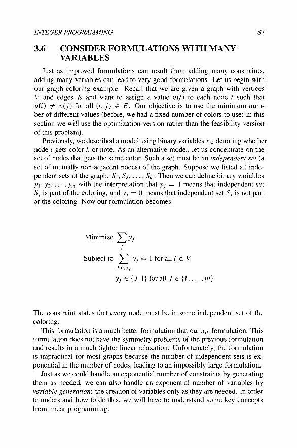
3.6 CONSIDER FORMULATIONS WITH MANY VARIABLES

Just as improved formulations can result from adding many constraints, adding many variables can lead to very good formulations. Let us begin with our graph coloring example. Recall that we are given a graph with vertices V and edges E and want to assign a value v{i) to each node / such that v{i) ^ v{j) for all (/, y) e E. Our objective is to use the minimum number of different values (before, we had a fixed number of colors to use: in this section we will use the optimization version rather than the feasibility version of this problem).

Previously, we described a model using binary variables xi^ denoting whether node / gets color k or note. As an alternative model, let us concentrate on the set of nodes that gets the same color. Such a set must be an independent set (a set of mutually non-adjacent nodes) of the graph. Suppose we fisted all independent sets of the graph: 5i, ^ 2 , . . . , 5^. Then we can define binary variables Jb J25. . . , Jm with the interpretation that yj = 1 means that independent set Sj is part of the coloring, and yj = 0 means that independent set Sj is not part of the coloring. Now our formulation becomes

Minimize T j ^ j

j

Subject to V" j j = 1 for all / e V j'JeSj

yj e {0, Ijforall j € { l , . . . ,m}

The constraint states that every node must be in some independent set of the coloring.

This formulation is a much better formulation that our xi^ formulation. This formulation does not have the symmetry problems of the previous formulation and results in a much tighter linear relaxation. Unfortunately, the formulation is impractical for most graphs because the number of independent sets is exponential in the number of nodes, leading to an impossibly large formulation.

Just as we could handle an exponential number of constraints by generating them as needed, we can also handle an exponential number of variables by variable generation: the creation of variables only as they are needed. In order to understand how to do this, we will have to understand some key concepts from linear programming.

88 BOSCH AND TRICK

Consider a linear program, where the variables are indexed by j and the constraints indexed by /:

Maximize /^^CjXj j

Subject to y <3!/7- /7 < bi for all / j

Xj > 0 for all j

When this linear program is solved, the result is the optimal solution x*. In addition, however, there is a value called the dual value, denoted jr,, associated with each constraint. This value gives the marginal change in the objective value as the right-hand side for the corresponding constraint is changed. So if the right-hand side of constraint / changes to Z?, + A, then the objective will change by 7r,A (there are some technical details ignored here involving how large A can be for this to be a valid calculation: since we are only concerned with marginal calculations, we can ignore these details).

Now, suppose there is a new variable Xn+\, not included in the original formulation. Suppose it could be added to the formulation with corresponding objective coefficient c„+i and coefficients a/,„+i. Would adding the variable to the formulation result in an improved formulation? The answer is certainly "no" in the case when

i

In this case, the value gained from the objective is insufficient to offset the cost charged marginally by the effect on the constraints. We need Cn+\ — J2i <^i,n+i^i > 0 in order to possibly improve on our solution.

This leads to the idea of variable generation. Suppose you have a formulation with a huge number of variables. Rather than solve this huge formulation, begin with a smaller number of variables. Solve the linear relaxation and get dual values n. Using TT, determine if there is one (or more) variables whose inclusion might improve the solution. If not, then the linear relaxation is solved. Otherwise, add one or more such variables to the formulation and repeat.

Once the linear relaxation is solved, if the solution is integer, then it is optimal. Otherwise, branch and bound is invoked, with the variable generation continuing in the subproblems.

Key to this approach is the algorithm for generating the variables. For a huge number of variables it is not enough to check all of them: that would be too time consuming. Instead, some sort of optimization problem must be defined whose solution is an improving variable. We illustrate this for our graph coloring problem.


Suppose we begin with a limited set of independent sets and solve our relaxation over them. This leads to a dual value 7ti for each node. For any other independent set 5, if X]/€5 / > 1. then S corresponds to an improving variable. We can write this problem using binary variables zt corresponding to whether / is in S or not:

Maximize Y^^/^/

Subject to Zi + Z; < 1 for all (/, y) e E

Zi e {0,1} for all/

This problem is called the maximum weighted independent set (MWIS) problem, and, while the problem is formally hard, effective methods have been found for solving it for problems of reasonable size.

This gives a variable generation approach to graph coloring: begin with a small number of independent sets, then solve the MWIS problem, adding in independent sets until no independent set improves the current solution. If the variables are integer, then we have the optimal coloring. Otherwise we need to branch.

Branching in this approach needs special care. We need to branch in such a way that our subproblem is not affected by our branching. Here, if we simply branch on the yj variables (so have one branch with yj = 1 and another with yj = 0), we end up not being able to use the MWIS model as a subproblem. In the case where yj = 0 we need to find an improving set, except that Sj does not count as improving. This means we need to find the second most improving set. As more branching goes on, we may need to find the third most improving, the fourth most improving, and so on. To handle this, specialized branching routines are needed (involving identifying nodes that, on one side of the branch, must be the same color and, on the other side of the branch, cannot be the same color).

Variable generation together with appropriate branching rules and variable generation at the subproblems is a method known as branch and price. This approach has been very successful in attacking a variety of very difficult problems over the last few years.

To summarize, models with a huge number of variables can provide very tight formulations. To handle such models, it is necessary to have a variable generation routine to find improving variables, and it may be necessary to modify the branching method in order to keep the subproblems consistent with that routine. Unlike constraint generation approaches, heuristic variable generation routines are not enough to ensure optimality: at some point it is necessary to prove conclusively that the right variables are included. Furthermore, these variable generation routines must be applied at each node in the branch-and-bound tree if that node is to be crossed out from further analysis.

90 BOSCH AND TRICK

3.7 MODIFY BRANCH-AND-BOUND PARAMETERS

Integer programs are solved with computer programs. There are a number of computer programs available to solve integer programs. These range from basic spreadsheet-oriented systems to open-source research codes to sophisticated commercial applications. To a greater or lesser extent, each of these codes offers parameters and choices that can have a significant affect on the solvability of integer programming models. For most of these parameters, the only way to determine the best choice for a particular model is experimentation: any choice that is uniformly dominated by another choice would not be included in the software.

Here are some common, key choices and parameters, along with some comments on each.

3.7.1 Description of Problem

The first issue to be handled is to determine how to describe the integer program to the optimization routine(s). Integer programs can be described as spreadsheets, computer programs, matrix descriptors, and higher-level languages. Each has advantages and disadvantages with regards to such issues as ease-of-use, solution power, flexibility and so on. For instance, implementing a branch-and-price approach is difficult if the underlying solver is a spreadsheet program. Using ''callable hbraries" that give access to the underlying optimization routines can be very powerful, but can be time-consuming to develop.

Overall, the interface to the software will be defined by the software. It is generally useful to be able to access the software in multiple ways (callable libraries, high level languages, command line interfaces) in order to have full flexibihty in solving.

3.7.2 Linear Programming Solver

Integer programming relies heavily on the underlying linear programming solver. Thousands or tens of thousands of linear programs might be solved in the course of branch-and-bound. Clearly a faster linear programming code can result in faster integer programming solutions. Some possibihties that might be offered are primal simplex, dual simplex, or various interior point methods. The choice of solver depends on the problem size and structure (for instance, interior point methods are often best for very large, block-structured models) and can differ for the initial linear relaxation (when the solution must be found ''from scratch") and subproblem linear relaxations (when the algorithm can use previous solutions as a starting basis). The choice of algorithm can also be affected by whether constraint and/or variable generation are being used.


3.73 Choice of Branching Variable

In our description of branch-and-bound, we allowed branching on any fractional variable. When there are multiple fractional variables, the choice of variable can have a big effect on the computation time. As a general guideline, more 'Important" variables should be branched on first. In a facility location problem, the decisions on opening a facility are generally more important than the assignment of a customer to that facility, so those would be better choices for branching when a choice must be made.

3.7.4 Choice of Subproblem to Solve

Once multiple subproblems have been generated, it is necessary to choose which subproblem to solve next. Typical choices are depth-first search, breadth-first search, or best-bound search. Depth-first search continues fixing variables for a single problem until integrahty or infeasibility results. This can lead quickly to an integer solution, but the solution might not be very good. Best-bound search works with subproblems whose linear relaxation is as large (for maximization) as possible, with the idea that subproblems with good linear relaxations may have good integer solutions.

3.7.5 Direction of Branching

When a subproblem and a branching variable have been chosen, there are multiple subproblems created corresponding to the values the variable can take on. The ordering of the values can affect how quickly good solutions can be found. Some choices here are a fixed ordering or the use of estimates of the resulting linear relaxation value. With fixed ordering, it is generally good to first try the more restrictive of the choices (if there is a difference).

3.7.6 Tolerances

It is important to note that while integer programming problems are primarily combinatorial, the branch-and-bound approach uses numerical linear programming algorithms. These methods require a number of parameters giving allowable tolerances. For instance, if ;c/ = 0.998 should Xj be treated as the value 1 or should the algorithm branch on Xj ? While it is tempting to give overly big values (to allow for faster convergence) or small values (to be ''more accurate"), either extreme can lead to problems. While for many problems, the default values from a quality code are sufficient, these values can be the source of difficulties for some problems.

92 BOSCH AND TRICK

3.8 TRICKS OF THE TRADE

After reading this tutorial, all of which is about ''tricks of the trade", it is easy to throw one's hands up and give up on integer programming! There are so many choices, so many pitfalls, and so much chance that the combinatorial explosion will make solving problems impossible. Despite this complexity, integer programming is used routinely to solve problems of practical interest. There are a few key steps to make your integer programming implementation go well.

• Use state-of-the-art software. It is tempting to use software because it is easy, or available, or cheap. For integer programming, however, not having the most current software embedding the latest techniques can doom your project to failure. Not all such software is commercial. The COIN-OR project is an open-source effort to create high-quahty optimization codes.

• Use a modehng language. A modeling language, such as OPL, Mosel, AMPL, or other language can greatly reduce development time, and allows for easy experimentation of alternatives. Callable Hbraries can give more power to the user, but should be reserved for ''final implementations", once the model and solution approached are known.

• If an integer programming model does not solve in a reasonable amount of time, look at the formulation first, not the solution parameters. The default settings of current software are generally pretty good. The problem with most integer programming formulations is the formulation, not the choice of branching rule, for example.

• Solve some small instances and look at the solutions to the Hnear relaxations. Often constraints to add to improve a formulation are quite obvious from a few small examples.

• Decide whether you need "optimal" solutions. If you are consistently getting within 0.1 % of optimal, without proving optimality, perhaps you should declare success and go with the solutions you have, rather than trying to hunt down that final gap.

• Try radically different formulations. Often, there is another formulation with completely different variables, objective, and constraints that will have a much different computational experience.

3.9 CONCLUSIONS

Integer programming models represent a powerful approach to solving hard problems. The bounds generated from linear relaxations are often sufficient


to greatly cut down on the search tree for these problems. Key to successful integer programming is the creation of good formulations. A good formulation is one where the linear relaxation closely resembles the underlying integer program. Improved formulations can be developed in a number of ways, including finding formulations with tight relaxations, avoiding symmetry, and creating and solving formulations that have an exponential number of variables or constraints. It is through the judicious combination of these approaches, combined with fast integer programming computer codes that the practical use of integer programming has greatly expanded in the last 20 years.

SOURCES OF ADDITIONAL INFORMATION Integer programming has existed for more than 50 years and has developed

a huge literature. This bibliography therefore makes no effort to be comprehensive, but rather provides initial pointers for further investigation.

General Integer Programming There are a number of excellent recent monographs on integer programming. The classic is Nemhauser and Wolsey (1988). A book updating much of the material is Wolsey (1998). Schri-jver (1998) is an outstanding reference book, covering the theoretical underpinnings of integer programming.

Integer Programming Formulations There are relatively few books on formulating problems. An exception is Williams (1999). In addition, most operations research textbooks offer examples and exercises on formulations, though many of the examples are not of realistic size. Some choices are Winston (1997), Taha (2002), and HilHer and Lieberman (2002).

Branch and Bound Branch and bound traces back to the 1960s and the work of Land and Doig (1960). Most basic textbooks (see above) give an outline of the method (at the level given in this tutorial).

Branch and Cut The cutting plane approach dates back to the late 1950s and the work of Gomory (1958), whose cutting planes are applicable to any integer program. Juenger et al. (1995) provides a survey of the use of cutting plane algorithms for specialized problem classes.

As a computational technique, the work of Crowder et al. (1983) showed how cuts could greatly improve basic branch-and-bound.

For an example of the success of such approaches for solving extremely large optimization problems, see Applegate et al. (1998).

Branch and Price Bamhart et al. (1998) is an excellent survey of this approach.

94 BOSCH AND TRICK

Implementations There are a number of very good implementations that allow the optimization of realistic integer programs. Some of these are commercial, like the CPLEX implementation of ILOG, Inc. (CPLEX, 2004). Bixby et al. (1999) gives a detailed description of the advances that this software has made.

Another commercial product is Xpress-MP from Dash, with the textbook by Gueret et al. (2002) providing a very nice set of examples and applications.

COIN-OR (2004) provides an open-source initiative for optimization. Other approaches are described by Ralphs and Ladanyi (1999) and by Cordieretal. (1999).

References Applegate, D., Bixby, R., Chvatal, V. and Cook, W., 1998, On the solution of

traveling salesman problems, in: Proc. Int. Congress of Mathematicians, Doc. Math. J. DMV, Vol. 645.

Bamhart, C, Johnson, E. L., Nemhauser, G. L., Savelsbergh, M. W. P. and Vance, P. H., 1998, Branch-and-price: column generation for huge integer programs, Oper. Res. 46:316.

Bixby, R. E., Fenelon, M., Gu, Z., Rothberg, E. and Wunderling, R., 1999, MIP: Theory and Practice—Closing the Gap, Proc. 19th IF IP TC7 Conf. on System Modelling, Kluwer, Dordrecht, pp. 19-50.

Common Optimization INterface for Operations Research (COIN), 2004, at http://www.coin-or.org

Cordier, C, Marchand, H., Laundy, R. and Wolsey, L. A., 1999, bc-opt: a branch-and-cut code for mixed integer programs. Math. Program. 86:335.

Crowder, H., Johnson, E. L. and Padberg, M. W., 1983, Solving large scale zero-one linear programming problems, Oper Res. 31:803-834.

Gomory, R. E., 1958, Outline of an algorithm for integer solutions to linear programs. Bulletin AMS 64:275-278.

Gueret, C , Prins, C. and Sevaux, M., 2002, Applications of Optimization with Xpress-MP, S. Heipcke, transl.. Dash Optimization, Blisworth, UK.

Hillier, F. S. and Lieberman, G. J., 2002, Introduction to Operations Research, McGraw-Hill, New York.

ILOG CPLEX 9.0 Reference Manual, 2004, ILOG. Juenger, M., Reinelt, G. and Thienel, S., 1995, Practical Problem Solving with

Cutting Plane Algorithms in Combinatorial Optimization, DIM ACS Series in Discrete Mathematics and Theoretical Computer Science, Vol. I l l , American Mathematical Society, Providence, RI.

Land, A. H. and Doig, A. G., 1960, An Automatic Method for Solving Discrete Programming Problems, Econometrica 28:83-97.


Nemhauser, G. L. and Wolsey, L. A., 1998, Integer and Combinatorial Optimization, Wiley, New York.

Ralphs, T. K. and Ladanyi, L., 1999, SYMPHONY: A Parallel Framework for Branch and Cut, White paper, Rice University.

Schrijver, A., 1998, Theory of Linear and Integer Programming, Wiley, New York.

Taha, H. A., 2002, Operations Research: An Introduction, Prentice-Hall, New York.

WilHams, H. R, 1999, Model Building in Mathematical Programming, Wiley, New York.

Winston, W,, 1997, Operations Research: Applications and Algorithms, Thomson, New York.

Wolsey, L. A., 1998, Integer Programming, Wiley, New York. XPRESS-MP Extended Modeling and Optimisation Subroutine Library, Ref

erence Manual, 2004, Dash Optimization, BHsworth, UK.

Chapter 3 INTEGER PROGRAMMING - CiteSeerX

Documents

Transcript of Chapter 3 INTEGER PROGRAMMING - CiteSeerX