Detecting and Removing Inconsistencies between Experimental Data and Signaling Network Topologies...

Detecting and Removing Inconsistencies betweenExperimental Data and Signaling Network TopologiesUsing Integer Linear Programming on Interaction GraphsIoannis N. Melas1., Regina Samaga2., Leonidas G. Alexopoulos1, Steffen Klamt2*

1 National Technical University of Athens, Athens, Greece, 2 Max Planck Institute for Dynamics of Complex Technical Systems, Magdeburg, Germany

Abstract

Cross-referencing experimental data with our current knowledge of signaling network topologies is one central goal ofmathematical modeling of cellular signal transduction networks. We present a new methodology for data-driveninterrogation and training of signaling networks. While most published methods for signaling network inference operate onBayesian, Boolean, or ODE models, our approach uses integer linear programming (ILP) on interaction graphs to encodeconstraints on the qualitative behavior of the nodes. These constraints are posed by the network topology and theirformulation as ILP allows us to predict the possible qualitative changes (up, down, no effect) of the activation levels of thenodes for a given stimulus. We provide four basic operations to detect and remove inconsistencies between measurementsand predicted behavior: (i) find a topology-consistent explanation for responses of signaling nodes measured in a stimulus-response experiment (if none exists, find the closest explanation); (ii) determine a minimal set of nodes that need to becorrected to make an inconsistent scenario consistent; (iii) determine the optimal subgraph of the given network topologywhich can best reflect measurements from a set of experimental scenarios; (iv) find possibly missing edges that wouldimprove the consistency of the graph with respect to a set of experimental scenarios the most. We demonstrate theapplicability of the proposed approach by interrogating a manually curated interaction graph model of EGFR/ErbB signalingagainst a library of high-throughput phosphoproteomic data measured in primary hepatocytes. Our methods detectinteractions that are likely to be inactive in hepatocytes and provide suggestions for new interactions that, if included,would significantly improve the goodness of fit. Our framework is highly flexible and the underlying model requires onlyeasily accessible biological knowledge. All related algorithms were implemented in a freely available toolbox SigNetTrainermaking it an appealing approach for various applications.

Citation: Melas IN, Samaga R, Alexopoulos LG, Klamt S (2013) Detecting and Removing Inconsistencies between Experimental Data and Signaling NetworkTopologies Using Integer Linear Programming on Interaction Graphs. PLoS Comput Biol 9(9): e1003204. doi:10.1371/journal.pcbi.1003204

Editor: Richard Bonneau, New York University, United States of America

Received February 14, 2013; Accepted July 16, 2013; Published September 5, 2013

Copyright: � 2013 Melas et al. This is an open-access article distributed under the terms of the Creative Commons Attribution License, which permitsunrestricted use, distribution, and reproduction in any medium, provided the original author and source are credited.

Funding: LGA and INM were funded via European Social Fund (ESF) and Greek National funds through the Operational Program ‘‘Education and LifelongLearning’’ of the National Strategic Reference Framework (NSRF) - Research Funding Program: ERC. SK and RS acknowledge funding and support by the GermanFederal Ministry of Education and Research (‘‘Virtual Liver’’ project (grant 0315744) and ‘‘JAK-Sys’’ project (grant 0316167B)) and by the Federal State of Saxony-Anhalt (Research Center ‘‘Dynamic Systems: Biosystems Engineering’’). The funders had no role in study design, data collection and analysis, decision to publish,or preparation of the manuscript.

Competing Interests: The authors have declared that no competing interests exist.

* E-mail: [email protected]

. These authors contributed equally to this work.

This is a PLOS Computational Biology Methods article.

Introduction

Recent advancements in high-throughput phosphoproteomic

technologies have led to the generation of large datasets, capturing

the cell’s response to factors of its biochemical micro-environment

[1,2]. However, interpreting the increasing amounts of available

data in such a manner that biologically relevant insights can be

drawn for the interrogated system is far from trivial. To this end,

signaling data are often examined in conjunction with network

models that represent our current knowledge of the causality of

cellular signal flows (as stored, for example, in online pathway

databases [3–5]). Finding, in a rigorous fashion, causal explanations

for experimental data in the context of a given network topology is

one of the key challenges for systems biology of cellular signaling.

Significant work has been published on this front attempting

to identify inconsistencies between measured data and signaling

topologies [6–16]. Some methods also facilitate an optimization

of the network structure to identify the wiring diagram that can

best fit the data at hand [6,7,15]. However, before such an

analysis can be conducted one has to choose an appropriate

modeling formalism. Common approaches used for modeling

signal transduction networks are based on graphs [12,13,17,18],

Bayesian networks [15], some form of logical modeling including

Boolean or constrained fuzzy logic [17,19,20], hybrid intelligent

systems [18,19,21–23], or ordinary differential equations (ODEs)

[24–26].

Deciding on the mathematical formalism to be used for

representing and modeling signal transduction networks is often

not trivial and depends on many factors such as the amount and

type of available data, the quality of prior knowledge, whether

transient or steady-state behavior needs to be addressed, the

PLOS Computational Biology | www.ploscompbiol.org 1 September 2013 | Volume 9 | Issue 9 | e1003204

biological questions that are to be answered, the computational

efforts and so forth. For example, ODE modeling or constrained

fuzzy logic are closer to the actual mechanics of signal transduction

than Boolean logic as they support continuous values for the

activation states of signaling species, but at the cost of numerous

free parameters. These parameters must be known (in addition to

the actual (initial) network structure) or estimated from exper-

imental data. A large number of parameters in the model often

gives rise to identifiability problems whose resolution requires

extensive and elaborate training datasets.

Graph models are probably the simplest models of signaling

networks one can think of. In particular, signed directed graphs

(also called interaction graphs, dependency graphs, or influence

graphs), where each edge indicates either a positive or a negative

effect of one node upon another, have frequently been used to

investigate basic functional properties of biological networks with

signal or information flows. Despite their simplicity, interaction

graphs (IG) capture the most important biological information and

are useful to uncover fundamental network properties such as

feedback and feedforward loops or global interdependencies

between the involved players. The fact that each Boolean and

each ODE model has an underlying IG renders the analysis of

IG directly relevant also for other modeling formalisms. A

famous example is the fact that a system (in an ODE or Boolean

model representation) exhibiting bistability must contain a

positive feedback loop in its underlying network structure

[27,28]. Properties that are uniquely identifiable from a given

IG immediately hold for all ODE and Boolean models that have

this IG as underlying wiring diagram, whereas the opposite

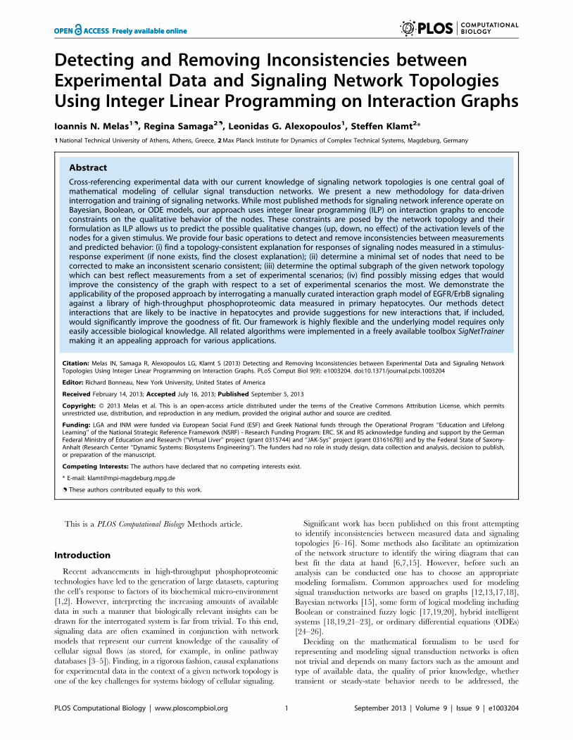
direction does not hold. For example, in Figure 1A we see that

there is (exactly) one path in the IG leading from node A to node

G and that this path is negative. We can therefore uniquely

conclude from the IG that, in any Boolean or ODE model derived

from it, a perturbation in A cannot lead to an increase in the

activation level of G. In contrast, there is a positive and a negative

path from A to F , hence, nothing can be concluded from the

graph alone when perturbing A. In fact, it will depend on the

kinetics and parameters in an ODE model (and the logical

functions in a logical model) whether the level of B will increase,

decrease, or, in the extreme case, remain constant.

The previous example shows that IG can be used to make

predictions (without needing any further parameters) on the

qualitative behavior of signaling and regulatory networks. These

predictions can easily be compared with (qualitative trends of)

experimental data, typically from stimulus-response experiments.

The concept of the dependency matrix introduced in [17] is

consequently based on the idea used above, namely to check—for

each (ordered) pair (A,B) of nodes A and B—the existence of

positive and negative paths (and negative feedback loops) to make

predictions on the effect of perturbations in A. This concept has

been applied, for instance, in [18] to experimental data of the

epidermal growth factor (EGF) receptor signaling network. The

comparisons of the predictions from the dependency matrix with

the measured behavior from several combinatorial stimulations

showed several inconsistencies from which some (cell-type specific)

conclusions on missing or probably inactive interactions could be

made. However, these conclusions were drawn by inspection only.

It is therefore one goal of this study to develop methods that find,

in an automatic way, corrections in the network structure

improving the consistency. The dependency matrix is useful to

get an overview on how a node can potentially influence the other

nodes in the network; however, it may become limiting if multiple

node values are measured in one experiment. Given the IG

topology, state changes measured for certain nodes are, in general,

not independent and therefore require stronger constraints. For

example, assume there would be another node Z in Figure 1A that

is activated by F (edge F?Z). From the IG topology we know

that F and Z can both decrease or increase their levels if A is

perturbed (as correctly predicted by the dependency matrix);

however, it is not possible that their new steady state levels change

in different directions.

A related class of methods for detecting discrepancies between

IG topology and experimental data relies on the sign consistency rule

[11–13]. The key idea is that, in a steady-state shift experiment,

the direction of change of the state of a node must be explainable

by the direction of change of at least one of its predecessor nodes

(except for the directly perturbed node(s)). For example, in

Figure 1A, after a perturbation in A, the steady-state level of Fmay have become larger only if E decreased its activation level (as

E inhibits F ) or if C increased its level (as C activates F ). The sign

consistency rule gives rise to constraints on the possible patterns of

‘‘ups and downs’’ of the nodes’ activation levels in a given IG.

These constraints can be encoded, for example, by Answer Set

Programming [13]. Confronting these constraints with experi-

mental data may then lead to the detection of topological

inconsistencies, namely if no sign pattern complying with the

given measurements and perturbations can be found [11–13].

The novel methods we will present herein are based on a similar

sign consistency rule; however, they differ in a number of aspects.

First, we will encode the sign constraints as an Integer Linear

Programming (ILP) problem which has not been described before.

This formulation gives us the opportunity to utilize the large

corpus of effective algorithms developed for ILP problems.

Furthermore, for the situation that multiple stimulus-response

experiments are available, we will address aspects that go beyond

the detection of inconsistencies from single experiments, namely to

correct a given network structure such that the number of

mismatches is minimized. For the structure optimization process

we will consider edge removals as well as edge additions.

Author Summary

Cellular signal transduction is orchestrated by communi-cation networks of signaling proteins commonly depictedon signaling pathway maps. However, each cell type mayhave distinct variants of signaling pathways, and wiringdiagrams are often altered in disease states. The identifi-cation of truly active signaling topologies based onexperimental data is therefore one key challenge insystems biology of cellular signaling. We present a newframework for training signaling networks based oninteraction graphs (IG). In contrast to complex modelingformalisms, IG capture merely the known positive andnegative edges between the components. This basicinformation, however, already sets hard constraints onthe possible qualitative behaviors of the nodes whenperturbing the network. Our approach uses Integer LinearProgramming to encode these constraints and to predictthe possible changes (down, neutral, up) of the activationlevels of the involved players for a given experiment.Based on this formulation we developed several algo-rithms for detecting and removing inconsistencies be-tween measurements and network topology. Demonstrat-ed by EGFR/ErbB signaling in hepatocytes, our approachdelivers direct conclusions on edges that are likely inactiveor missing relative to canonical pathway maps. Suchinformation drives the further elucidation of signalingnetwork topologies under normal and pathological phe-notypes.

Training Signaling Maps with Integer Programming


As starting point, we assume that we are given (i) an initial IG

topology, for example, a ‘‘master topology’’ of a signaling pathway

subsuming all reported (potential) interactions and (ii) a set of

stimulus-response experiments (scenarios) in each of which some

nodes were perturbed and the resulting up- or downregulation of

some readout nodes was measured. The IG is a signed directed

graph G~(V ,E,s), where V is the set of nodes (species), E is the

set of edges (interactions), and s is the set of signs corresponding to

edges in E (se[f{1,1g, e[E). Figure 1A and the three

experimental scenarios in Table 1 (defined by the columns

‘‘Perturbations’’ and ‘‘Measurements’’) provide an illustrative

example. Here, A and D are nodes that can be perturbed; F , Gand H are the readout nodes for which we get measurements, and

C and E are latent nodes which are neither perturbed nor

measured.

Our goal is now to analyze and improve the consistency of an

IG topology with respect to a given set of experimental data.

Central to all algorithms presented herein is the following

definition of sign consistency.

Definition 1 (Sign Consistency). We are given an IG and a

node labeling (sign pattern) s which stores for each node X a sign

sX[f{1,0,1g. We say that s is sign-consistent with respect to the IG if

the following conditions hold for each node X :

a) If sX ~{1: either sX was fixed to {1 (perturbed node), or

there is a predecessor node Y and an edge e : Y?X with

se:sY ~{1.

b) If sX ~1: either sX was fixed to 1 (perturbed node), or there is

a predecessor node Y and an edge e : Y?X with se:sY ~1.

c) If sX ~0: either (i) sX was fixed to 0, or (ii) X has no

predecessor, or (iii) for all edges Y?X we have sY ~0, or (iv)

there is an edge e : Y?X with se:sY ~{1 and another edge

h : Z?X with sh:sZ~1.

In our setting, the signs of the external perturbations as well as

the measured signs of the readout nodes can be described by a

specific node labeling (which we call the associated labeling of the

scenario). In realistic applications one usually has latent nodes

which are neither perturbed nor measured, hence, the associated

node labeling of an experimental scenario may contain unknown

values which we denote by NaN. We call incomplete sign patterns

partial labelings. A partial labeling ~ss is sign-consistent if there exists a

Figure 1. A simple example network used for illustration purposes. The interaction graph consists of 7 nodes and 7 edges. The green nodesA and D can be perturbed externally; the grey nodes F , G and H are the readouts of the network whose activation state is measured in theexperiments; the white nodes C and E are latent nodes which are neither perturbed nor measured (see scenarios in Table 1). (A) The initial topologyof the interaction graph representing the prior knowledge. This graph produces a total fitting error of 5 over the three scenarios in Table 1. (B) The(unique) optimal subgraph of (A) minimizing the total fitting error on the experimental scenarios to 2 (see Table 1). (C) Two optimal graphs obtainedfrom (A) by applying OPT_GRAPH: by adding edge A?G and either (left) removing E a F or (right) removing E a F and C?D, the fitting error iseradicated completely and becomes 0 (cf. Table 1).doi:10.1371/journal.pcbi.1003204.g001



complete sign-consistent labeling s for which we have ~ssX ~sX

wherever ~ssX=NaN . In this sense, we say that an experimental

scenario is sign-consistent if its associated (partial) labeling is sign-

consistent. Finally, if we have a collection of scenarios we say that

this collection is sign-consistent with the IG if all the (partial)

labelings associated with the scenarios are sign-consistent.

We can now consider four fundamental problems on the

consistency of experimental scenarios with respect to a given IG:

(1) SCEN_FITGiven a single experimental scenario, we fix the states of the

perturbed nodes (according to the experimental interventions)

and then search for a sign-consistent node labeling having a

minimal mismatch with the given measurements. In the ideal

case, where the associated labeling of the experimental scenario is

sign-consistent, the fitting error will be 0. The fitting error is

defined as the absolute differenceX

X :mX=NaNDmX {sX D between

the measurements mX and the optimal sign pattern s.

From Figure 1A/Table 1, we see that scenario 1 is sign-

consistent: A was externally increased and D decreased, and with

sA~sC~sG~sF ~sH~1 and sD~sE~{1, we obtain a sign-

consistent labeling giving us a possible explanation for the

measurements. In contrast, scenario 2 is not consistent with the

IG topology: if D is increased externally (no perturbation in A),

then we expect to see a decrease in F , G and H which is not seen

in F (unchanged). The minimal resulting fitting error for an

optimal sign pattern is thus 1. Generally, an error of 1 or {1occurs if a change was expected/not expected, but was not seen/

was seen in the experiments. For scenario 3, the predictions are

even worse: increase in A (no perturbation in D which thus

depends on C) should lead to down-regulation of G and H , but an

increase is measured for both. We thus get an absolute error of 2

for each of the two predictions. The fitting error of a sign-

consistent node labeling closest to scenario 3 can thus not be

smaller than 4.

It may happen that several solutions exist explaining a given

scenario equally well. For example, assume again that there was

another node Z in Figure 1A that is activated by F through an

edge F?Z. If we now measured G~H~F~{1 and Z~1 after

positively perturbing A (A~1), then the best scenario fit would

result in an error value of 2 since F and Z must have the same

value. However, there are three optimal solutions regarding F and

Z, namely F~Z~0, F~Z~1, and F~Z~{1, all leading to

the same minimal fitting error of 2. For some applications it will be

helpful to know all these optimal solutions and we will therefore

also address their enumeration.

(2) Minimal Correction Sets (MCoS)Another optimization problem for a single scenario directly

follows if a given scenario is not sign-consistent, i.e., if no sign-

consistent labeling can be found that results in a fitting error of

0. We can then try to identify a minimal set of nodes whose

states need to be corrected to obtain a consistent scenario. The

correction of a node’s state is simulated by adding an additional

external input that is either 1 or {1. We call these sets Minimal

Correction Sets (MCoS), the minimality property demanding that no

subset of a MCoS would lead to a consistent labeling. For

example, regarding scenario 3 in Table 1, there are four MCoS

suggesting that there was either an external up-regulation of G(1?G), or a down-regulation in one of the nodes E, D, or C, each

of unknown cause. Thus, MCoS show possible places in the

network that have a high probability to cause the observed

inconsistencies. With the MCoS problem we identify the

enumeration of MCoS of minimal size for a given scenario (a

simple extension not considered herein is to enumerate all MCoS

irrespective of their size).

(3) OPT_SUBGRAPHThe first two problems focus on a single scenario; now we

intend to optimize the network structure in such a way that the

total fitting error over all scenarios is minimized. Initially, we allow

only the removal of edges in the network, that is, we search for an

optimal subgraph. As there might be several solutions to this

optimization problem, we consider the following sub-problems:

computation of any/of the sparsest/of the largest sub-network of

the initial IG minimizing the mismatches. In addition, we may also

be interested in an enumeration of all sub-networks minimizing

the number of inconsistencies between IG topology and data. As

an example, Figure 1B shows the unique optimal subgraph of the

original IG in Figure 1A minimizing the fitting error over all three

scenarios in Table 1. This solution reduces the total fitting error

from 5 to 2 (and there is no solution that could reduce it further).

(4) OPT_GRAPHThe removal of certain edges may significantly improve the

agreement between measurements and network topology, but

some fitting errors can often only disappear if we have additionally

the opportunity to add new interactions. This fourth optimization

problem, therefore, intends to minimize the fitting error by

Table 1. Example scenarios and optimizations for the example network in Figure 1.

Perturbations MeasurementsInitial fitting error(Fig. 1A) MCoS

Remaining fitting error(Fig. 1B/Fig. 1C)

A D F G H F G H F G H

sc1 1 21 1 1 1 0 0 0 0/0 0/0 0/0

sc2 1 0 21 21 1 0 0 {1RF}, {1RC}, {1RA} 0/0 0/0 0/0

sc3 1 1 1 1 0 2 2 {1RG}, {21RE}, {21RD}, {21RC} 0/0 1/0 1/0

Rows ‘‘sc1’’, ‘‘sc2’’, ‘‘sc3’’ correspond to scenarios 1 to 3. The ‘‘Perturbations’’ column shows the externally imposed state of the nodes A and D which can be 21(downregulation), 0 (state of the node did not change), or 1 (activation level is increased). No value is given if the node was not perturbed. The ‘‘Measurements’’ columnshows the measured change of the activation level of F , G and H in the respective scenarios. The ‘‘Initial fitting error’’ column shows the total mismatch of predictionsand measurements with respect to the initial topology (shown in Figure 1A). The ‘‘MCoS’’ (Minimal Correction Sets) column shows artificial positive (1) or negative (21)external inputs to some nodes which would lead to a perfect fit of the data (resulting fitting error for the scenario becomes 0). The ‘‘Remaining fitting error’’ columnsshow the remaining mismatches for the optimal subgraph depicted in Figure 1B and for the two optimal graphs displayed in Figure 1C. The original network inFigure 1A has a total fitting error of 5; it is 2 for the optimal subgraph in Figure 1B and it becomes 0 in the optimal graphs in Figure 1C.doi:10.1371/journal.pcbi.1003204.t001



allowing edge removals and insertions in parallel. Obviously, the fit

cannot be worse than the one obtained by problem (3). For smaller

networks, a full enumeration of all optimal solutions might be

possible. However, as the insertion of new interactions increases

the solution space dramatically in large networks, we may consider

a greedy strategy which determines, in each iteration, the optimal

edge whose inclusion (in combination with the pruning step (3))

decreases the fitting error the most. One may then add this edge

permanently and repeat the algorithm described above until no

further significant improvement can be obtained by inserting a

new edge.

Figure 1C shows a result of this optimization step in our

example: the edge A?G is identified as missing edge which, in

combination with a pruning step, completely eradicates the

original fitting errors in all scenarios. The resulting network is

thus fully consistent with the entire set of experimental data. In this

example, nine other edges can be identified whose addition, in

combination with a pruning step by OPT_SUBGRAPH, lead to a

fitting error of 0. Furthermore, for each added edge, the

OPT_SUBGRAPH problem that is called after adding the edge

might return several optimal solutions. Figure 1C shows the two

existing optimal solutions (with a fitting error of 0) that are derived

after adding edge A?G.

The present paper is organized as follows: the Methods section

details how sign consistency and the four basic optimization

problems can be encoded as Integer Linear Programming

problems. The Methods section thus contains the main theoretical

achievements of our work. Readers not interested in the

mathematical details may skip this part and directly continue

with the Results section. In the latter we employ our proposed

methodology to identify the EGFR/ErbB signaling topology active

in primary hepatocytes [18] by using prior knowledge on network

topology and data from combinatorial stimulus-response experi-

ments. This study reveals interesting biological insights and

demonstrates that the introduced framework provides a highly

flexible and powerful approach for exploring and training wiring

diagrams of signaling networks based on large sets of experimental

data. We also provide results from benchmarks of our algorithms

and discuss the scalability of the presented method.

Methods

Basic definitions and ILP formulation of sign consistencyAs described in the Introduction section, we assume that we are

given an interaction graph (signed digraph) G~(V ,E,s) capturing

our prior knowledge on the signaling topology and, additionally, a

set of experimental scenarios each consisting of a specific set of

perturbed nodes and a set of measurements. The edges (also called

interactions) are indexed by i[IE , IE~f1, . . . ,nEg, nE~DED, the

nodes by j[IV , IV ~f1, . . . ,nVg, nV ~DV D, and the scenarios by

k[IS , IS~f1, . . . ,nSg. The experimental scenarios are specified

by two matrices: (i) the nV |nS perturbation matrix p with

pj,k[f{1,0,1g storing the (enforced) state of node j in scenario k

through external perturbation, and (ii) the nV |nS measurement

matrix m with mj,k[f{1,0,1g storing the measured change of the

(steady) state level of node j in scenario k. Perturbation and

measurement values thus indicate enforced/measured upregula-

tion (1), downregulation ({1), or unchanged state (0). Usually,

only a small subset of nodes is perturbed, and only a subset of

nodes can be measured; unperturbed and non-measured states are

therefore marked by NaN in the matrices p and m, respectively.

In what follows we translate sign-consistency of a node labeling

(according to Definition 1) into equality and inequality constraints

of an Integer Linear Programming (ILP) problem. In this

formulation, the predicted state of a node j in experiment k will

be represented by an integer variable xj,k[f{1,0,1g. Again,

xj,k~1 encodes upregulation and xj,k~{1 downregulation of

node j in scenario k, whereas xj,k~0 indicates that the activation

level of j remained unchanged.

The i-th signaling edge is defined as Si?Pi, where Si[V is the

start node and Pi[V the end node of edge i. Furthermore, the sign

of edge i is denoted by si.

We introduce the binary variables uzi,k and u{

i,k to represent the

potential of edge i to up- or downregulate its end node Pi in

experiment k. Edge i with start node j~Si has the potential of

upregulating its target node Pi in experiment k (i.e., uzi,k~1) if and

only if si:xj,k~1. In any other case we have uz

i,k~0. Accordingly,

edge i with start node j~Si has the potential of downregulating its

target Pi in experiment k (i.e., u{i,k~1) if and only if si

:xj,k~{1.

In any other case u{i,k~0. Thus, with j~Si,

uzi,k~max(0,si

:xj,k)

u{i,k~max(0,{si

:xj,k):ð1Þ

As the max operator is not linear (required for an ILP), we

introduce the binary variables d1i,k, . . . ,d4i,k to linearize (1) in the

following way:

uzi,k§0

uzi,k§si

:xj,k

uzi,kz2d1i,kƒ2

uzi,k{si

:xj,kz2d2i,kƒ2

d1i,kzd2i,k~1

u{i,k§0

u{i,k§{si

:xj,k

u{i,kz2d3i,kƒ2

u{i,kzsi

:xj,kz2d4i,kƒ2

d3i,kzd4i,k~1:

ð2Þ

Finally, the two binary variables xzj,k and x{

j,k are introduced to

represent the potential for node j of being up- or downregulated

depending on the activity of its upstream edges. Node j has the

potential of being upregulated (xzj,k~1) if and only if an edge i

exists such that j~Pi and uzi,k~1, and node j has the potential of

being downregulated (x{j,k~1) if and only if i exists such that j~Pi

and u{i,k~1. Thus,

xzj,k§uz

i,k , Vi with Pi~j

x{j,k§u{

i,k , Vi with Pi~j

xzj,kƒ

X

i[IEPi~j

uzi,k

x{j,kƒ

X

i[IEPi~j

u{i,k:

ð3Þ



The state xj,k of node j in scenario k is constrained by the values of

xzj,k and x{

j,k according to the definition of sign-consistency (see

Definition 1): (i) Node j may be upregulated (xj,k~1) if it has the

potential of being upregulated (xzj,k~1). (ii) Node j may be

downregulated (xj,k~{1) if it has the potential of being

downregulated (x{j,k~1). (iii) Node j may stay unchanged

(xj,k~0) if it has the potential of being both up- and downreg-

ulated (x{j,k~xz

j,k~1) or neither of the above (x{j,k~xz

j,k~0).

These rules are encoded in inequalities as follows:

xj,kƒxzj,k

xj,k§{x{j,k

xj,kƒ2xzj,k{x{

j,k

xj,k§{2x{j,kzxz

j,k:

ð4Þ

The equations and inequalities derived in this subsection describe

sign-consistent node labelings and provide the frame within which

we can now address the four basic optimization problems posed in

the Introduction section.

SCEN_FITThe goal of SCEN_FIT is to identify, for a given scenario k, a

sign-consistent vertex labeling that is closest to the measurements

of this scenario. We first have to constrain the values of the

perturbed nodes in scenario k:

xj,k~pj,k, Vj with pj,k=NaN: ð5Þ

Realistic perturbations typically affect either input nodes (e.g.,

ligands) or internal nodes in the case where a specific inhibitor was

added or where a constitutive activation or a knock-in/knock-out

is introduced. The state of the perturbed nodes are thus fixed to

the enforced value and the constraints (4) are omitted for these

nodes to preserve the consistency of the formulation.

We now search for a sign-consistent labeling x1,k, . . . ,xnV ,k

(fulfilling thus constraints (2)–(4) of the previous subsection) that

minimizes the measurement-prediction-mismatch. The following

objective function is used accordingly:

minimizeX

j[IVmj,k=NaN

Dmj,k{xj,kD: ð6Þ

The summation of mismatches in equation (6) is thus done over all

nodes for which measurements exist. By introducing

absj,k~Dmj,k{xj,kD, absj,k[f0,1,2g, the lower bound for the

absolute value of the mismatch above is formulated as follows

(an upper bound needs not to be defined because the objective

function (6) will automatically take the smallest possible value):

absj,k§mj,k{xj,k

absj,k§xj,k{mj,k:ð7Þ

The resulting states xj,k for scenario k represent an optimal

solution as desired for SCEN_FIT.

As discussed in the Introduction section, we also consider the

enumeration of all optimal SCEN_FIT solutions for a given

scenario. To this end, we solve the ILP repeatedly and after each

run we exclude previously found solutions by adding the following

constraints for each previous solution s:

X

j[IV

Dxj,k{xj,k,sD§1, ð8Þ

where xj,k,s represent the value of xj,k in solution s. Since

constraint (8) is again non-linear because of the absolute value, it is

reformulated in the following manner:

X

j[IV

X

k[IS

dxj,k,s§1

{xj,kzdxj,k,s{4dx2j,k,sƒxj,k,s

xj,kzdxj,k,s{4dx1j,k,sƒ{xj,k,s

dx1j,k,szdx2j,k,s~1,

ð9Þ

with the auxiliary variables dxj,k,s (integer) and dx1j,k,s and dx2j,k,s

(binary). We may then compute a new sign-consistent labeling of

the nodes by optimizing again objective function (6). To ensure

that only solutions with minimum fitting error are found, we

replace, after the first iteration, the objective function in (6) by

forcing instead the algorithm to find solutions with the same

minimum fitting error as in the first run:

X

j[IVmj,k=NaN

Dmj,k{xj,k D~objval: ð10Þ

Here, objval is the optimal (minimal) value of the objective

function (6) found in the first run of the algorithm. The resulting

problem becomes thus a simple search for a feasible solution and is

repeated until no further solution can be found.

Minimal Correction SetsComputing a single Minimal Correction Set. Next, we

address the identification of a Minimal Correction Set (MCoS) for

a sign-inconsistent scenario k (where the fitting error in equation

(6) after optimization is greater than zero). An MCoS indicates

possible causes of discrepancies between measured data and

assumed IG topology. As described in the Introduction section,

MCoS correspond to artificial perturbations of certain nodes

which render the measurements from a given inconsistent scenario

consistent with the network topology. Let a new set of binary

variables Bzj,k and B{

j,k denote these artificial perturbations. The

state xj,k of node j can be enforced to 1 by adding a positive input,

Bzj,k~1. Accordingly, xj,k can be enforced to {1 by adding a

negative input, B{j,k~1. To enforce the state of xj,k to 0, either a

positive (Bzj,k~1) or a negative (B{

j,k~1) input might be required.

To account for these artificial perturbations, we modify the

constraints (4) in the following manner:

xj,kƒxzj,kzBz

j,k

xj,k§{x{j,k{B{

j,k

xj,kƒ2xzj,k{x{

j,kz2Bzj,k

xj,k§{2x{j,kzxz

j,k{2B{j,k:

ð11Þ

Having introduced the correction terms Bzj,k and B{

j,k, we set as an

extra constraint the perfect fit for all measured nodes (which is now

always feasible):



X

j[IVmj,k=NaN

Dmj,k{xj,k D~0: ð12Þ

The absolute value is again reformulated as described in section

SCEN_FIT. As we are interested in MCoS with a minimum

number of corrections, we use the following objective function:

minimizeX

j[IV

(Bzj,kzB{

j,k): ð13Þ

Enumeration of Minimal Correction Sets. In general,

many MCoS of minimum size may exist; therefore, we address in

this subsection the enumeration of all minimum MCoS. To this

end, we solve the ILP repeatedly, and after each run, we exclude

previously found solutions by adding the following constraint (so-

called integer cuts) for each previous solution s:

X

j[IV

(DBzj,k{Bz

j,k,sDzDB{j,k{B{

j,k,sD)§1, ð14Þ

where Bzj,k,s and B{

j,k,s represent the value of Bzj,k and B{

j,k in

solution s. Constraint (14) can be linearized as follows:

X

j[IVBz

j,k,s~0

Bzj,k z

X

j[IVB{

j,k,s~0

B{j,k {

X

j[IVBz

j,k,s~1

(Bzj,k{1) {

X

j[IVB{

j,k,s~1

(B{j,k{1)§1:

ð15Þ

We may then compute a new MCoS by optimizing again objective

function (13). To focus only on MCoS with the minimum number

of corrections, we replace after the first iteration the objective

function (13) by forcing the algorithm to find a solution with the

same minimum number of corrections:

X

j[IV

(Bzj,kzB{

j,k)~objval: ð16Þ

Here, objval is the value of the objective function found in the first

run of the algorithm. The resulting problem becomes thus a simple

search for a feasible solution and is repeated until no further

solution can be found.

OPT_SUBGRAPHComputing a single optimal subgraph. As stated in the

Introduction section, OPT_SUBGRAPH searches for an optimal

subgraph of the original topology (i.e., for a set of suitable edge

removals) minimizing the total fitting error over all scenarios. In this

subsection we describe how we can identify one particular solution

to this problem before turning to the enumeration of optimal

subgraphs.

The removal of edges is implemented using binary variables yi.

The algorithm will set yi~1 if the edge i is removed by the

optimization procedure to improve the fit of the data (otherwise

yi~0). We impose again the constraints (1)–(4) for sign-consisten-

cy. The actual pruning is implemented by modifying constraints

(1) as follows:

uzi,k~max(0,si

:xj,k{yi)

u{i,k~max(0,{si

:xj,k{yi):ð17Þ

The max operator is again rewritten in form of linear constraints:

uzi,k§0

uzi,k§si

:xj,k{yi

uzi,kz3d1i,kƒ3

uzi,kzyi{si

:xj,kz3d2i,kƒ3

d1i,kzd2i,k~1

u{i,k§0

u{i,k§{si

:xj,k{yi

u{i,kz3d3i,kƒ3

u{i,kzyizsi

:xj,kz3d4i,kƒ3

d3i,kzd4i,k~1:

ð18Þ

We then reuse objective function (6), but now minimize the

measurement-prediction mismatch over all scenarios:

minimizeX

(j,k)[IV |ISmj,k=NaN

Dmj,k{xj,k D: ð19Þ

This optimization will deliver an optimal sub-network of the

original IG which can best explain the data. Usually, many

optimal solutions may exist yielding the same residual fitting error

in Equation (19). One might then be interested to focus on

particular solutions, for example, on those containing the

minimal/maximal number of edges in the remaining subgraph.

For this purpose, we may replace (19) by

minimizeX


Dmj,k{xj,k DzX

i[IE

biyi ð20Þ

(the absolute value is again reformulated in form of linear

constraints). The constant bi is defined as follows: in order to arrive

at a solution with minimal error between predicted and measured

values, the absolute value Dbi D needs to be less than 1=nE .

Furthermore, constants bi assume negative values ({1=nEv

biv0) for obtaining a minimum subgraph and positive values

(0vbiv1=nE ) for obtaining a maximum subgraph.

Another way to deal with non-unique solutions is to enumerate

all of them which we address next.

Enumeration of optimal subgraphs. To identify all

optimal subgraphs minimizing the inconsistencies between IG

topology and measurements of all scenarios, we solve the ILP

repeatedly and after each run we exclude previous solutions s by

adding the following constraints:

X

i[IE

Dyi{yi,sD§1, ð21Þ

where yi,s represents the value of yi in solution s. Constraint (21) is



reformulated in linear form as follows:

X

i[IEyi,s~0

yi {X

i[IEyi,s~1

(yi{1) §1: ð22Þ

Moreover, after the first run we replace the objective function in

(19) by enforcing the algorithm to obtain the same, optimal,

goodness of fit as in the first run:

X


Dmj,k{xj,k D~objval, ð23Þ

where objval is the value of the objective function (19) after the

first run of the algorithm. In the same way we may also consider

the enumeration of minimum and maximum subgraphs; we then

have to fix (20) to its optimal value instead of considering (19).

OPT_GRAPHAs motivated in the Introduction section, optimizing the IG

topology by edge removals may eliminate some, but often not all

mismatches. One reason could be that some real effects cannot

be transduced in the model due to missing edges. We therefore

propose an algorithm suggesting de-novo interactions whose

addition would minimize the fitting error. As the possibility to

insert new interactions increases the solution space dramatically in

large networks, we consider the following greedy strategy: for each

interaction not contained yet in the IG, we temporarily insert this

edge and determine the resulting optimal solution for the fitting

error by applying the OPT_SUBGRAPH algorithm introduced

above. The single interaction that reduces the fitting error the most

is picked by the greedy algorithm and permanently inserted in the

IG. This process is repeated until no further edge exists that could

improve the goodness of fit to the data significantly (significance can

be quantified by a certain threshold). Importantly, at the beginning

of each iteration, a list of eligible edges is computed consisting only

of those edges that do not form a positive cycle (see below).

Positive cycles and steady-state assumption(Feedback) cycles often hamper the analysis of causality and

many network inference techniques therefore exclude cycles from

the network or assume that no cycles exist (see, e.g., [7,15]). In

contrast to many other approaches, our method can readily deal

with negative cycles without any problems. However, positive

cycles may become problematic as they can provide explanations

for state changes without any external perturbation. A simple

example for such ‘‘self-explaining’’ state changes is the following

network: A?B?C?B (all edges are positive). Node A would

normally serve as an input. However, assuming that A has not

changed, a measured up-regulation of B would be explainable by

the sign-consistent labeling (0,1,1), that is, B activates C which

then activates B again. Although such a shift without external

perturbations could indeed happen in realistic systems (due to

fluctuations in bistable systems), we recommend that the initial IG

should not contain a positive feedback (otherwise, many observa-

tions might become sign-consistent just through the existence of

positive cycles). This is also the reason why a new candidate edge

can only be added to the network if it does not give rise to a new

positive cycle (see previous subsection). In many applications, this

requirement is not a real limitation, in particular when describing

early events in signaling networks.

We also restate another assumption for the analysis followed

herein, namely that the system moves from one steady state to

another upon imposing the perturbations (see also [11]; similar

assumptions are also required in other studies, e.g., [7,29]).

However, this does not necessarily mean that we have to wait until

the system has reached its new steady state completely; instead, we

can take the measurements if we can assume that the signs of the

state variations will not change anymore. It will therefore be

important to determine a suitable time point where all relevant

state changes induced by the perturbation have become visible in

the measurements. For example, if measurements are taken too

early, a signal has possibly not yet been propagated to all

downstream nodes at the bottom of the network resulting in

inconsistencies with the predictions made from the IG.

Model compressionIn the previous sections we presented several ILP formulations

related to detecting and resolving inconsistencies between IG and

experimental data. As long as one searches for a single (optimal)

solution it is likely that a solution will be found even in very large

networks due to an evolved library of effective ILP algorithms (see

also benchmarks discussed in the Results section). However, the

related enumeration approaches may quickly become intractable,

at least if one aims at an exhaustive enumeration. In those cases

one may stop the calculation if no new solution is found within a

given time interval. Another useful strategy is to use (loss-free)

network compression techniques by which (compressed) solutions

can be calculated from a smaller network and then subsequently

decompressed to solutions of the full network. Other advantages of

network compression are that differences between the original and

the compressed network structure may indicate non-identifiabil-

ities in the original network and that obtained optimal solutions

can be represented in a condensed manner (not explicitly

displaying all combinatorial solutions existing due to non-

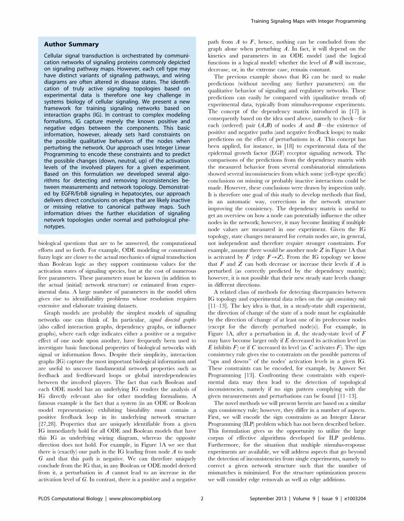
uniqueness). We use four simple compression rules (illustrated in

Figure 2) in an iterative manner which, as shown in the EGF

scenario below, may reduce the network size considerably so that

enumeration of solutions in large networks become possible (some

but not all rules are identical to those used in [7]). Compressing the

network is particularly useful for enumerating solutions for

OPT_GRAPH and OPT_SUBGRAPH.

Rule 1 (removal of non-controllable and non-observ-

able nodes): Non-controllable nodes (which cannot be

affected by any of the perturbed nodes in any scenario)

and non-observable nodes (which do not influence any

measured (readout) node in any scenario) define non-

identifiable parts of the network. Therefore, these nodes

as well as all edges they are connected to can be

removed. Non-observable and non-controllable nodes

can easily be identified by shortest path algorithms (cf.

[7]).

Rule 2 (removal of parallel edges): If there are two

parallel edges of the same sign, we may safely remove

one of them (Figure 2A).

Rule 3 (absorbing a node with a single input edge): If a

latent node (neither measured nor perturbed in any of

the experimental scenarios) has only one single incoming

edge, then we can remove this node (together with the

incoming edge) and reconnect all the outgoing edges of

this node to its only predecessor node (under consider-

ation of edge signs; see example in Figure 2B).

Rule 4 (absorbing a node with a single output edge): If a

latent node has only one single outgoing edge, then we



can remove this node (together with the outgoing edge)

and reconnect all its incoming edges to its only successor

node (under consideration of edge signs; see example in

Figure 2C).

Rule 1 is performed once at the beginning, whereas rules 2–4

are iteratively used until no further rule can be applied (note that

new parallel edges may arise after applying rules 3 or 4). The

compressed version of the example network in Figure 1A is shown

in Figure 2D).

By keeping track of the made compression steps it is, in principle,

possible to decompress solutions found by the described optimiza-

tion algorithms in the compressed network. However, as mentioned

above, it is often useful to discuss the obtained solutions directly in

the compressed network, thereby avoiding the interpretation of a

typically much larger number of decompressed solutions arising due

to non-uniqueness. For example, instead of listing all possible

(parallel) pathway combinations connecting A with B, one might

conclude that ‘‘at least one pathway between A and B must exist’’

which can easier be represented in a compressed network.

Implementation: SigNetTrainerThe ILP formulations presented in the previous sections

were implemented in the new software SigNetTrainer. The toolbox

is available in two versions, the first is written in C and uses

routines from the ILP solver GUROBI (http://www.gurobi.com),

whereas the second version is implemented in MATLAB and

uses the IBM ILOG CPLEX Optimizer (for which free academic

versions can be obtained via http://www-03.ibm.com/ibm/

university/academic/pub/page/membership) as ILP solver. Thus,

SigNetTrainer benefits from state-of-the-art-solvers for ILP problems

which use a number of methodologies to deal with large-scale

problems. For a more general introduction to ILP algorithms we

refer to [30].

SigNetTrainer is easy to use; the user has to provide three files to

define network training problems: (i) the network topology in.sif

format (also used by Cytoscape http://www.cytoscape.org), (ii) an

ASCII file describing the experimental scenarios (i.e., the imposed

state changes), and (iii) an ASCII file containing the experimen-

tally measured state changes for each scenario. The user may then

call different functions implementing the optimization routines as

described herein. Source code and manual of both versions of

SigNetTrainer are available on the following website:

http://www.mpi-magdeburg.mpg.de/projects/cna/

etcdownloads.html.

Preprocessing routines, in particular the network compression

algorithm, were implemented as MATLAB functions and are also

part of the package. The manual of SigNetTrainer is provided in the

Supporting Information (Text S1).

Results

EGFR/ErbB signaling in hepatocytesIn order to demonstrate the performance of the proposed

approach in a realistic situation, we apply it to a recently published

network topology of EGFR/ErbB signaling [18] with the aim to

identify topological particularities of this important signaling

pathway in hepatocytes. The network was built within the logical

modeling framework introduced in [17] and describes signal

transduction downstream of the members of the EGF receptor

family, ErbB1–4. Network reconstruction was based on signaling

reactions reported in literature and databases. As the included

reactions have been observed in a variety of cell types and tissues,

the model must be seen as a ‘‘master network’’ and it is likely that

not all of the included interactions are functional in primary

human hepatocytes considered herein. In [18], qualitative

predictions derived both from the logical model and its underlying

interaction graph were compared with a dataset (a subset of the

Figure 2. Basic network compression rules. (A) Parallel edges. (B) Nodes with single input. (C) Nodes with single output. (D) Shown is thecompressed version of the network in Figure 1A after applying the compression rules. For further explanations see main text.doi:10.1371/journal.pcbi.1003204.g002



http://www-03.ibm.com/ibm/university/academic/pub/page/membership

http://www-03.ibm.com/ibm/university/academic/pub/page/membership

http://www.mpi-magdeburg.mpg.de/projects/cna/etcdownloads.html

http://www.mpi-magdeburg.mpg.de/projects/cna/etcdownloads.html

phosphoproteomic data published in [2]) consisting of combina-

torial treatments of primary human hepatocytes with/without

TGFa and specific molecular inhibitors (see Figure S1). Note that

the measurements were taken at an optimal time point such that

the perturbation-induced changes in the phosphorylation level of

the proteins are well-reflected by the measurements [2]. The

interaction graph-based data analysis in [18] made use of the

dependency matrix of the network (see Introduction section): for

pairs of experiments (e.g., Exp. 1: stimuli A, inhibitor B, Exp. 2:

stimuli A, no inhibitor) it was checked whether the ratio of the

measured responses (e.g., Exp. 1/Exp. 2, showing the effect of

inhibitor B) is consistent with the causal dependencies in the

network topology (e.g., if B has a positive/negative/no influence

on a readout C, inhibiting B should lead to decreased/increased/

unchanged C). Resulting from this analysis, changes in the

network structure were proposed that would improve the

agreement between experimental data and model predictions.

These changes were derived solely by inspection; the ILP

approach presented herein can be seen as a step forward as it

adapts the model structure to the experimental data in an

automatic way and searches systematically for all possible solutions

resolving discrepancies between model and data.

PreprocessingBefore applying the ILP formulation, both the phosphoproteo-

mic data (Figure S1) and the EGFR/ErbB signaling network

topology used in [18] had to be preprocessed. The phosphopro-

teomic data were originally obtained via xMAP technology which

measures fluorescent units [2]. The dynamic range of the

measured signals depends on the antibody pair used for detection.

For example, the signal for JNK ranges from 100 units to 500

units, while MEK1/2 ranges up to 25000 units (Figure S1).

Variations such as these do not necessarily reflect that JNK is less

activated than MEK1/2, but may be attributed to protein

abundance or assay calibration issues. Furthermore, the proposed

formulation requires a qualitative view of signal transduction,

supporting only three discrete states indicating the variation of the

activation state of signaling nodes when changing external inputs

or adding inhibitors (‘‘21’’ for downregulated, ‘‘0’’ for unchanged,

and ‘‘1’’ for upregulated). Thus, the raw data need to be

discretized before it can be used in the ILP formulation. To this

end, the methodology introduced by Samaga et al. in [18] is

adopted: the ratios of all experiments that differ only by a single

perturbation (ligand or inhibitor treatment) are evaluated and the

respective measurement is considered to be (i) upregulated if the

fold-increase of the signal (with versus without perturbation) is

above 1.5, (ii) downregulated if the fold-decrease of the signal (with

versus without perturbation) is below 0.66 and (iii) unchanged

otherwise. The dataset analyzed in [18] contains measurements

with JNK inhibitor showing an effect of the inhibitor on many of

the measured signals. As these inhibitions are likely to be off-target

effects [2], we decided to exclude the JNK inhibitor data for our

analysis. The complete set of discretized data can be seen in

Figure 3.

Regarding the EGFR/ErbB network model, the original

interaction graph used by Samaga et al. [18] was adopted but

non-observable and non-controllable nodes were removed (see [7]

and Rule 1 of the model compression described in the Methods

section; the full compression will be applied in a later step). The

resulting graph is shown in Figure 4A.

Applying SCEN_FIT and Minimal Correction SetsFigure 3 depicts the discretized measurements and, for each

scenario, the corresponding SCEN_FIT solution. Recall that the

SCEN_FIT algorithm determines, for a given scenario, a sign-

consistent node labeling that is closest to the measurements and

can thus best explain how the EGFR network topology in

Figure 4A induces the measured node changes for the respective

scenario. Deviations between the determined optimal sign pattern

and the measured state changes (as indicated in Figure 3) uncover

inconsistencies between network structure and observed behavior.

For example, scenario 1 reflects the influence of the ligand TGFa,

that is, TGFa is the perturbed node and its state is fixed to 1. As

depicted in Figure 3, the SCEN_FIT solution for this scenario

shows a fitting error of 1: in the optimal sign-consistent node

labeling, all measured nodes have sign 1 as they are connected to

TGFa by positive paths only. This is in accordance with the

measured state of all nodes except STAT3: the latter shows no

significant change in response to TGFa inducing thus a fitting

error. Scenarios 2–6 reflect the influence of TGFa in presence of

different inhibitors. We assume that an inhibitor completely blocks

the signal flow through the inhibited species and thus define these

scenarios by fixing the state of TGFa to 1 and of the inhibited

node to 0. The remaining scenarios reflect the influence of the

inhibitors in presence (scenarios 7–11) and absence (scenarios 12–

16) of TGFa. In each of these scenarios the perturbed node is the

respective inhibitor and its state is fixed to 21. Importantly, by

using the enumeration algorithm for SCEN_FIT we could prove

that, for each scenario, the found solution for the optimal fit is

unique, hence, no other optimal solutions need to be considered.

We also assessed the sensitivity of the SCEN_FIT results with

respect to the chosen thresholds for data discretization and found a

fairly robust behavior for a relatively large range of the threshold

parameters (see Figure S2 and Text S2).

Figure 3 shows that there are several inconsistencies between

experimental data and the SCEN_FIT solutions derived from the

initial network topology. In order to understand where these

inconsistencies are induced in the network, we address the

identification of minimal correction sets (MCoS). We recall that

MCoS are minimum sets of (artificially) enforced changes of node

states (e.g., from up- to downregulated) which make an inconsis-

tent scenario consistent. Exemplarily, we focus on scenario 14 of

Figure 3 (where PI3K-i is added without presence of TGFa) whose

SCEN_FIT solution produced a total error value of 6.

As shown in Table 2, five MCoS are identified, each containing

three corrections (virtual perturbations) rendering the experimen-

tal scenario 14 sign-consistent. Common trend in all MCoS is to

remove the downregulating effect of PI3K on signals downstream

of Rac_Cdc42 by setting Rac_Cdc42 to unchanged (0) or one of

the nodes SOS1_Eps8_E3b1, Vav2, PI(3,4)P2 or PIP3 to

upregulated (1). Introducing this change, the states of p38, JNK,

MEK1/2, Hsp27, CREB and p90RSK are now in accordance

with the measurements (i.e., they show now response upon adding

PI3K inhibitor). However, by this modification, the states of

ERK1/2 and p70S6_1 would change their predicted level from

‘‘downregulated’’ to ‘‘unchanged’’ which is not in agreement with

the measured state. This is corrected in all MCoS by setting

ERK1/2 to 21. Again, this correction implies an undesired effect,

namely changing p90RSK from 0 to 21, which is countered by

assigning p90RSK the value 0 in all MCoS. Clearly, three

required corrections indicate that the observed behavior for this

scenario is not well-reflected by the network topology. It would

therefore be useful to consider all scenarios at the same time to

detect common points of errors produced in all or many scenarios.

Applying OPT_SUBGRAPHWe use the OPT_SUBGRAPH algorithm to find—by appro-

priate edge removals—an optimal subgraph of the EGFR network



structure which minimizes the fitting errors over all experimental

scenarios.

To be able to make meaningful conclusions, we need to find all

optimal solutions. However, enumerating all solutions for

OPT_SUBGRAPH in the full model structure becomes quickly

intractable as the highly branched network structure (e.g., various

feedforward routes running over different combinations of ErbB

dimers and adapter proteins connect TGFa with PI3K) leads to an

immense number of different optimal solutions. Therefore, we

compress the model structure as described in section ‘‘Model

compression’’ before searching for optimal subgraphs. As can be

seen in Figure 4B, the model structure can be compressed

substantially from 39 nodes and 67 edges to 14 nodes and 18

edges. Strikingly, Rac_Cdc42 remains as the only latent node in

the compressed structure. The compressed IG reflects the essential

dependencies in the original network structure that can be

addressed by the given set of perturbed/measured nodes. For

example, parallel signaling paths leading from a perturbed node to

a measured node without passing any other measured/perturbed

node cannot be distinguished in the analysis performed herein and

are therefore condensed to one single edge in the compressed

graph.

The computation of all optimal subgraphs of the compressed

network resulted in six solutions having the same minimal fitting

error of 26 which has thus reduced much in comparison to 45 in

the original model. Figure 5 shows a combined view of the six

optimal solutions; the single solutions are shown in Table S1. In

more detail, a positive influence of TGFa on STAT3 is not

reflected in the measurements (see Figure 3); consequently, the

edge TGFaRSTAT3 is removed in all optimal solutions. Another

edge that is removed in all solutions is PI3KRRac_Cdc42, as a

number of signals downstream of Rac_Cdc42 did not show the

expected downregulated response to the PI3K inhibitor in the

measurements (this is consistent with the results of the MCoS

disussed in the previous subsection). Finally, by removing the edge

ERK1/2Rp70S6_1 in all solutions, the missing influence of MEK

Figure 3. Discretized measurements of the 16 considered experimental scenarios and the resulting SCEN_FIT solutions computedfrom the EGFR/ErbB graph model. Each row corresponds to one experimental scenario, each column contains the measured state changes of thereadout species. The discretized measurements are mapped to the fill color of the respective fields: if a node is upregulated in the respective scenario,the corresponding field is filled green, if it is downregulated, the field is filled red, and if it shows no significant change, it is filled white. Accordingly,the color of the added circles shows the sign of the node in the closest sign-consistent node labeling derived by SCEN_FIT: green circles correspondto sign 1, red circles to sign 21 and white circles to sign 0. Note that circles only appear if the measurement is not in accordance with the respectivestate in the sign-consistent labeling.doi:10.1371/journal.pcbi.1003204.g003



Figure 4. Interaction graph model of the EGFR/ErbB signaling network. (A) The full network adopted from [18] after removal of non-observable and non-controllable nodes. All edges are activating edges (having positive signs). (B) The compressed model obtained after applying thecompression rules to (A).doi:10.1371/journal.pcbi.1003204.g004



Table 2. MCoS for scenario 14 in Figure 3.

MCoS 1 MCoS 2 MCoS 3 MCoS 4 MCoS 5

Node id Bzi B{

i Val Bzi B{

i Val Bzi B{

i Val Bzi B{

i Val Bzi B{

i Val

rac_cdc42 1 0

p90rsk 1 0 1 0 1 0 1 0 1 0

erk12 1 21 1 21 1 21 1 21 1 21

sos1_eps8_e3b1 1 1

vav2 1 1

pi34p2 1 1

pip3 1 1

Five MCoS are identified for the EGFR network model (Figure 4) with respect to scenario 14 in Figure 3. Each MCoS would lead to a perfect fit for this scenario and all fiveMCoS contain three nodes to be enforced to a certain value. Nodes p90rsk and erk12 are common in all MCoS. Nodes rac_cdc42, sos1_eps8_e3b1, vav2, pi34p2 andpip3 are perturbed respectively in MCoS 1–5. In columns MCoS 1–5, three sub-columns are shown: sub-column ‘‘Val’’ shows the corrected state of the node (the actualMCoS), the entry 1 in sub-column ‘‘Bz

i ’’ indicates that a positive input edge is added to the node in order to alter its state, and the entry 1 in sub-column ‘‘B{i ’’ indicates

that a negative input edge is added to the node (see Methods section).doi:10.1371/journal.pcbi.1003204.t002

Figure 5. Combined view of all optimal model structures derived from the compressed EGFR/ErbB model by applying theOPT_SUBGRAPH procedure with enumeration.doi:10.1371/journal.pcbi.1003204.g005



inhibitor on p70S6_1 is accommodated. The edges TGFaRMEK1/2 and Rac_Cdc42RMEK1/2 are only removed in some

of the solutions. This is an example for two parallel routes that

cannot be distinguished: the model structures containing both

routes or either route give rise to the same sign-consistent labeling.

In contrast, removing either of the edges p90RSKRCREB and

p38RCREB results in different sign-consistent labelings, both

showing the same number of discrepancies to the measurements:

the phosphorylation state of CREB is neither affected by MEK

inhibitor nor by p38 inhibitor. However, removing both edges at

the same time would interrupt all routes from TGFa to CREB

what is contradictory to the observed positive effect of TGFa in

scenarios 1–6. Thus, in this case, allowing only the removal of

edges is not sufficient to fully explain the observed measurements.

This can be seen in Figure 6, where the two possible optimal sign-

consistent labelings that SCEN_FIT would find for the six pruned

model structures are shown in comparison to the discretized

measurements: in each solution, there are three different

remaining errors in the CREB column. The errors for STAT3

as well as the errors in response to PI3K inhibitor (scenarios 9 and

14) could be significantly reduced by removing the respective

edges.

Applying OPT_GRAPHNext, we use the OPT_GRAPH procedure to identify edges

that may be missing from the EGFR network and whose addition

would therefore improve the goodness of fit to the data. Table 3

displays the edges that lead to the highest improvement as

determined by OPT_GRAPH. All these edges have in common

that they give rise to an additional route from TGFa to CREB not

running over p38 or MEK1/2. By adding any of these edges to the

model structure before reapplying the OPT_SUBGRAPH proce-

dure, we can further reduce the fitting error to 23 (compared to 26

if only edge removals are allowed).

As an example, we show the optimized model structures when

adding the edge TGFaRCREB. A combined view of the three

optimal solutions (that can be found by OPT_GRAPH after

adding this edge) is shown in Figure 7. As it was the case for the

optimization in the original network, the edges TGFaRSTAT3,

PI3KRRac_CDC42 and ERK1/2Rp70S6_1 are removed in all

Figure 6. Discretized data and the (two) SCEN_FIT solutions that result from the optimal subgraphs given in Figure 5. The colorcoding is the same as in Figure 3. All six optimal subgraphs contained in Figure 5 give rise to the same SCEN_FIT solution, except for the CREBcolumn. Here, three subgraphs show a mismatch in scenarios 5, 10, and 15 (indicated by the left semicycles), while the other three show a mismatchin scenarios 6, 11, and 16 (indicated by the right semicycles).doi:10.1371/journal.pcbi.1003204.g006



solutions, while the edges TGFaRMEK1/2 and Rac_Cdc42RMEK1/2 are two alternative routes (either both are present or at

least one of both; this gives the three optimal subgraphs). With the

added edge TGFaRCREB the model structure comprises an

activation route from TGFa to CREB that is independent of p38

and p90RSK, and removing both the p90RSKRCREB and

p38RCREB edge in all solutions is now optimal.

All three solutions induce the same optimal sign-consistent node

labeling. Figure 8 shows the mismatches of the experimental data in

the optimal graph (Figure 7) vs. the mismatches in the initial model

structure (Figure 4B). The measurements for CREB are now in full

accordance with the model structure and the errors for STAT3

could be significantly reduced. Furthermore, a number of errors in

scenarios 9 and 14 showing the influence of PI3K inhibitor could be

eliminated, although at the same time a few mismatches for some

nodes have been introduced. Finally, the influence of MEK

inhibitor on p70S6_1 is now predicted correctly. Here, we

considered only the addition of a single edge to improve the fit to

data. In principle, one could remove all remaining discrepancies by

adding further edges. However, in particular if the measurements

show inconsistencies (e.g., the different effect of PI3K inhibitor on

ERK1/2 with/without TGFa), some errors can only be removed by

introducing a positive and a negative edge between a pair of nodes.

Furthermore, edges leading only to a minor improvement of the

fitting error are unlikely to represents a real effect. We also

Table 3. Suggestions for new edges as computed byOPT_GRAPH.

tgfaRcreb

jnkRcreb

p70s61Rcreb

rac_cdc42Rcreb

tgfaRerk12

jnkRerk12

rac_cdc42Rerk12

Adding any of these edges to the model structure leads to a decrease of thefitting error from 26 to 23.doi:10.1371/journal.pcbi.1003204.t003

Figure 7. Combined view of the three optimal subgraphs resulting when adding TGFa to CREB to the initial model structure. In allthree solutions, the edges erk12Rp70s6_1, tgfaRstat3, p90rskRcreb and p38Rcreb are removed. Edges tgfaRmek12 and rac_cdc42Rmek12represent alternative pathways; at least one of both must be contained.doi:10.1371/journal.pcbi.1003204.g007



emphasize that proposed new edges may often indicate indirect

rather than direct effects (representing then (hidden) paths in the

network). In any case, dedicated experiments are required to

confirm or prove the suggested causal links.

To summarize, essential findings of the network structure

optimization in the EGFR/ErbB network—which may indicate

important specifics of this signaling pathway in hepatocytes—are:

(1) STAT3 is not activated by TGFa; (2) Phosphorylation of the

autocatalytic domain of p70S6 (termed p70S6_1 in the model) is

independent of ERK1/2; (3) The activation of CREB in response

to TGFa is likely to be caused by a p38 and MEK1/2 independent

route; and (4) The activation of Rac/Cdc42 is independent of

PI3K activity. These results, generated in an automated way,

confirm several of the conjectures formulated in [18] that were

derived by inspection only. In addition, by identifying parallel

activation routes that cannot be distinguished with the experi-

mental data at hand, the presented approach contributes to a

better understanding of the network topology and helps to suggest

further experiments for uncovering the true wiring diagram of this

important signaling pathway in the given cell type.

Evaluation of the runtime behavior with respect todifferent problem sizes

When applying the four fundamental optimization problems

SCEN_FIT, MCoS, OPT_SUBGRAPH and OPT_GRAPH to

the EGFR/ErbB case study, we observed that all problems for

both finding single and enumerating all solutions could be solved

in a few seconds (see Figure S3), although hundreds or (in case

of OPT_SUBGRAPH and OPT_GRAPH) even thousands of

integer variables and constraints might be involved. However,

since ILPs are in general NP-hard problems, we tested the runtime

behavior more systematically by means of benchmarks to provide

information on scalability and the ability of the algorithms to

tackle larger, more complex problems. The benchmarks shown in

Figure S3 evaluate the runtime of the formulations for problems of

different size. Four experimental/simulated datasets were used: (i)

the EGFR dataset interrogated throughout this paper, (ii) a

random dataset of equal size to the EGFR dataset, (iii) a random

dataset with the same number of signals (readouts) as the EGFR

dataset but with double the number of experimental scenarios, and

(iv) a random dataset with equal number of scenarios as the EGFR

Figure 8. Comparison of the fitting errors of the initial model structure (see Figures 3 and 4) and of the optimal interaction graphshown in Figure 7. Green fields indicate an error that has been present in the original model structure, but could be removed by optimizing themodel structure. Yellow fields refer to errors that could not be resolved, and red fields indicate errors that have not been present in the original modelstructure, but were introduced by the optimization.doi:10.1371/journal.pcbi.1003204.g008



dataset, but with more measured signals. Moreover, four networks

of different size were interrogated: (i) the compressed EGFR

network (numbering 18 edges; Figure 4B), (ii) the uncompressed

EGFR network, after removing non-observable and non-control-

lable parts of it (numbering 67 edges; Figure 4A), and two partially

compressed networks, (iii) one numbering 32 edges, and (iv) one

numbering 42 edges. For a detailed report on the benchmarks see

Text S3; here, we give a brief overview of the results.

First of all, the benchmarks clearly showed a significant effect of

the compression of the interaction graph as the amount of

required memory and the runtimes were greatly decreased. All

four problems (also in enumeration mode) could be solved within

seconds for all training datasets. This is not only due to smaller

network size (and thus fewer constraints and variables), but also

due to the fact that the number of alternate optimal solutions to be

found in the enumeration procedure, in particular for the

OPT_SUBGRAPH problem, is strongly reduced.

Figure S3 shows that single solutions could be found within

seconds for almost all problems, also in the larger networks.

However, the runtime rapidly increased for OPT_SUBGRAPH

and OPT_GRAPH problems when interrogated with the random

dataset with double the number of experimental scenarios. The

utilization of randomly generated data mimics a noisy dataset full

of internal conflicts (i.e., the signal does not follow certain motifs

like the actual data, but signals that are co-regulated in one

scenario are anti-regulated in the next). This slows down the

formulation and the runtime increases drastically, especially for

the uncompressed network.

Regarding the full enumeration of alternate optimal solutions, we

observed that all optimal SCEN_FIT and MCoS solutions could

be found for all problem sizes within seconds. As expected, full

enumeration of the optimal OPT_SUBGRAPH solutions (as

well as solving the OPT_GRAPH problem) becomes challenging

in larger networks for two reasons: (i) more than 17,000 variables

and 37,000 constraints might be required to represent the

problem, and (ii) a large number of alternate optimal solutions

might exist. For this reason, several runs stopped because either

the limit of the maximal number of solutions or the time limit was

exceeded.

Discussion

We presented a new framework for interrogating and training

signaling networks based on measurements from stimulus-response

experiments. Our approach represents signaling networks as

interaction graphs and can thus immediately be applied to

network topologies stored in many databases without the need

to convert these graphs into other modeling formalisms. Interac-

tion graphs capture merely the positive and negative edges

between the components in the network; however, this informa-

tion already sets constraints on the possible qualitative behavior of

the nodes when stimulating or perturbing the network. Our

approach uses Integer Linear Programming to encode these

constraints and to predict the possible changes (down, neutral, up)

of the activation levels of the involved players for a given

experiment. Based on this ILP formulation we presented four basic

optimization routines useful to detect and remove inconsistencies

between measurements and predicted behaviors:

(1) SCEN_FIT: Determination of a causal explanation for the

measured activation changes of readout nodes under a given

perturbation scenario. If the measurements are inconsistent

with the network topology, the closest feasible explanation is

identified.

(2) Minimal Correction Sets: In case of an inconsistent scenario,

determination of a minimal set of nodes whose states need to

be corrected to make a single inconsistent scenario consistent.

(3) OPT_SUBGRAPH: Determination of an optimal subgraph

of a given network topology that can reflect the measurements

for a set of scenarios at best.

(4) OPT_GRAPH: Identification of edge candidate(s) whose

insertion would improve the consistency of the graph with

respect to a set of experimental scenarios the most.

The first two optimization problems seek to match the network

topology with measurements from a single stimulus-response

experiment. In contrast, (3) and (4) operate on a set of scenarios

and seek to optimize (train) the network structure over all scenarios

by removing or/and adding edges. For the first three problems we

also provided enumeration algorithms to find multiple or all

solutions that solve the optimization problem equally well (e.g., for

problem (3), all optimal subgraphs that minimize the number of

inconsistencies between measurements and predictions). The

enumeration of all solutions is necessary to allow one to draw

general conclusions, for example, that a certain edge is removed in

all (not only in some) optimal solutions. However, the enumeration

of optimal solutions may quickly become prohibitive in larger

networks. We therefore employ effective compression techniques

to deal with the combinatorial complexity arising in large-scale

networks. In fact, this allowed us to also address the enumeration

of multiple optimal solutions in the EGFR/ErbB case study where

all performed computations could be finished within seconds on a

standard PC. To assess the runtime behavior and scalability of our

algorithms, we performed further benchmark tests showing that

finding single optimal solutions to the four basic problems is

feasible also in larger networks, whereas enumeration of all

solutions, in particular for OPT_SUBGRAPH, becomes challeng-

ing (see Figure S3 and Text S3).

In contrast to the globally optimal solutions that will be

delivered for problems (1)–(3), the identification of (a set of) missing

edges reducing the fitting error the most (problem (4)) is based on a

greedy algorithm which may deliver local instead of globally

optimal solutions when adding more than one edge. However,

given the huge search space of potentially missing (sets of) edges,

the employed greedy algorithm appears to be a suitable and useful

heuristics to suggest missing interactions in the IG model. If only

one candidate edge is to be added (instead of a set), it even delivers

the globally optimal solution, also in large networks.

To the best of our knowledge, our presented approach is the

first that uses Integer Linear Programming directly on interaction

graphs to systematically interrogate and train the wiring diagrams

of signaling networks. Our framework shares some similarities with

the approach of Saez-Rodriguez et al. [7] for which recently also

an ILP formulation was conceived [29]. This method also starts

with an IG representing the prior knowledge; however, the IG is

then translated to a superstructure of Boolean networks within

which the optimal (sub)model fitting the data at best is identified.

Although a correctly reconstructed Boolean network can poten-

tially provide a more specific view on the network structure than

an IG, the search space is considerably larger since usually a vast

number of possible Boolean networks can be constructed from a

given IG. This may lead to highly underdetermined problems and

enumeration strategies as discussed herein can become intractable.

Furthermore, Boolean networks require a strict binarization of

the nodes’ states whereas in the IG formulation we consider

‘‘influences’’. This may lead to different results. For example, the

Boolean function for a node Z may read Z~A OR B. Assume

that we consider the influence of (external) activation of node B



given the network state where A is active and B inactive; hence,

where Z is already in the active state. The Boolean model will

tell us that Z remains in state 1 when activating B, hence, the

influence of B seems to be not relevant. However, Boolean

functions are discrete approximations of the true mechanisms and

what one could probably see in the measurements is that the level

of Z goes from ‘‘high’’ to ‘‘very high’’. In the IG, we can still

account for this effect stating that an elevated level of B induces a

positive effect on Z. So discretized node states need not to be

considered in the IG model; however, similar as for the Boolean

model, some kind of discretization of the data will be required as

well when classifying a change of an activation level to be

significant or not. Finally, we also mention that methods for the

enumeration of solutions and for the search for missing edges were

not presented in [29].

The approach that is arguably closest to ours is the method

introduced in [11–13]. This framework is also based on IG and

uses a similar consistency rule as we did herein. However, there

are a number of key differences. First, we explicitly allow a ‘‘0’’

change to mark non-affected states of nodes. This extension

seems to be essential, for example, when perturbation of a node Acannot affect another node B simply because (in the true topology)

a path from A to B does not exist. Second, the four basic problem

formulations presented herein go beyond the techniques intro-

duced in [11–13]. In particular, the training of the topology, that

is, the identification of inactive or missing interactions based on a

library of stimulus-response experiments, was not considered in

these works. A third key difference is that we formulated the

constraints resulting from the consistency rules as an ILP problem,

whereas [13] uses Answer Set Programming (ASP). Both ILP and

ASP deliver globally optimal solutions and highly optimized

solvers exist. Using ILP or ASP solvers is not straightforward for

non-experts and with SigNetTrainer we provide an easy-to-use

toolbox. However, it would be an interesting aspect for future

work to compare ASP and ILP formulations of the training and

enumeration problems formulated herein.

We demonstrated the power of our proposed approach by

interrogating and (re-)training a manually curated IG model of

EGFR/ErbB signaling against a library of high-throughput

phosphoproteomic data measured in primary human hepatocytes.

Our algorithms could systematically uncover all inconsistencies

between measurements and network topology and gave possible

explanations for them. Novel biological insights for this important

signaling pathway could be revealed by listing interactions that are

likely to be inactive in hepatocytes and by giving suggestions for

possibly missing interactions that, if included, would significantly

improve the goodness of fit. Clearly, these predictions await

experimental validation.

This study gave a proof of principle for our methodology,

showing its flexibility and that it can be applied to a wide range of

problems arising when confronting signaling network topologies

with experimental datasets. Given that only fairly accessible

biological knowledge is required and that all related algorithms

were implemented in a freely available toolbox make it an

appealing approach for various applications.

Supporting Information

Figure S1 Raw training data. A subset of the phosphoprotein

data published in [2], capturing the signaling response of primary

human hepatocytes to TGFa in combination with six specific

molecular inhibitors (including the no-inhibitor treatment):

MEK12-i, p38-i, PI3K-i, mTORrap-i, GSK3-i, no-inhib. Each

subplot shows the phosphorylation state of the respective protein

in fluorescent units (obtained via xMAP technology), measured

0 minutes (left border) and 25 minutes (right border) after

stimulation.

(EPS)

Figure S2 Cumulative fitness error of optimal SCEN_-FIT solutions over all 16 scenarios in the (compressed)EGFR/ErbB network as a function of the two discretiza-tion thresholds. The cumulative fitness error of optimal

SCEN_FIT solutions over all 16 scenarios in the (compressed)

EGFR/ErbB network as a function of the significant increase and

significant decrease thresholds is plotted. The thresholds combi-

nation used for all analyses presented in this paper are plotted as a

blue rectangle. There is a relatively broad range for ‘‘significant

decrease’’ in ½0:2,0:7� and ‘‘significant increase’’ in ½1:5,1:9� where

the fitness error assumes its lowest values (40–50). Outside that

area the fitness error increases rapidly. The thresholds used in the

EGFR/ErbB study (0.66 and 1.5, respectively) are inside that

range and result in a total fitness error of 45 (see Figure 3 in main

text).

(PNG)

Figure S3 Evaluation of runtimes of SigNetTrainer(GUROBI version) with respect to the four basicoptimization problems and different problem sizes.Runs for all four ILP problems introduced in this paper

(SCEN_FIT, MCoS, OPT_SUBGRAPH, OPT_GRAPH) are

shown in the corresponding columns. For each run the CPU

time, number of variables, number of constraints, and number of

found solutions are reported, both for obtaining a single solution

and for enumeration of solutions. The first five columns give a

description of each run regarding the interrogated data and

network: the dataset used (EGFR data, random data, more

scenarios, more signals; see explanations in the main text and

in text S3), the number of reactions in the network (18, 32, 42,

67), number of measured signals, number of scenarios and

number of inputs. A time limit is set for each run at

64,000 seconds. For the enumeration benchmarks, a maximum

number of allowed solutions is set at 1000 solutions. The

maximum allowed memory is 4 GB. Instances where the

algorithm did not complete the run due to time-out are marked

with red. All calculations were done on a PC with a 2.2 GHz Intel

quad core i7 CPU (only a single core was used) and 4 GB

1333 MHz DDR3 memory. The default optimality tolerance was

used in all optimizations for the GUROBI solver (see also http://

www.gurobi.com/documentation/5.0/reference-manual/).

(PDF)

Table S1 Optimal model structures derived from thecompressed EGFR/ErbB model by OPT_SUBGRAPHwith enumeration.(PDF)

Text S1 Getting started with SigNetTrainer.(PDF)

Text S2 Sensitivity analysis of the SCEN_FIT solutionswith respect to the chosen discretization thresholds.(PDF)

Text S3 Systematic evaluation of ILP runtimes withrespect to problem size.(PDF)

Acknowledgments

We thank Alexander Mitsos and Julio Saez-Rodriguez for fruitful

discussions.



Author Contributions

Conceived and designed the experiments: LGA. Performed the experi-

ments: LGA. Analyzed the data: INM RS SK. Contributed reagents/

materials/analysis tools: LGA. Wrote the paper: INM RS LGA SK.

Designed the study: SK. Developed the software: INM SK. Tested, used,

and documented the software: INM RS SK.

References

1. Saez-Rodriguez J, Alexopoulos LG, Stolovitzky G (2011) Setting the standards

for signal transduction research. Sci Signal 4: pe10.2. Alexopoulos LG, Saez Rodriguez J, Cosgrove BD, Lauffenburger DA, Sorger

PK (2010) Networks inferred from biochemical data reveal profound differencesin toll-like receptor and inammatory signaling between normal and transformed

hepatocytes. Mol Cell Proteomics 9: 1849–1865.

3. Joshi-Tope G, Gillespie M, Vastrik I, D’Eustachio P, Schmidt E, et al. (2005)Reactome: a knowledgebase of biological pathways. Nucleic Acids Res 33:

D428–D432.4. Cerami EG, Gross BE, Demir E, Rodchenkov I, Babur O, et al. (2011) Pathway

Commons, a web resource for biological pathway data. Nucleic Acids Res 39:

D685–D690.5. Kanehisa M, Goto S (2000) KEGG: kyoto encyclopedia of genes and genomes.

Nucleic Acids Res 28: 27–30.6. Mitsos A, Melas IN, Siminelakis P, Chairakaki AD, Saez-Rodriguez J, et al.

(2009) Identifying drug effects via pathway alterations using an integer linearprogramming optimization formulation on phosphoproteomic data. PLoS

Comput Biol 5: e1000591.

7. Saez-Rodriguez J, Alexopoulos LG, Epperlein J, Samaga R, Lauffenburger DA,et al. (2009) Discrete logic modelling as a means to link protein signalling

networks with functional analysis of mammalian signal transduction. Mol SystBiol 5: 331.

8. Morris MK, Saez-Rodriguez J, Clarke DC, Sorger PK, Lauffenburger DA

(2011) Training signaling pathway maps to biochemical data with constrainedfuzzy logic: quantitative analysis of liver cell responses to inammatory stimuli.

PLoS Comput Biol 7: e1001099.9. Chu Y, Jayaraman A, Hahn J (2007) Parameter sensitivity analysis of IL-6

signalling pathways. IET Syst Biol 1: 342–352.

10. Zhang Y, Rundell A (2006) Comparative study of parameter sensitivity analysesof the TCRactivated ERK-MAPK signalling pathway. Syst Biol (Stevenage) 153:

201–211.11. Siegel A, Radulescu O, Le Borgne M, Veber P, Ouy J, et al. (2006) Qualitative

analysis of the relation between DNA microarray data and behavioral models ofregulation networks. Biosystems 84: 153–174.

12. Guziolowski C, Bourde A, Moreews F, Siegel A (2009) BioQuali Cytoscape

plugin: analysing the global consistency of regulatory networks. BMC Genomics10: 244.

13. Gebser M, Schaub T, Thiele S, Veber P (2011) Detecting inconsistencies in largebiological networks with answer set programming. Theory and Practice of Logic

Programming 11: 323–360.

14. Gutierrez-Rıos RM, Rosenblueth DA, Loza JA, Huerta AM, Glasner JD, et al.(2003) Regulatory network of Escherichia coli: consistency between literature

knowledge and microarray profiles. Genome Res 13: 2433–2443.

15. Sachs K, Perez O, Pe’er D, Lauffenburger DA, Nolan GP (2005) Causal protein-

signaling networks derived from multiparameter single-cell data. Science 308:

523–529.

16. Feiglin A, Hacohen A, Sarusi A, Fisher J, Unger R, et al. (2012) Static network

structure can be used to model the phenotypic effects of perturbations in

regulatory networks. Bioinformatics 28: 2811–2818.

17. Klamt S, Saez-Rodriguez J, Lindquist JA, Simeoni L, Gilles ED (2006) A

methodology for the structural and functional analysis of signaling and

regulatory networks. BMC Bioinformatics 7: 56.

18. Samaga R, Saez-Rodriguez J, Alexopoulos LG, Sorger PK, Klamt S (2009) The

logic of EGFR/ErbB signaling: theoretical properties and analysis of high-

throughput data. PLoS Comput Biol 5: e1000438.

19. Morris MK, Saez-Rodriguez J, Sorger PK, Lauffenburger DA (2010) Logic-

based models for the analysis of cell signaling networks. Biochemistry 49: 3216–

3224.

20. Wang RS, Saadatpour A, Albert R (2012) Boolean modeling in systems biology:

an overview of methodology and applications. Phys Biol 9: 055001.

21. Aldridge BB, Saez-Rodriguez J, Muhlich JL, Sorger PK, Lauffenburger DA

(2009) Fuzzy logic analysis of kinase pathway crosstalk in TNF/EGF/insulin-

induced signaling. PLoS Comput Biol 5: e1000340.

22. Klamt S, Saez-Rodriguez J, Gilles ED (2007) Structural and functional analysis

of cellular networks with CellNetAnalyzer. BMC Systems Biology 1: 2.

23. Bosl W (2007) Systems biology by the rules: hybrid intelligent systems for

pathway modeling and discovery. BMC Syst Biol 1: 13.

24. Schoeberl B, Eichler-Jonsson C, Gilles ED, Muller G (2004) Computational

modeling of the dynamics of the MAP kinase cascade activated by surface and

internalized EGF receptors. Nat Biotechnol 20: 370–375.

25. Quach M, Brunel N, d’Alche-Buc F (2007) Estimating parameters and hidden

variables in nonlinear state-space models based on ODEs for biological networks

inference. Bioinformatics 23: 3209–3216.

26. Qiu P, Plevritis SK (2011) Reconstructing directed signed gene regulatory

network from microarray data. IEEE Trans Biomed Eng 58: 3518–3521.

27. Thomas R (1981) On the relation between the logical structure of systems and

their ability to generate multiple steady states of sustained oscillations. Springer

Series Synergetics 9: 180–193.

28. Soule C (2003) Graphic requirements for multistationarity. ComPlexUs 1: 123–

133.

29. Melas IN, Mitsos A, Messinis DE, Weiss TS, Saez-Rodriguez J, et al. (2012)

Construction of large signaling pathways using an adaptive perturbation

approach with phosphoproteomic data. Mol Biosys 8: 1571–1584.

30. Bertsimas D, Tsitsiklis J (1997) Introduction to Linear Optimization. Belmont:

Athena Scientific.



Detecting and Removing Inconsistencies between Experimental Data and Signaling Network Topologies...

Documents

Transcript of Detecting and Removing Inconsistencies between Experimental Data and Signaling Network Topologies...