Complexity and Approximation in

Reoptimization

Giorgio Ausiello1, Vincenzo Bonifaci1,3,⋆, and Bruno Escoffier2

1 Sapienza University of Rome,Department of Computer and Systems Science,

Via Ariosto, 25 - 00185 Rome, Italy{ausiello,bonifaci}@dis.uniroma1.it

2 LAMSADE,Universite Paris Dauphine and CNRS,

Place du Marechal de Lattre de Tassigny, 75775 Paris Cedex 16, France.escoffier@lamsade.dauphine.fr

3 University of L’Aquila,Department of Electrical and Information Engineering,

Poggio di Roio, 67040 L’Aquila, Italy.

Abstract. In this survey the following model is considered. We assumethat an instance I of a computationally hard optimization problem hasbeen solved and that we know the optimum solution of such instance.Then a new instance I ′ is proposed, obtained by means of a slight pertur-bation of instance I . How can we exploit the knowledge we have on thesolution of instance I to compute a (approximate) solution of instance I ′

in an efficient way? This computation model is called reoptimization andis of practical interest in various circumstances. In this article we firstdiscuss what kind of performance we can expect for specific classes ofproblems and then we present some classical optimization problems (i.e.Max Knapsack, Min Steiner Tree, Scheduling) in which this approach hasbeen fruitfully applied. Subsequently, we address vehicle routing prob-lems and we show how the reoptimization approach can be used to obtaingood approximate solution in an efficient way for some of these problems.

1 Introduction

In this article we illustrate the role that a new computational paradigm calledreoptimization plays in the solution of NP-hard problems in various practicalcircumstances. As it is well-known a great variety of relevant optimization prob-lems are intrinsically difficult and no solution algorithms running in polynomialtime are known for such problems. Although the existence of efficient algorithmscannot be ruled out at the present state of knowledge, it is widely believed thatthis is indeed the case. The most renowned approach to the solution of NP-hardproblems consists in resorting to approximation algorithms which in polynomial

⋆ This work was partially supported by the Future and Emerging Technologies Unit ofEC (IST priority - 6th FP), under contract no. FP6-021235-2 (project ARRIVAL).

time provide a suboptimal solution whose quality (measured as the ratio betweenthe values of the optimum and approximate solution) is somehow guaranteed.In the last twenty years the definition of better and better approximation algo-rithms and the classification of problems based on the quality of approximationthat can be achieved in polynomial time have been among the most importantresearch directions in theoretical computer science and have produced a hugeflow of literature [4, 35].

More recently a new computational approach to the solution of NP-hardproblems has been proposed [1]. This approach can be meaningfully adoptedwhen the following situation arises: given a problem Π , the instances of Π thatwe need to solve are indeed all obtained by means of a slight perturbation of agiven reference instance I. In such case we can devote enough time to the exactsolution of the reference instance I and then, any time that a the solution fora new instance I ′ is required, we can apply a simple heuristic that efficientlyprovides a good approximate solution to I ′. Let us imagine, for example, thatwe know that a traveling salesman has to visit a large set S of, say, one thou-sand cities plus a few more cities that may change from time to time. In suchcase it is quite reasonable to devote a conspicuous amount of time to the exactsolution of the traveling salesman problem on the set S and then to reoptimizethe solution whenever the modified instance is known, with a (hopefully) verysmall computational effort.

To make the concept more precise let us consider the following simple example(Max Weighted Sat). Let φ be a Boolean formula in conjunctive normal form,consisting of m clauses over n variables, and let us suppose we know a truthassignment τ such that the weight of the clauses satisfied by τ is maximum; letthis weight be W . Suppose that now a new clause c with weight w over the sameset of variables is provided and that we have to find a “good” although possiblynot optimum truth assignment τ ′ for the new formula φ′ = φ∧ c. A very simpleheuristic can always guarantee a 1/2 approximate truth assignment in constanttime. The heuristic is the following: if W ≤ w then put τ ′ = τ , otherwise takeas τ ′ any truth assignment that satisfies c. It is easy to see that, in any case, theweight provided by this heuristic will be at least 1/2 of the optimum.

Actually the reoptimization concept is not new. A similar approach has beenapplied since the early 1980s to some polynomial time solvable optimizationproblems such as minimum spanning tree [16] and shortest path [14, 31] withthe aim to maintain the optimum solution of the given problem under inputmodification (say elimination or insertion of an edge or update of an edge weight).A big research effort devoted to the study of efficient algorithms for the dynamicmaintenance of the optimum solution of polynomial time solvable optimizationproblems followed the first results. A typical example of this successful line ofresearch has been the design of algorithms for the partially or fully dynamicmaintenance of a minimum spanning tree in a graph under edge insertion and/oredge elimination [12, 22] where at any update, the computation of the newoptimum solution requires at most O(n1/3 log n) amortized time per operation,much less than recomputing the optimum solution from scratch.

A completely different picture arises when we apply the concept of reop-timization to NP-hard optimization problems. In fact reoptimization providesvery different results when applied to polynomial time optimization problemswith respect to what happens in the case of NP-hard problems. In the case ofNP-hard optimization problems, unless P=NP polynomial time reoptimizationalgorithms can only help us to obtain approximate solutions since if we knewhow to maintain an optimum solution under input updates, we could solve theproblem optimally in polynomial time (see Section 3.1).

The application of the reoptimization computation paradigm to NP-hard op-timization problems is hence aimed at two possible directions: either at achievingan approximate solution of better quality than we would have obtained withoutknowing the optimum solution of the base instance, or to achieve an approximatesolution of the same quality but at a lower computational cost (as it is the casein our previous example).

In the first place the reoptimization model has been applied to classical NP-hard optimization problems such as scheduling (see Bartusch et al. [6], Schaffter[33], or Bartusch et al. [7] for practical applications). More recently it has beenapplied to various other NP-hard problems such as Steiner Tree [9, 13] or theTraveling Salesman Problem [1, 5, 8]. In this article we will discuss some generalissues concerning reoptimization of NP-hard optimization problems and we willreview some of the most interesting applications.

The article is organized as follows. First in Section 2 we provide basic def-initions concerning complexity and approximability of optimization problemsand we show simple preliminary results. Then in Section 3 the computationalpower of reoptimization is discussed and results concerning the reoptimization ofvarious NP-hard optimization problems are shown. Finally Section 4 is devotedto the application of the reoptimization concept to a variety of vehicle routingproblems. While most of the results contained in Section 3 and Section 4 derivefrom the literature, it is worth noting that a few of the presented results appearin this paper for the first time.

2 Basic definitions and results

In order to characterize the performance of reoptimization algorithms and an-alyze their application to specific problems we have to provide first a basic in-troduction to the class of NP optimization problems (NPO problems) and tothe notion of approximation algorithms and approximation classes. For a moreextensive presentation of the theory of approximation the reader can refer to [4].

Definition 1. An NP optimization (NPO) problem Π is defined as a four-tuple(I, Sol, m, opt) such that:

– I is the set of instances of Π and it can be recognized in polynomial time;– given I ∈ I, Sol(I) denotes the set of feasible solutions of I; for every

S ∈ Sol(I), |S| (the size of S) is polynomial in |I| (the size of I); givenany I and any S polynomial in |I|, one can decide in polynomial time ifS ∈ Sol(I);

– given I ∈ I and S ∈ Sol(I), m(I, S) denotes the value of S; m is polynomiallycomputable and is commonly called objective function;

– opt ∈ {min, max} indicates the type of optimization problem.

As it is well-known, several relevant optimization problems, known as NP-hard problems, are intrinsically difficult and no solution algorithms running inpolynomial time are known for such problems. For the solution of NP-hard prob-lems we have to resort to approximation algorithms which in polynomial timeprovide a suboptimal solution of guaranteed quality.

Let us briefly recall the basic definitions regarding approximation algorithmsand the most important approximation classes of NPO problems.

Given an NPO problem Π = (I, Sol, m, opt), an optimum solution of aninstance I of Π is usually denoted S∗(I) and its measure m(I, S∗(I)) is denotedopt(I).

Definition 2. Given an NPO problem Π = (I, Sol, m, opt) an approximationalgorithm A is an algorithm that given an instance I of Π returns a feasiblesolution S ∈ Sol(I).

If A runs in polynomial time with respect to |I|, A is called a polynomialtime approximation algorithm for Π .

The quality of an approximation algorithm is usually measured as the ra-tio ρA(I), approximation ratio, between the value of the approximate solution,m(I, A(I)), and the value of the optimum solution opt(I). For minimizationproblems, therefore, the approximation ratio is in [1,∞), while for maximiza-tion problems it is in [0, 1]. According to the quality of approximation algorithmsthat can be designed for their solution, NPO problems can be classified as follows.

Definition 3. An NPO problem Π belongs to the class APX if there exists a poly-nomial time approximation algorithm A and a rational value r such that, givenany instance I of Π, ρA(I) 6 r (resp. ρA(I) > r) if Π is a minimization prob-lem (resp. a maximization problem). In such case A is called an r-approximationalgorithm.

Examples of combinatorial optimization problems belonging to the class APX

are Max Weighted Sat, Min Vertex Cover, and Min Metric TSP.For particular problems in APX a stronger form of approximability can indeed

be shown. For such problems, given any rational r > 1 (or r ∈ (0, 1) for amaximization problem), there exists an algorithm Ar and a suitable polynomialp such that Ar is an r-approximation algorithm whose running time is boundedby p as a function of |I|. The family of algorithms Ar parameterized by r iscalled a polynomial time approximation scheme (PTAS for short).

Definition 4. An NPO problem Π belongs to the class PTAS if there exists apolynomial time approximation scheme Ar such that, given any rational r > 1(resp. r ∈ (0, 1)) and any instance I of Π, ρAr

(I) 6 r (resp. ρAr(I) > r) if Π

is a minimization problem (resp. a maximization problem).

Examples of combinatorial optimization problems belonging to the classPTAS are Min Partitioning, Max Independent Set on Planar Graphs, and MinEuclidean TSP.

Notice that in the definition of PTAS, the runnning time of Ar is polynomialin the size of the input, but it may be exponential (or worse) in the inverse ofr− 1. A better situation arises when the running time is polynomial in both theinput size and the inverse of r − 1 (or in the inverse of 1− r for a maximizationproblem). In the favorable case when this happens, the algorithm is called a fullypolynomial time approximation scheme (FPTAS).

Definition 5. An NPO problem Π belongs to the class FPTAS if it admits afully polynomial time approximation scheme.

It is important to observe that, under the (reasonable) hypothesis that P 6=NP it is possible to prove that FPTAS ( PTAS ( APX ( NPO.

3 Reoptimization of NP-hard Optimization Problem

As explained in the introduction, the reoptimization setting leads to interestingoptimization problems for which the complexity properties and the existence ofgood approximation algorithms have to be investigated. This section deals withthis question, and is divided into two parts: in Subsection 3.1, we give somegeneral considerations on these reoptimization problems, both on the positiveside (obtaining good approximate solutions) and on the negative side (hardnessof reoptimization). In Subsection 3.2, we survey some results achieved on reopti-mizing three well-known problems (the Min Steiner Tree problem, a schedulingproblem, and the Max Knapsack problem).

3.1 General properties

As mentioned previously, if one wishes to get an approximate solution on theperturbed instance, she/he can compute it by applying directly, from scratch,a known approximation algorithm for the problem dealt (on the modified in-stance). In other words, reoptimizing is at least as easy as approximating. Thegoal of reoptimization is to determine if it is possible to fruitfully use our knowl-edge on the initial instance in order to:

– either achieve better approximation ratios,– or devise much faster algorithms,– or both!

In this section, we present some general results dealing with reoptimizationproperties of some NPO problems. We first focus on a class of hereditary prob-lems, then we discuss the differences between weighted and unweighted versionsof classical problems, and finally present some ways to achieve hardness resultsin reoptimization.

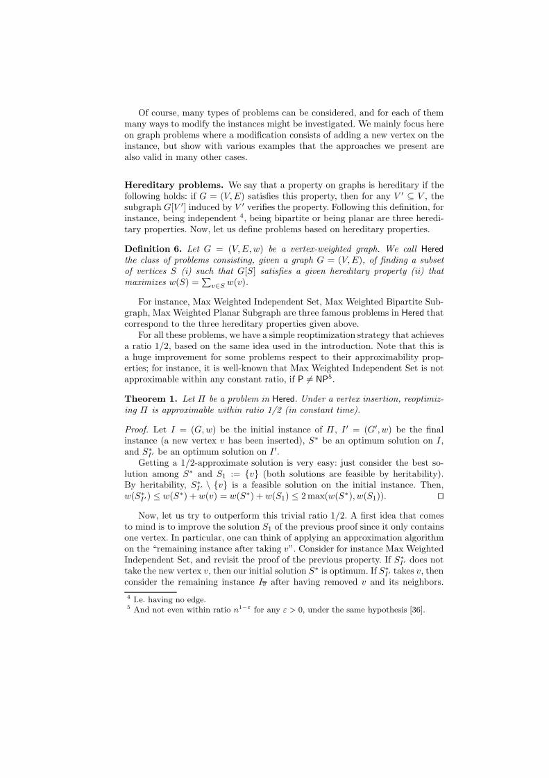
Of course, many types of problems can be considered, and for each of themmany ways to modify the instances might be investigated. We mainly focus hereon graph problems where a modification consists of adding a new vertex on theinstance, but show with various examples that the approaches we present arealso valid in many other cases.

Hereditary problems. We say that a property on graphs is hereditary if thefollowing holds: if G = (V, E) satisfies this property, then for any V ′ ⊆ V , thesubgraph G[V ′] induced by V ′ verifies the property. Following this definition, forinstance, being independent 4, being bipartite or being planar are three heredi-tary properties. Now, let us define problems based on hereditary properties.

Definition 6. Let G = (V, E, w) be a vertex-weighted graph. We call Hered

the class of problems consisting, given a graph G = (V, E), of finding a subsetof vertices S (i) such that G[S] satisfies a given hereditary property (ii) thatmaximizes w(S) =

∑v∈S w(v).

For instance, Max Weighted Independent Set, Max Weighted Bipartite Sub-graph, Max Weighted Planar Subgraph are three famous problems in Hered thatcorrespond to the three hereditary properties given above.

For all these problems, we have a simple reoptimization strategy that achievesa ratio 1/2, based on the same idea used in the introduction. Note that this isa huge improvement for some problems respect to their approximability prop-erties; for instance, it is well-known that Max Weighted Independent Set is notapproximable within any constant ratio, if P 6= NP5.

Theorem 1. Let Π be a problem in Hered. Under a vertex insertion, reoptimiz-ing Π is approximable within ratio 1/2 (in constant time).

Proof. Let I = (G, w) be the initial instance of Π , I ′ = (G′, w) be the finalinstance (a new vertex v has been inserted), S∗ be an optimum solution on I,and S∗

I′ be an optimum solution on I ′.Getting a 1/2-approximate solution is very easy: just consider the best so-

lution among S∗ and S1 := {v} (both solutions are feasible by heritability).By heritability, S∗

I′ \ {v} is a feasible solution on the initial instance. Then,w(S∗

I′) ≤ w(S∗) + w(v) = w(S∗) + w(S1) ≤ 2 max(w(S∗), w(S1)). ⊓⊔

Now, let us try to outperform this trivial ratio 1/2. A first idea that comesto mind is to improve the solution S1 of the previous proof since it only containsone vertex. In particular, one can think of applying an approximation algorithmon the “remaining instance after taking v”. Consider for instance Max WeightedIndependent Set, and revisit the proof of the previous property. If S∗

I′ does nottake the new vertex v, then our initial solution S∗ is optimum. If S∗

I′ takes v, thenconsider the remaining instance Iv after having removed v and its neighbors.

4 I.e. having no edge.5 And not even within ratio n1−ε for any ε > 0, under the same hypothesis [36].

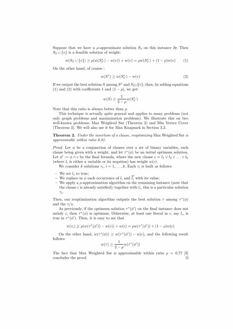
Suppose that we have a ρ-approximate solution S2 on this instance Iv. ThenS2 ∪ {v} is a feasible solution of weight:

w(S2 ∪ {v}) ≥ ρ(w(S∗I′) − w(v)) + w(v) = ρw(S∗

I′) + (1 − ρ)w(v) (1)

On the other hand, of course :

w(S∗) ≥ w(S∗I′) − w(v) (2)

If we output the best solution S among S∗ and S2∪{v}, then, by adding equations(1) and (2) with coefficients 1 and (1 − ρ), we get:

w(S) ≥1

2 − ρw(S∗

I′ )

Note that this ratio is always better than ρ.This technique is actually quite general and applies to many problems (not

only graph problems and maximization problems). We illustrate this on twowell-known problems: Max Weighted Sat (Theorem 2) and Min Vertex Cover(Theorem 3). We will also use it for Max Knapsack in Section 3.2.

Theorem 2. Under the insertion of a clause, reoptimizing Max Weighted Sat isapproximable within ratio 0.81.

Proof. Let φ be a conjunction of clauses over a set of binary variables, eachclause being given with a weight, and let τ∗(φ) be an initial optimum solution.Let φ′ := φ ∧ c be the final formula, where the new clause c = l1 ∨ l2 ∨ . . . ∨ lk(where li is either a variable or its negation) has weight w(c).

We consider k solutions τi, i = 1, . . . , k. Each τi is built as follows:

– We set li to true;– We replace in φ each occurrence of li and li with its value;– We apply a ρ-approximation algorithm on the remaining instance (note that

the clause c is already satisfied); together with li, this is a particular solutionτi.

Then, our reoptimization algorithm outputs the best solution τ among τ∗(φ)and the τi’s.

As previously, if the optimum solution τ∗(φ′) on the final instance does notsatisfy c, then τ∗(φ) is optimum. Otherwise, at least one literal in c, say li, istrue in τ∗(φ′). Then, it is easy to see that

w(τi) ≥ ρ(w(τ∗(φ′)) − w(c)) + w(c) = ρw(τ∗(φ′)) + (1 − ρ)w(c)

On the other hand, w(τ∗(φ)) ≥ w(τ∗(φ′)) − w(c), and the following resultfollows:

w(τ) ≥1

2 − ρw(τ∗(φ′))

The fact that Max Weighted Sat is approximable within ratio ρ = 0.77 [3]concludes the proof. ⊓⊔

It is worth noticing that the same ratio (1/(2 − ρ)) is achievable for othersatisfiability or constraint satisfaction problems. For instance, using the resultof Johnson [24], reoptimizing Max Weighted E3SAT6 when a new clause is in-serted is approximable within ratio 8/9.

Let us now focus on a minimization problem, namely Min Vertex Cover.Given a vertex-weighted graph G = (V, E, w), the goal in this problem is to finda subset V ′ ⊆ V such that (i) every edge e ∈ E is incident to at least one vertexin V ′, and (ii) the global weight of V ′

∑v∈V ′ w(v) is minimized.

Theorem 3. Under a vertex insertion, reoptimizing Min Vertex Cover is ap-proximable within ratio 3/2.

Proof. Let v denote the new vertex and S∗ the initial given solution. Then,S∗ ∪ {v} is a vertex cover on the final instance. If S∗

I′ takes v, then S∗ ∪ {v} isoptimum.

From now on, suppose that S∗I′ does not take v. Then, it has to take all

its neighbors N(v). S∗ ∪ N(v) is a feasible solution on the final instance. Sincew(S∗) ≤ w(S∗

I′), we get:

w(S∗ ∪ N(v)) ≤ w(S∗I′) + w(N(v)) (3)

Then, as for Max Weighted Independent Set, consider the following feasiblesolution S1:

– Take all the neighbors N(v) of v in S1;– Remove v and its neighbors from the graph;– Apply a ρ-approximation algorithm on the remaining graph, and add these

vertices to S1.

Since we are in the case where S∗I′ does not take v, it has to take all its neighbors,

and finally:

w(S1) ≤ ρ(w(S∗I′ ) − w(N(v))) + w(N(v)) = ρw(S∗

I′) − (ρ − 1)w(N(v)) (4)

Of course, we take the best solution S among S∗∪N(v) and S1. Then, a convexcombination of equations (3) and (4) leads to:

w(S) ≤2ρ − 1

ρw(S∗

I′ )

The results follows since Min Vertex Cover is well-known to be approximablewithin ratio 2. ⊓⊔

To conclude this section, we point out that these results can be generalizedwhen several vertices are inserted. Indeed, if a constant number k > 1 of verticesare added, one can reach the same ratio with similar arguments by consideringall the 2k possible subsets of new vertices in order to find the ones that willbelong to the new optimum solution. This brute force algorithm is still very fastfor small constant k, which is the case in the reoptimization setting with slightmodifications of the instance.6 Restriction of Max Weighted Sat when all clauses contain exactly three literals.

Unweighted problems. In the previous subsection, we considered the generalcases where vertices (or clauses) have a weight. It is well-known that all theproblems we focused on are already NP-hard in the unweighted case, i.e. whenall vertices/clauses receive weight 1. In this (very common) case, the previousapproximation results on reoptimization can be easily improved. Indeed, sinceonly one vertex is inserted, the initial optimum solution has an absolute error ofat most one on the final instance, i.e.:

|S∗| ≥ |S∗I′ | − 1

Then, in some sense we don’t really need to reoptimize since S∗ is alreadya very good solution on the final instance (note also that since the reoptimiza-tion problem is NP-hard, we cannot get rid of the constant −1). Dealing withapproximation ratio, we derive from this remark, with a standard technique, thefollowing result.

Theorem 4. Under a vertex insertion, reoptimizing any unweighted problem inHered admits a PTAS.

Proof. Let ε > 0, and set k = ⌈1/ε⌉. We consider the following algorithm:

1. Test all the subsets of V of size at most k, and set S1 be the largest one suchthat G[S1] satisfies the hereditary property,

2. Output the largest solution S between S1 and S∗.

Then, if S∗I′ has size at most 1/ε, we found it in step 1. Otherwise, |S∗

I′ | ≥ 1/εand:

|S∗|

|S∗I′ |

≥|S∗

I′ | − 1

|S∗I′ |

≥ 1 − ε

Of course, the algorithm is polynomial as long as ε is a constant. ⊓⊔

In other words, the PTAS is derived from two properties: the absolute errorof 1, and the fact that problems considered are simple. Following [29], a problemis called simple if, given any fixed constant k, it is polynomial to determinewhether the optimum solution has value at most k (maximization) or not.

This result easily extends to other simple problems, such as Min VertexCover for instance. It also generalizes when several (a constant number of) ver-tices are inserted, instead of only 1.

However, it is interesting to notice that, for some of other (unweighted) prob-lems, while the absolute error 1 still holds, we cannot derive a PTAS as in The-orem 4 because they are not simple. One of the most famous such problemsis the Min Coloring problem. In this problem, given a graph G = (V, E), onewishes to partition V into a minimum number of independent sets (called col-ors) V1, . . . , Vk. When a new vertex is inserted, an absolute error 1 can be easilyachieved while reoptimizing. Indeed, consider the initial coloring, and add a newcolor which contains only the newly inserted vertex. Then this coloring has an

absolute error of one since a coloring on the final graph cannot use less colorsthan an optimum coloring on the initial instance.

However, deciding whether a graph can be colored with 3 colors is anNP-hard problem. In other words, Min Coloring is not simple. We will discussthe consequence of this fact in the section on hardness of reoptimization.

To conclude this section, we stress the fact that there exist obviously manyproblems that do not involve weights and for which the initial optimum solutioncannot be directly transformed into a solution on the final instance with absoluteerror 1. Finding the longest cycle in a graph is such a problem: adding a newvertex may change considerably the size of an optimum solution.

Hardness of reoptimization. As mentioned earlier, the fact that we are inter-ested in slight modifications of an instance on which we have an optimum solutionmakes the problem somehow simpler, but unfortunately does not generally allowa jump in complexity. In other words, reoptimizing is generally NP-hard whenthe underlying problem is NP-hard.

In some cases, the proof of NP-hardness is immediate. For instance, considera graph problem where modifications consists of inserting a new vertex. Supposethat we had an optimum reoptimization algorithm for this problem. Then, start-ing from the empty graph, and adding the vertices one by one, we could find anoptimum solution on any graph on n vertices by using iteratively n times thereoptimization algorithm. Hence, the underlying problem would be polynomial.In conclusion, the reoptimization version is also NP-hard when the underlyingproblem is NP-hard. This argument is also valid for other problems under otherkinds of modifications. Actually, it is valid as soon as for any instance I, thereis a trivially solvable instance I ′ (the empty graph in our example) such that apolynomial number of modifications transform I ′ into I.

In other cases, the hardness does not directly follow from this argument, anda usual polynomial time reduction has to be provided. This situation occurs forinstance in graph problems where the modification consists of deleting a vertex.As we will see later, such hardness proofs have been given for instance for somevehicle routing problems.

Let us now focus on the hardness of approximation in the reoptimizationsetting. As we have seen in particular in Theorem 4, the knowledge of the initialoptimum solution may considerably help in finding an approximate solution onthe final instance. In other words, it seems quite hard to prove a lower boundon reoptimization. And in fact, few results have been obtained so far.

One method is to transform the reduction used in the proof of NP-hardness toget an inapproximability bound. Though more difficult than in the usual setting,such proofs have been provided for reoptimization problems, in particular forVRP problems, mainly by introducing very large distances (see Section 4).

Let us now go back to Min Coloring. As we have said, it is NP-hard todetermine whether a graph is colorable with 3 colors or not. In the usual setting,

this leads to an inapproximability bound of 4/3 − ε for any ε > 0. Indeed, anapproximation algorithm within ratio ρ = 4/3 − ε would allow to distinguishbetween 3-colorable graphs and graphs for which we need at least 4 colors. Now,we show that this result remains true for the reoptimization of the problem.

Theorem 5. Under a vertex insertion, reoptimizing Min Coloring cannot beapproximated within a ratio 4/3 − ε, for any ε > 0.

Proof. The proof is actually quite straightforward. Assume you have such areoptimization algorithm A within a ratio ρ = 4/3 − ε. Let G = (V, E) bea graph with V = {v1, · · · , vn}. We consider the subgraphs Gi of G inducedby Vi = {v1, v2, · · · , vi} (in particular Gn = G). Suppose that you have a 3-coloring of Gi, and insert vi+1. If Gi+1 is 3-colorable, then A outputs a 3-coloring.Moreover, if Gi is not 3-colorable, then neither is Gi+1. Hence, starting from theempty graph, and iteratively applying A, we get a 3-coloring of Gi if and only ifGi is 3-colorable. Eventually, we are able to determine whether G is 3-colorableor not. ⊓⊔

This proof is based on the fact that Min Coloring is not simple (according tothe definition previously given). A similar argument, leading to inapproximabil-ity results in reoptimization, can be applied to other non simple problems (underother modifications). It has been in particular applied to a scheduling problem(see Section 3.2).

For other optimization problems however, such as MinTSP in the metriccase, finding a lower bound in approximability (if any!) seems a challenging task.

Let us finally mention another kind of negative results. In the reoptimiza-tion setting, we look somehow for a possible stability when slight modificationsoccur on the instance. We try to measure how much the knowledge of a so-lution on the initial instance helps to solve the final one. Hence, it is naturalto wonder whether one can find a good solution in the “neighborhood” of theinitial optimum solution, or if one has to change almost everything. Do neighbor-ing instances have neighboring optimum/good solutions? As an answer to thesequestions, several results show that, for several problems, approximation algo-rithms that only “slightly” modify the initial optimum solution cannot lead togood approximation ratios. For instance, for reoptimizing MinTSP in the metriccase, if you want a ratio better than 3/2 (guaranteed by a simple heuristic), thenyou have to change (on some instances) a significant part of your initial solu-tion [5]. This kind of results, weaker than an inapproximability bound, providesinformation on the stability under modifications and lower bounds on classes ofalgorithms.

3.2 Results on some particular problems

In the previous section, we gave some general considerations on the reoptimiza-tion of NP-hard optimization problems. The results that have been presented

follow, using simple methods, from the structural properties of the problemdealt with and/or from known approximation results. We now focus on par-ticular problems for which specific methods have been devised, and briefly men-tion, without proofs, the main results obtained so far. We concentrate on theMin Steiner Tree problem, on a scheduling problem, and on the Max Knap-sack problem. Vehicle routing problems, which concentrated a large attention inreoptimization, deserve in our opinion a full section (Section 4), in which we alsoprovide some of the most interesting proofs in the literature together with a fewnew results.

Min Steiner Tree. The Min Steiner Tree problem is a generalization of the MinSpanning Tree problem where only a subset of vertices (called terminal vertices)have to be spanned. Formally, we are given a graph G = (V, E), a nonnegativedistance d(e) for any e ∈ E, and a subset R ⊆ V of terminal vertices. The goalis to connect the terminal vertices with a minimum global distance, i.e. to finda tree T ⊆ E that spans all vertices in R and minimizes d(T ) =

∑e∈T d(e). It

is generally assumed that the graph is complete, and the distance function ismetric (i.e. d(x, y)+d(y, z) ≥ d(x, z) for any vertices x, y, z): indeed, the generalproblem reduces to this case by initially computing shortest paths between pairsof vertices.

Min Steiner Tree is one of the most famous network design optimizationproblems. It is NP-hard, and has been studied intensively from an approximationviewpoint (see [18] for a survey on these results). The best known ratio obtainedso far is 1 + ln(3)/2 ≃ 1.55 [30].

Reoptimization versions of this problem have been studied with modificationson the vertex set [9, 13]. In Escoffier et al. [13], the modification consists of theinsertion of a new vertex. The authors study the cases where the new vertex isterminal or non terminal.

Theorem 6 ([13]). When a new vertex is inserted (either terminal or not),then reoptimizing the Min Steiner Tree problem can be approximated within ratio3/2.

Moreover, the result has been generalized to the case in which severalvertices are inserted. Interestingly, when p non terminal vertices are inserted,then reoptimizing the problem is still 3/2-approximable (but the running timegrows very fast with p). On the other hand, when q terminal vertices are added,the obtained ratio decreases (but the running time remains very low)7. Thestrategies consist, roughly speaking, of merging the initial optimum solutionwith Steiner trees computed on the set of new vertices and/or terminal vertices.The authors tackle also the case where a vertex is removed from the vertex set,and provide a lower bound for a particular class of algorithms.

7 The exact ratio is 2 − 1/(q + 2) when p non terminal and q terminal vertices areadded.

Bockenhauer et al. [9] consider a different instance modification. Rather thaninserting/deleting a vertex, the authors consider the case where the status of avertex changes: either a terminal vertex becomes non terminal, or vice versa.The obtained ratio is also 3/2.

Theorem 7 ([9]). When the status (terminal / non terminal) of a vertexchanges, then reoptimizing the Min Steiner Tree problem can be approximatedwithin ratio 3/2.

Moreover, they exhibit a case where this ratio can be improved. When allthe distances between vertices are in {1, 2, · · · , r}, for a fixed constant r, thenreoptimizing Min Steiner Tree (when changing the status of one vertex) is stillNP-hard but admits a PTAS.

Note that in both cases (changing the status of a vertex or adding a new ver-tex), no inapproximability results have been achieved, and this is an interestingopen question.

Scheduling. Due to practical motivations, it is not surprising that schedulingproblems received attention dealing with the reconstruction of a solution (oftencalled rescheduling) after an instance modification, such as a machine breakdown,an increase of a job processing time, etc. Several works have been proposed toprovide a sensitivity analysis of these problems under such modifications. Atypical question is to determine under which modifications and/or conditionsthe initial schedule remains optimal. We refer the reader to the comprehensivearticle [20] where the main results achieved in this field are presented.

Dealing with the reoptimization setting we develop in this article, Schaffter[33] proposes interesting results on a problem of scheduling with forbidden sets.In this problem, we have a set of jobs V = {v1, · · · , vn}, each job having aprocessing time. The jobs can be scheduled in parallel (the number of machinesis unbounded), but there is a set of constraints on these parallel schedules: aconstraint is a set F ⊆ V of jobs that cannot be scheduled in parallel (all ofthem at the same time). Then, given a set F = {F1, · · · , Fk} of constraints, thegoal is to find a schedule that respects each constraint and that minimizes thelatest completion time (makespan). Many situations can be modeled this way,such as the m-Machine Problem (for fixed m), hence the problem is NP-complete(and even hard to approximate).

Schaffter considers reoptimization when either a new constraint F is addedto F , or a constraint Fi ∈ F disappears. Using reductions from the Set Splittingproblem and from the Min Coloring problem, he achieves the following inap-proximability results.

Theorem 8 ([33]). If P 6= NP, for any ε > 0, reoptimizing the Scheduling withforbidden sets problem is inapproximable within ratio 3/2− ε under a constraintinsertion, and inapproximable within ratio 4/3 − ε under a constraint deletion.

Under a constraint insertion Schaffter also provides a reoptimization strat-egy that achieves approximation ratio 3/2, thus matching the lower bound ofTheorem 8. It consists of a simple local modification of the initial scheduling,by shifting one task (at the end of the schedule) in order to ensure that the newconstraint is satisfied.

Max Knapsack. In the Max Knapsack problem, we are given a set of n objectsO = {o1, . . . , on}, and a capacity B. Each objects has a weight wi and a valuevi. The goal is to choose a subset O′ of objects that maximizes the global value∑

oi∈O′ vi but that respects the capacity constraint∑

oi∈O′ wi ≤ B.

This problem is (weakly) NP-hard, but admits an FPTAS [23]. Obviously,the reoptimization version admits an FPTAS too. Thus, Archetti et al. [2] areinterested in using classical approximation algorithms for Max Knapsack to de-rive reoptimization algorithms with better approximation ratios but with thesame running time. The modifications considered consists of the insertion of anew object in the instance.

Though not being a graph problem, it is easy to see that the Max Knap-sack problem satisfies the required properties of heritability given in Section 3.1(paragraph on hereditary problems). Hence, the reoptimization version is 1/2-approximable in constant time; moreover, if we have a ρ-approximation algo-rithm, then the reoptimization strategy presented in section 3.1 has ratio 1

2−ρ

[2]. Besides, Archetti et al. [2] show that this bound is tight for several classicalapproximation algorithms for Max Knapsack.

Finally, studying the issue of sensitivity presented earlier, they show that anyreoptimization algorithm that does not consider objects discarded by the initialoptimum solution cannot have ratio better than 1/2.

4 Reoptimization of Vehicle Routing Problems

In this section we survey several results concerning the reoptimization of vehiclerouting problems under different kinds of perturbations. In particular, we focuson several variants of the Traveling Salesman Problem (TSP), which we definebelow.

The TSP is a well-known combinatorial optimization problem that has beenthe subject of extensive studies – here we only refer the interested reader tothe monographs by Lawler et al. [26] and Gutin and Punnen [19]. The TSPhas been used since the inception of combinatorial optimization as a testbed forexperimenting a whole array of algorithmic paradigms and techniques, so it isjust natural to also consider it from the point of view of reoptimization.

Definition 7. An instance In of the Traveling Salesman Problem is given bythe distance between every pair of n nodes in the form of an n × n matrix d,where d(i, j) ∈ Z+ for all 1 ≤ i, j ≤ n. A feasible solution for In is a tour, thatis, one directed cycle spanning the node set N := {1, 2, . . . , n}.

Notice that we did not define an objective function yet; so far we only spec-ified the structure of instances and feasible solutions. There are several pos-sibilities for the objective function and each of them gives rise to a differentoptimization problem. We need a few definitions. The weight of a tour T is thequantity w(T ) :=

∑(i,j)∈T d(i, j). The latency of a node i ∈ N with respect to a

given tour T is the total distance along the cycle T from node 1 to node i. Thelatency of T , denoted by ℓ(T ), is the sum of the latencies of the nodes of T .

The matrix d obeys the triangle inequality if for all i, j, k ∈ N we haved(i, j) ≤ d(i, k) + d(k, j). The matrix d is said to be a metric if it obeys thetriangle inequality and d(i, j) = d(j, i) for all i, j ∈ N .

In the rest of the section we will consider the following problems:

1. Minimum Traveling Salesman Problem (Min TSP): find a tour of minimumweight;

2. Minimum Metric TSP (Min MTSP): restriction of Min TSP to the case whend is a metric;

3. Minimum Asymmetric TSP (Min ATSP): restriction of Min TSP to the casewhen d obeys the triangle inequality;

4. Maximum TSP (Max TSP): find a tour of maximum weight;

5. Maximum Metric TSP (Max MTSP): restriction of Max TSP to the casewhen d is a metric;

6. Minimum Latency Problem (MLP): find a tour of minimum latency; d isassumed to be a metric.

TSP-like problems other than those above have also been considered in theliterature from the point of view of reoptimization; in particular, see Bockenhaueret al. [8] for a hardness result on the TSP with deadlines.

Given a vehicle routing problem Π from the above list, we will considerthe following reoptimization variants, each corresponding to a different type ofperturbation of the instance: insertion of a node (Π+), deletion of a node (Π−),and variation of a single entry of the matrix d (Π±).

Definition 8. An instance of Π+ is given by a pair (In+1, T∗n), where In+1 is

an instance of Π of size n + 1, and T ∗n is an optimum solution of Π on In, the

subinstance of In+1 induced by the nodes {1, . . . , n}. A solution for this instanceof Π+ is a solution to In+1. The objective function is the same as in Π.

Definition 9. An instance of Π− is given by a pair (In+1, T∗n+1), where In+1 is

an instance of Π of size n + 1, and T ∗n+1 is an optimum solution of Π on In+1.

A solution for this instance of Π− is a solution to In, the subinstance of In+1

induced by the nodes {1, . . . , n}. The objective function is the same as in Π.

Definition 10. An instance of Π± is given by a triple (In, I ′n, T ∗n), where In, I ′n

are instances of Π of size n, T ∗n is an optimum solution of Π on In, and I ′n differs

from In only in one entry of the distance matrix d. A solution for this instanceof Π± is a solution to I ′n. The objective function is the same as in Π.

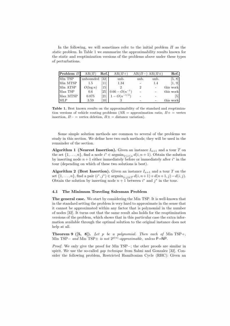
In the following, we will sometimes refer to the initial problem Π as thestatic problem. In Table 1 we summarize the approximability results known forthe static and reoptimization versions of the problems above under these typesof perturbations.

Problem Π AR(Π) Ref. AR(Π+) AR(Π−) AR(Π±) Ref.

Min TSP unbounded [32] unb. unb. unb. [5, 8]Min MTSP 1.5 [11] 1.34 - 1.4 [1, 9]Min ATSP O(log n) [15] 2 2 - this workMax TSP 0.6 [25] 0.66 − O(n−1) - - this work

Max MTSP 0.875 [21] 1 − O(n−1/2) - - [5]MLP 3.59 [10] 3 - - this work

Table 1. Best known results on the approximability of the standard and reoptimiza-tion versions of vehicle routing problems (AR = approximation ratio, Π+ = vertexinsertion, Π− = vertex deletion, Π± = distance variation).

Some simple solution methods are common to several of the problems westudy in this section. We define here two such methods; they will be used in theremainder of the section.

Algorithm 1 (Nearest Insertion). Given an instance In+1 and a tour T onthe set {1, . . . , n}, find a node i∗ ∈ argmin1≤i≤n d(i, n + 1). Obtain the solutionby inserting node n + 1 either immediately before or immediately after i∗ in thetour (depending on which of these two solutions is best).

Algorithm 2 (Best Insertion). Given an instance In+1 and a tour T on theset {1, . . . , n}, find a pair (i∗, j∗) ∈ argmin(i,j)∈T d(i, n+1)+d(n+1, j)−d(i, j).Obtain the solution by inserting node n + 1 between i∗ and j∗ in the tour.

4.1 The Minimum Traveling Salesman Problem

The general case. We start by considering the Min TSP. It is well-known thatin the standard setting the problem is very hard to approximate in the sense thatit cannot be approximated within any factor that is polynomial in the numberof nodes [32]. It turns out that the same result also holds for the reoptimizationversions of the problem, which shows that in this particular case the extra infor-mation available through the optimal solution to the original instance does nothelp at all.

Theorem 9 ([5, 8]). Let p be a polynomial. Then each of Min TSP+,Min TSP− and Min TSP± is not 2p(n)-approximable, unless P=NP.

Proof. We only give the proof for Min TSP−; the other proofs are similar inspirit. We use the so-called gap technique from Sahni and Gonzalez [32]. Con-sider the following problem, Restricted Hamiltonian Cycle (RHC): Given an

undirected graph G = (V, E) and a Hamiltonian path P between two nodesa and b in G, determine whether there exists a Hamiltonian cycle in G. Thisproblem is known to be NP-complete [27]. We prove the claim of the theorem byshowing that any approximation algorithm for Min TSP− with ratio 2p(n) canbe used to solve RHC in polynomial time.

Consider an instance of RHC, that is, a graph G = (V, E) on n nodes, twonodes a, b ∈ V and a Hamiltonian path P from a to b. Without loss of generalitywe can assume that V = {1, . . . , n}. We can construct in polynomial time thefollowing TSP instance In+1 on node set {1, . . . , n, n + 1}:

- d(i, j) = 1 if (i, j) ∈ E;- d(n + 1, a) = d(b, n + 1) = 1;- all other entries of the matrix d have value 2p(n) · n + 1.

Since all entries are at least 1, the tour T ∗n+1 := P ∪ {(b, n + 1), (n + 1, a)} is

an optimum solution of In+1, with weight w(T ∗n+1) = n + 1. Thus, (In+1, T

∗n+1)

is an instance of Min TSP−. Let T ∗n be an optimum solution of instance In.

Then w(T ∗n ) = n if and only if G has a Hamiltonian cycle. Finally, a 2p(n)-

approximation algorithm for Min TSP− allows to decide whether w(T ∗n) = n.

⊓⊔

Minimum Metric TSP. In the previous section we have seen that no constant-factor approximation algorithm exists for reoptimizing the Minimum TSP in itsfull generality. To obtain such a result, we are forced to restrict the problemsomehow. A very interesting case for many applications is when the matrix dis a metric, that is, the Min MTSP. This problem admits a 3/2-approximationalgorithm, due to Christofides [11], and it is currently open whether this fac-tor can be improved. Interestingly, it turns out that the reoptimization versionMin MTSP+ is (at least if one consider the currently best known algorithms)easier than the static problem: it allows a 4/3-approximation – although, again,we do not know whether even this factor may be improved via a more sophisti-cated approach.

Theorem 10 ([5]). Min MTSP+ is approximable within ratio 4/3.

Proof. The algorithm used to prove the upper bound is a simple combination ofNearest Insertion and of the well-known algorithm by Christofides [11]; namely,both algorithms are executed and the solution returned is the one having thelower weight.

Consider an optimum solution T ∗n+1 of the final instance In+1, and the solu-

tion T ∗n available for the initial instance In. Let i and j be the two neighbors of

vertex n + 1 in T ∗n+1, and let T1 be the tour obtained from T ∗

n with the NearestInsertion rule. Furthermore, let v∗ be the vertex in {1, . . . , n} whose distance ton + 1 is the smallest.

Using the triangle inequality, we easily get w(T1) ≤ w(T ∗n+1) + 2d(v∗, n + 1)

where, by definition of v∗, d(v∗, n + 1) = min{d(k, n + 1) : k = 1, . . . , n}. Thus

w(T1) ≤ w(T ∗n+1) + 2 max(d(i, n + 1), d(j, n + 1)) (5)

Now consider the algorithm of Christofides applied on In+1. This gives atour T2 of length at most (1/2)w(T ∗

n+1) + MST(In+1), where MST(In+1) is theweight of a minimum spanning tree on In+1. Note that MST(In+1) ≤ w(T ∗

n+1)−max(d(i, n + 1), d(j, n + 1)). Hence

w(T2) ≤3

2w(T ∗

n+1) − max(d(i, n + 1), d(j, n + 1)). (6)

The result now follows by combining equations (5) and (6), becausethe weight of the solution given by the algorithm is min(w(T1), w(T2)) ≤(1/3)w(T1) + (2/3)w(T2) ≤ (4/3)w(T ∗

n+1). ⊓⊔

The above result can be generalized to the case when more than a single ver-tex is added in the perturbed instance. Let Min MTSP+k be the correspondingproblem when k vertices are added. Then it is possible to give the following re-sult, which gives a tradeoff between the number of added vertices and the qualityof the approximation guarantee.

Theorem 11 ([5]). For any k ≥ 1, Min MTSP+k is approximable within ratio3/2 − 1/(4k + 2).

Reoptimization under variation of a single entry of the distance matrix (thatis, problem Min MTSP±) has been considered by Bockenhauer et al. [9].

Theorem 12 ([9]). Min MTSP± is approximable within ratio 7/5.

Minimum Asymmetric TSP. The Minimum Asymmetric Traveling SalesmanProblem is another variant of the TSP that is of interest for applications, as itgeneralizes the Metric TSP. Unfortunately, in the static case there seems to bea qualitative difference with respect to the approximability of Minimum MetricTSP: while in the latter case a constant approximation is possible, for Min ATSPthe best known algorithms give an approximation ratio of Θ(log n). The firstsuch algorithm was described by Frieze et al. [17] and has an approximationguarantee of log2 n. The currently best algorithm is due to Feige and Singh [15]and gives approximation (2/3) log2 n. The existence of a constant approximationfor Min ATSP is an important open problem.

Turning now to reoptimization, there exists a non-negligible gap between theapproximability of the static version and of the reoptimization version. In fact,reoptimization drastically simplifies the picture: Min ATSP+ is approximablewithin ratio 2, as we proceed to show.

Theorem 13. Min ATSP+ is approximable within ratio 2.

Proof. The algorithm used to establish the upper bound is extremely simple: justadd the new vertex between an arbitrarily chosen pair of consecutive vertices inthe old optimal tour. Let T be the tour obtained by inserting node n+1 betweentwo consecutive nodes i and j in T ∗

n . We have:

w(T ) = w(T ∗n) + d(i, n + 1) + d(n + 1, j) − d(i, j).

By triangle inequality, d(n + 1, j) ≤ d(n + 1, i) + d(i, j). Hence

w(T ) ≤ w(T ∗n) + d(i, n + 1) + d(n + 1, i).

Again by triangle inequality, w(T ∗n) ≤ w(T ∗

n+1), and d(i, n + 1) + d(n + 1, i) ≤w(T ∗

n+1), which concludes the proof. ⊓⊔

We remark that the above upper bound of 2 on the approximation ratio istight, even if we use Best Insertion instead of inserting the new vertex betweenan arbitrarily chosen pair of consecutive vertices.

Theorem 14. Min ATSP− is approximable within ratio 2.

Proof. The obvious idea is to skip the deleted node in the new tour, while visitingthe remaining nodes in the same order. Thus, if i and j are respectively the nodespreceding and following n + 1 in the tour T ∗

n+1, we obtain a tour T such that

w(T ) = w(T ∗n+1) + d(i, j) − d(i, n + 1) − d(n + 1, j). (7)

Consider an optimum solution T ∗n of the modified instance In, and the node l

that is consecutive to i in this solution. Since inserting n + 1 between i and lwould yield a feasible solution to In+1, we get, using triangle inequality:

w(T ∗n+1) ≤ w(T ∗

n) + d(i, n + 1) + d(n + 1, l)− d(i, l)

≤ w(T ∗n) + d(i, n + 1) + d(n + 1, i).

By substituting in (7) and using triangle inequality again,

w(T ) ≤ w(T ∗n) + d(i, j) + d(j, i).

Hence, w(T ) ≤ 2w(T ∗n). ⊓⊔

4.2 The Maximum Traveling Salesman Problem

Maximum TSP. While the typical applications of the Minimum TSP are in ve-hicle routing and transportation problems, the Maximum TSP has applicationsto DNA sequencing and data compression [25]. Like the Minimum TSP, theMaximum TSP is also NP-hard, but differently from what happens for the Min-imum TSP, it is approximable within a constant factor even when the distancematrix can be completely arbitrary. In the static setting, the best known resultfor Max TSP is a 0.6-approximation algorithm due to Kosaraju et al. [25]. Onceagain, the knowledge of an optimum solution to the initial instance is useful,as the reoptimization problem under insertion of a vertex can be approximatedwithin a ratio of 0.66 (for large enough n), as we show next.

Theorem 15. Max TSP+ is approximable within ratio (2/3) · (1 − 1/n).

Proof. Let i and j be such that (i, n + 1) and (n + 1, j) belong to T ∗n+1. The

algorithm is the following:

1. Apply Best Insertion to T ∗n to get a tour T1.

2. Find a maximum cycle cover C = (C0, . . . , Cl) on In+1 such that:(a) (i, n + 1) and (n + 1, j) belong to C0;(b) |C0| ≥ 4.

3. Remove the minimum-weight arc of each cycle of C and patch the pathsobtained to get a tour T2.

4. Select the best solution between T1 and T2.

Note that Step 2 can be implemented in polynomial time as follows. Wereplace d(i, n + 1) and d(n + 1, j) by a large weight M , and d(j, i) by −M (wedo not know i and j, but we can try each possible pair of vertices and returnthe best tour constructed by the algorithm). Hence, this cycle cover will contain(i, n + 1) and (n + 1, j) but not (j, i), meaning that the cycle containing n + 1will have at least 4 vertices.

Let a := d(i, n + 1) + d(n + 1, j). Clearly, w(T ∗n+1) ≤ w(T ∗

n) + a. Now, byinserting n + 1 in each possible position, we get

w(T1) ≥ (1 − 1/n)w(T ∗n) ≥ (1 − 1/n)(w(T ∗

n+1) − a).

Since C0 has size at least 4, the minimum-weight arc of C0 has cost at most(w(C0) − a)/2. Since each cycle has size at least 2, we get a tour T2 of value:

w(T2) ≥ w(C) −w(C0) − a

2−

w(C) − w(C0)

2

=w(C) + a

2≥

w(T ∗n+1) + a

2

Combining the two bounds for T1 and T2, we get a solution which is (2/3) ·(1 − 1/n)-approximate. ⊓⊔

The above upper bound can be improved to 0.8 when the distance matrix isknown to be symmetric [5].

Maximum Metric TSP. The usual Maximum TSP problem does not admita polynomial-time approximation scheme, that is, there exists a constant c suchthat it is NP-hard to approximate the problem within a factor better than c.This result extends also to the Maximum Metric TSP [28]. The best knownapproximation for the Maximum Metric TSP is a randomized algorithm with anapproximation guarantee of 7/8 [21].

By contrast, in the reoptimization of Max MTSP under insertion of a ver-tex, the Best Insertion algorithm turns out to be a very good strategy: it isasymptotically optimum. In particular, the following holds.

Theorem 16 ([5]). Max MTSP+ is approximable within ratio 1 − O(n−1/2).

Using the above result one can easily prove that Max MTSP+ admits apolynomial-time approximation scheme: if the desired approximation guaranteeis 1 − ǫ, for some ǫ > 0, just solve by enumeration the instances with O(1/ǫ2)nodes, and use the result above for the other instances.

4.3 The Minimum Latency Problem

Although superficially similar to the Minimum Metric TSP, the Minimum La-tency Problem appears to be more difficult to solve. For example, in the specialcase when the metric is induced by a weighted tree, the MLP is NP-hard [34]while the Metric TSP is trivial. One of the difficulties in the MLP is that lo-cal changes in the input can influence the global shape of the optimum solution.Thus, it is interesting to notice that despite this fact, reoptimization still helps. Infact, the best known approximation so far for the static version of the MLP givesa factor of 3.59 and is achieved via a sophisticated algorithm due to Chaudhuriet al. [10], while it is possible to give a very simple 3-approximation for MLP+,as we show in the next theorem.

Theorem 17. MLP+ is approximable within ratio 3.

Proof. We consider the Insert Last algorithm that inserts the new node n + 1at the “end” of the tour, that is, just before node 1. Without loss of generality,let T ∗

n = {(1, 2), (2, 3), . . . , (n− 1, n)} be the optimal tour for the initial instanceIn (that is, the kth node to be visited is k). Let T ∗

n+1 be the optimal tour forthe modified instance In+1. Clearly ℓ(T ∗

n+1) ≥ ℓ(T ∗n) since relaxing the condition

that node n + 1 must be visited cannot raise the overall latency.The quantity ℓ(T ∗

n) can be expressed as∑n

i=1 ti, where for i = 1, . . . , n,

ti =∑i−1

j=1 d(j, j + 1) can be interpreted as the “time” at which node i is firstvisited in the tour T ∗

n .In the solution constructed by Insert Last, the time at which each node i 6=

n+1 is visited is the same as in the original tour (ti), while tn+1 = tn+d(n, n+1).

The latency of the solution is thus∑n+1

i=1 ti =∑n

i=1 ti + tn + d(n, n + 1) ≤2ℓ(T ∗

n) + ℓ(T ∗n+1) ≤ 3ℓ(T ∗

n+1), where we have used ℓ(T ∗n+1) ≥ d(n, n + 1) (any

feasible tour must include a subpath from n to n + 1 or vice versa). ⊓⊔

Bibliography

[1] C. Archetti, L. Bertazzi, and M. G. Speranza. Reoptimizing the travelingsalesman problem. Networks, 42(3):154–159, 2003.

[2] C. Archetti, L. Bertazzi, and M. G. Speranza. Reoptimizing the 0-1 knap-sack problem, 2008. Manuscript.

[3] T. Asano, K. Hori, T. Ono, and T. Hirata. A theoretical framework ofhybrid approaches to MAX SAT. In Proc. 8th Int. Symp. on Algorithmsand Computation, pages 153–162, 1997.

[4] G. Ausiello, P. Crescenzi, G. Gambosi, V. Kann, A. Marchetti-Spaccamela,and M. Protasi. Complexity and approximation – Combinatorial optimiza-tion problems and their approximability properties. Springer, Berlin, 1999.

[5] G. Ausiello, B. Escoffier, J. Monnot, and V. T. Paschos. Reoptimization ofminimum and maximum traveling salesman’s tours. In Proc. 10th Scandi-navian Workshop on Algorithm Theory, pages 196–207, 2006.

[6] M. Bartusch, R. Mohring, and F. J. Radermacher. Scheduling project net-works with resource constraints and time windows. Annals of OperationsResearch, 16:201–240, 1988.

[7] M. Bartusch, R. Mohring, and F. J. Radermacher. A conceptional outlineof a DSS for scheduling problems in the building industry. Decision SupportSystems, 5:321–344, 1989.

[8] H.-J. Bockenhauer, L. Forlizzi, J. Hromkovic, J. Kneis, J. Kupke, G. Proi-etti, and P. Widmayer. Reusing optimal tsp solutions for locally modifiedinput instances. In Proc. 4th IFIP Int. Conf. on Theoretical ComputerScience, pages 251–270, 2006.

[9] H.-J. Bockenhauer, J. Hromkovic, T. Momke, and P. Widmayer. On thehardness of reoptimization. In Proc. 34th Conf. on Current Trends in The-ory and Practice of Computer Science, pages 50–65, 2008.

[10] K. Chaudhuri, B. Godfrey, S. Rao, and K. Talwar. Paths, trees, and min-imum latency tours. In Proc. 44th Symp. on Foundations of ComputerScience, pages 36–45, 2003.

[11] N. Christofides. Worst-case analysis of a new heuristic for the travellingsalesman problem. Technical Report 388, Graduate School of IndustrialAdministration, Carnegie-Mellon University, Pittsburgh, PA, 1976.

[12] D. Eppstein, Z. Galil, G. F. Italiano, and A. Nissenzweig. Sparsification– atechnique for speeding up dynamic graph algorithms. Journal of the ACM,44(5):669–696, 1997.

[13] B. Escoffier, M. Milanic, and V. T. Paschos. Simple and fast reoptimiza-tions for the Steiner tree problem. Cahier du LAMSADE 245, LAMSADE,Universite Paris-Dauphine, 2007.

[14] S. Even and H. Gazit. Updating distances in dynamic graphs. MethodsOper. Res., 49:371–387, 1985.

[15] U. Feige and M. Singh. Improved approximation ratios for traveling sales-person tours and paths in directed graphs. In Proc. 10th Int. Workshop

on Approximation, Randomization and Combinatorial Optimization, pages104–118, 2007.

[16] G. N. Frederickson. Data structures for on-line updating of minimum span-ning trees, with applications. SIAM Journal on Computing, 14(4):781–798,1985.

[17] A. M. Frieze, G. Galbiati, and F. Maffioli. On the worst-case performance ofsome algorithms for the asymmetric traveling salesman problem. Networks,12(1):23–39, 1982.

[18] C. Gropl, S. Hougardy, T. Nierhoff, and H. Promel. Approximation algo-rithms for the Steiner tree problem in graphs. In D.-Z. Du and X. Cheng,editors, Steiner Trees in Industry, pages 235–279. Kluwer Academic Pub-lishers, 2000.

[19] G. Gutin and A. P. Punnen, editors. The Traveling Salesman Problem andits Variations. Kluwer, Dordrecht, The Nederlands, 2002.

[20] N. G. Hall and M. E. Posner. Sensitivity analysis for scheduling problems.J. Scheduling, 7(1):49–83, 2004.

[21] R. Hassin and S. Rubinstein. A 7/8-approximation algorithm for metricMax TSP. Information Processing Letters, 81(5):247–251, 2002.

[22] M. R. Henzinger and V. King. Maintaining minimum spanning forests indynamic graphs. SIAM Journal on Computing, 31(2):367–374, 2001.

[23] O. H. Ibarra and C. E. Kim. Fast approximation algorithms for the knapsackand sum of subset problems. Journal of the ACM, 22(4):463–468, 1975.

[24] D. S. Johnson. Approximation algorithms for combinatorial problems. Jour-nal of Computer and Systems Sciences, 9:256–278, 1974.

[25] S. R. Kosaraju, J. K. Park, and C. Stein. Long tours and short superstrings.In Proc. 35th Symp. on Foundations of Computer Science, pages 166–177,1994.

[26] E. L. Lawler, J. K. Lenstra, A. Rinnooy Kan, and D. B. Shmoys, editors.The Traveling Salesman Problem: A Guided Tour of Combinatorial Opti-mization. Wiley, Chichester, England, 1985.

[27] C. H. Papadimitriou and K. Steiglitz. On the complexity of local search forthe traveling salesman problem. SIAM Journal on Computing, 6(1):76–83,1977. doi: 10.1137/0206005.

[28] C. H. Papadimitriou and M. Yannakakis. The traveling salesman problemwith distances one and two. Mathematics of Operations Research, 18(1):1–11, 1993.

[29] A. Paz and S. Moran. Non deterministic polynomial optimization problemsand their approximations. Theoretical Computer Science, 15:251–277, 1981.

[30] G. Robins and A. Zelikovsky. Improved Steiner tree approximation ingraphs. In Proc. 11th Symp. on Discrete Algorithms, pages 770–779, 2000.

[31] H. Rohnert. A dynamization of the all-pairs least cost problem. In Proc. 2ndSymp. on Theoretical Aspects of Computer Science, pages 279–286, 1985.

[32] S. Sahni and T. F. Gonzalez. P-complete approximation problems. Journalof the ACM, 23(3):555–565, 1976.

[33] M. W. Schaffter. Scheduling with forbidden sets. Discrete Applied Mathe-matics, 72(1–2):155–166, 1997.

[34] R. Sitters. The minimum latency problem is NP-hard for weighted trees.In Proc. 9th Integer Programming and Combinatorial Optimization Conf.,pages 230–239, 2002.

[35] V. V. Vazirani. Approximation Algorithms. Springer, Berlin, 2001.[36] D. Zuckerman. Linear degree extractors and the inapproximability of max

clique and chromatic number. In Proc. 38th Symp. on Theory of Computing,pages 681–690, 2006.