Complexity Classification in Infinite-Domain Constraint ... - arXiv
267
Complexity Classification in Infinite-Domain Constraint Satisfaction M´ emoire pour l’obtention d’une habilitation ` a diriger des recherches Universit´ e Paris Diderot – Paris 7 Sp´ ecialit´ e Informatique pr´ esent´ e par Manuel Bodirsky soutenue publiquement le 19 janvier 2012, devant le jury compos´ e de : Arnaud DURAND Universit´ e Paris 7, IMJ, ´ Equipe Logique Math´ ematique Christoph D ¨ URR CNRS / LIP6, Universit´ e Paris 6 Markus JUNKER Mathematisches Institut, Albert-Ludwigs-Universit¨ at Freiburg Pascal KOIRAN ENS Lyon Luc SEGOUFIN INRIA / LSV, CNRS+ENS Cachan Les rapporteurs sont : V´ ıctor DALMAU Universit´ e Pompeu Fabra, Barcelone, Espagne Arnaud DURAND Universit´ e Paris 7, IMJ, ´ Equipe Logique Math´ ematique Peter JONSSON Universit´ e de Link¨ oping, Suede arXiv:1201.0856v10 [cs.CC] 20 Apr 2019
-
Upload
khangminh22 -
Category
Documents
-
view
0 -
download
0
Transcript of Complexity Classification in Infinite-Domain Constraint ... - arXiv

Complexity Classification in Infinite-DomainConstraint Satisfaction
Memoire pour l’obtention d’une habilitation a diriger des recherchesUniversite Paris Diderot – Paris 7
Specialite Informatique
presente parManuel Bodirsky
soutenue publiquement le 19 janvier 2012, devant le jury compose de :
Arnaud DURAND Universite Paris 7, IMJ, Equipe Logique Mathematique
Christoph DURR CNRS / LIP6, Universite Paris 6Markus JUNKER Mathematisches Institut, Albert-Ludwigs-Universitat FreiburgPascal KOIRAN ENS LyonLuc SEGOUFIN INRIA / LSV, CNRS+ENS Cachan
Les rapporteurs sont :
Vıctor DALMAU Universite Pompeu Fabra, Barcelone, Espagne
Arnaud DURAND Universite Paris 7, IMJ, Equipe Logique MathematiquePeter JONSSON Universite de Linkoping, Suede
arX
iv:1
201.
0856
v10
[cs
.CC
] 2
0 A
pr 2
019

2
Acknowledgements. I want to thank my institution, the CNRS, for the greatfreedom in research that allowed me to write this text. The research leading to theresults presented here has also received funding from the European Research Coun-cil under the European Community’s Seventh Framework Program (FP7/2007-2013Grant Agreement no. 257039). I also want to thank all of my constraint satisfactionco-authors for the good time we had with our joint work.
My first address at the Equipe de Logique Mathematique has always been ArnaudDurand, and I am indebted to him for his great help with many things over the years,including the process of the habilitation. Many thanks also to Micha l Wrona, FrancoisBossiere, Trung van Pham, Antoine Mottet, Johannes Greiner, Michael Kompatscher,Christian Pech, and Florian Starke for reporting mistakes in earlier versions of thistext.
Special thanks to Christoph Durr for the permission to include his wonderfulpictures at the beginning of many chapters. More of his artwork can be found under
http://picasaweb.google.com/xtof.durr/LaVieEstDurr.
The pictures for Chapters 6, 9, and 10 are drawings that I kept from discussions withJan Kara, Martin Kutz, and Jaroslav Nesetril. The picture for Chapter 4 is by LewinBodirsky, Summer 2010, and the picture for Chapter 7 is by Otto Bodirsky, Summer2011.

Contents
Chapter 1. Introduction 11.1. The Homomorphism Perspective 41.2. The Sentence Evaluation Perspective 71.3. The Satisfiability Perspective 111.4. The Existential Second-Order Perspective 171.5. Examples 221.6. Overview 301.7. Uncovered Topics 30
Chapter 2. Preliminaries in Logic 35
Chapter 3. Model Theory 453.1. ω-categorical Structures 463.2. Fraısse Amalgamation 503.3. Oligomorphic Permutation Groups 533.4. Preservation Theorems 593.5. Existential Positive Completion 653.6. Quantifier-elimination, Model-completeness, Cores 67
Chapter 4. Examples 794.1. Phylogeny Constraints and Homogeneous C-relations 794.2. Branching-Time Constraints 824.3. Set Constraints 824.4. Spatial Reasoning 844.5. CSPs and Fragments of SNP 84
Chapter 5. Universal Algebra 915.1. Oligomorphic Clones 925.2. The Inv-Pol Galois Connection 935.3. Essential Arity 955.4. Schaefer’s Theorem 1015.5. Pseudo-varieties and Primitive Positive Interpretations 1045.6. Varieties 114
Chapter 6. Equality Constraint Satisfaction Problems 1216.1. Independence of Disequality 1226.2. Two-transitive Templates 1246.3. Horn Formulas 1256.4. Classification 127
Chapter 7. Topology 1297.1. Topological Spaces 1297.2. Topological Groups 1317.3. Oligomorphic Groups 135
3
4 CONTENTS
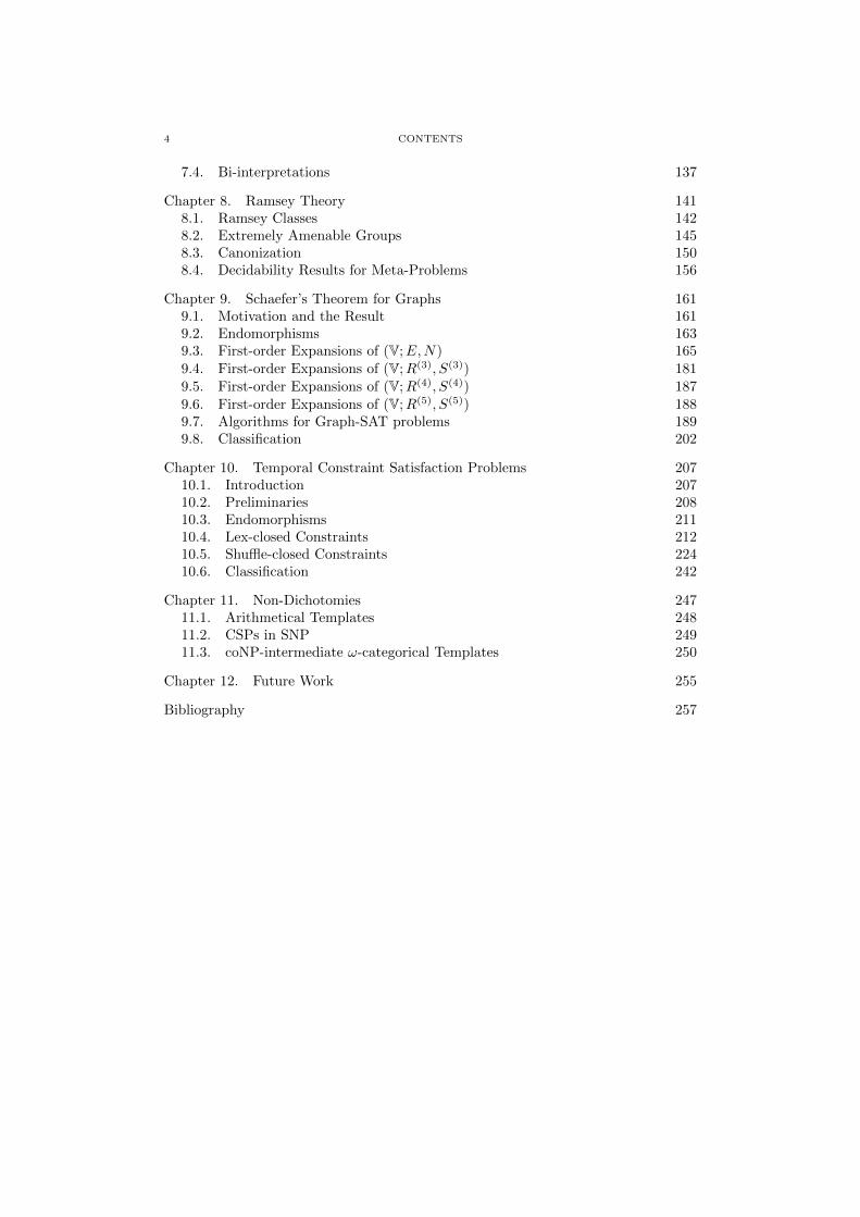
7.4. Bi-interpretations 137
Chapter 8. Ramsey Theory 1418.1. Ramsey Classes 1428.2. Extremely Amenable Groups 1458.3. Canonization 1508.4. Decidability Results for Meta-Problems 156
Chapter 9. Schaefer’s Theorem for Graphs 1619.1. Motivation and the Result 1619.2. Endomorphisms 1639.3. First-order Expansions of (V;E,N) 1659.4. First-order Expansions of (V;R(3), S(3)) 1819.5. First-order Expansions of (V;R(4), S(4)) 1879.6. First-order Expansions of (V;R(5), S(5)) 1889.7. Algorithms for Graph-SAT problems 1899.8. Classification 202
Chapter 10. Temporal Constraint Satisfaction Problems 20710.1. Introduction 20710.2. Preliminaries 20810.3. Endomorphisms 21110.4. Lex-closed Constraints 21210.5. Shuffle-closed Constraints 22410.6. Classification 242
Chapter 11. Non-Dichotomies 24711.1. Arithmetical Templates 24811.2. CSPs in SNP 24911.3. coNP-intermediate ω-categorical Templates 250
Chapter 12. Future Work 255
Bibliography 257

CHAPTER 1
Introduction
Constraint satisfaction problems (CSPs) appear in almost every area of theo-retical computer science, for instance in artificial intelligence, scheduling, compu-tational linguistics, computational biology, verification, and algebraic computation.Many computational problems studied in those areas can be modeled by appropriatelychoosing a set of constraint types, the constraint language, that are allowed in theinput instance of a CSP. In the last decade, huge progress was made to find generalcriteria for constraint languages that imply that the corresponding CSP can be solvedefficiently [12,61,63,64,66,95,123].
Lately, the complexity of the CSP became a topic that vitalizes the field of uni-versal algebra, since it turned out that questions about the computational complexityof CSPs translate to important universal-algebraic questions about algebras that canbe associated to CSPs. This approach is now known as the algebraic approach toconstraint satisfaction complexity. The algebraic approach has raised questions thatare of central importance in universal algebra.
Another reason why the complexity of CSPs attracts attention is an exciting con-jecture due to Feder and Vardi [95], which is still unresolved, and which is knownas the dichotomy conjecture. This conjecture says that every CSP with a finite do-main is either polynomial-time tractable (i.e., in P) or NP-complete. According toa well-known result by Ladner, it is known that there are NP-intermediate compu-tational problems, i.e., problems in NP that are neither tractable nor NP-complete(unless P=NP). But the known NP-intermediate problems are extremely artificial. Itwould be interesting from a complexity theoretic perspective to discover more naturalcandidates for NP-intermediate problems. Unlike many questions in computational

2 1. INTRODUCTION
complexity that are wide open, the dichotomy conjecture allows many promising par-tial results and different approaches (see the collection of survey articles in [80]), andtherefore is an attractive research topic.
Any outcome of the dichotomy conjecture is significant: a negative answer mightprovide relatively natural NP-intermediate problems, which would be interesting forcomplexity theorists. A positive answer probably comes with a criterion which de-scribes the NP-hard CSPs (and it would probably even provide algorithms for thepolynomial-time tractable CSPs). But then we would have a fascinatingly rich cata-logue of computational problems where the computational complexity is known. Sucha catalogue would be a valuable tool for deciding the complexity of computationalproblems: since CSPs are abundant, one might derive algorithmic results by reducingthe problem of interest to a known tractable CSP, and one might derive hardnessresults by reducing a known NP-hard CSP to the problem of interest.
Even though very powerful partial results on the dichotomy conjecture have beenobtained in recent years, the impact of constraint satisfaction complexity theory onother fields in theoretical computer science has so far been modest. A reason mightbe that the range of problems in the literature that can be described by specifying aconstraint language over a finite domain, and that have been studied independentlyfrom the CSP framework, is quite limited, and mostly focussed on specialized graphtheoretic problems or Boolean satisfiability problems.
If we consider the class of all problems that can be formulated by specifying aconstraint language over an infinite domain, the situation changes drastically. Manyproblems that have been studied independently in temporal reasoning, spatial reason-ing, phylogenetic reconstruction, and computational linguistics can be directly formu-lated as CSPs. Also feasibility problems in linear (and also non-linear) programming(over the rationals, the integers, or other domains) can be cast as CSPs.
The goal of this thesis is to generalize the universal-algebraic approach to infinitedomains. It turns out that this is possible when the constraint language, viewed as arelational structure B with an infinite domain, is ω-categorical. Many of the CSPs inthe mentioned application areas can be formulated with ω-categorical constraint lan-guages — in particular, problems coming from so-called qualitative calculi in artificialintelligence tend to have formulations with ω-categorical constraint languages. Whileω-categoricity is a quite strong assumption from a model-theoretic point of view (and,for example, constraint languages for linear programming cannot be ω-categorical),the class of computational problems that can be formulated with ω-categorical con-straint languages is still a very large generalization of the class of CSPs that canbe formulated with a constraint language over a finite domain. This will be amplydemonstrated by examples of ω-categorical constraint languages from many differentareas in computer science in Chapter 4.
There are several general results for ω-categorical structures that are relevantwhen studying the computational complexity of the respective CSPs. Every ω-categorical structure is homomorphically equivalent to an ω-categorical structurewhich is model-complete and a core. Model-complete cores have many good prop-erties: for example, those structures have quantifier elimination once expanded by allprimitive positive definable relations; this is treated in Chapter 3. Since homomorphi-cally equivalent structures have the same CSP, we can therefore focus on constraintlanguages that have those properties.
Moreover, it can be shown that the so-called polymorphism clone of an ω-categoricalstructure B fully captures the computational complexity of the corresponding CSP(Chapter 5). By this observation, universal-algebraic techniques can be used to ana-lyze the computational complexity of the CSP for B. Indeed, the study of CSPs has

1. INTRODUCTION 3
triggered questions that are of central interest in universal algebra, and that have ledto considerable new activity (see e.g. [13,22,159,187]).
Another tool that becomes useful specifically for polymorphisms over infinitedomains is Ramsey theory (Chapter 8). The basic idea here is to apply Ramsey theoryto show that polymorphisms must act canonically on large parts of their domain.Typically there are only finitely many possibilities for canonical behavior, and so thistechnique allows to perform combinatorial analysis when proving classification results.With this approach we can also show that, under further assumptions on B, manyquestions about the expressive power of B become decidable, such as the questionwhether a given quantifier-free first-order formula is in B equivalent to a primitivepositive formula.
An important feature of the universal-algebraic approach is that tractability ofa CSP can be linked to the existence of polymorphisms of the constraint language.This link can be exploited in several directions: first, when we already know that aconstraint language of interest has a polymorphism satisfying good properties, thenthis polymorphism can guide the search for an efficient algorithm for the correspond-ing CSP. Another direction is that we already have an algorithm (or an algorithmictechnique), and that we want to know for which CSPs the algorithm is a correctdecision procedure: again, polymorphisms are the key tool for this task. Finally, wemight use the absence of polymorphisms with good properties to prove that a CSPis NP-hard. There are several instances where these three directions of the algebraicapproach have been used very successfully for CSPs with finite domain constraintlanguages [12,64,73,123] or ω-categorical constraint languages [41,52].
In Chapter 9 and Chapter 10 we use polymorphisms to classify the computationalcomplexity in some large families of constraint satisfaction problems. In Chapter 9, westudy constraint languages definable over the random graph, and in Chapter 10 con-straint languages definable over (Q;<). Even though the two underlying structuresare very different from a model-theoretic point of view, and even though the classifi-cation proofs are very different in both cases, we can give a common formulation ofthe two classification results that delineates also the border between polynomial-timesolvable and NP-complete CSPs.
Chapter outline. Constraint satisfaction problems can appear in several differ-ent forms, because there are several ways how CSPs can be formalized. The differencesin formalizing constraint satisfaction problems are related to the way how instancesare coded and to how the problem itself is described. In the next sections we presentfour formalisms; each of those formalisms is attached to a different line of research.In later sections some arguments are more natural from one perspective than fromthe other, so it will be convenient to have them all discussed here. See Figure 1.1 foran illustration how the four perspectives we discuss can be put into relationship toeach other.
Perspective Instance Problem Description
Homomorphism Structure StructureSentence Evaluation Sentence StructureSatisfiability Sentence SentencesExistential Second-Order Structure Sentence
Figure 1.1. The four perspectives on the definition of CSPs.

4 1. INTRODUCTION
1.1. The Homomorphism Perspective
A relational signature τ is a set of relation symbols Ri, each of which has anassociated finite arity ki. A relational structure A over the signature τ (also calledτ -structure) consists of a set A (the domain or base set) together with a relationRA ⊆ Ak for each relation symbol R of arity k from τ . It causes no harm to allowstructures whose domain is empty.
A homomorphism h from a structure A with domain A to a structure B withdomain B and the same signature τ is a mapping from A to B that preserves eachrelation for the symbols in τ ; that is, if (a1, . . . , ak) is in RA, then (h(a1), . . . , h(ak))must be in RB. An isomorphism is a bijective homomorphism h such that the inversemapping h−1 : B → A that sends h(x) to x is a homomorphism, too.
In this thesis, a (non-uniform) constraint satisfaction problem (CSP) is a compu-tational problem that is specified by a single structure with a finite relational signa-ture, called the template (or the constraint language; the name ‘constraint language’is typically used in the context of the second perspective on CSPs that we present inSection 1.2).
Definition 1.1.1 (CSP(B)). Let B be a (possible infinite) structure with a finiterelational signature τ . Then CSP(B) is the computational problem to decide whethera given finite τ -structure A homomorphically maps to B.
CSP(B) can be considered to be a class — the class of all finite τ -structures thathomomorphically map to B.
A homomorphism from a given τ -structure A to B is called a solution of Afor CSP(B). It is in general not clear how to represent solutions for CSP(B) ona computer; however, for the definition of the problem CSP(B) we do not needto represent solutions, since we only have to decide the existence of solutions. Torepresent an input structure A of CSP(B) we can fix any representation of the relationsymbols in the signature τ , due to the assumption that τ is finite. Thus, CSP(B) is awell-defined computational problem for any infinite structure B with finite relationalsignature.
Example 1.1.2 (Digraph acyclicity). Next, consider the problem CSP((Z;<)).Here, the relation < denotes the strict linear order of the integers Z. An instance Aof this problem can be viewed as a directed graph (also called digraph), potentiallywith loops. It is easy to see that A homomorphically maps to (Z;<) if and only ifthere is no directed cycle in A (loops are considered to be directed cycles, too). Itis easy to see and well-known that this can be tested in linear time, for example byperforming a depth-first search on the digraph A. �
Example 1.1.3 (Betweenness). The so-called betweenness problem [170] can bemodeled as CSP((Z; Betw)) where Betw is the ternary relation
{(x, y, z) ∈ Z3 | (x < y < z) ∨ (z < y < x)} .This problem is one of the NP-complete problems listed in the book of Garey andJohnson [101]. �
Example 1.1.4 (Cyclic-Ordering). The Cyclic-order problem [99] can be modeledas CSP((Z; Cycl)) where Cycl is the ternary relation
{(x, y, z) ∈ Z3 | (x < y < z) ∨ (y < z < x) ∨ (z < x < y)} .This problem is again NP-complete and can be found in [101]. �
Example 1.1.5 (H-coloring problems). Let H be an (undirected) graph. We viewundirected graphs as τ -structures where τ contains a single binary relation symbol E,

1.1. THE HOMOMORPHISM PERSPECTIVE 5
which denotes a symmetric and anti-reflexive relation. Then the H-coloring problemis the computational problem to decide for a given finite graph G whether there existsa homomorphism from G to H. For instance, if H is the graph K3 (the complete graphon three vertices), then the H-coloring problem is the famous 3-colorability problem(see e.g. [101]). Similarly, for every fixed k, the k-colorability problem can be modeledas CSP(H), for an appropriate graph H. �
The next lemma (Lemma 1.1.7) is a useful test to determine whether a compu-tational problem can be formulated as CSP(B) for an infinite relational structure B.An (induced) substructure of a τ -structure A is a τ -structure B with B ⊆ A andRB = RA ∩ Bn for each n-ary R ∈ τ ; we also say that B is induced by B in A,and write A[B] for B. The union of two τ -structures A,B is the τ -structure A ∪Bwith domain A ∪ B and relations RA∪B = RA ∪ RB for all R ∈ τ . The intersectionA ∩B of A and B is defined analogously. A disjoint union of A and B is the unionof isomorphic copies of A and B with disjoint domains. As disjoint unions are uniqueup to isomorphism, we usually speak of the disjoint union of A and B, and denote itby A]B. The disjoint union of a set of τ -structures C is defined analogously (and thedisjoint union of an empty set of structures is the τ -structure with empty domain). Astructure is called connected if it is not the disjoint union of two non-empty structures.A maximal connected substructure of B is called a connected component of B.
Definition 1.1.6. We say that a class C of relational structures is
• closed under homomorphisms iff whenever A ∈ C and A homomorphicallymaps to B then B ∈ C;• closed under inverse homomorphisms iff whenever B ∈ C and A homomor-
phically maps to B then A ∈ C;• closed under (finite) disjoint unions iff whenever A,B ∈ C then the disjoint
union of A and B is also in C.
Note that a class C of τ -structures is closed under inverse homomorphisms if andonly if its complement in the class of all τ -structures is closed under homomorphisms.When a class is closed under inverse homomorphisms, or closed under homomor-phisms, it is in particular closed under isomorphisms. The following is a simple, butfundamental lemma for CSPs. When N is a class of τ -structures, we say that a struc-ture A is N -free if no B ∈ N homomorphically maps to A. The class of all finiteN -free structures we denote by Forb(N ).
Lemma 1.1.7. Let τ be a finite relational signature, and C a class of finite τ -structures. Then the following are equivalent.
(1) C = CSP(B) for some τ -structure B.(2) C = Forb(N ) for a class of finite connected τ -structures N .(3) C is closed under disjoint unions and inverse homomorphisms.(4) C = CSP(B) for a countably infinite τ -structure B.
Proof. It suffices to prove the implications (1)⇒ (2)⇒ (3)⇒ (4). For the im-plication from (1) to (2), let N be the class of all finite connected τ -structures that donot homomorphically map to B. Then by transitivity of the homomorphism relation,a τ -structure A homomorphically maps to B if and only if no C ∈ N homomorphicallymaps to A.
(2) implies (3). Suppose (2), and let A1 and A2 be two structures from Forb(N ).If there were a homomorphism from one of the structures C ∈ N into A1 ] A2, thenbecause C is connected, it must already be a homomorphism into A1 or A2, which isimpossible. Hence, Forb(N ) is closed under disjoint unions. Closure under inverse

6 1. INTRODUCTION
Triangle-FreenessINSTANCE: An undirected graph GQUESTION: Is G triangle-free?
Acyclic-BipartitionINSTANCE: A digraph GQUESTION: Is there a partition V = V1 ] V2 of the vertices V of G such thatboth G[V1] and G[V2] are acyclic?
No-Mono-TriINSTANCE: An undirected graph GQUESTION: Is there a partition V = V1 ] V2 of the vertices V of G such thatboth G[V1] and G[V2] are triangle-free?
Figure 1.2. Three computational problems that are closed underdisjoint unions and inverse homomorphisms.
homomorphisms follows straightforwardly from transitivity of the homomorphism re-lation.
(3) implies (4). Suppose that C is a class of finite relational structures that isclosed under disjoint unions and inverse homomorphisms. Let C′ be a subclass of Cwhere we select one structure from each isomorphism class of structures in C. Let Bbe the (countably infinite) disjoint union over all structures in C′ (if C is empty then Bis by definition the empty structure1). Clearly, every structure in C homomorphicallymaps to B. Now, let A be a finite structure with a homomorphism h to B. Byconstruction of B, the set h(A) is contained in the disjoint union C of a finite setof structures from C. Since C is closed under disjoint unions, C is in C. Clearly, Ahomomorphically maps to C, and because C is closed under inverse homomorphisms,A is in C as well. �
Example 1.1.8. The computational problems in Figure 1.2 are closed underdisjoint unions and inverse homomorphisms. Hence, Lemma 1.1.7 shows that theycan be formulated as CSP(B) for some relational structure B. It is easy to see thatnone of those three problems can be formulated as CSP(B) for a finite structure B.
We verify this for the problem of Triangle-freeness. For a fixed n, consider thegraph that contains vertices x1, . . . , xn, and that contains for every pair i, j with 1 ≤i < j ≤ n two additional vertices ui,j , vi,j and the edges (xi, ui,j), (ui,j , vi,j), (vi,j , xj).The resulting graph is clearly triangle-free. But note that every homomorphism f fromthis graph to a graph H with strictly less than n vertices must identify at least two ofthe vertices x1, . . . , xn. So suppose that f(xi) = f(xj). Because f is a homomorphism,we have that (f(xi), f(ui,j)), (f(ui,j , f(vi,j)), (f(vi,j), f(xj)) are edges in H. Hence,H either contains a triangle or a loop. In both cases, H cannot be the template forTriangle-Freeness. Hence we have ruled out all templates of size n−1. This concludesthe proof since n was chosen arbitrarily. �
We close with an important concept for finite structures B, the notion of corestructures; generalizations to infinite structures B are presented in Section 3.6.3. Twostructures A and B are called homomorphically equivalent if there exists a homomor-phism from A to B and vice versa. An embedding of A into B is an injective map
1Structures with an empty domain are often forbidden in model theory. Lemma 1.1.7 is one ofthe places that motivates our decision to allow them in this text.

1.2. THE SENTENCE EVALUATION PERSPECTIVE 7
f : A → B such that (a1, . . . , ak) is in RA if and only if (f(a1), . . . , f(ak)) is in RB.An endomorphism of a structure B is a homomorphism from B to B.
Definition 1.1.9. A structure B is a core if all its endomorphisms are embed-dings2. For structures A,B of the same signature, the structure B is called a core ofA if B is a core and homomorphically equivalent to A.
In fact, we speak of the core of a finite structure A, due to the following fact,whose proof is easy and left to the reader.
Proposition 1.1.10. Every finite structure A has a core. All cores of A areisomorphic.
Core structures B have many pleasant properties when it comes to studyingthe computational complexity of CSP(B) (see for instance Proposition 1.2.9 below).Clearly, when A and B are homomorphically equivalent, then CSP(A) = CSP(B).Therefore, and because of Proposition 1.1.10, we can assume without loss of generalitythat a finite structure B is a core when studying CSP(B). We finally remark thatstructures with a one-element core have a trivial CSP.
Proposition 1.1.11. Let B be a relational structure with a finite relational sig-nature and a one-element core. Then CSP(B) is in P.
Proof. Let C be the core of B, and let c be the unique element of C. Theproblem CSP(B) can be solved as follows. Let A be an input structure of CSP(B). Ifthere is (t1, . . . , tn) ∈ RA such that (c, . . . , c) /∈ RC, then reject. Otherwise accept. �
1.2. The Sentence Evaluation Perspective
Let τ be a relational signature. A first-order τ -formula φ(x1, . . . , xn) is calledprimitive positive if it is of the form
∃xn+1, . . . , xm(ψ1 ∧ · · · ∧ ψl)
where ψ1, . . . , ψl are atomic τ -formulas, i.e., formulas of the form R(y1, . . . , yk) withR ∈ τ and yi ∈ {x1, . . . , xm}, of the form y = y′ for y, y′ ∈ {x1, . . . , xm}, of the form⊥ or > for false and true, respectively. Note that if the domain is non-empty thenwe do not need a symbol > for true, since we can use the primitive positive sentence∃x. x = x to express it. As usual, formulas without free variables are called sentences.
From a model-checking perspective, CSPs are defined as follows. We will see (inPropositions 1.2.4 and 1.2.5) that this definition is essentially the same definition asDefinition 1.1.1, and that the differences are a matter of formalization3.
Definition 1.2.1. Let B be a (possibly infinite) structure with a finite relationalsignature τ . Then CSP(B) is the computational problem to decide whether a givenprimitive positive τ -sentence φ is true in B.
2For finite structures B, injective self-maps must be bijective, and in fact every injective homo-morphism of a structure B must be an isomorphism. For infinite structures, however, this need not
be true, and for reasons that become clear in Chapter 3 we chose the present definition.3A small difference between the homomorphism perspective and the sentence evaluation prob-
lem results from the fact that we do allow equality in primitive positive formulas; as we will see,adding equality to the constraint language does not affect the complexity of the CSP up to log-spacereductions. There are articles, though, that study the complexity of CSPs at an even finer level
than logspace-reducibility, and in those papers equality is not automatically allowed in the input toa constraint satisfaction problem.

8 1. INTRODUCTION
3SATINSTANCE: A propositional formula in conjunctive normal form (CNF) withat most three literals per clauseQUESTION: Is there a Boolean assignment for the variables such that in eachclause at least one literal is true?
Positive 1-in-3-3SATINSTANCE: A propositional 3SAT formula with only positive literalsQUESTION: Is there a Boolean assignment for the variables such that in eachclause exactly one literal is true?
Positive Not-All-Equal-3SATINSTANCE: A propositional 3SAT formula with only positive literalsQUESTION: Is there a Boolean assignment for the variables such that in eachclause neither all three literals are true nor all three are false?
Figure 1.3. Three Boolean satisfiability problems from the list ofNP-complete problems of [101] that can be formulated as CSP(B)for appropriate B.
The given primitive positive τ -sentence φ is also called an instance of CSP(B).The conjuncts of an instance φ are called the constraints of φ. A mapping from thevariables of φ to the elements of B that is a satisfying assignment for the quantifier-freepart of φ is also called a solution to φ.
Some authors omit the (existential) quantifier-prefix in instances φ of CSP(B),and the question is then whether φ is satisfiable over B. Clearly, this is just re-phrasing the problem above, but it explains the terminology of satisfiable and unsat-isfiable (rather than true and false) instances of CSP(B).
Example 1.2.2 (Boolean satisfiability problems). There are many Boolean sat-isfiability problems that can be cast as CSPs. Well-known examples are 3SAT (seeFigure 1.3), and the restricted versions of 3SAT called 1-in-3-3SAT and NOT-ALL-EQUAL-3SAT [101]. These three problems are NP-complete. An interesting featureof the last two problems is that they remain NP-complete even when all clauses inthe input only contain positive literals. With this additional restriction, the problemsare called positive 1-in-3-3SAT and positive NOT-ALL-EQUAL-3SAT, and their def-inition can be found in Figure 1.3.
All of these problems can be formulated as CSP(B), for an appropriate 2-elementstructure B. Positive 1-in-3-3SAT can be formulated as CSP(B) for the template
B = ({0, 1}; 1IN3) where 1IN3 = {(0, 0, 1), (0, 1, 0), (1, 0, 0)} ,
and Positive-Not-All-Equal-3SAT as CSP(B) for the template
B = ({0, 1},NAE) where NAE = {0, 1}3 \ {(0, 0, 0), (1, 1, 1)} .
These problems can also be formulated as CSPs if we do not impose the restrictionthat all literals are positive; the corresponding problems are then called 1-in-3-3SATand Not-All-Equal-3SAT, respectively. The idea is to use a different ternary relationfor each of the eight ways how three distinct variables in a clause with three literalsmight be negated. In this way, we can also model the classical problem of 3SAT(again, see Figure 1.3) as a CSP. Clauses of the type x∨ y ∨¬z in the 3SAT problemwill then be viewed as constraints R++−(x, y, z), where R++− = {0, 1}3 \ {(0, 0, 1)}

1.2. THE SENTENCE EVALUATION PERSPECTIVE 9
(here, x, y, z are not necessarily distinct variables). Similarly, the well-known 2SATproblem can be viewed as CSP(({0, 1};R++, R+−, R−+, R−−)) where
R++ = {(0, 1), (1, 0), (1, 1)},R+− = {(0, 0), (1, 1), (1, 0)},R−+ = {(1, 1), (0, 0), (0, 1)}, and
R−− = {(1, 0), (0, 1), (0, 0)} .�
Example 1.2.3 (Disequality constraints). Consider the problem CSP((N; =, 6=)).An instance of this problem can be viewed as an (existentially quantified) set ofvariables, some linked by equality, some by disequality4 constraints. Such an instanceis false in (N; =, 6=) if and only if there is a path x1, . . . , xn from a variable x1 toa variable xn that uses only equality edges, i.e., ‘xi = xi+1’ is a constraint in theinstance for each 1 ≤ i ≤ n − 1, and additionally ‘x1 6= xn’ is a constraint in theinstance. Clearly, it can be tested in linear time in the size of the input instancewhether the instance contains such a path. �
1.2.1. Canonical conjunctive queries. To every finite relational τ -structureA we can associate a τ -sentence, called the canonical conjunctive query of A, anddenoted by Q(A). The variables of this sentence are the elements of A, all of whichare existentially quantified in the quantifier prefix of the formula, which is followedby the conjunction of all formulas of the form R(a1, . . . , ak) for R ∈ τ and tuples(a1, . . . , ak) ∈ RA.
For example, the canonical conjunctive query Q(K3) of the complete graph onthree vertices K3 is the formula
∃u∃v∃w(E(u, v) ∧ E(v, u) ∧ E(v, w) ∧ E(w, v) ∧ E(u,w) ∧ E(w, u)
).
The proof of the following proposition is straightforward.
Proposition 1.2.4. Let B be a structure with finite relational signature τ , andlet A be a finite τ -structure. Then there is a homomorphism from A to B if and onlyif Q(A) is true in B.
1.2.2. Canonical databases. To present a converse of Proposition 1.2.4, wedefine the canonical database D(φ) of a primitive positive τ -formula, which is a re-lational τ -structure defined as follows. We require that φ does not contain ⊥. If φcontains an atomic formula of the form x = y, we remove it from φ, and replace alloccurrences of x in φ by y. Repeating this step if necessary, we may assume that φdoes not contain atomic formulas of the form x = y.
Then the domain of D(φ) is the set of variables (both the free variables and theexistentially quantified variables) that occur in φ. There is a tuple (v1, . . . , vk) in arelation R of D(φ) iff φ contains the conjunct R(v1, . . . , vk). The following is similarlystraightforward as Proposition 1.2.4.
Proposition 1.2.5. Let B be a structure with signature τ , and let φ be a prim-itive positive τ -sentence other than ⊥. Then φ is true in B if and only if D(φ)homomorphically maps to B.
Due to Proposition 1.2.5 and Proposition 1.2.4, we may freely switch between thehomomorphism and the logic perspective whenever this is convenient. In particular,
4We deliberately use the word disequality instead of inequality, since we reserve the word in-equality for the relation x ≤ y.

10 1. INTRODUCTION
instances of CSP(B) can from now on be either finite structures A or primitive positivesentences φ.
1.2.3. Expansions. Let A be a τ -structure, and let A′ be a τ ′-structure withτ ⊆ τ ′. If A and A′ have the same domain and RA = RA′ for all R ∈ τ , then A iscalled the τ -reduct (or simply reduct) of A′, and A′ is called a τ ′-expansion (or simplyexpansion) of A. When A is a structure, and R is a relation over the domain of A,then we denote the expansion of A by R by (A, R).
The following lemma says that we can expand structures by primitive positivedefinable relations without changing the complexity of the corresponding CSP. Hence,primitive positive definitions are an important tool to prove NP-hardness: to showthat CSP(B) is NP-hard, it suffices to show that there is a primitive positive definitionof a relation R such that CSP((B, R)) is already known to be NP-hard. Stronger toolsto prove NP-hardness of CSPs will be introduced in Section 5.5.
Lemma 1.2.6. Let B be a structure with finite relational signature, and let R be arelation that has a primitive positive definition in B. Then CSP(B) and CSP((B, R))are linear-time equivalent. They are also equivalent under deterministic log-spacereductions.
Proof. It is clear that CSP(B) reduces to the new problem. So suppose thatφ is an instance of CSP((B, R)). Replace each conjunct R(x1, . . . , xl) of φ by itsprimitive positive definition ψ(x1, . . . , xl). Move all quantifiers to the front, suchthat the resulting formula is in prenex normal form and hence primitive positive.Finally, equalities can be eliminated one by one: for equality x = y, remove y fromthe quantifier prefix, and replace all remaining occurrences of y by x. Let ψ be theformula obtained in this way.
It is straightforward to verify that φ is true in (B, R) if and only if ψ is true inB, and it is also clear that ψ can be constructed in linear time in the representationsize of φ. For the observation that the reduction is deterministic log-space, we needthe recent result that undirected reachability can be decided in deterministic log-space [178]. �
Example 1.2.7. The relation NAE(x1, x2, x3) has the following primitive positivedefinition in ({0, 1}; 1IN3).
∃u1, u2, u3, v1, v2, v3, z1, z2, z3
(1IN3(x1, u1, v1) ∧ 1IN3(x2, u2, v2) ∧ 1IN3(x3, u3, v3)
∧ 1IN3(v1, u2, z1)∧ 1IN3(v2, u3, z2) ∧ 1IN3(v3, u1, z3) ∧ 1IN3(z1, z2, z3))
To see that this works, note that when x1 = x2 = x3 = 1, then the first threeconjuncts imply that u1 = v1 = u2 = v2 = u3 = v3 = 0, and the next threeconjuncts imply that z1 = z2 = z3 = 1, and hence the last conjunct is violated. Whenx1 = x2 = x3 = 0, then the first conjunct implies that u1 = 0 and v1 = 1, or u1 = 1and v1 = 0. In both cases, the fourth conjunct implies that z1 = 0. Similarly, we caninfer that z2 = z3 = 0. Whence, the last conjunct is violated.
Now consider the case when exactly one out of x1, x2, x3 is 0. Since the formulais symmetric with respect to x1, x2, x3, we assume without loss of generality thatx1 = 0, x2 = 1, x3 = 1. Then we can set u1 = z1 = z2 = 1, and v1 = u2 = v2 = u3 =v3 = z3 = 0 and satisfy all conjuncts. Similarly, when exactly two out of x1, x2, x3 are0, we assume without loss of generality that x1 = 1, x2 = x3 = 0. Then we can setu1 = v1 = u2 = u3 = z2 = z3 = 0 and z1 = v2 = v3 = 1 and satisfy all conjuncts. �
An automorphism of a structure B with domain B is an isomorphism betweenB and itself. When applying an automorphism α to an element b from B we omitbrackets, that is, we write αb instead of α(b). The set of all automorphisms α of B

1.3. THE SATISFIABILITY PERSPECTIVE 11
is denoted by Aut(B), and α−1 denotes the inverse map of α. Let (b1, . . . , bk) be ak-tuple of elements of B. A set of the form S = {(αb1, . . . , αbk) | α ∈ Aut(B)} iscalled an orbit of k-tuples (the orbit of (b1, . . . , bk)).
Lemma 1.2.8. Let B be a structure with a finite relational signature and do-main B, and let R = {(b1, . . . , bk)} be a k-ary relation that only contains one tuple(b1, . . . , bk) ∈ Bk. If the orbit of (b1, . . . , bk) in B is primitive positive definable, thenthere is a polynomial-time reduction from CSP((B, R)) to CSP(B).
Proof. Let φ be an instance of CSP((B, R)) with variable set V . If φ containstwo constraints R(x1, . . . , xk) and R(y1, . . . , yk), then replace each occurrence of y1
by x1, then each occurrence of y2 by x2, and so on, and finally each occurrence ofyk by xk. We repeat this step until all constrains that involve R are imposed on thesame tuple of variables (x1, . . . , xk). Replace R(x1, . . . , xk) by the primitive positivedefinition θ of its orbits in B. Finally, move all quantifiers to the front, such thatthe resulting formula ψ is in prenex normal form and thus an instance of CSP(B).Clearly, ψ can be computed from φ in polynomial time. We claim that φ is true in(B, R) if and only if ψ is true in B.
Suppose φ has a solution s : V → B. Let s′ be the restriction of s to the variablesof V that also appear in φ. Since (b1, . . . , bn) satisfies θ, we can extend s′ to theexistentially quantified variables of θ to obtain a solution for ψ. In the oppositedirection, suppose that s′ is a solution to ψ over B. Let s be the restriction of s′ toV . Because (s(x1), . . . , s(xk)) satisfies θ it lies in the same orbit as (b1, . . . , bk). Thus,there exists an automorphism α of B that maps (s(x1), . . . , s(xk)) to (b1, . . . , bk).Then the extension of the map x 7→ αs(x) that maps variables yi of φ that have beenreplaced by xi in ψ to the value bi is a solution to φ over (B, R). �
Recall from Section 1.1 that every finite structure C is homomorphically equivalentto a core structure B, which is unique up to isomorphism. For core structures, allorbits are primitive positive definable. This fact has a simple proof for finite structuresB; however, the same fact is true for a large class of infinite structures, and presentedin Chapter 3, Theorem 3.6.11. Since Theorem 3.6.11 implies the following proposition,we omit the proof at this point.
Proposition 1.2.9. Let B be a finite core structure. Then orbits of k-tuples ofB are primitive positive definable.
Proposition 1.2.9 and Lemma 1.2.8 have the following well-known consequence.
Corollary 1.2.10. Let B be a finite core structure with elements b1, . . . , bn andfinite signature. Then CSP(B) and CSP((B, {b1}, . . . , {bn})) are polynomial timeequivalent.
1.3. The Satisfiability Perspective
Yet another perspective on the constraint satisfaction problem translates not onlythe instances, but also the template of the CSP into logic. This leads to a naturalperspective for various model-theoretic considerations in Chapter 3. Moreover, thisperspective is convenient when discussing the literature that uses relation algebras inthe context of constraint satisfaction [88, 142]; the connection will be described inSection 1.3.2 and Section 1.3.3.
We use the opportunity to introduce some inevitable terminology from logic. Weassume that the reader is already familiar with basic terminology of first-order logic;a highly recommendable text-book is Hodges [120].

12 1. INTRODUCTION
1.3.1. Theories. A (first-order) theory is a set of first-order sentences. Whenthe first-order sentences are over the signature τ , we also say that T is a τ -theory.A model of a τ -theory T is a τ -structure B such that B satisfies all sentences in T .Theories that have a model are called satisfiable.
Definition 1.3.1. Let τ be a finite relational signature, and let T be a τ -theory.Then CSP(T ) is the computational problem to decide for a given primitive positiveτ -sentence φ whether T ∪ {φ} is satisfiable.
The satisfiability perspective on CSPs stresses the fact that the problem CSP(B)is fully determined by the first-order theory of B, that is, by the theory that containsexactly those sentences that are true in B. In fact, it is already determined by theprimitive positive sentences that are false in B.
Example 1.3.2. Let T be the theory that consists of the following sentences.
∀x, y, z ((x < y ∧ y < z)→ x < z) (transitivity)
∀x, y ¬(x < x) (irreflexivity)
∀x, y, z ((x < y) ∨ (y < x) ∨ (x = y)) (totality)
It is straightforward to verify that CSP(T ) equals CSP((Z;<)) (Example 1.1.2). �
When T is a theory and φ a sentence, we say that T entails φ, in symbols T |= φ,if every model of T satisfies φ. The following is clear from the definitions.
Proposition 1.3.3. Let τ be a finite relational signature, and let T be a τ -theory.Suppose that T entails exactly those negations of primitive positive sentences φ suchthat B |= φ. Then CSP(T ) and CSP(B) are the same problem.
We have already seen that two structures that are homomorphically equivalenthave the same CSP; the following provides a necessary and sufficient condition thatdescribes when two theories have the same CSP. Its proof is simple once the relevantnotions from logic are introduced, and will be given in Section 2.1.3.
Proposition 1.3.4. Let T and T ′ be two first-order theories. Then the followingare equivalent.
• CSP(T ) equals CSP(T ′).• Every model of T ′ has a homomorphism to some model of T , and every
model of T has a homomorphism to some model of T ′.• T and T ′ entail the same negations of primitive positive sentences.
We now present a couple of basic observations relating the definition of CSP(T )for a theory T with the definition of CSP(B) for a relational structure B. We startwith the observation that there are theories T such that CSP(T ) cannot be formulatedas CSP(B).
Example 1.3.5. Let τ be the signature {R,G}, where R and G are unary relationsymbols, and let T be the τ -theory {∀x, y ¬(R(x) ∧ G(y))}. There is no structureB such that CSP(B) equals CSP(T ). To see this, observe that T ∪ {∃x.R(x)} issatisfiable, and T ∪ {∃x.G(x)} is satisfiable. But any structure B that satisfies both∃x.R(x) and ∃x.G(x) also satisfies ∃x, y(R(x)∧R(y)), which shows that CSP(B) andCSP(T ) are different. �
We next characterize those satisfiable theories T that have a model B such thatCSP(B) and CSP(T ) are the same problem.
Proposition 1.3.6. Let τ be a finite relational signature, and let T be a satisfiablefirst-order τ -theory. The following are equivalent.

1.3. THE SATISFIABILITY PERSPECTIVE 13
(1) There is a structure B such that CSP(B) and CSP(T ) are the same problem.(2) There is a model B of T such that CSP(B) and CSP(T ) are the same
problem.(3) For all primitive positive τ -sentences φ1 and φ2, if T ∪ {φ1} is satisfiable
and T ∪ {φ2} is satisfiable then T ∪ {φ1, φ2} is satisfiable as well.(4) T has the Joint Homomorphism Property (JHP), that is, when T has models
A and B, then it also has a model C such that both A and B homomorphicallymap to C.
We defer the proof of this fact to Section 2.1.3 when we have some more conceptsfrom logic available.
1.3.2. Relation Algebras. Many interesting infinite-domain CSPs, in partic-ular in spatial and temporal reasoning, have been studied in the context of relationalgebras (many examples will be given in Section 1.5 and Chapter 4). In ArtificialIntelligence, relation algebras are used as a framework to formalize and study qual-itative reasoning problems [88, 117, 142]. From the perspective of this thesis, therelation algebra approach does not bring substantially new tools, and Section 1.3.2and Section 1.3.3 can be safely skipped. Here we nonetheless give a quick introductionin order to link the relation algebra terminology with the satisfiability perspective onthe CSP (Section 1.3.3).
Relation algebras are designed to handle binary relations in an algebraic way; wefollow the presentation in [117].
Definition 1.3.7. A proper relation algebra is a domain D together with a setB of binary relations over D such that
(1) Id := {(x, x) | x ∈ D} ∈ B;(2) If B1 and B2 are from B, then B1 ∨B2 := B1 ∪B2 ∈ B;(3) 1 :=
⋃B∈B B ∈ B;
(4) 0 := ∅ ∈ B;(5) If B ∈ B, then −B := 1 \B ∈ B;(6) If B ∈ B, then B` := {(x, y) | (y, x) ∈ B} ∈ B;(7) If B1 and B2 are from B, then B1 ◦B2 ∈ B; where
B1 ◦B2 := {(x, z) | ∃y((x, y) ∈ B1 ∧ (y, z) ∈ B2)} .We want to point out that in this standard definition of proper relation algebras
it is not required that 1 denotes D2 (and this will be used for instance in the proof ofProposition 1.3.16). However, in most examples that we encounter, 1 indeed denotesD2. The minimal non-empty elements of B with respect to set-wise inclusion arecalled the basic relations of the relation algebra.
Example 1.3.8 (The Point Algebra). Let D = Q be the set of rational numbers,and consider
B = {∅,=, <,>,≤,≥, 6=,Q2} .Those relations form a proper relation algebra (with atoms <,>,=, and where 1denotes Q2) which is one of the most fundamental relation algebras and known underthe name point algebra. �
When B is finite, every relation in B can be written as a finite union of basic rela-tions, and we abuse notation and sometimes write R = {B1, . . . , Bk} when B1, . . . , Bkare basic relations, R ∈ B, and R = B1 ∪ · · · ∪ Bk. Note that composition of basicrelations determines the composition of all relations in the relation algebra, since
R1 ◦R2 =⋃
B1∈R1,B2∈R2
B1 ◦B2 .

14 1. INTRODUCTION
◦ = < >
= = < >< < < 1> > 1 >
Figure 1.4. The composition table for the basic relations in thepoint algebra.
An abstract relation algebra (Definition 1.3.9 below) is an algebra with signature{∨,−, 0, 1, ◦,` , Id} that satisfies laws that we expect from those operators in a properrelation algebra.
Definition 1.3.9 (Compare [88,117,142]). An (abstract) relation algebra A isan algebra with domain A and signature {∨,−, 0, 1, ◦,` , Id} such that
• the structure (A;∨,∧,−, 0, 1) is a Boolean algebra where ∧ is defined by(x, y) 7→ −(−x ∨ −y) from − and ∨;• ◦ is an associative binary operation on A;• (a`)` = a for all a ∈ A;• a ◦ (b ∨ c) = a ◦ b ∨ a ◦ c;• (a ∨ b)` = a` ∨ b`;• (−a)` = −(a`);• (a ◦ b)` = b` ◦ a`;• (a ◦ b) ∧ c` = 0 ⇔ (b ◦ c) ∧ a` = 0.
We define x ≤ y by x ∧ y = x. A subalgebra B of a relation algebra A withdomain A is a relation algebra with domain B ⊂ A such that for every function f ofA, the element obtained by applying f to elements from B is again in B.
A representation (D, i) of A consists of a set D and a mapping i from the domainA of A to binary relations over D such that the image of i induces a proper relationalgebra B, and i is an isomorphism with respect to the functions (and constants){∨,−, 0, 1, ◦,` , Id}. In this case, we also say that A is the abstract relation algebraof B.
There are finite relation algebras that do not have a representation [151]. Notethat when (D, i) is a representation of A, then i(a) is a basic relation of the inducedproper relation algebra if and only if a 6= 0, and for every b ≤ a we have b = a orb = 0; we call a an atom of A. Using the axioms of relation algebras, it can be shownthat the composition operator is uniquely determined by the composition operatoron the atoms. Similarly, the inverse of an element a ∈ A is the disjunction of theinverses of all the atoms below a.
Example 1.3.10. The (abstract) point algebra is a relation algebra with 8 ele-ments and 3 atoms, =, <, and >, and can be described as follows. The compositionoperator of the basic relations of the point algebra is shown in the table of Figure 1.4.By the observation we just made, this table determines the full composition table.The inverse of < is >, and Id denotes = which is its own inverse. This fully determinesthe relation algebra.
We can obtain a representation of the abstract point algebra from the pointalgebra with domain Q presented in Example 1.3.8 in the obvious way. �
1.3.3. Network Satisfaction Problems. The central computational problemsthat have been studied for relation algebras are network satisfaction problems [88,117,142]. Let A be a finite relation algebra with domain A. An (A-) network N = (V ; f)consists of a finite set of nodes V and a partial function f : V 2 → A. Here, we slightly

1.3. THE SATISFIABILITY PERSPECTIVE 15
deviate from the definition given in the papers listed above in that we allow f to beundefined on some pairs of nodes.
Two types of network satisfaction problems have been studied for A-networks.The first is the network satisfaction problem for a (fixed) representation of A, definedas follows.
Definition 1.3.11. Let (D, i) be a representation of a finite relation algebra A.Then the network satisfaction problem for (D, i) is the computational problem todecide whether a given A-network N = (V ; f) is satisfiable with respect to (D, i),that is, whether there exists a mapping s : V → D such that (s(u), s(v)) ∈ i(f(u, v))for all u, v ∈ V where f is defined.
The second problem is the (general) network satisfaction problem for A.
Definition 1.3.12. Let A be a finite relation algebra. Then the network satisfac-tion problem for A is the computational problem to decide whether a given A-networkN is satisfiable, i.e., whether there exists a representation (D, i) of A such that N issatisfiable with respect to (D, i).
It is not surprising that every network satisfaction problem for a fixed repre-sentation is closely related to a corresponding constraint satisfaction problem; thiscorrespondence will be described in the following. It is maybe less obvious that thesame also applies to the general network satisfaction problem: every finite relationalgebra A that has a representation also has a representation (D, i) such that thegeneral network satisfaction problem for A and the network satisfaction problem for(D, i) are one and the same problem (Proposition 1.3.16).
To present the link between network satisfaction problems and CSPs as definedearlier we need the following notation. Let τA be a signature consisting of a binaryrelation symbol Ra for each element a ∈ A. When (D, i) is a representation of τA,then this gives rise to a τA-structure BD,i in a natural way: the domain of thestructure is D, and the relation symbol Ra is interpreted by i(a). We can associateto each A-network N = (V ; f) a primitive positive τA-sentence φN , in the followingstraightforward way: the variables of φN are V , and φ contains the conjunct Ra(u, v)iff f(u, v) = a. Conversely, we can associate to each primitive positive τA-sentence φwith variables V a network Nφ as follows. The domain of Nφ is V . Let u, v ∈ V , andlist by a1, . . . , ak all those elements a of A such that φ contains the conjunct Ra(u, v).Then define f(u, v) = a for a = (a1∧a2∧ · · ·∧ak); if k = 0, then f(u, v) is undefined.
The following link between the network satisfaction problem for a fixed represen-tation (D, i) of A, and the constraint satisfaction problem for BD,i is straightforwardfrom the definitions.
Proposition 1.3.13. Let A be a finite relation algebra with representation (D, i).Then an A-network N is satisfiable with respect to (D, i) if and only if BD,i |= φN .Conversely, BD,i satisfies a primitive positive τA-sentence φ if and only if Nφ issatisfiable with respect to (D, i).
Proposition 1.3.13 shows that network satisfaction problems for fixed representa-tions essentially are constraint satisfaction problems, and that the differences are onlya matter of formalization. To also relate the general network satisfaction problem fora finite relation algebra A to a constraint satisfaction problem, we define in Figure 1.5the first-order τA-theory TA (as in [117], Section 2.3). The models of TA correspondto the representations of A, as described in the following.
Proposition 1.3.14. Let A be a finite relation algebra. When B models TA, then(B, i) where B is the domain of B and i is given by i(a) = RB
a is a representation of

16 1. INTRODUCTION
TA :={∀x, y(¬0(x, y) ∧ (Id(x, y)⇔ x = y))
}(1)
∪{∀x, y(1(x, y)⇔
∨a∈A
Ra(x, y))}
(2)
∪⋃a∈A
{∀x, y(Ra`(x, y)⇔ Ra(y, x) ∧ (R−a(x, y)⇔ ¬Ra(x, y))
}(3)
∪⋃a,b∈A
{∀x, y(Ra∨b(x, y)⇔ (Ra(x, y) ∨Rb(x, y)))
}(4)
∪⋃a,b∈A
{∀x, z(Ra◦b(x, z)⇔ ∃y(Ra(x, y) ∧Rb(y, z)))
}(5)
Figure 1.5. The definition of the τA-theory TA.
A. Conversely, for every representation (D, i) of A the τA-structure BD,i is a modelof TA.
Proof. The proof is straightforward by matching the sentences in TA with theitems of Definition 1.3.7. �
Corollary 1.3.15. Let A be a finite relation algebra. Then an A-network Nis satisfiable if and only if φN ∪ TA is satisfiable. Conversely, when φ is a primitivepositive τA-sentence, then the A-network Nφ is satisfiable if and only if φ ∪ TA issatisfiable.
It is easy to see that TA has the Joint Homomorphism Property (JHP, introducedin Proposition 2.4.6); in fact, the disjoint union of two models of TA is again a modelof TA.
Proposition 1.3.16. Every finite relation algebra A that has a representationalso has a representation (D; i) whose network satisfaction problem is the same prob-lem as the general network satisfaction problem for A.
Proof. Since A has a representation, and by Proposition 1.3.14, the theory TAis satisfiable. Since TA also has the JHP, we can apply Proposition 2.4.6 to obtaina model B of TA with domain B be such that CSP(B) and CSP(TA) are the sameproblem. Then by Proposition 1.3.14, for i given by i(a) = RB
a , the relation algebraA has the representation (B, i).
We then have for all A-networks N the following equivalences.
N is satisfiable ⇔ φN ∪ TA is satisfiable (Corollary 1.3.15)
⇔ B |= φN (by the properties of B)
⇔ φN is satisfiable wrt. (B, i) (Proposition 1.3.13)
This concludes the proof that the representation (B, i) of A has a network satisfactionproblem that equals the general network satisfaction problem for A. �
In combination with Proposition 1.3.13, this implies that also every general net-work satisfiability problem is essentially the same problem as a CSP for an infinitetemplate.
We close this section by discussing the weaknesses of the relation algebra approachto constraint satisfaction. First of all, the class of problems that can be formulated asa network satisfiability problem for finite relation algebra A is severely restricted. Therelations that we allow in the input network are closed under unions; this introduces
1.4. THE EXISTENTIAL SECOND-ORDER PERSPECTIVE 17
a sort of restricted disjunction that quickly leads to NP-hardness, and indeed onlya few exceptional situations have a polynomial-time tractable network satisfiabilityproblem [117]. The typical work-around here is to introduce another parameter,which is a subset B of the domain of A, and to study the network satisfaction problemfor networks N = (V ; f) where the image of f is contained in B. Such subsets B areoften called a fragment of A. Note that such an additional parameter is not necessaryfor CSPs as studied in this thesis: with the techniques of this section, we can alsoformulate the network satisfaction problems for fragments of A as CSPs.
Also note that the network satisfaction problem is restricted to binary relations,whereas many important CSPs can only be formulated in a natural way with relationsof higher arity (see e.g. Section 1.5.2 or Section 1.5.8). As we have seen in Proposi-tion 1.3.16, every network satisfaction problem can be formulated as CSP(B) for anappropriate infinite structure B; but as the above remarks show, only a very smallfraction of CSPs can be formulated as a network satisfaction problem. Even thoughonly very specific CSPs can be formulated as the network satisfaction problem fora finite relation algebra A, there are hardly any additional techniques available forstudying network satisfaction problems. The tools we have for network satisfactionusually also apply to constraint satisfaction problems.
The study of composition of relations in the context of the network satisfiabilityproblem is usually justified by the fact that a network with constraints over therelation R ◦ S can be simulated by networks that only have constraints over therelation R and over the relation S. To study the computational complexity of thenetwork satisfaction problem for a fragment B of a relation algebra A, one thereforetypically computes the closure of B under the operations of the relation algebra.But note that every binary relation in the closure of B is also primitive positivedefinable in any representation of A, and that the converse of this statement is false.Since the computational complexity is preserved also for expansions by primitivepositive definable relations (see Lemma 1.2.6), primitive positive definitions thereforeappear to be the more appropriate tool for studying network satisfaction problems.Apart from being more powerful, primitive positive definability has another advantagein comparison to closure in relation algebras: while the latter is intricate and notwell-understood, we can offer a powerful Galois theory to study primitive positivedefinability of relations (see Chapter 5).
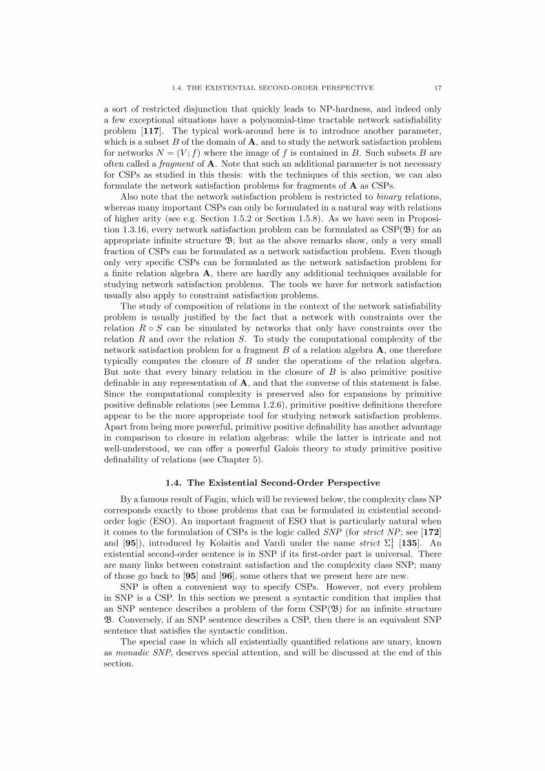
1.4. The Existential Second-Order Perspective
By a famous result of Fagin, which will be reviewed below, the complexity class NPcorresponds exactly to those problems that can be formulated in existential second-order logic (ESO). An important fragment of ESO that is particularly natural whenit comes to the formulation of CSPs is the logic called SNP (for strict NP ; see [172]and [95]), introduced by Kolaitis and Vardi under the name strict Σ1
1 [135]. Anexistential second-order sentence is in SNP if its first-order part is universal. Thereare many links between constraint satisfaction and the complexity class SNP; manyof those go back to [95] and [96], some others that we present here are new.
SNP is often a convenient way to specify CSPs. However, not every problemin SNP is a CSP. In this section we present a syntactic condition that implies thatan SNP sentence describes a problem of the form CSP(B) for an infinite structureB. Conversely, if an SNP sentence describes a CSP, then there is an equivalent SNPsentence that satisfies the syntactic condition.
The special case in which all existentially quantified relations are unary, knownas monadic SNP, deserves special attention, and will be discussed at the end of thissection.

18 1. INTRODUCTION
1.4.1. Fagin’s theorem. We start by reviewing Fagin’s theorem (see e.g. [90]).Fix a finite relational signature τ . Let C be a class of finite τ -structures that is closedunder isomorphisms (that is, if B ∈ C, and A is isomorphic to B, then A ∈ C). Wealso fix some standard way to code relational structures as finite strings so that theycan be given as an input to a Turing machine, see again [90]. We say that C is in NPwhen there exists a non-deterministic polynomial time algorithm that accepts exactlythe structures from C under this representation.
A sentence of the form ∃R1, . . . , Rm. φ where φ is a first-order sentence withsignature τ ∪ {R1, . . . , Rm} is called an existential second-order sentence. When astructure A satisfies Φ (and this is defined in the obvious way, see e.g. [90]), we writeA |= Φ.
Theorem 1.4.1 (Fagin’s Theorem, see e.g. [90]). An isomorphism-closed classof finite τ -structures is in NP if and only if there exists an existential second-ordersentence Φ that describes C in the sense that
A ∈ C if and only if A |= Φ .
1.4.2. SNP. An SNP sentence is an existential second-order sentence with auniversal first-order part, i.e., a sentence of the form
∃R1, . . . , Rk. ∀x1, . . . , xn. φ
where φ is quantifier-free and over the signature τ ∪ {R1, . . . , Rk}. The class ofproblems that can be described by SNP sentences is called SNP, too.
Example 1.4.2. The problem CSP((Z;<)) can be described by the followingSNP sentence.
∃T ∀x, y, z((x < y ⇒ T (x, y))
∧((T (x, y) ∧ T (y, z))⇒ T (x, z)
)∧ ¬T (x, x)
)�
Example 1.4.3. The Betweenness problem CSP((Z; Betw)) (Example 1.1.3) canbe described by the following SNP sentence.
∃T ∀x, y, z(¬T (x, x) ∧
((T (x, y) ∧ T (y, z))⇒ T (x, z)
)∧(
Betw(x, y, z)⇒((T (x, y) ∧ T (y, z)) ∨ (T (z, y) ∧ T (y, x))
))�
Example 1.4.4. The problem whether a given undirected graph can be parti-tioned into two triangle-free graphs (this problem has been called No-Mono-Tri inExample 1.1.8) can be described by the SNP sentence.
∃M ∀x, y, z(¬(M(x) ∧M(y) ∧M(z) ∧ E(x, y) ∧ E(y, z) ∧ E(z, x)
)∧¬(¬M(x) ∧ ¬M(y) ∧ ¬M(z) ∧ E(x, y) ∧ E(y, z) ∧ E(z, x)
))The following fundamental lemma for SNP sentences is due to Feder and Vardi [96],
and can be shown by a simple compactness argument (Theorem 2.3.1).
Lemma 1.4.5 (from [96]). Let A be an infinite structure, and Φ an SNP sentence.Then A |= Φ if and only if A′ |= Φ for all finite induced substructures A′ of A.
Since every finite induced substructure of B homomorphically maps to B, andtherefore satisfies Φ, we have the following consequence.
Corollary 1.4.6. Let Φ be an SNP sentence that describes CSP(B) for a struc-ture B. Then B itself satisfies Φ.
1.4. THE EXISTENTIAL SECOND-ORDER PERSPECTIVE 19
1.4.3. SNP and CSPs. We say that two SNP sentences Φ and Ψ are equivalentif for all structures (equivalently: all finite structures) A we have A |= Φ if and onlyif A |= Ψ. We assume in the following that the first-order part φ of Φ is written inconjunctive normal form.
Definition 1.4.7. Let Φ be an SNP sentence whose unquantified relation symbolsare from the signature τ . Then Φ is called monotone if each literal of Φ with a symbolfrom τ ∪ {=} is negative, that is, of the form ¬R(x), for R ∈ (τ ∪ {=}).
In particular, monotone SNP sentences do not contain literals of the form x = y(hence, in the terminology of Feder and Vardi [95], we work here with monotoneSNP without inequality ; the reason why Feder and Vardi add the attribute withoutinequalities is that for them, SNP sentences are written in negation normal form, soforbidding literals of the form x = y amounts to forbidding inequalities in negationnormal form).
We also assume that monotone SNP sentences do not contain literals of the formx 6= y. This is without loss of generality, since every monotone SNP sentence isequivalent to one which does not contain literals of the form x 6= y. To obtain theequivalent sentence, we remove literals of the form x 6= y and replace all occurrencesof y in the same clause by x. Note that the SNP sentences given in Example 1.4.2,1.4.3, and 1.4.4 can be easily re-written into equivalent monotone SNP sentences.
The class of structures that satisfy a given monotone SNP sentences is clearlyclosed under inverse homomorphisms. The converse is a result by Feder and Vardi [96];it shows that for SNP, the semantic restriction of closure under inverse homomor-phisms and the syntactic restriction of monotonicity match.
Theorem 1.4.8 (from [96]). Let Φ be an SNP sentence. Then the class of struc-tures that satisfy Φ is closed under inverse homomorphisms if and only if Φ is equiv-alent to a monotone SNP sentence.
Definition 1.4.9 (Connected SNP). When ψ is a clause of a first-order σ-formula φ in conjunctive normal form, let C be the σ-structure whose vertices arethe variables of ψ, and where (x1, . . . , xn) ∈ RC if and only if ψ contains a negativeliteral of the form ¬R(x1, . . . , xn). We say that ψ is connected if C is connected. Wesay that an SNP sentence Φ is connected if all clauses of the first-order part φ of Φare connected.
Theorem 1.4.10. Let Φ be an SNP sentence. Then the class of structures thatsatisfy Φ is closed under disjoint unions if and only if Φ is equivalent to a connectedSNP sentence.
Proof. Let Φ be of the form ∃R1, . . . , Rk ∀x1, . . . , xl. φ where φ is a quantifier-free first-order formula over the signature σ = (τ ∪ {R1, . . . , Rk}).
Suppose first that Φ is connected, and that A1 and A2 both satisfy Φ. In otherwords, there is a σ-expansion A∗1 of A1 and a σ-expansion A∗2 of A2 such that thoseexpansions satisfy ∀x.φ. We claim that the disjoint union A∗ of A∗1 and A∗2 alsosatisfies ∀x.φ; otherwise, there would be a clause ψ in φ and elements a1, . . . , aq ofA1 ∪ A2 such that ψ(a1, . . . , aq) is false in A∗. Since A∗1 and A∗2 satisfy ∀x.ψ, theremust be i, j such that ai ∈ A1 and aj ∈ A2. But then the canonical database for ψ isdisconnected, a contradiction.
For the opposite direction of the statement, assume that the class of struc-tures that satisfy Φ is closed under disjoint unions. Consider the SNP sentenceΨ = ∃R1, . . . , Rk, E. ∀x1, . . . , xl. ψ where ψ is the conjunction of the following clauses(we assume without loss of generality that l ≥ 3).

20 1. INTRODUCTION
• For each relation symbol R ∈ τ , say of arity p, and each i < j ≤ p, add theconjunct ¬R(x1, . . . , xp) ∨ E(xi, xj) to ψ.• Add the conjunct ¬E(x1, x2) ∨ ¬E(x2, x3) ∨ E(x1, x3) to ψ.• Add the conjunct ¬E(x1, x2) ∨ E(x2, x1) to ψ.• For each clause φ′ of φ with variables y1, . . . , yq ⊆ {x1, . . . , xl}, add to ψ the
conjunct
φ′ ∨∨
i<j≤q
¬E(yi, yj) .
We claim that the connected monotone SNP sentence Ψ is equivalent to Φ. Supposefirst that A is a finite structure that satisfies Φ. Then there is a σ-expansion A′ of Athat satisfies ∀x.φ. The expansion of A′ by the relation E = A2 shows that A alsosatisfies ∀x.ψ.
Now suppose that A is a finite structure with domain A that satisfies Ψ. Thenthere is a (σ∪{E})-expansion A′ of A that satisfies ∀x.ψ. Write A′ = A′1]· · ·]A′l forconnected σ-structures A′1, . . . ,A
′l. Note that the clauses of ψ force that the relation
E denotes A2i in the structure A′i, for each i ≤ l. Let Ai be the σ-reduct of A′i. Then
Ai satisfies ∀x.φ, because if there was a clause φ′ from φ violated in Ai then thecorresponding clause in ψ would be violated in A′i. Hence, Ai |= Φ for all i ≤ l, andsince Φ is closed under disjoint unions, we also have that A |= Φ. �
Theorem 1.4.8 combined with the previous result shows the following.
Corollary 1.4.11. An SNP sentence Φ describes a problem of the form CSP(B)for an infinite structure B if and only if Φ is equivalent to a monotone and connectedSNP sentence Ψ.
Proof. Suppose first that Φ is a monotone SNP sentence with connected clauses.To show that Φ describes a problem of the form CSP(B) we can use Lemma 1.1.7.It thus suffices to show that the class of structures that satisfy Φ is closed underdisjoint unions and inverse homomorphisms. But this has already been observed inTheorem 1.4.8 and Theorem 1.4.10.
For the implication in the opposite direction, suppose that Φ describes a prob-lem of the form CSP(B) for some infinite structure B. In particular, the class ofstructures that satisfy Φ is closed under inverse homomorphisms. By Theorem 1.4.8,Φ is equivalent to a monotone SNP sentence. Moreover, the class of structures thatsatisfy Φ is closed under disjoint unions, and hence Φ is also equivalent to a connectedSNP sentence. By inspection of the proof of Theorem 1.4.10, we see that when Φ isalready monotone, then the connected SNP sentence in the proof of Theorem 1.4.10will also be monotone. It follows that Φ is also equivalent to a connected monotoneSNP sentence. �
1.4.4. Monadic SNP. When we further restrict monotone SNP by only al-lowing unary existentially quantified relations, the corresponding class of problems,called montone monadic SNP (or, short, MMSNP), gets very close to finite domainconstraint satisfaction problems. Indeed, Feder and Vardi showed that the class MM-SNP exhibits a complexity dichotomy if and only if the class of all finite domain CSPsexhibits a complexity dichotomy (that is, if the dichotomy conjecture mentioned inthe introduction is true). In one direction, this is obvious since MMSNP obviouslycontains CSP(B) for all finite structures B (we may use a unary relation symbol foreach element of B). In the other direction, Feder and Vardi showed that every prob-lem in MMSNP is equivalent under randomized Turing-reductions to a finite domainconstraint satisfaction problem. The reduction has subsequently been derandomizedby Kun [141].

1.4. THE EXISTENTIAL SECOND-ORDER PERSPECTIVE 21
Theorem 1.4.12 (of [95] and [141]; see [155] for a formalization). Every problemin monotone monadic SNP is polynomial-time Turing equivalent to CSP(B) for afinite structure B.
Similarly as in the previous section, we might ask for a syntactic characterizationof those monadic SNP sentences that describe a CSP. Note that this does not directlyfollow from Corollary 1.4.11, since the reductions used there introduce additionalexistentially quantified relations that are not monadic. However, we have the followingmonadic version of Theorem 1.4.8.
Theorem 1.4.13 (Theorem 3 in [96]). Let Φ be a monadic SNP sentence. Thenthe class of structures that satisfy Φ is closed under inverse homomorphisms if andonly if Φ is equivalent to a monotone monadic SNP sentence.
Moreover, one can show the following monadic version of Proposition 1.4.10.
Proposition 1.4.14. Let Φ be a monadic SNP sentence. Then the class of struc-tures that satisfy Φ is closed under disjoint unions if and only if Φ is equivalent to aconnected monadic SNP sentence.
Proof. Let V be the set of variables of the first-order part φ of Φ, let P1, . . . , Pkbe the existential monadic predicates in Φ, and let τ be the input signature so thatφ has signature {P1, . . . , Pk} ∪ τ . If Φ is connected, then it describes a problem thatis closed under disjoint unions; this follows from Theorem 1.4.10.
For the opposite direction, suppose that Φ describes a problem that is closedunder disjoint unions. We can assume without loss of generality that Φ is minimal inthe sense that if we remove literals from some of the clauses the resulting SNP sentenceis inequivalent. We shall show that then Φ must be connected. Let us suppose thatthis is not the case, and that there is a clause ψ in φ that is not connected. Theclause ψ can be written as ψ1 ∨ ψ2 where the set of variables X ⊂ V of ψ1 and theset of variables Y ⊂ V of ψ2 are non-empty and disjoint. Consider the formulasΦX and ΦY obtained from Φ by replacing ψ by ψ1 and ψ by ψ2, respectively. Byminimality of Φ there is a τ -structure A1 that satisfies Φ but not ΦX , and similarlythere exists a τ -structure A2 that satisfies Φ but not ΦY . By assumption, the disjointunion A of A1 and A2 satisfies Φ. So there exists a τ ∪ {P1, . . . , Pk}-expansion A′
of A = A1 ] A2 that satisfies the first-order part of Φ. Consider the substructuresA′1 and A′2 of A′ induced by A1 and A2, respectively. We have that A′1 does notsatisfy ψ1 (otherwise A1 would satisfy ΦX). Consequently, there is an assignments1 : V → A1 of the universal variables that falsifies ψ1. By similar reasoning wecan infer that there is an assignment s2 : V → A2 that falsifies ψ2. Finally, fix anyassignment s : V → A1 ∪ A2 that coincides with s1 over X and with s2 over Y (suchan assignment exists because X and Y are disjoint). Clearly, s falsifies ψ and A doesnot satisfy Φ, a contradiction. �
Similarly as in Corollary 1.4.11 for SNP, we can combine the conditions of closureunder inverse homomorphisms and closure under disjoint unions, and arrive at thefollowing.
Corollary 1.4.15. A monadic SNP sentence Φ describes a problem of the formCSP(B) for an infinite structure B if and only if Φ is equivalent to a connectedmonotone monadic SNP sentence.
We want to remark that the problems that can be described by connected mono-tone monadic SNP sentences are exactly the problems called forbidden patterns prob-lems in the sense of Madelaine [154]. Clearly, for every finite B the problem CSP(B)is a forbidden patterns problem. In [157] is has been shown that the problems in

22 1. INTRODUCTION
MMSNP are exactly finite unions of forbidden patterns problems (going back to ideasfrom [95]).
We summarize the landscape of classes of computational problems from this sec-tion in Figure 1.6.
SNP
monotone SNP
connected SNP
SNP ∩ CSP(B) =connected monotone SNP
connected monotone
monadic SNP
CSP(B) for finite B
monotone monadic SNP
NP
Figure 1.6. Fragments of SNP.
1.5. Examples
We present computational problems that have been studied in various areas oftheoretical computer science, and that can be formulated as constraint satisfactionproblems in the sense of Section 1.1, 1.2, 1.3, or 1.4. We describe each problemfrom the perspective in which the computational problem has appeared first in theliterature.
Our list is by far not exhaustive; computational problems that can be exactlyformulated as CSP(B) for an infinite structure B are abundant in almost every areaof theoretical computer science.
1.5.1. Allen’s interval algebra. Allen’s interval algebra [5] is a formalism thatis famous in artificial intelligence, and which has been introduced to reason aboutintervals and about the relationships between intervals.
Formally, Allen’s interval algebra is a proper relation algebra (see Section 1.3.2);we can also view it as a structure with a binary relational signature. The domain isthe set I of all closed intervals [a, b] of rational numbers, where a, b ∈ Q, a < b. Whenx = [a, b] is an interval, then −x denotes the interval [−b,−a]. For R ⊆ Q2, R−
denotes the relation {(−x,−y) | (x, y) ∈ R}. Recall that in proper relation algebras,R` denotes the relation {(y, x) | (x, y) ∈ R}.
The basic relations of Allen’s interval algebra are the 13 relations P,M,O, S,D,E(defined in Figure 1.7), P−,M−, O−, S−, and the inverse of S, D, and S−, denoted byS`, D`, and (S−)`, respectively. Note that those 13 relations are pairwise disjoint,and that their union equals I2. Recall our convention that when R is a subset of the

1.5. EXAMPLES 23
Relation Symbol Definition ExplanationP {([a, b], [c, d]) | b < c} [a, b] preceeds [c, d]M {([a, b], [c, d]) | b = c} [a, b] meets [c, d]O {([a, b], [c, d]) | a < c < b < d} [a, b] overlaps with [c, d]S {([a, b], [c, d]) | a = c and b < d} [a, b] starts [c, d]D {([a, b], [c, d]) | c < a < b < d} [a, b] is during [c, d]E {([a, b], [c, d]) | a = c, b = d} [a, b] equals [c, d]
Figure 1.7. The definitions for the basic relations of Allen’s interval algebra.
basic relations, we write xRy if (x, y) ∈⋃R∈RR. For example, x{P, P−}y signifies
that the intervals x and y are disjoint. The 213 relations that arise in this way willbe called the relations of Allen’s interval algebra.
An important computational problem for Allen’s interval algebra is the networksatisfaction problem for Allen’s interval algebra. This problem can be viewed asCSP(A) where A is a structure with domain I and a signature containing 213 binaryrelation symbols (see Section 1.3.2). More on this structure can be found in Chapter 3,Example 3.1.11. We are sometimes sloppy and write Allen’s interval algebra when wemean A (rather than A).
The problem CSP(A) is NP-complete [5]. The complexity of the CSP for (binary)reducts of Allen’s interval algebra has been completely classified in [140].
1.5.2. Phylogenetic reconstruction problems. In modern biology it is be-lieved that the species in the evolution of life on earth developed in a mostly tree-likefashion: at certain time periods, species separated into sub-species. The goal ofphylogenetic reconstruction is to determine the evolutionary tree from given partialinformation about the tree. This motivates the computational problem of rooted triplesatisfiability (also called rooted triple consistency), defined below. In 1981, Aho, Sa-giv, Szymanski, and Ullman [4] presented a quadratic time algorithm to this problem,motivated independently from computational biology by questions in database theory.
Let T be a tree with vertex set T and with a distinguished vertex r, the root ofT. For u, v ∈ T , we say that u lies below v if the path from u to r passes through v.We say that u lies strictly below v if u lies below v and u 6= v. The youngest commonancestor (yca) of two vertices u, v ∈ T is the node w such that both u and v lies beloww and w has maximal distance from r.
Rooted-Triple SatisfiabilityINSTANCE: A finite set of variables V , and a set of triples xy|z for x, y, z ∈ V .QUESTION: Is there a rooted tree T with leaves L and a mapping s : V → L suchthat for every triple xy|z the yca of s(x) and s(y) lies strictly below the yca of s(x)and s(z) in T?
Another famous problem that has been studied in this context is the quartetsatisfiability problem, which is NP-complete [189].
Quartet SatisfiabilityINSTANCE: A finite set of variables V , and a set of quartets xy:uv with x, y, u, v ∈ V .QUESTION: Is there a tree T with leaves L and a mapping s : V → L such that forevery quartet xy:uv ∈ Ryca the shortest path from x to y is disjoint to the shortestpath from u to v?

24 1. INTRODUCTION
◦ = < > |= = < > |< < < {<,=, >} {<, |}> > 1 > || | | {>, |} 1
Figure 1.8. The composition table for the basic relations in theleft-linear point algebra.
It is straightforward to check that the class of positive instances (viewed as rela-tional structures) of each of those two computational problems is closed under disjointunions and inverse homomorphisms. By Lemma 1.1.7, both the rooted triple satis-faction problem and the quartet satisfaction problem can be formulated as CSP(B)for an infinite structure B. We come back to those CSPs in Chapter 4.
1.5.3. Branching-time constraints. An important model in temporal reason-ing is branching time, where for every time point the past is linearly ordered, but thefuture is only partially ordered.
This motivates the so-called left-linear point algebra [88,117], which is a relationalgebra with four basic relations, denoted by =, <, >, and |. Here we imaginethat ‘x < y’ signifies that x is earlier in time than y, and to the left of y when wedraw points in the plane, and this motivates the name left linear point algebra. Thecomposition operator on those four basic relations is given in Figure 1.8. The inverseof < is >, Id denotes =, and | is its own inverse, and the relation algebra is uniquelygiven by this data.
As explained in Section 1.3.2, the network consistency problem for the left-linearpoint algebra can be viewed as CSP(B) for an appropriate infinite structure with16 = 24 binary relations (one for each subset of {=, <,>, |}). In this structure, forevery x the set {y | y < x} is linearly ordered by by <. An explicit example of such astructure is given in Section 4.2. The network consistency problem of the left-linearpoint algebra is polynomial-time equivalent to the following problem, which we callbranching-time satisfiability problem.
Branching-Time SatisfiabilityINSTANCE: A finite relational structure A = (A;≤, ‖, 6=) where ≤, ‖, and 6= arebinary relations.QUESTION: Is there a rooted tree T and a mapping s : A→ T such that in T the fol-lowing is satisfied: a) If (x, y) ∈ ≤A, then s(x) lies above s(y); b) If (x, y) ∈ ||A, thenneither s(x) lies strictly above s(y), nor s(y) strictly above s(x); c) If (x, y) ∈ 6=A,then s(x) 6= s(y).
The idea why this problem is polynomial-time equivalent to the network satisfac-tion problem of the left-linear point algebra is the observation that in any represen-tation B of the left-linear point algebra, the relation x{<,>,=}y has the primitivepositive definition
∃z (x{<,=}z ∧ y{<,=}z) ,and the relation x{<, |,=}y has the primitive positive definition
∃z (x{<,=}z ∧ z{|,=}y) ;
we can then use Theorem 1.2.6 (for details, see [44]).The branching-time satisfiability problem can be formulated as CSP(C) for the
structure with domain C := {0, 1}∗ and relations ≤, ‖, and 6=, where ≤ denotes the

1.5. EXAMPLES 25
◦ = < > ≺ �= = < > ≺ �< < < {<,>} {<,≺} {<,�}> > 1 > ≺ �≺ ≺ ≺ {>,≺} ≺ 1� � � {>,�} 1 �
Figure 1.9. The composition table for the basic relations of Cor-nell’s tree algebra C.
relation{(u, v) ∈ C2 | u is a prefix of v} .
The relation 6= is the disequality relation, and u ‖ v holds if u and v are equal orincomparable with respect to ≤. Let < denote the intersection of ≤ and 6=. Notethat the structure C can not be used to obtain a representation of the left-linear pointalgebra, since (<) ◦ (<) does not equal <.
The first polynomial-time algorithm for the branching-time consistency problem(and therefore also for the network satisfaction problem of the left-linear point alge-bra) is due to Hirsch [117], and has a worst-case running time in O(n5). This hasbeen improved by Broxvall and Jonsson [59], who presented an algorithm running inO(n3.376) (this algorithm uses an O(n2.376) algorithm for fast integer matrix multipli-cation). A simpler algorithm which does not use fast matrix multiplication and runsin O(nm) has been found in [43].
1.5.4. Cornell’s tree description constraints. Motivated by problems incomputational linguistics, Cornell [78] introduced the following computational prob-lem5. It is a strictly more expressive problem than the branching time satisfactionproblem from the previous section, but has been introduced independently from [117]and [59]. There are many equivalent formulations of this problem. One is as the gen-eral network satisfaction problem for the relation algebra C with atoms =, <, >, ≺,and � which is given by the composition table in Figure 1.9. The idea is that < de-notes a dense semilinear order (see Section 1.5.3), and ≺ ∪ < denotes a linear order.The idea how to use this in natural language grammar formalisms like dependencygrammars is that < represents the syntactic structure of a natural language sentencewhereas ≺ ∪ < stands for the word order.
Similarly as in Section 1.5.3, all 25 relations of C can be obtained by repeatedcompositions and intersections of the four relations {<,=}, {≺,=}, {≺,�,=}, and{<,>,≺,�}; for details, see [44]. The algorithm presented for the general networksatisfaction problem for C in [78] is not complete. A polynomial-time algorithm hasbeen found in [44].
1.5.5. Set constraints. Many fundamental problems in artificial intelligence,knowledge representation, and verification involve reasoning about sets and relationsbetween sets and can be modeled as constraint satisfaction problems. One of the mostfundamental problems of this type is the following. We denote the set of all subsetsof N by P(N).
Basic Set Constraint SatisfiabilityINSTANCE: A finite set of variables V , and a set φ of constraints of the form x ⊆ y,x || y, or x 6= y, for x, y ∈ V .
5I feel personally committed to Cornell’s problem since it was the first CSP with an ω-categoricaltemplate I met.

26 1. INTRODUCTION
QUESTION: Is there a mapping s : V → P(N) such thata) If x ⊆ y is in φ, then s(x) is contained in s(y);b) If x || y is in φ, then s(x) and s(y) are disjoint sets;c) If x 6= y is in φ, then s(x) and s(y) are distinct sets.
This problem has the shorter description CSP((P(N);⊆, ||, 6=)) where ⊆, ||, 6= arebinary relations over P(N), standing for the binary relations containment, disjointness,and inequality between sets. Drakengren and Jonsson [85] showed that basic setconstraint satisfiability can be decided in polynomial time. They also showed that thegeneralization of the problem can be solved in polynomial time where each constrainthas the form
x1 6= y1 ∨ · · · ∨ xk 6= yk ∨ x0Ry0
where R is either ⊆, ||, or 6=, and where x0, . . . , xk, y0, . . . , yk are not necessarilydistinct variables.
1.5.6. Spatial reasoning. Qualitative spatial reasoning (QSR) is concernedwith representation formalisms that are considered close to conceptual schemata usedby humans for reasoning about their physical environment—in particular, about pro-cesses or events and about the spatial environment in which they are situated. Theapproach in qualitative reasoning is to develop relational schemas that abstract fromconcrete metrical data of entities (for example time points, coordinate positions, ordistances) by subsuming similar metric or topological configurations of entities intoone qualitative representation.
There are many formalisms for qualitative spatial reasoning. In particular, sev-eral relation algebras (see Section 1.3.2) have been studied in this context. A basicexample is the RCC5 relation algebra (with 5 atoms; the RCC5 relation algebra isalso known under the name containment algebra [21,88]), and the RCC8 relation al-gebra (with 8 atoms). In both formalisms, the variables denote ‘non-empty regions’.In RCC5, the five atoms are denoted by DR, PO, PP, PPI, EQ, and they standfor disjointness, proper overlap, proper containment (proper-part-or), its inverse, andequality, respectively. In RCC8, we further distinguish how the ‘boundaries’ of tworegions relate to each other. We do not further discuss RCC8, for details, see [55,88].
There are many equivalent ways to formally define RCC5. Often, this is doneby specifying the composition table for atomic relations, but we find this tedious.Here, we rather define RCC5 as the proper relation algebra whose domain are allopen (or all closed) disks in R2, and where the basic relations are disjointness (emptyintersection), proper overlap, containment, the inverse of containment, and equalityof disks. Then RCC5 is the abstract relation algebra of the proper relation algebraof closed disks (see Section 2.1.5 in [88]).
The network satisfaction problem for RCC5 is NP-complete; the computationalcomplexity of the CSP for the (binary) reducts of B has been classified in [127,179].A polynomial-time tractable case of particular interest is the network satisfactionproblem for the basic relations of RCC5 [179], i.e., the network satisfaction problemfor RCC5 when the input is restricted to networks N = (V ; f) where f maps to 1 orthe atoms in RCC5 only.
In any representation of RCC5, the atomic relations satisfy the following set ofaxioms T . We use P (x, y) as a shortcut for PP(x, y) ∨ EQ(x, y).
1.5. EXAMPLES 27
T :={∀x, y, z (DC(x, y) ∧ P (z, y)→ DC(x, z))
∀x, y, z (PO(x, y) ∧ P (y, z)→ (PO(x, z) ∨ PP (x, z)))
∀x, y, z (PP (x, y) ∧ PP (y, z)→ PP (x, z))
∀x, y, z (P−1(x, y) ∧ P (y, z)→ ¬DC(x, y))}
It is easy to see that the network satisfaction problem for the basic relations ofRCC5 is essentially the same problem as CSP(T ), where T is the first-order theorydefined as above. It can be checked easily that T satisfies item (2) in the statementof Proposition 1.3.6, and hence there exists an infinite structure B such that CSP(B)equals the satisfiability problem for RCC5. We will give more explicit descriptions ofsuch an infinite structure B in Chapter 4 (and it turns out that there are close linkswith the problem from Section 1.5.5).
1.5.7. Horn-SAT. The following problem is an important P-complete prob-lem [67]. It can be solved in linear time in the size of the input [84].
Horn-SATINSTANCE: A propositional formula in conjunctive normal form (CNF) with at mostone positive literal per clause.QUESTION: Is there a Boolean assignment for the variables such that in each clauseat least one literal is true?
We cannot model this problem as CSP(B) for a finite signature structure; how-ever, note that a clause ¬x1 ∨ · · · ∨ ¬xk ∨ x0 is equivalent to
∃y1, . . . , yk−1
((¬x1 ∨ ¬x2 ∨ y1) ∧ (¬y1 ∨ ¬x3 ∨ y2) ∧ · · · ∧ (¬yk−1 ∨ ¬xk ∨ x0)
).
Hence, by introducing new variables, there is a straightforward reduction of Horn-SAT to the restriction of Horn-SAT where every clause has at most three literals. Thisrestricted problem, which we call Horn-3SAT, can be formulated as CSP(B) for
B =({0, 1};{(x, y, z) | (x ∧ y)⇒ z}, {(x, y, z) | ¬x ∨ ¬y ∨ ¬z},
{((x, y) | x⇒ y}, {((x, y) | ¬x ∨ ¬y}, {0}, {1}).
1.5.8. Precedence constraints in scheduling. The following problem hasbeen studied in [164] in scheduling: given is a finite set of variables V , and a finiteset of and/or precedence constraints, i.e., constraints of the form
x0 > x1 ∨ · · · ∨ x0 > xk (6)
for x0, x1, . . . , xk ∈ V . The question is whether there exists an assignment V → Q(equivalently, we can replace Q by Z, or any other infinite linearly ordered set).
As in the case of Horn-SAT, we cannot directly model this problem as CSP(B)for a finite signature structure B. However, note that Formula (6) is equivalent to
∃y1, . . . , yk−1
((x0 > x1 ∨ x0 > y1)∧(y1 > x2 ∨ y1 > y2) ∧ · · · ∧ (yk−1 > xk−1 ∨ yk−1 > xk)
).
This shows that and/or precedence constraints can be translated into conjunctionsof constraints of the form x0 > x1 ∨ x0 > x2 by introducing new existentially quan-tified variables. Hence, the problem whether a given set of and/or precedence con-straints is satisfiable reduces naturally to CSP((Q;Rmin)) where Rmin is the ternaryrelation {(a, b, c) | a > b ∨ a > c}. Note that Rmin holds on exactly those triples(a, b, c) where a is larger than the minimum of b and c. The problem CSP((Q;Rmin))can be solved in polynomial time; this is essentially due to [164]. For more expressive

28 1. INTRODUCTION
constraint languages over Q that contain the relation Rmin and whose CSP can stillbe solved in polynomial time, see Section 10.5.2 or Section 10.4.1.
1.5.9. Ord-Horn constraints. In this section we work with first-order formulasover the signature {<}. We write x ≤ y as a shortcut for (x < y) ∨ (x = y) (recallour convention that equality is part of first-order logic). A formula over the signature{<} and with variables V is called Ord-Horn if it is a conjunction of disjunctions ofthe form
(x1 = y1) ∨ · · · ∨ (xk = yk) ∨ (x0Ry0)
where x0, x1, . . . , xk, y0, y1, . . . , yk ∈ V , and R is either ≤, <, 6=, or =.
Ord-Horn SatisfiabilityINSTANCE: A finite set of variables V , and a finite set of Ord-Horn formulas withvariables from V .QUESTION: Is there an assignment V → Q that satisfies all the given formulas over(Q;<)?
Nebel and Burckert [165] showed that Ord-Horn Satisfiability can be solved inpolynomial time. A relation R ⊆ Qk is called Ord-Horn if it is definable by an Ord-Horn formula over (Q;<). As in the case of Horn-SAT and of and/or precedenceconstraints, there are structures B with finitely many Ord-Horn relations such thatall Ord-Horn relations have a primitive positive definition in B. It can be shown thatthe following structure has this property (see Chapter 6).
(Q;≤, 6=, {(x, y, u, v) | (x = y)⇒ (u = v)}
)In Section 10.4.1 we see that constraint languages that contain and/or precedence
constraints and Ord-Horn constraints can still be solved in polynomial time.
1.5.10. Ord-Horn interval constraints. For some (binary) reducts B of Allen’sinterval algebra the problem CSP(B) can be solved in polynomial time. The most im-portant of these reducts is the class of Ord-Horn interval constraints, which has beenintroduced by Nebel and Burkert [165]. It consists of all the relations R of Allen’sinterval algebra such that the relation
{(x, y, u, v) | ([x, y], [u, v]) ∈ R
}is Ord-Horn
(see Section 1.5.9). Now it is not hard to see that satisfiability for Ord-Horn intervalconstraints has a polynomial-time reduction to Ord-Horn satisfiability. This type ofreduction will be studied in Section 5.5.
1.5.11. Linear program feasibility. Linear Programming is a computationalproblem of outstanding theoretical and practical importance (see e.g. [185]). It isknown to be computationally equivalent to the problem to decide whether a given setof linear (non-strict) inequalities is feasible, i.e., defines a non-empty set.
Linear Program FeasibilityINSTANCE: A finite set of variables V ; a finite set of linear inequalities of the forma1x1 + · · · + akxk ≤ a0 where x1, . . . , xk ∈ V and a0, . . . , ak are rational numberswhere numerator and denominator are represented in binary.QUESTION: Does there exist an x ∈ R|V | that satisfies all inequalities?
Kachyian showed in [134] that Linear Program Feasibility can be solved in poly-nomial time. It is clearly not possible to formulate this problem as CSP(B) for astructure B with a finite relational signature. However, we show below that it ispolynomial-time equivalent to CSP
((R; {(x, y, z) | x + y = z}, {1},≤)
). For this, we
need the following lemma.
1.5. EXAMPLES 29
Lemma 1.5.1 (from [38]). Let n0, . . . , nl ∈ Q be arbitrary rational numbers. Thenthe relation {(x1, . . . , xl) | n1x1 + . . . + nlxl = n0} is primitive positive definable in(R; {(x, y, z) | x + y = z}, {1}). Furthermore, the primitive positive formula thatdefines the relation can be computed in polynomial time.
The idea to prove this is to use iterated doubling to define large numbers withsmall primitive positive formulas. By extending the previous result to inequalities,one can prove the following.
Proposition 1.5.2 (from [38]). The linear program feasibility problem for linearprograms is polynomial-time equivalent to CSP((R; {(x, y, z) | x+ y = z}, {1},≤)).
1.5.12. The max-atoms problem. In our list of problems from the literaturethat can be formulated as CSP(B), we also want to include one problem in NP whereit is not known whether CSP(B) is in P or NP-hard. Our problem is closely related tothe following problem, which has been introduced in [23] and, independently, in [164].
The Max-Atoms ProblemINSTANCE: A finite set of variables V ; a finite set of constraints of the form x0 ≤max (a1x1, . . . , akxk) where x1, . . . , xk ∈ V and a0, . . . , ak (the coefficients) are inte-gers represented in binary.QUESTION: Does there exist an x ∈ Q|V | that satisfies all inequalities?
It is known that the Max-atoms problem is computationally equivalent to mean-payoff games [164], and therefore it is contained in NP ∩ coNP. It also follows thatdeciding the winner in Parity games and satisfiability of the propositional µ-calculuscan be reduced to the max-atoms problem. Bezem, Nieuwenhuis and Rodrıguez-Carbonell [23] give an alternative proof that the problem is in NP ∩ coNP. In thesame paper, they also shown that a certain hypergraph reachability problem, andan intensively studied problem in max/+ algebra are equivalent to the max-atomsproblem. Moreover, they show that the problem is in P when the coefficients in theinput are represented in unary.
Similarly as for linear program feasibility, the Max-atoms problem cannot beformulated as CSP(B) for a structure B with a finite relational signature. Theproblem we introduce instead is
CSP((Q; {(x, y) | y = x+ 1}, {(x, y) | y = 2x}, Rmin≤ ))
where Rmin≤ = {(x, y, z) | x ≥ y ∨ x ≥ z} is a variant of the relation Rmin from
Section 1.5.8. The max-atoms problem can be reduced to this problem: we replaceexpressions of the form xi + ai by a new variable yi, and add a primitive positiveformula φ(x, y) that defines yi = xi + ai and can be computed in polynomial time inthe input size of the max-atoms problem. We do not know how to prove hardness forthe CSP above, and rather think that the problem might well be in P.
1.5.13. Unification. Unification (and unification modulo equational theories)is an proper field in computational logic, and the complexity of the unification problemhas been studied in numerous variants [10]. Many unification problems can be viewedas CSP(B), for an appropriate infinite structure B, as we will see in the following.We start with the most fundamental unification problem.
Let σ := {f1, . . . , fk} be a finite set function symbols, and let x be a variablesymbol. Then F(x) denotes the set of all terms that can be constructed from τ andthe variable x. The unnested unification problem over τ is the following problem6.
6This problem is known to be equivalent to the standard unification problem where the inputis a single equation t1 ≈ t2 for ‘nested’ terms t1, t2 ∈ F(x).

30 1. INTRODUCTION
Unnested Unification Problem over τINSTANCE: a finite set of variables V , and a finite set of ‘un-nested’ term equations,i.e., expressions of the form y0 ≈ f(y1, . . . , yk) for y0, y1, . . . , yk ∈ V and f ∈ τ .QUESTION: is there an assignment s : V → F(x) such that for every expressiony0 = f(y1, . . . , yk) in the input we have s(y0) = f(s(y1), . . . , s(yk))?
For fixed τ as above, let T = (F(x);F1, . . . , Fk) be the structure where Fi is therelation {(t0, t1, . . . , tr) ∈ (F(x))r+1 | t0 = fi(t1, . . . , tr)} (here, r is the arity of fi).It is clear that the unnested unification problem over τ can be described as CSP(T).In a similar way, equational unification problems (see [10]) can be viewed as CSPs.
1.6. Overview
This text develops the universal-algebraic approach for complexity analysis ofconstraint satisfaction problems with countably infinite ω-categorical templates. Partsof the corresponding theory follow or generalize the universal-algebraic approach forCSPs with finite templates, whereas other parts are specific to infinite domains, suchas the way in which we apply Ramsey theory. We then present two complexityclassification results that have been obtained using this approach: the classificationof temporal CSPs in Chapter 10, and Schaefer’s theorem for graphs in Chapter 9.We close with Chapter 11 on classes of computational problems that probably do notexhibit a complexity dichotomy.
Publication Note. My PhD-thesis [24] also treated constraint satisfaction withω-categorical templates, and already hinted at the relevance of polymorphisms anduniversal algebra. But it is only here that we fully present the universal-algebraic ap-proach and its applications for classification projects of large classes of infinite-domainconstraint satisfaction problems. The self-contained presentation in this thesis is col-lecting and re-combining results that have been fragmented over various publications,and often come with new proofs.
Parts of the content of this thesis have been published by co-authors and myselfin conferences or journals. The example sections in Chapter 1 and Chapter 4 presentCSPs studied in [25, 31, 34, 37, 44, 45, 55]. Chapter 3 contains a new proof, to bepublished in the journal version of [35], of the main result in [25]. Chapter 5 coversoriginal results from [47], [27], and the survey [26]. Many results in Chapter 8 arefrom [54] and the survey [50].
The classification for equality constraint satisfaction problems has first been ob-tained in [40], but the proof presented here is new and borrows results and ideasfrom [29] and [51]. The classification for temporal constraint satisfaction problemsin Chapter 10 is based on [41] and [42], with some additions from the survey [50].Schaefer’s theorem for graphs is based on [52] and [51], again with additions from [50]Finally, Chapter 11 also contains some results from [33].
1.7. Uncovered Topics
When choosing the material to be included in this thesis, certain restrictive choiceshad to be made. We comment on related lines of research or facets of the area thatwe had to skip.
1.7.1. Infinite Signatures. Several natural computational problems could beformulated in the form CSP(B) when we would allow that the structure B has a count-ably infinite signature. For example, we might want to view the feasibility problemfor linear programs (Section 1.5.11) as CSP(B) where B contains all relations of theform {(x1, . . . , xk) | a1x1 + · · · + akxk ≤ a0}, for all rational numbers a0, a1, . . . , ak.

1.7. UNCOVERED TOPICS 31
Indeed, several general results for constraint satisfaction that we present in this thesiswould carry over to infinite signatures with no problems.
If we wanted to extend the present definition of CSP(B) to structures B with aninfinite signature, we are faced with the difficulty to specify how the constraints ininput instances of CSP(B) are represented. When B has a finite signature, this causesno problems, since we can fix any representation for the finite number of relationsymbols; since B is considered to be fixed, the precise choice of the representationis irrelevant. When B has an infinite signature, a good choice how to code theconstraints in the input very much depends on the structure B. In the example oflinear programming feasibility, for instance, we might want to represent the constrainta1x1 + · · ·+ akxk ≤ a0 by specifying the coefficients a0, a1, . . . , ak in binary.
Note that the issue of finite versus infinite constraint languages is not specificto infinite domains, but becomes relevant already for finite domains. Typically, forinfinite constraint languages over a finite domain each constraint in the input is rep-resented by listing all tuples of the corresponding relation in the constraint language.But this is not the only, and sometimes not even the most natural way to represent theconstraints. For instance for the Horn-SAT problem (see Section 1.5.7), the most nat-ural way to present the constraint is by writing them as conjunctions of Horn-clauses.In the general setting, several representations have been proposed, some of which aremore concise than listing all tuples [74], and some of which are less concise [161].
It turns out that typically when a constraint satisfaction problem with an infiniteconstraint language is computationally hard, then there is a finite set of relations inthis language such that the CSP for this sub-language is already NP-hard. For infiniteconstraint languages over a finite domain, and when the constraints are representedby explicitly listing all satisfying assignments to the variables of the constraint, ithas even been conjectured [65] that this might be true in general; that is, whenCSP(B) is NP-hard under this representation, then B has a finite signature reductwith a hard CSP. This conjecture is still open. We also want to mention a conditionalnon-dichotomy result for infinite constraint languages from [33].
We have decided to keep in this thesis the focus on CSPs for finite constraintlanguages, for the following reasons. This allows to work with one and the samedefinition of the computational problem CSP(B) for all infinite structures B with afinite signature. Moreover, for all of the algorithms presented in this thesis it will beimmediately clear under which input assumption they might be generalized to dealwith an infinite constraint language. This does not prevent us from stating relevantmathematical facts in full generality when they also hold for structures with an infinitesignature; only when it comes to statements about CSP(B) we insist that B has finiterelational signature.
1.7.2. Complexity classes below P. Besides the mentioned progress on thedichotomy conjecture for finite domain CSPs, there has been considerable researchactivity to localize the exact complexity of CSPs inside the complexity class P, orwith respect to definability in certain logics. By definability of CSP(B) we mean thatthere exists a sentence Φ is some logic (typically extensions of first-order logic andrestrictions of least fixed point logics) such that A |= Φ if and only if A homomorphi-cally maps to B (that is, in this case it is most natural to consider the definitions ofthe CSP presented in Section 1.1 and in Section 1.4).
One motivation for studying computational complexity within P is the questionwhether it is possible to solve problems faster in parallel models of computation.Another motivation, in particular for definability of CSPs in certain logics, is the goalto better understand the scope of existing algorithmic techniques to solve CSPs (suchas Datalog, or restrictions of Datalog).

32 1. INTRODUCTION
In this line of research, the computational complexity of CSP(B) has been com-pletely classified when B is a two-element structure [6]. Each problem in this classis complete for one of the complexity classes NP, P, ⊕L, NL, L, and AC0 underAC0 isomorphisms. For general finite domains, several universal-algebraic conditionsare known that imply hardness for various complexity classes [9, 145]. Concerningdefinability of CSPs, there are precise characterizations of those CSPs that are de-finable by a first-order sentence [8,144,180]. Moreover, if CSP(B) is not first-orderdefinable, then it is L-complete under AC0-reductions [145] (also see [82, 92]). Forinfinite domain constraint satisfaction, it appears that there are no general resultsabout localizing the complexity of CSPs within the complexity class P yet. However,we would like to remark that already in some concrete and model-theoretically well-behaved structures B the precise complexity of CSP(B) within P is open. We giveone example.
Example 1.7.1. Consider the problem
CSP((Q; 6=, {(x, y, z) | (x = y ⇒ y ≤ z) ∧ x ≤ y)) .
This problem is NL-hard since there is an easy reduction from directed reachabilityto this problem, and directed reachability is an NL-complete problem. By carefulinspection of Tarjan’s linear-time algorithm for strongly connected components [191]we see that the problem can be solved in linear time. However, the precise complexityof this problem is not known; it might be that the problem is contained in NL, but itmight also be P-hard.
1.7.3. Quantified CSPs. Let B be a structure with a finite relational signature.Then the quantified constraint satisfaction problem for B, denoted QCSP(B), is thecomputational problem to decide for a given first-order sentence φ in prenex normalform and without disjunction and negation symbols whether φ is true in B. Thedifference of QCSP(B) from CSP(B) as we have presented it in Section 1.1 is thatuniversal quantification is permitted in the input sentences φ.
The additional expressiveness often comes at the prize of higher computationalcomplexity; whereas for finite structures B, the CSP for B is always in NP, thereare finite structures B where QCSP(B) is PSPACE-complete. But quite surpris-ingly, several constraint languages with a polynomial-time tractable CSP also have apolynomial-time QCSP. This is for instance the case for 2SAT [7] (see Example 1.2.2),or for Horn-3SAT [130] (see Section 1.5.7). Similarly, it can be shown that the tem-poral constraint languages presented in Section 10.5.2 and Section 10.5.5 are not onlytractable for the CSP, but also for the QCSP. These are attractive results, since theyassert that we can solve an even more expressive computational problem than theCSP for the same constraint language without loosing polynomial-time tractability.From a methodological point of view, we remark that the universal-algebraic approachcan also be applied to study the complexity of the QCSP [57]; as in the case of theCSP, the computational complexity of QCSP(B) is captured by the polymorphismsof B (see Chapter 5). Classifications of the QCSP typically rely on the correspondingclassification for the CSP. In particular, any hardness result for the CSP immediatelytranslates into a hardness result for the QCSP. Moreover, in the cases where theCSP(B) is tractable, the algorithmic insight is often the starting point for furtherinvestigations of QCSP(B).
However, complexity classifications for QCSPs are typically harder to obtain thanthe corresponding complexity classifications for CSPs. One of the reasons is thatseveral relevant universal-algebraic facts require the assumption that the algebra beidempotent (see Section 5.6.1). The complexity of the QCSP, however, is not pre-served by homomorphic equivalence, and when we study QCSP(B) we can thus not

1.7. UNCOVERED TOPICS 33
pass to the core of B. Hence, we can in general not make the assumption that thepolymorphism clone of B is idempotent.
For CSP(B), a powerful way of proving NP-hardness is to give a primitive positiveinterpretation (see Section 5.5) of a Boolean template with a hard CSP. This is nolonger possible for the QCSP. There are for example 3-element templates B thatare preserved by a semi-lattice operation (and hence no hard Boolean CSP can beinterpreted in B) where QCSP(B) is PSPACE-complete [57]. Finally, we would liketo mention that PSPACE-hardness proofs for the QCSP are often much harder thanNP-hardness proofs for the CSP [28,57].
From the above is not surprising that a full classification of the QCSP complex-ity for three-element structures is still open. Similarly, there is no classification ofthe QCSP for the class of temporal constraint languages presented in Chapter 10.There are concrete temporal constraint languages where the QCSP is of unknowncomputational complexity, for instance the QCSP for(
Q; {(x, y, z) | x = y ⇒ y ≥ z}).
For this problem, we do not know hardness for any complexity class above P, and donot know containment in any complexity class below PSPACE.
1.7.4. Non ω-categorical templates. Most methods presented in this thesiscrucially rely on the assumption that the constraint languages are ω-categorical. How-ever, systematic complexity classification is also possible for large classes of constraintlanguages that are not ω-categorical.
1.7.4.1. Distance CSPs. The structure (Z; succ) of the integers with the sucessorrelation succ = {(x, y) | x = y + 1} constitutes one of the simplest infinite structureswith a finite signature that is not ω-categorical. Structures with a first-order definitionin (Z; succ) are particularly well-behaved from a model-theoretic perspective: theyare strongly minimal [120, 158], and therefore uncountably categorical (but usuallynot ω-categorical). In [32], the complexity of CSP(B) has been studied when B isfirst-order definable in (Z; succ). As an example, consider the directed graph withvertex set Z which has an edge between x and y if the difference between x andy is either 1 or 3. This graph can be viewed as the structure (Z;R{1,3}) whereR{1,3} = {(x, y) | x−y ∈ {1, 3}}, which has a first-order definition over (Z; succ) sinceR{1,3}(x, y) iff
succ(x, y) ∨ ∃u, v (succ(x, u) ∧ succ(u, v) ∧ succ(v, y)) .
Another example is the undirected graph with vertex set Z where two integers x, yare linked if the distance between x and y is one or two.
The corresponding class of CSPs contains many natural combinatorial problems.For instance, the CSP for the structure (Z;R{1,3}) is the computational problem tolabel the vertices of a given directed graph G such that if (x, y) is an arc in G, thenthe difference between the label for x and the label for y is one or three. It followsfrom the results in [32] that this problem is in P. The CSP for the undirected graph(Z;{
(x, y)∣∣ |x − y| ∈ {1, 2}}) mentioned above is exactly the 3-coloring problem,
and therefore NP-complete. In general, those problems have the flavor of assignmentproblems where the task is to map the variables to integers such that various givenconstraints on differences and distances (and Boolean combinations thereof) are sat-isfied. Therefore, CSPs whose template is definable over (Z; succ) are called distanceCSPs.
The complexity classification for distance CSPs presented in [32] is incomplete intwo respects. First, it might be the case that a structure B with a first-order definitionin (Z; succ) has a finite core A. Those cores have the property that they have a single

34 1. INTRODUCTION
orbit (see Section 1.2.3); this follows easily from the fact that the structure (Z; succ)also has only one orbit. But the dichotomy conjecture for finite domain CSPs hasnot yet been established for the particular case of finite templates that have onlyone orbit. The second point in which the complexity classification for distance CSPsgiven in [32] is incomplete is that it only studies templates B that are locally finite,an additional finiteness condition, defined as follows. A graph is called locally finiteif every vertex is contained in a finite number of edges; a relational structure is calledlocally finite if its Gaifman graph (definition given in Section 2) is locally finite. Themethod that is applied in [32] is relational, and not universal-algebraic.
1.7.4.2. Tractable Expansions of Linear Program Feasibility. Linear Program-ming is a computational problem of outstanding theoretical and practical importance.As we have seen, it is computationally equivalent to the CSP we have presented in Sec-tion 1.5.11. It seems to be interesting to investigate how far the constraint language ofall linear inequalities can be expanded such that the corresponding constraint satisfac-tion problem remains polynomial-time solvable. It has been shown in [38] that everyfirst-order expansion of linear programming is contained in a class called Horn-DLRfrom [126] and polynomial-time tractable, or otherwise NP-hard.
An important class of relations over the real numbers that generalizes the classof relations defined by linear inequalities is the class of all semi-algebraic relations,i.e., relations with a first-order definition in (R; +, ∗). By the fundamental theorem ofTarski and Seidenberg it is known that a relation S ⊆ Rn is semi-algebraic if and onlyif it has a quantifier-free first-order definition in (R; +, ∗, 0, 1,≤). Geometrically, wecan view semi-algebraic sets as unions of intersections of the solution sets of strict andnon-strict polynomial inequalities. The classification of the computational complexityof CSPs for real-valued semi-algebraic constraint languages is an ambitious researchproject, and has important links to semidefinite programming: every semidefinite rep-resentable set is semi-algebraic and convex. Surprisingly, there are many fundamentalquestions in this area that are wide open, for instance the complexity of semi-linearprogramming feasibility (see e.g. Section 6.4.4 in [197], or [177]), or the conjecturethat all convex semi-algebraic set are semidefinite representable [115], i.e., primitivepositive definable over the structure that has as its relations all the solution spaces ofsemi-definite programs. These important questions from real algebraic geometry areout of the scope of this thesis.
CHAPTER 2
Preliminaries in Logic
This chapter collects some basic terminology and facts from logic. The notationmostly follows Hodges’ text book [120], so many readers may safely skip this chapter;they can consult it later, if needed, for particular concepts that we introduce here.
2.1. Structures
In Section 1.1 we have already defined relational structures; we now give the gen-eral definition of structures that might also contain functions, since we need thoselater. One occasion where we need functions rather than relations is in Chapter 5when we consider algebras (by which we mean structures with a purely functionalsignature) that arise from the set of polymorphisms of a structure. Moreover, severaltemplates are most naturally defined over a structure having a functional signature,
35

36 2. PRELIMINARIES IN LOGIC
see e.g. Section 4.3. Most definitions go parallel for functional and relational signa-tures, so we give them together in this section.
A signature τ is a set of relation and function symbols, each equipped with anarity. A τ -structure A is a set A (the domain of A) together with a relation RA ⊆ Akfor each k-ary relation symbol in τ and a function fA : Ak → A for each k-ary functionsymbol in τ ; here we allow the case k = 0 to model constant symbols. Unless statedotherwise, A,B,C, . . . denote the domains of the structures A, B, C, . . . , respectively.We sometimes write (A;RA
1 , RA2 , . . . , f
A1 , f
A2 , . . . ) for the relational structure A with
relations RA1 , R
A2 , . . . and functions fA1 , f
A2 , . . . When there is no danger of confusion,
we use the same symbol for a function and its function symbol, and for a relation andits relation symbol. We say that a structure is infinite if its domain is infinite. Themost important special cases of structures that appear in this thesis are relationalstructures, that is, structures with a purely relational signature, and algebras, that is,structures with a purely functional signature. Algebras with domain A,B,C, . . . aretypically denoted by A, B, C, . . .
Example 2.1.1. A group is an algebra G with a binary function symbol · forcomposition, a unary function symbol −1 for the inverse, and a constant e for theidentity element of G, satisfying the sentences ∀x, y, z. x·(y ·z) = (x·y)·z, ∀x. x·x−1 =e, ∀x. e · x = x, and ∀x. x · e = x. In this signature, the subgroups of G are preciselythe subalgebras of G as defined below. We typically omit the function symbol · andwrite fg for the product of elements f, g of G. Such groups will also be called abstractgroups to distinguish them from permutation groups; a permutation group (over a setX) is a set of permutations of X closed under composition and inverse, and containingthe identity.
When working with function symbols, it is sometimes convenient to work withmulti-sorted structures, where we have distinguished unary predicates, called sorts,that define a partition of the domain, and where function symbols might only bedefined on some of the sorts (that is, the function symbols might not be defined onsome of the elements). We are sloppy with the formal details since they can alwaysbe worked out easily. In all our applications, the multi-sorted structures will in factbe two-sorted, in which case we denote them by (A,B) — here one sort induces thestructure A, and the other sort induces the structure B.
2.1.1. Expansions and reducts. Let σ, τ be signatures with σ ⊆ τ . WhenA is a σ-structure and B is a τ -structure, both with the same domain, such thatRA = RB for all relations R ∈ σ and fA = fB for all functions and constants f ∈ σ,then A is called a reduct of B, and B is called an expansion of A. An expansion Bof A is called first-order if all new relations in B are first-order definable over A. Astructure A is called a finite reduct of B if A is a reduct of B with a finite signature.We also write (A, R) (and, similarly, (A, f)) for the expansion of A by a new relationR (a new function or constant f , respectively).
If A is a τ -structure and (ai)i∈I a sequence of elements of A indexed by I, then(A; (ai)i∈I) is the natural (τ ∪ {ci|i ∈ I})-expansion of A with |I| new constants,where ci is interpreted by ai for all i ∈ I.
2.1.2. Extensions and substructures. A τ -structure A is a substructure of aτ -structure B iff
• A ⊆ B,• for each R ∈ τ and for all tuples a from A, a ∈ RA iff a ∈ RB, and• for each f ∈ τ we have that fA(a) = fB(a).

2.2. MAPPINGS 37
In this case, we also say that B is an extension of A. Substructures A of B andextensions B of A are called proper if the domains of A and B are distinct. Notethat for every subset S of the domain of B there is a unique smallest substructureof B whose domain contains S, which is called the substructure of B generated by S,and which is denoted by B[S]. We say that B is finitely generated if B = B[S] fora finite set S of elements. A subalgebra of an algebra B (induced by S) is simply asubstructure of B (generated by S) – recall that we have defined algebras as functionswith a purely functional signature.
The following is a concept that we only define for relational structures.
Definition 2.1.2. The Gaifman-graph of a relational structure B with domainB is the following undirected graph: the vertex set is B, and there is an edge betweendistinct elements x, y ∈ B when there is a tuple in one of the relations of B that hasboth x and y as entries.
A relational structure B is readily seen to be connected (in the sense of Sec-tion 1.1) if and only if its Gaifman graph is connected (in the usual graph-theoreticsense).
2.1.3. Products. Let A and B be two structures with domain A and B, andthe same signature τ . Then the (direct, or categorical) product C = A × B is theτ -structure with domain A × B, which has for each k-ary R ∈ τ the relation thatcontains a tuple ((a1, b1), . . . , (ak, bk)) if and only if R(a1, . . . , ak) holds in A andR(b1, . . . , bk) holds in B. For each k-ary f ∈ τ the structure C has the operationthat maps ((a1, b1), . . . , (ak, bk)) to (f(a1, . . . , ak), f(b1, . . . , bk)). The direct productA×A is also denoted by A2, and the k-fold product A× · · · ×A, defined analogously,by Ak.
We generalize the definition of products in the obvious way to infinite products.For a sequence of τ -structures (Ai)i∈I , the direct product B =
∏i∈I Ai is the τ -
structure on the domain∏i∈I Ai such that for R ∈ τ of arity k
((a1i )i∈I , . . . , (a
ki )i∈I) ∈ RB iff (a1
i , . . . , aki ) ∈ RAi for each i ∈ I ,
and for f ∈ τ of arity k, we have
fB((a1i )i∈I , . . . , (a
ki )i∈I) = (fAi(a1
i , . . . , aki ))i∈I .
2.2. Mappings
Throughout the text, we use the following conventions. When f : A → B is afunction, and S is a subset of A, then f(S) denotes the set {f(s) | s ∈ S} ⊆ B.When t = (t1, . . . , tk) is a k-tuple of elements of B, then f(t) denotes the tuple(f(t1), . . . , f(tk)). Moreover, we use the same convention for higher-ary functionsf : Bm → B: when t1, . . . , tm are k-tuples of elements of B, then f(t1, . . . , tm) de-notes the k-tuple (f(t11, . . . , t
m1 ), . . . , f(t1k, . . . , t
mk )) (that is, the k-tuple is computed
componentwise).In the following, let A be a τ -structure with domain A and B a τ -structure with
domain B. A homomorphism h from A to B is a mapping from A to B that preserveseach function and each relation for the symbols in τ ; that is,
• if (a1, . . . , ak) is in RA, then (h(a1), . . . , h(ak)) must be in RB;• fB(h(a1), . . . , h(ak)) = h(fA(a1, . . . , ak)).
When A,B are algebras with the same signature and domain A,B, respectively, andf is a homomorphism from A to B, then f(A) induces a subalgebra of B, and thissubalgebra is called a homomorphic image of A.

38 2. PRELIMINARIES IN LOGIC
When a mapping h preserves a relation R, we also say that R is invariant underh. If h does not preserve R, we also say that h violates R. A homomorphism fromA to B is called a strong homomorphism if it also preserves the complements of therelations from A. Injective strong homomorphisms are called embeddings. Surjectiveembeddings are called isomorphisms. A homomorphism from a substructure of A toB is called a partial homomorphism from A to B. An embedding from a substructureof A into B is called a partial isomorphism between A and B.
Homomorphisms and isomorphisms from B to itself are called endomorphismsand automorphisms, respectively. Structures where the identity is the only automor-phism are called rigid. When f : A→ B and g : B → C, then g ◦ f denotes the com-posed function x 7→ g(f(x)). Clearly, the composition of two homomorphisms (em-beddings, automorphisms) is again a homomorphism (embedding, automorphism).Let Aut(A) and End(A) be the sets of automorphisms and endomorphisms, respec-tively, of A. The set Aut(A) can be viewed as a group, and End(A) as a monoid withrespect to composition; more on that can be found in Section 3.3 and Section 3.4.2.
2.3. Formulas and Theories
We assume familiarity with basic concepts of classical first-order logic; see forexample [91]. In particular, we will use the concepts of conjunctive normal form(CNF), free and bound variables, terms and subterms, clauses, (positive and negative)literals, and atomic formulas.
We always allow the first-order formula x = y (for equality) and ⊥ (for ‘false’),independently of the signature, unless stated otherwise. A formula without free vari-ables will be called a sentence. A (first-order) theory is a set of (first-order) sentences.A structure B is a model of a sentence φ (or a theory T ) if φ (all sentences in T ,respectively) holds true in B; in this case we write B |= φ (B |= T ). The set ofall first-order sentences that are true in a given structure B is called the first-ordertheory of B, and denoted Th(B). If a sentence or a theory has a model, we call itsatisfiable. We state two basic facts that will be used later.
Theorem 2.3.1 (Compactness; see Theorem 5.1.1 in [120]). Let T be a first-ordertheory. If every finite subset of T is satisfiable then T is satisfiable.
When T is a theory and φ a sentence, we say that T entails φ, in symbols T |= φ,if every model of T satisfies φ. Two theories T1, T2 are said to be equivalent if T1 |= T2
and T2 |= T1.
Lemma 2.3.2 (see Lemma 2.3.2 in [120]). Let T be a first-order τ -theory, and φ afirst-order τ -formula with free variables x1, . . . , xn. Let c1, . . . , cn be distinct constantsthat are not in τ . Then T |= φ(c1, . . . , ck) if and only if T |= ∀x1, . . . , xn.φ.
Let B be a τ -structure. When φ is a first-order τ -formula, and when x1, . . . , xn isan ordered list that enumerates all the free variables, then φ(x1, . . . , xn) defines overB the relation {(b1, . . . , bn) | B |= φ(b1, . . . , bn)}. When φ is a τ -formula with freevariables x1, . . . , xn, and h is a k-ary function then h preserves φ if h preserves then-ary relation that is defined by φ(x1, . . . , xn). We say that a structure A is (first-order) definable in B if A and B have the same domain, and every relation from Ahas a first-order definition in B. Two structures A,B are (first-order) interdefinableif A is definable in B and vice versa.
A first-order τ -formula φ is said to be
• quantifier-free if it does not contain any quantifiers; that is, it is built fromthe logical connectives ∧,∨,¬, the binary relation =, the (free) variables,and the symbols from τ only (also see Section 3.6.1);

2.4. DIAGRAMS 39
• in prenex normal form if it is of the form Q1x1 . . . Qnxn.ψ where Qi ∈ {∀,∃}and ψ is quantifier-free;• Horn if it is written in conjunctive normal form and every clause has at
most one positive literal (those formulas appear e.g. in Section 6.3);• positive quantifier-free if φ is quantifier-free, and if in addition φ does not
contain negation symbols ¬.• existential if it is of the form ∃x1, . . . , xn. ψ where ψ is quantifier-free (those
formulas appear e.g. in Section 3.6.2);• universal if is of the form ∀x1, . . . , xn. ψ where ψ is quantifier-free;• ∃+ (existential positive) if it existential and if the quantifier-free part ofφ does not contain any negation symbols (those formulas appear e.g. inSection 3.6.4);• ∀− (universal negative) if it is of the form ∀x1, . . . , xn. ¬ψ where ψ is positive
quantifier-free;• universal conjunctive if it is universal and if the quantifier-free part of φ
does not contain any negation or disjunction symbols (those formulas appeare.g. in Section 5.6);• ∀∃ (forall-exists) if it is of the form ∀y1, . . . , ym. ψ where ψ is existential
(those formulas appear e.g. in Section 3.6.2);• ∀∃+ (positively restricted forall-exists) if it is of the form ∀y.φ(y), where φ(y)
is a positive boolean combination of quantifier-free formulas and existentialpositive formulas (those formulas appear throughout Section 3.6)• primitive positive if it is of the form ∃x1, . . . , xn. ψ1 ∧ · · · ∧ ψm, whereψ1, . . . , ψm are atomic (they are of central importance in this thesis).
We could have equivalently defined positively restricted forall-exists formulas asconjunctions of universally quantified disjunctions of primitive positive formulas andnegated atomic formulas. It is easy to see that every ∀∃+-formula can be re-writteninto such a formula.
Note that homomorphisms preserve all existential positive formulas. An impor-tant property of primitive positive sentences φ is that A × B |= φ iff A |= φ andB |= φ. Also note that partial isomorphisms preserve quantifier-free formulas, embed-dings preserve existential formulas, and isomorphisms preserve first-order formulas.Embeddings that preserve all first-order formulas are called elementary. When B isan extension of A such that the identity map from B to A is an elementary embed-ding, we say that B is an elementary extension of A, and that A is an elementarysubstructure of B.
Theorem 2.3.3 (Lowenheim-Skolem; see Corollary 3.1.4 in [120]). Let A be aτ -structure, X a set of elements of A, and λ a cardinal such that |τ |+ |X| ≤ λ ≤ |A|.Then A has an elementary substructure B of cardinality λ with X ⊆ B.
A first-order theory T is said to be existential if all sentences in T are existential,and the set of all existential τ -sentences that is true in a τ -structure B is called theexistential theory of B. Analogously, we define ∀∃+, ∀∃, universal, existential positive,and universal negative theories.
2.4. Diagrams
We need the concept of a diagram of a structure, in various variants. The idea isto transform a structure into a formula, similarly as in the definition of the canonicalquery given in Section 1.2.

40 2. PRELIMINARIES IN LOGIC
Definition 2.4.1. Let A be a τ -structure so that in A every element is named bya constant. Then
• the set of all positive quantifier-free sentences that hold on A is denoted bydiag+(A),• the set of all quantifier-free sentences that hold on A is denoted by diag(A),• the set of all universal negative sentences that hold on A, is denoted by
diag∀−(A),• the elementary diagram of A is the set of all first-order sentences true in A,
and is denoted by diagfo(A).
The following is straightforward from the definitions.
Lemma 2.4.2 (Diagram lemma; Lemma 1.4.2. in [120]). Let A and B be relationalτ -structures, and let A′ be (τ∪ρ)-expansion of A by constant symbols ρ such that everyelement of A′ is named by a constant. Then the following are equivalent.
(1) There is a (τ ∪ σ)-expansion B′ of B such that B′ |= diag+(A′);(2) There is a homomorphism from A to B.
Diagrams are useful in the proof of the following elementary, but importantlemma, which has been called the existential amalgamation theorem in [120]. Theproof is analogous to the proof of Lemma 2.4.4 given in full detail below, and wetherefore omit it.
Proposition 2.4.3 (Theorem 5.4.1 in [120]). Let A and B be τ -structures withdomain A and B, respectively. Suppose that a lists a subset S of A, and let h : S → Bbe a partial homomorphism from A to B such that every existential sentence true in(B, h(a)) is also true in (A, a). Then there exists an elementary extension C of A andan embedding g : B→ C such that g(h(a)) = a.
We will need several times a positive variant of Proposition 2.4.3, which is explic-itly given in [120], but without proof.
Lemma 2.4.4 (Theorem 5.4.7 in [120]). Let A and B be τ -structures with domainA and B, respectively. Suppose that a lists a subset S of A, and let h : S → B be apartial homomorphism from A to B such that every existential positive sentence truein (B, h(a)) is also true in (A, a). Then there exists an elementary extension C of Aand a homomorphism g : B→ C such that g(h(a)) = a.
Proof. Similar to the proof of 5.4.1 in [120]. Let σ be a set of constant symbolsand A′ be a (τ ∪ σ)-expansion of A such that every element of A′ is denoted by someconstant symbol from σ. Let B′ be an expansion of B by constant symbols such that
• every element of B′ is denoted by some constant, and• if c ∈ σ is such that cA
′ ∈ S in A′, then cB′
= h(cA′).
It suffices to show that the theory T := diagfo(A′) ∪ diag+(B′) has a model C′, sinceLemma 2.4.2 then asserts the existence of a homomorphism from B to the τ -reduct Cof C′, which will be an elementary extension of A. Moreover, such a homomorphismmust map h(a) to a.
If T has no model, then by the compactness theorem there is a τ -formula φ suchthat φ(c) ∈ diag+(B′) and A |= ¬∃y.φ(y). Since ∃y.φ(y) is existential positive, theassumptions imply that B |= ¬∃y.φ(a, y). This contradicts that B |= φ(c). �
We can now prove a generalization of the condition given in Proposition 1.3.4from Section 1.3 that characterizes when two theories have the same CSP.
Proposition 2.4.5. Let T and T ′ be τ -theories. The following are equivalent.

2.4. DIAGRAMS 41
(1) Every model of T has a homomorphism to a model of T ′, and every modelof T ′ has a homomorphism to a model of T .
(2) T and T ′ imply the same universal negative sentences.
Proof. To prove the implication from (1) to (2), assume (1), and let φ be auniversal negative sentence implied by T ′, and let C be a model of T . By (1), thereis a homomorphism from C to a model B of T ′. Since ¬φ is equivalent to an ex-istential positive sentence, it is preserved by homomorphisms, and hence we have acontradiction to the assumption that T ′ |= φ.
For the implication from (2) to (1), assume (2), and let B be a model of T . LetS be the existential positive theory of B. We claim that S ∪ T ′ is satisfiable. If not,then by compactness (Theorem 2.3.1) there is some finite subset {φ1, . . . , φk} of Ssuch that T ′ ` (¬φ1 ∨ · · · ∨ ¬φk). The formula ¬φ1 ∨ · · · ∨ ¬φk is equivalent to auniversal negative sentence ψ, and T ′ ` ψ, so by (2) we have that T ` ψ, and henceB |= ψ. We have reached a contradiction, since B |= φi for all i ≤ k. So there indeedexists a model A of S ∪ T ′. Lemma 2.4.4 applied to A and B for the empty sequencea gives a model C of T ′ ∪ S and a homomorphism from B to C. �
This indeed proves Proposition 1.3.4, since theories that imply the same universalnegative sentences have obviously the same CSP. It is now also easy to prove Propo-sition 1.3.6 from Section 1.3, characterizing those theories T for which there exists astructure B such that CSP(T ) = CSP(B). We first show the following.
Proposition 2.4.6. For any satisfiable theory T , the following are equivalent.
(1) there exists a structure B that satisfies an existential positive sentence φ ifand only if T ∪ {φ} is satisfiable.
(2) T has a model B that satisfies every existential positive sentence φ whereT ∪ {φ} is satisfiable.
(3) For all existential positive sentences φ1 and φ2, if T ∪{φ1} is satisfiable andT ∪ {φ2} is satisfiable, then T ∪ {φ1, φ2} is satisfiable as well.
(4) T has the Joint Homomorphism Property (JHP – confer Proposition 1.3.6).
Proof. We prove (1) ⇔ (2), (2) ⇔ (3), (3) ⇔ (4). For the implication from(1) to (2), let T ′ be the universal negative theory of B. By assumption, T ′ and Timply the same universal negative sentences, and hence by Proposition 2.4.5 there isa homomorphism from B to a model C of T . This model C has the desired property:if φ is existential positive such that T ∪{φ} is satisfiable, then B satisfies φ and sincehomomorphisms preserve existential positive formulas, C satisfies φ as well.
The implication from (2) to (1) and the implication from (2) to (3) are obvious.To show that (3) implies (2), assume (3). Let P be the set of all existential positivesentences φ such that T ∪ φ is satisfiable. By the assumption that T is satisfiable,and by (3), all finite subsets of T ∪ P are satisfiable, so by compactness of first-orderlogic (Theorem 2.3.1) we have that T ∪ P has a model B.
Now we show that (3) implies (4). Assume (3), and let τ be the signature of T .Let A1 and A2 be models of T . We have to show that there exists a model B of Tthat admits homomorphisms from A1 and A2. Let A′1 and A′2 be expansions of A1
and A2, respectively, where every element is denoted by a distinct constant symbol.Consider the theory T ′ := T ∪ diag+(A′1)∪ diag+(A′2); we claim that T ′ is satisfiable.By compactness (Theorem 2.3.1), it suffices to show that every finite subset S of T ′
is satisfiable. Let S1 := S ∩ diag+(A) and S2 := S ∩ diag+(A2). By forming a finiteconjunction, we see that S1 and S2 are logically equivalent to single sentences φ1 andφ2, respectively. Certainly T ∪ {φ1} and T ∪ {φ2} are satisfiable since A′1 and A′2are expansions of models of T and therefore satisfy all sentences from T . By (3), the

42 2. PRELIMINARIES IN LOGIC
theory T ∪ {φ1, φ2} is satisfiable as well. Therefore the claim is true, and there existsa model B′ of T ′. Let B be the τ -reduct of B′. Finally, Lemma 2.4.2 asserts theexistence of a homomorphism from A1 to B and from A2 to B, which proves (4).
For the implication from (4) to (3), suppose that T has the JHP, and that φ1 andφ2 are existential positive sentences such that T∪{φ1} has a model A1 and T∪{φ2} hasa model A2. By (4), there exists a model B of T such that A1 and A2 homomorphicallymap to B. Then B clearly satisfies T ∪ {φ1, φ2} since homomorphisms preserveexistential positive sentences. �
Note that in the statement and the proof above, the phrase existential positivecan be used interchangeably with the phrase primitive positive. With the additionalassumption that T has a finite relational signature, item (1) in Proposition 2.4.6becomes the statement that there exists a structure B such that CSP(B) and CSP(T )are the same problem, so we indeed proved in particular Proposition 1.3.6.
2.5. Chains and Direct Limits
Chains and direct limits of sequences of τ -structures are an important method toconstruct models of first-order theories, and will be used for instance in Section 3.4and Section 3.5.
Let (Ai)i<κ be a sequence of τ -structures for a relational signature τ . Then(Ai)i<κ is called a chain if Ai ⊆ Aj for all i < j < κ. A chain is called an elementarychain when for all i, j < κ, the extension Aj of Ai is elementary.
Definition 2.5.1. The union of the chain (Ai)i<γ is a τ -structure B defined asfollows. The domain of B is
⋃i≤γ Ai, and for each relation symbol R ∈ τ we put
a ∈ RB if a ∈ RAi for some (or all) Ai containing a.
Theorem 2.5.2 (Tarski-Vaught; Theorem 2.5.2 in [120]). Let (Ai)i<κ be an ele-mentary chain. Then
⋃i<κ Ai is an elementary extension of Ai for each i < κ.
We say that a formula φ is preserved in chains (of models of T ) if for all chains(Ai)0≤i<κ of τ -structures (where all the Ai and A :=
⋃i<κ Ai are models of T ), and
every a ∈ An we have A |= φ(a) whenever Ai |= φ(a) for every i < κ.
Proposition 2.5.3 (Theorem 2.4.4 in [120]). Every ∀∃-formula is preserved inunions of chains.
Direct limits can be seen as a positive variant of the notion of a union of chains;we essentially replace embeddings in chains by homomorphisms. Let τ be a relationalsignature, and let A0,A1, . . . be a sequence of τ -structures such that there are homo-morphisms fij : Ai → Aj . Those homomorphisms are called coherent if fjk ◦ fij = fikfor every i ≤ j ≤ k.
Definition 2.5.4. Let A0,A1, . . . be a sequence of τ -structures with coherenthomomorphisms fij : Ai → Aj. Then the direct limit limi<ω Ai is the τ -structureA defined as follows. The domain A of A comprises the equivalence classes of theequivalence relation ∼ defined on
⋃i<ω Ai by setting xi ∼ xj for xi ∈ Ai, xj ∈ Aj iff
there is a k such that fik(xi) = fjk(xj). Let gi : Ai → A be the function that mapsa ∈ Ai to the equivalence class of a in A. For R ∈ τ and a tuple a over A, defineA |= R(a) iff there is a k and a tuple b over Ak such that Ak |= R(b) and a = gk(b).
Note that the definition of limi<ω Ai also depends on the coherent family fij , butthis is left implicit and will be clear from the context. Also note that gi defines ahomomorphism from Ai to A; this function is called the limit homomorphism fromAi to the direct limit A. Note that gi = gj ◦ fij for all i < j < ω.

2.6. TYPES 43
We have seen that unions of chains preserve ∀∃-formulas; the analogous statementfor direct limits is as follows. We say that a first-order formula φ(x1, . . . , xn) ispreserved in direct limits (of models of T ) if for all sequences (Ai)0≤i<κ (where all theAi and A := limi<κ Ai are models of T ), and every a ∈ An we have A |= φ(a) wheneverthere is for every i < κ an n-tuples ai where the j-th entry is a representative of thej-th entry of a, and Ai |= φ(ai). The following is Theorem 2.4.6 in [119]; since it isgiven there without proof, we present it here for completeness.
Proposition 2.5.5 (Theorem 2.4.6 in [119]). Every ∀∃+-formula is preserved indirect limits of models of T .
Proof. Let (Ai)i<κ be a sequence of models of T with coherent homomorphismshij : Ai → Aj , for i, j < κ, such that A := limi<κ Ai is a model of T . Let gi be thelimit homomorphism from Ai to A. We have to show that if a ∈ An is such thatfor all i < κ there is ai with gi(ai) = a and Ai |= φ(ai), then A |= φ(a). Since φ is∀∃+, we can assume that φ(x) is of the form ∀y. φ′(x, y) where φ′ is a disjunction ofnegated atomic formulas and existential positive formulas. Suppose that φ′(a, b) isfalse in A for some tuple b of elements of A. Every disjunct ψ of φ′(a, b) is false inA. Then there exists an i < κ such that all entries of b have representatives in Ai,and the negated atomic disjuncts of φ′ are already false in Ai, by definition of directlimits. Let bi be a tuple of elements of Ai where the j-th entry is a representativeof the j-th entry in b. Since Ai |= φ(ai), there must exist a disjunct ψ of φ′ suchthat ψ(ai, bi) holds in Ai. The limit homomorphism gi maps (ai, bi) to (a, b) and isa homomorphism from Ai to A, and therefore preserves existential positive formulas,contradicting the assumption that φ′(a, b) is false in A. �
2.6. Types
A set Φ of formulas with free variables x1, . . . , xn is called satisfiable over astructure B if there are elements b1, . . . , bn of B such that for all sentences φ ∈ Φwe have B |= φ(b1, . . . , bn). We say that Φ is satisfiable if there exists a structure Bsuch that Φ is satisfiable over B. For n ≥ 0, an n-type of a theory T is a set p offormulas with free variables x1, . . . , xn such that p ∪ T is satisfiable. An n-type p ofT is maximal if T ∪ p ∪ {φ(x1, . . . , xn)} is unsatisfiable for any formula φ /∈ p. Theset of all complete n-types of Th(A) is denoted by SA
n . An n-type of a structure B isan n-type of the first-order theory of B.
In a similar manner, an existential positive n-type (ep-n-type) of a theory T is aset of existential positive formulas p with free variables x1, . . . , xn such that p ∪ T issatisfiable. A ep-n-type p of T is maximal if T ∪ p ∪ {φ(x1, . . . , xn)} is unsatisfiablefor any existential positive formula φ /∈ p. A (ep-) n-type of a structure A is a (ep-)n-type of the theory Th(A). When S is the universal negative theory of A, then notethat p∪Th(A) is satisfiable if and only if p∪S is satisfiable; thus we could equivalentlyhave defined ep-n-type with respect to the latter theory.
When p is an n-type, and I ⊆ {1, . . . , n} with |I| = k, then the subtype of pinduced by I is the k-type obtained from p by existentially quantifying in all formulasin p the variables xi for i ∈ {1, . . . , n} \ I, and then renaming the variables in theresulting set of formulas to x1, . . . , xk in a way that preserves the order on the indicesof the variables.
An n-type p of A is realized in A if there exist a1, . . . , an ∈ A such that A |=φ(a1, . . . , an) for each φ ∈ p. The set of all first-order formulas with free variablesx1, . . . , xn satisfied by an n-tuple a = (a1, . . . , an) in A is a maximal type of A, andcalled the type of a, and denoted by tpA(a).

44 2. PRELIMINARIES IN LOGIC
For an infinite cardinal κ, a structure A is κ-saturated if, for all β < κ andexpansions A′ of A by at most β constants, every 1-type of A′ is realized in A′. Wesay that an infinite A is saturated when it is |A|-saturated. Realization of pp-typesand pp-(κ)-saturation are defined analogously.
Theorem 2.6.1 (Corollary 8.2.2 in [120]). Let τ be a signature and λ ≥ |τ |. Thenevery τ -structure B has an λ+-saturated elementary extension of cardinality ≤ |B|λ.
CHAPTER 3
Model Theory
Hodges [120] writes that “model theory is about the classification of mathematicalstructures, maps and sets by means of logical formulas”. This text is about thecomputational complexity of constraint satisfaction problems for infinite structures B— and since the constraint satisfaction problem of B (and in particular its complexity)is fully determined by the first-order theory of B, it is not surprising that model theoryhas a great deal to say about constraint satisfaction problems.
Many important infinite-domain constraint satisfaction problems can be formu-lated with templates that are ω-categorical. The concept of ω-categoricity is of centralimportance in model theory, and for reasons that will become clear in Section 3.1 ofthis chapter, also in permutation group theory. From a model-theoretic perspective,ω-categoricity is a very strong assumption – but still many problems that have beenstudied in the literature, in particular constraint satisfaction problems for qualita-tive reasoning formalisms in artificial intelligence1, can be formulated as CSPs withω-categorical templates. We will also see that every connected monotone monadicSNP sentence (the corresponding problems have been called forbidden patterns prob-lems and studied in [154–156]) describes a constraint satisfaction problem of anω-categorical structure (Section 4.5).
In this section we present general results about ω-categorical structures: for ex-ample how to construct them (Sections 3.1 and 3.2, and 3.5), and how to algebraically
1The question which reasoning formalisms in Artificial Intelligence should be called qualitative
has been the topic of scientific discussion [150]. My own response to this question is: it is qualitativeif and only if it can be formulated with an ω-categorical template.
45

46 3. MODEL THEORY
characterize syntactically restricted definability of relations over ω-categorical struc-tures (Sections 3.3, 3.4, and 3.6). Section 3.5.2 gives an exact characterization of thoseconstraint satisfaction problems that can be formulated with ω-categorical templates.
There is already an excellent literature on ω-categoricty: most notably, the bookby Cameron [70], the recent survey by Macpherson [153], and the collection [131].Moreover, classical text-books on model theory, such as [120,133,158], always treatω-categority, and use ω-categorical structures as a rich source of examples. Thepresent chapter is different from those in that it focusses on techniques and factsthat will be relevant for complexity classification for the corresponding constraintsatisfaction problems. It contains many results that are not contained in any of thesources mentioned above (and which have been published in [35, 39–41, 47, 51, 52,114]). Some parts can be derived from proofs in Hodges’ book [120] and its originallonger version [119]; our citation policy is to give the reference to the shorter version,whenever this is possible, since it is more widely accessible. When this is not possible,we quote [119]; for what is relevant in this text, the long version subsumes the shortversion.
3.1. ω-categorical Structures
“Every statement about all ω-categorical structures is either trivial, or false.”(Martin Ziegler, 2005)
A satisfiable first-order theory T is called ω-categorical if all countable modelsof T are isomorphic. A structure is called ω-categorical if its first-order theory is ω-categorical. Since almost all ω-categorical structures that appear in this text will becountably infinite, we make the convention that ω-categorical structures are count-ably infinite. One of the first structures that were found to be ω-categorical (byCantor [71]) is the linear order of the rational numbers (Q;<), which we will use asa running example in this section. We will see many more examples of ω-categoricalstructures in this section, in Section 3.2, and in Chapter 4. One of the standardapproaches to verify that a structure is ω-categorical is via a so-called back-and-forthargument. To illustrate, we give the back-and-forth argument that shows that (Q;<)is ω-categorical; much more about this important concept in model theory can befound in [120,175].
Proposition 3.1.1. The structure (Q;<) is ω-categorical.
Proof. Let A be a countable model of the first-order theory T of (Q;<). It iseasy to verify that T contains (and, as this argument will show, is uniquely given by)
• ∃x. x = x (no empty model)• ∀x, y, z ((x < y ∧ y < z)⇒ x < z) (transitivity)• ∀x, y. ¬(x < x) (irreflexivity)• ∀x, y (x < y ∨ y < x ∨ x = y) (totality)• ∀x ∃y. x < y (no largest element)• ∀x ∃y. y < x (no smallest element)• ∀x, z ∃y (x < y ∧ y < z) (density).
An isomorphism between A and (Q;<) can be defined inductively as follows.Suppose that we have already defined f on a finite subset S of Q and that f is anembedding of the structure induced by S in (Q;<) into A. Since <A is dense andunbounded, we can extend f to any other element of Q such that the extension isstill an embedding from a substructure of Q into A (going forth). Symmetrically, forevery element v of A we can find an element u ∈ Q such that the extension of f that

3.1. ω-CATEGORICAL STRUCTURES 47
maps u to v is also an embedding (going back). We now alternate between going forthand going back; when going forth, we extend the domain of f by the next element ofQ, according to some fixed enumeration of the elements in Q. When going back, weextend f such that the image of A contains the next element of A, according to somefixed enumeration of the elements of A. If we continue in this way, we have definedthe value of f on all elements of Q. Moreover, f will be surjective, and an embedding,and hence an isomorphism between A and (Q;<). �
A second important running example of this section is the random graph (V;E),which is a (simple and undirected) graph with a countably infinite set of vertices Vthat is defined uniquely up to isomorphism by the following extension property : forall finite disjoint subsets U,U ′ of V there exists a vertex v ∈ V \ (U ∪U ′) such that vis adjacent to all vertices in U and to no vertex in U ′. We will see in Section 3.2 thatsuch a graph indeed exists (Theorem 3.2.2).
Proposition 3.1.2. The random graph (V;E) is ω-categorical.
Proof. Note that the defining property of (V;E) given above is a first-orderproperty; a simple back-and-forth argument shows that every countably infinite graphwith this property is isomorphic to (V;E). �
The theorem of Ryll-Nardzewski. There are many equivalent characteriza-tions of ω-categoricity; the most important one is in terms of the automorphism groupof B. In the following, let G be a set of permutations of a set X. We say that G isa permutation group if G contains the identity idX , and for g, f ∈ G the functionsx 7→ g(f(x)) and x 7→ g−1(x) are also in G . For n ≥ 1 the orbit of (t1, . . . , tn) ∈ Xn
under G is the set {(α(t1), . . . , α(tn)) | α ∈ G }.
Definition 3.1.3. A permutation group G over a countably infinite set X isoligomorphic if G has only finitely many orbits of n-tuples for each n ≥ 1.
An accessible proof of the following theorem can be found in Hodges’ book (The-orem 6.3.1 in [120]).
Theorem 3.1.4 (Engeler, Ryll-Nardzewski, Svenonius). For a countably infinitestructure B with countable signature, the following are equivalent:
(1) B is ω-categorical;(2) the automorphism group Aut(B) of B is oligomorphic;(3) for each n ≥ 1, there are finitely many inequivalent formulas with free vari-
ables x1, . . . , xn over B;(4) for all n ≥ 1, every set of n-tuples that is preserved by all automorphisms of
B is first-order definable in B.
The fourth of those conditions is missing in Theorem 6.3.1 of [120]; but theimplication from (3) to (4) follows from the proof given there. Conversely, supposethat Aut(B) are infinitely many orbits of n-tuples, for some n. Then the union ofany subset of the set of all orbits of n-tuples is preserved by all automorphisms of B;but there are only countably many first-order formulas over a countable language, sonot all the invariant sets of n-tuples can be first-order definable in B.
The second condition in Theorem 3.1.4 provides another possibility to verify thata structure is ω-categorical. We again illustrate this with the structure (Q;<). Itis not difficult but a good exercise to verify that the orbit of an n-tuple (t1, . . . , tn)from Qn with respect to the automorphism group of (Q;<) is determined by the weaklinear order induced by (t1, . . . , tn) in (Q;<). We write weak linear order, and notlinear order, because some of the elements t1, . . . , tn might be equal. That is, a weak
48 3. MODEL THEORY
linear order is a total quasiorder. There are less than nn such orders, and hence theautomorphism group of (Q;<) has a finite number of orbits of n-tuples, for all n ≥ 1.
Lemma 3.1.5 below states a useful property that ω-categorical structures have incommon with finite structures, and is an easy consequence of Konigs tree lemma.
Lemma 3.1.5. Let B be a finite or an infinite ω-categorical structure with rela-tional signature τ , and let A be a countable τ -structure. If there is no homomorphism(embedding) from A to B, then there is a finite substructure of A that does not ho-momorphically map (embed) to B.
Proof. We present the proof for homomorphisms; the proof for embeddings isanalogous. Suppose every finite substructure of A homomorphically maps to B. Weshow the contraposition of the lemma, and prove the existence of a homomorphismfrom A to B. Let a1, a2, . . . be an enumeration of A. We construct a rooted treewith finite out-degree, where each node lies on some level n ≥ 0. The nodes onlevel n are equivalence classes of homomorphisms from the substructure of A inducedby a1, . . . , an to B. Hence, there is only one vertex on level 0, which will be theroot of the tree. Two such homomorphisms f and g are equivalent if there is anautomorphism α of B such that αf = g. Two equivalence classes of homomorphismson level n and n + 1 are adjacent, if there are representatives of the classes suchthat one is a restriction of the other. Theorem 3.1.4 asserts that A has only finitelymany orbits of k-tuples, for all k ≥ 0 (clearly, this also holds if B is finite). Hence,the constructed tree has finite out-degree. By assumption, there is a homomorphismfrom the structure induced by a1, a2, . . . , an to B for all n ≥ 0, and hence the treehas vertices on all levels. Konig’s lemma asserts the existence of an infinite path inthe tree, which can be used to inductively to define a homomorphism h from A to Bas follows.
The restriction of h to {a1, . . . , an} will be an element from the n-th node of theinfinite path. Initially, this is trivially true if h is restricted to the empty set. Supposeh is already defined on a1, . . . , an, for n ≥ 0. By construction of the infinite path,we find representatives hn and hn+1 of the n-th and the (n + 1)-st element on thepath such that hn is a restriction of hn+1. The inductive assumption gives us anautomorphism α of A such that α(hn(x)) = h(x) for all x ∈ {a1, . . . , an}. We seth(an+1) to be α(hn+1(an+1)). The restriction of h to a1, . . . , an+1 will therefore bea member of the (n + 1)-st element of the infinite path. The operation h defined inthis way is indeed a homomorphism from A to B. �
The assumption that A is countable is necessary in Lemma 3.1.5; consider forexample A := (R;<), which does not admit a homomorphism to B := (Q;<) forcardinality reasons, even though any finite substructure of A does.
Corollary 3.1.6. For any structure C, there is a finite structure B with thesame CSP as C if and only if C has a finite core.
Proof. If there exists a finite structure B with the same CSP as C, then ev-ery finite substructure of C homomorphically maps to the core B′ of B, and byLemma 3.1.5 there exists a homomorphism from C to the finite core structure B′
(which is unique up to isomorphism); since B′ also maps to C, it is a core of C. Theconverse is trivial. �
Corollary 3.1.7. Two countable ω-categorical relational τ -structures A and Bhave the same CSP if and only if there is a homomorphism from A to B and ahomomorphism from B to A.

3.1. ω-CATEGORICAL STRUCTURES 49
Corollary 3.1.7 is false for general countable relational structures. Consider forexample the structure (Z; {(x, y) | y = x+ 1}) — the ‘infinite line’, and the structure(N; {(x, y) | y = x+ 1}) — the ‘infinite ray’. Clearly, these two structures give rise tothe same CSP, but there is no homomorphism from the line to the ray.
Several times we need variants of Lemma 3.1.5 that can be proved in the sameway. For instance, we can replace homomorphism in the statement and the proof bystrong homomorphism, or injective homomorphism, or mappings satisfying universalidentities such as ∀x, y. f(x, y) = f(y, x). What is common for all those statementsis that the respective property of the function can be expressed by universal first-order sentences. We make this more precise and derive the following generalizationof Lemma 3.1.5 based on the compactness theorem.
Lemma 3.1.8. Let B be a countable ω-categorical or finite structure with countablerelational signature τ , let A be a countably infinite τ -structure, and let σ be a countableset of function symbols. Then for any universal (τ ∪ σ)-theory T the following areequivalent.
(1) The two-sorted structure (A,B) has a (τ ∪σ)-expansion that satisfies T suchthat every f ∈ σ denotes a function from A to B.
(2) For every finite induced substructure C of A the two-sorted structure (C,B)has a (τ ∪ σ)-expansion that satisfies T such that every f ∈ σ denotes afunction from C to B.
Proof. Any substructure of a model of a universal theory is again a model ofthe theory, so (1) implies (2). Conversely, we prove the existence of a homomorphismfrom A to B by a compactness argument as follows. Let P be a unary relation symbolnot contained in τ . Let A′ be an expansion of A by countably many constants suchthat every element of A is named in A′ by a constant symbol; let τ ′ be the (countable)signature of A′. Let D be the diagram of A′, and let S be a set of universal first-ordersentences that
• forces that all function symbols from σ denote functions from the elementsin P to the elements that are not in P , and• expresses that the τ -reduct of the structure induced by the elements not inP has the same first-order theory as B.
We first prove that D ∪ S ∪ T is satisfiable. By compactness, it suffices to provesatisfiability of D′∪S∪T for all finite subsets D′ of D. Let c1, . . . , cn be the constantsymbols mentioned in D′. Let C′ be the structure induced by {c1, . . . , cn} in A′.Clearly, C′ |= D′. Let C be the τ -reduct of C′. By assumption, the two-sortedstructure (C,B) can be expanded to a two-sorted (τ ∪σ)-structure D that satisfies T ;this structure also satisfies S. When we additionally denote the constants c1, . . . , cn asin A′, then the expansion satisfies also D′, and so we have found a model of D′∪S∪T .
By compactness, there exists an (infinite) model ofD∪S∪T , and by Theorem 2.3.3and since τ ′ ∪ σ is countable there is also a countably infinite model M of D ∪ S ∪ T .Consider the substructure of M generated by the constants from τ ′, and all theelements in PB . It can be checked that the resulting structure M′ still satisfiesD and S, and since universal sentences are preserved by taking substructures, M′
also satisfies T . Note that in M′, the elements from P induce a copy of A, andthe complement induces a structure that is isomorphic to B, since B is finite or ω-categorical. So the functions of M′ denoted by the function symbols from σ providethe required (τ ∪ σ)-expansion of (A,B). �

50 3. MODEL THEORY
Lemma 3.1.8 is indeed a generalization of Lemma 3.1.5: to make sure that f is ahomomorphism, T contains for every relation symbol R ∈ τ the sentence ∀x.(R(x)⇒R(f(x)).
First-Order Interpretations. Many ω-categorical structures can be derivedfrom other ω-categorical structures via first-order interpretations (our definition fol-lows [120]).
If δ(x1, . . . , xk) is a first-order τ -formula with k free variables x1, . . . , xk, and Ais a τ -structure, we write δ(Ak) for the k-ary relation that is defined by δ on A.
Definition 3.1.9. A relational σ-structure B has a (first-order) interpretation Iin a τ -structure A if there exists a natural number d, called the dimension of I, and
• a τ -formula δI(x1, . . . , xd) – called domain formula,• for each atomic σ-formula φ(y1, . . . , yk) a τ -formula φI(x1, . . . , xk) where thexi denote disjoint d-tuples of distinct variables – called the defining formulas,• a surjective map h : δI(A
d)→ B – called coordinate map,
such that for all atomic σ-formulas φ and all tuples ai ∈ δI(Ad)
B |= φ(h(a1), . . . , h(ak)) ⇔ A |= φI(a1, . . . , ak) .
If the formulas δI and φI are all primitive positive, we say that the interpretationI is primitive positive. Note that the dimension d, the set S := δ(Ak), and thecoordinate map h determine the defining formulas up to logical equivalence; hence,we sometimes denote an interpretation by I = (d, S, h). Note that the kernel of hcoincides with the relation defined by (x = y)I , for which we also write =I , thedefining formula for equality.
We say that B is interpretable in A with finitely many parameters if there arec1, . . . , cn ∈ A such that B is interpretable in the expansion of A by the singletonrelations {ci} for all 1 ≤ i ≤ n. A first-order definition of one structure in anotheris in model theory often the special case of an interpretation I where =I is simplythe equality relation; in this text, however, we say that a structure B is (first-order)definable in A if B has a 1-dimensional interpretation I in B where =I is the equalityrelation and the domain formula δI is logically equivalent to true.
Lemma 3.1.10 (see Theorem 7.3.8 in [119]). Let A be an ω-categorical struc-ture. Then every structure B that is first-order interpretable in A with finitely manyparameters is ω-categorical or finite.
Note that in particular all reducts of an ω-categorical structure and all expansionsof an ω-categorical structure by finitely many constants are again ω-categorical.
Example 3.1.11. In Section 1.5 we have described Allen’s Interval Algebra fortemporal reasoning in Artificial Intelligence [5], and the corresponding CSP. Formally,it is easiest to describe the template A for this CSP by a first-order interpretationI in (Q;<). The dimension of the interpretation is two, and the domain formulaδI(x, y) is x < y. Hence, the elements of A can indeed be viewed as non-empty closedintervals [x, y] over Q. The template A contains for each inequivalent {<}-formulaφ with four variables a binary relation R such that (a1, a2, a3, a4) satisfies φ if andonly if ((a1, a2), (a3, a4)) ∈ R. In particular, A has relations for equality of intervals,containment of intervals, and so forth. By Lemma 3.1.10, A is ω-categorical. �
3.2. Fraısse Amalgamation
A versatile tool to construct ω-categorical structures is Fraısse-amalgamation. Wepresent it here for the special case of relational structures; this is all that is needed in

3.2. FRAISSE AMALGAMATION 51
the examples we are going to present. For a stronger version of Fraısse-amalgamationfor classes of structures that might involve function symbols, see [120].
In the following, let τ be a countable relational signature. The age of a τ -structureA is the class of all finite τ -structures that embed into A. Let B1,B2 be τ -structuressuch that A is an induced substructure of both B1 and B2 and all common elementsof B1 and B2 are elements of A; note that in this case A = B1 ∩B2. Then we callB1 ∪B2 the free amalgam of B1,B2 over A. More generally, a τ -structure C is anamalgam of B1 and B2 over A if for i = 1, 2 there are embeddings fi of Bi to C suchthat f1(a) = f2(a) for all a ∈ A. A strong amalgam of B1,B2 over A is an amalgamof B1,B2 over A where f1(B1) ∩ f2(B2) = f1(A)(= f2(A)).
Definition 3.2.1. An isomorphism-closed class C of τ -structures has the amal-gamation property if for all A,B1,B2 ∈ C with A = B1 ∩B2 there is a C ∈ C thatis an amalgam of B1 and B2 over A. A class of finite τ -structures that contains atmost countably many non-isomorphic structures, has the amalgamation property, andis closed under taking induced substructures and isomorphisms is called an amalga-mation class.
Analogously, an isomorphism-closed class C of τ -structures has the free amalga-mation property if for all A,B1,B2 ∈ C with A = B1∩B2 the free amalgam of B1,B2
over A is in C. The strong amalgamation property is defined analogously. Note thatsince we only look at relational structures here (and since we allow structures to havean empty domain), the amalgamation property of C implies the joint embedding prop-erty (JEP) for C, which says that for any two structures B1,B2 ∈ C there exists astructure C ∈ C that embeds both B1 and B2.
A structure A is homogeneous (sometimes also called ultra-homogeneous [120]) ifevery isomorphism between finitely generated substructures of A can be extended toan automorphism of A.
Theorem 3.2.2 (Fraısse [97,98]; see [120]). Let τ be a countable relational signa-ture and let C be an amalgamation class of τ -structures. Then there is a homogeneousand at most countable τ -structure C whose age equals C. The structure C is uniqueup to isomorphism, and called the Fraısse-limit of C.
When C is a strong amalgamation class, then the Fraısse-limit of C has a re-markable property. Let Γ be a structure, and A a finite set of elements of Γ. ThenaclΓ(A) denotes the model-theoretic algebraic closure of A in Γ, i.e., the elements ofΓ that lie in finite sets that are first-order definable over Γ with parameters from A.In ω-categorical structures, this is precisely the set of elements of Γ that lie in finiteorbits in Aut(Γ)(A). We say that a structure Γ has no algebraicity if aclΓ(A) = A forall finite sets of parameters A.
Theorem 3.2.3 (See (2.15) in [70]). A homogeneous ω-categorical structure Γhas no algebraicity if and only if the age of Γ has strong amalgamation.
Example 3.2.4. Let C be the class of all linear orders. Then C is clearly closedunder isomorphisms and induced substructures, and has countably many isomorphismtypes. To show that it also has the amalgamation property, let B1,B2 ∈ C, and letA be an induced substructure of both B1 and B2. Let C be the free amalgam of B1
and B2 over A. Then C is an acyclic finite graph; therefore, any depth-first traversalof C leads to a linear ordering of the elements that is an amalgam (but not a freeamalgam) in C of B1 and B2 over A. It follows that C is an amalgamation class. Byhomogeneity, the Fraısse-limit of C is unbounded and dense, and hence isomorphic to(Q;<) by Proposition 3.1.1. �
52 3. MODEL THEORY
Example 3.2.5. Let C be the class of all finite partially ordered sets. Amalgama-tion can be shown by computing the transitive closure: when C is the free amalgamof B1 and B2 over A, then the transitive closure of C gives an amalgam in C. TheFraısse-limit of C is called the homogeneous universal partial order. �
Example 3.2.6. Let C be the class of all finite graphs. It is even easier than inthe previous examples to verify that C is an amalgamation class, since here the freeamalgam itself shows the amalgamation property. We can use homogeneity to verifythat the Fraısse-limit of C satisfies the defining property of the random graph (V;E)(the existence of the random graph was left open in Section 3.1). �
Example 3.2.7. Henson [116] used Fraısse limits to construct 2ω many ω-categoricaldirected graphs. A tournament is a directed graph without self-loops such that forall pairs x, y of distinct vertices exactly one of the pairs (x, y), (y, x) is an arc in thegraph. Note that for all classes N of finite tournaments, Forb(N ) is an amalgamationclass, because if A1 and A2 are directed graphs in Forb(N ) such that A = A1 ∩A2 isan induced substructure of both A1 and A2, then the free amalgam A1 ∪A2 is also inForb(N ).
Henson in his proof specified an infinite set T of tournaments T1,T2, . . . withthe property that Ti does not embed into Tj if i 6= j; the set T will be described inSection 11.3. Note that this property implies that for two distinct subsets N1 andN2 of T the two sets Forb(N1) and Forb(N2) are distinct as well. Since there are 2ω
many subsets of the infinite set T , there are also that many distinct homogeneous(and therefore ω-categorical) directed graphs; they are often referred to as Hensondigraphs. �
The structures from Example 3.2.7 can be used to prove various negative resultsabout homogeneous structures with finite signature, for instance in Section 8.4 and inSection 11.3. A better behaved class of structures are homogeneous structures whoseage is finitely bounded (this is the same terminology as in [153]).
Definition 3.2.8. We say that a class C of finite relational τ -structures (or astructure with age C) is finitely bounded if τ is finite and there exists a finite set offinite τ -structures N such that C = Forb(N ).
Proposition 3.2.9. When B is finitely bounded, then CSP(B) is in NP.
Proof. The problem CSP(B) is in monotone SNP (Section 1.4). �
Fraısse’s theorem can be used to construct ω-categorical structures, because ho-mogeneous structures with finite relational signature are ω-categorical. More gener-ally, we have the following.
Lemma 3.2.10. Let C be a countably infinite homogeneous structure such thatfor each k only a finite number of distinct k-ary relations can be defined by atomicformulas. Then C is ω-categorical.
Proof. By homogeneity of C, the atomic formulas that hold on the elementsof a tuple t in C determine the orbit of t in Aut(C). Since there are only finitelymany inequivalent such atomic formulas, there are finitely many orbits of k-tuples inAut(C). The claim follows by Theorem 3.1.4. �
It is sometimes convenient to define an ω-categorical τ -structure B by specify-ing an amalgamation class C with a signature that is larger than τ such that B isa reduct of the Fraısse-limit of C. If the Fraısse-limit of C satisfies the conditionof Lemma 3.2.10, it will be ω-categorical, and therefore also all its reducts are ω-categorical (Lemma 3.1.10). This method is for instance used in Section 4.1.

3.3. OLIGOMORPHIC PERMUTATION GROUPS 53
This technique has also been used in [122] to give another proof of a theoremdue to Cherlin, Shelah, and Shi (Theorem 3.2.11). The result appears in [75] forthe special case where τ has a single binary relation denoting the edge relationship ofundirected graphs. The statement for general relational signatures τ also follows froma result of [79]. The theorem of Cherlin, Shelah, and Shi will be useful in Section 4.5.
Let N be a finite set of finite structures with a finite relational signature τ . Recallthat a τ -structure B is called N -free if there is no homomorphism from any structurein N to B. A structure A in a class of structures C is called universal for C if itcontains all structures in C as an induced substructure. Recall that a structure isconnected if it cannot be given as the disjoint union of non-empty structures.
Theorem 3.2.11 (of [75]; also see [122]). Let N be a finite set of finite connectedτ -structures. Then there is an ω-categorical N -free τ -structure B that is universalfor the class of all countable N -free structures. The structure B can be expanded byfinitely many primitive positive definable relations whose complement is existentialpositive definable so that the expanded structure is homogeneous.
We want to remark that the structure B from Theorem 3.2.11 is uniquely (up toisomorphism) given by the fact that it is N -free, universal for the class of all finite N -free graphs, and model-complete (Theorem 3.6.8); model-completeness will be treatedin Section 3.6.2.
3.3. Oligomorphic Permutation Groups
We have seen in Section 3.1 that a structure is ω-categorical if and only if itsautomorphism group is oligomorphic, i.e., has for each n ≥ 1 only finitely many orbitsof n-tuples. This section describes this connection between logic and permutationgroups in more detail.
3.3.1. Closure. Automorphism groups of relational structures B have the prop-erty that they are closed, in the following sense. We write S(B) for the set of allpermutations of the set B.
Definition 3.3.1. A set of permutations P of a set B is called closed (in S(B))if P contains all α ∈ S(B) with the property that for every finite subset A of B thereexists β ∈P such that αx = βx for all x ∈ A.
Proposition 3.3.2. Let P be a set of permutations of some base set B. Thenthe following are equivalent.
(1) P is the automorphism group of a relational structure;(2) P is a closed permutation group;(3) P is the automorphism group of a homogeneous relational structure.
In the proof of this proposition, the following concept is useful. When F isa subset of B → B, then Inv(F ) denotes the set of all relations over B that arepreserved by all functions from F . A relational structure over the base set B whoserelations are exactly the relations from Inv(F ) is called a canonical structure2 for F .
Proof of Proposition 3.3.2. For the implication from (1) to (2), let P be
the automorphism group of a relational structure B with domain B, and let α ∈P.Then α must preserve all relations from B, because if α violates a relation from B,
2Here, we slightly deviate from the definition given in [70], which only includes a k-ary relation
for each orbit of k-tuples, for all k. The difference does not matter here, but becomes important inlater sections.

54 3. MODEL THEORY
then this can be seen from the restriction of α to a finite subset of the domain. Hence,α ∈P.
For the implication from (2) to (3), first note that canonical structures B forP are homogeneous: when i is an isomorphism between finite substructures of B,say i has domain {a1, . . . , an}, consider the relation {(αa1, . . . , αan) | α ∈P}. Thisrelation is preserved by all operations in P and hence belongs to the relations ofB. Thus, i preserves this relation, and (i(a1), . . . , i(an)) = (αa1, . . . , αan) for someα ∈P. This shows that there is an automorphism of B that extends i. In fact, sinceP is closed, this also shows that every automorphism of B is from P.
The implication from (3) to (1) is trivial. �
3.3.2. The Inv-Aut Galois Connection. When B is a relational structure,we denote by 〈B〉fo the set of all relations that are first-order definable in B. We willsee in this section that the set
{〈B〉fo | B first-order definable in C} ,
partially ordered by inclusion, is closely connected to the set of all closed permutationgroups that contain the automorphisms of C, again partially ordered by inclusion; theconnection is one-to-one when C is ω-categorical.
Recall that the automorphism group of a relational structure B, i.e., the set of allautomorphisms of B, is denoted by Aut(B). In the following it will be convenient todefine the operator Aut also on sets R of relations over the same domain B, in whichcase Aut(R) denotes the set of all permutations α of B such that α and its inverseα−1 preserve all relations form R.
Definition 3.3.3. An (anti-tone) Galois connection is a pair of functions F : U →V and G : V → U between two posets U and V , such that v ≤ F (u) if and only ifu ≤ G(v) for all u ∈ U, v ∈ V .
It follows immediately from F (u) ≤ F (u) and Definition 3.3.3 that u ≤ G(F (u))for all u ∈ U , and similarly that F (G(v)) ≥ v for all v ∈ V . Moreover, F (u) =F (G(F (u))) and G(v) = G(F (G(v))) for all u ∈ U , v ∈ V .
Proposition 3.3.4. The operators Inv and Aut form a Galois connection betweensets of relations over the base set B and permutation groups of the set B, both partiallyordered by inclusion.
Proof. Let R be a set of relations over the set B, and let G be a permutationgroup on the set B. First suppose that G ⊆ Aut(R), and let R ∈ R and g ∈ G . Theng ∈ Aut(R) and hence g preserves R. Thus, R ⊆ Inv(G ).
Conversely, suppose that R ⊆ Inv(G ), and again let g ∈ G and R ∈ R. ThenR ∈ Inv(G ), and hence g preserves R. Since g−1 ∈ G , and g−1 also preserves R, wehave that g ∈ Aut(R). Thus, G ⊆ Aut(R). �
We now present descriptions of the closure operators G 7→ Aut(Inv(G )) andR 7→ Inv(Aut(R)).
Definition 3.3.5. Let G is a permutation group over a set B. Then G , theclosure of G in S(B), is the smallest subset of S(B) that is closed in S(B) andcontains G .
The following is a special case of Corollary 1.9 in [190] (which will be presentedin full generality in Proposition 5.2.1 of Chapter 5).
Proposition 3.3.6. Let G be a permutation group. Then Aut(Inv(G )) = G .
3.3. OLIGOMORPHIC PERMUTATION GROUPS 55
Proof. To show that Aut(Inv(G )) ⊇ G , let α ∈ G be arbitrary, and let R be
from Inv(G ). We have to show that α and α−1 preserve R. Let t ∈ R; since α ∈ G ,we have that αt = βt for some β ∈ G . Since β preserves R, we have that αt ∈ R.The argument for α−1 is analogous.
To show that Aut(Inv(G )) ⊆ G , let α be from Aut(Inv(G )). It suffices to showthat for every finite subset {a1, . . . , an} of B there is a β ∈ G such that αai = βaifor all i ∈ {1, . . . , n}. Consider the relation R := {(βa1, . . . , βan) | β ∈ G }. Notethat R is preserved by all permutations in G . Therefore, α preserves R. Since Gcontains the identity, R contains (a1, . . . , an), and hence (α(a1), . . . , α(an)) ∈ R.Thus, (α(a1), . . . , α(an)) = (β(a1), . . . , β(an)) for some β ∈ G as required. �
We now turn to characterisations of the hull operator B 7→ Inv(Aut(B)). Firstobserve the following, which is straightforward to prove.
Proposition 3.3.7. Let B be any structure. Then Inv(Aut(B)) contains 〈B〉fo,the set of all relations that are first-order definable in B.
An exact characterisation of B 7→ Inv(Aut(B)) can be given when B is ω-categorical. The analogous statement of Proposition 3.3.8 below has been observedfor finite structures B by Krasner [139]. The fact that it extends to ω-categoricalstructures is a direct consequence of the Theorem of Ryll-Nardzewski (Theorem 3.1.4).
Proposition 3.3.8. Let B be a countable ω-categorical structure with base setB, and let R ⊆ Bk be a relation. Then R is first-order definable in B if and only ifR is preserved by the automorphisms of B, in symbols,
Inv(Aut(B)) = 〈B〉fo .
As we have seen in the proof of Proposition 3.3.2, it follows in particular thatthe expansion of every ω-categorical structure by all first-order definable relations ishomogeneous. Recall that Theorem 3.1.4 even states that for countable structuresthe conclusion in Proposition 3.3.8 holds if and only if A is ω-categorical.
We have the following consequence of Proposition 3.3.6 and Proposition 3.3.8.An anti-isomorphism between two posets U and V is a bijection f from the elementsof U to the elements of V such that u ≤ v in U if and only if f(u) ≥ f(v) in V .
Corollary 3.3.9. Let C be a countable ω-categorical structure.
• The set of sets of the form 〈B〉fo, where B is first-order definable in C,ordered by inclusion, forms a lattice.
• The set of closed permutation groups that contain Aut(C), ordered by inclu-sion, forms a lattice.
• The operator Inv is an anti-isomorphism between those two lattices, and Autis its inverse.
We explicitly state another consequence. Recall that two structures B,C on thesame domain are said to be first-order interdefinable iff all relations of B have afirst-order definition in C and vice-versa. Then it follows from the above that two ω-categorical structures are first-order interdefinable if and only if they have the sameautomorphisms.
3.3.3. Transitivity and Primitivity. We define concepts from permutationgroup theory that will be needed later. A permutation group G on a set B is
• k-transitive if for any two k-tuples s, t of distinct elements from B there is anα ∈ G such that αs = t, where the action of α on tuples is componentwise,i.e., α(s1, . . . , sk) = (αs1, . . . , αsk). We say that G is transitive if it is 1-transitive.

56 3. MODEL THEORY
• k-set transitive if for any two sets S, T ⊆ B of cardinality k there is an α ∈ Gsuch that αS = {αs | s ∈ S} = T .
It is easy to see that a 2-set transitive permutation group G on an infinite set isalso transitive. We prove the contraposition: assume that G has more than one orbit.There must be an orbit O with two distinct elements c1, c2. Let c3 be an element notfrom O. Then there is no automorphism that maps {c1, c2} to {c1, c3}, and hence Gis not 2-set transitive. More generally, it holds that the number of orbits of n-subsetsis a non-decreasing sequence [70].
A congruence of G is an equivalence relation on B that is preserved by all per-mutations in G . The equivalence classes of a congruence are also called blocks. Acongruence is trivial if each block contains only one element (and non-trivial other-wise), and it is called proper if it is distinct from the equivalence relation that hasonly one block. When B is an ω-categorical structure and G its oligomorphic au-tomorphism group, then the congruences of G are exactly the first-order definableequivalence relations in B (and so we apply the terminology that we have for congru-ences also to those equivalence relations). A permutation group G is called primitive ifG is transitive and every proper congruence of G is trivial, and imprimitive otherwise.Clearly, 2-transitive structures are always primitive.
An orbital is an orbit of pairs, that is, a set of the form {(αa, αb) | α ∈ G } fora, b ∈ B. The trivial orbital is the orbital {(a, a) | a ∈ B}. When O is an orbital, theorbital graph is the directed graph with vertex set B and edges O. The rank r(G ) ofG is the number of distinct orbitals of G .
For a sequence a of elements of B, the pointwise stabilizer Ga of G is the set ofall elements of G that fix a. For a subset A of B, the setwise stabilizer GA of G is theset of all elements α of G that fix A set-wise, that is, satisfy αA = A.
3.3.4. Products. In this section we review the classical theory how to describea permutation group in terms of transitive ones. The same idea can be used toconstruct new oligomorphic permutation groups from known ones.
3.3.4.1. Group actions. It will be convenient to take a more general perspectiveon permutation groups (and this will again be used in Chapter 7). We now considerabstract groups, that is, algebraic structures G over a set G of group elements, witha function symbol for multiplication of group elements, a function for the inverse of agroup element, and the constant for the identity. The link to permutation groups isgiven by the concept of an action of such a group on a set, which is described below.
Let Sym(X) be the abstract group whose domain is the set of all permutationsof X, and where composition is defined as composition of permutations, the inverseof an element g of Sym(X) is the inverse of g as a permutation of X, and the identityis the identity permutation.
Definition 3.3.10. A (left) group action of an (abstract) group G on a set Xis a binary function · : G × X → X which satisfies that (gh) · x = g · (h · x) for allg, h ∈ G and x ∈ S, and e · x = x for every x ∈ X. The action is faithful if for anytwo distinct g, h ∈ G there exists an x ∈ X such that g · x 6= h · x.
Equivalently, a group action of G on a set X can be viewed as a homomorphismfrom G into Sym(X), and a faithful group action as an isomorphism between Gand a subgroup of Sym(X). Clearly, to every action of G on X we can associate apermutation group as considered before, namely the image of the action in Sym(X).An action is called oligomorphic if the associated permutation group is oligomorphic.Conversely, to every permutation group G on a set X we can associate an abstractgroup G whose domain is G, where composition and inverse are defined in the obvious
3.3. OLIGOMORPHIC PERMUTATION GROUPS 57
way, and which acts on X faithfully by g · x = g(x). When B is a structure, we callG the abstract automorphism group of B if there is an action of G on B such thatthe image of G under this action is the automorphism group of B.
When x ∈ X, the orbit of x with respect to an action of G on X is the set{g · x | g ∈ G}. Hence, an orbit of k-tuples in the corresponding permutation groupon X is an orbit of the action of G on Xk that is defined componentwise, that is, gmaps (x1, . . . , xk) to (gx1, . . . , gxk). In this way we can also use other terminologyintroduced for permutation groups (such a transitivity, congruences, primitivity, etc.)for group actions.
The product of a sequence of groups (Gi)i∈I is the product of this sequence asdefined in general in Chapter 2; note that the product is again a group. Productsappear in several ways when studying permutation groups; the first is when we wantto describe the relation between a permutation group and its ‘transitive constituents’,described in the following.
3.3.4.2. The intransitive action of a group product. When G acts on a set X andS ⊂ X is an orbit with respect to this action, then G naturally acts transitively onS by restriction; we call the corresponding group H the group induced by S, or atransitive constituent.
Proposition 3.3.11 (see [70]). Let G be a group acting on a set X, and let(Gi)i∈I be the groups induced by the orbits of G on X. Then G is isomorphic toa subgroup of
∏i∈I Gi, and there are surjective homomorphisms from G to Gi, for
each i.
We can use the same idea to construct new oligomorphic permutation groupsfrom known ones.
Definition 3.3.12. Let G1 and G2 be groups acting on disjoint countable sets Xand Y , respectively. Then the action of G1×G2 on X∪Y defined by (g1, g2) ·z = g1zif z ∈ X and g2z if y ∈ Y is called the natural intransitive action of G1 ×G2 onX ∪ Y .
Note that when G1 and G2 act oligomorphically on X and Y , respectively, thenthe natural intransitive action of G1 ×G2 is also oligomorphic: when F1(n) is thenumber of orbits of the componentwise action of G1 on Xn, and F2(n) is the numberof orbits of the componentwise action of G2 on Y , then the number of orbits of thecomponentwise of G1 ×G2 on X ∪ Y is
∑0≤i≤n F1(i)F2(n− i), and hence finite for
all n.When G1 and G2 are the automorphism groups of ω-categorical relational struc-
tures A and B with disjoint domains A and B, respectively, then the image of thenatural intransitive action on A∪B (as a homomorphism from G1×G2 to Sym(A∪B))can also be described as the automorphism group of a relational structure C: we cantake for C the disjoint union of A and B (defined in Section 1.1), expanded by a unarypredicate that contains exactly the elements of A. Since reducts of ω-categorical struc-tures are again ω-categorical, this shows in particular that the disjoint union of twoω-categorical structures is again ω-categorical.
3.3.4.3. The product action. When G1 is a group acting on a set X, and G2 agroup acting on a set Y , there is another important natural action of G := G1 ×G2 besides the intransitive natural action of G, which is called the product actionof G. In this action, G acts on X × Y by (g1, g2) · (x, y) = (g1x, g1y). If theactions of G1 and G2 are transitive, then the product action is clearly transitive, too.We claim that when the actions of G1 and G2 are oligomorphic, then the productaction is also oligomorphic. Let F1(n) and F2(n) then the number of orbits of the

58 3. MODEL THEORY
componentwise action of G1 on Xn and Y n, respectively. Then the number of orbitsof the componentwise action of G on X × Y is F1(n)F2(n), and in particular finite,which proves the claim.
When G1 and G2 are the automorphism groups of ω-categorical relational struc-tures A and B, then the image of the product action of G in Sym(A×B) is the auto-morphism group of the following structure, which we call the full product structure ofA and B, and denote by A�B. Let σ be the signature of A, and τ be the signature ofB; we assume that σ and τ are disjoint, otherwise we rename the relations so that theassumption is satisfied. For each k-ary R ∈ σ, the structure A�B contains the relation{((a1, b1), . . . , (ak, bk)) | (a1, . . . , ak) ∈ RA, b1, . . . , bk ∈ B}, and for each k-ary R ∈ τ ,it contains the relation {((a1, b1), . . . , (ak, bk)) | (b1, . . . , bk) ∈ RB, a1, . . . , ak ∈ A}.Finally, we also add the relations P1 = {((a1, b1), (a2, b2)) | a1 = a2} and P2 ={((a1, b1), (a2, b2)) | b1 = b2} to A�B.
Proposition 3.3.13. The automorphism group of C := A�B is Aut(A)×Aut(B)in its product action on A×B.
Proof. Let h be the product action of G := Aut(A)×Aut(B) on A×B, viewedas a homomorphism from G to Sym(A× B). Let (g1, g2) be an element of G. Thenh((g1, g2)) is the permutation (x, y) 7→ (g1x, g2y) of A × B, and this map preservesC: when ((a1, b1), . . . , (ak, bk)) ∈ RC, for R ∈ σ, then (a1, . . . , ak) ∈ RA, and so(g1a1, . . . , g1ak) ∈ RA. Therefore, ((g1a1, g2b1), . . . , (g1ak, g2bk)) ∈ RC. The proof forthe relation symbols R ∈ τ is analogous.
We now show that conversely, every automorphism g of C is in the image of h.Note that P1 and P2 are congruences of the automorphism group of C. Fix elementsa0 ∈ A, b0 ∈ B. Let g1 be the permutation of A that maps a ∈ A to a′ such thatg((a, b0)) = (a′, b′). Similarly, let g2 be the permutation of B that maps b ∈ B tob′ such that g((a0, b)) = (a′, b′). Since g preserves P1, P2, the definition of g1 and g2
does not depend on the choice of a0 and b0. Moreover, g1 ∈ Aut(A), since g preservesthe relations for the symbols from σ. Similarly, g2 ∈ Aut(B). Then g′ := h((g1, g2))equals g, since g′((a, b)) = (g1a, g2b) = g(a, b). Hence, g is a permutation of A × Bthat lies in the image of h. �
Note that Proposition 3.3.13 becomes false in general when we omit the relationsP1 and P2 in A �B. Consider for example the structure without structure B (thatis, B has empty signature). Then the automorphism group of B�B is imprimitive,but without the relations P1 and P2, the structure is isomorphic to B and henceprimitive. Also note that when A and B are ordered structures (and this will be atypical assumption in Chapter 8), we could omit P1 and P2 in the definition of thefull product without sacrificing Proposition 3.3.13, since P1(x, y) is definable from theorder < of A by the formula ¬(x < y) ∧ ¬(y < x), and similarly P2 is definable fromthe order of B.
Finally we remark that (A�B)�C and A�(B�C) have the same automorphismgroup (on the domain A × B × C). We explicitly define the d-fold full product asfollows.
Definition 3.3.14 (Full product of d structures). Let B1, . . . ,Bd be structureswith disjoint relational signatures τ1, . . . , τd. We denote by B1�· · ·�Bd the structurewith domain B := B1 × · · · × Bd that contains for every i ≤ d, and every m-aryR ∈ (τi ∪ {=}) an m-ary relation defined by
{((x11, . . . , x
d1), . . . , (x1
m, . . . , xdm)) ∈ Bm | (xi1, . . . , xim) ∈ RBi} .
If B := B1 = · · · = Bk, then we first rename R ∈ τi into Ri so that the factors havepairwise disjoint signatures, and then write B[d] for B1 � · · ·�Bd.

3.4. PRESERVATION THEOREMS 59
When A and B have the same signature τ , then the automorphism group ofthe τ -structure A × B (see Definition 3.3.4) contains the automorphism group ofA ×B, and hence A ×B is ω-categorical, by Theorem 3.1.4. As a consequence, theclass of all ω-categorical structures forms a lattice with respect to the homomorphismorder (where disjoint union is the join, and product the meet of two ω-categoricalstructures).
3.4. Preservation Theorems
Model-theoretic preservation theorems typically link definability in (a syntacti-cally restricted fragment of) a given logic with certain ‘semantic’ closure properties.For the syntactic restrictions on first-order formulas that we have introduced in Chap-ter 2 we have already made remarks about various types of mappings that automat-ically preserve the respective formulas. Surprisingly, very often these maps can beused to obtain an exact characterisation of definability in the corresponding fragmentof first-order logic.
In this text, preservation theorems become relevant in two contexts. The firstis that they can be used to give exact characterizations of existential, existentialpositive, and quantifier-free definability of relations over an ω-categorical structure,in a similar way as we characterized first-order definability in Section 3.3. Thesecharacterizations require that we pass from automorphism groups to endomorphismmonoids, and they turn out to be useful for the complexity analysis of CSPs. Thevarious relevant connections are displayed in Figure 3.1.
first-order definitions automorphismsexistential definitions self-embeddingspositive definitions surjective endomorphismsexistential positive definitions endomorphismsquantifier-free definitions partial automorphisms
Figure 3.1. Syntactically restricted definabilities and the corre-sponding preservation properties.
The second context where we encounter model-theoretic preservation theorems iswhen giving syntactic descriptions of ω-categorical theories themselves (rather thanrelations in ω-categorical structures). For instance, we will see that for every ω-categorical structure A there exists a homomorphically equivalent ω-categorical struc-ture B whose first-order theory is ∀∃+.
3.4.1. Model-theoretic preservation theorems. When T is a first-order the-ory, we say that φ and ψ are equivalent modulo T if T |= (φ ⇔ ψ) (see Section 1.3).The following theorems are well-known and can be found in most model theory books.
Theorem 3.4.1 ( Los-Tarski; see e.g. Corollary in 5.4.5 of [120]). Let T be a first-order theory. A first-order formula φ is equivalent to an existential formula moduloT if and only if φ is preserved by all embeddings between models of T .
Theorem 3.4.2 (Lyndon; see e.g. Corollary in 8.3.5 of [120]). Let T be a first-order theory. A first-order formula φ is equivalent to a positive formula modulo T ifand only if φ is preserved by all surjective homomorphisms between models of T .
Note that here the assumption that ⊥ is always part of first-order logic becomesrelevant: the first-order formula ∃x. x 6= x is preserved by all homomorphisms betweenmodels of T , but without ⊥ it might not be equivalent to a positive formula moduloT (for instance when T is the empty theory).

60 3. MODEL THEORY
Theorem 3.4.3 (Homomorphism Preservation Theorem; see e.g. Exercise 2 inSection 5.5 of [120]). Let T be a first-order theory. A first-order formula φ is equiv-alent to an existential positive formula modulo T if and only if φ is preserved by allhomomorphisms between models of T .
Theorem 3.4.4 (Chang- Los-Suszko Theorem; Theorem 5.4.9 in [120] and re-marks after the proof). Let T be a first-order τ -theory.
• A set of first-order τ -formulas Φ is equivalent to a set of ∀∃-formulas Ψmodulo T if and only if Φ is preserved in unions of chains of models of T .• A first-order τ -formula φ is equivalent to a ∀∃-formula ψ modulo T if and
only if φ is preserved in unions of chains of models of T .
Our next preservation theorem, Theorem 3.4.6, is a positive variant of the Chang- Los-Suszko preservation theorem, which we could not find in explicit form in theliterature. Its proof can be derived from the proof of the Chang- Los-Suszko theoremgiven in [120] by modification of a sequence of lemmata given there; since some ofthem require some care, we will present those modifications in full detail here. Besidesthe existential positive amalgamation theorem (Lemma 2.4.4), we need the followinglemma.
Lemma 3.4.5. Let T be a first-order theory, and let A be a model of the ∀∃+-consequences of T . Then A can be extended to a model B of T such that everyexistential positive formula that holds on a tuple a in B also holds on a in A.
Proof. Let A′ be an expansion of A by constants such that all elements of A′ aredenoted by a constant symbol. It suffices to prove that T ∪ diag(A′)∪ diag∀−(A′) hasa model B. Suppose for contradiction that it were inconsistent; then by compactness,there exists a finite subset U of diag∀−(A′)∪diag(A′) such that T ∪U is inconsistent.Let φ be the conjunction over U where all new constant symbols are existentiallyquantified. Then T ∪ {φ} is inconsistent as well. But ¬φ is equivalent to a ∀∃+
formula, and a consequence of T . Hence, A |= ¬φ, a contradiction. �
The following is a positive version of the Chang- Los-Suszko theorem (Theo-rem 3.4.4).
Theorem 3.4.6. Let T be a first-order τ -theory, and Φ a set of τ -formulas. Thenthe following are equivalent.
(1) Φ is modulo T equivalent to a set of ∀∃+-formulas Ψ.(2) Φ is preserved in direct limits of sequences of models of T ;(3) Φ is preserved in direct limits of countable sequences of models of T .
Proof. The implication from (1) to (2) is Proposition 2.5.5. The implicationfrom (2) to (3) is trivial. For the implication from (3) to (1), assume that φ ispreserved by direct limits of sequences (Ai) as in the statement of the proposition.We can assume that Φ is a set of sentences (by adding constants, Lemma 2.3.2). LetΨ be the set of all ∀∃+-sentences that are consequences of T ∪Φ. We first show thatT ∪Ψ implies φ. It suffices to show that every model of T ∪Ψ is elementary equivalentto a direct limit of a sequence (Bi)i<ω of models of T ∪ Φ where there are coherenthomomorphisms fij : Bi → Bj with fjk ◦ fij = fik for all i ≤ j ≤ k.
To construct this sequence, we define an elementary chain of models (Ai)i<ω ofT ∪Ψ such that there are
• homomorphisms fi : Ai → Bi, with Bi |= T ∪ Φ, such that for every tupleai of elements from Ai and every existential positive formula θ, if Bi |=θ(fi(ai)), then Ai |= θ(ai), and

3.4. PRESERVATION THEOREMS 61
• homomorphisms gi : Bi → Ai+1, such that gi ◦ fi is the identity on Ai.
Let A0 be a countable model of T ∪ Ψ. To construct the rest of the sequence,suppose that Ai has been chosen. Since A0 is an elementary substructure of Ai, inparticular all the ∀∃+-consequences of T∪Φ hold in Ai. By Lemma 3.4.5, the structureAi can be extended to a model Bi of T ∪ Φ such that every ep-sentence that holdsin (Bi, ai) also holds in (Ai, ai). By Lemma 2.4.4 there are an elementary extensionAi+1 of Ai and a homomorphism gi : Bi → Ai+1 such that gi ◦ fi is the identity onAi. Then C :=
⋃i<ω Ai equals limi<ωBi, and by the Tarski-Vaught elementary chain
theorem (Theorem 2.5.2) A0 is an elementary substructure of C. So C is a model ofT , and the direct limit of models Bi of T ∪ Φ, and hence C |= φ. This shows thatT ∪Ψ implies Φ. �
By compactness one can show that when Φ is finite, then the formula Ψ fromitem (1) in Theorem 3.4.6 above can be chosen to be finite as well.
3.4.2. Endomorphisms and self-embeddings. We apply the model-theoreticpreservation theorems from the previous section to characterize existential, positive,and existential positive definability of relations in ω-categorical structures.
For finite structures and existential positive definability the corresponding preser-vation theorem has already been noted by Krasner [139] (for finite structures, self-embeddings are necessarily automorphisms, and existential definability is the same asfirst-order definability).
Theorem 3.4.7 (from [24] and [39,51]). Let B be an ω-categorical structure withbase set B, and R ⊆ Bk be a relation.
(1) R has an existential positive definition in B if and only if R is preserved byall endomorphisms of B.
(2) R has an existential definition in B if and only if R is preserved by allself-embeddings of B.
(3) R has a positive definition in B if and only if R is preserved by all surjectiveendomorphisms of B.
Proof. We have already remarked in Chapter 2 that existential positive for-mulas are preserved by endomorphisms, and existential formulas are preserved byself-embeddings of B.
For the other direction, note that the endomorphisms and self-embeddings ofB contain the automorphisms of B, and hence Theorem 3.1.4 shows that R has afirst-order definition φ in B. Suppose for contradiction that R were preserved byall endomorphisms of B but has no existential positive definition in B. We use thehomomorphism preservation theorem (Theorem 3.4.3). Since by assumption φ is notequivalent to an existential positive formula in B, there are models B1 and B2 ofthe first-order theory of B and a homomorphism h from B1 to B2 that violates φ.By the theorem of Lowenheim-Skolem (Theorem 2.3.3) the first-order theory of thetwo-sorted structure (B1,B2;h) has a countable model (B′1,B
′2;h′). Since both B′1
and B′2 must be countably infinite, and because B is ω-categorical, we have thatB′1 and B′2 are isomorphic to B, and h′ can be seen as an endomorphism of B thatviolates φ; a contradiction.
The argument for existential definitions and positive definitions is similar, butinstead of the homomorphism preservation theorem we use the theorem of Los-Tarski(Theorem 3.4.1) and Lyndon’s theorem (Theorem 3.4.2). �
We now present a Galois connection for existential positive definability and trans-formation monoids, similar to the Galois connection for first-order definability and

62 3. MODEL THEORY
permutation groups. For a structure B, we denote the set of relations with an existen-tial positive definition in B by 〈B〉ep. Similarly as in Section 3.3, we say that a set ofoperations F ⊆ (B → B) is (locally) closed if it contains every operation f : B → Bsuch that for every finite subset A of B there exists a g ∈ F such that f(a) = g(a)for all a ∈ A. The closure of F is the smallest locally closed set of operations thatcontains F .
When F is a transformation monoid, then 〈F 〉 denotes the smallest locally closedtransformation monoid that contains F . The set of endomorphisms of a relationalstructure B (or the set of operations from B → B that preserve a set of relationsR over the domain B) is denoted by End(B) (or by End(R), respectively). Thefollowing can be shown in a similarly straightforward way as Proposition 3.3.2.
Proposition 3.4.8. For every F ⊆ (B → B), the following are equivalent.
(1) F is the transformation monoid of a relational structure;(2) F is a locally closed monoid.
The proof of the following statement is similar to the proof of Proposition 3.3.6.
Proposition 3.4.9. Let F ⊆ (B → B) be a transformation monoid. Theng : B → B is in the closure of F if and only if g preserves all relations in Inv(F ).In symbols,
End(Inv(F )) = 〈F 〉 .
Theorem 3.4.7 now implies the following analog to Corollary 3.3.9.
Corollary 3.4.10. Let C be an ω-categorical structure. Then the lattice of locallyclosed transformation monoids that contain Aut(C) is anti-isomorphic to the latticeof sets of the form 〈B〉ep where B is first-order definable in C.
To illustrate the use of this Galois connection, we present a simple and typicalapplication.
Lemma 3.4.11. Let B be such that Aut(B) is 2-set transitive. If B has a non-injective endomorphism f , then B also has a constant endomorphism.
Proof. Let f be an endomorphism of B such that f(b) = f(b′) for two distinctvalues b, b′ ∈ B. Let b1, b2, . . . be an enumeration of B. We construct an infinitesequence of endomorphisms e1, e2, . . ., where ei is an endomorphism that maps allof the values b1, . . . , bi to b1. This suffices, since then by local closure the mappingdefined by e(x) := b1 for all x is an endomorphism of B.
For e1, we take the identity map, which clearly is an endomorphism with thedesired properties. To define ei for i ≥ 2, let α be an automorphism of B thatmaps {b1, ei−1(bi)} to {b, b′}; such an automorphism exists because Aut(B) is 2-settransitive. Then the endomorphism f(αei−1(x)) is constant on b1, . . . , bi; recall thatb1 = ei−1(b1) = · · · = ei−1(bi−1). Since B is 2-transitive, it is in particular transitive,and there is an automorphism β that maps f(b) to b1. Then ei : x 7→ βf(αei−1(x)) isan endomorphism of B with the desired properties. �
3.4.3. Locally invertible self-embeddings. Let A and B be τ -structures, lete be an embedding of A into B, and let f be an embedding of B into A. We say thate and f locally invert each other if
• for every tuple a of elements of A there are β ∈ Aut(B) and α ∈ Aut(A)such that αf(βe(a)) = a, and
• for every tuple b of elements of B there are α ∈ Aut(A) and β ∈ Aut(B)such that βe(αf(b)) = b.

3.4. PRESERVATION THEOREMS 63
We say that e is locally invertible if there exists a self-embedding f such that e andf locally invert each other.
We will show that locally invertible self-embeddings preserve first-order formulas.To do so, we need the following concept. Let A and B be τ -structures. A back-and-forth system from A to B (our definition is taken from [120]) is a non-empty set I ofpairs (a, b) of tuples, with a from A and b from B, such that the following hold.
(1) If (a, b) ∈ I then a and b have the same length and (A, a) satisfies the sameatomic formulas as (B, b).
(2) (Going Forth.) For every pair (a, b) ∈ I and every element c of A there isan element d of B such that the pair (ac, bd) ∈ I.
(3) (Going Back.) For every pair (a, b) ∈ I and every element d of B there isan element c of A such that the pair (ac, bd) ∈ I.
There is a back-and-forth system from A to B if and only if A and B are isomorphic(combination of Lemma 3.2.2 and Theorem 3.2.3 (b) in [120]).
Theorem 3.4.12. A relation R has a first-order definition in an ω-categoricalstructure B if and only if R is preserved by all locally invertible self-embeddings of B.
Proof. We are in the remarkable situation (in comparison to the other preser-vation theorems discussed here) that the “if” direction of the statement is easy (itfollows directly from the theorem of Ryll-Nardzewski, since automorphisms are locallyinverted by their inverse), and that we only have to show the ‘only if’ direction.
Let e and f be self-embeddings of B that locally invert each other, and supposethat a is a tuple from B that satisfies a first-order formula φ. We claim that e(a)satisfies φ as well. It clearly suffices to show that the structures (B, a) and (B, e(a))are isomorphic. We claim that the set
I := {(u, v) | there are γ, δ ∈ Aut(B)
so that δeγ(u) = v}
is a back-and-forth system from (B, a) to (B, e(a)).The set I is non-empty, since (a, e(a)) ∈ I (we have γ = δ = id in the definition
of I). It is obvious that I satisfies item (1) in the definition of back-and-forth systemssince all involved operations are embeddings. Now, let (u, v) be from I. By definitionof I, there are γ ∈ Aut(B) and δ ∈ Aut(B) so that δe(γu) = v. For going forth, letc be an arbitrary element of B. Let d be δe(γc). The clearly (uc, vd) ∈ I.
For going back, let d be an arbitrary element of B. Since e is locally inverted byf , there exist α, β ∈ Aut(B) such that αf(βe(γu)) = γu. Since e(γu) = δ−1v, this isthe same as saying that αf(βδ−1v) = γu, and by multiplication with α−1 we note
f(βδ−1v) = α−1γu . (7)
We now set c to γ−1αf(βδ−1d), claiming that (uc, vd) ∈ I, which completes the proof.To show the claim, we have to find γ′, δ′ ∈ Aut(B) such that δ′e(γ′(uc)) = vd.
Let p be the tuple βδ−1(vd). By the second item in the definition of local inversion,there are α′, β′ ∈ Aut(B) such that β′e(α′f(p)) = p.
64 3. MODEL THEORY
Choose γ′ = α′α−1γ and δ′ = δβ−1β′. Then
δ′e(γ′(uc)) = δβ−1β′e(α′α−1γ(uc))
= δβ−1β′e(α′(α−1γu, α−1γc))
= δβ−1β′e(α′(f(βδ−1v), f(βδ−1d))) (see (7))
= δβ−1β′e(α′f(βδ−1(vd)))
= δβ−1βδ−1(vd)
= vd ,
and so (uc, vd) ∈ I. �
Theorem 3.4.12 will be used in Section 3.6, and later also in Chapter 10, as a toolfor proving that all automorphisms of certain structures B are locally generated bythe self-embeddings of B. We note the following consequence of Theorem 3.4.12.
Corollary 3.4.13. An endomorphism e of an ω-categorical structure is locallyinvertible if and only if e is locally generated by the automorphisms of Γ.
Proof. If e is locally generated by the automorphisms, then e is clearly locallyinvertible. The converse follows from Theorem 3.4.12 in combination with Proposi-tion 3.4.9. �
3.4.4. Partial Automorphisms. Recall that a formula is called quantifier-freeif it can be constructed from atomic formulas by usage of Boolean connectives only.Also quantifier-free definability can be characterized by a model-theoretic preservationtheorem; in this case, this is very easy to prove.
Proposition 3.4.14. Let T be a first-order theory over a relational signature. Afirst-order formula φ is equivalent to a quantifier-free formula modulo T if and onlyif φ is preserved by partial isomorphisms between models of T .
Proof. It is clear that quantifier-free formulas are preserved by partial isomor-phisms between models of T . For the converse, let φ be preserved by all partialisomorphisms between models of T . Let Ψ be the set of all quantifier-free formulasψ such that T |= ∀x(φ(x)⇒ ψ(x)). It suffices to prove that Ψ implies φ. Let A be amodel of T and a a tuple from A such that a satisfies Ψ in A. Let B be a model of Tand b a tuple from B such that b satisfies φ in B (if no such B exists, the statementof the proposition is trivial). Since a and b satisfy the same atomic formulas, themapping that sends b to a is a partial isomorphism. Since φ is by assumption pre-served by partial isomorphisms, a satisfies φ in A. The set Ψ modulo T equivalent toa single quantifier-free formula by compactness of first-order logic and this concludesthe proof. �
The following can be derived from the previous proposition.
Proposition 3.4.15. Let B be an ω-categorical structure. Then a relation Rhas a quantifier-free definition in B if and only if R is preserved by all partial au-tomorphisms of B, i.e., preserved by isomorphisms between induced substructures ofB.
Proof. If a relation R is preserved by all partial endomorphisms of B, then itis in particular preserved by all endomorphisms of B. By Theorem 3.4.7, R has anexistential positive definition in B. We can therefore use Proposition 3.4.14 in thesame way as we used model-theoretic preservation theorems to prove Theorem 3.4.7to conclude the argument. �

3.5. EXISTENTIAL POSITIVE COMPLETION 65
3.5. Existential Positive Completion
It might be that the same CSP can be formulated with different templates. Con-sider for example the random graph (V;E), which has exactly the same CSP as thetemplate (N; {(x, y) | x 6= y}). Recall that two structures B, C have the same CSP ifand only if they have the same existential positive theory T , or equivalently, if theyhave the same universal negative theory S. Moreover, any model of T ∪ S has thesame CSP as B and C. The topic of this section is how to produce a model B ofT ∪S such that B has many good properties for studying CSP(B). Good candidatesfor such models B are existential-positively closed models, which will be introducedhere. Much of the material presented here is analogous to the classical facts aboutexistential completion, which we briefly review in Section 3.5.1. Existential posi-tive completion is discussed in Section 3.5.2. The results in this section have beenpublished in [35].
3.5.1. Existential Completion. Let T be a first-order theory. A model A ofT is existentially closed for T (we also say that A is an existentially closed model ofT ) if A |= φ(a) for any embedding e from A into another model B of T , any tuple afrom A, and any primitive formula φ with B |= φ(e(a)).
To construct existentially closed models of T , we use unions of elementary chains(see Section 2.1.3). A first-order theory T is inductive if the union of every chain ofmodels of T is also a model of T . Note that by Proposition 2.5.3, when T is a ∀∃-theory, then T is inductive. The following lemma implies that if T is inductive, then ithas an existentially closed model. For a proof, see [120], or the proof of Lemma 3.5.3below, which is very similar.
Lemma 3.5.1 (Corollary 7.2.2 in [120]). Let T be an inductive theory and let κbe an infinite cardinal. Then any model A of T of cardinality at most κ embeds intoan existentially closed model B of T of cardinality at most κ.
3.5.2. Existential positive completion. Again, let T be a first-order theory.
Definition 3.5.2. A model A of T is existential-positively closed for T (or shortan epc model of T ) if A |= φ(a) for any homomorphism h from A into another modelB of T , any tuple a from A, and any existential positive formula φ with B |= φ(h(a)).
Note that we can equivalently replace ‘existential positive’ by ‘primitive positive’in the previous definition.
To show the existence of epc models we apply the direct limit construction fromSection 2.1.3.
Lemma 3.5.3 (from [35]; also see [20]). Let T be a ∀∃+ τ -theory and let κ =max (ω, |τ |). Then any model A of T of cardinality at most κ admits a homomorphismto an epc model B of T of cardinality at most κ.
Proof. Set B0 := A. Having constructed Bi of cardinality at most κ, for i < ω,let {(φα, aα) | α < κ} be an enumeration of all pairs (φ, a) where φ is existentialpositive with free variables x1, . . . , xn, and a is an n-tuple from Bi. We construct asequence (Bα
i )0≤α<κ of models of T of cardinality at most κ and a coherent sequence(fµ,αi )0≤µ<α<κ where fµ,αi is a homomorphism from Bµ
i to Bαi , as follows.
Set B0i = Bi−1. Now let α = β+1 < κ be a successor ordinal. Let bβ be the image
of aβ in Bβi under f0,β
i . If there is a model C of T and a homomorphism h : Bβi → C
such that C |= φβ(h(bβ)), then by the theorem of Lowenheim-Skolem there is also a
model C′ of cardinality at most κ of T and a homomorphism h′ : Bβi → C′ such that
C′ |= φβ(h′(bβ)). Set Bαi := C′ and fµ,αi := h′ ◦ fµ,βi for all µ < α. Otherwise, if

66 3. MODEL THEORY
there is no such model C, we set Bαi := Bβ
i and fβ,αi := id (the identity mapping)
and fµ,αi := fµ,βi . Finally, for limit ordinals α < κ, set Bαi := limµ<αB
µi and let fµ,αi
be the corresponding limit homomorphism from Bµi to Bα
i .Let Bi be limα<κB
αi and let gi : Bi−1 → Bi be the limit homomorphism mapping
each element of Bi−1 = B0i to its equivalence class in Bi. In the natural way, the
gi give raise to a coherent sequence of homomorphisms, and by Proposition 2.5.5,B := limi<ωBi is a model of T ; let hi : Bi → B for i < ω be the corresponding limithomomorphisms.
The structure B is epc in T . To verify this, let g be a homomorphism from B toa model C of T , and suppose that there is a tuple b over B and an existential positiveformula φ such that C |= φ(g(b)). Then there is an i < ω and an a ∈ Bi such thathi(a) = b. Then g ◦ hi is a homomorphism from Bi to C, and by construction wehave that Bi+1 |= φ(gi+1(a)). Note that hi+1 ◦ gi+1 = hi. Thus, since hi+1 preservesexistential positive formulas, we also have that B |= φ(b), which is what we had toshow. �
For an equivalent characterization of existentially closed models in terms of max-imal pp-types (Proposition 3.5.5), we need the following lemma, a close relative ofTheorem 10.3.1 in [119].
Lemma 3.5.4. Let A and B be τ -structures, where B is pp-|A|-saturated. Supposethat µ < |A| and that f is a mapping from {aα |α < µ} ⊆ A to B such that all pp-(τ ∪ {cα |α < µ})-sentences true on (A, (aα)α<µ) are true on (B, (f(aα))α<µ). Thenf can be extended to a homomorphism from A to B.
Proof. Let (a′α)α<|A| well-order A such that {a′α |α < µ} = {aα |α < µ} (thereis the implicit and harmless assumption that (aα)α<µ contains no repetitions). Set(bα)α<µ := (f(aα))α<µ.
We will construct by transfinite induction on β (up to |A|) a sequence (bα)α<βsuch that we maintain the inductive hypothesis
(∗) all pp-(τ ∪ {cα |α < β})-sentences true on (A; (a′α)α<β) are true on (B; (bα)α<β).
• (Base Case.) β = µ. Follows from the hypothesis of the lemma.• (Inductive Step. Limit ordinals.) β = λ. Property (∗) holds, since a sentence
can only mention a finite collection of constants, whose indices must all beless than some γ < λ.
• (Inductive Step. Successor ordinals.) β = γ+ < |A|. Set
Σ :={φ(x) | φ is a pp-(τ ∪ {cα |α < γ})-formula such that
(A; (a′α)α<γ) |= φ(a′γ)}.
By (∗), for every φ ∈ Σ, (B; (bα)α<γ) |= ∃x.φ(x). By compactness, since Σis closed under conjunction, we have that Σ is a pp-1-type of (B; (bα)α<γ).Then Σ is realized by some element bγ ∈ B because B is pp-|A|-saturated.By construction we maintain that all pp-(τ ∪ {cα |α < γ+})-sentences trueon (A; (a′α)α<γ+) are true on (B; (bα)α<γ+).
The result follows by reading f as the function that maps a′α to bα for all α < |A|. �
Proposition 3.5.5. Let T be a theory, and let A be a model of T . Then A is epcfor T if and only if every complete pp-n-type of A is a maximal pp-type of T .
Proof. (Forwards.) Suppose p(x1, . . . , xn) is an pp-n-type, realized in A by thetuple (a1, . . . , an). Let c1, . . . , cn be new constant symbols that denote a1, . . . , an inA. Let φ(x1, . . . , xn) be a primitive positive formula such that T ∪ p(c1, . . . , cn) ∪
3.6. QUANTIFIER-ELIMINATION, MODEL-COMPLETENESS, CORES 67
{φ(c1, . . . , cn)} has a model (C; c1, . . . , cn). Now, let (Csat; c1, . . . , cn) be an |A|-saturated model of Th(C; c1, . . . , cn); such a model always exists by Theorem 2.6.1.Clearly (Csat; c1, . . . , cn) is pp-|A|-saturated, and all primitive positive formulas trueon (A, c1, . . . , cn) are true on (Csat; c1, . . . , cn). By Lemma 3.5.4, there is a homomor-phism h from (A, c1, . . . , cn) to (Csat). Now, since φ(c1, . . . , cn) holds on Csat and Ais epc for T , we find that (A, c1, . . . , cn) |= φ(c1, . . . , cn), and conclude that p is amaximal pp-type of T .
(Backwards.) Take B |= T , h : A → B a homomorphism, a a tuple of elementsof A, and φ(x1, . . . , xn) a primitive positive formula such that B |= φ(h(a)). Let p bethe pp-type of a in A. Since B is a model of T and h preserves all primitive positiveformulas, it follows that T ∪ p ∪ {φ} is satisfiable. By maximality of p, we have thatφ ∈ p, and therefore A |= φ(a). �
We close this section with an observation that will be needed later on.
Lemma 3.5.6. The class of all epc models of a theory T is closed under directlimits.
Proof. Suppose that A = limλ<κ Aλ for a sequence (Aλ)λ<κ of epc models ofT , a is a tuple from A, φ an existential positive formula, and h is a homomorphismfrom A into another model of T such that B |= φ(h(a)). Then there exists a λ < κsuch that a = gλ(a′) for a′ from Aλ (where gλ is as in the definition of direct limits).Note that h ◦ gλ is a homomorphism from Aλ to B, and since Aλ is an epc modelof T , Aλ |= φ(a′). Since gλ preserves existential positive formulas, we thus also havethat A |= φ(a). �
3.6. Quantifier-elimination, Model-completeness, Cores
This section is concerned with structures B where various forms of syntacticrestrictions of first-order logic have equal expressive power. In particular, we considerthe situation that in B every first-order formula is equivalent to
• a quantifier-free formula (Section 3.6.1),• an existential formula (Section 3.6.2),• an existential positive formula (Sections 3.6.3 and 3.6.4).
For ω-categorical structures, such a definability collaps translates nicely into a prop-erty of the operations that preserve B, using the preservation theorems from Sec-tion 3.4. A survey picture is given in Figure 3.2. All these collapse results will beuseful when studying the complexity of CSPs. For example, these results clarify whenthe so-called constraint entailment problem for A can be reduced to the constraintsatisfaction problem for A (see Section 3.6.4).
We also develop a theory that can be viewed as a positive variant of the classicaltheory of model-completeness and model companions (Section 3.6.4 and 3.6.5). Thisallows us to clarify the question which CSPs can be formulated with an ω-categoricaltemplate (Section 3.6.6).
3.6.1. Quantifier-elimination. We say that a τ -structure A admits quantifierelimination if for every first-order τ -formula there exists an equivalent quantifier-freeτ -formula.
In this context, our assumption that we allow ⊥ as a first-order formula (de-noting the empty 0-ary relation) becomes relevant; Hodges [119] does not make thisassumption, and therefore has to distinguish between quantifier-elimination and whathe calls quantifier-elimination for non-sentences. We will later often make use of thefollowing fact.

68 3. MODEL THEORY
partial isomorphismsendomorphisms
surjective endomorphisms
self-embeddings
automorphisms
quantifier-freeexistential positive
existential positive
full first-order
core core
quantifier elimination homogeneity
model-completeness
model-completeness
Figure 3.2. Various forms of definability (left side), ordered by rel-ative strength, and the corresponding class of operations (right side).The labels on the arrows indicate the condition on the structurewhen the corresponding two forms of definability coincide (left side),and correspondingly when one set of operations locally generates theother (right side).
Lemma 3.6.1 (Statement 2.22 in [70]). An ω-categorical structure B admits quan-tifier elimination if and only if it is homogeneous.
Proof. By Theorem 3.1.4, the orbit of a k-tuple of elements of B is first-order definable. Suppose that B has quantifier-elimination. Then two k-tuplesa = (a1, . . . , ak) and b = (b1, . . . , bk) are in the same orbit if and only if the mappingthat sends ai to bi, for 1 ≤ i ≤ n, is an isomorphism between the structures inducedby {a1, . . . , ak} and by {b1, . . . , bk}. This proves homogeneity.
Now suppose that B is homogeneous, and let φ(x1, . . . , xk) be a first-order for-mula. By the theorem of Ryll-Nardzewski (Theorem 3.1.4), there are finitely manyorbits O1, . . . , Om of orbits of k-typles that satisfy φ. Clearly, it suffices to showthat each of those orbits can be defined by a quantifier-free formula. Let a ∈ Bk
be such that B |= φ(a). We claim that the set of quantifier-free formulas that holdon (a1, . . . , ak) defines the orbit of a over B. To see this, let (b1, . . . , bk) be an-other k-tuple that satisfies the same quantifier-free formulas as (a1, . . . , ak). Thenthe mapping that sends ai to bi is a partial isomorphism, and by homogeneity canbe extended to an automorphism of B. Since automorphisms preserve first-orderformulas, (b1, . . . , bk) also satisfies φ, which proves the claim. �
3.6.2. Model-Completeness. The purpose of this section is to recall classicalresults about model-completeness; they inspired the new results of the next sectionabout model-complete cores. A theory T is model-complete if every embedding be-tween models of T is elementary, i.e., preserves all first-order formulas. There areseveral equivalent characterizations of model-completeness, stated in Theorem 3.6.2below.
Theorem 3.6.2 (Theorem 7.3.1 in [120]). Let T be a theory. Then the followingare equivalent.
(1) T is model-complete.(2) Every model of T is an existentially closed model of T .

3.6. QUANTIFIER-ELIMINATION, MODEL-COMPLETENESS, CORES 69
(3) Every first-order formula is equivalent to an existential formula modulo T .
For the proof, we refer to [120]; but note that the theorem has a positive variant(Theorem 3.6.11 below) with an analogous proof that will be presented in full length.
Example 3.6.3. The structure (Q+0 ;<), where Q+
0 denotes the non-negative ra-tional numbers, is not model-complete, because the self-embedding x 7→ x + 1 of(Q+
0 ;<) does not preserve the formula φ(x) = ∀y (y > x⇒ ∃z (x < z∧z < y)) (whichis satisfied only by 0).
When A is not model-complete, we can sometimes find a model-complete structureB that satisfies the same universal first-order sentences as A.
Definition 3.6.4. A theory U is a model companion of a theory T if
• U is model-complete;• Every model of U embeds into a model of T ; and• every model of T embeds into a model of U .
Note that the last two conditions in this definition are equivalent to saying that Uand T imply exactly the same existential sentences (equivalently, the same universalsentences); the proof is analogous to the one of Proposition 2.4.5.
If T has a model-companion U , then U is unique up to equivalence of theories.
Theorem 3.6.5 (Theorem 7.3.6. in [120]). For any two model-companions U1, U2
of a theory T we have that U1 ` U2 and U2 ` U1.
The following theorem by Simmons [188] will not be used in this thesis; however,it has an existential positive version, Theorem 3.6.23 below, which has importantconsequences for the study of the CSP. Recall the joint embedding property, whichhas been defined for classes of structures in Section 3.2; a theory T has the jointembedding property (JEP) if for any two models B1,B2 of T there exists a model Cof T that embeds both B1 and B2.
Theorem 3.6.6 (from [188]). Let T be a theory with the JEP. Then the followingare equivalent.
• T has an ω-categorical model companion.• For every n, T has finitely many maximal existential n-types.
In particular, every ω-categorical theory has an ω-categorical model companion [181].
The consequence stated for ω-categorical theories T at the end of Theorem 3.6.6is an earlier result by Saracino [181], and clearly follows from the first part.
We say that a structure A is model-complete if and only if the first-order theoryTh(A) of A is model-complete. As we see below, for ω-categorical structures A model-completeness of A can be translated into a property of the self-embedding monoid ofA, and into a property concerning the axiomatization of Th(A). In the followingtheorem, the equivalence of (1) and (4) can be found in [51]. The implication from(5) to (1) has been observed in [41].
Theorem 3.6.7. Let B be ω-categorical. Then the following are equivalent.
(1) The structure B is model-complete.(2) Th(B) is equivalent to a ∀∃-theory.(3) B has a homogeneous expansion by relations R1, R2, . . . such that both the
Ri and their complements have existential definitions in B.(4) Every self-embedding of B is locally generated by the automorphisms of B.(5) Every self-embedding of B is locally invertible (see Section 3.4.3).
70 3. MODEL THEORY
Proof. The implication from (1) to (2) holds for all structures B (we do notneed ω-categoricity; see e.g. Theorem 7.3.3 in [120]). The reverse direction is a directconsequence of a result known as Lindstrom’s test (Theorem 7.3.4. in [120]).
We now prove (1) ⇒ (3) ⇒ (4) ⇒ (5) ⇒ (1).Suppose that (1) holds. By Theorem 3.6.2, every first-order definable relation has
an existential definition in B. Hence, when we expand B by all existentially definablerelations, every first-order formula has a quantifier-free definition. So Lemma 3.6.1shows that the expansion is homogeneous.
Now suppose that (3) holds. We claim that every self-embedding e of B is in theclosure of the automorphisms of B. The restriction e′ of e to a finite subset S of thedomain of B is an isomorphism between finite induced substructures of B, and alsoan isomorphism between the expansion of B by all existentially definable relations.Homogeneity of this expansion implies that e′ can be extended to an automorphismof B, which proves the claim.
The implication from (4) to (5) is trivial. Finally, the implication from (5) to (1)it is a direct consequence of Theorem 3.4.12. �
Note that all finite structures are model-complete: self-embeddings of B areautomorphisms, and hence they are elementary. Every relation that is first-orderdefinable in a finite structure also has an existential definition.
Using the concept of model completeness, we can restate Theorem 3.2.11, clari-fying in which sense the structure B constructed in Theorem 3.2.11 is unique. In thefollowing, τ is a finite relational signature.
Theorem 3.6.8 (a variant of Theorem 3.2.11). Let N be a finite set of finiteconnected τ -structures. Then there is a model-complete τ -structure B whose age isthe class of all finite N -free structures. The structure B is unique up to isomorphism.
Proof. Theorem 3.2.11 states the existence of an ω-categorical N -free struc-ture which is universal for the class of all countable N -free structures which has ahomogeneous expansion by primitive positive definable relations. By (3) ⇒ (1) inTheorem 3.6.7, the structure B is indeed model-complete. We have to show thatevery model-complete structure C with the same age as B is isomorphic to B. Let Tbe the first-order theory of B, and S be the first-order theory of C. Since B and Chave the same age, S and T imply the same existential sentences. By Theorem 3.6.5,S and T are equivalent theories. By ω-categoricity of T , B and C are isomorphic. �
3.6.3. Cores. We have already encountered the concept of a core of a finitestructure in Section 1.1. To recall, a core is a structure B such that all endomor-phisms of B are embeddings, and a structure B is a core of A if B is a core andhomomorphically equivalent to A. The concept of the core of a finite relational struc-ture plays an important role in the classification program for finite-domain CSPs.Three crucial properties of finite cores are:
• every finite structure A has a core B (Proposition 1.1.10);• all core structures B of A are isomorphic (Proposition 1.1.10);• orbits of k-tuples in finite cores B are primitive positive definable (Proposi-
tion 1.2.9).
Also for every infinite structure A there is a core B such that CSP(A) = CSP(B).This follows from Lemma 3.5.3 and the following proposition.
Proposition 3.6.9. If B is an epc model for its universal negative theory, thenB is a core.

3.6. QUANTIFIER-ELIMINATION, MODEL-COMPLETENESS, CORES 71
Proof. Suppose B is epc for its universal negative theory T , and let h be anendomorphism of B. By epc, for b1, . . . , bk in B, if B |= R(h(b1), . . . , h(bk)) orB |= (h(b1) = h(b2)), then B |= R(b1, . . . , bk) or B |= (b1 = b2), respectively. Itfollows that h is an embedding. �
There are many equivalent definitions of when a finite structure is a core: forexample, a finite structure is a core if and only if all endomorphisms are surjec-tive, or injective, or bijective, or all endomorphisms are automorphisms. For infinitestructures (even when they are ω-categorical), these definitions are in general notequivalent, see [17, 18, 25]. As we will see in this section, our definition of coresis the most appropriate definition in many contexts, in particular in the context ofconstraint satisfaction for ω-categorical templates.
Example 3.6.10. The structure (Q;<) is easily seen to be a core: every endo-morphism of (Q;<) must be injective, and must be strong. In contrast, the randomgraph (V;E) is not a core. By the defining property of the random graph, (V;E)contains arbitrarily large finite cliques. By Lemma 3.1.5, it even has an infinite cliqueas a subgraph. Therefore, (V;E) has endomorphisms with the property that theymap pairs of non-adjacent vertices to pairs of adjacent vertices, and thus is not acore.
Before we prove general results about existence and uniqueness of cores, we stateimportant properties of cores and model-complete cores for ω-categorical structuresthat follow in a straightforward way from previous facts3.
Theorem 3.6.11. Let B be ω-categorical. Then B is a core if and only if everyexistential formula is equivalent to an existential positive formula over B. Moreover,the following are equivalent.
(1) B is a model-complete core;(2) B has a homogeneous expansion by relations R1, R2, . . . such that the rela-
tions Ri and their complements have existential positive definitions;(3) Every first-order formula is equivalent to an existential positive one over B;(4) The orbits of n-tuples in B are primitive positive definable in B;(5) The automorphisms locally generate the endomorphisms of B.
Proof. The first statement is straightforward from Theorem 3.4.7. To prove theequivalence of (1)-(5), we show implications in cyclic order.
For the implication from (1) to (2), consider the expansion of B by all relationswith an existential positive definition in B. Since all endomorphisms of B also pre-serve the complements of those relations, the complements also have an existentialpositive definition by Theorem 3.4.7, and hence the expansion is of the desired type.The orbits of n-tuples of B (and its expansion) are by assumption preserved by allendomorphisms of B, and therefore have an existential positive definition in B, andthus a quantifier-free definition in the expansion. It follows that the expansion ishomogeneous.
For the implication from (2) to (3), let φ be a first-order formula. Then φ has inthe homogeneous expansion of B a quantifier-free definition ψ; assume without lossof generality that ψ is written in conjunctive normal form. If we replace all positiveliterals that involve relations Ri by their existential positive definition in B, andall negative literals that involve relations Ri by the existential positive definition ofthe complement of Ri in B, we arrrive at an equivalent formula which is existentialpositive in the signature of B.
3Yet another characterization of when an ω-categorical structure is a model-complete core canbe found in Proposition 3.6.20.

72 3. MODEL THEORY
For the implication from (3) to (4), let O be an orbit of n-tuples in B. ByTheorem 3.3.8, O has a first-order definition. Assuming (2), O even has an existentialpositive definition. Note that every existential positive formula can be written as adisjunction of primitive positive formulas, so let φ be such a definition of O. We canalso assume without loss of generality that none of the disjuncts in φ implies another(otherwise, we simply omit it). Since O is a minimal first-order definable relation, φcan only contain a single disjunct, and therefore is primitive positive.
(4) implies (5). Assume (4), and let e be an endomorphism of B. To show thate is locally generated by the automorphism of B, let t be a finite tuple of elementsof B. We have to show that there is an automorphism α of B such that e(t) = α(t).The orbit of t is primitive positive definable, and hence preserved by e. So e(t) is inthe same orbit as t, and we are done.
(5) implies (1). Suppose (5), that is, suppose that all endomorphisms are gener-ated by the automorphisms of B. Since the automorphisms preserve all first-orderformulas in B, the same is true for the endomorphisms of B, by Proposition 3.4.8. �
The fact that in ω-categorical model-complete cores the orbits of n-tuples areprimitive positive definable is one of the three key facts for finite cores B that wehave mentioned above. The other two facts, existence and uniqueness of model-complete cores for ω-categorical structures, follow from more general theorems thatapply not only to ω-categorical structures, as we will see in Section 3.6.6.
3.6.4. Core Theories. A theory T is called a core theory if every homomor-phism between models of T is an embedding. Note that a finite or ω-categoricalstructure B is a core if and only if it has a core theory (for ω-categorical B, this isan easy consequence of the Lowenheim-Skolem theorem – Theorem 2.3.3).
Proposition 3.6.12. Let T be a first-order τ -theory. Then T is a core theory ifand only if every existential formula is equivalent to an existential positive formula.
Proof. First assume that T is a core theory, and let φ be an existential formula.Then φ is preserved by all embeddings between models of T . Since all homomorphismbetween models of T are embeddings, φ is also preserved by all homomorphismsbetween models of T . Hence, Theorem 3.4.3 implies that φ is equivalent modulo T toan existential positive formula. The converse implication is trivial. �
We would like to point out an interesting corollary for CSPs. Let B be a structurewith finite relational signature τ . The constraint entailment problem for B is thefollowing computational problem. The input consists of a primitive positive τ -formulaφ, and a single atomic τ -formula ψ, both φ and ψ with free variables x1, . . . , xn. Thequestion is whether φ implies (entails) ψ in B, i.e., whether
B |= ∀x1, . . . , xn (φ⇒ ψ) .
Corollary 3.6.13. Let τ be a finite relational signature, and let B be a τ -structure whose first-order theory T is a core theory. Then there is a polynomial-timeTuring reduction from the constraint entailment problem for B to CSP(B).
Proof. Let φ, ψ be an input to the constraint entailment problem for B. SinceT is a core theory, ¬ψ is by Proposition 3.6.12 equivalent to an existential positiveτ -formula, and hence equivalent to a disjunction ψ1 ∨ · · · ∨ ψm of primitive positiveformulas. Since the signature τ is finite, we can consider the size of this disjunction isbounded by a constant, for all possible inputs. Then φ entails ψ if and only if for all1 ≤ i ≤ m, we have that ∃x1, . . . , xk (φ∧ψi) is false in B. Like this we have reduced theentailment problem to solving a constant number of constraint satisfaction problemsfor the structure B. �

3.6. QUANTIFIER-ELIMINATION, MODEL-COMPLETENESS, CORES 73
If we combine the assumption that T is a core theory with the assumption thatit is model-complete, we arrive at Theorem 3.6.14. Its proof closely follows the proofof Theorem 7.3.1 in [120].
Theorem 3.6.14. Let T be a first-order theory over signature τ . Then the fol-lowing are equivalent.
(1) T is a model-complete core theory.(2) Every model of T is an existential positive complete model of T .(3) If A,B are models of T and h is a homomorphism from A to B then there
are an elementary extension C of A and an embedding g of B into C suchthat gh is the identity on A.
(4) Every first-order formula is equivalent to an existential positive formula mod-ulo T .
Proof. (1) implies (2) is immediate from the definition of epc models: if A andB are models of T and h : A → B is a homomorphism from A to B, then h mustbe an embedding since T is a core theory, and in fact must be elementary since T ismodel-complete. Hence, for every tuple a from A and any existential positive formulaφ such that h(a) satisfies φ we have that a also satisfies φ.
(2) implies (3). Assume (2). Let A and B be models of T , and let h be ahomomorphism from A to B. Choose a to be a vector that enumerates the elementsof A. Since A is an epc model of T , h is an embedding. Hence, every existentialsentence that holds in (B, h(a)) also holds in (A, a). Proposition 2.4.3 now directlyimplies (3).
(3) implies (4). We first claim that if (3) holds, then every homomorphism be-tween models of T preserves all universal τ -formulas. For if h is a homomorphismof A into B, a a tuple from A and φ(x) a universal τ -formula such that A |= φ(a),then taking C and g as in (3) we have C |= φ(g(h(a))) and so B |= φ(h(a)) since φis a universal formula. This proves the claim. It follows from Theorem 3.4.3 that alluniversal τ -formulas are equivalent to existential positive τ -formulas.
To finally prove (4), let φ(x) be any first-order τ -formula, wlog. in prenex normalform. By a simple induction on the number of quantifier-blocks we can transform φto an existential formula, using the fact that the innermost quantifier block is eitherexistential or universal, and can therefore be transformed into an existential formula(see Theorem 7.3.1 in [120]). Finally, existential τ -formulas are preserved by homo-morphisms between models of T , since such homomorphisms must be embeddings.Hence, the entire formula is even equivalent to an existential positive formula byTheorem 3.4.3.
(4) implies (1). Existential positive formulas are preserved by homomorphismsbetween models of T . �
From this we obtain a positive version of a fact known as Lindstrom’s test (The-orem 7.3.4 in [120]).
Proposition 3.6.15. Let T be a λ-categorical τ -theory, for λ ≥ |τ |, which hasno finite models, and whose unique model of cardinality λ is epc for T . Then T is amodel-complete core theory.
Proof. We prove that every model of T is an epc model of T and use Theo-rem 3.6.14. So let A and B be two models of T and let h be a homomorphism fromA to B. Let a be a tuple such that B |= φ(h(a)) and suppose for contradiction thatA 6|= φ(a). Then we can put those two structures into a new 2-sorted structure (com-prising A, B, and the homomorphism h between them) with first-order theory T ′, andapply the Lowenheim-Skolem theorem (Theorem 2.3.3; here we use the assumption

74 3. MODEL THEORY
that λ ≥ |τ |) to produce a countable model of T ′ (where both sorts have the samecardinality since T has no finite models). By applying Lowenheim-Skolem again, thistime to T ′ augmented by sentences expressing a bijection between the two sorts overa signature expanded by a new function symbol, we obtain a two-sorted model ofT ′ where each sort has cardinality λ, inducing structures C and D, respectively. Byassumption there exists an epc model of cardinality λ, and by λ-categoricity C is anepc model of T . This contradicts the fact that we can express in T ′ that A is not anepc model of T . �
Proposition 3.6.16. Let T be a model-complete core theory. Then T is equivalentto a ∀∃+-theory.
Proof. This is an immediate consequence of Theorem 3.4.6 (where the theorydenoted by T in Theorem 3.4.6 is empty and Φ from Theorem 3.4.6 equals the theoryT from the statement here) because for any sequence (Bi)i<κ of models of T withhomomorphisms gij : Bi → Bj , the gij are elementary. By the Tarski-Vaught theorem(Theorem 2.5.2), we have that (limi<κBi) |= T . �
3.6.5. Core Companions. In this section we study when we can pass from atheory T to a model-complete core theory T ′ that has the same CSP.
Definition 3.6.17. Let T be a first-order τ -theory. Then a τ -theory U is calleda core companion of T if
• U is a model-complete core theory;• every model of U homomorphically maps to a model of T ;• every model of T homomorphically maps to a model of U .
Recall from Proposition 2.4.5 that the last two items in Definition 3.6.17 areequivalent to requiring that T and U imply the same universal negative sentences.
Proposition 3.6.18. Let T be a ∀∃+-theory with signature τ . If T has a corecompanion U , then U is up to equivalence of theories unique, and is the theory of theclass of all epc models of T .
Proof. It suffices to show that the epc models of T are precisely the models ofU . We first show that every model B of U is an epc model for T ; that is, we have toshow that B is a model of T , and that B is epc for T .
Since U is a core companion of T , there is a homomorphism e from B to a modelA of T . The assumption that U is a core companion of T also implies that thereexists a homomorphism f from A into a model C of U . Then f ◦e is a homomorphismbetween two models of U , and since U is a model-complete core theory it must be anelementary embedding. This shows in particular that e is an embedding.
We claim that B is a model of the ∀∃+-theory T . Let φ = ∀y.ψ be a sentencefrom T where ψ is a disjunction of existential positive and negated atomic τ -formulas,and let b be a tuple from B. Since A is a model of T and therefore satisfies ∀y.ψ, inparticular the tuple e(b) satisfies ψ. If e(b) satisfies a negated atom in the disjunctionψ then b also satisfies ψ as e is an embedding. Otherwise, e(b) satisfies an existentialpositive formula in the disjunction ψ, and f(e(b)) satisfies φ in C as well since f is ahomomorphism. But this shows that b satisfies ψ in B since f ◦e is elementary. Sincethis holds for all b, we have proven that B satisfies φ.
The verification that B is an epc model for T is similar, and as follows. Let gbe a homomorphism from B into another model A of T , b a tuple from B, and φan existential positive formula with A |= φ(g(b)). We have to show that B |= φ(b).Again, since U is a core companion of T there exists a homomorphism h from Ainto a model C of U . Since U is a model-complete core theory, the mapping h ◦ g
3.6. QUANTIFIER-ELIMINATION, MODEL-COMPLETENESS, CORES 75
is elementary. Since h preserves existential positive formulas, C |= φ(h(g(b))). Sinceh ◦ g is elementary, B |= φ(b).
Conversely, we show that every epc model B of T satisfies U . By Proposi-tion 3.6.16, U is equivalent to a ∀∃+-theory, and thus it suffices to show that Bsatisfies all ∀∃+-consequences ∀y.ψ(y) of U , where ψ is a disjunction of existentialpositive and negative atomic τ -formulas. Let b be a tuple of elements of B. We haveto show that B |= ψ(b). Since U is a core companion, there is a homomorphism hfrom B to a model A of U . Since A |= ∀y.ψ(y), at least one disjunct θ(h(b)) of ψ istrue in A. If θ is a negative atomic formula, then θ(b) is also true in B since h is ahomomorphism. Now suppose that θ is an existential positive formula. Since U is acore companion of T , there is a homomorphism g from A to a model C of T . Since gpreserves θ we have that C |= θ(g(h(b))). Now B |= θ(b), since B is an epc model ofT . In both cases we can conclude that B |= ψ(b). �
Proposition 3.6.19. Let T be a ∀∃+-theory with signature τ . Then T has a corecompanion if and only if the class of epc models of T is axiomatizable by a τ -theory.
Proof. If T has a core companion U , then Proposition 3.6.18 above implies thatU axiomatizes the epc models of T .
For the converse, suppose that the class of epc models of T is the class of allmodels of a τ -theory U . Then every model of U is in particular a model of T , andevery model of T homomorphically maps to a model of U by Lemma 3.5.3. So weonly have to verify that U is a model-complete core theory to show that U is thecore companion of T . Every model A of U is an epc model of T , and in fact an epcmodel of U . It follows by the equivalence of (1) and (2) in Theorem 3.6.14 that U isa model-complete core theory. �
3.6.6. ω-categorical model-complete cores. We have already seen in Theo-rem 3.6.11 that whether an ω-categorical structure is a model-complete core can becharacterized in many different ways. The results in Section 3.6.4 provide a furthercharacterization of ω-categorical model-complete cores in terms of their axiomatiza-tion, as we see in the following.
Proposition 3.6.20. Let B be a countable ω-categorical structure. Then B is amodel-complete core if and only if its theory is equivalent to a ∀∃+-theory.
Proof. One direction is Proposition 3.6.16. For the other direction, assume thatthe theory of B is equivalent to a ∀∃+-theory T . Then T has no finite models, andhence T has a countably infinite model that is epc for T , by Lemma 3.5.3. Hence,by Proposition 3.6.15, T is a model-complete core theory (since T is ω-categorical,it is easy to see that we can assume for this application that the signature of T iscountable), and so B is a model-complete core. �
We now present an existential positive version of Simmons’ theorem (Theo-rem 3.6.6), which answers the question which CSPs can be formulated with an ω-categorical template. For a satisfiable theory T , let ∼Tn be the equivalence relationdefined on existential positive formulas with n free variables x1, . . . , xn (we could haveequivalently used primitive positive formulas here) as follows. For two such formulasφ1 and φ2, let φ1 ∼Tn φ2 if for all existential positive formulas ψ with free variablesx1, . . . , xn we have that {φ1, ψ}∪T is satisfiable if and only if {φ2, ψ}∪T is satisfiable.
Theorem 3.6.21. Let T be a theory with the joint homomorphism property (JHP;confer Proposition 2.4.6). Then the following are equivalent.
(i) T has a core companion that is either ω-categorical or the theory of a finitestructure.

76 3. MODEL THEORY
(ii) ∼Tn has finitely many equivalence classes for each n.(iii) T has finitely many maximal existential positive n-types for each n.(iv) There is a finite or ω-categorical model-complete core B that satisfies an
existential positive sentence φ if and only if T ∪ {φ} is satisfiable.
Proof. We show (i)⇒ (ii)⇒ (iii)⇒ (iv)⇒ (i).(i) ⇒ (ii). Let U be the core companion of T . Since U and T entail the same
universal negative sentences, we can deduce that for every existential positive formulaψ the theory U ∪ {ψ} is satisfiable if and only if T ∪ {ψ} is satisfiable; from which itfollows that the indices of ∼Un and ∼Tn coincide.
For a proof by contraposition, assume that ∼Un has infinite index for some n. Letψ1 and ψ2 be two existential positive formulas from different equivalence classes of ∼Un .Hence, there is an existential positive formula ψ3 such that exactly one of {ψ1, ψ3}∪Uand {ψ2, ψ3} ∪ U is satisfiable. This shows that ψ1 and ψ2 are inequivalent moduloU . Therefore there are infinitely many first-order formulas with n variables that areinequivalent modulo U , and U can neither be ω-categorical by Theorem 3.1.4 nor thetheory of a finite structure.
(ii) ⇒ (iii). We show that every maximal ep-n-type p is determined completelyby the ∼Tn equivalence classes of the existential positive formulas contained in p. Sincethere are finitely many such classes, the result follows. Let p and q be maximal ep-n-types such that for every φ1 ∈ p there exists φ′1 ∈ q such that φ1 ∼Tn φ′1 and forevery φ2 ∈ q, there exists φ′2 ∈ p such that φ2 ∼Tn φ′2. We aim to prove that p = q.If not then there exists, without loss of generality, ψ ∈ p such that ψ /∈ q. Since q ismaximal, T ∪ q ∪ {ψ} is not satisfiable. By compactness, T ∪ {θ, ψ} is not satisfiablefor some finite conjunction θ of formulas from q. Now, θ ∈ q by maximality andthere exists by assumption θ′ ∈ p such that θ ∼Tn θ′. By definition of ∼Tn we deduceT ∪ {θ′, ψ} satisfiable iff T ∪ {θ, ψ} satisfiable. Since the latter is not satisfiable, wededuce that neither is the former, which yields the contradiction that T ∪ p ∪ {ψ} isnot satisfiable.
(iii) ⇒ (iv). An existential positive formula φ(x) is said to isolate a maximalep-n-type p(x) of T , if p is the only maximal ep-n-type of T of which φ is a member.If there is only a finite number of maximal ep-n-types of T , then it follows thateach has an isolating formula. Assume (iii), and let S be the set of all existentialpositive sentences φ such that T ∪ {φ} is satisfiable, together with the set of alluniversal negative consequences of T . By Proposition 2.4.6, S has a model C, and byTheorem 2.3.3 we can assume that C is either finite or countable. Lemma 3.5.3 givesa homomorphism from C to a finite or countable epc τ -model B of S. Note that alsoB satisfies exactly those existential positive sentences that are satisfiable togetherwith T . We consider the signature τ ′, which is the expansion of τ by µn relations ofeach arity n, corresponding to the maximal pp-n-types of T . Any model of T has acanonical (unique) expansion to a τ ′-structure, by the new relation symbols labelingtuples that attain their type. Consider this canonical τ ′-expansion B′ of B. We willshortly prove that B′ is homogeneous. From this it will follow that B′ and B arefinite, or ω-categorical by Lemma 3.2.10 (since variable identifications are primitivepositive, there is only a finite number of inequivalent atomic formulas of each arityn), whereupon ω-categoricity is inherited by its τ -reduct B.
To prove that B is a model-complete core, we use Theorem 3.6.11, and show thatevery first-order formula φ is equivalent to an existential positive formula over B.Since B has a homogeneous expansion B′ by primitive positive definable relations,φ is equivalent to a Boolean combination of primitive positive formulas. Because wehave added a relation symbol for each maximal pp-n-type of T , and there are finitelymany of those for each n, the negation of a primitive positive formula is equivalent to

3.6. QUANTIFIER-ELIMINATION, MODEL-COMPLETENESS, CORES 77
a finite disjunction of maximal pp-n-types. This proves that φ is in B equivalent toan existential positive formula.
It remains to be shown that B′ is homogeneous. Let f : (a1, . . . , am) 7→ (b1, . . . , bm)be a partial automorphism of B′ (in the signature τ ′). Let a′ be an arbitrary elementof B′. Consider the ep-n-types p(x1, . . . , xm) of (a1, . . . , am) and q(x1, . . . , xm, y) of(a1, . . . , am, a
′) in B.By Proposition 3.5.5, each of these types is maximal, and is isolated by the ep-
formulas θp(x1, . . . , xm) and θq(x1, . . . , xm, y), respectively. Furthermore, the type of(b1, . . . , bm) in B is p, because the partial automorphism of B′ respects the signatureτ ′. But now, since ∃y. θq(x1, . . . , xm, y) is in p (by maximality), we may deduce a b′
such that B′ |= θq(b1, . . . , bm, b′) and consequently B′ |= q(b1, . . . , bm, b
′). It followsthat f ′ : (a1, . . . , am, a
′) 7→ (b1, . . . , bm, b′) is a partial automorphism of B′ (in the
signature τ ′). A simple back-and-forth argument shows that we may extend to anautomorphism of B′, and the result follows.
For the implication (iv)⇒ (i), observe that a finite or ω-categorical structure Bis a model-complete core if and only if it has a model-complete core theory – this is aneasy consequence of the Lowenheim-Skolem theorem (Theorem 2.3.3). So it sufficesto show that the first-order theory of B and T have the same universal negativeconsequences, by Proposition 2.4.5. A universal negative sentence φ is implied by Tif and only if T ∪ {¬φ} is unsatisfiable, which is the case if and only if B does notsatisfy ¬φ (and hence satisfies φ). �
Theorem 3.6.21 implies a necessary and sufficient condition when an CSP can beformulated with an ω-categorical template.
Corollary 3.6.22. Let A be a structure with a finite relational signature. Thenthe following are equivalent.
(1) There is an ω-categorical template B such that CSP(B) = CSP(A);
(2) ∼Th(A)n has finite index for all n;
(3) There exists a structure B with CSP(B) = CSP(A) which has for all n ≥ 1finitely many primitive positive definable relations of arity n.
Proof. The implications from (1) to (3) and from (3) to (2) are easy. Theimplication from (2) to (1) follows from (ii)⇒ (iv) in Theorem 3.6.21. �
We present a simple new proof of the following result from [25].
Theorem 3.6.23 (of [25]). Every ω-categorical structure A is homomorphicallyequivalent to an ω-categorical model-complete core B. All model-complete cores of Aare isomorphic to B.
Proof. Let T be the first-order theory of A; clearly, T has the JHP. Since T isω-categorical, ∼Tn has finite index for each n (Theorem 3.1.4), and Theorem 3.6.21implies that T has a core companion S which is either ω-categorical or the theory ofa finite structure. By Proposition 3.6.18, the core companion of Th(A) is unique upto equivalence of first-order theories. Since Th(B) is ω-categorical or the theory of afinite structure, it follows that B is unique up to isomorphism. �
Since the model-complete core B of A from the previous theorem is unique upto isomorphism, we call it the model-complete core of A. The following gives anindication that the model-complete core of an ω-categorical structure A is typically‘simpler’ than A.
Proposition 3.6.24. Let A be an ω-categorical structure, and let B its model-complete core. Then

78 3. MODEL THEORY
• for every n, the number of orbits of n-tuples in B is at most the number oforbits of n-tuples in A;• if A is homogeneous, then B is homogeneous as well.
Proof. Let f be a homomorphism from A to B, and g be a homomorphism fromB to A. It suffices to show that when two n-tuples t1, t2 from B are mapped by gto tuples s1, s2 in the same orbit in A, then t1 and t2 lie in the same orbit in B. Letα be an automorphism of A that maps s1 to s2. Since B is an ω-categorical model-complete core, there are primitive positive definitions φ1 and φ2 of the orbits of t1 andt2. Since g, α, and f preserve primitive positive formulas, the tuple t3 := f(αg(t1))satisfies φ1. As αg(t1) = s2 = g(t2), the tuple t3 can also be written as f(g(t2)), andhence also satisfies φ2. Thus, φ1 and φ2 define the same orbit, and t1 and t2 are inthe same orbit.
For the second part of the statement, suppose that h is an isomorphism betweentwo finite substructures C and C′ of B. Then g(C) induces in A a structure thatis isomorphic to C, since otherwise the endomorphism e : x 7→ f(g(x)) of B wouldnot preserve all first-order formulas, contradicting the assumption that B is a model-complete core. Similarly, g(C′) induces in A a structure that is isomorphic to C′ andC, and by homogeneity of A there exists an automorphism α of A that maps g(C) tog(C′). The mapping e′ : x 7→ f(αg(x)) is an endomorphism of B. By Theorem 3.6.11,this mapping is locally generated by the automorphisms of B, and in particular thereexists an automorphism β of B such that β(x) = e′(x) for all elements x of C. Sincee is locally generated by the automorphisms of B, too, there exists γ ∈ Aut(B) suchthat γ(x) = e(x) for all elements x of C′. Then γ−1 ◦ β ∈ Aut(B) maps C to C′. Thisproves the homogeneity of B. �
When the template of a CSP is a model-complete core, then this can be exploitedin the study of the CSP in many ways. For instance, we have the following consequenceof Theorem 3.6.11 and Lemma 1.2.8, which is essentially from [25].
Corollary 3.6.25. Let B be an ω-categorical model-complete core, and let C bethe expansion of B by finitely many unary singleton relations, that is, relations of theform {c} for some element c of B. Then for every finite signature reduct C′ of C thereexists a finite signature B′ of B such that CSP(C′) has a polynomial-time reductionto CSP(B′).
Proof. Let {c1}, . . . , {ck} be the relations of C that have been added to B, andlet C′ be a finite signature reduct of C. By Theorem 3.6.11, the orbit of (c1, . . . , ck) inB has a primitive positive definition φ in B. Let B′ be the reduct of B whose signaturecontains all relation symbols mentioned in φ, and the relation symbols of C′ that arealso relation symbols in B; observe that the signature of B′ is finite. Lemma 1.2.8implies that there is a polynomial-time reduction from CSP(C′) to CSP(B′). �

CHAPTER 4
Examples
The running examples in the previous chapter were the linear order (Q;<) andthe random graph (V;E). Structures definable in those structures provide furtherexamples of ω-categorical structures, and they will be studied in great detail in Chap-ter 6, 9, and 10. In this chapter, we present other ω-categorical structures A that willnot be treated at the same level of detail as it will be done for (Q;<) and for (V;E)in Chapter 9 and Chapter 10. For example, we treat homogeneous C-relations, densesemi-linear orders, and the atomless Boolean algebra. In each case, we give a briefdiscussion on what is known about CSPs with templates that can be defined in thoseω-categorical structures. Thereby, we revisit many problems from Section 1.5. Wealso discuss ω-categorical structures that serve as templates for problems in connectedmonotone monadic SNP.
The ω-categorical structures presented in this chapter are chosen so that theyilluminate the diversity of the class of all ω-categorical structures, and so that manycomputational problems and classes of computational problems from the literaturecan be formulated as CSPs for those structures.
4.1. Phylogeny Constraints and Homogeneous C-relations
The rooted-triple satisfiability problem from Section 1.5.2 can be formulated asCSP(B) for an ω-categorical template B (an observation from [25]). There are variousdifferent ways how to define such a structure B; the most convenient for us is viaamalgamation.
79

80 4. EXAMPLES
Let T be the class of all finite rooted binary trees T. The leaf structure C of atree T ∈ T with leaves L is the relational structure (L; |) where | is a ternary relationsymbol, and ab|c holds in C iff yca(a, b) lies below yca(b, c) in T (recall that yca(a, b)denotes the youngest common ancestor of a and b in a rooted tree T; see Section 1.5.2).We also call T the underlying tree of C. Let C be the class of all leaf structures fortrees from T .
Proposition 4.1.1. The class C is an amalgamation class.
Proof. Closure under isomorphisms and induced substructures is by definition.For the amalgamation property, let B1,B2 ∈ C be such that A = B1 ∩ B2 is aninduced substructure of both B1 and B2. We want to show that there is an amalgamof B1 and B2 over A in C. We inductively assume that the statement has been shownfor all triples (A,B′1,B
′2) where B′1 ∪B′2 is a proper subset of B1 ∪B2.
Let T1 be the rooted binary tree underlying B1, and T2 the rooted binary treeunderlying B2. Let B1
1 ∈ C be the substructure of B1 induced by the vertices belowthe left child of T1, and B2
1 ∈ C be the substructure of B1 induced by the verticesbelow the right child of T1. The structures B1
2 and B22 are defined analogously for
B2 instead of B1.
u v
u v
B1
B2
(B1)1 (B1)
2
(B2)1 (B2)
2
Figure 4.1. Illustration for the proof of Proposition 4.1.1.
First consider the case that there is a vertex u that lies in both B11 and B1
2, and avertex v that lies in both B1
2 and B21 (see Figure 4.1 for an illustration). We claim that
in this case no vertex w from B22 can lie inside B1: for otherwise, w is either in B1
1,in which case we have uw|v in B1, or in B2
1, in which case we have vw|u in B1. Butsince u, v, w are in A, this is in contradiction to the fact that uv|w holds in B2. LetC′ ∈ C be the amalgam of B1 and B1
2 over A, which exists by inductive assumption,and let T′ ∈ T be its underlying tree. Now let T be the tree with root r and T′ as aleft subtree, and the underlying tree of B2
2 as a right subtree. It is straightforward toverify that the leaf structure of T is in C, and that it is an amalgam of B1 and B2
over A (via the identity embeddings).Up to symmetry, the only remaining essentially different case we have to consider
is that B11 ∪ B1
2 and B21 ∪ B2
2 are disjoint. In this case it is similarly straightforwardto first amalgamate B1
1 with B12 and B2
1 with B22 to obtain the amalgam of B1 and
B2; the details are left to the reader. �

4.1. PHYLOGENY CONSTRAINTS AND HOMOGENEOUS C-RELATIONS 81
Let B denote the Fraısse-limit of C. The structure B is homogeneous, so it isa fortiori model-complete. It is straightforward to verify that B is a core. Sincethe age of B is the class of all leaf structures for structures from T , it is obviousthat CSP(B) is the rooted triple consistency problem. The relation | in B is closelyrelated to so-called C-relations, following the terminology of [2]. C-relations becamean important concept in model theory, see e.g. [111]. They are given axiomatically;the presentation here follows [2,45].
A ternary relation C is said to be a C-relation on a set L if for all a, b, c, d ∈ Lthe following conditions hold:
C1 C(a; b, c)→ C(a; c, b);C2 C(a; b, c)→ ¬C(b; a, c);C3 C(a; b, c)→ C(a; d, c) ∨ C(d; b, c);C4 a 6= b→ C(a; b, b).
A C-relation is called dense if it satisfies
C7 C(a; b, c)→ ∃e (C(e; b, c) ∧ C(a; b, e)).
The structure (L;C) is also called a C-set. A structure Γ is said to be relativelyk-transitive if for every partial isomorphism f between induced substructures of Γof size k there exists an automorphism of Γ that extends f . Note that a relatively3-transitive C-set is necessarily 2-transitive (i.e., has a 2-transitive automorphismgroup, as defined in Section 3.3.3).
Theorem 4.1.2 (Theorem 14.7 in [2]). Let (L;C) be a relatively 3-transitive C-set. Then (L;C) is ω-categorical.
In fact, there is, up to isomorphism, a unique relatively 3-transitive countable C-set which is dense and uniform with branching number 2, that is, satisfies ∀x, y, z
((x 6=
y ∨ x 6= z ∨ y 6= z) ⇒ (C(x; y, z) ∨ C(y;x, z) ∨ C(z;x, y)))
(see the comments in [2]after the statement of Theorem 14.7).
It is straightforward to verify that the Fraısse-limit B of the amalgamation classfrom Proposition 4.1.1 has the same automorphism group (equivalently, is first-orderinterdefinable; see Section 3.3) as the relatively 3-transitive dense countable C-setthat is uniform with branching number 2.
A similar approach is possible to define a homogeneous template for the quartetsatisfiability problem from Section 1.5.2. Alternatively, an ω-categorical template(B;Q) for the quartet satisfiability problem can be given via a first-order definition inthe structure B = (B; |) constructed above for the rooted triple consistency problem.
The following definition will be useful now, and later. Since yca is associative asa binary operation, it makes sense to write yca(v1, . . . , vl) for
yca(v1, . . . , yca(vl−1, vl) . . . ) .
Definition 4.1.3. When u1, . . . , uk and v1, . . . , vl are leaves in a rooted tree T,then we write u1 . . . uk|v1 . . . , vl if u := yca(u1, . . . , uk) and v := yca(v1, . . . , vl) aredisjoint in T, i.e., neither u lies above v nor v lies above u in T.
The first-order definition of Q(x, y, u, v) is
(xy|uv) ∨ (uv|x ∧ vx|y) ∨ (xy|u ∧ yu|v) .
Indeed, when u, v, x, y ∈ B, and T is the tree underlying the substructure of (B; |)induced by {u, v, x, y}, then the given formula describes the situation that the shortestpath from x to y in T does not intersect the shortest path from u to v in T. Notethat whether this is true is in fact independent from the position of the root of T.We leave the verification to the reader that CSP((B;Q)) indeed describes the quartet
82 4. EXAMPLES
satisfiability problem studied in comptuational biololgy. Lemma 3.1.10 implies ω-categoricity of (B;Q). Similarly as for the C-relation given above, an axiomatictreatment of (B;Q) has been given in [2]; there, the relation Q has been calleda D-relation, and this became standard terminology in model theory. As we havementioned above, the structure (B;Q) can also be defined as a Fraısse-limit of finiteD-structures (see Cameron [70]).
4.2. Branching-Time Constraints
The branching-time satisfaction problem from Section 1.5.3 can be formulated asCSP(B) for an ω-categorical structure B = (D;≤, ‖, 6=); this has already been ob-served in [47]. This time, B has an explicit description. The domain B consists of theset of all non-empty finite sequences of rational numbers. For a = (q1, q1, . . . , qn), b =(q′1, q
′1, . . . , q
′m), n ≤ m, we write a < b if one of the following conditions holds:
• a is a proper initial subsequence of b, i.e., n < m and qi = q′i for 1 ≤ i ≤ n;• qi = q′i for 1 ≤ i < n, and qn < q′n.
We use a ≤ b to denote (a < b) ∨ (a = b), and ‖ denotes the binary relation thatcontains all pairs of elements that are incomparable with respect to <; in particular,we have a ‖ a for all a. A proof that B = (B;≤, ‖, 6=) is 1-transitive and ω-categoricalcan be found in [2] (Section 5).
The reduct (B;≤) of this structure is a semi-linear order, i.e., for all x ∈ D, the set{y | y ≤ x} is linearly ordered by <; such structures have been studied systematicallyin the context of infinite permutation groups; see [70, 87]. The structure B is nothomogeneous, and therefore cannot be described as the Fraısse-limit of a class of finitestructures. However, it has an expansion by primitive positive definable relationswhich is homogeneous. The following is well-known and straightforward to verify.
Proposition 4.2.1. The expansion of B by the ternary relation with the primitivepositive definition
∃u((u ≤ x) ∧ (u ≤ y) ∧ (u ‖ z)
)and the ternary relation with the primitive positive definition
∃u(x||y ∧ x 6= y ∧ (u ≤ x) ∧ (u ≤ y) ∧ (z ≤ u) ∧ (z 6= u)
)is homogeneous.
Therefore it is possible to describe the structure (D;≤, ‖, 6=) as the reduct of theFraısse-limit of an amalgamation class; the respective proof is similar to the proof ofProposition 4.1.1. Proposition 4.2.1 in combination with Theorem 3.6.7 also showsthat B is model-complete. The structure B has four orbitals, with the primitivepositive definitions x ≤ y ∧ x 6= y, y ≤ x ∧ x 6= y, x ‖ y ∧ x 6= y, and x = y. Sinceall relations of B are binary, this implies that every endomorphism of B must be anembedding, and hence B is a core.
The expansion B′ of B by the first of the two ternary relations given in Proposi-tion 4.2.1 also has an age that has amalgamation; however, its Fraısse-limit B′′ is notisomorphic to B′ because it lacks joins, that is, the second of the ternary relations inProposition 4.2.1 holds for all triples x, y, z with x||y, x 6= y, z < y, and z < y.
4.3. Set Constraints
Here we discuss how the set constraint satisfaction problems discussed in Sec-tion 1.5.5, and many other set constraint satisfaction problems, can be formulatedwith ω-categorical templates, following [34].
4.3. SET CONSTRAINTS 83
Here, a set constraint satisfaction problem is a CSP for a template with a first-order definition in the structure S with domain P(N), the set of all subsets of naturalnumbers, and with signature {∩,∪, c,0,1}, where
• ∩ is a binary function symbol that denotes intersection, i.e., ∩S = ∩;• ∪ is a binary function symbol for union, i.e., ∪S = ∪;• c is a unary function symbol for complementation, i.e., cS is the function
that maps S ⊆ N to N \ S;• 0 and 1 are constants (treated as 0-ary function symbols) denoting the empty
set ∅ and the full set N, respectively.
A set constraint language is a relational structure with a set of relations witha quantifier-free first-order definition in S; we always allow equality in first-orderformulas. For example, the relation {(x, y, z) ∈ P(N)3 | x∩ y ⊆ z} has the quantifier-free first-order definition z ∩ (x ∩ y) = x ∩ y over S.
Proposition 4.3.1 (follows from Proposition 5.8 in [160]). Let B be a set con-straint language with a finite signature. Then CSP(B) is in NP.
The first-order theory of the structure S is certainly not ω-categorical – it iseasy to verify that there are infinitely many pairwise inequivalent first-order formu-las with one free variable. However, all set constraint satisfaction problems can beformulated with an ω-categorical template. To see this, first note that the structure(P(N);∪,∩, c,0,1) is a Boolean algebra, with
• 0 playing the role of false, and 1 playing the role of true;• c playing the role of ¬;• ∩ and ∪ playing the role of ∧ and ∨, respectively.
To facilitate the notation, we write x instead of c(x), and x 6= y instead of ¬(x = y).An atom in a Boolean algebra is an element x 6= 0 such that for all y with
x ∩ y = y and x 6= y we have y = 0. If a Boolean algebra does not containsatoms, it is called atomless. It is well-known that there exist countable atomlessBoolean algebras, and that all countable atomless Boolean algebras are isomorphic(Corollary 5.16 in [137]; also see Example 4 on page 100 in [119]). Let A denotesuch a countable atomless Boolean algebra; the domain A is denoted by A. Since theaxioms of Boolean algebras and the property of not having atoms can all be writtenas first-order sentences, it follows that A is ω-categorical. We also remark that thestructure A has quantifier elimination (see Exercise 17 on Page 391 in [119]). Thelink between the set constraint satisfaction problems over 2N mentioned in Section 1.5and the atomless Boolean algebra is the following.
Proposition 4.3.2. Let C be a set constraint language. Then there exists anω-categorical structure B such that B and C have the same existential theory. Inparticular, when C has finite signature, then B and C have the same CSP.
Proof. Let φ1, φ2, . . . be quantifier-free first-order formulas that define the re-lations RC
1 , RC2 , . . . of C over S = (P(N);∪,∩, c,0,1). Let RA
1 , RA2 , . . . be the re-
lations defined by φ1, φ2, . . . over the atomless Boolean algebra A. The structureB = (A;RA
1 , RA2 , . . . ) is ω-categorical (see the comment after Lemma 3.1.10). To
verify that B and C have the same existential theory, let Φ be a conjunction ofatomic formulas over the signature {R1, R2, . . . }. Replace each atomic formula of theform Ri(x1, . . . , xk) in Φ by the formula φi(x1, . . . , xk). The resulting formula is aquantifier-free first-order formula in the language of Boolean algebras, {∪,∩, c,0,1}.We claim that Φ is satisfiable in S if and only if it is satisfiable in A. This followsfrom Corollary 5.7 in [160]: Φ is satisfiable in some infinite Boolean algebra if andonly if Φ is satisfiable in all infinite Boolean algebras. �

84 4. EXAMPLES
A large class of tractable set constraint languages has been described in [34]; theclass given there is maximal tractable in the sense that every strictly larger class ofset constraint languages contains a finite subset with an NP-hard CSP.
4.4. Spatial Reasoning
The essential reasons why the network satisfaction problem for RCC5 (introducedin Section 1.5.6) is not a set constraint satisfaction problem as introduced in theprevious section is that in RCC5 we exclude the empty set as a possible value for thevariables. To formulate the CSP for the network satisfaction problem of RCC5 andits fragments with ω-categorical templates, we again use structures with a first-orderdefinition in the atomless Boolean algebra, but restrict those structures to non-zeroelements (this observation has already been made in [89], Proposition 4.4).
Formally, let A be the atomless Boolean algebra, and let DR, PO, PP, PPI, EQ bethe binary relations with the following first-order definition in A (and their intuitivemeaning in quotes).
DR(x, y) iff (x ∩ y = 0) ∧ x 6= y ∧ x, y /∈ {0,1}‘x and y are disjoint’
PP(x, y) iff (x ∩ y = x) ∧ x 6= y ∧ x, y /∈ {0,1}‘y properly contains x’
PPI(x, y) iff (x ∩ y = y) ∧ x 6= y ∧ x, y /∈ {0,1}‘x properly contains y’
EQ(x, y) iff x = y ∧ x, y /∈ {0,1}‘x equals y’
PO(x, y) iff ¬DR(x, y) ∧ ¬PP(x, y) ∧ ¬PPI(x, y) ∧ x 6= y ∧ x, y /∈ {0,1}‘x and y properly overlap’
When D is the structure that contains all binary relations that are first-order defin-able in (A \ {0,1}; DR,PO,PP,PPI,EQ) (so that we can associate a binary relationfrom D to every element of RCC5 in the natural way), then CSP(D) and the networksatisfaction problem for RCC5 are essentially the same problem (in the sense of Sec-tion 1.3.2). The structure D has a (1-dimensional) first-order interpretation in A, andhence is ω-categorical by Lemma 3.1.10. It can be shown that the model companionof D gives a representation of RCC5.
4.5. CSPs and Fragments of SNP
Recall that a constraint satisfaction problem can be viewed as a class of finitestructures with finite relational signature (as described in Section 1.1 and Section 1.4),namely the class of all satisfiable instances of the CSP. In this section we study thequestion when this class can be described by a τ -sentence Φ from a fixed logic L inthe sense that for all finite structures A, we have that A |= Φ if and only if A ∈ C. Ifthere is such a sentence then we say that CSP(B) is in L.
The first two logics considered here will be first-order logic, and monadic SNP.It turns out that CSPs that can be described by a sentence from those logics canbe formulated with ω-categorical templates. Finally, we present a new and moreexpressive logic, called Amalgamation SNP. Again, every problem in amalgamationSNP describes a problem in NP that can be formulated as CSP(B) for an ω-categoricaltemplate B, and the universal-algebraic techniques presented in later sections can beapplied to study the computational complexity of the problems in this logic.

4.5. CSPS AND FRAGMENTS OF SNP 85
4.5.1. First-order Definable CSPs. We first consider the situation whereCSP(B) is in FO, i.e., can be described by a first-order sentence (in the sense justdescribed). The class of CSPs in FO is quite restricted. It is not hard to see thatwhen CSP(B) is in FO, then in particular it can be solved in deterministic logarith-mic space. We will see that when CSP(A) is in FO, then there exists an ω-categoricalstructure B that has the same CSP1. We use the following famous result.
Theorem 4.5.1 (Homomorphism Preservation in the Finite [180]). Let τ be afinite relational signature, and let Φ be a first-order τ -sentence. Then Φ is equivalentto an existential positive first-order sentence on all finite τ -structures if and only ifthe class of all finite τ -models of Φ is closed under homomorphisms (Definition 1.1.6).
In the rest of this section, τ is a finite relational signature, and B be a τ -structure.Recall that CSP(B), viewed as a class of finite τ -structures, is closed under inversehomomorphisms and disjoint unions. In particular, the class of all finite τ -structuresthat do not homomorphically map to B is closed under homomorphisms, and byTheorem 4.5.1 describable by an existential positive τ -sentence Ψ. This leads us tothe following.
Theorem 4.5.2. If CSP(B) is in FO, then there exists an ω-categorical structureB′ that has the same CSP.
Proof. From the remarks that precede the statement of the theorem, Theo-rem 4.5.1 shows that there is an existential positive τ -sentence Ψ such that A ho-momorphically maps to B if and only if A satisfies ¬Ψ. The sentence ¬Ψ can bere-written as a universal negative sentence in conjunctive normal form; let Φ be sucha universal negative sentence of minimal size. We claim that the canonical database Cfor each conjunct in Φ is connected. To see this, suppose that C has several connectedcomponents. If one of them does not homomorphically map to B, then Φ was notof minimal size, since the corresponding conjunct could have been replaced by the(smaller) conjunctive query for the component. If all components homomorphicallymap to B, then so does C, a contradiction to the fact that C is the canonical databaseof a conjunct of Φ.
Therefore each conjunct in Φ is connected, and we can apply Theorem 3.2.11 tothe finite setN of canonical databases for all the conjuncts in Φ. From Theorem 3.2.11we obtain an ω-categorical τ -structure which is universal for CSP(B), which is whatwe had to show. �
4.5.2. CSPs in Monadic SNP. Also every CSP in monadic SNP can be for-mulated with an ω-categorical template.
Theorem 4.5.3 (from [31]). Let C be a structure with a finite relational signa-ture. If CSP(C) can be described by a monadic SNP sentence Φ, then there is anω-categorical B such that CSP(B) = CSP(C).
Proof. By Corollary 1.4.15, we can assume without loss of generality that Φ isa connected and monotone monadic SNP sentence.
We assume without loss of generality that Φ is written in negation normal form.Let P1, . . . , Pk be the existential monadic predicates in Φ. Let τ ′ be the signaturecontaining the input relations from τ , the existential monadic relations Pi, and newsymbols P ′i for the negative occurrences of the existential relations.
By monotonicity, all such literals with input relations are positive. For each exis-tential monadic relation Pi we introduce an existentially quantified monadic relation
1An exact characterization of those ω-categorical structures that are in FO can be found in [35],obtained by a slight modification of a proof for finite domain CSPs in [144].

86 4. EXAMPLES
symbol P ′i , and replace negative literals of the form ¬Pi(x) in Φ by P ′i (x). We shalldenote the τ ′-formula obtained from Φ after this transformation by Φ′. We define Nto be the set of τ ′-structures containing for each clause ψ in Φ′ its canonical database(as defined in Section 1.4.3). We shall use the fact that a τ ′-structure A satisfies aclause ψ if and only if the canonical database of ψ is not homomorphic to A. SinceΦ is connected, all structures in N are connected.
Then Theorem 3.2.11 asserts the existence of a N -free ω-categorical τ ′-structureB′ that is universal for all N -free structures. We use B′ to define the template B withthe properties required in the statement of the theorem we are about to prove. Thestructure B is the τ -reduct of the restriction of B′ to the points with the propertythat for all existential monadic predicates Pi, 1 ≤ i ≤ k, either Pi or P ′i holds (butnot both Pi and P ′i ). It follows from Theorem 3.1.10 that reducts of ω-categoricalstructures, and restrictions to first-order definable subsets of ω-categorical structuresare again ω-categorical. Hence, the resulting τ -structure B is ω-categorical.
We claim that a τ -structure A satisfies Φ if and only if A homomorphically mapsto B. First, let A be a structure that has a homomorphism h to B. Let A′ be theτ ′-expansion of A such that for all i ≤ k and a ∈ A the relation Pi(a) holds in A′ ifand only if Pi(h(a)) holds in B′, and P ′i (a) holds in A′ if and only if P ′i (h(a)) holdsin B′. Clearly, h defines a homomorphism from A′ to B′. In consequence, none ofthe structures from N maps to A′. Hence, the τ -reduct A of A′ satisfies Φ.
Conversely, let A be a τ -structure satisfying Φ. Consequently, there exists a τ ′-expansion A′ of A that satisfies the first-order part of Φ′, and where for every a ∈ Aexactly one of Pi(a) or P ′i (a) holds. Clearly, no structure in N is homomorphic toA′, and by universality of B′ the τ ′-structure A′ is an induced substructure of B′.Since for every a ∈ A exactly one of Pi(a) and P ′i (a) holds, A′ is also an inducedsubstructure of the restriction of B′ to B. Consequently, A is homomorphic to theτ -reduct of this restriction. This completes the proof. �
4.5.3. Amalgamation SNP. In this section we introduce a logic that describesonly CSPs with ω-categorical templates, and which we call Amalgamation SNP, orshort ASNP.
Definition 4.5.4. Amalgamation SNP is the logic that consists of all monotoneSNP sentences Φ where the class of all finite models of the first-order part of Φ hasthe amalgamation property.
It can be verified that the examples of SNP sentences given for CSP((Z;<)) inExample 1.4.2 and for CSP((Z; Betw)) in Example 1.4.3 are in fact AmalgamationSNP sentences. Recall that a structure is called finitely bounded if its age can bedescribed by finitely many forbidden induced substructures (Definition 3.2.8).
Proposition 4.5.5. Every sentence in Amalgamation SNP describes a problemof the form CSP(B) for an ω-categorical structure B that can be expanded to a ho-mogeneous finitely bounded structure.
Proof. To prove the first statement, let Φ be a sentence in ASNP, let τ be theinput signature of Φ (i.e., the free relation symbols in Φ), and let φ be the first-orderpart of Φ (which is a σ-formula, for σ ⊇ τ). Since the class of all finite models of φhas the amalgamation property, Theorem 3.2.2 asserts the existence of a countablehomogeneous σ-structure C whose age is exactly the class of all finite σ-structuresthat satisfy φ. The structure C is finitely bounded; this is witnessed by the set Nof all σ-structures N with a minimal number of vertices that do not satisfy φ. Noneof those structures N can have larger size than the number of variables of φ, andhence N is finite. To see that N indeed bounds the age of C, let A be a finite

4.5. CSPS AND FRAGMENTS OF SNP 87
induced substructure of C. Then A cannot have a substructure from N , since anysuch substructure would falsify φ, and hence also A would not satisfy φ. Now supposethat C does not contain A as a finite induced substructure. This means that A falsifiesφ. Then there is a minimal number of elements witnessing that the universal formulaφ is false in A, and those elements induce a structure from N , which proves theclaim. By Lemma 3.2.10 the structure C is ω-categorical. The τ -reduct B of C is alsoω-categorical (Lemma 3.1.10).
We finally show that every finite τ -structure A satisfies Φ if and only if it homo-morphically maps (in fact, embeds) into B. When A is a τ -structure that satisfiesΦ, then there exists a σ-expansion A′ of A that satisfies φ. By universality of C thesame map is an embedding of A′ into C, and this gives an embedding of A into B.
Conversely, suppose that there is a homomorphism f from a τ -structure A to B.Then we construct the σ-expansion A′ of A by putting for all S ∈ σ \ τ the tuple
(t1, . . . , tn) into SA′ if and only if (f(t1), . . . , f(tn)) ∈ SC. Suppose for contradictionthat there were a tuple t = (t1, . . . , tk) of elements that violates a clause of φ in thisexpansion A′. Then the image of f induces a substructure in C that also violates φ,since all relation symbols from τ appear negatively in φ. This is a contradiction, andhence A′ satisfies φ. We conclude that A satisfies Φ. �
We want to give an example of an ω-categorical structure B such that CSP(B)is in NP, but not in Amalgamation SNP. To show that CSP(B) is not in ASNP, thesequence (mn)n≥1 of numbers of maximal pp-n-types of Th(B) turns out to be useful(see Section 3.6.6). Note that when two structures have the same CSP, then they havethe same number of maximal pp-n-types. Hence, when Φ is a sentence from ASNP,there is a unique sequence (mn)n≥1 such that mn equals the of maximal pp-n-types ofTh(B) for any B such that Φ describes CSP(B). We call (mn)n≥1 the characteristicsequence of Φ.
Proposition 4.5.6. Let Φ be a sentence from Amalgamation SNP. Then thecharacteristic sequence of Φ is in O(2P (n)), for some polynomial P .
Proof. Proposition 4.5.5 shows that there exists an ω-categorical structure Bsuch that Φ describes CSP(B). The proof of Proposition 4.5.5 shows that there existsan expansion C of B by finitely many relation symbols which is homogeneous. Hence,an orbit of n-tuples in C is uniquely described by the atomic formulas that hold ona (equivalently, all) tuples from this orbit, and since the signature of C is finite, thisgives a bound of 2P (n) on the number of orbits of n-tuples in C, for some polynomialwhose degree equals the maximal arity of the relations in C. The number of orbits ofn-tuples is an upper bound on the number of maximal pp-n-tpyes (since two tupleswith the same orbit clearly have the same pp-type). �
We can now present the example of an ω-categorical structure B such thatCSP(B) is in NP, but not in ASNP. We use a CSP for a set constraint languages, asintroduced in Section 1.5.5.
Example 4.5.7. Let B be the structure that contains all relations of arity at mostthree with a quantifier-free first-order definition in the atomless Boolean algebra A.Since A is ω-categorical, the signature of B is finite. By Proposition 4.3.1, CSP(B) isin NP. To prove that CSP(B) is not in ASNP it suffices to show that the characteristicsequence of Φ grows faster than O(2P (n)), for any polynomial P . We first show thatB is a model-complete core. Trivially, B is a core, since with each relation also thecomplement of the relation is a relation of B. To see that B is model-complete, letφ be a first-order formula that defines a first-order relation R over B; we have toshow that R also has an existential definition over B. By quantifier-elimination of A

88 4. EXAMPLES
(recall that A has function symbols ∪,∩, c,0,1), there is a quantifier-free first-orderformula ψ that defines R over A. By un-nesting terms in ψ with the help of newexistentially quantified variables, and replacing occurrences of atomic formulas bythe corresponding formulas in the language of B (for instance replacing formulas ofthe form x∩ y = z by S(x, y, z) where S is the relation of B defined by x∩ y = z), wefind the required existential definition of R in B. By Theorem 3.6.11, the orbits ofn-tuples in B are primitive positive definable, and so mn equals the number of orbitsof n-tuples of B.
We show that mn ≥ 22bn/2c. To see this, let l = bn/2c and X := {x1, . . . , xl}
be elements such that for any two distinct subsets S1, S2 of X the elements ∩S1 and∩S2 of A are distinct. Hence, there are 2l many elements a1, . . . , a2l that can by
formed from x1, . . . , xl by applying ∩, and there are 22l
many ways of selecting atuple (y1, . . . , yl) of elements from {a1, . . . , a2l}. For any such selection, and sincethe relations {(x, y, z) | x ∩ y = z} and {(x, y, z) | x ∪ y = z} are in B, the tuple(x1, . . . , xl, y1, . . . , yl) will lie in a distinct orbit, which shows the claim.
From this example and the proof of Proposition 4.5.6 we can also see the following,which we note for later use.
Corollary 4.5.8. There is no relational structure B that can define the atomlessBoolean algebra and is homogeneous in a finite relational signature.
4.5.4. CSPs in SNP without an ω-categorical template. We have seenin Section 1.4.3 that every CSP in SNP is also in connected monotone SNP. Wehave also seen a characterization of those CSPs that can be formulated with an ω-categorical template (Theorem 3.6.21). So it is natural to ask for a concrete example ofa connected monotone SNP sentence that cannot be formulated with an ω-categoricaltemplate.
Example 4.5.9. Let Φ be the following connected monotone SNP sentence.
∃E, T ∀x, y, z(‘E is equivalence relation’
∧‘T is transitive irreflexive and extends succ’
∧((succ(x, y) ∧ E(x, z))⇒ succ(z, y))
∧((succ(x, y) ∧ E(y, z))⇒ E(x, z))
∧((succ(x, y) ∧ succ(x, z))⇒ E(y, z))
∧((succ(x, y) ∧ succ(z, y))⇒ E(y, z))
∧(¬E(x, y) ∨ ¬succ(x, y)))
The sentence Φ describes CSP((Z; succ)) where succ = {(x, y) ∈ Z2 | y = x+1} (as inSection 1.7.4.1). The idea is that an {succ, E, T}-structure satisfies the quantifier-freepart of Φ if
• E(x, y) holds if for all homomorphisms from the {succ}-reduct of the struc-ture to (Z; succ) we have h(x) = h(y), and
• T (x, y) holds for all homomorphisms h from the {succ}-reduct of the struc-ture to (Z; succ) we have h(x) < h(y).
�
Proposition 4.5.10. CSP((Z; succ)) cannot be formulated with an ω-categoricaltemplate.
Proof. The number of maximal pp-n-types is the same in any structure B whereCSP(B) is described by Φ, so by Corollary 3.6.22 it suffices to check that (Z; succ)

4.5. CSPS AND FRAGMENTS OF SNP 89
has an infinite number of maximal pp-2-types. But this is clear since the formulaφn(x0, xn) defined by ∃x1, . . . , xn−1
∧ni=1 succ(xi−1, xi) is for each n in a different
pp-2-type. �

CHAPTER 5
Universal Algebra
One of the central concerns of universal algebra, similarly as in model-theory, isclassification of mathematical structures. Often, model-theory is considered to be anextension of universal algebra, as formulated by Chang and Keisler in
model-theory = univeral algebra + logic.
Universal algebra leads to classification results with finer distinctions: while modeltheory often considers two relational structures to be equal when they are first-order
91

92 5. UNIVERSAL ALGEBRA
interdefinable, universal algebra provides methods that allow to distinguish relationalstructures up to primitive positive definability. To do so, we study higher-dimensionalgeneralizations of endomorphisms monoids, called polymorphism clones; from theperspective of this text, we therefore have
model-theory = one-dimensional universal algebra.
The strongest universal-algebraic classification results are available on finite do-mains [118]. In recent years, strong links between deep and central questions inuniversal algebra and the Feder-Vardi conjecture have led to renewed activity. Infact, several important new and purely algebraic results, for example from [13,123,159,187], were originally motivated by questions about CSPs.
There has been less work on algebras over infinite domains. However, a consid-erable amount of universal-algebraic techniques also applies when the algebra underconsideration contains as operations all the permutations from an oligomorphic per-mutation group; we will call such algebras oligomorphic. The assumption that thealgebra be oligomorphic seems to provide the necessary amount of ‘finiteness’ that weneed for applying universal-algebraic methods.
We have decided to give a self-contained presentation of this section, even thoughthat this implies a certain redundancy for the reader who has already followed Chap-ter 3. The step from algebras with only unary functions to algebras that containhigher-ary functions is the step where universal algebra becomes interesting. At thesame time, the step from studying automorphisms and embeddings to studying poly-morphisms is the step that is new to model-theorists, so we found it natural to dividethe material into a chapter on model theoretic and a chapter on universal algebraicbackground.
This chapter contains original material from [26,27,29,30,47].
5.1. Oligomorphic Clones
Fix a countably infinite base set B, also called the domain or base set. Forn ≥ 1, denote by O(n) the set BB
n
= (Bn → B) of n-ary operations on B. ThenO :=
⋃n≥1 O(n) is the set of all operations on B of finite arity. A clone C is a subset
of O satisfying the following two properties:
• C contains all projections, i.e., for all 1 ≤ k ≤ n the operation πnk ∈ O(n)
defined by πnk (x1, . . . , xn) = xk, and
• C is closed under composition, that is, for all f ∈ C ∩O(n) and g1, . . . , gn ∈C ∩ O(m) the operation f(g1, . . . , gn) ∈ O(m) defined by
(x1, . . . , xm) 7→ f(g1(x1, . . . , xm), . . . , gn(x1, . . . , xm))
is an element of C .
For our applications of universal algebra in logic, we are interested in clones thatsatisfy an additional topological closure property1. A clone C is called locally closed2
if and only if it satisfies the following interpolation property:
for all n ≥ 1 and all g ∈ O(n), if for all finite A ⊆ Bn there existsan n-ary f ∈ C which agrees with g on A, then g ∈ C .
1The corresponding topology is defined as follows. Equip B with the discrete topology, and
O(n) = BBn
with the corresponding product (Tychonoff) topology, for every n ≥ 1. (For background
in topology, see Chapter 7.) A clone C is closed with respect to this topology iff each of its n-ary
fragments C ∩ O(n) is a closed subset of O(n).2In universal algebra, locally closed clones are often just called local clones. Topologists would
call such objects just closed clones since the reference to the specific topology under considerationis clear. Our choice to call those objects locally closed is a compromise, and standard [190].

5.2. THE INV-POL GALOIS CONNECTION 93
The following proposition is folklore in universal algebra, see e.g. [190]. Its proofis very similar to the proof of Proposition 3.3.2, and we leave it to the reader.
Proposition 5.1.1. Let F ⊆ O be a set of operations. Then the following areequivalent.
(1) F is the polymorphism clone of a relational structure;(2) F is a locally closed clone.
Arbitrary intersections of clones are clones, and arbitrary intersections of locallyclosed sets are locally closed. In fact, the set of all locally closed clones on B, partiallyordered by inclusion, forms a complete lattice. The join of a family (Ci)i∈I can beobtained as follows. First, take the set of all operations on B which can be obtainedby composing operations from
⋃i∈I Ci; this set is a clone, but might not be locally
closed. For this reason, we have to additionally form the topological closure of thisset in order to arrive at the join in this lattice. For a set of operations F ⊆ O, wewrite 〈F 〉 for the clone locally generated by F , i.e., for the smallest locally closedclone containing F .
Definition 5.1.2. Let C ⊆ O be a clone. A unary operation e ∈ C is calledinvertible in C if there exists a unary i ∈ C such that i(e(x)) = e(i(x)) = x for allx ∈ B.
Suppose that C is the polymorphism clone of a structure B. Then obviously anyinvertible operation of C is an automorphism of B.
Definition 5.1.3. A clone C ⊆ O is oligomorphic if the set of operations in Cthat are invertible in C forms an oligomorphic permutation group.
It is immediate from Theorem 3.1.4 that a locally closed clone is oligomorphic ifand only if it is the polymorphism clone of an ω-categorical structure.
5.2. The Inv-Pol Galois Connection
The exposition in this section parallels that of Section 3.3. Let f be from O(n),and let R ⊆ Bm be a relation. Then we say that f preserves R (and that R is in-variant under f) iff f(r1, . . . , rn) ∈ ρ whenever r1, . . . , rn ∈ R, where f(r1, . . . , rn) iscalculated componentwise. For a relational structure B (or for a set of relations R)with domain B, we write Pol(B) (or Pol(R), respectively) for the set of those oper-ations in O which preserve all relations from B (all relations in R). The operationsin Pol(B) are called polymorphisms of B. Note that the polymorphisms of B areexactly the homomorphism from finite powers of B to B.
We have seen how to assign sets of operations to sets of relations; likewise, wecan go the other way. Given a set of operations F ⊆ O, we write Inv(F ) for theset of all relations which are invariant under all f ∈ F . Using the Galois connectiondefined by the operators Pol and Inv, we obtain the following well-known descriptionof the hull operator F 7→ Pol(Inv(F )) (confer [190], in particular Corollary 1.9).
Proposition 5.2.1. Let F ⊆ O, and g ∈ O. Then the following are equivalent.
(1) g ∈ 〈F 〉;(2) g is in the local closure of the operations of the clone generated by F ;(3) For all n ≥ 1 and all a1, . . . , ak ∈ Bn there is a f in the clone generated by
F such that g(a1, . . . , ak) = f(a1, . . . , ak).(4) g ∈ Pol(Inv(F ));
In particular, 〈F 〉 = Pol(Inv(F )).

94 5. UNIVERSAL ALGEBRA
Proof. Note that the set F ′ of all operations that are in the local closure ofthe clone generated by F is a clone and locally closed. Therefore, the clone 〈F 〉 iscontained in F ′, and (1) implies (2).
For the implication from (2) to (3), let g be a k-ary operation that is in the localclosure of the clone F ′ generated by F . Let a1, . . . , ak be from Bn for some n ≥ 1.Suppose ai = (a1
i , . . . , ani ) for i ≤ k, and let aj = (aj1, . . . , a
jk) for j ≤ n. Since g is in
the closure of F ′, there exists an f ∈ F ′ that agrees with g on {a1, . . . , an} ⊆ Bk.In particular, g(a1, . . . , ak) = f(a1, . . . , ak).
For the implication from (3) to (4), assume (3), and let R be from Inv(F ).We have to show that g preserves R. Let t1, . . . , tk be from R. By assumptionf(t1, . . . , tk) = g(t1, . . . , tk) for some operation g generated from operations in F andprojections. Since all those operations preserve R, we have that f(t1, . . . , tk) ∈ R.
To show that (4) implies (1), let f be a k-ary operation from Pol(Inv(F )). LetC be the clone generated by F . It suffices to show that for every finite subset A ofB there is an operation g ∈ C such that f(a) = g(a) for all a ∈ Ak. List all elementsof Ak by a1, . . . , an, and consider the relation
R := {(g(a1), . . . , g(an)) | g ∈ C }.Note that R is preserved by all operations in F and so by assumption f preservesR. Also note that (a1
i , . . . , ani ) ∈ R since C contains the projections. Therefore,
(f(a1), . . . , f(an)) ∈ R, and hence (f(a1), . . . , f(an)) = (g(a1), . . . , g(an)) for a g ∈ C ,as required. �
The following is straightforward.
Proposition 5.2.2. Let B be any structure. Then Inv(Pol(B)) contains 〈B〉pp,the set of all relations that are primitive positive definable in B.
Proof. Suppose that R is k-ary, has a primitive positive definition ψ, and letf be an l-ary polymorphism of B. To show that f preserves R, let t1, . . . , tl betuples from R. Then there must be witnesses for the existentially quantified variablesxl+1, . . . , xn of ψ that show that ψ(ti) holds in B, for all 1 ≤ i ≤ n. Write si for theextension of ti such that si satisfies the quantifier-free part ψ′(x1, . . . , xl, xl+1, . . . , xn)of ψ (we assume that ψ is written in prenex normal form). Then the tuple
(f(s1[1], . . . , sl[1]), . . . , f(s1[n], . . . , sl[n]))
satisfies ψ′ as well. This shows that (f(s1[1], . . . , sl[1]), . . . , f(s1[k], . . . , sl[k])) satisfiesψ in B, which is what we had to show. �
A relation R has a primitive positive definition in a finite structure if and onlyif R is preserved by all polymorphisms of this structure. This was discovered byGeiger [102] and independently by Bodnarcuk et al. [56], and is of central importancein universal algebra. We have the following generalization of this theorem to ω-categorical structures [46].
Theorem 5.2.3 (from [46]). Let B be an ω-categorical or a finite structure. Arelation R has a primitive positive definition in B if and only if R is preserved by allpolymorphisms of B; in symbols, Inv(Pol(B)) = 〈B〉pp.
Proof. One direction has been shown in Proposition 5.2.2. For the other di-rection, let R be a k-ary relation that is preserved by all polymorphisms of B. Inparticular, R is preserved by all automorphisms of B, and hence R is a union of orbitsof k-tuples in the automorphism group of B. By item (2) of Theorem 3.1.4, there isa finite number of such orbits, O1, . . . , Ow. If R is empty, there is nothing to show(but we again use the assumption that ⊥ is allowed as a primitive positive formula),

5.3. ESSENTIAL ARITY 95
so let us assume that w ≥ 1. Fix for each 1 ≤ j ≤ w a k-tuple aj from Oj . Let Bbe the domain of B. Let b1, b2, . . . be an enumeration of all w-tuples in Bw with theadditional property that for 1 ≤ i ≤ k we have bi = (a1[i], . . . , aw[i]).
By Lemma 3.1.8, if for every finite substructure A of Bw that contains b1, . . . , bkthere is a homomorphism from A to B that maps (b1, . . . , bk) to a tuple that is not inR, then there is also a homomorphism from Bk to B that maps (b1, . . . , bk) to a tuplethat is not in R, and this would be a polymorphism of B violating R (the propertiesof a mapping to be a polymorphism and to violate R have universal axiomatizations).So there must be a finite substructure A containing the vertices b1, . . . , bk of Bw suchthat all homomorphisms from A to B map b1, . . . , bk to a tuple in R.
Let q1, . . . , ql be the vertices of A without b1, . . . , bk. Write ψ for the quantifier-free part of the canonical query of A (see Section 1.2.1). We claim that the for-mula ∃q1, . . . , ql. ψ is a primitive positive definition of R. The above argument showsthat ∃q1, . . . , ql. ψ implies R(b1, . . . , bk). To show that every tuple in R satisfies∃q1, . . . , ql. ψ, let f : A→ B be a homomorphism such that the tuple (f(b1), . . . , f(bk))is from R. Then (f(b1), . . . , f(bk)) ∈ Oj for some 1 ≤ j ≤ w. There is an automor-phism α of B sending aj to (f(b1), . . . , f(bk)). So we can extend f to a homomor-phism from Bw to B by setting f(x1, . . . , xn) := α(xj). This shows in particular thatf(b1), . . . , f(bk)) satisfies ∃q1, . . . , ql. ψ. �
Analogously to Corollary 3.3.9, we obtain a Galois connection between structureswith a first-order definition in an ω-categorical structure C, considered up to primitivepositive interdefinability, and locally closed clones containing Aut(C).
Theorem 5.2.4. Let C be a countable ω-categorical structure. Then we have thefollowing.
(1) The set of sets of the form 〈B〉pp, where B is first-order definable in C,ordered by inclusion, forms a lattice.
(2) The set of locally closed clones that contain Aut(C), ordered by inclusion,forms a lattice.
(3) The operator Inv is an anti-isomorphism between those two lattices, and Polis its inverse.
The above theorem tells us that classifying the reducts of an ω-categorical struc-ture C up to primitive positive interdefinability really amounts to understanding thelattice of locally closed clones containing the automorphisms of C.
5.3. Essential Arity
This section investigates the bottom of the lattice of locally closed clones C thatcontain a fixed oligomorphic permutation group.
5.3.1. Essentially unary operations. We say that f ∈ O(k) depends on theargument i ∈ {1, . . . , k} if there is no (k−1)-ary operation f ′ such that f(x1, . . . , xk) =f ′(x1, . . . , xi−1, xi+1, . . . , xk) for all x1, . . . , xk ∈ B. We can equivalently character-ize k-ary operations that depend on the i-th argument by requiring that there arex1, . . . , xk ∈ B and x′i ∈ B such that
f(x1, . . . , xk) 6= f(x1, . . . , xi−1, x′i, xi+1, . . . , xk) .
We say that an operation f is essentially unary iff there is an i ∈ {1, . . . , k} anda unary operation f0 such that f(x1, . . . , xk) = f0(xi). Operations that are notessentially unary are called essential.3
3This is standard in clone theory, and it makes sense also for us, since the essential operationsare those that are essential for complexity classification.

96 5. UNIVERSAL ALGEBRA
Definition 5.3.1. For any set B, the relations PB3 and PB4 over B are definedas follows.
PB3 ={
(a, b, c) ∈ B3 | a = b or b = c}
PB4 ={
(a, b, c, d) ∈ B4 | a = b or c = d}
Lemma 5.3.2. Let f ∈ O be an operation on a set B. Then the following areequivalent.
(1) f is essentially unary.(2) f preserves PB3 .(3) f preserves PB4 .(4) f depends on at most one argument.
Proof. Let k be the arity of f . The implication from (1) to (2) is obvious, sinceunary operations clearly preserve PB3 .
To show the implication from (2) to (3), we show the contrapositive, and assumethat f violates PB4 . By permuting arguments of f , we can assume that there are anl ≤ k and 4-tuples a1, . . . , ak ∈ PB4 with f(a1, . . . , ak) /∈ PB4 such that in a1, . . . , al
the first two coordinates are equal, and in al+1, . . . , ak the last two coordinates areequal. Let c be the tuple (a1
1, . . . , al1, a
l+14 , . . . , ak4). Since f(a1, . . . , ak) /∈ PB4 we
have f(a11, . . . , a
k1) 6= f(a1
2, . . . , fk2 ), and therefore f(c) 6= f(a1
1, . . . , ak1) or f(c) 6=
f(a12, . . . , a
k2). Let d = (a1
1, . . . , ak1) in the first case, and d = (a1
2, . . . , ak2) in the
second case. Likewise, we have f(c) 6= f(a13, . . . , a
k3) or f(c) 6= f(a1
4, . . . , ak4), and let
e = (a13, . . . , a
k3) in the first, and e = (a1
4, . . . , ak4) in the second case. Then for each
i ≤ k, the tuple (di, ci, ei) is from PB3 , but (f(d), f(c), f(e)) /∈ PB3 .The proof of the implication from (3) to (4) is again by contraposition. Sup-
pose f depends on the i-th and j-th argument, 1 ≤ i 6= j ≤ k. Hence thereexist tuples a1, b1, a2, b2 ∈ Bk such that a1, b1 and a2, b2 only differ at the en-tries i and j, respectively, and such that f(a1) 6= f(b1) and f(a2) 6= f(b2). Then(a1(l), b1(l), a2(l), b2(l)) ∈ PB4 for all l ≤ k, but (f(a1), f(b1), f(a2), f(b2)) /∈ PB4 ,which shows that f violates PB4 .
For the implication from (4) to (1), suppose that f depends only on the first ar-gument. Let i ≤ k be maximal such that there is an operation g with f(x1, . . . , xk) =g(x1, . . . , xi). If i = 1 then f is essentially unary and we are done. Otherwise,observe that since f does not depend on the i-th argument, neither does g, andso there is an (i − 1)-ary operation g′ such that for all x1, . . . , xn ∈ B we havef(x1, . . . , xn) = g(x1, . . . , xi) = g′(x1, . . . , xi−1), contradicting the choice of i. �
Combined with Theorem 3.4.7, we obtain for ω-categorical structures a character-ization of the situation where disjunction can be eliminated from existential positiveformulas.
Proposition 5.3.3. Let B be an ω-categorical structure, and let C be its poly-morphism clone. Then the following are equivalent.
(1) All relations with an existential positive definition in B also have a primitivepositive definition in B.
(2) The relation PB3 is contained in Inv(C ).(3) All operations in C are essentially unary.
Proof. (1) implies (2). The formula (x = y) ∨ (y = z) is existential positive,and thus has a primitive positive definition in B; such formulas are preserved by C .
(2) implies (3). Follows from Lemma 5.3.2.

5.3. ESSENTIAL ARITY 97
(3) implies (1). Unary operations preserve all existentially positive formulas.Hence, when φ is an existential positive formula, then by assumption all polymor-phisms of B preserve φ, and φ is equivalent to a primitive positive formula by Theo-rem 3.4.7. �
If all operations of a clone C are essentially unary, we say that C is essentiallyunary.
5.3.2. Elementary Clones. If every polymorphism of an ω-categorical struc-ture B is locally generated by the automorphisms of B, then B has the remarkableproperty that every first-order formula is equivalent to a primitive positive formulaover B. In this case, the polymorphism clone of B is the smallest element of thelattice of locally closed clones described in Section 5.2. The facts in this section arestraightforward combinations of previous results. We state them for future use.
Corollary 5.3.4. Let B be an ω-categorical structure, and let C be its polymor-phism clone. Then the following are equivalent.
(1) Every relation with a first-order definition also has a primitive positive def-inition in B.
(2) B is a model-complete core, and PB3 is primitive positive definable in B.(3) C is locally generated by the invertible operations in C .(4) All operations in C are elementary, i.e., preserve all first-order definable
relations in B.
Proof. (1) implies (2). We assume that every first-order definable relation hasa primitive positive definition, and hence is preserved by all polymorphisms of B. Inparticular, the endomorphisms of B preserve all first-order definable relations, andhence B is a model-complete core. Moreover, the relation PB3 is clearly first-orderdefinable, and therefore also primitive positive definable in B.
(2) implies (3). Assume (2). Then Proposition 5.3.3 implies that all polymor-phisms of B are essentially unary. Thus, for every n-ary polymorphism f of B thereis an endomorphism g of B and an j ≤ n such that f(x1, . . . , xn) = g(xj). SinceB is a model-complete core, and by Theorem 3.6.11, g is locally generated by theautomorphisms of B, and in particular by the invertible operations in C . Hence, fis locally generated by the locally invertible operations in C , which proves (3).
(3) implies (4). Invertible operations of C preserve all first-order definable rela-tions in B. Hence, the implication follows from Proposition 5.2.1.
(4) implies (1). By Theorem 5.2.3. �
We will see in Corollary 5.5.10 that when the equivalent conditions from Corol-lary 5.3.4 apply, then B has a finite signature reduct B′ whose CSP is NP-hard.
5.3.3. Arity Reduction. For many combinatorial arguments with oligomor-phic clones it is crucial to have bounds on the arity of operations with certain proper-ties. A basic, yet extremely useful observation to obtain such bounds is the following(which holds for arbitrary structures B).
Lemma 5.3.5. Let B be a relational structure and let R be a k-ary relation con-tained in m orbits of k-tuples of Aut(B). If B has a polymorphism f that violates R,then B also has an at most m-ary polymorphism that violates R.
Proof. Let f ′ be an polymorphism of B of smallest arity l that violates R.Then there are k-tuples t1, . . . , tl ∈ R such that f ′(t1, . . . , tl) /∈ R. For l > m thereare two tuples ti and tj that lie in the same orbit of k-tuples, and therefore B has

98 5. UNIVERSAL ALGEBRA
an automorphism α such that αtj = ti. By permuting the arguments of f ′, we canassume that i = 1 and j = 2. Then the (l − 1)-ary operation g defined as
g(x2, . . . , xl) := f ′(αx2, x2, . . . , xl)
is also a polymorphism of B, and also violates R, a contradiction. Hence, l ≤ m. �
We present applications of Lemma 5.3.5. Recall that r(G ) denotes the rank of G ,i.e., the number of orbitals of G (see Section 3.3).
Corollary 5.3.6. Let B be a structure with an automorphism group G . If Bhas an essential polymorphism, then it must also have an essential polymorphism ofarity at most 2r(G )− 1.
Proof. The structure B has an essential polymorphism if and only if it hasa polymorphism that violates the relation PB3 , where B is the domain of B, byProposition 5.3.3. The relation PB3 consists of at most 2r(G ) − 1 orbits of triples:there are at most r(G ) orbits of triples (t1, t2, t3) where t1 = t2 6= t3, and at most thatmany where t1 6= t2 = t3. Only the orbit of the tuple where t1 = t2 = t3 is countedtwice. The statement follows from Lemma 5.3.5. �
Corollary 5.3.7. Let B be first-order definable in (Q;<), and suppose there isa polymorphism of B that violates <. Then there is also an endomorphism of B thatviolates <.
Proof. Observe that < consists of a single orbit of pairs in Aut((Q;<)), andtherefore also in Aut(B). �
Corollary 5.3.8. Let F ⊆ O be a local clone that contains a 2-transitive per-mutation group G . If there is an f ∈ F that violates 6=, then F contains a constantoperation.
Proof. The relation 6= consists of a single orbit of pairs in G . Hence, thereis a unary operation in F that violates 6= by Lemma 5.3.5. The rest follows byLemma 3.4.11. �
Another application of Lemma 5.3.5 can be found in Section 5.4, and many ap-plications can be found in Chapters 9 and 10.
5.3.4. Kara’s method. We present another method for showing that an oligo-morphic clone with essential operations must contain a binary essential operation.The method applies in many cases where the arity bounds from Corollary 5.3.6 aretoo weak. The idea is taken from [40], where it has been stated only for structuresthat are preserved by all permutations of the domain, and it has been generalizedslightly in [51]. To state the method in full generality, we introduce the following,apparently new, concept.
Definition 5.3.9. A permutation group G on a set B has the orbital extensionproperty if there is an orbital O such that for all b1, b2 ∈ B there is an element c ∈ Bsuch that (c, b1) ∈ O and (c, b2) ∈ O.
Note that every permutation group with the orbital extension property is transi-tive, and that every 2-transitive infinite permutation group has the orbital extensionproperty. More examples of oligomorphic permutation groups with the orbital exten-sion property are the automorphism group of the Random graph, (Q;<), the univer-sal homogeneous poset, the universal homogeneous C-relation, and many more. Anexample of a structure without the orbital extension property is Kω,ω, the completebipartite graph where both parts are countably infinite. An example of an imprimitive

5.3. ESSENTIAL ARITY 99
oligomorphic permutation group with the orbital extension property is the automor-phism group of an equivalence relation on an infinite set with infinitely many infiniteclasses.
Lemma 5.3.10. Let C be a clone that contains a permutation group G with theorbital extension property. Then, if C contains an essential operation, it must alsocontain a binary essential operation.
Proof. Let f be an essential operation in C , and let k be the arity of f . Assumewithout loss of generality that f depends all its arguments and is at least ternary.In particular, there are a1, . . . , ak and a′1 such that f(a1, . . . , ak) 6= f(a′1, a2, . . . , ak).Let O be the orbital of G which exist due to the orbital extension property of G . Wedistinguish two cases.
Case 1. There are elements b1, . . . , bk such that (bi, ai) ∈ O for 2 ≤ i ≤ k andf(b1, a2, . . . , ak) 6= f(b1, . . . , bk). Then there are α3, . . . , αk ∈ G such that αi(a2) = aiand αi(b2) = bi. We define
g(x, y) := f(x, y, α3(y), . . . , αk(y)) ,
which clearly depends on both arguments.Case 2. For all b1, . . . , bk, if (ai, bi) ∈ O for 2 ≤ i ≤ k, then f(b1, a2, . . . , ak) =
f(b1, b2, . . . , bk). Since f depends on its second coordinate, there are c1, . . . , ck andc′2 such that f(c1, c2, c3, . . . , ck) 6= f(c1, c
′2, c3, . . . , ck). Then f(c1, a2, . . . , ak) can be
equal to either f(c1, c2, c3, . . . , ck), or to f(c1, c′2, c3, . . . , ck), but not to both. We
assume without loss of generality that f(c1, a2, . . . , ak) 6= f(c1, c2, c3, . . . , ck). SinceG has the orbital extension property, we can choose d2, . . . , dk such that for each2 ≤ i ≤ k, the pairs (di, ai) all lie in O and the pairs (di, ci) all lie in O. Hence,there are α3, . . . , αk ∈ G such that αi(c2) = ci and αi(d2) = di. We claim that theoperation g defined by
g(x, y) := f(x, y, α3(y), . . . , αk(y))
depends on both arguments. Indeed, we know that g(a1, d2) = f(a1, d2, . . . , dk) =f(a1, . . . , ak), and that f(a′1, d2) = f(a′1, d2, . . . , dk) = f(a′1, a2, . . . , ak). By the choiceof the values a1, . . . , ak and a′1 these two values are distinct, and we have that gdepends on the first argument. For the second argument, note that g(c1, d2) =f(c1, d2, . . . , dk) = f(c1, a2, . . . , ak) and that g(c1, c2) = f(c1, c2, . . . , ck). Becausef(c1, a2, . . . , ak) and f(c1, c2, . . . , ck) are distinct, the function g also depends on thesecond argument. �
Corollary 5.3.11. Let B be 2-transitive with an essential polymorphism. ThenB also has a binary essential polymorphism.
5.3.5. Minimal Operations. In some classification results, e.g. in Chapter 9and Chapter 10 it turns out that a bottom-up approach works best: for example inChapter 9 we first classify all the minimal (with respect to set inclusion) locally closedclones that strictly contain the automorphism group of the random graph, and thenthe classification argument is organised according to those minimal clones.
Definition 5.3.12. Let C ⊆ O be a locally closed clone. We say that
• a local clone D ⊆ O is minimal above C if C ( D , and C ( E ⊆ D impliesE = D for all locally closed clones E .• a function f ∈ O is minimal above C if f is not from C , and of minimal
arity such that for every g /∈ C that is locally generated by C ∪ {f} we havethat C ∪ {g} locally generates f .
The following is obvious from the definitions.
100 5. UNIVERSAL ALGEBRA
Proposition 5.3.13. Let C be a locally closed clone. Then every minimal oper-ation above C locally generates a clone that is minimal above C , and every clone thatis minimal above C is locally generated by a minimal operation above C .
For oligomorphic clones C , minimality translates into maximality of Inv(C ), andwe obtain the following.
Proposition 5.3.14. Let B be an ω-categorical structure, and let C be primitivepositive definable in B. Then Pol(C) is minimal above Pol(B) if and only if for everyR ∈ 〈B〉pp \ 〈C〉pp the structure B has a primitive positive definition in (C, R).
Proof. The equivalence follows from Proposition 5.2.4. �
It is well-known that every clone over a finite domain contains a clone D whichis minimal above the trivial clone that just contains the projections [81]. The sameis not true for infinite domains: the clone with domain N generated by the operationx 7→ x + 1 does not contain a clone that is minimal above the set of all projectionsover N. The situation is again better when C is oligomorphic.
Theorem 5.3.15 (from [27]). Let B be a finite or ω-categorical structure with afinite relational signature, and let B be its polymorphism clone. Then any clone Cthat contains B contains a locally closed clone D that is minimal above B.
Proof. By Proposition 5.3.14, it suffices to show that there is a structure Dwhose relations are a subset of Inv(B) such that for every R ∈ Inv(B) \ Inv(C ) thereis a primitive positive definition of B in (D, R).
Consider the partially ordered set of all locally closed clones that contain B andthat are contained in C , ordered by inclusion. From this poset we remove B, which isthe unique minimal element; the resulting poset will be denoted by P . We claim thatin P , all descending chains S1 ⊇ S2 ⊇ · · · are bounded, i.e., for all such chains thereexists an S ∈ P such that Si ⊇ S for all i ≥ 1. To see this, observe that
⋃i≥1 Inv(Si)
is closed under primitive positive definability in the sense that it can be written as〈S〉pp for some relational structure S (since only a finite number of relations can bementioned in a formula, and since each of the Si is closed under primitive positivedefinability).
Moreover, there must be a relation R ∈ B that is not contained in⋃i≥1 Inv(Si);
otherwise, since B has finitely many relations, there is a j < ω such that Inv(Sj)contains all relations from B, and hence equals Inv(B), which is impossible since Bis not an element of P . Hence, by Theorem 5.2.4, the structure S has a polymorphismf that is not from B. Then B ∪ {f} is contained in
⋂i≥1 Si and is a lower bound
of the descending chain (Si)i≥0. We can thus apply Zorn’s lemma and conclude thatP contains a minimal element S. Any structure D whose relations are exactly therelations from S satisfies the initial requirements. �
For essentially unary oligomorpic clones B, we can bound the arity of minimalfunctions above B; this follows from the following.
Proposition 5.3.16 (from [54]). Let B be any relational structure with a finitenumber p of orbitals. Then every minimal clone above End(B) is generated by afunction of arity at most 2 · p− 1 together with End(B).
Proof. Let C be a minimal clone above End(B). If all the functions in C areessentially unary, then C is generated by a unary operation together with End(B)and we are done. Otherwise, let f be an essential operation in C . By Lemma 5.3.2the operation f violates PB3 over the domain B of B; recall that PB3 is defined bythe formula (x = y) ∨ (y = z). The subset of PB3 that contains all tuples of the form

5.4. SCHAEFER’S THEOREM 101
(a, a, b), for a, b ∈ B, clearly consists of p orbits in B. Similarly, the subset of PB3 thatcontains all tuples of the form (a, b, c), for a, b ∈ B, consists of the same number oforbits. The intersection of these two relations consists of exactly one orbit (namely,the triples with three equal entries), and therefore P 3
3 is the union of 2 ·p−1 differentorbits. The assertion now follows from Lemma 5.3.5. �
In Section 8.3 we will see that under further Ramsey-theoretic assumptions onthe structure B, there are only finitely many minimal closed clones above the poly-morphism clone of B.
5.4. Schaefer’s Theorem
Schaefer’s theorem states that every CSP for a 2-element template is either in Por NP-hard. Via the Inv-Pol Galois connection (Section 5.2), most of the classificationarguments in Schaefer’s article follow from earlier work of Post [176], who classifiedall clones on a two-element domain. We present a short proof of Schaefer’s theoremhere, using the results and ideas from Section 5.3.
The following operations are important in this context. A ternary functionf : B3 → B is called a minority function if it satisfies f(x, y, y) = f(y, x, y) =f(y, y, x) = x for all x, y ∈ B. It is called a majority function if f(x, x, y) =f(x, y, x) = f(y, x, x) = x for all x, y ∈ B. Note that on Boolean domains, thegiven identities determine f uniquely. A k-ary operation f is called idempotent ifff(x, . . . , x) = x. Also recall the definition of NAE and 1IN3.
NAE ={(0, 0, 1), (0, 1, 0), (1, 0, 0), (1, 1, 0), (1, 0, 1), (1, 1, 0)}1IN3 ={(0, 0, 1), (0, 1, 0), (1, 0, 0)}
Lemma 5.4.1. Let f be an idempotent function on the domain {0, 1} that violates1IN3.
• If f is binary, then f must be (x, y) 7→ min(x, y) or (x, y) 7→ max (x, y).• If f is ternary, then f generates min, max, the majority, or the minority
operation.
Proof. There are only four binary idempotent operations on {0, 1}, two of whichare projections and therefore preserve 1IN3. The other two operations are min andmax . If f is ternary, then the operations defined by f(x, x, y), f(x, y, x), and f(y, x, x)must be projections, or otherwise they generate min or max and we are done. So weconsider the following eight cases.
Cases (1) (2) (3) (4) (5) (6) (7) (8)f(x, x, y) x x x x y y y yf(x, y, x) x x y y x x y yf(y, x, x) x y x y x y x y
In case (1) the operation f is a majority, and in case (8) a minority. The cases (2), (3),and (5) are impossible since in this case f would preserve 1IN3. In the remaining threecases, which are symmetric with respect to permuting arguments of f , the functiondefined by f(x, f(x, y, z), z) is a majority. �
The following is well-known; the short proof is taken from [72].
Theorem 5.4.2. If R is a Boolean relation preserved by the minority operation,then R has a definition by a conjunction of linear equalities modulo 2.

102 5. UNIVERSAL ALGEBRA
Proof. The proof is by induction on the arity k of R. The statement is clearwhen R is unary. Otherwise, let R0 be the Boolean relation of arity k − 1 de-fined by R0(x2, . . . , xk) ≡ R(0, x2, . . . , xk), and let R1 ⊆ {0, 1}k−1 be defined byR1(x2, . . . , xk) ≡ R(1, x2, . . . , xk). By the inductive assumption, there are con-junctions of linear equalities ψ0 and ψ1 defining R0 and R1, respectively. If R0
is empty, we may express R(x1, . . . , xk) by x1 = 1 ∧ ψ1. The case that R1 isempty can be treated analogously. When both R0 and R1 are non-empty, fix atuple (c02, . . . , c
0k) ∈ R0 and a tuple (c12, . . . , c
1k) ∈ R1. Define c0 to be (0, c02, . . . , c
0k)
and c1 to be (1, c02, . . . , c0k). Let b be an arbitrary tuple from {0, 1}k. Observe that
if b ∈ R, then minority(b, c0, c1) ∈ R, since c0 ∈ R and c1 ∈ R. Moreover, ifminority(b, c0, c1) ∈ R, then minority(minority(b, c0, c1), c0, c1) = b ∈ R. Thus, b ∈ Rif and only if minority(b, c0, c1) ∈ R. Specializing this to b1 = 1, we obtain
(b2, . . . , bk) ∈ R1 ⇔ (minority(b2, c02, c
12), . . . ,minority(bk, c
0k, c
1k)) ∈ R0 .
This implies
(b1, . . . , bk) ∈ R ⇔ (minority(b2, c02b1, c
12b1), . . . ,minority(bk, c
0kb1, c
1kb1)) ∈ R0 .
Thus, R(x1, . . . , xk) is defined by the formula
∃x′2, . . . , x′k(φ0(x′2, . . . , x′k) ∧
∧i∈{2,...,k}
(xi + c0ix1 + c1ix1 = x′i)) .
�
A binary relation is called bijunctive if it can be defined by a propositional formulathat is a conjunction of clauses of size two (aka 2CNF formulas).
Theorem 5.4.3 (of Post [176] and Schaefer [182]). Let B be a structure over atwo-element universe. Then either ({0, 1}; NAE) has a primitive positive definitionin B, and CSP(B) is NP-complete, or
(1) B is preserved by a constant operation.(2) B is preserved by min. In this case, every relation of B has a definition by
a propositional Horn formula.(3) B is preserved by max. In this case, every relation of B has a definition
by a dual-Horn formula, that is, by a propositional formula in CNF whereevery clause contains at most one negative literal.
(4) B is preserved by the majority operation. In this case, every relation of Bis bijunctive.
(5) B is preserved by the minority operation. In this case, every relation of Bcan be defined by a conjunction of linear equations modulo 2.
In case (1) to case (5), CSP(B) can be solved in polynomial time.
Proof. If the relation 1IN3 = {(0, 0, 1), (0, 1, 0), (1, 0, 0)} has a primitive positivedefinition in B, then Lemma 1.2.6 shows that the NP-hard problem positive 1-in-3-3SAT [101] (see Example 1.2.2) can be reduced to CSP(B). In this case, also therelation NAE is primitive positive definable in B, as we have seen in Example 1.2.7.
If 1IN3 is not primitive positive definable in B, then by Theorem 5.2.3 there isa polymorphism f of B that violates 1IN3; let f be such an operation of minimalarity. Because 1IN3 consists of three tuples only, Lemma 5.3.5 asserts that f is atmost ternary.
If f is not unary, then f : {0, 1} → {0, 1} defined by x 7→ f(x, . . . , x) must preserve
1IN3 by the choice of f . Hence, f is the identity and f is idempotent. If f is binary,then by Lemma 5.4.1 it is either min or max . In case that f is min, we show that allrelations in B can be defined by propositional Horn formulas. It is well-known that

5.4. SCHAEFER’S THEOREM 103
positive unit-resolution is a polynomial-time decision procedure for the satisfiabilityproblem of propositional Horn-clauses [183]. The case that f is max is dual to thiscase.
So let R be a Boolean relation preserved by min. Let φ be a propositional formulain CNF that defines φ. We can assume without loss of generality that for all literalsin clauses of φ, when we remove this literal from the clause, the resulting formula isnot equivalent to φ. (Otherwise, we keep on removing literals until the formula hasthe required property.) Now suppose for contradiction that φ contains a clause Cwith two positive literals x and y. Since φ is reduced, there is an assignment s1 thatsatisfies φ such that s1(x) = 1, and such that all other literals of C evaluate to 0.Similarly, there is a satisfying assignment s2 for φ such that s2(y) = 1 and all otherliteral s of C evaluate to 0. Then s0 : x 7→ min(s1(x), s2(y)) does not satisfy C, anddoes not satisfy φ, in contradiction to the assumption that min preserves R.
If f is ternary, then f either generates the minority or the majority operation,by Lemma 5.4.1 and the choice of f . If f generates the majority operation, we showthat every relation of B is bijunctive. Hence, in this case CSP(B) is equivalent tothe 2SAT problem, and can be solved in linear time [7]. Let again φ be a reduceddefinition of a relation from R, and suppose that φ contains a clause C with threeliterals l1, l2, l3. Since φ is reduced, there must be satisfying assignments s1, s2, s3 toφ such that under si all literals of C evaluate to 0 except for li. Then the mappings0 : x 7→ majority(s1(x), s2(x), s3(x)) does not satisfy C and therefore does not satisfyφ, in contradiction to the assumption that majority preserves R.
If f generates the minority operation, and R is a relation of B, then by Theo-rem 5.4.2 the relation R has a definition by a conjunction of linear equalities modulo2. Then CSP(B) can be solved in polynomial time by Gaussian elimination.
Finally, if f is unary, then f is either constant, and we are done, or f is theoperation ¬ defined by x 7→ 1−x. If f is ¬, then NAE consists of three orbits of triples.If NAE is primitive positive definable in Φ, then CSP(B) is NP-hard by reductionfrom positive not-all-equal-3SAT [101] (see again Example 1.2.2). Otherwise, byLemma 5.3.5, there is an at most ternary operation g that violates NAE. Sinceall non-constant unary operations preserve NAE, we can assume that g is at leastbinary. If g is binary and violates NAE, then there are t1, t2 ∈ NAE such thatt0 = g(t1, t2) /∈ NAE. For i ∈ {1, 2}, if ti ∈ 1IN3, set αi to be id, otherwise setαi to be ¬, and note that αiti ∈ 1IN3. Then either h : (x, y) 7→ g(α1x, α2y) orh : (x, y) 7→ ¬g(α1x, α2y) is idempotent and violates 1IN3, and the statement followsfrom the above proof when we take h ∈ Pol(B) in place of f . The argument forternary g follows the same lines. �
Hard Boolean constraint languages can be characterized in many equivalent waysvia Corollary 5.3.4. To see this, we need the following proposition.
Proposition 5.4.4. Let B be a structure over a two-element universe. Then thefollowing are equivalent.
(1) ({0, 1}; NAE) has a primitive positive definition in B.(2) B is neither preserved by min, max, minority, majority, nor the constant
operations.(3) The polymorphism clone of B either contains only projections, or is gener-
ated by the unary operation x 7→ −x.(4) In B every first-order formula is equivalent to a primitive positive formula.
Proof. The implication from (1) to (2) follows from the fact that NAE is not pre-served by min, max , minority, majority, and constant operations, which is straight-forward to verify. A proof that (2) implies (3) can for instance be found in [72]

104 5. UNIVERSAL ALGEBRA
(Theorem 5.1). The implication from (3) to (4) follows from Corollary 5.3.4. Forthe implication from (4) to (1), note that NAE is preserved by x 7→ −x, and hencepreserved by all automorphisms of B. In particular, NAE is first-order definable inB. So (4) implies that NAE also has a primitive positive definition in B. �
5.5. Pseudo-varieties and Primitive Positive Interpretations
Primitive positive definability is a strong tool to prove that certain CSPs arehard, but in some cases this tool is not strong enough. In this section we discuss theconcept of primitive positive interpretations, and the matching universal-algebraicconcept, which is the concept of pseudo-varieties.
5.5.1. Algebras. Algebras have been defined in Chapter 2: they are simplystructures with a purely functional signature. When A is an algebra with signatureτ and domain A, we denote by Clo(A) the set of all functions with domain A of theform (x1, . . . , xn) 7→ t(x1, . . . , xn) where t is any term over the signature τ whose setof variables is contained in {x1, . . . , xn}; clearly, Clo(A) is closed under compositions,and contains the projections, and therefore forms a clone. In this section we recallsome basic universal-algebraic facts that will be used in the following subsections.
When K is a class of algebras of the same signature, then
• P(K) denotes the class of all products of algebras from K.• Pfin(K) denotes the class of all finite products of algebras from K.• S(K) denotes the class of all subalgebras of algebras from K.• H(K) denotes the class of all homomorphic images of algebras from K.
(Products, subalgebras, and homomorphic images have been defined in Chapter 2.)Note that closure under homomorphic images implies in particular closure underisomorphism. For the operators P, Pfin, S and H we often omit the brackets whenapplying them to single algebras, i.e., we write H(A) instead of H({A}). The elementsof HS(A) are also called the factors of A.
A class V of algebras with the same signature τ is called a pseudo-variety if Vcontains all homomorphic images, subalgebras, and direct products of algebras inV, i.e., H(V) = S(V) = Pfin(V). The class V is called a variety if V also containsall (finite and infinite) products of algebras in V. So the only difference betweenpseudo-varieties and varieties is that pseudo-varieties need not be closed under directproducts of infinite cardinality. The smallest pseudo-variety (variety) that containsan algebra A is called the pseudo-variety (variety) generated by A.
Definition 5.5.1. Let B be a relational structure with domain B. An algebrawith domain B whose operations are exactly the polymorphisms of B is called a poly-morphism algebra of B.
Note that a relational structure can have many different polymorphism algebras,since Definition 5.5.1 does not prescribe how to assign function symbols to the poly-morphisms of B. In our applications, the precise choice of the signature never playsa role, and therefore we sometimes refer to the polymorphism algebra of B, and de-note it by Alg(B). So statements about a polymorphism algebra of B (or about thepolymorphism algebra Alg(B)) can typically be translated to statements that holdfor all polymorphism algebras of B (e.g. in Theorem 5.5.6 below).
Also note that when B is ω-categorical, then the signature of the polymorphismalgebra has cardinality 2ω. This follows directly from Theorem 7.3.2 and the remarkafter Lemma 3.1.10.

5.5. PSEUDO-VARIETIES AND PRIMITIVE POSITIVE INTERPRETATIONS 105
Congruences and Quotients. When µ : C → D is a map, then the kernel ofµ is the equivalence relation E on C where (c, c′) ∈ E if µ(c) = µ(c′). For c ∈ C, wedenote by c/E the equivalence class of c in E, and by C/E the set of all equivalenceclasses of elements of C. A congruence of an algebra A is an equivalence relationthat is preserved by all operations in A. The results in Section 5.2 show that forω-categorical structures B with polymorphism algebra B, the congruences of B areexactly the primitive positive definable equivalence relations over B.
Proposition 5.5.2 (see [68]). Let A be an algebra. Then E is a congruence ofA if and only if E is the kernel of a homomorphism from A to some other algebra B.
When K is a congruence of a τ -algebra A, then A/K denotes τ -algebra withdomain A/K where
fA/K(a1/K, . . . , ak/K) = fA(a1, . . . , ak)/K
where a1, . . . , ak ∈ A and f ∈ τ is k-ary. This is well-defined since K is preserved byall operations of A. If K is the kernel of µ then we also write A/µ instead of A/K.The following is well-known.
Lemma 5.5.3 (The Homomorphism Lemma). Let A be a τ -algebra, let K be acongruence of A, and let µ1 : A→ B1 and µ2 : A→ B2 be two mappings with kernelK. Then A/µ1 is isomorphic to A/µ2.
The following is also well known (see e.g. Theorem 6.3 in [68]).
Lemma 5.5.4. Let A and B be algebras with the same signature, and let µ : A→B be a homomorphism. Then the image of any subalgebra A′ of A under µ is asubalgebra of B, and the preimage of any subalgebra B′ of B under µ is a subalgebraof A.
Proof. Let f ∈ τ be k-ary. Then for all a1, . . . , ak ∈ A′,
fB(µ(a1), . . . , µ(ak)) = µ(fA(a1, . . . , ak)) ∈ h(A′) ,
so µ(A′) is a subalgebra of C. Now suppose that µ(a1), . . . , µ(ak) are in B′; thenfB(µ(a1), . . . , µ(ak)) ∈ B′ and hence µ(fA(a1, . . . , ak)) ∈ B′. So, fA(a1, . . . , ak)) ∈µ−1(B′) which shows that µ−1(B′) induces a subalgebra of A. �
5.5.2. Primitive Positive Interpretations. In Chapter 3, we have seen thatfirst-order interpretations are a convenient tool to construct ω-categorical structuresfrom other ω-categorical structures. Primitive positive interpretations are interpreta-tions I where the domain formula δI and all the defining formulas φI are primitivepositive. As we will see, such interpretations can be used to study the computationalcomplexity of constraint satisfaction problems.
Definition 5.5.5. Let I be an interpretation. If the domain formula δI andthe interpreting formulas φI are primitive positive, then we say that I is a primitivepositive interpretation.
We first start with a result that is known for finite domain constraint satisfaction,albeit not using the terminology of primitive positive interpretations [66]. In thepresent form, it appears first in [26].
Theorem 5.5.6. Let B and C be structures with finite relational signatures. Ifthere is a primitive positive interpretation of B in C, then there is a polynomial-timereduction from CSP(B) to CSP(C).
106 5. UNIVERSAL ALGEBRA
Proof. Let d be the dimension of the primitive positive interpretation I of theτ -structure B in the σ-structure C, let δI(x1, . . . , xd) be the domain formula, leth : δI(C
d)→ D(B) be the coordinate map, and let φI(x1, . . . , xdk) be the formula forthe k-ary relation R from B.
Let φ be an instance of CSP(B) with variable set U = {x1, . . . , xn}. We constructan instance ψ of CSP(C) as follows. For distinct variables V := {y1
1 , . . . , ydn}, we set
ψ1 to be the formula ∧1≤i≤n
δ(y1i , . . . , y
di ) .
Let ψ2 be the conjunction of the formulas θI(y1i1, . . . , ydi1 , . . . , y
1ik, . . . , ydik) over all
conjuncts θ = R(xi1 , . . . , xik) of φ. By moving existential quantifiers to the front, thesentence
∃y11 , . . . , y
dn (ψ1 ∧ ψ2)
can be re-written to a primitive positive σ-formula ψ, and clearly ψ can be constructedin polynomial time in the size of A.
We claim that φ is true in B if and only ψ is true in C. Let C be the domain ofC, B the domain of B, and suppose that f : U → C satisfies all conjuncts of ψ in C.Hence, by construction of ψ, if φ has a conjunct θ = R(xi1 , . . . , xik), then
C |= θI((f(y1i1), . . . , f(ydi1)), . . . , (f(y1
ik), . . . , f(ydik))) .
By the definition of interpretations, this implies that
B |= R(h(f(y1i1), . . . , f(ydi1)), . . . , h(f(y1
ik), . . . , f(ydik))) .
Hence, the mapping g : U → B that sends xi to h(f(y1i ), . . . , f(ydi )) satisfies all con-
juncts of φ in B.Now, suppose that f : U → B satisfies all conjuncts of φ over B. Since h is
a surjective mapping from δ(Cd) to B, there are elements c1i , . . . , cdi in C such that
h(c1i , . . . , cdi ) = f(xi), for all i ∈ {1, . . . , n}. We claim that the mapping g : V → C
that maps yji to cji is a homomorphism from ψ to C. By construction, any constraintin ψ either comes from ψ1 or from ψ2. If it comes from ψ1 then it must be of theform δI(y
1i , . . . , y
di ), and is satisfied since the pre-image of h is δI(C
d). If the constraintcomes from ψ2, then it must be a conjunct of a formula θI(y
1i1, . . . , ydi1 , . . . , y
1ik, . . . , ydik)
that was introduced for a constraint θ = R(xi1 , . . . , xik) in A. It therefore suffices toshow that
C |= θI(g(y1i1), . . . , g(ydi1), . . . , g(y1
ik), . . . , g(ydik)) .
By assumption, R(f(xi1), . . . , f(xik)) holds in B. By the choice of c11, . . . , cdn, this
shows that R(h(c1i1 , . . . , cdi1
), . . . , h(c1ik , . . . , cdik
)) holds in C. By the definition of in-
terpretations, this is the case if and only if θI(c1i1, . . . , cd1, . . . , c
1ik, . . . , cdik) holds in C,
which is what we had to show. �
We describe how to compose interpretations, and observe that compositions ofprimitive positive interpretations are again primitive positive. Note that if C2 has ad1-dimensional interpretation I1 in C1, and C3 has an d2-dimensional interpretationI2 in C2, then C3 has a natural (d1d2)-dimensional interpretation in C1, which wedenote by I2 ◦ I1. To formally describe I2 ◦ I1, suppose that the signature of Ci is τifor i = 1, 2, 3, and that I1 = (d1, S1, h1) and I2 = (d2, S2, h2). When φ is a τ2-formula,let φI1 denote the τ1-formula obtained from φ by replacing each atomic τ2 formula ψ inφ by the τ1-formula ψI1 . Note that when φ is primitive positive (existential positive),

5.5. PSEUDO-VARIETIES AND PRIMITIVE POSITIVE INTERPRETATIONS 107
and the interpreting formulas of I1 are primitive positive (existential positive), thenφI2 is again primitive positive (existential positive)4.
Now the interpretation I2◦I1 is given by (d1d2, S, h) where S := (δI2)I1((C1)d1d2),and where the coordinate map h : S → C3 is defined by
(a11, . . . , a
d11 , . . . , a
1d2 , . . . , a
d1d2
) 7→ h2(h1(a11, . . . , a
d11 ), . . . , h1(a1
d2 , . . . , ad1d2
)) .
Observe that when I1 and I2 are primitive positive interpretations, then I2 ◦ I1 is alsoprimitive positive.
In many hardness proofs we use Theorem 5.5.6 in the following way.
Corollary 5.5.7. Let B be an ω-categorical relational structure. If there is aprimitive positive interpretation of ({0, 1}; 1IN3) or ({0, 1}; NAE) in B, then B hasa reduct with finite signature whose CSP is NP-hard.
Proof. The primitive positive formulas involved in the primitive positive inter-pretation can mention only finitely many relations from B. Let B′ be the reduct ofB that contains exactly those relations. Then NP-hardness of CSP(B′) follows fromthe NP-hardness of CSP(({0, 1}; 1IN3)) and CSP(({0, 1}; NAE)) (see Section 1.2 inChapter 1, Example 1.2.2) via Theorem 5.5.6. �
We present an application of Theorem 5.5.6 and prove a hardness result thatbecomes useful at several occasions in later sections.
Definition 5.5.8. For any set B, we write IB6 for the relation{(x1, x2, y1, y2, z1, z2) ∈ B6 | (x1 = x2 ∧ y1 6= y2 ∧ z1 6= z2)
∨ (x1 6= x2 ∧ y1 = y2 ∧ z1 6= z2)
∨ (x1 6= x2 ∧ y1 6= y2 ∧ z1 = z2)}.
Proposition 5.5.9. For any set B with |B| ≥ 2, the structure ({0, 1}; 1IN3) hasa primitive positive interpretation in (B; IB6 ), and CSP((B; IB6 )) is NP-hard.
Proof. Recall that 1IN3 denotes the boolean relation {(1, 0, 0), (0, 1, 0), (0, 0, 1)}.We give a primitive positive interpretation I of the structure B := ({0, 1}; 1IN3) in(B; IB6 ). The dimension of I is 2, and the domain formula is δI := > (for true).The formula 1IN3(x1, x2, y1, y2, z1, z2)I is IB6 (x1, x2, y1, y2, z1, z2), and the formula=I (x1, x2, y1, y2) is
∃a1, a2, u1, u2, u3, u4, z1, z2
(a1 = a2 ∧ IB6 (a1, a2, u1, u2, u3, u4)
∧ IB6 (u1, u2, x1, x2, z1, z2) ∧ IB6 (u3, u4, z1, z2, y1, y2)).
Note that the primitive positive formula =I (x1, x2, y1, y2) is equivalent to x1 = x2 ⇔y1 = y2. The map h maps (b1, b2) ∈ B2 to 1 if b1 = b2, and to 0 otherwise. NP-hardness of CSP((B; IB6 )) then follows from Corollary 5.5.7. �
Corollary 5.5.10. Let B be an ω-categorical structure where all first-order for-mulas are equivalent to primitive positive formulas (or that satisfies some of the otherequivalent conditions from Corollary 5.3.4). Then there is a primitive positive in-terpretation of ({0, 1}; 1IN3) in B, and B has a finite signature reduct B′ such thatCSP(B′) is NP-hard.
Proof. Since IB6 is first-order definable, it also has a primitive positive definitionin B by assumption. Proposition 5.5.9 implies that the structure ({0, 1}; 1IN3) hasa primitive positive interpretation in B. The last part of the statement follows fromCorollary 5.5.7. �
4Note that this is in general false for existential formulas: there are existential formulas φ andexistential interpretations I1 such that φI1 is no longer existential.

108 5. UNIVERSAL ALGEBRA
In fact, we could have weakened the assumptions in Corollary 5.5.10 by only re-quiring that all polymorphisms of B are essentially unary, and that all endomorphismsof B are injective, because it is then easy to see that the relation IB6 is preserved by allpolymorphisms of B, and hence primitive positive definable in B, by Theorem 5.2.3.
There are many situations where Theorem 5.5.6 can be combined with Lemma 1.2.8to prove hardness of CSPs, as described in the following.
Proposition 5.5.11. Let A be a structure with finite relational signature, and letB be a structure with elements c1, . . . , ck such that
• the orbit of (c1, . . . , ck) in B is primitive positive definable, and• A has a primitive positive interpretation in (B, c1, . . . , ck).
Then there is a finite signature reduct B′ of B and a polynomial-time reduction fromCSP(A) to CSP(B′).
Proof. Let C denote the expansion of B by the unary relations {c1}, . . . , {ck}.Then the interpretation of A in (B, c1, . . . , ck) shows that there is also a primitivepositive interpretation of A in C, and this interpretation mentions only finitely manyrelations of C. Let C′ be the finite signature reduct of C that contains exactly thoserelations and the relations that are mentioned in the primitive positive definition of theorbit of (c1, . . . , ck). Since C′ still interprets A, there is a polynomial-time reductionfrom CSP(A) to CSP(C′) by Theorem 5.5.6. Since there is still a primitive positivedefinition of the orbit of (c1, . . . , ck) in C′, we can apply Corollary 3.6.25 and get apolynomial-time reduction from CSP(C′) to CSP(B′), where B′ is the reduct of Bthat only contains the relations that are also in C′; note that B′ has finite signature.Composing reductions, we conclude that there is a polynomial-time reduction fromCSP(A) to CSP(B′). �
Together with Corollary 3.6.25 we have the following consequence.
Corollary 5.5.12. Let B be an ω-categorical model-complete core, and let Abe a structure with a finite signature and a hard CSP. If A has a primitive positiveinterpretation with parameters in B, then B has a reduct with finite signature whoseCSP is NP-hard.
We give an application of this technique in Proposition 5.5.13 below. Many moreapplications can be found in Section 9.2 and Section 10.2.3. We have defined inExample 1.1.3 the relation Betw on Z; we use the analogous definition for Betw overQ, that is,
Betw := {(x, y, z) ∈ Q3 | x < y < z ∨ z < y < x} .Proposition 5.5.13. The structure ({0, 1}; NAE) has a primitive positive inter-
pretation in (Q; Betw, 0), and CSP((Q; Betw)) is NP-hard.
Proof. Recall that the relation NAE is {0, 1}3 \ {(0, 0, 0), (1, 1, 1)}. The dimen-sion of our interpretation I is one, and the domain formula is ∃z. Betw(x, 0, z), whichis equivalent to x 6= 0. The formula =I (x1, y1) is
∃z(
Betw(x1, 0, z) ∧ Betw(z, 0, y1)).
Note that =I is over (Q; Betw, 0) equivalent to (x1 > 0 ⇔ y1 > 0). Finally, theformula NAE(x1, y1, z1)I is
∃u(
Betw(x1, u, y1) ∧ Betw(u, 0, z1)).
The map h maps positive points to 1, and all other points from Q to 0.Since the orbit of 0 is the entire set Q it is in particular primitive positive definable,
and we can show NP-hardness of CSP((Q; Betw)
)using Proposition 5.5.11 and the
fact that CSP(({0, 1}; NAE)
)is NP-hard. �

5.5. PSEUDO-VARIETIES AND PRIMITIVE POSITIVE INTERPRETATIONS 109
5.5.3. Pseudo-varieties. We present the mentioned connection between prim-itive positive interpretations and pseudo-varieties.
Theorem 5.5.14 (from [26]). Let C be a finite or ω-categorical relational struc-ture, and let C be a polymorphism algebra of C. Then a structure B has a primitivepositive interpretation in C if and only if there is an algebra B in the pseudo-varietygenerated by C such that all operations of B are polymorphisms of B.
Proof. Let τ be the signature of C, and let V be the pseudo-variety generatedby C. Similarly to the famous HSP theorem for varieties (see e.g. [68]), every algebrain V is the homomorphic image of a subalgebra of a finite direct product of C. Tosee this, we have to verify that HSPfin(C) is closed under H, S, and Pfin. It isclear that H(HSPfin(C)) = HSPfin(C). Lemma 5.5.4 implies that S(HSPfin(C)) ⊆HSSPfin(C) = HSPfin(C). Finally,
Pfin(HSPfin(C)) ⊆ H Pfin S Pfin(C) ⊆ HSPfin Pfin(C) = HSPfin(C) .
First assume that there is an algebra B in V all of whose operations are polymor-phisms of B. Then there exists a finite number d ≥ 1, a subalgebra D of Cd, and asurjective homomorphism h from D to B. We claim that B has a first-order inter-pretation I of dimension d in C. All operations of C preserve D (viewed as a d-aryrelation over C), since D is a subalgebra of Cd. By Theorem 5.2.3, this implies thatD has a primitive positive definition δ(x1, . . . , xd) in C, which becomes the domainformula δI of I. As coordinate map we choose the mapping h.
If R is a k-ary relation in B, let R′ ⊆ Cdk be defined by
(a11, . . . , a
d1, . . . , a
1k, . . . , a
dk) ∈ R′ ⇔ (h(a1
1, . . . , ad1), . . . , h(a1
k, . . . , adk)) ∈ R .
Let f ∈ τ be arbitrary. By assumption, fB preserves R. It is easy to verify thatthen fC preserves R′. Hence, all polymorphisms of C preserve R′, and because C isω-categorical, the relation R′ has a primitive positive definition in C (Theorem 5.2.3),which becomes the defining formula for R(x1, . . . , xk) in I. Finally, since h is an alge-bra homomorphism, the kernel K of h is a congruence of D. It follows that K, viewedas a 2d-ary relation over C, is preserved by all operations from C. Theorem 5.2.3implies that K has a primitive positive definition in C. This definition becomes theformula =I . It is straightforward to verify that I is a primitive positive interpretationof B in C.
To prove the opposite direction, suppose that B has a primitive positive interpre-tation I in C. We have to show that V contains a τ -algebra B such that all operationsin B are polymorphisms of B. Let d be the dimension and δ be the primitive positivedomain formula of I. Clearly, the set δ(Cd) is preserved by all operations in C, andtherefore induces a subalgebra D of Cd.
We first show that the kernel K of the coordinate map h of the interpretation is acongruence of D. For all d-tuples a, b ∈ D, the 2d-tuple (a, b) satisfies =I in C if andonly if h(a) = h(b). Let S be the 2d-ary relation defined by =I over C. Then S can beviewed as a binary relation over Cd, and we have S ∩D2 = K. Since =I is primitivepositive definable in C, S is preserved by all polymorphisms of C. To show that Kis a congruence of D, let f ∈ τ be k-ary, and let (a1, b1), . . . , (ak, bk) be pairs fromK. Let a = fD(a1, . . . , ak) and b = fD(b1, . . . , bk). We have to show that (a, b) ∈ K.Since D is a subalgebra of Cd, a, b ∈ D, and hence it suffices to show that (a, b) ∈ S.Recall that fD is defined by applying fC component-wise. Since (ai, bi) ∈ S for alli ≤ k and fC preserves S, we thus have that (a, b) ∈ S. Hence, K is a congruence ofD and h is a surjective homomorphism from D to B := D/h.
We finally verify that every operation in B is a polymorphism of B, i.e., forevery f ∈ τ , every relation R of B is preserved by fB. The operation fB preserves

110 5. UNIVERSAL ALGEBRA
φ := R(x1, . . . , xk) if and only if fC preserves φI . Since fC is a polymorphism of C,and since φI is primitive positive over C, the operation fC indeed preserves φI . �
The proof of Theorem 5.5.14 above gives more information about the link betweenthe algebras in HSPfin(Alg(B)) and the primitive positive interpretations in B, andwe state it explicitly.
Theorem 5.5.15. Let C be a finite or ω-categorical structure, and let B be anarbitrary structure. Then the following are equivalent.
(1) there is a polymorphism algebra C of C, an algebra S ∈ S(Cd) with domainS, and a surjective homomorphism h from S to an algebra B such thatClo(B) ⊆ Pol(B);
(2) B has the primitive positive interpretation (d, S, h) in C.
We return to applications of these concepts to CSPs.
Corollary 5.5.16. Let B be ω-categorical. If there is an expansion C of themodel-complete core of B by finitely many constants such that the pseudo-variety Vgenerated by Alg(C) contains a 2-element algebra where all operations are projections,then B has a finite signature reduct with an NP-hard CSP.
Proof. Let D be the 2-element algebra in V where all operations are projections.All operations of D preserve the relation 1IN3. By Theorem 5.5.14, the structure({0, 1}; 1IN3) has a primitive positive interpretation in C. Then Corollary 5.5.7 showsthat B has a finite signature reduct B′ with an NP-hard CSP. �
All templates B with a first-order definition in a homogeneous structure withfinite relational signature known to the author that have an NP-complete CSP satisfythe condition from Corollary 5.5.16. For finite templates B there is the conjecture(and strong evidence) that CSP(B) is NP-hard if and only if B satisfies this condition(see Section 5.6.1).
Theorem 5.5.17. Let B be any structure. Then the following are equivalent.
(1) there is a primitive positive interpretation of ({0, 1}; 1IN3) in B.(2) there is a primitive positive interpretation of ({0, 1}; NAE) in B;(3) B interprets a structure with at least two elements where all first-order for-
mulas are equivalent to primitive positive formulas;(4) all finite structures have a primitive positive interpretation in B.
If B is ω-categorical, the following two conditions are equivalent to the conditionsabove.
(5) the pseudo-variety V generated by Alg(B) contains for all n an algebra onn elements all of whose operations are projections;
(6) the pseudo-variety V generated by Alg(B) contains a 2-element algebra allof whose operations are projections.
Proof. The first statement can be shown by proving implications in cyclic order,(1)⇒ (2)⇒ (3)⇒ (4)⇒ (1). Obviously, (4) implies (1). We have given a primitivepositive definition of NAE in ({0, 1}; 1IN3) in the proof of Theorem 5.4.3, whichimplies that (1) implies (2). The implication from (2) to (3) is by Proposition 5.4.4.
For the implication (3)⇒ (4), let B′ be the structure that has a primitive positiveinterpretation in B, has at least two elements, and where all first-order formulasare equivalent to primitive positive formulas. Let A be a τ -structure with domain{1, . . . , n}. We prove that A has a first-order interpretation in B′. This yields in facta primitive positive interpretation since every first-order formula is equivalent to a

5.5. PSEUDO-VARIETIES AND PRIMITIVE POSITIVE INTERPRETATIONS 111
primitive positive formula in B′. The claim then follows by composing the primitivepositive interpretation of B′ in B with that of A in B′.
Our first-order interpretation I of A in B′ is 2n-dimensional. The domain formulaδI(x1, . . . , xn, x
′1, . . . , x
′n) expresses that for exactly one i ≤ n we have xi = x′i; clearly
this is first-order. Equality is interpreted by the formula
=I (x1, . . . , xn, x′1, . . . , x
′n, y1, . . . , yn, y
′1, . . . , y
′n) :=
n∧i=1
((xi = x′i)⇔ (yi = y′i)
).
Note that the equivalence relation defined by =I on δ((B′)2n) has exactly n equiva-lence classes, and the coordinate map sends (x1, . . . , xn, x
′1, . . . , x
′n) to i if and only if
xi = x′i. It is now straightforward to write down first-order formulas φI that interpretatomic τ -formulas φ. When R ∈ τ is k-ary, then the formula R(x1, . . . , xk)I is a dis-junction of conjunctions with the 2nk variables x1,1, . . . , xk,n, x′1,1, . . . , x
′k,n. For each
tuple (t1, . . . , tk) from RA the disjunction contains the conjunct∧i≤k xi,ti = x′i,ti .
Now suppose that B is ω-categorical. We prove that (4) implies (5), that (5)implies (6), and that (6) implies (1). For (4) ⇒ (5), let A be the structure withdomain A = {1, . . . , n}, the relations PA3 , and for each i ∈ {1, . . . , n} the unaryrelation {i}. By (4) there is a primitive positive interpretation of A in B. Hence,Theorem 5.5.14 implies that there is an algebra A′ ∈ V such that all operations ofA′ are polymorphisms of A. But all polymorphisms of A are projections (Corol-lary 5.3.4). The implication (5) ⇒ (6) is trivial. The implication (6) ⇒ (1) followsfrom Theorem 5.5.14 and the fact that the projections preserve 1IN3. �
5.5.4. Bi-interpretations and Classification Transfer. Let C be a structurewith finite relational signature. By the classification project for C we mean a com-plexity classification for CSP(B) for all first-order expansions B of C that have finiterelational signature. For instance, the classification project for the random graph(V;E) is treated in Chapter 9, and the classification project for (Q;<) is treated inChapter 10.
Sometimes, it is possible to derive the complexity classification project for C fromthe complexity classification project for D, for another ω-categorical structure D. Forinstance, we will show below how to derive the classification project for the directedgraph
C := (N2; {(x, y), (u, v) | y = u})from the classification project for D := (N; =) (which will be given in Chapter 6);a more advanced application of such a classification transfer can be found in Theo-rem 5.5.23 below.
Primitive positive interpretability is a crucial concept for the transfer of complex-ity classifications. In particular, this section studies primitive positive bi-interpretationsin this context. Two interpretations of C in D with coordinate maps h1 and h2 arecalled homotopic5 if the relation {(x, y) | h1(x) = h2(y)} is first-order definable inD. If this relation is even primitive positive definable in D, we say that the two in-terpretations are pp-homotopic. The identity interpretation of a τ -structure C is theinterpretation I = (1, true, h) of C in C whose coordinate map h is the identity (notethat the identity interpretation is primitive positive). Recall that we write I1 ◦ I2 forthe natural composition of two interpretations I1 and I2, defined in Section 5.5.2.
Definition 5.5.18. Two structures C and D with an interpretation I of C in Dand an interpretation J of C in D are called mutually interpretable. If both I ◦J and
5We are following the terminology from [3].

112 5. UNIVERSAL ALGEBRA
J ◦ I are homotopic to the identity interpretation (of D and of C, respectively), thenwe say that C and D are bi-interpretable.
When both interpretations I and J are primitive positive, then C and D are calledmutually pp-interpretable. If moreover I◦J and J ◦I are pp-homotopic to the identityinterpretation, then C and D are called primitive positive bi-interpretable.
Example 5.5.19. The directed graph C := (N2;M) where
M :={
((u1, u2), (v1, v2)) | u2 = v1
}and the structure D := (N; =) are primitive positive bi-interpretable. The interpre-tation I of C in D is 2-dimensional, the domain formula is true, and the coordinatemap h is the identity. The interpretation J of D in C is 1-dimensional, the domainformula is true, and the coordinate map g sends (x, y) to x. Both interpretations areclearly primitive positive.
Then g(h(x, y)) = z is definable by the formula x = z, and hence I ◦ J is pp-homotopic to the identity interpretation of D. Moreover, h(g(u), g(v)) = w is primi-tive positive definable by
M(w, v) ∧ ∃p (M(p, u) ∧M(p, w)) ,
so J ◦ I is also pp-homotopic to the identity interpretation of C. �
Example 5.5.20. The structures C :=(N2; {(x, y), (u, v) | x = u}
)and D :=
(N; =) are mutually primitive positive interpretable, but not primitive positive bi-interpretable. There is a primitive positive interpretation I1 of D in C, and a primitivepositive interpretation of C in D such that I2 ◦ I1 is pp-homotopic to the identityinterpretation. However, the two structures are not even first-order bi-interpretable,as we will see in Example 7.4.2 in Section 7.4. �
Here comes the central lemma for complexity classification transfer.
Lemma 5.5.21. Suppose D has a primitive positive interpretation I in C, and Chas a primitive positive interpretation J in D such that J ◦ I is pp-homotopic to theidentity interpretation of C. Then for every first-order expansion C′ of C there is afirst-order expansion D′ of D such that C′ and D′ are mutually pp-interpretable.
Proof. Let I = (c, U, g) and J = (d, V, h) be the primitive positive interpreta-tions from the statement, and let C′ be a first-order expansion of C. Then we set D′
to be the expansion of D that contains for every k-ary R in the signature of C′ the(dk)-ary relation S defined as follows. When φ is the first-order definition of R in C,then S is the relation defined by φJ in D (see Section 3.1 and Section 5.5.2).
We claim that C′ has the primitive positive interpretation (d, V, h) in D′. Firstnote that V is primitive positive definable in D′ since D′ is an expansion of D.An atomic formula ψ with free variables x1, . . . , xk in the signature of C′ can beinterpreted in D′ as follows. We replace the relation symbol in ψ by its definition inC, and obtain a formula φ in the language of C. Let S be the symbol in the languageof D′ for the relation defined by φJ(x1
1, . . . , xd1, . . . , x
1k, . . . , x
dk) over D′. Then indeed
S(x11, . . . , x
d1, . . . , x
1k, . . . , x
dk) is a defining formula for ψ, because
C′ |= ψ(h(a11, . . . , a
d1), . . . , h(a1
k, . . . , adk))⇔ D′ |= S(a1
1, . . . , ad1, . . . , a
1k, . . . , a
dk)
for all a1, . . . , ak ∈ V .Conversely, we claim that D′ has the primitive positive interpretation (c, U, g)
in C′. Again, U is primitive positive definable in C′ since C′ is an expansion ofC. Let φ be an atomic formula in the (relational) signature of D′. If the rela-tion symbol in φ is already in the signature of D, then there is a primitive posi-tive interpreting formula in C and therefore also in C′. Otherwise, by definition of

5.5. PSEUDO-VARIETIES AND PRIMITIVE POSITIVE INTERPRETATIONS 113
D′, the relation symbol in φ has arity dk, and has been introduced for a k-ary re-lation R from C′. We have to find a defining formula having kcd variables. Letθ(x0, x1,1, . . . , x1,c, . . . , xd,1, . . . , xc,d) be the primitive positive formula of arity cd+ 1that shows that h(g(x1,1, . . . , xc,1), . . . , g(x1,d, . . . , xc,d)) = x0 is primitive positive de-finable in C. Then the defining formula for the atomic formula φ(x1
1, . . . , xkd) has free
variables x11,1, . . . , x
kc,d and equals
∃x1, . . . , xk(R(x1, . . . , xk) ∧
k∧i=1
θ(xi, xi1,1, . . . , xic,d)).
�
In particular, when C, D, C′ and D′ are as in Lemma 5.5.21, and C′ and D′ have afinite relational signature, then CSP(C′) and CSP(D′) have the same computationalcomplexity, by Theorem 5.5.6. Hence, Lemma 5.5.21 shows that the classificationproject for C can be reduced to the classification project for D. With a slightlystronger assumption we can get the following consequence.
Corollary 5.5.22. Let C and D be primitive positive bi-interpretable ω-categoricalstructures. Then every first-order expansion of C is primitive positive bi-interpretablewith a first-order expansion of D.
More about first-order bi-interpretability can be found in Section 7.4. Let usconclude with a concrete application of Corollary 5.5.22.
Theorem 5.5.23. Let B be a reduct of Allen’s interval algebra (Example 3.1.11)that contains the relation m =
{((u1, u2), (v1, v2)) |u2 = v1
}. Then CSP(B) is either
in P or NP-complete.
Proof. We show that the structure (I;m) is primitive positive bi-interpretablewith (Q;<). It follows that B is primitive positive bi-interpretable with a temporalconstraint language B′, and the result follows by the main result of Chapter 10 andCorollary 5.5.22.
Let I be the 2-dimensional interpretation of (I;m) in (Q;<) with domain formulax < y, the formula (y1 = y2)I is true, and the formula (m(y1, y2))I has variablesx1
1, x12, x
21, x
22 and is given by x1
2 = x21. The coordinate map g sends (x, y) ∈ Q2 with
x < y to the interval [x, y] ∈ I.Let J be the 1-dimensional interpretation with domain formula true, and where
the coordinate map h is [x, y] 7→ x. The formula (x < y)I is the primitive positiveformula
∃u, v(m(u, x1) ∧m(u, v) ∧m(v, x2)
).
We show that J ◦I and J ◦I are pp-homotopic to the identity interpretation. Therelation
{(x1, x2, y) |h(g(x1, x2)) = y
}has the primitive positive definition x1 = y.
To see that the relation R :={
(u, v, w) | g(h(u), h(v)) = w}
has a primitive positivedefinition in (I;m), first note that the relation{
(u, v) | u = [u1, u2], v = [v1, v2], u1 = v1
}has the primitive positive definition φ1(u, v) = ∃w
(m(w, u1) ∧m(w, u2)
)in (I;m).
Similarly, {(u, v) | u = [u1, u2], v = [v1, v2], u2 = v2} has a primitive positive definitionφ2(u, v). Then the formula φ1(u,w) ∧ φ2(v, w) is equivalent to a primitive positiveformula over (I;m), and defines R. �

114 5. UNIVERSAL ALGEBRA
5.6. Varieties
Varieties (which we have introduced briefly in Section 5.5) are a fascinatinglypowerful concept to study classes of algebras. For a finite structure B with finitesignature, the complexity of CSP(B) only depends on the variety generated by thepolymorphism algebra of B. This is in particular related to the fact that a finitealgebra is in the variety generated by a finite algebra B if and only if it is in thepseudo-variety generated by B; the link between the pseudo-variety generated by Band the CSP has already been explained in Section 5.5.
The section has two parts. In Section 5.6.1 we explain the role of varieties forthe study of CSPs with finite templates. In particular, we present various equivalentforms of the tractability conjecture for finite domain constraint satisfaction.
The second part studies the situation for ω-categorical templates. It is openwhether the complexity of an ω-categorical model-complete core only depends onthe variety generated by the polymorphism algebra of B. But it will turn out thatthe tractability frontier in the classification results in Chapter 9 and Chapter 10can be described elegantly using varieties, and the description is very similar to thetractability conjecture for finite domain constraint satisfaction. In Section 5.6.2 weprovide some partial explanation for this phenomenon.
5.6.1. The Tractability Conjecture. In this section, we present some clas-sical results that specifically hold for finite algebras and are relevant to constraintsatisfaction. We also discuss more recent universal-algebraic results about finite alge-bras. We cannot cover all recent developments here, but sketch in this section someof the highlights.
We have already mentioned in the introduction the dichotomy conjecture of Federand Vardi [95], which we state here since it is one of the central stimulating conjecturesfor finite domain constraint satisfaction.
Conjecture 5.1 (Dichotomy Conjecture [95]). Let B be a structure with finiterelational signature and finite domain. Then CSP(B) is in P or NP-complete.
We will now see a stronger conjecture, due to [65, 66], that exactly describeswhich finite-domain CSPs are NP-hard, and which can be solved in polynomial time.This conjecture is called the tractability conjecture, and it has been confirmed in manyimportant cases, for example for
• finite structures B that contain a unary relation symbol for each subset ofthe domain of B, due to [61] (see also [11]),
• structures over a 3-element domain [63], and• digraphs without sources and sinks [15], and which includes the case of
undirected graphs.
The tractability conjecture can be formulated in terms of primitive positive in-terpretability (Section 5.5) as follows.
Conjecture 5.2 (Tractability Conjecture). Let B be a finite structure with finiterelational signature, and let C be the core of B. Then CSP(B) is NP-hard if there isa primitive positive interpretation of ({0, 1}; 1IN3) with parameters in C, and can besolved in polynomial-time otherwise.
We remark that the first part of this conjecture follows directly from Corol-lary 5.5.12. Moreover, we have also seen that CSP(B) is polynomial-time equivalentto CSP(C), so all that remains to be shown is to prove polynomial-time tractability ofCSP(C) when C does not admit a primitive positive interpretation of a hard Boolean

5.6. VARIETIES 115
CSP. By the results in Section 5.5, this condition can be translated into a conditionof the pseudo-variety generated by the polymorphism algebra C of C.
When B is a finite algebra, it turns out that a finitely generated algebra (and inparticular a finite algebra) A is in the pseudo-variety generated by B if and only ifA is in the variety generated by B (see [68]; the claim follows from Exercise 11.5 incombination with the proof of Lemma 11.8 there). Varieties have the advantage thatthey can be described by the equations satisfied by its members.
Theorem 5.6.1 (Birkhoff; see e.g. [119] or [68]). Let τ be a functional signature,A a τ -algebra, and C be a class of τ -algebras. Then the following are equivalent.
• All universal conjunctive sentences that hold in all members of C also holdin A.• A is in the variety generated by C.• A ∈ HSP(C).
Theorem 5.6.1 is important for constraint satisfaction since it can be used totransform the ‘negative’ statement of not interpreting certain hard boolean CSPsinto a ‘positive’ statement of having polymorphisms satisfying non-trivial identities.The following theorem is an application of this philosophy, and goes back to WalterTaylor (Corollary 5.3 in [192]; see also Lemma 9.4 in [118]).
Theorem 5.6.2. Let B be a finite structure, and suppose that the polymorphismalgebra B of B is idempotent. Then the following are equivalent.
• ({0, 1}; 1IN3) does not have a primitive positive interpretation in B.• every 2-element algebra in the pseudo-variety generated by B contains an
essential operation.• every 2-element algebra in HSP(B) contains an essential operation.• B has a Taylor term, that is, an n-ary operation, for n ≥ 2, such that for
every 1 ≤ i ≤ n there are x1, . . . , xn, y1, . . . , yn ∈ {x, y} such that (B; f)satisfies
∀x, y. f(x1, . . . , xi−1, x, xi+1, . . . , xn)
=f(y1, . . . , yi−1, y, yi+1, . . . , yn) .
The equations satisfied by Taylor terms are a special form of a linear equation,that is, an equation of the form
∀x1, . . . , xn. f(u1, . . . , un) = f(v1, . . . , vn)
where u1, . . . , un, v1, . . . , vn ∈ {x1, . . . , xn}.Even though Theorem 5.6.2 is of central importance in universal algebra, it was
discovered only recently and under the influence of work in the context of constraintsatisfaction that the existence of Taylor terms is equivalent to the existence of variousother terms satisfying stronger conditions, which are likely to be of greater use in thequest for polynomial-time algorithms for CSPs.
Theorem 5.6.3 (of [14, 187]). Let B be a finite idempotent algebra. Then thefollowing are equivalent.
• B has a Taylor term.• B has a weak near unanimity, that is, an n-ary idempotent operation f , forn ≥ 2, that satisfies
∀x, y. f(x, . . . , x, y) = f(x, . . . , x, y, x) = · · · = f(y, x, . . . , x) .

116 5. UNIVERSAL ALGEBRA
• B has a Siggers term6, that is, a four-ary operation f that satisfies
∀x, y. f(y, y, x, x) = f(x, x, x, y) = f(y, x, y, x) .
• B has a cyclic term, i.e., an n-ary operation f , for n ≥ 2, that satisfies
∀x1, . . . , xn. f(x1, . . . , xn) = f(x2, . . . , xn, x1) .
Note that weak near unanimities, Siggers terms and cyclic terms are (special)Taylor terms, and that cyclic terms are (special) weak near unanimities. Also notethat the existence of a Siggers term can be decided (for an explicitly given finiteidempotent algebra B), and hence the condition of the tractability conjecture forfinite domain constraint satisfaction is decidable. We would also like to remark thatbinary commutative operations, that is, operations f satisfying f(x, y) = f(y, x), areTaylor terms, and that Conjecture 5.2 is already open in this special case.
Another improvement of Theorem 5.6.2 is the following result from [65] (Propo-sition 4.14).
Theorem 5.6.4 (of [65]). Let B be a finite idempotent algebra. Then HSP(B)contains an algebra without essential operations if and only if HS(B) does.
Since all algebras in HS(B) are smaller than B (or isomorphic to B), this leads toanother algorithm that decides whether a given structure B satisfies the equivalentconditions in Theorem 5.6.2 (besides the approach via searching for Siggers termsmentioned above).
5.6.2. Canonical Clones. We cannot offer an full analog of Theorem 5.6.2 forω-categorical structures B. This section treats the special case where the polymor-phism algebra of an ω-categorical structure B resembles a finite algebra in a certainformal sense; in this case, an analog of Theorem 5.6.2 can be transferred from thefinite.
Let B be a structure. Then f : Bk → B is called m-canonical (with respect toB) if for all m-tuples t1, . . . , tk, the m-type of f(t1, . . . , tk) in B only depends on them-types of t1, . . . , tk in B. It is called canonical if it is m-canonical for all finite m.A clone (or an algebra) is called canonical if all its operations are canonical (this isstill with respect to some base structure B).
Lemma 5.6.5. Let B be a structure with a finite number q of m-types, and let B bean algebra with signature τ such that all operations of B are m-canonical with respectto B. Then there exists a τ -algebra A of size q and a surjective homomorphism µfrom Bm to A.
Proof. Let p1, . . . , pq be the m-types of B. Define µ : Bm → {1, . . . , q} byg(b1, . . . , bm) = i if (b1, . . . , bm) has type pi. Since the operations of B arem-canonical,the kernel of µ is a congruence K of Bm. Then A := Bm/K satisfies the requirementsof the statement. �
The algebra A constructed from B in the proof of the previous lemma will becalled the type algebra of B, denoted by Tm(B).
Lemma 5.6.6. Let B be an ω-categorical model-complete core, and suppose thatall operations of the polymorphism algebra B of B are m-canonical with respect to B.Then Tm(B) is idempotent.
6Originally, Siggers gave equations for a six-ary operation, using the universal-algebraic formu-lation from [62] of the dichotomy theorem for the CSPs for undirected graphs H from [113]. This
was later improved by an anonymous referee of [187] to the given identities for a 4-ary operation,using the main result from [15]; see concluding comments in [187].

5.6. VARIETIES 117
Proof. When B is an ω-categorical model-complete core, then all orbits of m-tuples in B are preserved by the endomorphisms of B. It follows that every operationf of Tm(B) satisfies ∀x. f(x, . . . , x) = x. �
Note that if B is homogeneous in a relational signature with maximal arity m(or first-order interdefinable with such a structure), then being m-canonical impliesbeing n-canonical for all n ≥ m. In this case, we simply write T (B) instead of Tm(B).
We say that an operation f : Bn → B is cyclic modulo e1, e2 : B → B if
∀x1, . . . , xn. e1(f(x1, . . . , xn)) = e2(f(x2, . . . , xn, x1)) .
Similarly, we say that f : Bn → B is a weak near unanimity modulo e1, . . . , en : B → Bif the following is satisfied.
∀x. e1(f(x, . . . , x, y)) = e2(f(x, . . . , y, x)) = · · · = en(f(y, x, . . . , x))
The same definition can be made for any type of equation, and we therefore also defineTaylor operations modulo unary operations and Siggers polymorphisms modulo unaryoperations analogously.
The idea of the following lemma comes from the proof of Proposition 6.6 inBodirsky, Pinsker, and Pongracz [53], and has been used in [36].
Lemma 5.6.7. Let B be ω-categorical, and f ∈ Pol(B). Suppose that for everyfinite A ⊂ B there exists an α ∈ Aut(B) such that f(x1, . . . , xn) = αf(x2, . . . , xn, x1)for all x1, . . . , xn ∈ A. Then B has a cyclic polymorphism modulo endomorphisms.The analogous statement holds linear equations modulo unary operations in general.
Proof. We show that there are e1, e2 ∈ Aut(B) such that e1(f(x1, . . . , xn)) =e2(f(x2, . . . , xn, x1)) for all x1, . . . , xn from the domain B of B. Construct a rootedtree as follows. Each vertex of the tree lies on some level n ∈ N. Let d1, d2, . . .be an enumeration of B. Let Fn be the set of partial isomorphisms of B with do-main Dn := {d1, . . . , dn}, and define the equivalence relation ∼ on F 2
n as follows:(α1, α2) ∼ (β1, β2) if there exists a δ ∈ Aut(B) such that αi = δ ◦ βi for i ∈ {1, 2}.Note that for each n, the relation ∼ has finitely many equivalence classes on F 2
n , bythe ω-categoricity of B and Theorem 3.1.4. The vertices of the tree on level n areprecisely the equivalence classes E of ∼ on F 2
n such that for all (α1, α2) ∈ E andx1, . . . , xn ∈ B satisfying {f(x1, . . . , xn), f(x2, . . . , xn, x1)} ⊆ Dn := {d1, . . . , dn} wehave α1(f(x1, . . . , xn)) = α2(f(x2, . . . , xn, x1)).
The equivalence class of the partial map with the empty domain D0 becomes theroot of the tree, on level n = 0. We define adjacency in the tree by restriction asfollows: when E is a vertex on level n, and E′ a vertex on level n+ 1, and E contains(α1, α2) and E′ contains (α′1, α
′2) such that α1 = α′1 �Dn
and α2 = α′2 �Dn, then we
make E and E′ adjacent in the tree. Note that the resulting rooted tree is finitelybranching. By assumption, the tree has vertices on all levels. Hence, by Konig’s treelemma, there exists an infinite path E0, E1, E2, . . . in the tree, where Ei is from leveli ∈ N.
We define e1, e2 ∈ Aut(B) as follows. Suppose e1, e2 are already defined on Dn
such that α1 := e1 �Dn, α2 := e2 �Dn
, and (α1, α2) ∈ En. We want to define e1 ande2 on dn+1, and we will do it in such a way that (e1 �Dn+1
, e2 �Dn+1) ∈ En+1. Since
En and En+1 are adjacent, there exist (β1, β2) ∈ En and (β′1, β′2) ∈ En+1 such that
β1 = β′1 �Dn and β2 = β′2 �Dn . By the definition of ∼ there exists a δ ∈ Aut(B)such that α1 = δ ◦ β1 and α2 = δ ◦ β2. For j ∈ {1, 2}, define α′j := δ ◦ β′j so that(α′1, α
′2) ∈ En+1 and observe that
α′j �Dn := (δ ◦ β′j) �Dn= δ ◦ βj = αj ,
118 5. UNIVERSAL ALGEBRA
and hence that α′j extends αj . Define ej(dn+1) := α′j(dn+1). The proof for generallinear equations modulo unary operations is analogous. �
Corollary 5.6.8. Let C be a structure which is homogeneous in a finite relationallanguage, and let B be a model-complete core which is first-order interdefinable withC such that all the operations of the polymorphism algebra B of B are canonical withrespect to B. Then the following are equivalent:
(1) The type algebra T (B) contains a cyclic operation;(2) B has a cyclic polymorphism modulo endomorphisms;(3) B has a weak near unanimity polymorphism modulo endomorphisms;(4) B has a Siggers polymorphism modulo endomorphisms.
Proof. Let m be the maximal arity of τ . By Lemma 5.6.6 the finite algebraT (B) is idempotent. Hence, by Theorem 5.6.3 it has a cyclic operation if and only ifit has a weak near unanimity operation if and only if it has a Siggers operation.
Suppose now that B has a cyclic polymorphism gB modulo endomorphisms eB1and eB2 . Let µ be the homomorphism from B to T (B). , e
T (B)1 = e
T (B)2 must be the
identity, and gT (B) is a cyclic operation. Hence, 2 implies 1. Analogously one canshow that 3 implies 1 and that 4 implies 1.
Conversely, suppose that T (B) has an n-ary cyclic operation fT (B). We claimthat fB satisfies the assumptions of Lemma 5.6.7. To show this, it suffices to provethat for all finite m and all b1, . . . , bm ∈ Bn, the m-tuples (fB(b1), . . . , fB(bm)) and(fB(b12, . . . , b
1n, b
11), . . . , fB(bm2 , . . . , b
mn , b
m1 )) lie in the same orbit of C. Indeed, we
have
tpC(fB(b1), . . . , fB(bm)) = fT (B)(tp(b11, . . . , bm1 ), . . . , tp(b1n, . . . , b
mn ))
= fT (B)(tp(b12, . . . , bm2 ), . . . , tp(b1n, . . . , b
mn ), tp(b11, . . . , b
m1 ))
= tp(fB(b12, . . . , b1n, b
11), . . . , fB(bm2 , . . . , b
mn , b
m1 ))
Lemma 5.6.7 shows the existence of a cyclic polymorphism modulo endomorphisms ofB. Analogously one can show the existence of weak near unanimity polymorphismsand Siggers polymorphisms modulo endomorphisms. �
Another important consequence of Lemma 5.6.7 is that the existence of cyclicpolymorphisms modulo endomorphisms of an ω-categorical model-complete core isinherited by expansions by constants. I am thankful to Trung Van Pham for com-municating the proof of the following proposition to me which strengthens a weakerstatement in earlier versions of this text.
Proposition 5.6.9. Let B be an ω-categorical model-complete core. If B has ann-ary cyclic polymorphism modulo endomorphisms, then the expansion of B by finitelymany constants also has an n-ary cyclic polymorphism modulo endomorphisms. Anal-ogous statements hold for weak near unanimity operations modulo unary operations,and other operations satisfying linear equations modulo unary operations.
Proof. By the assumption there exist f ∈ Pol(B) of arity k and e1, e2 ∈ End(B)such that e1(f(x1, x2, . . . , xk)) = e2(f(x2, x3, . . . , xk, x1)) for all x1, . . . , xn from the
domain B of B. Let f : B → B be given by f(x) := f(x, x, . . . , x) for all x ∈ B.
Clearly, f is an endomorphism of B. Let a = (a1, . . . , an) ∈ Bn be an arbitrary tuple
of n constants. Then a, f(a), and e1(f(a)) = e2(f(a)) lie in the same orbit of Aut(B)
because B is a model-complete core. Let α, β ∈ Aut(B) be such that αe1(f(a)) = a
and β(f(a)) = a. Let h1 := αe1β−1 and h2 := αe2β
−1, and g := βf . Clearly, we

5.6. VARIETIES 119
have g(a, . . . , a) = βf(a) = a by the choice of β. We will show that h1(a) = a andh2(a) = a. We have
h1(a) = h1(g(a, . . . , a)) = αe1β−1(βf(a, . . . , a)) = αe1(f(a)) = a .
Similarly one can show that h2(a) = a. It follows that h1, h2 ∈ End(B, a1, a2, . . . , an)and that g ∈ Pol(B, a1, a2, . . . , an). Moreover, for all x1, x2, . . . , xk ∈ B we have that
h1(g(x1, x2, . . . , xk)) = αe1β−1(βf(x1, x2, . . . , xk))
= αe1(f(x1, . . . , xk))
= αe2(f(x2, . . . , xk, x1))
= αe2β−1(βf(x2, . . . , xk, x1))
= h2(g(x2, x3, . . . , xk, x1)) .
This shows that (B, a1, . . . , an) has a cyclic polymorphism modulo endomorphisms.The proof for other linear equations modulo endomorphisms is analogous. �
How strong is the assumption that every operation of an oligomorphic clone iscanonical with respect to some homogeneous structure C over a finite relational sig-nature? In Chapter 8, we see that under fairly general Ramsey-theoretic assumptionson C we can find canonical operations in a natural way. Indeed, it turns out thatwhen B is first-order definable over the random graph (V;E) and does not primi-tively positively interpret ({0, 1}; 1IN3), then B is the reduct of a structure where allpolymorphisms are canonical, and which still does not primitively positively interpret({0, 1}; 1IN3) (Theorem 9.8.3). The same statement is not true when we replace therandom graph by (Q;<). However, we make the following general conjecture.
Conjecture 5.3. Let B be a countable ω-categorical model-complete core. Theneither B interprets all finite structures primitively positively with parameters, or Bhas a k-ary weak near unanimity operation modulo endomorphisms.
This conjecture has been confirmed for all B that have a first-order definitionover (Q;<), and for all B that are definable over the random graph.
Let us remark that in order to ‘prevent’ primitive positive interpretations of allfinite structures, it suffices to have a Taylor term f modulo unary operations appliedto the arguments of f and to the function value of f , in the following sense.
Proposition 5.6.10. Let B be an ω-categorical structure whose polymorphismalgebra B contains an n-ary f and unary a0, . . . , an, b0, . . . , bn such that for all i ≤ nthere are x1, . . . , xn, y1, . . . , yn ∈ {x, y} such that B satisfies
∀x. a0(f(a1(x1), . . . , ai−1(xi−1), ai(x), ai+1(xi+1), . . . , an(xn)))
= b0(f(b1(y1), . . . , bi−1(yi−1), bi(y), bi+1(yi+1), . . . , bn(yn))) . (8)
Then there is no primitive positive interpretation of ({0, 1}; 1IN3) in B.
Proof. Suppose that ({0, 1}; 1IN3) had a primitive positive interpretation inB. Then by Theorem 5.5.17 there is a 2-element algebra A in the pseudo-varietygenerated by B all of whose operations are projections. The algebra A is in particularin the variety generated by B, and satisfies (8). Since the unary function symbols ofB must denote the identity in A, and A has more than one element, the i-th equationprevents that f is the i-th projection. Because we have such an equation for eachargument of f , the operation f cannot be a projection. �
In particular, if B is a structure with a weak near unanimity polymorphismmodulo endomorphisms, then ({0, 1}; 1IN3) is not primitively positively interpretablein B. Using Proposition 5.6.9, we even get the following.

120 5. UNIVERSAL ALGEBRA
Corollary 5.6.11. The two cases in Conjecture 5.3 are indeed disjoint: everyω-categorical model-complete core with a weak near unanimity polymorphism moduloendomorphisms does not interpret ({0, 1}; 1IN3) primitively positively with parame-ters.

CHAPTER 6
Equality Constraint Satisfaction Problems
Jan Kara, 2005
This section is about structures with a first-order definition in (N; =); such struc-tures will be called equality constraint languages. From a model-theoretic perspective,equality constraint languages appear to be trivial altogether. However, the set of allsuch structures, taken up to primitive positive interdefinability and ordered by inclu-sion, is a quite complicated object (there are actually 2ω many equality constraintlanguages that pairwise do not define each other primitively positively [30]).
By the results of Section 3.3, a structure B is isomorphic to an equality constraintlanguage if and only if B is preserved by all permutations of its domain. Therefore,this chapter is about locally closed clones that contain all permutations of the domain.On a finite domain, such clones have been completely described in [110]; it turns outthat the number of clones that contain all permutations of a fixed finite domainis finite. Clones on infinite sets that contain all permutations are of independentinterest in universal algebra [112,152,173,174]. Local closure is a strong additionalassumption, which allows a good understanding of the lattice of all locally closedclones that contain all permutations [30].
The CSP for a finite equality constraint language is called an equality constraintsatisfaction problem. Equality CSPs are of fundamental importance in infinite domainconstraint satisfaction; we mention some reasons.
• NP-hard equality relations are very good candidates for establishing hard-ness results of other infinite domain CSPs. For instance, it follows from theresults presented in this section that every structure which admits a primi-tive positive definition of the relation {(x, y, z) | (x = y 6= z) ∨ (x 6= y = z)}has an NP-hard CSP.
121

122 6. EQUALITY CONSTRAINT SATISFACTION PROBLEMS
• When analyzing an ω-categorical structure B with the universal-algebraicapproach, the question which equality constraint languages can be defined inB is of crucial importance, as we will see for instance in Chapter 9 and 10.For example, if the relation {(x, y, u, v) | x = y ⇔ u = v} is primitivepositive definable in B, then every polymorphism of B that depends on allits arguments must be injective (Proposition 6.1.4).• Suppose we want to classify the computational complexity of CSP(B) whenB has a first-order definition in a fixed infinite structure C; examples of suchclassifications will be given in Chapter 9 and 10. Then such a classificationincludes the classification of equality constraint satisfaction problems.
The complexity of equality CSPs has been completely classified [40]; those prob-lems are in P or NP-hard. In this chapter we present a new proof of this result, andshow that either the template B has a binary injective polymorphism, in which caseB has a quantifier-free Horn definition in (N; =), and CSP(B) is in P, or ({0, 1}; NAE)has a primitive positive interpretation in B, and CSP(B) is NP-complete. The newproof has the advantage that it divides the argument into several steps that eachholds for a much larger class of structures. Indeed, several results of this chapter turnout to be useful in later classification arguments, in particular in Chapter 9.
We would also like to mention that the fact that satisfiability of quantifier-freeHorn clauses over (N; =) can be decided in polynomial time has already been observedin [129]. Here, we derive the algorithm from more general principles that will also beimportant for our algorithmic results in Chapter 9 and Chapter 10.
6.1. Independence of Disequality
The importance of independence in constraint satisfaction has been recognizedseveral times; the first appearance of this concept in the literature seems to bein [148], and, subsequently, in [149]. In this thesis, we focus on independence ofdisequality, which found most applications; the general definition of independence hasbeen worked out in [76]. Applications of this concept have been studied in metrictemporal reasoning [126,138] and qualitative reasoning cacluli [59,60]; also see [37].
Definition 6.1.1 (Independence of Disequality). Let B be a structure with re-lational signature τ . Then we say that 6= is independent from B if for all primitivepositive τ -formula φ, if both φ ∧ x 6= y and φ ∧ u 6= v are satisfiable over B, thenφ ∧ x 6= y ∧ u 6= v is satisfiable over B as well.
In this section we prove that for many ω-categorical structures independence ofdisequality is equivalent to the existence of a binary injective polymorphism. Thefollowing definition comes from [40].
Definition 6.1.2. A relation R ⊆ Bk is called intersection-closed if for all k-tuples (u1, . . . , uk), (v1, . . . , vk) ∈ R there is a tuple (w1, . . . , wk) ∈ R such that for all1 ≤ i, j ≤ k we have wi 6= wj whenever ui 6= uj or vi 6= vj.
Lemma 6.1.3. Let B be an ω-categorical structure where 6= has an primitivepositive definition. Then the following are equivalent.
(1) Disequality is independent from B.(2) Every finite induced substructure of B2 admits an injective homomorphism
into B.(3) B has a binary injective polymorphism.(4) All primitive positive definable relations in B are intersection-closed.
Proof. Throughout the proof, let b1, b2, . . . be an enumeration of the domainB of B. If f is a binary injective polymorphism of B, then clearly every relation

6.1. INDEPENDENCE OF DISEQUALITY 123
in B is intersection-closed, so (3) implies (4). The implication from (4) to (1) isstraightforward as well.
We now show the implication from (1) to (2). Let A be a finite induced substruc-ture of B2. Then the domain of A is contained in {b1, . . . , bn}2, for sufficiently largen. It clearly suffices to show that the structure induced by {b1, . . . , bn}2 in B2 ho-momorphically and injectively maps to B, so let us assume without loss of generalitythat the domain of A is {b1, . . . , bn}2.
Consider the formula φ whose variables x1, . . . , xn2 are the elements of A,
x1 := (b1, b1), . . . , xn := (b1, bn), . . . , xn2−n+1 := (bn, b1), . . . , xn2 := (bn, bn) ,
and which is the conjunction over all literals R((bi1 , bj1), . . . , (bik , bjk)) such thatR(bi1 , . . . , bik) and R(bj1 , . . . , bjk) hold in B. So φ states precisely which relationshold in A.
Using induction over the number m of disequalities, we will now show that for anyconjunction σ :=
∧1≤k≤m xik 6= xjk with the property that ik 6= jk for all 1 ≤ k ≤ m,
the formula φ∧ σ is satisfiable over B. This implies that there exists an n2-tuple t inB with pairwise distinct entries which satisfies φ; the assignment that sends every xito ti is an injective homomorphism from A into B.
For the induction beginning, let xi 6= xj be any disequality. Let r, s be then2-tuples defined as follows.
r := (b1, . . . , b1, b2, . . . , b2, . . . , bn, . . . , bn)
s := (b1, b2, . . . , bn, b1, b2, . . . , bn, . . . , b1, b2, . . . , bn).
These two tuples satisfy φ, because the projections to the first and second coordinate,respectively, are homomorphisms from A to B. Now either r or s satisfies xi 6= xj ,proving that φ ∧ xi 6= xj is satisfiable in B.
In the induction step, let a conjunction σ :=∧k∈{1,...,m} xik 6= xjk be given,
where m ≥ 2. Set σ′ :=∧
3≤k≤m xik 6= xjk , and φ′ := φ ∧ σ′. Observe that φ′ hasa primitive positive definition in B, as φ and 6= have such definitions. By inductionhypothesis, both φ′ ∧ xi1 6= xj1 and φ′ ∧ xi2 6= xj2 are satisfiable in B. But thenφ′ ∧ xi1 6= xj1 ∧ xi2 6= xj2 , which is equivalent to φ ∧ σ, is satisfiable over B as wellby (1), concluding the proof.
The implication from (2) to (3) follows from Lemma 3.1.8, because the propertythat a function is injective can be described by the universal first-order sentence∀x, y
(x 6= y ⇒ f(x) 6= f(y)
). �
Also the situation that the polymorphisms f of an ω-categorical structure are‘essentially injective’ can be characterized using equality relations.
Proposition 6.1.4. Let f be an operation from Bk to B that depends on allarguments. Then the following is equivalent.
(1) f is injective.(2) f preserves the relation defined by x = y ⇔ u = v.(3) f preserves the relation defined by x = y ⇒ u = v.
Proof. For the implication from (1) to (2), suppose that f is injective. Wecheck that f preserves x = y ⇔ u = v. Let a, b, c, d be elements of Bk such thatai = bi ⇔ ci = di for all i ≤ k, and let t be the tuple (f(a), f(b), f(c), f(d)). Ifa = b, we thus have that ci = di for all i ≤ k, and so c = d. In this case, t satisfiest1 = t2 and t3 = t4, and we are done. Similarly, if c = d then a = b and we are done.Otherwise, a 6= b and c 6= d, and by injectivity of f we have t1 6= t2 and t3 6= t4. Sowe have in all cases that t1 = t2 if and only if t3 = t4.
124 6. EQUALITY CONSTRAINT SATISFACTION PROBLEMS
For the implication from (2) to (3), note that x = y ⇒ u = v is equivalent to aprimitive positive formula over (B;R) where R = {(a, b, c, d) | a = b⇔ c = d}). Theprimitive positive formula is
∃w (R(x, y, u, w) ∧R(x, y, w, v)) .
Finally, for the implication from (3) to (1), suppose that there are distinct a, b ∈Bk such that f(a) = f(b). We want to prove that f violates x = y ⇒ u = v. LetI be the set of all i ∈ {1, . . . , k} such that ai 6= bi. Since a and b are distinct, I isnon-empty; let i ∈ I be arbitrary. Since f depends on the i-th argument, there arec, d ∈ Dk with cj = dj for all j 6= i, and ci 6= di. We claim that (a, b, c, d) shows thatf violates x = y ⇒ u = v. First, note that for all j ∈ {1, . . . , k} \ I, we have thataj = bj and cj = dj . Next, note that for all j ∈ I we have that aj 6= bj . We concludethat for all j ∈ {1, . . . , k} we have that ai = bi implies ci = di. However, f(a) = f(b)and f(c) 6= f(d). �
We close with an application to CSPs. When A is an instance of CSP(B), thenan injective homomorphism from A to B is also called an injective solution for A.
Proposition 6.1.5. Suppose that B has a binary injective polymorphism h. Thenevery satisfiable instance A of CSP(B) either has an injective solution, or A has twodistinct elements a, a′ such that s(a) = s(a′) in all solutions s for A.
Proof. Suppose that A has a solution, but no injective solution. Let f be asolution such that the cardinality of f is maximal. Since there is no injective solution,there are two elements a, a′ of A such that f(a) = f(a′). We claim that s(a) = s(a′)in all solutions s of A. Otherwise, if s(a) 6= s(a′) for some solution s, then by thechoice of f there must be another pair b, b′ such that s(b) 6= s(b′) but f(b) 6= f(b′).Then the mapping x 7→ h(f(x), s(x)) is also a solution to A, but has a strictly largerimage than f , a contradiction. �
6.2. Two-transitive Templates
We show that two-transitive structures (in particular, equality constraint lan-guages) with essential but without constant polymorphisms also have binary injectivepolymorphisms. Here we use Corollary 5.3.11 about existence of binary essential poly-morphisms, and Lemma 6.1.3 about the existence of binary injective polymorphisms.
Theorem 6.2.1. Let B be a two-transitive structure without a constant polymor-phism, but with an essential polymorphism. Then B has a binary injective polymor-phism.
Proof. Corollary 5.3.11 implies that B is preserved by a binary essential opera-tion f . Since B has no constant polymorphism and is 2-set transitive, Corollary 5.3.8implies that all polymorphisms of B preserve 6=, and hence 6= is primitive positivedefinable in B. So we can apply Lemma 6.1.3, and have to show that for every prim-itive positive formula φ the formula φ ∧ x 6= y ∧ u 6= v is satisfiable over B wheneverφ ∧ x 6= y and φ ∧ u 6= v are satisfiable over B.
Let V be the variables of φ, and let s : V → B be a satisfying assignment forφ ∧ x 6= y, and t : V → B be a satisfying assignment for φ ∧ u 6= v. We can assumethat s(u) = s(v) and t(x) = t(y), otherwise we are done. Let k be the cardinality ofthe set {s(x), s(y), s(u), t(u), t(v), t(x)}; note that 4 ≤ k ≤ 6. Suppose that k = 6, theother cases are simpler. Since f is essential, it violates the relation PB3 (Lemma 5.3.2).
Since f preserves 6=, we can therefore assume that there are tuples (a, a, b) fora 6= b and (c, d, d) for c 6= d such that f(a, c) 6= f(a, d) and f(a, d) 6= f(b, d). By 2-transitivity of Aut(B), there are α, β ∈ Aut(B) such that α(s(u), s(x)) = (a, b), and
6.3. HORN FORMULAS 125
β(t(u), t(x)) = (c, d). Since s(x) 6= s(y) and t(v) 6= t(u), and f preserves 6=, we havef(α(s(x)), β(t(v))) 6= f(α(s(y)), β(t(u))). This implies that f(α(s(x)), β(t(v))) =f(α(s(y)), β(t(v))) and f(α(s(y)), β(t(v))) = f(α(s(y)), β(t(u))) cannot both be true.By 2-transitivity of Aut(B), there exist α′, β′ such that α′(a, α(u)) = (α(u), a), andβ′(d, β(v)) = (β(v), d).
If f(α(s(x)), β(t(v))) 6= f(α(s(y)), β(t(v))), then z 7→ f(αs(z), β′t(z)) is a satis-fying assignment for φ ∧ x 6= y ∧ u 6= v. If f(α(s(y)), β(t(v))) 6= f(α(s(y)), β(t(u))),then z 7→ f(α′s(z), βt(z)) is a satisfying assignment for φ ∧ x 6= y ∧ u 6= v. �
6.3. Horn Formulas
In this section we show that B has certain binary injective polymorphisms if andonly if all relations in B have a quantifier-free Horn definition over a ‘base’ structureC; this will often be useful to design algorithms for CSP(B).
The structure (N; =) has quantifier-elimination: this follows from Lemma 3.6.1by the observation that every bijection between finite subsets of N can be extended toa permutation of N. So we could have defined equality constraint languages as thoserelational structures where all relations have a quantifier-free definition in (N; =).Note that not all equality constraint languages have quantifier-elimination; however,all equality constraint languages are model-complete.
Proposition 6.3.1. Every equality constraint language B is model-complete.
Proof. The permutations of N locally generate all injective self-maps on N.Hence, the statement follows from Theorem 3.6.7 by the observation that the embed-dings of B are locally generated by automorphisms of B. �
The following is a simple, but very useful definition to prove syntactic results.
Definition 6.3.2 (as in [30]). A quantifier-free first-order formula φ in conjunc-tive normal form is called reduced (over a structure B) if every formula obtainedfrom φ by removing a literal or a clause is not equivalent to φ (over B).
Clearly, every quantifier-free formula is equivalent to a reduced formula over B,because we can find one by successively removing literals and clauses from φ. Thefollowing theorem is from [29] and [35] (stated there for quantifier-free Horn formulasonly).
Theorem 6.3.3. Let B be a structure with an embedding e from B2 into B.Then a relation R with a quantifier-free definition in B has a quantifier-free Horndefinition in B if and only if R is preserved by e.
Proof. (Backwards.) Let δ be a quantifier-free Horn definition of R over B,written in prenex conjunctive normal form. It suffices to demonstrate that e preserveseach clause in δ. Note that a Horn clause ψ of δ can always be written in the form(φ1 ∧ · · · ∧ φl) → φ0, for atomic τ -formulas φ0, . . . , φl. Let V be the variables of ψ,and let s1, s2 : V → N be two assignments that satisfy the clause. We claim thats3 : V → N defined by s3(x, y) = e(s1(x), s2(y)) satisfies ψ. There are two cases casesto consider. Either there is an i ≤ l such that s1 or s2 does not satisfy φi. In thiscase, since e is an embedding from B2 to B, s3 does not satisfy φi, and thereforesatisfies ψ. Or, if for all i ≤ l both s1 and s2 satisfy φi, then they also satisfy φ0.Since e is a polymorphism of B, it follows that s3 satisfies φ0, and therefore also ψ.
(Forwards.) Consider a quantifier-free definition δ of R in B such that δ isin prenex normal form, and that the quantifier-free part η of δ is a reduced CNFformula over B. Assume for contradiction that δ is not Horn, that is, η has a clauseψ = φ1 ∨ φ2 ∨ φ3 ∨ · · · ∨ φl where φ1, φ2 are positive literals, and φ3, . . . , φl are

126 6. EQUALITY CONSTRAINT SATISFACTION PROBLEMS
positive or negative literals. Let V be the variables of η. Since η is reduced, ithas a satisfying assignment s1 : V → N such that φi is false for all i ≤ l except fori = 1; otherwise, we could remove φi from ψ and would obtain a formula that isequivalent to η over B, contradicting the assumption that η is reduced. Similarly, ηhas a satisfying assignment s2 : V → N such that φi is false for all i ≤ l except fori = 2. Then s3 : V → N defined by s3(x, y) = e(s1(x), s2(y)) does not satisfy ψ, acontradiction. �
The structure B := (N; =) is an obvious example with an embedding from B2
into B. When B is a relational structure, then B¬ denotes the expansion of B by allrelations that are the complement of a relation from B. The following is from [29](note that we de not assume ω-categoricity of B and C).
Theorem 6.3.4. Let C be a structure with an embedding e from C2 into C. LetB be a relational structure with finite signature σ that is preserved by e and has aquantifier-free definition in C. Then there is a polynomial-time Turing reduction fromCSP(B) to CSP(C¬).
// Input: An instance φ of CSP(B)// Assumption: B has a quantifier-free Horn definition in a τ -structure C.Replace each constraint R(x1, . . . , xn) from φ by δ(x1, . . . , xn),
where δ is a quantifier-free Horn definition of R in C.Let ψ be the resulting τ -sentence, written in prenex conjunctive normal form.Repeat := trueWhile Repeat = true do
Repeat := falseLet Ψ be the set of all singleton clauses in ψ.If Ψ is unsatisfiable over C then reject.For each negative literal η of ψ do
If Ψ ∪ η, considered as an instance of CSP(C¬), is unsatisfiableRemove η from its clause in ψRepeat := true
End forLoopAccept
Figure 6.1. A polynomial-time Turing reduction from CSP(B) toCSP(C¬) when B has a polymorphism that is an embedding of C2
into C.
Proof. We use the algorithm shown in Figure 6.1, which is due to [76]. ByTheorem 6.3.3, every relation of B has a quantifier-free Horn definition in C. Letφ be an input instance of CSP(B), and let ψ be the sentence in the language of Cobtained from φ as described in the algorithm. Since σ is finite and fixed, and doesnot depend on the input, there is only a linear number of literals that can be deletedfrom ψ in the course of the algorithm. It is thus clear that the algorithm works inpolynomial time.
To show that the algorithm is correct, observe that φ is false in B if and only ifψ is false in C. We first show that if the algorithm rejects, then ψ is false in B. Thereason is that whenever a negative literal η is removed from a clause of ψ, then infact ¬η is implied by the other clauses in ψ, and therefore removing η from ψ leadsto an equivalent formula.

6.4. CLASSIFICATION 127
Finally, we show that if the algorithm accepts, then ψ is true in C. Let B be thedomain of B and C, and let V be the set of variables of ψ. Consider the negativeliterals η1, . . . , ηm that are in clauses of ψ at the final stage of the algorithm. For alli ≤ m, let ti : V → B be an assignment that satisfies all clauses of ψ without negativeliterals, and which also satisfies ηi. Such an assignment must exist, since otherwise ηiwould have been false in all solutions, and our algorithm would have removed ηi inthe inner loop of the algorithm. We claim that s : V → B given by
s(x) = e(t1(x), e(t2(x), . . . e(tm−1(x), tm(x)) . . . ))
satisfies all clauses of ψ. Negative literals ηk are satisfied because tk satisfies ηk, ande is an embedding of C2 into C. Positive literals from ψ are satisfied by s becausethey are satisfied by all the ti, and since e is a polymorphism of C. �
6.4. Classification
We now finish the complexity classification for CSP(B) where B is an equalityconstraint language, combining the results from the previous sections of this chapter.
Corollary 6.4.1. Let B be an equality constraint language. Then one of thefollowing cases applies.
(1) B has a constant polymorphism.(2) B has a binary injective polymorphism.(3) In B every first-order formula is equivalent to a primitive positive formula.
Proof. Suppose that B does not have a constant polymorphism. Since equalityconstraint languages have 2-transitive automorphism groups, we can use the contra-positive of Corollary 5.3.8 to derive that all polymorphisms of B must preserve 6=.The endomorphisms of B are therefore injective, and locally generated by the auto-morphisms of B. If B does not have essential polymorphisms, then Corollary 5.3.4shows that all relations that are first-order definable in B are also primitive positivedefinable in B, and we are in case (3). If B has an essential polymorphism, then Bhas a binary injective polymorphism by Theorem 6.2.1. �
We can now give the complexity classification for equality constraint languages,which confirms Conjecture 5.3 in a special case.
Theorem 6.4.2. Let B be an equality constraint language. Then exactly one ofthe following cases applies.
• B has a polymorphism f and an automorphism α such that
f(x, y) = αf(y, x)
for all elements x and y of B. In this case, for every finite reduct B′ of Bthe problem CSP(B′) can be solved in polynomial time.• There is a primitive positive interpretation of ({0, 1}; 1IN3) in B. In this
case, there is a finite reduct B′ of B such that CSP(B′) is NP-complete.
Proof. By Proposition 5.6.10, the two cases are disjoint. If B has a constantpolymorphism, then clearly there are f and α such that f(x, y) = αf(y, x) for allx, y ∈ B. The claim for finite reducts of B follows from Proposition 1.1.11.
Now suppose that B has a binary injective polymorphism f . Such an operationis an isomorphism between (N; =)2 and (N; =), and we can find a permutation α ofB such that f(x, y) = αf(y, x) for all x, y ∈ N. Since every relation of B has aquantifier-free definition over (N; =), Theorem 6.3.3 shows that every relation of Beven has a quantifier-free Horn definition over B. By Theorem 6.3.4, the CSP for everyfinite signature reduct of B can be reduced to CSP((N; =, 6=)) in polynomial time.
128 6. EQUALITY CONSTRAINT SATISFACTION PROBLEMS
Tractability of CSP((N; =, 6=)) has been shown in Section 1.1. By Corollary 6.4.1, theonly remaining case is that over B all first-order formulas are equivalent to primitivepositive formulas. In this case the claim follows from Corollary 5.5.10. �

CHAPTER 7
Topology
Several important properties of ω-categorical structures only depend on theirautomorphism group considered as a topological group, that is, on their automorphismgroup viewed as an abstract group, with the topology of pointwise convergence onthe group elements. This is in particular the case for certain Ramsey properties thatbecome important in the next chapter. We therefore give a self-contained introductionto basic topological background, with a focus on the topics that become relevant forour applications to automorphism groups of ω-categorical structures.
7.1. Topological Spaces
A topological space is a set S together with a collection of subsets of S, called theopen sets of S, such that
(1) the empty set and S are open;(2) arbitrary unions of open sets are open;(3) the intersection of two open sets is open.
Complements of open sets are called closed. For E ⊆ S, the closure of E is the set ofall points x such that every open set in S that contains x also contains a point from
129

130 7. TOPOLOGY
E. Clearly, the closure of E is a closed set. A subset E of S is called dense (in S)if its closure is the full space S. The subspace of S induced on E is the topologicalspace on E where the open sets are exactly the intersections of E with the open setsof S.
Definition 7.1.1. A mapping between two topological spaces is called continuousif the pre-images of open sets are open, and open if images of open sets are open. Abijective open and continuous map is called a homeomorphism.
A basis of S is a collection of open subsets of S such that every open set in Sis the union of sets from the collection. For s ∈ S, a collection of open subsets ofS is called a basis at s if each set from the collection contains s, and every open setcontaining s also contains an open set from the collection. For a sequence (sn)n≥1 ofelements of S, we write limn→∞ sn = s, and say that sn converges (against the limits) if for every open set U of S that contains s there exists an n0 such that sn ∈ U forall n ≥ n0. A topological space S is called
• discrete if every subset of S is open (and hence also closed);• compact if for an arbitrary collection {Ui}i∈A of open subsets of S withS =
⋃i∈A Ui there is a finite subset B of A such that S =
⋃i∈B Ui;
• Hausdorff if for any two distinct points u, v of S there are disjoint open setsU and V that contain u and v, respectively;• first-countable if for all s ∈ S there exists a countable basis at s.• separable if there is a countable dense set;
The following equivalent characterization of continuity of maps from a first-countable space S to a topological space T is often easier to work with. For x ∈ S,we say that f is continuous at x if for every open V ⊆ T containing f(x) there is anopen U ⊆ S containing x whose image f(U) is contained in V .
Proposition 7.1.2. Let S be a first-countable and T an arbitrary topologicalspace. Then for every f : S → T the following are equivalent.
(1) f is continuous.(2) For all sn, if limn→∞ sn = s then limn→∞ f(sn) = f(s).(3) f is continuous at every x ∈ S.
Proof. The implication from (1) to (2) is true even without the assumption thatS is first-countable. Let (sn)n≥1 be such that limn→∞ sn = s, and let V be open sothat f(s) ∈ V . Then U := f−1(V ) is open, and s ∈ U . So there exists an n withsn ∈ U . For this n, f(sn) ∈ V . So limn→∞ f(sn) = f(s).
For the implication from (2) to (3), we show the contraposition. Suppose that f isnot continuous at some s ∈ S. That is, there exists an open set V containing f(s) suchthat all open sets U that contain x have an image that is not contained in V . Since S isfirst-countable, there exists a countable collection Un of open sets containing x so thatany open V that contains x also contains some Un. Replacing Un by ∩nk=1Uk wherenecessary, we may assume that U1 ⊃ U2 ⊃ · · · . If Un ⊆ f−1(V ), then f(Un) ⊆ V , incontradiction to our assumption; so we can pick an xn ∈ Un \ f−1(V ) for all n, andobtain a sequence that converges to x. But sn /∈ f−1(V ) for all n, and so f(sn) doesnot converge to f(s) ∈ V .
Finally, the implication from (3) to (1) again holds in arbitrary topological spaces.Let V ⊆ T be open. We want to show that U := f−1(V ) is empty. When s is a pointfrom U , then because f is continuous at s, and V contains f(s) and is open, thereis an open set Us ⊆ S containing s whose image f(Us) is contained in V . Then⋃s∈U Us = U is open as a union of open sets. �

7.2. TOPOLOGICAL GROUPS 131
Important examples of topologies come from metric spaces. A sequence (sn)n∈Nof elements of a metric space (S; d) is called a Cauchy sequence if for every ε > 0 thereis an n0 ∈ N such that for all n,m > n0 we have that d(sn, sm) < ε. A topologicalspace S is called
• metrizable if there exists a metric d on S which is compatible, i.e., the opensets are unions of sets of the form {y ∈ S | d(c, y) ≤ r}, for x ∈ S, 0 ≤ r ∈ R;• completely metrizable if it has a compatible complete metric d, i.e., a metricd on S where every Cauchy sequence converges against an element of S;• Polish if S is separable and completely metrizable.
The product∏i∈I Si of a family of topological spaces (Si)i∈I is the topological
space on the cartesian product ×i∈ISi where the open sets are unions of sets of theform ×i∈IUi where Ui is open in Si for all i ∈ I, and Ui = Si for all but finitelymany i ∈ I. When I has just two elements, say 1 and 2, we also write S1×S2 for theproduct (this operation is clearly associative and commutative). We denote by Sk forthe k-th power S × · · · × S of S, equipped with the product topology as describedabove.
We also write SI to a |I|-th power of S, where the factors are indexed by theelements of I. In this case, we can view each element of T := SI as a function fromI to S in the obvious way. The product topology on T is also called the topology ofpointwise convergence, due to the following.
Proposition 7.1.3. Let S be a topological space, and I be a set. Let (fn)n∈N bea sequence of elements of the product space T := SI . Then limn→∞ fn = f if andonly if limn→∞ fn(j) = f(j) in S for all j ∈ I.
Proof. Suppose first that limn→∞ fn = f in T . Let j ∈ I be arbitrary and let Vbe an open set that contains f(j). Then the set U :=
∏i∈I Ti where Ti = V if i = j,
and Ti = S otherwise, is open in T and contains f . So there is an n0 such that fn ∈ Ufor all n ≥ n0. But then fn(j) ∈ V for all n ≥ n0, and so limn→∞ fn(j) = f(j).
Now suppose that limn→∞ fn(j) = f(j) in S for all j ∈ I, and let V be an openset of T that contains f . Then there exists a finite J ⊆ I and open subsets (Vj)j∈Jof S such that f ∈
∏i∈I Ti where Ti = Vi if i ∈ J and Ti = S otherwise. For each
j ≤ J there exists an nj so that fn(j) ∈ Vj for all n ≥ nj . Then fn ∈ V for alln ≥ max j∈Jnj , and hence limn→∞ fn = f . �
Example 7.1.4. When we equip the natural numbers N with the discrete topol-ogy, then NN with the topology of pointwise convergence is called the Baire space.The open sets are exactly the unions of sets of the form {g ∈ N → N | g(a) = b} forsome a, b ∈ Nk, k ∈ N. �
Theorem 7.1.5 (Tychonoff; see e.g. [124]). Products of compact spaces are com-pact.
7.2. Topological Groups
A topological group is an (abstract) group G together with a topology on theelements G of G such that (x, y) 7→ xy−1 is continuous from G2 to G. In other words,we require that the binary group operation and the inverse function are continuous.Two topological groups are said to be isomorphic if the groups are isomorphic, andthe isomorphism is a homeomorphism between the respective topologies.
Example 7.2.1. The elements of the group Sym(N) form a (non-closed) subsetof the Baire space NN (Example 7.1.4), and the topology induced by the Baire spaceon Sym(N) is also called the topology of pointwise convergence. The open sets are the

132 7. TOPOLOGY
unions of sets of the form {g ∈ Sym(N) | g(a) = b} for some finite tuples a, b overN. �
An action of a topological group G on a topological space S is continuous if itis continuous as a function from G× S into S. A continuous action of G on S givesrise to a homomorphism from G into the group of all homeomorphisms of S. Anaction is faithful if this homomorphism is injective. If G is a subgroup of Sym(N) andthe space S is countable and equipped with the discrete topology, it makes sense tocall a such a homomorphism topologically faithful if additionally the homomorphismis a homeomorphism whose image is closed in Sym(S) (equipped with the producttopology).
An important example of a continuous action of topological groups is the follow-ing. A left coset of a subgroup V of G is a set of the form {hg | g ∈ V } for h ∈ G,also written hV . Clearly, the set of all left cosets of G partitions G, and is denoted byG/V. The cardinality of G/V is the index of V in G. The set G/V can be vieweda topological space where a set of left-cosets is open if their union is open in G. Wecan define a continuous action of G on G/V by setting g · hV = ghV . This actionis also called the action of G on G/V by left translation. Analogously we define thespace G\V of all right-cosets V h, and the action of G on G\V by right translation.
Every open subgroup H of G is closed, since the complement of H in G is theopen set given by the union of open sets gH for g ∈ G \H. A topological group G is
• Hausdorff (metrizable, Polish) if the topology of G is Hausdorff (metrizable,Polish, respectively);• first-countable if it has a countable basis at the identity.• non-archimedian if it has a basis at the identity consisting of open subgroups.
We also recall the following.
Proposition 7.2.2 (Proposition 13 and Proposition 14 in [58]). Let G be atopological group, and let H be a subgroup of G. Then
• G/H is discrete if and only if H is open in G;• G/H is Hausdorff if and only if H is closed in G.
The following is sometimes useful to verify that an action is topologically faithful.
Proposition 7.2.3 (Proposition 2.2.1 in [100]). Let G be a Polish group and Ha subgroup of G with the subspace topology. Then H is Polish if and only if H isclosed in G.
The topological automorphism group of a structure B with domain B is a topolog-ical group obtained from the abstract automorphism group G of B (see Section 3.3.4)by equiping the elements G of G with the topology of pointwise convergence, that is,the topology induced on G by the one on Sym(B) as given in Example 7.2.1.
Proposition 7.2.4. A set B of permutations of a set B is a closed subset ofSym(B) if and only if it is locally closed as defined in Definition 3.3.1.
Proof. The set of operations B is not closed in the topology of pointwise con-vergence if and only if there exists a permutation g ∈ Sym(B) \B such that everyopen set containing g also contains an element of B. This is the case if and only thatfor every tuple a, B contains an operation h such that the restriction of g to the ele-ments of a equals the restriction of h to those elements. According to Definition 3.3.1,this is exactly the case when g is in the local closure by B. �
In the following, let G be a topological group that is the automorphism groupof a relational structure B, and let G be its domain (equipped with the topology

7.2. TOPOLOGICAL GROUPS 133
of pointwise convergence). Note that if G is compact then all orbits of G must befinite. Hence, when B is ω-categorical, G cannot be compact. It is clear that G isnon-archimedian. The topology on G has the following compatible metric d. Whenb1, b2, . . . is an enumeration of the domain B of B, then for elements f, g ∈ G wedefine d(f, g) = 1/2n+1 where n is the least natural number such that f(bn) 6= g(bn).In fact, d is an ultrametric, that is, it satisfies d(x, z) ≤ max(d(x, y), d(y, z)) for allx, y, z. Moreover, d is left-invariant, i.e., d(gx, gy) = d(x, y) for all g, x, y ∈ G. Thismetric is not complete: to see this, let f be an arbitrary injective non-surjectivemapping from B → B. For each n, there exists a permutation hn of B such thathn(bi) = f(bi) for all i ≤ n. Hence, the sequence (hn)n≥1 is Cauchy, but it does notconverge to a permutation.
The topology on G is also completely metrizable. To see this, we define a com-patible complete metric d′ by setting d′(f, g) = 1/2n+1 for elements f, g ∈ G wheren is the least natural number such that f(bn) 6= g(bn) or f−1(bn) 6= g−1(bn). Al-ternatively, and more generally, when d is a compatible left-invariant metric, thend(x, y) + d(x−1, y−1) defines a compatible complete metric (see [19]).
Finally, G is separable: for all finite tuples a, b that lie in the same orbit we fixan element of G that maps a to b; the (countable) set of all the selected elements ofG is clearly dense in G.
In this thesis, we will be exclusively interested in topological groups that arise asautomorphism groups of countable structures. Those groups can be characterised intopological terms, as demonstrated in Proposition 7.2.5 below.
Proposition 7.2.5 (Section 1.5 in [19]; also see Theorem 2.4.1 and Theorem2.4.4 in [100]). Let G be a topological group. Then the following are equivalent.
(1) G is isomorphic to the topological automorphism group of a countable rela-tional structure.
(2) G is isomorphic to a closed subgroup of Sym(N).(3) G is Polish and admits a compatible left-invariant ultrametric.(4) G is Polish and non-archimedian.(5) G is Polish and has an at most countable basis closed under left multiplica-
tion, that is, an at most countable basis B of G so that for any U ∈ B andg ∈ G we have gU ∈ B.
Proof. The equivalence of (1) and (2) has been shown in Proposition 3.3.2.The implication from (1) to (3) has been explained in the paragraphs preceding thestatement of the proposition. So it suffices to show (3) ⇒ (4) ⇒ (5) ⇒ (2).
For the implication from (3) to (4), let d be a left-invariant ultrametric on G.Let Un = {x ∈ G | d(x, 1) < 2−n}, for n ∈ N. We claim that the set of all those Unforms a basis at the identity consisting of open subgroups. Since d is a left-invariantultra-metric, for x, y ∈ G we have
d(x−1y, 1) = d(y, x) ≤ max (d(y, 1), d(1, x))
and thus Un is a indeed a subgroup.For the implication from (4) to (5), assume (4). Let {U1, U2, . . . } be an at most
countable basis at the identity (which exists since G is metrizable). Each Ui has anopen subset Vi which is a subgroup, since G has a basis at the identity consisting ofopen subgroups. Then {V1, V2, . . . } is a countable basis of the identity consisting ofopen subgroups. Each Vi has at most countably many cosets since G is separable. Sothe set of all cosets of those groups gives an at most countable basis that is closedunder left multiplication.
Finally, we show that (5) implies (2). Let B = {U1, U2, . . . } be an at mostcountable basis closed under left multiplication. If B is infinite, we define the map

134 7. TOPOLOGY
ξ : G→ Sym(N) by setting
ξ(g)(n) = m ⇔ gUn = Um .
If |B| = n0 is finite, we define the map ξ : G→ Sym(N) similarly, but set ξ(g)(n) = nfor all n > n0. It is straightforward to verify that ξ(fg) = ξ(f)ξ(g). The mappingξ is injective: when f and g are distinct, then there are disjoint open subsets U andV with f ∈ U and g ∈ V , because the topology is Hausdorff; since B is a basis,we can assume that U = Un1
and V = Un2, for some n1, n2 ≥ 1. If fUn1
= gUn1,
then g ∈ Un1= U since f ∈ Un1
, contradicting the assumption that U and Vare disjoint. Hence, ξ(f)(n1) 6= ξ(g)(n1), and so ξ(f) 6= ξ(g). Since bijective algebrahomomorphisms are isomorphisms, ξ is an isomorphism between G and a subgroup ofSym(N). To verify that ξ is continuous, let g ∈ G be arbitrary, and let V ⊆ Sym(N)be an open set containing ξ(g). Then V is a union of basic open sets of the formVa,b := {f ∈ Sym(N) | f(a) = b} for some a, b ∈ Nn. The preimage of Va,b under ξis {g ∈ G | gUa1 = Ub1 ∧ · · · ∧ gUan = Ubn}. Since multiplication in G is continuous,this set is open. Hence the preimage of V is a union of open sets and therefore openas well, which concludes the proof that ξ is continuous.
It can also be verified that ξ is open; for the details of this last step, we referto [100] (Theorem 2.4.4). Therefore, ξ is a homeomorphism between G and its imageξ(G), which is therefore also Polish, and a subgroup of the Polish group Sym(N). ByProposition 7.2.3, ξ(G) is a closed subgroup of Sym(N). �
A subgroup N of G with domain N is called normal if gN = Ng for all elementsg of G. Recall the following equivalent characterizations of normality of subgroups,which can be seen as a refinement of Proposition 5.5.2 for the case of groups.
Proposition 7.2.6. Let G be a group, and N be a subgroup of G. Then thefollowing are equivalent.
(1) N is normal.(2) G has the congruence E = {(a, b) | ab−1 ∈ N}.(3) There is a homomorphism h from G to some group such that N = h−1(0).(4) For every g ∈ G and every v ∈ N we have gvg−1 ∈ N .
Proof. (1) ⇒ (2): to verify that E is a congruence, we have to show that forall (a1, b1), (a2, b2) ∈ E, (a1a2, b1b2) ∈ E. Indeed, (a1a2)(b1b2)−1 = a1(a2b
−12 )b−1
1 ∈a1Nb
−11 = Na1b
−11 ⊆ NN = N .
(2) ⇒ (3): follows from Proposition 5.5.2: g 7→ gN is a group homomorphismfrom G to G/N.
(3) ⇒ (4): For g ∈ G and v ∈ h−1(0), we must show that gvg−1 ∈ h−1(0).Indeed, h(gvg−1) = h(g)h(v)h(g)−1 = h(g)0h(g)−1 = 0.
(4) ⇒ (1): assume that gNg−1 ⊆ N for all g ∈ G. Let a ∈ G be arbitrary.Applying the assumption for g = a we find that aN ⊆ Na. Applying the assumptionfor g = a−1 we find that a−1N(a−1)−1 = a−1Na ⊆ N , and hence Na ⊆ aN . Weconclude that aN = Na. �
When G is an automorphism group, then closed normal subgroups of G typicallyarise as the subgroups consisting of those elements of G that fix the equivalence classesof a congruence relation on the elements of G. This can be made precise as follows1.
Proposition 7.2.7. Let G be the automorphism group of a relational structureB with domain B. If E is a G-invariant equivalence relation on Bn, for some n, thenthe subgroup of G that preserves each equivalence class of E is closed and normal.
1I thank Todor Tsankov for pointing this out to me.

7.3. OLIGOMORPHIC GROUPS 135
Conversely, every closed normal subgroup of G is the intersection of closed normalsubgroups that arise in this way.
Proof. Let C be the expansion of B by a unary relation for each equivalenceclass of E. Then Aut(C) is closed by Proposition 3.3.2, and it is a normal subgroupof Aut(B): when g ∈ Aut(B) and h ∈ Aut(C), then g ◦ h ◦ g−1 preserves eachequivalence class of E, and thus is an automorphism of C. Normality of Aut(C)follows from Proposition 7.2.6.
For the second part, suppose that G has a closed normal subgroup N. Considerthe relation
Rn := {(x, y) | x, y ∈ Bn and there is h ∈ N such that h(x) = y} .
This relation is obviously an equivalence relation, and it is preserved by all the au-tomorphisms of B. For this, we have to show that for all g ∈ G and all (x, y) ∈ Rnwe have that (g(x), g(y)) ∈ Rn. So suppose that x, y ∈ Bn such that h(x) = y forsome h ∈ N . Then g(y) = g(h(x)) ∈ (gN)(x) = (Ng)(x) = N(g(x)) by normalityof N. Hence there exists an h′ ∈ N such that h′(g(x)) = g(y), which shows that(g(x), g(y)) ∈ Rn.
Let C be the structure that contains for all n the n-ary relations given by theequivalence classes of the relations Rn for all n ≥ 0. We claim that N is preciselythe automorphism group of C. As in the first part we can verify that every h ∈ N isan automorphism of C. The converse follows by local closure as follows. Let g be anautomorphism of C, and let x, y be from Bn so that g(x) = y. Since g preserves theequivalence classes of Rn, there exists an h ∈ N such that h(x) = y. Hence, g lies inthe closure of N, which implies that g is from N since N is closed. �
Example 7.2.8. The automorphism group G of the structure B = (Q; Betw),where Betw =
{(x, y, z) | (x < y < z) ∨ (z < y < x)
}, is 2-transitive and therefore
primitive. However, the relation{
((x1, x2), (y1, y2)) | (x1 < x2 ∧ y1 < y2) ∨ (x1 >
x2 ∧ y1 > y2)∨ (x1 = x2 ∧ y1 = y2)}
is a G-invariant equivalence relation on Q2. Andindeed, G has a closed normal subgroup N that is isomorphic to the automorphismgroup of (Q;<), and G/N has two elements, corresponding to the automorphismsthat reverse the order <, and the automorphisms that preserve the order. �
7.3. Oligomorphic Groups
In the last section we have seen conditions that describe when a topological groupis the automorphism group of a countable structure. In this section, we see conditionsthat describe when a topological group is the automorphism group of a countable ω-categorical structure. As a permutation group, we have seen that these groups areprecisely the closed oligomorphic permutation groups (as we have seen in Section 3.3);we therefore call a topological group oligomorphic if it is isomorphic to an oligomor-phic subgroup of Sym(N). In fact, Theorem 7.3.1 below shows that the informationwhether a topological group G is oligomorphic can be expressed quite naturally interms of the open subgroups of G without referring to any particular oligomorphicaction of G.
A topological group G is called Roelcke precompact if for every open set U ⊆ Gthat contains the identity there exists a finite set F ⊆ G such that G = UFU .The following theorem is essentially from Tsankov [195]; there, the focus has been acharacterization of Roelcke precompact groups in terms of oligomorphic groups. Here,on the other hand, the focus will be the characterization of oligomorphic groups in

136 7. TOPOLOGY
terms of Roelcke precompact ones, and this motivates the following formulation ofTsankov’s theorem2.
Theorem 7.3.1 (of Tsankov [195]). Let G be isomorphic to a closed subgroup ofSym(N). Then the following are equivalent.
(1) G is the automorphism group of a countably infinite ω-categorical structure.(2) G is Roelcke precompact, and G has an open subgroup V of countably infinite
index such that for all open subgroups U of G there are g1, . . . , gn ∈ G suchthat
⋂i≤n giV g
−1i ⊆ U .
(3) For every open subgroup U of G the set {UfU | f ∈ G} is finite, and Ghas an open subgroup V of countably infinite index such that for all opensubgroups U of G there are g1, . . . , gn ∈ G such that
⋂i≤n giV g
−1i ⊆ U .
(4) G has a topologically faithful transitive action on a countably infinite setwith the discrete topology, and every such action of G is oligomorphic.
(5) G is the automorphism group of a countably infinite ω-categorical structurewith only one orbit.
Proof. The implication from (5) to (1) is trivial, and we prove (1) ⇒ (2) ⇒(3)⇒ (4)⇒ (5). For the implication from (1) to (2), suppose that G is the automor-phism group of an ω-categorical structure B, and let G be the domain of G, which isa set of permutations of the domain B of B. Since B is ω-categorical, it has a finitenumber k of orbits by Theorem 3.1.4; choose orbit representatives b1, . . . , bk ∈ B,and write b for (b1, . . . , bk). Then the stabilizer V := Gb is an open subgroup of Gof countably infinite index. Let U be an arbitrary open subgroup of G. Then Ucontains Ga for some a ∈ Bn. For j ≤ n, let gj ∈ G be such that gj(aj) = b where
b ∈ {b1, . . . , bk} is from the same orbit as aj . We claim that K :=⋂j≤n g
−1j V gj ⊆ U .
To see this, let h ∈ K be arbitrary. Since h ∈ g−1j V gj we find that h(aj) = aj . Hence,
h ∈ Ga ⊆ U .To show that G is Roelcke precompact, let U ⊆ G be open with 1 ∈ U . Then
there exists an n such that U contains the stabilizer Ga for an n-tuple a of elements ofB. It suffices to show the existence of a finite number of elements g1, . . . , gk of G suchthat G =
⋃i≤kGagiGa. By Theorem 3.1.4, G has finitely many orbits of 2n-tuples;
so let (a, g1 · a), . . . , (a, gk · a) be a complete list of representatives for those orbits of2n-tuples that are contained in G·a×G·a. We claim that Gag1Ga∪· · ·∪GagkGa = G.Let f ∈ G be arbitrary. Let i ≤ k be such that (a, f · a) and (a, gi · a) lie in the sameorbit of n-tuples in Ga. So there exists an h ∈ Ga such that f · a = hgi · a. Thenf−1 ◦ h ◦ gi lies in Ga, so f ∈ GagiGa as required.
For the implication (2) implies (3), let U be an open subgroup of G. Since G isRoelcke precompact there exists a finite set F ⊆ G such that G = UFU . Then |F |bounds the sets of the form {UfU | f ∈ G} because those sets partition G.
(3) implies (4). Since V is open, G/V has the discrete topology, and the action ofG on the countably infinite set G/V by left translation is continuous and transitive.We show that this action, as a map ξ from G to Sym(G/V), is open. Let U ⊂ Gbe open. By assumption, there are g1, . . . , gn ∈ G such that K :=
⋂i≤n giV g
−1i ⊆ U .
Note that every h ∈ K fixes giV for all i ≤ n. Hence, ξ(U) contains the stabilizer offinitely many elements, and hence is open. It also follows that the action is faithful: tosee this, let f, g ∈ G be distinct. We have to show that φ(fg−1) 6= 1. Since fg−1 6= 1there is an open subgroup U that contains 1 but not fg−1. Since ξ(U) is open, thereare finitely many h1, . . . , hm such that
U ′ := {h ∈ U | hh1V = h1V ∧ · · · ∧ hhmV = hmV } ⊆ U .
2I am grateful to Todor Tsankov for his help with the presented reformulation of his result.

7.4. BI-INTERPRETATIONS 137
Then U ′ still contains 1 and not fg−1, so assume in the following that U ′ = U .Since the sets of the form gV g−1 are precisely the point stabilizers of G/V, wehave that the kernel φ−1(1) of ξ can be expressed as φ−1 =
⋂g∈G gV g
−1. Since
fg−1 /∈ U =⋂g∈{h1,...,hm} hV h
−1, it follows in particular that fg−1 /∈ φ−1(1), which
is what we wanted to show.Now ξ is a homeomorphism between the Polish group G and its image H := ξ(U)
and hence H is Polish as well. We can apply Proposition 7.2.3 to the subgroup H ofthe Polish group Sym(G/V), and conclude that H is closed in Sym(G/V). Hence,the action is topologically faithful.
We show by induction on n that this action has only finitely many orbits of n-tuples, for all n. Since the action is transitive, this is true for n = 1. For the inductionstep, fix a = (a1, . . . , an) ∈ Dn, and let c be an arbitrary element fromD\{a1, . . . , an}.By Roelcke precompactness of G, there exists a finite set {f1, . . . , fk} ⊆ G such thatG = Gacf1Gac ∪ · · · ∪GacfkGac. Let B(a) be {f1 · c, . . . , fk · c}.
Claim 1. For every d ∈ D \ {a1, . . . , an} there is an h ∈ Ga and b ∈ B(a) suchthat d = h · b. By transitivity of G, there is a g ∈ G so that d = g · c, for arbitraryd ∈ D \ {a1, . . . , an}. Let i, h1, h2 be such that h1, h2 ∈ Gac and g = h1fih2. Thend = gc = h1fih2 · c = h1fi · c, proving Claim 1.
Claim 2. When {a1, . . . , as} is a complete set of representatives for the orbits ofn-tuples of the permutation group G, then
{(ai, b) | i ≤ s, b ∈ B(ai)}is a complete set of representatives for the orbits of (n+ 1)-tuples. Let (c, d) ∈ Dn+1.By assumption there exists g ∈ G such that g · ai = c. Find h ∈ Gai and b ∈ B(ai)such that g−1 · d = h · b. Then one has
gh · (ai, b) = g · (ai, h · b) = (c, d) .
This shows that G has finitely many orbits of (n + 1)-tuples, and concludes theinduction step.
The implication from (4) to (5) follows from Corollary 3.3.9: let D be the count-ably infinite set on which G acts continuously, transitively, and topologically faithfully.Then the set of permutations of D induced by this action is a closed oligomorphicpermutation group, and hence the automorphism group of an ω-categorical relationalstructure with domain D. Since the action is transitive, the structure has only oneorbit. �
Note that the groups from Theorem 7.3.1 must always have continuum cardinality;this follows from the following and the remarks after Lemma 3.1.10.
Theorem 7.3.2 (Corollary 4.1.5 in [120]). Let B be a countable structure. Thenthe following are equivalent.
(1) |Aut(B)| ≤ ω(2) |Aut(B)| < 2ω
(3) There is a finite tuple a in B such that |Aut((B, a))| = 1
7.4. Bi-interpretations
When two ω-categorical structures share the same topological automorphismgroup, then the relationship between the two structures can be described model-theoretically.
Theorem 7.4.1 (Ahlbrandt and Ziegler [3]). Two ω-categorical structures B andC are bi-interpretable if and only if Aut(B) and Aut(C) are isomorphic as topologicalgroups.

138 7. TOPOLOGY
The subgroup of G consisting of the identity element only is called trivial, andsubgroups of G that are distinct from G are called proper.
Example 7.4.2. The structures C := (N2; {(x, y), (u, v) | x = u}) and D := (N; =)are mutually primitive positive interpretable, but not bi-interpretable. To see this,observe that Aut(C) has a proper non-trivial closed normal subgroup N such thatAut(C)/N is isomorphic to Aut(D) (see Proposition 7.2.7), whereas Aut(D), the sym-metric permutation group of a countably infinite set, has no proper non-trivial closednormal subgroups (it has exactly three proper non-trivial normal subgroups [184],none of which is closed). �
Theorem 7.4.1 has many consequences. For instance, it shows in combinationwith Theorem 7.3.1 that every ω-categorical structure is bi-interpretable with an ω-categorical structure that has only one orbit. Ahlbrandt and Ziegler also showed thefollowing.
Theorem 7.4.3 (From [3]; also see Theorem 5.3.5 and 7.3.7 in [119]). Let Cbe an ω-categorical structure with at least two elements. Then a structure B has afirst-order interpretation in C if and only if B is the reduct of a structure B′ suchthat there is a surjective continuous group homomorphism f : Aut(C)→ Aut(B′).
Several fundamental properties of ω-categorical structures B are preserved bybi-interpretability, and therefore, by Theorem 7.4.1, only depend on the topologicalautomorphism group of B. As we will see in Chapter 8, this is for instance the casefor the property whether an ordered homogeneous structure has the Ramsey property.We give another property of this type.
Definition 7.4.4. Let B be an ω-categorical structure. Then B has essentiallyinfinite signature if every relational structure C that is interdefinable with B (equiva-lently, has the same set of automorphisms as B, by Proposition 3.3.8) has an infinitesignature.
We show that the property to have essentially infinite language is preserved bybi-interpretability.
Proposition 7.4.5. Let B and C be ω-categorical structures that are first-orderbi-interpretable. Then B has essentially infinite signature if and only if C has.
Proof. Let τ be the signature of B. We have to show that if C has finitesignature, then B is interdefinable with a structure B′ with a finite signature. Let σ ⊆τ be the set of all relation symbols that appear in all the formulas of the interpretationof C in B. Since the signature of C is finite, the cardinality of σ is finite as well.
We will show that there is a first-order definition of B in the σ-reduct B′ ofB. Suppose that the interpretation I1 of C in B is d1-dimensional, and that theinterpretation I2 of B in C is d2-dimensional. Let θ(x, y1,1, . . . , yd1,d2) be the formulathat shows that I2 ◦ I1 is homotopic to the identity interpretation. That is, θ definesin B the (d1d2 + 1)-ary relation that contains a tuple (a, b1,1, . . . , bd1,d2) iff
a = h2(h1(b1,1, . . . , b1,d2), . . . , h1(bd1,1, . . . , bd1,d2)) .
Let φ be an atomic τ -formula with k free variables x1, . . . , xk. We will specify aσ-formula that is equivalent to φ over B′.
∃y11,1, . . . , y
kd1,d2
( ∧i≤k
θ(xi, yi1,1, . . . , y
id1,d2)
∧ φI1I2(y11,1, . . . , y
k1,d2 , y
12,d2 , . . . , y
k2,d2 , . . . , y
kd1,d2)
)

7.4. BI-INTERPRETATIONS 139
is equivalent to φ(x1, . . . , xk) over B. Indeed, by surjectivity of h2, for every elementai of B there are elements ci1, . . . , c
id2
of C such that h2(ci1, . . . , cid2
) = ai, and by
surjectivity of h1, for every element cij of C there are elements bi1,j , . . . , bid1,j
of B such
that h1(bi1,j , . . . , bid1,j
) = cij . Then
B |= R(a1, . . . , ak) ⇔ C |= φI2(c11, . . . , c1d2 , . . . , c
k1 , . . . , c
kd2)
⇔ B′ |= φI1I2(b11,1, . . . , bk1,d2 , b
12,d2 , . . . , b
k2,d2 , . . . , b
kd1,d2)
�
Note that if B and C are ω-categorical structures that are even primitive posi-tive bi-interpretable, then the above proof even shows that B is primitively positiveinterdefinable with a structure with a finite domain if and only if C is.
Proposition 7.4.5 shows via Theorem 7.4.1 that having essentially infinite sig-nature only depends on the topological automorphism group of B. But unlike theproperty of ω-categoricity and Theorem 7.3.1, we are not aware of any elegant char-acterization of those properties that is directly stated in terms of the topologicalgroup.


CHAPTER 8
Ramsey Theory
The application of Ramsey theory to study the expressive power of constraintlanguages via polymorphisms is one of the central contributions of this thesis. Theidea is that polymorphisms must behave in a regular way on large parts of theirdomain. This also leads us to decidability results for several meta-questions aboutthe expressive power of constraint languages. The same idea can be used to showstatements of the type ‘every polymorphism that violates R must locally generate g’,for certain fixed operations g with good properties. Such statements will be crucialin the classification projects in Chapters 9 and 10.
In this chapter we first revisit classical concepts and results from structural Ram-sey theory in Section 8.1. In order to apply Ramsey theory to analyze polymorphismclones, we need the product Ramsey theorem, but also other fundamental facts fromRamsey theory, some of which appear to be new (such as Corollary 8.2.13). Thosefacts will be derived from a recently discovered fundamental connection between Ram-sey theory and topological dynamics due to Kechris, Pestov, and Todorcevic [132].This connection allows a more systematic understanding of Ramsey-theoretic princi-ples, and we present it in Section 8.2. The way in which we apply Ramsey theory topolymorphisms is described in Section 8.3. We close with an application of our tech-nique in Section 8.4, and prove the decidability of various meta-problems concerningconstraint satisfaction problems, that is, problems where the input is a descriptionof a template B, and the question is whether the corresponding CSP has certainproperties (for instance, whether certain relations are primitive positive definable).
Some of the results presented here have been published in [54]; there is also asurvey article [50] that additionally covers the applications of our technique for theclassification of ‘the first-order reducts’ of a given homogeneous structure C, that is,the structures that are first-order definable in C.
141

142 8. RAMSEY THEORY
8.1. Ramsey Classes
This section is about classes C of finite structures that satisfy the followingRamsey-type property: for all A,B ∈ C there exists a C ∈ C such that B embedsinto C, and when we assign finitely many ‘colors’ to the substructures of C that areisomorphic to A, then we can find a ‘monochromatic’ copy of B in C, i.e., an inducedsubstructure of C that is isomorphic to B and in which all copies of A in this sub-structure have the same color. Before we formalize this in detail, we give the classicalresult of Ramsey, which provides a prototype of a class with the Ramsey property.
From now on, we denote the set {1, . . . , n} also by [n]. Subsets of a set of car-
dinality m will be called m-subsets in the following. Let(Sm
)denote the set of all
m-subsets of S. We also refer to mappings f :(Sm
)→ [r] as a coloring of S (with the
colors [r]).
Theorem 8.1.1 (Ramsey’s theorem). Let B be a countably infinite set, and let
m, r be finite integers. For every χ :(Bm
)→ [r] there exists an infinite P ⊆ B such
that χ is constant on all m-element subsets of P .
A proof of Theorem 8.1.1 can be found in [120] (Theorem 5.6.1); for a broaderintroduction to Ramsey theory see [105]. It is easy to derive the following finiteversion of Ramsey’s theorem from Theorem 8.1.1 via a compactness argument.
Theorem 8.1.2 (Finite version of Ramsey’s theorem). For all positive integers
r,m, k there is a positive integer l such that for every χ :(
[l]m
)→ [r] there exists a
k-subset S of [l] such that χ is constant on(Sm
).
Proof. A proof by contradiction: suppose that there are positive integers r,m, k
such that for all positive integers l there is a χ :(
[l]m
)→ [r] such that for all k-subsets S
of [l] the mapping χ is not constant on(Sm
). Since the property that for all k-subsets S
of [l] the mapping χ is not constant on(Sm
)is universal first-order, and since the image
of χ is finite, we can apply Lemma 3.1.8 and get the existence of a mapping χ withthe same property but defined on all integers. This contradicts Theorem 8.1.1. �
We write R(r,m, k) for the smallest number l whose existence is asserted byTheorem 8.1.2.
More generally, when A and B are τ -structures, we write(BA
)for the set of all
induced substructures of B that are isomorphic to A. When A,B,C are τ -structures,and r ≥ 1 is finite, we write
C→ (B)Ar
if for all χ :(CA
)→ [r] there exists B′ ∈
(CB
)such that χ is constant on
(B′
A
).
Definition 8.1.3. A class of relational structures that is closed under isomor-phisms and induced substructures is called Ramsey if for every A,B ∈ C and for everyfinite k ≥ 1 there exists a C ∈ C such that B embeds into C, and C→ (B)Ak .
Our first example of a Ramsey class is the class of all finite structures over theempty signature; this is an immediate consequence of Theorem 8.1.2. We also observethe following. Recall that the age of a τ -structure B is the class of all finite τ -structures that embed into B.
Corollary 8.1.4. The age of (Q;<) is Ramsey.
Proof. This is again a direct consequence of Theorem 8.1.2, since whether ornot an m-element substructure is isomorphic to an n-element substructure of (Q;<)only depends on n and m. �

8.1. RAMSEY CLASSES 143
We will now present further examples of Ramsey classes; the proofs are non-trivialand fall out of the scope of this thesis, but we provide references.
Example 8.1.5. The class of all finite Boolean algebras B = (B;t,u, c,0,1) hasthe Ramsey property. This is explicitly stated in [132], page 147, line 3ff (see alsopage 112, line 9ff), where it is observed that this follows from a result by Grahamand Rothschild [104]. �
It might be instructive to also see an example of a class of structures that is notRamsey. Typical examples come from classes that contain structures with non-trivialautomorphism groups, as in the following.
Example 8.1.6. The class of all finite graphs is not a Ramsey class. To see this,let A be the (undirected) graph
({0, 1, 2}; {{0, 1}, {1, 2}}
)(since the edge relation is
symmetric we write edges as 2-element subsets of the vertices) with three vertices andtwo edges, and let B be C4, that is, the undirected four-cycle(
{0, 1, 2, 3}; {{0, 1}, {1, 2}, {2, 3}, {3, 0}}).
Let C be an arbitrary graph. We want to show that there is a way to color the copiesof A in C without producing a monochromatic copy of B. For that, fix an arbitrarylinear order < on the vertices of C. We define a coloring χ :
(CA
)→ {0, 1} as follows.
If there is an embedding h of A into C such that h(0) < h(1) < h(2), then we colorthe corresponding copy of A in C with 0; all other copies of A in C are colored by 1.We claim that any copy of B in C contains a copy of A that is colored by 1, and onethat is colored by 0. The reason is that for any ordering of the vertices of B there isan embedding h′ of A into B such that h′(0) < h′(1) < h′(2), and an embedding h′′
of A into B such that not h′′(0) < h′′(1) < h′′(2). Hence, C 6→ (B)A2 . �
Frequently, a class without the Ramsey property can be made Ramsey by expand-ing its members appropriately with a linear ordering. We will see several examples.
Example 8.1.7. Nesetril and Rodl [168] and independently Abramson and Har-rington [1] showed that for any relational signature τ , the class C of all finite or-dered τ -structures is a Ramsey class. That is, the members of C are finite structuresA = (A;<,R1, R2, . . . ) for some fixed signature τ = {<,R1, R2, . . . }, where < is atotal linear order of A.
A shorter and simpler proof of this substantial result can be found in [169] and[166]; the proof there uses the partite method, which uses amalgamation to reducethe statement to proving the so-called partite lemma; the proof of the partite lemmarelies on the Hales-Jewett theorem from Ramsey theory (see [105]). �
Example 8.1.8. Recall the homogeneous structure B = (B; |) carrying a C-relation, introduced in Section 4.1. We consider the expansion of B by a linear order,defined as follows. It is easy to see that for every finite tree T there is an ordering< on the leaves L of T such that for all u, v, w ∈ L with u < v < w we have eitheru|vw or uv|w (recall Definition 4.1.3). This can be seen from the obvious existenceof an embedding of T on the plane so that all leaves lie on a line and none of theedges cross, and take the linear order induced by the line. We call such an orderingof L compatible with T. The class of all finite substructures C of B expanded by acompatible ordering of the underlying tree of C is a Ramsey class; this follows frommore general results by Milliken (Theorem 4.3 in [163], building on work in [83]),and has been shown explicitly in [49]. �
Example 8.1.9. The Ramsey classes from Example 8.1.7 have been further gen-eralized by Nesetril and Rodl as follows [168]. Suppose that N is a (not necessarily

144 8. RAMSEY THEORY
finite) class of structures with finite relational signature τ whose Gaifman graph (Def-inition 2.1.2) is a clique – such structures have been called irreducible in the Ramseytheory literature. It can be readily verified that C := Forb(N ) is an amalgamationclass. Then the class of all expansions of the structures in C by a linear order is aRamsey class; again, this can been shown by the partite method [169]. This exampleis indeed a generalization of Example 8.1.7 since we obtain the previous result bytaking N = ∅. �
The fact that all the above Ramsey classes could be described as the age of ahomogeneous structure is not a coincidence. We have the following (the proof isfrom [167], and presented here for the convenience of the reader).
Theorem 8.1.10 (of [167]). Let τ be a relational signature, and let C be a classof ordered finite τ -structures that is closed under induced substructures, isomorphism,and has the joint embedding property (see Section 3.2). If C is Ramsey, then it hasthe amalgamation property.
Proof. Let A,B1,B2 be members of C such that A is an induced substructureof both B1 and B2. Since C has the joint embedding property, there exists a structureC ∈ C with embeddings e1, e2 of B1 and B2 into C. If e1, e2 have the same restrictionto A, then we are done, so assume otherwise.
Let D ∈ C be such that D→ (C)A2 . Define a coloring χ :(DA
)→ {1, 2} as follows.
When A′ ∈(DA
), and f : A → A′ is an isomorphism, then χ(A′) = 1 if and only if
there is an embedding h of C into D such that f = h ◦ e1.Since D → (C)A2 , there exists C′ ∈
(DC
), witnessed by an embedding h′ of C into
D such that χ is constant on(C′
A
). Now any copy of C in D contains a copy A′ of A
with χ(A′) = 1. Thus χ is constant 1 on(C′
A
).
Consider the embedding h′ ◦ e2 of A into D; as we have seen above, the corre-sponding copy of A in D is colored 1. Thus there exists an embedding h′′ of C intoD such that f = h′′ ◦ e1 = h′ ◦ e2 (here we use the assumption that the structure Ais ordered). This shows that D together with the embeddings h′′ ◦ e1 : B1 → D andh′ ◦ e2 : B2 → D is the amalgam of B1 and B2 over A. �
It is often convenient to work with the Fraısse-limit of a Ramsey class rather thanthe class itself. Indeed, we have the following.
Proposition 8.1.11. Let C be an amalgamation class, and let C be the Fraısse-limit of C. Then C has the Ramsey property if and only if C→ (B)Ak for all A,B ∈ C,and k ≥ 2.
Proof. Let A,B ∈ C, and k ≥ 2 an integer. When k is the cardinality of(BA
),
then for any structure D the fact that D → (B)Ar can equivalently be expressed interms of r-colorability of a certain k-uniform hypergraph, defined as follows. LetG = (V ;E) be the structure whose vertex set V is
(DA
), and where (A1, . . . ,Ak) ∈ E
if there exists a B′ ∈(DB
)such that
(B′
A
)= {A1, . . . ,Ak}. Let H = ([r];E) be the
structure where E contains all tuples except the tuples (1, . . . , 1), . . . , (r, . . . , r). ThenD → (B)Ar if and only if G homomorphically maps to H. By Lemma 3.1.5, this isthe case if and only if all finite substructures of G homomorphically map to H. Thus,C→ (B)Ar if and only if C′ → (B)Ar for all finite substructure C′ of C. �
When B is a homogeneous structure with a finite relational signature whose ageis a Ramsey class, then this fact is useful for studying which relations are primitivepositive definable in B, as we will see for instance in Section 8.4. In fact, for thoseapplications of Ramsey theory it suffices that B can be expanded to a structure C

8.2. EXTREMELY AMENABLE GROUPS 145
that is homogeneous, Ramsey, and has a finite relational signature. The followingquestion has been asked.
Question 8.1. Let B be a homogeneous structure with a finite relational signa-ture. Then there is a homogeneous expansion C of B with finite relational signaturewhose age has the Ramsey property.
8.2. Extremely Amenable Groups
This section presents a link between Ramsey classes and Polish groups that areextremely amenable. The link rests on the theorem of Kechris, Pestov, and Todorcevicthat characterizes those ordered homogeneous structures that are Ramsey in termsof their topological automorphism group, and will be presented in Section 8.2.1. InSection 8.2.2, 3.3.4, and 8.2.4, we use this result to obtain a more systematic under-standing of Ramsey classes.
8.2.1. Extreme Amenability. The Ramsey property for ordered homogeneousstructures B has an elegant characterization in terms of the topological automorphismgroup of B: the age of B is Ramsey if and only if the topological automorphism groupof B is extremely amenable. Extreme amenability is a concept from group theorystudied since the 60s [106].
Definition 8.2.1. A topological group is extremely amenable iff every continuousaction of the group on a compact Hausdorff space has a fixed point.
The following is the combination of Proposition 4.2, Proposition 4.3, Theorem 4.5,and Theorem 4.7 from [132].
Theorem 8.2.2 (Kechris, Pestov, Todorcevic [132]). Let B be a homogeneousrelational structure, and let G be the topological automorphism group of B. Then thefollowing are equivalent.
(1) The age of B has the Ramsey property, and G preserves a linear order <on B.
(2) The age of B only contains rigid structures, and has the Ramsey property.(3) (a) For any finite subset F of B, the substructure induced by F in B is rigid,
and (b) for all orbits O1, O2 of finite subsets in B, and for every χ : O1 → [r]there is an i ≤ r and an F ∈ O2 such that χ(F ′) = i for all F ′ ⊆ F whereF ′ ∈ O1.
(4) For any open subgroup V of G, every χ : G/V → [r], and every finiteA ⊆ G/V there is g ∈ G and 1 ≤ i ≤ r such that χ(ga) = i for all a ∈ A.
(5) G is extremely amenable.
For structures B that are not homogeneous but ω-categorical, the equivalencebetween (3), (4), and (5) remains valid, since every ω-categorical structure has ahomogeneous expansion by first-order definable relations – and such an expansionhas the same automorphism group as B; we can then apply Theorem 8.2.2 to theexpansion. It therefore makes sense to call an ω-categorical structure B Ramsey ifthe age of the expansion of B by all first-order definable relations is Ramsey. There arealso interesting applications of Theorem 8.2.2 when B is not ω-categorical, see [132].
We point out a remarkable consequence of Theorem 8.2.2 in combination withProposition 3.3.8.
Corollary 8.2.3. Suppose that B is an ω-categorical Ramsey structure whereall finite induced substructures are rigid. Then a linear order is first-order definablein B.

146 8. RAMSEY THEORY
When a Ramsey structure B has substructures with non-trivial automorphisms,Theorem 8.2.2 is therefore not directly applicable. For the applications of Ramseytheory we have in mind, though, it is sufficient to know that B has a first-orderdefinition in an ordered Ramsey structure that is homogeneous in a finite relationalsignature (see Section 8.3 and 8.4).
The choice of the order is not arbitrary, but plays an important role when wewant to preserve the Ramsey property. To give another example, consider againthe countable atomless Boolean algebra, which is an example of an ω-categoricalstructure that is not homogeneous in a finite relational signature (Corollary 4.5.8).In this case an order expansion with an extremely amenable automorphism group hasbeen specified in [132], and can be found below.
Example 8.2.4. Let B = (B;t,u, c,0,1) be a finite Boolean algebra and A itsset of atoms (see Example 8.1.5 in Section 4.3). Then every ordering a1 < · · · < anof A gives an ordering of B as follows (we follow [132]). For x, y ∈ B, we set x < yif there exists an i0 ∈ {1, . . . , n} such that
• for all i ∈ {1, . . . , i0 − 1} we have that ai u x = ai u y, and• x u ai0 = 0 and y ∩ ai0 6= 0.
Such an ordering of the elements of B is called a natural ordering. It can be shown thatthe class C of all naturally ordered finite atomless Boolean algebras has the Ramseyproperty (see the comments preceding Theorem 6.14 in [132], and Proposition 5.6in [132]). By Theorem 8.1.10, C is an amalgamation class. The reduct of the Fraısse-limit of C with signature {t,u, c,0,1} is the atomless Boolean algebra (Propositions5.2 and 6.13 in [132]), so we indeed found an extremely amenable order expansion ofthe atomless Boolean algebra. �
The main focus of the article by Kechris, Pestov, and Todorcevic [132] is theapplication of Theorem 8.2.2 to prove that certain groups are extremely amenable,using known and deep Ramsey results. Here we are rather interested in the oppositedirection: we are applying Theorem 8.2.2 in the following sections to obtain a moresystematic understanding of which classes of structures have the Ramsey property.
8.2.2. Continuous Homomorphisms. Interestingly, whether an ω-categoricalstructure B is Ramsey only depends on the automorphism group of B viewed as atopological group. For this observation we do not need the full power of Theorem 8.2.2:the equivalence of (1) and (3) suffices. More generally, we have the following.
Proposition 8.2.5. Let G be an extremely amenable group, and let H be a Polishgroup. If there is a continuous homomorphism ξ : G→ H such that ξ(G) is dense inH, then H is also extremely amenable.
Proof. Let a : H × S → S be a continuous action of H on a compact Hausdorffspace S. Then b : G × S → S given by (g, s) 7→ a(ξ(g), s) is a continuous action ofG on S. Since G is extremely amenable, b has a fixed point s0. Now let h ∈ H bearbitrary. Since ξ(G) is dense in H, there exists a sequence (gi)i≥1 of elements of Gsuch that limi ξ(gi) converges against h in H. Therefore there exists an i0 such thatfor all j ≥ i0 we have that
a(h, s0) = a(ξ(gj), s0) = b(gj , s0) = s0
and hence s0 is also a fixed point under a. �
Example 8.2.6. Recall Example 3.1.11, where we introduced an ω-categoricalstructure A with binary relations and a two-dimensional first-order interpretation

8.2. EXTREMELY AMENABLE GROUPS 147
over (Q;<) – the corresponding relation algebra is also called Allen’s Interval Algebra(see Section 1.5.1).
It follows from the proof of Theorem 5.5.23 that A is first-order bi-interpretablewith (Q;<). Since the automorphism group of (Q;<) is extremely amenable, Theo-rem 8.2.2 therefore shows that the automorphism group of A is extremely amenable,and that A is Ramsey. Since A is homogeneous, we also have the Ramsey propertyfor the age of A. �
Unfortunately, Theorem 8.2.2 leaves Question 8.1 unresolved. An important vari-ant of Question 8.1 with a reformulation in terms of topological groups turned out tobe false.
Theorem 8.2.7 (Evans [93]). There exists a closed oligomorphic permutationgroup without a closed oligomorphic extremely amenable subgroup. Equivalently, thereexists an ω-categorical structure without an ordered ω-categorical Ramsey expansion.
8.2.3. Products. In this section we present an important tool to build newextremely amenable groups, Theorem 8.2.8 below. Recall the definition of directproducts of two groups from Section 3.3.4. The direct product of two topologicalgroups G1 and G2 is the direct product of the respective abstract groups, togetherwith the product topology on the group elements.
Theorem 8.2.8 (Proposition 6.7 in [132]). Let G be a topological group.
(1) Let N a normal subgroup of G. If both N and G/N are extremely amenable,then so is G.
(2) When G is a finite direct product of extremely amenable groups, then G isextremely amenable.
Item (1) has been stated in [132] under the additional assumption that N isclosed ; however, as we see in the proof, this assumption is not necessary. Item (2)can be generalized to infinite products of groups, but we do not need this here, andrefer to [132] instead.
Proof. We first show (1). Suppose G acts continuously on a compact Hausdorffspace S. Let SN be the subspace of S induced on {x ∈ S | h · x = x for all h ∈ N},which is clearly also Hausdorff. Moreover, it is closed. To see this, let x ∈ S andf ∈ N be such that f ·x 6= x. Then there exists an open set V (x, f) ⊆ S that containsx such that f · y 6= y for all y ∈ V (x, f). Otherwise, there exists a sequence (xn)n≥1
with xn → x such that f(xn) = xn for all n ≥ 1. But f · x = f · limxn = lim f · xn =limxn = x, a contradiction. Then
⋃f∈N,x∈S V (f, x) defines the complement of SN
and is open. So SN is closed, and also compact since S is compact and closed subsetsof compact spaces are compact.
As N is extremely amenable, SN is non-empty. The set SN is preserved by theaction of G on S: when x ∈ SN and g ∈ G, then for any h ∈ N
h · (g · x) = hg · x = g · (g−1hg) · x = g · x
(where the last equality is by normality of N and Proposition 7.2.6), and so g ·x ∈ SN.Now, consider the action of G/N on SN defined by (gN) · x = g · x, which is
clearly well-defined. To verify continuity of this action with Proposition 7.1.2, let(gnN, sn)→ (gN, s). Then (gnN) · sn = gn · sn → g · s = (gN)s since the action of Gon S is continuous.
By extreme amenability of G/N there is a point p ∈ SN such that f · p = pfor all f ∈ G/N. But then, p is also a fixed point for the action of G on S, sinceg · p = (gN) · p = p for any g ∈ G.

148 8. RAMSEY THEORY
(2) follows from (1): suppose that G = H1 × H2, and that H1 and H2 areextremely amenable. Then H1 is a normal subgroup of G, and G/H1 is isomorphicto H2, so G is extremely amenable by (1). The statement for H1 × · · · ×Hn followsby induction on n. �
When we later apply Ramsey theory to analyze polymorphism clones in Sec-tion 8.3 of this chapter, and when the polymorphisms are higher-ary, it will be crucialto apply the so-called product Ramsey theorem. For every ordered Ramsey class thereis a corresponding product Ramsey theorem (which usually has various slightly dif-ferent formulations). This can be shown either directly, or by applying the generalresults from topological dynamics.
For illustration, we give a direct proof for the class of all finite linear orders(Theorem 8.2.9, which will be used extensively for d = m = 2 in Chapter 10). Forconcreteness, we give specialized terminology in this case. If S1, . . . , Sd are sets, wecall a set of the form S1 × · · · × Sd a grid, and also write Sd for a product of theform S × · · · × S with d factors. A [k]d-subgrid of a grid S1 × · · · × Sd is a subset ofS1 × · · · × Sd of the form S′1 × · · · × S′d, where S′i is a k-element subset of Si.
Theorem 8.2.9 (Product Ramsey Theorem). For all positive integers d, r, m,and k ≥ m, there is a positive integer L = R(d, r,m, k) such that for every coloringof the [m]d subgrids of [L]d with r colors there exists a monochromatic [k]d subgrid Gof [L]d, i.e., G is such that all its [m]d subgrids have the same color.
Proof. Let d, r, m, and k ≥ m be positive integers. We claim that we canchoose L = R(d, r,m, k) to be R(r, dm, dk). To verify this, let χ be a coloring of the[m]d subgrids of [L]d with r colors. We have to find a monochromatic subgrid of [L]d.
We use χ to define an r-coloring ξ of the dm-subsets of [L] as follows. LetS = {s1, s2, . . . , sdm} be a dm-subset of [L], with s1 < s2 < · · · < sdm. Then define
ξ(S) = χ({s1, . . . , sm} × · · · × {sm(d−1)+1, . . . , sdm}) .By Theorem 8.1.2, there is a dk-subset {t1, t2, . . . , tdk} of [L] such that ξ is constanton the dm-element subsets of {t1, . . . , tdk}. Suppose that t1 < t2 < · · · < tdk. ThenG = {t1, . . . , tk}×· · ·×{tk(d−1)+1, . . . , tdk} is a subgrid of [L]d that is monochromaticwith respect to χ. �
We next present a formulation of the product Ramsey theorem for arbitraryordered Ramsey structures. The proof uses Theorem 8.2.2 and Theorem 8.2.8.
Theorem 8.2.10. Let B1, . . . ,Bd be ω-categorical ordered Ramsey structures.Then P := B1 � · · ·�Bd is Ramsey.
Proof. By Theorem 8.2.2, the automorphism groups G1, . . . ,Gd of B1, . . . ,Bd
are extremely amenable, and it suffices to show that the automorphism group G of Pis extremely amenable. The group G is given by the product action of G1× · · · ×Gd
on B1, . . . , Bd (see Section 3.3.4.3). Hence, extreme amenability of G follows fromTheorem 8.2.8. �
Theorem 8.2.10 indeed generalizes Theorem 8.2.9, which can be seen as follows.Let r, d,m, k be positive integers. We consider the ω-categorical ordered Ramseystructure (Q;<), and apply Theorem 8.2.10 where d in Theorem 8.2.10 equals thed given above. Let A be the structure induced in P := (Q;<)[d] by some (equiva-lently, every) [m]d subgrid of Qd, and let B be the structure induced in P by some(equivalently, every) [k]d subgrid of Qd. Since C is Ramsey, there exists an inducedsubstructure C of P such that C → (B)Ar . If C is not induced by an [L]d subgrid ofQd, for some large enough L, we can clearly choose a larger substructure C with this

8.2. EXTREMELY AMENABLE GROUPS 149
property, such that still C → (B)Ar . The occurrences of A in C correspond preciselyto the [m]d-subgrids of [L]d, which proves the claim.
8.2.4. Open Subgroups. In this section we show that open subgoups of ex-tremely amenable groups are again extremely amenable. This fact will be importantin Section 8.3.4 and 8.4 when it comes to the applications for analyzing polymorphismclones. We first show the following basic fact.
Proposition 8.2.11. Let X be a topological space, and Y be any set. Let G be atopological group that acts on XY . Then the action is continuous if for every y ∈ Y ,the map fy : G×XY → X given by fy(g, ξ) := (g · ξ)(y) is continuous.
Proof. Suppose that limn→∞(gn, ξn) = (g, ξ). Then by Proposition 7.1.3 wehave limn→∞ gn = g and limn→∞ ξn(y) = ξ(y) for all y ∈ Y . Since fy is continuousand by Proposition 7.1.2
limn→∞
(gn · ξn)(y) = limn→∞
fy(gn, ξn) = fy(g, ξ) = (g · ξ)(y)
for all y ∈ Y . We again apply Proposition 7.1.3 and obtain that limn→∞(gn·xn) = g·ξ,which implies continuity of the action of G, again using Proposition 7.1.2. �
Proposition 8.2.12 (from [54]). Let G be an extremely amenable group, and letH be an open subgroup of G. Then H is also extremely amenable.
In the proof, it is not essential but technically more convenient to use right cosetsinstead of left cosets.
Proof. Let H act continuously on a compact space X; we will show that thisaction has a fixed point. Denote by π : G→ H\G the quotient map and let s : H\G→G be a section for π (i.e., a mapping satisfying π ◦ s = id) such that s(H) = 1. Letα be the map from H\G×G→ H defined by
α(w, g) = s(w)gs(wg)−1 .
For w ∈ H\G and g ∈ G, note that s(w)g and s(wg) lie in the same right coset ofH, namely wg, and hence the image of α is H. The map α satisfies
α(w, g1g2) = s(w)g1g2(s(wg1g2))−1
= s(w)g1s(wg1)s(wg1)−1g2(s(wg1g2))−1
= α(w, g1)α(wg1, g2) .
As H is open, H\G is discrete. Hence, s is continuous, and therefore α is contin-uous as a composition of continuous maps.
Now consider the product space XH\G which is Hausdorff and compact by The-orem 7.1.5. The co-induced action of G on XH\G is defined by
(g · ξ)(w) = α(w, g) · ξ(wg).
We claim that this action is continuous. By Proposition 8.2.11, it suffices to verifythat the map (g, ξ) 7→ (g · ξ)(w) is a continuous map from G × XH\G → X forevery fixed w ∈ H\G. We already know that α is continuous and that the actionof H on X is continuous. To see that (g, ξ) 7→ ξ(wg) is continuous, suppose thatlimn→∞(gn, ξn) = (g, ξ). Let w = Hk. As limn→∞ gn = g and k−1Hk is open, wewill have that eventually gng
−1 ∈ k−1Hk, giving that kgn(kg)−1 ∈ H, or, which isthe same, Hkgn = Hkg. We obtain that for sufficiently large n, wgn = wg. Thereforelimn→∞ ξn(wgn) = ξ(wg).

150 8. RAMSEY THEORY
By the extreme amenability of G, the co-induced action has a fixed point ξ0.Now we check that ξ0(H) ∈ X is a fixed point of the action H y X. Indeed, for anyh ∈ H, h · ξ0 = ξ0 and we have
ξ0(H) =(h · ξ0)(H)
=α(H,h) · ξ0(Hh)
=s(H)hs(Hh)−1ξ0(H)
=h · ξ0(H),
finishing the proof. �
Proposition 8.2.12 can be applied to provide a short and elegant proof of thefollowing.
Corollary 8.2.13 (from [54]). Let B be ordered homogeneous Ramsey, and letc1, . . . , cn be elements of B. Then (B, c1, . . . , cn) is ordered homogeneous Ramseyas well.
Proof. It is easy to see that the expansion of any homogeneous structure B byfinitely many constants is again homogeneous. When B is additionally ordered Ram-sey, then Aut(B) is extremely amenable. The automorphism group of (B, c1, . . . , cn)is an open subgroup of Aut(B). The statement thus follows directly from Proposi-tion 8.2.12 and Theorem 8.2.2. �
Note that in order to preserve homogeneity, we have to add constants c as unaryfunction symbols, and not as unary singleton relations {c}. Consider for example thehomogeneous structure (V;E), and let u ∈ V (see Example 3.2.6). Then (V;E, {u})is not homogeneous, since there are no automorphisms that map neighbours of u tonon-neighbours.
8.3. Canonization
In this section we apply Ramsey theory to analyse endomorphism monoids andpolymorphism clones of Ramsey structures B. The central idea is that for arbitraryfinite substructures C of B, any mapping from Bk → B must ‘behave canonically’ ona copy of C in B. We first consider the more general case of functions between twopossibly distinct structures, and introduce a refinement of the notion of canonicityfrom Section 5.6.2.
Definition 8.3.1. Let C be a structure with domain C, and S a subset of C. LetB be a structure with domain B, and let f : C → B be a function. We say that fis canonical on S as a map from C to B if for all n and every n-tuple t over S then-type of f(t) in B only depends on the n-type of t in C.
The basic lemma to apply Ramsey theory in the analysis of functions is thefollowing.
Lemma 8.3.2. Let C be an ω-categorical ordered Ramsey structure with domainC and finite relational signature τ , let B be an ω-categorical structure with domainB, and let f : C → B be an operation. Then for all finite subsets S of C there is anautomorphism α of C so that the operation x 7→ f(αx) is canonical on S as a mapfrom C to B.
Proof. Let m be the maximal arity of the relations in τ , and < be the linearorder in the signature of C. Let C′ be the homogeneous ω-categorical expansion of Cby all relations that are first-order definable in C. Then the age of C′ is a Ramseyclass. Let S be the substructure induced by S in C′, and n := |S|.

8.3. CANONIZATION 151
When A is a substructure of C′ of size m, then aA is the tuple (a1, . . . , am) suchthat {a1, . . . , am} are the elements of A and t1 < · · · < tm.
Let A1, . . . ,Ak be a list all non-isomorphic substructures of S of cardinality m.Since C′ is Ramsey, there is a substructure C1 of C′ such that C1 → (S)A1
r . Further,there is a substructure C2 of C′ such that C2 → (C1)A2
r . We iterate this k times,arriving at a structure Ck. For each i ≤ k, the operation f defines a coloring χi of(Ck
Ai
)with finitely many colors as follows: the color of a copy A of Ai is just the type
of f(aA) in B; since B is ω-categorical, the number r of m-types in B is finite.Now going back the argument, we find that Ck contains a copy of S on which all
colorings χ1, . . . , χk are constant. Since C′ is homogeneous, there exists an automor-phism α of C′ that sends S to this copy. Then x 7→ f(αx) is canonical on S as a mapfrom C to B. �
Note that the assumption that B is ordered is necessary in Lemma 8.3.2: forinstance, if f is an injective function from X → (Q;<), then f is not canonical as amap from (X; =) to (Q;<) on any two-element subset of X.
8.3.1. Multivariate functions. The appropriate generalisation of canonicityfor multivariate functions is the following.
Definition 8.3.3. Let B be a structure with domain B, and C a structure withdomain C. When f : Cd → B is a function, and S is a subset of Cd we say that fis canonical on S if for all n and all n-tuples t1, . . . , td where (t1i , . . . , t
di ) ∈ S for all
i ≤ n the n-type of f(t1, . . . , td) in B only depends on the n-types of t1, . . . , td in C.We say that f is canonical (as a d-ary map from C to B) if f is canonical on Bd.
When B = C in the definition above, we say that f is canonical on B when it iscanonical as a d-ary map from B to B.
Example 8.3.4. Let lex be a binary operation on Q such that lex(a, b) < lex(a′, b′)if either a < a′, or a = a′ and b < b′. Clearly, such an operation exists. Note that lexis injective, that it preserves <, and that it is canonical as a binary polymorphism of(Q;<).
In the proof of the following we use the product Ramsey theorem, Theorem 8.2.10.
Theorem 8.3.5. Let B be an ω-categorical ordered Ramsey structure with finiterelational signature and domain B, and let f : Bd → B be any operation. Then forall finite subsets S1, . . . , Sd of B there are automorphisms α1, . . . , αd of B so that theoperation (x1, . . . , xd) 7→ f(α1x1, . . . , αdxd) is canonical on S1 × · · · × Sd.
Proof. By Theorem 8.2.10, the structure B[d] is Ramsey. Hence, Lemma 8.3.2shows the existence of an automorphism α of B[d] such that x 7→ f(αx) is canonicalon S1 × · · · × Sd as a map from B[d] to B.
Let G be the topological automorphism group of B. Since the automorphismgroup of B[d] is induced by the product action of Gk on Bk, there are group elementsa1, . . . , ad of G so that α(x1, . . . , xd)) = (α1x1, . . . , αdxd). Now clearly the function(x1, . . . , xd) 7→ f(α1x1, . . . , αdxd) is canonical on S1 × · · · × Sd as a multivariatefunction on B. �
8.3.2. Interpolation modulo automorphisms. One of the central questionswhen analysing a polymorphism of a structure B is to find out what functions itgenerates (since those functions will also be polymorphisms of B, see Section 5.2).Theorem 8.3.5 can be used for this purpose; to illustrate this, we present the following.

152 8. RAMSEY THEORY
Corollary 8.3.6. Let B be an ω-categorical ordered Ramsey structure with finiterelational signature. Then every injective operation f : Bk → B together with theautomorphisms of B locally generates a canonical injective operation g.
This corollary follows in a straightforward way from Theorem 8.3.5 and a com-pactness argument, which we do not present here since we will present a propergeneralisation of it in full detail, Theorem 8.3.8.
Note that when we drop the injectivity assumption for f in the statement ofCorollary 8.3.6 then the statement of the corollary becomes trivially true, since everyoperation locally generates the projections, which are canonical on the entire domain.We therefore need a concept that is weaker than local closure, but stronger thaninterpolation, to turn the idea of Corollary 8.3.6 into a meaningful statement for allfunctions from Bk to B.
Definition 8.3.7. Let B be an ω-categorical structure with domain B, andf, g : Bd → B be functions. Then f interpolates g modulo automorphisms of Bif for every finite S ⊆ B there are automorphisms α0, α1, . . . , αd of B such thatg(x1, . . . , xd) = α0(f(α1x1, . . . , αdxd)).
Theorem 8.3.8. Let B be an ordered ω-categorical Ramsey structure with finiterelational signature and domain B, and f : Bd → B any operation. Then there is acanonical operation g : Bd → B that is interpolated by f modulo automorphisms.
Theorem 8.3.8 is still not in its most general and most useful form. For this, weneed a further generalisation of the notion of interpolation modulo automorphisms tothe situation where f is a function from a structure C to a different structure B.
Definition 8.3.9. Let B, C be structures with domains B and C, and let f, g : C →B be functions. Then f interpolates g modulo automorphisms of C if for every finiteS ⊆ C there is an α ∈ Aut(C) and a β ∈ Aut(B) such that g(x) = β(f(αx)).
The following is the central statement about Ramsey structures and interpolationmodulo automorphisms.
Theorem 8.3.10. Let C be ω-categorical ordered Ramsey with finite relationalsignature and domain C, and let B be ω-categorical with domain B. Then everyf : C → B interpolates a canonical operation g : C → B modulo automorphisms of C.
Proof. By Lemma 3.1.8, it suffices to show that for every finite subset C ′ of Cthere is a function from C → B that is canonical on C ′ and interpolated by f moduloautomorphisms of C, since the property to be canonical on C ′ is a universal first-orderstatement about f . This follows from Lemma 8.3.2. �
Proof of Theorem 8.3.8. We apply Theorem 8.3.10 to the structure C :=B[d], expanded by the first-order definable lexicogrpahic ordering on B[d], which isRamsey when B is Ramsey, by Theorem 8.2.10. As in the proof of Theorem 8.3.5,canonicity of a function g from B[d] to B translate into canonicity of g as a d-aryfunction on B, and interpolation operations modulo automorphisms of B[d] and Bcorresponds to interpolation of d-ary functions modulo automorphisms of B. �
Note that Theorem 8.3.8 is indeed a generalization of Corollary 8.3.6, since clearlyoperations that are interpolated by injective operations modulo automorphisms areagain injective.
‘Canonization’ of operations as exhibited in Theorem 8.3.10 becomes particularlypowerful when we combine it with expansions by constants. The following theoremhas numerous applications.

8.3. CANONIZATION 153
Theorem 8.3.11 (fom [54]). Let B be an ω-categorical ordered Ramsey structurewith domain B and finite relational signature. Let c1, . . . , cm ∈ B, and let f : Bk → Bbe any function. Then {f} ∪ Aut(B) locally generates a function which is canonicalas a function from (B, c1, . . . , cm)k to B, and which equals f on all tuples containingonly values ci.
Proof. By Corollary 8.2.13, also the structure (B, c1, . . . , cm) is ordered Ram-sey. By Theorem 8.2.10, the structure C := (B, c1, . . . , cm)[k] is ordered Ramsey (andstill ω-categorical). Let d1, . . . , dn be an enumeration of the image of the restrictionof f to {c1, . . . , cm}. The structure (B, d1, . . . , dn) is still ω-categorical. Then Theo-rem 8.3.10 shows that f interpolates modulo automorphisms of C and (B, d1, . . . , dn)an operation which is canonical as a function to (B, d1, . . . , dn) and therefore alsoas a function to B. In particular, g is locally generated by {f} ∪ Aut(B), and therestrictions of f and g to {c1, . . . , cm} are equal. �
8.3.3. Behavior of Operations. It is sometimes important to work with op-erations that exhibit a ‘behavior’ that is only partially canonical. The followingdefinition from [50] gives us some flexibility in specifying such functions.
Definition 8.3.12. Let C and B be structures with domains C and B, and letk ≥ 1. An (n-)type condition between C and B is a k + 1-tuple (t1, . . . , td, s), whereeach ti is an n-type in C, and s is an n-type in B. A d-ary function f : Cd → Bsatisfies an n-type condition (t1, . . . , td, s) on S ⊆ Cd if for all n-tuples ai of type ti
in C with (ai1, . . . , aid) ∈ S for all i ≤ d, the n-tuple (f(a1
1, . . . , ad1), . . . , f(a1
n, . . . , adn))
is of type s in B.A behavior between two structures C and B is a set Λ of type conditions. A
function f : Cd → B has behavior Λ on S ⊆ Cd if it satisfies all the type conditionsof Λ on S. We say that f has behavior Λ if it has behavior Λ on all of Cd.
Note that a d-ary operation f : Cd → B is canonical if for all n ≥ 1 and alld-tuples (t1, . . . , td) of types of n-tuples in C there exists a type s of an n-tuple inB such that f satisfies the type condition (t1, . . . , td, s). When B is homogeneousin a relational signature with maximal arity n, then already the n-type conditionsdetermine the behavior of functions over B.
When B is ω-categorical then the clone generated by Aut(B) and a canonicald-ary function f over B is completely described by the behavior of f . In fact, whenf, g : Bd → B are functions with the same behavior, then {f} ∪ Aut(B) generates g,and {g} ∪Aut(B) generates f , by local closure.
Lemma 8.3.13. Let B be ordered ω-categorical with domain B. Let Λ be a be-haviour for functions from Bk to B, and let g : Bk → B be arbitrary. If for everyfinite substructure A of B there are copies A1, . . . ,Ak of A in B such that g hasbehavior Λ on A1 × · · · × Ak then {g} ∪ Aut(B) locally generates a function f ofbehaviour Λ.
Proof. A direct consequence of Lemma 3.1.8. �
An orbit of (B, c1, . . . , cm) is called full if it contains copies of all finite substruc-tures of B. The following follows from Lemma 8.3.13. As we will see in Chapter 9and Chapter 10, it becomes important in the context of canonization after expansionsby constants (Theorem 8.3.11).
Lemma 8.3.14. Let B be ω-categorical, and let c1, . . . , cm be elements from B.When A is the substructure induced in B by a full orbit O of (B, c1, . . . , cm), and fis a function from (B, c1, . . . , cm)k to B with behaviour Λ on O, then {f} ∪ Aut(B)locally generates a function from Bk to B with behaviour Λ.

154 8. RAMSEY THEORY
2 3
1 4
2 3
1 4
2 3
1 4
2 3
1 4
2 3
1 4
2 3
1 4
2 3
1 4
2 3
1 4
Figure 8.1. Canonical behavior on [2]2 grids.
2 3
1 4
2 3
1 4
2 3
1 4
2 3
1 4
Figure 8.2. When f is a canonical binary injective polymorphismof (Q;<), then there is one linear order of a [2]2 grid as depicted heresuch that all [2]2 subgrids of Q2 are linearly ordered in this way.
Not every behavior Λ between C and B is realized by a function in the sensethat there exists a function from C → B that has behavior Λ. We give an example.There are eight distinct candidates for canonical behavior of injective maps from(Q;<)2 to (Q;<); they are illustrated in Figure 8.1. However, only four of thosecanonical behaviors are realized by binary injective polymorphisms of (Q;<); thoseare illustrated in Figure 8.2. The others would imply the existence of three pointsx, y, z in the image such that x < y and y < z and z < x, which is impossible over(Q;<). The not necessarily injective case can be analyzed similarly, and we get thefollowing.
Lemma 8.3.15. Let f be a canonical binary polymorphism of (Q;<). Then f hasthe same behavior as one out of the following seven operations.
• lex(x, y) or lex(y, x);• lex(x,−y) or lex(y,−x).• (x, y) 7→ x or (x, y) 7→ y.• a constant operation
Together with Corollary 8.3.6, we find that every binary injective polymorphismof (Q;<) locally generates lex(x, y), lex(y, x), lex(x,−y), or lex(y,−x).
8.3.4. Canonical Violation. Let C be an ω-categorical ordered Ramsey struc-ture, and let B be a structure with a first-order definition in C. Suppose that arelation R does not have a primitive positive definition in B. We wish to show thatthen there exists a polymorphism of B that violates R and is canonical as a func-tion over C. Boldly stated like this, this cannot hold true. However, the resultsfrom Section 8.2.4 show us how to fix the statement. To illustrate the basic idea, wefirst discuss the unary case, with existential positive definability instead of primitivepositive definability.

8.3. CANONIZATION 155
Theorem 8.3.16. Let C be an ω-categorical ordered Ramsey structure, and let Bbe a structure with a first-order definition in C. Suppose that the k-ary relation R doesnot have an existential positive definition in B. Then there exists an endomorphisme of B and a k-tuple t = (t1, . . . , tk) ∈ R such that
• e(t) /∈ R• e is canonical as a map from (C, t1, . . . , tk) to C.
Proof. The structure B is ω-categorical. If R does not have an existentialdefinition, then by Theorem 3.4.7 there is an endomorphism e′ of B which violates R,that is, there is a k-tuple t = (t1, . . . , tk) ∈ R such that e′(t) /∈ R. By Theorem 8.3.11,{e′} ∪ Aut(B) locally generates an operation e that is canonical as a function from(B, t1, . . . , tk) to B that has the same restriction to {t1, . . . , tk} as e′, and e has therequired properties from the statement of the theorem. �
Here comes the multivariate analog of Theorem 8.3.16, whose proof is analogousto the proof of the previous theorem.
Theorem 8.3.17. Let C be an ω-categorical ordered Ramsey structure, let B be astructure with a first-order definition in C, and suppose that the k-ary relation R doesnot have a primitive positive definition in B. Then there exists a finite d, a d-arypolymorphism f of B, and k-tuples t1, . . . , td ∈ R such that
• f(t1, . . . , td) /∈ R• f is canonical as a map from (C, t1) � · · ·� (C, td) to C.
Proof. If R does not have a primitive positive definition in B, then since Bis ω-categorical, by Theorem 5.2.3 there is a polymorphism f ′ of B which violatesR. By Lemma 5.3.5, we can assume that the arity of f ′ equals the number d oforbits of k-tuples contained in R, which is bounded by oB(k). So there are k-tuplest1, . . . , td ∈ R such that f ′(t1, . . . , tm) /∈ R. By Corollary 8.2.13, for all i ≤ d thestructure (C, ti) is Ramsey, and by Theorem 8.2.10 the structure (C, t1)� · · ·� (C, td)is Ramsey. Then Theorem 8.3.10 shows that f ′ interpolates modulo automorphismsof (C, t1) � · · · � (C, td) a canonical operation f , and f(t1, . . . , td) = f ′(t1, . . . , td) /∈R. Since f is in particular locally generated by polymorphisms of B, it is itself anpolymorphism of B. �
We are now in the situation to prove the following, which has been announcedalready in Section 5.3.5.
Theorem 8.3.18 (from [54]). Let B be a structure with finite relational signature,and with a first-order definition in an ordered homogeneous Ramsey structure C with arelational signature of maximal arity k. Then there are finitely many minimal closedclones above Pol(B).
Proof. Every minimal closed clone above Pol(B) is locally generated by a mini-mal operation f (Proposition 5.3.14), and by Theorem 5.2.4 there must be a relation Rin B that is violated by f , that is, there are t1, . . . , td ∈ R such that f(t1, . . . , td) /∈ R.Since f is a minimal operation, Theorem 8.3.17 implies that f must be canonical as amap from (C, t1)� · · ·� (C, td)→ C. But since C is homogeneous is a finite relationalsignature, and B has finite relational signature, there are only finitely many canonicalbehaviors of such operations; since two minimal operations with the same behaviorlocally generate the same closed clone above Pol(B), we are done. �

156 8. RAMSEY THEORY
8.4. Decidability Results for Meta-Problems
We turn to another application of the ideas of the previous sections. For a fixedstructure C with a finite relational signature τ and domain C, consider the followingcomputational problem.
Expr-fo(C)INSTANCE: Quantifier-free first-order τ -formulas φ0, . . . , φn defining the relationsR0, . . . , Rn over C.QUESTION: Is there a first-order definition of R0 in (C;R1, . . . , Rn)?
We are also interested in the variants of this problem where we replace first-orderdefinability by other syntactically restricted versions of definability, in particular byprimitive positive definability. The corresponding computational problem for prim-itive positive definability is denoted by Expr-pp(C) (and the problem for existentialand existential positive definability by Expr-ex(C) and Expr-ep(C), respectively).
For finite structures C the problem Expr-pp(C) is in co-NEXPTIME (and inparticular decidable). For the variant where the finite structure Γ is part of theinput, the problem has recently shown to be also co-NEXPTIME-hard [196]. Analgorithm for Expr-pp(C) has theoretical and practical consequences in the study ofthe computational complexity of CSPs for structures that are first-order definable inC, as illustrated in the following examples.
Example 8.4.1. We can use an algorithm for Expr-pp(C) to decide whether allpolymorphisms of a structure (C;R1, . . . , Rn), given by τ -formulas φ1, . . . , φn that de-fine R1, . . . , Rn over C, are essentially unary. For that, we simply apply the algorithmto x 6= y ∨ y 6= z, φ1, . . . , φn, for each i; here we use Proposition 5.3.3.
Example 8.4.2. To decide whether a structure (C;R1, . . . , Rn), again given byτ -formulas φ1, . . . , φn that define R1, . . . , Rn over C, is a core, we apply the algorithmfor Expr-pp(C) to ¬φi, φ1, . . . , φn, for each i. Additionally, we apply the algorithm tox 6= y, φ1, . . . , φn. The structure (C;R1, . . . , Rn) is a core if and only if none of thosecalls reports false, that is, all the relations defined by ¬φi or by x 6= y are primitivepositive definable in (C;R1, . . . , Rn).
Example 8.4.3. We can use an algorithm for Expr-pp(C) to effectively test thehardness condition for CSP(B) given in Proposition 5.5.9 for structures B with afirst-order definition in C and a finite relational signature.
The main result of this section is the decidability of Expr-pp(C) for a certain classof structures C. Even for the simplest of countable structures, namely the structure(X; =) having no relations but equality, the decidability of Expr-pp(Γ) is not obvious(see [30]). Recall the concept of finitely bounded structures C (Definition 3.2.8): werequire that the age of C is given by a finite set of finite forbidden induced substruc-tures.
Theorem 8.4.4 (from [54]). Let C be of finite relational signature, and first-orderdefinable over a structure D which is homogeneous, ordered, Ramsey, finitely bounded,and with finite relational signature. Then Expr-pp(C) is decidable.
Proof. Let D be the domain of D and C. The input consists of formulasφ0, φ1, . . . , φk in the signature of C. Those formulas define the relations R0, R1, . . . , Rkover C. Set B to be the structure (D;R1, . . . , Rk). We will decide whether there isa primitive positive definition of R0 in B. We can without loss of generality assumethat in each formula φ0, . . . , φk, the variables are called x1, . . . , xp, for some p.

8.4. DECIDABILITY RESULTS FOR META-PROBLEMS 157
By Theorem 8.3.17, if R0 is m-ary and does not have a primitive positive def-inition in B, then there exists a finite d, a d-ary polymorphism f of B, and m-tuples t1, . . . , td ∈ R0 such that f(t1, . . . , td) /∈ R0, and f is canonical as a map from(D, t1) � · · · � (D, td) to D. Such a polymorphism of B will be called a witness att1, . . . , td (for the fact that R0 is not primitive positive definable in B). The questionwhether such a witness exists for a specific choice of tuples t1, . . . , td does of courseonly depend on the orbits of t1, . . . , td in D, and by ω-categoricity of D there are onlyfinitely many such orbits. Moreover, by homogeneity of D, the orbits of n-tuples arein one-to-one correspondence to the n-element induced substructures of D, which canbe effectively stored and enumerated on a computer. So it suffices in the followingto consider the case where t1, . . . , td are fixed, and to show how to decide whether awitness exists at this choice of t1, . . . , td.
Since expansions of homogeneous structures by finitely many constants are homo-geneous, the one-to-one correspondence between orbits of l-tuples, maximal l-types,and induced l-element substructures of D extends to the structures (D, ti). In thefollowing, let n be max (3, n′ + 1) where n′ is the maximal arity of the relations in D.Then by homogeneity of D the behavior of f is determined by the n-type conditionsthat are satisfied by f (for this property we only need that n ≥ n′; the requirementn ≥ 3 is motivated by the way how we treat equality in our approach, as we will seelater). When f is canonical, then the set Λ of n-type conditions can be viewed as
a function from S(D,t1)n × · · · × S(D,td)
n to SDn . By ω-categoricity of D and of (D, ti)
there are only finitely many such functions Λ.We decide the existence of a witness by reduction to a finite-domain constraint
satisfaction problem. The domain of the CSP is the set of all n-types of D. Theinstance of the CSP has a variable for every d-tuple (S1, . . . , Sd) where Si is an n-type of (D, ti); in fact, we identify the variables of the instance and those d-tuples ofn-types. The constraints are described below. The idea is that the solutions to thisCSP are exactly the functions Λ for witnesses as described above.
To implement this in detail, it will be convenient to make the assumption thatN is minimal in the sense that it does not contain structures A1,A2 such that A1
is an induced substructure of A2; this assumption is without loss of generality sinceotherwise we remove A2 from N , and find that the resulting set of structures stillbounds D.
• (Compatibility.) Note that every behavior of a witness must have an ex-
tension to a function from S(D,t1)l × · · · × S(D,td)
l to SDl , for all 1 ≤ l ≤ n.
Hence, when (S1, . . . , Sd), (T1, . . . , Td) ∈ S(D,t1)n × · · · × S(D,td)
n , and I ⊂ [n],and if for all i ≤ d the subtype of Si induced by I and the subtype of Tiinduced by I coincide, then we impose the binary constraint that I inducesthe same subtype in Λ(S1, . . . , Sd) ∈ SD
n and in Λ(T1, . . . , Td) ∈ SDn .
• (Realizability.) We also want to make sure that the behavior Λ can berealized by an operation (recall the example given in Section 8.3.3). The ideais that when D is finitely bounded, then Λ should not force the existence ofone of the forbidden substructures in the image, since in this case it wouldbe impossible to find an operation with image in D whose behavior is Λ. Aswe will see, it suffices here to consider structures A ∈ N whose number ofelements s exceeds n.
For each structure A ∈ N with s > n elements and each sequence
S1, . . . , Sd with Si ∈ S(D;ti)s for all i ≤ d we have a constraint of arity
r :=(sn
). Let a1, . . . , as be the elements of A. Observe that for every
subset I ⊆ [s] with |I| = n the structure induced by {ai | i ∈ I} in A is an

158 8. RAMSEY THEORY
induced substructure of D, by the minimality assumption on N . Let φA[I]be the formula with variables x1, . . . , xn that contains for i1, . . . , im ∈ Ithe conjunct R(xi1 , . . . , xim) if and only if (ai1 , . . . , aim) ∈ RA. By theobservation we just made, φA[I] is contained in a unique n-type of D.
The constraint of arity r requires that for some I ⊆ [s] with |I| = n thesubtype of Λ(S1, . . . , Sd) induced by I does not contain φA[I].• (Violation.) We want that Λ is the behavior of an operation that violates them-ary relation R0. For simplicity of presentation, we assume that m ≥ n;this is without loss of generality, since we can otherwise add dummy variablesto φ0.
For t = (t1, . . . , tm) and i1, . . . , in ∈ [m] with i1 < · · · < in, denote byt[{i1, . . . , in}] the tuple (ti1 , . . . , tin). When I ⊆ [m] we denote by φ0[I] thesubtype of {φ0} induced by I; here, {φ0} is viewed as a type over the emptytheory. We add the
(mn
)-ary constraint that for some I ⊂ [m] of cardinality
n the type Λ(tp(D,t1)(ti[I]), . . . , tp(D,td)(ti[I])) does not contain φ0[I].• (Preservation.) We also want that Λ is the behavior of an operation that
preserves B. Let j ≤ k, and suppose that the relation Rj of B defined by φjis p-ary. For simplicity of presentation, we assume that p ≥ n, otherwise we
add dummy arguments to Rj . For every list S1, . . . , Sd such that Si ∈ S(D,ti)p
contains φj for all i ≤ d, we impose the following constraint of arity q =(pn
).
For all I ⊆ [p] with |I| = n, let SIi be the subtype of Si induced by I, andlet SI0 be the subtype of {φj} (of the empty theory) induced by I. We addthe constraint that Λ(SI1 , . . . , S
Id) contains SI0 for all I ⊆ [p].
We now prove that there is a witness f at t1, . . . , td for the fact that R0 is notprimitive positive definable in B if and only if the described CSP instance has asatisfying assignment, which concludes the proof. For the easy direction, supposethat there exists such a witness, and let Λ be its behavior. Then Λ clearly satisfiescompatibility, realizability, violation, and preservation constraints.
For the opposite direction, suppose that α is a solution to the described CSP, i.e.,
a mapping from S(D,t1)n ×· · ·×S(D,td)
n to SDn that satisfies compatibility, realizability,
violation and preservation constraints. We show the existence of a witness f att1, . . . , td in three steps.
We first construct an infinite structure E with domain Dd of the same signature τ
as D as follows. When a1, . . . , ad ∈ Dn are such that ai ∈ S(D,ti)n , then for R ∈ σ the
relation R((a11, . . . , a
d1), . . . , (a1
n, . . . , adn)) holds in E if and only if R(x1, . . . , xn) is con-
tained in Λ(
tp(D,t1)(a1)×· · ·×tp(D,td)(ad)). This is well-defined by the compatibility
constraints.Next, we consider the relation ∼ on the domain of E such that a1 ∼ a2 for
a1, a2 ∈ Dd if and only if there exist a3, . . . , an ∈ Dd such that the subtype of
Λ((
tp(D,t1)((a11, . . . , a
1n))× · · ·× tp(D,td)(ad1, . . . , a
dn))
induced by {1, 2} contains x1 =x2. Note that since n ≥ 3, the relation ∼ must be an equivalence relation (since theproperties of an equivalence relation can be formulated with a universal formula withthree variables). Then the quotient structure E/∼ is defined to be the τ -structurewhose elements are the equivalence classes E/∼ of ∼, and where R(E1, . . . , Ep) holdsfor a p-ary R ∈ τ and E1, . . . , Ep ∈ E/∼ if and only if there are b1 ∈ E1, . . . , bp ∈ Epsuch that R(b1, . . . , bp) holds in E.
The final step is to show that there exists an embedding f of E/∼ into D. Byω-categoricity of D and Lemma 3.1.5, it suffices to show every finite substructure A ofE/∼ embeds into D. Since D is finitely bounded by N , we thus have to show that nostructure in N embeds into A. Suppose to the contrary that there is an embedding

8.4. DECIDABILITY RESULTS FOR META-PROBLEMS 159
e of F ∈ N into A. Let u1, . . . , us be the elements of F. Pick any elements v1, . . . , vsfrom the equivalence classes e(u1), . . . , e(us), respectively. The rest of the paragraphis devoted to the argument that the mapping e′ that maps ui to vi is an embeddingof F into E, which contradicts the realizability constraints. It is obvious that e′ isinjective. To see that it is a strong homomorphism, let R be an (n − 1)-ary symbolfrom τ ; the case that R has a smaller arity can be dealt with by adding dummyvariables. Note that in the following we use the assumption that n is strictly largerthan the maximal arity of D; intuitively, we implement Leibniz’ law for equality. Wehave R(e(ui1), . . . , e(uip)) if and only if there are v′i1 ∈ e(ui1), . . . , v′ip ∈ e(uip) so that
R(v′i1 , . . . , v′ip
) holds in E. Since the formula R(x1, . . . , xp) ∧ xp = xp+1 is containedin
Λ(
tp(D,t1)(v′i1 [1], . . . , v′ip [1], vn[1]), . . . , tp(D,td)(v′i1 [d]), . . . , v′ip [d], vin [d])),
this type of D must also contain R(x1, . . . , xp−1, xp+1). In this way we argue suc-cessively for all arguments of R, and finally obtain that R(vi1 , . . . , vip) holds in E.The argument can be reverted, and we have that e′ is a strong homomorphism. Weconclude that e′ is an embedding.
Observe that the mapping g from Dd to D that maps u to f(u/∼) is a polymor-phism of B, by the preservation constraints, and it is canonical by construction. Bythe violation constraints, g violates R0, and hence is the desired witness. �
Analogously to the proof of this theorem, one can show the following.
Theorem 8.4.5 (from [54]). Let C be with finite relational signature, and first-order definable over a structure D which is ordered, homogeneous, Ramsey, finitelybounded, and with finite relational signature. Then Expr-ex(C) and Expr-ep(C) aredecidable.
An important open problem is whether the method can be extended to showdecidability of Expr-fo(C), under the same assumptions on C as in Theorems 8.4.4and 8.4.5. By the theorem of Ryll-Nardzewski, first-order definability is character-ized by preservation under automorphisms, i.e., surjective self-embeddings. But therequirement of surjectivity is difficult to deal with in our approach.
Question 8.2. Let B be with finite relational signature, and definable in a struc-ture C which is ordered, homogeneous, Ramsey, finitely bounded, and with finite rela-tional signature. Is Expr-fo(B) decidable?
While the conditions of Theorem 8.4.4 might appear rather restrictive at firstsight, they actually are quite general: we want to point out that we only require thatC is first-order definable over an ordered, homogeneous, Ramsey, and finitely boundedstructure, rather than requiring that C itself to have these properties. We do not knowof a single homogeneous structure C with finite relational signature which does notsatisfy the conditions of Theorems 8.4.4 and 8.4.5. Examples of structures C that dosatisfy the assumptions, and the corresponding references, see Section 8.1.
We finally show that the assumption in Theorem 8.4.4 of C being finitely boundedis necessary.
Proposition 8.4.6. There exists a homogeneous ordered Ramsey structure Cwith finite relational signature such that Expr-fo(C), Expr-pp(C), Expr-ep(C), andExpr-ex(C) is undecidable.
Proof. Recall the definition of Henson digraphs from Example 3.2.7. When C′is the age of a Henson digraph C′, then the class C consisting of all structures obtainedfrom the digraphs in C′ by adding an arbitrary linear order on the vertices, is again

160 8. RAMSEY THEORY
an amalgamation class. In fact, it is even a Ramsey class by the results described inExample 8.1.9. Let C denote its Fraısse-limit.
We first show that non-isomorphic Henson digraphs C1 and C2 have distinctExpr-pp problems. In fact, we show the existence of a first-order formula φ1 over di-graphs such that the input with φ0 := E(x, y) and φ1 is a yes-instance of Expr-pp(C1)and a no-instance of Expr-pp(C2), or vice versa. Since there are uncountably manyHenson digraphs, but only countably many algorithms, this clearly shows the existenceof Henson digraphs C′ such that Expr-pp(C′) is undecidable. It follows that for theordered Ramsey structure C described above the problem Expr-pp(C) is undecidableas well.
Since C1 and C2 are non-isomorphic, there must be a structure A that embeds toC1 but not to C2, or that embeds to C2 but not to C1. Assume the former is the case;in the latter, simply exchange C1 and C2. Let s be the number of elements of A, anddenote the elements by a1, . . . , as. Let ψ be the formula with variables x1, . . . , xs thathas for distinct i, j ≤ s a conjunct E(xi, xj) if E(ai, aj) holds in A, and a conjunct¬E(xi, xj) ∧ xi 6= xj otherwise. Let φ be the formula ψ ⇒ E(xs+1, xs+2).
Let C1 be the domain of C1, and consider the relation R1 ⊆ (C1)s+2 defined byφ in C1. Let R be a relation symbol of arity s + 2, and B be the structures withsignature {R}, domain C1, and where R denotes the relation R1. It is clear that∃x1, . . . , xs. R(x1, . . . , xs, x, y) is a primitive positive definition of E(x, y) in B.
Now consider the relation R2 defined by φ in C2 over the domain C2. Since Adoes not embed into C2, the precondition of φ is never satisfied, and the relation R2
is empty. Hence, the structure (C2;R2) is preserved by all permutations. But therelation E(x, y) is certainly not first-order definable over a structure that is preservedby all permutations. �

CHAPTER 9
Schaefer’s Theorem for Graphs
Jaroslav Nesetril, 2004
This chapter is based on results from [51,52,193].
9.1. Motivation and the Result
In an influential paper in 1978, Schaefer [182] classified the computational com-plexity of CSP(B) for all structures B over a two-element universe; the result and asimple proof have been presented in Section 5.4. Schaefer’s theorem can be viewed asa complexity classification for systematic syntactic restrictions of the Boolean satisfi-ability problem, as reflected in the following formulation of the result.
Let Ψ = {ψ1, . . . , ψn} be a finite set of propositional (Boolean) formulas.
Boolean-SAT(Ψ)INSTANCE: Given a finite set of variables W and a propositional formula of the formΦ = φ1 ∧ · · · ∧ φl where each φi for 1 ≤ i ≤ l is obtained from one of the formulas ψin Ψ by substituting the variables of ψ by variables from W .QUESTION: Is there a satisfying Boolean assignment to the variables of W (equiva-lently, those of Φ)?
Schaefer’s theorem (Theorem 5.4.3) states that Boolean-SAT(Ψ) can be solvedin polynomial time if and only if Ψ is a subset of one of six sets of Boolean formulas
161

162 9. SCHAEFER’S THEOREM FOR GRAPHS
(called 0-valid, 1-valid, Horn, dual-Horn, affine, and bijunctive), and is NP-completeotherwise.
We prove a similar classification result, but for the first-order logic of graphsinstead for propositional logic. More precisely, let E be a relation symbol whichdenotes an antireflexive and symmetric binary relation and hence stands for the edgerelation of a (simple, undirected) graph. We consider formulas that are constructedfrom atomic formulas of the form E(x, y) and x = y by the usual boolean connectives(negation, conjunction, disjunction), and call formulas of this form graph formulas.A graph formula Φ(x1, . . . , xm) is satisfiable if there exists a graph H and an m-tuplea of elements in H such that Φ(a) holds in H.
The problem to decide whether a given graph formula is satisfiable can be verydifficult. For example the question whether the Ramsey number R(5, 5) is largerthan 43 (which is an open question, see e.g. [94]) can be easily formulated in termsof satisfiability of a single graph formula. Recall that R(5, 5) is the least numberk such that every graph with at least k vertices either contains a clique of size 5or an independent set of size 5. So the question whether R(5, 5) is greater than 43can be formulated using 43 variables x1, . . . , x43 by imposing the constraints that allvariables denote a different vertex in the graph, and by imposing for every subset ofthe variables of cardinality five a constraint that forbids that the corresponding fivevariables form a clique or an independent set. If there is a solution to this instance,then this implies that R(5, 5) > 43, and otherwise R(5, 5) ≤ 43.
Similarly as in Schaefer’s theorem, we systematically investigate restrictions ofthe satisfiability problem for graph formulas that can be solved in polynomial time.Let Ψ = {ψ1, . . . , ψn} be a finite set of graph formulas. Then Ψ gives rise to thefollowing computational problem.
Graph-SAT(Ψ)INSTANCE: Given a set of variables W and a graph formula of the form Φ =φ1 ∧ · · · ∧ φl where each φi for 1 ≤ i ≤ l is obtained from one of the formulas ψin Ψ by substituting the variables from ψ by variables from W .QUESTION: Is Φ satisfiable?
Example 9.1.1. Let Ψ be the set that just contains the formula
(E(x, y) ∧ ¬E(y, z) ∧ ¬E(x, z))
∨ (¬E(x, y) ∧ E(y, z) ∧ ¬E(x, z))
∨ (¬E(x, y) ∧ ¬E(y, z) ∧ E(x, z)) .
Then Graph-SAT(Ψ) is the problem of deciding whether there exists a graph suchthat certain prescribed subsets of its vertex set of cardinality at most three inducesubgraphs with exactly one edge. The problem Graph-SAT(Ψ) is NP-complete.
Example 9.1.2. There are also many interesting tractable Graph-SAT problems,for instance when Ψ consists of the formula
(E(x, y) ∧ ¬E(y, z) ∧ ¬E(x, z))
∨ (¬E(x, y) ∧ E(y, z) ∧ ¬E(x, z))
∨ (¬E(x, y) ∧ ¬E(y, z) ∧ E(x, z))
∨ (E(x, y) ∧ E(y, z) ∧ E(x, z)) .
It is obvious that the problem Graph-SAT(Ψ) is for all Ψ contained in NP. Thegoal of this chapter is to prove the following dichotomy result.

9.2. ENDOMORPHISMS 163
Theorem 9.1.3. For all Ψ, the problem Graph-SAT(Ψ) is NP-complete or in P.Moreover, the problem to decide for given Ψ whether Graph-SAT(Ψ) is NP-completeor in P is decidable.
We establish our result by translating Graph-SAT problems into CSPs. Morespecifically, for every set of formulas Ψ we present a relational structure BΨ such thatGraph-SAT(Ψ) is equivalent to CSP(BΨ). The relational structure BΨ has a first-order definition in the random graph (V;E) introduced in Chapter 3. This perspectiveallows us to use polymorphisms to classify the computational complexity of Graph-SAT problems as outlined in Chapter 5. Our proof also relies crucially on strongresults from structural Ramsey theory. Following the technique from Chapter 8, weuse such results to find regular patterns in the behavior of polymorphisms of structureson (V;E), which in turn allows us to find analogies with polymorphisms of structureson Boolean domains. Our dichotomy result can be stated as follows.
Theorem 9.1.4. Let B be a relational structure with a first-order definition in(V;E). Then exactly one of the following two statements applies.
(1) there is a primitive positive interpretation of all finite structures in themodel-complete core of B. In this case, B has a finite-signature reductwith an NP-hard CSP, by Corollary 5.5.7.
(2) B has a cyclic polymorphism f modulo an endomorphism, i.e., there aref ∈ Pol(B) and e ∈ End(B) satisfying
f(x1, . . . , xn) = e(f(x2, . . . , xn, x1))
for all x, y ∈ V. In this case, every finite-signature reduct of B has apolynomial-time tractable CSP.
The proof of this theorem can be found at the end of Section 9.8. The algorithmicpart of Theorem 9.1.4 is obtained by combinations of ideas from Section 6.3 andreductions to the tractable cases of Schaefer’s theorem (Theorem 5.4.3).
In the remainder of this chapter, B denotes a relational structure with a first-order definition in the random graph (V;E). Since all the polymorphism clones ofthis chapter contain the automorphism group Aut(V;E) of the random graph, wealso make the following convention, which exclusively holds for this chapter. For aset of functions F and a function g on the domain V, we say that F generates gwhen F ∪Aut(V;E) locally generates g; also, we say that a function f generates g if{f} generates g. That is, in this paper we consider the automorphisms of (V;E) bepresent in all sets of functions when speaking about the local generating process.
9.2. Endomorphisms
The goal of this section is the proof of Proposition 9.2.2, which allows us toreduce the classification task for B to the classification of those structures B wherethe Aut(B) is dense in End(B); moreover, we give a description of the five possibleautomorphism groups that can appear, due to Thomas [193].
We write N for the relation {(x, y) ∈ V2 | x 6= y ∧ ¬E(x, y)}. Note that (V;N)is the complement of the graph (V;E), and that (V;N) is isomorphic to (V;E) (itis straightforward to verify the extension property). Let − be such an isomorphism.For any finite subset S of V, if we flip edges and non-edges between S and V \ Sin (V;E), then the resulting graph is isomorphic to (V;E) (it is straightforward toverify the extension property). For any non-empty set S, we write iS for such anisomorphism. Note that when S and T are two finite non-empty subsets of V, theniS and iT generate one another. We also write sw for i{0}, where 0 ∈ V is any fixedelement of V.

164 9. SCHAEFER’S THEOREM FOR GRAPHS
Definition 9.2.1 (R(k) and S(k)). Let R(k) (S(k)) be the k-ary relation that holdson x1, . . . , xk ∈ V if x1, . . . , xk are pairwise distinct, and the number of edges betweenthese k vertices is odd (even).
Observe that R(3) and R(4) are preserved by sw , that R(4) and R(4) are pre-served by −, and that R(5) and S(5) are preserved by − and by sw , but not by allpermutations of V.
Proposition 9.2.2. Let B be first-order definable in (V;E). Then at least oneof the following holds.
(a) The endomorphisms of B are generated by Aut(V;E).(b) B has a constant endomorphism. In this case CSP(B) is trivial.(c) B is homomorphically equivalent to a countably infinite structure that is pre-
served by all permutations of its domain. Such structures have been classifiedin Chapter 6.
(d) The endomorphisms of B are precisely the functions generated by sw; equiv-alently, End(B) = End(V;R(3), S(3)).
(e) The endomorphisms of B are precisely the functions generated by −; equiv-alently, End(B) = End(V;R(4), S(4)).
(f) The endomorphisms of B are precisely the functions generated by {−, sw};equivalently, End(B) = End(V;R(5), S(5)).
To prove the proposition, we first cite a result about structures definable overthe random graph due to Thomas [194]; the formulation of the result presented herefirst appeared in [51]. The graph (V;E) contains all countable graphs as inducedsubgraphs. In particular, it contains an infinite complete subgraph, denoted by Kω.It is clear that any two injective operations from V→ V whose images induce Kω in(V;E) generate one another. Let eE be one such operation. Similarly, (V;E) containsan infinite independent set, denoted by Iω. Let eN be an injective operation fromV→ V whose image induces Iω in (V;E).
Theorem 9.2.3 (of [51,194]). Let B be first-order definable in (V;E). Then oneof the following cases applies.
(1) B has a constant endomorphism.(2) B has the endomorphism eE.(3) B has the endomorphism eN .(4) The endomorphisms of B are locally generated by the automorphisms of B.
Corollary 9.2.4 (from [51]). All relational structures B with a first-order def-inition in (V;E) are model-complete.
Proof. By Theorem 3.6.7, an ω-categorical structure B is model-complete ifand only if Aut(B) is dense in the monoid M of self-embeddings of B. We applyTheorem 9.2.3 to M , which, as a closed monoid containing Aut((V;E)), is also anendomorphism monoid of a structure B′ with a first-order definition in (V;E). Clearly,B′ and B have the same automorphisms, namely those permutations in M whoseinverse is also in M . Therefore we are done if the last case of Theorem 9.2.3 holds.Note that M cannot contain a constant operation as all its operations are injective.So suppose that M contains eN – the argument for eE is analogous. Let R be anyrelation of B, and φR be its defining quantifier-free formula; φR exists since (V;E) hasquantifier-elimination. Let ψR be the formula obtained by replacing all occurrencesof E by false; so ψR is a formula over the empty language. Then a tuple a satisfiesφR in (V;E) iff eN (a) satisfies φR in (V;E) (because eN is an embedding) if andonly if eN (a) satisfies ψR in (V;E) (as there are no edges on eN (a)) if and only if

9.3. FIRST-ORDER EXPANSIONS OF (V;E,N) 165
eN (a) satisfies ψR in the substructure induced by eN [V] (since ψR does not containany quantifiers). Thus, B is isomorphic to the structure on eN [V] which has therelations defined by the formulas ψR. Therefore, B is isomorphic to a structure witha first-order definition over the empty signature. This structure has, of course, allinjections as self-embeddings, and all permutations as automorphisms, and hence ismodel-complete; the same is true for B. �
The last case in Theorem 9.2.3 splits into five sub-cases, corresponding to the fivelocally closed permutation groups that contain Aut((V;E)) exhibited by Thomas [193].
Definition 9.2.5. For all k ≥ 3, let P (k) denote the k-ary relation that holds onx1, . . . , xk ∈ V if x1, . . . , xk are pairwise distinct, and the graph induced by {x1, . . . , xk}in (V;E) is neither an independent set nor a clique.
Theorem 9.2.6 (of [193]). Let B be a relational structure with a first-orderdefinition in (V;E). Then exactly one of the following is true.
(1) B is first-order interdefinable with (V;E); equivalently, Aut(B) = Aut((V;E)).(2) B is first-order interdefinable with (V;R(4)); equivalently, B is preserved by−, but not by sw.
(3) B is first-order interdefinable with (V;R(3)); equivalently, B is preserved bysw, but not by −.
(4) B is first-order interdefinable with (V;R(5)); equivalently, B is preserved by− and by sw, but not by all permutations of V.
(5) B is first-order interdefinable with (V; =); equivalently, B is preserved byall permutations of V.
We are now ready to prove Proposition 9.2.2.
Proof of Proposition 9.2.2. Theorem 9.2.3 states that B has a constant en-domorphism, or the endomorphism eE , or the endomorphism eN , or all endomor-phisms of B are generated by its automorphisms. If B has a constant endomorphismwe are in Case (b) and done. If B has the endomorphisms eE or eN , then we are inCase (c) since eE [V] and eN [V] induce structures in (V;E) which are invariant underall permutations of their domain. So assume in the following that B has neither eE ,nor eN , nor a constant as an endomorphism, and that all endomorphisms of B aregenerated by Aut(B). The statement now follow from Theorem 9.2.6. �
Proposition 9.2.2 allows us to focus in the following on the situation where Aut(B)is dense in End(B). Moreover, there are only five possibilities for Aut(B), and thecase Aut(B) = Aut(V; =) has already been solved.
9.3. First-order Expansions of (V;E,N)
We remark that since (V;E) has only binary relations, a function f : Vk → V iscanonical if and only if it is 2-canonical (Section 5.6.2). The polymorphisms thatimply tractability of CSP(B) will be canonical with respect to (V;E). We nowdefine different behaviors that some of these canonical functions might have. ForQ1, . . . , Qk ∈ {E,N,=, 6=}, we will in the following write Q1 · · ·Qk for the binaryrelation on Vk that holds between two k-tuples x, y ∈ Vk iff Qi(xi, yi) holds for all1 ≤ i ≤ k.
Definition 9.3.1. We say that a binary injective operation f : V2 → V is
• balanced in the first argument if for all u, v ∈ V2 we have that E=(u, v)implies E(f(u), f(v)) and N=(u, v) implies N(f(u), f(v));

166 9. SCHAEFER’S THEOREM FOR GRAPHS
• balanced in the second argument if (x, y) 7→ f(y, x) is balanced in the firstargument;• balanced if f is balanced in both arguments, and unbalanced otherwise;• E-dominated (N -dominated) in the first argument if for all u, v ∈ V2 with6==(u, v) we have that E(f(u), f(v)) (N(f(u), f(v)));• E-dominated (N -dominated) in the second argument if (x, y) 7→ f(y, x) isE-dominated (N -dominated) in the first argument;• E-dominated (N -dominated) if it is E-dominated (N -dominated) in both
arguments;• of type min if for all u, v ∈ V2 with 6= 6=(u, v) we have E(f(u), f(v)) if and
only if EE(u, v);• of type max if for all u, v ∈ V2 with 6=6=(u, v) we have N(f(u), f(v)) if and
only if NN(u, v);• of type p1 if for all u, v ∈ V2 with 6= 6=(u, v) we have E(f(u), f(v)) if and
only if E(u1, v1);• of type p2 if (x, y) 7→ f(y, x) is of type p1;• of type projection if it is of type p1 or p2.
Note that, for example, being of type max is a behavior of binary functions thatdoes not force a function to be canonical, since the condition only talks about certaintypes of pairs in V2, but not all such types; however, being of type max and balanceddoes mean that a function is canonical. The next definition contains some importantbehaviors of ternary functions.
Definition 9.3.2. An injective ternary function f : V3 → V is of type
• majority if for all u, v ∈ V3 we have that E(f(u), f(v)) if and only ifEEE(u, v), EEN(u, v), ENE(u, v), or NEE(u, v);
• minority if for all x, y ∈ V3 we have E(f(x), f(y)) if and only if EEE(u, v),NNE(u, v), NEN(u, v), or ENN(u, v).
While the polynomial-time tractability results of this section will be shown bymeans of a number of different canonical functions, all hardness cases will be estab-lished by the following single relation.
Definition 9.3.3. We define the 6-ary relation H1(x1, y1, x2, y2, x3, y3) on V by∧i,j∈{1,2,3},i6=j,u∈{xi,yi},v∈{xj ,yj}
N(u, v)
∧((E(x1, y1) ∧N(x2, y2) ∧N(x3, y3))
∨ (N(x1, y1) ∧ E(x2, y2) ∧N(x3, y3)) (9)
∨ (N(x1, y1) ∧N(x2, y2) ∧ E(x3, y3))).
The goal of this section is to prove the following proposition.
Proposition 9.3.4. Let B = (V;E,N, 6=, . . . ) be first-order definable in (V;E).Then at least one of the following holds:
(a) There is a primitive positive definition of H1 in B. In this case, CSP(B) isNP-complete.
(b) B has a canonical polymorphism of type minority, as well as a canonicalbinary injection which of type p1 and E-dominated or N -dominated in thesecond argument. In this case, CSP(B) is polynomial-time tractable.
(c) B has a canonical polymorphism of type majority, as well as a canonicalbinary injection which of type p1 and E-dominated or N -dominated in thesecond argument. In this case, CSP(B) is polynomial-time tractable.

9.3. FIRST-ORDER EXPANSIONS OF (V;E,N) 167
(d) B has a canonical polymorphism of type minority, as well as a canonical bi-nary injection which is balanced and of type projection. In this case, CSP(B)is polynomial-time tractable.
(e) B has a canonical polymorphism of type majority, as well as a canonical bi-nary injection which is balanced and of type projection. In this case, CSP(B)is polynomial-time tractable.
(f) B has a canonical polymorphism of type max or min. In this case, CSP(B)is polynomial-time tractable.
The remainder of this section contains the proof of Proposition 9.3.4, except forthe polynomial-time tractability proofs, which will be given in Section 9.7. For theother statements of Proposition 9.3.4, we proceed as follows. In Section 9.3.1, weshow that the relation H1 is hard. In particular, a structure B = (V;E,N, 6=, . . .)with a first-order definition in (V;E) must have an essential polymorphism, or has afinite reduct with an NP-hard CSP. In Section 9.3.2 we show when B has an essentialpolymorphism, it must also have a binary injective polymorphism. We finally provein Section 9.3.4 that B has one of the polymorphisms listed in cases (b) to (f) of theproposition.
9.3.1. Hardness of H1. This section is devoted to case (a) of Proposition 9.3.4.
Proposition 9.3.5. There is a primitive positive interpretation of ({0, 1}; 1IN3)in (V;H1), and CSP(V;H1) is NP-hard.
Proof. We give a 2-dimensional interpretation I of ({0, 1}; 1IN3) in B. Thedomain formula is true. The formula =I (x1, x2, y1, y2) is
∃z1, z2, u1, u2, v1, v2
(H1(x1, x2, u1, u2, z1, z2) ∧N(u1, u2)
∧ H1(z1, z2, v1, v2, y1, y2) ∧N(v1, v2))
This formula is equivalent to a primitive positive formula over B since N(x, y) isprimitive positive definable by H1. The formula 1IN3I(x1, x2, y1, y2, z1, z2) is
∃x′1, x′2, y′1, y′2, z′1, z′2(H1(x′1, x
′2, y′1, y′2, z′1, z′2)
∧ =I (x1, x2, x′1, x′2)∧ =I (y1, y2, y
′1, y′2)∧ =I (z1, z2, z
′1, z′2))
The coordinate map sends a tuple (x1, x2) to 1 if E(x1, x2) and to 0 otherwise. Thesecond part of the statement follows from Corollary 5.5.7. �
9.3.2. Producing binary injections. We now show that if a structure B =(V;E,N, 6=, . . .) with a first-order definition in (V;E) has an essential polymorphism,then B must also have a binary injective polymorphism. This is in particular the casewhen the relation H1 from the previous section is not primitive positive definable inB: since E and N are among the relations of B, and since any essentially unarypolymorphism preserving both E and N preserves all relations with a first-orderdefinition in (V;E), we have that the polymorphism violating H1 must be essential.
Theorem 9.3.6 (from [51]). Let B = (V;E,N, 6=, . . . ) be first-order definable in(V;E), and suppose that B has an essential polymorphism. Then B also has a binaryinjective polymorphism.
Proof. Let f : Vk → V be an essential polymorphism of B of minimal arity. ByLemma 5.3.10, f must be binary. Hence, we may apply Lemma 6.1.3 to B, and inorder to show that B is preserved by a binary injection, it suffices to show that if φis a primitive positive formula over B such that both φ ∧ x 6= y and φ ∧ s 6= t aresatisfiable over B, then φ ∧ x 6= y ∧ s 6= t is satisfiable over B as well. The prooffollows the idea of the proof of Theorem 6.2.1.

168 9. SCHAEFER’S THEOREM FOR GRAPHS
Let φ be a primitive positive formula over the signature of B such that
• there is a tuple t1 that satisfies φ ∧ x 6= y• there is a tuple t2 that satisfies φ ∧ s 6= t.
Let a1, a2, a3, a4 and b1, b2, b3, b4 be the values for x, y, s, t in t1 and t2, respectively.We have a1 6= a2 and b3 6= b4. We want to show that φ ∧ x 6= y ∧ s 6= t is satisfiableover B. Thus, if a3 6= a4 or b1 6= b2, there is nothing to show, and so we assume thata3 = a4 and b1 = b2.
We claim that there are automorphisms α, β of (V;E) such that in the tuplet3 := f(α(t1), β(t2)) the value of x is different from the value of y, and the value ofs is different from the value of t. Then, since f preserves B, the tuple t3 shows thatφ ∧ x 6= y ∧ s 6= t is satisfiable over B, and concludes the proof.
To prove the claim, we will find tuples c := (c1, c2, c3, c4) and d := (d1, d2, d3, d4)of the same type as (a1, a2, a3, a4) and (b1, b2, b3, b4), respectively, such that the tuplee := f(c, d) satisfies e1 6= e2 and e3 6= e4. Then, by the homogeneity of (V;E), wecan find automorphisms α and β of (V;E) sending a to c and b to d, which sufficesfor the proof of our claim.
In the sequel, we will assume that X(a1, a2) and Y (b3, b4), where X,Y ∈ {E,N}.
Case 1. Suppose first that a3 = a4 ∈ {a1, a2} and b1 = b2 ∈ {b3, b4}; withoutloss of generality, a3 = a2 and b1 = b3.
Case 1.1 There exists u ∈ V such that for all p, v ∈ V with (u, v) ∈ Y wehave f(p, u) = f(p, v). Then, because f preserves 6=, we have f(p, u) 6= f(q, u) forall p 6= q. If for all p, v ∈ V we have that f(p, u) = f(p, v), then this implies thatfor all p, v, v′ ∈ V we have that f(p, v′) = f(p, v), contradicting our assumptionthat f is essential. So there are p, v ∈ V such that f(p, u) 6= f(p, v). Pick w ∈ Vsuch that (w, u), (w, v) ∈ Y . Pick moreover q ∈ V such that (p, q) ∈ X. We havef(p, v) 6= f(p, u) = f(p, w). Moreover, f(p, w) = f(p, u) 6= f(q, u) = f(q, w). Hence,the tuples c := (q, p, p, p) and d := (w,w,w, v) prove the claim.
Case 1.2 For all u ∈ V there exist p, v ∈ V with (u, v) ∈ Y such that f(p, u) 6=f(p, v). Pick m,n, u ∈ V with (m,n) ∈ X and f(m,u) 6= f(n, u). Pick p, v ∈ Vsuch that (u, v) ∈ Y and f(p, u) 6= f(p, v). If we can pick p in such a way that(p,m), (p, n) ∈ X, then since either f(m,u) 6= f(p, u) or f(n, u) 6= f(p, u) we havethat either (m, p, p, p) or (n, p, p, p) proves the claim together with the tuple (u, u, u, v).So suppose that this is impossible. Then for any q ∈ V with (q,m), (q, n) ∈ X we havef(q, u) = f(q, v) 6= f(p, u), so we have that (q, p, p, p) and (u, u, u, v) satisfy the claim.
Case 2. Now suppose that a3 = a4 ∈ {a1, a2} and b1 = b2 /∈ {b3, b4}; wloga3 = a2. Write (b1, b3) ∈ Q3 and (b1, b4) ∈ Q4, where Q3, Q4 ∈ {E,N}.
Case 2.1 There exists u ∈ V such that for all p, v, r with (v, r) ∈ Y , (u, v) ∈ Q3
and (u, r) ∈ Q4 we have f(p, v) = f(p, r). Then one easily concludes that for allp ∈ V and all v, v′ ∈ V with v, v′ 6= u we have f(p, v) = f(p, v′). This implies thatf(p, v) 6= f(q, v) whenever p 6= q and v 6= u. Since f is essential, there exist p, v ∈ Vwith (u, v) ∈ Y such that f(p, u) 6= f(p, v). Now pick w, q ∈ V such that (w, u) ∈ Q3,(w, v) ∈ Q4, and (q, p) ∈ X. Then f(p, w) 6= f(q, w), and so the tuples (q, p, p, p) and(w,w, u, v) prove the claim.
Case 2.2 For all u there exist p, v, r with (v, r) ∈ Y , (u, v) ∈ Q3, (u, r) ∈ Q4 andf(p, v) 6= f(p, r). Pick m,n, u with (m,n) ∈ X and f(m,u) 6= f(n, u). Pick p, v, r ∈ Vsuch that (v, r) ∈ Y , (u, v) ∈ Q3, (u, r) ∈ Q4 and f(p, v) 6= f(p, r). If we can pick p insuch a way that (p,m), (p, n) ∈ X, then either (m, p, p, p) and (u, u, v, r) or (n, p, p, p)and (u, u, v, r) prove the claim. So suppose that this is impossible. Then for any qwith (q,m), (q, n) ∈ X and all v, r ∈ V with (v, r) ∈ Y , (u, v) ∈ Q3, (u, r) ∈ Q4

9.3. FIRST-ORDER EXPANSIONS OF (V;E,N) 169
we have f(q, v) = f(q, r). This implies that for all such q and all v, v′ 6= u we havef(q, v) = f(q, v′). Pick w such that (w, v) ∈ Q3, (w, r) ∈ Q4. Pick q such that(q, p) ∈ X. We have f(q, w) 6= f(p, w), and so (q, p, p, p) and (w,w, v, r) prove theclaim.
Case 3. To finish the proof, suppose that a3 = a4 /∈ {a1, a2} and b1 = b2 /∈{b3, b4}. Write (a3, a1) ∈ P1, (a3, a2) ∈ P2, (b1, b3) ∈ Q3 and (b1, b4) ∈ Q4, wherePi, Qi ∈ {E,N}.
Case 3.1 There exists u such that for all p, v, r with (v, r) ∈ Y , (u, v) ∈ Q3
and (u, r) ∈ Q4 we have f(p, v) = f(p, r). Then one easily concludes that for allp ∈ V and all v, v′ ∈ V with v, v′ 6= u we have f(p, v) = f(p, v′). This implies thatf(p, v) 6= f(q, v) whenever p 6= q and v 6= u. We claim that there exist p, v with(u, v) ∈ Y such that f(p, u) 6= f(p, v). Otherwise, if f(p, u) = f(p, v) for all p, V, thenf(p, v) = f(p, v′) for all p, v, v′, and f depends only on its first variable, contradictingthe assumption that f is essential. Now pick w,m, n such that (w, u) ∈ Q3, (w, v) ∈Q4, (m,n) ∈ X, (m, p) ∈ P1, and (n, p) ∈ P2. Then the tuples (m,n, p, p) and(w,w, u, v) prove the claim.
Case 3.2 For all u there exist p, v, r with (v, r) ∈ Y , (u, v) ∈ Q3, (u, r) ∈ Q4
and f(p, v) 6= f(p, r). Pick m,n, u with (m,n) ∈ X and f(m,u) 6= f(n, u). Pickp, v, r such that (v, r) ∈ Y , (u, v) ∈ Q3, (u, r) ∈ Q4 and f(p, v) 6= f(p, r). If wecan pick p in such a way that (p,m) ∈ P1 and (p, n) ∈ P2, then (m,n, p, p) and(u, u, v, r) prove the claim, so suppose that this is impossible. Then for any q with(q,m) ∈ P1 and (q, n) ∈ P2 and all v, r with (v, r) ∈ Y , (u, v) ∈ Q3, (u, r) ∈ Q4 wehave f(q, v) = f(q, r). This is easily seen to imply that for all such q and all v, v′ 6= uwe have f(q, v) = f(q, v′). Pick w such that (w, v) ∈ Q3, (w, r) ∈ Q4, and w 6= u. Pickq, q′ such that (q, q′) ∈ X, (q, p) ∈ P1 and (q′, p) ∈ P2. We have f(q, w) 6= f(q′, w),and thus (q, q′, p, p) and (w,w, v, r) prove the claim. �
9.3.3. Minimal Binary Functions. Let C be the clone generated by Aut(V;E).We know from Theorem 9.2.3 and Theorem 9.3.6 that all essential functions that areminimal above C are binary, injective, and preserve both E and N . It is the goal ofthis section to determine these binary minimal functions. To state the main result,we define the dual of an operation f on (V;E), which can be imagined as the functionobtained from f by exchanging the roles of E and N .
Definition 9.3.7. The dual of a function f(x1, . . . , xn) on (V;E) is the function−f(−x1, . . . ,−xn).
Theorem 9.3.8 (from [51]). If B = (V;E,N, 6=, . . .) is first-order definable in(V;E) and has an essential polymorphism, it must also have at least one of the fol-lowing binary injective canonical polymorphisms.
• a balanced operation of type p1;• a balanced operation of type max;• an E-dominated operation of type max;• an E-dominated operation of type p1;• a binary operation of type p1 that is balanced in the first and E-dominated
in the second argument;
or one of the duals of the last four operations (the first operation is self-dual).
Our proof of Theorem 9.3.8 makes essential use of the Ramsey techniques fromChapter 8. As we have seen in Example 8.1.6, the class of all finite graphs is nota Ramsey class. However, the class of all finite ordered graphs is a Ramsey class(see Example 8.1.7 for a more general result). This class is clearly an amalgamation
170 9. SCHAEFER’S THEOREM FOR GRAPHS
class, and we denote its Fraısse-limit by (V;E,<). Note that the reduct of thisstructure without the order has the extension property, and hence is isomorphic tothe random graph. It therefore makes sense to use the same symbol V for the elementsof (V;E,<) and the elements of the random graph. Also note that the reduct (V;<)is isomorphic to (Q;<). By the argument above, the following is a direct consequenceof Corollary 8.3.6.
Corollary 9.3.9. Every essential function that is minimal above the clone gener-ated by Aut(V;E) is a binary injection that is canonical as a function from (V;E,<)2
to (V;E,<).
In the rest of this section, canonical means canonical as a function from (V;E,<)2
to (V;E,<), and minimal means minimal as an operation above C . The followingbehavior of functions from (V;E,<)2 → (V;E,<) is useful to describe canonicalfunctions.
Definition 9.3.10. Let f : V2 → V, and let {R1, R2} = {E,N}. If for all(x1, x2), (y1, y2) ∈ V2 with x1 < y1, x2 < y2, R1(x1, y1), and R2(x2, y2) we have
• N(f(x1, x2), f(y1, y2)), then we say that f behaves like min on input (<,<).• E(f(x1, x2), f(y1, y2)), then we say that f behaves like max on input (<,<).• R1(f(x1, x2), f(y1, y2)), then we say that f behaves like p1 on input (<,<).• R2(f(x1, x2), f(y1, y2)), then we say that f behaves like p2 on input (<,<).
Analogously, we define behavior on input (<,>) using pairs (x1, x2), (y1, y2) ∈ V2
with x1 < y1 and x2 > y2.
Of course, we could also have defined “behavior on input (>,>)” and “behavior oninput (>,<)”; however, behavior on input (>,>) equals behavior on input (<,<), andbehavior on input (>,<) equals behavior on input (<,>) since graphs are symmetric.Thus, there are only two kinds of inputs to be considered, namely “straight input”(<,<) and “twisted input” (<,>).
Proposition 9.3.11. Let f : V2 → V be injective and canonical, and supposeit preserves E and N . Then it behaves like min, max, p1 or p2 on input (<,<).Moreover, it behaves like on min, max, p1 or p2 on input (<,>).
Proof. By canonicity it suffices to check the statement for all possible types ofpairs x, y ∈ V2. �
We remark that the four possibilities correspond to the four binary operations g onthe two-element domain {E,N} that are idempotent, i.e., that satisfy that g(E,E) =E and g(N,N) = N .
Definition 9.3.12. If f : V2 → V behaves like X on input (<,<) and like Y oninput (<,>), where X,Y ∈ {max ,min, p1, p2}, then we say that f is of type X/Y .
Fix an automorphism ↔ of the graph (V;E) that reverses the order on V;such an automorphism clearly exists since (V;E,<) and (V;E,>) are isomorphic.Lemma 8.3.15 shows that any canonical binary injective polymorphism of (V;<) hasthe same behavior as lex(x, y), lex(x,↔y), lex(y, x), or lex(y,↔x). If f is any functionthat is canonical as a map from (V;<;E)2 to (V;<), and does not preserve <, then(x, y) 7→ ↔f(x, y) preserves <. Moreover, by passing from f to (x, y) 7→ f(↔x, y) or(x, y) 7→ f(↔x, y) we can assume that f behaves either like lex(x, y) or lex(y, x).
We will now prove that minimal binary canonical injections are never of mixedtype, i.e., they have to behave the same way on straight and twisted inputs.
Lemma 9.3.13. Suppose that f : V2 → V is injective and canonical, and supposethat it is of type max/pi or of type pi/max, where i ∈ {1, 2}. Then f is not minimal.

9.3. FIRST-ORDER EXPANSIONS OF (V;E,N) 171
Proof. We prove that f generates a binary injective canonical function g whichis of type max/max . Clearly, all binary injective canonical functions generated by gthen are also of type max/max , so g cannot generate f , proving the lemma.
Assume without loss of generality that f is of type max/pi, and note that weassume that f behaves like lex(x, y). Set h(u, v) := f(u,↔v). Then h behaves likepi on input (<,<) and like max on input (<,>); moreover, f(x1, x2) < f(y1, y2) iffh(x1, x2) < h(y1, y2), for all x1 6= y1 and x2 6= y2. We then have that g(u, v) :=f(f(u, v), h(u, v)) is of type max/max , finishing the proof. �
Lemma 9.3.14. Suppose that f : V2 → V is injective and canonical, and supposethat it is of type min/pi or of type pi/min, where i ∈ {1, 2}. Then f is not minimal.
Proof. The dual proof works. �
Lemma 9.3.15. Suppose that f : V2 → V is injective and canonical, and supposethat it is of type max/min or of type min/max. Then f is not minimal.
Proof. Assume without loss of generality that f is of type max/min, and recallthat we assume that f behaves like lex(x, y). Consider h(u, v) := f(f(u, v),↔v).Then h is of type p2/p2, so it cannot reproduce f . �
Lemma 9.3.16. Suppose that f : V2 → V is injective and canonical, and supposethat it is of type p1/p2 or of type p2/p1. Then f is not minimal.
Proof. If f is of type p1/p2, then h(u, v) := f(f(u, v),↔v) is of type p2/p2 andcannot reproduce f . If f is of type p2/p1, then g(u, v) := f(u,↔v) is of type p1/p2
and still behaves like lex(x, y); hence, we are back in the first case. �
We have seen that actually no “mixed” types appear for minimal functions. Inother words, minimal functions that are canonical as functions from (V;E,<)2 →(V;E,<) are also canonical as functions from (V;E)2 → (V;E). This motivates thefollowing definition.
Definition 9.3.17. Let f : V2 → V. We say that f behaves like min (max , p1,p2) on input (6=, 6=) iff it behaves like min (max, p1, p2) both on input (<,<) and oninput (<,>). We also say that f is of type min (max , p1, p2). If f is of type p1 orp2 then we also say that f is of type projection.
Our observations so far can be summarized as follows.
Proposition 9.3.18. Let f : V2 → V be essential and minimal. Then it is injec-tive, canonical as a function from (V;E)2 → (V;E), and behaves like min, max, p1
or p2 on input ( 6=, 6=).
In the following, we consider further types of tuples x, y ∈ V2. So far, we did notconsider the case where x1 = y1 or x2 = y2.
Definition 9.3.19. Let f : V2 → V. We say that f behaves like eE (eN , id, −)on input ( 6=,=) iff for every fixed c ∈ V, the function g(x) := f(x, c) behaves like eE(eN , id, −). Similarly we define behavior on input (=, 6=).
If f is canonical and injective, then it behaves like one of the mentioned functionson input (6=,=) and (=, 6=), respectively. This motivates the following.
Definition 9.3.20. We say that f : V2 → V is of type E/N iff f behaves likeeE on input ( 6=,=) and like eN on input (=, 6=). Similarly we define the types E/E,N/E, E/ id, E/−, etc. Moreover, we say that f is balanced iff it is of type id / id,we say it is E-dominated iff it is of type E/E, and we say it is N -dominated iff it isof type N/N .

172 9. SCHAEFER’S THEOREM FOR GRAPHS
In the following theorem, we finally characterize those canonical behaviors thatyield minimal functions.
Theorem 9.3.21. The minimal polymorphisms of (V;E,N) are precisely the bi-nary injective canonical operations of the following types:
(1) Projection and balanced.(2) max and balanced.(3) min and balanced.(4) max and E-dominated.(5) min and N -dominated.(6) Projection and E-dominated.(7) Projection and N -dominated.(8) p2 and E/ id, or p1 and id /E.(9) p2 and N/ id, or p1 and id /N .
Moreover, these 9 different kinds of minimal functions do not generate one another,and any two functions in the same group do generate one another.
If e is essential, then it must be binary and injective by Theorem 9.3.6. Therest of the theorem follows from Proposition 9.3.18 and the following lemmas. Bythe homogeneity of (V;E) and local closure, it is easy to see that a binary canonicalinjection in one of the classes of Theorem 9.3.21 generates all other functions in thesame class. The verification of Lemmas 9.3.22 to 9.3.25 is left to the reader; the proofalways uses induction over terms.
Lemma 9.3.22. Any binary essential function generated by a binary canonicalinjection of type min, max, or projection, respectively, is of the same type.
Lemma 9.3.23. Any binary essential function generated by a binary canonicalinjection that is balanced and preserves E and N is balanced.
We thus have that the first three classes of functions of Proposition 9.3.21 areindeed minimal. The following lemma proves minimality for items (4) and (5).
Lemma 9.3.24. Any binary essential function generated by an E-dominated bi-nary canonical injection of type max is E-dominated. Dually, any binary essentialfunction generated by an N -dominated binary canonical injection of type min is N -dominated.
The following lemma proves minimality for items (6) and (7).
Lemma 9.3.25. Any binary essential function generated by an E-dominated bi-nary canonical injection of type projection is E-dominated. Dually, any binary essen-tial function generated by an N -dominated binary canonical injection of type projec-tion is N -dominated.
It remains to prove minimality for items (8) and (9), which is achieved in thefollowing lemma.
Lemma 9.3.26. Any binary essential function generated by a binary canonicalinjection of type E/ id and p2 is either of the same type or of type id /E and p1.Dually, any binary essential function generated by a binary canonical injection oftype N/ id and p2 generates is either of the same type or of type id /N and p1.
Proof. Let f(u, v) be of type E/ id and p2. f(v, u) is of type id /E and p1.Both f(u, f(u, v)) and f(v, f(u, v)) are of type E/ id and p2. So is f(f(u, v), v). Thefunction f(f(u, v), u) is of type id /E and p1. Finally, f(f(u, v), f(v, u)) also is oftype id /E and p1, so f cannot generate any new behaviors. �

9.3. FIRST-ORDER EXPANSIONS OF (V;E,N) 173
Next we claim that no other functions except for those listed in Theorem 9.3.21are minimal. This will be achieved in the following lemmas.
Lemma 9.3.27. Let f be a binary canonical injection of type max. If f is notbalanced or E-dominated, then f is not minimal.
Proof. If f is of type E/ id, then g(x, y) := f(f(x, y), x) is E-dominated. ByLemma 9.3.24, g cannot reproduce f . If f is of type E/N , then g is E-dominated aswell. So it is if f is of type E/−.
If f is of type N/ id, then g(x, y) := f(x, f(x, y)) is balanced, so f is not minimalby Lemma 9.3.23. If f is of type N/−, then g is balanced as well.
If f is of type id /− or of type −/−, then g(x, y) := f(x, f(x, y)) is of type E/ id,which we have already shown not to be minimal.
By symmetry, if we switch the arguments in a type of f , e.g., if f is of type id /E,then f is not minimal either. We have thus covered all possible types. �
Analogously, we find that every minimal binary injection of type min is balancedor N -dominated.
Lemma 9.3.28. Let f be a binary canonical injection of type p1. If f is notbalanced, E-dominated, N -dominated, of type id /E, or of type id /N , then f is notminimal.
Proof. If f is of type E/ id, E/−, −/ id, or −/−, then g(x, y) := f(x, f(x, y))is balanced and cannot reproduce f . If it is of type E/N or id /−, then g is of typeE/ id, and we are back in the preceding case. Dually, if f is of type N/ id or N/−,then g is balanced. If it is of type N/E, then g is of type N/ id, bringing us back to thepreceding case. If it is of type −/E, then g is of type id /E and p1, and hence cannotreproduce f by Lemma 9.3.26. The dual argument works if f is of type −/N . �
Analogously, we find that every minimal binary injection of type p2 is balanced,E-dominated, N -dominated, or of type E/ id.
9.3.4. Producing functions that are not of type projection. Theorem 9.3.8and the following proposition together imply that indeed, if case (a) of Proposi-tion 9.3.4 does not apply, then one of the other cases does.
Proposition 9.3.29. Suppose that f is an operation on V that preserves therelations E and N and violates the relation H1. Then f generates a binary injectivecanonical operation of type min or max, or a ternary injective canonical operation oftype minority or majority.
We first prove the following.
Lemma 9.3.30. Let f be an operation on (V;E) which preserves E and N andviolates H1. Then f generates a binary or ternary injection which shares the sameproperties.
Proof. Since the relation H1 consists of three orbits of 6-tuples, by Lemma 5.3.5f generates an at most ternary function that violates H1, and hence we can assumewithout loss of generality that f itself is at most ternary. The operation f mustcertainly be essential, since essentially unary operations that preserve E and N alsopreserve H1. Applying Theorem 9.3.8, we get that f generates a binary injectivecanonical function of type min, max , or p1. In the first two cases we are done, sincebinary injections of type min and max violate H1. So consider the last case and

174 9. SCHAEFER’S THEOREM FOR GRAPHS
denote the function of type p1 by g. By adding a dummy variable, we may assumethat f is ternary. Now consider
h(x, y, z) := g(g(g(f(x, y, z), x), y), z) .
Then h is clearly injective, and still violates H1 – the latter can easily be verifiedcombining the facts that f violates H1, g is of type p1, and all tuples in H1 havepairwise distinct entries. �
It will turn out that just as in the proof of Lemma 9.3.30, there are two cases forf in the proof of Proposition 9.3.29: either all binary canonical injections generatedby f are of type projection, and f generates an edge majority or an edge minority, orf generates a binary canonical injection of type min or max . We start by consideringthe first case, which is combinatorially less involved.
Proposition 9.3.31. Let f be an operation on (V;E) which preserves E and Nand violates H. Suppose moreover that all binary injections generated by f are oftype p1 or p2. Then f generates a canonical ternary injection of type majority orminority.
Proof. By Lemma 9.3.30, we can assume that f is a binary or ternary injection;if it was binary, it would be of type projection and thus preserve H1, so it must beternary. Because f violatesH1, there are x1, x2, x3 ∈ H such that (f(x1), . . . , f(x6)) /∈H, where xi := (x1
i , x2i , x
3i ) for 1 ≤ i ≤ 6.
If there was an automorphism α such that αxi = xj for i 6= j ≤ 3, then f generatesa binary injection that still violates H1, which contradicts the assumption that allbinary injections generated by f are of type projection. By permuting arguments off if necessary, we can therefore assume without loss of generality that
E(x11, x
12), N(x1
3, x14), N(x1
5, x16),
N(x21, x
22), E(x1
3, x14), N(x1
5, x16),
N(x31, x
32), N(x1
3, x14), E(x1
5, x16).
We set
S := {y ∈ V3 | NNN(xi, y) for all i ≤ 6} .Consider the binary relations Q1Q2Q3 on V3, where Qi ∈ {E,N} for 1 ≤ i ≤ 3;each of these relations defines a 2-type in (V;E)[3]. We claim that for every 2-types defined by one of those relations there is a 2-type s′ of (V;E) such that f satisfiesthe type condition (s, s′) on S. To prove the claim, fix a relation Q1Q2Q3 and letu, v ∈ S be such that Q1Q2Q3(u, v) holds; we must show that whether E(f(u), f(v))or N(f(u), f(v)) depends only on Q1Q2Q3 (and not on u, v). We go through allpossibilities of Q1Q2Q3.
(1) Q1Q2Q3 = ENN . Let α ∈ Aut(V;E) be such that α(x21, x
22, u2, v2) =
(x31, x
32, u3, v3); such an automorphism exists sinceNNN(x1, u), NNN(x1, u),
NNN(x2, u), NNN(x2, v) and since (x21, x
22) has the same type as (x3
1, x32),
and (u2, v2) has the same type as (u3, v3). By assumption, the operationg defined by g(x, y) := f(x, y, αy) must be of type projection. Hence,E(g(u1, u2), g(v1, v2)) iff E(g(x1
1, x21), g(x1
2, x22)). Combining this with the
equations (f(u), f(v)) = (g(u1, u2), g(v1, v2)) and (g(x11, x
21), g(x1
2, x22)) =
(f(x1), f(x2)), we get that E(f(u), f(v)) iff E(f(x1), f(x2)), and so we aredone.
(2) Q1Q2Q3 = NEN or Q1Q2Q3 = NNE. These cases are analogous to theprevious case.

9.3. FIRST-ORDER EXPANSIONS OF (V;E,N) 175
(3) Q1Q2Q3 = NEE. Let α be defined as in the first case. By assumption, theoperation defined by f(x, y, αy) must be of type projection. Reasoning asabove, one gets that E(f(u), f(v)) iff N(f(x1), f(x2)).
(4) Q1Q2Q3 = ENE or Q1Q2Q3 = EEN . These cases are analogous to theprevious case.
(5) Q1Q2Q3 = EEE or Q1Q2Q3 = NNN . These cases are trivial since fpreserves E and N .
To show that f generates an operation of type majority or minority, it sufficesto prove that f generates a function of type majority or minority on S (that is, hason S the same behavior as a function of type majority), since S contains copies ofarbitrary finite products of substructures of (V;E), and by Lemma 8.3.13. We provethis by another case distinction, based on the fact that (f(x1), . . . , f(x6)) /∈ H.
(1) Suppose that E(f(x1), f(x2)), E(f(x3), f(x4)), E(f(x5), f(x6)). Then f it-self is of type minority on S.
(2) Suppose that N(f(x1), f(x2)), N(f(x3), f(x4)), N(f(x5), f(x6)). Then f it-self is of type majority on S.
(3) Suppose that E(f(x1), f(x2)), E(f(x3), f(x4)), N(f(x5), f(x6)). Let e be aself-embedding of (V;E) such that for all w ∈ V and all i ≤ 6 we havethat N(xi, e(w)). Then (u1, u2, e(f(u1, u2, u3))) ∈ S for all (u1, u2, u3) ∈ S.Hence, by the above, the ternary operation defined by f(x, y, e(f(x, y, z)))is of type majority on S.
(4) Suppose that E(f(x1), f(x2)), N(f(x3), f(x4)), and E(f(x5), f(x6)), or thatN(f(x1), f(x2)), E(f(x3), f(x4)), and E(f(x5), f(x6)). These cases areanalogous to the previous case.
Let h(x, y, z) be a ternary injection of type majority or minority generated by f ; itremains to make h canonical. By Theorem 9.3.8, f generates a binary canonical injec-tion g(x, y), which is of type projection by our assumption on f . Assume without lossof generality that it is of type p1 and set t(x, y, z) := g(x, g(y, z)). Then the functionh(t(x, y, z), t(y, z, x), t(z, x, y)) is still of type majority or minority and canonical; weleave the straightforward verification to the reader. �
In order to obtain a full proof of Proposition 9.3.29, it remains to show thefollowing proposition.
Proposition 9.3.32. Let f : V2 → V be a binary injection preserving E and Nthat is neither of type p1 nor of type p2. Then f generates a binary injection of typemin or of type max.
In the remainder of this section we will show this by a Ramsey theoretic analysisof f . The global strategy behind what follows now is to take a binary injection fand fix finitely many constants c from V2 on which it can be seen that f is not oftype projection. Then, using Theorem 8.3.11, we generate a binary canonical functionwhich is identical with f on all tuples with elements from c; this canonical functionthen still is not of type projection, and can be handled more easily because it iscanonical. To reduce the number of cases that we have to consider, we rule out somebehaviors of canonical functions already before introducing the constants.
Lemma 9.3.33. Suppose that f : V2 → V is injective and canonical, and supposethat it is of type max/g or of type g/max, where g ∈ {min, p1, p2}. Then f generatesa binary injection of type max.
Proof. Assume without loss of generality that f is of type max/g (when f is oftype g/max , replace f by f(x,↔y), which is of type g/max ). We also assume that fobeys p1 for the order (otherwise, continue with f(y, x) instead of f(y, x)).
176 9. SCHAEFER’S THEOREM FOR GRAPHS
Set h(u, v) := f(u,↔v). Then h behaves like g on input (<,<) and like max oninput (<,>); moreover, f(x1, x2) < f(y1, y2) iff h(x1, x2) < h(y1, y2), for all x1 6= y1
and x2 6= y2. We then have that f(f(u, v), h(u, v)) is of type max/max , which meansthat it is of type max . �
Lemma 9.3.34. Suppose that f : V2 → V is injective and canonical, and supposethat it is of type min/pi or of type pi/min, where i ∈ {1, 2}. Then f generates abinary injection of type min.
Proof. The dual proof works. �
Lemma 9.3.35. Suppose that f : V 2 → V is injective and canonical as a functionfrom (V ;E,≺)2 to (V ;E,≺), and suppose that it is of type max /min or of typemin /max. Then f generates a binary injection of type max (and by duality, a binaryinjection of type min).
Proof. Assume without loss of generality that f is of type max /min, andremember that we may assume that f obeys p1 for the order. Then g(x, y) :=f(x, f(x, y)) is of type max /p1 and generates a binary injection of type max byLemma 9.3.33. �
We next consider the last remaining mixed behavior, p1/p2, by combining oper-ational with relational arguments.
Lemma 9.3.36. Let B be a structure that is first-order definable in (V;E), con-tains the relations E, N , 6=, and is preserved by a binary injection of type p1. Thenthe following are equivalent.
(1) B has a binary injective polymorphism of behavior min.(2) For every primitive positive formula φ over B, if φ∧N(x1, x2)∧
∧1≤i<j≤4 xi 6=
xj and φ ∧ N(x3, x4) ∧∧
1≤i<j≤4 xi 6= xj are satisfiable over B, then φ ∧N(x1, x2) ∧N(x3, x4) is satisfiable over B as well.
(3) For every finite F ⊆ V2 there exists a binary injective polymorphism of Bwhich behaves like min on F .
Proof. The implication from (1) to (2) follows directly by applying a binaryinjective polymorphism of behavior min to tuples r, s satisfying φ ∧ N(x1, x2) ∧∧
1≤i<j≤4 xi 6= xj and φ ∧N(x3, x4) ∧∧
1≤i<j≤4 xi 6= xj , respectively.
To prove that (2) implies (3), assume (2) and let F ⊂ V2 be finite. Withoutloss of generality we can assume that F is of the form {e1, . . . , en}2, for sufficientlylarge n. Let A be the structure induced by F in B2. We construct an injectivehomomorphism h from ∆ to B; every homomorphism can clearly be extended to abinary polymorphism of B, for example inductively by using universality of (V;E).We construct h in such a way that the extension behaves as min on F .
To construct h, consider the formula φ0 with variables xi,j for 1 ≤ i, j ≤ n whichis the conjunction over all literals R(xi1,j1 , . . . , xik,jk) such that R is a relation inB and R(ei1 , . . . , eik) and R(ej1 , . . . , ejk) hold in B. So φ0 states precisely whichrelations hold in B2 on elements from F . Since B is preserved by a binary injection,we have that φ1 := φ0 ∧
∧1≤i,j,k,l≤n,(i,j)6=(k,l) xi,j 6= xk,l is satisfiable.
Let P be the set of pairs of the form ((i1, i2), (j1, j2)) with i1, i2, j1, j2 ∈ {1, . . . , n},i1 6= j1, i2 6= j2, and where N(ei1 , ej1) or N(ei2 , ej2). We show by induction on thesize of I ⊆ P that the formula φ1∧
∧((i1,i2),(j1,j2))∈I N(xi1,i2 , xj1,j2) is satisfiable over
B. Note that this statement applied to the set I = P gives us the a homomorphismh from A to B such that for all a, b ∈ F we have N(h(a), h(b)) whenever EN(a, b)

9.3. FIRST-ORDER EXPANSIONS OF (V;E,N) 177
or NE(a, b) by setting h(ei, ej) := s(xi,j), where s is the satisfying assignment forφ1 ∧
∧((i1,i2),(j1,j2))∈P N(xi1,i2 , xj1,j2).
For the induction beginning, let p = ((i1, i2), (j1, j2)) be any element of P . Letr, s be the n2-tuples defined as follows.
r := (e1, . . . , e1, e2, . . . , e2, . . . , en, . . . , en)
s := (e1, e2, . . . , en, e1, e2, . . . , en, . . . , e1, e2, . . . , en)
In the following we use double indices for the entries of n2-tuples; for example, r =(r1,1, . . . , r1,n, r2,1, . . . , rn,n). The two tuples r and s satisfy φ0. To see this, observethat by definition of φ0 the tuple
((e1, e1), . . . , (e1, en), (e2, e1), . . . , (en, en))
satisfies φ0 in B2; since r and s are projections of that tuple onto the first and secondcoordinate, respectively, and projections are homomorphisms, r and s satisfy φ0 aswell. Let g be a binary injective polymorphism of B which is of type p1, and setr′ := g(r, s) and s′ := g(s, r). Then r′ and s′ satisfy φ1 since g is injective. Sincep ∈ P , we have that N(ei1 , ej1) or N(ei2 , ej2). Assume that N(ei1 , ej1); the othercase is analogous. Since ri1,i2 = ei1 , rj1,j2 = ej1 , r′ := g(r, s), and g is of type p1, wehave that N(r′i1,i2 , r
′j1,j2
), proving that φ1 ∧N(xi1,i2 , xj1,j2) is satisfiable in B.In the induction step, let I ⊆ P be a set of cardinality n ≥ 2, and assume that
the statement has been shown for subsets of P of cardinality n− 1. Pick any distinctq1, q2 ∈ I. We set
ψ := φ1 ∧∧
((i1,i2),(j1,j2))∈I\{q1,q2}
N(xi1,i2 , xj1,j2)
and observe that ψ is a primitive positive formula over B (here we use the as-sumption that B contains the relations N and 6=). Write q1 = ((u1, u2), (v1, v2))and q2 = ((u′1, u
′2), (v′1, v
′2)). Then the inductive assumption shows that each of
ψ ∧ N(xu1,u2 , xv1,v2) and ψ ∧ N(xu′1,u′2 , xv′1,v′2) is satisfiable in B. Note that ψ con-tains in particular conjuncts that state that the four variables xu1,u2
, xv1,v2 , xu′1,u′2 ,xv′1,v′2 denote distinct elements. Hence, by (2), the formula ψ ∧ N(xu1,u2
, xv1,v2) ∧N(xu′1,u′2 , xv′1,v′2) is satisfiable over B as well, which is what we had to show.
The implication from (3) to (1) follows from Lemma 3.1.8. �
Lemma 9.3.37. Let f : V2 → V be a binary injection of behavior p1/p2 whichpreserves E and N . Then f generates a binary injection of type min and a binaryinjection of type max.
Proof. By Theorem 9.3.8, f generates a binary injection of type max , min, orp1. Suppose first that it does not generate a binary injection of type max or min;we will lead this to a contradiction. Let B be the structure with domain V thatcontains all relations that are first-order definable in (V;E) and that are preservedby f . Since f generates a binary injection of type p1, we may apply implication (2)→ (1) from Lemma 9.3.36. Let φ be a primitive positive formula with variable setS, {x1, . . . , x4} ⊆ S, such that the formulas φ ∧ N(x1, x2) ∧
∧i<j≤4 xi 6= xj and
φ ∧ N(x3, x4) ∧∧i<j≤4 xi 6= xj have in B the satisfying assignments r and s from
S → V, respectively.We can assume without loss of generality that r(x1) < r(x2) and r(x3) < r(x4);
otherwise, since r(x1), . . . , r(x4) must be pairwise distinct, we can apply an automor-phism of (V;E) to r such that the resulting map has the required property. Similarly,
178 9. SCHAEFER’S THEOREM FOR GRAPHS
by applying an automorphism of (V;E) to s, we can assume without loss of general-ity that s(x1) < s(x2) and s(x3) > s(x4). Then the mapping t : S → V defined byt(x) = f(r(x), s(x)) shows that φ ∧N(x1, x2) ∧N(x3, x4) is satisfiable in B:
• The assignment t satisfies φ since f is a polymorphism of B.• We have that N(t(x1), t(x2)) since r(x1) < r(x2), s(x1) < s(x2), f is of typep1 on input (<,<), and N(r(x1), r(x2)).• We have that N(t(x3), t(x4)) since r(x3) < r(x4), s(x3) > s(x4), f is of typep2 on input (<,>), and N(s(x3), s(x4)).
By Lemma 9.3.36, we conclude that B is preserved by a binary injection of type min,and consequently f generates a binary injection of type min – a contradiction.
Therefore, f generates a binary injection of type max or min. Since the assump-tions of the lemma are symmetric in E and N , we infer a posteriori that f generatesboth a binary injection of type max and a binary injection of type min. �
Having ruled out some behaviors without constants, we now examine behaviorswhen we add constants to the language. In the sequel, we will also say that a functionf : V2 → V has behavior B between two points x, y ∈ V2 if it has behavior B on {x, y}.
Lemma 9.3.38. Let u ∈ V2, and set U := (V \ {u1})× (V \ {u2}). Let f : V2 → Vbe a binary injection which preserves E and N , behaves like p1 between all pointsv, w ∈ U , and which behaves like p2 between u and all points in U . Then f generatesa binary injection of type min as well as a binary injection of type max.
Proof. Let B be the structure with domain V that contains all relations thatare first-order definable in (V;E) and that are preserved by f . Since U containscopies of products of arbitrary finite graphs, f behaves like p1 on arbitrarily largefinite substructures of (V;E)2, and hence generates a binary injection of type p1 byLemma 8.3.13. Hence B is also preserved by such a function, and we may apply theimplication from (2) to (1) in Lemma 9.3.36 to B.
Let φ be a primitive positive formula with variable set S, {x1, . . . , x4} ⊆ S, suchthat φ ∧ N(x1, x2) ∧
∧1≤i<j≤4 xi 6= xj and φ ∧ N(x3, x4) ∧
∧1≤i<j≤4 xi 6= xj are
satisfiable over B, witnessed by satisfying assignments r, s : S → V, respectively.Let α be an automorphism of (V;E) that maps r(x3) to u1, and let β be an
automorphism of (V;E) that maps s(x3) to u2. Then (αr(x3), βs(x3)) = u, andv := (αr(x4), βs(x4)) ∈ U since αr(x4) 6= αr(x3) = u1 and βs(x4) 6= βs(x3) = u2.Thus, f behaves like p2 between u and v, and since s satisfies N(x3, x4), we have thatt : S → V defined by
t(x) = f(αx, βx)
satisfies N(x3, x4), too. Since α, β, f are polymorphisms of B, the assignment t alsosatisfies φ. To see that N(t(x1), t(x2)), observe that αr(x1) 6= αr(x3) and βs(x1) 6=βs(x3), and hence p := (αr(x1), βs(x1)) /∈ U . Similarly, q := (αr(x2), βs(x2)) /∈ U .Hence, f behaves as p1 between p and q, and since N(r(x1), r(x2)), so does t.
By Lemma 9.3.36 we conclude that B is preserved by a binary injection of typemin, and consequently f generates a binary injection of type min.
Since our assumptions on f were symmetric in E and N , it follows that f alsogenerates a binary injection of type max . �
Lemma 9.3.39. Let u ∈ V2, and let f : V2 → V be a binary injection that behaveslike p1 between all points v, w ∈ U := (V \ {u1})× (V \ {u2}), and which behaves likemin between u and all points in U . Then f generates a binary injection of type min.
Proof. The proof is identical with the proof in the preceding lemma; note thatour assumptions on f here imply more deletions of edges as the assumptions in thatlemma, so it can only be easier to generate a binary injection of type min. �

9.3. FIRST-ORDER EXPANSIONS OF (V;E,N) 179
Lemma 9.3.40. Let u, v ∈ V2 such that 6=6=(u, v) and set W := (V \ {u1, v1}) ×(V \ {u2, v2}). Let f : V2 → V be a binary injection that
• preserves E and N• behaves like p1 between all points w, r ∈W• behaves like p1 between u and all points w ∈W• behaves like p1 between v and all points w ∈W• does not behave like p1 between u and v.
Then f generates a binary injection of type min as wella s a binary injection of typemax.
Proof. We have to consider the case that EN(u, v) and N(f(u), f(v)), and thecase that NE(u, v) and E(f(u), f(v)). In the first case we prove that f generates abinary injection of type min; it then follows by duality that in the second case, fgenerates a binary injection of type max .
As in Lemma 9.3.38, we apply the implication (2)→ (1) from Lemma 9.3.36. LetB, φ, x1, . . . , x4, and S be as in the proof of Lemma 9.3.38; by the same argumentas before, B is preserved by a binary injection of type p1. If N(r(x3), r(x4)), thenthe assignment r shows that φ∧N(x1, x2)∧N(x3, x4) is satisfiable and we are done.Otherwise, since r(x3) 6= r(x4), we have E(r(x3), r(x4)). Therefore, there is an α ∈Aut(V;E) such that (αr(x3), αr(x4)) = (u1, v1). Similarly, since N(s(x3), s(x4)) andN(u2, v2), there is a β ∈ Aut(V;E) such that (βs(x3), βs(x4)) = (u2, v2). We claimthat the map t : S → V defined by
t(x) = f(αx, βx)
is a satisfying assignment for φ ∧ N(x1, x2) ∧ N(x3, x4). The assignment t satisfiesφ since α, β and f are polymorphisms of B. Then N(t(x3), t(x4)) holds because(αr(x3), βs(x3)) = u and (αr(x4), βs(x4)) = v, and N(f(u), f(v)). To prove thatN(t(x1), t(x2)) holds, observe that r(x1) 6= r(x3) and r(x1) 6= r(x4), and hence
αr(x1) /∈ {αr(x3), αr(x4)} = {u1, v1} .
Similarly, βs(x1) /∈ {βs(x3), βs(x4)} = {u2, v2}. Hence, (αr(x1), βs(x1) ∈ W . Asimilar argument for x2 in place of x1 shows that (αr(x2), βs(x2) ∈ W . Since fbehaves like p1 between all points of W , and since r satisfies N(x1, x2), we haveproved the claim. This shows that B is preserved by a binary injection of type min,and hence f generates such a function.
By symmetry of our assumptions on f in E and N , it follows that f generatesa binary injection of type min if and only if it generates a binary injection of typemax . �
We are now set up to prove Proposition 9.3.32, and hence complete the proof ofProposition 9.3.29.
Proof of Proposition 9.3.32. Let f be given. By Theorem 9.3.8, f generatesa binary canonical injection g of type projection, min, or max . In the last two cases weare done, so consider the first case. We claim that f also generates a (not necessarilycanonical) binary injection h of type min or max . Then h(g(x, y), g(y, x)) is still oftype min or max and in addition canonical, and the proposition follows.
To prove our claim, fix a finite set C := {c1, . . . , cm} ⊆ V such that the fact thatf does not behave like a projection is witnessed on C. Invoking Theorem 8.3.11, wemay henceforth assume that f is canonical as a function from (V;E,<, c1, . . . , cm)2
to (V;E,<) (and hence also to (V;E) since tuples of equal type in (V;E,<) haveequal type in (V;E)). It is clear that this new f must be injective.
180 9. SCHAEFER’S THEOREM FOR GRAPHS
In the following we consider orbits of elements in the structure (V;E,<, c1, . . . , cm).The infinite orbits are precisely the sets of the form
{v ∈ V | Qi(v, ci) and Ri(v, ci) for all 1 ≤ i ≤ m},
for Q1, . . . , Qm ∈ {E,N}, and R1, . . . , Rm ∈ {<,>}. The finite orbits are of the form{ci} for some 1 ≤ i ≤ m. Each infinite orbit of (V;E,<, c1, . . . , cm) contains copies ofarbitrary linearly ordered finite graphs, and in particular, forgetting about the order,of all finite graphs.
Therefore, if f behaves like min or max on an infinite orbit of (V;E,<, c1, . . . , cm),then by Lemma 8.3.13 it generates a function which behaves like min or max every-where, and we are done. Moreover, if f is of mixed type on an infinite orbit, then,again by Lemma 8.3.13, f generates a canonical function which has the same mixedbehavior everywhere. But then we are done by Lemmas 9.3.33, 9.3.34, and 9.3.37.Hence, we may henceforth assume that f behaves like a projection on every infiniteorbit. Fix in the following an infinite orbit O and assume without loss of generalitythat f behaves like p1 on O.
Now suppose that there exists an infinite orbit W such that f behaves like p2
between all points u ∈ O2 and v ∈ W 2 for which u1 < v1 and u2 < v2. Then fixany v ∈ W 2, and set O1 := {o ∈ O | o < v1} and O2 := {o ∈ O | o < v2}. SetO′1 := O1 ∪ {v1} and O′2 := O2 ∪ {v2}. We then have that f behaves like p2 betweenv and any point u of (O′1 \ {v1})× (O′2 \ {v2}), and like p1 between any two points of(O′1 \{v1})× (O′2 \{v2}). Since (O′i;E, vi) contains copies of all finite substructures of(V;E, vi), for i ∈ {1, 2}, by Lemma 8.3.13 we get that f generates a function whichbehaves like p2 between v and any point u of (V\{v1})×(V\{v2}), and which behaveslike p1 between any two points of (V \ {v1})× (V \ {v2}). Then Lemma 9.3.38 impliesthat f generates a binary injection of type min and we are done.
This argument is easily adapted to any situation where there exists an infiniteorbit W such that f behaves like p2 between all points u ∈ O2 and v ∈ W 2 withR1(u1, v1) and R2(u2, v2), for R1, R2 ∈ {<,>}.
When there exists an infinite orbit W such that f behaves like min betweenall points u ∈ O2 and v ∈ W 2 with R1(u1, v1) and R2(u2, v2), then we can arguesimilarly, invoking Lemma 9.3.39 at the end. Replacing min by max we can use thedual argument, with the notable difference that f generates a binary injection of typemax rather than min.
Since f is canonical, one of the situations described so far must occur. Puttingthis together, we conclude that for every infinite orbit W and all points u ∈ O2 andv ∈W 2, f behaves like p1 between u and v. Having that, suppose that for an infiniteorbit W , f behaves like p2 on W . Then exchanging the roles of O and W and of p1 andp2 above, we can again conclude that f generates a binary injection of type min. Wemay thus henceforth assume that f behaves like p1 between all points u, v ∈ (V\C)2.
Pick any u ∈ C2. Suppose that there exists v ∈ (V \ C)2 such that f doesnot behave like p1 between u and v; say without loss of generality that EN(u, v)and N(f(u), f(v)). Let Oi be the (infinite) orbit of vi, for i ∈ {1, 2}. Then for allv ∈ O1 × O2 we have EN(u, v) and N(f(u), f(v)) since f is canonical. Now letw ∈ O2 ×O1. We distinguish the two cases E(f(u), f(w)) and N(f(u), f(w)). In thefirst case, f behaves like p2 between u and all v ∈ (O1 ∪ O2)2. We can then argueas above and are done. In the second case, f behaves like min between u and allv ∈ (O1 ∪ O2)2, and we are again done by the corresponding argument above. Weconclude that we may assume that for all u ∈ C2 and all v ∈ (V \C)2, f behaves likep1 between u and v as well.

9.4. FIRST-ORDER EXPANSIONS OF (V;R(3), S(3)) 181
Now pick u, v ∈ C2 such that f does not behave like p1 between u and v, saywithout loss of generality EN(u, v) and N(f(u), f(v)); this is possible since the factthat f does not behave like p1 everywhere is witnessed on C. Pick any 16 infiniteorbits O1, . . . , O16 such that for all Q1, Q2, R1, R2 ∈ {E,N} there exists w ∈ (O1 ∪· · · ∪O16)2 with Q1Q2(u,w) and R1R2(v, w). Set S1 := {u1, v1} ∪O1 ∪ · · · ∪O16 andS2 := {u2, v2} ∪ O1 ∪ · · · ∪ O16. Then Si contains copies of all finite substructuresof (V;E, ui, vi), for i ∈ {1, 2}, and hence applying Lemma 8.3.13 to functions from(V;E, u1, v1)×(V;E, u2, v2) to (V;E) we see that f generates a function which behaveslike p2 between u and v, like p1 between u and all points w ∈ (V \ {u1, v1}) × (V \{u2, v2}), like p1 between v and all points w ∈ (V \ {u1, v1})× (V \ {u2, v2}), and likep1 between any two points w, r ∈ (V\{u1, v1})× (V\{u2, v2}). But then we are doneby Lemma 9.3.40. �
9.4. First-order Expansions of (V;R(3), S(3))
The structure of this section will be similar to the one of Section 9.3, but R(3) willtake the role of E, and S(3) will take the role of N . The relation H1 will be replacedby the following relation.
Definition 9.4.1. Let H2 be the smallest 9-ary relation that is preserved by {sw}and contains all tuples (x1, y1, z1, x2, y2, z2, x3, y3, z3) ∈ V9 such that∧
i,j∈{1,2,3},i6=j,u∈{xi,yi,zi},v∈{xj ,yj ,zj}
N(u, v)
∧((R(3)(x1, y1, z1) ∧ S(3)(x2, y2, z2) ∧ S(3)(x3, y3, z3))
∨ (S(3)(x1, y1, z1) ∧R(3)(x2, y2, z2) ∧ S(3)(x3, y3, z3))
∨ (S(3)(x1, y1, z1) ∧ S(3)(x2, y2, z2) ∧R(3)(x3, y3, z3))).
Proposition 9.4.2. Let B be a reduct of (V;E) whose endomorphisms are pre-cisely the unary functions generated by {sw}. Then either H2 is primitive positivedefinable in B, or B satisfies item (b) or (d) of Proposition 9.3.4.
Proposition 9.4.3. There is a primitive positive interpretation of ({0, 1}; 1IN3)in (V;H2), and CSP(V;H2) is NP-hard.
Proof. This can be shown analogously to Proposition 9.3.5, but this time werepresent 1 by triples from R(3) instead of pairs that satisfy E, and 0 by triples fromS(3), and then useH2 analogously as we have usedH1 in the proof of Proposition 9.3.5.
�
9.4.1. Producing canonical functions of type projection. As in Section 9.3.2,we show that if B has an essential polymorphism f , then it must also contain a binaryinjective polymorphism. Every binary injective function generates a binary injectivecanonical function, and those can be classified similarly as in Section 9.3.3. Luckily,even though we do not work in this section under the assumption that E and N arepreserved by f , we are able to reduce to this case in our argument.
Proposition 9.4.4. Suppose that B has an essential polymorphism. Then B ispreserved by a constant function, eE, eN , or by a canonical binary injection of typemin, max, or p1.
Proof. If there is a primitive positive definition of E and N , then the statementfollows from Theorem 9.3.8. So suppose that this is not that case; also suppose that Bis not preserved by eE , eN , or a constant function. Then Aut(B) is dense in End(B)by Proposition 9.2.2, and so they must violate E and N as otherwise these relations

182 9. SCHAEFER’S THEOREM FOR GRAPHS
would have a primitive positive definition. By Theorem 9.2.6, we then see that Aut(B)is 2-transitive. By Theorem 6.2.1, B has a binary injective polymorphism g. Since(V;E,≺) is Ramsey (Example 8.1.7), we can apply Corollary 8.3.6 and obtain that ggenerates a binary injective function h which is canonical as a function from (V;E,≺)2
to (V;E,≺). The function x 7→ h(x, x) either preserves E and N , or behaves like −,eE or eN . We can assume that it does not behave like eE or eN , and if it behaveslike −, we can replace h by −h and assume that x 7→ h(x, x) preserves E and N .Now consider the function x 7→ h(x, α(x)), where α ∈ Aut(V;E) reverses ≺. Again,we may exclude the possibility that it behaves like eE or eN . But then the function(x, y) 7→ h(h(x, y), h(y, x)) preserves E and N and we can apply Theorem 9.3.8 toconclude that it generates a binary injection which is canonical as a function from(V;E)2 to (V;E) and of type min, max, or p1. �
Corollary 9.4.5. Let B = (V;R(3), S(3), . . .) be first-order definable over (V;E)with an essential polymorphism. Then B is preserved by a binary canonical injectionof type p1.
Proof. Since eN and functions of type min do not preserve R(3) and eE andfunctions of type max do not preserve S(3), Proposition 9.4.4 implies that B is pre-served by a binary canonical injection of type p1. �
9.4.2. Eliminating mixed behavior.
Lemma 9.4.6. Let f : V2 → V be a binary injection that preserves R(3) and S(3).Then f is not of type p1/p2.
Proof. Suppose for contradiction that f does have the behavior p1/p2. Letu1, u2, u3 ∈ V with u1 ≺ u2 ≺ u3, E(u1, u2), N(u2, u3), and N(u1, u3). Let v1, v2, v3 ∈V with v1 ≺ v2 ≺ v3 and N(v1, v2), E(v2, v3), N(v1, v3). Then E(f(u1, v1), f(u2, v3))and N(f(u1, v1), f(u3, v2)) since f behaves like p1 on input (≺,≺). Moreover, we haveE(f(u2, v3), f(u3, v2)) since f behaves like p2 on input (≺,�). Then (u1, u2, u3) ∈R(3) and (u1, u2, u3) ∈ R(3), but (f(u1, v2), f(u2, v3), f(u3, v2)) /∈ R(3), in contradic-tion to our assumptions. �
9.4.3. Behaviors relative to vertices.
Lemma 9.4.7. Let u ∈ V2, and set U := (V \ {u1})× (V \ {u2}). Let f : V2 → Vbe a binary injection which behaves like p1 on U , and which behaves like p2 or maxbetween u and all points in U . Then f does not preserve R(3).
Proof. Let v, w ∈ U be such that NE(u, v), EN(v, w), and NN(u,w). Thenwe have E(f(u), f(v)), E(f(v), f(w)), and N(f(u), f(w)). Hence, R(3)(ui, vi, w) fori ∈ {1, 2}, but S(3)(f(u), f(v), f(w)). �
Definition 9.4.8. We say that a binary injective function f : V2 → V is
• of type R(3)-pi, for i ∈ {1, 2}, iff for all u, v, w ∈ V2 with 6=6=(u, v), 6= 6=(v, w),and 6= 6=(u,w) we have R(3)(f(u), f(v), f(w)) if and only if R(3)(ui, vi, wi).
• of type R(3)-projection iff it is of type R(3)-p1 or of type R(3)-p2.
Proposition 9.4.9. Suppose that f : V2 → V preserves R(3) and S(3)). Then fis of type R(3)-projection.
Proof. The proof is similar to the proof of Proposition 9.3.32. Fix a finiteset C := {c1, . . . , cm} ⊆ V such that the fact that f is not of type R(3)-projectionis witnessed on C. Invoking Theorem 8.3.11, we may henceforth assume that f iscanonical as a function from (V;E,≺, c1, . . . , cm)2 to (V;E,≺).

9.4. FIRST-ORDER EXPANSIONS OF (V;R(3), S(3)) 183
In the following we consider orbits in the structure (V;E,≺, c1, . . . , cm). Theinfinite orbits are precisely the sets of the form
{v ∈ V | Qi(v, ci) and Ri(v, ci) for all 1 ≤ i ≤ m},
for Q1, . . . , Qm ∈ {E,N}, and R1, . . . , Rm ∈ {≺,�}. The finite orbits are of theform {ci} for some 1 ≤ i ≤ m. Each infinite orbit of (V;E,≺, c1, . . . , cm) inducesin (V;E,≺) a structure isomorphic to (V;E,≺). Lemma 8.3.14 implies that if f hasa certain behaviour on such an infinite orbit, then it generates a canonical functionwhich has the same behaviour everywhere. Therefore we have for all infinite orbits Othat f
• cannot be of type min or max on O since it preserves R(3) and S(3);• cannot have behaviour max /pi or pi/max for i ∈ {1, 2} onO, by Lemma 9.3.33;• cannot have behaviour min /pi or pi/min for i ∈ {1, 2} on O, by 9.3.34;• it cannot have behaviour max /min or min /max on O, by Lemma 9.3.35;• it cannot have behavior p1/p2 or p2/p1 on O, by Lemma 9.4.6.
Hence, we may assume that f behaves like a projection on every infinite orbit. Fix inthe following an infinite orbit O and assume without loss of generality that f behaveslike p1 on O.
Let W be any infinite orbit. Then since f is canonical, it behaves like p1, p2, min,or max between all u, v with u ∈ O2, v ∈ W 2 and u1 ≺ v1 and u2 ≺ v2. Considerthe case where there exists an infinite orbit W such that f behaves like p2 or maxbetween all points u ∈ O2 and v ∈ W 2 for which u1 ≺ v1 and u2 ≺ v2. Then fixany v ∈ W 2, and set O1 := {o ∈ O | o ≺ v1} and O2 := {o ∈ O | o ≺ v2}. SetO′1 := O1 ∪ {v1} and O′2 := O2 ∪ {v2}. We then have that f behaves like p2 or maxbetween v and any point u of (O′1 \ {v1})× (O′2 \ {v2}), and like p1 between any twopoints of (O′1 \ {v1}) × (O′2 \ {v2}). Since (O′i;E, vi) is isomorphic to (V;E, vi), fori ∈ {1, 2}, by Lemma 8.3.14 we get that f generates a function which behaves like p2
or max between v and any point u of (V\{v1})×(V\{v2}), and which behaves like p1
between any two points of (V\{v1})× (V\{v2}). This is impossible by Lemma 9.4.7.This argument is easily adapted to any situation where there exists an infinite orbitW such that f behaves like p2 between all points u ∈ O2 and v ∈W 2 with R1(u1, v1)and R2(u2, v2), for R1, R2 ∈ {≺,�}. When there exists an infinite orbit W suchthat f behaves like min between all points u ∈ O2 and v ∈ W 2 with R1(u1, v1) andR2(u2, v2), then we can argue similarly.
Since f is canonical, one of the situations described so far must occur. Puttingthis together, we conclude that for every infinite orbit W and all points u ∈ O2 andv ∈W 2, f behaves like p1 between u and v. Having that, suppose that for an infiniteorbit W , f behaves like p2 on W . Then exchanging the roles of O and W and of p1
and p2 above, we again arrive at a contradiction. We may thus henceforth assumethat f behaves like p1 on (V \ C)2.
Pick any u ∈ C2. Suppose that there exists v ∈ (V \ C)2 such that f doesnot behave like p1 between u and v. Assume first that EN(u, v) and N(f(u), f(v)).Let Oi be the (infinite) orbit of vi, for i ∈ {1, 2}. Then for all v ∈ O1 × O2 we haveEN(u, v) and N(f(u), f(v)) since f is canonical. Now let w ∈ O2×O1. We distinguishthe two cases E(f(u), f(w)) and N(f(u), f(w)). In the first case, f behaves like p2
between u and all v ∈ (O1 ∪ O2)2. We can then argue as above and are done. Inthe second case, f behaves like min between u and all v ∈ (O1 ∪ O2)2, and we areagain done by the corresponding argument above. The dual argument works whenNE(u, v) and E(f(u), f(v)). Now assume that EE(u, v) and N(f(u), f(v)). Weclaim that EE(u, v′) implies N(f(u), f(v′)) and NN(u, v′) implies E(f(u), f(v′)) forall v′ ∈ (V \ C)2. Suppose that v′ ∈ (V \ C)2 is a counterexample. We can find

184 9. SCHAEFER’S THEOREM FOR GRAPHS
v′′ ∈ (V \ C)2 such that v′1, v′′1 and v′2, v
′′2 belong to the same orbit and such that
R(3)(ui, vi, v′′i ) for i ∈ {1, 2}. But then S(3)(f(u), f(v), f(v′′)), a contradiction. By
applying a version of sw which switches edges and non-edges with respect to f [C2]to f from the left, we may assume that f behaves like p1 between all u ∈ C2 and allv ∈ (V \ C)2
Since f does not behave like R(3)-p1 on C2, in particular it does not behave likep1 on C2. Pick u, v ∈ C2 witnessing this. Then f behaves like p1 between any pointin {u, v} and any point in (V \ C)2. Since (V \ C) ∪ {ui, vi} induces an isomorphiccopy of the random graph for i ∈ {1, 2}, we can refer to Lemma 9.3.40 to arrive ata contradiction: f generates eE , eN , or a binary injection of type min or max, all ofwhich violate either R(3) or S(3). �
Definition 9.4.10. We say that a ternary injective function f : V3 → V is
• of type R(3)-majority iff for all u, v, w ∈ V3 with 6= 6= 6=(u, v), 6= 6= 6=(u,w),6= 6= 6=(v, w) we have R(3)(f(u), f(v), f(w)) if and only if R(3)R(3)R(3)(u, v, w),R(3)R(3)S(3)(u, v, w), R(3)S(3)R(3)(u, v, w), or S(3)R(3)R(3)(u, v, w).• of type R(3)-minority iff for all u, v, w ∈ V3 with 6= 6=6=(u, v), 6= 6= 6=(u,w),6= 6= 6=(v, w) we have R(3)(f(u), f(v), f(w)) if and only if R(3)R(3)R(3)(u, v, w),R(3)S(3)S(3)(u, v, w), S(3)R(3)S(3)(u, v, w), or S(3)S(3)R(3)(u, v, w).
Lemma 9.4.11. Functions f : V3 → V of type R(3)-majority do not preserve R(3).
Proof. Let u1, u2, u3 ∈ V4 be such that
• E(u11, u
12) and N(u1
i , u1j ) for all pairs (i, j) of distinct elements from {1, . . . , 4}
that are distinct from (1, 2).• E(u2
2, u23) and N(u1
i , u1j ) for all pairs (i, j) of distinct elements from {1, . . . , 4}
that are distinct from (2, 3).• E(u3
1, u33) and N(u3
i , u3j ) for all pairs (i, j) of distinct elements from {1, . . . , 4}
that are distinct from (1, 3).
Since f is of type R(3)-majority S(3)(f(u1), f(u2), f(u4)), S(3)(f(u1), f(u3), f(u4)),and S(3)(f(u2), f(u3), f(u4)). Since for all four-element subsets of V there must alwaysbe an even number of three-element subsets in R(3), we have S(3)(f(x1), f(x2), f(x3)),and hence f does not preserve R(3). �
Lemma 9.4.12. Let f : V3 → V be of type R(3)-minority. Then {f, sw} generatesa function of type minority.
Proof. Let g be any ternary injection of type minority, and let u, v, w ∈ V3 with6= 6= 6=(u, v), 6= 6= 6=(u,w), 6=6= 6=(v, w) be given. We will show that R(3)(g(u), g(v), g(w))if and only if R(3)(f(u), f(v), f(w)). Recall that R(3)(f(u), f(v), f(w)) if and only if
R(3)S(3)S(3)(u, v, w),
S(3)R(3)S(3)(u, v, w),
S(3)S(3)R(3)(u, v, w),
or R(3)R(3)R(3)(u, v, w) .
This is in turn the case if and only if the cardinality of the set
E ∩⋃
i∈{1,2,3}
{(ui, vi), (ui, wi), (vi, wi)}
is odd, which is the case if and only if E ∩ {(g(u), g(v)), (g(u), g(w)), (g(v), g(w))} isodd, which is the case if and only if R(3)(g(u), g(v), g(w)) holds.

9.4. FIRST-ORDER EXPANSIONS OF (V;R(3), S(3)) 185
By Corollary 9.4.5, f generates a binary canonical injection s(x, y) of type p1.Set t(x, y, z) := s(x, s(y, z)). As in the proof of Proposition 9.3.31 the functionp(x, y, z) := f(t(x, y, z), t(y, z, x), t(z, x, y)) is still of type R(3)-minority, and the func-tion q(x, y, z) := g(t(x, y, z), t(y, z, x), t(z, x, y)) is still of type minority. Moreover, bythe above we have R(3)(p(u), p(v), p(w)) if and only if R(3)(q(u), q(v), q(w)) for allu, v, w ∈ V3, since t is injective. Therefore, the homogeneity of (V;R(3)) implies thatfor all finite S ⊆ V3 there exists a unary operation a generated by {sw} such that theternary function a(p(x, y, z)) agrees with q(x, y, z) on S. By local closure, q is thusgenerated by {f, sw}. �
Lemma 9.4.13. Let B = (V;R(3), S(3), . . .) be a reduct of (V;E) such that H2 isnot primitive positive definable. Then B has a ternary injective polymorphism whichviolates H2.
Proof. Since the relation H2 consists of three orbits of 9-tuples in Aut(V;R(3)),Lemma 5.3.5 implies that f generates an at most ternary function that violates H2,and hence we can assume that f itself is at most ternary; by adding a dummy variableif necessary, we may assume that f is actually ternary. Moreover, f must certainly beessential, since essentially unary operations that preserve R(3) and S(3) are generatedby {sw} and hence also preserve H2. Corollary 9.4.5 implies that B is preserved bya binary canonical injection g of type p1. Consider
h(x, y, z) := g(g(g(f(x, y, z), x), y), z) .
Then h is clearly injective, and still violates H2 – the latter can easily be verifiedcombining the facts that f violates H2, g is of type p1, and all tuples in H2 havepairwise distinct entries. �
Proposition 9.4.14. Let f be an operation on (V;E) that preserves R(3) andS(3) and violates H2. Then {f, sw} generates a ternary canonical injection of typeminority.
Proof. The proof is similar to the proof of Proposition 9.3.31. By Lemma 9.4.13,we can assume that f is a ternary injection. Because f violates H2, there arex1, x2, x3 ∈ H2 such that f(x1, x2, x3) /∈ H2. In the following, we will write xi :=(x1i , x
2i , x
3i ) for 1 ≤ i ≤ 9. So (f(x1), . . . , f(x9)) /∈ H2. If there were a map a generated
by sw such that a(xi) = xj for 1 ≤ i 6= j ≤ 3, then {f, sw} would generate a binaryinjection that still violates H2. Proposition 9.4.9 asserts that all binary injectionsgenerated by {f, sw} are of type R(3)-projection, so we have reached a contradictionsince operations of type R(3)-projection preserve H2. By permuting arguments of fif necessary, we can therefore assume without loss of generality that
R(3)S(3)S(3)(x1, x2, x3), S(3)R(3)S(3)(x4, x5, x6), and S(3)S(3)R(3)(x7, x8, x9).
We set
S := {y ∈ V3 | NNN(xi, y) for all 1 ≤ i ≤ 9} .Consider the ternary relations Q1Q2Q3 on V3, where Qi ∈ {R(3), S(3)} for 1 ≤ i ≤ 3;each of these relations defines a 3-type in (V;R(3)). We claim that for fixed Q1Q2Q3,whether or not R(3)(f(u), f(v), f(w)) holds for u, v, w ∈ S with Q1Q2Q3(u, v, w) doesnot depend on u, v, w. We go through all possibilities of Q1Q2Q3.
(1) Q1Q2Q3 = R(3)S(3)S(3). Let α ∈ Aut(V;R(3)) be such that the tuple(x2
1, x22, x
23, u2, v2, w2) is mapped to (x3
1, x32, x
33, u3, v3, w3); such an automor-
phism exists since NNN(x1, u), NNN(x1, v), NNN(x1, w), NNN(x2, u),NNN(x2, v), NNN(x2, w) and since the tuple (x2
1, x22, x
23) has the same type

186 9. SCHAEFER’S THEOREM FOR GRAPHS
as (x31, x
32, x
33), and (u2, v2, w2) has the same type as (u3, v3, w3) in (V;R(3)).
By Proposition 9.4.9, the operation g defined by g(x, y) := f(x, y, α(y))must be of type R(3)-projection. Hence, R(3)(g(u1, u2), g(v1, v2), g(w1, w2))iff R(3)(g(x1
1, x21), g(x1
2, x22), g(x1
3, x23)). Combining this with the equations
(f(u), f(v), f(w)) = (g(u1, u2), g(v1, v2), g(w1, w2)) and
(g(x11, x
21), g(x1
2, x22), g(x1
3, x23)) = (f(x1), f(x2), f(x3))
we get that R(3)(f(u), f(v), f(w)) iff R(3)(f(x1), f(x2), f(x3)), and so we aredone.
(2) Q1Q2Q3 = S(3)R(3)S(3) or Q1Q2Q3 = S(3)S(3)R(3). These cases are analo-gous to the previous case.
(3) Q1Q2Q3 = S(3)R(3)R(3). Let α be defined as in the first case. By Propo-sition 9.4.9, the operation defined by f(x, y, α(y)) must be of type pro-jection. Reasoning as above, one obtains that R(3)(f(u), f(v), f(w)) iffS(3)(f(x1), f(x2), f(x3)).
(4) Q1Q2Q3 = R(3)S(3)R(3) or Q1Q2Q3 = R(3)R(3)S(3). These cases are analo-gous to the previous case.
(5) Q1Q2Q3 = R(3)R(3)R(3) or Q1Q2Q3 = S(3)S(3)S(3). These cases are trivialsince f preserves R(3) and S(3).
To show that f generates an operation of type minority, by Lemma 8.3.14 itsuffices to prove that f generates a function of type minority on S, since S is theproduct of isomorphic copies of (V;E). We show this by another case distinction,based on the fact that (f(x1), . . . , f(x9)) /∈ H2.
(1) Suppose that R(3)(f(x1), f(x2), f(x3)), R(3)(f(x4), f(x5), f(x6)) and thatR(3)(f(x7), f(x8), f(x9)). By the above, note that R(3)(f(u), f(v), f(w))for u, v, w ∈ S if and only if R(3)S(3)S(3)(u, v, w), S(3)R(3)S(3)(u, v, w),S(3)S(3)R(3)(u, v, w), or R(3)R(3)R(3)(u, v, w). Hence, f behaves like anR(3)-minority on S, and we are done by Lemma 9.4.12.
(2) Suppose that S(3)(f(x1), f(x2), f(x3)), S(3)(f(x4), f(x5), f(x6)), and thatS(3)(f(x7), f(x8), f(x9)). Then f behaves like an R(3)-majority on S, whichis impossible by Lemma 9.4.11.
(3) Suppose that R(3)(f(x1), f(x2), f(x3)), R(3)(f(x4), f(x5), f(x6)), and thatS(3)(f(x7), f(x8), f(x9)). Let e be a self-embedding of (V;E) such that for
all w ∈ V, all 1 ≤ j ≤ 3, and all 1 ≤ i ≤ 9 we have that N(xji , e(w)). Then(u1, u2, e(f(u1, u2, u3))) ∈ S for all (u1, u2, u3) ∈ S. Hence, by the above,the ternary operation defined by f(x, y, e(f(x, y, z))) is of type R(3)-majorityon S; but this is impossible by Lemma 9.4.11.
(4) Suppose that R(3)(f(x1), f(x2), f(x3)), S(3)(f(x4), f(x5), f(x6)), and thatR(3)(f(x7), f(x8), f(x9)). Analogous to the previous case.
(5) Suppose that S(3)(f(x1), f(x2), f(x3)), R(3)(f(x4), f(x5), f(x6)), and thatR(3)(f(x7), f(x8), f(x9)). Analogous to the previous case.
Let h(x, y, z) be a ternary injection of type minority generated by f ; it remains tomake h canonical. By Corollary 9.4.5, f generates a binary canonical injection g(x, y)of type p1. Set t(x, y, z) := g(x, g(y, z)). As in the proof of Proposition 9.3.31 thefunction h(t(x, y, z), t(y, z, x), t(z, x, y)) is still of type minority and canonical. �
Proof of Proposition 9.4.2. Assume that H2 is not primitive positive defin-able; by Theorem 5.2.3 there exists a polymorphism f of B that violates H2. SinceAut(B) contains sw , the relations R(3) and S(3) consist of only one orbit of triplesin B. Therefore, since they are preserved by all endomorphisms of B, it follows by

9.5. FIRST-ORDER EXPANSIONS OF (V;R(4), S(4)) 187
Theorem 5.2.3 and Lemma 5.3.5 that these relations are primitive positive definablein B.
We can now apply Proposition 9.4.14 and obtain that {f, sw} generates a ternaryinjection of type minority which is canonical as a function from (V;E) to (V;E).Corollary 9.4.5 implies that B is preserved by a binary injection of type p1 whichis canonical as a function from (V;E) to (V;E), and the statement follows fromTheorem 9.3.8. �
9.5. First-order Expansions of (V;R(4), S(4))
We assume that the endomorphisms of B are exactly the functions generated by{−}. In particular, Aut(B) contains − but not sw , and the automorphisms of Bgenerate its endomorphisms.
Definition 9.5.1. Let H ′1 be the smallest 6-ary relation that is preserved by {−}and contains H1.
Proposition 9.5.2. There is a primitive positive interpretation of ({0, 1}; NAE)in (V;H ′1), and CSP(V;H ′1) is NP-hard.
Proof. Similar to the proof of Proposition 9.3.5. �
The following is an analog of Proposition 9.3.4 for the situation of this section.
Proposition 9.5.3. Let B be a reduct of (V;E) whose endomorphisms are pre-cisely the unary functions generated by {−}. Then either H ′1 is primitive positivedefinable in B, or one of the cases (b)-(e) of Proposition 9.3.4 applies.
Proof. Note that H ′1 consists of three orbits of 6-tuples in Aut(B), and hence,if H ′1 is not primitive positive definable in B, then there exists by Theorem 5.2.3and Lemma 5.3.5 a ternary polymorphism f of B that violates H ′1. That is, thereare t1, t2, t3 ∈ H ′1 such that f(t1, t2, t3) /∈ H ′1. Note that for each tj , either tj or−tj ∈ H1. In the first case we set gj to be the identity function on V, in thesecond case we let gj be the operation −. Now consider the function f ′ defined by
f ′(x1, x2, x3) := f(g1(x1), g2(x2), g3(x3)). We have that sj := g−1j (tj) ∈ H1, but
f ′(s1, s2, s3) = f(t1, t2, t3) is not in H ′1. Consider the function h(x) := f ′(x, x, x);since the endomorphisms of B are generated by {−}, h either preserves E and N ,or it flips them. By replacing f ′ by −(f ′) in the latter case we may assume thath preserves E and N . Note that we still have that f ′(s1, s2, s3) is not in H ′1, andtherefore not in H1 either. Hence, f ′ violates H1.
Now suppose that f ′ violates E or N ; we will derive a contradiction. Say withoutloss of generality that there are u, v ∈ V3 with EEE(u, v) such that E(f ′(u), f ′(v))does not hold. Pick distinct a, b, c, d ∈ V such that {a, b, c, d} induces a clique in(V;E), and such that each element is connected to all entries on u, v by an edge. Pickthen α1, α2, α3 ∈ Aut(V;E) such that αi(a) = ui and αi(b) = vi for all i ∈ {1, 2, 3},and such that α1(c) = α2(c) = α3(c) = c and α1(d) = α2(d) = α3(d) = d. We thenhave that the function x 7→ f ′(α1(x), α2(x), α3(x)) maps (c, d) to an edge since h(x)preserves E, but it does not map (a, b) to an edge, by our assumption on u and v.This is, however, impossible, since the function must be generated by {−}.
Therefore, f ′ preserves E and N . Then Proposition 9.3.4 implies that f ′ generatesfunctions with the desired properties, or a binary canonical injection of type max ormin. A binary canonical injection of type max together with {−} generates a binarycanonical injection of type min, and vice versa. Then
max(min(x, y),min(y, z),min(x, z))

188 9. SCHAEFER’S THEOREM FOR GRAPHS
is a ternary canonical injection of type majority with the desired properties, andwe are also done in this case, since identifying two of its variables yields a binarycanonical injection of type projection. �
9.6. First-order Expansions of (V;R(5), S(5))
We assume that the endomorphisms of B are precisely the unary functions gen-erated by {−, sw}. In particular, Aut(B) contains −, sw , and the automorphisms ofB generate its endomorphisms.
Definition 9.6.1. Let H ′2 be the smallest 9-ary relation that is preserved by −and contains H2.
Proposition 9.6.2. There is a primitive positive interpretation of ({0, 1}; NAE)in (V;H ′2), and CSP(V;H ′2) is NP-hard.
Proof. Similar to Proposition 9.4.3. �
The following is an analog of Proposition 9.3.4 for the situation of this section.
Proposition 9.6.3. Let B be a reduct of (V;E) whose endomorphisms are pre-cisely the unary functions generated by {−, sw}. Then H ′2 is primitive positive defin-able in B, or (b) or (d) from Proposition 9.3.4 applies.
Proof. Note that H ′2 consists of three orbits of 9-tuples in Aut(B), and hence,if H ′2 is not primitive positive definable in B, then there exists by Theorem 5.2.3and Lemma 5.3.5 a ternary polymorphism f of B that violates H ′2. That is, thereare t1, t2, t3 ∈ H ′2 such that f(t1, t2, t3) /∈ H ′2. Note that for each tj , either tj or−tj ∈ H2. In the first case we set gj to be the identity function on V, in thesecond case we let gj be the operation −. Now consider the function f ′ defined by
f ′(x1, x2, x3) := f(g1(x1), g2(x2), g3(x3)). We have that sj := g−1j (tj) ∈ H2, but
f ′(s1, s2, s3) = f(t1, t2, t3) is not in H ′2, and therefore not in H2 either. Hence, f ′
violates H2. The function h(x) := f ′(x, x, x) is generated by {−, sw}, and henceh either preserves R(3) and S(3), or it flips them. Since f ′(s1, s2, s3) is not in H ′2,neither is −f ′(s1, s2, s3), and in particular not in H2, so also −f ′ violates H2. Hence,by replacing f ′ with −f ′ if necessary, we may assume that h preserves R(3) and S(3).
We claim that f ′ preserves R(3) and S(3). Suppose for contradiction that there areu, v, w ∈ V3 with R(3)(ui, vi, wi) for all i ∈ {1, 2, 3} such that R(3)(f ′(u), f ′(v), f ′(w))does not hold; the case where f ′ violates S(3) can be treated similarly. If (u1, v1, w1),(u2, v2, w2), and (u3, v3, w3) all lie in the same orbit of triples in (V;E), then wechoose a, b, c ∈ V with R(3)(a, b, c) such that N(x, y) for x ∈ {a, b, c} and y ∈{u1, v1, w1, u2, v2, w2, u3, v3, w3}. Then by the homogeneity of (V;E) there is foreach i ∈ {2, 3} a unary operation αi ∈ Aut(V;E) such that αi(u1, v1, w1, a, b, c) =(ui, vi, wi, a, b, c). We then have that the unary function g(x) := f ′(x, α2(x), α3(x))maps (u1, v1, w1) ∈ R(3) to (f ′(u), f ′(v), f ′(w)) /∈ R(3). But g and the function habove agree on {a, b, c}, and hence g preserves R(3) on {a, b, c}, but violates it on{u1, v1, w1}. This contradicts the assumption that g is generated by {−, sw}.
So suppose in the following that R(3)(f ′(u), f ′(v), f ′(w)) for all u, v, w ∈ V3
with R(3)(ui, vi, wi) for all i ∈ {1, 2, 3} such that u, v, w belong to the same orbitof triples in (V;E). We now show that R(3)(f ′(u), f ′(v), f ′(w)) for all u, v, w ∈V3 with R(3)(ui, vi, wi) for all i ∈ {1, 2, 3}. To this end, note that for each i ∈{2, 3} there is a subset Si of {ui, vi, wi} such that (swSi(ui), swSi(vi), swSi(wi)) and(u1, v1, w1) belong to the same orbit in (V;E). Hence, there is βi ∈ Aut(V;E)such that βi(swSi
(u1)) = ui, βi(swSi(v1)) = vi, and βi(swSi
(w1)) = wi. Picka, b, c ∈ V \
⋃i∈{1,2,3}{ui, vi, wi}. Note that for both i ∈ {2, 3} we have that the

9.7. ALGORITHMS FOR GRAPH-SAT PROBLEMS 189
triples (a, b, c) and (swSi(a), swSi(b), swSi(c)) lie in the same orbit. We then havethat the function x 7→ f ′(x, β2(swS2
(x)), β3(swS3(x))) maps (u1, v1, w1) ∈ R(3) to
(f ′(u), f ′(v), f ′(w)) /∈ R(3). But the same unary function also maps (a, b, c) ∈ R(3)
to a tuple in R(3) since f ′ by assumption preserves R(3) on tuples R(3) that liein the same orbit, and indeed we have that for i ∈ {2, 3} the triples (a, b, c) and(βi(swSi
(a)), βi(swSi(b)), βi(swSi
(c))) lie in the same orbit. This again contradictsthe assumption that the unary function is generated by {−, sw}.
We therefore have that f ′ preserves R(3) and S(3). Since it violates H2, Propo-sition 9.4.3 implies that {f ′, sw} generates a ternary canonical injection of type mi-nority, and we are done. �
9.7. Algorithms for Graph-SAT problems
Throughout this section we assume that B is a structure with finite relationalsignature τ and a first-order definition in (V;E).
9.7.1. The unbalanced case. We now prove tractability of the CSP for tem-plates B as in cases (b) and (c) of Proposition 9.3.4, that is, for structures with afirst-order definition in (V;E) that have
• a ternary polymorphism of type majority or minority, and• a binary polymorphism of type p1 which is either E-dominated orN -dominated
in the second argument.
By duality, we may assume that the polymorphism of type p1 is E-dominated in thesecond argument.
It turns out that for such templates B we can reduce CSP(B) to the CSP of astructure that we call the injectivization of B. This implies in turn that the CSP canbe reduced to a CSP over a Boolean domain.
Definition 9.7.1. A tuple is called injective if all its entries have pairwise dis-tinct entries. A relation is called injective if all its tuples are injective. A structureis called injective if all its relations are injective.
Definition 9.7.2. We define injectivizations for relations, atomic formulas, andstructures.
• Let R be any relation. Then the injectivization of R, denoted by inj(R), isthe (injective) relation consisting of all injective tuples of R.• Let φ(x1, . . . , xn) be an atomic formula in the language of B, where x1, . . . , xn
is a list of the variables that appear in φ. Then the injectivization ofφ(x1, . . . , xn) is the formula Rinj
φ (x1, . . . , xn), where Rinjφ is a relation symbol
which stands for the injectivization of the relation defined by φ.• The injectivization of a relational structure B, denoted by inj(B), is the
relational structure C with the same domain as B whose relations are theinjectivizations of the atomic formulas over B, i.e., the relations Rinj
φ .
Note that inj(B) also contains the injectivizations of relations that are definedby atomic formulas in which one variable might appear several times. In particular,the injectivization of an atomic formula φ might have smaller arity than the relationsymbol that appears in φ.
To state the reduction to the CSP of an injectivization, we also need the followingoperations on instances of CSP(B). Here, it will be convenient to view instances ofCSP(B) as primitive positive τ -sentences (see Section 1.2).

190 9. SCHAEFER’S THEOREM FOR GRAPHS
// Input: An instance φ of CSP(B) with variables WWhile φ contains a constraint that implies x = y for x, y ∈W do
Replace each occurrence of x by y in φ.If φ contains a false constraint then reject
LoopAccept if and only if inj(φ) is satisfiable in inj(B).
Figure 9.1. Algorithm for CSP(B) when B is preserved by an un-balanced binary injection, using an algorithm for inj(B).
Definition 9.7.3. Let φ be an instance of CSP(B). Then the injectivization ofφ, denoted by inj(φ), is the instance ψ of CSP(inj(B)) obtained from φ by replacing
each conjunct φ(x1, . . . , xn) of φ by Rinjφ (x1, . . . , xn).
We say that a constraint in an instance of CSP(B) is false if it defines an emptyrelation in B. Note that a constraint R(x1, . . . , xk) might be false even if the relationR is non-empty (simply because some of the variables from x1, . . . , xk might be equal).
Proposition 9.7.4. Let B be preserved by a binary injection f of type p1 that isE-dominated in the second argument. Then the algorithm shown in Figure 9.1 is apolynomial-time reduction of CSP(B) to CSP(inj(B)).
Proof. In the main loop, when the algorithm detects a constraint that is falseand therefore rejects, then φ cannot hold in B, because the algorithm only contractsvariables x and y when x = y in all solutions to φ – and contractions are the onlymodifications performed on the input formula φ. So suppose that the algorithm doesnot reject, and let ψ be the instance of CSP(B) computed by the algorithm when itreaches the final line of the algorithm.
By the observation we just made it suffices to show that ψ holds in B if and onlyif inj(ψ) holds in inj(B). It is clear that when inj(ψ) holds in inj(B) then ψ holds inB (since the constraints in inj(ψ) have been made stronger). We now prove that if ψhas a solution s in B, then there is also a solution for inj(ψ) in inj(B).
Let s′ be any mapping from the variable set W of ψ to V such that for all distinctx, y ∈W we have that
• if E(s(x), s(y)) then E(s′(x), s′(y));• if N(s(x), s(y)) then N(s′(x), s′(y));• if s(x) = s(y) then E(s′(x), s′(y)).
By universality of (V;E), such a mapping exists. We claim that s′ is a solution to ψin B. Since s′ is injective, it is then clearly also a solution to inj(ψ). To prove theclaim, let γ be a constraint of ψ on the variables x1, . . . , xk ∈ W . Since we are atthe final stage of the algorithm, we can conclude that γ(x1, . . . , xk) does not implyequality of any of the variables x1, . . . , xk, and so there is for all 1 ≤ i < j ≤ k a tuplet(i,j) such that R(t(i,j)) and ti 6= tj hold. Since γ(x1, . . . , xk) is preserved by a binaryinjection, it is also preserved by injections of arbitrary arity (it is straightforward to
build such terms from a binary injection). Application of an injection of arity(k2
)to
the tuples t(i,j) shows that γ(x1, . . . , xk) is satisfied by an injective tuple (t1, . . . , tk).Consider the mapping r : {x1, . . . , xk} → V given by r(xl) := f(s(xl), tl). This
assignment has the property that for all i, j ∈ S if E(s(xi), s(xj)), then E(r(x), r(y)),and if N(s(xi), s(xj)) then N(r(xi), r(xj)), because f is of type p1. Moreover, ifs(xi) = s(xj) then E(r(xi), r(xj)) because f is E-dominated in the second argument.Therefore, (s′(x1), . . . , s′(xn)) and (r(x1), . . . , r(xn)) have the same type in (V;E).Since f is a polymorphism of B, we have that (r(x1), . . . , r(xn)) satisfies the constraint
9.7. ALGORITHMS FOR GRAPH-SAT PROBLEMS 191
γ(x1, . . . , xn). Hence, s′ satisfies γ(x1, . . . , xn) as well. We conclude that s′ satisfiesall the constraints of ψ, proving our claim. �
To reduce the CSP for injective structures to Boolean CSPs, we make the followingdefinition.
Definition 9.7.5. Let t be a k-tuple of distinct vertices of (V;E), and let q be(k2
). Then Boole(t) is the q-tuple (a1,2, a1,3, . . . , a1,k, a2,3, . . . , ak−1,k) ∈ {0, 1}q such
that ai,j = 0 if N(ti, tj) and ai,j = 1 if E(ti, tj). If R is a k-ary injective relation,then Boole(R) is the q-ary Boolean relation {Boole(t) | t ∈ R}. If φ is a formulathat defines an injective relation R over (V;E), then we also write Boole(φ) insteadof Boole(inj(R)). Finally, for injective B, we write Boole(B) for the structure overa Boolean domain with the relation Boole(R) for each relation R of B.
Proposition 9.7.6. Let B be injective. Then there is a polynomial-time reductionfrom CSP(B) to CSP(Boole(B)).
Proof. Let φ be an instance of CSP(B) with variable set W . We create aninstance ψ of CSP(Boole(B)) as follows. The variable set of ψ is the set of unorderedpairs of variables from φ. When γ = R(x1, . . . , xk) is a constraint in φ, then ψ containsthe constraint Boole(R)(x1,2, x1,3, . . . , x1,k, x2,3, . . . , xk−1,k). It is straightforward toverify that ψ can be computed from φ in polynomial time, and that φ is a satisfiableinstance of CSP(B) if and only if ψ is a satisfiable instance of CSP(Boole(B)). �
The following proposition, together with Propositions 9.7.4 and 9.7.6, solves thecase where Pol(B) contains a ternary injection of type minority or majority as well asone of the functions of Theorem 9.3.8 which are unbalanced and of type projection.It thus shows tractability of cases (b) and (c) of Proposition 9.3.4 given that none ofthe other cases applies.
Proposition 9.7.7. Let B be injective, and suppose it has an polymorphism oftype minority (majority). Then Boole(B) has a minority (majority) polymorphism,and CSP(Boole(B)) can be solved in polynomial time.
Proof. It is straightforward to show that Boole(B) has a minority (majority)polymorphism. We have seen in Theorem 5.4.3 that CSP(Boole(B)) can then besolved in polynomial time. �
9.7.2. Tractability for type minority. We show tractability of CSP(B) whenB has a polymorphism of type minority as well as a binary canonical injection of typep1 which is balanced. We start by proving that in this case the relations of B canbe defined in (V;E) by first-order formulas of a certain restricted syntactic form; thisnormal form will later be essential for our algorithm.
Recall that a Boolean relation R is affine if it can be defined by a conjunctionof linear equations modulo 2, which is the case if and only if R is preserved by theBoolean minority operation (see Theorem 5.4.3). In the following, we denote theBoolean exclusive-or connective (xor) by ⊕.
Definition 9.7.8. A graph formula is called edge affine if it is a conjunction offormulas of the form
x1 6= y1 ∨ . . . ∨ xk 6= yk
∨(u1 6= v1 ∧ · · · ∧ ul 6= vl
∧ E(u1, v1)⊕ · · · ⊕ E(ul, vl) = p)
∨ (u1 = v1 ∧ · · · ∧ ul = vl) ,
where p ∈ {0, 1}, variables need not be distinct, and each of k and l can be 0.

192 9. SCHAEFER’S THEOREM FOR GRAPHS
Definition 9.7.9. A ternary operation f : V3 → V is called balanced if for everyc ∈ V, the binary operations (x, y) 7→ f(x, y, c), (x, z) 7→ f(x, c, z), and (y, z) 7→f(c, y, z) are balanced injections of type p1.
Observe that the existence of balanced operations and even balanced minorityoperations follows from the fact that (V;E) contains all countable graphs as inducedsubgraphs.
Proposition 9.7.10. Let R be a relation with a first-order definition in (V;E).Then the following are equivalent:
(1) R can be defined by an edge affine formula;(2) R is preserved by every injection of type minority which is balanced;(3) R is preserved by an injection of type minority, and a balanced binary injec-
tion of type p1.
Proof. We first show the implication from 1 to 2, that every n-ary relation Rdefined by an edge affine formula ψ(x1, . . . , xn) is preserved by balanced functions fof type minority. We verify that each clause φ from ψ is preserved by f . By injectivityof f , it is easy to see that we only have to show this for the case that φ does notcontain disequality disjuncts (i.e., for the case k = 0). In this case φ is of the followingform, for p ∈ {0, 1} and u1, . . . , ul, v1, . . . , vl ∈ {x1, . . . , xn}.
φ =(u1 6= v1 ∧ · · · ∧ ul 6= vl
∧ (E(u1, v1)⊕ · · · ⊕ E(ul, vl) = p))
∨ (u1 = v1 ∧ · · · ∧ ul = vl)
In the following, it will sometimes be notationally convenient to consider tuples in(V;E) satisfying a formula as mappings from the variable set of the formula to V. Lett1, t2, t3 : {x1, . . . , xn} → V be three mappings that satisfy φ. We have to show thatthe mapping t0 : {x1, . . . , xn} → V defined by t0(x) = f(t1(x), t2(x), t3(x)) satisfies φ.
Suppose first that each of t1, t2, t3 satisfies u1 6= v1 ∧ · · · ∧ ul 6= vl. In this case,t0(u1) 6= t0(v1)∧· · ·∧ t0(ul) 6= t0(vl), since f preserves 6=. Note that E(t0(ui), t0(vi)),for 1 ≤ i ≤ l, if and only if E(t1(ui), t1(vi))⊕E(t2(ui), t2(vi))⊕E(t3(ui), t3(vi)) = 1.Therefore, since each t1, t2, t3 satisfies E(u1, v1)⊕ · · · ⊕E(ul, vl) = p, we find that t0also satisfies E(u1, v1)⊕ · · · ⊕ E(ul, vl) = p⊕ p⊕ p = p.
Next, suppose that one of t1, t2, t3 satisfies ui = vi for some (and therefore for all)1 ≤ i ≤ l. By permuting arguments of f , we can assume that t1(ui) = t1(vi) for all i ∈{1, . . . , l}. Since the function f is balanced, the operation g : (y, z) 7→ f(t1(ui), y, z) isa balanced injection of type p1. Suppose that t2(ui) = t2(vi). Then E(t0(ui), t0(vi))if and only if E(t3(ui), t3(vi)), since g is balanced. Hence, t0 satisfies φ. Now supposethat t2(ui) 6= t2(vi). Then E(t0(ui), t0(vi)) if and only if E(t2(ui), t2(vi)), since g isof type p1. Again, t0 satisfies φ. This shows that f preserves φ.
The implication from 2 to 3 is trivial, since every balanced function of typeminority generates a balanced binary injection of type p1 by identification of two ofits variables. It is also here that we have to check the existence of balanced injectionsof type minority; as mentioned above, this follows easily from the universality of(V;E).
We show the implication from 3 to 1 by induction on the arity n of the relation R.Let g be the balanced binary injection of type p1, and let h be the operation of typeminority. For n = 2 the statement of the theorem holds, because all binary relationswith a first-order definition in (V;E) can be defined over (V;E) by expressions as inDefinition 9.7.8:

9.7. ALGORITHMS FOR GRAPH-SAT PROBLEMS 193
• For x 6= y we set k = 1 and l = 0.• For ¬E(x, y) we can set k = 0, l = 1, p = 0.• For ¬N(x, y) we can set k = 0, l = 1, p = 1.• Then, E(x, y) can be expressed as (x 6= y) ∧ ¬N(x, y).• N(x, y) can be expressed as (x 6= y) ∧ ¬E(x, y).• x = y can be expressed as ¬E(x, y) ∧ ¬N(x, y).• The empty relation can be expressed as E(x, y) ∧N(x, y).• Finally, V2 can be defined by the empty conjunction.
For n > 2, we construct a formula φ that defines the relation R(x1, . . . , xn) asfollows. If there are distinct i, j ∈ {1, . . . , n} such that for all tuples t in R wehave ti = tj , consider the relation defined by ∃xi.R(x1, . . . , xn). This relation is alsopreserved by g and h, and by inductive assumption has a definition ψ as required.Then the formula φ := (xi = xj) ∧ ψ proves the claim. So let us assume that for alldistinct i, j there is a tuple t ∈ R where ti 6= tj . Note that since R is preserved bythe binary injective operation g, this implies that R also contains an injective tuple.
Since R is preserved by an operation of type minority, the relation Boole(inj(R))is preserved by the Boolean minority operation, and hence has a definition by aconjunction of linear equations modulo 2 (Theorem 5.4.3). From this definition it isstraightforward to obtain a definition ψ(x1, . . . , xn) of inj(R) which is the conjunctionof∧i<j≤n xi 6= xj and of formulas of the form
E(u1, v1)⊕ · · · ⊕ E(ul, vl) = p ,
for u1, . . . , ul, v1, . . . , vl ∈ {x1, . . . , xn}. It is clear that we can assume that none of theformulas of the form E(u1, v1)⊕ · · · ⊕E(ul, vl) = p in ψ can be equivalently replacedby a conjunction of shorter formulas of this form.
For all i, j ∈ {1, . . . , n} with i < j, let Ri,j be the relation that holds for the tuple(x1, . . . , xi−1, xi+1, . . . , xn) iff R(x1, . . . , xi−1, xj , xi+1, . . . , xn) holds. Because Ri,j ispreserved by g and h, but has arity n− 1, it has a definition ψi,j as in the statementby inductive assumption. We call the conjuncts of ψi,j also the clauses of ψi,j .
Let φ be the conjunction composed of conjuncts from the following two groups:
(1) γ ∨ (xi 6= xj) for all i < j ≤ n and each clause γ of ψi,j ;(2) when η = (E(u1, v1)⊕· · ·⊕E(ul, vl) = p) is a conjunct of ψ, then φ contains
the formula
(u1 6= v1 ∧ · · · ∧ ul 6= vl ∧ η)
∨ (u1 = v1 ∧ · · · ∧ ul = vl) .
Obviously, φ is a formula of the required form. We have to verify that φ defines R.Let t be an n-tuple such that t /∈ R. If t is injective, then t violates a formula of
the formE(u1, v1)⊕ · · · ⊕ E(ul, vl) = p
from the formula ψ defining inj(R), and hence it violates a conjunct of φ of the secondgroup. If there are i, j such that ti = tj then the tuple ti := (t1, . . . , ti−1, ti+1, . . . , tn) /∈Ri,j . Therefore some conjunct γ of ψi,j is not satisfied by ti, and γ ∨ (xi 6= xj) is notsatisfied by t. Thus, in this case t does not satisfy φ either.
It remains to verify that all t ∈ R satisfy φ. Let γ ∨ (xi 6= xj) be a conjunct of φcreated from some clause in ψi,j . If ti 6= tj , then t satisfies xi 6= xj . If ti = tj , then(t1, . . . , ti−1, ti+1, . . . , tn) ∈ Ri,j and thus this tuple satisfies ψi,j . This also impliesthat t satisfies φ. Now, let η be a conjunct of φ from the second group. We distinguishthree cases.
(1) For all 1 ≤ i ≤ l we have that t satisfies ui = vi. In this case we are clearlydone since t satisfies the second disjunct of η.
194 9. SCHAEFER’S THEOREM FOR GRAPHS
(2) For all 1 ≤ i ≤ l we have that t satisfies ui 6= vi. Suppose for contradictionthat t does not satisfy E(u1, v1)⊕· · ·⊕E(ul, vl) = p. Let r ∈ R be injective,and consider the tuple s := g(t, r). Then s ∈ R, and s is injective since thetuple r and the function g are injective. However, since g is of type p1, wehave E(s(ui), s(vi)) if and only if E(t(ui), t(vi)), for all 1 ≤ i ≤ l. Hence, sviolates the conjunct E(u1, v1)⊕ · · · ⊕E(ul, vl) = p from ψ, a contradictionsince s ∈ inj(R).
(3) The remaining case is that there is a proper non-empty subset S of {1, . . . , l}such that t satisfies ui = vi for all i ∈ S and t satisfies ui 6= vi for alli ∈ {1, . . . , n} \ S. We claim that this case cannot occur. Suppose that alltuples t′ from inj(R) satisfy that
⊕i∈S E(ui, vi) = 1. In this case we could
have replaced E(u1, v1) ⊕ · · · ⊕ E(ul, vl) = p by the two shorter formulas⊕i∈S E(ui, vi) = 1 and
⊕i∈[n]\S E(ui, vi) = p ⊕ 1, in contradiction to our
assumption on ψ. Hence, there is a tuple s ∈ inj(R) where⊕
i∈S E(ui, vi) =1. Now, for the tuple g(t, s) we have⊕
i∈[n]
E(ui, vi) =⊕i∈S
E(ui, vi)⊕⊕
i∈[n]\S
E(ui, vi)
= 1⊕ p6= p
which is a contradiction since g(t, s) ∈ inj(R).
Hence, all t ∈ R satisfy all conjuncts of φ. We conclude that φ defines R. �
We now present a polynomial-time algorithm for CSP(B) for the case that B hasfinitely many relations that are all edge affine.
Definition 9.7.11. Suppose all relations of B are edge affine, and let φ be aninstance of CSP(B). Then the graph of φ is the (undirected) graph whose vertices areunordered pairs of distinct variables of φ, and which has an edge between distinct sets{a, b} and {c, d} if φ contains a constraint whose definition as in Definition 9.7.8 hasa conjunct of the form(
u1 6= v1 ∧ · · · ∧ ul 6= vl ∧ (E(u1, v1)⊕ · · · ⊕ E(ul, vl) = p))
∨ (u1 = v1 ∧ · · · ∧ ul = vl)
such that {a, b} = {ui, vi} and {c, d} = {uj , vj} for some i, j ∈ {1, . . . , l}.
It is clear that for B with finite signature, the graph of an instance φ of CSP(B)can be computed in linear time from φ.
Definition 9.7.12. Let B only have edge affine relations, and let φ be an instanceof CSP(B). For a set C of 2-element subsets of variables of φ, we define inj(Φ, C) tobe the following affine Boolean formula. The set of variables of inj(φ,C) is C. Theconstraints of inj(φ,C) are obtained from the constraints γ of φ as follows. If γ hasa definition as in Definition 9.7.8 with a clause of the form(
u1 6= v1 ∧ · · · ∧ ul 6= vl ∧ (E(u1, v1)⊕ · · · ⊕ E(ul, vl) = p))
∨ (u1 = v1 ∧ · · · ∧ ul = vl)
where all pairs {ui, vi} are in C, then inj(φ,C) contains the conjunct {u1, v1}⊕ · · · ⊕{ul, vl} = p.
Tractability of case (d) of Proposition 9.3.4 now follows from the following propo-sition and Proposition 9.7.10.

9.7. ALGORITHMS FOR GRAPH-SAT PROBLEMS 195
// Input: An instance φ of CSP(B)Repeat
For each connected component C of the graph of φ doLet ψ be the affine Boolean formula inj(φ,C).If ψ is unsatisfiable then
For each {x, y} ∈ C doReplace each occurrence of x by y in φ.
If φ contains a false constraint then rejectLoop
Until inj(φ,C) is satisfiable for all components CAccept
Figure 9.2. A polynomial-time algorithm for CSP(B) when B ispreserved by a balanced operation of type minority.
Proposition 9.7.13. Let B be a structure with a first-order definition in (V;E)and a finite signature, and suppose that B is preserved by a balanced injection of typeminority. Then the algorithm shown in Figure 9.2 solves CSP(B) in polynomial time.
Proof. We first show that when the algorithm detects a constraint that is falseand therefore rejects in the innermost loop, then φ must be unsatisfiable. Sincevariable contractions are the only modifications performed on the input formula φ, itsuffices to show that the algorithm only equates variables x and y when x = y in allsolutions to φ. To see that this is true, assume that ψ := inj(φ,C) is an unsatisfiableBoolean formula for some connected component C. Hence, in any solution s to φthere must be a pair {x, y} in C such that s(x) = s(y). It follows immediately fromthe definition of the graph of φ that then s(u) = s(v) for all {u, v} adjacent to {x, y}in the graph of φ. By connectivity of C, we have that s(u) = s(v) for all {u, v} ∈ C.Since this holds for any solution to φ, the contractions in the innermost loop of thealgorithm preserve satisfiability.
So we only have to show that when the algorithm accepts, there is indeed asolution to φ. When the algorithm accepts, we must have that inj(φ,C) has a solutionsC for all components C of the graph of φ. Let s be a mapping from the variablesof φ to the V such that E(xi, xj) if {xi, xj} is in component C of the graph of φ andsC({xi, xj}) = 1, and N(xi, xj) otherwise. It is straightforward to verify that thisassignment satisfies all of the constraints. �
9.7.3. Tractability for type majority. We turn to case (e) of Proposition 9.3.4,i.e., the case where B has ternary injection of type majority and a binary canonicalinjection of type p1 which is balanced.
Recall that a Boolean relation is called bijunctive if it can be defined by a con-junction of clauses of size at most two. It is well-known that a Boolean relationis bijunctive if and only if it is preserved by the Boolean majority operation (seeSection 5.4).
Definition 9.7.14. A formula is called graph bijunctive iff it is a conjunctionof graph bijunctive clauses, i.e., formulas of the form
x1 6= y1 ∨ · · · ∨ xk 6= yk ∨ φwhere φ is of one of the following forms
(i) u1 = v1;(ii) L1(u1, v1);
(iii) L1(u1, v1) ∨ L2(u2, v2);
196 9. SCHAEFER’S THEOREM FOR GRAPHS
(iv) L1(u1, v1) ∨ u1 = v1;(v) (L1(u1, v1) ∨ u1 = v1 ∨ L2(u2, v2)) ∧ (u1 6= v1 ∨ L2(u2, v2) ∨ u2 = v2);
for L1, L2 ∈ {E,N}, and k ≥ 0.
Note that when M1,M2 are such that {Li,Mi} = {E,N} for i ∈ {1, 2}, then thegraph bijunctive clause in Item (v) can be equivalently written in the form
(M1(u1, v1)⇒ L2(u2, v2)) ∧ (u1 = v1 ⇒ ¬M2(u2, v2)) .
Theorem 9.7.15. Let R be a relation with a first-order definition over (V;E).Then the following are equivalent.
(1) R can be defined by a graph bijunctive formula;(2) R is preserved by every ternary injection which is of type majority and bal-
anced;(3) R is preserved by some ternary injection of type majority and some binary
balanced injection of type p1.
Proof. We show the equivalence of (1) and (2); the equivalence between (2) and(3) is easy and is to be added later.
For the implication (1) ⇒ (2), let ψ be a graph bijunctive clause. It suffices toshow that ψ is preserved by every balanced injection f of type majority. Let t1, t2, t3be three tuples that satisfy ψ. If ψ contains an inequality disjunct xi 6= yi, and one oft1, t2, t3 satisfies xi 6= yi, then by injectivity of f we have that t0 = f(t1, t2, t3) satisfiesxi 6= yi and therefore also ψ. So we can focus on the case k = 0, i.e., ψ does notcontain any inequality disjunct. If ψ is of the form u1 = v1, ψ is clearly preserved. Ifψ is of the form L1(u1, v1) or of the form ¬L1(u1, v1), then f preserves ψ since it is oftype majority and balanced. Suppose now that ψ is of the form L1(u1, v1)∨L2(u2, v2)for L1, L2 ∈ {E,N}. Then at least two of t1, t2, t3 satisfy L1(u1, v1), or at least twoof t1, t2, t3 satisfy L2(u2, v2). In the former case, t0 satisfies L1(u1, v1), in the lattercase t0 satisfies L2(u2, v2), since f is of type majority and balanced.
Finally, suppose that ψ is as in item (v) of the definition of graph bijunctiveformulas. If t0 = f(t1, t2, t3) satisfies ¬M1(u1, v1) ∧ u1 6= v1, then t0 satisfies bothconjuncts of ψ and we are done. We thus may assume that t0 satisfies either u1 = v1
or M1(u1, v1). If t0 satisfies u1 = v1, then t0 satisfies the first conjunct of ψ. Byinjectivity of f we must have that all of t1, t2, t3 satisfy u1 = v1, and therefore allthree tuples satisfy L2(u2, v2) ∨ u2 = v2. Since f is of type majority and balanced,also t0 satisfies L2(u2, v2) ∨ u2 = v2, which is the second conjunct of ψ, and we aredone also in this case.
Suppose now that t0 satisfies M1(u1, v1). Since f is of type majority and balanced,either
(a) at least two out of t1, t2, t3 satisfy M1(u1, v1), or(b) t1 satisfies M1(u1, v1) and exactly one out of t2, t3 satisfy u1 = v1, or(c) t1 satisfies u1 = v1 and t2 satisfies M1(u1, v1).
If at least two tuples out of t1, t2, t3 satisfyM1(u1, v1), then they also satisfy L2(u2, v2),and so does t0 since f is of type majority and balanced. We conclude that t0 satisfies ψ.Now assume (b). Then t1 satisfies M1(u1, v1), and therefore also satisfies L2(u2, v2).Moreover, one of t2, t3 satisfies u1 = v1, and therefore also L2(u2, v2)∨u2 = v2. Sincef is balanced and of type majority we have that t0 satisfies L2(u2, v2), and there-fore also ψ. Suppose finally that (c) holds, i.e., t1 satisfies u1 = v1 and t2 satisfiesM1(u1, v1). In this case t1 satisfies L2(u2, v2) ∨ u2 = v2 and t2 satisfies L2(u2, v2).Again, since f is balanced and of type majority, we have that t0 satisfies L2(u2, v2),and therefore also ψ.

9.7. ALGORITHMS FOR GRAPH-SAT PROBLEMS 197
We next show the implication (2) ⇒ (1). Let R be a relation preserved by aternary injection f which is of type majority and balanced. Let Φ be a formula inCNF that defines R over (V;E,N) such that all literals of Φ are of the form E(x, y),N(x, y), x 6= y, or x = y. This can be achieved by replacing literals of the form¬L(x, y) by M(x, y) ∨ x = y, for M such that {L,M} = {E,N}. Also suppose thatΦ is minimal in the sense that no clause φ of Φ can be replaced by a set of clausessuch that
(1) each replacing clause has fewer literals of the form L(x, y) for L ∈ {E,N}than φ, or
(2) each replacing clause has the same number of literals of the form L(x, y),but fewer literals of the form x = y than φ, or
(3) each replacing clause has the same number of literals of the form L(x, y) andof the form x = y, but fewer literals of the form x 6= y than φ.
Let Ψ be the set of all graph bijunctive clauses that are implied by Φ. To prove(2)⇒ (1), it suffices to show that Ψ implies all clauses φ of Φ. Let φ such a clause. Inthe entire proof we make the convention that L1, . . . , Ln denote elements of {E,N},and M1, . . . ,Mn are such that {Li,Mi} = {E,N}, for all i ≤ n.
Observation 1: The clause φ cannot contain two different literals of the formx1 = y1 and x2 = y2. Otherwise, since Φ is minimal, the formula obtained by re-moving x1 = y1 from φ is inequivalent to Φ, and hence there exists a tuple t1 thatsatisfies Φ, and none of the literals in φ except for x1 = y1. Similarly, there existsa tuple t2 that satisfies Φ, and none of the literals in φ except for x2 = y2. By theinjectivity of f , the tuple t0 = f(t1, t2, t2) satisfies x1 6= y1 and x2 6= y2. Moreover,t0 does not satisfy any other literal of φ because the fact that it is of type majorityand balanced implies that f preserves the negations of all literals of the form x = y,E(x, y), N(x, y), and x 6= y. Therefore, t0 satisfies none of the literals in φ, contra-dicting the assumption that f preserves Φ.
Observation 2: The clause φ contains at most two literals of the form L(x, y),where L ∈ {E,N}. Suppose to the contrary that φ contains three different literals ofthe form L1(x1, y1), L2(x2, y2), and L3(x3, y3). Let θ be the clause obtained from φ byremoving those three literals from φ. Note that it is impossible that Φ has satisfyingassignments t1, t2, t3 with
t1 |=M2(x2, y2) ∧M3(x3, y3) ∧ ¬θt2 |=M1(x1, y1) ∧M3(x3, y3) ∧ ¬θt3 |=M1(x1, y1) ∧M2(x2, y2) ∧ ¬θ .
Otherwise, t0 = f(t1, t2, t3) satisfies M1(x1, y1)∧M2(x2, y2)∧M3(x3, y3) since f is oftype majority and balanced. Moreover, t0 satisfies ¬θ, since f preserves the negationsof literals of the form x = y, E(x, y), N(x, y), and x 6= y. Therefore, t0 does not satisfyφ, in contradiction to the assumption that f preserves Φ.
Suppose without loss of generality that there is no satisfying assignment t1 asabove. In other words, Φ implies the clause
θ ∨ L2(x2, y2) ∨ (x2 = y2) ∨ L3(x3, y3) ∨ (x3 = y3) . (10)
Note that Φ also implies the clauses
θ ∨ L1(x1, y1) ∨ L2(x2, y2) ∨ (x3 6= y3) (11)
θ ∨ L1(x1, y1) ∨ (x2 6= y2) ∨ L3(x3, y3) (12)

198 9. SCHAEFER’S THEOREM FOR GRAPHS
since they are obvious weakenings of φ. We claim that the clauses in (10), (11), and(12) together imply φ. To see this, suppose they hold for a tuple t which does notsatisfy φ. Then t satisfies neither θ nor any of the Li, and hence it satisfies both(x2 6= y2) and (x3 6= y3), by (11) and (12). On the other hand, in this situation (10)implies x2 = y2 ∨ x3 = y3, a contradiction. Hence φ is equivalent to the conjunctionof these three clauses. Now replacing φ by this conjunction in Φ, we arrive at a con-tradiction to the minimality of Φ.
Taking the two observations together, we conclude that φ contains at most oneliteral of the form x = y, and at most two literals of the form L(x, y). If it hasno literal of the form x = y or no literal of the form L(x, y) then it is itself graphbijunctive and hence an element of Ψ, and we are done. So assume henceforth thatφ contains a literal x1 = y1 and a literal of the form L2(x2, y2). It may or may notcontain at most one more literal L3(x3, y3); all other literals of φ are of the formx 6= y.
Let us first consider the case where φ does not contain the literal L3(x3, y3). Letθ be the clause obtained from φ by removing x1 = y1 and L2(x2, y2); all literals in θare of the form x 6= y. We claim that Φ implies the following formula.
θ ∨ (x1 6= y1) ∨ L2(x2, y2) ∨ (x2 = y2) (13)
To show the claim, suppose for contradiction that there is a tuple t1 that satisfiesΦ∧¬θ∧(x1 = y1)∧M2(x2, y2). By minimality of Φ, there is also a tuple t2 that satisfiesΦ∧¬θ∧(x1 6= y1)∧L2(x2, y2). Then f(t1, t1, t2) satisfies Φ∧¬θ∧x1 6= y1∧M2(x2, y2)since f is of type majority and balanced; but this is a contradiction since such a tupledoes not satisfy φ. We next show that Φ implies the graph bijunctive formulas
θ ∨ (E(x1, y1) ∨ x1 = y1 ∨ L2(x2, y2)) ∧ (x1 6= y1 ∨ L2(x2, y2) ∨ x2 = y2) (14)
θ ∨ (N(x1, y1) ∨ x1 = y1 ∨ L2(x2, y2)) ∧ (x1 6= y1 ∨ L2(x2, y2) ∨ x2 = y2) . (15)
Since Φ implies (13), it suffices to show that Φ implies θ ∨ E(x1, y1) ∨ (x1 = y1) ∨L2(x2, y2) and θ ∨ N(x1, y1) ∨ (x1 = y1) ∨ L2(x2, y2). But this is clear since thoseformulas are weakenings of φ. Hence, the formulas (14) and (15) are in Ψ. AsE(x1, y1) ∨ (x1 = y1) ∨ L2(x2, y2) and N(x1, y1) ∨ (x1 = y1) ∨ L2(x2, y2) implies(x1 = y1)∨L2(x2, y2), the formulas (14) and (15) imply φ, and therefore Ψ implies φ.
Finally, we consider the case where φ also contains a literal L3(x3, y3). Let θ be theclause obtained from φ by removing x1 = y1, L2(x2, y2), and L3(x3, y3); all literals ofθ are of the form x 6= y. If Φ implies θ∨¬M2(x2, y2), then we could have replaced φ bythe two clauses θ∨L2(x2, y2)∨(x2 = y2) and θ∨(x1 = y1)∨(x2 6= y2)∨L3(x3, y3) whichtogether imply φ, in contradiction to the minimality of Φ. The same argument showsthat Φ does not imply θ ∨ ¬M3(x3, y3). Now observe that Φ implies the following.
θ ∨ x1 = y1 ∨ x2 6= y2 ∨ x3 6= y3 (16)
θ ∨ ¬M2(x2, y2) ∨ ¬M3(x3, y3) (17)
θ ∨ x2 6= y2 ∨ L3(x3, y3) ∨ x3 = y3 (18)
θ ∨ x3 6= y3 ∨ L2(x2, y2) ∨ x2 = y2 . (19)
This is obvious for (16). For (17), assume otherwise that there is an assignment tsatisfying Φ ∧ ¬θ ∧ M2(x2, y2) ∧ M3(x3, y3). By minimality of Φ there is also anassignment t′ satisfying Φ ∧ ¬θ ∧ (x1 6= x2). Then f(t, t, t′) satisfies none of theliterals of φ, a contradiction. We now show that (18) is implied; the proof for (19)is symmetric. Assume otherwise that t satisfies Φ ∧ ¬θ ∧ (x2 = y2) ∧ M3(x3, y3).There also exists a tuple t′ that satisfies Φ ∧ ¬θ ∧M2(x2, y2) since Φ does not imply

9.7. ALGORITHMS FOR GRAPH-SAT PROBLEMS 199
θ∨¬M2(x2, y2) as we have observed above. Then f(t, t, t′) satisfies ¬θ∧M2(x2, y2)∧M3(x3, y3), which contradicts (17).
We now claim that Φ also implies at least one of the following two formulas.
θ ∨ L2(x2, y2) ∨ x2 = y2 ∨ L3(x3, y3) (20)
θ ∨ L3(x3, y3) ∨ x3 = y3 ∨ L2(x2, y2) . (21)
Otherwise, there would be a tuple t satisfying Φ ∧ ¬θ ∧ M2(x2, y2) ∧ ¬L3(x3, y3)and a tuple t′ satisfying Φ ∧ ¬θ ∧ ¬L2(x2, y2) ∧M3(x3, y3). Then f(t, t′, t′) wouldsatisfy ¬θ ∧M2(x2, y2) ∧M3(x3, y3), which is impossible by (17). Suppose withoutloss of generality that Φ implies θ ∨ L2(x2, y2) ∨ (x2 = y2) ∨ L3(x3, y3). Since Φ alsoimplies (18), we have that Ψ contains the graph bijunctive formula
θ ∨((L2(x2, y2) ∨ x2 = y2 ∨ L3(x3, y3)) ∧ (x2 6= y2 ∨ L3(x3, y3) ∨ x3 = y3)
). (22)
We finally show that Ψ implies φ. Let t be a tuple that satisfies Ψ. If t satisfiesθ ∨ (x1 = y1) there is nothing to show, so suppose otherwise. Then (16), which isgraph bijunctive and thereofore in Ψ, implies that either x2 6= y2 or x3 6= y3. Ifx2 6= y2, then by the first conjunct in (22) we have that L2(x2, y2) or L3(x3, y3), inwhich case t satisfies φ and we are done. Otherwise, suppose that x2 = y2. Thenx3 6= y3 as we have seen above. But then the second conjunct in (22) implies thatL3(x3, y3), and we are again done. �
Proposition 9.7.16. Let B be a reduct of (V;E) with finite relational signature,and suppose that B has a balanced ternary polymorphism of type majority. ThenCSP(B) can be solved in polynomial time.
Proof. Let Φ be an instance of CSP(B) with variables S, and let Ψ be the set ofclauses obtained from Φ by replacing each constraint by its graph bijunctive definitionover (V;E,N) which exists by Theorem 9.7.15. Clearly, Φ is satisfiable in B if andonly if Ψ is satisfiable in (V;E,N).
We associate to Ψ a 2SAT instance ψ = ψ(Ψ) as follows. For each unordered pair{u, v} of distinct variables u, v of Ψ we have a variable x{u,v} in ψ(Ψ). Then
• if Ψ contains the clause E(u, v) or the clause E(u, v) ∨ u = v then ψ(Ψ)contains the clause {x{u,v}};
• if Ψ contains the clause N(u, v) or the clause N(u, v) ∨ u = v then ψ(Ψ)contains the clause {¬x{u,v}};
• if Ψ contains the clause N(a, b) ∨ E(c, d) then ψ(Ψ) contains the clause{¬x{a,b}, x{c,d}}. Clauses of the form L1(a, b) ∨ L2(c, d) are translated cor-respondingly for all L1, L2 ∈ {E,N};• if Ψ contains the clause (N(a, b) ∨ a = b ∨ E(c, d)) ∧ (a 6= b ∨ E(c, d) ∨ c =d) then ψ(Ψ) contains the clause {¬x{a,b}, x{c,d}}. Clauses of the form(L1(u1, v1) ∨ u1 = v1 ∨ L2(u2, v2)) ∧ (u1 6= v1 ∨ L2(u2, v2) ∨ u2 = v2) aretranslated correspondingly for all L1, L2 ∈ {E,N}.
All other clauses of Ψ are ignored for the definition of ψ(Ψ).We recall an important and well-known concept to decide satisfiability of 2SAT
instances ψ. If ψ contains clauses of size one, we can reduce to the case whereall clauses have size two by replacing the clause {x} by {x, x}. The implicationgraph Gψ of a conjunction ψ of propositional clauses of size two is the directed graphwhose vertices T are the variables x, y, z, . . . of ψ, and the negations ¬x,¬y,¬z of thevariables. The edge set of Gψ contains (x, x′) ∈ V 2 if ψ contains the clause {¬x, x′}(here we identify ¬(¬x) with x). It is well-known that ψ is unsatisfiable if and onlyif there exists x ∈ T such that x and ¬x belong to the same strongly connectedcomponent (SCC) of Gψ.

200 9. SCHAEFER’S THEOREM FOR GRAPHS
// Input: A set of graph bijunctive clauses ΨDo
While Ψ contains a clause of the form u = v doReplace each occurrence of v by u in Ψ.Remove literals of the form E(u, u), N(u, u), and u 6= u from Ψ.If Ψ contains an empty clause then reject.
Loop.Compute the 2SAT instance ψ = ψ(Ψ), and the graph Gψ.If Gψ contains x{u,v} such that x{u,v} and ¬x{u,v} are in the same SCC then
Replace each occurrence of v by u in Ψ.Remove literals of the form E(u, u), N(u, u), and u 6= u from Ψ.If Ψ contains an empty clause then reject.
Loop until Ψ does not change any more.Accept.
Figure 9.3. Polynomial-time algorithm to test satisfiability of agiven set of graph bijunctive clauses.
Now consider the algorithm displayed in Figure 9.3. We make the followingclaims.
(1) Whenever the algorithm replaces all occurrences of a variable v in Ψ by avariable u, then u and v must have the same value in all solutions of Ψ.
(2) When the algorithm rejects an instance, then Ψ is unsatisfiable.(3) When the algorithm accepts, then the input formula indeed is indeed satis-
fiable.
The first claim can be shown inductively over the execution of the algorithm as follows.When the algorithm replaces all occurrences of v by u in line 4 of the algorithm, thefirst claim is trivially true. The only other variable contraction can be found in line10 of the algorithm.
So let Ψ be the set of graph bijunctive clauses when we reach line 10, and supposethat x{u,v} and ¬x{u,v} lie in the same SCC of Gψ. Since x{u,v} and ¬x{u,v} belongto the same SCC, there is a path x{u,v} = x0, x1, . . . , xn = ¬x{u,v} from x{u,v} to¬x{u,v}, and a path ¬x{u,v} = y0, y1, . . . , ym = x from ¬x{u,v} to x{u,v}.
Suppose that Ψ has a solution s : S → V . We have to show that s(u) = s(v).Suppose otherwise that s(u) 6= s(v); without loss of generality, E(s(u), s(v)) holds.Let {ui, vi} be the pair of variables of Φ that corresponds to xi. We show by inductionon i that if xi is positive, then E(s(ui), s(vi)), and if xi is negative then N(s(ui), s(vi)).Suppose without loss of generality that xi is positive, and suppose inductively thatE(s(ui), s(vi)). There is a clause in Ψ that contributed the edge (xi, xi+1) to Gψ. Ifxi+1 is a positive literal, then this clause is either of the form N(ui, vi)∨E(ui+1, vi+1),or of the form
(N(ui, vi) ∨ ui = vi ∨ E(ui+1, vi+1)) ∧ (ui 6= vi ∨ E(ui+1, vi+1) ∨ ui+1 = vi+1) .
In both cases, the clause together with E(s(ui), s(vi)) implies that E(s(ui+1), s(vi+1)).The argument in the case that xi+1 is a negative literals is similar. For i+ 1 = n weobtain that N(s(u), s(v)), in contradiction to our assumption. Therefore, we concludethat s(u) = s(v), which concludes the proof of the first claim.
Since the only modifications to Ψ are variable contractions, the first claim impliesthat when at some stage during the execution of the algorithm the formula Ψ containsan empty clause, then there is indeed no solution to the original input formula; thisproves the second claim.
9.7. ALGORITHMS FOR GRAPH-SAT PROBLEMS 201
To prove the third claim, suppose that the algorithm accepts. Let ψ = ψ(Ψ) bethe 2SAT instance in the final round of the main loop of the algorithm, and let T bethe set of variables of ψ. The 2SAT formula ψ must have a solution, since otherwisethe algorithm would have changed Φ, in contradiction to our assumptions. From asolution t : T → {0, 1} for ψ we obtain a solution s : S → V for the clause set Ψ atthe end of the execution of the algorithm by assigning distinct vertices of V to everyvariable of Ψ such that (s(u), s(v)) ∈ E if and only if s(x{u,v}) = 0. We also geta solution to the originally given set of clauses (before contractions of variables) bysetting contracted variables to the same value.
The three claims show the correctness of the algorithm. It is easy to see that thealgorithm can be implemented in polynomial (in fact, in quadratic) time in the inputsize. �
9.7.4. Tractability of types max and min. We are left with the case where Bhas a canonical binary injective polymorphism of type max or min, which correspondsto case (f) of Proposition 9.3.4.
We claim that we can assume that this polymorphism is either balanced, or oftype max and E-dominated, or of type min and N -dominated.
Proposition 9.7.17. If B = (V;E,N, 6=, . . .) is first-order definable in (V;E)and has a canonical binary injective polymorphism of type max (min), then it alsohas a canonical binary injective polymorphism of type max which is balanced or E-dominated (N -dominated).
Proof. We prove the statement for type max (the situation for min is dual). Letp be the polymorphism of type max. Then h(x, y) := p(x, p(x, y)) is not N -dominatedin the first argument; this is easy to see. But then p(h(x, y), h(y, x)) is either balancedor E-dominated, and still of type max. �
We apply Theorem 6.3.4 to our setting as follows.
Proposition 9.7.18. Let B be a structure with a first-order definition in (V;E)and a finite relational signature, and suppose B is preserved by a binary canonicalinjection which is of type max and balanced or E-dominated, or of type min andbalanced or N -dominated. Then CSP(B) can be solved in polynomial time.
Proof. First note that
CSP(V;E,¬E,N,¬N,=, 6=)
can be solved in polynomial time. One way to see this is to verify that all relationsare preserved by a balanced polymorphism of type majority, and to use the algorithmpresented in Section 9.7.3. We observe the following.
• A canonical binary injection which is of type min and N -dominated is anembedding of (V;E,=)2 into (V;E,=).
• A canonical binary injection which is of type max and E-dominated is a anembedding of (V;N,=)2 into (V;N,=).
• A canonical binary injection which is of type max and balanced is an em-bedding of (V;¬E,=)2 into (V;¬E,=).
• A canonical binary injection which is of type min and balanced is an em-bedding of (V;¬N,=)2 into (V;¬N,=).
In each case, polynomial-time tractability of CSP(B) follows from Theorem 6.3.4. �
This completes the proof of Proposition 9.3.4.

202 9. SCHAEFER’S THEOREM FOR GRAPHS
9.8. Classification
In this section we present a refined description of the polymorphisms of structureswith a first-order definition in (V;E) that imply tractability. This leads to a dichotomyresult that has already been stated in Theorem 9.1.4, and which holds without anycomplexity-theoretic assumptions: either
(1) there is a primitive positive interpretation of all finite structures in themodel-complete core of B, or
(2) B has a cyclic polymorphism modulo an endomorphism.
It follows from Proposition 5.6.10 that (1) and (2) are indeed disjoint cases. In order toprove that every B satisfies (1) or (2) above, we first determine a list of 17 operationswith the following properties:
(a) every structure B with a first-order definition in (V;E) either interprets({0, 1}; 1IN3) or ({0, 1}; NAE) or is preserved by one of those 17 operations;and
(b) the list is minimal, that is, if any operation is removed from the list, thenthe list looses property (a).
Our next step (Proposition 9.8.4) will be the verification that each of the 17operations generates an operation that is cyclic modulo an endomorphism of (V;E).It will also turn out that CSP(B) can be solved in polynomial time if B has one ofthose operations as a polymorphism (Proposition 9.8.5).
Definition 9.8.1. Let B be a behaviour for binary functions on (V;E). A ternaryinjection f : V3 → V is hyperplanely of type B if the binary functions (x, y) 7→f(x, y, c), (x, z) 7→ f(x, c, z), and (y, z) 7→ f(c, y, z) have behaviour B for all c ∈ V.
We have already met a special case of this concept in Definition 9.7.9 of Sec-tion 9.7.2: a ternary function is balanced if and only if it is hyperplanely balanced oftype p1. The following behaviors of binary functions appear hyperplanely in ternaryfunctions of our classification result.
Definition 9.8.2. A binary injection f : V2 → V is of type
• E-constant if the image of f is a clique;• N -constant if the image of f is an independent set;• xnor if for all u, v ∈ V2 with 6= 6=(u, v) the relation E(f(u), f(v)) holds if
and only if EE(u, v) or NN(u, v) holds;• xor if for all u, v ∈ V2 with 6= 6=(u, v) the relation E(f(u), f(v)) holds if and
only if neither EE(u, v) nor NN(u, v) hold.
Recall from Definition 5.5.8 that I6 := IV6 denotes the 6-ary relation defined by
{(x1, x2, y1, y2, z1, z2) ∈ V6 | (x1 = x2 ∧ y1 6= y2 ∧ z1 6= z2)
∨ (x1 6= x2 ∧ y1 = y2 ∧ z1 6= z2)
∨ (x1 6= x2 ∧ y1 6= y2 ∧ z1 = z2)} .Similarly, we define relations E6 and N6 by altering the above definition and replacingall occurrences of 6= by E and N , respectively.
Theorem 9.8.3. Let B be a structure with a first-order definition in (V;E).Then either one of the following relations is primitive positive definable in B: I6,E6, N6, H1, H ′1, H2, H ′2, and ({0, 1}; 1IN3) or ({0, 1}; NAE) are primitive positiveinterpretable in B, or B has a polymorphism of one of the following types.
(1) A constant operation,(2) a balanced binary injection of type max,

9.8. CLASSIFICATION 203
(3) an E-dominated binary injection of type max,(4) a function of type majority which is hyperplanely of type projection and
balanced,(5) a function of type majority which is hyperplanely E-constant,(6) a function of type majority which is hyperplanely of type max and E-dominated.(7) a function of type minority which is hyperplanely of type projection and
balanced,(8) a function of type minority which is hyperplanely of type projection and E-
dominated,(9) a function of type minority which is hyperplanely of type xnor and balanced,
(10) a binary injection which is E-constant,
or the dual of one of the last seven operations.
Proof. If B has a constant endomorphism, then we are in case (1), so we mayassume that this is not the case.
First consider the case where all polymorphisms of B are essentially unary. Theneither I6, N6, or E6 is preserved by all polymorphisms of B, and hence primitivepositive definable in B, and we are done. So we assume that B has an essentialoperation. By Lemma 5.3.10, we even have a binary essential polymorphism f .
Consider now the case that eE ∈ Pol(B). Then consider the structure D inducedin B on the image D := eE [V]. This structure D is preserved by all permutationsof its domain, and hence is first-order definable in (D; =). It follows from Corol-lary 6.4.1 that D either has a constant polymorphism, or a binary injection, or allpolymorphisms of D are essentially unary. The structure D cannot have a constantendomorphism as otherwise also B has a constant polymorphism by composing theconstant with eE . Suppose that f(a, a) = f(a, b) for all a, b ∈ V with E(a, b). Weclaim that f(u, u) = f(u, v) for every u, v ∈ V. To see this, let w ∈ V be such thatE(u,w) and E(v, w). Then f(u, u) = f(u,w) = f(u, v), as required. It follows that fdoes not depend on its first variable, a contradiction. Hence, there exist a, b ∈ V suchthat E(a, b) and f(a, a) 6= f(a, b). Similarly, there exist c, d ∈ V such that E(c, d)and f(c, c) 6= f(d, c). Let T be an infinite clique adjacent to a, b, c, d. Then f is eitheressential on T ∪{a, b} or on T ∪{c, d}, both cliques. Suppose without loss of generalitythat f is essential on C = T ∪ {a, b}. Since all operations with the same behaviouras eE generate each other, we can also assume that the image of eE is C. Then therestriction f ′ of (x1, x2) 7→ eE(f(x1, x2)) to eE [V] is an essential polymorphism ofD. Hence, Corollary 6.4.1 implies that D has a binary injective polymorphism h′.Then h(x, y) := h′(eE(x), eE(y)) is a polymorphism of B. But h is a binary canonicalinjection which is E-constant, and so B has a polymorphism from Item (10) of ourlist. When B is preserved by eN the dual argument works.
Hence, by Theorem 9.2.3 it remains to consider the case where the endomorphismsof B are generated by the automorphisms of B, that is, B is a model-complete core(Theorem 3.6.11). By Theorem 9.2.6 there are five possibilities for End(B). Supposefirst that B is preserved by all permutations on V. Then by Corollary 6.4.1, B ispreserved by all binary injections, and in particular B is preserved by, say, a balancedbinary canonical injection operation of type max.
We can therefore assume that End(B) does not contain all permutations. Weconsider the case where the automorphism of (V;E) are dense in End(B). If H1 isprimitive positive definable in B, then we have found a primitive positive interpreta-tion of ({0, 1}; 1IN3) in B by Proposition 9.4.3. Otherwise, Proposition 9.3.4 applies,and Pol(B) contains a binary canonical injection of type max or min, or a functionof type minority or majority. If it contains a canonical injection of type max or min,then B is preserved by some of the operations from case (2), (3), or their duals, by

204 9. SCHAEFER’S THEOREM FOR GRAPHS
Proposition 9.7.17. Otherwise, Pol(B) contains a ternary injection t of type minorityor majority, and one of the binary canonical injections of type projection listed inTheorem 9.3.8, which we denote by p. Set s(x, y, z) := t(p(x, y), p(y, z), p(z, x)) andw(x, y, z) := s(p(x, y), p(y, z), p(z, x)). Then w has the same behavior as one of theoperations from case (4) to case (9) — see Figure 9.4; we leave the verification to thereader.
Now suppose that End(B) is the monoid generated by sw . If H2 is primitive pos-itive definable in B, then we have a primitive positive interpretation of ({0, 1}; 1IN3)in B by Proposition 9.4.3. Otherwise we are done by Proposition 9.4.2, since thefunctions that appear in Proposition 9.4.2 are a subset of the function that appear inProposition 9.3.4 and that we have treated above.
Next consider the case where End(B) is the monoid generated by−. If the relationH ′1 is primitively positively definable in B, then ({0, 1}; NAE) has a primitive positiveinterpretation in B by Proposition 9.5.2. Otherwise we are done by Proposition 9.5.3.
If End(B) is the monoid generated by {sw ,−} and H ′2 is primitive positive de-finable in B, then we have a primitive positive interpretation of ({0, 1}; NAE) in Bby Proposition 9.4.3. Otherwise we are done by Proposition 9.6.3. �
Proposition 9.8.4. The 17 operations listed in Theorem 9.8.3 generate 17 dis-tinct clones, each containing an operation which is cyclic modulo a unary operation.
Proof. Observe that all of the 17 operations listed in Theorem 9.8.3 are canon-ical as functions over (V;E). Let g be one of them. By Lemma 5.6.5 there is ahomomorphism µ from (V; g)2 to an algebra A = ({=, E,N}, f) (where =, E, andN are the image of µ for the pairs (x, y) ∈ V2 such that x = y, E(x, y), or N(x, y),respectively).
In case (1), case (10), and its dual, the algebra A is not idempotent. In case (1),when g is constant, then g is in particular a cyclic polymorphism. In case (10), theimage of g induces an infinite clique in (V;E). As in the proof of Corollary 3.6.2we see that B is preserved by all permutations of its domain. Also note that A hasa congruence with the congruence classes {=} and {E,N} (see Proposition 6.1.4),and in the corresponding quotient algebra g denotes max with respect to the order{=} < {E,N}. It is then easy to see that f : (x, y, u, v) 7→ g(g(g(x, y), u), v) is a cyclicoperation modulo an endomorphism of (V;E). The dual proof works for the dual ofcase (10).
By Theorem 5.6.4 in combination with Theorem 5.6.2 and Theorem 5.6.3, everyfinite idempotent algebra either
• has a 2-element factor all of whose operations are projections, or• has a cyclic term.
If the second case applies, then Corollary 5.6.8 shows that B has a cyclic polymor-phism modulo an endomorphism. Therefore, it suffices to show in the remaining 14cases that all factors of A contain operations that are not projections. Since in those14 cases both E and N are preserved by g, the relation 6= is also preserved, and{E,N} induce a subalgebra of A. In this subalgebra and if the operation g is ternary,it either acts as a majority (that is, g(x, x, y) = g(x, y, x) = g(y, x, x) = x), or as aminority (that is, g(x, x, y) = g(x, y, x) = g(y, x, x) = y). If f is binary, it satisfiesg(x, y) = g(y, x) in this subalgebra. In all cases, f does not act as a projection. Fourout of the 14 remaining operations are balanced, which is equivalent to saying thatboth {E,=} and {N,=} induce a subalgebra B in A. In this case it is easy to check

9.8. CLASSIFICATION 205
Binary injection type p1 Type majority Type minority
Balanced Hp. balanced, type p1 Hp. balanced, type p1E-dominated Hp. E-constant Hp. type p1, E-dominatedN -dominated Hp. N -constant Hp. type p1, N -dominatedBalanced in 1st, E-dom. in 2nd arg. Hp. type max, E-dom. Hp. type xnor, balanced.Balanced in 1st, N -dom. in 2nd arg. Hp. type min, N -dom. Hp. type xor, balanced.
Figure 9.4. Minimal tractable canonical functions of type majorityand minority, and their corresponding canonical binary injections oftype projection.
from the description of the balanced operations in Theorem 9.8.3 that
g(x, y) satisfies g(x, y) = g(y, x) if f is binary, and (23)
h(x, y) := g(x, x, y) satisfies h(x, y) = h(y, x) if g is ternary. (24)
So g is not a projection in those factors as well. For five of the remaining non-balancedoperations we have that {E,=} induces a subalgebra of A. Again, g satisfies thecondition in (23). For the other five remaining operations, the set {N,=} inducesa subalgebra, and the argument that the operation f is not a projection in thosealgebras is analogous.
Finally, we have to argue that the operation g is in none of the 2-element ho-momorphic images of A a projection. Since all of the 14 remaining operations areinjective, they have a congruence with the classes {E,N} and {=} (Proposition 6.1.4).Then the operation g satisfies (23) in the corresponding factor. It can be verified thatfrom all 14 operations, only
• the balanced operation of type max,• the N-dominated operation of type min,• and the edge majority that is hyperplanely of type min and N-dominated
preserve the relation E(x, y)⇔ E(u, v). In those cases, the algebra A has a congru-ence with the classes {E} and {N,=}. For the balanced operation of type max, andthe N-dominated operation of type min, in the corresponding quotient the operation gsatisfies the condition in (23). For the edge majority that is hyperplanely of type minand N-dominated, the condition in (24) applies. Congruences of A with the classes{N} and {E,=} can be checked analogously. �
Lemma 9.8.5. Suppose that Pol(B) contains one of the 17 operations from Theo-rem 9.8.3. Then every finite signature reduct B′ of B has a polynomial-time tractableCSP.
Proof. For the constant operation this is Proposition 1.1.11. Cases (2) and (3)are tractable by case (f) of Proposition 9.3.4. In all cases, the duals can be solvedanalogously. The functions of type majority or minority are tractable by cases (b)to (e) of Proposition 9.3.4: in those cases, certain binary canonical injections oftype projection are required – these are obtained by identifying any two variables ofthe function of type majority / minority; Figure 9.4 shows which function of typemajority / minority yields which type of binary injection. We leave the verificationto the reader. Finally, let f(x, y) be an E-constant binary injection (case (10)),and denote the reduct corresponding to this clone by B. Then g(x) := f(x, x) is ahomomorphism from B to the structure C induced by the image g[V] in B. Thisstructure C is invariant under all permutations of its domain, and hence is definablein (g[V]; =); such structures have been treated in Chapter 6. The structure C has a

206 9. SCHAEFER’S THEOREM FOR GRAPHS
balanced max sw
constant
eE
E-constant
NP-complete
in P
-
E-dom max
p1 E-dom
p1 balanced
p1 E-semi-dom
majorityhp balanced
p1
minorityhp p1
balanced
majorityhp E-
constant
minorityhp xnor
balanced
majorityhp max E-
dom
minority hp p1
E-dom
Pol(H1) Pol(H2) Pol(H'1) Pol(E6)
12,13: 14,15:
6:
7,8:
11:9,10:
16,17:
2,3:
1:
4,5:
Pol(H'2) Pol(I6)
Figure 9.5. The border: Minimal tractable and maximal hardclones containing Aut((V;E)).
binary injection among its polymorphisms (namely, the restriction of f to C). It thenfollows from Theorem 6.4.2 that CSP(C) is tractable. Hence, CSP(B) is tractable aswell, since B and C are homomorphically equivalent. �
Figure 9.5 shows the border between the hard and the tractable clones. Thepicture contains all minimal tractable clones as well as all maximal hard clones, plussome other clones that are of interest in this context. Lines represent containment ofclones, but edges that are implied by transitivity of containment are not drawn. Notethat lines do not mean to imply that there are no other clones between them whichare not shown in the picture. Clones are symbolized with a double border when theyhave a dual clone (generated by the dual function in the sense of Definition 9.3.7,whose behavior is obtained by exchanging E with N , max with min, and xnor withxor). Of two dual clones, only one representative (the one which has E and max inits definition) is included in the picture. The numbers of the minimal tractable clonesrefer to the numbers in Theorem 9.8.3. “E-semidom” refers to “balanced in the firstand E-dominated in the second argument”.
Proof of Theorem 9.1.4. By Theorem 9.8.3, either there is a primitive pos-itive interpretation of ({0, 1}; 1IN3) in B, and the statement follows from Corol-lary 5.5.7, or B is preserved by one out of the 17 canonical operations listed in Theo-rem 9.8.3. By Proposition 9.8.4, these operations are cyclic modulo an endomorphismof B, and polynomial-time tractability for the CSP of finite-signature reducts of Bfollows from Proposition 9.8.5. �
CHAPTER 10
Temporal Constraint Satisfaction Problems
Martin Kutz, 2001
This chapter contains results from [41,42,50].
10.1. Introduction
A temporal relation is a relation R ⊆ Qk, for some finite k, with a first-orderdefinition in (Q;<), the ordered rational numbers (which can be thought of timepoints). A temporal constraint language is a set of temporal relations, and will betreated here as a relational structure with a first-order definition in (Q;<). Constraintsatisfaction problems for temporal constraint languages will be called temporal CSPsin the following. We have already discussed some temporal constraint languages inSection 1.5: for instance and/or precedence constraints from scheduling, and Ord-Horn constraints on time points.
There are also several famous NP-complete temporal CSPs. For example theBetweenness Problem [101], which has been introduced in Example 1.1.3 as a CSPwith domain Z, can also be formulated as CSP((Q; Betw)) where Betw is the ternaryrelation Betw = {(x, y, z) ∈ Q3 | (x < y < z)∨ (z < y < x)}. We have seen in Propo-sition 5.5.13 that this CSP is NP-hard. Similarly, the Cyclic Ordering Problem [101]can be formulated as the CSP for (Q; {(x, y, z) | (x < y < z) ∨ (y < z < x) ∨ (z <x < y)}), and is also NP-complete [99] (a hardness proof using primitive positiveinterpretations can be found in Section 10.2.3).
207

208 10. TEMPORAL CONSTRAINT SATISFACTION PROBLEMS
A subclass of temporal CSPs called ordering CSPs has been introduced in [109].An ordering CSP is a temporal CSP where the constraint language only containsrelations where the arguments are pairwise distinct (thus, CSP((Q;≤, 6=)) is not anordering CSP). Satisfiability thresholds for random instances of ordering CSPs havebeen studied in [103]. Approximability of ordering CSPs has been studied in [121].
The class of temporal constraint languages is of fundamental importance for in-finite domain constraint satisfaction, since CSPs for such languages appear as im-portant special cases in several other classes of CSPs that have been studied, e.g.,constraint languages about branching time, partially ordered time, spatial reasoning,and set constraints [59,85,127]. Moreover, several polynomial-time solvable classesof constraint languages on time intervals [86,140,165] can be solved by translationinto polynomial-time solvable temporal constraint languages.
In this chapter we prove a complete classification of the computational complexityof CSP(B) when B is a temporal constraint language.
Theorem 10.1.1. Let B be a structure with a first-order definition in (Q;<), andlet C be the model-complete core of B. Then exactly one of the following two cases istrue.
• C has an (at most ternary) weak near unanimity polymorphisms moduloendomorphisms. In this case, CSP(B′) is in P for every finite reduct B′ ofB.
• All finite structures have a primitive positive interpretation with parametersin C. In this case, CSP(B) is NP-hard by Corollary 5.5.7.
Our classification proof is based on the universal-algebraic approach and Ramseytheory as described in Chapter 5 and Chapter 8.
10.2. Preliminaries
10.2.1. Cameron’s theorem. In this subsection we recall the classical resultof Cameron [69] that describes temporal constraint languages up to first-order inter-definability. For x1, . . . , xn ∈ Q write −−−−−→x1 · · ·xn when x1 < · · · < xn.
Theorem 10.2.1 (Relational version of Cameron’s theorem; see e.g. [128]). LetB be a temporal constraint language. Then B is first-order interdefinable with exactlyone out of the following five homogeneous structures.
• The dense linear order (Q;<) itself,• The structure (Q; Betw), where Betw is the ternary relation{
(x, y, z) ∈ Q3 | −−→xyz ∨ −−→zyx},
• The structure (Q; Cycl), where Cycl is the ternary relation{(x, y, z) | −−→xyz ∨ −−→yzx ∨ −−→zxy
},
• The structure (Q; Sep), where Sep is the 4-ary relation{(x1, y1, x2, y2) | −−−−−−→x1x2y1y2 ∨ −−−−−−→x1y2y1x2 ∨ −−−−−−→y1x2x1y2 ∨ −−−−−−→y1y2x1x2
∨ −−−−−−→x2x1y2y1 ∨ −−−−−−→x2y1y2x1 ∨ −−−−−−→y2x1x2y1 ∨ −−−−−−→y2y1x2x1
},
• The structure (Q; =).
The relation Sep is the so-called separation relation; note that Sep(x1, y1, x2, y2)holds for elements x1, y1, x2, y2 ∈ Q iff all four points x1, y1, x2, y2 are distinct andthe smallest interval over Q containing x1, y1 properly overlaps with the smallestinterval containing x2, y2 (where properly overlaps means that the two intervals havea non-empty intersection, but none of the intervals contains the other).

10.2. PRELIMINARIES 209
The next theorem is also due to Cameron [69], and was his original motivation forthe investigation of structures with a first-order definition in (Q;<). It is not used forour results; however, we would like to state it here because it provides a fundamentallydifferent characterization of the class of temporal constraint languages.
Theorem 10.2.2. A relational structure B is highly set-transitive if and only ifit is a temporal constraint language.
10.2.2. Polymorphisms of Temporal Constraint Languages. For this chap-ter only, we make the following convention. We say that a set of operations F gener-ates an operation g if F together with all automorphisms of (Q;<) locally generatesg. In case that F contains just one operation f , we also say that f generates g.
A k-ary operation f on Q defines a weak linear order� on Qk, as follows: for x, y ∈Qk, let x � y iff f(x) ≤ f(y). The following observation follows straightforwardlyfrom Proposition 5.2.1.
Observation 10.2.3. Let f and g be two k-ary operations that define the sameweak linear order on Qk. Then f generates g and g generates f .
We now define fundamental operations on Q. The unary operation ↔ is definedas ↔(x) := −x in the usual sense. Let c be any irrational number, and let e beany order-preserving bijection between (−∞, c) and (c,∞). Then the operation � isdefined by e(x) for x < c and by e−1(x) for x > c. With these operations and thenotion of generation, Cameron’s theorem can be rephrased as follows.
Theorem 10.2.4 (Operational version of Camerons theorem; see e.g. [128]). LetB be a temporal constraint language. Then exactly one of the following holds.
• Aut(B) equals Aut((Q;<));• The automorphisms of B are the permutations generated by ↔;• The automorphisms of B are the permutations generated by �;• The automorphisms of B are the permutations generated by ↔ and �;• Aut(B) equals Sym(Q).
If f is a k-ary operation on Q, then the operation↔f(↔x1, . . . ,↔xk) is called thedual of f . Note that if f preserves anm-ary relationR, then the dual of f preserves therelation↔R, which is defined to be the relation {(↔a1, . . . ,↔am) | (a1, . . . , am) ∈ R}.Clearly, CSP((Q;R1, . . . , Rk)) and CSP((Q;↔R1, . . . ,↔Rk)) are exactly the samecomputational problem.
10.2.3. Hard temporal CSPs. In this subsection we discuss various importantNP-complete temporal constraint satisfaction problems. We have already mentionedin the introduction that the Betweenness and the Cyclic Ordering Problem in [101]can be formulated as temporal CSPs, and that these problems are NP-complete.The corresponding relations Betw and Cycl re-appeared in Cameron’s theorem (The-orem 10.2.1). Another important relation for our classification is the relation T3,defined as follows.
Definition 10.2.5. Let T3 be the ternary relation
{(x, y, z) ∈ Q3 | (x = y < z) ∨ (x = z < y)}Proposition 10.2.6. The structure ({0, 1}; 1IN3) has a primitive positive inter-
pretation in (Q;T3, 0). The problem CSP((Q;T3)) is NP-hard.
Proof. We give a 2-dimensional primitive positive interpretation I of the struc-ture ({0, 1}; 1IN3) in (Q;T3, 0). The domain formula δI(x1, x2) is T3(0, x1, x2); theformula 1IN3I(x1, x2, y1, y2, z1, z2) is
∃u (T3(u, x1, y1) ∧ T3(0, u, z1));

210 10. TEMPORAL CONSTRAINT SATISFACTION PROBLEMS
the formula =I (x1, x2, y1, y2) is T3(0, x1, y2). The coordinate map h : δI(B2)→ {0, 1}
is defined as follows. Let (b1, b2) be a pair of elements of B that satisfies δI . Thenexactly one of b1, b2 must have value 0, and the other element is strictly greater than0. We define h(b1, b2) to be 1 if b1 = 0, and to be 0 otherwise.
To see that this is the intended interpretation, let (x1, x2), (y1, y2), (z1, z2) ∈δI(B
2), and suppose that t := (h(x1, x2), h(y1, y2), h(z1, z2)) = (1, 0, 0) ∈ 1IN3. Wehave to verify that (x1, x2, y1, y2, z1, z2) satisfies 1IN3I in B. Since h(x1, x2) = 1, wehave x1 = 0, and similarly we get that y1, z1 > 0. We can then set u to 0 and haveT3(u, x1, y1) since 0 = u = x1 < y1, and we also have T3(0, u, z1) since 0 = u < z1.The case that t = (0, 1, 0) is analogous. Suppose now that t = (0, 0, 1) ∈ 1IN3.Then x1, y1 > 0, and z1 = 0. We can then set u to min(x1, y1), and thereforehave T3(u, x1, y1), and T3(0, u, z1) since 0 = z1 < u. Conversely, suppose that(x1, x2, y1, y2, z1, z2) satisfies 1IN3I in B. Since T3(0, u, z1), exactly one out of u, z1
equals 0. When u = 0, then because of T3(u, x1, y1) exactly one out of x1, y1 equals0, and we get that (h(x1, x2), h(y1, y2), h(z1, z2)) ∈ {(0, 1, 0), (1, 0, 0)} ⊆ 1IN3. Whenu > 0, then x1 > 0 and y1 > 0, and so (h(x1, x2), h(y1, y2), h(z1, z2)) = (0, 0, 1) ∈1IN3.
Since the orbit of 0 is primitive positive definable, NP-hardness of CSP((Q;T3))follows from the NP-hardness of CSP(({0, 1}; 1IN3)) via Proposition 5.5.11. �
We will see in Theorem 10.6.3 that if no relation among Betw, Cycl, Sep, T3,↔T3, or E6 is primitive positive definable in a temporal constraint language B, thenCSP(B) is tractable. In fact, when B is (Q;R) for one of the relations R above, thenwe give primitive positive interpretations of ({0, 1}; 1IN3) with finitely many constantsin B. Thus, hardness of temporal CSPs can always be shown with Proposition 5.5.11.We have already seen this for Betw, T3 (and thus↔T3), and E6, and close by showingit for Cycl and Sep. We thank Trung Van Pham for pointing out a simpler proof forCycl than our original proof which was inspired by the NP-hardness proof of [99] forthe ‘Cyclic ordering problem’ (see [101]).
Theorem 10.2.7. The structure ({0, 1};<,Betw) has a primitive positive inter-pretation in (Q; Cycl, 0, 1). The structure ({0, 1}; 1IN3) has a primitive positive in-terpretation with parameters in (Q; Cycl), and CSP((Q; Cycl)) is NP-hard.
Proof. Our interpretation of (Q;<,Betw) in (Q; Cycl, 0, 1) is 1-dimensional.The domain formula δ(x) is Cycl(0, x, 1), and defines the open interval (−1, 1) ⊆ Q.The coordinate map c is any isomorphism between (Q;<) and the substructure in-duced by these numbers. The interpreting relation for x < y is Cycl(0, x, y). It iseasy to verify that the relation Cycl is not preserved by any of the relations listed inLemma 10.6.2. Hence, Betw has a primitive positive definition in (Q; Cycl, <), whichis the interpreting formula for Betw in the interpretation.
Since (Q; Betw) can in turn interpret primitively positively ({0, 1}; 1IN3) with pa-rameters by Proposition 5.5.13, the desired interpretation can be obtained by compos-ing interpretations (see Section 5.5.4). We can then apply Proposition 5.5.11, and theNP-hardness of CSP((Q; Cycl)) follows from the NP-hardness of ({0, 1}; 1IN3). �
Another relation that appeared in Theorem 10.2.1 is the separation relation Sep.The corresponding CSP is again NP-complete.
Proposition 10.2.8. There is a primitive positive interpretation of (Q; Betw) in(Q; Sep,−1, 1, 2), and therefore also a primitive positive interpretation of ({0, 1}; 1IN3)in (Q; Sep) with parameters. The problem CSP((Q; Sep)) is NP-hard.
Proof. Our interpretation of (Q; Betw) in (Q; Sep,−1, 1, 2) is 1-dimensional.The domain formula δ(x) is Sep(−1, 1, x, 2), and defines the open interval (−1, 1) ⊆

10.3. ENDOMORPHISMS 211
Q. The coordinate map c is any isomorphism between (Q;<) and the substructureinduced by these numbers. Then the formula Sep(x, z, y, 1) interprets Betw: x and ymust satisfy δ, and so −1 < x, y < 1. Therefore,
Betw(c(x), c(y), c(z))⇔ −1 < x < y < z < 1 or − 1 < z < y < x < 1
⇔ Sep(x, z, y, 1)
A primitive positive interpretation of ({0, 1}; 1IN3) can be obtained as follows.The argument above shows that the structure (Q; Sep) can interpret primitively pos-itively (Q; Betw, 0) with parameters, which in turn can interpret primitively posi-tively ({0, 1}; 1IN3) by Proposition 5.5.13. Then the desired interpretation can beobtained by composing interpretations (see Section 5.5.4). We can then apply Propo-sition 5.5.11, and the NP-hardness of CSP((Q; Sep)) follows from the NP-hardness of({0, 1}; 1IN3). �
10.3. Endomorphisms
In this section we study the endomorphisms of temporal constraint languages.As an application, we obtain a reduction of the complexity classification for temporalconstraint satisfaction problems to the classification for those languages that admit aprimitive positive definition of the binary relation <.
Theorem 10.3.1. Let B be a temporal constraint language. Then exactly one ofthe following cases applies.
(1) B has a constant endomorphism;(2) All endomorphisms of B preserve <;(3) End(B) equals the set of unary operations generated by ↔;(4) End(B) equals the set of unary operations generated by �;(5) End(B) equals the set of unary operations generated by ↔ and �;(6) End(B) equals the set of all injective unary operations.
Proof. First note that all the cases are indeed disjoint: a constant endomor-phism violates <, and cannot be generated by a set of injective unary operations;this shows that the first case is distinct from all others. Disjointness of the remainingcases follows from Theorem 10.2.4.
If B has a non-injective endomorphism, then Corollary 5.3.7 shows that thereis also a constant endomorphism. Otherwise all endomorphisms of B are injec-tive. We show that then all endomorphisms e of B are locally invertible: for anya1, . . . , al ∈ Q there exists a self-embedding f of B into B such that f(e(ai)) = aifor all i ∈ {1, . . . , l}. Because e is injective, there is an α ∈ Aut((Q;<)) such thatαe({a1, . . . , al}) = {a1, . . . , al}. Then (αe)l!, i.e., the composition of (αe) . . . (αe)with l-factorial many terms of the form (αe), maps ai to itself for all 1 ≤ i ≤ l. Then(αe)l!−1α is also an endomorphism of B, and we have
((αe)l!−1α
)(e(a1), . . . , e(al)) =
(αe)l!(a1, . . . , al) = (a1, . . . , al). This proves that e is locally invertible.Theorem 3.6.7 shows that the endomorphisms of B are generated by the automor-
phisms of B. The claim of the statement follows directly from Theorem 10.2.4. �
The following theorem shows that we can focus on constraint languages where <is primitive positive definable.
Theorem 10.3.2. Let B be a temporal constraint language. Then it satisfies atleast one of the following:
(a) There is a primitive positive definition of Cycl, Betw, or Sep in B.(b) Pol(B) contains a constant operation.(c) Aut(B) contains all permutations of Q.

212 10. TEMPORAL CONSTRAINT SATISFACTION PROBLEMS
(d) There is a primitive positive definition of < in B.
Proof. If there is a pp definition of Betw in B we are in case (a). Otherwise,since Betw consists of two orbits of triples of the automorphism group of (Q;<),Lemma 5.3.5 shows that B has a binary polymorphism that violates Betw. If thereis a pp definition of < in B, we are in case (d). Otherwise, again by Lemma 5.3.5,there is a unary polymorphism of B that violates <. Proposition 10.3.1 shows thatB is preserved by a constant, −, or �. For each of these three operations we showthe claim of the statement separately in the following three paragraphs.
If B is preserved by a constant we are in case (b), so we assume in the followingthat B is not preserved by a constant.
If B is preserved by −, the relation Betw consists of only one orbit of triples,and Lemma 5.3.5 shows that there is an endomorphism that violates Betw. Proposi-tion 10.3.1 then implies that B is also preserved by �. Thus, the relation Sep consistsof only one orbit of 4-tuples. Again, either Sep has a pp definition, and we are in case(a), or there is an endomorphism that violates Sep. Proposition 10.3.1 now showsthat B is preserved by all injective unary operations and we are in case (c).
If B is preserved by �, then the relation Cycl consists of only one orbit of triples.If Cycl has a pp definition in B, we are in case (a). Otherwise, Lemma 5.3.5 showsthat there is an endomorphism that violates Cycl. Proposition 10.3.1 then shows thatB is also preserved by −. But the statement of the lemma has already been shown inthe case that B is preserved by both − and � in the previous paragraph, so we aredone. �
In case (a), there is a finite signature reduct B′ of B such that CSP(B′) is NP-hard, as we have seen in Section 10.2.3. In case (b), for all finite signature reducts B′
of B the problem CSP(B) is trivially in P (see Proposition 1.1.11). In case (c) thecomplexity of CSP(B) has been classified in Chapter 6. In the following, we thereforestudy only those temporal constraint languages where < is pp definable.
10.4. Lex-closed Constraints
First-order expansions of (Q;<) can be divided into four (non-disjoint) groups:those where the betweenness relation is primitive positive definable, those that arepreserved by an operation called pp, an operation called dual-pp, or by the binaryinjective operation called lex that we have already encountered in Section 8.3.3. Noneof the three polymorphisms pp, dual-pp, and lex alone guarantees tractability of theCSP. An illustration of the complexity classification result for first-order expansionsof (Q;<) can be found in Figure 10.1.
10.4.1. The operations lex and ll. An important class of temporal constraintlanguages are the languages preserved by the operation lex, introduced in Section 8.3.3.Recall that lex is a binary injective operation on Q such that lex(a, b) < lex(a′, b′) ifeither a < a′, or a = a′ and b < b′. By Observation 10.2.3, all such operationsgenerate the same clone. We also write
• lexy,x for the operation (x, y) 7→ lex(y, x),• lexy,−x for the operation (x, y) 7→ lex(y,−x),• lexx,−y for the operation (x, y) 7→ lex(x,−y),• lexx,y for the operation (x, y) 7→ lex(x, y),• px for the operation (x, y) 7→ x, and• py for the operation (x, y) 7→ y.
A k-ary operation f : Qk → Q is dominated by the i-th argument when for alla, b ∈ Qk it holds that f(a1, . . . , ak) ≤ f(b1, . . . , bk) if and only if ai ≤ bi. Examples of
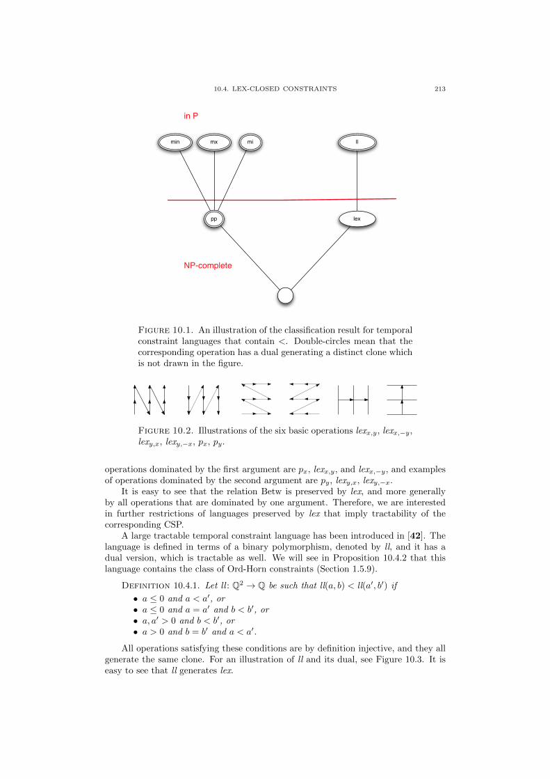
10.4. LEX-CLOSED CONSTRAINTS 213
ll
NP-complete
in P
pp lex
min mx mi
Figure 10.1. An illustration of the classification result for temporalconstraint languages that contain <. Double-circles mean that thecorresponding operation has a dual generating a distinct clone whichis not drawn in the figure.
Figure 10.2. Illustrations of the six basic operations lexx,y, lexx,−y,lexy,x, lexy,−x, px, py.
operations dominated by the first argument are px, lexx,y, and lexx,−y, and examplesof operations dominated by the second argument are py, lexy,x, lexy,−x.
It is easy to see that the relation Betw is preserved by lex, and more generallyby all operations that are dominated by one argument. Therefore, we are interestedin further restrictions of languages preserved by lex that imply tractability of thecorresponding CSP.
A large tractable temporal constraint language has been introduced in [42]. Thelanguage is defined in terms of a binary polymorphism, denoted by ll, and it has adual version, which is tractable as well. We will see in Proposition 10.4.2 that thislanguage contains the class of Ord-Horn constraints (Section 1.5.9).
Definition 10.4.1. Let ll : Q2 → Q be such that ll(a, b) < ll(a′, b′) if
• a ≤ 0 and a < a′, or• a ≤ 0 and a = a′ and b < b′, or• a, a′ > 0 and b < b′, or• a > 0 and b = b′ and a < a′.
All operations satisfying these conditions are by definition injective, and they allgenerate the same clone. For an illustration of ll and its dual, see Figure 10.3. It iseasy to see that ll generates lex.

214 10. TEMPORAL CONSTRAINT SATISFACTION PROBLEMS
xy xy
Figure 10.3. A visualization of ll (left) and dual-ll (right).
All Ord-Horn relations (Section 1.5.9) are preserved by ll.
Proposition 10.4.2. All relations in Ord-Horn are preserved by ll and dual ll.
Proof. We give the argument for ll only; the argument for dual ll is analogous.It suffices to show that every relation that can be defined by a formula φ of the form(x1 = y1 ∧ · · · ∧ xk−1 = yk−1)→ xk O yk is preserved by ll, where O ∈ {=, <,≤, 6=}.Let t1 and t2 be two 2k-tuples that satisfy φ. Consider a 2k-tuple t3 obtained byapplying ll componentwise to t1 and t2. Suppose first that there is an i ≤ k − 1 suchthat one of the tuples does not satisfy xi = yi. Then xi = yi is not satisfied in t3as well, by injectivity of ll, and therefore the tuple t3 satisfies φ. Now consider thecase that xi = yi holds for all i ≤ k − 1 in both tuples t1 and t2. Since t1 and t2satisfy φ, the literal xkOyk holds in both t1 and t2. Because ll preserves all relationsin {=, <,≤, 6=}, the literal xkOyk holds in t3, and therefore t3 satisfies φ as well. �
Since the relation Rmin defined by (x > y) ∨ (x > z) (see Section 1.5.8) ispreserved by ll but not by dual ll, the class of ll-closed constraints is strictly largerthan Ord-Horn.
10.4.2. Operations generating ll, dual-ll, or lex. In this section we presentoperations that generate ll, dual-ll, or lex. We again use the concept of a behaviorof operations over a relational structure; note that a k-ary operation f behaves likea k-ary operation g on S = S1 × · · · × Sk if for all t, t′ ∈ S we have f(t) ≤ f(t′)iff g(t) ≤ g(t′). That is, the weak linear order induced by f on the tuples from G(in the sense of Observation 10.2.3) is the same as the weak linear order induced onthese tuples by g. Let Q+ denote the set of all positive rational numbers, and let Q−0denote Q \Q+.
Definition 10.4.3. Let f, g be from Q2 → Q. Then [f |g] denotes an arbitraryoperation from Q2 → Q with the following properties. For all x, x′, y, y′ ∈ Q,
• if x ≤ 0 and x′ > 0 then [f |g](x, y) < [f |g](x′, y′);• [f |g] behaves like f on Q−0 ×Q;• [f |g] behaves like g on Q+ ×Q;
For example, if f = lexx,y and g = lexy,x, then [f |g] behaves like ll.
Lemma 10.4.4. Let f, g ∈ {lexx,y, lexx,−y, lexy,x, lexy,−x, px, py}, and let f ′ (g′)be lexx,y if f (g) is dominated by the first argument, and lexy,x otherwise. Then{lex, [f |g]} generates [f ′|g′](x, y).
Proof. By Proposition 5.2.1 it suffices to show that every relation R preservedby lex and [f |g] is preserved by [f ′|g′]. So let R be an arbitrary relation preservedby lex and [f |g], let k denote its arity, and let t1, t2 be k-tuples from R. We have toshow that t3 := [f ′|g′](t1, t2) is in R.

10.4. LEX-CLOSED CONSTRAINTS 215
xy y x
Figure 10.4. An illustration of the operation [py|py] (on the left)and the operation [lexy,x|lexy,x] (on the right).
Let α ∈ Aut((Q;<)) be such that for each entry x of t1 and for each entry y oft2, the value of αlex(x, y) is negative when x ≤ 0, and positive otherwise. We willshow that there is an automorphism of (Q;<) that maps the tuple
s := [f |g](αlex(t1, t2), lex(t2, t1))
to t3, which proves that t3 is in R. It suffices to show for j1, j2 ∈ [k] that
s[j1] ≤ s[j2] if and only if t3[j1] ≤ t3[j2] . (25)
We can assume that t1[j1] ≤ t1[j2] by exchanging the name of j1 and j2 if neces-sary, and distinguish three cases:
• t1[j1] ≤ 0, t1[j2] > 0. Then t3[j1] < t3[j2] by definition of [f ′|g′]. Since forj ∈ [k], the value of αlex(t1[j], t2[j]) is positive if and only if the value oft1[j] is positive, we have s[j1] < s[j2] by definition of [f |g]. Thus we haveverified (25) in this case.
• t1[j2] ≤ 0. Note that f(lex(x, y), lex(y, x)) behaves like f ′(x, y). Thus, writ-ing a[j] for lex(t1[j], t2[j]) and b[j] for lex(t2[j], t1[j]), we have the followingequivalences.
t3[j1] ≤ t3[j2] iff f ′(t1[j1], t2[j1]) ≤ f ′(t1[j2], t2[j2])
iff f(a[j1], b[j1]) ≤ f(a[j2], b[j2])
iff f(αa[j1], b[j1]) ≤ f(αa[j2], b[j2])
iff s[j1] ≤ s[j2]
• t1[j1] > 0. This case is analogous to the previous one and left to the reader.
�
Lemma 10.4.5. For f, g ∈ {py, lexy,x} the operation [f |g] generates [lexx,y|g].
In particular, for f = g = lexy,x the lemma shows that [f |g] generates ll. Forf = g = py, the lemma shows that [f |g] generates [lexx,y|py] and in particular lexx,y.See Figure 10.4 for illustrations of those two cases.
Proof of Lemma 10.4.5. We show that every relation R preserved by [f |g] ispreserved by [lexx,y|g], and conclude by Proposition 5.2.1 that [f |g] generates [lexx,y|g].So let R be an arbitrary relation preserved by [f |g], let k denote its arity, and let t1, t2be k-tuples from R. We have to show that t3 := [lexx,y|g](t1, t2) is in R.
Let l denote the number of non-positive values in t1. We take α1, . . . , αl fromAut((Q;<)) such that αi maps all but the i smallest values in t1 to positive values.
216 10. TEMPORAL CONSTRAINT SATISFACTION PROBLEMS
We define a sequence of tuples s1, . . . , sl as follows: s1 = t2, and for i ≥ 2
si := [f |g](αit1, si−1) .
Clearly, for all i ∈ [l] the tuple si is in R. We will show that there is an automor-phism of (Q;<) that maps sl to t3, which proves that t3 is also in R. By symmetryit is enough to show for j1, j2 ∈ [k] with t1[j1] ≤ t1[j2] that
sl[j1] ≤ sl[j2] if and only if t3[j1] ≤ t3[j2] . (26)
We distinguish three cases:
• t1[j1] = t1[j2] ≤ 0. Since αit1[j1] = αit1[j2] for all i ∈ [l], we have sl[j1] ≤sl[j2] if and only if s1[j1] ≤ s1[j2]. Since s1 = t2 and t1[j1] ≤ 0, andbecause f is dominated by the second argument, s1[j1] ≤ s1[j2] if and onlyif t3[j1] ≤ t3[j2], which proves (26).
• t1[j1] < t1[j2], t1[j1] ≤ 0. Let i ∈ [l] be such that αit1[j1] ≤ 0 and αit1[j2] >0. By definition of [f |g] we see that si[j1] < si[j2]. Because αit1[j1] <αit1[j2] for all i ∈ [l], and because [f |g] preserves <, by induction on i′ ≥ iwe have that si′ [j1] < si′ [j2]. In particular, sl[j1] < sl[j2]. On the otherhand, t3[j1] < t3[j2] by definition of lexx,y and [lexx,y|g], and so (26) alsoholds in this case.
• t1[j1] > 0. Observe that by the choice of l we have αit1[j1] > 0 for all i ∈ [l].Thus (26) holds, because both [f |g] and [lexx,y|g] behave like g on Q+ ×Q.
�
10.4.3. A syntactic description of ll-closed constraints. In this section wepresent a syntactic characterisation of ll-closed relations. As a consequence, we alsoobtain a better understanding of the clone generated by ll.
Definition 10.4.6. A formula is called ll-Horn if it is a conjunction of formulasof the following form
(x1 = y1 ∧ · · · ∧ xk = yk)⇒ (z1 < z0 ∨ · · · ∨ zl < z0) , or
(x1 = y1 ∧ · · · ∧ xk = yk)⇒ (z1 < z0 ∨ · · · ∨ zl < z0 ∨ (z0 = z1 = · · · = zl))
where 0 ≤ k, l.
Note that k or l might be 0: if k = 0, we obtain a formula of the form z1 <z0∨· · ·∨zl < z0 or (z1 < z0∨· · ·∨zl < z0∨(z0 = z1 = · · · = zl)), and if l = 0 we obtaina disjunction of disequalities. Also note that the variables x1, . . . , xk, y1, . . . , yk, z0,. . . , zl need not be pairwise distinct. On the other hand, the clause z1 < z2 ∨ z3 < z4
is an example of a formula that is not ll-Horn.The following result is from [42], but Antoine Mottet found a mistake in the proof
presented there; the new proof presented below is also due to him.
Proposition 10.4.7. A temporal relation is preserved by ll if and only if it canbe defined by an ll-Horn formula.
Proof. The proof that every relation defined by an ll-Horn formula is ll-closedis similar to the proof of Proposition 10.4.2. We just need to additionally checkthat the relation defined by z1 < z0 ∨ · · · ∨ zl < z0 and the relation defined byz1 < z0 ∨ · · · ∨ zl < z0 ∨ (z0 = · · · = zl) are preserved by ll. So let s and t betwo assignments that satisfy φ := z1 < z0 ∨ · · · ∨ zl < z0, and let r := ll(s, t). Leti ∈ {1, . . . , l} be such that s(zi) = min(s(z1), . . . , s(zl)). Note that s(zi) < s(z0). Letj ∈ {1, . . . , l} be such that t(zj) < t(z0).
• If s(zi) ≤ 0 then ll(s(zi), t(zi)) < ll(s(z0), s(z0)) since s(zi) < s(z0), andhence r satisfies φ.

10.4. LEX-CLOSED CONSTRAINTS 217
• If s(zi) > 0, then s(z0) > s(zi) > 0 and s(zj) > s(zi) > 0, and hencell(s(zj), t(zj)) < ll(s(z0), s(z0)) since t(zj) < t(z0), and hence r satisfies φ.
When t1 and t2 are satisfying assignments of z1 < z0 ∨ · · · ∨ zl < z0 ∨ (z0 = · · · = zl)where one of the assignments satisfies the last clause, then the statement follows fromthe fact that ll is injective and preserves ≤.
Let R be a temporal relation, and let φ be a quantifier-free formula in CNF thatdefines R over (Q;<). In this formula, we replace literals of the form ¬(y < x) byx < y ∨ x = y, and we use x ≤ y as shortcut for those two literals. For reasonsthat will become clear later, we additionally allow that clauses contain ‘clusteredequations’ which are expressions of the form x1 = x2 = · · · = xn and which stand forx1 = x2 ∧ · · · ∧ x1 = xn; such an expression will be treated as one literal.
We describe four rewriting rules that yield a formula ψ that also defines R over(Q;<) such that R is preserved by ll if and only if ψ is ll-Horn.
(1) If φ implies x = y for distinct variables x, y of φ, replace all occurrences ofu in φ by x and add the clause x = y.
(2) Suppose that φ contains a clause θ of the form
x < y ∨ u < v ∨ θ′ ,let φ′ be the other clauses of φ, and suppose that
(φ′ ∧ ¬θ′ ∧ x < y) implies (u ≤ v ∨ x ≤ v)
and (φ′ ∧ ¬θ′ ∧ u < v) implies (x ≤ y ∨ u ≤ y) .
Then replace θ by
(u ≤ v ∨ x ≤ v ∨ θ′) ∧ (u 6= v ∨ x < y ∨ θ′)∧ (x ≤ y ∨ u ≤ y ∨ θ′) ∧ (x 6= y ∨ u < v ∨ θ′) .
(3) Suppose that φ contains a clause θ of the form
x < y ∨ u < v ∨ θ′ .Let φ′ be the other clauses of φ, and suppose that
(φ′ ∧ ¬θ′ ∧ x < y) implies u ≤ v .Then replace θ by
(u ≤ v ∨ θ′) ∧ (x < y ∨ u 6= v ∨ θ′).
(4) Suppose that θ is a clause of φ of the form
x1 6= y1 ∨ · · · ∨ xk 6= yk ∨ z1 < z0 ∨ · · · ∨ zl < z0 ∨ u = v ,
let φ′ be the other clauses of φ, and that
φ′ ∧ x1 = y1 ∧ · · · ∧ xk = yk ∧ z0 ≤ z1 ∧ · · · ∧ z0 ≤ zl ∧ u = v
implies that z0 = z1 = · · · = zl. Then replace θ by
(x1 6= y1 ∨ · · · ∨ xk 6= yk ∨ z0 6= z1 ∨ · · · ∨ z0 6= zl ∨ u = v)
∧ (x1 6= y1 ∨ · · · ∨ xk 6= yk ∨ z1 < z0 ∨ · · · ∨ zl < z0 ∨ z0 = z1 = · · · = zl) .
(5) If φ contains a literal such that removing this literal from φ results in anequivalent formula, then remove the literal.
We claim that for each of the four rewriting rules, the resulting formula ψ is equivalentto φ. This is obvious for rules (1) and (5). To see that φ implies the new clauses inrule (2), let s be a satisfying assignment to φ. If s satisfies θ′, then s also satisfiesthe new clauses, so let us assume that θ′ is false. Then s satisfies x < y or u < v.The two cases are symmetric, so we only treat the case that s satisfies x < y in the

218 10. TEMPORAL CONSTRAINT SATISFACTION PROBLEMS
following. By assumption, s must then satisfy u ≤ v ∨ y ≤ v, and hence the first newclause is satisfied by s. Since x < y, the other new clauses are satisfied, too.
Now suppose conversely that s is a solution to φ′ and the four new clauses, andsuppose for contradiction that θ does not hold. Because of the second and fourth newclause, we then must have u 6= v and x 6= y. Then the first new clause implies thatx ≤ v and the third new clause implies that u ≤ y. But then x ≤ v ≤ u ≤ y ≤ x, acontradiction to x 6= y.
For rule (3), let s be a solution to φ. Then s obviously satisfies the first new clauseif u < v or θ′ holds; otherwise, s must satisfy x < y because of θ. But then u ≥ v byassumption and hence the first new clause also holds in this case. The second newclause is weaker then θ, so it is also satisfied by s. Now suppose conversely that ssatisfies φ′ and the two new clauses, and suppose for contradiction that θ does nothold. Then in particular v ≤ u holds and the first new clause implies that u = v, andhence x < y because of the second new clause, contradiction to the assumption thatθ does not hold.
Finally, for the fourth rule, the first new clause is a weakening of θ, and the secondnew clause is a consequence of φ by assumption. Conversely, suppose that s satisfiesall clauses of φ except for θ which is not satisfied. Then the first new clause impliesthat z1 < z1 ∨ · · · ∨ zl < z0, and thus the second new clause implies that u = v, andhence θ holds, contradiction. Hence, ψ is indeed equivalent to φ.
Note that rules (2) and (3) strictly reduce the number of pairs of literals x < yand u < v in the same clause where y and v are distinct variables. Rule (4) leavesthis number invariant, but strictly reduces the number of literals of the form u = v orof the form u < v in the clause (here, we do not count complex equations). Rules (1)and (5) do not increase these numbers, and strictly reduce the number of variablesthat occur more than once, or strictly reduce the total number of literals. Hence,when we repeatedly apply these rules, the procedure will eventually terminate.
Claim 1. The formula ψ cannot contain a clause θ of the form x < y∨u < v∨ θ′where x and u are distinct variables. Since rule (2) is not applicable, there must exista solution s to φ′ ∧¬θ′ ∧ x < y ∧ v < u∧ v < x or to φ′ ∧¬θ′ ∧ u < v ∧ y < x∧ y < u.Suppose the former is the case, since the latter case can be treated similarly. Sincerule (3) is not applicable, there exists a solution t to φ′ ∧ ¬θ′ ∧ u < v ∧ y < x. Letα ∈ Aut(Q;<) be such that αs(v) = 0. We claim that r = ll(αs, t) does not satisfy θ:
• we have r(y) < r(x) since 0 < s(x), s(y) and t(y) < t(x);• we have r(v) < r(u) since s(v) = 0 and s(u) > 0;• finally, r does not satisfy θ′ since neither s nor t satisfy θ′.
Hence, r does not satisfy ψ, in contradiction to the assumption that ll preserves R.Claim 2. The formula ψ cannot contain a clause with two distinct literals x = y
and u = v. This is because rule (5) and since φ is preserved by the injective functionll.
Claim 3. If ψ contains a clause with a literal z1 < z0 and a literal u = v, then{u, v} = {x, y}. This is because of Claim 1 and Claim 2, any such clause must be ofthe form x1 6= y1 ∨ · · · ∨ xk 6= yk ∨ z1 < z0 ∨ · · · ∨ zl < z0 ∨ u = v. Since rule (4) doesnot apply, there exists a solution s to
φ′ ∧ x1 = y1 ∧ · · · ∧ xk = yk ∧ z0 ≤ z1 ∧ · · · ∧ z0 ≤ zl ∧ u = v
∧ z0 6= z1 ∨ · · · ∨ z0 6= zl .
Hence, there exists an i ∈ {1, . . . , l} such that s(z0) 6= s(zi). Because the literalzi < z0 cannot be removed from ψ with rule (5), there exists a solution t to φ suchthat zi < z0 is the only literal in θ satisfied by t. Let α ∈ Aut(Q;<) be such thatαt(zi) = 0. Then r := ll(αt, s) does not satisfy θ:

10.4. LEX-CLOSED CONSTRAINTS 219
Figure 10.5. Illustration of an operation f generated by ll thatsatisfies f(x, y) = αf(β(x), β(y)).
• r satisfies θ′∧x1 = y1∧ · · · ∧xk = yk since both t and s satisfy this formula.• r(zi) < r(z0) since 0 = αt(zi) < αt(z0).• r(zj) ≤ r(z0) for all i ∈ {1, . . . , k}\{i} since t(z0) ≤ t(zj) and s(z0) ≤ s(zj).• r(u) 6= r(v) since t(u) 6= t(v) and ll is injective.
The three claims imply that each of the clauses of ψ must be logically equivalent toan implication as in Definition 10.4.6, and this concludes the proof. �
10.4.4. Weak Commutativity. In this section we present a different descrip-tion of ll-closed temporal constraint languages. Let c1, . . . , cn ∈ Q be arbitrary.Partition the rationals Q = Q1 ]Q1 such that each of Q1 and Q2 is dense in Q, andlet f be any injective binary operation that preserves < and ≤ such that
• f(ci, ci) = ci for all i ≤ n;• for x ∈ Q1, we have that f(x, y1) > f(y2, x) for all y1, y2 > x;• for x ∈ Q2, we have that f(x, y1) < f(y2, x) for all y1, y2 > x.
We even assume that f is bijective: since the image of any such function will inducea dense linear order without endpoints in (Q;<), the existence of such a functionfollows from ω-categoricity of (Q;<).
For an illustration of f , see Figure 10.5. The red vertices are the elements of{(x, x) | x ∈ Q1}, and the blue blue vertices the elements of {(x, x) | x ∈ Q2}.Observe that f(x, y) < f(z, z) for all x, y, z such that x < z or y < z.
Proposition 10.4.8. There are automorphisms α, β of (Q;<, c1, . . . , cn) suchthat f(x, y) = αf(βy, βx) holds for all x, y ∈ Q.
Proof. Let β be an automorphism of (Q;<, c1, . . . , cn) that mapsQ1\{c1, . . . , cn}toQ2\{c1, . . . , cn} andQ2\{c1, . . . , cn} toQ1\{c1, . . . , cn}; such an automorphism caneasily be constructed by going back-and-forth. To define α ∈ Aut((Q;<, c1, . . . , cn)),let d ∈ Q be arbitrary. Since f and β are bijective, f ′ : (x, y) 7→ f(βy, βx) is bijec-tive as well, so there exists a unique pair (a, b) ∈ Q2 such that f ′(a, b) = d. Defineα(d) = f(a, b). Then by definition αf(βy, βx) = f(x, y) holds for all x, y ∈ Q, and itis straightforward to verify that α ∈ Aut((Q;<, c1, . . . , cn)). �

220 10. TEMPORAL CONSTRAINT SATISFACTION PROBLEMS
Proposition 10.4.9. The operation f defined above is generated by ll, and gen-erates ll.
Proof. It is easy to see that f interpolates ll. For the converse, it suffices toverify that f preserves all ll-Horn formulas, by Proposition 10.4.7. Since f is injective,it suffices to show that f preserves formulas of the form
(z0 > z1) ∨ · · · ∨ (z0 > zl)
and formulas of the form
(z0 > z1) ∨ · · · ∨ (z0 > zl) ∨ (z0 = z1 = · · · = zl) .
Preservation of formulas of the latter type reduces to the former type, since f preserves≤ and is injective binary. Now suppose that a = (a0, a1, . . . , al) and b = (b0, b1, . . . , bl)are two tuples that satisfy z1 < z0 ∨ · · · ∨ zl < z0. Assume that a0 ≤ b0. Let i besuch that ai = min(a1, . . . , al). Then ai < a0, and we get that f(a0, b0) ≥ f(a0, a0) >f(ai, bi) by the properties of f . Therefore, min(f(a1, b1), . . . , f(al, bl)) < f(a0, b0).We can argue analogously in the case that a0 ≥ b0. �
10.4.5. Weak near-unanimity modulo endomorphisms. For a uniform pre-sentation of the classification result in Section 10.6, we need yet another descriptionof the clone generated by ll.
We write lex(x1, . . . , xn) as a shortcut for lex(x1, lex(x2, . . . lex(xn−1, xn) . . . )).
Proposition 10.4.10. There are a, b, c ∈ End(Q;<) such that the ternary func-tion f : Q3 → Q defined by
f(x, y, z) = lex(min(x, y, z),max (min(x, y),min(x, z),min(y, z)), x, y, z)
satisfies for all x, y ∈ Qa(f(x, x, y)) = b(f(x, y, x)) = c(f(y, x, x)) .
That is, f is a weak near unanimity modulo endomorphisms of (Q;<).
Proof. By Lemma 5.6.7, it suffices to show that for every finite S ⊂ Q there areα, β ∈ Aut(Q;<) such that for all x, y ∈ S
f(y, x, x) = α1f(x, y, x) = α2f(x, x, y) .
By the properties of f we have that f(y, x, x) ≤ f(y′, x′, x′) if and only if one of thefollowing holds:
• min(x, y) < min(x′, y′);• min(x, y) = min(x′, y′) and x < x′;• min(x, y) = min(x′, y′), x = x′, and y < y′;• x = x′ and y = y′.
Note that this is the case if and only if f(x, y, x) < f(x′, y′, x′), and if and only iff(x, x, y) < f(x′, x′, y′). Hence, the existence of α1 and α2 follows from the homo-geneity of (Q;<). �
Note that the function f defined in Proposition 10.4.10 is injective and preserves≤.
Theorem 10.4.11. Let R ⊆ Qn be first-order definable over (Q;<). Then thefollowing are equivalent.
(1) R is preserved by the operation f as defined in Proposition 10.4.10 (a weaknear unanimity modulo endomorphisms).
(2) R is preserved by ll.(3) R has an ll-Horn definition.

10.4. LEX-CLOSED CONSTRAINTS 221
Proof. The implication from (1) to (2) follows from the observation that (x, y) 7→f(x, x, y) interpolates ll. The implication from (2) to (3) is Lemma 10.4.7. For theimplication from (3) to (1), it suffices to verify that f preserves all ll-Horn formulas.Since f is injective, it suffices to show that f preserves formulas φ of the form
(z1 < z0) ∨ · · · ∨ (zl < z0)
and of the form
(z1 < z0) ∨ · · · ∨ (zl < z0) ∨ (z0 = z1 = · · · = zl) .
Suppose that s1, s2, s3 are assignments that satisfy φ; we have to show that theassignment s defined by s(x) := f(s1(x), s2(x), s3(x)) satisfies φ. Let j ∈ {1, 2, 3} besuch that sj(z0) = min(s1(z0), s2(z0), s3(z0)).
Suppose first that sj satisfies (z1 < z0 ∨ · · · ∨ zl < z0). Let i be such thatsj(zi) = min(sj(z1), . . . , sj(zl)). Then sj(zi) < sj(z0) by assumption, and hence
min(s1(zi), s2(zi), s3(zi)) < min(s1(z0), s2(z0), s3(z0)) .
Therefore, f(s1(zi), s2(zi), s3(zi)) < f(s1(z0), s2(z0), s3(z0)) by the properties of f ,and s satisfies (z1 < z0 ∨ · · · ∨ zl < z0).
Otherwise, sj must satisfy z0 = z1 = · · · = zl. Let a, b be such that a < b and{a, b} = {1, 2, 3} \ {j}. We next consider the case that there exists c ∈ {a, b} andp ∈ {1, . . . , l} such that sj(z0) > sc(zp). Let d ∈ {a, b} \ {c}. Note that
min(sc(zp), sd(zp)) ≤ sc(zp) < sj(zp) = sj(z0) = min(sc(z0), sd(z0))
min(sj(zp), sc(zp)) = sc(zp) < sj(zp) = sj(z0) = min(sc(z0), sj(z0))
min(sj(zp), sc(zp)) = sc(zp) < sj(zp) = sj(z0) = min(sc(z0), sj(z0))
and hence
max (min(sc(zp), sd(zp)),min(sj(zp), sc(zp)),min(sj(zp), sd(zi)))
< max (min(sc(z0), sd(z0)),min(sj(z0), sc(z0)),min(sj(z0), sd(zi))) .
Thus, by the definition of f , we have s(zp) < s(z0) and s satisfies φ.Otherwise, sj(z0) ≤ min(sa(z1), . . . , sa(zl)) and sj(z0) ≤ min(sb(z1), . . . , sb(zl)).
For all i ∈ {0, 1, . . . , l} we have sj(zi) = sj(z0) and hence
max (min(sa(zi), sb(zi)),min(sj(zi), sa(zi)),min(sj(zi), sb(zi)))
= min(sa(zi), sb(zi)) ≥ sj(zi) .
The definition of f then implies that f(s1(zi), s2(zi), s3(zi)) < f(s1(z0), s2(z0), s3(z0))if and only if sa(zi) < sa(z0). If there exists an i ∈ {1, . . . , l} such that sk(zi) < sk(z0),we therefore have s(zi) < s(z0) and s satisfies (z1 < z0) ∨ · · · ∨ (zl < z0). Otherwise,we must have that
sa(z0) = sa(z1) = · · · = sa(zl)
If also sb(z0) = sb(z1) = · · · = sb(zl) then s satisfies z0 = z1 = · · · = zl, too. Sosuppose that there exists a p ∈ {1, . . . , l} such that sb(zp) < sb(z0). Since sj(zp) =sj(z0) and sa(zp) = sa(z0) we then have s(zp) < s(z0) since s is injective and preserves≤. Hence, s satisfies φ also in this case. �
10.4.6. An Algorithm for ll-closed Constraints. In this section we presentan algorithm for ll-closed constraints. One of the underlying ideas of the algorithm isto use a subroutine that tries to find a solution where every variable has a differentvalue. If this is impossible, the subroutine must return a set of at least two variablesthat denote the same value in all solutions – since the constraints are preserved by abinary injective operation, such a set must exist (Proposition 6.1.5).

222 10. TEMPORAL CONSTRAINT SATISFACTION PROBLEMS
The i-th entry in a k-tuple t is called minimal if t[i] ≤ t[j] for every j ∈ [k]. It iscalled strictly minimal if t[i] < t[j] for every j ∈ [k] \ {i}.
Definition 10.4.12. Let R be a k-ary temporal relation. A set S ⊆ [k] is calleda min-set for the i-th entry in R if there exists a tuple t ∈ R such that the i-th entryis minimal in t, and for all j ∈ [k] it holds that j ∈ S if and only if t[i] = t[j]. Wesay that t is a witness for this min-set.
Let R be a k-ary relation that is preserved by lex (recall that ll-closed constraintsare preserved by lex as well), and suppose that the i-th entry has the min-setsS1, . . . , Sl, for l ≥ 1, with the corresponding witnesses t1, . . . , tl. Consider the tu-ple t := lex(t1, lex(t2, . . . lex(tl−1, tl))). Since the entry i is minimal in every tuplet1, . . . , tl, and since lex preserves both < and ≤, it is also minimal in t. Because lexis injective, we have that t[i] = t[j] if and only if these two entries are equal in eachtuple t1, . . . , tl. Hence, the min-set for the i-th entry in R witnessed by the tuple t isa subset of every other min-set S1, . . . , Sl. We then call this set the minimal min-setfor the i-th entry in R.
Lemma 10.4.13. Let R be a k-ary relation preserved by lex, and let S be theminimal min-set for the i-th entry in R. If t ∈ R is such that t[j] ≥ t[i] for everyj ∈ S, then t[i] = t[j] for every j ∈ S.
Proof. Let t′ ∈ R be the tuple that witnesses the minimal min-set S. Let t ∈ Rbe such that not all entries in S are equal (in particular, |S| > 1). Consider the tuples := lex(t′, t). By the properties of lex it holds that s[i] < s[j] for every j ∈ [k] \ S.Furthermore, s[i] ≤ s[j] for j ∈ S if and only if t[i] ≤ t[j]. Thus, unless s witnesses asmaller min-set for i in R (which would be a contradiction), we have that s[i] > s[j]for some j ∈ S. �
To develop our algorithm, we use a specific notion of constraint graph of a tem-poral CSP instance, defined as follows.
Definition 10.4.14. The constraint graph Gφ of a temporal CSP instance φ isa directed graph (V ;E) defined on the variables V of φ. For each constraint of theform R(x1, . . . , xk) from φ we add a directed edge (xi, xj) to E if in every tuple fromR where the i-th entry is minimal, the j-th entry is minimal as well.
Definition 10.4.15. If an instance of a temporal CSP contains a constraint φimposed on y such that φ does not admit a solution where y denotes the minimalvalue, the we say that y is blocked (by φ).
We can easily determine for each constraint which variables are blocked by thisconstraint: For a constraint represented by weak linear orders we just check all weaklinear orders and build a set of variables that are not minimal in any of them. Thus, byinspecting all the constraints it is possible to compute the blocked variables in lineartime in the input size. We want to use the constraint graph to identify variables thathave to denote the same value in all solutions, and therefore introduce the followingconcepts.
Definition 10.4.16. A strongly connected component K of the constraint graphGφ for a temporal CSP instance φ is called a sink component if no edge in Gφ leavesK, and no variable in K is blocked. A vertex of G that belongs to a sink componentof size one is called a sink.
Lemma 10.4.17. Let B be a lex-closed temporal constraint language. Let φ bean instance of CSP(B) with variables V , and let K ⊆ V be a sink component of thegraph Gφ. Then in every solution of φ all variables from K must have equal values.

10.4. LEX-CLOSED CONSTRAINTS 223
Proof. We assume that φ has a solution s : V → Q, and that K has at leasttwo vertices; otherwise the statement is trivial. Define M := {x ∈ K | s(x) ≤s(y) for all y ∈ K}. We want to show that M = K. Otherwise, because K is astrongly connected component, there is an edge in Gφ from some vertex u ∈ M tosome vertex v ∈ K \M . By the definition of Gφ, there is a constraint ψ in φ suchthat whenever u denotes the minimal value of a solution of ψ, then v has to denotethe minimal value as well. By permuting arguments, we can assume without loss ofgenerality that ψ is of the form R(w1, . . . , wk) where w1 = u. Because K is a sinkcomponent, the variable u cannot be blocked, and hence there is a minimal min-setS for the first entry in R.
Note that Gφ contains an edge from u to wi for all i ∈ S. Since K is a stronglyconnected component, all these variables wi are in K. Because s(u) ≤ s(y) for ally ∈ K, there is no variable wi, i ∈ S, such that s(wi) < s(u). This contradictsLemma 10.4.13, because s(u) 6= s(v). �
Lemma 10.4.17 immediately implies that we can add constraints of the type x = yfor all variables x, y from the same sink component K. Equivalently, we can considerthe CSP instance where all the variables in K are contracted, i.e., where all variablesfrom K are replaced by the same variable. When φ = ∃x1, . . . , xn (φ1∧· · ·∧φm) is aninstance of a CSP(B), and xi ∈ V := {x1, . . . , xn}, then we write φ[V \ {xi}] for theformula ∃x1, . . . , xi−1, xi+1, . . . , xn
((∃xi.φ1)∧· · ·∧(∃xi.φm)
). Note that if B contains
all primitive positive definable relations whose arity is bounded by the maximal arityof the relations in B, then φ[V \ {xi}] can be viewed as an instance of CSP(B).
Lemma 10.4.18. Let B be an ll-closed temporal constraint language. Let φ be aninstance of CSP(B) with variables V , and let x be a sink in Gφ. If φ[V \ {x}] has aninjective solution, then φ has an injective solution as well.
Proof. Let s : V → Q be an injective solution to φ[V \ {x}]. We claim that anyextension r of s to x such that r(x) < s(y) for all y ∈ V \ {x} is injective and satisfiesφ. If x appears in no constraint in φ, the statement is trivial. Consider a constraintψ = R(x1, . . . , xk) from φ that is imposed on x, and let S ⊆ [k] be such that i ∈ S ifand only if x = xi. By the definition of φ[V \ {x}], the mapping s has an extensions′ that is also defined on x such that (s′(x1), . . . , s′(xk)) ∈ R. Because x is a sink,there is tuple t ∈ R such that S is the minimal min-set for the i-th entry of R foreach i ∈ S. Let t′ be the tuple (s′(x1), . . . , s′(xk)), and let α ∈ Aut((Q;<)) be suchthat αs′(x) = 0. Then r := ll(αt′, t) ∈ R. Note that for i, j ∈ [k] \ S, we have thatr[i] ≤ r[j] if and only if r(xi) ≤ r(xj). Hence, r satisfies all constraints from φ, whichis what we had to show. �
Our algorithm for ll-closed constraints can be found in Figure 10.7; we are nowready to prove its correctness.
Theorem 10.4.19. The procedure Solve(φ) in Algorithm 10.7 decides whether agiven set of ll-closed constraints φ has a solution. There is an implementation of thealgorithm that runs in time O(nm), where n is the number of variables of φ and mis the size of the input.
Proof. The correctness of the procedure Spec immediately implies the correct-ness of the procedure Solve. In the procedure Spec, after iterated deletion of sinks inGφ, we have to distinguish three cases.
First, consider the case V = X. In this case it follows by a straightforwardinduction from Lemma 10.4.18 that φ has an injective solution. Otherwise, considerthe case that Gφ contains a sink component S with |S| ≥ 2. We claim that for all

224 10. TEMPORAL CONSTRAINT SATISFACTION PROBLEMS
Spec(φ)// Input: An instance φ of CSP(B) with variables V .// Output: If algorithm returns false then φ has no solution.// If φ has an injective solution, then algorithm returns true.// Otherwise return S ⊆ V , |S| ≥ 2, such that// for all x, y ∈ S we have x = y in all solutions to φ.Set X := ∅While Gφ contains a sink sX := X ∪ {s}If X = V then return trueelse φ := φ[V \X]
If Gφ has sink component S return Selse return false
end if
Figure 10.6. A polynomial-time algorithm for CSP(B) when B isll-closed: the sub-procedure Spec.
Solve(Φ)// Input: An instance φ.// Output: accept if φ is true, reject otherwise.S := Spec(φ)If S = false then rejectelse if S = true then acceptelse
Let φ′ be contraction of S in φ.Return Solve(φ′).
end if
Figure 10.7. A polynomial-time algorithm for CSP(B) when B isll-closed: the main procedure.
variables x, y ∈ S we have x = y in all solutions to φ. Lemma 10.4.17 applied toφ[V \X] implies that all variables in the same sink component must have the samevalue in every solution, and hence the output is correct in this case as well.
In the third case we have X 6= V but Gφ does not contain a sink component.Note that in every solution to φ some variable must take the minimal value. However,since each strongly connected component without outgoing edges contains a blockedvertex, there is no variable that can denote the minimal element, and hence φ has nosolution. Because φ is at all times of the execution of the algorithm implied by theoriginal input constraints, the algorithm correctly rejects.
Since in each recursive call of Solve the instance in the argument has at leastone variable less, Solve is executed at most n times. It is not difficult to implementthe algorithm such that the total running time is cubic in the input size. However,it is possible to implicitly represent the constraint graph and to implement all sub-procedures such that the total running time is in O(nm); for the details, we referto [42]. �
10.5. Shuffle-closed Constraints
An important subclass of temporal constraint languages are shuffle-closed con-straint languages. As we will see, there are NP-complete shuffle-closed constraint
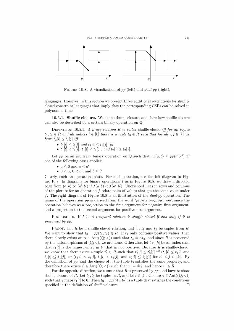
10.5. SHUFFLE-CLOSED CONSTRAINTS 225
xy xy
Figure 10.8. A visualization of pp (left) and dual-pp (right).
languages. However, in this section we present three additional restrictions for shuffle-closed constraint languages that imply that the corresponding CSPs can be solved inpolynomial time.
10.5.1. Shuffle closure. We define shuffle closure, and show how shuffle closurecan also be described by a certain binary operation on Q.
Definition 10.5.1. A k-ary relation R is called shuffle-closed iff for all tuplest1, t2 ∈ R and all indices l ∈ [k] there is a tuple t3 ∈ R such that for all i, j ∈ [k] wehave t3[i] ≤ t3[j] iff
• t1[i] ≤ t1[l] and t1[i] ≤ t1[j], or• t1[l] < t1[i], t1[l] < t1[j], and t2[i] ≤ t2[j].
Let pp be an arbitrary binary operation on Q such that pp(a, b) ≤ pp(a′, b′) iffone of the following cases applies:
• a ≤ 0 and a ≤ a′• 0 < a, 0 < a′, and b ≤ b′.
Clearly, such an operation exists. For an illustration, see the left diagram in Fig-ure 10.8. In diagrams for binary operations f as in Figure 10.8, we draw a directededge from (a, b) to (a′, b′) if f(a, b) < f(a′, b′). Unoriented lines in rows and columnsof the picture for an operation f relate pairs of values that get the same value underf . The right diagram of Figure 10.8 is an illustration of the dual-pp operation. Thename of the operation pp is derived from the word ‘projection-projection’, since theoperation behaves as a projection to the first argument for negative first argument,and a projection to the second argument for positive first argument.
Proposition 10.5.2. A temporal relation is shuffle-closed if and only if it ispreserved by pp.
Proof. Let R be a shuffle-closed relation, and let t1 and t2 be tuples from R.We want to show that t3 = pp(t1, t2) ∈ R. If t1 only contains positive values, thenthere clearly exists an α ∈ Aut((Q;<)) such that t3 = αt2, and since R is preservedby the automorphisms of (Q;<), we are done. Otherwise, let l ∈ [k] be an index suchthat t1[l] is the largest entry in t1 that is not positive. Because R is shuffle-closed,we know that there exists a tuple t′3 ∈ R such that t′3[i] ≤ t′3[j] iff (t1[i] ≤ t1[l] andt1[i] ≤ t1[j]) or (t1[l] < t1[i], t1[l] < t1[j], and t2[i] ≤ t2[j]) for all i, j ∈ [k]. Bythe definition of pp, and the choice of l, the tuple t3 satisfies the same property, andtherefore there exists β ∈ Aut((Q;<)) such that t3 = βt′3, and hence t3 ∈ R.
For the opposite direction, we assume that R is preserved by pp, and have to showshuffle closure of R. Let t1, t2 be tuples in R, and let l ∈ [k]. Choose γ ∈ Aut((Q;<))such that γ maps t1[l] to 0. Then t3 = pp(γt1, t2) is a tuple that satisfies the conditionsspecified in the definition of shuffle-closure. �

226 10. TEMPORAL CONSTRAINT SATISFACTION PROBLEMS
Due to Proposition 10.5.2, we use the phrase ‘B is shuffle-closed’ interchangeablywith ‘B is preserved by pp’ . The following lemma states an important property ofshuffle-closed languages that will be used several times in the next subsections.
Lemma 10.5.3. Let t1, . . . , tl be tuples from a k-ary shuffle-closed relation R, and
let M1, . . . ,Ml ⊂ [k] be disjoint sets of indices such that⋃li=1Mi = [k] and such that
for all i, j ∈ [l] with i < j and for all i′ ∈ Mi, j′ ∈ Mj it holds that ti[i
′] < ti[j′].
Then there is a tuple t ∈ R such that
• t[i′] < t[j′] for all i, j ∈ [l] with i < j and for all i′ ∈Mi, j′ ∈Mj;
• t[i′] ≤ t[i′′] iff ti[i′] ≤ ti[i′′] for all i ∈ [l] and all i′, i′′ ∈Mi.
Proof. Let β1, . . . , βl−1 ∈ Aut((Q;<)) be such that βi maps max{ti[i′]|i′ ∈Mi}to 0. We set
t := pp(β1t1, pp(β2t2, . . . , pp(βl−1tl−1, tl) . . . )) .
The tuple t clearly belongs to R.We prove by induction on l that t satisfies the other conditions of the lemma.
Observe that β1 maps all the entries of t1 at M1 to non-positive values. Thus forl = 2, it is easy to check from the properties of pp that for each i ∈ M1 and i′ ∈ M2
we have t[i] < t[i′] as required by the statement of the lemma. Also the secondcondition is immediate. For l > 2 let t′ be defined by
t′ := pp(β2t2, pp(β3t3, . . . , pp(βl−1tl−1, tl) . . . )) .
Then we have t = pp(β1t1, t′). Now we apply the same argument as for l = 2. Because
the order on [k]\M1 is preserved by the application of pp, we know that the conditionsare satisfied for the sets M2, . . . ,Ml. The argument also shows that the entries at M1
are smaller than the entries at [k] \M1 and that their order is the same as in t1. �
The following lemma is a simple criterion for showing that certain operationsgenerate pp.
Lemma 10.5.4. Let f be a binary operation preserving < such that for someα, β ∈ Aut((Q;<)) we have f(x, y) = αx for all x ≤ −1, 0 < y < 1, and f(x, y) = βyfor all x > 1, 0 < y < 1. Then f generates pp.
Proof. It suffices to show that every relation preserved by f is also preserved bypp. Let R be preserved by f , and let t1, t2 be two tuples from R. Let γ1 ∈ Aut((Q;<))be such that γx = x + 1 for all positive entries x of t2 and γ1x = x − 1 for all otherentries x of t2. Let γ2 ∈ Aut((Q;<)) be such that all entries of γ2t2 are larger than0 and smaller than 1. Then f(γ1t1, γ2t2) is in the same orbit as pp(t1, t2), which iswhat we wanted to show. �
It is easy to verify that the relation T3, defined in Section 10.2.3, is shuffle-closed.Proposition 10.2.6 shows that CSP((Q;S)) is NP-complete, and thus the property ofshuffle-closure is not strong enough to guarantee tractability.
10.5.2. Min-union closure. This section introduces and studies a strongerproperty than shuffle-closure, namely preservation under the binary operation minthat maps two values x and y to the smaller of the two values; see Figure 10.9 for anillustration of the operation min. We also present a sufficient condition that impliesthat a temporal constraint language is preserved by min.
For constraint languages over a finite domain, min- and max-closed relationswere studied in [125]. An equivalent clausal description of such constraints is known;however, the equivalence only holds for finite domains. The tractability of the CSPwhere the constraint language has such a clausal description has also been shown forinfinite domains [77]. But the algorithm presented in [77] cannot be applied to all

10.5. SHUFFLE-CLOSED CONSTRAINTS 227
Figure 10.9. Illustration of the operation min.
min-closed constraint languages over an infinite domain; it is already not clear howto adapt this approach to deal with the relation {(x, y, z) | x > y ∨ x > z}, which ispreserved by min. In Section 10.5.7 we describe an algorithm that efficiently solvesthe CSP for temporal constraint languages that are preserved by min.
Definition 10.5.5. Let t be from Qk. The set of indices
{i ∈ [k] | t[i] ≤ t[j] for all j ∈ [k]}is called the min-set of t, and denoted by M(t).
Definition 10.5.6. A relation is called min-union closed if for all tuples t1, t2in R there exists a tuple t3 in R such that M(t3) = M(t1) ∪M(t2).
We now want to link min-union closure of the relations in the constraint languageto the existence of certain polymorphisms.
Definition 10.5.7. Let f be a binary operation preserving <. We say that fprovides min-union closure if f(0, 0) = f(0, x) = f(x, 0) for all integers x > 0.
The operation min is an example of an operation providing min-union closure.The following lemma connects Definition 10.5.6 and Definition 10.5.7.
Lemma 10.5.8. Let R be a temporal relation preserved by an operation f providingmin-union closure. Then R is min-union closed.
Proof. Let t1 and t2 be tuples in R, and let a1 and a2 be the minimal valuesamong the entries of t1 and t2, respectively. Then there are α1, α2 ∈ Aut((Q;<)) suchthat α1a1 = α2a2 = 0, and such that α1 and α2 map all other entries of t1 and t2to integers. Observe that all entries at M(t1) ∪M(t2) in the tuple t3 = f(α1t1, α2t2)have the same value. Because f preserves <, this value is strictly smaller than thevalues at all other entries in t3. Hence, M(t3) = M(t1) ∪M(t2). �
The following proposition implies that {f, pp} generates min for every operationf that provides min-union closure.
Proposition 10.5.9. A temporal relation R is preserved by pp and an operationproviding min-union closure if and only if R is preserved by min.
Proof. Clearly, min provides min-union closure. Also observe that min satisfiesthe conditions of Lemma 10.5.4, and hence generates pp.
For the opposite direction, suppose that R is k-ary and preserved by pp and anoperation f providing min-union closure. We show that for any two tuples t1, t2 ∈ Rthe tuple t3 = min(t1, t2) is in R as well. Let l be the number of distinct values in t3and v1 < v2 < · · · < vl be these values. We define Mi, i ∈ [l], to be the set of indicesof t3 with the i-th lowest value, i.e., Mi = {j ∈ [k] | t3[j] = vi}.
Now let α1, . . . , αl ∈ Aut((Q;<)) be such that αivi = 0 and such that the en-tries of αit1 and αit2 are integers. Using these automorphisms we define the tuples

228 10. TEMPORAL CONSTRAINT SATISFACTION PROBLEMS
s1, . . . , sl by si = f(αit1, αit2). Clearly, these tuples belong to R. It also holds thatsi is constant at Mi because for each j ∈ Mi at least one of the entries t1[j], t2[j] isequal to vi (the other one can be only greater) which is subsequently mapped to 0by αi and f maps all such pairs to the same value. Furthermore, for each j′ ∈ Mi′
for i < i′ ≤ l we have that si[j′] is greater than the value of si at Mi, because
min(t1[j′], t2[j′]) = vi′ is greater than vi and f preserves <.Now we can apply Lemma 10.5.3 to the obtained tuples s1, . . . , sl and the corre-
sponding sets M1, . . . ,Ml. The lemma gives us some tuple t′3 from R which is constantat each set Mi, i ≤ [l], and such that for each i < j ≤ l the value of t′3 at Mi is lowerthan the value of t′3 at Mj . Thus t′3 has the same order of entries as t3 which showsthat t3 is in R as well. �
10.5.3. Min-intersection closure. In this section, we study a different restric-tion of shuffle-closed constraint languages.
Definition 10.5.10. A relation R is called min-intersection closed if for all tuplest1, t2 in R, if M(t1)∩M(t2) 6= ∅, then there exists a tuple t3 in R such that M(t3) =M(t1) ∩M(t2).
Definition 10.5.11. Let f be a binary operation preserving <. We say that fprovides min-intersection closure if f(0, 0) < f(0, x) and f(0, 0) < f(x, 0) for allintegers x > 0.
Lemma 10.5.12. Let R be a temporal relation that is preserved by an operation fthat provides min-intersection closure. Then R is min-intersection closed.
Proof. Let t1 and t2 be two tuples in R such that M(t1)∩M(t2) is non-empty,that is, it contains an index i. Choose α1, α2 ∈ Aut((Q;<)) such that α1t1[i] =α2t2[i] = 0, and such that α1 and α2 map all other entries of t1 and t2 to integers.Consider the tuple t3 = f(α1t1, α2t2). Because at the entries fromM(t1) (fromM(t2))the tuple α1t1 (α2t2) equals 0, and because f(0, 0) < f(0, x) and f(0, 0) < f(x, 0)for all positive integers x, it follows that in t3 all entries at M(t1) ∩ M(t2) havea strictly smaller value than all values at the symmetric difference M(t1)4M(t2).Because f preserves <, it also follows that all entries at M(t1)∩M(t2) have a strictlysmaller value than the entries not at M(t1) ∪ M(t2). We conclude that M(t3) =M(t1) ∩M(t2). �
An example of an operation that provides min-intersection closure is the operationmi , defined by
mi(x, y) :=
a(x) if x < yb(x) if x = yc(y) if x > y
where a, b, c are unary operations that preserve < such that
b(x) < c(x) < a(x) < b(x+ ε)
for all x ∈ Q and all 0 < ε ∈ Q (see Figure 10.10). Operations a, b, c with theseproperties can be constructed as follows. Let q1, q2, . . . be an enumeration of Q.Inductively assume that we have already defined a, b, c on {q1, . . . , qn} such thatb(qi) < c(qi) < a(qi) < b(qj) whenever qi < qj , for i, j ∈ [n]. Clearly, this ispossible for n = 1. If qn+1 > qi for all i ∈ [n], let qj be the maximum of {q1, . . . , qn},and define a(qj) < b(qn+1) < c(qn+1) < a(qn+1). In the case that qn+1 < qi for alli ∈ [n] we proceed analogously. Otherwise, let i, j ∈ [n] such that qi is the largestpossible and qj is smallest possible such that qi < qn+1 < qj . In this case, definea(qi) < b(qn+1) < c(qn+1) < a(qn+1) < b(qj). In this way we define unary operationsa, b, c on all of Q with the desired properties.

10.5. SHUFFLE-CLOSED CONSTRAINTS 229
Figure 10.10. Illustration of the operation mi.
In fact, the operation mi will be of special importance, because the followingproposition shows that pp together with any operation providing min-intersectionclosure generates the operation mi.
Proposition 10.5.13. A temporal relation R is preserved by pp and an operationf providing min-intersection closure if and only if R is preserved by mi.
Proof. It is clear that mi provides min-intersection closure, and Lemma 10.5.4shows that mi generates pp.
For the opposite direction, suppose R is k-ary and preserved by pp and an opera-tion f providing min-intersection closure. We show that for any two tuples t1, t2 ∈ Rthe tuple t3 = mi(t1, t2) is in R as well. Let a, b, c be the mappings from the definitionof the operation mi . Let v1 < · · · < vl be the minimal-length sequence of rationalnumbers such that for each i′ ∈ [k] it holds that t3[i′] ∈
⋃j∈[l]{a(vj), b(vj), c(vj)}.
Let Mi be {i′ ∈ [k] | t3[i′] ∈ {a(vi), b(vi), c(vi)}
}.
Observe that for each i′ ∈ Mi at least one of t1[i′] and t2[i′] is equal to vi and theother value is greater or equal to vi. Let Ma
i be the set of those i′ ∈ Mi wherevi = t1[i′] < t2[i′], M b
i the set of those i′ ∈ Mi where vi = t1[i′] = t2[i′], and M ci the
set of those i′ ∈Mi where vi = t2[i′] < t1[i′].Let α1, . . . , αl ∈ Aut((Q;<)) be such that αi maps vi to 0 and such that the
entries of αit1 and αit2 are integers. Let β ∈ Aut((Q;<)) be such that βf(0, 0) = 0.For each i ∈ [l] we define
si := pp(βf(αit1, αit2)), pp(αit2, t1) . (27)
We verify that for all i ∈ [l] the tuple si is constant on each of the setsMai ,M
bi ,M
ci ,
the value at M bi is lower than the value at M c
i which is lower than the value atMai . Furthermore, for each j ∈ [l], j > i, and each i′ ∈ Mi, j
′ ∈ Mj , it holds thatsi[i′] < si[j
′]. Having this, we can apply Lemma 10.5.3 and obtain a tuple from Rwith the same ordering of entries as in t3, which proves the lemma.
Because αi maps vi to 0, the properties of pp imply that the tuple t′i = pp(αit2, t1)is constant at M b
i ∪M ci and at Ma
i , and the value at the first set is smaller than the
value at the second set. Because the values of t2 at Mai ∪⋃lj=i+1Mj are greater than
vi and the values of t1 at⋃lj=i+1Mj are also greater than vi (recall that for each
j ∈ [l], j′ ∈Mj it holds that min(t1[j′], t2[j′]) = vj) we conclude that the values of t′iat⋃lj=i+1Mj are greater than those at Mi.
The application of f in (27) yields a tuple which is constant on M bi and its
value there (which is consequently mapped to 0 by β) is smaller than the values at

230 10. TEMPORAL CONSTRAINT SATISFACTION PROBLEMS
Mai ∪M c
i ∪⋃lj=i+1Mj . Thus it is easy to verify from the properties of pp that the
outer application of pp in (27) yields a tuple with the desired properties. �
Example 10.5.14. An interesting example of a relation that is preserved by mibut not by min is the 4-ary relation I defined as follows.
I(a, b, c, d) ≡ (a = b ∧ b < c ∧ c = d)
∨ (a = b ∧ b > c ∧ c = d)
∨ (a = b ∧ b < c ∧ c < d)
∨ (a > b ∧ b > c ∧ c = d)
To see that I is preserved by mi , let t1 and t2 be two tuples from I. We have toshow that t3 := mi(t1, t2) ∈ I. First note that I(a, b, c, d) is equivalent to
(a ≥ b) ∧ (b 6= c) ∧ (c ≤ d) ∧ (a = b ∨ b > c) ∧ (b < c ∨ c = d) ,
and that mi preserves ≤ and 6=.We distinguish the following cases.
(1) t1[2] < t1[3] and t2[2] < t2[3]. Then t1[1] = t1[2] and t2[1] = t2[2], and hencet3[1] = t3[2]. Since mi preserves <, we have t3[2] < t3[3]. Since mi preserves≤, we have that t3[3] ≤ t3[4], and hence t3[1] = t3[2] < t3[3] < t3[4] ort3[1] = t3[2] < t3[3] = t3[4], which proves the claim.
(2) t1[2] < t1[3] and t2[2] > t2[3]. Then t1[1] = t1[2] and t2[3] = t2[4]. We verifythat t3 satisfies the equivalent characterization of I given above; since mipreserves ≤ and 6=, this amounts to proving that t3 satisfies the two clauses(a = b ∨ b > c) ∧ (b < c ∧ c = d).
The first sub-case we consider is t3[2] < t3[3]. Then by the assumptionson t1 and t2 and by definition of mi we have that t1[2] < t2[2]. Therefore,t1[1] = t1[2] < t2[2] ≤ t2[1] and thus t3[1] = t3[2] again by the propertiesof mi ; we see that both clauses are satisfied. The second sub-case is thatt3[2] > t3[3]. Then by the assumptions on t1 and t2 and by definition of miwe have that t1[4] ≥ t1[3] > t2[3] = t2[4]. Thus t3[3] = t3[4] and again bothclauses are satisfied.
(3) t1[2] > t1[3] and t2[2] > t2[3]. This is analogous to the first case.(4) t1[2] > t1[3] and t2[2] < t2[3]. This is analogous to the second case.
The relation I is not preserved by min since (0, 0, 1, 2) ∈ I and (2, 1, 0, 0) ∈ I butmin((0, 0, 1, 2), (2, 1, 0, 0)) = (0, 0, 0, 0) /∈ I. �
Example 10.5.15. The following ternary temporal relation U is preserved by min(we omit the easy proof), but not preserved by mi .
U(x, y, z) ≡ (x = y ∧ y < z)
∨ (x = z ∧ z < y)
∨ (x = y ∧ y = z)
To see that U is not preserved by mi , note that the tuple mi((0, 0, 1), (0, 1, 0))has three distinct values and hence is not in U , but (0, 0, 1), (0, 1, 0) ∈ U . An al-gorithm that solves temporal constraint languages preserved by mi can be found inSection 10.5.7. �

10.5. SHUFFLE-CLOSED CONSTRAINTS 231
10.5.4. Weak near-unanimity modulo endomorphisms. For a uniform pre-sentation of the classification result in Section 10.6, we need the following alternativedescription of the clone generated by mi . When A,B are two subsets of Q3, andf : Q3 → Q, we write A <f B if for all (x, y, z) ∈ A and (x′, y′, z′) ∈ B we havef(x, y, z) < f(x′, y′, z′).
Proposition 10.5.16. There exists a function f : Q3 → Q whose kernel has thefollowing classes: for each u ∈ Q
(1) x(u) := {(a, b, c) | u = b = c, a > c};(2) y(u) := {(a, b, c) | u = a = c, b > a};(3) z(u) := {(a, b, c) | u = a = b, c > a};(4) X(u) := {(a, b, c) | u = a, b > a, c > a};(5) Y (u) := {(a, b, c) | u = b, a > b, c > b};(6) Z(u) := {(a, b, c) | u = c, a > c, b > c};(7) D(u) := {(u, u, u)}.
Moreover, for u < v, we have
D(u) <f x(u) <f y(u) <f z(u) <f Z(u) <f Y (u) <f X(u) <f D(v) .
Proof. The specified countable family of subsets of Q3 indeed forms a partitionof Q3. To see this, note that we distinguish which entries of the tuple are equal tothe minimum u of the entries of the tuple. This splits Q3 into seven different classesfor a given u, all of them pairwise disjoint. See Figure 10.11. Note that <f definesa linear order on this countable family, and since (Q;<) embeds all countable linearorders, the existence of such a function f follows. �
Proposition 10.5.17. Let f : Q3 → Q be any function with the properties inProposition 10.5.16. Then there are a, b, c ∈ End(Q;<) such that for all x, y ∈ Q
a(f(y, x, x)) = b(f(x, y, x)) = c(f(x, x, y)) .
That is, f is a weak near unanimity modulo endomorphisms of (Q;<).
Proof. By Lemma 5.6.7, it suffices to show that for all finite S ⊂ Q there areα, β ∈ Aut((Q;<)) such that for all x, y ∈ S
f(y, x, x) = α(mi(y, x)) (28)
f(x, y, x) = β(mi(y, x)) (29)
f(x, x, y) = γ(mi(y, x)) (30)
Observe that for all u, v, u′, v′ ∈ Q we have f(v, u, u) ≤ f(v′, u′, u′) iff one of thefollowing cases applies:
• (v, u, u) ∈ D(u), (v′, u′, u′) ∈ D(u′) ∪ x(u′) ∪X(u′), and u ≤ u′;• (v, u, u) ∈ x(u), (v′, u′, u′) ∈ x(u′) ∪X(u′), and u ≤ u′;• (v, u, u) ∈ x(u), (v′, u′, u′) ∈ D(u′), and u < u′;• (v, u, u) ∈ X(u), (v′, u′, u′) ∈ X(u′), and u ≤ u′;• (v, u, u) ∈ X(u), (v′, u′, u′) ∈ D(u′) ∪ x(u′), and u < u′.
Note that this is the case if and only if
• u = v ≤ u′ = v′;• u < v, u′ 6= v′, u ≤ u′,• u < v, u′ = v′, u < u′,• v < u, v′ < u′, u ≤ u′,• v < u, u′ = v′, u < u′.

232 10. TEMPORAL CONSTRAINT SATISFACTION PROBLEMS
This in turn is the case if and only if mi(v, u) ≤ mi(v′, u′). Then the statementfor (28) follows from homogeneity of (Q;<). The proof for (29) and for (30) isanalogous. �
1 2
3
4
5
6
7
Figure 10.11. Illustration of the function f from Proposition 10.5.17.
The addition of the third item in the following proposition is a result of Micha lWrona [198].
Theorem 10.5.18. Let R ⊆ Qn be first-order definable over (Q;<). Then thefollowing are equivalent.
(1) R is preserved by the operation f as defined in Proposition 10.5.16 (a weaknear unanimity modulo endomorphisms of (Q;<) by Proposition 10.5.17).
(2) R is preserved by mi.(3) R can be defined by a conjunction of formulas of the form
(x1 6= z) ∨ · · · ∨ (xk 6= z)
∨ (y1 < z) ∨ · · · ∨ (yl < z) (31)
∨ (y0 ≤ z) .
Proof. The implication from (1) to (2) follows from the observation that (x, y) 7→f(x, x, y) induces the same weak linear order on Q2 as mi and hence generates mi .The implication from (2) to (3) is an unpublished result from [198]. For the implica-tion from (3) to (1) we verify that f preserves formulas φ of the form as in (31). Lett1, t2, t3 be assignments that satisfy φ. Suppose for contradiction that t0 := f(t1, t2, t3)does not satisfy φ. In particular, t0(z) = t0(x1) = · · · = t0(xk). By the definition off , there exists a u ∈ Q such that
D :={
(t1(z), t2(z), t3(z)), (t1(x1), t2(x2), t3(x3)), . . . , (t1(xk), t2(xk), t3(xk))}
is contained in one of x(u), y(u), z(u), X(u), Y (u), Z(u), orD(u). It follows that thereexists an i ∈ {1, 2, 3} such that ti(z) = ti(x1) = · · · = ti(xk) = u. Suppose withoutloss of generality that i = 1. Since t1 satisfies φ, there must be a j ∈ {0, 1, . . . , l} suchthat t1(yj) < t1(z) = u or t1(y0) = t1(z) = u.
• If t1(y0) = u and t2(y0) < t1(y0) = u or t3(y0) < t1(y0) = u then t0(y0) <t0(z).• If t2(y0) > t1(y0) = u and t3(y0) > t1(y0) = u then t0(y0) = t0(z).• If t1(yj) < t1(z) = u, then t0(yj) < t0(z).
In each of the three cases, we have reached a contradiction to the assumption that t0does not satisfy φ. �

10.5. SHUFFLE-CLOSED CONSTRAINTS 233
Figure 10.12. Illustration of the operation mx.
10.5.5. Min-xor closure. We now introduce the last of the three mentionedclosure conditions.
Definition 10.5.19. A relation is called min-xor closed if for all tuples t1, t2 inR where the symmetric difference M(t1)4M(t2) is nonempty there exists a tuple t3in R such that M(t3) = M(t1)4M(t2).
Definition 10.5.20. Let f be a binary operation preserving <. We say that fprovides min-xor closure if f(0, 0) > f(0, x) = f(y, 0) for all integers x, y > 0.
For an example of a binary operation that provides min-xor closure, consider thefollowing binary operation, which we denote by mx .
mx (x, y) :=
{a(min(x, y)) if x 6= yb(x) if x = y
where a and b are unary operations that preserve < such that a(x) < b(x) < a(x+ ε)for all x ∈ Q and all 0 < ε ∈ Q (see Figure 10.12). Similarly as in the definition ofmi , such operations a, b can be easily constructed. It is easy to see that the operationmx neither preserves the relation I nor the relation U introduced in Section 10.5.3.
Lemma 10.5.21. Let R be a temporal relation that is preserved by an operation fproviding min-xor closure. Then R is min-xor closed.
Proof. Let t1 and t2 be tuples in R, and suppose that the symmetric differenceM(t1)4M(t2) of M(t1) and M(t2) is non-empty. Let v1 and v2 be the minimal valuesof the entries of t1 and of t2, respectively. Then there are α1, α2 ∈ Aut((Q;<)) suchthat α1v1 = 0 and α2v2 = 0 and such that α1 and α2 map all other entries of t1 and t2to integers. Consider the tuple t3 = f(α1t1, α2t2). Because α1t1 is 0 for all entries atM(t1), α2t2 is 0 for all entries at M(t2), and f(0, 0) > f(0, x) = f(y, 0) for all x, y > 0,it follows that in t3 all entries at M(t1) ∩M(t2) have a strictly larger value than allentries at M(t1)4M(t2), which all have the same value. Because f preserves <, allentries of t3 atM(t1)∩M(t2) have a smaller value than all entries not atM(t1)∪M(t2).We conclude that the tuple t3 ∈ R satisfies M(t3) = M(t1)4M(t2). �
The following lemma implies that {f, pp} generates mx for any operation f thatprovides min-xor closure.
Proposition 10.5.22. A temporal relation R is preserved by pp and an operationf providing min-xor closure if and only if R is preserved by mx.
Proof. Clearly, mx provides min-xor closure. Lemma 10.5.4 shows that mxgenerates pp.

234 10. TEMPORAL CONSTRAINT SATISFACTION PROBLEMS
For the opposite direction, suppose that R is k-ary and preserved by pp and anoperation f providing min-xor closure. We show that for any two tuples t1, t2 ∈ Rthe tuple t3 = mx (t1, t2) is in R as well. Let a, b be the mappings as in the definitionof the operation mx . Let v1 < · · · < vl be minimal set of rational numbers suchthat t3[i] ∈
⋃j∈[l]{a(vj), b(vj)} for all i ∈ [k], and let Mi be the set of indices {i′ ∈
[k]|t3[i′] ∈ {a(vi), b(vi)}}. Observe that for each i′ ∈Mi at least one of t1[i′] and t2[i′]is equal to vi and the other value is greater or equal to vi. Let Ma
i be the set of thosei′ ∈Mi where t1[i′] 6= t2[i′] and M b
i the set of those i′ ∈Mi where vi = t1[i′] = t2[i′].Let α1, . . . , αl ∈ Aut((Q;<)) be such that αi maps vi to 0 and such that the
entries of αit1 and αit2 are integers. For each i ∈ [l] we define si := f(αit1, αit2).It is easy to see from the choice of αi and properties of f that for each i ∈ [l] thetuple si is constant at Ma
i ,Mbi , and that the value at Ma
i is lower than the value at
M bi . Furthermore, because f preserves <, because the values of t1 at
⋃lj=i+1Mj are
greater than vi, and because the values of t2 at⋃lj=i+1Mj are greater than vi, we
see that for each j ∈ [l], j > i and each i′ ∈ Mi, j′ ∈ Mj , it holds that si[i
′] < si[j′].
Having this, we can apply Lemma 10.5.3 and obtain a tuple from R with the sameordering of entries as in t3, which proves the lemma. �
Example 10.5.23. An interesting example of a temporal relation that is preservedby mx is the ternary relation X defined as follows.
X(x, y, z) ≡ (x = y ∧ y < z)
∨ (x = z ∧ z < y)
∨ (y = z ∧ y < x)
The relation is not preserved by min and by mi: the tuples t1 = (0, 0, 1), t2 =(0, 1, 0) are in X, but min(t1, t2) = (0, 0, 0) /∈ R, and mi(t1, t2) has three distinctentries and hence is not in X as well. �
An algorithm that solves constraint languages preserved by mx can be found inSection 10.5.7.
10.5.6. Operations generating min, mi, mx. As we have seen in Proposi-tion 10.2.6, if the relation T3 has a primitive positive definition in B, then CSP(B) isNP-hard. We show that if a temporal constraint language is shuffle-closed and doesnot admit a primitive positive definition of T3, then it is preserved by min, mi, or mx.
If the relation T3 does not have a primitive positive definition in B, then Theo-rem 5.2.3 implies that B has a polymorphism that does not preserve T3. By Theo-rem 10.3.2, it suffices to consider operations that preserve <. We start with a sequenceof auxiliary lemmas.
Lemma 10.5.24. Let f be a binary operation preserving <, and suppose thatthere is an infinite sequence x1 < x2 < . . . of elements of Q and y1 ∈ Q suchthat f(x1, y1) ≥ f(x2, y1) < f(xi, y1) for all i > 2. Then f generates an operationproviding min-intersection closure.
Proof. Because f preserves <, we have that for any infinite sequence y1 <y2 < . . . it holds that f(x2, yi) > f(x1, y1). Hence, the binary operation defined byf(α(x), β(y)) provides min-intersection closure, where α ∈ Aut((Q;<)) maps 0, 1, . . .to x2, x3, . . . and β ∈ Aut((Q;<)) maps 0, 1, 2, . . . to y, y1, y2, . . . �
Lemma 10.5.25. Suppose f preserves < and generates a sequence of operationsf1, f2, . . . such that for each fk it holds that fk(0, 0) < fk(x, 0) and fk(0, 0) < fk(0, x)

10.5. SHUFFLE-CLOSED CONSTRAINTS 235
for all integers x ∈ [k]. Then f generates an operation g providing min-intersectionclosure.
Proof. A direct consequence of Lemma 8.3.13. �
Lemma 10.5.26. Let f be a binary operation preserving < such that there is aninfinite sequence x1 < x2 < . . . and y1 ∈ Q satisfying f(xi, y1) > f(xj , y1) for all1 ≤ i < j. Then {f, pp} generates an operation providing min-intersection closure.
Proof. By Lemma 10.5.25, it suffices to show that there is a sequence of op-erations f1, f2, . . . , generated by {f, pp} such that fk(0, 0) < fk(x, 0) and fk(0, 0) <fk(0, x) for all k ≥ 1 and all x ∈ [k].
So let k ≥ 0 be a fixed integer, and y1 < y2 < . . . be an arbitrary infinite sequence.Let αk be from Aut((Q;<))such that
α{f(x1, yi)
∣∣ 1 ≤ i ≤ k} ∪ {f(xi, y1) | 1 ≤ i ≤ k}⊆ {x2, . . . , x2k}
and β1, β2 ∈ Aut((Q;<)) such that β1 maps 0, 1, 2, . . . to x1, x2, x3, . . . and β2 maps0, 1, 2, . . . to y1, y2, y3, . . . We define
fk(x, y) := f(αkf(β1x, β2y), β2y) ,
and show that fk has the required properties. It follows from the assumptions onf that for all positive integers x we have f(β10, β20) = f(x1, y) > f(β1x, y1) =f(β1x, β20), and due to the properties of αk it holds that fk(0, 0) < fk(x, 0) for allintegers x ∈ [k].
We also have for every x ∈ [k] that β2x > y1 and αkf(β10, β2x) > x1. Because fpreserves <, this shows that fk(0, x) = f(αkf(β10, β2x)), β2x) > f(x1, y1). Moreover,fk(0, 0) = f(αkf(x1, y1), y1) < f(x1, y1) by the assumptions on f . Hence, fk(0, x) >f(x1, y1) > fk(0, 0) for all x ∈ [k]. �
The following lemma applies (a special case of) Ramsey’s theorem; more substan-tial applications of Ramsey theory can be found in Section 10.6.
Lemma 10.5.27. Let f be a binary operation preserving < such that there is aninfinite sequence x1 < x2 < . . . and y1 ∈ Q satisfying f(x1, y1) > f(xi, y1) = f(xj , y1)for all 1 < i < j. Then {f, pp} generates an operation providing min-intersection ormin-xor closure.
Proof. By the infinite pigeon-hole principle there must be an infinite sequencey2 < y3 < . . . of elements of Q larger than y1 such that
(1) f(x2, y1) = f(x1, yi) for all i ≥ 2, or(2) f(x2, y1) > f(x1, yi) for all i ≥ 2, or(3) f(x2, y1) < f(x1, yi) for all i ≥ 2.
In case 1, f generates an operation providing min-xor closure and we are done. Incase 2, we apply Ramseys theorem (Theorem 8.1.1) in the special case of m = 2,r = 3 as follows. Let D be {y1, y2, . . . }. For i < j, define χ({yi, yj}) = 1 iff(x1, yi) = f(x1, yj), χ({yi, yj}) = 2 if f(x1, yi) > f(x1, yj), and χ({yi, yj}) = 3if f(x1, yi) < f(x1, yj). Then Theorem 8.1.1 applied to χ shows that there exists aninfinite subsequence z1 < z2 < . . . of y1 < y2 < . . . such that
2a. f(x1, zi) = f(x1, zj) for all 1 ≤ i < j, or2b. f(x1, zi) > f(x1, zj) for all 1 ≤ i < j, or2c. f(x1, zi) < f(x1, zj) for all 1 ≤ i < j.
In case 2a, we swap arguments of f and proceed as in case 3. In case 2b, we swaparguments of f , apply Lemma 10.5.26, and conclude that f generates an operationproviding min-intersection closure. In case 2c, note that f(x1, y1) > f(x2, y1) >

236 10. TEMPORAL CONSTRAINT SATISFACTION PROBLEMS
x1 x2 x3 x4 x5 x6
y1
y2
y3
y4
. . .
...
Figure 10.13. Illustration for Case 3 of Lemma 10.5.27.
f(x1, yi) for all i ≥ 2, and thus we can apply Lemma 10.5.24 to conclude that fgenerates an operation providing min-intersection closure.
In case 3, we show that similarly as in Lemma 10.5.26 there is a sequence ofoperations f1, f2, . . . generated by {f, pp} such that for each fk it holds that fk(0, 0) <fk(x, 0) and fk(0, 0) < fk(0, x) for all integers x ∈ [k], and conclude by application ofLemma 10.5.25. See Figure 10.13 for an illustration.
Let αk be from Aut((Q;<))such that αkf(x2, y1) = x1 and α{f(x1, yi) | 1 ≤ i ≤k} ⊆ {x2, . . . , xk+1}. Furthermore let β1, β2 ∈ Aut((Q;<)) be such that β1 maps0, 1, 2, . . . to x1, x2, x3, . . . and β2 maps 0, 1, 2, . . . to y1, y2, y3, . . . We define
fk(x, y) := f(αkf(β1x, β2y), β2y) .
Then for all integers x > 0
fk(0, 0) = f(αkf(x1, y1), y1) = f(x2, y1) , and
fk(x, 0) = f(αkf(β1x, y1), y1) = f(x1, y1) .
Hence fk(0, 0) < fk(x, 0) for all integers x > 0. Finally, since β2x > y1 andαkf(x1, β2x) > x1 for all integers x > 0, we have that fk(0, x) > f(x1, y1) >f(x2, y1) = fk(0, 0). �
The previous two lemmas are combined in the following result.
Lemma 10.5.28. Let f be a binary operation that preserves < and violates therelation ≤. Then {f, pp} generates an operation providing min-intersection or min-xor closure.
Proof. As f violates ≤, we can without loss of generality assume that there isy ∈ Q and x1, x2 ∈ Q, x1 < x2, such that f(x1, y) > f(x2, y).
We claim that there are only three possibilities:
a) There is an infinite sequence x3 < x4 < . . . such that x2 < x3 and f(xi, y) >f(x2, y) for all i > 2.
b) There is an infinite sequence x3 < x4 < . . . such that x2 < x3 and f(xi, y) >f(xj , y) for all 2 ≤ i < j.
c) There is an infinite sequence x3 < x4 < . . . such that x2 < x3 and f(xi, y) =f(x2, y) for all i > 2.
To show this claim, observe that by the infinite pigeon-hole principle there is aninfinite sequence x3 < x4 < . . . with x2 < x3 such that f(xi, y) > f(x2, y) for alli > 2, f(x′i, y) = f(x2, y) for all i > 2, or f(xi, y) < f(x2, y) for all i > 2. In the firstand the second case the claim holds. In the third case, we repeat the argument withx2 < x3 instead of x1 < x2. Again, we distinguish three cases, and as before in two ofthem we are immediately done. In the third case, we repeat again. If we repeat this

10.5. SHUFFLE-CLOSED CONSTRAINTS 237
for infinitely many times we obtain a sequence x3 = x′3 < x′4 < . . . such that x2 < x3
and f(x′i, y) > f(x′j , y) for all 2 ≤ i < j.In a) the conditions of Lemma 10.5.24 are satisfied and we conclude that {f, pp}
generates an operation providing min-intersection closure. In b) Lemma 10.5.26 showsthat {f, pp} generates an operation providing min-intersection closure. In c) we ap-ply Lemma 10.5.27 and conclude that {f, pp} generates an operation providing min-intersection or min-xor closure. �
The following is the main result of this subsection. Recall that the relation T3
was defined in Definition 10.2.5 to be
{(x, y, z) ∈ Q3 | (x = y < z) ∨ (x = z < y) } .
Lemma 10.5.29. Let f be a binary operation that preserves < and violates therelation T3. Then {f, pp} generates min, mi, or mx.
Proof. By Proposition 10.5.9, 10.5.13, and 10.5.22, it suffices to show that{f, pp} generates an operation providing min-intersection, min-union, or min-xor clo-sure. If f violates ≤, then we are immediately done by Lemma 10.5.28. So we furtherassume that f preserves ≤.
Because f preserves < and violates T3, we can assume without loss of generality(possibly after swapping arguments) that there are x1, x2, y1, y2 ∈ Q such that x1 <x2, y1 < y2 and t := (f(x1, y1), f(x2, y1), f(x1, y2)) 6∈ T3. Because f preserves ≤ wehave that f(x1, y1) ≤ f(x2, y1) and f(x1, y1) ≤ f(x1, y2). Since t 6∈ T3, there are onlytwo possibilities:
(1) t[1] < t[2] and t[1] < t[3]. In this case, choose infinite sequences x3 < x4 <. . . and y3 < y4 < . . . such that x2 < x3, y2 < y3. Because f preserves ≤, wehave for all i > 1 that f(x2, y1) ≤ f(xi, y1) and f(x1, y2) ≤ f(x1, yi). Sincet[1] = f(x1, y1) < t[2] = f(x2, y1) we have that f(x1, y1) < f(xi, y1) for alli > 1, and since t[1] = f(x1, y1) < t[3] = f(x1, y2) we have that f(x1, y1) <f(x1, yi) for all i > 1. Hence, f provides min-intersection closure.
(2) t[1] = t[2] = t[3]. In this case we can choose infinite sequences x′2 < x′3 < . . .and y′2 < y′3 < . . . such that x1 < x′2, y1 < y′2, and for all i > 1, x′i < x2 andy′i < y2. As f preserves ≤, we see that f(x′i, y1) = f(x1, y1) = f(x1, y
′i) for
all i > 1 and thus f provides min-union closure.
�
10.5.7. Algorithms for shuffle-closed languages. In this section we presentthree algorithms, for the languages preserved by mi , by min, and by mx , respectively.All three algorithms follow a common strategy. They are searching for a subset ofthe variables that can have the minimal value in a solution. If they have found sucha a subset, S, the algorithms add equalities and inequalities that are implied by allconstraints under the assumption that the variables in S denote the minimal valuein all solutions. Next, the algorithms recursively solve the instance consisting of theprojections of all constraints to the variables that do not denote the minimal valuein all solutions. We later show that for languages preserved by pp it is true thatif the instance has a solution, it also has a solution that satisfies all the additionalconstraints.
Throughout this section we assume that B is a structure with a first-order defini-tion in (Q;<) and a finite relational signature. For the formulation of the algorithmsand their correctness proofs it will be convenient to work with an expanded con-straint language, that contains the binary relation = for the equality relation. Wealso add to the temporal constraint language B several other temporal relations thatare primitive positive definable in B.

238 10. TEMPORAL CONSTRAINT SATISFACTION PROBLEMS
Definition 10.5.30. Let R be an n-ary temporal relation and L = {p1, . . . , pk} ⊆[n] where p1 < · · · < pk. Let {q1, . . . , ql} be [n] \L. Then the ordered projection of Rto L is the k-ary relation R′ with the primitive positive definition
R′(xp1 , . . . , xpk) ≡ ∃xq1 , . . . , xql .R(x1, . . . , xn) ∧∧
i∈[n]\L, j∈L
xi < xj .
Note that if B is a finite temporal constraint language, then there are only finitelymany projections and ordered projections of relations in B. In case that there is aprimitive positive definition of < in B, ordered projections are primitive positivedefinable. By Lemma 1.2.6, we can assume in this case that B contains all relationsthat can be defined by ordered projections from relations in B.
To formally introduce our algorithms, we also need the concept of an orderedprojection of instances of the CSP.
Definition 10.5.31. Let B be a temporal constraint language that contains all or-dered projections of relations from B. Let Φ be an instance of CSP(B) and X ⊆ V (Φ).Then the ordered projection of Φ to X is the instance of CSP(B) that contains foreach constraint R(x1, . . . , xn) in Φ, with not necessarily distinct variables x1, . . . , xn,the constraint R′(xk1 , . . . , xkl) where k1 < · · · < kl are such that {k1, ..., kl} = {k ∈[n] | xk ∈ X}, and R′ is the ordered projection of R to {k1, . . . , kl}.
Let Φ be an instance of a temporal CSP.
Definition 10.5.32. If ψ = R(x1, . . . , xk) is a constraint from Φ, then a subsetX of the variables of ψ is called a min-set (of ψ) if there exists a k-tuple t satisfyingψ such that x ∈ X iff the value for x in t is the minimum of all entries of t. Aset of variables S ⊂ V (Φ) is called free iff it is non-empty and for all constraintsR(x1, . . . , xk) in Φ the set S ∩ {x1, . . . , xk} is either empty or a min-set of R.
We will show how to use the concept of freeness to solve instances of CSP(B) forshuffle closed temporal constraint languages.
Lemma 10.5.33. Let Φ be an instance of CSP(B) for some shuffle closed B, andlet S be a free set of variables of Φ. Then Φ has a solution if and only if the orderedprojection Φ′ of Φ to V (Φ) \ S has a solution.
Proof. First suppose Φ′ has a solution s′. Let ψ = R(x1, . . . , xm) be a constraintof Φ such that V (ψ) ∩ S = {xp1 , . . . , xpk} 6= ∅. Let {xq1 , . . . , xql} = V (ψ) \ S forq1 < · · · < ql. By the definition of an ordered projection, there is a tuple t1 ∈ Rsuch that s′(xi) = t1[i] for all i ∈ {q1, . . . , ql}. Since V (ψ) ∩ S is a min-set of R,there is a tuple t2 ∈ R such that M(t2) = {p1, . . . , pk}. Let α ∈ Aut((Q;<)) be suchthat α maps the minimal value of t2 to 0. Because R is preserved by pp, the tuplet3 := pp(α(t2), t1) is in R. It is easy to verify that M(t3) = {p1, . . . , pk} and thatthere is β ∈ Aut((Q;<)) such that βt3[i] = s′(xi) for i ∈ {q1, . . . , ql}. Because we canfind such a tuple for all the constraints ψ in Φ where V (ψ)∩S 6= ∅, we conclude thata solution s′ of Φ′ can be extended to a solution s of Φ by setting all the variablesin S to some value that is smaller than the smallest value in {s′(x) | x ∈ V (Φ′)}.Clearly, all the constraints ψ in Φ with V (ψ) ∩ S = ∅ or V (ψ) ⊂ S are satisfied by sas well.
Now suppose that Φ has a solution s. Let x1, . . . , xn be the variables of Φ,and let {xr1 , . . . , xr|S|} be S. Let s′ be a mapping from V (Φ) to Q such that
M((s′(x1), . . . , s′(xn))) = {r1, . . . , r|S|}, and s′(x) = s(x) for x ∈ V (Φ) \ S. Weclaim that s′ is a solution for Φ′. Let ψ = R(y1, . . . , ym) be a constraint of Φ suchthat V (ψ) ∩ S 6= ∅. Clearly, t1 := (s(y1), . . . , s(ym)) is in R since s is a solutionof Φ. Let {yp1 , . . . , ypl} be S ∩ {y1, . . . , ym}. Since {yp1 , . . . , ypl} is a min-set of R,

10.5. SHUFFLE-CLOSED CONSTRAINTS 239
Solve(Φ)// Input: An instance Φ of CSP(B)// for a shuffle closed temporal language B// Output: A solution s to Φ, or reject if there is no solution.i := 0while V (Φ) 6= ∅ do begin
S := FindFreeSet(Φ)if S = false then rejectfor each x ∈ S do s(x) := ii := i+ 1Φ := ordered projection of Φ to V (Φ) \ S
endreturn s
Figure 10.14. An algorithm that efficiently solves instances of ashuffle closed constraint language if free sets can be computed effi-ciently.
there is a tuple t2 ∈ R such that M(t2) = {p1, . . . , pl}. Let α ∈ Aut((Q;<)) be suchthat α maps the minimal value of t2 to 0. Because R is preserved by pp, the tuplet3 := pp(αt2, t1) is in R. It is easy to verify that M(t3) = {p1, . . . , pl}, and that thereis an automorphism β such that βt3[i] = s(yi) for i ∈ [m] \ {p1, . . . , pl}. Clearly, therestriction of s′ to V (Φ)\S is a solution to the ordered projection Φ′ of Φ to V (Φ)\Ssince s′ also satisfies all the inequalities imposed by the ordered projection. ThereforeΦ′ is satisfied by s′. �
The above lemma asserts that if we are able to identify a free set for instancesof CSP(B) for a shuffle-closed temporal language B in polynomial time, then wealso have a polynomial time algorithm that solves CSP(B). The running time of thealgorithm is O(n · (m + t(n,m))), where n = |V |, m is the number of constraints inΦ, and t(n,m) is the running time of the procedure that computes the free set of aninstance with n variables and m constraints.
An algorithm for languages preserved by min. Now, we concentrate on theproblem to find a free set of Φ if B is preserved by the operation min.
Let ψ = R(x1, . . . , xk) be a constraint where R is from B and let L be a subset of{x1, . . . , xk}. Let A1, . . . , Al be all min-sets of ψ that are contained in L. When l ≥ 1,i.e., when such min-sets exist, there is a unique set Aj , j ∈ [l], with the property thatAi ⊆ Aj for all i ∈ [l], because R is preserved by min, and thus min-union closed byLemma 10.5.8. We call this min-set the maximal min-set of ψ contained in L. Notethat for some L it could be that l = 0, i.e., L does not contain min-sets of R.
Figure 10.15 shows our procedure for finding a free set for a min-union closedconstraint language. It is straightforward to check that the procedure FindFreeSetUChas a running time O(nm), where n is the number of variables and m is the numberof constraints of Φ.
Lemma 10.5.34. The procedure FindFreeSetUC in Figure 10.15 returns a free setof Φ, or rejects. If it rejects, Φ is unsatisfiable.
Proof. Suppose that the algorithm returns a (non-empty) set S. Then recheckmust be set to false. Therefore, for all constraints R(x1, ..., xk) of Φ such that S ∩{x1, . . . , xk} 6= ∅ the maximal min-set of ψ contained in S equals S ∩ {x1, . . . , xk}.We conclude that S is a free set of Φ.

240 10. TEMPORAL CONSTRAINT SATISFACTION PROBLEMS
FindFreeSetUC(Φ)// Input: An instance Φ of CSP(B) with variables V// for a temporal constraint language B preserved by min.// Output: A free set S ⊆ V of Φ, or reject.// If the algorithm rejects, Φ is unsatisfiableS := Vrecheck := truewhile recheck do begin
recheck := falsefor all ψ ∈ Φ do begin
if S ∩ V (ψ) 6= ∅ then beginS := (S \ V (ψ)) ∪ the maximal min-set of ψ contained in S ∩ V (ψ)if S changed then recheck := true
endend
endif S 6= ∅ then return Selse rejectend
Figure 10.15. A polynomial time algorithm that computes free setsfor constraint languages preserved by min.
We now have to argue that in case that Φ is satisfiable, the algorithm does notreject (i.e., it finds a free set). If Φ has a solution, there is some set S′ of variables thathave the minimal value in this solution. At the beginning of the procedure, S is setto V and therefore S′ ⊆ S. We show that S′ ⊆ S during the entire execution of theprocedure. Let ψ = R(x1, . . . , xk) be a constraint from Φ. Because S′ ∩ {x1, . . . , xk}is a min-set of ψ that is contained in S, the maximal min-set of ψ added to S \{x1, . . . , xk} certainly contains S′ ∩{x1, . . . , xk}. Therefore, after the modification toS it still holds that S ⊇ S′. When the procedure terminates, it returns the set S,because ∅ 6= S′ ⊆ S. �
Theorem 10.5.35. If B is preserved by min there is an algorithm solving CSP(B)in time O(n2m).
Proof. We use the procedure FindFreeSetUC in Figure 10.15 for the subroutineFindFreeSet in Figure 10.14. Then Lemma 10.5.33 and Lemma 10.5.34 imply thecorrectness of the resulting algorithm. �
An algorithm for languages preserved by mi. In this section we describehow to find free sets in instances of CSP(B) for languages B that are preserved bymi . We define the notion of a minimal min-set: Let ψ = R(x1, . . . , xk) be a constraintfrom an instance Φ of CSP(B), and let L ⊆ {x1, . . . , xk}. Let A1, . . . , Al be all min-sets of ψ that contain L. Because R is preserved by mi , and thus is min-intersectionclosed by Lemma 10.5.12, there is a min-set Aj of ψ that is a subset of every min-setcontaining L. We call Aj the minimal min-set of R containing L.
The procedure for finding a free set for min-intersection closed constraint lan-guages is given in Figure 10.16. It is straightforward to verify that the above algo-rithm runs in time O(n2m) where n is the number of variables and m is the numberof constraints in Φ.
Lemma 10.5.36. The procedure FindFreeSetIC in Figure 10.16 returns a free setS of Φ, or rejects. If it rejects, Φ is unsatisfiable.

10.5. SHUFFLE-CLOSED CONSTRAINTS 241
FindFreeSetIC(Φ)// Input: An instance Φ of CSP(B) where B is preserved by mi// Output: A free set S ⊆ V (Φ) of Φ, or reject// If the algorithm rejects, Φ is unsatisfiablefor all x ∈ V (Φ) do begin
S := {x}recheck := true; correct := truewhile recheck ∧ correct do begin
recheck := falsefor all constraints ψ of Φ such that (V (ψ) ∩ S) 6= ∅ do begin
if there is no min-set of ψ containing S ∩ V (ψ) then correct := falseelse begin
S := S ∪ the minimal min-set of ψ containing S ∩ V (ψ)if S changed then recheck := true
endend
endif correct then return S
endreject
Figure 10.16. A polynomial time algorithm that computes free setsfor min-intersection and shuffle closed constraint languages.
Proof. Suppose that the algorithm returns a set S. The variable correct mustthen be equal to true. When the while loop terminates, recheck equals false, and sofor all constraints ψ ∈ Φ such that V (ψ) ∩ S 6= ∅ the set S did not change. Thisimplies that for all these constraints the minimal min-set of ψ containing S ∩ V (ψ) isequal to S ∩ V (ψ). We conclude that S is a free set of Φ.
We now have to argue that in case that Φ is satisfiable, the algorithm does notreject. If Φ has a solution, then there is some set S′ of variables that have the minimalvalue in this solution. Consider a run of the while loop in the procedure FindFreeIC
for some variable x ∈ S′. In the beginning, it holds that S = {x} ⊆ S′. For eachconstraint ψ from Φ we have that S′∩V (ψ) is a min-set of ψ if S′∩V (ψ) is non-empty.Therefore, the program variable correct cannot be set to false while S ⊆ S′. Becausewe always add only variables of the minimal min-set of ψ containing S ∩ V (ψ) to S,all these variables are always in S′. Therefore, S remains a subset of S′ all the time,and the algorithm does not reject. �
Theorem 10.5.37. If B is preserved by mi there is an algorithm solving CSP(B)in time O(n3m).
Proof. We use the procedure FindFreeSetIC in Figure 10.16 for the sub-routineFindFreeSet in Figure 10.14. Lemma 10.5.33 and Lemma 10.5.36 imply the correct-ness of these algorithms. �
An algorithm for languages preserved by mx. Finally, we consider languagesB preserved by mx . Let R be a relation from B. For a tuple t ∈ R, we define χmin(t)to be a vector from {0, 1}k such that χmin(t)[i] = 1 if and only if t[i] is minimal int. We define χmin(R) to be {χmin(t) | t ∈ R}. Since R is preserved by mx andhence min-xor closed by Lemma 10.5.21, the set χmin(R) is closed under additionof distinct vectors over GF (2), and hence in particular closed under the Boolean
242 10. TEMPORAL CONSTRAINT SATISFACTION PROBLEMS
minority operation minority(x, y, z) = x⊕ y ⊕ z. By Theorem 5.4.3, χmin(R) ∪ {0k}is exactly the set of solutions of a system of linear equations.
Theorem 10.5.38. If B is preserved by mx there is an algorithm solving CSP(B)in time O(n4).
Proof. To find a free set of variables of an instance Φ of CSP(B) (if it exists), wefirst construct a system S of linear equations overGF (2) with variable set {xv | v ∈ V }and linear equations as described above for each constraint in Φ. It is well-known thata solution of S that is distinct from 0n can be computed in cubic time (by Gaussianelimination). If there is such a solution, then the set of variables mapped to 1 is afree set of Φ. If the system has no such solution, then there is no free set of variables,and there is no solution for Φ. Now the claim follows from Lemma 10.5.33 as inTheorem 10.5.35 and Theorem 10.5.37. �
10.6. Classification
This section combines the previous results to show that every temporal constraintlanguage has a polynomial-time constraint satisfaction problem, or is NP-complete.
10.6.1. Classification in the presence of <.
Lemma 10.6.1. Let f be a binary operation violating Betw and preserving <.Then there are t1, t2 ∈ Betw such that f(t1, t2) has three distinct entries and f(t1, t2) 6∈Betw.
Proof. Since f violates Betw, there are two triples t1, t2 ∈ Betw such thatt := f(t1, t2) 6∈ Betw. Because f preserves <, we can assume without loss of generalitythat t1[1] < t1[2] < t1[3] and t2[1] > t2[2] > t2[3]. If t has three distinct entries (inthis case, we also say that t is injective), we are done. Otherwise we distinguish twocases:
(1) t[1] = t[2] = t[3]: In that case, take a triple s1 such that s1[1] < t1[1],s1[2] = t1[2], and s1[3] = t1[3]. We also choose a triple s2 such that t2[2] <s2[1] < t2[1], s2[2] = t2[2], and s2[3] = t2[3]. It is straightforward to checkthat s1[1] < s1[2] < s1[3] and s2[1] > s2[2] > s2[3] and thus both triplesbelong to Betw. Now, consider s := f(s1, s2). We have that s[2] = t[2],s[3] = t[3], and s[1] < t[1] = s[2] = s[3] because f preserves <. Therefores 6∈ Betw. Take s1 instead of t1, s2 instead of t2 and proceed with case 2.
(2) If exactly two entries in t have the same value, let i, j be their indices and letk be the index of the entry with the unique value. We assume that t[k] > t[i](the other case is symmetric). It is straightforward to verify that there isan entry in t such that making the value of this entry smaller would make tinjective and it would still not be in Betw. We can assume without loss ofgenerality that i is an index of such an entry. We choose s1 so that s1[i] <t1[i], s1[j] = t1[j], s1[k] = t1[k], and s1[1] < s1[2] < s1[3]. We choose s2 suchthat s2[i] < t2[i], s2[j] = t2[j], s2[k] = t2[k], and s2[1] > s2[2] > s2[3]. Notethat s1, s2 ∈ Betw. The tuple s := f(s1, s2) satisfies s[i] < t[i], s[j] = t[j],and s[k] = t[k]. By the choice of i we conclude that s is injective, s 6∈ Betwand we are done.
�
We use Ramsey theory via Theorem 8.3.17 to prove the following.
Lemma 10.6.2. Let f be a binary operation that preserves < and violates Betw.Then f generates ll, dual-ll, pp, or dual-pp.
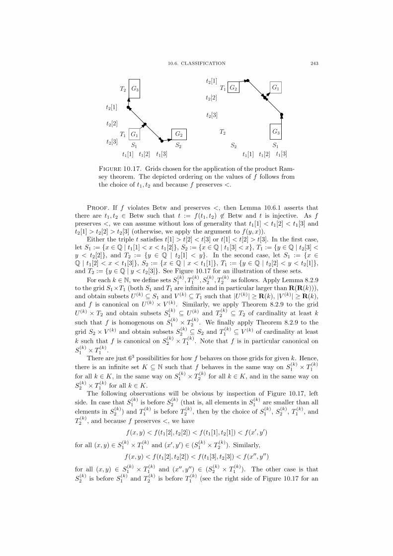
10.6. CLASSIFICATION 243
G1 G2
G3
S1 S2
T1
T2
t2[1]
t2[2]
t2[3]
t1[1] t1[2] t1[3]
G1G2
G3
S1S2
T1
T2
t2[1]
t2[2]
t2[3]
t1[1] t1[2] t1[3]
Figure 10.17. Grids chosen for the application of the product Ram-sey theorem. The depicted ordering on the values of f follows fromthe choice of t1, t2 and because f preserves <.
Proof. If f violates Betw and preserves <, then Lemma 10.6.1 asserts thatthere are t1, t2 ∈ Betw such that t := f(t1, t2) 6∈ Betw and t is injective. As fpreserves <, we can assume without loss of generality that t1[1] < t1[2] < t1[3] andt2[1] > t2[2] > t2[3] (otherwise, we apply the argument to f(y, x)).
Either the triple t satisfies t[1] > t[2] < t[3] or t[1] < t[2] > t[3]. In the first case,let S1 := {x ∈ Q | t1[1] < x < t1[2]}, S2 := {x ∈ Q | t1[3] < x}, T1 := {y ∈ Q | t2[3] <y < t2[2]}, and T2 := {y ∈ Q | t2[1] < y}. In the second case, let S1 := {x ∈Q | t1[2] < x < t1[3]}, S2 := {x ∈ Q | x < t1[1]}, T1 := {y ∈ Q | t2[2] < y < t2[1]},and T2 := {y ∈ Q | y < t2[3]}. See Figure 10.17 for an illustration of these sets.
For each k ∈ N, we define sets S(k)1 , T
(k)1 , S
(k)2 , T
(k)2 as follows. Apply Lemma 8.2.9
to the grid S1×T1 (both S1 and T1 are infinite and in particular larger than R(R(k))),and obtain subsets U (k) ⊆ S1 and V (k) ⊆ T1 such that |U (k)| ≥ R(k), |V (k)| ≥ R(k),and f is canonical on U (k) × V (k). Similarly, we apply Theorem 8.2.9 to the grid
U (k) × T2 and obtain subsets S(k)1 ⊆ U (k) and T
(k)2 ⊆ T2 of cardinality at least k
such that f is homogenous on S(k)1 × T (k)
2 . We finally apply Theorem 8.2.9 to the
grid S2 × V (k) and obtain subsets S(k)2 ⊆ S2 and T
(k)1 ⊆ V (k) of cardinality at least
k such that f is canonical on S(k)2 × T (k)
1 . Note that f is in particular canonical on
S(k)1 × T (k)
1 .There are just 63 possibilities for how f behaves on those grids for given k. Hence,
there is an infinite set K ⊆ N such that f behaves in the same way on S(k)1 × T (k)
1
for all k ∈ K, in the same way on S(k)1 × T (k)
2 for all k ∈ K, and in the same way on
S(k)2 × T (k)
1 for all k ∈ K.The following observations will be obvious by inspection of Figure 10.17, left
side. In case that S(k)1 is before S
(k)2 (that is, all elements in S
(k)1 are smaller than all
elements in S(k)2 ) and T
(k)1 is before T
(k)2 , then by the choice of S
(k)1 , S
(k)2 , T
(k)1 , and
T(k)2 , and because f preserves <, we have
f(x, y) < f(t1[2], t2[2]) < f(t1[1], t2[1]) < f(x′, y′)
for all (x, y) ∈ S(k)1 × T (k)
1 and (x′, y′) ∈ (S(k)1 × T (k)
2 ). Similarly,
f(x, y) < f(t1[2], t2[2]) < f(t1[3], t2[3]) < f(x′′, y′′)
for all (x, y) ∈ S(k)1 × T
(k)1 and (x′′, y′′) ∈ (S
(k)2 × T
(k)1 ). The other case is that
S(k)2 is before S
(k)1 and T
(k)2 is before T
(k)1 (see the right side of Figure 10.17 for an

244 10. TEMPORAL CONSTRAINT SATISFACTION PROBLEMS
illustration). In this case f(x, y) > f(t1[2], t2[2]) > f(x′, y′) for all (x, y) ∈ S(k)1 ×T
(k)1
and (x′, y′) ∈ (S(k)1 × T (k)
2 ) ∪ (S(k)2 × T (k)
1 ).
First suppose that f is dominated by the same argument on all the grids S(k)1 ×
T(k)1 , S
(k)1 × T (k)
2 , and S(k)2 × T (k)
1 for all k ∈ K. We can assume that f is dominatedon these grids by the second argument; otherwise we swap the arguments of f . Let
g, h ∈ {lexy,x, lexy,−x, py} be such that f behaves like g on S(k)1 × T (k)
1 and like h on
S(k)2 ×T (k)
1 . Then by the above observations and local interpolation f generates [g|h]if S1 is before S2, and [h|g] if S2 is before S1. Moreover, we show that f also generateslex.
• If g or h is lexx,y or lexy,x, then f clearly generates lex.• If g or h is lexx,−y or lexy,−x, then f generates lex as well, as lex(x,−lex(x,−y))
behaves like lex(x, y).• If g is py and h is py, then f generates lex by Lemma 10.4.5.
Note that the operation [g|h] satisfies the conditions in Lemma 10.4.4, and hence{lex, [g|h]} generates [lexy,x|lexy,x]. By Lemma 10.4.5, f generates ll.
Now we consider the case that f is dominated by different arguments on the grids
S(k)1 ×T
(k)1 and S
(k)1 ×T
(k)2 , or by different arguments on the grids S
(k)1 ×T
(k)1 and S
(k)2 ×
T(k)1 , for all k ∈ K. We only consider the first case; the second case is symmetric under
swapping the arguments of f . Let g, h be from {lexx,y, lexx,−y, lexy,x, lexy,−x, px, py}such that f behaves like h on the grids S
(k)1 ×T (k)
1 and like g on the grids S(k)2 ×T (k)
1 .Again, by local interpolation f generates [h|g] if S1 is before S2, and [g|h] if S2 isbefore S1. We assume without loss of generality that f generates [h|g] (in the othercase we can exchange the names of h and g and proceed in the same way).
If h is py and g is px, then [h|g] behaves like pp; hence f generates pp and we aredone. Dually, if h is px and g is py, then f generates dual-pp. In all other cases, eitherh or g is from lexx,y, lexy,x, lexx,−y, or lexy,−x, and thus f generates lex as we havealready seen before. But then Lemma 10.4.4 shows that f generates ll or dual-ll. �
10.6.2. Summary. We summarize our findings in the following classificationstatement; also see Figure 10.18.
Theorem 10.6.3. Let B be a temporal constraint language. Then one of thefollowing applies.
• B is preserved by at least one of the following nine operations: ll,min,mi ,mx,their duals, or a constant operation.
• Betw, Cycl, Sep, T3, −T3, or I6 is primitive positive definable in B.
Proof. Theorem 10.3.2 asserts that one of the following cases is true:
(1) There is a primitive positive definition of Cycl, Betw, or Sep in B.(2) Pol(B) contains a constant operation.(3) Pol(B) contains all permutations of Q. In this case, Theorem 6.4.2 shows
that B either has a binary injective polymorphism g, or the relation I6 hasa primitive positive definition in B. In the first case, by composing g witha permutation, we see that all binary injective operations preserve B, andhence in particular the operation ll is a polymorphism of B.
(4) all f ∈ Pol(B) preserve <.
We are done in all cases except the fourth. Also, we can assume that B has apolymorphism f that violates Betw. By Lemma 5.3.10, we can assume that f isbinary. Then Lemma 10.6.2 implies that the operation f generates pp, dual-pp, ll, ordual-ll. If f generates ll or dual-ll there is nothing to show. If f generates pp then

10.6. CLASSIFICATION 245
-constant
NP-complete
in P
cycl
lexpp
min llmx
mi
Pol(Betw)
Pol(Cycl)Pol(E6) Pol(Sep)
Pol(T3)
Figure 10.18. An illustration of the classification result for tempo-ral constraint languages. Double-circles mean that the correspondingoperation has a dual generating a distinct clone which is not drawnin the figure.
Lemma 10.5.29 shows that either T3 has a primitive positive definition in B, or B ispreserved by min, mi , or mx . Dually, if f generates dual-pp then either −T3 has aprimitive positive definition in B, or B is preserved by one of the duals of min, mi ,or mx , which completes the proof. �
With the previous theorem it is easy to obtain the full complexity classificationfor temporal constraint satisfcation problems, and finally show Theorem 10.1.1.
Proof of Theorem 10.1.1. When B is preserved by ll, min, mi , mx , one oftheir duals, or the constant operation, then B has an at most ternary weak near una-nimity polymorphism modulo endomorphisms; this is immediate for the commutativebinary functions mx , min, their duals, and for the constant function. For ll, this hasbeen shown in Theorem 10.4.11, and for mi in Theorem 10.5.18. For dual mi anddual ll the dual argument works.
Now let B′ be a finite signature reduct of B. If B′ is preserved by a constantoperation, then tractability of CSP(B′) follows from Proposition 1.1.11. For the casethat B′ is preserved by ll or dual-ll we have presented a polynomial-time algorithmfor CSP(B′) in Theorem 10.4.19. If B′ is preserved by min,mi ,mx , or one of theirduals, tractability of CSP(B′) is shown in Section 10.5.7.
Now suppose that B is not preserved by one of the listed operations. Then byTheorem 10.6.3 we know that one of the relations Betw, Cycl, Sep, T3, −T3, or I6has a primitive positive definition in B. Each of those relations together with finitelymany constants primitively positively interprets ({0, 1}; 1IN3):
• For (Q; Betw, 0) a primitive positive interpretation of ({0, 1}; NAE) has beenshown in Proposition 5.5.13,which also gives a primitive positive interpreta-tion of ({0, 1}; 1IN3) in (Q; Betw, 0) via Theorem 5.5.17.

246 10. TEMPORAL CONSTRAINT SATISFACTION PROBLEMS
• a primitive positive interpretation of ({0, 1}; 1IN3) in (Q; Cycl) with param-eters has been given in Theorem 10.2.7.• The structure (Q; Sep, 0, 1) primitively positively interprets ({0, 1}; 1IN3) by
Proposition 10.2.8.• The structure (Q;T3, 0) primitively positively interprets ({0, 1}; 1IN3) by
Proposition 10.2.6; the proof for −T is dual.• I6 primitively positively interprets ({0, 1}; 1IN3) by Proposition 5.5.9.
Finally, recall from Theorem 10.3.1 that if B does not have a constant endomorphism,then it is a model-complete core, and hence Corollary 5.6.11 shows that the two casesin the statement of Theorem 10.1.1 are distinct. �
See Figure 10.19 for an overview over the nine largest tractable temporal con-straint languages; the entries also mention typical relations for the respective lan-guage, i.e., a set of relations that is contained in the language, but not contained inany other of the nine languages – hence, these relations show that all the languagesare distinct.
Polymorphism Typical Relations Complexity Referencemin {U,<} O(n2m) Theorem 10.5.35mi {I} O(n3m) Theorem 10.5.37mx {X} O(n4) Theorem 10.5.38max = dual min {−U,<} O(n2m)dual mi {−I} O(n3m)dual mx {−X} O(n4)ll {(u 6= v) ∨ (x > y) ∨ (x > z)} O(nm) Theorem 10.4.19dual ll {(u 6= v) ∨ (x < y) ∨ (x < z)} O(nm)constant {(x ≤ y ≤ z) ∨ (z ≤ y ≤ x)} O(m)
Figure 10.19. Summary of the various tractable languages. Forthe last three operations, the typical relations are given by theirfirst-order definition; in all other cases, see Section 10.5.
10.6.3. Decidability of Tractability. We want to remark that the so-calledmeta-problem for tractability is decidable; this is formally stated in the followingcorollary.
Corollary 10.6.4. There is an algorithm that, given quantifier-free first-orderformulas φ1, . . . , φn that define over (Q;<) the relations R1, . . . , Rn, decides whetherCSP(Q;R1, . . . , Rn) is tractable or NP-complete.
Proof. Follows from Theorem 8.4.4 in combination with Theorem 10.6.3. �

CHAPTER 11
Non-Dichotomies
There are basically two methods for proving that a subclass of NP does not havea complexity dichotomy. The first is to show that for every problem in NP there is apolynomial-time equivalent problem in the subclass. By polynomial-time equivalentwe mean that there are polynomial-time Turing reductions between the two problems.The non-dichotomy result then follows from Ladner’s theorem [143], which assertsthat there are problems in NP that are neither in P nor NP-complete, unless P=NP.This method has been applied to show that, for example, the class of monotoneSNP does not exhibit a complexity dichotomy [95]. We will apply this technique inSection 11.1 and Section 11.2 to give two different proofs of the fact that the class of
247
248 11. NON-DICHOTOMIES
all constraint satisfaction problems with infinite domains does not have a complexitydichotomy.
The second technique to show a non-dichotomy is to directly use Ladner’s prooftechnique, which is sometimes called delayed diagonalization. We will use this methodin Section 11.3 to show that there are ω-categorical structures B such that CSP(B)is in coNP, but neither in P nor coNP-complete (unless P=coNP). The questionwhether there are ω-categorical structures B such that CSP(B) is in NP \ P but notNP-complete is still open.
This chapter contains results from [33] (in Section 11.3) as well as previouslyunpublished results.
11.1. Arithmetical Templates
In this section we show that for every computational decision problem there existsa polynomial-time equivalent constraint satisfaction problem with an infinite templateB. This result was first shown in [33]. Here we present a new proof that usesMatiyasevich’s theorem. In fact, we prove a stronger result, namely the existence ofa single structure C such that for every recursively enumerable problem P there is astructure B with a first-order definition in C such that CSP(B) is polynomial-timeequivalent to P. A second proof, based on the results in Section 1.4.2 of Chapter 1,can be found in the next section.
Previously, Bauslaugh [16] showed that for every recursive function f there existsan infinite structure B such that CSP(B) is decidable, but has time complexity atleast f . More recently, Schwandtner gave upper and lower bounds in the exponen-tial time hierarchy for some infinite domain CSPs [186]; but these bounds leave anexponential gap.
In this section we make essential use of the following theorem, which is due toDavis, Matiyasevich, Putnam, and Robinson.
Theorem 11.1.1 (See e.g. [162]). A subset of Z is recursively enumerable if andonly if it has a primitive positive definition in (Z; ∗,+, 1), the integers with additionand multiplication.
Theorem 11.1.2. For every recursively enumerable problem P there exists a re-lational structure B with a first-order (in fact, a primitive positive) definition in(Z; ∗,+, 1) such that CSP(B) is polynomial-time Turing equivalent to P.
Proof. Code P as a set L of natural numbers, viewing the binary encodingsof natural numbers as bit strings. More precisely, s ∈ P if and only if the numberrepresented in binary by the string 1s is in L. That is, we append the symbol 1 atthe front so that for instance 00 ∈ P and 01 ∈ P correspond to different numbers inL. Now consider the structure B := (Z;S,D,L′, N) where
• S is the binary relation defined by
S(x, y)⇔((y = x+ 1 ∧ x ≥ 0) ∨ (x = y = −1)
)• D is the binary relation defined by
D(x, y)⇔((y = 2x ∧ x ≥ 0) ∨ (x = y = −1)
)• L′ := L ∪ {−1}• N := {0}
Clearly, if P is recursively enumerable, then L and L′ are recursively enumerable, too.We have to verify that CSP(B) is polynomial time equivalent to P. We first show
that there is a polynomial-time reduction from P to CSP(B). View an instance ofP as a number n ≥ 0 as above, and let η(x) be a primitive positive definition for

11.2. CSPS IN SNP 249
x = n in B. It is possible to find such a definition in polynomial time by repeatedlydoubling (y = x+ x) and incrementing (y = x+ 1) the value 0 (this also follows fromthe more general Lemma 1.5.1). It is clear that n codes a yes-instance of P if andonly if ∃x(η(x) ∧ L′(x)) is true in B.
To reduce CSP(B) to P, we present a polynomial-time algorithm for CSP(B) thatuses an oracle for P (so our reduction will be a polynomial-time Turing reduction).Let φ be an instance of CSP(B), and let H be the undirected graph whose verticesare the variables W of φ, and which has an edge between x and y if φ contains theconstraint S(x, y) or the constraint D(x, y). Compute the connected components ofH. If a connected component does not contain x with a constraint N(x) in φ, thenwe can set all variables of that component to −1 and satisfy all constraints involvingthose variables.
Otherwise, suppose that we have a component C that does contain x0 with aconstraint N(x0). Observe that by connectivity, if there exists a solution, then allvariables in C must take non-negative value. Consider the following linear system:for each constraint of the form S(x, y) for x, y ∈ C we add y = x+ 1 and x ≥ 0 to thesystem, and for each constraint of the form D(x, y) for x, y ∈ D we add z = 2x andx ≥ 0. Subject to x0 = 0 this system has either one or no solution. We can checkin polynomial time whether a linear system with 2 variables per constraint has nointeger solution [48], and if there is no solution, the algorithm rejects. Otherwise, thealgorithm assigns to each variable x ∈ C its unique integer value, and if φ contains aconstraint L′(x), we call the oracle for P with the binary encoding of this value. Ifany of those oracle calls has a negative result, reject. Otherwise, we have found anassignment that satisfies all constraints, and accept. �
The universal-algebraic approach fails badly when it comes to analysing the com-putational complexity of CSP(B): the semi-lattice operation (x, y) 7→ max (x, y) pre-serves B for all structures B considered in the previous proof, and from that wecannot draw any consequences for the computational complexity of CSP(B).
11.2. CSPs in SNP
Another proof that shows that every problem in NP is polynomial-time Turingequivalent to an infinite domain CSP is based on a result by Feder and Vardi, andthe results from Section 1.4.3.
Theorem 11.2.1 (Theorem 3 in [95]). Every problem in NP is equivalent to aproblem in monotone SNP under polynomial-time reductions.
We show the following.
Proposition 11.2.2. Every problem in monotone SNP is equivalent to a problemin monotone connected SNP under polynomial-time Turing reductions.
Proof. Let Φ be a monotone SNP sentence of the form ∃R1, . . . , Rk ∀x1, . . . , xl. φfor φ quantifier-free and in conjunctive normal form. The sentence Ψ that we are go-ing to construct from Φ has an additional free relation symbol E, and an existentiallyquantified relation symbol T , and is defined by
∃R1, . . . , Rk, T ∀x1, . . . , xl. ψ
where ψ is the quantifier-free first-order formula with the following clauses.
(1) ¬E(x1, x2) ∨ T (x1, x2);(2) ¬T (x1, x2) ∨ ¬T (x2, x3) ∨ T (x1, x3);(3) ¬T (x1, x2) ∨ T (x2, x1);

250 11. NON-DICHOTOMIES
(4) for each clause φ′ of φ with variables x1, . . . , xq, the clause
φ′ ∨∨
i<j<q
¬T (xi, xj) .
The sentence Ψ is clearly connected and monotone. We are therefore left with thetask to verify that Φ and Ψ are equivalent under polynomial-time Turing reductions.
We start with the reduction from Φ to Ψ. When A is a finite τ -structure, weexpand A to a (τ ∪{E})-structure A′ by choosing for E the full binary relation. Thenalso T must denote the full binary relation (so that the clauses from item (1), (2),and (3) above are satisfied), and the clauses introduced in (4) are equivalent to φ′.Hence, Φ holds on A if and only if Ψ holds on A′.
For the reduction from Ψ to Φ, let A be an instance of Ψ. We can compute theconnected components C1, . . . , Ck of the {E}-reduct of A in polynomial time in thesize A. For each of those connected components C, we evaluate Φ on the τ -reduct ACof A[C]. If for one component this evaluation is negative, then A[C] and consequentlyA do not satisfy Ψ. Otherwise, for each C there exists an τ ∪{R1, . . . , Rk}-expansionof AC that satisfies φ. Let A′ be the expansion of the disjoint union of all those(τ ∪ {R1, . . . , Rk})-structures by the relation T denotes the equivalence relation withequivalence classes C1, . . . , Ck. Clearly, all clauses from items (1), (2), and (3) in thedefinition of Ψ are satisfied by A′. Each q-tuple (a1, . . . , aq) from elements of A′ eithercontains entries from different components, and hence satisfies the disjunctions fromitem (4), or contains only entries from the same component C, but in this case thetuple also satisfies the disjunctions from item (4) since AC satisfies Φ. �
Corollary 11.2.3. For every problem in NP there is a structure B such thatthe problem is polynomial-time Turing equivalent to CSP(B).
Proof. By Theorem 11.2.1, every problem in NP is equivalent to a monotoneSNP sentence Φ under polynomial-time reductions. We have shown in Proposi-tion 11.2.2 that Φ is equivalent to a monotone connected SNP sentence Ψ, and byTheorem 1.4.11 there exists an infinite structure B such that Ψ describes CSP(B). �
In Figure 11.1 the diagram about the fragments of SNP from Section 1.4 has beendecorated with information about the complexity classification status.
11.3. coNP-intermediate ω-categorical Templates
In this section we show that there exists an ω-categorical directed graph B suchthat CSP(B) is in coNP, but neither coNP-complete nor in P (unless coNP=P). Allstructures in this section will be Fraısse limits of classes of directed graphs.
Let N be a class of finite tournaments, and recall that Forb(N ), the class ofall finite digraphs that does not embed a tournament from N , is an amalgamationclass (Example 3.2.7). We write BN for the Fraısse-limit of Forb(N ). Observe thatfor finite N the problem CSP(BN ) can be solved in deterministic polynomial time,because for a given instance A of this problem an algorithm simply has to checkwhether there is a homomorphism from one of the structures in N to A, which is thecase if and only if there is a homomorphism from A to BN .
When proving that there are uncountably many homogeneous digraphs, Hensonspecified an infinite set T of tournaments T3, T4, . . . with the property that Ti doesnot embed into Tj if i 6= j. The tournament Tn, for n ≥ 3, in Henson’s set T hasvertices 0, . . . , n+ 1, and the following edges:
• (i, j) for j = i+ 1 and 0 ≤ i ≤ n;• (0, n+ 1);• (j, i) for j > i+ 1 and (i, j) 6= (0, n+ 1).

11.3. CONP-INTERMEDIATE ω-CATEGORICAL TEMPLATES 251
SNP
monotone SNP
connected SNP
SNP ∩ CSP(inf)
connected monotone
monadic SNP
SNP ∩ CSP(ω-cat)
CSP(fin)
monotone monadic SNP
Feder-Vardi Conjecture:Dichotomy
No Dichotomy
DichotomyUnknown
NP
Figure 11.1. Dichotomies and non-dichotomies for fragments ofSNP. CSP(inf) (CSP(ω-cat), CSP(fin)) refers to the class of all prob-lems CSP(B) where B is an infinite (ω-categorical, finite, respec-tively) structure with finite relational signature.
Proposition 11.3.1. The problem CSP(BT ) is coNP-complete.
Proof. The problem is contained in coNP, because we can efficiently test whethera sequence v1, . . . , vk of distinct vertices of a given directed graph A induces Tk inA, i.e., whether (vi, vj) is an arc in A if and only if (i, j) is an arc in Tk, for alli, j ∈ {1, . . . , k}. If for all such sequences of vertices this test is negative, we can besure that A is from Forb(T ), and hence homomorphically maps to BT . Otherwise, Aembeds a structure from T , and hence does not homomorphically map to BT .
The proof of coNP-hardness goes by reduction from the complement of the NP-complete 3SAT problem (see Example 1.2.2), and is inspired by a classical reductionfrom 3-SAT to Clique. For a given 3-SAT instance, we create an instance A ofCSP(BT ) as follows: If
{x10, x
20, x
30}, . . . , {x1
k+1, x2k+1, x
3k+1}
are the clauses of the 3-SAT formula (we assume without loss of generality that the3-SAT instance has at least three clauses), then the vertex set of A is
{(0, 1), (0, 2), (0, 3), . . . , (k + 1, 1), (k + 1, 2), (k + 1, 3)} ,
and the arc set of A consists of all pairs ((i, j), (p, q)) of vertices such that xji 6= ¬xqpand such that (i, p) is an arc in Tk.
We claim that a 3-SAT instance is unsatisfiable if and only if the created in-stance A homomorphically maps to BT . The 3-SAT instance is satisfiable iff thereis a mapping from the variables to true and false such that in each clause at least
one literal, say xj00 , . . . , xjk+1
k+1 , is true. This is the case if and only if the vertices(0, j1), . . . , (k + 1, jk+1) induce Tk in A, i.e., ((i, ji), (p, jp)) is an edge if and only if

252 11. NON-DICHOTOMIES
(i, p) is an edge in Tk. This is the case if and only if Tk embeds into A. To conclude,it suffices to prove that Tk embeds into A if and only if A does not homomorphicallymap to BT . It is clear that if Tk embeds into A, then A does not homomorphicallymap to BT . Conversely, if A does not homomorphically embed to BT , then thereexists a j such that there is an embedding e of Tj into A. Then for any (i, j), (p, q)in the image of e we have that (i, p) is an edge of Tk. Therefore, the mapping thatsends an element u of Tj to the first component of e(u) is an embedding of Tj into Tk.Since Tj and Tk are homomorphically inequivalent for all distinct j, k ≥ 3 we obtainthat j = k and that Tk embeds into A, which finishes the proof. �
We now modify the proof of Ladner’s Theorem given in [171] (which is basicallyLadner’s original proof) to create a subset T0 of T such that CSP(BT0) is in coNP,but neither in P nor coNP-complete (unless coNP=P). One of the ideas in Ladner’sproof is to ‘blow holes into SAT’, such that the resulting problem is too sparse to beNP-complete and to dense to be in P. Our modification is that we do not blow holesinto a computational problem itself, but that we ‘blow holes into the obstruction setT of CSP(BT )’.
In the following, we fix one of the standard encodings of graphs as strings over thealphabet {0, 1}. Let M1,M2, . . . be an enumeration of all polynomial-time boundedTuring machines, and letR1, R2, . . . be an enumeration of all polynomial time boundedreductions. We assume that these enumerations are effective; it is well-known thatsuch enumerations exist.
The definition of T0 uses a Turing machine F that computes a function f : N→ N,which is defined below. The set T0 is then defined as follows.
T0 = {Tn | f(n) is even }The input number n is given to the machine F in unary representation. The compu-tation of F proceeds in two phases. In the first phase, F simulates itself1 on input1, then on input 2, 3, and so on, until the number of computation steps of F in thisphase exceeds n (we can always maintain a counter during the simulation to recognizewhen to stop). Let k be the value f(i) for the last input i for which the simulationwas completely performed by F .
In the second phase, the machine stops if phase two takes more than n compu-tation steps, and F returns k. We distinguish whether k is even or odd. If k is even,all directed graphs A on s = 1, 2, 3, . . . vertices are enumerated. For each directedgraph A in the enumeration the machine F simulates Mk/2 on the encoding of A.Moreover, F computes whether A homomorphically maps to BT0 . This is the caseif for all structures Tl ∈ T that embed into A the value of f(l) is even. So F testsfor l = 1, 2, . . . , s whether Tl embeds to A (F uses any straightforward exponentialtime algorithm for this purpose), and if it does, simulates itself on input l to find outwhether f(l) is even. If
(1) Mk/2 rejects and A homomorphically maps to BT0 , or(2) Mk/2 accepts and A does not homomorphically map to BT0 ,
then F returns k + 1 (and f(n) = k + 1).The other case of the second phase is that k is odd. Again F enumerates all
directed graphs A on s = 1, 2, 3, . . . vertices, and simulates the computation of Rbk/2con the encoding of A. Then F computes whether the output of Rbk/2c encodes adirected graph A′ that homomorphically maps to BT0 . The graph A′ homomorphi-cally maps to BT0 iff for all tournaments Tl that embed into A′ the value f(l) is
1Note that by the fixpoint theorem of recursion theory we can assume that F has access to itsown description.

11.3. CONP-INTERMEDIATE ω-CATEGORICAL TEMPLATES 253
even. Whether Tl embeds into A′ is tested with a straightforward exponential-timealgorithm. To test whether f(l) is even, F simulates itself on input l. Finally, F testswith a straightforward exponential-time algorithm whether A homomorphically mapsto BT . If
(3) A homomorphically maps to BT and A′ does not homomorphically map toBT0 , or
(4) A does not homomorphically map to BT and A′ homomorphically maps toBT0 ,
then F returns k + 1.
Lemma 11.3.2. The function f is a non-decreasing function, that is, for all n wehave f(n) ≤ f(n+ 1).
Proof. We inductively assume that f(s − 1) ≤ f(s) for all s ≤ n, and have toshow that f(n) ≤ f(n+ 1). Since F has more time to simulate itself when we run iton n + 1 instead of n, the value i computed in the first phase of F cannot becomesmaller. By inductive assumption, k = f(i) cannot become smaller as well. In thesecond phase, we either return k or k + 1. Hence, if k becomes larger in the firstphase, the output of F cannot become smaller. If k does not become larger, then theonly difference between the second phase of F for input n + 1 compared to input nis that there is more time for the computations. Hence, if the machine F on input nverifies condition (1),(2),(3),(4) for some graph A (and hence returns k + 1), then Falso verifies this condition for A on input n+ 1, and returns k+ 1 as well. Otherwise,f(n) = k, and also here f(n+ 1) ≥ f(n) holds. �
Lemma 11.3.3. For all n0 there exists an n > n0 such that f(n) > f(n0) (unlesscoNP 6= P).
Proof. Assume for contradiction that there exists an n0 such that f(n) equalsa constant k0 for all n ≥ n0. Then there also exists an n1 such that for all n ≥ n1
the value of k computed by the first phase of F on input n is k0.If k0 is even, then on all inputs n ≥ n1 the second phase of F simulates Mk0/2
on encodings of an enumeration of graphs. Since the output of F must be k0, for allgraphs neither (1) nor (2) can apply. Since this holds for all n ≥ n1, the polynomial-time bounded machine Mk0/2 correctly decides CSP(BT0), and hence CSP(BT0) is inP. But then there is the following polynomial-time algorithm that solves CSP(BT ),a contradiction to coNP-completeness of CSP(BT ) (Proposition 11.3.1) and our as-sumption that coNP 6= P.
Input: A directed graph A.
If A homomorphically maps to BT0 then accept.Test whether one of the finitely many graphs in T \ T0 embeds into A.Accept if none of them embeds into A.Reject otherwise.
If k0 is odd, then on all inputs n ≥ n1 the second phase of F does not find a graphA for which (3) or (4) applies, because the output of F must be k0. Hence, Rbk0/2c isa polynomial-time reduction from CSP(BT ) to CSP(BT0), and by Proposition 11.3.1the problem CSP(BT0) is coNP-hard. But note that because f(n) equals the oddnumber k0 for all but finitely many n, the set T0 is finite. Therefore, CSP(BT0) canbe solved in polynomial time, contradicting our assumption that coNP 6= P. �
254 11. NON-DICHOTOMIES
Theorem 11.3.4. CSP(BT0) is in coNP, but neither in P nor coNP-complete(unless coNP=P).
Proof. It is easy to see that CSP(BT0) is in coNP. On input A the algorithmnon-deterministically chooses a sequence of l vertices, and checks in polynomial timewhether this sequence induces a copy of Tl. If yes, the algorithm computes f(l), whichcan be done in linear time by executing F on the unary representation of l. If f(l)is even, the algorithm accepts. Recall that A does not homomorphically map to BT0iff a tournament Tl ∈ T0 embeds into A, which is the case iff there is an acceptingcomputation path for the above non-deterministic algorithm.
Suppose that CSP(BT0) is in P . Then for some i the machine Mi decidesCSP(BT0). By Lemma 11.3.2 and Lemma 11.3.3 there exists an n0 such that f(n0) =2i. Then there must also be an n1 > n2 such that the value k computed during thefirst phase of F on input n1 equals 2i. Since Mi correctly decides CSP(BT0), themachine F returns 2i on input n1. By Lemma 11.3.2, the machine F also returns 2ifor all inputs from n1 to n2, and by induction it follows that it F returns 2i for allinputs larger than n ≥ n0, in contradiction to Lemma 11.3.3.
Finally, suppose that CSP(BT0) is coNP-complete. Then for some i the machineRi is a valid reduction from CSP(BT ) to CSP(BT0). Again, by Lemma 11.3.2 andLemma 11.3.3 there exists an n1 such that the value k computed during the first phaseof F on input n1 equals 2i. Since the reduction Ri is correct, the machine F returns2i on input n1, and in fact returns 2i on all inputs greater than n1. This contradictsLemma 11.3.3. �

CHAPTER 12
Future Work
We conclude the thesis by mentioning four promising directions of future work.
12.1. Phylogeny Constraints
We have presented a classification of the complexity of CSP(B) for all structuresB with a first-order definition over (Q;<), or over the random graph (V;E). Onemight ask which other structures, besides (Q;<) and the random graph (V;E), areinteresting and promising candidates for such a classification. A very interestingcandidate is the structure (L; |) (or equivalently, over a relatively 3-transitive C-set),introduced in Section 4.1. The class of CSPs that can be formulated with templatesthat can be defined over this structure is very large and contains many problems thathave been independently studied in the literature, capturing for instance the rootedtriple satisfaction problem and the quartet satisfiability problem from phylogeneticanalysis. All the tools we needed for complexity classification are available: (L; |) ishomogeneous, and an appropriate order expansion of it is Ramsey (see Example 8.1.8).
12.2. Datalog
Feder and Vardi [95] observed that all the known algorithms for solving CSP(B),for a finite structure B, are either based on algebraic algorithms that can be seen asgeneralizations of Gaussian elimination, or based on simple ‘constraint propagation’,or combinations of these two paradigms. This is still the case today. An elegant wayto formalize algorithms that perform constraint propagation is Datalog. Datalog canbe seen as conjunctive queries that have been extended by a recursion mechanisms;alternatively, one can view Datalog as Prolog (see e.g. [183]) without function sym-bols. In the context of constraint satisfaction Datalog has been introduced in [95]and further studied in [136]. Some of the early contributions were equivalent char-acterizations of the expressive power of Datalog in terms of bounded treewidth dualityand existential pebble games.
Recently, Barto and Kozik [12] presented an exact characterization of those CSPswhere CSP(B) can be solved by a Datalog program. The characterization is universal-algebraic (see Chapter 5), and confirming a conjecture of Larose and Zadori [147]. Itwas later shown to be equivalent to a conjecture made already by Feder and Vardiin [95], see [146].
Datalog programs are very useful to solve infinite-domain constraint satisfactionproblems as well. It has been shown in [31] that when B is an ω-categorical structure,then the characterizations of the expressive power of Datalog in terms of boundedtreewidth duality and existential pebble games remain valid. This has been applied toshow that several fundamental infinite-domain CSPs in the literature cannot be solvedby Datalog [42,45]. It would be very interesting to have an algebraic characterizationof the expressive power of Datalog for CSPs with ω-categorical templates.
255

256 12. FUTURE WORK
12.3. Topological Clones
We have seen in Section 7.4 that the topological automorphism group of an ω-categorical structure Γ describes Γ up to bi-interpretability; that is, two ω-categoricalstructures Γ and ∆ whose automorphism groups are isomorphic as topological groupsare first-order bi-interpretable.
We have also seen that the right tool for the complexity study of CSPs is primitivepositive interpretability, and not first-order interpretability; see Section 5.5. So itis natural to ask in this context whether primitive positive interpretability can becharacterized in terms of the polymorphism clone viewed as a topological clone, thatis, viewed as an abstract clone equipped with the topology of point-wise convergence.We did not define abstract clones; but in this context it suffices to know that theyrelate to clones in the same way as permutation groups relate to abstract groups.
A partial result in this direction has been obtained in joint work with Junker [39];one of the results proven there is that two ω-categorical structures without constantendomorphism are existential positive bi-interpretable1 if and only if their transfor-mation monoids, viewed as topological monoids, are isomorphic.
The goal to lift this further to primitive positive interpretability amounts to show-ing that the topological clone of B characterizes the pseudo-variety generated by thepolymorphism algebra of B, via Theorem 5.5.14.
12.4. A Logic for P?
In Section 1.4 we have seen a logical characterization of the complexity class NP:by Fagin’s theorem, a problem is in NP if and only if it can be described in existentialsecond-order logic. A similar logic for the complexity class P is not known. Thequestion whether there exists a logic for P has been formalized by Gurevich [108] andbecame one of the most influential questions in finite model theory [107].
One approach to shed some light on this question is to identify large fragmentsof existential second-order logic such that the set of sentences in this fragment thatdescribe problems in P has an effective enumeration. For example, consider the logicof connected monotone SNP. Theorem 11.2.1 and Proposition 11.2.2 show that everyproblem in NP is polynomial-time equivalent to a problem in connected monotoneSNP. The proof of Theorem 11.2.1 and Proposition 11.2.2 is constructive in the sensethat from a non-deterministic Turing machine we can effectively construct the cor-responding connected monotone SNP sentence. So if there were an algorithm thatenumerates those connected monotone SNP sentences that describe a problem in P,then the question to Gurevich’s question is positive (Gurevich conjectured that theanswer is negative). Such an algorithm probably does not exist. But it might existfor fragments of connected monotone SNP. Recall that every sentence in connectedmonotone SNP describes a CSP. Hence, complexity classification for infinite domainconstraint satisfaction can also be motivated by the quest for a logic for P.
1A first-order interpretation is called existential positive if all the involved formulas of the
interpretation are existential positive; existential positive bi-interpretations are defined by a similarmodification of first-order bi-interpretations.

Bibliography
[1] F. G. Abramson and L. Harrington. Models without indiscernibles. Journal of Symbolic Logic,
43(3):572–600, 1978.
[2] S. A. Adeleke and P. M. Neumann. Relations related to betweenness: their structure andautomorphisms, volume 623 of Memoirs of the AMS. American Mathematical Society, 1998.
[3] G. Ahlbrandt and M. Ziegler. Quasi-finitely axiomatizable totally categorical theories. Annals
of Pure and Applied Logic, 30(1):63–82, 1986.[4] A. Aho, Y. Sagiv, T. Szymanski, and J. Ullman. Inferring a tree from lowest common ancestors
with an application to the optimization of relational expressions. SIAM Journal on Computing,10(3):405–421, 1981.
[5] J. F. Allen. Maintaining knowledge about temporal intervals. Communications of the ACM,
26(11):832–843, 1983.[6] E. Allender, M. Bauland, N. Immerman, H. Schnoor, and H. Vollmer. The complexity of sat-
isfiability problems: Refining Schaefer’s theorem. Journal of Computer and System Sciences,
75(4):245–254, 2009.[7] B. Aspvall, M. F. Plass, and R. E. Tarjan. A linear-time algorithm for testing the truth of
certain quantified boolean formulas. Information Processing Letters, 8(3):121–123, 1979.
[8] A. Atserias. On digraph coloring problems and treewidth duality. In Proceedings of LICS, pages106–115, 2005.
[9] A. Atserias, A. A. Bulatov, and A. Dawar. Affine systems of equations and counting infinitary
logic. Theoretical Computer Science, 410(18):1666–1683, 2009.[10] F. Baader and T. Nipkow. Term rewriting and all that. Cambridge University Press, 1999.
[11] L. Barto. The dichotomy for conservative constraint satisfaction problems revisited. In Pro-ceedings of the Symposium on Logic in Computer Science (LICS), Toronto, Canada, 2011.
[12] L. Barto and M. Kozik. Constraint satisfaction problems of bounded width. In Proceedings of
the Annual Symposium on Foundations of Computer Science (FOCS), pages 595–603, 2009.[13] L. Barto and M. Kozik. New conditions for Taylor varieties and CSP. In Proceedings of LICS,
pages 100–109, 2010.
[14] L. Barto and M. Kozik. Absorbing subalgebras, cyclic terms and the constraint satisfactionproblem. Logical Methods in Computer Science, 8/1(07):1–26, 2012.
[15] L. Barto, M. Kozik, and T. Niven. The CSP dichotomy holds for digraphs with no sources
and no sinks (a positive answer to a conjecture of Bang-Jensen and Hell). SIAM Journal onComputing, 38(5), 2009.
[16] B. L. Bauslaugh. The complexity of infinite H-coloring. Journal of Combinatorial Theory,
Series B, 61(2):141–154, 1994.[17] B. L. Bauslaugh. Core-like properties of infinite graphs and structures. Discrete Mathematics,
138(1):101–111, 1995.[18] B. L. Bauslaugh. Cores and compactness of infinite directed graphs. Journal of Combinatorial
Theory, Series B, 68(2):255–276, 1996.[19] H. Becker and A. Kechris. The Descriptive Set Theory of Polish Group Actions. Number 232
in LMS Lecture Note Series. Cambridge University Press, 1996.
[20] I. Ben Yaacov. Positive model theory and compact abstract theories. Journal of Mathematical
Logic, 3(1):85–118, 2003.[21] B. Bennett. Spatial reasoning with propositional logics. In Proceedings of the International
Conference on Knowledge Representation and Reasoning, pages 51–62. Morgan Kaufmann,1994.
[22] J. Berman, P. Idziak, P. Markovic, R. McKenzie, M. Valeriote, and R. Willard. Varieties with
few subalgebras of powers. Transactions of the American Mathematical Society, 362(3):1445–
1473, 2010.
257

258 BIBLIOGRAPHY
[23] M. Bezem, R. Nieuwenhuis, and E. Rodrıguez-Carbonell. The max-atom problem and its rel-evance. In Proceedings of the International Conference on Logic for Programming, Artificial
Intelligence, and Reasoning (LPAR), pages 47–61, 2008.
[24] M. Bodirsky. Constraint satisfaction with infinite domains. Dissertation, Humboldt-Universitatzu Berlin, 2004.
[25] M. Bodirsky. Cores of countably categorical structures. Logical Methods in Computer Science,
3(1):1–16, 2007.[26] M. Bodirsky. Constraint satisfaction problems with infinite templates. In H. Vollmer, editor,
Complexity of Constraints (a collection of survey articles), volume 5250 of Lecture Notes in
Computer Science, pages 196–228. Springer, 2008.[27] M. Bodirsky and H. Chen. Oligomorphic clones. Algebra Universalis, 57(1):109–125, 2007.
[28] M. Bodirsky and H. Chen. Quantified equality constraints. SIAM Journal on Computing,39(8):3682–3699, 2010. A preliminary version of the paper appeared in the proceedings of
LICS’07.
[29] M. Bodirsky, H. Chen, J. Kara, and T. von Oertzen. Maximal infinite-valued constraint lan-guages. Theoretical Computer Science (TCS), 410:1684–1693, 2009. A preliminary version
appeared at ICALP’07.
[30] M. Bodirsky, H. Chen, and M. Pinsker. The reducts of equality up to primitive positive inter-definability. Journal of Symbolic Logic, 75(4):1249–1292, 2010.
[31] M. Bodirsky and V. Dalmau. Datalog and constraint satisfaction with infinite templates. Jour-
nal on Computer and System Sciences, 79:79–100, 2013. A preliminary version appeared inthe proceedings of the Symposium on Theoretical Aspects of Computer Science (STACS’05).
[32] M. Bodirsky, V. Dalmau, B. Martin, and M. Pinsker. Distance constraint satisfaction problems.
In P. Hlineny and A. Kucera, editors, Proceedings of Mathematical Foundations of ComputerScience, Lecture Notes in Computer Science, pages 162–173. Springer Verlag, August 2010.
[33] M. Bodirsky and M. Grohe. Non-dichotomies in constraint satisfaction complexity. In L. Aceto,I. Damgard, L. A. Goldberg, M. M. Halldorsson, A. Ingolfsdottir, and I. Walukiewicz, edi-
tors, Proceedings of the International Colloquium on Automata, Languages and Programming
(ICALP), Lecture Notes in Computer Science, pages 184 –196. Springer Verlag, July 2008.[34] M. Bodirsky, M. Hils, and A. Krimkevitch. Tractable set constraints. In T. Walsh, editor,
Proceedings of International Joint Conferences on Artificial Intelligence (IJCAI), pages 510–
515. AAAI, July 2011.[35] M. Bodirsky, M. Hils, and B. Martin. On the scope of the universal-algebraic approach to
constraint satisfaction. Logical Methods in Computer Science (LMCS), 8(3:13), 2012. An ex-
tended abstract that announced some of the results appeared in the proceedings of Logic inComputer Science (LICS’10).
[36] M. Bodirsky, P. Jonsson, and T. V. Pham. The complexity of phylogeny constraint satisfaction.
In Proceedings of the Symposium on Theoretical Aspects of Computer Science (STACS), 2016.Preprint arXiv:1503.07310.
[37] M. Bodirsky, P. Jonsson, and T. von Oertzen. Horn versus full first-order: complexity di-chotomies for algebraic constraint satisfaction. Journal of Logic and Computation, 22(3):643–
660, 2011.
[38] M. Bodirsky, P. Jonsson, and T. von Oertzen. Essential convexity and complexity of semi-algebraic constraints. Logical Methods in Computer Science, 8(4), 2012. An extended abstract
about a subset of the results has been published under the title Semilinear Program Feasibility
at ICALP’10.[39] M. Bodirsky and M. Junker. ℵ0-categorical structures: interpretations and endomorphisms.
Algebra Universalis, 64(3-4):403–417, 2011.
[40] M. Bodirsky and J. Kara. The complexity of equality constraint languages. Theory of Comput-ing Systems, 3(2):136–158, 2008. A conference version appeared in the proceedings of Computer
Science Russia (CSR’06).[41] M. Bodirsky and J. Kara. The complexity of temporal constraint satisfaction problems. Jour-
nal of the ACM, 57(2):1–41, 2009. An extended abstract appeared in the Proceedings of the
Symposium on Theory of Computing (STOC).[42] M. Bodirsky and J. Kara. A fast algorithm and Datalog inexpressibility for temporal reasoning.
ACM Transactions on Computational Logic, 11(3), 2010.
[43] M. Bodirsky and M. Kutz. Pure dominance constraints. In Proceedings of the Symposium onTheoretical Aspects of Computer Science (STACS), pages 287–298, 2002.
[44] M. Bodirsky and M. Kutz. Determining the consistency of partial tree descriptions. Artificial
Intelligence, 171:185–196, 2007.

BIBLIOGRAPHY 259
[45] M. Bodirsky and J. K. Mueller. Rooted phylogeny problems. Logical Methods in ComputerScience, 7(4), 2011. An extended abstract appeared in the proceedings of ICDT’10.
[46] M. Bodirsky and J. Nesetril. Constraint satisfaction with countable homogeneous templates.
In Proceedings of CSL, pages 44–57, Vienna, 2003.[47] M. Bodirsky and J. Nesetril. Constraint satisfaction with countable homogeneous templates.
Journal of Logic and Computation, 16(3):359–373, 2006.
[48] M. Bodirsky, G. Nordh, and T. von Oertzen. Integer programming with 2-variable equationsand 1-variable inequalities. Information Processing Letters, 109(11):572–575, 2009.
[49] M. Bodirsky and D. Piguet. Finite trees are Ramsey with respect to topological embeddings.
Technical report, arXiv:1002.1557, 2010.[50] M. Bodirsky and M. Pinsker. Reducts of Ramsey structures. AMS Contemporary Mathematics,
vol. 558 (Model Theoretic Methods in Finite Combinatorics), pages 489–519, 2011.[51] M. Bodirsky and M. Pinsker. Minimal functions on the random graph. Israel Journal of Math-
ematics, 200(1):251–296, 2014.
[52] M. Bodirsky and M. Pinsker. Schaefer’s theorem for graphs. Journal of the ACM, 62(3):52pages (article number 19), 2015. A conference version appeared in the Proceedings of STOC
2011, pages 655–664.
[53] M. Bodirsky, M. Pinsker, and A. Pongracz. Projective clone homomorphisms. PreprintarXiv:1409.4601, 2014.
[54] M. Bodirsky, M. Pinsker, and T. Tsankov. Decidability of definability. Journal of Symbolic
Logic, 78(4):1036–1054, 2013. A conference version appeared in the Proceedings of LICS 2011.[55] M. Bodirsky and S. Woelfl. RCC8 is tractable on instances of bounded treewidth. In T. Walsh,
editor, Proceedings of International Joint Conferences on Artificial Intelligence (IJCAI), pages
756–761. AAAI, July 2011.[56] V. G. Bodnarcuk, L. A. Kaluznin, V. N. Kotov, and B. A. Romov. Galois theory for Post
algebras, part I and II. Cybernetics, 5:243–539, 1969.[57] F. Borner, A. A. Bulatov, H. Chen, P. Jeavons, and A. A. Krokhin. The complexity of constraint
satisfaction games and QCSP. Information and Computation, 207(9):923–944, 2009.
[58] N. Bourbaki. General Topology, Volume 1. Springer, 1998.[59] M. Broxvall and P. Jonsson. Point algebras for temporal reasoning: Algorithms and complexity.
Artificial Intelligence, 149(2):179–220, 2003.
[60] M. Broxvall, P. Jonsson, and J. Renz. Disjunctions, independence, refinements. Artificial In-telligence, 140(1/2):153–173, 2002.
[61] A. A. Bulatov. Tractable conservative constraint satisfaction problems. In Proceedings of the
Symposium on Logic in Computer Science (LICS), pages 321–330, Ottawa, Canada, 2003.[62] A. A. Bulatov. H-coloring dichotomy revisited. Theoretical Computer Science, 349(1):31–39,
2005.
[63] A. A. Bulatov. A dichotomy theorem for constraint satisfaction problems on a 3-element set.Journal of the ACM, 53(1):66–120, 2006.
[64] A. A. Bulatov and V. Dalmau. A simple algorithm for Mal’tsev constraints. SIAM Journal onComputing, 36(1):16–27, 2006.
[65] A. A. Bulatov and P. Jeavons. Algebraic structures in combinatorial problems. Technical report
MATH-AL-4-2001, Technische Universitat Dresden, 2001.[66] A. A. Bulatov, A. A. Krokhin, and P. G. Jeavons. Classifying the complexity of constraints
using finite algebras. SIAM Journal on Computing, 34:720–742, 2005.
[67] H. K. Buning and T. Lettmann. Propositional Logic: Deduction and Algorithms. CambridgeUniversity Press, 1999.
[68] S. N. Burris and H. P. Sankappanavar. A Course in Universal Algebra. Springer Verlag, Berlin,
1981.[69] P. J. Cameron. Transitivity of permutation groups on unordered sets. Mathematische
Zeitschrift, 148:127–139, 1976.[70] P. J. Cameron. Oligomorphic permutation groups. Cambridge University Press, Cambridge,
1990.
[71] G. Cantor. Uber unendliche, lineare Punktmannigfaltigkeiten. Mathematische Annalen,
23:453–488, 1884.[72] H. Chen. A rendezvous of logic, complexity, and algebra. ACM Computing Surveys, 42(1),
2009.[73] H. Chen and V. Dalmau. (Smart) look-ahead arc consistency and the pursuit of CSP tractabil-
ity. In Proceedings of CP, pages 182–196, 2004.
[74] H. Chen and M. Grohe. Constraint satisfaction with succinctly specified relations. Journal ofComputer and System Sciences, 76(8):847–860, 2010.

260 BIBLIOGRAPHY
[75] G. Cherlin, S. Shelah, and N. Shi. Universal graphs with forbidden subgraphs and algebraicclosure. Advances in Applied Mathematics, 22:454–491, 1999.
[76] D. Cohen, P. Jeavons, P. Jonsson, and M. Koubarakis. Building tractable disjunctive con-
straints. Journal of the ACM, 47(5):826–853, 2000.[77] D. A. Cohen, P. Jeavons, P. Jonsson, and M. Koubarakis. Building tractable disjunctive con-
straints. Journal of the ACM, 47(5):826–853, 2000.
[78] T. Cornell. On determining the consistency of partial descriptions of trees. In Proceedings ofthe ACL, pages 163–170, 1994.
[79] J. Covington. Homogenizable relational structures. Illinois Journal of Mathematics, 34(4):731–
743, 1990.[80] N. Creignou, P. G. Kolaitis, and H. Vollmer, editors. Complexity of Constraints - An Overview
of Current Research Themes [Result of a Dagstuhl Seminar], volume 5250 of Lecture Notes inComputer Science. Springer, 2008.
[81] B. Czakany. Minimal clones. Algebra Universalis, 54(1):73–89, 2005.
[82] V. Dalmau. Linear datalog and bounded path duality of relational structures. Logical Methodsin Computer Science, 1(1), 2005.
[83] W. Deuber. A generalization of Ramsey’s theorem for regular trees. Journal of Combinatorial
Theory, Series B, 18:18–23, 1975.[84] W. F. Dowling and J. H. Gallier. Linear-time algorithms for testing the satisfiability of propo-
sitional Horn formulae. The Journal of Logic Programming, 1(3):267–284, 1984.
[85] T. Drakengren and P. Jonsson. Reasoning about set constraints applied to tractable inferencein intuitionistic logic. Journal of Logic and Computation, 8(6):855–875, 1998.
[86] T. Drakengren and P. Jonsson. Computational complexity of temporal constraint problems. In
Handbook of Temporal Reasoning in Artificial Intelligence, pages 197–218. Elsevier, 2005.[87] M. Droste. Structure of partially ordered sets with transitive automorphism groups. AMS
Memoir, 57(334), 1985.[88] I. D. Duentsch. Relation algebras and their application in temporal and spatial reasoning.
Artificial Intelligence Review, 23:315–357, 2005.
[89] I. Duntsch, H. Wang, and S. McCloskey. A relation algebraic approach to the region connectioncalculus. Theoretical Computer Science, 255:63–83, 2001.
[90] H.-D. Ebbinghaus and J. Flum. Finite Model Theory. Springer, Berlin, Heidelberg, New York,
1999. 2nd edition.[91] H.-D. Ebbinghaus, J. Flum, and W. Thomas. Mathematical Logic. Springer, Berlin, Heidelberg,
New York, 1984.
[92] L. Egri, B. Larose, and P. Tesson. Symmetric datalog and constraint satisfaction problems inlogspace. In Proceedings of LICS, pages 193–202, 2007.
[93] D. M. Evans. A closed oligomorphic permutation group without oligomorphic extremely
amenable subgroups. Announced at the workshop “Homogeneous structures” in Banff, 2015.[94] G. Exoo. A lower bound for R(5, 5). Journal of Graph Theory, 13:97–98, 1989.
[95] T. Feder and M. Y. Vardi. The computational structure of monotone monadic SNP and con-straint satisfaction: a study through Datalog and group theory. SIAM Journal on Computing,
28:57–104, 1999.
[96] T. Feder and M. Y. Vardi. Homomorphism closed vs. existential positive. In Proceedings ofLICS, pages 311–320, 2003.
[97] R. Fraısse. Sur l’extension aux relations de quelques proprietes des ordres. Annales Scientifiques
de l’Ecole Normale Superieure, 71:363–388, 1954.
[98] R. Fraısse. Theory of Relations. Elsevier Science Ltd, North-Holland, 1986.
[99] Z. Galil and N. Megiddo. Cyclic ordering is NP-complete. Theoretical Computer Science,5(2):179–182, 1977.
[100] S. Gao. Invariant Descriptive Set Theory. Pure and applied mathematics. Taylor and Francis,
2008.[101] M. Garey and D. Johnson. A guide to NP-completeness. CSLI Press, Stanford, 1978.
[102] D. Geiger. Closed systems of functions and predicates. Pacific Journal of Mathematics, 27:95–100, 1968.
[103] A. Goerdt. On random ordering constraints. In Computer Science Russia (CSR), pages 105–
116, 2009.[104] R. L. Graham and B. L. Rothschild. Ramsey’s theorem for n-parameter sets. Transactions of
the AMS, 159:257–292, 1971.
[105] R. L. Graham, B. L. Rothschild, and J. H. Spencer. Ramsey theory. Wiley-Interscience Seriesin Discrete Mathematics and Optimization. John Wiley & Sons, Inc., New York, 1990. Second
edition.

BIBLIOGRAPHY 261
[106] E. E. Granirer. Extremely amenable semigroups 2. Mathematica Scandinavica, 20:93–113, 1967.[107] M. Grohe. The quest for a logic capturing PTIME. In Proceedings of LICS, pages 267–271,
2008.
[108] Y. Gurevich. Toward logic tailored for computational complexity. Computation and Proof The-ory, pages 175–216, 1984.
[109] W. Guttmann and M. Maucher. Variations on an ordering theme with constraints. In Proceed-
ings of TCS, pages 77–90, 2006.[110] L. Haddad and I. G. Rosenberg. Finite clones containing all permutations. Canadian Journal
of Mathematics, 46(5):951–970, 1994.
[111] D. Haskell and D. Macpherson. Cell decompositions of C-minimal structures. Annals of Pureand Applied Logic, 66:113–162, 1994.
[112] L. Heindorf. The maximal clones on countable sets that include all permutations. AlgebraUniversalis, 48:209–222, 2002.
[113] P. Hell and J. Nesetril. On the complexity of H-coloring. Journal of Combinatorial Theory,
Series B, 48:92–110, 1990.[114] P. Hell and J. Nesetril. The core of a graph. Discrete Mathematics, 109:117–126, 1992.
[115] J. W. Helton and J. Nie. Sufficient and necessary conditions for semidefinite representability
of convex hulls and sets. SIAM Journal on Optimization, 20(2):759–791, 2009.[116] C. W. Henson. Countable homogeneous relational systems and categorical theories. Journal of
Symbolic Logic, 37:494–500, 1972.
[117] R. Hirsch. Expressive power and complexity in algebraic logic. Journal of Logic and Compu-tation, 7(3):309 – 351, 1997.
[118] D. Hobby and R. McKenzie. The structure of finite algebras, volume 76 of Contemporary
Mathematics. American Mathematical Society, 1988.[119] W. Hodges. Model theory. Cambridge University Press, 1993.
[120] W. Hodges. A shorter model theory. Cambridge University Press, Cambridge, 1997.[121] J. Hastad, R. Manokaran, P. Raghavendra, and M. Charikar. Beating the random ordering is
hard: Every ordering CSP is approximation resistant. SIAM Journal on Computing, 2011. To
appear.[122] J. Hubicka and J. Nesetril. Homomorphism and embedding universal structures for restricted
classes. ArXiv:0909.4939, 2009.
[123] P. M. Idziak, P. Markovic, R. McKenzie, M. Valeriote, and R. Willard. Tractability and learn-ability arising from algebras with few subpowers. SIAM Journal on Computing, 39(7):3023–
3037, 2010.
[124] K. Janich. Topologie. Springer, 2000. In German; seventh edition.[125] P. G. Jeavons and M. C. Cooper. Tractable constraints on ordered domains. Artificial Intelli-
gence, 79(2):327–339, 1995.
[126] P. Jonsson and C. Backstrom. A unifying approach to temporal constraint reasoning. ArtificialIntelligence, 102(1):143–155, 1998.
[127] P. Jonsson and T. Drakengren. A complete classification of tractability in RCC-5. Journal ofArtificial Intelligence Research, 6:211–221, 1997.
[128] M. Junker and M. Ziegler. The 116 reducts of (Q, <, a). Journal of Symbolic Logic, 74(3):861–
884, 2008.[129] P. C. Kanellakis, G. M. Kuper, and P. Z. Revesz. Constraint query languages. In Proceedings
of Symposium on Principles of Database Systems (PODS), pages 299–313, 1990.
[130] M. Karpinski, H. Kleine Buning, and P. H. Schmitt. On the computational complexity of quan-tified Horn clauses. In E. Borger, H. Kleine Buning, and M. M. Richter, editors, Proceedings
of CSL, Lecture Notes in Computer Science, pages 129–137, 1987. 1st Workshop on Computer
Science Logic, Karlsruhe, Germany.[131] R. Kaye and D. Macpherson, editors. Automorphisms of first-order structures. Oxford Univer-
sity Press, 1994.[132] A. Kechris, V. Pestov, and S. Todorcevic. Fraisse limits, Ramsey theory, and topological dy-
namics of automorphism groups. Geometric and Functional Analysis, 15(1):106–189, 2005.
[133] J. Keisler. Reduced products and Horn classes. Transactions of the AMS, 117:307–328, 1965.
[134] L. Khachiyan. A polynomial algorithm in linear programming. Doklady Akademii Nauk SSSR,244:1093–1097, 1979.
[135] P. G. Kolaitis and M. Y. Vardi. The decision problem for the probabilities of higher-orderproperties. In Proceedings of the Symposium on Theory of Computing (STOC), pages 425–
435, 1987.
[136] P. G. Kolaitis and M. Y. Vardi. Conjunctive-query containment and constraint satisfaction. InProceedings of Symposium on Principles of Database Systems (PODS), pages 205–213, 1998.

262 BIBLIOGRAPHY
[137] S. Koppelberg. Projective boolean algebras. In Handbook of Boolean Algebras, volume 3, pages741–773. North Holland, Amsterdam-New York-Oxford- Tokyo, 1989.
[138] M. Koubarakis. Tractable disjunctions of linear constraints: Basic results and applications to
temporal reasoning. Theoretical Computer Science, 266:311–339, 2001.[139] M. Krasner. Generalisations et analogues de la theorie de Galois. In Congres de la Victoire,
Association Francaise pour l’Avancement des Sciences, pages 54–58, 1945.
[140] A. A. Krokhin, P. Jeavons, and P. Jonsson. Reasoning about temporal relations: The tractablesubalgebras of Allen’s interval algebra. Journal of the ACM, 50(5):591–640, 2003.
[141] G. Kun. Constraints, MMSNP, and expander relational structures. Combinatorica, 33(3):335–
347, 2013.[142] P. B. Ladkin and R. D. Maddux. On binary constraint problems. Journal of the Association
for Computing Machinery, 41(3):435–469, 1994.[143] R. E. Ladner. On the structure of polynomial time reducibility. Journal of the ACM, 22(1):155–
171, 1975.
[144] B. Larose, C. Loten, and C. Tardif. A characterisation of first-order constraint satisfactionproblems. Logical Methods in Computer Science, 3(4:6), 2007.
[145] B. Larose and P. Tesson. Universal algebra and hardness results for constraint satisfaction
problems. Theoretical Computer Science, 410(18):1629–1647, 2009.[146] B. Larose, M. Valeriote, and L. Zadori. Omitting types, bounded width and the ability to
count. International Journal of Algebra and Computation, 19(5), 2009.
[147] B. Larose and L. Zadori. Bounded width problems and algebras. Algebra Universalis, 56(3-4):439–466, 2007.
[148] J.-L. Lassez and K. McAloon. Independence of negative constraints. In International Joint
Conference on Theory and Practice of Software Development (TAPSOFT), Volume 1, pages19–27, 1989.
[149] J.-L. Lassez and K. McAloon. A constraint sequent calculus. In Proceedings of LICS, pages52–61, 1990.
[150] G. Ligozat and J. Renz. What is a qualitative calculus? A general framework. In Proceedings
of Pacific Rim International Conferences on Artificial Intelligence (PRICAI), pages 53–64,2004.
[151] R. Lyndon. The representation of relational algebras. Annals of Mathematics, 51(3):707–729,
1950.[152] H. Machida and M. Pinsker. The minimal clones above the permutations. Semigroup Forum,
75:181–211, 2007.
[153] D. Macpherson. A survey of homogeneous structures. Discrete Mathematics, 311(15):1599–1634, 2011.
[154] F. Madelaine. Constraint satisfaction problems and related logic. PhD-thesis, University of
Leicester, 2003.[155] F. Madelaine and I. A. Stewart. Constraint satisfaction, logic and forbidden patterns. SIAM
Journal on Computing, 37(1):132–163, 2007.[156] F. R. Madelaine. On the containment of forbidden patterns problems. In Proceedings of CP,
pages 345–359, 2010.
[157] F. R. Madelaine and I. A. Stewart. Some problems not definable using structure homomor-phisms. Ars Combinatorica, 67:153–159, 2003.
[158] D. Marker. Model Theory: An Introduction. Springer, New York, 2002.
[159] M. Maroti and R. McKenzie. Existence theorems for weakly symmetric operations. AlgebraUniversalis, 59(3), 2008.
[160] K. Marriott and M. Odersky. Negative Boolean constraints. Theoretical Computer Science,
160(1&2):365–380, 1996.[161] D. Marx. Tractable structures for constraint satisfaction with truth tables. Theory of Comput-
ing Systems, 48(3):444–464, 2011.[162] Y. V. Matiyasevich. Hilbert’s Tenth Problem. MIT Press, Cambridge, Massachusetts, 1993.[163] K. R. Milliken. A Ramsey theorem for trees. Journal of Combinatorial Theory, Series A,
26(3):215 – 237, 1979.
[164] R. H. Mohring, M. Skutella, and F. Stork. Scheduling with and/or precedence constraints.SIAM Journal on Computing, 33(2):393–415, 2004.
[165] B. Nebel and H.-J. Burckert. Reasoning about temporal relations: A maximal tractable sub-class of Allen’s interval algebra. Journal of the ACM, 42(1):43–66, 1995.
[166] J. Nesetril. Ramsey theory. Handbook of Combinatorics, pages 1331–1403, 1995.
[167] J. Nesetril. Ramsey classes and homogeneous structures. Combinatorics, Probability & Com-puting, 14(1-2):171–189, 2005.

BIBLIOGRAPHY 263
[168] J. Nesetril and V. Rodl. Ramsey classes of set systems. Journal of Combinatorial Theory,Series A, 34(2):183–201, 1983.
[169] J. Nesetril and V. Rodl. The partite construction and Ramsey set systems. Discrete Mathe-
matics, 75(1-3):327–334, 1989.[170] J. Opatrny. Total ordering problem. SIAM Journal on Computing, 8(1):111–114, 1979.
[171] C. H. Papadimitriou. Computational Complexity. Addison-Wesley, 1994.
[172] C. H. Papadimitriou and M. Yannakakis. Optimization, approximation, and complexity classes.Journal of Computer and System Sciences, 43:425–440, 1991.
[173] M. Pinsker. Maximal clones on uncountable sets that include all permutations. Algebra Uni-
versalis, 54(2):129–148, 2005.[174] M. Pinsker. The number of unary clones containing the permutations on an infinite set. Acta
Scientiarum Mathematicarum (Szeged), 71:461–467, 2005.[175] B. Poizat. A Course in Model Theory: An Introduction to Contemporary Mathematical Logic.
Springer, 2000.
[176] E. L. Post. The two-valued iterative systems of mathematical logic. Annals of MathematicsStudies, 5, 1941.
[177] M. V. Ramana. An exact duality theory for semidefinite programming and its complexity
implications. Mathematical Programming, 77:129–162, 1997.[178] O. Reingold. Undirected connectivity in log-space. Journal of the ACM, 55(4), 2008.
[179] J. Renz and B. Nebel. On the complexity of qualitative spatial reasoning: A maximal tractable
fragment of the region connection calculus. Artificial Intelligence, 108(1-2):69–123, 1999.[180] B. Rossman. Homomorphism preservation theorems. Journal of the ACM, 55(3), 2008.
[181] D. Saracino. Model companions for ℵ0-categorical theories. Proceedings of the AMS, 39:591–
598, 1973.[182] T. J. Schaefer. The complexity of satisfiability problems. In Proceedings of the Symposium on
Theory of Computing (STOC), pages 216–226, 1978.[183] U. Schoning. Logic for Computer Scientists. Springer, 1989.
[184] J. Schreier and Stanis law Marcin Ulam. Uber die Permutationsgruppe der naturlichen Zahlen-
folge. Studia Mathematica, 4:134–141, 1933.[185] A. Schrijver. Theory of Linear and Integer Programming. Wiley - Interscience Series in Discrete
Mathematics and Optimization, 1998.
[186] G. Schwandtner. Datalog on infinite structures. Dissertation, Humboldt-Universitat zu Berlin,2008.
[187] M. H. Siggers. A strong Mal’cev condition for varieties omitting the unary type. Algebra Uni-
versalis, 64(1):15–20, 2010.[188] H. Simmons. Large and small existentially closed structures. Journal of Symbolic Logic,
41(2):379–390, 1976.[189] M. Steel. The complexity of reconstructing trees from qualitative characters and subtrees.
Journal of Classification, 9:91–116, 1992.
[190] A. Szendrei. Clones in universal algebra. Seminaire de Mathematiques Superieures. Les Pressesde l’Universite de Montreal, 1986.
[191] R. Tarjan. Depth-first search and linear graph algorithms. SIAM Journal on Computing,
1(2):146–160, 1972.[192] W. Taylor. Varieties obeying homotopy laws. Canadian Journal of Mathematics, 29:498–527,
1977.
[193] S. Thomas. Reducts of the random graph. Journal of Symbolic Logic, 56(1):176–181, 1991.[194] S. Thomas. Reducts of random hypergraphs. Annals of Pure and Applied Logic, 80(2):165–193,
1996.
[195] T. Tsankov. Unitary representations of oligomorphic groups. Geometric and Functional Anal-ysis, 22(2):528–555, 2012.
[196] R. Willard. Testing expressibility is hard. In Proceedings of CP, pages 9–23, 2010.[197] H. Wolkowicz, R. Saigal, and L. Vandenberghe, editors. Handbook of semidefinite programming:
theory, algorithms, and applications. Springer, 2000.
[198] M. Wrona. Clausal descriptions of temporal relations. Personal Communication, 2008.