
Environmental Modelling: Finding Simplicity in Complexity
432
Environmental Modelling Finding Simplicity in Complexity Editors John Wainwright and Mark Mulligan Environmental Monitoring and Modelling Research Group, Department of Geography, King’s College London, Strand London WC2R 2LS UK
-
Upload
khangminh22 -
Category
Documents
-
view
1 -
download
0
Transcript of Environmental Modelling: Finding Simplicity in Complexity
Environmental ModellingFinding Simplicity in Complexity
Editors
John Wainwrightand
Mark Mulligan
Environmental Monitoring and Modelling Research Group,Department of Geography,
King’s College London,Strand
London WC2R 2LSUK


Environmental Modelling


Environmental ModellingFinding Simplicity in Complexity
Editors
John Wainwrightand
Mark Mulligan
Environmental Monitoring and Modelling Research Group,Department of Geography,
King’s College London,Strand
London WC2R 2LSUK

Copyright 2004 John Wiley & Sons Ltd, The Atrium, Southern Gate, Chichester,West Sussex PO19 8SQ, England
Telephone (+44) 1243 779777
Email (for orders and customer service enquiries): [email protected] our Home Page on www.wileyeurope.com or www.wiley.com
All Rights Reserved. No part of this publication may be reproduced, stored in a retrieval system or transmitted in anyform or by any means, electronic, mechanical, photocopying, recording, scanning or otherwise, except under the terms ofthe Copyright, Designs and Patents Act 1988 or under the terms of a licence issued by the Copyright Licensing AgencyLtd, 90 Tottenham Court Road, London W1T 4LP, UK, without the permission in writing of the Publisher. Requests tothe Publisher should be addressed to the Permissions Department, John Wiley & Sons Ltd, The Atrium, Southern Gate,Chichester, West Sussex PO19 8SQ, England, or emailed to [email protected], or faxed to (+44) 1243 770620.
This publication is designed to provide accurate and authoritative information in regard to the subject matter covered. Itis sold on the understanding that the Publisher is not engaged in rendering professional services. If professional adviceor other expert assistance is required, the services of a competent professional should be sought.
Other Wiley Editorial Offices
John Wiley & Sons Inc., 111 River Street, Hoboken, NJ 07030, USA
Jossey-Bass, 989 Market Street, San Francisco, CA 94103-1741, USA
Wiley-VCH Verlag GmbH, Boschstr. 12, D-69469 Weinheim, Germany
John Wiley & Sons Australia Ltd, 33 Park Road, Milton, Queensland 4064, Australia
John Wiley & Sons (Asia) Pte Ltd, 2 Clementi Loop #02-01, Jin Xing Distripark, Singapore 129809
John Wiley & Sons Canada Ltd, 22 Worcester Road, Etobicoke, Ontario, Canada M9W 1L1
Wiley also publishes its books in a variety of electronic formats. Some content that appearsin print may not be available in electronic books.
Library of Congress Cataloging-in-Publication Data
Environmental modelling : finding simplicity in complexity / editors, John Wainwright andMark Mulligan.
p. cm.Includes bibliographical references and index.ISBN 0-471-49617-0 (acid-free paper) – ISBN 0-471-49618-9 (pbk. : acid-free paper)1. Environmental sciences – Mathematical models. I. Wainwright, John, 1967-II.
Mulligan, Mark, Dr.
GE45.M37E593 2004628–dc22
2003062751
British Library Cataloguing in Publication Data
A catalogue record for this book is available from the British Library
ISBN 0-471-49617-0 (Cloth)ISBN 0-471-49618-9 (Paper)
Typeset in 9/11pt Times by Laserwords Private Limited, Chennai, IndiaPrinted and bound in Great Britain by Antony Rowe Ltd, Chippenham, WiltshireThis book is printed on acid-free paper responsibly manufactured from sustainable forestryin which at least two trees are planted for each one used for paper production.

For my parents, Betty and John, without whose quiet support over theyears none of this would be possible. (JW)
To my parents, David and Filomena, who taught (and teach) me so muchand my son/daughter-to-be whom I meet for the first time in a few weeks
(hopefully after this book is complete). (MM)


Contents
List of contributors xvii
Preface xxi
Introduction 1John Wainwright and Mark Mulligan
1 Introduction 12 Why model the environment? 13 Why simplicity and complexity? 14 How to use this book 25 The book’s website 4
References 4
Part I Modelling and Model Building 5
1 Modelling and Model Building 7Mark Mulligan and John Wainwright
1.1 The role of modelling in environmental research 71.1.1 The nature of research 71.1.2 A model for environmental research 71.1.3 The nature of modelling 81.1.4 Researching environmental systems 8
1.2 Models with a purpose (the purpose of modelling) 101.2.1 Models with a poorly defined purpose 12
1.3 Types of model 131.4 Model structure and formulation 15
1.4.1 Systems 151.4.2 Assumptions 151.4.3 Setting the boundaries 161.4.4 Conceptualizing the system 171.4.5 Model building 171.4.6 Modelling in graphical model-building tools: using SIMILE 181.4.7 Modelling in spreadsheets: using Excel 201.4.8 Modelling in high-level modelling languages: using PCRASTER 221.4.9 Hints and warnings for model building 28

viii Contents
1.5 Development of numerical algorithms 291.5.1 Defining algorithms 291.5.2 Formalizing environmental systems 291.5.3 Analytical models 341.5.4 Algorithm appropriateness 351.5.5 Simple iterative methods 381.5.6 More versatile solution techniques 40
1.6 Model parameterization, calibration and validation 511.6.1 Chickens, eggs, models and parameters? 511.6.2 Defining the sampling strategy 521.6.3 What happens when the parameters don’t work? 541.6.4 Calibration and its limitations 541.6.5 Testing models 551.6.6 Measurements of model goodness-of-fit 56
1.7 Sensitivity analysis and its role 581.8 Errors and uncertainty 59
1.8.1 Error 591.8.2 Reporting error 661.8.3 From error to uncertainty 661.8.4 Coming to terms with error 67
1.9 Conclusion 67References 68
Part II The State of the Art in Environmental Modelling 75
2 Climate and Climate-System Modelling 77L.D. Danny Harvey
2.1 The complexity 772.2 Finding the simplicity 79
2.2.1 Models of the atmosphere and oceans 792.2.2 Models of the carbon cycle 812.2.3 Models of atmospheric chemistry and aerosols 832.2.4 Models of ice sheets 842.2.5 The roles of simple and complex climate-system models 84
2.3 The research frontier 852.4 Case study 86
References 89
3 Soil and Hillslope Hydrology 93Andrew Baird
3.1 It’s downhill from here 933.2 Easy does it: the laboratory slope 93
3.2.1 Plane simple: overland flow on Hillslope 1 933.2.2 Getting a head: soil-water/ground-water flow in Hillslope 2 95
3.3 Variety is the spice of life: are real slopes too hot to handle? 973.3.1 Little or large?: Complexity and scale 973.3.2 A fitting end: the physical veracity of models 993.3.3 Perceptual models and reality: ‘Of course, it’s those bloody macropores again!’ 100

Contents ix
3.4 Eenie, meenie, minie, mo: choosing models and identifying processes 102Acknowledgements 103References 103
4 Modelling Catchment Hydrology 107Mark Mulligan
4.1 Introduction: connectance in hydrology 1074.2 The complexity 108
4.2.1 What are catchments? 1084.2.2 Representing the flow of water in landscapes 1084.2.3 The hydrologically significant properties of catchments 1134.2.4 A brief review of catchment hydrological modelling 1134.2.5 Physically based models 1144.2.6 Conceptual and empirical models 1154.2.7 Recent developments 116
4.3 The simplicity 1174.3.1 Simplifying spatial complexity 1174.3.2 Simplifying temporal complexity 1174.3.3 Simplifying process complexity 1174.3.4 Concluding remarks 118
References 119
5 Modelling Fluvial Processes and Interactions 123Katerina Michaelides and John Wainwright
5.1 Introduction 1235.2 The complexity 123
5.2.1 Form and process complexity 1235.2.2 System complexity 126
5.3 Finding the simplicity 1265.3.1 Mathematical approaches 1275.3.2 Numerical modelling of fluvial interactions 1295.3.3 Physical modelling of fluvial processes and interactions 131
5.4 Case study 1: modelling an extreme storm event 1355.5 Case study 2: holistic modelling of the fluvial system 1365.6 The research frontier 138
Acknowledgements 138References 138
6 Modelling the Ecology of Plants 143Colin P. Osborne
6.1 The complexity 1436.2 Finding the simplicity 144
6.2.1 A question of scale 1446.2.2 What are the alternatives for modelling plant function? 1456.2.3 Applying a mechanistic approach 146
6.3 The research frontier 1486.4 Case study 1486.5 Conclusion 152
Acknowledgements 152References 152

x Contents
7 Spatial Population Models for Animals 157George L.W. Perry and Nick R. Bond
7.1 The complexity: introduction 1577.2 Finding the simplicity: thoughts on modelling spatial ecological systems 158
7.2.1 Space, spatial heterogeneity and ecology 1587.2.2 Three approaches to spatially explicit ecological modelling 1587.2.3 Top-down or bottom-up? 162
7.3 The research frontier: marrying theory and practice 1627.4 Case study: dispersal dynamics in stream ecosystems 163
7.4.1 The problem 1637.4.2 The model 1647.4.3 The question 1647.4.4 Results 165
7.5 Conclusion 165Acknowledgements 167References 167
8 Ecosystem Modelling: Vegetation and Disturbance 171Stefano Mazzoleni, Francisco Rego, Francesco Giannino and Colin Legg
8.1 The system complexity: effects of disturbance on vegetation dynamics 1718.1.1 Fire 1718.1.2 Grazing 1728.1.3 Fire and grazing interactions 172
8.2 Model simplification: simulation of plant growth under grazing and after fire 1738.3 New developments in ecosystem modelling 1768.4 Interactions of fire and grazing on plant competition: field experiment and modelling
applications 1778.4.1 A case study 1778.4.2 A model exercise 177
8.5 Conclusion 183Acknowledgements 183References 183
9 Erosion and Sediment Transport 187John N. Quinton
9.1 The complexity 1879.2 Finding the simplicity 189
9.2.1 Parameter uncertainty 1899.2.2 What are the natural levels of uncertainty? 1909.2.3 Do simple models predict erosion any better than more complex ones? 190
9.3 Finding simplicity 1919.4 The research frontier 1929.5 Case study 192
Note 195References 195
10 Modelling Slope Instability 197Andrew Collison and James Griffiths
10.1 The complexity 197

Contents xi
10.2 Finding the simplicity 19810.2.1 One-dimensional models 19810.2.2 Two-dimensional models 19910.2.3 Three-dimensional models 20010.2.4 Slope instability by flow 20110.2.5 Modelling external triggers 20110.2.6 Earthquakes 202
10.3 The research frontier 20210.4 Case study 203
10.4.1 The problem 20310.4.2 The modelling approach 20310.4.3 Validation 20410.4.4 Results 205
10.5 Conclusion 207References 207
11 Finding Simplicity in Complexity in Biogeochemical Modelling 211Hordur V. Haraldsson and Harald U. Sverdrup
11.1 Introduction to models 21111.2 Dare to simplify 21211.3 Sorting 21411.4 The basic path 21611.5 The process 21611.6 Biogeochemical models 21711.7 Conclusion 221
References 222
12 Modelling Human Decision-Making 225John Wainwright and Mark Mulligan
12.1 Introduction 22512.2 The human mind 22612.3 Modelling populations 22812.4 Modelling decisions 229
12.4.1 Agent-based modelling 22912.4.2 Economics models 23412.4.3 Game theory 23512.4.4 Scenario-based approaches 23712.4.5 Integrated analysis 239
12.5 Never mind the quantities, feel the breadth 23912.6 Perspectives 241
References 242
13 Modelling Land-Use Change 245Eric F. Lambin
13.1 The complexity 24513.1.1 The nature of land-use change 24513.1.2 Causes of land-use changes 245
13.2 Finding the simplicity 24613.2.1 Empirical-statistical models 246

xii Contents
13.2.2 Stochastic models 24713.2.3 Optimization models 24713.2.4 Dynamic (process-based) simulation models 248
13.3 The research frontier 24913.3.1 Addressing the scale issue 25013.3.2 Modelling land-use intensification 25013.3.3 Integrating temporal heterogeneity 250
13.4 Case study 25113.4.1 The problem 25113.4.2 Model structure 251
References 253
Part III Models for Management 255
14 Models in Policy Formulation and Assessment: The WadBOS Decision-Support System 257Guy Engelen
14.1 Introduction 25714.2 Functions of WadBOS 25814.3 Decision-support systems 25814.4 Building the integrated model 259
14.4.1 Knowledge acquisition and systems analysis 25914.4.2 Modelling and integration of models 26014.4.3 Technical integration 261
14.5 The integrated WadBOS model 26214.5.1 The economic submodel 26214.5.2 Landscape 26414.5.3 The ecological subsystem 265
14.6 The toolbase 26614.7 The database 26714.8 The user interface 26814.9 Conclusion 269
Acknowledgements 270References 271
15 Decision-Support Systems for Managing Water Resources 273Sophia Burke
15.1 Introduction 27315.2 Why are DSS needed? 27315.3 Design of a decision-support system 27415.4 Conclusion 27615.5 DSS on the web 276
References 276
16 Soil Erosion and Conservation 277Mark A. Nearing
16.1 The problem 27716.2 The approaches 27916.3 The contributions of modelling 281
16.3.1 Potential changes in rainfall erosivity in the USA during the twenty-first century 282

Contents xiii
16.3.2 Effects of precipitation intensity changes versus number of days of rainfall 28416.4 Lessons and implications 287
Acknowledgements 288Note 288References 288
17 Modelling in Forest Management 291Mark J. Twery
17.1 The issue 29117.2 The approaches 292
17.2.1 The empirical approach 29217.2.2 The mechanistic approach 29217.2.3 The knowledge-based approach 292
17.3 The contribution of modelling 29317.3.1 Models of the forest system 29317.3.2 Models of human responses and interactions 29417.3.3 Integrating techniques 295
17.4 Lessons and implications 29717.4.1 Models can be useful 29717.4.2 Goals matter 29717.4.3 People need to understand trade-offs 297
Note 298References 298
18 Stability and Instability in the Management of Mediterranean Desertification 303John B. Thornes
18.1 Introduction 30318.2 Basic propositions 30418.3 Complex interactions 306
18.3.1 Spatial variability 30918.3.2 Temporal variability 310
18.4 Climate gradient and climate change 31118.5 Implications 31318.6 Plants 31318.7 Conclusion 314
References 314
Part IV Current and Future Developments 317
19 Scaling Issues in Environmental Modelling 319Xiaoyang Zhang, Nick A. Drake and John Wainwright
19.1 Introduction 31919.2 Scale and scaling 320
19.2.1 Meanings of scale in environmental modelling 32019.2.2 Scaling 320
19.3 Causes of scaling problems 32219.4 Scaling issues of input parameters and possible solutions 322
19.4.1 Change of parameters with scale 32219.4.2 Methods of scaling parameters 323

xiv Contents
19.5 Methodology for scaling physically based models 32419.5.1 Incompatibilities between scales 32419.5.2 Methods for upscaling environmental models 32519.5.3 Approaches for downscaling climate models 328
19.6 Scaling land-surface parameters for a soil-erosion model: a case study 32819.6.1 Sensitivity of both topographic slope and vegetation cover to erosion 32819.6.2 A fractal method for scaling topographic slope 32919.6.3 A frequency-distribution function for scaling vegetation cover 32919.6.4 Upscaled soil-erosion models 329
19.7 Conclusion 332References 332
20 Environmental Applications of Computational Fluid Dynamics 335Nigel G. Wright and Christopher J. Baker
20.1 Introduction 33520.2 CFD fundamentals 335
20.2.1 Overview 33520.2.2 Equations of motion 33620.2.3 Grid structure 33620.2.4 Discretization and solution methods 33820.2.5 The turbulence-closure problem and turbulence models 33820.2.6 Boundary conditions 33920.2.7 Post-processing 33920.2.8 Validation and verification 339
20.3 Applications of CFD in environmental modelling 33920.3.1 Hydraulic applications 33920.3.2 Atmospheric applications 342
20.4 Conclusion 345References 347
21 Self-Organization and Cellular Automata Models 349David Favis-Mortlock
21.1 Introduction 34921.1.1 The ever-decreasing simplicity of models? 349
21.2 Self-organization in complex systems 35121.2.1 Deterministic chaos and fractals 35121.2.2 Early work on self-organizing systems 35221.2.3 Attributes of self-organizing systems 35221.2.4 The counter-intuitive universality of self-organization 354
21.3 Cellular automaton models 35521.3.1 Self-organization on a cellular grid 35621.3.2 Kinds of CA models 35621.3.3 Computational constraints to CA modelling 35621.3.4 Modelling self-organization: the problem of context and boundaries 35621.3.5 Terminology: self-organization and cellular automata 35721.3.6 Geomorphological applications of CA models 357
21.4 Case study: modelling rill initiation and growth 35821.4.1 The RillGrow 1 model 35821.4.2 The RillGrow 2 model 359

Contents xv
21.5 Conclusion 363Acknowledgements 365Notes 366References 367
22 Data-Based Mechanistic Modelling and the Simplification of Environmental Systems 371Peter C. Young, Arun Chotai and Keith J. Beven
22.1 Introduction 37122.2 Philosophies of modelling 37222.3 Statistical identification, estimation and validation 373
22.3.1 Structure and order identification 37322.3.2 Estimation (optimization) 37322.3.3 Conditional validation 373
22.4 Data-based mechanistic (DBM) modelling 37422.5 The statistical tools of DBM modelling 37622.6 Practical examples 376
22.6.1 A linear example: modelling solute transport 37622.6.2 A nonlinear example: rainfall-flow modelling 380
22.7 The evaluation of large deterministic simulation models 38322.8 Conclusion 385
Notes 386References 386
23 Pointers for the Future 389John Wainwright and Mark Mulligan
23.1 What have we learned? 38923.1.1 Explanation 38923.1.2 Qualitative issues 39123.1.3 Reductionism, holism and self-organized systems 39223.1.4 How should we model? 39223.1.5 Modelling methodology 39323.1.6 Process 39323.1.7 Modelling in an integrated methodology 39323.1.8 Data issues 39423.1.9 Modelling and policy 39523.1.10 What is modelling for? 39523.1.11 Moral and ethical questions 395
23.2 Research directions 39523.3 Is it possible to find simplicity in complexity? 396
References 396
Index 397


List of Contributors
Andrew Baird, Department of Geography, University of Sheffield, Sheffield, S10 2TN, UK.http://www.shef.ac.uk/geography/staff/baird andrew.html
Chris J. Baker, School of Engineering, Mechanical Engineering, The University of Birmingham, Edgbaston,Birmingham, B15 2TT, UK.http://www.eng.bham.ac.uk/civil/people/bakercj.htm
Keith J. Beven, Centre for Research on Environmental Systems and Statistics, Institute of Environmental andNatural Sciences, Lancaster University, Lancaster LA1 4YQ, UK.http://www.es.lancs.ac.uk/hfdg/kjb.html
Nick R. Bond, School of Biological Sciences, Monash University (Clayton Campus), Victoria 3800, Australia.http://biolsci.dbs.monash.edu.au/directory/labs/fellows/bond/
Sophia Burke, Environmental Monitoring and Modelling Research Group, Department of Geography, King’sCollege London, Strand, London WC2R 2LS, UK.http://www.kcl.ac.uk/kis/schools/hums/geog/smb.htm
Arun Chotai, Centre for Research on Environmental Systems and Statistics, Institute of Environmental andNatural Sciences, Lancaster University, Lancaster LA1 4YQ, UK.http://www.es.lancs.ac.uk/cres/staff/achotai/
Andrew Collison, Senior Associate, Philip Williams and Associates, 720 California St, San Francisco, CA94108, USA.http://www.pwa-ltd.com
Nick A. Drake, Environmental Monitoring and Modelling Research Group, Department of Geography, King’sCollege London, Strand, London WC2R 2LS, UK.http://www.kcl.ac.uk/kis/schools/hums/geog/nd.htm
Guy Engelen, Research Institute for Knowledge Systems bv, P.O. Box 463, 6200 AL Maastricht, The Netherlands.http://www.riks.nl/Projects/WadBOS
David Favis-Mortlock, School of Geography, Queen’s University Belfast, Belfast BT7 1NN, NorthernIreland, UK.http://www.qub.ac.uk/geog
Francesco Giannino, Facolta di Agraria, Universita di Napoli ‘Federico II’, Portici (NA), Italy.http://www.ecoap.unina.it
James Griffiths, River Regimes Section, Centre for Ecology and Hydrology, Wallingford OX10 1BB, UK.http://www.nwl.ac.uk/ih/

xviii List of Contributors
Hordur V. Haraldsson, Unit of Biogeochemistry, Chemical Engineering, Lund University, Box 124, 221 00Lund, Sweden.http://www2.chemeng.lth.se/staff/hordur/index.shtml
L.D. Danny Harvey, Department of Geography, University of Toronto, 100 St. George Street, Toronto, Ontario,M5S 3G3 Canada.http://www.geog.utoronto.ca/info/faculty/Harvey.htm
Eric F. Lambin, Department of Geography, University of Louvain, 3, place Pasteur, B-1348Louvain-la-Neuve, Belgium.http://www.geo.ucl.ac.be/Recherche/Teledetection/index.html
Colin Legg, School of GeoSciences, The University of Edinburgh, Darwin Building, King’s Buildings, MayfieldRoad, Edinburgh EH9 3JU, Scotland, UK.http://www.geos.ed.ac.uk/contacts/homes/clegg/
Stefano Mazzoleni, Facolta di Agraria, Universita di Napoli ‘Federico II’, Portici (NA), Italy.http://www.ecoap.unina.it
Katerina Michaelides, School of Geographical Sciences, University of Bristol, University Road, Bristol, BS81SS, UK.http://www.ggy.bris.ac.uk/staff/staff michaelides.htm
Mark Mulligan, Environmental Monitoring and Modelling Research Group, Department of Geography, King’sCollege London, Strand, London WC2R 2LS, UK.http://www.kcl.ac.uk/kis/schools/hums/geog/mm.htm
Mark A. Nearing, United States Department of Agriculture, Agricultural Research Service, Southwest WatershedResearch Center, 2000 E. Allen Road, Tucson, AZ 85719, USA.http://www.tucson.ars.ag.gov/
Colin P. Osborne, Department of Animal and Plant Sciences, University of Sheffield, Sheffield, S10 2TN, UK.http://www.shef.ac.uk/aps/staff-colin-osborne.html
George L.W. Perry, Environmental Monitoring and Modelling Research Group, Department of Geography, King’sCollege London, Strand, London WC2R 2LS, UK.http://www.kcl.ac.uk/kis/schools/hums/geog/gp.htm
John N. Quinton, Cranfield University, Silsoe, Bedford MK45 4DT, UK. (Now at Department of EnvironmentalScience, Institute of Environmental and Natural Sciences, Lancaster University, Lancaster LA1 4YQ, UK.)http://www.es.lancs.ac.uk/people/johnq/
Francisco Rego, Centro de Ecologia Aplicada Prof. Baeta Neves, Instituto Superior de Agronomia, Tapada daAjuda 1349-017, Lisbon, Portugal.http://www.isa.utl.pt/ceabn
Harald U. Sverdrup, Unit of Biogeochemistry, Chemical Engineering, Lund University, Box 124, 221 00Lund, Sweden.http://www2.chemeng.lth.se/staff/harald/
John B. Thornes, Environmental Monitoring and Modelling Research Group, Department of Geography, King’sCollege London, Strand, London WC2R 2LS, [email protected]

List of Contributors xix
Mark J. Twery, Research Forester, USDA Forest Service, Northeastern Research Station, Aiken Forestry SciencesLaboratory, 705 Spear Street, PO Box 968, Burlington, VT 05402-0968, USA.http://www.fs.fed.us/ne/burlington
John Wainwright, Environmental Monitoring and Modelling Research Group, Department of Geography, King’sCollege London, Strand, London WC2R 2LS, UK.http://www.kcl.ac.uk/kis/schools/hums/geog/jw.htm
Nigel G. Wright, School of Civil Engineering, The University of Nottingham, University Park, Nottingham NG72RD, UK.http://www.nottingham.ac.uk/%7Eevzngw/
Peter C. Young, Centre for Research on Environmental Systems and Statistics, Systems and Control Group,Institute of Environmental and Natural Sciences, Lancaster University, Lancaster LA1 4YQ, UK; and CRES,Australian National University, Canberra, Australia.http://www.es.lancs.ac.uk/cres/staff/pyoung/
Xiaoyang Zhang, Department of Geography, Boston University, 675 Commonwealth Avenue, Boston, MA02215, USA.http://crsa.bu.edu/∼zhang


Preface
Attempting to understand the world around us has beena fascination for millennia. It is said to be part of thehuman condition. The development of the numericalmodels, which are largely the focus of this book, isa logical development of earlier descriptive tools usedto analyse the environment such as drawings, classifica-tions and maps. Models should be seen as a complementto other techniques used to arrive at an understanding,and they also, we believe uniquely, provide an importantmeans of testing our understanding. This understandingis never complete, as we will see in many examplesin the following pages. This statement is meant to berealistic rather than critical. By maintaining a healthyscepticism about our results and continuing to test andre-evaluate them, we strive to achieve a progressivelybetter knowledge of the way the world works. Mod-elling should be carried out alongside field and labora-tory studies and cannot exist without them. We wouldtherefore encourage all environmental scientists not tobuild up artificial barriers between ‘modellers’ and ‘non-modellers’. Such a viewpoint benefits no-one. It maybe true that the peculiarities of mathematical notationand technical methods in modelling form a vocabularywhich is difficult to penetrate for some but we believethat the fundamental basis of modelling is one which,like fieldwork and laboratory experimentation, can beused by any scientist who, as they would in the field orthe laboratory, might work with others, more specialistin a particular technique to break this language barrier.
Complexity is an issue that is gaining much attentionin the field of modelling. Some see new ways of tacklingthe modelling of highly diverse problems (the economy,wars, landscape evolution) within a common framework.Whether this optimism will go the way of other attemptsto unify scientific methods remains to be seen. Ourapproach here has been to present as many ways aspossible to deal with environmental complexity, and toencourage readers to make comparisons across theseapproaches and between different disciplines. If a unifiedscience of the environment does exist, it will onlybe achieved by working across traditional disciplinary
boundaries to find common ways of arriving at simpleunderstandings. Often the simplest tools are the mosteffective and reliable, as anyone working in the field inremote locations will tell you!
We have tried to avoid the sensationalism of plac-ing the book in the context of any ongoing envi-ronmental ‘catastrophe’. However, the fact cannot beignored that many environmental modelling researchprogrammes are funded within the realms of work onpotential impacts on the environment, particularly dueto anthropic climate and land-use change. Indeed, themodelling approach – and particularly its propensity tobe used in forecasting – has done much to bring poten-tial environmental problems to light. It is impossible tosay with any certainty as yet whether the alarm has beenraised early enough and indeed which alarms are ringingloudest. Many models have been developed to evaluatewhat the optimal means of human interaction with theenvironment are, given the conflicting needs of differentgroups. Unfortunately, in many cases, the results of suchmodels are often used to take environmental exploita-tion ‘to the limit’ that the environment will accept,if not beyond. Given the propensity for environmentsto drift and vary over time and our uncertain knowl-edge about complex, non-linear systems with thresh-old behaviour, we would argue that this is clearly notthe right approach, and encourage modellers to ensurethat their results are not misused. One of the valuesof modelling, especially within the context of decision-support systems (see Chapter 14) is that non-modellersand indeed non-scientists can use them. They can thusconvey the opinion of the scientist and the thrust of sci-entific knowledge with the scientist absent. This givesmodellers and scientists contributing to models (poten-tially) great influence over the decision-making process(where the political constraints to this process are notparamount). With this influence comes a great responsi-bility for the modeller to ensure that the models used areboth accurate and comprehensive in terms of the drivingforces and affected factors and that these models are not

xxii Preface
applied out of context or in ways for which they werenot designed.
This book has developed from our work in envi-ronmental modelling as part of the EnvironmentalMonitoring and Modelling Research Group in theDepartment of Geography, King’s College London. Itowes a great debt to the supportive research atmospherewe have found there, and not least to John Thornes whoinitiated the group over a decade ago. We are particu-larly pleased to be able to include a contribution fromhim (Chapter 18) relating to his more recent work inmodelling land-degradation processes. We would alsolike to thank Andy Baird (Chapter 3), whose thought-provoking chapter on modelling in his book Ecohy-drology (co-edited with Wilby) and the workshop fromwhich it was derived provided one of the major stim-uli for putting this overview together. Of course, thestrength of this book rests on all the contributions, andwe would like to thank all of the authors for providing
excellent overviews of their work and the state-of-the-art in their various fields, some at very short notice. Wehope we have been able to do justice to your work.
We would also like to thank the numerous individualswho generously gave their time and expertise to assist inthe review of the chapters in the book. Roma Beaumontre-drew a number of the figures in her usual cheerfulmanner. A number of the ideas presented have beentested on our students at King’s over the last fewyears – we would like to thank them all for their inputs.Finally, we would like to thank Keily Larkins and SallyWilkinson at John Wiley and Sons for bearing with usthrough the delays and helping out throughout the longprocess of putting this book together.
John Wainwright and Mark MulliganLondon
December 2002

Introduction
JOHN WAINWRIGHT AND MARK MULLIGAN
1 INTRODUCTION
We start in this introduction to provide a prologue forwhat follows (possibly following a tradition for books oncomplex systems, after Bar-Yam, 1997). The aim hereis to provide a brief general rationale for the contentsand approach taken within the book.
In one sense, everything in this book arises from theinvention of the zero. Without this Hindu-Arabic inven-tion, none of the mathematical manipulations required toformulate the relationships inherent within environmen-tal processes would be possible. This point illustrates theneed to develop abstract ideas and apply them. Abstrac-tion is a fundamental part of the modelling process.
In another sense, we are never starting our investiga-tions from zero. By the very definition of the environ-ment as that which surrounds us, we always approach itwith a number (nonzero!) of preconceptions. It is impor-tant not to let them get in the way of what we aretrying to achieve. Our aim is to demonstrate how thesepreconceptions can be changed and applied to providea fuller understanding of the processes that mould theworld around us.
2 WHY MODEL THE ENVIRONMENT?
The context for much environmental modelling atpresent is the concern relating to human-induced cli-mate change. Similarly, work is frequently carried outto evaluate the impacts of land degradation due to humanimpact. Such application-driven investigations providean important means by which scientists can interactwith and influence policy at local, regional, national andinternational levels. Models can be a means of ensur-ing environmental protection, as long as we are careful
about how the results are used (Oreskes et al., 1994;Rayner and Malone, 1998; Sarewitz and Pielke, 1999;Bair, 2001).
On the other hand, we may use models to develop ourunderstanding of the processes that form the environ-ment around us. As noted by Richards (1990), processesare not observable features, but their effects and out-comes are. In geomorphology, this is essentially thedebate that attempts to link process to form (Richardset al., 1997). Models can thus be used to evaluatewhether the effects and outcomes are reproducible fromthe current knowledge of the processes. This approachis not straightforward, as it is often difficult to evaluatewhether process or parameter estimates are incorrect,but it does at least provide a basis for investigation.
Of course, understanding-driven and applications-driven approaches are not mutually exclusive. It is notpossible (at least consistently) to be successful in thelatter without being successful in the former. We followup these themes in much more detail in Chapter 1.
3 WHY SIMPLICITY AND COMPLEXITY?
In his short story ‘The Library of Babel’, Borges (1970)describes a library made up of a potentially infinitenumber of hexagonal rooms containing books thatcontain every permissible combination of letters andthus information about everything (or alternatively, asingle book of infinitely thin pages, each one openingout into further pages of text). The library is a model ofthe Universe – but is it a useful one? Borges describesthe endless searches for the book that might be the‘catalogue of catalogues’! Are our attempts to modelthe environment a similarly fruitless endeavour?
Environmental Modelling: Finding Simplicity in Complexity. Edited by J. Wainwright and M. Mulligan 2004 John Wiley & Sons, Ltd ISBNs: 0-471-49617-0 (HB); 0-471-49618-9 (PB)
2 John Wainwright and Mark Mulligan
Compare the definition by Grand (2000: 140): ‘Some-thing is complex if it contains a great deal of informationthat has a high utility, while something that contains a lotof useless or meaningless information is simply compli-cated.’ The environment, by this definition, is somethingthat may initially appear complicated. Our aim is to ren-der it merely complex! Any explanation, whether it is aqualitative description or a numerical simulation, is anattempt to use a model to achieve this aim. Althoughwe will focus almost exclusively on numerical models,these models are themselves based on conceptual mod-els that may be more-or-less complex (see discussionsin Chapters 1 and 11). One of the main questions under-lying this book is whether simple models are adequateexplanations of complex phenomena. Can (or should)we include Ockham’s Razor as one of the principal ele-ments in our modeller’s toolkit?
Bar-Yam (1997) points out that a dictionary defini-tion of complex means ‘consisting of interconnectedor interwoven parts’. ‘Loosely speaking, the complex-ity of a system is the amount of information neededin order to describe it’ (ibid.: 12). The most com-plex systems are totally random, in that they cannotbe described in shorter terms than by representing thesystem itself (Casti, 1994) – for this reason, Borges’Library of Babel is not a good model of the Universe,unless it is assumed that the Universe is totally random(or alternatively that the library is the Universe!). Com-plex systems will also exhibit emergent behaviour (Bar-Yam, 1997), in that characteristics of the whole aredeveloped (emerge) from interactions of their compo-nents in a nonapparent way. For example, the propertiesof water are not obvious from those of its constituentcomponents, hydrogen and oxygen molecules. Riversemerge from the interaction of discrete quantities ofwater (ultimately from raindrops) and oceans from theinteraction of rivers, so emergent phenomena may oper-ate on a number of scales.
The optimal model is one that contains sufficientcomplexity to explain phenomena, but no more. Thisstatement can be thought of as an information-theoryrewording of Ockham’s Razor. Because there is adefinite cost to obtaining information about a system,for example by collecting field data (see discussion inChapter 1 and elsewhere), there is a cost benefit todeveloping such an optimal model. In research termsthere is a clear benefit because the simplest model willnot require the clutter of complications that make itdifficult to work with, and often difficult to evaluate (seethe discussion of the Davisian cycle by Bishop, 1975,for a geomorphological example).
Opinions differ, however, on how to achieve this opti-mal model. The traditional view is essentially a reduc-tionist one. The elements of the system are analysed andonly those that are thought to be important in explainingthe observed phenomena are retained within the model.Often this approach leads to increasingly complex (orpossibly even complicated) models where additionalprocess descriptions and corresponding parameters andvariables are added. Generally, the law of diminishingreturns applies to the extra benefit of additional vari-ables in explaining observed variance. The modellingapproach in this case is one of deciding what levelof simplicity in model structure is required relative tothe overall costs and the explanation or understand-ing achieved.
By contrast, a more holistic viewpoint is emerging.Its proponents suggest that the repetition of simplesets of rules or local interactions can produce thefeatures of complex systems. Bak (1997), for example,demonstrates how simple models of sand piles canexplain the size of and occurrence of avalanches onthe pile, and how this approach relates to a series ofother phenomena. Bar-Yam (1997) provides a thoroughoverview of techniques that can be used in this wayto investigate complex systems. The limits of theseapproaches have tended to be related to computingpower, as applications to real-world systems requirethe repetition of very large numbers of calculations.A possible advantage of this sort of approach is thatit depends less on the interaction and interpretationsof the modeller, in that emergence occurs through theinteractions on a local scale. In most systems, theselocal interactions are more realistic representations ofthe process than the reductionist approach that tends tobe conceptualized so that distant, disconnected featuresact together. The reductionist approach therefore tendsto constrain the sorts of behaviour that can be producedby the model because of the constraints imposed by theconceptual structure of the model.
In our opinion, both approaches offer valuable meansof approaching an understanding of environmental sys-tems. The implementation and application of bothare described through this book. The two differentapproaches may be best suited for different types ofapplication in environmental models given the currentstate of the art. Thus, the presentations in this book willcontribute to the debate and ultimately provide the basisfor stronger environmental models.
4 HOW TO USE THIS BOOK
We do not propose here to teach you how to suckeggs (nor give scope for endless POMO discussion),
Introduction 3
but would like to offer some guidance based on theway we have structured the chapters. This book isdivided into four parts. We do not anticipate that manyreaders will want (or need) to read it from coverto cover in one go. Instead, the different elementscan be largely understood and followed separately, inalmost any order. Part I provides an introduction tomodelling approaches in general, with a specific focuson issues that commonly arise in dealing with theenvironment. We have attempted to cover the processof model development from initial concepts, throughalgorithm development and numerical techniques, toapplication and testing. Using the information providedin this chapter, you should be able to put together yourown models. We have presented it as a single, largechapter, but the headings within it should allow simplenavigation to the sections that are more relevant to you.
The twelve chapters of Part II form the core of thebook, presenting a state of the art of environmentalmodels in a number of fields. The authors of thesechapters were invited to contribute their own viewpointsof current progress in their specialist areas using a seriesof common themes. However, we have not forced theresulting chapters back into a common format as thiswould have restricted the individuality of the differentcontributions and denied the fact that different topicsmight require different approaches. As much as wewould have liked, the coverage here is by no meanscomplete and we acknowledge that there are gaps in thematerial here. In part, this is due to space limitationsand in part due to time limits on authors’ contributions.We make no apology for the emphasis on hydrologyand ecology in this part, not least because these are theareas that interest us most. However, we would alsoargue that these models are often the basis for otherinvestigations and thus are relevant to a wide rangeof fields. For any particular application, you may findbuilding blocks of relevance to your own interests acrossa range of different chapters here. Furthermore, it hasbecome increasingly obvious to us while editing thebook that there are a number of common themes andproblems being tackled in environmental modelling thatare currently being developed in parallel behind differentdisciplinary boundaries. One conclusion that we havecome to is that if you cannot find a specific answer to amodelling problem relative to a particular type of model,then a look at the literature of a different disciplinecan often provide answers. Even more importantly, thiscan lead to the demonstration of different problemsand new ways of dealing with issues. Cross-fertilizationof modelling studies will lead to the development ofstronger breeds of models!
In Part III, the focus moves to model applications. Weinvited a number of practitioners to give their viewpointson how models can or should be used in their particularfield of expertise. These chapters bring to light thedifferent needs of models in a policy or managementcontext and demonstrate how these needs might bedifferent from those in a pure research context. This isanother way in which modellers need to interface withthe real world, and one that is often forgotten.
Part IV deals with a number of current approaches inmodelling: approaches that we believe are fundamentalto developing strong models in the future. Again, theinclusion of subjects here is less than complete, althoughsome appropriate material on error, spatial models andvalidation is covered in Part I. However, we hope thispart gives at least a flavour of the new methods beingdeveloped in a number of areas of modelling. In general,the examples used are relevant across a wide rangeof disciplines. One of the original reviewers of thisbook asked how we could possibly deal with futuredevelopments. In one sense this objection is correct, inthe sense that we do not possess a crystal ball (and wouldprobably not be writing this at all if we did!). In another,it forgets the fact that many developments in modellingawait the technology to catch up for their successfulconclusion. For example, the detailed spatial modelsof today are only possible because of the exponentialgrowth in processing power over the past few decades.Fortunately the human mind is always one step aheadin posing more difficult questions. Whether this is agood thing is a question addressed at a number of pointsthrough the book!
Finally, a brief word about equations. Because the bookis aimed at a range of audiences, we have tried to keepit as user-friendly as possible. In Parts II, III and IV weasked the contributors to present their ideas and resultswith the minimum of equations. In Part I, we decidedthat it was not possible to get the ideas across without theuse of equations, but we have tried to explain as much aspossible from first principles as space permits. Sooner orlater, anyone wanting to build their own model will needto use these methods anyway. If you are unfamiliar withtext including equations, we would simply like to passon the following advice of the distinguished professor ofmathematics and physics, Roger Penrose:
If you are a reader who finds any formula intimidating(and most people do), then I recommend a procedureI normally adopt myself when such an offending linepresents itself. The procedure is, more or less, toignore that line completely and to skip over to thenext actual line of text! Well, not exactly this; one

4 John Wainwright and Mark Mulligan
should spare the poor formula a perusing, rather thana comprehending glance, and then press onwards.After a little, if armed with new confidence, one mayreturn to that neglected formula and try to pick outsome salient features. The text itself may be helpful inletting one know what is important and what can besafely ignored about it. If not, then do not be afraid toleave a formula behind altogether.
(Penrose, 1989: vi)
5 THE BOOK’S WEBSITE
As a companion to the book, we have developed arelated website to provide more information, links,examples and illustrations that are difficult to incorporatehere (at least without having a CD in the back ofthe book that would tend to fall out annoyingly!).The structure of the site follows that of the book,and allows easy access to the materials relating toeach of the specific chapters. The URL for the siteis www.kcl.ac.uk/envmod. We will endeavour to keepthe links and information as up to date as possibleto provide a resource for students and researchersof environmental modelling. Please let us know ifsomething does not work and, equally importantly, ifyou know of exciting new information and models towhich we can provide links.
REFERENCES
Bair, E. (2001) Models in the courtroom, in M.G. Andersonand P.D. Bates (eds) Model Validation: Perspectives in
Hydrological Science, John Wiley & Sons, Chichester,57–76.
Bak, P. (1997) How Nature Works: The Science of Self-Organized Criticality, Oxford University Press, Oxford.
Bar-Yam, Y. (1997) Dynamics of Complex Systems, PerseusBooks, Reading, MA.
Bishop, P. (1975) Popper’s principle of falsifiability and theirrefutability of the Davisian cycle, Professional Geographer32, 310–315.
Borges, J.L. (1970) Labyrinths, Penguin Books, Harmon-dsworth.
Casti, J.L. (1994) Complexification: Explaining a ParadoxicalWorld Through the Science of Surprise, Abacus, London.
Grand, S. (2000) Creation: Life and How to Make It, Phoenix,London.
Oreskes, N., Shrader-Frechette, K. and Bellitz, K. (1994) Veri-fication, validation and confirmation of numerical models inthe Earth Sciences, Science 263, 641–646.
Penrose, R. (1989) The Emperor’s New Mind, Oxford Univer-sity Press, Oxford.
Rayner, S. and Malone, E.L. (1998) Human Choice and Cli-mate Change, Batelle Press, Columbus, OH.
Richards, K.S. (1990) ‘Real’ geomorphology, Earth SurfaceProcesses and Landforms 15, 195–197.
Richards, K.S., Brooks, S.M., Clifford, N., Harris, T. andLowe, S. (1997) Theory, measurement and testing in ‘real’geomorphology and physical geography, in D.R. Stoddart(ed.) Process and Form in Geomorphology, Routledge, Lon-don, 265–292.
Sarewitz, D. and Pielke Jr, R.A. (1999) Prediction in scienceand society, Technology in Society 21, 121–133.

Part I
Modelling and Model Building

1
Modelling and Model Building
MARK MULLIGAN AND JOHN WAINWRIGHT
Modelling is like sin. Once you begin with one formof it you are pushed to others. In fact, as with sin,once you begin with one form you ought to considerother forms. . . . But unlike sin – or at any rate unlikesin as a moral purist conceives of it – modelling isthe best reaction to the situation in which we findourselves. Given the meagreness of our intelligencein comparison with the complexity and subtlety ofnature, if we want to say things which are true, aswell as things which are useful and things which aretestable, then we had better relate our bids for truth,application and testability in some fairly sophisticatedways. This is what modelling does.
(Morton and Suarez, 2001: 14)
1.1 THE ROLE OF MODELLING INENVIRONMENTAL RESEARCH
1.1.1 The nature of research
Research is a means of improvement through under-standing. This improvement may be personal, but it mayalso be tied to broader human development. We mayhope to improve human health and well-being throughresearch into diseases such as cancer and heart disease.We may wish to improve the design of bridges or aircraftthrough research in materials science, which provideslighter, stronger, longer-lasting or cheaper bridge struc-tures (in terms of building and of maintenance). Wemay wish to produce more or better crops with feweradverse impacts on the environment through research inbiotechnology. In all of these cases, research providesin the first instance better understanding of how thingsare and how they work, which can then contribute to the
improvement or optimization of these systems throughthe development of new techniques, processes, materialsand protocols.
Research is traditionally carried out through theaccumulation of observations of systems and systembehaviour under ‘natural’ circumstances and duringexperimental manipulation. These observations providethe evidence upon which hypotheses can be generatedabout the structure and operation (function) of thesystems. These hypotheses can be tested against newobservations and, where they prove to be reliabledescriptors of the system or system behaviour, thenthey may eventually gain recognition as tested theoryor general law.
The conditions, which are required to facilitateresearch, include:
1. a means of observation and comparative observation(measurement);
2. a means of controlling or forcing aspects of thesystem (experimentation);
3. an understanding of previous research and the stateof knowledge (context);
4. a means of cross-referencing and connecting threadsof 1, 2 and 3 (imagination).
1.1.2 A model for environmental research
What do we mean by the term model? A model isan abstraction of reality. This abstraction represents acomplex reality in the simplest way that is adequatefor the purpose of the modelling. The best model isalways that which achieves the greatest realism (mea-sured objectively as agreement between model outputs
Environmental Modelling: Finding Simplicity in Complexity. Edited by J. Wainwright and M. Mulligan 2004 John Wiley & Sons, Ltd ISBNs: 0-471-49617-0 (HB); 0-471-49618-9 (PB)
8 Mark Mulligan and John Wainwright
and real-world observations, or less objectively as theprocess insight gained from the model) with the leastparameter complexity and the least model complexity.
Parsimony (using no more complex a model orrepresentation of reality than is absolutely necessary) hasbeen a guiding principle in scientific investigations sinceAristotle who claimed: ‘It is the mark of an instructedmind to rest satisfied with the degree of precision whichthe nature of the subject permits and not to seek anexactness where only an approximation of the truth ispossible’ though it was particularly strong in medievaltimes and was enunciated then by William of Ockham,in his famous ‘razor’ (Lark, 2001). Newton stated it asthe first of his principles for fruitful scientific researchin Principia as: ‘We are to admit no more causes ofnatural things than such as are both true and sufficientto explain their appearances.’
Parsimony is a prerequisite for scientific explanation,not an indication that nature operates on the basis ofparsimonious principles. It is an important principle infields as far apart as taxonomy and biochemistry andis fundamental to likelihood and Bayesian approachesof statistical inference. In a modelling context, a par-simonious model is usually the one with the greatestexplanation or predictive power and the least parametersor process complexity. It is a particularly important prin-ciple in modelling since our ability to model complexityis much greater than our ability to provide the data toparameterize, calibrate and validate those same mod-els. Scientific explanations must be both relevant andtestable. Unvalidated models are no better than untestedhypotheses. If the application of the principle of parsi-mony facilitates validation, then it also facilitates utilityof models.
1.1.3 The nature of modelling
Modelling is not an alternative to observation but,under certain circumstances, can be a powerful toolin understanding observations and in developing andtesting theory. Observation will always be closer totruth and must remain the most important componentof scientific investigation. Klemes (1997: 48) describesthe forces at work in putting the modelling ‘cart’ beforethe observation ‘horse’ as is sometimes apparent inmodelling studies:
It is easier and more fun to play with a computer thanto face the rigors of fieldwork especially hydrologicfieldwork, which is usually most intensive during themost adverse conditions. It is faster to get a resultby modeling than through acquisition and analysis of
more data, which suits managers and politicians aswell as staff scientists and professors to whom it meansmore publications per unit time and thus an easierpassage of the hurdles of annual evaluations andother paper-counting rituals. And it is more glamorousto polish mathematical equations (even bad ones) inthe office than muddied boots (even good ones) inthe field.
(Klemes, 1997: 48)
A model is an abstraction of a real system, it is asimplification in which only those components whichare seen to be significant to the problem at handare represented in the model. In this, a model takesinfluence from aspects of the real system and aspectsof the modeller’s perception of the system and itsimportance to the problem at hand. Modelling supportsin the conceptualization and exploration of the behaviourof objects or processes and their interaction as ameans of better understanding these and generatinghypotheses concerning them. Modelling also supportsthe development of (numerical) experiments in whichhypotheses can be tested and outcomes predicted. Inscience, understanding is the goal and models serve astools towards that end (Baker, 1998).
Cross and Moscardini (1985: 22) describe modellingas ‘an art with a rational basis which requires the use ofcommon sense at least as much as mathematical exper-tise’. Modelling is described as an art because it involvesexperience and intuition as well as the development of aset of (mathematical) skills. Cross and Moscardini arguethat intuition and the resulting insight are the factorswhich distinguish good modellers from mediocre ones.Intuition (or imagination) cannot be taught and comesfrom the experience of designing, building and usingmodels. Tackling some of the modelling problems pre-sented on the website which complements this book willhelp in this.
1.1.4 Researching environmental systems
Modelling has grown significantly as a research activitysince the 1950s, reflecting conceptual developmentsin the modelling techniques themselves, technologicaldevelopments in computation, scientific developmentsin response to the increased need to study systems(especially environmental ones) in an integrated manner,and an increased demand for extrapolation (especiallyprediction) in space and time.
Modelling has become one of the most power-ful tools in the workshop of environmental scien-tists who are charged with better understanding the
Modelling and Model Building 9
interactions between the environment, ecosystems andthe populations of humans and other animals. Thisunderstanding is increasingly important in environ-mental stewardship (monitoring and management) andthe development of increasingly sustainable means ofhuman dependency on environmental systems.
Environmental systems are, of course, the same sys-tems as those studied by physicists, chemists and biolo-gists but the level of abstraction of the environmentalscientist is very different from many of these scien-tists. Whereas a physicist might study the behaviour ofgases, liquids or solids under controlled conditions oftemperature or pressure and a chemist might study theinteraction of molecules in aqueous solution, a biologistmust integrate what we know from these sciences tounderstand how a cell – or a plant or an animal – livesand functions. The environmental scientist or geogra-pher or ecologist approaches their science at a muchgreater level of abstraction in which physical and chem-ical ‘laws’ provide the rule base for understanding theinteraction between living organisms and their nonliv-ing environments, the characteristics of each and theprocesses through which each functions.
Integrated environmental systems are different inmany ways from the isolated objects of study inphysics and chemistry though the integrated study ofthe environment cannot take place without the buildingblocks provided by research in physics and chemistry.The systems studied by environmental scientists arecharacteristically:
• Large-scale, long-term. Though the environmentalscientist may only study a small time-scale and space-scale slice of the system, this slice invariably fitswithin the context of a system that has evolved overhundreds, thousands or millions of years and whichwill continue to evolve into the future. It is also aslice that takes in material and energy from a hierar-chy of neighbours from the local, through regional, toglobal scale. It is this context which provides muchof the complexity of environmental systems com-pared with the much more reductionist systems of thetraditional ‘hard’ sciences. To the environmental sci-entist, models are a means of integrating across timeand through space in order to understand how thesecontexts determine the nature and functioning of thesystem under study.
• Multicomponent. Environmental scientists rarely havethe good fortune of studying a single componentof their system in isolation. Most questions askedof environmental scientists require the understand-ing of interactions between multiple living (biotic)
and nonliving (abiotic) systems and their interaction.Complexity increases greatly as the number of com-ponents increases, where their interactions are alsotaken into account. Since the human mind has someconsiderable difficulty in dealing with chains ofcausality with more than a few links, to an environ-mental scientist models are an important means ofbreaking systems into intellectually manageable com-ponents and combining them and making explicit theinteractions between them.
• Nonlaboratory controllable. The luxury of controlledconditions under which to test the impact of individualforcing factors on the behaviour of the study systemis very rarely available to environmental scientists.Very few environmental systems can be re-built inthe laboratory (laboratory-based physical modelling)with an appropriate level of sophistication to ade-quately represent them. Taking the laboratory to thefield (field-based physical modelling) is an alterna-tive, as has been shown by the Free AtmosphereCO2 Enrichment (FACE) experiments (Hall, 2001),BIOSPHERE 2 (Cohn, 2002) and a range of otherenvironmental manipulation experiments. Field-basedphysical models are very limited in the degree ofcontrol available to the scientist because of the enor-mous expense associated with this. They are also verylimited in the scale at which they can be applied,again because of expense and engineering limita-tions. So, the fact remains that, at the scale at whichenvironmental scientists work, their systems remaineffectively noncontrollable with only small compo-nents capable of undergoing controlled experiments.However, some do argue that the environment itselfis one large laboratory, which is sustaining global-scale experiments through, for example, greenhousegas emissions (Govindasamy et al., 2003). These arenot the kind of experiments that enable us to predict(since they are real-time) nor which help us, in theshort term at least, to better interact with or managethe environment (notwithstanding the moral implica-tions of this activity!). Models provide an inexpensivelaboratory in which mathematical descriptions of sys-tems and processes can be forced in a controlled way.
• Multiscale, multidisciplinary. Environmental systemsare multiscale with environmental scientists need-ing to understand or experiment at scales from theatom through the molecule to the cell, organism orobject, population of objects, community or landscapethrough to the ecosystem and beyond. This presenceof multiple scales means that environmental scien-tists are rarely just environmental scientists, they maybe physicists, chemists, physical chemists, engineers,

10 Mark Mulligan and John Wainwright
biologists, botanists, zoologists, anthropologists, pop-ulation geographers, physical geographers, ecologists,social geographers, political scientists, lawyers, envi-ronmental economists or indeed environmental scien-tists in their training but who later apply themselvesto environmental science. Environmental science isthus an interdisciplinary science which cuts acrossthe traditional boundaries of academic research.Tackling contemporary environmental problems ofteninvolves large multidisciplinary (and often multina-tional) teams working together on different aspects ofthe system. Modelling provides an integrative frame-work in which these disparate disciplines can workon individual aspects of the research problem andsupply a module for integration within the mod-elling framework. Disciplinary and national bound-aries, research ‘cultures’ and research ‘languages’ arethus no barrier.
• Multivariate, nonlinear and complex. It goes withoutsaying that integrated systems such as those handledby environmental scientists are multivariate and as aresult the relationships between individual variablesare often nonlinear and complex. Models providea means of deconstructing the complexity of envi-ronmental systems and, through experimentation, ofunderstanding the univariate contribution to multivari-ate complexity.
In addition to these properties of environmental systems,the rationale behind much research in environmentalsystems is often a practical or applied one such thatresearch in environmental science also has to incorporatethe following needs:
• The need to look into the future. Environmentalresearch often involves extrapolation into the futurein order to understand the impacts of some currentstate or process. Such prediction is difficult, not leastbecause predictions can only be tested in real time.Models are very often used as a tool for integrationof understanding over time and thus are well suitedfor prediction and postdiction. As with any means ofpredicting the future, the prediction is only as goodas the information and understanding upon which itis based. While this understanding may be sufficientwhere one is working within process domains thathave already been experienced during the period inwhich the understanding was developed, when futureconditions cross a process domain, the reality may bequite different to the expectation.
• The need to understand the impact of events thathave not happened (yet). Environmental research
very often concerns developing scenarios for changeand understanding the impacts of these scenarios onsystems upon which humans depend. These changesmay be developmental such as the building of houses,industrial units, bridges, ports or golf courses and thusrequire environmental impact assessments (EIAs).Alternatively, they may be more abstract events suchas climate change or land use and cover change(LUCC). In either case where models have beendeveloped on the basis of process understandingor a knowledge of the response of similar sys-tems to similar or analogous change, they are oftenused as a means of understanding the impact ofexpected events.
• The need to understand the impacts of human beha-viour. With global human populations continuing toincrease and per capita resource use high and increas-ing in the developed world and low but increasing inmuch of the developing world, the need to achieverenewable and nonrenewable resource use that can besustained into the distant future becomes more andmore pressing. Better understanding the impacts ofhuman resource use (fishing, forestry, hunting, agri-culture, mining) on the environment and its abilityto sustain these resources is thus an increasing thrustof environmental research. Models, for many of thereasons outlined above, are often employed to inves-tigate the enhancement and degradation of resourcesthrough human impact.
• The need to understand the impacts on human beha-viour. With human population levels so high andconcentrated and with per capita resource needs sohigh and sites of production so disparate from sitesof consumption, human society is increasingly sen-sitive to environmental change. Where environmen-tal change affects resource supply, resource demandor the ease and cost of resource transportation, theimpact on human populations is likely to be high.Therefore understanding the nature of variation andchange in environmental systems and the feedback ofhuman impacts on the environment to human popula-tions is increasingly important. Environmental scienceincreasingly needs to be a supplier of reliable fore-casts and understanding to the world of human healthand welfare, development, politics and peacekeeping.
1.2 MODELS WITH A PURPOSE (THE PURPOSEOF MODELLING)
Modelling is thus the canvas of scientists on whichthey can develop and test ideas, put a number ofideas together and view the outcome, integrate and
Modelling and Model Building 11
communicate those ideas to others. Models can play oneor more of many roles, but they are usually developedwith one or two roles specifically in mind. The type ofmodel built will, in some way, restrict the uses to whichthe model may be put. The following seven headingsoutline the purposes to which models are usually put:
1. As an aid to research. Models are now a fairly com-monplace component of research activities. Throughtheir use in assisting understanding, in simulation, asa virtual laboratory, as an integrator across disciplinesand as a product and means of communicating ideas,models are an aid to research activities. Models alsofacilitate observation and theory. For example, under-standing the sensitivity of model output to parame-ter uncertainty can guide field data-collection activi-ties. Moreover, models allow us to infer informationabout unmeasurable or expensively measured propertiesthrough modelling them from more readily measuredvariables that are related in some way to the variableof interest.2. As a tool for understanding. Models are a tool forunderstanding because they allow (indeed, require)abstraction and formalization of the scientific conceptsbeing developed, because they help tie together ideasthat would otherwise remain separate and because theyallow exploration of the outcomes of particular ‘experi-ments’ in the form of parameter changes. In building amodel, one is usually forced to think very clearly aboutthe system under investigation and in using a model oneusually learns more about the system than was obviousduring model construction.3. As a tool for simulation and prediction. Though thereare benefits to be gained from building models, their realvalue becomes apparent when they are extensively usedfor system simulation and/or prediction. Simulation withmodels allows one to integrate the effects of simple pro-cesses over complex spaces (or complex processes oversimple spaces) and to cumulate the effects of those sameprocesses (and their variation) over time. This integra-tion and cumulation can lead to the prediction of systembehaviour outside the time or space domain for whichdata are available. This integration and cumulation areof value in converting a knowledge or hypothesis of pro-cess into an understanding of the outcome of this processover time and space – something that is very difficultto pursue objectively without modelling. Models arethus extensively employed in extrapolation beyond mea-sured times and spaces, whether that means prediction(forecasting) or postdiction (hindcasting) or near-termcasting (nowcasting) as is common in meteorology andhydrology. Prediction using models is also a commonly
used means of making better any data that we do havethrough the interpolation of data at points in which wehave no samples, for example, through inverse distanceweighting (IDW) or kriging techniques. Furthermore, anunderstanding of processes can help us to model highresolution data from lower resolution data as is commonin climate model downscaling and weather generation(Bardossy, 1997; see also Chapters 2 and 19).4. As a virtual laboratory. Models can also be ratherinexpensive, low-hazard and space-saving laboratoriesin which a good understanding of processes can supportmodel experiments. This approach can be particularlyimportant where the building of hardware laboratories(or hardware models) would be too expensive, toohazardous or not possible (in the case of climate-systemexperiments, for example). Of course, the outcomeof any model experiment is only as good as theunderstanding summarized within the model and thususing models as laboratories can be a risky businesscompared with hardware experimentation. The morephysically based the model (i.e. the more based onproven physical principles), the better in this regardand indeed the most common applications of models aslaboratories are in intensively studied fields in which thephysics are fairly well understood such as computationalfluid dynamics (CFD) or in areas where a laboratorycould never be built to do the job (climate-systemmodelling, global vegetation modelling).5. As an integrator within and between disciplines. Aswe will see in Chapters 14 and 15, models also have theability to integrate the work of many research groupsinto a single working product which can summarize theunderstanding gained as well as, and sometimes muchbetter than, traditional paper-based publications. Under-standing environmental processes at the level of detailrequired to contribute to the management of chang-ing environments requires intensive specialization byindividual scientists at the same time as the need toapproach environmental research in an increasingly mul-tidisciplinary way. These two can be quite incompati-ble. Because of these two requirements, and because offunding pressures in this direction, scientific researchis increasingly a collaborative process whereby largegrants fund integrated analysis of a particular envi-ronmental issue by tens or hundreds of researchersfrom different scientific fields, departments, institutions,countries and continents working together and hav-ing to produce useful and consensus outcomes, some-times after only three years. This approach of big sci-ence is particularly clear if we look at the scientificapproach of the large UN conventions: climate change,biological diversity, desertification and is also evident

12 Mark Mulligan and John Wainwright
in the increasingly numerous authorship on individualscientific papers.
Where archaeologists work with hydrologists work-ing with climate scientists working with ecologists andpolitical scientists, the formal language of mathematicsand the formal data and syntax requirements of modelscan provide a very useful language of communication.Where the research group can define a very clear pictureof the system under study and its subcomponents, eachcontributing group can be held responsible for the pro-duction of algorithms and data for a number of subcom-ponents and a team of scientific integrators is chargedwith the task of making sure all the subcomponents ormodules work together at the end of the day. A teamof technical integrators is then charged with making thismathematical construct operate in software. In this waythe knowledge and data gained by each group are tightlyintegrated where the worth of the sum becomes muchmore than the worth of its individual parts.6. As a research product. Just as publications, websites,data sets, inventions and patents are valid researchproducts, so are models, particularly when they canbe used by others and thus either provide the basisfor further research or act as a tool in practicalenvironmental problem solving or consultancy. Equally,models can carry forward entrenched ideas and canset the agenda for future research, even if the modelsthemselves have not been demonstrated to be sound.The power of models as research products can be seenin the wealth of low cost publicly available modelsespecially on the online repositories of models heldat the CAMASE Register of Agro-ecosystems Models(http://www.bib.wau.nl/camase/srch-cms.html) and theRegister of Ecological Models (http://eco.wiz.uni-kassel.de/ecobas.html). Furthermore, a year-by-yearanalysis of the number of English language academicresearch papers using one prominent, publicly availablehydrological model (TOPMODEL) indicates the amountof research that can stem from models. Accordingto ISI, from 1991 to 2002 inclusive, some 143scientific papers were published using TOPMODEL,amounting to more than 20 per year from 1997 to2002 (this figure therefore does not include the rashof papers in conference proceedings and other nonpeer-reviewed publications). Models can also be veryexpensive ‘inventions’, marketed to specialist marketsin government, consultancy and academia, sometimespaying all the research costs required to produce them,often paying part of the costs.7. As a means of communicating science and the resultsof science. To write up science as an academic paper,in most cases, confines it to a small readership and to
fewer still users. To add the science as a componentto a working model can increase its use outside theresearch group that developed it. In this way, models canmake science and the results of science more accessibleboth for research and for education. Models can bemuch more effective communicators of science because,unlike the written word, they can be interactive andtheir representation of results is very often graphical ormoving graphical. If a picture saves a thousand words,then a movie may save a million and in this wayvery complex science can be hidden and its outcomescommunicated easily (but see the discussion below onthe disadvantages in this approach).
Points 1–4 above can be applied to most models while5, 6 and 7 apply particularly to models that are interface-centred and focused on use by end users who are not themodellers themselves. In environmental science thesetypes of model are usually applied within the context ofpolicy and may be called ‘policy models’ that can beused by policy advisers during the decision-making orpolicy-making process. They thus support decisions andcould also be called decision-support systems (DSS: seeChapters 14 and 15) and which perform the same taskas do policy documents, which communicate researchresults. The hope is that policy models are capableof doing this better, particularly in the context ofthe reality of scientific uncertainty compared with themyth that policy can be confidently based on exact,hard science (Sarewitz, 1996). The worry is that theextra uncertainties involved in modelling processes(parameter uncertainty, model uncertainty, predictionuncertainty) mean that although models may be goodcommunicators, what they have to communicate can berather weak, and, worse still, these weaknesses may notbe apparent to the user of the model output who maysee them as prophecy, to the detriment of both scienceand policy. There is no clear boundary between policymodels and nonpolicy (scientific models) but policymodels or DSS in general tend to focus on 5, 6 and7 much more than purely scientific models, which areusually only used by the model builder and few others.We will see later how the requirements of research andpolicy models differ.
1.2.1 Models with a poorly defined purpose
We have seen why modelling is important and howmodels may be used but before building or using amodel we must clearly define its purpose. There areno generic models and models without a purpose aremodels that will find little use, or worse, if they do find
Modelling and Model Building 13
use, they will often be inappropriate for the task at hand.In defining the purpose of a model, one must first clearlydefine the purpose of the research: what is the problembeing addressed?; what are the processes involved?; whoare the stakeholders?; what is the physical boundary ofthe problem and what flows cross it from outside of themodelling domain?; over which timescale should theproblem be addressed?; and what are the appropriatelevels of detail in time and space?
Here, the research question is the horse and the modelthe cart. The focus of all activities should be to answerthe research question, not necessarily to parameterizeor produce a better model. Once the research hasbeen defined, one must ask whether modelling is theappropriate tool to use and, if so, what type of model.Then follows the process of abstracting reality anddefining the model itself.
1.3 TYPES OF MODEL
Models are by no means a new tool in the scientists’toolbox. Environmental scientists have used spatial mod-els of populations, environments, infrastructures, geolo-gies and geographies in the form of maps and drawingsfor as long as science itself. Maps and drawings areabstractions of the form of nature in the same waythat models are (usually) abstractions of the process ofnature. Mathematics has its origins in the ancient Orientwhere it developed as a practical science to enable agri-culture and agricultural engineering through the devel-opment of a usable calendar, a system of mensurationand tools for surveying and design. With the ancientGreeks, mathematics became more abstract and focusedmuch more on deduction and reasoning. Mathematicalmodels have been developed since the origin of mathe-matics, but there was a significant increase in modellingactivity since the development of calculus by Newtonand Leibniz working independently in the second halfof the seventeenth century. Cross and Moscardini (1985)define three ages of modelling: (1) the ‘Genius Age’;(2) the ‘Transitional Age’; and (3) the ‘ContemporaryAge’. The ‘Genius Age’ followed the development ofcalculus and is characterized by the development ofmodels of complex physical phenomena such as thoseof gravitation by Newton, of electromagnetic waves byClerk Maxwell (of our own university) and of relativityby Einstein. Modelling in the ‘Genius Age’ was alwayslimited by the need to produce analytical solutions tothe set of equations developed. Cross and Moscardini’s‘Transitional Age’ was initiated by the availability ofmechanical and then electromechanical aids to arith-metic but these devices were expensive, difficult to use
and slow. The development of increasingly inexpensivecomputer power, a bank of numerical techniques thatcan yield accurate solutions to most equation sets andthe softening of the human–computer communicationbarrier through the development of personal comput-ers (PCs) and high-level programming languages havemoved the ‘Transitional Age’ into the ‘ContemporaryAge’. Thus, modern numerical computer models can beseen rather simply as the continuation of the relation-ship between science and mathematics with the greatersophistication afforded by advances in the power ofcomputer input, processing and display. No-one knowswhat will come next but we make some educatedguesses in the last chapters of this book.
Models can be classified hierarchically. The two top-level model types are the mathematical models andthe physical or hardware models (not to be confusedwith physically based, mathematical models). Hardwaremodels are scaled-down versions of real-world situa-tions and are used where mathematical models wouldbe too complex, too uncertain or not possible because oflack of knowledge. Examples include laboratory chan-nel flumes, wind tunnels, free atmosphere CO2 enrich-ment apparatus, rhizotrons and lysimeters, and the BIO-SPHERE 2 laboratory (Cohn, 2002). Many instrumentsare also hardware models which allow control of someenvironmental conditions and the measurement of theresponse of some system to these controls. The Parkin-son leaf chamber which forms the basis of most leafphotosynthesis systems is a good example. The cham-ber is a small chamber (usually 5 cm3) which is clampedonto a leaf in vivo and controls the input humidityand CO2 concentration and measures the output ofthe same so that photosynthesis and transpiration canbe measured.
Hardware models are usually small-scale comparedwith the systems which they simulate and their resultsmay be prone to uncertainty resulting from scale effectswhich have to be balanced against the increased costof larger-scale hardware models. Hardware models arealso expensive. The 1.27 ha BIOSPHERE 2 (BIO-SPHERE 1 is, apparently, the Earth) experiment in theSanta Catalina Hills, near Oracle, Arizona, USA, is nowused to test how tropical forest, ocean and desert ecosys-tems might respond to rising CO2 and climate changeand cost some US$150 million (UK-based readers maywant to visit the Eden project near St Austell, Corn-wall, to get an impression of a similar physical model[www.edenproject.com]). Most physical models are con-siderably less ambitious and thus much cheaper butthis does, nevertheless, give an indication of the kindof costs that are required to ‘simulate’ ecosystems in
14 Mark Mulligan and John Wainwright
hardware. Hardware models give a degree of controlon the systems under investigation, in the case of BIO-SPHERE 2, CO2, water and nutrient inputs can be con-trolled. There is, however, always the problem that thehardware representation of a process is only as good asour understanding of that process and our ability to repli-cate it: BIOSPHERE 2 cannot simulate storms with highwinds or damaging downpours or the diversity of soilcomplexes that exist in the rainforest which it simulates.This may render the BIOSPHERE 2 rainforest responseto climate change rather simplistic compared with thefield reality. Furthermore, the structure of the hardwaremodel may also interfere with natural processes in theenvironment, for example, the glass windows of BIO-SPHERE 2 cut out some 50% of the incoming light.Because of the cost involved, it is also usually diffi-cult to replicate hardware experiments: there is only oneBIOSPHERE 2 and laboratories usually only have onewind tunnel or channel flume. Nevertheless hardwaremodels couple the scientific rigour of observation withthe controllability of mathematical modelling. For manyapplications, it is only logistic difficulties and cost whichkeep them as a relatively uncommon approach to mod-elling: physical models require a great deal more set-upand maintenance costs than software and data.
Mathematical models are much more common andrepresent states and rates of change according to for-mally expressed mathematical rules. Mathematical mod-els can range from simple equations through to complexsoftware codes applying many equations and rules overtime and space discretizations. One can further definemathematical models into different types but most mod-els are actually mixtures of many types or are transi-tional between types. One might separate mathematicalmodels into empirical, conceptual or physically based:
• Empirical models describe observed behaviourbetween variables on the basis of observations aloneand say nothing of process. They are usually thesimplest mathematical function, which adequatelyfits the observed relationship between variables. Nophysical laws or assumptions about the relationshipsbetween variables are required. Empirical modelshave high predictive power but low explanatory depth,they are thus rather specific to the conditions underwhich data were collected and cannot be generalizedeasily for application to other conditions (i.e. othercatchments, other forests, other latitudes).
• Conceptual models explain the same behaviour onthe basis of preconceived notions of how the sys-tem works in addition to the parameter values,which describe the observed relationship between the
variables. A conceptual model of hillslope hydrologymay separately model processes of surface runoff,subsurface matrix quickflow and subsurface pipeflow(see Chapter 4). While all these models are empiri-cal, their separation incorporates some process under-standing. Conceptual models have slightly greaterexplanatory depth but are as nongeneralizable as theempirical models which make them up.
• Physically based models should be derived deduc-tively from established physical principles andproduce results that are consistent with observa-tions (Beven, 2002) but in reality physically basedmodels often do one of these but rarely both. In gen-eral use, there is a continuum of models that fallsbroadly under the heading of physically based, butthat might include some level of empirical generaliza-tion in order to allow them to operate at an appropriateenvironmental scale, or to fill gaps where the physicsis not known. Process models emphasize the impor-tance of the processes transforming input to output.In some respects, this tradition may arise from thelink between the study of process and form withinthe discipline of geomorphology. Similarly, ecolo-gists often talk of mechanistic models. It may bethat the choice of terminology (relating to physics ormechanics) represents a desire to suggest the scienceunderlying the model has a sound basis. Physicallybased models tend to have good explanatory depth(i.e. it is possible to interrogate the model to findout exactly why, in process terms, an outcome is asit is). On the other hand, physically based modelsare characterized by low predictive power: they oftendo not agree with observations. This lack of agree-ment often demonstrates a poor understanding of thephysics of the system. These models thus often needto be calibrated against observations (see Chapter 4,for example). One has to think carefully about theexplanatory depth of a model that does not replicatethe observed reality well (Beven, 2001). Where theyare not highly calibrated to observed data and if theyare appropriately and flexibly structured, physicallybased models offer a greater degree of generality thanempirical models.
According to the level of process detail and understand-ing within the model, it may be termed black box orwhite box. In a black box model, only the input andoutput are known and no details on the processes whichtransform input to output are specified, and the trans-formation is simulated as a parameter or parametersdefining the relationship of output to input. On the otherhand, in a white box model, all elements of the physical
Modelling and Model Building 15
processes transforming input to output are known andspecified. There are very few systems for which whitebox models can be built and so most models, being amixture of physically based and empirical approaches,fall in between white and black to form various shadesof grey boxes. Empirical models are usually closer to theblack box end of the spectrum while physically basedmodels fall in between this and the white box, dependingon their detail and the extent to which they are calibratedto observed data.
There are no universally accepted typologies of mod-els and, given the diversity of approaches apparent ineven a single model code in the multi-process mod-els, which are increasingly common, there is little pointin specifying one. Nevertheless, it is useful to under-stand the properties according to which models maybe classified. We have already discussed the differenttypes of model (empirical, conceptual, physically based).Models can be further subdivided according to howthe equations are integrated (either analytically solv-ing the model equations as differential equations ornumerically solving them within a computer as differ-ence equations, see this chapter). Further subdivisioncan take place according to the mathematics of themodel, for example, whether the equations are deter-ministic, that is, a single set of inputs always pro-duces one (and the same) output. In the alternative,stochastic approach, a single set of inputs can producevery different outputs according to some random pro-cesses within the model. Up to this point most mod-els are still mixtures of many of these types, thoughtwo further properties are still to be specified. Modelsare of different spatial types. Lumped models simu-late a (potentially) spatially heterogeneous environmentas a single – lumped – value. Semi-distributed modelsmay have multiple lumps representing clearly identifi-able units such as catchments. Distributed models breakspace into discrete units, usually square cells (rasters) ortriangular irregular networks (TINs, e.g. Goodrich et al.,1991) or irregular objects. The spatial realm of a modelmay be one-dimensional, two-dimensional (sometimeswithin the context of a geographical information systemor GIS) and, sometimes, three-dimensional. All mod-els are lumped at the scale of the cell or triangle andbecause the sophistication of modelling techniques isway ahead of the sophistication of measurement tech-niques, data limitations mean that most distributed mod-els use lumped data. Finally, one has to consider themanner in which the model handles time. Static modelsexclude time whereas dynamic ones include it explic-itly. A summary of the potential means of classifyingmodels is given below:
Conceptual type: empirical, conceptual, physicallybased or mixed
Integration type: analytical, numerical or mixedMathematical type: deterministic or stochastic or mixedSpatial type: lumped, semi-distributed, distributed,
GIS, 2D, 3D or mixedTemporal type: static, dynamic or mixed.
1.4 MODEL STRUCTURE AND FORMULATION
1.4.1 Systems
Contemporary mathematical modelling owes much tosystems thinking and systems analysis. A system is aset of inter-related components and the relationshipsbetween them. Systems analysis is the ‘study of the com-position and functioning of systems’ (Huggett, 1980). Inpractice, systems analysis involves the breaking downor modularization of complexity into simple manage-able subsystems connected by flows of causality, matter,energy or information. The purpose of systems analy-sis is to make complex systems more easily understood.Systems usually comprise of compartments or stores thatrepresent quantities such as height (m), mass (kg), vol-ume (m3), temperature (◦C), annual evaporation (mm)and which are added to or subtracted from by flows orfluxes such as height increment (m a−1), weight gain (kga−1), volume increment (m3 a−1) and evaporation (mmmonth−1). Further details on systems analysis can befound in Chorley and Kennedy (1971), Huggett (1980)and Hardisty et al. (1993).
In modelling a variable is a value that changes freelyin time and space (a compartment or flow) and a statevariable is one which represents a state (compartment).A constant is an entity that does not vary with the systemunder study, for example, acceleration due to gravity isa constant in most Earth-based environmental models(but not in geophysics models looking at gravitationalanomalies, for example). A parameter is a value whichis constant in the case concerned but may vary from caseto case where a case can represent a different model runor different grid cells or objects within the same model.
1.4.2 Assumptions
In order to abstract a model from reality, a set of assump-tions has to be made. Some of these assumptions willbe wrong and known to be so but are necessary forthe process of abstraction. The key to successful mod-elling is to know which assumptions are likely to bewrong and to ensure that they are not important forthe purpose for which the model is intended. Further,
16 Mark Mulligan and John Wainwright
one should only use the model for that purpose andensure that no-one else uses the model for purposeswhich render incorrect assumptions significant or cor-rect assumptions invalid. The value of a model dependstotally on the validity and scope of these assumptions.These assumptions must be well understood and explic-itly stated with reference to the conditions under whichthey are valid and, more importantly, the conditionsunder which they are invalidated. Abstraction shouldalways be guided by the principle of parsimony. Perrinet al. (2001) indicate that simple models (with few opti-mized parameters) can achieve almost as high a levelof performance as more complex models in terms ofsimulating their target variable. Although the additionof model parameters and more detailed process descrip-tion may have benefits from a theoretical point of view,they are unlikely to add greatly to model predictivecapability even if substantial data resources are avail-able to keep the uncertainty in these parameters to aminimum (de Wit and Pebesma, 2001). The greater thenumber of parameters, the greater the likelihood thatthey will be cross-correlated and that each extra param-eter will add relatively little to the explanation (van derPerk, 1997). Perrin et al. (2001) concur with Steefel andvan Cappellen (1998) who indicate, for models withequal performance, that the best model is the simplestone. Simplicity must be strived for, but not at the cost ofmodel performance. In this way building models is bestachieved by starting with the simplest possible structureand gradually and accurately increasing the complex-ity as needed to improve model performance (see Nashand Sutcliffe, 1970). Figures 11.3–11.5 (in Chapter 11)indicate the manner in which model performance, modelcomplexity, the costs (in time and resources) of modelbuilding and the uncertainty of results can be related.
1.4.3 Setting the boundaries
We have now defined the problem and agreed thatmodelling is part of the solution. Further, we know whatthe purpose of the model is and can thus define whatkind of model is appropriate. The next task is to beginbuilding the model. We must first set the boundariesin time and space to identify which times and spaceswill be modelled and which must be supplied as data.We call these data the boundary conditions for data,representing processes outside the spatial domain of themodel and the initial conditions for data, representingprocesses internal to the model spatial domain butexternal (before) the model temporal domain. Modelresults, from those of planetary rotation (Del Genio,1996), through river flooding (e.g. Bates and Anderson,
1996) to moth distributions (Wilder, 2001) are usuallysensitive to the initial and boundary conditions sothese must be carefully specified. In the case of ageneral circulation model of the atmosphere (GCM),the boundary is usually the top of the atmosphere andthus one of the variables which must be supplied as aboundary condition, because it is not modelled withinthe GCM, is the incoming solar radiation flux. It isimportant to mention that boundary conditions mayexist outside the conceptual space of a model even ifthey are inside the physical space of the same. Forexample, until recently, global vegetation cover wasnot simulated within GCMs and thus, despite the factthat it resides within the spatial domain of GCMs, ithad to be specified as a boundary condition for alltime steps (and also as an initial condition for thefirst time step). Nowadays many GCMs incorporate aninteractive vegetation modelling scheme so this is nolonger necessary. GCMs have to be supplied with aninitial condition sea surface temperature (SST) field foreach sea surface grid cell (GCMs are usually 3D rasterdistributed) for time zero after which the model willcalculate the SST for each timestep.
Let us consider a simple model of soil erosion. Theobjective of the model is for us to understand more ofthe relative importance of climatic, landscape and plantfactors on soil erosion. Specifically, we will simulatewash erosion (E, variable over space and time) which issimulated on the basis of runoff (Q, variable over spaceand time), slope gradient (S, variable over space constantover time), vegetation cover (V , state variable overspace and time) and the erodibility (K , variable overspace constant in time) of the soil and three parameters,m,n and i. Wash erosion is soil erosion by water runningacross the land surface and, after Thornes (1990) themodel can be expressed as:
E = kQmSne−iV (1.1)
whereE = erosion (mm month−1)k = soil erodibility
Q = overland flow (mm month−1)m = flow power coefficient (1.66)S = tangent of slope (mm−1)n = slope constant (2.0)V = vegetation cover (%)i = vegetation erosion exponential function
(dimensionless).
In this way, soil erosion is a function of the erodibilityof the soil (usually controlled by its organic mattercontent, structure, texture and moisture), the ‘stream

Modelling and Model Building 17
power’ of runoff (Qm), the slope angle effect (Sn) andthe protection afforded by vegetation cover (e−0.07V ).Let us say that it is a distributed model runningover 25-metre raster cells and at a time resolutionof one month for 50 years. Erosion and runoff arefluxes (flows), vegetation, slope gradient and erodibilityare states (compartments). Since the model is of soilerosion, it does not simulate vegetation growth norrunoff generation, hence these are outside the boundaryof the model and they must be specified for eachtimestep as a boundary condition. No initial conditionsneed be specified since the only state variable, vegetationcover, is already specified as a boundary condition. If wewere to calculate the change in soil thickness (Z, statevariable) according to erosion, then we must specify aninitial condition for Z.
1.4.4 Conceptualizing the system
The understanding gained from being forced to ratio-nalize one’s conceptual view of a process or systemand quantify the influence of each major factor is oftenthe single most important benefit of building a math-ematical model (Cross and Moscardini, 1985). If themodel results match reality, then this conceptual viewis supported and, if not, then the conceptualization maybe, partly or wholly, at fault and should be reviewed.Different people will produce quite different concep-tualizations of the same system depending upon theirown background and experience: to a climate scientista forest is a surface cover interacting with the atmo-sphere and land surface and affecting processes suchas the CO2 concentration of the atmosphere and theenergy and water fluxes across the atmospheric boundarylayer. To a forester a forest is a mass of wood-producingtrees of different ages, sizes and monetary values. Crossand Moscardini (1985) specify five stages of mathemat-ical modelling: problem identification, gestation, modelbuilding, simulation and pay-off. These stages are takensequentially, although one may move back to earlierstages at any time as needed.
Problem identification is a fairly obvious first stage.If the problem is not properly identified, then it willnot be possible to arrive at a solution through mod-elling or any other means. The gestation stage is animportant, though often neglected, stage consisting ofthe gathering of background information, amassing anunderstanding of the system under investigation, separat-ing relevant information from irrelevant and becomingfamiliar with the whole context of the problem. Thetwo substages of gestation may be considered as mod-ularization and reviewing the science. Modularization
breaks the problem down into solvable chunks in themanner of systems analysis. A clear mental map of theprocesses involved will help very much in the separa-tion of big complex processes into families of small andsolvable self-contained modules. Once modularized, theexisting science and understanding of each process mustbe reviewed, allowing abstraction of the relevant fromthe irrelevant. On departing from this stage the mod-eller should have a good conceptual understanding ofthe problem, its context and how it will be solved. Thisis where the process of abstraction is most important andthe modeller’s intuition as to what is and is not impor-tant will be most valuable. Having devised an acceptableconceptual framework and a suitable data subset, theformulation of the mathematical model is usually fairlystraightforward. The process of model building incorpo-rates a further three substages: developing the modules,testing the modules and verifying the modules. Devel-oping the modules will often involve some re-use ofexisting models, some routine model development andsome flashes of inspiration. It is important that, evenat this early stage, the modules are tested so that thesolution developed has a reasonable chance of produc-ing consistent results and not, for example, negativemasses, humidities or heights. In addition to defining themodel itself, one will also have to, at this stage, givesome thought to the method of solution of the modelequations. Before detailing the numerical methods avail-able for this, we will outline in some detail the practicalaspects of putting a simple model together.
1.4.5 Model building
Model building may consist of stringing together setsof equations to which an analytical solution will bederived, but more likely these days it will involve com-partmentalization of the problem and its specification aseither compartments and flows within a graphical modelbuilding environment such as STELLA (http://hps-inc.com), VENSIM (http://www.vensim.com), Power-Sim (http://www.powersim.com), ModelMaker (http://www.cherwell.com), SIMULINK, the graphical mod-elling environment of MATLAB or SIMILE (http://www.simulistics.com) or as routines and procedures ina high level computer programming language such asBASIC, FORTRAN, Pascal, C++ or Java, or a custommodelling language such as PCRASTER (http://www.pcraster.nl).
Some modellers prefer to build their models graph-ically by adding compartments and flows, linkingthem with dependencies and entering the appropri-ate equations into the relevant compartments, flows
18 Mark Mulligan and John Wainwright
or variables. Indeed, this approach is fairly closeto systems analysis and the way that many non-programmers conceptualize their models. Others, usu-ally those who are well initiated in the art of com-puter programming, prefer to construct their modelsin code, or indeed even in the pseudo-code whichmodern spreadsheet programs allow for the solutionof equations as reviewed extensively by Hardisty et al.(1994). By way of an introduction to model build-ing let us look back on the soil-erosion equation weintroduced a few pages back and examine the man-ner in which this could be constructed in (a) a graph-ical model building program, in this case SIMILEwhich is produced by the Edinburgh-based simulis-tics.com and is currently distributed free of charge foreducational use from http://www.simulistics.com; (b) aspreadsheet program, in this case Microsoft Excel, avail-able from http://www.microsoft.com; and (c) a spatialmodel building language called PCRASTER producedby the University of Utrecht in The Netherlands anddistributed free of charge for educational use fromhttp://www.pcraster.nl. For simplicity we will keep themodel simple and nonspatial in the SIMILE and Excelimplementation and make it spatial in the PCRASTERimplementation.
Though the graphical user interface (GUI) and syntaxof these specific software tools will not be identical toany others that you may find, the basic principles ofworking with them will be similar and so this exerciseshould also prepare you for work using other tools.There is not space here to enter into the complexities ofhigh-level programming syntax but suffice to say that,for a modeller, knowing a programming language – andthey all share the same basic constructs – is a veryuseful but not indispensable skill to have mastered.Coding in a high-level language does allow moreefficient models to be developed in terms of the timethey take to run (excluding BASIC and Java from theabove list because they interpret commands just likePCRASTER) and the memory they occupy. Coding alsosidesteps the limitations of software tools by giving theprogrammer full, unlimited access to the computer’sfunctions.
1.4.6 Modelling in graphical model-building tools:using SIMILE
SIMILE is a new addition to the suite of graphicalsystems-modelling tools and is attractive because of itslow cost, comprehensive online documentation and pow-erful modelling capabilities. The construction of a modelin SIMILE is achieved first through the specification
of compartments and the flow variables between themand subsequently by the specification of the parametersthat affect the flow variables and the direction of theinfluence they have. The SIMILE interface is as shownin Figure 1.1. The modelling canvas is initially blankand the modeller adds compartments, flows, parameters,variables and influences using the toolbar short cuts.These are then given a label and are populated with therelevant values or equations through the equation barabove the model canvas, which becomes active when acompartment, flow or variable is clicked with the com-puter mouse or other pointing device. The model shownon the canvas is our soil-erosion model but do not looktoo closely at this yet as we will now attempt to con-struct it.
The first step is to define the compartment or statevariable. In this case of soil erosion, this could be soilthickness so we will label it as such. Note that thesymbols that SIMILE produces are standard systems-analysis symbols. Now let’s add the flow (Figure 1.2).This is, of course, soil erosion that is a flow out ofthe soil-thickness compartment and not into it because,for simplicity, we are only simulating erosion and notdeposition. The flow is given the label E and an influ-ence arrow must be drawn from E to the compartmentwhich represents soil thickness since erosion affects soilthickness (note that we use a bold symbol to denotethe parameter as used in the model formalization com-pared to the italicized symbol when discussing themodel form in an equation). Note that until all influ-ences and equations are fully specified, the flow andits associated arrows remain red. On full parameteri-zation all model components will be black in colour.We cannot now specify the equation for erosion untilwe have fully specified all of the parameters and vari-ables that influence it. We therefore add the variables:Q, k, s, m, n, i and V (Figure 1.3) and draw influencearrows from each of them to soil erosion (Figure 1.4)since they all affect soil erosion. We can now spec-ify the parameter values of each of Q, k, s, m, n, iand V either as (fixed) parameters or as variables whichare time dependent and either calculated in SIMILE orread from an input file or is the outcome of anotherequation or submodel in SIMILE. To keep things sim-ple we will enter these values as constants, Q = 100(mm month−1), k = 0.2, s = 0.5, m = 1.66, n = 2.0,i = −0.07 and V = 30(%). Finally, we can click onthe flow, E and enter the equation (from Equation 1.1),which determines the value of E as a function of Q, k, s,m, n, i, V (see the equation bar in Figure 1.1). Note thatin the SIMILE syntax we only enter the right-hand sideof the equals sign in any equation and so Equation 1.1
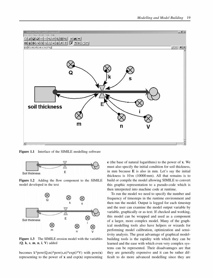
Modelling and Model Building 19
Figure 1.1 Interface of the SIMILE modelling software
Soil thickness E
Figure 1.2 Adding the flow component to the SIMILEmodel developed in the text
Soil thickness
Qk s
E
m n V
i
Figure 1.3 The SIMILE erosion model with the variables(Q, k, s, m, n, i, V) added
becomes k*pow(Q,m)*pow(s,n)*exp(i*V) with pow(x)representing to the power of x and exp(x) representing
e (the base of natural logarithms) to the power of x. Wemust also specify the initial condition for soil thickness,in mm because E is also in mm. Let’s say the initialthickness is 10 m (10000 mm). All that remains is tobuild or compile the model allowing SIMILE to convertthis graphic representation to a pseudo-code which isthen interpreted into machine code at runtime.
To run the model we need to specify the number andfrequency of timesteps in the runtime environment andthen run the model. Output is logged for each timestepand the user can examine the model output variable byvariable, graphically or as text. If checked and working,this model can be wrapped and used as a componentof a larger, more complex model. Many of the graph-ical modelling tools also have helpers or wizards forperforming model calibration, optimization and sensi-tivity analysis. The great advantage of graphical model-building tools is the rapidity with which they can belearned and the ease with which even very complex sys-tems can be represented. Their disadvantages are thatthey are generally expensive and it can be rather dif-ficult to do more advanced modelling since they are

20 Mark Mulligan and John Wainwright
Figure 1.4 Influences between the variables and the flow for the SIMILE soil-erosion model
rather more constrained than modelling in code. If youwant to look into it further, the online help and tutorialfiles of SIMILE provide much greater detail on the morepowerful aspects of its functionality including its abilityto deal with many (spatial) instances of a model rep-resenting for example, individual hillslopes or plants orcatchments. You can download this erosion model fromthe companion website for this book.
1.4.7 Modelling in spreadsheets: using Excel
A very detailed training for modelling in Excel isgiven in Hardisty et al. (1994), so we only provide asimple example here. To build the same soil-erosionmodel in a spreadsheet such as Microsoft Excel requiresthe specification of the time interval and number oftimesteps upfront since these will be entered directly intothe first column of the spreadsheet. Open the spreadsheetand label column A as Timestep at position A:2 in thespreadsheet (column A, row 2). Then populate the next30 rows of column A with the numbers 1 to 30. Thiscan be easily achieved by adding the number 1 to A:3.At position A:4 type the following equation: =A3+1
and press enter. The spreadsheet will now calculatethe results of this equation which will appear as thenumber in A:4. We can now highlight cells A:4 throughto A:32 with our pointing device (left click and dragdown) and go to the menu item Edit and the Fill andthen Down (or Ctrl-D) to copy this equation to all thecells in the highlighted range. Note that in each cell,the cell identifier to the left of the plus sign in theequation (which for the active cell can be viewed inthe equation bar of Excel) is changed to represent thecell above it so that in A:4 it is A:3 but in A:5 it is A:4and so on. This is relative referencing which is a veryuseful feature of Excel as far as modelling is concernedbecause it allows us to define variables, i.e. parameterswhich change with time and time, which are usuallyrepresented along the rows of the spreadsheet or evenon another spreadsheet. Model instances representingdifferent locations or objects are usually representedacross the columns of the spreadsheet, as are thedifferent compartment, flow and variable equations.
If we want to avoid relative referencing in order tospecify a constant or parameter (rather than a variable),
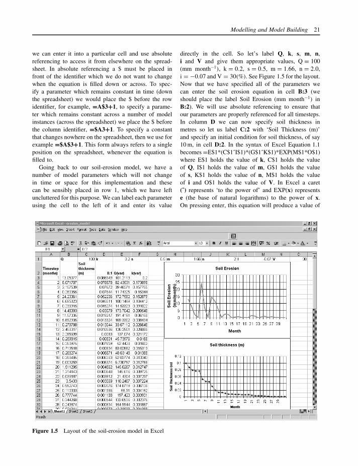
Modelling and Model Building 21
we can enter it into a particular cell and use absolutereferencing to access it from elsewhere on the spread-sheet. In absolute referencing a $ must be placed infront of the identifier which we do not want to changewhen the equation is filled down or across. To spec-ify a parameter which remains constant in time (downthe spreadsheet) we would place the $ before the rowidentifier, for example, =A$3+1, to specify a parame-ter which remains constant across a number of modelinstances (across the spreadsheet) we place the $ beforethe column identifier, =$A3+1. To specify a constantthat changes nowhere on the spreadsheet, then we use forexample =$A$3+1. This form always refers to a singleposition on the spreadsheet, whenever the equation isfilled to.
Going back to our soil-erosion model, we have anumber of model parameters which will not changein time or space for this implementation and thesecan be sensibly placed in row 1, which we have leftuncluttered for this purpose. We can label each parameterusing the cell to the left of it and enter its value
directly in the cell. So let’s label Q, k, s, m, n,i and V and give them appropriate values, Q = 100(mm month−1), k = 0.2, s = 0.5, m = 1.66, n = 2.0,i = −0.07 and V = 30(%). See Figure 1.5 for the layout.Now that we have specified all of the parameters wecan enter the soil erosion equation in cell B:3 (weshould place the label Soil Erosion (mm month−1) inB:2). We will use absolute referencing to ensure thatour parameters are properly referenced for all timesteps.In column D we can now specify soil thickness inmetres so let us label C:2 with ‘Soil Thickness (m)’and specify an initial condition for soil thickness, of say10 m, in cell D:2. In the syntax of Excel Equation 1.1becomes =E$1*(C$1ˆI$1)*(G$1ˆK$1)*EXP(M$1*O$1)where E$1 holds the value of k, C$1 holds the valueof Q, I$1 holds the value of m, G$1 holds the valueof s, K$1 holds the value of n, M$1 holds the valueof i and O$1 holds the value of V. In Excel a caret(ˆ) represents ‘to the power of’ and EXP(x) representse (the base of natural logarithms) to the power of x.On pressing enter, this equation will produce a value of
Figure 1.5 Layout of the soil-erosion model in Excel
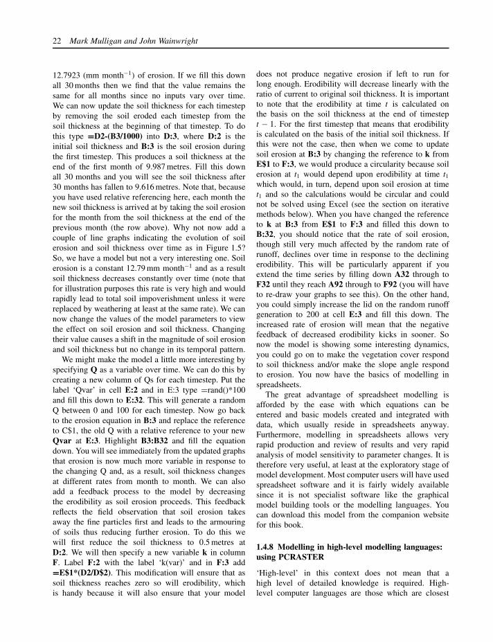
22 Mark Mulligan and John Wainwright
12.7923 (mm month−1) of erosion. If we fill this downall 30 months then we find that the value remains thesame for all months since no inputs vary over time.We can now update the soil thickness for each timestepby removing the soil eroded each timestep from thesoil thickness at the beginning of that timestep. To dothis type =D2-(B3/1000) into D:3, where D:2 is theinitial soil thickness and B:3 is the soil erosion duringthe first timestep. This produces a soil thickness at theend of the first month of 9.987 metres. Fill this downall 30 months and you will see the soil thickness after30 months has fallen to 9.616 metres. Note that, becauseyou have used relative referencing here, each month thenew soil thickness is arrived at by taking the soil erosionfor the month from the soil thickness at the end of theprevious month (the row above). Why not now add acouple of line graphs indicating the evolution of soilerosion and soil thickness over time as in Figure 1.5?So, we have a model but not a very interesting one. Soilerosion is a constant 12.79 mm month−1 and as a resultsoil thickness decreases constantly over time (note thatfor illustration purposes this rate is very high and wouldrapidly lead to total soil impoverishment unless it werereplaced by weathering at least at the same rate). We cannow change the values of the model parameters to viewthe effect on soil erosion and soil thickness. Changingtheir value causes a shift in the magnitude of soil erosionand soil thickness but no change in its temporal pattern.
We might make the model a little more interesting byspecifying Q as a variable over time. We can do this bycreating a new column of Qs for each timestep. Put thelabel ‘Qvar’ in cell E:2 and in E:3 type =rand()*100and fill this down to E:32. This will generate a randomQ between 0 and 100 for each timestep. Now go backto the erosion equation in B:3 and replace the referenceto C$1, the old Q with a relative reference to your newQvar at E:3. Highlight B3:B32 and fill the equationdown. You will see immediately from the updated graphsthat erosion is now much more variable in response tothe changing Q and, as a result, soil thickness changesat different rates from month to month. We can alsoadd a feedback process to the model by decreasingthe erodibility as soil erosion proceeds. This feedbackreflects the field observation that soil erosion takesaway the fine particles first and leads to the armouringof soils thus reducing further erosion. To do this wewill first reduce the soil thickness to 0.5 metres atD:2. We will then specify a new variable k in columnF. Label F:2 with the label ‘k(var)’ and in F:3 add=E$1*(D2/D$2). This modification will ensure that assoil thickness reaches zero so will erodibility, whichis handy because it will also ensure that your model
does not produce negative erosion if left to run forlong enough. Erodibility will decrease linearly with theratio of current to original soil thickness. It is importantto note that the erodibility at time t is calculated onthe basis on the soil thickness at the end of timestept − 1. For the first timestep that means that erodibilityis calculated on the basis of the initial soil thickness. Ifthis were not the case, then when we come to updatesoil erosion at B:3 by changing the reference to k fromE$1 to F:3, we would produce a circularity because soilerosion at t1 would depend upon erodibility at time t1which would, in turn, depend upon soil erosion at timet1 and so the calculations would be circular and couldnot be solved using Excel (see the section on iterativemethods below). When you have changed the referenceto k at B:3 from E$1 to F:3 and filled this down toB:32, you should notice that the rate of soil erosion,though still very much affected by the random rate ofrunoff, declines over time in response to the decliningerodibility. This will be particularly apparent if youextend the time series by filling down A32 through toF32 until they reach A92 through to F92 (you will haveto re-draw your graphs to see this). On the other hand,you could simply increase the lid on the random runoffgeneration to 200 at cell E:3 and fill this down. Theincreased rate of erosion will mean that the negativefeedback of decreased erodibility kicks in sooner. Sonow the model is showing some interesting dynamics,you could go on to make the vegetation cover respondto soil thickness and/or make the slope angle respondto erosion. You now have the basics of modelling inspreadsheets.
The great advantage of spreadsheet modelling isafforded by the ease with which equations can beentered and basic models created and integrated withdata, which usually reside in spreadsheets anyway.Furthermore, modelling in spreadsheets allows veryrapid production and review of results and very rapidanalysis of model sensitivity to parameter changes. It istherefore very useful, at least at the exploratory stage ofmodel development. Most computer users will have usedspreadsheet software and it is fairly widely availablesince it is not specialist software like the graphicalmodel building tools or the modelling languages. Youcan download this model from the companion websitefor this book.
1.4.8 Modelling in high-level modelling languages:using PCRASTER
‘High-level’ in this context does not mean that ahigh level of detailed knowledge is required. High-level computer languages are those which are closest

Modelling and Model Building 23
to human language compared with low-level languageswhich are closer to machine code. High-level languagesdefine a rigid syntax in which the user is able to developsoftware or a string of calculations without knowing toomuch about how the computer actually performs thecalculations or functions that will be done. Examplesof high level computer programming languages includeBASIC, Pascal, FORTRAN, C++ and Java.
A number of researchers have designed generic com-puter modelling languages for the development of spatialand nonspatial models (van Deursen, 1995; Wesselinget al., 1996; Maxwell and Costanza, 1997; Karssenberget al., 2000). None has been universally accepted andmany have not been realized in software. The flexibil-ity required of a generic modelling language is so greatthat few codes are robust enough to handle all poten-tial applications. PCRASTER (http://www.pcraster.nl) isa good example of a high-level, spatial modelling lan-guage. Instead of working with parameters, constants andvariables which point to single numbers, PCRASTERparameters, constants and variables point to raster gridmaps which may contain categorical data, ordinal values,real numbers, a Boolean (true or false) value or one ofa number of more specialist types of data. PCRASTERis a pseudo-code interpreter, which provides the mod-eller with high-level functions for cartographic modelling(GIS) and dynamic modelling (spatial modelling overtime). These functions can be invoked at the MS-DOScommand line to perform simple calculations or in modelscript files for the integration of dynamic spatial mod-els. A number of utilities are available for map and timeseries display, import and export and map attribute con-version. A PCRASTER model consists of a simple ASCIItext file in which commands are listed in the sequencein which calculation is required. PCRASTER reads andinterprets this file line by line at runtime to realize themodel simulation. A PCRASTER model consists of the
following sections: binding, areamap, timer, initial anddynamic. In the binding section the user specifies a setof variable names that will be used in the model scriptand the corresponding disk file names from which thedata can be read or written, in the format:
VariableName=mapname.map; for a variable whichpoints to a single map and always reads or writes tothat map.
VariableName=mapname; for a variable which pointsto a different map each timestep, in the first timestepthe map is given the suffix mapname0.001, in thesecond timestep mapname0.002 and so on, with zerosbeing used to fill the file name to eight characters andalso to fill the unused parts of the file extension.
VariableName=timeseriesname.tss; for a variablewhich reads from or to columns in a timeseries file.
VariableName=tablename.tbl; for a variable whichreads or writes to a data table or matrix.
Note that like many programming and scripting lan-guages PCRASTER is case sensitive. You must beconsistent with the usage of lower and upper case inyour scripts.
In the areamap section the user specifies a clonemap of Boolean type that identifies the area for cal-culations with a TRUE (1) and the area in which nocalculations will be performed with a FALSE (0). In thetimer section the user specifies the initial timestep, thetime interval and the number of timesteps. In the initialsection the user specifies any initial conditions (calcu-lations that will be performed only once at the startof the simulation). The bulk of a PCRASTER modelusually falls within the dynamic section which speci-fies calculations that will be performed in sequence forevery timestep. The text below represents a PCRASTERversion of the soil-erosion model.
# Erosion Model.binding#inputDem=dem.map;#outputErosion=eros;#time series and tablesErosTss=Erosion.tss;OflowTss=oflow.tss;
#constantsm=1.66;n=2.0;

24 Mark Mulligan and John Wainwright
e=2.718;Q=100;i=-0.07;k=0.2;V=30;areamapclone.map;timer1 92 1;initialSlopeDeg=scalar(slope(Dem));#slope tangentThickness=scalar(10);dynamicreport Erosion=k*(Q**m)*(SlopeDeg**n)*(e**(i*V);#(mm)report ErosTss=maptotal(Erosion);Thickness=Thickness-(Erosion/1000);#(m)
Note that in this very simple model the only spatiallyvariable quantity is slope angle (SlopeDeg), which isderived from the digital elevation model (Dem) usingthe PCRASTER slope() command which performs awindow operation to define the slope on the basis ofthe change in altitude between each cell and its eightcontiguous neighbours (see Chapter 4). All other quan-tities are defined as constants. Even the soil thickness,which is specified here as an initial condition equal to100, is constant across the map though, as a state vari-able, it will vary over time. Equation 1.1 in PCRASTERsyntax becomes:
report Erosion= k∗(Q∗∗m)∗(SlopeDeg∗∗n)
∗(e∗∗(i∗V); #(mm)
where ‘report’ is the keyword which ensures that theresults of the calculation are written to the output mapon disk, ** represents ‘to the power of’ and * repre-sents ‘multiplied by’. All PCRASTER script commandlines (except the section headings) must end in a :..The # (hash) symbol indicates that all material to theright of the hash and on the same line is a commentwhich is not to be interpreted by PCRASTER. Thespatial functionality of PCRASTER is used in the map-total function that, in this case, sums erosion across thewhole map for output as a single value per timestepin a time series file. The final line of the code updatesthe soil thickness according to the erosion which hastaken place. It might seem unusual to have a state-ment such as Thickness=Thickness-(Erosion/1000);because the same variable is both sides of the equalssign. This is in fact a fairly common construct inprogramming and modelling languages and is equiv-alent to Thicknesst = Thicknesst−1 – (Erosiont/1000);
in other words, it allows passage of informationbetween timesteps. In order that soil thickness is neverallowed to become negative we should use the syntaxThickness=max(Thickness-(Erosion/1000),0);.
Again this is not a particularly interesting model.When supplied with a DEM, in this case for a catchmentin Spain, this model will produce a series of 92 maps oferosion, which will vary over space according to slopeangle but will be constant in time (Figure 1.6). To makethe model more interesting we may, for example, usesome of the functionality of PCRASTER to (a) makethe spatial distribution of Q more realistic; (b) producea temporally variable Q; and (c) vary soil thicknessaccording to landscape and provide a negative feedbackto soil erosion to represent armouring. In order to dis-tribute Q spatially we must define the local drainagedirection (LDD) and then specify a precipitation andan infiltration rate and calculate the difference betweenthem (the runoff) for each timestep. Further, we mustaccumulate this runoff down the stream network orLDD. The cumulated runoff will represent a much morerealistic situation than a uniform runoff. In the initialsection we use the PCRASTER function LDDCREATEto calculate the drainage direction for each cell basedon the steepest drop to its eight contiguous neigh-bours (the so-called D8 algorithm; see O’Callaghan andMark, 1984, or Endreny and Wood, 2001). The syn-tax is: Ldd=lddcreate(Dem, elevation, outflowdepth,corevolume, corearea, catchmentprecipitation) wherethe five latter parameters are thresholds used in theremoval of local pits that can be produced by inaccura-cies in the production of the DEM and can be safelyset to 1e31 each here since the DEM to be used is
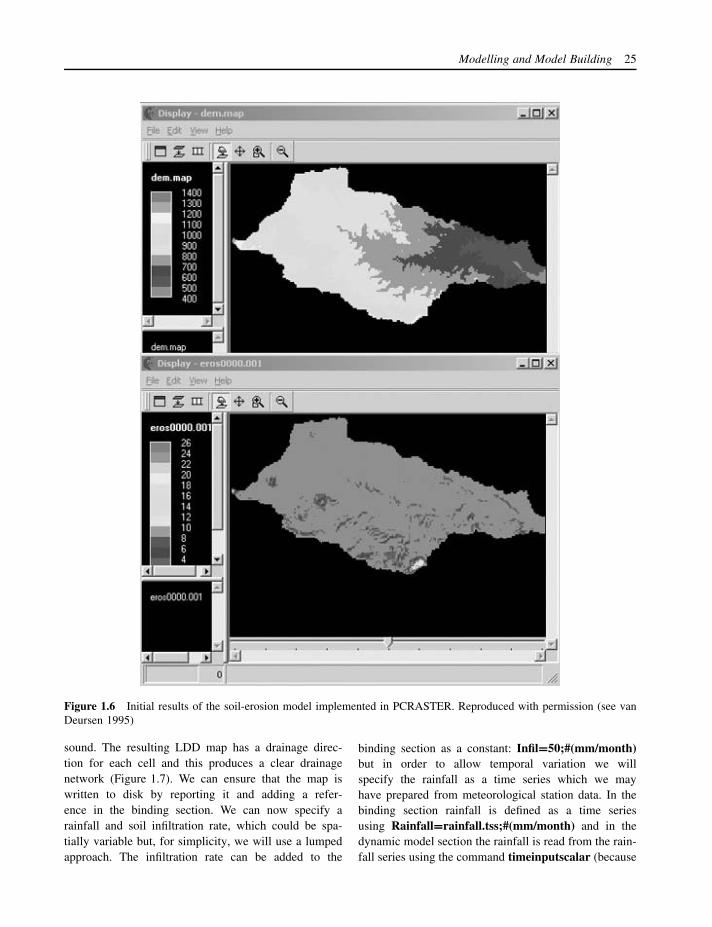
Modelling and Model Building 25
Figure 1.6 Initial results of the soil-erosion model implemented in PCRASTER. Reproduced with permission (see vanDeursen 1995)
sound. The resulting LDD map has a drainage direc-tion for each cell and this produces a clear drainagenetwork (Figure 1.7). We can ensure that the map iswritten to disk by reporting it and adding a refer-ence in the binding section. We can now specify arainfall and soil infiltration rate, which could be spa-tially variable but, for simplicity, we will use a lumpedapproach. The infiltration rate can be added to the
binding section as a constant: Infil=50;#(mm/month)but in order to allow temporal variation we willspecify the rainfall as a time series which we mayhave prepared from meteorological station data. In thebinding section rainfall is defined as a time seriesusing Rainfall=rainfall.tss;#(mm/month) and in thedynamic model section the rainfall is read from the rain-fall series using the command timeinputscalar (because

26 Mark Mulligan and John Wainwright
Figure 1.7 Drainage direction for each cell in the PCRASTER soil-erosion model and its corresponding altitude.Reproduced with permission (see van Deursen 1995)
rainfall is a scalar quantity that is a continuous, real, asopposed to integer, number). The command which mustbe added to the dynamic section before erosion is cal-culated is Rainfallmm=timeinputscalar(Rainfall,1);.The number 1 indicates that the first column of therainfall file is read and applied to all cells, but a mapof nominal values could have equally been suppliedhere allowing the reading of different columns of thetime series file for different cells or areas of the map.As in the spreadsheet, time passes down the rows oftime series files. The format for time series files isgiven in the PCRASTER online documentation. Wecan now specify the infiltration excess for each cell as:InfilExcess=max(Rainfallmm-Infil,0);. The max state-ment ensures that InfilExcess is never less than zero.In order to cumulate this excess along the flow net-work we use the accuflux command in the form: reportQ=accuflux(Ldd, InfilExcess);. Now remove (or com-ment out using #) the reference to Q as a constant andthe new Q will be distributed along the local drainagenetwork. We can now specify soil thickness as a spatiallyvariable entity instead of a constant by commenting outits definition as a constant in the initial section and
by specifying it as a function of landscape propertiesinstead. Saulnier et al. (1997) model soil thickness as adecreasing function of slope on the basis of greater ero-sion on steep slopes and greater deposition on shallowones. Here we will approximate a distribution of soilthickness according to a compound topographic index,the so-called TOPMODEL wetness index (WI), whichis the ratio of upslope area to local slope angle andtherefore expresses the potential for soil accumulationas well as erosion. We can calculate the WI in the initialsection as WI=accuflux(Ldd,25*25)/SlopeDeg; where25 is the width of the individual raster grid cells (inmetres). We can scale soil thickness in a simple way asThickness=(WI/mapmaximum(WI))*MaxThickness;where MaxThickness is the maximum potential soilthickness. Finally, we can replicate the armouring algo-rithm we developed in the spreadsheet model by stor-ing the initial soil thickness using InitialThickness=Thickness; in the initial section, removing the definitionof erodibility (k) as a constant in the binding section andreplacing it with the following definition in the dynamicsection of the model script: k = 0.2*(Thickness/Initial-Thickness);.

Modelling and Model Building 27
We now have a more sophisticated model in whicherosion will respond to passing rainfall events over timeand spatially to the cumulation of infiltration excessdown the spatially variable stream network. Further-more, the soil erosion will vary with slope gradient anda negative feedback mechanism reduces erosion as itprogresses to simulate surface armouring. The modelis still very simple and could be made more realis-tic in many ways (by making the vegetation respondto soil moisture and soil thickness, by making slope
angle responsive to erosion, and so on). However,even this simple model can enhance our understand-ing of the spatial patterns of soil erosion. Figure 1.8shows (a) the DEM; (b) the calculated slope angle;(c) the natural log of soil erosion for month 4 (72.4 mmrainfall); and (d) the natural log of soil erosion formonth 32 (53.8 mm rainfall). The scale used is loga-rithmic in order that the spatial pattern can be morereadily seen. The final PCRASTER code is given inthe box:
# Erosion Model.binding#inputDem=dem.map;Rainfall=rainfall.tss;#(mm/month)#outputErosion=eros;Ldd=ldd.map;#time series and tablesErosTss=Erosion.tss;OflowTss=oflow.tss;#constantsm=1.66;n=2.0;e=2.718;#Q=100;i=-0.07;#k=0.2;V=30;Infil=50;#(mm/month)areamapclone.map;timer1 92 1;initialSlopeDeg=scalar(slope(Dem));#slope tangentWI=accuflux(Ldd,25*25)/SlopeDeg;Thickness=(WI/mapmaximum(WI))*10;InitialThickness=Thickness;report Ldd=lddcreate(dem.map,1e31,1e31,1e31,1e31);
dynamick=0.2*(Thickness/InitialThickness);Rainfallmm=timeinputscalar(Rainfall,1);InfilExcess=max(Rainfallmm-Infil,0);report Q=accuflux(Ldd,InfilExcess);Erosion=k*(Q**m)*(SlopeDeg**n)*(e**(i*V));#(mm)report ErosTss=maptotal(Erosion);Thickness=max(Thickness-(Erosion/1000),0);#(m)

28 Mark Mulligan and John Wainwright
Figure 1.8 Final PCRASTER soil-erosion model results showing: (a) the DEM; (b) the calculated slope angle; (c) thenatural log of soil erosion for month 4 (72.4 mm rainfall); and (d) the natural log of soil erosion for month 32(53.8 mm rainfall). Reproduced with permission (see van Deursen 1995)
You can download this model from the companionwebsite for this book.
The main advantage of scripting languages likePCRASTER is in their power and flexibility and in therapidity with which even complex operations can be per-formed through the application of pre-coded high-levelfunctions. The main disadvantage is that such languagesrequire a considerable effort to learn and have steeplearning curves, but, once mastered, significant mod-elling feats are relatively easy. Scripting languages arenot, however, as flexible and powerful as high-levelcomputer languages but these in turn can require largeprogramming marathons to achieve the same as a fewlines in a well-crafted scripting language. High-levelcomputer languages offer the advantages of flexibilityto implement new procedures and the ability to opti-mize complex procedures to run as quickly as possi-ble. For detailed climate (Chapter 2) or computationalfluid dynamics (Chapter 20) modelling, such optimiza-tion (perhaps by running a model in parallel on a numberof processors at once) is an absolute necessity so thatresults may be obtained within a reasonable time frame.Even in general applications, a compiled language (e.g.FORTRAN, Pascal or C++) will be noticeably faster thanan interpreted one (e.g. PCRASTER, BASIC and usu-ally Java).
So, we have used three modelling approaches toproduce essentially the same model. Each approach hasits advantages and disadvantages and you will probablyhave made up your mind already which approach youfeel more comfortable with for the kind of modellingthat you wish to do. Whichever technique you use tobuild models, it is critically important to keep focusedon the objective and not to fall into the technology trapthat forces all of your mental power and effort intojumping the technological hurdles that may be needed toachieve a set of calculations and as a result leaves littleenergy and time after the model building stage for itstesting, validation and application to solving the problemat hand. A simpler model which is thoroughly testedand intelligently applied will always be better than atechnically advanced model without testing or sufficientapplication.
1.4.9 Hints and warnings for model building
Cross and Moscardini (1985) give a series of hintsand warnings intended to assist novice modellers inbuilding useful models. This list is expanded hereaccording to our own environmentally biased perspec-tive on modelling.

Modelling and Model Building 29
1. Remember that all models are partial and willnever represent the entire system. Models are neverfinished, they always evolve as your understand-ing of the system improves (often with thanks tothe previous model). In this way all models arewrong (Sterman, 2002)! Nevertheless, it is impor-tant to draw some clear lines in model developmentwhich represent ‘finished’ models which can betested thoroughly and intensively used.
2. Models are usually built for a specific purpose sobe careful of yourself or others using them forpurposes other than those originally intended. Thisissue is particularly relevant where models are givena potentially wide user base through distribution viathe Internet.
3. Do not fall in love with your model (it will not loveyou back!).
4. Take all model results with a grain of salt unlessthose specific results have been evaluated in someway.
5. Do not distort reality or the measurement of realityto fit with the model, however convincing yourconceptualization of reality appears to be.
6. Reject properly discredited models but learn fromtheir mistakes in the development of new ones.
7. Do not extrapolate beyond the region of validityof your model assumptions, however powerful itmakes you feel!
8. Keep ever present the distinction between modelsand reality. The sensitivity of a model to climatechange is not the sensitivity of reality to climatechange. If you write about ‘model sensitivity’ thendo not omit the word ‘model’ (Baker, 2000).
9. Be flexible and willing to modify your modelas the need arises. Note that this is modify notexpand upon.
10. Keep the objectives ever present by continuallyasking ‘What is it that I am trying to do?’
11. As in all aspects of science, keep the model honestand realistic despite any short-term financial orstatus gain that may seem to accrue from doingthe opposite.
1.5 DEVELOPMENT OF NUMERICALALGORITHMS
1.5.1 Defining algorithms
An algorithm is the procedure or set of rules that we useto solve a particular problem. Deciding on the algorithmto use in any particular model can be thought about intwo stages. The first has already been covered in the
previous section – that of conceptualizing the systemand developing a mental model of the system. Thesecond is the conversion of this conceptualization to aform that can be calculated. It may be that, at this stage,the problem as formalized is not calculable, and we mustreturn to the former stage and try to re-evaluate anddescribe the system in question, so that an approximationcan be arrived at without compromising the reliabilityof the model results.
1.5.2 Formalizing environmental systems
Environmental models are focused upon change. Thischange may be of properties in time or in space.Increasingly, models are being developed where bothtemporal and spatial variations are evaluated, so weneed to have techniques that can assess both of thesechanges. The branch of mathematics that allows us toassess change is known as calculus, initially derivedin the seventeenth century independently by Newtonand Leibniz. A basic understanding of calculus isfundamental for all modelling, so we will provide abrief overview here. More detailed information can befound in numerous books, some of the more accessiblebeing Bostock and Chandler (1981), De Sapio (1976),Ferrar (1967), Friedman (1968), Haeussler and Paul(1988), Lang (1978) and Thompson (1946).
Consider the case where we are interested in the trans-port of coarse sediment through a river. To investigatethe process we have tagged rocks with radio transmit-ters that allow us to record the location of the rocksthrough time (e.g. Schmidt and Ergenzinger, 1992). InFigure 1.9 we have plotted the position along the riverchannel of a rock over a period of 24 hours. Theseresults can also be plotted as a graph showing thelocation in space and time of the rock (Figure 1.9b).This graph can also be used to define the change inposition through time. The change in position throughtime is effectively the velocity of the rock as it moves.Remember that velocity is the change in distance overthe time to move that distance. Over the 24 hours, therock moved a total of 8.57 m, so that its average veloc-
ity was8.57 m
24 h= 0.36 m h−1. Notice, however, that the
rock was not moving at a constant velocity through theday, as the graph is not a straight line. We can use thesame technique to show how the velocity of the particlevaried over time. In the second hour, the particle moved0.72 m, so its velocity was 0.72 m h−1. Fourteen hourslater, the velocity was 0.22 m h−1 (Figure 1.9c). Thesevelocities are simply the slope of the graph at succes-sive points in time. We now have enough information

30 Mark Mulligan and John Wainwright
(a)
(c)
(e)
(d)
0123456789
0 6 12 18 24
Time h
Time h
Dis
tanc
e m
oved
m
Dis
tanc
e m
oved
m0.72 m
1 h
1 h 0.22 m
9876543210
12 18 2460(b)
0
0.5
1
1.5
2
2.5
3
0 5 10 15 20Time h
Vel
ocity
m h
−1
Independent variable x
Dep
ende
nt v
aria
ble
y
y = f (x)
Figure 1.9 (a) Map showing position along a stream channel of a tagged rock over a period of 24 hours; (b) Graphshowing the location in time and space of the tagged rock as shown in Figure 1.9a. The line interpolates the positionof the rock at times between those measured; (c) Graph showing how the variation in the velocity of the measuredrock can be calculated as the local slope of the graph; (d) Graph showing relationship between the two variables as acontinuous function. The thick lines show examples of the tangent of the slope at specific points; (e) Graph showing thevelocity of the rock particle through time. The line shows the continuous change in velocity calculated using the formulady
dx= y ′ = 0.875x−0.5, obtained by differentiation, whereas the points show the measured points at hourly intervals. Note
the major difference in the early part of the graph, where the velocity is rapidly changing, due to the fact that the hourlymeasurements are based on an average rather than continuous measurements
to model the movement of the rock at a daily andhourly timestep.
However, if we need to model movements at shortertime intervals, we need to have some method forestimating the velocity of the rock, and thus the slope ofthe line, at these shorter intervals. To do this, we may
be able to use a function that shows us how the twovariables are related, either empirically or from physicalprinciples. Typically, this function may be written inthe form:
y = f (x) (1.2)

Modelling and Model Building 31
In this case, we find empirically (for example, usingregression analysis) that the relationship has a sim-ple form:
y = 1.75x0.5 (1.3)
where the variable y is the distance moved in metresand x is the time in hours. The velocity of the particleis still the slope at each point on the graph; we can nowestimate these slopes continuously from our function,as the tangent to the curve at each successive point(Figure 1.9d). To calculate this tangent, we need to workout the derivative of the function, which has the standardform for power-law relationships such as Equation 1.3:
dy
dx= nxn−1 (1.4)
How this standard form is obtained is shown inFigure 1.10.
The derivativedy
dx(usually said as ‘dy by dx’) may
also be written as y ′ or f′(x). (The difference betweenthese is essentially that the former is Newton’s notation,whereas the latter is that of Leibniz.) Applying this ruleto the example of Equation 1.3, we have:
dy
dx= y ′ = 0.875x−0.5 (1.5)
Thus, we can now calculate the instantaneous velocity ofour rock at any point in time. The process of calculatingthe derivative is known as differentiation. More complexfunctions require different rules for differentiation, andthese can be found in the standard texts cited above andon the book’s website.
Environmental models may also commonly use termsrelating to acceleration or diffusion. Acceleration isthe change in velocity through time, so we can alsocalculate it using differentiation. This time, we plotvelocity against time (Figure 1.9e) and find the tangentat a point by differentiating this curve. Relative to ouroriginal measurement, we have calculated:
ddy
dx
dx= d2y
dx2= f′′(x) = y ′′ (1.6)
This term is called the second derivative. The standardform for power-law relationships means that we simplyneed to repeat the operation in Equation 1.4 twice tocalculate the specific value of the second derivative:
d2y
dx2= n(n − 1)xn−2 (1.7)
Thus, our rock particle is accelerating at a rate of y ′′ =−0.5 × 0.875x−1.5 = −0.4375x−1.5 m h−1, or in otherwords it is consistently decelerating.
Thornes (1985, 1988) uses derivatives in modellingthe interaction between vegetation and erosion to showcases of stability in the landscape. Given a functionalrelationship for vegetation change, it is possible to findthe conditions where vegetation cover becomes constant.
This is simply wheredV
dt= 0, where V is the vegetation
amount and t is time. This example is examined furtherin Chapter 18. Another use for derivatives is in theprocess of optimization to find the optimal values ofparameters in a model. These optimal values may fall atmaximum or minimum points of the graph showing therelationship. At these points, the following conditionsfor the first and second derivatives will hold:
Maximum:dy
dx= 0
d2y
dx2< 0 (1.8a)
Minimum:dy
dx= 0
d2y
dx2> 0 (1.8b)
Care must, however, be taken that the graph is notsimply at a local plateau, or inflexion point, where:
Inflexion:dy
dx= 0
d2y
dx2= 0. (1.8c)
Integration is the opposite process to differentiation.It allows us to calculate the sum of a property overspace or time. If we plot the function that representsthe relationship we are interested in, then the sum ofthis property is the area under the curve. To see whythis is so, consider a function that relates the change indepth of water along a section of river (Figure 1.11).If the depth (h) is constant along section of length y,then the sum of the values of y is simply y · h. In otherwords, it is the area under water along the section lengthin which we are interested – in this case representedby a simple rectangle. If, however, the depth increaseslinearly along the section, then the area under the curvewill be a trapezium with area 0.5(h1 + h2) · y, whereh1 is the depth at the start of the reach and h2 isthe depth at the end. We often use this approach tocalculate integrals where the shape of the relationshipis complex, or known only from data at certain points.The ‘trapezium rule’ involves dividing the curve or datainto a set of known intervals, calculating the area of thetrapezium that is a simple representation of each interval,and summing the total area. This approach is best whenwe know the change between points is linear, or thedistance between points is sufficiently small. Note thatwe are not restricted to integration in one dimension.If we integrated the area of water by the width of the

32 Mark Mulligan and John Wainwright
Deriving the Standard Form for Differential Calculus
Let us take, as an example, the function y = x2 + 2x. Intabular and graphical forms, this function is:
x = y =0 01 32 83 154 245 35. . . . . .
0 420
6 8 10
20
40
60
80
100
120
y
x
A line joining any two points on the curve is known as achord. In the graph below, the line PQ is a chord.
y = f(x)
P
Q
A B
C
y
x
The slope of this line is:
gradient of PQ = QC
PC
To define the gradient at a point, let the length of PC in thegraph above be h (an arbitrary length). If the point C is (2,8), then the value of the coordinates of point Q are given bythe function, by inserting the x value of Q, which is (2 + h).The y value at Q is then:
y = (2 + h)2 + 2(2 + h)
which is 8 + 6h + h2. The distance QC is then 6h + h2 (the8 disappears because it is the value of y at C) and the
gradient of the chord PQ is:
gradient of PQ = QC
PC= 6h + h2
h= 6 + h
To find the value of the gradient at the point P, we let thevalue of h become vanishingly small, so that the points Pand Q are in the same location. In other words, the valueof h approaches zero. This process is known as taking the
limit and is written: hlim 0. Thus, we have:
gradient at P = h 0 (6 + h) = 6
In more general terms, if P is any point (x, y), then Q isgiven by the function as (x + h, (x + h)2 + 2(x + h)), or byexpansion of terms (x + h, x2 + 2xh + h2 + 2x + 2h) andthe gradient of the chord PQ is:
gradient of PQ = 2xh + h2 + 2h
h= 2x + h + 2
In this case, the value of y at P (i.e. x2 + 2x) disappearswhen calculating the distance from Q, leaving the remainingterms (i.e. 2xh + h2 + 2h). The gradient at P then becomes:
gradient at P = h 0 (2x + h + 2) = 2x + 2
which we can verify by substitution, so that if x = 2, thegradient at P is 6. The derivative of y = x2 + 2x is thus
demonstrated as beingdy
dx= 2x + 2, which is the same as
given by the standard form in the main text (i.e. we applydy
dx= nxn −1 to each of the terms which contain an x in
the function).It is more usual to use the incremental notation as
illustrated below:
A B x
y
CP(x,y)dx
dy
Q (x + dx,y + dy)
y = f(x)
where dx means the increment in x and dy the increment iny. We can then re-write:
gradient of PQ = QC
PC= dy
dx
dx
and by definition:
dy
dx= 0 = dy
dx
lim
lim
lim
Figure 1.10 Derivation of the standard form of differentiation
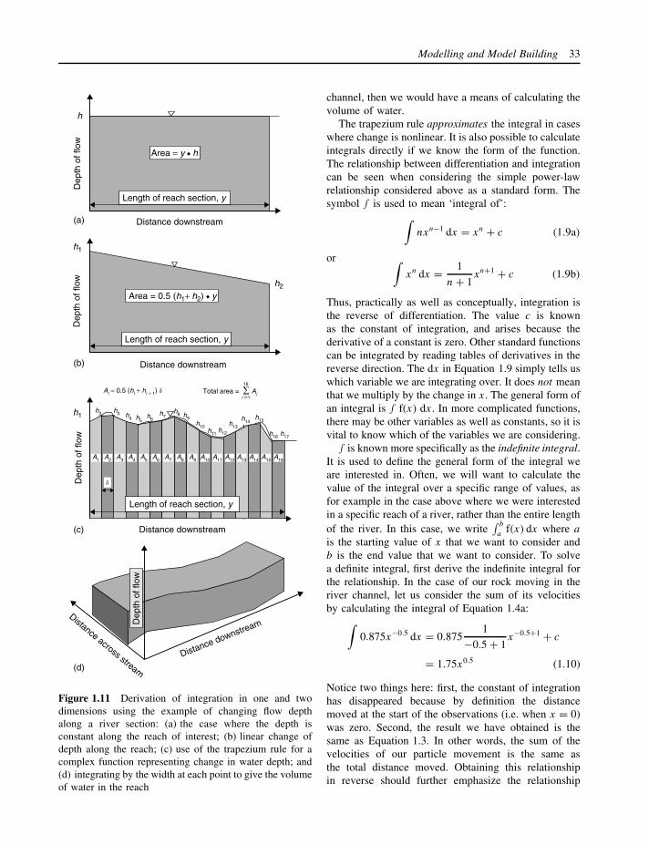
Modelling and Model Building 33
Distance downstream
Dep
th o
f flo
w
(a)
(b)
(c)
(d)
h
Length of reach section, y
Area = y • h
Distance downstream
Dep
th o
f flo
w
Length of reach section, y
h1
h1
h2
Area = 0.5 (h1+ h2) • y
Distance downstreamDistance across stream
Dep
th o
f flo
w
Distance downstream
Dep
th o
f flo
w
5
Ai = 0.5 (hi + hi + 1) d
A1 A2 A3 A4 A5 A6 A7 A8 A9 A10 A11 A12 A13 A14 A15 A16
h2 h3 h4 h5h6
h7h8 h9
h10h11
h12
h13
h14h15
h16 h17
Length of reach section, y
d
Total area = ∑ Ai
16
i =1
Figure 1.11 Derivation of integration in one and twodimensions using the example of changing flow depthalong a river section: (a) the case where the depth isconstant along the reach of interest; (b) linear change ofdepth along the reach; (c) use of the trapezium rule for acomplex function representing change in water depth; and(d) integrating by the width at each point to give the volumeof water in the reach
channel, then we would have a means of calculating thevolume of water.
The trapezium rule approximates the integral in caseswhere change is nonlinear. It is also possible to calculateintegrals directly if we know the form of the function.The relationship between differentiation and integrationcan be seen when considering the simple power-lawrelationship considered above as a standard form. Thesymbol ∫ is used to mean ‘integral of’:∫
nxn−1 dx = xn + c (1.9a)
or ∫xn dx = 1
n + 1xn+1 + c (1.9b)
Thus, practically as well as conceptually, integration isthe reverse of differentiation. The value c is knownas the constant of integration, and arises because thederivative of a constant is zero. Other standard functionscan be integrated by reading tables of derivatives in thereverse direction. The dx in Equation 1.9 simply tells uswhich variable we are integrating over. It does not meanthat we multiply by the change in x. The general form ofan integral is ∫ f(x) dx. In more complicated functions,there may be other variables as well as constants, so it isvital to know which of the variables we are considering.
∫ is known more specifically as the indefinite integral.It is used to define the general form of the integral weare interested in. Often, we will want to calculate thevalue of the integral over a specific range of values, asfor example in the case above where we were interestedin a specific reach of a river, rather than the entire lengthof the river. In this case, we write
∫ b
af(x) dx where a
is the starting value of x that we want to consider andb is the end value that we want to consider. To solvea definite integral, first derive the indefinite integral forthe relationship. In the case of our rock moving in theriver channel, let us consider the sum of its velocitiesby calculating the integral of Equation 1.4a:∫
0.875x−0.5 dx = 0.8751
−0.5 + 1x−0.5+1 + c
= 1.75x0.5 (1.10)
Notice two things here: first, the constant of integrationhas disappeared because by definition the distancemoved at the start of the observations (i.e. when x = 0)was zero. Second, the result we have obtained is thesame as Equation 1.3. In other words, the sum of thevelocities of our particle movement is the same asthe total distance moved. Obtaining this relationshipin reverse should further emphasize the relationship
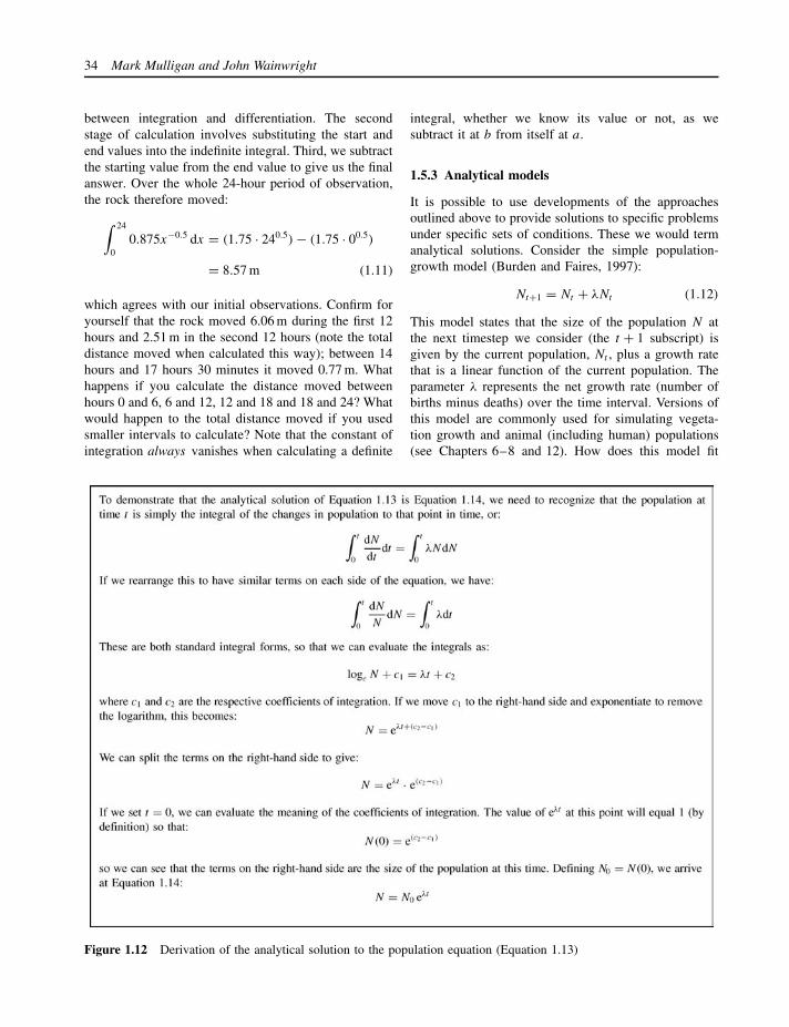
34 Mark Mulligan and John Wainwright
between integration and differentiation. The secondstage of calculation involves substituting the start andend values into the indefinite integral. Third, we subtractthe starting value from the end value to give us the finalanswer. Over the whole 24-hour period of observation,the rock therefore moved:
∫ 24
00.875x−0.5 dx = (1.75 · 240.5) − (1.75 · 00.5)
= 8.57 m (1.11)
which agrees with our initial observations. Confirm foryourself that the rock moved 6.06 m during the first 12hours and 2.51 m in the second 12 hours (note the totaldistance moved when calculated this way); between 14hours and 17 hours 30 minutes it moved 0.77 m. Whathappens if you calculate the distance moved betweenhours 0 and 6, 6 and 12, 12 and 18 and 18 and 24? Whatwould happen to the total distance moved if you usedsmaller intervals to calculate? Note that the constant ofintegration always vanishes when calculating a definite
integral, whether we know its value or not, as wesubtract it at b from itself at a.
1.5.3 Analytical models
It is possible to use developments of the approachesoutlined above to provide solutions to specific problemsunder specific sets of conditions. These we would termanalytical solutions. Consider the simple population-growth model (Burden and Faires, 1997):
Nt+1 = Nt + λNt (1.12)
This model states that the size of the population N atthe next timestep we consider (the t + 1 subscript) isgiven by the current population, Nt , plus a growth ratethat is a linear function of the current population. Theparameter λ represents the net growth rate (number ofbirths minus deaths) over the time interval. Versions ofthis model are commonly used for simulating vegeta-tion growth and animal (including human) populations(see Chapters 6–8 and 12). How does this model fit
Figure 1.12 Derivation of the analytical solution to the population equation (Equation 1.13)

Modelling and Model Building 35
into what we have just been saying about differentialequations? The model is expressing change in the pop-ulation, so we can also specify how the population ischanging. In this case, it is the second part on the right-hand side of Equation 1.11 that represents the change,so that we can also say:
dN
dt= λN (1.13)
The solution (see Figure 1.12) to this equation is:
Nt = N0 eλt (1.14)
where N0 is the initial population. The solution showsthat populations with a linear growth rate will growin size exponentially through time. In reality, this(Malthusian) assumption only tends to be valid overshort time periods because of resource constraints tosustained linear growth rates. We will consider how tomake the model more valid below.
However, in many cases, environmental systemsmay be described by functions for which there areno analytical solutions. In other words, we cannotuse algebra to reformulate the problem into a finalform. Alternatively, we may be interested in spatialor temporal variability in our initial and/or boundaryconditions that cannot be described in a functional form.For example, in rainfall-runoff modelling, we have todeal with rainfall rates that vary through space andtime and irregular topography that is not a simplefunction of distance along a slope. In these cases, weneed to develop alternative approaches that allow us toapproximate solutions to the systems we are trying tomodel. These approaches require numerical solutions.Numerical solutions typically involve approximationand iterative attempts to provide an answer to theproblem in hand. The use of iterative approaches isconsidered in more detail below.
1.5.4 Algorithm appropriateness
In most systems, there will be more than one way of rep-resenting the system components and their interlinkages.At the most fundamental level, we can contrast blackbox approaches with grey box or white box approaches.How do we evaluate whether an algorithm is appropri-ate?
One set of criteria to evaluate for appropriateness is tojudge in terms of process representation. If we considerthe example of population growth, we have alreadyseen what is probably the simplest possible model, inEquations 1.12 to 1.14. The population is considered as
a single, simple unity, and one parameter is used tocontrol how it changes. This parameter is meaningful,in that it represents the difference between births anddeaths through time, but assumes that this value isconstant. In other words, there is always the sameproportion of births and deaths relative to the size of thepopulation. This assumption is reasonable on average,but might not be appropriate in all circumstances. Wehave also noted that the model predicts exponentialgrowth, which is usually only true for short timeperiods, for example, because increased competition forresources means that continued growth is unsustainable.We might want to account for these limitations bymodifying the model as follows:
dN
dt= β
(1 − N
Nmax
)N − θN (1.15)
where β is the birth rate in individuals per unit time,θ is the death rate in individuals per unit time andNmax is the maximum number of individuals that canexist in the specific environment. Nmax is often calledthe carrying capacity of the environment. In the firstpart of this model, we have essentially added a compo-
nent,
(1 − N
Nmax
), which says that as the population
approaches the carrying capacity, and thus the ratioN
Nmaxapproaches one, the birth rate is multiplied by an
increasingly small number, and so the rate of increasegets smaller. This effect is illustrated in Figure 1.13.This S-shaped curve is known as the logistic growthcurve. Note that in the second part of this model, wehave simply assumed that death rates are again a con-stant proportion of the population. In terms of processrepresentation, we may again feel that this is inadequate,because it fails to deal with different ways in whichmembers of the population may die – for example, dueto old age, disease or accidents – and want to add extracomponents to account for these processes and how theymight change with population or resources. These com-ponents may be simple functions, or may depend on thepopulation size or density. Alternatively, we may wantto account for apparently random elements in these pro-cesses by using stochastic functions to represent them(see below).
One assumption we have still incorporated implicitlyin this model is that the population grows in anisolated environment, without competition from otherpopulations. For example, it is common to investigatepopulation changes in terms of separate populations ofpredators and prey. These investigations form the basisof the Lotka–Volterra population models. These models
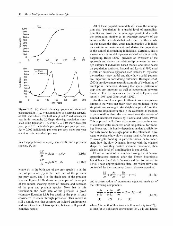
36 Mark Mulligan and John Wainwright
0 50 100 150 200 250 300Time years
0 50 100 150 200 250 300Time years
0100200300400500600700800900
1000
Pop
ulat
ion
Nmax
PreyPredator
(a)
0102030405060708090
100
Pop
ulat
ion
(b)
Figure 1.13 (a) Graph showing population simulatedusing Equation 1.12, with a limitation to a carrying capacityof 1000 individuals. The birth rate β is 0.05 individuals peryear in this example; (b) Graph showing population simu-lated using Equation 1.16, with βH = 0.05 individuals peryear, p = 0.01 individuals per predator per prey per year,βH = 0.002 individuals per year per prey eaten per yearand θ = 0.06 individuals per year
link the populations of a prey species, H , and a predatorspecies, P , as:
dH
dt= βHH − pHP (1.16a)
dP
dt= βP HP − θP (1.16b)
where βH is the birth rate of the prey species, p is therate of predation, βP is the birth rate of the predatorper prey eaten, and θ is the death rate of the predatorspecies. Figure 1.13b shows an example of the outputof this model, showing cycles of increase and decreaseof the prey and predator species. Note that in thisformulation the death rate of the predator is given(compare Equation 1.15) but death of the prey is onlyconsidered to occur through predation. This model isstill a simple one that assumes an isolated environmentand an interaction of two species, but can still providecomplex results.
All of these population models still make the assump-tion that ‘population’ is a useful level of generaliza-tion. It may, however, be more appropriate to deal withthe population number as an emergent property of theactions of the individuals that make it up. In other words,we can assess the birth, death and interaction of individ-uals within an environment, and derive the populationas the sum of all remaining individuals. Certainly, this isa more realistic model representation of what is actuallyhappening. Berec (2002) provides an overview of theapproach and shows the relationship between the aver-age outputs of individual-based models and those basedon population statistics. Pascual and Levin (1999) useda cellular automata approach (see below) to representthe predator–prey model and show how spatial patternsare important in considering outcomes. Bousquet et al.(2001) provide a more specific example of the hunting ofantelope in Cameroon, showing that spatial patterns oftrap sites are important as well as cooperation betweenhunters. Other overviews can be found in Epstein andAxtell (1996) and Ginot et al. (2002).
Another useful example of different process represen-tations is the ways that river flows are modelled. In thesimplest case, we might take a highly empirical form thatrelates the amount of rainfall in the catchment to the bulkor peak outflow from the catchment (see the review oflumped catchment models by Blackie and Eeles, 1985).This approach will allow us to make basic estimationsof available water resources or of the potential for flood-ing. However, it is highly dependent on data availabilityand only works for a single point in the catchment. If wewant to evaluate how flows change locally, for example,to investigate flooding in particular areas, or to under-stand how the flow dynamics interact with the channelshape, or how they control sediment movement, thenclearly this level of simplification is not useful.
Flows are most often simulated using the St Venantapproximations (named after the French hydrologistJean-Claude Barre de St Venant) and first formulated in1848. These approximations state that water flows arecontrolled by the continuity (mass balance) equation:
∂h
∂t+ h
∂u
∂x+ u
∂h
∂x− q = 0 (1.17a)
and a conservation of momentum equation made up ofthe following components:
1
g
∂u
∂t+ u
g
∂u
∂x+ ∂h
∂x− (S − Sf ) = 0
(1) (2) (3) (4)
(1.17b)
where h is depth of flow (m), u is flow velocity (m s−1), tis time (s), x is distance downstream (m), q is unit lateral

Modelling and Model Building 37
inflow (m s−1), g is acceleration due to gravity (m s−2),S is the slope of the channel bed (m m−1) and Sf isthe slope of the water slope (also known as the frictionslope) (m m−1). If we use all of these components(1–4), then the model is known as a dynamic waveapproximation (Graf and Altinakar, 1998; Singh, 1996;Dingman, 1984). Component (1) reflects the inertia ofthe flow; (2) the gravity effect on the flow; (3) thepressure effect; and (4) the friction effect. However, itmay be possible to ignore the inertial term because itsvalue is so small. In this case we omit the component(1) and produce the diffusive wave approximation:
u
g
∂u
∂x+ ∂h
∂x− (S − Sf ) = 0 (1.18a)
which, when combined with the continuity equation1.15a, gives the diffusion-wave approximation:
∂h
∂t+ u
∂h
∂x− D
∂2h
∂x2− q = 0 (1.18b)
where D is the diffusion coefficient (equal toQ
2wSwhere Q is the discharge [m3 s−1] and w the flow width[m]). This approach may be valid under conditions ofnegligible convective acceleration. In other cases wecan omit the diffusive component of the flow, so thatwe assume the flows are simply controlled by a singlerelationship between depth and discharge. In this case,components 2 and 3 become negligible, S = Sf and:
∂h
∂t+ u
∂h
∂x− q = 0 (1.19)
which is known as the kinematic wave approximation.This approximation is valid particularly in overlandflows on hillslopes (see below) and where waves inthe flow are of low amplitude relative to their wave-length. Where there are backwater effects, as at trib-utary junctions or upstream of lakes and estuaries, theassumptions of the kinematic wave approximation breakdown (Dingman, 1984) so that diffusive or dynamicwave algorithms should be used in these cases. Singh(1996) contains numerous references to and examplesof the use of these equations. Further details are alsogiven in Chapter 5.
In all these cases, we have simply made one-dimensional approximations to the flow process. In otherwords, we assume that it is valid to model average con-ditions at a series of cross-sections down the channel. Ifwe want to estimate flooding, then this approach may bevery reasonable (e.g. Bates and De Roo, 2000). How-ever, we may want to know how conditions change
across a cross-section, or as a continuum along a chan-nel. These approaches would be better for looking at theeffects of flows on structures, for example, bridge sup-ports, or on how the flow interacts with the morphology.In these cases, approaches using more complex, compu-tational fluid dynamics (CFD) models will usually bemore appropriate. Such models are covered in detail inChapter 20.
Overall, we can summarize that the process represen-tation is not a single definition, and different criteria willbe used depending on our modelling objectives. Bothbottom-up and top-down approaches may be useful formodelling the same system in different conditions. Wecan see how this difference can lead to different levelsof complexity in terms of model components, equationsrepresenting their interactions, and expectations in termsof outputs.
Second, we might evaluate algorithm appropriatenessin terms of computational resources. With the rapidlyincreasing rate of progress of microprocessor design andreduction of costs of microprocessors, memory and datastorage, it is possible to design and implement larger andmore complex models on desktop computers. Moore’s‘law’ of increasing computer power is based on the factthat more transistors can be crammed into successivelysmaller spaces on integrated circuits, allowing them torun progressively faster. In the past 35 years, transistordensity has doubled about once every 18 months, allow-ing the corresponding exponential increase of model size(number of points simulated) and complexity (Voller andPorte-Agel, 2002). The design of supercomputers andparallel processing, where a number of calculations canbe carried out simultaneously, is also proceeding apace.One criterion we might use is the time taken to exe-cute the model. This time will include that required toread in all of the data and parameters required, carryout the calculations in our algorithm, and output all ofthe results. Algorithms are often evaluated in terms ofthe number of operations required, as this can often berelated to the processing speed (measured in FLOPS orfloating-point operations per second – modern machinesare capable of megaflops [millions] or gigaflops [thou-sands of millions]). Modern computers are designedto be able to make calculations on the several mem-ory addresses involved in a floating-point calculationat once.
For example, if we consider the population-growthmodels from this section, the models based on grosspopulation characteristics have substantially fewer cal-culations than those based on individuals. Therefore,if either algorithm is appropriate from a process pointof view, but we need the calculations to be carried

38 Mark Mulligan and John Wainwright
out quickly (for example, if we then use these calcu-lations to drive another part of a larger model) or ifcomputer time has an associated cost which we needto minimize, then it would be better to choose thepopulation-based approach. A second criterion in termsof computational resources is that of available mem-ory while the model is running or data storage forinputs and outputs. Many environmental models arespatially distributed, requiring a large amount of spa-tial information to be stored to carry out calculations.This information is usually held in dynamic (volatile)memory, which is relatively expensive, although muchless so than even a few years ago. If parts of the spa-tial information need to be read from and stored backonto other media, such as hard drives, model perfor-mance suffers significantly. Thus, it may be necessaryto design large spatial models to store only absolutelynecessary information, and to access other informationas and when necessary. Specific techniques are cur-rently being designed to implement these approaches.For example, in the analysis of large digital elevationmodels (DEMs), Arge et al. (2002) demonstrated thata parallel approach to flow routing is between twiceand ten times as fast as a serial approach for largedatasets (they used examples with 13 500 × 18 200 and11 000 × 25 500 cells). It is also capable of process-ing larger datasets (e.g. 33 454 × 31 866 cells, occupy-ing 2 Gb of memory) that are not possible to evalu-ate using a serial approach due to machine-memorylimitations.
Third, we need to consider our models in rela-tion to available data. Data are required as basicinputs, or parameters, and for use in testing the resultsthat are obtained. It may be better to use avail-able data rather than have to produce estimates orlarge-scale interpolations or extrapolations from thosethat are available. On the other hand, this restrictionshould not always be too strongly applied, as mod-els can often be used in the design of field data-collection campaigns by suggesting where critical mea-surements could be made. Increasingly, techniques arebecoming available for relating model results at coarsescale to field measurements, which are often takenat points. These techniques are investigated further inChapter 19.
1.5.5 Simple iterative methods
The most straightforward numerical approaches involvesimple repetition or iteration of a calculation to evaluatehow it changes through time. As an example, we willuse a simple ‘bucket’ storage model of how a lake level
will behave through time. The model is illustrated inFigure 1.14a and is described by the equation:
dh
dt= r + i − e − kh (1.20a)
and the inequality:
0 ≤ h ≤ hmax (1.20b)
In other words, the depth in the lake changes eachyear by an amount equal to the rainfall, r (in m a−1) plusthe river and surface inflow, i (in m a−1), less the annualevaporation from the lake, e (in m a−1) less the seepagefrom the base of the lake, which is a linear function ofthe depth of water, h (in m) in the lake. This function is
Rainfall
Evaporation
Seepage
Overflow
Inflow
Currentwater depth
Maximumwater depth
05
101520253035404550
0 20 40 60 80 100 120 140 160 180 200Time years
Dep
th m
abc
(b)
(a)
Figure 1.14 (a) Schematic diagram showing the represen-tation of a lake water balance as a ‘bucket’ model with aseries of inputs: rainfall and inflow from rivers; and out-puts: evaporation, seepage and overflow once the maximumdepth of the lake has been reached; and (b) graph showingthe results of the ‘bucket’ model representing lake depthchanges. Curve (a) represents rainfall of 1 m a−1, an inflowrate of 0.8 m a−1, evaporation rate of 0.05 m a−1 and seep-age intensity of 0.05 a−1; curve (b) has a lower inflow rateof 0.2 m a−1, and higher evaporation rate of 1 m a−1, con-ditions perhaps reflecting higher temperatures than in (a);curve (c) has a higher inflow of 2 m a−1, compared to (a),perhaps representing vegetation removal, or the existenceof a larger catchment area. In case (c), overflow from thelake occurs because the maximum depth threshold of 50 mis reached

Modelling and Model Building 39
controlled by a rate coefficient k, which is related to thepermeability of the lake bed. There is a maximum levelto which the lake can be filled, hmax , in m, above whichoverflow occurs. Similarly, the level cannot go belowthe ground surface. We need to use a numerical solutionbecause of the inequalities constraining the minimumand maximum depths. To calculate iteratively, we usethe following steps:
1. Define initial lake level ht=0.
2. Calculate the annual change in leveldh
dtusing
Equation 1.20a.3. Calculate the new level ht+1 by adding the annual
change value.4. If ht+1 > hmax (Equation 1.20b), then calculate the
overflow as ht+1 − hmax , and constrain ht+1 = hmax .Alternatively, if ht+1 < 0, constrain ht+1 = 0.
5. Go back to step (2) and repeat until the simulationtime is complete.
Figure 1.14b illustrates the results for simple scenariosof environmental change, or for comparing lakes in dif-ferent geomorphic settings. Similar sorts of models havebeen used for lake-level studies in palaeoenvironmentalreconstructions (see discussion in Bradley, 1999). Thistype of storage model is also used in studies of hillslopehydrology, where the bucket is used to represent theability of soil to hold water (e.g. Dunin, 1976). Notethat this method is not necessarily the most accurateiterative solution, as it employs a backward-differencecalculation (see below). More accurate solutions can beachieved using Runge–Kutta methods (see Burden andFaires, 1997; Engeln-Mullges and Uhlig, 1996).
Another example of where we would want to useiterative solutions is where we cannot calculate a closedalgebraic form for a relationship that might be used inthe model. For example, many erosion models use thesettling velocity of particles to predict the amount ofdeposition that will occur (e.g. Beuselinck et al., 2002;Morgan et al., 1998). The settling velocity states that asediment particle will move downwards (settle) througha body of water at a rate given by Stokes’ Law:
v2s = 4
3
g
(ρs
ρ− 1
)d
CD
(1.21)
where vs is the settling velocity (m s−1), g is accelerationdue to gravity (m s−2), ρs is the density of the particle(kg m−3), ρ is the density of water (kg m−3), d is theparticle diameter (m) and CD is the drag coefficientof the particle. As noted by Woolhiser et al. (1990),
the drag coefficient is a function of the Reynoldsnumber (Re) of the particle, a dimensionless relationshipshowing the balance between the gravitational andviscous forces on the particle:
CD = 24
Re+ 3√
Re+ 0.34 (1.22)
However, the Reynolds number is itself a function ofthe particle settling velocity:
Re = vsd
ν(1.23)
where ν is the kinematic viscosity of the water (m2 s−1).Now we have the settling velocity on both sides of theequation, and no way of algebraically rearranging theequation to provide a simple solution in terms of vs .
We can use a set of techniques for finding roots ofequations (e.g. Burden and Faires, 1997) to tackle thisproblem. If we have an equation in the form:
f(x) = 0 (1.24)
then a root-solving technique allows us to find thevalue of x for which the function gives the result ofzero. This approach can be implemented by combiningEquations 1.21 to 1.23 and rearranging them to give:
v2s
24
vsd
ν
+ 3√vsd
ν
+ 0.34
− 4
3g
(ρs
ρ− 1
)d = 0.
(1.25)
The bisection method is a very robust technique forfinding roots, as it will always converge to a solution.One problem that we will find with a number ofnumerical techniques is that they can fail to find thecorrect solution, or may even provide incorrect solutionsto the model.
Bisection works by choosing an interval in which thesolution is known to lie. Estimates are made of the lowerand the upper value of this interval. This choice caneasily be checked by calculating the function with thespecific values. We can find the root by successivelyhalving the interval, and comparing the midpoint withthe two end points to find which subinterval the root lies.The computational steps are as follows (Figure 1.15):
1. Set an iteration counter i equal to 1.2. Calculate the midpoint mi of the lower (li) and upper
(ui) estimates of the interval:
mi = 12 (li + ui)

40 Mark Mulligan and John Wainwright
0 0.05 0.1 0.15 0.2 0.25 0.3
-
l = l1
u = u1
vs m s−1
l1 m1
l2
u1
−0.03
−0.02
−0.01
0
0.01
0.02
0.03
0.04
f(u1)
f(l1)
f(v s
)
s
u2m2
l3 u3m3
l4 u4m4
Figure 1.15 Graph to show how the bisection technique can be used to solve a root numerically by taking an intervalabout the solution, and successively arriving at the solution, s, by subdivision of the interval it is known to be in. Thelower value of the interval is called l and the upper value u in this diagram. The numbered subscripts show the successiveiterations of these values. The function shown is Equation 1.25, used to calculate the settling velocity of a 1-mm diametersediment particle with a density of 2500 kg m−3
3. Calculate f(mi). If the value is zero, then the root hasbeen found. Otherwise . . .
4. Compare f(mi ) with f(li). If they have the same sign,then the root must lie between mi and ui , so setli+1 = mi and ui+1 = ui . If they have different signs,then the root must lie between li and mi , so setli+1 = li and ui+1 = mi .
5. If the interval between li+1 and ui+1 is acceptablysmall (i.e. less than a predefined tolerance, ε), thenaccept the midpoint as the root.
6. Otherwise, increment the value of i. If i is withina predefined limit, return to step 2 and repeatthe process.
The bisection method is useful because it always con-verges to a solution. It is thus useful even where quitesophisticated techniques will fail. The disadvantages ofthe technique are that it is very slow in convergingand that in the process we can be close to a goodapproximation at an intermediate stage in the processwithout realizing it. The efficiency of the algorithmcan be assessed because the number of iterations (n)required to achieve a result with a given toleranceε is:
n = log2ui − li
ε. (1.26)
The Newton–Raphson technique is far more efficient inthat it converges much more rapidly. However, problemswith the Newton–Raphson technique can arise (a) if theinitial estimate is too far away from the root; (b) ifthe function has a local maximum or minimum; or(c) in the case of some functions that can cause thealgorithm to enter an infinite loop without arriving ata solution. Numerous other techniques for root solution,together with discussion of their respective advantagesand limitations, can be found in Burden and Faires(1997) and Press et al. (1992).
1.5.6 More versatile solution techniques
In this section, we consider a range of techniques thatcan be used to solve environmental models where ana-lytical and simple iterative approaches are not appropri-ate. There are many variants of these techniques avail-able, but space here only permits a brief overview. Inall these cases, we assume that a model formalizationis available in the form of a differential equation, start-ing with straightforward examples, but then consideringmore commonly used and more complicated forms.
1.5.6.1 Finite differences
The finite difference approach assumes that a solu-tion to a differential equation can be arrived at by

Modelling and Model Building 41
Af(x − h)
P
B
x − h x + hx
f(x) f(x + h)
y=
f(x
)
Figure 1.16 Graph showing the derivation of the finitedifference technique for finding a solution to a functionat point x. The distance h is the ‘finite difference’ of thename, and the entire function can be solved by repeating thecalculations with x located at different places along the axis
approximation at a number of known, fixed points.These points are separated from each other by a known,fixed distance – the finite difference of the name of thetechnique (as compared with the infinitesimal distancesused to calculate derivatives). In a simple case, we canconsider how the technique works by looking at thefunction in Figure 1.16. To evaluate the rate of changein our model at point x, we need to find the slope of the
function f(x)
(i.e.
dy
dx
)at this point. If the distance (h)
between our calculation points is small and/or the func-tion does not change too dramatically, then the slope isbest estimated by the line AB, in other words, the slopebetween the values of the function at x + h and x – h.
This estimate is called the central difference approx-imation, and is given by the relationship:
f′(x) ≈ f(x + h) − f(x – h)
2h(1.27)
Similarly, the line PB is also an estimate of theslope at P. This estimate is the forward differenceapproximation with:
f′(x) ≈ f(x + h) − f(x)
h(1.28)
In the same way, the line AP is also an estimate,called the backward difference approximation, with:
f′(x) ≈ f(x) − f(x − h)
h(1.29)
It is also possible to define the second derivative atx using a similar approach. The central difference
approximation is:
f′′(x) ≈ f(x + h) − 2f(x) + f(x − h)
h2(1.30)
Note that in talking about the finite difference approach,the term approximation is fundamental (observe the useof ≈ meaning ‘approximately equal to’ in Equations1.27 to 1.30 and in general through the rest of thissection). We will see in a later section that evaluating theerrors inherent in models is also fundamental. The errorinvolved in these approximations can be assessed usinga technique called Taylor expansion. For the centraldifference approximations the error is related to valuesof h2f′′(x) + h3f′′′(x) + h4f′′′′(x) + . . .. This sequence iscommonly written as O(h2), which means ‘values ofthe order h2 and greater’. Because the value of thehigher order derivatives rapidly approaches zero, theapproximation is reasonable. Similarly, the error in thebackward difference approximations is O(h). Clearlythis is a much poorer approximation, but is valid in caseswhere the values change less rapidly, or if such error iswithin the bounds of acceptability.
We will commonly come across the case where thevariable we are looking at is a function of more than onevariable, e.g. y = f(x, t), so that the variable changesthrough space and time. In this case it is useful to thinkof the value on a regularly spaced grid, as shown inFigure 1.17. Our finite differences are given by distancesh, which is the increment in the x direction, and k, theincrement in the t direction. We define index parametersto describe points on the grid – i in the x direction andj in the t direction – which have integer values. Wewould then denote the value at any point on the gridP(ih, jk ) as:
yP = y(ih, jk) = yi,j (1.31)
The central difference approximation of∂y
∂tat P is:
∂y
∂t≈ yi,j+1 − yi,j−1
2k(1.32)
while the central difference approximation of∂y
∂xat P is:
∂y
∂x≈ yi+1,j − yi−1,j
2h(1.33)
Other derivations are given in Figure 1.17. Note the
change in notation fromdy
dxto
∂y
∂x. The first case, with
the normal d, denotes an ordinary differential equation(ODE); that is, the change we are interested in relatesto one variable only. The curly ∂ denotes a partial

42 Mark Mulligan and John Wainwright
P(ih, jk)
i, j
i, j −1
i − 1, j i + 1, j
i, j + 1
t
jk
ih
k = dt
h = dxx
Approximations of at P:
Backwardyi,j − yi,j − − −−1
k
Centralyi,j+1 yi,j 1
2k
Forwardyi,j+1 yi,j
k
Approximations of at P:
Backwardyi,j yi 1,j
h
Centralyi+1,j yi 1,j
2h
Forwardyi+1,j yi,j
h
Central difference approximation of2y
t2at P:
2y
t2
yi,j+1 2yi,j + yi,j 1
k2.
Central difference approximation of2y
x2at P:
2y
x2
yi+1,j 2yi,j + yi 1,j
h2.
− −
− −
− −
− −−
t
t
y
y
x y
x y
x y
x y
t y
t y
Figure 1.17 Finite difference approximations to partial differential equations
differential equation (PDE). Change in this exampleis partially related to two different variables – x andt – at the same time. There are three different types ofpartial differential equation – hyperbolic, parabolic andelliptic – as shown in Figure 1.18.
We will commonly want to solve two forms ofproblem. The first occurs as above where one of thevariables we are looking at is time, and we want to solvechange through time from a set of given conditions,known as initial values. These conditions will usuallybe prescribed for t = t0. On our grid, the solution wouldappear as in Figure 1.19.
This is called an initial value problem. Note that wealso have to specify the values immediately beyond our
grid so we can make statements about the solution of theproblem at the edges. These values are called boundaryconditions, and may be specific values, or functions ofvalues at the edges of the grid.
A less frequent problem involves two (or more)variables which do not include time and require thesolution of the function in terms of the variableat a single point in time over a finite are. Thevariables are commonly spatial coordinates, but maydefine another parameter space. A heat-flow problemmight be a common example of the former – eitherin two or three dimensions. In this case our gridappears as in Figure 1.20, and we have a boundary-value problem.

Modelling and Model Building 43
Partial Differential Equations
PDEs come in three different varieties, and the solution methods for each vary. The three types are:
1. hyperbolic – for which the one-dimensional wave equation is the prototype form:
∂2u
∂t2= v2 ∂2u
∂x2
where v is the velocity of wave propagation.2. parabolic – for which the diffusion equation is the prototype form:
∂u
∂t= ∂
∂tD
∂u
∂x
where D is the diffusion rate.3. elliptic – for which the Poisson equation is the prototype form:
∂2u
∂t2+ ∂2u
∂y2= r(x, y)
where r is a given source term. If r = 0, this is called Laplace’s equation.
Figure 1.18 Types of differential equation
t
t = 0x
Initial values
Boundaryconditions
Solution through time
Figure 1.19 Illustration of an initial value problem. Givenstarting conditions at time t = 0 and boundary conditionsbeyond the domain of interest, solution is progressivelycarried out for each spatial location at successive timeintervals on the finite difference grid
The most straightforward way of solving a finite dif-ference approximation to a partial differential equationis to use the backward difference technique (also calledEuler’s method in some texts). As an example, considerthe kinematic wave approximation to the flow of waterover a hillslope on which runoff is being generated at a
y
x
Boundaryvalues
Single solution atinterior grid nodes
Figure 1.20 Illustration of a boundary-value problem. Asingle (steady-state) solution is calculated across the grid,given known boundary values or boundary conditions
known rate:∂d
∂t+ v
∂d
∂x= e(x, t) (1.34)
where d is depth of water (L), t is time (T), v is flowvelocity (L T−1), x is horizontal distance (L) and e(x, t)
is the unit runoff rate at a given location and time (LT−1) (Singh, 1996: compare the general derivation of

44 Mark Mulligan and John Wainwright
Equation 1.19 above which is identical apart from thesource term has changed from q to e (x, t) to make itexplicitly relate to runoff from infiltration excess). Thisis an example of a hyperbolic equation. If we know theinitial condition:
d(x, 0) = g(x), x ≥ 0 (1.35a)
and the boundary condition
d(0, t) = b(t), t > 0 (1.35b)
then we can solve the equation using backward differ-ences. The backward difference expression for the firstterm is:
∂d
∂t≈ d(x, t) − d(x, t − k)
k+ O(k) (1.36)
and for the second term:
∂d
∂x≈ d(x, t − k) − d(x − h, t − k)
h+ O(h) (1.37)
Putting these together and ignoring the error terms, wehave a full solution, which is:
d(x, t) − d(x, t − k)
k
+ vd(x, t − k) − d(x − h, t − k)
h= e(x, t) (1.38)
As we know the runoff rate (possibly using a simplebucket model of infiltration as described above), and aretrying to solve for the new water depth, we rearrangethis equation to give:
d(x, t) = d(x, t − k) + kv
h{d(x, t − k)
− d(x − h, t − k)} + {e(x, t)k} (1.39)
Thus, to calculate the solution for a given surface,we define the grid of values in x and t , and carryout an iterative solution for x = ih, i = 1, 2, . . . , n, foreach value t = jk , j = 1, 2, . . . , N . The solution worksbecause at each time t , the solution depends only onknown values of d at the previous timestep t − k. Thesolution then follows from the initial condition. Thistype of solution is known as an explicit scheme. All thevalues needed for the calculations at a specific timestepare known explicitly because we are using a backwarddifference solution. Other details required for the fullsolution of this equation as applied to desert hillslopesare given in Scoging (1992) and Scoging et al. (1992).
Implications of its use are discussed in Parsons et al.(1997; see also Chapter 3).
An advantage of the backward difference schemegiven above is its simplicity, but it has two disad-vantages which can lead to problems in certain cir-cumstances. First, as noted above, the error terms arerelatively high, being O(h) + O(k). Second, the solu-tion can become unstable under specific conditions. Suchconditions are known as the Courant–Friedrichs–Lewystability criterion, which states that stable solutions willonly be produced if:
vk
h≤ 1 (1.40)
The practical implication of this is that for cases wherethe velocity, v, is high, the timestep k must be reduced tomaintain stability. Very short timesteps may mean thatthe computer time required becomes excessively highto solve the problem, and thus the algorithm may notbe appropriate in computer-resource terms, as discussedabove. Alternatively, the spatial resolution would haveto be compromised by increasing h, which may not beviable or useful in certain applications.
There are a number of other explicit techniques whichcan be used to solve similar equations, which improvethe accuracy of the solution by reducing the error terms.Alternatively, higher accuracy and reduced error may beobtained by using an implicit solution to the problem.In this case, there are several unknowns during the cal-culations at any one timestep. Solution of simultaneousequations and/or iterative calculations are thus requiredto arrive at a final solution. Further details can befound in a number of texts, such as Reece (1976), Smith(1985), Ames (1992) or Press et al. (1992).
Boundary conditions are a critical element of anynumerical solution. Basically, we must define whathappens at the edge of the solution space so that itinteracts realistically with the space around it. In somecases, the boundary conditions can be very simple. Forexample, when simulating water flows on hillslopes,the boundary at the top of a catchment will have nowater flux entering the solution domain because thereis nowhere for it to come from. At the base of thehillslope, flow may occur freely out of the system. Wemay set the gradient that controls the speed of this flowas equal to the gradient at the edge cell. Other ways ofcontrolling the behaviour at the edges of the solutiondomain are to define the values of boundary cellsas a function of time (Dirichelet boundary condition)or to specify the gradient at the boundary (Neumannboundary condition) (Press et al., 1992). For example,in our hillslope-hydrology case, a Dirichelet boundary

Modelling and Model Building 45
condition might be used if the channel flow is knownat the base of the slope as a function of time (perhapsusing an approximation such as the instantaneous unithydrograph [see Chapter 5]); the Neumann boundarycondition might be appropriate where there is a floodcontrol structure where the slope is fixed. Correctdefinition of boundary conditions is often fundamentalin controlling the correct solution of simulations, forexample by preventing the development of numericaloscillations or exponentially increasing values.
1.5.6.2 Finite elements
An alternative method for solving models of this typeis the finite element method. Rather than dividing thearea in which we are interested into a regular grid,finite elements allow us to use regular shapes (triangles,quadrilaterals) to represent the area of interest. It isalso possible to use cubes, cuboids and hexahedronsto represent volumes in three-dimensional models, andto have curved boundaries to the solution domain.Although it is possible to use a regular grid, it ismuch more common to vary the size of the elementsso that locations where change occurs rapidly arerepresented by much smaller areas. In this way, theeffects of errors in approximations may be minimized.This compares with the finite difference approach,where changes in grid size must take place uniformlyacross the same row or same column of the grid,allowing much less flexibility. A second advantagecomes with the way in which boundary conditionsare addressed. Because the boundary conditions aredirectly included in the formulation in the finite elementapproach, it is not necessary to approximate gradientsat the boundaries. On the other hand, finite elementcalculations can require much more computer memoryand computing power (see Smith and Griffiths, 1998,for example).
The finite element method is based on the fact that anyintegral over a specific range can be evaluated by addingthe integrals of subintervals making up that range (seethe discussion of definite integrals above) (Henwoodand Bonet, 1996). In one dimension, we have:∫ xn
x1
f(x) dx =∫ x2
x1
f(x) dx +∫ x3
x2
f(x) dx
+ · · · +∫ xn
xn−1
f(x) dx (1.41)
In other words, we can provide a solution over thewhole domain by splitting it into subdomains (elements)and using local solutions, or approximations to them, to
evaluate the whole. We need to solve the overall integralin a way that provides the best approximations to thelocal conditions. One way of doing this is to use theweighted residuals (R) of the function:∫
R · w dx = 0 (1.42)
where w are a series of weights, to provide a spatiallyaveraged best solution.
The simplest approach is to use approximations tolocal solutions of the elements using linear interpolation,using the ‘hat’ function (Figure 1.21). At any point i, thevalue of the hat function, Ni , using this approach is:
Ni =
0 if x ≤ xi−1
x − xi−1
xi − xi−1if xi−1 ≤ x ≤ xi
xi+1 − x
xi+1 − xi
if xi ≤ x ≤ xi+1
0 if x ≥ xi+1
(1.43)
We therefore have an approximation to function f(x) atany point within an element, based on known values atany point i as:
f(x) ≈ Nif(xi) + Ni+1f(xi+1) (1.44)
which is called the linear basis function for the approxi-mation. In the Galerkin approach to finite elements, theweights in Equation 1.42 are set as equal to the valuesof the basis function, i.e. w = Ni .
As an example, consider the case where we areinterested in the distribution of heat in a soil, for whichwe have a temperature measurement at the surface andat a known depth. Under steady-state conditions, thetemperature distribution will be described by a functionof the form:
∂
∂x
(−k
∂τ
∂x
)+ τ = 0 (1.45)
where τ is the temperature in ◦C and k the rate of heattransmission or thermal conductivity (W m−1 ◦C−1). Inthe finite element method, this function becomes theresidual term to be minimized, so that we insert thisequation into Equation 1.42:
∫ xn
0
{∂
∂x
(−k
∂τ
∂x
)w + τw
}dx = 0 (1.46)
Integration by parts (see Wilson and Kirkby, 1980) canbe used to transform this relationship into a set of

46 Mark Mulligan and John Wainwright
N1
N2
N3
N4
1 2 3 4x
1 2 3 4x
1 2 3 4x
1 2 3 4x
Ni
i − 1 x
(a)
(b)
(c)
i i + 1
dxdt
x = 0
kK11
t3t4
t2
t1K12 0 000
K21 K22 K23 00 K32 K33 K340 0 K43 K44
−
dxdt
x = 1
k
=
Figure 1.21 Solution method using finite elements: (a) hatfunction; (b) solution of by piece-wise interpolation usingsliding hat function; and (c) finite element matrix
ordinary differential equations:
∫ xn
0
(−k
dτ
dx
dw
dx+ τw
)dx =
[k
dτ
dxw
]xn
0
(1.47)
Next, we split the whole domain into a number of ele-ments – in this example, three – and apply the Galerkinestimate of the weights using the linear basis functionsand estimate the local value of τ using Equation 1.44.
Taking the element as having unit length, and multiply-
ing by a scaling factor
∣∣∣∣dx
dξ
∣∣∣∣, we have at node i:
τi
∫ 1
0
(k
dNi−1
dξ
dξ
dx
dNi
dξ
dξ
dx+ Ni−1Ni
) ∣∣∣∣dx
dξ
∣∣∣∣ dξ
=[k
dτ
dxNi
]1
0
(1.48)
where ξ (the Greek letter ‘xi’) refers to the fact that weare integrating along the element rather than the solutiondomain as a whole. For each node in the area of interest(Figure 1.21b) we now have a relationship based onthe values of Ni and Ni−1 that can be used to solve
within the elements. AsdNi−1
dξ= −1,
dNi−1
dξ= 1 and
dξ
dx= 3 (the number of elements), we can now define
directly the values of the integral used to multiply thevalues τi on the left-hand side of Equation 1.48. Thisprovides a matrix of values (Figure 1.21c) that is usuallyknown as the ‘stiffness’ matrix (because of the historicalorigins of the technique in structural analysis). It nowremains to solve the right-hand side of Equation 1.48by inserting the relevant weights. In all but the firstand last cases, these cancel, providing source and sinkterms at each of the boundaries of interest (the soilsurface and the location of the temperature probe inour case). Using our known boundary conditions atthese points (T1 is the temperature at the surface andT4 is the temperature at the probe), we produce a set ofsimultaneous equations:
τ1 = T1
K21τ1 + K22τ2 + K23τ3 = 0
K32τ2 + K33τ3 + K34τ4 = 0
τ4 = T4
(1.49)
that can be solved using standard techniques (see Presset al., 1992, for details). Finally, the values of τ1 canbe substituted into Equation 1.48 to give the heat fluxesinto the top of the soil and out of the base of the soil(Equation 1.49).
Finite elements are widely used in structural andengineering applications, including slope stability (seeChapter 10), fluid and heat-flow studies. More detailson the technique can be found in Henwood and Bonet(1996), Wait and Mitchell (1985), Smith and Griffiths(1998), Gershenfield (1999), Burden and Faires (1997)and Zienkiewicz and Taylor (2000), including informa-tion on how to model time-dependent conditions. Flow

Modelling and Model Building 47
modelling examples can be found in the articles byMunoz-Carpena et al. (1993, 1999), Motha and Wigham(1995) and Jaber and Mohtar (2002). Beven (1977) pro-vides a subsurface flow example as applied to hills-lope hydrology.
1.5.6.3 Finite volumes
The finite volume or control volume approach is sim-ilar to the finite element method in that it uses inte-gration over known areas, but differs in the solutionmethods used. Versteeg and Malalasekera (1995) pro-vide a very readable introduction to the technique, whichwe largely follow here. The area under study is firstdivided into a series of control volumes by locating anumber of nodes throughout it. The boundaries of thecontrol volumes are located midway between each pairof nodes (Figure 1.22). The process studied is inves-tigated by integrating its behaviour over the controlvolume as:∫ V
0f′(x)dV = A
i+ 12 δx
f(xi+ 1
2 δx) − A
i− 12 δx
f(xi− 1
2 δx)
(1.50)
which is the same as looking at the mass balance overthe control volume.
Using the soil heat-flow example of Equation 1.45again, the control-volume equation becomes:∫ V
0
∂
∂x
(−k
∂τ
∂x
)+ τ dV =
(−kA
dτ
dx
)i+ 1
2 δx
−(
−kAdτ
dx
)i− 1
2 δx
+ τ iV = 0 (1.51)
and we can use linear interpolation to calculate theappropriate values of k and finite differences to estimate
the values ofdτ
dxat the edges of the control volume.
dxwP
∆x = dxwe
dxPE
dxPe
dxWP
wW EP e
Figure 1.22 Discretization of the solution space in thefinite volume techniqueSource: Versteeg and Malalasekera, 1995
Assuming a uniform node spacing, these approxima-tions give:(
−kAdτ
dx
)i+ 1
2 δx
= −ki+1 + ki
2A
i+ 12 δx
(τi+1 − τi
0.5δx
)
(1.52a)(−kA
dτ
dx
)i− 1
2 δx
= −ki−1 + ki
2A
i− 12 δx
(τi − τi−1
0.5δx
)
(1.52b)
Substitution of these into Equation 1.51 gives:
− ki+1 + ki
2A
i+ 12 δx
(τi+1 − τi
0.5δx
)+ ki−1 + ki
2A
i− 12 δx(
τi − τi−1
0.5δx
)+ τiV = 0 (1.53)
Rearranging to give common terms in τi−1, τi and τi+1,we have:(ki+1 + ki
δxA
i+ 12 δx
+ ki−1 + ki
δxA
i− 12 δx
+ V
)τi
=(
ki−1 + ki
δxA
i− 12 δx
)τi−1 +
(ki+1 + ki
δxA
i+ 12 δx
)τi+1
(1.54)
Over the whole solution domain, this equation is againa set of simultaneous equations that can be solved inexactly the same ways as mentioned before.
Finite volume approaches are used commonly in com-putational fluid dynamics approaches (see Chapter 20).More detailed applications in this area can be foundin the books by Versteeg and Malalasekera (1995)and Ferziger and Peric (1999). Applications relatingto simpler flow models (such as the kinematic waveapproximation used in the finite difference example) canbe found in the articles by Gottardi and Venutelli (1997)and Di Giammarco et al. (1996).
1.5.6.4 Alternative approaches
There is increasing interest in models that do notdepend on numerical discretization as described in thesections above. Of these, the most common is thecellular automata approach. This method is dealt within detail in Chapter 21, so only a summary is givenhere. The advantages of cellular automata are that theycan represent discrete entities directly and can reproduceemergent properties of behaviour. However, becausethe number of entities simulated in realistic models ishigh, they can have a large computational load, although

48 Mark Mulligan and John Wainwright
special computer architectures that take advantage of thestructure of cellular automata have been used to speedthe process considerably (Gershenfield, 1999).
Cellular automata use a large number of cells or nodesthat can take a number of states. Each cell or node isprogressively updated using a fixed set of rules thatdepend only on local conditions. Thus at no stage isinformation on the whole solution space required. Themost commonly cited example is John Conway’s ‘Gameof Life’. A cell can either be ‘on’ or ‘off’, representinglife or no life in that location. There are three rules thatdetermine the state of a cell in the next iteration of themodel based on counting the number of occupied cellsin the immediate eight neighbours (Figure 1.23a):
1. ‘Birth’ – a cell will become alive if exactly threeneighbours are already alive.
2. ‘Stasis’ – a cell will remain alive if exactly twoneighbours are alive.
3. ‘Death’ – a cell will stop living under any otherconditions (0 or 1 neighbours reflecting isolation;or ≥ 4 neighbours reflecting overcrowding).
Compare these rules to the population models dis-cussed above. One of the interesting outcomes of thisapproach is that patterns can be generated that are self-reproducing.
Cellular automata have been used in a wide vari-ety of applications, in particular fluid flows. It is pos-sible for example to demonstrate the equivalence ofthe Navier–Stokes equations of fluid flow to cellularautomata approximations (Wolfram, 1986; Gershenfield,1999). More details of how to apply the method canbe found in Ladd (1995), Bar-Yam (2000) and Wolfram(2002). See Chapter 21 for a discussion of environmen-tal applications in more detail.
A further approach is the use of artificial neural net-works. An artificial neural network is a computer rep-resentation of the functioning of a human brain. It doesso by representing the neurons that are the fundamen-tal building blocks of the brain structure. A numberof inputs are passed through weighting functions rep-resenting synapses (Figure 1.24). The weighted valuesare summed and then affected by a local bias value.The result is passed to a function that decides whetherthe current neurone should be activated, and thus con-trols its output. The number of inputs and the numberof neurons and ways in which they are combined con-trol the function of the neural network. An importantfeature of neural networks is their ability to capture non-linear behaviour.
A common use of artificial neural networks isin rainfall-runoff modelling. A feed-forward model
structure is usually used, with a single hidden layer ofneurons (Figure 1.24). For example, Xu and Li (2002)used 29 input variables to estimate the next inflow intoa reservoir in Japan. These inputs were hourly averageupstream rainfall over seven hours, the seven hours ofprevious releases from two upstream reservoirs, the fourprevious hours of tributary inflow and the four previoushours of inflow into the reservoir. Xu and Li found rea-sonable predictions for small and medium-sized flows upto seven hours in advance. It is also possible to interpretthe weights on the different inputs and their combina-tions to suggest the relative importance of the differentinput parameters. Essentially, though the issues relatingto the use of artificial neural networks are those relatingto any data-based approach (see Chapter 22). There arelimits to what can be captured based on the data usedto train the neural network. It is unlikely that signif-icant numbers of extreme events will be available forforecasting of major events using this approach. Imrieet al. (2000) discuss these issues and suggest poten-tial improvements relating to restricting the values ofthe weighting function during the learning process, andensuring that the structure of the artificial neural networkis appropriate for all cases.
Haykin (1999), Bar-Yam (2000), Blum (1992), Wel-stead (1994) and Rogers (1997) provide extensivedetails of how to apply the approach. Other appli-cations in rainfall-runoff and flow modelling can befound in Hsu et al. (1995), Sajikumar and Thandav-eswara (1999), Shamseldin (1997) and Campolo et al.(1999). French et al. (1992) present an applicationto rainfall forecasting; Dekker et al. (2001) use theapproach in a forest transpiration model; Tang and Hsieh(2002) use it in atmospheric modelling; and De Falcoet al. (2002) have used it to predict volcanic eruptions.
Stochastic approaches can provide important simpli-fications, particularly when key elements of the systemare incompletely known. In a stochastic model, one ormore probability distributions are employed to repre-sent either deviations from known values of parametersor specific processes that have an apparently randombehaviour (at least at the scale of observation). As anexample of the former, consider the population-growthmodel discussed above in Equation 1.15. It has threeparameters – β the birth rate, θ the death rate and Nmax
the environmental carrying capacity. Measurements ofeach of these variables may show that they are not con-stant through time, but exhibit a natural variability. Birthand death rates may vary according to the incidence ofdisease, whereas the carrying capacity may vary accord-ing to climatic conditions (e.g. rainfall controlling cropproduction). Assuming that the deviations are normally

Modelling and Model Building 49
(a)
(b)
‘Birth’(three
neighbours)
‘Stasis’(two
neighbours)
‘Isolation death’(less than twoneighbours)
‘Overcrowding death’(more than three
neighbours)
Stable (bottom left) and unstable (becoming extinct: top right) forms
‘Blinkers’
‘Glider’
Figure 1.23 Conway’s ‘Game of Life’ cellular automata model: (a) rules; and (b) examples of how the rules operateon the local scale to produce stable, unstable and self-reproducing features
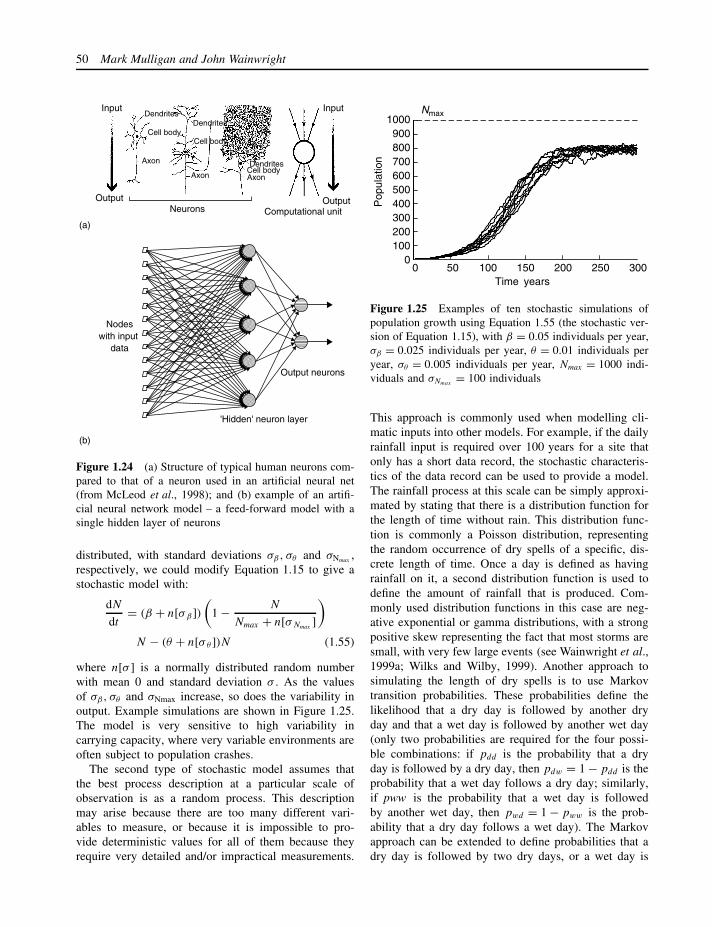
50 Mark Mulligan and John Wainwright
Nodeswith input
data
'Hidden' neuron layer
Output neurons
InputDendrites
Dendrites
Dendrites
Cell bodyCell body
Cell bodyAxon
Axon Axon
Neurons Computational unit
Output
(a)
(b)
Input
Output
Figure 1.24 (a) Structure of typical human neurons com-pared to that of a neuron used in an artificial neural net(from McLeod et al., 1998); and (b) example of an artifi-cial neural network model – a feed-forward model with asingle hidden layer of neurons
distributed, with standard deviations σβ, σθ and σNmax ,respectively, we could modify Equation 1.15 to give astochastic model with:
dN
dt= (β + n[σβ ])
(1 − N
Nmax + n[σNmax ]
)
N − (θ + n[σ θ ])N (1.55)
where n[σ ] is a normally distributed random numberwith mean 0 and standard deviation σ . As the valuesof σβ, σθ and σNmax increase, so does the variability inoutput. Example simulations are shown in Figure 1.25.The model is very sensitive to high variability incarrying capacity, where very variable environments areoften subject to population crashes.
The second type of stochastic model assumes thatthe best process description at a particular scale ofobservation is as a random process. This descriptionmay arise because there are too many different vari-ables to measure, or because it is impossible to pro-vide deterministic values for all of them because theyrequire very detailed and/or impractical measurements.
0
1000900800700600500400300200100
0 50 100 150 200 250 300Time years
Pop
ulat
ion
Nmax
Figure 1.25 Examples of ten stochastic simulations ofpopulation growth using Equation 1.55 (the stochastic ver-sion of Equation 1.15), with β = 0.05 individuals per year,σβ = 0.025 individuals per year, θ = 0.01 individuals peryear, σθ = 0.005 individuals per year, Nmax = 1000 indi-viduals and σNmax
= 100 individuals
This approach is commonly used when modelling cli-matic inputs into other models. For example, if the dailyrainfall input is required over 100 years for a site thatonly has a short data record, the stochastic characteris-tics of the data record can be used to provide a model.The rainfall process at this scale can be simply approxi-mated by stating that there is a distribution function forthe length of time without rain. This distribution func-tion is commonly a Poisson distribution, representingthe random occurrence of dry spells of a specific, dis-crete length of time. Once a day is defined as havingrainfall on it, a second distribution function is used todefine the amount of rainfall that is produced. Com-monly used distribution functions in this case are neg-ative exponential or gamma distributions, with a strongpositive skew representing the fact that most storms aresmall, with very few large events (see Wainwright et al.,1999a; Wilks and Wilby, 1999). Another approach tosimulating the length of dry spells is to use Markovtransition probabilities. These probabilities define thelikelihood that a dry day is followed by another dryday and that a wet day is followed by another wet day(only two probabilities are required for the four possi-ble combinations: if pdd is the probability that a dryday is followed by a dry day, then pdw = 1 − pdd is theprobability that a wet day follows a dry day; similarly,if pww is the probability that a wet day is followedby another wet day, then pwd = 1 − pww is the prob-ability that a dry day follows a wet day). The Markovapproach can be extended to define probabilities that adry day is followed by two dry days, or a wet day is
Modelling and Model Building 51
followed by two wet days and so on. This approachis useful if the climate system can be thought to have a‘memory’. For example, in regions dominated by frontalrainfall, it is likely that there will be periods of contin-uously wet weather, whereas thunderstorms in drylandsevents generally occur on particular days and changeatmospheric conditions such that a further thunderstormis unlikely. Note that it is still possible to interpretthe meaning of such stochastic models in a physicallymeaningful way. Further details on stochastic rainfallgenerators can be found in Wilks and Wilby (1999).Markov models are described in more detail in Collins(1975) and Guttorp (1995), with other applications insedimentology (e.g. Parks et al., 2000), mapping (e.g.Kovalevskaya and Pavlov, 2002) and ecology (e.g. Hillet al., 2002) among others.
Another commonly employed example of a stochas-tic model is related to sediment transport. Although thebalance of forces on individual particles is generallywell understood (e.g. Middleton and Southard, 1984),there are a number of factors that make it impracti-cal to measure all the necessary controls in an opera-tional way. For example, the likelihood of movementdepends on the way in which a stone sits on the bedof a channel. If there is a variable particle size (whichthere is in all but the best-controlled laboratory experi-ments), then the angle at which the stone sits will varyaccording to the size of the stones in the bed and theirorientation. Similarly, river flows exhibit turbulence,so that the force exerted on the stone is not exactlypredictable. Einstein (1942) defined an approach thatdefines the sediment-transport rate as a function of thetime periods over which sediment particles do not moveand a function of the travel distance once a particle startsmoving (see Raudkivi, 1990, for a derivation). Naden(1987) used this approach successfully to simulate thedevelopment of bedforms in gravel-bed rivers. A mod-ified version of this approach was used by Wainwrightet al. (1999b) to simulate the development of desertpavements.
It is a common misconception that stochastic modelswill always be faster than corresponding determinis-tic models. This situation is not necessarily the casebecause there is often a high computational overheadin generating good random numbers with equal likeli-hood that all values appear and that successive valuesare not correlated or repeated over short time inter-vals. In fact, it is impossible for a computer to generatea true random number. Most random-number genera-tors depend on arithmetic manipulations that ensure thatthere are cycles of numbers that repeat but that the num-ber over which they repeat is very large. The outputs are
called pseudo-random numbers. Generating and evalu-ating good pseudo-random numbers are dealt with indetail in Press et al. (1992) and Kloeden et al. (1994).Problems in certain packages are presented in Sawitzki(1994) and McCullough and Wilson (2002).
1.6 MODEL PARAMETERIZATION,CALIBRATION AND VALIDATION
1.6.1 Chickens, eggs, models and parameters?
Should a model be designed around available measure-ments or should data collection be carried out only oncethe model structure has been fully developed? Manyhardened modellers would specify the latter choice asthe most appropriate. The parameters that are requiredto carry out specific model applications are clearly bestdefined by the model structure that best represents theprocesses at work. Indeed, modelling can be used in thisway to design the larger research programme. Only bytaking the measurements that can demonstrate that theoperation of the model conforms to the ‘real world’ isit possible to decide whether we have truly understoodthe processes and their interactions.
However, actual model applications may not be sosimple. We may be interested in trying to reconstructpast environments, or the conditions that led to catas-trophic slope collapse or major flooding. In such cases,it is not possible to measure all of the parameters of amodel that has a reasonable process basis, as the condi-tions we are interested in no longer exist. In such cases,we may have to make reasonable guesses based on indi-rect evidence. The modelling procedure may be carriedout iteratively to investigate which of a number of recon-structions may be most feasible.
Our optimal model structure may also produce param-eters that it is not possible to measure in the field setting,especially at the scales in which they are representedin the model. The limitations may be due to cost, orthe lack of appropriate techniques. It may be necessaryto derive transfer functions from (surrogate) parametersthat are simpler to measure. For example, in the caseof infiltration into hillslopes, the most realistic resultsare generally obtained using rainfall simulation, as thisapproach best represents the process we are trying toparameterize (although simulated rain is never exactlythe same as real rain – see Wainwright et al., 2000,for implications). However, rainfall simulation is rela-tively difficult and expensive to carry out, and generallyrequires large volumes of water. It may not be feasi-ble to obtain or transport such quantities, particularly inremote locations – and most catchments contain some

52 Mark Mulligan and John Wainwright
remote locations. Thus, it may be better to parameter-ize using an alternative measurement such as cylinderinfiltration, or pedo-transfer functions that only requireinformation about soil texture. Such measurements maynot give exactly the same values as would occur underreal rainfall, so it may be necessary to use some formof calibration or tuning for such parameters to ensureagreement between model output and observations. Inextreme cases, it may be necessary to attempt to cali-brate the model parameter relative to a known outputif information is not available. We will return to theproblems with this approach later.
Parameterization is also costly. Work in the fieldrequires considerable investment of time and generallyalso money. Indeed, some sceptics suggest that theresearch focus on modelling is driven by the need tokeep costs down and PhDs finished within three years(Klemes, 1997). Equipment may also be expensive and,if it is providing a continuous monitored record, willneed periodic attention to download data and carry outrepairs. Therefore, it will generally never be possible toobtain as many measurements as might be desirable inany particular application. As a general rule of thumb,we should invest in parameter measurement accordingto how great an effect the parameter has on the modeloutput of interest. The magnitude of the effect ofparameters on model output is known as the sensitivityof a model to its parameters. This important stage ofanalysis will be dealt with in more detail below.
1.6.2 Defining the sampling strategy
Like models, measurements are also abstractions ofreality, and the results of a measurement campaign willdepend as much upon the timing, technique, spatialdistribution, scale and density of sampling as on thereality of the data being measured. As in modelling,it is imperative that careful thought is put into theconceptualization and design of a sampling strategyappropriate to the parameter being measured and theobjective of the measurement. This is particularly truewhen the sampled data are to be used to parameterizeor to validate models. If a model under-performs interms of predictive or explanatory power, this can bethe result of inappropriate sampling for parameterizationor validation as much as model performance itself. Itis often assumed implicitly that data represents realitybetter than a model does (or indeed that data is reality).Both are models and it is important to be critical of both.
We can think of the sampling strategy in termsof (a) the variables and parameters to be measuredfor parameterization, calibration and validation; (b) the
direct or indirect techniques to be used in measurementand their inherent scale of representation; (c) the spatialsampling scheme (distributed, semi-distributed, lumped)and its density; and (d) the temporal sampling scheme(duration and temporal resolution). Choosing whichvariables will be measured for parameterization andthe intensity of measurement will depend very muchon the sensitivity of the significant model outputs tothose (see below). Highly sensitive parameters shouldbe high on the agenda of monitoring programmesbut since model sensitivity to a parameter is usuallydependent also on the value of other parameters, thisis not always as straightforward as it might at firstappear. Where variables are insensitive, either theyshould not be in the model in the first place ortheir measurement can be simplified to reflect this.Calibration parameters should be as much as possiblethose without physical meaning so as not to compromisethe physical basis of the model and their measurementwill be necessary for the application of models tonew environments or epochs. Validation parametersand variables should be those which are the criticalmodel outputs in terms of the purpose of the model.A robust validation of the key model output wouldtend to indicate that the model has performed well ina predictive sense. This outcome does not mean thatthe results have been obtained for the correct reasons,in other words, good prediction is no guarantee ofgood explanation. In this way, if one were to validatethe output of a catchment hydrological model usingmeasured discharge data and obtain good agreementbetween model and data, this success can come aboutas the result of many different configurations of thedriving variables for discharge. It is thus importantto validate the output required but also some internalvariable which would indicate whether that outputhas been arrived at for the correct reasons, in thiscase the spatial distribution of soil moisture aroundthe catchment.
The techniques used for measurement will dependupon a number of logistic constraints such as avail-ability, cost, dependence on power supplies, trainingrequired for use and safety, but must also depend uponthe spatial and temporal structure of the model forwhich these techniques will provide data since it isimportant that the model and the data are represent-ing the same thing. A good example is soil mois-ture. Soil is a three-phase medium consisting of thesoil matrix, rock fragments greater than 2 mm in diam-eter and porosity. Soil moisture occupies the porositywhich is usually around half of the soil volume. Inmany soils, rock-fragment content can be in excess of

Modelling and Model Building 53
30% (van Wesemael et al., 2000) and while rock frag-ments sometimes have a small porosity, it is usuallypretty insignificant for the purposes of moisture reten-tion. Volumetric measurement of soil moisture usuallyprovides an output of m3 water per m3 soil fine fractionwhich does not usually contain rock fragments. Thesetend to be avoided in the installation of electronic sen-sors of soil moisture and not accounted for in calibration,and which tend to be avoided or sieved out of gravimet-ric samples. Soil-moisture measurements are usually anaggregate of small sample measurements of the fine soilfraction. However, soil tends to be represented as largeblocks with dimensions of tens to hundreds of metresin hydrological models. This must therefore incorporatea significant loss of available porespace because of thepresence of rock fragments and thus the nature of soilmoisture at this scale is quite different to that at thepoint scale of measurement. The need to balance dataand model attributes is particularly clear where indirectmeasurements, in particular remote sensing, are used formodel parameterization.
Over recent decades there has been a move awayfrom lumped models in which spatial heterogeneity isnot represented towards distributed models in which itis. Advances in computing power and GIS technolo-gies have enabled the development of complex spatialmodels based on the discretization of landscapes intovector polygons, triangular irregular networks, objectsof complex form or simple raster grids. Despite recentadvances in remote sensing, there are still very manyparameters that cannot be measured using electromag-netic radiation and thus remote sensing. The sophistica-tion of spatial models has rapidly outgrown our abilityto parameterize them spatially and they thus remain con-ceptually lumped (Beven, 1992). The appropriate scaleof distribution and the optimum configuration of mea-surements for model parameterization or calibration arethe subject of much debate. For example, Musters andBouten (2000) used their model of root-water uptaketo determine the optimal sampling strategy for thesoil-moisture probes used to parameterize it. Fieldworkis an expensive, labour-intensive, time-consuming andsometimes uncomfortable or even hazardous activity.Traditional random or structured sampling proceduresusually require that a very large number of samples becollected in order to fulfil the assumptions of statisticalinference. In order to reduce the sampling effort, priorknowledge about the system under study may be used toguide convenience or nonrandom sampling which is stillstatistically viable, with the appropriate method depend-ing on the type of prior knowledge available (Modeet al., 2002). Ranked set sampling (Mode et al., 1999)
reduces the cost of sampling by using ‘rough but cheap’quantitative or qualitative information to guide the sam-pling process for the real, more expensive samplingprocess. Chao and Thompson (2001) and others indi-cate the value of optimal adaptive sampling strategiesin which the spatial or temporal sampling evolves overtime according to the values of sites or times alreadysampled. A number of authors indicate how optimalsampling can be achieved by algorithmic approacheswhich maximize entropy in the results obtained (e.g.Bueso et al., 1998; Schaetzen et al., 2000). The lux-ury of optimizing your sampling scheme in this wayis, however, not always available to the modeller, espe-cially within the context of policy models which areapplied using existing datasets generated by governmentagencies, for example, where ‘you get what you aregiven’ and which may not be collected with uniformor standard protocols (e.g. as outlined for soils data inSpain by Barahona and Iriarte, 2001) or where the pro-tocol may evolve over time, affecting the legitimacyof time-series analysis. Usually the spatial samplingscheme chosen is a compromise between that whichbest represents the system under review and the compu-tational resources and data available. This compromiseis most clearly seen in the extensive discussions on theproblem of grid size and subgrid variability in generalcirculation models (GCMs). May and Roeckner (2001),among others, indicate the importance of grid resolutionin affecting the results of GCMs. Smaller grid sizes pro-duce more realistic results, especially in highly moun-tainous areas, but smaller grids also have substantiallyhigher computational and data costs.
Wainwright et al. (1999a) indicated the importance ofthe temporal detail of climate data for accurate hydro-logical modelling. The calculation of evapotranspirationusing the Penman–Monteith formula for hourly dataand then the same data aggregated to a single valuefor each day and then separately for each day and nightindicates that the day–night aggregation produces muchcloser results to the original hourly data than does thedaily aggregation because of the domain change in netradiation values from daylight hours when they are pos-itive to night-time hours when they are negative. Theerror induced by aggregation to daily timestep is of theorder of 100% and varies with the month of the yeartoo. This indicates that one must pay attention to thenatural scales and boundaries of the processes beingmodelled when devising the time (or space) scale forsampling. Similarly, Mulligan (1998) demonstrated theimportance of high temporal resolution rainfall inten-sity data in understanding the partitioning between infil-tration and overland flow. Where soil infiltration rates

54 Mark Mulligan and John Wainwright
fall within the range of measured instantaneous rain-fall intensities (as they often do), it is important tounderstand rainfall intensities as the distribution functionof instantaneous intensities. The greater the timescaleover which these intensities are aggregated, the lowerthe measured intensity would be. Such aggregation canhave major effects on the predicted levels of Hortonianor infiltration-excess overland-flow production – whichis, after all, a threshold process (see Wainwright andParsons, 2002, for spatial implications). Hansen et al.(1996) suggested the importance of data quality in deter-mining streamflow prediction for the lumped IHACRESrainfall-runoff model to conclude that rain-gauge densityand the sampling interval of rainfall are the most crit-ical across a range of catchments. Understanding thesesensitivities is critical to designing an appropriate sam-pling scheme.
1.6.3 What happens when the parametersdon’t work?
It is frequently the case that initial parameter estimateswill produce model outputs that are incompatible withthe known behaviour of the system. There are usuallygood reasons for this outcome, so do not give up!Given that the parameter base for distributed modelsis generally small relative to the detail simulated, it isperhaps not surprising. Similarly, lumped models havea sparse parameter representation relative to naturalvariability in the system. Point measurements or spatialaverages are often poor representations of the parameterinteractions in this case. Evaluating errors from thesesources will be dealt with later.
However, in terms of model parameterization, it maybe impossible to return to the field to carry out moremeasurements, but we still need to obtain results forour model application. Thus, we need to adopt aniterative approach to the evaluation of the correct modelparameters. This procedure is generally known as modelcalibration.
1.6.4 Calibration and its limitations
Kirkby et al. (1992) distinguish between physical param-eters, which define the physical structure of the systemunder study, and process parameters, which define theorder of magnitude of processes. Most models will con-tain both types of parameter. Definition of these processparameters is known as calibration or model tuning.Where they are physically based, this can be achieved bytheir measurement, where not, they are calibrated using a
process of optimization (optimized) against a measure ofthe agreement between model results and a set of obser-vations used for calibration. The calibration dataset mustbe independent from any dataset which is used later tovalidate the model, if the same dataset is used for bothit should be no surprise that the model is a perfect pre-dictor! Split sample approaches, in which the availabledata is separated into a calibration set and a separatevalidation set, are usually the solution to this problem.
Calibration should pay particular attention to the sen-sitivity of parameters with sensitive parameters beingcalibrated carefully against high quality datasets toensure that the resulting model will produce reliable out-comes. The simplest form of optimization is trial anderror whereby model parameters are altered and a mea-sure of goodness of fit between model results and thecalibration dataset is noted. This process is repeated iter-atively to obtain the best possible fit of observed againstpredicted. Of course the calibration will be specific tothe model results calibrated against and will producea model which should forecast this result well at theexpense of other model outputs not involved in thecalibration procedure. The choice of calibration param-eters, measures and techniques will thus depend uponthe purpose to which the model will be put. Moreover,a model calibration by one user with a particular under-standing of its function may be quite different fromthat of another (Botterweg, 1995) and a model cali-brated to a particular objective such as the predictionof peak runoff may then be useless in the predictionof total annual runoff. Some prior knowledge of, forexample, the reasonable ranges of parameter values, willalso be necessary and calibration will usually follow apreliminary sensitivity or uncertainty analysis which isperformed to test the validity of the model. The relation-ship between the range of values for a parameter andthe model agreement is known as the calibration curvefor that parameter. A parameter that shows a signifi-cant change in error with a change in its value (with allother parameters held constant) is known as a sensitiveparameter. If a model has only one parameter, it is usu-ally fairly straightforward to find the optimal value forthat parameter. This procedure becomes only marginallymore difficult for models with more than one param-eter where the parameters are independent. In mostmodels, parameters are highly interdependent and thiswill confound the definition of an optimum parameter-ization. In these cases other – automated – techniquesare used to define the optimal parameter set. Thesetechniques include genetic algorithms and fuzzy logicapproaches as used to calibrate a rainfall-runoff modelto multiple objectives (peak discharge, peak time and

Modelling and Model Building 55
total runoff volume) by Cheng et al. (2002). Calibra-tion is particularly challenging in distributed modelswhich tend to have a large number of parameters.Stochastic or evolutionary genetic algorithms seem tobe the most successful approaches under these circum-stances (Eckhardt and Arnold, 2001) and have beenapplied widely where there are multiple objectives of thecalibration (Madsen, 2000; 2003). In distributed models,there may also be advantages of calibrating differentareas, such as subcatchments, separately and indepen-dently rather than as an integrated whole (e.g. Seibertet al., 2000). Ratto et al. (2001) highlight the utility ofthe global sensitivity analysis (GSA) and generalizedlikelihood uncertainty estimation (GLUE) approaches(see below) in the calibration of over-parameterizedmodels with strong parameter interaction. GSA is amodel-independent approach, which is based on esti-mating the fractional contribution of each input factorto the variance in the model output, accounting also forinteraction terms. GLUE allows model runs to be clas-sified according to the likelihood of their being a goodsimulator of the system, recognizing that many differentcombinations of parameter values can produce accuratemodel results (the issue of equifinality). By applyingGSA to the GLUE likelihoods, the parameter sets driv-ing model simulations with a good fit to observations areidentified along with the basic features of the parameterinteraction structure. Extensive model calibration tendsto remove the physical basis of a model. Part of theobjective in building a physically based model shouldbe to produce a sufficiently good model structure andconceptualization to avoid the need for substantial cali-bration.
1.6.5 Testing models
The terms verification and validation have very specificmeanings in computer science. Verification is used todenote the process of checking that the computer code(program) does exactly what the algorithm is designedto do. As well as a formal confirmation, the procedurealso involves the removal of bugs that have crept intothe program during its writing (due to typing mistakes aswell as mis-conceptualizations). Validation, on the otherhand, refers to the testing of the model output to confirmthe results that should be produced in reality (Fishmanand Kiviat, 1968). One common method of validationis the comparison of a numerical model against theanalytical solution for specific boundary conditions oragainst field measured data for the period and place ofthe model simulation.
However, Oreskes et al. (1994) point out that thedifference between these specific uses and the commonusage of the same terms can often lead to confusion,particularly when model results are being presented tononmodellers. Rykiel (1996) suggests that the terms areessentially synonymous in everyday language, so thedistinction is hard to see to a nonuser. Furthermore, theroots of the words may imply that a model is betterthan was actually intended when the author of a papernoted that the model was verified and validated. Theroot meaning of verify comes from the Latin verus,meaning truth, while the Latin validare means to declareor give legal authority to something. Thus Oreskes et al.(1994) suggest that the nonmodeller may tend to feela verified model presents the truth, and one that isvalidated can have legal authority, or is at least ‘doesnot contain known or detectable flaws and is internallyconsistent’. They suggest that benchmarking is a moreappropriate term for verification and model evaluationshould be used in place of validation. However, it couldbe argued that these are equally value-laden terms. Inreality, most model output actually seems to generatea healthy dose of scepticism in nonmodellers (see thedebate in Aber, 1997, 1998; Dale and Van Winkle,1998; Van Winkle and Dale, 1998, for example). Laneand Richards (2001), on the other hand, suggest thatvalidation is used as a linguistic means of hiding fromsuch criticism.
Much more fundamentally in this debate, the natureof environment systems and scientific practice meansthat whatever term is used for validation/model eval-uation, it will always tend to overstate the case forbelief in the model results. There are six reasons statedby Oreskes et al. (1994) for this problem. First, allenvironmental systems are open. Logically, it is onlypossible to demonstrate the truth of a closed system(although even this proposition is called into ques-tion by Godel’s theorem – see the excellent overviewby Hofstadter, 1979). Second, there are problems dueto the presence of unknown parameters and the scalingof nonadditive parameters (see below and Chapter 19).Third, inferences and embedded assumptions under-lie all stages of the observation and measurement ofvariables – dependent and independent alike. Fourth,most scientific theories are developed by the addi-tion of ‘auxiliary hypotheses’, that is, those not centralto the principal theory, but fundamental in a specificcontext for putting it into action. Thus, it is impos-sible to tell whether the principal or an auxiliaryhypothesis is incorrect should deductive verification fail.Fifth, as we have seen, more than one model formu-lation can provide the same output. This property is

56 Mark Mulligan and John Wainwright
known formally as nonuniqueness or underdetermina-tion (the Duhem–Quine thesis: Harding, 1976). Sixth,errors in auxiliary hypotheses may cancel, causing incor-rect acceptance of the model. Many modellers wouldnow accept that full validation is a logical impossi-bility (e.g. Refsgaard and Storm, 1996; Senarath et al.,2000). Morton and Suarez (2001) suggest that in mostpractical contexts the term ‘model’ can be thought of asbeing synonymous with ‘theory’ or ‘hypothesis’, withthe added implication that they are being confronted andevaluated with data. Often the models represent simplifi-cations of complex, physically based theories, analogiesof other systems, summaries of data, or representationsof the theories themselves. It is this set of approachesthat allows the provisional nature of scientific knowl-edge to be tested. Conversely, it is possible for modelsto continue being used for a range of reasons relatingto the social, economic and political contexts of sci-ence (Oreskes and Bellitz, 2001).
Rykiel (1996) provides an overview of how valida-tion has been employed in modelling, and distinguishes(a) operational or whole-model validation (correspon-dence of model output with real-world observations);(b) conceptual validation (evaluation of the underlyingtheories and assumptions); and (c) data validation (eval-uation of the data used to test the model). He suggeststhat there are at least 13 different sorts of validationprocedure that are commonly employed, explicitly orimplicitly. These procedures are:
(a) face validation – the evaluation of whether modellogic and outputs appear reasonable;
(b) Turing tests – where ‘experts’ are asked to distin-guish between real-world and model output (byanalogy with the test for artificial intelligence);
(c) visualization techniques – often associated with astatement that declares how well the modelledresults match the observed data;
(d) comparison with other models – used for examplein general circulation model evaluations (althoughnote the high likelihood of developing an argumentbased on circular logic here!);
(e) internal validity – e.g. using the same data setrepeatedly in a stochastic model to evaluate whetherthe distribution of outcomes is always reasonable;
(f) event validity – i.e. whether the occurrence andpattern of a specific event are reproduced bythe model;
(g) historical data validation – using split-sample tech-niques to provide a subset of data to build a modeland a second subset against which to test the modelresults (see also Klemes, 1983);
(h) extreme-condition tests – whether the model be-haves ‘reasonably’ under extreme combinationsof inputs;
(i) traces – whether the changes of a variable throughtime in the model are realistic;
(j) sensitivity analyses – to evaluate whether changesin parameter values produce ‘reasonable’ changesin model output (see below);
(k) multistage validation (corresponding to the stagesa, b and c noted above);
(l) predictive validation – comparison of model outputwith actual behaviour of the system in question;
(m) statistical validation – whether the range of modelbehaviour and its error structure match that of theobserved system (but see the discussion on errorpropagation below).
Clearly, all these tests provide some support for theacceptance of a model, although some are more rigorousthan others. The more tests a model can successfullypass, the more confidence we might have in it, althoughthis is still no reason to believe it absolutely forthe reasons discussed above. But in complex models,validation is certainly a nontrivial procedure – Brownand Kulasiri (1996: 132) note, for example, that ‘a modelcan be considered to be successfully validated if allavailable techniques fail to distinguish between field andmodel data’. Any model test will in part be evaluatingthe simplifications upon which the model is based,and in part the reasonableness of its parameterization.However, if a number of parameterizations fail fora specific model, we might seriously reconsider itsconceptual basis. As with other aspects of modelling,evaluation is an iterative process.
1.6.6 Measurements of model goodness-of-fit
Calibration and validation or model evaluation as out-lined above all require some measurement of how wellthe model represents actual measurements. These mea-surements are often known as objective functions, orgoodness-of-fit statistics. It should be recognized thatthere are a number of different goodness-of-fit mea-sures, and they will each be sensitive to different aspectsof model (mis.)behaviour. The choice of an appropriatemeasure is therefore vital in a robust model evaluation.In the following discussion, we use Mi as a sequence ofmodel outputs to be compared to Oi observed systemvalues, M is the mean model output and O the meanobserved value.
We can use the coefficient of determination, r2, torepresent the proportion of variance in the observed

Modelling and Model Building 57
data explained by the model results. The value iscalculated as:
r2 =
n∑i=1
[Oi − O] · [Mi − M]
√√√√ n∑i=1
[Oi − O]2 ·
√√√√ n∑i=1
[Mi − M]2
2
(1.56)
or the ratio of the covariance in the observed andmodelled values to the product of the individual vari-ances. The value of r2 varies from 1, which meansall of the variance in the data is explained by themodel, to 0, where none of the variance is explained.As noted by Legates and McCabe (1999), this mea-sure is insensitive to constant, proportional deviations.In other words, perfect agreement occurs if the modelconsistently underestimates or overestimates by a spe-cific proportion, so that there is a linear relationshipbetween Mi and Oi which does not lie on the 1:1line (compare the use of the coefficient of determina-tion in evaluating regression models). As correlation isnot a robust statistical measure, the value of r2 willbe sensitive to outliers (values that lie a large dis-tance away from the mean), which will tend to increaseits value spuriously if there are extreme events in theobserved dataset.
The Nash and Sutcliffe (1970) model-efficiency mea-sure is commonly used:
NS = 1 −
n∑i=1
(Oi − Mi)2
n∑i=1
(Oi − O)2
(1.57)
which is a measure of the mean square error to theobserved variance. If the error is zero, then NS = 1,and the model represents a perfect fit. If the error is thesame magnitude as the observed variance, then NS = 0and the observed mean value is as good a representa-tion as the model (and thus the time invested in themodel is clearly wasted). As the error continues toincrease, the values of the index become more negative,with a theoretical worst-case scenario of NS = −∞. NSdoes not suffer from proportional effects as in the caseof r2, but it is still sensitive to outliers (Legate andMcCabe, 1999).
A modified ‘index of agreement’ was defined asthe ratio of mean-square error to total potential error
by Willmott (1981):
W = 1 −
n∑i=1
(Oi − Mi)2
n∑i=1
(|Mi − O| + |Oi − O|)2
(1.58)
where 1 again means a perfect model fit, but the worstmodel fit is represented by a value of 0. As with the twoprevious measures, the squared terms make it sensitiveto outliers. Legates and McCabe suggest that it may bebetter to adjust the comparison in the evaluation of NSand W to account for changing conditions, so that ratherthan using the observed mean, a value that is a functionof time (e.g. a running mean) is more appropriate ifthe model covers highly variable situations. It may alsobe desirable to calculate absolute errors such as theroot-mean square (RMSE : see below) and the meanabsolute error:
MAE =
n∑i=1
|Oi − Mi |
n(1.59)
and to use the extent to whichRMSE
MAE> 1 as an indica-
tor of the extent to which outliers are affecting the modelevaluation. In a comparison of potential evapotranspi-ration and runoff models, Legates and McCabe foundthe best way of evaluating the results was to ignorer2, and to use baseline-adjusted NS and W indices,together with an evaluation of RMSE and MAE. Otherauthors have suggested that it is also useful to pro-vide a normalized MAE, by dividing by the observedmean (thus giving a ratio measurement – compare thenormalized RMSE discussed below) (Alewell and Man-derscheid, 1998). The effects of outliers can be min-imized by making the comparison on values below aspecific threshold (e.g. Madsen, 2000) or by using log-transformed values.
The choice of appropriate objective functions andmodel-evaluation procedures is a critical one. UsingBayesian analysis, Kirchner et al. (1996) demonstratehow insufficiently strict tests will cause a reasonablesceptic to continue to disbelieve a model, while themodel developer may continue regardless. Only if amodel has a chance of 90% of being rejected whenit is a poor representation of observed values will thetesting procedure be found convincing. As with allaspects of science, we must endeavour to use the mostrigorous tests available that do not wrongly reject themodel when the data are at fault.

58 Mark Mulligan and John Wainwright
1.7 SENSITIVITY ANALYSIS AND ITS ROLE
Sensitivity analysis is the process of defining modeloutput sensitivity to changes in its input parameters.Sensitivity analysis is usually carried out as soon asmodel coding is complete and at this stage it hastwo benefits: to act as a check on the model logicand the robustness of the simulation and to define theimportance of model parameters and thus the effortwhich must be invested in data acquisition for differentparameters. The measurement of the sensitivity of amodel to a parameter can also be viewed relative tothe uncertainty involved in the measurement of thatparameter in order to understand how important thisuncertainty will be in terms of its impact on the modeloutcomes. If sensitivity analysis at this stage indicatesthat the model has a number of parameters to whichthe model is insensitive, then this may indicate over-parameterization and the need for further simplificationof the model.
Sensitivity analysis is usually also carried out whena model has been fully parameterized and is often usedas a means of learning from the model by understand-ing the impact of parameter forcing, and its cascadethrough model processes to impact upon model out-puts (see, for example, Mulligan, 1996; Burke et al.,1998; Michaelides and Wainwright, 2002). In this waythe behaviour of aggregate processes and the nature oftheir interaction can better be understood. After cal-ibration and validation, sensitivity analysis can alsobe used as a means of model experiment and this isvery common in GCM studies where sensitivity exper-iments of global temperature to greenhouse forcing,to large-scale deforestation or to large-scale deserti-fication are common experiments. Sensitivity analy-sis is also used in this way to examine the impactsof changes to the model structure itself, its bound-ary or initial conditions or the quality or quantity ofdata on its output (for example, May and Roeckner,2001).
The sensitivity of model parameters is determinedby their role in the model structure and if this roleis a reasonable representation of their role in the sys-tem under study, then there should be similaritiesbetween the sensitivity of model output to param-eter change and the sensitivity of the real systemresponse to physical or process manipulation. Never-theless one must beware of attributing the model sen-sitivity to parameter change as the sensitivity of thereal system to similar changes in input (see Baker,2000).
The methods of sensitivity analysis are covered insome detail by Hamby (1994) and, more recently, by
Saltelli et al. (2000) and will not be outlined in detailhere. In most sensitivity analyses a single parameter isvaried incrementally around its normal value, keepingall other parameters unaltered. The model outputs ofinterest are monitored in response to these changes andthe model sensitivity is usually expressed as the propor-tional change in the model output per unit change inthe model input. In Figure 1.26 we show an examplesensitivity analysis of the simple soil-erosion model(Equation 1.1), first in terms of single parameters andthen as a multivariate sensitivity analysis. The for-mer demonstrates the relative importance of vegeta-tion cover, then slope, runoff and finally soil erodi-bility in controlling the amount of erosion accordingto the model. The multivariate analysis suggests thatspatially variable parameters can have significant andsometimes counter-intuitive impacts on the sensitivityof the overall system. A sensitive parameter is one thatchanges the model outputs of interest significantly perunit change in its value and an insensitive parameteris one which has little effect on the model outputs ofinterest (though it may have effects on other aspectsof the model). Model sensitivity to a parameter willalso depend on the value of other model parameters,especially in systems where thresholds operate, evenwhere these remain the same between model runs. Itis important to recognize the propensity for parameterchange in sensitivity analysis, that is a model can behighly sensitive to changes in a particular parameter butif changes of that magnitude are unlikely ever to berealized, then the model sensitivity to them will be oflittle relevance. In this way, some careful judgement isrequired of the modeller to set the appropriate boundsfor parameter variation and the appropriate values ofvarying or nonvarying parameters during the process ofsensitivity analysis.
Sensitivity analysis is a very powerful tool for inter-acting with simple or complex models. Sensitivity anal-ysis is used to do the following:
1. better understand the behaviour of the model, par-ticularly in terms of the ways in which parame-ters interact;
2. verify (in the computer-science sense) multi-compo-nent models;
3. ensure model parsimony by the rejection of parame-ters or processes to which the model is not sensitive;
4. target field parameterization and validation pro-grammes for optimal data collection;
5. provide a means of better understanding parts of orthe whole of the system being modelled.

Modelling and Model Building 59
−100
0
100
200
300
400
500
600
700
800
−100 −75 −50 −25 0 25 50 75 100
% Change in input variable
% C
hang
e in
out
put (
eros
ion
rate
)
QkSV
(a)
−150
−100
−50
0
50
100
150
200
250
300
350
0 25 50 75 100
Variability as % of input variable base value
% C
hang
e in
out
put (
eros
ion
rate
)
(b)
Figure 1.26 Example sensitivity analysis of the simple erosion model given in Equation 1.1: (a) univariate sensitivityanalysis of the simple erosion model given in Equation 1.1. Base values are Q = 100 mm month−1, k = 0.2, S = 0.5,
m = 1.66, n = 2.0, i = 0.07 and V = 30%. The variables Q, k, S and V are varied individually from −100% to +100%of their base values and the output compared. Note that k has a positive linear response; Q a nonlinear response fasterthan k; S a nonlinear response faster than Q (because Q is raised to the power m = 1.66 while S is raised to the powern = 2); and V a negative exponential response. The order of parameter sensitivity is therefore V > S > Q > k.; and(b) Multivariate sensitivity analysis of the same model, where normally distributed variability is randomly added to eachof the parameters as a proportion of the base value. Note the large fluctuations for large amounts of variability, suggestingthat the model is highly sensitive where variability of parameters is >50% of the mean parameter value. No interactionsor autocorrelations between parameter variations have been taken into account
1.8 ERRORS AND UNCERTAINTY
1.8.1 Error
No measurement can be made without error. (If youdoubt this statement, get ten different people to write
down the dimensions in mm of this page, without tellingeach other their measurements, and compare the results.)Although Heisenberg’s uncertainty principle properlydeals with phenomena at the quantum scale, there isalways an element of interference when making an

60 Mark Mulligan and John Wainwright
observation. Thus, the act of observation perturbs whatwe are measuring. Some systems may be particularlysensitive to these perturbations, for example, whenwe introduce devices into a river to measure patternsof turbulence. The very act of placing a flow meterinto the flow causes the local structure of flow tochange. If we were interested in the section dischargerather than the local changes in velocity, our singlemeasuring device would have less significant impacts byperturbation, but the point measurement would be a verybad measurement of the cross-section flow. To counterthis problem, we may repeat the measurement at anumber of positions across the cross-section and providean average discharge (usually weighting by the widthof flow represented by each measurement). But thisaverage will only be as good as the choice of positionstaken to represent the flow. Sampling theory suggeststhat a greater number of measurements will provide abetter representation, with the standard error decreasingwith the square root of the number of measurementsmade. However, a larger number of samples will take alonger time to make, and thus we have possible temporalchanges to contend with in giving added error. Clearly,this approach is impractical when flows are rapidlychanging. If we require continuous measurements, wemay build a structure into the flow, such as a flumeor weir (e.g. French, 1986) which again perturbs thesystem being measured (possibly with major effects ifthe local gradient is modified significantly, or if sedimentis removed from the system). Furthermore, the devicesused to measure flow through these structures will havetheir own uncertainties of measurement, even if theyare state-of-the-art electronic devices. In the flume case,the measurement is usually of a depth, which is thencalibrated to a discharge by use of a rating curve. Therating curve itself will have an uncertainty element,and is usually proportional to depth to a power greaterthan one. Any error in measurement of depth willtherefore be amplified in the estimation of discharge.Such measurements also tend to be costly, and the costand disturbance therefore prevent a large number ofmeasurements being taken in a specific area, which isproblematic if we are interested in spatial variability.
Other environmental modelling questions might re-quire even further perturbation of the system. Forexample, soil depth is a critical control of water flowinto and through the soil and thus has an impact onother systems too, such as vegetation growth or massmovement. In a single setting, we might dig a soilpit. Even if we try to replace the soil as closely aspossible in the order in which we removed it, there willclearly be a major modification to the local conditions
(most notably through bulk-density changes, which oftenmean a mound is left after refilling; a lower bulk den-sity means more pore space for water to flow through,so we have significantly altered what we intended toobserve). Even if we were foolish enough to want touse this approach at the landscape scale, it is clearly notfeasible (or legal!), so we might use a spatial sampleof auger holes. However, the auger might hit a stoneand thus have difficulty penetrating to the soil base – instony soils, we usually only reach into the upper partof the C horizon. We might therefore try a noninva-sive technique such as ground-penetrating radar (GPR).GPR uses the measured reflections of transmitted radiofrequency waves (usually in the 25–1200 MHz range)to provide ‘observations’ of the changes in dielectricconstant, in engineering structures such as building andbridges or in the ground. Dielectric constant is con-trolled by changes in material density and water content.Where transmitted waves encounter a change in dielec-tric constant, some energy passes through the interfaceand some is reflected. The reflected energy from a GPRtransmitter is recorded on a nearby receiver with thetime delay (in nanoseconds) between the transmissionof the pulse and its receipt indicating the distance of thereflecting object from the transmitter-receiver array. Inthis way GPR can image the subsurface and has foundapplications in archaeology (Imai et al., 1987), hydrol-ogy (van Overmeeren et al., 1997), glaciology (Nicollinand Kofman, 1994) and geology (Mellett, 1995). Thedifficulty with electromagnetic noninvasive techniquesis that while dielectric discontinuities can be fairly obvi-ously seen, the techniques provide little information onwhat these discontinuities are (rocks, roots or moisture,for example). Thus, noninvasive techniques are also sub-ject to significant potential error. The implication is thatall measurements should have their associated error citedso that the implications can be considered and due carebe taken in interpreting results. Care is particularly nec-essary in the use of secondary data, where you may havevery little idea about how the data were collected andquality controlled.
Field measurements are often particularly prone toerror, because of the difficulty of collecting data. Wemay choose to use techniques that provide rapid resultsbut which perhaps provide less precise measurements,because of the high costs involved in obtaining fielddata. Note the difference between error and precision(sometimes called the tolerance of a measurement) – thelatter relates only to the exactness with which a measure-ment is taken. A lack of precision may give very specificproblems when measuring features with fractal charac-teristics, or when dealing with systems that are sensitive

Modelling and Model Building 61
to initial conditions. Thus, a consideration of the mod-elling requirements is often important when deciding theprecision of a measurement.
Specification errors can arise when what is being mea-sured does not correspond to the conceptualization ofa parameter in the model. This problem may arise ifa number of processes are incorporated into a singleparameter. For example, if erosion is being considered asa diffusion process in a particular model, diffusion mayoccur by a number of processes, including rainsplash,ploughing, animal activity and soil creep. The first twomight be relatively easy to measure, albeit with theirown inherent problems (e.g. Torri and Poesen, 1988),while the latter may be more difficult to quantify eitherbecause of inherent variability in the case of bioturbationor because of the slow rate of the process in the case ofcreep. Interactions between the different processes maymake the measurement of a compound diffusion param-eter unreliable. It is also possible that different ways ofmeasurement, apparently of the same process, can givevery different results. Wainwright et al. (2000) illustratehow a number of measurements in rainfall-runoff mod-elling can be problematic, including how apparent differ-ences in infiltration rate can be generated in very similarrainfall-simulation experiments. Using pumps to removewater from the surface of the plot led to significantover-estimation of final infiltration because of incom-plete recovery of ponded water, when compared to directmeasurement of runoff from the base of the plot (whichitself incorporates ponding into the amount of infiltrationand thus also over-estimates the real rate). The pump-ing technique also introduces a significant time delayto measurements, so that unsaturated infiltration is verypoorly represented by this method. Differences betweeninfiltration measured using rainfall simulation, cylinderinfiltration and the falling-head technique from soil coresfor the same location can be orders of magnitude (e.g.Wainwright, 1996) because each are representing infil-tration in different ways. Different infiltration modelsmay be better able to use measurements using onetechnique rather than another. Such specification errorscan be very difficult to quantify, and may in fact onlybecome apparent when problems arise during the mod-elling process. It should always be borne in mind thaterrors in model output may be due to incorrect param-eter specification. When errors occur, it is an importantpart of the modelling process to return to the parame-ters and evaluate whether the errors could be caused inthis way.
Environmental models operate in a defined space inthe real world. However, the representation of that spacewill always be some form of simplification. At the
Area or volume being measured
Val
ue o
f mea
sure
d pa
ram
eter
REAor
REV
Figure 1.27 Definition of the representative elementalarea (REA) or volume (REV) concept
extreme case, the system will be completely lumped,with single values for parameters and each input andoutput. Such models can be a useful generalization, forexample in the forecasting of flooding or reservoir fill-ing (e.g. Blackie and Eeles, 1985 – another example isthe population models discussed above, although thesecan be spatialized as shown by Thornes, 1990). How-ever, the definition of each parameter may be non-trivial for all but the simplest of catchments. Woodet al. (1988) used the term representative elemental area(REA) to evaluate the scale at which a model parame-ter might be appropriate (Figure 1.27). At the oppositeend of the spectrum is the fully distributed model, inwhich all parameters are spatialized. There still remainsthe issue of the REA in relation to the grid size used(distributed applications may still have grid sizes ofkilometres or hundreds of kilometres in the case of Gen-eral Circulation Models). However, in addition, thereis the issue of how to estimate parameters spatially.Field measurements are costly so that extensive datacollection may be impossible financially, even if the peo-ple and equipment were available on a sufficient scale.Therefore, it is usual to use some sort of estimationtechnique to relate parameters to some easily measuredproperty. For example, Parsons et al. (1997) used sur-face stone cover to estimate infiltration rates, findingthat the spatial structure provided by this approach gavea better solution than simply assigning spatial valuesbased on a distribution function of measured infiltrationrates, despite the relatively high error in the calibrationbetween stone cover and infiltration rate. Model sensi-tivity to different parameters (see above) may mean thatdifferent techniques of spatialization are appropriate forthe parameters of the model in question. It is impor-tant that distributed models are tested with spatiallydistributed data, otherwise it is possible to arrive at

62 Mark Mulligan and John Wainwright
completely different conclusions about their reliability(Grayson et al., 1992a,b). Similarly, if the scale of theoutput is not related to the scale of the test data, errorsin interpretation can arise. It is for this reason that tech-niques of upscaling or downscaling of model results areimportant (see Chapter 19).
Engeln-Mullges and Uhlig (1996) classify all of theabove problems as input errors. They may be presentas errors in model parameterization, or in data againstwhich the model is tested. It is possible that a modelcould be rejected because of the latter errors, so weshould be careful to specify the magnitude of errors asfar as possible at every stage in our approach. There arethree further types of error associated with the modellingprocess itself. These are procedural, computational andpropagation errors (Engeln–Mullges and Uhlig 1996).
Procedural errors arise from using a numericalapproximation to a problem where there is no knownanalytical solution. These errors are the differencebetween the exact and approximate solutions. Indeed,a useful test for model behaviour is a comparison ofa numerical approximation against a known analyticalsolution. We saw above how the backward-differencesolution to the kinematic wave equation for waterflow (Equations 1.34 to 1.39) had errors associated withO(h) and O(k) – that is of the same order of magnitudeof the timestep and grid size. In terms of the procedu-ral error, a central difference solution is better in that itserrors would be O(h2) and O(k2) and thus much smaller
Binary representation of number Decimalequivalent
Sign Exponent Mantissa
0 1 0 0 0 0 0 1 0 1 1 0 0 0 0 0 0 0 0 0 0 0 0 0 0 0 0 0 0 0 0 0 30 0 1 1 0 1 0 0 1 1 1 0 1 0 1 1 0 1 0 1 1 1 1 1 1 1 0 0 1 0 1 0 10−7
because of the higher order differences involved. Thus,some balance must be made between the amount of pro-cedural error, the computational resources required andthe potential for side effects such as numerical diffusion.
Computational errors arise during the computer rep-resentation of the algorithm that operationalizes themodel. Accumulated computational error is the sum oflocal computational errors incurred during the carryingout of the algorithm. Local computational errors are typ-ically due to rounding or truncation. To see how thismight be a problem, let us look at how a computer (orcalculator, for that matter) actually stores a number.
All computers store numbers in binary format. Allinteger numbers can be exactly represented in this
format. However, we may encounter two commonproblems when using integer values. First, overflow (orunderflow) may occur if the space (memory) allocatedto storing the number is not sufficient. For a two-byte,signed integer (i.e. 15 binary bits used to store thenumber and one bit to store the sign), the range of valuespossible is ±32 767 (i.e. ±215). Using four bytes, therange increases to ±2 147 483 647 (i.e. ±231 as 31 bitsare used to store the number and one bit for the sign).Second, if we divide one integer by another, there maybe a remainder, which will be discarded if the result isalso stored in integer format.
Floating-point numbers are stored in a three-part for-mat, made up of a single bit representing the sign,eight bits representing the exponent and 23 bits rep-resenting the mantissa. These make up any numberas sign × Mantissa × 2exponent−bias, where the bias ofthe exponent is a fixed integer for any given com-puter (Press et al., 1992). Some numbers cannot be rep-resented exactly in this format – either because they areirrational (e.g. π , e,
√2), or because the binary form is
not precise enough to accommodate them. In the formabove, numbers with more than six or seven decimaldigits cannot be represented. The resulting number mayeither be chopped (truncated) or rounded depending onthe computer, and the associated error is called round-offerror. Press et al. (1992) give the example of calculating3 + 10−7. With a bias of 151, the two values are storedas shown in this table:
To carry out the addition in binary arithmetic, theexponent must be identical. To maintain the identicalnumber, every time the exponent is increased, the binarynumber in the mantissa must be right-shifted (all thedigits are moved one space to the right and a zeroadded in the empty space at the beginning). To convert10−7 (exponent 01101001 binary = 105 decimal) intothe same form as 3 (exponent 10000010 binary = 130decimal), we require 25 right shifts of the mantissa. Asthe length of the mantissa is only 23 bits, it will now befull of zeroes, so the result of 3 + 10−7 would simply be3, and a truncation error of 10−7 would have occurred.
Many programming languages allow the possibilityof storing numbers with 64 bits (called either long real
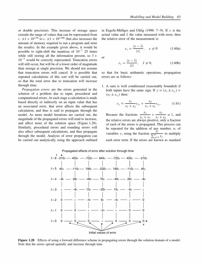
Modelling and Model Building 63
or double precision). This increase of storage spaceextends the range of values that can be represented fromc. ±1 × 10±38 to c. ±1 × 10±308 (but also increases theamount of memory required to run a program and storethe results). In the example given above, it would bepossible to right-shift the mantissa of 10−7 25 timeswhile still storing all the information present, so 3 +10−7 would be correctly represented. Truncation errorswill still occur, but will be of a lower order of magnitudethan storage at single precision. We should not assumethat truncation errors will cancel. It is possible thatrepeated calculations of this sort will be carried out,so that the total error due to truncation will increasethrough time.
Propagation errors are the errors generated in thesolution of a problem due to input, procedural andcomputational errors. At each stage a calculation is madebased directly or indirectly on an input value that hasan associated error, that error affects the subsequentcalculation, and thus is said to propagate through themodel. As more model iterations are carried out, themagnitude of the propagated errors will tend to increase,and affect more of the solution space (Figure 1.28).Similarly, procedural errors and rounding errors willalso affect subsequent calculations, and thus propagatethrough the model. Analysis of error propagation canbe carried out analytically using the approach outlined
in Engeln-Mullges and Uhlig (1996: 7–9). If x is theactual value and x the value measured with error, thenthe relative error of the measurement is:
εx = |x − x||x| , x = 0 (1.60a)
or
εx = |x − x||x| , x = 0, (1.60b)
so that for basic arithmetic operations, propagationerrors are as follows:
1. A sum is well conditioned (reasonably bounded) ifboth inputs have the same sign. If y = (x1 ± εx1) +(x2 ± εx2) then:
εy ≈ x1
x1 + x2εx1 + x2
x1 + x2εx2 . (1.61)
Because the fractionsx1
x1 + x2+ x2
x1 + x2≡ 1, and
the relative errors are always positive, only a fractionof each of the errors is propagated. This process canbe repeated for the addition of any number, n, of
variables x, using the fractionxi∑n
j=1 xj
to multiply
each error term. If the errors are known as standard
t
t = 0x
Initial values of error
Propagated effects of error after solution through time
t = 1
t = 2
t = 3
t = 4
e0 0 0 00
e e
e e
e
t = 5
t = 6
0 0 0
0
−2e
−4e −4e
−6e −6e
−8e
6e
15e −20e 15e
28e 28e70e−46e −46e
−232e190e 190e−110e −110e 45e
844e−722e −722e455e 455e
0
e
0
0
−8e
45e
−210e −210e
Figure 1.28 Effects of using a forward difference scheme in propagating errors through the solution domain of a model.Note that the errors spread spatially and increase through time

64 Mark Mulligan and John Wainwright
deviations σxi, then the propagated error has a slightly
different form:
εy ≈√√√√ n∑
i=1
σ 2xi
(1.62)
2. However, if the values of x1 and x2 have oppositesigns and are nearly equal, amplification of errorsoccurs, because even though the fractions above stillsum to one, at least one will be < −1 or >1. Thus,the magnitude at least one of the errors will increasethrough propagation. This form of model shouldtherefore be avoided. (But note that if both x1 and x2
are negative, the first rule applies.)3. In the case of a product (y = (x1 ± εx1) · (x2 ± εx2)),
error propagation is well conditioned, and related tothe sum of the individual errors of the inputs:
εy ≈ εx1 + εx2 (1.63)
Again, any number of multiplications can be propa-gated by successive adding of the error terms. Wherethe errors are known as standard deviations, we use:
εy ≈√√√√ n∑
i=1
σ 2xi
xxi
(1.64)
4. For a quotient
(y = x1 ± εx1
x2 ± εx2
, assuming x2 = 0
),
error propagation is well conditioned, and relatedto the difference in the error of the numerator anddenominator in the function:
εy ≈ εx1 − εx2 (1.65)
5. Propagation error of a power (y = (x1 ± εx1)p)
is related to the product of the power and theinput error:
εy ≈ pεx1 (1.66)
Thus roots (powers less than one) are well condi-tioned, and powers (>1) are ill conditioned. As thevalue of the power term increases, so does the errorpropagation. Wainwright and Parsons (1998) note theimplications of this results in soil-erosion modelling,where certain model formulations will be signifi-cantly more susceptible to error than others. For anerror defined as a standard deviation, we use:
εy ≈√
pσ 2x1
xx1
(1.67)
6. Combinations of the above operations can be carriedout by combination of the relevant rules in theappropriate order.
7. Other functions require differentiation to be carriedout, so that if y = f(x), then:
εy ≈ df(x)
dxεx (1.68)
so that if y = sin(x ± εx), εy ≈ (cos x) · εx or εy ≈√[(cos x) · σx]2. For multiple functions y = f(xi),
i = 1, . . . , n, partial differentiation with respect toeach variable xi must be carried out and summed:
εy ≈n∑
i=1
∣∣∣∣∂f(xi)
∂xi
∣∣∣∣ εxi(1.69)
For the example, if y = sin(x1 ± εx) · e(x2±εx2 ), theassociated error will be εy ≈ (cos x1) · εx1 + ex2εx2 orεy ≈ √
[(cos x1) · σx1 ]2 + [ex2σx2 ]2.
An alternative approach to looking at error propa-gation is to use Monte Carlo analysis. This approachuses multiple realizations of a model using distribu-tion functions to generate errors in inputs (e.g. De Rooet al., 1992; Phillips and Marks, 1996; Fisher et al.,1997; Parsons et al., 1997; Nitzsche et al., 2000). Fromthese multiple realizations, error bands can be definedto give the range of possible outputs or even confidenceintervals on outputs (e.g. Hakanson, 1996). The advan-tages of Monte Carlo analysis are that it can deal withthe effects of spatially distributed parameters, whereasthe analytical approach outlined above is more limitedin this case, and that it can deal with relatively com-plex interactions of parameter error, which is impossibleusing the analytical approach. As a disadvantage, reli-able results often require many tens or hundreds of sim-ulations (Heuvelink, 1992), which are extremely costlyin terms of computer resources for large simulations.
Beven and Binley (1992) developed the GeneralizedLikelihood Uncertainty Estimation (GLUE) technique toevaluate error propagation. The technique uses Bayesianestimators to evaluate the likelihood that specific com-binations of model parameters are good predictors ofthe system in question. Monte Carlo simulations areused to provide the various parameter combinations, andthe likelihood measured against a specified objectivefunction (Figure 1.29). The choice of parameter com-binations may be subjective, based on the experienceof the user of the technique, and often fails to accountfor necessary relationships between parameter values.An advantage of the technique is that it requires noassumptions to be made about the distribution functions

Modelling and Model Building 65
Com
bine
d lik
elih
ood
Sand content (%)
80604020
0.137
0.135
0.133
0.131
0.129
0.127
0.1250
Com
bine
d lik
elih
ood
Clay content (%)0 20 40 60
0.137
0.135
0.133
0.131
0.129
0.127
0.125
0.125
0.127
0.129
0.131
0.133
0.135
0.137
20,00,000 40,00,000 60,00,000 80,00,000 1,00,00,000
Ki - Interrill erodibility (kg s m−4)
Com
bine
d lik
elih
ood
0.125
0.127
0.129
0.131
0.133
0.135
0.137
0 0.02 0.04 0.06
Kr - Rill erodibility (s m−1)
Com
bine
d lik
elih
ood
00.125
0.127
0.129
0.131
0.133
0.135
0.137
10 20 30
Kb - Effective hydraulic conductivity (mm hr−1)
Com
bine
d lik
elih
ood
0.125
0.127
0.129
0.131
0.133
0.135
0.137
0.5 1.5 2.5 3.5 4.5
Tau - Critical shear (Pa)
Com
bine
d lik
elih
ood
Com
bine
d lik
elih
ood
Initial rill width (m)
10.80.60.40.2
0.137
0.135
0.133
0.131
0.129
0.127
0.1250
Com
bine
d lik
elih
ood
Canopy cover coefficient
14 1610 1264 82
0.137
0.135
0.133
0.131
0.129
0.127
0.125
Figure 1.29 Example of error analysis using the GLUE approach: the study by Brazier et al. (2000) looking at theWEPP soil-erosion model showing the joint likelihood of goodness-of-fit for different combinations of eight parameters

66 Mark Mulligan and John Wainwright
of the input data (Beven, 1993). Choice of the objec-tive function requires care that the key outputs of themodel simulations are being tested reliably, as notedby Legates and McCabe (1999). Other techniques thatcan be used to estimate model uncertainty include Latinhypercube simulation, Rosenbleuth’s and Harr’s point-estimation methods, all of which can be used to samplethe input-parameter space efficiently. Yu et al. (2001)found that Latin hypercube simulation provided a veryefficient means of replicating more time-intensive MonteCarlo techniques (see Press et al., 1992, for more detailon Latin hypercube sampling).
Hall and Anderson (2002) criticize error-estimationtechniques based on objective measures because thelevel of data and detailed measurements required arelacking in many environmental modelling applications.For example, in the case of an extreme flood, the effectsof the flood might be measurable (water depth fromtrash lines, aerial photographs of flood extent) after theevent, but there may be little in the way of detailedmeasurements during the event. Rainfall fields areparticularly difficult to reconstruct in high resolution inspace and time; even if flow monitoring equipment werepresent, it may have been damaged during the passageof the flood wave (Reid and Frostick, 1996). Techniquestherefore need to be developed that incorporate allinformation appropriate to model evaluation, includingqualitative indications of permissible model behaviour.
1.8.2 Reporting error
We noted how the relative error of a measurement can bemade (Equation 1.60). Different types of measurementsof error also exist (Engeln-Mullges and Uhlig, 1996).Using the same notation as before, the true error of x is:
x = x − x (1.70)
while the absolute error of x is:
|x | = |x − x| (1.71)
and the percentage error of x is:
|x − x||x| . 100 x = 0 (1.72)
If we have a series of values, xi , representing measure-ments with error on true values xi , it is common tocombine them as a root-mean square (RMS) error asfollows:
RMS x =√√√√ n∑
i=1
(xi − xi )2 (1.73)
RMS errors are in the same units as the originalmeasurements, so are easy to interpret on a case-by-case basis. When comparing between cases withvery different values, it may be useful to calculate anormalized RMS error:
NRMS x =
√√√√ n∑i=1
(xi − xi)2
n∑i=1
xi
(1.74)
which gives the proportion of error relative to theoriginal value, and can thus be easily converted intoa percentage error. In other cases, the goodness-of-fitmeasures described above may also be appropriate.
1.8.3 From error to uncertainty
Zimmermann (2000) defines six causes of uncertaintyin the modelling process: lack of information, abun-dance of information, conflicting evidence, ambiguity,measurement uncertainty and belief. A lack of informa-tion requires us to collect more information, but it isimportant to recognize that the quality of the informa-tion also needs to be appropriate. It must be directedtowards the modelling aims and may require the modi-fication of the ways in which parameters are conceivedof and collected. Information abundance relates to thecomplexity of environmental systems and our inabil-ity to perceive large amounts of complex information.Rather than collecting new data, this cause of uncer-tainty requires the simplification of information, perhapsusing statistical and data-mining techniques. Conflict-ing evidence requires the application of quality controlto evaluate whether conflicts are due to errors or arereally present. Conflicts may also point to the fact thatthe model being used is itself wrong, so re-evaluationof the model structure and interaction of componentsmay be necessary. Ambiguity relates to the reportingof information in a way that may provide confusion.Uncertainty can be removed by questioning the originalinformant, although this approach may not be possiblein all cases. Measurement uncertainty may be reducedby invoking more precise techniques, although it mustbe done in an appropriate way. There is often a tendencyto assume that modern gadgetry will allow measurementwith fewer errors. It must be noted that other errors canbe introduced (e.g. misrecording of electronic data ifa data logger gets wet during a storm event) or thatthe new measurement may not be measuring exactly thesame property as before. Beliefs about how data are to be

Modelling and Model Building 67
interpreted can also cause uncertainty because differentoutcomes can result from the same starting point. Over-coming this uncertainty is a matter of iterative testingof the different belief structures. Qualitative assessmentis thus as much an aspect of uncertainty assessment asqualitative analysis.
The quantitative evaluation of uncertainty has beendiscussed above in detail. Error-propagation techniquescan be used in relatively simple models (or their sub-components) to evaluate the impact of an input error(measurement uncertainty) on the outcome. In morecomplex scenarios, Monte Carlo analysis is almostcertainly necessary. If sufficient runs are performed,then probability estimates can be made about the out-puts. Carrying out this approach on a model with alarge number of parameters is a nontrivial exercise,and requires the development of appropriate samplingdesigns (Parysow et al., 2000). The use of sensitiv-ity analysis can also be used to optimize this pro-cess (Klepper, 1997; Barlund and Tattari, 2001). Halland Anderson (2002) note that some applications mayinvolve so much uncertainty that it is better to talk aboutpossible outcomes rather than give specific probabili-ties. Future scenarios of climate change evaluated usingGeneral Circulation Models (see Chapters 2 and 12)are a specific case in point here. Another approachthat can be used to evaluate the uncertainty in out-come as a function of uncertain input data is fuzzyset theory. Torri et al. (1997) applied this approach tothe estimation of soil erodibility in a global datasetand Ozelkan and Duckstein (2001) have applied it torainfall-runoff modelling. Because all measurements areuncertain, the data used for model testing will alsoinclude errors. It is important to beware of rejectingmodels because the evaluation data are not sufficientlystrong to test it. Monte et al. (1996) presented a tech-nique for incorporating such uncertainty into the modelevaluation process.
Distributed models may require sophisticated visu-alization techniques to evaluate the uncertainty of thespatial data used as input (Wingle et al., 1999). Animportant consideration is the development of appropri-ate spatial and spatio-temporal indices for model eval-uation, based on the fact that spatial data and theirassociated errors will have autocorrelation structuresto a greater or lesser extent. Autocorrelation of errorscan introduce significant nonlinear effects on the modeluncertainty (Henebry, 1995).
Certain systems may be much more sensitive to theimpacts of uncertainty. Tainaka (1996) discusses theproblem of spatially distributed predator–prey systems,
where there is a phase transition between the occur-rence of both predator and prey, and the extinction ofthe predator species. Such transitions can occur para-doxically when there is a rapid increase in the numberof the prey species triggered by instability in nutrientavailability, for example. Because the phase transitionrepresents a large (catastrophic) change, the model willbe very sensitive to uncertainty in the local region ofthe parameter space, and it can thus become difficult orimpossible to interpret the cause of the change.
1.8.4 Coming to terms with error
Error is an important part of the modelling process(as with any scientific endeavour). It must thereforebe incorporated within the framework of any approachtaken, and any corresponding uncertainty evaluated asfar as possible. A realistic approach and a healthy scep-ticism to model results are fundamental. It is at best mis-leading to present results without corresponding uncer-tainties. Such uncertainties have significant impacts onmodel applications, particularly the use of models indecision-making. Large uncertainties inevitably lead tothe rejection of modelling as an appropriate techniquein this context (Beck, 1987). Recent debates on possiblefuture climate change reinforce this conclusion (see theexcellent discussion in Rayner and Malone, 1998).
In terms of modelling practice, it is here that wecome full circle. The implication of error and uncertaintyis that we need to improve the basic inputs into ourmodels. As we have seen, this improvement does notnecessarily just mean collecting more data. It maymean that it is better to collect fewer samples, butwith better control. Alternatively, it may be necessaryto collect the same number of samples, but with amore appropriate spatial and/or temporal distribution.Ultimately, the iterations involved in modelling shouldnot just be within computer code, but also between fieldand model application and testing.
1.9 CONCLUSION
Modelling provides a variety of tools with which we canincrease our understanding of environmental systems.In many cases, this understanding is then practicallyapplied to real-world problems. It is thus a powerful toolfor tackling scientific questions and answering (green!)engineering problems. But its practice is also some-thing of an art that requires intuition and imagination toachieve appropriate levels of abstraction from the realworld to our ability to represent it in practical terms. As

68 Mark Mulligan and John Wainwright
a research tool, it provides an important link betweentheory and observation, and provides a means of testingour ideas of how the world works. This link is importantin that environmental scientists generally deal with tem-poral and spatial scales that are well beyond the limitsof observation of the individual. It is important to recog-nize that modelling is not itself a ‘black box’ – it formsa continuum of techniques that may be appropriatelyapplied in different contexts. Part of the art of mod-elling is the recognition of the appropriate context forthe appropriate technique.
Hopefully, we have demonstrated that there is nosingle way of implementing a model in a specificcontext. As we will see in the following chapters,there are many different ways to use models in similarsettings. How the implementation is carried out dependson a range of factors including the aims and objectivesof the study, the spatial and temporal detail required,and the resources available to carry it out. This chapterhas presented the range of currently available techniquesthat may be employed in model building and testing.More details of these techniques are found on thebook’s website and in the numerous references provided.We have also addressed a number of the importantconceptual issues involved in the modelling process,again to suggest that the modelling process is not asuniform as is often assumed, and that debate is oftenfruitful within and between disciplines in order to tacklesome of these issues.
REFERENCES
Aber, J. (1997) Why don’t we believe the models?, Bulletin ofthe Ecological Society of America 78, 232–233.
Aber, J. (1998) Mostly a misunderstanding, I believe, Bulletinof the Ecological Society of America 79, 256–257.
Alewell, C. and Manderscheid, B. (1998) Use of objectivecriteria for the assessment of biogeochemical ecosystemmodels, Ecological Modelling 107, 213–224.
Ames, W.F. (1992) Numerical Methods for Partial DifferentialEquations, Academic Press, London.
Arge, L., Chase, J.S., Halpin, P., Vitter, J.S., Urban, D. andWickremesinghe, R. (2002) Flow computation on massivegrid terrains, http://www.cs.duke.edu/geo*/terrflow/.
Baker, V.R. (1998) Paleohydrology and the hydrological sci-ences, in G. Benito, V.R. Baker and K.J. Gregory (eds)Palaeohydrology and Environmental Change, John Wiley &Sons, Chichester, 1–10.
Baker, V.R. (2000) South American palaeohydrology: futureprospects and global perspective, Quaternary International72, 3–5.
Barahona, E. and Iriarte, U.A. (2001) An overview of thepresent state of standardization of soil sampling in Spain,The Science of the Total Environment 264, 169–174.
Bardossy, A. (1997) Downscaling from GCMs to local climatethrough stochastic linkages, Journal of Environmental Man-agement 49, 7–17.
Barlund, I. and Tattari, S. (2001) Ranking of parameters on thebasis of their contribution to model uncertainty, EcologicalModelling 142, 11–23.
Bar-Yam, Y. (2000) Dynamics of Complex Systems, PerseusBooks, Reading, MA.
Bates, P.D. and Anderson, M.G. (1996) A preliminary inves-tigation into the impact of initial conditions on flood inun-dation predictions using a time/space distributed sensitivityanalysis, Catena 26, 115–134.
Bates, P.D. and De Roo, A.P.J. (2000) A simple raster-basedmodel for flood inundation simulation, Journal of Hydrology236, 54–77.
Beck, M.B. (1987) Water quality modelling: a review ofthe analysis of uncertainty, Water Resources Research 23,1393–1442.
Berec, L. (2002) Techniques of spatially explicit individual-based models: construction, simulation and mean-field anal-ysis, Ecological Modelling 150, 55–81.
Beuselinck, L., Hairsine, P.B., Sander, G.C. and Govers, G.(2002) Evaluating a multiclass net deposition equation inoverland flow conditions, Water Resources Research 38 (7),1109 [DOI: 10.1029/2001WR000250].
Beven, K. (1977) Hillslope hydrographs by the finite elementmethod, Earth Surface Processes 2, 13–28.
Beven, K. (1992) Future of distributed modelling (editorial),Hydrological Processes 6, 279–298.
Beven, K. (1993) Prophecy, reality and uncertainty in dis-tributed hydrological modelling, Advances in Water Resour-ces 16, 41–51.
Beven, K. (2001) On explanatory depth and predictive power,Hydrological Processes 15, 3069–3072.
Beven, K. (2002) Towards an alternative blueprint for a phys-ically based digitally simulated hydrologic response mod-elling system, Hydrological Processes 16, 189–206.
Beven, K. and Binley, A.M. (1992) The future of distributedmodels: model calibration and predictive uncertainty, Hydro-logical Processes 6, 279–298.
Blackie, J.R. and Eeles, C.W.O. (1985) Lumped catchmentmodels, in M.G. Anderson and T.P. Burt (eds) HydrologicalForecasting, John Wiley & Sons, Chichester, 311–345.
Blum, A. (1992) Neural Networks in C++: An Object-Oriented Framework for Building Connectionist Systems,John Wiley & Sons, Chichester.
Bostock, L. and Chandler, S. (1981) Mathematics: The CoreCourse for A-Level, ST(P) Ltd., Cheltenham.
Botterweg, P. (1995) The user’s influence on model calibrationresults: an example of the model SOIL, independentlycalibrated by two users, Ecological Modelling, 81, 71–81.
Bousquet, F., Le Page, C., Bakam, I. and Takforyan, A. (2001)Multiagent simulations of hunting wild meat in a village ineastern Cameroon, Ecological Modelling 138, 331–346.
Bradley, R.S. (1999) Palaeoclimatology: Reconstructing Cli-mates of the Quaternary. 2nd edn, Academic Press, London.
Modelling and Model Building 69
Brazier, R.E., Beven, K.J., Freer, J. and Rowan, J.S. (2000)Equifinality and uncertainty in physically based soil ero-sion models: Application of the GLUE methodology toWEPP – the Water Erosion Prediction Project – for sites inthe UK and USA, Earth Surface Processes and Landforms25, 825–845.
Brown, T.N. and Kulasiri, D. (1996) Validating models ofcomplex, stochastic, biological systems, Ecological Mod-elling 86, 129–134.
Bueso, M.C., Angulo, J.M. and Alonso, F.J. (1998) A state-space model approach to optimum spatial sampling designbased on entropy, Environmental and Ecological Statistics 5,29–44.
Burden, R.L. and Faires, J.D. (1997) Numerical Analysis, 7thedn, Brooks/Cole, Pacific Grove, CA.
Burke, S., Mulligan, M. and Thornes, J.B. (1998) Key parame-ters that control recharge at a catchment scale: using sensitiv-ity analysis and path analysis to define homogenous rechargeclasses, in H.S. Wheater and C. Kirby (eds) Hydrology in aChanging Environment, Vol. II, John Wiley & Sons, Chich-ester, 229–243.
Campolo, M., Andreussi, P. and Soldati, A. (1999) River floodforecasting with a neural network model, Water ResourcesResearch 35, 1191–1197.
Chao, C.T. and Thompson, S.K. (2001) Optimal adaptiveselection of sampling sites, Environmetrics 12, 517–538.
Cheng, C.T., Ou, C.P. and Chau, K.W. (2002) Combining afuzzy optimal model with a genetic algorithm to solvemulti-objective rainfall-runoff model calibration, Journal ofHydrology 268, 72–86.
Chorley, R.J. and Kennedy, B.A. (1971) Physical Geography:A Systems Approach, Prentice Hall, London.
Cohn, J.P. (2002) Biosphere 2: turning an experiment into aresearch station, BioScience 52, 218–223.
Collins, L. (1975) An Introduction to Markov Chain Analysis.GeoAbstracts, Norwich.
Cross, M. and Moscardini, A.O. (1985) Learning the Art ofMathematical Modelling John Wiley & Sons, Chichester.
Dale, V.H. and Van Winkle, W. (1998) Models provide under-standing, not belief, Bulletin of the Ecological Society ofAmerica 79, 169–170.
De Falco, I., Giordanoa, A., Luongob, G., Mazzarella, B. andTarantino, E. (2002) The eruptive activity of Vesuvius and itsneural architecture, Journal of Volcanology and GeothermalResearch 113, 111–118.
Dekker, S.C., Bouten, W. and Schaap, M.G. (2001) Analysingforest transpiration model errors with artificial neural net-works, Journal of Hydrology 246, 197–208.
Del Genio, A.D. (1996) Simulations of superrotation on slowlyrotating planets: sensitivity to rotation and initial condition,Icarus 120, 332–343.
De Roo, A.P.J., Hazelhoff, L. and Heuvelink, G.B.M. (1992)The use of Monte Carlo simulations to estimate the effects ofspatial variability of infiltration on the output of a distributedhydrological and erosion model, Hydrological Processes 6,127–143.
De Sapio, R. (1976) Calculus for the Life Sciences, Freeman,San Francisco.
De Wit, M.J.M. and Pebesma, E.J. (2001) Nutrient fluxes at theriver basin scale. II: the balance between data availability andmodel complexity, Hydrological Processes 15, 761–775.
Di Giammarco, P., Todini, E. and Lamberti, P. (1996) A con-servative finite elements approach to overland flow: the con-trol volume finite element formulation, Journal of Hydrology175, 267–291.
Dingman, S.L. (1984) Fluvial Hydrology, W.H. Freeman, NewYork.
Dunin, F.X. (1976) Infiltration: its simulation for field condi-tions, in J.C. Rhodda (ed.) Facets of Hydrology, John Wiley& Sons, Chichester, 199–227.
Eckhardt, K. and Arnold, J.G. (2001) Automatic calibration ofa distributed catchment model, Journal of Hydrology 251,103–109.
Einstein, H.A. (1942) Formulae for transportation of bed-load,Transactions of the American Society of Civil Engineers 107,561–577.
Endreny, T.A. and Wood, E.F. (2001) Representing elevationuncertainty in runoff modelling and flowpath mapping,Hydrological Processes 15, 2223–2236.
Engeln-Mullges and Uhlig, F. (1996) Numerical Algorithmswith FORTRAN, Springer Verlag, Berlin.
Epstein, J.M. and Axtell, R. (1996) Growing Artificial Soci-eties: Social Science from the Bottom Up, Brookings Institu-tion Press, Washington, DC. See also http://www.brookings.edu/sugarscape/
Ferrar, W.L. (1967) Calculus for Beginners, Clarendon Press,Oxford.
Ferziger, J.H. and Peric, M. (1999) Computational Methods forFluid Dynamics, Springer Verlag, Berlin.
Fisher, P., Abrahart, R.J. and Herbinger, W. (1997) The sensi-tivity of two distributed non-point source pollution modelsto the spatial arrangement of the landscape, HydrologicalProcesses 11, 241–252.
Fishman, G.S. and Kiviat, P.J. (1968) The statistics of discrete-event simulation, Simulation 10, 185–191.
Freer, J., Beven, K. and Ambroise, B. (1996) Bayesian-estima-tion of uncertainty in runoff prediction and the valueof data – an application of the GLUE approach, WaterResources Research 32, 2161–2173.
French, M.N., Krajewski, W.F. and Cuykendall, R.R. (1992)Rainfall forecasting in space and time using a neuralnetwork, Journal of Hydrology 137, 1–31.
French, R.H. (1986) Open-Channel Hydraulics, McGraw-Hill,New York.
Friedman, N.A (1968) Basic Calculus, Scott, Foresman, Glen-view, IL.
Gershenfield, N. (1999) The Nature of Mathematical Mod-elling, Cambridge University Press, Cambridge.
Ginot, V., Le Page, C. and Souissi, S. (2002) A multi-agent’s architecture to enhance end-user individual-basedmodelling, Ecological Modelling 157, 23–41. See alsohttp://www.avignon.inra.fr/mobidyc
Goodrich, D.C., Woolhiser, D.A. and Keefer, T.O. (1991)Kinematic routing using finite-elements on a triangular irreg-ular network, Water Resources Research, 27, 995–1003.
70 Mark Mulligan and John Wainwright
Gottardi, G. and Venutelli, M. (1997) LANDFLOW: computerprogram for the numerical simulation of two-dimensionaloverland flow, Computers and Geosciences 23, 77–89.
Govindasamy, B., Caldeira, K. and Duffy, P.B. (2003) Geo-engineering Earth’s radiation balance to mitigate climatechange from a quadrupling of CO2, Global and PlanetaryChange 771, 1–12.
Graf, W.H. and Altinakar, M.S. (1998) Fluvial Hydraulics:Flow and Transport Processes in Channels of Simple Geom-etry, John Wiley & Sons, Chichester.
Grayson, R.B., Moore, I.D. and McMahon, T.A. (1992a) Phys-ically based hydrologic modelling. 1. A terrain-based modelfor investigative purposes, Water Resources Research 28,2639–2658.
Grayson, R.B., Moore, I.D. and McMahon, T.A. (1992b) Phys-ically based hydrologic modelling. 2. Is the concept realis-tic?, Water Resources Research 28, 2659–2666.
Guttorp, P. (1995) Stochastic Modeling of Scientific Data,Chapman & Hall, London.
Haeussler, E.F. and Paul, R.S. (1988) Calculus for the Man-agerial, Life and Social Sciences. Prentice Hall International,London.
Hakanson, L. (1996) A general method to define confidencelimits for model predictions based on validations, EcologicalModelling 91, 153–168.
Hall, G.W. (2001) Elevated atmospheric CO2 alleviates droughtstress in wheat, Agriculture, Ecosystems & Environment 87,261–271.
Hall, J. and Anderson, M.G. (2002) Handling uncertainty inextreme or unrepeatable hydrological processes – the needfor an alternative paradigm, Hydrological Processes 16,1867–1870.
Hamby, D.M. (1994) A review of techniques for parametersensitivity analysis of environmental models, EnvironmentalMonitoring and Assessment 32, 135–154.
Hansen, D.P., Ye, W., Jakeman, A.J., Cooke, R. and Sharma, P.(1996) Analysis of the effect of rainfall and streamflow dataquality and catchment dynamics on streamflow predictionusing the rainfall-runoff model IHACRES, EnvironmentalSoftware 11, 193–202.
Harding, S. (1976) Can Theories Be Refuted? Essays on theDuhem–Quine Thesis, Reidel, Dordrecht.
Hardisty, J., Taylor, D.M. and Metcalfe, S.E. (1993) Comput-erised Environmental Modelling: A Practical IntroductionUsing Excel, John Wiley & Sons, Chichester.
Haykin, S. (1999) Neural Networks: A Comprehensive Foun-dation, 2nd edn, Prentice Hall, Upper Saddle River, NJ.
Henebry, G.M. (1995) Spatial model error analysis usingautocorrelation indices, Ecological Modelling 82, 75–91.
Henwood, D. and Bonet, J. (1996) Finite Elements: A GentleIntroduction, Macmillan, Basingstoke.
Heuvelink, G.B.M. (1992) Error Propagation in QuantitativeSpatial Modelling: Applications in Geographical InformationSystems, Netherlands Geographical Studies, Knag/FaculteitRuimtelijke Wetenschappen Universiteit Utrecht, Utrecht.
Hill, M.F., Witman, J.D. and Caswell, H. (2002) Spatio-tempo-ral variation in Markov chain models of subtidal communitysuccession, Ecology Letters 5, 665–675.
Hofstadter, D.R. (1979) Godel, Escher, Bach: An EternalGolden Braid, Penguin Books, Harmondsworth.
Hsu, K.-L., Gupta, H.V. and Sorooshian, S. (1995) Artificialneural network modeling of the rainfall-runoff process,Water Resources Research 31, 2517–2530.
Huggett, R.J. (1980) Systems Analysis in Geography, Claren-don Press, Oxford.
Imai, T., Sakayama, T. and Kanemori, T. (1987) Use ofground-probing radar and resistivity surveys for archaeolog-ical investigations, Geophysics 52, 137–150.
Imrie, C.E., Durucan, S. and Korre, S. (2000) River flowprediction using artificial neural networks: generalisationbeyond the calibration range, Journal of Hydrology 233,138–153.
Jaber, F. and Mohtar, R.H. (2002) Stability and accuracyof finite element schemes for the one-dimensional kine-matic wave solution, Advances in Water Resources 25,427–438.
Karssenberg, D., De Jong, K. and Burrough, P.A. (2000) Aprototype computer language for environmental model-ing in the temporal, 3D spatial and stochastic dimension,Proceedings of the 4th International Conference on Inte-grating GIS and Environmental Modelling (GIS/EM4): Prob-lems, Prospects and Research Needs, Banff, Alberta, Canada,September 2–8.
Kirchner, J.W., Hooper, R.P., Kendall, C., Neal, C. andLeavesley, G. (1996) Testing and validating environmen-tal models, The Science of the Total Environment 183,33–47.
Kirkby, M.J., Naden, P.S., Burt, T.P. and Butcher, D.P. (1992)Computer Simulation in Physical Geography, John Wiley &Sons, Chichester.
Klemes, V. (1983) Conceptualization and scale in hydrology,Journal of Hydrology 65, 1–23.
Klemes, V. (1997) Of carts and horses in hydrological mod-elling, Journal of Hydrologic Engineering 1, 43–49.
Klepper, O. (1997) Multivariate aspects of model uncertaintyanalysis: tools for sensitivity analysis and calibration, Eco-logical Modelling 101, 1–13.
Kloeden, P.E., Platen, E. and Schurz, H. (1994) NumericalSolution of SDE Through Computer Experiments, SpringerVerlag, Berlin.
Kovalevskaya, N. and Pavlov, V. (2002) Environmental map-ping based on spatial variability, Journal of EnvironmentalQuality 31, 1462–1470.
Ladd, S.R. (1995) C++ Simulations and Cellular Automata.Hungry Minds, Inc., New York.
Lane, S.N. and Richards, K.S. (2001) The ‘validation’ ofhydrodynamic models: some critical perspectives, in M.G.Anderson and P.D. Bates (eds) Model Validation: Perspec-tives in Hydrological Science, John Wiley & Sons, Chich-ester, 413–438.
Lang, S. (1978) A First Course in Calculus, Addison-Wesley,Reading, MA.
Lark, R.M. (2001) Some tools for parsimonious modellingand interpretation of within-field variation of soil and cropsystems, Soil and Tillage Research 58, 99–111.

Modelling and Model Building 71
Legates, D.R. and McCabe, Jr, G.J. (1999) Evaluating the useof ‘goodness-of-fit’ measures in hydrologic and hydro-climatic model validation, Water Resources Research 35,233–241.
Madsen, H. (2000) Automatic calibration of a conceptualrainfall-runoff model using multiple objectives, Journal ofHydrology 235, 276–288.
Madsen, H. (2003) Parameter estimation in distributed hydro-logical catchment modelling using automatic calibrationwith multiple objectives, Advances in Water Resources 26,205–216.
Maxwell, T. and Costanza, R. (1997) A language for modu-lar spatio-temporal simulation, Ecological Modelling 103,105–113.
May, W. and Roeckner, E. (2001) A time-slice experimentwith the ECHAM 4 AGCM at high resolution: the impactof horizontal resolution on annual mean climate change,Climate Dynamics 17, 407–420.
McCullough, B.D. and Wilson, B. (2002) On the accuracy ofstatistical procedures in Microsoft Excel 2000 and Excel XP,Computational Statistics and Data Analysis 40, 713–721.
McLeod, P., Plunkett, K. and Rolls, E.T. (1998) Introductionto Connectionist Modelling of Cognitive Processes, OxfordUniversity Press, Oxford.
Mellett, J.S. (1995) Ground-penetrating radar applications inengineering, environmental management and geology, Jour-nal of Applied Geophysics 33, 157–166.
Michaelides, K. and Wainwright, J. (2002) Modelling theeffects of hillslope-channel coupling on catchment hydro-logical response, Earth Surface Processes and Landforms 27,1441–1458.
Middleton, G.V. and Southard, J.B. (1984) Mechanics of Sed-iment Movement, 2nd edn, Society of Economic Palaeontol-ogists and Mineralogists, Short Course 3, Tulsa, OK.
Mode, N.A., Conquest, L.L. and Marker, D.A. (1999) Rankedset sampling for ecological research: accounting for the totalcosts of sampling, Environmetrics 10, 179–194.
Mode, N.A., Conquest, L.L. and Marker, D.A. (2002) Incorpo-rating prior knowledge in environmental sampling: rankedset sampling and other double sampling procedures, Envi-ronmetrics 13, 513–521.
Monte, L., Hakanson, L., Bergstrom, U., Brittain, J. andHeling, R. (1996) Uncertainty analysis and validation ofenvironmental models: the empirically based uncertaintyanalysis, Ecological Modelling 91, 139–152.
Morgan, R.P.C., Quinton, J.N., Smith, R.E., Govers, G., Poe-sen, J.W.A., Auerswald, K., Chisci, G., Torri, D. and Sty-czen, M.E. (1998) The European soil erosion model (EURO-SEM): a process-based approach for predicting sedimenttransport from fields and small catchments, Earth SurfaceProcesses and Landforms 23, 527–544.
Morton, A. and Suarez, M. (2001) Kinds of models, inAnderson, M.G. and Bates, P.D. (eds) Model Validation:Perspectives in Hydrological Science, John Wiley & Sons,Chichester, 11–21.
Motha, J.A. and Wigham, J.M. (1995) Modelling overlandflow with seepage, Journal of Hydrology 169, 265–280.
Mulligan, M. (1996) Modelling the complexity of landscaperesponse to climatic variability in semi arid environ-ments, in M.G. Anderson and S.M. Brooks (eds) Advancesin Hillslope Processes, John Wiley & Sons, Chichester,1099–1149.
Mulligan, M. (1998) Hydrology in a varying as well aschanging environment, in H.S. Wheater and C. Kirby (eds)Hydrology in a Changing Environment , Vol. II, John Wiley& Sons, Chichester, 591–604.
Munoz-Carpena, R., Miller, C.T. and Parsons, J.E. (1993) Aquadratic Petrov–Galerkin solution for kinematic wave over-land flow, Water Resources Research 29, 2615–2627.
Munoz-Carpena, R., Parsons, J.E. and Gilliam, J.W. (1999)Modelling hydrology and sediment transport in vegetativefilter strips, Journal of Hydrology 214, 111–129.
Musters, P.A.D. and Bouten, W. (2000) A method for identify-ing optimum strategies of measuring soil water contents forcalibrating a root water uptake model, Journal of Hydrology227, 273–286.
Naden, P.S. (1987) Modelling gravel-bed topography fromsediment transport, Earth Surface Processes and Landforms12, 353–367.
Nash, J.E. and Sutcliffe, J.V. (1970) River flow forecastingthrough conceptual models. Part I – a discussion of prin-ciples, Journal of Hydrology 27, 282–290.
Nicollin, F. and Kofman, W. (1994) Ground-penetrating radarsounding of a temperate glacier – modelling of a multilay-ered medium, Geophysical Prospecting 42, 715–734.
Nitzsche, O., Meinrath, G. and Merkel, B. (2000) Data-base uncertainty as a limiting factor in reactive trans-port prognosis, Journal of Contaminant Hydrology 44,223–237.
O’Callaghan, J.F. and Mark, D.M. (1984) The extraction ofdrainage networks from digital elevation data, ComputerVision, Graphics and Image Processing 28, 323–344.
Oreskes, N. and Bellitz, K. (2001) Philosophical issues inmodel assessment, in M.G. Anderson and P.D. Bates (eds)Model Validation: Perspectives in Hydrological Science,John Wiley & Sons, Chichester, 23–41.
Oreskes, N., Shrader-Frechette, K. and Bellitz, K. (1994) Veri-fication, validation and confirmation of numerical models inthe Earth Sciences, Science 263, 641–646.
Ozelkan, E.C. and Duckstein, L. (2001) Fuzzy-conceptual rain-fall-runoff models, Journal of Hydrology 253, 41–68.
Parks, K.P., Bentley, L.R. and Crowe, A.S. (2000) Capturinggeological realism in stochastic simulations of rock systemswith Markov statistics and simulated annealing, Journal ofSedimentary Research B 70, 803–813.
Parsons, A.J., Wainwright, J., Abrahams, A.D. and Siman-ton, J.R. (1997) Distributed dynamic modelling of interrilloverland flow, Hydrological Processes 11, 1833–1859.
Parysow, P., Gertner, G. and Westervelt, J. (2000) Efficientapproximation for building error budgets for process models,Ecological Modelling 135, 111–125.
Pascual, M. and Levin, S.A. (1999) From individuals to pop-ulation densities: searching for the intermediate scale ofnontrivial determinism, Ecology 80, 2225–2236.
72 Mark Mulligan and John Wainwright
Perrin, C., Michel, C. and Andreassian, V. (2001) Does a largenumber of parameters enhance model performance? Compar-ative assessment of common catchment model structures on429 catchments, Journal of Hydrology 242, 275–301.
Phillips, D.L. and Marks, D.G. (1996) Spatial uncertainty anal-ysis: propagation of interpolation errors in spatially dis-tributed models, Ecological Modelling 91, 213–229.
Press, W.H., Teukolsky, S.A., Vetterling, W.T. and Flannery,B.P. (1992) Numerical Recipes in FORTRAN: The Art of Sci-entific Computing, Cambridge University Press, Cambridge[or the equivalent versions in C++ or PASCAL].
Ratto, M., Tarantola, S. and Saltelli, A. (2001) Sensitivity anal-ysis in model calibration: GSA-GLUE approach, ComputerPhysics Communications 136, 212–224.
Raudkivi, A.J. (1990) Loose Boundary Hydraulics, PergamonPress, Oxford.
Rayner, S. and Malone, E.L. (1998) Human Choice and Cli-mate Change, Vol. 1, Batelle Press, Columbus, OH.
Reece, G. (1976) Microcomputer Modelling by Finite Differ-ences. MacMillan, Basingstoke.
Refsgaard, J.C. and Storm, B. (1996) Construction, calibrationand validation of hydrological models, in M.B. Abbott andJ.C. Refsgaard (eds) Distributed Hydrological Modelling,Reidel, Dordrecht, 41–45.
Reid, I. and Frostick, L.E. (1996) Channel form, flows andsediments in deserts, in D.S.G. Thomas (ed.) Arid ZoneGeomorphology, Form and Change in Drylands, John Wiley& Sons, Chichester, 205–229.
Rogers, J. (1997) Object-Oriented Neural Networks in C++,Academic Press, London.
Rykiel Jr, E.J. (1996) Testing ecological models: the meaningof validation, Ecological Modelling 90, 229–244.
Sajikumar, N. and Thandaveswara, B.S. (1999) A non-linearrainfall-runoff model using an artificial neural network,Journal of Hydrology 216, 32–55.
Saltelli, A., Chan, K. and Scott, M. (2000) Sensitivity Analysis,John Wiley & Sons, Chichester.
Sarewitz, D. (1996) Frontiers of Illusion, Temple UniversityPress, Philadelphia, PA.
Saulnier, G.M., Beven, K. and Obled, C. (1997) Includingspatially effective soil depths in TOPMODEL, Journal ofHydrology 202, 158–172.
Sawitzki, G. (1994) Report on the numerical reliability of data-analysis systems, Computational Statistics and Data Analysis18, 289–301.
Schaetzen, W.B.F. de, Walters, G.A. and Savic, D.A. (2000)Optimal sampling design for model calibration using short-est path, genetic and entropy algorithms, Urban Water 2,141–152.
Schmidt, K.H. and Ergenzinger, P. (1992) Bedload entrain-ment, travel lengths, step lengths, rest periods – studied withpassive (iron, magnetic) and active (radio) tracer techniques,Earth Surface Processes and Landforms 17, 147–165.
Scoging, H.M. (1992) Modelling overland-flow hydrology fordynamic hydraulics, in A.J. Parsons and A.D. Abrahams(eds) Overland Flow: Hydraulics and Erosion Mechanics,UCL Press, London, 89–103.
Scoging, H.M., Parsons, A.J. and Abrahams, A.D. (1992) App-lication of a dynamic overland-flow hydraulic model to asemi-arid hillslope, Walnut Gulch, Arizona, in A.J. Parsonsand A.D. Abrahams (eds) Overland Flow: Hydraulics andErosion Mechanics, UCL Press, London, 105–145.
Seibert, J., Uhlenbrook, S. Leibundgut, C. and Halldin, S.(2000) Multiscale calibration and validation of a conceptualrainfall-runoff model, Physics and Chemistry of the Earth B25, 59–64.
Senarath, S.U.S., Ogden, F., Downer, C.W. and Sharif, H.O.(2000) On the calibration and verification of two-dimen-sional, distributed, Hortonian, continuous watershed models,Water Resources Research 36, 1495–1510.
Shamseldin, A.Y. (1997) Application of a neural networktechnique to rainfall-runoff modelling, Journal of Hydrology,199, 272–294.
Singh, V.P. (1996) Kinematic Wave Modelling in Water Re-sources: Surface–Water Hydrology, John Wiley & Sons,Chichester.
Smith, G.D. (1985) Numerical Solution of Partial Differen-tial Equations: Finite Difference Methods, Clarendon Press,Oxford.
Smith, I.M. and Griffiths, D.V. (1998) Programming the FiniteElement Method, John Wiley & Sons, Chichester.
Steefel, C.I. and van Cappellen, P. (1998) Reactive transportmodelling of natural systems, Journal of Hydrology 209,1–7.
Sterman, J.D. (2002) All models are wrong: reflections onbecoming a systems scientist, System Dynamics Review 18,501–531.
Tainaka, K.-I. (1996) Uncertainty in ecological catastrophe,Ecological Modelling 86, 125–128.
Tang, Y. and Hsieh, W.W. (2002) Hybrid coupled models ofthe tropical Pacific: II – ENSO prediction, Climate Dynam-ics 19, 343–353.
Thompson, S.P. (1946) Calculus Made Easy: Being a Very-Simplest Introduction to Those Beautiful Methods of Reckon-ing which are Generally Called by the Terrifying Names ofthe Differential Calculus and the Integral Calculus, Macmil-lan, London. [Difficult to get hold of, but a wonderful title!]
Thornes, J.B. (1985) The ecology of erosion, Geography 70,222–236.
Thornes, J.B. (1988) Erosional equilibria under grazing, inJ. Bintliff, D. Davidson and E. Grant (eds) ConceptualIssues in Environmental Archaeology, Edinburgh UniversityPress, Edinburgh, 193–211.
Thornes, J.B. (1990) The interaction of erosional and vegeta-tional dynamics in land degradation: spatial outcomes, inJ.B. Thornes (ed.) Vegetation and Erosion, John Wiley &Sons, Chichester, 41–55.
Torri, D. and Poesen, J. (1988) The effect of cup size on splashdetachment and transport measurements. Part II: theoreticalapproach, in A. Imeson and M. Sala (eds) GeomorphicProcesses in Environments with Strong Seasonal Contrasts:Vol. 1 Hillslope Processes, Catena Supplement 12 Catena,Cremlingen, 127–137.

Modelling and Model Building 73
Torri, D., Poesen, J. and Borselli, L. (1997) Predictability anduncertainty of the soil erodibility factor using a globaldataset, Catena 31, 1–22.
Van Deursen, W.P.A. (1995) A geographical informationsystem and dynamic model development and application of aprototype spatial modelling language, PhD thesis, UtrechtKnag/Faculteit Ruimtelijke Wetenschappen UniversiteitUtrecht, Netherlands.
Van Overmeeren, R.A., Sariowan, S.V. and Gehrels, J.C.(1997) Ground-penetrating radar for determining volumetricwater content; results of comparative measurements at twotest sites, Journal of Hydrology 197, 316–338.
Van der Perk, M. (1997) Effect of model structure on theaccuracy and uncertainty of results from water qualitymodels, Hydrological Processes 11, 227–239.
Van Wesemael, B., Mulligan, M. and Poesen, J. (2000) Spatialpatterns of soil water balance on intensively cultivatedhillslopes in a semi-arid environment: the impact of rockfragments and soil thickness, Hydrological Processes 14,1811–1828.
Van Winkle, W. and Dale, V.H. (1998) Model interactions: areply to Aber, Bulletin of the Ecological Society of America79, 257–259.
Versteeg, H.K. and Malalasekera, W. (1995) An Introduction toComputational Fluid Dynamics: The Finite Volume Method,Longman, Harlow.
Voller, V.R. and Porte-Agel, F. (2002) Moore’s law andnumerical modelling, Journal of Computational Physics 179,698–703.
Wainwright, J. (1996) A comparison of the infiltration, runoffand erosion characteristics of two contrasting ‘badland’ areasin S. France, Zeitschrift fur Geomorphologie Supplement-band 106, 183–198.
Wainwright, J., Mulligan, M. and Thornes, J.B. (1999) Plantsand water in drylands, in A.J. Baird and R.L. Wilby (eds)Ecohydrology, Routledge, London, 78–126.
Wainwright, J. and Parsons, A.J. (1998) Sensitivity of sedi-ment-transport equations to errors in hydraulic models ofoverland flow, in J. Boardman and D. Favis-Mortlock (eds)Modelling Soil Erosion by Water, Springer-Verlag, Berlin,271–284.
Wainwright, J. and Parsons, A.J. (2002) The effect of tem-poral variations in rainfall on scale dependency in runoffcoefficients, Water Resources Research 38 (12), 1271 [Doi:10.1029/2000WR000188].
Wainwright, J., Parsons, A.J. and Abrahams, A.D. (1999) Fieldand computer simulation experiments on the formation ofdesert pavement, Earth Surface Processes and Landforms 24,1025–1037.
Wainwright, J., Parsons, A.J. and Abrahams, A.D. (2000) Plot-scale studies of vegetation, overland flow and erosion
interactions: case studies from Arizona and New Mexico,Hydrological Processes 14, 2921–2943.
Wait, R. and Mitchell, A.R. (1985) Finite Element Analysis andApplications, John Wiley & Sons, Chichester.
Welstead, S.T. (1994) Neural Network and Fuzzy Logic Appli-cations in C/C++. John Wiley & Sons, Chichester.
Wesseling, C.G., Karssenberg, D. van Deursen, W.P.A. andBurrough, P.A. (1996) Integrating dynamic environmentalmodels in GIS: the development of a dynamic modellinglanguage, Transactions in GIS 1, 40–48.
Wilder, J.W. (2001) Effect of initial condition sensitivity andchaotic transients on predicting future outbreaks of gypsymoths, Ecological Modelling 136, 49–66.
Wilks, D.S. and Wilby, R.L. (1999) The weather generationgame: a review of stochastic weather models, Progress inPhysical Geography 23, 329–357.
Willmott, C.J. (1981) On the validation of models, PhysicalGeography 2, 184–194.
Wilson, A.G. and Kirkby, M.J. (1980) Mathematics forGeographers and Planners. Oxford University Press,Oxford.
Wingle, W.L., Poeter, E.P. and McKenna, S.A. (1999)UNCERT: geostatistics, uncertainty analysis and visuali-zation software applied to groundwater flow and contam-inant transport modelling, Computers and Geosciences 25,365–376.
Wolfram, S. (1986) Cellular automaton fluids 1: basic theory,Journal of Statistical Physics 45, 471–526.
Wolfram, S. (2002) A New Kind of Science. Wolfram Media,Champaign, IL.
Wood, E.F., Sivapalan, M., Beven, K. and Band, L. (1988)Effects of spatial variability and scale with implications tohydrologic modelling, Journal of Hydrology 102, 29–47.
Woolhiser, D.A., Smith, R.E. and Goodrich, D.C. (1990)KINEROS, a Kinematic Runoff and Erosion Model: Doc-umentation and User Manual. US Department of Agri-culture, Agricultural Research Service, ARS-77, Washing-ton, DC.
Xu, Z.X. and Li, J.Y. (2002) Short-term inflow forecastingusing an artificial neural network model, Hydrological Pro-cesses 16, 2423–2439.
Yu, P.-S., Yang, T.-C. and Chen, S.-J. (2001) Comparison ofuncertainty analysis methods for a distributed rainfall-runoffmodel, Journal of Hydrology 244, 43–59.
Zienkiewicz, O.C. and Taylor, R.L. (2000) The Finite ElementMethod, Vol. 3 Fluid Dynamics, Butterworth-Heinemann,Oxford.
Zimmermann, H.-J. (2000) An application-oriented view ofmodelling uncertainty, European Journal of OperationalResearch 122, 190–198.


Part II
The State of the Art in EnvironmentalModelling


2
Climate and Climate-System Modelling
L.D. DANNY HARVEY
2.1 THE COMPLEXITY
Climate and climatic change are particularly difficultto model because of the large number of individualcomponents involved in the climate system, the largenumber of processes occurring within each component,and the multiplicity of interactions between components.The identification of separate, interacting componentsof the climate system is to some extent arbitrary anda matter of convenience in order to facilitate humananalysis and thinking. Here, the climate system will bethought of as consisting of the following components:the atmosphere, the oceans, the cryosphere (glaciers,sea ice, seasonal snow cover), the biosphere and thelithosphere (the Earth’s crust). All of these componentsaffect, and are affected by, the other components, sothey form a single system. For example, the atmosphereand oceans influence each other through the transfer ofmomentum (by winds), heat and moisture. The growthand decay of glaciers, and the formation of sea ice andland-snow cover, depend on atmospheric temperatureand the supply of moisture, but ice and snow surfaces inturn influence the absorption of solar energy and henceinfluence temperature, and modulate the flow of watervapour between the land or ocean and the atmosphere.The biosphere is clearly affected by atmospheric and/oroceanic conditions, but also influences climate throughthe effect of land vegetation on surface roughness andhence on winds, and through its effect on evaporationand the reflection or absorption of solar energy. Micro-organisms in the upper ocean affect the reflectivity of theocean surface to sunlight. Both the marine and terrestrialbiosphere play an important role in determining theatmospheric concentration of a number of climaticallyimportant trace gases, the most important being carbon
dioxide (CO2). Finally, the Earth’s crust affects theclimate through the influence of land topography onwinds and the distribution of rain, through the role of theocean-continent configuration and the shape of the oceanbasin on ocean currents, and through the role of chemicalweathering at the Earth’s surface and the depositionof marine carbonates in modulating the atmosphericconcentration of CO2 at geological time scales.
Even this thumbnail sketch of the climate systemleaves out many important considerations. The occur-rence of clouds, which are part of the atmosphere, isstrongly influenced by conditions at the land surface.Their optical properties are influenced in part by micro-organisms in the upper few metres of the ocean, whichemit sulphur compounds that ultimately become cloud-condensation nuclei. The occurrence of clouds dramati-cally affects the flow of both solar and infrared radiationbetween the atmosphere, land surface, and space. Manychemical reactions occur in the atmosphere which deter-mine the concentrations of climatically important tracegases and aerosols; many of the important reactants inatmospheric chemistry are released from the terrestrialor marine biosphere. Cloud droplets serve as impor-tant sites for many important chemical reactions, andthe optical properties of clouds are themselves influ-enced to some extent by the chemical reactions thatthey modulate. A more thorough discussion of theinteractions between and within the various compo-nents of the climate system can be found in Chapter 2of Harvey (2000a).
In building computer models of the climate system,as with any system, there are a number of basic consid-erations. The first involves the number of componentsto be included. The various components of the climatesystem change at different time scales. For example, at
Environmental Modelling: Finding Simplicity in Complexity. Edited by J. Wainwright and M. Mulligan 2004 John Wiley & Sons, Ltd ISBNs: 0-471-49617-0 (HB); 0-471-49618-9 (PB)

78 L.D. Danny Harvey
the decadal to century time scale, changes in the extentof the large ice caps (Greenland, Antarctica) can beignored. There would thus be no need to include mod-els of these components for a simulation of 100 years orless; rather, the observed present-day distribution can besimply prescribed as a lower boundary condition on theatmosphere. Similarly, changes in the geographical dis-tribution of the major terrestrial biomes can be ignored atthis time scale. However, at longer time scales, changesin biomes and in ice sheets, and their feedback effectson the atmosphere and oceans, would need to be consid-ered. Thus, the comprehensiveness of a climate model(the number of components retained) depends in part onthe time scale under consideration. The comprehensive-ness is also dictated in part by the particular purpose forwhich one is building the climate model.
The flipside to comprehensiveness is model com-plexity. Generally, more comprehensive models tend tobe less complex – that is, each component representsfewer of the processes that occur in reality, or representsthem in a more simplified manner. This is because themore comprehensive models tend to be used for longertime scales, so limitations in computing power requirethat less detailed calculations be performed for a givenperiod of simulated time. Furthermore, the addition ofmore climate-system components also tends to increasethe overall computational requirements, which can beoffset by treating each component in less detail.
Nature varies continuously in all three spatial dimen-sions, thus comprising an infinite number of infinites-imally close points (at least according to classicalphysics!). However, due to the finite memory capac-ity of computers, it is necessary to represent variablesat a finite number of points, laid out on a grid of somesort. The calculations are performed only at the gridpoints. The spacing between the grid points is calledthe model resolution. In global atmospheric models thetypical horizontal resolution is a few hundred kilome-tres. In ocean models the resolution can be as fine asa few tens of kilometres. Many important elements ofthe climate system (e.g. clouds, land-surface variation)have scales much smaller than this. Detailed models athigh resolution are available for such processes by them-selves, but these are computationally too expensive tobe included in a climate model, and the climate modelhas to represent the effect of these subgrid-scale pro-cesses on the climate system at its coarse grid-scale.The formulation of the effect of a small-scale process onthe large scale is called a parameterization. All climatemodels use parameterizations to some extent. Anotherkind of simplification used in climate models is to aver-age over a complete spatial dimension. Instead of, for
instance, a three-dimensional longitude–latitude–heightgrid, one might use a two-dimensional latitude–heightgrid, with each point being an average over all longi-tudes at its latitude and height. When the dimensionalityis reduced, more processes have to be parameterized butless computer time is required.
The equations used in climate models are a mix-ture of fundamental principles which are known to becorrect (such as Newton’s Laws of Motion and theFirst Law of Thermodynamics), and parameterizations.Parameterizations are empirical relationships betweenmodel-resolved variables and subgrid-scale processesthat are not rigorously derived from physical princi-ples (although the overall form of the parameteriza-tion might be derived from physical considerations),but are derived from observed correlations. An exampleof a parameterization would be to compute the per-centage of cloud cover in a given atmospheric gridbox based on the grid-averaged relative humidity andwhether the vertical motion is upward or downward.However, because parameterizations are not rigorouslyderived, the observed correlation might not be applica-ble if the underlying conditions change – that is, as theclimate changes.
Another critical issue in the formulation of climatemodels is the problem of upscaling. This arises dueto the fact that the mathematical formulation of a par-ticular process that is valid at a point is, in general,not valid when applied over an area as large as amodel grid square. There are a number of reasons whyupscaling problems arise, including but not limited to:the occurrence of spatial heterogeneity combined withnonlinear processes (this is especially important forland–air fluxes of heat, water vapour and momentum);feedbacks between different scales (especially impor-tant for the interaction between an ensemble of cumulusclouds and the larger-scale atmosphere); and the devel-opment of emergent system properties as more elementsare added with increasing scale (this is important forthe properties of sea ice). These and other concep-tually distinct causes of upscaling problems, and therange of solutions adopted across a number of dis-ciplines involved in global-change research, are thor-oughly reviewed in Harvey (2000b). Closely related tothe upscaling problem is the question of how best toincorporate the effects of subgrid-scale variability innature. The mirror image of the upscaling problem isthat of downscaling – taking model output that is aver-aged over a grid cell and deriving specific output valuesfor a specific point within the grid cell. However, thisis a problem of determining how the climate of specific

Climate and Climate-System Modelling 79
surface types or slopes differs from the grid-average cli-mate, rather than a problem of how to formulate themodel equations (see also Chapter 19).
2.2 FINDING THE SIMPLICITY
In this section the major kinds of models used foreach of the climate system components identified aboveare outlined. A comprehensive treatment of the mostcomplex models used to simulate the various climate-system components can be found in the volume editedby Trenberth (1992), while a recent assessment ofmodel performance can be found in the Third Assess-ment Report of the Intergovernmental Panel on ClimateChange (IPCC, 2002).
2.2.1 Models of the atmosphere and oceans
2.2.1.1 One-dimensional radiative-convectiveatmospheric models
These models are globally averaged horizontally butcontain many layers within the atmosphere. They treatprocesses related to the transfer of solar and infraredradiation within the atmosphere in considerable detail,and are particularly useful for computing the changes innet radiation – one of the possible drivers of climaticchange – associated with changes in the compositionof the atmosphere (e.g. Lal and Ramanathan, 1984;Ko et al., 1993). The change in atmospheric watervapour amount as climate changes must be prescribed(based on observations), but the impact on radiationassociated with a given change in water vapour can beaccurately computed. The increase in water vapour in theatmosphere is thought to be the single most importantfeedback that amplifies an initial radiative perturbation,and radiative-convective models provide one meansfor assessing this feedback through a combination ofobservations and well-established physical processes.
2.2.1.2 One-dimensional upwelling-diffusionocean models
In this type of model, which was first applied to ques-tions of climatic change by Hoffert et al. (1980), theatmosphere is treated as a single well-mixed box thatexchanges heat with the underlying ocean and land sur-face. The absorption of solar radiation by the atmosphereand surface depends on the specified surface reflectiv-ity and the atmospheric transmissivity and reflectivity.The emission of infrared radiation to space is a lin-early increasing function of atmospheric temperature
in this model; this increase serves to ‘dampen’ tem-perature changes and thus limits the final temperatureresponse for a given radiative perturbation. Throughan appropriate choice of the constant of proportionalityin the parameterization of infrared radiation to space,the model can be forced to have any desired climateresponsiveness to a given radiative perturbation. Thisprocess is in turn useful if one is trying to replicate thebehaviour of more complex models in a computationallyefficient way for the purposes of scenario analysis andtesting the interactions between different model compo-nents. The ocean is treated as a one-dimensional columnthat represents a horizontal average over the real ocean,excluding the limited regions where deep water formsand sinks to the ocean bottom, which are treated sepa-rately. Figure 2.1 illustrates this model. The sinking inpolar regions is represented by the pipe to the side of thecolumn. This sinking and the compensating upwellingwithin the column represent the global-scale advectiveoverturning (the thermohaline circulation).
2.2.1.3 One-dimensional energy balance models
In these models the only dimension that is representedis the variation with latitude; the atmosphere is averagedvertically and in the east–west direction, and oftencombined with the surface to form a single layer. Themultiple processes of meridional (north–south) heattransport by the atmosphere and oceans are usuallyrepresented as diffusion, while infrared emission tospace is represented in the same way as in the upwellingdiffusion model. Figure 2.2 illustrates a single east–westzone in the energy balance model of Harvey (1988),which separately resolves land and ocean, surface andair, and snow- or ice-free and snow- or ice-coveredregions within each land or ocean surface box. Thesemodels have provided a number of useful insightsconcerning the interaction of horizontal heat transportfeedbacks and high-latitude feedbacks involving ice andsnow (e.g. Held and Suarez, 1974).
2.2.1.4 Two-dimensional atmosphere and ocean models
Several different two-dimensional (latitude–height orlatitude–depth) models of the atmosphere and oceanshave been developed (e.g. Peng et al., 1982, for theatmosphere; Wright and Stocker, 1991, for the ocean).The two-dimensional models permit a more physicallybased computation of horizontal heat transport than inone-dimensional energy balance models. In some two-dimensional ocean models (e.g. Wright and Stocker,

80 L.D. Danny Harvey
Q
ATM
Equivalent mixed layer
Qα
qB
qB
qB
IR
IRH LE
Figure 2.1 Illustration of the one-dimensional upwellingdiffusion model. The model consists of boxes representingthe global atmosphere and ocean mixed layer, underlainby a deep ocean. Bottom water forms at temperature θB ,sinks to the bottom of the ocean, and upwells with anupwelling velocity w. The temperature profile in the deepocean is governed by the balance between the upwellingof cold water (straight arrows) and downward diffusion ofheat from the mixed layer (wavy arrows). Latent (LE) andsensible (H) heat and infrared radiation (IR) are transferredbetween the atmosphere and the surface. Q is solar radiationand α is albedo. The physical mixed layer depth is reducedto account for the fact that part of the Earth’s surfaceconsists of land, which responds more quickly than theocean mixed layer to changes in the surface energy balance
1991), the intensity of the thermohaline overturning isdetermined by the model itself, while in others (e.g.de Wolde et al., 1995), it is prescribed, as in theone-dimensional upwelling-diffusion model. The one-dimensional energy balance atmosphere–surface climatemodel has also been coupled to a two-dimensionalocean model (Harvey, 1992; Bintanja, 1995; de Wolde
et al., 1995). It is relatively easy to run separate two-dimensional ocean models for each of the Atlantic,Pacific and Indian Ocean basins, with a connection attheir southern boundaries (representing the AntarcticOcean) and interaction with a single, zonally-averagedatmosphere (as in de Wolde et al., 1995).
2.2.1.5 Three-dimensional atmosphere and oceangeneral circulation models
The most complex atmosphere and ocean modelsare the three-dimensional atmospheric general circu-lation models (AGCMs) and ocean general circula-tion models (OGCMs), both of which are extensivelyreviewed in Gates et al. (1996) and in various chaptersof Trenberth (1992). These models divide the atmo-sphere or ocean into a horizontal grid with a typicalresolution of 2–4◦ latitude by 2–4◦ longitude in thelatest models, and typically 10 to 20 layers in the ver-tical. They directly simulate winds, ocean currents, andmany other features and processes of the atmosphereand oceans. Figure 2.3 provides a schematic illustra-tion of the major processes that occur within a singlehorizontal grid cell of an AGCM. Both AGCMs andOGCMs have been used extensively in a stand-alonemode, with prescribed ocean–surface temperatures inthe case of AGCMs and with prescribed surface tem-peratures and salinities, or the corresponding heat andfreshwater fluxes, in the case of OGCMs. Only when thetwo models are coupled together do we have what canbe considered to be a climate model, in which all thetemperatures are freely determined. Coupled AOGCMsautomatically compute the feedback processes associ-ated with water vapour, clouds, seasonal snow and ice,as well as the uptake of heat by the oceans whendriven by a prescribed, anthropogenic increase of atmo-spheric CO2. The uptake of heat by the oceans delaysand distorts the surface temperature response but con-tributes to sea-level rise through expansion of oceanwater as it warms. AOGCMs compute radiative trans-fer through the atmosphere (explicitly modelling clouds,water vapour and other atmospheric components), snowand sea-ice, surface fluxes, transport of heat and waterby the atmosphere and ocean, and storage of heat inthe ocean. Because of computational constraints, themajority of these processes are parameterized to someextent (see Dickinson et al., 1996, concerning processesin atmospheric and oceanic GCMs). More detailed rep-resentations are not practical, or have not been devel-oped, for use in a global model. Some parameterizationsinevitably include constants which have been tuned toobservations of the current climate.
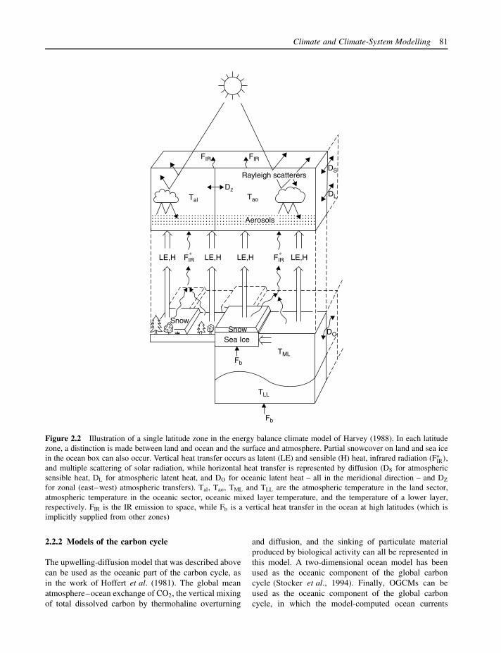
Climate and Climate-System Modelling 81
DS
DO
DL
FIR FIR
Tao
Dz
Tal
Rayleigh scatterers
LE,H LE,H
SnowSnow
Fb
Fb
TML
TLL
Sea Ice
LE,H LE,HFIR FIR∗ ∗
Aerosols
Figure 2.2 Illustration of a single latitude zone in the energy balance climate model of Harvey (1988). In each latitudezone, a distinction is made between land and ocean and the surface and atmosphere. Partial snowcover on land and sea icein the ocean box can also occur. Vertical heat transfer occurs as latent (LE) and sensible (H) heat, infrared radiation (F∗
IR),and multiple scattering of solar radiation, while horizontal heat transfer is represented by diffusion (DS for atmosphericsensible heat, DL for atmospheric latent heat, and DO for oceanic latent heat – all in the meridional direction – and DZ
for zonal (east–west) atmospheric transfers). Tal, Tao, TML and TLL are the atmospheric temperature in the land sector,atmospheric temperature in the oceanic sector, oceanic mixed layer temperature, and the temperature of a lower layer,respectively. FIR is the IR emission to space, while Fb is a vertical heat transfer in the ocean at high latitudes (which isimplicitly supplied from other zones)
2.2.2 Models of the carbon cycle
The upwelling-diffusion model that was described abovecan be used as the oceanic part of the carbon cycle, asin the work of Hoffert et al. (1981). The global meanatmosphere–ocean exchange of CO2, the vertical mixingof total dissolved carbon by thermohaline overturning
and diffusion, and the sinking of particulate materialproduced by biological activity can all be represented inthis model. A two-dimensional ocean model has beenused as the oceanic component of the global carboncycle (Stocker et al., 1994). Finally, OGCMs can beused as the oceanic component of the global carboncycle, in which the model-computed ocean currents

82 L.D. Danny Harvey
Figure 2.3 Illustration of the major processes occurring inside a typical horizontal grid cell of an atmospheric generalcirculation model (AGCM).Source: Reproduced from Washington and Meehl (1989), where a full explanation can be found.Note: ‘Sigma level’ refers to the ratio of pressure at a give height to the surface pressure
and other mixing processes are used, in combinationwith simple representations of biological processes andair–sea exchange (e.g., Bacastow and Maier-Reimer,1990; Najjar et al., 1992). CO2 uptake calculations using3-D models have so far been published only for stand-alone OGCMs, in which the circulation field and surfacetemperatures have been fixed. In a coupled simulation,changes in both of these variables in response toincreasing greenhouse gas concentrations would alter thesubsequent uptake of CO2 to some extent.
The terrestrial biosphere can be represented by aseries of interconnected boxes, where the boxes repre-sent components such as leafy material, woody mate-rial, roots, detritus, and one or more pools of soilcarbon. Each box can be globally aggregated such that,for example, the detrital box represents all the sur-face detritus in the world. The commonly used, glob-ally aggregated box models are quantitatively comparedin Harvey (1989). Figure 2.4 gives an example of a
globally aggregated terrestrial biosphere model, wherenumbers inside boxes represent the steady state amountsof carbon (Gt) prior to human disturbances, and thenumbers between boxes represent the annual rates ofcarbon transfer (Gt a−1). In globally aggregated boxmodels it is not possible to simulate separate responsesin different latitude zones (e.g. net release of carbonthrough temperature effects at high latitudes, net uptakeof carbon in the tropics due to CO2 fertilization). Sinceregional responses vary nonlinearly with temperatureand atmospheric CO2 concentration, extrapolation intothe future using globally aggregated models undoubt-edly introduces errors. An alternative is to run separatebox models for major regions, as in van Minnen et al.(1996), rather than lumping everything together.
The role of the terrestrial biosphere in global climaticchange has also been simulated using relatively simplemodels of vegetation on a global grid with resolutionas fine as 0.5◦ latitude × 0.5◦ longitude. These models
[Image not available in this electronic edition.]

Climate and Climate-System Modelling 83
Atmosphere
Groundvegetation
59
Nonwoodytree parts 38
Woody treeparts 634
Detritus96
Mobile soil700
Resistant soil800
0.22
4.635 2.78
2.785 9.4
0.365
14
10
30 31
14
6151151.6
0.80.215
Figure 2.4 The six-box, globally aggregated terrestrialbiosphere model of Harvey (1989). The numbers in eachbox are the steady state amounts of carbon (in Gt), whilethe arrows between the boxes represent the annual transfers(Gt C yr−1)
have been used to evaluate the impact on net ecosystemproductivity of higher atmospheric CO2 (which tends tostimulate photosynthesis and improve the efficiency ofwater use by plants) and higher temperatures (which canincrease or decrease photosynthesis and increase decayprocesses). These models distinguish, as a minimum,standing biomass from soil organic matter. The moresophisticated varieties track the flows of both carbonand nitrogen (taken to be the limiting nutrient), andinclude feedbacks between nitrogen and the rates of bothphotosynthesis and decay of soil carbon (e.g. Rastetteret al., 1991, 1992; Melillo et al., 1993).
Grid-point models of the terrestrial biosphere havebeen used to assess the effect on the net biosphere–atmosphere CO2 flux of hypothetical (or GCM-gener-ated) changes in temperature and/or atmospheric CO2
concentration, but generally without allowing for shiftsin the ecosystem type at a given grid point as climatechanges. More advanced ecosystem models are beingdeveloped and tested that link biome models (whichpredict changing ecosystem types) and ecophysiologi-cal models (which predict carbon fluxes) (e.g. Plochland Cramer, 1995). Different biomes vary in the pro-portion of ‘plant functional types’, examples of whichare tropical evergreen forest, cool-temperate evergreen
trees, and cool grasses. An alternative to simulatingthe location of specific ecosystems is to predict theproportions of different plant functional types at eachgrid cell based on the carbon balance for each func-tional type, as determined from an ecophysiologicalmodel (Foley et al., 1996). This effectively allows forthe simulation of both rapid biophysical processes andthe long-term adjustment of ecosystems to changingclimate and atmospheric CO2 concentration. Simula-tions with these and earlier models demonstrate thepotential importance of feedbacks involving the nutrientcycle and indicate the potential magnitude of climate-induced terrestrial biosphere–atmosphere CO2 fluxes.However, individual models still differ considerablyin their responses (VEMAP Members, 1995). As withmodels of the oceanic part of the carbon cycle, suchsimulations have yet to be carried out interactively withcoupled AOGCMs. These models also have not yet beencombined with ocean carbon uptake OGCMs.
Rather detailed models of the marine biosphere,involving a number of species and interactions, havealso been developed and applied to specific sites orregions (e.g. Gregg and Walsh, 1992; Sarmiento et al.,1993; Antoine and Morel, 1995; Oschlies and Garcon,1999; Oschlies et al., 2000).
2.2.3 Models of atmospheric chemistry and aerosols
Atmospheric chemistry is central to the distribution andamount of ozone in the atmosphere. The dominant chem-ical reactions and sensitivities are significantly differentfor the stratosphere and troposphere. These processescan be adequately modelled only with three-dimensionalatmospheric models (in the case of the troposphere) orwith two-dimensional (latitude–height) models (in thecase of the stratosphere). Atmospheric chemistry is alsocritical to the removal of CH4 from the atmosphere and,to a lesser extent, all other greenhouse gases exceptH2O and CO2. In the case of CH4, a change in itsconcentration affects its own removal rate and, hence,subsequent concentration changes. An accurate simula-tion of changes in the removal rate of CH4 requiresspecification of the concurrent concentrations of otherreactive species, in particular NOx (nitrogen oxides), CO(carbon monoxide) and the VOCs (volatile organic com-pounds); and use of a model with latitudinal and verticalresolution. However, simple globally averaged modelsof chemistry–climate interactions have been developed.These models treat the global CH4 –CO–OH cycle ina manner which takes into account the effects of theheterogeneity of the chemical and transport processes,and provide estimates of future global or hemispheric

84 L.D. Danny Harvey
mean changes in the chemistry of the Earth’s atmo-sphere. Some of the models also simulate halocarbonconcentrations and the resulting atmospheric chlorineconcentration, as well as radiative effects due to halocar-bons (Prather et al., 1992). An even simpler approach,adopted by Osborn and Wigley (1994), is to treat theatmosphere as a single well-mixed box but to accountfor the effects of atmospheric chemistry by making theCH4 lifetime depend on CH4 concentration in a way thatroughly mimics the behaviour of the above-mentionedglobally averaged models or of models with explicit spa-tial resolution. Atmospheric O3 and CH4 chemistry hasnot yet been incorporated in AGCMs used for climatesimulation purposes, although two-dimensional interac-tive chemistry-climate models have been built (Wanget al., 1998).
Atmospheric chemistry is also central to the distribu-tion and radiative properties of small suspended parti-cles in the atmosphere referred to as aerosols, althoughchemistry is only part of what is required in order tosimulate the effects of aerosols on climate. The primaryaerosols that are affected by atmospheric chemistry aresulphate aerosols (produced from the emission of SO2
and other S-containing gases), nitrate aerosols (producedfrom emission of nitrogen oxides), and organic carbonaerosols (produced from the emission of a variety oforganic compounds from plants and gasoline). The keyprocesses that need to be represented are the sourceemissions of aerosols or aerosol precursors; atmospherictransport, mixing, and chemical and physical transfor-mation; and removal processes (primarily deposition inrainwater and direct dry deposition onto the Earth’s sur-face). Since part of the effect of aerosols on climatearises because they serve as cloud condensation nuclei,it is also important to be able to represent the relation-ship between changes in the aerosol mass input to theatmosphere and, ultimately, the radiative properties ofclouds. Establishing the link between aerosol emissionsand cloud properties, however, involves several poorlyunderstood steps and is highly uncertain.
Geographically distributed sulphur-aerosol emissionshave been used as the input to AGCMs and, in com-bination with representations of aerosol chemical andphysical processes, have been used to compute thegeographical distributions of sulphur-aerosol mass usingonly natural emission sources and using natural +anthropic emission sources (e.g. Langner and Rodhe,1991; Chin et al., 1996; Pham et al., 1996). Given thedifferences in the GCM-simulated aerosol distributionsfor these two sets of emission sources and a variety ofassumptions concerning the aerosol optical properties,other studies have estimated the possible range of direct
(cloud-free) effects on radiative forcing (e.g. Haywoodet al., 1997). With yet further assumptions concerninghow clouds respond to sulphur aerosols, a range of indi-rect (cloud-induced) effects can also be computed (e.g.Boucher and Lohmann, 1995; Jones and Slingo, 1996;Kogan et al., 1996; Lohmann and Feichter, 1997). Theresults of these and other calculations are extensivelyreviewed in Harvey (2000a: Chapter 7).
2.2.4 Models of ice sheets
High resolution (20 km × 20 km horizontal grid), two-and three-dimensional models of the polar ice sheetshave been developed and used to assess the impact onglobal mean sea level of various idealized scenarios fortemperature and precipitation changes over the ice sheets(e.g. Huybrechts and Oerlemans, 1990; Huybrechtset al., 1991). AGCM output has also recently been usedto drive a three-dimensional model of the East Antarcticice sheet (Verbitsky and Saltzman, 1995), but has not yetbeen used to assess the possible contribution of changesin mountain glaciers to future sea-level rise. Output fromhigh resolution ice-sheet models can be used to developsimple relationships in which the contribution of ice-sheet changes to future sea level is scaled with changesin global mean temperature.
2.2.5 The roles of simple and complexclimate-system models
Climate-system models have been used to understandthe role of different processes in determining the presentclimate and atmospheric composition, in trying to under-stand the causes of past climatic change, and in tryingto estimate the range of possible future climate changesdue to human activities (emissions of greenhouse gases,emissions of aerosols and aerosol precursors), andchanges in the land vegetation (particularly past andongoing large-scale deforestation). Atmospheric GCMsare also used for day-to-day weather prediction (theproblem of weather prediction and of predicting cli-matic change are quite different, however, since weatherprediction is concerned with specific events at specificplaces and times, whereas climate prediction is con-cerned with long-term changes and trends, averaged overa period of several decades). Simple and complex mod-els have different but complementary roles to play inclimate research.
Simple models allow investigation of the basicrelationships between the components of the climatesystem, the factors driving climatic change, and theoverall response of the system. They are useful mainly

Climate and Climate-System Modelling 85
for exploring global-scale questions. The upwelling-diffusion model, for example, has been used to inves-tigate the role of the oceans in delaying the climaticresponse to increasing greenhouse-gas concentrationsand the role of ocean mixing–climate feedbacks inmodifying the transient response (e.g. Hoffert et al.,1980; Harvey and Schneider, 1985; Morantine andWatts, 1990), in exploring the importance of naturalvariability in observed global mean temperature varia-tions during the past century (Wigley and Raper, 1990;Schlesinger and Ramankutty, 1994), in setting con-straints on the magnitude of the global mean aerosolcooling effect (Wigley, 1989), and in assessing the rel-ative roles of greenhouse gases, aerosols, and solarvariability in explaining global mean temperature varia-tions during the past century (Kelly and Wigley, 1992;Schlesinger and Ramankutty, 1992). Because simplemodels are relatively easy to analyse (due to their lowdimensionality and the fact that only the most basic pro-cesses are included), and because multiple diagnostictests can be performed (due to the fact that they requirelittle computer time), simple models have provided anumber of important insights into the climate systemthat would not have been easily discovered using com-plex models.
Three-dimensional models, on the other hand, allowfor the explicit simulation of many of the key processesthat determine climate sensitivity (the change in globalmean temperature for a given radiative perturbation) andthe longer-term feedbacks involving the terrestrial andmarine biosphere. Although the strengths of many ofthe feedbacks in these models ultimately depend on theway in which subgrid-scale processes are parameterized(and can sometimes change dramatically when theparameterization is changed), more of the processes thatdetermine climate sensitivity are explicitly represented.This in turn allows the investigation of interactions, andthe development of insights, that could not be obtainedusing simple models.
One of the most important applications of climatesystem models is in projecting the global and regional-scale effects on climate of anthropic emissions ofgreenhouse gases and aerosols (or aerosol precursors).Three-dimensional AOGCMs are the only models thatcan make predictions at the regional scale (due totheir regional resolution), but it is widely agreed thatthe regional-scale results are less reliable than theglobal-scale results (which themselves have a factor ofthree uncertainty for temperature). Nevertheless, three-dimensional AOGCMs present an internally consistentpicture of regionally varying climatic change, and indi-cate the magnitude of climatic change that could occur
in specific regions in association with a given global-average change. They therefore indicate the risks asso-ciated with a given global-average climatic change. Theglobally averaged temperature change can therefore bethought of as an index of the risks posed by a particu-lar scenario of global GHG emissions. Simple models,on the other hand, generally only predict the globalmean temperature change. They can be directly and eas-ily driven by scenarios of anthropogenic emissions, thebuild-up of greenhouse-gas concentrations can be com-puted, and the computed concentration changes can beused to project the temporal variation in global meantemperature. This projection can be carried out for avariety of assumptions concerning the response of theterrestrial biosphere carbon sink to changes in temper-ature and atmospheric composition, concerning climatesensitivity and the intensity of ocean mixing, and con-cerning the role of aerosols. Simple models have theadditional advantage that they do not generate internalvariability (‘noise’) that can obscure the interpretationof AOGCM output.
There is no scientific justification for developing pol-icy responses at the national level based on the cli-matic changes and impacts within the jurisdiction underconsideration, as given by any one model. Rather, theclimate models can be used to support a collective(i.e. global-scale) policy response based on general-ized risks, rather than nation-by-nation responses basedon expected nation-by-nation impacts. Simple but com-prehensive models provide an easy means for generat-ing scenarios of global mean temperature change (therisk index), while complex, regionally resolved mod-els – through the range of responses at the regional levelgiven by different models – serve to illustrate the spe-cific risks associated with a given value of the risk index(global mean temperature). Thus, simple and complexmodels play complementary roles in the developmentof a policy response to the threat of global warming.
2.3 THE RESEARCH FRONTIER
A long-term goal of the climate-research communityis the development of increasingly sophisticated mod-els that couple more and more components of the cli-mate system. A large number of modelling groups havecreated three-dimensional models that couple the atmo-spheric and oceanic components of the climate system,and that include increasingly realistic representationsof sea-ice and land-surface processes (in particular, thebuild-up and melting of snow cover, runoff generation,and the modulation of the fluxes of heat, moisture andmomentum by vegetation).

86 L.D. Danny Harvey
Until very recently, land-surface modules in AGCMsrepresented the vegetation canopy (if at all) as a pas-sive vegetated surface that modulated the fluxes of heatand moisture between the atmosphere and surface. Themost recent schemes include the vegetation–atmospherecarbon flux, and its coupling to the heat and moisturefluxes through changes in the plant stomata. Consistentmodelling of the surface–air carbon flux requires repre-senting the processes of photosynthesis and respiration,and hence of plant growth. Hence the incorporation ofsimple plant biophysical models is required for the sim-ulation of the climatically important fluxes of heat andmoisture in a way that most closely mimics nature. Theneed for this inclusion is because these fluxes depend inpart on the stomatal resistance, which in turn depends onthe photosynthetic demand for carbon, as well as on thesimulated leaf temperature and soil moisture content.The incorporation of such biophysical modules in theland-surface scheme allows simulation of the climaticeffects of higher atmospheric CO2 through its effect onsurface–air moisture fluxes, as well as through its radia-tive effect (Sellers et al., 1996). The next step will be toincorporate ecosystem models that allow for changes inthe vegetation species composition at a given grid cell,as in the stand-alone model of Foley et al. (1996). Thesemodels are based on a small number of plant functionaltypes (e.g. moist tropical forest, temperate broadleaf for-est, boreal forest). Once joint ecosystem–biophysicalmodels are coupled to AGCMs, on a latitude–longitudegrid, it will be possible to simulate the effect of cli-matic change on vegetation and the CO2 flux to theatmosphere through shifts in biome zones, as well asthrough changes in the rates of photosynthesis and res-piration. This advance will in turn allow a full couplingbetween the atmosphere and terrestrial biosphere in aregionally resolved model. The effect of altered stom-atal conductance as climate and the atmospheric CO2
concentration change can be quite important to the sim-ulated climatic change on a regional scale, although theeffects are much less important when averaged glob-ally (Sellers et al., 1996).
Another major area of intensive research is in therepresentation of clouds in AGCMs. Differences in theway in which clouds are modelled are the main reasonfor the wide uncertainty in long-term warming resultingfrom a doubling atmospheric CO2 concentration (withglobal mean responses ranging from 2.1◦C to 4.8◦Cin recent models, as summarized by Harvey, 2000a:Chapter 9). The climatic effects of clouds depend on thedetails: exactly when, where and how high clouds are;their detailed microphysical properties, such as clouddroplet radius, ice-crystal radius and shape, and the
extent of impurities (such as soot) in cloud droplets.As the climate changes, the various cloud propertieswill change in hard-to-predict ways, with a range ofstrong but competing effects on climatic change (somecloud changes will tend to amplify the change, therebyserving as a positive feedback, while others will serveto diminish the change, thereby serving as a negativefeedback). Increasingly sophisticated cloud schemes arebeing developed for and implemented in AGCMs (e.g.Del Genio et al., 1996; Kao and Smith, 1999), thatexplicitly compute more and more of the cloud processesof climatic importance. However, greater sophisticationand detail do not guarantee that the predicted changesin climate will be more reliable. This problem arisesbecause even the most detailed schemes still requireparameterizations to represent the effects of subgrid-scale processes, and the nature of the parameterizationscan strongly influence the results.
Other areas of ongoing research include improvedtreatment of sea ice, the realistic routing of runoff to theoceans, and the incorporation of atmospheric chemistrywithin AGCMs used for climate simulation purposes.Better determination of the magnitude of the variousdirect and indirect effects of different aerosols on solarand infrared radiation, which are computed from butaffect the behaviour of AGCMs, is also an importantpriority, since it is a necessary step in being able toinfer the climate sensitivity from observed temperaturechanges during the past century or so.
2.4 CASE STUDY
As a case study to illustrate the use of climate modelsin global warming policy analysis, and as an example ofthe constructive interplay between simple and complexclimate models, I will discuss the MAGICC/SCENGENmodel system of Hulme et al. (2000). This model wasdeveloped to be used in developing assessments ofregional or national vulnerability to anthropogenic cli-matic change. MAGICC (Model for the Assessmentof Greenhouse-gas Induced Climate Change) consistsof a suite of simple models of each of the climatesystem components discussed under ‘Finding the Sim-plicity’. MAGICC contains a simple representation ofthe carbon cycle and other trace gas cycles needed tocompute the build-up in their concentration, given emis-sions scenarios for each of the gases. Simple relation-ships are then used to relate the change in greenhousegas concentrations to the trapping of heat in the atmo-sphere. Simple relationships are also used to directlyrelate aerosol emissions to the heating or cooling effectsof aerosols. Schematic ice-melt models for mountain

Climate and Climate-System Modelling 87
glaciers, Antarctica and Greenland are used to calculatethe contribution of small and large glaciers to sea-levelrise. The climate component of the model is similar tothe upwelling-diffusion model that was illustrated ear-lier; it is used to compute the time-dependent, globallyaveraged change in surface temperature, as well as thevertical variation of warming with depth in the ocean,from which the component of sea level rise due to ther-mal expansion of sea water can be computed.
The globally averaged surface temperature producedby MAGICC is used in conjunction with the spatialpatterns of surface temperature change as simulatedby a variety of atmospheric or coupled atmosphere-ocean GCMs. These patterns are provided by the SCEN-GEN (SCENario GENerator) part of the model. Thispart of the model is based on the observation that thetime–space pattern of climatic change when GCMs aredriven by increasing greenhouse gas (GHG) concentra-tions can be well represented by a fixed spatial pattern,which can be uniformly scaled up or down in propor-tion to the global mean warming (Mitchell et al., 1999).This approach has been referred to as the pattern-scalingmethod, and was first used by Santer et al. (1990). Eventhough the cooling effect of sulphate aerosols (whichmust also be taken into account when assessing futureclimatic change) is concentrated over and downwind ofpolluted regions, the spatial patterns of climatic changewith GHGs only or with GHGs and aerosols are remark-ably similar. This result is due to the fact that theregional pattern of climatic change is to a large extentcontrolled by the large-scale climate feedbacks that aretriggered by overall climatic change, rather than by thelocal forcing (see Chapter 3.6 of Harvey, 2000a, for amore thorough discussion of this property of the cli-mate system). Since simple models, such as MAGICC,are capable of quickly computing the time variationin global mean warming for a wide variety of GHGand aerosol-precursor emission scenarios, one can easilygenerate scenarios of regional climatic change by com-bining the global mean temperature change from MAG-ICC with the regional pattern of temperature change asprovided by one or more GCMs.
Thus, rather than running a computationally expen-sive AOGCM for every conceivable scenario of futureGHG and aerosol-precursor emissions, one need run theAOGCM for only one scenario, determine the spatialpattern produced by the AOGCM in question, and thenscale this spatial pattern up or down in proportion toglobal mean warming as computed by a suite of coupledclimate–gas cycle–aerosol forcing models. This thenmakes it practical to consider a wide range of emissionscenarios. Furthermore, the global mean temperature
responsiveness (or climate sensitivity) to a given radia-tive heating perturbation can easily be adjusted in simplemodels to match that of any given AOGCM, as can therate of mixing of heat into the deep ocean. This approachensures that the global mean temperature response ofthe simple model will match that which would havebeen produced by the AOGCM with the altered scenar-ios (Raper and Cubasch, 1996, have demonstrated theability of simple models to closely replicate the globalmean behaviour of AOGCMs).
Different GCMs can give quite different spatial pat-terns of temperature change. MAGICC/SCENGEN isset up to allow the user to specify the spatial responsepattern from one of 16 GCMs. The user also selectsone of several pre-programmed emission scenarios, orcan choose his or her own scenario. The climate sen-sitivity can be prescribed independently of the spa-tial pattern used to generate regional climatic change.Figures 2.5 and 2.6 give an example of the global meanand regional temperature output that are produced bythe model.
The pattern-scaling approach has also been appliedto precipitation in MAGICC/SCENGEN. In this case,the spatially varying percentage change in precipitationassociated with a particular global mean warming ina GCM is computed. This percentage is scaled up ordown in proportion to the global mean temperature atany given time as computed by MAGICC; the resultingpercentage change is applied to the observed present-day precipitation. However, whereas over 90% of thetime–space variation in surface temperature in a GCMsimulation can be accounted for by scaling a fixed tem-perature pattern, much less of the precipitation variationcan be captured in this way. Thus, regional precipita-tion changes deduced with the pattern-scaling methodcan be expected to differ, often substantially, from thatwhich would have been obtained from the AOGCM.Compounding this uncertainty in the regional precipita-tion change is the fact that there is substantial yearly anddecadal variability (‘noise’) in the precipitation responseof any given GCM to global warming, and the differ-ences in the response between different GCMs in manycritical regions and times (such as the Southeast Asiansummer monsoon) can be substantial.
Note on web links
The website associated with this chapter (www.kcl.ac.uk/envmod) contains a link to websites devoted to thedetailed description and comparison of high-resolutionmodels of many of the components of the climate system(namely, the atmosphere, oceans, oceanic part of the

88 L.D. Danny Harvey
2000 2050 2100−1
0
1
2
3
Temperature change (°C) w.r.t. 1990
Reference: IPCC emissions scenario 92a
Policy: IPCC emissions scenario 92c
Reference rangeReference best guess
Figure 2.5 Illustration of the global mean temperature for a CO2 doubling climate sensitivity of 2.5◦C, and the rangein global mean temperature for sensitivities ranging from 1.5◦C to 4.5◦C, produced by MAGICC
deg C
3.02.52.01.51.0
Figure 2.6 Illustration of the regional temperature change for 2050, generated by SCENGEN based on the temperaturepattern of the Canadian Climate Centre atmosphere–ocean GCM

Climate and Climate-System Modelling 89
carbon cycle and the terrestrial biosphere). These sitescontain numerous tables and colour figures comparingthe models with one another and with observations,and also contain comprehensive lists of references.Some also contain links to the research centres wherethe models were developed. The website associatedwith this chapter also contains a link to the ClimateResearch Unit of the University of East Anglia, wherea demonstration of the MAGGIC/SCENGEN schematicmodel can be found. A copy of the model can bedownloaded, so that those who are interested (and whosign a licence agreement) can run the model on theirown personal computers.
REFERENCES
Antoine, D. and Morel, A. (1995) Modelling the seasonalcourse of the upper ocean pCO2 (i): development of a one-dimensional model, Tellus 47B, 103–121.
Bacastow, R. and Maier-Reimer, E. (1990) Ocean-circulationmodel of the carbon cycle, Climate Dynamics 4, 95–125.
Bintanja, R. (1995) The Antarctic ice sheet and climate, PhDthesis, Utrecht University.
Boucher, O. and Lohmann, U. (1995) The sulfate-CCN-cloudalbedo effect: a sensitivity study with two general circulationmodels, Tellus 47B, 281–300.
Chin, M., Jacob, D.J., Gardner, G.M., Foreman-Fowler, M.S.and Spiro, P.A. (1996) A global three-dimensional model oftropospheric sulfate, Journal of Geophysical Research 101,18667–18690.
Del Genio, A.D., Yao, M.-S., Kovari, W. and Lo, K.K. (1996)A prognostic cloud water parameterization for global climatemodels, Journal of Climate 9, 270–304.
De Wolde, J.R., Bintanja, R. and Oerlemans, J. (1995) Onthermal expansion over the last one hundred years, Journalof Climate 8, 2881–2891.
Dickinson, R.E., Meleshko, V., Randall, D., Sarachik, E., Sil-va-Dias, P. and Slingo, A. (1996) Climate processes, inJ.T. Houghton, L.G.F. Filho, B.A. Callander, N. Harris, A.Kattenberg and K. Maskell (eds) Climate Change 1995: TheScience of Climate Change, Cambridge University Press,Cambridge, 193–227.
Foley, J.A., Prentice, C., Ramankutty, N., Levis, S., Pol-lard, D., Sitch, S. and Haxeltine, A. (1996) An integratedbiosphere model of land surface processes, terrestrial carbonbalance, and vegetation dynamics, Global BiogeochemicalCycles 10, 603–628.
Gates, W.L. et al. (1996) Climate models – evaluation, in J.T.Houghton, L.G.F. Filho, B.A. Callander, N. Harris, A.Kattenberg and K. Maskell (eds) Climate Change 1995:The Science of Climate Change, Cambridge University Press,Cambridge, 229–284.
Gregg, W.W. and Walsh, J.J. (1992) Simulation of the 1979spring bloom in the mid-Atlantic bight: a coupled phys-ical/biological/optical model, Journal of Geophysical Re-search 97, 5723–5743.
Harvey, L.D.D. (1988) A semi-analytic energy balance climatemodel with explicit sea ice and snow physics, Journal ofClimate 1, 1065–1085.
Harvey, L.D.D. (1989) Effect of model structure on theresponse of terrestrial biosphere models to CO2 and temper-ature increases, Global Biogeochemical Cycles 3, 137–153.
Harvey, L.D.D. (1992) A two-dimensional ocean model forlong-term climatic simulations: stability and coupling toatmospheric and sea ice models, Journal of GeophysicalResearch 97, 9435–9453.
Harvey, L.D.D. (2000a) Global Warming: The Hard Science,Prentice Hall, Harlow.
Harvey, L.D.D. (2000b) Upscaling in global change research,Climatic Change 44, 225–263.
Harvey, L.D.D., Gregory, J., Hoffert, M., Jain, A., Lal, M.,Leemans, R., Raper, S., Wigley, T. and de Wolde, J. (1997)An Introduction to Simple Climate Models Used in theIPCC Second Assessment Report , Intergovernmental Panelon Climate Change, Technical Paper II.
Harvey, L.D.D. and Huang, Z. (1995) An evaluation of thepotential impact of methane-clathrate destabilization onfuture global warming, Journal of Geophysical Research100, 2905–2926.
Harvey, L.D.D. and Schneider, S.H. (1985) Transient climaticresponse to external forcing on 100−104 year time scales,1, Experiments with globally averaged coupled atmosphereand ocean energy balance models, Journal of GeophysicalResearch 90, 2191–2205.
Haywood, J.M., Roberts, D.L., Slingo, A., Edwards, J.M. andShine, K.P. (1997) General circulation model calculationsof the direct radiative forcing by anthropogenic sulfate andfossil-fuel soot aerosol, Journal of Climate 10, 1562–1577.
Held, I.M. and Suarez, M.J. (1974) Simple albedo feedbackmodels of the icecaps, Tellus 26, 613–630.
Hoffert, M.I., Callegari, A.J. and Hseih, C.-T. (1980) The roleof deep sea heat storage in the secular response to climaticforcing, Journal of Geophysical Research 85, 6667–6679.
Hoffert, M.I., Callegari, A.J. and Hseih, C.-T. (1981) A box-diffusion carbon cycle model with upwelling, polar bottomwater formation and a marine biosphere, in B. Bolin (ed.)Carbon Cycle Modeling, SCOPE 16, John Wiley & Sons,New York, 287–305.
Houghton, J.T., Ding, Y., Griggs, D.J., Noguer, M., vander Linden, P.J., Dai, X., Maskell, K. and Johnson, C.A.(eds) (2001) Climate Change 2001: The Scientific Basis,Cambridge University Press, Cambridge.
Hulme, M., Wigley, T.M.L., Barrow, E.M., Raper, S.C.B.,Centella, A., Smith, S. and Chipanshi, A. (2000) Using aClimate Scenario Generator in Vulnerability and AdaptationAssessments: MAGICC and SCENGEN Workbook, ClimaticResearch Unit, UEA, Norwich.
Huybrechts, P. and Oerlemans, J. (1990) Response of theAntarctic ice sheet to future greenhouse warming, ClimateDynamics 5, 93–102.
Huybrechts, P., Letreguilly, A. and Reeh, N. (1991) TheGreenland ice sheet and greenhouse warming, Palaeogeog-raphy, Palaeoclimatology, Palaeoecology 89, 399–412.

90 L.D. Danny Harvey
Jones, A. and Slingo, A. (1996) Predicting cloud-droplet effec-tive radius and indirect sulphate aerosol forcing using ageneral circulation model, Quarterly Journal of the RoyalMeteorological Society 122, 1573–1595.
Kao, C.Y.J. (1999) Sensitivity of a cloud parameterizationpackage in the National Center for Atmospheric ResearchCommunity Climate model, Journal of Geophysical Research104, 11961–11983.
Kao, C.Y.J. and Smith, W.S. (1999) Sensitivity of a cloudparameterization package in the National Center for Atmo-spheric Research Community Climate Model, Journal ofGeophysical Research-Atmospheres 104, 11961–11983.
Kelly, P.M. and Wigley, T.M.L. (1992) Solar cycle length,greenhouse forcing and global climate, Nature 360, 328–330.
Ko, M.K.W., Sze, N.D., Wang, W.-C., Shia, G., Goldman, A.,Murcray, F.J., Murcray, D.G. and Rinsland, C.P. (1993)Atmospheric sulfur hexaflouride: sources, sinks, and green-house warming, Journal of Geophysical Research 98,10499–10507.
Kogan, Z.N., Kogan, Y.L. and Lilly, D.K. (1996) Evaluationof sulfate aerosol’s indirect effect in marine stratocumulusclouds using observation-derived cloud climatology, Geo-physical Research Letters 23, 1937–1940.
Lal, M. and Ramanathan, V. (1984) The effects of moistconvection and water-vapor radiative processes on cli-mate sensitivity, Journal of the Atmospheric Sciences 41,2238–2249.
Langner, J. and Rodhe, H. (1991) A global three-dimensionalmodel of the tropospheric sulfur cycle, Journal of Atmo-spheric Chemistry 13, 225–263.
Lohmann, U. and Feichter, J. (1997) Impact of sulfate aerosolson albedo and lifetime of clouds: a sensitivity study withthe ECHAM4 GCM, Journal of Geophysical Research 102,13685–13700.
Melillo, J.M., McGuire, A.D., Kicklighter, D.W., Moore III, B.,Vorosmarty C.J. and Schloss, A.L. (1993) Global climatechange and terrestrial net primary production, Nature 363,234–240.
Mitchell, J.F.B., Johns, T.C., Eagles, M., Ingram, W.J. andDavis, R.A. (1999) Towards the construction of climatechange scenarios, Climatic Change 41, 547–581.
Morantine, M. and Watts, R.G. (1990) Upwelling diffu-sion climate models: analytical solutions for radiative andupwelling forcing, Journal of Geophysical Research 95,7563–7571.
Najjar, R.G., Sarmiento, J.L. and Toggweiler, J.R. (1992)Downward transport and fate of organic matter in theocean: simulations with a general circulation model, GlobalBiogeochemical Cycles 6, 45–76.
Osborn, T.J. and Wigley, T.M.L. (1994) A simple model forestimating methane concentrations and lifetime variations,Climate Dynamics 9, 181–193.
Oschlies, A. and Garcon, V. (1999) An eddy-permitting cou-pled physical-biological model of the North Atlantic, 1,Sensitivity to physics and numerics, Global BiogeochemicalCycles 13, 135–160.
Oschlies, A., Koeve, W. and Garcon, V. (2000) An eddy-permitting coupled physical-biological model of the NorthAtlantic 2. Ecosystem dynamics and comparison with satel-lite and JGOFS local studies data, Global BiogeochemicalCycles 14, 499–523.
Peng, L., Chou, M.-D. and Arking, A. (1982) Climate studieswith a multi-layer energy balance model. Part I: Modeldescription and sensitivity to the solar constant, Journal ofthe Atmospheric Sciences 39, 2639–2656.
Pham, M., Muller, J.-F., Brasseur, G.P., Granier, C. andMegie, G. (1996) A 3D model study of the global sulphurcycle: contributions of anthropogenic and biogenic sources,Atmospheric Environment 30, 1815–1822.
Plochl, M. and Cramer, W. (1995) Coupling global models ofvegetation structure and ecosystem processes, Tellus 47B,240–250.
Prather, M., Ibrahim, A.M., Sasaki, T. and Stordal, F. (1992)Future chlorine-bromine loading and ozone depletion, inUnited Nations Environment Programme Staff (eds) Scien-tific Assessment of Ozone Depletion: 1991, World Meteoro-logical Organization, Geneva.
Raper, S.C.B. and Cubasch, U. (1996) Emulation of the resultsfrom a coupled GCM using a simple climate model, Geo-physical Research Letters 23, 1107–1110.
Rastetter, E.B., McKane, R.B., Shaver, G.R. and Melillo, J.M.(1992) Changes in C storage by terrestrial ecosystems: howC-N interactions restrict responses to CO2 and temperature,Water, Air, and Soil Pollution 64, 327–344.
Rastetter, E.B., Ryan, M.G., Shaver, G.R., Melillo, J.M., Nadel-hoffer, K.J., Hobbie, J. and Aber, J.D. (1991) A general bio-geochemical model describing the responses of the C and Ncycles in terrestrial ecosystems to changes in CO2, climate,and N deposition, Tree Physiology 9, 101–126.
Santer, B.D., Wigley, T.M.L., Schlesinger, M.E. and Mitchell,J.F.B. (1990) Developing Climate Scenarios from Equilib-rium GCM Results , Max Planck Institute fur Meteorologie,Report No. 47, Hamburg.
Sarmiento, J.L., Slater, R.D., Fasham, M.J.R., Ducklow, H.W.,Toggweiler, J.R. and Evans, G.T. (1993) A seasonal three-dimensional ecosystem model of nitrogen cycling in theNorth Atlantic euphotic zone, Global Biogeochemical Cycles7, 417–450.
Schlesinger, M.E. and Ramankutty, N. (1992) Implications forglobal warming of intercycle solar irradiance variations,Nature 360, 330–333.
Schlesinger, M.E. and Ramankutty, N. (1994) An oscillationin the global climate system of period 65–70 years, Nature367, 723–726.
Sellers, P.J. et al. (1996) Comparison of radiative and phys-iological effects of doubled atmospheric CO2 on climate,Science 271, 1402–1406.
Stocker, T.F., Broecker, W.S. and Wright, D.G. (1994) Carbonuptake experiment with a zonally averaged global oceancirculation model, Tellus 46B, 103–122.
Trenberth, K.E. (ed.) (1992) Climate System Modeling, Cam-bridge University Press, Cambridge.

Climate and Climate-System Modelling 91
Van Minnen, J.G., Goldewijk, K.K. and Leemans, R. (1996)The importance of feedback processes and vegetationtransition in the terrestrial carbon cycle, Journal of Biogeog-raphy 22, 805–814.
VEMAP Members (1995) Vegetation ecosystem modeling andanalysis project: comparing biogeography and biogeochem-istry models in a continental-scale study of terrestrial ecosys-tem responses to climate change and CO2 doubling, GlobalBiogeochemical Cycles 9, 407–437.
Verbitsky, M. and Saltzman, B. (1995) Behavior of the EastAntarctic ice sheet as deduced from a coupled GCM/Ice-sheet model, Geophysical Research Letters 22, 2913–2916.
Wang, C., Prinn, R.G. and Sokolov, A. (1998) A global inter-active chemistry and climate model: formulation and testing,Journal of Geophysical Research 103, 3399–3417.
Wigley, T.M.L. (1989) Possible climate change due to SO2-derived cloud condensation nuclei, Nature 339, 365–367.
Wigley, T.M.L. and Raper, S.C.B. (1990) Natural variability ofthe climate system and detection of the greenhouse effect,Nature 344, 324–327.
Wright, D.G. and Stocker, T.F. (1991) A zonally averagedocean model for the thermohaline circulation, I, Modeldevelopment and flow dynamics, Journal of PhysicalOceanography 21, 1713–1724.

3
Soil and Hillslope Hydrology
ANDREW BAIRD
3.1 IT’S DOWNHILL FROM HERE
Any child can tell you ‘water flows downhill’. However,it would be truer to say that water flows down anenergy gradient from areas where the water has greaterenergy to areas where it has lower energy. This is trueof water flowing over the ground surface and waterflowing through a porous medium such as soil. Indeed,water can flow uphill if a suitable energy gradient exists.Hydrologists, ecologists and engineers, among others,are not just interested in the direction of flow, but also inthe speed of flow, the amount (mass or volume) involvedin the flow, and how flows cause variability in the amountof water on and in hillslopes both in space and time.Part of this interest involves a desire to model or predictwater flows on and in hillslopes. With advancementsin high-speed digital computing, the 1970s seemed topromise the development of sophisticated and accuratemodels of hillslope hydrology. The reality has beenrather different (Beven, 1996, 2000). Some researcherswould argue that our models are too complicated whileothers would suggest that they are too simple (cf. Baird,1999). Certainly few, if any, models incorporate allknown water-transfer processes on and in hillslopes. Therest of this chapter considers whether this is a good thingand also reviews current ideas on how we should modelhillslope hydrology.
3.2 EASY DOES IT: THE LABORATORY SLOPE
Before looking at the real world, it is perhaps betterto consider how water flows over and through simpleartificial hillslopes in the laboratory. Such a consider-ation will allow us to readily identify the problems ofdescribing and modelling flow on and in real slopes. Let
us consider two artificial hillslopes. The first, Hillslope1, consists simply of a relatively smooth, inclined planeconstructed from impermeable material (Figure 3.1a).The second, Hillslope 2, also consists of an inclinedplane of impermeable material but this time a homoge-nous soil (say, a sandy loam) of constant thickness (say,50 cm) has been spread across the plane (Figure 3.1b).The soil does not contain organic matter and is unvege-tated. Water can be added to both slopes from above atany intensity commonly found in nature using a rainfallsimulator. How does water flow on and through theseidealized/artificial hillslopes?
3.2.1 Plane simple: overland flow on Hillslope 1
Almost immediately after the start of simulated rainfall,water will start to flow over the surface of Hillslope 1.How will water flow over the surface? A number ofmodels exist to describe such flow. One of the most com-monly used is the so-called kinematic wave. A kinematicwave model consists of an equation that describes flowcoupled with a balance equation. Flow velocity is usu-ally expressed as a power function of the depth of wateron the slope, the gradient of the slope, and a frictionfactor describing the effects of frictional drag on waterflow (see Baird, 1997a). To simulate changes in veloc-ity and flow depth over time, this equation is combinedwith the balance equation describing time-variant inputsand outputs along the slope surface (Chow, 1959; Baird,1997a,b). Because this approach ignores the effect ofchanges in momentum, it is called the kinematic approx-imation or kinematic wave approach (Ponce et al., 1978;Dingman, 1984; Ponce, 1991) (‘kinematic’ means thestudy of motion without reference to mass or force;Hanks, 1986).
Environmental Modelling: Finding Simplicity in Complexity. Edited by J. Wainwright and M. Mulligan 2004 John Wiley & Sons, Ltd ISBNs: 0-471-49617-0 (HB); 0-471-49618-9 (PB)
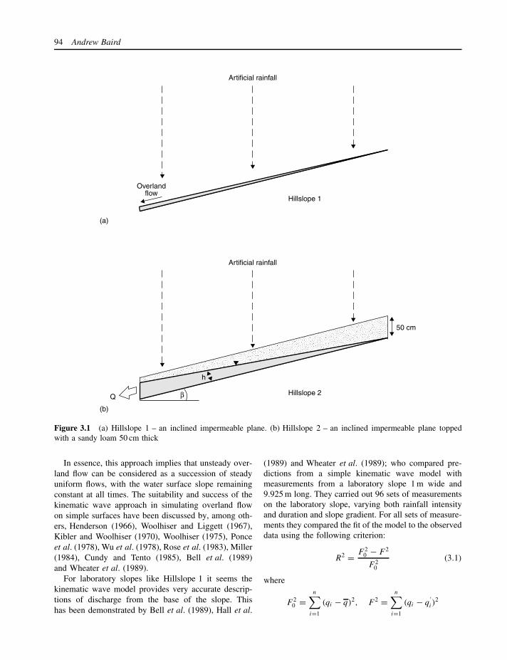
94 Andrew Baird
Artificial rainfall
Artificial rainfall
Overlandflow
Hillslope 1
Hillslope 2
50 cm
h
βQ
(a)
(b)
Figure 3.1 (a) Hillslope 1 – an inclined impermeable plane. (b) Hillslope 2 – an inclined impermeable plane toppedwith a sandy loam 50 cm thick
In essence, this approach implies that unsteady over-land flow can be considered as a succession of steadyuniform flows, with the water surface slope remainingconstant at all times. The suitability and success of thekinematic wave approach in simulating overland flowon simple surfaces have been discussed by, among oth-ers, Henderson (1966), Woolhiser and Liggett (1967),Kibler and Woolhiser (1970), Woolhiser (1975), Ponceet al. (1978), Wu et al. (1978), Rose et al. (1983), Miller(1984), Cundy and Tento (1985), Bell et al. (1989)and Wheater et al. (1989).
For laboratory slopes like Hillslope 1 it seems thekinematic wave model provides very accurate descrip-tions of discharge from the base of the slope. Thishas been demonstrated by Bell et al. (1989), Hall et al.
(1989) and Wheater et al. (1989); who compared pre-dictions from a simple kinematic wave model withmeasurements from a laboratory slope 1 m wide and9.925 m long. They carried out 96 sets of measurementson the laboratory slope, varying both rainfall intensityand duration and slope gradient. For all sets of measure-ments they compared the fit of the model to the observeddata using the following criterion:
R2 = F 20 − F 2
F 20
(3.1)
where
F 20 =
n∑i=1
(qi − q)2, F 2 =n∑
i=1
(qi − q′i )
2

Soil and Hillslope Hydrology 95
350300250200150100500
0 50 100 150 200 250 300
Time (seconds)
0 50 100 150 200 250 300
Time (seconds)
0.0
0.2
0.4
0.6
0.8
1.0
Rai
nfal
l (m
m/h
r)D
isch
arge
(l/s
)
DataModel output
Figure 3.2 Comparison of measured and modelled (usinga kinematic wave) overland flow on an artificial hillslope.In the example shown the slope gradient was 0.005Source: Wheater et al. (1989)
and qi is the observed discharge, q′i the modelled
discharge, n the number of discharge values and q
the mean of the observed discharges. An R2 of 1represents a perfect correspondence between predictedand observed. Wheater et al. (1989) found that the meanR2 of the 96 comparisons was very high at 0.967.An example of one of their comparisons is given inFigure 3.2.
3.2.2 Getting a head: soil-water/ground-water flowin Hillslope 2
Rainfall on Hillslope 2 will enter the soil and will thenflow vertically and downslope through the soil profile.How the water enters the soil (infiltration) is dealt within Chapter 4. Before we consider flow throughout thesoil on Hillslope 2, it is useful to consider flow througha relatively small cube (say 50 × 50 × 50 cm) of thesoil. Saturated flow in such a soil is described well byDarcy’s law, which, for steady flow in one dimension,is given by:
q = −KdH
dx(3.2)
where q is the discharge per unit area (L3 T−1 L−2 = LT−1), K is the hydraulic conductivity (L T−1), H is the
hydraulic head (L) and x is the distance in the directionof flow (L). q is often called the specific dischargeand K is the specific discharge under a unit hydraulicgradient (i.e. dH/dx = 1). H is a measure of the energyof the soil water and has units of length because it isexpressed as energy per unit weight (i.e. (M L2 T−2)/(ML T−2) = L) (Fetter, 1994). To make q positive, a minussign appears before K . This ‘correction’ is necessarybecause water flows down the hydraulic gradient, i.e. itflows along a negative gradient from areas of higher H
to areas of lower H .Flow is rarely one-dimensional. Sometimes it is nec-
essary to consider dH/dz and dH/dy where z is depthand y the other horizontal direction. Sometimes, also,hydraulic conductivity varies according to direction, i.e.we need to consider Kx, Ky and Kv (Freeze and Cherry,1979). When this occurs, the medium is said to beanisotropic (as opposed to isotropic). Flow is also rarelysteady. To consider time-variant flows we would need toconsider changes in soil water storage. In our cube thismeans that the water table will rise and fall dependingon the difference between inflows and outflows of water.Of course, it is also possible for the water table to riseto the surface and for surface ponding to occur whichmight result in overland flow (see above). An exposi-tion of the derivation of the transient flow equations forunconfined flow is beyond the scope of this chapter.Good descriptions can be found in Freeze and Cherry(1979) and Fetter (1994).
Darcy’s law can also be modified to describe flowthrough unsaturated soil, where K is assumed to be afunction of water content (θ ), i.e.
q = −K(θ)dH
dx. (3.3)
Where flow is unsteady, i.e. in most natural conditions,water content will change and so will K . Thus in unsat-urated flow, unlike saturated flow, K is time-variant(except for some very simple cases). The unsaturatedform of Darcy’s law is usually called the Richardsequation (especially when combined with the balanceequation for time-variant flows) after L.A. Richardswho was the first to realize that Darcy’s law could beapplied to unsaturated flows (Richards, 1931, cited inHillel, 1980).
Darcy’s law is the single most important relationused to describe saturated water flow through soils.Indeed, in a review of methods used to characterizethe hydraulic properties of porous media, Narasimhan(1998) suggests:
It is reasonable to state that all the hydraulic char-acterization methods in use today have two themes

96 Andrew Baird
in common: an empirical equation of motion, famil-iarly known as Darcy’s law . . . and the equationof transient heat conduction, originally proposed byFourier in 1807, which has established itself as theworking model for diffusion-type processes in physi-cal sciences.
Provided the pores in our soil are not too large ortoo small, the hydraulic gradient not too large, and thesoil fully saturated, it appears Darcy’s law providesa good description of flow in laboratory soils. Thishas been demonstrated in numerous studies where alinear relationship between specific discharge and thehydraulic gradient has been observed. The physical basisof the law and its more general applicability to soilscan be found in a classic paper by Hubbert (1940) andin standard hydrogeology text books (e.g. Freeze andCherry, 1979; Fetter, 1994).
So, how can Darcy’s law be used to model flow in oursimple artificial slope? Various models based on Darcy’slaw have been developed to describe hillslope flow. Themost sophisticated (at least mathematically) can modeltwo- and three-dimensional time-variant flow, allow forspatial variability in soil physical properties and cansimulate both saturated and unsaturated flow in a densegrid of points or nodes representing the hillslope. Mod-els have even been developed to consider, for example,the effect of heat on water flow. For example, as waterwarms, its viscosity is reduced and it flows more readily.Thus K increases with water temperature (Klute, 1965;de Marsily, 1986). These sophisticated models are usu-ally solved using numerical methods such as the finite-element and finite-difference method (see Chapter 1 andWang and Anderson, 1982; Beven, 1985; Baird, 1999).Examples of these state-of-the-art models include theUnited States Geological Survey’s MODFLOW andVS2D, the US Salinity Laboratory’s HYDRUS, theGerman-based Institute for Water Resources Planningand Systems Research Ltd.’s FEFLOW, and Analyticand Computational Research Inc.’s PORFLOW (web-site details for all of these are given at the end of thelist of references).
Some of the sophisticated models would be relativelyeasy to apply to our hillslope and many of their fea-tures would not be required for our simple flow case.For example, we could ignore variability and, perhaps,anisotropy of K . We could also ignore cross-slope vari-ations in water table elevation and soil moisture con-tent. An example of the application of this type ofmodel to a relatively simple artificial slope can be foundin Sloan and Moore (1984). Sloan and Moore used afinite-element model based on the 2-D Darcy–Richards
equation to model saturated–unsaturated flow in anexperimental hillslope in the Coweeta HydrologicalLaboratory in the southern Appalachian mountains,USA (Hewlett and Hibbert, 1963). The artificial hill-slope consisted of a 0.92 × 0.92 × 13.77 m concrete-lined trough constructed on a 40% slope and filledwith recompacted C horizon forest soil. Measurementsreported by Hewlett (1961) and Hewlett and Hibbert(1963) were used to assign values to the model’s param-eters, i.e. the model was not optimized to give thebest possible predictions. Model predictions of dischargefrom the base of the slope were found to compare quitewell with measurements. However, due to limitations ofthe experimental data it was not possible to comparemeasurements and predictions of water-table dynamicswithin the hillslope.
Although sophisticated Darcy-type models could beused, it is also possible to simplify our descriptionof processes occurring in our artificial soil-coveredslope (e.g. Sloan and Moore, 1984; Steenhuis et al.,1988; Pi and Hjelmfelt, 1994; Fan and Bras, 1998;Wigmosta and Lettenmaier, 1999). A popular group ofsimple models for subsurface flow are, like the overlandflow models described above, kinematic wave models.The simplest of this class of model ignore or greatlysimplify flow in the unsaturated zone and (a) assumethat flow in the soil is parallel with the soil surface;and (b) that the hydraulic gradient at any point withinthe saturated zone is equal to the slope (Hendersonand Wooding, 1964; Beven, 1981). Thus, Darcy’s lawnow becomes
Q = Kh sin β (3.4)
where Q is the discharge per unit width of hillslope inthe downslope direction (L2 T−1) (i.e. specific dischargemultiplied by depth of flow), h is the depth below thewater table measured orthogonally to the impermeableplane at the base of the soil, and β is the slope of theplane (and soil surface) (see Figure 3.1b).
Equation 3.4 can be combined with a balance equationand solved numerically (finite-difference or finite-elementmethod) or analytically (cf. Baird, 1999) to simulatethe level of the water table at different points along ahillslope under both transient and steady rainfall. Sub-surface flow models based on Equation 3.4 are linearkinematic wave models, whereas surface flow modelsbased on a power law flow description produce nonlin-ear kinematic waves. For simple cases, the subsurfacekinematic wave model has been shown by Beven (1981)to accord quite closely with models based on more rig-orous Darcian assumptions. The model has also beenextended to include one-dimensional unsaturated flow

Soil and Hillslope Hydrology 97
10000
1000
100
0102 103 104 105
Acc
umul
ated
dra
inag
e vo
lum
e (x
10−3
m)
Time from beginning of drainage (min)
ObservedKinematic wave modelKinematic storage model1-D Finite element model2-D Finite element modelBoussinesq storage model
Figure 3.3 Comparison of measured and modelled dis-charge from the base of the Coweeta experimental soiltroughSource: Sloan and Moore (1984)
above the water table, time-variant rainfall, and variationof the hydraulic properties of the soil (Beven, 1982 – seealso Sloan and Moore, 1984) and has even been usedas a standard against which other models of hillslopehydrology are compared (e.g. Wigmosta and Lettenmaier,1999). Even simpler models of hillslope hydrology arepossible in which the whole hillslope segment is treatedas a single control volume (see below and Sloan andMoore, 1984).
How good are these simplified models? This is a dif-ficult question to answer because very few studies existwhere model results have been compared to laboratoryor field measurements. Sloan and Moore (1984) com-pared the complex 2-D model mentioned above withfour other models of varying complexity, including akinematic wave model and two very simple store andflow models. They found that some of the simpler mod-els predicted flow from the base of the Coweeta labora-tory slope as reliably as the 2-D model (see Figure 3.3).Moreover, the same simple models gave similar water-table predictions as the complex model.
3.3 VARIETY IS THE SPICE OF LIFE: ARE REALSLOPES TOO HOT TO HANDLE?
Real hillslopes are rarely, if ever, as simple as our labo-ratory slopes. In fact, the more we think about hydrolog-ical processes on and within real slopes, the harder theybecome to conceptualize. For example, in the real world,hillslopes rarely have a constant gradient. They rarelyconsist of homogenous and isotropic soils (e.g. Quintonet al. 2000). Their soils usually vary in thickness and
they can be underlain by both permeable and imperme-able strata. Stones within the soil might alter patternsand rates of surface and subsurface flow (Poesen, 1992;Mulligan, 1996; van Wesemael et al., 2000). Subsur-face flow might also be dominated by a few large pores(macropores – see Beven and Germann, 1982; McCoyet al., 1994). Some pores may contain trapped gas bub-bles that reduce flow through them. These bubbles maygrow or shrink through time depending on their origin,and as they change size so rates of flow vary (Fayerand Hillel, 1986a; Faybishenko, 1995). The slope sur-face may not be a simple plane but instead consistof a complex (and sometimes living) microtopography.Water flow on this surface will tend to occur as different-sized threads of water moving at a range of velocities.Plant cover on the hillslope might also be highly vari-able, and different growth stages and species of plantswill affect the storage and movement of water on andin the hillslope differently (Sanchez and Puigdefabregas,1994; Verrecchia et al., 1995). The soil surface might besusceptible to sealing and crusting before and after rain-fall, and this, in turn, may alter the infiltration potentialof the soil (Romkens et al., 1990).
Although apparently reasonable for laboratory slopes,we might expect our kinematic wave models to bequite inadequate at simulating the real world asdescribed above, and even our so-called sophisticatedDarcy–Richards models might prove poor descriptorsof subsurface flow processes in real soils. Attemptingto model the complexity described above would seemto be a formidable task. Indeed, we might ask, can wemodel such variability and complexity? Or even, is itdesirable to model such variability and complexity?
A pragmatic and perhaps mordant answer to the firstquestion would be that Nature is generally too complexto model successfully and that we should pay moreattention to runoff from entire hillslopes or at least largeblocks of hillslope rather than the fine detail of runoff.That is, we should ignore the pattern and detail of theprocesses responsible for water movement and storageon and within the hillslope and instead view an entirehillslope as our smallest modelling unit. Such a view isnot as radical as it first appears. Many models ignore finedetail for the very reason that the detail makes modellingtoo difficult or because the detail is unimportant. A goodexample of such a model is already under our noses.
3.3.1 Little or large?: Complexity and scale
It was suggested above that saturated flow through ablock of laboratory soil is relatively simple and thus easyto describe using Darcy’s law. However, the description
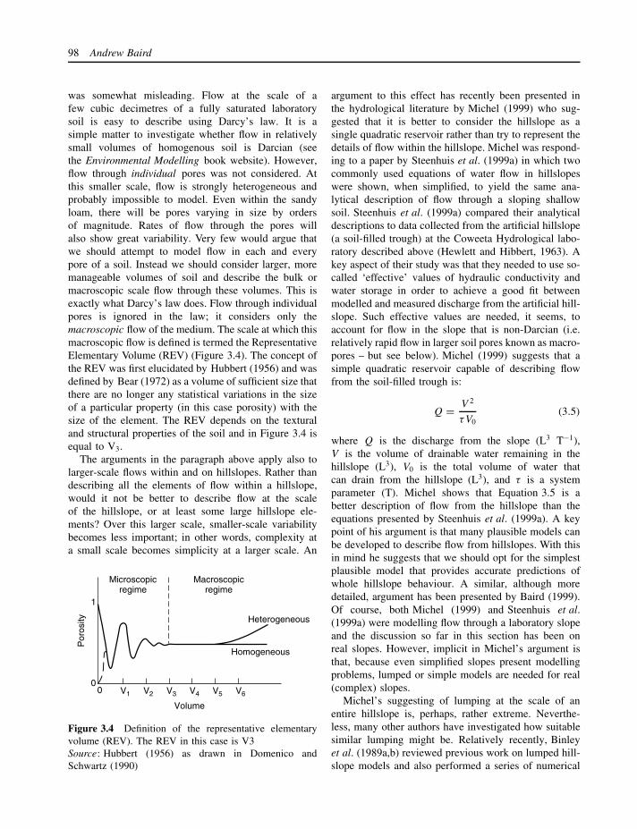
98 Andrew Baird
was somewhat misleading. Flow at the scale of afew cubic decimetres of a fully saturated laboratorysoil is easy to describe using Darcy’s law. It is asimple matter to investigate whether flow in relativelysmall volumes of homogenous soil is Darcian (seethe Environmental Modelling book website). However,flow through individual pores was not considered. Atthis smaller scale, flow is strongly heterogeneous andprobably impossible to model. Even within the sandyloam, there will be pores varying in size by ordersof magnitude. Rates of flow through the pores willalso show great variability. Very few would argue thatwe should attempt to model flow in each and everypore of a soil. Instead we should consider larger, moremanageable volumes of soil and describe the bulk ormacroscopic scale flow through these volumes. This isexactly what Darcy’s law does. Flow through individualpores is ignored in the law; it considers only themacroscopic flow of the medium. The scale at which thismacroscopic flow is defined is termed the RepresentativeElementary Volume (REV) (Figure 3.4). The concept ofthe REV was first elucidated by Hubbert (1956) and wasdefined by Bear (1972) as a volume of sufficient size thatthere are no longer any statistical variations in the sizeof a particular property (in this case porosity) with thesize of the element. The REV depends on the texturaland structural properties of the soil and in Figure 3.4 isequal to V3.
The arguments in the paragraph above apply also tolarger-scale flows within and on hillslopes. Rather thandescribing all the elements of flow within a hillslope,would it not be better to describe flow at the scaleof the hillslope, or at least some large hillslope ele-ments? Over this larger scale, smaller-scale variabilitybecomes less important; in other words, complexity ata small scale becomes simplicity at a larger scale. An
1
0
Microscopicregime
Macroscopicregime
Heterogeneous
Homogeneous
Por
osity
0 V1 V2 V3 V4 V5 V6
Volume
Figure 3.4 Definition of the representative elementaryvolume (REV). The REV in this case is V3Source: Hubbert (1956) as drawn in Domenico andSchwartz (1990)
argument to this effect has recently been presented inthe hydrological literature by Michel (1999) who sug-gested that it is better to consider the hillslope as asingle quadratic reservoir rather than try to represent thedetails of flow within the hillslope. Michel was respond-ing to a paper by Steenhuis et al. (1999a) in which twocommonly used equations of water flow in hillslopeswere shown, when simplified, to yield the same ana-lytical description of flow through a sloping shallowsoil. Steenhuis et al. (1999a) compared their analyticaldescriptions to data collected from the artificial hillslope(a soil-filled trough) at the Coweeta Hydrological labo-ratory described above (Hewlett and Hibbert, 1963). Akey aspect of their study was that they needed to use so-called ‘effective’ values of hydraulic conductivity andwater storage in order to achieve a good fit betweenmodelled and measured discharge from the artificial hill-slope. Such effective values are needed, it seems, toaccount for flow in the slope that is non-Darcian (i.e.relatively rapid flow in larger soil pores known as macro-pores – but see below). Michel (1999) suggests that asimple quadratic reservoir capable of describing flowfrom the soil-filled trough is:
Q = V 2
τV0(3.5)
where Q is the discharge from the slope (L3 T−1),V is the volume of drainable water remaining in thehillslope (L3), V0 is the total volume of water thatcan drain from the hillslope (L3), and τ is a systemparameter (T). Michel shows that Equation 3.5 is abetter description of flow from the hillslope than theequations presented by Steenhuis et al. (1999a). A keypoint of his argument is that many plausible models canbe developed to describe flow from hillslopes. With thisin mind he suggests that we should opt for the simplestplausible model that provides accurate predictions ofwhole hillslope behaviour. A similar, although moredetailed, argument has been presented by Baird (1999).Of course, both Michel (1999) and Steenhuis et al.(1999a) were modelling flow through a laboratory slopeand the discussion so far in this section has been onreal slopes. However, implicit in Michel’s argument isthat, because even simplified slopes present modellingproblems, lumped or simple models are needed for real(complex) slopes.
Michel’s suggesting of lumping at the scale of anentire hillslope is, perhaps, rather extreme. Neverthe-less, many other authors have investigated how suitablesimilar lumping might be. Relatively recently, Binleyet al. (1989a,b) reviewed previous work on lumped hill-slope models and also performed a series of numerical

Soil and Hillslope Hydrology 99
(computer) experiments designed to investigate whetherlumped models can reproduce the behaviour of a het-erogeneous hillslope. The first stage of their analysiswas to simulate flow in a heterogenous hillslope usinga 3-D saturated–unsaturated finite-element model basedon Darcy’s law. The model simulated a hillslope 150 mwide and 100 m long comprising 3024 finite-elementnodes. Values of saturated hydraulic conductivity (froma known distribution) were assigned randomly across themodel’s nodes. Binley et al. (1989b) then attempted toreproduce the runoff from the modelled heterogeneousslope with a modelled slope that had a single ‘effective’value of saturated hydraulic conductivity. They foundthat both the surface and subsurface runoff response ofheterogeneous hillslopes with a generally high hydraulicconductivity could be described quite well by homoge-neous slopes with single effective values of saturatedhydraulic conductivity. However, in low hydraulic con-ductivity slopes, where the amount of surface runoff wasquite high, the lumped models were unable to reproduceaccurately the two components of runoff. Thus it appearsthat lumped models based on Darcy’s law might havelimited usefulness. A key difference between lumpedmodels of the sort tested by Binley et al. (1989b) andthat suggested by Michel (1999) is that those of Binleyet al. (1989b) were lumped only in terms of a singleparameter. That is, the model hillslopes used by Bin-ley et al. were still divided up spatially, rather thanbeing considered as single hillslope-sized stores. Moreon the problems of scale in hydrological modelling can
be found in special issues of Hydrological Processes(see Bloschl and Sivapalan, 1995) and Water ResourcesResearch (see Bloschl et al., 1997).
Single-store representations of hillslope behaviour arenot new, and many lumped conceptual-mathematicalmodels of catchment runoff response to rainfall assumehillslope soils can be represented by single linear or non-linear ‘reservoirs’. An example of a model containingsuch stores is HYRROM (Hydrological Rainfall-RunoffModel – Blackie and Eeles, 1985) which represents acatchment using only four stores: the interception store,the soil store, the ground water store, and the routing(channel) store (Figure 3.5). Details of more physicallybased single store models can be found in Sloan andMoore (1984; see also Watts, 1997).
Similar arguments to those presented above havebeen made in the context of modelling catchmentrunoff where it has been suggested that it is possibleto define Representative Elementary Areas (REAs) atwhich runoff behaviour is stable (see Wood et al., 1988,and Chapter 4), i.e. not affected by small-scale changesin, say, rainfall delivery or soil-hydraulic properties.
3.3.2 A fitting end: the physical veracity of models
An objection to models such as Equation 3.5 is that theyare not physically meaningful (Steenhuis et al., 1999b).However, care has to be taken in deciding what we meanby ‘physically meaningful’. It is widely recognized thata good fit between an observed data set and part of a
Rainfall
Time
Input
Evaporation
Interceptionstore
Runoffstore
Timedelay
Timedelay
Output
Evaporationand transpiration
Soil storeFlow
Groundwaterstore
Time
Figure 3.5 The structure of HYRROM (Hydrological Rainfall-runoff Model)Source: Based on an original diagram by Blackie and Eeles (1985)

100 Andrew Baird
model’s output is not a guarantee that the physical basisof the model has been validated (Beven, 1996; Baird,1999; Gupta, 2001). For example, a model capable ofpredicting both water-table level and discharge from thebase of a slope, is not validated if only its predictions ofdischarge have been shown to correspond closely withmeasurements (see Sloan and Moore, 1984). Clearly, itis important to check that the model also predicts watertable elevations (in both space and time) accurately.Checking the veracity of different components of amodel in this way is often termed internal validation.
A good example of internal validation is foundin Parsons et al. (1997) who tested the detailed pre-dictions of a distributed kinematic wave overland flowmodel. Remarkably, except for Scoging et al. (1992),it appears Parsons et al. (1997) are almost unique intesting the ability of such a model to predict both theslope hydrograph and patterns of flow on the slope.By performing a thorough internal validation of theirmodel, Parsons et al. (1997) were able to reveal thelimitations of a class of model that hitherto had beenregarded as a good or satisfactory descriptor of hillslopeoverland flow. In particular, they found that such mod-els only give acceptable predictions of overland flowhydraulics if they are finely tuned for each surface towhich they are applied. Such fine tuning requires huge,and for many applications unrealistic, amounts of fielddata. This conclusion led Parsons et al. to suggest thatprocess-based modelling of soil erosion may not be arealistic goal for hillslope researchers.
Even when a good fit is observed, it is important tobear in mind that a similarly good fit could be pro-duced by a different suite of processes, i.e. it is pos-sible that in Nature different groups of processes pro-duce similar hydrological behaviour at certain scales ofintegration such as the hillslope or large hillslope seg-ments (10 s–1000 s m2) (see Grayson et al., 1992a,b).This problem is similar to, but not quite the same as, theproblem of ‘model equifinality’ as defined and discussedby Beven (1996, 2001) (see also Baird, 1999) wheredifferent combinations (or values) of rate parametersapplied to a fixed set of modelled processes can resultin similar model predictions. It is important to realizethat we are still very uncertain, and lack fundamen-tal knowledge, about some of the processes controllingwater flow in soils (despite the implicit claims of somemodellers that we now know the suite of factors affect-ing water-transfer processes, with the only remainingchallenge being that of identifying which of the fac-tors are important in certain circumstances). This pointis explored in more detail below. It seems we tend to
dismiss a soil-water model as lacking in physical mean-ing if it does not incorporate an explicit Darcy-baseddescription of flow. However, to dismiss a model as notbeing physically meaningful on this basis may be mis-guided. A lumped model may not look physically based,but it could actually represent very well the integratedbehaviour (at certain scales) of a number of key pro-cesses occurring within a soil. These processes may notbe Darcian.
3.3.3 Perceptual models and reality: ‘Of course, it’sthose bloody macropores again!’
Notwithstanding the problems of model equifinality,the need for checking a model’s predictions with datais almost universally recognized (but see Fagerstrom,1987; see also the discussion in Baird, 1999, p. 330).If we accept Popper’s classical model of falsifica-tion (Popper, 1968; see also Wilby, 1997) in the sci-ences, then we might expect a mismatch between mod-elled and observed to be treated as evidence that a modelis false. It might seem surprising, therefore, to findexamples in the literature where authors have found mis-matches between observed and modelled behaviour butstill assume that their model provides a reliable descrip-tion of part, even a substantial part, of the system beingmodelled. Moreover, we might be even more surprisedto find that a lack of fit between model output and datais presented as evidence in its own right that some othernamed process is occurring in a soil. For example, thereare examples in the literature where models based onthe Darcy–Richards equation give relatively poor fits toobserved data. When this happens, some authors sug-gest that the lack of a good correspondence betweenthe model and the data is due to macropore flow. Fur-thermore, the authors suggest that the model is still agood description of flow in that part of the soil withoutmacropores. Such statements might seem quite reason-able until it is realized that the authors have based theirconclusions on an assumption that macropores occur inthe soil. In other words they have no measurements ofmacropore flow, or indeed observations of macroporeson which to base their conclusions about the impor-tance of macropore flow. So why do researchers invokemacropores as an explanation of a lack of fit betweenDarcy–Richards models and observed data? And, arethey right to do so?
Macropores are known to be very important controlsof both patterns and rates of saturated and unsaturatedwater flow through certain soils (e.g. Beven and Ger-mann, 1982; McCoy et al., 1994; Buttle and Leigh,1997). Macropores are relatively large pores present
Soil and Hillslope Hydrology 101
within a matrix of smaller pores. Exact definitions ofmacropores vary, but most agree they include featuressuch as desiccation cracks, faunal (e.g. earthworm) bur-rows, and root channels in which capillary forces arenegligible. Water flow in macropores (if it occurs) tendsto be relatively rapid and bypasses more slowly mov-ing water in the smaller pores of the matrix of thesoil. Although often comprising a small proportion ofthe total pore space within a soil, macropores can bethe dominant route of soil water movement. In addi-tion, water flow through systems of macropores canbe non-Darcian. The flow is often not strictly laminaras required by Darcy’s law, and large discontinuitiesin the energy status of soil water over scales smallerthan the REV (see above) can occur in the vicinityof macropores. A huge research effort on macroporeeffects began in the early 1980s and continues today, andmuch observed non-Darcian behaviour is now attributedto macropores. However, there are other phenomenaof soil water flow, which are often overlooked, thatcould explain non-Darcian behaviour. An example isquasi-saturation. Quasi-saturation is the term given tosoils that are not fully water-saturated below the watertable (Faybishenko, 1995). Quasi-saturation exists for avariety of reasons. Pockets of soil air can be trappedduring infiltration and subsequent water-table rise (Bondand Collis-George, 1981; Constantz et al., 1988; Fayerand Hillel, 1986a,b; Faybishenko, 1995). Gases can alsobe generated in situ by soil bacteria (Reynolds et al.,1992; Walter et al., 1996; Beckwith and Baird, 2001).Surprisingly little work has been done on the effectsof entrapped gas bubbles below the water table on flow.Yet these effects could be very important (e.g. Fayer andHillel, 1986a,b; Reynolds et al., 1992; Delozada et al.,1994; Faybishenko, 1995; Beckwith and Baird, 2001),resulting in large reductions in hydraulic conductivityfrom the fully water-saturated condition. It is interestingto note how different branches of science make advancesat different times. For example, in plant physiology theeffect of gas bubbles on water flow through plant tissueis now widely recognized as being fundamental in affect-ing water movement in plants (see, for example, Tyreeand Sperry, 1989; Tyree and Ewers, 1991; Huang andNobel, 1993; Kolb et al., 1996; Sobrado, 1997; Williamset al., 1997). In soils, the same cannot be said. Althoughuseful advances have been made in our understanding ofquasi-saturation, most soil hydrologists are unaware ofits potential importance. A search of the Web of Sciencedatabase for journals published between 1996 and 2000revealed only 17 papers dealing with quasi-saturation/airentrapment in soils. Fewer than half of these papers con-sidered the effects of trapped gas on soil hydraulics. In
contrast, in the same five-year period, 213 papers con-tained the words ‘macropore’ and ‘soil’ in their titles orabstracts. Macropores are the current fashion and havebeen for over 15 years.
Let us return to the example of a Darcy–Richardsmodel being applied to a hillslope soil. It would beinvidious to name specific authors who have rashlyinvoked macropore flow when a Darcy–Richards modeldoes not provide a good description of observed data. Solet us take a theoretical example. First, assume that weare comparing modelled and measured discharge fromthe base of the slope after a rainfall event. Second,assume that the model underpredicts the initially highrate of discharge from the slope but can be fitted quitewell to the later recession. One explanation of thediscrepancy between the Darcy–Richards model andobservations is that the initially high rate of dischargefrom the slope is due to the rapid flow of water inmacropores in the unsaturated zone, when these empty,Darcian flow processes in the saturated zone start tobecome dominant. The above conceptual model for thehillslope is certainly plausible and could be the truth.But we have to be careful. Other equally good andplausible models could be developed to explain whatis going on. The problem is that these other plausibleexplanations do not exist in our ‘perceptual model’, i.e.we are unaware of the effects of quasi-saturation on thehydraulics of flow below the water table or we assumethat it is unimportant. We are surrounded by paperstelling us that macropores are important and do not feelthe need to look elsewhere. As Beven (1996) noted: ‘Theperceptual model is inherently qualitative, but conditionsboth responses to experimental evidence and decisionsabout the dominant processes and representations ofthose processes to be included in quantitative models.’
It is quite possible that in our real system macroporeflow is unimportant and the Darcy–Richards model isa modest or even poor descriptor of flow through theremainder of the soil. What really happens might be asfollows. During and after a rain storm, the water tablerises. With this increase in water table there is a generalincrease in the hydraulic conductivity of the soil (i.e. asdry soil becomes wetter) and outflow from the base ofthe hillslope increases sharply. However, during water-table rise, some pockets of air become trapped in thesoil. The flow of water through soil pores entrains someof the trapped air bubbles. These soon start to coalesce atpore necks causing a decline in K and, therefore, flowfrom the soil (see Figure 3.6). Now we have another,quite reasonable, explanation for the high initial flowrates in the soil, followed by a steep decline. The patternis the same but the processes are quite different.
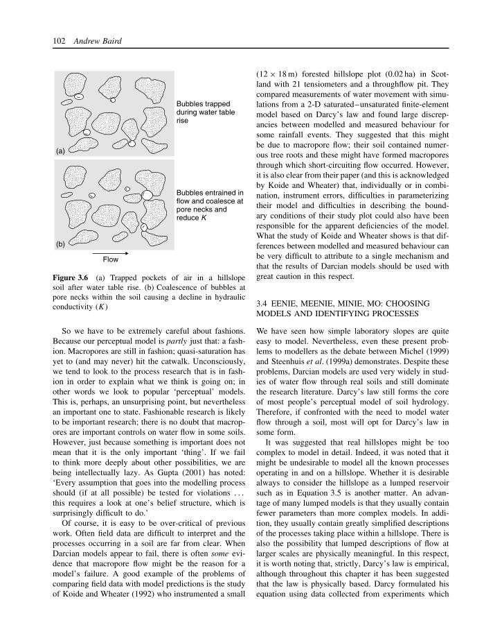
102 Andrew Baird
(a)
(b)
Bubbles trappedduring water tablerise
Bubbles entrained inflow and coalesce atpore necks andreduce K
Flow
Figure 3.6 (a) Trapped pockets of air in a hillslopesoil after water table rise. (b) Coalescence of bubbles atpore necks within the soil causing a decline in hydraulicconductivity (K)
So we have to be extremely careful about fashions.Because our perceptual model is partly just that: a fash-ion. Macropores are still in fashion; quasi-saturation hasyet to (and may never) hit the catwalk. Unconsciously,we tend to look to the process research that is in fash-ion in order to explain what we think is going on; inother words we look to popular ‘perceptual’ models.This is, perhaps, an unsurprising point, but neverthelessan important one to state. Fashionable research is likelyto be important research; there is no doubt that macrop-ores are important controls on water flow in some soils.However, just because something is important does notmean that it is the only important ‘thing’. If we failto think more deeply about other possibilities, we arebeing intellectually lazy. As Gupta (2001) has noted:‘Every assumption that goes into the modelling processshould (if at all possible) be tested for violations . . .
this requires a look at one’s belief structure, which issurprisingly difficult to do.’
Of course, it is easy to be over-critical of previouswork. Often field data are difficult to interpret and theprocesses occurring in a soil are far from clear. WhenDarcian models appear to fail, there is often some evi-dence that macropore flow might be the reason for amodel’s failure. A good example of the problems ofcomparing field data with model predictions is the studyof Koide and Wheater (1992) who instrumented a small
(12 × 18 m) forested hillslope plot (0.02 ha) in Scot-land with 21 tensiometers and a throughflow pit. Theycompared measurements of water movement with simu-lations from a 2-D saturated–unsaturated finite-elementmodel based on Darcy’s law and found large discrep-ancies between modelled and measured behaviour forsome rainfall events. They suggested that this mightbe due to macropore flow; their soil contained numer-ous tree roots and these might have formed macroporesthrough which short-circuiting flow occurred. However,it is also clear from their paper (and this is acknowledgedby Koide and Wheater) that, individually or in combi-nation, instrument errors, difficulties in parameterizingtheir model and difficulties in describing the bound-ary conditions of their study plot could also have beenresponsible for the apparent deficiencies of the model.What the study of Koide and Wheater shows is that dif-ferences between modelled and measured behaviour canbe very difficult to attribute to a single mechanism andthat the results of Darcian models should be used withgreat caution in this respect.
3.4 EENIE, MEENIE, MINIE, MO: CHOOSINGMODELS AND IDENTIFYING PROCESSES
We have seen how simple laboratory slopes are quiteeasy to model. Nevertheless, even these present prob-lems to modellers as the debate between Michel (1999)and Steenhuis et al. (1999a) demonstrates. Despite theseproblems, Darcian models are used very widely in stud-ies of water flow through real soils and still dominatethe research literature. Darcy’s law still forms the coreof most people’s perceptual model of soil hydrology.Therefore, if confronted with the need to model waterflow through a soil, most will opt for Darcy’s law insome form.
It was suggested that real hillslopes might be toocomplex to model in detail. Indeed, it was noted that itmight be undesirable to model all the known processesoperating in and on a hillslope. Whether it is desirablealways to consider the hillslope as a lumped reservoirsuch as in Equation 3.5 is another matter. An advan-tage of many lumped models is that they usually containfewer parameters than more complex models. In addi-tion, they usually contain greatly simplified descriptionsof the processes taking place within a hillslope. There isalso the possibility that lumped descriptions of flow atlarger scales are physically meaningful. In this respect,it is worth noting that, strictly, Darcy’s law is empirical,although throughout this chapter it has been suggestedthat the law is physically based. Darcy formulated hisequation using data collected from experiments which

Soil and Hillslope Hydrology 103
involved measuring water flow through beds of sand. Itwas also noted above that Darcy’s law ignores the fine-scale physics of water flow through individual pores.Despite its empirical origins and scale dependency, it hasa physical basis as has been demonstrated by Hubbert(1940) and Gray and O’Neil (1976). Darcy’s law, there-fore, serves as an example of a lumped model having aclear physical basis. Therefore, there is every possibil-ity that empirical equations such as Equation 3.5 whichlump at larger scales also have a physical basis.
Yet good modelling practice should not just boil downto a search for the simplest model that describes hillslopehydrological behaviour as implied by Baird’s (1999)complexity–simplicity dichotomy. In order to knowwhether a larger-scale description of system behaviouris physically meaningful, it is important to know whatprocesses at smaller scales are contributing in an inte-grated fashion to the larger behaviour of the system.Thus, although it is impossible and quite undesirableto include every known hillslope hydrological processin a model, choosing a model is not just a questionof choosing the simplest equation or set of equationsthat ‘does the job’ (cf. Baird, 1999). A further point inthis respect is that many scientists are curious (althoughnot as many as we might hope); they want to knowhow things work (knowing why is another matter). Assuch, they want to know what are the most importantprocesses within a system. Darcy’s law has dominatedsoil- and groundwater hydrology for well over 50 years,although many now recognize that macropores may con-trol rates of flow in certain circumstances. However,even if we include macropores within our perceptualmodels, we are in danger of being too restrictive. Weneed to look beyond fashion and work hard in consider-ing the range of possible factors that may be importantin affecting soil water flow.
Finally, there needs to be a wider debate on howwe use models and the relationship between modelling,fieldwork and laboratory work. As noted by Baird(1999), there is a tendency to assume, based on ourexisting perceptual models, that a certain suite ofprocesses is important and to build a model that includesonly these processes. Field work is then seen purelyin terms of model verification. Even then, there havebeen remarkably few attempts to test a model thoroughly(Parsons et al., 1997, being a notable exception). Fieldand laboratory work should also be seen in terms ofdriving the development of new models. Equally, it isimportant to realize that innovative model use can meanusing a model to indicate possible phenomena worthyof further field investigation, i.e. models can be used asvery valuable exploratory conceptual tools. Woolhiser
et al. (1996), Melone et al. (1998) and Singh (1998),for example, show how simple models can be used togive clues about what processes we should investigatein more detail in Nature. Thus, numerical explorationcan be used as a precursor to field work.
ACKNOWLEDGEMENTS
Mark Mulligan, John Wainwright and an anonymousreferee offered perceptive and helpful comments onan earlier draft of this chapter. The diagrams weredrawn by Paul Coles and Graham Allsopp of Carto-graphic Services, Department of Geography, Universityof Sheffield.
REFERENCES
Baird, A.J. (1997a) Continuity in hydrological systems, inR.L. Wilby (ed.) Contemporary Hydrology, John Wiley &Sons, Chichester, 25–58.
Baird, A.J. (1997b) Runoff generation and sediment mobilisa-tion by water, in D.S.G. Thomas (ed.) Arid Zone Geomor-phology, John Wiley & Sons, Chichester, 165–184.
Baird, A.J. (1999) Modelling, in A.J. Baird and R.L. Wilby(eds) Eco-Hydrology: Plants and Water in Terrestrial andAquatic Environments, Routledge, London, 300–345.
Bear, J. (1972) Dynamics of Fluids in Porous Media, Elsevier,New York.
Beckwith, C.W. and Baird, A.J. (2001) Effect of biogenic gasbubbles on water flow through poorly decomposed blanketpeat, Water Resources Research 37 (3), 551–558.
Bell, N.C., Wheater, H.S. and Johnston, P.M. (1989) Evalu-ation of overland flow models using laboratory catchmentdata. II. Parameter identification of physically based (kine-matic wave) models, Hydrological Sciences Journal 34 (3),289–317.
Beven, K. (1981) Kinematic subsurface stormflow, WaterResources Research 17, 1419–1424.
Beven, K. (1982) On subsurface stormflow: predictions withsimple kinematic theory for saturated and unsaturated flows,Water Resources Research 18, 1627–1633.
Beven, K. (1985) Distributed models, in M.G. Anderson andT.P. Burt (eds) Hydrological Forecasting, John Wiley &Sons, Chichester, 405–435.
Beven, K. (1996) Equifinality and uncertainty in geomorpho-logical modelling, in B.L. Rhoads and C.E. Thorne (eds)The Scientific Nature of Geomorphology: Proceedings ofthe 27th Binghampton Symposium in Geomorphology held27–29 September 1996, John Wiley & Sons, Chichester,289–313.
Beven, K. (2000) On the future of distributed modelling inhydrology, Hydrological Processes 14, 3183–3184.
Beven, K. (2001) On an acceptable criterion for model rejec-tion, Circulation (The Newsletter of the British HydrologicalSociety) 68, 9–11.
104 Andrew Baird
Beven, K. and Germann, P. (1982) Macropores and water flowin soils, Water Resources Research 18, 1311–1325.
Binley, A., Beven, K. and Elgy, J. (1989a) A physically basedmodel of heterogeneous hillslopes. 2. Effective hydraulicconductivities, Water Resources Research 25, 1227–1233.
Binley, A., Elgy, J. and Beven, K. (1989b) A physically basedmodel of heterogeneous hillslopes. 1. Runoff production.Water Resources Research 25, 1219–1226.
Blackie, J.R. and Eeles, C.W.O. (1985) Lumped catchmentmodels in M.G. Anderson and T.P. Burt (eds) HydrologicalForecasting, John Wiley & Sons, Chichester, 311–345.
Bloschl, G. and Sivapalan, M. (1995) Scale issues in hydro-logical modelling: a review, Hydrological Processes 9,251–290.
Bloschl, G., Sivapalan, M., Gupta, V., Beven, K. and Letten-maier, D. (1997) Preface to the special section on scaleproblems in hydrology, Water Resources Research 33 (12),2881–2881.
Bond, W.J. and Collis-George, N. (1981) Ponded infiltrationinto simple soil systems. 1. The saturation and transmissionzones in the moisture content profile, Soil Science 131,202–209.
Buttle, J.M. and Leigh, D.G. (1997) The influence of artificialmacropores on water and solute transport in laboratory soilcolumns, Journal of Hydrology 191, 290–314.
Chow, V.T. (1959) Open-Channel Hydraulics, McGraw-Hill,London.
Constantz, J., Herkelrath, W.N. and Murphy, F. (1988) Airencapsulation during infiltration, Soil Science Society ofAmerica Journal 52, 10–16.
Cundy, T.W. and Tento, S.W. (1985) Solution to the kinematicwave approach to overland flow routing with rainfall excessgiven by Philip’s equation, Water Resources Research 21,1132–1140.
Delozada, D.S., Vandevivere, P., Baveye, P. and Zinder, S.(1994) Decrease of the hydraulic conductivity of sandcolumns by Methanosarcina barkeri, World Journal ofMicrobiology and Biotechnology 10, 325–333.
de Marsily, C. (1986) Quantitative Hydrogeology: Groundwa-ter Hydrology for Engineers. Academic Press, London.
Dingman, S.L. (1984) Fluvial Hydrology, Freeman, New York.Domenico, P.A. and Schwartz, F.W. (1990) Physical and
Chemical Hydrogeology, John Wiley & Sons, New York.Fagerstrom, T. (1987) On theory, data and mathematics in
ecology, Oikos 50, 258–261.Fan, Y. and Bras, R.L. (1998) Analytical solutions to hillslope
subsurface storm flow and saturation overland flow, WaterResources Research 34, 921–927.
Faybishenko, B.A. (1995) Hydraulic behavior of quasi-saturatedsoils in the presence of entrapped air: laboratory experiments,Water Resources Research 31, 2421–2435.
Fayer, M.J. and Hillel, D. (1986a) Air encapsulation. 1. Mea-surement in a field soil, Soil Science Society of AmericaJournal 50, 568–572.
Fayer, M.J. and Hillel, D. (1986b) Air encapsulation. 2. Profilewater storage and shallow water table fluctuations, SoilScience Society of America Journal 50, 572–577.
Fetter, C.W. (1994) Applied Hydrogeology, 3rd edn, Macmil-lan, New York.
Freeze, R.A. and Cherry, J.A. (1979) Groundwater, Prentice-Hall, Englewood Cliffs, NJ.
Gray, W.G. and O’Neil, K. (1976) On the general equationsfor flow in porous media and their reduction to Darcy’s law,Water Resources Research 12 (2), 148–154.
Grayson, R.B., Moore, I.D. and McMahon, T.A. (1992a) Phys-ically based hydrologic modeling. 1. A terrain-based modelfor investigative purposes, Water Resources Research 28(10), 2639–2658.
Grayson, R.B., Moore, I.D. and McMahon, T.A. (1992b) Phys-ically based hydrologic modeling. 2. Is the concept realistic?Water Resources Research 28 (10), 2659–2666.
Gupta, H. (2001) The devilish Dr. M or some comments onthe identification of hydrologic models, Circulation (TheNewsletter of the British Hydrological Society) 68, 1–4.
Hall, M.J., Johnston, P.M. and Wheater, H.S. (1989) Evalua-tion of overland flow models using laboratory catchmentdata. I. An apparatus for laboratory catchment studies,Hydrological Sciences Journal 34 (3), 277–288.
Hanks, P. (ed.) (1986) Collins English Dictionary, 2nd edn,Collins, Glasgow.
Henderson, F.M. (1966) Open Channel Flow, Macmillan, NewYork.
Henderson, F.M. and Wooding, R.A. (1964) Overland flow andgroundwater flow from a steady rainfall of finite duration,Journal of Geophysical Research 69, 1531–1540.
Hewlett, J.D. (1961) Soil Moisture as a Source of Base Flowfrom Steep Mountain Watersheds, USDA Forest ServiceResearch Paper SE, 132, 1–10, Southeastern Forest Experi-ment Station, Asheville, NC.
Hewlett, J.D. and Hibbert, A.R. (1963) Moisture and energyconditions within a sloping mass during drainage, Journalof Geophysical Research 68, 1081–1087.
Hillel, D. (1980) Fundamentals of Soil Physics, AcademicPress, San Diego.
Huang, B. and Nobel, P.S. (1993) Hydraulic conductivity andanatomy along lateral roots of cacti – changes with soilwater status, New Phytologist 123 (3), 499–507.
Hubbert, M.K. (1940) The theory of groundwater motion,Journal of Geology 48, 25–184.
Hubbert, M.K. (1956) Darcy’s law and the field equations ofthe flow of underground fluids, Transactions of the AmericanInstitute of Mining, Metallurgical and Petroleum Engineers207, 222–239.
Kibler, D.F. and Woolhiser, D.A. (1970) The Kinematic Cas-cade as a Hydrologic Model, Colorado State Univer-sity Hydrology Paper 39, Colorado State University, FortCollins.
Klute, A. (1965) Laboratory measurements of hydraulic con-ductivity of saturated soil, in C.A. Black (ed.) Methods ofSoil Analysis. Part 1: Physical and Mineralogical Properties,American Society of Agronomy, Madison, WI, 210–221.
Koide, S. and Wheater, H.S. (1992) Subsurface flow simula-tion of a small plot at Loch Chon, Scotland, HydrologicalProcesses 6, 299–326.
Soil and Hillslope Hydrology 105
Kolb, K.J., Sperry, J.S. and Lamont, B.B. (1996) A methodfor measuring xylem hydraulic conductance and embolismin entire root and shoot systems, Journal of ExperimentalBotany 47, 1805–1810.
McCoy, E.L., Boast, C.W., Stehouwer, R.C. and Kladivko, E.J.(1994) Macropore hydraulics: taking a sledgehammer toclassical theory, in R. Lal and B.A. Stewart (eds) SoilProcesses and Water Quality, Lewis Publishers, London,303–349.
Melone, F., Corradini, C. and Singh, V.P. (1998) Simulationof the direct runoff hydrograph at basin outlet, HydrologicalProcesses 12, 769–779.
Michel, C. (1999) Comment on ‘Can we distinguish Richards’and Boussinesq’s equations for hillslopes?: The Coweetaexperiment revisited’ by T.S. Steenhuis et al., Water Resour-ces Research 35, 3573.
Miller, J.E. (1984) Basic Concepts of Kinematic Wave Models.United States Geological Survey Professional Paper 1302.Government Printing Office, Washington, DC.
Mulligan, M. (1996) Modelling hydrology and vegetationchange in a degraded semi-arid environment, unpublishedPhD thesis, King’s College, University of London.
Narasimhan, T.N. (1998) Hydraulic characterization of aquifers,reservoir rocks, and soils: a history of ideas, Water ResourcesResearch 34, 33–46.
Parsons, A.J., Wainwright, J., Abrahams, A.D., and Siman-ton, J.R. (1997) Distributed dynamic modelling of interrilloverland flow Hydrological Processes 11, 1833–1859.
Pi, Z. and Hjelmfelt, A.T. Jr (1994) Hybrid finite analytic solu-tion of lateral subsurface flow, Water Resources Research 30(5), 1471–1478.
Poesen, J.W.A. (1992) Mechanisms of overland-flow gener-ation and sediment production on loamy and sandy soilswith and without rock fragments, in A.J. Parsons andA.D. Abrahams (eds) Overland Flow: Hydraulics and Ero-sion Mechanics, UCL Press, London, 275–305.
Ponce, V.M. (1991) The kinematic wave controversy, Journalof Hydraulic Engineering, American Society of Civil Engi-neers 117, 511–525.
Ponce, V.M., Li, R.M. and Simons, D.B. (1978) Applicabilityof kinematic and diffusion models, Journal of the HydraulicsDivision of the American Society of Civil Engineers 104,353–360.
Popper, K. (1968) Conjectures and Refutations: The Growth ofScientific Knowledge, Harper and Row, New York.
Quinton, W.L., Gray, D.M. and Marsh, P. (2000) Subsurfacedrainage from hummock-covered hillslopes in the Arctictundra, Journal of Hydrology 237, 113–125.
Reynolds, W.D., Brown, D.A., Mathur, S.P. and Overend, R.P.(1992) Effect of in-situ gas accumulation on the hydraulicconductivity of peat, Soil Science 153, 397–408.
Richards, L.A. (1931) Capillary conduction of liquids in porousmediums, Physics 1, 318–333.
Romkens, M.J.M., Prasad, S.N. and Whisler, F.D. (1990) Sur-face sealing and infiltration, in M.G. Anderson and T.P. Burt(eds) Process Studies in Hillslope Hydrology, John Wiley &Sons, Chichester, 127–172.
Rose, C.W., Parlange, J.-Y., Sander, G.L., Campbell, S.Y. andBarry, D.A. (1983) Kinematic flow approximation to runoffon a plane: an approximate analytic solution, Journal ofHydrology 62, 363–369.
Sanchez, G. and Puigdefabregas, J. (1994) Interactions of plantgrowth and sediment movement on slopes in a semi-aridenvironment, Geomorphology 9, 243–260.
Scoging, H., Parsons, A.J. and Abrahams, A.D. (1992) Appli-cation of a dynamic overland-flow hydraulic model to asemi-arid hillslope, Walnut Gulch, Arizona, in A.J. Parsonsand A.D. Abrahams (eds) Overland Flow Hydraulics andErosion Mechanics, UCL Press, London, 105–145.
Singh, V.P. (1998) Effect of the direction of storm movementon planar flow. Hydrological Processes 12, 147–170.
Sloan, P.G. and Moore, I.D. (1984) Modeling subsurfacestormflow on steeply sloping forested watersheds, WaterResources Research 20, 1815–1822.
Sobrado, M.A. (1997) Embolism vulnerability in drought-deciduous and evergreen species of a tropical dry forest,Acta Oecologica – International Journal of Ecology 18 (4),383–391.
Steenhuis, T.S., Parlange, J.-Y., Parlange, M.B. and Stag-nitti, F. (1988) A simple model for flow on hillslopes, Agri-cultural Water Management 14, 153–168.
Steenhuis, T.S., Parlange, J.-Y., Sanford, W.E., Heilig, A.,Stagnitti, F. and Walter, M.F. (1999a) Can we distinguishRichards’ and Boussinesq’s equations for hillslopes?: TheCoweeta experiment revisited, Water Resources Research 35,589–593.
Steenhuis, T.S., Parlange, J.-Y., Sanford, W.E., Heilig, A.,Stagnitti, F. and Walter, M.F. (1999b) Reply (to Michel1999), Water Resources Research 35, 3575–3576.
Tyree, M.T. and Ewers, F.W. (1991) Tansley review number34: the hydraulic architecture of trees and other woodyplants, New Phytologist 119, 345–360.
Tyree, M.T. and Sperry, J.S. (1989) The vulnerability of xylemto cavitation and embolism, Annual Review of Plant Physi-ology and Molecular Biology 40, 19–38.
van Wesemael, B., Mulligan M. and Poesen J. (2000) Spatialpatterns of soil water balance on intensively cultivatedhillslopes in a semi-arid environment: the impact of rockfragments and soil thickness, Hydrological Processes 14(10), 1811–1828.
Verrecchia, E., Yair, A., Kidron, G.J. and Verrecchia, K. (1995)Physical properties of the psammophile cryptogamic crustand their consequences to the water regime of sandy soils,north-western Negev Desert, Israel, Journal of Arid Environ-ments 29, 427–437.
Walter, B.P., Heimann, M., Shannon, R.D. and White, J.R.(1996) A process-based model to derive methane emissionsfrom natural wetlands, Geophysical Research Letters 23,3731–3734.
Wang, H.F. and Anderson, M.P. (1982) Introduction to Ground-water Modeling: Finite Difference and Finite Element Meth-ods, Academic Press: San Diego.
Watts, G. (1997) Hydrological modelling in practice, inR.L. Wilby (ed.) Contemporary Hydrology: Towards Holistic

106 Andrew Baird
Environmental Science, John Wiley & Sons, Chichester,151–193.
Wheater, H.S., Bell, N.C. and Johnston, P.M. (1989) Evalu-ation of overland flow models using laboratory catchmentdata. III. Comparison of conceptual models, HydrologicalSciences Journal 34 (3), 319–337.
Wigmosta, M.S. and Lettenmaier, D.P. (1999) A comparisonof simplified methods for routing topographically drivensubsurface flow, Water Resources Research 35, 255–264.
Wilby, R.L. (1997) Beyond the river catchment, in R.L. Wilby(ed.) Contemporary Hydrology: Towards Holistic Environ-mental Science, John Wiley & Sons, Chichester, 317–346.
Williams, J.E., Davis, S.D. and Portwood, K. (1997) Xylemembolism in seedlings and resprouts of Adenostoma fas-ciculatum after fire, Australian Journal of Botany 45 (2),291–300.
Wood, E.F., Sivapalan, M., Beven, K. and Band, L. (1988)Effects of spatial variability and scale with implications tohydrologic modeling, Journal of Hydrology 102, 29–47.
Woolhiser, D.A. (1975) Simulation of unsteady flows, inK. Mahmood and V. Yevjevich (eds) Unsteady Flow inOpen Channels, Water Resources Publications, Fort Collins,485–508.
Woolhiser, D.A. and Liggett, J.A. (1967) Unsteady, one-dimensional flow over a plane – the rising hydrograph,Water Resources Research 3, 753–771.
Woolhiser, D.A., Smith, R.E. and Giraldez, J.-V. (1996) Effectsof spatial variability of saturated hydraulic conductivity onHortonian overland flow, Water Resources Research 32,671–678.
Wu, Y.H., Yevjevich, V. and Woolhiser, D.A. (1978) Effectsof Surface Roughness and its Spatial Distribution on Run-Off Hydrographs. Hydrology Paper 96, Colorado StateUniversity, Fort Collins.
WWW addresses for subsurface flow models
FEFLOW (variably saturated 3-D water, solute and heatflow): follow the links from http://www.wasy.de/
HYDRUS (variably saturated 2-D water and soluteflow): follow the links from http://www.ussl.ars.usda.gov/MODELS/MODELS.HTM
MODFLOW (3-D saturated water and solute move-ment): follow the links from http://water.usgs.gov/software/ground water.html
PORFLOW (includes variably saturated 3-D water,solute, and heat flow): follow the links from http://acriCFD.com/
VS2D (variably saturated 2-D water, solute and heatmovement): use the same link as MODFLOW

4
Modelling Catchment Hydrology
MARK MULLIGAN
4.1 INTRODUCTION: CONNECTANCEIN HYDROLOGY
In Chapter 3, Baird outlines the complexities of waterflow in soils and hillslopes and the importance oftheir spatial variability. In Chapter 5, Michaelides andWainwright outline the factors controlling the move-ment of the same water within channels and the modelapproaches available in which to simulate and betterunderstand this movement. This chapter takes a land-scape view of water movement and examines the aggre-gation of hillslope processes into nested catchments con-nected by stretches of flowing water. We will examinethe complexity of catchments in process, time and spaceand highlight some of the simple rules that determinetheir behaviour. We start by analysing the hydrologi-cal and computational definition of a catchment beforediscussing the range of models applied for hydrologicalmodelling at this scale. We then present some of the stateof the art and future directions in catchment modellingbefore identifying some of the gaps in our understandingof catchments and some of the simplicities which haveemerged from the modelling of complex catchments.
Studying the hydrology of catchments involves anunderstanding of the water balance of individual hydro-logical response units (HRUs) through the interaction ofclimate, vegetation and soils in the determination of thelocal water balance (precipitation minus evapotranspi-ration) and resulting soil moisture and the partitioningof this balance between more rapid surface pathways forflow such as runoff and slower subsurface pathways suchas throughflow (interflow in the US) or groundwaterrecharge. In addition, one has to understand the spatialdistribution and topological network for connectance ofthese response units such that the propagation of water
between them can be understood. This propagation mayinvolve amplification or diminution of flows depend-ing upon the characteristics of the HRU. Finally, therapid flows less connected with their substrate providedby permanent channels are added as a further layer ofcomplexity. The interaction of spatially varying climaticand human impacts must also be taken into account.Thus, the spatial complexity of catchment hydrologycan be significant, not to mention the fact that manyof these factors change also in time, for secular pro-cesses at scales from minutes (for the meteorological)to hundreds of thousands of years (for the topological)and for extreme events at all scales and in any time.
The types of questions asked of hydrologists at thecatchment scale are diverse. Leaving aside those relatedto hydrology (such as the impact of land-use changeon soil and nutrient erosion, the transport of pointsource and nonpoint source contaminants, the extentand distribution of salinization, variations and changein aquatic or wetland environments and associatedspecies) and concentrating on the solely hydrologicalissues, scientists, policy-makers and citizens are mainlyinterested in the following:
(a) the reasons for a devastating flood event or events;(b) the reasons for a devastating hydrological (as
opposed to climatic) drought;(c) the potential impact of climate change on flooding
and water resources;(d) the potential impacts of land cover and/or land-
use change or housing development on flooding andwater resources;
(e) the seasonal and long-term regime of a river or setof rivers (for engineering purposes);
Environmental Modelling: Finding Simplicity in Complexity. Edited by J. Wainwright and M. Mulligan 2004 John Wiley & Sons, Ltd ISBNs: 0-471-49617-0 (HB); 0-471-49618-9 (PB)

108 Mark Mulligan
(f) the potential downstream impacts of channel engi-neering, flood alleviation or other river or near-riverengineering developments.
Tackling these issues is not solely a matter ofmodelling but, at the catchment scale (because con-trolled experiments are not possible), modelling plays anincreasing important role alongside field monitoring and(paired) catchment experimentation. At the catchmentscale we tend to be interested in streamflow (surfacerunoff), its magnitude and timing.
4.2 THE COMPLEXITY
4.2.1 What are catchments?
The catchment of any point in the landscape is thatarea which provides water to the point through lateralflow over the surface and underground. Catchments areusually delineated on the basis of watersheds determinedfrom surface topography. In this way the complexand long-term processes which determine landscapeform (geomorphology) also determine the topologicalproperties of catchments at all scales. A watershedis a positive topographic anomaly which defines theboundary between two catchments such that the wateron either side of the watershed flows into differentcatchments (often to different outlets). Topographicallydefined watersheds may not always be an accuraterepresentation of the actual watershed since subsurfacelateral flow within the soil and particularly within thebedrock will not always follow surface topographiccontrol. Indeed, subterranean flows between catchmentscan be significant. Nevertheless, topographically definedwatersheds are appropriate for most surface hydrologicalstudies and are widely used. The term watershed isusually reserved for the boundary of a catchment butis also used to represent the catchment itself. The termdrainage basin is also used to represent the hydrologicalcatchment and indicates the catchment as a system andcomponent of the hydrological cycle transferring waterfrom the atmosphere through the interception of rainfall(and cloud; Zadroga, 1981) by land and plant eitherback to the atmosphere or to the sea by river. Thedrainage basin is thus a cog in the machine that is thehydrological cycle.
As well as this conceptual separation, catchments arevery clearly spatially separated through their watershedsand are, indeed, one of the more easily separated aspectsof the natural world. Catchments are multiscale withmany small subcatchments joining to make up theestimated 6152 global catchments with coastal outletsthat can be defined using the Vorosmarty et al. (2000)
30-minute global topological network of rivers. Thesecatchments are similar in many ways even though theyvary enormously in size. Vorosmarty et al. define theAmazon as the largest catchment in the world withan area of 5.854 × 10⁶ km2 and a length of 4327 kmfollowed by the Nile, Zaire and Mississippi catchments.The Amazon has 33 main tributary catchments and amultitude of tributary streamsWWW.
4.2.2 Representing the flow of water in landscapes
Flow paths for surface water are usually defined usinga neighbourhood operation on a digital elevation model(DEM) of topography. DEMs are common in hydro-logical modelling and provide a raster (square cel-lular, grid-based) representation of the topography ofan area (O’Callaghan and Mark, 1984; Tarboton et al.,1992). Each cell has a single value for altitude and thecell size of DEMs varies according to the area understudy and data availability, but those applied in hydro-logical modelling are usually between 5 and 50 metres inlength. Many hydrological parameters have been shownto be sensitive to DEM resolution, coarser DEMs lead-ing to reduced slope and more sparse river networks.Increased catchment wetness and peak flow in the TOP-MODEL have been observed using coarser representa-tions of topography (Zhang and Montgomery, 1994) anda number of other models have been shown to be sensi-tive though the sensitivity is greatest for models with ahigh temporal resolution (e.g. Yang et al., 2001). Thus,there needs to be appropriate balance between the spatialand temporal resolution of a catchment scale model.
DEMs are usually constructed by the interpolation ofa raster grid from point-based altitude dataWWW. Suchdata are acquired over small areas using field surveywith an EDM (electronic distance measurement) systemor, over larger areas, directly from the computerizedinterpretation of stereo ortho-photographic surveys or,most commonly, through the digitization of contour lineson existing cartography (with the contours usually hav-ing been derived from the prior manual interpretationof ortho-photographic survey). Alternatives to a rasterinterpretation of spatial data include (a) triangular irregu-lar networks (TINs: Palacios-Velez and Cuevas-Renaud,1986) the cells of which vary in size according to thetopographic complexity and (b) contour-based models(O’Loughlin, 1986; Moore et al., 1988). Contour-basedmodels discretize a topographic surface into irregularshaped cells made of two consecutive contours con-nected by two lines which represent the steepest slope
WWW indicates material covered in more detail in the website whichaccompanies this book: http://www.kcl.ac.uk/envmod

Modelling Catchment Hydrology 109
Figure 4.1 A digital elevation model (DEM) for the Tambito catchments in Colombia with cellular flow directionssuperimposed
connecting the two contours. While raster cells might notbe the best representation for hydrological purposes, theyare certainly the most practical for integration with pixel-based remotely sensed datasets and raster GIS calculationtools and are thus the most popular representation.
A DEM for the Tambito catchments in the Occi-dental Cordillera of the Colombian Andes is shown inFigure 4.1WWW. In order to define the catchments, onemust first define the flow paths for water. Flow paths aredefined according to the difference in altitude betweenthe cell in which the flow originates and the altitudeof neighbouring cells. Algorithms can be classified intothose which flow into a single neighbouring cell andthose which apportion flow to multiple neighbours. Anumber of algorithms have been used, including theso-called D8 algorithm (O’Callaghan and Mark, 1984),the MF (multiple flow direction) algorithm (Quinnet al., 1991), the D-infinity algorithm (Tarboton, 1997),the digital elevation model network – DEMON (Costa-Cabral and Burges, 1994), the Rho 8 algorithm (Fairfieldand Leymarie, 1991) and the kinematic routing algo-rithm (Lea, 1992). The D8 algorithm uses a nearestneighbour approach to define the relationship between acentral cell and its eight contiguous neighbours (4 sides,4 vertices) and defines the steepest downslope gradientalong which all of the water is deemed to flow. Thereare only eight possible flow directions, each 45◦ apartand all water in the cell flows to only one of them.This algorithm is used in many geographical information
WWW indicates material covered in more detail in the website whichaccompanies this book: http://www.kcl.ac.uk/envmod
systems (GIS) and some hydrological models but doestend to produce rather linear flow networks when appliedin areas of smoothed or shallow topography. An exampleof a D8 drainage network is superimposed on the Tam-bito DEM in Figure 4.1.
The Rho-8 algorithm randomly assigns the direc-tion of flow to downslope neighbours weighted accord-ing to the degree of slope. The MF algorithm alsouses the eight nearest neighbours but then apportionsflow to all lower neighbouring cells based on the rel-ative magnitude of their slopes. The aspect-based kine-matic routing algorithm assigns flow direction accord-ing to the calculated aspect. A plane is fitted to thecorners of the cell through interpolation of the alti-tudes of the pixel centres. Flow is routed as if itwere a ball rolling along this plane. The DEMON andD-infinity algorithms use surface-fitting algorithms todetermine a surface slope vector for the central pixeland the direction of this vector is used to propor-tion flow between the two neighbouring cells whichfall either side of the vector (the two nearest cardi-nal directions in the case of DEMON and the cardi-nal and diagonal in the case of D-infinity). Multipleflow direction algorithms tend to produce flow disper-sion while single flow direction algorithms lead to flowconcentration.
Different algorithms will produce different definitionsof a hydrological catchment and of many hydrologi-cally important topographic indices such as a point’supslope area, A, and the specific catchment area, a.Upslope area is the total catchment area above apoint or length of contour and the specific catchment

110 Mark Mulligan
area is the upslope area per width of contour or cellsize, L (Moore et al., 1991). Specific catchment areais used to calculate saturation and saturation excessoverland flow in hydrological models such as TOP-MODEL (Beven and Kirkby, 1979) and, along withother topographic indices, to calculate erosion and lands-liding in many other models. Upslope area is commonlyused for channel mapping on the basis of threshold ups-lope areas for channel initiation. Channels are usuallyestimated on the basis of either a constant thresholdupslope area for channel initiation (O’Callaghan andMark, 1984; Tarboton et al., 1992) or a slope dependentone (Dietrich et al., 1993). This threshold area can usu-ally be obtained from a log, log plot of upslope areaversus local slope (Tarboton et al., 1992). Vogt et al.(2002) extended this concept to include the geological,soil, topographic and climatic characteristics which canaffect the upslope area and local slope required for chan-nel initiation.
Figure 4.2 shows a set of cumulative frequencydistributions of upslope area calculated using thesedifferent algorithms for a random 65535 of the TambitoDEM cells. The MF and the D-infinity tend to producea peak of subcatchments in the range 1500–5100 m2
whereas the kinematic algorithm produces a sharppeak of subcatchments sized 1200 m2 and the DEMONalgorithm produces a broader peak centred at 2100 m2.D-8 and rho-8 produce a rather stepped distribution ofsubcatchment sizes especially for small basins, reflectingthe limited number of flow directions and thus basinaggregations that are possible. Depending on the routingalgorithm used, individual cells can have very differentupslope areas (and thus occupy hydrologically differentzones). Figure 4.3 shows the spatial outcomes of thesedifferences at the catchment scale. The upslope area
value of the D8 algorithm minus the equivalent value foreach of the other algorithms is shown, in addition to thedifferences in subcatchment properties at the small scaleoutlined in Figure 4.2. Figure 4.3 indicates that, even atthe catchment scale, large differences in the upslope areacan occur between these algorithms.
The calculation of flow direction allows the delin-eation of catchments and subcatchments, the routing oflateral flows of water, the calculation of stream proper-ties such as stream order and the calculation of trendsin controlling variables, such as slope gradient, downthe hydrological network. Figure 4.4 shows some ofthese properties calculated for the Tambito catchments.Slope gradient (the change in height per unit horizon-tal distance) is calculated using the method of Horn(1981) as implemented within the PCRASTER GIS (vanDeursen, 1995) although other methods also exist, suchas Zevenbergen and Thorne (1986). (Note the unrealis-tic slopes in the SE corner resulting from lack of datafor interpolation of the topography because of cloudcover in the initial ortho-photography.) The methodof Horn (1981) is also used to calculate aspect (thedirection of the maximum rate of change in elevation).The catchment of any identified point may be calcu-lated by following the drainage network upwards to thewatershed. Figure 4.4 shows the catchments of the out-flows of the Tambito DEM. Many of these are partialbecause the DEM boundaries are those of the map sheetbut the largest catchment (that of the Tambito itself)is complete. Stream channels are calculated here as iscommonly the case by initiating a channel when ups-lope area is greater than a threshold value, in this case1 000 000 m2 (1 km2), though this is, of course, ratherarbitrary. The stream order is calculated directly from
70,000
60,000
50,000
40,000
30,000
20,000
10,000
0
0
900
1,80
0
2,70
0
3,60
0
4,50
0
5,40
0
6,30
0
7,20
0
8,10
0
9,00
0
9,90
0
10,8
00
11,7
00
Catchment area (m2)
Cum
ulat
ive
freq
uenc
y
D-8rho-8D-infinityMFDemonKinematic
Figure 4.2 Differences in the distribution of micro-catchments within the Tambito catchment for six different routingalgorithms

Modelling Catchment Hydrology 111
16 million – 21 million11 million – 16 million7 million – 11 million2 million – 7 million−2 million – 2 million−7 million – −2 million−11 million – −7 million−16 million – −11 million−21 million – −16 millionNo Data
D-8-MF
D-8-Kinematic
D-8-rho8
D-8-Demon
Figure 4.3 Spatial differences in accumulated upslope area between the D8 and four other algorithms for flow routing

112 Mark Mulligan
Altitude Slope gradient
Slope aspect Catchments
Stream channel
TOPMODEL wetness
Order according to Strahler
Figure 4.4 Topographic and hydrological factors derived from the Tambito DEM using the D8 algorithm for flow routing
Modelling Catchment Hydrology 113
the flowlines according to the summation of flowlineconfluences using the method of Strahler. TOPMODELwetness is a compound topographic index commonlyused in hydrology to account for spatial variations inmoisture. It is compound because it combines upslopearea, A (the propensity to receive water) with localslope, s (the propensity to shed water) to yield an overallindex of wetness as ln(A/tan(s)).
4.2.3 The hydrologically significant propertiesof catchments
We have considered some of the complexities of catch-ment definition, now let us look a little at the hydrolog-ically significant properties of catchments themselves.These include the following:
(a) The topological structure of their drainage network,which determines the lag time for arrival of rainfallto a point in the network and the temporal concen-tration of the streamflow hydrograph which results.
(b) Their geomorphological and pedological character-istics (and spatial variation) which determine thepotential for infiltration and local storage over runoffand thus contribution to streamflow. The large-scalegeomorphology will also control the topology ofthe drainage network and, in large catchments, thismay be the most important control on a catchment’shydrology (Vorosmarty et al., 2000).
(c) Their climatic characteristics (and spatial variation).The spatial distribution of temperature, radiation andrainfall, which are themselves highly correlated withaltitude, will determine the spatial distribution ofcontributions from areas within a catchment.
(d) Their vegetation cover and land-use characteristicsand its spatial variation. Chapter 3 on hillslopehydrology indicates the significance of vegetationfor the hydrological balance of hillslopes and thepartitioning of rainfall into local infiltration andinfiltration excess, that is, runoff.
(e) The spatial distribution of their populations. Pop-ulations are the source of demand for water andtheir locations may determine the locations of localextractions and artificial storage of water from thechannel network or from locally generated runoff(as in the Aljibes of North Africa and the Mediter-raneanWWW) and local groundwater sources. Thelocation of populations will also determine the mag-nitude of local land-use change with correspond-ing impacts and the sources of point and nonpoint
WWW indicates material covered in more detail in the website whichaccompanies this book: http://www.kcl.ac.uk/envmod
agricultural, industrial and domestic pollution to thewater courses.
Because of surface and subsurface lateral flows, hydro-logical catchments are highly connected such that achange in any one part of them can have implications fora number of other parts downstream. Furthermore, thespatial distribution of all of these factors relative to thedirection of streamflow is particularly important sinceit determines the potential for cumulation or diminutionof streamflow along the flow path. A series of sourceareas in line with the flow path will cumulate outflowalong the flowline, whereas a mixture of source andsink areas will tend to diminute outflow along the flowpathWWW.
4.2.4 A brief review of catchmenthydrological modelling
The use of models to better understand and to pre-dict the behaviour of water in catchments has a longhistory, and, because models are rarely successful inapplication outside the catchments for which they weredeveloped, there are many models to be found. Themodels range from simple ‘black box’ representationsof input and output which are often successful in theprediction of runoff, from rainfall, through to morecomplex representations of some of the spatio-temporalcomplexity of catchments which are more capable offostering a better understanding of the reasons forobserved behaviour. Catchments themselves are superbsimplifiers, converting a spatial complexity of patternsand processes into a relatively simple and well under-stood output – the hydrograph. The range of modelsavailable reflects the need to predict the outcomes ofspecific interventions and scenarios for change, theemphasis on prediction as well as scientific investiga-tion (for the purposes of flood prediction and mitiga-tion or water resource management) and the paucityof data available for larger catchments compared withsmaller ones.
The types of catchment model available include phys-ically based models, based solidly on an understandingof the physical processes, empirical models based onthe patterns observed in data, and conceptual modelswhich pay little attention to the physics of the processesbut, rather, represent the catchment conceptually as, forexample, a series of cascading stores for water and thefluxes between them. Models may be deterministic mod-els in which a given set of inputs will always producethe same output, or stochastic models, which representthe variability of processes or events using probability

114 Mark Mulligan
distributions and which thus attempt to handle some ofthe inherent uncertainty in modelling and in data. Mod-els may be lumped at the catchment scale, meaning thatdata and modelling are aggregated at this scale, they maybe lumped at the subcatchment scale (and thus semi-distributed at the catchment scale) or they may be fullydistributed, that is lumped at the raster grid cell or TINpolygon scale.
Empirical models tend to be lumped, conceptual mod-els tend to be semi-distributed and physically basedmodels tend to be fully distributed. The increase incomputing power and of available spatial data in theform of GIS datasets, especially DEMs, and remotelysensed imagery has vastly increased the potential for dis-tributed modelling. At the catchment scale, to be basedon physics, physically based models have to be dis-tributed and so ‘distributed’ and ‘physically based’ oftengo together in catchment hydrological modelling. More-over, many large catchments are ungauged and thus can-not provide the calibration data necessary for the devel-opment and parameterization of conceptual or empiricalmodels. A driving force for the development of phys-ically based models is their application in ungaugedcatchments, though we will see later that gaps in param-eterization data and process knowledge create modeluncertainty and thus the requirement for these modelsto be calibrated against gauging station data.
4.2.5 Physically based models
Since it was first ‘blueprinted’ by Freeze and Har-lan in 1969, distributed physically based modelling hasbecome very widespread, on the assumption that a spa-tially variable physical system is inherently more realis-tic than a lumped one. This is likely to be true but mustbe considered within the context of spatially distributedmodels being themselves often crude simplifications ofany spatial variability that does exist in real catchments.Remote sensing has gone some way towards improvingthe observability of surface properties at the catchmentscale but subsurface properties are still largely unob-servable at any scale other than the point or line tran-sect. Examples of current distributed, physically basedmodels include the SHE model (Systeme HydrologiqueEuropeen, see Abbott et al., 1986) and the MIKE SHEand SHETRAN descendants of it (Bathurst et al., 1995;Refsgaard and Storm, 1995), the IHDM model (Instituteof Hydrology Distributed Model, e.g. Calver and Wood,1995), the CSIRO TOPOG model (e.g. Vertessy et al.,1993), Thales (Grayson et al., 1992), and WEC-C (Cro-ton and Barry, 2001), among others. Physically basedmodels should be derived deductively from established
physical principles and produce results that are consis-tent with observations (Beven, 2002). In reality they areoften one of these but rarely both.
According to Ward and Robinson (2000), SHE wasdeveloped jointly by the UK Institute of Hydrology (IH),the Danish Hydraulic Institute (DHI) and the SocieteGrenoblois d’Etudes et d’Applications Hydrauliques(SOGREAH). It was specifically designed to address theimpact of human activities on catchment processes. Thistype of scenario analysis is very difficult to address withempirical or conceptual models but is the main focus ofmost physically based models. In SHE a finite difference(grid-based) approach is used in three dimensions withup to 30 horizontal layers. Surface and groundwater floware two-dimensional while flow in the unsaturated zoneis one-dimensional. The model has been widely appliedand continuously updated since 1986.
While remote sensing provides some high quality spa-tial datasets for properties such as vegetation cover andtopography, there are many hydrologically importantproperties of catchments, notably those of the soils andthe surface that cannot be measured remotely and thusrequire intensive field campaigns which still cannot pro-vide the kind of spatial coverage required to justify theirdistribution in modelsWWW. For example, most hydro-logical models are highly sensitive to the (saturated)hydraulic conductivity of soils (Ksat), see Davis et al.(1999) and Chappell et al. (1998), and this is notori-ously difficult to measure for volumes greater than a fewhundred cm3, in part because of Baird’s (bloody) macro-pores of Chapter 3. It is fair to say that there is a sig-nificant mismatch in the sophistication of our physicallybased models and the sophistication of the data collec-tion technologies used to parameterize them. Moreover,as highlighted in Chapter 1, modelling is rather inex-pensive compared with fieldwork and is also perhapsmore glamorous, more comfortable and more suited toproducing publications – see the discussion by Klemes(1997: 48). So, the gap between the models and the datato fill them widens.
It is the imbalance between the model sophisticationand the availability of data at appropriate scales (as wellas our incomplete understanding and thus mathematiza-tion of the processes themselves), that means that eventhe most sophisticated models rarely perform well in apredictive capacity. Empirical models tend to be bet-ter predictors. Thus, a process of parameter calibrationis often exercised on physically based distributed mod-els to ensure agreement of predicted versus observed
WWW indicates material covered in more detail in the website whichaccompanies this book: http://www.kcl.ac.uk/envmod
Modelling Catchment Hydrology 115
runoff. This process, of course, compromises the phys-ical realism of the model and thus its ability to explainas well as to predict. Since explanation is why phys-ically based distributed models exist, this compromiseis a serious one. If it were not for explanation thenan equally predictive empirical model would always bethe best model because of its parsimony. Some authorshave argued that calibration can render physically baseddistributed models closer to over-parameterized con-ceptual, lumped models (Beven, 1989, 1996). Further-more, physically based, distributed models – even thevery widely used ones – have rarely been validated onvariables other than the output variables. Very few stud-ies have validated the internal state variables of thesemodels in order to understand whether the models areproducing validatable results for the correct physical(internal) reasons. In other words, have the lack ofdata, lack of detailed process understanding and over-calibration rendered physically based models into overlysophisticated conceptual models or do they indeed retainsome useful explanatory power? Fewer researchers stillconcentrate on validation which is focused specificallyon the purpose for which the model is intended, suchas suitability for the analysis of the impact of climateor land use change (Ewen and Parkin, 1996). Further-more, few studies focus on the evaluation of distributedbehaviour as opposed to catchment-integrated outcomessuch as runoff (Grayson et al., 1995); the correct predic-tion of patterns may be a better measure of explanatorypower than is success in the prediction of catchmentoutflows. In complex models, a number of differentparameter sets can give rise to the correct outflow (theproblem of equifinality). As a result, and given theuncertainty in most parameterization datasets, under-standing whether your calibrated model has producedthe right answers for the right physical reasons is ratherdifficult. Beven and Binley (1992) and a number of oth-ers since have used generalized likelihood uncertaintyestimator (GLUE) approaches to look at the implicationsof parameter uncertainty on model outcomes.
It is these problems and others, amply spelled outby Rosso (1994), Beven (1989, 1996) and Refsgaard(1997), that are the reasons why physically based dis-tributed models have tended to remain in the researchdomain and have had relatively little impact in theworld of practical hydrology. The problems with build-ing and using distributed, physically based models asper the Freeze and Harlan (1969) blueprint may be sogreat that an alternative blueprint is required (Reggianiet al., 2000; Beven, 2002). Those problems associatedwith the application of Darcy’s law for matrix flow(see Chapter 3) at a range of scales where it does not
apply or, if it does apply, we cannot test that it does,are particularly seriousWWW. The alternative blueprintof Beven (2002) emphasized a more observation-basedinductive approach over the more theoretical deductiveapproach of Freeze and Harlan (1969). See the data-based mechanistic approach outlined by Young et al. inChapter 22 for an example. In this way the observa-tions, and not the theory, determine which models areappropriate.
4.2.6 Conceptual and empirical models
Simpler models have been shown to give a good empir-ical fit to observed behaviour, though their very naturemeans that they must be calibrated to runoff recordsand thus cannot easily be used in ungauged catchmentsor transferred between catchments. IHACRES (Jakemanand Hornberger, 1993) is an example of a lumpedparameter rainfall-runoff model with only five calibra-tion parameters. It consists of two modules, one of whichconverts rainfall to rainfall excess and another whichtransforms rainfall excess to streamflow. A compromisebetween the lumped and the distributed approaches is touse a probability distribution approach which recognizesvariability but says nothing of its spatial arrangement(e.g. Moore, 1985) or the subcatchment or flow-segmentbased semi-distributed approach.
TOPMODEL (Beven and Kirkby, 1979; Beven et al.,1995) is a very widely used conceptual approach withsome physical basis. It is a collection of concepts asmuch as a model (Beven et al., 1995) and thus a widerange of versions have been implemented. It uses DEMsto recognize the importance of catchment topographyin controlling the spatial pattern of stormflow sourceareas and has, more recently, been extended to includesediment, geochemical fluxes, evapotranspiration andattachment to land surface–atmosphere transfer mod-els. Though TOPMODEL originates in the descriptionof humid temperate environments, it has also beenapplied to a wide range of other environments. TOP-MODEL has been widely applied on a variety of scalesfrom small headwaters (Molicova et al., 1997) to verylarge catchments where it is semi-distributed on a sub-catchment basis (e.g. Band and Wood, 1988). TOP-MODEL makes conceptual advances over many othersimple approaches by taking into account the propen-sity for differences in catchment saturation in accor-dance with the compound topographic index and itseffect on the generation of saturation overland flow.
WWW indicates material covered in more detail in the website whichaccompanies this book: http://www.kcl.ac.uk/envmod

116 Mark Mulligan
These differences are represented statistically rather thanphysically. In TOPMODEL, rainfall occurs and waterenters the soil along with water draining from otherparts of the catchment causing the groundwater tableto rise. When groundwater rises to the land surface,the area becomes saturated and saturation overland flowoccurs. Water below the surface is also assumed to movedownslope as throughflow since the hydraulic gradi-ent of the saturated zone is approximated as the localtopographic slope. Total outflow is throughflow plussaturation and infiltration-excess overland flow. Morerecent versions have added further sophistication to pro-cesses such as subsurface flow routing (Beven and Freer,2001) and a spatially variable soil thickness (Saulnieret al., 1997).
The Stanford Watershed Model (SWM) is one of theearliest and best-known conceptual catchment models.The model has an hourly soil-moisture budget and stor-age and routing functions for the redistribution of waterentering the channels to provide catchment scale runoffon a daily timestep (Crawford and Linsley, 1966; Viess-man and Lewis, 1996). The model requires climate dataand some 34 parameters describing the physical prop-erties of the catchment. More recent models have givengreater importance to the overarching control of the geo-morphological properties of the catchment as exercisedthrough the influence of the Horton–Strahler streamorder configuration. Furthermore, it is envisaged thatthis type of model can be applied in ungauged catch-ments for the calculation of geomorphologically con-trolled unit hydrographs (Gupta et al., 1996; Schmidtet al., 2000; Yang et al., 2001), particularly for largecatchments. The fractal scaling properties of river basinshelp significantly to simplify runoff modelling. Szilagyiand Parlange (1999) describe a semi-distributed concep-tual model in which the catchment is conceptualized asa series of stores whose dimensions are derived from theHorton–Strahler stream order (see Figure 4.4). Overlandflow fills these stores and water is routed between them.A separate groundwater model provides baseflow. Themodel requires the calibration of only seven parameterson the basis of a year-long rainfall-runoff record.
4.2.7 Recent developments
Recent trends in catchment modelling have seenthe integration of catchment hydrology modelswith ecological and physiological ones (e.g. Hattonet al., 1992) and with erosion and sediment-transportmodels (De Roo, 1998; Ewen et al., 2000). Modellingscales have increased from regional through tocontinental and global (Vorosmarty et al., 2000) in part
to provide interfaces with general circulation modelsof the atmosphere for climate change (Stieglitz et al.,1997) and climate change impact (Bronstert et al., 2002)studies. These larger scales and this deeper integrationhave been in response to increasing pressures tomake the models address some of the most seriousenvironmental problems that face governments andcitizens – accelerated land use and climate change.Since computer power has risen exponentially in thelast decades, the models (and the modellers) have beenable to keep up with these demands. However, the gapbetween capability and parameterizability (the C:P gap)continues to increase.
Recent years have also seen better integration of dataresources within flexible and intuitive databases, partic-ularly in GIS. More catchment models are designed towork with data held in common GIS formats or indeed torun within GIS software. This trend has both facilitatedthe spatialization of models and the potential for mod-elling over larger catchments and has also prevented theC:P gap from being even wider. The hydrological func-tionality of GIS and the links between common spatialhydrological models and GIS are reviewed by Ogdenet al. (2001) while the advances in data availability andmanipulation within a GIS context that have facilitatedthis integration of hydrology and GIS are reviewed in thecompanion paper by Garbrecht et al. (2001)WWW. DeRoo (1998) outlines the state of the art in dynamicspatial modelling languages for the development andapplication of hydrological models but reminds us thatall of this spatial detail does not necessarily mean bet-ter results.
In line with the greater emphasis on having hydrolog-ical models contribute to the solution of environmentalproblems and in line with the greater accessibility of per-sonal computers, catchment hydrological models havealso moved into the public domain. Decision-supporttools, which incorporate hydrological models for thepurposes of integrated catchment management (Walkerand Johnson, 1996; Matens and Di Biase, 1996) orspatial land-use planning (Greiner, 1996), are now notuncommonWWW. These tools are often used for betterunderstanding the unforeseen consequences of humanintervention in the hydrological system (e.g. Engelen,2000) or in larger systems of which hydrology is a small,but significant, part (Engelen, this volume). Though it isgenerally policy-makers who use these tools to supportthe decision-making process, there are even efforts tomake catchment scale model results available direct to
WWW indicates material covered in more detail in the website whichaccompanies this book: http://www.kcl.ac.uk/envmod
Modelling Catchment Hydrology 117
the public in real time over the WWW for flood warningpurposes (Al-Sabhan et al., 2002)WWW.
4.3 THE SIMPLICITY
4.3.1 Simplifying spatial complexity
Thus far we have concentrated on understanding theimplications of spatial complexity for modelling needsat the catchment scale. We know that lumped models donot represent this complexity and that distributed mod-els do, insofar as they can, but do not insofar as therequired data is often not available. Semi-distributed (orsemi-lumped!) approaches are a compromise betweenthe two end points but say nothing of the interactionbetween neighbouring patches, which can be importantin hydrological studies. Different aspects of the spatialvariability of catchments have different magnitudes ofimpact on the hydrological system and different spatio-temporal scales of interaction with it. Soil and vegetationproperties are likely to be more important for smallcatchments and short periods but their influence willbecome less as the size of the catchment or length ofthe period increases, at which point geomorphologicaland geomorphometric processes become more impor-tant. A nested hierarchy of catchment response unitsmight be identified with climate, geomorphology, vege-tation and soils having progressively greater variabilityand progressively smaller scales of influence (see Mul-ligan, 1996).
4.3.2 Simplifying temporal complexity
In addition to spatial complexity, catchment modelsmust also handle the temporal complexity of hydro-logical processes and their interaction with each other.Catchments integrate rapid rate processes such as thepartitioning of rainfall into runoff and infiltration or therouting of water through channels, with slower rate pro-cesses such as the trickle of groundwater recharge andthe continuous draw of evapotranspiration. Hydrologi-cal models are sensitive to the timestep of simulation;large errors can ensue by aggregating evapotranspi-ration calculations (from hourly through day/night todaily) and by representing instantaneous rainfall inten-sities that can reach over 100 mm/hr as hourly averages,which are unlikely ever to do so (see Wainwright et al.,1999, for an extended analysis). The temporal and spa-tial complexity of a catchment model must match the
WWW indicates material covered in more detail in the website whichaccompanies this book: http://www.kcl.ac.uk/envmod
spatio-temporal complexity of the processes, though theavailability of data is usually the greater constraint.For simplicity, natural timesteps are always preferableto artificial ones (day and night separated at sunriseand sunset instead being aggregated into a whole day;rainfall-rate-based timesteps reflecting the real passageof rainfall intensities instead of hourly lumps of rainfall).
4.3.3 Simplifying process complexity
There are many areas of hydrology where our under-standing of processes is basic but still sufficient todevelop models. But there are still areas in which thecomplexity of hydrological processes is so great, orthe information so little, that we do not understandthe processes well enough to develop reliable models.This complexity of processes is separate from the issuesrelated to spatial and temporal variation and the lack ofdata available to represent them as outlined above. Someof the areas in which there is still much progress to bemade are outlined below:
(a) The hydrology of sparse vegetation. Though tech-niques for modelling the interception, drainage andevapotranspiration from forest canopies are now wellestablished, there are still difficulties in understand-ing the role of canopy properties in determiningthe partitioning of water between the various fluxes.These difficulties are particularly clear for nonclosedcanopies or sparse vegetation where the impactof surface roughness is less well known and theparameterization of evapotranspiration is much moredifficult. Furthermore, the separation of vegetationinto patches may change evapotranspiration loadsin complex ways (see Veen et al., 1996). Patchinessis not just important for evapotranspiration but alsoaffects the generation and propagation of runoff andsediment, especially in arid and semi-arid environ-ments (see Dunkerly and Brown, 1995)WWW.
(b) Subsurface quickflow mechanisms. The parameter-ization of Ksat at scales greater than a few hun-dred cm3 remains a major obstacle to progressin subsurface hydrological modelling, particularlygiven the importance of macropores in providinga mechanism for subsurface quickflow in manyenvironments (Elsenbeer and Vertessy, 2000; Uchidaet al., 2001). Though our understanding of themechanisms of runoff generation through Hortonianand saturation-excess mechanisms has improvedconsiderably in recent years with the extensiveincorporation of partial contributing area concepts
118 Mark Mulligan
into hydrological models, our understanding of sub-surface quickflow mechanisms through macroporepipe networks and shallow subsurface quickflow ismuch less advanced. This lack of progress is partlythe result of the difficulty in measuring variations inthe physical properties that control these processesat the catchment scale, and partly the result of therelatively recent recognition of subsurface quickflowas hydrologically important.
(c) Hillslope-channel coupling. Modelling catchmentsis about modelling the hydrology of hillslopes andof channels. Many of the processes that determinechannelization are still poorly understood and thecoupling of hillslopes to channels is an area in whichnew insights are being made but further researchis required to help improve catchment models ofstreamflow, of the storm hydrograph and of flooding(see Chapter 5).
(d) Nonrainfall precipitation. There is still a relativedearth of modelling efforts focused upon the hydrol-ogy of nonrainfall inputs such as snow (Bloschl,1999) and occult precipitation (Mulligan, 2003) atthe catchment scale. These inputs are significant inmany catchments but are more difficult to measureand to model than rainfall.
(e) Tropical lowlands and tropical mountains. Thehydrological impacts of land-use and cover changein the tropics are much discussed in the literature butthere are very few studies which apply modellingto better understand these systems (Mulligan, 2003)and fewer still that combine modelling with inten-sive field monitoring programmes (Chappell et al.,1998). As a result, there is still much confusion aboutthe implications of land use change in these environ-ments and myths abound (Bruijnzeel, 1989; Calder,1999; Mulligan, 2003).
(f) Hydrological connectance. A key characteristic ofcatchment scale studies is the lateral connectancebetween patches which results from surface and sub-surface runoff. The properties of this connectancedetermine the manner in which patch scale outputaggregate to catchment totals. Total catchment runoffis not a simple sum of the constituent patch-levelrunoff. Recent work by the author using a distributedhydrological model applied in tropical montane envi-ronments indicates the importance of hydrologi-cal connectance for catchment level outputs andthe implications for the study of the hydrologicalimpacts of land use changeWWW. This study, which
WWW indicates material covered in more detail in the website whichaccompanies this book: http://www.kcl.ac.uk/envmod
is described in more detail on the accompanyingwebsite, looks at the implications of progressivedeforestation on the catchment scale runoff and thesensitivity of runoff to forest loss. The study con-cludes that in the initial stages of deforestation(0–75% forest cover lost), the sensitivity of runoffto forest loss is significant but low compared withthe situation beyond 75% loss. It is concluded thatwhere patches of forest remain along the surface andsubsurface flowlines, these absorb excess water gen-erated on the deforested patches and thus extra runoffdoes not cumulate downstream. When so much for-est is lost that flowlines are more or less deforestedalong their whole length, runoff generation accu-mulates down the flowlines and saturated wedgespenetrate further upslope, thus providing a positivefeedback for further runoff generation. In this waythe sensitivity of catchment scale runoff to the defor-estation of patches in this last 25% is very high,each patch contributing greatly to the continuity ofdeforested flow paths and thus to enhanced (flashy)streamflow. Furthermore, the location of the defor-estation relative to the geometry of the flow networkand the properties of the soil beneath and vegetationabove it determine the exact outcome of forest loss.This example only goes to indicate the importance oflateral connectivity in driving the overall response ofcatchments and in integrating (in a relatively simpleway) the complex spatial hydrology of them.
4.3.4 Concluding remarks
We have seen how catchments are defined by the flownetworks that landscapes generate as a function of theirtopography. These flow networks can be representedwithin a geographical information system and can facil-itate the modelling of hydrological processes at thecatchment scale in a distributed manner such that theprocesses of precipitation, interception, evapotranspira-tion, infiltration and recharge can be calculated for indi-vidual cells or patches and routed between them towardsthe catchment outlet. We have reviewed the main typesof model applied at the catchment scale and highlightedsome of the best of these, some of which are discussedfurther and linked to from the website that accompaniesthis book. Further we have seen some of the complexi-ties of modelling at the catchment scale and some of theobstacles to improved models. Finally we have lookedat some of the simple but key controls on catchmentbehaviour that emerge from the connected interaction ofspatial, temporal and process complexity at the catch-ment scale.

Modelling Catchment Hydrology 119
Catchment behaviour at scales from the magnificentAmazon through to the most modest drainage system isstill poorly understood. Studies of catchment responseto meteorological events, climate change and land usechange is confounded by the interacting effects ofspatial variability, spatio-temporal variation, processcomplexity and scaling, not to mention the scarcityand paucity of hydrological data at this scale. We areonly just beginning to understand the simple outcomesthat result from flow connectivity across these complex,spatially organized systems. Distributed modelling hasfar to go but distributed data has much further. Whiledistributed modelling can help us understand the innerworkings of catchments and the interactions within andbetween them, massive advances in data acquisition(rather than data integration) are required before theycan reach their full worth in practical as well asacademic enterprise.
REFERENCES
Abbott, M.B., Bathurst, J.C., Cunge, J.A., O’Connell, P.E. andRasmussen, J. (1986) An introduction to the EuropeanHydrological System – Systeme Hydrologique Europeen,SHE. 2. Structure of a physically-based, distributed mod-elling system, Journal of Hydrology 87, 61–77.
Al-Sabhan, W., Mulligan, M. and Blackburn, A. (2002) A real-time hydrological model for flood prediction using GIS andthe WWW, Computers, Environment and Urban Systems27 (1), 5–28.
Band, L.E. and Wood, L.F. (1988) Strategies for large-scale,distributed hydrologic simulation, Applied Mathematics andComputation 27 (1), 23–37.
Bathurst, J.C., Wicks, J.M. and O’Connell, P.E. (1995) TheSHE/SHESED basin scale water flow and sediment transportmodelling system, in V.P. Singh (ed.) Computer Modelsof Watershed Hydrology, Water Resources Publications,Highland Ranch, CO, 563–594.
Beven, K. (1989) Changing ideas in hydrology – the caseof physically based models, Journal of Hydrology 105,157–172.
Beven, K. (1996) A discussion of distributed hydrologicalmodelling, in M.B. Abbott and J.C. Refsgaard (eds) Dis-tributed Hydrological Modelling, Kluwer Academic, Dor-drecht, 255–278.
Beven, K. (2002) Towards an alternative blueprint for a phys-ically based digitally simulated hydrologic response mod-elling system, Hydrological Processes 16, 189–206.
Beven, K. and Binley, A. (1992) The future of distributed mod-els: model calibration and uncertainty prediction, Hydrolog-ical Processes 6, 279–298.
Beven, K. and Freer, J. (2001) A dynamic TOPMODEL,Hydrological Processes 15, 1993–2011.
Beven, K.J. and Kirkby, M.J. (1979) A physically based vari-able contributing area model of basin hydrology, Hydrolog-ical Sciences Bulletin 24 (1), 43–69.
Beven, K.J., Lamb, R., Quinn, P.F., Romanowicz, R. andFreer, J. (1995) ‘TOPMODEL’ in V.P. Singh (ed.)Computer Models of Watershed Hydrology, Water ResourcesPublications, Highland Ranch, CO, 627–668.
Bloschl, G. (1999) Scaling issues in snow hydrology, Hydro-logical Processes 13, 2149–2175.
Bronstert, A., Niehoff, D. and Burger, G. (2002) Effects ofclimate and land-use change on storm runoff generation:present knowledge and modelling capabilities, HydrologicalProcesses 16, 509–529.
Bruijnzeel, L.A. (1989) (De)forestation and dry season flow inthe humid tropics: a closer look, Journal of Tropical ForestScience 1, 229–243.
Calder, I. (1999) The Blue Revolution: Land Use and Inte-grated Water Resources Management, Earth Scan, London,208pp.
Calver, A. and Wood, W.L. (1995) The Institute of hydrologydistributed model, in V.P. Singh (ed.) Computer Models ofWatershed Hydrology, Water Resources Publications, High-land Ranch, CO, 595–626.
Chappell, N.A., Franks, S.W. and Larenus, J. (1998) Multi-scale permeability estimation for a tropical catchment,Hydrological Processes 12, 1507–1523.
Costa-Cabral, M.C. and Burges, S.J. (1994) Digital elevationmodel networks (DEMON): a model of flow over hillslopesfor computation of contributing and dispersal areas, WaterResources Research 30, 1681–1692.
Crawford, N.H. and Linsley, R.K. (1966) Digital Simulationin Hydrology: Stanford Watershed Model IV, Tech. ReportNo 39, Dept. Civil Engineering, Stanford University, Stan-ford, CA.
Croton, J.T. and Barry, D.A. (2001) WEC-C: a distributed,deterministic catchment model – theory, formulation andtesting, Environmental Modelling & Software 16, 583–599.
Davis, S.H., Vertessy, R.A. and Silberstein, R.P. (1999) Thesensitivity of a catchment model to soil hydraulic propertiesobtained by using different measurement techniques, Hydro-logical Processes 13, 677–688.
De Roo, A.P.J. (1998) Modelling runoff and sediment trans-port in catchments using GIS, Hydrological Processes 12,905–922.
Dietrich, W., Wilson, C., Montgomery, D. and Mckean, J.(1993) Analysis of erosion thresholds, channel networks andlandscape morphology using a digital terrain model, Journalof Geology 101, 259–278.
Dunkerly, D.L. and Brown, K.L. (1995) Runoff and runonareas in a patterned chenopod shrubland, arid Western NewSouth Wales, Australia: characteristic and origin, Journal ofArid Environments 20, 41–55.
Elsenbeer, H. and Vertessy, R.A. (2000) Stormflow generationand flowpath characteristics in an Amazonian rainforestcatchment, Hydrological Processes 14, 2367–2381.
Engelen, G. (2000) MODULUS: A Spatial Modelling Toolfor Integrated Environmental Decision Making, (FinalProject report to European Commission ENV4-CT97-0685),http://www.riks.nl/RiksGeo/proj mod.htm
120 Mark Mulligan
Ewen, J. and Parkin, G. (1996) Validation of catchment modelsfor predicting land use and climate change impacts. 1Method, Journal of Hydrology 175, 583–594.
Ewen, J., Parkin, G. and O’Connell, P.E. (2000) SHETRAN:a coupled surface/subsurface modelling system for 3D waterflow and sediment and solute transport in river basins, ASCEJournal of Hydrologic Engineering 5, 250–258.
Fairfield, J. and Leymarie, P. (1991) Drainage networks fromgrid digital elevation models, Water Resources Research27 (5), 709–717.
Freeze, R.A. and Harlan, R.L. (1969) Blueprint for a physi-cally-based, digitally-simulated hydrologic response model,Journal of Hydrology 9, 237–258.
Garbrecht, J., Ogden, F.L., DeBarry, P.A. and Maidment, D.R.(2001) GIS and distributed watershed models. I: data cover-ages and sources, Journal of Hydrologic Engineering 6 (6),506–514.
Grayson, R.B., Bloschl, G. and Moore, I.D. (1995) Distributedparameter hydrological modelling using vector elevationdata: THALES and TAPES-C, in V.P. Singh (ed.) ComputerModels of Watershed Hydrology, Water Resources Publica-tions, Highland Ranch, CO, 669–696.
Grayson, R.B., Moore, I.D. and McMahon, T.A. (1992) Phys-ically based hydrological modelling. 1 Terrain based mod-elling for investigative purposes, Water Resources Research28 (10), 2639–2658.
Greiner, R. (1996) SMAC: spatial optimisation model foranalysing catchment management, Environmental Software11 (1–3), 159–165.
Gupta, V.K., Castro, S.L. and Over, T.M. (1996) On scalingexponents of spatial peak flows from rainfall and rivernetwork geometry, Journal of Hydrology 187, 81–104.
Hatton, T.J., Dawes, W.R. and Dunin, F.X. (1992) Simulationof hydroecological responses to elevated CO2 at the catch-ment scale, Australian Journal of Botany 40, 679–696.
Horn, B.K.P. (1981) Hill Shading and the Reflectance Map,Proceedings of the IEEE 69 (1), 14–47.
Jakeman, A.J. and Hornberger, G.M. (1993) How much com-plexity is warranted in a rainfall-runoff model? WaterResources Research 29, 2637–2649.
Klemes, V. (1997) Of carts and horses in hydrological model-ing, Journal of Hydrologic Engineering 1 (4), 43–49.
Lea, N.L. (1992) An aspect-driven kinematic routing algo-rithm, in A.J. Parsons and A.D. Abrahams, Overland Flow:Hydraulics and Erosion Mechanics, UCL Press, London,147–175.
Martens, D.M. and Di Biase, J.F. (1996) TCM-Manager: a PC-based total catchment management decision support system,Environmental Software 11 (1–3), 1–7.
Molicova, H., Grimaldi, M., Bonell, M. and Hubert, P. (1997)Using TOPMODEL towards identifying and modelling thehydrological patterns within a headwater, humid, tropicalcatchment, Hydrological Processes 11, 1169–1196.
Moore, I., O’Loughlin, E. and Burch, G. (1988) A contourbased topographic model for hydrological and ecologicalapplications, Earth Surface Processes and Landforms 13,305–320.
Moore, I.D., Grayson, R.B. and Ladson, A.R. (1991) Digitalterrain modelling: a review of hydrological, geomorpholog-ical, and biological applications, Hydrological Processes 5(1), 3–30.
Moore, R.J. (1985) The probability-distributed principle andrunoff production at point and basin scales, HydrologicalScience Journal 30, 273–297.
Mulligan, M. (1996) Modelling the complexity of land-scape response to climatic variability in semi-arid environ-ments, in M.G. Anderson and S.M. Brooks (eds) Advancesin Hillslope Processes, John Wiley & Sons, Chichester,1099–1149.
Mulligan, M. (2003) Modelling the hydrological response oftropical mountainous environments to land cover and landuse change, in M. Ulli, H. Huber, K.M. Bugmann andM.A. Reasoner (eds) Global Change and Mountain Regions:A State of Knowledge Overview, Kluwer, Dordrecht.
O’Callaghan, J.F. and Mark, D.M. (1984) The extraction ofdrainage networks from digital elevation data, ComputerVision, Graphics, and Image Processing 28, 323–344.
Ogden, F.L. Garbrecht, J., DeBarry, P.A. and Johnson, L.E.(2001) GIS and distributed watershed models. II: modules,interfaces, and models, Journal of Hydrologic Engineering 6(6), 515–523.
O’Loughlin, E.M. (1986) Prediction of surface saturationzones in natural catchments by topographic analysis, WaterResources Research 22 (5), 794–804.
Palacios-Velez, O. and Cuevas-Renaud, B. (1986) Automatedriver-course, ridge and basin delineation from digital eleva-tion data, Journal of Hydrology 86, 299–314.
Quinn, P., Beven, K., Chevallier, P. and Planchon, O. (1991)The prediction of hillslope flow paths for distributed hydro-logical modelling using digital terrain models, HydrologicalProcesses 5, 59–79.
Refsgaard, J.C. (1997) Parameterisation, calibration and vali-dation of distributed hydrological models, Journal of Hydrol-ogy 198, 69–97.
Refsgaard, J.C. and Storm, B. (1995) MIKE SHE, inV.P. Singh (ed.) Computer Models of Watershed Hydrology,Water Resources Publications, Highland Ranch, CO,809–846.
Reggiani, P., Sivapalan, M. and Hassanizadeh, S.M. (2000)Conservation equations governing hillslope responses: ex-ploring the physical basis of water balance, Water ResourcesResearch 36, 1845–1863.
Rosso, R. (1994) An introduction to spatially distributed mod-elling of basin response, in R. Rosso, A. Peano, I. Becchiand G.A. Bemporad (eds) Advances in Distributed Hydrol-ogy, Water Resources Publications, Highland Ranch, CO,3–30.
Saulnier, G.M., Beven, K. and Obled, C. (1997) Includingspatially variable effective soil depths in TOPMODEL,Journal of Hydrology 202, 158–172.
Schmidt, J., Hennrich, K. and Dikau, R. (2000) Scales andsimilarities in runoff processes with respect to geomorphom-etry, Hydrological Processes 14, 1963–1979.
Skidmore, A.K. (1989) A comparison of techniques for calcu-lating gradient and aspect from a gridded digital elevation

Modelling Catchment Hydrology 121
model, International Journal of Geographical InformationSystems 3, 323–334.
Stieglitz, M., Rind, D., Famiglietti, J.S. and Rosenzweig, C.(1997) An efficient approach to modeling the topographiccontrol of surface hydrology for regional and global climatemodeling, Journal of Climate 10, 118–137.
Szilagyi, J. and Parlange, M.B. (1999) A geomorphology-based semi-distributed watershed model, Advances in WaterResources 23, 177–187.
Tarboton, D.G. (1997) A new method for the determination offlow directions and upslope areas in grid digital elevationmodels, Water Resources Research 33, 309–319.
Tarboton, D.G., Bras, R.L. and Rodriguez-Iturbe, I. (1992)A physical basis for drainage density, Geomorphology 5,59–76.
Uchida, T., Kosugi, K. and Mizuyama, T. (2001) Effects ofpipeflow on hydrological process and its relation to land-slide: a review of pipeflow studies in forested headwatercatchments, Hydrological Processes 15, 2151–2174.
Van Deursen, W.P.A. (1995) A geographical information sys-tems and dynamic model: development and applicationof a prototype spatial modelling language, PhD thesis,Utrecht Knag/Faculteit Ruimtelijke Wetenschappen Univer-siteit Utrecht, Netherlands.
Veen, A.W.L., Klaassen, W., Kruijt, B. and Hutjes, R.W.A.(1996) Forest edges and the soil–vegetation–atmosphereinteraction at the landscape scale: the state of affairs,Progress in Physical Geography 20, 292–310.
Vertessy, R.A., Hatton, T.J., O’Shaughnessy, P.J. and Jaya-suriya, M.D.A. (1993) Predicting water yield from a moun-tain ash forest using a terrain analysis based catchmentmodel, Journal of Hydrology 150, 665–700.
Viessman, W. and Lewis, G.L. (1996) Introduction to Hydrol-ogy, 4th edn, HarperCollins, London.
Vogt, J.V. Colombo, R. and Bertolo, F. (2002) Deriving drain-age networks and catchment boundaries: a new methodologycombining digital elevation data and environmental charac-teristics, Geomorphology 1285, 1–18.
Vorosmarty, C.J., Fekete, B.M., Meybeck, M. and Lammers,R.B. (2000) Geomorphometric attributes of the global systemof rivers at 30-minute spatial resolution, Journal of Hydrol-ogy 237, 17–39.
Wainwright, J., Mulligan, M. and Thornes, J.B. (1999) Plantsand water in drylands, in A. Baird and R. Wilby (eds)Ecohydrology, Routledge, London, 78–126.
Walker, D.H. and Johnson, A.K.L (1996) NRM Tools: a flex-ible decision support environment for integrated catchmentmanagement, Environmental Software 11 (1–3), 19–24.
Ward, R.C. and Robinson, M. (2000) Principles of Hydrology,McGraw-Hill, London.
Yang, D., Herath, S. and Musiake, K. (2001) Spatial resolutionsensitivity of catchment geomorphologic properties and theeffect on hydrological simulation, Hydrological Processes15, 2085–2099.
Zadroga, F. (1981) The hydrological importance of a montanecloud forest area of Costa Rica, in R. Lal and E.W. Russell(eds) Tropical Agricultural Hydrology, John Wiley & Sons,New York, 59–73.
Zevenbergen, L.W. and Thorne, C.R. (1986) Quantitative anal-ysis of land surface topography, Earth Surface Processes andLandforms 12, 47–56.
Zhang, W. and Montgomery, D.R. (1994) Digital elevationmodel grid size, landscape representation, and hydrologicsimulations, Water Resources Research 30 (4), 1019–1028.


5
Modelling Fluvial Processes and Interactions
KATERINA MICHAELIDES AND JOHN WAINWRIGHT
5.1 INTRODUCTION
Since Bathurst (1988), it has been recognized that thereis a growing need to address issues of complexity inthe modelling of fluvial systems. Despite the abilityof computers to solve numerical approximations to theequations of unsteady flow, models are still unable toestimate flows in real channels to a consistently highlevel of accuracy. Recent studies have highlighted theneed to address interactions between elements in thefluvial system to provide a more complete understandingof processes. Coupled with the issues of data qualityand representation of processes at different scales (seeChapters 2 and 19), we are still faced with challenges ofhow to make progress in modelling the fluvial system.There are a huge number of models in the literature,some of which are discussed below, some simple andsome complex. As we will see, model complexity doesnot always guarantee success!
5.2 THE COMPLEXITY
5.2.1 Form and process complexity
A complex system is one that consists of interconnectedor interwoven parts (Bar-Yam, 1997). The fluvial sys-tem is a complex system that consists not only of theriver channel but also the surrounding hillslopes andfloodplains together with their subsystems (e.g. soil sub-surface, soil surface, vegetation, etc.). In order to under-stand the behaviour of the fluvial system, we need tounderstand not only how the individual parts behavein isolation but also how they interact to form thebehaviour of the whole system (ibid.). Furthermore, ifthe individual components of the fluvial system are
themselves complex systems, then it is harder to describeand understand the behaviour of the whole. What makesthe fluvial system complex is the large number of inter-connected, complex parts, the interactions and feedbacksbetween them over a range of time- and space-scales, thelarge spatio-temporal heterogeneity in the surface char-acteristics and the presence of chaotic (or random) pro-cesses in most hydrological systems (Rodrıguez-Iturbeet al., 1989; Thornes, 1990; Phillips, 1992).
The morphology of natural river channels isdetermined by the interaction of the fluid flowwith the erodible materials in the channel boundary(Figure 5.1; Knighton, 1998). This nonstatic propertyof river channels means that there is a complexinterdependence between flow characteristics and theform of the channel. Flow velocity varies with resistancewithin the channel boundary while the shape of thechannel varies according to discharge and channelsediment composition. Furthermore, flow velocity ishighly variable through time and space and in turnaffects patterns and thresholds of erosion of the channelboundaries. Erosion of the channel boundary alsodepends on the physical properties of the materialthat makes up the channel. In general, erosion willvary according to whether the channel is madeup of cohesive or noncohesive sediment althoughagain nonuniform grain-size distributions along andacross the channel add to the further complexity oferosion patterns and feedbacks with flow characteristics.Fluvial interactions between the fluid flow and thechannel boundary take place across a wide range ofspatio-temporal scales, ranging from the movement ofindividual particles at the instantaneous time-scale to themovement of sediment through a drainage basin overthe long term. Moreover, the fluvial system contains
Environmental Modelling: Finding Simplicity in Complexity. Edited by J. Wainwright and M. Mulligan 2004 John Wiley & Sons, Ltd ISBNs: 0-471-49617-0 (HB); 0-471-49618-9 (PB)
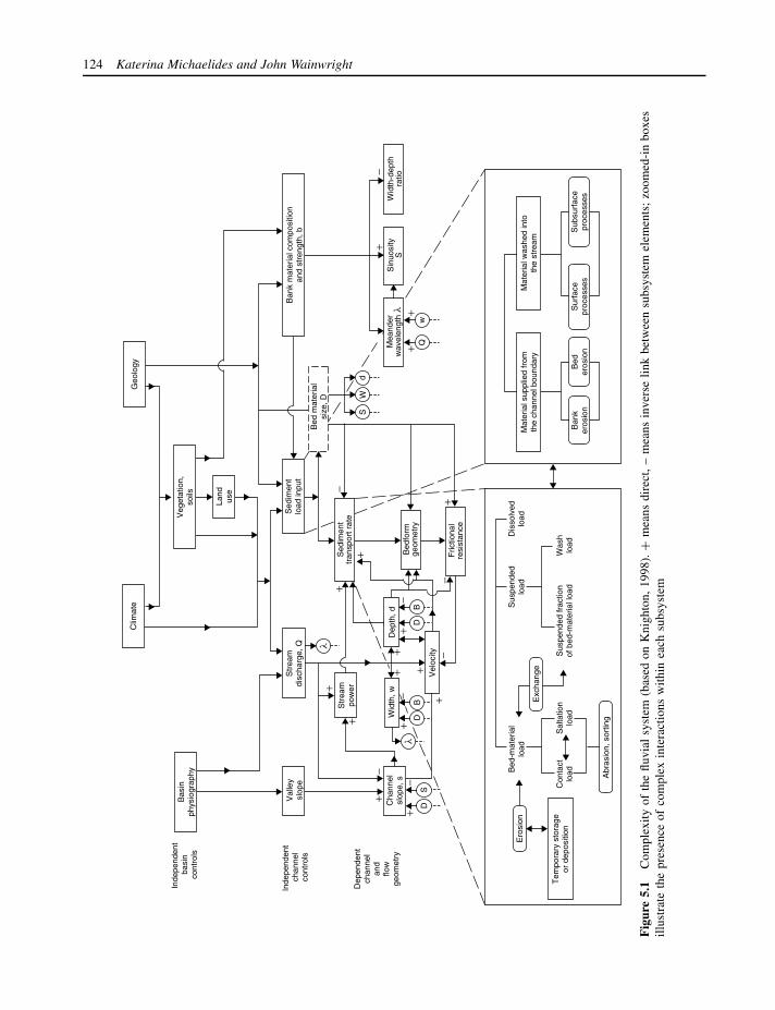
124 Katerina Michaelides and John Wainwright
Bas
inph
ysio
grap
hyV
eget
atio
n,so
ils
Land
use
Val
ley
slop
e
Cha
nnel
slop
e, s
Str
eam
disc
harg
e, Q
Str
eam
pow
er
Wid
th, w
Dep
th, d
Vel
ocity
Tem
pora
ry s
tora
geor
dep
ositi
on
Ero
sion
Bed
-mat
eria
llo
ad
Exc
hang
e
Sed
imen
ttr
ansp
ort r
ate
Bed
form
geom
etry
Fric
tiona
lre
sist
ance
Mea
nder
wav
elen
gth
lS
inuo
sity
SW
idth
-dep
thra
tio
Sed
imen
tlo
ad in
put
Ban
k m
ater
ial c
ompo
sitio
nan
d st
reng
th, b
DD
SB
DB
SW
d
w
l
l
Inde
pend
ent
basi
nco
ntro
ls
Inde
pend
ent
chan
nel
cont
rols
Dep
ende
ntch
anne
lan
dflo
wge
omet
ry
Con
tact
load
Sal
tatio
nlo
ad
Abr
asio
n, s
ortin
g
Sus
pend
ed fr
actio
nof
bed
-mat
eria
l loa
dW
ash
load
Sus
pend
edlo
adD
isso
lved
load
Mat
eria
l sup
plie
d fr
omth
e ch
anne
l bou
ndar
yM
ater
ial w
ashe
d in
toth
e st
ream
Geo
logy
Clim
ate
Ban
ker
osio
nB
eder
osio
nS
urfa
cepr
oces
ses
Sub
surf
ace
proc
esse
s
Q
+
++
+
+
+
+
+
++
+
++
+
+
−
−
−
−
−
−
−−
+B
ed m
ater
ial
size
, D
Fig
ure
5.1
Com
plex
ityof
the
fluvi
alsy
stem
(bas
edon
Kni
ghto
n,19
98).
+m
eans
dire
ct,
–m
eans
inve
rse
link
betw
een
subs
yste
mel
emen
ts;
zoom
ed-i
nbo
xes
illus
trat
eth
epr
esen
ceof
com
plex
inte
ract
ions
with
inea
chsu
bsys
tem
Modelling Fluvial Processes and Interactions 125
a variety of landforms that can change through timeas the system adjusts to climatic changes and humaninfluences. As such, the fluvial system also has acomplex history of adjustment of all the variables toexternally imposed effects. Fluvial processes can beinvestigated on a range of time and space scales, fromthe drainage basin over geological time and the riverreach, through to individual bed forms such as rifflesand pools over instantaneous time scales. However,despite our ability to reduce process investigationsto minute scales, individual elements of the fluvialsystem cannot be adequately viewed in isolation as thereis an interaction between the hydrological, hydraulic,geological and geomorphological processes at all scales(Schumm, 1988).
Primarily, this interaction between and within scalesof the fluvial system takes place across the hillslope,floodplain and channel elements of the catchmentthrough what is termed ‘hillslope-channel coupling’(Michaelides and Wainwright, 2002). The term ‘hill-slope-channel coupling’ has been used sporadically inthe literature since the late 1970s (e.g. Nortcliff andThornes, 1984; Caine and Swanson, 1989; Harvey,1992; Brunsden, 1993; Rice, 1994) to denote the degreeof connectivity between the hillslope and channel interms of the runoff- and sediment-delivery rates fromthe hillslopes to the channel and in terms of the fluvialactivity imposed by the channel on the hillslope base.Coupling takes place at varying time and space scales.
In the long term, the coupling between hillslopes andchannels determines drainage-network evolution sincedrainage patterns and hillslopes show a high degreeof adjustment to each other (Kirkby, 1993a,b; Willgo-ose et al., 1991a–d). The channel network provides afundamental link between hillslopes and rivers in thatit determines, largely through its density, the level ofinteraction between these two systems of water andsediment transfer (Knighton, 1998). Hillslope form isinfluenced by channels, which act as local base lev-els through lateral undercutting and vertical incisionor aggradation (Kirkby, 1993a). In return, channelsare influenced by hillslopes, which are a source ofwater and sediment to which they must respond. Kirkby(1993a) stresses the need to learn how the channelnetwork evolves and coevolves with the hillslopes inthe catchment. As hillslopes evolve, their hydrologicalresponse changes with both gradient and soil and veg-etation development. As a result, there are consistentdifferences in hillslope response from different partsof a catchment, and these differences are related tothe long-term evolution of the hillslope. In the longterm, hillslope form is controlled by the way in which
sediment-transport processes vary along the length ofthe hillslope and their interaction with channel processesacting at the slope base (Kirkby, 1993b). Dynamicinteractions between hillslope- and channel-sedimenttransport therefore determine the mutual coevolution ofchannels and hillslopes as a result of varying rates of cutand fill. Steep slope-base gradients promote higher ratesof hillslope erosion that may lead to higher inputs ofsediment into the channel thereby causing aggradationat the slope base. Aggradation may, however, reducethe slope-base gradient, thereby also reducing hillslope-erosion rates, leading to a relative equilibrium betweenthe hillslope and corresponding channel.
In the short term, hillslopes provide the input of waterto the channels together with direct rainfall on the chan-nels and floodplains themselves. Coupling is affected byvarious factors within the catchment (Michaelides andWainwright, 2002) discussed further below.
The floodplain is an integral part of the fluvial sys-tem as its deposits affect channel form through thecomposition of the channel boundary, and therefore thetype of material supplied to a stream (Knighton, 1998).Furthermore, floodplains are storage elements for sedi-ment as it moves through a catchment, the capacity ofwhich generally increases as they become wider withdistance downstream. This effect has implications forthe hillslope–channel relationship, which becomes moredisjunct as the floodplain becomes wider, due to thebuffering effects that a floodplain has both on the out-puts from the hillslopes into the channel, and on theaction of the channel at the hillslope base. In terms ofwater and sediment, their position means that they inter-act with both the hillslope and the channel, and thereforethey can either buffer inputs from the hillslope or theycan directly contribute significant inputs to the channel.
Work on temperate rivers by Archer (1989) andMcCartney and Naden (1995) has shown that floodplainstorage significantly reduces the magnitude of majorfloods and has a major impact on flood frequency. Thereasons for this are that a floodplain acts as a weakform of lake or reservoir, providing an area of extrawater storage during periods of high flow (McCartneyand Naden, 1995). In addition, the dispersal of waterfrom the main channel to the floodplain modifies theflow velocity because of the transfer of momentumbetween areas of different depths (Knight, 1989) andfloodplain storage may change the shape of thehydrograph (McCartney and Naden, 1995). Abovebankfull flow, increasing water storage on the floodplainand associated delays due to frictional resistancesuppress flood growth downstream (Archer, 1989).

126 Katerina Michaelides and John Wainwright
Below bankfull, as flood peak and volume increase,attenuation decreases and downstream flood growthbecomes steeper.
5.2.2 System complexity
Are fluvial systems inherently difficult to model? At thesmallest scales, flow features in most rivers are domi-nated by turbulence. Turbulence is the phenomenon bywhich flows exhibit apparently random motions as wellas more structured bursts, whorls and eddies. Despitedecades of intensive research, the causes of turbulenceare still not well understood (e.g. Hunt, 1995, 1999;Lesieur, 1997) not least because the nonlinear characterof the system at these scales causes the development ofchaotic behaviour. Modelling at small scales requires agreat deal of attention to the behaviour of turbulence,generally requiring simplification of the process to thelevel of the grid scale being used, not least because ofcomputational power limitations (see Chapter 20 for amore detailed discussion). However, if turbulent bursts,where the local flow energy dramatically increases overa short period of time, are responsible for initiatingsediment movement (e.g. Nearing, 1994) and this sed-iment movement causes a modification of the channelconditions, it is unlikely that a fully specified modelof fluvial systems at this scale using such averagingis ever fully meaningful: ‘The mechanics of sedimenttransport is so complex that it is extremely unlikely thata full understanding will ever be obtained. A univer-sal sediment transport equation is not and may never beavailable’ (Simons and Senturk, 1977). In such cases,stochastic approaches may be more appropriate not onlybecause of the process variability, but because of ourinability to describe the system in sufficient detail inany practical application. To do so would require agrain-by-grain description of size and relative location.Stochastic models of sediment transport in gravel-bedchannels have been relatively successful in overcomingthis limitation (e.g. Naden, 1987; Malmaeus and Has-san, 2002).
Streamflows at larger scales of observation – forexample, at the outflow of individual reaches orlarger catchments also tend to exhibit chaoticbehaviour. Porporato and Ridolfi (1997) found chaoticbehaviour in streamflow from 28 US catchments rangingin scale from 31 km2 to 35 079 km2, while Wang andGan (1998) found chaotic and long-term persistentbehaviour in their study of six Canadian rivers. Liu et al.(1998) and Sivakumar (2000) discuss the difficultiesof evaluating whether such signals exist in detail.An important, ongoing research question is whether
this chaotic behaviour is an emergent property of theturbulence phenomena at smaller scales or whetherit is related to interactions at larger spatial andtemporal scales.
A tentative answer to this question can be arrivedat from the opposite perspective. Channel networksand fluvial landscapes overall tend to exhibit fractalcharacteristics (Rodrıguez-Iturbe and Rinaldo, 1996). Atthe finer scale, studies by Robert and Richards (1988)and Robert (1988, 1991) have shown that the eleva-tions of a river bed exhibit fractal properties. Thus, itseems that fractal characteristics of fluvial systems occurover nine orders of magnitude. Studies looking at catch-ment development at large spatial and long temporalscales have demonstrated that fluvial systems can bedescribed as self-organizing systems (De Boer, 1999).Self-organization implies the evolution of a system overa long period of time into a state where rapid changecan occur at all spatial scales (Bak, 1997) so that asystem can communicate ‘information throughout itsentire structure, [with] connections being distributed onall scales’ (Rodrıguez-Iturbe and Rinaldo, 1996: 356)implying fractal characteristics of river basins (see alsoChapter 21 for a more detailed discussion). This formof model takes a simple process description and initialtopography and attempts to produce realistic (i.e. com-plex) fluvial landscapes. Bak (1997) suggests that thisform of self-organized criticality can explain the frac-tal characteristics of landscapes in a way that chaoticdynamics cannot. For this reason, we will present moredetail on this approach in the case study section below.
In summary, fluvial systems (and the landscapefeatures that interact with them) tend to demonstratechaotic behaviour at all scales. Realistic models offluvial systems should therefore attempt to characterizethis behaviour in a reasonable way, whether it be byusing simple or complex models. While carrying outthe simplifications necessary for simulating for differentpurposes, it is important to maintain the elements thatreproduce these characteristics.
5.3 FINDING THE SIMPLICITY
The increasing focus on small-scale processes and thecomplexity of fluvial processes has led to a reductionistapproach that has tended to concentrate on individualfluvial elements in isolation from each other. Such anapproach has tended to ignore important interactions ina system where the process complexity lies precisely inthese interactions that are paramount in controlling thebehaviour of the fluvial system.

Modelling Fluvial Processes and Interactions 127
For the purpose of understanding the complexitywithin fluvial systems, catchments are often subdividedinto stores and process units (Baird, 1997), such as veg-etation, the ground surface, the unsaturated zone of thesoil, the saturated zone of the soil, groundwater and thestream channel, or spatial units (Baird, 1997), whichcould be discrete catchment areas, each with its ownset of stores and processes. Commonly, modelling thefluvial system has also involved breaking down the sys-tem into its constituent components and modelling themseparately. As a result, there have been many modellingattempts on hillslope processes, floodplain processesand river-channel processes, but all in isolation fromeach other. There have been efforts to incorporate pairsof fluvial elements in models (i.e. hillslope–floodplain,river–floodplain, hillslope–river), but rarely are all ele-ments considered together in a dynamic way.
The following sections consider some approachescurrently adopted in modelling interactions within thefluvial system.
5.3.1 Mathematical approaches
Mathematical approaches to the complexity of the fluvialsystem depend on two levels (Figure 5.2). First, thecomplexity of the equations used to represent theprocesses at work within the system will vary fromrelatively simple to highly complex representations,accounting for a wide range of interactions. Second, thetopography and other parameters representing system
behaviour in the specific environment can also vary fromvery simplistic to highly detailed approximations. Thesetwo levels of complexity interact and it is the role ofthe modeller to choose the appropriate intersection ofprocess and environmental representation.
In Chapter 2, we saw how descriptions of flow pro-cesses can be very simple. At the simplest level, theymay be represented by a form of regression equation thatlinks rainfall to runoff. Neural network models are cur-rently being developed (e.g. Campolo et al., 1999) thatfollow a very similar empirical approach. Topographicand other parameter representation is often limited toa single variable, which may deal with the compoundeffects of a number of variables including topographywithin a basin. Spatial complexity may be dealt with byusing a cascading model, where the inputs of one spatialcomponent are derived from the outputs of the upstreamcomponents. The required complexity in this sort ofapproach has been evaluated by Perrin et al. (2001) whocompared model structure for 429 catchments in France,the USA, Australia, the Ivory Coast and Brazil. Theirsample covers catchments with annual average rainfallfrom 300 to 2300 mm, mean annual potential evapotran-spiration of 630 to 2040 mm and mean annual stream-flow of 0.2 to 2040 mm (equivalent depth over the catch-ment) and thus represents a wide range of environments.Using a split-sample procedure, they found that modelswith a greater number of parameters tended to do betterduring the calibration step, but during the testing step,
Complexity in parameterization
Pro
cess
com
plex
ity
Cellularmodels
Fullydistributedmodels
Kin
emat
ic w
ave
Dyn
amic
wav
e
CFD
Lumped models
Figure 5.2 Schematic comparison of the levels of complexity used in modelling fluvial systems, comparing process andparameter representations
128 Katerina Michaelides and John Wainwright
models with a smaller number of parameters (three com-pared to nine calibrated parameters) tended to do equallyas well. Parsimony in parameterization is thus an advan-tage that can be derived from this approach to modellingstreamflow. However, all such models tend to be limitedby the lack of generality beyond the catchment for whichthey have been developed and deal poorly with nonlinearbehaviour, particularly when extrapolation is requiredfor understanding extreme events. Thus, although thissort of model is often useful for looking at the ongo-ing behaviour of a particular catchment, perhaps withinthe remit of real-time flood forecasting (e.g. Lardet andObled, 1994), it is otherwise restricted, particularly whenwe are trying to use a model to understand the processesat work in more detail.
At the next level of mathematical complexity arethe simplified routing schemes. The Muskingum rout-ing method relates the change in storage to the inflowand outflow within a reach and the travel time requiredfor water to flow through the reach. It is thus a simplestorage form of the continuity equation. Cunge (1969)demonstrated that it is possible to derive this approachfrom the kinematic wave approximation to the St Venantequations that describe flow (see Chapter 2), and thatthe Muskingum–Cunge routing method is equivalent toan approximate solution of the diffusion-wave equation(see Singh, 1996, for a full derivation and workedexample). The topographic information required to runsuch models can be very simple, being simply thelength of the reach, slope of the channel bed, andcross-sectional area of the channel at the computationpoint. Developments of this approach have been usedto account for far more variability in the channel sys-tem, including complex channel networks and morerealistic shapes of the channel cross section (Garbrechtand Brunner, 1991). Attempts to make this type ofapproach more geomorphically realistic have been car-ried out using the concept of a geomorphic instanta-neous unit hydrograph approach (Rodrıguez-Iturbe andValdez, 1979; Rodrıguez-Iturbe, 1993; Snell and Siva-palan, 1994).
Interactions with the catchment system are a funda-mental part of fluvial systems as outlined above andin Chapter 4. The KINEROS model (Smith et al., 1995b;Woolhiser et al., 1990) provides an example of the nextlevel of complexity in that the models use a kinematicwave approximation to the routing of flow within chan-nel networks but allow input from hillslope elementswithin the catchment. These elements are defined as aseries of rectangular planes of fixed size and slope. Thehydrographs produced from these kinematic planes (e.g.Smith and Woolhiser, 1971) are thus highly stylized.
KINEROS2 provides a further improvement in that it has arepresentation of floodplains (El-Shinnawy, 1993; Smithet al., 1995a), albeit a highly simplified one that assumesfor routing purposes that the combined width of thefloodplains on both sides of the channel is only locatedon one side of the channel. The sensitivity of channelflows to inputs from the hillslope will therefore be over-estimated on the bank where the floodplain has beenremoved, but under-estimated on the bank where thefloodplain has been augmented.
The CASC2D model links a fully dynamic wave repre-sentation of the St Venant equations for channel flow indifferent channel cross-sections, with two-dimensionaldiffusive wave modelling of overland flow from hill-slopes and more detailed, spatially distributed catch-ment accounting of rainfall, interception, retention andinfiltration (Senarath et al., 2000). This model requiresa separate interface between GIS representations ofdatasets and their generation as model inputs. The sen-sitivity analysis of Senarath et al. demonstrated thatoutflows are most sensitive to three hillslope param-eters – soil saturated hydraulic conductivity, overlandflow roughness and overland flow retention depth – andthen to the channel hydraulic roughness, demonstrat-ing the importance of understanding the whole catch-ment behaviour in low-order catchments. Calibrationsfollowed by model testing on the Goodwin Creek, Mis-sissippi, USA, showed that larger rainfall events tendto be better simulated than smaller ones, which is acommon outcome of this form of model, because ofthe lesser relative importance of errors in estimatinginfiltration rates. These forms of model provide a bet-ter approach to the understanding of the catchmentprocesses, although it is important to remember thata model is only as good as the severity of the testimposed upon it. The results of Senarath et al. (2000),for example, have been evaluated at a number of loca-tions within the channel system, which provides moreconfidence than a simple evaluation of the model at thecatchment outlet. Grayson et al. (1992a,b) demonstratedusing their THALES model of distributed flow within acatchment in Australia that it is possible to ‘obtain theright results for the wrong reasons’ by calibrating dif-ferent infiltration models (saturated and Hortonian) toproduce equivalent outputs at the catchment boundary.The dangers of calibrating such models can lead to over-confidence in their output, particularly when trying toextrapolate beyond the original calibration dataset sothat the meaning of the process basis to the model can belost (cf. Beven, 1996). Large amounts of time, effort andmoney are required to apply such an approach in terms
Modelling Fluvial Processes and Interactions 129
of collecting appropriately detailed data for parameter-ization and testing of the model. Often, the final stageof checking whether calibrated parameters are realisticestimates is missing from the design of research projectsthat use this approach.
At the most extreme end of the level of math-ematical complexity is the application of Computa-tional Fluid Dynamics models (CFDs) to solve the fullNavier–Stokes equations of fluid flow. CFDs will bedealt with in far more detail in Chapter 20, so we willonly provide a brief overview here. Finite element andfinite volume techniques are generally used in CFDs tosolve the two- or three-dimensional flow fields in termsof their velocity, pressure and density characteristics,taking account of some simplification of the turbulenceof the flow. Thus, they tend to be highly complex numer-ically and more limited in terms of the topographythat can be accommodated. Most studies tend to con-centrate on the detail of flow processes within a shortreach, relating, for example, to channel confluences (e.g.Biron et al., 2002). Furthermore, only very recentlyhave approaches been developed that can accommodateinteractions with the sediment-transport components offluvial processes (e.g. Lane et al., 2002). Thus, suchmodels provide a great opportunity for enhancing ourunderstanding of process operation at the small scale,but at the cost of significant effort in producing themodel grids and data for model testing at appropri-ate spatial and temporal scales. In a recent exampleby Horritt and Bates (2001) two approaches of mod-elling floodplain inundation are compared. The first is arelatively simple raster-based approach with simple pro-cess representation and with channel flows being routedseparately from the floodplain using a kinematic waveapproximation called LISFLOOD-FP (Bates and De Roo,2000). The second is a more complex finite-elementhydraulic model that solves the full two-dimensionalshallow-water equations called TELEMAC 2D. They foundthat the raster and finite-element models offer simi-lar levels of performance when compared with SAR-derived shoreline data. They conclude that given thelikely accuracy of the validation data, and the increas-ing complexity of the calibration process for modelsrepresenting more complex processes, the simple raster-based model using a kinematic wave approximationover the channel is the simplest (and fastest) modelto use and adequate for inundation prediction overthis reach.
All of the above model descriptions deal with mod-els that are deterministic. A great deal of effort hasbeen expended since the 1970s to develop stochastic
approaches that can reproduce the apparent variability inthe flow process. Stochastic models can either incorpo-rate random functions into the representation of the flowprocess (e.g. Naden, 1987) or in terms of the param-eterization (e.g. Fisher et al., 1997; Veihe and Quin-ton, 2000), often employing Monte Carlo simulationtechniques and recently fuzzy logic approaches (e.g.Ozelkan and Duckstein, 2001). Random fluctuationsin flow patterns have been studied since the work ofHurst in the 1950s on the flood flows of the RiverNile. This work was employed by Mandelbrot and Wal-lis (1969; Kirkby, 1987) to demonstrate the presenceof deterministic chaos in fluvial systems. Deterministicchaos can produce the same apparently random resultsas random processes because of nonlinearities in theprocess behaviour. Baird (1997) suggested that deter-ministic chaos is a fundamental consideration in hydro-logical systems whose presence is hard to distinguishfrom simple stochastic behaviour. However, most mod-els of fluvial flow are formulated in a way that precludesthe development of chaotic behaviour. A reappraisal ofthe modelling approaches described above is requiredto make them compatible with observations exhibit-ing chaotic behaviour, and would be one explanationof the difficulty of producing consistently successfulsimulations.
5.3.2 Numerical modelling of fluvial interactions
5.3.2.1 Hillslope–channel interactions
Since the early work of Wooding (1965a,b, 1966) onone of the first explicit investigations into catchmenthydrological response, there have been numerous mod-els of hillslope–channel interactions. In his initialpaper (Wooding, 1965a) developed a simple model forexamining catchment hydrological response by describ-ing hillslope and channel responses using the kinematicwave formulation. Wooding’s initial analyses subse-quently prompted a number of similar studies, albeit ofincreasing sophistication, which have provided insightinto the problem of understanding how catchmentsof different sizes and composition respond to rainfallevents (Calver et al., 1972; Kirkby, 1976; Beven andWood, 1993; Robinson et al., 1995).
Calver et al. (1972) investigated the hydrologicalresponse of small catchments with a flow model thataccounted specifically for hillslope flows, thus over-coming limitations associated with empirical basin-hydrograph models that have tended to ignore hillslopeprocesses. They modelled the catchment by dividing itinto zones of overland flow and channel flow in which
130 Katerina Michaelides and John Wainwright
the corresponding processes were represented. Theirresults suggest that the ratio between the flow traveltimes of the hillslope and channel is the most importantfactor affecting the catchment hydrograph, implying thatthe longest flow time will also have the most dominanteffect on the overall flow. Therefore, in small catch-ments with low rainfall, the hillslope hydrograph willdominate, whereas for larger catchments and storms, thechannel hydrograph will tend to become increasinglyimportant on the catchment response.
More recently, Beven and Wood (1993) have devel-oped a scale-independent model of catchment networkresponse in order to investigate the effect of variablelateral inflows from hillslopes on the catchment hydro-graph. They used hypothetical hillslope hydrographs torepresent the variable inputs to the channel that wererouted through the appropriate link in the channel net-work. Their results demonstrated how the predictedcatchment hydrograph varies in relation both to therelative time scales of the hillslope and channel net-work responses, and to the degree of heterogeneity inrunoff production. Lateral inflows from the hillslopesaffected the catchment hydrograph, depending on therunoff production and network-routing processes. A sim-ilar study carried out by Robinson et al. (1995) exam-ined the relative roles of hillslope processes, channelrouting and network geomorphology in the hydrologicresponse of catchments. Their results illustrate, first, thatsmall catchment response is governed primarily by thehillslope response; second, that large catchment responseis governed primarily by network geomorphology; and,third, that nonlinearity in catchment response is just asgreat in large catchments as in small catchments. Thenonlinearity exhibited in hillslope and channel responsesoccurs as a result of the spatial variability of runoffacross hillslopes, and due to the delay between rain-fall and the onset of flow (Calver et al., 1972). Theadvantage of most hillslope–channel models is that theycan be applied at varying scales from small catchmentup to drainage basin scale in a relatively simple waydue to the simple representations of the topography intochannel and hillslope areas. However, these models donot account for the presence of a floodplain that hasbeen shown to significantly affect both channel and hill-slope flows.
5.3.2.2 Channel–floodplain interactions
There has also been an increasing surge in floodplain andchannel–floodplain numerical modelling. These modelshave increased in numerical sophistication with time,and range from simple one-dimensional to complex
three-dimensional models, mostly formulated for andapplied to temperate catchments.
Wolff and Burges (1994) used a one-dimensionalflood-routing model (DAMBRK) to investigate the com-bined influence of some channel and floodplain hydraulicand geometric properties on the frequency distributionof peak flood flow rates as flood waves propagate down-stream. The channel and floodplain properties exploredincluded channel and floodplain roughness, channel bedslope, channel width-to-depth ratio and floodplain width.The results emphasize the importance of floodplain andchannel characteristics in flood routing and highlightthe fact that channels and floodplains should be cou-pled when investigating the hydrological response ofa catchment. Their results indicated that the variabil-ity in the flood-frequency distribution was reduced inthe downstream direction due to the effects of the chan-nel and floodplain geometry and hydraulic roughness,while the amount of reduction in peak flow rates andflood-frequency distribution variability depended on theeffective storage of the reach which again is influencedboth by geometry (wider floodplains gave greater atten-uation), and hydraulic roughness.
Two-dimensional modelling of floodplains andchannel–floodplain interactions has also been reportedextensively in the literature. These models either solvea two-dimensional form of the simplified St. Venantequations with finite difference schemes (Cunge, 1975;Cunge et al., 1980; Hromadka et al., 1985; Nicholasand Walling, 1997), or solve the depth-integratedReynolds equation for two-dimensional free-surfaceflow using the finite element technique (Gee et al.,1990; Anderson and Bates, 1994; Bates et al.,1997) with the benefit of being able to generatefloodplain velocity vectors and inundation zones inaddition to flow hydrographs. These floodplain modelsare generally concerned with predicting floodplainhydraulics, overbank sedimentation rates and patternsof inundation over extensive areas of floodplain.However, they require high resolution of spatial dataand are thus difficult to parameterize, and can producenonconservative results (see Chapter 1).
Recent advances in numerical techniques have alsoseen the development of three-dimensional models offluid flow that have been used in the simulation offlow patterns in channel and floodplain areas (Fal-coner and Chen, 1996; Hervouet and Van Haren,1996). Krishnappan and Lau (1986) developed a river-floodplain model based on the equations of continuityand three-dimensional turbulent momentum. It has theadvantage of representing certain flow processes in a
Modelling Fluvial Processes and Interactions 131
more advanced way, such as lateral momentum trans-fer, secondary circulation and other three-dimensionaleffects associated with river channel and floodplainflow interactions. However, three-dimensional modelsare even more complex and difficult to parameterizethan the two-dimensional models and in addition tendto only be useful for modelling flows at small spatialand temporal scales.
5.3.2.3 Hillslope–floodplain–channel interactions
Many models attempt to account for the various flu-vial elements by combining different models (e.g. Bateset al., 1997; El-Hames and Richards, 1998; Stewartet al., 1999) and using the output from one model asan input to another. Such an approach ignores impor-tant interactions in a setting where the process com-plexity lies precisely in the interactions and feedbacksthat are paramount in controlling the behaviour of thefluvial system. The model COUP2D (Michaelides andWainwright, 2002) is a two-dimensional, distributedcatchment hydrological model of hillslope–channel cou-pling during a single rainfall event in a semi-arid riverreach or small catchment. COUP2D combines a grid-based representation of the hillslope elements with araster-based representation of the channel component.Hillslopes are represented by a two-dimensional DEM,which is used to route flow according to the kinematicwave approximation. The channel is represented as aone-dimensional series of cross-sections. Flow routing isagain carried out along the channel using the kinematicwave approximation which was chosen for this modelbecause it has been found to be particularly suitable forrepresenting many steady uniform flow conditions forchannel slopes greater than 1% (Moramarco and Singh,2000) and for its relative simplicity and wide applicabil-ity to a variety of conditions (Moussa and Bocquillon,1996). The model differs from the many existing catch-ment runoff models in that it accounts for a low-flowactive channel and for changes in its width and loca-tion within the main channel belt with discharge. Thisparticular function of the model enables the investiga-tion of the effect that the low-flow channel may haveon the coupling. The model differs from existing catch-ment hydrology models in that the hillslopes, floodplainsand channel are represented in a dynamic and unifiedway. An extensive sensitivity analysis (Michaelides andWainwright, 2002) has shown that under the appropri-ate conditions of hillslope and floodplain infiltrationrates, roughness and hillslope-floodplain geometry, atopographically-decoupled catchment can produce morerunoff than a topographically-coupled catchment. This
result means that hillslope-channel coupling is deter-mined by more than just the topographic linkages withinthe catchment and implies that the presence of a barrierbetween a hillslope and the channel can either attenu-ate or reinforce flows by altering the runoff responsedepending on the surface characteristics of both the bar-rier and the adjacent hillslope. The degree of couplingor decoupling has been shown to be influenced by thecatchment topography, the catchment surface properties,the spatial variability of the surface properties and therainfall intensity. However, we found that rainfall inten-sity and duration were actually more important thanany other factor in affecting the hydrological responseand the relative importance of other factors decreasedas the rainfall intensity and duration increased. Thus,the effects of hillslope–channel coupling decreased asthe magnitude of the rainfall event increased. Over-all, the implications of this study are that it is impor-tant to represent the detail of catchment structure andits variability when trying to predict its hydrologicalresponse. The structure interacts in important ways withthe surface characteristics, so that further field investi-gations into these interactions are necessary. Althoughtopographic coupling was found to be significant, theinteractions between rainfall variability and topographicand surface factors are far more important. Thus, accu-rate characterization of the spatial and temporal patternsin rainfall is fundamental in making accurate predic-tions. Although the model has produced some interest-ing findings about hillslope–floodplain–channel interac-tions and highlighted some potential threshold responseswithin the fluvial system, it has the disadvantage ofrequiring quite large amounts of topographic informa-tion for the characterization of the floodplain–channelcross-sections and thus it is impractical to apply for verylarge catchments or very long river reaches (see CaseStudy 1 below for further information).
5.3.3 Physical modelling of fluvial processesand interactions
Modelling of fluvial processes and interactions has notjust been carried out using numerical techniques. Experi-ments are also being carried out in miniature, laboratorymodels that attempt to replicate a real fluvial systemat a smaller scale. These laboratory models are calledscaled physical models. Scaled physical models havebeen used quite widely throughout the past two centuriesby scientists in various fields (Ashworth et al., 1994).Their popularity lies in the fact that complex naturalprocesses can be investigated in a controlled and simpli-fied laboratory setting. Nowadays, laboratory-modelling

132 Katerina Michaelides and John Wainwright
experiments can be highly sophisticated and enable theinvestigation of many processes and interactions withinthe fluvial system. In order to use or construct a realisticphysical model of the fluvial system, some sort of pro-cedure must be applied which would correctly representthe characteristics of the system while reducing it inscale. This procedure is called ‘scaling’ and it is basedon the concept that complete similarity between modeland prototype is achieved when the model displays geo-metric, kinematic and dynamic similitude (Wallersteinet al., 2001; Yalin, 1971). Geometric, kinematic anddynamic similitude imply that all homologous geomet-ric ratios and particle-path lengths to travel-time ratiosare equal, as well as that all homologous forces, workmagnitudes and power rates are in the same propor-tion (Wallerstein et al., 2001; Yalin, 1971). However, atrue model would require that all the above ratios areequal, something that cannot be achieved when usingthe same fluid (i.e. water) in both prototype and model.Therefore, in order to reduce the scale while retain-ing similar characteristics as the prototype, one or moreof the controlling variables must be relaxed (Ashworthet al., 1994). The most common method of scaling influvial models is called Froude scaling and is based onthe principle whereby the flow Reynolds (Re) number(a dimensionless measure of flow rate that indicates theconditions under which laminar or turbulent flow occur)is relaxed while correctly modelling the Froude (Fr)number (used to distinguish different flow states suchas subcritical, critical and supercritical). Yalin (1971)provides a comprehensive and detailed description ofthe theory behind the construction of hydraulic mod-els, while Wallerstein et al. (2001) and Ashworth et al.(1994) outline the main principles behind scaling in aconcise manner.
5.3.3.1 Fluvial processes
In the field of fluvial hydrology and geomorphology,scaled physical models have mostly been used to inves-tigate fluvial processes. Earlier examples include workby Leopold and Wolman (1957) and Schumm and Khan(1972) on the development of channel patterns andthe effects of flow structure and bedload transport onchannel geometry. More recently, physical modelling offluvial processes has involved investigations into feed-backs between channel morphology and bedload trans-port in gravel-bed rivers (Ashworth and Ferguson, 1986;Ashmore, 1991; Hoey and Sutherland, 1991), mecha-nisms of anabranch avulsion within gravel-bed braidedrivers (Leddy et al., 1993), processes of fine-grainedsediment deposition within braided rivers (Ashworth
et al., 1994) and the geomorphic and hydraulic impactof large woody debris elements within a river chan-nel (Wallerstein et al., 2001).
5.3.3.2 Channel–floodplain interactions
Laboratory modelling of channel–floodplain interac-tions has been ongoing since the 1950s and has beenundertaken by scientists from a variety of disciplinesranging from engineering to geography. These experi-ments have aimed primarily at understanding the waysin which channels behave during floods, especially atthe transition between bankfull and overbank stage, anddetermining the effect of a floodplain on flood flow.
Subsequently, these laboratory studies have involvedexperiments on a number of different factors that mightaffect either discharge or velocity distributions. A sig-nificant number of studies have been concerned withassessing the role of floodplains in the flood dischargeof channels (Barishnikov and Ivanov, 1971; Wormleatonand Merrett, 1990; Chatila and Townsend, 1995; Rashidand Chaudhry, 1995). This work has generally shownthat floodplains are important components of the chan-nel whose effects on flood discharge should alwaysbe accounted for, because they act as storage fea-tures and can significantly attenuate the flood hydro-graph by suddenly increasing the width and thereforereducing the velocity of flow. However, further exper-iments have concluded that it is not sufficient merelyto represent the floodplain but that the interactions andexchanges of momentum between the channel and flood-plain should also be accounted for (Sellin, 1964; Knightand Demetriou, 1983; Wormleaton et al., 1982). Notincluding these interactions can lead to an overestima-tion of the total discharge in the main channel, par-ticularly when the overbank region contributes a smallproportion of the total cross-sectional area and whenthe depth of water on the floodplain is small comparedwith the bankfull depth of the channel (Sellin, 1964).Other experiments have investigated the effects of chan-nel shape on the resistance in floodplain channels (Yenand Overton, 1973), while others have examined thethree-dimensional mixing which occurs in meanderingcompound flows (Ervine et al., 1994). Several studieshave also combined laboratory and numerical modellingof flood hydraulics in compound channels for purposesof comparison and validation of the numerical mod-els (Kohane and Westrich, 1994; Lyness and Myers,1994; Wark and James, 1994).
Generally, these studies demonstrate the importanceof floodplain and channel characteristics for the fre-quency distribution of peak flood flows, and of allow-ing for the interaction between the overbank flow and

Modelling Fluvial Processes and Interactions 133
the channel flow. They also illustrate how great theeffects of varying roughness and geometry can be onthe shape of the hydrograph. However, as all thesestudies have been carried out in relation to temperateenvironments where the hillslope input is not significantand the floodplains are dominant in the landscape, theydo not account for lateral inflows from hillslopes or forany hillslope–floodplain coupling. Ignoring a potentiallyimportant element in experiments like these may lead toan erroneous, or at least incomplete, picture of what isgoing on in the fluvial system. This means that con-clusions regarding the importance of variables on theobserved processes are, at best, only tentative as theymay miss out important interactions.
5.3.3.3 Hillslope–floodplain–channel interactions
Recently, a unique physical model was constructed inorder to investigate hillslope–floodplain–channel cou-pling. A tributary–junction recirculating channel flumewas modified to include tiltable hillslope elements withoverflow troughs for applying flow (Figure 5.3). The
aim of this work was to obtain data from a con-trolled setting in order to validate the numerical modelCOUP2D (Michaelides and Wainwright, 2002) as well asto observe the processes for a further understandingof coupling. By varying factors in a controlled andsystematic way observations can be made about how thesystem adjusts to the change in one single factor. Fac-tors varied include channel and hillslope angles, channeland hillslope discharges, channel and floodplain sedi-ment size and the presence of a floodplain. In terms ofusing the physical model to validate the numerical modelCOUP2D, the results were encouraging, and indicatedinteresting thresholds of behaviour under varying condi-tions of channel discharge and hillslope–floodplain lat-eral inputs. In terms of understanding hillslope–channelcoupling, the results indicated the importance of theinputs from lateral elements such as hillslopes and flood-plains on channel flow and sediment movement, both interms of total discharge and timing of discharge patternsthroughout the event. The results also demonstrated thesignificance of varying hillslope, floodplain and channelcharacteristics (i.e. angle, infiltration rates, roughness,
Figure 5.3 Scaled physical model used to investigate hillslope–channel coupling processes

134 Katerina Michaelides and John Wainwright
200 Rainfall isohyet (mm)
River channel
Badland
Agricultural land
Vaison-la-Romaine
200
200
150
100
250
300
0 5 km
N
0
500
1000
1500
2000
2500
08:52 11:16 13:40 16:04 18:28 20:52
Time
Dis
char
ge m
3 s−1
0
50
100
150
200
250
300
350
400
450
500
Rai
nfal
l int
ensi
ty m
m h
−1
Kinematic plane −Kinematic plane +Coup2dObservedRainfall
(a)
(b)
Figure 5.4 Modelling of the 22 September 1992 flood in the Ouveze basin: (a) the discretization of the Ouveze catchmentusing a kinematic plane approach; (b) model results; and (c) discretization using the COUP2D approach of Michaelidesand Wainwright (2002); image to the left is the bridge at Vaison-la-Romaine which was overtopped in the event

Modelling Fluvial Processes and Interactions 135
Total rainfall isohyets in mm for 22/9/92 1000.00
m
186.00209.63233.25256.88280.50304.13327.75351.38375.00398.63422.25445.88469.50493.13516.75540.38564.00
Altitudem
(c)
Figure 5.4 (continued )
etc.) on the overall hydrological and hydraulic responseof the river system. As with most physical models, ourmodel of hillslope–floodplain–channel coupling suffersfrom the disadvantage that it can only be configuratedto simulate a limited range of conditions and in dis-crete (rather than continuous) steps. Data collection isalso prone to errors, as the instrumentation and repli-cation of model runs under the exact same conditionscan never be guaranteed due to the human input in theset-up of each run.
5.4 CASE STUDY 1: MODELLING AN EXTREMESTORM EVENT
On 22 September 1992, a major storm event affectedlarge areas of southern France. Up to 300 mm of rain fellin a period of five hours in the basin of the River Ouveze,with recorded intensities of 190 mm h−1 over a six-minute duration at surface stations and 370 mm h−1 overa fifteen-minute duration from radar images (Benechet al., 1993; Wainwright, 1996). Over 35 people werekilled as flood levels rose to 15 m in the town of Vaison-la-Romaine, sweeping away a camp site located ona floodplain level 6 m above the current active chan-nel. Based on field data from rainfall-simulation exper-iments, Wainwright (1996) modelled the flood eventusing a kinematic plane model for runoff from hillslopesections with flow routed through the channel systemusing a kinematic wave approximation. Active hillslopesegments were defined based on land use, which sug-gested that only areas under cultivation and heavily
gullied badlands were sources of runoff. The discretiza-tion of the catchment using this approach is shown inFigure 5.4a. The results of this simulation suggestedboth an overprediction of the peak discharge and a floodwave that was significantly too early (Figure 5.4b).
To attempt to address these problems, a secondmodel (COUP2D) was developed that uses a grid-basedrepresentation of the catchment topography togetherwith a raster-based representation of the channel net-work (Michaelides and Wainwright, 2002). Flow routingis by two-dimensional kinematic wave on the hillslopesand floodplains (at low flows) and one-dimensional kine-matic wave in the channel (and the compound chan-nel–floodplain at high flows). The advantage of thisapproach is that it enables a better representation of theconnectivity of the system, particularly in terms of thedynamics of the hillslope–floodplain–channel coupling.Catchment discretization using a digital elevation model(DEM) is shown in Figure 5.4c. This model was bet-ter able to reproduce the peak flow of the event andimproves on the timing of the main flood wave, but stilltends to produce a peak too early.
One possible explanation for the simulation of a floodwave that arrives too rapidly is in the simplificationsthat are still present in the catchment representation.Massive limestones are common throughout the Ouvezecatchment area, and thus karstic phenomena could beimportant in transferring water through the basin at aslower rate than the surface flows. Indeed, Lastennet andMudry (1995) demonstrated that there was a significantelement of flow from the karst system in this event.

136 Katerina Michaelides and John Wainwright
This case study illustrates the use of modelling inimproving the understanding of processes at work inthe fluvial system. In one sense, both of our attemptsat modelling the storm event of 22 September 1992in the Ouveze basin were unsuccessful, in that theysimulate either too high or too rapid flows (or both).However, they do demonstrate the importance of link-ages within the fluvial system and that dealing withthe hillslope–floodplain–channel coupling is fundamen-tal in process-based simulations of this type of system.There have been few attempts at this sort of modelling,and none that attempt to link subsurface flow pathwaysat this scale. There is seldom a linkage of research intokarstic and surface pathways given the current researchagenda within geomorphology and hydrology, whichtends to focus on reductionist approaches.
5.5 CASE STUDY 2: HOLISTIC MODELLINGOF THE FLUVIAL SYSTEM
An alternative strategy that attempts to introduce a holis-tic approach to the modelling of fluvial systems is thatbased on self-organized criticality (SOC) by Rodrıguez-Iturbe and Rinaldo (1996). These authors attempt togenerate river basins using a simple set of rules for theirevolution (Figure 5.5a–f). An initial topography, whichmay be random or have a simple slope, is defined usinga grid of cells (i.e. a DEM). For each cell, the drainagedirection is defined by looking for the lowest immedi-ate cell in the neighbourhood of the eight surroundingcells. The cumulative drainage area is then evaluatedusing the drainage direction of each cell to add catch-ment areas progressively in a downstream direction. The
7
4 5 6
1 2 3
8 9
Numbering
7
6 5 4
1 2 3
8 9
Elevations zi
(b)(a)
1
1 2 3
9 5 1
1 1
Cumulative area Ai(c)
Drainage directions(e)
2
5 5.66 4
2.23
4 5
Shear stress ti = Ai0.5 ∆ zi
(d)
(f)
3
2.52
1.5
2.5
2
1.51
1
2468
1
Figure 5.5 Cell-based models used to investigate the existence of self-organized criticality in fluvial networks:(a–f) rules used to generate channel networks; and (g) an example of simulated networkSource: Rodrıguez-Iturbe and Rinaldo (1996)

Modelling Fluvial Processes and Interactions 137
(g)
Figure 5.5 (continued )
value of the cumulative drainage area is used as a sim-ple indicator of how much flow would be present ina particular cell. The network evolves by erosion atspecific cells. Erosion occurs where the shear stressexceeds a threshold value (i.e. the shear strength of thesediment or surface). The shear stress is defined as asimple function of area (and therefore flow) and slopeangle, in other words providing a simple representationof stream power, and the shear strength is assumed tobe spatially constant. This approach can produce rivernetworks that both appear realistic (Figure 5.5g), andfollow network-scaling behaviour observed in actualnetworks (see also Caldarelli, 2001) and that is char-acteristic of SOC. Simulations that incorporate elementsof climatic variability demonstrate that these networkscan reproduce the characteristic complex responses ofreal fluvial systems when undergoing externally forcedchange (Schumm, 1977). Other examples of this sort ofapproach can be found in Willgoose et al. (1991a–d),Tucker et al. (2001) and Coulthard et al. (2002), whichuse a variety of approaches and levels of complexity inprocess and parameter representation.
An important question arises as to whether theseapproaches are really holistic in a meaningful way.There are two critical issues here. First, there is the ques-tion of how we evaluate whether the simulated networksare realistic or not. Kirchner (1993) has demonstratedthat the fit of Horton’s ‘laws’ to networks is statisti-cally inevitable, rather than demonstrating the presenceof geomorphic phenomena. Thus, we need to exercisecaution in the interpretation of these results – even ifthey look sensible, do they actually mean anything interms of understanding real-world fluvial systems? Sec-ond, there is a significant element of process reduc-tionism at play in this approach. Although we knowthat many processes are involved in channel develop-ment, they have been reduced to one form here – asimple excess shear stress, reflecting when a channelcan remove material from its bed. However, we knowthat rill and gully initiation (and thus channel develop-ment) is one of the most difficult unsolved problemsof geomorphology (see discussion in Chapter 21). Fur-thermore, some channels develop by mass movementsand subsurface flow processes (Bocco, 1991; Collison,

138 Katerina Michaelides and John Wainwright
1996; Rinaldi and Casagli, 1999), so the simple shear-stress approximation is not appropriate in all cases. Wehave also seen how interactions within the entire system(surface and subsurface) are important in understandinglandscape-forming events. Do these objections matter?The usual response is that the stream-power processessentially ‘drowns out’ the effects of the other pro-cesses. In the long term, it is therefore not necessary tounderstand them to evaluate the overall development ofthe network. However, the development of new branchesto the channel system quite literally produces importantbifurcations in the behaviour of the system, so it cannotbe possible to ignore other ways in which these bifur-cations can occur and still understand the developmentof fluvial systems. As with the smaller-scale examplesnoted above, we may have the right answer, but the rea-son for arriving at it is incorrect. Thus, although theseholistic approaches are important, we believe that muchprogress is required before they can provide meaningfulunderstandings of real-world fluvial systems.
5.6 THE RESEARCH FRONTIER
Models need to be developed that account for both theprocess and form complexity. This requirement doesnot simply mean the addition of increasingly complexequations and subsystems, but accounting better for dif-ferent elements and their interactions within the systemas a whole. There remains scope for using relativelysimple models for a whole range of applications withsuccess. Simple models may be more successful at iden-tifying underlying patterns of nonlinear behaviour thatit will never be possible to simulate using increasinglycomplex, linearized models. Also, a better understand-ing of how processes operate and may be linked acrossdifferent spatial and temporal scales is a fundamentalrequirement.
More successful models will not be developed ontheir own. In most cases, there are insufficient dataavailable to test models appropriately. We simply cannotsay with any certainty in most cases that the modelis wrong compared to our parameterization of it oruncertainties in the data used to test it. Without aninteractive link between modelling and data collection,there will be no progress. It is not simply a case ofcollecting more data, but more a requirement to collectdata of an appropriate quality for input and testing ofour results. If spatial models are being developed, thendata for parameterization and testing need to be spatiallydistributed as well. Otherwise, the tests we make willcontinue to be insufficient.
Interactions with other components seem to be afundamental part of understanding the fluvial system(see also Chapter 4). Yet research into channel processesis often carried out independently of that into hillslopes(and vice versa of course). There is a need to take aholistic view in disciplinary terms as well as in relationto the system we are trying to understand.
ACKNOWLEDGEMENTS
The work on hillslope–floodplain–channel interactionsdiscussed in this chapter was sponsored by NERC grantGR3/12067. We would also like to thank JonathanTooby for drawing Figure 5.1 and DIREN-PACA andMeteoFrance for the provision of data used in theOuveze modelling case study.
REFERENCES
Anderson, M.G. and Bates, P.D. (1994) Evaluating data con-straints on two-dimensional finite element models of flood-plain flow, Catena 22, 1–15.
Archer, D.R. (1989) Flood wave attenuation due to floodplainstorage and effects on flood frequency, in K. Beven andP. Carling (eds) Floods: Hydrological, Sedimentological andGeomorphological Implications, John Wiley & Sons, Chich-ester, 37–46.
Ashmore, P.E. (1991) Channel morphology and bed loadpulses in braided, gravel-bed streams, Geografiska Annaler73A, 37–52.
Ashworth, P.J., Best, J.L., Leddy, J.O. and Geehan, G.W.(1994) The physical modelling of braided rivers and depo-sition of fine-grained sediment, in M.J. Kirkby (ed.) Pro-cess Models and Theoretical Geomorphology, John Wiley &Sons, Chichester, 115–139.
Ashworth, P.J. and Ferguson, R.I. (1986) Interrelationships ofchannel processes, changes and sediments in a proglacialriver, Geografiska Annaler 68, 361–371.
Baird, A.J. (1997) Continuity in hydrological systems, inR.L. Wilby (ed.) Contemporary Hydrology, John Wiley &Sons, Chichester, 25–58.
Baird, A.J. (1999) Modelling, in A.J. Baird and R.L. Wilby(eds) Eco-Hydrology: Plants and Water in Terrestrial andAquatic Environments, Routledge, London, 300–345.
Bak, P. (1997) How Nature Works, Oxford University Press,Oxford.
Barishnikov, N.B. and Ivanov, G.V. (1971) Role of floodplainin flood discharge of a river channel, Proceedings of the 14thInternational Conference of the International Association forHydraulic Research , Paris, France, 141–144.
Bar-Yam, Y. (1997) Dynamics of Complex Systems, Addison-Wesley Longman, Reading, MA.
Bates, P.D., Anderson, M.G., Hervouet, J.-M. and Hawkes,J.C. (1997) Investigating the behaviour of two-dimensional

Modelling Fluvial Processes and Interactions 139
finite element models of compound channel flow EarthSurface Processes and Landforms 22, 3–17.
Bates, P.D. and De Roo, A.P.J. (2000) A simple raster basedmodel for flood inundation simulation, Journal of Hydrology236, 54–77.
Bathurst, J.C. (1988) Flow processes and data provision forchannel flow models, in M.G. Anderson (ed.) ModellingGeomorphological Systems, John Wiley & Sons, Chichester,127–152.
Benech, B., Brunet, H., Jacq, V., Payen, M., Rivrain, J.-C. andSanturette, P. (1993) La catastrophe de Vaison-la-Romaineet les violentes precipitations de septembre 1992: aspectsmeteorologiques, La Meteorologie 8 (1), 72–90.
Beven, K. (1996) The limits of splitting: hydrology, TheScience of the Total Environment 183, 89–97.
Beven, K. and Wood, F.E. (1993) Flow routing and the hydro-logical response of channel networks, in K. Beven andM.J. Kirkby (eds) Channel Network Hydrology, John Wiley& Sons, Chichester, 99–128.
Biron, P.M., Richer, A., Kirkbride, A.D., Roy, A.G. andHan, S. (2002) Spatial patterns of water surface topographyat a river confluence, Earth Surface Processes and Landforms27, 913–928.
Bocco, G. (1991) Gully erosion: processes and models, Progressin Physical Geography 15, 392–406.
Brooks, R.J. and Tobias, A.M. (1996) Choosing the bestmodel: level of detail, complexity, and model performance,Mathematical and Computer Modelling 24, 1–14.
Brunsden, D. (1993) The persistance of landforms, Zeitschriftfur Geomorphologie, Supplementband 93, 13–28.
Caine, N. and Swanson, F.J. (1989) Geomorphic coupling ofhillslope and channel systems in two small mountain basins,Zeitschrift fur Geomorphologie 33 (2), 189–203.
Caldarelli, G. (2001) Cellular models for river networks, Phys-ical Review E 63, art. no. 021118 Part 1 FEB 2001.
Calver, A., Kirkby, M.J. and Weyman, D.R. (1972) Modellinghillslope and channel flows, in R.J. Chorley (ed.) SpatialAnalysis in Geomorphology, Methuen, London, 197–218.
Campolo, M., Andreussi, P. and Soldati, A. (1999) River floodforecasting with a neural network model, Water ResourcesResearch 35, 1191–1197.
Chatila, J.G. and Townsend, R.D. (1995) Modelling floodplainconveyance in compound channel flows, Canadian Journalof Civil Engineering 22, 660–667.
Chwif, L., Barretto, M.R.P. and Paul, R.J. (2000) On simula-tion model complexity, in J.A. Joines, R.R. Barton, K. Kangand P.A. Fishwick (eds) Proceedings of the 2000 Winter Sim-ulation Conference, The Society for Computer Simulation,San Diego, CA, 449–455.
Collison, A.J.C. (1996) Unsaturated strength and preferen-tial flow as controls on gully head development, inM.G. Anderson and S.M. Brooks (eds) Advances in Hill-slope Processes, John Wiley & Sons, Chichester, 753–770.
Coulthard, T.J., Macklin, M.G. and Kirkby, M.J. (2002) Acellular model of Holocene upland river basin and alluvialfan evolution, Earth Surface Processes and Landforms 27,269–288.
Cunge, J. (1969) On the subject of a flood propagation compu-tation method (Muskingum method), Journal of HydraulicResearch 7, 205–230.
Cunge, J.A. (1975) Two-dimensional modelling of floodplains,in K. Mahmood and V. Yevjevich (eds) Unsteady Flow inOpen Channels, Vol. II, Water Resources Publications, FortCollins, CO, 705–762.
Cunge, J.A., Holly, F.M. and Verwey, A. (1980) PracticalAspects of Computational River Hydraulics, Pitman Publish-ing, London.
De Boer, D.H. (1999) Self-organization in fluvial land-scapes: sediment dynamics as an emergent property,in Proceedings of the Geocomputation 99 Conference,http://www.geovista.psu.edu/sites/geocomp99/Gc99/074/gc074.htm
El-Hames, A.S. and Richards, K.S. (1998) An integrated, phys-ically based model for arid region flash flood predictioncapable of simulating dynamic transmission loss, Hydrolog-ical Processes 12, 1219–1232.
El-Shinnawy, I.A. (1993) Evaluation of transmission losses inephemeral streams, Unpublished PhD thesis, Department ofCivil Engineering, University of Arizona.
Ervine, D.A., Sellin, R.J. and Willetts, B.B. (1994) Large flowstructures in meandering compound channels, in W.R. Whiteand J. Watts (eds) 2nd International Conference on RiverFlood Hydraulics, H.R. Wallingford Ltd. and John Wiley &Sons, Chichester, 459–469.
Falconer, R.A. and Chen, Y. (1996) Modelling sediment trans-port and water quality processes on tidal floodplains, inM.G. Anderson, D.E. Walling and P.D. Bates (eds) Flood-plain Processes, John Wiley & Sons, Chichester, 361–398.
Fisher, P., Abrahart, R.J. and Herbinger, W. (1997) The sensi-tivity of two distributed non-point source pollution modelsto the spatial arrangement of the landscape, HydrologicalProcesses 11, 241–252.
Garbrecht, J. and Brunner, G. (1991) Hydrologic channel-flow routing for compound sections, Journal of HydraulicEngineering 177, 629–642.
Gee, M.D., Anderson, M.G. and Baird, L. (1990) Large-scalefloodplain modelling, Earth Surface Processes and Land-forms 15, 513–523.
Grayson, R.B., Moore, I.D. and McMahon, T.A. (1992a)Physically based hydrologic modelling. 1. A terrain-basedmodel for investigative purposes, Water Resources Research28, 2639–2658.
Grayson, R.B., Moore, I.D. and McMahon, T.A. (1992b)Physically based hydrologic modelling. 2. Is the conceptrealistic?, Water Resources Research 28, 2659–2666.
Harvey, A.M. (1992) Process interactions, temporal scales andthe development of hillslope gully systems: Howgill Fells,Northwest England, Geomorphology 5, 323–344.
Hervouet, J.-M. and Van Haren, L. (1996) Recent advancesin numerical methods for fluid flow, in M.G. Anderson,D.E. Walling and P.D. Bates (eds) Floodplain Processes,John Wiley & Sons, Chichester, 183–214.

140 Katerina Michaelides and John Wainwright
Hoey, T.B. and Sutherland, A.J. (1991) Channel morphologyand bedload pulses in braided rivers: a laboratory study,Earth Surface Processes and Landforms 16, 447–462.
Horritt, M.S. and Bates, P.D. (2001) Predicting floodplaininundation: raster-based modelling versus the finite elementapproach, Hydrological Processes 15, 825–842.
Hromadka, T.V. II., Berenbrock, C.E., Freckleton, J.R. andGuymon, G.L. (1985) A two-dimensional dam-break floodplain model, Advances in Water Resources 8, 7–14.
Hunt, J.C.R. (1995) Practical and fundamental developmentsin the computational modelling of fluid flows, Journalof Mechanical Engineering Scientific Proceedings C 209,297–314.
Hunt, J.C.R. (1999) Environmental forecasting and turbulencemodelling, Physica D 133, 270–295.
Jakeman, A.J. and Hornberger, G.M. (1993) How much com-plexity is warranted in a rainfall-runoff model? WaterResources Research 29, 2637–2649.
Kirchner, J.W. (1993) Statistical inevitability of Horton’s lawsand the apparent randomness of stream channel networks,Geology 21, 591–594.
Kirkby, M.J. (1976) Tests of the random network model andits application to basin hydrology, Earth Surface Processes1, 197–212.
Kirkby, M.J. (1987) The Hurst effect and its implications forextrapolating process rates, Earth Surface Processes andLandforms 12, 57–67.
Kirkby, M.J. (1993a) Network hydrology and geomorphology,in K. Beven and M.J. Kirkby (eds) Channel Network Hydrol-ogy, John Wiley and Sons, Chichester, 1–11.
Kirkby, M.J. (1993b) Long term interactions between net-works and hillslopes, in K. Beven and M.J. Kirkby (eds)Channel Network Hydrology, John Wiley & Sons, Chich-ester, 255–293.
Klemes, V. (1983) Conceptualization and scale in hydrology,Journal of Hydrology 65, 1–23.
Knight, D.W. (1989) Hydraulics of flood channels, in K. Bevenand P. Carling (eds) Floods: Hydrological, Sedimentologicaland Geomorphological Implications, John Wiley & Sons,Chichester, 83–105.
Knight, D.W. and Demetriou, J.D. (1983) Flood plain and mainchannel flow interaction, Journal of the Hydraulics Division,ASCE 109 (8), 1073–1092.
Knighton, D. (1998) Fluvial Forms and Processes: A NewPerspective. Arnold, London.
Kohane, R. and Westrich, B. (1994) Modelling of floodhydraulics in compound channels, in W.R. White andJ. Watts (eds) 2nd International Conference on River FloodHydraulics, H.R. Wallingford Ltd and John Wiley & Sons,Chichester, 415–423.
Krishnappan, B.G. and Lau, Y.L. (1986) Turbulence modellingof flood plain flows, Proceedings of the American Society ofCivil Engineers, Journal of Hydraulic Engineering 112 (4),251–266.
Lane, S.N., Hardy, R.J., Elliott, L. and Ingham, D.B. (2002)High-resolution numerical modelling of three-dimensional
flows over complex river bed topography, HydrologicalProcesses 16, 2261–2272.
Lane, S.N. and Richards, K.S. (1997) Linking river channelform and process: time, space and causality revisited, EarthSurface Processes and Landforms 22, 249–260.
Lardet, P. and Obled, C. (1994) Real-time flood forecastingusing a stochastic rainfall generator, Journal of Hydrology162, 391–408.
Lastennet, R. and Mudry, J. (1995) Impact of an excep-tional storm episode on the functioning of karst system – thecase of the 22/9/92 storm at Vaison-la-Romaine (Vaucluse,France), Comptes Rendus de l’Academie de Science Serie II,320, 953–959.
Leddy, J.O., Ashworth, P.J. and Best, J.L. (1993) Mechanismsof anabranch avulsion within gravel-bed braided rivers:observations from a scaled physical model, in J.L. Bestand C.S. Bristow (eds) Braided Rivers, Geological SocietySpecial Publication No. 75, London, 119–127.
Leopold, L. and Wolman, M.G. (1957) River channel patterns:braided, meandering, and straight, US Geological SurveyProfessional Paper 262-B.
Lesieur, M. (1997) Turbulence, 3rd edn. Kluwer AcademicPublishers, Dordrecht.
Liu, Q., Islam, S., Rodrıguez-Iturbe, I. and Le, Y. (1998)Phase-space analysis of daily streamflow: characteriza-tion and prediction, Advances in Water Resources 21,463–475.
Lyness, J.F. and Myers, W.R.C. (1994) Comparisons betweenmeasured and numerically modelled unsteady flow in acompound channel using different representations of frictionslope, in W.R. White and J. Watts (eds) 2nd InternationalConference on River Flood Hydraulics, H.R. Wallingford Ltdand John Wiley & Sons, Chichester, 383–391.
Malmaeus, J.M. and Hassan, M.A. (2002) Simulation of indi-vidual particle movement in a gravel streambed, Earth Sur-face Processes and Landforms 27, 81–97.
Mandelbrot, B.B. and Wallis, J.R. (1969) Some long-run prop-erties of geophysical records, Water Resources Research 5,321–340.
McCartney, M.P. and Naden, P.S. (1995) A semi-empiricalinvestigation of the influence of floodplain storage on floodflow, Journal of CIWEM 9, 236–246.
Michaelides, K. and Wainwright, J. (2002) Modelling theeffects of hillslope–channel coupling on catchment hydro-logical response, Earth Surface Processes and Landforms 27,1441–1457.
Moramarco, T. and Singh, V.P. (2000) A practical methodfor analysis of river waves and for kinematic wave routingin natural channel networks, Hydrological Processes 14,51–62.
Moussa, R. and Bocquillon, C. (1996) Criteria for the choiceof flood routing methods in natural channels, Journal ofHydrology 186, 1–30.
Naden, P. (1987) Modelling gravel-bed topography from sedi-ment transport, Earth Surface Processes and Landforms 12,353–367.
Modelling Fluvial Processes and Interactions 141
Nearing, M.A. (1994) Detachment of soil by flowing waterunder turbulent and laminar conditions, Soil Science Societyof America Journal 58, 1612–1614.
Nicholas, A.P. and Walling, D.E. (1997) Modelling floodhydraulics and overbank deposition on river floodplains,Earth Surface Processes and Landforms 22, 59–77.
Nortcliff, S. and Thornes, J.B. (1984) Floodplain responseof a small tropical stream, in T.P. Burt and D.E. Walling(eds) Catchment Experiments in Fluvial Geomorphology,GeoBooks, Norwich.
Ozelkan, E.C. and Duckstein, L. (2001) Fuzzy conceptualrainfall-runoff models, Journal of Hydrology 253, 41–68.
Perrin, C., Michel, C. and Andreassian, V. (2001) Does a largenumber of parameters enhance model performance? Compar-ative assessment of common catchment model structures on429 catchments, Journal of Hydrology 242, 275–301.
Phillips, J.D. (1992) Deterministic chaos in surface runoff,in A.J. Parsons and A.D. Abrahams (eds) Overland Flow:Hydraulics and Erosion Mechanics, UCL Press, London,275–305.
Porporato, A. and Ridolfi, L. (1997) Nonlinear analysis ofriver flow time sequences, Water Resources Research 33,1353–1367.
Rashid, R.S.M.M. and Chaudhry, M.H. (1995) Flood routing inchannels with floodplains, Journal of Hydrology 171 (1–2),75–91.
Rice, S. (1994) Towards a model of changes in bed materialtexture at the drainage basin scale, in M.J. Kirkby (ed.)Process Models and Theoretical Geomorphology, John Wiley& Sons, Chichester, 159–172.
Rinaldi, M. and Casagli, N. (1999) Stability of streambanksformed in partially saturated soils and effects of negativepore water pressures: the Sieve River (Italy), Geomorphol-ogy 26, 253–277.
Robert, A. (1988) Statistical properties of sediment bed profilesin alluvial channels, Mathematical Geology 20 (3), 205–225.
Robert, A. (1991) Fractal properties of simulated bed profilesin coarse-grained channels, Mathematical Geology 23 (3),367–382.
Robert, A. and Richards, K.S. (1988) On the modelling of sandbedforms using the semivariogram, Earth Surface Processesand Landforms 13 (5), 459–473.
Robinson, J.S., Sivapalan, M. and Snell, J.D. (1995) On therelative roles of hillslope processes, channel routing, andnetwork geomorphology in the hydrological response ofnatural catchments, Water Resources Research 31 (12),3089–3101.
Rodrıguez-Iturbe, I. (1993) The geomorphological unit hydro-graph, in K. Beven and M.J. Kirkby (eds) Channel NetworkHydrology, John Wiley & Sons, Chichester.
Rodrıguez-Iturbe, I., de Power, B.F., Sharifi, M.B. and Geor-gakakos, K.P. (1989) Chaos in rainfall, Water ResourcesResearch 25, 1667–1675.
Rodrıguez-Iturbe, I. and Rinaldo, A. (1996) Fractal RiverBasins: Chance and Self-Organization, Cambridge Univer-sity Press, Cambridge.
Rodrıguez-Iturbe, I. and Valdez, J.B. (1979) The geomorpho-logic structure of hydrology response, Water ResourcesResearch 15, 1409–1420.
Schumm, S.A. (1977) The Fluvial System, John Wiley & Sons,Chichester.
Schumm, S.A. (1988) Variability of the fluvial system in spaceand time, in T. Rosswall, R.G. Woodmansee and P.G. Risser(eds) Scales and Global Change: Spatial and Temporal Vari-ability in Biospheric and Geospheric Processes, SCOPE Pub-lication, No. 35, John Wiley & Sons, Chichester, 225–250.
Schumm, S.A. and Khan, H.R. (1972) Experimental study ofchannel patterns, Geological Society of America Bulletin 93,1755–1770.
Schumm, S.A. and Lichty, R.W. (1965) Time, space, andcausality in geomorphology, American Journal of Science263, 110–119.
Sellin, R.H.J. (1964) A laboratory investigation into the inter-action between the flow in the channel of a river and thatover its flood plain, La Houille Blanche 7, 793–801.
Senarath, S.U.S., Ogden, F., Downer, C.W. and Sharif, H.O.(2000) On the calibration and verification of two-dimensional, distributed, Hortonian, continuous watershedmodels, Water Resources Research 36, 1495–1510.
Simons, D.B. and Senturk, F. (1977) Sediment Transport Tech-nology, Water Resources Publications, Littleton, CO.
Singh, V.P. (1996) Kinematic Wave Modelling in WaterResources: Surface-Water Hydrology, John Wiley & Sons,Chichester.
Sivakumar, B. (2000) Chaos theory in hydrology: importantissues and interpretations, Journal of Hydrology 227, 1–20.
Smith, R.E., Goodrich, D.C. and Quinton, J.N. (1995a)Dynamic, distributed simulation of watershed erosion: theKINEROS2 and EUROSEM models, Journal of Soil andWater Conservation 50 (5), 517–520.
Smith, R.E., Goodrich, D.C. and Woolhiser, D.A. (1995b)KINEROS, A KINematic runoff and EROSion model, inV.P. Singh (ed.) Computer Models of Watershed Hydrology,Water Resources Publication, Fort Collins, CO, 697–732.
Smith, R.E. and Woolhiser, D.A. (1971) Overland flow on aninfiltrating surface, Water Resources Research 7, 899–913.
Snell, J.D. and Sivapalan, M. (1994) On geomorphologicaldispersion in natural catchments and the geomorphologicalunit hydrograph, Water Resources Research 30, 2311–2323.
Stewart, M.D., Bates, P.D., Anderson, M.G., Price, D.A. andBurt, T.P. (1999) Modelling floods in hydrologically com-plex lowland river reaches, Journal of Hydrology 223,85–106.
Thornes, J.B. (1990) Big rills have little rills. . ., Nature 345,764–765.
Tucker, G.E., Lancaster, S.T., Gasparini, N.M. and Bras, R.L.(2001) The channel-hillslope integrated landscape develop-ment (CHILD) model, in R.S. Harmon and W.W. Doe III(eds) Landscape Erosion and Evolution Modelling, KluwerAcademic/Plenum Publishers, Dordrecht, 349–388.
Veihe, A. and Quinton, J. (2000) Sensitivity analysis ofEUROSEM using Monte Carlo simulation. I: hydrological,

142 Katerina Michaelides and John Wainwright
soil and vegetation parameters, Hydrological Processes 14,915–926.
Wainwright, J. (1996) Hillslope response to extreme stormevents: the example of the Vaison-la-Romaine event, inM.G. Anderson and S.M. Brooks (eds) Advances inHillslope Processes, John Wiley & Sons, Chichester,997–1026.
Wallerstein, N.P., Alonso, C.V., Bennett, S.J. and Thorne, C.R.(2001) Distorted Froude-scaled flume analysis of largewoody debris, Earth Surface Processes and Landforms 26,1265–1283.
Wang, Q. and Gan, T.Y. (1998) Biases of correlation dimen-sion estimates of streamflow data in the Canadian prairies,Water Resources Research 34, 2329–2339.
Wark, J.B. and James, C.S. (1994) An application of a newprocedure for estimating discharges in meandering overbankflows to field data, in W.R. White and J. Watts (eds)2nd International Conference on River Flood Hydraulics,H.R. Wallingford Ltd and John Wiley & Sons, Chichester,405–414.
Willgoose, G., Bras, R.L. and Rodrıguez-Iturbe, I. (1991a)A coupled channel network growth and hillslope evo-lution model, 1: Theory, Water Resources Research 27,1671–1684.
Willgoose, G., Bras, R.L. and Rodrıguez-Iturbe, I. (1991b) Acoupled channel network growth and hillslope evolutionmodel, 2: Nondimensionalization and applications, WaterResources Research 27, 1685–1696.
Willgoose, G., Bras, R.L. and Rodrıguez-Iturbe, I. (1991c) Aphysical explanation of an observed link area-slope relation-ship, Water Resources Research 27, 1697–1702.
Willgoose, G., Bras, R.L. and Rodrıguez-Iturbe, I. (1991d)Results from a new model of river basin evolution, EarthSurface Processes and Landforms 16, 237–254.
Wolff, C.G. and Burges, S.J. (1994) An analysis of the influ-ence of river channel properties on flood frequency, Journalof Hydrology 153 (1–4), 317–337.
Wooding, R.A. (1965a) A hydraulic model for the catchment-stream problem. I. Kinematic wave theory, Journal ofHydrology 3, 254–267.
Wooding, R.A. (1965b) A hydraulic model for the catchment-stream problem. II. Numerical solutions, Journal of Hydrol-ogy 3, 268–282.
Wooding, R.A. (1966) A hydraulic model for the catchment-stream problem. III. Comparisons with runoff observations,Journal of Hydrology 4, 21–37.
Woolhiser, D.A., Smith, R.E. and Goodrich, D.C. (1990)KINEROS: A Kinematic Runoff and Erosion Model:Documentation and User Manual, USDA – AgriculturalResearch Service, ARS-77, Washington, DC.
Wormleaton, P.R. and Merrett, D.J. (1990) An improvedmethod of calculation for steady uniform flow in prismaticmain channel/flood plain sections, Journal of HydrologicalResearch 28 (2), 157–174.
Wormleaton, P.R., Allen, J. and Hadjipanos, P. (1982) Dis-charge assessment in compound flow, Journal of theHydraulics Division, ASCE 182, 975–994.
Yalin, M.S. (1971) Theory of Hydraulic Models, Macmillan,London.
Yen, C.L. and Overton, D.E. (1973) Shape effects on resistancein floodplain channels, Journal of the Hydraulics Division,ASCE 99, 219–238.
6
Modelling the Ecology of Plants
COLIN P. OSBORNE
6.1 THE COMPLEXITY
Plant ecology encompasses an enormous range of spatialand temporal scales, covering several orders of magni-tude. Its models span the microscopic scale of plank-ton populations (Krivtsov et al., 1999) and the globaldimensions of forest biogeography (Cox et al., 2000),with timescales ranging from the geological, for leafevolution in the earliest land plants, 400 million yearsago (Beerling et al., 2001), to the seconds needed forphotosynthesis to respond to sunflecks (Gross et al.,1991). Despite this diversity, all are united by a gen-eral purpose – to understand plant function, structureand dynamics in terms of the interactions among plants,animals, microbes, atmosphere and soil (Figure 6.1).
The interactions between plant function and the bioticand abiotic (Figure 6.1) environments are studied inplant physiological ecology, and commonly consideredin terms of the flow of energy or biogeochemical (car-bon, nitrogen, hydrological) cycles. Particular emphasisis placed on the physiological processes that exchangethese essential resources with the environment. Carbonis acquired in the form of atmospheric or dissolvedCO2 by photosynthesis (Lawlor, 2000), and lost as aby-product of energy generation in respiration (Amthor,2000). Nutrients such as nitrogen or phosphorus areacquired from the soil by the roots of land plantsor absorbed directly from the surrounding water byalgae, and lost by the shedding of leaves and ephemeralroots (Aerts and Chapin, 2000). Water is obtained byroots on land and lost by transpiration from leaves,and absorbed light in leaves provides the energy forchemical fixation of CO2 by photosynthesis (Lawlor,2000). Biotic interactions may be critical in mediatingthe acquisition and use of these resources. For example,
the chemical forms of soil nitrogen utilized by a plantdepend critically on the type of association formedbetween roots and mycorrhizal fungi (Read, 1990).
The structure – i.e. architecture, shape and size – of aplant is intimately linked with its physiological function(Figure 6.1). For example, the number and size of leavesin a plant canopy are key factors in determining its totalwater consumption. Since excessive water use will leadto soil drought, plant wilting and leaf death, the sizeof a canopy is thus tightly coupled with the physiologyof water transport and loss in transpiration (Woodward,1987). Similar coupling between structure and functionexists for stems/wood (Osborne and Beerling, 2002b)and root systems (Woodward and Osborne, 2000). Theserelationships between form and function offer the poten-tial for generalizing across the enormous diversity ofstructure seen in the world’s plant species. An accu-rate representation of this structure is vital in ecologicalmodels, because it is the feature of plants most readilymeasured by observation and used in model testing. Forexample, inferences from satellite remote sensing mea-surements allow assessment of canopy structure modelson both large spatial and long temporal scales (Osborneand Woodward, 2001).
The dynamics of specific plant parts and individ-ual plants within a community are key determinants ofplant and vegetation structure. For example, the long-lived leaves of some conifers may develop into verydeep and dense canopies compared with those of nearbydeciduous hardwood trees that shed their leaves annu-ally (Gower et al., 1997). Plant structure is thereforegoverned by life history (Schulze, 1982), populationdynamics (Smith and Shugart, 1996) and disturbanceby climate, catastrophic events such as hurricanes andfires (Turner et al., 1997), and grazing (Hester et al.,
Environmental Modelling: Finding Simplicity in Complexity. Edited by J. Wainwright and M. Mulligan 2004 John Wiley & Sons, Ltd ISBNs: 0-471-49617-0 (HB); 0-471-49618-9 (PB)
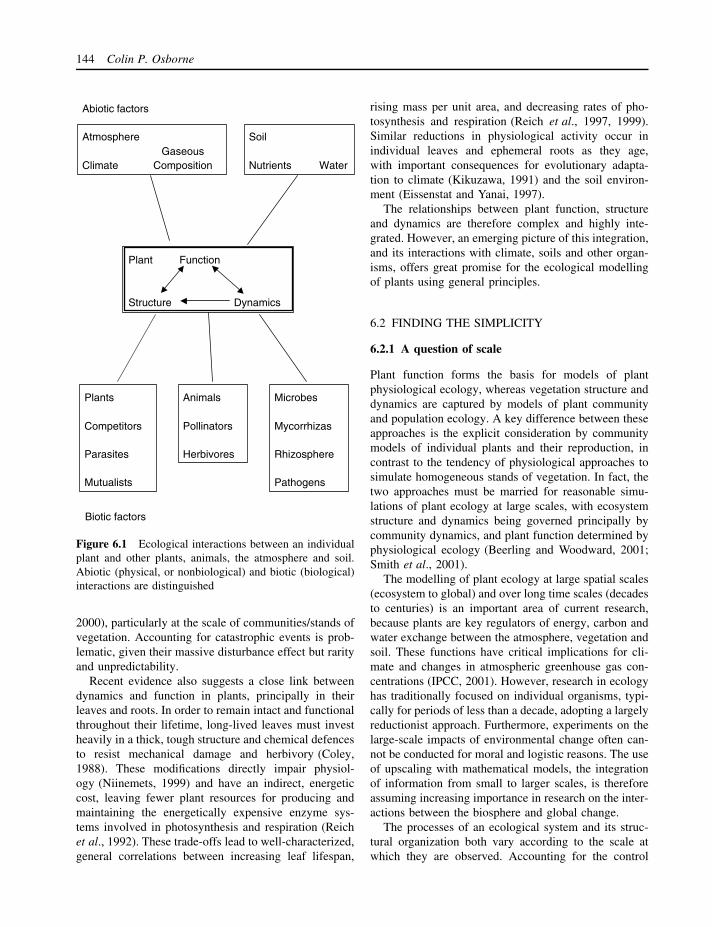
144 Colin P. Osborne
Plant Function
Structure Dynamics
AtmosphereGaseous
Climate Composition
Animals
Pollinators
Herbivores
Plants
Competitors
Parasites
Mutualists
Soil
Nutrients Water
Microbes
Mycorrhizas
Rhizosphere
Pathogens
Abiotic factors
Biotic factors
Figure 6.1 Ecological interactions between an individualplant and other plants, animals, the atmosphere and soil.Abiotic (physical, or nonbiological) and biotic (biological)interactions are distinguished
2000), particularly at the scale of communities/stands ofvegetation. Accounting for catastrophic events is prob-lematic, given their massive disturbance effect but rarityand unpredictability.
Recent evidence also suggests a close link betweendynamics and function in plants, principally in theirleaves and roots. In order to remain intact and functionalthroughout their lifetime, long-lived leaves must investheavily in a thick, tough structure and chemical defencesto resist mechanical damage and herbivory (Coley,1988). These modifications directly impair physiol-ogy (Niinemets, 1999) and have an indirect, energeticcost, leaving fewer plant resources for producing andmaintaining the energetically expensive enzyme sys-tems involved in photosynthesis and respiration (Reichet al., 1992). These trade-offs lead to well-characterized,general correlations between increasing leaf lifespan,
rising mass per unit area, and decreasing rates of pho-tosynthesis and respiration (Reich et al., 1997, 1999).Similar reductions in physiological activity occur inindividual leaves and ephemeral roots as they age,with important consequences for evolutionary adapta-tion to climate (Kikuzawa, 1991) and the soil environ-ment (Eissenstat and Yanai, 1997).
The relationships between plant function, structureand dynamics are therefore complex and highly inte-grated. However, an emerging picture of this integration,and its interactions with climate, soils and other organ-isms, offers great promise for the ecological modellingof plants using general principles.
6.2 FINDING THE SIMPLICITY
6.2.1 A question of scale
Plant function forms the basis for models of plantphysiological ecology, whereas vegetation structure anddynamics are captured by models of plant communityand population ecology. A key difference between theseapproaches is the explicit consideration by communitymodels of individual plants and their reproduction, incontrast to the tendency of physiological approaches tosimulate homogeneous stands of vegetation. In fact, thetwo approaches must be married for reasonable simu-lations of plant ecology at large scales, with ecosystemstructure and dynamics being governed principally bycommunity dynamics, and plant function determined byphysiological ecology (Beerling and Woodward, 2001;Smith et al., 2001).
The modelling of plant ecology at large spatial scales(ecosystem to global) and over long time scales (decadesto centuries) is an important area of current research,because plants are key regulators of energy, carbon andwater exchange between the atmosphere, vegetation andsoil. These functions have critical implications for cli-mate and changes in atmospheric greenhouse gas con-centrations (IPCC, 2001). However, research in ecologyhas traditionally focused on individual organisms, typi-cally for periods of less than a decade, adopting a largelyreductionist approach. Furthermore, experiments on thelarge-scale impacts of environmental change often can-not be conducted for moral and logistic reasons. The useof upscaling with mathematical models, the integrationof information from small to larger scales, is thereforeassuming increasing importance in research on the inter-actions between the biosphere and global change.
The processes of an ecological system and its struc-tural organization both vary according to the scale atwhich they are observed. Accounting for the control

Modelling the Ecology of Plants 145
of ecological processes by the appropriate negative andpositive feedbacks is particularly important for upscal-ing, since they vary greatly in significance with scale.In the case of the structural organization of ecologi-cal systems, accounting for heterogeneity can be criticalfor accurate upscaling, especially if properties of thesystem show nonlinear responses to structural changes.For example, the clumping of leaves within a vege-tation canopy, the clustering of individuals within aplant community and the patches of different vegeta-tion types within a landscape all significantly modifythe absorption of solar radiation by vegetation in com-parison with uniform distributions of each (Asner et al.,1998). This modification occurs because absorption withrespect to leaf area is nonlinear. Good estimates ofsolar energy absorption are vital in models of vegeta-tion function because this energy source is the driver ofphotosynthesis. Heterogeneity in the absorption of solarenergy therefore has important consequences for boththe upscaling of energy balance and photosynthesis, andfor the downscaling of satellite remote sensing measure-ments. Scaling in models of plant ecology is discussedin greater depth by Jarvis (1995).
6.2.2 What are the alternatives for modellingplant function?
The remainder of this chapter focuses on the mod-elling of plant physiological ecology, however, many ofthe principles covered have a more general application.The reader is referred to Pacala (1997) for an intro-duction to the modelling of plant-community dynamicsand to Silvertown and Lovett-Doust (1993) for infor-mation on the simulation of plant-population biology.Approaches to modelling plant physiological ecologymay be grouped into three broad categories: mechanis-tic, teleonomic and empirical (Thornley and Johnson,1990). Each differs in the extent to which it accountsfor causal mechanisms, and is best viewed as a con-venient way to describe the philosophy underpinning aparticular model, rather than a rigid way of defining it.
The mechanistic approach is reductionist, seekingto build models based on plant processes occurringat lower spatial and temporal scales than the scaleof interest (Loomis et al., 1979). In the case of awhole plant or its organs (e.g. leaves and roots), thisinvolves an explicit consideration of the physiological orbiochemical pathways involved. A mechanistic model ismore flexible in its usage than the other two approachesbecause, by considering the way in which an ecologicalsystem works, it permits limited extrapolation to newcircumstances. In addition, by providing insight into the
operation of this system, it is a useful investigative toolfor explaining ecological phenomena.
Many aspects of plant ecology cannot be describedusing mechanistic models because their operation is justtoo poorly understood. However, if the net outcome ofa process is well described, a model can be devisedto reproduce this end-point. Such a ‘goal-directed’, orteleonomic model empirically simulates the operationof a plant process and its relationship with externalfactors such as climate, without describing the underly-ing physiological or biochemical mechanisms, i.e. howthis outcome is reached (Thornley and Johnson, 1990).For example, while the physiological mechanisms con-trolling the acquisition of carbon in photosynthesis arewell characterized, those involved in the partitioningof this carbon between the growth of different plantorgans remain poorly understood. Partitioning dependson the balance between carbon supply from photosyn-thesis, its demand in the growth of specific plant organsand its rate of transport through plant vascular sys-tems (Farrar and Jones, 2000). However, models basedon these principles remain largely theoretical and, whilethey are useful tools for interpreting and investigatingplant physiology, remain impractical for most ecologicalapplications (Minchin et al., 1993; Bidel et al., 2000).
By contrast, the relative proportions of plant car-bon in each organ type (e.g. leaves, roots, stem) arebroadly predictable within a particular environment andconsistent between species (Friedlingstein et al., 1999).These generalized relationships have long been utilizedin teleonomic models of carbon partitioning, followinga functional approach (Woodward and Osborne, 2000).Carbon is invested predominantly in organs that acquirethe most limiting resource for plant growth so that,say, in a nutrient-limited ecosystem, root growth isfavoured over stem and leaf growth. This leads to anincrease in root:shoot ratio that is typical of nutrient-limited plants (Gleeson, 1993). A functional scheme ofthis type has recently met reasonable success in a globalmodel for terrestrial vegetation, which simulates car-bon partitioning relative to light, water and nitrogenavailability (Friedlingstein et al., 1999). Presumably this‘optimization’ of plant resources mimics the evolution-ary process at some level, because it represents themost efficient use of carbon, maximizing reserves forreproduction or the survival of extreme conditions, andthereby increasing fitness.
A purely empirical model takes no account of theprocesses underlying the aspect of plant ecology beingsimulated, although biological meaning may be attachedto the mathematical formula used. For example, thezero intercept of a curve relating the abundance of a

146 Colin P. Osborne
species to mean annual temperature (MAT) presumablyreflects some critical threshold of plant cold tolerance.However, it is unlikely to be the MAT per se that limitsabundance, but rather the minimum winter temperature,a feature of climate that correlates reasonably wellwith the mean. Although this results in a mathematicalrelationship between plant abundance and MAT, thetwo are not causally linked. In this case, a teleonomicmodel would recognize a linkage between minimumtemperature and the tolerance or resistance of a plantto freezing, but would not account for the physiologicalmechanisms responsible (Woodward, 1987). In theory, afully mechanistic model would simulate the freezing ofplant tissues and the lethal effects of cellular desiccationand damage caused by ice crystals, but these processesare insufficiently understood for such an approach to bepractical (ibid.).
As a descriptive tool for making broad generaliza-tions, a purely empirical model may be both prac-tical and useful, but gives no information beyondthe data used in its construction (Thornley and John-son, 1990). For example, the net primary productiv-ity (NPP) or ‘annual growth’ of terrestrial biomes isbroadly related to mean annual precipitation (MAP)and MAT (Lieth, 1975). These relationships can there-fore be used to produce integrated estimates of today’sglobal NPP, an approach that shows reasonable agree-ment with two independent assessments (Figure 6.2).
Time period
GlacialHolocenePresent
Glo
bal N
PP
(P
g C
y−1
)
0
20
40
60
80
100Lieth modelWoodward modelsatellite-based
Figure 6.2 Estimates of global net primary productiv-ity (NPP) for terrestrial vegetation during the present,mid-Holocene (6000 years before present, BP) and lastGlacial (21 000 years BP) time periods. These were madeusing either an empirical model based on modern veg-etation–climate relationships (Lieth, 1975), a mechanis-tic model of vegetation function (Beerling, 1999), or amethod for inferring vegetation activity from satellite-basedreflectance measurements (Field et al., 1998)
However, without the explanatory detail of a mecha-nistic approach, an empirical model is unlikely to bereliable as a predictive or explanatory tool when con-ditions are encountered beyond those used to fit modelrelationships. The Lieth method suggests high valuesof global NPP during the last ice age and the subse-quent warm mid-Holocene period compared with thepresent (see Figure 6.2). These changes would havebeen driven by the warmer or wetter past climate. Bycontrast, a sophisticated mechanistic model (Woodwardet al., 1995) estimates significantly reduced NPP dur-ing both the mid-Holocene and last ice age comparedwith the present (see Figure 6.2; Beerling, 1999). Thecause of this marked qualitative difference is a fail-ure of the empirical model to account for atmosphericCO2 concentration, which was 45% (glacial) and 27%(Holocene) lower than at present. Experiments demon-strate a severe limitation of growth by these concen-trations (Polley et al., 1993), suggesting that estimatesusing the mechanistic model are more likely, since theyaccount for the interacting influences of CO2, temper-ature and precipitation (Woodward et al., 1995). Formost ecological purposes, some consideration of mech-anisms is therefore advantageous, and the remainderof this section discusses the practical application ofthis approach.
6.2.3 Applying a mechanistic approach
The problems, practicalities and compromises involvedin applying a mechanistic approach are well illustratedby reference to the example of leaf-nitrogen content. Theconcentration of nitrogen within plant foliage is a keycomponent of many process-based models of plant ecol-ogy, because it has critical physiological implications atthe leaf scale, but is closely coupled with processes atwhole-plant and ecosystem scales (Osborne and Beer-ling, 2002a). At the leaf scale, nitrogen concentrationis tightly linked with physiological function, becausethe proteins required for photosynthesis are rich in theelement (Evans, 1989), and tissues high in protein aremetabolically expensive to maintain (Penning de Vries,1975). Nitrogen also has important effects on the con-sumption of leaves by herbivores, although the mecha-nisms at work remain unclear (Hartley and Jones, 1997).The availability of nitrogen is a primary limitation onplant growth in natural ecosystems because soil reser-voirs of mineral nitrogen are highly mobile, and regu-lated by the biological mineralization of organic mat-ter (Vitousek and Howarth, 1991). Foliar nitrogen con-centration is therefore closely related to the limitationof growth rate at the whole-plant scale, and the leaves
Modelling the Ecology of Plants 147
of plants growing in nitrogen-poor soils tend to havea lower nitrogen content than those of well-nourishedplants (Gutschick, 1993). At the ecosystem scale, differ-ences in nitrogen concentration between species reflectcontrasting ecological strategies with, for example, ever-green plants on infertile or dry soils tending to havelower concentrations than their deciduous counterpartson more fertile or wetter sites (Aerts, 1995). The nitro-gen content of a leaf has further implications after itsabscission, being an important correlate of leaf litterdecomposition rate (Aerts, 1997), and hence nitrogencycling within the soil. An accurate estimate of leaf-nitrogen concentration is therefore vital for reasonablesimulations of a whole suite of physiological, plant andecosystem processes.
Model estimates of leaf-nitrogen concentration gen-erally follow one of two approaches. Both are widelyused in plant ecological modelling, with the aim ofsimplifying the vast range of plant form and functioninto a manageable and well-characterized scheme, whileretaining a realistic representation of biological diver-sity (Woodward and Beerling, 1997):
1. A division of plants into ‘functional types’ or‘functional groups’, using shared physiological andecological responses to the biotic or abiotic environ-ment (Smith et al., 1997). Classification schemes aredesigned according to functional responses that areof particular interest and, for this reason, may dif-fer significantly between models, even for the samebiome (e.g. Pausas, 1999; Osborne et al., 2000). Sup-port for classifications based on climate comes fromthe observation that plants of taxonomically distantspecies growing in similar, but geographically sepa-rated, climates tend to evolve comparable suites ofphysical characteristics (Wolfe, 1985). This conver-gence suggests that evolution in each climate regimeis constrained by the same basic limitations of plantphysiological ecology. In the case of leaf-nitrogenconcentration, functional groups or individual speciesmay each be assigned a value based on direct mea-surements.
2. The definition of general rules that can be safelyapplied to a wide range of plants. In seeking thisgoal, a common approach is to attempt simulationsof plant structure, function and dynamics in terms ofthe underlying, causal mechanisms (e.g. Woodwardet al., 1995; Osborne et al., 2000). This method ispowerful because, at a physiological or biochemicallevel, there may be a high degree of similaritybetween plants from disparate groups, suggestingminimal evolutionary radiation in some of these basic
properties (e.g. Larcher, 1994; Long et al., 1996).For example, leaf-nitrogen concentration is correlatedstrongly with the rate of plant-nitrogen uptake, andthe latter can be simulated using soil propertiesand temperature using a basic understanding ofroot associations with mycorrhizal fungi (Woodwardet al., 1995).
The mechanistic model of photosynthesis developedby Farquhar and co-workers (Farquhar et al., 1980;von Caemmerer, 2000) is proven and widely used, andillustrates further some of the advantages and problemsin adopting a process-based approach. Photosynthesisfixes gaseous CO2 to form sugars, which are used tofuel plant growth and ultimately feed most organisms inevery ecosystem. It is a complex, highly integrated phys-iological process, involving numerous interacting bio-chemical pathways (Baker, 1996). Despite this complex-ity, it can be simulated accurately by representing reg-ulation in only a few key steps (Farquhar et al., 1980).Scaling up from biochemical reactions to photosynthesisby the whole leaf turns out to be straightforward becausethe physiology of cells adjusts to the profile of absorbedlight in the leaf (Farquhar, 1989). Further scaling of themodel to whole plant canopies is more difficult, but pos-sible given appropriate estimates of light absorption andphysiological properties (de Pury and Farquhar, 1997).The Farquhar model has therefore proved useful at cel-lular, leaf and whole plant scales and, in the 20 yearssince its first publication, has been widely adopted bythe plant ecology modelling community (Farquhar et al.,2001). An important reason for its appeal is the highlyconserved nature of many simulated processes, allowingthe same equations and constant parameters to be usedfor a wide range of species – a useful property in eco-logical modelling. For example, catalysis by the primaryenzyme responsible for fixing CO2 into sugars is simi-lar in diverse plant species (Parry et al., 1989; Delgadoet al., 1995).
Farquhar’s model has been widely applied at globaland regional scales, where it forms the basis for severalimportant models of the interactions between terrestrialbiosphere and climate (Sellers et al., 1996; Betts et al.,1997; Cox et al., 2000). The model performs adequatelyin the context of these applications, operating witha temporal resolution of 30–60 minutes. By contrast,during very short periods in a rapidly changing lightregime as experienced on a forest floor, the dynamicsof photosynthesis become critical, and the basic modelrequires refinement (Cheeseman and Lexa, 1996). Forbetter reliability in these conditions, it must be modifiedusing empirical functions and parameters with no direct
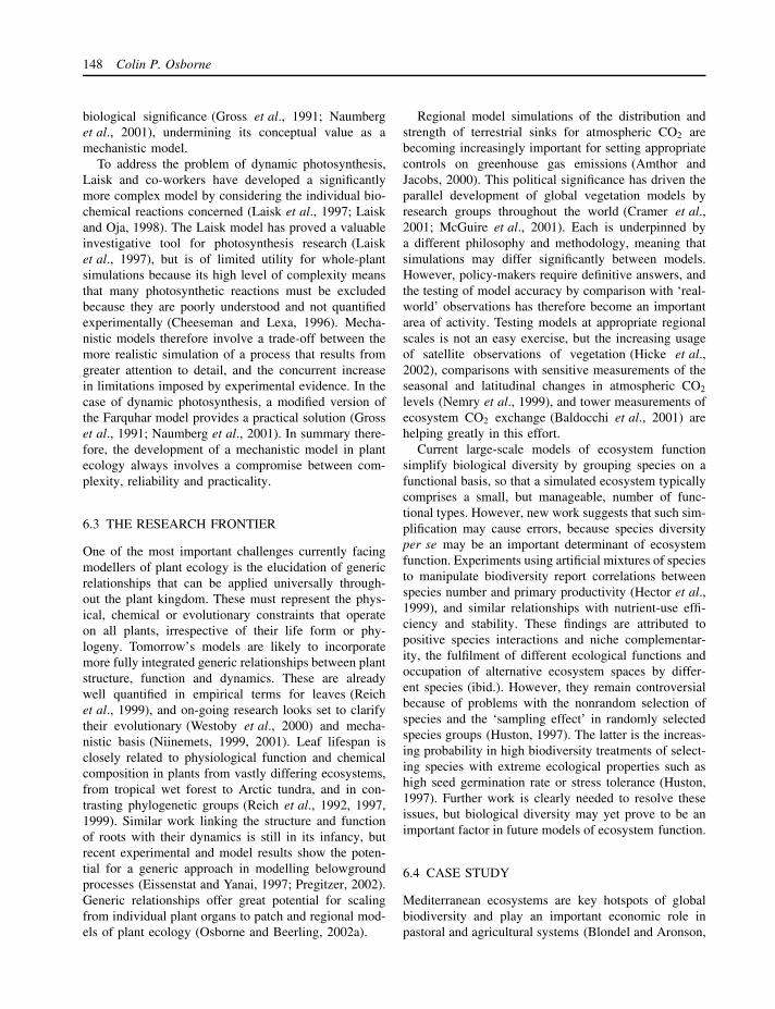
148 Colin P. Osborne
biological significance (Gross et al., 1991; Naumberget al., 2001), undermining its conceptual value as amechanistic model.
To address the problem of dynamic photosynthesis,Laisk and co-workers have developed a significantlymore complex model by considering the individual bio-chemical reactions concerned (Laisk et al., 1997; Laiskand Oja, 1998). The Laisk model has proved a valuableinvestigative tool for photosynthesis research (Laisket al., 1997), but is of limited utility for whole-plantsimulations because its high level of complexity meansthat many photosynthetic reactions must be excludedbecause they are poorly understood and not quantifiedexperimentally (Cheeseman and Lexa, 1996). Mecha-nistic models therefore involve a trade-off between themore realistic simulation of a process that results fromgreater attention to detail, and the concurrent increasein limitations imposed by experimental evidence. In thecase of dynamic photosynthesis, a modified version ofthe Farquhar model provides a practical solution (Grosset al., 1991; Naumberg et al., 2001). In summary there-fore, the development of a mechanistic model in plantecology always involves a compromise between com-plexity, reliability and practicality.
6.3 THE RESEARCH FRONTIER
One of the most important challenges currently facingmodellers of plant ecology is the elucidation of genericrelationships that can be applied universally through-out the plant kingdom. These must represent the phys-ical, chemical or evolutionary constraints that operateon all plants, irrespective of their life form or phy-logeny. Tomorrow’s models are likely to incorporatemore fully integrated generic relationships between plantstructure, function and dynamics. These are alreadywell quantified in empirical terms for leaves (Reichet al., 1999), and on-going research looks set to clarifytheir evolutionary (Westoby et al., 2000) and mecha-nistic basis (Niinemets, 1999, 2001). Leaf lifespan isclosely related to physiological function and chemicalcomposition in plants from vastly differing ecosystems,from tropical wet forest to Arctic tundra, and in con-trasting phylogenetic groups (Reich et al., 1992, 1997,1999). Similar work linking the structure and functionof roots with their dynamics is still in its infancy, butrecent experimental and model results show the poten-tial for a generic approach in modelling belowgroundprocesses (Eissenstat and Yanai, 1997; Pregitzer, 2002).Generic relationships offer great potential for scalingfrom individual plant organs to patch and regional mod-els of plant ecology (Osborne and Beerling, 2002a).
Regional model simulations of the distribution andstrength of terrestrial sinks for atmospheric CO2 arebecoming increasingly important for setting appropriatecontrols on greenhouse gas emissions (Amthor andJacobs, 2000). This political significance has driven theparallel development of global vegetation models byresearch groups throughout the world (Cramer et al.,2001; McGuire et al., 2001). Each is underpinned bya different philosophy and methodology, meaning thatsimulations may differ significantly between models.However, policy-makers require definitive answers, andthe testing of model accuracy by comparison with ‘real-world’ observations has therefore become an importantarea of activity. Testing models at appropriate regionalscales is not an easy exercise, but the increasing usageof satellite observations of vegetation (Hicke et al.,2002), comparisons with sensitive measurements of theseasonal and latitudinal changes in atmospheric CO2
levels (Nemry et al., 1999), and tower measurements ofecosystem CO2 exchange (Baldocchi et al., 2001) arehelping greatly in this effort.
Current large-scale models of ecosystem functionsimplify biological diversity by grouping species on afunctional basis, so that a simulated ecosystem typicallycomprises a small, but manageable, number of func-tional types. However, new work suggests that such sim-plification may cause errors, because species diversityper se may be an important determinant of ecosystemfunction. Experiments using artificial mixtures of speciesto manipulate biodiversity report correlations betweenspecies number and primary productivity (Hector et al.,1999), and similar relationships with nutrient-use effi-ciency and stability. These findings are attributed topositive species interactions and niche complementar-ity, the fulfilment of different ecological functions andoccupation of alternative ecosystem spaces by differ-ent species (ibid.). However, they remain controversialbecause of problems with the nonrandom selection ofspecies and the ‘sampling effect’ in randomly selectedspecies groups (Huston, 1997). The latter is the increas-ing probability in high biodiversity treatments of select-ing species with extreme ecological properties such ashigh seed germination rate or stress tolerance (Huston,1997). Further work is clearly needed to resolve theseissues, but biological diversity may yet prove to be animportant factor in future models of ecosystem function.
6.4 CASE STUDY
Mediterranean ecosystems are key hotspots of globalbiodiversity and play an important economic role inpastoral and agricultural systems (Blondel and Aronson,

Modelling the Ecology of Plants 149
1999). Continuing changes in the Mediterranean climatetherefore have potentially huge consequences for humansocieties in the region (Lavorel et al., 1998). Increasesin atmospheric CO2 and other greenhouse gases sincethe Industrial Revolution have caused regional warmingof around 0.5◦C and, more recently, a localized declinein precipitation (Kutiel et al., 1996; Esteban-Parra et al.,1998; Jones et al., 1999). These atmospheric and cli-matic trends are set to continue well into the twenty-first century (Palutikof et al., 1994), and have sharp-ened concern for the future welfare of Mediterraneanecosystems (Lavorel et al., 1998). The recent develop-ment of models designed to investigate the ecology ofvegetation in the region (Pausas, 1999; Osborne et al.,2000) is an important first step in assessing the scale ofthis problem.
Osborne et al. (2000) developed a patch-scalemodel of Mediterranean vegetation to examine climaticresponses of plants in the region, and evaluate thepotential mediating role of rising atmospheric CO2.This vegetation model was initially a componentof a landscape model, used in assessing land deg-radation (Kirkby et al., 1998), but was subsequentlyexpanded for independent applications (Osborne et al.,2000; Woodward and Osborne, 2000; Osborne andWoodward, 2001). Within the model, plant diversitywas managed by grouping species into functional typesbased on their physiological and life history responsesto drought. Some of these are illustrated in Figure 6.3.Seasonal drought is a characteristic feature of theMediterranean climate that has exerted a critical controlon the evolution of plant ecological strategies (Dallman,
(a)
(b)
(c)
Figure 6.3 Examples of functional types used in modelling and some key distinctions between them: (a) Evergreensclerophyllous shrub (Quercus coccifera in Murcia, Spain) – retains drought-tolerant foliage during the summer, and hasan extensive rooting system which maximizes access to soil water during this dry period; (b) Drought-deciduous shrub(Anthyllis cytisoides in Almeria, Spain) – sheds foliage at the beginning of summer, avoiding drought by remainingdormant until the autumn, when new shoot growth occurs; (c) Perennial tussock grass (Stipa tenacissima in Almeria,Spain) – has a much more limited capacity for the storage of energy reserves than shrubs, and a shallow, fibrous rootsystem, but is extremely drought-tolerant
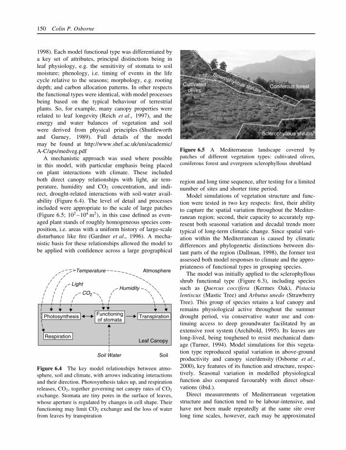
150 Colin P. Osborne
1998). Each model functional type was differentiated bya key set of attributes, principal distinctions being inleaf physiology, e.g. the sensitivity of stomata to soilmoisture; phenology, i.e. timing of events in the lifecycle relative to the seasons; morphology, e.g. rootingdepth; and carbon allocation patterns. In other respectsthe functional types were identical, with model processesbeing based on the typical behaviour of terrestrialplants. So, for example, many canopy properties wererelated to leaf longevity (Reich et al., 1997), and theenergy and water balances of vegetation and soilwere derived from physical principles (Shuttleworthand Gurney, 1989). Full details of the modelmay be found at http://www.shef.ac.uk/uni/academic/A-C/aps/medveg.pdf
A mechanistic approach was used where possiblein this model, with particular emphasis being placedon plant interactions with climate. These includedboth direct canopy relationships with light, air tem-perature, humidity and CO2 concentration, and indi-rect, drought-related interactions with soil-water avail-ability (Figure 6.4). The level of detail and processesincluded were appropriate to the scale of large patches(Figure 6.5; 102 –104 m2), in this case defined as even-aged plant stands of roughly homogeneous species com-position, i.e. areas with a uniform history of large-scaledisturbance like fire (Gardner et al., 1996). A mecha-nistic basis for these relationships allowed the model tobe applied with confidence across a large geographical
Functioningof stomata
Photosynthesis
Respiration
Transpiration
Soil Water
Temperature
Leaf Canopy
HumidityCO2
Light
Atmosphere
Soil
Figure 6.4 The key model relationships between atmo-sphere, soil and climate, with arrows indicating interactionsand their direction. Photosynthesis takes up, and respirationreleases, CO2, together governing net canopy rates of CO2
exchange. Stomata are tiny pores in the surface of leaves,whose aperture is regulated by changes in cell shape. Theirfunctioning may limit CO2 exchange and the loss of waterfrom leaves by transpiration
Sclerophyllous shrubs
Coniferous forestCultivatedolives
Sclerophyllous shrubs
Figure 6.5 A Mediterranean landscape covered bypatches of different vegetation types: cultivated olives,coniferous forest and evergreen sclerophyllous shrubland
region and long time sequence, after testing for a limitednumber of sites and shorter time period.
Model simulations of vegetation structure and func-tion were tested in two key respects: first, their abilityto capture the spatial variation throughout the Mediter-ranean region; second, their capacity to accurately rep-resent both seasonal variation and decadal trends moretypical of long-term climatic change. Since spatial vari-ation within the Mediterranean is caused by climaticdifferences and phylogenetic distinctions between dis-tant parts of the region (Dallman, 1998), the former testassessed both model responses to climate and the appro-priateness of functional types in grouping species.
The model was initially applied to the sclerophyllousshrub functional type (Figure 6.3), including speciessuch as Quercus coccifera (Kermes Oak), Pistacialentiscus (Mastic Tree) and Arbutus unedo (StrawberryTree). This group of species retains a leaf canopy andremains physiological active throughout the summerdrought period, via conservative water use and con-tinuing access to deep groundwater facilitated by anextensive root system (Archibold, 1995). Its leaves arelong-lived, being toughened to resist mechanical dam-age (Turner, 1994). Model simulations for this vegeta-tion type reproduced spatial variation in above-groundproductivity and canopy size/density (Osborne et al.,2000), key features of its function and structure, respec-tively. Seasonal variation in modelled physiologicalfunction also compared favourably with direct obser-vations (ibid.).
Direct measurements of Mediterranean vegetationstructure and function tend to be labour-intensive, andhave not been made repeatedly at the same site overlong time scales, however, each may be approximated

Modelling the Ecology of Plants 151
using an indirect technique. First, canopy size and lightabsorption may be assessed with satellite remote sens-ing. Since appropriate satellite records are available from1981, this allows canopy properties to be studied on adecadal time scale (Myneni et al., 1997, 1998). Second,leaf physiological function can be investigated usingits stable carbon isotope content. Herbarium specimensfrom the same geographical area, dating from the nine-teenth and twentieth centuries, permit centennial-scalereconstructions of leaf physiological function using thistechnique (Penuelas and Azcon-Bieto, 1992; Beerlingand Woodward, 1995). Since reconstructed climatolo-gies for the Mediterranean region now stretch from1901 to the present day (New et al., 2000), model sim-ulations may be compared with these findings. Themodel’s mechanistic basis means that the properties ofleaf canopies measured by satellite can be explicitly sim-ulated from first principles, allowing direct comparisonbetween model and satellite data (Figure 6.6). Similarly,mechanistic modelling of leaf physiology allows stablecarbon-isotope discrimination by key leaf processes tobe simulated, and direct comparison between model andherbarium leaf isotope compositions (Figure 6.7). Bothcomparisons have revealed good agreement between themagnitude of, and trends in, observed and modelledvalues (Figures 6.6 and 6.7), supporting long-term sim-ulations of canopy structure and function with twentieth-century global change. Because the model has a mech-anistic basis, these trends can be interpreted in termsof the underlying control of vegetation properties byclimate and atmospheric CO2.
Model simulations for Mediterranean sclerophyllousshrubland have produced two key findings. First, thatwater availability, rather than temperature, exerts thedominant control on both canopy size and productiv-ity in this vegetation type (Osborne and Woodward,2001). This result provides the first confirmation andquantification of this control on a decadal time scale.Second, it suggests that rising concentrations of atmo-spheric CO2 have significantly altered plant water-use,increasing carbon fixation in relation to water loss, andoffsetting the negative impacts on plant growth of allbut the harshest droughts (Osborne et al., 2000). Underthese severe droughts, CO2 had no effect on simu-lated growth. Modelled effects occurred during the past50 years, in response to a modest increase in CO2 from300 to 365 ppm, and demonstrate the extreme sensitivityof water-limited Mediterranean shrubland to concentra-tions of the gas.
Interestingly, since these model results were first pub-lished, similar interactions between CO2 and droughthave been observed experimentally for the desert shrub
Figure 6.6 Model testing using a time series of satel-lite measurements. (a) Reflectivity by a typical leaf andsoil at a range of wavelengths. By measuring radia-tion reflected in the visible and near infrared wavebandsfrom the land surface, a satellite may detect the den-sity of leaves covering a particular area. Soil and leavesreflect visible radiation approximately equally, but differstrongly in their reflectance of near infrared. The differencebetween measurements of these wavebands therefore indi-cates green plant cover, and is standardised to produce thenormalized-difference vegetation index (NDVI). (b) Com-parison of NDVI measured by US weather satellites overthe Mediterranean region, and NDVI calculated using sim-ulated canopy properties in the vegetation model (redrawnfrom Woodward & Osborne, 2000)Source: Reproduced by permission of Blackwell Publishing
Larrea tridentata in Nevada. In a year when annual rain-fall was typical of a moderate Mediterranean droughtbut wet for the desert site, shoot growth doubled withan increase in CO2 from 365 to 550 ppm (Smith et al.,2000). By contrast, growth was completely unrespon-sive to CO2 under severe drought conditions, whichoccur only rarely in the Mediterranean (Osborne et al.,
[Image not available in this electronic edition.]

152 Colin P. Osborne
Figure 6.7 Leaf discrimination against the heavy isotopeof carbon (13C, top), and instantaneous leaf water-use effi-ciency (IWUE, bottom). A comparison is made betweenvalues derived from herbarium specimens of four sclero-phyllous shrub species, collected at intervals during thetwentieth century, and values calculated using the vege-tation model. Stable carbon-isotope composition reflectsthe efficiency of water-use during leaf growth, followinga well-characterized relationship (Farquhar et al., 1989)Source: Reproduced from Osborne et al. (2000) by permis-sion of Blackwell Science Ltd
2000), but were typical of the desert environment (Smithet al., 2000). Thus experimental observations replicatedmodelled growth characteristics, providing further inde-pendent support for these simulations.
6.5 CONCLUSION
Mechanistic models provide a useful means of integrat-ing our current knowledge of plant ecology, allowinginvestigations at large spatial and temporal scales that
are technically and ethically difficult with experiments,or simply impossible. Comparison of simulations bythese models with large-scale field observations of veg-etation provides both confidence in their results andinsight into the drivers and mechanisms of change. On-going developments in vegetation modelling focus onthe inter-relationships between plant structure, functionand dynamics, and aim to produce widely applicable,generic models. Until such generic relationships aredeveloped, the modelling of plant ecology using func-tional groups of species provides a practical way of sim-plifying biological complexity, while retaining a realisticdescription of functional diversity.
ACKNOWLEDGEMENTS
I thank David Beerling for helpful suggestions, dis-cussion and financial support during the preparation ofthis manuscript, Ian Woodward for his comments, JosepPenuelas for access to stable carbon-isotope data, andGlyn Woods for help in preparing the illustrations. Fund-ing from the European Community Environment Pro-gramme, Mediterranean Desertification and Land Use(MEDALUS) Project supported the modelling work onMediterranean vegetation.
REFERENCES
Aerts, R. (1995) The advantages of being evergreen, Trends inEcology and Evolution 10, 502–507.
Aerts, R. (1997) Nitrogen partitioning between resorption anddecomposition pathways: a trade-off between nitrogen-useefficiency and litter decomposibility?, Oikos 80, 603–606.
Aerts, R. and Chapin, F.S. (2000) The mineral nutrition of wildplants revisited: a re-evaluation of processes and patterns,Advances in Ecological Research 30, 1–67.
Amthor, J.S. (2000) The McCree-de Wit-Penning de Vries-Thornley respiration paradigms: 30 years later, Annals ofBotany 86, 1–20.
Amthor, J.S. and Jacobs, G.K. (2000) Carbon sequestrationin terrestrial ecosystems: goals, processes, and limits, Eos,Transactions of the American Geophysical Union 81 (suppl.),F245.
Archibold, O.W. (1995) Ecology of World Vegetation, Chap-man & Hall, London.
Asner, G.P., Wessman, C.A. and Archer, S. (1998) Scaledependence of absorption of photosynthetically active radi-ation in terrestrial ecosystems, Ecological Applications 8,1003–1021.
Baker, N.R. (ed.) (1996) Photosynthesis and the Environment,Kluwer Academic Publishers, Dordrecht.
Baldocchi, D., Falge, E., Gu, L., Olson, R., Hollinger, D., Run-ning, S., Anthoni, P., Bernhofer, C., Davis, K., Evans, R.,Fuentes, J., Goldstein, A., Katul, G., Law, B., Lee, X.,
[Image not available in this electronic edition.]
Modelling the Ecology of Plants 153
Malhi, Y., Meyers, T., Munger, W., Oechel, W., Paw, K.T.,Pilegaard, K., Schmid, H.P., Valentini, R., Verma, S., Ve-sala, T., Wilson, K. and Wofsy, S. (2001) FLUXNET: anew tool to study the temporal and spatial variability ofecosystem-scale carbon dioxide, water vapor, and energy fluxdensities, Bulletin of the American Meteorological Society82, 2415–2434.
Beerling, D.J. (1999) New estimates of carbon transfer toterrestrial ecosystems between the last glacial maximum andthe Holocene, Terra Nova 11, 162–167.
Beerling, D.J., Osborne, C.P. and Chaloner, W.G. (2001) Evo-lution of leaf form in land plants linked to atmospheric CO2
decline in the Late Palaeozoic era, Nature 410, 352–354.Beerling, D.J. and Woodward, F.I. (1995) Leaf stable carbon
isotope composition records increased water-use efficiencyof C3 plants in response to atmospheric CO2 enrichment,Functional Ecology 9, 394–401.
Beerling, D.J. and Woodward, F.I. (2001) Vegetation and theTerrestrial Carbon Cycle, Cambridge University Press, Cam-bridge.
Betts, R.A., Cox, P.M., Lee, S.E. and Woodward, F.I. (1997)Contrasting physiological and structural vegetation feed-backs in climate change simulations, Nature 387, 796–799.
Bidel, L.P.R., Pages, L., Riviere, L.M., Pelloux, G. and Loren-deau, J.Y. (2000) MassFlowDyn I: a carbon transport andpartitioning model for root system architecture, Annals ofBotany 85, 869–886.
Blondel, J. and Aronson, J. (1999) Biology and Wildlife of theMediterranean Region, Oxford University Press, Oxford.
Cheeseman, J.M. and Lexa, M. (1996) Gas exchange: modelsand measurements, in N.R. Baker (ed.) Photosynthesis andthe Environment, Kluwer Academic Publishers, Dordrecht,223–240.
Coley, P.D. (1988) Effects of plant growth rate and leaf lifetimeon the amount and type of anti-herbivore defence, Oecologia74, 531–536.
Cox, P.M., Betts, R.A., Jones, C.D., Spall, S.A., Totterdell, I.J.(2000) Acceleration of global warming due to carbon-cyclefeedbacks in coupled climate model, Nature 408, 184–187.
Cramer, W., Bondeau, A., Woodward, F.I., Prentice, I.C.,Betts, R.A., Brovkin, V., Cox, P.M., Fisher, V., Foley, J.A.,Friend, A.D., Kucharik, C., Lomas, M.R., Ramankutty, N.,Sitch, S., Smith, B., White, A. and Young-Molling, C.(2001) Global response of terrestrial ecosystem structureand function to CO2 and climate change: results from sixdynamic global vegetation models Global Change Biology7, 357–373.
Dallman, P.R. (1998) Plant Life in the World’s MediterraneanClimates, Oxford University Press, Oxford.
Delgado, E., Medrano, H., Keys, A.J. and Parry, M.A.J. (1995)Species variation in Rubisco specificity factor, Journal ofExperimental Botany 46, 1775–1777.
de Pury, D.G.G. and Farquhar, G.D. (1997) Simple scaling ofphotosynthesis from leaves to canopies without the errors ofbig-leaf models, Plant Cell and Environment 20, 537–557.
Eissenstat, D.M. and Yanai, R.D. (1997) The ecology of rootlifespan, Advances in Ecological Research 27, 1–60.
Esteban-Parra, M.J., Rodrigo, F.S. and Castro-Diez, Y. (1998)Spatial and temporal patterns of precipitation in Spain forthe period 1880–1992, International Journal of Climatology18, 1557–1574.
Evans, J.R. (1989) Photosynthesis and nitrogen relationships inleaves of C3 plants, Oecologia 78, 9–19.
Farquhar, G.D. (1989) Models of integrated photosynthesis ofcells and leaves, Philosophical Transactions of the RoyalSociety of London, Series B 323, 357–367.
Farquhar, G.D., von Caemmerer, S. and Berry, J.A. (1980) Abiochemical model of photosynthetic CO2 assimilation inleaves of C3 species, Planta 149, 78–90.
Farquhar, G.D., von Caemmerer, S. and Berry, J.A. (2001)Models of photosynthesis, Plant Physiology 125, 42–45.
Farrar, J.F. and Jones, D.L. (2000) The control of carbonacquisition by roots, New Phytologist 147, 43–53.
Field, C.B., Behrenfield, M.J., Randerson, J.T. and Falkow-ski, P. (1998) Primary production of the biosphere: inte-grating terrestrial and oceanic components, Science 281,237–240.
Friedlingstein, P., Joel, G., Field, C.B. and Fung, I.Y. (1999)Toward an allocation scheme for global terrestrial carbonmodels, Global Change Biology 5, 755–770.
Gardner, R.H., Hargrove, W.W., Turner, M.G. and Romme,W.H. (1996) Climate change, disturbances and landscapedynamics, in B. Walker and W. Steffan (eds) Global Changeand Terrestrial Ecosystems, Cambridge University Press,Cambridge, 149–172.
Gleeson, S.K. (1993) Optimization of tissue nitrogen and root-shoot allocation, Annals of Botany 71, 23–31.
Gower, S.T., Vogel, J.G., Norman, J.M., Kucharik, C.J., Steele,S.J. and Stow, T.K. (1997) Carbon distribution and above-ground net primary production in aspen, jack pine, and blackspruce stands in Saskatchewan and Manitoba, Canada, Jour-nal of Geophysical Research 102, D24, 29029–29041.
Gross, L.J., Kirschbaum, M.U.F. and Pearcy, R.W. (1991) Adynamic model of photosynthesis in varying light takingaccount of stomatal conductance, C3-cycle intermediates,photorespiration and Rubisco activation, Plant, Cell andEnvironment 14, 881–893.
Gutschick, V.P. (1993) Nutrient-limited growth rates: roles ofnutrient-use efficiency and of adaptations to increase uptakerate, Journal of Experimental Botany 44, 41–51.
Hartley, S.E. and Jones, C.G. (1997) Plant chemistry andherbivory, or why the world is green, in M.J. Crawley (ed.)Plant Ecology, Blackwell Science, Oxford, 284–324.
Hector, A., Schmid, B., Beierkuhnlein, C., Caldeira, M.C.,Diemer, M., Dimitrakopoulos, P.G., Finn, J.A., Freitas, H.,Giller, P.S., Good, J., Harris, R., Hogberg, P., Huss-Dan-ell, K., Joshi, J., Jumpponen, A., Korner, C., Leadley, P.W.,Loreau, M., Minns, A., Mulder, C.P.H., O’Donovan, G.,Otway, S.J., Pereira, J.S., Prinz, A., Read, D.J., Scherer-Lorenzen, M., Schulze, E.D., Siamantziouras, A.S.D., Spehn,E.M., Terry, A.C., Troumbis, A.Y., Woodward, F.I., Yachi, S.and Lawton, J.H. (1999) Plant diversity and productiv-ity experiments in European grasslands, Science 286,1123–1127.

154 Colin P. Osborne
Hester, A.J., Edenius, L., Buttenschon, R.M. and Kuiters, A.T.(2000) Interactions between forests and herbivores: the roleof controlled grazing experiments, Forestry 73, 381–391.
Hicke, J.A., Asner, G.P., Randerson, J.T., Tucker, C., Los, S.,Birdsey, R., Jenkins, J.C., Field, C. and Holland, E. (2002)Satellite-derived increases in net primary productivity acrossNorth America, 1982–1998, Geophysical Research Letters29, 10.1029/2001GL013578.
Huston, M.A. (1997) Hidden treatments in ecological experi-ments: re-evaluating the ecosystem function of biodiversity,Oecologia 110, 449–460.
IPCC (2001) Climate Change 2001: The Scientific Basis.Contribution of Working Group I to the Third AssessmentReport of the Intergovernmental Panel on Climate Change,J.T. Houghton, Y. Ding, D.J. Griggs, M. Noguer, P.J. vander Linden, X. Dai, K. Maskell and C.A. Johnson (eds)Cambridge University Press, Cambridge.
Jarvis, P.G. (1995) Scaling processes and problems, Plant, Celland Environment 18, 1079–1089.
Jones, P.D., New, M., Parker, D.E., Martin, S. and Rigor, I.G.(1999) Surface air temperature and its changes over the past150 years, Reviews of Geophysics 37, 173–199.
Kikuzawa, K. (1991) The basis for variation in leaf longevityof plants, Vegetatio 121, 89–100.
Kirkby, M.J., Abrahart, R., McMahon, M.D., Shao, J. andThornes, J.B. (1998) MEDALUS soil erosion models forglobal change, Geomorphology 24, 35–49.
Krivtsov, V., Bellinger, E.G. and Sigee, D.C. (1999) Mod-elling of elemental associations in Anabaena , Hydrobiologia414, 77–83.
Kutiel, H., Maheras, P. and Guika, S. (1996) Circulation andextreme rainfall conditions in the Eastern Mediterraneanduring the last century, International Journal of Climatology16, 73–92.
Laisk, A. and Oja, V. (1998) Dynamics of Leaf Photosynthe-sis: Rapid-Response Measurements and their Interpretations,CSIRO Publishing, Melbourne.
Laisk, A., Oja, V., Rasulov, B., Eichelmann, H. and Sum-berg, A. (1997) Quantum yields and rate constants ofphotochemical and nonphotochemical excitation quenching:experiment and model, Plant Physiology 115, 803–815.
Larcher, W. (1994) Photosynthesis as a tool for indicating tem-perature stress events, in E.D. Schultze and M.M. Caldwell(eds) Ecophysiology of Photosynthesis, Springer-Verlag,Berlin, 261–277.
Lavorel, S., Canadell, J., Rambal, S. and Terradas, J. (1998)Mediterranean ecosystems: research priorities on globalchange effects, Global Ecology and Biogeography Letters7, 157–166.
Lawlor, D.J. (2000) Photosynthesis, Bios Scientific Publishers,Oxford.
Lieth, H. (1975) Modeling the primary productivity of theworld, in H. Lieth and R. Whittaker (eds) Primary Produc-tivity of the Biosphere, Springer-Verlag, New York.
Long, S.P., Postl, W.F. and Bolhar-Nordenkampf, H.R. (1996)Quantum yields for uptake of carbon dioxide in C3 vascularplants of contrasting habitats and taxonomic groupings,Planta 189, 226–234.
Loomis, R.S., Rabbinge, R. and Ng, E. (1979) Explanatorymodels in crop physiology, Annual Review of Plant Phys-iology 30, 339–367.
McGuire, A.D., Sitch, S., Clein, J.S., Dargaville, R., Esser, G.,Foley, J., Heimann, M., Joos, F., Kaplan, J., Kicklighter,D.W., Meier, R.A., Melillo, J.M., Moore, B., Prentice, I.C.,Ramankutty, N., Reichenau, T., Schloss, A., Tian, H.,Williams, L.J. and Wittenberg, U. (2001) Carbon balance ofthe terrestrial biosphere in the twentieth century: analysesof CO2, climate and land use effects with four process-based ecosystem models, Global Biogeochemical Cycles 15,183–206.
Minchin, P.E.H., Thorpe, M.R. and Farrar, J.F. (1993) A sim-ple mechanistic model of phloem transport which explainssink priority, Journal of Experimental Botany 44, 947–955.
Myneni, R.B., Keeling, C.D., Tucker, C.J., Asrar, G. andNemani, R.R. (1997) Increased plant growth in the northernhigh latitudes from 1981 to 1991, Nature 386, 698–702.
Myneni, R.B., Tucker, C.J., Asrar, G. and Keeling, C.D.(1998) Interannual variations in satellite-sensed vegetationindex data from 1981–1991, Journal of GeophysicalResearch 103, 6145–6160.
Naumberg, E., Ellsworth, D.S. and Katul, G.G. (2001) Model-ing dynamic understory photosynthesis of contrasting speciesin ambient and elevated carbon dioxide, Oecologia 126,487–499.
Nemry, B., Francois, L., Gerard, J.C., Bondeau, A., Hei-mann, M. and the participants of the Potsdam NPP modelintercomparison (1999) Comparing global models of terres-trial net primary productivity (NPP): analysis of the seasonalatmospheric CO2 signal, Global Change Biology 5 (suppl. 1),65–76.
New, M., Hulme, M. and Jones, P. (2000) Representing twen-tieth-century space–time climate variability. Part II: Devel-opment of 1901–1996 monthly grids of terrestrial surfaceclimate, Journal of Climate 13, 2217–2238.
Niinemets, U. (1999) Components of leaf mass per area – thi-ckness and density – alter photosynthetic capacity in reversedirections in woody plants, New Phytologist 144, 35–47.
Niinemets, U. (2001) Global-scale climatic controls of leaf drymass per unit area, density, and thickness in trees and shrubs,Ecology 82, 453–469.
Osborne, C.P. and Beerling, D.J. (2002a) A process-basedmodel of conifer forest structure and function with specialemphasis on leaf lifespan, Global Biogeochemical Cycles 16(4), doi: 10.1029/2001GB001467, 1097.
Osborne, C.P. and Beerling, D.J. (2002b) Sensitivity of treegrowth to a high CO2 environment – consequences forinterpreting the characteristics of fossil woods from ancient‘greenhouse’ worlds, Palaeogeography, Palaeoclimatology,Palaeoecology 182, 15–29.
Osborne, C.P., Mitchell, P.L., Sheehy, J.E. and Woodward, F.I.(2000) Modelling the recent historical impacts of atmo-spheric CO2 and climate change on Mediterranean vegeta-tion, Global Change Biology 6, 445–458.
Osborne, C.P. and Woodward, F.I. (2001) Biological mecha-nisms underlying recent increases in the NDVI of

Modelling the Ecology of Plants 155
Mediterranean shrublands, International Journal of RemoteSensing 22, 1895–1907.
Pacala, S.W. (1997) Dynamics of plant communities, inM.J Crawley (ed.) Plant Ecology. Blackwell Science, Ox-ford, 532–555.
Palutikof, J.P., Goodess, C.M. and Guo, X. (1994) Climatechange, potential evapotranspiration and moisture availabil-ity in the Mediterranean Basin, International Journal of Cli-matology 14, 853–869.
Parry, M.A.J., Keys, A.J. and Gutteridge, S. (1989) Variationin the specificity factor of C3 higher plant Rubiscos deter-mined by the total consumption of Ribulose-P2, Journal ofExperimental Botany 40, 317–320.
Pausas, J.G. (1999) Mediterranean vegetation dynamics: mod-elling problems and functional types, Plant Ecology 140,27–39.
Penning de Vries, F.W.T. (1975) The cost of maintenanceprocesses in plant cells, Annals of Botany 39, 77–92.
Penuelas, J. and Azcon-Bieto, J. (1992) Changes in leaf 13Cof herbarium plant species during the last 3 centuries of CO2
increase, Plant, Cell and Environment 15, 485–489.Polley, H.W., Johnson, H.B., Marino, B.D. and Mayeux, H.S.
(1993) Increase in C3 plant water-use efficiency and biomassover Glacial to present CO2 concentrations, Nature 361,61–64.
Pregitzer, K.S. (2002) Fine roots of trees – a new perspective,New Phytologist 154, 267–273.
Read, D.J. (1990) Mycorrhizas in ecosystems, Experientia 47,376–391.
Reich, P.B., Walters, M.B. and Ellsworth, D.S. (1992) Leaflife-span in relation to leaf, plant, and stand characteristicsamong diverse ecosystems, Ecological Monographs 62,365–392.
Reich, P.B., Walters, M.B. and Ellsworth, D.S. (1997) Fromtropics to tundra: global convergence in plant functioning,Proceedings of the National Academy of Sciences USA 94,13730–13734.
Reich, P.R., Ellsworth, D.S., Walters, M.B., Vose, J.M., Gre-sham, C., Volin, J.C. and Bowman, W.D. (1999) Generalityof leaf trait relationships: a test across six biomes, Ecology80, 1955–1969.
Schulze, E.-D. (1982) Plant life forms and their carbon,water and nutrient relations, in O.L. Lange, P.S. Nobel,C.B. Osmond and H. Ziegler (eds) Plant Physiological Ecol-ogy II: Water Relations and Carbon Assimilation, Springer-Verlag, Berlin and Heidelberg, 615–676.
Sellers, P.J., Bounoua, L., Collatz, G.J., Randall, D.A., Daz-lich, D.A., Los, S.O., Berry, J.A., Fung, I., Tucker, C.J.,Field, C.B. and Jensen, T.G. (1996) Comparison of radiativeand physiological effects of doubled atmospheric CO2 onclimate, Science 271, 1402–1406.
Shuttleworth, W.J. and Gurney, R.J. (1989) The theoreticalrelationship between foliage temperature and canopy resis-
tance in sparse crops, Quarterly Journal of the Royal Mete-orological Society 116, 497–519.
Silvertown, J.W. and Lovett-Doust, J. (1993) Introduction toPlant Population Biology, Blackwell Scientific Publications,Oxford.
Smith, B., Prentice, I.C. and Sykes, M.T. (2001) Representa-tion of vegetation dynamics in the modelling of terrestrialecosystems: comparing two contrasting approaches withinEuropean climate space, Global Ecology and Biogeography10, 621–637.
Smith, S.D., Huxman, T.E., Zitzer, S.F., Charlet, T.N., Hous-man, D.C., Coleman, J.S., Fenstermaker, L.K., Seemann,J.R. and Nowak, R.S. (2000) Elevated CO2 increases pro-ductivity and invasive species success in an arid ecosystem,Nature 408, 79–82.
Smith, T.M. and Shugart, H.H. (1996) The application ofpatch models in global change research, in B. Walker andW. Steffan (eds) Global Change and Terrestrial Ecosystems,Cambridge University Press, Cambridge, 127–148.
Smith, T.M., Shugart, H.H. and Woodward, F.I. (eds) (1997)Plant Functional Types, Cambridge University Press, Cam-bridge.
Thornley, J.H.M. and Johnson, I.R. (1990) Plant and CropModelling: A Mathematical Approach to Plant and CropPhysiology, Clarendon Press, Oxford.
Turner, I.M. (1994) Sclerophylly: primarily protective?, Func-tional Ecology 8, 669–675.
Turner, M.G., Dale, V.H. and Everham, E.H. (1997) Fires,hurricanes, and volcanoes: comparing large disturbances,Bioscience 47, 758–768.
Vitousek, P.M. and Howarth, R.W. (1991) Nitrogen limitationon land and in sea. How can it occur?, Biogeochemistry 13,87–115.
von Caemmerer, S. (2000) Biochemical Models of Leaf Photo-synthesis, CSIRO Publishing, Melbourne.
Westoby, M., Warton, D. and Reich, P.B. (2000) The timevalue of leaf area, The American Naturalist 155, 649–656.
Wolfe, J.A. (1985) Distribution of major vegetation types dur-ing the Tertiary, American Geophysical Union Monographs32, 357–375.
Woodward, F.I. (1987) Climate and Plant Distribution, Cam-bridge University Press, Cambridge.
Woodward, F.I. and Beerling, D.J. (1997) The dynamics ofvegetation change: health warnings for equilibrium ‘dodo’models, Global Ecology and Biogeography Letters 6,413–418.
Woodward, F.I. and Osborne, C.P. (2000) The represen-tation of root processes in models addressing the responsesof vegetation to global change, New Phytologist 147,223–232.
Woodward, F.I., Smith, T.M. and Emanuel, W.R. (1995) Aglobal land primary productivity and phytogeography model,Global Biogeochemical Cycles 9, 471–490.


7
Spatial Population Models for Animals
GEORGE L.W. PERRY AND NICK R. BOND
7.1 THE COMPLEXITY: INTRODUCTION
Ecology has come to play an increasingly important,sometimes central, role in natural resource management.The problems to be addressed are diverse, but commonare two particular factors that present ecologists with aparticularly strong challenge: complexity and scale. Theinherent complexity of ecosystems has long been rec-ognized by ecologists (Bradbury et al., 1996; Shugart,1998). Ecosystems consist of large numbers of species,each cycling through patterns of births and deaths asindividual organisms interact with one anther via pro-cesses such as competition and predation. At the sametime, these biotic processes (births, deaths and interac-tions) are themselves affected by the physical environ-ment; factors such as resource supply rates (nutrients,water, habitat, etc.) as well as punctuated (often unpre-dictable) ‘disturbance’ events such as floods, fires andstorms, which can induce sudden and dramatic changesto the biota. These interactions occur over different spa-tial and temporal scales depending on the mobility andlongevity of the organisms involved (Wiens and Milne,1989; MacNally, 1999), but played out in real land-scapes, such as in forests and oceans, these scales can belarge. Likewise, management decisions are often basedon outcomes across large spatial scales. Consequently,in areas of applied research and management, ecolo-gists are (quite reasonably) now being asked to addresslarge-scale questions directly.
The tradition, however, has been largely to sidestepthe problems of complexity and scale by conducting rel-atively simple experiments (often with fewer species)at small spatio-temporal scales, in which just one ora few factors are allowed to vary at the one time(Eberhardt and Thomas, 1991). It is generally argued
that results from such experiments can then be scaledup (or generalized) to provide a picture of what willhappen in ‘real’, much larger and more complex, sys-tems (Beck, 1997; Thrush et al., 1997). This philoso-phy of experimentation developed under the belief thatmanipulative experiments provide significantly strongerinference than most other types of evidence that onemight acquire (Underwood, 1990; Weiner, 1995; Bey-ers, 1998). In adopting an experimental approach, thedifficulties (both practical and ethical) of manipulatingand observing whole ecosystems, and hence the needto upscale, are quite obvious, although similar logisticaldifficulties can also apply to nonmanipulative studies(Eberhardt and Thomas, 1991). The question of scalingup has stimulated considerable debate among ecolo-gists (e.g. see Rastetter et al., 1992), but the emergingview acknowledges the pitfalls that beset inappropriatelyscaled research (Schneider, 1994; Mac Nally, 1999). Yet,while an holistic ecosystem-level focus makes an attrac-tive goal for experiments, the sheer logistics and expenseof conducting even single trials (ignoring issues such asreplication and the availability of logical controls) willoften prove too difficult (Turner et al., 1995). In addi-tion, the decision to manipulate at the ecosystem leveltypically comes only once ideas about important pro-cesses at work within the system have become reason-ably well established, typically from conducting muchsmaller-scale experiments.
The point of the foregoing discussion is to highlightthe difficulties that complexity and scale impose on ourability to understand the dynamics of ecosystems usingdirect methods of observation and experimentation, par-ticularly at large spatial scales. As we discuss in thischapter, ecological modelling is increasingly being usedto answer questions at these large spatial scales because
Environmental Modelling: Finding Simplicity in Complexity. Edited by J. Wainwright and M. Mulligan 2004 John Wiley & Sons, Ltd ISBNs: 0-471-49617-0 (HB); 0-471-49618-9 (PB)

158 George L.W. Perry and Nick R. Bond
Dat
a
Understanding
Heuristicmodels
Predictivemodels
GoodPoor
Sparse
Rich
Figure 7.1 Position of ecological models in a data-under-standing conceptual space. Often ecological modelling atlarger scales occurs with limited data and mechanisticunderstanding – this colours the way model outputs are(best) used (after Starfield and Beloch, 1986)
of the relative ease with which logistical problems canbe overcome. Equally, modelling has aided our under-standing of ecological processes at quite small spatialscales (e.g. With and Crist, 1996). Modelling has thusbecome a valuable strategy for increasing our ecologi-cal understanding at both small and large spatial scales(Jackson et al., 2000). Modelling now plays several keyroles in the progression and consolidation of knowl-edge in ecology, from cases where we are relativelyknowledge- and data-poor (in which heuristic modelshelp guide development), to cases where our knowledgeand data are rich, permitting the creation of complex pre-dictive models (Figure 7.1; Peters, 1991; Jackson et al.,2000). In keeping with the title of this book, our focusin this chapter is on the role that heuristic models canplay in tackling any particular ecological problem, andwe are of the opinion that such models play a vitalrole in forwarding our current understanding of howecosystems work. We begin by examining the histor-ical development of ecological modelling, as well asmore recent approaches (focusing on spatially explicitmodels) drawing examples from the ‘animal ecology’literature. Nevertheless, many of our general points arerelevant to all types of spatial (ecological) modelling.
7.2 FINDING THE SIMPLICITY: THOUGHTS ONMODELLING SPATIAL ECOLOGICAL SYSTEMS
7.2.1 Space, spatial heterogeneity and ecology
Mathematical modelling has a long and rich history inecology (Kingsland, 1995). Models such as the logistic
and the Lotka-Volterra have played a key role in thedevelopment of ecological theory and have been termed‘classical ecological models’. These classical models arecharacterized by low dimensionality, a focus on findingsystem equilibria and an interest in temporal, rather thanspatial, patterns. Typically, classical equilibrium ecolog-ical models have assumed that ecological interactionstake place in a spatially homogeneous environment. Thereasons behind the adoption of this view are many, butare largely centred on a desire to keep theoretical andexperimental studies relatively simple (Wiens, 1997).The classical approach to modelling ecological systemsignores space by assuming, at least implicitly, that everyindividual is equally accessible to every other individ-ual. The resulting model takes the form of a series ofdifference or differential equations for the mean abun-dance of the various model elements (e.g. individuals ina population, etc., different species). Because every indi-vidual is assumed to see the average or mean-field, thisapproach is termed the ‘mean-field’ solution (Hastings,1994). Although several seminal early papers (notablyWatt, 1947; Huffaker, 1958) addressed the role of spacein ecological dynamics, it has only been in the past 15to 20 years that space has been more routinely consid-ered by most ecologists. Recently, theoretical ecologistshave begun to consider how an explicit representationof space may alter the dynamics of nonspatial (or spa-tially implicit) ecological models. Over the past 15 to 20years as spatial heterogeneity has been explicitly incor-porated into many ecological field studies and models,it has become obvious that it is important in many situa-tions. For example, species diversity within an area maybe related to habitat heterogeneity (Tilman, 1994), thedynamics of populations and predator–prey interactionsmay be more stable or persistent in patchy environ-ments (Kareiva, 1990; Hassell et al., 1994), the spreadof contagious disturbances such as fire or pathogen out-breaks is altered by patchiness (Turner and Romme,1994; Li and Apps, 1996; Logan et al., 1998) and dis-persal and recruitment dynamics are affected by thepatch structure of the environment (Pulliam, 1988; Pul-liam and Danielson, 1991; Wiens et al., 1993). Inter-estingly the development of spatial ecology has variedgreatly between the various ecological subdisciplines;Perry (2002) discusses the development of ‘spatial ecol-ogy’ in more detail.
7.2.2 Three approaches to spatially explicitecological modelling
Ecological models fall into two broad domains: analyti-cal models and simulation models (Horn et al., 1989).

Spatial Population Models for Animals 159
Analytical models may be regarded as mathematicalmodels that are potentially tractable or solvable in aclosed form (e.g. differential systems, Markov models,etc.). Such models tend to be abstract and notconcerned with the dynamics of a particular ecosystem.Conversely, simulation models tend to incorporate morebiological detail, often including explicit nonlinearities,are usually system-specific, and are also much moreconstrained to the ‘real’ region of parameter space.However, this increased detail carries with it a lossof mathematical tractability and generality. We willdescribe both types of model approach before using asimulation model to highlight specific issues associatedwith spatial ecological modelling.
Hastings (1994) considered there to be three broad‘frameworks’ for the introduction of space into eco-logical models. The first of these is based on reaction-diffusion systems, which may be either discrete or con-tinuous in both time and space. A second approachis to consider changes in the occupation of differentpatches over time; such models may be termed patch-occupancy or metapopulation models (Hanski and Sim-berloff, 1997). A third, and spatially explicit, approachis to use cellular automata or grid-based models; thesemay be individual-based or more aggregated.
7.2.2.1 Reaction-diffusion systems
Reaction-diffusion systems model the growth and inter-action of populations in the absence of dispersal (the‘reaction’ component) and then add a representation ofdispersal processes to the system (the ‘diffusion’ com-ponent, see Kareiva, 1990; Hastings, 1994). They are ofthe general form (for one species in one-dimension) incontinuous space–time:
∂N
∂t= ∂
∂x
(D(x)
∂N
∂x
)+ Nf (N, x) (7.1)
where N(x, t) is the density function for the populationsize at x at t, D(x) is the diffusion coefficient (dispersalrate), and the function f (N, x) is the per capita rate ofincrease of the population at position x.
A discrete space analogue of the continuous form(Equation 7.1) is given by:
dNi
∂t=∑
j=1,n
Dij (Nj − Ni) + Nfi(N) (7.2)
where Ni(t) is the population size at position i at timet , Dij = Dji is the rate of exchange between patches i
and j , and the function fi(N) is the per capita increaseof the population at position i.
A widely used example of a continuous form of areaction-diffusion model is the Fisher equation, whichhas been frequently used to model invasion processes(e.g. see Holmes et al., 1994):
∂N(x,t)
∂t= D
∂2N(x,t)
∂x2+ rN(x,t)
(1 − N(x,t)
K
)(7.3)
where r = the rate of population increase, and K is thecarrying capacity of the environment.
In this example the reaction component is the famil-iar logistic equation. The population will spread in awave at a rate dependent upon the parameters r andD. Note that the diffusion term will equal zero if theenvironment is either entirely uniform or the spatio-temporal variation in N is strictly linear (Tilman et al.,1997). An advantage of this approach is that space canbe considered to be continuous. Reaction-diffusion sys-tems are mathematically tractable and provide a richframework in which the implication of changes in dis-persal dynamics and population growth and interactionsmay be analysed. The major assumptions made by suchmodels are that (a) local population dynamics are deter-ministic, and (b) although individuals move randomlythroughout their lifetime, at the population level move-ment is deterministic.
Andow et al. (1990) used the example of muskrats(Ondatra zibethicus) spreading from Prague after theirrelease there in 1905 to highlight some of the strengthsof this approach. Based on data for location and timingof first sightings after release, a contour map of pop-ulation range over time could be created and the realrate of spread could be compared with the theoreticalmean squared displacement of the wave front. Predictedrate of spread was between 6 and 32 km a−1; observedspread ranged between 1 and 25 km a−1. Thus, at leastin this case, the diffusion model offers clear and testablehypotheses about the movement of organisms. Further,the examples described by Andow et al. (1990) showa good relationship between prediction and observedspread; variation in these measurements is most likelydue to landscape heterogeneity.
7.2.2.2 Metapopulation and patch-occupancy models
The use of the ‘metapopulation’ as a framework for spa-tial population modelling has become popular in thepast 10 to 15 years (Hanski, 1998). A metapopulationrefers to a group of spatially separated subpopulationsthat exchange individuals infrequently (two to three gen-erations). Metapopulation ecology is concerned with thedynamic consequences of migration among local pop-ulations and the conditions of regional populations of
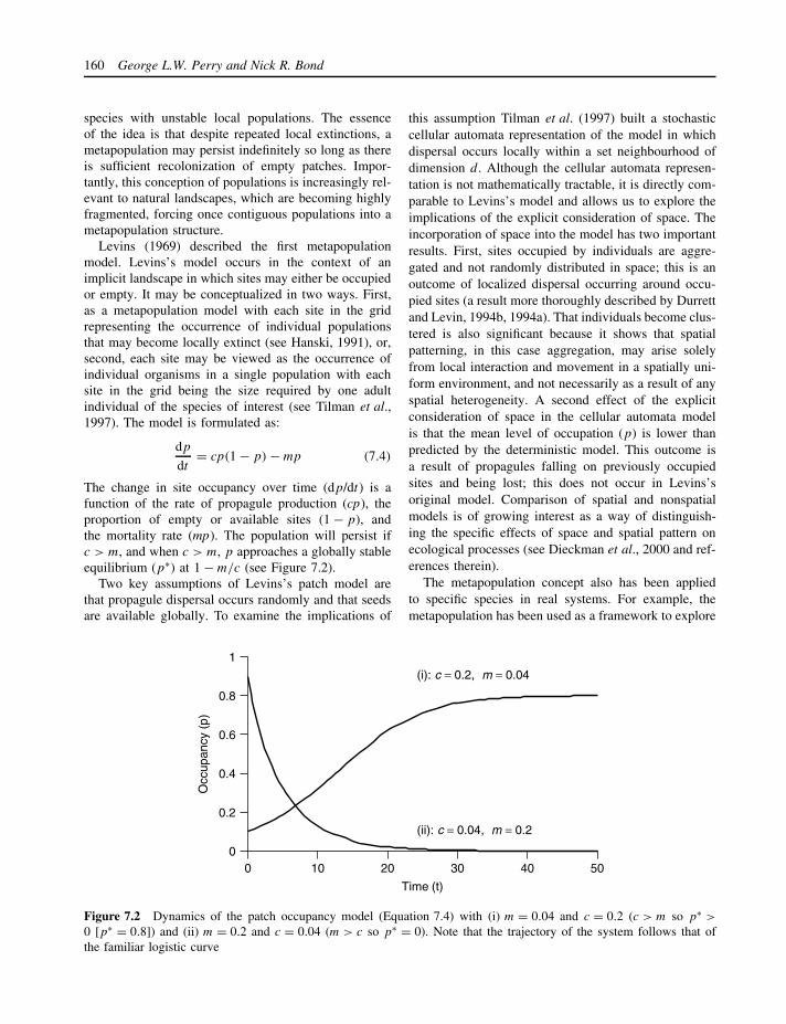
160 George L.W. Perry and Nick R. Bond
species with unstable local populations. The essenceof the idea is that despite repeated local extinctions, ametapopulation may persist indefinitely so long as thereis sufficient recolonization of empty patches. Impor-tantly, this conception of populations is increasingly rel-evant to natural landscapes, which are becoming highlyfragmented, forcing once contiguous populations into ametapopulation structure.
Levins (1969) described the first metapopulationmodel. Levins’s model occurs in the context of animplicit landscape in which sites may either be occupiedor empty. It may be conceptualized in two ways. First,as a metapopulation model with each site in the gridrepresenting the occurrence of individual populationsthat may become locally extinct (see Hanski, 1991), or,second, each site may be viewed as the occurrence ofindividual organisms in a single population with eachsite in the grid being the size required by one adultindividual of the species of interest (see Tilman et al.,1997). The model is formulated as:
dp
dt= cp(1 − p) − mp (7.4)
The change in site occupancy over time (dp/dt) is afunction of the rate of propagule production (cp), theproportion of empty or available sites (1 − p), andthe mortality rate (mp). The population will persist ifc > m, and when c > m, p approaches a globally stableequilibrium (p∗) at 1 − m/c (see Figure 7.2).
Two key assumptions of Levins’s patch model arethat propagule dispersal occurs randomly and that seedsare available globally. To examine the implications of
this assumption Tilman et al. (1997) built a stochasticcellular automata representation of the model in whichdispersal occurs locally within a set neighbourhood ofdimension d . Although the cellular automata represen-tation is not mathematically tractable, it is directly com-parable to Levins’s model and allows us to explore theimplications of the explicit consideration of space. Theincorporation of space into the model has two importantresults. First, sites occupied by individuals are aggre-gated and not randomly distributed in space; this is anoutcome of localized dispersal occurring around occu-pied sites (a result more thoroughly described by Durrettand Levin, 1994b, 1994a). That individuals become clus-tered is also significant because it shows that spatialpatterning, in this case aggregation, may arise solelyfrom local interaction and movement in a spatially uni-form environment, and not necessarily as a result of anyspatial heterogeneity. A second effect of the explicitconsideration of space in the cellular automata modelis that the mean level of occupation (p) is lower thanpredicted by the deterministic model. This outcome isa result of propagules falling on previously occupiedsites and being lost; this does not occur in Levins’soriginal model. Comparison of spatial and nonspatialmodels is of growing interest as a way of distinguish-ing the specific effects of space and spatial pattern onecological processes (see Dieckman et al., 2000 and ref-erences therein).
The metapopulation concept also has been appliedto specific species in real systems. For example, themetapopulation has been used as a framework to explore
0
0.2
0.4
0.6
0.8
1
0 10 20 30 40 50
Time (t)
Occ
upan
cy (
p)
(i): c = 0.2, m = 0.04
(ii): c = 0.04, m = 0.2
Figure 7.2 Dynamics of the patch occupancy model (Equation 7.4) with (i) m = 0.04 and c = 0.2 (c > m so p∗ >
0 [p∗ = 0.8]) and (ii) m = 0.2 and c = 0.04 (m > c so p∗ = 0). Note that the trajectory of the system follows that ofthe familiar logistic curve
Spatial Population Models for Animals 161
the population dynamics of various arboreal marsupi-als in south-eastern Australia (e.g. Leadbeater’s PossumGymnobelideus leadbeateri, Mountain Brushtail PossumTrichosurus caninus, and the Greater Glider Petauroidesvolans). Possingham et al. (1994) coupled spatial habi-tat information in a GIS database, relationships betweenhabitat attributes and quality, and the dynamics of thosehabitat attributes, to assess long-term metapopulationviability of the Greater Glider in old-growth Eucalyptusforest, south-eastern Australia. They found that patchsize is the key factor in metapopulation persistence,with large patches having the longest median persis-tence time for the populations. Other similar studies haveshown the potential importance of inter-patch dispersalin metapopulation persistence, and the high extinctionrisk of small and isolated subpopulations (Lindenmayerand Lacy, 1995a,b). McCarthy and Lindenmayer (1999)used metapopulation models, modified to include distur-bance (fire), to assist in reserve design for arboreal mar-supials in old-growth forests, and explored the influenceof the spatial configuration of reserves on extinctionrisk of greater glider populations. Similar to the studyof Possingham et al. (1994), their model suggests thatlarge, contiguous areas of old-growth forest were impor-tant for population persistence. The importance of largeold-growth forest patches identified by these models isin direct conflict with the current use of these forests fortimber production, and in this context the modelling hasserved a particularly important role in recognizing theneed to modify the current management strategy.
7.2.2.3 Individual-based simulation models
Individual-based models (IBMs) have become widelyused over the past 10 to 15 years (Huston et al., 1988;Judson, 1994; Grimm, 1999). Unlike the frameworkspresented above, in IBMs individual organisms arerepresented as the basic entity, thus, they may be usedto explore how aggregate system properties emergefrom interactions between these fundamental units. Inessence they conceptualize the dynamics of the systemof interest as a result of individual interactions. Thereare a number of reasons why IBMs are useful tools:(a) in evolutionary theory the individual is used asthe basic unit on which natural selection acts; (b) notwo biological organisms are ever identical (even whenthey have identical genes) because they will differ inage, size, condition, behavioural characteristics, etc.;(c) ecological populations are often very small andsubject to stochasticity and so it is unrealistic to modelthem as continuous state variables; and (d) the behaviourof most organisms is spatially complex. IBMs may be
grid-based (e.g. Bond et al., 2000) or represent spacein a more continuous way by assigning individualsx,y positions on some plane (e.g. Deutschmann et al.,1997). IBMs are being increasingly used to aid inthe conservation of threatened species (e.g. Wiegandet al., 1999; Mortia and Yokota, 2002); this approachis valuable where models are needed to evaluate case-specific conditions (Dunning et al., 1995).
The earliest ecological IBMs were developed forplants with an emphasis on economic applications (e.g.stand growth and production). In the early 1970s theJABOWA model of hardwood forest dynamics wasdeveloped by Botkin and co-workers (Botkin et al.,1972b; Botkin et al., 1972a). Since then JABOWA-type models (‘gap models’) have been used in a widerange of systems with some success (in terms of theirability to reproduce, if not always explain, temporalpatterns observed in the ‘real’ world). Typically theyinvolve simulation of stand dynamics on a small area(typically less than 1 ha); all individuals above a certainsize threshold are followed on the plot with birth,death, recruitment and growth processes modelled forall. While the earliest gap models focused on horizontalheterogeneity (diffusion of light through the canopyto the forest floor, etc.) recent incarnations, such asSORTIE (Deutschmann et al., 1997), have been spatiallyexplicit and include detailed mechanistic representationsof the processes of interest.
A large number of individual-based models have alsobeen developed for animals across a diverse range oftaxonomic groups (e.g. fish, arthropods, invertebrates,mammals and birds). A recent trend in the develop-ment of these models has been their integration withGIS to look at resource and organism dynamics in reallandscapes (e.g. Liu et al., 1995). An example of thisapproach is provided by the BACH-MAP model devel-oped by Pulliam et al. (1992) to explore the fate ofsmall populations of Bachman’s Sparrow (Aimophilaaestivalis) in southern US woodlands. The BACHMAPmodel has been extended to create a model (ECOLE-CON, see Liu et al., 1994) that links the original eco-logical model with an economic model. In ECOLECON,forest economic indices are calculated to determine theeconomic costs of managing the species. Integration ofecological models with, for example, economic modelsis likely to become more frequent in the future (Peterson,2000; Liu, 2001). Individual-based models of animalpopulation dynamics are also becoming widely used ascomponents of population viability assessment for rareor threatened species (e.g. Wiegand et al., 1999; Mortiaand Yokota, 2002).
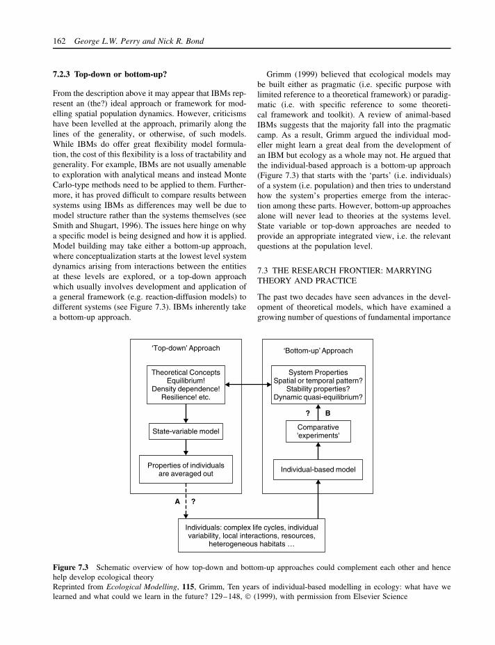
162 George L.W. Perry and Nick R. Bond
7.2.3 Top-down or bottom-up?
From the description above it may appear that IBMs rep-resent an (the?) ideal approach or framework for mod-elling spatial population dynamics. However, criticismshave been levelled at the approach, primarily along thelines of the generality, or otherwise, of such models.While IBMs do offer great flexibility model formula-tion, the cost of this flexibility is a loss of tractability andgenerality. For example, IBMs are not usually amenableto exploration with analytical means and instead MonteCarlo-type methods need to be applied to them. Further-more, it has proved difficult to compare results betweensystems using IBMs as differences may well be due tomodel structure rather than the systems themselves (seeSmith and Shugart, 1996). The issues here hinge on whya specific model is being designed and how it is applied.Model building may take either a bottom-up approach,where conceptualization starts at the lowest level systemdynamics arising from interactions between the entitiesat these levels are explored, or a top-down approachwhich usually involves development and application ofa general framework (e.g. reaction-diffusion models) todifferent systems (see Figure 7.3). IBMs inherently takea bottom-up approach.
Grimm (1999) believed that ecological models maybe built either as pragmatic (i.e. specific purpose withlimited reference to a theoretical framework) or paradig-matic (i.e. with specific reference to some theoreti-cal framework and toolkit). A review of animal-basedIBMs suggests that the majority fall into the pragmaticcamp. As a result, Grimm argued the individual mod-eller might learn a great deal from the development ofan IBM but ecology as a whole may not. He argued thatthe individual-based approach is a bottom-up approach(Figure 7.3) that starts with the ‘parts’ (i.e. individuals)of a system (i.e. population) and then tries to understandhow the system’s properties emerge from the interac-tion among these parts. However, bottom-up approachesalone will never lead to theories at the systems level.State variable or top-down approaches are needed toprovide an appropriate integrated view, i.e. the relevantquestions at the population level.
7.3 THE RESEARCH FRONTIER: MARRYINGTHEORY AND PRACTICE
The past two decades have seen advances in the devel-opment of theoretical models, which have examined agrowing number of questions of fundamental importance
B
‘Bottom-up’ Approach
System PropertiesSpatial or temporal pattern?
Stability properties?Dynamic quasi-equilibrium?
Comparative'experiments'
Individual-based model
Individuals: complex life cycles, individualvariability, local interactions, resources,
heterogeneous habitats …
‘Top-down’ Approach
Theoretical ConceptsEquilibrium!
Density dependence!Resilience! etc.
State-variable model
Properties of individualsare averaged out
A ?
?
Figure 7.3 Schematic overview of how top-down and bottom-up approaches could complement each other and hencehelp develop ecological theoryReprinted from Ecological Modelling, 115, Grimm, Ten years of individual-based modelling in ecology: what have welearned and what could we learn in the future? 129–148, (1999), with permission from Elsevier Science

Spatial Population Models for Animals 163
to ecology. Due in part to the speed with which modelscan be developed (one of their inherent virtues), exper-imental and empirical testing of much of this theorynow lags well behind the modelling ‘frontier’ (Steinbergand Kareiva, 1997). While the need to link theory andpractice better is well recognized (e.g. Kareiva, 1989;Steinberg and Kareiva, 1997), the problem stands thatmany theoretical developments remain intractable froma practical standpoint. In part, this stems from the dif-ficulties of designing and replicating large-scale fieldexperiments capable of putting model predictions to thetest (e.g. see Kareiva et al., 1996 in the context of geneti-cally modified organisms [GMOs]). Equally, empiricistshave been slow to embrace the benefits that modellingcan provide when combined with empirical research.One possible avenue to marry models and empiri-cal/experimental ecology at large spatial scales, and toapply the outcomes of this approach, is through the ideaof ‘adaptive management’ (Walters, 1986, 1993). Underan adaptive management framework, model predictionsand empirical observations influence, in an iterativesequence, management decisions and in turn enhancemodel development. In this framework, successive man-agement decisions represent the experimental treatmentsof a traditional experimental framework, although thusfar, failure to properly monitor the outcomes of particu-lar management decisions has limited the effectivenessof the strategy as a whole (e.g. see Downs and Kon-dolf, 2002, in the context of river restoration). Clearly,though, models developed and applied for managementmust make predictions that managers need and can use,and as much as possible these predictions should bevalidated (MacNally, 2002). There is also a need tothink more clearly about issues of parameterization andmodel error. Surrogate measures for difficult-to-obtaindata could be developed, for example, a key param-eter in many animal IBMs is dispersal and dispersal-mortality – parameters that are very difficult to mea-sure but often ones to which models are very sensitive(e.g. Kareiva et al., 1997; Ruckleshaus et al., 1997). Inour eyes, overcoming the divide between empirical andtheoretical developments stands at the forefront of cur-rent research needs. A number of possibilities exist.One is for theory to take a more pattern-orientatedapproach (i.e. to consider specific ‘real-world’ patternsWiener, 1995; Grimm et al., 1996), while at the sametime adopting an experimental approach to model anal-ysis (Grimm, 1999). Perhaps the greatest successes willcome where ecological modelling is applied to specificresearch needs in which empirical methods (at least atpresent) limit our ability to study particular phenom-ena. Such a problem is explored in detail below. It is
also perhaps worth considering that in some situationsquantitative prediction is too much to ask of even thebest-designed experiment or model. In such cases mod-els may be best used in an heuristic sense, for example,in aiding the design and implementation of environmen-tal monitoring programmes (e.g. Kareiva et al., 1996;Urban, 2000).
Finally, scaling of ecological models remains apressing issue. Increasingly ecologists are being askedregional and global-scale questions yet much ecolog-ical research is conducted at much smaller scales. Theproblem of scale has been a critical impediment to incor-porating important fine-scale processes and informationinto coarser-scale ecosystem and landscape models. Ourknowledge of fine-scale physiological and ecologicalprocesses comes from a variety of measurements, rang-ing from forest plot inventories to remote sensing, madeat spatial resolutions considerably smaller than the largescale at which global ecosystem models are defined. Thedevelopment of methods to link information at these twodisparate scales is a critical challenge. Thus, there is stilla need to develop methods of up- and downscaling eco-logical data (Rastetter et al., 1992) and there have beensome developments in that area through meta-modelling(statistical abstraction of fine-scale models to coarserscales, see Urban et al., 1999) and other methods (e.g.Moorcroft et al., 2001).
7.4 CASE STUDY: DISPERSAL DYNAMICSIN STREAM ECOSYSTEMS
Our aim here is to illustrate the way in which a rela-tively simple spatial model can produce quite complexand unexpected outcomes when applied to a rela-tively basic, yet experimentally ‘challenging’, ecolog-ical phenomenon.
7.4.1 The problem
The beds of streams and rivers typically harbour a richand abundant assemblage of invertebrates, dominated byinsects, crustaceans and gastropods. These organismsfill a wide range of ecological roles (predators, graz-ers, detritivores, etc.), and many exhibit complex lifecycles, spending only part of their life in the stream(Allan, 1995). Common to most, however, is their ten-dency (while in the stream) to spend most of theirtime in direct contact with the bed; hence acquiringthe label of ‘benthic’ fauna. Yet, despite their strongstreambed relation, the tendency to periodically leavethe streambed and ‘drift’ downstream in the water

164 George L.W. Perry and Nick R. Bond
current (eventually to return to the streambed) is abehavioural characteristic common to many species, anda distinctive feature of most benthic stream communi-ties (Brittain and Eikekland, 1988; Allan, 1995). Whilethe behavioural basis of this drift phenomena has longbeen debated (Waters, 1972), its importance in the dis-persal of benthic fauna and the colonization of down-stream areas is now quite well understood (Downes andKeough, 1998). To ecologists interested in drift, fac-tors influencing drift distances have come to the foreas an important theme – particularly how drift mightaffect upstream–downstream population linkages andthe recovery rates of benthic assemblages followingdisturbance (Lancaster et al., 1996; Moser and Min-shall, 1996).
There has thus been great interest in determining thedrift distances of benthic fauna in real streams (e.g.Elliott, 1971, 2002; Lancaster et al., 1996). Three initialobservations have an important bearing on the devel-opment of such models. First, most of these animalsare weak swimmers relative to the current speeds theyexperience when they drift downstream (Fonseca, 1999).This means that drift can be modelled as passive par-ticles (Fonseca, 1999). Second, the flow environmentin streams is often extremely complex when examinedat small spatial scales, but this complexity in flow canbe factored out when examined at larger spatial scales(Carling, 1992). Finally, attempting to track the driftand settlement of individual animals is a complex taskthat has met with limited success (Downes and Keough,1998).
As a mean-field problem (i.e. at the larger scale),the field of drift-distance models developed quickly,describing drift distance as a simple exponential decayfunction in which drift distance is governed by heightabove the bed at which animals enter the drift (itselfan interesting issue!) and average stream velocity (e.g.Ciborowski, 1983; Reynolds et al., 1990). These mod-els were, in places, quite successful at describing actualobserved drift distances, but discrepancies in drift dis-tances between sites with similar mean-field velocitieswere also common (Lancaster et al., 1996).
Generalizing from both theoretical and empiricalstudies in other systems, we hypothesized that spatialvariation in localized flow environments could influencedispersal even where mean-field conditions are similar.Central to this argument is the assumption that driftinganimals settle in complex flow environments when theyenter local areas of near-zero flow (so called dead-waterzones [DWZ]) behind small obstacles and in backwatersalong the stream margins (Lancaster and Hildrew, 1993).Thus while average velocities will be influenced only
by the abundance of such DWZ within a stream reach,differences in the spatial distribution of DWZ may haveindependent effects on average drift distances (Bondet al., 2000).
7.4.2 The model
Because of our interest in understanding how the spatialpattern of DWZ (settlement sites) might affect driftdistances of individual organisms, we adopted a cellularautomata or grid-based model structure that predicts thefate of each individual. We used a spatial lattice torepresent the stream reaches, which provided a simplecontrol on the proportion and spatial pattern of obstacles(which created downstream DWZ) within the land orstreamscape. Individual organisms were introduced intothis landscape and allowed to move (drift) accordingto a set of predefined behavioural rules. These rulesvaried depending on the position of individuals relativeto DWZ and obstacles, and were designed to encapsulatein a simple fashion the ways in which turbulent flowoccurs around obstacles in real streams.
Complete details of the model can be found in Bondet al. (2000). Essentially, streams were represented asa two-dimensional lattice (depth was ignored) 30 cellswide and 1000 cells long. Cells within the lattice tookone of three states: flowing water, obstacles or DWZ.DWZ were always located directly below obstacles, andwere also always of equal size. Obstacles representedrocks and other obstructions observed in streams; theirsize (and that of associated DWZ) were taken from fieldsurveys of several streams. Organisms moved throughthe landscape according to a biased (downstream) ran-dom walk, with a set of simple probabilistic behaviouralrules determining their movement patterns around obsta-cles, and their likelihood of entering DWZ, where set-tlement occurred (ending drift). These simplified rulesprovided a practical way of overcoming the otherwiseintractable problem of modelling complex flow dynam-ics (see Carling, 1992).
7.4.3 The question
Here we discuss two central questions addressed bythe model. First, how do the proportion and spatialpatchiness of obstacles in a stream reach affect the meandistance travelled by drifting animals? We fixed theproportion of obstacles at either 5% or 15%, and at eachof these proportions we varied the size (mean ± SD)of individual DWZs from 2 ± 1 to 6 ± 1 square cells(Figure 7.4). We hypothesized that both of these factors
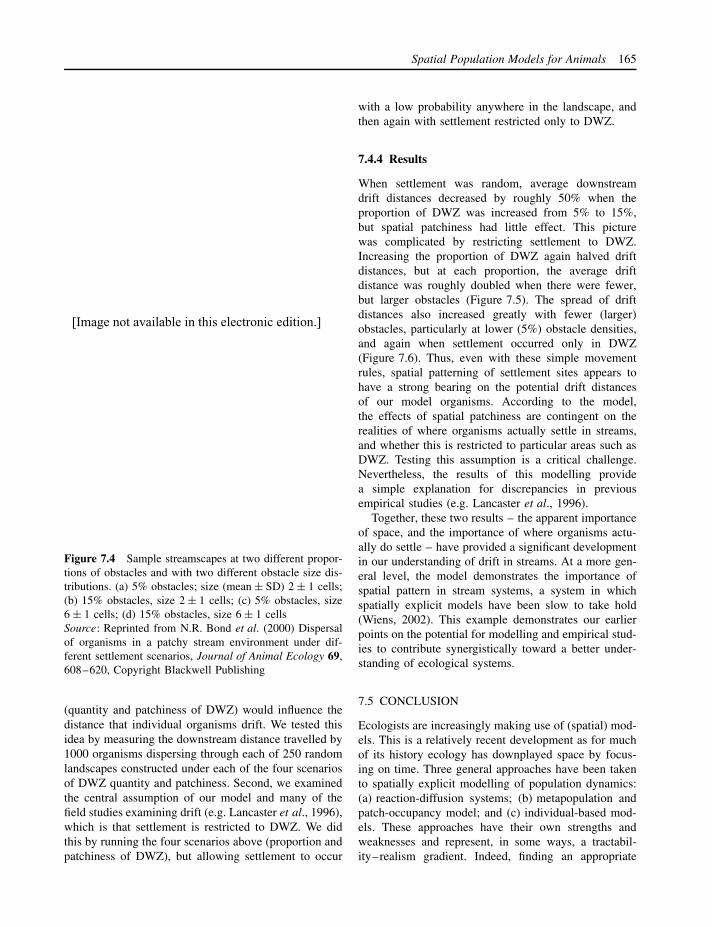
Spatial Population Models for Animals 165
Figure 7.4 Sample streamscapes at two different propor-tions of obstacles and with two different obstacle size dis-tributions. (a) 5% obstacles; size (mean ± SD) 2 ± 1 cells;(b) 15% obstacles, size 2 ± 1 cells; (c) 5% obstacles, size6 ± 1 cells; (d) 15% obstacles, size 6 ± 1 cellsSource: Reprinted from N.R. Bond et al. (2000) Dispersalof organisms in a patchy stream environment under dif-ferent settlement scenarios, Journal of Animal Ecology 69,608–620, Copyright Blackwell Publishing
(quantity and patchiness of DWZ) would influence thedistance that individual organisms drift. We tested thisidea by measuring the downstream distance travelled by1000 organisms dispersing through each of 250 randomlandscapes constructed under each of the four scenariosof DWZ quantity and patchiness. Second, we examinedthe central assumption of our model and many of thefield studies examining drift (e.g. Lancaster et al., 1996),which is that settlement is restricted to DWZ. We didthis by running the four scenarios above (proportion andpatchiness of DWZ), but allowing settlement to occur
with a low probability anywhere in the landscape, andthen again with settlement restricted only to DWZ.
7.4.4 Results
When settlement was random, average downstreamdrift distances decreased by roughly 50% when theproportion of DWZ was increased from 5% to 15%,but spatial patchiness had little effect. This picturewas complicated by restricting settlement to DWZ.Increasing the proportion of DWZ again halved driftdistances, but at each proportion, the average driftdistance was roughly doubled when there were fewer,but larger obstacles (Figure 7.5). The spread of driftdistances also increased greatly with fewer (larger)obstacles, particularly at lower (5%) obstacle densities,and again when settlement occurred only in DWZ(Figure 7.6). Thus, even with these simple movementrules, spatial patterning of settlement sites appears tohave a strong bearing on the potential drift distancesof our model organisms. According to the model,the effects of spatial patchiness are contingent on therealities of where organisms actually settle in streams,and whether this is restricted to particular areas such asDWZ. Testing this assumption is a critical challenge.Nevertheless, the results of this modelling providea simple explanation for discrepancies in previousempirical studies (e.g. Lancaster et al., 1996).
Together, these two results – the apparent importanceof space, and the importance of where organisms actu-ally do settle – have provided a significant developmentin our understanding of drift in streams. At a more gen-eral level, the model demonstrates the importance ofspatial pattern in stream systems, a system in whichspatially explicit models have been slow to take hold(Wiens, 2002). This example demonstrates our earlierpoints on the potential for modelling and empirical stud-ies to contribute synergistically toward a better under-standing of ecological systems.
7.5 CONCLUSION
Ecologists are increasingly making use of (spatial) mod-els. This is a relatively recent development as for muchof its history ecology has downplayed space by focus-ing on time. Three general approaches have been takento spatially explicit modelling of population dynamics:(a) reaction-diffusion systems; (b) metapopulation andpatch-occupancy model; and (c) individual-based mod-els. These approaches have their own strengths andweaknesses and represent, in some ways, a tractabil-ity–realism gradient. Indeed, finding an appropriate
[Image not available in this electronic edition.]

166 George L.W. Perry and Nick R. Bond
Figure 7.5 Mean downstream distance (±1 SD) travelled in each landscape type with (a) random settlement and(b) settlement in DWZ only. Mean obstacle sizes are 2 × 2 cells (white columns) and 6 × 6 cells (hatched columns)Source: Reprinted from N.R. Bond et al. (2000) Dispersal of organisms in a patchy stream environment under differentsettlement scenarios, Journal of Animal Ecology 69, 608–620, Copyright Blackwell Publishing
Figure 7.6 Frequency distributions of average downstream distance travelled per landscape, for each landscape type.(a) 5% obstacles, random settlement; (b) 15% obstacles, random settlement; (c) 5% obstacles, settlement in DWZ only;(d) 15% obstacles. Mean obstacle sizes are 2 × 2 cells (white columns) and 6 × 6 cells (hatched columns)Source: Reprinted from N.R. Bond et al. (2000) Dispersal of organisms in a patchy stream environment under differentsettlement scenarios, Journal of Animal Ecology 69, 608–620, Copyright Blackwell Publishing
[Image not available in this electronic edition.]
[Image not available in this electronic edition.]
Spatial Population Models for Animals 167
balance between tractability and realism (complexity)remains a major challenge to ecological modellers.
A spatial model of drift by invertebrate larvae instreams was presented to illustrate some of these points.The drift of invertebrates in streams has been the focusof a considerable amount of research yet is empiricallychallenging (e.g. the difficulty of tracking individuallarvae, etc.). Using a relatively simple spatial modelwe show how such a model can produce quite complexand unexpected outcomes when applied to a relativelybasic phenomenon. It has also provided a possiblesolution to some puzzling discrepancies in previousempirical studies. The recent interest in spatial patternsand processes in ecology has resulted in the developmentof a wealth of spatial ecological theory. However,empirical testing of this theory has not proceededas quickly, in part, because of inherent problems inexperimental design and analysis at extended spatialscales, but also because some of this spatial theory hasnot been framed in an obviously testable manner.
ACKNOWLEDGEMENTS
We would like to thank Ralph Mac Nally for his usefulcomments on an earlier draft of this chapter.
REFERENCES
Allan, J.D. (1995) Stream Ecology: Structure and Function ofRunning Waters, Chapman & Hall, London.
Andow, D.A., Kareiva, P.M., Levin, S.A. and Okubo, A.(1990) Spread of invading organisms, Landscape Ecology4, 177–188.
Beck, M.W. (1997) Inference and generality in ecology: cur-rent problems and an experimental solution, Oikos 78,265–273.
Beyers, D.W. (1998) Causal inference in environmental impactstudies, Journal of the North American Benthological Society17, 367–373.
Bond, N.R., Perry, G.L.W. and Downes, B.J. (2000) Dispersalof organisms in a patchy stream environment under dif-ferent settlement scenarios, Journal of Animal Ecology 69,608–620.
Botkin, D.B., Janak, J.F. and Wallis, J.R. (1972a) Rationale,limitations and assumptions of a northeast forest growthsimulator, IBM Journal of Research and Development 16,101–116.
Botkin, D.B., Janak, J.F. and Wallis, J.R. (1972b) Some eco-logical consequences of a computer model of forest growth,Journal of Ecology 60, 849–872.
Bradbury, R.H., van der Laan, J.D. and Green, D.G. (1996)The idea of complexity in ecology, Senckenbergiana Mar-itima 27, 89–96.
Brittain, J.E. and Eikekland, T.J. (1988) Invertebrate drift – areview, Hydrobiologia 166, 77–93.
Carling, P.A. (1992) In-stream hydraulics and sediment trans-port, in P. Calow and G.E. Petts (eds) The Rivers Handbook,Blackwell, Oxford, 101–125.
Ciborowski, J.J.H. (1983) Downstream and lateral transport ofnymphs of two mayfly species (Ephemeroptera), CanadianJournal of Fisheries and Aquatic Sciences 40, 2025–2029.
Deutschmann, D.H., Levin, S.A., Devine, C. and Buttle, L.A.(1997) Scaling from trees to forests: analysis of a complexsimulation model, Science (Online): http://www.sciencemag.org/feature/data/deutschman/index.htm
Dieckman, U., Law, R. and Metz, J.A.J. (eds) (2000) TheGeometry of Ecological Interactions: Simplifying SpatialComplexity, Cambridge, Cambridge University Press.
Downes, B.J. and Keough, M.J. (1998) Scaling of colonizationprocesses in streams: parallels and lessons from marine hardsubstrata, Australian Journal of Ecology 23, 8–26.
Downs, P.W. and Kondolf, G.M. (2002) Post-project appraisalsin adaptive management of river channel restoration, Envi-ronmental Management 29, 477–496.
Dunning, J.B.J., Stewart, D.J., Noon, B.R., Root, T.L., Lam-berson, R.H. and Stevens, E.E. (1995) Spatially explicit pop-ulation models: current forms and future uses, EcologicalApplications 5, 2–11.
Durrett, R. and Levin, S.A. (1994a) The importance of beingdiscrete (and spatial), Theoretical Population Biology 46,363–394.
Durrett, R. and Levin, S.A. (1994b) Stochastic spatial models:a user’s guide to ecological applications, PhilosophicalTransactions of the Royal Society of London, Series B 343,329–350.
Eberhardt, L.L. and Thomas, J.M. (1991) Designing environ-mental field studies, Ecological Monographs 61, 53–73.
Elliott, J.M. (1971) The distances travelled by drifting inverte-brates in a Lake District stream, Oecologia 6, 350–379.
Elliott, J.M. (2002) Time spent in the drift by downstream-dispersing invertebrates in a Lake District stream, Freshwa-ter Biology 47, 97–106.
Fonseca, D.M. (1999) Fluid-mediated dispersal in streams:models of settlement from the drift, Oecologia 121,212–223.
Grimm, V. (1999) Ten years of individual-based modelling inecology: what have we learned and what could we learn inthe future?, Ecological Modelling 115, 129–148.
Grimm, V., Frank, K., Jeltsch, F., Brandl, R., Uchmanski, J.and Wissel, C. (1996) Pattern-oriented modelling in pop-ulation ecology, Science of the Total Environment 183,151–166.
Hanski, I.A. (1991) Single-species metapopulation dynamics:concepts, models and observations, Biological Journal of theLinnean Society 42, 17–38.
Hanski, I. (1998) Metapopulation dynamics, Nature 396,41–49.
Hanski, I.A. and Simberloff, D. (1997) The metapopulationapproach, its history, conceptual domain and application to

168 George L.W. Perry and Nick R. Bond
conservation, in I.A. Hanski and M.E. Gilpin (eds) Metapop-ulation Biology: Ecology, Genetics and Evolution, AcademicPress, San Diego, 5–26.
Hassell, M.P., Comins, N.N. and May, R.M. (1994) Species-coexistence and self-organising spatial dynamics, Nature370, 290–292.
Hastings, A. (1994) Conservation and spatial structure: theo-retical approaches, in S.A. Levin (ed.) Frontiers in Mathe-matical Biology, Springer-Verlag, Berlin, 494–503.
Holmes, E.E., Lewis, M.A., Banks, J.E. and Veit, R.R. (1994)Partial differential equations in ecology: spatial interactionsand population dynamics, Ecology 75, 17–29.
Horn, H.S., Shugart, H.H. and Urban, D.L. (1989) Simulatorsas models of forest dynamics, in J. Roughgarden, R.M. May,and S.A. Levin (eds) Perspectives in Ecological Theory,Princeton University Press, Princeton, NJ, 256–267.
Huffaker, C.B. (1958) Experimental studies on predation: dis-persion factors and predator–prey oscillation, Hilgardia 27,343–383.
Huston, M.A., DeAngelis, D.L. and Post, W. (1988) Newcomputer models unify ecological theory, BioScience 38,682–691.
Jackson, L.J., Trebitz, A.S. and Cottingham, K.L. (2000) Anintroduction to the practice of ecological modelling, Bio-Science 50, 694–706.
Judson, O.P. (1994) The rise of the individual-based model inecology, Trends in Ecology and Evolution 9, 9–14.
Kareiva, P. (1989) Renewing the dialogue between theoryand experiments in population ecology, in J. Roughgarden,R.M. May and S.A. Levin (eds) Perspectives in EcologicalTheory, Princeton University Press, Princeton, NJ, 69–88.
Kareiva, P. (1990) Population dynamics in spatially complexenvironments: theory and data, Philosophical Transactionsof the Royal Society of London, Series B 330, 175–190.
Kareiva, P., Parker, I.M. and Pascual, M. (1996) Can we useexperiments and models in predicting the invasiveness ofgenetically engineered organisms? Ecology 77, 1670–1675.
Kareiva, P.M., Skelly, D.K. and Ruckelshaus, M. (1997)Reevaluating the use of models to predict the consequencesof habitat loss and fragmentation, in S.T.A. Pickett,R.S. Ostfeld, H. Schchak and G.E. Likens (eds) Enhancingthe Ecological Basis of Conservation: Heterogeneity,Ecosystem Function and Biodiversity, Chapman & Hall, NewYork, 156–167.
Kingsland, S. (1995) Modeling Nature: Episodes in the Historyof Population Ecology, 2nd edn, University of Chicago Press,Chicago.
Lancaster, J. and Hildrew, A.G. (1993) Characterizing in-stream flow refugia, Canadian Journal of Fisheries andAquatic Science 50, 1663–1675.
Lancaster, J., Hildrew, A.G. and Gjerlov, C. (1996) Inverte-brate drift and longitudinal transport processes in streams,Canadian Journal of Fisheries and Aquatic Science 53,572–582.
Levins, R. (1969) Some demographic and genetic conse-quences of environmental heterogeneity for biologicalcontrol, Bulletin of the Entomological Society of America 15,237–240.
Li, C. and Apps, M.J. (1996) Effects of contagious disturbanceon forest temporal dynamics, Ecological Modelling 87,143–151.
Lindenmayer, D.B. and Lacy, R.C. (1995a) Metapopulationviability of arboreal marsupials in fragmented old-growthforests: comparison among species, Ecological Applications5, 183–199.
Lindenmayer, D.B. and Lacy, R.C. (1995b) Metapopulationviability of Leadbeater’s possum, Gymnobelideus leadbeat-eri, in fragmented old-growth forests, Ecological Applica-tions 5, 164–182.
Liu, J. (2001) Integrating ecology with human demography,behavior, and socioeconomics: needs and approaches, Eco-logical Modelling 140, 1–8.
Liu, J., Cubbage, F. and Pulliam, H.R. (1994) Ecological andeconomic effects of forest structure and rotation lengths: sim-ulation studies using ECOLECON, Ecological Economics10, 249–265.
Liu, J., Dunning, J.B.J. and Pulliam, H.R. (1995) Potentialeffects of a forest management plan on Bachman’s sparrows(Aimophila aestivalis): linking a spatially explicit model withGIS, Conservation Biology 9, 62–75.
Logan, J.E., White, P., Bentz, B.J. and Powell, J.A. (1998)Model analysis of spatial patterns in mountain pine beetleoutbreaks, Theoretical Population Biology 53, 236–255.
Mac Nally, R. (1999) Dealing with scale in ecology, inJ.A. Wiens and M.R. Moss (eds) Issues in LandscapeEcology, International Association for Landscape Ecology,Guelph, ON, Canada.
Mac Nally, R. (2002) Improving inference in ecologicalresearch: issues of scope, scale and model validation, Com-ments on Theoretical Biology 7, 235–254.
McCarthy, M.A. and Lindenmayer, D.B. (1999) Incorporatingmetapopulation dynamics of greater gliders into reservedesign in disturbed landscapes, Ecology 80, 651–667.
Moorcroft, P.R., Hurtt, G.C. and Pacala, S.W. (2001) Amethod for scaling vegetation dynamics: the ecosystemdemography model (ED), Ecological Monographs 71,577–586.
Mortia, K. and Yokota, A. (2002) Population viability ofstream-resident salmonids after habitat fragmentation: acase study with white-spotted charr (Salevnius leucomaenis)by an individual based model, Ecological Modelling 155,85–94.
Moser, D.C. and Minshall, G.W. (1996) Effects of localizeddisturbance on macroinvertebrate community structure inrelation to mode of colonization and season, AmericanMidland Naturalist 135, 92–101.
Perry, G.L.W. (2002) Landscapes, space and equilibrium: somerecent shifts, Progress in Physical Geography 26, 339–359.
Peters, R.H. (1991) A Critique for Ecology, Cambridge Uni-versity Press, Cambridge.
Peterson, G. (2000) Political ecology and ecological resilience:an integration of human and ecological dynamics, EcologicalEconomics 35, 323–336.
Possingham, H.P., Lindenmayer, D.B., Norton, T.W. andDavies, I. (1994) Metapopulation viability analysis of the

Spatial Population Models for Animals 169
greater glider (Petauroides volans) in a wood productionarea, Biological Conservation 70, 227–236.
Pulliam, H.R. (1988) Sources, sinks and population regulation,American Naturalist 132, 652–661.
Pulliam, H.R. and Danielson, B.J. (1991) Sources, sinks andhabitat selection: a landscape perspective on populationdynamics, American Naturalist 137 (suppl): S50–S66.
Pulliam, H.R., Dunning, J.B.J. and Liu, J. (1992) Populationdynamics in complex landscapes: a case study, EcologicalApplications 2, 165–177.
Rastetter, E.B., King, A.W., Cosby, B.J., Hornberger, G.M.,O’Neill, R.V. and Hobbie, J.E. (1992) Aggregating fine-scale ecological knowledge to model coarser-scale attributesof ecosystems, Ecological Applications 2, 55–70.
Reynolds, C.S., White, M.L., Clarke, R.T. and Marker, A.F.(1990) Suspension and settlement of particles in flowingwater: comparison of the effects of varying water depthand velocity in circulating channels, Freshwater Biology 24,23–34.
Ruckleshaus, M., Hartway, C. and Kareiva, P.M. (1997)Assessing the data requirements of spatially explicit dispersalmodels, Conservation Biology 11, 1298–1306.
Schneider, D.C. (1994) Quantitative Ecology: Spatial and Tem-poral Scaling, Academic Press. San Diego.
Shugart, H.H. (1998) Terrestrial Ecosystems in Changing Envi-ronments, Cambridge University Press, Cambridge.
Smith, T.M. and Shugart, H.H. (1996) The application ofpatch models to global change research, in B.H. Walker andW.L. Steffen (eds) Global Change and Terrestrial Ecosys-tems, Cambridge University Press, Cambridge, 127–148.
Starfield, A.M. and Beloch, A.L. (1986). Building Models forConservation and Wildlife Management, Macmillan, NewYork.
Steinberg, E.K. and Kareiva, P.M. (1997) Challenges andopportunities for empirical evaluation of ‘spatial theory’,in D.A. Tilman and P.M. Kareiva (eds) Spatial Ecology:The Role of Space in Population Dynamics and Interspe-cific Interactions, Princeton University Press, Princeton, NJ,318–333.
Thrush, S.F., Schneider, D.C., Legendre, P., Whitlatch, R.B.,Dayton, P.K., Hewitt, J.E., Hines, A.H., Cummings, V.J.,Lawrie, S.M., Grant, J., Pridmore, R.D. and Turner, S.J.(1997) Scaling-up from experiments to complex ecologicalsystems: where to next?, Journal of Experimental MarineBiology and Ecology 216, 243–254.
Tilman, D.A. (1994) Competition and biodiversity in spatiallystructured habitats, Ecology 75, 2–16.
Tilman, D.A., Lehman, C.L. and Kareiva, P.M. (1997) Pop-ulation dynamics in spatial habitats, in D.A. Tilman andP.M. Kareiva (eds) Spatial Ecology: The Role of Space inPopulation Dynamics and Interspecific Interactions, Prince-ton University Press, Princeton, NJ, 3–21.
Turner, M.G., Arthaud, G.J., Engstrom, R.T., Hejl, S.J., Liu, J.,Loeb, S. and McKelvey, K. (1995) Usefulness of spatiallyexplicit population models in land management, EcologicalApplications 5, 12–16.
Turner, M.G. and Romme, W.H. (1994) Landscape dynamicsin crown fire ecosystems, Landscape Ecology 9, 59–77.
Underwood, A.J. (1990) Experiments in ecology and manage-ment: their logics, functions and interpretations, AustralianJournal of Ecology 15, 365–389.
Urban, D.L. (2000) Using model analysis to design monitoringprograms for landscape management and impact assessment,Ecological Applications 10, 1820–1832.
Urban, D.L., Acevedo, M.F. and Garman, S.L. (1999) Scalingfine-scale processes to large-scale patterns using modelsderived from models: meta-models, in D.J. Mladenoff andW.L. Baker (eds) Spatial Modeling of Forest Landscapes:Approaches and Applications, Cambridge University Press,Cambridge, 125–163.
Walters, C.J. (1986) Adaptive Management of RenewableResources, Macmillan Publishing Co., New York.
Walters, C.J. (1993) Dynamic models and large scale fieldexperiments in environmental impact assessment and man-agement, Australian Journal of Ecology 18, 53–61.
Waters, T.F. (1972) The drift of stream insects, Annual Reviewof Entomology 17, 253–272.
Watt, A.S. (1947) Pattern and process in the plant community,Journal of Ecology 35, 1–22.
Weiner, J. (1995) On the practice of ecology, Journal ofEcology 83, 153–158.
Wiegand, T., Naves, J., Stephan, T. and Fernandez, A. (1999)Assessing the risk of extinction for the Brown Bear (Ursusarctos) in the Cordillera Cantabrica, Spain, Ecological Appli-cations 68, 539–570.
Wiener, J. (1995) On the practice of ecology, Journal ofEcology 83, 153–158.
Wiens, J.A. (1997) The emerging role of patchiness in conser-vation biology, in S.T.A. Pickett, R.S. Ostfeld, H. Schchakand G.E. Likens (eds) Enhancing the Ecological Basis ofConservation: Heterogeneity, Ecosystem Function and Bio-diversity, Chapman & Hall, New York, 93–108.
Wiens, J.A. (2002) Riverine landscapes: taking landscape ecol-ogy into the water, Freshwater Biology 47, 501–515.
Wiens, J.A. and Milne, B.T. (1989) Scaling of ‘landscapes’ inlandscape ecology, or, landscape ecology from a beetle’sperspective, Landscape Ecology 3, 87–96.
Wiens, J.A., Stenseth, N.C., van Horne, B. and Ims, R.A.(1993) Ecological mechanisms and landscape ecology, Oikos66, 369–380.
With, K.A. and Crist, T.O. (1996) Translating across scales:simulating species distributions as the aggregate responseof individuals to heterogeneity, Ecological Modelling 93,125–137.


8
Ecosystem Modelling: Vegetationand Disturbance
STEFANO MAZZOLENI, FRANCISCO REGO, FRANCESCO GIANNINOAND COLIN LEGG
8.1 THE SYSTEM COMPLEXITY: EFFECTSOF DISTURBANCE ON VEGETATION DYNAMICS
Vegetation is continuously changing in time and space.The changes may be autogenic, driven by the propertiesof the component plant species, or allogenic, drivenby external factors. Allogenic change may be a resultof gradual changes in the environment, but more oftenresults from disturbance events, and the way vegetationresponds will be very dependent upon the disturbancehistory (Miles, 1979).
The term disturbance is used in ecology to refer tothe partial or complete reduction of biomass due to someexternal factors and does not include natural mortalityor decay processes. Typical causes of disturbance aregrazing, cutting, fire and frost. Disturbance can also bedefined as an event that causes a significant change fromthe normal pattern in an ecological system (Formanand Godron, 1986), but the problem with this relativedefinition of disturbance stems from the difficulty ofdefining the ‘normal’ range of conditions for an ecosys-tem (White and Harrod, 1997). This is why an absolutedefinition requiring measures of real change is moreappropriate for a mechanistic modelling approach. Thiswas the choice taken by Waring and Running (1998),for example, who defined disturbance in a forest as anyfactor that brings about a significant reduction in theoverstory leaf area index for a period of more than oneyear. Grubb (1985) reviewed the concept of disturbanceand distinguished vegetation resilience ‘in situ’ and ‘bymigration’ (Grubb and Hopkins, 1986), referring to the
regeneration capacity of surviving individuals in the dis-turbed area and recolonization from neighbouring areasrespectively.
In the simplest case of one type of disturbance on ahomogeneous site the disturbance regime can be gener-ally described by its frequency and its intensity. How-ever, if intensity is associated with biomass accumulated,as in the case of fire, there is an inverse relationshipbetween intensity and frequency. These considerationswere very well established for fire regimes in NorthAmerica (see, for instance, Heinselman, 1978) and inEurope (e.g. Angelstam, 1997). Therefore the simplestway to describe a fire regime is to determine the aver-age time between disturbances (years) or conversely, themean frequency of the disturbance (expressed in year−1).
This chapter focuses only on fire and grazing. Hender-son and Keith (2002) performed a canonical correspon-dence analysis on the sources of variation in shrubcomposition of eucalypt forests which showed that fireand grazing accounted for more variation than the com-bination of all other environmental and spatial vari-ables. Although they are perhaps the two most importantsources of disturbance, they differ very much in char-acter; the former causes an abrupt discontinuity in thesystem while the latter is characterized by a gradual andcontinuous process of selective biomass removal.
8.1.1 Fire
The immediate effects of fire are the removal of themajority of above-ground biomass and the pulse of
Environmental Modelling: Finding Simplicity in Complexity. Edited by J. Wainwright and M. Mulligan 2004 John Wiley & Sons, Ltd ISBNs: 0-471-49617-0 (HB); 0-471-49618-9 (PB)

172 Stefano Mazzoleni, Francisco Rego, Francesco Giannino and Colin Legg
heat through the upper soil horizons. Some plants arekilled, but those that survive and can resprout arechanged physiologically because of the imbalance inthe root:shoot ratio. The exposure of the modified soilhorizons results in a new post-fire microclimate andchanges in hydrology. However, the resilience of vege-tation to fire has been reported for several ecosystems.For example, Quercus coccifera garrigue and Ulex parv-iflorus and Rosmarinus officinalis shrublands regainedtheir total cover in less than five years after burn-ing (Ferran and Vallejo, 1998). Similarly, few changesfollowing fire were reported for oak scrub in Floridauplands where species composition and structure largelyrecovered in less than two years (Abrahamson and Abra-hamson, 1996). In general, after fire, the most obviouschange is that of the composition and relative abun-dance of herbaceous species. As succession proceedsand the canopy closes, the early flush of herbaceousvegetation is either restricted to small canopy openingsor remains dormant in the soil in the form of seedswaiting for the next fire to come (Arianoutsou, 1998).Similar results were found in California (Hanes, 1971),in Australia (Specht et al., 1958), in Italy (Mazzoleniand Pizzolongo, 1990) and in Portugal (Espırito-Santoet al., 1993).
Two broad groups of communities can be distin-guished related to the reproductive strategy of the dom-inant plant species and their comparative rates of plantcover regenerating after fire:
• Plant communities dominated by resprouters withdeep root systems (e.g. species of Quercus, Pista-cia, Arbutus, Rhamnus, Phyllirea, Erica, Daphne andsome Ulex ) that recover very rapidly after fire fromorgans which have been preserved below ground.
• Plant communities dominated by species regeneratingafter fire from seeds (e.g. species of Cistus, Rosmar-inus officinalis and Ulex parviflorus). The responseof these obligate seeders to fire in terms of pro-jected plant cover is much slower than that of theresprouters.
In general, tree survival can vary according to the inten-sity of the fire, the height of the crown and bark thick-ness (Ryan and Reinhardt, 1988). Other considerationssuch as fire intensity, fire season and water availabil-ity at the time of the fire and during the immediatepost-fire period can be of great importance in determin-ing rate of recovery for seeders and, to a lesser extent,for sprouters (Moreno and Cruz, 2000). Also the shadetolerance of species and light conditions after fire canbe fundamental in determining the post-fire recoveryof vegetation.
In most cases, however, plants are top-killed by fire;plant succession in fire-adapted systems, as, for example,in most Mediterranean communities, consists largely ofthe recovery of the species present before fire throughtheir respective life-cycle and growth processes. Thisprocess is called autosuccession (Hanes, 1971) in whichthe burned stand, although initially appearing to bedifferent from the pre-burned one, retains its floristicidentity in time.
8.1.2 Grazing
Grazing effects on vegetation have been studied in manyecosystems. It is clear that herbivores cause changes inspecies richness (Basset, 1980; Persson, 1984; Bakkeret al., 1983; Wimbush and Costin, 1979).
An important parameter of grazing disturbance isthe specificity of grazers to species, to age and sizeclasses and to community structure. However, there arelarge differences in selectivity between animals. Largeanimals are generally less selective in their diet than aresmaller animals. In general, animals select the smaller oryounger plants within a species, they select only somespecies within a plant community and select only someplant community types within a landscape (Dumont,1997; Legg et al., 1998).
Grazing animals exert controls on the rates of severalimportant processes in ecosystems. The significance ofthis fact can be easily understood from the conclusionby Wolfe and Berg (1988) that selective browsing ofyoung deciduous trees by ungulates has effectivelyeliminated many deciduous hardwood species fromEuropean forests, while conifers usually escape damage.
Many similar studies can be found in the literaturefor other herbivores. The spatial distribution of wildrabbit (Oryctolagus cuniculus) in dry conditions, forexample, was found to be correlated with water andforage availability, but also with the existence of aprotective cover of shrubs or oak trees. At the same timeconsumption of acorns and oak seedlings by rabbits canaffect natural oak regeneration (Martins, 2001).
8.1.3 Fire and grazing interactions
It has been suggested that where multiple disturbancesoccur simultaneously they generally have nonadditiveeffects on ecosystems (White and Pickett, 1985). Theseeffects may be either synergistic (greater than additive)or antagonistic (less than additive).
Fire and grazing may have antagonistic effects overrelatively short time scales. Grazing reduces plantgrowth and removes available fuel, thus reducing the
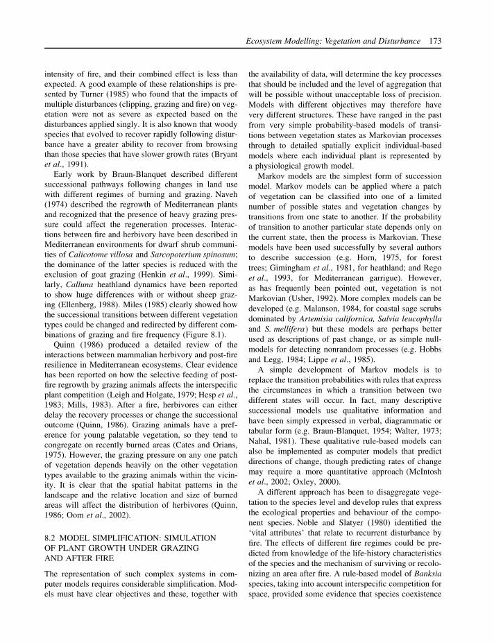
Ecosystem Modelling: Vegetation and Disturbance 173
intensity of fire, and their combined effect is less thanexpected. A good example of these relationships is pre-sented by Turner (1985) who found that the impacts ofmultiple disturbances (clipping, grazing and fire) on veg-etation were not as severe as expected based on thedisturbances applied singly. It is also known that woodyspecies that evolved to recover rapidly following distur-bance have a greater ability to recover from browsingthan those species that have slower growth rates (Bryantet al., 1991).
Early work by Braun-Blanquet described differentsuccessional pathways following changes in land usewith different regimes of burning and grazing. Naveh(1974) described the regrowth of Mediterranean plantsand recognized that the presence of heavy grazing pres-sure could affect the regeneration processes. Interac-tions between fire and herbivory have been described inMediterranean environments for dwarf shrub communi-ties of Calicotome villosa and Sarcopoterium spinosum;the dominance of the latter species is reduced with theexclusion of goat grazing (Henkin et al., 1999). Simi-larly, Calluna heathland dynamics have been reportedto show huge differences with or without sheep graz-ing (Ellenberg, 1988). Miles (1985) clearly showed howthe successional transitions between different vegetationtypes could be changed and redirected by different com-binations of grazing and fire frequency (Figure 8.1).
Quinn (1986) produced a detailed review of theinteractions between mammalian herbivory and post-fireresilience in Mediterranean ecosystems. Clear evidencehas been reported on how the selective feeding of post-fire regrowth by grazing animals affects the interspecificplant competition (Leigh and Holgate, 1979; Hesp et al.,1983; Mills, 1983). After a fire, herbivores can eitherdelay the recovery processes or change the successionaloutcome (Quinn, 1986). Grazing animals have a pref-erence for young palatable vegetation, so they tend tocongregate on recently burned areas (Cates and Orians,1975). However, the grazing pressure on any one patchof vegetation depends heavily on the other vegetationtypes available to the grazing animals within the vicin-ity. It is clear that the spatial habitat patterns in thelandscape and the relative location and size of burnedareas will affect the distribution of herbivores (Quinn,1986; Oom et al., 2002).
8.2 MODEL SIMPLIFICATION: SIMULATIONOF PLANT GROWTH UNDER GRAZINGAND AFTER FIRE
The representation of such complex systems in com-puter models requires considerable simplification. Mod-els must have clear objectives and these, together with
the availability of data, will determine the key processesthat should be included and the level of aggregation thatwill be possible without unacceptable loss of precision.Models with different objectives may therefore havevery different structures. These have ranged in the pastfrom very simple probability-based models of transi-tions between vegetation states as Markovian processesthrough to detailed spatially explicit individual-basedmodels where each individual plant is represented bya physiological growth model.
Markov models are the simplest form of successionmodel. Markov models can be applied where a patchof vegetation can be classified into one of a limitednumber of possible states and vegetation changes bytransitions from one state to another. If the probabilityof transition to another particular state depends only onthe current state, then the process is Markovian. Thesemodels have been used successfully by several authorsto describe succession (e.g. Horn, 1975, for foresttrees; Gimingham et al., 1981, for heathland; and Regoet al., 1993, for Mediterranean garrigue). However,as has frequently been pointed out, vegetation is notMarkovian (Usher, 1992). More complex models can bedeveloped (e.g. Malanson, 1984, for coastal sage scrubsdominated by Artemisia californica, Salvia leucophyllaand S. mellifera) but these models are perhaps betterused as descriptions of past change, or as simple null-models for detecting nonrandom processes (e.g. Hobbsand Legg, 1984; Lippe et al., 1985).
A simple development of Markov models is toreplace the transition probabilities with rules that expressthe circumstances in which a transition between twodifferent states will occur. In fact, many descriptivesuccessional models use qualitative information andhave been simply expressed in verbal, diagrammatic ortabular form (e.g. Braun-Blanquet, 1954; Walter, 1973;Nahal, 1981). These qualitative rule-based models canalso be implemented as computer models that predictdirections of change, though predicting rates of changemay require a more quantitative approach (McIntoshet al., 2002; Oxley, 2000).
A different approach has been to disaggregate vege-tation to the species level and develop rules that expressthe ecological properties and behaviour of the compo-nent species. Noble and Slatyer (1980) identified the‘vital attributes’ that relate to recurrent disturbance byfire. The effects of different fire regimes could be pre-dicted from knowledge of the life-history characteristicsof the species and the mechanism of surviving or recolo-nizing an area after fire. A rule-based model of Banksiaspecies, taking into account interspecific competition forspace, provided some evidence that species coexistence

174 Stefano Mazzoleni, Francisco Rego, Francesco Giannino and Colin Legg
Ulex andSarothamnus
scrub
Ulex andSarothamnus
scrub
Callunadominant
heath/moor
Callunadominant
heath/moor
Dominant Nardus orDeschampsia flexuosa
Dominant Nardusor Deschampsia
flexuosaAgrostis-Festucagrassland
Agrostis-Festucagrassland
Pinus sylvestriswoodland
Pinus sylvestriswoodlandBetula
woodland
Betulawoodland
Juniperusscrub
Juniperusscrub
Pteridiumdominant
stands
Pteridiumdominant
stands
(a)
Ulex andSarothamnus
scrub
Callunadominant
heath/moor
Dominant Nardus orDeschampsia flexuosa Agrostis-Festuca
grassland
Pinus sylvestriswoodland
Betulawoodland
Juniperusscrub
Pteridiumdominant
stands
(c)
(b)
Figure 8.1 Successional transitions in northeast Scotland under (a) low grazing pressure and no fire; (b) high grazingpressure and frequent fires; and (c) intermediate grazing pressure and infrequent burning. Arrow thickness refers tofrequency of transitionSource: Miles (1985)
depended on both fire regime and topographic gradi-ents (Groeneveld et al., 2002).
Historically, models of forest dynamics have beendeveloped either at the stand level, with individual treesgrown deterministically using an annual time-step differ-ence equation, and by simulation calculating the fate ofeach individual, or at the level of some integrated unit,such as an age cohort. This approach was initially devel-oped in JABOWA by Botkin et al. (1972) and appliedto different forest ecosystems (e.g. FORET by Shugart
and West, 1977; BRIND by Shugart and Noble, 1981).However, in spite of their widespread use, this familyof individual-based gap-phase models provided limitedexplanations for the simulated successional response anddid not account for spatial processes.
Spatial structure modelling has largely been derivedfrom individual-based ideology, taking into accountnearest-neighbour interactions (Ford, 1975). These inter-actions could be a result of shading and/or redistribu-tion of the soil and water resources among the trees.
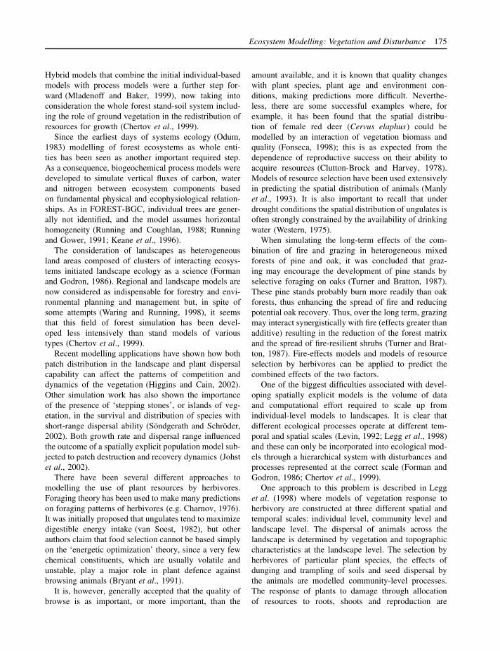
Ecosystem Modelling: Vegetation and Disturbance 175
Hybrid models that combine the initial individual-basedmodels with process models were a further step for-ward (Mladenoff and Baker, 1999), now taking intoconsideration the whole forest stand-soil system includ-ing the role of ground vegetation in the redistribution ofresources for growth (Chertov et al., 1999).
Since the earliest days of systems ecology (Odum,1983) modelling of forest ecosystems as whole enti-ties has been seen as another important required step.As a consequence, biogeochemical process models weredeveloped to simulate vertical fluxes of carbon, waterand nitrogen between ecosystem components basedon fundamental physical and ecophysiological relation-ships. As in FOREST-BGC, individual trees are gener-ally not identified, and the model assumes horizontalhomogeneity (Running and Coughlan, 1988; Runningand Gower, 1991; Keane et al., 1996).
The consideration of landscapes as heterogeneousland areas composed of clusters of interacting ecosys-tems initiated landscape ecology as a science (Formanand Godron, 1986). Regional and landscape models arenow considered as indispensable for forestry and envi-ronmental planning and management but, in spite ofsome attempts (Waring and Running, 1998), it seemsthat this field of forest simulation has been devel-oped less intensively than stand models of varioustypes (Chertov et al., 1999).
Recent modelling applications have shown how bothpatch distribution in the landscape and plant dispersalcapability can affect the patterns of competition anddynamics of the vegetation (Higgins and Cain, 2002).Other simulation work has also shown the importanceof the presence of ‘stepping stones’, or islands of veg-etation, in the survival and distribution of species withshort-range dispersal ability (Sondgerath and Schroder,2002). Both growth rate and dispersal range influencedthe outcome of a spatially explicit population model sub-jected to patch destruction and recovery dynamics (Johstet al., 2002).
There have been several different approaches tomodelling the use of plant resources by herbivores.Foraging theory has been used to make many predictionson foraging patterns of herbivores (e.g. Charnov, 1976).It was initially proposed that ungulates tend to maximizedigestible energy intake (van Soest, 1982), but otherauthors claim that food selection cannot be based simplyon the ‘energetic optimization’ theory, since a very fewchemical constituents, which are usually volatile andunstable, play a major role in plant defence againstbrowsing animals (Bryant et al., 1991).
It is, however, generally accepted that the quality ofbrowse is as important, or more important, than the
amount available, and it is known that quality changeswith plant species, plant age and environment con-ditions, making predictions more difficult. Neverthe-less, there are some successful examples where, forexample, it has been found that the spatial distribu-tion of female red deer (Cervus elaphus) could bemodelled by an interaction of vegetation biomass andquality (Fonseca, 1998); this is as expected from thedependence of reproductive success on their ability toacquire resources (Clutton-Brock and Harvey, 1978).Models of resource selection have been used extensivelyin predicting the spatial distribution of animals (Manlyet al., 1993). It is also important to recall that underdrought conditions the spatial distribution of ungulates isoften strongly constrained by the availability of drinkingwater (Western, 1975).
When simulating the long-term effects of the com-bination of fire and grazing in heterogeneous mixedforests of pine and oak, it was concluded that graz-ing may encourage the development of pine stands byselective foraging on oaks (Turner and Bratton, 1987).These pine stands probably burn more readily than oakforests, thus enhancing the spread of fire and reducingpotential oak recovery. Thus, over the long term, grazingmay interact synergistically with fire (effects greater thanadditive) resulting in the reduction of the forest matrixand the spread of fire-resilient shrubs (Turner and Brat-ton, 1987). Fire-effects models and models of resourceselection by herbivores can be applied to predict thecombined effects of the two factors.
One of the biggest difficulties associated with devel-oping spatially explicit models is the volume of dataand computational effort required to scale up fromindividual-level models to landscapes. It is clear thatdifferent ecological processes operate at different tem-poral and spatial scales (Levin, 1992; Legg et al., 1998)and these can only be incorporated into ecological mod-els through a hierarchical system with disturbances andprocesses represented at the correct scale (Forman andGodron, 1986; Chertov et al., 1999).
One approach to this problem is described in Legget al. (1998) where models of vegetation response toherbivory are constructed at three different spatial andtemporal scales: individual level, community level andlandscape level. The dispersal of animals across thelandscape is determined by vegetation and topographiccharacteristics at the landscape level. The selection byherbivores of particular plant species, the effects ofdunging and trampling of soils and seed dispersal bythe animals are modelled community-level processes.The response of plants to damage through allocationof resources to roots, shoots and reproduction are

176 Stefano Mazzoleni, Francisco Rego, Francesco Giannino and Colin Legg
individual-level processes. These three spatial scalescan be modelled separately in a hierarchical systemwith each level modelling only a sample of the arearepresented at the level above, but a sufficient sample tocapture the behaviour of that level of the whole system.
8.3 NEW DEVELOPMENTS IN ECOSYSTEMMODELLING
In general, simple population models (see Renshaw,1991, for a review) have described the competitionbetween species with few state variables, either withoutor with poor explicit representation of spatial inter-actions, whereas individual-based models of ecolog-ical populations (e.g. De Angelis and Gross, 1992)have been facing the complexity of competitive spa-tial interactions among neighbours. More recently, theincreasing interest in spatial modelling has been associ-ated with integrated applications of Geographic Infor-mation Systems (GIS) and with the development ofspecific object-oriented methodologies (Sequeira et al.,1991; Muetzelfeldt and Massheder, 2003).
The understanding of systems as complex as veg-etation and ecosystems requires integrated analysis atdifferent scales. Engelen et al. (1995) recognized howGIS, beside their great capability of handling spatialinformation, have intrinsic limitations for representingdynamic processes. Thus, these authors proposed a mod-elling system based on two interacting components formicro and macro-level processes. They reported as anexample an integrated simulation of socio-economic andenvironmental models applied at different scales (ibid.).This work was a very good proof of concept, but the sys-tem was not fully accessible to users since the changeof input maps and model functions was difficult.
More recently, Boumans et al. (2001) pointed outthe need for the ‘formulation of general unit modelsfor simulation of temporal processes’ at the landscapelevel, in contrast to specific models for particular habitattypes. They provided an example of the applicationof a nonspatial ecological model within elements of ariver landscape.
An interesting example of the coupling of a biologicalmodel based on differential equations with a spatialcellular automata model has been presented recentlyby Aassine and El Jaı (2002), who underlined how thisintegrated approach is consistent with a natural way ofdescribing different processes. We fully agree with theirconclusion and believe that their approach needs to beimplemented with an integration of generic models aspointed out by Boumans et al. (2001).
Another aspect to be considered is that traditionalmodel implementation has been by conventional pro-gramming languages, such as Fortran, Basic and C,whereas recent trends in the scientific literature showan increasing application of generic modelling environ-ments. These software tools (see Costanza and Got-tilieb, 1998, and Costanza and Voinov, 2001) allowthe construction of models by graphical interfaces thatdo not require knowledge of conventional program-ming languages because the executable program isautomatically compiled by the system. Among these,STELLA (www.hps-inc.com) has a wide application inthe field of ecology and agriculture modelling (e.g. Lid-del, 2001; Pan and Raynal, 1995; Chiavaura-Mususaet al., 2000). SIMULINK (www.mathworks.com) is asupporting tool for MATLAB package and is charac-terized by strong computational capacity and accessto mathematical libraries. Other available packages arePOWERSIM (www.powersim.com) and ModelMaker(www.cherwell.com).
SIMILE (www.simulistics.com) is a recent addi-tion to the family of the system dynamic modellingenvironments and presents very interesting enhancedcapabilities well suited for ecological modelling work(Muetzelfeldt and Massheder, 2003).
A new software tool named SIMARC (www.ecoap.unina.it/software.htm) was recently developed to inter-face models created by SIMILE with ArcView (ESRIInc.) GIS environment. The tool enables users to linka model to input data from the GIS database. Thisessentially amounts to running a model in each polygonelement of the ArcView map with inputs from layersof the relative shapefile and creating new GIS layersfrom any selected model output variable. Consideringthe intrinsic power of SIMILE for ecological modelling,its combination with the spatial analysis power of a GIShas great potential for many applications.
The system described in the following modellingexercise illustrates a step in the direction outlined above.We made use of two modelling environments: the SIM-ILE system and a raster-based spatial modelling systemcalled LANDLORD (Mazzoleni and Legg, 2001). Theformer system has been used to model plant community-level processes, whereas the latter system handles spatialprocesses at the landscape level. An additional softwaretool named LSD (Landlord Simile Dynamic link) allowsthe dynamic integration of models produced by the twosystems. The advantage of using a new dedicated spa-tial tool instead of an established GIS package lies inits enhanced modelling capabilities, i.e. the possibilityof making use of temporal simulations at both local andspatial scales in a highly integrated way. The graphical

Ecosystem Modelling: Vegetation and Disturbance 177
interfaces of the integrated system are quite simple anduser-friendly and allow the flexible creation of differ-ent modelling workspaces of increasing complexity in atransparent and modular way.
The future of advanced ecological modelling will bebased on the possibility of implementation on new com-putational scenarios, such as enhanced power by gridcomputing and parallelization techniques. Moreover, theuse of remote access to modelling workstations willmake feasible the development of much more complexecological models and simulation applications.
8.4 INTERACTIONS OF FIRE AND GRAZINGON PLANT COMPETITION: FIELD EXPERIMENTAND MODELLING APPLICATIONS
8.4.1 A case study
An experiment to study the interactions of fire andcutting with grazing in Mediterranean shrubland wasestablished in the Tapada Nacional de Mafra, a forestedhunting reserve 40 km north of Lisbon in Portugal. Themain shrub species in the area are Erica scoparia andE. lusitanica, Ulex jussiaei and Rubus ulmifolius. Thetotal area of the Tapada is about 900 hectares intensivelyused by around 500 fallow deer (Dama dama), 60 reddeer (Cervus elaphus), and a similar number of wildboar (Sus scrofa).
Only part of the experiment is reported in this chapter,i.e. a fire treatment with four replicates plots of 5 m ×20 m subdivided into two subplots (grazed and pro-tected). The experiment was established in December1997, and vegetation sampling was carried out fromJanuary 1998 using the line-intercept method first pro-posed by Canfield (1941) for cover measurements madeat each plant intercepted. Average densities (individualstems per m2) were 2.1, 17.4 and 3.2 for Ulex, Ericaand Rubus respectively.
In order to evaluate the effects of herbivory andits interactions with fire, the post-treatment recoveryof major plant species was regressed on time for thedifferent treatment combinations.
The results are shown in Figure 8.2 which highlightssome interesting interactions. Rubus ulmifolius is knownto have high palatability because of the high proteincontent of its leaves. Moreover, herbivores like thevery young twigs and leaves produced by vegetativeresprouting after fire. This is clearly reflected by the totalsuppression of this species under the grazing treatment.A similar trend, though to a lesser extent, is shown byUlex jussiaei, whereas Erica spp. showed the oppositebehaviour by gaining a competition advantage in the
grazed areas, thus reflecting the dislike of animals forthis species. These results fully agree with the theoreticalview of selective foraging behaviour affecting post-firesuccessional pathways (Quinn, 1986).
8.4.2 A model exercise
In order to reflect the post-fire regrowth patternsobserved in the experimental study, a simple model wasdefined with plant species being characterized by dif-ferent growth rates, competition sensitivities and palata-bility values. No differences between species were setin terms of post-fire resprouting capacity. The modelresembles in some aspects Tilman’s (1988, 1994) com-petition models, but it presents a more flexible behaviourwithout a predefined dominance hierarchy betweenspecies. In our model, the growth rate of all speciesis affected (with different sensitivities) by resourcelevel and by the available space, whereas mortality isincreased by grazing. Biomass growth is a function ofgrowth rate and density of growing stems. This latterfunction makes the model sensitive to the initial com-position and it does not show asymptotic convergenceto equilibrium values as in the Tilman approach.
The SIMILE model structure is shown in Figure 8.3,the mathematical model functions are listed below:
dUlex
d t= MaxGrowthRateUlex
∗ (1 − AllCover) ∗ Uw ∗ Uc ∗ Density
− (Ud + GrazingEffect) ∗ Ulex 2 (8.1)
dErica
d t= MaxGrowthRateErica
∗ (1 − AllCover) ∗ Ew ∗ Ec ∗ Density
− (Ed + GrazingEffect) ∗ Erica2 (8.2)
dRubus
d t= MaxGrowthRateRubus
∗ (1 − AllCover) ∗ Rw ∗ Rc ∗ Density
− (Rd + GrazingEffect) ∗ Rubus2 (8.3)
and Table 8.1 reports the description of model elementsand inputs.
The exercise below starts with an application of theSIMILE model at the same spatial and temporal scaleas the real study case reported above. The application isthen extended both in time and space in order to showthe system capability to upscale local (pixel) functionaldynamics and to integrate them with other landscape-level processes.
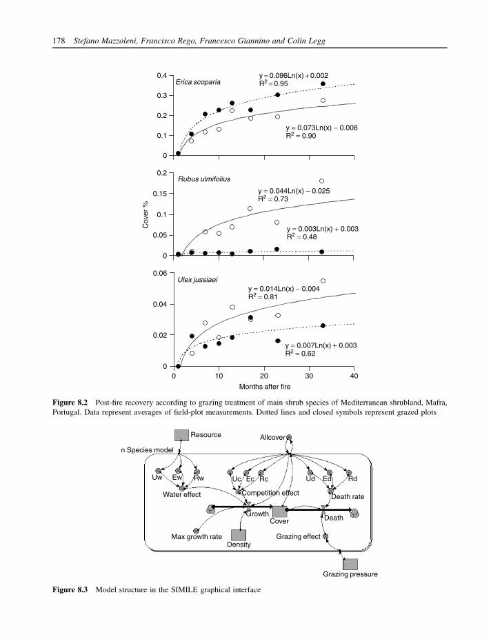
178 Stefano Mazzoleni, Francisco Rego, Francesco Giannino and Colin Legg
Ulex jussiaei
0
0.02
0.04
0.06
0 10 20 30 40
Erica scoparia
0
0.1
0.2
0.3
0.4
Rubus ulmifolius
0
0.05
0.1
0.15
0.2
Cov
er %
y = 0.096Ln(x) + 0.002R2 = 0.95
y = 0.044Ln(x) − 0.025R2 = 0.73
y = 0.003Ln(x) + 0.003R2 = 0.48
y = 0.014Ln(x) − 0.004R2 = 0.81
y = 0.007Ln(x) + 0.003R2 = 0.62
y = 0.073Ln(x) − 0.008R2 = 0.90
Months after fire
Figure 8.2 Post-fire recovery according to grazing treatment of main shrub species of Mediterranean shrubland, Mafra,Portugal. Data represent averages of field-plot measurements. Dotted lines and closed symbols represent grazed plots
Grazing pressure
Uw Ew Rw Uc Ec Rc Ud Ed Rd
Death rate
Death
Competition effectWater effect
Grazing effectMax growth rateDensity
CoverGrowth
AllcoverResource
n Species model
Figure 8.3 Model structure in the SIMILE graphical interface

Ecosystem Modelling: Vegetation and Disturbance 179
Table 8.1 Model elements and inputs
Name Meaning Units
Erica Erica cover %Rubus Rubus cover %Ulex Ulex cover %AllCover Sum of cover of all species %MaxGrowthRateSpecie Maximum growth rate (for all species)Death Rate (Ud, Ed, Rd) Death rate (for all species)Water effect (Uw, Ew, Rw) Growth resource function (for each species) [0,1]Competition effect (Uc, Ec, Rc) Growth competition sensitivity (for each species) [0,1]Resource Resource [0,1]Density Number of initial individuals for each species 0–20Grazing pressure Animal presence 0,1Grazing effect Response to grazing pressure (for each species) [0,1]
Ulex jussiaei
0
0.02
0.04
0.06
0 10 20 30 40
Erica scoparia
0
0.1
0.2
0.3
0.4
Rubus ulmifolius
0
0.05
0.1
0.15
0.2
Cov
er %
Months after fire
Figure 8.4 Results of model simulation of cover changes of three competing species according to grazing treatment.Data are the same as reported in Figure 8.2. Dashed lines and closed symbols represent grazed plots

180 Stefano Mazzoleni, Francisco Rego, Francesco Giannino and Colin Legg
No Grazing
0
0.2
0.4
0.6
Ulex jussiaei
Ulex jussiaei
Erica scoparia
Erica scoparia
Rubus ulmifolius
Rubus ulmifolius
Grazing
0
0.2
0.4
0.6
0 5 10 15 20 25 30
Time (years)
Cov
er %
Figure 8.5 Long-term modelled successional changes according to grazing disturbance
First, the changes of relative cover in the three specieswere modelled under the same post-fire conditions (plantdensities and grazing treatments) as in the real studycase. The good fit between the regressions based on realdata (Figure 8.2) and the outputs of the process-basedmodel (Figure 8.4) are evident.
Second, another simulation of plant regrowth afterfire was done with equal numbers of individuals forthe different species; this removed the competitiveadvantage due to the higher initial density of Ericaspecies. Moreover, the model run was extended to30 years in order to investigate longer-term successionalbehaviour (Figure 8.5). In this case, without grazing,Rubus shows an initial dominance followed by a declinedue to its sensitivity to competition, whereas Erica andUlex can shift their final dominance in relation to thegrazing pressure.
A schematic representation of the vegetation modellinked to pixels of the spatial raster system is shownin Figure 8.6a. Results of a simple exercise simula-tion show the emergence of spatial patterns of speciesdominance being related to both the grazing pressure
and initial density conditions (Figure 8.7). Such patternssimply reflect the isolated model behaviour being dis-tributed in space with changing conditions.
The complexity of the exercise can be increased(Figure 8.6b) by adding a fire disturbance with removalof biomass in burned pixels and by the use of a dynamicmodel to simulate the distribution of animals in the land-scape and hence grazing pressure (Legg et al., 1998).The simulation shows (Figure 8.8) a concentration ofherbivores in the burned area, which reflects the highergrazing value for the early successional-stage vegeta-tion. However, as grazing removes the highly palatableRubus, and to a lesser extent Ulex, the animals spreadagain around the landscape with a more even distri-bution. The distribution of animals, of course, createsfeedback to the growth of plants and the process ofvegetation dynamics.
A final exercise included in the workspace a seed-dispersal model (Figure 8.6c) (Heathfield et al., 2001).While in the previous examples all species were consid-ered to be present in all pixels from the start of the sim-ulation, in this case patchy distributions were considered
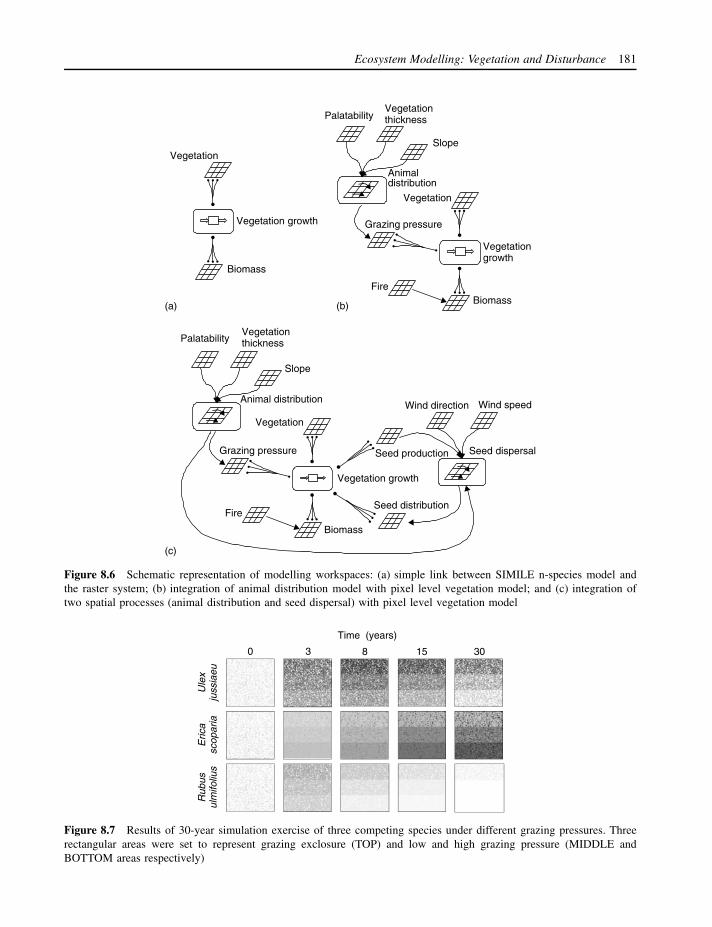
Ecosystem Modelling: Vegetation and Disturbance 181
Vegetation growth
Biomass
Vegetationgrowth
BiomassFire
Palatability
Slope
Grazing pressure
Vegetation growth
Biomass
Vegetation
Fire
VegetationthicknessPalatability
Slope
Grazing pressure
Animal distribution
Seed dispersal
Wind speed
Seed production
Seed distribution
Vegetation
Vegetationthickness
Animaldistribution
Vegetation
Wind direction
(a)
(c)
(b)
Figure 8.6 Schematic representation of modelling workspaces: (a) simple link between SIMILE n-species model andthe raster system; (b) integration of animal distribution model with pixel level vegetation model; and (c) integration oftwo spatial processes (animal distribution and seed dispersal) with pixel level vegetation model
Time (years)
0 3 8 15 30
Eric
asc
opar
iaR
ubus
ulm
ifoliu
sU
lex
juss
iaeu
Figure 8.7 Results of 30-year simulation exercise of three competing species under different grazing pressures. Threerectangular areas were set to represent grazing exclosure (TOP) and low and high grazing pressure (MIDDLE andBOTTOM areas respectively)

182 Stefano Mazzoleni, Francisco Rego, Francesco Giannino and Colin Legg
Time
Fire 6 48
Ule
x ju
ssia
euE
rica
scop
aria
Rub
us u
lmifo
lius
Gra
zing
pre
ssur
e
12
Figure 8.8 Results of 48-year model run of simulated post-fire recovery of three competing species with dynamicchanges of grazing pressure
Time (months)
No grazing Grazing
Ule
x ju
ssia
euE
rica
scop
aria
Rub
us u
lmifo
lius
Figure 8.9 Results of 60-year model run of simulated vegetation dynamics including plant growth (pixel process) andseed dispersal (spatial process). At start, only three competing species are present, whereas the fourth is introduced astwo plantations after 35 years. Dispersal from planted plots alter the dominance patterns of the natural vegetation in thesurrounding area

Ecosystem Modelling: Vegetation and Disturbance 183
with new establishment by colonization from neighbour-ing cells occurring during the modelling exercise.
The results are shown in Figure 8.9 and demonstratean expanding area of dominance by Ulex and to a lesserextent by Erica, whereas Rubus is strongly reduced bycompetition with the other species.
8.5 CONCLUSION
The modelling exercise reported in this chapter showsthe power of existing modelling tools to recover com-plex interactions of ecological processes, such as thecombined effects of grazing and fire on patterns of plantcompetition.
Other modelling workspaces can be built whichinclude other integrated objects and spatial models. Inparticular, the addition of changing resource levels (e.g.water uptake and infiltration processes) can be addedto look at their effect on the spatial pattern of plantcommunities (Rietkerk et al., 2002).
These new modelling environments can be con-sidered revolutionary in their flexibility and powerto represent complex systems and to integrate acrossscales. The traditional gap between ‘field’ ecologistsand mathematically-minded or computer-programmingmodellers seems to have been closed by the newly avail-able modelling technologies. It is now time to buildup banks of models to be used as elementary build-ing blocks of larger-scale dynamic systems. This shouldenable the development of truly process-based modelsthat are more robust, with greater generality, and withbehaviour that better resembles that in the real world.
ACKNOWLEDGEMENTS
The development of the modelling system used in thesimulation exercise has been largely supported by theEU-DG.XII ModMED research projects (ENV4-CT97-0680).
We thank Antonello Migliozzi for support to inputdata and graphical preparation.
REFERENCES
Aassine, S. and El Jaı, M.C. (2002) Vegetation dynamicsmodelling: a method for coupling local and space dynamics,Ecological Modelling 154, 237–249.
Abrahamson, W.G. and Abrahamson, C.R. (1996) Effects offire on long-unburned Florida uplands, Journal of VegetationScience 7, 564–574.
Angelstam, P. (1997) Landscape analysis as a tool for thescientific management of biodiversity, Ecological Bulletins46, 140–170.
Arianoutsou, M. (1998) Aspects of demography in post-firemediterranean plant communities of Greece, in P.W. Rundel,G. Montenegro and F.M. Jaksic (eds) Landscape Distur-bance and Biodiversity in Mediterranean-Type Ecosystems,Springer-Verlag, Berlin, 273–295.
Bakker, J.P., de Bie, S., Dallinga, J.H., Tjaden, P. and deVries, Y. (1983) Sheep-grazing as a management tool forheathland conservation and regeneration in the Netherlands,Journal of Applied Ecology 20, 541–560.
Bassett, P.A. (1980) Some effects of grazing on vegetationdynamics in the Camargue, France, Vegetatio 43, 173–184.
Botkin, D.B., Janak, J.F. and Wallis, J.R. (1972) Some eco-logical consequences of a computer model of forest growth,Journal of Ecology 60, 849–872.
Boumans, R.M., Villa, F., Costanza, R., Voinov, A., Voinov, H.and Maxwell, T. (2001) Non-spatial calibrations of a generalunit model for ecosystem simulations, Ecological Modelling146, 17–32.
Braun-Blanquet, J. (1954) Pflanzensoziologie, 2nd edn, Sprin-ger, Vienna.
Bryant, J.P., Provenza, F.D., Pastor, J., Reichardt, P.B.,Clause, T.P. and du Toit, J.T. (1991) Interactions betweenwoody plants and browsing animals mediated by secondarymetabolites, Annual Review of Ecology and Systematics 22,431–446.
Canfield, R.H. (1941) Application of the line interceptionmethod in sampling range vegetation, Journal of Forestry39, 388–394.
Cates, R. and Orians, G. (1975) Successional status and thepalatability of plants to generalized herbivores, Ecology 56,410–418.
Charnov, E.L. (1976) Optimal foraging: the marginal valuetheorem, Theoretical Population Biology 9, 129–136.
Chertov, O.G., Komarov, A.S. and Karev, G.P. (1999) ModernApproaches in Forest Ecosystem Modelling, European ForestInstitute Research Report 8, Koninklijke Brill NV, Leiden.
Chiavaura-Mususa, C., Campbell, B. and Kenyon, W. (2000)The value of mature trees in arable fields in the smallholdersector, Zimbabwe, Ecological Economics 33, 395–400.
Clutton-Brock, T.H. and Harvey, P.H. (1978) Mammals,resources and reproductive strategies, Nature 273, 191–195.
Costanza, R. and Gottilieb, S. (1998) Modelling ecologicaland economic systems with STELLA: Part II, EcologicalModelling 112, 81–84.
Costanza, R. and Voinov, A. (2001) Modelling ecological andeconomic systems with STELLA: Part III, Ecological Mod-elling 143, 1–7.
De Angelis, D.L. and Gross, L.J. (1992) Individual-basedModels and Approaches in Ecology, Chapman & Hall, NewYork.
Dumont, B. (1997) Diet preferences of herbivores at pasture,Annales de Zootechnie 46 (2), 105–116.
Ellenberg, H. (1988) Vegetation Ecology of Central Europe,Cambridge University Press, Cambridge.
184 Stefano Mazzoleni, Francisco Rego, Francesco Giannino and Colin Legg
Engelen, G., White, R., Uljee, I. and Drazan, P. (1995) Usingcellular automata for integrated modelling of socio-environ-mental systems, Environmental Monitoring and Assessment34, 203–214.
Espırito-Santo, M.D., Rego, F. and Costa, J.C. (1993) Vegeta-tion dynamics in the Serra dos Candeeiros (central Portugal),in L. Trabaud and R. Prodon (eds) Fire in MediterraneanEcosystems, Ecosystem Research Report no. 5, Commissionof the European Communities, Brussels, 29–46.
Ferran, A. and Vallejo, V.R. (1998) Long-term plant regen-eration after wildfires in Mediterranean ecosystems of NESpain, in L. Trabaud (ed.) Fire Management and LandscapeEcology, International Association of Wildland Fire, Wash-ington, DC, 155–166.
Fonseca, M.M. (1998) Plasticity of mating behaviour in reddeer (Cervus elaphus) in a Mediterranean environment, PhDdissertation, University of London. London.
Ford, E.D. (1975) Competition and stand structure in someeven-aged plant monocultures, Journal of Ecology 63,311–333.
Forman, R.T.T. and Godron, M. (1986) Landscape Ecology,John Wiley & Sons, New York.
Gimingham, C.H., Hobbs, R.J. and Mallik, A.U. (1981) Com-munity dynamics in relation to management of heathlandvegetation in Scotland, Vegetatio 46, 149–155.
Groeneveld, J., Enright, N.J., Lamont, B.B. and Wissel, C.(2002) A spatial model of coexistence among three Banksiaspecies along a topographic gradient in fire-prone shrub-lands, Journal of Ecology 90, 762–774.
Grubb, P.J. (1985) Plant populations in relation to habitat.Disturbance and competition: problem of generalization, inJ. White and W. Beeftink (eds) The Population Structure ofVegetation. Handbook of Vegetation Science, vol. 3, Harperand Row, New York, 83–97.
Grubb, P.J. and Hopkins, A.J.M. (1986) Resilience at thelevel of the plant community, in B. Dell, A.J.M. Hopkinsand B.B. Lamont (eds) Resilience in Mediterranean-TypeEcosystems. Task for Vegetation Science 16, Dr. W. JunkPublishers, Dordrecht, 113–128.
Hanes, T.L. (1971) Succession after fire in the chaparral ofsouthern California, Ecological Monographs 41, 27–52.
Heathfield, D., Arianoutsou, M., Georghiou, K., Thanos, C.and Loureiro, C. (2001) Seed dispersal, in S. Mazzoleniand C.J. Legg (eds) ModMED: Modelling MediterraneanEcosystem Dynamics, Final Report, ModMED III Project,EU-DGXII Environment (IV) Research Programme, Con-tract ENV4-CT97-0680, Brussels.
Heinselman, M.L. (1978) Fire intensity and frequency as fac-tors in the distribution and structure of northern ecosystems,in Fire Regimes and Ecosystems Properties: Proceedings ofthe Conference, USDA – Forest Service. General TechnicalReport WO-26, Washington, DC, 7–57.
Henderson, M.K. and Keith, A.D. (2002) Correlation of burn-ing and grazing indicators with composition of woody under-storey flora of dells in a temperate eucalypt forest, AustralianEcology 27, 121–131.
Henkin, Z., Seligam, G.S., Noy-Meir, I. and Kafkafi, U.(1999) Secondary succession after fire in a Mediterranean
dwarf-shrub community, Journal of Vegetation Science 10,503–514.
Hesp, P., Wells, M., Ward, B. and Riches, J. (1983) LandResource Survey of Rottnest Island, Bulletin No. 4086, Soiland Conservation Service Branch, Division of ResourceManagement, Department of Agriculture, Western Australia,Perth.
Higgins, S. and Cain, L.M. (2002) Spatially realistic plantmetapopulation models and the colonization-competitiontrade-off, Journal of Ecology 90, 616–626.
Hobbs, R.J. and Legg, C.J. (1984) Markov models and initialfloristic composition in heathland vegetation dynamics, Veg-etatio 56, 31–43.
Horn, H.S. (1975) Markovian properties of forest succession, inM.L. Cody and J.M. Diamond (eds) Ecology and Evolutionof Communities, Harvard University Press, Cambridge MA,196–211.
Johst, K., Brandl, R. and Eber, S. (2002) Metapopulation per-sistence in dynamic landscapes: the role of dispersal dis-tance, Oikos 98, 263–270.
Keane, R.E., Morgan, P. and Running, S.W. (1996) FIRE-BGCA Mechanistic Ecological Process Model for Simulating FireSuccession on Coniferous Forest Landscapes of the NorthernRocky Mountains, USDA Forestry Service Research Paper,INT-RP-484, Washington, DC.
Legg, C., Papanastasis, V., Heathfield, D., Arianoutsou, M.,Kelly, A., Muetzelfeldt, R. and Mazzoleni, S. (1998)Modelling the impact of grazing on vegetation in theMediterranean: the approach of the ModMED Project, inV.P. Papanastasis and D. Peter (eds) Ecological Basis ofLivestock Grazing in Mediterranean Ecosystems, EC ScienceResearch and Development, Brussels, 189–199.
Leigh, J. and Holgate, W. (1979) The response of the under-storey of forest and woodlands of the Southern Tablelandsto grazing and browsing, Australian Journal of Ecology 4,23–43.
Levin, S.A. (1992) The problem of pattern and scale inecology, Ecology 73, 1943–1967.
Liddel, M. (2001) A simple space competition model usingstochastic and episodic disturbance, Ecological Modelling143, 33–41.
Lippe, E., de Smidt, J.T. and Glenn-Lewin, D.C. (1985)Markov models and succession: a test from heathland inthe Netherlands, Journal of Ecology 73, 775–791.
Malanson, G.P. (1984) Linked Leslie matrices for the simula-tion of succession, Ecological Modelling 21, 13–20.
Manly, B.F., McDonald, L.L. and Thomas, D.L. (1993)Resource Selection by Animals: Statistical Design andAnalysis for Field Studies, Chapman & Hall, London.
Martins, H. (2001) Aspectos da ecologia e da gestao cinegeticado coelho bravo (Oryctolagus cuniculus L.) em montado,PhD thesis, Instituto Superior de Agronomia, UTL, Lisbon.
Mazzoleni, S. and Legg, C.J. (eds) (2001) ModMED: Mod-elling Mediterranean Ecosystem Dynamics: Final Report,ModMED III Project, EU-DGXII Environment (IV) ResearchProgramme, Contract ENV4-CT97-0680, Brussels.
Mazzoleni, S. and Pizzolongo, P. (1990) Post-fire regenerationpatterns in Mediterranean shrubs in the Campania region,

Ecosystem Modelling: Vegetation and Disturbance 185
southern Italy, in J.G. Goldammer and M.J. Jenkins (eds)Fire in Ecosystem Dynamics: Mediterranean and NorthernPerspectives, SPB Academic, The Hague, 43–52.
McIntosh, B.S., Muetzelfeldt, R.I., Legg, C.J., Mazzoleni, S.and Csontos, P. (2003) Reasoning with direction and rate ofcange in vegetation state transition modelling, EnvironmentalModelling and Software (in press).
Miles, J. (1979) Vegetation Dynamics. Chapman & Hall,London.
Miles, J. (1985) The pedogenic effects of different species andvegetation types and the implications of succession, Journalof Soil Science 36, 571–584.
Mills, J. (1983) Herbivory and seedling establishment in post-fire southern California chapparal, Oecologia 60, 267–270.
Mladenoff, D.J. and Baker, W.L. (eds) (1999) Spatial Mod-elling of Forest Landscape Change: Approaches and Appli-cations, Cambridge University Press, Cambridge.
Moreno, J.M. and Cruz, A. (2000) La respuesta de las plantasal fuego, in R. Velez (ed.) La Defensa contra Incendios Fore-stales: Fundamentos y Experiencias, McGraw-Hill, Madrid,413–436.
Muetzelfeldt, R. and Massheder, J. (2003) The Simile visualmodelling environment, European Journal of Agronomy 18,345–358.
Nahal, I. (1981) The Mediterranean climate from a biologicalviewpoint, in F. Di Castri, D.W. Goodall and R.L. Specht(eds) Mediterranean-Type Shrublands: Ecosystems of theWorld 11, Elsevier, Amsterdam, 63–86.
Naveh, Z. (1974) Effect of fire in the Mediterranean region,in T.T. Kozlowski and C.E. Ahlgren (eds) Fire and Ecosys-tems, Academic Press, New York, 401–432.
Noble, I.R. and Slatyer, R.O. (1980) The use of vital attributesto predict successional changes in plant communities subjectto recurrent disturbance, Vegetatio 43, 5–21.
Odum, H.T. (1983) Systems Ecology: An Introduction, JohnWiley & Sons, New York.
Oom, S.P., Hester, A.J., Elston, D.A. and Legg, C.J. (2002)Spatial interaction models from human geography to plant-herbivore interactions, Oikos 98, 65–74.
Oxley, T., McIntosh, B.S., Mulligan, M. and de Roode, R.(2000) Adaptation, integration and application of an inte-grative modelling framework in MODULUS, in G. Engelen(ed.) MODULUS: A Spatial Modelling Tool for IntegratedEnvironmental Decision Making: Final Report, The ModulusProject, EU-DGXII Environment, Brussels.
Pan, Y. and Raynal, D.J. (1995) Decomposing tree annualvolume increments and constructing a system dynamicmodel of tree growth, Ecological Modelling 82, 299–312.
Persson, S. (1984) Vegetation development after the exclusionof grazing cattle in a meadow area in the south of Sweden,Vegetation 55, 65–92.
Quinn, R.D. (1986) Mammalian herbivory and resilience inmediterranean-climate ecosystems, in B. Dell, A.J.M. Hop-kins and B.B. Lamont (eds) Resilience in Mediterranean-Type Ecosystems: Tasks for Vegetation Science 16, Dr. W.Junk Publishers, Dordrecht, 113–128.
Rego, F., Pereira, J. and Trabaud, L. (1993) Modelling com-munity dynamics of a Quercus coccifera L. garrigue in rela-tion to fire using Markov chains, Ecological Modelling 66,251–260.
Renshaw, E. (1991) Modelling Biological Populations in Spaceand Time, Cambridge University Press, Cambridge.
Rietkerk, M., Boerlijst, M.C., van Langevelde, F., HilleRis-Lambers, R., van de Koppel, J., Kumar, L., Prins, H. andde Roos, A.M. (2002) Self-organization of vegetation in aridecosystems, The American Naturalist, 160 (4), 524–530.
Running, S.W. and Coughlan, J.C. (1988) A general modelof forest ecosystem processes for regional applications.I. Hydrologic balance, canopy gas exchange and primaryproduction processes, Ecological Modelling 42, 125–154.
Running, S.W. and Gower, S.T. (1991) FOREST-BGC, a gen-eral model of forest ecosystem processes for regional appli-cations, II. Dynamic carbon allocation and nitrogen budgets,Tree Physiology 9, 147–160.
Ryan, K.C. and Reinhardt, E.D. (1988) Predicting postfiremortality of seven western conifers, Canadian Journal ofForest Research 18, 1291–1297.
Sequeira, R.A., Sharpe, P.J.H., Stone, N.D., El-Zik, K.M. andMakela, M.E. (1991) Object-oriented simulation: plantgrowth and discrete organ-to-organ interaction, EcologicalModelling 58, 25–54.
Shugart, H.H. and Noble, I.R. (1981) A computer model ofsuccession and fire response of the high altitude Eucalyptusforest of the Brindabella Range, Australian Capital Territory,Australian Journal of Ecology 6, 149–164.
Shugart, H.H. and West, D.C. (1977) Development of anAppalachian deciduous forest succession model and itsapplication to assessment of the impact of the chestnut blight,Journal of Environmental Management 5, 161–179.
Sondgerath, D. and Schroder, B. (2002) Population dynamicsand habitat connectivity affecting the spatial spread ofpopulation – a simulation study, Landscape Ecology 17,57–70.
Specht, R.L., Rayson, P. and Jackman, M.E. (1958) DarkIsland heath (Ninety-Mile Plain, South Australia). VI. Pyricsuccession: changes in composition, coverage, dry weightand mineral nutrient status, Australian Journal of Botany 6,193–202.
Tilman, D. (1988) Plant Strategies and the Dynamics andStructure of Plant Communities, Princeton University Press,Princeton, NJ.
Tilman, D. (1994) Competition and biodiversity in spatiallystructured habitats, Ecology 75, 2–16.
Turner, M. (1985) Ecological effects of multiple perturbationson a Georgia salt marsh, Doctoral dissertation, University ofGeorgia, Athens, GA.
Turner, M. and Bratton, S. (1987) Fire, grazing and the land-scape heterogeneity of a Georgia Barrier Island, in M. Turner(ed.) Landscape heterogeneity and disturbance, EcologicalStudies 64, Springer-Verlag, Berlin, 85–101.
Usher, M.B. (1992) Statistical models of succession, inD.C. Glenn-Lewin, R.K. Peet and T.T. Veblen (eds) PlantSuccession: Theory and Prediction, Chapman & Hall, Lon-don, 215–248.

186 Stefano Mazzoleni, Francisco Rego, Francesco Giannino and Colin Legg
Van Soest, P.J. (1982) Nutritional Ecology of the Ruminant, O.and B. Books, Inc, Corvallis, OR.
Walter, H. (1973) Vegetation of the Earth and EcologicalSystems of the Geobiosphere, Springer-Verlag, New York.
Waring, R.H. and Running, S.W. (1998) Forest Ecosystems:Analysis at Multiple Scales, 2nd edn, Academic Press, SanDiego.
Western, D. (1975) Water availability and its influence onthe structure and dynamics of a savannah large mammalcommunity, East African Wildlife Journal 13, 265–268.
White, P.S. and Harrod, J. (1997) Disturbance and diversityin a landscape context, in J.A. Bissonette (ed.) Wildlife and
Landscape Ecology: Effects of Pattern and Scale, Springer-Verlag, New York, 128–159.
White, P.S. and Pickett, S.T.A. (1985) Natural disturbanceand patch dynamics: an introduction, in S.T.A. Pickett andP.S. White (eds) The Ecology of Natural Disturbance andPatch Dynamics, Academic Press, New York, 3–13.
Wimbush, D.J. and Costin, A.B. (1979) Trends in vegetationat Kosciusko. I Grazing trials in the sub-alpine zone,1957–1971, Australian Journal of Botany 27, 741–787.
Wolfe, M.L. and Berg, F.C. (1988) Deer and forestry inGermany – half a century after Aldo Leopold, Journal ofForestry 86, 25–28.

9
Erosion and Sediment Transport
JOHN N. QUINTON
9.1 THE COMPLEXITY
Erosion and sediment transport appears to be a relativelystraightforward topic for modelling. Rain falls andimpacts on the soil surface, soil particles are dislodgedand may be transported by rain splash or overland flow.Overland flow can also detach material and transportit. This conceptualization of erosion processes on aninter-rill area (Figure 9.1) was used by Meyer andWischmeier (1969) in their mathematical model of theprocess of soil erosion and is still found at the heartof many process-based soil-erosion models today. Twokey processes are identified: detachment and transport.Meyer and Wischmeier modelled splash detachment asa function of rainfall intensity, an approach also adoptedin ANSWERS, KINEROS2, and GUEST (Morgan andQuinton, 2001). The transport capacity of the rainfallwas described as a function of soil, slope and rainfallintensity. Flow detachment was modelled as a functionof discharge slope and soil erodibility and the transportcapacity of the flow as a function of slope, dischargeand a soil factor. For splash and flow detachment, thesediment detached is compared with a value for transportcapacity; if the value is below the transport capacityfigure, the material is transported, above it is deposited.Meyer and Wischmeier recognized that their model wasnot comprehensive and highlighted the need for furthercomponents to be added to it.
Similar conceptual flowcharts can be found for anumber of current generation erosion models, such asEUROSEM (Morgan et al., 1998) and WEPP (Flanaganand Nearing, 1995; Laflen, et al. 1997). However,unlike the model of Meyer and Wischmeier, the cur-rent generation of erosion models has tried to model thecontrols on these processes in more detail. Figure 9.2
illustrates some of the other factors that have to be takeninto account when calculating detachment and transport.The inclusion of submodels to describe these processesmakes the representation more complex. Many of theprocesses included are known to be important, but areonly poorly described mathematically, with expressionsonly tested using data from a handful of situations. Forexample, EUROSEM contains an expression linking soilcohesion to the resistance of the soil to erosion by flow-ing water based on only a few measurements made inthe laboratory.
Figure 9.2 is probably reasonably complete fordescribing erosion on an inter-rill area. However,erosion does not take place only on inter-rill areas. It isa process that often links inter-rill areas with transientor permanent channel networks, the position of whichmay vary in time and space, with some parts of thehill slope contributing sediment and water and otherscontributing none at all. The processes within rills andgullies, such as bank collapse and headwall retreat, arepoorly understood and are almost universally ignored inerosion models, yet may contribute more than 50% ofthe sediment from a gully system (Blong, 1985). Whererills are included in models, such as EUROSEM andWEPP, sidewall and head processes are not simulatedand the models erode the channels by assuming thatmaterial is removed equally from the sidewalls and bed.
This discussion focuses on processes that take placeover timescales of minutes or hours. However, for manysituations, such as global change studies (Williamset al., 1996), we may wish to understand erosion andsedimentation over years, decades or centuries. To do sorequires us to understand changes in the controls overerosion that may take place over differing timescales,for example, the consolidation of soil after tillage and
Environmental Modelling: Finding Simplicity in Complexity. Edited by J. Wainwright and M. Mulligan 2004 John Wiley & Sons, Ltd ISBNs: 0-471-49617-0 (HB); 0-471-49618-9 (PB)
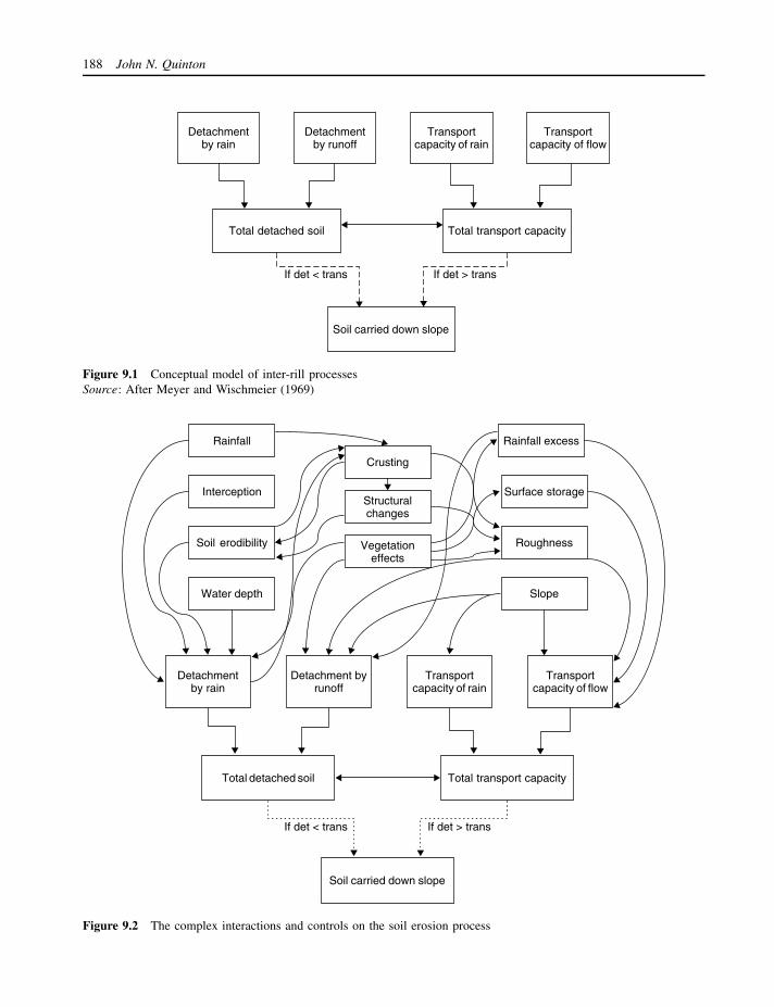
188 John N. Quinton
Detachmentby rain
Detachmentby runoff
Transportcapacity of rain
Transportcapacity of flow
Total detached soil Total transport capacity
Soil carried down slope
If det < trans If det > trans
Figure 9.1 Conceptual model of inter-rill processesSource: After Meyer and Wischmeier (1969)
Detachmentby rain
Detachment byrunoff
Transportcapacity of rain
Transportcapacity of flow
Total detached soil Total transport capacity
Soil carried down slope
If det < trans If det > trans
Rainfall
Interception
Soil erodibility
Water depth
Crusting
Structuralchanges
Vegetationeffects
Rainfall excess
Surface storage
Roughness
Slope
Figure 9.2 The complex interactions and controls on the soil erosion process
Erosion and Sediment Transport 189
its effects on soil erodibility (Nearing et al., 1988).Although water-erosion processes take place over fairlyshort timescales, the factors which control them maychange over periods lasting several minutes, such as sur-face sealing, to several centuries for changes in topog-raphy or rates of pedogenesis. This spatial and temporaldimension to the erosion problem makes describing ero-sion processes even more complex.
Not only are the processes variable in time but alsoin space. In a study of 36 erosion plots all treatedidentically, Wendt (1986) found that erosion rates var-ied between 18 and 91%. This may be a response tothe variability of parameters that control the genera-tion of runoff and erosion. The spatial variability ofhydraulic parameters, such as hydraulic conductivity, iswell documented (Beckett and Webster, 1971; Warrickand Nilesen, 1980). Other parameters such as soil cohe-sion (Quinton, 1994) also exhibit considerable variationin the field.
So we find ourselves in a situation where many ofthe current generation of erosion models are gettingmore complex, with more processes being incorporatedinto them. They also suffer from considerable uncer-tainty (Quinton, 1997; Brazier et al., 2000) associatedwith parameterization difficulties, and are generally poorat reproducing measured data (see, for example, Favis-Mortlock, 1998), which is highly variable (Wendt et al.,1986; Nearing et al., 1999). This chapter sets out toanswer the question: does the level of uncertainty asso-ciated with both erosion model predictions and erosionmodel measurement mean that we can utilize simplerapproaches to erosion prediction to those which are cur-rently in vogue?
9.2 FINDING THE SIMPLICITY
As Kant (1885) states, ‘hypotheses always remainhypotheses i.e. suppositions to the full reality of what wecan never obtain’. In other words, even the most com-plex model of erosion and sedimentation processes canonly still be a representation of reality, so how complexdo they need to be?
As with most environmental modelling there arebroadly two groups of people interested in buildingmodels: scientists and managers (Bunnel, 1989). Scien-tists usually do most of the model building, but tendto focus on representing all the processes which theybelieve control a particular system, while managers aremore concerned about getting an accurate answer fromthe model so that they can make a decision. The factthat scientists have been driving the construction of ero-sion and sediment transport models perhaps explains the
trend towards ever more complex models in recent years.While, on the face of it, this drive to ever more com-plex models has resulted in a better representation of theerosion system, it does have its problems.
9.2.1 Parameter uncertainty
Determining the inputs for soil-erosion models is diffi-cult. Input parameters vary in time and space, and someare difficult to measure. Spatial variability poses dif-ficulties for the modeller when trying to parameterizemodels. The spatial variability of many input parametersof commonly used erosion models is known to be high.For example, saturated hydraulic conductivity measure-ments may have coefficients of variation of 150% for asingle soil-map unit (Warrick and Nilesen, 1980). Eventhough many erosion models are distributed, allowingdifferent parameter sets to be used for different parts ofthe catchment, the model will impose a grid or elementupon the landscape. Within each grid square or element,the model inputs may vary considerably, but they willbe represented in the model as a single value. Beven(1989) gives the example of a variation in hydraulicconductivity causing runoff in one part of an element,where it is low, and infiltrating it in another area. Ifan average value has been used, it may be possiblethat the model erroneously predicts small amounts ofrunoff. In the case of EUROSEM, many of the param-eters were identified as sensitive during the sensitivityanalysis of the model (Veihe and Quinton, 2000; Veiheet al., 2000), for example, saturated hydraulic conductiv-ity and hydraulic roughness, and therefore have a greatinfluence over the model outputs.
Temporal variation causes more uncertainty in theparameterization of erosion models. Here the problemis to identify the initial conditions for the model atthe beginning of the simulation. The characteristics ofthe soil and vegetation are not static: their propertieschange through time owing to biological, chemical andphysical processes. In the case of event-based models,even where regular measurement programmes to collectinput data (e.g. soil and vegetation characteristics)have been undertaken, it is only by chance that astorm occurs directly after measurements have takenplace. This problem can, for some of the inputs, beremedied by using automated sampling equipment, forexample, tensiometers linked into a data-logger can giveinformation on soil-water potential. However, at presentthe number of input parameters that can be measured inthis way is limited.
Rather than measure the inputs, a different approachis to use a continuous simulation model to simulate the

190 John N. Quinton
change in the key model inputs prior to an event. Thisis the approach that has been adopted for MIKE SHESEM (Styczen and Nielsen, 1989) and WEPP (Flanaganand Nearing, 1995). This approach also has its limi-tations: describing the dynamics of soil structure, soilwater and the vegetation is not straightforward, result-ing in further uncertainty surrounding the values ofinput parameters.
Uncertainty surrounding the value of input-parametervalues will have a limited impact on model out-put if the model is not sensitive to changes in thevalue of the parameter in question. Sensitivity analy-sis of the EUROSEM model by Quinton (1994), Veihe(2000) and Veihe et al. (2000) showed that many ofEUROSEM’s parameters did not invoke a sensitiveresponse from the model. A similar pattern can beobserved for WEPP in the work of Brazier et al. (2000).However, both models are sensitive to a number of inputparameters and when this is combined with uncertaintyover parameter values, there will be uncertainty in themodel output results.
To investigate the impact of parameter uncertainty,Quinton (1997) applied the EUROSEM model to 0.1-haerosion plots from the Woburn Erosion Reference Exper-iment (Catt et al., 1994; Quinton et al., 2001). He ranthe EUROSEM model 525 times using different param-eter sets. The parameter sets were constructed by takingfour parameters to which the model was sensitive andconstructing probability distributions for them based onthe results of field sampling. Thus, all parameter setshad the same parameter values, except for the four sen-sitive parameters. All parameter sets could be assumedto be an equally likely representation of the system.The results showed that uncertainty bands on the out-put were large. The mean width of the 95% confidenceinterval for peak sediment discharge was 62.5 kg min−1,and for soil loss 217 kg. Using the same source ofobserved data, Brazier et al. (2000) assessed the uncer-tainty surrounding predictions of annual soil loss fromthe WEPP model and found uncertainty bands of up to10 t a−1.
9.2.2 What are the natural levels of uncertainty?
Given the levels of uncertainty reported in the previoussection, two things come to mind: is the natural world asuncertain as the virtual one described in erosion models?If so, can we use this uncertainty to make the casethat we should describe the erosion system with simplermodels than those that are currently in vogue?
Work carried out by Wendt et al. (1986) using 40 ero-sion plots, all with the same treatment, in Kingdom City,
Minnesota, found that coefficients of variation for the25 storms ranged from 18% to 91%. The larger erosionevents showed less variability. Very little of the vari-ability could be attributed to measured plot properties,and the plots did not perform in the same manner rel-ative to each other in subsequent events. Nearing et al.(1999) also considered the performance of replicates inerosion experiments. They took 2061 replicated stormevents from 13 sites in the USA and found, like Wendtet al., that the measured coefficient variation in the soilloss declined with event magnitude. It would appear thatmeasured erosion rates will be subject to high degreesof variation. If this is the case and as Nearing et al.(1999) state, the study of Wendt et al. strongly impliesthat given our current ability to measure plot charac-teristics in the field, we will not be able to improvemodel-simulation results for these data, i.e. we cannotmeasure and therefore parameterize our models to reflectthe differences between replicated plots. If this is thecase, then is the addition of more process descriptionsand their associated parameters simply a waste of time?
9.2.3 Do simple models predict erosion any betterthan more complex ones?
So far this chapter has demonstrated that predictionsfrom erosion models suffer from considerable uncer-tainty and that there is considerable variation betweensimilar sites exposed to the same rainfall. Do these highlevels of uncertainty mean that even those models whichoffer an apparently more complete description of theerosion process perform no better than simple models?
Recently there have been a number of attempts tocompare erosion models. Favis-Mortlock (1997) drewtogether the results from models simulating annual soilloss for a field site in the USA. The models rangedfrom simple models, such as CSEP (Kirkby and Cox,1995) and those based on the USLE (Wischmeier andSmith, 1978) such as EPIC (Williams et al., 1984) andGLEAMS (Leonard et al., 1987), to the more process-based, and complex WEPP. Favis-Mortlock’s resultsshow no significant difference between the performanceof the models. Morgan and Nearing (2000) comparethe performance of the USLE, RUSLE and WEPPusing 1700 plot years of data from 208 natural runoffplots (Figure 9.3). Once again it becomes clear that themore complex model, in this case WEPP, performs nobetter than the empirical, five parameter USLE (seeChapter 16).
It might be argued that the examples given aboveare based on models with quite different structures, andare therefore unfair. However, recent work by Morgan

Erosion and Sediment Transport 191
0
1
2
3
4
5
6
Measured USLE RUSLE WEPP
Ann
ual s
oil l
oss
kg m
−2
Figure 9.3 Comparison of the USLE, RUSLE and WEPPwith measured data representing 1700 plot years of datafrom 208 natural runoff plots (average annual soil loss3.51 kg m−2)
Source: Morgan and Nearing (2000)
(2001) allows us to consider the impact of increasingthe number of parameters within a model, on thatmodel’s ability to simulate data from a wide variety ofconditions. Morgan takes the Morgan–Morgan–Finneyerosion model (Morgan et al., 1984) and modifies it todeal with flow-erosion processes – the previous versiondealt solely with inter-rill erosion. He then applied itto erosion data from 67 sites around the world, thesame data set that he originally used to test the previousversion of the model. The information in Morgan’s
paper can be plotted (Figure 9.4), and illustrates thatthere is little difference in the performance of the twomodels. In fact, a comparison of the Nash and Sutcliffe(1970) coefficient of efficiency suggests that the olderversion with fewer parameters does marginally better atsimulating mean annual soil loss across all the sites.
So it appears that more parameters do not producebetter simulation results; that is not to say however,that the inclusion of further process descriptions in amodel is not a worthy activity. From a scientific pointof view, the inclusion of a flow detachment module inthe MMF model makes the model a better representationof reality, but it does not make it better able to predicterosion rates.
There appear to be few comparisons between spatiallycomplete data sets and incomplete data sets. One ofthe few is that of Loague (1990) who studied theeffect that 157 extra infiltration measurements had onmodel simulations and found that there was not an‘overwhelming improvement in model performance’.
9.3 FINDING SIMPLICITY
In a situation where variability in observed sedimenttransport and difficulties in parameterization make theuse of complex models unnecessary or simply notfeasible, it might be expected that there would beefforts made to develop simpler approaches to ero-sion prediction.
0
2
4
6
8
10
12
14
16
18
20
0 5 10 15 20
Observed max annual soil loss (kg m−2)
Sim
ulat
ed m
ax a
nnua
l soi
l los
s (k
g m
−2)
NewOld
Figure 9.4 Comparison of simulated maximum annual soil loss against observed maximum annual soil loss for therevised (new) MMF model with the original (old) version of the modelSource: Morgan (2000)

192 John N. Quinton
To date, the response of the modelling communityto this problem has been to try to mask the complex-ity. Both the EUROSEM and WEPP developers havedeveloped user-friendly interfaces with database supportto supply parameter values. As yet, there appear to befew attempts to develop models with a reduced numberof processes or number of parameters. Where there isactivity in producing simpler models is where there is aneed to make regional-scale assessments of erosion ratesor erosion risks. Kirkby et al. (2000) present a model forestimating erosion risk as a soil loss in tonne ha−1. Themodel captures the key driver influencing erosion rates:topography. Soil erodibility, topography, vegetation andclimate and data requirements appear low, with eightdatabase layers and two tables needed to provide infor-mation for the model. However, a number of the parame-ters required by the model need to be derived from thesedata using transfer functions. The initial application ofthe model of Kirkby et al. was to the whole of France.However, as yet, they have conducted no validation oftheir approach.
So it seems that at present the search for simplicity isbeing driven forward by the need to make erosion esti-mates at ever increasing scales. However, erosion pre-diction is still dominated by the use of one model – theUSLE. It provides the user with a simple model whichcan be executed using nothing more sophisticated than apocket calculator, yet in model comparison studies pre-dicts annual erosion as well as any model. This may notreflect any superiority in terms of the model, but sim-ply the fact that a five-parameter empirical model cando as well as a multi-parameter model in capturing theextremely variable response of a hillside system.
9.4 THE RESEARCH FRONTIER
The combination of our inability to measure modelinputs and the high levels of variation in the very thingswe are trying to predict suggest that increasing the num-ber of processes represented in soil-erosion models andtherefore the number of inputs required will not leadto better predictions of erosion and sedimentation. Weneed simpler ways to simulate erosion and sedimenta-tion. Rule-based approaches, such as those describedby Favis-Mortlock et al. (2000; see also Chapter 21),provide one possibility, although they still require largeamounts of data. Perhaps it is more necessary to embracethe uncertainty in model simulation results and theuncertainty in data sets with which models are comparedand use it as an opportunity to simplify our approachesto erosion prediction. The extra process descriptions and
the extra parameters may make interesting science butthey do not produce better predictions.
9.5 CASE STUDY
This case study tests the hypothesis that only a smallnumber of parameters control the response of an erosionmodel and the remainder become largely inconsequen-tial. To do this the revised Morgan–Morgan–Finneymodel (MMF) (Morgan, 2001) is selected. The MMFmodel is used because it is relatively simple, yet physi-cally based, and can be programmed into a spreadsheetquickly. It is expected that other more complex mod-els such as EUROSEM and WEPP will exhibit similarcharacteristics if they were to be tested in a similar way.
Full details of the model can be found in Morgan(2001) and the operating equations can be found inTable 9.1. A copy of the spreadsheet containing theprogram can be downloaded from the book’s website(http://www.kcl.ac.uk/envmod). The MMF model sepa-rates erosion into the water and sediment phases. Theenergy available for soil detachment is derived from therainfall and the volume of water determines the trans-port capacity. The model uses Meyer and Wischmeier’s(1969) scheme in which sediment production is com-pared with the amount of sediment that the water is ableto hold and the lower value taken as the sediment trans-port rate. The model operates on an annual timestep.
The model was applied to an erosion plot fromthe Woburn Erosion Reference Experiment (Catt et al.,1994; Quinton, 1994; Quinton et al., 2001). The soilsat the site range in texture from loamy sand to sandyloam and correspond to the Cottenham and Lowlandsseries defined by Clayden and Hollis (1984) and clas-sified as Lamellic Ustipsamment and Udic Haplusteptrespectively (Soil Survey Staff, 1999). The experimentwas established after harvest in 1988 and the first cropof potatoes was planted in the following spring. Thiscrop was followed by two winter cereals, then sugarbeet and two more years of winter cereals – a crop rota-tion common in the area. The plot was cultivated up anddown with residues removed before mouldboard plough-ing. The plot measured approximately 25 m by 35 m(894 m2) and was isolated from the rest of the slope bya low earth bank. Soil and water flowing off each plotwas channelled to a collecting trough and through a pipeto two 2000-litre tanks where it was stored until sam-pled. The amount of runoff and soil loss from each plotwas determined as soon after each runoff event as prac-tically possible and usually within 48 hours. Annual soillosses were calculated for each agricultural year (cropand following fallow combined).

Erosion and Sediment Transport 193
Table 9.1 Operating equations of the MMF model
No. Description Operating equation Parameter definitions
9.1 Effective rainfall (mm) Re = RA R = rainfall (mm) A = proportion ofrainfall reaching soil surface
9.2 Leaf drainage (mm) Ld = Re Cc Cc = Canopy cover9.3 Direct throughfall (mm) Dt = Re − Ld
9.4 Kinetic energy of directthroughfall (J m−2)
Ket = Dt(11.9 + logI) I = typical rainfall intensity value forerosive rain (mm hr−1)
9.5 Kinetic energy of leafdrainage (J m−2)
Kel = Ld(15.8 P0.5h ) − 5.87 Ph is the plant canopy height (m)
9.6 Total Kinetic energy (J m−2) Ke = Ket + Kel
9.7 Annual runoff (mm) Q = Re−RcRo Ro = mean rain per day (mm)
Soil moisture capacity (mm) Rc = 1000 Mc Bd Hd (Et/Eo) Mc = soil moisture content at fieldcapacity (% w/w) Bd = Bulk densityof the soil (Mg m−3) Hd = Effectivehydraulic depth (m) Et/Eo = the ratioof actual to potentialevapotranspiration.
9.8 Soil particle detachment byraindrop impact (kg m−2)
F = 0.001 K Ke K the erodibility of the soil (g J−1)
9.9 Soil particle detachment byrunoff (kg m−3)
H = Z Q1.5 sin S (1 − Gc) 10−3 S = slope steepness Gc = Ground cover
9.10 Resistance of the soil Z = 1
0.5σσ = soil cohesion (kPa)
9.11 Transport capacity of runoff TC = C Q2 sin 10−3 C = the product of the C and P factorsof the Universal Soil Loss Equation
Source: Morgan (2000)
Rather than apply the model in a deterministic fash-ion, probability distributions were assigned to each ofthe parameters (Table 9.2). These were either deter-mined from field measurement, the literature or frombest estimates. To facilitate this a commercial risk-analysis package – Crystal Ball1 – was used. This pack-age allows distributions to be assigned to single spread-sheet cells and makes Monte Carlo analysis possiblewithin a spreadsheet environment. To avoid improbablecombinations of parameters, where parameters dependedupon one another, they were identified as either posi-tively or negatively correlated prior to the simulation.The sampling of these parameter distributions is thenconstrained to produce the desired correlation.
Monte Carlo analysis was performed by randomlysampling from each distribution and executing themodel; 1000 model runs were performed. To investigatethe role of model parameters to the overall output,a sensitivity analysis was first performed. This wasconducted by computing the Spearman rank correlationcoefficient between every parameter and the simulatedannual erosion. Three further simulations were then
run, with increasing numbers of parameters having theirvalues frozen (Table 9.2), following their influence oncalculated erosion, i.e. the parameters to which themodel was least sensitive to were held constant first.For the last simulations only four of the parameters wereallowed to vary.
The results of this exercise are presented in Fig-ure 9.5. A log scale is used in an attempt to separatethe distributions. No significant difference can be foundbetween the four probability distributions simulated,demonstrating that the four most sensitive parametersare controlling the shape of the distribution. Chang-ing some of the parameters which impact on the ero-sion equations can shift the position of the distributionon the y-axis. For example, if the slope steepness isincreased from 9 to 14% the distribution can be shiftedup (Figure 9.5).
This distribution can be compared with the observeddata from the Woburn Erosion Reference Experiment(Figure 9.5). The observed data sit below the simulateddistributions. However, since the observation period wasonly ten years, it could be argued that the extreme

194 John N. Quinton
Table 9.2 Parameter values and distributions used in the simulations and the run in which the parameter was heldconstant
Parameter Mean SD Frozen Run number
value 1 2 3 4
Soil erodibility g J−1 0.8 0.08 0.77 X XSlope steepness o 9 1 7.5 X X XCohesion kPa 3.5 0.6 3.49 X X XGround cover 0.2 0.02 0.2 X XC factor 0.2 0.02 0.18 X XP factor X XMean annual rainfall Mm 644.5 113.4Number of rain days 40 14.8Soil moisture at field capacity %w/w 0.45 0.03 0.42 XBulk density Mg m−3 1.2 0.12 1.17 XEffective hydrological depth m 0.08 0.02Ratio of actual to potential
evaporation0.8 0.08
Interception ratio 0.7 0.07 0.62 XCanopy cover 0.5 0.1 0.83 XTypical value of rainfall intensity
for erosive stormsmm hr−1 10.0 5.0 10.37 X X
Plant canopy height m 0.7 0.07 0.71 X X X
1
10
100
1000
10 000
1 00 000
0% 20% 40% 60% 80% 100%
Percentile
Soi
l los
s kg
/ha/
yr
12345Observed
Figure 9.5 Cumulative distribution of total soil loss forplot seven of the Woburn Erosion Experiment (o) andas simulated by the MMF model with (1) all parame-ters enabled; (2) five parameters frozen; (3) ten parametersfrozen; (4) 14 parameters frozen; and (5) with 14 parame-ters frozen, but slope increased from 9◦ to 14◦
values at the upper end of the distribution were notencountered. If this were the case, then the distributioncould be shifted to the left, making the fit to thesimulated data much closer. Normalizing the distribution
0.001
0.01
0.1
1
10
0% 20% 40% 60% 80% 100%
Percentile
Per
cent
of m
ean
soil
loss
SimulatedObserved
Figure 9.6 Comparison of the normalized distribution ofsoil loss for plot seven of the Woburn Erosion ReferenceExperiment with that simulated by the MMF model
using the mean soil loss can test this idea to a certainextent. In Figure 9.6 the soil loss, expressed as apercentage of the mean, is compared for parameterset one and the observed data. The fit is extremelyclose. We should not be surprised to see the closerfit between the observed and simulated distributionsthan plots of observed and simulated points, such asfor Figure 9.4, as comparing distributions of outputs inthis way we remove the direct link between individualobserved and simulated data points. In fact, if the data

Erosion and Sediment Transport 195
presented in Figure 9.4 are compared in the same way,the observed and simulated distributions also look verysimilar. However, by comparing distributions we do geta sense of how well erosion models are able to simulatelonger-term means and the variability surrounding them,and this may be more useful for models producingannual predictions, given the likely variation in observedannual soil loss for any one site.
This example shows that the distribution of modeloutputs from the MMF model is controlled largelyby four parameters: mean annual rainfall, the numberof rain days, the effective hydrological depth and theratio of actual to potential evapotranspiration. The otherparameters influence the position of the distribution butnot its shape.
The question therefore is, could a model, such asthe MMF, be simplified by removing or modifyingequations to reduce its complexity? If the results of theMonte Carlo analysis and the equations presented inTable 9.1 are considered, some reduction in complex-ity would seem possible. If leaf drainage is ignored,due to its limited influence over the final model simu-lations, then Equations 9.5 and 9.6 and their associatedparameters can be removed. Equation 9.10 could alsobe simplified to combine the two resistance terms Z andGc. If these changes are made, and the simulations arerun again, the distribution is remarkably similar to thosewith all equations and parameters. The removal of theleaf drainage equations do reduce the complexity of themodel, but it is arguable whether the other changes makemuch difference. A resistance term is still required byEquation 9.10, which then becomes an empirical param-eter requiring calibration, whereas the two parameterscurrently included in Equation 9.10 are measurable inthe field.
This approach demonstrates that even in a model suchas MMF, which has a low number of input parametersand operating equations, there is still some, if limited,scope for simplification.
NOTE
1 At the time of writing an evaluation copy of CrystalBall could be downloaded from www.decisioneering.com
REFERENCES
Beckett, P.H.T. and Webster, R. (1971) Soil variability: areview, Soils and Fertilisers 34, 1–15.
Beven, K. (1989) Changing ideas in hydrology – the caseof physically-based models, Journal of Hydrology 105,157–172.
Blong, R.J. (1985) Gully sidewall development in New SouthWales, Australia, in S.A. El-Swaify, W.C. Moldenhauer andA. Lo (eds) Soil Erosion and Conservation, Soil Conserva-tion Society of America, Ames, IO, 575–584.
Brazier, R.E., Beven, K.J., Freer, J. and Rowan, J.S. (2000)Equifinality and uncertainty in physically based soil ero-sion models: application of the GLUE methodology toWEPP – The Water Erosion Prediction Project – for sites inthe UK and USA, Earth Surface Processes and Landforms25, 835–845.
Bunnel, F.R. (1989) Alchemy and Uncertainty: What Good AreModels? USDA Forest Service, Pacific Northwest ResearchStation, Portland, OR.
Catt, J.A., Quinton, J.N., Rickson, R.J. and Styles, P.D.R.(1994) Nutrient losses and crop yields in the Woburn Ero-sion Reference Experiment, in R.J. Rickson (ed.) ConservingSoil Resources: European Perspectives, CAB International,Wallingford, 94–104.
Clayden, B. and Hollis, J.M. (1984) Criteria for Differentiat-ing Soil Series, Soil Survey Technical Monograph No. 17,Harpenden, UK.
Favis-Mortlock, D.T. (1997) Validation of field scale soilerosion models using common data sets, in J. Boardman andD.T. Favis-Mortlock (eds) Modeling Soil Erosion by Water,NATO ASI series, Springer-Verlag, Berlin, 89–127.
Favis-Mortlock, D.T. (1998) A self-organizing dynamic sys-tems approach to the simulation of rill initiation and develop-ment on hillslopes, Computers in Geoscience 24, 353–372.
Favis-Mortlock, D.T., Boardman, J., Parsons, A.J. and Las-celles, B. (2000) Emergence and erosion: a model forrill initiation and development, Hydrological Processes 14,2173–2205.
Flanagan, D.C. and Nearing, M.A. (1995) USDA-Water Ero-sion Prediction Project: Hillslope Profile and WatershedModel Documentation, NSERL Report No. 10, USDA-ARSNational Soil Erosion Research Laboratory, West Lafayette,IN 47097–1196.
Kant, I. (1885) An Introduction to Logic (trans. T.K. Abbott),Longmans Green and Company, London.
Kirkby, M.J. and Cox, N.J. (1995) A climatic index for soil-erosion potential (CSEP) including seasonal and vegetationfactors, Catena 25 (1–4), 333–352.
Kirkby, M.J., Le Bissonais, Y., Coulthard, T.J., Daroussin, J.and McMahon, M.D. (2000) The development of land qual-ity indicators for soil degradation by water erosion, Agricul-ture, Ecosystems and Environment 81, 125–135.
Laflen, J.M., Elliot, W.J., Flanagan, D.C., Meyer, C.R. andNearing, M.A. (1997) WEPP – Predicting water erosionusing a process-based model, Journal of Soil and WaterConservation 52, 96–102.
Leonard, R.A., Knisel, W.G. and Still, D.A. (1987) GLE-AMS – Groundwater loading effects of agricultural man-agement systems, Transactions of the ASAE 30,1403–1418.
Loague, K.M. (1990) R-5 revisited. 2, Reevaluation of a quasi-physically-based rainfall-runoff model with supplementalinformation, Water Resources Research 26, 973–987.

196 John N. Quinton
Meyer, L.D. and Wischmeier, W.H. (1969) Mathematical sim-ulation of the process of soil erosion by water, Transactionsof the ASAE 12, 754–758.
Morgan, R.P.C. (1994) A predictive model for the assessmentof soil erosion risk, Journal of Agricultural EngineeringResearch 30, 245–253.
Morgan, R.P.C. (2001) A simple approach to soil loss predic-tion: a revised Morgan–Morgan–Finney model, Catena 44,305–322.
Morgan, R.P.C. and Quinton, J.N. (2001) Erosion modelling,in W.W. Doe and R.S. Harmon (eds) Landscape Erosion andEvolution Modelling, Kluwer Academic Press, New York.
Morgan, R.P.C. and Newing, M.A. (2002) Soil erosion models:present and future, in J.L. Rubio, R.P.C. Morgan, S. Asinsand V. Andreu (eds) Man and Soil at the Third Millennium,Geoforma Ediciones, Logrono, 187–205.
Morgan, R.P.C., Quinton, J.N., Smith, R.E., Govers, G., Poe-sen, J.W.A., Auerswald, K., Chisci, G., Torri, D. and Sty-czen, M.E. (1998) The European soil erosion model(EUROSEM): a process-based approach for predicting sed-iment transport from fields and small catchments, EarthSurface Processes and Landforms 23, 527–544.
Nash, J.E. and Sutcliffe, J.V. (1970) River flow forecastingthrough conceptual models 1. A discussion of principles,Journal of Hydrology 10, 282–90.
Nearing, M.A., West, L.T. and Brown, L.C. (1988) A con-solidation model for estimating changes in rill erodibility,Transactions of the ASAE 31, 696–700.
Nearing, M.A., Govers, G. and Norton, L.D. (1999) Variabilityin soil erosion data from replicated plots, Soil Science Societyof America Journal 63, 1829–1835.
Quinton, J.N. (1997) Reducing predictive uncertainty in modelsimulations: a comparison of two methods using the Euro-pean Soil Erosion Model, Catena 30, 101–117.
Quinton, J.N. (1994) The validation of physically based erosionmodels – with particular reference to EUROSEM. Unpub-lished PhD thesis, Cranfield University, Silsoe, Bedford, UK.
Quinton, J.N., Catt, J.A. and Hess, T.M. (2001) The selectiveremoval of phosphorus from soil: is event size important?Journal of Environmental Quality 30, 538–545.
Soil Survey Staff (1999) Soil Taxonomy: A Basic System ofSoil Classification for Making and Interpreting Soil Surveys,2nd edn, United States Department of Agriculture, NaturalResources Conservation Service, Washington, DC.
Styczen, M. and Nielson, S.A. (1989) A view of soil erosiontheory, process research and model building: possible inter-actions and future developments, Quaderni di Science deSuolo 2, 27–45.
Veihe, A. and Quinton, J.N. (2000) Sensitivity analysis ofEUROSEM using Monte Carlo simulation: I hydrologic, soiland vegetation parameters, Hydrological Processes 14 (5),915–926.
Veihe, A., Quinton, J.N. and Poesen, J.A. (2000) Sensitivityanalysis of EUROSEM using Monte Carlo simulation: II theeffects of rills and rock fragments, Hydrological Processes14, 927–939.
Warrick, A.W. and Nilesen, D.R. (1980) Spatial variabilityof soil physical properties in the field, in D. Hillel (ed.)Applications of Soil Physics, Academic Press, New York andLondon, 319–344.
Wendt, R.C., Alberts, E.E. and Hjelmfelt, A.T. (1986) Vari-ability of runoff and soil loss from fallow experimental plots,Soil Science Society of America Journal 50, 730–736.
Williams, J., Nearing, M., Nicks, A., Skidmore, E., King, K.and Savabi, R. (1996) Using soil erosion models for globalchange studies, Journal of Soil and Water Conservation 51,381–385.
Williams, J.R., Jones, C.A. and Dyke, P.T. (1984) A modelingapproach to determining the relationship between erosionand productivity, Transactions of the ASAE 27, 129–144.
Wischmeier, W.H. and Smith, D.D. (1978) Predicting WaterErosion Losses: A Guide to Conservation Planning, USDepartment of Agriculture Handbook No. 537, Washing-ton, DC.

10
Modelling Slope Instability
ANDREW COLLISON AND JAMES GRIFFITHS
10.1 THE COMPLEXITY
Slope instability encompasses an enormous temporaland spatial range of processes, from soil creep in whichindividual particles move a few centimetres over hun-dreds of years, to catastrophic landslides where entiremountainsides run several kilometres in a few minutes.What binds this continuum of processes together is theunderlying system of movement based predominantlyon the gravitational force acting on the slope material,rather than stresses imposed by an external source.
Slope instability occurs when a mass of soil or rockexperiences a greater downslope driving force than theforce binding it into the slope. The balance betweenthese forces can be expressed as a Factor of Safety(FS) where:
FS = Resisting Forces
Driving Forces(10.1)
When FS = 1, the slope exists at the limit of equilib-rium. Below this limit, slope instability will occur. Whenseeking to model slope instability, we must establish thenature of the resisting and driving forces for the particu-lar processes and materials involved, and represent themin a spatially and temporally relevant manner.
This task is complicated by the fact that slope insta-bility encompasses a wide range of physical processes,with ongoing debate about fundamentally new poten-tial mechanisms. The failure mechanism can range fromsimple shear along a planar surface (e.g. translationallandslide), through visco-plastic deformation (e.g. mud-flow) to granular flow (e.g. debris avalanche). In eachcase the most significant driving forces will be dif-ferent, and the resistance will be based on different
physical properties of the material involved (e.g. inter-particle friction and cohesion, viscosity or rock jointstrength). Thus, before we can model an unstable hills-lope, we must first determine the type of failure that hasoccurred, or is likely to occur. In the case of existingor historical slope failures, there are numerous clas-sification schemes. Examples include the schemes byVarnes (1978), Hansen (1984) and Hutchinson (1988).However, use of a morphological classification schemeis no substitute for detailed field investigations, and inmany cases even intensive study may not conclusivelyshow the precise failure mechanism (see, for example,the debate over the mechanism in the 1963 Vaiont land-slide; Muller, 1964; Trollope, 1981). This situation iseven more complex when modelling first-time failures,as potentially several failure mechanisms may have tobe simulated to see which is most likely.
In general, the driving force Fd can be consideredto be a function of the weight of the material above apotential failure surface and the slope gradient:
Fd = zγ sin β (10.2)
where:z = thickness of material (m)γ = unit weight of material (kN m−3)β = slope angle (degrees).
However, while these relatively static (in humantimescales) properties help determine the long-termsusceptibility of a slope to instability, more dynamicprocesses act on the slope to trigger movement.These include acceleration due to seismic waves (seeMurphy, 1995), slope loading due to precipitation (seeBrooks and Richards, 1994; Capecchi and Focardi,1988; Polemio and Sadao, 1999), and the effects of
Environmental Modelling: Finding Simplicity in Complexity. Edited by J. Wainwright and M. Mulligan 2004 John Wiley & Sons, Ltd ISBNs: 0-471-49617-0 (HB); 0-471-49618-9 (PB)

198 Andrew Collison and James Griffiths
vegetation (Greenway, 1987). While most of the effortin the geotechnical and geophysical community hasbeen focused on the identification and representation ofnew process mechanisms, most of the recent modellingeffort in environmental research has focused on waysof realistically incorporating these external triggeringprocesses into landslide simulations. A major problemin modelling slope instability is deciding which externaltrigger processes to incorporate, and with what degreeof complexity.
The issues surrounding resisting forces are equallycomplex. Resistance is a function of the inertia of theslope body (a function of mass and gradient) and itsmaterial strength. Depending on the materials involved,and the process mechanisms, different material strengthmodels may be relevant.
In the simplest cases slope instability involves shear-ing along a failure plane. The strength along this planeis defined by the Terzaghi–Coulomb equation:
τf = c′ + (σ − uw) tan φ′ (10.3)
where:τf = shear stress at failure (kPa)c′ = effective cohesion (kPa)σ = normal stress (kPa)
uw = pore-water pressure (kPa)φ′ = effective angle of friction (degrees).
While cohesion and friction vary little in humantimescales, pore-water pressure is very dynamic, and onhillslopes composed of soil rather than rock, account-ing for water movement is likely to be a prerequi-site in order to successfully simulate slope instability.In recent years the role of negative pore-water pres-sure (matric suction) has also been recognized as animportant control on instability, following the workof Fredlund (1987a, 1987b) who quantified the effectof suction on soil strength.
In rock hillslopes, a different set of factors needs tobe taken into account, including the role of rock jointstrength and the orientation of bedding planes relativeto topography. The tensile or compressive strength ofthe rock may also have to be taken into account, ratherthan shear strength. More complex models of behaviourinvolving plastic or granular flow may also be requiredto simulate movement once instability has occurred inrock slopes.
In addition to the fundamental complexity causedby process uncertainty and differences in materialbehaviour, there is complexity due to parameter uncer-tainty. Parameter uncertainty in landslide models has
three sources: the inherent spatial or temporal variabil-ity of the property in question, problems in measuringthe property accurately, and uncertainty as to the loca-tion and nature of the failure surface. While the first twosources are common to many environmental processes,the latter is a particular problem with landslides, wherethe most important boundary surface to be modelled maybe several metres or more below ground level.
Slope instability therefore encompasses a highly com-plex set of processes, landforms and materials. Thereare many ways to tackle that complexity, ranging frombetter methods of data collection to more powerful mod-elling approaches. The most important sources of uncer-tainty are arguably fundamental disagreement over pro-cess mechanisms for several types of landslide, and theneed to incorporate appropriate environmental trigger-ing mechanisms.
10.2 FINDING THE SIMPLICITY
Models of slope instability vary from simple, staticformulae that can be solved by hand, through tohighly complex, physically based, distributed modelsthat require high-performance computers. The oldestgroup of models simulates stability as a static balanceof forces (limit equilibrium methods) while more recentmodels are rheological and dynamic.
10.2.1 One-dimensional models
The simplest model of slope instability is the infiniteslope model (Figure 10.1). This one-dimensional modelassumes a translational landslide with the shear surfaceparallel to the slope surface, and ignores all upslope,downslope and lateral boundaries. The only boundarysimulated is the basal shear surface, which is assumed
m
z
Water table
b
Figure 10.1 The infinite slope stability model

Modelling Slope Instability 199
to be homogenous in angle, material properties and pore-water pressure. The factor of safety is calculated thus:
FS = c′ + (γ − mγw)z cos2 β tan φ′
γ z sin β cos β(10.4)
where:γw = unit weight of water (9.81 kN m−3)m = water table as a proportion of soil thickness z
(dimensionless).
Though the infinite slope model is very simplistic, ithas two great strengths for modellers. First, it reducesthe system to its simplest, but most important, physicalcomponents, and is thus a good ‘first pass’ method ofassessing relative slope stability for a situation wherefew data exist. Second, it can easily be executed within aGIS, making it a potentially powerful investigative tool.Slope angle can be derived from a DEM, as can relativewater table using the TOPMODEL index (see Beven andKirkby, 1979). Soil depth and strength can be derived orinferred from a soil or geology map. Running the infiniteslope model in this way provides a very good methodof identifying areas of potential instability over a widescale, and a pseudo-three dimensional model of stability(Burroughs et al. 1986). The infinite slope model is alsowell suited to analysis of predominately frictional soils(soils where strength is largely due to a high frictionangle φ, and little or no cohesion c′) which tend to formshallow translational failures along the bedrock interfaceor a stratigraphic boundary such as an iron pan (Brookset al., 1995). The infinite slope model’s biggest failing isarguably its inability to assess rotational failures (whichare common in most sediments where strength is largelydue to cohesion), and to represent slopes with variablegradients and nonhomogeneous mechanical properties.
10.2.2 Two-dimensional models
A number of two-dimensional models have been devel-oped to achieve these tasks. All take a two-dimensionalslice through a hillslope and simulate the driving andresisting forces acting on the shear surface (or poten-tial shear surfaces). They thus capture the upslopeand downslope boundaries that the infinite slope modelignores, but continue to exclude the lateral boundaries.
The simplest two-dimensional models represent theshear surface as an arc, and divide the material above thesurface into slices. The factor of safety is calculated foreach slice (with any toe slices where the shear surface isorientated ‘uphill’ acting against the downslope drivingforce), the sum of the forces being used to calculatethe overall safety factor. Numerous numerical schemesexist to account for the inter-slice forces that occur,and this is the main source of differences between themodels. Analysis can either be by force equilibrium, oras a moment equilibrium about a radius. The ‘standard’two-dimensional limit equilibrium slope stability modelis the Simplified Bishop Method (Bishop, 1955), inwhich individual slices are assessed for factor of safetyaccordingly (Figure 10.2):
FS =i=n∑i=1
{[c′b + (W − ub) tan φ′] ·[
1/[
cos α
(1 + tan α tan φ′
FS
)]]}i=n∑i=1
[W sin α]
(10.5)
where:b = width of slice (m)
W = weight of slice (kN m−3)u = pore water pressure (kPa)α = angle between radius of slippage and vertical
line through slice (degrees).
W
Slip-surface focus
a
Figure 10.2 The rotational slip stability model
200 Andrew Collison and James Griffiths
Since FS appears on both sides of the equation, thesolution must be iterative, with the term being varieduntil both sides of the equation balance (see Chapter 1).Where the potential shear surface location is not known,the analysis is performed using a matrix of potentialslip surface foci, and a set of shear surfaces of differentradius, so that the surface with the lowest factor of safetycan be located. An automated procedure for carryingthis search out is described by Wilkinson et al. (2000).More complex adaptations of these models (for example,the Morgenstern–Price method) can employ irregularlyshaped slip surfaces, and can therefore be used to sim-ulate translational and complex-form landslides as wellas true rotational slides. Since both the shear surfaceand the pore pressure conditions can be physically dis-tributed, two-dimensional models are well suited to link-age with hydrological models that predict pore pressure(see, for example, Anderson and Burt, 1990; Andersonand Brooks, 1996; Geo-Slope International, 1992).
Two-dimensional rotational slip models such as theSimplified Bishop Method are the most common typesof analysis used in detailed slope-stability simulations.They have the advantage of capturing most of the com-plexity of ‘real’ landslides, simulating the upper andlower boundaries as well as the base, and encompassingvariability in slope profile, shear surface depth, mate-rial properties and pore-water pressures, while avoidingthe complexity of three-dimensional solutions. The rota-tional shape is suitable for modelling most cohesive-soillandslides, and can be adapted for application to fail-ures on river banks and gully heads (Collison, 2001). Aswith the infinite slope stability model, rotational mod-els can be incorporated into GISs to allow automatedsearches to be performed, though this is much rarerand more complex (see, for example, Wilkinson et al.,2000). However, a limitation of these models is that theassumption of a purely circular slip surface, combinedwith failure by exceeding the Coulomb strength criteria,places a priori constraints on the geometry, and so thecalculated factor of safety, of the slope. These limita-tions have led Griffiths and Lane (1999) to argue thatlimit equilibrium models of slope instability are becom-ing redundant, and that the widespread availability ofrelatively powerful computers means that the finite ele-ment method of slope stability analysis should becomethe new standard method for most applications.
The finite element method (FEM) provides a com-pletely different approach to assessing hillslope insta-bility. The FEM breaks the slope down into a numberof elements, each having internally homogeneous prop-erties. Numerous elements (typically hundreds to thou-sands for a hillslope) may be defined, usually with a
relatively small number (typically one to five) of differ-ent material types, depending on the problem and theparticular model. Each material is defined according toone of a number of mechanical models that describethe relationship between stress and strain. For soils thisis most likely to be an elasto-plastic (St Venant) orviscoelastic-plastic model. Where the FEM is used tosimulate rock-slope instability, a Kelvin or Burger modelmay be more appropriate (Selby, 1993). Within a FEMsimulation the distribution of stresses is calculated, tak-ing into account the unit weight of the material acting oneach computational node, the pore-water pressure andthe material strength at that point. Stresses can act inany direction (unlike limit equilibrium analysis whichonly considers stress normal to the assumed shear sur-face), and where local strength is exceeded failure anddeformation will occur. Similarly, FEM models alsopermit the extent of the movement to be calculated, pro-vided that the final yield strength of the material is notexceeded, enabling processes such as creep and bulgingto be modelled.
Slope instability modelling by FEM is considered tobe the most physically realistic approach at present,since stresses are modelled in all directions and fail-ure is ‘allowed’ to occur ‘naturally’ rather than alonga prescribed shear surface. However, FEM models aremore complex to set up and run than limit equilib-rium models, and require more user input. While thegeotechnical engineering community has begun to shiftto FEM modelling, the geographical community is onlyjust beginning to use this approach.
10.2.3 Three-dimensional models
In reality, landslides have three-dimensional forms, andon deep-seated rotational landslides the shear surfacecurves in both the x and y planes. Two-dimensionalmodels tend to under-estimate the factor of safety ofsuch slides by about 10% when used to simulate thecentral line. While this is often acceptable or evendesirable for engineers who wish to have a conservativesafety margin, researchers may wish to investigate alandslide in three dimensions. Computationally this isvery expensive; as a rule of thumb, computational timeincreases by an order of magnitude every time anadditional dimension is added to a model. In addition, itis debatable whether the additional numerical accuracyis relevant, given the problems of parameter uncertaintyinvolved in three-dimensional modelling because ofthe difficulties of making detailed, spatially distributedmeasurements.

Modelling Slope Instability 201
The simplest method of representing a three-dimen-sional landslide is to perform a series of two-dimensionalanalyses along cross-sections through the slope, from thecentreline to the margins. The factor of safety valuesresulting from these analyses are then summed to pro-duce a pseudo-three-dimensional value. An extension ofthis approach is to carry out three-dimensional analysiswhere the slices of the Simplified Bishop Method aresubdivided into columns, allowing the full geometry ofthe slope to be captured (see, for example, Lam andFredlund, 1993). In this model the limit equilibrium iscalculated for each column, and assumptions made con-cerning inter-column forces analogous to those carriedout on the slices of a two-dimensional model. The factorof safety is calculated for each column and then summedfor the slope as a whole.
Arguably the most physically realistic method cur-rently available to model slope instability for non-flowing materials is to use a three-dimensional finiteelement model. This approach has been taken by Caiet al. (1998) in their simulation of the effects ofinstalling drains into a hillslope. Their approach com-bined a three-dimensional saturated–unsaturated hydrol-ogy model with a three-dimensional finite elementelasto-plastic shear strength model, and probably repre-sents the current state-of-the-art both in terms of trigger-ing mechanism and instability assessment for this typeof landslide.
10.2.4 Slope instability by flow
The models outlined above have been developed topredict the stability of a coherent mass of slope material.However, many failures (for example, debris and mudflows, and rock avalanches) occur by visco-plastic flowprocesses rather than by shearing (e.g. Brunsden, 1979;Selby, 1993). These failures are often modelled asBingham processes, in which a solid plug of materialmoves, surrounded by a viscous layer which is incontact with the external shear surface. Movementoccurs when the plastic yield strength (τo) of the materialis exceeded, and then proceeds at a rate determined bythe force acting and the viscosity of the material. Thestrength of a visco-plastic material can be expressedas follows:
τ = τo + ηdv
dy(10.6)
where:τ = shear stress (kPa)τo = yield stress (kPa)η = viscosity (N s m−2)
dv = flow rate (m s−1)
dy = change in depth (m).
This modelling approach has been successfully usedto simulate several landslides, but parameterizationremains a problem, particularly for models that incor-porate kinematic viscosity (i.e. viscosity is a function ofrate of shear, which in turn controls velocity in a positivefeedback loop). An alternative approach which has beenused to model ‘dry’ debris flows and rock avalanchesis to simulate granular flow processes using Bagnold’smodel or other approaches to account for momentumtransfers between particles.
10.2.5 Modelling external triggers
In addition to modelling the failure process, we usuallyneed to simulate the triggering mechanism. This require-ment is especially common where the field conditionsat the time of failure are unknown, for example, whensimulating the consequences of environmental changeon a hillslope. The most common trigger is pore-waterpressure, and schemes exist to model this with widelyvarying degrees of complexity.
The simplest models assume a fixed water table andcalculate the resulting pore-water pressure. In engineer-ing applications this is often a ‘worst-case scenario’where water is assumed to saturate the complete slopeprofile. In the case of a saturated slope with seepageparallel with the surface the pore pressure u is:
u = γwz cos2 β (10.7)
where:z = thickness of the slope, or the slice (in 2-d
analysis) (m)β = slope angle (degrees).
However, for most environmental research applicationsthis worst-case assumption is too crude. Greater realismcan be obtained by using a hydrology model thatgenerates pore-water pressures and passes them to thestability model. Detailed coverage of complexity inhydrological models is covered in Chapter 3, and thischapter will only provide a brief overview.
The choice of hydrology model is clearly closelyrelated to the type of stability model, in terms ofdimensionality (one, two or three), and the spatialand temporal resolution that is required. Where slopeinstability is being simulated using the infinite slopemodel, a simple ‘tank’ model may be appropriate.Tank models represent the soil hydrology as a smallnumber of stores (typically unsaturated zone, saturated

202 Andrew Collison and James Griffiths
zone and groundwater) with movement between storesbased on empirical power functions or simple transferequations such as Darcy’s law. The resulting water tableheight is then used in the safety factor calculation.This approach has also been successfully used tosimulate pore pressure and resulting motion for a visco-plastic mudflow model (see Obrien et al., 1993; Laigleand Coussot, 1997). For more detailed but shorter-term predictions, a one-dimensional finite differencehydrology model can be used to explore the effects ofslope stability in translational slides with differentiatedsoil profiles (see, for example, Brooks and Collison,1996).
Two-dimensional stability analyses require two-dimensional hydrology models. A well-known exampleis the Combined Hydrology and Stability Model(CHASM) developed by Anderson and Howes (1985).This uses a two-dimensional finite difference hydrologymodel to generate pore-water pressure and suctionfor a Simplified Bishop Method stability analysis.Applications have included assessing hydrologicalcontrols on mass failure in the tropics (Andersonet al., 1988) and the mechanical and hydrologicaleffects of vegetation (Collison et al., 1995; Collisonand Anderson, 1996). A similar framework is providedby the GeoSlope model SEEP/W coupled with thelimit equilibrium model SLOPE/W, which uses a finiteelement hydrology model in a similar way (GeoSlopeInternational, 1994).
Combined three-dimensional modelling of landslidehydrology is rare, though as computer power increasesit should become more common. The work of Cai et al.(1998) referred to above is the only published studyknown to the authors so far. Pseudo-three-dimensionalmodelling is, however, common, using simple ‘tank’hydrology models within a GIS. Examples includethe work of Montgomery and Dietrich (1994), Dietrichet al. (1995) and Montgomery et al. (2000), who lookedat spatial occurrence of landslides in forested catchmentsusing a linked tank model and infinite slope stabilitymodel to assess the effects of timber removal. Hydro-logical triggers can also be incorporated statistically intoempirical models of slope stability; for example, thework of Crozier (1999) on landslides in New Zealandwhere a rainfall threshold was determined based onantecedent condition and current rainfall.
Incorporating hydrological models presupposes thatthe triggering rainfall event is known. An extensionof this method is to link General Circulation Models(GCMs) to hydrology models, to permit prediction ofslope instability as a result of climate change scenarios.This approach has been used by Buma and Dehn (1998),
Dehn and Buma (1998) and Dehn et al. (2000) for theFrench Alps, and by Collison et al. (2000) for south-east England. Since this type of modelling involveslong timescales (tens of years), using physically baseddistributed hydrology models is not feasible, and bothexamples referred to above apply the GCM output tosimple ‘tank’ hydrology models to drive slope instabil-ity models.
10.2.6 Earthquakes
In addition to hydrological processes, earthquakes areanother major trigger of landslides. Tectonic accelera-tion can easily be incorporated into limit equilibriummethods as a lateral (out of slope) acceleration term,allowing researchers to calculate the force required tocause slope instability, or the ability of a slope to with-stand a given magnitude of earthquake. For wide-areainvestigations of seismic impact, simple slope stabil-ity models can be set up within a GIS and fixed, orwhere known, spatially variable, tectonic shocks applied(Miles and Ho, 1999). This approach has the advan-tage of permitting the investigator to vary accelerationspatially in accordance with ground conditions. Morecomplex modelling is required to incorporate seismicfactors other than simple acceleration. Holzer et al.(1988, 1989, 1999) have recorded excess pore-waterpressures and liquefaction during earthquakes, and Mur-phy (1995) has shown analytically that these pressuresmay be required to explain slope failures during the 1908earthquake at Messina, Italy. However, as with hydro-logical modelling, the main source of difficulty is not inincorporating the trigger into the landslide model, butrather in assessing the magnitude of the trigger effect ata local site.
10.3 THE RESEARCH FRONTIER
Modelling slope instability more successfully requiresprogress in four research areas: process understanding,process representation in models, modelling of environ-mental triggers, and data acquisition. For many typesof slope instability, particularly in large rock landslides,there is still disagreement over the underlying processesthat are responsible. For example, there is disagreementover whether long runout landslides are made possibleby pore-water pressure effects or by granular rollingand momentum conservation within the moving mass.Likewise, the growing interest in small-scale landslidemodelling has exposed a need for more information onsoil-strength properties at very low normal loads, where

Modelling Slope Instability 203
soil mechanics models such as the Coulomb envelope donot fully apply. Clearly, these issues need to be resolvedbefore realistic modelling can be performed.
There is also considerable variability in how pro-cesses are represented within models. While most newmodel development is focusing on rheological models,most model applications are still using the older limitequilibrium models. Though the limit equilibrium mod-els still have a lot to offer for spatial investigations andlarge-scale research, detailed site modelling is likely tomove towards finite element deformation modelling.
An alternative to searching for ever-greater degrees ofprocess realism is the cellular automata approach, whichhas been used for spatial studies of predicted landslideoccurrence as an alternative to the GIS methods (e.g.Di Gregorio et al., 1999; Clerici and Perego, 2000;Avolio et al., 2001). Early applications seem promisingand this may prove to be the most effective methodof predicting landslide occurrence where detailed dataare unavailable, though its ability to shed light on theunderlying processes is debatable.
For environmental scientists the most importantresearch frontier is probably in the determination, repre-sentation and assessment of environmental triggers forslope instability. A huge area of research lies in pre-dicting the impact of global climate change on landslideactivity rates. Early research suggests that these impactswill vary hugely even within Europe, and much work isneeded to assess the global pattern. Allied to this is thecontinuing need for research on the effects of land usechange on slope instability, both as a research area inits own right and to assess possible remedies for slopesthat appear to be vulnerable to climate change. In themore immediate timescale, the landslides in Hondurasassociated with Hurricane Mitch in 1999 highlight theassociated need for wide-area landslide models that canbe linked to real-time meteorological forecasts to pro-vide hazard warnings for threatened communities.
Finally, slope instability research suffers greatly fromthe difficulty in obtaining data for model parameteriza-tion. In particular, it is difficult to measure strength prop-erties for potential failure surfaces in statistically signif-icant numbers where drilling or augering to great depthis required. In situ data collection methods such as theIowa borehole shear test device offer some advantageshere, and research is needed to develop other more rapidmethods of collecting strength data. Research by Allison(1988, 1990) suggests that rock-strength properties canbe obtained indirectly, and it is possible that similarprogress might be made for granular materials suchas soil.
10.4 CASE STUDY
10.4.1 The problem
The lower Greensand escarpment, the most landslide-prone geological formation in Britain, passes throughKent, SE England, and forms an abandoned sea cliffnear Hythe. The escarpment is occupied by numerousdormant landslides that reactivate during periods ofhigher effective precipitation. The research questionasked was, ‘Given the projected change in rainfall andevapotranspiration predicted as a consequence of climatechange, what will the effect be on landslide activityalong the escarpment?’ A secondary question was, ‘Iflandslide activity does increase, can it be mitigated witha change in vegetation cover?’
10.4.2 The modelling approach
Since the question required long-term modelling, aphysically based, distributed model was impractical. Aone-dimensional ‘tank’ model was therefore used inconjunction with the infinite slope stability model topredict water table and factor of safety respectively.The potentially unstable soil profile was represented byjust three layers: root zone, colluvium and underlyingimpermeable layer (see Figure 10.3). Total daily watercontent of each layer was calculated using the followingmass-balance equations:
Layer 1 : Wt+1 = Wt + [r(1 − bp)]
− ETa − d1 (10.8a)
Layer 2 : Wt+1 = Wt + [r(bp)] + d1 − d2 (10.8b)
Layer 3 : Wt+1 = Wt + d2 − d3 (10.8c)
Soil surface
Topsoil
Semi-impermeable layer
ETRain
Layer 1
Layer 2
Layer 3
Bypass
Colluvium
D1
D2
D3
Figure 10.3 Schematic illustration of 1D tank model

204 Andrew Collison and James Griffiths
where:Wt = initial water content (mm)
Wt+1 = resulting water content (mm)r = net rainfall (mm)
ETa = actual ET (mm)bp = bypass coefficientd1 = drainage from layer 1 (mm)d2 = drainage from layer 2 (mm)d3 = deep percolation (mm).
The rate of moisture drainage between layers wascalculated as a function of hydraulic conductivityand soil moisture using the method described by vanGenuchten (1980). A bypass-flow coefficient (bp) wasalso employed to represent the fraction of incident rain-fall that passes directly from the surface into the lowersoil layers via macropores created by surface desicca-tion and tension cracks. Evapotranspiration from the soilsurface was calculated as a function of temperature andvegetation type.
10.4.3 Validation
The model was calibrated against a one-year periodof observed water-table height, by varying values ofsaturated hydraulic conductivity used to calculate mois-ture drainage from each soil layer. These values wereinevitably higher than field values in order to compen-sate for the lack of a lateral drainage component withinthe model. The determined values were validated againsta second period of similar duration (see Figure 10.4).As the model was calibrated to predict critical watertable threshold exceedance (i.e. water-table height at
which slope becomes unstable [−0.65 m]), the accuracyof water table predictions below −2 m was less good.
Long-term simulation of slope instability was madefor a 30-year period of rainfall and temperature data.It can be seen from Figure 10.5 that the simulatedwater-table peaks correlated well with periods of knownlandsliding as described from local sources (Collisonet al., 1998). This information helped to confirm theexistence of a critical water-table threshold at whichslope stability tended to occur at the site (−0.65 m fora soil depth of 3.5 m).
The model was also used to predict water-table heightunder different vegetation types over a two-year period(Figure 10.6). It can be seen that predictions for grass-covered slopes, and recently felled woodland slopes,produced the most dynamic water table response (espe-cially in winter). By contrast, the predictions for decid-uous- and coniferous-covered slopes tended to respondmore slowly, reflecting higher soil-moisture deficitsand greater canopy interception and evapotranspirationlosses. While the model correctly predicted the periodof slope instability that occurred under the currentlygrass-covered slope in December 1998 (water table ≈−0.65 m), model runs parameterized for other vegeta-tion types suggested that more stable conditions wouldprevail under coniferous, deciduous or arable cover.
In order to assess the impact of climate change onthe stability of the site, the hydrological model wasrun for 90 years of ‘forecast’ rainfall and temperaturedata (1990–2019; 2020–49; 2050–79), and for 30 yearsof ‘hindcast’ data (for the period 1960–90). Projectedmonthly climate data was first spatially downscaled fromthe UK Hadley Centre’s second-generation, coupledocean-atmosphere General Circulation Model (HadCM2
−0.5
−1.0
−1.5
−2.0
−2.5
−3.0
−3.5
−4.0
−4.5J J A S O N D J F M A
WT
bel
ow g
roun
d le
vel (
m)
0
10
20
30
40
50
60
70
80
90
100
Rai
nfal
l (m
m/d
ay)
RainfallPredictedObserved
Figure 10.4 Comparison of observed and predicted water table for the period between June to April 1997 (r2 = 0.936;Standard Error = 0.191)
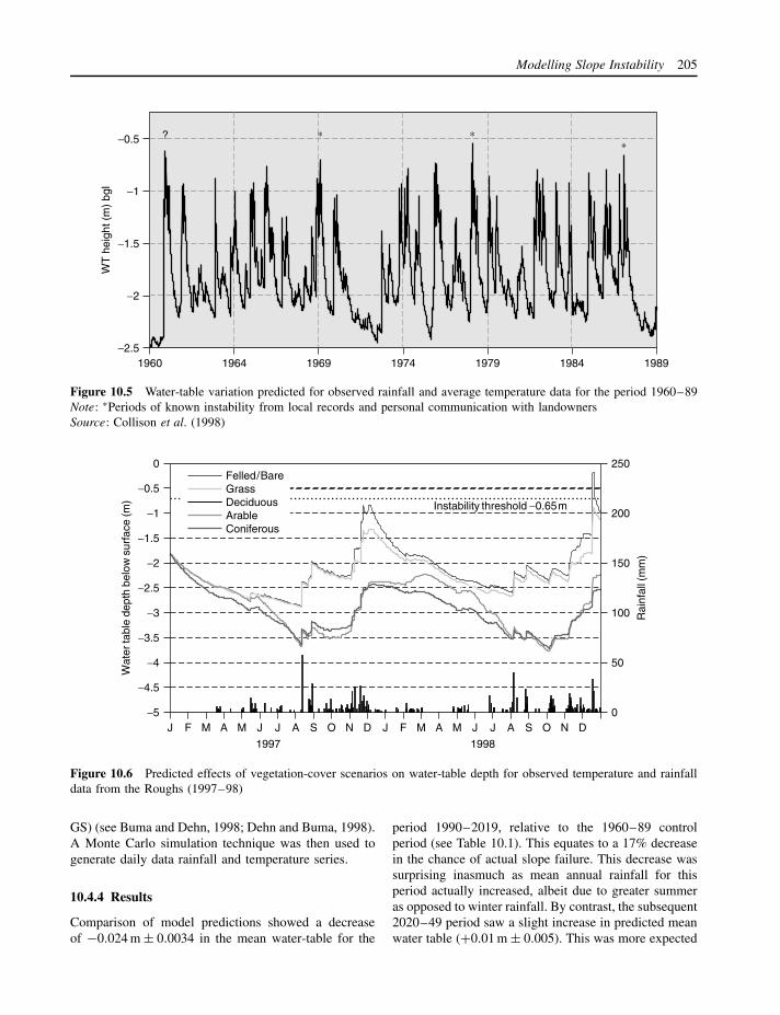
Modelling Slope Instability 205
1960 1964 1969 1974 1979 1984 1989
WT
hei
ght (
m)
bgl
∗∗∗?−0.5
−1
−1.5
−2
−2.5
Figure 10.5 Water-table variation predicted for observed rainfall and average temperature data for the period 1960–89Note: ∗Periods of known instability from local records and personal communication with landownersSource: Collison et al. (1998)
0
−0.5
−1
−1.5
−2
−2.5
−3
−3.5
−4
−4.5
−5J F M A M J J A S O N D J F M A M J J A S O N D
Wat
er ta
ble
dept
h be
low
sur
face
(m)
0
50
100
150
200
250
Rai
nfal
l (m
m)
1998
Instability threshold −0.65m
1997
Felled / BareGrassDeciduousArableConiferous
Figure 10.6 Predicted effects of vegetation-cover scenarios on water-table depth for observed temperature and rainfalldata from the Roughs (1997–98)
GS) (see Buma and Dehn, 1998; Dehn and Buma, 1998).A Monte Carlo simulation technique was then used togenerate daily data rainfall and temperature series.
10.4.4 Results
Comparison of model predictions showed a decreaseof −0.024 m ± 0.0034 in the mean water-table for the
period 1990–2019, relative to the 1960–89 controlperiod (see Table 10.1). This equates to a 17% decreasein the chance of actual slope failure. This decrease wassurprising inasmuch as mean annual rainfall for thisperiod actually increased, albeit due to greater summeras opposed to winter rainfall. By contrast, the subsequent2020–49 period saw a slight increase in predicted meanwater table (+0.01 m ± 0.005). This was more expected
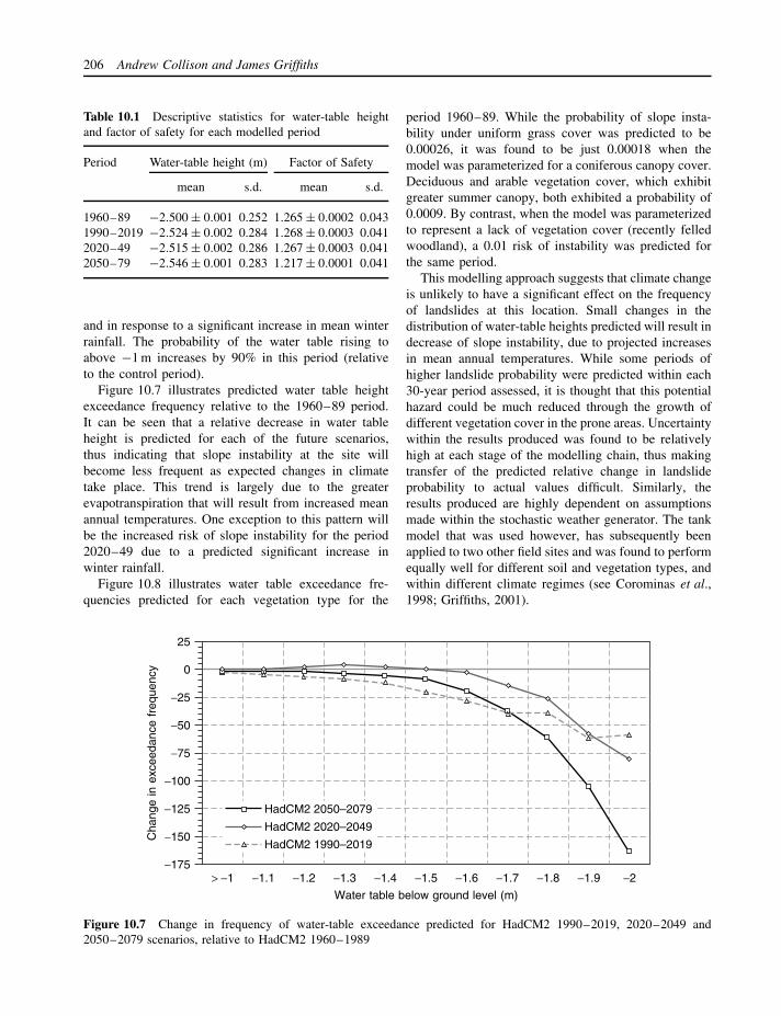
206 Andrew Collison and James Griffiths
Table 10.1 Descriptive statistics for water-table heightand factor of safety for each modelled period
Period Water-table height (m) Factor of Safety
mean s.d. mean s.d.
1960–89 −2.500 ± 0.001 0.252 1.265 ± 0.0002 0.0431990–2019 −2.524 ± 0.002 0.284 1.268 ± 0.0003 0.0412020–49 −2.515 ± 0.002 0.286 1.267 ± 0.0003 0.0412050–79 −2.546 ± 0.001 0.283 1.217 ± 0.0001 0.041
and in response to a significant increase in mean winterrainfall. The probability of the water table rising toabove −1 m increases by 90% in this period (relativeto the control period).
Figure 10.7 illustrates predicted water table heightexceedance frequency relative to the 1960–89 period.It can be seen that a relative decrease in water tableheight is predicted for each of the future scenarios,thus indicating that slope instability at the site willbecome less frequent as expected changes in climatetake place. This trend is largely due to the greaterevapotranspiration that will result from increased meanannual temperatures. One exception to this pattern willbe the increased risk of slope instability for the period2020–49 due to a predicted significant increase inwinter rainfall.
Figure 10.8 illustrates water table exceedance fre-quencies predicted for each vegetation type for the
period 1960–89. While the probability of slope insta-bility under uniform grass cover was predicted to be0.00026, it was found to be just 0.00018 when themodel was parameterized for a coniferous canopy cover.Deciduous and arable vegetation cover, which exhibitgreater summer canopy, both exhibited a probability of0.0009. By contrast, when the model was parameterizedto represent a lack of vegetation cover (recently felledwoodland), a 0.01 risk of instability was predicted forthe same period.
This modelling approach suggests that climate changeis unlikely to have a significant effect on the frequencyof landslides at this location. Small changes in thedistribution of water-table heights predicted will result indecrease of slope instability, due to projected increasesin mean annual temperatures. While some periods ofhigher landslide probability were predicted within each30-year period assessed, it is thought that this potentialhazard could be much reduced through the growth ofdifferent vegetation cover in the prone areas. Uncertaintywithin the results produced was found to be relativelyhigh at each stage of the modelling chain, thus makingtransfer of the predicted relative change in landslideprobability to actual values difficult. Similarly, theresults produced are highly dependent on assumptionsmade within the stochastic weather generator. The tankmodel that was used however, has subsequently beenapplied to two other field sites and was found to performequally well for different soil and vegetation types, andwithin different climate regimes (see Corominas et al.,1998; Griffiths, 2001).
25
0
−25
−50
−75
−100
−125
−150
−175> −1 −1.1 −1.2 −1.3 −1.4 −1.5 −1.6 −1.7 −1.8 −1.9 −2
Water table below ground level (m)
Cha
nge
in e
xcee
danc
e fr
eque
ncy
HadCM2 2050–2079
HadCM2 2020–2049
HadCM2 1990–2019
Figure 10.7 Change in frequency of water-table exceedance predicted for HadCM2 1990–2019, 2020–2049 and2050–2079 scenarios, relative to HadCM2 1960–1989
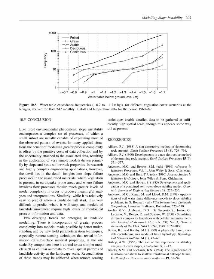
Modelling Slope Instability 207
1
10
100
1000
> −0.7 −0.8 −0.9 −1 −1.1 −1.2 −1.3 −1.4 −1.5 −1.6 −1.7
Water table below ground level (m)
Fre
quen
cy
FelledGrassArableDeciduousConiferous
Figure 10.8 Water-table exceedance frequencies (−0.7 to −1.7 m bgl), for different vegetation-cover scenarios at theRoughs, derived for HadCM2 monthly rainfall and temperature data for the period 1960–89
10.5 CONCLUSION
Like most environmental phenomena, slope instabilityencompasses a complex set of processes, of which asmall subset are usually capable of explaining most ofthe observed pattern of events. In many applied situa-tions the benefit of modelling greater process complexityis offset by the punitive costs of data collection and bythe uncertainty attached to the associated data, resultingin the application of very simple models driven primar-ily by slope and basic soil or rock properties. In researchand highly complex engineering applications, however,the devil lies in the detail: insights into slope failureprocesses in the unsaturated materials, where vegetationis present, in earthquake-prone areas and where failureinvolves flow processes require much greater levels ofmodel complexity in order to produce meaningful anal-yses and interpretations. Similarly, while it is relativelyeasy to predict where a landslide will start, it is verydifficult to predict where it will stop, and models oflandslide movement require high levels of rheologicalprocess information and data.
Two diverging trends are emerging in landslidemodelling. There is incorporation of greater processcomplexity into models, made possible by better under-standing and by new field parameterization techniques,especially remote sensing techniques that reveal infor-mation on subsurface material properties, at the sitescale. By comparison there is a trend to use simpler mod-els such as cellular automata to reveal spatial patterns oflandslide activity at the landscape scale. Reconciliationof these trends may be achieved when remote sensing
techniques enable detailed data to be gathered at suffi-ciently high spatial scale, though this appears some wayoff at present.
REFERENCES
Allison, R.J. (1988) A non-destructive method of determiningrock strength, Earth Surface Processes 13 (8), 729–736.
Allison, R.J. (1990) Developments in a non-destructive methodof determining rock strength, Earth Surface Processes 15 (6),571–577.
Anderson, M.G. and Brooks, S.M. (eds) (1996) Advances inHillslope Processes, Vol. 1, John Wiley & Sons, Chichester.
Anderson, M.G. and Burt, T.P. (eds) (1990) Process Studies inHillslope Hydrology, John Wiley & Sons, Chichester.
Anderson, M.G. and Howes, S. (1985) Development and appli-cation of a combined soil water-slope stability model, Quar-terly Journal of Engineering Geology 18, 225–236.
Anderson, M.G., Kemp, M. and Lloyd, D.M. (1988) Applica-tions of soil water finite difference models to slope stabilityproblems, in G. Bonnard (ed.) Fifth International LandslideSymposium, Lausanne, Balkema, Rotterdam, 525–530.
Avolio, M.V., Ambrosio, D.D., Di Gregorio, S., Iovine, G.,Lupiano, V., Rongo, R. and Spataro, W. (2001) Simulatingdifferent complexity landslides with cellular automata meth-ods, Geological Research Abstracts (CD) Vol. 3, GeneralAssembly of the EGS, GRA3, 8746, ISSN: 1029-7006.
Beven, K.J. and Kirkby, M.J. (1979) A physically based, vari-able contributing area model of basin hydrology, Hydrolog-ical Sciences Bulletin 24 (1), 43–69.
Bishop, A.W. (1955) The use of the slip circle in stabilityanalysis of earth slopes, Geotechnic 5, 7–17.
Brooks, S.M. and Richards, K.S. (1994) The significance ofrainstorm variations to shallow translational hillslope failure,Earth Surface Processes and Landforms 19, 85–94.

208 Andrew Collison and James Griffiths
Brooks, S.M. and Collison, A.J.C. (1996) The significance ofsoil profile differentiation to hydrological response and slopeinstability: a modelling approach, in M.G. Anderson andS.M. Brooks (eds) Advances in Hillslope Processes, JohnWiley & Sons, Chichester, 471–486.
Brooks, S.M., Anderson, M.G. and Crabtree, K. (1995) Thesignificance of frangipans to early-Holocene slope fail-ure – application of physically-based modelling, Holocene5 (3), 293–303.
Brunsden, D. (1979) Mass movement, in C. Embleton andJ. Thornes (eds) Process in Geomorphology, Butler andTanner, London, 130–186.
Buma, J. and Dehn, M. (1998) A method for predicting theimpact of climate change on slope stability, EngineeringGeology 35 (2–3), 190–196.
Burroughs, E.R., Hammond, C.J. and Booth, G.D. (1986)Relative stability estimation for potential debris avalanchesites using field data, in Proceedings of the InternationalSymposium on Erosion, Debris Flow and Disaster Preven-tion, Erosion Control Engineering Society, Tsukuba, Japan,335–339.
Cai, F., Ugai, K., Wakai, A. and Li, Q. (1998) Effects ofhorizontal drains on slope stability under rainfall bythree-dimensional finite element analysis, Computers andGeotechnics 23 (4), 255–275.
Capecchi, F. and Focardi, P. (1988) Rainfall and landslides:research into a critical precipitation coefficient in an areaof Italy, in C. Bonnard (ed.) Landslides: Proceedings of theFifth International Symposium on Landslides, 10–15 July1988, Lausanne, Balkema, Rotterdam, Vol. 2, 1131–1136.
Clerici, A. and Perego, S. (2000) Simulation of the ParmaRiver blockage by the Corniglio landslide (Northern Italy),Geomorphology 33, 1–23.
Collison, A.J.C. (2001) The cycle of instability: stress releaseand fissure flow as controls on gully head retreat, Hydrolog-ical Processes 15 (1), 3–12.
Collison, A.J.C. and Anderson, M.G. (1996) Using a com-bined slope hydrology/stability model to identify suitableconditions for landslide prevention by vegetation in thehumid tropics, Earth Surface Processes and Landforms 21,737–747.
Collison, A.J.C., Anderson, M.G. and Lloyd, D.M. (1995)Impact of vegetation on slope stability in a humid tropi-cal environment – a modelling approach, Proceedings of theInstitute of Civil Engineers – Water, Maritime and Energy112 (2), 168–175.
Collison, A.J.C., Wade, S. and Griffiths, J.A. (1998) UKnational report in J. Corominas, J. Moya, A. Ledesma,J. Gili, A. Lloret and J. Rius (eds) New Technologies forLandslide Hazard Assessment and Management in Europe:Final Report, CEC Environment Programme (Contract ENV-CT966-0248), EU, Brussels.
Collison, A.J.C., Wade, S., Griffiths, J. and Dehn, M. (2000)Modelling the impact of predicted climate change onlandslide frequency and magnitude in SE England, Engi-neering Geology 55, 205–218.
Corominas, J., Moya, J., Ledesma, A., Gili, J.A., Lloret, A.and Rius, J. (1998) New Technologies for Landslide HazardAssessment and Management in Europe: Final Report, CECEnvironment Programme (Contract ENV-CT966-0248), EU,Brussels.
Crozier, M.J. (1999) Prediction of rainfall triggered landslides:a test of the antecedent water status model, Earth SurfaceProcesses and Landforms 24 (9), 763–779.
Dehn, M. and Buma, J. (1998) Modelling future landslideactivity based on general circulation models, Geomorphol-ogy 30, 175–187.
Dehn, M., Burger, G., Buma, J. and Gasparetto, P. (2000)Impact of climate change on slope stability using expandeddownscaling, Engineering Geology 55, 193–204.
Dietrich, W.E., Reiss, R., Hsu, M. and Montgomery, D.R.(1995) A process-based model for colluvial soil depth andshallow landsliding using digital elevation data, Hydrologi-cal Processes 9, 383–400.
Di Gregorio, S., Rongo, R., Siciliano, C., Sorriso-Valvo, M.and Spataro, W. (1999) Mount Ontake landslide simulationby the cellular automata model SCIDDICA-3, Physics andChemistry of the Earth Part A – Solid Earth Geodesy 24,131–137.
Fredlund, D.G. (1987a) The shear strength of unsaturated soiland its relationship with slope stability problems in HongKong, Hong Kong Engineer 8, 57–9.
Fredlund, D.G. (1987b) Slope stability analysis incorporat-ing the effect of soil suction, in M.G. Anderson andK.S. Richards (eds) Slope Stability, John Wiley & Sons,Chichester, 113–144.
GeoSlope International (1992) SEEP/W User’s Guide, Alta,Calgary.
GeoSlope International (1994) SLOPE/W User’s Guide, Alta,Calgary.
Greenway, D.R. (1987) Vegetation and slope stability, inM.G. Anderson and K.S. Richards (eds) Slope Stability, JohnWiley & Sons, Chichester, 187–230.
Griffiths, D.V. and Lane, P.A. (1999) Slope stability analysisby finite elements, Geotechnique 49 (3), 387–403.
Griffiths, J.A. (2001) Modelling the sensitivity and response ofshallow landslides in SE England and SE Spain, unpublishedPhD thesis, University of London.
Hansen, M.J. (1984) Strategies for classification of landslides,in D. Brunsden and D.B. Prior (eds) Slope Instability, JohnWiley & Sons, Chichester, 363–418.
Holzer, T.L., Bennett, M.J., Ponti, D.J. and Tinsley, J.C. et al.(1999) Liquefaction and soil failure during 1994 Northridgeearthquake, Journal of Geotechnical and GeoenvironmentalEngineering 125 (6), 438–452.
Holzer, T.L., Bennett, M.J., Youd, T.L. and Chen, A.T.F. et al.(1988) Parkfield, California, liquefaction prediction, Bulletinof the Seismological Society of America 78 (1), 385–389.
Holzer, T.L., Youd, T.L. and Hanks, T.C. (1989) Dynamics ofliquefaction during the 1987 Superstition Hills, California,earthquake, Science 244 (4900), 56–59.
Hutchinson, J.N. (1988) Morphological and geotechnicalparameters of landslides in relation to geology and

Modelling Slope Instability 209
hydrogeology, in C. Bonnard (ed.) Landslides, Proceedingsof the 5th International Symposium on Landslides, Balkema,Rotterdam, Vol. 1, 3–35.
Laigle, D. and Coussot, P. (1997) Numerical modeling ofmudflows, Journal of Hydraulic Engineering – ASCE 123(7), 617–623.
Lam, L. and Fredlund, D.G. (1993) A general limit equilibriummodel for 3-dimensional slope stability analysis, CanadianGeotechnical Journal 30 (6), 905–919.
Miles, S.B. and Ho, C.L. (1999) Applications and issues of GISas tool for civil engineering modeling, Journal of Computingin Civil Engineering 13 (3), 144–152.
Montgomery, D.R. and Dietrich, W.E. (1994) A physicallybased model for the topographic control on shallow land-sliding, Water Resources Research 30 (4), 1153–1171.
Montgomery, D.R., Schmidt, K.M., Greenberg, H.M. and Diet-rich, W.E. et al. (2000) Forest clearing and regional lands-liding, Geology 28 (4), 311–314.
Muller, L. (1964) The rock slide in the Vaijont Valley, RockMechanics and Engineering Geology 2, 148–228.
Murphy, W. (1995) The geomorphological controls on seismi-cally triggered landslides during the 1908 Staits of Messinaearthquake, Southern Italy, Quarterly Journal of EngineeringGeology 28, 61–74.
Obrien, J.S., Julien, P.Y. and Fullerton, W.T. (1993) 2-Dimensional water flood and mudflow simulation, Journalof Hydraulic Engineering – ASCE 119 (2), 244–261.
Polemio, M. and Sadao, F. (1999) The role of rainfall inthe landslide hazard: the case of the Avigliano urban area(Southern Apennines, Italy), Engineering Geology 53 (3/4),297–309.
Selby, M.J. (1993) Hillslope Materials and Processes, OxfordUniversity Press, Oxford.
Trollope, D.H. (1981) The Vaiont slide failure, Rock Mechanics13, 71–88.
van Genuchten, M. Th. (1980) A closed-form equation forpredicting the hydraulic conductivity of unsaturated soils,Soil Science Society of America 48, 892–898.
Varnes, D.J. (1978) Slope movement types and processes, inR.L. Schuster and R.J. Krizek (eds) Landslides: Analysisand Control, National Academy of Sciences, TransportResearch Board – Special Report 176, Washington, DC,11–33.
Wilkinson, P.L., Brooks, S.M. and Anderson, M.G. (2000)Design and application of an automated non-circular slipsurface search within a combined hydrology and stabil-ity model (CHASM), Hydrological Processes 14 (11–12),2003–2017.

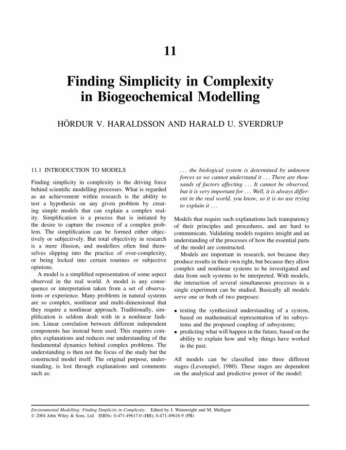
11
Finding Simplicity in Complexityin Biogeochemical Modelling
HORDUR V. HARALDSSON AND HARALD U. SVERDRUP
11.1 INTRODUCTION TO MODELS
Finding simplicity in complexity is the driving forcebehind scientific modelling processes. What is regardedas an achievement within research is the ability totest a hypothesis on any given problem by creat-ing simple models that can explain a complex real-ity. Simplification is a process that is initiated bythe desire to capture the essence of a complex prob-lem. The simplification can be formed either objec-tively or subjectively. But total objectivity in researchis a mere illusion, and modellers often find them-selves slipping into the practice of over-complexity,or being locked into certain routines or subjectiveopinions.
A model is a simplified representation of some aspectobserved in the real world. A model is any conse-quence or interpretation taken from a set of observa-tions or experience. Many problems in natural systemsare so complex, nonlinear and multi-dimensional thatthey require a nonlinear approach. Traditionally, sim-plification is seldom dealt with in a nonlinear fash-ion. Linear correlation between different independentcomponents has instead been used. This requires com-plex explanations and reduces our understanding of thefundamental dynamics behind complex problems. Theunderstanding is then not the focus of the study but theconstructed model itself. The original purpose, under-standing, is lost through explanations and commentssuch as:
. . . the biological system is determined by unknownforces so we cannot understand it . . . There are thou-sands of factors affecting . . . It cannot be observed,but it is very important for . . . Well, it is always differ-ent in the real world, you know, so it is no use tryingto explain it . . .
Models that require such explanations lack transparencyof their principles and procedures, and are hard tocommunicate. Validating models requires insight and anunderstanding of the processes of how the essential partsof the model are constructed.
Models are important in research, not because theyproduce results in their own right, but because they allowcomplex and nonlinear systems to be investigated anddata from such systems to be interpreted. With models,the interaction of several simultaneous processes in asingle experiment can be studied. Basically all modelsserve one or both of two purposes:
• testing the synthesized understanding of a system,based on mathematical representation of its subsys-tems and the proposed coupling of subsystems;
• predicting what will happen in the future, based on theability to explain how and why things have workedin the past.
All models can be classified into three differentstages (Levenspiel, 1980). These stages are dependenton the analytical and predictive power of the model:
Environmental Modelling: Finding Simplicity in Complexity. Edited by J. Wainwright and M. Mulligan 2004 John Wiley & Sons, Ltd ISBNs: 0-471-49617-0 (HB); 0-471-49618-9 (PB)

212 Hordur V. Haraldsson and Harald U. Sverdrup
Stage 1 Stage 2 Stage 3
Qualitative Direct Differentialdescription → quantitative
description interms ofobservableconditions
→ rate based onunderlyingphysics andprocessing
The stage 1 model is typical of classifications intocategories where a certain occurrence is predictablebased on the present conditions. Geological mappingis typical of stage 1 models; rocks and minerals occuraccording to geographical distributions. Such modelshave very limited predictive power.
Stage 2 models are based on ‘case-by-case’ predictivepower, and they must be recalibrated on new data eachtime the initial and boundary conditions change. Plottinga pH over time in an acidified lake is an example ofa stage 2 model. These type 2 models are limited bycases, and the properties cannot be transferred to anothercase.
Stage 3 models involve changes through time and usethe differential approach first used in physics, and laterin all natural science. They relate how changes at everypoint in time are related to the state of the system atthat time. Stage 3 models introduce the mechanism ofchange which depends on state variables for the sys-tem and is generally valid. The state of the system ischaracterized by conditions in terms of order, spatialdistribution, concentration and adaptation capabilities.A stage 3 model is generally valid and applicable whenit can be parameterized properly and the coefficientsestimated, but it is in differential form, and requiresmathematical manipulation when used. This used topose difficulties, but with modern computers and user-friendly modelling software, such problems are muchreduced.
In modelling, it is important to distinguish between‘good models’ and ‘bad models’, and ‘good perfor-mance’ and ‘bad performance’. The definition of a‘good model’ is when everything inside it is visible,inspectable and testable. It can be communicated effort-lessly to others. A ‘bad model’ is a model that does notmeet these standards, where parts are hidden, undefinedor concealed and it cannot be inspected or tested; theseare often labelled black box models. Intuitive models are‘bad’ because they do not explain what they do. Oftenstatistical models produced from automated statisticalpackages are bad models, as it remains totally unclearto the user what the implication of the package-proposed
model is, how the relation was established and, finally,what on earth it is good for. Models do have differentperformances depending on the model developing pro-cess and definitions. A model must work with inputs thatcan be defined and determined, and it must yield outputsthat can be observed. A model can perform poorly, butstill adhere to the principles of good models. Many ofour models will start like this when we develop them.With a good model we can analyse its performance inorder to change the model iteratively and improve itsperformance. Bad models may perform well, but sincethey can neither be tested nor inspected, there is no wayto determine whether this is pure chance or somethingsubstantial, and as parts are not visible, there is not muchwe can do to improve them, hence, the term ‘bad model’.A ‘bad model’ does not allow a learning process and itfails to communicate its principles. A good model is onethat adheres to the following rules:
• The model must be transparent. It must be possibleto inspect and understand the rules and principles themodel is using.
• It must be possible to test the model. It must workon inputs that can be defined and determined, and itmust yield outputs that can be observed.
‘Goodness’ or ‘badness’ of a model has nothing todo with the adequacy of the principles inside themodel. If the model is ‘good’, then we can verify orfalsify the performance of the model with a specificprinciple incorporated. If the model is ‘bad’, then wecannot verify or falsify the performance of the modelwith a specific principle incorporated. The model canbe a mental understanding of a mechanism, system,pattern or principle, and it can be substantiated as anequation or a set of equations or rules. If the principlesand rules are numerous, then it is practical to let acomputer program keep track of all connections and theaccounting of numbers.
11.2 DARE TO SIMPLIFY
All models are mental projections of our understandingof processes and feedbacks of systems in the real world.The general approach is that models are as good as thesystem upon which they are based. Models should bedesigned to answer specific questions and only incor-porate the necessary details that are required to pro-vide an answer. Collecting massive amounts of dataand information ahead of the modelling procedure is

Finding Simplicity in Complexity in Biogeochemical Modelling 213
costly and does not necessarily generate understand-ing of the problem. More often, it adds to the con-fusion. Modelling starts with problem definition andsimplification of the causalities. It means raising theobservation to a higher level in order to extract clearcausal links and driving forces from the problem. Focusshould be on what is essential for the model andwhat is not needed. One of the common pitfalls is toassume that models need to be complex and data-hungry.The performance of the model need not be perfect,it only needs to be good enough to answer the rele-vant questions – better than good enough is extra workwith no purpose. Thus, it is always relevant to reflect:what was the objective of the model application in thefirst place?
• A simple model must make complex assumptions.A simple model is easy to use, and the input datacan be obtained at relatively low cost. Because of thesimplicity, the applicability may be limited, and wewill have problems with addressing the effect of theassumptions.
• A complex model can make simple assumptions.The model will have better general applicability andless restriction on use. But it will require moreinput data and be relatively more expensive to use.Further increases in model complexity may removeassumptions and consider more feedbacks, but higherdemands are made on input data.
The total complexity of a system in modelling is dividedbetween the assumptions and the model itself. For everyquestion there is an optimal complexity, and great caremust be exercised to evaluate this aspect. Failing todo so will result in loss of control over uncertainties.And it is important to realize that we cannot get ridof the complexity in a system, but only decide if itgoes into the model or into assumptions. Claims toany other effect can safely be laughed at. All modelsmust fulfil some minimum requirements. They mustbe able to describe events at single sites based onreal data. If a model cannot describe single sites andtheir past history, then it has no credibility in futurepredictions.
A model of causalities is a system and all systemsare defined by their boundaries, internal structure andinternal quantities. In order for us to understand a systemproperly, we need to understand how systems behaveand what their properties are. Systems are usuallyconfined by certain inflow and outflow of physicalmatter or energy. When we create mental models, wedo not intend to capture the whole reality in one
model. Such models are as complex as reality itself.What we want to do is to map part of the realityin such a way that it gives us a basic understandingof a complex problem. The level of details neededto explain and analyse a problem is dependent onthe type of answer that is desired. The number ofcomponents depends on the level of detail when theobservation takes place. When creating a model itis necessary to have a holistic perspective on thecausal relations in the problem and understand thebasic driving forces to hand. The following exampleuses a causal loop diagram (CLD) to demonstratethe phosphorus cycle in eutrophic lakes (Figure 11.1).The CLD concept (Richardson and Pugh, 1981) isa systematic way of thinking in causes and effectswhere variables either change in the same direction(indicated by a ‘plus’) or change in the oppositedirection (indicated by a ‘minus’).
It is evident that model complexity depends directlyon the question asked, as illustrated in Figures 11.1 and11.2. In the case of the phosphorus cycle, the com-plex model did not enhance the understanding of theoverall behaviour but increased the uncertainty that wasinvolved by increasing the number of observation levelsin the system. The simple model used a less compli-cated observation level but used a more sophisticatedexplanation of assumption to the causal links.
Plankton
Fish Sediment Phosphorus inwater body
Outflow of water
B
R
RB
Inflow ofphosphorus
+
+
+ +
+
+ −
−
−
+
Figure 11.1 A simple conceptual model of the phospho-rus cycle in lakes that is powerful enough to illustrate andpredict the phosphorous dynamics between the key ele-ments: phytoplankton, fish and sediment. The different fishspecies have been simplified to one ‘fish’. All plankton andzooplankton have been simplified to one general ‘plankton’.The shaded area illustrates the core-driving loop that runsthe cycle. If lake-water transparency is the issue, then thiswill be a fully sufficient model

214 Hordur V. Haraldsson and Harald U. Sverdrup
Zooplankton
Prey fish sedimentPhosphorus in
water body
Outflow of water
Inflow ofphosphorus
B
R
Predatorfish
Phytoplankton
B
B
Fishing
Burial
B
R
++
+
−
−
−
+
+ ++ +
+
+ −
−
−
−
−+
+
−
Figure 11.2 A complex model of the phosphorous cycle, which is based on the simple model but includes componentsthat add details to the driving loop for eutrophication. This does not necessarily enhance the performance of the model withrespect to the water transparency issue; the simple model will be good enough. If the issue is fish population dynamics,then the added details will be required
11.3 SORTING
Building models is a long process especially if the modelis designed to answer many questions. The general ruleof thumb is that a specific question requires one model.If a problem involves many questions, then equallymany models may be required to address them and thenthe ‘model’ becomes a cluster of models. Nevertheless,constructing a model with many components can becostly (Figure 11.3). The art is to construct a model thatis robust, answers the desired questions and is simple.The performance need not be perfect, it should onlybe sufficient, and nothing more. Such models can bothsave time and money, and be useful building blocks forfurther model developments.
The process starts by sorting the causalities in theproblem in relation to their importance to answer thespecific question. Then they are sorted according to theircontribution to performance. Causalities with obviousdriving forces explicitly related to the problem have thehighest performance. Then the sorting process continuesdownwards. If several components are identified asoutlining the main driving forces in the problem, thesecomponents may describe sufficiently the dynamics inthe problem. Subsequently, the system boundaries canbe drawn. A problem can never be fully explained due to
Effort and cost ofbuilding model
Modelcomponent
Number of components
Con
trib
utio
n to
per
form
ance
Figure 11.3 The number of components and their influ-ence are in proportion with the cost and effort of buildinga model
uncertainties in the structure and components. Usuallythe model performance will level out (Figure 11.4) anddecrease from a maximum level (Figure 11.5) even iffurther causes are added. This is because adding acause involves adding uncertainty, and at some time theaccumulated uncertainties will overtake the contributionto performance (see Chapter 1).
Causalities always involve some amount of uncer-tainty. Adding further causalities to the model will

Finding Simplicity in Complexity in Biogeochemical Modelling 215
Model complexity; number of components
Per
form
ance
1
2
3
4
5
6
Mechanismcontribution toperformance
Mechanismnumber
Uncertaintyreduction ofperformance
1 2 3 4 5 6
Figure 11.4 Adding a cause contributes to the overall performance of the model, but its contribution is not necessarilysymmetrical to other causalities in the model
Model complexity; number of components
Per
form
ance 1
2
3
4
5
6
Mechanismcontribution toperformance
Uncertainty lossof performance
Mechanismnumber
Effectiveperformance
1 2 3 4 5 6
Figure 11.5 Adding a cause involves a certain amount of uncertainty, which can overshoot the contribution to the modelperformance by adding the cause
increase the necessary details that the model will haveto incorporate, but at the cost of increased uncertainty.Increased uncertainty will lower the overall performanceup to the level where uncertainty from added causal-ities outweighs added performance. This point of no
improvement is characterized as the point where morecomplexity costs more in extra inputs and added inac-curacies than it achieves in improved performance. InFigure 11.5, the highest model performance is achievedwith three causalities, but further addition involves

216 Hordur V. Haraldsson and Harald U. Sverdrup
Lowdetails
Highdetails
System levels
Phy
sica
l siz
e of
the
syst
em
Number of variables/Increased time scale
Figure 11.6 Focus of models depends on the observationlevel. Global-scaled models can require many variables andhigh time integration but must address lower detail levels,compared to local models
higher uncertainty, not a better contribution to perfor-mance.
All models have this type of peak performance inrelation to number of causes, which can be severalor many hundred. By adding further components, acomplex model may end up being poorer in performancethan a simple one. It may be useful for impressing one’scolleagues with how large and complex a model you canmake, but for predictions, it may be worse than a blindguess, and in reality completely useless.
Models are based on subsystems themselves and theircomponents on subsystems, etc. It is important to iden-tify the system level that we operate on. Greater numbersof components mean more interaction between themand it becomes important to observe the transparencybetween the components. A model can have compo-nents that are on different system levels depending onthe level of details. Large models on the global scalecan be based on numbers that are derived locally. Suchmodels need simplification and balance between numberof components and the observation level (Figure 11.6).
We should select the level needed to understandthe interrelationship among our selected variables – thelevel we want to influence. After defining that level,detailed knowledge of the underlying components isnot needed. That knowledge falls into the complexassumption made during the sorting process. Driving acar, for instance, does not require detailed knowledgeof the construction of the engine; the vehicle can beoperated without such knowledge.
11.4 THE BASIC PATH
The process from specifying the question and buildingthe model starts by gathering information and listing
all the variables we feel are appropriate for the system.Then we try to categorize the critical and the indicatorvariables. It gives us much more clarity when we startto assemble the causal links. This is highlighted in twopoints by Dorner (1996):
• We need to know what other variables those that wewant to influence depend on. We need to understand,in other words, how the causal relationships amongthe variables in a system work together in that system.
• We need to know how the individual components ofa system fit into a hierarchy of broad and narrowconcepts. This can help us fill in, by analogy, thoseparts of a structure unfamiliar to us.
After performing basic sorting, previously unrecognizedinteractions between variables may require alteration orrevision of the hypothesis. Some light may have beenshed on the larger complexes outside the defined systemboundaries, in which elements of the defined systemare embedded. This process is iterative and may requireseveral revisions before the model is fixed according todesired standards.
11.5 THE PROCESS
Generalization is often the key to understanding com-plex systems. Modelling is without exception based onsome sort of recipe. Whatever approach is used, allmethods focus on answering a specific question. We pro-pose that the basic process should start by defining andconfining system boundaries according to the specificquestion, or questions requiring an answer. The wholeprocess should be considered iterative (Figure 11.7)
Developmentalmodel
Learn
Concludeand report
Test themodel
Defineproblem
Establishedknowledge
Data fromliterature
Data fromexperiments
Data
R
R
B
+−
+ ++
+
+
+
++
+ +
Figure 11.7 The learning loop is an iterative processwhere the steps from building a mental model and pro-ducing results can always be improved

Finding Simplicity in Complexity in Biogeochemical Modelling 217
where experience from previous evaluation is used toredefine the problem. The learning experience gainedand the conclusions from the testing will help us re-evaluate our problem and our mental model.
Modelling never starts with data, contrary to whatmany believe. Just collecting ‘even more’ data withouta clear model does not create greater understandingnor clarity, it merely adds to general confusion. Noteverybody would agree, but the track record is just tooconsistent to accept any objections. All research startswith a definition of a problem and through that anunderstanding of that problem. This is ‘the model’, themental image of how the problem is to be understood.Thus, no models are ‘wrong’; if something does notwork, the cause is to be found in faulty understanding.After a model has been created, we can test andchallenge it. Then a specific demand for data will arise.Not all data is needed, only what is relevant to ourproblem. The rest must be sorted. From the test wewill learn and redevelop our understanding, our ‘model’.Model development requires iteration in such a cycleseveral times and will continue as long as there issufficient data from experiments or literature to support
the testing of the model. In that way the communicationof the model is effective, both to the user and thedeveloper. Furthermore, it enables us to communicatethe success and problems encountered.
11.6 BIOGEOCHEMICAL MODELS
We define biogeochemical models as models thatdescribe the connection from biology through chem-istry, to geology and back. Geology (the solid phase) isonly visible to biology through its expression in chem-istry. The only way that geology (solids) affects chem-istry is through chemical weathering and ion exchange.Ion exchange is always in the form of reversible reac-tions, whereas chemical weathering reactions are almostalways irreversible and slow. Decomposition of organicmatter, however, we regard as part of the biotic cycle.For all biogeochemical models where the connectionbetween biological and geological aspects is signifi-cant, the representation of the weathering process willbe a vulnerable point for overall model performance(Figure 11.8).
Soil solution
Organicmaterial
Primaryminerals
Decomposition Weathering
Leaching
Uptake
Wetdeposition
Litte
r-Fa
ll
Ion exchange
Precipitation
Timberharvest
Soil surface
Recrystallization
Amorphousprecipitates
Secondaryclay minerals
Ion exchange
Depletion
Redissolution
Biomass
Roots
Canopyleaching
Particulatedeposition
Management
Figure 11.8 A box-arrow diagram for the process system in soil, typical for many biogeochemical models.Biogeochemical models range from describing a small part of this diagram to having it as a small subcompartment

218 Hordur V. Haraldsson and Harald U. Sverdrup
There are many biogeochemical codes available forbiogeochemical calculations in ecosystems. Some ofthese are easy to obtain and use, while others existonly on paper and in scientific articles. If the purposeof your modelling is to predict, assess or design, thenusing an existing model is often an efficient way to getthe work done. If the issue is to explain your research,investigate your own understanding and develop it, it isrecommended that you build your own model rather thanusing an existing one. If you use an existing model, donot start to use it before you have thoroughly understoodthe principles and assumptions it applies and preferablywhen you agree with how it is made. We can definethree types of model:
1. models based on process-oriented kinetics;2. models based on equilibrium principles;3. empirical models.
Here we will be mainly concerned with the first twotypes. The traditional soil-chemistry models, originallydeveloped for issues in agriculture and groundwater geo-chemistry, were based on equilibrium processes. Thisbasis had historical reasons: before the advent of mod-ern computers, systems of differential equations wereunsolvable for any practical use. Still the traditionalmodels rely heavily on large amounts of data for cal-ibration. If this requirement is fulfilled, they will pro-duce useful back-casting and can be used for makingextrapolative predictions. These models quickly run intoproblems without large amounts of data to calibrateon, and this is caused by a specific shortcoming thatmust be pointed out. The traditional geochemical mod-els use equilibrium formulations for processes whichare valid for soluble salts, carbonate-dominated sys-tems and other reversible reaction systems. But suchmodels are not formally valid for kinetically con-trolled irreversible systems. The so-called ‘thermody-namic equilibrium databases’ for soil and geochemicalsilicate reactions referred to are not ‘thermodynamic’at all, they are steady state balance coefficients thathave been misinterpreted as equilibria. Thus, such mod-els may be useful for simulations or design work aftercareful calibration, but do not expect them to explainprocesses. Without the calibration, these models lack theability to generate a priori predictions.
In modelling the focus is often on the output insteadof robustness and performance, which makes the ‘cultof success’ very strong. The ‘cult of success’ impliesthat the calculated output is expected to pass through allobservation points. If not, the user of a model might soonhear ‘The model is wrong . . .’ or ‘Well, it is obvious thatthe model does not work . . .’. On the other hand, if it is
obvious that the model was calibrated by adjusting oneor several parameters, critics will soon remark, ‘Youcan probably make the thing fit anything . . .’. Resistthis! Resist the temptation to overcalibrate! Ignore suchderogative comments, they are never made from insight!The fit need not be perfect, the line need not go throughall data points. Performance should only be sufficient togive an adequate answer! It is from the lack of perfectfit that learning is gained.
We may classify existing models into categories,depending on which scale they are applied to as wellas the degree of integration of multiple processes overthose scales. A list, not claiming to be comprehen-sive, would include examples as follows: Single prob-lem models: Sverdrup and de Vries, 1994; Cosby et al.,1985; de Vries et al., 1989; Wright et al., 1998; Botkinet al., 1972; Kimmins et al., 1999; Kram et al., 1999;Chen, 1993; Crote et al., 1997; Crote and Erhard 1999;Sverdrup and Stjernquist, 2002; Jansson, 1991; Sver-drup and Warfvinge, 1995; Warfvinge et al., 1998; Kros,2002; Berge and Jakobsen, 1998. Integrated multiplesystem models: Parton et al., 1987; Sykes, 1996; Sver-drup and Stjernquist, 2002; Mohren et al., 1993; Kramet al., 1999. Higher hierarchy models: Alcamo et al.,1990; den Elzen, 1994; Gough et al., 1994:
• Single problem models— Acidification models (SAFE, MAGIC, SMART)— Eutrophication models (MERLIN, MAGIC-
WAND, Vollenweider eutrophication model)— Forest models (JABOWA, FORECAST, TREE-
GRO, FOREST-BGC/PnET, NuChem, FOR-SANA)
— Simple cycle models (carbon, nitrogen, mer-cury, magnesium, etc.) (GOUDRIAN, DECOMP,SOIL, SOIL-N, COUP, PROFILE)
— Atmosphere models (EMEP)— Groundwater substance transport models
magic (FREEQUE).• Integrated multiple system models
— Nutrient cycle – population models— Nutrient cycle – tropic cascade models— Climate change – carbon cycle – vegetation mod-
els (CENTURY, FORSKA, BIOME)— Climate change – acidification models (FOR-
SAFE)— Forest – management – nutrient cycle models
(FORGRO, FORSAFE, PnET).• Higher hierarchy models
— Decision – management-biogeochemical models(RAINS, IMAGE, CASM)
— Neural network models for complex societalsystems (Adaptive Learning Networks).
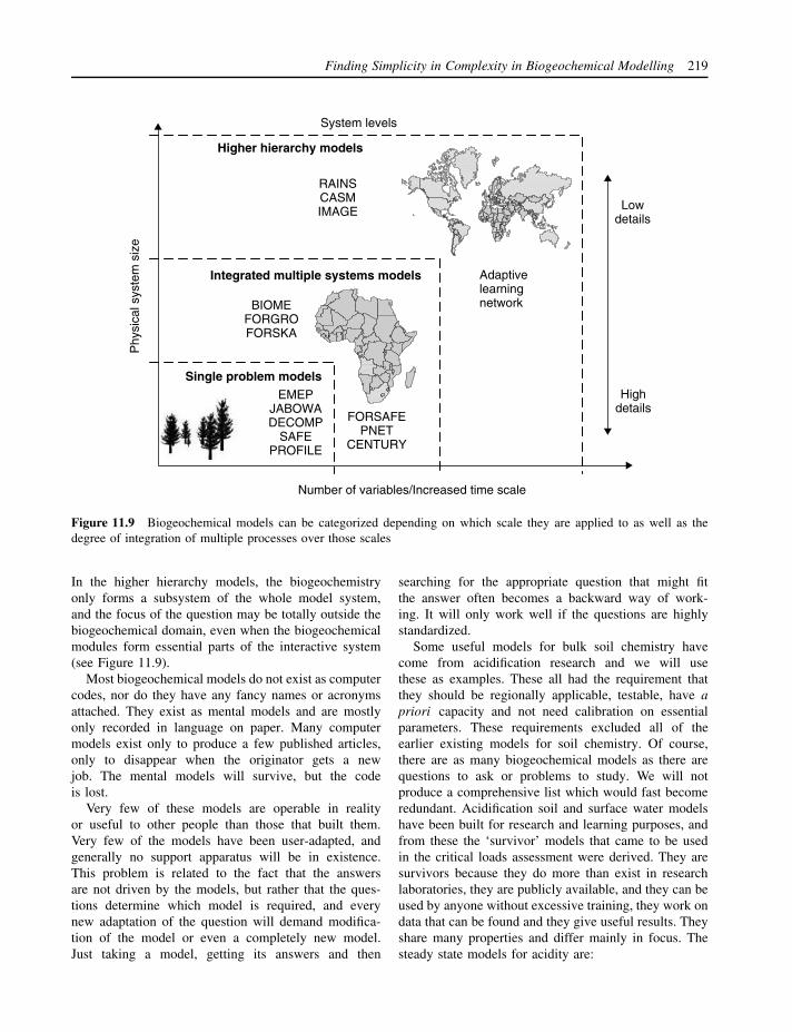
Finding Simplicity in Complexity in Biogeochemical Modelling 219
Lowdetails
Highdetails
System levelsP
hysi
cal s
yste
m s
ize
Number of variables/Increased time scale
Single problem modelsEMEP
JABOWADECOMP
SAFEPROFILE
Integrated multiple systems models
BIOMEFORGROFORSKA
FORSAFEPNET
CENTURY
RAINSCASMIMAGE
Adaptivelearningnetwork
Higher hierarchy models
Figure 11.9 Biogeochemical models can be categorized depending on which scale they are applied to as well as thedegree of integration of multiple processes over those scales
In the higher hierarchy models, the biogeochemistryonly forms a subsystem of the whole model system,and the focus of the question may be totally outside thebiogeochemical domain, even when the biogeochemicalmodules form essential parts of the interactive system(see Figure 11.9).
Most biogeochemical models do not exist as computercodes, nor do they have any fancy names or acronymsattached. They exist as mental models and are mostlyonly recorded in language on paper. Many computermodels exist only to produce a few published articles,only to disappear when the originator gets a newjob. The mental models will survive, but the codeis lost.
Very few of these models are operable in realityor useful to other people than those that built them.Very few of the models have been user-adapted, andgenerally no support apparatus will be in existence.This problem is related to the fact that the answersare not driven by the models, but rather that the ques-tions determine which model is required, and everynew adaptation of the question will demand modifica-tion of the model or even a completely new model.Just taking a model, getting its answers and then
searching for the appropriate question that might fitthe answer often becomes a backward way of work-ing. It will only work well if the questions are highlystandardized.
Some useful models for bulk soil chemistry havecome from acidification research and we will usethese as examples. These all had the requirement thatthey should be regionally applicable, testable, have apriori capacity and not need calibration on essentialparameters. These requirements excluded all of theearlier existing models for soil chemistry. Of course,there are as many biogeochemical models as there arequestions to ask or problems to study. We will notproduce a comprehensive list which would fast becomeredundant. Acidification soil and surface water modelshave been built for research and learning purposes, andfrom these the ‘survivor’ models that came to be usedin the critical loads assessment were derived. They aresurvivors because they do more than exist in researchlaboratories, they are publicly available, and they can beused by anyone without excessive training, they work ondata that can be found and they give useful results. Theyshare many properties and differ mainly in focus. Thesteady state models for acidity are:

220 Hordur V. Haraldsson and Harald U. Sverdrup
1. SMB is the general European default model for ter-restrial ecosystems, which all countries are supposedto use. It is a mass balance, one-box formulation,involving one mass balance for ANC, coupled toa mass balance for base cations (Sverdrup and deVries, 1994).
2. F-factor models are semi-empirical mass balancemodels developed for aquatic systems, applicable toacidity only. All the different models philosophi-cally go back to the original ideas of Henriksen (theHenriksen Model). They make complex assumptions,but are easy to use on existing data (Brakke et al.,1990).
3. PROFILE was developed for forest soils in Sweden,and it is a fully integrated process-oriented model.It focuses on the kinetics of chemical weathering,nutrient uptake to vegetation and cycling, nitrogentransformation reactions and solute flow in the soilhorizon (Sverdrup and Warfvinge, 1995). It calcu-lates soil chemistry layer by layer: it is a multi-layermodel. It differs from the two other models by cal-culating the chemical weathering a priori, withoutany calibration, from physical and geological soilproperties, and not using the weathering rate as acalibration parameter. PROFILE is the only exist-ing model which will predict the weathering rateunder field conditions from soil mineralogy and geo-physics.
There are also a number of ‘survivor’ models fordynamic assessments for acidity. Dynamic models areimportant for interpreting the critical loads, the timeaspect of effects and the devolution of effects after emis-sion reductions. The dynamic models are no substitutefor the steady state models, and do not do a better jobjust because they are more complex; often the com-plexity is offset by additional uncertainty brought bythe increased complexity. Calculating critical loads withdynamic models are just a more complex and expensiveway to do something that could be done at less cost andsometimes with better accuracy with models like SMBor PROFILE. All these ‘survivor’ models are availableand easy to use:
1. MAGIC was originally developed in the UnitedStates (Cosby et al., 1985), but it has found moreuse in Europe after the discontinuation of America’sacid-rain research, and now the focus is on surfacewater. The core processes are alkalinity mass bal-ances, sulphate adsorption and cation exchange. Theminimum time resolution of the model is one year,equal to the numerical integration step in the model.
It is a one-layer soil model. The model is calibratedby adjusting weathering, initial base saturation, selec-tivity coefficients, gibbsite coefficients and presentbase saturation and present stream chemistry is usedas optimizing targets (Cosby et al., 1985). On surfacewaters, the model is acceptably well confined.
2. SMART is a more recent model (de Vries et al.,1989), and its focus is on average major soil chem-istry. The core processes are alkalinity mass balance,sulphate adsorption and cation exchange. The mini-mum time resolution of the model is one year, equalto the numerical integration step in the model. Themodel is calibrated by adjusting two parameters: theweathering rate and the initial base saturation (deVries et al., 1989); present base saturation and soilchemistry are used as optimizing targets. It is a one-layer soil model. The model is reasonably well con-fined on soils and surface waters.
3. SAFE was developed for forest soils in Sweden,and focuses on chemical weathering, simple nutri-ent cycling and development of cation exchange withtime (Warfvinge et al., 1998). It is the dynamic ver-sion of PROFILE. It calculates soil chemistry layerby layer. It is a multi-layer model. It differs from thetwo other models by calculating the chemical weath-ering from physical and geological soil properties,and not by using the weathering rate as a calibrationparameter. The core processes are weathering andcation exchange. This tends to cause difficulties withapplication to catchments and lakes when the aver-age soil depth for the whole watershed is needed.The model is calibrated by adjusting initial base sat-uration with present base saturation as the optimizingtarget. The model is uniquely defined for soils andacceptably well defined for surface waters.
In summary, the MAGIC and SMART models are easierto apply than SAFE because of the smaller amount ofinput data and the greater freedom in calibration. Theyare cheaper to use, but lead to simpler results. SAFE issignificantly better constrained by its stricter calibrationon fewer parameters, its higher demand on input dataand its higher stratigraphic resolution. It is more expen-sive to use, but provides more elaborate results. Whichis best depends on the purpose of the user.
There are several model proposals for nitrogen assess-ments, but these should be classified as tentative atbest. Existing models operate with excessive calibra-tion, the models are actually calibrated in such a waythat inputs become output directly. Once the demandis made for no excessive calibration, there is virtuallyno model available. For calculation of critical loads for
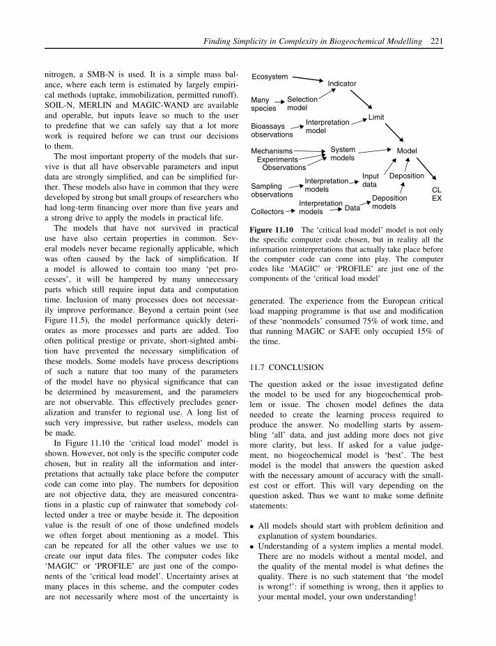
Finding Simplicity in Complexity in Biogeochemical Modelling 221
nitrogen, a SMB-N is used. It is a simple mass bal-ance, where each term is estimated by largely empiri-cal methods (uptake, immobilization, permitted runoff).SOIL-N, MERLIN and MAGIC-WAND are availableand operable, but inputs leave so much to the userto predefine that we can safely say that a lot morework is required before we can trust our decisionsto them.
The most important property of the models that sur-vive is that all have observable parameters and inputdata are strongly simplified, and can be simplified fur-ther. These models also have in common that they weredeveloped by strong but small groups of researchers whohad long-term financing over more than five years anda strong drive to apply the models in practical life.
The models that have not survived in practicaluse have also certain properties in common. Sev-eral models never became regionally applicable, whichwas often caused by the lack of simplification. Ifa model is allowed to contain too many ‘pet pro-cesses’, it will be hampered by many unnecessaryparts which still require input data and computationtime. Inclusion of many processes does not necessar-ily improve performance. Beyond a certain point (seeFigure 11.5), the model performance quickly deteri-orates as more processes and parts are added. Toooften political prestige or private, short-sighted ambi-tion have prevented the necessary simplification ofthese models. Some models have process descriptionsof such a nature that too many of the parametersof the model have no physical significance that canbe determined by measurement, and the parametersare not observable. This effectively precludes gener-alization and transfer to regional use. A long list ofsuch very impressive, but rather useless, models canbe made.
In Figure 11.10 the ‘critical load model’ model isshown. However, not only is the specific computer codechosen, but in reality all the information and inter-pretations that actually take place before the computercode can come into play. The numbers for depositionare not objective data, they are measured concentra-tions in a plastic cup of rainwater that somebody col-lected under a tree or maybe beside it. The depositionvalue is the result of one of those undefined modelswe often forget about mentioning as a model. Thiscan be repeated for all the other values we use tocreate our input data files. The computer codes like‘MAGIC’ or ‘PROFILE’ are just one of the compo-nents of the ‘critical load model’. Uncertainty arises atmany places in this scheme, and the computer codesare not necessarily where most of the uncertainty is
EcosystemIndicator
Limit
Model
Selectionmodel
Bioassaysobservations
Interpretationmodel
Mechanisms
ObservationsExperiments
Systemmodels
Samplingobservations
Interpretationmodels
Inputdata
Collectors DataDepositionmodels
Deposition
Manyspecies
CLEX
Interpretationmodels
Figure 11.10 The ‘critical load model’ model is not onlythe specific computer code chosen, but in reality all theinformation reinterpretations that actually take place beforethe computer code can come into play. The computercodes like ‘MAGIC’ or ‘PROFILE’ are just one of thecomponents of the ‘critical load model’
generated. The experience from the European criticalload mapping programme is that use and modificationof these ‘nonmodels’ consumed 75% of work time, andthat running MAGIC or SAFE only occupied 15% ofthe time.
11.7 CONCLUSION
The question asked or the issue investigated definethe model to be used for any biogeochemical prob-lem or issue. The chosen model defines the dataneeded to create the learning process required toproduce the answer. No modelling starts by assem-bling ‘all’ data, and just adding more does not givemore clarity, but less. If asked for a value judge-ment, no biogeochemical model is ‘best’. The bestmodel is the model that answers the question askedwith the necessary amount of accuracy with the small-est cost or effort. This will vary depending on thequestion asked. Thus we want to make some definitestatements:
• All models should start with problem definition andexplanation of system boundaries.
• Understanding of a system implies a mental model.There are no models without a mental model, andthe quality of the mental model is what defines thequality. There is no such statement that ‘the modelis wrong!’: if something is wrong, then it applies toyour mental model, your own understanding!

222 Hordur V. Haraldsson and Harald U. Sverdrup
• Simplification is necessary in order to sort vari-ables and get a basic understanding of the systemfunctionalities.
• Data collected without purpose is not research, it is‘redundant information with potential for use’, untila problem is found that defines a use for a specifiedpart of it.
• Basic principles and driving forces need to be iden-tified in order to determine effectively the requiredlevel of detail in the model building.
• Make sure that the calibration of the model is robust,in order to avoid telling the model what to give you(the input becomes the output).
• A transparent and testable model is required for effec-tive communication of the model to others. Simplermodels are easier to communicate than complex ones.
In terms of making research a learning process, theauthors encourage researchers actively to build their ownmodel using user-friendly software such as STELLA,POWERSIM, MATLAB, MAPLE, etc.
REFERENCES
Alcamo, J., Shaw, R. and Hordijk, L. (1990) The RAINS Modelof Acidification: Science and Strategies in Europe, KluwerAcademic Publishers, Dordrecht.
Berge, E. and Jakobsen, H.A. (1998) A regional scale multi-layer model for the calculation of long-term transport anddeposition of air pollution in Europe, Tellus 50B, 205–223.
Botkin, D.B., Janak, J.F. and Wallis, J.R. (1972) Some eco-logical consequences of a computer model of forest growth,Journal of Ecology 60, 849–872.
Brakke, D.F., Henriksen, A. and Norton, S.A. (1990) A vari-able F-factor to explain changes in base cation concentra-tions as a function of strong acid deposition, VerhandlungenInternationale Vereinigung fur Theoretische und AngewandteLimnologie 24, 146–149.
Chen, C.J. (1993) The Response of Plants to InteractingStresses, PGSM version 1.3 model documentation.
Cosby, B.J., Wright, R.F., Hornberger, G.M. and Galloway,J.N. (1985) Modelling the effects of acidic deposition,assessment of a lumped-parameter model of soil waterand stream water chemistry, Water Resources Research 21,51–63.
Crote, R. and Erhard, M. (1999) Simulation of tree and standdevelopment under different environmental conditions witha physiologically based model, Forest Ecology and Manage-ment 120, 59–76.
Crote, R., Erhard, M. and Suckow, F. (1997) Evaluation of thePhysiologically-Based Forest Growth Model FORSANA 22,Potsdam Institute for Climate Impact Research, Potsdam.
den Elzen, M. (1994) Global Environmental Change and Inte-grated Modeling Approach, International Books, Utrecht.
de Vries, W., Posch, M. and Kamari, J. (1989) Simulation ofthe long-term soil response to acid deposition in variousbuffer ranges, Water, Air and Soil Pollution 48, 349–390.
Dorner, D. (1996) The Logic of Failure: Recognizing andAvoiding Error in Complex Situations, Perseus Books, Cam-bridge, MA.
Gough, C.A., Bailey, P.D., Biewald, B., Kuylenstierna, J.C.I.and Chadwick, M.J. (1994) Environmentally targeted objec-tives for reducing acidification in Europe, Energy Policy 22,1055–1066.
Jansson, P.E. (1991) SOIL Water and Heat Model: TechnicalDescription, Soil Science Department, University of Agri-cultural Sciences, Uppsala.
Kimmins, J.P., Mailly, D. and Seely, B. (1999) Modeling for-est ecosystem net primary production: the hybrid simulationapproach used in FORECAST, Ecological Modeling 122,195–224.
Kram, P., Santore, R.C., Driscoll, C.T., Aber, J.D. and Hru-ska, J. (1999) Application of the forest-soil-water model(PnET-BGC/CHESS) to the Lysina catchments, CzechRepublic, Ecological Modelling 120, 9–30.
Kros, H. (2002) Evaluation of biogeochemical modeling atlocal and regional scale, PhD thesis, Alterra Green WorldInstitute, Wageningen, Netherlands.
Levenspiel, O. (1980) The coming of age of chemical reactionengineering, Chemical Engineering Science 35, 1821–1839.
Mohren, G.M.J., Bartelink, H.H., Jorristma, I.T.M. and Kra-mer, K. (1993) A process-based growth model (FORGRO)for analysis of forest dynamics in relation to environmen-tal factors, in M.E.A. Brockmeyer, W. Vos and H. Koep(eds) European Forest Reserves, Workshop, 6–8 May 1992,PUDOC, Wageningen, Netherlands, 273–280.
Parton, W.J., Schimel, D.S., Cole, C.V. and Ojima, D.S. (1987)Analysis of factors controlling soil organic levels of grass-lands in the Great Plains, Soil Science Society of AmericaJournal 51, 1173–1179.
Richardson, P.G. and Pugh, A.L. (1981) Introduction to SystemDynamics Modelling with DYNAMO, Productivity Press,New York.
Rotmans, J., van Asselt, M.B.A., de Bruin, A.J., den Elzen,M.G.J., de Greef, J., Hilderink, H., Hoekstra, A.Y., Janssen,M.A., Koster., H.W., Martens, W.J.M., Niessen, L.W. andde Vries, H.J.M. (1994) Global Change and SustainableDevelopment: A Modelling Perspective for the Next Decade,National Institute of Public Health and Environmental Pro-tection (RIVM), Bilthoven.
Sykes, M.T., Prentice, I.C. and Cramer, W. (1996) A biocli-matic model for the potential distributions of north Europeantree species under present and future climates, Journal ofBiogeography 23, 203–233.
Sverdrup, H. and Stjernquist, I. (2002) Developing Princi-ples for Sustainable Forestry, Kluwer Academic Publishers,Dordrecht.
Sverdrup, H. and de Vries, W. (1994) Calculating critical loadsfor acidity with the simple mass balance method, Water, Airand Soil Pollution 72, 143–162.
Sverdrup, H. and Warfvinge, P. (1995) Estimating field weath-ering rates using laboratory kinetics, in A.F. White and

Finding Simplicity in Complexity in Biogeochemical Modelling 223
S.L. Brantley (eds) Chemical Weathering Rates of Silicate,Mineralogical Society of America, Washington, DC.
Warfvinge, P., Sverdrup, H. and Wickman, T. (1998). Estimat-ing the weathering rate at Gardsjon using different methods,in H. Hultberg and R. Skeffington (eds) Experimental Rever-sal of Acid Rain Effects; The Gardsjon Roof Project, JohnWiley & Sons, Chichester, 231–250.
Wright, R.F., Beier, C. and Cosby, B.J. (1998) Effects of nitro-gen deposition and climate change on nitrogen runoff atNorwegian boreal forest catchments: the MERLIN modelapplied to Risdalsheia (RAIN and CLIMEX projects),Hydrology and Earth System Sciences 2, 399–414.


12
Modelling Human Decision-Making
JOHN WAINWRIGHT AND MARK MULLIGAN
12.1 INTRODUCTION
This book is a complex system. It is made up ofa series of interconnecting parts with inputs from alarge number of external sources – the experiences ofthe contributing authors. These experiences combineto provide a whole that can function in a numberof ways – as a manual, a reference, and a source ofideas. The way in which it is put together providesone means of using (reading) it, but as noted in theIntroduction, you needn’t have found this chapter abouthalf-way through, because the best way to read thebook is not necessarily from beginning to end. Butthen, who always chooses to read the Introduction?When we first decided it would be a good idea toput together a book about environmental modelling,we thought it would be best to benefit from theinsights of specialists in particular areas rather than writeeverything ourselves. We also thought this approachwould make the whole process quicker (something ourpublisher is beginning to doubt!), which is an advantagegiven the pressure on time and resources in the relativelyunder-funded world of UK academia. But consider whatthis means – we now have 32 different contributors,all with their different decisions to make about whatto include, how to do so, and when to do it (evenmodellers occasionally prefer going to the cinema or aconcert or to watch a football match than to sit in frontof the computer for a few hours more). Being in themiddle of the book, we cannot fit page numbers to theremainder until it is complete (and in fact are awaiting
one or two preceding chapters so we can’t even getthis far!). So the whole thing is strongly interdependentin its structure and output. Why did we ever decide todo it in the first place? The answer may lie in a mixof prestige, expectation and satisfaction (certainly notfor the money!). For any contributor working under thewatchful eye of the Research Assessment Exercise inUK universities for which edited volumes score verylittle in comparison with journal articles and researchmonographs, the decision is something of an irrationalone, and not necessarily one for which our headsof department will thank us. So is human behaviourrational? In this case obviously not. How can we hope tomodel something that can appear to be almost randomlyirrational? What’s more, why did any of the contributorsdecide to take up modelling in the first place ratherthan drive trains or become firefighters? What madeyou pick the book from the shelf of the library orbookshop (or have your mouse inexplicably drawn toit on the Internet)?
How this chapter got to be here and how you gotto be there reading it is therefore a function of a longseries of decisions whose ultimate explanation is, quiteliterally, lost in the mists of time. If we cannot explainthese decisions, how can we expect to model the hugenumber of interacting human decisions that interact withand affect the environment at scales from local to global?At this point, should we just throw up our hands indismay and wander off (or spend endless hours – andpages – engaged in discourse about the undecidabilityof decision-making . . .)?
Environmental Modelling: Finding Simplicity in Complexity. Edited by J. Wainwright and M. Mulligan 2004 John Wiley & Sons, Ltd ISBNs: 0-471-49617-0 (HB); 0-471-49618-9 (PB)

226 John Wainwright and Mark Mulligan
If you are still with us, then hopefully you willagree that some attempt to model human decision-making is necessary – especially if the models we comeup with help us understand why we make decisions(both rational and irrational) and how the process worksoverall. Of course, having elements relating to humandecisions is fundamental for most models, especiallythose in the applied field, as we will see in the nextsection. (Indeed, all models relate to human decisions bythe very nature of how they are built and implemented.After a long day of trying to remove a ‘totally obvious’error from our model code, we might wish that thishuman element were not the case! Developments ingenetic algorithms [e.g. Mitchell, 1996], that is, modelsthat essentially build themselves, have yet to reachenvironmental models in a significant way.)
Human activities within the environment continue toincrease. (We will leave aside the debate about whetherhumans are part of the environment or ‘nature’ – seePhillips and Mighall, 2000, for discussions.) Hooke(2000) has demonstrated that human activity has nowovertaken rivers as the principal transport agent ofsediment. Human-induced climate change and land useare a fundamental part of this increase in impact, andthe modelling of human behaviour is a central elementof attempts to assess the nature and extent of change(IPCC, 2001). Indeed, the interest in environmentalmodelling (and part of the rationale for this book) at thepresent time is largely spurred on by the potential threatsof climate change and its two-way relationship withland use. So, increasingly, all types of environmentalmodelling require consideration of at least some aspectof human behaviour. Why is this human behaviour socomplex compared with other animals, plants and abioticaspects of the environment?
12.2 THE HUMAN MIND
The structure of the human brain is complex. Despitebeing the most remarkable object we know, it resemblesa bowl of cold porridge, at least according to one of thefounding fathers of computation, Alan Turing (cited inPenrose, 1989). At the top is the deeply wrinkled, greycerebral cortex, divided into two almost symmetricalparts and sitting above the ancestral mammalian brainor cerebellum (Figure 12.1; Carter, 1998). The limbicsystem is located beneath the cerebral cortex and com-municates with the rest of the body via the brain stem,but is also responsible for most of our behaviour directlyrelated to survival and the formation of memories. Thecerebral cortex is itself divided into five main areas,each of which seem to serve specific functions. For
Frontallobe
Corpus callosum
Frontallobe
Parietal lobeCerebellum
Occipital lobeBrain stemLimbic system
Temporal lobe Occipital lobe
Parietal lobe
Cerebellum
Figure 12.1 General structure of the human brainSource: Carter (1998)
example, the parietal lobes deal with movement amongother things, while the frontal lobes deal with conceptualand planning issues as well as emotions. One-tenth ofthe cells in the brain are the 1012 neurons – responsiblefor brain activity (see also Chapter 1) – and connectedby long, thin nerve cells of two types. Axons carryinformation away from a neuron, while dendrites carryinformation towards it. The location where an axonjoins a dendrite is known as a synapse, and informa-tion is passed chemically along the nerve by succes-sively changing the balance of sodium then potassiumions across the cell membrane (see Penrose, 1989, fora simple explanation). There may be several thousandsuch connections from a single neuron to others. Thenerves are sheathed in myelin, which permits this sys-tem to operate at very rapid speeds. As well as thesespecific connections, there are also general chemicalconnections within the brain, as a result of cells that pro-duce specific substances called neurotransmitters, which

Modelling Human Decision-Making 227
themselves have specific effects on brain activity andhence behaviour.
Even with recent advances in brain-scanning tech-nology, understanding the operation of the brain andits interconnections is fraught with difficulties. Often,explanations come most clearly when dealing withparts of the brain that are known to have been dam-aged (Ramachandran and Blakeslee, 1998). It is per-haps, therefore, unsurprising that understanding humanbehaviour is a difficult process:
When one considers the structure of the brain it isremarkable that it ever manages to come to the cor-rect conclusion about anything. By any conventionalstandards neurons are an entirely unsuitable mediumfor computation; they die throughout the brain’s life,causing random loss of stored information; they havea finite probability of firing even when they are notengaged in signal processing; the response of a neu-ron to any particular input is probabilistic, not fixed.
(McLeod et al., 1998: 32)
Thus far, the discussion has been specifically on thebrain. Issues of consciousness, soul and mind aredifficult ones to explain convincingly. Nathan (1987)suggests talking about mental processes rather thangetting bogged down in issues of what the mind mightbe. A relatively simple viewpoint is to regard themind as the emergent property of the various brainfunctions (e.g. Bar-Yam, 1997), although there existsconsiderable debate as to which functions to include soas to distinguish the human mind or consciousness fromthat of other animals – most, for example, insisting onthe inclusion of language (Noble and Davidson, 1996).Aleksander (2000) centres his definition on imagination.
The decision-making process can be characterized asthe various ways in which mental processes can be madeto affect human behaviour. These processes may relateto relatively ‘primitive’ behaviour relating to the sur-vival instinct (decisions on whether to run away or standone’s ground when threatened; what to eat), all the wayup to the more considered ideas and plans that maydevelop in the frontal lobes, perhaps via discussionswith others. Of course, the ever-present potential forinteraction between brains complicates the matter fur-ther. As noted by Thagard (2000), it is necessary forany theory of decision-making to evaluate personal goalsand constraints on them, rather than simply optimize aset of potential preferences. Decisions are not alwaysright, nor successful! These features of mental activ-ity and behaviour seem to have developed along withmodern humans. Both Noble and Davidson (1996) and
Mithen (1996) see the onset of features characteristic ofpresent ways of thinking around 250 000–300 000 yearsago (but see Jaynes, 1980, for a significantly later date),so even environmental models that deal with the distantpast may need to include significant elements relating tohuman activity. It is clear that our brain power (and itsapplication to industry and technology) as well as ourpopulation have, over time, enormously increased ourimpact on, and (arguably) decreased our dependence on,the natural world.
Underlying our ability to model human activity isa fundamental question: can a computer be made tothink? Essentially, in trying to simulate decision-makingand the corresponding behaviour, we need to be ableto replicate the thought process within a computationalframework. This is the discipline of artificial intelligence(AI; Crevier, 1993). Searle distinguishes between ‘weak’and ‘strong’ AI. The former assumes that principlesrelating to brain function can be reproduced computa-tionally and corresponding hypotheses tested. The latterconsiders that ‘the appropriately programmed computerreally is a mind in the sense that computers given theright programs can literally be said to understand andhave other cognitive states . . . the programs are not meretools that enable us to test psychological explanations;rather, the programs are themselves the explanations’(1980: 417: emphasis in original). While he is happyto accept weak AI, Searle strongly criticizes the strongform, using the example of a non-Chinese speaker beingpassed a list of rules for translating and commenting(in English) upon a story given to them in Chinese.Although a native speaker might be fooled by the output(i.e. the system – essentially a replication of a computerprogram [the list of rules] with input [the story] and out-put [the translation and commentary] – passes a Turingtest), Searle demonstrates that the person does not under-stand Chinese and thus the process does not representan intelligent system. Penrose (1989) points out that theweakest point of Searle’s argument is when he allowsthe different stages in the translation and commentaryto be carried out by (large numbers of) different people,as the system then becomes more analogous to the neu-rons in the brain – we do not need to argue that everysingle neuron understands the outcome for intelligenceto be demonstrated. The process here is one of emer-gence (see also Aleksander, 2000). Hofstadter (1979,1981) argues for the possibility of strong AI in comput-ers (but not necessarily other human attributes such asemotions). He suggests that a (large) book containinga complete description of Einstein’s brain would allowus to interrogate it and give equivalent answers to thoseEinstein would have given. Compare this example to
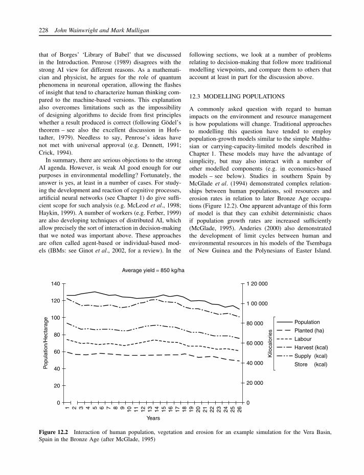
228 John Wainwright and Mark Mulligan
that of Borges’ ‘Library of Babel’ that we discussedin the Introduction. Penrose (1989) disagrees with thestrong AI view for different reasons. As a mathemati-cian and physicist, he argues for the role of quantumphenomena in neuronal operation, allowing the flashesof insight that tend to characterize human thinking com-pared to the machine-based versions. This explanationalso overcomes limitations such as the impossibilityof designing algorithms to decide from first principleswhether a result produced is correct (following Godel’stheorem – see also the excellent discussion in Hofs-tadter, 1979). Needless to say, Penrose’s ideas havenot met with universal approval (e.g. Dennett, 1991;Crick, 1994).
In summary, there are serious objections to the strongAI agenda. However, is weak AI good enough for ourpurposes in environmental modelling? Fortunately, theanswer is yes, at least in a number of cases. For study-ing the development and reaction of cognitive processes,artificial neural networks (see Chapter 1) do give suffi-cient scope for such analysis (e.g. McLeod et al., 1998;Haykin, 1999). A number of workers (e.g. Ferber, 1999)are also developing techniques of distributed AI, whichallow precisely the sort of interaction in decision-makingthat we noted was important above. These approachesare often called agent-based or individual-based mod-els (IBMs: see Ginot et al., 2002, for a review). In the
following sections, we look at a number of problemsrelating to decision-making that follow more traditionalmodelling viewpoints, and compare them to others thataccount at least in part for the discussion above.
12.3 MODELLING POPULATIONS
A commonly asked question with regard to humanimpacts on the environment and resource managementis how populations will change. Traditional approachesto modelling this question have tended to employpopulation-growth models similar to the simple Malthu-sian or carrying-capacity-limited models described inChapter 1. These models may have the advantage ofsimplicity, but may also interact with a number ofother modelled components (e.g. in economics-basedmodels – see below). Studies in southern Spain byMcGlade et al. (1994) demonstrated complex relation-ships between human populations, soil resources anderosion rates in relation to later Bronze Age occupa-tions (Figure 12.2). One apparent advantage of this formof model is that they can exhibit deterministic chaosif population growth rates are increased sufficiently(McGlade, 1995). Anderies (2000) also demonstratedthe development of limit cycles between human andenvironmental resources in his models of the Tsembagaof New Guinea and the Polynesians of Easter Island.
20
40
60
80
100
120
140
0
1 2 3 4 5 6 7 8 9 10 11 12 13 14 15 16 17 18 19 20 21 22 23 24 25 26
20 000
1 20 000
0
Years
Average yield = 850 kg/ha
40 000
60 000
80 000
1 00 000
Population
Pop
ulat
ion/
Hec
tara
ge
Planted (ha)
Labour
Harvest (kcal)
Supply (kcal)
Store (kcal)
Kilo
calo
ries
Figure 12.2 Interaction of human population, vegetation and erosion for an example simulation for the Vera Basin,Spain in the Bronze Age (after McGlade, 1995)

Modelling Human Decision-Making 229
326.784.86
0.488
11.510.0200
0.00972
90.331.23
0.129
169.152.44
0.249
247.963.65
0.368
123
1 Production 2 Soils 3 Erosion
0.0 15.00 30.00
Time
45.00 60.00
1
1
1
1
1
1
1
2
3
3
3 3 3 3
3
2
2
2 2 22
Figure 12.2 (continued )
Thus this approach provides a means of explainingapparently random population changes, relating to therapid increases and decreases that are apparent throughprehistory and history. However, many people feelunhappy with the determinism implicit in these models.A concept of free will is often thought to be central to thehuman condition, while these models ignore all possi-bility of its existence, even allowing for chaotic results.
12.4 MODELLING DECISIONS
Perhaps the most important, related, criticism of theabove approaches is that they fail to account forthe reasons why population size changes. Populationschange because of the decisions taken by individuals(e.g. choice of partner, use of contraception, spacingbetween children, etc.) as affected by social norms(e.g. acceptability of large families, infanticide, modesof marriage, etc.) and historical and environmentalcontingency. (Note that a growing number of ecologistsare also suggesting the use of individual-based modelsin their modelling of plants or animals; see Chapters 6to 8.) Population growth is thus an emergent propertyor consequence of individual and social interactions andnot a process in itself.
12.4.1 Agent-based modelling
Epstein and Axtell (1996) provide an agent-basedapproach in their Sugarscape model. Sugarscape is a
simplified landscape laid out on a grid, on which a foodresource (sugar) is distributed in some initial, specifiedpattern. The landscape is populated by a number ofagents who can move around the landscape accordingto specified rules in order to harvest and consume thesugar. Once harvested, the sugar is able to grow backaccording to a simple set of rules. The agents are ran-domly assigned a metabolism – how fast they consumethe sugar they collect, so that if their sugar resourcefalls to zero, they die off. They are also assigned adistance of vision allowing a form of differential plan-ning of their movements, and are randomly distributedin space at the start of a simulation. Agents can col-lect more sugar than they need to survive and thusaccumulate ‘wealth’. The results with very simple mod-els show important patterns. The spatial location of theagents varies according to different rates of regrowth ofthe harvested sugar, thus not all landscapes are equal.The landscapes converge to specific numbers of indi-viduals for given sets of conditions. In other words,a carrying capacity (see Chapter 1) emerges from theagents’ behaviour (Figure 12.3a). Furthermore, this car-rying capacity is a function of characteristics of theagents, so that if their metabolisms and depths of visionbecome dynamic properties, the carrying capacity toowould be variable. This result overcomes a major limita-tion of the carrying-capacity approach to human popula-tions, in that the path of human history has been one ofadaptation, allowing (environmentally imposed) carry-ing capacities to be overcome through better technology,

230 John Wainwright and Mark Mulligan
for example. Such adaptations are impossible to includein the traditional form of the population model. Anotheremergent property is the unequal distribution of wealthof individuals, even if they start off with a relativelyuniform initial amount (Figure 12.3b).
More complex Sugarscape rules were also devel-oped by Epstein and Axtell to account for the pro-cesses of sexual reproduction (and genetic attributes),group affiliations, pollution, warfare, trade (of a sec-ond commodity – spice) and disease (with the possi-bility of overcoming it and transmitting immunity).Thus, it was possible to generate relatively complexpatterns of emergent behaviour from relatively simplerules. For example, population cycles with a wavelengthexceeding the average lifetime of individual agents canemerge in the presence of the spice trade, comparedto the extinction under equivalent conditions withouttrade (Figure 12.3c). The modelling approach allowsthe investigation of the realism of different economicand policy models and ideas of sustainability withinthe landscape.
While Sugarscape looks at an artificial landscapeto investigate general patterns, other attempts havebeen made to simulate real landscapes. Gumerman andKohler (1995) and Axtell et al. (2002) have used theapproach to investigate changing populations in Long
House Valley in northeastern Arizona. The area has beenoccupied for over 3000 years, and particular emphasiswas placed on the period of agriculture under theAnasazi from c. 200 CE until its collapse in c. 1300 CE.Tree-ring records were used to derive a climate recordbased on drought intensity, which was then used toestimate maize yields. Agents in this case were basedon family groups who make annual decisions on whereto live and farm. Initial simulations track the historicalpattern of household change and the spatial locationof households relatively well. The simulations suggestthat although population would decline in the laterperiods due to environmental degradation, there wereprobably other external factors that led to the completeabandonment of the area around 1300 CE.
Bura et al. (1996) and Sanders et al. (1997) used amodel called SIMPOP to investigate patterns of urbandevelopment in a generalized area based on the southernRhone valley in France. Their agents represented aggre-gation at the level of the settlement, which for obviousreasons were not allowed to move through the landscape.The landscape was divided into hexagonal cells with ini-tial resources (agricultural, mineral or maritime) whichcould be occupied by settlements of different types. Allsites start off as rural, but can develop into a variety ofcommercial, industrial or administrative centres, based
200
250
300
350
400
450
500
0 2 4
Mean agent vision (number of grid cells)
6 8 10
Car
ryin
g ca
paci
ty (
num
ber
of a
gent
s)
<m> = 1<m> = 2<m> = 3
(a)
Figure 12.3 Examples of results from the Sugarscape model of Epstein and Axtell (1996). (a) Emergent carrying capacityin numbers of agents of a 50 × 50 cell landscape; (b) emergence of unequal distributions of wealth (measured in unitsof sugar) for similar simple rules to the results shown in (a); and (c) behaviour comparing the effect of no trade inspice, leading to extinction, with the existence of trade leading ultimately to the development of ‘long wave’ populationoscillations

Modelling Human Decision-Making 231
27 54 81 108 135 162 189 216 243 270
Units of wealth possessed
0
20
40
60
80
100
120
140
Num
ber
of a
gent
s
20 40 60 80 100 120 140 160 180 200
Units of wealth possessed
0
Num
ber
of a
gent
s
1020304050607080
11
Units of wealth possessed
0
Num
ber
of a
gent
s
10
20
30
40
50
60
22 33 44 55 66 77 88 99 110
Num
ber
of a
gent
s
03
Units of wealth possessed
51015202530354045
6 9 12 15 18 21 24 27 30
Time
(b)
Figure 12.3 (continued )

232 John Wainwright and Mark Mulligan
50
Time
100 150 200 250 300 350 400 450
500
Num
ber
of a
gent
s
1000
1500
20 40 60 80 100 120 140 160 180
Time
Num
ber
of a
gent
s
100
200
300
400
500
600
500
Time
550 600 650 700 750 800 850 900
500
Num
ber
of a
gent
s
1000
1500
(c)
Figure 12.3 (continued )
on a series of economic models. Exchange is allowedbetween settlements and population is modelled as aseries of stochastic functions based on settlement size,neighbourhood and ability to satisfy local demand. Thesimulations resulted in the emergence of a highly hierar-chical urban landscape, with similar properties to that ofthe modern landscape, albeit with a poor spatial distribu-tion of the major centres (Figure 12.4). See Chapter 14for a discussion of more complex socio-economic inter-actions in agent-based models.
To summarize, we can see that environmental as wellas historical contingency is important in the simula-tion of population change using agents. Agent-basedmodels offer distinct explanatory power over previousapproaches, in that observed phenomena emerge frominteractions, rather than being imposed by the modellingframework and preconceived notions. Furthermore, theyenable the testing of different hypotheses relating tosocial and economic phenomena, and the evaluation of
contingency in different realizations of the same setof conditions.
Of course, when interacting with the landscape, it isnot just population-related properties that are importantemergent features. Even more important is what is donewith the land, as demonstrated in the previous twoexamples, for only when account is taken of changingland use are fully dynamic interactions between humansand their landscapes investigated. Many impact-relatedmodels that fail to do so are thus oversimplified to theextent of being poor representations of the system beingresearched. Issues relating to the modelling of land useand land-use change are covered fully by Lambin in thenext chapter.
At relatively small scales, Gimblett et al. (2001) andRoberts et al. (2002) have used agent-based modelsto investigate the specific problem of the impact ofrecreational use of the Grand Canyon National Park inthe US. Agents within the model plan raft trips, the
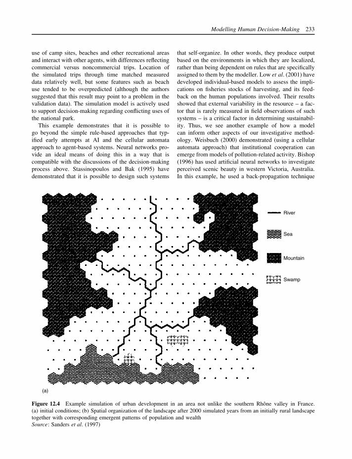
Modelling Human Decision-Making 233
use of camp sites, beaches and other recreational areasand interact with other agents, with differences reflectingcommercial versus noncommercial trips. Location ofthe simulated trips through time matched measureddata relatively well, but some features such as beachuse tended to be overpredicted (although the authorssuggested that this result may point to a problem in thevalidation data). The simulation model is actively usedto support decision-making regarding conflicting uses ofthe national park.
This example demonstrates that it is possible togo beyond the simple rule-based approaches that typ-ified early attempts at AI and the cellular automataapproach to agent-based systems. Neural networks pro-vide an ideal means of doing this in a way that iscompatible with the discussions of the decision-makingprocess above. Stassinopoulos and Bak (1995) havedemonstrated that it is possible to design such systems
that self-organize. In other words, they produce outputbased on the environments in which they are localized,rather than being dependent on rules that are specificallyassigned to them by the modeller. Low et al. (2001) havedeveloped individual-based models to assess the impli-cations on fisheries stocks of harvesting, and its feed-back on the human populations involved. Their resultsshowed that external variability in the resource – a fac-tor that is rarely measured in field observations of suchsystems – is a critical factor in determining sustainabil-ity. Thus, we see another example of how a modelcan inform other aspects of our investigative method-ology. Weisbuch (2000) demonstrated (using a cellularautomata approach) that institutional cooperation canemerge from models of pollution-related activity. Bishop(1996) has used artificial neural networks to investigateperceived scenic beauty in western Victoria, Australia.In this example, he used a back-propagation technique
River
Sea
Mountain
Swamp
(a)
Figure 12.4 Example simulation of urban development in an area not unlike the southern Rhone valley in France.(a) initial conditions; (b) Spatial organization of the landscape after 2000 simulated years from an initially rural landscapetogether with corresponding emergent patterns of population and wealthSource: Sanders et al. (1997)

234 John Wainwright and Mark Mulligan
RiverNatural elements
Population size1000 000
Different levels of functions
Retail1 1
Administration
Sea
Mountain
Swamp
250 000
60 000
2
3
4
2
(b)
Figure 12.4 (continued )
to estimate the relative importance of a number of mea-sured variables estimated within a GIS to the meanperceived beauty of the area by a sample of 48 observers(note that this is an analytical rather than self-organizingapproach, though). Bezerra et al. (1996) have designed asimple neural network model that takes account of fac-tors relating to personality (distanciation from reality,knowledge, relation to time, expansiveness, ego, cre-ativity, risk shift, anxiety and authoritarian attitude) andinstantaneous state of the individual (fatigue, coping,sleep deprivation, morale and motivation as affected bythe environment in which the individual is situated) inrelation to the decision-making process. This processis a function of six factors in their model: perception,mental representation, data processing, problem solving,choice of solution and action. Such approaches are asyet in their infancy, and their ability to provide work-able models has yet to be thoroughly evaluated (forother examples, see Gilbert and Doran, 1994; Kohlerand Gumerman, 2000). Alternative approaches that mayprove useful in the future include the use of virtual real-ity models (van Veen et al., 1998).
12.4.2 Economics models
At the opposite end of the spectrum, models are requiredthat deal with decisions at national and internationallevels. Models based on principles of economics arecommonly used at this scale. Cantor and Yohe (1998)provide an excellent overview of the limitations ofthis approach, which we summarize below. Standardmacroeconomic models depend on projections of fac-tors such as income, economic activity and trade withthe application of cost-benefit analysis for different envi-ronmental factors. Governmental and international orga-nizations such as the World Bank will tend to evalu-ate costs and benefits relative to gross domestic prod-uct (GDP) or gross national product (GNP). Compar-isons between countries are difficult because differentcategorizations may be used, because of the need toevaluate the relative effects of different activities andbecause of exchange-rate issues. Even though morereliable comparisons using purchasing-power paritiesare possible, these are not used by institutions suchas the World Bank, leading to obvious problems ininterpretation.

Modelling Human Decision-Making 235
Cantor and Yohe divide other issues into two cate-gories. First, measurement problems relate to difficul-ties in providing reasonable comparisons. It may bedifficult to evaluate the true level of economic activ-ity, particularly in less industrialized nations, where theinformal economy has been estimated to be responsiblefor 80–98% of activity relative to the GDP, 30–57%of employment and 33–75% of credit. Other means arerequired for evaluating these roles. Ignoring them wouldsignificantly impact on particularly the rural sectors inless industrialized areas. There is the related issue ofhow to measure inequality at the international scale, sothat issues of equity may be addressed within a mod-elling framework. Second, there are more difficult con-ceptual problems. How can the aggregation of individualneeds and desires be addressed? This is the question ofemergence that we have previously highlighted. Howcan social and cultural differences be accounted for? Ifthey are ignored, any policy developed will be difficultor impossible to implement effectively (see below). Howcan time and the requirements of future generations beaccounted for? Most economic models discount futureeffects so that the value of a benefit received in thefuture is less than one received now. The rate at whichfuture benefits are discounted is a very sensitive modelparameter – $1000 m received in 200 years would havean estimated present-day value of $137 m if discountedat 1% but only $5.27 if discounted at 10%! A ‘careful’choice of rate can therefore greatly bias the outcometo benefit particular parties and is at best inappropriatebut at worst unethical. How can sociopolitical aspects ofgrowth be accounted for? The ways in which industrial-ization occurs may differentially affect the rates at whichgreenhouse gas emissions (GHG) are produced. Again,‘one size fits all’ models are likely to be inappropri-ate. Finally, how can different ideas of sustainability beaccounted for? Different viewpoints suggest highly con-trasting views: optimism that technological fixes willbe possible due to continued economic growth, pes-simism that major thresholds will be crossed leadingto catastrophic decline in environmental resources andeconomic growth, or intermediate viewpoints relatingto adaptation (Figure 12.5). The standard approach is toproduce a series of scenarios based on different assump-tions of interactions, using different measurement meth-ods, which we will discuss in more detail below.
Gielen and Yagita (2002) modelled the impactsof different policies to reduce greenhouse gases onglobal trade in the petrochemical industry. Using sixregions – western Europe, Japan, North America, east-ern Europe, the Middle East and the rest of theworld – they simulated demand for CO2 emissions at
different stages in the production cycle of 50 petrochem-icals. Energy and transportation costs were consideredalong with other constraints such as resource availabil-ity. Different scenarios were assessed using taxes ongreenhouse gases applied either globally, or to specificregional subsets. Without imposition of taxes, they pre-dicted a 67% increase in CO2 emissions compared todecreases of 4% with taxes of ¥7500 t−1 in westernEurope and up to 58% with global taxes of ¥15 000 t−1.However, in the case of nonglobal taxes, production mayonly shift location.
Such an approach to abatement had led many tosuggest that it would be unfeasible due to the high costs.However, Azar and Schneider (2002) used a simplemacro-economic model to suggest the costs of CO2
abatement to maintain 350 ppm in 2100 to be of theorder of $18 (US) trillion (1012) discounted to 1990values. This figure compares to a total world economyof $20 trillion in 1990. Clearly seen by this comparison,the proportion is high. But the standard approach is toassume income growth over the same period. Put in thiscontext, the extra cost is very marginal. This exampledemonstrates once again the need for extreme care ininterpreting results (and ensuring that our results are notmisinterpreted by others).
12.4.3 Game theory
Game theory provides one means by which such inter-actions can be simulated at this level. Parsons andWard (1998) note that the standard level of analysisassumes that participants in the models can be builtusing individual-based approaches, but because suchmodels would tend to be large and cumbersome, mostcurrent models assume simplification at the level of thenation, sub- or trans-national group is possible. If apriori assumptions can be made about the benefits toeach of the groups, then game theory can provide opti-mal solutions for cooperation versus noncooperation foreach of them. Clearly, this requirement is a problem inmost approaches to future change, as it is impossible toevaluate what the benefits would be. Solutions to thisproblem include the use of stochastic measurements ofbenefits and the use of iterated ‘supergame’ approaches.The outcome of the latter tend to be multiple equilib-rium solutions, so that some qualitative evaluation ofthe different outcomes is required. Other forms of sim-ulation may thus be required to deal with the complexinteractions (Parsons and Ward, 1998).
Frisvold and Caswell (2000) used game theory toinvestigate the need for assistance projects and tech-nical support in the management of water supply and

236 John Wainwright and Mark Mulligan
Natural capital
Human-made capital
Revenues from growthcould be used to preserve nature
Present time
Qua
ntity
(a)
Natural capital
Human-made capital
Possible recoveryafter crash
Present time
Qua
ntity
(b)
Natural capitalHuman-made capital
Range ofuncertaintyaboutpossibilitiesfor qualitativeimprovements
Present time
Qua
ntity
and
qua
lity
(c)
Figure 12.5 Summary of different schematic models of economic and environmental interaction. (a) ‘The economicoptimist’; (b) ‘the environmental pessimist’; (c) ‘the ecological economic vision’Source: Cantor and Yohe (1998)
treatment issues across the border of Mexico and theUnited States. Negotiations within the InternationalBoundary and Water Commission established by the1944 Water Treaty between the two nations can betreated as a cooperation game because commitments arelegally binding. Decisions such as that made in 1951regarding the pollution of Nogales can be regarded as
economically efficient within this framework as theyapportioned costs to benefits – the US side benefitedmore in this example, and was prepared and able topay a higher proportion of the costs. In contrast, USpolicy in the period of the Reagan administration statedthat costs should be met equally, leading to its beinghighly unlikely that mutually agreeable, economically
Modelling Human Decision-Making 237
efficient solutions could be reached. After a number ofproject failures, equal cost sharing was abandoned as aprinciple in 1990. Game theoretic approaches may alsoprove useful in deciding the need to provide grants andtechnical assistance for the development of water sanita-tion measures. However, they point out that game theorymay provide unsatisfactory solutions when one side isresponsible for the problem and the other is the vic-tim. In these cases, standard game theoretic solutionswill tend towards victim-pays outcomes, which contra-vene the internationally accepted polluter-pays principle.They also do not allow for cases where countries do notwish to appear weak nor for the victim to offer pay-ments to prevent the problem where it has a significantlylower income than the polluter. Frisvold and Caswellsuggest that iterated games (similar to the ‘supergame’discussed above) may be more appropriate techniquesin such cases.
A game theoretic approach was also applied to theanalysis of agreements to reduce CO2 in the globalcontext by Frankhauser and Kverndokk (1996). In theirapproach, CO2-reduction agreements are considered asa five-player game between the USA, other OECDcountries, countries of the former USSR, China andthe rest of the world. Each player tries to maximize itsbenefits in relation to CO2 emitted in order to increase itsown wealth measured as GNP. At the same time, theseemissions will lead to future effects on the wealth of theemitter and all the other players in the game, discountedat a fixed rate (see above for problems relating to theseapproaches), and are related to the costs in reducingemissions. In the case of noncooperation, the major costsare borne by the other OECD countries primarily andthen the USA, with almost negligible impacts on therest of the world. This outcome seemed to be due to thesignificantly higher costs in reducing emissions in thedeveloping world. The results also suggested that themain beneficiaries of cooperation in reducing emissionswould be the rest of the world, followed by the otherOECD nations, then China and the ex-USSR countries.In the latter, there would be no financial benefit inany of the simulations assessed, implying that thesecountries would be reluctant to reduce emissions withoutother incentives. Care must still be taken, however, ininterpreting these results as they are calculated as afunction of GDP.
12.4.4 Scenario-based approaches
Scenarios are a common way of dealing with the effectsof human decision-making on impact analyses at scalesranging from local to global. Essentially they allow
us to deal with ‘what if?’ questions. As an example,simulations may be carried out to evaluate what happensif flood defences in particular low-lying areas are built.They may even account for predicted future changes inclimate and sea-level rise. But there is a common failureto account for all the corresponding decisions that maybe taken as a response to the subsequent constructionof the flood defences. More homes may be built onfloodplains as developers see opportunities in apparentlysafe areas, without accounting for the ways in whichthis urbanization will affect the hydrological regime,for example, perhaps producing more rapid runoff intothe system and lowering the threshold flood requiredto cause overtopping of the defences. Developers maycynically make such decisions because they know thatthe costs of damage will be met through governmentassistance and insurance claims and therefore spreadacross the population and thus be bearable (althoughrecent developments suggest that this may not bethe case for much longer). Land use upstream maychange, so that the production of runoff from the landsurface may change. Again, this problem may arisedue to urbanization, or the change in crop cycles (seeBoardman, 2001, on changes relating to winter-wheatproduction in southern England). Such changes mayeven be encouraged as people believe the downstreamsites can cope due to the presence of the new defences(that have been paid for out of everyone’s taxes!). Evenat such local scales, such ‘what if?’ questions are thusby no means simple.
Karjalainen et al. (2002) used a scenario-based ap-proach to assess the potential impacts of forest man-agement and climate change on the carbon budget ofGerman forests. Their model uses scenarios of growthrate, availability, age and rate of felling of different treespecies over medium timescales (up to 70 years) and at acoarse spatial resolution (10 000 ha) and climate-changescenarios based on the HadCM2 model. They simulateda decrease in the net carbon sink from 1.7 Mg C ha−1 a−1
in 1995 to 0.7 Mg C ha−1 a−1 in 2050 under currentclimate conditions. In contrast, for the changing cli-mate scenario, the model simulated a later onset of thedecline – some time after 2020 – and a higher sink of0.9 Mg C ha−1 a−1 in 2050. Soil sinks remained low ataround 0.2 Mg C ha−1 a−1 in both cases. Thus, althoughincreasing tree stocks is a potential means of mitigatingCO2 emissions, its efficiency is predicted to decreasethrough time.
At the international scale, the so-called Blue Planmade a number of projections relating to environ-mental degradation in the Mediterranean (Grenon andBatisse, 1989). Population projections were made using

238 John Wainwright and Mark Mulligan
relatively detailed economics models for 2000 and 2025using three ‘trend scenarios’ assuming different con-tinuing patterns of current (in 1985) behaviour andtwo ‘alternative scenarios’ representing more basin-wideintegration and cooperation. As noted by Wainwrightand Thornes (2003), comparison of the results of the2000 estimates with FAO statistics suggests that thetrend scenarios were far more realistic, so that the alter-native approaches had failed to enter into the perspec-tives of the policy-makers in the governments involved(plus ca change!).
The Intergovernmental Panel on Climate Change(IPCC) simulations of potential future climate changeare the most widely known scenario approach at theglobal scale. The different scenarios used in the 1992assessment (IS92) produced a range of estimates ofcarbon emissions for the year 2100 ranging from4.6 Gt C a−1 to 34.9 Gt C a−1 with such a wide rangecausing enormous potential for debate about the mean-ing of their results (Cantor and Yohe, 1998). These sce-narios form the inputs of carbon-budget models which,in turn, provide the atmospheric greenhouse gas sce-narios for the general circulation models themselves.Despite (or possibly because of) this potential for debate,a similar approach has been taken in the most recentassessment, the SRES of 2000, the only differencebeing a ‘fine-tuning’ of the scenarios used and anadmission of the complexity involved in their deter-mination (Houghton et al., 2001). The SRES scenariostake into account changes to or improved knowledgeof the carbon intensity of energy supply, the incomegap between developed and developing countries, andchanges to sulphur emissions (IPCC, 2000). They incor-porate lower population growth than IS92, with a nar-rowing of income differences between regions and agreater emphasis than IS92 on technological change.The SRES scenarios were developed as four narrativestorylines (A1, A2, B1 and B2) depicting divergentfutures and describing the factors controlling emis-sions and their evolution over time in response todemographic, social, economic, technological and envi-ronmental developments. Within each storyline severalmodels and approaches have been used to generate theemissions scenarios in order that they reflect the uncer-tainty in the science. The four SRES scenarios can besummarized as:
A1: Rapid economic growth, global population peak-ing mid-century and then declining thereafter,rapid introduction of new efficient energy technolo-gies, convergence among regions, capacity build-ing and reduced region to region differences in
per capita income. This is further subdivided intoa fossil fuel-intensive future (A1F1), an alterna-tive energy future (A1T) and a balance across allsources (A1B).
A2: This scenario describes a very heterogeneous worldof self-reliance and preservation of local identities.Fertility patterns between regions converge veryslowly and this leads to a continuously increasingglobal population. Per capita economic growth andtechnological change are fragmented and slowerthan in other scenarios.
B1: This scenario describes a convergent world withthe same population trends as A1 but with rapidchanges towards a service- and information-basedeconomy with the introduction of clean andresource-efficient technologies. The emphasis is onglobal solutions and increased equity.
B2: A world of continuously increasing global popula-tion (at a rate lower than A2) where the emphasis ison local solutions to economic, social and environ-mental sustainability. It is a world of intermediatelevels of economic development and of less rapidand more diverse technological change than B1and A1.
These rather general statements define quite specificmodel parameters for carbon-budget models and thusspecific greenhouse-emissions scenarios and even morespecific climate change outcomes. Scenarios, like modelpredictions, can only ever represent one of many pos-sible futures and one will only know which, if any,of these will be the future when it is already here.The danger is that, while this is obvious when oneis working with the scenarios themselves, it becomesless and less obvious as these scenarios are deeper anddeeper hidden within models so that many read theresults of GCMs with very vague or no reference tothe nature of the scenarios on which their representationof greenhouse futures are based. This issue is particu-larly important given the difficulty in modelling humanactions highlighted in this chapter (even at much smallertime and space scales than the global 100-year emis-sions scenarios).
Another major problem with this approach is the sepa-ration of the climate system and the human–landscape–carbon budget system. Climatic factors are a majordeterminant of carbon and other GHG emissions and ofthe human activity which underlies these. One has onlyto look at the global power consumption for heating andair conditioning and of the importance of temperature-dependent natural and agricultural ecosystems and oceansurfaces as sources and sinks of GHGs to see this.
Modelling Human Decision-Making 239
Though there are now efforts to include carbon-budgetmodels online within GCM simulations (Cox et al.,2000), this is really only a recent development which,through highlighting the importance of positive feed-back processes between atmospheric CO2, global tem-perature and source sink dynamics, may significantlyincrease GCM estimates of climate change. The majorproblem with decoupled models is that they fail to dealwith exactly the human–environment interactions thatare critical in controlling the decisions that underliethe issues that are being addressed in the first place.Static projections are inappropriate in a dynamic envi-ronment and fail to deal with the adaptations, whichwill always take place to account for resource shortagesdue to pressure of the environment and the impacts ofenvironmental change. If such adaptations did not takeplace (as we know they have as conscious decisions byhumans for 250 000 years), then the decoupled modelswould still be inaccurate, because they would be rep-resenting extinct populations by those with continuedgrowth! The lack of realism in this way encourages theuse of model results by policy-makers for self-centredgains and can act to accentuate the very disparities thatsuch models are supposedly trying to avoid (see discus-sion in Oreskes et al., 1994). US failure to take on boardthe Kyoto Agreement is the most obvious and importantoutcome of this problem.
12.4.5 Integrated analysis
Integrated analysis of change is required to overcomesuch limitations. This approach allows for there tobe dynamic interactions and feedbacks between thedecision-making process and their impacts. Rotmansand Dowlatabadi (1998) provide a thorough overviewand suggest that integrated assessment is vital becauseof the ability to explore such interactions and feed-backs; the production of tools that can quickly and flex-ibly produce results; the production of counter-intuitiveresults (allowing us to evaluate our preconceptions);and the provision of tools for communication. How-ever, they also suggest eight major limitations of thetechnique: (a) the models produced may be overly com-plex, affecting their ability to communicate ideas simply;(b) they may aggregate processes to an unacceptablycoarse level; (c) the crossing of disciplinary boundariesusually causes suspicion from all sides!; (d) the modelsgenerally deal with uncertainty poorly; (e) they tend notto account for stochastic behaviour; (f) they are diffi-cult to verify and validate (in the traditional sense: seediscussion in Chapter 1); (g) as with most models, ourknowledge and methodology are generally limited (but
remember that model building can provide a means ofassessing this issue); and (h) there are ‘significant pit-falls [in] that policymakers and researchers may treatintegrated assessment models as “truth machines”, ratherthan as heuristic tools for developing a better under-standing of the issues’ (ibid., 1998: 302).
Because of the integration of a wide range of aspects,such models may be much more vulnerable to thepropagation of errors (see Chapter 1). It is impor-tant that these errors are communicated as part ofthe results. As an example, Rotmans and Dowlatabadidemonstrate the large errors that can arise in inte-grated assessments of population, energy use, CO2 con-centration, temperature change, economic output andthe economic impact of climate change (Figure 12.6).Such results clearly require a more qualitative appraisalof the potential impacts. Lund and Iremonger (2000)demonstrate that integrated assessment should be partof the methodology used to investigate environmen-tal models from the stage of data collection. Informa-tion on different land uses, for example, are usuallycarried out by very different organizations, often lead-ing to major disparities in estimates. Integrated assess-ment is receiving increasing attention in the develop-ment of appropriate policies at all levels (Abaza andHamwey, 2001).
12.5 NEVER MIND THE QUANTITIES,FEEL THE BREADTH
We have presented a viewpoint in this chapter that weknow will raise the hackles of many working in variousfields of social science. This choice has been quite delib-erate, and we have attempted to present the limitationsof each approach discussed. However, a major criticismof the viewpoint remains. Human behaviour and societyare not predictable, all interpretation is purely subjec-tive and thus any results obtained using the techniquespresented are highly suspect, if not totally invalid.
On one level, we agree totally that it is fundamentalto bear qualitative aspects of the research questionin mind. As a simple example, we consider the caseof policy in relation to land-use change and tourismin Mediterranean Europe. In this environment, landdegradation has generally been taken to occur whenthe landscape is dominated by maquis – open shrublandwith significant areas of bare soil permitting high erosionrates. Recovery is generally thought to occur whenthis form of cover is replaced by more dense shrubsand trees. Yet Green and Lemon (1996) found that thelocal populations considered the reverse to be the case.‘Degradation’ to them was what happened when the

240 John Wainwright and Mark Mulligan
Global population (billions)
19750
10
20
2000 2025 2050 2075 2100
75th percentile
95th percentile
5th percentile25th percentile
Median
Total primary energy (EJ per yr)
19750
2000
4000
2000 2025 2050 2075 2100
CO2 concentration (ppmv)
19750
500
1000
0
200
400
0
200
400
2000 2025 2050 2075 2100
1975 2000 2025 2050 2075 2100 1975 2000 2025 2050 2075 2100
Change in global averagetemperature (°C)
Global economic output(1990 trillion US$)
Global climate impacts(1990 trillion US$)
19750
5
10
2000 2025 2050 2075 2100
Figure 12.6 The effects of error propagation in a global estimation of climate change and human impacts using anintegrated assessment modelSource: Rotmans and Dowlatabadi (1998)
landscape that had been present as far back as anyonecould remember began to change. Similar attitudeswere reported by Phillips (1998) with regard to thebadlands of Tuscany in Italy. In contrast, O’Rourke(1999) investigated the attitudes of tourists to changinglandscapes in southern France and found that thosewith second homes in particular attempted to make
aesthetic changes to what they perceived as degradedlandscapes, without contributing to the sustainabilityof the indigenous rural population. Clearly, a single,centralized policy aimed at reversing ‘degradation’ inany of these cases is doomed to failure, because it failsto deal with the qualitative aspects of what differentindividuals might consider the ‘problem’ to be!

Modelling Human Decision-Making 241
But qualitative differences such as these do not nec-essarily suggest that they cannot be dealt with within amodelling framework, simply that the modelling frame-work must be sufficiently sophisticated to accommodatethem. As noted by Casti (1994), complex systems arecharacterized by decentralized decision-making. Com-plex systems analysis therefore provides a valuablemeans of investigating social phenomena, particularlyin these days of increasing globalization!
Many simple models of human decision-makingare based on a concept of Homo economicus – therational person who does everything to maximizehis own personal wealth and has access to all theinformation required to do this. This perspective hasincreasingly been quite rightly criticized in recentyears. Gintis (2000) points to aspects of commonbehaviour – drug addiction, self-interest in charitabledonation, vengeance, generosity, courting of risk andpresent-orientated acts – that clearly run counter tothis principle. Experimental data also suggest that keyideas underlying the model do not apply. For example,although individuals may discount effects of theiractions on the near future quite strongly, they actu-ally discount the effects on the more distant futureless so. This hyperbolic model is fundamentally dif-ferent from the exponential one commonly assumed(see the discussion above on its general limitations) andwill produce significantly different consequences. Simi-larly, cooperative and altruistic behaviour is documentedin experimental situations far more frequently thanthe neo-Darwinistic model – that such behaviour willbe progressively removed by natural selection – wouldsuggest. Jager et al. (2000) used a multi-agent approachto investigate different cognitive processes (deliberation,social comparison, repetition and imitation) in agentsthey defined as Homo psychologicus compared to Homoeconomicus agents who only engaged in deliberation.In investigating a transition from a fishing to a miningeconomy, they found that the former tended to producea more complete transition than the latter, with varyinglevels of impact on environmental resources. To theseconcepts, Faber et al. would add a concept of Homopoliticus as someone who ‘tries to consider what is bestfor society’ (2002: 238), which may overlap to someextent with Siebenhuner’s (2000) Homo sustinens – aperson who makes considerations with respect to futuresustainability. Recent work on agent-based modellinghas attempted to include emotional aspects in the cogni-tive process (Staller and Petta, 2001), so there is scopefor further development of these concepts into our mod-elling approaches. Clearly, there are wide ranges ofpossible behaviour that need to be accounted for in our
models of the human decision-making process. As ever,the need is to provide the right sort of simplification toaccommodate this variability in a meaningful way.
12.6 PERSPECTIVES
The human being is a talkative, imaginative beast,which behaves according to a whole series of mentalprocesses involving rational and apparently irrationaldecisions (which may turn out to be irrational andrational, respectively). So what do we need to knowto start modelling human decisions in the environment?Stern (2000) used a psychological framework to evaluateeight widely held beliefs about human–environmentinteractions:
1. He questioned whether individual choice alwaysplays as important a role as is often suggested, giveninstitutional and social constraints on behaviour.
2. He points out that specific forms of consumption byspecific sections of society are more important thanothers in determining environmental impacts.
3. Similarly, not all sacrifices made to protect theenvironment are equal.
4. Values and attitudes are very often determined bysituation and may not be as fixed as is oftenassumed; similarly, individuals’ values and attitudesmay not unambiguously represent the socioculturalor religious norms in which they are situated.
5. Education may have little beneficial effect in theshort term, particularly if blocked by institutionalpractices.
6. Motivation is not always best achieved by doom-laden scenarios.
7. Incentives to change may not always function asintended.
8. Emulation of other societies in producing changemay not be as clear-cut as is often assumed.
Based on these ideas, Stern developed a frameworkfor research into environmentally relevant behaviour, inwhich behavioural patterns of individuals are succes-sively constrained by higher orders of personal, socialand political factors (Table 12.1). In reality, these higherorders emerge through time as a function of the dis-course that occurs as a result of individual behaviour.The dynamics of this emergence is an ongoing two-wayprocess that the theory of complex systems tells us mayoccur on a whole range of different timescales. Thus,we should be surprised as little by rapid change as weare by inertia.
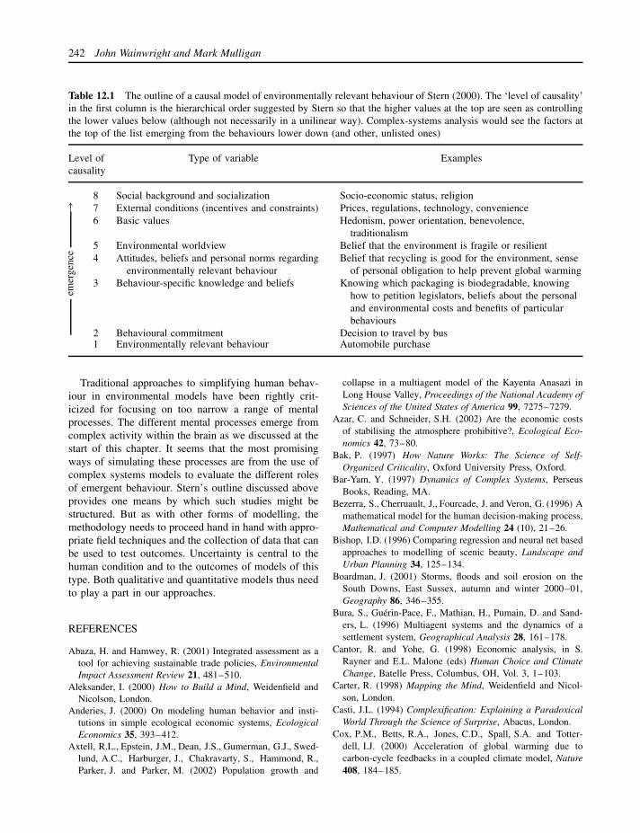
242 John Wainwright and Mark Mulligan
Table 12.1 The outline of a causal model of environmentally relevant behaviour of Stern (2000). The ‘level of causality’in the first column is the hierarchical order suggested by Stern so that the higher values at the top are seen as controllingthe lower values below (although not necessarily in a unilinear way). Complex-systems analysis would see the factors atthe top of the list emerging from the behaviours lower down (and other, unlisted ones)
Level ofcausality
Type of variable Examples
8 Social background and socialization Socio-economic status, religion7 External conditions (incentives and constraints) Prices, regulations, technology, convenience6 Basic values Hedonism, power orientation, benevolence,
traditionalism5 Environmental worldview Belief that the environment is fragile or resilient4 Attitudes, beliefs and personal norms regarding
environmentally relevant behaviourBelief that recycling is good for the environment, sense
of personal obligation to help prevent global warming3 Behaviour-specific knowledge and beliefs Knowing which packaging is biodegradable, knowing
how to petition legislators, beliefs about the personaland environmental costs and benefits of particularbehaviours
2 Behavioural commitment Decision to travel by bus
emer
genc
e→
1 Environmentally relevant behaviour Automobile purchase
Traditional approaches to simplifying human behav-iour in environmental models have been rightly crit-icized for focusing on too narrow a range of mentalprocesses. The different mental processes emerge fromcomplex activity within the brain as we discussed at thestart of this chapter. It seems that the most promisingways of simulating these processes are from the use ofcomplex systems models to evaluate the different rolesof emergent behaviour. Stern’s outline discussed aboveprovides one means by which such studies might bestructured. But as with other forms of modelling, themethodology needs to proceed hand in hand with appro-priate field techniques and the collection of data that canbe used to test outcomes. Uncertainty is central to thehuman condition and to the outcomes of models of thistype. Both qualitative and quantitative models thus needto play a part in our approaches.
REFERENCES
Abaza, H. and Hamwey, R. (2001) Integrated assessment as atool for achieving sustainable trade policies, EnvironmentalImpact Assessment Review 21, 481–510.
Aleksander, I. (2000) How to Build a Mind, Weidenfield andNicolson, London.
Anderies, J. (2000) On modeling human behavior and insti-tutions in simple ecological economic systems, EcologicalEconomics 35, 393–412.
Axtell, R.L., Epstein, J.M., Dean, J.S., Gumerman, G.J., Swed-lund, A.C., Harburger, J., Chakravarty, S., Hammond, R.,Parker, J. and Parker, M. (2002) Population growth and
collapse in a multiagent model of the Kayenta Anasazi inLong House Valley, Proceedings of the National Academy ofSciences of the United States of America 99, 7275–7279.
Azar, C. and Schneider, S.H. (2002) Are the economic costsof stabilising the atmosphere prohibitive?, Ecological Eco-nomics 42, 73–80.
Bak, P. (1997) How Nature Works: The Science of Self-Organized Criticality, Oxford University Press, Oxford.
Bar-Yam, Y. (1997) Dynamics of Complex Systems, PerseusBooks, Reading, MA.
Bezerra, S., Cherruault, J., Fourcade, J. and Veron, G. (1996) Amathematical model for the human decision-making process,Mathematical and Computer Modelling 24 (10), 21–26.
Bishop, I.D. (1996) Comparing regression and neural net basedapproaches to modelling of scenic beauty, Landscape andUrban Planning 34, 125–134.
Boardman, J. (2001) Storms, floods and soil erosion on theSouth Downs, East Sussex, autumn and winter 2000–01,Geography 86, 346–355.
Bura, S., Guerin-Pace, F., Mathian, H., Pumain, D. and Sand-ers, L. (1996) Multiagent systems and the dynamics of asettlement system, Geographical Analysis 28, 161–178.
Cantor, R. and Yohe, G. (1998) Economic analysis, in S.Rayner and E.L. Malone (eds) Human Choice and ClimateChange, Batelle Press, Columbus, OH, Vol. 3, 1–103.
Carter, R. (1998) Mapping the Mind, Weidenfield and Nicol-son, London.
Casti, J.L. (1994) Complexification: Explaining a ParadoxicalWorld Through the Science of Surprise, Abacus, London.
Cox, P.M., Betts, R.A., Jones, C.D., Spall, S.A. and Totter-dell, I.J. (2000) Acceleration of global warming due tocarbon-cycle feedbacks in a coupled climate model, Nature408, 184–185.

Modelling Human Decision-Making 243
Crevier, D. (1993) AI: The Tumultuous History of the Searchfor Artificial Intelligence, Basic Books, New York.
Crick, F. (1994) The Astonishing Hypothesis: The ScientificSearch for the Soul, Simon and Schuster, London.
Dennett, D.C. (1991) Consciousness Explained, Penguin Books,Harmondsworth.
Epstein, J.M. and Axtell, R. (1996) Growing Artificial Soci-eties: Social Science from the Bottom Up, Brookings Institu-tion Press, Washington, DC. See also http://www.brookings.edu/sugarscape/
Faber, M., Petersen, T. and Schiller, J. (2002) Homo oeco-nomicus and Homo politicus in ecological economics, Eco-logical Economics 40, 323–333.
Ferber, J. (1999) Multi-Agent Systems: An Introduction toDistributed Artificial Intelligence, Addison Wesley, Harlow.
Frankhauser, S. and Kverndokk, S. (1996) The global warminggame – simulations of a CO2-reduction agreement, Resourceand Energy Economics 18, 83–102.
Frisvold, G.B. and Caswell, M.F. (2000) Transboundary watermanagement: game-theoretic lessons for projects on theUS–Mexico border, Agricultural Economics 24, 101–111.
Gielen, D.J. and Yagita, H. (2002) The long-term impact ofGHG reduction policies on global trade: a case study forthe petrochemical industry, European Journal of OperationalResearch 139, 665–681.
Gilbert, N. and Doran, J. (eds) (1994) Simulating Societies:The Computer Simulation of Social Phenomena, UCL Press,London.
Gimblett, R., Daniel, T., Cherry, S. and Meitner, M.J. (2001)The simulation and visualization of complex human–environ-ment interactions, Landscape and Urban Planning 54,63–79.
Ginot, V., Le Page, C. and Souissi, S. (2002) A multi-agent’s architecture to enhance end-user individual-basedmodelling, Ecological Modelling 157, 23–41. See alsohttp://www.avignon.inra.fr/mobidyc
Gintis, H. (2000) Beyond Homo economicus: evidence fromexperimental economics, Ecological Economics 35, 311–322.See also http://www-unix.oit.umass.edu/∼gintis.
Grand, S. (2000) Creation: Life and How to Make It, Phoenix,London.
Green, S. and Lemon, M. (1996) Perceptual landscapes inagrarian systems: degradation processes in north-westernEpirus and the Argolid valley, Greece, Ecumene 3, 181–199.
Grenon, M. and Batisse, M. (1989) Futures for the Mediter-ranean Basin: The Blue Plan, Oxford University Press,Oxford.
Gumerman, G.J. and Kohler, T.A. (1995) Creating alternativecultural histories in the prehistoric Southwest: agent-basedmodelling in archaeology, in Proceedings of the DurangoConference on Southwest Archaeology, Durango, Co, Sept15 1995, and at http://www.santafe.edu/sfi/publications/wpabstract/199603007
Haykin, S. (1999) Neural Networks: A Comprehensive Foun-dation, 2nd edn, Prentice Hall, Upper Saddle River, NJ.
Hofstadter, D.R. (1979) Godel, Escher, Bach: An EternalGolden Braid, Penguin Books, Harmondsworth.
Hofstadter, D.R. (1981) A conversation with Einstein’s brain,in D.R. Hofstadter and D.C. Dennett (eds) The Mind’s I,Penguin Books, Harmondsworth, 430–457.
Houghton, J.T., Ding, Y., Griggs, D.J., Noguer, M., van derLinden, P.J., Dai, X., Maskell, K. and Johnson, C.A. (eds)(2001) Climate Change 2001: The Scientific Basis, Cam-bridge University Press, Cambridge.
Hooke, R. LeB. (2000) On the history of humans as geomor-phic agents, Geology 28, 843–846.
IPCC (2000) IPCC Special Report, Emissions Scenarios: Sum-mary for Policymakers, A Special Report of IPCC WorkingGroup III, IPCC Working Group III, http://www.ipcc.ch/pub/sres-e.pdf.
Jager, W., Janssen, M.A., De Vries, H.J.M., De Greef, J. andVlek, C.A.J. (2000) Behaviour in commons dilemmas:Homo economicus and Homo psychologicus in anecological-economic model, Ecological Economics 35,357–379.
Jaynes, J. (1979) The Origin of Consciousness in the Break-down of the Bicameral Mind, Houghton Mifflin, Boston.
Karjalainen, T., Pussinen, A., Liski, J., Nabuurs, G.-J.,Erhard, M., Eggers, T., Sonntag, M. and Mohren, G.M.J.(2002) An approach towards an estimate of the impact offorest management and climate change on the Europeanforest sector carbon budget: Germany as a case study,Forest Ecology and Management 162, 87–103. See alsohttp://www.efi.fi/projects/eefr/.
Kohler, T.A. and Gumerman, G.J. (eds) (2000) Dynamicsin Human and Primate Societies: Agent-Based Modellingof Social and Spatial Processes, Oxford University Press,Oxford.
Low, B., Costanza, R., Ostrom, E., Wilson, J. and Simon, C.P.(1999) Human–ecosystem interactions: a dynamic integratedmodel, Ecological Economics 31, 227–242.
Lund, H.G. and Iremonger, S. (2000) Omissions, commissions,and decisions: the need for integrated resource assessments,Forest Ecology and Management 128, 3–10.
McGlade, J. (1995) Archaeology and the ecodynamics ofhuman-modified landscapes, Antiquity 69, 113–132.
McGlade, J., Castro, P., Courty, M.-A., Fedoroff, N. andJones, M.K. (1994) The socioecology of the Vera basin:towards a dynamic reconstruction, in S.E. van der Leeuw(ed.) Understanding the Natural and Anthropogenic Causesof Soil Degradation and Desertification in the MediterraneanBasin. Volume 2: Temporalities and Desertification in theVera Basin, Final Report on Contract EV5V-CT91-0021, EU,Brussels, 297–321.
McLeod, P., Plunkett, K. and Rolls, E.T. (1998) Introductionto Connectionist Modelling of Cognitive Processes, OxfordUniversity Press, Oxford.
Mitchell, M. (1996) An Introduction to Genetic Algorithms,MIT Press, Cambridge, MA.
Mithen, S. (1996) The Prehistory of the Mind: A Search for theOrigins of Art, Religion and Science, Thames and Hudson,London.
Nathan, P.W. (1987) Nervous system, in R.L. Gregory (ed.)The Oxford Companion to the Mind, Oxford University Press,Oxford, 514–534.

244 John Wainwright and Mark Mulligan
Noble, W. and Davidson, I. (1996) Human Evolution, Lan-guage and Mind: A Psychological and ArchaeologicalEnquiry, Cambridge University Press, Cambridge.
O’Reilly, R.C. and Munakata, Y. (2000) Computational Explo-rations in Cognitive Neuroscience: Understanding the Mindby Simulating the Brain, MIT Press, Cambridge, MA.
Oreskes, N., Shrader-Frechette, K. and Bellitz, K. (1994) Veri-fication, validation and confirmation of numerical models inthe Earth Sciences, Science 263, 641–646.
O’Rourke, E. (1999) Changing identities, changing landscapes:human-land relations in transition in the Aspre, Roussillon,Ecumene 6, 29–50.
Parson and Ward, (1998) Games and simulations, in S. Raynerand E.L. Malone (eds) Human Choice and Climate Change,Batelle Press, Columbus, OH, Vol. 3, 105–139.
Penrose, R. (1989) The Emperor’s New Mind, Oxford Univer-sity Press, Oxford.
Phillips, C.P. (1998) The Crete Senesi, Tuscany: a vanishinglandscape?, Landscape and Urban Planning 41, 19–26.
Phillips, M. and Mighall, T. (2000) Society and ExploitationThrough Nature, Prentice Hall, London.
Ramachandran, V.S. and Blakeslee, S. (1998) Phantoms in theBrain: Human Nature and the Architecture of the Mind,Fourth Estate, London.
Rayner, S. and Malone, E.L. (1998) Human Choice and Cli-mate Change, Batelle Press, Columbus, OH.
Roberts, C.A., Stallman, D. and Bieri, J.A. (2002) Modelingcomplex human–environment interactions: the Grand Can-yon river trip simulator, Ecological Modelling 153, 181–196.Also at http://mathcs.holycross.edu/∼croberts/research.
Rotmans, J. and Dowlatabadi, H. (1998) Integrated assessmentmodelling, in S. Rayner and E.L. Malone (eds) Human
Choice and Climate Change, Batelle Press, Columbus, OH,Vol. 3, 291–377.
Sanders, L., Pumain, D., Mathian, H., Guerin-Pace, F. andBura, S. (1997) SIMPOP: a multiagent system for the studyof urbanism, Environment and Planning B 24, 287–305.
Searle, J.R. (1980) Minds, brains and programs, Behavioraland Brain Sciences 3, 417–424.
Siebenhuner, B. (2000) Homo sustinens: towards a new con-ception of human for the science of sustainability, EcologicalEconomics 32, 15–25.
Staller, A. and Petta, P. (2001) Introducing emotions into thecomputational study of social norms: a first evaluation,Journal of Artificial Societies and Social Simulation 4 (1),http://www.soc.surrey.ac.uk/JASSS/4/1/2.html
Stassinopoulos, D. and Bak, P. (1995) Democratic reinforce-ment: a principle for brain function, Physical Review E 51,5033–9.
Stern, P.C. (2000) Psychology and the science of human–envi-ronment interactions, American Psychologist 55, 523–530.
Thagard, P. (2000) Coherence in Thought and Action, MITPress, Cambridge, MA.
Van Veen, H.A.H.C., Distler, H.K., Braun, S.J. and Bulthoff,H.H. (1998) Navigating through a virtual city: using virtualreality technology to study human action and perception,Future Generation Computer Systems 14, 231–242.
Wainwright, J. and Thornes, J.B. (2003) Environmental Issuesin the Mediterranean: Processes and Perspectives from thePast and Present, Routledge, London.
Weisbuch, G. (2000) Environment and institutions: a complexdynamical systems approach, Ecological Economics 34,381–391.
13
Modelling Land-Use Change
ERIC F. LAMBIN
13.1 THE COMPLEXITY
13.1.1 The nature of land-use change
Land-use changes are cumulatively transforming landcover at an accelerating pace, mainly in the trop-ics (Turner et al., 1994). These changes have impor-tant implications for a range of issues such as bio-sphere–atmosphere interactions, species and geneticdiversity associated with endangered habitats, soil condi-tions, water and sediment flows, vulnerability of ecosys-tems and social groups, and sustainable use of naturalresources in the development process of human soci-eties (Meyer and Turner, 1994). It is crucial for the mod-elling of the problem to distinguish between land coverand land use. The term land cover refers to the attributesof a part of the Earth’s land surface and immediate sub-surface, including biota, soil, topography, surface andgroundwater, and human structures. The term land userefers to the purposes for which humans exploit theland cover. Common land-use types include agriculture,grazing, forestry, mineral extraction and recreation. For-est is a land cover dominated by woody species, whichmay be exploited for land uses as varied as recreation,timber production or wildlife conservation. Changesin land use are frequent causes of land-cover change.One generally distinguishes between land-cover conver-sion – i.e. the complete replacement of one cover typeby another – and land-cover modification – i.e. moresubtle changes that affect the character of the landcover without changing its overall classification (Turneret al., 1995), such as land degradation or land-useintensification. Land-cover modifications may result indegraded ecosystems. Land-cover modifications are gen-erally more prevalent than land-cover conversions.
The most widespread contemporary example of land-cover conversion is tropical deforestation. Forest degra-dation through selective logging and fires also affectslarge areas of forests. Forest conversion and degradationin the humid tropics account for a significant part of thecarbon flux from terrestrial ecosystems and contributeto a large share of the loss of biodiversity. Anothereconomically and demographically important process ofconversion is urbanization. Land degradation is mostsevere and widespread in semi-arid regions. It encom-passes processes such as soil erosion or soil salinization.Land degradation implies a decline in the usable naturalresource base and, thus, directly affects the food supply.A synthesis of the most recent global assessments ofhuman-induced land degradation estimated that 69.5%of the world’s drylands are affected by various formsof land degradation (Dregne et al., 1991). Other authorshighlight the dynamic and resilient character of temper-ate and tropical rangelands, in response to the randominterplay of human and biophysical drivers. This makesit difficult to distinguish directional change (such as lossof biological diversity or soil degradation) from read-ily reversible fluctuations, such that interpretations ofdegradation must be viewed cautiously (Lambin et al.,2001). Land-use intensification may be associated withagricultural, agroforestry or grazing systems. Intensifiedmanagement of land can be based on such techniquesas irrigation, fertilizer use or the integration of differentproduction activities (Netting, 1993).
13.1.2 Causes of land-use changes
There is a high variability in the land-cover types,the physical environments, the socio-economic activi-ties and the cultural contexts which are associated with
Environmental Modelling: Finding Simplicity in Complexity. Edited by J. Wainwright and M. Mulligan 2004 John Wiley & Sons, Ltd ISBNs: 0-471-49617-0 (HB); 0-471-49618-9 (PB)

246 Eric F. Lambin
land-use change. The driving forces of land-use changesare categorized into the following groups: (a) factorsthat affect the demands that will be placed on theland, i.e. population and affluence; (b) factors that con-trol the intensity of exploitation of the land: throughtechnology; (c) factors that are related to access to orcontrol over land resources: the political economy; and(d) factors that create the incentives that motivate indi-vidual decision-makers: the political structure, attitudesand values (Turner et al., 1995). Identifying the causesof land-use change requires an understanding of howthese different factors interact in specific environmen-tal, historical and social contexts to produce differentuses of the land (ibid.).
For example, deforestation results from slash-and-burn cultivation, both by landless migrants and bytraditional shifting cultivators, government-sponsoredresettlement schemes, fuelwood gathering and char-coal production, the conversion of forested areas forcattle ranching, inefficient commercial logging opera-tions, the provision of infrastructure, and large-scale,uncontrolled forest fires of an exceptional nature.The proximate causes of deforestation are generallythought to be driven by a combination of someof the following underlying driving forces: popula-tion growth, land hunger, inequitable social conditions,property-rights regimes, misguided government policies,collective action problems, inappropriate technology,international trade relations, economic pressures afflict-ing debt-burdened developing countries and corruptionin the forestry sector (e.g. Myers, 1989; Lambin, 1994;Kaimowitz and Angelsen, 1998). The relative impor-tance of these causes varies widely in space and time.
The synthesis of extensive, local, case-study evidenceon processes of land-use change supports the conclu-sion that neither population nor poverty are the primarycauses of land-use change worldwide. Rather, people’sresponses to economic opportunities, as mediated byinstitutional factors, drive land-use changes. Opportu-nities and constraints for new land uses are created bymarkets and policies, increasingly influenced by globalfactors. Extreme biophysical events occasionally trig-ger further changes. Various human–environment con-ditions react to and reshape the impacts of driversdifferently, leading to specific pathways of land-usechange (Lambin et al., 2001). The dependency of causesof land-use changes on historical, geographic and otherfactors makes it a particularly complex issue to model.
13.2 FINDING THE SIMPLICITY
The modelling of land-use change is aimed at addressingat least one of the following questions:
1. Which socio-economic and biophysical variablescontribute most to an explanation of land-use changesand why?
2. Which locations are affected by land-use changes –where?
3. At what rate do land-use and land-cover changeprogress – when?
Four broad categories of land-use change modelsaddress some of these questions: empirical-statisticalmodels, stochastic models, optimization models anddynamic (process-based) simulation models (Lambinet al., 2000). All these model designs attempt to rep-resent the complex land-use change pathways based ongeneral rules, which often involve a great deal of sim-plification. Land-use change models offer the possibilityto test the sensitivity of land-use patterns to changes inselected variables. They also allow testing of the sta-bility of linked social and ecological systems throughscenario building. While, by definition, any model fallsshort of incorporating all aspects of reality, it providesvaluable information on the system’s behaviour under arange of conditions (Veldkamp and Lambin, 2001).
13.2.1 Empirical-statistical models
Empirical-statistical models attempt to identify explic-itly the causes of land-use changes using multivariateanalyses of possible exogenous contributions to empiri-cally derived rates of changes. Multiple linear regressiontechniques are generally used for this purpose. The find-ing of a statistically significant association does notestablish a causal relationship. Moreover, a regressionmodel that fits well in the region of the variable spacecorresponding to the original data can perform poorlyoutside that region. Thus, regression models cannot beused for wide-ranging extrapolations. Such models areonly able to explain, in a statistical sense, patterns ofland-use changes which are represented in the calibra-tion data set.
Regression models are intrinsically not spatial. Theyare based on the unrealistic assumption that land-usechange in an administrative unit is primarily a functionof factors originating within that unit, i.e. that cross-boundary effects are minor. However, multi-level regres-sion techniques overcome such limitations (Polsky andEasterling, 2001). In summary, regression models aremainly an exploratory tool to test for the existenceof links between candidate driving forces and land-usechange. Such models therefore contribute to address thewhy question. They are not reliable for prediction andare not spatial.
Modelling Land-Use Change 247
Spatial, statistical models are born from the com-bination of geographic information systems (GIS) andmultivariate statistical models. Their emphasis is onthe spatial distribution of landscape elements and onchanges in land-use patterns. The goal of these modelsis the projection and display, in a cartographic form,of future land-use patterns which would result from thecontinuation of current land management practices orthe lack thereof. The approach analyses the location ofland-use changes in relation to maps of natural and cul-tural landscape variables in a GIS (Chomitz and Gray,1996; Mertens and Lambin, 2000). A model is built todescribe the relationship between the dependent vari-able, e.g. the binary variable forested/deforested, andthe independent landscape variables. Results of spa-tial, statistical models demonstrate that a few landscapevariables from the previous time period provide strongpredictions of patterns of land-use change. Predictingthe spatial pattern of land-use change is thus a mucheasier task than predicting future rates of change. Spa-tial, statistical models primarily identify predictors ofthe location of areas with the greatest propensity forland-use changes. They are not suited to the predictionof when land-use change will occur and only touch onproximate causes of change processes.
An example of an advanced statistical land-usechange model is CLUE (Conversion of Land Use andits Effects). Veldkamp and Fresco (1996) developed aregression-based model to simulate land-use conversionsas a result of interacting biophysical and human drivers.A broad spectrum of proxy variables for driving forcesare incorporated. A land-use allocation module was alsodeveloped, to generate spatially explicit land-use changeprojections. This model has been applied at a nationalscale in several Latin American and Asian countries.
13.2.2 Stochastic models
Stochastic models, for land-use change, consist mainlyof transition probability models such as Markov chains,stochastically describe processes that move in a sequenceof steps through a set of states. For land-use change,the states of the system are defined as the amount ofland covered by various types of land use. The transi-tion probabilities can be statistically estimated from asample of transitions occurring during some time inter-val. Probabilities of transitions are defined for changesfrom one land-use category to another. Transition prob-ability models generally assume that land-use changeis a first-order process, that is the conditional proba-bility of land use at any time, given all previous usesat earlier times, depends at most upon the most recent
use and not upon any earlier ones (Bell and Hino-josa, 1977). Such models also rely on the assumptionof the stationarity of the transition matrix, i.e. tempo-ral homogeneity. Dynamic transition probabilities canbe introduced by switching between stationary transi-tion matrices at certain intervals or by modelling thecontribution of exogenous or endogenous variables tothe transitions (Baker, 1989). Transition probabilitiesbetween certain land-use categories could also be drivenby ecological or socio-economic submodels, leading toprocess-based models (Sklar and Costanza, 1991). Spa-tial adjacency influences can also be taken into accountin such models (Turner, 1987).
Simple, first-order transition probability models havebeen applied to model processes of changes in vegeta-tion types and land use (e.g. Burnham, 1973; Robinson,1978). However, there are few applications of Markovchain at spatial scales near or broader than the landscapescale. Thornton and Jones (1998) recently presented aconceptual model of agricultural land-use dynamics,based on Markov chains governed by a few simple deci-sion rules. This model could be applied to assess thepotential ecological impact of technological and eco-nomic change on agricultural land use, which could beof value in a range of impact assessment studies (Thorn-ton and Jones, 1998: 519).
The main advantage of Markov chain analysis liesin its mathematical and operational simplicity. The onlydata requirement is for current land-use information. Thestochastic nature of Markov chain masks the causativevariables. Thus, the model has little explanatory power.Finally, an area is described in aggregate terms – itis a distributional (as opposed to a spatial) landscapemodel (Baker, 1989). In summary, transition probabilitymodels can only predict when changes in land use mighttake place in the short term, under a strict assumptionof stationarity of the process. Such models can beused where no information on the driving forces andmechanisms of land-use changes is available.
Some other forms of stochastic models, such asspatial diffusion models, do appear to be useful inresearch on land-use change. Cellular automata are alsoincreasingly used in land-use change models (Whiteet al., 1997; Wu, 1998).
13.2.3 Optimization models
In economics, many models of land-use change applyoptimization techniques based either on whole-farmanalyses using linear programming, at the micro-economic level, or general equilibrium models, at themacro-economic scale (Kaimowitz and Angelsen, 1998).

248 Eric F. Lambin
Many of these approaches originate in the land rent the-ories of von Thunen (1966) and Ricardo. Any parcel ofland, given its attributes and its location, is modelledas being used in the way that yields the highest rent.Land-use change is therefore an issue of choices by landmanagers among alternate rents. Land conservation isan issue of investment decisions by land managers bycomparing discounted benefits and costs. In econometricapproaches, the supply and demand functions of the landmarket under investigation (assumed to be a competitivemarket) are estimated. Such models allow investigationof the influence of various policy measures on land allo-cation choices. However, models of urban and periurbanland allocation appear to be much more developed thantheir rural counterparts (Riebsame et al., 1994).
A major strength of micro-economic models com-pared to the other model designs reviewed here is thatthey usually assume that the agents whose behaviouris described within the model do have the capacity tomake informed predictions and plans, so as to try toavoid disasters (Fischer et al., 1996). The applicabilityof such models for projections is, however, limited dueto unpredictable fluctuations of prices and demand fac-tors, and to the role of noneconomic factors drivingchanges. For example, in the case of deforestation, itis not unusual that loggers, through their links withgovernment officials, decide upon the economic andinstitutional context in which they operate. This leadsto low and fixed timber prices, lack of competition andweak mechanisms to regulate access to resources. Giventhis inherent unpredictability of socio-economic drivingforces of land-use changes, economic models usuallyadopt a normative approach.
The agricultural land rent theory of von Thunen(1966) explains optimal crop-production allocation fol-lowing degrees of agricultural intensity. A limited num-ber of variables used in the basic, mainly static anddeterministic, model of agricultural systems explainsintensity as depending on the achievable economic rent.This rent is determined by market demands in the con-sumer centre, transportation costs, production costs anddegrees of perishability of goods produced for the cen-tral market. Price expectations and interest rates havealso been shown to be important factors. Thus, thesemodels link agricultural intensity, population density,the actual transportation network and the market econ-omy (Jones and O’Neill, 1993, 1994).
Several partial or general equilibrium models of landuse have been developed to describe the trade-offsbetween land clearance for agriculture and resource con-servation and maintenance (Walker, 1987; Southgate,1990; Jones and O’Neill, 1992). The work of Jones
and O’Neill is particularly relevant since it modelsprofit maximization decisions at the individual levelbut examines region-wide environmental outcomes. Sev-eral of these models highlight, in addition to popu-lation pressure, the institutional problems of skewedtenurial regimes and misdirected government policies(e.g. Sandler, 1993).
Optimization models suffer from other limitations,such as the somewhat arbitrary definition of objec-tive functions and non-‘optimal’ behaviour of people,e.g. due to differences in values, attitudes and cultures.While, at an aggregate level, these limitations are likelyto be nonsignificant, they are more important as onelooks at fine-scale land-use change processes and isinterested in the diversity between actors. A new gen-eration of agent-based models simulate decisions byand competition between multiple actors and land man-agers (e.g. Walker, 1999; Rouchier et al., 2001). Land-use change models recently developed by economistsintegrate spatial heterogeneity and broaden the objectivefunction of actors from profit to utility maximization,including multiple uses of land (Irwin and Geoghegan,2001). Behavioural models of land-use decisions byagents can be made spatially explicit thanks to cellu-lar automata techniques. This approach accounts for thefact that landscape patterns and spatial interactions doinfluence land use decisions.
13.2.4 Dynamic (process-based) simulation models
Patterns of land-use changes in time and space areproduced by the interaction of biophysical and socio-economic processes. Dynamic (process-based) simula-tion models have been developed to imitate the run ofthese processes and follow their evolution. Simulationmodels emphasize the interactions among all compo-nents forming a system. They condense and aggregatecomplex ecosystems into a small number of differen-tial equations in a stylized manner. Simulation modelsare therefore based on an a priori understanding of theforces driving changes in a system. Integrated Assess-ment Models, e.g. IMAGE (Alcamo et al., 1998), seekto integrate a wide range of sectors and process descrip-tions and usually operate at global scales. IntegratedAssessment Models are seldom able to model the man-agement and decision-making processes of individuals.This stems from their requirement to operate at globalscales which often results in simplistic treatment of land-use change processes.
White et al. (1997) demonstrated the use of a land-usechange model that combined a stochastic, cellularautomata approach with dynamic systems models of

Modelling Land-Use Change 249
regional economics. The approach allows spatiallyexplicit geographic processes to be constrained by lessspatially precise economic processes within the frame-work of a Geographic Information System (GIS). Theapproach has been used as a decision-support sys-tem (see Chapters 14 and 15), by allowing regionalland-use planners to investigate the consequences ofalternative management strategies. The combination ofdynamic, process-based models with optimization tech-niques underpinned the development of the IMPELmodel (Integrated Model to Predict European LandUse) (Rounsevell et al., 1998). The requirement forIMPEL was to be able to assess modifications to thespatial distribution of agricultural land use in responseto climate change.
Land-use change models that rely on a populationapproach and assume subsistence behaviour and limitedmarket integration are rooted in the models of Boserup(1965) and Chayanov (1966). These models relate agri-cultural intensification to household needs, accordingto which households balance consumption and leisureand/or follow a subsistence strategy. Other simula-tion models integrate demands from the market. Forexample, in a numerical simulation model, Angelsen(1999) considers land-use intensity as one of 12 vari-ables besides exogenously given prices and a newlyintroduced labour market, in that any amount of labourcan be sold or hired with migrational flows in and out ofthe local economy. Within market-based theorizing, thedominant views used to be based on a purely market orcommodity approach. This postulates that farmers acceptcommodity production and respond to market demandswithin constraints placed upon them by maximizing pro-duction to the level of maximum reward.
The strength of a simulation model depends onwhether the major features affecting land-use changesare integrated, whether the functional relationshipsbetween factors affecting processes of change are appro-priately represented, and on the capacity of the modelto predict the most important ecological and economicimpacts of land-use changes. The development of simu-lation models requires a priori knowledge of the factorsand mechanisms driving land-use change. The modelsimply formalizes and articulates in a comprehensivemanner the key relationships. Process-based ecosystemmodels are well suited to representing nonstationary pro-cesses since they mimic (at least in an aggregated way)the underlying processes in the system and include feed-backs and thresholds in the systems dynamics. Simula-tion models allow rapid exploration of probable effectsof the continuation of current land-use practices or of
changes in cultural or ecological parameters. These mod-els allow testing of scenarios on future land-use changes.
When dynamic ecosystem-simulation models are spa-tially explicit (i.e. include the spatial heterogeneity oflandscapes), they can predict temporal changes in spa-tial patterns of land use. In system landscape mod-els, the course of every individual parcel of a land-scape matrix is predicted by a process-based modelintegrating flows between adjacent cells. The transi-tion probabilities are generated dynamically rather thanempirically. This approach allows for greater cyclicchanges between land uses and longer-term predictionof landscape patterns (Sklar and Costanza, 1991). Ithas been successfully applied in environments drivenby physical factors (Sklar et al., 1985) but is difficultto translate to land-use patterns due to the need toincorporate the economic or social mechanisms drivingland-use transitions (Turner, 1987). While many indi-vidual processes of decision-making cannot be mod-elled deterministically, it is possible to identify themain determinants of decisions on when and where tochange land use. A few dynamic spatial simulations,using actor-based models, have been developed to date,e.g. for tropical deforestation in roadside areas occu-pied by shifting cultivators (Wilkie and Finn, 1988),in regions of official resettlement schemes associatedwith road development (Southworth et al., 1991) or inareas dominated by shifting cultivation (Gilruth, 1995).These grid-cell models combine spatially explicit eco-logical information with socio-economic factors relatedto land-use decisions by farmers. The modelling isbased on rules of behaviour determined by locationalattributes, land-tenure systems and vegetation succes-sions (see Chapter 12).
Dynamic landscape-simulation models are not purepredictive systems, even though projections of futuretrends in land-use change as a function of current landuse practices can be performed. They are rather ‘game-playing tools’ designed to understand the ecologicalimpacts of changes in land use. The dynamic land-scape simulation models developed to date are specificto narrow geographic situations and cannot easily begeneralized. These models allow the testing of scenarioson changes in land-use patterns.
13.3 THE RESEARCH FRONTIER
Some of the major research challenges to improve themodelling of land-use change include better integrat-ing the scale factor in models, representing processesof land-use modification such as agricultural intensi-fication, and dealing with temporal heterogeneity, e.g.
250 Eric F. Lambin
as driven by endogenous factors such as technologi-cal innovation.
13.3.1 Addressing the scale issue
The scale at which land-use changes are modelled affectsthe type of explanation given to land-use change. Atbroad scales, the high level of aggregation of dataobscures the variability of situations and relationships,and produces sometimes meaningless averages. Predic-tions based on broad-scale models are inaccurate, espe-cially for regional and local assessments, because, atthe aggregate level, key processes are masked (Turneret al., 1995). On the other hand, the development offine-scale models for every local situation would beboth impractical and inadequate if there is no possi-bility of generalizing these models. Moreover, in scal-ing up several local processes and dynamics, emergentproperties may appear due to synergism at a higherlevel of system integration, i.e. at a regional scale.Thus, regional-scale processes are more than the sumof local-scale processes.
A hierarchical approach needs therefore to be adoptedin both the observation and explanation of land-usechange processes. Blaikie and Brookfield (1987) suggestusing a nested set of four scales to explain landdegradation:
Local and site specific where individuals or smallgroups make the relevant decisions; the regional scaleinvolving more generalised patterns of physiographicvariation, types of land use, and property relations andsettlement history; the national scale in which the par-ticular form of class relations give the economic, polit-ical and administrative context for land-managementdecisions; and the international scale, which, in themost general manner, involves almost every element inthe world economy, particularly through the commod-ization of land, labour and agricultural production.
Models of land-use change should thus be based on ananalysis of the system at various spatial and temporalscales. Yet, most existing regional-scale models addressneither structural nor functional complexity. Models thatopt to incorporate and link a larger number of factors fora spatially heterogenous area (e.g. integrated assessmentmodels) severely simplify the land-use system. Incorpo-rating structural complexity becomes necessary at thecoarser scales (Veldkamp and Lambin, 2001). Actually,at local scales, the direct actors of land-use changecan be identified and process-based relationships can bedetermined. With decreasing resolution and increasing
extent, it becomes increasingly difficult to identify keyprocesses. Thus, at these aggregated levels, the structureand assumptions of the model have to be adapted, as onecannot simply use knowledge derived from local studiesand apply it at another level.
13.3.2 Modelling land-use intensification
While future food supplies will have to come mostlyfrom agricultural intensification rather than from agri-cultural expansion, most modelling efforts in land-usechange have been concerned with issues of land-use con-version rather than land-use modification. Note, how-ever, that economists have a long tradition of study-ing agricultural intensification in relation to manage-ment practices and conditions (e.g., prices of inputs,production functions). Several studies reveal the driv-ing factors (e.g. price differentials, tenure conditions,family cycle conditions, etc.) that cause managementto change. Different modelling approaches are moreor less appropriate in tackling the question of inten-sification at different locations. In general, however,dynamic simulation models are better suited to predictchanges in land-use intensity than empirical, stochasticor static optimization models, although some stochasticand optimization methods may be useful in describ-ing the decision-making processes that drive land man-agement (Lambin et al., 2000). The ability to predictchanges in land-use intensity requires models of the pro-cess of decision-making by land managers.
13.3.3 Integrating temporal heterogeneity
Many land-use patterns have developed in the con-text of long-term instability, including nonlinear pro-cesses in the biophysical variables (climate, disease)and in the political economic forces (market dynam-ics, price fluctuations, state policy influences). Decision-making by individuals and communities has thereforeto manage variable time horizons, in particular thosethat link the short-term management of growing sea-sons and cycles of consumer needs, the mid-term expe-rience of year-to-year fluctuations (in rainfall, prices,policies), random ‘chaotic’ events (war, policy interven-tions) and the long-term horizons implied in sustainablesocial and ecological systems. Land-use models shouldtherefore be built on the assumption of temporal het-erogeneity rather than on the common assumptionof progressive, linear trends (e.g. established modelsof progressive intensification of material resources).In other words, rapidly and unpredictably changing

Modelling Land-Use Change 251
variables are as important in shaping land-use dynam-ics as the slowly and cumulatively changing variables.For example, technological innovations are one of themajor sources of temporal heterogeneity. Given theimportant role of technology and management prac-tices in driving land-use change, incorporating thesefactors into prognostic models of land-use change is amajor challenge.
13.4 CASE STUDY
N. Stephenne and E.F. LambinThe following case study illustrates some of the issuesdiscussed above. It introduces a dynamic simulationmodel of rural land use in semi-arid Africa, to generateregional-scale projections over several decades, mostlyfor climate modelling applications.
13.4.1 The problem
To investigate the impact of land surface changes onregional climate, authors generally conduct experimentswith General Circulation Models (GCM) at a coarsespatial resolution (e.g. Chase et al., 1996). These stud-ies require historical reconstructions of past land-coverchanges and/or projections of likely future land-coverchanges. While, at a local scale, part of these histori-cal data can be generated from direct or indirect fieldevidence (e.g. old vegetation maps, aerial photographs,high temporal resolution pollen studies), at a regionalscale, the reconstruction of past land-cover changes hasto rely on backward projections using land-use changemodels. The SALU model (SAhelian Land Use model)(Stephenne and Lambin, 2001a) is a dynamic simulationmodel which was constructed to reconstruct past land-use and land-cover changes in the African Sahel over thepast 30 years, and to develop scenarios of likely futurechanges. Spatial resolution is an important issue in theintegration of land-use change projections in Global Cli-matic Models (GCM). The land-use change model gen-erates projections of land-use areas for administrativeunits, e.g. countries or provinces. To be integrated in aGCM, these land-use projections need to be mapped at agrid-scale level, which roughly corresponds to the size ofa small Sahelian country or of an eco-climatic region ofa larger country. Below, we summarize the basic princi-ples of the SALU model. A more detailed presentation ofthe model is given in Stephenne and Lambin (2001a) andat http://www.geo.ucl.ac.be/Recherche/Teledetection/projects.html.
13.4.2 Model structure
In the Sudano-Sahelian region, we assume that thefollowing land uses generate the basic resources for thepopulation: fuelwood in natural vegetation areas, foodfor subsistence and market needs in cropland and fallow,livestock in pastoral land. Note that these land-usecategories do not strictly coincide with land-cover types.In this model, the land-use classes ‘fuelwood extractionareas’ and ‘pastoral lands’ refer to a variety of vegetationcover types such as woodland, savannah or steppe. Theexogenous variables drive yearly changes in land-useallocation. For any given year, the land-use demand iscalculated under the assumption that there should be anequilibrium between the production and consumptionof resources. In other words, the supply of food andenergy resources derived from the areas allocated tothe different land uses must satisfy the demand forthese resources by the human and animal populations,given the exploitation technologies used at a given time.Fuelwood extraction areas, cropland, fallow and pastoralland compete for land through different processes ofland-use change (Figure 13.1).
The competition between the different land uses takesplace within the national space, which is finite. Thetotal demand for land in a given year is the sum ofdemands for cropland and pastoral land. We assumethat the fuelwood extraction area can be reduced onan annual basis by the expansion of cropland andpastoral land. Initially, all unused land is covered bynatural vegetation. In the pastoral land, the equilibriumassumption requires that the consumption of forage isequal to the biomass production. As, in the Sahel,pastoralism is extensive, biomass production relies onthe natural productivity of grasslands.
In the cultivated land, we distinguish between sub-sistence food crops and cash crops. The demand forsubsistence food crops depends on the rural popula-tion and its basic consumption requirements. The cropswhich are commercialized consist mainly of food cropsfor the urban population, but may include some cashcrops (e.g. cotton). This part of the production competeswith cereal imports which are only directed toward theconsumption of the urban population. In the above def-initions, the cropland area includes fallow. At the mostextensive level of cultivation, corresponding to a pre-intensification stage, the crop–fallow cycle is assumedto be two years of fallow for one year of cultiva-tion (Ruthenberg, 1980).
The model simulates two processes of land-usechange: agricultural expansion at the most extensivetechnological level, followed by agricultural intensifi-cation once some land threshold is reached. Expansion

252 Eric F. Lambin
Ruralpopulation
Urbanpopulation
Livestock Rainfall
ForageMarketcrops
FuelwoodSubsistence
crops
Pastoral landCompetition between
land uses Cropland Fuelwood extraction area
National area
Cerealsimports
Regression of pasture + intensificationof farming‘Deforestation’
Pastoral and cultivated areas
Regression ofunused area
Pastoral andcultivated
Alternative energycost
Fuelwood extractionarea/population
threshold: fuelwooddemand unsatisfied
Labourproductivity
Level ofwell-being =incomes −
agric. inputs
Land degradation
Fallow area induces labourand agricultural investments
Overgrazing
Pastoralarea
Population or rainfall
Agricultural expansion Agricultural intensification
Legend :
Land-use changeprocesses
Exogenous variables
Endogenous variables
Pressure indicatorsAll land is used
Rainfall
Creation ofunused area
Figure 13.1 Overall structure of the SALU model
of cropland and pastoral land is driven by two setsof factors: changes in human and animal population,which increase the consumption demand for food cropsand forage, and interannual variability in rainfall, whichmodifies land productivity and therefore increases ordecreases production for a given area under a pastoralor cultivation use. Expansion of cultivation can takeplace into previously uncultivated areas or by migrationinto unsettled areas. Agricultural expansion thus leadsto deforestation or to a regression of pastoral land. Pas-toral land can also expand into natural vegetation areasand cropland. Expansion of cropland and pastoral landin temporarily unused land is associated with a lowerenvironmental cost than in the case of deforestation.The unused land will only become reforested if it is leftunused for a period of at least 20 years. Moreover, notall natural vegetation areas can be destroyed. We assumethat the local population will always protect a certainfuelwood extraction area: a minimum area to satisfysome of the fuelwood requirements for domestic con-sumption, forest reserves, national parks, sacred forests,inaccessible forests or forests with a high incidence oftse-tse flies or onchocerciasis. If fuelwood needs exceedthe wood production through natural regrowth of veg-etation, we assume that rural households will turn toother energy sources such as kerosene. Actually, one
generally observes a sustainable use of natural vegeta-tion resources in the Sahel, except in peri-urban areas.
Once the expansion of cropland and pastoral land hasoccupied all unused land, and once fuelwood extractionareas have reached their minimal area, the land is satu-rated and another phase of land-use change takes place.Additional demand for food crops will result mainlyin agricultural intensification but also, in a lesser way,in expansion of cultivation in pastoral land. In Sahe-lian agriculture, intensification mostly takes place asa shortening of the fallow cycle, compensated by theuse of labour and agricultural inputs such as organic ormineral fertilizers to maintain soil fertility. Agriculturalintensification leads to a decrease in labour productivityand requires the use of organic or chemical inputs. Ashortening of the crop–fallow cycle without input usewould deplete soil fertility. As the economic value ofthe output per unit of area of cultivated fields is muchhigher than the value of the output per unit of area ofpastoral land in an extensive system, thus, part of theadditional demand for food crops will also lead to theexpansion of cultivation in pastoral land. The increasein livestock population combined with shrinking pas-toral lands (due to agricultural expansion) will resultin overgrazing, which will affect the productivity ofpastoral land. See Stephenne and Lambin (2001a) formore detailed results.

Modelling Land-Use Change 253
The model was first tested at a national scale usingdata from Burkina Faso, over the period 1960–97. Therates of change in cropland predicted by the modelsimulations for Burkina Faso were similar to ratesmeasured for local-scale case studies by remote sens-ing (Stephenne and Lambin, 2001a). The application ofthe model to five other countries (Senegal, Mali, Niger,Chad and Nigeria) also demonstrated the robustnessof the approach (Stephenne and Lambin, 2001b). ForChad and Mali, land-use projections were disaggregatedper eco-climatic zone (e.g. mostly pastoral Sahelianzone versus Sudanian zone dominated by farming). Theregional-scale projections generated by the model werecompared to the IGBP-DISCover land-cover map of1992/93, produced from 1-km resolution remote sensingdata. A very good agreement between the two sourceswas found. The model was then used to test hypothe-ses on driving forces of land-use change via scenar-ios (Stephenne and Lambin, 2002). Results from thesesimulations were consistent with the expertise knowl-edge on the processes of land-use change derived fromlocal-scale case studies in the region. This convergencesuggested that the major processes of land-use change inthe region were well represented in the model. The sce-nario simulations performed with SALU provided usefulinsights to better understand the processes of land-usechanges in the Sudano-Sahelian countries.
REFERENCES
Alcamo, J., Leemans, R. and Kreileman, E. (1998) GlobalChange Scenarios of the 21st Century, Pergamon, Oxford.
Angelsen, A. (1999) Agricultural expansion and deforestation:modelling the impact of population, market forces andproperty rights, Journal of Development Economics 58 (1),185–218.
Baker, W.L. (1989) A review of models of landscape change,Landscape Ecology 2, 111–133.
Bell, E.J. and Hinojosa, R.C. (1977) Markov analysis of landuse change: continuous time and stationary processes, Socio-Economic Planning Science 11, 13–17.
Blaikie, P. and Brookfield, H.C. (1987) Land Degradation andSociety, Methuen, London.
Boserup, E. (1965) The Condition of Agricultural Growth,Allen and Unwin, London.
Burnham, B.O. (1973) Markov intertemporal land use simu-lation model, Southern Journal of Agricultural EconomicsJuly, 253–258.
Chase, T.N., Pielke, R.A., Kittel, T.G.F., Nemani, R. and Run-ning, S.W. (1996) The sensitivity of a general circulationmodel to global changes in leaf area index, Journal of Geo-physical Research 101, 7393–7408.
Chayanov, A.V. (1966) Peasant farm organization, in D. Thor-ner, B. Kerblay and R.E.F. Smith (eds) A.V. Chayanov on theTheory of Peasant Economy, Irwin, Homewood, IL, 21–57.
Chomitz, K.M. and Gray, D.A. (1996) Roads, Land, Marketsand Deforestation: A Spatial Model of Land Use in Belize,Report from the Environment, Infrastructure, and Agricul-tural Division, Policy Research Department, World BankEconomic Review, Washington, DC.
Dregne, H., Kassas, M. and Rozanov, B. (1991) A new assess-ment of the world status of desertification, DesertificationControl Bulletin 20, 6–19.
Gilruth, P.T., Marsh, S.E. and Itami, R. (1995) A dynamicspatial model of shifting cultivation in the highlands ofGuinea, West Africa, Ecological Modelling 79, 179–197.
Fischer, G., Ermoliev, Y., Keyzer, M.A. and Rosenzweig, C.(1996) Simulating the socio-economic and biogeophysicaldriving forces of land-use and land-cover change: theIIASA land-use change model, Working Paper WP-96-010, International Institute for Applied Systems Analysis,Luxenbourg.
Irwin, E.G. and Geoghegan, J. (2001) Theory, data, methods:developing spatially explicit economic models of land usechange, Agriculture, Ecosystems and Environment 85, 7–24.
Jones, D.W. and O’Neill, R.V. (1992) Endogeneous environ-mental degradation and land conservation: agricultural landuse in a large region, Ecological Economics 6, 79–101.
Jones, D.W. and O’Neill, R.V. (1993) Human–environmentalinfluences and interactions in agriculture, in T.R. Laksh-manan and P.N. Nijkamp (eds) Structure and Change in theSpace Economy, Springer, Berlin, 297–309.
Jones, D.W. and O’Neill, R.V. (1994) Development policies,rural land use, and tropical deforestation, Regional Scienceand Urban Economics 24 (6), 753–771.
Kaimowitz, D. and Angelsen, A. (1998) Economic Models ofTropical Deforestation: A Review, Centre for InternationalForestry Research, Jakarta.
Lambin, E.F. (1994) Modelling deforestation processes: areview, TREES Publications Series B: Research Report 1,EUR 15744 EN, European Commission, Luxembourg.
Lambin, E.F., Rounsevell, M. and Geist, H. (2000) Are currentagricultural land use models able to predict changes in landuse intensity? Agriculture, Ecosystems and Environment 82,321–331.
Lambin, E.F., Turner II, B.L., Geist, H., Agbola, S., Angel-sen, A., Bruce, J.W., Coomes, O., Dirzo, R., Fischer, G.,Folke, C., George, P.S., Homewood, K., Imbernon, J., Lee-mans, R., Li, X., Moran, E.F., Mortimore, M., Ramakrish-nan, P.S., Richards, J.F., Skanes, H., Steffen, W., Stone,G.D., Svedin, U., Veldkamp, T., Vogel, C. and Xu, J. (2001)The causes of land-use and land-cover change: movingbeyond the myths, Global Environmental Change 11, 5–13.
Mertens, B. and Lambin, E.F. (2000) Land-cover trajectories inSouthern Cameroon, Annals of the Association of AmericanGeographers 90 (3), 467–494.
Meyer, W.B. and Turner II, B.L. (1994) Changes in LandUse and Land Cover: A Global Perspective, CambridgeUniversity Press, Cambridge.
Myers, N. (1989) Tropical Deforestation: Rates and Causes,Friends of the Earth, London.

254 Eric F. Lambin
Netting, R.McC. (1993) Smallholders, Householders: FarmFamilies and the Ecology of Intensive, Sustainable Agricul-ture, Stanford University Press, Stanford, CA.
Polsky, C. and Easterling, W.E. (2001) Adaptation to climatevariability and change in the US Great Plains: a multi-scale analysis of Ricardian climate sensitivities, Agriculture,Ecosystems and Environment 85, 133–144.
Riebsame, W.E., Meyer, W.B. and Turner, B.L. (1994) Mod-eling land-use and cover as part of global environmentalchange, Climatic Change 28 (1/2), 45–64.
Robinson, V.B. (1978) Information theory and sequencesof land use: an application, Professional Geographer 30,174–179.
Rouchier, J., Bousquet, F., Requier-Desjardins, M. andAntona, M. (2001) A multi-agent model for describingtranshumance in North Cameroon: comparison of differentrationality to develop a routine, Journal of EconomicDynamics Control 25, 527–559.
Rounsevell, M.D.A., Evans, S.P., Mayr, T.R. and Audsley, E.(1998) Integrating biophysical and socio-economic modelsfor land use studies, Proceedings of the ITC & ISSS Confer-ence on Geo-information for Sustainable Land Management,Enschede, 17–21 August (1997).
Ruthenberg, H. (1980) Farming Systems in the Tropics, Claren-don Press, Oxford.
Sandler, T. (1993) Tropical deforestation: markets and marketfailures, Land Economics 69, 225–233.
Sklar, F.H. and Costanza, R. (1991) The development ofdynamic spatial models for landscape ecology: a reviewand prognosis, in M.G. Turner and R.H. Gardner (eds)Quantitative Methods in Landscape Ecology, EcologicalStudies Vol. 82, Springer-Verlag, New York, 239–288.
Sklar, F.H., Costanza, R. and Day, J.W. (1985) Dynamic spa-tial simulation modeling of coastal wetland habitat succes-sion, Ecological Modelling 29, 261–281.
Southgate, D. (1990) The causes of land degradation along‘spontaneously’ expanding agricultural frontiers in the ThirdWorld, Land Economics 66, 93–101.
Southworth, F., Dale, V.H. and O’Neill, R.V. (1991) Contrast-ing patterns of land use in Rondonia, Brazil: simulating theeffects on carbon release, International Social Science Jour-nal 130, 681–698.
Stephenne, N. and Lambin, E.F. (2001a) A dynamic simulationmodel of land-use changes in the African Sahel (SALU),Agriculture, Ecosystems and Environment 85, 145–162.
Stephenne, N. and Lambin, E.F. (2001b) Backward land-coverchange projections for the Sudano-Sahelian countries of
Africa with a dynamic simulation model of land-use change(SALU), in T. Matsuno and H. Kida (eds) Present andFuture of Modeling Global Environmental Change: TowardsIntegrated Modeling, Terra Scientific Publishing Company,Tokyo, 255–270.
Stephenne, N. and Lambin, E.F. (2002) Scenarios of land-usechange in Sudano-Sahelian countries of Africa: understand-ing the driving forces of environmental change, Geojournal.
Thornton, P.K. and Jones, P.G. (1998) A conceptual approachto dynamic agricultural land-use modelling, AgriculturalSystems 57 (4), 505–521.
Turner II, B.L., Meyer, W.B. and Skole, D.L. (1994) Globalland-use/land-cover change: towards an integrated study,Ambio 23, 91–95.
Turner II, B.L., Skole, D.L., Sanderson, S., Fischer, G., Fres-co, L. and Leemans, R. (1995), Land-Use and Land-CoverChange: Science/Research Plan, IGBP Report 35, HDPReport 7, The Royal Swedish Academy of Sciences, Stock-holm.
Turner, M.G. (1987) Spatial simulation of landscape changes inGeorgia: a comparison of three transition models, LandscapeEcology 1, 29–36.
Veldkamp, A. and Fresco, L.O. (1996) CLUE: a conceptualmodel to study the conversion of land use and its effects,Ecological Modelling 85, 253–270.
Veldkamp, T. and Lambin, E.F. (2001) Predicting land-usechange, Special issue, Agriculture, Ecosystems and Environ-ment 85, 1–6.
van Thunen, J.H. (1966) Der isolierte Staat in Beziehung aufLandwirtschaft und Nationalokonomie: Neudruck nach derAusgabe letzter Hand (1842/1850), Fischer, Stuttgart.
Walker, R.T. (1987) Land use transition and deforestation indeveloping countries, Geographical Analysis 19, 18–30.
Walker, R.T. (1987) The structure of uncultivated wilderness:land use beyond the extensive margin, Journal of RegionalScience 39 (2), 387–409.
White, R., Engelen, D. and Uljee, I. (1997) The use of con-strained cellular automata for high-resolution modelling ofurban land-use dynamics, Environment and Planning B,Planning and Design 24 (3), 323–343.
Wilkie, D.S. and Finn, J.T. (1988) A spatial model of land useand forest regeneration in the Ituri forest of NortheasternZaire, Ecological Modelling 41, 307–323.
Wu, F. (1998) SimLand: a prototype to simulate land conver-sion through the integrated GIS and cellular automata withAHP-derived transition rules, International Journal of Geo-graphic Information Systems 12, 63–82.

Part III
Models for Management

14
Models in Policy Formulationand Assessment
The WadBOS Decision-Support System
GUY ENGELEN
14.1 INTRODUCTION
In the past five to ten years, an increasing number ofgovernment organizations have started to develop rathersophisticated model-based information systems to sup-port the policy-making process. The development ofso-called Policy Support Systems is currently a boomingactivity. A few examples from the Netherlands only are:IMAGE (Alcamo, 1994), TARGETS (Rotmans and deVries, 1997), Landscape Planning of the river Rhine-DSS (Schielen, 2000) and Environment Explorer (deNijs et al., 2001). This trend is propelled by the grow-ing understanding that policy-making should be basedon an integrated approach. Systems theory has clearlyshown that systems and problems do not exist in iso-lation, rather that they are part of larger entities (see,for example, Sterman, 2000). They have dimensions thatextend into other domains, other disciplines, other levelsof detail and other temporal and spatial scales. Com-plexity and computation theory have shown that evenseemingly weak linkages may have major repercussionson the behaviour of the system as a whole (Prigogine,1981; Kauffman, 1990). Policy-makers, responsible forthe management of cities, watersheds or coastal zones,are confronted with this reality on a daily basis. Theyare required to manage fragile systems that exhibit anextremely rich behaviour not least because of the manyintelligent actors, the human inhabitants or users thatsteer the development in the direction of their own inter-est (Chapter 12). Confronted with this complexity, onthe one hand, and with better-informed, agile recipients
of the policies on the other, policy-makers have to beable to rely on adequate instruments enabling them tounderstand better and anticipate the effects of their inter-ventions in the system as fully as possible.
As a result, today’s policy programmes strongly advo-cate integrated policies for land-use management, water-shed management and coastal zone management amongothers, and today’s research and development agendastrongly promotes the development of tools enabling anintegrated approach. The work is propelled by the rev-olution in the computing hardware and software sincethe beginning of the 1980s, putting computation poweron the desk of the individual scientist, modeller anddecision-maker that could not be dreamed of 30 yearsago. Information systems of growing levels of sophis-tication go along with the increasing capacity of thepersonal and micro computer. Most relevant in the fieldof spatial planning and policy-making has been the rapidgrowth of high resolution remote sensing and Geo-graphical Information Systems (GIS) in the past twodecades. Many users of the latter techniques are inter-ested in the detail only – the precise knowledge of whatis where – but there is a growing community of usersand developers exploiting their potential for high reso-lution spatial modelling and its use as a policy-supportinstrument. As a result, new modelling techniques havebeen added to the toolbox of the spatial scientists andthe policy-maker, including simulation, neural networks,genetic algorithms and cellular automata.
Environmental Modelling: Finding Simplicity in Complexity. Edited by J. Wainwright and M. Mulligan 2004 John Wiley & Sons, Ltd ISBNs: 0-471-49617-0 (HB); 0-471-49618-9 (PB)

258 Guy Engelen
However, the task ahead is still huge. Today, thescientific community cannot offer policy-makers theinstruments that will solve their ill-defined problemsin an absolute and indisputable manner. It probablynever will. The problems encountered are too big andthe knowledge available is too limited to produceunambiguous answers. But lessons are learned on howto work with models as instruments for exploration,representing a part of the complex reality with somelevel of certainty. These are mainly ‘thinking tools’that shed light on problems that otherwise could notbe manageable by the human brain alone.
In our effort to build practical instruments for plan-ning and policy-making we have developed integratedsimulation models representing the policy domain inits appropriate spatial and temporal dimensions andhave embedded them in decision support systems (seehttp://www.riks.nl for other examples). In the remain-der of this chapter we will take the reader through thedesign and implementation phases of the kind of sys-tem. In particular, we will dwell on the developmentof the WadBOS policy support system developed forand applied to the Dutch Wadden Sea. The very exis-tence of the WadBOS system is proof of the fact that thetechnology and the skills exist to develop model-basedpolicy-support tools. However, in the concluding para-graph we will contemplate briefly the many problemsthat still need to be solved before the kind of systempresented will be a typical or a standard product usedfor integrated policy-making.
14.2 FUNCTIONS OF WadBOS
The Wadden Sea is part of a coastal system extendingfrom the north of the Netherlands into northern Germanyand western Denmark. In the Netherlands, the sea isa protected nature reserve because of the importantecological functions it fulfils. At the same time, the seahas important economic functions. Fishing, recreation,transportation and mining are among the main economicactivities. It generates employment, income, leisure andfood for many households. The management of thedifferent activities and functions of the sea is distributedover a great number of institutions, ranging from themunicipal to the European level. When decisions are tobe made or policies need to be developed relative tothe exploitation or protection of the area, incompatibleviews tend to slow down the decision-making process.
The development of WadBOS started in 1996 whenCUBWAD, the association of government organiza-tions responsible for the management of the WaddenSea, concluded that policy-making could be enhanced
if the abundant existing knowledge about the Wad-den Sea, which is generally spread among the manypolicy-making, management and research bodies activein the region, was gathered, ordered, combined and madeavailable in an operational form to those responsible forpolicy-making. It was expected that an information sys-tem of some sort, a knowledge-based system (KBS),expert system (ES) or decision-support system (DSS),representing the Wadden Sea in a holistic manner, inte-grating ecological functions and human activities at theappropriate temporal and spatial scales would be a veryuseful instrument for this purpose. Such a system wasexpected to enable the exploration of the autonomousdynamics of the Wadden system as well as the analy-sis of effects of policy measures thereon. Thus it wouldboost the analytic capabilities of the policy-makers whenit came to searching for solutions and alternatives tosolving policy problems. It would facilitate communica-tion when the results obtained in the different steps ofthe policy-making process needed to be shared and dis-cussed with others involved: stakeholders, fellow policy-makers, or the public as the ultimate recipient of the poli-cies. It would enable learning when it came to deepen-ing understanding about particular topics, processes andlinkages in the Wadden system. Finally, it would enableknowledge storage and retrieval when it came to amass-ing and integrating existing knowledge and accessing itwhen and where necessary. Once the available knowl-edge was integrated, the system would equally revealmissing or unsatisfactory elements in the knowledgebase and thus give impetus to future research activities.
Thus, the scope and function of WadBOS wereas a broadly defined system providing informationand knowledge in support of the preparation of, andpossibly the implementation of, integrated policies forthe Wadden Sea. In order to do so, it has an analytic,a communication, a library and a learning function.This is an ambitious set of functions, which is noteasily attained by traditional information systems suchas databases or GIS systems. Rather, an informationsystem is envisaged with the ability to manipulate andaggregate data as the result of statistical, mathematical,heuristic or algorithmic operations (Catanese, 1979).This is where models as part of decision-support systemsbecome essential instruments.
14.3 DECISION-SUPPORT SYSTEMS
Decision-support systems (DSS) are computer-basedinformation systems developed to assist decision-makersto address semi-structured (or ill-defined) tasks in a

Models in Policy Formulation and Assessment 259
specific decision domain. They provide support of a for-mal nature by allowing decision-makers to ‘access’ anduse ‘data’ and appropriate ‘analytic models’ (El-Najdawiand Stylianou, 1993). The term ‘semi-structured’ in thisdefinition refers to the fact that DSS are typically appliedto work on problems for which the scientific knowledgeis missing, to solve them in an unambiguous manner, orproblems for which there is insufficient consensus rel-ative to the values, criteria or norms to define them inan unambiguous manner (van Delden, 2000). The term‘appropriate’ refers to the fact that use is made of thebest available solution methods to approximate heuris-tically the unique answer. Thus, the DSS provides thedecision-maker with a suite of domain-specific ‘analyticmodels’ considered appropriate to represent the decisiondomain. Integrated models play a key role in any DSSin the sense that their constituting submodels are cov-ering, at least in part, the (sub-)domains related to thedecision problem, but also because integrated modelsexplicitly include the many complex linkages betweenthe constituting models and related domains. Thus, theyprovide immediate access to very rich and operationalknowledge of the decision domain.
The usefulness, richness and scope of DSS are pre-dominantly determined by the spectrum and appropri-ateness of the models available from its model base(Figure 14.1). Three more components fulfil specifictasks within the DSS (Engelen et al., 1993): (1) a userinterface, the vehicle of interaction between the user andthe system; (2) a database containing the raw and pro-cessed data of the domain and the area being studied;and (3) a toolbase with the decision-theory methods,analytical techniques and software instruments requiredto work in an effective manner with the domain modelsand the data. Each of the four components has a complexinternal structure.
14.4 BUILDING THE INTEGRATED MODEL
In line with the stated objectives, the approach takenin WadBOS was clearly bottom-up. It was based on a
User interface
Model-base
Data-base
Tool-base
Figure 4.1 Basic functional components of the WadBOSdecision-support system
reasonable understanding of the characteristic processesand problems typifying the Wadden Sea, and based onexpertise, a fair amount of complementary knowledge,and modelling material available from a large numberof organizations. In this way an integrated model wasdesigned and constructed. This integrated WadBOSmodel is the core element of the model base of theDSS. It consists of linked submodels and representsthe Wadden system as completely as possible witha view to facilitating the design and evaluation ofintegrated policies.
The Wadden Sea is an extensively studied coastalsystem and an amazing amount of data, informationand knowledge is available. However, this materialis very diverse in nature and spread out among themany organizations and people who produced it. Witha view to carrying out a gradual systems analysis andto gather, structure and conflate the available material,three consecutive knowledge-acquisition/modelling ses-sions were organized (Firley and Hellens, 1991; Gon-zalez and Dankel, 1993; de Kok et al., 1997). Priorto these sessions, a preliminary requirements analysishad been carried out focusing strongly on the use anduser of the system. The intended use and functions ofWadBOS have been described earlier in this chapter.The envisaged end-users are coastal zone managers andpolicy-makers. Their profile is best described as high-level technicians actively involved in the design andevaluation of coastal zone management policies. Theyperform policy work of a formal/analytic nature in sup-port of the administrator or politically appointed personresponsible for taking the actual decision and starting theactual policy-implementation process. Thus, this policy-maker is a technician, not a politician.
14.4.1 Knowledge acquisition and systems analysis
In the first series of knowledge-acquisition sessions,an extensive group of potential end-users, all activelyinvolved in policy-making, were interviewed. Fromthese sessions answers were obtained to the follow-ing questions:
• What and where are the (system) boundaries of theWadden system?
• What knowledge should be included in WadBOS?What knowledge is available, and from whom or fromwhere can it be obtained?
• What are desirable levels of detail and accuracyof WadBOS?
The expectations were diverse, but consensus grew overa representation covering the entire Wadden Sea, not
260 Guy Engelen
the land adjoining it, representing the natural systemand all the major human activities that take place onthe water. The reciprocal linkages between the naturaland the human system as well as the appropriate rep-resentation of the processes in their complexly coupledmulti-spatial and multi-temporal context were consid-ered essential.
The information thus gathered, complemented bymaterial obtained from literature research and the anal-ysis of policy documents, was the input of an initialsystems analysis: the main processes were identified andtheir definition in terms of measurable characteristicsand state variables was carried out. Next, an initial setof system diagrams and conceptual models were draftedand for each process considered experts were identi-fied.
In a second series of knowledge-acquisition sessions,structured interviews were organized with the selecteddomain experts. Most of the work with the expertswas carried out in sessions involving two to fivepeople only. Often one of the potential end-users wouldparticipate. During the interviews, visual modelling wasapplied: a graphical modelling tool was used to draft,discuss, upgrade and complete the system diagrams andconceptual models according to the experts’ knowledge.At the end of these sessions a complete descriptionof the Wadden system was available in the formof graphical, qualitative models. There was a veryreasonable consensus relative to this representation.Ambiguity and difference of opinion had been resolvedas much as possible in a number of consecutive visitsand discussions in which conflicting views were clarifiedand resolved.
As part of the knowledge-acquisition sessions, anumber of existing mathematical models had beendetected and evaluated for incorporation (see below)and the translation of the qualitative models into amathematical representation began. As far as possible,existing models were incorporated or adapted for thispurpose. However, a lot of knowledge was not availablein the form of readily usable mathematical models.These missing models needed to be developed.
Partway through the modelling phase, a third knowl-edge-acquisition round began, in which end-users,domain experts, scientists and model developers wereconfronted with the mathematical representation of thesystem. These were very intense exercises in which con-sensus was sought relative to the formal representationschosen, the level of integration accomplished and thesimplifications introduced.
With the information thus obtained, the knowledgeacquisition and modelling phases were completed, and
the technical integration of models and the technicalimplementation of the system began.
14.4.2 Modelling and integration of models
With a view to meeting the general objectives of theWadBOS system, a great deal of effort went into sep-arating the detail from the essence in the domain rep-resentations. Component (sub-)models were integratedin the WadBOS model base with a view to complet-ing the system diagram of the integrated model and tomake it operational. The models, necessary for integra-tion, are what Mulligan (1998) calls policy models asopposed to research models. The selection and incor-poration of models was based on both scientific andend-user criteria.
The following scientific criteria were taken intoconsideration:
• Models fitting the integration scheme. Only modelswere integrated that fulfil a specific task within theWadBOS integration scheme not dealt with by anyother (sub-)model. (Sub-)models compute a subsetof the state-variables and exchange the necessaryinformation among one another at the right temporaland spatial scales during the calculations.
• Compatibility of scientific paradigms. Only modelswere integrated that could be integrated from a scien-tific/operational point of view. The scientific assump-tions and constraints underlying the models wereassessed. Most of the models used in WadBOS arespatial, dynamic, nonequilibrium or quasi-equilibriummodels that are solved by means of simulation. Mod-els using both rule-based and algebraic solution meth-ods were retained.
• Timescales and temporal dynamics. Only dynamicmodels were integrated. Models need to span a strate-gic time horizon (10 years) and operate at timestepsreflecting the inherent characteristics of the processesand decision-making time frame (tidal cycle, 1 month,1 year).
• Spatial resolution and spatial dynamics. Only spa-tial models or models that can be spatialized wereintegrated. Models are applied to the entire WaddenSea and operate at an appropriate spatial resolution toreflect realistically the processes represented, the spa-tial variability across the region, and its constituentgeographical entities, subject to decision and policy-making requirements. With a view to simplifying oraggregating the model, the effect of increasing ordecreasing the spatial resolution on the performanceof the model is a criterion for selection.

Models in Policy Formulation and Assessment 261
• Scientifically proven basis. The process descriptionswithin the models should be well understood andscientifically proven. The model results should be asrobust, reliable and accurate as possible.
The following list of key end-user criteria was taken asa guideline:
• All processes represented. The WadBOS modelshould adequately represent all the important pro-cesses necessary to provide the required policyoutputs.
• Spatial scale, temporal scale, time horizon. The Wad-BOS model should provide information at a sufficientlevel of spatial and temporal resolution to reflect thespatial and temporal scale of variation in the mostimportant ecological and socio-economic variables, aswell as at a spatial and temporal resolution at whichproblems occur that need to be addressed as part ofcoastal zone policies. Finally, a time horizon that isrelevant for policy design, implementation and assess-ment, is needed.
• Routine data. The WadBOS model should be suffi-ciently simple to run from routinely measured andavailable data. In principle, no dedicated data are col-lected to run WadBOS.
• Output-centred. The WadBOS model should bejudged mostly upon the quality of its output and lessupon the scientific or technical innovative characterof its models.
• Policy-centred. The WadBOS model should provideappropriate results using indicators or variables thatdirectly interface with the policy implementation pro-cess and focus on environmental changes, anthropicimpacts and management options. More abstract, sci-entific or technical variables are less suitable forthis purpose.
• Interactive. The WadBOS model should be fast,responsive and interactive and should cater for a veryshort attention span. A response time of less than15 minutes per simulation run covering a period of10 years should be aimed for. Clever models, fastalgorithms and efficient software code are required toachieve this aim.
The key trade-offs in the selection process were verymuch between accuracy (of outputs and of processrepresentations) and simplicity (of models and of inputdata). The resulting model needed to have sufficientspatial and temporal detail and model complexity toaccurately represent the processes but needed to achievethis over large areas in a fast and responsive manner witha minimum of data.
14.4.3 Technical integration
Technical integration deals mostly with the hardware andsoftware aspects of model integration: how can pieces ofexecutable code be efficiently linked so that together theyperform the operations specified in the integrated modelat the right time, and so that data are exchanged in away that is consistent with the temporal and spatial logicof the model? Is it possible to do this in a manner thatenables reconfiguration of the model in a straightforwardmanner? And, can the material developed be re-usedfor DSS systems implemented elsewhere to addresssimilar aspects? Two aspects are decisive in answeringthese questions: the architecture chosen to represent themodel base and the integrated model and the softwaretechnology used to implement the DSS.
With a view to developing a fast, responsive system,operating stand-alone on the PCs of its end-users, anarchitecture was chosen for WadBOS featuring theintegrated model as the core element of the DSS. Thus,the model base is equipped with an integrated model fullytailored and purposely developed to suit the precise needsof the end-users. Rather than a suite of loosely coupledsubmodels, it is a complex model by design. Each of itssubmodels is adapted to that effect and (re-)coded as asoftware component according to a strict template. Next,the components are coupled to one another as requiredin order to establish the many linkages of the integratedmodel. This architecture will generally result in a user-friendly system. More than in other solutions (e.g. Hahnand Engelen, 2000), it will represent most relevantprocesses at the same level of abstraction and detailand will give good performance because of the limitedoverhead in accessing and running the submodels. It is amedium- to high-cost solution because of the effort spentin the design and (re-)implementation. Unless object-oriented or component-based technology (D’Souza andCameron Wills, 1999) is used to implement the solution,the maintenance costs can be very high, certainly ifthe end-user requirements change and/or if the modelrepresentation needs major repair and upgrading.
For the technical implementation of WadBOS theDSS-Generator GEONAMICA was used. A DSS Gen-erator is ‘a package of hardware/software which providesa set of capabilities to build specific DSS[s] quickly andeasily’ (Sprague and Carlson, 1982). Hence, it concernsa special purpose software-development environment forthe creation of new DSS applications in a more or lessnarrowly defined domain. GEONAMICA is an object-oriented application framework, developed by RIKS bv.It is specially geared towards developing spatial DSSfeaturing models that run at multiple spatial and temporal
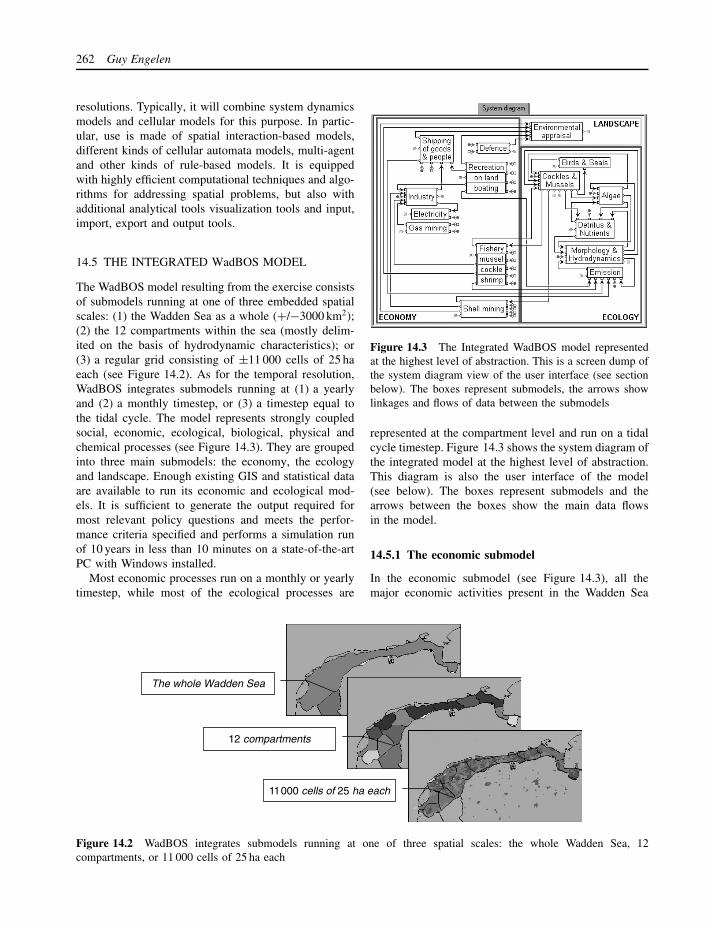
262 Guy Engelen
resolutions. Typically, it will combine system dynamicsmodels and cellular models for this purpose. In partic-ular, use is made of spatial interaction-based models,different kinds of cellular automata models, multi-agentand other kinds of rule-based models. It is equippedwith highly efficient computational techniques and algo-rithms for addressing spatial problems, but also withadditional analytical tools visualization tools and input,import, export and output tools.
14.5 THE INTEGRATED WadBOS MODEL
The WadBOS model resulting from the exercise consistsof submodels running at one of three embedded spatialscales: (1) the Wadden Sea as a whole (+/−3000 km2);(2) the 12 compartments within the sea (mostly delim-ited on the basis of hydrodynamic characteristics); or(3) a regular grid consisting of ±11 000 cells of 25 haeach (see Figure 14.2). As for the temporal resolution,WadBOS integrates submodels running at (1) a yearlyand (2) a monthly timestep, or (3) a timestep equal tothe tidal cycle. The model represents strongly coupledsocial, economic, ecological, biological, physical andchemical processes (see Figure 14.3). They are groupedinto three main submodels: the economy, the ecologyand landscape. Enough existing GIS and statistical dataare available to run its economic and ecological mod-els. It is sufficient to generate the output required formost relevant policy questions and meets the perfor-mance criteria specified and performs a simulation runof 10 years in less than 10 minutes on a state-of-the-artPC with Windows installed.
Most economic processes run on a monthly or yearlytimestep, while most of the ecological processes are
Figure 14.3 The Integrated WadBOS model representedat the highest level of abstraction. This is a screen dump ofthe system diagram view of the user interface (see sectionbelow). The boxes represent submodels, the arrows showlinkages and flows of data between the submodels
represented at the compartment level and run on a tidalcycle timestep. Figure 14.3 shows the system diagram ofthe integrated model at the highest level of abstraction.This diagram is also the user interface of the model(see below). The boxes represent submodels and thearrows between the boxes show the main data flowsin the model.
14.5.1 The economic submodel
In the economic submodel (see Figure 14.3), all themajor economic activities present in the Wadden Sea
The whole Wadden Sea
12 compartments
11000 cells of 25 ha each
Figure 14.2 WadBOS integrates submodels running at one of three spatial scales: the whole Wadden Sea, 12compartments, or 11 000 cells of 25 ha each

Models in Policy Formulation and Assessment 263
are represented at some level of detail. Shell mining,Fishery and Recreation have currently been worked outin greatest detail. Most activities carried out at sea arean input into the local Industry and generate directlyor indirectly Shipping of Goods & People. Shell min-ing and Fishery directly extract biological resourcesfrom the Wadden Sea, while Recreation, Electricity(generation) and Defence use the open space as theirprime resource. Finally, Gas mining taps undergroundresources and may thus have an impact on the Morphol-ogy of the seafloor. The presence and the noise generatedby nearly all activities affect the landscape: its ecolog-ical state, the species present and its attractiveness tohumans. Furthermore, each human activity causes someform of emission of pollutants into the waters.
Most economic activities are modelled on the basis ofthe Platvis economic fishery model (Salz et al., 1994).Thus, they all have the same general modelling scheme,represented in Figure 14.4. This greatly increases theconsistency, the learnability and the transparency ofWadBOS. The calculations proceed through a seriesof interlinked relations on a monthly basis. In thistext, the example of the Recreational boating sector(Recreatievaart) is given but the scheme of relationsapplies to all other sectors too, with minor adaptationsin the terminology and definitions.
The Effort (Overnight stays, recreational boating) ofan economic activity is determined by the availableInfrastructure. Infrastructure for recreational boating isthe number of mooring positions in the harbours. Forother economic activities, it is, for example, the amountof equipment on board boats (expressed in horsepower)
Figure 14.4 Screen dump of the model of an economicsector in WadBOS. Recreational boating is used as anexample. The shaded boxes represent submodels that arenot accessible from this diagram in the user interface
to drag fishing nets or suck up and wash shells, or thenumber of hotel beds available for visitors. In orderto operate the Infrastructure, a workforce is required,thus determining the Employment in the sector. Thedeployment of Effort and the availability of visitors(in the recreation sector), or resources to be extracted(as calculated in the Ecology subsystem), determine theextent of the activity: Presence recreational boating (seeFigure 14.5: 1�) for the recreational boating sector or,for example, total catch for the mussel fishery. At afixed rate of spending, the recreational boaters gen-erate a particular Revenue. In WadBOS, expendituresand prices are externally determined constants. Debits,Labour costs and Technical costs are subtracted fromthe Revenue and thus the Added value of the sector iscalculated. If the latter is positive, Investments may bemade to increase the Infrastructure. Policies can inter-vene directly and set a maximum limit on infrastructure(Policy on infrastructure), or indirectly through Taxes &Subsidies. Another way of intervening into an economicsector is by setting a quota. These will see to it that thequantity of shells mined or fish caught is reduced andthus prevent the exhaustion of the resources.
The above relations are calculated for the entire Wad-den Sea or per compartment (i.e. Quota can be set percompartment). Further to these, there are calculationsrelative to a more precise location of the activity at thelevel of the 25 ha cells. This is because the activity (Pres-ence recreational boating (see Figure 14.5: 1�) is notequally distributed over the entire sea, nor is it equallyintense during the whole year (see Figure 14.5: 2�).It is in particular the cell’s Suitability (see Figure 14.5:
3�) for an activity that determines where the Inten-sity (see Figure 14.5: 5�) is high or low. However,the distribution of activities can be controlled throughZoning policies by closing areas (see Figure 14.5: 4�)permanently or for particular periods during the year.The latter is an important policy lever, because a highintensity may cause Exposure (see Figure 14.6: 1�) ofparticular species of bird or sea animals. Each activitycontributes to one or more of the three types of Pressureon the natural system: presence and noise, mechanicalinfluence and extraction.
All variables calculated at the cellular level areavailable as dynamic maps, updated on a monthly basis.Maps can be consulted at any time during the simulationfor: Intensity for each activity, the three types ofPressure, and 11 forms of Disturbance (a combination ofan activity causing the disturbance, the species affected,and the kind of disturbance, including noise, presenceand mechanical).

264 Guy Engelen
5
3
4
1
2
Figure 14.5 Screen dumps from WadBOS showing a map and dialogue windows relative to the recreational boatingactivity. The numbered items are explained in the text
For each activity the Suitability map is a compositemeasure calculated on the basis of physical, environ-mental and infrastructure elements characterizing eachcell. Similarly, for each activity there is a Zoning mapcalculated from different factors characterizing the insti-tutional and legal status of each cell. The Suitability willexpress the extent to which a cell is appropriate for car-rying out the activity, while the zoning map will indicatewhether or when in the course of the year the activityis allowed in the cell. Both maps can be interactivelyedited in the system thus enabling the user to define dif-ferent kinds of spatial policy measures. The OVERLAYtool, available from the toolbase of WadBOS, enablesthe interactive generation of the Suitability and Zon-ing maps.
14.5.2 Landscape
The economic activities will affect the pristine charac-ter and landscape of the Wadden Sea. These too arelocalized effects that are calculated in WadBOS at thecellular level and on a monthly basis. An assessmentin ecological terms (see Figure 14.6: 2�) is calculated,based on the Ecotopes present in each cell and on thepotential biodiversity of the ecotope. This assessmentis done with and without the effect of economic Activi-ties and Cultural elements present in the landscape. Thisapproach enables a straightforward visualization of thehuman impacts. On the basis of the same information,patches of contiguous Landscape types are calculated.Types vary from ‘nearly natural’ to ‘entirely human’.

Models in Policy Formulation and Assessment 265
1
3
4
5
2
Figure 14.6 Screen dumps from WadBOS showing a few map and system diagram windows relative to the Landscapesubmodel. The numbered elements are explained in the text
The ecological characteristics of the type and the size ofthe patch will determine the kind and number of Species(see Figure 14.6: 3�) potentially populating it in a sus-tained manner. Finally the Wadden Sea is assessed rel-ative to the way it is perceived (see Figure 14.6: 4�)by humans as ‘typical and attractive’. This too is donewith and without human elements present. The differ-ent characteristics mentioned – Ecological assessment,Perception, Landscape types and potential Species – arepresented as dynamic maps on a monthly basis. For mostof the assessment calculations there are no ‘hard scien-tific facts’ to build into the model, rather, expert rulesand judgements are used. Even then, the sequence ofmonthly maps demonstrates in a very interesting man-ner how the sea loses a lot of its ecological value andits attractiveness during the summer when human activ-ity booms. During winter, however, the sea returns to amuch more natural state.
14.5.3 The ecological subsystem
Where activities are carried out some form of pollu-tion is caused and particular Emissions (see Figure 14.6:
5�) (copper, TBT, PAK and Oil) will end up inthe water (see Figure 14.3). River-borne pollutants willenter the sea mainly from Lake Ijssel and the RiverEems. A simple hydrodynamic model calculates howthe water moves from one compartment to the next toeventually flow into the North Sea. Not only will pol-lutants move with the water, but so will other dissolvedmatter – Detritus & Nutrients – including phosphates,silicon and nitrogen. In a food chain model derivedfrom the EcoWasp model (Brinkman, 1993) the Nutri-ents serve as an input to the Algae dynamics. Simplystated, the growth of the latter is determined by the avail-ability of nutrients, the right climatic conditions, light, orinflux from the North Sea and fresh water systems. The

266 Guy Engelen
algae in turn are grazed by filter feeders, including thecommercial species Cockles & Mussels. The latter areprey for Birds and the Fishery. Every year, policy-makers decide on the quantity of cockles and musselsneeded for the survival of the species and as food forBirds. The rest can be fished commercially. Cockles arefished and cooked at sea and their shells are returnedto the sea to become a resource for the Shell miningindustry. The food chain dynamics are calculated on atidal cycle timestep and mostly on the spatial level ofthe compartments. Some information, such as the musseland cockle biomass and the consumption rates of birds,is calculated at the cellular level. The latter serves as acellular input into the fishing activity.
This description is very superficial. The interestedreader can find more ample and more precise descrip-tions of the models used in the online documentation ofthe WadBOS DSS itself, or in the technical reports writ-ten (Engelen, 1999; Huizing et al., 1998; Uljee et al.,2000). From this description, however, it should be clearhow the different submodels are linked to each otherin a network of mutual, reciprocal influence. It shouldbe clear too, that the outputs are visualized by meansof a large number of dynamic maps, each of which isupdated at the appropriate timestep during the simula-tion. Outputs are also presented and stored in the form oftext, MS Excel tables and time graphs. Dynamic mapsgenerated during a simulation can be stored in files forinteractive comparison and further analysis by means ofthe ANALYSE tool (see below). The input maps canbe prepared in a commercial GIS package and importedinto WadBOS. Once imported, each input map can beinteractively edited by means of an appropriate editor.Thus, spatial policy measures can be localized and triedout. The interactive generation of the Zoning and Suit-ability maps is supported by means of the OVERLAYtool. OVERLAY and ANALYSE and many other similarinstruments are part of the Toolbase of WadBOS.
14.6 THE TOOLBASE
In the DSS, it is the role of the models to provide anadequate and truthful representation of the real worldsystem and it is the role of the tools to enable thedecision-maker to work with the models. The user willhardly be aware of the fact that he is using a toolwhen he is editing a parameter or map, or viewing avariable graphed against time. However, without tools,the most sophisticated model is nothing but a number-cruncher, running out of control, drowning its user in alake of numbers.
Most of the tools available in WadBOS are standard inthe GEONAMICA DSS Generator, hence were readilyavailable for integration. In this overview the tools areordered relative to the type of task they carry out inWadBOS. A distinction is made between Input tools,Output tools, Exploration tools and Evaluation Tools(see Table 14.1).
• Among the Input tools are the typical editors forchanging single numbers, or series of numbers in atextual or graphical manner. As part of the latter,the table editor, which enables entering 2-D relationsas a curve, and the map editors are essential andpowerful instruments in WadBOS. But so are the toolsto open, close, import and export files, scenarios andpolicy exercises.
• The Output tools fulfil the difficult task of presentingthe massive amounts of data generated interactivelyin as concise and precise a manner as possible.To present dynamic spatial data interactively, fastdynamic mapping facilities are available. To storesimulation results and enable their in-depth analysis ata later stage, WadBOS features recorders and playersof animated maps, tools for storing dynamic mapoutput in so-called .LOG files, and tools to writeresults to a linked MS Excel spreadsheet.
• Exploration tools enable the user to interactivelysearch the solution space. The capacity to generatescenarios and to produce map overlays (OVERLAYtool), compare maps (ANALYSE tool), and carry outsensitivity analysis (MONTE-CARLO tool) interac-tively, puts great analytical power in the hands of theend-user.
• Evaluation tools support the user in their choice of a‘best’ solution. WadBOS to that effect features ScoreTables, and will be equipped with a Multi CriteriaAnalysis tool in its next version. A built-in GoalSeeking tool presents, based on a sensitivity analysis,the dependency of state variables on policy relevantparameters in the integrated model. When searchingfor potential solutions, it greatly reduces the parameterspace to be analysed.
According to the function the system is to carry outin the policy-making process, the tools play a moreor less pronounced role. From Table 14.1 it is clearthat the analyst uses the complete set extensively. Heneeds both the down-to-earth instruments for enteringdata and viewing output as well as the sophisticatedinstruments for evaluating output. When the main pur-pose of WadBOS is communication, pertinent outputinstruments are essential. The learner is foremost

Models in Policy Formulation and Assessment 267
Table 14.1 Tools available or wanted in WadBOS and their usefulness in relation to the functions ofWadBOS (on a scale from + to ++++)
Tools Analysis Communication Learning Library
Input toolstext editor ++ + +++ +++value editor +++ + +++ +++series editor +++ + +++ +++table editor +++ ++ +++ +++function editor ++ + + +++network (points and lines) editor (∗) ++++ ++ ++++ +++2D map editor ++++ ++ ++++ +++Open/close files ++++ ++ ++++ ++Import/export files ++++ ++ +++ +Output toolsonline documentation ++++ +++ ++++ ++++online help ++ ++ ++++ ++++time graphs ++++ + ++++ +dynamic maps (2D) ++++ ++ ++++ +dynamic maps (network) (∗) ++++ ++ ++++ +3D representation ++ +++ +++ +Animation tool (∗) ++ ++++ +++ +Tracing tool +++ ++ +++ +Link to Excel ++++ + +++ +Log to file ++++ ++ +++ +Exploration toolsOVERLAY tool ++++ +++ +++ +ANALYSE tool ++++ +++ +++ +SCENARIO tool (∗) ++ ++++ ++ +MONTE CARLO tool (∗) +++ ++ +++ +Evaluation toolsSCORE Table tool ++++ ++++ ++++ +EVALUATE tool (MCA) (∗) +++ ++++ ++++ +Goal seeking +++ + + +Note: (∗) available in GEONAMICA, to be implemented in the next version of WadBOS
interested in transparent input and output tools and thedocumentation systems. Finally, for the library function,a good documentation system is paramount, as are facili-ties to quickly enter, update and retrieve the informationstored in the library.
14.7 THE DATABASE
Given the fact that none of the models incorporatedin WadBOS requires data from an online connectionto an external database or to a monitoring system, theintegration of data has been implemented by means of astand-alone database. In fact, the original geographicalinformation is generated, maintained and stored inthe GIS system of the National Institute for Coastal
and Marine Management. A dedicated reduced versionof this database is distributed with WadBOS. It isrenewed when better quality data become available. Theeconomic and ecological data are obtained from a widevariety of sources, some of which were not originally ina digital format, and have been added to the database.When used, WadBOS takes entire care of the retrievaland storage of its data: new or additional information isentered via the dialogues of the system and is stored in ahierarchically organized directory structure. In addition,all the data files are in a readable format, hence can beviewed and edited by means of standard software by theend-users if they wish to do so.
In the future, when WadBOS is installed on themachines of the many end-users of the member orga-nizations of CUBWAD, there will be a need for a
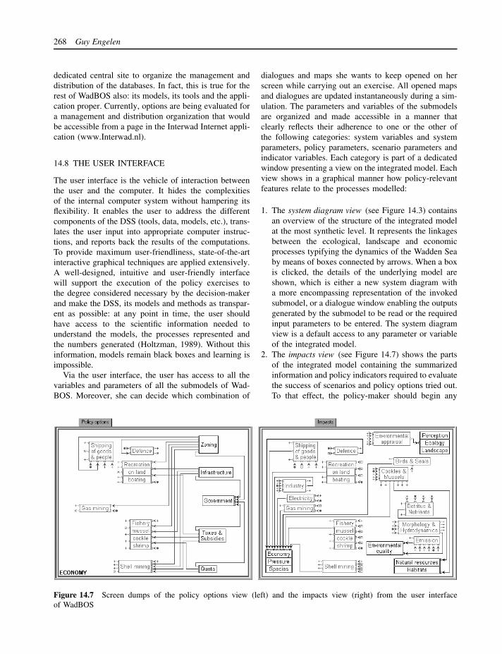
268 Guy Engelen
dedicated central site to organize the management anddistribution of the databases. In fact, this is true for therest of WadBOS also: its models, its tools and the appli-cation proper. Currently, options are being evaluated fora management and distribution organization that wouldbe accessible from a page in the Interwad Internet appli-cation (www.Interwad.nl).
14.8 THE USER INTERFACE
The user interface is the vehicle of interaction betweenthe user and the computer. It hides the complexitiesof the internal computer system without hampering itsflexibility. It enables the user to address the differentcomponents of the DSS (tools, data, models, etc.), trans-lates the user input into appropriate computer instruc-tions, and reports back the results of the computations.To provide maximum user-friendliness, state-of-the-artinteractive graphical techniques are applied extensively.A well-designed, intuitive and user-friendly interfacewill support the execution of the policy exercises tothe degree considered necessary by the decision-makerand make the DSS, its models and methods as transpar-ent as possible: at any point in time, the user shouldhave access to the scientific information needed tounderstand the models, the processes represented andthe numbers generated (Holtzman, 1989). Without thisinformation, models remain black boxes and learning isimpossible.
Via the user interface, the user has access to all thevariables and parameters of all the submodels of Wad-BOS. Moreover, she can decide which combination of
dialogues and maps she wants to keep opened on herscreen while carrying out an exercise. All opened mapsand dialogues are updated instantaneously during a sim-ulation. The parameters and variables of the submodelsare organized and made accessible in a manner thatclearly reflects their adherence to one or the other ofthe following categories: system variables and systemparameters, policy parameters, scenario parameters andindicator variables. Each category is part of a dedicatedwindow presenting a view on the integrated model. Eachview shows in a graphical manner how policy-relevantfeatures relate to the processes modelled:
1. The system diagram view (see Figure 14.3) containsan overview of the structure of the integrated modelat the most synthetic level. It represents the linkagesbetween the ecological, landscape and economicprocesses typifying the dynamics of the Wadden Seaby means of boxes connected by arrows. When a boxis clicked, the details of the underlying model areshown, which is either a new system diagram witha more encompassing representation of the invokedsubmodel, or a dialogue window enabling the outputsgenerated by the submodel to be read or the requiredinput parameters to be entered. The system diagramview is a default access to any parameter or variableof the integrated model.
2. The impacts view (see Figure 14.7) shows the partsof the integrated model containing the summarizedinformation and policy indicators required to evaluatethe success of scenarios and policy options tried out.To that effect, the policy-maker should begin any
Figure 14.7 Screen dumps of the policy options view (left) and the impacts view (right) from the user interfaceof WadBOS

Models in Policy Formulation and Assessment 269
policy exercise with a clearly defined set of criteriadefining the desired state at a particular point intime. In general, the set of indicators in the impactsview are taken from the management plan of theWadden Sea. Indicators expressing the economic,social, ecological, biological, chemical and physicalstate of the system can be viewed. For most indicatorsnorms are available which can be entered as areference value in the score tables of the dialoguesassociated with the boxes in this view.
3. The policy options view (see Figure 14.7) showsthe parts of the model that are most subject topolicy interventions. These are elements that areunder the control of the policy-maker. The user canexplore different combinations of policy measuresand set values for Zoning, including closure of partsof the sea; limitations on Infrastructure; Taxes &Subsidies; and Quota on fishing and mining. Thecosts and benefits of the policies for the Governmentcan be assessed. In an iterative process, she cantune her policy measures in an attempt to approachthe desired state with a minimum amount of effortand costs.
4. The scenarios view (not represented) shows the partsof the model that are most subject to external influ-ences. These are elements not under the control ofthe policy-maker. In order to test the robustness ofthe chosen policy measures, he can impose effectson the system that in the real world are beyondhis control. The user can enter a hypothesis for thefollowing external influences: Atmospheric and Cli-matologic variability; Economic growth and declinein each economic sector; development of the levelof Prosperity in the Netherlands; and exchanges ofwater and dissolved matter between the Wadden Sea,the North Sea and Lake Ijssel.
14.9 CONCLUSION
When the intention was originally formulated to developa system ‘to gather, order and link the knowledgeavailable about the Wadden Sea to facilitate the policy-making process’, it was clear that WadBOS was pri-marily a tool for analysis and evaluation of autonomousdynamics and the effect of policy interventions thereon.Other views coexisted relative to its function: (1) a stor-age tank of data, information and knowledge; (2) a toolfor communication (of results); or (3) a tool for themanagement of information and knowledge about theWadden system. Practice so far has shown that the roleof WadBOS as an instrument for communication hasbeen at least as important. The fact that this instrument
integrates in a formal manner the many processes thatmake and change the Wadden Sea gives direction toa lot of the discussions. It does not necessarily makestakeholders and policy-makers agree on issues moreeasily, but it helps in clarifying what they do or do notagree about. The capacity to visualize conflicting viewsand reduce these conflicts in an interactive session is ofparamount importance.
A core element in WadBOS is the integrated modelof the Wadden Sea. The use of and need for suchinstruments are strongly advocated in new disciplinessuch as Integrated Assessment (Gough et al., 1998). Yet,and despite the fact that the term ‘integrated model’ isused to mean a wide variety of things, there are veryfew operational definitions and recipes or procedures formodel integration available from the scientific literature.Thus, the development of integrated models seemsmore an art than a science at present. It is a deepscientific problem but also a pragmatic multi-criteriamulti-objective problem as it requires dealing with end-use aspects: what is appropriate to be integrated inview of the intended use; scientific aspects: what canand cannot be integrated on scientific grounds; andtechnical aspects: how the integrated model will beassembled and run.
The WadBOS example has shown that integratedmodels used to support the policy-making process comewith a set of requirements of their own, distinguishingthem clearly from research models (see also Mulligan,1998). Policy-makers are best served by models in whichthe time horizon, the spatial and the temporal resolutionare policy problem-oriented and not as process-orientedas research models. They need adequate rather thanaccurate representations of the processes modelled andsketchy but integral rather than in depth and sectorialmodels. While research models are as complicated asnecessary and scientifically innovative, the policy-makeris better served with an instrument that is as simple aspossible and scientifically proven, and which producesusable results as fast as possible, but certainly within10 minutes. If these differences are ignored in theintegration process, the result will often be a large-scalesluggish model not tailored to the needs and expectationsof its end-user. Clearly, a fast, interactive model will domuch better for policy exploration.
A model will only serve the policy end-user if it ispresented in a format that enables it to be worked with.In decision-support systems, models are supplementedwith sets of tools to structure and carry out the analysisin a manner that makes intuitive sense to the policy-maker. One of the crucial elements in the DSS is theuser interface. Attaining the level of user-friendliness
270 Guy Engelen
and flexibility that policy-makers seem to desire remainsa very big challenge for computer scientists, modeldevelopers and domain specialists alike. Indeed, it isvery difficult to package in a single application a systemwith the level of interactivity, flexibility and the fastresponse times wanted, the user-friendliness, simplicityand the transparency desired, and, the level of accuracyand certainty expected. A lot more innovative research,design and implementation work will need to be carriedout to get to this point, if ever we will. Certainly,the demand for the kind of instruments is real. Policyquestions have reached a level of complexity that canno longer be dealt with by politicians alone. High-level technicians are playing an ever-increasing role, andthe revolution in hardware and software technologieshas equipped them with very powerful multimediacalculators.
The technology presented in this chapter is not analternative for calibration and good modelling practices.On the contrary, as long as a model is not calibrated,it should stay in the hands of the model developer andshould be used for policy-making purposes under verystrict conditions. Calibration remains a very difficult andtime-consuming task. It is more so for a complex inte-grated model than for a simple and small one. However,linking individual models into an integrated model doesnot necessarily increase the level of uncertainty anderror in the final product. Rather, the strong connectionsand loops between the individual models and the factthat the values of variables are passed from submodelto submodel at every simulation timestep, bring to thesurface mistakes in the model formulations and calcu-lations much more easily than when the same modelsare applied in isolation (de Kok et al., 2001). Neverthe-less, it should be emphasized that even extensively cali-brated WadBOS-like models will only generate potentialdevelopments rather than predictions of future states orchanges. This is not only due to the problem of cali-bration, but because of the inherent uncertainty in theprocesses represented. Consequently, the model and theencompassing DSS should be used for explorative ratherthan predictive purposes at all times.
From the WadBOS project it can be concludedthat a policy-support tool can be developed withinvery reasonable constraints relative to budget, humanresources and development time. This development ismuch easier when good base material and expertise areavailable and when a stimulating collaboration betweenvisionary end-users and competent DSS developers ispropelling the development. However, the developmentphase described is only the first one in the life ofa decision-support system. It needs to be followed
by an in-depth evaluation of the technical contentsof the system: its constituent models, its coverage ofthe decision domain(s), its way of dealing with thespatial and temporal dynamics of the processes andthe policies. Also an evaluation on behalf of the end-users is pertinent. How do they believe their decisiondomain has been represented? Does the system speaktheir language? Does it work in a way they find usefuland pleasant? With the answers to all these questionsa more or less major redesign of the DSS might bepossible or necessary.
Introducing and institutionalizing the DSS in the end-user organization is the ultimate factor determining itssuccess (Alter, 1980; Klein and Methie, 1995). Even thebest DSS will go unnoticed or will fail if the wrongimplementation and introduction strategy are chosen.Generally speaking, the development and acceptanceof the DSS will be much easier if the development isinitiated by its end-users right from the beginning. Themore they feel the need for a change and the morethey are involved in defining the precise role of theinstrument in the organization, the more likely it is thatthe DSS will be accepted and used (Marakas, 1998). Themore the product itself fulfils tasks that are perceivedas real, in ways that are transparent to the end-user,and in ways that solve the problem in an obviouslybetter way than before its introduction, the better theproduct’s chances of survival. It is therefore crucial todetermine the right moment in the development phaseof the DSS to have it change state from a prototypeinto an operational version. At this stage, the gradualintroduction, good technical documentation, hands-ontraining and prolonged technical assistance during usagebecome of paramount importance. A hasty, unpreparedintroduction should be avoided in all circumstances.
ACKNOWLEDGEMENTS
WadBOS was developed by a consortium of DutchR&D institutes consisting of the Research Institute forKnowledge Systems bv (Maastricht), Infram bv (Zee-wolde), Delft Hydraulics (Delft), Institute for Environ-mental Studies (Amsterdam), Resource Analysis (Delft)and DHV (Amersfoort). The work was supported by theLand Water Information Technology Programme of theDutch Government as well as the Ministry of Trans-port, Public Works and Water Management. A moreelaborate, earlier version of this text was produced forthe National Institute for Coastal and Marine Manage-ment/RIKZ, The Hague, The Netherlands as part ofContract 42002555 (Engelen, 2000).
Models in Policy Formulation and Assessment 271
REFERENCES
Alcamo, J. (1994) IMAGE 2.0: Integrated Modeling of GlobalClimate Change, Kluwer, Dordrecht.
Alter, S.L. (1980) Decision Support Systems: Current Practicesand Continuing Challenges, Addison-Wesley, Reading, MA.
Brinkman, A. (1993) Biological Processes in the EcoWaspEcosystem Model, IBN-DLO report 93/6, Texel.
Catanese, A.J. (1979) Information for planning, in The Practiceof Local Government Planning, International City Manage-ment Association, Washington, DC.
de Kok, J.L., Arifin, T., Noor, A., Wind, H.G. and Augusti-nus, P.G.E.F. (1997) Systems analysis as a methodologyfor sustainable coastal-zone management in tropical coun-tries, Torani, Marine Science and Technology Bulletin 8,31–41.
de Kok, J.L., Engelen, G., White, R. and Wind, H.G. (2001)Modeling land-use change in a decision-support systemfor coastal-zone management, Environmental Modeling andAssessment 6, 123–132.
de Nijs, T., Engelen, G., White, R., van Delden, H. andUljee, I. (2001) De LeefOmgevingsVerkenner. Technischedocumentatie, RijksInstituut voor Volksgezondheid enMilieuhygiene, Bilthoven, Report 408505007/2001.
D’Souza, D.F. and Cameron Wills, D. (1999) Objects, Compo-nents, and Frameworks with UML: The Catalysis Approach,Addison-Wesley, Reading, MA.
El-Najdawi, M.K. and Stylianou, A.C. (1993) Expert supportsystems: integrating AI technologies, Communications of theACM 36 (2), 55–65.
Engelen, G. (ed.) (1999) BOS Integraal beheer van Estuarieneen Waddensystemen. Deelproject: Case Waddenzee, StichtingLWI, Gouda.
Engelen, G. (2000) The Development of the WadBOS DecisionSupport System: A Bridge between Knowledge and Policy inthe Wadden Sea, National Institute for Coastal and MarineManagement, The Hague.
Engelen, G., White, R. and Uljee, I. (1993) Exploratory mod-elling of socio-economic impacts of climatic change, inG. Maul (ed.) Climate Change in the Intra-Americas Sea,Edward Arnold, London, 306–324.
Fayad, M.E., Schmidt, D.C. and Johnson, R.E. (1999)Building Application Frameworks: Object-Oriented Foun-dations of Framework Design, Wiley Computer Publishing,Chichester.
Firley, M. and Hellens, D. (1991) Knowledge Elicitation: APractical Handbook, Prentice Hall, New York.
Gonzalez, A.J. and Dankel, D.D. (1993) The Engineering ofKnowledge-based Systems: Theory and Practice, PrenticeHall, Englewood Cliffs, NJ.
Gough, C., Castells, N. and Funtowics, S. (1998) Integratedassessment; an emerging methodology for complex issues,Environmental Modelling and Assessment 3, 19–29.
Hahn, B. and Engelen, G. (2000) Concepts of DSS sys-tems, Veranstaltungen 4, Bundesanstalt fur Gewasserkunde,Koblenz, 9–44.
Huizing, J.J., Engelen, G., van de Ven, K., Pothof, I. andUljee, I. (1998) WadBOS: Een prototype van een kennissys-teem voor beleidsanalyse van de Waddenzee, Eindrapport,Directie Noord Nederland, Rijkswaterstaat, Leeuwarden.
Holtzman, S. (1989) Intelligent Decision Systems, Addison-Wesley, Reading, MA.
Kauffman, S.A. (1990) Requirements for evolvability in com-plex systems: orderly dynamics and frozen components,Physica D 42, 135–152.
Klein, M.R. and Methie, L.B. (1995) Knowledge-Based Deci-sion Support Systems, John Wiley & Sons, New York.
Marakas, G.M. (1998) Decision Support Systems in the 21stCentury, Prentice Hall, Upper Saddle River, NJ.
Mulligan, M. (1998) Modelling Desertification: EU ConcertedAction on Mediterranean Desertification, thematic report,King’s College London, London.
Prigogine, I. (1981) From Being to Becoming, Freeman, SanFrancisco.
Rotmans, J. and de Vries, B. (1997) Perspectives on GlobalFutures: The TARGETS Approach, Harvard University Press,Cambridge, MA.
Salz, P., Dol, W. and Smit, W. (1994) Schol Case: EconomischModel, LEI-DLO, Den Haag.
Schielen, R.M.J. (2000) Recent history and future develop-ments of decision support systems for the Dutch rivers, Ver-anstaltungen 4, Bundesanstalt fur Gewasserkunde, Koblenz,77–87.
Sprague, R.H. Jr. and Carlson, E.D. (1982) Building Effec-tive Decision Support Systems, Prentice Hall, EnglewoodCliffs, NJ.
Sterman, J.D. (2000) Business Dynamics: Systems Thinkingand Modeling for a Complex World, Irwin/McGraw-Hill,Boston, MA.
Uljee, I., Hahn, B., van der Meulen, M. and Engelen, G.(2000) WadBOS Gebruikershandleiding, National Institutefor Coastal and Marine Management/RIKZ, Haren.
van Delden, H. (2000) A Generic Approach for the Designof Decision Support Systems for River Basin Management,University of Twente, Enschede.

15
Decision-Support Systems for ManagingWater Resources
SOPHIA BURKE
15.1 INTRODUCTION
Chapter 14 addresses how decision-support systems canbe used for policy making in the coastal zone andthis chapter identifies how models are used within adecision-support tool for optimal management of waterresources. Optimal water-resource management involvesthe identification of the best possible protection and effi-cient utilization of available water resources, whetherfor hydropower, water supply, agricultural use (suchas irrigation and drainage) or for environmental man-agement of freshwater or marine resource management.This chapter will outline why decision-support systems(DSS) are needed, how they are designed, and will givesome brief examples of their use in water resource man-agement. Further reviews of the use of DSS in waterresources can be found in Loucks and Gladwell (1999),Simonovic (2000) and Watkins and McKinney (1995).
15.2 WHY ARE DSS NEEDED?
Water-resource managers are charged with the long-termoptimal management, regulation and protection of waterresources. However, it is recognized that water-resourcemanagers must take into account the multitude of waterresources development preferences that are put forwardby stakeholders such as agriculturalists, water suppliersand environmental groups. As a result, conflicts over theutilization of a particular resource may occur. In recentyears, there has been increasing interest in the potentialof using integrated catchment management (ICM) as ameans of sustainable management of water resources on
a catchment scale. ICM is a holistic, natural, resources-management system comprising interrelated elements ofwater, soils and other environmental and socio-economicfactors, in a river basin, managed on an environmentaland economic basis. The rationale of managing waterresources on a basin scale instead of on a project-by-project basis at a subcatchment scale is based on therecognition that the water and land resources of a basinare integrated together and hence must be treated assuch. Given the complexity of the hydrological system,the development and use of mathematical modellingare often necessary. However, to facilitate the identi-fication of the best development strategy of catchmentswe need to identify and evaluate alternative water man-agement plans and policies and to predict and under-stand their short- and long-term physical, economicand social impacts. An adequate understanding of thecomplex hydrological function of the resource and thelimits of resource exploitation is necessary, given theenvironmental (soil, land use, climate), human (socio-economics, policy) and infrastructural constraints. Inaddition, we need to understand the impacts of addi-tional pressures on water in the future due to populationgrowth and land use development, climate variabilityand regulatory requirements. For example, the supplyof water often does not keep up with demand, and inthe face of increasing population and an uncertain cli-mate, computer models can be used to simulate futurescenarios for water-supply systems. The complexity ofland-surface controls such as soils, climate and humanactivity on water-resource quality and quantity and theneeds of the users for adequate and predictable suppliesof water means that an improved approach to modelling
Environmental Modelling: Finding Simplicity in Complexity. Edited by J. Wainwright and M. Mulligan 2004 John Wiley & Sons, Ltd ISBNs: 0-471-49617-0 (HB); 0-471-49618-9 (PB)
274 Sophia Burke
is needed. Additionally, the use and interpretation ofthe hydrological model output can be difficult for thenonspecialist, particularly for nondeterministic modelsor where complex calibration procedures are needed.To incorporate the complexity into the decision-makingprocess and to facilitate the practical use of existingcomplex models and technologies for decision-making,the development and use of decision-support systems isoften necessary.
DSSs can be defined as ‘interactive computer pro-grams that utilize analytical methods, such as decisionanalysis, optimization algorithms, program schedulingroutines, and so on, for developing models to helpdecision makers formulate alternatives, analyse theirimpacts, and interpret and select appropriate options forimplementation’ (Adelman, 1992). They are interactiveframeworks built around established technologies thataddress the questions or issues pertaining to problemsand contribute to option selection. They allow the userto use existing modelling technology from a range ofdisciplines and investigate the impacts of future scenar-ios. Traditional modelling assessments of water qualityand quantity are joined by assessments of ecology, biodi-versity, geomorphology and environmental economics,and the DSS should be able to integrate the output ofthese previously independent models of processes to aiddecision-making.
Moreover DSS are based on formalized knowledge,and their application in the decision-making process pro-vides the additional benefit that the final decisions areby definition as rational as possible, and the processof arriving at that decision is documented and repro-ducible (Vacik and Lexer, 2001).
15.3 DESIGN OF A DECISION-SUPPORT SYSTEM
The needs of the end-users must be taken into accountduring the early stages of design of the DSS (Wilsonand Droste, 2000). Good communication between devel-opers and end-users throughout development is imper-ative in order that it truly reflects the needs of theusers (Loucks and da Costa, 1991; Argent and Grayson,2001). In addition, advice is needed on the criteria ofthe post-model evaluation and optimization tools.
The availability and quality of appropriate data alsoneed to be established at an early stage. The develop-ment of a DSS has the advantages of bringing togetherexisting available environmental and economic data sothat they can usefully be analysed together. One of themain problems in inter-disciplinary, regional decision-making where there is an environment of entrenched
bureaucracy is the lack of synthesis of even basic spa-tial information. The DSS is therefore also useful forthe display and analysis of existing resource data asa user-friendly Geographic Information System (GIS),database or website. The DSS provides a synoptic viewof the main elements of water resource managementin a particular catchment, combining rainfall, land useand water quality with infrastructure, economic data andother sectors.
The DSS comprises a network of models, such aswater-balance models and economic forecasting models.Often simpler models are favoured where there area large number of models in the network so thatdesign, computing and data demands are kept to aminimum. For example, Georgopoulou et al. (2001)used a DSS in the Mediterranean to investigate thephysical and economic feasibility of extracting brackishgroundwater for desalination together with artificialrecharging the groundwater using treated wastewater toprevent further saline intrusion. Suitable models weretherefore needed to describe each main process thataffects the system or forms part of the proposed scheme.The elements described were therefore the hydrologicbudget, natural recharge (infiltration) of the aquifer, agroundwater model that included seawater intrusion,water demands on the aquifer, a desalinization model,and recharge of the treated reclaimed water. The modelsranged from complex, well-tested existing models (forthe groundwater) to simple mathematical expressions(for cost functions) and historical data functions (forwater demand).
The models in a DSS are linked to the databaseof existing information for the parameterization andvalidation of the models in the target region. The DSSmay demand spatial and temporal data of differentscales, such as hydrological model data at a hillslopescale and data for upscaling to the catchment scale. GISare useful databases as these hold geographical data aswell as tabular data and they are often used for theoutput of results for the user too. Data for possible futurescenarios are also held in the database such as climatedata from GCM (General Circulation Model) output, orforecasts of future water demands.
The DSS should have a user-friendly interface if itis to be readily adopted by the decision-maker. Thecomplexity of this interface must be balanced with theease of application. An example of a fairly sophisticatedDSS is where the user can interact with both the modelparameters and optimization models (see later discussionon optimization), such as that described and illustratedin Ostfeld et al. (2001). This DSS is called ‘HANDSS’and was designed to assist in the operation of the canal
Decision-Support Systems for Managing Water Resources 275
network fed from the River Jordan in Israel to the LakeHula wetlands. HANDSS consists of the MODFLOWgroundwater model, visualization layer, a simulationlayer and a management layer. The visualization layeruses GIS to provide spatial maps of solutions, thesimulation layer is linked to the selection of modelequations and the management layer allows the user tocontrol the optimization procedure.
The user interface must be flexible enough to allowinteraction with as many parameters as possible sothat a series of scenarios can be fully tested by theuser. The parameters that are affected by the end-users’decisions could be altered within limits, for example,land-use decisions or economic markets. A number offuture scenarios for factors that are not directly influ-enced by the decision-maker, such as external mar-kets or climate change, could also be selected. Forexample, Staudenrausch and Flugel (2001) have devel-oped an application for Southern Africa, a region ofcomplex political economy where unfavourable climatesmean that renewable water resources are scarce. Sce-narios of land-use and climate change were coupledwith scenarios of population growth and policy fore-casts and applied to a hydrological and socio-economicmodel linked by a rule-based expert system.
Users are encouraged to perform sensitivity analysesof the impacts of change, which greatly enhancesthe understanding the system behaviour. Through aniterative process, the user can explore the multipleimpacts of various management options. For example,the user may investigate the sensitivity of the riverregime to anthropic influences within the catchment suchas irrigation, and changes in the sensitivity in the faceof different climate change scenarios. The DSS is oftenmenu-driven and uses graphics to display data inputand output, which facilitates their use. The output isdisplayed in a meaningful way, for example, using mapsand animations, and these can be quickly assimilated bythe decision-maker and communicated to a variety ofstakeholder groups (Welp, 2001).
The final step is to find the optimal solution for waterresource management. Automated optimization tools areused in many DSS, and the optimization model is oneof the most important components of the DSS. It com-prises rule-based or linguistic algorithms that interrogatethe DSS models. For example, the rules can be setto optimize the allocation of water for a given objec-tive or set of objectives. The model is run many timeswithin given constraints (economic, hydrological, cul-tural). The optimal solutions will fulfil the maximumnumber of objectives and the model run result willallow for sensitivity testing of the solutions and for
proposing and illustrating the trade-offs and the lessthan optimal solutions. For example, Ghoneim et al.(1996) use a simple linear programming optimizationsimulation model to find the best possible allocationof water in part of the Nile Valley. The optimality isbased upon the planner’s preferences for using differentresources, the physical constraints, and the desired oper-ation rules that constrain the model. Finding the optimalsolution for multiple nonlinear objectives is exploredby Eskandari et al. (1995), who describe a DSS of apine-forested catchment in north-central Arizona. TheDSS was used to test four forestry strategies to maximizeobjectives of water production, wildlife habitat, aesthet-ics, livestock and wood production and to minimizecosts. Distance-minimizing methods are used, which arecomputed by first maximizing each objective individ-ually and then calculating the feasible solution withminimal distance from the ideal point. However, theobjectives will vary according to interest groups (waterusers, livestock producers, foresters, environmentalistsand land-use planners), and so after consultation withthese groups the objectives were defined by a distribu-tion function, the form of which varies according to itsrelative importance to each group. Five different meth-ods of optimization by distance minimization are used.They found that for each optimization method, differ-ent alternative management techniques appeared to bethe best.
DSS is most useful where there are a large number ofobjectives for assimilation. Optimal solutions thereforedemand the exact preference of each objective. Tweryand Hornbeck (2001) analysed forests in the north-eastern United States with respect to water (quantityand quality), wildlife, timber production, visual qual-ity and general ecological goals. Model results showedthat some of the desired objectives were linked, forexample, water and ecological goals, and others were notcompatible with each other (see also Chapter 17). Vacikand Lexer (2001) use an algorithm for comparing goals.They apply a DSS to forest management in Vienna, alsousing a large number of management objectives, includ-ing water production, timber production, conservationof biodiversity, recreation objectives and rock stability.The decision model decomposes the objectives into sev-eral hierarchically structured decision criteria based onpartial objectives. Qualitative expert knowledge is usedto compute preference values, and the preferences areaggregated additively at each hierarchical level.
Improved optimization techniques have come to thefore in water management models. One example isDynamic Programming, which is not dependent on theshape of the objective function as it is discretized

276 Sophia Burke
into a finite set of stages, with an optimal solution ateach stage, although this is computationally expensive.Second, there is a growing interest in evolutionary orgenetic algorithms (for example, Booty et al., 2001),based on Darwinian evolutionary theory. The solutionspace is evaluated for fitness and the fittest of thepopulations are selected and combined to produce a newgeneration of solution points with increased likelihoodof increased fitness. The process is iterated until the‘gene’ with the best fitness value meets the pre-definedconvergence criteria.
15.4 CONCLUSION
Decision-support systems are a useful platform forallowing nonexperts to exploit state-of-the-art hydrolog-ical modelling technology. They allow the visualizationof the holistic water-management framework and can aidpolicy decision-making where complexities of the waterresources management demand a number of factors to betaken into account. In the face of climatic, environmentaland socio-economic change, water resources manage-ment will become more complex and DSS allows theimpacts of decisions on the system under a number ofscenarios to be analysed. The DSS must be tested androbust enough to be passed safely into the hands of non-experts but also be flexible enough to future-proof thedecision-making environment.
15.5 DSS ON THE WEB
There are water resources DSS freely available on theInternet for academic/research purposes. One such pack-age was released by IIASA (International Institute forApplied Systems Analysis) and IWEP (Institute forWater and Environmental Problems) in 1996 and iscalled DESERT (DEcision Support system for Evalu-ation of River basin sTrategies). The current websiteaddress is http://www.iiasa.ac.at/Research/WAT/docs/desert.html. This was designed for decision support forwater-quality management on a river-basin scale. Moreinformation can be found in the manual, which is down-loadable from this website.
REFERENCES
Adelman, L. (1992) Evaluating Decision Support and ExpertSystems, John Wiley & Sons, New York.
Argent, R.M. and Grayson, R.B. (2001) Design of informa-tion systems for environmental managers: an example usinginterface prototyping, Environmental Modelling and Soft-ware with Environment Data News 16 (5), 433–438.
Booty, W.G., Lam, D.C.L., Wong, I.W.S. and Siconolfi, P.(2001) Design and implementation of an environmental deci-sion support system, Environmental Modelling and Softwarewith Environment Data News 16 (5), 453–458.
Eskandari, A., Ffolliott, P. and Szidarovsky, F. (1995) Deci-sion support system in watershed management, in T.J. Ward(ed.) Watershed Management: Planning for the 21st Century,American Society of Civil Engineers, New York.
Georgopoulou, E., Kotronarou, A., Koussis, A., Restrepo, P.J.,Gomez-Gotor, A. and Rodriguez Jimenez, J.J. (2001) Amethodology to investigate brackish groundwater desalina-tion coupled with aquifer recharge by treated wastewater asan alternative strategy for water supply in Mediterraneanareas, Desalination 136 (1), 307–315.
Ghoneim, G.A., El-Terzy, A.I., Bahjat, A.M. and Fontane,D.G. (1996) Optimal operational guidelines for conjunctiveuse of multi-water resources system, in M.A. Abu-Zeid andA.K. Biswas (eds) River Basin Planning and Management,Water Resources Management Series 4, Oxford UniversityPress, Calcutta.
Loucks, D.P. and da Costa, J.R. (1991) Computer aided deci-sion support in water resources planning and management,in D.P Loucks and J.R. da Costa (eds) Decision Support Sys-tems, Water Resources Planning, NATO ASI Series G, Vol.26, Springer-Verlag, Berlin.
Loucks, D.P. and Gladwell, J.S. (1999) Sustainability Criteriafor Water Resource Systems, International Hydrology Series,Cambridge, Cambridge University Press.
Ostfeld, A., Muzaffar, E. and Lansey, K. (2001) HANDSS:The Hula Aggregated Numerical Decision Support Sys-tem, Journal of Geographic Information and DecisionAnalysis 5 (1), 16–31 (also available for download athttp://www.geodec.org/Ostfeld.pdf).
Simonovic, S.P. (2000) Tools for water management: one viewof the future, Water International 25 (1), 76–88.
Staudenrausch, H. and Flugel, W.A. (2001) Development of anintegrated water resources management system in southernAfrican catchments, Physics and Chemistry of the Earth, PartB: Hydrology, Oceans and Atmosphere 26 (7), 561–564.
Twery, M.J. and Hornbeck, J.W. (2001) Incorporating watergoals into forest management decisions at a local level,Forest Ecology and Management 143 (1), 87–93.
Vacik, H. and Lexer, M.J. (2001) Application of a spatialdecision support system in managing the protection forests ofVienna for sustained yield of water resources, Forest Ecologyand Management 143 (1), 65–76.
Watkins, D.W. and McKinney, D.C. (1995) Recent develop-ments associated with decision support systems in waterresources, Reviews of Geophysics Supplement 33, Ameri-can Geophysical Union (also available at http://earth.agu.org/revgeophys/watkin00/watkin00.html).
Welp, M. (2001) The use of decision support tools in partic-ipatory river basin management, Physics and Chemistry ofthe Earth, Part B: Hydrology, Oceans and Atmosphere 26,535–539.
Wilson, D.J. and Droste, R.L. (2000) Design considerationsfor watershed management decision support systems, WaterQuality Research Journal of Canada 35, 2–26.

16
Soil Erosion and Conservation
MARK A. NEARING
16.1 THE PROBLEM
Accelerated soil erosion induced by human activities isthe principal cause of soil degradation across the world.The main culprit behind the problem is agriculture, andat stake is the long-term viability of the agricultural pro-duction capacity of the planet. Barring major, unknownscientific advances in the future, and if soil erosion andpopulation growth remain unchecked from their currentrates, humanity will eventually lose the ability to feeditself. Another significant problem associated with soilerosion is off-site sediment pollution. Costs associatedwith the delivery of sediment to streams and other waterbodies worldwide are huge (e.g. Pimental, 1995). Thischapter will focus on models of soil erosion as they areused for purposes of soil conservation. In particular, wefocus here exclusively on soil erosion by water (see alsoChapter 9). Models of other agricultural erosion pro-cesses, such as wind erosion and tillage erosion, arecertainly important, but they will not be addressed here.
Models can be used in conservation work for threeprimary purposes: (a) to help a land owner or managerchoose suitable conservation practices from among alter-natives; (b) to make large-scale erosion surveys in orderto understand the scope of the problem over a regionand to track changes in erosion over time; and (c) toregulate activities on the land for the purposes of con-servation compliance.
In selecting or designing an erosion model, a decisionmust be made as to whether the model is to be used foron-site or off-site concerns, or both. On-site concerns aregenerally associated with degradation or thinning of thesoil profile in the field, which may become a problemof crop-productivity loss. Conservationists refer to thisprocess as soil loss, referring to the net loss of soil over
only the portion of the field that experiences net lossover the long term. Areas of soil loss end where netdeposition begins. Off-site concerns, on the other hand,are associated with the sediment that leaves the field,which we term here sediment yield. In this case, we arenot necessarily concerned with the soil loss, or for thatmatter the amount of sediment deposited prior to leavingthe field, although estimation of both of these may beused to estimate sediment yields. Ideally, a model willcompute soil loss, deposition and sediment yield, andthus have the capability to address both on-site and off-site issues.
Data variability and model uncertainty are two relatedand important issues associated with the applicationof erosion models. Data from soil-erosion plots con-tain a large amount of unexplained variability, whichis an important consideration for using erosion data toevaluate soil-erosion models, as well as for interpret-ing erosion data. This variability is due both to naturalcauses and measurement errors. When comparing mea-sured rates of erosion to predicted values, a portion ofthe difference between the two will be due to modelerror, but a portion will also be due to unexplainedvariance of the measured sample value from the rep-resentative, mean value for a particular treatment.
Knowledge of variability in soil-erosion data, how-ever, is somewhat limited, though recent studies haveenlightened us to some degree. Only one experimen-tal erosion study to date has been conducted with asufficient number of replicated erosion plots to allowan in-depth analysis of variability. Wendt et al. (1986)measured soil-erosion rates on 40 cultivated, fallow,experimental plots located in Kingdom City, MO, in1981. All the 40 plots were cultivated and in other waystreated identically. The coefficients of variation for the
Environmental Modelling: Finding Simplicity in Complexity. Edited by J. Wainwright and M. Mulligan 2004 John Wiley & Sons, Ltd ISBNs: 0-471-49617-0 (HB); 0-471-49618-9 (PB)

278 Mark A. Nearing
25 storms ranged from 18% to 91%, with 15 of thestorms falling in the range of less than 30%. The moreerosive storms tended to show the lesser degree of vari-ability. Of the 15 storms with mean erosion rates ofgreater than 0.1 kg m−2 (1.0 Mg ha−1), 13 showed coef-ficients of variation of less than 30%. The results of thestudy indicated that ‘only minor amounts of observedvariability could be attributed to any of several mea-sured plot properties, and plot differences expressed bythe 25 events did not persist in prior or subsequent runoffand soil loss observations at the site’.
Ruttimann et al. (1995) reported a statistical anal-ysis of data from four sites, each with five to sixreported treatments. Each treatment had three replica-tions. Reported coefficients of variation of soil lossranged from 3.4% to 173.2%, with an average of 71%.The authors concluded by suggesting ‘as many replica-tions as possible’ for erosion experiments.
Nearing et al. (1999) studied erosion variability usingdata from replicated soil-loss plots from the UniversalSoil Loss Equation (USLE) database. Data from repli-cated plot pairs for 2061 storms, 797 annual erosionmeasurements and 53 multi-year erosion totals wereused. They found that the relative differences betweenreplicated plot pair measurements tended to decreaseas the magnitude of the measured soil loss increased.Using an assumption that soil-loss magnitude was theprincipal factor in explaining variance in the soil-lossmeasurements, the authors were able to calculate thecoefficient of variation of within-treatment, plot repli-cate values of measured soil loss. Variances betweenreplicates decreased as a power function (r2 = 0.78) ofmeasured soil loss, and were independent of whether themeasurements were event-, annual- or multi-year val-ues. Values of the coefficient of variability ranged fromnearly 150% for a soil loss of 0.1 kg m−2 to as low as18% or less for soil-loss values greater than 10 kg m−2.
One important question for scientists is: ‘How do weknow when an erosion model is working adequately?’Given that the data are highly variable, when we askthe question about how well a model works, the answeris not so simple. One cannot just compare the modeloutput to an erosion rate. One must simultaneously askthe question: ‘How variable is nature?’
Risse et al. (1993) applied the USLE to 1700 plotyears of data from 208 natural runoff plots. Annualvalues of measured soil loss averaged 3.51 kg m−2 withan average magnitude of prediction error of 2.13 kg m−2,or approximately 60% of the mean. Zhang et al. (1996)applied the Water Erosion Prediction Project (WEPP)computer simulation model to 290 annual values and
obtained an average of 2.18 kg−2 for the measured soilloss, with an average magnitude of prediction error of1.34 kg−2, or approximately 61% of the mean. In bothcases the relative errors tended to be greater for thelower soil-loss values. Given these results and othersfrom similar types of studies (Liu et al., 1997; Rapp,1994; Govers, 1991), the question may be asked: arethe predictions ‘good enough’ relative to measured data?What is an acceptable and expected level of modelprediction error?
One manner in which we can address this problemis to think of the replicated plot as the best possi-ble ‘real-world, physical model’ of soil erosion. Assuch, one might further consider that the physical modelrepresented by the replicate plot represents essentiallya ‘best-case’ scenario in terms of erosion prediction,which we can use as a baseline with which the perfor-mance of erosion prediction models might be compared.Using, as discussed above, data from natural runoff plotsfrom the USLE plot database, Nearing (2000) suggesteda basis for an erosion-model evaluation method usingthe idea of the replicate plot as a physical model ofthe replicated plot. He suggested that if the differencebetween the model prediction and a measured plot datavalue lies within the population of differences betweenpairs of measured values, then the prediction is con-sidered ‘acceptable’. A model ‘effectiveness’ coefficientwas defined for studies undertaken on large numbers ofprediction vs. measured data comparisons. The methodprovides a quantitative criterion for taking into accountnatural variability and uncertainty in measured erosion-plot data when those data are used to evaluate ero-sion models.
Nearing (2000) outlines the specific procedures forhow erosion model evaluation can be done in the pres-ence of data uncertainty. The method is straightforward,but requires some detail in the computations. Using sim-ilar arguments with the erosion plot replicates data, butusing a slightly less complex analysis, we can achievea rule-of-thumb measure of model validity simply bylooking at the coefficient of determination for the regres-sion line between measured and predicted soil loss val-ues. Using measured soil loss data pairs from 3007storms (overlapping with some of the same data used inthe pre-mentioned studies), Nearing (1998) obtained acoefficient of determination between measured and pre-dicted soil loss of 0.77. One certainly would not expect(on uncalibrated data) to obtain results between modelpredictions and measured data substantively better thanthis, and for all practical purposes expectations of fitmust be less. In the study by Risse et al. (1993) usingthe USLE and 1700+ plot years of data, the overall

Soil Erosion and Conservation 279
coefficients of determination were 0.58 for annual valuesand 0.75 for annual average soil-loss data. In the studyby Zhang et al. (1996), the WEPP model was appliedusing data from 4124 storm events, the coefficients ofdetermination were 0.36 for the individual storms, 0.60for annual values, and 0.85 for annual average soil lossvalues. The observation that the fit improves from stormto annual to average annual predictions reflects the trendthat data variability decreases with increasing soil-lossmagnitudes, as discussed above.
Given that we know, based on the data from erosionplots, that soil erosion is highly variable, and then usingthe information on variability to set limits on the abilityof models to predict soil-erosion rates, the question thenbecomes one of utility. Is the model accurate enough tosolve our problems? We will address this question laterin this chapter. But first we need to look at the modelsthemselves, and look at an example of how an erosionmodel might be used to solve a problem.
16.2 THE APPROACHES
Erosion models used in application for conservationplanning fall into two basic categories: empirical andprocess-based. Undoubtedly the prime example of anempirically based model is the Universal Soil LossEquation (USLE), which was developed in the UnitedStates during the 1950s and 1960s (Wischmeier andSmith, 1965, 1978). This equation has been adapted,modified, expanded and used for conservation purposesthroughout the world (e.g. Schwertmann et al., 1990;Larionov, 1993).
The USLE was originally based on statistical anal-yses of more than 10 000 plot-years of data collectedfrom natural runoff plots located at 49 erosion researchstations in the United States, with data from addi-tional runoff plots and experimental rainfall simulatorstudies incorporated into the final version published in1978 (Wischmeier and Smith, 1978). The large databaseupon which the model is based is certainly the principalreason for its success as the most used erosion model inthe world, but its simplicity of form is also important:
A = R K L S C P (16.1)
where A (t ha−1 a−1) is average annual soil loss overthe area of hillslope that experiences net loss, R
(MJ mm h−1 ha−1 a−1) is rainfall erosivity, K (t hr MJ−1
mm−1) is soil erodibility, L (unitless ratio) is the slopelength factor, S (unitless ratio) is the slope steepnessfactor, C (unitless ratio) is the cropping factor, andP (unitless ratio) is the conservation practices fac-tor. Terminology is important here. Note first that the
USLE predicts soil loss (see discussion above) and notsediment yield. Second, the word erosivity is used todenote the driving force in the erosion process (i.e.,rainfall in this case) while the term erodibility is usedto note the soil resistance term. These two terms arenot interchangeable. Third, the model predicts averageannual soil loss: it was not intended to predict soilloss for storms or for individual years. Conservation-ists often describe the predictions as long term, whilefrom the geomorphic perspective the predictions wouldbe referred to as medium term (Govers, 1996).
The units of the USLE appear a bit daunting aswritten (Equation 16.1), but become somewhat clearerwith explanation. The units were originally written, andare still used in the United States, as imperial, butconversion to metric is generally straightforward (Fosteret al., 1981). The key to understanding the dimensionalunits lies with the definition of rainfall erosivity andthe concept of the unit plot. Wischmeier (1959) foundfor the plot data that the erosive power of the rainwas statistically best related to the total storm energymultiplied by the maximum 30-minute storm intensity.Thus, we have the energy term (MJ) multiplied by theintensity term (mm h−1) in the units of R, both of whichare calculated as totals per hectare and per year. The unitplot was defined as a standard of 9% slope, 22.13 mlength,1 and left fallow (cultivated for weed control).The K value was defined as A/R for the unit plot. Inother words, erodibility was the soil loss per unit valueof erosivity on the standard plot. The remaining terms,L, S, C and P , are ratios of soil loss for the experimentalplot to that of the unit plot. For example, the C valuefor a particular cropped plot is the ratio of soil loss onthe cropped plot to the value for the fallow plot, otherfactors held constant.
The USLE reduced a very complex system to a quitesimple one for the purposes of erosion prediction. Thereare many complex interactions within the erosionalsystem which are not, and cannot be, represented withinthe USLE. We will illustrate a few of these interactionsbelow. On the other hand, for the purposes as statedabove for which an erosion model is used, the USLEhas been, and still can be, very successful. This issue isalso discussed below in more detail.
The USLE was upgraded to the Revised UniversalSoil Loss Equation (RUSLE) during the 1990s (Renardet al., 1997). RUSLE is a hybrid model. Its basicstructure is the multiplicative form of the USLE, butit also has many process-based auxiliary components.It is computer based, and has routines for calculat-ing time-variable soil erodibility, plant growth, residuemanagement, residue decomposition and soil surface
280 Mark A. Nearing
roughness as a function of physical and biologicalprocesses. RUSLE also has updated values for erosiv-ity (R), new relationships for L and S factors whichinclude ratios of rill and inter-rill erosion, and additionalP factors for rangelands and subsurface drainage, amongother improvements. RUSLE has the advantage of beingbased on the same extensive database as is the USLE,with some of the advantages of process-based compu-tations for time-varying environmental effects on theerosional system. It still has the limitations, however, inmodel structure that allows only for limited interactionsand inter-relationships between the basic multiplicativefactors of the USLE (Equation 16.1).
Various process-based erosion models have beendeveloped in the past ten years including EUROSEMin Europe (Morgan et al., 1998), the GUEST model inAustralia (Misra and Rose, 1996), and the WEPP modelin the United States (Flanagan and Nearing, 1995). Wewill focus here on the example of the WEPP model,largely because it is the technology most familiar tothe author.
The WEPP profile computer model includes sevenmajor components, including climate, infiltration, waterbalance, plant growth and residue decomposition, sur-face runoff, erosion and channel routing for water-sheds. The climate component of the profile computermodel (Nicks, 1985) generates daily precipitation, dailymaximum and minimum temperature, and daily solarradiation based on a statistical representation of weatherdata at a particular location. The climate model hasbeen tested for erosion and well parameterized forthe United States (Baffaut et al., 1996). The infiltra-tion component of the hillslope model is based on theGreen and Ampt equation, as modified by Mein and Lar-son (1973), with the ponding time calculation for anunsteady rainfall (Chu, 1978). The water balance andpercolation component of the profile model is basedon the water balance component of SWRRB (Simula-tor for Water Resources in Rural Basins) (Williams andNicks, 1985; Arnold et al., 1990), with some modifi-cations to improve estimation of percolation and soilevaporation parameters. The plant-growth component ofthe model simulates plant growth and residue decom-position for cropland and rangeland conditions. Theresidue and root decomposition model simulates decom-position of surface residue (both standing and flat),buried residue, and roots for the annual crops spec-ified in the WEPP User Requirements (Flanagan andLivingston, 1995) plus perennial crops of alfalfa andgrasses. Surface runoff is calculated using a kinematicwave equation. Flow is partitioned into broad sheetflow for inter-rill erosion calculations and concentrated
flow for rill erosion calculations. The erosion compo-nent of the model uses a steady-state sediment conti-nuity equation that calculates net values of detachmentor deposition rates along the hillslope profile (Nearinget al., 1989). The erosion process is divided into rilland inter-rill components where the inter-rill areas actas sediment feeds to the rills, or small channel flows. Themodel is applicable to hillslopes and small watersheds.
Because the model is based on all of the processesdescribed above, and more, it is possible with WEPP tohave an enormous array of possible system interactionsrepresented in the simulations. Just to name a veryfew examples, slope-length and steepness effects arefunctions of soil consolidation, surface sealing, groundresidue cover, canopy cover, soil water content, croptype and many other factors. Ground residue cover is afunction of biomass production rates, tillage implementtypes, residue type, soil moisture, temperature and solarradiation, previous rainfall and many other factors. Rill-erosion rates are a function of soil-surface roughness,ground cover, consolidation of the soil, soil physicaland chemical properties, organic matter, roots, inter-rill erosion rates, slope, and runoff rates, among otherfactors. The lists continue ad infinitum. These areinteractions which are simply not possible to representby an empirical model. WEPP is a very complex modelin this sense.
The disadvantage of the process-based model is alsothe complexity of the model. Data requirements arehuge, and with every new data element comes the oppor-tunity to introduce uncertainty, as a first-order erroranalysis would clearly indicate. Model structure inter-actions are also enormous in number, and with everystructural interaction comes the opportunity for error, aswell. In a sense, the goal in using the process-basedmodel is to capture the advantages of the complex-ity of model interactions, while gaining the accuracyand dependability associated with the simpler empiri-cally based model. This goal can be achieved, and wasachieved with the WEPP model, using a combination ofdetailed sensitivity analyses and calibration of the modelto the large database of natural runoff-plot informationused to develop the USLE and RUSLE. Without thetie between model and database, and without knowl-edge of the sensitive input variables so as to knowwhere to focus efforts, turning a complex model such asWEPP into a useful conservation tool would not be pos-sible. Thus in a sense, even though WEPP routines areprocess-based descriptors of various components of theerosional system, ultimately the model must be empir-ically based on the same type of data as was used to

Soil Erosion and Conservation 281
develop the USLE and RUSLE, along with additionalexperimental data collected specifically for WEPP.
16.3 THE CONTRIBUTIONS OF MODELLING
The accuracy of the three models introduced abovehas been tested using measured soil-loss data fromplots. We mentioned above the study by Risse et al.(1993) using the USLE and 1700+ plot years of data,and the study by Zhang et al. (1996) of the WEPPmodel using data from 4124 storm events. The dataof Risse et al. (1993) were also applied to the RUSLEmodel with very similar levels of accuracy as obtainedwith the USLE (Rapp, 1994). These three models allproduced essentially equivalent levels of accuracy forprediction of soil loss, and the level was somewhatless than the level of fit obtained with the ‘best-case’ replicate plot-model discussed above. The resultssuggest that we have approached with these modelsthe maximum level of possible soil-loss accuracy forungauged, uncalibrated sites.
This does not imply, however, that the three modelsare equivalent in usage. RUSLE has certain advantagesover the USLE because its database and internal rela-tionships have been expanded beyond that of the USLEfor particular applications such as rangelands in thewestern United States and no-till cropped lands in theeastern United States. The data comparisons reportedin the three studies above included no rangeland dataand very little no-till data, so these advantages were notapparent from those studies. The USLE may have advan-tages, however, in other applications. In areas wheredata are few, or computations need to be kept simple,the USLE has distinct advantages over both RUSLEand WEPP.
Another category of differences between the mod-els is the type of information provided, rather thanthe accuracy of the information. USLE provides essen-tially only average annual soil loss over the area ofthe field experiencing net loss. RUSLE also providesonly average annual values of erosion, however, it pro-vides estimates of off-slope sediment delivery in addi-tion to estimates of on-slope soil loss. RUSLE can alsoprovide estimates of certain auxiliary system variables,such as residue amounts and crop yields. The WEPPmodel provides a massive array of system informa-tion to the user, if such information is desired. Themodel predicts both on-site soil loss and off-site sedi-ment delivery, including ephemeral gully erosion, whichneither USLE nor RUSLE attempts to predict. Sedimentdelivery information includes not just the amount of sed-iment yield, but the particle-size distribution information
for that sediment, which can be important in terms ofchemical transport by sediment. WEPP also providesa detailed description of the spatial and temporal dis-tributions of soil loss, deposition and sediment yields,both along the hillslopes and across the watershed.Auxiliary system information from WEPP is enormous,and is available on a daily basis. Information includessoil-water content with depth, surface residue amountsand coverage in both rill and inter-rill areas separately,buried residue and root masses, canopy cover and leafarea index, evapotranspiration rates, soil-surface rough-ness, soil bulk density, changes in hydraulic conductiv-ities of the soil surface layer, changes in soil erodibilitywith consolidation and surface sealing, crop biomass andyields, subsurface interflow of water, tile drainage, andsurface runoff amounts and peak rates, among others.
USLE, RUSLE and WEPP (or other process-basedmodels) constitute a complementary suite of models tobe chosen to meet the specific user need. To illustratethis idea, we will take a look at recent applications of theUSLE and WEPP to address the question of the potentialimpact of climate change on erosion rates in the UnitedStates. As we will see, we are able to use the USLE toprovide certain information which WEPP simply cannotprovide because of the restrictions of model complexity,and we are able to use the WEPP model in a way whereonly the complex model interactions will provide us withthe information we want regarding system response.
In the first study we used the RUSLE R-factor toestimate the potential changes during the next centuryfor rainfall erosivity across the whole of the UnitedStates, southern Canada and northern Mexico. In thiscase, we do not want to become embroiled in the subtledifferences between effects of various soils, slopes,cropping systems and other system variables. Instead,we are looking for the primary effects over regions. Withthe USLE and RUSLE we can do this, because RUSLEuses an R-factor that was derived from a wide arrayof plot conditions, and it is not interdependent with theother system variables. Also, there have been developed,as we will see, statistical relationships between generalprecipitation data and erosivity. If we attempted toconduct such a large-scale study with the WEPP model,we would quickly find ourselves with complicated setsof analyses, which we would then need to compose backto the general trends that RUSLE and the USLE providedirectly. There would also be a data problem in this case,because WEPP requires certain details of precipitationwhich are not available from the Global CirculationModels used to predict future climate change.
In the second study we review here, the objective wasto determine the specific effects of changes in rainfall
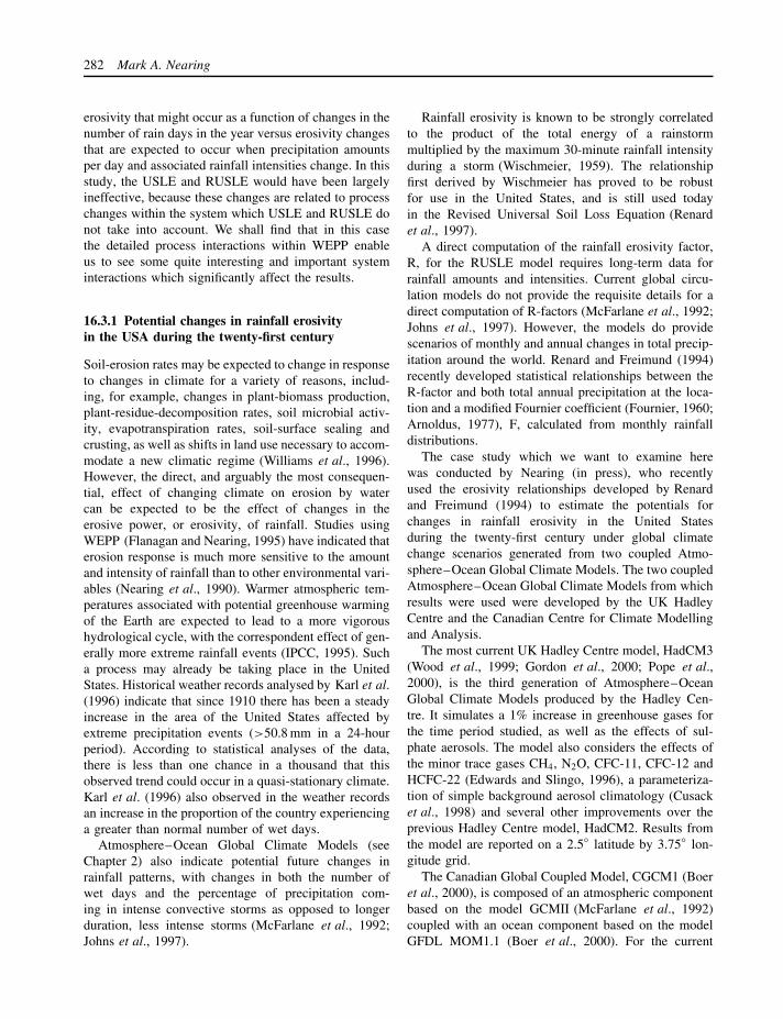
282 Mark A. Nearing
erosivity that might occur as a function of changes in thenumber of rain days in the year versus erosivity changesthat are expected to occur when precipitation amountsper day and associated rainfall intensities change. In thisstudy, the USLE and RUSLE would have been largelyineffective, because these changes are related to processchanges within the system which USLE and RUSLE donot take into account. We shall find that in this casethe detailed process interactions within WEPP enableus to see some quite interesting and important systeminteractions which significantly affect the results.
16.3.1 Potential changes in rainfall erosivityin the USA during the twenty-first century
Soil-erosion rates may be expected to change in responseto changes in climate for a variety of reasons, includ-ing, for example, changes in plant-biomass production,plant-residue-decomposition rates, soil microbial activ-ity, evapotranspiration rates, soil-surface sealing andcrusting, as well as shifts in land use necessary to accom-modate a new climatic regime (Williams et al., 1996).However, the direct, and arguably the most consequen-tial, effect of changing climate on erosion by watercan be expected to be the effect of changes in theerosive power, or erosivity, of rainfall. Studies usingWEPP (Flanagan and Nearing, 1995) have indicated thaterosion response is much more sensitive to the amountand intensity of rainfall than to other environmental vari-ables (Nearing et al., 1990). Warmer atmospheric tem-peratures associated with potential greenhouse warmingof the Earth are expected to lead to a more vigoroushydrological cycle, with the correspondent effect of gen-erally more extreme rainfall events (IPCC, 1995). Sucha process may already be taking place in the UnitedStates. Historical weather records analysed by Karl et al.(1996) indicate that since 1910 there has been a steadyincrease in the area of the United States affected byextreme precipitation events (>50.8 mm in a 24-hourperiod). According to statistical analyses of the data,there is less than one chance in a thousand that thisobserved trend could occur in a quasi-stationary climate.Karl et al. (1996) also observed in the weather recordsan increase in the proportion of the country experiencinga greater than normal number of wet days.
Atmosphere–Ocean Global Climate Models (seeChapter 2) also indicate potential future changes inrainfall patterns, with changes in both the number ofwet days and the percentage of precipitation com-ing in intense convective storms as opposed to longerduration, less intense storms (McFarlane et al., 1992;Johns et al., 1997).
Rainfall erosivity is known to be strongly correlatedto the product of the total energy of a rainstormmultiplied by the maximum 30-minute rainfall intensityduring a storm (Wischmeier, 1959). The relationshipfirst derived by Wischmeier has proved to be robustfor use in the United States, and is still used todayin the Revised Universal Soil Loss Equation (Renardet al., 1997).
A direct computation of the rainfall erosivity factor,R, for the RUSLE model requires long-term data forrainfall amounts and intensities. Current global circu-lation models do not provide the requisite details for adirect computation of R-factors (McFarlane et al., 1992;Johns et al., 1997). However, the models do providescenarios of monthly and annual changes in total precip-itation around the world. Renard and Freimund (1994)recently developed statistical relationships between theR-factor and both total annual precipitation at the loca-tion and a modified Fournier coefficient (Fournier, 1960;Arnoldus, 1977), F, calculated from monthly rainfalldistributions.
The case study which we want to examine herewas conducted by Nearing (in press), who recentlyused the erosivity relationships developed by Renardand Freimund (1994) to estimate the potentials forchanges in rainfall erosivity in the United Statesduring the twenty-first century under global climatechange scenarios generated from two coupled Atmo-sphere–Ocean Global Climate Models. The two coupledAtmosphere–Ocean Global Climate Models from whichresults were used were developed by the UK HadleyCentre and the Canadian Centre for Climate Modellingand Analysis.
The most current UK Hadley Centre model, HadCM3(Wood et al., 1999; Gordon et al., 2000; Pope et al.,2000), is the third generation of Atmosphere–OceanGlobal Climate Models produced by the Hadley Cen-tre. It simulates a 1% increase in greenhouse gases forthe time period studied, as well as the effects of sul-phate aerosols. The model also considers the effects ofthe minor trace gases CH4, N2O, CFC-11, CFC-12 andHCFC-22 (Edwards and Slingo, 1996), a parameteriza-tion of simple background aerosol climatology (Cusacket al., 1998) and several other improvements over theprevious Hadley Centre model, HadCM2. Results fromthe model are reported on a 2.5◦ latitude by 3.75◦ lon-gitude grid.
The Canadian Global Coupled Model, CGCM1 (Boeret al., 2000), is composed of an atmospheric componentbased on the model GCMII (McFarlane et al., 1992)coupled with an ocean component based on the modelGFDL MOM1.1 (Boer et al., 2000). For the current
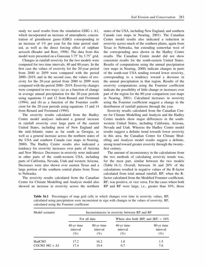
Soil Erosion and Conservation 283
study we used results from the simulation GHG + A1,which incorporated an increase of atmospheric concen-tration of greenhouse gases (GHG) corresponding toan increase of 1% per year for the time period stud-ied, as well as the direct forcing effect of sulphateaerosols (Reader and Boer, 1998). The data from thismodel were presented on a Gaussian 3.75◦ by 3.75◦ grid.
Changes in rainfall erosivity for the two models werecomputed for two time intervals, 40 and 80 years. In thefirst case the values of erosivity for the 20-year periodfrom 2040 to 2059 were compared with the period2000–2019, and in the second case, the values of ero-sivity for the 20-year period from 2080 to 2099 werecompared with the period 2000–2019. Erosivity changeswere computed in two ways: (a) as a function of changein average annual precipitation for the 20-year periodsusing equations 11 and 12 from Renard and Freimund(1994); and (b) as a function of the Fournier coeffi-cient for the 20-year periods using equations 13 and 14from Renard and Freimund (1994).
The erosivity results calculated from the HadleyCentre model analyses indicated a general increasein rainfall erosivity over large parts of the easternUnited States, including most of New England andthe mid-Atlantic states as far south as Georgia, aswell as a general increase across the northern states ofthe USA and southern Canada (see maps in Nearing,2000). The Hadley Centre results also indicated atendency for erosivity increases over parts of Arizonaand New Mexico. Decreases in erosivity were indicatedin other parts of the south-western USA, includingparts of California, Nevada, Utah and western Arizona.Decreases were also shown over eastern Texas and alarge portion of the southern central plains from Texasto Nebraska.
The erosivity results calculated from the CanadianCentre for Climate Modelling and Analysis model alsoshowed an increase in erosivity across the northern
states of the USA, including New England, and southernCanada (see maps in Nearing, 2001). The CanadianCentre model results also indicated a reduction inerosivity across much of the southern plains, again fromTexas to Nebraska, but extending somewhat west ofthe corresponding area shown in the Hadley Centreresults. The Canadian Centre model did not showconsistent results for the south-eastern United States.Results of computations using the annual precipitation(see maps in Nearing, 2000) indicate changes in partsof the south-east USA tending toward lower erosivity,corresponding to a tendency toward a decrease inthe annual precipitation in that region. Results of theerosivity computations using the Fournier coefficientindicate the possibility of little change or increases overpart of the region for the 80-year comparison (see mapsin Nearing, 2001). Calculated increases in erosivityusing the Fournier coefficient suggest a change in thedistribution of rainfall patterns through the year.
Erosivity results calculated from the Canadian Cen-tre for Climate Modelling and Analysis and the HadleyCentre models show major differences in the south-western United States, including California, Arizona,Nevada and Utah. Whereas the Hadley Centre modelresults suggest a definite trend towards lower erosivityin this area, the Canadian Centre for Climate Mod-elling and Analysis model results suggest a definite,strong trend toward greater erosivity through the twenty-first century.
The amount of inconsistency in the calculations fromthe two methods of calculating erosivity trends was,for the most part, similar between the two models(Table 16.1). Overall, between 16 and 20% of thecalculations resulted in negative values of the R-factorcalculated from total annual rainfall, RP, when the R-factor calculated from the Modified Fournier coefficient,RF, was positive, or vice versa. For the cases where bothRP and RF were large, i.e., greater than 10%, those
Table 16.1 Percentages of map grid cells in which changes over time in erosivity values, RP,calculated using precipitation were inconsistent in sign with changes in the values of erosivity, RF,calculated using the Fournier coefficient
Model scenario Inconsistencies in erosivity between RP and RF
For all data Where also both |RP| and |RF| < 10%
40-yr timeinterval
(%)
80-yr timeinterval
(%)
40-yr timeinterval
(%)
80-yr timeinterval
(%)
HadCM3 17.2 16.2 1.0 1.5CGCM1 HG + A1 17.4 19.4 0.7 7.6

284 Mark A. Nearing
percentages were much smaller, although 7.6% of thepairs were inconsistent in this case for the Canadianmodel results for the 80-year time interval (2000–2019to 2080–2099). It is not out of the question to expectinconsistencies between results of RP and RF, sinceRP is based on total annual precipitation and RF isbased on the monthly distributions of precipitation. Bothrelationships are statistically based, and we have noreason to favour one over the other.
One might expect a consistent trend for the changeof erosivity as a function of time, and in generalthis was true (Table 16.2). In this case, the Canadianmodel exhibited more inconsistency as a function oftime when using the monthly precipitation values tocalculate erosivity, though it was consistent temporallyin terms of the erosivity calculated using the annualprecipitation.
The RF values tended to show a somewhat greatermagnitude, in terms of the average of the absolutevalue of percentage erosivity change, than did theRP values (Table 16.3). The difference between thetwo models in this regard was striking. The Canadianmodel indicated a much greater level of erosivity
changes overall as compared to the Hadley Centre model(Table 16.3). Both models suggested erosivity changeswhich generally increased in magnitude from the 40-year to the 80-year comparison.
16.3.2 Effects of precipitation intensity changesversus number of days of rainfall
Now we take a look at another study of the effectsof precipitation changes on soil-erosion rates, but thistime we use the WEPP model. As we mentionedabove, historical weather records analysed by Karl et al.(1996) indicate that since 1910 there has been a steadyincrease in the area of the United States affected byextreme precipitation events as well as an increase inthe proportion of the country experiencing a greaterthan normal number of wet days. The results given byNearing (2001) discussed above provide a broad viewof expected changes in erosivity based on the statisticalmodels, but an important question not addressed is theexpected differences in erosivity that come about relativeto rainfall intensity versus a simple increase in theaverage number of rain days in a year. Erosion is not
Table 16.2 Percentages of map grid cells in which changes over time inerosivity values calculated over the 40-year time interval were inconsistent insign with changes in the values of erosivity calculated over the 80-year timeinterval
Model scenario Inconsistencies in erosivity between 40- and80-year time intervals
For all data Where also both the 40 yr |R|and the 80 yr |R| < 10%
RP RF RP RF(%) (%) (%) (%)
HadCM3 16.2 15.2 1.5 1.0CGCM1 HG + A1 7.6 23.6 0 5.6
Table 16.3 Average magnitudes (absolute values) of erosivity changecalculated
Model scenario Average magnitude of change
40-yr time interval 80-yr time interval
RP RF RP RF(%) (%) (%) (%)
HadCM3 11.8 16.5 15.9 20.9CGCM1 HG + A1 23.4 29.1 53.4 58.3

Soil Erosion and Conservation 285
linearly proportional to rainfall intensity (Wischmeierand Smith, 1978; Nearing et al., 1990).
Pruski and Nearing (2002) recently performed com-puter simulations to obtain estimates of potential runoffand soil loss changes as a function of precipita-tion changes. In particular, they studied the differentresponses of the erosional system to changes in precipi-tation as they occurred with changes in rainfall intensi-ties, including the amount of rainfall which occurs on agiven day of rain, versus responses to changes in simplythe average number of days of rain. Assessments weremade using WEPP for several combinations of geo-graphic locations, soils, crops and slopes. Geographiclocations included West Lafayette, IN, Temple, TX, andCorvallis, OR. Soils were sandy clay loam, silt loamand clay loam. Crops included grazing pasture, cornand soybean rotation, winter wheat and fallow. Slopeswere 3, 7 and 15%. Three scenarios of precipitationchanges were considered: (a) all precipitation changeoccurring as number of days of rainfall; (b) all precipi-tation change occurring as amount of rainfall in a givenday; and (c) half of the precipitation change occurringfrom each source. Under these scenarios, and using theclimate generator for WEPP, changes in the number ofdays of rainfall do not influence rainfall intensity, whilechanges in the amount of rainfall on a given day increasethe duration, peak intensities and average intensities ofrain. Levels of changes considered in each case wereapproximately zero, ±10% and ±20% of total precipi-tation, with the same relative proportion of precipitationfor the year maintained as a function of month.
Erosion rates changed much more with changes in theamount of rainfall per precipitation event, which alsoimplies changes in the rainfall durations and intensitiesfor the events. When total precipitation in this case wasincreased by 10%, soil loss increased by an averageof 26%. Realistically, we can expect that any changesin precipitation will come as a combination of bothchanges in the number of wet days as well as inchanges in the amount and intensities of rainfall. As wediscussed earlier, historical changes in rainfall over thepast century have occurred in both of these terms (Karlet al., 1996). For the combined case of both changesin wet days and changes in rainfall per day, Pruskiand Nearing (2002) found that erosion response wasintermediate to the two extremes. For a 10% increasein total precipitation, simulated erosion increased by anaverage of 16%.
The average results for the combined case of changesin both number of days of precipitation and changes inamount of rain per day from the study by Pruski andNearing (2002) are similar to those for the empirical
relationship proposed by Renard and Freimund (1994)between erosivity and total annual precipitation forthe RUSLE model as discussed above. Using Renardand Freimund’s first equation for erosivity results in a17% change as a function of a 10% change in totalannual precipitation. However, it is important to notethat regardless of this fact, obtaining the large-scaleerosivity change information similar to the informationwe obtained from the study discussed in the previoussection (Nearing, 2001) would have been extremelydifficult using WEPP.
Now let’s look at some of the details of the resultsfrom the WEPP erosivity study. Greater amounts andrates of runoff, other factors being equal, will generallytend to cause an increase in erosion. Increased runoffcauses increased energy of surface flow, which increasesthe detachment capability and the sediment-transportcapacity of the flow. Inter-rill erosion also increases withincreased rain.
The simulation results of Pruski and Nearing (2002)showed a general increase in soil loss with increasein precipitation, and vice versa (Table 16.4), how-ever, the changes were generally not as great as forrunoff (Table 16.5). One major reason for the differ-ence between the sensitivity results for runoff and thosefor soil loss is related to biomass production. Bothrunoff and soil loss are sensitive to biomass, but soilloss is more so. Soil loss is affected by plant canopy,which reduces the impact energy of rainfall; by cropresidues which protect the soil from raindrop impactand reduce rill detachment rates and sediment trans-port capacities; and from subsurface roots and decayingresidue, which mechanically hold the soil in place andprovide a medium for micro-organisms to live. Thus, theincrease of biomass production with increased rainfalltends to counteract to some degree the increased erosiv-ity of the rain. This argument is supported by the resultsof the simulations for fallow conditions in comparisonto the other treatments. The sensitivity values for thethree precipitation scenarios for fallow conditions aver-age 1.63 for soil loss and 1.55 for runoff. Thus fallowwas the only crop treatment for which the sensitivitiesfor runoff were less than for soil loss.
The difference between a sensitivity of 0.95 forsoil loss and 1.06 for runoff for the fallow scenarioof change only in the number of days of rainfall(Tables 16.4 and 16.5) can be explained in terms ofsurface sealing and consolidation processes. Surfacesealing and consolidation occur as a function of rainfallamount in nature and in the WEPP model (Flanaganand Nearing, 1995), so that any increase in rainfall willincrease soil resistance to erosion via consolidation. This

286 Mark A. Nearing
Table 16.4 Sensitivities of changes in soil loss to changes in average annual precipi-tation. Sensitivity values are calculated as the ratio of the percentage change in soil lossto the percentage change in precipitation. Values represent averages for all simulationruns associated with the soil, crop, slope or location listed in the first column. Valuesgreater than zero indicate that soil loss increases with increased annual precipitation.A value of greater than one indicates a greater percentage change in soil loss than thepercentage change in precipitation
Scenarios Normalized sensitivity of soil loss to changesin average annual precipitation
Change innumber
of wet days
Change inamount of rain
per day
Combinedchanges in
both
Silt loam soil 0.90 2.45 1.72Sandy loam soil 0.89 2.60 1.82Clay soil 0.79 2.10 1.46
Grazing pasture 1.02 2.66 1.96Fallow 0.95 2.22 1.71Corn and soybean 0.70 2.46 1.48Wheat winter 0.77 2.18 1.50
S-shape (0%–3%–1%) 40 m 0.92 2.47 1.71S-shape (0%–7%–1%) 40 m 0.84 2.40 1.67S-shape (0%–15%–1%) 40 m 0.82 2.27 1.61
West Lafayette, IN 0.74 2.35 1.56Temple, TX 0.88 2.10 1.50Corvallis, OR 0.92 2.69 1.93
Overall average 0.85 2.38 1.66
process also acts as a feedback effect, similar to, but inless degree, the effect of biomass on partially offsettingthe impact of increased rainfall on erosion. This explainsthe lesser sensitivity of 0.95 for soil loss as comparedto 1.06 for runoff.
The soil-loss sensitivity value for fallow conditionsfor the scenario of change in amount of rainfall perday was greater (2.22) than that for runoff (1.99),whereas for the other crops the trend was reversed(Tables 16.4 and 16.5). Although the effect of surfacesealing and consolidation as discussed above is presentin this case also, that effect is apparently supersededby yet another process when rainfall amounts andintensities per day are increased. These processes wererelated to rill- and inter-rill soil-detachment processes.Inter-rill erosion rates are represented in the WEPPmodel as proportional to the rainfall intensity andthe runoff rate (Flanagan and Nearing, 1995), whichare relationships based on experimental data (Zhanget al., 1996). Since both of these variables increasewith increased rainfall intensity, the effect of increased
rainfall intensity on inter-rill erosion is greater thanunity. Also, rill erosion occurs as a threshold process.Rill detachment occurs proportional to the excess shearstress of water flow above the threshold critical shearstress of the soil, rather than to the shear stress of theflow itself. The overall effect is that the sensitivity of therill erosion rate to runoff rate will be somewhat morethan unity, other factors being constant. The effect isnot present in the precipitation scenario of changes in thenumber of rainfall days because in that case, the averagerunoff rate is essentially not changing, but rather onlythe frequency of runoff events changes.
These are only a portion of the interactions discussedby Pruski and Nearing (2002) that were evident inthe results of this study, but they provide a flavourof the types of information which the process-basedmodel provides that the empirical model cannot address.Hopefully the above discussions of these two modelapplications will provide the reader with a sense ofhow each type of model might be used to advantagedepending upon the desired application.

Soil Erosion and Conservation 287
Table 16.5 Sensitivities of changes in runoff to changes in average annual precipi-tation. Sensitivity values are calculated as the ratio of the percentage change in runoffto the percentage change in precipitation. Values represent averages for all simulationruns associated with the soil, crop, slope or location listed in the first column. Valuesgreater than zero indicate that runoff increases with increased annual precipitation.A value of greater than one indicates a greater percentage change in runoff than thepercentage change in precipitation
Scenarios Normalized sensitivity of runoff to changesin average annual precipitation
Change innumber ofwet days
Change inamount of rain
per day
Combinedchangesin both
Silt loam soil 1.32 2.57 2.00Sandy loam soil 1.31 2.80 2.17Clay soil 1.15 2.17 1.75
Grazing pasture 1.54 3.09 2.41Fallow 1.06 1.99 1.60Corn and soybean 1.32 2.51 1.97Wheat winter 1.21 2.43 1.91
S-shape (0%–3%–1%) 40 m 1.32 2.59 2.03S-shape (0%–7%–1%) 40 m 1.29 2.49 1.98S-shape (0%–15%–1%) 40 m 1.23 2.42 1.91
West Lafayette, IN 1.16 2.61 1.94Temple, TX 1.19 2.25 1.73Corvallis, OR 1.50 2.64 2.23
Overall average 1.28 2.50 1.97
16.4 LESSONS AND IMPLICATIONS
At the start of this chapter we listed three primaryuses for soil-erosion models: (a) to help a land owneror manager choose suitable conservation; (b) to makelarge-scale erosion surveys in order to understand thescope of the problem over a region and to track changesin erosion over time; and (c) to regulate activities onthe land for purposes of conservation compliance. Letus look at each of these goals in turn.
Choosing how to manage land, from the practicalperspective, is often a matter of choosing between anarray of potential options. Often, therefore, what weneed to know is not necessarily the exact erosion ratefor a particular option to a high level of accuracy, butrather we want to know how the various options stackup against one another. We may certainly be interestedin having a general quantitative idea of the erosionrate, but for purposes of land management, this is notcritical. Choosing which model to use then becomes amatter of (a) what type of information we would like
to know, and (b) what information (data) we have forthe particular site of application. We know from ourdiscussions above that the USLE provides only estimatesof average annual soil loss on the portion of the field thatexperiences a net loss of soil. If we have an interest inoff-site impacts, then we probably want to choose eitherRUSLE, which will provide us with a rough idea of thesediment leaving the profile, or WEPP, if we want morecomprehensive sediment-yield information or if we aremodelling a small watershed. If we have an interest inobtaining other, auxiliary information about our choiceof management strategy, such as soil moisture or cropyields, we might also decide to use WEPP. On the otherhand, if data are limited for the situation to be modelled,then the USLE might be the best option in any case,and one would be forced to move to other options forassessing information not supplied by the USLE. At thecurrent time most applications of WEPP are possiblein the United States because of the availability of soil,climate and crop information, but in other areas thismight not be the case.

288 Mark A. Nearing
Making large-scale erosion surveys in order to under-stand the scope of the erosion problem over a region andto track changes in erosion over time can be done withany of the models discussed above. Often what is doneis to use a statistical sampling scheme to take randompoints over the area of interest, and to apply the erosionmodel to each point (USDA, 1996). In this case, too, weare not so concerned about the individual prediction foreach point of application, but rather the ability of themodel to predict overall averages of soil loss in a quan-titatively accurate manner. While we know that none ofthese models will necessarily predict erosion for a partic-ular site to the quantitative level of accuracy we wouldlike to see for survey assessment purposes (Nearing,2000), each of the three models does predict the aver-ages for treatments quite effectively (Risse, et al., 1993;Rapp, 1994; Zhang, et al., 1996). As with the case dis-cussed above, the issues related to choosing the correctmodel are related to the information desired and theavailable data.
Conservation compliance, governmental policy-mak-ing, and regulation of land-users’ actions follow thesame guidelines as for the other two applications:information desired and data availability are again thekeys to choice of model. In this case, however, theargument is often given, most often by the farmerwho is being regulated, that if we know that there areuncertainties in the erosion predictions for individualapplications, how can we be sure that his field is beingevaluated accurately? The answer is, of course, that wecannot be sure. If the model predicts that the farmer’sfield is eroding at a rate in excess of what our society’spolicy indicates to be acceptable, the model could wellbe wrong for this particular field. This problem is reallyno different from that faced by insurance companies asthey set rates for insurance coverage. My home maybe more secure from the possibility of fire than myneighbour’s home because I am more careful than myneighbour. But unless my home falls in a differentcategory (e.g. better smoke-alarm protection), I will nothave much luck in going to my insurance company andasking for a lower payment rate. Likewise, if I am thefarmer, I cannot expect to give a coherent argument forlower soil loss than the model predicts unless I conductsome practice, such as reduced tillage or buffers, whicharguably reduces erosion.
Complexity and uncertainty are key issues relativeto the development, understanding and use of erosionmodels for conservation purposes. They are inevitableconsiderations because of the many complex interac-tions inherent in the erosional system as well as theenormous inherent variability in measured erosion data.
These issues do not, however, prevent us from usingmodels effectively for conservation planning. In fact,the scientific evidence indicates that choice of models,which implies choice of model complexity, is more amatter of the type of information desired and the qualityand amount of data available for the specific applica-tion. If our goal is to know to a high level of accuracythe erosion rate on a particular area of ungauged land,we cannot rely upon the models. Natural variability istoo great, and uncertainty in predictions is too high (seeNearing, et al., 1999, 2000). For appropriate and com-mon uses, such as those discussed above, models can beeffective conservation tools.
ACKNOWLEDGEMENTS
The precipitation data from the HadCM3 model forthe period 2000–2099 were supplied by the ClimateImpacts LINK Project (DETR Contract EPG 1/1/68) onbehalf of the Hadley Centre and the UK MeteorologicalOffice. The precipitation data from the CGCM1 model,GHG + A1 scenario, for the period 2000–2099 wassupplied by the Canadian Centre for Climate Modellingand Analysis.
NOTE
1 Most of the early erosion plots were 1.83 m (6 feet)wide. A length of 22.13 m (72.6 feet) and a widthof 1.83 m (6 feet) resulted in a total area of 1/100of an acre. Prior to the days of calculators andcomputers this was obviously a convenient value forcomputational purposes.
REFERENCES
Arnold, J.G., Williams, J.R., Nicks, A.D. and Sammons, N.B.(1990) SWRRB: A Basin Scale Simulation Model for Soil andWater Resource Management, Texas A&M University Press,College Station, TX.
Arnoldus, H.M.L. (1977) Methodology used to determine themaximum potential average annual soil loss due to sheet andrill erosion in Morocco, FAO Soils Bulletin 34, 39–51.
Baffaut, C., Nearing, M.A. and Nicks, A.D. (1996) Impactof climate parameters on soil erosion using CLIGEN andWEPP, Transactions of the American Society of AgriculturalEngineers 39, 447–457.
Boer, G.J., Flato, G., Reader, M.C. and Ramsden, D. (2000)A transient climate change simulation with greenhouse gasand aerosol forcing: experimental design and comparisonwith the instrumental record for the 20th century, ClimateDynamics 16, 405–425.

Soil Erosion and Conservation 289
Chu, S.T. (1978) Infiltration during an unsteady rain, WaterResources Research 14 (3), 461–466.
Cusack, S., Slingo, A., Edwards, J.M. and Wild, M. (1998)The radiative impact of a simple aerosol climatology on theHadley Centre GCM, Quarterly Journal of the Royal Mete-orological Society 124 (551), 2517–2526.
Edwards, J.M. and Slingo, A. (1996) Studies with a flexiblenew radiation code. 1: choosing a configuration for a largescale model, Quarterly Journal of the Royal MeteorologicalSociety 122, 689–719.
Flanagan, D.C. and Livingston, S.J. (1995) USDA-Water Ero-sion Prediction Project: WEPP User Summary, NSERLReport No. 11, USDA-ARS National Soil Erosion ResearchLaboratory, West Lafayette, IN, 47097–1196.
Flanagan, D.C. and Nearing, M.A. (1995) USDA–Water Ero-sion Prediction Project: Hillslope Profile and WatershedModel Documentation, NSERL Report No. 10, USDA-ARSNational Soil Erosion Research Laboratory, West Lafayette,IN, 47097–1196.
Foster, G.R., McCool, D.K., Renard, K.G. and Moldenhauer,W.C. (1981) Conversion of the universal soil loss equationto SI metric units, Journal of Soil and Water Conservation36, 355–359.
Fournier, F. (1960) Climat et Erosion, Universitaries de France,Paris.
Gordon, C., Cooper, C., Senior, C.A., Banks, H., Gregory, J.M.,Johns, T.C., Mitchell, J.F.B. and Wood, R.A. (2000) Thesimulation of SST, sea ice extents and ocean heat transportsin a version of the Hadley Centre coupled model withoutflux adjustments, Climate Dynamics 16 (2–3), 147–168.
Govers, G. (1991) Rill erosion on arable land in centralBelgium: rates, controls, and predictability, Catena 18,133–155.
Govers, G. (1996) Soil erosion process research: a state ofthe art, Academie voor Wetenschappen, Letteren en SchoneKunsten van Belgie, Klasse der Wettenschappen 58 (1).
IPCC (1995) Second Assessment Synthesis of Scientific-Technical Information Relevant to Interpreting Article 2of the UN Framework Convention on Climate Change,Intergovernmental Panel on Climate Change, Geneva,Switzerland.
Johns, T.C., Carnell, R.E., Crossley, J.F., Gregory, J.M., Mit-chell, J.F.B., Senior, C.A., Tett, S.F.B. and Wood, R.A.(1997) The second Hadley Centre coupled ocean–at-mosphere GCM: model description, spin-up and validation,Climate Dynamics 13, 103–134.
Karl, T.R., Knight, R.W., Easterling, D.R. and Quayle, R.G.(1996) Indices of climate change for the United States,Bulletin of the American Meteorological Society 77 (2),279–292.
Larionov, G.A. (1993) Erosion and Wind Blown Soil, MoscowState University Press, Moscow.
Liu, B.Y., Nearing, M.A., Baffaut, C. and Ascough II, J.C.(1997) The WEPP watershed model: III. Comparisons tomeasured data from small watersheds, Transactions of theAmerican Society of Agricultural Engineers 40 (4), 945–951.
McFarlane, N.A., Boer, G.J., Blanchet, J.-P. and Lazare, M.(1992) The Canadian Climate Centre second-generation
general circulation model and its equilibrium climate, Jour-nal of Climate 5, 1013–1044.
Mein, R.G. and Larson, C.L. (1973) Modeling infiltration dur-ing a steady rain, Water Resources Research 9 (2), 384–394.
Misra, R.K. and Rose, C.W. (1996) Application and sensitivityanalysis of process-based erosion model GUEST, EuropeanJournal of Soil Science 47, 593–604.
Morgan, R.P.C., Quinton, J.N., Smith, R.E., Govers, G., Poe-sen, J.W.A., Auerswald, K., Chisci, G., Torri, D. and Sty-czen, M.E. (1998) The European Soil Erosion Model(EUROSEM): a dynamic approach for predicting sedimenttransport from fields and small catchments, Earth SurfaceProcesses and Landforms 23, 527–544.
Nearing, M.A. (1998) Why soil erosion models over-predictsmall soil losses and under-predict large soil losses, Catena32, 15–22.
Nearing, M.A. (2000) Evaluating soil erosion models usingmeasured plot data: accounting for variability in the data,Earth Surface Processes and Landforms 25, 1035–1043.
Nearing, M.A. (2001) Potential changes in rainfall erosivity inthe U.S. with climate change during the 21st century, Journalof Soil and Water Conservation 56, 229–232.
Nearing, M.A., Ascough, L.D. and Laflen, J.M. (1990) Sensi-tivity analysis of the WEPP hillslope profile erosion model,Transactions of the American Society of Agricultural Engi-neers 33, 839–849.
Nearing, M.A., Foster, G.R., Lane, L.J. and Finkner, S.C.(1989) A process-based soil erosion model for USDA–WaterErosion Prediction Project technology, Transactions of theAmerican Society of Agricultural Engineers 32, 1587–1593.
Nearing, M.A., Govers, G. and Norton, L.D. (1999) Variabilityin soil erosion data from replicated plots, Soil Science Societyof America Journal 63 (6), 1829–1835.
Nicks, A.D. (1985) Generation of climate data, in D.G. De-Coursey (ed.) Proceedings of the Natural ResourcesModeling Symposium, Pingree Park, CO, 16–21 October1983, USDA-ARS ARS-30.
Ott, L. (1977) An Introduction to Statistical Methods and DataAnalysis, Duxbury Press, North Scituate, MA.
Pimentel, D.E. et al. (1995) Environmental and economic costsof soil erosion and conservation benefits, Science 267,1117–1123.
Pope, V.D., Gallani, M.L., Rowntree, P.R. and Stratton, R.A.(2000) The impact of new physical parametrizations in theHadley Centre climate model – HadAM3, Climate Dynamics16 (2–3), 123–146.
Pruski, F.F. and Nearing, M.A. (2002) Runoff and soil-lossresponses to changes in precipitation: a computer simulationstudy, Journal of Soil and Water Conservation 57, 7–16.
Rapp, J.F. (1994) Error assessment of the Revised UniversalSoil Loss Equation using natural runoff plot data, MSthesis, School of Renewable Natural Resources, Universityof Arizona, Tucson, AZ.
Reader, M.C. and Boer, G.J. (1998) The modification of green-house gas warming by the direct effect of sulphate aerosols,Climate Dynamics 14, 593–607.
Renard, K.G., Foster, G.R., Weesies, G.A., McCool, D.K.and Yoder, D.C. (1997) Predicting Soil Erosion by Water:

290 Mark A. Nearing
A Guide to Conservation Planning with the Revised Uni-versal Soil Loss Equation (RUSLE), Agricultural HandbookNo. 703, US Government Printing Office, Washington, DC.
Renard, K.G. and Freimund, J.R. (1994) Using monthly pre-cipitation data to estimate the R-factor in the revised USLE,Journal of Hydrology 157, 287–306.
Risse, L.M., Nearing, M.A., Nicks, A.D. and Laflen, J.M.(1993) Assessment of error in the Universal Soil LossEquation, Soil Science Society of America Journal 57,825–833.
Ruttimann, M., Schaub, D., Prasuhn, V. and Ruegg, W. (1995)Measurement of runoff and soil erosion on regularly culti-vated fields in Switzerland – some critical considerations,Catena 25, 127–139.
Schwertmann, U., Vogl, W. and Kainz, M. (1990) Bodenero-sion durch Wasser, Eugen Ulmer GmbH and Co., Stuttgart.
USDA (1996) Summary Report 1992: National Resource Inven-tory, US Government Printing Office, Washington, DC.
Walpole, R.E. and Myers, R.H. (1993) Probability and Statis-tics for Engineers and Scientists, 5th edn, Prentice Hall,Englewood Cliffs, NJ.
Wendt, R.C., Alberts, E.E. and Hjelmfelt, A.T. Jr. (1986) Vari-ability of runoff and soil loss from fallow experimental plots,Soil Science Society of America Journal 50, 730–736.
Williams, J., Nearing, M.A., Nicks, A., Skidmore, E., Valen-tine, C., King, K. and Savabi, R. (1996) Using soil erosion
models for global change studies, Journal of Soil and WaterConservation 51 (5), 381–385.
Williams, J.R. and Nicks, A.D. (1985) SWRRB, a simula-tor for water resources in rural basins: an overview, inD.G. DeCoursey (ed.) Proceedings of the Natural ResourcesModeling Symposium, Pingree Park, CO, 16–21 October1983, USDA-ARS, ARS-30, 17–22.
Wischmeier, W.H. (1959) A rainfall erosion index for a uni-versal soil loss equation, Soil Science Society of AmericaProceedings 23, 322–326.
Wischmeier, W.H. and Smith, D.D. (1965) Predicting RainfallErosion Losses in the Eastern US: A Guide to ConservationPlanning, Agricultural Handbook No. 282, US GovernmentPrinting Office, Washington, DC.
Wischmeier, W.H. and Smith, D.D. (1978) Predicting RainfallErosion Losses: A Guide to Conservation Planning, Agricul-tural Handbook No. 537, US Government Printing Office,Washington, DC.
Wood, R.A., Keen, A.B., Mitchell, J.F.B. and Gregory, J.M.(1999) Changing spatial structure of the thermohaline circu-lation in response to atmospheric CO2 forcing in a climatemodel, Nature 399, 572–575.
Zhang, X.C., Nearing, M.A., Risse, L.M. and McGregor, K.C.(1996) Evaluation of runoff and soil loss predictions usingnatural runoff plot data, Transactions of the American Societyof Agricultural Engineers 39 (3), 855–863.

17
Modelling in Forest Management
MARK J. TWERY
17.1 THE ISSUE
Forest management has traditionally been consideredmanagement of trees for timber. It really includes veg-etation management and land management and peoplemanagement as multiple objectives. As such, forest man-agement is intimately linked with other topics in thisvolume, most especially those chapters on ecologicalmodelling and human dimensions. The key to responsi-ble forest management is to understand both how forestecosystems work and how to use this understanding tosatisfy society’s expectations and values. The key to for-est modelling is to portray accurately the dynamics offorests. Successful forest-management modelling findsa means to improve management through accurate rep-resentation of all parts of the system. In this chapter Iwill review both modelling approaches and the typesof applications that various modelling techniques havebeen used to address.
The complexity of forest management does not stopwith the intricate details of the biological system foundin a forest. Because all forest management is by peopleto meet goals or objectives desired by people, forestryis at its core a social activity. Thus, it demands that weunderstand the relationships among land owners, pro-fessional forest managers, forest-dependent communitiesand other stakeholders if we are to model the results ofdecisions regarding forest management. Individuals andcommunities have broad interests in the physical, biolog-ical and social goods and services that forest ecosystemsprovide. To meet the challenges of today we need toknow as much about the people as about the physicaland biological conditions, and to deepen our understand-ing of the social goods and services that we expect ourforest ecosystems to supply.
Models used to assist in forest management consist ofseveral types. First and most prevalent are growth andyield models, which predict the development of standsof trees through time. Initially, these models focusedon single species, single age stands, such as one wouldfind in plantations. Little wonder, because in plantationswere the highest investments of forest managers whoprimarily sought timber value from the forest. Asmodelling sophistication increased, so did the models.Multiple species and multiple age and size classes in anindividual stand have been included in growth modelswith varying success. Further developments along adifferent track have seen modelling techniques used tohelp schedule activities, such as harvesting or thinningin forests. Linear programming and other techniques thatallow a modeller to specify constraints on resources haveallowed models to find solutions to allocation problems,again primarily for those interested in extracting timbervalue from forests.
As various public and private groups have come torecognize the importance of forests for values beyondtimber and focused research into those topics, furthermodelling efforts have begun to characterize theseresources. Wildlife habitat, recreation opportunities andwatershed protection are just a few of the benefits thatnow must be modelled and presented to decision-makersfor their evaluation of alternative forest managementstrategies. These efforts face many challenges due tothe inherent complexities of the systems they attempt tomodel and the lack of good quantitative date for many ofthe factors involved. In addition, the most complex andfuzziest of the factors is that of the role of humans in theforest. Models capable of predicting human needs anddesires, and their implications for the state of forestedecosystems, are a great need that is still largely unmet.
Environmental Modelling: Finding Simplicity in Complexity. Edited by J. Wainwright and M. Mulligan 2004 John Wiley & Sons, Ltd ISBNs: 0-471-49617-0 (HB); 0-471-49618-9 (PB)
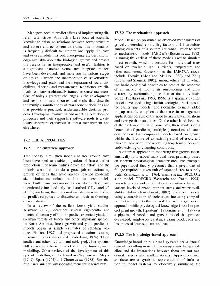
292 Mark J. Twery
Managers need to predict effects of implementing dif-ferent alternatives. Although a large body of scientificknowledge exists on relations between forest structureand pattern and ecosystem attributes, this informationis frequently difficult to interpret and apply. To haveand to use models that both incorporate the best knowl-edge available about the biological system and presentthe results in an interpretable and useful fashion isa significant challenge. Some such integrated modelshave been developed, and more are in various stagesof design. Further, the incorporation of stakeholders’knowledge and goals, and the integration of social dis-ciplines, theories and measurement techniques are dif-ficult for many traditionally trained resource managers.One of today’s greatest challenges is the developmentand testing of new theories and tools that describethe multiple ramifications of management decisions andthat provide a practical, understandable decision pro-cess. Developing, evaluating and adapting new decisionprocesses and their supporting software tools is a crit-ically important endeavour in forest management andelsewhere.
17.2 THE APPROACHES
17.2.1 The empirical approach
Traditionally, simulation models of tree growth havebeen developed to enable projection of future timberproduction. Economic values drove the effort, and themodels were built to do a good job of estimatinggrowth of trees that have already reached moderatesize. Limitations include the fact that these modelswere built from measurements on stands that haveintentionally included only ‘undisturbed, fully stocked’stands, rendering them of questionable use when tryingto predict responses to disturbances such as thinningsor windstorms.
In a review of the earliest forest yield studies,Assmann (1970) describes several eighteenth- andnineteenth-century efforts to predict expected yields inGerman forests of beech and other important species.In North America, forest growth and yield predictionmodels began as simple estimates of standing vol-ume (Pinchot, 1898) and progressed to estimates usingincrement cores (Fenska and Lauderburn, 1924). Thesestudies and others led to stand table projection systemsstill in use as a basic form of empirical forest-growthmodelling. Other reviews of the development of thistype of modelling can be found in Chapman and Meyer(1949), Spurr (1952) and Clutter et al. (1983). See alsohttp://sres.anu.edu.au/associated/mensuration/xref.htm.
17.2.2 The mechanistic approach
Models based on presumed or observed mechanisms ofgrowth, theoretical controlling factors, and interactionsamong elements of a system are what I refer to hereas mechanistic models. JABOWA (Botkin et al., 1972)is among the earliest of these models used to simulateforest growth, which it predicts for individual treesbased on available light, nutrients, temperature andother parameters. Successors to the JABOWA modelinclude Fortnite (Aber and Melillo, 1982) and Zelig(Urban and Shugart, 1992), among others, all of whichuse basic ecological principles to predict the responseof an individual tree to its surroundings and growa forest by accumulating the sum of the individuals.Sortie (Pacala et al., 1993, 1996) is a spatially explicitmodel developed using similar ecological variables tothe earlier gap models. The stochastic element addedto gap models complicates their use in managementapplications because of the need to run many simulationsand average their outcomes. On the other hand, becauseof their reliance on basic principles, these models do abetter job of predicting multiple generations of forestdevelopment than empirical models based on growthwithin the lifetime of an existing stand of trees, andthus are more useful for modelling long-term successionunder existing or changing conditions.
A different approach to modelling tree growth mech-anistically is to model individual trees primarily basedon inherent physiological characteristics. For example,the pipe-model theory presumes that a given unit offoliage requires a given unit of sapwood area to supplywater (Shinozaki et al., 1964; Waring et al., 1982). Onesuch model, TREGRO (Weinstein and Yanai, 1994),predicts growth and carbon allocation patterns based onvarious levels of ozone, nutrient stress and water avail-ability. Hybrid (Friend et al., 1997) is a growth modelusing a combination of techniques, including competi-tion between plants that is modelled with a gap modelapproach, while physiological knowledge is used to pre-dict plant growth. Pipestem∗1
(Valentine et al., 1997) isa pipe-model-based stand growth model that projectseven-aged, single-species stands using production andloss rates of leaves, stems and roots.
17.2.3 The knowledge-based approach
Knowledge-based or rule-based systems are a specialcase of modelling in which the components being mod-elled and the interactions between them are not nec-essarily represented mathematically. Approaches suchas these use a symbolic representation of informa-tion to model systems by effectively simulating the

Modelling in Forest Management 293
logical processes of human experts (Reynolds et al.,1999). Knowledge-based systems have the advantagesthat they do not necessarily require the specific, detaileddata that many simulation models do, and they canbe adapted to situations in which some informationmay be lacking entirely. As such, they can be veryuseful in providing assistance to decision-makers whomust analyse situations and choose actions without com-plete knowledge. Schmoldt and Rauscher (1996) pointout that knowledge-based systems also prove useful asagents to codify institutional memory, manage the col-lection and delivery of scientific knowledge, and trainmanagers through their ability to provide explanationsof their reasoning processes. All these characteristicsmake knowledge-based models extremely useful in for-est management.
17.3 THE CONTRIBUTION OF MODELLING
17.3.1 Models of the forest system
17.3.1.1 Growth and yield models
Predicting growth and yield has long been at the heart ofsimulating the future of forests. Growth and yield mod-els were classified by Clutter et al. (1983) as for naturalforests (either even-aged or uneven-aged) or plantations(either thinned or unthinned). Early modelling efforts,restricted by lack of computational power, typicallyresulted in the publication of yield tables that presentedbasal area or volume of a stand at regular intervals ofdevelopment. See Hann and Riitters (1982) for a sum-mary of such models in the western United States orSchumacher and Coile (1960) for an example from thesoutheastern United States. Assmann (1970) presents acomprehensive description of the history of Europeanforest-yield modelling. Often, such yield tables are stilladequate for managers interested primarily in timber-volume production and who have only extensive data onsize class and basal area in their stands. Without moredetailed data to run computer-based simulation models,yield tables still prove useful.
Computer-based simulation models now dominate thefield. Simulators may be divided between stand-levelmodels that project stand-level summary variables suchas basal area and number of stems, or individual treemodels that project individual trees from a tree list orby species and size class. Individual tree models can befurther classified as distance-independent or distance-dependent. Clutter (1983) provides a detailed review ofthe various techniques. Ritchie (1999) has compiled anexhaustive description of the numerous growth and yield
simulators available for the western United States andan extensive bibliography of publications using the var-ious simulators. Ritchie (1999)∗ describes some newertechniques in individual tree modelling, including disag-gregative techniques in which stands grown as a wholeare disaggregated among trees in a list, which is main-tained to allow more detailed stand parameters needed inpredicting other variables. His analysis includes an eval-uation of the suitability of the models for managementplanning. Pretzsch (2001) reviews forest growth mod-elling from a European perspective, including recentlydeveloped simulators of growth and visualization suchas SILVA.
Examples of growth models in use in the easternUnited States include FIBER, SILVAH and TWIGS.FIBER∗ (Solomon et al., 1995) is a two-stage matrixmodel using dynamic transition probabilities for differ-ent ecological classifications to obtain the growth oftrees between diameter classes. These transition prob-abilities are a function of diameter, initial and resid-ual stand basal area, proportion of hardwoods, andelevation. SILVAH∗ (Marquis and Ernst, 1992) is anexpert system for making silvicultural decisions in hard-wood stands of the Allegheny Plateau and AlleghenyMountain region that recommends appropriate treat-ments based on user objectives and overstorey, under-storey and site data provided by the user. SILVAHalso contains a forest-stand growth simulator, providesthe ability to test alternative cuts, enables develop-ment of a forest-wide inventory database, and facilitatesother forest management planning functions. TWIGS∗(Miner et al., 1988) is a computer program used tosimulate growth and yield for forests in the NorthCentral region of the United States. It grows indi-vidual tree lists, has a regeneration component, andalso includes management and economic analyses. Twovariants are available: Central States (Indiana, Illinois,and Missouri) and Lake States (Michigan, Minnesota,and Wisconsin).
17.3.1.2 Regeneration models
Models of forest regeneration that provide reasonableestimates of tree species composition and density aftera disturbance have been difficult to develop. Gap-dynamics models in the JABOWA family tend to usean approach of generating many small individuals in apredetermined proportion based on their prevalence inthe seed bank or in the overstorey before disturbanceand letting them die in early steps of the simulation.Empirical stand models typically have no regenerationfunction or a crude one that applies ingrowth to the
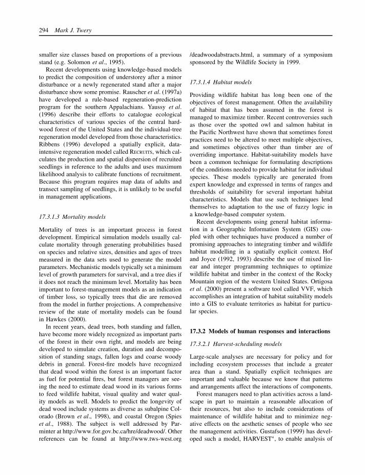
294 Mark J. Twery
smaller size classes based on proportions of a previousstand (e.g. Solomon et al., 1995).
Recent developments using knowledge-based modelsto predict the composition of understorey after a minordisturbance or a newly regenerated stand after a majordisturbance show some promise. Rauscher et al. (1997a)have developed a rule-based regeneration-predictionprogram for the southern Appalachians. Yaussy et al.(1996) describe their efforts to catalogue ecologicalcharacteristics of various species of the central hard-wood forest of the United States and the individual-treeregeneration model developed from those characteristics.Ribbens (1996) developed a spatially explicit, data-intensive regeneration model called RECRUITS, which cal-culates the production and spatial dispersion of recruitedseedlings in reference to the adults and uses maximumlikelihood analysis to calibrate functions of recruitment.Because this program requires map data of adults andtransect sampling of seedlings, it is unlikely to be usefulin management applications.
17.3.1.3 Mortality models
Mortality of trees is an important process in forestdevelopment. Empirical simulation models usually cal-culate mortality through generating probabilities basedon species and relative sizes, densities and ages of treesmeasured in the data sets used to generate the modelparameters. Mechanistic models typically set a minimumlevel of growth parameters for survival, and a tree dies ifit does not reach the minimum level. Mortality has beenimportant to forest-management models as an indicationof timber loss, so typically trees that die are removedfrom the model in further projections. A comprehensivereview of the state of mortality models can be foundin Hawkes (2000).
In recent years, dead trees, both standing and fallen,have become more widely recognized as important partsof the forest in their own right, and models are beingdeveloped to simulate creation, duration and decompo-sition of standing snags, fallen logs and coarse woodydebris in general. Forest-fire models have recognizedthat dead wood within the forest is an important factoras fuel for potential fires, but forest managers are see-ing the need to estimate dead wood in its various formsto feed wildlife habitat, visual quality and water qual-ity models as well. Models to predict the longevity ofdead wood include systems as diverse as subalpine Col-orado (Brown et al., 1998), and coastal Oregon (Spieset al., 1988). The subject is well addressed by Par-minter at http://www.for.gov.bc.ca/hre/deadwood/. Otherreferences can be found at http://www.tws-west.org
/deadwoodabstracts.html, a summary of a symposiumsponsored by the Wildlife Society in 1999.
17.3.1.4 Habitat models
Providing wildlife habitat has long been one of theobjectives of forest management. Often the availabilityof habitat that has been assumed in the forest ismanaged to maximize timber. Recent controversies suchas those over the spotted owl and salmon habitat inthe Pacific Northwest have shown that sometimes forestpractices need to be altered to meet multiple objectives,and sometimes objectives other than timber are ofoverriding importance. Habitat-suitability models havebeen a common technique for formulating descriptionsof the conditions needed to provide habitat for individualspecies. These models typically are generated fromexpert knowledge and expressed in terms of ranges andthresholds of suitability for several important habitatcharacteristics. Models that use such techniques lendthemselves to adaptation to the use of fuzzy logic ina knowledge-based computer system.
Recent developments using general habitat informa-tion in a Geographic Information System (GIS) cou-pled with other techniques have produced a number ofpromising approaches to integrating timber and wildlifehabitat modelling in a spatially explicit context. Hofand Joyce (1992, 1993) describe the use of mixed lin-ear and integer programming techniques to optimizewildlife habitat and timber in the context of the RockyMountain region of the western United States. Ortigosaet al. (2000) present a software tool called VVF, whichaccomplishes an integration of habitat suitability modelsinto a GIS to evaluate territories as habitat for particu-lar species.
17.3.2 Models of human responses and interactions
17.3.2.1 Harvest-scheduling models
Large-scale analyses are necessary for policy and forincluding ecosystem processes that include a greaterarea than a stand. Spatially explicit techniques areimportant and valuable because we know that patternsand arrangements affect the interactions of components.
Forest managers need to plan activities across a land-scape in part to maintain a reasonable allocation oftheir resources, but also to include considerations ofmaintenance of wildlife habitat and to minimize neg-ative effects on the aesthetic senses of people who seethe management activities. Gustafson (1999) has devel-oped such a model, HARVEST∗, to enable analysis of
Modelling in Forest Management 295
such activities across a landscape, including an edu-cational version, HARVEST Lite. The model has nowbeen combined with LANDIS∗ (Mladenoff et al., 1996)to integrate analyses of timber harvesting, forest suc-cession and landscape patterns (Gustafson and Crow,1999; Gustafson et al., 2000). Hof and Bevers (1998)take a mathematical optimization approach to a simi-lar problem, to maximize or minimize a managementobjective using spatial optimization given constraints oflimited area, finite resources and spatial relationships inan ecosystem.
17.3.2.2 Recreation-opportunity models
Providing recreation opportunities is an important part offorest management, especially on public lands. Indeed,the total value generated from recreation on NationalForests in the United States competes with that fromtimber sales, and may well surpass it soon (USDA For-est Service, 1995). Forest managers have long used theconcept of a ‘recreation opportunity spectrum’ (Driverand Brown, 1978) to describe the range of recreationactivities that might be feasible in a particular area, withthe intention of characterizing the experience and evalu-ating the compatibility of recreation with other activitiesand goals in a particular forest or other property.
RBSIM∗ (Gimblett et al., 1995, 1996) is a computerprogram that simulates the behaviour of human recre-ationists in high-use natural environments using GISto represent the environment and autonomous humanagents to simulate human behaviour within geographicspace. In RBSim, combinations of hikers, mountain bik-ers and jeep tours are assigned individual characteristicsand set loose to roam mountain roads and trails. Thebehaviours and interactions of the various agents arecompiled and analysed to provide managers with eval-uations of the likely success of an assortment of man-agement options.
17.3.2.3 Visualization
Many people tend to respond to visual images, leading tothe adage, ‘a picture is worth a thousand words’. Muchinformation generated by forest models is in the form ofdata tables, which are intelligible to the well initiated,but meaningless to many, including public stakehold-ers and many forest managers. Photographs of a forestmay be nearly as good at conveying an image of theconditions as actually visiting a site, but models areused to project conditions that do not yet exist. Thebest available means of providing an image of poten-tial future conditions is a computer representation of the
data. One such system, the Stand Visualization System(SVS∗) (McGaughey, 1997), generates graphic imagesdepicting stand conditions represented by a list of indi-vidual stand components, e.g., trees, shrubs and downmaterial. It is in wide use as a secondary tool, connectedto growth models such as FVS∗ (Stage, 1973, 1997),LMS (McCarter et al., 1998) and NED (Twery et al.,2000). UTOOLS∗ and UVIEW are geographic analy-sis and visualization software for watershed-level plan-ning (Ager and McGaughey, 1997). The system uses aParadox database to store spatial information and dis-plays landscape conditions of a forested watershed in aflexible framework. Another similar visualization tool isSmartForest∗ (Orland, 1995), which is also an interac-tive program to display forest data for the purposes ofvisualizing the effects of various alternative treatmentsbefore actually implementing them. Different versionshave been developed on a variety of platforms, manyof them requiring more data or computer power thanis practical for management activities, but SmartForestII (Orland et al., 1999) is designed to run on a PC anddisplay either stand-level or landscape data. Recently,McGaughey has developed an advanced landscape-scalevisualization program addressing the same issues, enti-tled EnVision∗.
17.3.3 Integrating techniques
17.3.3.1 Decision-support systems
Adaptive management has recently been viewed as avery promising and intuitively useful conceptual strate-gic framework for defining ecosystem management(Rauscher, 1999). Adaptive management is a continu-ing cycle of four activities: planning, implementation,monitoring and evaluation (Walters and Holling, 1990;Bormann et al., 1993). Planning is the process of decid-ing what to do. Implementation is deciding how to doit and then doing it. Monitoring and evaluation incor-porate analysing whether the state of the managed sys-tem was moved closer to the desired goal state or not.After each cycle, the results of evaluation are providedto the planning activity to produce adaptive learning.Unfortunately, this general theory of decision analysis isnot specific enough to be operational. Further, differentdecision-making environments typically require differ-ent, operationally specific decision processes. Decision-support systems are combinations of tools designed tofacilitate operation of the decision process (Oliver andTwery, 1999).
Mowrer et al. (1997) surveyed 24 of the lead-ing ecosystem-management decision-support systems

296 Mark J. Twery
(EM-DSS) developed in the government, academic andprivate sectors in the United States. Their report iden-tified five general trends: (1) while at least one EM-DSS fulfilled each criterion in the questionnaire used,no single system successfully addressed all importantconsiderations; (2) ecological and management interac-tions across multiple scales were not comprehensivelyaddressed by any of the systems evaluated; (3) theability of the current generation EM-DSS to addresssocial and economic issues lags far behind biophys-ical issues; (4) the ability to simultaneously considersocial, economic and biophysical issues is entirely miss-ing from current systems; (5) group consensus-buildingsupport was missing from all but one system – a systemwhich was highly dependent upon trained facilitationpersonnel (Mowrer et al., 1997). In addition, systemsthat did offer explicit support for choosing amongalternatives provided decision-makers with only onechoice of methodology.
There are few full-service DSSs for ecosystem man-agement (Table 17.1). At each operational scale, com-peting full-service EM-DSSs implement very differentdecision processes because the decision-making envi-ronment they are meant to serve is very different. Forexample, at the management-unit level, EM-DSSs canbe separated into those that use a goal-driven approachand those that use a data-driven approach to the deci-sion support problem. NED (Rauscher et al., 1997a;Twery et al., 2000) is an example of a goal-drivenEM-DSS where goals are selected by the user(s). Infact, NED is the only goal-driven, full-service EM-DSSoperating at the management-unit level. These goalsdefine the desired future conditions, which define thefuture state of the forest. Management actions shouldbe chosen that move the current state of the forestcloser to the desired future conditions. In contrast,INFORMS (Williams et al., 1995) is a data-driven sys-tem that begins with a list of actions and searches the
Table 17.1 A representative sample of existing ecosystem management decision-support software for forest conditionsof the United States arranged by operational scale and function
Full service EM-DSS Functional service modules
Operational scale Models Function Models
Regional EMDS Group negotiations AR/GISAssessments LUCAS ∗ IBIS ∗
Vegetation dynamics FVSRELM LANDIS
Forest-level SPECTRUM CRBSUMplanning WOODSTOCK SIMPPLLE
ARCFORESTSARA Disturbance FIREBGCTERRA VISION simulations GYPSESEZ-IMPACT ∗ UPESTDECISION PLUS ∗DEFINITE ∗ UTOOLS/UVIEW
Spatial visualization SVS ∗NED SMARTFOREST ∗INFORMS
Management-unit- MAGIS LOKIlevel planning KLEMS Interoperable system CORBA ∗
TEAMS architectureLMS ∗ IMPLAN
Economic impactanalysis SNAPActivity scheduling
Note: ∗ References for models not described in Mowrer et al. (1997): EZ-IMPACT (Behan, 1994); DECISION PLUS (Sygenex, 1994); IBIS(Hashim, 1990); DEFINITE (Janssen and van Herwijnen, 1994); SMARTFOREST (Orland, 1995); CORBA (Otte et al., 1996); SVS (McGaughey,1997); LMS (Oliver and McCarter, 1996); LUCAS (Berry et al., 1996).
Modelling in Forest Management 297
existing conditions to find possible locations to imple-ment those management actions.
Group decision-making tools are a special categoryof decision support, designed to facilitate negotiationand further progress toward a decision in a situation inwhich there are multiple stakeholders with varied per-spectives and opinions of both the preferred outcomesand the means to proceed. Schmoldt and Peterson (2000)describe a methodology using the analytic hierarchy pro-cess (Saaty, 1980) to facilitate group decision-makingin the context of a fire-disturbance workshop, in whichthe objective was to plan and prioritize research activi-ties. Faber et al. (1997) developed an ‘Active ResponseGIS’ that uses networked computers to display proposedoptions and as intermediaries to facilitate idea generationand negotiation of alternative solutions for managementof US national forests.
17.4 LESSONS AND IMPLICATIONS
17.4.1 Models can be useful
Models of various kinds have been very useful to forestmanagement for a long time. The most basic modelsprovide at least an estimate of how much timber isavailable and what it may be worth on the market, sothat managers can determine the economic feasibility oftimber cutting. More sophisticated modelling techniquesprovide better estimates of timber, include other forestcharacteristics, and project likely developments intothe future. Reliability of empirical models tends to berestricted to the current generation of trees, for whichthey are very good.
Other forest-growth models use ecological and phys-iological principles to make projections of growth. The-oretical, mechanistically based models tend to be betterfor general pictures of forest characteristics in a moredistant future projection, but may be less reliable fornear-term forecasts. They tend to require more data thanmanagers are capable of collecting for extensive tracts,and thus are often restricted to use in scientific researchcontexts, rather than management decisions directly.Still, such research-oriented models are still very use-ful in the long term, as they help increase understandingof the system and direct further investigations.
With greater and greater computing power in recentyears, modelling techniques have expanded to includespatially explicit models of landscape-level change.These models now help provide the context in which astand-level forest management decision is made, givinga manager a better understanding of the implicationsone action has on other areas. Positive effects arebeing seen in wildlife management, fire management,
watershed management, land-use changes and recreationopportunities.
Other improvements in computing power and col-laboration between forestry and landscape architecturehave resulted in greatly enhanced capabilities to dis-play potential conditions under alternative managementscenarios before they are implemented. This capabilityenhances the quality of planning and management deci-sions by allowing more of the stakeholders and decision-makers to understand the implications of choosing oneoption over another. As computing power increases anddigital renderings improve, care must be taken to ensurethat viewers of the renderings do not equate the picturesthey see with absolute certainty that such conditions willoccur. We are still subject to considerable uncertainty inthe forest system itself, and there is considerable dangerthat people will believe whatever they see on a computerscreen simply because the computer produced it.
17.4.2 Goals matter
Forestry practice in general and silviculture in particularare based on the premise that any activity in theforest is intended to meet the goals of the land owner.Indeed, identification of the landowner’s objectivesis the first step taught to silviculturists in forestryschools (Smith, 1986). However, there has always beensocietal pressure for management practices, even onprivate lands, to recognize that actions on any particularprivate tract influence and are influenced by conditionson surrounding lands, including nearby communities andsociety at large. This implies that decision-makers needto be cognizant of the social components and contextof their actions. Forest-management models intendedto help land owners or managers determine appropriateactions must focus on meeting the goals defined by theuser if they are to be used. Models that predeterminegoals or constrain options too severely are unlikely tobe useful to managers.
17.4.3 People need to understand trade-offs
There are substantial and well-developed theory andmethodological tools of the social sciences to increaseour understanding of the human element of forestecosystem management (Burch and Grove, 1999; Cort-ner and Moote, 1999; Parker et al., 1999). Modelsof human behaviour, social organizations and institu-tional functions need to be applied to forest planning,policy and management. Existing laws, tax incentivesand best management practices provide some contextfor delivering social goods, benefits and services from

298 Mark J. Twery
forest management (Cortner and Moote, 1999). In addi-tion, recent forest initiatives such as sustainable forestrycertification through the forest industry’s SustainableForestry Initiative (SFI) and the independent ForestStewardship Council’s (FSC) ‘Green Certification’ pro-grammes include explicit, albeit modest, social consid-erations (Vogt et al., 1999). Unfortunately, these side-boards to forest management fail to deal with the com-plexity of forest ecosystem management. Indeed, newmodelling approaches are needed to identify effectively,collect and relate the social context and components offorest ecosystem management in order to enhance andguide management decisions (Burch and Grove, 1999;Villa and Costanza, 2000). One of today’s greatest chal-lenges is the development and testing of new theoriesand tools that describe the multiple ramifications of man-agement decisions and that provide a practical, under-standable decision process. Developing, evaluating andadapting new decision processes and their supportingsoftware tools are critically important endeavours.
NOTE
1 Models with an asterisk next to their name have URLsgiven in the list at the end of the chapter.
REFERENCES
Ager, A.A. and McGaughey, R.J. (1997) UTOOLS: Microcom-puter Software for Spatial Analysis and Landscape Visualiza-tion. Gen. Tech. Rep. PNW-GTR-397. Portland, OR: PacificNorthwest Research Station, Forest Service, US Departmentof Agriculture, Washington, DC.
Assmann, E. (1970) The Principles of Forest Yield Study,(translated by S.H. Gardner), Pergamon Press, Oxford.
Behan, R.W. (1994) Multiresource management and planningwith EZ-IMPACT, Journal of Forestry 92 (2), 32–36.
Berry, M.W., Flamm, R.O., Hazen, B.C. and MacIntyre, R.M.(1996) The land-use change and analysis (LUCAS) for eval-uating landscape management decisions, IEEE Computa-tional Science and Engineering 3, 24–35.
Bormann, B.T., Brooks, M.H., Ford, E.D., Kiester, A.R., Oli-ver, C.D. and Weigand, J.F. (1993) A Framework for Sus-tainable Ecosystem Management, USDA Forest Service Gen.Tech. Rep. PNW-331, Portland, OR.
Botkin, D.B., Janak, J.F. and Wallis, J.R. (1972) Some eco-logical consequences of a computer model of forest growth,Journal of Ecology 60, 849–872.
Brown, P.M., Shepperd, W.D., Mata, S.A. and McClain, D.L.(1998) Longevity of windthrown logs in a subalpine forestof central Colorado, Canadian Journal of Research 28, 1–5.
Burch, W.R. and Morgan Grove, J. (1999) Ecosystem man-agement – some social and operational guidelines for prac-titioners, in W.T. Sexton, A.J. Malk, R.C. Szaro and N.C.
Johnson (eds) Ecological Stewardship: A Common Refer-ence for Ecosystem Management, Oxford: Elsevier Science,Vol. 3, 279–295.
Chapman, H.H. and Meyer, W.H. (1949) Forest Mensuration,McGraw-Hill, New York.
Clutter, J.L., Fortson, J.C., Pienaar, L.V., Brister, G.H. andBailey, R.L. (1983) Timber Management: A QuantitativeApproach, John Wiley & Sons, Chichester.
Cortner, H. and Moote, M.A. (1999) The Politics of EcosystemManagement, Island Press, New York.
Driver, B.L. and Brown, P.J. (1978) The opportunity spectrumconcept and behavioral information in outdoor recreationresource supply inventories: a rationale, in Integrated Inven-tories of Renewable Natural Resources, USDA Forest Ser-vice General Technical Report RM-55, Fort Collins, CO,24–31.
Faber, B.G., Wallace, W., Croteau, K., Thomas, V. andSmall, L. (1997) Active response GIS: an architecture forinteractive resource modeling, in Proceedings of GIS ’97Annual Symposium, GIS World, Inc., Vancouver, 296–301.
Fenska, R.R. and Lauderburn, D.E. (1924) Cruise and yieldstudy for management, Journal of Forestry 22 (1), 75–80.
Friend, A.D., Stevens, A.K., Knox, R.G. and Cannell, M.G.R.(1997) A process-based, biogeochemical, terrestrial bio-sphere model of ecosystem dynamics (Hybrid v3.0), Eco-logical Modelling 95, 249–287.
Gimblett, H.R., Durnota, B. and Itami, R.M. (1996) Spatially-Explicit Autonomous Agents for Modelling Recreation Usein Wilderness: Complexity International, Vol. 3, http://www.csu.edu.au/ci/vol03/ci3.html
Gimblett, H.R., Richards, M., Itami, R.M. and Rawlings, R.(1995) Using interactive, GIS-based models of recreationopportunities for multi-level forest recreation planning, Geo-matics 1995, Ottawa, Ontario, Canada, June 1995.
Gustafson, E.J. (1999) Harvest: a timber harvest alloca-tion model for simulating management alternatives, inJ.M. Klopatek and R.H. Gardner (eds) Landscape Ecolog-ical Analysis Issues and Applications, Springer-Verlag, NewYork, 109–124.
Gustafson, E.J. and Crow, T.R. (1999) HARVEST: link-ing timber harvesting strategies to landscape patterns, inD.J. Mladenoff and W.L. Baker (eds) Spatial Modeling ofForest Landscapes: Approaches and Applications, Cam-bridge University Press, Cambridge, 309–332.
Gustafson, E.J., Shifley, S.R., Mladenoff, D.J., He, H.S. andNimerfro, K.K. (2000) Spatial simulation of forest succes-sion and timber harvesting using LANDIS, Canadian Jour-nal of Forest Research 30, 32–43.
Hann, D.W. and Riitters, K. (1982) A Key to the Litera-ture of Forest Growth and Yield in the Pacific Northwest:1910–1981: Research Bulletin 39, Oregon State University,Forest Research Laboratory, Corvallis, OR.
Hashim, S.H. (1990) Exploring Hypertext Programming, Wind-crest Books, Blue Ridge Summit, PA.
Hawkes, C. (2000) Woody plant mortality algorithms: descrip-tion, problems, and progress, Ecological Modelling 126,225–248.

Modelling in Forest Management 299
Hof, J. and Bevers, M. (1998) Spatial Optimization for Man-aged Ecosystems, Columbia University Press, New York.
Hof, J. and Joyce, L. (1992) Spatial optimization for wildlifeand timber in managed forest ecosystems, Forest Science 38(3), 489–508.
Hof, J. and Joyce, L. (1993) A mixed integer linear program-ming approach for spatially optimizing wildlife and timber inmanaged forest ecosystems, Forest Science 39 (4), 816–834.
Janssen, R. and van Herwijnen, M. (1994) DEFINITE: Deci-sions on a Finite Set of Alternatives, Institute for Environ-mental Studies, Free University Amsterdam, The Nether-lands, Kluwer Academic Publishers, software on 2 disks.
Marquis, D.A. and Ernst, R.L. (1992) User’s Guide to SILVAH:Stand Analysis, Prescription, and Management SimulatorProgram for Hardwood Stands of the Alleghenies, Gen. Tech.Rep. NE-162, US Department of Agriculture, Forest Service,Northeastern Forest Experiment Station, Radnor, PA.
McCarter, J.B., Wilson, J.S., Baker, P.J., Moffett, J.L. andOliver, C.D. (1998) Landscape management through integra-tion of existing tools and emerging technologies, Journal ofForestry, June, 17–23 (also at http://lms.cfr.washington.edu/lms.html).
McGaughey, R.J. (1997) Visualizing forest stand dynamicsusing the stand visualization system, in Proceedings ofthe 1997 ACSM/ASPRS Annual Convention and Exposition,April, 7–10, American Society for Photogrammetry andRemote Sensing, Seattle, WA, 4, 248–257.
Miner et al. (1988) A Guide to the TWIGS program for theNorth Central United States, Gen. Tech. Rep. NC-125,USDA Forest Service, North Central Forest ExperimentStation, St Paul, MN.
Mladenoff, D.J., Host, G.E., Boeder, J. and Crow, T.R. (1996)Landis: a spatial model of forest landscape disturbance, suc-cession, and management, in M.F. Goodchild, L.T. Steyaert,B.O. Parks, C.A. Johnston, D.R. Maidment and M.P. Crane(eds) GIS and Environmental Modeling: Progress andResearch Issues, Fort Collins, CO, 175–179.
Mowrer, H.T., Barber, K., Campbell, J., Crookston, N., Dahms,C., Day, J., Laacke, J., Merzenich, J., Mighton, S., Rauscher,M., Reynolds, K., Thompson, J., Trenchi, P. and Twery, M.(1997) Decision Support Systems for Ecosystem Manage-ment: An Evaluation of Existing Systems, USDA ForestService, Interregional Ecosystem Management CoordinationGroup, Decision Support System Task Team, Rocky Moun-tain Forest and Range Experiment Station, RM-GTR-296,Fort Collins, CO.
Oliver, C.D. and McCarter, J.B. (1996) Developments indecision support for landscape management, in M. Heit,H.D. Parker and A. Shortreid (eds) GIS Applications in Nat-ural Resource Management 2, Proceedings of the 9th Amer-ican Symposium on Geographic Information Systems, Van-couver, BC, 501–509.
Oliver, C.D. and Twery, M.J. (1999) Decision support sys-tems/models and analyses, in W.T. Sexton, A.J. Malk,R.C. Szaro and N.C. Johnson (eds) Ecological Stewardship:A Common Reference for Ecosystem Management, Oxford:Elsevier Science, Vol. III, 661–685.
Orland, B. (1995) SMARTFOREST: a 3-D interactive forestvisualization and analysis system, in J.M. Power, M. Stromeand T.C. Daniel (eds) Proceedings of the Decision Support-2001 Conference, 12–16 September 1994, Toronto, Ontario,181–190.
Orland, B., Liu, X., Kim, Y. and Zheng, W. (1999) Smart-Forest-II: Dynamic forest visualization, software release toUS Forest Service, Imaging Systems Laboratory, Universityof Illinois, Urbana (http://www.imlab.psu.edu/smartforest/)
Ortigosa, G.R., de Leo, G.A. and Gatto, M. (2000) VVF:integrating modelling and GIS in a software tool for habitatsuitability assessment, Environmental Modelling & Software15 (1), 1–12.
Otte, R., Patrick, P. and Roy, M. (1996) UnderstandingCORBA: The Common Object Request Broker Architecture,Prentice-Hall, Englewood Cliffs, NJ.
Pacala, S.W., Canham, C.D. and Silander, J.A.J. (1993) Forestmodels defined by field measurements: I. the design of anortheastern forest simulator, Canadian Journal of ForestResearch 23, 1980–1988.
Pacala, S.W., Canham, C.D., Silander, J.A.J., Kobe, R.K. andRibbens, E. (1996) Forest models defined by field measure-ments: Estimation, error analysis and dynamics, EcologicalMonographs 66, 1–43.
Parker, J.K. et al. (1999) Some contributions of social theoryto ecosystem management, in N.C. Johnson, A.J. Malk,W.T. Sexton and R. Szaro (eds) Ecological Stewardship:A Common Reference for Ecosystem Management, ElsevierScience, Oxford, 245–277.
Pinchot, G. (1898) The Adirondack Spruce. Critic Co, NewYork.
Pretzsch, H. (2001) Modelling Forest Growth, Blackwell Ver-lag, Berlin.
Rauscher, H.M. (1999) Ecosystem management decision sup-port for federal forests of the United States: a review, ForestEcology and Management 114, 173–197.
Rauscher, H.M., Kollasch, R.P., Thomasma, S.A., Nute, D.E.,Chen, N., Twery, M.J., Bennett, D.J. and Cleveland, H.(1997b) NED-1: a goal-driven ecosystem management deci-sion support system: technical description, in Proceedings ofGIS World ’97: Integrating Spatial Information Technologiesfor Tomorrow, 17–20 February, Vancouver, BC, 324–332.
Rauscher, H.M., Loftis, D.L., McGee, C.E. and Worth, C.V.(1997a) Oak regeneration: a knowledge synthesis, TheCOMPILER 15, 52 + 3 disks.
Reynolds, K., Bjork, J., Riemann Hershey, R., Schmoldt, D.,Payne, J., King, S., DeCola, L., Twery, M. and Cunning-ham, P. (1999) Decision support for ecosystem management,in W.T. Sexton, A.J. Malk, R.C. Szaro and N.C. Johnson(eds) Ecological Stewardship: A Common Reference forEcosystem Management. Oxford: Elsevier Science, Vol. III,687–721.
Ribbens, E. (1996) Spatial modelling of forest regeneration:how can recruitment be calibrated?, in J.P. Skovsgaardand V.K. Johannsen (eds) IUFRO Conference on ForestRegeneration and Modelling, Danish Forest and LandscapeResearch Institute, Hoersholm, 112–120.

300 Mark J. Twery
Ritchie, M.W. (1999) A Compendium of Forest Growth andYield Simulators for the Pacific Coast States, Gen. Tech. Rep.PSW-GTR-174, Pacific Southwest Research Station, ForestService, S Department of Agriculture, Albany, CA.
Saaty, T.L. (1980) The Analytic Hierarchy Process, McGraw-Hill, New York.
Schmoldt, D.T. and Peterson, D.L. (2000) Analytical groupdecision making in natural resources: methodology andapplication, Forest Science 46 (1), 62–75.
Schmoldt, D.T. and Rauscher, H.M. (1996) Building Know-ledge-Based Systems For Resource Management, Chapman& Hall, New York.
Schumacher, F.X. and Coile, T.S. (1960) Growth and Yield ofNatural Stands of the Southern Pines, T.S. Coile, Durham,NC.
Shinozaki, K., Yoda, K., Hozumi, K. and Kiro, T. (1964) Aquantitative analysis of plant form – the pipe model theory,I. Basic analysis, Japanese Journal of Ecology 14, 97–105.
Smith, D.M. (1986) The Practice of Silviculture, 8th edn, JohnWiley & Sons, New York.
Solomon, D.S., Herman, D.A. and Leak, W.B. (1995) FIBER3.0: An Ecological Growth Model for Northeastern ForestTypes, USDA Forest Service Northeastern Forest ExperimentStation, GTR-NE-204, Radnor, PA.
Solomon, D.S., Hosmer, R.A. and Hayslett, Jr. H.T. (1987) Atwo-stage matrix model for predicting growth of forest standsin the Northeast, Canadian Journal of Forest Research 16(3), 521–528.
Spies, T.A., Franklin, J.F. and Thomas, T.B. (1988) Coarsewoody debris in Douglas-fir forests of western Oregon andWashington, Ecology 69, 1689–1702.
Spurr, S.H. (1952) Forest Inventory, Roland Press, New York.Stage, A.R. (1973) Prognosis Model for Stand Development.
Research Paper INT-137, US Department of Agriculture,Forest Service, Intermountain Forest and Range ExperimentStation, Ogden, UT.
Stage, A.R. (1997) Using FVS to provide structural classattributes to a forest succession model (CRBSUM), inR. Teck, M. Moeur and J. Adams (eds) Proceedings ofForest Vegetation Simulator Conference, February 3–71997, Fort Collins, CO, Gen. Tech. Rep. INT-GTR-373, Ogden, UT: US Department of Agriculture, For-est Service, Intermountain Research Station, Ogden, UT,139–147.
Sygenex (1994) Criterium Decision Plus: The Complete Deci-sion Formulation, Analysis, and Presentation for Windows:
User’s Guide, Sygenex Inc., 15446 Bel-Red Road, Redmond,WA 98052.
Twery, M.J., Rauscher, H.M., Bennett, D., Thomasma, S.,Stout, S., Palmer, J., Hoffman, R., DeCalesta, D.S., Gustaf-son, E., Cleveland, H., Grove, J.M., Nute, D., Kim, G.and Kollasch, R.P. (2000) NED-1: integrated analyses forforest stewardship decisions, Computers and Electronics inAgriculture 27, 167–193.
Urban, D.L. and Shugart, H.H. (1992) Individual-based modelsof forest succession, in D.C. Glenn-Lewin, R.K. Peet andT.T. Veblen (eds) Plant Succession, Chapman & Hall, NewYork, 249–292.
USDA Forest Service. (1995) The Forest Service Program forForest and Rangeland Resources: A Long-Term StrategicPlan, Washington: US Department of Agriculture, ForestService.
Valentine, H.T., Gregoire, T.G., Burkhart, H.E. and Hollinger,D.Y. (1997) A stand-level model of carbon allocation andgrowth, calibrated for loblolly pine, Canadian Journal ofForest Research 27, 817–830.
Villa, F. and Costanza, R. (2000) Design of multi-paradigmintegrating modelling tools for ecological research, Environ-mental Modelling & Software 15 (2), 169–177.
Vogt, K.A., Larson, B.C., Gordon, J.C., Vogt, D.J. and Franz-eres, A. (1999) Forest Certification: Roots, Issues, Chal-lenges, and Benefits, CRC Press, New York.
Walters, C.J. and Holling, C.S. (1990) Large-scale manage-ment experiments and learning by doing, Ecology 71,2060–2068.
Waring, R.H., Schroeder, P.E. and Oren, R. (1982) Applica-tion of the pipe model theory to predict canopy leaf area,Canadian Journal of Forest Research 12, 556–560.
Weinstein, D.A. and Yanai, R.D. (1994) Integrating the effectsof simultaneous multiple stresses on plants using the simula-tion model TREGRO, Journal of Environmental Quality 23,418–428.
Williams, S.B., Roschke, D.J. and Holtfrerich, D.R. (1995)Designing configurable decision-support software: lessonslearned. AI Applications 9 (3), 103–114.
Yaussy, D.A., Sutherland, E.K. and Hale, B.J. (1996) Rule-based individual-tree regeneration model for forest simu-lators, in J.P. Skovsgaard and V.K. Johannsen (eds) Mod-elling Regeneration Success and Early Growth of ForestStands: Proceedings from the IUFRO Conference, Copen-hagen, 10–13 June 1996, Danish Landscape Research Insti-tute, Horsholm, 176–182.

Modelling in Forest Management 301
Models available on the Web
EnVision – http://forsys.cfr.washington.edu/envision.htmlFIBER – http://www.fs.fed.us/ne/durham/4104/products/fiber.shtml
FVS – http://www.fs.fed.us/fmsc/fvs/index.phpHARVEST – http://www.ncrs.fs.fed.us/products/Software.htm
LANDIS – http://landscape.forest.wisc.edu/Projects/LANDIS overview/landis overview.htmlNED – http://www.fs.fed.us/ne/burlington/ned
Pipestem – http://www.fs.fed.us/ne/durham/4104/products/pipestem.htmlRBSim – http://www.srnr.arizona.edu/∼gimblett/rbsim.htmlRitchie – http://www.snr.missouri.edu/silviculture/tools/index.html for numerous useful links to
models of various kinds that are available for downloadingSILVAH – http://www.fs.fed.us/ne/warren/silvah.html
SmartForest – http://www.imlab.psu.edu/smartforest/SVS – http://forsys.cfr.washington.edu/svs.html
TWIGS – http://www.ncrs.fs.fed.us/products/Software.htm (this site also contains other relatedmodels)
UTOOLS – http://faculty.washington.edu/mcgoy/utools.html

18
Stability and Instability in the Managementof Mediterranean Desertification
JOHN B. THORNES
18.1 INTRODUCTION
In this chapter, the main aim is to introduce the problemsof desertification and to develop some ideas based onthe complexity of response, as a basis for a freshtheoretical approach to understanding and managingdesertification. The emphasis will be on the stabilityof soil and vegetation, the relationships between themand the behaviour of this relationship in the light ofvarying climatic conditions. Surprisingly, in the early1990s there were some who believed that the issue ofdesertification in the Mediterranean required not muchmore than the solution of the differential equations ofatmospheric motion over flat regions, provided that theboundary conditions and the model parameters could beproperly identified and satisfied.
The approach here is heuristic reasoning, revitalizedby Polya (1964). Heuristic reasoning is not regardedas final and strict, but as provisional and plausibleonly, the purpose of which is to discover the solutionof the present problem. Before obtaining certainty, wemust be satisfied with a more or less plausible guess.We may need the provisional before we obtain thefinal (ibid.: 113). This approach is not intended toprovide an excuse for lack of rigour, but rather to admitthe possibility of a creative approach to the problem,where ‘technical fixes’ (solutions) have largely failed.The creative–technical dichotomy of approaches is analternative expression of the culture/nature dichotomyso carefully exposed and discussed by van der Leeuw(1998), following Evernden (1992). Hudson (1992) alsoidentifies the contrast between the technical and land-husbandry approaches to land degradation. The problem
is not simply to identify and apply technical fixes tosolve soil erosion. Rather, it is to develop a deeperconsciousness of the problem and cultivate the notionof social responsibility to the land, so well encapsulatedin the term ‘land husbandry’.
Nevertheless, at the end of the day, efforts have tobe focused in the right direction on a common basis,especially in a multidisciplinary context, to avoid repe-tition, replication and poor return for the effort applied.To this end, ‘desertification’ is understood here to be:‘land degradation in arid, semi-arid and dry subhumidareas, resulting from various factors, including climaticvariations and human activities’. ‘Land’ means the ter-restrial bio-productive system that comprises soil, veg-etation, other biota and the ecological and hydrologicalprocesses that operate within the system. ‘Land degra-dation’ means reduction and loss of the biological oreconomic productivity caused by land-use change, froma physical process. These include processes arising fromhuman activities and habitation patterns such as soilerosion, deterioration of the physical, chemical and bio-logical or economic properties of the soil and long-termloss of vegetation.
In this chapter, the priority is to engage with thephysical processes that involve the interaction betweensoil erosion and vegetation cover. The chapter startsby examining this interaction in a complex systemscontext, developing the argument that soil erosion resultsfrom the instability between soil production and removalrates, which in turn is a function of the stability of thevegetation cover. This interaction in turn leads to theconcept of competition between soil and plant cover that
Environmental Modelling: Finding Simplicity in Complexity. Edited by J. Wainwright and M. Mulligan 2004 John Wiley & Sons, Ltd ISBNs: 0-471-49617-0 (HB); 0-471-49618-9 (PB)
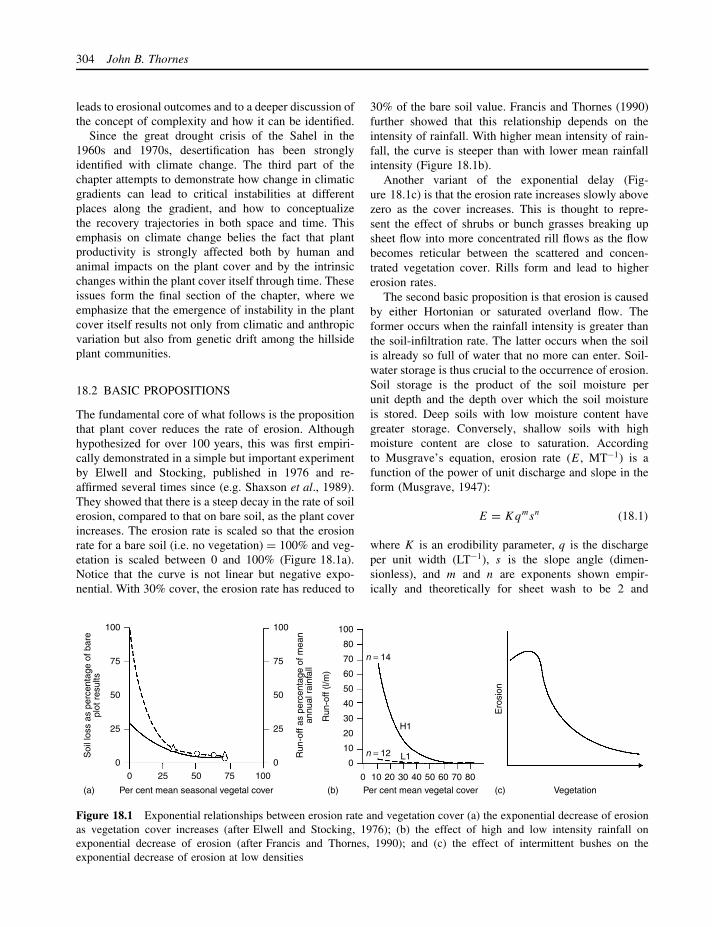
304 John B. Thornes
leads to erosional outcomes and to a deeper discussion ofthe concept of complexity and how it can be identified.
Since the great drought crisis of the Sahel in the1960s and 1970s, desertification has been stronglyidentified with climate change. The third part of thechapter attempts to demonstrate how change in climaticgradients can lead to critical instabilities at differentplaces along the gradient, and how to conceptualizethe recovery trajectories in both space and time. Thisemphasis on climate change belies the fact that plantproductivity is strongly affected both by human andanimal impacts on the plant cover and by the intrinsicchanges within the plant cover itself through time. Theseissues form the final section of the chapter, where weemphasize that the emergence of instability in the plantcover itself results not only from climatic and anthropicvariation but also from genetic drift among the hillsideplant communities.
18.2 BASIC PROPOSITIONS
The fundamental core of what follows is the propositionthat plant cover reduces the rate of erosion. Althoughhypothesized for over 100 years, this was first empiri-cally demonstrated in a simple but important experimentby Elwell and Stocking, published in 1976 and re-affirmed several times since (e.g. Shaxson et al., 1989).They showed that there is a steep decay in the rate of soilerosion, compared to that on bare soil, as the plant coverincreases. The erosion rate is scaled so that the erosionrate for a bare soil (i.e. no vegetation) = 100% and veg-etation is scaled between 0 and 100% (Figure 18.1a).Notice that the curve is not linear but negative expo-nential. With 30% cover, the erosion rate has reduced to
30% of the bare soil value. Francis and Thornes (1990)further showed that this relationship depends on theintensity of rainfall. With higher mean intensity of rain-fall, the curve is steeper than with lower mean rainfallintensity (Figure 18.1b).
Another variant of the exponential delay (Fig-ure 18.1c) is that the erosion rate increases slowly abovezero as the cover increases. This is thought to repre-sent the effect of shrubs or bunch grasses breaking upsheet flow into more concentrated rill flows as the flowbecomes reticular between the scattered and concen-trated vegetation cover. Rills form and lead to highererosion rates.
The second basic proposition is that erosion is causedby either Hortonian or saturated overland flow. Theformer occurs when the rainfall intensity is greater thanthe soil-infiltration rate. The latter occurs when the soilis already so full of water that no more can enter. Soil-water storage is thus crucial to the occurrence of erosion.Soil storage is the product of the soil moisture perunit depth and the depth over which the soil moistureis stored. Deep soils with low moisture content havegreater storage. Conversely, shallow soils with highmoisture content are close to saturation. Accordingto Musgrave’s equation, erosion rate (E, MT−1) is afunction of the power of unit discharge and slope in theform (Musgrave, 1947):
E = Kqmsn (18.1)
where K is an erodibility parameter, q is the dischargeper unit width (LT−1), s is the slope angle (dimen-sionless), and m and n are exponents shown empir-ically and theoretically for sheet wash to be 2 and
100
75
50
25
0
100
75
50
25
0
0 25 50 75 100
Soi
l los
s as
per
cent
age
of b
are
plot
res
ults
Per cent mean seasonal vegetal cover
Run
-off
as p
erce
ntag
e of
mea
nan
nual
rai
nfal
l
100
80
70
60
50
40
30
20
10
0
0 10 20 30 40 50 60 70 80
Per cent mean vegetal cover
Run
-off
(l/m
)
Ero
sion
Vegetation(a) (b) (c)
n = 14
n = 12 L1
H1
Figure 18.1 Exponential relationships between erosion rate and vegetation cover (a) the exponential decrease of erosionas vegetation cover increases (after Elwell and Stocking, 1976); (b) the effect of high and low intensity rainfall onexponential decrease of erosion (after Francis and Thornes, 1990); and (c) the effect of intermittent bushes on theexponential decrease of erosion at low densities
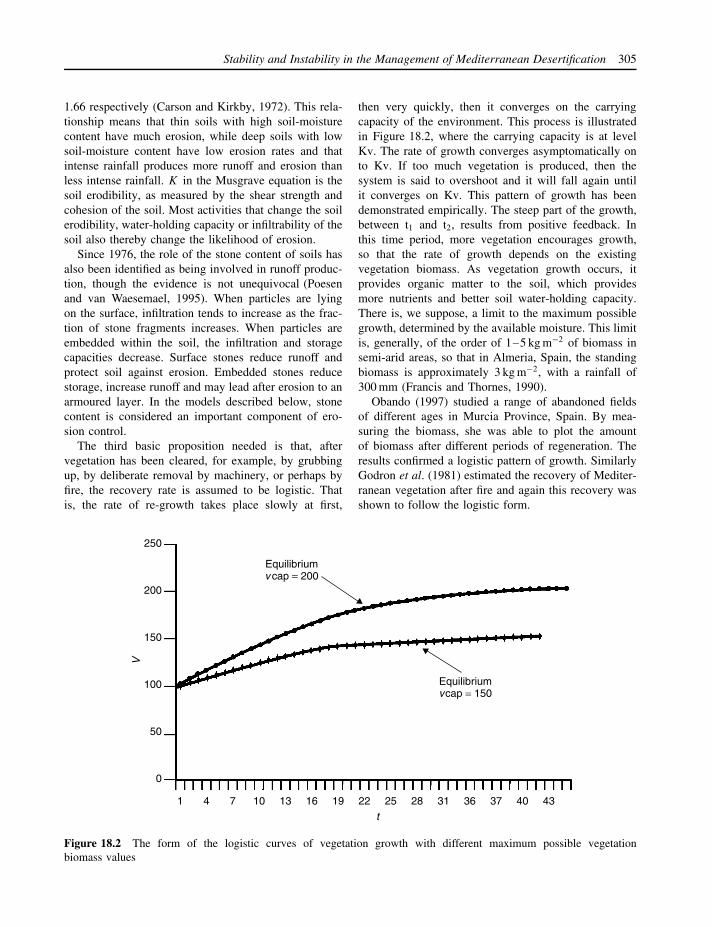
Stability and Instability in the Management of Mediterranean Desertification 305
1.66 respectively (Carson and Kirkby, 1972). This rela-tionship means that thin soils with high soil-moisturecontent have much erosion, while deep soils with lowsoil-moisture content have low erosion rates and thatintense rainfall produces more runoff and erosion thanless intense rainfall. K in the Musgrave equation is thesoil erodibility, as measured by the shear strength andcohesion of the soil. Most activities that change the soilerodibility, water-holding capacity or infiltrability of thesoil also thereby change the likelihood of erosion.
Since 1976, the role of the stone content of soils hasalso been identified as being involved in runoff produc-tion, though the evidence is not unequivocal (Poesenand van Waesemael, 1995). When particles are lyingon the surface, infiltration tends to increase as the frac-tion of stone fragments increases. When particles areembedded within the soil, the infiltration and storagecapacities decrease. Surface stones reduce runoff andprotect soil against erosion. Embedded stones reducestorage, increase runoff and may lead after erosion to anarmoured layer. In the models described below, stonecontent is considered an important component of ero-sion control.
The third basic proposition needed is that, aftervegetation has been cleared, for example, by grubbingup, by deliberate removal by machinery, or perhaps byfire, the recovery rate is assumed to be logistic. Thatis, the rate of re-growth takes place slowly at first,
then very quickly, then it converges on the carryingcapacity of the environment. This process is illustratedin Figure 18.2, where the carrying capacity is at levelKv. The rate of growth converges asymptomatically onto Kv. If too much vegetation is produced, then thesystem is said to overshoot and it will fall again untilit converges on Kv. This pattern of growth has beendemonstrated empirically. The steep part of the growth,between t1 and t2, results from positive feedback. Inthis time period, more vegetation encourages growth,so that the rate of growth depends on the existingvegetation biomass. As vegetation growth occurs, itprovides organic matter to the soil, which providesmore nutrients and better soil water-holding capacity.There is, we suppose, a limit to the maximum possiblegrowth, determined by the available moisture. This limitis, generally, of the order of 1–5 kg m−2 of biomass insemi-arid areas, so that in Almeria, Spain, the standingbiomass is approximately 3 kg m−2, with a rainfall of300 mm (Francis and Thornes, 1990).
Obando (1997) studied a range of abandoned fieldsof different ages in Murcia Province, Spain. By mea-suring the biomass, she was able to plot the amountof biomass after different periods of regeneration. Theresults confirmed a logistic pattern of growth. SimilarlyGodron et al. (1981) estimated the recovery of Mediter-ranean vegetation after fire and again this recovery wasshown to follow the logistic form.
250
200
150
100
50
0
1 4 7 10 13 16 19
t22 25 28 31 36 37 40 43
V
Equilibriumv cap = 200
Equilibriumvcap = 150
Figure 18.2 The form of the logistic curves of vegetation growth with different maximum possible vegetationbiomass values

306 John B. Thornes
Days since abandonment
Bio
mas
s g/
m2
0
020406080
100120140160180200
73 146
219
292
365
438
511
584
657
730
803
876
949
1022
1095
NormalWetDry
Figure 18.3 The modelled recovery of vegetation cover from bare ground, starting at different times and thereforehaving different rainfall histories in the recovery periodSource: Obando (1997)
Obando (1997) also modelled plant production onabandoned land, using a plant growth model developedby Thornes (1990) on the basis of Tilman’s (1982)resource-based model using essentially a daily growthperiod and making growth proportional to water effi-ciency and then partitioning the growth to leaf, stemand root according to partition coefficients. Respirationneeds are also budgeted in the model. An importantresult emerged – that the rate of recovery was heav-ily determined by the amount and pattern of rainfall(as modelled of course), so that generation that startedat different times and therefore having different rain-fall histories during the regeneration period has differentrates of recovery. This process is shown in Figure 18.3,where each curve of regeneration starts at a differentyear and years with large extreme rainfalls usually showfaster regeneration.
The same logistic growth is assumed to hold for soilerosion. That is, the more erosion there is, the morethere will be. Erosion starts slowly, accelerates andthen slows down as equilibrium is reached. The positivefeedback occurs because shallower soils produce morerunoff, more erosion and therefore shallower soils. Therate of erosion slows down eventually as more andmore soil is removed. This slowing is mainly becauselower horizons are denser and have a higher stonecontent (Thornes, 1990). Ultimately, when there is nosoil left, there can be no more erosion, so the maximum‘carrying capacity’ that can be reached (Ks) is thetotal soil depth. Unfortunately, in soil erosion formulae,such as the Universal Soil Loss Equation (USLE: seeChapter 16), the erosion is assumed to proceed topotential depth, even where this might be deeper thanthe actual soil depth. Sometimes it is assumed by the
unwitting model user that bedrock can be consumed atthat rate! Claims for very high soil-erosion rates basedon the USLE should be treated with caution. Althoughthe logistic equation has not been validated for soilerosion, the ‘slowing down’ effect is often recordedfrom suspended sediment data and is ascribed to soil‘depletion’. This depletion is usually taken to indicatethat all the ‘available’ soil has been used up.
The logistic assumption is very important becauseit underpins many ecological models developed byLotka and Voltera (Lotka, 1925; Voltera, 1926) anddescribed by Maynard Smith (1974) and May (1973).These models form the basis of the following sections ofthis chapter. A more detailed discussion of the techniqueand the details of the modelling approach which followsis contained in Thornes (1985).
18.3 COMPLEX INTERACTIONS
There are constraints to the logistic growth describedabove and these give rise to some very interesting andcomplex behaviour. The interactions can be set up ascompetition between erosion and plant growth. As inthe above section, more plant cover means less erosion,so the tendency to erosion is inhibited by vegetationcover. Thinner soils mean less available soil moistureand so less plant growth. Following Maynard Smith’sanalysis (1974), Thornes (1985) set up the differentialgrowth equations for plant logistic growth and erosionlogistic growth, constrained by erosion and vegetationrespectively. The mathematical argument is not repeatedhere but, by solving the partial differential equations, thebehaviour of the erosion–vegetation interactions can be

Stability and Instability in the Management of Mediterranean Desertification 307
Emax
Isoline Trajectories fromdifferent starting points
V
E = 0E
Figure 18.4 System behaviour in terms of erosion in theabsence of vegetation. The solid line is the isocline alongwhich there is no change in the erosion (dE/dt = 0)
explored. By this procedure, we can start the systemat any value of E and V and follow the behaviouras solved in time by the equations. Figure 18.4 showshow the erosion behaves in the absence of vegetation.
The linedE
dt= E = 0 is called an isocline. It shows
all the values along which there is no change in theerosion rate (i.e. it is in equilibrium). For a pointbelow the isocline, the erosion rate increases (movesup) until the isocline is reached. For points above theisocline, their time trajectories move down to the line ofequilibrium. Figure 18.5 shows the equivalent diagramfor the vegetation system behaviour in the absence oferosion. In this case, the isocline is the point along
whichdV
dt= V = 0 and if the system is in any state
in the plane (given by E,V values), the trajectorieswithin the isocline carry the system towards higher V
until they eventually reach the isocline. Notice that,outside the isocline, the system moves to the left until
E
aII
aIII
aI
VmaxV
V= 0
a
Figure 18.5 Isocline for vegetation in the absence oferosion (dV /dt = 0)
it again reaches the isocline V = 0. For the left-handrising limb, the system always flows away from theequilibrium. Thus, at point a, the vegetation will moveto full cover at point a1 if it is just to the right of theisocline. If it is just to the left of the isocline, it willmove towards zero vegetation cover at point a11. So, allthe points on the left-hand, rising limb of the isoclineare unstable equilibria because a slight perturbation willcarry the system away from the equilibrium to eitherzero or complete cover (nearly 100%). Because thereis convergence on the right-hand set of equilibria (e.g.point a111), these are stable equilibria. If the systemstarts on the equilibrium, it is impossible for it to moveaway and, in fact, if it is artificially displaced (e.g. bygrazing) the dynamics of the system force it to return tothe isocline.
A few general comments are in order here. First,the equilibria we have shown here are both unstableand stable. In unstable equilibria, slight perturbationscarry the system away from the equilibrium, sometimesfar away and even a tiny perturbation can cause a bigchange. This situation is like a ball balanced on the noseof a sea lion. A tiny wobble (perhaps caused by a breeze)can easily upset the balance. In the stable equilibrium,considerable effort is needed to drive the system awayfrom the isocline and if it is driven away, then thecomplex behaviour forces it back to the equilibrium,like a marble displaced from its resting place at thebottom of a tea cup and then rolling back to thelowest point. Stable equilibria which draw in the systemafter perturbations are called attractors. Figure 18.6shows another metaphor for this behaviour. Ball A isin unstable equilibrium and a slight perturbation willpush it into local attractor basins at B or C. Furtherperturbations can force it into D or E. F is called theglobal equilibrium because the ball will remain stablefor all perturbations and, following a set of sequentialperturbations, the system (ball) will end up at F. Thereis another point here. The deeper the attractor basin, thebigger the perturbation needed to displace the systemfrom the equilibrium.
Local
StableUnstable
Global
ED
B
A
C F
Figure 18.6 Metaphor for different types of equilibria:local, stable, unstable and global

308 John B. Thornes
V
E
Emax
Vm
ax
V = 0•
•E = 0
'Safe' zone for erosion systemalways goes to Vmax where E is close to zero
C
A
DY
X
B
Figure 18.7 Combined effects of vegetation and erosion. The intersection of the isoclines is where both variables areunchanging. The shaded area is the ‘safe’ zone for erosion
In Figure 18.7, the combined effect of both the ero-sion and vegetation components are shown. The pointswhere E and V intersect are the joint equilibria – thepoint where neither erosion nor vegetation is changing.At A, both vegetation and erosion are zero. At B, vege-tation is at a maximum and erosion is 0. At C, erosionis at a maximum and vegetation is 0. The behaviourat D is a mixture of unstable and stable. If the systemis perturbed in the areas with shading, it will move intowards D, so now the point D is acting as a repeller. Inthe triangle ADB, the system behaviour will carry it tothe attractor at B, which is very attractive for soil con-servationists, because it has zero erosion and maximumvegetation cover. In the shaded area ADC, the systemis forced to the attractor at C, which is very undesirablebecause it represents zero vegetation cover and maxi-mum erosion. In fact, we can go further. The line A–D(if we can locate it) separates all trajectories to attrac-tor C from those to attractor B. In conservation terms,this is a most desirable line. Ideally, we want to keepthe system to the right of this line, or move it there bymanagement actions. The triangle ABD is the area wewish our system to be in. Any combined values of E
and V in this area take the system to B. Conversely,in ACD the system will move to the attractor (stable)equilibrium at C with maximum erosion and minimumvegetation cover and it will then require a great effort tomove it away. At D, it could go either way and A, C andB are possible destinations. Another feature emerges. Ifthe system is at point X according to its values of E
and V , then it has a long way to go before the system
dynamics take over. In this sense, point X is fairly stable.By contrast, if it is in condition (state) Y, then quite asmall perturbation will carry it to C, D or B. So, in somecases, very small adjustments to the system can quicklytake the result to stable conditions (states) or to unstableconditions. In complex systems, a little change goes along way, principally because of the positive feedbacksthat were described above. The difficulty is to know(a) where are the isoclines (thresholds) over which thebehaviour changes very rapidly with only small pertur-bations?; (b) where are the attractors and are they stableor unstable? and (c) what are the equilibria and are theystable or unstable or saddles? Thornes (1990) examinedthese questions with more elaborate systems, includingthose with stony soils.
There are two catches to this optimistic picture. First,descent to the attractor is not smooth; the approach isvery fuzzy in the sense that there may be a variabil-ity that ‘captures’ the system for the attractor before itgets there. If the ‘external’ forces perturbing the systemare also noisy (vary a lot in their strength), then thesystem may be forced onto a trajectory from an unex-pected position. Thornes and Brandt (1993) exploredthe behaviour of the erosion–vegetation dynamical sys-tem for stochastic (unpredictable in time) variations inrainfall for a system in the dry Mediterranean in south-east Spain. Although this fuzziness produced some quiteunexpected behaviour, the vegetation showed a strongoscillation of high and low vegetation covers and cor-responding low and high erosion rates. This kind ofbehaviour in dynamical systems usually indicates that

Stability and Instability in the Management of Mediterranean Desertification 309
there is no strongly preferred attractor and that the sys-tem is moving between attractors. An alternative expla-nation is that the vegetation–moisture–erosion system isa ‘hypercycle’ (Eigen and Schuster, 1979) that can alsoproduce nonlinear oscillations. This alternative explana-tion has been explored very recently in the context ofgrazing (Thornes, in preparation). The results of Thornesand Brandt also showed that occasionally there would beovershoots. With a lot of rainfall, the vegetation grewwell in excess of carrying capacity and in subsequentyears had to ‘die’ back to the carrying capacity throughnegative feedback. It was also found that the stability ofthe system, as formulated, was significantly affected bythe stone content.
Note that two controlling influences have been iden-tified in this section, internal or intrinsic and exter-nal or extrinsic. The intrinsic influences are thresholdsand behaviour within the system itself, the trajectories,thresholds and equilibria (repellers and attractors) thatdetermine the courses of behaviour, their final desti-nations (unless they go off the graph, far away fromequilibrium) and their stability. Extrinsic forces are thosethat perturb the system away from the internal controlstowards new equilibria. If we had a good understandingof both sets of mechanisms, and there was not too muchfuzziness or randomness, then we might be in a positionto use this knowledge to determine the future trajec-tories or the reactions to deliberate perturbations, suchas ‘over-grazing’ or torrential rainfall. Obtaining abso-lute values for this behaviour, such as the trajectoriesin space and time, requires not only an understandingof the system couched in this framework, but also agood knowledge of the parameters of the system andthe initial conditions (what are the values of E and V atthe start?). These are demanding requirements, though ifsome of the many plot experiments were reconfigured,the data could be easily obtained.
Because there are several (sometimes many) thresh-olds in the system separating attractor basins, an impor-tant question is, how close to the threshold can we getbefore the system is captured by an attractor basin? InFigure 18.7, how close can we get to the A–D linebefore we go to either complete cover and no erosion(attractor B) or no cover and very high erosion (attractorC)? Obviously this is a crucial question for management.If we accidentally tip the system across the boundary, theresulting outcome could be the exact opposite of what isrequired. The judgement as to what is a good outcomeand a bad outcome is independent of the dynamics. Butin the case of the management implications, it mightbe a question of how many kg m−2 of biomass shouldbe harvested or animals should be allowed to graze.
This decision will determine the horizontal movement inFigure 18.7 and hence depends on two things: (a) howfar the system is away from the boundary; and (b) how‘noisy’ the process is. This last point is very important.
18.3.1 Spatial variability
Because the value of E depends on the soil and rain-fall characteristics over space, the runoff prediction isextremely variable. On two adjacent soil patches theerosion rate could be quite different, putting us eitherside of the threshold. So bare and strongly vegetatedpatches could co-exist and indeed they do! Throughtime, the intensity varies, changing the overland flowproduction. Although generally one uses a mean inten-sity to fix the position in the space E –V , if this variationis very large, then it is likely to straddle the thresh-old. In fact, the distribution of intensity is exponential(Kosmas et al., 1999). So if the mean is located onthe threshold between two attractors, we can define a‘belt’ either side of the threshold, in which there isa risk of the system moving to another attractor. Thelarger the deviation, the larger the risk. The ‘noisier’the system, the larger the risk. This ‘noise’ varies spa-tially, as does the runoff production, vegetation coverand erosion. Consequently, spatial outcomes could bequite varied and it is interesting to ask where the thresh-olds exist in geographical space. In a patchy landscapewith different soil types and different runoff produc-tions, the system is differentially located with respectto the thresholds. Just crossing a soil boundary or theedge of a vegetation patch could trip us towards anotherattractor. Human-induced patchiness is, in this respect,critically important in trying to foresee the locationof desertification in space (Thornes, 1990). What hasnot yet been studied or modelled is any ‘contagion’effect of desertification, though given the catena con-cept and patch dynamical growth approaches (Tilmanand Karieva, 1997), this is clearly an important problemfor the near future. Often in Mediterranean environ-ments, one can observe a whole hillside fairly uniformlycovered with a single shrub species (such as Anthyl-lis cytisoides) and the following question arises. If asmall locus of erosion breaks out somewhere in themiddle, will it propagate outwards in an unstable fash-ion, moving the whole hillside to the erosion attractor?This evolution has been suggested by Kosmas for thecase of the bush Saceropoterium, on the island of Les-bos, Greece (Kosmas, personal comm.). Alternatively,given that different species have hydrologically differ-ent characteristics, if a different species invades such aslope, could it shift the system across a threshold to a

310 John B. Thornes
different attractor? We shall refer back to this questionin the fourth section of this chapter, arguing that speciesmixtures may lead to conditions that are ‘unstably con-tagious’ by virtue of their genetic evolutionary potentialand population dynamics.
18.3.2 Temporal variability
Of course, the very word dynamical implies that the ana-lytical models are evolutionary (changing through time)according to their internal mechanism, but the externalcontrols are also changing through time. Theoretically,it should be possible to use the equations of dynamicalbehaviour to determine how long the system will taketo adjust to a perturbation or external change (the relax-ation time: Brunsden and Thornes, 1979). This delay hasimportant impacts in dynamical systems and externalchanges can be scaled. High frequency changes (suddenstorms) may have significantly different impacts fromlower frequency changes (such as internal variations instorm intensities).
In desertification studies, these continue to be a preoc-cupation, with climate change as a major cause in spiteof the overwhelming evidence that socio-economic con-trols are probably more important. In this respect, Allenand his colleagues developed the human dimensionsaspect of dynamical systems models in desertificationstudies (Allen, 1988). There also, thresholds, attractors,intrinsic and extrinsic forces all have their roles.
Climate variation can also be regarded as perturba-tions operating over the long timescale (tens of years).The main effects, in terms of the models outlined above,are on the overall carrying capacities (Vcap), the instan-taneous growth rate coefficient in the logistic equations(k1), the soil moisture constraining plant growth andthe direct production of overland flow through vary-ing rainfall intensities and therefore the rate of erosion.The variability in rainfall is also important, as indicatedin the previous section. Temperature and CO2 concen-trations also affect plant growth and are therefore anintegral component of modelling the impacts of cli-mate change on desertification, as used by Diamond andWoodward (1998).
There are several ways of attempting to model theimpacts of climate change on desertification. The mostcommon is direct digital simulation of the impacts ofchange. For the Mediterranean, the MEDALUS teamat Leeds University under Mike Kirkby has produceda variety of simulation models for different space andtime scales. The MEDALUS hillslope model (Thorneset al., 1996) investigates field-scale erosion in semi-arid environments and operates at an hourly event
scale. It is essentially based on the principles of TOP-MODEL (Beven and Kirkby, 1979). The MEDRUSHmodel (Kirkby et al., 2002) operates at the large catch-ment scale and uses the technique of a statistical ensem-ble of a ‘characteristic’ flow strip whose hydrology,vegetation growth and erosion are modelled by phys-ical process laws and applied to the representative stripswhich thus change its morphology. The theory devel-oped permits this changed morphology to cause thestrips to migrate within a basin and the sediment isrouted down the channel. In this model, the initial veg-etation cover is provided in the catchment GIS fromremotely sensed imagery and the models can be used topredict the impacts of different physical (rainfall) andhuman (land-use) perturbations on runoff and sedimentyields from the catchment.
Empirical models have also been used to examinethe effects of climate change on land degradation andrunoff, both over space (Kirkby and Cox, 1995) andover time (Arnell, 1996). These examples have theusual problems of such models. Time series have beenparameterized by particular data sets and thereforeare not readily transportable. They often have (andshould have) error bands attached to them that maybe quite wide. This rather ancient technology is highlyspeculative and often misleadingly simple.
Even further down the line are analogue studies inwhich the authors seek contemporary or historical ana-logues for supposed climate changes among existing orpast environments. Thus one might expect parts of thesouth shore of the Mediterranean to be suitable ana-logues for the northern shore. The problem is obvious.Obtaining suitable analogues is very difficult especiallywhen the systems are only weakly understood. This isthe kind of approach that enables us to hope that, 70years from now, southern Britain might be like southernSpain and therefore the farmers of Sussex can changetheir potato fields for vineyards.
A special version of this argument that has becomepopular in recent years is the gradient analogue. Wherethere is a strong climatic gradient, detailed studies ofgeomorphological and ecological processes with theirrespective responses can be used to demonstrate how thechanging climatic parameters along the gradient controlthe erosion rates. When these are coupled with plotstudies, the linkages so made can be confirmed. Anoutstanding study of this type was carried out by Laveeand Pariente (1998) between Jerusalem and Jericho, agradient of strongly decreasing rainfall from the uplandsof central Israel to the Dead Sea. The methodology is toseek along the gradients for analogues of expected futureclimate conditions. This might reveal what the future

Stability and Instability in the Management of Mediterranean Desertification 311
Temperature
'Fitn
ess'
'Fitn
ess'
Rainfall
Temperature
Rainfall
Figure 18.8 Pianka’s representation of the hypothesized impact of climate change on plant fitness
processes and responses will be, but does not revealthe trajectories of change. As was shown earlier, thesetrajectories are crucial in determining the final state,especially if they carry the system across thresholdsbetween quite different attractor basins. The path toequilibrium need be neither steady nor smooth. Thisproblem often occurs in mathematical modelling ofchange when, by setting the rate of change equal tozero and solving for equilibrium, the equilibrium stateis obtained but not the trajectories towards it. Kirkby(1971) used this technique in his characteristic slope-form paper, in which the characteristic forms are derivedfrom the values of the parameters in the Musgraveerosion equation (Musgrave, 1947). The equilibriumforms obtained are in fact attractors in the m–n spacethough neither the trajectories nor the relaxation timesto equilibrium were obtained in the analysis. Thisexample appears to be one of the earliest analyticalapplications of dynamical systems analysis in the field ofgeomorphology, though it is rarely recognized as such.
Another approach (Pianka, 1978) is to provide thefitness distribution for plants in a climate phase spaceand then judge the climatic change impacts by shiftingthe curves in the phase space (Figure 18.8) and adjustingthe fitness response.
18.4 CLIMATE GRADIENT AND CLIMATECHANGE
Using the tools described earlier, we consider inthis section how the gradient-change problem can beapproached heuristically using the dynamical systemsapproach. A novel treatment of the gradient problem
was developed by Pease et al. (1989). They envisagedthe production of the vegetation at ground level by theintersection of an atmospheric gradient with a planar sur-face over which the change is passing (Figure 18.9). Theresponse at equilibrium is controlled by Lotka–Volteracompetitive growth (cf. Thornes, 1988) whereby notonly is there competition between the plants, but also thestability of the outcomes can be specified from a studyof the modelled interactions, as described below (Lotka,1925; Voltera, 1926). As the climate changes, the atmo-spheric zones shift across the land, generating new veg-etation in response to this change. The species, in fact,track the moving environment by adjustment of thepatches through a critical patch size dynamic, in whichthe population within the patch is counter-balanced bydispersal into an unsuitable habitat (Skellam, 1951). Thedispersal changes the mean phenotype and, becauseof the environmental gradient, natural selection willfavour different phenotypic values in different parts ofthe environment. The model also incorporates additivegenetic variance.
Changing the climate also changes the carrying capac-ity (Vcap) in the logistic equations for plant response (seebelow). But soil moisture is the control over the above-ground biomass. Hence the cover and soil-moisture con-tent are not a simple function of mean annual rainfall,but also of the magnitude and frequency of rainfall andthe evapotranspiration conditions forced mainly by tem-perature. So rainfall (R) and temperature (T ) variationsoffer a good approximation to plant cover (Eagleson,1979), given all other co-linearities. Different coeffi-cients of water use efficiencies may also determine themain functional vegetation type (bare, grass, shrubs or
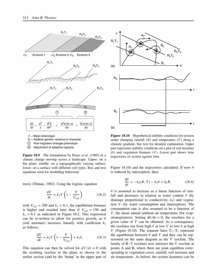
312 John B. Thornes
dzdt
z
d2zdx2
s2
zs2d (In n)
dxG d (In w)
dz= + + +
1 2
12
G= Mean phenotype= Additive genetic variance in character How migration changes phenotype Adjustment of adaptive capacity
s1s2 s3
R3T3R2T2R1T1
R3T3
R3T3
R2T2
R2T2
R1T1
R1T1
v t1 v t2 v t3Ecotone 1 Ecotone 2 Ecotone 3
Figure 18.9 The formulation by Pease et al. (1989) of aclimate change moving across a landscape. Upper: on aflat plane; middle: on a topographically varying surface;lower: on a surface with different soil types. Box and textequations used for modelling behaviour
trees) (Tilman, 1982). Using the logistic equation
dV
dt= k1V
(1 − V
Vcap
)(18.2)
with Vcap = 200 and k1 = 6.1, the equilibrium biomassis higher and reached later than if Vcap = 150 andk1 = 6.1 as indicated in Figure 18.2. This expressioncan be re-written to allow for positive growth, as θ
(soil moisture) increases linearly with coefficient k3
as follows:
dV
dt= k2V
(1 − V
Vcap
)+ k3θ. (18.3)
This equation can then be solved for dV/dt = 0 withthe resulting isocline in the plane as shown in theearlier section (and by the ‘hump’ in the upper part of
q
R1T1
R2
B2
(a)
(b)
R2T2
R3T3
V
t
t
A1
A2
B2
B1
Figure 18.10 Hypothetical stability conditions for erosionunder changing rainfall (R) and temperature (T ) along aclimatic gradient. See text for detailed explanation. Upperpart represents stability conditions on a plot of soil moisture(θ ) and vegetation biomass (V ). Lower part shows timetrajectories of system against time
Figure 18.10) and the trajectories calculated. If now θ
is reduced by interception, then:
dθ
dt= −k4(R, T ) − k5θ + k6R. (18.4)
θ is assumed to increase as a linear function of rain-fall and decreases in relation to water content θ (bydrainage proportional to conductivity, k5) and vegeta-tion V (by water consumption and interception). Theconsumption rate is also assumed to be a function ofT , the mean annual ambient air temperature (for evap-otranspiration). Setting dθ/dt = 0, the isoclines for agiven value of T can be obtained. As a consequence,the isoclines run from high θ at low V to low θ at highV (Figure 18.10). The separate lines T1 –T3 representthe equilibrium between θ and V and they can be rep-resented on the same diagram as the V isocline. Thefamily of R–T isoclines now intersect the V isocline atpoints A and B, where there are joint equilibria corre-sponding to vegetation cover, rainfall, soil moisture andair temperature. As before, the system dynamics can be
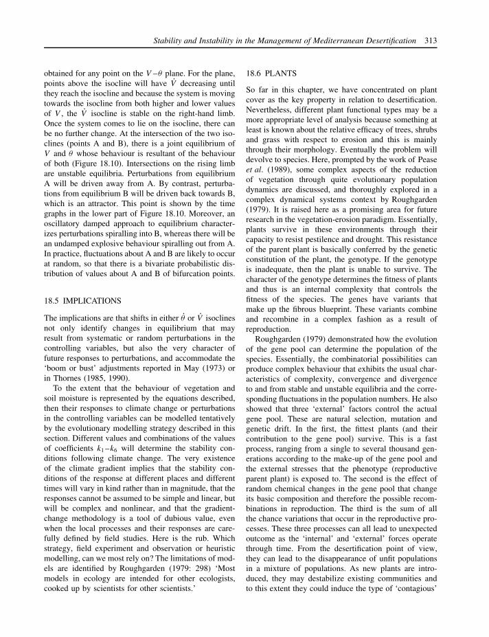
Stability and Instability in the Management of Mediterranean Desertification 313
obtained for any point on the V –θ plane. For the plane,points above the isocline will have V decreasing untilthey reach the isocline and because the system is movingtowards the isocline from both higher and lower valuesof V , the V isocline is stable on the right-hand limb.Once the system comes to lie on the isocline, there canbe no further change. At the intersection of the two iso-clines (points A and B), there is a joint equilibrium ofV and θ whose behaviour is resultant of the behaviourof both (Figure 18.10). Intersections on the rising limbare unstable equilibria. Perturbations from equilibriumA will be driven away from A. By contrast, perturba-tions from equilibrium B will be driven back towards B,which is an attractor. This point is shown by the timegraphs in the lower part of Figure 18.10. Moreover, anoscillatory damped approach to equilibrium character-izes perturbations spiralling into B, whereas there will bean undamped explosive behaviour spiralling out from A.In practice, fluctuations about A and B are likely to occurat random, so that there is a bivariate probabilistic dis-tribution of values about A and B of bifurcation points.
18.5 IMPLICATIONS
The implications are that shifts in either θ or V isoclinesnot only identify changes in equilibrium that mayresult from systematic or random perturbations in thecontrolling variables, but also the very character offuture responses to perturbations, and accommodate the‘boom or bust’ adjustments reported in May (1973) orin Thornes (1985, 1990).
To the extent that the behaviour of vegetation andsoil moisture is represented by the equations described,then their responses to climate change or perturbationsin the controlling variables can be modelled tentativelyby the evolutionary modelling strategy described in thissection. Different values and combinations of the valuesof coefficients k1 –k6 will determine the stability con-ditions following climate change. The very existenceof the climate gradient implies that the stability con-ditions of the response at different places and differenttimes will vary in kind rather than in magnitude, that theresponses cannot be assumed to be simple and linear, butwill be complex and nonlinear, and that the gradient-change methodology is a tool of dubious value, evenwhen the local processes and their responses are care-fully defined by field studies. Here is the rub. Whichstrategy, field experiment and observation or heuristicmodelling, can we most rely on? The limitations of mod-els are identified by Roughgarden (1979: 298) ‘Mostmodels in ecology are intended for other ecologists,cooked up by scientists for other scientists.’
18.6 PLANTS
So far in this chapter, we have concentrated on plantcover as the key property in relation to desertification.Nevertheless, different plant functional types may be amore appropriate level of analysis because something atleast is known about the relative efficacy of trees, shrubsand grass with respect to erosion and this is mainlythrough their morphology. Eventually the problem willdevolve to species. Here, prompted by the work of Peaseet al. (1989), some complex aspects of the reductionof vegetation through quite evolutionary populationdynamics are discussed, and thoroughly explored in acomplex dynamical systems context by Roughgarden(1979). It is raised here as a promising area for futureresearch in the vegetation-erosion paradigm. Essentially,plants survive in these environments through theircapacity to resist pestilence and drought. This resistanceof the parent plant is basically conferred by the geneticconstitution of the plant, the genotype. If the genotypeis inadequate, then the plant is unable to survive. Thecharacter of the genotype determines the fitness of plantsand thus is an internal complexity that controls thefitness of the species. The genes have variants thatmake up the fibrous blueprint. These variants combineand recombine in a complex fashion as a result ofreproduction.
Roughgarden (1979) demonstrated how the evolutionof the gene pool can determine the population of thespecies. Essentially, the combinatorial possibilities canproduce complex behaviour that exhibits the usual char-acteristics of complexity, convergence and divergenceto and from stable and unstable equilibria and the corre-sponding fluctuations in the population numbers. He alsoshowed that three ‘external’ factors control the actualgene pool. These are natural selection, mutation andgenetic drift. In the first, the fittest plants (and theircontribution to the gene pool) survive. This is a fastprocess, ranging from a single to several thousand gen-erations according to the make-up of the gene pool andthe external stresses that the phenotype (reproductiveparent plant) is exposed to. The second is the effect ofrandom chemical changes in the gene pool that changeits basic composition and therefore the possible recom-binations in reproduction. The third is the sum of allthe chance variations that occur in the reproductive pro-cesses. These three processes can all lead to unexpectedoutcome as the ‘internal’ and ‘external’ forces operatethrough time. From the desertification point of view,they can lead to the disappearance of unfit populationsin a mixture of populations. As new plants are intro-duced, they may destabilize existing communities andto this extent they could induce the type of ‘contagious’

314 John B. Thornes
desertification that is referred to above. Furthermore, cli-matic fluctuations (Thornes, 2003) and grazing densities(Thornes, in preparation) are implicated in desertifica-tion contagion.
18.7 CONCLUSION
In desertification, vegetation and land degradation areinextricably mixed and strongly interactive. This inter-action can be modelled using the predator–prey strategythat produces clear separations (bifurcations) betweenstable attractors and unstable repeller equilibria. Byidentifying the bifurcations in phase space, with prop-erly parameterized equations, we can anticipate how thebehaviour of the system will lead to one of the equilibria.As with all complex systems, small variations in initialconditions can lead to strongly different outcomes and,because natural systems are very noisy, there are manypossibilities for diversion along the routes to stability.The beauty of the approach is that a basic knowledgeof the underlying dynamics provides a good insight intothe likely possible trajectories. Another important aspectis the separation of the ‘intrinsic’ or ‘internal’ con-trols of evolution and the external controls that push orforce the trajectories. A further dichotomy is betweenthe deterministic modelling represented by the differ-ential equations of change and the manipulations thatexplore the nature of the equilibria, on the one hand,and the probabilistic modelling exposed by the combi-natorial possibilities within the genetic modelling andthe genetic drift as a stochastic process, on the other.These are the intrinsic probabilistic elements. The ‘exter-nal’ forcing, climate, human activities and natural spatialvariability also lead to probabilistic behaviour and mod-elling near the bifurcation sets (thresholds) and at theattractors themselves.
The implications for desertification are beginning toemerge. The first and most important is that the intrinsiccomplexity has to be appreciated before mitigationactions are undertaken. Tiny changes can have majoroutcomes. They can set the system along trajectories thathave far-reaching and (usually) unpredictable outcomes.In this chapter, some of the major bifurcations have beenidentified but, for desertification, many more wait to berevealed. The second major implication for managementand history is that observed outcomes are not necessarilya good guide to process mechanisms. The inference ofprocess from form is still in its infancy. The best hope isthat following the trajectories of specific changes fromknown perturbations will lead us to a better appreciationof the vegetation-degradation system.
It is too naıve always to seek climate-change expla-nations for land degradation. This outlook is a residuefrom the denudation-chronology preoccupation of earlyto mid-twentieth-century geomorphology, compoundedwith the contemporary concerns with global climatechange. Semi-arid environments are often located at ornear to the isoclines and are therefore especially sus-ceptible to small perturbations of both physical andsocio-economic origins. Recognition and acceptance ofthe complexity (in the technical sense intended in thischapter) are the first step towards better management ofdesertification. Further research is needed into complex-ity for more fruitful management.
REFERENCES
Allen, P.M. (1988) Dynamic models of evolving systems,Systems Dynamics Review 4, 109–130.
Arnell, N. (1996) Global Warming, River Flows and WaterResources, John Wiley & Sons, Chichester.
Beven, K.J. and Kirkby, M.J. (1979) A physically based, vari-able contributing area model of basic hydrology, Hydrolog-ical Sciences Bulletin 24, 43–69.
Brunsden, D. and Thornes, J.B. (1979) Landscape sensitivityand change, Transactions of the Institute of British Geogra-phers 4 (4), 463–484.
Carson, M.A. and Kirkby, M.J. (1972) Hillslope Form andProcess. Cambridge University Press, Cambridge.
Diamond, S. and Woodward, F.E.I. (1998) Vegetation mod-elling, in P. Mairota, J.B. Thornes and N. Geeson (eds) AnAtlas of Mediterranean Europe: The Desertification Context,John Wiley & Sons, Chichester, 68–69.
Eagleson, P.S. (1979) Climate, soil and vegetation, 4: theexpected value of annual evapotranspiration, Water Resour-ces Research 14 (5), 731–764.
Eigen, M. and Schuster, P. (1979) The Hypercycle, Berlin,Springer-Verlag.
Elwell, H.A. and Stocking, M.A. (1976) Vegetative cover toestimate soil erosion hazard in Rhodesia, Geoderma 15,61–70.
Evernden, N. (1992) The Social Creation of Nature, JohnsHopkins University Press, Baltimore, MD.
Francis, C.F. and Thornes, J.B. (1990) Runoff hydrographsfrom three Mediterranean cover types, in J.B. Thornes (ed.)Vegetation and Erosion, John Wiley & Sons, Chichester,363–384.
Godron, M., Guillerm, J.L., Poissonet, J., Poissonet, P., Thi-ault, M. and Trabaud, L. (1981) Dynamics and managementof vegetation, in F. di Castri, D. Goodall and R.L. Specht(eds) Ecosystems of the World 11: Mediterranean-typeShrublands, Elsevier Scientific Publishing Co, Amsterdam,317–445.
Hudson, N. (1992) Land Husbandry, B.T. Batsford Limited,London.

Stability and Instability in the Management of Mediterranean Desertification 315
Kirkby, M.J. (1971) Hillslope process-response models basedon the continuity equation, Institute of British GeographersSpecial Publication 3, 15–30.
Kirkby, M.J, Abrahart, R.J., Bathurst, J.C., Kilsby, C.G.,McMahon, M.L, Osborne, C.P., Thornes, J.B. and Wood-ward, F.E.I. (2002) MEDRUSH: a basin-scale physi-cally based model for forecasting runoff and sedimentyield, in N.A. Geeson, C.J. Brandt, and J.B. Thornes (eds)Mediterranean Desertification: A Mosaic of Processes andResponses, John Wiley & Sons, Chichester, 203–229.
Kirkby, M.J. and Cox, N.J. (1995) A climatic index for soilerosion potential (CSEP) including seasonal and vegetationfactors, Catena 25, 333–352.
Kosmas, C., Kirkby, M.J. and Geeson, N. (1999) TheMEDALUS Project Mediterranean Desertification and LandUse: Manual on Key Indicators of Desertification andMapping Environmentally Sensitive Areas to Desertification,Official Publications of the European Communities,Luxembourg, EUR 18882.
Lavee, H. and Pariente, S. (1998) Resilience of soil struc-tures to environmental changes, in J. Brandt (ed.) MEDALUSIII Project 1: Core Project, Final Report covering theperiod 1 January 1996–31 December 1998, EU, Brussels,433–485.
Lotka, A.J. (1925) Elements of Physical Biology, Williams andWilkins, Baltimore, MD.
May, R.L. (1973) Stability and Complexity in Model Ecosys-tems, University Press, Princetown, NJ.
Maynard Smith, J. (1974) Models in Ecology, CambridgeUniversity Press, Cambridge.
Musgrave, G.W. (1947) Quantitative evaluation of factors inwater erosion: a first approximation, Journal of Soil andWater Conservation 2, 133–138.
Obando, J.A. (1997) Modelling the impact of land abandon-ment on runoff and soil erosion in a semi-arid catchment,PhD thesis, King’s College London.
Pease, C.M., Land, R. and Bull, J.J. (1989) A model of pop-ulation growth, dispersal and evolution in a changing envi-ronment, Ecology 70 (6), 1657–1664.
Pianka, E.R. (1978) Evolutionary Ecology, 2nd edn, Harper andRow, New York.
Poesen, J. and van Waesemael, B. (1995) Effects of rockfragments on the structure of tilled topsoil during rain,in E. Derbyshire, T. Dikstra and I.J. Smalley (eds) Gene-sis and Properties of Collapsible Soils, NATO AdvancedStudies Institute Series, Series C: Mathematical and Phys-ical Sciences, 486, Kluwer Academic Publishers, Dordrecht,333–343.
Polya, G. (1957) How to Solve It: A New Aspect of MathematicalMethod, 2nd edn, Princeton University Press, Princeton, NJ.
Roughgarden, J. (1979) The Basics of Population Genetics,Macmillan, New York.
Shaxson, T.F.N., Hudson, W., Sanders, D.W., Roose, E. andMoldenhauer, W.C. (1989) Land Husbandry: A Frameworkfor Soil and Water Conservation, Soil and Water Conserva-tion Society, Ankeny, IO.
Skellam, J.G. (1951) Random dispersal in theoretical popula-tions, Biometrica 38, 196–218.
Thornes, J.B. (1990) The interaction of erosional and vegeta-tional dynamics in land degradation: spatial outcomes, inJ.B. Thornes (ed.) Vegetation and Erosion, John Wiley &Sons, Chichester, 41–53.
Thornes, J.B. (1985) The ecology of erosion, Geography,70 (3), 222–236.
Thornes, J.B. (1988) Erosional equilibria under grazing, inJ. Bintliff, D. Davidson and E. Grant (eds) ConceptualIssues in Environmental Archaeology, Edinburgh UniversityPress, Edinburgh, 193–211.
Thornes, J.B. (2003) (in press) Exploring the grass-bush tran-sitions in South Africa through modelling the response ofbiomass to environmental change, Geographical Journal.
Thornes, J.B. (in preparation) Vegetation, erosion and grazing:a hypercycle approach. Paper to be presented at the COM-LAND Conference on Land Degradation and Mitigation,Iceland, August 2003.
Thornes, J.B. and Brandt, C.J. (1993) Erosion-vegetation com-petition in an environment undergoing climatic changewith stochastic rainfall variations, in A.C. Millington andK.T. Pye (eds) Environmental Change in the Drylands: Bio-geographical and Geomorphological Responses, John Wiley& Sons, Chichester, 305–320.
Thornes, J.B, Shao, J.X., Diaz, E., Roldan, A., Hawkes, C.and McMahon, M. (1996) Testing the MEDALUS HillslopeModel, Catena 26, 137–160.
Tilman, D. (1982) Resources Competition and CommunityStructure, Princeton University Press, Princeton, NJ.
Tilman, D. and Karieva, P. (1997) Spatial Ecology: The Role ofSpace in Population Dynamics and Interspecific Interactions,Princeton University Press, Princeton, NJ.
Van der Leeuw, S. (ed.) (1998) Understanding the Naturaland Anthropogenic Causes of Land Degradation and Deser-tification in the Mediterranean Basin, Office for OfficialPublications of the European Communities, Luxembourg,EUR18181 EN.
Voltera, B. (1926) Fluctuations in the abundance of a speciesconsidered mathematically, Nature 118, 558–560.


Part IV
Current and Future Developments


19
Scaling Issues in Environmental Modelling
XIAOYANG ZHANG, NICK A. DRAKE AND JOHN WAINWRIGHT
19.1 INTRODUCTION
Modelling is useful for understanding and predictingenvironmental changes at various times and areas. Itcan incorporate descriptions of the key processes thatmodulate system performance or behaviour with varyingdegrees of sophistication (Moore et al., 1993). Over thepast few hundred years, we have invested considerableeffort to understand the processes of the environmen-tal system, to build up a long record of environmentalparameters, and to create a number of reasonable mod-els at local (plot) scales. For example, land-surface andhydrological processes are usually monitored and exper-imented on an isolated uniform plot or under laboratorycontrol with a spatial scale between one metre and onehundred metres and a time period of hours or days. Anal-ysis of an ecological system is built up by observing theregulation of stomatal conductance, photosynthesis, andthe flux of water and carbon at the scale of a leaf ora canopy (plant) with a corresponding timescale fromseconds to hours. Our knowledge and correspondingphysically realistic models of environmental processeshave been extensively developed and validated, basedon field measurements at local scales. The underlyingprocesses occurring at these scales reveal critical causesof environmental changes.
Many pressing environmental problems affectinghumans are, however, always to be found at regional andglobal scales. The assessments of regional and globalenvironmental changes force us to address large-scaleand long-term issues. Thus, we must focus on how ourEarth system is changing and how the future changes ofthe Earth system can be estimated, for example, in termsof carbon cycling and climate change at regional andglobal scales. Hence we primarily use our knowledge at
local scales to address hydrology, climatic change andthe carbon dioxide cycle at regional and global scalesusing grid data ranging from 0.5◦ × 0.5◦ to 5◦ × 5◦.For example, a dataset with a resolution of 0.5◦ × 0.5◦
was used in the Vegetation/Ecosystem Modelling andAnalysis Project (VEMAP members, 1995). Althoughenvironmental processes at large scales are to a greatextent the result of processes at local scales, the modelsrepresenting these processes can vary considerably fromone scale to another (Heuvelink, 1998).
Global databases are gradually being built up withgood quality information for environmental modelling.High spatial and temporal resolution data are not alwaysavailable at a regional or global scale. In contrast,the coarse spatial and fine temporal resolution datasetsare widely available. These databases include 0.5◦ and1◦ soil types, vegetation types and land use in theGlobal Ecosystems Database (GED), daily 1 kilometreglobal Advanced Very High Resolution Radiometer(AVHRR), 1 kilometre MODerate Resolution ImagingSpectroradiometer (MODIS) products including landcover, temperature, albedo, leaf-area index (LAI) andFraction of Photosynthetically Active Radiation (FPAR),and daily climatic data in the Global Climate DataCenter. Nevertheless, it is still not clear how thesedata change with scales and to what extent they fitboth environmental processes and models from local toglobal scales.
Because many environmental processes and patternsare scale-dependent, we currently face two pairs of con-tradictions. One is that although the local environmentalprocesses can be simulated accurately, many environ-mental managers require the environmental assessmentsat a regional or global scale. Another is that most phys-ically based models have been developed and validated
Environmental Modelling: Finding Simplicity in Complexity. Edited by J. Wainwright and M. Mulligan 2004 John Wiley & Sons, Ltd ISBNs: 0-471-49617-0 (HB); 0-471-49618-9 (PB)

320 Xiaoyang Zhang, Nick A. Drake and John Wainwright
at uniform field-plot scales or under laboratory condi-tions while the widely available data for model inputsare very coarse and heterogeneous. The scaling issuesof environmental parameters and modelling restrict theapplicability of the principles and theories learned underplot conditions to the assessment of environmental riskat a regional or global scale. They arise because lit-tle understanding has been achieved about the linkagebetween well-developed models at fine scales and envi-ronmental processes operating at large scales.
This chapter discusses the scaling issues facing envi-ronmental modelling and the currently used methodsreducing the scaling effects on both models and theirparameters. A case study is then presented on theapproaches to scale up a soil-erosion model establishedat a plot scale to regional or global scales by scalingland-surface parameters. A primary focus is to developa scale-invariant soil-erosion model by scaling the slopeand vegetation-cover factors that control erosion to fitthe modelling scale.
19.2 SCALE AND SCALING
19.2.1 Meanings of scale in environmentalmodelling
‘Scale is a confusing concept often misunderstood, andmeaning different things depending on the context anddisciplinary perspective’ (Goodchild and Quattrochi,1997). ‘The various definitions for scale are often usedinterchangeably and it is not always clear which oneis used. The term “scale” refers to a rough indicationof the order of magnitude rather than to an accuratefigure’ (Bloschl and Sivapalan, 1995). Although thereare over 30 meanings of the word (scale) (Curran andAtkinson, 1999), five meanings are commonly usedin environmental analysis (Lam and Quattrochi, 1992;Bloschl and Sivapalan, 1995). A cartographic map scalerefers to the proportion of a distance on a map to thecorresponding distance on the ground. A large-scalemap covers a smaller area generally with more detailedinformation, while a small-scale map covers a larger areaoften with brief information about the area. In contrast,a geographic scale is associated with the size or spatialextent of the study. A large geographic scale deals witha larger area, as opposed to a small geographic scale,which covers a smaller area.
An operational scale (process scale, characteristicscale) is defined as the scale at which a process operatesin the environment. This scale is associated with thespatial extent and temporal duration (lifetime and cycle)depending on the nature of the process. The property of
an object is identified at this scale. An environmentalphenomenon is best observed at its operational scale.
Measurement scale (observational scale) is the spatialresolution that is used to determine an object. Atthis scale a construct is imposed on an object in anattempt to detect the relevant variation (Collins, 1998).Measurement scale can be defined as the spatial ortemporal extent of a dataset, the space (resolution)between samples, and the integration time of a sample.The spatial scale is related to the size of the smallestpart of a spatial dataset, such as the plot size inthe field investigation, pixel size of remotely senseddata and digital elevation data. With the change ofmeasurement scale, the environmental parameters mayrepresent different information in concerned disciplines.For example, the observed characteristics in biosphereprocesses may represent leaf, plant and ecosystemrespectively when the spatial data are aggregated froma small scale to a large scale.
Modelling (working) scale, building up an environ-mental model, is partly related to processes and partly tothe application models. Typical hydrological modellingscales in space include the local (plot) scale (1 m), thehillslope (research) scale (100 m), the catchment scale(10 km), and the regional scale (1000 km). The corre-sponding temporal scales are the event scale (1 day),the seasonal scale (1 year), and the long-term scale(100 years: Figure 19.1; Dooge, 1986). In the assessmentof biospheric ecosystem function, data for fine-scalephysiology models are measured at leaf level over sec-onds. The prediction of canopy photosynthesis for foreststands is operated with daily climatic information and aspatial scale from 1 to 10 ha. On the contrary, coarse-scale biogeochemical models are designed to estimatebiosphere processes over regional scale extrapolating toa 10 to 100 km2 spatial resolution with monthly climatedata (McNulty et al., 1996).
Application of environmental modelling always in-volves four different scales. These are geographic scaleof a research area, temporal scale related to the timeperiod of research, measurement scale of parameters(input data resolution) and model scale referring toboth temporal and spatial scales when a model wasestablished.
19.2.2 Scaling
Scaling focuses on what happens to the characteristicsof an object when its scale (size/dimension) is changedproportionately. An object in the real world can be con-sidered as the composition of line, area and volume.To explain the scaling issue, we consider a unit side of
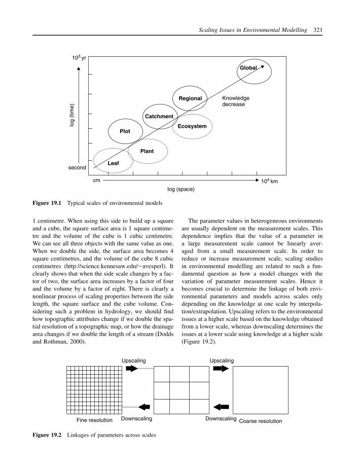
Scaling Issues in Environmental Modelling 321
Plot
Catchment
Regional
Global
Leaf
Plant
Ecosystem
cm
103 yr
log (space)
second
log
(tim
e)
Knowledgedecrease
104 km
Figure 19.1 Typical scales of environmental models
1 centimetre. When using this side to build up a squareand a cube, the square surface area is 1 square centime-tre and the volume of the cube is 1 cubic centimetre.We can see all three objects with the same value as one.When we double the side, the surface area becomes 4square centimetres, and the volume of the cube 8 cubiccentimetres (http://science.kennesaw.edu/∼avesperl). Itclearly shows that when the side scale changes by a fac-tor of two, the surface area increases by a factor of fourand the volume by a factor of eight. There is clearly anonlinear process of scaling properties between the sidelength, the square surface and the cube volume. Con-sidering such a problem in hydrology, we should findhow topographic attributes change if we double the spa-tial resolution of a topographic map, or how the drainagearea changes if we double the length of a stream (Doddsand Rothman, 2000).
The parameter values in heterogeneous environmentsare usually dependent on the measurement scales. Thisdependence implies that the value of a parameter ina large measurement scale cannot be linearly aver-aged from a small measurement scale. In order toreduce or increase measurement scale, scaling studiesin environmental modelling are related to such a fun-damental question as how a model changes with thevariation of parameter measurement scales. Hence itbecomes crucial to determine the linkage of both envi-ronmental parameters and models across scales onlydepending on the knowledge at one scale by interpola-tion/extrapolation. Upscaling refers to the environmentalissues at a higher scale based on the knowledge obtainedfrom a lower scale, whereas downscaling determines theissues at a lower scale using knowledge at a higher scale(Figure 19.2).
Upscaling
Downscaling Downscaling
Upscaling
Fine resolution Coarse resolution
Figure 19.2 Linkages of parameters across scales

322 Xiaoyang Zhang, Nick A. Drake and John Wainwright
19.3 CAUSES OF SCALING PROBLEMS
There are a number of conceptually distinct reasonsresulting in scaling problems (Heuvelink, 1998; Har-vey, 2000; Peterson, 2000). First of all, the most com-mon and fundamental cause of scaling problems isthe existence of both spatial heterogeneity and relevantprocess nonlinearities. Environmental models more orless require both climatic/weather input data and land-surface parameters, which are derived from measure-ments including precipitation, temperature, topography,soil physical and chemical properties, land cover/landuse and hydrological properties. These data are consid-erably variable both spatially and temporally, creatingdifficulties in aggregating large-scale behaviour fromlocal processes.
Second, different processes are primarily dominatedat different scales. This means the correlations derived atone scale might not be applicable at another. Because ofthe existence of different dominant processes at variousscales, the effects of an increasing number of processesneed to be incorporated as a scaling method attemptsto span over a wider range of scale. Third, feedbackis associated with the interaction between small-scaleparameters of a system and large-scale variables sinceprocesses at different scales affect each another. Pro-cesses operating at small and fast scales are constrainedby processes operating at slow and large scales, whilelarge and slow processes are constructed and organizedby the interactions of many small fast processes (Ahland Allen, 1996). These cross-scale connections sug-gest that scaling should only be applied over a lim-ited range of scales and in specific situations. Fourth,emergent properties arise from the mutual interaction ofsmall-scale components among themselves rather thansome outside force. The processes can abruptly reor-ganize themselves through time, rendering previouslydeveloped scaling relationships invalid as the structureand processes that they incorporate cease to exist. Fifth,when there is a temporal lag in the response of a systemto perturbation, a scaling problem may arise becauseof the lack of information about process linkages in adynamic environment.
19.4 SCALING ISSUES OF INPUT PARAMETERSAND POSSIBLE SOLUTIONS
19.4.1 Change of parameters with scale
Data required for environmental modelling are measuredeither at a point such as precipitation, temperature andsoil properties, or over a given area such as remotely
sensed data. The reliability of the data value in an areais affected by both its neighbours and internal hetero-geneity. Pixels in remote sensing imagery, which arethe smallest element of an electronic image, have beenwidely used to measure environmental properties. Nev-ertheless, sensors are commonly centre-biased such thatthe reflectance towards the centre of the field of viewhas most influence on the reflectance (Fisher, 1997).It is poorly understood whether the reflectance fromone location on the ground only influences the cor-responding pixel, or whether it may have an effecton values for surrounding pixels. On the other hand,information in one pixel, especially a large pixel, isusually the mixture of different ground objects ratherthan presenting a true geographical object (Settle andDrake, 1993; Fisher, 1997). The environmental param-eter extracted from a large grid only indicates a rep-resentative value rather than a real physical meaning.For example, if there are more than three types of soilor land cover/land use, the corresponding categoricalvalue in a large grid is only a domain value whichmay represent a proportion less than 50% of reality.It is a snare and a delusion to take pixels with vari-ous resolutions as a homogenous reality on the ground(Fisher, 1997).
Changing the scale of measurement has a significantimpact on the variability of object quantities. A land-surface parameter at various scales represents the differ-ent amount of details referring to both spatial patternsand observed values. The most well-known example isthe measurement of the length of Britain’s coastline,in which the values change greatly from one measure-ment to another when different spatial resolution mapsare used. If the whole of Britain were reduced to onepixel, the length measurement of the coastline would beno more than the sum of four pixel sides. It would beignored if the pixel size were as large as the whole ofEurope. In contrast, it would be huge if a measurementscale were less than a millimetre. Obviously, all thesevalues are not able to represent reality. In many casesof the natural world, a single value of a parameter is notmeaningful when the measurement scale is too small ortoo large.
It has been recognized that measured data are anexplicit representation, abstraction or model of someproperties varying in N-dimensional Euclidean spaceinstead of reality itself (Gatrell, 1991; Burrough andMcDonnell, 1998; Atkinson and Tate, 1999). Sinceall data are a function of the underlying reality andsampling framework, the data we obtained can generallybe described as the following equation (Atkinson, 1999):
Z(x) = f (Y (x), d) (19.1)
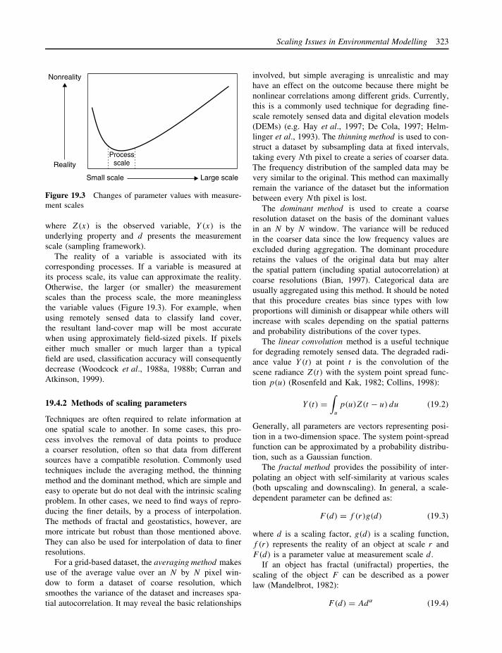
Scaling Issues in Environmental Modelling 323
Small scale Large scale
Reality
Nonreality
Processscale
Figure 19.3 Changes of parameter values with measure-ment scales
where Z(x) is the observed variable, Y (x) is theunderlying property and d presents the measurementscale (sampling framework).
The reality of a variable is associated with itscorresponding processes. If a variable is measured atits process scale, its value can approximate the reality.Otherwise, the larger (or smaller) the measurementscales than the process scale, the more meaninglessthe variable values (Figure 19.3). For example, whenusing remotely sensed data to classify land cover,the resultant land-cover map will be most accuratewhen using approximately field-sized pixels. If pixelseither much smaller or much larger than a typicalfield are used, classification accuracy will consequentlydecrease (Woodcock et al., 1988a, 1988b; Curran andAtkinson, 1999).
19.4.2 Methods of scaling parameters
Techniques are often required to relate information atone spatial scale to another. In some cases, this pro-cess involves the removal of data points to producea coarser resolution, often so that data from differentsources have a compatible resolution. Commonly usedtechniques include the averaging method, the thinningmethod and the dominant method, which are simple andeasy to operate but do not deal with the intrinsic scalingproblem. In other cases, we need to find ways of repro-ducing the finer details, by a process of interpolation.The methods of fractal and geostatistics, however, aremore intricate but robust than those mentioned above.They can also be used for interpolation of data to finerresolutions.
For a grid-based dataset, the averaging method makesuse of the average value over an N by N pixel win-dow to form a dataset of coarse resolution, whichsmoothes the variance of the dataset and increases spa-tial autocorrelation. It may reveal the basic relationships
involved, but simple averaging is unrealistic and mayhave an effect on the outcome because there might benonlinear correlations among different grids. Currently,this is a commonly used technique for degrading fine-scale remotely sensed data and digital elevation models(DEMs) (e.g. Hay et al., 1997; De Cola, 1997; Helm-linger et al., 1993). The thinning method is used to con-struct a dataset by subsampling data at fixed intervals,taking every N th pixel to create a series of coarser data.The frequency distribution of the sampled data may bevery similar to the original. This method can maximallyremain the variance of the dataset but the informationbetween every N th pixel is lost.
The dominant method is used to create a coarseresolution dataset on the basis of the dominant valuesin an N by N window. The variance will be reducedin the coarser data since the low frequency values areexcluded during aggregation. The dominant procedureretains the values of the original data but may alterthe spatial pattern (including spatial autocorrelation) atcoarse resolutions (Bian, 1997). Categorical data areusually aggregated using this method. It should be notedthat this procedure creates bias since types with lowproportions will diminish or disappear while others willincrease with scales depending on the spatial patternsand probability distributions of the cover types.
The linear convolution method is a useful techniquefor degrading remotely sensed data. The degraded radi-ance value Y (t) at point t is the convolution of thescene radiance Z(t) with the system point spread func-tion p(u) (Rosenfeld and Kak, 1982; Collins, 1998):
Y (t) =∫
u
p(u)Z(t − u) du (19.2)
Generally, all parameters are vectors representing posi-tion in a two-dimension space. The system point-spreadfunction can be approximated by a probability distribu-tion, such as a Gaussian function.
The fractal method provides the possibility of inter-polating an object with self-similarity at various scales(both upscaling and downscaling). In general, a scale-dependent parameter can be defined as:
F(d) = f (r)g(d) (19.3)
where d is a scaling factor, g(d) is a scaling function,f (r) represents the reality of an object at scale r andF(d) is a parameter value at measurement scale d .
If an object has fractal (unifractal) properties, thescaling of the object F can be described as a powerlaw (Mandelbrot, 1982):
F(d) = Adα (19.4)

324 Xiaoyang Zhang, Nick A. Drake and John Wainwright
withα = D − L + 1 (19.5)
where D is the fractal dimension, L is a Euclideandimension and A is the amplitude or prefactor whichis related to the lacunarity (patchiness) of an object.
This universal scaling law has been widely appliedin biological and environmental research. For example,the metabolic rate for a series of organisms ranging fromthe smallest microbes to the largest mammals is a powerfunction of mass (West et al., 2000). The number ofspecies found in a censused patch of habitat on the areaof that patch can be described by a power function ofarea (Harte, 2000). Hydrological parameters and mor-phological attributes are clear special scaling featureswith this power law (Braun et al., 1997; Zhang et al.,1999). Note that the spatial distribution of the fractaldimension has to be determined if we need to scale aparameter spatially (Zhang et al., 1999). The limitationof the fractal method is that multifractal properties ofobjects may exist over a broad range of scales (e.g.Evens and McClean, 1995), and the unifractal relation-ship may break down when the measurement scales arevery small or very large.
The kriging method denotes a set of techniques topredict (extrapolate) data quantities and their spatial dis-tribution. Commonly used methods are simple kriging,universal kriging and co-kriging. Simple kriging is aheterogeneous best linear unbiased predictor in terms ofboth the mean function and the covariance of sampledata, whereas universal kriging only requires determin-ing a variogram for the extrapolation of point data. Co-kriging provides a consistent framework to incorporateauxiliary information, which is easy to obtain, into theprediction. This technique can predict spatial data moreprecisely (Papritz and Stein, 1999). Other robust mea-surements of spatial interpolation include the fitting ofsplines (e.g. De Boor, 1978) and the modelling processitself (see Chapter 20).
19.5 METHODOLOGY FOR SCALINGPHYSICALLY BASED MODELS
19.5.1 Incompatibilities between scales
A major source of error in environmental models comesfrom the incompatibilities between model scale, input-parameter (database) scale and the intended scale ofmodel outputs. The most common issue is that theparameters are measured at one scale (or several dif-ferent scales) and are input into a model constructed atanother scale. When we build an environmental model,
at least two groups of measurements at the same ora similar scale are required. One is used to estab-lish a model while another is employed to test themodel. When changing measurement scales, the mod-els based on these measurements may vary considerably.For example, Campbell et al. (1999) found that effectivedispersion values estimated using data from each typeof probe were systematically different when using dif-ferent devices to obtain solute transport parameters formodelling. This difference may be a scale issue result-ing from the probe sampling volumes. Even if a modeloperates linearly across the range of model-input val-ues, the aggregation of the model-parameter values withincreased scale still biases model predictions becauseof the heterogeneity. Both the model constants and therelationship significance between dependent and inde-pendent variables are usually controlled by the scale ofprocessing of the model. For example, when investigat-ing a linear model between elevation and biomass indexusing different spatial resolution of parameters, Bian(1997) found the constants in the model and the cor-relation coefficient between independent variables andthe dependent variable to be very changeable. The sameresult was also identified by Walsh et al. (1997) whenanalysing a linear regression model between NormalizedDifference Vegetation Index (NDVI) and elevation on amountain. Therefore, if a model is established at a pro-cess scale and input parameters measured at the samescale, the model output should be accurate and accept-able. The relationship between process and measurementscale is that processes larger than the coverage appearas trends in the data, whereas processes smaller thanthe resolution appear as noise (Figure 19.4; Bloschl andSivapalan, 1995).
Trend
Observation scale
Pro
cess
sca
le
Resolution
Coverage
Noise
Commensurate
Figure 19.4 Process scale versus observation scaleSource: Bloschl and Sivapalan (1995). Reproduced bypermission of John Wiley & Sons
Scaling Issues in Environmental Modelling 325
19.5.2 Methods for upscaling environmental models
If we could take the Earth as a unit to build up aglobal model, it would produce a very accurate out-put of our interests when each input and output is onlyone single measured value at the global scale. How-ever, global-scale model operation should rely on scalelinkages of environmental objects to certain conceptualframeworks due to the difficulties in making direct mea-surements at a large scale. Although it is very hard toscale a complex assemblage of parameters and mod-els to corresponding process scales, it is feasible toidentify a few scaleable parameters within the complexenvironment in an attempt to reduce the scale uncer-tainties of modelling. Any methods reducing the scal-ing effects would be a great improvement to modellingresults since it seems impossible to completely eliminatethe impact of scale on environmental modelling (Luo,1999). There are several methods available to trans-late ecological and environmental models across spatialscales (King, 1991; Rastetter et al., 1992; Harvey, 2000;Bugmann et al., 2000).
19.5.2.1 Calibration of a model
This approach is to adopt a model, which is applicableat small scales, for application at large scales using‘calibration’ values. The calibration technique is to setup an empirically calibrated relationship between fine-and coarse-scale data. This approach requires that bothfine- and coarse-scale data are available to perform thecalibration. The calibrated models may only be treatedas valid within the ranges of input and output dataused for the calibration, and the incorporation of newmodel variables requires recalibration of the relationship(Rastetter et al., 1992; Friedl et al., 1997). In practicalterms, it is difficult to carry out measurements forcalibration at various scales, especially very large scales.However, because of the nonlinearity of the processesinvolved, together with the heterogeneity of the naturalsystem, there is no reason to suppose that the use ofcalibration values should be any more successful inreproducing the areal average result (Beven, 1995).
19.5.2.2 Multi-scale models
Since the processes change with various scales, a setof different models are required for various particularscales, such as specifically used at field plot, watershed,regional and global scales (David et al., 1996; Kirkbyet al., 1996; Poesen et al., 1996). Separate scalingmethods could be developed for each individual process,
and the rules for transitions between them could beused to synthesize these separate scaling methods intoan aggregate scaling method which incorporates thebehaviour of the ensemble of scales (Peterson, 2000).The plot-scale environmental models may representphysical and other processes in detail while large-scalemodels can provide a potential value, such as potentialcumulative soil erosion at the global scale (Kirkbyand Cox, 1995; Kirkby et al., 1996). In doing so, thescale effects are included in each individual model andthe environment could be accurately simulated. Unlikeplot-scale models, however, regional- and global-scalemodels are rarely available.
19.5.2.3 Lumped models
The lumping method is carried out by integrating theincreased heterogeneity that accompanies the change inmodel extent by aggregating across heterogeneity inenvironmental parameters. Since an area is taken as awhole to calculate the model result, a lumped modelis like a zero-dimensional representation of spatial fea-tures (Maidment, 1993). A major concern in using alumped model is the possibility of obtaining a singlevalue of a spatially changeable parameter that allowsa model to predict the mean response of the mod-elled area (Moore and Gallant, 1991). To address thisneed in upscaling studies, the most common way totreat a lumped system is that the related properties arespatially averaged and the mean values are calculatedfor the modelling parameters. This approach is basedon the assumption that a model is linear in its struc-ture, and no attempt is made to describe the spatialheterogeneity. Alternatively, a more effective way ofprocessing a lumped model is to choose aggregated rep-resentative parameters accounting for the heterogeneity.A noticeable example is that the representative param-eters across scales are calculated by using self-similarfractals, such as topographic properties for hydrologicalmodels (Braun et al., 1997; Zhang et al., 1999). Sinceone single set of model calculations is applied acrossthe whole area, the spatial distribution of model resultsis not taken into consideration.
19.5.2.4 Distributed (partitioning) method
A research area is divided into many grid cells (orsubareas, patches and strata) with relatively homoge-neous environmental conditions. Each grid cell is rep-resented by mean values of environmental processes inthe computation of regional and global estimates, such as
326 Xiaoyang Zhang, Nick A. Drake and John Wainwright
in a grid-based approach. The heterogeneity (variance)within a grid cell is minimized while it is maximizedbetween cells. The environmental behaviour in a largearea is determined as the areally weighted average ofthe behaviour of all those cells after a local model isemployed in each grid cell. The resultant value in alarge area can be estimated in Equation 19.6:
F =i=k∑i=1
pif (xi) (19.6)
where pi is the proportion of the total area that stratumi occupies, and xi is the mean of x in the stratum i.
A number of practical approaches can be used todetermine homogeneous areas. First, a straightforwardmethod is to run the model in each grid cell across aregion. It is assumed that each grid cell is homogeneousand fits the modelling scale no matter what the sizeof the cell is. For example, land vulnerability to watererosion was assessed directly by running a plot modelon a 0.5◦ dataset by Batjes (1996). There are severalmore reasonable ways to apply distributed models.
Second, when studying rainfall and runoff, Woodet al. (1988, 1990) created the representative elementaryarea (REA) concept and gave it a definition of the‘smallest discernible point which is representative ofthe continuum’ (see also Chapter 3). The REA conceptis employed for finding a certain preferred time andspatial scale over which the process representationscan remain simple and at which distributed catchmentbehaviours can be represented without the apparentlyundefinable complexity of local heterogeneity. Thisconcept provides a motivation for measurements ofspatial variability as it highlights the interaction betweenscale and variability. It indicates that the variances andcovariances of key variables are invariant in land unitsabove a certain threshold size. It is difficult in practice,however, to determine the size of the REA because itis strongly controlled by environmental characteristics(Bloschl et al., 1995).
Third, in regional hydrological modelling, the con-cept of a hydrological response unit (HRU) has beendeveloped. The HRU is a distributed, heterogeneouslystructured entity having a common climate, land use andunderlying pedo-topo-geological associations control-ling their hydrological dynamics. The crucial assumptionfor each HRU is that the variation of the hydro-logical process dynamics within the HRU must besmall compared with the dynamics in a different HRU(Flugel, 1995).
Fourth, geostatistics, such as measures of spatial auto-correlation between data values, provides a methodol-ogy of determining a relative homogeneous size for
environmental modelling. Homogeneous areas are seenas having high spatial autocorrelation such that a coarsespatial resolution would be appropriate, and heteroge-neous areas are seen as having low spatial autocorrela-tion so that a fine spatial resolution would be needed(Curran and Atkinson, 1999). Analysing the variogramchange with spatial resolution can help to identify thepredominant scale of spatial variation, which might bean optimal scale for environmental modelling. Severalstatistical models can provide ways to identify the opti-mum scale of a variable. The average local varianceestimating from a moving window is a function ofmeasurement scale (Woodcock and Strahler, 1987). Thescale at which the peak occurs may be used to selectthe predominant scale of variables. Similar to the localvariance method, the semi-variance at a lag of one pixelplotted against spatial resolution is an effective meansof determining the optimal scale. For example, whenusing this technique with remote sensing data, Curranand Atkinson (1999) found that a spatial scale of 60 mwas suitable for the analysis of urban areas, whereas120 m was suitable for agricultural areas. The dispersionvariance of a variable defined on a spatial scale withina specified region may also be applied to link informa-tion pertinent to the choice of optimal scale (Van derMeer, 1994). All the above approaches are acceptablefor dealing with scaling problems that arise due to spa-tial heterogeneity combined with process nonlinearity,but are not valid when there are interactions betweenadjacent grids (or areas).
19.5.2.5 Routing approach
The model structure remains the same across scaleswhile the variables (fluxes) for the models are spatiallyand temporally modified. Such interactions always occurin hydrological processes, where the model output atlarge scales is far from being the simple sum of eachgrid cell. When water flow and sediment move from thedivide to the outflow of a catchment and from a smallcatchment to a large catchment, the values of relatedhydrological variables in a grid are affected not onlyby the environmental characteristics within this grid butalso by properties in the surrounding grid cells. Therunoff in a pixel is determined by the precipitation andinfiltration within this grid, and water inputting from anddischarging to neighbouring grids. The amount of sed-iment deposited or detached in a grid cell is stronglydependent on the movement of both water and sed-iment in surrounding neighbouring grids. Hence therouting approach is usually employed after calculat-ing the drainage direction on the basis of the steepest

Scaling Issues in Environmental Modelling 327
Figure 19.5 The routing of hydrological models accord-ing to the steepest topographic slope
descent of topography (Figure 19.5). This technique hasbeen effectively employed in runoff and sediment trans-port models at large scales (e.g. Richards, 1993; Pilottiand Bacchi, 1997).
19.5.2.6 Frequency-distribution-based method(expected value or partial transformations)
This approach is defined as the calculation of theexpected value of the model output based on the jointfrequency distribution of the variables describing envi-ronmental heterogeneity (King, 1991; Rastetter et al.,1992). Probability density functions that describe theheterogeneity at subgrid scales in the input data haveto be determined to estimate the expected model outputvalue over the region of interest. The equation used maybe expressed as:
F = E[f (X)] =∫ +∞
−∞f (x)p(x)dx (19.7)
where f (X) is a local model, E[f (X)] is the expectationvalue of f (X), X is a random variable (or vector ofrandom variables), and p(x) is the probability densityfunction (or the joint frequency distribution) describingthe subgrid scale variance in X. In an environmentalmodel, parameters always include attributes derivedfrom factors such as climate, landscape and soil. Clearly,the joint frequency distribution of such parameters israrely known if there are a large number of parametersfor a model. Nevertheless, using such an approach toaccount for one or two of the most important nonlinearmodel input parameters can substantially improve modelresults (Avissar, 1992; Friedl, 1997).
To solve this equation simply, Bresler and Dagan(1988) and Band (1991) use a Taylor series expansionabout the vector mean of model parameters, wherethe distribution information required is reduced to thevariance-covariance matrix of the key model variables.Taylor series expansions can transform models from fineto coarse scales. The equation becomes:
F =∑ f (i)(µx)
i!E[(X − µx)
i] (19.8)
where µx is the mean of X, f (i)(µx) is the ith derivativeof f (X) evaluated at µx with respect to X, and E(X −µx)
i is the expected value of the ith moment of X
about µx . To implement this type of solution, the modelmust either have higher-order derivatives all equal tozero, or the expansions must be estimated from sampledata. In either case, this approach is typically limitedto an approximation of the exact solution providedby partial transformations (Friedl, 1997). Using thismethod, it is only possible to derive areal average valuesof environmental variables rather than their spatialdistribution. Such a result is a very useful means ofapproximating values over large areas, for example inestimating the average global carbon storage, whereas itwould be meaningless to talk in these terms in relationto land-surface properties.
19.5.2.7 Analytical integration
The method of analytical integration is used to extrapo-late a model employing explicit, analytical integration ofthe local model in time and space, which of course pro-vides not only an accurate, but even an ‘exact estimate’:
F =∫
x
∫y
∫t
f (x, y, t) dt dy dx (19.9)
where f (x, y, t) is the local model in time t and space(x, y). This method is typically not feasible becauseclosed-form analytical integrals cannot be found formany environmental models (Bugmann et al., 2000).
19.5.2.8 Parameterizing interaction
Fluxes in the natural world not only interfere butalso have feedback with each other (Harvey, 2000).It is necessary either to parameterize the interactioneffects between grid cells directly, or to create awhole new model which incorporates these interactionsand their effects. The parameterization approach ofrepresenting inter-grid interactions can be used when the
328 Xiaoyang Zhang, Nick A. Drake and John Wainwright
small-scale effects do not significantly affect the processat large scales.
19.5.3 Approaches for downscaling climate models
Downscaling is concerned with taking the output ofglobal change models and deducing the changes thatwould occur at finer scales than those resolved bysuch a model as a general circulation model (GCM).This approach has subsequently emerged as a means ofinterpolating regional-scale atmospheric predictor vari-ables (such as a mean sea level pressure or vorticity)to station-scale meteorological series or agriculturalproduction (Karl et al., 1990; Wigley et al., 1990;Hay et al., 1992; Wilby and Wigley, 1997: see alsoChapter 2). The fundamental assumption is that rela-tionships can be established between atmospheric pro-cesses occurring at disparate temporal and/or spatialscales. Wilby and Wigley (1997) reviewed four cate-gories of downscaling methods in GCM. First, regres-sion methods involve establishing linear or nonlinearrelationships between fine-resolution parameters andcoarse-resolution predictor variables. Second, weather-pattern approaches of downscaling typically involvestatistically relating observed station or area-averagemeteorological data to a given weather classificationscheme, which may be either objectively or subjec-tively derived. Third, stochastic weather generators aredesigned to simulate daily time-series of climate datafor each successive day governed by the characteris-tics of previous days based on first or multiple-orderMarkov renewal processes. These models are commonlyused for climate-impact studies. Fourth, limited-area cli-mate models are high-resolution limited-area climatemodels embedded with GCM and use GCM to definethe boundary conditions. These models have the abil-ity to simulate small-scale atmospheric features andmay provide atmospheric data for impact assessmentsthat reflect the natural heterogeneity of the climate atregional scales.
19.6 SCALING LAND-SURFACE PARAMETERSFOR A SOIL-EROSION MODEL: A CASE STUDY
Soil erosion is recognized as a major problem arisingfrom agricultural intensification, land degradation andpossibly global climatic change (see Chapters 9 and16). However, the extent of the problem is hard toquantify as field measurements of erosion are rare,time-consuming, and are only acquired over restrictedtemporal and spatial scales. Global scale soil-erosion
modelling can provide a quantitative and consistentapproach to estimating erosion. Such a methodology canbe used to define regions where erosion is high andmanagement is needed (Drake et al., 1999).
Current erosion models are developed from the analy-sis of the results of plot-scale erosion experiments (1 m2
to 30 m2). One of the physically based models developedby Thornes (1985, see also Chapter 18) is defined as:
E = k OF2s1.67e−0.07v (19.10)
where E is erosion (mm day−1), k is a soil erodibilitycoefficient, OF denotes overland flow (mm day−1), s isthe slope (m m−1) and v the vegetation cover (%).
In order to overcome the scaling problem, methodshave been developed to upscale this plot-scale modelby downscaling topography and vegetation cover fromthe global scale (10 arc minutes) to the plot scale(30 m). Global soil erosion has then been calculated byimplementing this upscaled erosion model.
19.6.1 Sensitivity of both topographic slope andvegetation cover to erosion
Both the nonlinearity between model output and param-eters and the spatial heterogeneity of parameters can beidentified using sensitivity analysis. In order to inves-tigate the sensitivity of the soil-erosion model to thescale of the slope measurement, a global 30′′ DEM wasdegraded to lower resolutions using pixel thinning (seeabove). The slope values were calculated from theseDEMs and then erosion was calculated using averagemonthly values of both overland flow and vegetationcover. Thus, the only changing parameter is the spa-tial resolution of the slope. Average slope is reducedfrom 3.93% at 30′′ to 0.39% at 30′ in the area of Eura-sia and northern Africa. Estimated erosion is reducedexponentially by two orders of magnitude (from 0.03 to0.0007 mm month−1) as slope is reduced by the scalingeffect over this range (Zhang et al., 1997).
When changing spatial distributions and scales ofvegetation cover, the amount of soil loss predicatedby using the erosion model varies considerably (Drakeet al., 1999). This variability occurs because the nega-tive exponential relationship between cover and erosioncombined with the heterogeneity of vegetation covermeans that erosion is very high in bare areas but verylow once cover is greater than 30%. If we consider ahigh-resolution image of individual plants with 100%cover surrounded by bare soil, each pixel is homoge-nous with either vegetation or bare soil. Erosion is thenvery high in bare areas and nonexistent under the plants.

Scaling Issues in Environmental Modelling 329
When the spatial resolution of the image is reduced to apoint exceeding the size of the field plant, heterogeneitywithin a pixel occurs and predicted erosion is reducedbecause some of the vegetation cover of the field isassigned to the bare areas. Thus a scaling technique mustbe employed to account for the original structure of thevegetation cover.
19.6.2 A fractal method for scalingtopographic slope
When analysing the regular decrease of slope valueswith the increase of spatial resolution of DEMs, Zhanget al. (1999) directly link the scaling of slope mea-surements with the fractal dimension of topography.When focusing on the difference in elevation betweentwo points and the distance between them, the vari-ogram equation used to calculate the fractal dimensionof topography (Klinkenberg and Goodchild, 1992) canbe converted to the following formula:
∣∣∣∣Zp − Zq
d
∣∣∣∣ = γ d1−D (19.11)
where Zp and Zq are the elevations at points p and q, d
is the distance between p and q, γ is a coefficient and
D is fractal dimension. Because the equation
∣∣∣∣Zp − Zq
d
∣∣∣∣represents the surface slope it can be assumed that theslope value s is associated with its corresponding scale(grid size) d by the equation:
s = rd1−D (19.12)
This result implies that if topography is unifractal in aspecified range of measurement scale, slope will then bea function of the measurement scale. If a research areawere taken as a whole to determine the parameters γ andD, there would be only one value of scaled slope. It isnecessary in practice to keep the spatial heterogeneity ofslope values. After analysing the spatial variation of γ
and D in different subareas, it was discovered that bothγ and D are mainly controlled by the standard deviationof the elevations (Zhang et al., 1999). Hence correlationfunctions are established between γ and D and localstandard deviation. When the standard deviation in eachpixel is determined by moving a 3 × 3 pixel window, thespatial distributions of both γ and D are then calculated.Therefore, the slope values for each pixel with finermeasurement scales can be successfully estimated onthe basis of coarse resolution DEMs.
19.6.3 A frequency-distribution function for scalingvegetation cover
The entire information required for environmental mod-elling is saved in distribution functions. Instead ofassuming a Gaussian distribution, different distributionmodes are discovered after analysing multi-scale data ofvegetation cover (Zhang et al., 2002). The Polya distri-bution, a mixture distribution of a beta and a binomialdistribution, is very effective in simulating the distri-bution of vegetation cover at numerous measurementscales (Zhang et al., 2002).
f (x) = nCx
∫ 1
0θx(1 − θ)n−x
[�(α + β)
�(α)�(β)
]
× θα−1(1 − θ)β−1dθ 0 ≤ x ≤ n ≤ N (19.13)
where n is the number of sampling events, α and β arethe parameters defined by variance and expected value,x represents a random variable between 0 and n, and θ
is a variable that ranges between 0 and 1.Both the expected value and the variance in this
function have to be calculated for the determinationof parameters α and β. When changing the spatialresolution of vegetation cover, it is seen that theexpectation is stable across scales while the varianceis reduced at increasingly smaller scales. Therefore amethod of predicting this reduction in variance is neededin order to employ the Poyla function to predict thefrequency distribution at the fine scales from coarseresolution data. When a multi-scale dataset degradingthe high resolution vegetation cover (0.55 m) derivedfrom aerial photography is analysed, it can be seen thata logarithmic function between variance and scale inall the subimages can effectively describe the declineof subimage variance with increasing spatial resolution(Zhang et al., 2002):
σ 2 = a + b ln(d) (19.14)
where σ 2 represents variance, d represents measurementscale, and a and b are coefficients.
After the subimage variance is calculated, the distri-bution of vegetation cover in a subimage (or a pixel) canbe estimated across (up or down) scales. Using this tech-nique, the frequency distributions of vegetation cover ata measurement scale of 30 m are predicted on the basisof vegetation cover derived from AVHRR-NDVI at aresolution of 1 km (Figure 19.6).
19.6.4 Upscaled soil-erosion models
It is clear that for accurately calculating soil erosion atthe global scale, the Thornes erosion model needs to
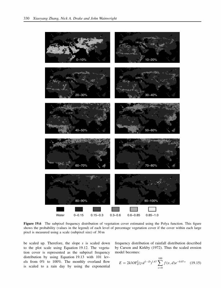
330 Xiaoyang Zhang, Nick A. Drake and John Wainwright
0–10% 10–20%
20–30% 30–40%
40–50% 50–60%
60–70% 70–80%
80–90%
Water 0–0.15 0.15–0.3 0.3–0.6 0.6–0.85 0.85–1.0
90–100%
Figure 19.6 The subpixel frequency distribution of vegetation cover estimated using the Polya function. This figureshows the probability (values in the legend) of each level of percentage vegetation cover if the cover within each largepixel is measured using a scale (subpixel size) of 30 m
be scaled up. Therefore, the slope s is scaled downto the plot scale using Equation 19.12. The vegeta-tion cover is represented as the subpixel frequencydistribution by using Equation 19.13 with 101 lev-els from 0% to 100%. The monthly overland flowis scaled to a rain day by using the exponential
frequency distribution of rainfall distribution describedby Carson and Kirkby (1972). Thus the scaled erosionmodel becomes:
E = 2klOF20(γ d1−D)1.67
100∑v=0
f (v, d)e−0.07 v (19.15)

Scaling Issues in Environmental Modelling 331
Jan. Feb.
Mar. Apr.
May Jun.
Jul. Aug.
Sept. Oct.
Nov.
Water 0–0.005 0.005–0.1 0.1–0.4 0.4–2.0 > 2
Dec.
Figure 19.7 Spatial and temporal distributions of soil erosion in Eurasia and North Africa (mm month−1)

332 Xiaoyang Zhang, Nick A. Drake and John Wainwright
where E is monthly erosion (mm), k is a soil erodibilitycoefficient, OF is average daily overland flow (mm), l
is the monthly number of rainfall events (days), D isthe local topographic fraction dimension, γ is a localtopographic parameter, v is the percentage vegetationcover, f (v, d) is the Polya mass function, d representsthe original modelling scale and s is the slope (m m−1).
This upscaled model is employed to calculate monthlyglobal erosion in Eurasia and North Africa based on adataset of 1 km-resolution (Figure 19.7). The requireddataset includes monthly overland flow calculated usinga modified Carson and Kirkby (1972) model (Zhanget al., 2002), monthly vegetation cover estimated interms of AVHRR-NDVI (Zhang et al., 1997), anda DEM selected from http://edcwww.cr.usgs.gov/land-daac/. The resultant spatial pattern of soil erosion sug-gests that high rates of soil erosion can be accountedfor in terms of the steep unstable terrain, highly erodiblesoil, high monthly precipitation, and vegetation removalby human activity or seasonal factors. Conversely, lowsoil-erosion rates reflect the lower relief, the greaterdensity of the vegetation canopy, and the areas of lowprecipitation. Erosion is serious in southern East Asia,India, along the Himalayas and Alps, and in West Africa.In seasonal terms, the erosion rate is high from springto autumn in south-east China, summer and autumnin India, and from April to October in West Africa.Relatively high erosion rates occur in Western Europeduring the winter months while very low soil loss occursin summer.
19.7 CONCLUSION
The importance of scaling issues in environmentalmodeling has been widely recognized. A number oftechniques have been developed to reduce the scalingeffects on modelling outputs. A very effective approachis to identify scaleable parameters that characterizethe relevant intrinsic environmental processes. Whenscaling several important environmental parameters tofit the scales of environmental models, the resultantvalues can be greatly improved. Since an environmentalmodel is generally complex and related to severaltypes of parameters, it may be necessary to combineseveral scaling techniques of scaling both parametersand models for the reduction of scale uncertainties. Thisprocedure has been demonstrated in the modelling ofsoil erosion at the global scale. However, we need topay more attention to the following issues.
1. Few scaling methods have effectively dealt withintrinsic environmental behaviour at regional and
global scales since our solid knowledge remains onthe local processes.
2. There are mainly two purposes of upscaling a modelto regional or global scales. One is to derive thespatial distribution of our interests while the second isto calculate a single value in a large area. The outputmodelled on the basis of a distributed dataset may justrepresent the spatial distribution of the result in theresolution of the dataset. In many cases, the sum ofthe spatially distributed output cannot be taken as thevalue in a whole region (globe) since the spatial andtemporal interaction and feedback of the processesmay occur at large scales.
3. An applicable technique is required for a reasonablevalidation of scaled models at regional and globalscales. It is insufficient to only verify the reliabilityof global scale results by comparing the differenceamong several typical spatial areas such as the Ama-zon tropical forest area and the Sahara desert, sinceany kind of model can produce several obviously dif-ferent patterns at a global scale.
REFERENCES
Ahl, V. and Allen, T.F.H. (1996) Hierarchy Theory: A Vision,Vocabulary, and Epistemology, Columbia University Press,New York.
Atkinson, P.M. (1999) Spatial statistics, in A. Stein, F. vander Meer and B. Gorte (eds) Spatial Statistics for RemoteSensing, Kluwer Academic Publishers, Dordrecht, 57–81.
Atkinson, P.M. and Tate, N.J. (1999) Extracting informationfrom remotely sensed and GIS data, in P.M. Atkinsonand N.J. Tate (eds) Advances in Remote Sensing and GISAnalysis, John Wiley & Sons, Chichester, 263–268.
Avissar, R. (1992) Conceptual aspects of a statistical-dynamicalapproach to represent landscape subgrid scale heterogeneitiesin atmospheric models, Journal of Geophysical Research-Atmospheres 97, 2729–2742.
Band, L.E. (1991) Distributed parameterization of complex ter-rain, in E.F. Wood (ed.) Land Surface–Atmosphere Interac-tions for Climate Modelling, Kluwer Academic, Dordrecht,249–270.
Batjes, N.H. (1996) Global assessment of land vulnerability towater erosion on a 1/2 degrees by 1/2 degrees grid, LandDegradation & Development 7 (4), 353–365.
Beven, K. (1995) Linking parameters across scales: subgridparameterizations and scale dependent hydrological models,in J.D. Kalma and M. Sivapalan (eds) Scale Issues in Hydro-logical Modelling, John Wiley & Sons, Chichester, 263–282.
Bian, L. (1997) Multiscale nature of spatial data in scal-ing up environmental models, in D.A. Quattrochi andM.F. Goodchild (eds) Scale in Remote Sensing and GIS,Raton Lewis Publishers, Boca Raton, FL, 13–26.
Bloschl, G., Grayson, R.B. and Sivapalan, M. (1995) On therepresentative elementary area (REA) concept and its utility
Scaling Issues in Environmental Modelling 333
for distributed rainfall-runoff modelling, in J.D. Kalma andM. Sivapalan (eds) Scale Issues In Hydrological Modelling,John Wiley & Sons, Chichester, 71–88.
Bloschl, G. and Sivapalan, M. (1995) Scale issues in hydro-logical modeling: a review, in J.D. Kalma and M. Sivapalan(eds) Scale Issues in Hydrological Modelling, John Wiley &Sons, Chichester, 9–48.
Braun, P., Molnar, T. and Kleeberg, H.-B. (1997) The problemof scaling in grid-related hydrological process modelling,Hydrological Processes 11, 1219–1230.
Bresler, E. and Dagan, G. (1988) Variability of yield of anirrigated crop and its causes, 1, Statement of the problemand methodology, Water Resources Research 24, 381–388.
Bugmann, H., Linder, M., Lasch, P, Flechsig, M., Ebert, B.and Cramer, W. (2000) Scaling issues in forest successionmodelling, Climatic Change 44, 265–289.
Burrough, P.A. and McDonnell, R.A. (1998) Principles ofGeographical Information Systems. Spatial Information Sys-tems and Geostatics, Oxford University Press, New York.
Campbell, C.G., Ghodrati, M. and Garrido, F. (1999) Compar-ison of time domain reflectometry, fiber optic mini-probes,and solution samplers for real time measurement of solutetransport in soil, Soil Science 164 (3), 156–170.
Carson, M.A. and Kirkby, M.J. (1972) Hillslope Form andProcess, Cambridge University Press, Cambridge.
Collins, J.B. (1998) Geostatistical methods for analysis ofmultiple scales of variation in spatial data, PhD thesis,Boston University.
Curran, P.J. and Atkinson, P.M. (1999) Issues of scale andoptimal pixel size, in A. Stain, F. van der Meer and B. Gorte(eds) Spatial Statistics for Remote Sensing, Kluwer Aca-demic Publishers, Dordrecht, 115–1333.
David, T.F., John, N.Q. and Dickinson, W.T. (1996) TheGCTE validation of soil erosion models for global changestudies, Journal of Soil and Water Conservation 15 (5),397–403.
De Boor, C. (1978) A Practical Guide to Splines, SpringerVerlag, Berlin.
De Cola, L. (1997) Multiresolution covariation among Landsatand AVHRR vegetation indices, in D.A. Quattrochi andM.F. Goodchild (eds) Scale in Remote Sensing and GIS,Lewis Publishers, Boca Raton, FL, 72–91.
Dodds, P.S. and Rothman, D.H. (2000) Scaling, university,and geomorphology, Annual Review of Earth and PlanetarySciences 28, 571–610.
Dooge, J.C.I. (1986) Looking for hydrologic laws, WaterResources Research 22, 465–585.
Drake, N.A., Zhang, X., Berkhout, E., Bonifacio, R.,Grimes, D., Wainwright, J. and Mulligan, M. (1999) Mod-elling soil erosion at global and regional scales using remotesensing and GIS techniques, in P. Atkinson and N.J. Nate(eds) Spatial Analysis for Remote Sensing and GIS, JohnWiley & Sons, Chichester, 241–261.
Evans, I.S. and McClean, C.J. (1995) The land surface is notunifractal: variograms, cirque scale and allometry, Zeitschriftfur Geomorphologie, N.F., Supplementband 101, 127–147.
Fisher, P. (1997) The pixel: a snare and a delusion, Interna-tional Journal of Remote Sensing 18 (3), 679–685.
Flugel, W.-A. (1995) Delineating hydrological response unitsby geographical information system analyses for regionalhydrological modelling using PRMS/MMS in the drainagebasin of the river Brol, Germany, in J.D. Kalma andM. Sivapalan (eds) Scale Issues in Hydrological Modelling,John Wiley & Sons, Chichester, 181–194.
Friedl, M.A. (1997) Examining the effects of sensor resolutionand sub-pixel heterogeneity on spectral vegetation indices:implications for biophysical modelling, in D.A. Quattrochiand M.F. Goodchild (eds) Scale in Remote Sensing and GIS,Lewis Publishers, Boca Raton, FL, 113–139.
Gatrell, A.C. (1991) Concepts of space and geographical data,in D.J. Maguire, M.F. Goodchild and D. Rhind (eds) Geo-graphical Information Systems: Principles and Applications,Longman, London, 119–134.
Goodchild, M.F. and Quattrochi, D.A. (1997) Scale, multi-scaling, remote sensing, and GIS, in D.A. Quattrochi andM.F. Goodchild (eds) Scale in Remote Sensing and GIS,Lewis Publishers, Boca Raton, FL, 1–11.
Harte, J. (2000) Scaling and self-similarity in species distri-butions: implication for extinction, species richness, abun-dance, and range, in J.H. Brown and G.B. West (eds) Scalingin Biology, Oxford University Press, Oxford, 325–342.
Harvey, L.D.D. (2000) Upscaling in global change research,Climatic Change 44, 225–263.
Hay, G.J., Niemann, K.O. and Gooddenough, D.G. (1997)Spatial thresholds, images-objects, and upscaling: a multi-scale evaluation, Remote Sensing of Environment 62, 1–19.
Hay, L.E., McCabe, G.J., Wolock, D.M. and Ayers, M.A.(1992) Use weather types of disaggregate general circulationmodel predictions, Journal of Geophysical Research 97,2781–2790.
Helmlinger, K.R., Kumar, P. and Foufoula-Georgiou, E. (1993)On the use of digital elevation model data for Hortonianand fractal analyses of channel networks, Water ResourcesResearch 29 (8), 2599–2613.
Heuvelink, G.B.M. (1998) Uncertainty analysis in environ-mental modelling under a change of spatial scale, NutrientCycling in Agroecosystems 50 (1–3), 255–264.
Karl, T.R., Wang, W.C., Schlesinger, M.E., Kniht, R.W. andPortman, D. (1990) A method of relating general circulationmodel simulated climate to the observed local climate. PartI. Seasonal statistics, Journal of Climate 3, 1053–1079.
King, A.W. (1991) Translating models of across scales inthe landscape, in M.G. Turnere and R.H. Gardner (eds)Quantitative Methods in Landscape Ecology: EcologicalStudies, Springer, New York, 479–517.
Kirkby, M.J. and Cox, N.J. (1995) A climatic index for soilerosion potential (CSEP) including seasonal and vegetationfactors, Catena 25, 333–352.
Kirkby, M.J., Imeson, A.C., Bergkamp, G. and Cammeraat,L.H. (1996) Scaling up process and models, Journal of Soiland Water Conservation 15 (5), 391–396.
Klinkenberg, B. and Goodchild, M.F. (1992) The fractal prop-erties of topography: a comparison of methods, Earth Sur-face Processes and Landforms 17 (3), 217–234.
334 Xiaoyang Zhang, Nick A. Drake and John Wainwright
Lam, N. and Quattrochi, D.A. (1992) On the issue of scale,resolution, and fractal analysis in the mapping sciences,Professional Geographer 44, 88–98.
Luo, Y. (1999) Scaling against environmental and biologicalvariability: general principles and A case study, in Y. Luoand H.A. Mooney (eds) Carbon Dioxide and EnvironmentalStress, Academic Press, San Diego, 309–331.
Maidment, D.R. (1993) GIS and hydrological modeling, inM.F. Goodchild, B.O. Parks and L.T. Steyaert (eds) Envi-ronmental Modeling with GIS, Oxford University Press, NewYork, 147–167.
Mandelbrot, B.B. (1982) The Fractal Geometry of Nature,Freeman, New York.
McNulty, S.G., Vose, J.M. and Swank, W.T. (1996) Scalingpredicted pine forest hydrology and productivity across thesouthern United States, in D.A. Quattrochi and M.F. Good-child (eds) Scale in Remote Sensing and GIS, Lewis Publish-ers, Boca Raton, FL, 187–209.
Moore, I.D. and Gallant, J.C. (1991) Overview of hydrologicand water quality modeling, in I.D. Moor (ed.) Modeling theFate of Chemicals in the Environment, Center for Resourceand Environmental Studies, the Australian National Univer-sity, Canberra, 1–8.
Moore, I.D., Turner, A.K., Wilson, J.P., Jenson, S.K. andBand, L.E. (1993) GIS and land surface-subsurface processmodeling, in M.F. Goodchild, B.O. Parks and L.T. Steyaert(eds) Environmental Modelling with GIS, Oxford UniversityPress, New York, 196–229.
Papritz, A. and Stein, A. (1999) Spatial prediction by linearkriging, in A. Stain, F. van der Meer and B. Gorte (eds)Spatial Statistics for Remote Sensing, Kluwer AcademicPublishers, Dordrecht, 83–113.
Peterson, G.D. (2000) Scaling ecological dynamics: self-organization, hierarchical structure, and ecological resilience,Climatic Change 44, 291–309.
Pilotti, M. and Bacchi, B. (1997) Distributed evaluation ofthe contribution of soil erosion to the sediment yield froma watershed, Earth Surface Processes and Landforms 22,1239–1251.
Poesen, J.W., Boordman, J., Wilcox, B. and Valentin, C.(1996) Water erosion monitoring and experimentation forglobal change studies, Journal of Soil and Water Conserva-tion 15 (5), 386–390.
Rastetter, E.B., King, A.W., Cosby, B.J., Hornberger, G.M.,O’Neill, R.V. and Hobbie, J.E. (1992) Aggregating fine-scale ecological knowledge to model coarser-scale attributesof ecosystems Ecological Application 2, 55–70.
Richards, K. (1993) Sediment delivery and the drainage net-work, in K. Beven and M.J. Kirkby (eds) Channel NetworkHydrology, John Wiley & Sons, Chichester, 221–254.
Rosenfeld, A. and Kak, A.C. (1982) Digital Picture Process-ing, Academic Press, New York.
Settle, J.J. and Drake, N.A. (1993) Linear mixing and the esti-mation of ground cover proportions, International Journalof Remote Sensing 14 (6), 1159–1177.
Thornes, J.B. (1985) The ecology of erosion, Geography 70,222–234.
Van der Meer, F. (1994) Extraction of mineral absorption fea-tures from high-spectral resolution data using non-parametricgeostatistical techniques, International Journal of RemoteSensing 15, 2193–2214.
VEMAP Members (1995) Vegetation/ecosystem modelling andanalysis project: comparing biogeography and biogeochem-istry models in a continental-scale study of terrestrial ecosys-tem response to climate change and CO2 doubling, GlobalBiogeochemical Cycles 4, 407–437.
Walsh, S.J., Moody, A., Allen, T.R. and Brown, D.G. (1997)Scale dependence of NDVI and its relationship to mountain-ous terrain, in D.A. Quattrochi and M.F. Goodchild (eds)Scale in Remote Sensing and GIS, Lewis Publishers, BocaRaton, FL, 27–55.
West, G.B., Brown, J.H. and Enquist, B.J. (2000) The originof universal scaling laws in biology, in J.H. Brown andG.B. West (eds) Scaling in Biology, Oxford University Press,Oxford, 87–112.
Wigley, T.M.L., Jones, P.D., Briffa, K.R. and Sith, G. (1990)Obtaining sub-grid scale information from coarse resolutiongeneral circulation model output, Journal of GeophysicalResearch 95, 1943–1953.
Wilby, R.L. and Wigley, T.M.L. (1997) Downscaling generalcirculation model output: a review of methods and limita-tions, Progress in Physical Geography 21 (4), 530–548.
Wood, E.F., Sivapalan, M. and Beven, K.J. (1990) Similarityand scale in catchment storm response, Review of Geophysics28, 1–18.
Wood, E.F., Sivapalan, M., Beven, K.J. and Band, L. (1988)Effects of spatial variability and scale with implications tohydrologic modelling, Journal of Hydrology 102, 29–47.
Woodcock, C.E. and Strahler, A.H. (1987) The factor of scalein remote sensing, Remote Sensing of Environment 21,311–332.
Woodcock, C.E., Strahler, A.H. and Jupp, D.L.B. (1988a) Theuse of variograms in remote sensing I: Scene modelsand simulated images, Remote Sensing of Environment 25,323–348.
Woodcock, C.E., Strahler, A.H. and Jupp, D.L.B. (1988b) Theuse of variograms in remote sensing I: Real digital images,Remote Sensing of Environment 25, 349–379.
Zhang, X., Drake, N.A., Wainwright, J. and Mulligan, M.(1997) Global scale overland flow and soil erosion modellingusing remote sensing and GIS techniques: model imple-mentation and scaling, in G. Griffiths and D. Pearson (eds)RSS97 Observations and Interactions: 23rd Annual Confer-ence and Exhibition of the Remote Sensing Society, TheRemote Sensing Society, Nottingham, 379–384.
Zhang, X.Y., Drake, N.A., Wainwright, J. and Mulligan, M.(1999) Comparison of slope estimates from low resolu-tion DEMs: scaling issues and a fractal method for theirsolution, Earth Surface Processes and Landforms 24 (9),763–779.
Zhang, X., Drake, N.A. and Wainwright, J. (2002) Scalingland-surface parameters for global scale soil-erosion esti-mation, Water Resources Research 38 (10), 1180. Doi: 10.1029/2001 WR000356.

20
Environmental Applicationsof Computational Fluid Dynamics
NIGEL G. WRIGHT AND CHRISTOPHER J. BAKER
20.1 INTRODUCTION
Computational Fluid Dynamics (CFD) has been in usein various fields of science and engineering for over40 years. Aeronautics and aerospace were the main fieldsof application in the early days, but its application hasmuch to offer in other fields if due consideration is givento their particular requirements. CFD offers:
• Full-scale simulation as opposed to the model scale ofmany physical simulations. In environmental applica-tions this can be of vital importance as the domain ofinterest may be of considerable size.
• Interpolation between measured data. Measured dataare often both temporally and spatially sparse. As longas sufficient data are available, they can be used tocalibrate a CFD model that will provide informationat many time and space points.
• Excellent visualization as results are easily amenableto graphical representation.
• Repeatability: a CFD simulation can be run again andagain with the same parameters or with many vari-ations in parameters. As computer power develops,this approach also opens the route to optimizationand parameter-uncertainty studies for more complexproblems.
• CFD simulations can be carried out in situations wherea real-life simulation is impossible such as the releaseof toxic substances into the natural environment.
As well as drawing attention to the advantages andpossibilities of CFD, it is also necessary to explain thedrawbacks and issues that must be addressed in any CFDstudy. These are:
• The results output by a CFD package are not necessar-ily a valid solution for a particular fluid flow problem.Knowledge and experience of fluid mechanics areneeded to evaluate the results critically. Furthermore,some understanding of how a CFD code works isneeded to evaluate whether it has been applied appro-priately in a given situation. This combination of skillsis not widely available and is not quickly learnt.
• Although hardware costs are much lower now thatmost software can be run on PCs, the cost is stillreasonably high given that a high-specification PC isrequired. If a commercial CFD package is used, thecost of a licence will be much higher than the costof a PC. This, combined with the cost of employ-ing someone with the skills previously described,can make CFD an expensive undertaking. However,this must be weighed against the cost of more tradi-tional methods.
• There are several guidelines available on the valida-tion of CFD simulations (ASME, 1993; AIAA, 1998;Casey and Wintergerste, 2000) and these should becarefully studied (especially in view of the commentson skills above). In some cases there may be no dataavailable to validate or calibrate the CFD model andin this situation care must be taken not to interprettoo much into the results (Lane and Richards, 2001).
20.2 CFD FUNDAMENTALS
20.2.1 Overview
Computational Fluid Dynamics is concerned with takingthe physical laws of fluid flow and producing solutions
Environmental Modelling: Finding Simplicity in Complexity. Edited by J. Wainwright and M. Mulligan 2004 John Wiley & Sons, Ltd ISBNs: 0-471-49617-0 (HB); 0-471-49618-9 (PB)

336 Nigel G. Wright and Christopher J. Baker
in particular situations with the aid of computers. Soonafter the advent of computers, mathematicians beganto investigate their use in solving partial differentialequations and by the 1970s the use of computers tosolve nonlinear partial differential equations governingfluid flow was under active investigation by researchers.During the 1980s, CFD became a viable commercial tooland a number of companies were successfully marketingCFD software.
While in general the term CFD is taken to imply a fullthree-dimensional calculation of a fully turbulent flowfield, in environmental calculations it is often possible touse calculations that are either one- or two-dimensional,or include significant simplifications of the flow field inother ways. Thus, while in this section CFD is describedin its conventional three-dimensional form, many ofthe applications discussed below utilize models that aremuch simpler, which gives significant advantages interms of practicality and ease of use.
There are many books devoted to CFD and it is notpossible to cover the field in a short chapter. In view ofthis, the following discussion highlights the major issuesin environmental applications. For more detail, readersare referred to other texts: Versteeg and Malalasekera(1995) for a general treatment and Abbott and Basco(1989) for applications to the shallow water equations.
20.2.2 Equations of motion
CFD is based on solving the physical laws of Conser-vation of Mass and Newton’s 2nd Law as applied toa fluid. These are encapsulated in the Navier–Stokesequations for incompressible flow:
∂ui
∂xi
= 0 (20.1)
∂(ρui)
∂t+ ∂(ρuiuj )
∂xj
= − ∂p
∂xi
+ ∂
∂xj
(µ
∂ui
∂xj
)+ Si (20.2)
where xi (i = 1, 2, 3) are the three coordinate directions[L], ui (i = 1, 2, 3) are the velocities in these directions[L T−1], p is pressure [M L−1 T−2], ρ is density [ML−3] and µ is viscosity [M L−1 T−2]. The first equationencapsulates conservation of mass. The second is amomentum equation where the first term is the timevariation and the second is the convection term: on theright-hand side the terms are, respectively, a pressuregradient, a diffusion term and the source term (i.e.Coriolis force, wind shear, gravity). In most cases these
equations cannot be solved to give an explicit function.CFD opens up the possibility of providing approximatesolutions at a finite number of discrete points.
20.2.3 Grid structure
Initial investigations into the solutions of PDEs used thefinite difference method and this approach was carriedthrough into early CFD. The finite difference methodapproximates a derivative at a point in terms of values atthat point and adjacent points through the use of a Taylorseries approximation (see Chapter 1). It is simple tocalculate and implement for basic cases. However, it wasfound to have limitations in its application to fluid-flowproblems. Engineering CFD researchers developed andfavoured an alternative, more versatile method calledthe finite volume method. This divides the whole areaof interest into a large number of small control volumes.These control volumes are distinct and cover the wholedomain. The physical laws are integrated over eachcontrol volume to give an equation for each law in termsof values on the face of each control volume. Theseface values or fluxes are then calculated from adjacentvalues by interpolation. This method ensures that mass isconserved in the discrete form of the equations just as itis in the physical situation. The finite volume techniqueis the most widely used in 3D CFD software.
The initial CFD work with finite differences and finitevolumes used what is known as a structured mesh.Essentially, this is a mesh that can be represented in aCartesian grid system as shown in Figure 20.1. As CFDdeveloped, there was a desire to apply it to geometriesthat did not conform to this rectilinear form. One solu-tion is to deform the grid as shown in Figure 20.2. Thisapproach was successful, but cases arose where the gridwas so deformed that it was difficult to obtain solutionsto the problem. In view of this problem, attention wasdrawn to the finite element method that had originallybeen developed for structural analysis (Zienkiewicz andTaylor, 2000) which allowed for an irregular splittingup of the domain (see Figure 20.3). This proved suc-cessful in dealing with complex geometries. It is there-fore popular for software solving the Shallow WaterEquations (TELEMAC: Hervouet, 1994, and RMA2:King et al., 1975), but less so for 3D CFD packages.Because the method minimizes error globally rather thanlocally, it does not guarantee conservation of physicalquantities without extremely fine grids or special treat-ments. In view of this problem, the method has limitsfor applications to sediment transport or water quality.
A significant development in tackling complex geo-metries was a combination of the finite element and

Environmental Applications of Computational Fluid Dynamics 337
Figure 20.1 Cartesian grid
X Y
Z
Figure 20.2 Curvilinear grid for a river cross-section(after Morvan, 2001)
finite volume approach. Researchers (Schneider andRaw, 1987) took the unstructured grids of finite ele-ments, but applied the finite volume methodology. Thisapproach now forms the basis for the main commer-cial 3D CFD packages (CFX, FLUENT, STAR-CD). Ithas the advantages of ease of application to complexgeometries (including natural geometries) and implicitconservation of physical quantities.
Constructing a suitable mesh is often the mostdemanding part of a CFD simulation both in terms ofoperator time and expertise. Adequate details of thephysical situation must be included in the mesh, but toogreat a level of detail will lead to a mesh that containsmore cells than can be accommodated on the computer.
Figure 20.3 Example of an unstructured grid

338 Nigel G. Wright and Christopher J. Baker
An appropriate spatial scale must be selected. Further,a mesh should be refined in certain key areas such asboundary layers where velocity gradients are highest.
20.2.4 Discretization and solution methods
As described above, there are several methodologiesfor converting the continuous equations to a set ofalgebraic equations for the discrete values. Even withineach methodology there are different ways of makingthe approximations. These different approximations forproducing discrete values are known as discretizationtechniques. Within the finite volume framework theequations are integrated over a control volume andthe problem is reduced to finding a face value fromvalues in surrounding volumes. A popular method forthis is the upwind method (Versteeg and Malalasekera,1995) which uses the intuitive idea that the face valuesare more closely related to upstream than downstreamvalues and therefore approximates them by the valueimmediately upstream. This scheme is the default inmany packages, but it must be used with caution. Ananalysis of the error in the approximation reveals that ithas the form of a false, numerically generated diffusion.This numerical diffusion gives the scheme excellentstability, but also poor accuracy. Other schemes existthat are more accurate (Versteeg and Malalasekera,1995) and each of these is a balance between robustnessand accuracy.
Once a particular discretization method has beenadopted, a set of nonlinear algebraic equations isobtained. This nonlinearity and the lack of an explicitequation for pressure are the main difficulties that haveto be addressed in devising a robust solution algorithmfor these equations. The SIMPLE algorithm of Patankarand Spalding (1972) used a derived, approximate pres-sure equation that was solved separately from the veloc-ity equations. It rapidly became the most popular tech-nique and was the mainstay of commercial packagesuntil recently. During the 1980s research was conductedon alternatives that solved for velocity and pressuresimultaneously and removed the necessity of derivinga pressure equation (Schneider and Raw, 1987; Wright,1988). Unsegregated solvers have now been adopted forsome commercial codes and are delivering significantincreases in computational efficiency and robustness.
20.2.5 The turbulence-closure problemand turbulence models
One of the fundamental phenomena of fluid dynamics isturbulence. As the Reynolds number of a flow increases,
random motions are generated that are not suppressedby viscous forces. The resulting turbulence consists ofa hierarchy of eddies of differing sizes. They form anenergy cascade which extracts energy from the meanflow into large eddies and in turn smaller eddies extractenergy from these which is ultimately dissipated viaviscous forces.
In environmental flows, turbulence is particularlyimportant. The rough boundaries usually found in sur-face water and atmospheric flows generate significantturbulence. Further, an understanding of turbulence isvital in studying dispersion. Turbulence is perhaps themost important remaining challenge for CFD. In the-ory, it is possible to predict all the eddy structures fromthe large ones down to the smallest. This approach isknown as Direct Numerical Simulation (DNS). How-ever, for practical flows it requires computing powerthat is not available at present and may not be avail-able for many years. A first level of approximation canbe made through the use of Large Eddy Simulations(LES). These use a length scale to differentiate betweenlarger and smaller eddies. The larger eddies are predicteddirectly through the use of an appropriately fine grid thatallows them to be resolved. The smaller eddies are notdirectly predicted, but are accounted for through what isknown as a subgrid scale model (Smagorinsky, 1963).This methodology can be justified physically through theargument that large eddies account for most of the effecton the mean flow and are highly anisotropic whereas thesmaller eddies are less important and mostly isotropic.Care is needed in applying these methods as an inap-propriate filter or grid size and low accuracy spatio-temporal discretization can produce spurious results. Ifthis is not done, LES is not much more than an inac-curate laminar flow simulation. Although less compu-tationally demanding than DNS, LES still requires finegrids and consequently significant computing resourcesthat still mean it is not a viable, practical solution.
In view of the demands of DNS and LES, mostturbulence modelling still relies on the concept ofReynolds averaging where the turbulent fluctuationsare averaged out and included as additional modelledterms in the Navier–Stokes equations. The most popularoption is the k − ε model which is usually the defaultoption in CFD software. k represents the kinetic energyin the turbulent fluctuations and ε represents the rateof dissipation of k. Equations for k and ε can bederived from the Navier–Stokes equations and solvedin a manner similar to the momentum equations. Torepresent the effect of turbulence on the momentumequation, the eddy-viscosity hypothesis of Boussinesq(1877) is used. This hypothesis assumes an analogy
Environmental Applications of Computational Fluid Dynamics 339
between the turbulent stresses and the viscous stressesand calculates an additional ‘turbulent’ viscosity basedon values of k and ε. Interested readers are referred toCFD texts (Versteeg and Malalasekera, 1995) for furtherdetails and details of variants of this standard modelsuch as RNG k − ε and nonlinear k − ε models. Suchtexts also give details of Reynolds Stress models thatdo not use the Boussinesq hypothesis and can calculateanisotropic turbulence. In some situations, these modelsrepresent a significant advantage over the isotropick − ε model.
20.2.6 Boundary conditions
Whether computational or purely analytic, any solutionto the Navier–Stokes equations requires that values arespecified at the boundaries of the domain of interest.These can take a variety of forms and have variouslevels of computational complexity. The most commonand easiest to implement specify a fixed value of avariable at the boundary which is known mathematicallyas a Dirichlet condition (Smith, 1978). In fluid flowthis is commonly a fixed velocity at an inlet althoughpressure may sometimes be specified. At a flow outletit is more difficult to specify conditions. It can besaid that, for a steady state problem, the outflow mustequal the inflow or that the flow profile must beuniform in the along stream direction. The latter wouldrequire that the outlet is sufficiently downstream of thearea of interest and, if this is so, a condition on thederivative of the along stream velocity may be imposed.This condition must be approached carefully, in orderto prevent poor convergence or unphysical solutions.Another condition, common in CFD, is a symmetrycondition which may be used to allow for solution ofonly half of a symmetric domain by imposing zeroderivatives on all variables except velocity into thesymmetry plane which has a value of zero. Beforemaking use of a symmetry plane it must be certainthat the flow solution will be symmetric – a symmetricdomain and boundary conditions do not guarantee astable, symmetric solution. Other boundary conditionsoccur, such as periodic and shear-free, and readers arereferred to CFD texts (e.g. Versteeg and Malalasekera,1995) for details of these.
In environmental flows, care must be taken to ensurethat the turbulence quantities are correctly specified atinlets and that the inlet profiles are consistent withthe definition of roughness along the boundaries ofthe domain.
In most flow situations the velocity gradients inthe boundary layer are so high that an adequate grid
size to resolve the flow would result in an unfeasiblylarge mesh. In these cases a coarser mesh is used andthe Navier–Stokes equations are replaced by a modelof boundary layer flow known as ‘the Law of theWall’. Care must be taken in setting a grid size thatis appropriate for the Law of the Wall and guidancecan be found in most CFD software manuals andtextbooks (e.g. Versteeg and Malalasekera, 1995). TheLaw of the Wall can be amended to take account ofsurface roughness which is obviously important in manyenvironmental flows. Again, guidance can be foundelsewhere on appropriate values for this.
20.2.7 Post-processing
Visualization is one of the great strengths of CFD, butcan also be one of its downfalls in inexperienced hands.The ability to predict results at positions throughout thedomain offers a great advantage over experimental meth-ods that often have a restricted number of measuringpoints. The many forms of graphics techniques such asshaded contours, velocity vectors, iso-surfaces, particletrajectories and 3D virtual reality allow CFD users togain tremendous and unprecedented insights into thecalculated solutions. However, these powerful visual-ization tools can give false confidence in the results.Incorrect results are still incorrect, however well theyare visualized.
20.2.8 Validation and verification
The rapid development of CFD has not brought it tothe level of a ‘black-box’ analysis tool. Experience andunderstanding are still needed on the part of the operatorboth in setting up a problem and analysing its results.A number of efforts have been made to assist andthe recently produced ERCOFTAC Guidelines (Caseyand Wintergerste, 2000) are an excellent example ofthese. Guidance is also available from reports such asthat produced by the ASME (1993) and AIAA (1998).Lane and Richards (2001) have also discussed the morescientific questions of what is meant by validation andverification and their arguments should be borne in mindby any CFD user (see also the discussion in Chapter 1).
20.3 APPLICATIONS OF CFDIN ENVIRONMENTAL MODELLING
20.3.1 Hydraulic applications
As mentioned above, the term CFD is often taken tocover solutions to the Navier–Stokes equations in three
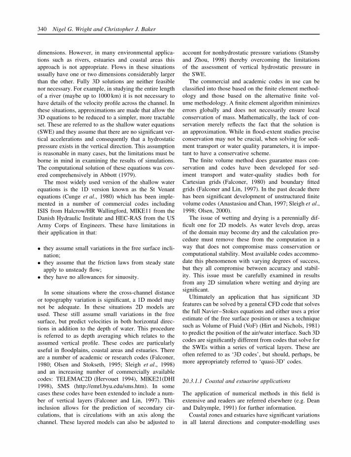
340 Nigel G. Wright and Christopher J. Baker
dimensions. However, in many environmental applica-tions such as rivers, estuaries and coastal areas thisapproach is not appropriate. Flows in these situationsusually have one or two dimensions considerably largerthan the other. Fully 3D solutions are neither feasiblenor necessary. For example, in studying the entire lengthof a river (maybe up to 1000 km) it is not necessary tohave details of the velocity profile across the channel. Inthese situations, approximations are made that allow the3D equations to be reduced to a simpler, more tractableset. These are referred to as the shallow water equations(SWE) and they assume that there are no significant ver-tical accelerations and consequently that a hydrostaticpressure exists in the vertical direction. This assumptionis reasonable in many cases, but the limitations must beborne in mind in examining the results of simulations.The computational solution of these equations was cov-ered comprehensively in Abbott (1979).
The most widely used version of the shallow waterequations is the 1D version known as the St Venantequations (Cunge et al., 1980) which has been imple-mented in a number of commercial codes includingISIS from Halcrow/HR Wallingford, MIKE11 from theDanish Hydraulic Institute and HEC-RAS from the USArmy Corps of Engineers. These have limitations intheir application in that:
• they assume small variations in the free surface incli-nation;
• they assume that the friction laws from steady stateapply to unsteady flow;
• they have no allowances for sinuosity.
In some situations where the cross-channel distanceor topography variation is significant, a 1D model maynot be adequate. In these situations 2D models areused. These still assume small variations in the freesurface, but predict velocities in both horizontal direc-tions in addition to the depth of water. This procedureis referred to as depth averaging which relates to theassumed vertical profile. These codes are particularlyuseful in floodplains, coastal areas and estuaries. Thereare a number of academic or research codes (Falconer,1980; Olsen and Stokseth, 1995; Sleigh et al., 1998)and an increasing number of commercially availablecodes: TELEMAC2D (Hervouet 1994), MIKE21(DHI1998), SMS (http://emrl.byu.edu/sms.htm). In somecases these codes have been extended to include a num-ber of vertical layers (Falconer and Lin, 1997). Thisinclusion allows for the prediction of secondary cir-culations, that is circulations with an axis along thechannel. These layered models can also be adjusted to
account for nonhydrostatic pressure variations (Stansbyand Zhou, 1998) thereby overcoming the limitationsof the assessment of vertical hydrostatic pressure inthe SWE.
The commercial and academic codes in use can beclassified into those based on the finite element method-ology and those based on the alternative finite vol-ume methodology. A finite element algorithm minimizeserrors globally and does not necessarily ensure localconservation of mass. Mathematically, the lack of con-servation merely reflects the fact that the solution isan approximation. While in flood-extent studies preciseconservation may not be crucial, when solving for sedi-ment transport or water quality parameters, it is impor-tant to have a conservative scheme.
The finite volume method does guarantee mass con-servation and codes have been developed for sed-iment transport and water-quality studies both forCartesian grids (Falconer, 1980) and boundary fittedgrids (Falconer and Lin, 1997). In the past decade therehas been significant development of unstructured finitevolume codes (Anastasiou and Chan, 1997; Sleigh et al.,1998; Olsen, 2000).
The issue of wetting and drying is a perennially dif-ficult one for 2D models. As water levels drop, areasof the domain may become dry and the calculation pro-cedure must remove these from the computation in away that does not compromise mass conservation orcomputational stability. Most available codes accommo-date this phenomenon with varying degrees of success,but they all compromise between accuracy and stabil-ity. This issue must be carefully examined in resultsfrom any 2D simulation where wetting and drying aresignificant.
Ultimately an application that has significant 3Dfeatures can be solved by a general CFD code that solvesthe full Navier–Stokes equations and either uses a priorestimate of the free surface position or uses a techniquesuch as Volume of Fluid (VoF) (Hirt and Nichols, 1981)to predict the position of the air/water interface. Such 3Dcodes are significantly different from codes that solve forthe SWEs within a series of vertical layers. These areoften referred to as ‘3D codes’, but should, perhaps, bemore appropriately referred to ‘quasi-3D’ codes.
20.3.1.1 Coastal and estuarine applications
The application of numerical methods in this field isextensive and readers are referred elsewhere (e.g. Deanand Dalrymple, 1991) for further information.
Coastal zones and estuaries have significant variationsin all lateral directions and computer-modelling uses

Environmental Applications of Computational Fluid Dynamics 341
the 2D shallow water equations or more complexmodels. Early examples are given by Abbott (1979).The DIVAST code was developed by Falconer (1980)and has been applied successfully in both coastal andestuarial situations by a number of different researchers.Other models have been developed from this basis anda review of earlier work is given by Cheng and Smith(1989). More recently models have been extended towhole regions of the continental shelf (Sauvaget et al.,2000).
In addition to the solution of the depth-averagedequations, computational solutions in this field requireaccount to be taken of the effects of wind shear andCoriolis forces. The former is accommodated as amomentum source on the free surface and the latter asa source term.
The motion of waves is a significant factor in coastalstudies. The modelling of waves is not possible withthe shallow water equations because of the neglect ofvertical acceleration and the consequent assumption ofno significant free surface curvature. Models have beendeveloped based on the Boussinesq equations for wavesin shallow water (Berzins and Walkley, 2003). Li andFleming (2001) have developed fully 3D models forcoastal zones that predict wave motions directly.
In estuaries there can be significant effects due tothermal and saline stratification. Adequate resolution ofthese effects necessitates the use of software that solvesthe shallow water equations within a number of verticallayers. This approach allows for different temperaturesand salinities in the vertical and makes some allowancefor vertical velocities. Falconer and Lin (1997) havedeveloped this technique and applied it to studies ofmorphological changes and the transport of heavy metalsin the Humber Estuary.
20.3.1.2 Rivers
1D models are in widespread use in commercial consul-tancy and are the main tool for assessing flood risk,water quality and construction impact in rivers andchannels. In addition to modelling the discharge anddepth at river cross-sections, these codes have unitsthat model hydraulic structures such as sluice gates andweirs. Through use of these units a model of a com-plex network of rivers and artificial channels can bebuilt up. In this way current computer power is begin-ning to allow for models of whole catchments andreal-time flood prediction. Cunge et al. (1980) containsan excellent background to the theory and applicationof river models. Predominantly, the 1D equations aresolved by the Preissmann or other ‘box’ method. These
methods allow for the simple inclusion of units suchas sluice gates and weirs. However, they do not takeaccount of the fact that the equations are hyperbolic (seeSmith, 1978, for a definition). Other techniques havebeen proposed (Garcia-Navarro et al., 1992; Alcrudoand Garcia-Navarro, 1993; Garcia-Navarro et al., 1995;Crossley, 1999), but these have yet to be put intocommon use.
2D modelling of rivers is now being used commer-cially, although the recent work on flood extent predic-tion undertaken by the Environment Agency for Englandand Wales used 1D models indicating that this is not yetaccepted as standard practice. Various research groupshave developed and validated these techniques (Bateset al., 1996; Sleigh et al., 1998; Bates et al., 1999). Asignificant amount of work has been carried out on theuse of remotely-sensed data in 2D modelling (Horrittet al., 2001) which offers the advantages of increasedaccuracy and faster model development.
In many cases 2D solutions are only required in partsof a river model and thus in the majority of the riversystem a 1D model is adequate. Dhondia and Stelling(2002) have implemented a combined 1D/2D approachthat allows for a complete 1D model to be augmented,rather than replaced, in key areas.
The use of fully 3D CFD codes within rivers isstill a predominantly research activity. However, thiswork can give new understanding of the fundamentalsof fluid flow in channels. The first attempts at usingCFD considered simplified channels (Rastogi and Rodi,1978; Leschziner and Rodi, 1979; Rodi, 1980; Naotand Rodi, 1982; Demuren and Rodi, 1986; Gibsonand Rodi, 1989), but did demonstrate the potentialapplication. Bradbrook et al. (2000) have also publishedLES results for a laboratory-type channel. Althoughthese results require substantial computing resources andmay be some way off practical application, they offera means of understanding the fundamental processes ofturbulence in river channels.
One of the first 3D models to attempt to modelnatural river geometry in full was reported by Olsenand Stokseth (1995) who modelled a short reach (20× 80 m) of the Skona River in Norway. The use of3D modelling for the design of river rehabilitationschemes has been developed (Swindale and Wright,1997; Swindale, 1999; Wright et al., 2000) with thefree surface being determined from 1D and 2D models.In this situation the extra information available from3D is of great benefit in analysing the varied habitatrequired for different species. Lane et al. (1999) carriedout 3D simulations and compared the results with a2D simulation for flow at a river confluence for which

342 Nigel G. Wright and Christopher J. Baker
high quality field data was available. They found that3D simulations offered better predictions for secondarycirculations. The 3D model also gave better estimatesof shear stress and provided better information forcalculating mixing processes. For more detail on theuse of higher dimensional models in river modelling,readers are referred to a review paper commissioned byHR Wallingford for the Environment Agency of Englandand Wales (Wright, 2001).
20.3.1.3 Small-scale river works
3D CFD software can also be used for analysingflows at small-scale river works such as sluice gates,weirs, outfalls and fish passes (Rodrıguez et al., 2001).This work is neither straightforward nor rapid, butwith further verification may become an acceptablealternative to scale models. In these cases CFD has theadvantage over physical models of being able to workat full scale.
20.3.2 Atmospheric applications
In this section we consider the application of CFDtechniques to two categories of atmospheric flows.As above, the appropriate length scale is used todifferentiate them. First, we discuss work on predictingthe wind flow over large topography (with a scale ofthe order of 0.1 to 10 km). Second, we consider the useof CFD in small-scale engineering and environmentalproblems with scales of the order of 10 to 100 m. Wedo not consider the application of CFD techniques (andin particular the LES technique) to the prediction oflarge-scale atmospheric circulations. For details of suchapplications, the reader is referred to Mason (1994).
20.3.2.1 Wind over large-scale topography
The calculation of wind speeds and other atmosphericvariables, such as temperature and moisture, over large-scale topography such as hills, is of some practicalimportance for assessing local wind climate for planningpurposes, the construction of wind farms, the dispersionof atmospheric pollutants, etc., and also for providinga means by which larger-scale numerical weather pre-dictions can be used to predict smaller-scale effects.An excellent historical review of the subject has beenpresented by Wood (2000) and the following few para-graphs draw heavily on this work.
Work in this field began in the 1940s and 1950s withinviscid flow calculations over a range of large-scale
topography. The work of Scorer (1949) on trapped leewaves stands out as being of considerable importance.While these calculations were of fundamental impor-tance, they could not of course take into account the realsurface boundary condition, nor the turbulent nature ofthe boundary layer. To assess the flow regions in whichthese methods were applicable, the concepts of differ-ent layers of the flow were derived – in particular, theidea that there was a relatively thin region close to thesurface of the topography where the effects of the topog-raphy and of turbulence were important, and a regionabove that that could be regarded as inviscid to a firstapproximation. This concept was central to the workof Jackson and Hunt (1975) who formalized it in theirlinear analysis of turbulent flow over low hills, defin-ing an inner layer close to the hill and an outer layerabove that. This theory led to quantifiable predictions ofwind speed-up and the change of turbulent structure overa variety of topographical shapes. When tested againstactual full-scale experimental data obtained from con-trolled measurements over simple topography (such asthe Black Mountain and Askervein Hill), this theory wasshown to perform more than adequately. The theory con-tinued to be developed over the next decade or so (Huntet al., 1988; Belcher, 1990; Belcher and Hunt, 1998) andforms the basis of a number of calculation methods thatare currently in use for the prediction of wind fieldsand dispersion over arbitrary topography. An exampleof this is provided in the work of Inglis et al. (1995) forthe prediction of wind conditions over Kintyre (whichwas carried out to assess the impact of wind on forests).Typical comparisons of the predictions with theory areshown in Figure 20.4.
Although the linear type of model is a CFD model inthat it requires a numerical solution to the equationsof fluid flow, it is not a CFD model in the termsdescribed in previous sections. So what of the adequacyof standard CFD models to predict flow over largetopography? At this point it is worth directly quotingthe words of Wood (2000):
Using standard closure schemes, simulated flow overhills exhibits a strong dependence on the specific clo-sure employed and yet for various reasons (knowndeficiencies, dependence on unknown tuneable con-stants, misrepresentation of the near wall behaviour),none of the currently available closures are sat-isfactory in the complex geometry to which theyare applied.
Wood then goes on to advocate the continued develop-ment of LES models in this field, and this seems to be

Environmental Applications of Computational Fluid Dynamics 343
14
50 se
5 10
Distance east from origin (km)
Dis
tanc
e no
rth
from
orig
in (
km)
150
5 10 150
0
5
10
15
0
5
10
15
se
se
se
xxxxxx
100
1 2
12
100200
5010
0
x
300
13
xxx
3 4 5 6
11
78
300
se
se
se
100
300
200
300
100
300
200200
200
−0.8−0.6−0.4−0.2D
S
0.00.20.4
Figure 20.4 Comparison of observed (filled circles) andmodelled fractional speed-ups (continuous and dottedlines – with and without modelling of atmospheric stability)along a line connecting sites 1 to 8Source: Inglis et al. (1995)
generally accepted as the way forward for the use ofCFD techniques for such problems. It has the particu-lar advantage of being able to predict flow fluctuations,extreme values, etc., which are often the parametersrequired in practical situations. An example of the cur-rent use of LES is the RANS model developed at Col-orado State University, which has been used extensivelyin predicting topographical flows (see, for example, Caiet al., 1995; Cai and Steyn, 1996).
20.3.2.2 Small-scale wind modelling
The use of CFD techniques at relatively small engi-neering scales is becoming increasingly common bothwithin the research community and within an industrialcontext. The proceedings of the three recent confer-ences on computational wind engineering (in Tokyo in1992, Fort Collins, Colorado in 1996 and Birminghamin 2000) indicate the considerable effort that is beingput into developing and using models to predict windeffects on pedestrians, pollution dispersion, and wind
loads on buildings and other structures. The motiva-tion for this is often the reduced cost compared withphysical model testing. This point will be discussed fur-ther below.
The main type of model that is used is standardRANS models, usually in the form of one of the standardsoftware packages, such as FLUENT, CFX, STAR-CD,etc. Thus, in general, only time-mean averages of theflow field or of contaminant transport can be predicted,although there is an increasing use of unsteady RANSmodelling. The major problem with the use of thesemethods is the general inability to predict the extent ofseparated flow fields. This problem is associated with theover-prediction of turbulent kinetic energy in stagnationregions by such models (see Murakami, 1997).
Examples of the type of results that can be obtainedare given in Figure 20.5, which shows calculations ofpedestrian-level wind velocities in Auckland (Richardset al., 2000), pollutant transport from a storage tank(Fothergill et al., 2000) and forces on a wall (plottedfrom data in Robertson et al., 1997). The latter investi-gation only gives mean pressures and forces of course.In reality, in design, extreme values of the parametersare needed. These cannot be predicted by RANS models,which thus have a limited application in the predictionof structural forces due to turbulent winds.
Other types of modelling technique are also beingused. The discrete vortex method, in which vorticity isfed into the flow field from surfaces, has been shown tobe of particular use in predicting the flow around bridgedecks, and can be incorporated into dynamic models ofbridge movement in high winds (Walther, 1998). Typicalresults are given in Figure 20.6. Also the LES techniqueis beginning to be applied for small-scale engineeringproblems. Again, this technique is likely to becomeof increasing use in the future because of its abilityto predict unsteady flows and forces, which are oftendesign requirements (Murakami, 1997).
Having described the techniques that are in use, it isnecessary to urge caution in their use. First, as has beenstated above, the standard RANS techniques currentlyin use cannot predict unsteady fluctuating flows andforces. Whilst this might be adequate for some applica-tions where only time-averaged conditions are required(average pedestrian-level wind speeds, average plumetrajectories), it is not adequate for most structural cal-culations. Second, the paper by Cowan et al. (1997) isof some interest. The trials reported in that paper wereof calculations of pollutant concentrations for a varietyof well-documented cases, most of which have experi-mental verification. They were carried out independentlyby a number of different organizations, using the same
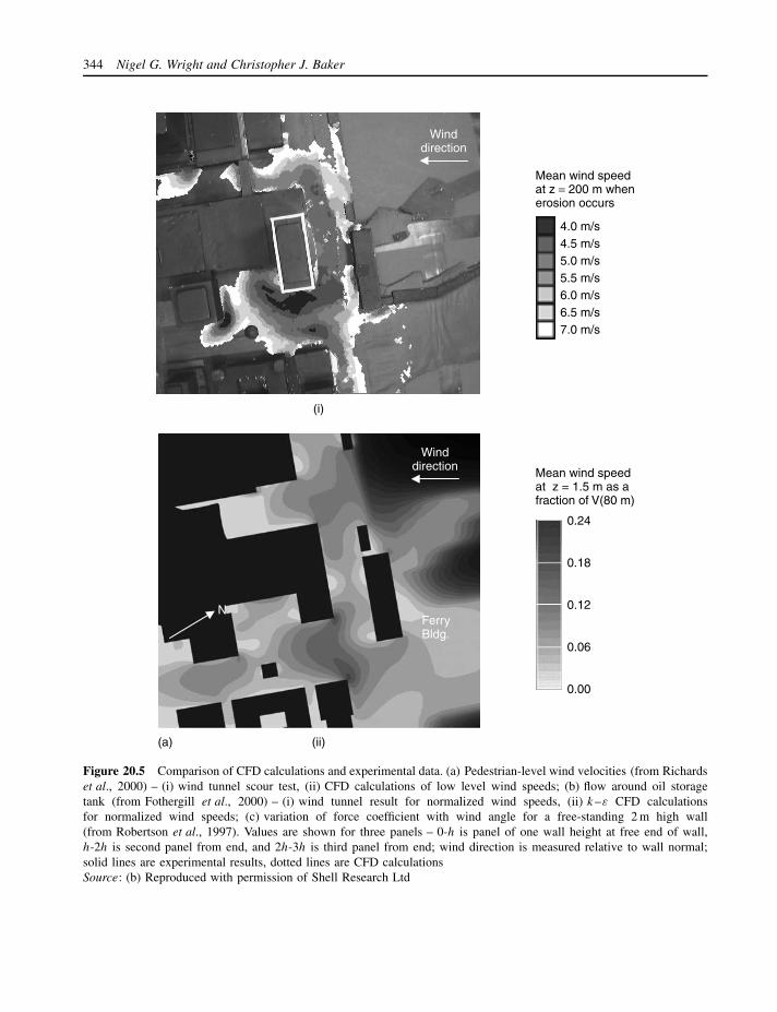
344 Nigel G. Wright and Christopher J. Baker
(a)
(i)
Winddirection
Mean wind speedat z = 200 m whenerosion occurs
4.0 m/s
7.0 m/s6.5 m/s6.0 m/s5.5 m/s5.0 m/s4.5 m/s
Mean wind speedat z = 1.5 m as afraction of V(80 m)
0.24
0.18
0.12
0.06
0.00
NFerryBldg.
Winddirection
(ii)
Figure 20.5 Comparison of CFD calculations and experimental data. (a) Pedestrian-level wind velocities (from Richardset al., 2000) – (i) wind tunnel scour test, (ii) CFD calculations of low level wind speeds; (b) flow around oil storagetank (from Fothergill et al., 2000) – (i) wind tunnel result for normalized wind speeds, (ii) k–ε CFD calculationsfor normalized wind speeds; (c) variation of force coefficient with wind angle for a free-standing 2 m high wall(from Robertson et al., 1997). Values are shown for three panels – 0-h is panel of one wall height at free end of wall,h-2h is second panel from end, and 2h-3h is third panel from end; wind direction is measured relative to wall normal;solid lines are experimental results, dotted lines are CFD calculationsSource: (b) Reproduced with permission of Shell Research Ltd

Environmental Applications of Computational Fluid Dynamics 345
2.0
1.0
0.0
3.0
90 120
2h-3h
h-2h
0-h
Wind direction q (deg)
For
ce c
oeffi
cien
t
150 180
(ii)
(i)
(b)
(c)
6.4 3.2 1.6
0.2
0.4
0.3
U
6.46.43.2 1.6 0.8
0.20.4
Figure 20.5 (continued )
computer code. The differences between the calculationswere thus in the realms of grid generation, numericalschemes, etc. The results produced by different inves-tigators were found to vary very significantly (often byan order of magnitude or more). Typical comparisonsare given in Figure 20.7. These results serve as a warn-ing against placing too great a reliance on the accuracyof any one calculation that does not have some sortof experimental validation. The unverified use of CFDcodes to reduce the costs of physical model tests may,if great care is not used, simply produce results thatare unreliable. These points are further discussed andemphasized by Castro and Graham (1999). It must beconcluded that CFD and physical modelling should beseen as complementary technologies that should be used
in conjunction with one another to varying degrees forany particular situation.
20.4 CONCLUSION
While CFD has many applications in environmentalflows as outlined here, there are still challenges tobe faced to increase its accuracy and ability to dealwith more complex situations. It is also vital that usersunderstand the difficulties and pitfalls in CFD. Thisrequires experience in CFD, but also an understandingof the particular applications area.
In future, new techniques will become feasible forpractical modelling which will open up new areas of
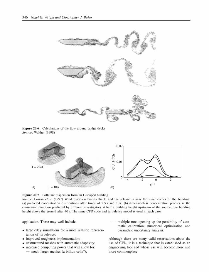
346 Nigel G. Wright and Christopher J. Baker
Figure 20.6 Calculations of the flow around bridge decksSource: Walther (1998)
20−2−40
0.01
0.02
y/H
C.U
h.H
2 /Q
s
T = 10s
T = 2.5s
(a) (b)
Figure 20.7 Pollutant dispersion from an L-shaped buildingSource: Cowan et al. (1997) Wind direction bisects the L and the release is near the inner corner of the building:(a) predicted concentration distributions after times of 2.5 s and 10 s; (b) dimensionless concentration profiles in thecross-wind direction predicted by different investigators at half a building height upstream of the source, one buildingheight above the ground after 40 s. The same CFD code and turbulence model is used in each case
application. These may well include:
• large eddy simulations for a more realistic represen-tation of turbulence;
• improved roughness implementation;• unstructured meshes with automatic adaptivity;• increased computing power that will allow for:
— much larger meshes (a billion cells?);
— multiple runs opening up the possibility of auto-matic calibration, numerical optimization andparametric uncertainty analysis.
Although there are many valid reservations about theuse of CFD, it is a technique that is established as anengineering tool and whose use will become more andmore commonplace.
Environmental Applications of Computational Fluid Dynamics 347
REFERENCES
Abbott, M. and Basco, D. (1989) Computational Fluid Dynam-ics: An Introduction for Engineers, Longman Scientific, Sin-gapore.
Abbott, M.B. (1979) Computational Hydraulics: Elements ofthe Theory of Free Surface Flows, Pitman, London.
AIAA (1998) Guide for the Verification and Validation ofComputational Fluid Dynamics Simulations, AIAA.
Alcrudo, F. and Garcia-Navarro, P. (1993). A high-resolutionGodunov-type scheme in finite volumes for the 2D shallow-water equations, International Journal for Numerical Meth-ods in Fluids 16 (6), 489–505.
Anastasiou, K. and Chan, C. (1997) Solution of the 2D shallowwater equations using the finite volume method on unstruc-tured triangular meshes, International Journal for NumericalMethods in Fluids 24, 1225–1245.
ASME (1993) Statement on the control of numerical accuracy,Journal of Fluids Engineering 115 (3), 339–340.
Bates, P., Anderson, M., Price, D., Hardy, R. and Smith, C.(1996) Analysis and Development of Hydraulic Models forFloodplain Flows in Floodplain Processes, John Wiley &Sons, Chichester.
Bates, P., Wilson, C., Hervouet, J.-M. and Stewart, M. (1999)Modelisation a deux dimensions par elements finis d’unecoulement en plaine, La Houille Blanche 3/4, 61–67.
Belcher, S. (1990) Turbulent Boundary Layer Flow over Undu-lating Surfaces, Cambridge University Press, Cambridge.
Belcher, S. and Hunt, J. (1998) Turbulent flow over hills andwaves, Annual Review of Fluid Mechanics 30, 507–538.
Berzins, M. and Walkley, M. (2003) A finite element methodfor the two-dimensional extended Boussinesq equations,International Journal for Numerical Methods in Fluids 39(10), 865–885.
Boussinesq, J. (1877) Essai sur la theorie des eaux courantes,Memoires a l’Academie des Sciences, XXIII, Paris.
Bradbrook, K., Lane, S., Richards, K., Biron, P. and Roy, A.(2000) Large eddy simulation of periodic flow characteristicsat river channel confluences, Journal of Hydraulic Research38 (3), 207–215.
Cai, X.-M. and Steyn, D. (1996) The Von Karman constantdetermined by large eddy simulation, Boundary Layer Mete-orology 78, 143–164.
Cai, X.-M., Steyn, D. and Gartshore, I. (1995) Resolved scaleturbulence in the atmospheric surface layer from a large eddysimulation, Boundary Layer Meteorology 75, 301–314.
Casey, M. and Wintergerste, T. (2000) Best Practice Guide-lines, ERCOFTAC Special Interest Group on Quality andTrust in CFD, Swiss Federal Institute of Technology,Lausanne.
Castro, I. and Graham, M. (1999) Numerical Wind Engineer-ing: The Way Ahead?, Proceedings of the Institute of CivilEngineers, Structures & Buildings 134, 275–277.
Cheng, R. and Smith, P. (1989) A Survey of Three-Dimen-sional Numerical Estuarine Models, in M. Spaulding (ed.)Estuarine and Coastal Modeling: American Society of CivilEngineers Specially Conference, 1–15, ASCE, Reston, VA.
Cowan, I.R., Castro, I.P. and Robins, A.G. (1997) Numericalconsiderations for simulations of flow and dispersion aroundbuildings, Journal of Wind Engineering and Industrial Aero-dynamics 67–68, 535–545.
Crossley, A. (1999) Accurate and Efficient Numerical Solutionsfor the Saint Venant Equations of Open Channel Flow, Schoolof Civil Engineering, University of Nottingham, Nottingham.
Cunge, J., Holly Jr, F. and Verwey, A. (1980) PracticalAspects of Computational River Hydraulics, Pitman, London.
Dean, R. and Dalrymple, R. (1991) Water Wave Mechanics forEngineers and Scientists, World Scientific, Singapore.
Demuren, A. and Rodi, W. (1986) Calculation of flow andpollutant dispersion in meandering channels, Journal ofFluid Mechanics 172 (1), 65–92.
DHI (1998) User Guide and Scientific Documentation, DanishHydraulic Institute.
Dhondia, J. and Stelling, G. (2002) Application of One Dimen-sional – Two Dimensional Integrated Hydraulic Model forFlood Simulation and Damage Assessment, Hydroinformat-ics 2002, IWA Publishing, Cardiff.
Falconer, R. (1980) Numerical modelling of tidal circulation inharbours, Proceedings of the Institution of Civil Engineers,Waterway, Port and Coastal Division 106, 32–33.
Falconer, R. and Lin, B. (1997) Three-dimensional modellingof water quality in the Humber Estuary, Water Research,IAWQ 31 (5), 1092–1102.
Fothergill, C., Roberts, P. and Packwood, A. (2000) Flowand Dispersion around Storage Tanks: Comparison betweenWind Tunnel Studies and CFD Simulation, CWE2000,Birmingham.
Garcia-Navarro, P., Alcrudo, F. and Saviron, J.M. (1992) 1-D open-channel flow simulation using Tvd-McCormackscheme, Journal of Hydraulic Engineering-Asce 118 (10),1359–1372.
Garcia-Navarro, P., Hubbard, M.E. and Preistley, A. (1995)Genuinely multidimensional upwinding for the 2D shallowwater equations, Journal of Computational Physics 121,79–93.
Gibson, M. and Rodi, W. (1989) Simulation of free surfaceeffects on turbulence with a Reynolds stress model, Journalof Hydraulic Research 27 (2), 233–244.
Hervouet, J.-M. (1994) Computation of 2D Free Surface Flows:The State of the Art in the TELEMAC System, Hydroinfor-matics 94, Balkema.
Hirt, C. and Nichols, B. (1981) Volume of fluid methods forthe dynamics of free boundaries, Journal of ComputationalPhysics 39, 201–225.
Horritt, M., Mason, D. and Luckman, A. (2001) Flood bound-ary delineation from synthetic aperture radar imagery usinga statistical active contour model, International Journal ofRemote Sensing 22, 2489–2507.
Hunt, J., Leibovich, S. and Richards, K. (1988) Turbulentshear flow over low hills, Quarterly Journal of the RoyalMeteorological Society 114, 1435–1470.
Inglis, D., Choularton, T., Stromberg, I., Gardiner, B. andHill, M. (1995) Testing of a linear airflow model for flow

348 Nigel G. Wright and Christopher J. Baker
over complex terrain and subject to stable structured strati-fication, in J. Grace (ed.) Wind and Trees, Cambridge Uni-versity Press, Cambridge, 71–87.
Jackson, P. and Hunt, J. (1975) Turbulent wind flow over a lowhill, Quarterly Journal of the Royal Meteorological Society101, 929–955.
King, I., Norton, W. and Iceman, K. (1975) A finite ele-ment solution for two-dimensional stratified flow prob-lems, in O.C. Zienkiewicz (ed.) Finite Elements in Flu-ids: International Conference on the Finite Element Methodin Flow Analysis, John Wiley & Sons, New York, 1,133–156.
Lane, S., Bradbrook, K., Richards, K., Biron, P. and Roy, A.(1999) The application of computational fluid dynamicsto natural river channels: three-dimensional versus two-dimensional approaches, Geomorphology 29, 1–20.
Lane, S.N. and Richards, K.S. (2001) The ‘validation’ ofhydrodynamic models: some critical perspectives, in M.G.Anderson and P.D. Bates, Model Validation: Perspectivesin Hydrological Science, John Wiley & Sons, Chichester,413–438.
Leschziner, M. and Rodi, W. (1979) Calculation of stronglycurved open channel flow, Journal of Hydraulic Engineering105 (10), 1297–1314.
Li, B. and Fleming, C. (2001) Three-dimensional model ofNavier–Stokes equations for water waves, Journal of Water-way, Port, Coastal and Ocean Engineering 127 (1), 16–25.
Mason, P. (1994) Large eddy simulation: a critical review ofthe technique, Quarterly Journal of the Royal MeteorologicalSociety 120, 1–26.
Murakami, S. (1997) Current status and future trends in com-putational wind engineering, Journal of Wind Engineeringand Industrial Aerodynamics 67–68, 3–34.
Naot, D. and Rodi, W. (1982) Calculation of secondary cur-rents in channel flow, Journal Hydraulic Division ASCE 108(HY8), 948–968.
Olsen, N. (2000) Unstructured Hexahedral 3D Grids for CFDModelling in Fluvial Geomorphology, 4th International Conf.Hydroinformatics 2000, Iowa, USA.
Olsen, N.R.B. and Stokseth, S. (1995) 3-dimensional numeri-cal modelling of water flow in a river with large bed rough-ness, Journal of Hydraulic Research 33 (4), 571–581.
Patankar, S. and Spalding, D. (1972) A calculation procedurefor heat, mass and momentum transfer in three-dimensionalparabolic flows, International Journal of Heat Mass Transfer15, 1787–1806.
Rastogi, A. and Rodi, W. (1978) Predictions of heat and masstransfer in open channels, Journal of Hydraulic Division 104,397–420.
Richards, P., Mallinson, G. and McMillan, D. (2000) Pedes-trian Level Wind Speeds in Downtown Auckland, CWE 2000,Birmingham.
Robertson, A., Hoxey, R., Short, J. and Ferguson, W. (1997)Full-scale measurements and computational predictions ofwind loads on free standing walls, Journal of Wind Engi-neering and Industrial Aerodynamics 67–68, 639–646.
Rodi, W. (1980) Turbulence Models and Their Application inHydraulics: State of the Art Paper, IAWR, Delft.
Rodrıguez, J., Belby, B., Bombardelli, F., Garcıa, C., Rhoads,B. and Garcıa, M. (2001) Numerical and Physical Modelingof Pool-Riffle Sequences for Low-Gradient Urban Streams,3rd International Symposium on Environmental Hydraulics,Tempe, Arizona, USA.
Sauvaget, P., David, E. and Guedes Soares, C. (2000) Mod-elling tidal currents on the coast of Portugal, Coastal Engi-neering 40, 393–409.
Schneider, G. and Raw, M. (1987) Control-volume finite ele-ment method for heat transfer and fluid flow using co-located variables – 1 computational procedure, NumericalHeat Transactions 11, 363–390.
Scorer, R. (1949) Theory of waves in the lees of mountains,Quarterly Journal of the Royal Meteorological Society 76,41–56.
Sleigh, P., Gaskell, P., Berzins, M. and Wright, N. (1998) Anunstructured finite-volume algorithm for predicting flow inrivers and estuaries, Computers & Fluids 27 (4), 479–508.
Smagorinsky, J. (1963) General circulation experiments withprimitive equations Part 1: basic experiments, MonthlyWeather Review 91, 99–164.
Smith, G. (1978) Numerical Solution of Partial DifferentialEquations: Finite Difference Methods, Oxford UniversityPress, Oxford.
Stansby, P. and Zhou, J. (1998) Shallow-water flow solverwith non-hydrostatic pressure: 2D vertical plane problems,International Journal of Numerical Methods in Fluids 28,541–563.
Swindale, N. (1999) Numerical Modelling of River Rehabilita-tion Schemes, Department of Civil Engineering, Universityof Nottingham, Nottingham.
Swindale, N. and Wright, N. (1997) The Analysis of RiverRehabilitation Schemes Using One and Two DimensionalHydraulic Modelling, IAHR Congress, 27th Congress of theIAHR, San Francisco, August.
Versteeg, H. and Malalasekera, W. (1995) An Introduction toComputational Fluid Dynamics – the Finite Volume Method,Longman, London.
Walther, J. (1998) Discrete vortex methods in bridge aerody-namics and prospects for parallel computing techniques, inBridge Aerodynamics, Esdahl, Rotterdam, Balkema.
Wood, N. (2000) Wind flow over complex terrain: a historicalperspective and the prospect for large eddy modelling,Boundary Layer Meteorology 96, 11–32.
Wright, N. (1988) Multigrid Solution of Elliptic Fluid FlowProblems, Department of Mechanical Engineering, Univer-sity of Leeds, Leeds.
Wright, N. (2001) Conveyance Implications for 2D and 3DModelling, Environment Agency, London.
Wright, N., Swindale, N., Whitlow, C. and Downs, P. (2000)The Use of Hydraulic Models in the Rehabilitation of theRiver Idle, UK, Hydroinformatics 2000, Iowa, USA.
Zienkiewicz, O. and Taylor, R. (2000) The Finite ElementMethod, McGraw-Hill, London.

21
Self-Organization and CellularAutomata Models
DAVID FAVIS-MORTLOCK
21.1 INTRODUCTION
Models are one of the main tools available to help usunderstand the environment, and to attempt to predictwhat will happen in it. Indeed, ‘The control [which]science gives us over reality, we normally obtain bythe application of models’ (Ackoff et al., 1962: 108).Many aspects of the environment, however, are toocomplex for mere humans to grasp fully: if this isthe case, we are forced to simplify, in effect to fallback on making analogies. The aim of an analogy isto highlight similarities between the things compared,and in the same way environmental models aim to linkthe more easily understood system (the model) withthe less comprehensible system (some aspect of theenvironment). Analogies, though, are never perfect, andin the same way models are always less than perfectin making this link. To return to the original point,it could hardly be otherwise, since a model which isas complicated as the thing it represents would be noeasier to understand. ‘The best material model of a catis another, or preferably the same, cat’ (Rosenblueth andWiener, 1945; see also the discussion in the Introductionand Chapter 1).
The resulting tension, between the robustness of ourmodels and their complexity, is the focus of this chapter.It deals with recent theoretical developments in self-organization of complex systems, and how these maybe used in a practical way to construct spatial mod-els. The resulting approach (cellular automata mod-elling) is one which appears to have great promisefor lessening this tension in future spatial models ofall kinds.
While many of the examples presented here are drawnfrom physical geography, since that is the area of sciencein which work, the ideas and approaches discussed areof wide applicability (cf. Wolfram, 2002).
21.1.1 The ever-decreasing simplicity of models?
Models used by geographers have steadily become moreand more complex, from the ‘quantitative revolution’in geography in the 1960s (e.g. Harvey, 1969) whenmodels first began to be used widely, to the present.This is a trend that looks set to continue. Figure 21.1uses the number of lines of programming code asa surrogate for model complexity1 for a selectionof computer implementations of US-written field-scalemodels of soil erosion by water. Model complexityin this particular domain has clearly increased in asomewhat nonlinear way.
21.1.1.1 The quest for ‘better’ models
The reason for this increased complexity is, of course,the desire for ‘better’ models. Although environmentalmodels differ widely, two general criteria have come todominate in assessment of any model’s ‘success’ (orotherwise).2 First, the model is usually ranked morehighly if it is physically based, i.e. if it is foundedon the laws of conservation of energy, momentum andmass; and if it has its parameters and variables definedby means of equations that are at least partly basedon the physics of the problem, such as Darcy’s lawand the Richards equation (Kirkby et al., 1992; see
Environmental Modelling: Finding Simplicity in Complexity. Edited by J. Wainwright and M. Mulligan 2004 John Wiley & Sons, Ltd ISBNs: 0-471-49617-0 (HB); 0-471-49618-9 (PB)
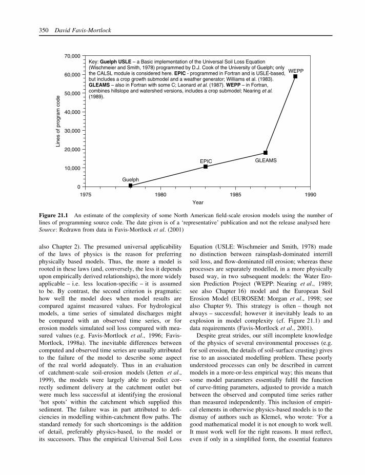
350 David Favis-Mortlock
0
10,000
20,000
30,000
40,000
50,000
60,000
70,000
1975 1980 1985 1990
Year
Line
s of
pro
gram
cod
eKey: Guelph USLE – a Basic implementation of the Universal Soil Loss Equation(Wischmeier and Smith, 1978) programmed by D.J. Cook of the University of Guelph; onlythe CALSL module is considered here. EPIC - programmed in Fortran and is USLE-based,but includes a crop growth submodel and a weather generator; Williams et al. (1983).GLEAMS – also in Fortran with some C; Leonard et al. (1987). WEPP – in Fortran,combines hillslope and watershed versions, includes a crop submodel; Nearing et al.(1989).
Guelph
EPIC GLEAMS
WEPP
Figure 21.1 An estimate of the complexity of some North American field-scale erosion models using the number oflines of programming source code. The date given is of a ‘representative’ publication and not the release analysed hereSource: Redrawn from data in Favis-Mortlock et al. (2001)
also Chapter 2). The presumed universal applicabilityof the laws of physics is the reason for preferringphysically based models. Thus, the more a model isrooted in these laws (and, conversely, the less it dependsupon empirically derived relationships), the more widelyapplicable – i.e. less location-specific – it is assumedto be. By contrast, the second criterion is pragmatic:how well the model does when model results arecompared against measured values. For hydrologicalmodels, a time series of simulated discharges mightbe compared with an observed time series, or forerosion models simulated soil loss compared with mea-sured values (e.g. Favis-Mortlock et al., 1996; Favis-Mortlock, 1998a). The inevitable differences betweencomputed and observed time series are usually attributedto the failure of the model to describe some aspectof the real world adequately. Thus in an evaluationof catchment-scale soil-erosion models (Jetten et al.,1999), the models were largely able to predict cor-rectly sediment delivery at the catchment outlet butwere much less successful at identifying the erosional‘hot spots’ within the catchment which supplied thissediment. The failure was in part attributed to defi-ciencies in modelling within-catchment flow paths. Thestandard remedy for such shortcomings is the additionof detail, preferably physics-based, to the model orits successors. Thus the empirical Universal Soil Loss
Equation (USLE: Wischmeier and Smith, 1978) madeno distinction between rainsplash-dominated interrillsoil loss, and flow-dominated rill erosion; whereas theseprocesses are separately modelled, in a more physicallybased way, in two subsequent models: the Water Ero-sion Prediction Project (WEPP: Nearing et al., 1989;see also Chapter 16) model and the European SoilErosion Model (EUROSEM: Morgan et al., 1998; seealso Chapter 9). This strategy is often – though notalways – successful; however it inevitably leads to anexplosion in model complexity (cf. Figure 21.1) anddata requirements (Favis-Mortlock et al., 2001).
Despite great strides, our still incomplete knowledgeof the physics of several environmental processes (e.g.for soil erosion, the details of soil-surface crusting) givesrise to an associated modelling problem. These poorlyunderstood processes can only be described in currentmodels in a more-or-less empirical way; this means thatsome model parameters essentially fulfil the functionof curve-fitting parameters, adjusted to provide a matchbetween the observed and computed time series ratherthan measured independently. This inclusion of empiri-cal elements in otherwise physics-based models is to thedismay of authors such as Klemes, who wrote: ‘For agood mathematical model it is not enough to work well.It must work well for the right reasons. It must reflect,even if only in a simplified form, the essential features

Self-Organization and Cellular Automata Models 351
of the physical prototype’ (Klemes, 1986: 178S). Modelparameterization under such conditions then becomesmore and more a curve-fitting exercise (Kirchner et al.,1996). As an example, a recent evaluation of field-scaleerosion models (Favis-Mortlock, 1998a) found calibra-tion to be essential for almost all models involved,despite the supposed physical basis of the models.
Additionally, results from a more complex modelmay not necessarily improve upon those of a simplermodel if interactions between processes are inadequatelyrepresented within the model (Mark Nearing, personalcommunication, 1992; Beven, 1996). Since the additionof more model parameters increases the number ofdegrees of freedom for the model, adding extra freeparameters to a model means that changes in thevalue of one input parameter may be compensated bychanges in the value of another. Therefore unrealisticvalues for individual input parameters may still producerealistic results (in the sense of a close match betweenthe observed and computed time series). The modelis ‘unidentified’ with its parent theory3 in the senseof Harvey (1967: 159), and results from the model maybe ‘right for the wrong reasons’ (Favis-Mortlock et al.,2001). To illustrate this point, Jakeman and Hornberger(1993) found that commonly used rainfall-runoff datacontains only enough information to constrain a simplehydrological model with a maximum of four freeparameters. An end-point to this problem is Beven’s‘model equifinality’,4 whereby entirely different setsof input parameters can still produce similar modelresults (Beven, 1989).
The result of the above-described pressures uponmodel development is a nonvirtuous circle, whereby a‘better’ environmental model inexorably has to describemore processes, or existing processes in more detail.Doing so:
• will probably increase the model’s predictive powerin a specific domain, but may cause it to fail unexpect-edly elsewhere (because it is giving ‘the right answerfor the wrong reasons’ in the original domain);
• requires more data, and so in practical terms narrowsthe circumstances in which the model may be used;
• may make the model less comprehensible.
Is there any way out of this vicious circle?
21.2 SELF-ORGANIZATIONIN COMPLEX SYSTEMS
The foregoing suggests that, if an environmental modelis to be considered ‘better’, it has to describe the
environment in greater physically based detail. Doesthis necessarily imply a more complex model? Putmore generally: does real-world complexity inevitablyimply an equivalent complexity of the underlying gen-erative process?
21.2.1 Deterministic chaos and fractals
Along with much other change, the 1960s brought aclue that this might not always be so. During thisdecade, deterministic chaos was first discovered by anumber of workers such as the atmospheric physicistEdward Lorentz (Ruelle, 2001). However, the mathe-matical roots of chaos are a good deal older: notably inthe work of mathematician Henri Poincare around thebeginning of the twentieth century (e.g. Jones, 1991).Deterministic chaos took some time to enter the scien-tific mainstream. This began in the 1970s, for example,with the work of biologist Robert May on chaotic pop-ulation dynamics (May, 1976).
The tongue-in-cheek question5 ‘Does the flap of abutterfly’s wings in Brazil set off a tornado in Texas?’summarizes one major attribute of deterministic chaos.In effect, the question asks if a large effect have a tinycause. It can: such nonlinear ‘extreme sensitivity to ini-tial conditions’ is a hallmark of chaotic systems. Smalluncertainties in measurement or specification of initialconditions become exponentially larger, and the even-tual state of the system cannot be predicted. Thus, forexample, the chaotic component of the Earth’s atmo-sphere means that weather forecasts rapidly diminishin reliability as one moves more than a few days intothe future. It is important to note that whereas weather(i.e. the particular set of meteorological conditions on aspecific day, at a specific location) cannot be predicted,climate (here, the range of meteorological conditions ofa number of replicates of the meteorological conditionssimulated for that day and location) can be predicted.This notion is at the heart of recently devised ‘ensem-ble forecasting’ techniques which are carried out usingatmospheric models (Washington, 2000).
Deterministic chaos is also often associated with frac-tal (i.e. self-similar, scale-independent) patterns. Follow-ing seminal work by Benoit Mandelbrot (1975; see alsoAndrle, 1996), fractal patterns were acknowledged to bepresent in a wide variety of natural situations (but seee.g. Evans and McClean, 1995). This linkage betweenfractals and systems exhibiting deterministic chaos issuggestive of some deeper connection (cf. Cohen andStewart, 1994).
But for environmental modellers, perhaps the mostinteresting insight from chaotic systems is that they do

352 David Favis-Mortlock
not have to be complicated to produce complex results.Lorentz’s atmospheric model comprised only three non-linear equations, and May’s population dynamics modelswere even simpler. In all such models, the results at theend of one iteration (in the case of a time-series model,at the end of one ‘timestep’) are fed back into the modeland used to calculate results for the next iteration. Thisprocedure produces a feedback loop. Some values ofthe model’s parameters will cause it to eventually6 set-tle down to a static equilibrium output value; with othervalues, the model’s output will eventually settle down tocycle forever between a finite number of end-point val-ues; but for others, the model will switch unpredictablybetween output values in an apparently random way.Thus in such chaotic systems, complex patterns can bethe results of simple underlying relationships.
Both positive and negative implications follow fromthe discovery of such systems. For those of a determin-istic cast of mind this is sobering since it represents thefinal death rattle of the notion of a predictable, ‘clock-work’, universe, even at the macroscale.7 But there isalso a strongly positive implication: complexity does nothave to be the result of complexity!
Nonetheless, while this early work on deterministicchaos was intriguing and suggestive, it was not imme-diately ‘useful’ for most environmental modellers:
• While the output from chaotic functions is complex, itincludes little in the way of immediately recognizablestructure: at first glance it more resembles randomnoise. It is therefore qualitatively very different fromthe complex but highly structured patterns which weobserve in many environmental systems.
• When analysing real-world measurements which plau-sibly possess a chaotic component, it has proved tobe very difficult to go from the data to a descrip-tion of the underlying dynamics (e.g. Wilcox et al.,1991), even though simple models may be devisedwhich produce simulated data closely resembling themeasured values. But since there may be many suchmodels, what certainty can we have that any one ofthem has captured the workings of the real-world sys-tem? (Again cf. Beven’s ‘model equifinality’: Beven,1993.)
For a while, it seemed that deterministic chaos mightremain little more than an interesting diversion forenvironmental modellers.
21.2.2 Early work on self-organizing systems
Pioneering research carried out from the late 1980s,however, strongly supported the notion that structured
complexity does not always require an underlying com-plexity of process. A major centre for this work wasthe Santa Fe Institute (Waldrop, 1994). Overviews ofthis diverse body of early research on self-organizationand emergence in complex systems are presentedby Coveney and Highfield (1995), Kauffman (1995)and Holland (1998), among others.
These early studies demonstrated that responseswhich are both complex and highly structured may resultfrom relatively simple interactions (but very many ofthem) between the components of a system. Interac-tions between such components are governed by ‘local’rules, but the whole-system (‘global’) response is tomanifest some higher-level ‘emergent’ organization, fol-lowing the formation of ordered structures within thesystem. The system thus moves from a more uni-form (‘symmetrical’) state to a less uniform – but morestructured – state: this is so-called ‘symmetry-breaking’.Several aspects of the phenomenon of self-organizationare summarized in Figure 21.2. Note the definition ofemergence which is given: ‘emergent responses cannotbe simply inferred from the behaviour of the system’scomponents’.
21.2.3 Attributes of self-organizing systems
Three key concepts which characterize self-organizingsystems are feedback, complexity and emergence. Allare interlinked.
21.2.3.1 Feedback
Feedback occurs when a system processes data about itsown state. Thus, to use a humanly-engineered example,the governor of a steam engine is an arrangementwhereby a valve is controlled by weighted arms whichrevolve at a rate that is controlled by the speed ofthe steam engine. As the arms rotate faster, increasedcentrifugal force makes them close the valve somewhatand so slow the engine. As the engine slows, thearms of the governor also rotate more slowly and soopen the valve a little; the engine thus speeds up. Itis the dynamic balance between the opening of thevalve (‘positive feedback’) and the closing of the valve(‘negative feedback’) that enables the steam engine tomaintain a constant speed. This interaction betweenpositive and negative feedback permits the steam engineto process data about its own state.
In general, negative feedback in a system occurs whenthe system functions in such a way that the effects of adisturbance are counteracted over time, bringing the sys-tem back to its pre-disturbance state. In landscapes, an

Self-Organization and Cellular Automata Models 353
Characteristics of complex systems
Self-organization
Emergence
Manycomponents
A number oflevels or scaleswhich exhibitcommonbehaviours
Dynamicallyinteracting andgiving rise to
Complex systemsS
ize
scal
e
Time scale
Control structures
Hierarchies
Fine scales influencelarge scale behaviour
Chaos
Composites
SubstructureDecomposability
Involve:
A 'complex' systemEmergent behaviour that cannot be simply inferred from the behaviour of the components
Evolution
Transdisciplinary concepts
Across types of systems,across scales, and thusacross disciplines
A ‘simple’system
347.86395762345675988354283764
Figure 21.2 Schematic representation of some attributes of self-organizing complex systems. Graphic by MarshallClemens (http://www.idiagram.com), from the ‘Visualizing Complex Systems Science’ project at http://necsi.org/projects/mclemens/viscss.html. Used by permission
example of negative feedback can occur when depo-sition of coarse sediment takes place in a channelsection. The resulting increase in gradient at the down-stream end of the deposit is reflected in an increase inflow velocity and bed shear strength, ultimately result-ing in increased erosion of the channel bed and removalof the coarse sediment deposit, and a return to the ear-lier conditions.
Positive feedback takes place when a disturbancecontinues to force the system away from its earlier state.Whereas negative feedback counterbalances change anddrives the system back to the pre-disturbance conditions,positive feedback reinforces change and may lead toan entirely new state of the system. An example ofpositive feedback can occur when soil erosion exposesan underlying soil horizon with a low permeability,which reduces the infiltration rate. Consequently, therate of overland flow production increases and, in somecases, erosion increases as a result.8
In self-organizing systems, feedback plays a crucialrole in the formation of spatial and temporal patterns.An example of the role of positive feedback in land-scape evolution occurs when erosion locally lowers thesurface, resulting in an increased concentration of waterand still more erosion, until at some point a valleyis formed which ultimately becomes part of a largerchannel network. Viewed in this manner, the forma-tion of a drainage network on a continental surfaceis the direct result of positive feedback that enhancesinitially minor differences in surface elevation. At thesame time, however, the occurrence of negative feed-back prevents the valleys from becoming overly deep,by the deposition of sediment in any low spots in thedrainage network. Thus a balance is maintained: while‘successful’ channels (see below) are deepened, no chan-nel can become too deep too quickly. It is this nonlinearrecursive interplay9 which leads to the emergence ofchannel networks.
354 David Favis-Mortlock
21.2.3.2 Complexity
In order to exhibit self-organization, a system mustbe complex i.e. must possess sufficient scope,10 forcomponent-level interactions (which can be character-ized as positive and negative feedback) to give riseto system-wide, emergent responses. However, whileall self-organizing systems are complex, not all com-plex systems are self-organizing (Cambel, 1993: 20). Atpresent there is, though, no single, precise definition ofcomplexity (Bar-Yam, 1997; Chaitin, 1999). Gallagherand Appenzeller (1999) loosely define a complex sys-tem as a system with properties that cannot be describedfully in terms of the properties of its parts. Most authorsdo not provide a single definition of complexity, butinstead describe various characteristics of complexity.
The notion of complexity is closely tied to ourconceptualization of scale. Bar-Yam (1997: 258) pointsout that:
The physics of Newton and the related concepts ofcalculus, which have dominated scientific thinking forthree hundred years, are based upon the understand-ing that at smaller and smaller scales – both in spaceand in time – physical systems become simple, smoothand without detail.
From this viewpoint, the assumption is that even themost complex of systems, when viewed at a ‘com-ponent scale’, somehow11 becomes simpler, and thusmore mathematically tractable. This assumption is atthe heart of much of present-day mathematical mod-elling. The assumption is a reasonable one for systemsin which self-organization does not take place,12 butfor those systems which self-organize, to ignore thecomplex within-system interactions which give rise tothat self-organization is to throw the baby out with thebath water.
21.2.3.3 Emergence
The roots of the notion of emergence go back at leastto c.330 BCe with Aristotle’s description of synergy:‘The whole is more than the sum of its parts.’ Anemergent response is synergistic, but ‘more so’ (in aqualitative sense).
The continual flow of energy and matter through athermodynamically dissipative system maintain it in astate far from equilibrium (Ruelle, 1993; Cambel, 1993).Ordered structures ‘emerge’ as a result of interactionsbetween the system’s subcomponents, such interactionsbeing driven by the flow of matter and energy which
characterizes such systems. As these structures growmore common within the system, the system as awhole ‘self-organizes’. This transition (see ‘symmetry-breaking’ above) often occurs quite rapidly and abruptly,in the manner of a phase change e.g. from water toice. It is crucial to note that this increase in systemicorganization is entirely a result of internal interactions,rather than resulting from some externally imposedcontrolling factor (although a flow of energy and matterthrough the system is essential).
Bar-Yam (1997: 10) points out that even in thescientific community there is still confusion regardingthe nature of emergence. One ‘fingerprint’ of emergenceis that the emergent properties of a system cannot easilybe derived from the properties of the system componentsor subsystems (see Figure 21.2). Additionally, Bar-Yam(1997: 10–12) distinguishes between local and globalemergence. In local emergence, the emergent responseof the system is relatively resistant to local perturbations:for example, a standing wave on the lip of a waterfallwill remain, despite innumerable small variations inflow conditions in its vicinity. In global emergence, theemergent response of the system is more susceptibleto local perturbations: thus any living thing will beadversely affected by disturbance of even small parts ofits body. Local and global emergence presumably formend-points in a continuum.
21.2.3.4 Self-organized criticality
Studies by Bak and co-workers (Bak et al., 1988; Bak,1996) on sand-pile models have provided a numberof insights into other generic aspects of complex sys-tems. While still controversial, this work on so-called‘self-organized criticality’ (SOC) suggests that the pres-ence of power law frequency-magnitude relationships,1/f properties of time-series data, and spatial fractal-ity form a kind of fingerprint for SOC, and hencefor self-organization in the more general sense (Bak,1996; Buchanan, 2000). This view suggests that self-organization can be manifested not only in emergentpattern formation, but also in terms of particular config-urations of the internal dynamics of systems.
21.2.4 The counter-intuitive universalityof self-organization
Self-organizing systems have been proposed or identi-fied all around us:
• In purely physical systems e.g. crackling noise(Sethna et al., 2001), chemical reactions (Tam, 1997)and sand-dune dynamics (Hansen et al., 2001).
Self-Organization and Cellular Automata Models 355
• In biological systems e.g. population dynam-ics (Sole et al., 1999), bacterial patterns (Ben-Jacoband Levine, 2001), embryonic pattern forma-tion (Goodwin, 1997), ecology (Laland et al., 1999;Peterson, 2000), evolutionary dynamics (Lewin,1997) and Gaia Theory (Lenton, 1998).
• In human systems e.g. urban structure (Portugaliet al., 1997), social networks (Watts, 1999; Winder,2000), and the discipline of geography (Clifford,2001).
Yet since our common experience is that bricks donot spontaneously organize themselves into houses, nordoes a child’s bedroom spontaneously tidy itself, at firstacquaintance the notion of self-organization is distinctlycounter-intuitive (Bar-Yam, 1997: 623).
This is probably to some extent a matter of preconcep-tions. An everyday observation that the hot cappuccinoalways cools to muddy uniformity. It is perhaps this kindof much-repeated experience which colours our expec-tations of ‘the way things are’. But equally, we see liv-ing things – plants and animals – come into being, andmaintain their organization for some time (i.e. as longas they are alive). Accustomed to this since infancy, weunquestioningly intuit that these ‘kinds’ of system aredifferent in some fundamental way (although we mayseldom ask ourselves what this difference is). So: whydo these two kinds of systems behave so differently?
Distinctions between living and nonliving systemswere much discussed at the end of the nineteenth cen-tury, when the laws of thermodynamics were being for-mulated by physicists such as Ludwig Boltzmann. Theselaws express some of the most profound scientific truthsyet known, in particular the universal inexorability ofdissolution and decay. To develop an understanding ofself-organization, it is essential to comprehend the impli-cations of the second law of thermodynamics. This statesthat entropy, or disorder, in a closed system can neverdecrease: it can be colloquially expressed as ‘There isno such thing as a free lunch’. Thus in a ‘closed’ finiteuniverse, the end result is a kind of cold-cappuccinouniformity, often described in studies of chemical equi-librium (Chorley, 1962). However, pioneering work byIlya Prigogine and colleagues at the Free University ofBrussels in the 1960s (e.g. Nicolis and Prigogine, 1989;Ruelle, 1993; Klimontovich, 2001) focused on systemswhich are ‘open’ from a thermodynamic perspective. Ina thermodynamically open system (also called a ‘dissi-pative system’: Cambel, 1993: 56), there is a continuousflow of matter and energy through the system. Thiscontinuous flow of matter and energy permits the sys-tem to maintain itself in a state far from thermodynamic
equilibrium (Huggett, 1985) – at least while the flowcontinues. This is in contrast to the thermodynamicallyclosed (or ‘conservative’) system, such as the cup ofcappuccino together with its immediate surroundings:here there is no such flow of matter and energy into thesystem, only a movement of energy between the coffeeand its surroundings. Thus, the coffee and its environ-ment gradually equilibrate, with the coffee cooling andmixing, and the surrounding air warming slightly. Liv-ing systems, though, maintain their structure and do notequilibrate, as long as food and oxygen, etc. are avail-able. So in a sense, the second law of thermodynamicsdefines the current against which all living things suc-cessfully swim while they are alive.
All self-organizing systems, living or nonliving,are alike in being thermodynamically open. This isnot a new insight for many Earth scientists: forexample, Leopold et al. (1964: 267) note that dynamicequilibrium of fluvial systems refers
to an open system in which there is a continuous inflowof materials, but within which the form or characterof the system remains unchanged. A biological cellis such a system. The river channel at a particularlocation over a period of time similarly receives aninflow of sediment and water, which is dischargeddownstream, while the channel itself remains essen-tially unchanged.
Thus, each nonliving dissipative system must, as mustany living system, maintain a flow of matter andenergy through itself in order to retain its integrity.Without this, it becomes a thermodynamically closedsystem, with bland equilibration as its only future. Whileour intuition correctly distinguishes between closedand dissipative systems when the dissipative system isliving, it does not reliably distinguish between closedand dissipative systems when the dissipative system isnonliving. Nonliving dissipative systems which organizethemselves are therefore a surprise to us.13
21.3 CELLULAR AUTOMATON MODELS
If a real system is presumed to manifest self-organizationand emergence, then one way to study this is bymeans of a model which is also capable of manifestingthese phenomena. The main tool for modelling self-organization in spatial systems is the ‘cellular automa-ton’ (CA) model.
356 David Favis-Mortlock
21.3.1 Self-organization on a cellular grid
CA models discretize continuous space14 into a seriesof cells. These are usually part of a regular square orrectangular grid, but can also be e.g. hexagonal. Thisspatial discretization15 is necessary if the model is to becomputationally tractable. The rules and relationshipswhich comprise the model are then applied at the scaleof individual cells.
These rules and relationships may be viewed aspositive and negative feedbacks, and thus each cellmay be seen as an ‘automaton’ with its behaviourcontrolled by the positive and negative feedbacks towhich it is subject. Interactions are usually (but notalways: see e.g. Li, 1997) between adjacent or nearbycells: thus the model’s interactions are all ‘local’. Ifthe CA model then self-organizes and gives rise tolarger-scale responses, these will manifest as patternson the cellular grid (e.g. Mahnke, 1999; Wooton, 2001;Wolfram, 2002).
Bar-Yam (1997: 490) suggests that ‘The idea ofa cellular automaton is to think about simulating thespace rather than the objects that are in it’, and(ibid.: 139) that ‘Cellular automata are an alternativeto differential equations for the modelling of physicalsystems.’ While the same real-world system may bedescribed either by a CA model, or by a more con-ventional approach (e.g. a fluid dynamics model for afluvial system), it appears to be the case that the CAapproach usually brings out different characteristics ofthe system when compared with the more conventionalrepresentation.16
21.3.2 Kinds of CA models
Watts (1999: 181ff.) gives a good overview of thehistory and development of CA models. They are nowused in the study of self-organization in a wide rangeof fields (e.g. Bar-Yam, 1997). Wolfram (2002) gives amagisterial overview of CA models: however this bookappeared after this chapter was drafted, so that a fulltreatment here is infeasible.
Several CA models are freely available on theInternet.17 Note that whereas the rules in the ‘Gameof Life’ CA model are deterministic, this is not nec-essarily the case particularly in more complicated CAmodels, such as the rill growth models described below.Similarly, the original configuration of the CA grid (i.e.at the beginning of the simulation) may be arrived bydeterministic or stochastic means.18
A variant of the simple CA model which is suggestedto be better suited to representing continuum systemssuch as fluvial flow is the ‘lattice-gas model’ (Wolfram,1986; Garcia-Sanchez et al., 1996; Pilotti and Menduni,1997; see also http://poseidon.ulb.ac.be/lga en.html).
21.3.3 Computational constraints to CA modelling
One constraint to the application of CA models iscomputational. Since the rules/relationships of the CAmodel are implemented on a per-cell basis rather thanupon the entire grid, any calculations specified by thelocal rules may well need to be carried out a very largenumber of times during a lengthy simulation. Since themajority of present-day computers are fundamentally‘serial’, i.e. processing user instructions on a strictlysequential basis, this can result in very long run timesfor large grids. An obvious solution is to use a parallelcomputer (Bar-Yam, 1997: 488), on which a numberof instructions can be processed simultaneously. Toimplement a CA model on a parallel computer is not,however, as simple as it might appear in all cases.19 Thisremains an area of active development.
21.3.4 Modelling self-organization: the problemof context and boundaries
‘If everything in the universe depends on everythingelse in a fundamental way, it may be impossible to getclose to a full solution by investigating parts of the prob-lem in isolation’ (Hawking, 1988). As Stephen Hawkingacknowledges, it is increasingly recognized that reduc-tionism, i.e. breaking apart many systems – includingthose of interest to geographers – into smaller, moretractable units, poses a risk for full understanding. Thereductionist’s concentration on the components of a self-organizing system, away from the context in whichsuch components interact and give rise to emergentself-organization, will miss vital points about the waythe system works. Even with a more holistic focus,the imposition of an artificial boundary between thesystem’s components will constrain the interactionsbetween components in the region of the boundary, withpotentially strong effects on emergent responses of thesystem.20 This is notably the case for CA models ofself-organizing systems, where the ‘problem of bound-ary conditions’ may be severe. We must set boundaries,but doing so conceptually breaks some of the model’sconnections to the ‘outside world’, and so can result in

Self-Organization and Cellular Automata Models 357
a distorted model (Bar-Yam, 1997: 8). So in the finalanalysis, we must accept that even the best possiblemodel of a self-organizing system remains incomplete.
21.3.5 Terminology: self-organizationand cellular automata
The relationship between model and theory is the subjectof much debate among philosophers of science andlogicians. Harvey, during an extensive discussion ofthe model-theory dichotomy (1969: Chapters 10 to 12),suggests (ibid.: 145) that a model may be regarded asa formalized expression of a theory. Thus a CA modelmay be regarded as an expression of the notion of self-organization and emergence in complex systems.
In any developing area of science, it is inevitable thatterminology is somewhat fluid and unsettled. Thus someworkers (e.g. Coulthard and Macklin, 2002) eschew thephrase CA model altogether, preferring ‘cellular model’.The distinction made appears to be the nature of the localrules applied to each automaton, with ‘cellular model’used if these rules are relatively complicated, and ‘CAmodel’ used only if the local rules are relatively simple.Notwithstanding its imprecision, this is a usage whichmay or may not become generally accepted in time.Here, the two expressions are used interchangeably.
However, it is certainly undesirable to focus only onthe methodology (CA or cellular model) to the neglect ofthe underlying theory (self-organization and emergence).To do so is tantamount to describing the operation ofan internal combustion engine without considering theexpanding gases which drive it. CA models, when usedto represent some real-world system, are just tools forreproducing the self-organization and emergence whichis assumed to also manifest in the real-world system. Itis self-organization and emergence that are the deeperconcepts, and which thus best deserve our attention.
21.3.6 Geomorphological applications of CA models
Geomorphological modellers have eagerly embracedself-organization. A number of studies have made useof CA models from the early 1990s.
21.3.6.1 Early geomorphological CA modelling studies
Chase (1992) used a cellular model to investigatethe evolution of fluvially eroded landscapes over longperiods of time and at large spatial scales. In this model,rainfall occurs on the simulated landscape in single
increments called precipitons. After being dropped ata random position, a precipiton runs downslope andstarts eroding and depositing sediment, depending onthe conditions in the cell. Through time, as numerousprecipitons modify the landscape, the simple rules giverise to a complex, fluvially sculpted landscape.
Werner and Hallet (1993) also used the CA approachto investigate the formation of sorted stone stripesby needle ice, and found that the formation of stonestripes and similar features, such as stone polygonsand nets, reflects self-organization resulting from localfeedback between stone concentration and needle icegrowth rather than from an externally applied, large-scale template. Werner and Fink (1993) similarly sim-ulated the formation of beach cusps as self-organizedfeatures: the CA model here was based on the inter-action of water flow, sediment transport and morpho-logical change. Werner (1995) again used the approachto study the formation of aeolian dunes, and Werner(1999) reviewed earlier work and pointed out researchdirections.
The CA model of Murray and Paola (1994, 1996,1997) was developed to investigate the formation ofbraided channel patterns. Their model replicated thetypical dynamics of braided rivers, with lateral chan-nel migration, bar erosion and formation, and channelsplitting, using local transport rules describing sedi-ment transport between neighbouring cells. Thomas andNicholas (2002) also tackled a similar problem.
Simulation of rill networks formed by soil erosionby water was the goal of the plot-scale RillGrow 1model constructed by Favis-Mortlock (1996, 1998b).The model successfully reproduced realistic-appearingrill networks, and was also able to reproduce other‘global’ responses such as the relationship between totalsoil loss and slope gradient.
In addition to focusing on the pattern-forming aspectsof self-organization, there has also been a flurry ofinterest in modelling the more statistical aspects of self-organization such as SOC. Hergarten and Neugebauer(1998, 1999) investigated the magnitude-frequency dis-tribution of landslides with a cellular model. Landslideswere also the focus of a CA modelling study by Clericiand Perego (2000).
More recently, Hergarten et al. (2000) and Her-garten and Neugebauer (2001) have shifted the focusof their magnitude-frequency CA modelling work todrainage networks. Modelled and observed drainagebasins and their channel networks were also the focusof the work of Rodrıguez-Iturbe and co-workers (e.g.
358 David Favis-Mortlock
Rodrıguez-Iturbe and Rinaldo, 1997). This investiga-tion concentrated on the fractal and multifractal prop-erties of channel networks. The models developed byRodrıguez-Iturbe and co-workers are based on the con-tinuity equations for flow and sediment transport whichare solved on a two-dimensional, rectangular grid. Asimilar approach is used in the long-term landscape-evolution modelling of Coulthard et al. (2002), whichfocuses on small catchments, and the models of Tuckerand Slingerland (1996, 1997) and De Boer (2001) whichemphasise larger catchments.
21.3.6.2 The next generation of geomorphologicalCA models
All modelling approaches from this first generation ofstudies have been ‘conceptual’ in the sense that arbitraryunits are used for cell size, elevation etc. In manycases (e.g. Murray and Paola, 1997) the scaling of theirmodel is undefined, so that the size of the landscapearea being simulated is unclear. Thus validation ofthese models by comparison of model results withobservations is impossible.
While these models have clearly established thegeneral validity and potential of the CA approach forlandscape modelling, an obvious next step is to use morerealistic units and to construct the models in such a waythat their outputs can be more rigorously validated. Thisis the aim of the RillGrow 2 model, as described below.
21.4 CASE STUDY: MODELLING RILLINITIATION AND GROWTH
21.4.1 The RillGrow 1 model
Conventional process-oriented models of soil erosion bywater represent flow in hillslope rills (channels cut byerosive flow) by applying commonly used hydraulicsrelationships, just as can be done for flow in any openchannel. This is an empirically rooted, ‘engineering’approach which works well in many circumstances.However, it also leads to a number of deficiencies inmodels which employ it. The first major deficiency isthat it is a poor description of reality, since ‘all rills arenot created equal’. Hillslope erosion models representrills as prismatic channels, equally spaced, and witha similar hydrological efficiency. This is not the casein reality: each rill has its own unique characteristics,although it probably shares a ‘family resemblance’ withothers on the same hillslope. This assumed uniformitymeans that the ‘patchiness’ of hillslope erosion isnot captured very well in models. Spatial variability
is under-estimated; in a classic study using multiply-replicated plots, Wendt et al. (1986) found a variabilityof both hydrology and erosion that was far greater thanwould be estimated by running a conventional erosionmodel with data for each plot. The second importantdeficiency takes the form of a logical inconsistency:on an uneroded surface (e.g. a freshly tilled field),rills do not yet exist. Since there are no rills, thereare no channels, and the laws of hydraulic flow inchannels cannot be applied. Thus, it is necessary toassume that, in some sense, rills ‘pre-exist’ whenconventional erosion models are used. WEPP (Nearinget al., 1989) assumes a 1-m rill spacing, whereas theuser needs to specify initial rill spacing and dimensionsfor EUROSEM (Morgan et al., 1998). Thus we have a‘what comes first: the chicken or the egg?’ problem. Totackle these and other problems, we need to go beyondan engineering-type approach and focus on the initiationand temporal development of rill erosion.
Favis-Mortlock (1996, 1998b) constructed the Rill-Grow 1 model in order to test the hypothesis that theinitiation and development of hillslope rills may bemodelled using a self-organizing systems approach, i.e.driven by simple rules governing systemic interactionson a much smaller scale than that of the rills. The cen-tral idea was that some rills are more ‘successful’ thanothers, since they preferentially grow in size and sustainflow throughout a rainfall event. Thus they compete forrunoff. From an initial population of many microrills,only a subset subsequently develops into larger rills aspart of a connected network (Table 21.1).
Modification of the soil microtopography by ero-sion produces a positive feedback loop, with the most‘successful’ rills (i.e. those conveying the most runoff)modifying the local microtopography to the greatestextent, and so most effectively amplifying their chances
Table 21.1 ‘Successful’ and ‘unsuccessful’ rills
Categoryof rill
Rate ofgrowth
Effectiveness duringrainfall event
Successful Higher Becomes major carrier for runoffand eroded soil for part ofhillslope; may ‘capture’weaker rills
Unsuccessful Lower Becomes less and less importantas a carrier for runoff andsediment; may eventually be‘captured’ or becomecompletely inactive
Source: Favis-Mortlock (1996)
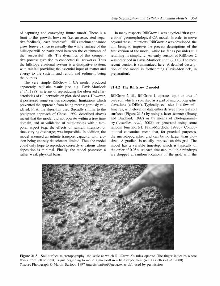
Self-Organization and Cellular Automata Models 359
of capturing and conveying future runoff. There is alimit to this growth, however (i.e. an associated nega-tive feedback); each ‘successful’ rill’s catchment cannotgrow forever, since eventually the whole surface of thehillslope will be partitioned between the catchments ofthe ‘successful’ rills. The dynamics of this competi-tive process give rise to connected rill networks. Thusthe hillslope erosional system is a dissipative system,with rainfall providing the essential input of matter andenergy to the system, and runoff and sediment beingthe outputs.
The very simple RillGrow 1 CA model producedapparently realistic results (see e.g. Favis-Mortlocket al., 1998) in terms of reproducing the observed char-acteristics of rill networks on plot-sized areas. However,it possessed some serious conceptual limitations whichprevented the approach from being more rigorously val-idated. First, the algorithm used (broadly similar to theprecipiton approach of Chase, 1992, described above)meant that the model did not operate within a true timedomain, and so validation of relationships with a tem-poral aspect (e.g. the effects of rainfall intensity, ortime-varying discharge) was impossible. In addition, themodel assumed an infinite transport capacity, with ero-sion being entirely detachment-limited. Thus the modelcould only hope to reproduce correctly situations wheredeposition is minimal. Finally, the model possesses arather weak physical basis.
In many respects, RillGrow 1 was a typical ‘first gen-eration’ geomorphological CA model. In order to movebeyond these limitations, RillGrow 2 was developed, theaim being to improve the process descriptions of thefirst version of the model, while (as far as possible) stillretaining its simplicity. An early version of RillGrow 2was described in Favis-Mortlock et al. (2000). The mostrecent version is summarized here. A detailed descrip-tion of the model is forthcoming (Favis-Mortlock, inpreparation).
21.4.2 The RillGrow 2 model
RillGrow 2, like RillGrow 1, operates upon an area ofbare soil which is specified as a grid of microtopographicelevations (a DEM). Typically, cell size is a few mil-limetres, with elevation data either derived from real soilsurfaces (Figure 21.3) by using a laser scanner (Huangand Bradford, 1992) or by means of photogramme-try (Lascelles et al., 2002); or generated using somerandom function (cf. Favis-Mortlock, 1998b). Compu-tational constraints mean that, for practical purposes,the microtopographic grid can be no larger than plot-sized. A gradient is usually imposed on this grid. Themodel has a variable timestep, which is typically ofthe order of 0.05 s. At each timestep, multiple raindropsare dropped at random locations on the grid, with the
Figure 21.3 Soil surface microtopography: the scale at which RillGrow 2’s rules operate. The finger indicates whereflow (From left to right) is just beginning to incise a microrill in a field experiment (see Lascelles et al., 2000)Source: Photograph Martin Barfoot, 1997 ([email protected]), used by permission

360 David Favis-Mortlock
number of drops depending on rainfall intensity. Run-onfrom upslope may also be added at an edge of the grid.Often, the soil is assumed to be saturated so that no infil-tration occurs; however, a fraction of all surface watermay be removed each timestep as a crude representationof infiltration losses.
Splash redistribution is simulated in RillGrow 2.Since this is a relatively slow process it is not nor-mally calculated at every timestep. The relationshipby Planchon et al. (2000) is used: this is essentially adiffusion equation based on the Laplacian of the conti-nuity equation describing splash erosion, with a ‘splashefficiency’ term which is a function of rainfall inten-sity and water depth. Currently, the splash redistribution
and overland flow components of RillGrow 2 are onlyloosely coupled; while sediment which is redistributedby splash can be moved in or out of the store offlow-transported sediment, this is not done in an explic-itly spatial manner.
Movement of overland flow between ‘wet’ cellsoccurs in discrete steps between cells of this grid.Conceptually, overland flow in RillGrow 2 is thereforea kind of discretized fluid rather like the ‘sheepflow’illustrated in Figure 21.4.
For the duration of the simulation, each ‘wet’ cell isprocessed in a random sequence which varies at eachtimestep. The simple logic outlined in Figure 21.5 isused for the processing.
Figure 21.4 ‘Sheepflow’: a visual analogy of RillGrow 2’s discretized representation of overland flow. Which shouldwe best focus on: an individual sheep or the ‘flow’ of the flock of sheep?Source: Photograph Martin Price, 1999 ([email protected]), used by permission

Self-Organization and Cellular Automata Models 361
Select thenext wet cell
Outflowfrom this cell
possible?
Sufficienttime elapsed tocross the cell?
Calculatetransportcapacity
Move water
Calculate potential flowspeed, based upon
water depth and flowspeed of adjacent cells
Select outflowdirection with thesteepest energy
gradient
Deposition
Sediment loadexceeds transport
capacity?
Soil surface‘downhill’ in outflow
direction?
Detachment
Erosion
Hydrology
Yes
No
No
Yes
No
Yes
Yes
No
Figure 21.5 A partial flowchart of the RillGrow 2 model
Outflow may occur from a ‘wet’ cell to any of theeight adjacent cells. If outflow is possible, the direc-tion with the steepest energy gradient (i.e. maximumdifference in water-surface elevation) is chosen. Thepotential velocity of this outflow is calculated as afunction of water depth and hydraulic radius. However,
outflow only occurs if sufficient time has elapsedfor the water to have crossed this cell. Thus out-flow only occurs for a subset of ‘wet’ cells ateach timestep.
When outflow does occur, the transport capacity ofthe flow is calculated using the previously calculated
362 David Favis-Mortlock
flow velocity with this S-curve relationship (Equation 5in Nearing et al., 1997):
loge(qs) = α + β · eγ+δ·loge(�)
1 + eγ+δ·loge(�)(21.1)
where:qs is unit sediment load [kg m−1 s−1]α, β, γ , δ are constants
and:� = ρ · g · S · q
where:ω = stream power [W m−2]ρ = density of water [kg m−3]g = gravitational acceleration [m s−2]S = energy slope [m m−1]q = unit discharge of water [m2 s−1].
If the sediment concentration of the water on thecell exceeds its transport capacity, deposition occurs.Deposition is calculated using a version of Equation 12in Lei et al. (1998), which assumes deposition to be alinear function of the difference between sediment loadand transport capacity. Note that no consideration ismade of different settling times for each size fraction ofthe deposited sediment, nor of differences in properties(e.g. bulk density, erodibility) between re-entrained andnewly eroded sediment.
Whereas outflow velocity and transport capacity areboth determined by the energy gradient, it is assumed tobe the soil-surface gradient which controls detachment.In RillGrow 2, detachment occurs only if both energygradient and soil surface gradient are downhill. If thesoil-surface gradient is uphill, then the energy gradient-driven outflow is assumed to be merely hydrostaticlevelling. Where detachment does occur, its value iscalculated using a probabilistic equation by Nearing(1991). This assumes that detachment is controlledby the probability of occurrence of random turbulentbursts and the difference between soil strength andshear stress generated by these bursts. The relationshipused in RillGrow 2 is a reformulation of Equation 10in Nearing (1991):
e = K · S · u · P (21.2)
where:e = detachment [kg s−1]K = a constantu = outflow speed [m s−1]
and:
P = 1 − �
(T − τb√
ST2 + Sτb
2
)(21.3)
where:� = the cumulative probability function of a
standard normal deviateT = a constantST = the coefficient of variation of T (assumed
constant)Sτb = the coefficient of variation of τb (assumed
constant)
and:τb = 150 · ρ · g · h · S
where:h = water depth [m].
While still relatively simple, RillGrow 2 is thus adevelopment of the earlier RillGrow model in thatit attempts to explicitly reproduce, in a true timedomain, the effects of several processes involved inrill formation.
21.4.2.1 Results from RillGrow 2
During a series of 12 laboratory-based experiments atthe University of Leicester (Lascelles et al., 2000, 2002;Favis-Mortlock et al., in preparation) simulated rainfall(i.e. from an overhead sprinkler system) was applied toa sandy soil in a 4 × 1.75 m flume. A range of slopeangles and rainfall intensities were used (Table 21.2).Each experiment lasted for 30 minutes, during whichtime surface flow, discharge, sediment removal and flowvelocities were measured. Prior to and following each
Table 21.2 Some characteristics of the Leicesterflume experiments used to evaluate RillGrow 2
ExperimentNo.
Slope angle(degrees)
Rainfall(mm h−1)
X09 5 108X10 10 129X11 15 125X12 5 117X13 10 127X14 15 126X15 5 120X16 10 126X17 15 131X18 5 121X19 10 123X20 15 125
Source: Adapted from Favis-Mortlock et al. (in preparation)
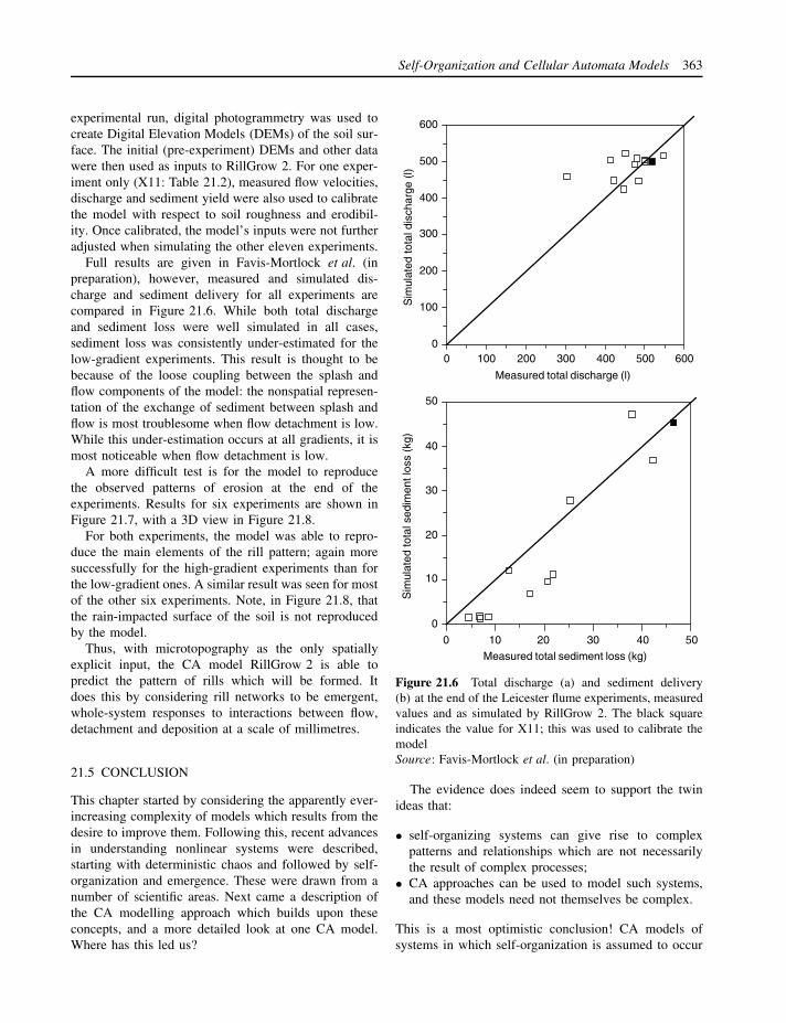
Self-Organization and Cellular Automata Models 363
experimental run, digital photogrammetry was used tocreate Digital Elevation Models (DEMs) of the soil sur-face. The initial (pre-experiment) DEMs and other datawere then used as inputs to RillGrow 2. For one exper-iment only (X11: Table 21.2), measured flow velocities,discharge and sediment yield were also used to calibratethe model with respect to soil roughness and erodibil-ity. Once calibrated, the model’s inputs were not furtheradjusted when simulating the other eleven experiments.
Full results are given in Favis-Mortlock et al. (inpreparation), however, measured and simulated dis-charge and sediment delivery for all experiments arecompared in Figure 21.6. While both total dischargeand sediment loss were well simulated in all cases,sediment loss was consistently under-estimated for thelow-gradient experiments. This result is thought to bebecause of the loose coupling between the splash andflow components of the model: the nonspatial represen-tation of the exchange of sediment between splash andflow is most troublesome when flow detachment is low.While this under-estimation occurs at all gradients, it ismost noticeable when flow detachment is low.
A more difficult test is for the model to reproducethe observed patterns of erosion at the end of theexperiments. Results for six experiments are shown inFigure 21.7, with a 3D view in Figure 21.8.
For both experiments, the model was able to repro-duce the main elements of the rill pattern; again moresuccessfully for the high-gradient experiments than forthe low-gradient ones. A similar result was seen for mostof the other six experiments. Note, in Figure 21.8, thatthe rain-impacted surface of the soil is not reproducedby the model.
Thus, with microtopography as the only spatiallyexplicit input, the CA model RillGrow 2 is able topredict the pattern of rills which will be formed. Itdoes this by considering rill networks to be emergent,whole-system responses to interactions between flow,detachment and deposition at a scale of millimetres.
21.5 CONCLUSION
This chapter started by considering the apparently ever-increasing complexity of models which results from thedesire to improve them. Following this, recent advancesin understanding nonlinear systems were described,starting with deterministic chaos and followed by self-organization and emergence. These were drawn from anumber of scientific areas. Next came a description ofthe CA modelling approach which builds upon theseconcepts, and a more detailed look at one CA model.Where has this led us?
00 100 200 300 400 500 600
100
200
300
400
500
600
Measured total discharge (l)
Sim
ulat
ed to
tal d
isch
arge
(l)
0
10
20
30
40
50
0 10 20 30 40 50
Measured total sediment loss (kg)
Sim
ulat
ed to
tal s
edim
ent l
oss
(kg)
Figure 21.6 Total discharge (a) and sediment delivery(b) at the end of the Leicester flume experiments, measuredvalues and as simulated by RillGrow 2. The black squareindicates the value for X11; this was used to calibrate themodelSource: Favis-Mortlock et al. (in preparation)
The evidence does indeed seem to support the twinideas that:
• self-organizing systems can give rise to complexpatterns and relationships which are not necessarilythe result of complex processes;
• CA approaches can be used to model such systems,and these models need not themselves be complex.
This is a most optimistic conclusion! CA models ofsystems in which self-organization is assumed to occur

364 David Favis-Mortlock
(a)
(b)
(c)
(d)
(e)
(f)
(g)
(h)
(i)(j)
(k)
(l)
Fig
ure
21.7
Pla
nvi
ews
ofth
eso
il’s
surf
ace
inth
eL
eice
ster
flum
e.D
arke
rar
eas
have
low
erel
evat
ion.
Top
row
:15
◦sl
ope
(a)
X11
(cal
ibra
ted)
;(b
)X
11si
mul
ated
byR
illG
row
2;(c
)X
14;
(d)
X14
sim
ulat
ed;
Mid
dle
row
:10
◦sl
ope;
(e)
X13
;(f
)X
13si
mul
ated
;(g
)X
16;
(h)
X16
sim
ulat
ed.
Low
erro
w:
5◦sl
ope;
(i)
X15
;(j
)X
15si
mul
ated
;(k
)X
12;
(l)
X12
sim
ulat
edSo
urce
:Fa
vis-
Mor
tlock
etal
.(i
npr
epar
atio
n)

Self-Organization and Cellular Automata Models 365
(a) (b)
Figure 21.8 3D views of the soil surface in the Leicester flume, showing X13 with 10◦ slope: (a) experiment;(b) simulated by RillGrow 2Source: Favis-Mortlock et al. (in press)
need only be simple at the ‘component’ level, yet arestill capable of producing a great wealth of complex,emergent responses. When such models are designedto use realistic real-world values (e.g. RillGrow 2), itseems that the models, while simple, are nonethelesscapable of reproducing realistic facsimiles of some ofthe complex features of real environments.
Finally, an important point re. discretization. Wolfram(2002, p. 327) notes that many systems in nature appearsmooth or continuous, yet CA models involve onlydiscrete elements. How can such models ever hope toreproduce what we see in nature? The crucial pointhere is that even though the individual elements of asystem may be discrete, the average behaviour seenwhen looking at a large number of these componentsmay well be continuous. The question then becomes,‘Are there a sufficient number of CA elements for theiraverage behaviour to approximate the average behaviourof the real system?’
The mounting weight of model-based evidence,together with field- and laboratory-based studies notdiscussed here, tends to confirm the assumption that self-organization is a real feature of the real world. If this is
so, then one implication is a message of hope for envi-ronmental modellers. We are not doomed to ever morecomplex models!
While it may seem perverse that the study of com-plexity can lead us to simplicity, ground-breakingresearch on self-organization during the late 1980s and1990s appears to have been a fresh wind, doing awaywith the tired idea of fitting the results of data-hungrymodels to sparse, observed data. Instead of the cumber-some drudgery of varying a large number of parametersand variables to obtain a better fit between the computedand observed data, models may again be used to generatenew and exciting ideas, and to help solve the loomingand difficult environmental problems which humanitymust successfully tackle if it is to survive.
ACKNOWLEDGEMENTS
There is some overlap between this chapter andthe rather longer paper of Favis-Mortlock and DeBoer (in press). As in that paper, I would like tothank the following: John Boardman (University of

366 David Favis-Mortlock
Oxford), Jack Cohen (University of Warwick), AntonImeson (University of Amsterdam), Mark Nearing(USDA-ARS), John Thornes (King’s College London),Brian Whalley (Queen’s University Belfast); the ‘self-organized lunchers’ at Oxford (Susan Canney, CliveHambler, Mike Packer and David Raubenheimer); andfinally all those who attended the NATO-ASI ‘Nonlin-ear Dynamics in Life and Social Sciences’ (Moscow,2000). Development of RillGrow 2 was partly funded bythe UK Natural Environment Research Council (NERCGR3/11417: ‘Rill initiation by overland flow and its rolein modelling soil erosion’).
NOTES
1. Cf. Chaitin’s (1999) notion of ‘algorithmic com-plexity’.
2. This is particularly the case in practical applicationswhere the main aim is a successful replication ofmeasured values, perhaps with the subsequent aimof estimating unmeasurable values, e.g. under somehypothetical conditions of climate or land use.
3. See section on terminology below.4. The concept of equifinality is originally due to Von
Bertalanffy (1968).5. Originally the title of a 1970s lecture by Lorentz.
There are now many variants.6. The word ‘eventually’ is important here. The repet-
itive calculations which are often necessary areideally suited to a computer, but not to a human.This is one reason why deterministic chaos had towait for the widespread usage of computers for itsdiscovery.
7. ‘But what we’ve realized now is that unpredictabilityis very common, it’s not just some special case.It’s very common for dynamical systems to exhibitextreme unpredictability, in the sense that you canhave perfectly definite equations, but the solutionscan be unpredictable to a degree that makes itquite unreasonable to use the formal causality builtinto the equations as the basis for any intelligentphilosophy of prediction’ (Berry 1988).
8. In some cases the exposed B horizon will havegreater shear strength and so be better able to resistdetachment by the extra flow. Here, an increase inrunoff will not result in increased erosion.
9. Referred to as ‘complicity’ in Cohen and Stew-art (1994). As Jack Cohen put it in an emailto [email protected] on 10 December2000:
a more exquisite problem for complex thinkingis the problem of recursion. The system doesn’t
simply respond to the environment, the environ-ment also responds to the system. The pattern ofa river bed is the result of genuine interaction ofthis kind, and so is nearly every ongoing processin physics, biology or management.
Another term for this is ‘autocatalysis’.10. In other words, a large number of independently
varying degrees of freedom.11. Because of the centre-tending effect of the law of
large numbers: see e.g. Harvey (1969: 246).12. Such as a idealized gas: see Bar-Yam (1997). It is
also true (but in a different way) for almost allsystems, even quite complicated ones, which havebeen constructed by some external agency e.g. bya human. A first question to ask when attemptingto identify self-organization is, ‘Is this system morethan the sum of its parts?’
13. Yet from still another point of view, they certainlyshouldn’t be. For if nonliving systems do notorganize themselves, how would they get organizedin the first place? Unless we invoke an organizer(i.e. teleology), then from this perspective ‘if self-organization did not exist, it would be necessary toinvent it’.
14. Just as almost all models which operate in atrue time dimension discretize continuous time intodistinct ‘timesteps’.
15. Discretization appears to be a fundamental operationfor humans attempting to make sense of the world;see e.g. Chapter 1 of Bohm (1980).
16. This is related to the concepts of ‘trivial duality’and ‘nontrivial duality’ in physics (Greene, 1999:297 ff.). If each of two different descriptions of thesame system tell us something that the other doesnot, this is ‘nontrivial duality’.
17. For example:• http://psoup.math.wisc.edu/Life32.html• http://sero.org/sero/homepages/• http://www.automaton.ch/• http://www.exploratorium.edu/complexity/
CompLexicon/automaton.html18. See http://www.santafe.edu/∼hag/class/class.html
for a hierarchical classification of cellular automata.19. For example, what is the best way of splitting up
the cellular grid between processors if cells must beprocessed in a random sequence (cf. Watts, 1999:205)? What about local interactions between cellsallocated to different processors?
20. ‘Biologists cannot adopt a reductionist approachwhen working with a living organism, or it dies’(Jack Cohen, personal communication, 2000).

Self-Organization and Cellular Automata Models 367
REFERENCES
Ackoff, R.L., Gupta, S.K. and Minas, J.S. (1962) ScientificMethod: Optimizing Applied Research Decisions, John Wiley& Sons, New York.
Andrle, R. (1996) The west coast of Britain: statistical self-similarity vs. characteristic scales in the landscape, EarthSurface Processes and Landforms 21 (10), 955–962.
Aristotle (c. 330 BCE) Metaphysica 10f–1045a.Bak, P. (1996) How Nature Works, Springer-Verlag, New York.Bak, P., Tang, C. and Wiesenfeld, K. (1988) Self-organized
criticality, Physical Review A 38 (1), 364–374.Bar-Yam, Y. (1997) Dynamics of Complex Systems, Perseus,
Reading, MA.Ben-Jacob, E. and Levine, H. (2001) The artistry of nature,
Nature 409, 985–986.Berry, M. (1988) The electron at the end of the universe, in
L. Wolpert and A. Richards (eds) A Passion for Science,Oxford University Press, Oxford, 39–51.
Beven, K.J. (1993) Prophecy, reality and uncertainty in dis-tributed hydrological modelling, Advances in Water Re-sources 16, 41–51.
Beven, K.J. (1996) The limits of splitting: hydrology, TheScience of the Total Environment 183, 89–97.
Bohm, D. (1980) Wholeness and the Implicate Order, Rout-ledge, London.
Buchanan, M. (2000) Ubiquity, Weidenfeld and Nicolson,London.
Cambel, A.B. (1993) Applied Chaos Theory: A Paradigm forComplexity, Academic Press, Boston.
Chaitin, G.J. (1999) The Unknowable, Springer-Verlag, Singa-pore.
Chase, C.G. (1992) Fluvial landsculpting and the fractal dimen-sion of topography, Geomorphology 5, 39–57.
Chorley, R.J. (1962) Geomorphology and General SystemsTheory , US Geological Survey Professional Paper, No. 500-B.
Clerici, A. and Perego, S. (2000) Simulation of the ParmaRiver blockage by the Corniglio landslide (Northern Italy),Geomorphology 33, 1–23.
Clifford, N.J. (2001) Physical Geography – the naughty worldrevisited, Transactions of the Institute of British GeographersNS 26, 387–389.
Cohen, J. and Stewart, I. (1994) The Collapse of Chaos, Pen-guin, London.
Coulthard, T.J., Macklin, M.G. and Kirkby, M.J. (2002) Acellular model of Holocene upland river basin and alluvialfan evolution, Earth Surface Processes and Landforms 27(3), 269–288.
Coveney, P. and Highfield, R. (1995) Frontiers of Complexity,Faber and Faber, London.
De Boer, D.H. (2001) Self-organization in fluvial landscapes:sediment dynamics as an emergent property, Computers andGeosciences 27 (8), 995–1003.
Evans, I.S. and McClean, C.J. (1995) The land surface is notunifractal: variograms, cirque scale and allometry, Zeitschriftfur Geomorphologie N.F. Supplement 101, 127–147.
Favis-Mortlock, D.T. (1996) An evolutionary approach tothe simulation of rill initiation and development, inR.J. Abrahart (ed.) Proceedings of the First InternationalConference on GeoComputation (Vol. 1), School ofGeography, University of Leeds, Leeds, 248–281.
Favis-Mortlock, D.T. (1998a) Validation of field-scale soilerosion models using common datasets, in J. Boardman andD.T. Favis-Mortlock (eds) Modelling Soil Erosion by Water,Springer-Verlag NATO-ASI Series I-55, Berlin, 89–128.
Favis-Mortlock, D.T. (1998b) A self-organizing dynamic sys-tems approach to the simulation of rill initiation and devel-opment on hillslopes, Computers and Geosciences 24 (4),353–372.
Favis-Mortlock, D.T. (in preparation) The RillGrow 2 model.Favis-Mortlock, D.T., Boardman, J. and MacMillan, V.J.
(2001) The limits of erosion modeling: why we shouldproceed with care, in R.S. Harmon and W.W. Doe III(eds) Landscape Erosion and Evolution Modeling, KluwerAcademic/Plenum Publishing, New York, 477–516.
Favis-Mortlock, D.T., Boardman, J., Parsons, A.J. and Las-celles, B. (2000) Emergence and erosion: a model forrill initiation and development, Hydrological Processes 14(11–12), 2173–2205.
Favis-Mortlock, D.T. and De Boer, D. (2003) Simple atheart? Landscape as a self-organizing complex system, inS.T. Trudgill and A. Roy (eds) Contemporary Meanings InPhysical Geography, Edward Arnold, London, 127–171.
Favis-Mortlock, D.T., Guerra, A.J.T. and Boardman, J. (1998)A self-organising dynamic systems approach to hillslope rillinitiation and growth: model development and validation,in, W. Summer, E. Klaghofer and W. Zhang (eds) Mod-elling Soil Erosion, Sediment Transport and Closely RelatedHydrological Processes, IAHS Press Publication No. 249,Wallingford, 53–61.
Favis-Mortlock, D.T., Parsons, A.J, Boardman, J. and Las-celles, B. (in preparation) Evaluation of the RillGrow 2model.
Favis-Mortlock, D.T., Quinton, J.N. and Dickinson, W.T.(1996) The GCTE validation of soil erosion modelsfor global change studies, Journal of Soil and WaterConservation 51 (5), 397–403.
Gallagher, R. and Appenzeller, T. (1999) Beyond reduction-ism, Science 284, 79.
Garcia-Sanchez, L., Di Pietro, L. and Germann, P.F. (1996)Lattice-gas approach to surface runoff after rain, EuropeanJournal of Soil Science 47 (4), 453–462.
Goodwin, B. (1997) How the Leopard Changed its Spots: TheEvolution of Complexity, Phoenix, London.
Greene, B. (1999) The Elegant Universe, Jonathan Cape, Lon-don.
Hansen, J.L., Van Hecke, M., Haaning, A., Ellegaard, C.,Andersen, K.H., Bohr, T. and Sams, T. (2001) Instabilitiesin sand ripples, Nature 410, 324.
Harvey, D. (1969) Explanation in Geography, Edward Arnold,London.
Hawking, S. (1988) A Brief History of Time, Bantam Books,New York.

368 David Favis-Mortlock
Hergarten, S. and Neugebauer, H.J. (1998) Self-organized crit-icality in a landslide model, Geophysical Research Letters25 (6), 801–804.
Hergarten, S. and Neugebauer, H.J. (1999) Self-organizedcriticality in landsliding processes, in S. Hergarten andH.J. Neugebauer (eds) Process Modelling and LandformEvolution, Springer, Berlin, 231–249.
Hergarten, S. and Neugebauer, H.J. (2001) Self-organized crit-ical drainage networks, Physical Review Letters 86 (12),2689–2692.
Hergarten, S., Paul, G. and Neugebauer, H.J. (2000) Model-ing surface runoff, in J. Schmidt (ed.) Soil Erosion: Appli-cation of Physically-Based Models, Springer-Verlag, Berlin,295–306.
Holland, J.H. (1998) Emergence: From Chaos to Order, PerseusBooks, Reading, MA.
Huang, C. and Bradford, J.M. (1992) Applications of a laserscanner to quantify soil microtopography, Soil Science Soci-ety of America Journal 56 (1), 14–21.
Huggett, R.J. (1985) Earth Surface Systems, Springer-Verlag,Berlin.
Jakeman, A.J. and Hornberger, G.M. (1993) How much com-plexity is warranted in a rainfall-runoff model? WaterResources Research 29, 2637–2649.
Jetten, V., de Roo, A.P.J. and Favis-Mortlock, D.T. (1999)Evaluation of field-scale and catchment-scale soil erosionmodels, Catena 37 (3/4), 521–541.
Jones, H. (1991) Fractals before Mandelbrot: a selective his-tory, in A.J. Crilly, R.A. Earnshaw and H. Jones (eds) Frac-tals and Chaos, Springer-Verlag, Berlin, 7–33.
Kauffman, S. (1995) At Home in the Universe: The Search forLaws of Self-Organization and Complexity, Oxford Univer-sity Press, Oxford.
Kirchner, J.W., Hooper, R.P., Kendall, C., Neal, C. andLeavesley, G. (1996) Testing and validating environmentalmodels, The Science of the Total Environment 183, 33–47.
Kirkby, M.J., Naden, P.S., Burt, T.P. and Butcher, D.P. (1992)Computer Simulation in Physical Geography, 2nd edn, JohnWiley & Sons, Chichester.
Klemes, V. (1986) Dilettantism in hydrology: transition ordestiny? Water Resources Research 22, 177S–188S.
Klimontovich, Y.L. (2001) Entropy, information and orderingcriteria in open systems, in W. Sulis and I. Trofimova (eds)Nonlinear Dynamics in the Life and Social Sciences, IOSPress, Amsterdam, 13–32.
Laland, K.N., Odling-Smee, F.J. and Feldman, M.W. (1999)Evolutionary consequences of niche construction and theirimplications for ecology, Proceedings of the NationalAcademy of Science 96, 10242–10247.
Lascelles, B., Favis-Mortlock, D.T., Parsons, A.J. and Board-man, J. (2002) Automated digital photogrammetry: a valu-able tool for small-scale geomorphological research for thenon-photogrammetrist? Transactions in GIS 6 (1), 5–15.
Lascelles, B., Favis-Mortlock, D.T., Parsons, A.J. and Guerra,A.J.T. (2000) Spatial and temporal variation in two rainfallsimulators: implications for spatially explicit rainfall simu-lation experiments, Earth Surface Processes and Landforms25 (7), 709–721.
Lei, T., Nearing, M.A., Haghighi, K. and Bralts, V.F. (1998)Rill erosion and morphological evolution: a simulationmodel, Water Resources Research 34 (11), 3157–3168.
Lenton, T.M. (1998) Gaia and natural selection, Nature 394,439–447.
Leonard, R.A., Knisel, W.G. and Still, D.A. (1987) GLEAMS:Groundwater Loading Effects of Agricultural ManagementSystems, Transactions of the American Society of Agricul-tural Engineers 30 (5), 1403–1418.
Leopold, L.B., Wolman, M.G. and Miller, J.P. (1964) FluvialProcesses in Geomorphology, Freeman, San Francisco.
Lewin, R. (1997) Critical mass: complexity theory may explainbig extinctions better than asteroids, New Scientist, 155, 23August, 7.
Li, W. (1997) Nonlocal cellular automata, in H.F. Nijhout,L. Nadel, and D.S. Stein (eds) Pattern Formation in thePhysical and Biological Sciences, Addison-Wesley, Reading,MA, 189–200.
Mahnke, R. (1999) Pattern formation in cellular automatonmodels, in J. Schmelzer, G. Ropke and R. Mahnke (eds)Aggregation Phenomena in Complex Systems, Wiley-VCH,Weinheim, 146–173
Mandelbrot, B.B. (1975) Stochastic models for the earth’srelief, the shape and the fractal dimension of the coastlines,and the number-area rules for islands, Proceedings of theNational Academy of Sciences, USA 72 (10), 3825–3828.
May, R.M. (1976) Simple mathematical models with verycomplicated dynamics, Nature 261, 459–467.
Morgan, R.P.C., Quinton, J.N., Smith, R.E., Govers, G., Poe-sen, J.W.A., Chisci, G. and Torri, D. (1998) The EUROSEMmodel, in J. Boardman and D.T. Favis-Mortlock (eds) Mod-elling Soil Erosion by Water, Springer-Verlag NATO-ASISeries I-55, Berlin, 389–398.
Murray, A.B. and Paola, C. (1994) A cellular model of braidedrivers, Nature 371, 54–57.
Murray, A.B. and Paola, C. (1996) A new quantitative test ofgeomorphic models, applied to a model of braided streams,Water Resources Research 32 (8), 2579–2587.
Murray, A.B. and Paola, C. (1997) Properties of a cellularbraided-stream model, Earth Surface Processes and Land-forms 22 (11), 1001–1025.
Nearing, M.A. (1991) A probabilistic model of soil detachmentby shallow turbulent flow, Transactions of the AmericanSociety of Agricultural Engineers 34 (1), 81–85.
Nearing, M.A., Foster, G.R., Lane, L.J. and Finkner, S.C.(1989) A process-based soil erosion model for USDA-Water Erosion Prediction Project technology, Transactionsof the American Society of Agricultural Engineers 32 (5),1587–1593.
Nearing, M.A., Norton, L.D., Bulgakov, D.A., Larionov, G.A.,West, L.T. and Dontsova, K. (1997) Hydraulics and erosionin eroding rills, Water Resources Research 33 (4), 865–876.
Nicolis, G. and Prigogine, I. (1989) Exploring Complexity,Freeman, New York.
Peterson, G.D. (2000) Scaling ecological dynamics: self-organization, hierarchical structure, and ecological resilience,Climatic Change 44, 291–309.

Self-Organization and Cellular Automata Models 369
Pilotti, M. and Menduni, G. (1997) Application of lattice gastechniques to the study of sediment erosion and transportcaused by laminar sheetflow, Earth Surface Processes andLandforms 22 (9), 885–893.
Planchon, O., Esteves, M., Silvera, N. and Lapetite, J.M.(2000) Raindrop erosion of tillage induced microrelief:Possible use of the diffusion equation, Soil and TillageResearch 56 (3–4), 131–144.
Portugali, J., Benenson, I. and Omer, I. (1997) Spatial cog-nitive dissonance and socio-spatial emergence in a self-organizing city, Environment and Planning B 24, 263–285.
Rodrıguez-Iturbe, I. and Rinaldo, A. (1997) Fractal RiverBasins: Chance and Self-Organization, Cambridge Univer-sity Press, Cambridge.
Rosenblueth, A. and Wiener, N. (1945) The role of models inscience, Philosophy of Science 12.
Ruelle, D. (1993) Chance and Chaos, Penguin, London.Ruelle, D. (2001) Applications of chaos, in W. Sulis and
I. Trofimova (eds) Nonlinear Dynamics in the Life and SocialSciences, IOS Press, Amsterdam, 3–12.
Sethna, J.P., Dahmen, K.A. and Myers, C.R. (2001) Cracklingnoise, Nature 410, 242–250.
Sole, R.V., Manrubia, S.C., Benton, M., Kauffman, S. andBak, P. (1999) Criticality and scaling in evolutionary ecol-ogy, Trends in Evolutionary Ecology 14 (4), 156–160.
Tam, W.Y. (1997) Pattern formation in chemical systems: rolesof open reactors, in H.F. Nijhout, L. Nadel and D.S. Stein(eds) Pattern Formation in the Physical and BiologicalSciences, Addison-Wesley, Reading, MA, 323–347.
Thomas, R. and Nicholas, A.P. (2002) Simulation of braidedriver flow using a new cellular routing scheme, Geomorphol-ogy 43 (3–4), 179–195
Tucker, G.E. and Slingerland, R. (1996) Predicting sedimentflux from fold and thrust belts, Basin Research 8, 329–349.
Tucker, G.E. and Slingerland, R. (1997) Drainage basinresponses to climate change, Water Resources Research 33(8), 2031–2047.
Von Bertalanffy, L. (1968) General Systems Theory: Foun-dations, Development, Applications, George Braziller, NewYork.
Waldrop, M.M. (1994) Complexity, Penguin, London.Washington, R.W. (2000) Quantifying chaos in the atmosphere,
Progress in Physical Geography 24 (2), 499–514.Watts, D.J. (1999) Small Worlds: The Dynamics of Networks
between Order and Randomness, Princeton University Press,Princeton, NJ.
Wendt, R.C., Alberts, E.E. and Hjemfelt Jr, A.T. (1986) Vari-ability of runoff and soil loss from fallow experimental plots,Soil Science Society of America Journal 50 (3), 730–736.
Werner, B.T. (1995) Eolian dunes: computer simulations andattractor interpretation, Geology 23, 1107–1110.
Werner, B.T. (1999) Complexity in natural landform patterns,Science 284, 102–104.
Werner, B.T. and Fink, T.M. (1993) Beach cusps as self-organized patterns, Science 260, 968–971.
Werner, B.T. and Hallet, B. (1993) Numerical simulation ofself-organized stone stripes, Nature 361, 142–145.
Wilcox, B.P., Seyfried, M.S. and Matison, T.H. (1991) Search-ing for chaotic dynamics in snowmelt runoff, WaterResources Research 27 (6), 1005–1010.
Williams, J.R., Renard, K.E. and Dyke, P.T. (1983) EPIC – anew method for assessing erosion’s effect on soil productiv-ity, Journal of Soil and Water Conservation 38 (5), 381–383.
Winder, N. (2000) Contemporary human ecodynamics andthe mathematics of history, in G. Bailey, R. Charles andN. Winder (eds) Human Ecodynamics, Oxbow, Oxford,1–9.
Wischmeier, W.H. and Smith, D.D. (1978) Predicting RainfallErosion Losses, US Department of Agriculture, AgriculturalResearch Service Handbook 537, Washington, DC.
Wolfram, S. (1982) Cellular Automata as Simple Self-Organising Systems, Caltech preprint CALT-68-938, Pasu-dena, CA.
Wolfram, S. (1986) Cellular automaton fluids 1. Basic theory,Journal of Statistical Physics 45, 471–526.
Wolfram, S. (2002) A New Kind of Science, Wolfram MediaInc., Champaign, IL, USA.
Wooton, J.T. (2001) Local interactions predict large-scale pat-tern in empirically derived cellular automata, Nature 413,841–844.


22
Data-Based Mechanistic Modelling and theSimplification of Environmental Systems1
PETER C. YOUNG, ARUN CHOTAI AND KEITH J. BEVEN
22.1 INTRODUCTION
The environment is a complex assemblage of interact-ing physical, chemical and biological processes, many ofwhich are inherently nonlinear, with considerable uncer-tainty about both their nature and their interconnections.It is surprising, therefore, that stochastic dynamic mod-els are the exception rather than the rule in environmen-tal science research. One reason for this anomaly lies inthe very successful history of physical science over thelast century. Modelling in deterministic terms has per-meated scientific endeavour over this period and has ledto a pattern of scientific investigation which is heavilyreductionist in nature. Such deterministic reductionismappears to be guided by a belief that physical systemscan be described very well, if not exactly, by deter-ministic mathematical equations based on well knownscientific laws, provided only that sufficient detail canbe included to describe all the physical processes thatare perceived to be important by the scientists involved.This leads inexorably to large, nonlinear models reflect-ing the scientist’s perception of the environment as anexceedingly complex dynamic system.
Although deterministic reductionism still dominatesenvironmental modelling, there are some signs that atti-tudes may be changing. There is a growing realiza-tion that, despite their superficially rigorous scientificappearance, simulation models of the environment basedon deterministic concepts are more speculative exten-sions of our mental models and perceptions of the realworld than necessarily accurate representations of thereal world itself. The recent revived interest in the‘top-down’ approach to modelling in the hydrological
literature (e.g. Jothityangkoon et al., 2000 and the ref-erences therein), for instance, is a response to the rela-tive failure of the alternative reductionist (‘bottom-up’)philosophy in this area of study. But such scepticismis not new. It has its parallels in the environmental(e.g. Young, 1978, 1983; Beck, 1983) and ecosystems(e.g. see prior references cited in Silver, 1993) litera-ture of the 1970s and early 1980s, where the presentfirst author’s contributions were set within the con-text of ‘badly defined’ environmental systems. To quotefrom Young (1983), which echoes earlier ideas (Young,1978), for instance:
Although such reductionist analysis is perfectlyrespectable, it must be used very carefully; the dangersinherent in its application are manifold, but theyare not, unfortunately, always acknowledged by itsproponents. It is well known that a large and complexsimulation model, of the kind that abounds in currentecological and environmental system analysis, hasenormous explanatory potential and can usually befitted easily to the meagre time-series data often usedas the basis for such analysis. Yet even deterministicsensitivity analysis will reveal the limitation of theresulting model: many of the ‘estimated’ parametersare found to be ill-defined and only a comparativelysmall subset is important in explaining the observedsystem behaviour.
This paper goes on to point out that such over-parameterization and the associated identifiabilityproblems are quite often acknowledged, often implic-itly, by the reductionist simulation model-builder. For
Environmental Modelling: Finding Simplicity in Complexity. Edited by J. Wainwright and M. Mulligan 2004 John Wiley & Sons, Ltd ISBNs: 0-471-49617-0 (HB); 0-471-49618-9 (PB)
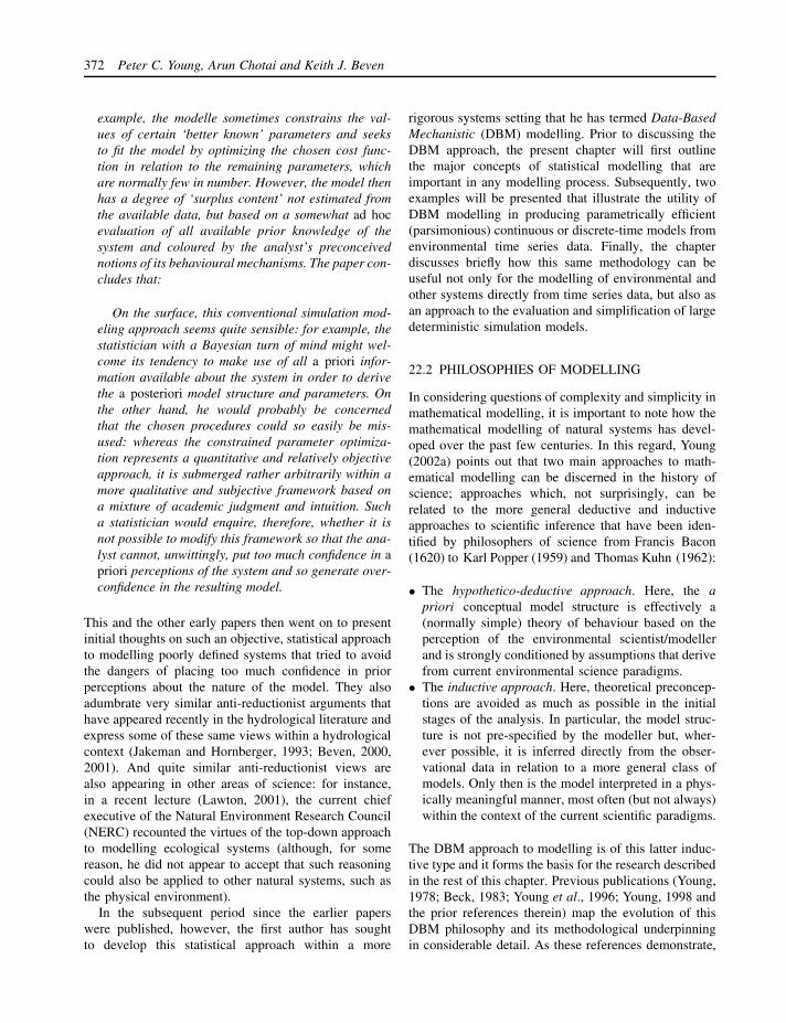
372 Peter C. Young, Arun Chotai and Keith J. Beven
example, the modelle sometimes constrains the val-ues of certain ‘better known’ parameters and seeksto fit the model by optimizing the chosen cost func-tion in relation to the remaining parameters, whichare normally few in number. However, the model thenhas a degree of ‘surplus content’ not estimated fromthe available data, but based on a somewhat ad hocevaluation of all available prior knowledge of thesystem and coloured by the analyst’s preconceivednotions of its behavioural mechanisms. The paper con-cludes that:
On the surface, this conventional simulation mod-eling approach seems quite sensible: for example, thestatistician with a Bayesian turn of mind might wel-come its tendency to make use of all a priori infor-mation available about the system in order to derivethe a posteriori model structure and parameters. Onthe other hand, he would probably be concernedthat the chosen procedures could so easily be mis-used: whereas the constrained parameter optimiza-tion represents a quantitative and relatively objectiveapproach, it is submerged rather arbitrarily within amore qualitative and subjective framework based ona mixture of academic judgment and intuition. Sucha statistician would enquire, therefore, whether it isnot possible to modify this framework so that the ana-lyst cannot, unwittingly, put too much confidence in apriori perceptions of the system and so generate over-confidence in the resulting model.
This and the other early papers then went on to presentinitial thoughts on such an objective, statistical approachto modelling poorly defined systems that tried to avoidthe dangers of placing too much confidence in priorperceptions about the nature of the model. They alsoadumbrate very similar anti-reductionist arguments thathave appeared recently in the hydrological literature andexpress some of these same views within a hydrologicalcontext (Jakeman and Hornberger, 1993; Beven, 2000,2001). And quite similar anti-reductionist views arealso appearing in other areas of science: for instance,in a recent lecture (Lawton, 2001), the current chiefexecutive of the Natural Environment Research Council(NERC) recounted the virtues of the top-down approachto modelling ecological systems (although, for somereason, he did not appear to accept that such reasoningcould also be applied to other natural systems, such asthe physical environment).
In the subsequent period since the earlier paperswere published, however, the first author has soughtto develop this statistical approach within a more
rigorous systems setting that he has termed Data-BasedMechanistic (DBM) modelling. Prior to discussing theDBM approach, the present chapter will first outlinethe major concepts of statistical modelling that areimportant in any modelling process. Subsequently, twoexamples will be presented that illustrate the utility ofDBM modelling in producing parametrically efficient(parsimonious) continuous or discrete-time models fromenvironmental time series data. Finally, the chapterdiscusses briefly how this same methodology can beuseful not only for the modelling of environmental andother systems directly from time series data, but also asan approach to the evaluation and simplification of largedeterministic simulation models.
22.2 PHILOSOPHIES OF MODELLING
In considering questions of complexity and simplicity inmathematical modelling, it is important to note how themathematical modelling of natural systems has devel-oped over the past few centuries. In this regard, Young(2002a) points out that two main approaches to math-ematical modelling can be discerned in the history ofscience; approaches which, not surprisingly, can berelated to the more general deductive and inductiveapproaches to scientific inference that have been iden-tified by philosophers of science from Francis Bacon(1620) to Karl Popper (1959) and Thomas Kuhn (1962):
• The hypothetico-deductive approach. Here, the apriori conceptual model structure is effectively a(normally simple) theory of behaviour based on theperception of the environmental scientist/modellerand is strongly conditioned by assumptions that derivefrom current environmental science paradigms.
• The inductive approach. Here, theoretical preconcep-tions are avoided as much as possible in the initialstages of the analysis. In particular, the model struc-ture is not pre-specified by the modeller but, wher-ever possible, it is inferred directly from the obser-vational data in relation to a more general class ofmodels. Only then is the model interpreted in a phys-ically meaningful manner, most often (but not always)within the context of the current scientific paradigms.
The DBM approach to modelling is of this latter induc-tive type and it forms the basis for the research describedin the rest of this chapter. Previous publications (Young,1978; Beck, 1983; Young et al., 1996; Young, 1998 andthe prior references therein) map the evolution of thisDBM philosophy and its methodological underpinningin considerable detail. As these references demonstrate,

Data-Based Mechanistic Modelling and the Simplification of Environmental Systems 373
DBM models can be of various kinds depending uponthe nature of the system under study. In the contextof the present chapter, however, they take the form oflinear and nonlinear, stochastic Transfer Function (TF)representations of the hydrological processes active inriver catchments.
22.3 STATISTICAL IDENTIFICATION,ESTIMATION AND VALIDATION
The statistical approach to modelling assumes that themodel is stochastic: in other words, no matter howgood the model and how low the noise on the observa-tional data happens to be, a certain level of uncertaintywill remain after modelling has been completed. Con-sequently, full stochastic modelling requires that thisuncertainty, which is associated with both the modelparameters and the stochastic inputs, should be quan-tified in some manner as an inherent part of the mod-elling analysis.
In the statistical, time-series literature, such a stochas-tic modelling procedure is normally considered in twomain stages: identification of an appropriate, identifiablemodel structure; and estimation (optimization, calibra-tion) of the parameters that characterize this structure,using some form of estimation or optimization. Nor-mally, if the data provision makes it possible, a furtherstage of validation (or conditional validation: see later)is defined, in which the ability of the model to explainthe observed data is evaluated on data sets different tothose used in the model identification and estimationstages. In this section, we outline these three stages inorder to set the scene for the later analysis. This discus-sion is intentionally brief, however, since the topic is solarge that a comprehensive review is not possible in thepresent context.
22.3.1 Structure and order identification
In the DBM approach to modelling, the identificationstage is considered as a most important and essentialprelude to the later stages of model building. It usu-ally involves the identification of the most appropriatemodel order, as defined in dynamic system terms. How-ever, the model structure itself can be the subject ofthe analysis if this is also considered to be ill-defined.In the DBM approach, for instance, the nature of lin-earity and nonlinearity in the model is not assumed apriori (unless there are good reasons for such assump-tions based on previous data-based modelling studies).Rather it is identified from the data using nonparametricand parametric statistical estimation methods based on
a suitable, generic model class. Once a suitable modelstructure has been defined within this class, there area variety of statistical methods for identifying modelorder, some of which are mentioned later. In gen-eral, however, they exploit some order identificationstatistics, such as the correlation-based statistics pop-ularized by Box and Jenkins (1970), the well-knownAkaike Information Criterion (AIC: Akaike, 1974), andthe more heuristic YIC statistic (see e.g. Young et al.,1996) which provides an alternative to the AIC in thecase of transfer functions (where the AIC tends to iden-tify over-parameterized models).
22.3.2 Estimation (optimization)
Once the model structure and order have been iden-tified, the parameters that characterize this structureneed to be estimated in some manner. There aremany automatic methods of estimation or optimiza-tion available in this age of the digital computer.These range from the simplest, deterministic proce-dures, usually based on the minimization of least squarescost functions, to more complex numerical optimizationmethods based on statistical concepts, such as Maxi-mum Likelihood (ML). In general, the latter are morerestricted, because of their underlying statistical assump-tions, but they provide a more thoughtful and reliableapproach to statistical inference; an approach which,when used correctly, includes the associated statisti-cal diagnostic tests that are considered so importantin statistical inference. In the present DBM modellingcontext, the estimation methods are based on optimal,linear Instrumental Variable (IV) methods for transferfunction models (e.g. Young, 1984, and the referencestherein) and nonlinear modifications of these methods(see later).
22.3.3 Conditional validation
Validation is a complex process and even its definition iscontroversial. Some academics (e.g. Konikow and Bre-dehoeft (1992), within a ground-water context; Oreskeset al. (1994), in relation to the whole of the earth sci-ences) question even the possibility of validating mod-els. To some degree, however, these latter arguments arerather philosophical and linked, in part, to questions ofsemantics: what is the ‘truth’; what is meant by termssuch as validation, verification and confirmation? etc.Nevertheless, one specific, quantitative aspect of valida-tion is widely accepted; namely ‘predictive validation’(often referred to as just ‘validation’), in which the pre-dictive potential of the model is evaluated on data other
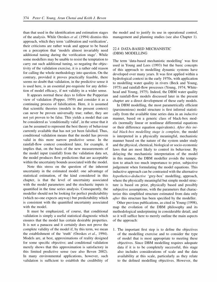
374 Peter C. Young, Arun Chotai and Keith J. Beven
than that used in the identification and estimation stagesof the analysis. While Oreskes et al. (1994) dismiss thisapproach, which they term ‘calibration and verification’,their criticisms are rather weak and appear to be basedon a perception that ‘models almost invariably needadditional tuning during the verification stage’. Whilesome modellers may be unable to resist the temptation tocarry out such additional tuning, so negating the objec-tivity of the validation exercise, it is a rather odd reasonfor calling the whole methodology into question. On thecontrary, provided it proves practically feasible, thereseems no doubt that validation, in the predictive sense itis used here, is an essential pre-requisite for any defini-tion of model efficacy, if not validity in a wider sense.
It appears normal these days to follow the Popperianview of validation (Popper, 1959) and consider it as acontinuing process of falsification. Here, it is assumedthat scientific theories (models in the present context)can never be proven universally true; rather, they arenot yet proven to be false. This yields a model that canbe considered as ‘conditionally valid’, in the sense that itcan be assumed to represent the best theory of behaviourcurrently available that has not yet been falsified. Thus,conditional validation means that the model has provenvalid in this more narrow predictive sense. In therainfall-flow context considered later, for example, itimplies that, on the basis of the new measurements ofthe model input (rainfall) from the validation data set,the model produces flow predictions that are acceptablewithin the uncertainty bounds associated with the model.
Note this stress on the question of the inherentuncertainty in the estimated model: one advantage ofstatistical estimation, of the kind considered in thischapter, is that the level of uncertainty associatedwith the model parameters and the stochastic inputs isquantified in the time series analysis. Consequently, themodeller should not be looking for perfect predictability(which no-one expects anyway) but predictability whichis consistent with the quantified uncertainty associatedwith the model.
It must be emphasized, of course, that conditionalvalidation is simply a useful statistical diagnostic whichensures that the model has certain desirable properties.It is not a panacea and it certainly does not prove thecomplete validity of the model if, by this term, we meanthe establishment of the ‘truth’ (Oreskes et al., 1994).Models are, at best, approximations of reality designedfor some specific objective; and conditional validationmerely shows that this approximation is satisfactory inthis limited predictive sense (see also Beven 2002).In many environmental applications, however, suchvalidation is sufficient to establish the credibility of
the model and to justify its use in operational control,management and planning studies (see also Chapter 1).
22.4 DATA-BASED MECHANISTIC(DBM) MODELLING
The term ‘data-based mechanistic modelling’ was firstused in Young and Lees (1993) but the basic conceptsof this approach to modelling dynamic systems havedeveloped over many years. It was first applied within ahydrological context in the early 1970s, with applicationto modelling water quality in rivers (Beck and Young,1975) and rainfall-flow processes (Young, 1974; White-head and Young, 1975). Indeed, the DBM water qualityand rainfall-flow models discussed later in the presentchapter are a direct development of these early models.
In DBM modelling, the most parametrically efficient(parsimonious) model structure is first inferred statisti-cally from the available time series data in an inductivemanner, based on a generic class of black-box mod-els (normally linear or nonlinear differential equationsor their difference equation equivalents). After this ini-tial black-box modelling stage is complete, the modelis interpreted in a physically meaningful, mechanisticmanner based on the nature of the system under studyand the physical, chemical, biological or socio-economiclaws that are most likely to control its behaviour. Bydelaying the mechanistic interpretation of the modelin this manner, the DBM modeller avoids the tempta-tion to attach too much importance to prior, subjectivejudgement when formulating the model equations. Thisinductive approach can be contrasted with the alternativehypothetico-deductive ‘grey-box’ modelling, approach,where the physically meaningful but simple model struc-ture is based on prior, physically based and possiblysubjective assumptions, with the parameters that charac-terize this simplified structure estimated from data onlyafter this structure has been specified by the modeller.
Other previous publications, as cited in Young (1998),map the evolution of the DBM philosophy and itsmethodological underpinning in considerable detail, andso it will suffice here to merely outline the main aspectsof the approach:
1. The important first step is to define the objectivesof the modelling exercise and to consider the typeof model that is most appropriate to meeting theseobjectives. Since DBM modelling requires adequatedata if it is to be completely successful, this stagealso includes considerations of scale and the dataavailability at this scale, particularly as they relateto the defined modelling objectives. However, the

Data-Based Mechanistic Modelling and the Simplification of Environmental Systems 375
prior assumptions about the form and structure of thismodel are kept at a minimum in order to avoid theprejudicial imposition of untested perceptions aboutthe nature and complexity of the model needed tomeet the defined objectives.
2. Appropriate model structures are identified by a pro-cess of objective statistical inference applied directlyto the time-series data and based initially on agiven generic class of linear Transfer Function (TF)models whose parameters are allowed to vary overtime, if this seems necessary to satisfactorily explainthe data.
3. If the model is identified as predominantly linear orpiece-wise linear, then the constant parameters thatcharacterize the identified model structure in step 2are estimated using advanced methods of statisticalestimation for dynamic systems. The methods used inthe present chapter are based on optimal Instrumen-tal Variable (IV) estimation algorithms (see Young,1984) that provide a robust approach to model iden-tification and estimation and have been well testedin practical applications over many years. Here theimportant identification stage means the application ofobjective statistical methods to determine the dynamicmodel order and structure. Full details of these timeseries methods are provided in the above referencesand they are outlined more briefly in both Young andBeven (1994) and Young et al. (1996).
4. If significant parameter variation is detected overthe observation interval, then the model parametersare estimated by the application of an approach totime dependent parameter estimation based on theapplication of recursive Fixed Interval Smoothing(FIS) algorithms (e.g. Bryson and Ho, 1969; Young,1984; Norton, 1986). Such parameter variation willtend to reflect nonstationary and nonlinear aspectsof the observed system behaviour. In effect, theFIS algorithm provides a method of nonparametricestimation, with the Time Variable Parameter (TVP)estimates defining the nonparametric relationship,which can often be interpreted in State-DependentParameter (SDP) terms (see section 22.6.2).
5. If nonlinear phenomena have been detected and iden-tified in stage 4, the nonparametric state dependentrelationships are normally parameterized in a finiteform and the resulting nonlinear model is estimatedusing some form of numerical optimization, suchas nonlinear least squares or Maximum Likelihood(ML) optimization.
6. Regardless of whether the model is identified andestimated in linear or nonlinear form, it is onlyaccepted as a credible representation of the system
if, in addition to explaining the data well, it alsoprovides a description that has direct relevance tothe physical reality of the system under study.This is a most important aspect of DBM modellingand differentiates it from more classical ‘black-box’modelling methodologies, such as those associatedwith standard TF, nonlinear autoregressive-movingaverage-exogenous variables (NARMAX), neuralnetwork and neuro-fuzzy models.
7. Finally, the estimated model is tested in variousways to ensure that it is conditionally valid. Thiscan involve standard statistical diagnostic tests forstochastic, dynamic models, including analysis whichensures that the nonlinear effects have been modelledadequately (e.g. Billings and Voon, 1986). It alsoinvolves validation exercises, as well as exercisesin stochastic uncertainty and sensitivity analysis (seesection 22.6).
Of course, while step 6 should ensure that the modelequations have an acceptable physical interpretation,it does not guarantee that this interpretation will nec-essarily conform exactly with the current scientificparadigms. Indeed, one of the most exciting, albeit con-troversial, aspects of DBM models is that they can tendto question such paradigms. For example, DBM meth-ods have been applied very successfully to the charac-terization of imperfect mixing in fluid flow processesand, in the case of pollutant transport in rivers, haveled to the development of the Aggregated Dead Zone(ADZ) model (Beer and Young, 1983; Wallis et al.,1989). Despite its initially unusual physical interpre-tation, the acceptance of this ADZ model (e.g. Davisand Atkinson, 2000 and the prior references therein)and its formulation in terms of physically meaningfulparameters, seriously questions certain aspects of theubiquitous Advection Dispersion Model (ADE) whichpreceded it as the most credible theory of pollutant trans-port in stream channels (see the comparative discussionin Young and Wallis, 1994). An example of ADZ mod-elling is described in section 22.6.1.
One aspect of the above DBM approach which dif-ferentiates it from alternative deterministic ‘top-down’approaches (e.g. Jothityangkoon et al., 2000) is itsinherently stochastic nature. This means that the uncer-tainty in the estimated model is always quantified andthis information can then be utilized in various ways. Forinstance, it allows for the application of uncertainty andsensitivity analysis based on Monte Carlo Simulation(MCS) analysis, as well as the use of the model in statis-tical forecasting and data assimilation algorithms, suchas recursive parameter estimation and the Kalman filter.

376 Peter C. Young, Arun Chotai and Keith J. Beven
The uncertainty analysis is particularly useful becauseit is able to evaluate how the covariance properties ofthe parameter estimates affect the probability distribu-tions of physically meaningful, derived parameters, suchas residence times and partition percentages in parallelhydrological pathways (see e.g. Young, 1992, 1999a andthe examples below).
The DBM approach to modelling is widely applica-ble: It has been applied successfully to the characteriza-tion of numerous environmental systems including thedevelopment of the ADZ model for pollution transportand dispersion in rivers (e.g. Wallis et al., 1989; Young,1992); rainfall-flow modelling (Young and Beven, 1994;Young, 2001b and the prior references therein); adaptiveflood forecasting and warning (Lees et al., 1994; Youngand Tomlin, 2000; Young, 2002a); and the modelling ofecological and biological systems (Young, 2000; Jarviset al., 1999); Other applications, in which the DBMmodels are subsequently utilized for control systemdesign, include the modelling and control of climate inglasshouses (e.g. Lees et al., 1996), forced ventilation inagricultural buildings (e.g. Price et al., 1999), and inter-urban road traffic systems (Taylor et al., 1998). Theyhave also been applied in the context of macro-economicmodelling (e.g. Young and Pedregal, 1999).
22.5 THE STATISTICAL TOOLS OF DBMMODELLING
The statistical and other tools that underpin DBM mod-elling are dominated by recursive methods of timeseries analysis, filtering and smoothing. These includeoptimal Instrumental Variable (IV) methods of iden-tifying and estimating discrete and continuous-timeTF models (e.g. Young, 1984, 2002b), including theSimplified Refined Instrumental Variable (SRIV) algo-rithm used in later practical examples; Time Vari-able Parameter (TVP) estimation and its use in themodelling and forecasting of nonstationary time series(e.g. Young, 1999b, and the prior references therein);and State Dependent Parameter (SDP) parameter esti-mation methods for modelling nonlinear stochastic sys-tems (see Young, 1978, 1984, 1993a, 1998, 2000, 2001a;Young and Beven, 1994). Here, the TVP and SDP esti-mation is based on optimized Fixed Interval Smoothing(FIS) algorithms.
These recursive statistical methods can also be uti-lized for other environmental purposes. For example,as discussed in section 22.7, they can provide a rigor-ous approach to the evaluation and exploitation of largesimulation models (e.g. Young et al., 1996), where theanalysis provides a means of simplifying the models.
Such reduced order representations can then providea better understanding of the most important mecha-nisms within the model; or they can provide dominantmode models that can be used for control and oper-ational management system design, adaptive forecast-ing, or data assimilation purposes (see e.g. Young et al.,1996; Young, 1999a). The DBM data analysis tools canalso be used for the statistical analysis of nonstationarydata, of the kind encountered in many areas of environ-mental science (see Young, 1999b). For example, theyhave been applied to the analysis and forecasting oftrends and seasonality in climate data (e.g. Young et al.,1991); and the analysis of palaeoclimatic data (Youngand Pedregal, 1998).
22.6 PRACTICAL EXAMPLES
Two practical examples will be considered here, bothconcerned with hydrological systems. The first will showhow even a purely linear representation, in the form ofthe ADZ model for solute transport and dispersion, canprovide a powerful approach to analysing experimentaldata. However, many environmental systems are non-linear and so the second example will show how SDPmodelling procedures can be exploited to handle suchnonlinearity.
22.6.1 A linear example: modelling solute transport
Tracer experiments2 are an excellent way of evaluatinghow a river transports and disperses a dissolved, conser-vative pollutant. Figure 22.1 shows a typical set of tracerdata from the River Conder, near Lancaster in NorthWest England. This river is fairly small, with a cob-bled bed, and the experiment involved the injection of199 mg of the dye tracer Rhodamine WT, with the mea-surement locations situated 400 metres apart, some waydownstream of the injection location to allow for initialmixing. The river flow rate was measured at 1.3 m3.s−1.
Since the ADZ model was first introduced by Beerand Young (1983), it has become conventional to esti-mate the model in discrete-time TF form (since equiva-lent continuous-time estimation algorithms are not freelyavailable) and then deduce the continuous-time (differ-ential equation) model parameters from the estimatedparameters of this discrete-time TF. In this example,however, discrete-time modelling is not very successfulwhen applied to the data in Figure 22.1 using a relativelyfast sampling interval of 0.25 minutes, both the discrete-time SRIV algorithm and the alternative Prediction ErrorMinimisation (PEM) algorithm in MatlabTM (Matlab isa well known and widely available numeric computation
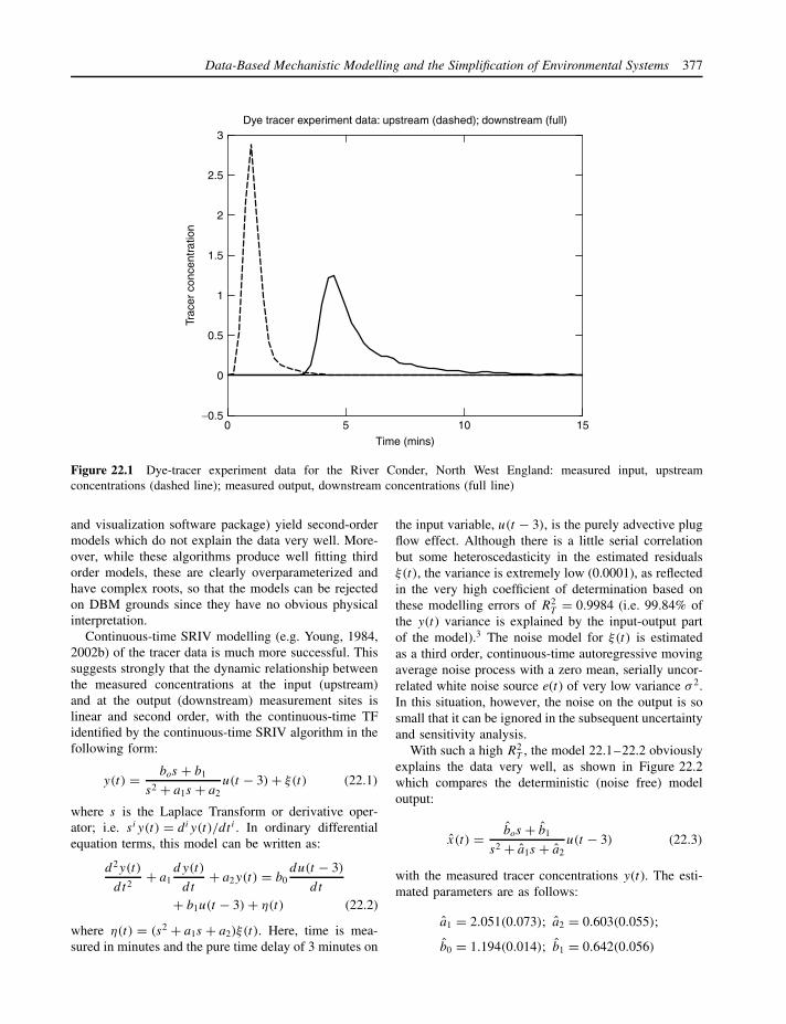
Data-Based Mechanistic Modelling and the Simplification of Environmental Systems 377
0 5 10 15−0.5
0.5
1
1.5
2
2.5
0
3Dye tracer experiment data: upstream (dashed); downstream (full)
Time (mins)
Trac
er c
once
ntra
tion
Figure 22.1 Dye-tracer experiment data for the River Conder, North West England: measured input, upstreamconcentrations (dashed line); measured output, downstream concentrations (full line)
and visualization software package) yield second-ordermodels which do not explain the data very well. More-over, while these algorithms produce well fitting thirdorder models, these are clearly overparameterized andhave complex roots, so that the models can be rejectedon DBM grounds since they have no obvious physicalinterpretation.
Continuous-time SRIV modelling (e.g. Young, 1984,2002b) of the tracer data is much more successful. Thissuggests strongly that the dynamic relationship betweenthe measured concentrations at the input (upstream)and at the output (downstream) measurement sites islinear and second order, with the continuous-time TFidentified by the continuous-time SRIV algorithm in thefollowing form:
y(t) = bos + b1
s2 + a1s + a2u(t − 3) + ξ(t) (22.1)
where s is the Laplace Transform or derivative oper-ator; i.e. siy(t) = diy(t)/dt i . In ordinary differentialequation terms, this model can be written as:
d 2y(t)
d t2+ a1
dy(t)
d t+ a2y(t) = b0
du(t − 3)
d t
+ b1u(t − 3) + η(t) (22.2)
where η(t) = (s2 + a1s + a2)ξ(t). Here, time is mea-sured in minutes and the pure time delay of 3 minutes on
the input variable, u(t − 3), is the purely advective plugflow effect. Although there is a little serial correlationbut some heteroscedasticity in the estimated residualsξ(t), the variance is extremely low (0.0001), as reflectedin the very high coefficient of determination based onthese modelling errors of R2
T = 0.9984 (i.e. 99.84% ofthe y(t) variance is explained by the input-output partof the model).3 The noise model for ξ(t) is estimatedas a third order, continuous-time autoregressive movingaverage noise process with a zero mean, serially uncor-related white noise source e(t) of very low variance σ 2.In this situation, however, the noise on the output is sosmall that it can be ignored in the subsequent uncertaintyand sensitivity analysis.
With such a high R2T , the model 22.1–22.2 obviously
explains the data very well, as shown in Figure 22.2which compares the deterministic (noise free) modeloutput:
x(t) = bos + b1
s2 + a1s + a2u(t − 3) (22.3)
with the measured tracer concentrations y(t). The esti-mated parameters are as follows:
a1 = 2.051(0.073); a2 = 0.603(0.055);
b0 = 1.194(0.014); b1 = 0.642(0.056)
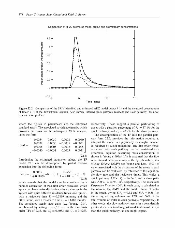
378 Peter C. Young, Arun Chotai and Keith J. Beven
0 5 10 15−0.2
0.2
0.4
0.6
0.8
1
1.2
0
Comparison of RIVC estimated model output and downstream concentrations
Time (mins)
Trac
er c
once
ntra
tion
(mic
rogr
ams/
litre
)
Figure 22.2 Comparison of the SRIV identified and estimated ADZ model output x(t) and the measured concentrationof tracer y(t) at the downstream location. Also shown: inferred quick pathway (dashed) and slow pathway (dash-dot)concentration profiles
where the figures in parentheses are the estimatedstandard errors. The associated covariance matrix, whichprovides the basis for the subsequent MCS analysis,takes the form:
P(a) =
0.0054 0.0039 −0.0008 −0.00400.0039 0.0030 −0.0005 −0.0031
−0.0008 −0.0005 0.0002 0.0005−0.0040 −0.0031 0.0005 0.0031
(22.4)Introducing the estimated parameter values, the TFmodel 22.3 can be decomposed by partial fractionexpansion into the following form:
x(t) = 0.6083
1 + 0.5899su(t − 3) + 0.4753
1 + 2.8118su(t − 3)
(22.5)
which reveals that the model can be considered as aparallel connection of two first order processes whichappear to characterize distinctive solute pathways in thesystem with quite different residence times: one ‘quick’,with a residence time Tq = 0.5899 minutes; and theother ‘slow’, with a residence time Ts = 2.8188 minutes.The associated steady state gains (e.g. Young, 1984),as obtained by setting s = d/dt = 0 in the two first-order TFs of 22.5, are Gq = 0.6083 and Gs = 0.4753,
respectively. These suggest a parallel partitioning oftracer with a partition percentage of Pq = 57.1% for thequick pathway, and Ps = 42.9% for the slow pathway.
The decomposition of the TF into the parallel path-way form 22.5, provides the information required tointerpret the model in a physically meaningful manner,as required by DBM modelling. The first order modelassociated with each pathway can be considered as adifferential equation describing mass conservation, asshown in Young (1999a). If it is assumed that the flowis partitioned in the same way as the dye, then the ActiveMixing Volume (AMV: see Young and Less, 1993) ofwater associated with the dispersion of the solute in eachpathway can be evaluated, by reference to this equation,the flow rate and the residence times. This yields aquick pathway AMV, Vq = 26.3m3; and a slow path-way AMV, Vs = 94.1m3, respectively. The associatedDispersive Fraction (DF), in each case, is calculated asthe ratio of the AMV and the total volume of waterin the reach, giving DFq = 0.12 and DFs = 0.56 (i.e.the acting mixing volumes are 12% and 56% of thetotal volume of water in each pathway, respectively). Inother words, the slow pathway results in a considerablygreater dispersion (and longer-term detention) of the dyethan the quick pathway, as one might expect.
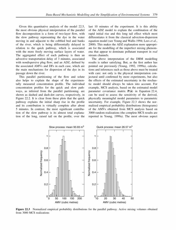
Data-Based Mechanistic Modelling and the Simplification of Environmental Systems 379
Given this quantitative analysis of the model 22.5,the most obvious physical interpretation of the parallelflow decomposition is a form of two-layer flow, withthe slow pathway representing the dye in the watermoving in and adjacent to the cobbled bed and banksof the river, which is being differentially delayed inrelation to the quick pathway, which is associatedwith the more freely moving surface layers of water.The aggregated effect of each pathway is then anadvective transportation delay of 3 minutes, associatedwith nondispersive plug flow; and an ADZ, defined bythe associated AMVs and DFs in each case, which arethe main mechanisms for dispersion of the dye in itspassage down the river.
This parallel partitioning of the flow and solutealso helps to explain the shape of the experimen-tally measured concentration profile. The individualconcentration profiles for the quick and slow path-ways, as inferred from the parallel partitioning, areshown as dashed and dash-dot curves, respectively, inFigure 22.2. It is clear from these plots that the quickpathway explains the initial sharp rise in the profileand its contribution is virtually complete after about5 minutes. In contrast, the most significant contribu-tion of the slow pathway is its almost total explana-tion of the long, raised tail on the profile, over the
last 10 minutes of the experiment. It is this abilityof the ADZ model to explain the combination of therapid initial rise and this long tail effect which mostdifferentiates it from the classical advection-dispersionequation model (see Young and Wallis 1994; Lees et al.,2000). This makes the ADZ explanation more appropri-ate for the modelling of the imperfect mixing phenom-ena that appear to dominate pollutant transport in realstream channels.
The above interpretation of the DBM modellingresults is rather satisfying. But, as the first author haspointed out previously (Young, 1992, 1999a), calcula-tions and inferences such as those above must be treatedwith care: not only is the physical interpretation con-jectural until confirmed by more experiments, but alsothe effects of the estimated uncertainty in the stochas-tic model should always be taken into account. Forexample, MCS analysis, based on the estimated modelparameter covariance matrix P(a) in Equation 22.4,can be used to assess the sensitivity of the derived,physically meaningful model parameters to parametricuncertainty. For example, Figure 22.3 shows the nor-malized empirical probability distributions (histograms)of the AMVs obtained from MCS analysis based on3000 random realizations (the complete MCS results arereported in Young, 1999a). The most obvious aspect
0 50 100 150 2000
0.2
0.4
0.6
0.8
1
AMV (cubic metres)
Nor
mal
ized
freq
uenc
y
0
0.2
0.4
0.6
0.8
1
Nor
mal
ized
freq
uenc
y
10 20 30 40 50
Quick process: mean 26.57 m3
AMV (cubic metres)
Slow process: mean 93.93 m3
Figure 22.3 Normalized empirical probability distributions for the parallel pathway. Active mixing volumes obtainedfrom 3000 MCS realizations

380 Peter C. Young, Arun Chotai and Keith J. Beven
of these distributions is that, whereas the fast path-way AMV is quite tightly defined, despite the uncer-tainty on the estimated TF model parameters, the slowpathway AMV is rather poorly defined. In particular,while Vq is distributed quite tightly around the meanvalue of 26.56m3 (SRIV estimated value 26.27m3),with a standard deviation of 4.76m3, Vs has a muchbroader distribution about its mean value of 94.41m3
(SRIV estimated value 94.12m3), with a standard devi-ation of 32.29m3.
In the case of the other physically meaningful modelparameters, the uncertainty levels on the partitioningpercentages are quite similar for both pathways andthere is some evidence of skewness in the distributions,with Pq skewed towards higher percentages and Ps
towards lower. The standard deviation on the steadystate gain for the slow pathway (0.2129) is over 10 timesthe standard deviation on the quick pathway (0.0209),showing that it is much less well defined; and it isinteresting to note that the total steady state gain forthe complete TF has a mean of 1.085 (SRIV estimate1.066), with a standard deviation of 0.198, showing thatit is insignificantly different from unity. This confirmsthat the tracer experiment was satisfactory, since thesteady state gain is an estimate of the ratio of thearea under the downstream concentration profile tothat under the upstream profile; areas which shouldbe the same if there are no dye losses (the computedratio of areas is 1.0737). If this steady state gain wassignificantly different from unity, therefore, it wouldthrow doubt on the efficacy of the experiment: forexample, it would suggest that there had been significantadsorption on to organic material or that the pumpswhich supplied the river water to the fluorometers werepoorly located and did not provide water which had arepresentative measure of the dye concentration at themeasurement site.
It is clear that the kind of MCS analysis illustratedin Figure 22.3 provides valuable additional insight intothe nature of parallel pathway models such as 22.5.This is also true for the related parallel pathway mod-els used in rainfall-flow analysis (see next subsection),particularly when the parallel flow partitioning is to beused as a basis for exercises such as base-flow sep-aration (see Jakeman et al., 1990; Young 1992). ButMCS analysis should not be limited to these kind ofwater resource applications: it is a generally useful andeasy-to-use tool in data-based environmental systemsanalysis and so should be considered as a standard pro-cedure that is essential for evaluating the efficacy ofdata-based environmental models and their sensitivity touncertainty. It is certainly considered sine qua non for
success in DBM modelling. And, as shown in Young(1998, 1999a) and pointed out later in section 22.7, itis also valuable in the evaluation of large, deterministicsimulation models.
22.6.2 A nonlinear example: rainfall-flow modelling
This example is concerned with the analysis of dailyrainfall, flow and temperature data from the ‘ephemeral’Canning River in Western Australia which stops flowingover Summer, as shown in Figure 22.4. These datahave been analysed before and reported fully in Younget al. (1997). The results of this previous analysis areoutlined briefly below but most attention is focused onmore recent analysis that shows how the inductive DBMmodelling can help to develop and enhance alternativeconceptual (‘grey-box’) modelling that has been carriedout previously in a more conventional hypothetico-deductive manner.
Young et al. (1997) show that, in this example, themost appropriate generic model form is the nonlinearSDP model (see section 22.5). Analysis of the rainfall-flow data in Figure 22.4, based on this type of model,is accomplished in two stages. First, nonparametricestimates of the SDPs are obtained using the StateDependent parameter Auto-Regressive eXogenous Vari-able (SDARX) model form (see Young, 2001a, b inwhich it is discussed at some length within a rainfall-flow context):
yt = zTt pt + et et = N(0, σ 2) (22.6)
where:
zTt = [yt−1 yt−2 . . . yt−n rt−δ . . . rt−δ−m]
pt = [a1(zt ) a2(zt ) . . . an(zt ) b0(zt ) . . . bm(zt )]T
where, in the present context, yt and rt are, respectively,the measured flow and rainfall and δ is a pure advectivetime delay. Here, the elements of the triad [n m δ] areidentified as n = 2,m = 3, δ = 0 and the parameters areall assumed initially to be dependent on a state variablezt . In this case, the SDP analysis then shows that thestate dependency is apparently in terms of the measuredflow variable (i.e. zt = yt : see later explanation) andis limited to those parameters associated with therainfall rt .
In the second stage of the analysis, the nonparamet-ric estimate of the nonlinearity is parameterized in thesimplest manner possible; in this case as a power lawin yt . The constant parameters of this parameterizednonlinear model are then estimated using a nonlinear

Data-Based Mechanistic Modelling and the Simplification of Environmental Systems 381
1985.4 1985.6 1985.8 1986 1986.2 1986.4 1986.6 1986.8 19870
2
4Flow, rainfall and temperature: Canning River, W.A., 1985–1987
Flo
w (
cum
ecs)
1985.4 1985.6 1985.8 1986 1986.2 1986.4 1986.6 1986.8 19870
20
40
60
Rai
nfal
l (m
m)
1985.4 1985.6 1985.8 1986 1986.2 1986.4 1986.6 1986.8 19870
20
40
Date
Tem
pera
ture
(de
g.C
)
Figure 22.4 Daily rainfall-flow and temperature data for the ephemeral Canning River in Western Australia for theperiod 23 March 1985 to 26 February 1987
optimization procedure (see Young, 2001b). The result-ing model is the following simplified version of thenonlinear, discrete-time, SDP Transfer Function (SDTF)model (e.g. Young, 2000):
yt = B(z−1)
A(z−1)ut + ξt (22.7)
where z−i is the backward shift operator, i.e. z−iyt =yt−i :
A(z−1) = 1 − 1.646z−1 + 0.658z−2
B(z−1) = 0.0115 + 0.0185z−1 − 0.0028z−2
ut = c.yβt .rt (22.8)
with β = 0.85. This shows that the input variable ut
is a nonlinear function in which the measured rainfallrt is multiplied by the flow raised to a power β, withthe normalization parameter c simply chosen so that thesteady state gain of the linear TF between ut and yt isunity.4 In other words, the SDP analysis shows, in a
relatively objective manner, that the underlying dynam-ics are predominantly linear but the overall responseis made nonlinear because of a very significant inputnonlinearity.
This model not only explains the data well (R2T =
0.958) it is also consistent with hydrological theory,as required by the tenets of DBM modelling. Thissuggests that the changing soil-water storage conditionsin the catchment reduce the ‘effective’ level of therainfall and that the relationship between the measuredrainfall and this effective rainfall (sometimes termedrainfall excess) ut is quite nonlinear. For example, ifthe catchment is very dry because little rain has fallenfor some time, then most new rainfall will be absorbedby the dry soil and little, if any, will be effectivein promoting increases in river flow. Subsequently,however, if the soil-water storage increases because offurther rainfall, so the ‘runoff ’ of excess water from thecatchment rises and the flow increases because of this.In this manner, the effect of rainfall on flow dependsupon the antecedent conditions in the catchment and asimilar rainfall event occurring at different times and

382 Peter C. Young, Arun Chotai and Keith J. Beven
under different soil-water storage conditions can yieldmarkedly different changes in river flow.
The linear TF part of the model conforms also withthe classical ‘unit hydrograph’ theory of rainfall-flowdynamics: indeed, its unit impulse response at any timeis, by definition, the unit hydrograph. And the TF modelitself can be seen as a parametrically efficient methodof quantifying this unit hydrograph. Additionally, asin the solute-transport example, the TF model can bedecomposed by partial fraction expansion into a parallelpathway form which has a clear hydrological interpreta-tion. In particular, it suggests that the effective rainfall ispartitioned into three pathways: the instantaneous effect,arising from the [2 3 0] TF model form which, as mightbe expected, accounts for only a small 5.8% of the flow;a fast flow pathway with a residence time of 2.65 dayswhich accounts for the largest 53.9% of the flow; and aslow flow pathway of 19.86 days residence time account-ing for the remaining 40.3% of the flow. It is this latterpathway that leads to an extended tail on the associatedhydrograph and can be associated with the slowly chang-ing baseflow in the river (for a more detailed explana-tion and other examples, see Young, 1992, 1993a, 1998,2001b; Young and Beven, 1994; Young et al., 1997).
The most paradoxical and, at first sight, least inter-pretable model characteristic is that the effective rainfallnonlinearity is a function of flow. Although this is phys-ically impossible, the analysis produces such a clearlydefined relationship of this sort that it must have somephysical connotations. The most hydrologically reason-able explanation is that the flow is acting as a surrogatefor soil-water storage. Of course, it would be better toinvestigate this relationship directly by measuring thesoil-water storage in some manner and incorporatingthese measurements into the SDP analysis. Unfortu-nately, it is much more difficult to obtain such ‘soilmoisture’ measures and these were not available in thepresent example.
The temperature measurements are available, how-ever, and this suggests that we should explore the model22.7–22.8 further, with the object of enhancing its phys-ical interpretation using these additional data.
Two interesting conceptual (‘grey-box’) models ofrainfall-flow dynamics are the Bedford-Ouse Rivermodel (e.g. Whitehead and Young, 1975); and adevelopment of this, the IHACRES model (Jakemanet al., 1990). Both of these ‘Hybrid-Metric-Conceptual ’(HCM) models (Wheater et al., 1993) have the samebasic form as 22.7–22.8, except that the nature of theeffective rainfall nonlinearity is somewhat different. Inthe case of the IHACRES model, for instance, this
nonlinearity is modelled by the following equations:
τs(Tt ) = τseT t−Tt
f (22.9a)
st = st−1 + 1
τs(Tt )(rt − st−1) (22.9b)
ut = c.sβt .rt (22.9c)
where Tt is the temperature; T t is the mean temperature;st represents a conceptual soil-water storage variable;and c, τs, f and β are a priori unknown parameters.Comparing 22.9c with 22.8, we see that the maindifference between the two models is that the measuredyt in 22.8, acting as a surrogate for soil-water storage,has been replaced by a modelled (or latent) soil-waterstorage variable st . The model 22.9b that generates thisvariable is a first order discrete-time storage equationwith a residence time τs(Tt ) defined as τs multipliedby an exponential function of the difference betweenthe temperature Tt and its mean value T t , as definedin 22.9a.
In the original IHACRES model (e.g. Jakeman andHornberger, 1993), T t is normally set at 20◦C, but theestimation results are not sensitive to this value. Also, st
is not raised to a power, as in 22.9c. Some later versionsof IHACRES have incorporated this parameter, but ithas been added here so that the two nonlinearities in22.8 and 22.9c can be compared. More importantly, itsintroduction is practically important in this particularexample since, without modification, the IHACRESmodel (Figure 22.5) is not able to model the ephemeralCanning flow very well.
Using a constrained nonlinear optimization proceduresimilar to that in the previous example, the parameters inthis modified IHACRES model are estimated as follows:
A(z−1) = 1 − 1.737z−1 + 0.745z−2
B(z−1) = 0.0285 + 0.140z−1 − 0.160z−2 (22.10)
τs = 65.5, f = 30.1; β = 6.1; T t = 15.9
These parameters are all statistically well defined andthe model explains 96.9% of the flow yt (R2
T = 0.969),marginally better than the DBM model. Moreover, asshown in Figure 22.5, it performs well in validationterms when applied, without re-estimation, to the datafor the years 1977–78. The coefficient of determinationin this case is 0.91 which is again better than thatachieved by the DBM model (0.88). However, whenvalidated against the 1978–79 data, the positions arereversed and the DBM model is superior. Overall,therefore, the two models are comparable in their abilityto explain and predict the Canning River data.
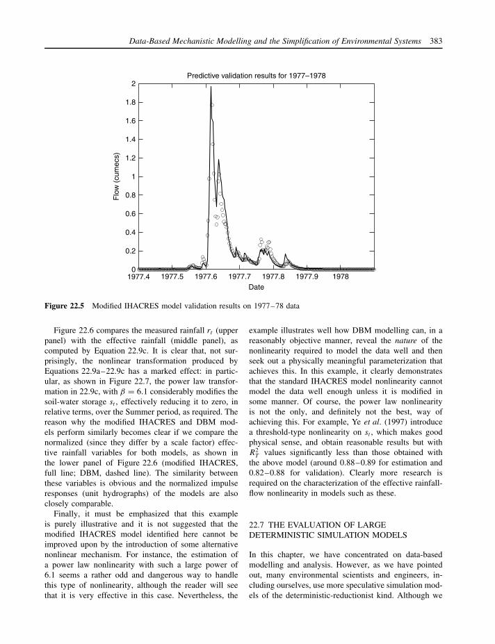
Data-Based Mechanistic Modelling and the Simplification of Environmental Systems 383
1977.4 1977.5 1977.6 1977.7 1977.8 1977.9 19780
0.2
0.4
0.6
0.8
1
1.2
1.4
1.6
1.8
2
Date
Flo
w (
cum
ecs)
Predictive validation results for 1977–1978
Figure 22.5 Modified IHACRES model validation results on 1977–78 data
Figure 22.6 compares the measured rainfall rt (upperpanel) with the effective rainfall (middle panel), ascomputed by Equation 22.9c. It is clear that, not sur-prisingly, the nonlinear transformation produced byEquations 22.9a–22.9c has a marked effect: in partic-ular, as shown in Figure 22.7, the power law transfor-mation in 22.9c, with β = 6.1 considerably modifies thesoil-water storage st , effectively reducing it to zero, inrelative terms, over the Summer period, as required. Thereason why the modified IHACRES and DBM mod-els perform similarly becomes clear if we compare thenormalized (since they differ by a scale factor) effec-tive rainfall variables for both models, as shown inthe lower panel of Figure 22.6 (modified IHACRES,full line; DBM, dashed line). The similarity betweenthese variables is obvious and the normalized impulseresponses (unit hydrographs) of the models are alsoclosely comparable.
Finally, it must be emphasized that this exampleis purely illustrative and it is not suggested that themodified IHACRES model identified here cannot beimproved upon by the introduction of some alternativenonlinear mechanism. For instance, the estimation ofa power law nonlinearity with such a large power of6.1 seems a rather odd and dangerous way to handlethis type of nonlinearity, although the reader will seethat it is very effective in this case. Nevertheless, the
example illustrates well how DBM modelling can, in areasonably objective manner, reveal the nature of thenonlinearity required to model the data well and thenseek out a physically meaningful parameterization thatachieves this. In this example, it clearly demonstratesthat the standard IHACRES model nonlinearity cannotmodel the data well enough unless it is modified insome manner. Of course, the power law nonlinearityis not the only, and definitely not the best, way ofachieving this. For example, Ye et al. (1997) introducea threshold-type nonlinearity on st , which makes goodphysical sense, and obtain reasonable results but withR2
T values significantly less than those obtained withthe above model (around 0.88–0.89 for estimation and0.82–0.88 for validation). Clearly more research isrequired on the characterization of the effective rainfall-flow nonlinearity in models such as these.
22.7 THE EVALUATION OF LARGEDETERMINISTIC SIMULATION MODELS
In this chapter, we have concentrated on data-basedmodelling and analysis. However, as we have pointedout, many environmental scientists and engineers, in-cluding ourselves, use more speculative simulation mod-els of the deterministic-reductionist kind. Although we

384 Peter C. Young, Arun Chotai and Keith J. Beven
1985.4 1985.6 1985.8 1986 1986.2 1986.4 1986.6 1986.8 19870
2
4
6
Comparison of normalized rainfall and effective rainfall variables
Nor
m. r
ainf
all (
mm
)
1985.4 1985.6 1985.8 1986 1986.2 1986.4 1986.6 1986.8 19870
5
10
Eff.
rai
nfal
l (m
m)
1985.4 1985.6 1985.8 1986 1986.2 1986.4 1986.6 1986.8 19870
5
10
Eff.
rai
nfal
l (m
m)
Date
Figure 22.6 Comparison of rainfall and effective rainfall measures
1985.4 1985.6 1985.8 1986 1986.2 1986.4 1986.6 1986.8 19870
1
2
3
4
5
6Soil-water storage variables
Date
Nor
mal
ized
soi
l-wat
er s
tora
ge v
aria
bles
Figure 22.7 Comparison of the estimated soil-water storage variable st (dashed line) and sβt (full line)

Data-Based Mechanistic Modelling and the Simplification of Environmental Systems 385
would not advocate the use of such models if adequateexperimental or monitored data are available, they canprovide a very good method of extending our ‘mentalmodels’ of environmental systems, often as a valuableprelude to the design of experimental and monitoringexercises or, more questionably, as an aid in operationalcontrol, management and planning exercises.
When we exploit speculative simulation models inthese ways, however, we must ensure that their con-struction and use is preceded by considerable criticalevaluation. One advantage of the DBM approach tomodelling is that its methodological tools can also beexploited in such evaluation exercises. For instance, inYoung et al. (1996), Young (1998, 1999a) and Youngand Parkinson (2002), a technique known as DominantMode Analysis (DMA), which employs the same optimalIV methods of model identification and estimation usedfor DBM modelling, is able to identify simple, reducedorder representations of a 26th order, nonlinear globalcarbon cycle dynamic model used in climate research.In particular, DMA shows that over the whole historicalperiod, from the start of the Industrial Revolution to theend of the twentieth century, the output of this modelcan be reproduced to a remarkably accurate degree by afourth-order, linear differential equation comprising thefollowing third-order equation,
d3y(t)
dt3+ 0.284
d2y(t)
dt2+ 0.0126
dy(t)
dt+ 0.0000255y(t)
= 0.255d3u(t)
dt3+ 0.518
d2u(t)
dt2
+ 0.0668du(t)
dt+ 0.000815u(t), (22.11)
together with a mass conservation integrator. Further-more, as in the examples of section 22.6 this third-orderequation can be decomposed into a parallel connectionof first-order models with residence times of 4.4, 19.1and 467 years that makes reasonable physical sense. Theshorter time constants are not dissimilar to the tropo-sphere–stratosphere exchange time of 6 ± 2 years, andthe air–sea exchange time of 11 ± 4 years, respectively,as assumed in the simulation model. And the larger timeconstant is almost certainly associated with the assumedvalue of 900 ± 250 years for the deep-ocean turnovertime. Naturally, the complex interconnected nature ofthe simulation model modifies the ‘effective’ values ofthese time constants when the model is integrated, andso the identified dominant-mode residence times seemvery reasonable.
Model reduction exercises of this kind demon-strate rather dramatically how the superficial com-plexity of simulation models can, as in the real data
examples described in section 22.6, conceal underly-ing simple dynamics that are the main engine for theobserved behaviour of the model in its response toinput variations. Such reduced order models can func-tion, therefore, as replacements for the model in thoseapplications, such as forecasting and control, where theinternal descriptive aspects of the complex model are ofless importance. In other applications, such as ‘what-if’studies, environmental planning and risk analysis, how-ever, the reduced order model may not disclose clearlythose physically meaningful parameters that control thedominant reduced order modes of behaviour and are,therefore, important in such applications. In these sit-uations, it is possible to exploit other DBM tools thatare able to identify the most important parameters in thecomplex simulation model and examine how these affectits dynamic behaviour. This is the domain of uncer-tainty and sensitivity analysis; analysis that has beenrevolutionized in recent years by our ability to applyMCS-based methods to complex simulation models (seee.g. Saltelli et al., 2000; Beven et al, 2000; Thiemannet al., 2001).
A typical example of such Monte Carlo analysisis described in Parkinson and Young (1998), whereMCS and the related technique of Generalized (orregional) Sensitivity Analysis (GSA: see Spear andHornberger, 1980) are used to assess the effect ofinput and parametric uncertainties (as defined by climatescientists) on the behaviour of the global carbon cyclesimulation model mentioned above. This helps to revealthe most important physical parameters in the model andenhances the DMA-based model reduction exercises.
22.8 CONCLUSION
For too long in the environmental sciences, determin-istic reductionism has reigned supreme and has hada dominating influence on mathematical modelling inalmost all areas of the discipline. In general, such‘bottom-up’, reductionist models are over-parameterizedin relation to the information content of the experi-mental data, and their determinism sits uncomfortablywith the acknowledged uncertainty that characterizesmost environmental systems. This chapter has arguedthat parsimonious, ‘top-down’ models provide a moreappropriate parameterization in most situations and thatthe uncertainty which pervades most environmental sys-tems demands an alternative stochastic approach. Inparticular, stochastic models and statistical modellingprocedures provide a means of acknowledging thisuncertainty and quantifying its effects. Most often, how-ever, the conventional statistical approach to stochas-tic model building is posed in a ‘black-box’ manner

386 Peter C. Young, Arun Chotai and Keith J. Beven
that fails to produce models that can be interpreted inphysically meaningful terms. The Data-Based Mecha-nistic (DBM) approach to modelling discussed in thischapter tries to correct these deficiencies. It provides amodelling strategy that not only exploits powerful sta-tistical techniques but also produces models that canbe interpreted in physically meaningful terms and arenormally more acceptable to environmental scientistsand engineers.
Finally, it should be noted that most of the mod-elling and associated numerical analysis described in thischapter was carried out using the CAPTAIN Toolboxdeveloped in CRES at Lancaster within the Matlab soft-ware environment (see http://www.es.lancs.ac.uk/cres/systems.html).
NOTES
1. This chapter is based, in part, on the papersby Young (1999a, 2001c).
2. The interested reader will find a more complexexample of ADZ modelling in Young (2001c),where the same approach used here is applied todata from a tracer experiment conducted in a largeFlorida wetland area.
3. R2T is defined as R2
T = 1 − cov{y(t) − x(t)}/cov{y(t)}, where x(t) is the deterministic modeloutput defined in Equation 22.3. Note that thisis sometimes referred to as the ‘Nash-SutcliffeEfficiency’ in the hydrological literature. It isnot, however, the conventional coefficient ofdetermination which, in classical statistics and timeseries analysis, is normally based on one step aheadprediction errors, rather than the modelling error, ashere: see, e.g. Young (1993b).
4. This is an arbitrary decision in this case. However, ifthe rainfall and flow are in the same units, then thisensures that the total volume of effective rainfall isthe same as the total flow volume.
REFERENCES
Akaike, H. (1974) A new look at statistical model identi-fication, IEEE Transactions on Automatic Control AC19,716–722.
Bacon, F. (1620) Novum Organum. [See: L. Jardine andM. Silverthorne (eds) (2000) The New Organon, CambridgeUniversity Press, Cambridge.]
Beck, M.B. (1983) Uncertainty, system identification and theprediction of water quality, in M.B. Beck and G. VanStraten (eds), Uncertainty and Forecasting of Water Quality,Springer-Verlag, Berlin, 3–68.
Beck, M.B. and Young, P.C. (1975) A dynamic model forBOD-DO relationships in a non-tidal stream, Water Research9, 769–776.
Beer, T. and Young, P.C. (1983) Longitudinal dispersion innatural streams, Journal of the Environmental Engineer-ing Division, American Society of Civil Engineers 102,1049–1067.
Beven, K.J. (2000) Uniqueness of place and process repre-sentations in hydrological modelling, Hydrology and EarthSystem Sciences 4, 203–213.
Beven, K.J. (2001) How far can we go in distributed hydro-logical modelling? Hydrology and Earth System Sciences 5,1–12.
Beven, K.J. (2002) Towards a coherent philosophy for envi-ronmental modelling, Proceedings of the Royal Society ofLondon A 458, 2465–2484.
Beven, K.J., Freer, J., Hankin, B. and Schulz, K. (2000) Theuse of generalized likelihood measures for uncertainty esti-mation in high order models of dynmaic systems, inW.J. Fitzgerald, A. Walden, R. Smith and P.C. Young (eds)Nonstationary and Nonlinear Signal Processing, CambridgeUniversity Press, Cambridge, 115–151.
Billings, S.A. and Voon, W.S.F. (1986) Correlation basedmodel validity tests for nonlinear models, International Jour-nal of Control 44, 235–244.
Box, G.E.P. and Jenkins, G.M. (1970) Time-Series Analysis:Forecasting and Control, Holden-Day, San Francisco.
Bryson, A.E. and Ho, Y.-C. (1969) Applied Optimal Control,Blaisdell Publishing, Massachusetts.
Davis, P.M. and Atkinson, T.C. (2000) Longitudinal dispersionin natural channels: 3. An aggregated dead zone modelapplied to the River Severn, U.K., Hydrology and EarthSystem Sciences 4, 373–381.
Jakeman, A.J. and Hornberger, G.M. (1993) How much com-plexity is warranted in a rainfall-runoff model? WaterResources Research 29, 2637–2649.
Jakeman, A.J., Littlewood, I.G. and Whitehead, P.G. (1990)Computation of the instantaneous unit hydrograph andidentifiable component flows with application to two smallupland catchments, Journal of Hydrology 117, 275–300.
Jarvis, A.J., Young, P.C., Taylor, C.J. and Davies, W.J. (1999)An analysis of the dynamic response of stomatal conductanceto a reduction in humidity over leaves of Cedrella odorata ,Plant Cell and Environment 22, 913–924.
Jothityangkoon, C., Sivapalan, M. and Farmer, D.L. (2001)Process controls of water balance variability in a large semi-arid catchment: downward approach to hydrological modeldevelopment, Journal of Hydrology 254, 174–198.
Konikow, L.F. and Bredehoeft, J.D. (1992) Ground watermodels cannot be validated, Advances in Water Resources15, 75–83.
Kuhn, T. (1962) The Structure of Scientific Revolutions, Uni-versity of Chicago Press, Chicago.
Lawton, J. (2001) Understanding and prediction in ecology,Institute of Environmental and Natural Sciences, LancasterUniversity, Distinguished Scientist Lecture.
Lees, M.J., Camacho, L.A. and Chapra, S. (2000) On therelationship of transient storage and aggregated dead zone
Data-Based Mechanistic Modelling and the Simplification of Environmental Systems 387
models of longitudinal solute transport in streams, WaterResources Research 36 (1), 213–224.
Lees, M.J., Taylor, J., Chotai, A., Young, P.C. and Chalabi, Z.S.(1996) Design and implementation of a Proportional-Integral-Plus (PIP) control system for temperature, humidityand carbon dioxide in a glasshouse, Acta Horticulturae 406,115–123.
Lees, M., Young, P.C., Beven, K.J., Ferguson, S. and Burns, J.(1994) An adaptive flood warning system for the River Nithat Dumfries, in W.R. White and J. Watts (eds) River FloodHydraulics, Institute of Hydrology, Wallingford, 65–75.
Norton, J.P. (1986) An Introduction to Identification, AcademicPress, London.
Oreskes, N., Shrader-Frechette, K. and Bellitz, K. (1994) Ver-ification, validation, and confirmation of numerical modelsin the earth sciences, Science 263, 641–646.
Parkinson, S.D. and Young, P.C. (1998) Uncertainty and sen-sitivity in global carbon cycle modelling, Climate Research9, 157–174.
Popper, K. (1959) The Logic of Scientific Discovery, Hutchin-son, London.
Price, L., Young, P.C., Berckmans, D., Janssens, K. and Tay-lor, J. (1999) Data-based mechanistic modelling and controlof mass and energy transfer in agricultural buildings, AnnualReviews in Control 23, 71–82.
Saltelli, A., Chan, K. and Scott, E.M. (2000) Sensitivity An-alysis, John Wiley & Sons, Chichester.
Silvert, W. (1993) Top-down modelling in ecology, in P.C.Young (ed.) Concise Encyclopedia of Environmental Sys-tems, Pergamon Press, Oxford, 605.
Spear, R.C. and Hornberger, G.M. (1980) Eutrophication inPeel Inlet – identification of critical uncertainties via gen-eralized sensitivity analysis, Water Research 14, 43–49.
Taylor, C.J., Young, P.C., Chotai, A. and Whittaker, J. (1998)Nonminimal state space approach to multivariable rampmetering control of motorway bottlenecks, IEEE Proceed-ings, Control Theory and Applications 145, 568–574.
Thiemann, M., Trosset, M., Gupta, H. and Sorooshian, S.(2001) Bayesian recursive parameter estimation for hydro-logic models, Water Resources Research 37, 2521–2535.
Wallis, S.G., Young, P.C. and Beven, K.J. (1989) Experimentalinvestigation of the Aggregated Dead Zone (ADZ) model forlongitudinal solute transport in stream channels, Proceedingsof the Institute of Civil Engineers Part 2, 87, 1–22.
Wheater, H.S., Jakeman, A.J. and Beven, K.J. (1993) Progressand directions in rainfall-run-off modelling. Chapter 5 inA.J. Jakeman, M.B. Beck and M.J. McAleer (eds) Mod-elling Change in Environmental Systems, John Wiley & Sons,Chichester, 101–132.
Whitehead, P.G. and Young, P.C. (1975) A dynamic-stochasticmodel for water quality in part of the Bedford-Ouse Riversystem, in G.C. Vansteenkiste (ed.) Computer Simulationof Water Resources Systems, North Holland, Amsterdam,417–438.
Ye, W., Bates, B.C., Viney, N.R., Sivapalan, M. and Jake-man, A.J. (1997) Performance of conceptual rainfall-runoffmodels in low-yielding ephemeral catchments, Water Re-sources Research 33, 153–166.
Young, P.C. (1974) Recursive approaches to time-series anal-ysis, Bulletin: Institute of Mathematics and its Applications10, 209–224.
Young, P.C. (1978) A general theory of modeling forbadly defined dynamic systems, in G.C. Vansteenkiste(ed.) Modeling, Identification and Control in EnvironmentalSystems, North Holland, Amsterdam, 103–135.
Young, P.C. (1983) The validity and credibility of mod-els for badly defined systems, in M.B. Beck and G. VanStraten (eds), Uncertainty and Forecasting of Water Quality,Springer-Verlag, Berlin, 69–100.
Young, P.C. (1984) Recursive Estimation and Time-SeriesAnalysis, Springer-Verlag, Berlin.
Young, P.C. (1992) Parallel processes in hydrology and waterquality: a unified time series approach, Journal of the Insti-tution of Water and Environmental Management 6, 598–612.
Young, P.C. (1993a) Time variable and state dependent mod-elling of nonstationary and nonlinear time series, in T. SubbaRao (ed.) Developments in Time Series Analysis, Chapman& Hall, London, 374–413.
Young, P.C. (ed.) (1993b) Concise Encyclopaedia of Environ-mental Systems, Pergamon Press, Oxford.
Young, P.C. (1998) Data-based mechanistic modelling of envi-ronmental, ecological, economic and engineering systems,Environmental Modelling and Software 13, 105–122.
Young, P.C. (1999a) Data-based mechanistic modelling, gen-eralized sensitivity and dominant mode analysis, ComputerPhysics Communications 115, 1–17.
Young, P.C. (1999b) Nonstationary time series analysis andforecasting, Progress in Environmental Science 1, 3–48.
Young, P.C. (2000) Stochastic, dynamic modelling and sig-nal processing: time variable and state dependent parame-ter estimation, in W.J. Fitzgerald, A. Walden, R. Smith andP.C. Young (eds) Nonstationary and Nonlinear Signal Pro-cessing, Cambridge University Press, Cambridge, 74–114.
Young, P.C. (2001a) The identification and estimation ofnonlinear stochastic systems, in A.I. Mees (ed.) NonlinearDynamics and Statistics, Birkhauser, Boston.
Young, P.C. (2001b) Data-based mechanistic modelling andvalidation of rainfall-flow processes, in M.G. Anderson andP.D Bates (eds) Model Validation in Hydrological Science,John Wiley & Sons, Chichester, 117–161.
Young, P.C. (2001c) Data-based mechanistic modelling ofenvironmental systems, Keynote paper presented at the firstplenary session of the International Federation on AutomaticControl (IFAC) Workshop on Environmental Systems, Tokyo,Japan, August 21st, 2001.
Young, P.C. (2002a) Advances in real-time flood forecasting,Philosophical Transactions of the Royal Society: Mathemat-ical, Physical and Engineering Sciences 360, 1433–1450.
Young, P.C. (2002b) Optimal IV identification and estima-tion of continuous-time TF models, Proceedings Interna-tional Federation on Automatic Control (IFAC) Congress,Barcelona.
Young, P.C. and Beven, K.J. (1994) Data-based mechanisticmodelling and the rainfall-flow nonlinearity, Environmetrics5, 335–363.

388 Peter C. Young, Arun Chotai and Keith J. Beven
Young, P.C. and Lees, M.J. (1993) The active mixing vol-ume: a new concept in modelling environmental systems, inV. Barnett and K.F. Turkman (eds) Statistics for the Envi-ronment, John Wiley & Sons, Chichester, 3–43.
Young, P.C. and Parkinson, S.D. (2002) Simplicity out ofcomplexity, in M.B. Beck (ed.) Environmental Foresight andModels, Elsevier, Amsterdam, 251–301.
Young, P.C. and Pedregal, D.J. (1998) Recursive and en-blocapproaches to signal extraction, Journal of Applied Statistics26, 103–128.
Young, P.C. and Pedregal, D.J. (1999) Macro-economic rela-tivity: government spending, private investment and unem-ployment in the USA 1948–1998, Journal of StructuralChange and Economic Dynamics 10, 359–380.
Young, P.C. and Tomlin, C.M. (2000) Data-based mechanis-tic modelling and adaptive flow forecasting, in M.J. Leesand P. Walsh (eds) Flood Forecasting: What Does Current
Research Offer the Practitioner?, BHS Occasional PaperNo. 12, produced by the Centre for Ecology and Hydrologyon behalf of the British Hydrological Society, 26–40.
Young, P.C. and Wallis, S.G. (1994) Solute transport anddispersion in channels, in K.J. Beven and M.J. Kirkby(eds) Channel Networks, John Wiley & Sons, Chichester,129–173.
Young, P.C., Jakeman, A.J. and Post, D.A. (1997) Recentadvances in data-based modelling and analysis of hydrolog-ical systems, Water Science Technology 36, 99–116.
Young, P.C., Parkinson, S.D. and Lees, M. (1996) Simplicityout of complexity in environmental systems: Occam’s Razorrevisited, Journal of Applied Statistics 23, 165–210.
Young, P.C., Ng, C.N., Lane, K. and Parker, D. (1991) Recur-sive forecasting, smoothing and seasonal adjustment of non-stationary environmental data, Journal of Forecasting 10,57–89.

23
Pointers for the Future
JOHN WAINWRIGHT AND MARK MULLIGAN
23.1 WHAT HAVE WE LEARNED?
The task now returns to us to highlight the simplicityin the complexity that has gone before. Are thereways in which the complexity of environmental systemscan be understood, and, if so, what are the toolsthat are used to evaluate them? As suggested by thetitle of one of the most commonly used texts onnumerical computing (Press et al., 1992; see also Crossand Moscardini, 1985), modelling is as much of an artas a science. A number of discussions in this book(particularly the model-comparison exercises discussedin Chapters 20 and 21) suggest that this is especiallythe case for environmental models. Models test ourconceptualizations of our environment, so it is notsurprising perhaps that models do not always (ever?)agree. What we are looking at is how best to representthe environment, and ‘best’ will of course depend onwhy it is we want to represent the environment at all.In the same ways that artistic representations of theenvironment may modify the way it looks to tell usmore about it (and ourselves) than a simple photographicreproduction could do (Figure 23.1), so too do ourmodels attempt to abstract meaning from the complexitywe observe. Many environmental scientists will be usedto making schematic sketches of their observations inthe field. In a lot of respects, the development ofmodels attempts to take this schematization further,within a more formal framework that provides somemeans of testing our ideas. Only by an iterative testingof our models – confronting them with as wide arange of different datasets and simulation contexts aspossible – can we hope to learn more and providesyntheses of our understanding in which we can havea high degree of confidence. In this section, we provide
an overview of some of the ways in which this processmight happen and related limitations, drawn on thepreceding chapters of the book.
23.1.1 Explanation
As noted by Baird in Chapter 3, there are a numberof situations where different explanations of the samephenomena are available. Favis-Mortlock related this sit-uation to the debate on equifinality as defined by Beven(1996; see also Cooke and Reeves, 1976, for an ear-lier debate based on qualitative modelling). In a sense,these debates relate to ideas of using multiple workinghypotheses (Chamberlain, 1890) to evaluate competingideas. Both Baird and Haraldsson and Sverdrup see mod-elling as part of a methodology employing Popperianfalsification to test between competing ideas. Yet wehave seen that in a number of cases, our data are insuf-ficiently strong to allow us to use such an approach (seebelow). Explanation comes as part of an iterative processwhere we question both our models and our data (seeWainwright et al., 2000, for examples). In a number ofplaces, Baird and others suggest that there is a ‘Nature’or a ‘real world’ that we are trying to model. In thissense, a lot of ongoing modelling work employs a crit-ical realist methodology (cf. Richards, 1990; Bhaskar,1997). There is an underlying assumption that thereare real features that we attempt to reproduce, struc-tured by processes which we can only observe via theireffects. Modelling allows us to close the explanatoryloop by providing the link between cause and effect.Some would see this process as tinkering to producethe correct answer (Oreskes et al., 1994). While thenaıve calibration of models to produce the ‘right’ answer
Environmental Modelling: Finding Simplicity in Complexity. Edited by J. Wainwright and M. Mulligan 2004 John Wiley & Sons, Ltd ISBNs: 0-471-49617-0 (HB); 0-471-49618-9 (PB)

390 John Wainwright and Mark Mulligan
(a)
(b)
Figure 23.1 Comparison of (a) an ‘absolute’ and (b) an abstract representation of a landscape

Pointers for the Future 391
against some measured value is certainly problematic inthis respect, the use of this criticism is itself question-able, as pointed out by Young, Chotai and Beven. Asnoted by Haraldsson and Sverdrup, we can learn morewhen the result is incorrect than when it is correct. Mod-els are always an approximation, and always limited interms of their ‘truth’ to the extent that their use doesnot go beyond the assumptions made in making thatapproximation. The truth is out there!
In disciplines such as ecology (Osborne) and geo-morphology, this explanatory loop enables us to tackledifficult questions relating to the link between processand form (see below). Without this link, most empir-ical approaches to these disciplines possess very poorexplanatory power. But not all models provide the samelevel of explanatory power – as is suggested here byLambin. While different models are perhaps more suitedto different methodological contexts, we should bewareof placing too high a burden on some types of model.This issue poses something of a problem, though, whenthe results of our modelling pass out of the hands ofthe modeller and into the policy domain (Engelen, Mul-ligan). Oreskes et al. (1994) have suggested that thisproblem means that we should place strict limits on theways models are employed. Models are an importantway of communicating our results (see below), but weshould be careful to consider that science is a sociallysituated activity. As we saw in Chapter 12, there arecomplex levels of behaviour and interaction that con-trol decisions relating to environmental questions. Ulti-mately, this process becomes a recursive one, where themodel results are employed within a wider frameworkthat then controls what sort of research is carried out,and thus the sorts of future models that are produced.The history of climate modelling, as discussed by Har-vey, is a very clear example here as is that of catchmenthydrological modelling (Mulligan).
But we should remember that the social situation isnot simply an external issue. It occurs within scienceitself and the practice of modelling too. Baird pointsout issues of scientific fashions, where certain explana-tions tend to be preferred over others, despite the factthat there is no clear rationale for making one choiceover another. Future discoveries and methodologies maymean that either choice is ultimately incorrect, so weshould beware of becoming too dogmatic about ourexplanations, and continue to question current orthodox-ies. Major advances in science have tended to developin this way. Preconceptions, as we pointed out in theIntroduction (see also Favis-Mortlock) are always withus; we accept them at our peril! They may relate to disci-plinary boundaries that prevent the rapid advancement of
our understanding (Michaelides and Wainwright). Thereis sufficient commonality across the modelling method-ology that is carried out within traditional disciplinaryboundaries for us to be able to discuss issues and over-come the limitations posed by such myopia and after all,models can help us to communicate across these verysame boundaries, because the language of modelling iscommon to them all. In environmental modelling thereis no such thing as ‘not my field’, as the criticism ofincreased specialization as a function of reductionist per-spectives in a number of the chapters has illustrated.Communication between different modellers is impor-tant, as the discussion by Zhang, Drake and Wainwrightof different definitions of the term ‘scale’ has illustrated.
There is no reason to prefer one form of workingover another. Young, Chotai and Beven illustrate thebenefits of both hypothetic-deductive and inductiveapproaches, while Thornes highlights the use of aheuristic framework. All can provide powerful means ofreaching conclusions in different contexts. If one modeof working leaves us at an impasse, we should considerwhether an alternative might provide a way out.
Most explanations in environmental science are basedon a tension between parsimony and generality as notedfor fluvial systems by Michaelides and Wainwrightand for catchments by Mulligan. As we pointed outin the Introduction, complex systems theory is essen-tially a rewording of Ockham’s razor (there is noth-ing new under the Sun, as Newton might have said!).Although we might often talk about ‘laws of nature’,environmental science deals with a higher level ofaggregation where fundamental laws are not appro-priate. Thus, it is difficult to produce models witha sufficient level of generality to be suitable for allapplications (even assuming sufficient computer powerwere available). In this vein, Michaelides and Wain-wright question how easy it is to interpret holisticresults. Such a question relates to perceptual problemsrelated to scale as pointed out by Osborne, Perry andBond, and Zhang, Drake and Wainwright, among oth-ers. It is often assumed that we simply need to findthe right model components and link them together totackle this problem. But, as noted by Young, Bevenand Chotai, there are different ways of linking themtogether too. To reach our ultimate explanatory goals,we thus need to provide the means of finding optimalmodel structures.
23.1.2 Qualitative issues
As we noted above, modelling can often be consid-ered to be as much of an art as a science (consider
392 John Wainwright and Mark Mulligan
Penrose’s [1989] discussion of ‘inspirational flashes’).Integrated models are considered to be a fundamentalway forward of improving our understanding, but asnoted by Engelen, their development remains a rela-tively subjective process (see discussion in Chapter 12also). The production of such models often throws up anumber of ambiguities and inconsistencies. Thus, theirdevelopment provides another means of furthering ourunderstanding of environmental systems, following aniterative approach, as discussed above. The level towhich we can represent the environment depends on ourunderstanding and computational power. But as notedby Engelen, the very process of producing models inthis way forces us to refine our ways of thinking aboutproblems and produce tools that assist our thought pro-cess. There is a tendency not to question the use ofcalculators in everyday life (for example, in shop tillsor indeed in sophisticated laboratory equipment) – whyshould there be so much resistance to using models asappropriate tools to solving questions of environmen-tal understanding? Without such tools, our explanationsare reduced to the level of analogies, as pointed outby Favis-Mortlock. The limitations of such approachesare well understood by every archaeologist, and con-sidered in relation to environmental problems in Meyeret al. (1998).
The model-building process often provides a meansof collecting information from ‘nonscientific’ sourcesabout the ways in which specific systems operate.Engelen points to an intermediate stage in integratedanalysis where qualitative models can be built up fromknowledge acquired from a wide range of sources.Twery also demonstrates how rule-based approachesto modelling can allow the codification of institutionalknowledge. Such knowledge is often lost as individualsretire or die (or goes out of disciplinary fashion). Theloss of such information often leads to the reinventionof modelling wheels.
In a related sense we should beware of assuming thatmodels provide a totally objective means of tacklingproblems. Often, there are hidden assumptions in theways different people approach the modelling process.Wright and Baker discuss this problem in relation toa comparison of different applications of the samemodel to the same problem (see also the comparisonof erosion models in Favis-Mortlock, 1998). Modelsare sensitive to boundary conditions, discretizations andparameterizations as discussed in Chapter 1, so weshould not be surprised at this result. Such comparisonsallow us to investigate more robust approaches andthe extent to which knowledge and interpretations areembedded within our models.
23.1.3 Reductionism, holismand self-organized systems
Favis-Mortlock notes that ‘We are not doomed toever more complex models!’ The coupling together ofsimple models can provide significant insights, evenin modelling the global climate, as noted by Harvey.Reductionist approaches come about because of ourdifficulties in conceptualizing processes beyond scalesrelating to human experience, as noted above. But theyfrequently defeat the object, in that we are interested inexplaining the whole. Simple models that can illustrateemergent behaviour are useful exploratory tools, andcan illustrate the dominant controls on different partsof the environmental system. They can help explainchaotic and complex behaviour in a way that linearizedmodels cannot, as pointed out by Favis-Mortlock. Perryand Bond, Osborne and Mazzoleni et al. demonstratehow the use of individual-based models can provideexplanations of emergent behaviour in this respect (seealso the discussion in Chapter 12).
Michaelides and Wainwright question whether thereare different levels of emergent behaviour and whetheror not they form hierarchies that might allow usto simplify the modelling process between differentscales. Where different forms of complex system cometogether, we may need to deal with one as a stochasticvariable to assist analysis, as demonstrated by Thornes.
23.1.4 How should we model?
Sverdrup and Haraldsson suggest that if modelling isbeing carried out to develop our understanding of theenvironmental system, we should build our own modelsrather than simply apply a readily available model. Theready-made model may be inappropriate to our specificapplication, and it may be difficult a priori to assess theextent to which this may be so. The opposite viewpointis expounded by Wright and Baker, who suggest that(at least for complex CFD code), we are better offapplying a tried-and-trusted code, perhaps even froma commercial source. Even so, it is important for theunderlying concepts to be thoroughly understood toavoid the occurrence of problems further down the lineof the modelling process.
An appropriate answer to this question is, as is oftenthe case, something of a compromise between thesetwo extremes. In particular, the purpose of the mod-els is an important consideration, as noted by Perry andBond. Similarly, Twery notes that in policy applicationsas well as in others, different questions may be mostappropriately answered by different forms of model.
Pointers for the Future 393
This is clearly a case of horses for courses! While thedevelopment of more efficient modelling frameworksand toolkits means that it is increasingly easy to developour own models, we need to beware of reinventing thewheel. Thornes and Haraldsson and Sverdrup questionthe wider usefulness of models other than to modellers.This viewpoint is essentially derived from the ‘under-standing’ perspective. As illustrated by Engelen, somemodels may be designed specifically for use, even if theymight lack the most powerful levels of explanation. Har-aldsson and Sverdrup define ‘survivor’ models as thosewhich remain in use after some time by the wider com-munity. It is not necessarily the case that such modelsare always the best – they may simply be the easiestto apply, or the cheapest, or the ones that fit a particu-lar pattern of explanatory fashion, or the ones that aremost prolifically written about – but it may be appropri-ate to investigate what models others are using beforeembarking on a new study.
Lambin defines a number of more advanced modelsas ‘game-playing tools’ in order to develop furtherunderstanding. In some senses, this approach is similarto the heuristic method put forward by Thornes. It isimportant to retain a sense of fun in our investigations,not least so that our ideas do not become dulled and wefail to see alternatives.
23.1.5 Modelling methodology
We have discussed modelling methodology in detail inChapter 1, so only provide a few brief points here. Har-vey notes that parameterization is a function of the scalesat which environmental models operate (see also the dis-cussion above). In one sense, it can be considered as anemergent property of the way a system operates at asmaller spatial and/or temporal scale. Yet parameteriza-tion is often paid too scant a regard in the application ofmodels. The sophistication of our models is often muchgreater than the capacity of our data collection effortsto parameterize them. Similarly, Haraldsson and Sver-drup note that calibration is too often used to force aresult that tells us nothing about the system (and every-thing about the modeller’s preconceptions – see alsoYoung, Chotai and Beven). If calibration is employed,there should always be an attempt to assess whether itis reasonable, otherwise the whole exercise is virtuallypointless. In their assessment of traditional approaches toslope-stability analysis, Collison and Griffiths emphasizethe need for user input into the model, which meant thatthe model was often simply used to confirm the investi-gator’s initial hunch. Self-finding solutions of the newerapproaches reduce the potential for operator-inducederror, as discussed above.
Visualization can be an important role of the mod-elling process, as illustrated by Engelen, Burke, Twery,Mulligan and Wright and Baker. But we should notbe misled by the presentation of graphical results thatmay hide underlying weaknesses in the approach. (KeithBeven often warns to be wary of modellers present-ing 3D graphics, because it means they have generallyspent more time in producing them than the modelresults!). However, the communication and understand-ing of model results are often as important as the resultsthemselves and output sophistication has to grow in linewith model sophistication or we will not learn enoughabout model (and system) behaviour from the processof modelling. As with every aspect of our scientificapproach, there should be a transparency in what wedo and how we present our methods and results (seeHaraldsson and Sverdrup).
23.1.6 Process
Models provide a means of addressing the link betweenthe observable and the underlying cause. The under-lying process-form debate is a critical one in ecology(Osborne) and geomorphology. One of the main advan-tages of the modelling approach is that it allows us tounderstand the limitations of traditional forms of expla-nation. Interactions of simple processes lead to the emer-gence of form. Difficulties in interpretation arise becauseof inherent nonlinearities due to scale effects in bothprocess and form (e.g. Zhang, Drake and Wainwright).Both process and form possess elements of complexity(Michaelides and Wainwright), and it is not necessar-ily the case that we need complexity in one to explaincomplexity in the other.
23.1.7 Modelling in an integrated methodology
Despite isolationist claims (unfortunately from bothsides), modelling is not an activity that exists in iso-lation. Baird notes that field or laboratory work is oftenseen simply as a means of testing model output – it isnot surprising then that modellers are often perceived asaloof and ignorant! As we have noted already, we alwaystake our preconceptions into the modelling process, sowe should at least try to make these informed precon-ceptions. In reality, there is a strong loop between fieldwork that suggests new models, that require new datafor testing, that suggest further model developments,and so on. Michaelides and Wainwright also demon-strate that there is an important interaction of physicaland numerical models in the same way. Modelling isoften promoted because of its relatively low cost (e.g.

394 John Wainwright and Mark Mulligan
Collison and Griffiths, Wright and Baker), and indeedthis is a major strength, allowing detailed analysis. Butit can only provide a partial solution on its own (e.g.Klemes, 1986, 1997).
23.1.8 Data issues
The distinction of ‘modellers’ and ‘field workers’ canlead to problems with the use of field data for modeltesting (Baird). Data collected in particular ways maycontain hidden effective parameterizations that gener-ally lead to unnecessary calibrations and the propaga-tion of further error through the model system. Errorenters the problem throughout of the modelling pro-cess, where Quinton notes that our ability to measureproperties accurately means problems in terms of param-eterization and model testing. Although there is generalacceptance that parameters contain uncertainty, it is gen-erally assumed, albeit implicitly, that the data used totest models is without error (but see Young, Chotai andBeven). This assumption is completely illogical! Mostmeasurements themselves are models: a mercury ther-mometer represents temperature change as the change involume of a thin tube of mercury, a pyranometer uses theincrease in temperature of an assumed perfect absorber(black body) as a surrogate for the incident radiationload. Nearing demonstrates that natural variability inmeasured properties has significant implications for thebest-case scenarios of model tests. We cannot hope toproduce more accurate results than the properties wemeasure or their spatio-temporal variability (see alsoQuinton). The baby should remain with its bath water!
Complex models have significant data requirements,as illustrated by Nearing for process-based soil-erosionmodels. Yet there is often a reluctance to fund the workrequired to collect the necessary data. The low-costconundrum strikes again! But without detailed spatialmeasurements and long time series, we will be unableto evaluate model performance beyond simply triviallevels. This lack makes the modelling no more thanan inexpensive research pastime that may lead to abetter system conceptualization, but is held short of itspotential use in contributing to the solution of seriousenvironmental problems. Large datasets are becomingavailable via remote sensing and GIS integration ofexisting databases, but as Zhang, Drake and Wainwrightpoint out, there is a need to interpret field and remotesensing measurements appropriately when using them toparameterize or evaluate a model.
Models may require unmeasurable properties, suchas the complex three-dimensional structure of thesubsurface (see Mulligan and Collison and Griffiths) or
properties which are measurable but not at the ‘effec-tive’ scale required by the models. All robust modelsrequire some form of observational paradox, in that weperturb the system in order to collect data for param-eters or testing. The integration of the modelling andfield-work programmes can help to reduce the impactsof these perturbations. It could be questioned (Engelenand Chapter 12) whether the development of databasesfrom local informants for integrated models incorporat-ing human behaviour might cause behavioural modifi-cations, and such models always to be one step behindreality. It is also important to support models with suffi-cient observations. Quinton illustrates the case that somerelationships built into models may only be based on asmall number of measurements. Without an understand-ing of this limitation, it is impossible to know where tofocus the research effort to provide improvements whenmodels fail.
23.1.8.1 Data and empirical models
Empirically based approaches may be found even inprocess-based models, as illustrated by Haraldsson andSverdrup and by Nearing. In a sense, this statement is thesame as Harvey’s definition of parameterization. Veryfew environmental models contain no empirical con-tent (e.g. some CFD applications: Wright and Baker),and it is important to be aware of this limitation. Giventhat process-based modelling is designed to provide animprovement in terms of portability issues (cf. Graysonet al., 1992), this limitation is significant. There willalways be some limit to portability, and unless weremember this, we may end up unnecessarily rejectingthe process model (rather than the hidden parameteri-zation). Inductive approaches may mean that empiricalapproaches are very useful for defining the appropriatemodel structure from data (Young, Beven and Chotai),at least at a particular level of aggregation. Twery alsonotes that empirical models may provide an adequatelevel of process representation for certain applications.
23.1.8.2 Data and scale
Zhang, Drake and Wainwright illustrate how ‘scale’ canbe a thorny issue in that different researchers perceive itto be a completely different question. Certainly, dealingwith scale is a nontrivial process that requires quitesophisticated analysis, as illustrated by Harvey andPerry and Bond. Scale is implicitly built into all ourmodel representations and into our field measurements.Applications of data measured at one scale to a modelthat is integrated at another may lead to completely
Pointers for the Future 395
misleading results. Further work is required on how tomake measurements at scales that are appropriate, bothfor parameterization and model evaluation, and how tomake the scales of modelling converge with those ofmeasurement.
23.1.9 Modelling and policy
As noted above, Twery points out that models used in anapplied context can often be relatively simple becauserelatively straightforward predictions are required. Sup-porting this argument, Nearing suggests that differentapproaches are appropriate in modelling for conserva-tion issues, while Thornes demonstrates how simpleconcepts can give relative directions of change that canbe used in management decisions. Yet there is a contra-diction here in that Quinton suggests that environmentalmanagers require ‘accuracy’ in prediction and Osbornenotes that ‘policy-makers require definitive answers’.However, Twery also notes that there are problems ofdealing with uncertainty in an applied context (as withall other contexts!). Visualization may be an appropriatemeans of dealing with the latter problem (Engelen), butthere are serious issues of how uncertainty is conceptu-alized by different groups. Is an incorrect but definit(iv)eresult better than a result that will be perceived as vague(or evasive) when it is presented with a large margin oferror? Certainly, there needs to be more communica-tion about what is possible in terms of prediction (seeabove), even if there is no clear answer to this questionat present.
Engelen demonstrates another need for simplicity inpolicy-based approaches, in that speed in producingresults can have a significant impact on the uptakeof a particular model. Simplicity in individual compo-nents may lead to models being better able to deal withintegrated analysis. However, Quinton cautions againstthe hidden complexity of many models, in that a GUImay hide a vast database of hidden parameterizationsand assumptions. Schneider (1997) highlights the sameissue within the context of integrated assessment models(IAMs) for the impact of global climate change. In themultidisciplinary issues of climate change and land usechange impacts that have been the mainstay of researchin environmental science research of late, it is very dif-ficult to get away from hidden complexity because indi-cating the whole complexity would disable any capacityfor understanding by any other than the model architect.
23.1.10 What is modelling for?
We have elaborated in detail above how modelling isan important component of explanation. It is a means of
evaluating our lack of understanding (Haraldsson andSverdrup, Michaelides and Wainwright). But as notedby Kirkby (1992), models can serve a whole range ofdifferent purposes. Among other things, modelling canbe used for integration of information from differentdisciplines (Michaelides and Wainwright), interpolation(Wright and Baker), knowledge storage and retrieval(Engelen), communication (Haraldsson and Sverdrup)and learning (Engelen) and as a digital laboratory. Itis a virtual Swiss army knife to complement the one wetake into the field!
23.1.11 Moral and ethical questions
Perhaps as a subset of the last question, Osborne pointsout that modelling can be important for addressing ques-tions of environmental change where direct experimen-tation would be morally unacceptable. As well as moralgrounds, Wright and Baker suggest we can also addressthe practically unfeasible. Since environmental issuesincorporate economic, social, health, welfare, cultural,natural and geographical factors, there will always beimportant moral questions at stake, and it is thus vitalthat we adopt an appropriate ethical stance towards theresults we produce, and the interpretations we allow tobe placed upon them.
23.2 RESEARCH DIRECTIONS
There is a tendency to assume that all modellers followthe same methodology. What should be apparent fromthe different contributions in this book is that thereare many different approaches, and a lot of healthydebate about the ways forward. We provide here a briefoverview of developments that may be productive inthis light. This list should be read in conjunction withthe text of Chapter 1.
• There is a need to define frameworks for the robustanalysis of environmental systems that deal with theircomplex, open character.
• Complex systems analysis may provide one wayforward in this respect, but there is a clear needto integrate bottom-up approaches with top-downapproaches, at least while computer power is limited.
• Nevertheless, appropriate levels of aggregation ofdifferent processes need to be defined, not leastbecause they represent the progress in our level ofunderstanding.
• As part of this question, parameterization may best beunderstood as an emergent characteristic of a systemat different hierarchical levels.

396 John Wainwright and Mark Mulligan
• Techniques must be developed to deal with errors atall stages of the modelling (including data-collection)process. We know that error propagation is important,but lack the means of overcoming it.
• There is a need to encourage re-use of good mod-elling concepts while ensuring that outdated conceptsare not incentivized to remain in circulation whenthey have ‘passed their sell-by date’. Tools need to bedeveloped which open up modelling to a wider audi-ence through the removal of the technical overheadswhich currently exist in the development of mod-els. This will help break down the barriers between‘modellers’ and ‘field workers’ and ensure a widerunderstanding of the role and purpose of modelling inenvironmental science. Generic modelling languagesand graphical model-building tools are the first stepin this direction.
• Models are a potentially important research outputsince they can summarize research findings in amuch more interactive (and sometimes more useful)way than scientific publications. They will never bethe mainstream scientific publications until ways arefound to peer review and quality control them. Indeed,it is worrying that many models are so complex thattheir construction is rarely transparent in the publica-tions which use them. This lack of transparency is notacceptable for laboratory or field methodologies andshould not be acceptable for modelling experimentseither. The WWW provides the means to distributeeven complex model descriptions to the audience ofacademic journals.
23.3 IS IT POSSIBLE TO FIND SIMPLICITYIN COMPLEXITY?
The straightforward answer to this question is yes.Whether we will ever be happy with the particularanswer is another question (probably answered by aresounding no!). Fundamentally, do the possibilities ofcomplex system theory offer us progress in terms of find-ing more than the sum of the parts of our environmentalsystem? Much work on General Systems Theory fromthe 1960s and 1970s made similar claims as to providingthe ‘ultimate answer’. As people became progressivelymore bogged down in increasingly complicated (if notcomplex) models, disillusion set in as it was realizedthat increasing amounts of computer power would onlytend to compound problems. As people await sufficientcomputer power to run cellular or individual-based mod-els with 10EXTREMELY LARGE NUMBER of cells/individuals,will we see history repeating itself? You will be awarefrom the Introduction that we do not possess a crystal
ball, so this question we will leave unanswered for thepresent . . .
REFERENCES
Beven, K.J. (1996) The limits of splitting: hydrology, TheScience of the Total Environment 183, 89–97.
Bhaskar, R. (1997) A Realist Theory of Science, 2nd edn, Verso,London.
Chamberlain, T.C. (1890) The method of multiple workinghypotheses, Science 15 [It may be easier to find the reprintedversions in Science 148, 754–759 (1965) or in R. Hilbornand M. Mangel (1997) The Ecological Detective, PrincetonUniversity Press, Princeton, NJ.]
Cooke, R.U. and Reeves, R. (1976) Arroyos and Environmen-tal Change in the American South-West, Clarendon Press,Oxford.
Cross, M. and Moscardini, A.O. (1985) Learning the Art ofMathematical Modelling, John Wiley & Sons, Chichester.
Favis-Mortlock, D.T. (1998) Validation of field-scale soil ero-sion models using common datasets, in J. Boardman andD.T. Favis-Mortlock (eds) Modelling Soil Erosion by Water,Springer-Verlag NATO-ASI Series I-55, Berlin, 89–128.
Grayson, R.B., Moore, I.D. and McMahon, T.A. (1992) Physi-cally based hydrologic modelling: II. Is the concept realistic?Water Resources Research 28, 2659–2666.
Kirkby, M.J. (1992) Models, in M.J. Clark, K.J. Gregoryand A.M Gurnell (eds) Horizons in Physical Geography,Macmillan, London.
Klemes, V. (1986) Operational testing of hydrologic simulationmodels, Hydrological Sciences Journal 31, 13–24.
Klemes, V. (1997) Of carts and horses in hydrological mod-elling, Journal of Hydrologic Engineering 1, 43–49.
Meyer, W.B., Butzer, K.W., Downing, T.E., Turner II, B.L.,Wenzel, G.W. and Wescoata, J.L. (1998) Reasoning by anal-ogy, in S. Rayner and E.L. Malone (eds) Human Choice andClimate Change Vol. 3: Tools for Policy Analysis, BattellePress, Columbus, OH, 217–289.
Oreskes, N., Shrader-Frechette, K. and Bellitz, K. (1994) Veri-fication, validation and confirmation of numerical models inthe Earth Sciences, Science 263, 641–646.
Penrose, R. (1989) The Emperor’s New Mind, Oxford Univer-sity Press, Oxford.
Press, W.H., Teukolsky, S.A., Vetterling, W.T. and Flannery,B.P. (1992) Numerical Recipes in FORTRAN: The Art of Sci-entific Computing, Cambridge University Press, Cambridge.
Richards, K.S. (1990) ‘Real’ geomorphology, Earth SurfaceProcesses and Landforms 15, 195–197 [and discussion invol. 19, 269f.].
Schneider, S.H. (1997) Integrated assessment modelling ofglobal climate change: transparent rational tool for policymaking or opaque screen hiding value-laden assumptions?Environmental Modelling and Assessment 2, 229–249.
Wainwright, J., Parsons, A.J. and Abrahams, A.D. (2000) Plot-scale studies of vegetation, overland flow and erosioninteractions: case studies from Arizona and New Mexico,Hydrological Processes 14, 2921–2943.

Index
absolute error, 57, 66abstraction, 1, 7, 8, 9, 11, 16, 17, 67, 163, 261, 262, 322acceptance of a model, 56active mixing volume (AMV), 392advection-dispersion equation (ADE) modelage cohort, 174agenda, research, 12, 139agent-based model, 228, 229, 232, 233, 241, 248aggregated dead zone (ADZ), 375aggregation, 53, 54, 107, 160, 173, 230, 235, 250, 323,
324, 391, 395air entrapment, 101akaike information criterion (AIC), 373algorithm appropriateness, 35, 37Algorithm development, 3Allocation of resources, 175Almeria, Spain, 149, 305analogy, 56, 216, 338, 350, 360analytic hierarchy process, 297analytical integration, 327analytical models, 34, 159analytical solution, 13, 17, 34, 35, 55, 62, 259antagonistic effects, 172Anthyllis cytisoides, 149, 309anti-reductionist, 372application-driven investigations, 1Arbutus, 150, 172archaeology, 60ArcView, 176Artemisia, 173artificial intelligence, 56, 227artificial intelligence, strong, 227artificial intelligence, weak, 227artificial neural networks, 48, 228, 233assumptions, 14–16, 29, 37, 53, 55, 56, 64, 84, 85, 96,
159, 160, 201, 206, 213, 218, 220, 235, 250, 260,372–375, 391–392, 395
atmospheric aerosols, 77, 84–87, 282–283atmospheric chemistry, 84, 86atmospheric CO2, 149, 77, 83, 84, 86, 143, 146–151, 235,
237, 239, 310
attractor basin, 30, 309–311attractors, 307–311, 313, 314autosuccession, 172
backward difference, 39backward difference approximation, 39, 40, 41, 43, 44, 62badly defined systems, 372Banksia, 173base-flow, 116, 382BASIC, 17, 18, 23, 28basin (hydrological), 108, 110, 116, 123, 125, 127, 130,
135, 136, 238, 273, 276, 280, 357bifurcation, 138, 313, 314big science, 11biodiversity, 11, 147–148, 245, 264, 274, 275biological diversity See biodiversityBIOSPHERE, 2, 9, 13–14biotechnology, 7birth rate, 35, 36, 48bisection method, 39, 40black box, 14, 15, 35, 68, 113, 212, 268, 339, 374, 385bottom-up, 37, 162, 259, 371, 385, 395boundary conditions, 16, 17, 43, 44–46, 55, 78, 212, 328,
339, 342, 392boundary-value problem, 44Boussinesq, 97, 338, 339, 341BRIND (model), 174bucket model, 38, 44burning, See Fire
C++, 17, 23, 28calculus, 13, 29, 32, 354calibration, 19, 51, 51–56, 58, 61, 114–116, 127–129,
195, 218–220, 222, 246, 270, 274, 280, 325, 346,351, 373, 374, 389, 393, 394
Calluna, 173CAMASE register of agro-ecosystems models, 12carbon cycle, 81, 83, 86, 89, 218, 385carbon partitioning, 145carrying capacity, 35, 48, 50, 159, 228, 229, 305, 306,
309, 311
Environmental Modelling: Finding Simplicity in Complexity. Edited by J. Wainwright and M. Mulligan 2004 John Wiley & Sons, Ltd ISBNs: 0-471-49617-0 (HB); 0-471-49618-9 (PB)
398 Index
cartographic map scale, 320CASC2D, 128catchment, 14, 15, 20, 24, 36, 38, 51, 52, 54, 55, 61, 99,
107–109, 110, 113, 114–119, 125–131, 135, 136,189, 202, 220, 273–275, 310, 320, 326, 341, 350,358, 359, 373, 381, 382 391
catchment, characteristics, 113catchment, models, 36, 107, 113–118causality, 9, 15, 242, 366cellular automata, 36, 47, 159, 160, 176, 203, 207, 233,
247, 248, 257, 262, 251, 355–357, 366central difference approximation, 41, 42Cervus, 175, 177CFD, See Computational Fluid Dynamicschannel, 13, 29, 33, 36, 37, 45, 51, 99, 101, 107, 108,
110, 113, 116, 117, 118, 123, 125–133, 135,136–138, 187, 280, 310, 340, 341, 353, 355, 357,358, 375, 379
channel flume, 4, 133chaos, 129, 228, 351, 352, 363, 366Cistus, 172climate, 1, 28, 77–81, 83–87, 116–119, 144–147,
149–150, 172, 192, 202–204, 206, 237–239, 250,273–275, 280, 281–283, 285, 287, 310–313,326–328, 351, 366, 376, 385, 391, 392, 395
climate change, 10, 11, 13, 14, 67, 78, 79, 84, 86, 107,116, 119, 149, 150, 151, 202, 203, 204, 206, 218,226, 237, 238, 239, 240, 249, 275, 281, 304,310–314, 319, 395
climate model, 11, 78, 79, 84–86, 251, 280, 282, 283,288, 328, 332, 391
CO2, 9, 13, 14, 17, 77, 80–83, 86, 143, 146, 147,148–151, 235, 237, 239, 310
coastal sage scrub, 173coefficient of determination, 56, 57, 276, 382, 386cohesion, 188, 189, 197, 198, 199, 305communicating Science, 12communication, 12, 13, 222, 239, 258, 266, 269, 274,
351, 391, 393, 395community level, 175comparison of erosion models, 190–191, 279- 282competition, 33, 35, 157, 173, 175–177, 180, 183, 248,
251, 292, 303, 306, 311complex system theory, 391, 396complexity definition, 354complexity, process, 8, 117, 119, 126, 131, 207complexity, spatial, 107, 113, 117, 127complexity, temporal, 113, 117computational errors, 62, 63computational fluid dynamics, 11, 37, 129, 335–346, 392,
394computational resources, 37, 38, 53, 62computer power, 13, 37, 116, 202, 295, 336, 341, 391,
395, 396computer programming, 17, 23, 183
computer representation of numbers, 62conceptual models, 2, 14, 101, 113–115, 247, 260, 372conceptualization, 8, 17, 29, 52, 55, 65, 162, 187, 354,
390, 394conditional validation, 373–374confidence intervals, 190constant, 15, 18, 20, 21, 22, 23, 24, 25, 26, 29, 31,
33–35, 48, 54, 57, 60, 80, 93, 94, 97, 263, 324, 342,375, 380
continuity equation, 37, 128, 280continuous-time models, 376control volume, 47, 97, 336, 338convergence, 147, 177, 253, 276, 307, 313, 339COUP2D, 131, 133Coupling, 86, 118, 125, 131, 133, 136, 143, 176, 212,
363, 392Courant-Friedrichs-Lewy stability criterion, 44Crystal Ball, 193, 195crystal ball, 3, 396cutting, 171, 177, 297
D8 algorithm, 24, 109, 110Dama dama, 177Daphne, 172Darcy’s law, 95, 96, 97, 98, 99, 100, 101, 102, 103, 115,
202, 349data, sampling, 52, 53, 54, 60, 66, 67data-based mechanistic (DBM) modelling, 372–378, 379,
380, 381, 382, 383, 389data-collection, 11, 51, 58, 114, 135, 138, 198, 203, 207,
239, 393, 396death rate, 35, 36, 48, 178, 179decision makers, 246, 257, 258, 259, 266, 268, 274, 275,
291, 293, 296, 297decision making, 67, 116, 225, 226, 227, 228, 233, 237,
239, 240, 241, 248, 249, 250, 258, 260, 274, 275,276, 295, 297
decision page, 226decision support system, 249, 257, 258, 269, 270, 274,
276, 295decision-support systems, 249, 258, 269, 270, 274, 276,
295deforestation, 58, 84, 118, 246, 248, 249, 252DEM, See digital elevation modeldeposition, 18, 26, 39, 77, 84, 132, 221, 276, 280, 281,
353, 359, 362, 363derivative, 31, 31–33, 41, 327, 336, 339, 377desert pavements, 51desertification, 11, 58, 152, 303, 304, 309, 310, 313, 314determinism, 229, 385deterministic reductionism, 371difference equation, 15, 373differentiation, 30, 31, 33, 34, 64diffusive wave approximation, 37
Index 399
digital elevation model, 24, 38, 108–109, 110, 131, 135,136, 206, 320, 323, 328, 332, 359, 363
direct numerical simulations, 338dirichelet boundary condition, 44disciplinary boundaries, 3, 239discrete-time models, 372, 376discretization, 14, 47, 53, 135, 338, 356, 366, 392dispersal ability, 175dispersal, 125, 158, 159, 160, 161, 163, 164, 175, 180,
181, 311Dispersive Fraction (DF), 378distributed models, 15, 17, 53, 54, 55, 61, 67, 68,
114–117, 118, 127, 198, 203, 326disturbance regime, 171disturbance, 60, 82, 143, 150, 158, 161, 164, 171, 172,
173, 175, 180, 263, 292, 293, 294, 297, 352, 353,354
dominance hierarchy, 177dominant method, 323dominant mode analysis (DMA), 385downscaling, 11, 62, 78, 145, 163, 321, 323, 328downscaling, climate models, 328drainage direction, 24, 25, 26, 136, 326drought, 107, 149, 150, 151, 175, 230, 304, 313Duhem-Quine thesis, 56dunging, 175dynamic photosynthesis, 147, 148dynamic wave approximation, 37, 127dynamical systems, 308–313, 366
earthquakes, 202, 207ecology, 3, 143, 144, 145, 148, 157, 158, 159, 162, 163,
165, 171, 175, 176, 262, 263, 274, 298, 313, 391,393
ecosystem management, 295–298ecosystems, 9, 12, 13, 83, 144, 146, 148, 149, 157, 158,
159, 163, 171, 172–176, 218, 220, 238, 245, 248,249, 291, 292, 294, 295, 297, 298, 319, 320, 371
Eden Project, 13effective (values of) hydraulic conductivity, 65, 98, 99,
193effective rainfall, 193, 381, 383, 384, 386elliptic equation, 43emergence, 2, 185, 227, 232, 235, 241, 304, 352, 353,
354, 355, 357, 363, 393emergent behaviour, 2, 230, 242, 392emergent property, 36, 126, 227, 229, 230, 393empirical models, 14, 15, 102, 113–115, 145, 146, 192,
202, 218, 280, 286, 292, 297, 310, 394energetic optimization, 175energy balance climate model, 81environmental assessment, 319environmental change, 10, 39, 144, 201, 239, 261, 319,
395environmental impact assessment, 10
environmental model, 2–4, 15, 29, 31, 38, 40, 60, 61, 66,98, 189, 225, 226–228, 239, 242, 319–322,324–326, 327, 329, 332, 339, 351, 352, 389, 391,393–394
environmental parameters, 320, 322, 325, 332environmental processes, 11, 198, 319, 325, 332, 350environmental science, 10, 12, 372, 389, 391, 395, 396environmental systems, 2, 8, 9, 10, 29, 35, 55, 66, 67,
352, 371, 376, 380, 385, 392, 395equations of motion, 96, 336equifinality, 55, 100, 115, 351, 352, 366, 389Erica, 172, 177, 180, 183erodibility, 16, 17, 22, 26, 58, 67, 187, 189, 192, 279,
281, 304, 305, 328, 332, 363erosion, 16–28, 31, 39, 58, 61, 64, 100, 107, 110, 116,
123, 125, 137, 187, 189–194, 228, 229, 239, 242,275–288, 303, 304, 305, 306–313, 320, 325, 328,329, 332, 349, 350, 351, 353, 357–361, 366, 392,394
erosion and sediment transport, 116, 187–195error, 3, 41, 44, 53, 54, 56, 57, 59, 60, 61, 62, 63, 64, 66,
67, 163, 226, 270, 275, 276, 280, 310, 324, 336,338, 376, 377, 386, 394–396
error analysis, 65error propagation, 63, 64, 67, 240, 396error structure, 56error terms, 44, 64estimation, 36, 55, 60, 61, 64, 66, 240, 275, 280, 363,
373–376, 382, 383, 385Euler’s method, 43evaporation, 15, 38, 77, 82, 99, 194, 280evapotranspiration, 53, 57, 107, 115, 117, 118, 127, 193,
195, 203, 204, 206, 281, 282, 311, 312, 314Excel, 18, 20–22, 55, 266explanation, 8, 16, 115, 246, 250, 380, 389, 393, 395explanatory depth, 14explicit scheme, 44exponential distribution, 50extrapolation, 8, 10, 11, 38, 82, 128, 145, 246, 321, 324extreme event, 48, 57, 107, 128extreme-condition tests, 56
FACE experiments, 9factor of safety, 197, 199–203, 206Fallow deer, See Dama damafalsification, 100, 374, 389Farquhar model, 147, 148, 152fashion (perceptual models), 101, 102, 103feedback(s), 10, 22, 24, 27, 78, 79, 80, 83, 85–87, 118,
123, 131, 132, 145, 180, 201, 212, 213, 233, 239,249, 286, 305, 306, 308, 309, 322, 327, 332,352–354, 356–359
feed-forward model, 48, 50FEFLOW, 96, 106FIBER, 293, 301

400 Index
field data, 2, 11, 38, 103, 135, 342, 394fieldwork, 8, 53, 103, 114, 396finite difference method/model, 40, 41, 43, 45, 47, 96,
114, 130, 202, 336finite element method/model, 45–47, 96, 97, 99, 102, 129,
130, 200, 201, 203, 336, 337, 340finite volume method/model, 47, 129, 336–338, 340fire, 143, 150, 157, 161, 171–175, 177, 180, 181, 183,
245, 246, 288, 294, 297, 305fire intensity, 172fire regime, 171, 173, 174fire season, 172fire-adapted systems, 172fixed interval smoothing (FIS), 375, 376floating-point numbers, 62floating-point operations per second, 37flooding, 16, 36, 37, 51, 61, 108, 118floodplain, 123, 125, 127–133, 135, 136FLOPS, See floating-point operations per secondflow path/direction, 108, 109, 110, 113, 136, 350, 382fluvial system, 123, 125–127, 131–133, 136, 138, 356foraging theory, 175forest dynamics, 161, 174forest management modelling, 291FOREST-BGC, 175, 218FORET, 174FORTNITE, 292FORTRAN, 17, 23, 28, 176forward difference approximation, 41fractal, 60, 116, 126, 323–325, 329, 351, 354, 358fractal method, 323, 324, 329frequency distribution, 130, 323, 327, 329, 330, 357frost, 171fuel, 147, 172, 238, 246, 251, 252, 294fuzzy logic/set theory, 54, 129, 294FVS, 295, 296, 301
Galerkin, 45, 46Game of Life, 49, 356game-playing tools, 393gamma distributions, 50gap-phase, 174GCM, See general circulation modelgeneral circulation model, 16, 53, 58, 80–87, 202, 238,
239, 251, 274, 282, 328general systems theory, 396generalized likelihood uncertainty estimation, 55, 64, 115,
195generalized sensitivity analysis (GSA), 55, 385generic modelling environments, 176generic relationships, 147, 148genetic algorithms, 54, 226, 257, 276geographic information system, 15, 109, 118, 247, 249,
257, 258, 274, 294, 295geology, 60, 96, 199, 217
geomorphology, 1, 14, 108, 113, 117, 130, 132, 136, 137,274, 311, 314, 333, 391, 393
GIS, See geographical information systemglacial, 146glaciology, 60global sensitivity analysis, 55global vegetation models, 148GLUE. See generalized likelihood uncertainty estimationGodel’s theorem, 55, 228goodness-of-fit, 56, 66GPR, See ground-penetrating radargraphical user interface, 395gravel-bed rivers, 51, 132grazing, 143, 171–175, 177–183, 245, 252, 285–287,
307, 309, 314Green and Ampt, 280grey box, 15, 35, 374, 380, 382grid cells, 15, 16, 26, 78, 80, 83, 86, 114, 249, 325–327grid size, 45, 61, 62, 329, 338, 339grid-based model, 159, 164grids, 53ground water (storage and flow), 95, 99, 103, 108,
113–117, 127, 150, 202, 218, 245, 274, 275, 276ground-penetrating radar, 60growth and yield, 292growth rate, 34, 35, 146, 173, 175, 177, 228, 310GSA. See global sensitivity analysisGUI, See graphical user interface
habitat models, 294hardware models, 13, 14HARVEST, 294, 295harvest scheduling, 294heat flow, 42, 46, 47heathland, 173heisenberg’s principle, 59herbivores, 144, 146, 172, 173, 175, 177, 180herbivory, 144, 173, 175, 177heterogeneity, 53, 78, 83, 123, 130, 145, 158, 159, 160,
161, 248, 249–251, 322, 324, 325–329heuristic framework, 158, 163, 239, 258, 259, 303, 311,
313, 373, 391, 393hidden assumptions, 392hierarchical system, 175, 176hillslope, 14, 20, 37, 39, 43, 44, 47, 51, 68, 93–103, 107,
113, 118, 123, 125, 127, 128–131, 133, 135, 136,138, 197, 198, 199, 200, 201, 274, 279, 280, 281,310, 320, 358, 359
hillslope hydrology, 14, 44, 93, 97hillslope-channel coupling, 118, 125, 131holism, 392holocene, 146Homo, economicus, 241Homo, politicus, 241Homo, psychologicus, 241
Index 401
Homo, sustinens, 241homogeneous, 98, 99, 144, 150, 158, 171, 199, 200, 325,
326human behaviour, 10, 225, 226, 227, 242, 295, 297, 394human brain, 48, 226, 258human brain and mind, 226human impact, 10, 107, 227, 264hybrid, 175, 222, 279, 292, 382hybrid-metric-conceptual (HCM) model, 382hydrological response unit, 326hydrological systems, 123, 376hydrology, 3, 11, 14, 39, 44, 47, 60, 93, 97, 107,
113–118, 131, 132, 136, 172, 201, 202, 310, 321,358
hydrology questions, 107–108hydrology, purpose, 107HYDRUS, 96, 106hyperbolic equation, 44hypothetic-deductive methods, 391hypothetico-deductive, 372, 374
IAMs. See Integrated Assessment ModelsIBM, See Individual-Based Modelidentification, 17, 198, 373–375ill-conditioned errors, 64implicit solution, 44index of agreement, 57index parameters, 41individual-based model, 36, 161, 165, 176, 228, 229, 233,
392Inductive, 115, 372, 373, 374, 380, 391, 394inductive approaches, 372, 394infiltration, 24–27, 44, 51–54, 61, 95, 97, 101, 113,
116–118, 128, 131, 133, 183, 191, 274, 280, 304,305, 326, 353, 360
infinite slope model, 199information theory, 2initial conditions, 16, 17, 19, 23, 24, 44, 58, 61, 126, 189,
309, 314initial value problem, 42, 43input errors, 62, 64, 67inspirational flashes, 406instability, 67, 250, 303–314. See also slope instabilityinstrumental variable (IV), 373, 375, 376integrated analysis, 11, 176, 239, 395integrated assessment models, 239, 395integrated models, 249, 259, 260–262, 266, 268, 269,
270, 292, 392, 394integration of models, 260, 261, 269interactions, 54, 61, 64, 77, 79, 83, 85, 118, 119, 123,
126–133, 138, 143–145, 148, 150, 151, 157, 158,159, 161, 162, 172–174, 176, 177, 183, 216, 229,232, 235, 239, 241, 245, 248, 275, 279, 280, 281,282, 286, 288, 292, 294, 295, 296, 306, 311, 326,327, 351, 352, 354, 356, 358, 363, 366, 393, 396
interannual climatic variation, 150, 252interdisciplinary science, 9, 10, 11, 303, 395internal validation (of models), 100interpolation, 11, 38, 45, 47, 108–110, 321, 323, 324,
335, 336, 395intuition, 8, 17, 67, 355, 372inverse distance weighting, 11iterative methods, 22, 38iterative testing of models, 67, 389
JABOWA, 161, 174, 218, 292–293java, 17, 18, 23, 28joint frequency distribution, 327
Kalman Filter (KF), 375kinematic wave (model) (overland flow), 93, 94, 95, 100,
135, 280kinematic wave (model) (subsurface flow), 96, 97, 135kinematic wave approximation, 37, 43, 47, 62, 128–129KINEROS, 128, 187knowledge-based models, 293, 294kriging, 11, 324
laboratory modelling, 131, 132laboratory models, 131, 132laboratory slope, 93, 94, 97, 98, 102lake level, 38, 39land cover, 107, 245–247, 251, 322, 323land degradation, 1, 149, 245, 252, 303, 310, 314, 328land husbandry, 303land rent, 248land use, 10, 107, 113, 116, 118, 119, 135, 173, 203, 226,
232, 237, 239, 245–252, 257, 273–275, 282, 288,297, 303, 310, 319, 322, 326, 366, 395
LANDIS, 295, 296, 301LANDLORD, 176landscape, 9, 16, 24, 26, 31, 53, 60, 107, 108, 118, 126,
133, 138, 145, 149, 157, 159, 160, 161, 163–165,172, 173, 175–177, 180, 189, 207, 229, 230, 232,238, 239, 240, 247–249, 257, 262–268, 294, 295,297, 309, 312, 327, 352, 353, 357, 358
landscape ecology, 175landscape level, 175, 176, 297landscape models, 149, 163, 175, 249, 294, 358large eddy simulations, 338, 346Latin hypercube simulation, 66laws, 9, 14, 78, 137, 297, 310, 335, 336, 349, 350, 355,
358, 371, 374leaf area, 145, 171, 281, 319leaf lifespan, 144, 148Leibniz, 13, 29, 31Lesbos, Greece, 309Library of Babel, 2, 228life-history characteristics, 173

402 Index
limit equilibrium, 198–203linear basis function, 45, 46linear convolution method, 323linear programming, 247, 293LISFLOOD-FP, 129logistic equation, 35, 159, 160, 305, 306, 310–312logistic growth, 35, 306Lotka-Volterra, 35, 158Lotka-Volterra equation See models, Lotka-Voltera,
predator-prey systemslower greensand, 203LSD, 176lumped (hillslope) model, 98, 99, 100, 102, 103lumped models, 15, 53, 54, 99, 100, 102, 103, 115, 117,
127, 325
macropore(s), 97, 98, 100, 101, 102, 103, 114, 117Malthusian population model, 35, 228maps, 13, 23, 24, 176, 247, 251, 263–268, 275, 283,
322Markov models, 51, 159, 173mass balance equation, See continuity equationmass conservation, See continuity equationmathematical models, 13–15, 17, 144, 158, 177, 187, 260,
273, 311, 350, 354, 372, 385mathematics, integration, 31, 33mathematics, neural networks, 48, 50MATLAB, 17, 176, 222, 376, 377, 386Maximum Likelihood (ML), 375measurement scale, 320–324, 326, 329measurement uncertainty, 66, 67mechanistic models, 14, 145–148, 150–152, 171, 292,
294, 374Mediterranean ecosystems, 148, 149, 150, 151, 173mental models, 29, 217, 221metapopulation, 159, 160, 161, 165model boundary conditions, 16, 17, 43–46, 55, 78, 212,
303, 328, 339, 342, 392model building, 7, 17–29, 162, 189, 214, 239, 371, 385,
392model calibration, 19, 51–56, 58, 61, 114–116, 127–129,
195, 218–220, 222, 246, 270, 274, 280, 325, 346,351, 373, 374, 389, 393, 394
model complexity, 8, 78, 123, 213, 261, 281, 349, 350model equifinality, 55, 100, 115, 351, 352, 366, 389model initial conditions, 16, 17, 19, 23, 24, 44, 58, 61,
189, 309, 314model order identification, 77, 100, 102, 198, 373, 375model parameterization, 8, 13, 18, 51–56, 58, 62, 78–80,
85, 86, 102, 114–117, 127–131, 138, 163, 189–191,201, 203, 204, 206, 207, 212, 274, 280, 282, 310,314, 327, 351, 371, 373, 375, 376, 381, 385,392–395
model parsimony, 8, 16, 58, 115, 128, 391
model performance, 16, 38, 52, 79, 129, 147, 190, 191,214–217, 221, 262, 276, 394
model purpose, 7, 10–13, 15–16, 29, 52, 54, 78, 79, 107,109, 113, 115, 126–128, 132, 143, 162, 211,218–220, 228, 246, 258, 260, 270, 275, 279, 287,288, 295, 332, 342, 376, 392, 395, 396
model sensitivity, 22, 29, 52, 58, 61, 177. See alsosensitivity analysis
model structure, 15, 48, 51, 55, 58, 66, 127, 162, 164,177, 178, 251, 280, 326, 372–375, 391, 394
model testing, 94, 95, 96, 97, 98, 99, 100, 101, 102, 103,150–152
model, assumptions, 15, 16, 29, 35–37, 56, 84, 85, 96,100, 102, 159, 160, 164, 165, 200, 201, 206, 213,216, 218, 220, 235, 246, 247, 250, 260, 306, 325,326, 340, 341, 354, 365, 372–375, 391, 392, 395
model, conceptual, 2, 14, 101, 113–115, 188, 247, 260,372
model, empirical, 14, 15, 102, 113–115, 145, 146, 192,202, 218, 280, 286, 292, 297, 310, 394
model, goodness of fit, 54, 56–57, 65, 66, 100, 212, 276,281
model, Markov, 50, 51, 159, 173, 247, 328model, physical, 9, 13, 14, 131–133, 135, 276, 342, 343,
345model, physically based, 11, 13–15, 54–56, 99, 100, 114,
115, 198, 202–203, 324, 328, 349–351, 374model, sensitivity analysis, 55, 56, 58–59, 131, 189, 190,
193, 266, 275, 280, 328, 371, 375, 377model, stochastic, 15, 35, 48, 50, 51, 55, 56, 113, 126,
129, 160, 161, 206, 232, 235, 239, 246–248, 250,292, 308, 314, 328, 356, 371, 373, 375, 376, 379,385, 392
model, testing, 56, 67, 128, 129, 143, 151, 343, 394model, types, 3, 12–15, 47–51, 113–116, 212, 218, 226,
292, 343, 374, 380, 391model, validation, 8, 28, 51–52, 54–56, 58, 100, 115,
129, 132, 192, 204, 233, 274, 332, 335, 339, 358,359, 373–375, 382, 383
model, verification, 55, 103, 339, 342–344modelling as an art, 8, 18, 67, 68, 214, 269, 389, 391modelling carbon budgets, 81–83, 86, 218, 237–239, 292,
385modelling carbon emissions strategies, 84, 85, 87, 148,
235, 238modelling languages, 17, 18, 23, 28modelling methodology, 148, 233, 242, 297, 324, 338,
357, 389, 391, 393modelling scale, 320, 326, 332modelling, as a digital laboratory, 395modelling, as a learning process, 58, 212, 216, 217, 219,
258, 395modelling, as integration of information, 10, 144, 260,
267, 292, 394, 395

Index 403
modelling, for communication, 12, 222, 239, 258, 266,269, 395
modelling, for knowledge storage and retrieval, 12, 158,258–260, 269, 275, 292–294, 392, 395
modelling, software, EXCEL, 18, 20–22, 266, 267modelling, software, PCRASTER, 17, 18, 22–28, 110modelling, software, SIMILE, 17, 18–20, 176–178, 181ModelMaker, 17, 176models, agent-based, 228, 229–234, 241, 248. See also
models, individual-basedmodels, decision making, 67, 116, 225–242, 248–250,
258, 260, 274, 275, 295, 297. See alsodecision-support systems
models, economics, 228, 234–235, 238, 247, 249, 274models, game theory, 235–237models, individual-based, 36, 159, 161–162, 173–176,
228, 235, 392. See also models, agent-basedmodels, population, 35, 36, 48, 61, 157–167, 175, 176,
218, 230models, SIMPOP, 230models, SUGARSCAPE, 229–231models, IHACRES, 54, 115, 382, 383models, IHDM, 114models, Lotka-Voltera, 35, 158, 306, 311. See also
predator-prey systemsmodels, MIKE, 11 340models, MIKE SHE, 114, 190models, SHE, 114models, SHETRAN, 114models, soil-erosion, 16–17, 18–28, 58, 64, 65, 187–195,
275–288, 328–332, 350models, TOPMODEL, 12, 26, 108, 112, 113, 115, 116,
199, 310. See also topographic indicesmodels, TOPOG, 114models, CFD, 11, 37, 127, 129, 335–346, 392, 394. See
also computational fluid dynamicsMODFLOW, 96, 106, 275modularization, 15, 17momentum equation, 36, 336, 338, 349momentum transfer, 77, 93, 125, 130–132, 201Monte Carlo analysis, 64, 66, 67, 129, 193, 195, 205, 266,
267, 375Moore’s ‘law’, 37moral and ethical questions, 7, 9, 144, 395Morgan, Morgan, Finney erosion model, 191–192mortality, 160, 163, 171, 177, 294mortality models, 294mudflow, 197, 201, 202multidisciplinary approaches, 9–11, 303, 395multiple disturbances, 172, 173multiple objectives, 54–55, 291, 294multiple working hypotheses, 389multi-scale models, 108, 325Musgrave equation, 304, 305, 311
Nash and Sutcliffe criterion, 16, 57, 191, 386Nature, 13, 78, 86, 93, 97, 100, 103, 226, 276, 303, 389,
391Navier-Stokes equations, 48, 129, 336, 338–340NDVI See normalized-difference vegetation indexnearest-neighbour interactions, 109, 174NED, 295, 296net primary productivity, 146Neumann boundary condition, 44–45neurons, 48, 50, 226–228Newton, 8, 13, 29, 31, 78, 336, 354, 391Newton-Raphson technique, 40nitrogen, 83, 84, 143, 146, 147, 175, 218, 220, 221, 265nonadditive effects, 55, 172nonparametric modelling, 373, 375, 380nonrandom processes, 148, 173nonstationary data, 249, 375–376nonuniqueness, 56normalized-difference vegetation index, 151, 324NPP See net primary productivitynull models, 173numerical approximation, 29, 35, 36, 62, 123, 327, 336,
338numerical models, 2, 38–47, 55, 129–130, 393numerical oscillations, 45numerical techniques, 3, 13, 39, 130
oak See Quercusobjective functions, 56, 57, 248, 275object-oriented methodologies, 176, 261observation, 7, 8, 11, 14, 22, 48, 50, 52, 55, 56, 60, 79,
87, 100, 114, 115, 129, 133, 143, 148, 157, 193,211, 216, 221, 250, 313, 355, 372, 373, 389, 394
observational scale, 320Ockham’s Razor, 2, 8, 391ODE See ordinary differential equationoperational scale, 296, 320optimal model structures, 2, 51, 275, 376, 391optimal scale, 326optimization, 16, 19, 28, 31, 53, 54, 67, 96, 145, 220,
227, 246–249, 274–275, 295, 335, 346, 372–373,375, 380, 382
ordinary differential equation, 41, 46, 377Oryctolagus cuniculus, 172outliers, 57outputs, 7, 11, 13–15, 19, 24, 36–38, 48, 50–52, 54–56,
58, 59, 61, 62, 64, 66, 67, 78, 88, 99, 100, 115, 118,125, 128, 158, 180, 189, 194, 212, 227, 261, 262,266, 274, 324, 327, 335, 351, 352, 358, 359, 372,377, 393
overland flow, 16, 37, 53, 54, 93, 94, 95, 100, 110, 115,116, 128, 129, 187, 304, 309, 310, 328, 330, 332,353, 360. See also runoff
over-parameterized models, 55, 115, 371, 373, 385

404 Index
palaeoenvironmental reconstructions, 39palatability, 177, 181parabolic equations, 42, 43parallel partitioning, 378, 379parallel processing, 28, 37, 38, 356parallelization, 177parameter, 11, 14–16, 18, 20, 22, 31, 34, 37, 38, 41, 48,
51–52, 54, 58, 61, 64, 66, 67, 96, 99, 100, 108, 127,137, 147, 159, 189, 191–193, 218, 219, 221, 238,249, 266, 268, 275, 292–294, 303, 309, 311, 320,322–325, 327, 328–322, 335, 343, 349, 371–372,373–376, 379, 380, 394
parameter uncertainty, 12, 115, 189–190, 198, 200parameterization, 13, 18, 51–54, 62, 78–79, 80, 85, 86,
100, 101, 114, 116, 117, 128–131, 138, 163, 189,201, 206, 212, 274, 280, 310, 327, 351, 383, 385,392, 393, 395
parameterizing interaction, 327–328parametric modelling, 372–373parsimony, 8, 16, 58, 115, 128, 391partial differential equation, 42–43, 64, 306, 336Pascal, 17, 23, 28patch-scale model, 149, 150pattern-scaling, 87PCRASTER See modelling, software, PCRASTERPDE See partial differential equationpedo-transfer functions, 52PEM See prediction error minimizationPenman-Monteith, 53percentage error, 66perceptual model, 100, 101, 102, 103, 391PhD, modelling as component of, 52photosynthesis, 13, 83, 86, 143–145, 147, 148, 150, 319,
320Phyllirea, 172physical modelling See model, physicalphysically based models See model, physically basedpipe model, 292pipeflow, 14Pipestem, 292, 301Pistacia, 150, 152, 172pixel thinning See thinning methodplant community ecology, 144, 176plant defence, 175plant dynamics, 143plant functional types, 83, 147, 149, 150, 313plant physiological ecology, 116, 143–151, 163, 173, 292,
297plant physiology, 101, 145, 147plant structure, 143, 147, 152Poisson distribution, 50Poisson equation, 43policy models, 12, 53, 116, 230, 258, 262, 268. See also
decision-support systems
policy, 3, 85, 86, 235, 236, 239, 240, 248, 250, 252, 273,275, 294, 297, 391, 395
policy-makers, 107, 115, 148, 238, 239, 257–270, 288,395
Popper, 100, 372, 374, 389population models See models, populationpore water, 198–202PORFLOW, 96, 106Portugal, 172, 177, 178, 355post-fire microclimate, 172power-law relationships, 31, 33, 96, 324, 354, 380, 383,
385POWERSIM, 17, 176, 222Polya, 303Polya function, 329–332precipitation, 24, 82, 84, 87, 118, 146, 197, 203, 217,
280–287, 322, 326, 332. See also rainfallprecision, 8, 60, 61, 63, 173preconceptions, 1, 239, 355, 372, 391, 393predator-prey systems, 35–36, 67, 158, 214, 314. See also
models, Lotka-Volteraprediction, 8, 10, 11, 52, 54, 84, 85, 94, 98, 100, 113,
115, 131, 159, 163, 175, 189, 190–192, 202, 213,216, 218, 238, 246–250, 270, 276, 279, 281, 288,292, 309, 324, 340–342, 366, 374, 395
prediction error, 276, 386prediction error minimization, 376predictive power, 8, 14, 211, 212, 351. See also
explanationpredictive validation, 56, 373, 383probability-based models, 173, 247. See also model,
stochasticproblem identification, 17procedural errors, 62–63process, 17, 22, 50, 51, 61, 77–80, 83–86, 93, 96–102,
107–108, 113–118, 123–135, 138, 143–148, 151,157–163, 171–176, 187–189, 197–198, 200–202,212–214, 217, 218, 221, 227–228, 238, 242,245–250, 258–262, 276–280, 286, 294–296, 303,309, 319–320, 322, 328, 341–342, 350–351, 359,371, 389, 393
process and form, 14, 108, 123–126, 138, 143, 393process-based soil-erosion models, 187, 394process domains, 10, 11, 13, 16, 351process models, 14, 175process representation, 2, 8, 12, 35–37, 61, 80, 82,
84–86, 99, 101, 113, 123, 127, 129, 137, 159, 161,173, 176, 187, 189–191, 198, 202, 217, 232, 260,266, 292, 322, 326, 346, 360, 373, 375, 394
process scale, 320, 323–325process-based modelling, 14, 100, 136, 146, 147, 180,
183, 187, 246, 247–250, 279–281, 286, 294. Seealso model, physically based
Index 405
programming languages, 13, 23, 62, 176. See also BASIC,C, C++, FORTRAN, JAVA, modelling languages,PASCAL
propagation errors, 62–64pseudo-code, 18, 19, 23publications, 8, 11, 12, 114, 396
quadratic reservoir, 98qualitative information, 53, 66, 67, 146, 173, 212, 235,
239, 240, 275, 352, 372, 391–392qualitative models, 2, 101, 242, 260, 389quasi-equilibrium, 162, 260quasi-saturation, 101, 102Quercus, 149, 150, 172, 175quickflow, 14, 117, 118quick-flow pathway, 282
rabbit See Oryctolagus cuniculusradiative-convective model, 79rainfall, 25–28, 35, 38, 48, 50, 51, 53–54, 66, 94–97,
108, 113, 117, 118, 125, 127–131, 151, 187, 188,190, 192, 193–195, 202, 204–207, 250, 252, 274,279, 281–286, 304–306, 308–312, 330, 332, 357,359–360, 380. See also precipitation
rainfall simulation, 51, 61, 93, 135, 279rainfall-flow processes, 374rainfall-runoff model, 61, 67, 115, 326, 351, 374, 376,
380–386random numbers, 22, 50, 51random walk, 164raster, 15–17, 26, 53, 108–109, 114, 129, 131, 135, 176,
180, 181RBSim, 295, 301REA See representative elemental areareaction-diffusion model, 159, 162, 165real world, 2, 13, 51, 56, 61, 93, 137–138, 161, 163, 183,
211, 266, 269, 276, 320, 350–352, 356, 357, 365,371, 389
recolonization, 160, 171recreation opportunity spectrum, 295RECRUITS, 294recurrent disturbance See multiple disturbancerecursive parameter estimation, 375red deer See Cervus elaphusreduced order models, 376reductionism, 2, 9, 126, 136, 144, 145, 356, 366, 371,
372, 385, 391, 392refined instrumental variable, 376regeneration, 171, 173, 293, 305, 306regeneration models, 293–294Register of Ecological Models, 12regression analysis, 31, 57, 127, 180, 211, 246, 247, 252,
276, 324, 328
remote sensing, 53, 114, 143, 145, 151, 163, 207, 253,258, 322, 326, 394
report (PCRASTER command) 24–27reporting error, 66representation of the environment See process
representationrepresentative elemental area, 61, 99, 326representative elemental volume, 61, 98, 101reproductive strategy, 172research, 1, 8–13, 51–52, 101–102, 115, 144, 148, 157,
211, 217–218, 222, 226, 297, 313, 343, 352, 357,365, 391, 394
research and development, 258research models, 10, 260, 269, 340research, environmental, 1–2, 8–12, 198, 201, 241, 324,
371, 395residence time, 376, 378, 382residue, 192, 279–282, 285resilience, 162, 171–173resolution, 11, 17, 44, 52, 53, 66, 78, 80, 82–85, 108,
130, 147, 163, 201, 220, 237, 250, 251, 253,259–262, 269, 319–324, 326, 328, 329, 332,341
resource use, 10resprouter, 172REV See representative elemental volumerevised universal soil-loss equation See RUSLEReynolds averaging, 338Reynolds number, 39, 130, 132, 338Reynolds stress models, 339Rhamnus, 172Richards equation (the) 95, 96, 97, 100, 101, 349RIV See refined instrumental variableriver flows, 36, 51, 376, 381River Ouveze, 134–136RMS or RMSE See root-mean square errorroot:shoot ratio, 145, 172root-mean square error, 57, 66root-solving technique, 39–40Rosmarinus, 172rotational slip, 199–200roughness, 77, 117, 128, 130, 131, 133, 188, 189, 280,
281, 338, 346, 363rounding, 62round-off or rounding error, 62–63routing, 38, 86, 99, 109–112, 116, 117, 128, 130, 135,
280, 326–327routing approach, 326–327Rubus, 177–183rule-based models, 173, 192, 233, 260, 262, 275, 292,
294, 392Runge-Kutta, 39runoff, 14, 16, 17, 22, 24, 35, 43, 44, 48, 54, 55, 57, 58,
61, 67, 82, 85, 86, 97, 99, 107, 108, 113, 115–118,125, 127, 130, 131, 135, 188–193, 221, 237,

406 Index
276–281, 285–287, 305–306, 309, 310, 326, 327,351, 358, 359, 366, 381. See also overland flow
RUSLE, 190, 191, 279–282, 285, 287
Sahel, 251–253, 304Salvia, 173sampling strategy, 52–54, 66, 67, 148, 177, 193, 288, 322sand piles, 2, 354Sarcopoterium, 173satellite remote sensing, 151. See also remote sensingscale (or scaling) 2, 9, 14, 15, 26, 38, 48, 50–55, 58–62,
68, 78–79, 84–87, 97–100, 102–103, 107–108,110, 113–119, 123, 126, 129, 130, 132, 136–138,143–149, 152, 157, 163–164, 175, 176, 192, 199,202–203, 207, 218, 225, 232, 234, 235, 237,246–250, 257, 261, 269, 274, 275, 281, 287,294–296, 310, 319–332, 338, 342, 343, 350–354,357, 358, 374, 391–395. See also timescale
scale dependent, 103, 319scale invariant, 320scaling vegetation cover, 329scenario, development, 10, 84, 165, 237, 246, 266, 269,
275scenario, IPCC IS92 88, 238scenario, IPCC SRES, 238scenario, of carbon budgets, 237scenario, of climate change, 85, 86, 202, 206, 282–287scenario, of environmental change, 39, 113scenario, of greenhouse gas emissions, 87, 235, 238scenario, of human impacts, 114, 249, 251, 253, 273, 297scenario, Blue Plan, 237, 238scepticism, 55, 67, 371scientific fashions, 101–103, 391sclerophyllous shrubs, 149–152scripting languages, 23, 28SDARX See state-dependent parameter autoregressive
exogenous variable modelSDP See state-dependent parameter estimationseasonal climatic variation, 80, 148–150, 376sediment, 29, 36, 39, 60, 115, 117, 123, 199, 213, 214,
226, 310, 326, 355, 360, 362sediment transport, 36, 51, 116, 124–126, 132, 187–195,
275–287, 327, 336, 340, 350, 353, 357–359, 363seed dispersal, 158, 175, 181, 182seeder, 172selective foraging, 172, 173, 175, 177selectivity, 172, 220self-organized systems, 126, 136, 233–234, 349–366,
392self-reproducing patterns, 48–49sensitivity, 11, 22, 29, 52, 61, 108, 118, 128, 150, 151,
180, 246, 286–287, 328, 351, 379, 380sensitivity analysis, 19, 54, 56, 58–59, 67, 128, 131, 189,
190, 193, 266, 275, 280, 285, 371, 375, 377. Seealso generalized sensitivity analysis
sensitivity, climate, 85–97shade tolerance, 172shallow water equations, 129, 336, 340–341shear strength, 137, 198, 201, 305, 353, 366shear stress, 136, 137, 198, 286, 246, 264shear surface, 197–203SILVAH, 293, 301SIMARC, 176SIMILE See modelling, software, SIMILE
simple erosion models, 59, 190–195SIMPLE algorithm, 338simplified Bishop model, 199–202simplified refined instrumental variable, 376–379simulation, 11, 18, 64, 66, 80, 82–86, 130, 136, 144, 147,
161, 173, 180–181, 218, 235, 336, 357, 389simulation models, 158–159, 248–249, 258, 275–276,
292–294, 371, 383, 385SIMULINK, 17, 176simultaneous equations, 44, 46, 47slope (in)stability, 46, 197–207, 393slow-flow pathway, 382SmartForest, 295, 296, 301social, economic and political contexts of science, 56,
391social processes and controls, 229, 232, 235, 238, 239,
241–242, 245–246, 249, 250, 262, 269, 273,291–292, 296–298, 303, 305
soil erosion, 16, 187–195, 245, 275–288, 303, 306soil erosion and vegetation, 16–28, 188–192, 303–314,
328–332soil-erosion model, 16–28, 58, 64, 65, 192, 281–288,
325, 328–332, 349–351, 357–366, 394. See alsoEUROSEM, RUSLE, USLE, WEPP
soil moisture, 27, 52–53, 82, 86, 96, 107, 116, 150, 193,194, 204, 280, 287, 304–306, 310, 311–313
soil thickness, 17, 18, 21, 22, 24, 26, 27, 116, 199soil water (storage and flow) 95, 100, 101, 103, 149, 150,
280, 305, 381–384solution domain, 44–47, 63SORTIE, 161, 292spatial distribution, 24, 52, 113, 164, 172, 175, 232, 247,
249, 324, 325, 327, 329, 332spatial habitat patterns, 161, 173spatial heterogeneity, 53, 78, 145, 158, 160, 249, 322,
325, 326, 328, 329spatial interactions, 176, 248, 262, 324spatial modelling, 13, 15, 18, 23, 38, 53, 116, 157–167,
176, 257, 349spatial processes, 174, 176, 181, 182spatially explicit models, 158, 159, 165, 173, 175, 247,
248, 249, 292, 294, 297species coexistence, 173species composition, 86, 150, 172, 293species richness, 172split-sample validation, 54, 56, 127

Index 407
spreadsheet, 192, 193. See also modelling software, EXCEL
sprouter See resprouterSRIV See simplified refined instrumental variableSSG See steady state gainSt Venant equations, 36, 128, 130, 200, 340stability, 44, 246, 338, 340. See also slope stabilitystable carbon isotope discrimination (δ13C) 151, 152stand models, 175, 293Stand Visualization System, 295, 296, 301Stanford watershed model, 116state-dependent parameter autoregressive exogenous
variable model, 380state-dependent parameter estimation, 375, 376, 380–382statistical (stochastic) modelling, 212, 246–247, 326, 372,
385steady state gain, 378, 379, 380steady state conditions, 45STELLA, 17, 176, 222stepping stones, 175stiffness matrix, 46stochastic See model, stochasticStokes’ Law, 39strain, 200stream ecosystems, 163–167stream invertebrates, 161, 163, 167stream network, 24–27, 108–110, 113, 118, 125, 126,
128, 130, 135–138, 187, 341, 353, 358strength See shear strengthstress See shear stresssub-basin, 108–110sub-grid variability, 53, 78, 338succession, 172–174, 177, 249, 292, 295succession model, 173, 180successional pathways, 173, 177successional transitions, 173, 173supercomputers, 37surplus content, 372Sus scrofa, 177SVS See Stand Visualization Systemsynergistic effects, 165, 172, 175, 354system boundaries, 214, 216, 221, 259system(s), theory, 15–16, 257, 391, 396system(s), analysis, 15, 17, 18, 259, 311, 380systemic approach, 213
tank model, 201–203, 206Tapada Nacional de Mafra, 177Taylor expansion, 41, 327, 336technical fixes, 303technological developments, 8, 235, 247, 250, 251TELEMAC, 2D 129, 336, 340teleonomic models, 145, 146temporal scale See timescaleterrestrial biosphere, 78, 82, 83, 85, 86, 89, 146Terzaghi-Coulomb equation, 198
THALES, 114, 128theory, 1, 8, 11, 55, 56, 68, 158, 161–163, 167, 175, 227,
235, 241, 248, 276, 295, 297, 310, 341, 342, 351,355, 357, 372, 374, 375, 381, 382 391
thermodynamics, 78, 218, 354, 355thinning method, 323, 328thresholds, 24, 38, 54, 57, 58, 110, 123, 131, 133, 137,
146, 161, 202, 204, 235, 237, 249, 251, 252, 286,294, 308–310, 314, 326, 383
time-series data, 22–27, 53, 151, 310, 328, 350, 352, 354,371–386, 394
time-variable parameter, 375–376timescale, 13, 54, 77, 78, 123, 125, 126, 130, 131, 143,
145, 150–151, 157, 158, 172, 177, 187, 189, 197,198, 202, 216, 219, 237, 241, 238, 261, 310
timestep, 16, 19, 20–24, 34, 44, 53, 62, 116, 117, 174,192, 260, 262, 266, 270, 352, 356, 359–361, 366
TINs See triangular irregular networktolerance, 40, 60, 146, 148, 172top-down approaches, 37, 162, 372, 375, 385, 395TOPMODEL See models, TOPMODELtopographic gradients, 174topographic index, 109–113, 115topographic slope, 116, 327–329topography, 35, 77, 82, 97, 108, 110, 114–115, 118, 126,
127, 129–131, 135, 136, 189, 192, 198, 245, 322,327–329, 340, 342, 358, 359, 363
trampling, 175transfer function, 51, 192, 373, 375, 380transfer-function decomposition, 379transition probabilities, 50, 173, 247, 293translational landslides, 197, 199, 200, 202trapezium rule, 31–33TREGRO, 292triangular irregular network, 15, 53, 108triggering, 198, 201, 202true error, 66truncation errors, 62–63truncation, 62Turing tests, 56, 227TVP See time-variable parameterTWIGS, 293, 301
Ulex, 172, 174, 177–183UN conventions, 11uncertainty, 11–13, 16, 54, 58–67, 85–87, 114–115,
189–192, 198, 200, 206, 213–216, 220, 221, 236,238, 239, 242, 270, 275–276, 280, 288, 297, 335,346, 371, 373–380, 385, 394, 395
underdetermination, 56universal soil-loss equation See USLEunstructured meshes, 337, 340, 346upscaling, 62, 78, 144, 145, 274, 321, 323, 325–328upwelling-diffusion ocean model, 79–81, 85, 87USLE, 190–193, 276–281, 287, 306, 350

408 Index
UTOOLS, 295, 296, 301UVIEW, 295, 296
validation, 8, 28, 51–58, 100, 115, 129, 132, 204, 233,274, 332, 335, 339, 358, 359, 373–374, 381,383
van Genuchten, 204variability, 35, 48, 50, 53, 54, 59–61, 78, 85, 87, 93,
96–98, 107, 113–118, 126, 128–131, 137, 162,189–191, 195, 198, 200, 203, 233, 241, 245, 250,252, 260, 269, 273, 275–279, 288, 309–311, 314,322, 326, 328, 358, 394
variability of input parameters See parameter uncertaintyvariable, definition, 15–16VariableName (PCRASTER command), 23variogram, 326, 329vegetation, 77, 82–86, 107, 113, 114, 117, 123–125, 127,
143–152, 171–183, 188, 189, 192, 202–207, 218,220, 247, 249, 251, 252, 291–298, 303–314,328–330
vegetation cover, 16–17, 22, 31, 113, 114, 203, 205–207,303, 306, 308, 312, 320, 328–330, 332
vegetation dynamics, 171–183, 180, 182, 296, 308vegetation growth, 17, 60, 172, 181, 305, 310velocity, 29–31, 36, 39–40, 43, 44, 60, 80, 93, 123–125,
129, 130, 132, 164, 201, 338–340, 353, 361–362
VENSIM, 17verification, 55, 103, 339, 342, 343, 373, 374virtual laboratory, 11visco-plastic flow, 197, 201, 202viscosity 39, 96, 197, 201, 336, 338–339visualization, 56, 67, 262, 264, 266, 269, 274–275, 293,
295, 296, 335, 339, 377, 393, 395vital attributes, 173VS2D, 96, 106
water erosion, 189. See also soil erosionwater erosion prediction project See WEPPwater resources, 36, 107, 113, 174, 273–276, 280, 380watershed, 108, 109, 220, 257, 280, 281, 287, 291, 295,
297, 325website, 4, 8, 12, 20, 22, 28, 31, 87, 89, 96, 98, 118, 192,
274, 276well-conditioned errors, 63, 64WEPP, 65, 189–192, 276–282, 284–287, 350, 358white box, 14, 15, 35wild boar See Sus scrofawind tunnel, 13, 14, 344
Young Identification Statistic (YIC), 373
Zelig, 292