Contents lists available at ScienceDirect

Engineering Structures

journal homepage: www.elsevier.com/locate/engstruct

Wind-load fragility analysis of monopole towers by Layered Stochastic-Approximation-Monte-Carlo method

Gian Felice Giaccua, Luca Caracogliab,⁎

a Department of Architecture, Design and Urban Planning, University of Sassari, Palazzo del Pou Salit, Piazza Duomo 6, 07041 Alghero, ItalybDepartment of Civil and Environmental Engineering, Northeastern University, 360 Huntington Avenue, Boston, MA 02115, USA

A R T I C L E I N F O

Keywords:Slender structuresWind loading uncertaintiesAlong-wind dynamic responseStochastic approximationMonte Carlo methodFirst-order reliability method

A B S T R A C T

This paper describes a novel numerical algorithm for the simulation of the along-wind dynamic response of aprototype of slender towers under turbulent winds, using a Layered Stochastic Approximation Monte Carloalgorithm (LSAMC). The proposed algorithm is applied to derive the statistics of the dynamic response in thepresence of uncertainties in the structural properties and in the wind loading. Standard “brute force” Monte-Carlo methods are also used for validating the LSAMC results. The proposed methodology efficiently estimatesstructural fragility curves under extreme wind loads. The methodology enables a significant speedup in thecomputing time compared to standard Monte Carlo sampling. Furthermore, it is demonstrated that accuracy inthe estimation of structural fragility curves is superior to ordinary reliability methods (e.g. “First-order reliabilitymethods” or FORM).

1. Introduction

Comprehensive research activities in the recent past have beenundertaken in the area of risk-based assessment of structural integritywith a specific focus on earthquake engineering (performance-basedengineering) [1]. In performance-based engineering, the basic idea is toensure that a structure, for example subjected to various hazard levels(as opposed to the largest predictable event), can achieve a selectedperformance objective [2]. Performance-based engineering approachesare frequently adopted for large structures and infrastructures, forwhich a pre-scribed level of safety or a serviceability state level must beguaranteed. The overall concept of performance-based engineeringprovides an attractive alternative for owners, since it enables cost-ef-fective design, reduces planning in the aftermath of a catastrophic eventand avoids expensive repairs of the system consequent to exceedance ofa limit state. Structural optimization under uncertainties has recentlygained importance in many engineering fields such as aerospace,aeronautics, infrastructural engineering [2,3] and more recently inwind engineering [4,5]. Randomness in the design variables is an im-portant issue for the performance-based engineering approach, alsobecause uncertainty can regard various design variables [6]. In windengineering spectral-based and peak-estimation methods have beenrecognized since the early stages of the research activities on high-risebuilding response (e.g., [7–10]) due to the presence of random

turbulence in the structural loading and dynamic vibration. Never-theless, the concept of performance-based engineering still deservescareful consideration.

Researchers recently proposed several optimization methods forwind-excited structures, considering uncertainty in structural para-meters and wind loads [11–13] and uncertainties in the mass dis-tribution [12,14]. Among wind sensitive structures, self-supportingtowers present specific design problems, related to the definition ofwind load and the dynamic properties of the structure (e.g. monopoletowers [15,16], wind turbine towers [17–19]).

Uncertainties can arise from errors in wind tunnel test, modelingsimplifications or as a result of unanticipated modifications of somestructural characteristics during structural lifetime [6]. Moreover, theproblem of icing can introduce uncertainties in the definition of bothdead and wind loads [20].

It is generally recognized that flexible structures, such as commu-nication towers or masts utilized for meteorological measurements, arevery sensitive to wind effects and to uncertainties related to wind loadand structural dynamic characteristics [6,14]. For these reasons, theoptimal design of these structures cannot disregard the importance ofparameter uncertainties [16] with a focus on structural performance.

Generally, uncertainties can be grouped into two sets of variables(e.g. [6]); the first set includes structural parameters such as mass,stiffness and the size of structural elements; the second set characterizes

https://doi.org/10.1016/j.engstruct.2018.07.081Received 7 April 2018; Received in revised form 15 June 2018; Accepted 25 July 2018

⁎ Corresponding author at: Department of Civil and Environmental Engineering, 400 Snell Engineering Center, Northeastern University, 360 Huntington Avenue,Boston, MA 02115, USA.

E-mail address: lucac@coe.neu.edu (L. Caracoglia).

Engineering Structures 174 (2018) 462–477

0141-0296/ © 2018 Elsevier Ltd. All rights reserved.

T

the dynamic load acting on the structure such as wind, wind speed,turbulence spectra, tributary or projected areas of the loads and aero-dynamic force coefficients.

In the present work, the along-wind response of a generalized modelof a monopole tower is employed as a first prototype application. Thisstructure is examined, without any loss of generality, as a point-likestructure; a generalized single Degree-Of-Freedom (DOF) model is uti-lized to simulate the dynamic behavior of the considered monopoletower. Two random variables are selected as representative examples ofthe two fundamental problems, introduced above and usually asso-ciated with the analysis of the structural performance via structuralfragility functions (e.g. [21,22]): experimental errors in the aero-dynamic wind loads and insufficient knowledge of the structuralsystem. The two selected variables are, respectively, the aerodynamicdrag coefficient of the tower elements and the mass of the structure[6,12]. Even though other sources of uncertainty are possible (e.g.structural damping, etc. [23–25]), the two quantities above are em-ployed as illustrative indicators for verification of the proposed methodalong with the benchmark structural model.

Following recent advances in wind engineering of long-span bridges

and tall buildings [22,26,27], performance-based structural analysis isaccomplished through construction of fragility functions. These areusually assembled as the probability of exceeding a pre-selected limit-state threshold, conditional on the value of mean wind speed at a re-ference elevation (e.g. [21,22]). The Monte Carlo approach is con-veniently employed for structural analysis and commonly applied forthe fragility analysis of wind-sensitive structures (e.g. [21,28]). In thepresent paper a Layered Stochastic-Approximation-Monte-Carlo(LSAMC) approach, based on implementation of the Stochastic Ap-proximation (SA) is proposed [29,30] to accomplish this task. TheLSAMC approach enables the statistical assessment of the wind-inducedresponse in presence of ‘‘uncertain scenarios’’. The LSAMC approach isa viable alternative to a standard Monte Carlo simulation (“brute forcemethod”; e.g. [31]), which requires the generation of a large and sta-tistically meaningful number of realizations of the stochastic problem todetermine the response to wind load.

Originally conceived as a tool for statistical computation, the SA hasbeen widely used in electrical engineering, subsequently extended tostudy the non-linear dynamics of cable networks in cable-stayed bridges[32,33] and the dynamic performance of tall buildings subjected to

Nomenclature

Abbreviations

BF “brute force” (Monte-Carlo sampling)DOF degree of freedomFORM first-order reliability methodLSAMC layered stochastic approximation Monte-CarloSA stochastic approximationSGA stochastic gradient approximation

Symbols and variables

A projected area of communication devices installed onmonopole tower

ak gain parameter at step k (Stochastic Approximation)a arbitrary constant of the gain parameter (Stochastic

Approximation)C arbitrary constant of the gain parameter (Stochastic

Approximation)CD simulated drag coefficient (stochastic variable)CD,i i-the element of the simulated drag coefficient sequence

(stochastic variable)E modulus of elasticity of the material (mast cross section)FT structural response fragilityf natural frequency [Hz]f01 fundamental-mode natural frequency of the monopole

tower [Hz]g peak response factorh monopole tower heightH f( ) normalized mechanical admittance function for point-like

structure (Davenport Chain [50])I moment of inertia of area of the reference cross section of

the tower mastMbase,0 overturning moment at the base of the monopole tower,

limit-state thresholdm simulated mass of the tower (lumped mass, stochastic

variable)mj j-th element of simulated mass m sequence (stochasticvariable)N number equally-probable sets (LSAMC approach)n number of samples (Monte Carlo sampling)P probability of exceedance

PE,AA probability of exceedance found by approximate approach(FORM or LSAMC)

PE,BF probability of exceedance found by Monte-Carlo sampling(BF)

p generic stochastic variable p (FORM)Suu along-wind horizontal turbulence velocity spectrumt0 reference duration of the observation for peak estimationU mean wind speed at =z h (tower top)UM average value of the mean-wind speed corresponding to

structural response threshold crossing (MC approach)∗UM average value of the mean-wind speed corresponding to

structural response threshold crossing (LSAMC approach)Vz mean wind velocity at =z h (tower top)Xpeak random variable (peak lateral displacement)x mean along-wind displacement at =z h (tower top)x0 peak lateral displacement threshold for the predefined

limit state at =z h (tower top)xpeak peak lateral displacement at =z h (tower top)z elevation or vertical coordinate along the vertical axis of

the towerδ arbitrary constant of the gain parameter (Stochastic

Approximation)Λr,CD r-th subset of simulated drag coefficient (stochastic vari-

able)Λs,m s-th subset of simulated mass (stochastic variable)+υ x0, arrival rate of up-crossings of the peak value (Davenport

Chain [50])ξ1 generalized response variable (first lateral mode)ρ air densityσξ1 along-wind RMS response corresponding to generalized

response ξ1Uϒ( ) threshold function Eq. (4) (Stochastic Approximation)

Φ1(z) normalized lateral first-mode shape of the tower/mastχ f( ) aerodynamic admittance function for point-like structure

(Davenport Chain [50])

Subscripts and superscripts

k index of k-th iteration step of SA algorithm (Eq. (5))r index of r-th equally probable set of drag coefficient

(Λr,CD)s index of s-th equally probable set of mass (Λs,m)

G.F. Giaccu, L. Caracoglia Engineering Structures 174 (2018) 462–477

463

turbulent wind loads [29,34]. After briefly reviewing the main problemand the SA fundamentals, this paper examines a novel implementationof the SA to compute the higher-order statistical moments of the peakrandom structural dynamic response in presence of “two-variable un-certainty”, related to both wind loading and modeling simplifications.For example, computation of higher statistical moments is needed if theinput random variables (namely the aerodynamic loads [21,35,36]) arerepresented through non-standard probability distribution models (e.g.gamma distribution) and, consequently, the fragility analysis of theoutput structural response either requires evaluation of the skewnesscoefficient or a distribution model that differs from the one commonlyemployed in the practice (e.g. log-normal).

The main objective of this study is the formulation of the LSAMCapproach in wind engineering and its verification through applicationto the dynamics of a monopole tower accounting for the two sources ofuncertainty defined above. The accuracy and efficiency of the algo-rithm, in terms of computing time, are investigated through systematiccomparison against more computationally expensive Monte-Carlosampling methods (e.g. [31,37]) and another popular method, used forstructural reliability, i.e. the first-order reliability method (FORM, e.g.[38,39]). Needless to say, other methods have been proposed for thereliability analysis of wind-sensitive structures, such as Markov-ChainMonte Carlo simulation methods (e.g. for offshore wind turbine design[40]), subset simulation methods [41], response surface methods [42].Nevertheless, the comparison and verification is restricted to the FORMsince it is widely employed in the wind engineering field (for examplein long-span bridge aerodynamics [43,44]) and can easily be adapted tothe numerical estimation of structural fragility curves (as later de-monstrated in this study).

The article is organized as follows. In Section 2 a brief backgroundon dynamic response under turbulent loads is presented. In Sections 3and 4 the LSAMC methodology is illustrated. Section 5 briefly in-troduces the use of Monte-Carlo sampling methods and the derivationof the FORM in relation to the estimation of structural fragility func-tions. Section 6 contains the numerical verification of the proposedalgorithm, the numerical fragility results and the comparisons againstthe FORM. The conclusions are summarized in Section 7.

2. Background: dynamic response under turbulent wind loads

The proposed methodology utilizes standard frequency-domainrandom-vibration analysis for the estimation of wind-induced loadingand dynamic response on a slender vertical structure. The procedureassumes that the dynamic behavior of the monopole structure underconsideration is linear-elastic. The approach is employed to analyze thedynamic response at large wind velocities, for which buffeting responseis the main concern. The aerodynamic loading is based on equivalentquasi-steady formulation of wind forces [8,10,45]. Mean direction ofthe incident wind is considered horizontal and orthogonal to the prin-cipal lateral plane of structural deformation. The wind force is con-centrated on the top of the structure where a lumped mass m is used tosimulate the weight of the monopole tower; distributed loads along thevertical shaft are neglected. Load induced by vortex shedding is alsoneglected in this preliminary investigation, since aeroelastic effects dueto vortex shedding are primarily important at lower wind speeds, andare usually less critical for displacements as opposed to accelerations[10,46]. Other aeroelastic instabilities are not considered in the presentformulation. Fig. 1 is a schematic depicting both the prototype appli-cation and the structural mode with axis orientation, concentrated windloading Fd(t), and lateral bending displacements as a result of the dy-namic response; displacements are considered continuous along thecantilever structure, x z t( , ), and simulated through the product of afirst-mode generalized model [dimensionless mode shape zΦ ( )1 , nor-malized to 1 at =z h] and a generalized time-dependent coordinateξ t( )1 (coincident with the tower-top lateral displacement at =z h).

The first-mode generalized model of the structure, considered

herein as a prototype of a monopole tower, essentially consists of onedynamic degree of freedom, where the quantities m and A are respec-tively used to simulate the lumped mass and the projected area of thecommunication devices which are the main source of mass (weight) andwind loads. The main properties of the structure are summarized inTable 1. It is noted that several authors have used a similar formulation,i.e., a generalized equivalent SDOF model, accounting for first-modevibration only to describe the structural response of lighting supportstructures, masts and utility poles [23–25].

Even though the distributed mass of the mast and aerodynamicforces acting on the mast are neglected at this stage, the same approachcan be readily extended to a more detailed structural system. Since themain objective of this study is the characterization, verification and firstimplementation of the LSAMC approach, more complete applicationswill be considered in future studies.

The wind loads are simulated by exclusively considering the along-wind (drag) forces acting on the communication devices, located at thetop of the tower. The loads account for both the wind pressure effectassociated with both horizontal mean wind speed (U ) and along-windhorizontal turbulence component (u) at the elevation of the commu-nicating devices ( =z h). The turbulent component of the wind velocityis modeled as a zero-mean stationary random process, whose prob-abilistic properties are completely defined by its power spectral densityfunction [S f( )uu ]. In the present study the power spectrum proposed byKaimal [47] is employed. The conversion from turbulence spectrum towind load spectrum utilizes the Davenport approach for point-likestructures [48,49] (i.e., the “Davenport chain”, [50]). This approachincludes derivation of aerodynamic admittance function χ f( ) and me-chanical admittance function H f( ) (with f frequency in Hz), and sub-sequent evaluation of the peak response through peak-factor analysis[50].

The standard deviation and the spectrum [S f( )uu ] of the turbulentcomponent of the wind velocity at =z h are obtained from wind loadinformation derived from the Eurocode 1 standard for exposure terraincategory II [51].

The main equations for the evaluation of dynamic response of thesystem in the along-wind direction can be summarized as follows (e.g.,[49]):

∫ ∫= =∞ ∞

σ S f dfρC AUm πf

H f χ f f S f( )( )(2 )

| ( )| | ( )| ( ) dξ ξ ξD

uu12

0 1 1

2

201

4 02 2

(1)

= +x x gσpeak ξ1 (2)

)b()a(

AU+u(t)

h x(z,t)= z) t)

1

1

m

h

F (t) zd

x(h,t)= t)

1

Fig. 1. Monopole tower: (a) Schematic of the structure, (b) generalized model,orientation, loading and displacements.

G.F. Giaccu, L. Caracoglia Engineering Structures 174 (2018) 462–477

464

= +++

g υ tυ t

2ln( ) 0.5772ln( )

xx

0, 00, 0 (3)

In Eq. (1) the variance of the lateral along-wind generalized responseξ t( )1 is found from the integration along the frequency axis f [Hz] of thecombined complex aerodynamic admittance and mechanical ad-mittance functions. The response depends on the aerodynamic loadthrough the CD drag coefficient, the lumped mass m of the tower point-like structural model, the fundamental-mode natural frequency f01 andthe air density ρ; Eq. (2) provides, through the peak coefficient g [Eq.(3)], the peak displacement xpeak of the monopole tower top at =z h; t0is the reference duration of the observation (equivalent to averagingtime of wind speed, 10min) and +υ x0, is the up-crossing rate of the givenresponse threshold (equal to the rate of zero crossings for a narrowband process, in accordance with Davenport’s theory, [49]). The Da-venport chain and its relationship to wind-induced response and un-certainty analysis are presented in Fig. 2.

3. Formulation of the LSAMC approach

This chapter discusses the fundamentals of the LSAMC approach andits algorithmic implementation. In the present paper, the algorithm has

been employed to statistically derive the along-wind stochastic dynamicresponse of a prototype monopole tower, modeled as a generalizedsystem (first-mode response).

Without any loss of generality, the proposed methodology has beenapplied to an SDOF dynamic problem with uncertainties in the windloading and in the structural properties. Uncertain parameters are thedrag coefficientCD and the lumped massm, which respectively simulatethe effect of variable shapes and weight of the communication devices[14,53]. In the present work, the lognormal distribution model is usedto describe the two uncertain parameters; the two random parametersare uncorrelated [6]. Previous studies [6,21,29] indicated that thenumber of random samples n must be adequately chosen to examine theempirical probability distribution of the output variable xpeak, and toevaluate its mean and standard deviation. Contrary to standard appli-cation of the Davenport Chain, the peak value becomes a randomvariable because of the random CD and m; mean values and coefficientof variation of the uncertain model parameters were calibrated usingliterature results (e.g., [21]). Numerical values are described in Table 2.

3.1. Brute force approach

The stochastic response of the considered system can be examinedby repeatedly solving Eqs. (1)-(3) assuming a random sequence of dragcoefficient values …C C C{ , , , }D D D n,1 ,2 , and mass values …m m m{ , , , }n1 2 .To apply the SA approach, combined with Monte Carlo sampling, it isuseful to re-define the problem of xpeak exceeding a pre-selected

Table 1Main properties of the monopole structure.

Structural or geometrical property Units Value assigned

Lumped mass m [kg] 600Total reference height h [m] 35.0Moment of inertia I [m4] 2.04×10−2

Modulus of elasticity E [MPa] 2.00×105

Projected area A [m2] 8.0Fundamental-mode structural frequency [Hz] 0.7Structural damping ratio [–] 0.02

Fig. 2. Davenport Chain and its relationship to wind-induced response and uncertainty analysis.Image reproduced from [52].

Table 2Mean values and coefficient of variation of the uncertain model parameters.

Statistical moments CD [–] m [kg]

Mean value 1.20 600Coefficient of variation 0.42 0.17

G.F. Giaccu, L. Caracoglia Engineering Structures 174 (2018) 462–477

465

threshold x0. The function below is defined:

= + −U C m x U C m gσ U C m xϒ ( , , ) [ ( , , ) ( , , )] .k k D k k k D k k ξ k D k k, , 1 , 0 (4)

In the previous equation ϒk is a function that depends on Eq. (2), whichhas been appropriately rewritten as function of the random variables CDand m. This equation implies that the gust effect factor g remains ap-proximately constant despite the randomness in the mass m and CD; +υ x0,(Eq. (3)) is approximately constant if the overall shape of the responsespectrum (i.e., the integral in Eq. (1)) does not considerably changewith the randomness in the variables CD and m. The present approx-imation is acceptable in the context of this exploratory study. Fur-thermore, it may be further relaxed in the implementation of theLSAMC approach but it was not discussed herein also to enable thecomparison against other probability-based methods (e.g. FORM), laterpresented in the paper. In any case, it can be considered in futurestudies.

The roots of this equation correspond to the crossing of thethreshold x0, i.e. the mean wind speed at the monopole tower top Ukthat yields =ϒ 0k for a given value of CD k, and mk. This equation mustbe numerically solved for each k-th value of the n samples to find theroots.

Once a threshold related to the limit state x0 is selected, Eq. (4) with= …k n1, , leads to the sequence corresponding to the first-threshold

crossings values of the mean-wind speed …U U U{ , , , }n1 2 , at which thepredefined limit state is reached. It must be noted that the lateral dis-placement limit state at the monopole top (i.e., the threshold x0) can beeasily replaced by the corresponding bending moment acting at thebase of the monopole through the relationship = −M EIh x3base,0

20, where

E is the elastic modulus of the mast cross section and I the moment ofinertia of area.

3.2. Stochastic approximation algorithm (estimation of the mean windspeed ∗UM)

Originally conceived as a tool for statistical computations, the SAhas been widely used in engineering. The areas of “adaptive signalprocessing” in communication engineering and of control engineeringhave extensively employed the SA algorithms. A similar algorithm,called stochastic gradient approximation (SGA), has been introducedfor optimization problems in Variational Quantum Monte Carlo Many-Body Physics [54]. In the present work the SA is used to find the sto-chastic response under preselected ‘‘uncertain scenarios’’, which simu-late the presence of structural uncertainties, modeling simplifications

and aerodynamic load variability.According to the Robbins-Monro Theorem [55,56] and to previous

works performed by the authors [30,57], an approximate value ∗UM ofthe true average value ∗UM (average of the mean wind speed at thresholdcrossing) related to the sequence …U U U{ , , , }n1 2 can be found recur-sively, at the k-th step, as follows:

= −+∗ ∗ ∗U U a U C mϒ ( , , ),M k M k k k M k D k k, 1 , , , (5)

where ∗UM k, represents the independent variable (mean wind speed [m/s]) of the function ϒk, which is needed to find the root [m] (Eq. (4)), andak is the damping term [1/s] utilized for the convergence of the pro-cedure.

The SA simple recursive formula estimates the average of the meanwind speed at first crossing of x0 at the k-th step, ∗UM k, , from the randomsequence of drag coefficientsCD k, and mass distributionmk. At each k-thiteration, the recursive procedure selectsCD k, andmk randomly from thedistributions of the sampled random variables [30,57] without solvingfor =ϒ 0k at each step. The recursive procedure stops when the varia-tion of the solution is below a predefined tolerance, assuming

=∗+

∗U UM k M k, , 1. Eq. (5) uses a “damping term” ak that satisfies theRobbins-Monro condition [56].

∑ ∑< ∞ = ∞=

∞

=

∞

a aand .k

kk

k1

2

1 (6)

A possible solution for ak can be written as [55]

=+ +

a ak C( 1 )

,k δ (7)

where < <δ0.5 2.0, a and C are arbitrary constants that are chosen toaccelerate the numerical convergence. Previous studies [33,57] havesuggested that, in standard conditions and for the problem analyzedherein, the values =δ 0.51, =a 10 and =C 0 are good choices forconvergence of the method.

Figs. 3–5 illustrate, as a proof-of-concept, the application of the SA.The procedure examines three cases: CD random and deterministic massm, deterministic CD and m random, both CD and m are random vari-ables. Inspection of Figs. 3–5 reveals that the SA tends to an approx-imate value of ∗UM ; it also shows a direct comparison between the ap-proximate value ∗UM , obtained by SA, and the “exact” value of ∗UM ,which is obtained by Monte Carlo sampling since evaluation of a closed-form solution is usually impractical.

)b()a(Fig. 3. (a) Empirical distribution of uncertain drag coefficient CD ( =n 10, 000) of the monopole structure with deterministic mass =m 600 kg; (b) sequence of first-threshold-crossing mean-wind speed for the limit state corresponding to x0= 0.70m.

G.F. Giaccu, L. Caracoglia Engineering Structures 174 (2018) 462–477

466

3.3. Description of the LSAMC approach

According to Eq. (4), the analysis of the along-wind response ex-ceeding a predefined limit state provides the corresponding sequence ofmean wind speeds U{ }k for threshold crossing, based on the randomsequences C{ }D k, and m{ }k .

The LSAMC approach extends the standard SA algorithm, describedin the previous section, and estimates, in a computationally efficientway, mean and higher statistical moments of the sequence U{ }k .

The approach considers a layered sampling from the sequences ofthe continuous random variables C{ }D k, and m{ }k , forming a finitenumber of sub-sets Λr C, D and Λs m, , respectively identified by indices rand s. Each sub-set is based on a subdivision of the original set intoadjacent non-overlapping equally-probable sets (i.e., the intervals to-ward the tail of the distribution are larger in extension compared to theones near the mean value of the distribution). The continuous randomvariables over each sub-set can be replaced by a discrete randomvariable with given probability mass function, centered at the meanvalue for each set. For example, ∈C ΛD k r C, , D and ∈m Λk s m, are sampledfrom the N by N equal-probability independent intervals or “sets”, with= …r N1, , and = …s N1, , . The following equations must be satisfied:

⋃ = ⋂ = ∅CΛ { } and Λ ,r

r C Dr

r C, ,D D (8)

⋃ = ⋂ = ∅mΛ { } and Λ .s

s ms

s m, ,(9)

The standard SA is independently applied to each sub-set, and theaverage of the mean-wind speed corresponding to the crossing of thethreshold x0 is found as +

∗U( )M k, 1 (Λ ,Λ )r CD s m, , using Eq. (5). The subscriptin the variable +

∗U( )M k, 1 (Λ ,Λ )r CD s m, , pertains to the index associated with ageneric set Λr C, D and Λs m, . This proposition yields:

=

−

+∗ ∗

∗

( )

( ) ( )

U U

a U C m

( ) ( )

ϒ [( ) , ( ) , ( ) ].

M k M k

k k M k D k k

, 1 (Λ ,Λ ) , Λ ,Λ

, Λ ,Λ , Λ (Λ )

r CD s m r CD s m

r CD s m r CD s m

, , , ,

, , , ,

(10)

The recursive Eq. (10), applied separately in each Λr C, D and Λs m, set,converges to a representative discrete point which is the local expectedvalue of ∗UM r s, , ; the notation is simplified and Λr C, D and Λs m, are simplydenoted by their indices r and s. Consequently, the SA is applied N by Ntimes, “layering” the sampling to each Λr C, D and Λs m, ; this procedure issimilar to the Latin Hypercube sampling often employed for better

)b()a(Fig. 4. (a) Empirical distribution of uncertain mass m ( =n 10, 000 as an example) of the monopole structure with deterministic drag coefficient =C 1.2D ; (b)sequence of the first-threshold-crossing mean-wind speeds for the limit state corresponding to x0= 0.70m.

)b()a(Fig. 5. (a) Empirical distributions of uncertain parameters CD and m ( =n 10, 000 as an example); (b) sequence of first-threshold-crossing mean-wind speed for thelimit state corresponding to x0= 0.70m.

G.F. Giaccu, L. Caracoglia Engineering Structures 174 (2018) 462–477

467

convergence of the Monte Carlo method [31,37].In the case of a single uncertain variable (e.g., random CD and de-

terministic mass m), the proposed approach is applied with probabilitymass function = NPMF 1/ [30] to approximate the mean, standarddeviation (SD) and skewness (SK) coefficient of the continuous targetrandom variable U at first crossing of the threshold x0:

∑≈ =∗

=

∗U UE ( ·PMF),U Mr

N

M r1

,(11)

∑≈ ⎡

⎣⎢ − ⎤

⎦⎥

=

∗ ∗U USD (( )·PMF) ,Ur

N

M r M1

,

0.5

(12)

∑≈

−=

∗ ∗U U

SD USK

(( ) ·PMF)

[ ( )].U

r

N

M r M1

,3

3 (13)

Although the skewness coefficient is not directly needed if the log-normal model is employed for fragility curve estimation, this additionalmoment can be useful in case that other distribution models are em-ployed. Furthermore, the evaluation of Eq. (13) is useful for the ver-ification of the numerical approach and, consequently, it is included inthe numerical simulations of Section 4.

Fig. 6 illustrates, as a proof-of-concept, application of the LSAMC tothe present case. The algorithm converges to an approximate value of∗UM , standard deviation (SD) and skewness coefficient (SK) are also

indicated; the total number of realizations is 10,000, according to Eqs.(11)-(13) for =N 4 equally-probable sets, designated by variables

∈C ΛD k r C, , D with = …r N1, , and constant mass m. The four areas, de-limited by the vertical dashed lines and enclosed by the empirical dis-tribution bins in Fig. 6, are the same.

The SA algorithm has been separately applied to each r-th set, Λr C, D,with the random variable ∈C ΛD k r C, , D corresponding to the data mar-kers with red dots in Fig. 6a. The algorithm converges to an approx-imate value ∗UM of the “exact” mean speedUM , obtained by Monte Carlosampling; the equivalent discrete points are indicated by red-dot mar-kers in Fig. 6b.

In presence of two uncertain parameters (CD andm), mean, standarddeviation and skewness continuous target random variable U at firstcrossing of the threshold x0 are evaluated, with probability massfunction = NPMF 1/ 2, as:

∑ ∑≈ =∗

= =

∗U UE ( ·PMF),U Mr

N

s

N

M r s1 1

, ,(14)

∑ ∑≈ ⎡

⎣⎢ − ⎤

⎦⎥

= =

∗ ∗U USD (( ) ·PMF) ,Ur

N

s

N

M r s M1 1

, ,2

0.5

(15)

∑ ∑≈

−= =

∗ ∗U U

SD USK

(( ) ·PMF)

[ ( )].U

r

N

s

N

M r s M1 1

, ,3

3 (16)

The same approach illustrated in Fig. 6, can be readily extended to thecase of two-variable uncertainty, where the stochastic variables are CDand m. In this second case, the SA algorithm can separately be appliedto each r-th set, Λr C, D, and s-th set, Λs m, , with the random variables

∈C ΛD k r C, , D, ∈m Λk s m, and with r and s varying between 1 and N .Fig. 7 illustrates a second application of the LSAMC algorithm in the

case of two uncertain parameters. The procedure is applied to assess anapproximate value of mean, standard deviation and skewness ofU withrandom variables CD and m; the total number of realizations (n) is10,000. According to Eqs. (14)-(16) the procedure employs a layeringthat comprises × = ×N N 4 4 equally-probable sets, designated as Λr C, Dwith = …r N1, , and Λs m, with = …s N1, , .

4. Verification of the layered LSAMC algorithm

Verification of the LSAMC algorithm is illustrated in this section.Comparison between LSAMC (approximate) and Monte Carlo (BF) re-ference solutions is carried out. We examine the mean, standard de-viation and skewness of the random mean-wind speed U , which is re-lated to the dynamic response of the monopole structure crossing thethreshold x0. Figs. 8–10 illustrate various verification examples withboth one uncertain input random variable and two uncertain inputrandom variables.

The sensitivity of the “exact” solution by Monte Carlo simulation(BF) is also studied by varying the sample size n; each Monte Carlosimulation is also repeated twenty times. Figs. 8–10 present the scatterplots with the results of the 20 consecutive Monte Carlo simulations(small-size markers), as a function of the sample size∈n {500, 5000, 10, 000, 15, 000}.The figures also show the approximated values of the mean, stan-

dard deviation and skewness of U obtained by LSAMC (large-sizemarkers), as a function of the number of the subsets

)b()a(

Fig. 6. Random estimations of the mean-wind speedU (at =z h), relative to the response limit state corresponding to threshold crossing x0= 0.70m with randomdrag coefficient:(a) empirical histogram of the random input CD with indication of the “layered sub-sets” Λr CD, ( =N 4; note: equally-probable sub-sets are sche-matically illustrated), (b) PMF of the output discrete ∗UM r, derived by LSAMC (mean value ∗UM , standard deviation, SD, and skewness, SK, computed from the discrete∗UM r, points are also indicated).

G.F. Giaccu, L. Caracoglia Engineering Structures 174 (2018) 462–477

468

∈N {10, 20, 40, 60}. The results in Fig. 8 are presented for the threecases of: random CD and deterministic mass m (Fig. 8a); deterministicCD and random mass m (Fig. 8b) and both CD and m random (Fig. 8c).Inspection of the results reveals that the LSAMC method provides a veryprecise estimation of the mean value for =N 20 sub-sets (equally-probable sets) in the case of one input random variable (e.g., for =N 20the relative error between LSAMC and BF is less than 0.2% in Fig. 8aand b); in the case of two random variables (Fig. 8c) the same precisionof the LSAMC requires a larger number of sub-sets× = × =N N 10 10 100.Furthermore, as can be seen from Fig. 8, the precision increases with

the number of sets N .Fig. 9 shows the comparisons between the two approaches related to

the estimation of the standard deviation ofU , which is connected to thedynamic response of the monopole structure crossing the threshold x0.

Initial examination of Fig. 9 suggests that a good approximation ofthe SD is achieved at N=20 (error less than 2%) in the case of oneinput random variable (Fig. 9a and b), and × = × =N N 20 20 400 withtwo input random variables. Even in this second scenario, the precisionof the LSAMC increases with the increment of the number of subsets(Fig. 8).

It is also noted in Fig. 9b that, despite the small SD values, theLSAMC achieves a very precise approximation with a relative smallnumber of sub-sets (e.g., with N=20 the relative error of SD estimationis less than 3%); this remark proves that the LSAMC algorithm can beconsidered a reliable approach even in the case that the estimatedquantity has of small magnitude.

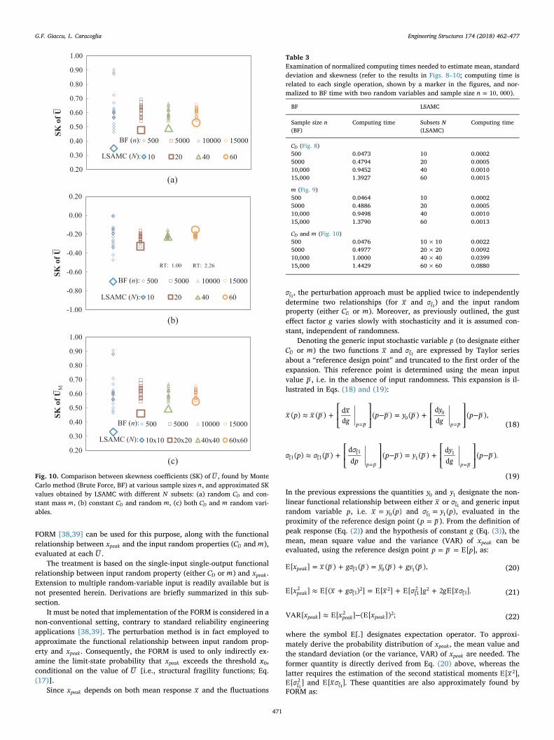
Fig. 10 suggests that the LSAMC algorithm is apparently less accu-rate in estimating the skewness coefficient ofU . The normalized error isabout 10% with one input random variable (Fig. 10a and b) and=N 60; in case of two random variables, the number of sub-sets needed

to achieve the same precision becomes × = × =N N 60 60 1200. The“exact” value of the skewness ofU , suggested by Monte Carlo sampling,is in fact very small. This leads to larger relative errors of the LSAMCestimators, around 15%. Nevertheless, the SK estimation by LSAMCmethod is adequate, despite seemingly larger errors, as it can stillpreserve sufficient information on the probability distribution of therandom U for fragility analysis. It will be demonstrated in the sub-sequent section that the relative errors in case of a fragility analysis aresmaller and that the LSMAC is quite accurate. It is also observed thatthe small discrepancies, noted for the skewness values obtained by theLSAMC, do not affect the fragility results later shown in this paper.

The same procedure described in this section was extended to otherthreshold levels x0; results are similar but are not shown for the sake ofbrevity. Information on mean and standard deviation of U will beemployed in the next section to evaluate the structural fragility curves,directly by LSAMC.

The results, shown in Figs. 8–10, confirm the high potentialities ofthe proposed LSAMC algorithm, which allows determining very preciseapproximations of mean and standard deviation ofU with a very smallnumber of subsets. Moreover, examination of Figs. 8–10 suggests thatthe standard Monte Carlo method needs a much higher number ofsamples n to achieve good estimations of the same quantities since theprocedure needs to solve for the roots of Eq. (4) for all repetitions.

Table 3 shows the comparison of the normalized computing timesneeded to obtain the results shown in Figs. 8–10 by Monte Carlo sam-pling and LSAMC approach for various sample sizes n. Numerical effi-ciency of the LSAMC approach is evident from the data shown in thetable.

5. Fragility analysis by stochastic methods: theoreticalbackground

Fragility analysis has been recently examined for performance-based structural analysis against wind hazards [58–61]. The objectiveof a fragility analysis is the computation of the conditional probabilityof exceedance of representative limit states through the assessment ofindicators (designated as “engineering demand parameters”), whichcorrespond to a specific feature of the dynamic response. Examples are:the maximum lateral drift of the tower, the internal bending momentsor shear forces in the generic section. A set of thresholds is usuallydefined to represent different levels of structural performance, based onsuch indicators, which may be selected by the designer.

Complementary cumulative distributions functions (CCDF) are usedto derive the structural fragility (FT), i.e., to find the probability that thegeneric random variable xpeak(e.g., peak response of monopole towertop) exceeds a preselected threshold T , conditional on the presence of awind storm with mean speed =V Uz at the reference height =z h, as

= > =F V X T V U( ) Prob[ | ].T z peak z (17)

In the derivation of Eq. (17) the effect of random variables simulatinguncertainty in the wind load estimation and modeling errors (i.e.,random variables CD and m in the specific application) can readily beincluded.

)b()a(Fig. 7. Random estimations of the mean-wind speed U (at =z h), relative to the response limit state corresponding to threshold crossing x0= 0.70 m with bothrandom drag coefficient and mass: (a) empirical histograms of the random input CD and m with indication of the “layered sub-sets” Λr CD, and Λs m, ( × = ×N N 4 4;note: equally-probable sub-sets are schematically illustrated), (b) PMF of the output discrete ∗UM r s, , derived by LSAMC (mean value ∗UM , standard deviation, SD, andskewness, SK, computed from the discrete ∗UM r s, , points are also indicated).

G.F. Giaccu, L. Caracoglia Engineering Structures 174 (2018) 462–477

469

5.1. Fragility functions via Monte-Carlo sampling (Brute force approach)

Traditionally, fragility curves are numerically estimated throughMonte Carlo sampling [21,22], for example utilizing Eq. (2) to em-pirically estimate the peak response (random variable Xpeak in equationabove) and compare it against threshold T through sampling. This ap-proach is usually preferred by researchers due to its accuracy and ro-bustness. Nevertheless, large computing time is usually needed andrepresents the “bottle-neck” of this method. Details are omitted in thisstudy for the sake of brevity but examples may be found in previousstudies (e.g. [21,22]).

5.2. Fragility functions via LSAMC approach

The LSAMC approach, presented above, can also be employed forthe fragility analysis of wind-sensitive monopole towers. The LSAMCalgorithm allows determining the mean and standard deviation of U ,

mean wind speed associated with peak lateral response that corre-sponds to the first crossing of the threshold x0. The quantity U is arandom variable, as shown in the previous sections. Information aboutmean and statistical moments of the randomU can be used to constructthe curves in Eq. (17), noting that =V Uz and using the cumulativedistribution function ofU to approximate the structural fragility curve.Preliminary investigation is necessary to determine the distributionmodel that best describes the random U which is needed to postulatethe model of the fragility function.

5.3. Fragility functions via implementation of perturbation methods(FORM)

In the case of a uni-variate random property, such as CD and m, thequantity xpeak (Eq. (2)) becomes a random variable. Estimation of theprobability density function of xpeak, affected by random CD andm, canbe approximated through perturbation methods. Implementation of the

(a)

(b)

(c)

28.00

28.50

29.00

29.50

30.00M

ean

valu

e of

U

500 5000 10000 1500010 20 40 60

BF (n):LSAMC (N):

27.00

27.20

27.40

27.60

27.80

28.00

Mea

n va

lue

of U

500 5000 10000 1500010 20 40 60

BF (n):LSAMC (N):

28.00

28.50

29.00

29.50

30.00

Mea

n va

lue

of U

500 5000 10000 1500010x10 20x20 40x40 60x60

BF (n):LSAMC (N):

Fig. 8. Comparison between expected value of U , found by Monte Carlomethod (Brute Force, BF) for various sample sizes n, and approximatedaverages obtained by LSAMC with different N subsets: (a) random CD andconstant mass m, (b) constant CD and random m, (c) both CD and m randomvariables.

(a)

(b)

(c)

5.00

5.50

6.00

6.50

7.00

SD o

f U

500 5000 10000 15000

10 20 40 60

BF (n):

LSAMC (N):

0.02

0.04

0.06

0.08

0.10

0.12

0.14

SD o

f U

500 5000 10000 15000

10 20 40 60

BF (n):

LSAMC (N):

5.00

5.50

6.00

6.50

7.00

SD o

f U

500 5000 10000 15000

10x10 20x20 40x40 60x60

BF (n):

LSAMC (N):

Fig. 9. Comparison between standard deviations (SD) of U , found by MonteCarlo method (Brute Force, BF) at various sample sizes n, and approximated SDvalues obtained by LSAMC with different N subsets: (a) random CD and con-stant mass m, (b) constant CD and random m, (c) both CD and m random vari-ables.

G.F. Giaccu, L. Caracoglia Engineering Structures 174 (2018) 462–477

470

FORM [38,39] can be used for this purpose, along with the functionalrelationship between xpeak and the input random properties (CD andm),evaluated at each U .

The treatment is based on the single-input single-output functionalrelationship between input random property (either CD orm) and xpeak.Extension to multiple random-variable input is readily available but isnot presented herein. Derivations are briefly summarized in this sub-section.

It must be noted that implementation of the FORM is considered in anon-conventional setting, contrary to standard reliability engineeringapplications [38,39]. The perturbation method is in fact employed toapproximate the functional relationship between input random prop-erty and xpeak. Consequently, the FORM is used to only indirectly ex-amine the limit-state probability that xpeak exceeds the threshold x0,conditional on the value of U [i.e., structural fragility functions; Eq.(17)].

Since xpeak depends on both mean response x and the fluctuations

σξ1, the perturbation approach must be applied twice to independentlydetermine two relationships (for x and σξ1) and the input randomproperty (either CD or m). Moreover, as previously outlined, the gusteffect factor g varies slowly with stochasticity and it is assumed con-stant, independent of randomness.

Denoting the generic input stochastic variable p (to designate eitherCD or m) the two functions x and σξ1 are expressed by Taylor seriesabout a “reference design point” and truncated to the first order of theexpansion. This reference point is determined using the mean inputvalue p , i.e. in the absence of input randomness. This expansion is il-lustrated in Eqs. (18) and (19):

≈ + ⎡

⎣⎢

⎤

⎦⎥ − = + ⎡

⎣⎢

⎤

⎦⎥ −

= =

x p x p xg

p p y pyg

p p( ) ( ) dd

( ) ( )dd

( ),p p p p

00

(18)

≈ + ⎡

⎣⎢

⎤

⎦⎥ − = + ⎡

⎣⎢

⎤

⎦⎥ −

= =

σ p σ pσp

p p y pyg

p p( ) ( )dd

( ) ( )dd

( ).ξ ξξ

p p p p1 1

11

1

(19)

In the previous expressions the quantities y0 and y1 designate the non-linear functional relationship between either x or σξ1 and generic inputrandom variable p, i.e. =x y p( )0 and =σ y p( )ξ 11 , evaluated in theproximity of the reference design point ( =p p ). From the definition ofpeak response (Eq. (2)) and the hypothesis of constant g (Eq. (3)), themean, mean square value and the variance (VAR) of xpeak can beevaluated, using the reference design point = =p p pE[ ], as:

= + = +x x p gσ p y p gy pE[ ] ( ) ( ) ( ) ( ),peak ξ1 0 1 (20)

≈ + = + +x x gσ x σ g g xσE[ ] E[( ) ] E[ ] E[ ] 2 E[ ],peak ξ ξ ξ2

12 2

12 2

1 (21)

≈ −x x xVAR[ ] E[ ] (E[ ]) ;peak peak peak2 2 (22)

where the symbol E[.] designates expectation operator. To approxi-mately derive the probability distribution of xpeak, the mean value andthe standard deviation (or the variance, VAR) of xpeak are needed. Theformer quantity is directly derived from Eq. (20) above, whereas thelatter requires the estimation of the second statistical moments xE[ ]2 ,σE[ ]ξ21 and xσE[ ]ξ1 . These quantities are also approximately found by

FORM as:

(a)

(b)

(c)

0.20

0.30

0.40

0.50

0.60

0.70

0.80

0.90

1.00SK

of U

500 5000 10000 15000

10 20 40 60

BF (n):

LSAMC (N):

-1.00

-0.80

-0.60

-0.40

-0.20

0.00

0.20

SK o

f U

500 5000 10000 15000

10 20 40 60

BF (n):

LSAMC (N):

RT: 1.00 RT: 2.26

0.20

0.30

0.40

0.50

0.60

0.70

0.80

0.90

1.00

SK o

f UM

500 5000 10000 15000

10x10 20x20 40x40 60x60

BF (n):

LSAMC (N):

Fig. 10. Comparison between skewness coefficients (SK) ofU , found by MonteCarlo method (Brute Force, BF) at various sample sizes n, and approximated SKvalues obtained by LSAMC with different N subsets: (a) random CD and con-stant mass m, (b) constant CD and random m, (c) both CD and m random vari-ables.

Table 3Examination of normalized computing times needed to estimate mean, standarddeviation and skewness (refer to the results in Figs. 8–10; computing time isrelated to each single operation, shown by a marker in the figures, and nor-malized to BF time with two random variables and sample size =n 10, 000).

BF LSAMC

Sample size n(BF)

Computing time Subsets N(LSAMC)

Computing time

CD (Fig. 8)500 0.0473 10 0.00025000 0.4794 20 0.000510,000 0.9452 40 0.001015,000 1.3927 60 0.0015

m (Fig. 9)500 0.0464 10 0.00025000 0.4886 20 0.000510,000 0.9498 40 0.001015,000 1.3790 60 0.0013

CD and m (Fig. 10)500 0.0476 10×10 0.00225000 0.4977 20×20 0.009210,000 1.0000 40×40 0.039915,000 1.4429 60×60 0.0880

G.F. Giaccu, L. Caracoglia Engineering Structures 174 (2018) 462–477

471

≈ + ⎡

⎣⎢

⎤

⎦⎥ −

=x y p

yp

p pE[ ] E[ ( )]dd

E[( ) ],p p

202 0

2

2

(23)

≈ + ⎡

⎣⎢

⎤

⎦⎥ −

=σ y p

yp

p pE[ ] E[ ( )]dd

E[( ) ],ξp p

12

12 1

2

2

(24)

≈ + − ⎡

⎣⎢

⎤

⎦⎥⎡

⎣⎢

⎤

⎦⎥

= =xσ y p y p p p

yp

yp

E[ ] E[ ( ) ( )] E[( ) ]dd

dd

.ξp p p p

1 0 12 0 1

(25)

In deriving Eq. (25) the relationship −p pE[ ]=0 is used; the derivativesof y0 and y1 with respect to p are evaluated at the reference designpoint. After rewriting the variance term as − =p p pE[( ) ] VAR[ ]2 andcombining Eqs. (23)-(25) with Eqs. (21) and (22) the variance of thepeak response, xVAR[ ]peak , becomes:

≈⎧⎨⎩

⎛

⎝⎜

⎞

⎠⎟ + ⎛

⎝⎜

⎞

⎠⎟⎛

⎝⎜

⎞

⎠⎟

+ ⎛

⎝⎜

⎞

⎠⎟⎫⎬⎭

= = =

=

x pyp

gyp

yp

gyp

VAR[ ] VAR[ ]dd

2dd

dd

dd

.

peakp p p p p p

p p

02

0 1

2 12

(26)

Eqs. (20) and (26) can be used to find an expression for the probabilitydistribution function of xpeak at each wind speedU , using =p pE[ ] and

pVAR[ ]; the probability model describing the response variable xpeak isin fact the same as the one of the input random variable p owing to theapproximate linear relationship established by FORM. This informationcan be employed to re-construct the cumulative distribution function ofxpeak at each U and, consequently the complementary cumulative dis-tribution function dictated by the fragility relationship ((Eq. (17)), afterthe threshold level x0 is chosen. Since the relationships y0 and y1 cannottypically be found in closed form, numerical estimation of the deriva-tives in Eq. (26) is found by sampling these functions in the proximity of= =p p pE[ ].

6. Structural fragility analysis: Results and comparisons (LSAMC,FORM and BF)

6.1. Computation of structural fragility functions with one input randomproperty (either CD or m)

This sub-section examines the structural fragility analysis of thesingle-DOF generalized model of the prototype monopole tower underthe influence of both wind loading (CD variable) and structural propertyuncertainties (mass m). As described earlier, randomization of theseparameters reflects the presence of either measurement errors in thewind tunnel or structural uncertainties related to the modification ofthe structural mode shape or structural mass during the lifetime.

The main purpose is to evaluate the effectiveness of the LSAMCapproach. The comparisons of the fragility curves include the variousmethods (Monte Carlo sampling, LSAMC approach and FORM). In thisinvestigation, fragility curves are evaluated by computation of theprobability that the along-wind peak dynamic response at =z h ex-ceeds a pre-selected threshold x0, corresponding to the limit state of thepeak lateral displacement at the monopole tower top.

For the Monte-Carlo simulations, the number of samples =n 10, 000has been considered as the reference value. From the verification resultsof the LSAMC approach, presented in the previous section, it is sug-gested that the lognormal model can be used to replicate the cumulativedistribution function of U and, consequently, the fragility function.

Table 4 summarizes the predefined threshold levels, utilized for thefragility analysis ∈x {T1, T2, T3, T4, T5}0 . Threshold T5 is related to apossibly unrealistic peak displacement, but is utilized herein mainly forverification of the proposed procedure. Table 4 also presents the cor-responding base bending moment thresholds M0, derived from x0 and

the properties of the monopole structure; this second quantity can beused to examine the ultimate limit state either associated with eithermaximum overturning moment of the tower or material strength in thebase cross section.

The main results are presented in Figs. 11 and 12. Fig. 11 shows thefragility curves calculated for random CD (random aerodynamic loads)and deterministic mass =m 600 kg. Fig. 12 similarly depicts the fragi-lity curves for deterministic aerodynamic load (CD) and random massm. In both Figs. 11 and 12 the graphs found with Monte-Carlo sampling(Brute Force, BF) are used as the reference solution; the left panels ofboth figures present the comparisons with the LSAMC whereas the rightsides illustrate the results found with the FORM.

Comparison of Fig. 9(a) with (b) indicates that the standard de-viation of the random U is larger in the case of a CD random variableand becomes almost negligible in the case of deterministic CD andrandom mass m. This observation is also confirmed by examination ofthe fragility curves shown in Fig. 12, where a small variation of thewind speed U induces an abrupt performance loss; the steep slope lo-cally exhibited by the fragility curves is indeed an indicator of limitedsensitivity to randomness.

Overall, as anticipated by the small errors found with the LSAMC inFigs. 8 and 9, the agreement of the approximated LSAMC estimationswith the “exact” curves, found by Monte-Carlo sampling, is very good inboth Figs. 11 and 12. The FORM is still adequate when uncertaintypropagation considers the random CD (Fig. 11(b)), whereas substantialdiscrepancies are observed in Fig. 12(b) with random mass m. From acursory analysis of the results shown in Figs. 11 and 12, it is noted thatLSAMC provides a good approximation of fragility curves with relativesmall differences (or errors). Estimation errors can be qualitativelynoticed by inspection of the fragility curves.

The LSAMC approach is usually adequate, in particular when smallvariability in the random input property or parameter leads to “step-like” fragility functions in Fig. 12(a). On the contrary, the FORM isunable to replicate the structural fragility in Fig. 11(b). The estimationerror of the LSAMC, approximately evaluated by inspection of the fra-gility curves, is about few percent. A quantitative examination of theerror is presented in the next sub-section.

6.2. Analysis of simulation errors with one input random property (eitherCDor m)

The relative estimation error provided by the two approximatedapproaches (AA) is defined as −P P P( )/E AA E BF E BF, , , , where PE AA, and PE BF,respectively designate probability of exceedance obtained by approx-imate solution (LSAMC or FORM) and “exact” probability of ex-ceedance obtained by Monte-Carlo sampling (Brute Force, BF).Estimation error calculations are carried out by comparing the graphsin Figs. 11 and 12 at several values ofU ; results are illustrated in Fig. 13for random drag coefficient CD and Fig. 14 for random mass m. In eachcase, the left panels present the SLAMC results while the right panelsthe FORM ones, enabling cross-examination of the two methods.

In Fig. 13, the error of the LSAMC is larger at low wind speedsU anddecrease to about 4% for wind speeds greater than 40m/s; the FORMgives considerably larger errors for all considered wind velocities. In

Table 4Thresholds for fragility analysis of the generalized model of the monopolestructure.

Threshold level x0 Tower top displacementthreshold level [m]

Base bending momentthreshold level [kNm]

T1 =h0.010 0.35 3488T2 =h0.020 0.70 6977T3 =h0.036 1.26 12, 558T4 =h0.052 1.82 18, 140T5 =h0.068 2.38 23, 722

G.F. Giaccu, L. Caracoglia Engineering Structures 174 (2018) 462–477

472

(b)(a)

0.0

0.2

0.4

0.6

0.8

1.0

25 30 35 40 45 50 55 60 65 70

Prob

abili

ty o

f exc

eeda

nce

U [m/s]

T1 (BF)T1(LSAMC)T2 (BF)T2 (LSAMC)T3 (BF)T3 (LSAMC)T4 (BF)T4 (LSAMC)T5 (BF)T5 (LSAMC)

0.0

0.2

0.4

0.6

0.8

1.0

25 30 35 40 45 50 55 60 65 70

Prob

abili

ty o

f exc

eeda

nce

U [m/s]

T1 (BF)T1 (FORM)T2 (BF)T2 (FORM)T3 (BF)T3 (FORM)T4 (BF)T4 (FORM)T5 (BF)T5 (FORM)

Fig. 11. Fragility curves obtained by Monte-Carlo (BF) sampling, LSAMC and FORM approaches. Analysis of monopole structure with random aerodynamic load (CDvariable) and limit state associated with the lateral peak displacement at =z h and the thresholds T1 – T5 (Table 3): (a) Comparison between Monte Carlo (BF) andLSAMC, (b) Comparison between Monte Carlo (BF) and FORM.

(b)(a)

0.0

0.2

0.4

0.6

0.8

1.0

25 30 35 40 45 50 55 60 65 70

Prob

abili

ty o

f exc

eeda

nce

U [m/s]

T1 (BF)T1 (LSAMC)T2 (BF)T2 (LSAMC)T3 (BF)T3 (LSAMC)T4 (BF)T4 (LSAMC)T5 (BF)

0.0

0.2

0.4

0.6

0.8

1.0

25 30 35 40 45 50 55 60 65 70

Prob

abili

ty o

f exc

eeda

nce

U [m/s]

T1 (BF)T1 (FORM)T2 (BF)T2 (FORM)T3 (BF)T3 (FORM)T4 (BF)T4 (FORM)T5 (BF)T5 (FORM)

Fig. 12. Fragility curves obtained by Monte-Carlo (BF) sampling, LSAMC and FORM approaches. Analysis of monopole structure with random structural properties(m mass variable) and limit state associated with the lateral peak displacement at =z h and the thresholds T1 – T5 (Table 3): (a) Comparison between Monte Carlo(BF) and LSAMC, (b) Comparison between Monte Carlo (BF) and FORM.

(b)(a)

-20%

-15%

-10%

-5%

0%

5%

10%

15%

20%

25 30 35 40 45 50 55 60 65 70

Rel

ativ

e err

or

U [m/s]

T1 (LSAMC)

T2 (LSAMC)

T3 (LSAMC)

T4 (LSAMC)

T5 (LSAMC)

-20%

-15%

-10%

-5%

0%

5%

10%

15%

20%

25 30 35 40 45 50 55 60 65 70

Rel

ativ

e err

or

U [m/s]

T1 (FORM)

T2 (FORM)

T3 (FORM)

T4 (FORM)

T5 (FORM)

Fig. 13. Relative error of LSAMC and FORM compared to the “exact” solution (Monte Carlo, BF) – CD random variable and T2, T5 thresholds: (a) Comparisonbetween Monte Carlo (BF) and LSAMC, (b) Comparison between Monte Carlo (BF) and FORM [notes: relative errors shown in the range of wind speeds between25m/s and 70m/s; “60”=number of equiprobable sets].

G.F. Giaccu, L. Caracoglia Engineering Structures 174 (2018) 462–477

473

Fig. 14, the discrepancy between Monte-Carlo and approximate solu-tions is exacerbated by a considerably smaller random variability in-troduced by the random mass m in the estimation of the xpeak. Clearly,the FORM is not adequate as relative errors are very large while theestimation errors associated with the LSAMC approach are still rea-sonably small. This figure is important since it suggests that, even in thepresence of a limiting case associated with small random variability and“steeper” fragility functions for intermediate values of U (thus leadingto abrupt variations in exceedance probabilities), the LSAMC approachstill provides better results compared with FORM.

General examination of Figs. 13 and 14 suggests that the estimationerror in the case of LSAMC is localized; fragility curves usually exhibitgood agreement with the ones obtained numerically by Monte-Carlosampling. On the contrary, the error committed by FORM is not ac-ceptable. This problem can be explained accounting for the limitationintroduced by the FORM and used for determining the variance of xpeak,as illustrated in Eq. (26). Finally, even though verification of theLSAMC procedure has been examined, further validation may be de-sirable in the future (e.g., through testing and experimental assessmentof structural fragility).

6.3. Computation of structural fragility functions with two input randomproperties (both CD and m)

Fig. 15(a) presents the structural fragility curves when both CD andm are the input random properties. This investigation is restricted to thecomparison between LSAMC and Monte-Carlo sampling, since theFORM is unable to provide adequate estimation of the fragility curveswhen the contribution of a random m is incorporated. In this last sce-nario with two input random variables the relative deviations (errors)between the approximate fragility curves found by LSAMC and the“exact” curves determined by Monte Carlo sampling are illustrated inFig. 15(b). The relative error, computed as explained in Section 6.2 isslightly smaller than the error found for the first scenario with randomCD only and shown in Fig. 13(a).

The supplementary numerical results illustrated in Fig. 15 confirmthe good performance of the LSAMC approach. Qualitative differencesbetween approximate and Monte-Carlo fragility curves (Fig. 15(a)) arealmost imperceptible. The relative error between LSAMC and Monte-Carlo sampling is less than 5% for wind speeds U larger than 35m/s.

All the results presented in Figs. 11–15 are preliminary since theyare based on the analysis of a generalized structural model of a

(b)(a)

-20%

-15%

-10%

-5%

0%

5%

10%

15%

20%

25 30 35 40 45 50 55 60 65 70

Rel

ativ

e err

or

U [m/s]

T1 (LSAMC)

T2 (LSAMC)

T3 (LSAMC)

T4 (LSAMC)

T5 (LSAMC)

-20%

-15%

-10%

-5%

0%

5%

10%

15%

20%

25 30 35 40 45 50 55 60 65 70

Rel

ativ

e err

or

U [m/s]

T1 (FORM)

T2 (FORM)

T3 (FORM)

T4 (FORM)

T5 (FORM)

Fig. 14. Relative error of LSAMC and FORM compared to the “exact” solution (Monte Carlo, BF) –m random variable and T2, T5 thresholds: (a) Comparison betweenMonte Carlo (BF) and LSAM, (b) Comparison between Monte Carlo (BF) and FORM notes: relative errors shown in the range of wind speeds between 25m/s and70m/s; “60”=number of equiprobable sets].

(b)(a)

0.0

0.2

0.4

0.6

0.8

1.0

Prob

abili

ty o

f exc

eeda

nce

U [m/s]

T1 (BF)T1(LSAMC)T2 (BF)T2 (LSAMC)T3 (BF)T3 (LSAMC)T4 (BF)T4 (LSAMC)T5 (BF)

-20%

-15%

-10%

-5%

0%

5%

10%

15%

20%

25 30 35 40 45 50 55 60 65 70

Rel

ativ

e err

or

U [m/s]

T1 (LSAMC)

T2 (LSAMC)

T3 (LSAMC)

T5 (LSAMC)

T5 (LSAMC)

25 30 35 40 45 50 55 60 65 70

Fig. 15. Fragility curves obtained by Monte-Carlo (BF)sampling and LSAMC approach. Analysis of monopole structure with random structural properties (m massvariable) and random aerodynamic loads (CD variable) for limit state associated with lateral peak displacement at =z h and thresholds T1 – T5 (Table 3): (a) fragilitycurves, (b) relative errors [note: relative errors shown between 25m/s and 70m/s].

G.F. Giaccu, L. Caracoglia Engineering Structures 174 (2018) 462–477

474

monopole tower. They require further investigation prior to general-ization of the LSAMC algorithm and its implementation to other andmore complex wind-sensitive vertical structures (tall buildings, windturbines, etc.). This task is, however, beyond the scope of this study andwill be considered in the future.

6.4. Examination of computing time savings

Computational efficiency of the proposed methodology is examinedin this sub-section Fig. 16 summarizes the results of this investigation.

The computing time of the LSAMC algorithm is examined as afunction of the number of equiprobable sets (N ). The execution time isnormalized with respect to Monte-Carlo computing (BF-normalized)and compared against the FORM computing time.

The results illustrated in Fig. 16 indicate that, in the case of a singleinput random variable, the LSAMC achieves sufficient approximation(illustrated in Figs. 11–15) with equiprobable sets =N 60 and a BFnormalized computing time equal to 0.18%. In Fig. 16(a) and (b) thecomputing time of LSMAC is modestly longer than the time required byFORM. As expected, in case of two input random variables (Fig. 16(c))the normalized computing time increases since it is proportional to thenumber of equiprobable sets needed to obtain the same accuracy, whichare 3600 (60×60). Examination of Fig. 16(c) suggests that, in the caseof two random variables, the LSAMC algorithm is less performing. Eventhough the performance of the LSAMC approach may progressivelydeteriorate as the number of input random variables increase, theLSAMC approach is still 90% faster than Monte-Carlo sampling withtwo random variables, indicating that it may still be adequate for or-dinary applications in performance-based wind engineering.

7. Discussion and conclusions

This study summarizes the results of a research activity aiming atthe derivation of computationally-efficient performance-based meth-odologies for the estimation of structural fragility curves of wind-sen-sitive structures. Implementation of SA algorithms was employed toderive the dynamic response of a prototype structure, a monopoletower, under stationary wind loads in the frequency domain.

Uncertainty and measurement errors were considered by suitablerandom perturbation of selected but representative variables (physicalproperties) of the structure and the load, following implementationspresented in previous work [21,22]. The numerical procedure, desig-nated as LSAMC algorithm, was employed to analyze the effects ofuncertainty and errors in the modeling of structural properties and inthe estimation of wind forces, often carried out in wind tunnel. Linearelastic along-wind dynamic response was considered.

In the first part of the study, initial verification of the LSAMC al-gorithm was conducted by comparing the simulated results againstMonte Carlo sampling results. The comparison was based on the ana-lysis of mean values, variance and skewness coefficients embedded inthe implicit stochastic function (Eq. (4)).

In the second part, the LSAMC approach was employed to derivestructural fragility curves of the prototype monopole tower, associatedwith various limit states. The peak lateral response at the top of thetower was employed as the control variable, or engineering demandparameter. Five different limit-state thresholds were considered to as-sess the stochastic response of the prototype system and evaluatecomputation of the fragility curves. For the sake of completeness and toidentify advantages and potential limitations of the LSAMC, the in-vestigation also examined another popular approach for reliabilityanalysis, the FORM.

Numerical simulations confirm that the LSAMC approach is ade-quate for approximate estimation of structural fragility curves. Theerror is usually limited to few percent values. Furthermore, the LSAMCoutperforms the FORM when the propagation of uncertainty is eitherinfluenced by nonlinearity (mass m) or the steepness in the fragility

curves is large (refer to error comparisons in Section 6).The LSAMC also proves to be an efficient algorithm from the com-

putational point of view, since a significant speedup in the computingtime was observed in comparison with Monte-Carlo sampling results(Fig. 16). For example, in the case of single input random property orvariable, the computing time required by LSAMC is less than 1%compared to the time needed by Monte-Carlo simulation. In the case oftwo input random properties or variables, the computing time ofLSAMC is about 12% compared to standard sampling approach;

(a)

(b)

(c)

0.00%

0.05%

0.10%

0.15%

0.20%

10 15 20 25 30 35 40 45 50 55 60

BF-

norm

aliz

ed c

ompu

ting

time

Equiprobable sets N

LSAMC

FORM

0.00%

0.05%

0.10%

0.15%

0.20%

10 15 20 25 30 35 40 45 50 55 60

BF-

norm

aliz

ed c

ompu

ting

time

Equiprobable sets N

LSAMC

FORM

0.00%

2.00%

4.00%

6.00%

8.00%

10.00%

12.00%

0 1000 2000 3000 4000

BF-

norm

aliz

ed c

ompu

ting

time

Equiprobable sets N×N

LSAMC

FORM

Fig. 16. Computing time of LSAMC and FORM, as a function of the number ofequiprobable sets, normalized to the Monte-Carlo (BF) time: (a) random CD, (b)random m, (c) random CD and m.

G.F. Giaccu, L. Caracoglia Engineering Structures 174 (2018) 462–477

475

computing time reductions were obtained by preserving adequate ac-curacy in the approximated structural fragility curves. It is noted that,even though the computing time savings progressively deterioratewhen the number of input random variables increase, they appear to beadequate for ordinary applications and conventional structures.

The study primarily examined two types of random behavior, i.e.uncertainty in the aerodynamic loads (simulated through static coeffi-cient CD) and modeling uncertainty due to imperfect knowledge of thestructure (simulate through mass m). Clearly, these two variables areprovided as examples, since several other parameters or structuralproperties (e.g. damping ratios) are perhaps equally relevant [23–25] tothe dynamic response. Consequently, more investigation is needed toextend these results to other random variables. Nevertheless, the mainobjective of the study was the examination of the LSAMC approach as acomputationally efficient method for structural fragility analysis.

Future studies should include more complex structural systems,examine other parameter uncertainties, account for across-wind re-sponse in addition to along-wind response, and expand the treatment tothe stochastic structural analysis in the presence of high-dimensionalproblems (multi-degree-of-freedom structures).

Acknowledgements

Gian Felice Giaccu acknowledges the financial support of RegioneAutonoma della Sardegna, Italy (L.R. n. 3/2008 “RientroCervelli” andL.R. n. 7/2007 “Promozione della Ricerca Scientifica e dell'InnovazioneTecnologica in Sardegna”). The authors would also like to thankProfessor Bernardo Barbiellini from the Department of Physics ofLappeenranta University of Technology (Finland) for fruitful discus-sions about the SA mehods and for providing the original motivationthat led to the implementation of the SA algorithm, described in thisstudy.

References

[1] Inokuma A. Basic study of performance-based design in civil engineering; 2002.[2] Tsompanakis Y, Lagaros ND, Papadrakakis M. Structural design optimization con-

sidering uncertainties. London; 2008.[3] Yao W, Chen X, Luo W, Van Tooren M, Guo J. Review of uncertainty-based mul-

tidisciplinary design optimization methods for aerospace vehicles. Prog Aerosp Sci2011;47:450–79.

[4] Ciampoli M, Petrini F. Performance-based aeolian risk assessment and reduction fortall buildings. Prob Eng Mech 2012;28:75–84.

[5] Ciampoli M, Petrini F, Augusti G. Performance-based wind engineering: towards ageneral procedure. Struct Saf 2011;32:367–78.

[6] Venanzi I, Materazzi AL, Ierimonti L. Robust and reliable optimization of wind-excited cable stayed masts. J Wind Eng Indust Aerodyn 2015;147:368–79.

[7] Davenport AG. Response of supertall buildings to wind. In: Third internationalconference on tall buildings. Chicago, IL, United States of America. p. 705–705.

[8] Davenport AG. Response of six building shapes to turbulent wind. Phil Trans R SocLondon Ser A 1971;269(1199):385–94.

[9] Kareem A. Dynamic response of high-rise buildings to stochastic wind loads. J WindEng Indust Aerodyn 1992;42(1–3):1101–12.

[10] Kareem A. Model for predicting the acrosswind response of buildings. Eng Struct1984;6(2):136–41.

[11] Spence SMJ, Gioffrè M. Large scale reliability-based design optimization of windexcited tall buildings. Prob Eng Mech 2012;28:206–15.

[12] Spence SMJ, Kareem A. Performance-based design and optimization of uncertainwind-excited dynamic building systems. Eng Struct 2014;78:133–44.

[13] Spence SMJ, Gioffrè M. Efficient algorithms for the reliability optimization of tallbuildings. J Wind Eng Indust Aerodyn 2011;99(6–7):691–9.

[14] Venanzi I, Materazzi AL. Robust optimization of a hybrid control system for wind-exposed tall buildings with uncertain mass distribution. Smart Struct Sys2013;12(6):641–59.

[15] Pavan Kumar M. Effect of wind speed on structural behaviour of Monopole and self-support telecommunication towers. Asian J Civil Eng 2017;18(6):911–27.

[16] Støttrup-Andersen U. Masts and towers. J Int Assoc Shell Spatial Struct2014;55:79–88.

[17] Dimopoulos CA, Koulatsou K, Petrini F, Gantes CJ. Assessment of stiffening type ofthe cutout in tubular wind turbine towers under artificial dynamic wind actions. JComput Nonlin Dyn 2015;10(4). 041004-041004-9.

[18] AlHamaydeha M, Hussain S. Optimized frequency-based foundation design for windturbine towers utilizing soil–structure interaction. J Franklin I2011;348(7):1470–87.

[19] Petrini F, Manenti S, Gkoumas K, Bontempi F. Structural design and analysis of

offshore wind turbines from a system point of view. Wind Eng 2010;34(1):85–108.[20] Makkonen L, Lehtonen P, Hirviniemi P. Determining ice loads for tower structure

design. Eng Struct 2014;74:224–32.[21] Smith MA, Caracoglia L. A Monte Carlo based method for the dynamic “fragility

analysis” of tall buildings under turbulent wind loading. Eng Struct2011;33(2):410–20.

[22] Cui W, Caracoglia L. Simulation and analysis of intervention costs due to wind-induced damage on tall building. Eng Struct 2015;87:183–97.

[23] Pagnini L. Reliability analysis of wind-excited structures. J Wind Eng IndustAerodyn 2010;98(1):1–9.

[24] Pagnini L, Repetto M. The role of parameter uncertainties in the damage predictionof the alongwind-induced fatigue. J Wind Eng Indust Aerodyn2012;104–106:227–38.

[25] Pagnini L, Solari G. Gust buffeting and turbulence uncertainties. J Wind Eng IndustAerodyn 2002;90(4):441–59.

[26] Seo D-W, Caracoglia L. Estimating life-cycle monetary losses due to wind hazards:fragility analysis of long-span bridges. Eng Struct 2013;56:1593–606.

[27] Cui W, Caracoglia L. Exploring hurricane wind speed along US Atlantic Coast inwarming climate and effects on predictions of structural damage and interventioncosts. Eng Struct 2016;112:209–25.

[28] Gao B, Cen D, Wu H. Static performances and reliability sensitivity analysis on rigidcable dome structures. J Shenzhen Univ Sci Eng 2013;30(3):325–30.

[29] Giaccu GF, Scintu L, Barbiellini B. Stochastic approach for the dynamic perfor-mance analysis of tall buildings subject to turbulent wind load. In: ICWE14Conference. Porto Alegre, Brazil; 2015.

[30] Caracoglia L, Giaccu GF, Barbiellini B. Estimating the standard deviation of ei-genvalue distributions for the nonlinear free-vibration stochastic dynamics of cablenetworks. Meccanica 2016:1–15.

[31] Robert CP, Casella G. Monte Carlo statistical methods. 2nd ed. New York, NewYork, USA: Springer Science; 2004.

[32] Giaccu GF, Barbiellini B, Caracoglia L. Parametric study on the nonlinear dynamicsof a three-stay cable network under stochastic free vibration. J Eng Mech, ASCE2015;141(6):04014166.

[33] Giaccu GF, Barbiellini B, Caracoglia L. Stochastic unilateral free vibration of an in-plane cable network. J Sound Vib 2015;340:95–111.

[34] Scintu L. Approccio stocastico per l'analisi dinamica- prestazionale di edifici altisoggetti all'azione turbolenta del vento [MS Thesis] Italy: University of Cagliari;2014.

[35] Cui W, Caracoglia L. Simulation and analysis of intervention costs due to wind-induced damage on tall buildings. Eng Struct 2015;87:183–97.

[36] Caracoglia L, Jones NP. Experimental derivation of the dynamic characteristics ofhighway light poles. In: Twenty-forth International Modal Analysis Conference(IMAC-XXIV). St. Louis, Missouri, USA; January 30-February 2, 2006, CD-ROM.

[37] Bucher C. Computational analysis of randomness in structural mechanics. London,UK: Taylor Francis Group; 2009.

[38] Der Kiureghian A. First- and second-order reliability methods. Engineering designreliability handbook. Boca Raton, Florida, USA: CRC Press; 2005.

[39] Haldar A, Mahadevan S. Reliability assessment using stochastic finite-elementanalysis. New York, NY, USA: John Wiley and Sons; 2000.

[40] Dragt RC, Allaix DL, Maljaars J, Tuitman JT, Salman Y, Otheguy ME. Approach toinclude load sequence effects in the design of an Offshore Wind Turbine sub-structure. In: Proceedings of the 27th International Ocean and Polar EngineeringConference, ISOPE 2017. p. 312–319.

[41] Au SK, Beck JL. Estimation of small failure probabilities in high dimensions bysubset simulation. Prob Eng Mech 2001;16(4):263–77.

[42] Cheng J, Cai CS, Xiao R-C, Chen SR. Flutter reliability analysis of suspensionbridges. J Wind Eng Indust Aerodyn 2005;93(10):757–75.

[43] Ge YJ, Xiang HF, Tanaka H. Application of a reliability analysis model to bridgeflutter under extreme winds. J Wind Eng Indust Aerodyn 2000;86(2–3):155–67.

[44] Baldomir A, Kusano I, Jurado JA, Hernandez S. A reliability study for the MessinaBridge with respect to flutter phenomena considering uncertainties in experimentaland numerical data. Comput Struct 2013;128:91–100.

[45] Piccardo G, Solari G. Generalized equivalent spectrum technique. Wind Struct1998;1(2):161–74.

[46] Kareem A. Aerodynamic response of structures with parametric uncertainties.Struct Saf 1988;5(3):205–25.

[47] Kaimal JC, Wyngaard JC, Izumi Y, Coté OR. Spectral characteristics of surface-layerturbulence. Q J R Meteorol Soc 1972;98(417):563–89.

[48] Davenport AG. Note on the distribution of the largest value of a random functionwith application to gust loading. J Proc Inst Civ Eng 1964;28(2):187–96.

[49] Davenport AG. A statistical approach to the treatment of wind loading on tall mastsand suspension bridges. United Kingdom: University of Bristol; 1961.

[50] Isyumov N, Alan G. Davenport's mark on wind engineering. J Wind Eng IndustAerodyn 2012;104:12–24.

[51] EC-1.4. Eurocode 1: Actions on structures – Part 1-4: General Actions –Wind actions(prEN 1991-1-4.6). European Committee for Standardisation (CEN); 2002.

[52] Cui W, Caracoglia L. Examination of experimental variability in HFFB testing of atall building under multi-directional winds. J Wind Eng Indust Aerodyn2017;171:34–49.

[53] Gioffrè M, Gusella V, Materazzi AL, Venanzi I. Removable guyed mast for mobilephone networks: wind load modeling and structural response. J Wind Eng IndustAerodyn 2004;92:463–75.

[54] Harju A, Barbiellini B, Siljamäki S, Nieminen RM, Ortiz G. Stochastic gradient ap-proximation: an efficient method to optimize many-body wave functions. Phys RevLett 1997;1997(79):1173–7.

[55] Spall JC. Introduction to stochastic search and optimization: estimation, simulation

G.F. Giaccu, L. Caracoglia Engineering Structures 174 (2018) 462–477

476

and control. Hoboken, New Jersey, USA: John Wiley and Sons; 2003.[56] Robbins H, Monro S. Stochastic approximation method. Ann Math Stat

1951;22(3):400–7.[57] Giaccu GF, Barbiellini B, Caracoglia L. Parametric study on the nonlinear dynamics

of a three-stay cable network under stochastic free vibration. J Eng Mech, ASCE2015;141(6):04014166.

[58] Norton T, Abdullah MM, Stephens D. Proposed methodology for performance-basedvulnerability assessment of wind-excited tall buildings. In: Choi C-K, Holmes JD,Kim Y-D, Kwak HG, editors. Fourth International Conference on Advances in Windand Structures (AWAS'08). Jeju Island, South Korea: Techno-Press, South Korea;2008. p. 1228–46. ISBN 978-89-89693-23-9-98530.

[59] Bashor R, Kareem A. Probabilistic performance evaluation of buildings: an occupantcomfort perspective. In: 12th International Conference on Wind Engineering (12-ICWE). Cairns, Australia, July 1–6, 2007. p. 1335–1342.

[60] Filliben JJ, Gurley K, Pinelli J-P, Simiu E. Fragility curves, damage matrices, andwind induced loss estimation. In: Third International Conference on ‘ComputerSimulation in Risk Analysis and Hazard Mitigation’. Sintra, Portugal; 2002. p.119–126.

[61] Le V, Caracoglia L. Computationally efficient stochastic approach for the fragilityanalysis of vertical structures subjected to thunderstorm downburst winds. EngStruct 2018;165:152–69.

G.F. Giaccu, L. Caracoglia Engineering Structures 174 (2018) 462–477

477