Towards a definition of topographic divisions for Italy

E L S E V I E R Geomorphology 11 (1994) 57-74

GEOHORHHIOGY

Towards a definition of topographic divisions for Italy

Fausto Guzzetti, Paola Reichenbach CNR-IRPI via Madonna Alta, 126, 06128 Perugia, Italy

(Received November 27, 1993; accepted March 7, 1994)

Abstract

The study has divided Italy into eight major topographic divisions (provinces) and 30 minor divisions (sections) that are similar to N. Fenneman's units of the United States. Provinces and sections are generally consistent with observed morphology. The new units were defined step-wise in a semi-quantitative approach that combined an unsupervised three-class cluster analysis of four derivatives of altitude, visual interpretation of morphometric maps (including shaded relief), and comparative inspection of small-scale geological and structural maps. The four variables are altitude, slope curvature, frequency of slope reversal, and elevation-relief ratio. Highland, upland, and lowland topographic types were identified. The variables were computed from a 230 m resolution digital terrain model, regridded from the original 230 m DEM obtained by mosaicking the entire Italian mean elevation archive.

1. Introduct ion

The recognition of topographic divisions through an orderly system of landform taxonomy is a basic step in the scientific study of the physical landscape (Fenne- man, 1917; Hammond, 1964). Truly "homogeneous" regions are an idealised concept; in reality, topographic divisions are stochastic, statistical constructs. Charac- terising terrain to recognise divisions that maximise internal homogeneity and external heterogeneity is difficult. The great variety of observed topography must be expressed well enough in quantitative or analytical terms so that different landscapes, formed by contrast- ing processes, can be distinguished and individually described and interpreted (Pike and Thelin, 1989).

Topography is described and analysed quantitatively for many purposes (Weibel and DeLotto, 1988). Besides parsing topography (Wood and Snell, 1960), morphometric characterisation is used to derive traff- icability maps for military operations and to automate the creation of hill-shaded images. Other applications

0169-555X/94/$07.00 © 1994 Elsevier Science B.V. All rights reserved SSDIO169-555X(94)OOOO9-G

include assessment of geomorphic hazards and risk (Pike, 1988; Brabb et al., 1989; Carrara et al., 1991), analysis of regional morphology and structure (Lid- mar-Bergstrom et al., 1991; Onorati et al., 1992), evaluation of energy resources (Elliott et al., 1991), hydrological modelling ( Beven and Moore, 1992), and regional planning (Bernknopf et al., 1988).

Recently, the availability of digital elevation models (DEMs) has provided geomorphologists with new tools for quantitatively analysing topography (for an exhaustive bibliography see Pike, 1993). Numerical classifications of landforms have been attempted by computer manipulation of DEMs, either by automating previously proposed manual classifications (Dikau et al., 1991) or, as here, by devising new ones (Evans, 1980; Pike, 1988).

Formal topographic divisions, physiographic units, or types of land-surface form have not been recognised in Italy. This paper presents a preliminary subdivision of the entire Italian territory into formal topographic units and describes the rationale and the largely DEM-

58 F. Guzzeni, P. Reichenbach / Geomorphology 11 (1994)57-74

based techniques by which it was prepared. The classification is semi-quantitative, derived from an unsupervised three-class cluster analysis of four derivatives of elevation and from the visual inspection of both geological maps and digital maps of morphome- r~c parameters.

2. Elevation data

The elevation data on which much of our classification was based are the archive of "Mean Height Values for Italy" compiled by estimating mean elevation values, by both manual and machine methods, on 1:25,000 scale topographic maps (Carrozzo et al., 1985). The manual data, prepared for central and ,~outhern Italy, for Sicily and Sardinia, were read off contour maps using a square-grid template spaced at 7.7 arc-seconds of latitude and 10 arc-seconds of lon- gitude. Each point was assigned an altitude value, to the nearest metre, by averaging contour lines and spot heights within each grid square. Machine-gathered data were obtained for the rest of the country (i.e., northern Italy) by computer interpolation of digitised contours. The elevations gridded by both methods were organi- sed into 280 separate matrices of 160 rows and 180 columns arranged on a geographic grid, each matrix corresponding to an IGMI topographic sheet in the 1:100,000 scale series (Carrozzo et al., 1985).

A joint CNR/USGS project assembled the DEM for lhe entire Italian state at a ground resolution of 230 m ,5886 rows by 4546 columns, for a total of about 8 millions land heights) by mosaicking and correcting all 280 files of the original mean-elevation archive. Such non-systematic errors as missing or mislabelled data, incorrectly coded pixels and projection inconsis- lencies were identified during the data-assembly phase and most of them were corrected. The procedures used to compile, test, and correct the DEM are described by Reichenbach et al. (1993).

3. Morphometric variables

The main criteria by which Italy was divided into topographic regions were four of the eleven numerical derivatives of altitude described below. We prepared a coloured digital map of Italy (not enclosed) for each

of the eleven variables so that we could study all the spatial patterns and from them choose those with which to subdivide the country. Maps of all eleven variables played at least a qualitative role in our classification of Italy.

Elevation. The raw DEM was displayed as a coloured hypsographic map. Because the frequency distribution of elevation in Italy is left-skewed (mean 573 m, mode 1 m, standard deviation 635 m, skewness 1.74), for display purposes elevations were converted to logarithms to avoid concealing information and thus better express the morphology of the country. The log- transformed DEM nicely emphasises low-elevation details in the extremely fiat Po valley and along the Adriatic coastline south of the Po delta. All successive computations were performed on the original, untransformed DEM.

Minimum, maximum and mean elevation. Minimum elevation (Hn~,) and maximum elevation (Hm~x) were mapped by respectively assigning the lowest and highest height value, within a pre-defined neighbourhood, to the central pixel of a moving window. We tested windows of different shapes and dimensions. Square windows produced maps with a blocky appearance, the result of including isolated peaks or sinks; this problem was partially solved by using circular windows. Mean elevation (H . . . . ) generalisesraw altitude by averaging the DEM within a sampling window moved through the elevation grid. Although not differing significantly from elevation, the resulting map has less detail, which makes elevation more comparable to other generalised variables for regional analysis.

Local relief Relative, or local, relief is the difference between highest and lowest elevations within a given window. It has long been used to quantify elevation contrast and surface roughness (Neuenschwander, 1944). The frequency distribution of relief is so highly left-skewed that we transformed it to remove skew and thus avoided concealing information in the resulting map.

The arbitrariness of window size is an old problem (Wood and Snell, 1960). A window too small to include at least one major ridge and valley is unlikely to properly represent the dominant local wavelength, and local relief instead becomes a measure of gradient

F. Guzzetti, P. Reichenbach / Geomorphology 11 (1994) 57- 74 59

(Evans, 1972). Computing relief within nested windows of increasing size identifies the optimum window size and thus the grain of the local topography. Grain, a measure of spatial auto-correlation (Pike et al., 1989a), is the characteristic wavelength (horizontal spacing) of major ridges and valleys (Wood and Snell, 1960). In homogeneous topography relief increases rapidly with size of the sampled area until the full range of local elevation is encountered at the optimum window size, or grain, beyond which it increases much more slowly. Grain loses its descriptive capacity in extremely low-relief terrain.

Measuring grain pixel-by-pixel was prohibitively time-consuming on our facilities. We experimented computing an average relief for each topographic division within windows of increasing size, from 2 to 35 cells in radius - - 1.3 to over 200 km 2. Values of relief were plotted against the area of the sampling window and the cell size at the inflection point, if any, was taken as the average grain. More than one inflection point was occasionally observed for the same topographic division, indicating multiple characteristic wave- lengths of terrain. For some topographic units no clear inflection point was identified, indicating the absence of a well-defined grain, unduly complex or mixed-type topography, or an incomplete or insufficiently detailed sample.

Elevation-relief ratio. Mathematically identical to the hypsometric integral (Strahler, 1952; Pike and Wil- son, 1971), and a measure of elevation skewness, elevation-relief is expressed as the dimensionless ratio E= (Hmean-Hmin)/(Hmax-Hmin), where 0 < E < 1 and H . . . . . Hm~n and Hmax are computed within moving windows. E can be regarded as a measure of the degree of dissection of a landscape (Evans, 1972), the extent to which topography has been opened up by erosion (Clarke, 1966). The elevation-relief ratio is symmet- rically distributed and requires no transformation for mapping or further calculations. Low E represents a plain with a small hummock, whereas high E represents a plain with a narrow incision. In the present study E covers the full range of possible values (Table 1 ).

Slope angle. Terrain slope (i.e., topographic gradient), which controls the gravitational force available for geomorphic work (Strahler 1956), is possibly the single most descriptive measure of mesoscale topog-

raphy (Wood and Snell, 1960; Hammond, 1964; Dikau 1990). Theoretically a point value, slope measures the rate of change of altitude over a finite length and is therefore highly sensitive to pixel size. The computed value is usually less than, or equal to, the true ground value. Slope was calculated across a 3 × 3 cell window moved one grid point at a time through the DEM, with the resulting value assigned to the central pixel (Thorne et al., 1987). Computed slope throughout Italy at 0.47 km 2 resolution ranges from 0 to 72 °. Its frequency distribution is so strongly left-skewed (mean 7.78 °, mode < 1 °, standard deviation 8.75 °, skewness 1.40) that even a logarithmic transformation fails to impart sym- metry to the histogram.

Slope reversal. Also known as slope-direction change (Wood and Snell, 1960), slope reversal is a measure of terrain intricacy. It is defined by the inflection in profile slope from uphill to downhill (a ridge top) and vice versa (a valley bottom). The map of slope reversal reveals an incomplete and discontinuous network of drainageways and ridge lines (Pike et al., 1988, 1992). Frequency of slope reversal, the inverse of ridge-to-valley spacing, is a function of drainage density and represents the only measure of topographic plan-form available to our study. It was computed averaging the count of ridge-tops and valley-bottoms along DEM rows and columns and the orthogonal diagonals within a circular moving window of 7 km 2. Its distribution for Italy is bimodal reflecting the contrast between lowlands (e.g., the Po plain) and hilly or mountainous terrain (e.g., the Alps, the Apennines).

Curvature. Slope curvature, the second vertical derivative of elevation, is the rate of change of slope over a distance (Thome et al., 1987; Pike, 1988). It describes one aspect of terrain roughness, and its general pattern thus resembles those of slope angle and local relief. Curvature was computed along DEM rows and columns over a moving window of 7 km 2. The frequency distribution of curvature for Italy is an exag- gerated version of the bimodal histogram found for slope reversal, again reflecting the influence of the Alps and Po plain landforms. Curvature in the direction of slope (profile curvature) and transverse to the slope (planform curvature) were also computed (Zevenber- gen and Thorne, 1987).

60 F. Guzzetti, P. Reichenbach / Geomorphology 11 (1994) 57-74

Table 1 Summary statistics of morphometric variables for the thirty minor topographic divisions (sections) of Italy. Statistics are for untransformed ~ariables. Sections vary largely in area and therefore dispersions are not strictly comparable. A larger division is likely to encompass extra ,~ ariation, providing for a higher standard deviation. Note that s.l. means sea level

Minor topographic division Parameter Min. Max. Mean Mode S.D.

i. 1 Western Alps Elevation (m) s.1. 4810 1599 824 -Xrea 19,256 km 2 Slope (°) 0.0 61.6 19.0 20.0 9.5 (3 rain 6 km (3200 m) Elev. relief ratio 0.02 0.86 0.46 0.50 0.10

SDCF ( l / k m 2) 0.14 9.57 3.42 3.35 1.54 Curvature ( 1 / m) - 6.31 5.03 0.18

1.2 Central-Eastern Alps Elevation (m) 20 3932 1387 759 Area 39,588 km 2 Slope (°) 0.0 72.0 19.0 22.0 9.9 Grain 6 km (2600 m) Elev. relief ratio 0.02 0.96 0.45 0.50 0.11 Grain 11 km (3250 m) SDCF ( 1/km 2) 0.14 10.28 3.38 3.36 1.49

Curvature ( 1/m) - 6.65 5.66 0.18 t.3 Carso Elevation (m) s.1. 715 214 145 Area 865 km 2 Slope (°) 0.0 33.0 3.7 1.0 4.2 Grain 8.5 km (700 m) Elev. relief ratio 0.05 0.85 0.40 0.33 0.13

SDCF ( l / km 2) 0.14 8.79 3.30 3.64 1.73 Curvature ( 1/m) - 0.51 0.62 0.06

2.1 Po Plain Elevation (m) s.l. 695 75 73 Area 31,604 km 2 Slope (°) 0.0 38.0 0.07 0.0 0.5

Elev. relief ratio 0.0 0.99 0.43 0.46 0.14 SDCF ( 1/km 2) 0.14 9.14 1.00 0.21 0.95 Curvature ( 1/m) - 1.13 4.02 0.01

22 Veneto Plain Elevation (m) s.l. 269 29 35 Area 8951 km 2 Slope (°) 0.0 9.3 0.03 0.0 0.3

Elev. relief ratio 0.00 0.99 0.38 0.46 0.16 SDCF ( 1/km 2) 0.14 6.79 0.81 0.21 0.72 Curvature ( I / m ) - 0 . 1 3 0.26 0.04

2.3 Alpine Foothills Elevation (m) 43 842 269 123 Area 6906 km 2 Slope (°) 0.0 37.0 1.58 0.0 2.6

Elev. relief ratio 0.00 0.96 0.41 0.44 0.14 SDCF ( 1/km 2) 0.14 9.07 2.61 0.14 1.73 Curvature ( 1/m) - 1.39 0.64 0.04

3.1 Monferrato Hills Elevation (m) 84 674 237 78 Area 2328 km 2 Slope (°) 0.0 18.0 2.8 0.0 2.6 Grain 4 km (450 m) Elev. relief ratio 0.06 0.86 0.39 0.41 0.11

SDCF ( 1/km 2) 0.14 10.79 4.64 ( 1 )-6.28 2.30 Curvature ( 1/m) - 0.37 0.45 0.06

3.2 Ligurian Upland Elevation (m) s.l. 1287 412 193 Area 4006 km 2 Slope (°) 0.0 36.0 6.96 3.0 4.9 Grain 8.5 km (1250 m) Elev. relief ratio 0.09 0.88 0.43 0.41 0.09

S DCF ( 1 / km z ) 0.14 10.07 4.62 5.07 1.79 Curvature ( 1/m) - 0.79 0.71 0.09

4.1 Northern Apennines Elevation (m) s.1. 2121 579 335 Area 22,459 km 2 Slope (°) 0.0 49.0 9.81 8.0 5.8 Grain 5 km ( 1550 m) Elev. relief ratio 0.01 0.86 0.43 0.43 0.08


4.2 Central Apennines Elevation (m) 27 2914 906 444 Area 16,837 km 2 Slope (°) 0.0 57.0 11.64 7.0 7.9 Grain 7 km (2350 m) Elev. relief ratio 0.02 0.86 0.42 0.42 0.11

SDCF ( 1/km 2) 0.14 10.29 3.73 3.79 1.64 Curvature ( 1/m) - 5.59 3.46 0.11

F. Guzzetti, P. Reichenbach / Geomorphology 11 (1994) 57-74 61


4.3 Molise Apennines Elevation (m) 14 2050 673 342 -Xrea 4920 km 2 Slope (°) 0.0 39.0 8.95 8.0 6.1 Grain 4 km ( 1250 m) Elev. relief ratio 0.07 0.86 0.42 0.43 0.11 Grain 24 km ( 1800 m) SDCF ( l / km 2) 0.14 9.71 2.58 3.29 1.59

Curvature ( 1/m) - 0.75 0.89 0.07 4.4 Molise-Lucanian Hills Elevation (m) 51 1786 566 209 ~rea 8099 km 2 Slope (°) 0.0 39.0 6.39 7.0 3.6 Grain 5 k m ( 1300 m) Elev. relief ratio 0.14 0.80 0.45 0.46 0.09

SDCF ( l / km 2) 0.14 10.86 3.55 3.57 1.57 Curvature ( 1 / m) - 0.68 0.81 0.06

4.5 Lucanian Apennines Elevation (m) s.l. 2267 616 380 ~rea 12,975 km 2 Slope (°) 0.0 48.0 9.71 0-8 6.7 Grain 5 k m ( 1550 m) Elev. relief ratio 0.03 0.98 0.41 0.40 0.10


4.6 Sila Elevation (m) s.l. 1928 558 486 Area 6231 km 2 Slope (°) 0.0 33.0 6.66 0.0 5.3 Grain 11 km ( 1150 m) Elev. relief ratio 0.04 0.84 0.42 0.40 0.12

SDCF ( 1/km-') 0.14 9.64 3.74 4.14 1.62 Curvature ( 1/m) - 0.72 0.52 0.07

4.7 Aspromonte Elevation (m) s.l. 1955 446 371 ~rea 5394 km z Slope (°) 0.0 36.0 7.15 2.0 5.7

Elev. relief ratio 0.06 0.84 0.44 0.47 0.12 SDCF ( 1/km -~) 0.14 9.57 3.57 4.10 1.74 Curvature ( 1/m) - 0.88 0.72 0.08

4.8 Sicilian Apennines Elevation (m) s.l. 1940 660 406 Area 4326 km 2 Slope (°) 0.0 43.0 10.63 10.0 5.5 Grain 5.7 km ( 1600 m) Elev. relief ratio 0.04 0.86 0.43 0.46 0.10

SDCF ( I /km 2) 0.14 9.00 3.42 3.71 1.64 Curvature ( l / m ) - 1.16 1.03 0.01

5.1. Central Italian Hills Elevation (m) s.l. 1738 259 201 Area 25,653 km 2 Slope (°) 0.0 32.0 4.04 0.0 4.00 Grain 7.5 km ( 1300 m) Elev. relief ratio 0.00 0.98 0.36 0.39 0.12

SDCF ( 1/km z) 0.14 11.21 3.99 4.82 2.07 Curvature ( 1/m) - 1.82 0.86 0.06

5.2 Tosco--Laziale Section Elevation (m) 10 1020 230 160 Area 6136 km 2 Slope (°) 0.0 28.0 2.21 0.0 2.6 Grain 4 km (750 m) Elev. relief ratio 0.01 0.95 0.34 0.37 0.12

SDCF ( 1/km 2) 0.14 10.71 2.99 0.14-3.57 1.95 Curvature ( 1/m) - 0.30 0.39 0.03

5.3 Lazio-Campanian Section Elevation (m) s.l. 1494 219 241 Area 6436 km 2 Slope (°) 0.0 41.0 5.29 1.0 6.9 Grain 5.7 km ( 1400 m) Elev. relief ratio 0.06 0.93 0.47 0.5 0.12


6.1 Central Apennine Slope Elevation (m) s.I. 1485 195 149 Area 9072 km 2 Slope (°) 0.0 35.0 4.29 3.0 3.2 Grain 5.7 km (900 m) Elev. relief ratio 0.05 0.91 0.40 0.42 0.09


6.2 Murge-Apulia Lowland Elevation (m) s.1. 715 180 148 Area 20,279 km ~ Slope (°) 0.0 26.0 1.21 0.0 2.0

Elev. relief ratio 0.00 0.97 0.45 0.44 0.12 SDCF ( 1/km 2) 0.14 11.43 2.60 1.00 1.68 Curvature ( 1/m) -0 .45 0.33 0.02

62

Table 1 (continued)

F. Guzzetti, P. Reichenbach / Geomorphology 11 (1994) 57-74


6 3 Gargano Upland Area 1684 km 2 (;rain 6.5 km (900 m)

7 1 Marsala Lowland Area 1094 km 2

7.2 Sicilian Hills Area 13,368 km 2 Grain 3 km ( 1200 m)

;.3 Iblei Plateau Area 5376 km 2 Grain 7.5 km (700 m)

".4 Etna Area 1507 km 2

8.1 Sardinian Hills Area 16,643 km 2 Grain 4km ( 1050 m)

8,2 Gennargentu Highland Area 2589 km 2 Grain 5 km ( 1200 m)

,~.~ Campidano Plain Area 1949 km 2

~.4 Iglesiente Hills Area 3046 km 2 Grain 5.7 km ( 1000 m)

Elevation (m) Slope (°) Elev. relief ratio SDCF ( 1/km 2) Curvature, 1/m) Elevation (m) Slope (°) Elev. relief ratio SDCF ( l /km 2) Curvature. 1/m) Elevation (m) Slope (°) Elev. relief ratio SDCF ( I/km 2) Curvature 1/m) Elevation (m) Slope (o) Elev. relief ratio SDCF ( l /km 2) Curvature 1/m) Elevation (m) Slope (°) Elev. relief ratio SDCF ( 1/km 2) Curvature 1/m) Elevation (m) Slope (°) Elev. relief ratio SDCF ( 1/km 2) Curvature 1/m) Elevation (m) Slope (°) Elev. relief ratio SDCF ( 1/km 2) Curvature I /m) Elevation (m) Slope (°) Elev. relief ratio SDCF ( 1/km 2) Curvature 1/m) Elevation (m) Slope (°) Elev. relief ratio SDCF ( 1/km 2) Curvature l /m)

s.l. 1055 283 263 0.0 29.0 5.34 2.0 4.6 0.06 0.9 0.45 0.48 o. 12 0.14 10.50 3.40 (0.2)-3.42 13.70

- 0.64 0.68 0.06 s.I. 294 67 51

0.0 22.0 1.03 0.0 1.6 0.01 0.83 0.41 0.37 o. 13 0.14 7.21 2.24 0.2 2.28 1.48

- 0.35 0.45 0.02 s.l. 1613 411 236

0.0 43.0 6.0 2.0 4.6 0.07 0.91 0.41 0.4 o. 10 o. 14 9.43 3.74 4.00 1.55

- 2.57 1.04 0.06 s.I. 986 258 207

0.0 30.0 2.96 0.0 3.2 0.04 0.88 0.44 0.5 o. 13 0.14 10.07 3.36 3.71 1.81

- 0.52 0.57 0.04 s.l. 3340 738 606

0.0 33.0 5.71 2.0 4.6 o. 15 0.80 0.43 0.46 0.09 o. 14 8.71 2.27 0.42 1.81

- 2.07 1.65 0.07 s.l. 1317 339 227

0.0 40.0 5.33 1.0 4.9 0.04 0.93 0.42 0.4 o. 13 0.14 9.93 3.89 4.37 1.66

- 2.07 1.65 0.07 s.I. 1786 668 369

0.0 48.0 9.86 5.0 6.7 0.04 0.88 0.44 0.50 o. 13 0.14 9.43 3.85 4.21 1.73

-5 .25 2.71 0.01 s.1. 761 38 42

0.0 27.0 0.4 0.0 1.3 0.01 0.8 0.23 0.40 o. 12 0.14 7.93 1.56 0.21 1.19

-0 .28 0.39 0.01 s.l. 1236 238 202

0.0 34.0 6.18 0.0 5.7 0.04 0.82 0.36 0.38 o. 11 0.14 9.21 3.74 4.64 1.90

-0.91 1.17 0.08

S h a d e d re l i e f A l s o k n o w n as ana ly t i ca l h i l l - shad ing ,

s h a d e d r e l i e f is b a s e d on the f irs t d e r i v a t i v e o f a l t i tude

c o m p r i s i n g a s p e c t and g rad i en t . T h e c o m p u t e r - g e n e r -

a ted i m a g e (F ig . 1 ) r e s e m b l e s a c l o u d - f r e e b l a c k - a n d -

wh i t e a e r i a l - p h o t o g r a p h , and is a d e t a i l e d s y n o p t i c

r e p r e s e n t a t i o n o f t o p o g r a p h y ( R e i c h e n b a c h et al.,

1992) . E a c h p ixe l is a theore t i ca l r e f l e c t e d - l i g h t i n t en -

s i ty ( I ) c o m p u t e d f r o m a m a t h e m a t i c a l r e l a t ion

b e t w e e n g r o u n d s l o p e and d i r ec t ion , sun pos i t i on , a n d

loca t ion o f the o b s e r v e r . Th i s re la t ion , the p h o t o m e t r i c

f unc t i on , has m a n y va r i an t s ( H o r n , 1981) . T h e s i m -

p l e s t c a s e is t he c o s i n e l aw o f L a m b e r t , I = KdCOS(i),

F. Guzzetti, P. Reichenbach / Geomorphology 11 (1994)57-74 63

Fig. 1. Shaded-relief image of Italy. Sun azimuth is N270 °, sun elevation 30 °, no vertical exaggeration. Reflectance values are shown in 256 shades of grey. To increa~se image contrast in areas of gently sloping topography, a linear stretch was applied to reflectance values between 30 and 225. This image, a reduced version of the I : 1,200,000 scale map prepared by Reichenbach et al. (1992), is a marked improvement over previous digital ( Pike et al., 1989 ) and manual ( Raisz, 1944) relief maps of Italy.

where i is the s lope ang le b e t w e e n the inc iden t l ight

( the S u n ) and a vec to r no rma l to the s lop ing ground,

and Kd is a coef f ic ien t de sc r ib ing ref lect ivi ty of the

surface mater ia l .

4. Delimiting topographic divisions

The p resen t topograph ic d iv i s ion of I taly was

app roached in a semi -quan t i t a t ive s tep-wise manne r .

64 F. Guzzetti, P. Reichenbach / Geomorphology 11 (1994) 57-74

The process involved: ( 1 ) multivariate statistical clas- sitication of morphometric maps, (2) visual interpretation of the shaded-relief image and other digital morphometric maps, (3) study of descriptive statistics, and finally (4) refinement of division boundaries by i~Tspection of small-scale geological maps and reports.

Selection of input variables for the computer analysis ~as heuristic. We computed two-, four-, and ten-class statistical groupings from four to six input variables. q he three terrain types resulting from elevation, cur- ~ature, frequency of slope reversal, and elevation- r,Aief ratio were judged to be the "best" result, in that these four variables were the least correlated of the eleven and their spatial pattern and level of detail makes the most sense for the country as a whole (Fig. 2). The r,zsulting topographic classes are the three most com- mon morphologic types: highland or mountain terrain, upland or hilly terrain, and lowland or plains (Ham- mond, 1964). The two-class outputs divided Italy into tt at, low-lying terrain (plains) and sloping terrain (hills and mountains), and were too generalised to delimit recognisable divisions. The ten-class outputs were (~ verly detailed and highly correlated with altitude, i.e., terrain types corresponded to elevation classes. Increas- i,g the number of variables did not improve the crisp- ness of the area units, because of the strong correlation among relief, slope, curvature and elevation.

The four input maps represent diverse topographic characteristics and the results (Fig. 2) should be interpreted with this limited variety of measures in mind. Our measures include three of the six used by Wood and Snell (1960) in their study of Central Europe - - elcvation, slope-reversal, and elevation skewness, and substitute curvature (e.g., roughness) for the highly correlated slope and relief. Only one of Hammond's (1964) criteria is included here: profile type, but cur- ature substitutes for relief and slope. Accordingly,

these four maps account for three of the five basic attributes emphasised by Evans ( 1972, 1980) - - ele-

ation, profile curvature, and curvature.

4. I. Cluster analysis

In the first step, the topographic types, or classes, were synthesised by the method of numerical taxonomy (Sokal and Sneath, 1963), in this case adapted from remote-sensing classification of multispectral images ( Hlavka and Sheffner, 1988). Cluster analysis grouped

pixels according to their similarities and differences at the same locations on all four data sets. In the interest of computational economy, input variables were generated from a coarser 600 m DEM, obtained by inter- polating the original 230 m terrain model.

The clustering is a two-stage procedure (Swain and Davis, 1978) that treats each location, or pixel, as one taxonomic unit. A degree of similarity, or taxonomic distance, between each location and every other location is computed statistically in n-dimensional space, where n is the number of maps ( here, n = 4). The pixels are then sorted into unique categories according to values of a coefficient of similarity (here, the Euclidean distant function). From the descriptive statistics computed for each of m categories by a maximum-likeli- hood algorithm (here, of m = 3 topographic types), the procedure creates a single output image (Fig. 2).

Fig. 2 was computed from an unsupervised cluster analysis of the four input maps. That is, the image was not prefigured by training samples - - map locations having the characteristics of terrain classes determined beforehand (supervised clustering; Swain and Davis, 1978). Unsupervised classification requires only that the number of desired classes be input and is not as subjective as the supervised mode.

4.2. Topographic boundaries

In the second step, boundaries of topographic divisions were drawn manually by visual inspection. Trans- parent sheets were placed over the cluster-analysis types (Fig. 2), the shaded relief image (Fig. 1) and the other digital maps. Fig. 2 and morphometric maps were used to sketch first-order provisional boundaries where differences in topographic pattern are distinct and consistent across all digital maps. Such boundaries separate the North Italian Plain from the Alps and the Apennines and divide the Apennines from the Tyrrhe- nian and Adriatic Borderlands. Next we outlined areas that clearly were a systematic mixture of two topographic types (the Central Italian Hills, the Central Apennine Slope) and divisions that were particularly distinctive on individual maps (the Sicilian Hills, the Tosco-Laziale section). The shaded-relief map (Fig. 1 ) was then used to locally refine some provisional units by breaking out divisions that reflected important textural differences not evident on the other computer-

F. Guzzetti, P. R eichenbach / Geomorphology 11 (1994)57-74 65

Lowland Upland

1 Highland

Fig. 2. Map of three-fold unsupervised cluster analysis of Italian topography into highland, upland, and lowland. The four input variables were elevation, slope curvature, frequency of slope reversal, and elevation/relief ratio (see text).

generated maps (the Ligurian Upland, the Sila and the Aspromonte sections).

In step three, descriptive statistics on the four input variables as well as other morphometric variables (e.g.,

H . . . . . H~i., Hm~x, Local relief, and Slope) were computed for each topographic division providing an early version of Table 1. This analysis revealed some unduly large standard deviations that indicated excess disper-

66 F. Guzzetti, P. Reichenbach / Geomorphology 11 (1994)57-74

sion in the data and thus minor inconsistencies in the position of topographic boundaries, which were locally modified. These statistics also revealed the need to add entire new subdivisions, for example the Alpine Foot- hills and the Etna volcano, to further reduce excess dispersion in the terrain measures.

Lastly, topographic boundaries were compared for c ontrol with important features on small-scale (e.g., for all of Italy) geological and structural maps (CNR, 1973; Desio, 1973; Servizio Geologico d'Italia, 1976- 1983; Funicello et al., 1981; Ambrosetti et al., 1983; Castiglioni et al., 1993). Unit boundaries were locally adjusted to match such regional tectonic or structural lineaments as that separating the Molise-Lucanian ttills from the Murge-Apulia Lowland, and Table 1 was recalculated to provide the version reproduced here.

The resulting divisions (Fig. 3), although generalised, visually correspond to major geological, litholog- ical and structural domains of Italy (cf. Desio, 1973; Servizio Geologico d'Italia, 1976-1983), and thus resemble physiographic regions (Fenneman, 1917; Thornbury, 1965) more than landform types (Ham- mond, 1964; Pike, 1988). Only meso- and macroforms ~Dikau, 1990) were used to ascertain the divisions. River terraces and meanders, landslides, badlands, glacial forms (other than the largest moraines), coastal and karstic forms that locally dominate a landscape, were too small to be resolved by the 230 m DEM and were not used to draw the topographic boundaries.

5. T o p o g r a p h i c d i v i s i o n s

We recognised 8 major units or provinces, and 30 Tn inor units or sections for Italy (Fig. 3, Table 2), using the nomenclature established by Fenneman (1917). Our divisions are, on average, much smaller than Fen- neman's divisions of the conterminous United States. Provinces defined for Italy have areal extents ranging from 6334 km 2, for the Alpine-Apennine Transition Zone (3), to 81,241 km 2, for the Apennine Mountain System (4). Sections range in area from only 865 km 2

Carso, 1.3) up to 39,588 klTl 2 (Central-Eastern Alps, 1.2) (cf. Table 1 ). An additional difference with Fen- neman's divisions is that some of our provinces, namely (1) and (2), have internal subdivisions (sections) defined arbitrarily by straight lines (cf. the

boundary between the Western Alps and the Central- Eastern Alps, and the boundary between the Po and Veneto Plains).

The most significant morphometric properties of each division are outlined below. A detailed large-scale atlas such as the Grande Atlante d'Italia (Istituto Geo- grafico De Agostini, 1987) contains all the names used here and can be consulted for assistance with geography and toponymy.

Similarities and differences among topographic divisions are best understood by graphing each unit according to its descriptors (Pike and Thelin, 1989), and then comparing their values in the light of observed contrasts in morphology and geology. The overall makeup of Italian topographic divisions, particularly with respect to internal homogeneity, can be seen from a plot of percentages of each of the three constituent terrain types resulting from the cluster analysis - - lowland, upland, and highland (Fig. 4, Table 2). Of the 30 sections plotted in Fig. 4, half (15) consist of mostly upland, a third (10) are largely lowland, three are high upland, and two are essentially highland.

Fig. 4 shows that the clustering procedure has been successful, in that each of the 30 minor divisions is made up of only one or two of the three dominant terrain types. There are no badly mixed topographic divisions - - heterogeneous units that comprise lowland, upland, and highland in nearly equal parts or that tend to be an even mixture of lowland and highland. In this respect, the Sila section (4.6) - - at 17% lowland, 51% upland, and 32% highland - - is the least satisfactory. Inclusion of rough coastal lowlands between Catanzaro and Cro- tone and of a gentle low-relief plateau are probably responsible for the heterogeneity of this largely upland-highland division. The same applies to the Aspromonte (4.7) and the Lazio--Campanian (5.3) sections where the inclusion of coastal plains has some- what biased the classification. Other anomalies undoubtedly have analogous explanations and inter- pretations.

The North Italian Plain (2) is indubitably the least diverse province, being nearly 100% lowland. The Alps, not considering the small Carso section (1.3), is the next least diverse province, being mostly highland, the low percentage of lowland representing large U- shaped valley bottoms (e.g., Valtellina, Aosta and Adige valleys). Sardinia (8) and Sicily (7) are the most diversified provinces. The former is a mixture of

F. Guzzetti, P. Reichenbach / Geomorphology l I (1994) 57-74 67

1.2

2 .1 \ -

5.1

1.1 - Western Alps 1.2 - Ce~nlxal-Eastcm Alps 1 . 3 - Carso 2.1 - Po Plain 2.2 - Veneto Plain 2.3 - Alpine Foothills 3.1 - Monferrato Hills 3.2 - Ligt~ian Upland 4.1 - Northern Apennines 4.2 - Central Apennines 4.3 - Molise Apetmincs 4.4 - Molise-l..ucanian Hills 4.5 - I.,ucanian Apennines 4.6 - Si l t 4.7 - Aspromonte 4.8 - Sicilian Apennines 5.1 - Central Italian Hills 5.2 - Tosc, o-Laziale Section 5.3 - Lazio-CL-npanitn Section 6 . 1 - Central Apennine Slope 6.2 - M u r g e - A p u l i a l ow land 6.3 - G ~ g a n o Upland 7.1 - Marsala Lowland 7.2 - Sicilian Hills 7.3 - Iblei Platean 7.4 - Etna 8.1 - Strdinian Hills 8 . 2 - G e n n E ' g e n t u Highland 8.3 - Campidano Pl t in 8.4 - Iglesiente Hills

• I 4.5

6.2

-, 7.2

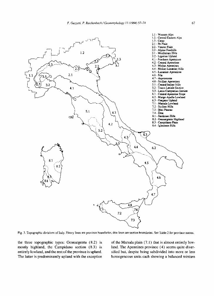
Fig . 3, T o p o g r a p h i c d i v i s i o n s o f Italy. H e a v y l ines are p rov ince boundar ie s , thin l ines are sec t ion boundar ies . See Tab le 2 for p r o v i n c e n a m e s .

the three topographic types: Gennargentu (8.2) is mostly highland, the Campidano section (8.3) is entirely lowland, and the rest of the province is upland. The latter is predominantly upland with the exception

of the Marsala plain (7.1) that is almost entirely lowland. The Apennines province (4) seems quite diversified but, despite being subdivided into more or less homogeneous units each showing a balanced mixture

68 F. Guzzetti, P. Reichenbach / Geomorphology 11 (1994) 57- 74

Table 2 Topographic divisions of Italy (~e also Fig. 3). Percentages of lowland, upland, and highland for the thirty minor topographic divisions of Italy ( from Fig. 4)

Major division Minor division Lowland Upland Highland (~'rovince) (Section) (%) (%) (%)

1 Alpine Mountain System 1.1 Western Alps 0.5 17.2 82.3 1.2 Central-Eastern Alps 0.8 19.3 79.8 1.3 Carso 40.2 59.4 0.3

2 North Italian Plain

3 Alpine-Apennine Transition Zone

4 Apennine Mountain System

5 Tyrrhenian Borderland

6 Adriatic Borderland

7 Sicily

8 Sardinia

2.1 Po Plain 99.3 0.7 0.0 2.2 Veneto Plain 99.8 0.2 0.0 2.3 Alpine Foothills 79.5 20.5 0.0

3.1 Monferrato Hills 53.1 46.9 0.0 3.2 Ligurian Upland 9.5 77.0 13.6

4.1 Northern Apennines 3.4 60.0 36.6 4.2 Central Apennines 1.7 39.9 58.4 4.3 Molise Apennines 1.3 63.1 35.6 4.4 Molise-Lucanian Hills 1.4 86.0 12.6 4.5 Lucanian Apennines 5.1 56.8 38.1 4.6 Sila 17.6 50.7 31.7 4.7 Aspromonte 9.9 67.5 22.6 4.8 Sicilian Apennines 2.3 46.6 51.1

5.1 Central Italian Hills 35.7 61.3 3.1 5.2 Tosco--Laziale Section 72.0 27.7 0.3 5.3 Lazio-Campanian Section 58.6 31.1 10.3

6.1 Central Apennine Slope 24.6 74.6 0.8 6.2 Murge-Apulia Lowland 87.5 12.5 0.0 6.3 Gargano Upland 20.0 80.0 0.0

7.1 Marsala Lowland 96.8 3.2 0.0 7.2 Sicilian Hills 9.6 82.8 7.6 7.3 lblei Plateau 54.2 44.5 1.3 7.4 Etna 36.7 52.1 11.2

8. I Sardinian Hills 22.9 72.0 5. I 8.2 Gennargentu Highland 4.3 41.7 54.0 8.3 Campidano Plain 96.0 4.0 0.0 8.4 Iglesiente Hills 27.8 66.7 5.5

of upland and highland, retains an overall consistency of form. The Central Apenn ines (4 .2) , with the highest

percentage of highland of the province, is the section more similar to the Alps, whereas the Mol i se -Lucan ian

Hills (4.4) with 86% upland shows a characteristic hilly landscape. Lastly, the Adriat ic and Tyrrhenian coastal provinces are a mixture of upland and lowland terrain types that well represent their morphological complexity.

Based on the distr ibution of morphometr ic parame-

ters (Table 1) and in particular on the dispersion of elevation and computed slope (Fig. 5) the 30 topo-

graphic divisions can be grouped into four main classes or terrain types: plains, hills, low mountains , and high mountains. The two e x t r e m e s - - plains and high mountains - - show very distinct morphometr ic attributes representing low and gentle versus high and steep terrain types. Between these two extremes low mounta ins and hills constitute two separate groups.


HIGHLAND

69

1.1

4.2

8.2 A

4.8

2.2" 7.1 6.2

LOWLAND

2.3 5.2

S5"3 ~ / A7'4 5.1

7.3, 1.3 •

4.7

8.4 8.1 &7.2 \ A A \ ~ 6 . 3

UPLAND

m 1. Alpine Mountain System • 2. Northern Italian Plain [] 3. Alpine-Apennine Transition Zone

O4. Apennine Mountain System • 5 . TyrrhenianBorderland O6. Adriatic Borderland

[& 7. Sicily A8. Sardinia

Fig. 4. Topographic divisions of Italy compared by their three constituent types of land-surface form. Few divisions are "purely" highland, upland, or lowland (2.1, 2.2, the Po and Veneto Plains), but none is an equal mixture of the three (4.6, Sila, is closest) or mixes highland with lowland - - which, along with the fair to excellent grouping of ,sections into their provinces ( 1.1 and 1.2, the Alps, and 4.1-4.8, the Apennines) implies a successful parsing of the territory.

P l a i n s - - the Po (2.1) and Veneto (2.2) plains in northern Italy, the Marsala Lowland in Sicily (7.1), and the Campidano Plain in Sardinia (8.3) - - have very low and gentle terrain and show a limited dispersion of both altitude and computed slope (Fig. 5). They are made up almost entirely by lowland (the percentage is greater than 95%) with a complete lack of highland.

The sections within the North Italian Plain province (2.1 and 2.2) extend for 47,500 km z and represent 70% of all Italian lowland areas. They exhibit the lowest dispersions both of altitude (73 and 35 m, respectively) and gradient (0.46 and 0.2, respectively) of the country. Local relief is also very low (11 to 16 m), and

mean slope values are the lowest measured (0.08 ° and 0.03 °, respectively). High values of slope (up to 35 °) associated with sharp curvatures locally identify fluvial escarpments along the Tanaro and Ticino rivers (Fig. 2). The Marsala (7.1) and Campidano (8.3) lowland areas are mostly low and gentle terrain showing slightly higher dispersions of altitude (51 and 42.3 m, respectively) and slope ( 1.58 and 1.34).

H i l l s a re represented by the Adriatic and Tyrrhenian borderlands, the Alpine-Apennine Transition Zone, the Alpine Foothills, and by sections within Sicily and Sardinia. They exhibit a relatively narrow range in the

7O

10

¢3.,

8 e-,

o

• ~ 6

0


ml

1.1

I % a1.2 I ' % .| . . . . . . . . . . . . . . . . . . . . . . . . . . . . . . . . . . . . . . . : . . . . , 4 2 . . . . . . . . . . . . . : . . . . . . . . : . . . . . . . . . . . . . . . . .

I . % 5.3 o I % .

| 8'2 ~ 4 . ' 5

.......................... | .%. , ..................

8.4A | 4A 4.7 ~,.e 3 2-" 8.1 I 4.6 .

- IA: A& O I '174 \ : \ . 6 . 3 1 . . . . . . . . . . . . . . . . . . . . . . . . . . . . . . . . . ! . . . . . . . . . . . . . . . . . . . . . . . . . . . . . . . . . . . :. _\ . .a .

\ !o4. 4 I 6.~o\ [ \ . i~

~ 3.1rl i m 0 \ \ . .'rig7"3 I Low \Mountains _ ,2.3 5.2 ,\ J ~a i l l s Mountains \

. . . . X.. . :.. 6.2ta . . . . ' . . . . . . . . . . . . . . . . . . . . . . . . . . . . . . . . . . . . . . . . . / Low\ , , -

z ~ rim2,1: % /Pl*ins"

0 1~ 2 ~ 3 ~ 400 500 600 700 800 900

Dispersion of Elevation [m]

• I. Alpine Mountain System

04 . Apennine Mountain System

• 7. Sicily

• 2. Nocthem Italian Plain [] 3. Alpine-Al~nnine Transition Zone

• 5. Tyrrhenian Borderland O 6. Adriatic Bocaerla~

A8. Sardinia

Fig. 5. Graph of the dispersion of elevation versus dispersion of computed slope values. Topographic units are grouped into four main terrain types: plains hills low mountains and high mountains (see text).

dispersion of elevation (from a few tens to a few hun- dreds of metres) associated with a much larger dispersion of slope values (from 2 ° to about 6.8°). The frequency distribution of slopes is invariably left skewed with the mode smaller, and locally much smaller, than the mean.

Hills are a mixture of lowland and upland topographic types, highland being only marginally present. Sections where lowland predominates, i.e. where the percentage is greater than 70%, exhibit low dispersion ,d" elevation (80 to 150 m) and computed slope (2.0 ° to 3.4 ° ) (e.g., most of the Adriatic Borderland, the Alpine Foothills). Alternatively, sections where the percentage of upland exceeds 60 have higher dispersion of elevation ( 145-200 m) and much higher dispersion of slope (3.2°-6.9 °) (e.g., part of the Tyrrhenian Bor- derland, the Sardinia Hills, the Iglesiente Hills, the Gar-

gano range). The former represent low and gentle hills, whereas the latter are higher, rolling hills.

Within the hills the Lazio-Campanian section (5.3) can be considered an outlier, in that the dispersion of slope is too large for the dispersion of altitude. Inclusion of the Aversa coastal plain, the Vesuvio and Rocca- monfina volcanoes, and of the Lepini, Aurunci and Ausoni ridges, are responsible for the heterogeneity of the section that partly belongs to the low mountains and partly to the plains. Similarly, the Monferrato Hills (3.1), an almost even mixture of lowland and upland, is the closest to the plain group in Fig. 5, mostly because this section contains part of the Po Plain. In that area the boundary between the two topographic provinces is fuzzy, and not at all definite.

L o w moun ta ins are well represented by the Apen- nines province (4), with the exception of the Molise-

F. Guzzeni, P. Reichenbach / Geomorphology 11 (1994) 57-74 71

Lucanian Hills; and by the Gennargentu Highland ( 8.1 ) in Sardinia. Low mountains are characterised by high percentages of upland, generally greater than 50%, moderately high percentages of highland, generally greater than 30%, and limited percentages of lowland. Dispersion of elevation and gradient are from moderately high to high. The standard deviation of elevation ranges from 335 to over 600 m, and average slope values range from 6 ° to 12 ° . Slope distributions are always left skewed with the mode generally much smaller than the mean. The Central Apennines (4.2) and the Sila (4.6) sections show morphometric values closer to the high mountain sections, the former due to the high dispersion of slope, the latter because of the dispersion of elevation.

The Etna Volcano (7.4) exhibits a unique setting. The standard deviation of altitude is much higher and the dispersion of slope is lower than that of the other sections within the low mountains group. Gradient is also quite low (average value 5.7 ° , mode 2°). This unique combination of large dispersion of elevation with moderate dispersion of slope values makes the Etna Volcano a unique morphometric feature, difficult Io classify within any of our terrain types.

High mountains are represented by the portion of the Alps, Europe's major mountain system, lying within the Italian border ( 19% of Italy). The chain runs for 750 km on a mostly E-W direction, widening from 60 km in the west (Col di Tenda) to 360 km in the east (Tarvisio Pass). The Western (1.1) and the Central- Eastern (1.2) sections show very similar morphometric characteristics. High mountains are about 80% highland, the rest being mostly upland. They are character- i sed by the highest dispersion of both altitude and slope values of the country. Total relief locally exceeds 2000 m, mean slope values reach 19 °, with maximum values of 70 ° , with frequency distributions that are only slightly left skewed. Profile curvature is high and the average frequency of slope direction changes is in the order of 3.3 inversions per km e.

6. Concluding remarks

Topography is a three-dimensional surface of com- plicated geometry and topology. Although land-surface form has been described successfully in rather general

terms, Earth's terrain is much too varied and complex to be neatly categorised by most systems of classification (Evans, 1972). The best path to recognising order in the face of such seeming chaos is to array the surface systematically, into nested components and describe them separately (Hammond, 1964). Such a hierarchical approach to spatial classification is a powerful method for investigating landforms defined by size, order, and geometric complexity (Dikau, 1990).

Adopting the hierarchical model, we partitioned Italy into topographic provinces and sections. Provinces are first-order divisions with distinct or unique geomor- phologic characteristics that distinguish them from neighbouring areas. Boundaries between provinces are easily traced and correspond to major morphological and geological features or coastlines. The North Italian Plain (2) is separated from the Alps and the Apennines by a profound break in slope. The rest of the Apennines (4) are bounded by well-defined geological and morphological limits. The boundary of Sardinia (8) is the coast, whereas Sicily (7) is circumscribed both mor- phologically and by the coast.

Sections are the minor topographic divisions within provinces. Section boundaries are less distinct and generally more open to interpretation. Subdivisions within the Apennines are largely morphological, but visual inspection of small-scale geological maps (Servizio Geologico d'Italia, 1976-1983) shows that they cor- relate with geology as well. This is also true within the Tyrrhenian and Adriatic Borderlands, and in Sicily and Sardinia. Section boundaries are locally arbitrary. The division between Western and Central-Eastern Alps and that between the Po and Veneto Plains have no morphological manifestation. They were adopted to match geographical subdivisions and could possibly be eliminated without compromising the parsing (cf. Table 1, Figs. 4 and 5). Finally, distinct local landscapes can be identified within each section - - e.g., the Rieti and Fucino plains in the Central Apennines, the Apuane range in the Northern Apennines, the Gioia Tauro plain in Calabria, the Catania plain in Sicily - - as well as single geomorphophic features, e.g., the Somma-Vesuvio and Vulture volcanoes.

Topographic units are spatial divisions that ideally should maximise internal homogeneity and between- unit heterogeneity (Fenneman, 1917; Wood and Snell, 1960). Despite all efforts, some of our units are more distinct and easily recognisable than others. Provinces

72 F. Guzzetti, P. Reichenbach / Geomorphology 11 (1994)57-74

bounded by distinct morphological or geological limits (e.g., the Alps, the Apennines, the Northern Italian Plain) are better defined (Figs. 4 and 5) than provinces partially circumscribed by a geographic boundary, such as the coastline (e.g., Sardinia, and partly Sicily).

The proposed divisions reflect real physical, geological and structural differences in the Italian landscape, but they remain provisional and can certainly be refined. Being based to some extent on the visual inspection of the shaded relief, unit boundaries can be expected to change slightly with changes to the shading parameters (Lidmar-Bergstrom et al., 1991; Onorati et al., 1992). Portrayal of the landscape in three dimensions using stereo shaded-relief images, which would improve the perception of terrain form, might refine our division of the Italian state.

A more detailed DEM would permit the description of meso- and microforms (Dikau, 1990) not available for this investigation. A detailed terrain model at 50 m spacing and vertical resolution of 10 cm, between the Ticino and Mincio rivers in the Po Plain, has revealed alluvial fans, meanders, and fluvial escarpments in an area that appears completely flat in this study (Mar- chetti et al., 1993). Likewise, detailed DEMs at 25 m spacing prepared for limited areas in central Italy, have proved effective in describing morphometric and hydrological parameters for landslide hazard assessment (Carrara et al., 1991). Such a 25 m grid for the whole country would contain more than 2 billion elevations, and while awkward to use even on present super-computers, might well prove important in future geomorphometric work on Italy.

The multivariate statistical analysis on which our classification is developed can also be improved. The ansupervised cluster-classification included only a few, highly correlated variables, all but one describing the vertical variability of topography. Such topographic properties as azimuth (aspect) and the topologic arrangement of ridges and valleys, which describe landscape pattern in plan, would vastly improve the numerical taxonomy (Pike, 1988), and thus bring the computer results into closer agreement with the classification that we derived from combined information. Lastly, further improvements in the definition of formal topographic divisions in Italy may include an automated land-surface classification of the entire country, based on the association of different terrain types

(Dikau et al., 1991 ), and its comparison with the semi- quantitative classification created here.

Acknowledgements

The investigation was supported by CNR-GNDCI and CNR-IRPI grants. The digital archive of "Mean Height Values" for Italy was provided by the Italian Geological Survey. We thank William Acevedo and Robert Mark (USGS, Menlo Park) who contributed to the assembling of the DEM and to the multivariate statistical analysis; Mauro Cardinali (CNR-IRPI, Peru- gia), Andrew Hansen (GEO, Hong Kong), and Alberto Carrara (CNR-CIOC, Bologna) for providing ideas and comments on the identification of topographic divisions; Andrew Hansen also reviewed an early version of the manuscript. We are also grateful to Mario Panizza (University of Modena) who reviewed the final draft of the manuscript. We are particularly indebted to Richard Pike (USGS, Menlo Park) whose precious suggestions and illuminating ideas were fun- damental to the success of the project. His comments and thorough review have greatly improved the quality of the manuscript.

This report is CNR-GNDCI Publication No. 1001, and CNR-IRPI Publication No. 200.

References

Ambrosetti, P., Bosi, C., Carraro, F., Garanfi, N., Panizza, M., Papani, G., Vezzani, L. and Zanferrari, A., 1983. Neotectonic map of Italy. CNR, Progetto Finalizzato Geodinamica, Sottopro- getto Neotettonica, Rome, Italy, scale 1 : 500,000, 6 sheets.

Bernknopf, R.L., Campbell, R.H., Brookshire, D.S. and Shapiro, C.D., 1988. A probabilistic approach to landslide hazard mapping in Cincinnati, Ohio, with applications for economic evaluation: Bull. Assoc. Eng. Geol., 25: 39-56.

Beven, K.J. and Moore, I.D. (Editors), 1992. Terrain Analysis and Distributed Modelling in Hydrology: Advances in Hydrological Processes. Wiley, Chichester, 249 pp.

Brabb, E.E., Guzzetti, F., Mark, R.K. and Simpson, R.W., 1989. The extent of landsliding in northern New Mexico. In: P.M. Sadler and D.M. Morton (Editors), Landslide in Semi-arid Environ- ment with Emphasis on the Inland Valleys of Southern Califor- nia. Publ. Inland Geol. Soc., 2: 163-173.

Carrara, A., Cardinali, M., Detti, R., Guzzetti, F., Pasqui, V. and Reicbenbach, P., 1991. GIS techniques and statistical models in evaluating landslide hazard. Earth Surf. Process. Landforms, 16: 427~45.

F. Guzzetti, P. Reichenbach / Geomorphology 11 (1994) 57-74 73

Carrozzo, M.T., Chirenti, A., Luzio, D., Margiotta, C., Quarta, T., Tundo, A.M. and Zuani, F., 1985. Database of mean height values for the whole Italian landmass and surrounding areas-determin- ing and statistical analysis. Boll. Geodesia Sci. Affini, 44: 37- 56.

Castiglioni, G.B., Federici, P.R., Lupia Palmieri, E. and Panizza, M., 1993. Geomorphology in Italy. In: H.J. Walker and W.E. Grabau (Editors), The Evolution of Geomorphology. Wiley, New York, pp. 239-253.

Clarke, J.l., 1966. Morphometry from maps. In: G.H. Dury (Editor), Essays in Geomorphology. Heinemann, London, pp. 235-274.

CNR (Editor), 1973. Modello Strutturale d' Italia. Rome, Italy, scale I : 1,000,000, two sheets.

I)esio, A., 1973. Geologia dell'Italia. UTET, Torino. Italy, 1081 pp. I)ikau, R., 1990. Geomorphic landform modelling based on hierar-

chy theory. Proc. 4th Int. Symp. on Spatial Data Handling, Ztir- ich, Switzerland, July 23-27 1990, Vol. I, pp. 230-239.

Dikau, R., Brabb, E.E. and Mark, R.K., 1991. Landform classification of New Mexico by computer. U.S. Geol. Surv. Open-file Rep. 91-634, 15 pp.

Elliott, D.L., Wendell, L.L. and Gower, G.L., 1991. An assessment of the available windy land area and wind energy potential in the contiguous United States. Richland, WA, Pacific Northwest Lab. Report PNL-7789, 61 pp.

Evans, I.S., 1972. General geomorphometry, derivatives of altitude, and descriptive statistics: In: R.J. Chorley (Editor), Spatial Anal- ysis in Geomorphology. Harper and Row, London, pp. 17-90.

Evans, 1.S., 1980. An integrated system of terrain analysis and slope mapping. Z. Geomorphol. Suppl., 36: 274-295.

Fenneman, N.M., 1917. Physiographic divisions of the United States. Ann. Assoc. Am. Geogr., 6:19-98.12nd ed. 1921.3rd ed. revised and enlarged, 1928, 18: 261-353, with map].

Funicello, R., Parotto, M. and Praturlon, A., 1981. Carta tettonica d'ltalia: scale 1: 1,500,000, CNR Progetto Finalizzato Geodi- namica Publ. No. 269, Rome, Italy.

Hammond, E.H., 1964. Analysis of properties in land form geography: an application to broad-scale land form mapping. Ann. Assoc. Am. Geogr., 54:11-19.

Hlavka, C.A. and Sheffner, E.J., 1988. The California Cooperative Remote Sensing Project. Final Report, Moffett Field, California, Ames Research Center, NASA Technical Memorandum TM- 100073, 98 pp.

Horn, B.K.P., 1981. Hill shading and the reflectance map. Proc. Inst. Electr. Electron. Eng., 69: 14--47.

lstituto Geografico De Agostini (Editor), 1987. Grande Atlante d'ltalia. Novara, Italy, 488 pp.

Lidmar-Bergstrom, K., Elvhage, C. and Ringberg, B., 1991. Land- forms in Skane, South Sweden. Geogr. Ann., 73A: 61-91

Marchetti, M, Guzzetti, F. and Reichenbach, P., 1993. Morphome- tric reconstruction of late-glacial fans along the Alpine Fringe of the Central Po-Plain. Int. Symp. on Dynamics and Fluvial- Coastal System and Environmental Change, San Benedetto del Tronto, Italy, June 22-24, 1993, Poster Session.

Neuenschwander, G., 1944. Morphometrische begriffe, Eine kritis- che ubersicht auf grund der literatur. Univ. Ztirich, Inaugural Dissertation, 135 pp.

Onorati, G., Pascolieri, M., Ventura, R., Chiarini, V. and Crucill~t, U., 1992. The digital elevation model of ltaly for geomorphology and structural geology. Catena, 19: 147-178.

Pike, R.J., 1988. The geometric signature-quantifying landslide-terrain types from digital elevation models. Math. Geol., 20: 491- 511.

Pike, R.J., 1993. A bibliography of geomorphometry. U.S. Geol. Surv. Open-File Rep. 93-262-A, 132 pp.

Pike, R.J. and Thelin, G.P., 1989. Cartographic analysis of U.S. topography from digital data. Proc. Int. Symp. on Computer Assisted Cartography, Auto-Carto 9, ASPRS/ACSM, Baltimore, April 2-7, 1989, pp. 631~:~40.

Pike, R.J. and Wilson, S.E., 1971. Elevation-relief ratio, hypsometric integral, and geomorphic area-altitude analysis. Geol. Soc. Am. Bull., 82: 1079-1084.

Pike, R.J., Acevedo, W. and Thelin, G.P., 1988. Some topographic ingredients of a geographic information system. Proc. Int. Geo- graphic Information Systems Symp., Arlington, VA, November 15-18, 1987, Vol. 2. NASA, Washington, DC, pp. 151-164.

Pike, R.J., Acevedo, W. and Card, D.H., 1989a. Topographic grain automated from digital elevation models. In: Proc. 9th Int. Symp. on Computer Assisted Cartography, Baltimore, April 2-7, 1989. ASPRS/ACSM, pp. 128-137.

Pike, R.J., Guzzetti, F., Mark, R.K., Bortoluzzi, G., Ligi, M., Bennett, B., Acevedo, W. and Thelin, G.P., 1989b. Synoptic maps of Italy's topography from a digital elevation model. Proc. First Workshop lnformatica e Scienze della Terra, Samano, Italy, October 18-20, 1989, Napoli, DeFrede, 27/1-7.

Pike, R.J., Acevedo, W. and Showalter, P.K., 1992. Mapping topographic form by digital image-processing in the San Jos6 1 : 100,000 sheet, California. U.S. Geol. Surv. Open-File Rep. 92-420, 56 pp.

Raisz, E., 1944. Landform map of Italy. Cambridge MA, USA, one sheet, scale about I :5,000,000.

Reichenbach, P., Acevedo, W., Mark, R.K. and Pike, R.J,, 1992. Landforms of Italy, scale 1 : 1,200,000. National Group for Pre- vention of Hydrogeologic Hazards, GNDCI Publ. No. 581, Rome, Italy.

Reichenbach, P., Acevedo, W., Mark, R.K. and Pike, R.J., 1993. A new landform map of Italy in computer shaded relief. Boll. Geo- desia Sci. Affini IGMI, Florence, Italy, 52: 21-44, with fold-out I : 2,000,000 scale map.

Servizio Geologico d'ltalia, 1976-1983. Carta Geologica d'ltalia. Rome, Italy, scale 1 : 500,000, 5 sheets.

Sokal, R.R. and Sneath, P.A., 1963. Principles of Numerical Tax- onomy. W.H. Freeman, San Francisco, 359 pp.

Strahler, A.N., 1952. Hypsometric area-altitude analysis of erosional topography. Bull. Geol. Soc. Am., 63: I 117-1142.

Strahler, A.N., 1956. Quantitative slope analysis. Bull. Geol. Soc. Am., 65: 571-596.

Swain, P,H. and Davis, S.M. (Editors), 1978. Remote Sensing: The Quantitative Approach. McGraw-Hill, New York, 396 pp.

Thornbury, W.B., 1965. Regional Geomorphology of the United States. Wiley, New York, 609 pp.

Thorne, C.R., Zevenbergen, L.W., Butt, T.P. and Butcher, D.P., 1987. Terrain analysis for quantitative description of zero-order basins. In: R.L. Beschta et al. (Editors), Erosion and Sedimen-

7.~ F. Guzzetti. P. Reichenbach / Geomorphology 11 (1994) 57-74

tation in the Pacific Rim. Proc. Corvallis Syrup., August, 1987. IAHS Publ. No. 165, pp. 121-130.

'A cibel, R. and DeLotto, J.S., 1988. Automated terrain classification for GIS modeling. Proc. GIS/LIS '88 Conf., San Antonio, Texas, November 30-December 2, 1988, Vol. 2, pp, 618-627.

Wood. W.F. and Snell, J.B., 1960. A quantitative system for classi- fying landforms. U.S. Army Quartermaster Research and Engi- neering Center, Natick, MA, Tech. Rep. EP-124, 20 pp.

Zevenbergen, L.W. and Thorne, C.R., 1987. Quantitative analysis of land surface topography. Earth Surf. Process. Landforms, 12: 47-56.

Towards a definition of topographic divisions for Italy

Documents

Transcript of Towards a definition of topographic divisions for Italy