Viscous effects on wave generation by strong winds

J. Fluid Mech. (2008), vol. 597, pp. 343–369. c© 2008 Cambridge University Press

doi:10.1017/S0022112007009858 Printed in the United Kingdom

343

Viscous effects on wave generationby strong winds

A. ZEISEL, M. STIASSNIE, AND Y. AGNONDepartment of Civil and Environmental Engineering, Technion – Israel Institute

of Technology, Haifa 32000, Israel

(Received 17 April 2007 and in revised form 28 October 2007)

This paper deals with the stability of water waves in a shear flow. Both temporaland spatial growth rates are derived. A carefully designed numerical solver enablesus to extend the range of previous calculations, and to obtain results for largerwavelengths (up to 20 cm) and stronger winds (up to a friction-velocity of 1 m s−1).The main finding is the appearance of a second unstable mode which often turnsout to be the dominant one. A comparison between results from the viscous model(Orr–Sommerfeld equations) and those of the inviscid model (Rayleigh equations),for 18 cm long waves, reveals some similarity in the structure of the eigenfunctions,but a significant difference in the imaginary part of the eigenvalues (i.e. the growthrate). It is found that the growth rate for the viscous model is 10 fold larger than thatof the inviscid one.

1. Introduction1.1. Background and motivation

The discussion of wave generation in modern science is almost 150 years old, sincethe days of Kelvin, Stokes, Rayleigh and others. The history of scientific publicationson the subject in the 20th century began when Jeffreys (1925) published his shelteringtheory. Major progress was made with the publication of two groundbreaking studiesby Miles (1957a) and by Phillips (1957). These two studies suggest two differentmechanisms for wave generation. Phillips argued that waves can be generated by aresonance mechanism between the air turbulent eddies and the water. He assumedthat the water is an inviscid fluid and the initial water state is rest. Miles proposedthat the growth of waves is caused by interaction of the surface waves with a parallelshear flow. He assumed that the fluids are inviscid and presented Rayleigh’s equationas the governing equation of the problem. In recent years, it has become clear thatthe shorter waves (with a wavelength less than say 20 cm), which contain only a smallfraction of the total energy-density, play a significant role in the overall dynamics. Forthese waves we must include surface tension as well as viscous effects in the analysis.The growth of these shorter waves, under the influence of rather strong winds, is thefocus of this paper.

1.2. Theoretical and numerical references

Valenzuela (1976) provides a comprehensive numerical study of the growth of gravity–capillary waves. He adopts Miles’ approach and solves the coupled air–water stabilityproblem for two viscous fluids with a shear flow. Valenzuela uses finite-differencemethods in order to transform the problem into an algebraic eigenvalue problem.

344 A. Zeisel, M. Stiassnie, and Y. Agnon

Valenzuela uses the lin–log profile in both media as the base flow and showsthat the shear flow in the water cannot be ignored. Kawai (1979) investigates thegeneration of initial wavelets, and combines experimental and theoretical studies.Kawai’s main interest is in the most unstable wave which can grow under a specificfriction velocity. Kawai uses a lin–log wind profile and an error-function-like currentprofile in his calculations. The numerical solution that Kawai uses is based on anintegration of the Orr–Sommerfeld equation using a Runge–Kutta method with afiltering procedure, in order to keep the solution stable. He argues that the linearinstability mechanism controls the process of wave generation from the beginning. VanGastel, Janssen & Komen (1985) study the effect of wind on gravity–capillary wavesusing asymptotic methods. They too solve a pair of Orr–Sommerfeld equations. Theyargue that the growth rate of the initial wavelets (i.e the first waves to be generated)is proportional to u3

∗. Van Gastel et al. (1985) also study the effect of the wind andcurrent profile shape, and find that the growth rate is very sensitive to the windprofile shape; the influence of the current shape is much smaller, but the drift currentand the shear of the current at the interface have a significant influence on thephase velocity. Wheless & Csanady (1993) use compound matrix methods in order tointegrate the Orr–Sommerfeld equation and investigate the stability of short waves.In their calculations, they use an error-function-like wind profile and an exponentialcurrent profile. They also study the effects of wind profile on the growth rate, andargue that the surface tension has a small influence; the growth rate increases whenthe surface tension decreases. Wheless & Csanady try to study the meaning of theeigenfunction’s vertical structure and argue that the perturbation vorticity is ratherhigh; the streamwise surface velocity perturbation in typical cases can be five timesthe orbital velocity of free waves on an undisturbed water surface. Hence, they suggestthat unstable waves should be thought of as a fundamentally different flow structurefrom free waves. Boomkamp et al. (1997) solve the problem of waves on a thin filmof liquid sheared by gas, which is a very similar problem. Boomkamp et al. (1997) usethe Chebyshev collocation method for solving the stability problem. They introduce arobust method which converges easily for many cases and that is easy to apply. Tsai,Grass & Simons (2005) study the spatial growth of gravity-capillary waves shearedby laminar air flow, using experimental and theoretical tools. They use a fourth-orderRunge–Kutta method to integrate the Orr–Sommerfeld equation and some kind offiltering scheme in order to remove parasitic errors. They use a Lock-like profile forboth the wind and the current. Zhang (2005) studies the effects of shear flow onthe stability of short surface waves. He uses an inviscid model, and as a result usesRayleigh’s equation as the governing equation. Zhang proposes a simplified methodin order to obtain an approximate solution. The method which he calls piecewiselinear approximation (PLA), approximates the wind and current profile as linear ina specific segment, and thus the curvature is zero and the equation has a very simpleform. A segment of particular interest is the one that contains the critical point, wherethe base flow is equal to the phase velocity, and Zhang gives this segment specialtreatment. Stiassnie, Agnon & Janssen (2007) also study the instability of water waveswhere the fluids are assumed to be inviscid. They use the so-called regular approachin order to avoid the critical point when integrating Rayleigh’s equation. The resultsof their calculation are similar to those of previous calculations for friction velocityto phase velocity ratio smaller than 2, (u∗/c0 < 2); however, for friction velocityto phase velocity ratio larger than 2, they obtain a maximum in the growth rate,which does not appear in previous studies. They study both temporal and spatialgrowths.

Viscous effects on wave generation by strong winds 345

1.3. Experimental references

Larson & Wright (1974) provide a comprehensive experimental study of the temporalgrowth of gravity–capillary waves. They use microwave backscatter as a measurementtechnique. Larson & Wright find that the growth rate is independent of the fetch,dependent on the wavenumber and varies with u∗ like a power law. Caulliez, Ricci& Dupont (1998) study experimentally the first visible ripples that appear on thewater surface. They argue that the laminar–turbulent transition of the near-surfacewater flow causes an explosive growth of the wind-generated ripples. As previouslymentioned, Tsai et al. (2005), also perform experimental studies of the spatial growthof gravity–capillary waves. They measure a laminar wind profile at varying fetchesand emphasize the development of the boundary layer with fetch. In all these papers,the subject of the wind velocity profile is a dominant issue and a variety of profilesis used.

1.4. Wind profile studies

Charnock (1955) measures the air mean velocity profile above a large reservoir. Hefinds that the air flow fits a logarithmic law. Miles (1957b) suggests an approximationto the solution of the boundary-layer equation which has a linear zone and alogarithmic-like profile. Many authors find this profile useful because of its smoothfirst derivative for all values of u∗ and matching height between the linear and thelogarithmic regions. Most of the field measurements were conducted at low windspeeds. As evidence of the nature of air flow above water at high-speed wind, wecan cite Powell, Vickery & Rienhold (2003) who made field measurements in tropicalcyclones. They found that the wind profile correlates very well with the logarithmicshape in the first 200 m.

2. Mathematical formulation2.1. Linear stability model

The starting point is the governing equations for an incompressible viscous fluid flow,which are the Navier–Stokes and continuity equations.

ρ

(∂V∂t

+ V · ∇V)

= −∇P + µ∇2V + gρ, (2.1)

∇ · V = 0. (2.2)

We write the velocity and the pressure fields as:

V = (U (z) + u(x, z, t), v(x, z, t)), (2.3)

P = p0 − ρgz + p(x, z, t). (2.4)

Where U (z) is the mean flow profile, u, v and p are harmonic perturbations of thehorizontal velocity, vertical velocity, and pressure, respectively; in the above equationsx and z are the horizontal and vertical coordinates, respectively, and t is the time;g, µ, ρ are the acceleration due to gravity, dynamic viscosity and density, respectively.We can separate the equations into harmonic terms and steady terms, and apply theassumption that the perturbations are infinitesimal, in order to linearize them. Sincewe are looking for a solution which has a harmonic part and a vertical dependentpart, we write:

u = u(z)ei(kx−ωt), v = v(z)ei(kx−ωt), p = p(z)ei(kx−ωt), η = η0ei(kx−ωt). (2.5)

https://www.researchgate.net/publication/45940780_On_the_spatial_linear_growth_of_gravity-capillary_water_waves_sheared_by_a_laminar_air_flow?el=1_x_8&enrichId=rgreq-c7660f99-5e04-4b30-8d4e-12526d02518f&enrichSource=Y292ZXJQYWdlOzIzMTk2NDU0MTtBUzoxMDE5Nzc3ODI0ODkwODlAMTQwMTMyNDgwNjI4Mw==


Where ω, k, η are the wave frequency, wavenumber and interface elevation,respectively. We can define a perturbation streamfunction which has the form:

ψ = f (z)ei(kx−ωt), (2.6)

where f (z) is the auxiliary function, and the relations between the streamfunctionand the velocity components give:

v = −ikf (z), u = f ′(z). (2.7)

The prime denotes vertical differentiation. After a simple elimination process, we findthat the governing ODE for f (z) is the Orr–Sommerfeld equation:

iν(f (4) − 2k2f ′′ + k4f ) + k[(U − c)(f ′′ − k2f ) − U ′′f

]= 0, (2.8)

where ν and c are the kinematic viscosity and the phase velocity, respectively. Thedomains of the air and water are assumed to be semi-infinite, and we have boundaryconditions at positive or negative infinity and at the interface between the fluids. Atinfinity, the perturbations are assumed to decay exponentially. At the interface, weimpose the kinematic boundary condition, horizontal velocity continuity, shear stresscontinuity and the dynamic boundary condition (continuity of normal stress). All ofthe boundary conditions are imposed at z = 0, after the linearization procedure. Forthe full formulation of the boundary conditions see Valenzuela (1976). We choosethe reference problem of linear water waves without wind and current, neglecting theinfluence of the air, for which the wavenumber and the wave frequency are relatedby:

ω20 = gk0 +

σk30

ρw

, (2.9)

where σ is the surface tension. Transforming to dimensionless quantities (note thatthe circumflex in (2.10) denotes a dimensional quantity):

ω =ω

ω0

, k =k

k0

, c =c

c0

,

z = zk0, U =U

c0

, f =f k0

η0ω0

.

(2.10)

Defining the dimensionless numbers of the problem:

Rw,a =c0

νw,ak0

, F =1

F 2r

=gk0

ω20

, W =1

We

=σk3

0

ρwω20

, ρ =ρa

ρw

, µ =µa

µw

, (2.11)

where R is the Reynolds number, F is the inverse square Froude number, W is theinverse Weber number, ρ is the density ratio and µ is the dynamic viscosity ratio.The subscripts w and a refer to water and air, respectively. The complete eigenvalueproblem must satisfy the following system:Two ODEs:

iR−1w

(f (4)

w − 2k2f ′′w + k4fw

)︸︷︷︸Viscous terms

+k[(Uw − c)

(f ′′

w − k2fw

)− U ′′

wfw

]= 0, z ∈ (−∞, 0],

(2.12)

iR−1a

(f (4)

a − 2k2f ′′a + k4fa


+k[(Ua − c)

(f ′′

a − k2fa

)− U ′′

a fa

]= 0, z ∈ [0, ∞). (2.13)

https://www.researchgate.net/publication/231873798_The_growth_of_gravity-capillary_waves_in_a_coupled_shear_flow?el=1_x_8&enrichId=rgreq-c7660f99-5e04-4b30-8d4e-12526d02518f&enrichSource=Y292ZXJQYWdlOzIzMTk2NDU0MTtBUzoxMDE5Nzc3ODI0ODkwODlAMTQwMTMyNDgwNjI4Mw==


Nine boundary conditions:

fa(0) = c − U (0), fw(0) = c − U (0), (2.14)

f ′w + U ′

w = f ′a + U ′

a at z = 0, (2.15)

µ(f ′′a + k2fa + U ′′

a ) = (f ′′w + k2fw + U ′′

w) at z = 0, (2.16)

kf ′w(c − U0) + kfwU ′

w + iR−1w

(3k2f ′

w − f ′′′w


−kF

= ρ

⎡⎢⎣kf ′

a(c − U0) + kfaU′a + iR−1

a

(3k2f ′

a − f ′′′a


−kF

⎤⎥⎦ + Wk3 at z = 0, (2.17)

fw(z) → 0, f ′w(z) → 0, z → −∞, (2.18)

fa(z) → 0, f ′a(z) → 0, z → ∞. (2.19)

When formulating the inviscid model, we neglect the viscous terms in (2.12) and (2.13)and obtain two Rayleigh equations. The boundary conditions will be the kinematicboundary condition in the same form (2.14), and the dynamic boundary conditionwithout the viscous terms (2.17). Conditions (2.15) and (2.16) do not apply whenformulating the inviscid case. Both the viscous and inviscid models are classified aseigenvalue problems. The calculations will focus on the temporal and spatial cases,meaning that the growth can be only either in space, or in time. For the temporalcase we specify k and search for ω, and for the spatial case we specify ω and searchfor k.

2.2. Mean flow profile

In (2.12) to (2.19), U (z) represents the mean flow profile. It is already well known(Kawai 1979; Van Gastel et al. 1985; Wheless & Csanady 1993), that the results aresensitive to the profile shape. The exact mean flow profile above water waves is stilluncertain. Miles (1957b) suggests a profile which fits well the mean flow profile abovea flat plate. This profile was used in previous studies Valenzuela 1976; Kawai 1979;Van Gastel et al. 1985), and was named the ‘lin–log’ profile. We use this profile forthe air, and an exponential profile for the current in the water.In the air (wind profile):

Ua =

⎧⎪⎨⎪⎩

U0 +u2

∗νa

z, z � z1,

U0 + mu∗ +u∗

κ

[α − tanh

(α

2

)], z � z1,

(2.20)

and in the water (current profile):

Uw = U0 exp

(ρau

2∗

U0µw

z

)(2.21)

where,

α = sinh−1(β), β =2κu∗

νa

(z − z1), z1 =mνa

u∗, U0 = Bu∗, m = 5, B = 0.5, (2.22)

where u∗ is the friction velocity. The wind profile has a linear segment with a possibleoffset (drift current) and a segment that is asymptotically logarithmic. The parameter


0 2 4 6–2

0

2

4

6

8

10

Ua (m s–1) Ua (s–1) Ua (m–1 s–1)

z (m

)

(a)

0 5000 10000 15000

(b)

–10 –5 0

(c)u* = 0.1 (m s–1)

u* = 0.3 (m s–1)

u* = 0.5 (m s–1)

(×107)

(×10–4)

–2

0

2

4

6

8

10(×10–4)

–2

0

2

4

6

8

10(×10–4)

Figure 1. The base flow and its first two derivatives for the linear–logarithmic profile andvarious values of u∗ (m= 5). (a) The velocity profile, (b) the first derivative, (c) the secondderivative.

m in (2.22) defines the thickness of the viscous sublayer (the linear segment), andthus influences the derivative at the interface. This profile enables continuity of thefunction and its first two derivatives at the matching point z = z1 for all values of theparameters m and U0. The value of m is set to 5 (usually m =5−8), whereas the valueof B is chosen to be B = 0.5 according to Kawai (1979), this value can sometimes betaken as B = 0.3 as found by Zhang & Harrison (2004), but qualitatively it would notchange the results. The value of B controls the drift current, but also influences thederivatives of the current. This profile, in (2.20) and (2.21), maintains the continuityof the shear stress between the air and the water, µaU

′a =µwU ′

w .As can be seen in figure 1, the friction velocity u∗ defines the wind intensity as

well as the current profile. The first and second derivatives have discontinuities atthe interface, but are continuous in the air. The first two derivatives have increasingabsolute values as u∗ increases.

2.3. Alternative wind profile

As an alternative wind profile, we present a wind profile which will enable us tocompare the inviscid and viscous solutions under strong winds. This profile is basedon the numerical solution of the turbulent boundary-layer equation, which is:

µa

dU

dz︸︷︷︸Laminar stress

+ ρaκ2z2

(dU

dz

)2

︸︷︷︸Turbulent stress

= τ0 = ρau2∗. (2.23)

The equation is based on Prandtl’s mixing-length theory. The numerical solutionproduces a profile which is very similar to the lin–log profile, but with a much thinnerviscous sublayer. This profile has zero curvature only at z = 0. The current (waterflow) used is exactly the same as in (2.21). Note that the parameter m is not needed,and the parameter B = 0.5. The meanings of the other parameters are the same as in

https://www.researchgate.net/publication/231915892_Generation_of_initial_wavelets_by_instability_of_a_coupled_shear_flow_and_their_evolution_to_wind_waves?el=1_x_8&enrichId=rgreq-c7660f99-5e04-4b30-8d4e-12526d02518f&enrichSource=Y292ZXJQYWdlOzIzMTk2NDU0MTtBUzoxMDE5Nzc3ODI0ODkwODlAMTQwMTMyNDgwNjI4Mw==


(×107)0 2 4

–2

0

2

4

6

8

10

Ua (m s–1) Ua (s–1) Ua (m–1 s–1)

z (m

)(a)

0 5000 10000 15000

(b)

–10 –5 0

(c)u* = 0.1 (m s–1)

u* = 0.3 (m s–1)

u* = 0.5 (m s–1)

(×10–4)

–2

0

2

4

6

8

10(×10–4)

–2

0

2

4

6

8

10(×10–4)

Figure 2. The base flow and its first two derivatives from the numerical integration of theboundary-layer equation for various values of u∗. (a) The velocity profile, (b) the first derivative,(c) the second derivative.

§ 2.2. The benefit from this kind of profile is that it enables to compare the viscousand inviscid solutions at any wind intensity. We named this profile the ‘numerical’profile. The profile and its derivatives are described in figure 2; it is very similar tothe lin–log profile, but with a much thinner viscous sublayer.

3. Numerical procedure and its validation3.1. Numerical procedure

The numerical procedure which we used to solve the eigenvalue problem of the viscousmodel is based on the Chebyshev collocation method. We chose this method becauseof the difficulties in the integration of the Orr–Sommerfeld equation, which forcedsome of the previous authors to use filters in order to remove parasitic errors. Anotherreason for this choice is the nature of the Chebyshev grid which is characterized bya high density of grid points near the boundaries. The Chebyshev grid is:

xj = cos

(jπ

N

)∀j = 0, 1, . . . , N. (3.1)

The method approximates an unknown function by a finite series of Chebyshevpolynomials see (Trefethen 2000).

φ(x) =

N∑n=0

anTn(x). (3.2)

Chebyshev expansions are done in the interval [−1, 1], where the Chebyshevpolynomials are orthogonal. In the numerical solution, the computational domainwas divided into three finite subintervals. This subdivision is similar to that ofBoomkamp et al. (1997). The size of the finite interval is set to be z∞ =10, which


Air2

Air1

Water

z = z∞

z = z∞

z = z1z = 0

Figure 3. Computational domain of the problem.

means that zdimensional,±∞ ≈ ± 1.6λ, where λ=2π/k0 is the reference wavelength. Thelower interval is for the water, the upper layer (air2) is for the logarithmic air region,and the intermediate interval (air1) is for the viscous sublayer region (see figure 3).Linear transformations are used to transform each interval into [−1, 1], which iswhere the Chebyshev polynomials are orthogonal.

Since the problem at hand is an eigenvalue problem, we search for a pair ω, k whichcauses the solution to obey all 9 boundary conditions. An iterative process to find thiseigenvalue was built. This process begins with an initial guess for the eigenvalue; thenext stage is to solve the coupled BVP (boundary value problem) and finally to use astandard secant method to produce an improved guess. The process is stopped whena convergence condition, requiring four significant digits in the imaginary part of theeigenvalue, is satisfied. The Chebyshev collocation method is used for the solutionof the BVP. This search process provides only one eigenvalue at a time; the specificeigenvalue which the process converges to depends on the initial guess. This approachis different from the one of solving the generalized eigenvalue problem and findingall of the eigenvalues, see Boomkamp et al. (1997).

In practice, we reduce the order of the Orr–Sommerfeld equation by definingV � f ′′ and replacing the Orr–Sommerfeld equation with the system:

V − f ′′ = 0, (3.3a)

iR−1(V ′′ − 2k2V + k4fa) + k[(Ua − c)(V − k2fa) − U ′′

a fa

]= 0. (3.3b)

The next step is to transform the differential equations into an algebraic form withthe help of the Chebyshev differentiation matrices. We solved the BVP with all of theboundary conditions, except for the dynamic boundary condition (2.17). In practicewe, add an artificial interface between the air1 domain and the air2 domain, andactually solve three coupled Orr–Sommerfeld equations. The boundary conditionsbetween air1 and air2 are similar to the boundary conditions between the water andair in their physical meaning; but since the density, viscosity and the base flow arecontinuous, they are written as:

fa2(z1) = fa1(z1), f ′a2(z1) = f ′

a1(z1), f ′′a2(z1) = f ′′

a1(z1), f ′′′a2(z1) = f ′′′

a1(z1). (3.4)

The iterative process is built for the function G(ω, k), which is defined as:

G(k, ω) = kf ′w(c − U0) + kfwU ′

w + iR−1w (3k2f ′

w − f ′′′w ) − kF

− ρ[kf ′


a (3k2f ′a − f ′′′

a ) − kF]

− Wk3 at z = 0. (3.5)

G =0 is the dynamic boundary condition, see (2.17). Using the function G, we candefine the dynamic boundary condition plot. A dynamic boundary condition plot isa plot of the isolines of ‖G‖2 in the complex ω (or k) plane. The function G is a


u ∗ = 0.3m s−1 , λ= 0.01m temporal case lin log wind profile exponential current

Na1 M = 2.2 M = 1

30 1.35384 + 0.017398i 1.35748+ 0.014870i50 1.35360 + 0.017512i 1.35344+ 0.017645i70 1.35360 + 0.017512i 1.35358+ 0.017526i90 1.35360 + 0.017512i 1.35360+ 0.017509i

110 1.35360 + 0.017512i 1.35360+ 0.017512i130 1.35360 + 0.017512i 1.35360+ 0.017512i

ual = 1m s−1, λ= 0.2m temporal case lin log–wind profile exponential current

Na1 M = 2.2 M = 1.5

120 0.79809 + 0.59893i 2.20140+ 0.12182i140 0.51149 + 1.01276i 1.74337+ 0.22800i160 0.48421 + 1.12226i 1.19489+ 0.39902i180 0.48430 + 1.12786i 0.71359+ 0.66407i200 0.48834 + 1.11202i 0.52574+ 0.96493i220 0.49267 + 1.09481i 0.49011+ 1.09063i240 0.49585 + 1.08125i 0.48329+ 1.12708i260 0.49821 + 1.07237i 0.48389+ 1.12925i

Table 1. Convergence of the Chebyshev collocation method for two wind intensities andwavelengths, temporal case. Where Na1 = Nw, Na2 = MNa1. (Values of ω.)

property of the BVP, and, to a certain extent, it defines the distance between a chosensolution of the BVP and that of the eigenvalue problem. Note that all the results inthis paper were calculated using the following numerical values:

κ = 0.41, µw = 10−3pa s, µa = 1.83 10−5pa s,

ρa = 1.225kgm−3, ρw = 1000kg m−3, g = 9.81ms−2, σ = 0.075Nm−1

}(3.6)

3.2. Validation of the numerical results

In this section we will show the convergence of the Chebyshev collocation method,test the sensitivity of the model to the interval size and compare the results with atest case and previous studies. An analytical solution for the viscous problem with alinear wind profile and a constant current is given in the Appendix, and serves as thetest case.

3.2.1. Convergence of the Chebyshev collocation method

As mentioned above, the computational domain is divided into three sub intervals:the water [−z∞, 0], the air1 [0, z1] and the air2 interval [z1, z∞]. In each of theseintervals we can control the number of collocation points (the grid). If the methodconverges, the change in the results should be minor when changing the number ofcollocation points. From numerical experiments, we learn that the interval air1 isthe most important interval and therefore requires a high resolution grid. We showconvergence, for the case where the number of collocation points in the interval air1Na1 is equal to those in the water Nw , and the number of collocation points in air2will be Na2 = MNa1, where M is a parameter (see table 1). As we can see from thedata in the table, the process converges up to at least two significant digits. Of course,the case of longer wavelength and high wind intensities required more grid points.Note that differences between M = 1, 1.5 to M = 2.2 are of the order of 1%.


u∗ = 0.3 m s−1 λ= 0.01 m u∗ = 0.8 m s−1 λ= 0.01 m

z∞ = 5 1.35357+ 0.017523i 1.55164 + 0.22261iz∞ = 10 1.35360+ 0.017512i 1.55166 + 0.22260iz∞ = 15 1.35360+ 0.017512i 1.55166 + 0.22260iz∞ = 20 1.35360+ 0.017512i 1.55166 + 0.22260i

Table 2. The sensitivity of ω to different z∞, temporal case, lin–log wind profile, exponentialcurrent.

Temporal case

λ= 0.001m λ= 0.1m λ= 0.2m

u∗ = 0.001 m s−1 Numerical 1.0705 − 0.017431i 1.1246+ 0.0071116i 1.0908 + 0.0091061iAnalytical 1.0705 − 0.017431i 1.1246+ 0.0071115i 1.0908 + 0.0091070i

u∗ = 0.005 m s−1 Numerical 1.3628 − 0.016102i 1.7260+ 2.2254i 1.7684 + 2.5485iAnalytical 1.3628 − 0.016102i 1.7262+ 2.2254i 1.7680 + 2.5489i

u∗ =1ms−1 Numerical 1.7132 − 0.000028672i 0.47194 − 7.6548i 5.3226 + 8.4767iAnalytical 1.7132 − 0.000029147i 0.46973 − 7.6153i 5.3219 + 8.4752i

Table 3. Comparison with test case, temporal case for various wind intensities andwavelength. (Values of ω.)

3.2.2. Sensitivity to z∞

Since, in practice, we need to use a finite interval for the numerical calculations,we must show that our choice does not have a major effect on the results. The z

coordinate is normalized by k0 in the form z = zdimensionalk0. From a physical aspect,the value of z∞ should be related to the wavelength. From linear theory of waterwaves, it is known that at depths below half a wavelength, the influence of the waveson the flow field is minor. The value which we use for most of our calculations isz∞ = 10, which means that z∞,dimensional = 10λ/(2π) = 1.591λ. In order to justify thisvalue, we made a few runs with different values of z∞. Note that in this method, whenwe change the interval size we need to change the number of collocation points inorder to keep a fine grid in the critical region. From table 2 we can state that if thereis an error it is in the fourth digit.

3.2.3. Comparison with the test case

In order to validate the numerical results, we want to compare them with ananalytical solution. The case which we compare them with is the one mentioned atthe beginning of § 3.2. The analytical solution of this case is based on a combinationof Airy and exponential functions, thus the numerical solution is not so trivial,for details see Appendix. Such a comparison has significant meaning, because themethods which were used to obtain the results are completely different from eachother. The comparison was made for the spatial case, as well as for the temporal case.The current was constant with the value of Uw = 0.5u∗ and the velocity slope of thewind was u∗/νa . These conditions are similar to those which were used in the lin-logprofile. The results are described in table 3. The maximum error in this comparisonis 2%, whereas in most of the cases the error is smaller than 1%.

3.2.4. Comparison with previous studies

The last stage in the validation process will be a comparison with previouscalculations of Kawai (1979), Van Gastel et al. (1985) and Tsai & Lin (2004).


1 3 5 7 90

1

2

3

k (cm–1)

2β (

s–1)

u* = 0.13 m s–1

u* = 0.17 m s–1

u* = 0.214 m s–1

u* = 0.248 m s–1

Figure 4. Energy growth rate vs. wavenumber, temporal case. Comparison with previousstudies. Solid line, our study; five point star, results from Tsai & Lin (2004), (analogous tofigure 2 in Tsai & Lin 2004).

They all compute similar values for the temporal growth rate, but for a rather smalldomain in the (λ, u∗)-plane. Figure 4 is analogous to figure 2 in Tsai & Lin (2004).

In figure 4, there are symbols of our calculations and symbols of Tsai & Lin’scalculations taken from figure 2 in Tsai & Lin (2004). We can see that the resultsof Tsai & Lin (2004) are similar to our results; the difference is up to 5%, but istypically of the order of 1%. For the spatial case, we are not familiar with previousstudies to which it may be compared. Finally, it seems safe to say that for the rangeof λ ∈ (0.001, 0.2) m, u∗ ∈ (0, 1) m s−1, our numerical results are reliable. In mostcases, accuracy is to the first four digits, whereas in the more difficult cases it is onlyto the first two significant digits.

4. A second eigenvalue at high wind intensities4.1. Results for the temporal case

A number of studies concerning the surface wave stability problem have beenconducted (e.g. Valenzuela 1976; Tsai et al. 2005 and references therein). All ofthe results that we found were limited in wind intensity and in wavelength/waveperiod. Most of the theoretical studies focus on the temporal case, except for Tsaiet al. (2005) which deals with spatial evolution for a laminar base flow. The domainof previous calculations in the range of approximately, wavelength 0 < λ< 7 cm, andfriction velocities 0 <u∗ < 0.5m s−1, is plotted in figure 5. As described in § 3.2, oursolver for the viscous problem is valid in the domain 0 < λ< 20cm, 0 <u∗ < 1m/sec

(the entire region of figure 5). The calculations were done using several types ofprofiles for the temporal case as well as for the spatial case. From previous studies, welearn that for each scenario there can be only one unstable mode. This unstable modewas calculated by several authors and has been confirmed by our calculations (seefigure 4). Since the problem is an eigenvalue problem, it is reasonable to search formore eigenvalues. However, we are dealing with a physical problem, and the physicalmeaning is also important. When we began to expand the domain of calculations, wediscovered the presence of a second unstable mode. In certain cases, this can meanthat for a given wavelength and wind intensity, there are two kinds of unstable waveswith different growth rates and different phase velocities. As described in figure 5, the


0.04 0.08 0.12 0.16 0.200

0.2

0.4

0.6

0.8

1.0λ = 0.04 m λ = 0.12 m λ = 0.18 m

u* = 0.3 m s–1

u* = 0.6 m s–1

u* = 0.8 m s–1

Previous studies

One unstable mode

Two unstable modes

Rayleigh's equation does not produces growth

u * (m

s–1

)

λ (m)

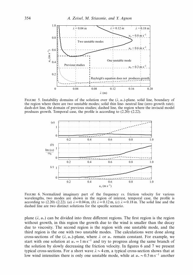
Figure 5. Instability domains of the solution over the (λ, u∗)-plane. solid line, boundary ofthe region where there are two unstable modes; solid thin line- neutral line (zero growth rate);dash-dot line, the domain of previous studies; dashed line, the region where the inviscid modelproduces growth. Temporal case, the profile is according to (2.20)–(2.22).

0.2 0.4 0.6 0.8 1.00

1

(a)

Im (ω)——–ω0

u* (m s–1)

0.2 0.4 0.6 0.8 1.00

1(b)

0.2 0.4 0.6 0.8 1.00

1(c)

Figure 6. Normalized imaginary part of the frequency vs. friction velocity for variouswavelengths, two modes are shown in the region of interest, temporal case, the profile isaccording to (2.20)–(2.22). (a) λ= 0.04 m, (b) λ= 0.12m, (c) λ= 0.18 m. The solid line and thedashed line are two distinct solutions for the specific scenario.

plane (λ, u∗) can be divided into three different regions. The first region is the regionwithout growth, in this region the growth due to the wind is smaller than the decaydue to viscosity. The second region is the region with one unstable mode, and thethird region is the one with two unstable modes. The calculations were done alongcross-sections of the (λ, u∗)-plane, where λ or u∗ remain constant. For example, westart with one solution at u∗ = 1 m s−1 and try to progress along the same branch ofthe solution by slowly decreasing the friction velocity. In figures 6 and 7 we presenttypical cross-sections. For a short wave λ∼ 4 cm, a typical cross-section shows that atlow wind intensities there is only one unstable mode, while at u∗ ∼ 0.5 m s−1 another


0.2 0.4 0.6 0.8 1.0

2.0

1.0

(a)

Re (ω)——–ω0

u* (m s–1)

0.2 0.4 0.6 0.8 1.0

0.5

1.0

0.5

1.0

(b)

0.2 0.4 0.6 0.8 1.0

(c)

Figure 7. Normalized real part of the frequency vs. friction velocity for various wavelengths,two modes are shown in the region of interest, temporal case, the profile is according to(2.20)–(2.22). (a) λ= 0.04 m, (b) λ= 0.12 m, (c) λ= 0.18 m. The solid line and the dashed lineare two distinct solutions for the specific scenario.

0.04 0.08 0.12 0.16 0.20

1.0

0.5

0

0

0.04 0.08 0.12 0.16 0.200

0.04 0.08 0.12 0.16 0.200

(a)

Im (ω)——–ω0

λ (m )

0

0.2

–0.2

–0.02

0.4

0.06

0.020

(b)

(c)

Figure 8. Normalized imaginary part of the frequency vs. wavelength for various frictionvelocities, two modes are shown in the region of interest, temporal case, the profile is accordingto (2.20)–(2.22). (a) u∗ = 0.8m s−1, (b) u∗ = 0.6 m s−1, (c) u∗ = 0.3m s−1. The solid line and thedashed line are two distinct solutions for the specific scenario.

mode becomes unstable. We can see that the lines cross each other in the imaginarypart, but in the real part these two lines never intersect. At longer wavelengths, theline of the second unstable mode passes the zero growth level at a stronger wind, andthen turns back and becomes stable; at even longer wavelengths the second mode isalways stable. When looking at the real part of the same results, figure 7, we can seethat, for the short waves, the lines of the separate modes never cross each other, whilein longer waves the lines intersect. The meaning of these intersection points is thatthere are two waves with the same wavelength and wave frequency, but with differentgrowth rates. When looking at the cross-sections along λ (see figures 8 and 9), we


0.04 0.08 0.12 0.16 0.20

1.5

1.0

0.5

1.5

1.0

0.5

1.4

1.2

1.0

0

0.04 0.08 0.12 0.16 0.200

0.04 0.08 0.12 0.16 0.200

(a)

Re (ω)——–ω0

λ (m )

(b)

(c)

Figure 9. Normalized real part of the frequency vs. wavelength for various friction velocities,two modes are shown in the region of interest, profile is according to (2.20)–(2.22). (a)u∗ = 0.8m s−1, (b) u∗ = 0.6 m s−1, (c) u∗ = 0.3 m s−1. The solid line and the dashed line are twodistinct solutions for the specific scenario.

0.04 0.08 0.12 0.16 0.200

40

80

120

160

λ (m)

Im (ω

) (s

–1)

Figure 10. Temporal growth rate vs. wavelength, u∗ = 1 m s−1, the profile is according to(2.20)–(2.22). The solid line and the dashed line are two distinct solutions for the specificscenario.

can distinguish a few characteristics of the solution. First, at low wind intensities,there is only one unstable mode for every wavelength, while at stronger winds, abovea critical value, there are two unstable modes in a range of wavelengths. For example,see the lines of u∗ = 0.6 m s−1, 0.8 m s−1 in figure 8. All of the lines in the figure ofthe imaginary part are characterized by one maximum point. These maximum pointsdescribe the most unstable wave, but since figure 8 presents the normalized quantityit is simpler to look at the dimensional figure (see figure 10). When there are twolines, it is typical that the maximum point of the second unstable mode occurs at alonger wavelength. Another point that may be of some interest is the point of zerogrowth (neutral point) on the left-hand side, which indicates the shortest wave thatcan be generated. In this aspect, again, the lines of the second unstable mode start to


0 5 10–1.0

–0.8

–0.6

–0.4

–0.2

0

0.2

0.4

0.6

0.8

1.0

| f |/η0 (m s–1)

z (m

)(a) (b) (c)

1 2 3arg( f )

0 5 10 15ρ(u2 + v2)/2η0

2 (kg m–2 s–2) (×108)

branch1 ω = 1.17 + 0.14i

critical point

branch2 ω = 0.43 + 0.71i

critical point

z1

–1.0

–0.8

–0.6

–0.4

–0.2

0

0.2

0.4

0.6

0.8

1.0

z1

–1.0

–0.8

–0.6

–0.4

–0.2

0

0.2

0.4

0.6

0.8

1.0

z1

(×10–3) (×10–3) (×10–3)

Figure 11. Comparison of the vertical structure of the eigenfunction and the kinetic energydensity between the two modes for λ= 0.04 m, u∗ = 0.7 m s−1, temporal case, profile is accordingto (2.20)–(2.22). (a) absolute value of the eigenfunction, (b) argument of the eigenfunction, (c)kinetic energy density.

produce growth for longer wavelengths. The results for both, the point of maximumgrowth and the neutral point, are very intuitive and show that: when increasing thewind intensity, the value of maximum growth becomes larger and the wavelengths ofmaximum growth and zero growth become shorter. The real part of the eigenvalue,described in figure 9, shows a major difference between these two branches of thesolution. While one of the branches has a phase velocity which is often higher thanthe reference case, (Re(ω)/ω0 > 1), the second branch has a phase velocity which islower than the reference case, (Re(ω)/ω0 < 1). The result that the phase velocity ofthe wave usually decreases when the friction velocity increases is not very intuitive.This result was also obtained by Valenzuela (1976).

In figure 10 the temporal growth rate is presented in dimensional form. As we cansee, the values of the growth rate are very large, especially for waves in the gravity–capillary range. These ‘explosive’ growth rates which can exist in very strong winds(u∗ = 1 m s−1, i.e. U10 = 37 m s−1), indicate that these ripples attain their maximumsteepness almost immediately, and break continuously.While comparing the eigenfunctions of both modes in figure 11, we can see asignificant similarity in the air region, but a profound difference in the water region.The horizontal dashed line in this figure indicates the edge of the laminar layer, andit is clear that most of the energy transfer from the mean flow to the disturbancehappens within this layer. The square and circle symbols indicate the location of theso-called critical point, where the mean flow velocity is equal to the actual phasevelocity. We can see that the critical-points, for both modes, are in the water and thatthey do not play any significant role in the case at hand.

After finding the second unstable mode, we try to characterize the conditions forthe existence of this mode. We cannot formulate a complete condition yet, but we


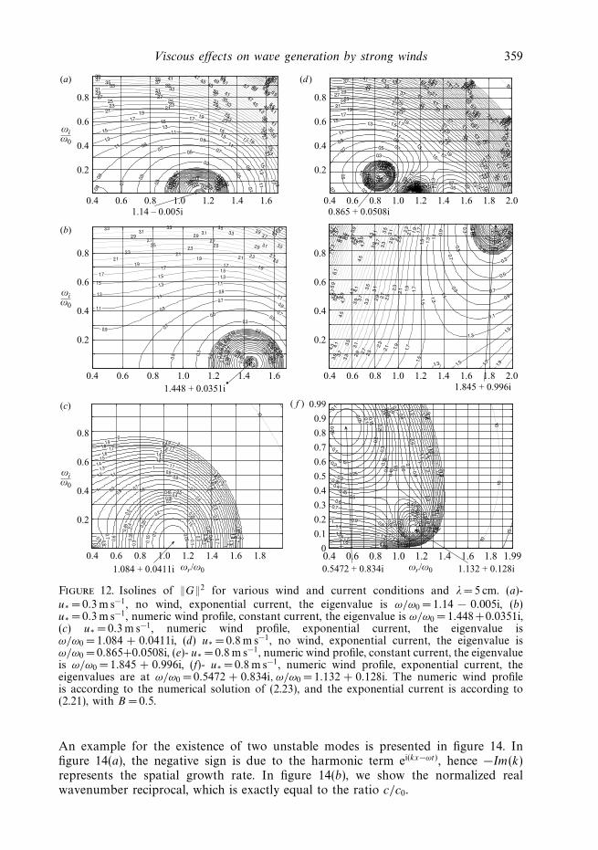
can state that the second unstable mode appears only when the mean flow profileincludes a shear current. Another condition is that the wind intensity will be above acritical value. The results in the figures were calculated for a specific lin–log profile(m =5, B = 0.5 see (2.22)), the parameter B which controls the drift current has amajor influence on the critical conditions for the appearance of the second mode. Inorder to identify the conditions that influence the appearance of the second unstablemode, we have tried many combinations of wind profiles/intensities and currentprofile/intensities. In figure 12, we present six dynamic boundary condition plots,(see definition in § 3.1) that demonstrate the behaviour of the problem for differentscenarios. The left-hand column is for a relatively low wind intensity (u∗ = 0.3 m s−1),and the right-hand column is for a high wind intensity (u∗ = 0.8 m s−1), whereasthe three different rows are for current only (no wind), wind with constant current(no shear in the water), and wind with exponential current; from top to bottom,respectively. From figures 12(a) and 12(d), we can see that the exponential current byitself can cause instability, but does not cause two unstable modes. From figures 12(b)and 12(e), we can conclude that a current without shear can not cause two unstablemodes. In figures 12(c) and 12(f), we can see that for the combination of the windand current the picture looks very different, particularly at strong winds, where thetwo unstable modes appear.

As already mentioned, the physical reason for the appearance of the second growingeigenvalue is not entirely clear. However, the fact that its phase velocity is smallerthan c0 (sometimes much smaller), and that it appears only above a threshold of u∗,which corresponds to a threshold in the drift-current, provides some indication thatthe second eigenvalue originates from a left moving wave which evolved into a rightmoving wave under the influence of the current. To check if this assumption makessense, we refer to figure 13 where we compare the solid-line separating the domainsof one and two solutions with two approximated theoretical lines. An approximationfor the lower boundary of the solid line can be obtained by a simple equation (dashedline) which states the equality of the drift velocity and the unperturbed phase velocity:

12u∗ = c0. (4.1)

Note that (4.1) is motivated by the case of a constant (i.e. a z independent) current.To attain an approximation for the upper boundary, which separates the domainsof one and two solutions, we have to consider the fact that the current varies withdepth, and compare its vertical decay rate with that of the disturbance. From (2.21),we see that the decay rate of the current is (2ρau∗)/µw , whereas the vertical decayrate of the wave is given by k0; comparing the two yields:

2ρau∗

µw

= αk0, (4.2)

where α is a somewhat free dimensionless constant. Note that the dash-dot line infigure 13 is plotted with α = 30, this value was chosen to obtain a fit at u∗ = 1 m s−1.

4.2. Results for the spatial case

Similar calculations were made for the spatial case. Computationally, the processof finding the eigenvalues and eigenfunctions is similar to the process previouslymentioned. Note that in the spatial, case the eigenvalue problem is nonlinear, sincethe wavenumber k is the eigenvalue. The iterative search process in this case is morecomplicated in practice, since the eigenvalue can pass through regions where thesolver is not valid during the search; despite this, similar phenomena were detected.


0.020.03 0.040.050.060.07

0.080.09

0.10.11

0.12

0.13

0.130.14 0.14

0.15

0.15

0.16

0.160.17

0.17

0.18 0.180.1

9

0.190.2

0.20.30.3

0.5

0.5

0.5

0.7

0.7 0.7

0.70.9

0.9

0.90.9

0.9

1.1

1.1

1.1

1.1

1.3

1.3

1.3

1.3

1.5

1.5

1.5

1.5

1.7

1.7

1.71.7

1.9

1.9

1.91.92.1

2.1

2.1

2.1

2.3 2.3

2.3

2.3

2.5 2.5

2.5

2.5

2.7 2.7

2.7

2.7

2.9 2.9

2.9

2.9

3.1 3.1

3.1

3.1

3.3 3.3

3.3

3.3

3.53.5

3.5

3.5

3.7 3.7

3.7

3.7

3.9 3.9

3.9

3.9

4.1

4.1

4.1

4.3

4.3

4.5

4.5

4.7

4.7

4.9

4.9

5.1

5.1

5.3

5.3

5.5

5.5

5.7 5.96.16.36.5

6.7 6.9

7.17.37.57.77.98.1

8.38.58.7

ωi—ω0

0.4 0.6 0.8 1.0 1.2 1.4 1.6

0.2

0.4

0.6

0.8

1.14 – 0.005i

(a)

0.010.02

0.03

0.04

0.050.06

0.070.08

0.09

0.1

0.1

0.11

0.11

0.12

0.12

0.13

0.13

0.14

0.14

0.15

0.15

0.16

0.16

0.17

0.17

0.18

0.18

0.19

0.19

0.2 0.2

0.3

0.3

0.3

0.5

0.5

0.5 0.50.7 0.7

0.70.7

0.70.9

0.90.9

0.9

1.1

1.11.1

1.1

1.3

1.3

1.3

1.3 1.31.5 1.5

1.5

1.51.5

1.7 1.7

1.7

1.7

1.7

1.9

1.9

1.9

1.9

1.9

2.1

2.1

2.1

2.1

2.1

2.3

2.3

2.3

2.3

2.3

2.5

2.5

2.5

2.5

2.5

2.7

2.7

2.7

2.7

2.7

2.9

2.9

2.9

2.9

2.9

3.1

3.1

3.1

3.1

3.1

3.3

3.3

3.3

3.3

3.3

3.5

3.5

3.5

3.5

3.5

3.7

3.7

3.7

3.7

3.73.9

3.9

3.9

3.9

3.9

4.1

4.1

4.1

4.1

4.1

4.3

4.3

4.3

4.3

4.3

4.5

4.5

4.5

4.5

4.5

4.7

4.74.7

4.7

4.7

4.9

4.9

4.9

4.9

5.1

5.1

5.1

5.1

5.3

5.3

5.3

5.35.5

5.5

5.5

5.5

5.7

5.7

5.7

5.7

5.9

5.9

5.9

5.9

6.1

6.1

6.1

6.1

6.3

6.3

6.3

6.3

6.5

6.5

6.5

6.7

6.7

6.7

6.9

6.9

6.9

7.1

7.1

7.1

7.3

7.3

7.3

7.5

7.5

7.5

7.7

7.7

7.7

7.9

7.9

7.9

8.1

8.1

8.1

8.3

8.38.3

8.5

8.5

8.5

8.7

8.78.7

8.9

8.9

8.9

9.1

9.1

9.1

9.3

9.3

9.3

9.5

9.59.5

9.7

9.79.7

9.9

9.9

9.9

10

10

10

15

15

20

0.865 + 0.0508i

0.0030.0050.007

0.009

0.020.0

3

0.04

0.05

0.06

0.07

0.070.08

0.080.09 0.09

0.1

0.10.11

0.110.12

0.120.13

0.13

0.14

0.14

0.15 0.15

0.16

0.16

0.17

0.17

0.18

0.18

0.19

0.19

0.2

0.2

0.3

0.3

0.5

0.5 0.5

0.7

0.7

0.7

0.9

0.9

0.9

0.91.1

1.1

1.1

1.11.3

1.3

1.31.5

1.51.5

1.71.7

1.71.91.9

1.9

2.12.1

2.12.3

2.3

2.3

2.5 2.5

2.5

2.7 2.7

2.7

2.9 2.9

2.9

3.1 3.1

3.1

3.3 3.33.3

3.5

3.5

3.73.9 4.1

4.34.5

4.7

1.448 + 0.0351i

0.020.030.04

0.05

0.06

0.070.080.090.1

0.11

0.12

0.13

0.140.15 0.16

0.170.18

0.19

0.2

0.3

0.3

0.5

0.5

0.7

0.7

0.9

0.9

0.9

1.1

1.1

1.1

1.3

1.3

1.3

1.3

1.5

1.5

1.5

1.5

1.5

1.7

1.7

1.7

1.7

1.9

1.9

1.9

1.9

2.1

2.1

2.1

2.3

2.3

2.3

2.5

2.5

2.5

2.7

2.7

2.7

2.9

2.9

2.9

3.1

3.1

3.1

3.3

3.3

3.3

3.5

3.5

3.5

3.7

3.7

3.7

3.9

3.9

3.9

4.1

4.1

4.1

4.3

4.3

4.3

4.5

4.5

4.7

4.7

4.9

4.9

5.1

5.1

5.3

5.3

5.5

5.5

5.7

5.7

5.9

5.9

6.1

6.36.5

6.76.9

7.17

.37.

57.7

7.98.1

1.845 + 0.996i

0.05

0.05

0.05

0.1

0.1

0.1

0.1

0.15

0.15

0.15

0.2

0.2

0.2

0.25

0.25

0.25

0.3

0.3

0.3

0.3

0.35

0.35

0.35

0.35

0.4

0.4

0.4

0.4

0.4

0.45

0.45

0.45

0.45

0.45

0.5

0.5

0.5

0.5

0.5

0.6

0.6

0.60.6

0.6

0.7

0.7

0.7

0.7

0.7

0.8

0.8

0.8

0.8

0.9

0.9

0.9

0.9

1

1

1

1

1

1.1

1.1

1.1

1.1

1.2

1.2

1.2

1.2

1.3

1.3

1.3

1.3

1.4

1.4

1.4

1.4

1.5

1.5

1.51.5

1.6

1.6

1.61.6

1.7

1.7

1.7

1.7

1.8

1.8

1.8

1.81.9

1.9

1.9

1.9

2

2

2

2

10

10

10

15

ωr/ω0ωr/ω0

0.4 0.6 0.8 1.0 1.2 1.4 1.6 1.8 1.990

0.1

0.2

0.3

0.4

0.5

0.6

0.7

0.8

0.9

0.99

1.132 + 0.128i0.5472 + 0.834i

0.050.1

0.10.15

0.15

0.2

0.2

0.25

0.25

0.3

0.3

0.30.35

0.35

0.35

0.4

0.4

0.4

0.45

0.45

0.45

0.5

0.5

0.50.6

0.6

0.6

0.70.7 0.7

0.70.80.8

0.8

0.8

0.9

0.9

0.9

0.9

1

1

1

1

1

1.1

1.1

1.1

1.2

1.2

1.2

1.2

1.3

1.3

1.3

1.3

1.4

1.4

1.4

1.4

1.5

1.5

1.51.5

1.6

1.6

1.61.6

1.7

1.7

1.71.7

1.8

1.8

1.81.8

1.9

1.9

1.91.9

2

2

22

10

1.084 + 0.0411i

0.4 0.6 0.8 1.0 1.2 1.4 1.6 1.8 2.0

0.2

0.4

0.6

0.8

(d )

ωi—ω0

0.4 0.6 0.8 1.0 1.2 1.4 1.6

0.2

0.4

0.6

0.8

0.2

0.4

0.6

0.8

(b)

0.4 0.6 0.8 1.0 1.2 1.4 1.6 1.8 2.0

( f )

ωi—ω0

0.4 0.6 0.8 1.0 1.2 1.4 1.81.6

0.2

0.4

0.6

0.8

(c)

Figure 12. Isolines of ‖G‖2 for various wind and current conditions and λ= 5 cm. (a)-u∗ =0.3 m s−1, no wind, exponential current, the eigenvalue is ω/ω0 = 1.14 − 0.005i, (b)u∗ =0.3 m s−1, numeric wind profile, constant current, the eigenvalue is ω/ω0 = 1.448+0.0351i,(c) u∗ = 0.3 m s−1, numeric wind profile, exponential current, the eigenvalue isω/ω0 = 1.084 + 0.0411i, (d) u∗ = 0.8m s−1, no wind, exponential current, the eigenvalue isω/ω0 = 0.865+0.0508i, (e)- u∗ =0.8 m s−1, numeric wind profile, constant current, the eigenvalueis ω/ω0 = 1.845 + 0.996i, (f)- u∗ = 0.8 m s−1, numeric wind profile, exponential current, theeigenvalues are at ω/ω0 = 0.5472 + 0.834i, ω/ω0 = 1.132 + 0.128i. The numeric wind profileis according to the numerical solution of (2.23), and the exponential current is according to(2.21), with B = 0.5.

An example for the existence of two unstable modes is presented in figure 14. Infigure 14(a), the negative sign is due to the harmonic term ei(kx−ωt), hence −Im(k)represents the spatial growth rate. In figure 14(b), we show the normalized realwavenumber reciprocal, which is exactly equal to the ratio c/c0.


0.04 0.08 0.12 0.16 0.200

0.2

0.4

0.6

0.8

1.0

One unstable mode

Two unstable modes

u * (m

s–1

)

λ (m)

Figure 13. Boundary between zones with one and two solutions; numerical computation(solid line), dashed line (4.1) , dash-dotted line (4.2).

0.2 0.4 0.6 0.8 1.0

0

1

2

3(a)

–Im(k)——–

k0

0

0.5

1.0

1.5(b)

u* (m s–1)

k0——Re(k)

0.2 0.4 0.6 0.8 1.0

Figure 14. Normalized imaginary and real parts of the wavenumber vs. friction velocity, twomodes are shown in the region of interest, T = 0.146 s, (λ0 = 0.04 m), spatial case, profile isaccording to (2.20)–(2.22). (a) minus the imaginary part, (b)- real part reciprocal.

When comparing figure 14 with figures 6(a) and 7(a), we can see similar behaviourof these two cases. However, a more detailed investigation is warranted in this case,as well as in the more complicated spatio-temporal case.

4.3. Is there experimental evidence for the second mode?

Most of the experimental measurements were mode at relatively weak winds. Theonly experimental study which conducted measurements at strong winds is Larson &Wright (1974), which measured temporal growth rates under friction velocities up to1.24m s−1. If the scenario of two unstable modes is real, we expect that at low windintensities, as well as at high wind intensities, there should be only one governingmode. For intermediate winds both modes may be relevant. In figure 15, we comparethe present results with the experimental results from Larson & Wright (1974), whilethere are two lines which result from our calculations, there is only one line that


0.1 0.2 0.3 0.4 0.5 0.6 0.7 0.8 0.9 1.010–1

100

101

u* (m s–1)

2β +

4k 02

ν w (

s–1)

λ = 6.98 cmcalc. numeric profile U0 = 0.5u*

calc. numeric profile U0 = 0.5u*

L & W best fit

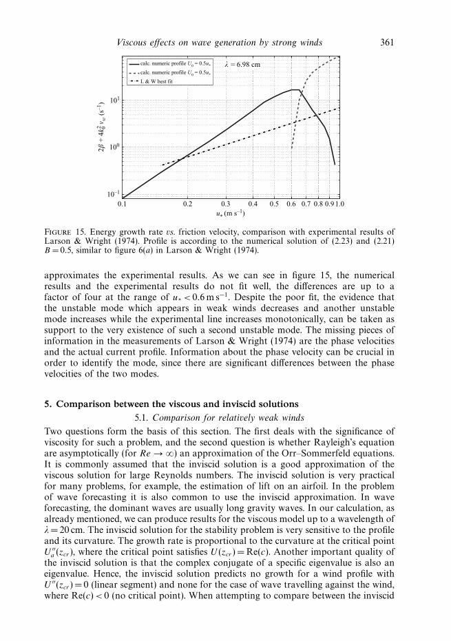
Figure 15. Energy growth rate vs. friction velocity, comparison with experimental results ofLarson & Wright (1974). Profile is according to the numerical solution of (2.23) and (2.21)B = 0.5, similar to figure 6(a) in Larson & Wright (1974).

approximates the experimental results. As we can see in figure 15, the numericalresults and the experimental results do not fit well, the differences are up to afactor of four at the range of u∗ < 0.6 m s−1. Despite the poor fit, the evidence thatthe unstable mode which appears in weak winds decreases and another unstablemode increases while the experimental line increases monotonically, can be taken assupport to the very existence of such a second unstable mode. The missing pieces ofinformation in the measurements of Larson & Wright (1974) are the phase velocitiesand the actual current profile. Information about the phase velocity can be crucial inorder to identify the mode, since there are significant differences between the phasevelocities of the two modes.

5. Comparison between the viscous and inviscid solutions5.1. Comparison for relatively weak winds

Two questions form the basis of this section. The first deals with the significance ofviscosity for such a problem, and the second question is whether Rayleigh’s equationare asymptotically (for Re → ∞) an approximation of the Orr–Sommerfeld equations.It is commonly assumed that the inviscid solution is a good approximation of theviscous solution for large Reynolds numbers. The inviscid solution is very practicalfor many problems, for example, the estimation of lift on an airfoil. In the problemof wave forecasting it is also common to use the inviscid approximation. In waveforecasting, the dominant waves are usually long gravity waves. In our calculation, asalready mentioned, we can produce results for the viscous model up to a wavelength ofλ= 20 cm. The inviscid solution for the stability problem is very sensitive to the profileand its curvature. The growth rate is proportional to the curvature at the critical pointU ′′

a (zcr ), where the critical point satisfies U (zcr ) = Re(c). Another important quality ofthe inviscid solution is that the complex conjugate of a specific eigenvalue is also aneigenvalue. Hence, the inviscid solution predicts no growth for a wind profile withU ′′(zcr ) = 0 (linear segment) and none for the case of wave travelling against the wind,where Re(c) < 0 (no critical point). When attempting to compare between the inviscid


0.04 0.08 0.12 0.16 0.200

2

4Im (ω)——–

ω0

Re (ω)——–

ω0

viscousinviscid

1.00

1.02

1.04

1.06

1.08

λ (m)

(a)

(b)

0.04 0.08 0.12 0.16 0.20

(×10–4)

Figure 16. Normalized frequency components vs. wavelength, for u∗ = 0.06 m s−1, comparisonbetween the viscous and inviscid solutions, the profile is according to (2.20)–(2.22). (a)Imaginary part, (b) real part.

solution and the viscous solution, using the lin–log profile (see (2.20)), we foundthat the critical point is often inside the linear segment and thus the inviscid modelproduces no growth. The dashed line in figure 5 is the boundary between the regionwhere the inviscid solution can produce growth and the region where it produceszero growth, for this particular profile. In figure 16, the results of these two modelsare compared along a cross-section where the inviscid model produces growth. Notethat the effect of dissipation due to viscosity does not exist in the inviscid results. Thecomparison shows very good agreement in the real part of the eigenvalues, whichmeans that they predict waves with almost the same phase velocity. In figure 16(a),we can see that the resulting growth rate by these two models is of the same order,but we can state that for most wavelengths the growth predicted by the viscous modelis approximately three times larger than that predicted by the inviscid model.

A more detailed comparison tool is to test the dynamic boundary condition plot.The dynamic boundary condition plot is the plot of the isolines of the squared normof G(ω, k), see (3.5) and § 3.1. Such a comparison enables us to compare the patternsof these two solutions as well. In figure 17, the dynamic boundary condition plotof these two solutions is presented. As we can see, the pattern of the surface of thesolution is almost the same. The arrowhead points to the minimum point of thissurface (where G =0), this point is the eigenvalue of the solution. In figure 18, we cansee that the structure of the eigenfunctions for the viscous and inviscid solutions issimilar in nature, however, the eigenfunctions are somewhat different in their actualvalues, corresponding to what we have seen in figure 17. Another point which is madeclear by figure 18 is the dominance of the critical layer, compared to its insignificancein the case of figure 11. The apparent difference between the two scenarios couldbe related to the fact that in figure 18 the critical point is in the air and above thelaminar viscous layer.

5.2. Comparison for strong winds

The comparison between viscous and inviscid solutions using the lin–log profile islimited because of the linear segment which results in zero growth in the inviscid


0.00

5 0.005

0.01

0.01

0.010.02

0.02

0.02

0.02

0.04

0.04

0.04

0.040.04

0.040.06

0.06

0.06

0.06

0.060.06

0.06

0.08

0.08

0.08

0.08

0.080.08

0.08

0.1

0.1

0.1

0.1

0.10.1

0.10.1

0.2

0.2

0.2

0.2

0.

0.20.2

0.20.2

0.4

0.4

0.4

0.4

0.4

0.40.4

0.40.4

0.6

0.60.6

0.60.6

0.6

0.6

0.6

0.80.8

0.80.8

11

11

0.00

50.

01

0.01

0.02

0.02

0.04

0.040.04

0.06

0.06

0.060.06

0.08

0.08

0.08

0.080.08

0.1

0.1

0.1

0.10.10.

20.

20.

2 0.20.2

0.2

0.4

0.4

0.4

0.40.4

0.4

0.6

0.6

0.60.6

0.60.8

0.80.8

11

1

0.5 0.7 0.9 1.1 1.3 1.50

0.04

0.08

0.12

0.16

(a) (b)

1.0214+1.4550 10–4i1.0193+1.5065 10–3i

Im (ω)——–

ω0

Re (ω)/ω0

.

0.5 0.7 0.9 1.1 1.3 1.50

0.04

0.08

0.12

0.16

Re (ω)/ω0

Figure 17. Isolines of ‖G‖2 in the ω-plane, u∗ = 0.1 m s−1, λ= 0.18 m, comparison betweenviscous and inviscid solutions, profile is according to (2.20)–(2.22). (a) Viscous solution, (b)inviscid solution.

0 0.5 1.0–0.4

–0.3

–0.2

–0.1

0

0.1

0.2

0.3

| f |/η0 (m s–1) | f |/η0 (m s–1)

z (m

)

(a) (b) (c)

0 0.5 1.0

–2

–1

0

1

2

0 1 2 3arg( f )

viscous ω = 1.019 + 0.0015i

critical point

inviscid ω = 1.021 + 0.00014i

critical point

z1

–2

–1

0

1

2

z1

(×10–3) (×10–3)

Figure 18. Comparison of the eigenfunctions between viscous and inviscid solutions,u∗ =0.1 m s−1, λ= 0.18 m, profile is according to (2.20)–(2.22). (a) Absolute value of theeigenfunction, (b) absolute value of the eigenfunction, enlargement, (c) argument of theeigenfunction, enlargement.

model. In order to compare these two models more comprehensively we looked fora wind profile that is similar to the profile of a turbulent boundary layer and whichhas non-zero curvature in a layer close to the interface. A good candidate for such aprofile is the numerical solution for the mean velocity of the boundary-layer equation,


0.005

0.010.02

0.05

0.05

0.08

0.08

0.2

0.2

0.20.5

0.5

0.5

0.50.5

0.8

0.8

0.8 0.8

0.80.8

2

0.4 0.8 1.2 1.60

0.1

0.2

0.3

0.4

0.5(a) (b)

0.00

50.

005

0.01 0.01

0.02

0.020.02

0.05

0.050.050.

08

0.080.08

0.2

0.2

0.2

0.2

0.50.5

0.5

0.5

0.50.5

0.80.8

0.8

0.8

0.8

0.80.8

0.8

2

1.084 + 0.0411i 1.088 + 0.0272i

0.4 0.8 1.2 1.60

0.1

0.2

0.3

0.4

0.5

Im (ω)——–

ω0

Re (ω)/ω0 Re (ω)/ω0

Figure 19. Isolines of ‖G‖2 in the ω-plane, u∗ =0.3 m s−1, λ= 0.05 m, comparison betweenviscous and inviscid solutions, profile is according to the numerical solution of (2.23) and(2.21) B =0.5. (a) Viscous solution, (b) inviscid solution.

which is (2.23). The results of the viscous model, when using this profile with thesame exponential current, are very similar to those of the lin–log profile, including thesecond unstable mode. The use of this profile provides the opportunity to comparebetween the viscous and inviscid models at stronger winds.

In order to examine the differences between the solutions, we present twocomparisons of the dynamic boundary condition plots. In figure 19, the comparisonis for λ= 0.05 m, u∗ = 0.3 m s−1. As can be seen, the behaviour is similar to figure 17;the real part is almost the same, whereas the imaginary part of the viscous solution is1.5 times larger than that in the inviscid solution. The pattern of the isolines is verysimilar.

In figure 20, we present the same comparison, but for a much stronger wind. Ascan be seen, in this figure the picture is completely different. There is no connectionbetween the solutions, neither in the real part nor in the imaginary part, and even thenumber of unstable eigenvalues is different.

The comparison at strong winds shows a more dramatic disagreement between theviscous and inviscid models, where not only can the growth rate of the viscous modelbe a hundred times larger than the growth rate of the inviscid model, but also the realpart and the number of unstable modes indicate a disagreement between the models.Within the range of our calculations, the results indicate that the inviscid solutioncannot be taken as a sensible approximation to the viscous one.

6. Summary and conclusionsAfter formulating the linear stability problem of surface waves for a viscous/inviscid

fluid, we built a robust solver in order to solve these eigenvalue problems for thespatial and temporal case and a range of mean flow profiles. The results of the solver


0.00

50.

010.02

0.02

0.05

0.05

0.05

0.08

0.08

0.08

0.2

0.2

0.2

0.5

0.5

0.5

0.5

0.5

0.8

0.8

0.8

0.8

2

2

2

3

3

3

4

4

5

5

8

0.4 0.8 1.2 1.60

0.2

0.4

0.6

0.8

0.95

0.0050.01

0.020.05

.08

0.080.2

0.2

0.20.5

0.5

0.50.5

0.5

0.8 0.8

0.8

0.8

2

2

3

34 5678910

0.547 + 0.834i 1.132 + 0.128i 1.519+0.00633i

0.4 0.8 1.2 1.60

0.2

0.4

0.6

0.8

0.95(a) (b)

Im (ω)——–

ω0

Re (ω)/ω0 Re (ω)/ω0

Figure 20. Isolines of ‖G‖2 in the ω-plane, u∗ = 0.8 m s−1, λ= 0.05m, comparison betweenviscous and inviscid solutions, profile is according to the numerical solution of (2.23) and(2.21) B = 0.5. (a) Viscous solution, (b) inviscid solution.

were validated for the range 0< λ< 20 cm, 0 <u∗ < 1 m s−1, and hence expand thecomputational domain in the (λ, u∗)-plane, relative to previous studies.

This expansion leads to the discovery of a new unstable mode. The main conditionsfor the appearance of this mode are the simultaneous existence of a shear flow in thewater and a wind intensity above a critical value. A non-vanishing viscosity is alsoa prerequisite for the appearance of two modes. From the results of the strong windscenarios, we can say that the nature of the generated waves is significantly differentfrom the nature of waves without the influence of air.

The comparison between the viscous model and the inviscid model at low windintensities shows very good agreement in the real part of the eigenvalue; however,the comparison of the imaginary part is less agreeable in this case. A comparison forstronger winds shows total disagreement between the two models. All these resultslead to the conclusion that the use of the inviscid approximation is problematic at thisrange of wavelengths, and it will be interesting to see the comparison at wavelengthsof the order of ∼ 1 m.

This research is part of an MSc thesis submitted by A. Z. to the Graduate Schoolat the Technion – Israel Institute of Technology. The research was supported byThe Israel Science Foundation (Grant 695/04) and by the Fund for Promotion ofResearch at the Technion.

Appendix. The test caseIn this section we present the analytical solution for the case of linear wind profile

and constant current. The profile has the form:

Ua = U0 + az, Uw = U0. (A 1)

The Orr–Sommerfeld equation is:

iε(f (4) − 2k2f ′′ + k4f ) + k[(U − c)(f ′′ − k2f ) − U ′′f

]= 0, (A 2)


where εw,a = 1/Rew,a = νw,a/k20ω0 is the inverse Reynolds number. Substituting (A 1)

into (A 2) gives:

f (4) − kf ′′(

2k +i

ε(U − c)

)+ k3f

(k +

i

ε(U − c)

)= 0. (A 3)

Now we can define F � f ′′ − k2f . Hence (A 3) becomes:

F ′′ − k

(k +

i

ε(U − c)

)F = 0, (A 4)

By a transformation of variables, (A 4) is transformed into Airy’s equation.

F ′′(u) − uF (u) = 0, (A 5)

where:

u =

(iε

ka

)2/3

k

(k +

i

ε(U − c)

)=

k

2(1 + i

√3)( ε

ka

)2/3(

k +i

ε(U − c)

). (A 6)

Thus, F (u(z)) is a solution of Airy’s equation. Since it is a second-order equation,it has two independent solutions. There are a few common pairs of independentsolutions, see Abramowitz & Stegun (1972), Vallee & Soares (2004).

Ai(u), Bi(u)Ai(u), Ai(ue2πi/3)Ai(u), Ai(ue−2πi/3)

⎫⎬⎭ (A 7)

Since the solution and its derivative must vanish at infinity, We choose the pairAi(u), Ai(ue−2πi/3), so that:

F = f ′′ − k2f = c1Ai(u) + c2Ai(ue−2πi/3) (A 8)

At this stage, we must look at the asymptotic behaviour of the independent solutionsfor large values of |z| in order to be sure that we satisfy the boundary condition atinfinity. As mentioned in Vallee & Soares (2004), the Airy function Ai blows up forlarge |u| outside the section | arg(u)| < π/3. Hence, we should look at the behaviourof arg(u) at infinity z → ±∞.

arg(u) =

⎧⎪⎨⎪⎩

5π

6+

arg(k)

3, z → ∞,

−π

6+

arg(k)

3, z → −∞,

(A 9)

arg(ue−2πi/3) =

⎧⎪⎨⎪⎩

π

6+

arg(k)

3, z → ∞,

−5π

6+

arg(k)

3, z → −∞,

(A 10)

If we take Re(k) > 0 ⇒ | arg(k)| < π/2 we can be sure that:

| arg(u)| < π3, z → −∞, (A 11)

| arg(ue−2πi/3)| < π3, z → ∞, (A 12)

Thus in the air:

Fa = f ′′a − k2fa = c1Ai(ue−2πi/3). (A 13)


Solving the above second-order equation:

fa = c1

[ekz

2k

∫ z

0

e−ktAi(ue−2πi/3)dt − e−kz

2k

∫ z

0

ektAi(ue−2πi/3)dt

]+ c2e

−kz + c3ekz. (A 14)

Since we require decay at infinity:

c1

2k

∫ ∞

0

e−ktAi(ue−2πi/3)dt + c3 �c1

2kp1(k, c, a, U0) + c3 = 0, (A 15)

c3 = − c1

2kp1. (A 16)

For the case of constant current in the water Uw ≡ U0, the solution for the water willbe:

fw = b1exp(kz) + b2exp(±

√k

(k +

i

ε(U0 − c)

)z) � b1exp(kz) + b2exp(Bz). (A 17)

If Re(B) < 0, we must choose e−Bz as the second independent solution; and ifRe(k) < 0, we must choose e−kz instead of ekz.And the derivatives are:

f ′w = kb1e

kz + Bb2eBz, (A 18)

f ′′w = k2b1e

kz + B2b2eBz, (A 19)

f ′′′w = k3b1e

kz + B3b2eBz. (A 20)

At the interface it reduces to:

fw(0) = b1 + b2, f ′w(0) = kb1 + Bb2,

f ′′w(0) = k2b1 + B2b2, f ′′′

w (0) = k3b1 + B3b2.

}(A 21)

In order to find the unknown coefficients, we must apply the boundary conditionsat the interface. In these boundary conditions the derivatives of f play a main role.Thus, we must calculate fw,a(0), f ′

w,a(0), f ′′w,a(0), f ′′′

w,a(0). This must be done carefully,using Leibniz’s rule for differentiation of integrals.

d

dz

∫ f2(z)

f1(z)

g(t)dt = g(f2(z))f′2(z) − g(f1(z))f

′1(z). (A 22)

Hence:

f ′a = c1

[ekz

2

∫ z

0

e−ktAi(ue−2πi/3)dt +e−kz

2

∫ z

0


]− kc2e

−kz + kc3ekz,

(A 23)

f ′′a = c1

[kekz

2

∫ z

0

e−ktAi(ue−2πi/3)dt − ke−kz

2

∫ z

0


+ Ai(ue−2πi/3)

]+ k2c2e

−kz + k2c3ekz (A 24)

f ′′′a = c1

[k2ekz

2

∫ z

0

e−ktAi(ue−2πi/3)dt +k2e−kz

2

∫ z

0


+ Ai′(ue−2πi/3)eπi/6

(ka

ε

)1/3 ]− k3c2e

−kz + k3c3ekz (A 25)


It will be helpful to use the following notation:

u(0) = u0 =

(iε

ka

)2/3

k

(k +

i

ε(U0 − c)

), (A 26)

Ai(u(0)e−2πi/3) = Ai0 = Ai(u0e−2πi/3), (A 27)

Ai(u(0)) = Ai0 = Ai(u0). (A 28)

Now we can present the derivatives at the interface:

fa(0) = c2 + c3, f ′a(0) = k(c3 − c2), f ′′

a (0) = c1Ai0 + k2(c2 + c3),

f ′′′a (0) = c1Ai

′0e

πi/6(

kaε

)1/3+ k3(c3 − c2),

}(A 29)

fw(0) = b1 + b2, f ′w(0) = kb1 + Bb2,

f ′′w(0) = k2b1 + B2b2, f ′′′

w (0) = k3b1 + B3b2.

}(A 30)

Writing the boundary condition at the interface:

fa(0) = fw(0) = c − U0 ⇒ c2 + c3 = b1 + b2 = c − U0, (A 31)

f ′w(0) + U ′

w(0) = f ′a(0) + U ′

a(0) ⇒ k(c3 − c2) = kb1 + Bb2 − aa, (A 32)

µ(f ′′a (0) + k2fa(0) + U ′′

a (0)) = (f ′′w(0) + k2fw(0) + U ′′

w(0))

⇒ µ(c1Ai0 + k2(c2 + c3) + k2(c2 + c3)) = k2b1 + B2b2 + k2(b1 + b2)

⇒ µc1Ai0 − k2b1 − B2b2 = k2(c − U0)(1 − 2µ). (A 33)

We obtain a system of five linear equations with five unknowns c1, c2, c3, b1, b2. Aftersolving the system we have the value of the functions fa, fw and their derivatives atthe interface. Note that all of these constants are functions of the specific case whichis defined by (Ra, Rw, a, U0) and the value of ω, k. After we obtain these values, wecan substitute them into the dynamic boundary condition and solve it, in order tofind ω, k.

kf ′w(c − U0) + kfwU ′

w + iR−1w (3k2f ′

w − f ′′′w ) − F

= ρ[kf ′


a (3k2f ′a − f ′′′

a ) − F]+ Wk3 at z = 0 (A 34)

In practice, we are unable to obtain a simple dispersion relation for this case, thusin order to calculate it we must do it numerically. The value of the constant p1 (seeequation (A 15)) can be calculated numerically and then the dispersion equation willbe solved by a numeric solver for a nonlinear equation.

REFERENCES

Abramowitz, M. & Stegun, I. A. 1972 Handbook of Mathematical Functions . Dover.

Boomkamp, P. A. M., Boersma, B. J., Miesen, R. H. M. & Beijnon, G. V. 1997 Chebyshev collocationmethod for solving two-phase flow stability problem. J. Comput. Phys. 132, 191–200.

Caulliez, G., Ricci, N. & Dupont, R. 1998 The generation of the first visible wind waves. Phys.Fluids Lett. 10, 757–759.

Charnock, H. 1955 Wind stress on water surface. Q. J. R. Met. Soc. 81, 639–640.

Jeffreys, H. 1925 On the formation of water waves by wind. Proc. R. Soc. A 104, 189–206.

Kawai, S. 1979 Generation of initial wavelets by instability of a coupled shear flow and theirevolution to wind waves. J. Fluid Mech 93, 661–703.


Larson, T. R. & Wright, J. W. 1974 Wind-generated gravity capillary waves: laboratorymeasurements of temporal growth rates using microwave backscatter. J. Fluid Mech. 70,417–436.

Miles, J. W. 1957a On the generation of surface waves by shear flows. J. Fluid Mech. 3, 185–204.

Miles, J. W. 1957b On the velocity profile for turbulent flow near a smooth wall. J. Aero. Sci. 24,704.

Phillips, O. M. 1957 On the generation of waves by turbulent wind. J. Fluid Mech. 2, 417–445.

Powell, M. D., Vickery, P. J. & Rienhold, T. A. 2003 Reduced drag coefficient for high windspeeds in tropical cyclones. Nature 422, 279–283.

Stiassnie, M., Agnon, Y. & Janssen, P. A. E. M. 2007 Temporal and spatial growth of wind waves.J. Phys. Oceanogr. 37, 106–114.

Trefethen, L. N. 2000 Spectral Methods in MATLAB . SIAM.

Tsai, W. T. & Lin, M. Y. 2004 Stability analysis on the initial surface-wave generation within anair-sea coupled shear flow. J. Mar. Sci. Technol. 12, 200–208.

Tsai, Y. S., Grass, A. J. & Simons, R. R. 2005 On the spatial linear growth of gravity–capillarywater waves sheared by a laminar air flow. Phys. Fluids 17, 095101–1–095101–13.

Valenzuela, G. R. 1976 The growth of gravity-capillary waves in a coupled shear flow. J. FluidMech. 76, 229–250.

Vallee, O. & Soares, M. 2004 Airy Functions and Application to Physics . Imperial College Press.

Van Gastel, K., Janssen, P. A. E. M. & Komen, G. J. 1985 On phase velocity and growth rate ofwind-induced gravity-capillary waves. J. Fluid Mech. 161, 199–216.

Wheless, G. H. & Csanady, G. T. 1993 Instability waves on the air–sea interface. J. Fluid Mech.248, 363–381.

Zhang, X. 2005 Short surface waves on surface shear. J. Fluid Mech. 541, 345–370.

Zhang, X. & Harrison, S. 2004 A laboratory observation of the surface temperature and velocitydistributions on a wavy and windy airwater interface. Phys. Fluids 16(1), L5–L8.

Viscous effects on wave generation by strong winds

Documents

Transcript of Viscous effects on wave generation by strong winds