Viscous Flows and Turbulence - profs.sci.univr.it
432
Lectures in Fluid Mechanics Viscous Flows and Turbulence
-
Upload
khangminh22 -
Category
Documents
-
view
3 -
download
0
Transcript of Viscous Flows and Turbulence - profs.sci.univr.it

Lectures inFluid Mechanics
Viscous Flowsand
Turbulence


Lectures inFluid Mechanics
Viscous Flowsand
Turbulence
by
Alexander J. SmitsDepartment of Mechanical Engineering
Princeton UniversityPrinceton, NJ 08544, USA
September 17, 2009
Copyright A.J. Smits©2000.


Contents
Preface xi
1 Equations of Motion 11.1 Integral Forms . . . . . . . . . . . . . . . . . . . . . . . . . . . . 2
1.1.1 Flux . . . . . . . . . . . . . . . . . . . . . . . . . . . . . . 21.1.2 Continuity equation . . . . . . . . . . . . . . . . . . . . 31.1.3 Momentum equation . . . . . . . . . . . . . . . . . . . . 5
1.2 Stresses and Strain Rates . . . . . . . . . . . . . . . . . . . . . . 81.2.1 Strain rates and deformation . . . . . . . . . . . . . . . 101.2.2 Normal stresses in a fluid in motion . . . . . . . . . . . 12
1.3 Differential Equations of Motion . . . . . . . . . . . . . . . . . 151.3.1 Continuity equation . . . . . . . . . . . . . . . . . . . . 151.3.2 Euler equation . . . . . . . . . . . . . . . . . . . . . . . 181.3.3 Navier-Stokes equations . . . . . . . . . . . . . . . . . . 22
1.4 Bernoulli Equation . . . . . . . . . . . . . . . . . . . . . . . . . 261.5 Constitutive Relationships Revisited . . . . . . . . . . . . . . . 271.6 Energy . . . . . . . . . . . . . . . . . . . . . . . . . . . . . . . . 29
1.6.1 Derivation of energy equation . . . . . . . . . . . . . . 311.6.2 Enthalpy equation . . . . . . . . . . . . . . . . . . . . . 341.6.3 Entropy equation . . . . . . . . . . . . . . . . . . . . . . 34
1.7 Summary . . . . . . . . . . . . . . . . . . . . . . . . . . . . . . . 391.8 Non-Dimensional Equations of Motion . . . . . . . . . . . . . 40
1.8.1 Continuity . . . . . . . . . . . . . . . . . . . . . . . . . . 411.8.2 Energy . . . . . . . . . . . . . . . . . . . . . . . . . . . . 411.8.3 Momentum equation . . . . . . . . . . . . . . . . . . . . 43
1.9 Vorticity Transport Equation . . . . . . . . . . . . . . . . . . . . 451.10 Summary:Equations of motion . . . . . . . . . . . . . . . . . . 51
1.10.1 Continuity equation . . . . . . . . . . . . . . . . . . . . 511.10.2 Linear momentum equation . . . . . . . . . . . . . . . . 521.10.3 Energy equation . . . . . . . . . . . . . . . . . . . . . . 531.10.4 Summary . . . . . . . . . . . . . . . . . . . . . . . . . . 54
v

vi CONTENTS
2 Exact Solutions 572.1 Parallel Flows . . . . . . . . . . . . . . . . . . . . . . . . . . . . 58
2.1.1 Plane Couette flow . . . . . . . . . . . . . . . . . . . . . 592.1.2 Poiseuille flow . . . . . . . . . . . . . . . . . . . . . . . 592.1.3 Fully-developed duct flow . . . . . . . . . . . . . . . . 602.1.4 Fully-developed pipe flow . . . . . . . . . . . . . . . . 642.1.5 Rayleigh flow I . . . . . . . . . . . . . . . . . . . . . . . 682.1.6 Rayleigh flow II . . . . . . . . . . . . . . . . . . . . . . . 712.1.7 Note on vorticity diffusion . . . . . . . . . . . . . . . . 72
2.2 Fully-Developed Flow With Heat Transfer . . . . . . . . . . . . 732.2.1 Couette flow . . . . . . . . . . . . . . . . . . . . . . . . . 742.2.2 Parallel duct flow . . . . . . . . . . . . . . . . . . . . . . 742.2.3 Circular pipe flow . . . . . . . . . . . . . . . . . . . . . 752.2.4 Free convection between heated plates . . . . . . . . . 75
2.3 Compressible Couette flow . . . . . . . . . . . . . . . . . . . . 772.4 Similarity Solutions . . . . . . . . . . . . . . . . . . . . . . . . . 81
2.4.1 Cylinder rotating at constant speed . . . . . . . . . . . 812.4.2 Suddenly stopped rotating cylinder . . . . . . . . . . . 832.4.3 Viscous stagnation point flow . . . . . . . . . . . . . . . 84
2.5 Creeping Flow and Lubrication Theory . . . . . . . . . . . . . 892.5.1 Stokes flow . . . . . . . . . . . . . . . . . . . . . . . . . 892.5.2 Slider bearing . . . . . . . . . . . . . . . . . . . . . . . . 92
2.6 Additional Exact Solutions . . . . . . . . . . . . . . . . . . . . . 95
3 Laminar Boundary Layers 973.1 Boundary Layer Growth . . . . . . . . . . . . . . . . . . . . . . 99
3.1.1 Control volume analysis . . . . . . . . . . . . . . . . . . 993.1.2 Similarity solution . . . . . . . . . . . . . . . . . . . . . 102
3.2 Boundary Layer Approximation . . . . . . . . . . . . . . . . . 1073.3 General Observations . . . . . . . . . . . . . . . . . . . . . . . . 1093.4 Blasius Solution . . . . . . . . . . . . . . . . . . . . . . . . . . . 1113.5 General Similarity Scaling . . . . . . . . . . . . . . . . . . . . . 1173.6 Displacement and Momentum Thickness . . . . . . . . . . . . 120
3.6.1 Displacement thickness . . . . . . . . . . . . . . . . . . 1203.6.2 Momentum thickness . . . . . . . . . . . . . . . . . . . 1223.6.3 Shape factor . . . . . . . . . . . . . . . . . . . . . . . . . 1233.6.4 Momentum integral equation . . . . . . . . . . . . . . . 123
3.7 Other Methods of Solution . . . . . . . . . . . . . . . . . . . . . 1253.7.1 Profile guessing methods . . . . . . . . . . . . . . . . . 1253.7.2 Pohlhausen method . . . . . . . . . . . . . . . . . . . . 1263.7.3 Thwaites method . . . . . . . . . . . . . . . . . . . . . . 128
3.8 Wake of a Flat Plate . . . . . . . . . . . . . . . . . . . . . . . . . 1293.9 Plane Laminar Jet . . . . . . . . . . . . . . . . . . . . . . . . . . 132
CONTENTS vii
4 Compressible Laminar Boundary Layers 1374.1 Boundary Layer Approximations . . . . . . . . . . . . . . . . . 1384.2 Crocco-Busemann Relations . . . . . . . . . . . . . . . . . . . . 1394.3 Howarth-Dorodnitsyn Transformation . . . . . . . . . . . . . . 1414.4 Flat Plate Boundary Layer . . . . . . . . . . . . . . . . . . . . . 1434.5 Boundary Layer Properties . . . . . . . . . . . . . . . . . . . . 145
4.5.1 Skin friction . . . . . . . . . . . . . . . . . . . . . . . . . 1454.5.2 Heat transfer . . . . . . . . . . . . . . . . . . . . . . . . 1454.5.3 Integral parameters . . . . . . . . . . . . . . . . . . . . . 148
5 Stability and Transition 1535.1 Introduction . . . . . . . . . . . . . . . . . . . . . . . . . . . . . 1535.2 Stability Analysis . . . . . . . . . . . . . . . . . . . . . . . . . . 159
5.2.1 Small perturbation analysis . . . . . . . . . . . . . . . . 1595.2.2 Orr-Somerfeld equation . . . . . . . . . . . . . . . . . . 1615.2.3 Inviscid stability theory . . . . . . . . . . . . . . . . . . 164
5.3 Experimental Evidence . . . . . . . . . . . . . . . . . . . . . . . 1665.4 Effects on Transition . . . . . . . . . . . . . . . . . . . . . . . . 1685.5 The Origin of Turbulence . . . . . . . . . . . . . . . . . . . . . . 1755.6 Inviscid Stability Examples . . . . . . . . . . . . . . . . . . . . 1755.7 Viscous Stability Examples . . . . . . . . . . . . . . . . . . . . . 176
6 Introduction to Turbulent Flow 1876.1 The Nature of Turbulent Flow . . . . . . . . . . . . . . . . . . . 1876.2 Examples of Turbulent Flow . . . . . . . . . . . . . . . . . . . . 1976.3 The Need to Study Turbulence . . . . . . . . . . . . . . . . . . 1996.4 Approaches to Turbulence . . . . . . . . . . . . . . . . . . . . . 202
6.4.1 Reynolds-averaged approach . . . . . . . . . . . . . . . 2036.4.2 Ensemble-averaged approach . . . . . . . . . . . . . . . 2046.4.3 Instantaneous realization approach . . . . . . . . . . . 2056.4.4 Connections among the approaches . . . . . . . . . . . 206
6.5 Model Flows . . . . . . . . . . . . . . . . . . . . . . . . . . . . . 208
7 Reynolds-Averaged Equations 2117.1 Continuity Equation . . . . . . . . . . . . . . . . . . . . . . . . 2127.2 Momentum Equation . . . . . . . . . . . . . . . . . . . . . . . . 2127.3 The Reynolds Stresses . . . . . . . . . . . . . . . . . . . . . . . 2157.4 Turbulent Transport of Heat . . . . . . . . . . . . . . . . . . . . 2187.5 The Reynolds Stress Equations . . . . . . . . . . . . . . . . . . 2197.6 The Turbulent Kinetic Energy Equation . . . . . . . . . . . . . 2217.7 Mean Flow Kinetic Energy Equation . . . . . . . . . . . . . . . 224

viii CONTENTS
8 Vorticity and Turbulence 2298.1 Introduction . . . . . . . . . . . . . . . . . . . . . . . . . . . . . 2298.2 Basic Concepts . . . . . . . . . . . . . . . . . . . . . . . . . . . . 230
8.2.1 Circulation . . . . . . . . . . . . . . . . . . . . . . . . . . 2308.2.2 Vorticity . . . . . . . . . . . . . . . . . . . . . . . . . . . 2308.2.3 Vortex tubes and filaments . . . . . . . . . . . . . . . . 2328.2.4 Vortex sheet . . . . . . . . . . . . . . . . . . . . . . . . . 233
8.3 Biot-Savart Law . . . . . . . . . . . . . . . . . . . . . . . . . . . 2348.4 The Vorticity Transport Equation . . . . . . . . . . . . . . . . . 235
8.4.1 Vortex tilting and stretching . . . . . . . . . . . . . . . . 2378.5 Vortex Interactions . . . . . . . . . . . . . . . . . . . . . . . . . 237
8.5.1 Velocity field induced by a vortex filament . . . . . . . 2388.5.2 The Rankine vortex . . . . . . . . . . . . . . . . . . . . . 2408.5.3 Filaments of opposite sign and equal strength . . . . . 2408.5.4 Filaments of the same sign and strength . . . . . . . . . 2428.5.5 Filaments not parallel to each other . . . . . . . . . . . 2428.5.6 Vortex rings . . . . . . . . . . . . . . . . . . . . . . . . . 244
8.6 Vorticity Diffusion . . . . . . . . . . . . . . . . . . . . . . . . . . 2458.6.1 Note on vorticity diffusion . . . . . . . . . . . . . . . . 248
8.7 The Pressure Field and Vorticity . . . . . . . . . . . . . . . . . . 2498.8 Splat and Spin . . . . . . . . . . . . . . . . . . . . . . . . . . . . 250
9 Statistical Description of Turbulence 2559.1 Probability Density . . . . . . . . . . . . . . . . . . . . . . . . . 2559.2 Joint Probability Density . . . . . . . . . . . . . . . . . . . . . . 2589.3 Correlation Coefficients . . . . . . . . . . . . . . . . . . . . . . 259
9.3.1 Space correlations: r , 0, τ = 0 . . . . . . . . . . . . . . 2609.3.2 Autocorrelations: r = 0, τ , 0 . . . . . . . . . . . . . . . 2649.3.3 Space-time correlations . . . . . . . . . . . . . . . . . . 2679.3.4 Recapitulation of correlations . . . . . . . . . . . . . . . 269
9.4 Frequency Spectra . . . . . . . . . . . . . . . . . . . . . . . . . . 2769.5 Wave Number Spectra . . . . . . . . . . . . . . . . . . . . . . . 2799.6 Wavelet Transforms . . . . . . . . . . . . . . . . . . . . . . . . . 281
9.6.1 Introduction . . . . . . . . . . . . . . . . . . . . . . . . . 2819.6.2 One-Dimensional Continuous Wavelet Transforms . . 2829.6.3 The Admissibility Condition . . . . . . . . . . . . . . . 2839.6.4 Choice of Wavelet Function . . . . . . . . . . . . . . . . 2849.6.5 Examples . . . . . . . . . . . . . . . . . . . . . . . . . . 2859.6.6 A Simple Eddy . . . . . . . . . . . . . . . . . . . . . . . 287
10 Homogeneous Isotropic Turbulence 29110.1 Introduction . . . . . . . . . . . . . . . . . . . . . . . . . . . . . 29110.2 Lateral and Longitudinal Correlations . . . . . . . . . . . . . . 294

CONTENTS ix
10.3 Decay of Turbulence . . . . . . . . . . . . . . . . . . . . . . . . 29810.4 Spectra and the Energy Cascade . . . . . . . . . . . . . . . . . . 30110.5 Vortex Stretching and the Energy Cascade . . . . . . . . . . . . 303
10.5.1 The energy transfer process . . . . . . . . . . . . . . . . 30510.5.2 How does this get started? . . . . . . . . . . . . . . . . 30610.5.3 How does it continue? . . . . . . . . . . . . . . . . . . . 306
10.6 Isotropicity of the Small Scales . . . . . . . . . . . . . . . . . . 30710.7 The Initial Period of Decay . . . . . . . . . . . . . . . . . . . . . 30710.8 Kolmogorov Hypothesis . . . . . . . . . . . . . . . . . . . . . . 30810.9 Form of the Spectrum in the Dissipation Range . . . . . . . . . 31210.10The Decay of Isotropic Turbulence: Summary . . . . . . . . . . 31410.11Isotropicity in the Dissipation Range . . . . . . . . . . . . . . . 31510.12Summary . . . . . . . . . . . . . . . . . . . . . . . . . . . . . . . 317
11 Turbulent Shear Flows 31911.1 Channel Flow . . . . . . . . . . . . . . . . . . . . . . . . . . . . 31911.2 Turbulent Couette Flow . . . . . . . . . . . . . . . . . . . . . . 32311.3 Turbulent Pipe Flow . . . . . . . . . . . . . . . . . . . . . . . . 32311.4 Turbulent Boundary Layers . . . . . . . . . . . . . . . . . . . . 325
11.4.1 Turbulence characteristics . . . . . . . . . . . . . . . . . 33011.4.2 Stress Behavior Near the Wall . . . . . . . . . . . . . . . 33211.4.3 Scaling Laws for the Mean Velocity . . . . . . . . . . . 333
11.5 Reynolds-Number Dependence . . . . . . . . . . . . . . . . . . 33811.6 Friction Law for Pipe and Channel Flows . . . . . . . . . . . . 34011.7 Momentum-Integral Methods . . . . . . . . . . . . . . . . . . . 34211.8 Power Laws . . . . . . . . . . . . . . . . . . . . . . . . . . . . . 34311.9 Mixing Length and Eddy Viscosity Concepts . . . . . . . . . . 344
11.9.1 Prandtl’s eddy viscosity . . . . . . . . . . . . . . . . . . 34711.9.2 Taylor and von Karman’s mixing length method . . . . 347
11.10Mixing length and eddy viscosity . . . . . . . . . . . . . . . . . 35011.10.1 Early ideas about turbulence . . . . . . . . . . . . . . . 35011.10.2 Special cases where `m and νt are simple functions . . . 35111.10.3 Relation between `m and eddy length scales . . . . . . . 35311.10.4 Conclusions . . . . . . . . . . . . . . . . . . . . . . . . . 354
12 Engineering Calculation Methods 35512.1 Introduction . . . . . . . . . . . . . . . . . . . . . . . . . . . . . 35512.2 Integral Methods . . . . . . . . . . . . . . . . . . . . . . . . . . 35612.3 Zero-Equation Models . . . . . . . . . . . . . . . . . . . . . . . 357
12.3.1 Nature of the hypothesis . . . . . . . . . . . . . . . . . . 35712.3.2 Mixing-Length Hypothesis . . . . . . . . . . . . . . . . 359
12.4 One-Equation Models . . . . . . . . . . . . . . . . . . . . . . . 36012.5 Two-Equation Models . . . . . . . . . . . . . . . . . . . . . . . 366

x CONTENTS
12.6 Stress-Equation Models . . . . . . . . . . . . . . . . . . . . . . 37012.7 Large Eddy Simulation . . . . . . . . . . . . . . . . . . . . . . . 373
12.7.1 General considerations . . . . . . . . . . . . . . . . . . . 37312.7.2 Governing equations . . . . . . . . . . . . . . . . . . . . 37512.7.3 The residual stress model . . . . . . . . . . . . . . . . . 377
13 Structure of Turbulence 38313.1 Physical Models for Turbulent Boundary Layers . . . . . . . . 38313.2 Inner Layer Structures . . . . . . . . . . . . . . . . . . . . . . . 38513.3 Outer Layer Structures . . . . . . . . . . . . . . . . . . . . . . . 39213.4 Interactions . . . . . . . . . . . . . . . . . . . . . . . . . . . . . 39613.5 A Study of Near Wall Scaling Laws . . . . . . . . . . . . . . . . 401
A Equations of Motion 413A.1 Continuity equation . . . . . . . . . . . . . . . . . . . . . . . . . 413A.2 Linear momentum equation . . . . . . . . . . . . . . . . . . . . 414A.3 Energy equation . . . . . . . . . . . . . . . . . . . . . . . . . . . 415A.4 Summary . . . . . . . . . . . . . . . . . . . . . . . . . . . . . . . 416
B References 419

Preface
These notes are intended for use by students enrolled in Princeton Universitycourses MAE 552, “Viscous Flows and Boundary Layers,” and MAE 553,“Turbulent Flow,” and they should not be reproduced or distributed withoutpermission of the author.
Alexander J. SmitsPrinceton, New Jersey, USA
References for Turbulence Course MAE 537
S.B. Pope, “Turbulent Flows,” Cambridge University Press, 2000P.S. Bernard and J.M. Wallace, “Turbulent Flow: Analysis, Measure-ment, and Prediction,” John Wiley & Sons, 2002
J. Mathieu and J. Scott, “An Introduction to Turbulent Flow,” Cam-bridge University Press, 2000
Hinze, J.O., “Turbulence,” McGraw-Hill, New York, 2nd edition, 1975
H. Tennekes and J.L. Lumley, “A First Course in Turbulence,” MITPress, 1972
P. Bradshaw, “An Introduction to Turbulence and Its Measurement,”Pergamon Press, 1971
P. A. Libby, “Introduction to Turbulence,” Taylor & Francis,1996
J. T. Davies, “Turbulence Phenomena,” Academic Press, 1972
M. Lesieur, “Turbulence in Fluids,” Kluwer, 3rd edition, 1993
H. Schlichting and K. Gersten, “Boundary-Layer Theory,” McGraw-Hill, 8th edition, 2000
D. C. Wilcox, “Turbulence Modeling for CFD,” DCW Industries, 1993
xi

xii PREFACE
B. E. Launder and D. B. Spalding, “Mathematical Models of Turbu-lence,” Academic Press, 1972
U. Frisch, “Turbulence,” CUP paperback, 1995
Cebeci, T. and Smith, A. M. O., “Analysis of Turbulent BoundaryLayers,” Academic Press, 1974
Bradshaw, P., Cebeci, T. and Whitelaw, J. H., “Engineering CalculationMethods for Turbulent Flow,” Academic Press, 1981
Cebeci, T. and Bradshaw, P., “Momentum Transfer in Boundary Lay-ers,” Hemisphere, 1977
Cebeci, T. and Bradshaw, P., “Physical and Computational Aspects ofConvective Heat Transfer,” Springer-Verlag, 1984
Smits, A.J. and Dussauge, J.P., “Turbulent Shear Layers in SupersonicFlow,” Springer Verlag, AIP Imprint, 1996
Chapter 1
Equations of Motion
Here, we consider the equations of motion briefly. Full derivations canbe found in a number of places, notably in Batchelor Introduction to FluidDynamics, and Currie Fundamental Mechanics of Fluids.
We consider only flows of fluids where the continuum hypothesis is valid.That is, the smallest volume of interest (a fluid element) will always contain asufficient number of molecules for statistical averages to be meaningful. Thecontinuum hypothesis fails when the mean free path is comparable to thesmallest significant dimension. This can happen under normal temperaturesand pressures when the body dimensions are very small, as for the flowaround a very thin wire, such as the sensitive element of a hot wire probewhere typical diameters range from 1 to 5 µm, or at very high altitudes,where the densities are very small and the mean free path can be very large.The relevant non-dimensional quantity is the Knudsen number, which isthe ratio of the mean free path to a typical flow dimension. When theKnudsen number exceeds unity we expect rarified gas effects to becomeimportant. For a hot wire in a supersonic flow, the Knudsen number for thewire filament is about 0.2 at normal temperatures and pressures, and for theregion occupied by the shock wave it approaches unity. It is difficult to justifythe continuum hypothesis within the shock since for shocks of moderatestrength the thickness is equal to a few mean free paths in the downstreamgas. Nevertheless, the equations of motion for a continuum gas predictshock structures which agree well with experiment. For the flow over thefilament itself, however, slip-flow effects associated with a breakdown inthe continuum hypothesis have been observed when the Knudsen numberbased on the filament diameter is of order 0.1 (Davis, 1972). When Knudsennumber effects are negligible, and the flow behavior can be described interm of its macroscopic properties such as its pressure, density, and velocity,the flow of a fluid is described completely by the continuity, momentumand energy equations, together with an equation of state and a suitable setof boundary conditions.
1

2 CHAPTER 1. EQUATIONS OF MOTION
The principles of mass conservation, Newton’s Second Law, and theconservation of energy will be used to derive the continuity equation, themomentum equation and the energy equation for fluids in motion. Theequations can be written in integral form, appropriate for large controlvolumes, and in differential form, necessary for understanding the motionof fluid particles.
1.1 Integral Forms
Before we derive the integral equations of motion, we first introduce theconcept of flux, which simplifies the derivations considerably.
1.1.1 Flux
When fluid flows across the surface area of a control volume, it carries withit many properties. For example, if the fluid has a certain temperature, itcarries this temperature with it across the surface into the control volume.If it has a particular density, it carries this density with it as it crossesthe surface. The fluid also carries with it momentum and energy. This“transport” of fluid properties by the flow across a surface is embodied inthe concept of flux.
The flux of (something) is the amount of that (something)being transported across a surface per unit time.
Consider volume flux, that is, the volume of all particles going through anarea dA in time ∆t. For a three-dimensional, time-dependent flow, the veloc-ity and density are functions of three space variables and time. That is, wehave a velocity field V(x, y, z, t) and a density field ρ(x, y, z, t) (figure 1.1a).1
If we mark a number of fluid particles and visualized their motion over ashort time ∆t, we could identify the fluid that passes through dA during thistime interval (figure 1.1b).
If the area dA is small enough, the distribution of ρ and V can be ap-proximated by their average values over the area. We can now identify thevolume which contains all the particles that will pass through dA in time∆t. This volume = (V∆t cosθ) dA = (n ·V∆t) dA where n is the unit normalwhich defines the orientation of the surface dA (figure 1.1c). That is,
1This is called an Eulerian description. See Smits A First Course in Fluid Mechanics forfurther details.

1.1. INTEGRAL FORMS 3
Figure 1.1: (a) Three-dimensional, unsteady flowfield with V(x, y, z, t) andρ(x, y, z, t); (b) Edge-on view of element of control surface of area dA; (c) Volumeswept through dA in time ∆t.
amount of volume per unit time
transported across an areadA with a direction n
=
total
volumeflux
= (n ·V)dA
where n ·VdA is the volume flux (dimensions of L3T−1), and n ·V representsthe volume flux per unit area (dimensions of LT−1).
Once we have written the volume flux we can easily write down otherfluxes, such as
mass flux ρ(n ·V) dA = n · ρV dA
momentum flux (n · ρV)V dA
kinetic energy flux 12 (n · ρV)V2 dA, etc.
The dimensions of mass flux are MT−1, momentum flux are MLT−2 (= force),and kinetic energy flux are ML2T−3 (= force × velocity = power).
1.1.2 Continuity equation
The conservation of mass requires that the difference between the mass flowrates in and out of a given control volume is equal to the rate at whichmass accumulates inside the volume. Here, we will derive the equationdescribing mass conservation for an unsteady, three-dimensional flow in itsintegral form. The differential form will be derived in section 1.3.1.
Consider the fixed control volume CV shown in figure 1.2. When theflow is unsteady, the outflux and influx of mass are not equal, so that masscontained inside the control volume may be increasing or decreasing. So:
(a) A fluid element of volume dυ has a mass ρdυ. Therefore the massof fluid inside the control volume at any time is
∫ρdυ. Hence:
rate of change of mass in CV =∂∂t
∫ρ dυ (1.1)

4 CHAPTER 1. EQUATIONS OF MOTION
Figure 1.2: Fixed control volume for derivation of the integral form of the conti-nuity equation.
(for a fixed control volume, either the partial or the regular derivativewith respect to time can be used, since the volume itself is not changingwith time). This rate of change of mass will be negative if the massinside the control volume is decreasing with time (that is, when theoutflux exceeds the influx).
(b) For a small element of surface area dA, the mass outflux throughdA per unit time = ρV · ndA. Therefore
total mass flux out of CV =
∫ρV · n dA. (1.2)
The integrand will be positive when the direction of the flow is inthe same direction as the outward-facing unit normal vector n, andnegative when the direction of the flow is opposite to that of n.
Hence, from equations 1.1 and 1.2, the conservation of mass requires that
∂∂t
∫ρ dυ +
∫n · ρV dA = 0. (1.3)
This is the integral form of the continuity equation for a fixed control volume,in a three-dimensional, time-dependent flow. In words:
rate of increase of massinside control volume
+
net rate of mass flux
out of control volume
=
0
When the mass inside the control volume is fixed,
∫n · ρV dA = 0 Fixed mass

1.1. INTEGRAL FORMS 5
(usually, of course, having a fixed mass inside the control volume impliesconstant density). When the flow is steady the flow properties do not depend
on time, and therefore, since the control volume is fixed,∫n · ρV dA = 0. Steady flow
The same equation is obtained when the mass inside the control volume isfixed, or when the flow is steady. These conditions have somewhat differentimplications, however, depending on the flow. When the flow is steady, theinlet and outlet mass flow rates, and the mass inside the control volume,do not change with time. When only the mass inside the control volume isconstant in time, however, it is possible for the inlet and outlet mass flowrates to be unsteady, as long as they are equal.
For steady or unsteady incompressible flow,∫n ·VdA = 0. Incompressible flow
1.1.3 Momentum equation
We now derive the integral form of the three-dimensional, time-dependentmomentum equation. We start with a fixed control volume similar to thatused in the derivation of the continuity equation (see figure 1.3). If a resultantforce F acts on the fluid in the control volume, its momentum will changewith time. The momentum of the fluid in the control volume can change intwo ways:
1. By a non-zero momentum flux over the surface of the control volume.If the momentum influx is smaller (say) than the momentum outflux,there is a net positive momentum outflux that will tend to decrease themomentum of the fluid in the control volume.
2. By the unsteady variation of momentum contained within the volume,due to unsteady variations in the density or the velocity of the fluidinside the control volume.
This is somewhat similar to the conservation of mass, where a net outfluxof mass leads to an unsteady variation of mass contained in the controlvolume. In other words, the sum of the rate of change of mass in the control

6 CHAPTER 1. EQUATIONS OF MOTION
Figure 1.3: Fixed control volume for derivation of the integral form of the momen-tum equation.
volume and the net outflux of mass from the control volume is zero, sincemass must be conserved. That is,
rate of change ofmass inside
control volume
+
net outflux of
mass fromcontrol volume
=
0,
For the momentum, however, the sum of the rate of change of momentumin the control volume and the net outflux of momentum is not necessarilyzero: momentum is not conserved if there is a resultant force acting on thefluid. That is,
rate of change ofmomentum inside
control volume
+
net outflux of
momentum fromcontrol volume
=
Resultant forcesacting on fluid
.
We see that the resultant force (equal to the mass of fluid in the control vol-ume times the acceleration of the fluid passing through the control volume)is the sum of an unsteady term and a flux term. Consider each term in themomentum balance, from left to right.
Unsteady term
For the rate of change of momentum inside the control volume, consider anelement of volume dυ. The mass of this volume is ρdυ, and its momentumis ρVdυ. The total momentum contained in the control volume is found byintegration, and its rate of change with time is found by differentiating withrespect to time. So:
rate of change of momentuminside control volume
=
∂∂t
∫ρV dυ. (1.4)
This quantity is positive if the momentum inside the control volume isincreasing with time. Note that we have used the partial derivative withrespect to time. In fact, we could have used a regular derivative: the control
1.1. INTEGRAL FORMS 7
volume is fixed in shape and location and so the integral (not the integrand)depends only on time.
Flux term
For an element of surface area dA, we have a volume flux n · VdA (seesection 1.1.1). The flux is positive if the velocity is directed along n, that is, itis positive if the flux is out of the control volume. The mass flux is thereforegiven by n · ρVdA, and the momentum flux is given by
(n · ρV
)VdA. So:
net outflux of momentumfrom control volume
=
∫ (n · ρV
)V dA. (1.5)
Resultant force
We have surface forces, body forces and forces due to external surfaces.
1. The surface forces include viscous forces acting over the surface of thecontrol volume, and forces due to pressure acting at right angles to thesurface. If the vector ~Σ is the surface force per unit area due to stressdifferences acting on the surface of the control volume, then
net resultant force due to stressdifferences acting on the surface
of the control volume
=
∫~Σ dA (1.6)
2. Body forces include gravitational, magnetic and electrical forces actingover all the fluid contained in the control volume. The only body forceconsidered here is the force due to gravity. An element of volume dυhas a mass ρdυ, and the vector force due to gravity acting on this massis ρgdυ. So:
resultant force due to gravityacting on the mass contained
in the control volume
=
∫ρg dυ = g
∫ρ dυ = mg,
(1.7)where m is the total mass of fluid contained in the control volume.
3. The forces due to external surfaces, Fext, are the forces applied to thefluid by the walls of a duct, the surfaces of a deflector, or the forcesacting in the solid cut by the control volume. An example of the latteris when a control volume is drawn to cut through the solid walls of aduct: we must include the forces transmitted through the walls in the

8 CHAPTER 1. EQUATIONS OF MOTION
force balance on the fluid. (Remember: when a fluid exerts a force ona solid surface, an equal but opposite force acts on the fluid.)
By combining the terms given in equations 1.5 to 1.7, and including theviscous forces Fv and the forces due to external surfaces Fext, we obtain theintegral form of the momentum equation for a fixed control volume:
Fext +
∫~Σ dA +
∫ρgdυ =
∂∂t
∫ρVdυ +
∫ (n · ρV
)VdA (1.8)
This is a vector equation, so that in Cartesian coordinates it has componentsin the x-, y- and z-directions.
1.2 Stresses and Strain Rates
The stress term in the momentum equation (equation 1.8) contains normalstresses and shear stresses. To evaluate the components of ~Σ, consider theelemental control volume shown in figure 1.4. If we take only the stressesthat contribute to the x-component of the surface force, we see that there aretwo kinds:
(a) Normal stresses, acting in the x-direction, normal to the face in they-z plane (σxx);
(b) Tangential stresses, acting in the x-direction, along faces in the z-xand y-x planes (σyx and σzx).
For a large control volume, therefore, the x-component of the surface forceis given by
i ·∫~Σ dA =
∫ (σxx + σyx + σzx
)dA.
Similar results can be obtained for the surface forces in the y- and z-directions, so that∫
~Σ dA = i∫ (
σxx + σyx + σzx
)dA
+ j∫ (
σxy + σyy + σzy
)dA
+ k∫ (
σxz + σyz + σzz
)dA.

1.2. STRESSES AND STRAIN RATES 9
Figure 1.4: Control volume for a steady two-dimensional flow.
Therefore three normal stresses and six tangential stresses contribute to thetotal surface force. We could write this as∫
Σ j dA =
∫σi jni dA,
where
σi j =
σxx σyx σzx
σxy σyy σzy
σxz σyz σzz
and ni is a unit vector defined such that σi jni gives the j-component of thestress. It is, in fact normal to the surface, pointing out from the controlvolume.
The parameter σi j is a tensor known as the stress tensor. The resultantforce per unit area, ~Σ, is a function of space, time and surface orientation.That is,
~Σ = ~Σ (n, x, t) .
Writing ~Σ in terms of the stress tensor σi j makes its dependence on theorientation of the surface clear. The stress tensor itself is independent ofthe surface orientation, but its scalar product with a unit vector gives thesurface force per unit area acting in that direction. That is, the contributionof the surface force in the j-direction, Σ j, is given by the component of thestress tensor acting in that direction, so that
Σ j = σi jni
(see also Batchelor Introduction to Fluid Dynamics, p. 10).The stress tensor σi j:

10 CHAPTER 1. EQUATIONS OF MOTION
(a) The stress tensor σi j is independent of the surface orientation.
(b) It can be shown that σi j is symmetric, so that σxy = σyx, σxz = σzx
and σyz = σzy.
(c) By convention σxy denotes the stress acting in the y-direction, on aface aligned so that x is constant (that is, in the y-z plane.
(d) A fluid is as a medium that will continue to deform under anapplied shear stress. Therefore, in a fluid at rest, all shear stresses arezero, by definition, and we are left only with the three normal stresses,σxx, σyy and σzz. What is more,
σxx = σyy = σzz = −p,
where p is the thermodynamic pressure, and by convention is taken tobe positive when it tends to compress (hence the negative sign).
(e) In a fluid in motion, we can define a mean or “bulk” pressure p,where
p = − 13
(σxx + σyy + σzz
).
Now, p must equal p when the fluid is at rest, but p and p need not beequal when the fluid is in motion (although the differences are usuallysmall, as we shall see).
In order to proceed, we need to find the relationship between the stresstensor and the strain rates, that is, between the stress tensor and the velocityfield, so that we can introduce the velocities into the stress term.
1.2.1 Strain rates and deformation
Rate of strain
When a fluid is in motion, every fluid element is, generally speaking, dis-placed to a new position at every instant. As this displacement takes place,the elements are strained, and the local rate of strain depends on the relativemotion between any two points. Consider points A at x and B at x+dx. If thevelocity at A is [u, v,w], the velocity at B is given by [u + du, v + dv,w + dw],where
u + du = u +∂u∂x
dx +∂u∂y
dy +∂u∂z
dz,
v + dv = v +∂v∂x
dx +∂v∂y
dy +∂v∂z
dz,
w + dw = w +∂w∂x
dx +∂w∂y
dy +∂w∂z
dz.

1.2. STRESSES AND STRAIN RATES 11
Thus the relative motion of B with respect to A is described by the velocitygradient tensor
∂ui
∂x j=
∂u∂x
∂u∂y
∂z∂x
∂v∂x
∂v∂y
∂v∂z
∂w∂x
∂w∂y
∂w∂z
.We can write this as:
∂ui
∂x j=
∂u∂x
12
(∂v∂x + ∂u
∂y
)12
(∂w∂x + ∂u
∂z
)12
(∂u∂y + ∂v
∂x
)∂v∂y
12
(∂w∂y + ∂v
∂z
)12
(∂u∂z + ∂w
∂x
)12
(∂v∂z + ∂w
∂y
)∂w∂z
+
0 −
12
(∂v∂x −
∂u∂y
)−
12
(∂w∂x −
∂u∂z
)−
12
(∂u∂y −
∂v∂x
)0 −
12
(∂w∂y −
∂v∂z
)−
12
(∂u∂z −
∂w∂x
)−
12
(∂v∂z −
∂w∂y
)0
.The first matrix on the right hand side describes the deformation of the fluidelement by compression and shearing, and it is called the “rate of strain”tensor, Si j. The second matrix on the right hand side describes the rotationof the fluid element if it were to rotate as a rigid body without deformation,and it is called the “rate of rotation” tensor, Ri j. It does not deform the fluidelement. Note that the instantaneous angular velocity of the fluid elementis given by ωk where Ri j = εi jkωk.2 The vector ~ω is related to the vorticity Ωby ~ω = 1
2∇ ×V = 12Ω. So:
∂ui
∂x j= Si j + Ri j.
where
Si j = 12
(∂ui
∂x j+∂u j
∂xi
)and Ri j = 1
2
(∂ui
∂x j−∂u j
∂xi
). (1.9)
Stress tensor
It is also convenient to identify the elements of the stress tensor that areconnected with fluid motion. When the fluid is at rest, or in rigid bodymotion, all velocity gradients are zero, and the only stress is due to the
2εi jk is the alternating tensor, such that
εi jk = ±1 for i , j , k= 0 for i = j, j = k, or i = k
12 CHAPTER 1. EQUATIONS OF MOTION
thermodynamic pressure, p. Hence for a fluid in motion, that is, for a fluidwhere there is relative motion between fluid elements, we can write
σi j = −p [I] + di j
orσi j = −pδi j + di j
where di j is that part of σi j which is due to relative motion, and it is calledthe shear stress tensor, or the deviatoric stress tensor. The matrix [I] is theunit matrix, and δi j is the Kronecker delta.3
Constitutive relationship
To find the relationship between the stress and the strain rate, we need tofind only the relationship between di j and Si j, since they are respectively thestress due to relative motion, and the strain rate due to deformation of fluidelements. The simplest connection is linear, but even a linear relationshipbetween two second order tensors requires 81 coefficients. When combinedwith the conditions of symmetry and isotropy, the number of coeficientsreduces to two, so that,
di j = 2µSi j + λ∇ ·V [I] ,
where the coefficient µ is called the “dynamic viscosity” and λ is called the“second coefficient of viscosity.” Note that for incompressible flows, where∇ ·V = 0, the second term vanishes. Also,
σi j = −p [I] + 2µSi j + λ∇ ·V [I] .
The rate-of-strain tensor is the only part of the velocity gradient tensorgoverned by relative motions among fluid particles. The simplest stress-strain rate relationship is a linear one, and fluids that follow this relationshipare called Newtonian. For isotropic Newtonian fluids, the shear stress tensorbecomes
di j = λSkkδi j + 2µSi j (1.10)
1.2.2 Normal stresses in a fluid in motion
For a fluid in motion, we defined a bulk pressure p, where
p = −13
(σxx + σyy + σzz
).
That is,p − p = −
(λ + 2
3µ)∇ ·V,
3δi j = 1 for i = j, and 0 for i , j.

1.2. STRESSES AND STRAIN RATES 13
where p is the thermodynamic pressure. We see that for a fluid in relativemotion, the normal stress is not equal to the pressure p. However, p mustequal p when:
(a) ∇ ·V = 0 (incompressible flow);
(b) λ = −23µ (“Stokes Hypothesis”); or
(c)(λ + 2
3µ)∇ ·V is very small.
For the rest of these notes we will assume that λ = −23µ (“Stokes Hypothe-
sis”), so that p = p. Experience shows this to be a good approximation undera wide variety of conditions. Hence,
σi j = −(p + 2
3µ∇ ·V)
[I] + 2µSi j. (1.11)
This constitutive relationship holds for all Newtonian fluids, with and with-out compressibility.
We see that the stress tensor has normal components, such as
σxx = −(p + 2
3µ∇ ·V)
+ 2µ∂u∂x
and tangential components such as
σxy =
(∂u∂y
+∂v∂x
)= σyx.
Both the normal and the tangential stresses depend on viscosity. The averagenormal stress p = − 1
3
(σxx + σyy + σzz
)is independent of viscosity, but the
individual normal stresses σxx, σyy and σzz are not. This observation holdstrue for compressible and incompressible flows.
Inviscid flows
In an inviscid or “ideal” fluid, the only stress component is the normal stress,it is equal to the pressure p, and it is isotropic. Hence:∫
~Σ dA = −
∫np dA
(the unit normal n gives the direction to the force due to pressure differences,and by convention pressure is positive when it acts to compress the fluid —see figure 1.5). So, for an inviscid fluid, the integral form of the momentum

14 CHAPTER 1. EQUATIONS OF MOTION
Figure 1.5: The vector force due to pressure acting on an element of surface.
equation is
Fext −
∫np dA +
∫ρgdυ =
∂∂t
∫ρVdυ +
∫ (n · ρV
)VdA (1.12)
This is a valid approximation for real fluids when the resultant force com-ponents due to viscous stresses are small compared to the forces due topressure differences (that is, when velocity gradients and relative motionsare small).
Viscous flows
To include viscous effects in this momentum balance, we could use (for thej-component) ∫
~Σ j dA =
∫σi jni dA.
However, for many purposes and applications, the variation of σi j over thesurface is not known. In fact, the control volume approach is often takenbecause we are only interested in gross properties, rather than detailedinformation on the fluid flow behavior. In that case, we can simply write
Fext + Fv −
∫np dA +
∫ρgdυ =
∂∂t
∫ρVdυ +
∫ (n · ρV
)VdA (1.13)
where Fv is the resultant force due to viscous effects. It is often possible tochoose the control volume so that this viscous force appears only at solidsurfaces, and this particular form of the momentum equation can be veryuseful.
However, we are generally more interested (certainly in these notes) indescribing the detailed motion of the fluid inside the control volume. Thiswould allow us to find, for example, the variation of the viscous forces

1.3. DIFFERENTIAL EQUATIONS OF MOTION 15
along the surface of the control volume, not just the overall, integratedviscous force, or (another example) the details of the velocity profile, ratherthan just the overall momentum outflux.
1.3 Differential Equations of Motion
We can obtain the differential forms of the continuity and momentum equa-tions directly from their integral forms.
1.3.1 Continuity equation
For the continuity equation (equation 10.19):
∂∂t
∫ρ dυ +
∫n · ρV dA = 0.
Since the control volume is fixed, the partial derivative can be moved insidethe integral, so that ∫
∂ρ
∂tdυ +
∫n · ρV dA = 0.
The area integral can be converted to a volume integral using the divergencetheorem. Hence, ∫ (
∂ρ
∂t+ ∇ · ρV
)dυ = 0.
Since the control volume is arbitrary, the integrand itself must be zero, sothat
∂ρ
∂t+ ∇ · ρV = 0.
That is,
∇ · ρV = −∂ρ
∂t. (1.14)
This can be expanded as
u∂ρ
∂x+ ρ
∂u∂x
+ v∂ρ
∂y+ ρ
∂v∂y
+ w∂ρ
∂z+ ρ
∂w∂z
= −∂ρ
∂t.
Hence:∂u∂x
+∂v∂y
+∂w∂z
= −1ρ
DρDt,

16 CHAPTER 1. EQUATIONS OF MOTION
or:
∇ ·V = −1ρ
DρDt
. (1.15)
Equations 1.14 and 1.15 are two forms of the continuity equation in differ-ential form. Since they are written in vector form, they are independent ofthe coordinate system.
The total derivative D/Dt represents the rate of change of density follow-ing a particle of fluid in an Eulerian system. A fluid particle has a fixed massm, and therefore a variable volume. In terms of the volume v (= m
/ρ):
−1ρ
DρDt
= −vm
D (v/m)Dt
=1υ
DυDt, (1.16)
and so the divergence of the velocity is equal to the fractional rate of changeof volume of a fluid element of given mass. This is called the rate of dilata-tion, or simply the dilatation. In tensor notation we have:
∂ρ
∂t+∂ρu j
∂x j= 0. (1.17)
By definition, an incompressible fluid is a fluid where DρDt = 0. From equa-
tion 1.15, we see that this requires ∇ ·V = 0. Constant density is special caseof an incompressible fluid, but commonly no distinction is made betweenan incompressible fluid and one with constant density.
We can also derive the differential form of the continuity equation fromfirst principles, for an Eulerian system in cartesian coordinates. Consider anelemental volume dx dy dz (figure 1.6). At the point 0, in the middle of thebox, at time t,
u = u0, v = v0, w = w0, and ρ = ρ0.
First we find the net mass outflow per unit time. By using a Taylor seriesexpansion, and dropping higher order terms:
On face abcd: u = u0 −
(∂u∂x
)0
dx2, and ρ = ρ0 −
(∂ρ
∂x
)0
dx2
On face e f gh: u = u0 +
(∂u∂x
)0
dx2, and ρ = ρ0 +
(∂ρ
∂x
)0
dx2.

1.3. DIFFERENTIAL EQUATIONS OF MOTION 17
Figure 1.6: Elemental control volume for derivation of the differential form of thecontinuity equation.
We can find the mass flow through the box by finding the mass flow througheach of its six faces and summing the result. We start with faces abcd ande f gh:
Mass influx throughabcd in time dt = ρu dA dt
=
(ρ0 −
(∂ρ
∂x
)0
dx2
) (u0 −
(∂u∂x
)0
dx2
)dy dz dt
Mass outflux throughe f gh in time dt = ρu dA dt
=
(ρ0 +
(∂ρ
∂x
)0
dx2
) (u0 +
(∂u∂x
)0
dx2
)dy dz dt
Net outflow through abcd and e f gh =
[u0
(∂ρ
∂x
)0
+ ρ0
(∂u∂x
)0
]dx dy dz dt
=
[∂(ρu)∂x
]0
dx dy dz dt.
Similar expressions can be derived for the other faces:
Net outflow through cdhg and ab f e =
(∂(ρv)∂y
)0
dx dy dz dt
Net outflow through cb f g and aehd =
(∂(ρw)∂z
)0
dx dy dz dt.
By adding up the contributions over all six faces, we have:
Total net mass outflow in time dt =
[∂(ρu)∂x
+∂(ρv∂y
+∂(ρw)∂z
]dx dy dz dt

18 CHAPTER 1. EQUATIONS OF MOTION
(we have dropped the subscript because the result should not depend on theparticular point that was considered). This must be equal to the decrease inmass contained in this volume during the same time interval (mass must beconserved). That is,[
∂(ρu)∂x
+∂(ρv∂y
+∂(ρw)∂z
]dx dy dz dt = −dx dy dz
∂ρ
∂tdt.
Or,∂(ρu)∂x
+∂(ρv∂y
+∂(ρw)∂z
= −∂ρ
∂t,
so that
∇ · ρV = −∂ρ
∂t.
Hence:∂u∂x
+∂v∂y
+∂w∂z
= −1ρ
DρDt,
or:
∇ ·V = −1ρ
DρDt,
as in equations 1.14 and 1.15.
Particular forms
In Cartesian coordinates,
∂(ρu)∂x
+∂(ρv)∂y
+∂(ρw)∂z
= −∂ρ
∂t. (1.18)
In cylindrical coordinates,
1r∂rρur
∂r+
1r∂ρuθ∂θ
+∂ρuz
∂z= −
∂ρ
∂t. (1.19)
1.3.2 Euler equation
We can take a similar approach for the momentum equation. If we start withthe integral form for an inviscid fluid (equation 1.12):
Fext −
∫n p dA +
∫ρg dυ =
∂∂t
∫ρV dυ +
∫ (n · ρV
)V dA.

1.3. DIFFERENTIAL EQUATIONS OF MOTION 19
If we look at the interior of the fluid, we can ignore Fext. Since the controlvolume is fixed, the partial derivative can be moved inside the integral, sothat ∫
∂ρV∂t
dυ +
∫ (n · ρV
)V dA = −
∫n p dA +
∫ρg dυ.
Changing the area integrals to volume integrals and collecting terms,∫ (∂ρV∂t
+(∇ · ρV
)V +
(ρV · ∇
)V)
dυ = −
∫ (∇ p + ρg
)dυ.
Simplifying: ∫ (ρ∂V∂t
+ ρ (V · ∇) V + ∇ p − ρg)
dυ = 0.
Since the control volume is arbitrary, the integrand itself must be zero, sothat
ρ
(∂V∂t
+ (V · ∇) V)
+ ∇ p − ρg = 0.
Therefore:
ρDVDt
= −∇p + ρg. (1.20)
This is the differential form of the linear momentum equation for an inviscidfluid, in vector form. This equation is often called the Euler equation, and itholds for compressible and incompressible flows.
We can also derive the differential form of the momentum equation forinviscid flows from first principles.
Consider a fixed, control volume of infinitesimal size (figure 1.7). There isflow through the six faces of the volume, and surface forces and body forcesact on the fluid inside the box. The only surface forces taken into accountare forces due to pressure differences, and the only body forces consideredare forces due to gravity. The volume element dxdydz is similar to the oneused to derive the continuity equation except that only one face is shown,and this face has an arbitrary orientation with respect to the gravitationalvector g (that is, g may have components in or out of the page, as well asbeing at an angle to the x- and y-axes). The point 0 is at the center of thevolume element.
The resultant force in the x-direction, Fx, has two contributions: the forcedue to pressure differences acting on the two faces of area dydz, and thex-component of the force due to the weight of the fluid contained in the

20 CHAPTER 1. EQUATIONS OF MOTION
Figure 1.7: Elemental control volume for derivation of the differential form of themomentum equation.
volume dxdydz. Using a Taylor series expansion about the center of thevolume, and neglecting second-order terms, we have
Fx =
[p0 −
∂p∂x
∣∣∣∣∣0
dx2
]dy dz −
[p0 +
∂p∂x
∣∣∣∣∣0
dx2
]dy dz + ρ0g · i dx dy dz.
That is,
Fx = −∂p∂x
∣∣∣∣∣0
dx dy dz + ρ0g · i dx dy dz
Similarly for the y- and z-directions:
Fy = −∂p∂y
∣∣∣∣∣0
dx dy dz + ρ0g · j dx dy dz
Fz = −∂p∂z
∣∣∣∣∣0
dx dy dz + ρ0g · k dx dy dz,
so that
F = Fxi + Fyj + Fzk
= −
(i∂p∂x
+ j∂p∂y
+ k∂p∂z
)+ ρ(g · i) i + ρ(g · j) j + ρ(g · k) k
= −∇p + ρg,
where the subscript has been dropped since the result should be independentof the particular location chosen for the derivation.
By Newton’s second law of motion, F is equal to the rate of change ofmomentum following a fluid particle. For a velocity field in an Euleriansystem, the acceleration following a fluid particle is given by DV/Dt, and

1.3. DIFFERENTIAL EQUATIONS OF MOTION 21the rate of change of momentum
following a fluid particle
= ρ dx dy dz
DVDt
Therefore:ρ
DVDt
= −∇p + ρg,
as in equation 1.20.
In words, we can write the Euler equation as
ρDVDt︸︷︷︸
inertiaforce
(mass x acceleration)
= −∇p︸︷︷︸surfaceforce
due topressure
differences
+ ρg︸︷︷︸bodyforce
due togravitational
attraction
Euler equation in Cartesian coordinates
The Euler equation may also be written as:
DVDt
= −1ρ∇p + g = −
1ρ∇p − g∇h,
where we have defined a function h such that g = −g∇h (h may be identifiedas the elevation of the fluid particle, so that h increases as the particle in-creases its altitude, and the vector∇h is a unit vector. Therefore, in Cartesiancoordinates, we have:
∂u∂t
+ u∂u∂x
+ v∂u∂y
+ w∂u∂z
= −1ρ
∂p∂x− g
∂h∂x, (1.21)
∂v∂t
+ u∂v∂x
+ v∂v∂y
+ w∂v∂z
= −1ρ
∂p∂y− g
∂h∂y, (1.22)
∂w∂t
+ u∂w∂x
+ v∂w∂y
+ w∂w∂z
= −1ρ
∂p∂z− g
∂h∂z. (1.23)
Euler equation in cylindrical coordinates
In cylindrical coordinates, we have:
∂u∂t
+ u∂u∂r
+vr∂u∂θ
+ w∂u∂z−
v2
r= −
1ρ
∂p∂r− g
∂h∂r, (1.24)

22 CHAPTER 1. EQUATIONS OF MOTION
∂v∂t
+ u∂v∂r
+vr∂v∂θ
+ w∂v∂z
+uvr
= −1ρ
1r∂p∂θ− g
1r∂h∂θ, (1.25)
∂w∂t
+ u∂w∂r
+vr∂w∂θ
+ w∂w∂z
= −1ρ
∂p∂z− g
∂h∂z. (1.26)
1.3.3 Navier-Stokes equations
We will now consider the effects of viscosity. As we saw earlier, the viscousstress for a Newtonian fluid is given by the coefficient of viscosity times thevelocity gradient. If the only velocity gradient that acts is the gradient ofthe x-component of velocity in the y-direction (as in figure 1.8), the principalshear stress is τyx = µ
(∂u
/∂y
), where the subscript yx denotes a stress that
acts in the x-direction and is associated with a velocity gradient in the y-direction. The resultant force acting on the element shown in figure 1.8 dueto viscous forces is given by(
τyx +∂τyx
∂ydy
)dxdz − τyx dxdz =
∂τyx
∂ydxdydz = µ
∂2u∂y2 dxdydz.
That is, for this simple case where(∂u
/∂y
)is the only velocity gradient and
µ is constant, the resultant force due to viscous friction in the x-direction,per unit volume, is given by:4
∂τyx
∂y= µ
∂2u∂y2 .
Note that if the shear stress is uniform throughout the flow, the fluid particleswill distort but there will be no resultant force. A resultant force will occuronly if the viscous stress varies in the flow, that is, if there are non-zerogradients of the stress τyx.
In addition to the shear stresses such as τyx, normal stresses due toextensional strain rates also lead to viscous stresses. A similar analysis tothat given above shows that for a flow where (∂u/∂x) is the only velocitygradient and µ is constant, the resultant force due to viscous friction in thex-direction, per unit volume, is given by
∂τxx
∂x= µ
∂2u∂x2 .
In the general case, where velocity gradients act in all directions, thex-component of the viscous force per unit volume in Cartesian coordinatesbecomes
µ
(∂τxx
∂x+∂τyx
∂y+∂τzx
∂z
).
4The dimensions of ∂τyx
/∂y are stress/length = force/area × length = force/volume.

1.3. DIFFERENTIAL EQUATIONS OF MOTION 23
Figure 1.8: Viscous flow showing an element in shear. The velocity U = U(y), only.
By expressing the stresses in terms of the velocity gradients, and using thecontinuity equation (equation 1.18) to simplify the result, we obtain:
µ
(∂2U∂x2 +
∂2U∂y2 +
∂2U∂z2
)= µ∇2U,
where∇2 is the Laplacian operator. In vector notation, therefore, the viscousforce per unit volume is given by µ∇2V. In Cartesian coordinates,
∇2V =
∂2V∂x2 +
∂2V∂y2 +
∂2V∂z2 .
This viscous force per unit volume can be added to the Euler equation, andwe obtain
ρDVDt
= −∇p + ρg + µ∇2V. (1.27)
This equation is known as the Navier-Stokes equation. It is the momentumequation for the flow of a viscous fluid. In the form written here it onlyapplies to constant property flows (such as incompressible flows) since theviscosity was taken to be constant. The equation carries the names Navierand Stokes because they independently derived it in the early nineteenthcentury.
More formally, consider the j-component of the total stress term in theintegral equation
∫σi jnidA. Using the divergence theorem, we have∫
σi jni dA =
∫∂σi j
∂xidυ
(∫∇ · σi j dA in White’s notation). Hence:
DVDt
= g + −1ρ
∂σi j
∂xi. (1.28)

24 CHAPTER 1. EQUATIONS OF MOTION
Figure 1.9: Normal and tangential stresses.
This can also be obtained from first principles by considering the stresses(normal and tangential) acting on an element of fluid (figure 1.9). Themagnitude of the net force acting in the x-direction
=∂σxx
∂xdxdydz +
∂σyx
∂ydxdydz +
∂σzx
∂zdxdydz
=
(∂σxx
∂x+∂σyx
∂y+∂σzx
∂z
)dxdydz
The net force per unit volume
= i(∂σxx
∂x+∂σyx
∂y+∂σzx
∂z
)+ j
(∂σxy
∂x+∂σyy
∂y+∂σzy
∂z
)+ k
(∂σxz
∂x+∂σyz
∂y+∂σzz
∂z
).
That is, for the j-component,
the net force per unit volume =∂σi j
∂xi.
HenceDVDt
= g +1ρ
∂σi j
∂xi.
We can write out the components in full. For the x-component,
ρ
(∂u∂t
+ u∂u∂x
+ v∂u∂y
+ w∂u∂z
)= ρg · i −
∂p∂x
+∂∂x
(µ
(2∂u∂x−
23∇ ·V
))+∂∂y
(µ
(∂u∂y
+∂v∂x
))+∂∂z
(µ
(∂w∂x
+∂u∂z
)),

1.3. DIFFERENTIAL EQUATIONS OF MOTION 25
and similarly for the other two components.
For a constant property fluid, we have, for the x-component:
ρDuDt
= ρg · i −∂p∂x
+ µ
(2∂2u∂x2 +
∂2u∂y2 +
∂2v∂x∂y
+∂2w∂x∂z
+∂2w∂z2
),
and the y-component:
ρDvDt
= ρg · j −∂p∂y
+ µ
(2∂2v∂y2 +
∂2v∂z2 +
∂2w∂y∂z
+∂2u∂x∂y
+∂2v∂x2
),
and the z-component:
ρDwDt
= ρg · k −∂p∂z
+ µ
(2∂2w∂z2 +
∂2w∂x2 +
∂2u∂x∂z
+∂2v∂y∂z
+∂2w∂y2
).
Adding them all up, we have
ρDVDt
= −∇p + ρg + µ∇2V + µ∂∂x
(∂u∂x
+∂v∂y
+∂w∂z
)+µ
∂∂y
(∂u∂x
+∂v∂y
+∂w∂z
)+ µ
∂∂z
(∂u∂x
+∂v∂y
+∂w∂z
).
That is,
ρDVDt
= −∇p + ρg + µ∇2V. (1.29)
Finally, we can introduce the concept of a potential function. This conceptis relatively straightforward in a gravity field because of the related conceptof potential energy. We will simply define a function h such that
g = −g∇ψ.
The vector ∇ψ is a unit vector that points in the direction opposite to thevector g. The parameter ψ is called a “potential function,” and in this caseis identified with the altitude or elevation. Here the word “potential” isclearly connected with the idea of potential energy, which is only a functionof elevation. If a body moves from point a to point b, its potential energy willbe unchanged as long as the elevation of the two points is the same. Gravityis called a “conservative” force field since the potential energy of a bodydepends only on the elevation and not on the particular path used to getfrom a to b. The quantity that measures the change in potential energy is theelevation, which is the potential function associated with the conservativeforce field due to gravity.
The Navier-Stokes equation for a constant property fluid becomes
ρDVDt
= −∇p − ρg∇ψ + µ∇2V. (1.30)

26 CHAPTER 1. EQUATIONS OF MOTION
Figure 1.10: Vector notation for the derivation of Bernoulli’s equation.
1.4 Bernoulli Equation
The Bernoulli equation states that:
p + 12ρV2 + ρgψ = constant. (1.31)
This equation holds under the conditions of steady, constant density flow,with no losses along a streamline. It will also apply across streamlines if theflow is irrotational, that is, when ∇ ×V = 0.
We will now derive the Bernoulli equation formally from the momentumequation, first along a streamline, and then for irrotational flow. If the fluidis inviscid, the momentum equation (equation 1.30) states that
ρ
(∂V∂t
+ ∇(
12V2
)−V × ∇ ×V
)= −∇p − ρg∇ψ. (1.32)
Consider an element ds along a streamline (figure 1.10). We can find thecomponent of the momentum equation along the streamline by forming thescalar product with the vector ds:
∂V∂t· ds + ∇
(12V2
)· ds − (V × ∇ ×V) · ds = −
(∇pρ
+ g∇ψ)· ds.
The direction of V×∇×V is perpendicular to V, and, since ds is in the samedirection as V (see figure 1.10),
(V × ∇ ×V) · dds = 0.
That is,∫ 2
1
∂V∂t· dds +
∫ 2
1∇
(12V2
)· ds +
∫ 2
1
∇pρ· ds +
∫ 2
1g∇ψ · ds = 0.

1.5. CONSTITUTIVE RELATIONSHIPS REVISITED 27
Now, for any scalar φ,
∇φ · ds =
(∂φ
∂xi +
∂φ
∂yj +
∂φ
∂zk)·(dx i + dy j + dz k
)=
∂φ
∂xdx +
∂φ
∂ydy +
∂φ
∂zdz,
and therefore∇φ · ds = dφ.
For steady flow, we then obtain:∫ 2
1
[d(
12V2
)+
dpρ
+ g dψ]
= 0. (1.33)
This equation applies to compressible flows, since no restrictions have so farbeen placed on the density. Since the integral is independent of the startingand ending point (points 1 and 2 are arbitrary points on a streamline), itfollows that
d(
12V2
)+
dpρ
+ g dψ = 0. (1.34)
This differential form of the Bernoulli equation is also called the one-dimension-al Euler equation (the Bernoulli equation as we know it was actually derivedby Leonhard Euler). To complete the integration of equation 1.33, we needto know how the density varies as a function of pressure. For frictionless,steady flow of a constant density fluid along a streamline, we obtain theusual form of the Bernoulli equation:
V22 − V2
1
2+
p2 − p1
ρ+ g(ψ2 − ψ1) = 0.
If we now back up a few steps, we see that the cross-product term V × ∇ ×V was eliminated in this derivation by restricting the flow to be along astreamline. However, if the flow is irrotational, that is, if ∇ × V = 0, thisterm is identically zero everywhere and we need not confine ourselves tothe flow along a streamline. In fact, for irrotational, inviscid, steady flowof a constant density fluid, the Bernoulli equation applies between any twopoints in the flow field.
1.5 Constitutive Relationships Revisited
As we saw earlier, the rate-of-strain tensor is the only part of the velocitygradient tensor governed by relative motions among fluid particles. The

28 CHAPTER 1. EQUATIONS OF MOTION
simplest stress-strain rate relationship is a linear one, and fluids that followthis relationship are called Newtonian. For isotropic Newtonian fluids, theshear stress tensor becomes (see equation 1.10):
di j = λSkkδi j + 2µSi j
(see, for example, Currie Fundamental Mechanics of Fluids), where µ and λare constants: µ is the dynamic viscosity, and λ is usually written in terms ofthe bulk viscosity µ′′, where µ′′ = λ + 2
3µ. The viscosity coefficients relate theshear-stress tensor to the rate-of-strain tensor. They are material propertiesof a fluid, and may be directly related to the molecular interactions thatoccur inside the fluid. They may therefore be considered as thermodynamicproperties in the macroscopic sense, varying with pressure and temperature.They are proper scalars, independent of direction. Hence:
τi j = −pδi j + µ′′Skkδi j + 2µ(Si j −
13Skkδi j
). (1.35)
This is the constitutive equation for stress in a Newtonian fluid. The lineardependence holds over a surprising variety of conditions for compressibleand incompressible fluids, and it will be assumed to describe all the flowsconsidered here.
In a fluid at rest only normal stresses are exerted, and the normal stressis independent of the direction of the surface element across which it acts.We see that in a fluid in motion both the normal and the tangential stressesdepend on viscosity.
The dynamic viscosity of a gas is the result of momentum exchangeamong molecules with the same average molecular velocities but with dif-ferent bulk velocities. Since the interactions will occur within a distancecomparable to the mean free path, the dynamic viscosity must depend onthe average molecular speed, the number density and the mean free path.The magnitude is very small but the associated stress µSi j can take largevalues, especially near a solid wall where the velocity gradients are large.Also, as the temperature of the gas increases, the number of collisions willincrease and therefore the dynamic viscosity will increase with tempera-ture. It is nearly independent of pressure. The variation with temperature,between 150K to 500K, may be approximated by the formula
µ
µ0=
( TT0
)0.76
. (1.36)
For a wider range of temperatures, between 100K and 1900K, Sutherland’sformula is more accurate:
µ
µ0=
T0 + 110.3T + 110.3
( TT0
)3/2
(1.37)

1.6. ENERGY 29
(NACA Report 1135).With respect to the bulk viscosity, we can introduce the mechanical pres-
sure p which is the pressure measured in a moving fluid. That is:
p − p = µ′′∂uk
∂xk= µ′′∇ ·V.
(see Section 1.2.2). Now p = − 13τii, which defines the mechanical pressure in
a moving fluid (naturally, for a fluid at rest, p = p). The mechanical pressurein a moving fluid differs from the thermodynamic pressure by a term pro-portional to the volumetric dilatation with a coefficient of proportionalitycalled the bulk viscosity. Note that for an incompressible fluid we need notconsider the bulk viscosity — it only becomes important for compressiblefluid flow.
The pressure p is a measure of the translational energy of the moleculesonly, whereas the thermodynamic pressure is a measure of the total energy,which includes vibrational and rotational modes as well as the translationalmodes. Different modes have different relaxation times, so that energymay be transferred between modes, and the bulk viscosity is a measure ofthis transfer. For a monatomic gas the only mode of molecular energy istranslational and the bulk viscosity is always zero. For polyatomic gases thebulk viscosity is never zero, and in fact it may be orders of magnitude largerthan the dynamic viscosity (see, for example, Thompson Compressible-FluidDynamics). For instance, during the passage of a polyatomic gas througha shock wave, the vibrational modes of energy of the molecules are excitedat the expense of the translational modes, so that the bulk viscosity of thegas will be non-zero. However, the stress associated with the bulk viscosityis µ′′∇ ·V, and in many cases of interest the stress is small enough to beneglected (this is usually called Stokes’s Hypothesis). Here, we will assumethat µ′′∇ ·V is negligible.
The final form of the momentum equation, known as the Navier-Stokesequation, is given by:
ρ∂ui
∂t+ ρu j
∂ui
∂x j= −
∂p∂xi
+∂∂x j
(µ
(∂ui
∂x j+∂u j
∂xi−
23
∂uk
∂xkδi j
)). (1.38)
1.6 Energy
We now have two equations, the continuity and momentum equations —equations 1.38 and 1.15, with three unknowns: p,ui and ρ (it is assumed thatµ is a known function of the state variables).
For a flow in thermodynamic equilibrium, an extra equation is providedby the equation of state. For the flows considered here it will be assumed

30 CHAPTER 1. EQUATIONS OF MOTION
that the pressure, temperature and density are related to each other by theideal gas law, that is,
p = ρRT (1.39)
where R is the gas constant (= 287.03 m2s2K for air). We are interested insystems where velocity, temperature and pressure gradients are present,systems which may not be in perfect equilibrium. When the rates of changeare large, the flow does not have time to achieve local equilibrium, andthen the equations of state will contain time as a variable. Lagging internalprocesses such as dissociation, ionization, evaporation, chemical reactions,and the transfer of energy between molecular modes are called relaxationprocesses. We have already indicated how the transfer of energy amongmolecular modes can give rise to a non-zero bulk viscosity coefficient. Nev-ertheless, variables of state can still be used if the rates of change are not toolarge. If we restrict our attention to the flow of non-hypersonic continuumgases, and we do not consider the flow inside shock waves, the experimen-tal evidence suggests that the assumption of thermodynamic equilibriumappears to be reasonable.
To close this system of equations we need to consider the energy of thesystem. When the flow can no longer be treated as incompressible, and whenheat transfer becomes significant, then the number of variables increasesfrom two for the constant property case (p and V) to include the densityρ, temperature T, viscosity µ, and heat transfer coefficient k (assuming thespecific heats Cp and Cv are constant). Generally it is assumed that theequation of state ρ = ρ(p,T) is known, as are the fluid property variationsµ = µ(p,T) and k = k(p,T). Note that p, V and T are usually called the primaryvariables. Thus we need another equation, called the energy equation, whichis derived from the first law of thermodynamics applied to a fluid in motion.
It is useful at this stage to distinguish between two general classes offlow: low-speed flows where temperature differences give rise to significantbuoyancy effects but the Mach number is small compared to one, and high-speed (gasdynamic) flows where buoyancy effects are negligible but theMach number is of order one or larger.
1. In the first class of flows, it is usually assumed that the fluid hasconstant properties (µ and k are constant), and that the temperatureeffects in the momentum equation are confined to the addition of abuoyancy term as an additional body force. That is, the total bodyforce
=(ρ0 + ∆ρ
)g
= ρ0(1 − β∆T
)g

1.6. ENERGY 31
where β, the coefficient of thermal expansion, is given by
β = −1ρ
(∂ρ
∂T
)p
(=1/T for a perfect gas). Except for this treatment of the body force,the density is assumed to be constant (ρ = ρ0). Of course, in real fluids,ρ, µ, k, and Cp all vary with temperature, especially µ and k, and thisapproach must be seen as an approximation.
2. In the second class of flows, buoyancy effects are generally neg-ligible, but density variations are now important, and fluid propertyvariations can no longer be neglected.
We will consider some examples from the first class of flows (low speedheat transfer problems with coupled and uncoupled temperature and ve-locity fields) but concentrate mainly on gasdynamic flows, that is boundarylayer flows at supersonic speeds.
1.6.1 Derivation of energy equation
The energy equation is the first law of thermodynamics applied to a fluidflow system. The first law states:
There exists a variable of state E, the internal energy. If a systemis transformed from one state of equilibrium to another one bya process in which a certain amount of work dW is done by thesystem, and a certain amount of heat dQ is added to the system,then the change in the internal energy is given by
dE = dQ − dW.
For a process occurring at a finite rate,
dEdt
=dQdt−
dWdt
where the substantial derivatives are used because the mass of the systemis fixed, and the time scales for the rate of change are much larger than thetime scales necessary to attain thermodynamic equilibrium.
Consider the internal energy balance for a fixed mass of fluid enclosed bya large control volume. The control volume conatins a fixed mass of fluid,so that it is not fixed. The rate of work being done on the fluid in the control

32 CHAPTER 1. EQUATIONS OF MOTION
volume is made up of the rate of work done by the body forces∫ρg · Vdυ,
plus the rate of work done by the surface forces∫~Σ ·VdA. Now,∫
~Σ ·V dA =
∫σi ju jni dA =
∫∂u jσi j
∂xidυ
=
∫ (u j∂σi j
∂xi+ σi j
∂u j
∂xi
)dυ
The first term on the right hand side is associated with small differences instresses on opposite sides of a fluid element and contributes (together withthe rate of work due to body forces) to the gain in kinetic energy of bulkmotion of the element. The second term on the right hand side is associatedwith small differences in velocities on opposite sides of a fluid element andrepresents the rate of work done in deforming the element without changingits bulk velocity. This work in deforming the element is the only work termwhich contributes to an increase in the thermodynamic property called theinternal energy E.
The other term contributing to the change in E is the heat transfer byconduction (temperature differences are assumed to be small enough toneglect radiative heat transfer). If the rate of heat flow per unit area ofcontrol volume surface is q, then the total heat transferred to the fluid in thecontrol volume = −
∫n · qdA. With the Fourier heat conduction law, where
k = thermal conductivity of fluid (W/mK),
q = −k∇T,
we get
−
∫n · q dA = +
∫n · −k∇T dA
= +
∫∇ · k∇T dυ.
HenceD(ρe)
Dt=σi j
ρ
∂u j
∂xi+
1ρ∂∂x j
(k∂T∂x j
)where
e = E/ρ = internal energy per unit mass= specific internal energy.
We saw that only a part of the total work term contributes to changing E.The other part contributes to the kinetic energy of the bulk motion. Therefore

1.6. ENERGY 33
we need to consider the total energy, which is the sum of the internal energyE and the kinetic energy of the bulk motion 1
2ρV2. For the control volumewith a fixed mass:
DDt
∫ρ(e + 1
2V2)
dυ = −
∫n · q dA
+
∫~Σ ·V dA +
∫ρg ·V dA.
For a fixed control volume, we have
∂∂t
∫ρ(e + 1
2V2)
dυ +
∫ (n · ρV
) (e + 1
2V2)
dA =
∫n · k∇T dA
+
∫σi jniu j dA +
∫ρg ·V dA. (1.40)
By the usual procedures (Divergence Theorem, Leibniz’s Theorem, etc.) wecan convert this to a differential equation
∂∂tρ(e + 1
2V2)
+ ∇ · ρV(e + 1
2V2)
= ∇ · k∇T +∂∂xi
(σi ju j
)+ ρg ·V.
Using the continuity equation, we can simplify this to
ρDDt
(e + 1
2V2)
= ∇ · k∇T +∂∂xi
(σi ju j
)+ ρg ·V.
By introducing
g = −g∇ψσi j = −pδi j + di j
and h = e + p/ρ = enthalpy
(where ψ is altitude), we obtain
DDt
(h + 1
2V2 + gψ)
=1ρ
∂p∂t
+∂∂t
(gψ
)+
1ρ
[∂∂xi
(di ju j
)+ ∇ · k∇T
](1.41)
from which we can say that, for a steady flow of an inviscid fluid where heatconduction effects are negligible,
h + 12V2 + gψ = constant
along along a streamline (streamlines are pathlines in steady flow).Note that, when the fluid is incompressible as well, the specific internal
energy e is constant (as we shall show later), andpρ
+ 12V2 + gψ = constant
which is just Bernoulli’s equation again.

34 CHAPTER 1. EQUATIONS OF MOTION
1.6.2 Enthalpy equation
By using the momentum equation, we can write the energy equation as anenthalpy equation:
ρDhDt
=DpDt
+ ∇ · k∇T + di j∂u j
∂xi(1.42)
where
di j = µ
(∂ui
∂x j+∂u j
∂xi
)−
23µδi j
∂uk
∂xk
and di j∂u j
∂xi= Φ (the dissipation function)
≥ 0 for µ ≥ 0.
The function Φ represents the part of the viscous work going into deforma-tion, rather than the acceleration of the fluid element.
There is also a positive definite part of the heat conduction term:
∇ · k∇T = T∇ ·(
k∇TT
)+
kT
(∇T)2 ,
where the second term on the right hand side is always greater than zero,as long as k > 0.
1.6.3 Entropy equation
We have the following two relationships between the thermodynamic prop-erties of pressure, temperature, density, internal energy e and enthalpy h:
de = T ds − p d(
1ρ
)and dh = T ds +
1ρ
dp.
These relationships correspond to the first law of thermodynamics when thefluid is at rest (or moving at a constant speed) and in equilibrium, and theprocess of heat addition is reversible. However, since they are relationshipsbetween state variables, and we have neglected non-equilibrium processeswhereby the bulk pressure and the thermodynamic pressure could differ,we can simply accept these relationships as definitions of a new quantity

1.6. ENERGY 35
s called entropy, which we could measure even if the fluid is in relativemotion.
From the enthalpy equation
ρDhDt−
DpDt
= ∇ · k∇T + Φ.
Using dh − dp/ρ = Tds, we get
ρTDsDt
= ∇ · k∇T + Φ. (1.43)
Note: when q = 0 (adiabatic flow), and there is no dissipation, then theflow is isentropic (the rate of change of entropy following a fluid particle iszero). If this is true for all fluid particles, the flow is homentropic, that is, s isconstant everywhere.
If we return to Bernoulli’s equation:
h + 12V2 + gψ = H
where H is a constant for a frictionless, non-conducting fluid in steadymotion along a streamline (H is sometimes called the stagnation enthalpy).We can see that under these conditions (µ = 0, k = 0), the flow is isentropic,and we could say that H is a constant for steady flow along a streamline.
1. For incompressible flow, we see that for isentropic flow, the en-thalpy is constant (dh = Tds + dp/ρ). Hence the Bernoulli equation forincompressible flow reduces to
pρ
+ 12V2 + gψ = B
where B is a constant for steady, isentropic flow along a streamline.
2. For a compressible, isentropic flow, dh = (dp/ρ), and we get anotherversion of Bernoulli’s equation∫
dpρ
+ 12V2 + gψ = H.
For a perfect gas, p = ρRT, and dh = CpdT. When Cp (and Cv) areconstant (as is common), p ∝ ργ, and
CpT + 12V2 + gψ = H.
This equation is often referred to as the one-dimensional energy equa-tion, and it is written in the form
CpT0 = CpT + 12V2

36 CHAPTER 1. EQUATIONS OF MOTION
when applied to compressible flow. This may be considered as a defi-nition of the “total temperature” T0, being the temperature measuredif the fluid was brought to rest isentropically. We can also write thisequation as
T0
T= 1 +
γ − 12
Ma2
The energy equation for a compressible fluid may be written as:
ρ∂∂t
(e + 1
2V2)
+ ρu j∂∂x j
(e + 1
2V2)
=∂σi jui
∂x j−∂qi
∂xi, (1.44)
where the left-hand-side represents the rate of change of the total energy perunit volume following a fluid particle, and the right hand side is the sum ofthe rate of work done on the fluid by the surface forces and the rate of heatadded to the fluid by conduction. Temperature differences will be assumedto be small enough to neglect radiative heat transfer. For high-speed flows,the work done by the body forces can be neglected since buoyancy effectsare rarely important.
The total energy is the sum of the internal energy e and the kineticenergy of the bulk motion 1
2V2. The internal energy is a measure of theenergy contained in the translational, rotational and vibrational motions ofthe gas molecules (as well as electron energies), and it is a state variable. Itis Galilean invariant (that is, it is independent of translational motion of theobserver) whereas the kinetic energy of the bulk motion is not. (Note thatany term involving the absolute value of the velocity will depend on theobserver, whereas terms which depend on velocity differences will not.)
The rate of work done by the surface forces may be written as:
∂σi jui
∂x j= ui
∂σi j
∂x j+ σi j
∂ui
∂x j. (1.45)
The first part on the right-hand-side arises from small differences in stresseson opposite sides of a fluid element, and it contributes to the gain in kineticenergy of the bulk motion of the fluid. The second part is associated withsmall differences in velocity on opposite sides of the fluid element, and itrepresents the rate of work done in deforming the element without a changein its bulk velocity. The work done in deforming the element is the onlywork term which contributes to an increase in the internal energy.
By convention, q is the conductive heat flux leaving the fluid element(the rate of heat outflow per unit area). Heat conduction contributes to thechange in internal energy of the fluid, and makes no contribution to thekinetic energy of the bulk motion. It will be assumed that the heat flux is

1.6. ENERGY 37
given by the Fourier heat-conduction relationship:
q j = −k∂T∂x j
. (1.46)
This is a constitutive equation in that it relates a heat flux to a temperaturegradient. A single coefficient of proportionality is used, the heat conductiv-ity k, which is a property of the fluid and depends on the temperature andpressure.
For many applications it is more useful to express the energy equationin terms of the enthalpy h, where h = e + p
/ρ, or the stagnation enthalpy or
total enthalpy h0, whereh0 = h + 1
2V2. (1.47)
For constant pressure flows, the enthalpy and total enthalpy have conserva-tion properties which make them attractive variables to use. By using thecontinuity equation, we can write an equation for the total enthalpy:
ρ∂h0
∂t+ ρu j
∂h0
∂x j=∂p∂t−∂qi
∂xi+∂di jui
∂x j. (1.48)
We see that the total enthalpy can change only through the actions of heattransfer, unsteady pressure variations or diffusion of kinetic energy by vis-cosity. Hence the total enthalpy is constant for the flow of a frictionless,non-conducting fluid with a steady pressure distribution. Even for a turbu-lent boundary layer in the steady flow of air, it is a matter of observationthat the total enthalpy is nearly constant if there is no heat transfer.
For one-dimensional steady flow, equations 1.47 and 1.48 are equivalent,and 1.47 is usually called the one-dimensional energy equation. Under theseconditions, equation 1.48 can be integrated between two positions along astreamline, and the total enthalpy will have the same value at these twopoints if the gradients of velocity and temperature vanish at these locations(see, fro example, Batchelor Introduction to Fluid Dynamics). This result isparticularly useful when considering shock waves or other discontinuitiesin the flow. The total enthalpy within the shock can vary along a streamlinebut its value will be the same at all points that lie outside the shock. In otherwords, the increase and decrease of h0 along the streamline due to viscousforces and heat conduction exactly cancel over the particular range coveredby the shock. Of course, the entropy always increases.
An equation for the enthalpy may be obtained by using the momentumequation to simplify equation 1.48. Hence,
ρ∂h∂t
+ ρu j∂h∂x j
=∂p∂t
+ u j∂p∂x j−∂qi
∂xi+ di j
∂ui
∂x j. (1.49)

38 CHAPTER 1. EQUATIONS OF MOTION
The last term on the right-hand-side involves the viscous stresses and itis usually called the dissipation function Φ (= dissipation rate per unitvolume). The dissipation function represents that part of the viscous workgoing into deformation, rather than acceleration of the fluid particle. If weassume Stokes’s Hypothesis,
Φ = di j∂u j
∂xi= 1
2µ
(∂ui
∂x j+∂u j
∂xi
)2
, (1.50)
and we see thatΦ is always positive.To write the energy equation in terms of temperature, it is usually as-
sumed that the gas is a perfect gas with constant specific heats. That is,h = CpT and h0 = CpT0, where T0 is called the stagnation or total temperature.Then,
ρCpDTDt
=DpDt−∂qi
∂xi+Φ. (1.51)
which shows that the temperature of a fluid particle can change by variationsin pressure in the direction of the flow, by heat transfer, and by dissipationof kinetic energy by viscosity and thermal conduction.
The energy equation can also be written in terms of entropy. Entropy isanother useful parameter primarily because it may also be taken as constantin many flows. By writing the enthalpy in terms of the entropy,
Tds = dh −1ρ
dp
we obtain
ρTDsDt
= −∂qi
∂xi+Φ. (1.52)
That is:DsDt
=Φ
ρT+
1ρT
∂∂x j
(k∂T∂x j
). (1.53)
The heat conduction term can be written as the sum of a flux term (thatis, a divergence of a temperature gradient), and term that is quadratic intemperature gradients (positive definite). That is,
DsDt−
1ρ∂∂x j
(k∂ ln T∂x j
)=Φ
ρT+
kρT2
(∂T∂x j
)2
. (1.54)
The left-hand side is the sum of a rate of change of entropy per unit mass,plus the net outflow of entropy per unit mass. The right-hand side is zerofor a reversible process, and positive for an irreversible process, so that itrepresents the rate of entropy production per unit mass. It depends on the

1.7. SUMMARY 39
square of velocity and temperature gradients, and therefore, if the gradientsare small, the entropy is changed only by heat conduction.
When there is no heat conduction, the flow is called adiabatic. Sometimes,in considering the flow in and out of a control volume, the flow is calledadiabatic if there is no heat conduction across the boundaries of the controlvolume. When there is no heat conduction and the entropy production(called dissipation) is also negligible, then the flow is isentropic. A flow iscalled homentropic if this is true for all particles. For an isentropic flow of asimple system (such as a perfect gas), any state variable can be expressed asa unique function of any one other state variable. Isentropic flows are there-fore barotropic, that is, density is only a function of pressure. Furthermore,dh = dp
/ρ, and p varies as ργ (for a perfect gas with constant specific heats).
1.7 Summary
The equations of motion for a compressible, viscous, heat conducting fluidare:
∂ρ
∂t+∂ρui
∂xi= 0, (1.55)
ρ∂ui
∂t+ ρu j
∂ui
∂x j= −
∂p∂xi
+∂di j
∂x j, (1.56)
ρ∂h∂t
+ ρu j∂h∂x j
=DpDt
+∂∂xi
(k∂T∂xi
)+ di j
∂ui
∂x j, (1.57)
which are, respectively, the continuity, momentum and energy equations.The deviatoric stress tensor di j is given by
di j = µ
(∂ui
∂x j+∂u j
∂xi−
23
∂uk
∂xkδi j
). (1.58)
With the addition of an equation of state and the known variation of vis-cosity and thermal conductivity with temperature and pressure, this is acomplete set of equations describing compressible fluid flow, provided that:the continuum hypothesis holds, the fluid particles are in local thermody-namic equilibrium, body forces can be neglected, the fluid is Newtonian,heat conduction follows Fourier’s law and radiative heat transfer can beneglected.
The equations of motion are complete once the boundary conditions arespecified. The general formulation of boundary conditions in compressibleflow is a specialized topic that will not be addressed here, and we will onlyconsider the specific conditions introduced by the presence of a wall. The

40 CHAPTER 1. EQUATIONS OF MOTION
no-slip condition means that the fluid in contact with a solid surface has norelative velocity with respect to the surface. That is, at the wall
V = Vw. (1.59)
When there is heat transfer from the surface, there is an analog to the no-slip condition in that the temperature of the fluid in contact with the solidsurface has the same temperature as the surface itself. That is,
T = Tsur f ace. (1.60)
Alternatively, the heat flux must be specified:
k∂T∂n
= qw, (1.61)
where qw is the heat flux from the surface to the fluid and n is the directionnormal to the surface.
The no-slip condition breaks down at scales comparable to the meanfree path of the molecules, and therefore the assumption of continuum flowgenerally implies that the no-slip condition holds. Under certain conditions,the no-slip condition may break down, even if the fluid still behaves as acontinuum. These conditions are usually only found at high Mach numbers,where Uslip
/U∞ ≈MC f .A further discussion of the no-slip condition is given
by White Viscous Fluid Flow, and a fascinating historical note may be foundin Goldstein Modern Developments in Fluid Dynamics, Page 676.
The Euler equation does not include the viscous stress so that it cannotsatisfy the no-slip condition, and slip is allowed. However, relative to thesolid surface the velocity of the fluid normal to a solid surface must go tozero so that there is no flow through the surface. That is, at the wall
n ·V = n ·Vw. (1.62)
1.8 Non-Dimensional Equations of Motion
By making the equations of motion non-dimensional, we will be able toidentify the important non-dimensional groups that govern the dynamicsimilarity of fluid flows, and we will also be able to use order-of-magnitudearguments to see when and how different terms in the equations becomeimportant.
(a) Choose constant reference properties for the flow:1. Reference length L (might be cylinder diameter, distance fromleading edge, chord length, pipe diamter, etc.)

1.8. NON-DIMENSIONAL EQUATIONS OF MOTION 41
2. Reference velocity V0 (freestream velocity, velocity differenceacross a mixing layer, etc. In free convection problems chooseν0/L.)
3. Reference properties p0, ρ0, T0, µ0, k0, Cp0 and ∆T = Tw − T0.Usually taken to be freestream values, or ambient conditions.)
(b) Define non-dimensional variables:
x′ =xL, y′ =
yL, z′ =
zL
V′ =V′
V0, t′ =
tV0
L
p′ =p − p0
ρV20
, T′ =T − T0
Tw − T0
µ′ =µ
µ0, k′ =
kk0, C′p =
Cp
Cp0
(c) Non-dimensionalize equations.
1.8.1 Continuity
∂ρ′
∂t′+ ∇′ · ρ′V′ = 0
(where ∆′ = L∇). In this non-dimensional form, the coefficients of both termsare unity. If the non-dimensionalizing variables are chosen “correctly” (thatis, they are representative of the scales in the problem), the two terms are ofthe same order.
1.8.2 Energy
ρ′C′pDT′
Dt′= Ec
Dp′
Dt′+
1RePr
∇′· (k′∇′T′) +
Ec
ReΦ′
(where D/Dt′ = (V0/L)D/Dt). In this non-dimensional form, three coef-ficients appear. If the non-dimensionalizing variables are chosen so thatthey are representative of the scales in the problem, the coefficients indi-cate the relative magnitude of each term. The coefficients contain threenon-dimensional parameters:
Reynolds number Re =ρ0V0Lµ0
Prandtl number Pr =µ0Cp0
k0

42 CHAPTER 1. EQUATIONS OF MOTION
Eckert number Ec =V2
0
Cp0 (Tw − T0)
Peclet number Pe = PrRe =ρ0V0LCp0
k0.
In high-speed flows, all three dimensionless groups are important. Inlow-speed flows, we can usually neglect both the pressure term and thedissipation term, leaving the Peclet number (= RePr) as the single non-dimensional parameter. This may be seen from the following simplifiedanalysis:
Ec =V2
0
Cp0∆T=
V20
Cp0T0
T0
∆T.
Now, for a perfect gas,
R = Cp − Cv = Cp
(1 −
1γ
)=γ − 1γ
Cp.
Therefore,
Ec =V2
0
γRT0
γRCp0
T0
∆T=
V20
a20
(γ − 1
) T0
∆T=
(γ − 1
)Ma2 T0
∆T.
Thus the work of compression and that due to friction are important whenthe freestream velocity is comparable to the speed of sound, and when thetemperature difference between the wall and the fluid is comparable to thefreestream temperature.
With Ec→ 0, we have
ρ′C′pDT′
Dt′=
1Pe∇′· (k′∇′T′) .
But for large Peclet number, we then get T′ = constant along a streamline.This implies that for subsonic heat transfer problems (where the variationof T′ must be known to determine buoyancy effects), and where the Pecletnumber is large, the scales used to define the Peclet number must be rede-fined so that it is of order unity. This, in turn, implies that we need a newscaling analysis similar to the problem of non-dimensionalizing p − p0 with12ρV2
0 at high Re and µ0V0/L0 at low Reynolds numbers.Note that for low-speed flows, in order to neglect the dissipation term
and the pressure term, we require Ec 1. That is, we need
(γ − 1
)Ma2 T0
∆T 1.
1.8. NON-DIMENSIONAL EQUATIONS OF MOTION 43
(a) If temperature differences are due to compressibility effects, then
∆TT0
= f (Ma)
(= non-dimensional adiabatic temperature rise), and we require Ma2
f (Ma) →
0.We can calculate f (Ma) (= adiabatic temperature rise) and show thatMa2
f (Ma) is small for low Mach number flows.
(b) If temperature differences are due to heat transfer from the wall,then ∆T
T0can be 1. In some cases, it may still be possible to have
Ec 1. For air, for example, at Ma = 0.1 (≈ 33 m/s), we have Ec < 0.1for ∆T
T0< 1
25 , that is, about 12 at NTP. For very small temperature differ-ences, viscous effects can no longer be neglected. On the other hand,the temperature field becomes less interesting (from an engineeringviewpoint) and so for many practical cases we can assume that Ec 1(see also Panton pp.254–258).
Now, what is the cut-off point between a “low-speed” flow and a “high-speed” flow? Some sense of this distinction is obtained by considering whenchanges in density due to compressibility become significant in an isentropicflow. Then we have:
∆p =∂p∂ρ
∣∣∣∣∣s∆ρ.
That is,∆ρ
ρ=
∆pρ
(∂p∂ρ
∣∣∣∣∣s
)−1
=∆pρa2 .
Using Bernoulli’s equation (since the flow is sentropic), we see that ∆p =
O(
12ρV2
0
). Hence,
∆ρ
ρ=
u2
2a2 = 12Ma2,
and we see that the flow may be considered incompressible when Ma 1.Now for air at sea level, a = 330 m/s. If we take ∆ρ/ρ = 0.05 to be theupper limit for “incompressible” flow approximations to be valid, we getu = 100 m/s (Ma ≈ 0.3) for the upper limit of a “low-speed” flow. Notethat for water, a ≈ 8, 000 m/s, and compressibility effects are almost alwaysnegligible.
1.8.3 Momentum equation
We begin with
ρDVDt
= −∇p + ρg +∂σ′i j
∂xi.

44 CHAPTER 1. EQUATIONS OF MOTION
(see equation 1.28). It’s best to consider low-speed (constant property, exceptfor the additional body force due to buoyancy) separately from high-speedflows (body forces negligible). Starting with the latter, we obtain
ρ′DV′
Dt′= −∇′p′ +
1Re
∂σ′i j
∂xi
′
(only the Reynolds number appears, although the Prandtl and Eckert num-bers are also important, appearing through the energy equation).
Low-speed heat transfer problems
Here it is usually assumed that the fluid has constant transport properties, sothat the viscosity and coefficient of thermal conductivity are constant), andthat the momentum equation is modified to take account of the “additional”body force due to buoyancy. That is,
Total body force =(ρ0 + ∆ρ
)g ≈ ρ0
(1 − β∆T
)g
where β is the coefficient of thermal expansion at constant pressure (1/T fora perfect gas). Otherwise, the density is assumed constant.The momentum equation then becomes
ρDVDt
= −∇p + ρ0(1 − β∆T
)g + µ∇2V
where ∆T = T − T0, the difference between the temperature at some pointin the flow, and the temperature at some constant reference point (the wall,the freestream, etc.). Non-dimensionalizing, we get
DV′
Dt′= −∇′p′ − g′ −
GrRe2β
′T′g′ +1
Re∇′2V′,
orDV′
Dt′= −∇′P′ −
GrRe2β
′T′g′ +1
Re∇′2V′,
where
P′ = p′ +ghV2
0
, g′ =gg.
The Reynolds number has reappeared in a very important way: wesee now that it indicates the relative magnitude of the viscous forces inproducing an acceleration. In addition, a new parameter called the Grashofnumber,
Gr =gβ0ρ2
0L3 (Tw − T0)
µ20
,

1.9. VORTICITY TRANSPORT EQUATION 45
indicates the strength of the buoyancy or free convectionterms in the flow.If there is a freestream (called “forced” convection, or “mixed” convection,depending on the strength of the buoyancy effects), the Grashof number iseffectively a Froude number. That is, for forced convection,
GrRe2 = β∆T
gLV2
0
=β∆TFr2 ,
and when the Froude number Fr is large (V20 gL), buoyancy is not impor-
tant.
High-speed compressible flow
Here the momentum equation reads
ρDVDt
= −∇p +∂σ′i j
∂xi
where all gravitational acceleration effects have been neglected (all Froudenumbers are large). When we non-dimensionalize,
ρ′DV′
Dt′= −∇′p′ +
1Re
∂σ′i j
∂xi
′
which has only the Reynolds number as the important non-dimensionalparameter. Since temperature variations are always important in high-speed gas flows, the Prandtl and Eckert numbers also influence such flowsthrough the energy equation. Note that the Mach number does not make anexplicit appearance anywhere, except that it is contained within the Eckertnumber.
1.9 Vorticity Transport Equation
Equations 1.55 to 1.57 represent a complete set of equations describing com-pressible fluid flow. However, the concept of vorticity can be very useful forgaining further insight, especially in turbulent flows where rotational fluidis often distributed in space in rather compact forms such as vortex tubesand sheets.
For a compressible fluid, the vorticity transport equation is written interms of the specific vorticity Ω
/ρ. By taking the curl of the momentum
equation, we obtain:
∂(Ωk
/ρ)
∂t+ u j
∂(Ωk
/ρ)
∂x j=
Ω j
ρ∂uk
∂x j+
1ρ3∇ρ × ∇p
+1ρεi jk
∂2
∂xi∂x j
(µ
(∂ui
∂x j+∂u j
∂xi
)). (1.63)

46 CHAPTER 1. EQUATIONS OF MOTION
Figure 1.11: Generation of vorticity through baroclinic torques.
The first term on the right-hand side of equation 1.63 is sometimes calledthe stretching and tilting term: part of this term describes the exchange ofvorticity between components because of the rotation of vortex lines dueto presence of velocity gradients; another part gives the rate of change ofvorticity due to stretching of vortex lines. The third term on the right-hand-side represents the rate of change of vorticity due to molecular diffusion. Thesecond term is the baroclinic term and it is of particular interest here becauseit can be an important source term for vorticity in compressible flows. Wesee from the baroclinic term that in a compressible flow the pressure stillappears in the vorticity transport equation. If the density is only a functionof pressure, pressure and density gradients are always parallel, and thisterm does not contribute to the vorticity transport. Under these conditions,the pressure force acting on a fluid element will pass through the center ofgravity of the fluid element and no moment results (see figure 1.11). Theflow is then called barotropic (for example, isentropic flow of a perfect gas).If the pressure gradients are not parallel to the density gradients, there is acontribution to the rate of change of vorticity: the pressure force does notpass through the center of gravity, a moment about the center of gravityexists and the rotation vector will change with time. The flow is callednon-barotropic.
When the flow is inviscid, barotropic and two-dimensional, the right-hand side is zero, and the specific vorticity remains constant following afluid particle: for example, if the flow was initially irrotational, it remainsirrotational. So vorticity can change by stretching and tilting, barotropictorques and viscous diffusion.
Consider a constant property fluid:
ρDVDt
= −∇p − ρg∇h + µ∇2V.

1.9. VORTICITY TRANSPORT EQUATION 47
Taking the curl of both sides, we obtain
D~ΩDt
=(~Ω · ∇
)V + ν∇2~Ω.
Note that the pressure and gravitational terms have been eliminated. Now:
D~ΩDt
=rate of change of vorticity following a fluid ele-ment
ν∇2~Ω =rate of change of vorticity due to molecular dif-fusion of vorticity
(~Ω · ∇
)V =
part of this term describes the exchange of vor-ticity among different components because of thetilting of vortex lines due to the presence of veloc-ity gradient; another part gives the rate of changeof vorticity due to stretching of vortex lines.
Now,(~Ω · ∇
)V = 0 in two-dimensional flow, where we get
D~ΩDt
= ν∇2~Ω.
Remember, the energy equation for a constant property fluid (low-speedflow) is given by a very similar equation
DTDt
= α∇2T.
In fact, both equations are diffusion equations, and
ν =µ
ρ= viscous diffusivity
α =kρCp
= thermal diffusivity.
In addition, if C represents the proportion of marked molecules in a fluidmixture (the concentration of one component of the mixture), then the con-centration obeys obeys a simple conservation law, where the concentrationof a given fluid particle can only change by molecular transport across itssurface. That is,
DCDt
= ℘∇2C
where ℘ is the mass diffusivity.

48 CHAPTER 1. EQUATIONS OF MOTION
Figure 1.12: Velocity and temperature profiles for (a) liquid metals (Pr 1), (b)gases (Pr ≈ 0.7), (c) oils (Pr 1).
The ratios of these diffusivities give a measure of the relative diffusivityof vorticity, heat and mass:
να
=µCp
k= Pr =
viscous diffusion ratethermal diffusion rate
ν℘
=µ
ρ℘= Sc =
viscous diffusion ratemass diffusion rate
℘
α=
ρCp℘
k= Le =
mass diffusion ratethermal diffusion rate
Note that Pr = Sc Le and some typical values are
PrHg = 0.024, Prair = 0.72, PrH2O = 7.0, PrSAE30 = 3, 500.
Thus, if we were to compare the temperature and velocity profiles in thesuddenly accelerated (hot) flat plate case, we see that only for gases (wherePr ≈ 1) do the thermal and velocity profiles almost coincide (see figure 1.12).
A useful result for inviscid compressible flows may be obtained directlyfrom the momentum equation:
∂V∂t
+ (V · ∇) V = −1ρ∇p. (1.64)
That is:∂V∂t
+ ∇12
V2−V ×Ω = −
1ρ∇p. (1.65)

1.9. VORTICITY TRANSPORT EQUATION 49
When the pressure is eliminated in terms of the entropy and enthalpy, weobtain Crocco’s equation for inviscid flows with no body forces:
V ×Ω + T∇s = ∇(h +
12
V2)
+∂V∂t. (1.66)
If the flow is steady and adiabatic,
V ×Ω + T∇s = ∇h0 (1.67)
and the total enthalpy will be constant along each streamline. Hence∇h0 is avector which is perpendicular to the streamlines. Since V ×Ω is also perpen-dicular to the streamlines, the remaining vector T∇s is also. Equation 1.67can then be written in scalar form:
VΩ + Tdsdn
=dh0
dn. (1.68)
where n is the coordinate perpendicular to the streamlines. Crocco’s equa-tion shows that when the total enthalpy is constant everywhere, the vorticityin a homentropic flow must be zero. More interestingly, as a flow passesthrough a curved shock, the total enthalpy remains constant but the entropywill increase by an amount which depends on the local strength of the shock.Therefore an initially irrotational flow will acquire vorticity proportional tothe entropy gradient generated by the curved shock. This is another ex-ample of the production of vorticity by baroclinic torques: the term T∇s inequation 1.67 corresponds to the baroclinic term in the vorticity transportequation.
There are a number of other useful properties of vorticity and circulationin inviscid compressible flow. For example, the circulation Γ is defined as:
Γ =
∮V · d` (1.69)
where counter-clockwise contour integration is taken to be positive. Thatis, the circulation contained within a closed contour in a body of fluid isdefined as the integral around the contour of the velocity vector which islocally tangential to the contour itself. In the absence of shocks and otherdiscontinuities, we can use Stokes’s Theorem, so that:
Γ =
∫∫Ω · n dS. (1.70)
So the circulation can also be expressed as an area integral of the vortic-ity component normal to the surface enclosed by the contour, as it is inincompressible flow.

50 CHAPTER 1. EQUATIONS OF MOTION
From the definition of vorticity, we have as a vector identity
∇ ·Ω = ∇ · ∇ ×V = 0. (1.71)
That is, there are no sources or sinks of vorticity inside the fluid, and vorticitycan only be generated at the boundaries of the fluid. Therefore vortex tubesmust close on themselves or terminate on the boundaries, which may beeither a solid surface, or in a compressible flow, a shock wave (since it canbe a source of vorticity). Furthermore, in the absence of sources or sinks ofvorticity: ∫∫∫
∇ ·Ω dυ =
∫∫n ·Ω dS. (1.72)
A vortex tube is a tube defined by vortex lines (lines which are tangent tothe local vorticity vector). There is no flux of vorticity normal to the surfaceof the vortex tube, and equation 1.72 shows that the flux of vorticity alongthe vortex tube is constant, that is, the circulation around a vortex tube inan inviscid flow is constant. This result, known as Helmholtz’s Theorem,will hold for compressible and incompressible flows since it is based onthe vector identity given in equation 1.71. Since the circulation remainsconstant along the length of the vortex tube, the vorticity will increase if thearea decreases. What about the rate of change of the circulation as the vortextube moves? Consider the circulation about a fluid circuit, that is, a circuitwhich is defined by fluid particles of fixed identity. We need to find DΓ/Dt,where the symbol D/Dt is understood to be the rate of change following afluid circuit. For an inviscid fluid, the momentum equation can be used toshow that:
DΓ
Dt= −
∮δpρ, (1.73)
where δp is the pressure difference between adjacent fluid particles on theclosed contour (see Batchelor Introduction to Fluid Dynamics). If the fluid isalso barotropic (so that the pressure is only a function of density), the right-hand side of equation 1.73 is zero, and the circulation around any closedmaterial curve is invariant. This is Kelvin’s Theorem, and it will apply tocompressible and incompressible flows as long as the flow is barotropic.Using the definition of circulation, we can also write
DDt
(∫∫Ω · n dS
)= 0.
Thus the flux of vorticity across an open material surface is invariant.For an inviscid, barotropic flow we can therefore make the following
observations: If at some instant the flow is without vorticity (such that thecirculation around any contour is zero), Kelvin’s Theorem states that thecirculation must remain without vorticity at any future time. In particular,
1.10. SUMMARY:EQUATIONS OF MOTION 51
a fluid initially at rest has no vorticity, and must remain without vorticity;vortex tubes are in some sense permanent — a vortex tube specified at aninitial instant by the vortex-lines that intersect a given closed curve in thefluid has a continuing identity. We may say that in a barotropic, inviscidfluid a vortex-tube moves with the fluid and its strength remains constant.Since the fluid making up the vortex tube retains its identity as the vortextube moves and deforms, we must conserve mass. In an incompressibleflow, therefore, stretching a vortex tube will inevitably increase its vorticitybecause the cross-sectional area will always decrease. In a compressibleflow, we need to know how the density varies before we can say what ishappening to the vorticity: it was clear from the vorticity transport equationthat we need to consider the specific vorticity.
1.10 Summary:Equations of motion
1.10.1 Continuity equation
Integral forms of the continuity equation for a fixed control volume:
∂∂t
∫ρ dυ +
∫n · ρV dA = 0
∫n · ρV dA = 0 Fixed mass
∫n · ρV dA = 0 Steady flow
∫n ·VdA = 0 Incompressible flow
Differential forms of the continuity equation:
∂ρ
∂t+ ∇ · ρV = 0
∇ ·V = −1ρ
DρDt
In tensor notation:∂ρ
∂t+∂ρui
∂xi= 0

52 CHAPTER 1. EQUATIONS OF MOTION
1.10.2 Linear momentum equation
Integral form of the momentum equation for a fixed control volume, wheregravity is the only body force:
Fext +
∫~Σ dA +
∫ρgdυ =
∂∂t
∫ρVdυ +
∫ (n · ρV
)VdA
For an inviscid fluid: ∫~Σ dA =
∫p dA
Differential form of the momentum equation (the Navier-Stokes equation):
ρDui
Dt= ρ
∂ui
∂t+ ρu j
∂ui
∂x j= ρgi +
∂σi j
∂x j
or∂(ρui)∂t
+∂(ρuiu j)∂x j
= ρgi +∂σi j
∂x j
whereσi j = −pδi j + di j
and di j depends on the motion of the fluid only and it is called the shear stresstensor, or the deviatoric stress tensor (= σ′i j in my notes, or τi j in Currie). Forisotropic, Newtonian fluids,
di j = λSkkδi j + 2µSi j
where λ is called the “second viscosity coefficient” (µ′′ in Batchelor),
∂ui
∂x j= Si j + Ri j
Si j = ei j and Ri j = ξi j in my notes, and
Si j = 12
(∂ui
∂x j+∂u j
∂xi
)and Ri j = 1
2
(∂ui
∂x j−∂u j
∂xi
).
With the definition of the bulk viscosity µ′′ (K in Currie, and κ in Batchelor):
µ′′ = λ + 23µ
we havedi j = µ′′Skkδi j + 2µ
(Si j −
13Skkδi j
)

1.10. SUMMARY:EQUATIONS OF MOTION 53
andσi j = −pδi j + µ′′Skkδi j + 2µ
(Si j −
13Skkδi j
).
Differential form of the momentum equation where only the dynamic vis-cosity is retained:
ρ∂ui
∂t+ ρu j
∂ui
∂x j= −
∂p∂xi
+∂∂x j
(µ
(∂ui
∂x j+∂u j
∂xi−
23
∂uk
∂xkδi j
))For a constant-property fluid:
ρDVDt
= −∇p + ρg + µ∇2V
or, with ψ = altitude:
ρDVDt
= −∇p − ρg∇ψ + µ∇2V.
For an inviscid fluid we obtain Euler’s equation:
ρDVDt
= −∇p + ρg
1.10.3 Energy equation
Integral form of the energy equation for a fixed control volume:
∂∂t
∫ρ(e + 1
2V2)
dυ +
∫ (n · ρV
) (e + 1
2ρV2)
dA =
∫n · k∇T dA
+
∫σi jniu j dA +
∫ρg ·V dA.
Differential form (h = e + p/ρ):
DDt
(h + 1
2V2 + gψ)
=1ρ
∂p∂t
+∂∂t
(gψ
)+
1ρ
[∂∂xi
(di ju j
)+ ∇ · k∇T
]Therefore, for a steady flow of an inviscid fluid where heat conduction effectsare negligible, along along a streamline (streamlines are pathlines in steadyflow):
h + 12V2 + gψ = constant
When the fluid is incompressible as well, the specific internal energy e isconstant, and
pρ
+ 12V2 + gψ = constant
which is Bernoulli’s equation.

54 CHAPTER 1. EQUATIONS OF MOTION
Enthalpy equation
By using the momentum equation, we can write the energy equation as anenthalpy equation:
ρDhDt
=DpDt
+ ∇ · k∇T + di j∂u j
∂xi
where
di j∂u j
∂xi= Φ (the dissipation function)
Entropy equation
From the enthalpy equation
ρDhDt−
DpDt
= ∇ · k∇T + Φ.
Using dh − dp/ρ = Tds, we get
ρTDsDt
= ∇ · k∇T + Φ
Note: when q = 0 (adiabatic flow), and there is no dissipation, then theflow is isentropic (the rate of change of entropy following a fluid particle iszero). If this is true for all fluid particles, the flow is homentropic, that is, s isconstant everywhere.
1.10.4 Summary
The equations of motion for a compressible, viscous, heat conducting fluidare:
∂ρ
∂t+∂ρui
∂xi= 0, (1.74)
ρ∂ui
∂t+ ρu j
∂ui
∂x j= −
∂p∂xi
+∂di j
∂x j, (1.75)
ρ∂h∂t
+ ρu j∂h∂x j
=DpDt
+∂∂xi
(k∂T∂xi
)+ di j
∂ui
∂x j, (1.76)
which are, respectively, the continuity, momentum and energy equations.The deviatoric stress tensor di j is given by
di j = µ
(∂ui
∂x j+∂u j
∂xi−
23
∂uk
∂xkδi j
). (1.77)

1.10. SUMMARY:EQUATIONS OF MOTION 55
With the addition of an equation of state and the known variation of vis-cosity and thermal conductivity with temperature and pressure, this is acomplete set of equations describing compressible fluid flow, provided that:the continuum hypothesis holds, the fluid particles are in local thermody-namic equilibrium, body forces can be neglected, the fluid is Newtonian,heat conduction follows Fourier’s law and radiative heat transfer can beneglected.

56 CHAPTER 1. EQUATIONS OF MOTION

Chapter 2
Exact Solutions
We begin with incompressible flow, or, more generally, with constant-property flows. The Navier-Stokes equation for a constant property fluid isgiven by equation 1.30, that is,
ρDVDt
= −∇p − ρg∇h + µ∇2V. (2.1)
Each term in the equation is of the form force per unit volume. The firstterm on the right hand side is the acceleration due to pressure gradients, andthe last term is the acceleration due to viscous stress gradients. Resultantforces exist only when there are gradients of stresses: when stresses areuniform in space, no resultant forces will act. The momentum equation fora constant property fluid can also be written as
DVDt
= −∇
(pρ
+ gh)
+ ν∇2V. (2.2)
where(p/ρ + gh
)is sometimes called the “hydrostatic pressure.”
The main source of difficulty in solving the momentum equation is notthe viscous term but the acceleration term. The acceleration term is nonlin-ear, in that it involves products of velocity (note that u∂u/∂x can be writtenas 1
2∂u2/∂x). The Euler and Navier-Stokes equations are nonlinear, partialdifferential equations, and no general solutions exist. Solutions exist onlyunder particular conditions, such as incompressible, irrotational flow, or“fully-developed” flows where the acceleration term is zero. Numericalsolutions are possible, and it is now routinely possible to solve the Eulerequation for an entire airplane at transonic Mach numbers, as long as it isnot maneuvering too quickly. When viscous effects are included, however,numerical solutions require a great deal more computer speed and memory,and full Navier-Stokes solutions are only possible at Reynolds numbers notmuch greater than the value where transition to turbulence occurs.
57
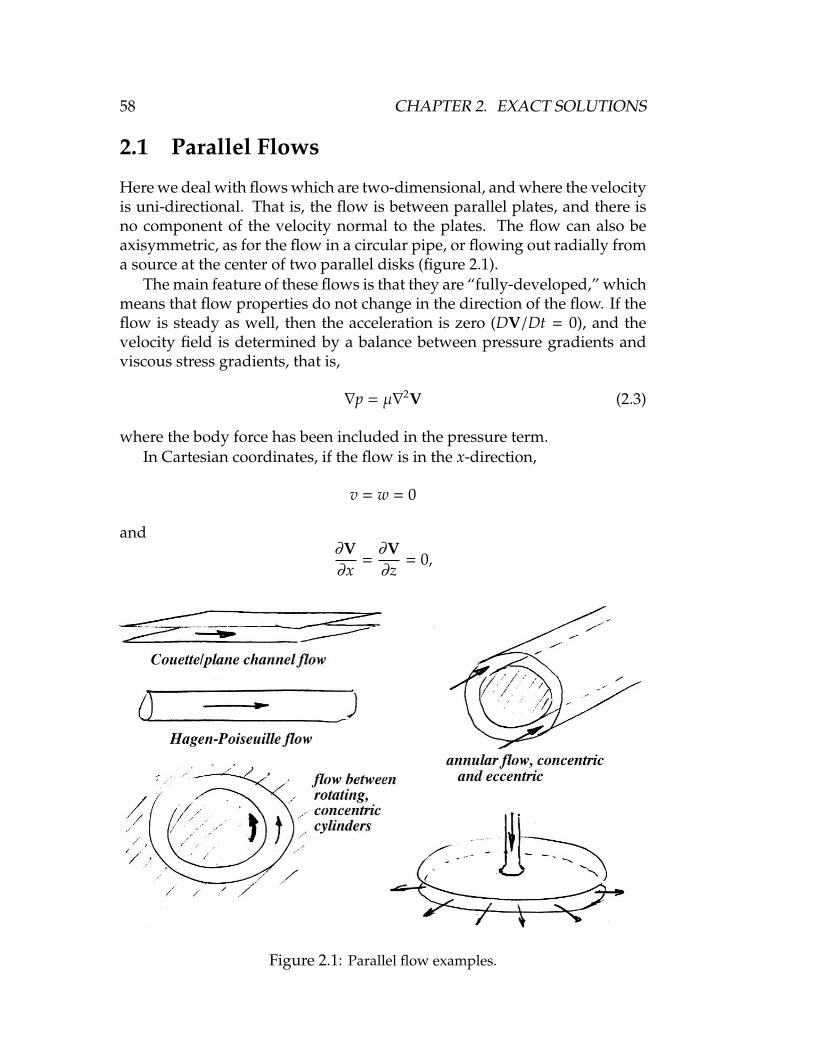
58 CHAPTER 2. EXACT SOLUTIONS
2.1 Parallel Flows
Here we deal with flows which are two-dimensional, and where the velocityis uni-directional. That is, the flow is between parallel plates, and there isno component of the velocity normal to the plates. The flow can also beaxisymmetric, as for the flow in a circular pipe, or flowing out radially froma source at the center of two parallel disks (figure 2.1).
The main feature of these flows is that they are “fully-developed,” whichmeans that flow properties do not change in the direction of the flow. If theflow is steady as well, then the acceleration is zero (DV/Dt = 0), and thevelocity field is determined by a balance between pressure gradients andviscous stress gradients, that is,
∇p = µ∇2V (2.3)
where the body force has been included in the pressure term.In Cartesian coordinates, if the flow is in the x-direction,
v = w = 0
and∂V∂x
=∂V∂z
= 0,
Figure 2.1: Parallel flow examples.

2.1. PARALLEL FLOWS 59
and thereforedpdx
= µd2Vdy2 . (2.4)
2.1.1 Plane Couette flow
In plane Couette flow, two plates are a fixed distance h apart, and the topplate moves at a speed U0 with respect to the bottom plate (see figure 2.2).Due to the no-slip condition, a flow is generated so that
at y = 0, u = 0,and y = h, u = U0.
With these boundary conditions, with a constant pressure gradient, equa-tion 2.4 gives
uU0
=yh
+ Byh
(1 −
yh
)(2.5)
where B is the pressure gradient parameter,
B = −h2
2µU0
dpdx.
When dp/dx = 0, the velocity gradient is linear (see figure 2.2), and the shearstress is constant:
τ = µdudy
=µ
hU0.
When B < −1, there is backflow in the lower part of the flow.
2.1.2 Poiseuille flow
For a smooth pipe of length L and diameter D, dimensional analysis can beused to show that
∆p12ρV2
= φ1
(ρVDµ
,LD
)
Figure 2.2: Couette flow geometry and velocity profiles.

60 CHAPTER 2. EXACT SOLUTIONS
where the pressure drop over the length L is ∆p, and V average velocityintegrated across the cross-section (= volume flow rate/area). Since pipes aretypically long compared to their diameter, an asymptotic, fully-developedstate exists where the flow properties do not change with further increase inlength. This happens after a distance of 20–40 diameters from the entrance,and the flow properties become free of entrance effects. The mean velocityprofile is then independent of the distance along the pipe. In that case, theparameter L/D is no longer important, and the resistance relationship forfully-developed pipe flow becomes:
f =
(∆pL
)D
12ρV2
= φ
(ρVDµ
),
where f is the friction factor, defined by
f =
(∆pL
)D
12ρV2
.
For fully-developed flow in a smooth pipe, therefore, the friction factor isonly a function of the Reynolds number based on average velocity and pipediameter.
It is possible to find exact solutions of the Navier-Stokes equations forfully-developed pipe flow, as long as the flow is laminar and not turbu-lent (this is called Poiseuille flow). In practice, this requires that the pipeflow Reynolds number is less than about 2,300. It is also possible to finda solution for fully-developed, laminar channel flow (this is called planePoiseuille flow). Here, we will derive the solutions for these two cases,starting with channel flow. The results are very similar, and they differ onlyin the constants that appear in the equations.
2.1.3 Fully-developed duct flow
Consider laminar, two-dimensional, steady, constant density duct flow, farfrom the entrance, so that the flow is fully-developed. The duct is rectangularin cross-section, of width w and height D, and it is horizontal, so we do nothave to include the forces due to gravity. For a duct, laminar flow requiresthat the Reynolds number UD/ν is less than about 2,000, where U is theaverage velocity.
First, we use an integral analysis applied to a large control volume oflength dx (figure 2.3). The pressure varies in the streamwise direction, but itdoes not vary across the flow since the streamlines are parallel. The pressureover the inflow area is p − 1
2dp, and over the outflow area it is p + 12dp. If
the flow is fully-developed, the influx and outflux of momentum have the

2.1. PARALLEL FLOWS 61
Figure 2.3: Integral control volume for fully-developed flow in a rectangular duct.
same magnitude and so they cancel. Since there is no change in the flowmomentum, the flow must be in equilibrium under the applied forces: theforce acting on the fluid due to the pressure drop is balanced by the force dueto the viscous stress acting on the interior surface of the duct. The pressuresact on the cross-sectional area wD. The flow is fully-developed and thereforethe velocity gradient is independent of x, and the viscous stress τw will notvary in the streamwise direction. If we assume that τw is constant over theperimeter of the duct, it acts on the area 2 (w + D) dx. Hence,(
p − 12dp
)wD −
(p + 1
2dp)
wD = 2τw (w + D) dx
and sodpdx
= − 2τw(w + D)
wD.
The duct was taken to be two-dimensional, which implies that w D.Hence,
dpdx
= −2Dτw. (2.6)
The pressure gradient is negative because the pressure drops due to viscousfriction.
Second, we use a differential analysis applied to a small control volumeof size dxdydz (figure 2.4), located at a distance y from the centerline. (Wecould use equation 2.4 directly, but we choose to start from first principles.)The flow is two-dimensional, and there is no variation of the velocity inthe spanwise direction. Since the flow is also fully-developed, there isno variation of velocity in the streamwise direction. The only velocityvariation that exists is in the cross-stream direction, that is, in the y-direction.Therefore, the only shearing stresses acting on the elemental volume willact on its top and bottom faces which have an area dxdz. Let τ be the shearstress in the middle of the control volume. Using a Taylor series expansion,and retaining only the first-order terms, the net viscous force Fv acting in the

62 CHAPTER 2. EXACT SOLUTIONS
Figure 2.4: Differential control volume for fully-developed flow in a rectangularduct.
x-direction is given by
Fv =
(τ +
∂τ∂y
dy2
)dxdz −
(τ −
∂τ∂y
dy2
)dxdz
=∂τ∂y
dxdydz.
we see that the net viscous force only makes a contribution if if the viscousstress varies through the flowfield (that is, if ∂τ/∂y , 0). The viscous stressitself is given by
τ = µdUdy,
since the velocity only varies in the y-direction. Therefore,
Fv = µd2Udy2 dxdydz.
We see that the viscous force depends on the second derivative of the velocityfield.
Now we evaluate the force due to pressure differences. If the pressurehalfway along the length of the control volume is p, the net force Fp due topressure acting in the x-direction is given by
Fp =
(p −
∂p∂x
dx2
)dydz −
(p +
∂p∂x
dx2
)dydz
= −∂p∂x
dxdydz.
Since the pressure does not vary in the z-direction (the flow is assumed tobe two-dimensional so that nothing varies in the z-direction), and it cannotvary in the y-direction (the streamlines are straight and forces due to gravityare neglected),
∂p∂z
=∂p∂y
= 0, and∂p∂x
=dpdx,

2.1. PARALLEL FLOWS 63
and so
Fp = −dpdx
dxdydz.
Since there is no acceleration, Fv and Fp must sum to zero, so that
dpdx
= µd2Udy2 . (2.7)
This equation can be solved by observing that the pressure term only de-pends on x, whereas the viscous term only depends on y. The equation canonly be satisfied if both terms are equal to a constant, −K, say. Hence:
dpdx
= −K (2.8)
µd2Udy2 = −K, (2.9)
where K is positive since the pressure decreases with distance down theduct.
We can integrate equation 2.9 twice to obtain the velocity profile. Thevelocity at the top and bottom surface is zero because of the no-slip condition,and the velocity profile will be symmetric about the centerline where y = 0.Therefore the boundary conditions are:
U = 0 at y = ±D2
dUdy
= 0 at y = 0.
Hence:
U =KD2
8µ
1 −(
2yD
)2 .That is:
U =D2
8µ
(−
dpdx
) 1 −(
2yD
)2 . (2.10)
The average velocity U is defined by
U =1A
∫UdA
so that U is equal to the volume flow rate divided by the cross-sectional areaA. For a duct, the average velocity is given by
U =1
wD
D/2∫−D/2
Uwdy =KD2
12µ=
D2
12µ
(−
dpdx
). (2.11)

64 CHAPTER 2. EXACT SOLUTIONS
From equation 2.10 we obtain,
UU
=32
1 −(
2yD
)2 . (2.12)
The laminar velocity profile is parabolic, as illustrated in figure 11.7. Thefriction factor is given by:
f =
∆pL D
12ρU2
=−
dpdxD
12ρU2
= −dpdx
2DρU2
=24µρUD
,
where the pressure gradient was eliminated using equation 2.11. That is,
f =24Re. (2.13)
which holds for all two-dimensional rectangular ducts with Re < 2, 000,where Re = ρUD/µ. It will hold for higher values of Reynolds number ifthe conditions are such to allow laminar flow to exist.
We can find the stress at the wall (y = −D/2) by differentiating equa-tion 2.10. That is,
τw = µ∂U∂y
∣∣∣∣∣w
= −D2
dpdx,
which agrees with the result obtained earlier using a large control volume(equation 2.6).
Finally, examine the Navier-Stokes equation (equation 1.27). For ductflow, the nonlinear acceleration term, DV/Dt, is zero, and equation 2.7follows directly. This equation holds for all fully-developed flows in theabsence of gravity), and therefore it is usually possible to find analyticsolutions for the velocity distributions in fully-developed flows, as long asthe boundary conditions can be satisfied.
2.1.4 Fully-developed pipe flow
Here we consider fully-developed laminar flow in a smooth, circular, hori-zontal pipe. For a smooth pipe of length L and diameter D,
∆p12ρV2
= φ1
(ρVDµ
,LD
)where the pressure drop over the length L is ∆p, and V is the average velocityover the cross-section of the pipe. Since pipes are typically long compared

2.1. PARALLEL FLOWS 65
Figure 2.5: Integral control volume for fully-developed flow in a circular pipe.
to their diameter, an asymptotic, fully-developed state exists where the flowproperties do not change with further increase in length. This happens aftera distance of 20–40 diameters from the entrance, and the flow properties be-come free of entrance effects. The mean velocity profile is then independentof the distance along the pipe. In that case, the parameter L/D is no longerimportant, and the resistance relationship for fully-developed smooth pipeflow becomes:
f ≡
(∆pL
)D
12ρV2
= φ
(ρVDµ
)= φ (Re) ,
where f is the friction factor. Therefore, the friction factor depends only onthe Reynolds number based on average velocity and pipe diameter, Re.
As before, we begin with an integral analysis using a control volume oflength dx, as shown in figure 2.5. The pressure over the inflow area is p− 1
2dp,and over the outflow area it is p + 1
2dp. Since the flow is fully-developed, theflow is in equilibrium under the applied forces. The pressure drop acts onthe cross-sectional area πD2/4, and the viscous stress acts on the area 2πDdx.Hence, (
p − 12dp
) πD2
4−
(p + 1
2dp) πD2
4= τwπD dx
so thatdpdx
= −4Dτw.
Next, we apply a differential analysis by using an annular control vol-ume, located at a distance r from the centerline (figure 2.6). Since the flow istwo-dimensional, there is no variation of the velocity in the circumferentialdirection. Since the flow is fully-developed, there is no variation of velocityin the streamwise direction. The only velocity variation that exists is in theradial, that is, in the r-direction. The only place shearing stresses act areon the inner and outer faces. If the shear stress at the center of the annularcontrol volume is τ, the net viscous force Fv acting in the x-direction is given

66 CHAPTER 2. EXACT SOLUTIONS
Figure 2.6: Differential control volume for fully-developed flow in a circular pipe.
by
Fv =
(τ +
∂τ∂r
dr2
)2π
(r +
dr2
)dx −
(τ −
∂τ∂r
dr2
)2π
(r −
dr2
)dx
= τ 2πdrdx +∂τ∂r
2πrdrdx,
neglecting second-order terms.The net force due to pressure differences in the x-direction, Fp, is given
by
Fp =
(p −
∂p∂x
dx2
)2πrdr −
(p +
∂p∂x
dx2
)2πrdr
= −∂p∂x
2πrdrdx,
where p is the pressure halfway along the length of the control volume.Since there is no acceleration, Fp and Fv must balance, so that
∂p∂x
=τr
+∂τ∂r
=1r∂(rτ)∂r
.
The pressure term depends only on x and the viscous term can only dependon r. Therefore,
dpdx
=1r
d(rτ)dr
. (2.14)
This equation can be satisfied only if the left hand side and the right handside are equal to a constant, K′, say. Hence:
dpdx
= −K′ (2.15)
1r
d(rτ)dr
= −K′, (2.16)

2.1. PARALLEL FLOWS 67
where K′ is positive since the pressure decreases with distance down theduct. Integrating equation 2.16 gives
r τ = −r2
2K′ + c1
orτ = −
r2
K′ +c1
rSince the only velocity gradient is in the r-direction, the viscous stress isgiven by
τ = µdUdr,
andµ
dUdr
= −r2
K′ +c1
rand
U = −r2
4µK′ +
c1
µln r + c2
Using the boundary conditions:
U = 0 at r = ±D/2dUdr
= 0 at r = 0,
we find
U =K′D2
16µ
(1 −
( rD
)2),
so that
U =D2
16µ
(−
dpdx
) (1 −
(2rD
)2), (2.17)
and the velocity profile is parabolic, as found for the duct flow. For a pipe,the average velocity is given by
U =D2
32µ
(−
dpdx
), (2.18)
so that
UU
= 2(1 −
(2rD
)2). (2.19)
The friction factor is then given by:
f =
∆pL D
12ρU2
=−
dpdxD
12ρU2
=64µρUD
,

68 CHAPTER 2. EXACT SOLUTIONS
where equation 2.18 was used to eliminate the pressure gradient. Hence,
f =64Re
(2.20)
which holds for all circular pipes and tubes with Re < 2, 300, although itcan continue to hold at higher Reynolds numbers under favorable circum-stances.
What does Re < 2, 300 mean? For water at 20C, ν = µ/ρ ≈ 1 × 10⁻⁶ m2/s.If D = 10 mm, then to maintain laminar flow, we need U < 0.23 m/s. IfD = 1 mm, we need U < 2.3 m/s. For air at 20C, ν ≈ 15 × 10−6 m2/s, and ifD = 10 mm, U < 3.5 m/s. If D = 1 mm, we need U < 35 m/s.
2.1.5 Rayleigh flow I
Rayleigh flow is the flow that develops above a suddenly accelerated planesurface. It is an unsteady flow that develops with time (Lord Rayleigh, 1911Phil. Mag. 21, 697). Consider a flat plate that is initially at rest in a stationaryfluid. At t = 0, the plate starts to move with a constant velocity U in thepositive x-direction (see figure 2.7). The fluid begins to move, first by theno-slip condition at the surface, and then by the action of viscous stresseswithin the fluid. For this parallel unsteady flow, the convective accelerationterm V · ∇V = 0, and the momentum equation reduces to
∂u∂t
= ν∂2u∂y2 , (2.21)
with the boundary conditions
for t ≤ 0, u = 0 for all y,for t > 0, u = U0 for y = 0,
and u = 0, for y = ∞. (2.22)
This “diffusion” equation is exactly the same as that governing the tem-perature distribution in a stationary medium of thermal diffusivity ν. Theboundary conditions correspond to a suddenly heated wall which is main-tained at a constant temperature. This analogy between temperature andvelocity, and heat transfer and vorticity was discussed in more detail insection 1.9.
For now, we obtain the solution (see Carslaw & Jaeger)
uU0
= erfc(
y
2√νt
).

2.1. PARALLEL FLOWS 69
Figure 2.7: Stokes flow geometry and velocity profile in similarity coordinates.
That is,
f = erfc η
=2√π
∫∞
η
e−η2dη
= 1 − erf η
so that f = 1 −2√π
∫∞
0e−η
2dη.
The velocity profiles for varying times are “similar” in that they can beplotted as a unique function of η when u is non-dimensionalized by U0 (seefigure 2.7). The variables f and η are therefore called “similarity” variables.
Similarity is a very useful concept in the analysis of shear layers. Ingeneral, the solution of equations 2.21 and 2.22 is
uU0
= g′(y, ν, t
), (2.23)
where g′ is a general function of y, ν and t. There are special cases in which
uU0
= g(η), (2.24)
where η, called a similarity variable, is a specific function of y, ν and t. Insuch cases, the number of independent variables is reduced from three (y, νand t) to one (η) so that equations 2.21 becomes an ODE for u. Note that itis a necessary condition that the boundary conditions (equation 2.22) can beexpressed in terms of the similarity variables.

70 CHAPTER 2. EXACT SOLUTIONS
Dimensional analysis can help identify the similarity variables. Startingwith u
U0= g′
(y, ν, t
),
we obtainu
U0= g
(y√νt
).
Therefore f and η are similarity variables in that they describe the dynamicsimilarity of flow fields, as understood in dimensional analysis. In gen-eral, similarity variables are used to convert partial differential equationsto ordinary differential equations (which are much easier to handle). Thisis possible because similarity variables reduce the number of parametersdescribing the flowfield. In the example given here, the dependence of f ony and t is reduced to a dependence on a single variable, η.
To see how this works, we start with the one-dimensional diffusionequation for the Rayleigh flow problem:
∂u∂t
= ν∂2u∂y2 ,
and convert it to an ordinary differential equation using f and η as similarityvariables. Introducing f = u/U0, we get
∂ f∂t
= ν∂2 f∂y2 .
Then we note that
∂ f∂t
=∂ f∂η
∂η
∂t= −
η
2t∂ f∂η
∂ f∂y
=∂ f∂η
∂η
∂y= +
1
2√νt
∂ f∂η
and∂2 f∂y2 =
∂2 f∂η2
(∂η
∂y
)2
= +1
4νt∂2 f∂η2
so that∂ f∂t− ν
∂2 f∂y2 = −
ν4νt
∂2 f∂η2 −
η
2t∂ f∂η
= 0.
Since the only independent variable is η, we obtain the ordinary differentialequation
f ′′ + 2η f ′ = 0.
If we take the region of flow affected by the plate motion to be theregion where y is such that u/U0 < 0.01, we can see from tables of the

2.1. PARALLEL FLOWS 71
Figure 2.8: Rayleigh flow initial condition and velocity profile in similarity coor-dinates.
complementary error function that this occurs at y = 4√νt. This is the usual
definition of a boundary layer thickness δ, and we see that δ depends on√νt, where
√νt is sometimes called the characteristic length for the diffusion
of vorticity, or sometimes simply the Stokes length.
2.1.6 Rayleigh flow II
The second Rayleigh flow is the flow that develops with time starting witha discontinuity in velocity (see figure 2.8). The velocity discontinuity isinitially of zero thickness. The momentum equation is the same as for thefirst Rayleigh flow,
∂u∂t
= ν∂2u∂y2 ,
with the boundary conditions
at t = 0, u = +U0 for y > 0,and t = 0, u = −U0 for y < 0.
We find
f = erf η,
where f = u/U0, and η = y/√
2νt. The shear layer thickness (to ±0.99U0) isequal to 8
√νt (see figure 2.8).

72 CHAPTER 2. EXACT SOLUTIONS
Figure 2.9: Velocity profile evolution as a function of time for the Rayleigh problem(a) t = 0, (b) t > 0, (c) t 0.
2.1.7 Note on vorticity diffusion
The circulation Γ is defined as the line integral of the velocity around a closedcontour (see equation 1.69)
Γ =
∮V · d`
where counter-clockwise contour integration is taken to be positive. ByStokes’s Theorem
Γ =
∫n · ∇ ×V dA
=
∫n ·Ω dA,
where A is the area enclosed by the contour, and Ω = ∇ × V. In cartesiancoordinates,
∇ ×V =
∣∣∣∣∣∣∣i j k∂∂x
∂∂y
∂∂z
u v w
∣∣∣∣∣∣∣So the circulation can also be expressed as an area integral of the vorticitycomponent normal to the surface enclosed by the contour.
Consider the Rayleigh problem, and evaluate the circulation around thecontour C of unit length in the x-direction (see figure 2.9).
At t = 0, Γ = −2U per unit lengthAt t > 0, Γ = −2U per unit length.
That is, the irculation has remained constant, despite the action of viscosityinside the contour. However,
At t 0, Γ < −2U per unit length

2.2. FULLY-DEVELOPED FLOW WITH HEAT TRANSFER 73
because of viscous diffusion across the contour, out of the control volume.Of course, if the contour was large enough, the circulation would al-
ways remain constant, although the vorticity distribution inside the controlvolume would be continualy changing.
Another example might be the bucket on a turntable. If at t < 0 thefluid was moving with solid body rotation, then the circulation aroundany contour enclosing all the fluid would be given by 2πR2ω. If at t = 0 thebucket was suddenly brought to rest, the no-slip condition at the wall wouldinstantaneously cancel out this circulation. Within the bucket, the vorticitygenerated at the wall diffuses out with time, until the vorticity everywhereis also zero.
2.2 Fully-Developed Flow With Heat Transfer
Here we consider only low-speed flows where compressibility effects andviscous effects make a negligible contribution to the temperature field. Forparallel, steady, fully-developed flows, the momentum equation is inde-pendent of the temperature distribution since there are no buoyancy effects(parallel flow) and the fluid properties are taken to be constant. There-fore, the solutions obtained earlier for Couette flow, parallel duct flow, andcircular pipe flow apply unchanged.
For these flows, the energy equation reduces to
d2Tdy2 = 0 (2.25)
which shows that (a) the temperature field is independent of the velocityfield (the two are “uncoupled”), and (b) the temperature profile is linear.
Figure 2.10: Incompressible Couette flow with heat transfer.

74 CHAPTER 2. EXACT SOLUTIONS
Figure 2.11: Incompressible parallel duct flow with heat transfer.
The particular temperature profile depends on the boundary conditions.
2.2.1 Couette flow
Incompressible Couette flow between two parallel plates at different tem-perature has the boundary conditions:
T = T0 at y = 0
T = T1 at y = D
(see figure 2.10). Hence,T − T0
T1 − T0=
yD
To see how viscous effects can affect the temperature profile, see WhiteViscous Flows, section 3.2.1 (but note especially the last paragraph).
2.2.2 Parallel duct flow
For flow between two fixed plates at different temperatures, the boundaryconditions are:
T = T0 at y = −D/2
T = T1 at y = +D/2
(see figure 2.11). Hence,
T − T0
T1 − T0=
12
(1 +
yD
)

2.2. FULLY-DEVELOPED FLOW WITH HEAT TRANSFER 75
2.2.3 Circular pipe flow
For flow in a circular pipe, equation 2.25 becomes, in cylindrical coordinates,
ddr
(rdTdr
)= 0.
The boundary conditions are:
T = Tw at y = D/2
dTdr
= 0 at y = 0
(see figure 2.12). Hence,T = Tw
So the temperature is constant throughout the fluid. To see the effects ofviscous dissipation, see White Viscous Flows, section 3.3.5.
2.2.4 Free convection between heated plates
For free convection, there is no imposed velocity field. Consider two parallelplates. For horizontal plates (see figure 2.13),
when T1 > T0 the flow is stable
when T1 < T0 the flow is unstable for largeRayleigh number, Ra, where
Ra =ρ2CpgβD3∆T
µ
For unstable flows, Benard cells develop, as seen in figure 5.20.For vertical plates (see figure 2.14), we get a simple analytical solution.
We assume a steady, zero pressure gradient, fully-developed flow. Themomentum equation reduces to
−ρβg(T − T
)= −µ
d2wdy2
Figure 2.12: Incompressible pipe flow with heat transfer.

76 CHAPTER 2. EXACT SOLUTIONS
Figure 2.13: Free convection between two horizontal plates.
Figure 2.14: Free convection between two vertical plates.
where T = (T0 + T1)/2 is the average temperature and z is positive upwards.The energy equation is again
d2Tdy2 = 0
if we neglect viscous effects and compressibility effects. Note that the buoy-ancy term couples the velocity and temperature fields, and the convectiveterm is then dependent on the driving temperature difference T1−T0. How-ever, the temperature field is independent of the velocity.
The boundary conditions are:
w = 0 at y = ±D/2T = T0 at y = −D/2T = T1 at y = +D/2
Solving for the temperature field:
T − T0
T1 − T0=
12
(1 +
yD
).

2.3. COMPRESSIBLE COUETTE FLOW 77
We could also express this as
T − TT1 − T0
=yD
(as in the parallel duct flow). To solve for the velocity field, we begin with
−ρβg (T1 − T0)yD
= µd2wdy2
Integrating twice and applying the boundary conditions, we get
w =ρgD2β
(T1 − T
)24µ2
2yD−
(2yD
)3 .This cubic profile could be written non-dimensionally
w∗ =Gr24
(y∗ − y∗3
)where
w∗ =ρwDµ
, y∗ =2yD, Gr =
ρ2gD3β(T1 − T
)µ2 .
To see how viscous effects in the energy equation modify this solution, seeWhite Viscous Flows, section 3.2.2.
2.3 Compressible Couette flow
To illustrate the use of the equations of motion, and to introduce some ofthe concepts encountered in compressible viscous flows, we will considercompressible, laminar Couette flow in some detail. The flow configurationis shown in figure 2.15. Air flows between two parallel plates, where theupper plate moves at a constant velocity Ue relative to the lower plate. Bythe no-slip condition, the velocity of the air in contact with the upper plate isalso Ue relative to the air in contact with the lower plate. The other boundaryconditions are as shown. The temperature of the upper and lower platesare Te and Tw, respectively, and there is a heat flux qw from the lower plateinto the flow and a shear stress τw also acts on the lower plate. The flow istwo-dimensional so that ∂/∂z = 0; it is fully-developed so that ∂/∂x = 0, andit is steady so that ∂/∂t = 0. We will assume that the gas has constant specificheats.
The continuity equation gives:
∂ρv∂y
= 0, (2.26)

78 CHAPTER 2. EXACT SOLUTIONS
Figure 2.15: Notation for compressible Couette flow.
where V = ui + vj + wk. Hence, V = 0 by symmetry, and the flow is parallel.The momentum equation gives:
∂σ12
∂y= 0, that is
∂∂y
(µ∂u∂y
)= 0. (2.27)
Therefore the shear stresses and pressure are constant throughout the flowfield. If the flow were incompressible, the viscosity would be constantand equation 2.27 could be integrated to show that the velocity profileis linear. When the flow is compressible, variations in temperature willproduce variations in viscosity, and we need to solve for the temperaturedistribution before equation 2.27 can be integrated.
The energy equation gives:
∂∂y
(µu∂u∂y
+ k∂T∂y
)= 0. (2.28)
That is, the diffusion of kinetic energy and heat are in equilibrium. If wewrite the energy equation in terms of the enthalpy, we find:
Φ −∂qi
∂xi= 0. (2.29)
That is, the dissipation and the heat flux are in equilibrium. In fact, the tworelations give the same result since:
∂uiσi j
∂x j= Φ + ui
∂σi j
∂x j
and the viscous stress is constant. It follows that in this fully-developedflow the temperature distribution depends only on how the kinetic energyis dissipated and how the heat is diffused.

2.3. COMPRESSIBLE COUETTE FLOW 79
Integrating equation 2.28 from the lower wall outward gives:
µu∂u∂y
+µCp
Pr∂T∂y
= −qw.
Here we have introduced the Prandtl number Pr = µCp
/k. By using the
fact that the stress is constant and by assuming that the Prandtl number isconstant (this is a good approximation for many gases) we find that:
∂∂y
(CpT + 1
2Pru2)
= −Prqw
τw
∂u∂y.
By further integration:
Cp (T − Tw) +12
Pru2 = −Prqw
τwu, (2.30)
and using the boundary conditions at the upper wall, we obtain:
Tw = Te +PrCp
(12U2
e +qw
τwUe
). (2.31)
Consider the case where the lower wall is adiabatic(qw = 0
). Here,
Tw = Tr = Te + 12
PrU2e
Cp= Te
(1 + Pr
γ − 12
M2e
)where Me is the Mach number based on the velocity and temperature ofthe upper wall, and Tr is called the recovery temperature or adiabatic walltemperature. Since the velocity of the air in contact with the lower wall iszero, Tw is equal to the total temperature at that point. The total temperatureat the upper wall is T0e = Te + 1
2U2e
/Cp. We see that if the Prandtl number is
not equal to one, the temperature of the stationary wall is not equal to thetotal temperature at the upper boundary: the kinetic energy is not exactly“recovered” in the form of heat at the lower boundary. The ratio of therecovered energy to the external energy is called the recovery factor, r, where
r =Tr − Te
T0e − Te. (2.32)
In the case of laminar Couette flow, the recovery factor is simply equal to thePrandtl number. Note that when the Prandtl number is less than one (forair Pr = 0.72 at NTP), the temperature of the stationary wall is lower thanthe total temperature evaluated at the moving boundary.
Equation 2.31 gives the solution for the heat transfer from the lower wall:
qw =τwCp
PrUe(Tw − Tr) (2.33)

80 CHAPTER 2. EXACT SOLUTIONS
which shows that the heat transfer is proportional to the temperature differ-ence Tw − Tr, and not Tw − Te as in low-speed flows. Also, we see that theheat transfer is proportional to the wall shear. That is, for the lower wall,
Ch =1
2PrC f (2.34)
where C f =τw
12ρeU2
e, and Ch =
qw
ρeUeCp (Tw − Tr).
C f is the skin friction coefficient and Ch is the heat transfer coefficient, orStanton number. Relationships such as Equation 2.34 which connect the heat-transfer and skin-friction coefficients are called Reynolds Analogies, and theratio s = 2Ch
/C f is called the Reynolds Analogy Factor.
We can find the skin friction coefficient by integrating the momentumequation (equation 2.27). If we assume that the viscosity is proportional tothe temperature (the actual variation is given by equations 1.36 and 1.37),we obtain:
C f =1
Re
(1 +
Tw
Te+ 2
3Pr(γ − 1
)M2
e
). (2.35)
For compressible Couette flow, the skin friction coefficient increases withheating and Mach number (this is not necessarily true for other wall-bounded flows such as boundary layer flows).
In addition, we obtain from equations 2.30 and 2.31:
TTe
=Tw
Te+
Tr − Tw
Te
( uUe
)−γ − 1
2PrM2
e
( uUe
)2
. (2.36)
This temperature-velocity relationship, derived for compressible Couetteflow, is often used in the analysis of laminar and turbulent wall-boundedflows by replacing the Prandtl number in equation 2.36 with the recoveryfactor appropriate to those flows. In that form, it is often called the CroccoRelation or Crocco’s Law. Velocity and temperature profiles for a numberof Mach numbers are shown in figure 2.16.
One conclusion we can draw from this example is that in the absenceof pressure gradients the kinetic energy of a supersonic flow is of suchmagnitude that when it is transformed into heat and redistributed in spaceby molecular diffusion significant temperature variations can occur. Thiscan also be understood from the definition of Mach number: M = U
/√γRT.
Here the numerator (squared) is proportional to the kinetic energy and thedenominator (squared) is proportional to the internal energy. When theMach number is of order unity the two forms of energy are of the sameorder of magnitude, and changes in the kinetic energy will result in changesin the temperature and its distribution in space.

2.4. SIMILARITY SOLUTIONS 81
Figure 2.16: Velocity and temperature profiles in compressible Couette flow.
2.4 Similarity Solutions
We saw how it is sometimes possible to change a partial differential equa-tion to an ordinary differential equation by using specially chosen non-dimensional dependent and independent variables. These variables arecalled similarity variables, and the method is called the method of simi-larity solutions. We did one example when discussing the Rayleigh prob-lem. Here, we consider some other problems that can be solved using themethod of similarity solutions: viscous stagnation point flow, and a sud-denly stopped rotating cylinder.
2.4.1 Cylinder rotating at constant speed
Consider a steady laminar flow produced by a long circular cylinder rotatingcounterclockwise with a constant angular velocity ω in an infinite body ofviscous fluid. The equations of motion, in cylindrical coordinates are (withu = w = 0), for the radial component
dpdr
=ρv2
r
and for the tangential component
d2vdr2 +
1r
dvdr−
vr2 = 0.
To solve for v, we note that the tangential momentum equation can be writtenas
ddr
(1r
dvrdr
)= 0

82 CHAPTER 2. EXACT SOLUTIONS
which has the general solution
v = ar +br,
that is, a combination of a solid body rotation plus a potential vortex. Withthe boundary conditions
v = r0ω and p = p0 at r = r0
v = 0 at r = ∞
we obtain
v =r2
0ω
r.
For any closed contour enclosing the spinning cylinder,
Γ = 2πvr = constant = Γ0
so that
v =Γ0
2πr. (2.37)
where Γ is positive for counterclockwise rotation.We should note that for two-dimensional incompressible flow, we can
define a function ψ called the streamfunction, where
u =1r∂ψ
∂θ, and v = −
∂ψ
∂r
so that the continuity equation is precisely satisfied. For the spinning cylin-der problem, u = 0, and
ψ =Γ
2πln r
which is the streamfunction for a line vortex.Now, for the pressure, we obtain
Cp ≡p − p012ρr2
0ω2
= 1 −(r0
r
)2
(see figure 2.17).

2.4. SIMILARITY SOLUTIONS 83
Figure 2.17: Velocity and pressure distributions for a cylinder rotating at a constantspeed in a viscous fluid.
2.4.2 Suddenly stopped rotating cylinder
Consider now the motion that results when the cylinder stops suddenly.The momentum equation becomes
1ν∂v∂t
=∂2v∂r2 +
1r∂v∂r−
vr2
with the boundary conditions
v =Γ0
2πrat t = 0
v = 0 at r = r0 for t > 0.
Consider the case where r0 r (the far-field solution). Then we could write
v = v (Γ0, r, ν, t) .
By dimensional analysis this could be written as
2πvrΓ0
= f (η) where η =r2
νt.
These similarity variables turn the partial differential equation into an ordi-nary differential equation:
f ′′ + 14 f ′ = 0
with the boundary conditions
f = 1 at η = ∞
f = 0 at η = 0.
Hence,f = 1 − e−η/4.
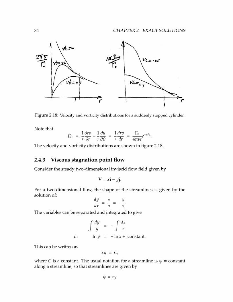
84 CHAPTER 2. EXACT SOLUTIONS
Figure 2.18: Velocity and vorticity distributions for a suddenly stopped cylinder.
Note that
Ωz =1r∂rv∂r−
1r∂u∂θ
=1r
drvdr
=Γ0
4πνte−η/4.
The velocity and vorticity distributions are shown in figure 2.18.
2.4.3 Viscous stagnation point flow
Consider the steady two-dimensional inviscid flow field given by
V = xi − yj.
For a two-dimensional flow, the shape of the streamlines is given by thesolution of:
dydx
=vu
= −yx.
The variables can be separated and integrated to give∫dyy
= −
∫dxx
or ln y = − ln x + constant.
This can be written asxy = C,
where C is a constant. The usual notation for a streamline is ψ = constantalong a streamline, so that streamlines are given by
ψ = xy

2.4. SIMILARITY SOLUTIONS 85
Figure 2.19: Viscous stagnation point flow.
(u = ∂ψ/∂y, v = −∂ψ/∂x). That is, the streamlines are parabola in the x-yplane. The flowfield represents a stagnation point flow, as illustrated infigure 2.19 (the stagnation streamline is the one corresponding to ψ = 0).
For the viscous flow, we could try a new streamfunction
ψ∗ = kx f (y)
which gives
u = kxd fdy, v = −k f .
It is not immediately obvious that the modified streamfunction will describeviscous flow near a stagnation point. At first glance, its main justification isthat when ψ∗ ∝ x, the viscous terms in the Navier-Stokes equation containsonly terms that involve second derivatives with respect to y. However,
(a) ψ∗ will satisfy the no-slip condition if
f (0) = 0, andd fdy
∣∣∣∣∣y=0
= f ′(0) = 0
(so that u and v are zero at the wall for all x).
(b) Far away from the wall, viscous effects should be negligible so thatinviscid stagnation point flow is recovered. That is, we require
d fdy
∣∣∣∣∣y→∞
= 1
which means thatf (∞) = y + constant,
as required.

86 CHAPTER 2. EXACT SOLUTIONS
So, with the right boundary conditions, ψ∗ can represent viscous stagnationpoint flow.
The Navier-Stokes equation for this two-dimensional flow becomes
k f ′2 − k f f ′′ − ν f ′′′ = −1ρkx
∂p∂x
(2.38)
ν f ′′ + k f f ′ = −1ρk∂p∂y
(2.39)
(the dash represents differentiation with respect to y). The second equationshows that
∂p∂y
= a function of y only, (2.40)
and∂2p∂x∂y
= 0. (2.41)
Hence
∂p∂x
= g(x) + C1. (2.42)
That is1ρkx
∂p∂x
=g(x)ρkx
+C1
ρkx(2.43)
where C1 is a constant which must be zero by symmetry. From equation 2.39,we see that the left hand side of equation 2.43 is a function of y only. SinceC1 = 0, g(x) must therefore be of the form C2x. Now what is the value ofthis constant C2? At large distances from the origin, the streamlines becomenearly parallel, ∂p/∂y → 0, and ∂p/∂x must therefore approach the valuegiven by the potential flow (inviscid flow) solution. That is, C2 = ρk2. Hence
∂p∂x
= ρk2x
which is independent of y. Note that ∂p/∂x is given by the inviscid Bernoulliequation, so that ∂p/∂x = U(dU/dx), where U is the x-component velocityoutside the viscous layer. Equation 2.39 becomes
ν f ′′′ + k f f ′′ + k(1 − f ′2
)= 0.
To non-dimensionalize this equation, we put
η = αy, and f (y) = βφ(η)

2.4. SIMILARITY SOLUTIONS 87
and we find
β2α2 = 1, and βα3 =kν. (2.44)
That is, η =
√kν
y, and φ(η) =
√kν
f (y). (2.45)
Finally:φ′′′ + φφ′′ − φ′2 + 1 = 0 (2.46)
(the dash represents differentiation with respect to η), with the boundaryconditions
φ = 0, φ′ = 0 at η = 0φ′ = 1 at η = ∞.
Note that when we compare u and v to the inviscid values, we have
uU
= f ′ = φ′, andvV
=f (y)
y=φ
η.
The numerical solution of this nonlinear ordinary differential equationwas first given by Hiemenz in 1911. The results are given in table 2.1 andfigure 2.20. If we note the distance at which u/U = 0.99, we have η = 2.4.That is,
δ = 2.4
√νk.
Thus u/U and δ99 are both independent of x.Finally, we can calculate C f using
τw = µ
(∂u∂y
+∂v∂x
)y=0
Therefore,
C f =τw
12ρU2
=µkx
√kνφ′′
0
12ρU2
= 2
√ν
Uxφ′′0 =
2φ′′0√
Rex
(note that, as x→ 0, C f →∞ but τw → 0).
Viscous layer thickness
The viscous layer or “boundary” layer thickness is usually small. For thecylinder example given here, k = 4U∞/D.
(a) With U∞ = 3 m/s, and D = 30 cm, k = 40 s−1. In air, this givesδ = 1.4 mm. The Reynolds number ReD = 60, 000.(a) With U∞ = 0.3 m/s, and D = 30 cm, k = 4 s−1, and δ = 4.5 mm(ReD = 6, 000).

88 CHAPTER 2. EXACT SOLUTIONS
Table 2.1: Tabulated flowfield solutions for viscous stagnation point flow(Howarth, 1934).
Figure 2.20: Viscous stagnation point flow profiles.

2.5. CREEPING FLOW AND LUBRICATION THEORY 89
2.5 Creeping Flow and Lubrication Theory
Consider the momentum equation for constant-property, constant-densityflows, without heat transfer. In non-dimensional form we had
DV′
Dt′= −∇′p′ +
1Re∇′2V′,
which means that, if we have chosen the reference parameters in a reasonableway, all the derivative terms should be of the same order. This would suggestthat at very low Reynolds numbers the inertia term and the pressure gradientterm should go to small values compared to the viscous term. However, thisis not correct. If the inertia term becomes very small, the dynamic pressure12ρ0U2
0 goes to very small values, and therefore it is no longer an appropriatescaling parameter for the pressure (the only reason we use the dynamicpressure is because of its prominence in the Bernoulli equation, and in veryviscous, low Reynolds number flows, the Bernoulli equation is very wrong).So we should use some kind of viscous scaling, such as
p∗ =p − p0
µ0V0/L.
Starting withDVDt
= −∇p + µ∇2V,
we can re-work the non-dimensionalization, and this time we get
DV′
Dt′=
1Re
(−∇
′p∗ + ∇′2V′),
which shows that as the Reynolds number goes to very small values, theinertia terms become negligible but the pressure gradient terms do not.Hence, the momentum equation for very low Reynolds number flows is
∇p = µ∇2V (2.47)
This equation looks very much like the one derived for parallel, fully-developed flows, but of course the present case is not restricted to theseconditions, only that the Reynolds number is small enough.
2.5.1 Stokes flow
One general solution of this equation is available for flow over a sphere(Stokes flow). The details of the solution are given by White (p.204) and

90 CHAPTER 2. EXACT SOLUTIONS
Batchelor (p.230). In spherical polar coordinates, the radial and tangentialvelocities are given by
ur = U∞ cosθ(1 +
a3
2r3 −3a2r
),
vθ = U∞ sinθ(−1 +
a3
4r3 +3a4r
).
Note:
(1) The velocities are independent of the viscosity µ.
(2) The streamlines are symmetrical fore and aft (there is no wake). Asthe Reynolds number increases, the inertia terms will become impor-tant, and it is the convective acceleration terms that break the symme-try.
(3) The velocity everywhere is less than U∞ (unlike potential flowwhere the velocity at the diameter plane is 1.5U∞).
(4) The effect of the sphere extends to large distances: at r = 10a,0.85 < |u|/U∞ < 0.95 (see figures 2.21 and 2.22).
Figure 2.21: Comparison of creeping flow (left ) and potential flow (right ) past asphere. From White Viscous Flows.

2.5. CREEPING FLOW AND LUBRICATION THEORY 91
Figure 2.22: Streamlines and velocity distributions in Stokes’ solution for a spherein parallel flow. From Schlichting Boundary Layers.
With ur and uθ known, the pressure is found by integrating the momen-tum equation. The result is
p = p∞ −3µaU
2r2 cosθ
where p∞ is the uniform freestream pressure. Thus the pressure deviation isproportional toµ and antisymmetric, being positive at the front and negativeat the rear of the sphere (see figure 2.23). This creates a pressure drag on thesphere. There is also a surface shear stress which creates a drag force. Theshear-stress distribution in the fluid is given by
τ = µ
(1r∂ur
∂θ+∂uθ∂r
)= −
Uµ sinθr
(1 −
3a4r
+5a3
4r3
).
Figure 2.23: Pressure distribution around a sphere in parallel flow. From Schlicht-ing Boundary Layers.

92 CHAPTER 2. EXACT SOLUTIONS
Figure 2.24: Drag on a sphere.
The total drag is found by integrating pressure and shear around the surface:
F = −
∫ π
0τr=a sinθ dA −
∫ π
0pr=a cosθ dA
dA = 2πa2 sinθ dθ
F = 4πµUa + 2πµUa = 6πµUa
This is the famous result found by Stokes (1851). For what it is worth, frictionin this case contributes two-thirds of the drag and pressure one-third. Theformula is strictly valid only for Re 1, the “creeping” flow assumption,but figure 2.24 shows that it is accurate up to about Re = 1.
2.5.2 Slider bearing
The second example of low Reynolds number flow is the flow in an oillubricated bearing. This flow is modeled by considering a sliding blockmoving over a plane guide surface (see figure 2.25). To make the flowsteady, we move with the slide block, which is considered to be large in thetransverse direction.
We allow the block to be inclined at a small angle α to the guide surface,so that u(∂u/∂x), for example, is not zero. However,
ρu∂u∂x
µ∂2u∂y2
≈ρU2/`
µU/h2 =ρU`µ
(h`
)2
,
and we can neglect the acceleration (inertia) terms when
ρU`µ
(h`
)2
1, orρUhµ
(h`
) 1.

2.5. CREEPING FLOW AND LUBRICATION THEORY 93
Figure 2.25: Notation for a slider bearing.
Take, for example, U = 10 m/s, ` = 100 mm, h = 0.2 mm, ν = 40 × 10−6 m2/s,gives
U`ν
= 25, 000,ρU`µ
(h`
)2
= 0.1.
Similarly,∂2u/∂x2
∂2u/∂y2 ≈U/`2
U/h2 =
(h`
)2
1
and
v ≈ 0,∂p∂y
∂p∂x.
Finally,dpdx
= µ∂2u∂y2 . (2.48)
Note that dp/dx may be a function of x, and so u = u(x, y). This is notan example of fully developed , parallel flow. Therefore we need anotherequation, since u and p are unknowns. We can use the continuity equation,∫ h(x)
0u dy = constant = Q. (2.49)
The boundary conditions are
u = U, y = 0 p = 0, x = 0u = 0, y = h p = 0, x = `.
Hence, from the momentum equation (equation 2.48, we obtain
uU
=(1 −
yh
) (1 −
h2
2µUdpdx
yh
)

94 CHAPTER 2. EXACT SOLUTIONS
and from the continuity equation (eqation 2.49,
dpdx
= 12µ( U2h2 −
Qh3
)which gives
p = 6µU∫ x
0
dXh2 − 12µQ
∫ x
0
dXh3 .
With p = 0 at x = `, we get
Q =
12U
∫ `
0duh2∫ `
0duh3
.
Consider a flat slider on a flat guide surface, so that
h = h1 − βx
= h1 −(h1 − h2) x
`.
This gives
Q =
12U
∫ h2
h1
dhh2∫ h2
h1
dhh3
= Uh1h2
h1 + h2
andp = 6µU
(h1 − h2) (h − h2)(h2
1 − h22
)h2
.
(see figure 2.26). Note that
(a) The pressure gradient
dpdx
= 12µ( U2h2 −
Qh3
)= 0
when h =2QU
=2h1h2
h1 + h2.
That is, the pressure has a maximum (or minimum) at 2h1h2/h1 + h2.(b) For p > 0 everywhere, we require h > h2. That is, the block mustslope down in the direction of motion.
(c) Back flow occurs in the region of pressure rise near the wall at rest,just as we found in the Couette flow with adverse pressure gradient.
(d) The total pressure load P =∫ `
0pdx has a maximum value when
h1/h2 ≈ 2.2, which gives
P = 0.16µU`h2
(`h2
).

2.6. ADDITIONAL EXACT SOLUTIONS 95
Figure 2.26: Lubrication in a bearing: a) Flow in a wedge between slide block andplane guide surface; b) Pressure distribution over block, a/` = 1.57 (h1/h2 = 2.75).From Schlichting Boundary Layers.
2.6 Additional Exact Solutions
Flow between rotating concentric cylinders (White p.117, Schlichtingp.80).
Non-circular duct flows (White p.123).
Eccentric annulus flow (White p.125).
Thermal entrance problem (White p.132).
Starting flow in a circular pipe (White p.141, Schlichting p.84, Batchelorp.193).
Pipe flow with an oscillating pressure gradient (White p.143).
Flow near an oscillating flat plate (White p.148, Schlichting p.85, Batch-elor p.191). Note similarity with the case of an unsteady pressuregradient, Lam p.217.
Flow formation in Couette flow (White p.141, Schlichting p.84, Batch-elor p.193).
Model of a paint brush (Batchelor p.183).

96 CHAPTER 2. EXACT SOLUTIONS

Chapter 3
Laminar Boundary Layers
Consider again the flow generated by an infinite flat plate set impulsively inmotion at t = 0 with a constant velocity U. Initially, the fluid velocity is zeroeverywhere, and the vorticity and circulation are also zero everywhere. Att = 0, the no-slip condition sets an infinitely thin layer of fluid into motion.At interior points in the fluid, the velocity and vorticity remain zero, but atthe wall, there exists now a discontinuity in tangential velocity, such thatthe circulation per unit length is −U (constant and finite), and we havetherefore a constant strength vortex sheet at the wall. For t > 0, the vorticitywhich was concentrated at the boundary at t = 0 diffuses into the fluid bythe action of viscosity (figure 3.1). Remember that vorticity in a constantdensity, constant property fluid obeys a diffusion equation, and thereforethe spread of vorticity into the fluid is similar to the spread of temperatureaway from a suddenly heated plate kept at a constant temperature. Thecharacteristic distance for this diffusion process is
√νt for vorticity and
√αt
for temperature.In this simple example, the convective acceleration terms were all zero,
and we hadDΩDt
=∂Ω∂t, and
DTDt
=∂T∂t.
Let’s consider a case where these convective terms are important, such asthe case of fluid set in motion by a solid body moving through it. Thetransport of vorticity away from the body then depends on convection anddiffusion, and the convection may limit the parts of the fluid that becomevortical. Near the nose of the body, for example, the relative velocity of thefluid toward the body will limit the extent to which the vorticity is spread(figure 3.2). In cases where the convection is strong (U is large), or wherethe diffusion is weak (ν is small), there will be a large region of the fluid,ahead of and to the sides of the body, untouched by the viscous diffusion ofvorticity where the fluid is irrotational in the steady state.
When the body is a flat plate of length `, which is put into motion at t = 0
97

98 CHAPTER 3. LAMINAR BOUNDARY LAYERS
Figure 3.1: Vorticity diffusion for a plate set impulsively into motion.
with a velocity U, and also suddenly heated to a constant temperature, thenthe vorticity and temperature diffuse out across streamlines to a character-istic distance
√νt (ν = α when Pr = 1). The time t that a material element
spends in the vicinity of the flat plate is given by `/U. The ratio of theconvection distance ` to the diffusion distance
√ν`/U defines a Reynolds
number√
U`/ν. Thus, if U`/ν 1, the vorticity and heat are convecteddownstream before they can be diffused very far laterally, and there is arather narrow region of heated, vortical fluid next to the body. If U`/ν 1,the effect of convection is very small, and both vorticity and temperaturerise more or less equally in all directions away from the body, as we sawin the case of Stokes flow over a sphere. (Note that even for Re 1, thesmall convection terms give rise to a wake, as shown by Oseen’s correctionto Stokes’ analysis in figure 2.24.)
(To analyze the flow near the leading edge of the plate, the qualitativestatements regarding the convective and diffusive terms will still hold butthe quantitative conclusions are different: the analysis must be based onstagnation point flow considerations.)
Thus, in cases where convection and diffusion are important, the effectof increasing Reynolds number is to confine the vorticity diffused from asolid boundary to a layer of relatively small thickness, the magnitude ofthis vorticity being greater as the layer becomes thinner with increasingReynolds number. Within this layer (the boundary layer), viscous effects are
Figure 3.2: The competition between diffusion and convection.

3.1. BOUNDARY LAYER GROWTH 99
always important, no matter what the Reynolds number, whereas outsidethis layer the flow may be treated as inviscid (Prandtl’s 1904 boundary layerhypothesis). The boundary layer is, in effect, the layer in which the fluidvelocity makes a transition from the required value of zero at the boundaryto a freestream value which is appropriate to an inviscid fluid.
3.1 Boundary Layer Growth
When a fluid flows over a solid surface, we know that the no-slip conditioncauses steep velocity gradients to occur in a region near the surface. As theflow proceeds downstream, the thickness of this “boundary” layer growsbecause lower layers of fluid exert friction on the higher layers, and moreand more fluid is decelerated by viscous friction. In a two-dimensionalduct, the layers grow on the upper and lower walls, and after some distancethey meet, merge, and eventually the flow becomes fully-developed so thatfurther growth stops. A similar process occurs in the entrance region of apipe.
However, in an external flow, such as the flow over a flat plate placed inthe center of a wind tunnel, the boundary layer continues to grow and thereis no fully-developed state. The analysis is consequently more difficultbecause the flow continuous to accelerate and the nonlinear accelerationterm in the Navier-Stokes equation is no longer zero. Nevertheless, it ispossible to determine approximately the growth rate of the layer and thedrag exerted by the flow on the plate by using the integral forms of thecontinuity and momentum equations.
3.1.1 Control volume analysis
We will begin by analyzing a laminar boundary layer, which is the flow thatoccurs over a plate when the Reynolds number Rex = ρUex
/µ < 100, 000,
where x is the distance from the leading edge, and Ue is the velocity of theflow outside the boundary layer. The velocity Ue is taken to be constant sothat ∂p
/∂x = 0.Also, we will assume that the plate is flat and that the bound-
ary layer is thin, so that the streamlines are nearly parallel and therefore∂p
/∂y ≈ 0. The flow is steady and the fluid has a constant density.Consider a rectangular control volume extending a distance L from the
leading edge, with a height equal to the extent of the boundary layer at x = L(figure 3.3). The incoming velocity is uniform, and the outgoing profile isdecelerated near the wall because of friction, so that for a distance δ thevelocity U(y) < Ue. Actually, U approaches the value Ue asymptotically, sothat the boundary layer thickness δ is defined to be the distance where the Uis virtually indistinguishable from Ue. The most common definition of the

100 CHAPTER 3. LAMINAR BOUNDARY LAYERS
Figure 3.3: Control volume for the analysis of a laminar boundary layer.
boundary layer thickness is
U = 0.99Ue at y = δ.
Note that δ increases with x, so that δ = δ(x). For many purposes, thevelocity variation outside the boundary layer can be neglected. For example,in applying the continuity and momentum equations, these small velocityvariations are routinely ignored because their contributions are negligiblysmall (see section 3.6).
We begin with the conservation of mass. Since there is a greater mass-flow into the control volume over face ab than out of the control volume overface cd, because U(y) < Ue, there must be a mass-flow through face bc. Onface bc, the velocity in the x-direction is constant and equal to Ue (remember,∂p/∂x = 0), but the y-component of the velocity Vn is unknown. For now,we shall simply proceed. Using the continuity equation,
h∫0
(n1 ·Uei)wdy +
h∫0
(n2 ·U
(y)
i)wdy +
L∫0
(n3 ·
(Uei + Vn (x) j
))wdx = 0,
where w is the width of the plate, and n1, n2 and n3 are the unit normalvectors on faces ab, cd and bc, respectively. That is,
−Ueh +
h∫0
U dy +
L∫0
Vn dx = 0, (3.1)
where U = U(y) and Vn = Vn(x).

3.1. BOUNDARY LAYER GROWTH 101
Next, we use the x-component of the momentum equation. It is under-stood that Fv is the force exerted by the plate on the fluid, so that
−Fv = i ·
h∫0
(n1 · ρUei
)Uei wdy + i ·
h∫0
(n2 · ρUi
)Ui wdy
+ i ·
L∫0
(n3 · ρ
(Uei + Vnj
)) (Uei + Vnj
)wdx.
That is,
−Fv = −
h∫0
ρU2e wdy +
h∫0
ρU2 wdy +
L∫0
ρVnUe wdx
and so
−Fv
ρw= −U2
e h +
h∫0
U2 dy +
L∫0
VnUe dx.
The continuity equation can be used to eliminate the unknown velocityVn(x). Multiplying equation 3.1 by Ue and subtracting the result from themomentum equation gives
−Fv
ρw= −U2
e h +
h∫0
U2 dy + U2e h −
h∫0
UUe dy
=
h∫0
(U2−UUe
)dy.
Hence,Fv
ρwU2e
=1
U2e
h∫0
(UUe −U2
)dy
=
h∫0
(UUe−
U2
U2e
)dy.
Finally,Fv
ρwU2e
=
h∫0
UUe
(1 −
UUe
)dy. (3.2)
To go further, we need to know (or guess) how the velocity varies withdistance from the wall. In other words, we need to know how U varies withy, and δ varies with x.

102 CHAPTER 3. LAMINAR BOUNDARY LAYERS
3.1.2 Similarity solution
It was shown by Prandtl in 1904 that for a boundary layer the full Navier-Stokes equation can be approximated by a simpler equation. The approx-imations are based on the observation that a boundary layer only growsslowly and the streamlines within the layer are nearly parallel. In particu-lar, the pressure across the layer is nearly constant, (which helps to justifyour earlier assumption that the pressure was constant throughout the controlvolume). These approximations yield an equation called the boundary layerequation, and Paul Richard Heinrich Blasius (1883–1970), one of Prandtl’sstudents, showed that this equation has a “similarity” solution. The bound-ary layer equation is derived in the next section, but a few preliminary wordsare useful.
Blasius supposed that the velocity distribution in a laminar boundarylayer on a flat plate was a function only of the freestream velocity Ue, thedensity ρ, the viscosity µ, the distance from the wall y, and the distancealong the plate x. Dimensional analysis gives:
UUe
= f(Uexν,
yx
).
By an ingenious coordinate transformation Blasius showed that, insteadof depending on two dimensionless variables, the dimensionless velocitydistribution was a function of only one composite dimensionless variable η,so that
UUe
= f ′y
x
√Uexν
= f ′(η√
2).
The variables U/Ue and η (= y√
Ue/(2νx)) are called similarity variables,which means that if the velocity distribution is plotted using these non-dimensional variables (instead of dimensional variables such as U and y),it is defined by a single universal curve, for any Reynolds number and anyposition along the plate.
These particular similarity variables transform the boundary layer equa-tion (a PDE) into an ODE which can be solved numerically. The solutionis called the Blasius velocity profile, and the results are usually given inthe form of a table (see table 3.1). The Blasius velocity profile matches theexperimental data, such as those shown in figure 3.4, very well.
The contribution by Blasius was important in that he used similarityarguments (firmly rooted in dimensional analysis) to find an exact solutionto an approximate equation describing the flow in a laminar boundary layer(Prandtl’s boundary layer equation). Furthermore, the results describe theexperimental data very well, thereby justifying the assumptions that weremade.

3.1. BOUNDARY LAYER GROWTH 103
Table 3.1: Dimensionless velocity profile for a laminar boundary layer: tabulatedvalues (η = y
√Ue/(2νx)). Adapted from F.M. White, Fluid Mechanics, McGraw-Hill,
1986.
The Blasius solution is not an analytical solution, and tabulated valuesdo not reveal the physics very well. It is convenient to have analyticalform for the velocity profile, and it turns out that a parabola is a reasonable

104 CHAPTER 3. LAMINAR BOUNDARY LAYERS
Figure 3.4: Dimensionless velocity profile for a laminar boundary layer: compar-ison with experiments by Liepmann, NACA Rept. 890, 1943. Adapted from F.M.White, Viscous Flow, McGraw-Hill, 1991.
approximation (see figure 3.5). That is, we can use the approximation that
UUe
= 2( yδ
)−
( yδ
)2
for y ≤ δ (3.3)
andUUe
= 1 for y > δ.
which satisfies the boundary conditions that U = 0 at y = 0, and U = Ue aty = δ. Most importantly, it retains the correct similarity scaling, as we shallsee. Then, for this particular profile, we have from equation 3.2:
Fv
ρwU2eδ
=
1∫0
UUe
(1 −
UUe
)d( yδ
)=
215. (3.4)
To eliminate δ we use the fact that the total force due to friction Fv is theintegral of the shear stress at the wall τw over the area of the plate:
Fv =
L∫0
τw wdx.
Differentiating and using the Newtonian stress-strain rate relationship gives
1w
dFv
dx= τw = µ
∂U∂y
∣∣∣∣∣w. (3.5)

3.1. BOUNDARY LAYER GROWTH 105
Figure 3.5: Comparison of dimensionless laminar and turbulent flat-plate velocityprofiles. Adapted from F.M. White, Fluid Mechanics, McGraw-Hill, 1986.
For the parabolic profile approximation,
τw =2µUe
δ. (3.6)
Combining this result with equation 3.4 to eliminate the boundary layerthickness δ, we obtain
FvdFv
dx=
415µρU3
e w2,
and by integration,
Fv =√
815µρU3
e w2L.

106 CHAPTER 3. LAMINAR BOUNDARY LAYERS
Non-dimensionalizing Fv gives
CF =1.46√
ReL
for a parabolic velocity profile. The skin friction coefficient CF and theReynolds number ReL are defined by
CF =Fv
12ρU2
e Lwand ReL =
ρUeLµ
. (3.7)
CF is called the total skin friction coefficient since it measures the total viscousdrag on the plate.
We can find the variation of boundary layer thickness with streamwisedistance by using the result for CF in equation 3.4 to eliminate Fv. For theparabolic profile approximation:
δL
=5.48√
ReL.
For any position along the plate, therefore,
δx
=5.48√
Rex, (3.8)
so that the boundary layer thickness grows as√
x.The total skin friction coefficient CF expresses the magnitude of the vis-
cous force on a plate of width w and length L. We can find the local shearstress variation from equations 3.6 and 3.8. For the parabolic velocity profile:
C f =0.73√
Rex
where the local skin friction coefficient C f is defined as
C f ≡τw
12ρU2
e. (3.9)
C f is called the local skin friction coefficient since it measures the local viscousstress on the plate. The stress at the wall decreases with distance downstreambecause the velocity gradient at the wall decreases as a result of the boundarylayer growth.
We can compare these approximate results with the “exact” results ob-tained by Blasius, who found that
CF =1.328√
ReL,
δL
=5.0√
ReLand C f =
0.664√
Rex. (3.10)

3.2. BOUNDARY LAYER APPROXIMATION 107
We see that the parabolic velocity profile approximation gave the correctdependence on Reynolds number (that is, it gave the correct scaling), butthe skin friction coefficients were about 10% low and the boundary layerthickness was about 10% high.
3.2 Boundary Layer Approximation
Here we derive the boundary layer approximation. Consider constant den-sity, two-dimensional flow. When the boundary layer is thin, compared tosome characteristic length of the boundary layer (δ/L 1), then certainapproximations to the Navier-Stokes equations are possible. These approx-imations follow from an order-of-magnitude analysis of the full equations,which begin by making the equations non-dimensional with respect to thecharacteristic dimensions and velocities of the flow field.
δ = characteristic length scale for variations in the y-direction
L = characteristic length scale for variations in the x-direction (it is thedistance over which the velocity U in the x-direction changes appre-ciably).
U, V = characteristic velocity scales in the x- and y-directions, repre-sentative of the velocity differences across the layer, as given by thecharacteristic freestream velocity components.
Write the non-dimensional variables
u′ =uU, v′ =
vV
x′ =xL, y′ =
yδ
p′ =p − p0
ρU2 , t′ =tUL
The continuity equation becomes
∂u′
∂x′+
(Lδ
) (VU
) (∂v′
∂y′
)= 0.
If we have non-dimensionalized correctly (that is, if we have chosen the char-acteristic scaling parameters in a way that is representative of the problem),then all non-dimensional derivatives are of the same order, and hence(V
U
)= O
(δL
).

108 CHAPTER 3. LAMINAR BOUNDARY LAYERS
The momentum equation in the x-direction becomes
∂u′
∂t′+ u′
∂u′
∂x′+
(VU
) (Lδ
)v′∂u′
∂y′= −
∂p′
∂x′+
1Re
(∂2u′
∂x′2+
(Lδ
)2 ∂2u′
∂y′2
)where Re = UL/ν. We can see that, from the continuity equation, all termson the left hand side of the momentum equation are of the same order. Onthe right hand side, inside the brackets, we see that the first term is muchsmaller than the second term, when δ/L 1, and it is therefore neglected infurther analysis.
The boundary layer is the region where the inertia terms (the left handside of the momentum equation) and the viscous terms (the second termon the right hand side) are of the same order. If the derivatives have beennon-dimensionalized appropriately, we see that
1Re
= O(δL
)2
, that is,δL
= O1√
Re.
As the Reynolds number becomes large, this relationship becomes moreexact, since the boundary layer approximations made in this analysis becomemore exact as the Reynolds number increases. The momentum equation inthe x-direction becomes
∂v′
∂t′+ u′
∂v′
∂x′+
(VU
) (Lδ
)u′∂v′
∂y′= −
(UV
) (Lδ
) ∂p′
∂y′+
1Re
(∂2v′
∂x′2+
(Lδ
)2 ∂2v′
∂y′2
).
WithVU
Lδ
= O (1) ,δL 1, and
1Re
= O(δL
)2
,
we see that the pressure gradient term is very much larger than all the otherterms, so that
∂p∂y
= 0.
Thus the pressure is approximately uniform across the boundary layer. Thepressure is said to be “impressed” on the boundary layer by the outer,inviscid flow. Near the edge of the layer, the viscous terms must vanish aswe approach the inviscid flow, and all velocity gradients in the y-directionmust be small, and the x-momentum equation reduces to
∂Ue
∂t+ Ue
∂Ue
∂x= −
1ρ
∂p∂x
and for steady flow we get
pρ
+ 12U2
e = constant

3.3. GENERAL OBSERVATIONS 109
along the streamlines at the outer edge of the boundary layer (the subscripte is used to emphasize the fact that Ue is the velocity at the edge of the layer).Clearly, p can now be regarded as an externally applied boundary conditionrather than as an independent variable.
Finally, we have Prandtl’s boundary layer equations for two-dimensional,constant density, constant property flow:
∂u∂t
+ u∂u∂x
+ v∂u∂y
= −1ρ
∂p∂x
+ ν∂2u∂y2 (3.11)
0 = −1ρ
∂p∂y
(3.12)
∂u∂x
+∂v∂y
= 0 (3.13)
with the boundary conditions
y = 0, u = 0, v = 0y = ∞ u = U(x, t).
3.3 General Observations
First, the boundary layer equation is a second order partial differential equa-tion of parabolic type (unlike the full equation of motion which is elliptic inx and y), and allows straightforward integration with respect to x. Conse-quently, conditions at any value of x are determined by the upstream historyof the boundary layer (when dp/dx is a specified function of x). Note thatsuch an equation cannot describe flows where the boundary layer sepa-rates, that is, where there is backflow near the wall and the conditions at xare determined by the upstream and downstream conditions.Second, from the boundary layer equations, at y = 0, where u = v = 0,
dpdx
= µ∂2u∂y2
∣∣∣∣∣0.
That is, the curvature of the velocity profile at the wall is determined by thepressure gradient (figure 3.6).
(a) For dp/dx = 0, the curvature of the velocity profile at the wall is zero,and the velocity gradient is constant there. Further from the wall, itmust decrease to zero as the edge of the boundary layer is approached.
(b) For dp/dx < 0 (accelerating flow: a “favorable” pressure gradient),the curvature of the velocity profile at the wall is negative, and thevelocity gradient continually decreases away from the wall.

110 CHAPTER 3. LAMINAR BOUNDARY LAYERS
Figure 3.6: Laminar boundary layer profiles in zero, favorable and adverse pres-sure gradients.
(c) For dp/dx > 0 (decelerating flow: an “adverse” pressure gradient),the curvature of the velocity profile at the wall is positive, that is,the velocity gradient increases with distance from the wall. Sincethe velocity gradient must eventually decrease to zero at the edge ofthe boundary layer, there must be an “inflection” point in the profile.The pressure force acting on a fluid element due to an adverse pressuregradient acts in a direction opposite to the flow direction, and thereforeretards the velcoity of any fluid element. The pressure gradient actswith the same magnitude on all fluid elements within the boundarylayer (within the boundary layer approximation), and therefore if thepressure gradient is strong enough those elements next to the wall willbe stopped first, and turned around in the direction of the pressuregradient (since they have the least momentum). Therefore, under theaction of a persistent adverse pressure gradient (in laminar flows itdoes not have to be very large), the flow will “separate,” that is, areverse flow region forms (figure 3.7).
Third, the shear stress in a two-dimensional boundary layer is given by
τ = µ
(∂u∂y
+∂v∂x
).
Non-dimensionally,τ
Uµ/δ
=∂u′
∂y′+
(VU
) (δL
)∂v′
∂x′
Clearly,
τ = µ∂u∂y

3.4. BLASIUS SOLUTION 111
Figure 3.7: Laminar boundary layer separating in a persistent adverse pressuregradient.
is a very good approximation.
3.4 Blasius Solution
Here we solve the boundary layer equation for two-dimensional flow overa very thin flat plate, where the freestream velocity U∞ is (initially) parallelto the plate. The velocity of the potential flow is constant in this case, andtherefore dp/dx = 0. The boundary layer equation becomes
∂u∂t
+ u∂u∂x
+ v∂u∂y
= ν∂2u∂y2 (3.14)
∂u∂x
+∂v∂y
= 0 (3.15)
with the boundary conditions
y = 0, u = v = 0y = ∞ u = U∞.
Because these equations are parabolic, they could be solved by finite-differencetechniques, marching downstream in the x-direction. Alternatively, a sim-ilarity solution was first derived by Blasius (1908), who recognized that auseful first step is to combine the momentum equation and the continuity

112 CHAPTER 3. LAMINAR BOUNDARY LAYERS
equation using the stream function
u =∂ψ
∂y, v = −
∂ψ
∂x,
so that the continuity equation is satisfied identically. Thus we get
∂ψ
∂y∂2ψ
∂x∂y−∂ψ
∂x∂2ψ
∂y2 = ν∂3ψ
∂y3 .
We now introduce the non-dimensional distance from the wall, η = y/∆,where ∆ is the characteristic length scale for the viscous layer. With U∞ asthe characteristic velocity scale,
η =y∆
=y√νt
= y
√U∞νx.
To non-dimensionalize the stream function, we can use the same variables,so that
ψ∗ =ψ
U∞∆=
ψ√
U∞νx= f (η)
where we note that for the similarity solution to work,ψ∗ = f (η), that is,ψ∗ isa function of η only. Hence u/U∞ = F(η), rather than u/U∞ = F(U∞x/ν, y/x).That is,
uU∞
=d fdη
= f ′(η)
andv
U∞
√U∞xν
=12(η f ′ − f
).
Finallyf f ′′ + 2 f ′′′ = 0, (3.16)
with boundary conditions
η = 0, f = f ′ = 0η = ∞ f ′ = 1.
The tabulated solutions for f , f ′ and f ′′ are given in table 3.2 and f ′ = u/U∞and v/U∞ are plotted in figures 3.8 and 3.9, respectively.
Transverse velocity
Note that, as η → ∞, v = 0.8604U∞√
νxU∞
, which means that at the outer
edge of the boundary layer there is flow outward, due to the fact that theincreasing boundary layer thickness causes the fluid to be displaced fromthe wall as it flows along it. That is, the streamlines in the boundary layerdiverge.

3.4. BLASIUS SOLUTION 113
Table 3.2: The function f (η) for a laminar boundary layer along a flat plate at zeroincidence, from Howarth (1938).
Skin friction
The drag on one side of a flat plate of length L and width w is given by
D = w∫ L
0τw dx. (3.17)

114 CHAPTER 3. LAMINAR BOUNDARY LAYERS
Figure 3.8: Velocity distribution in a laminar boundary layer along a flat plate,from Blasius (1908).
Figure 3.9: Transverse velocity distribution in a laminar boundary layer along aflat plate, from Blasius (1908).
The local shear stress at the wall τw is given by
τw (x) = µ∂u∂y
∣∣∣∣∣y=0
= µU∞
√U∞νx
f ′′ (0) = 0.332µU∞
√U∞νx
where the value of f ′′ (0) was taken from table 3.2. The dimensionless shearstress becomes
τw
ρU2∞
=12
C f = 0.332√
νU∞x
=0.332√
Rex. (3.18)
From equation 3.17 we obtain the drag on one side
D = 0.332µwU∞
√U∞ν
L∫0
dx√
x= 0.664wU∞
√µρLU∞
so that, for one side, the total skin friction coefficient becomes
CF =D
12ρU2
∞A=
0.664√
ReL. (3.19)

3.4. BLASIUS SOLUTION 115
Convective terms
The convective terms near the wall are small and of opposite sign. We canwrite
u∂u∂x
v∂u∂y
= −1
1 −(
fη f ′
)and
fη f ′
= 0.50 for η = 1
0.52 for η = 20.55 for η = 3,
so thatu∂u∂x≈ −2v
∂u∂y
for y <δ2.
Boundary layer thickness
The most common definition of the boundary layer thickness is
U = 0.99Ue at y = δ.
We see that
δ = 4.92√νxU∞
,
that isδx
=4.92√
Rex. (3.20)
Two other thicknesses can be defined, the displacement thickness δ∗, andthe momentum thickness θ.
Displacement thickness
We can also define a “displacement thickness” δ∗, which can be thought ofas the distance through which the streamlines just outside the boundarylayer are displaced laterally by the retardation of fluid in the boundarylayer. The decrease in volume flow rate due to the influence of friction is∫∞
0(U∞ − u) dy, so that δ∗ is defined by
U∞δ∗ =
∫∞
0(U∞ − u) dy,
so that δ∗ =
∫∞
0
(1 −
uU∞
)dy. (3.21)

116 CHAPTER 3. LAMINAR BOUNDARY LAYERS
Figure 3.10: The velocity profile and its contribution to the evaluation of thedisplacement and momentum thicknesses.
For the Blasius boundary layer,
δ∗ =
√νxU∞
∫∞
0
(1 − f ′
)dη =
√νxU∞
(η1 − f
(η1
))where η1 > 5 (so that it is outside the boundary layer), and we find
δ∗
x=
1.721√
Rex. (3.22)
Figure 3.10 shows how the integrand contributes to the integral.
Momentum thickness
The loss of momentum in the boundary layer, as compared with potentialflow, is given by ρ
∫∞
0u (U∞ − u) dy so that a “momentum thickness” θ may
be defined by
ρU2∞θ = ρ
∫∞
0u (U∞ − u) dy,
so that θ =
∫∞
0
uU∞
(1 −
uU∞
)dy. (3.23)
For the Blasius boundary layer we find
θx
=0.664√
Rex. (3.24)
Figure 3.10 shows how the integrand contributes to the integral.

3.5. GENERAL SIMILARITY SCALING 117
Shape factor
By definition, θ < δ∗, and so the ratio δ∗/θ, called the “shape factor” H isalways greater than unity. For the Blasius boundary layer, H = 2.59.
Experiments
Experiments are in good agreement with the Blasius solution (justifying theassumptions made) as long as the Reynolds number based on x (xU∞/ν)is less than about 50,000 to 100,000, where the boundary layer is alwayslaminar. laminar flow can persist to higher Reynolds numbers (see, forexample, figure 3.4), but at some value the boundary layer will becometurbulent, and the preceding analysis no longer holds.
3.5 General Similarity Scaling
In examining the Rayleigh problem, viscous stagnation point flow, and theflat plate (zero pressure gradient) boundary layer equations, we saw howsimilarity methods combine two independent variables into one, therebyturning a partial differential equation into an ordinary differential equa-tion. Falkner and Skan (1931) investigated the general laminar boundarylayer equations to see what specific external flows (Ue(x)) would also allowsimilarity solutions.
They assumed that the non-dimensional wall distance
η =y
∆(x)
where ∆(x) is to be determined. Similarly, the stream function was non-dimensionalized according to
ψ∗ =ψ
Ue(x)∆(x)= f (η)
where Ue(x) is also to be determined. Hence,
uUe
=d fdη
= f ′
andv
Ue=
d∆
dxη f ′ −
1Ue
dUe∆
dxf .
Substituting in the boundary layer equation for steady two-dimensionalflow
u∂u∂x
+ v∂u∂y
= UedUe
dx+ ν
∂2u∂y2

118 CHAPTER 3. LAMINAR BOUNDARY LAYERS
givesf ′′′ + α f f ′′ + β
(1 − f ′2
)= 0
where
α =∆
νd
dx(Ue∆)
and β =∆2
νdUe
dx.
This equation will only be an ordinary differential equation if α and β are in-dependent of x. The conditions under which this occurs defines the possibleexternal flows which have similarity solutions. Note that
2α − β =1ν
ddx
(∆2Ue
),
that is(2α − β
)x =
1ν
∆2Ue
(the integration constant is arbitrary and was put to zero — it simply definesthe origin for x). Hence,
∆ =
√(2α − β
)νx
Ue.
The factor 2α − β can take any value, since it is just another scaling factor1.the important thing is that α and β are independent of x. To be consistentwith the flat plate boundary layer solution, we put 2α−β = +1 (if x
Ue< 0, we
use −1). Other people (for example, Schlichting, White) use α = 1, so thattheir ∆ is
√2 − β times ours. Hence,
∆ =
√νxUe
as in the flat plate boundary layer solution. What about Ue? From thedefinition of β, we now get
β =x
Ue
dUe
dx.
HenceUe
U0=
(xL
)β(3.25)
where U0 and L are arbitrary constants (Ue = U0 at x = L). Thus similaritysolutions of the boundary layer equations are obtained when the velocity
1If y/∆ is a similarity variable, then y/(∆ × constant) is also a similarity variable. Toavoid difficulties with η, 2α − β , 0.
3.5. GENERAL SIMILARITY SCALING 119
distribution of the external potential flow is proportional to a power of thedistance from the stagnation point.
Hence we get the ordinary differential equation for the non-dimensionalstream function
f ′′′ + 12
(β + 1
)f f ′′ + β
(1 − f ′2
)= 0 (3.26)
with boundary conditions
η = 0, f = f ′ = 0η = ∞ f ′ = 1.
Note that when different scaling factors were chosen so that α′ = 1, thenβ′ =
2ββ+1 , and the differential equation becomes
f ′′′ + f f ′′ + β′(1 − f ′2
)= 0
with the same boundary conditions as before.Equation 3.26 is a third order, nonlinear ordinary differential equation
and we have to worry about non-uniqueness, for example. There exist awide variety of flow fields that have a potential velocity field modeled byUeU0
=(
xL
)β.
Particular cases
See figure 3.11.
(1) β = 1 (α′ = 1, β′ = 1): viscous stagnation point flow, where Ue = x.
(2) β = 0 (α′ = 1, β′ = 0): Ue = constant, flat plate, zero pressuregradient boundary layer.
(3) 0 ≤ β ≤ ∞ (α′ = 1, 0 ≤ β′ ≤ 2): flow past a wedge of angle β′π.
(4) β = −1 (β′ = ∞): for U0 > 0, flow toward a point sink (Jeffery-Hamelflow in a convergent wedge).
(5) β = −12 (β′ = −2): the “fullness” of the profiles decreases, and at
β = −0.091 (β = −0.19884), f ′′(0) = 0. Called “incipient separation.”There are generally two solutions in the range −0.091 < β < 0, and forβ < −0.091 there exist whole families of solutions.

120 CHAPTER 3. LAMINAR BOUNDARY LAYERS
Figure 3.11: Velocity distributions in the laminar boundary layer flow past a wedge(here m = β). From Schlichting.
3.6 Displacement and Momentum Thickness
As we noted earlier, the velocity U near the edge of the boundary layerapproaches the freestream value Ue asymptotically, so that the boundarylayer thickness δ is defined to be the distance where the U is “close enough”to Ue. The most common definition of the boundary layer thickness is
U = 0.99Ue at y = δ.
Two other thicknesses were defined, the displacement thickness δ∗, and themomentum thickness θ. Here we consider δ∗ and θ in more detail.
3.6.1 Displacement thickness
By definition, the displacement thickness is given by
δ∗ ≡
∞∫0
(1 −
UUe
)dy. (3.27)
What does this mean, and why is this useful? Equation 3.27 can be rewrittenas
ρU2eδ∗ =
∞∫0
ρ (Ue −U) dy
so that the mass flux passing through the distance δ∗ in the absence of aboundary layer is the same as the deficit in mass flux due to the presence ofthe boundary layer. To make this point further, consider a velocity profile

3.6. DISPLACEMENT AND MOMENTUM THICKNESS 121
Figure 3.12: Displacement thickness: (a) Velocity profile; (b) Interpretation.
Figure 3.13: Flow in the entrance region of a two-dimensional duct.
where U = 0 for y ≤ ∆, and U = Ue for y > ∆ (see figure 3.12). For thisprofile,
δ∗ =
∞∫0
(1 −
UUe
)dy =
∆∫0
dy = ∆.
Therefore, from the point of view of the flow outside the boundary layer, δ∗
can be interpreted as the distance that the presence of the boundary layerappears to “displace” the surface outward (hence the name).
To illustrate an application of this concept, consider the entrance regionof a two-dimensional duct of width w and height D. The flow is steady andincompressible. Boundary layers will grow on the top and bottom surfaces,as shown in figure 3.13. By continuity, if the flow near the wall is sloweddown, the fluid outside the boundary layers (in the “core” region), mustspeed up. If the incoming velocity has a value U∞, what is the core velocityUe at a point where the boundary layer thickness is δ? Take a control volumeextending from the entrance plane to the location of interest. The continuityequation gives
−U∞wD +
D/2∫−D/2
U wdy = 0.

122 CHAPTER 3. LAMINAR BOUNDARY LAYERS
So, U∞D =
D/2∫−D/2
Ue dy −
D/2∫−D/2
(Ue −U) dy
U∞D = UeD − 2Ue
D/2∫(D/2)−δ
(1 −
UUe
)dy.
That is,
Ue = U∞( DD − 2δ∗
),
where we have made the approximation, that as far as the contributionto the displacement thickness is concerned, δ ≈ ∞. This assumption iscommonly made. We see that the increase in the freestream velocity is givenby the effective decrease in the cross-sectional area due to the growth of theboundary layers, and this decrease in area is measured by the displacementthickness.
3.6.2 Momentum thickness
By definition, the momentum thickness is given by
θ ≡
∞∫0
UUe
(1 −
UUe.)dy (3.28)
What does this mean, and why is this useful? Equation 3.28 can be rewrittenas
ρUeθ =
∞∫0
ρU (Ue −U) dy
so that the momentum flux passing through the distance θ in the absenceof a boundary layer is the same as the deficit in momentum flux due to thepresence of the boundary layer.
To illustrate this concept, we return to the analysis of the laminar, two-dimensional boundary layer. We start by rewriting equation 3.2 as
Fv
ρwU2e
=
δ∫0
UUe
(1 −
UUe
)dy.
If we make the approximation, that as far as the contribution to the momen-tum thickness is concerned, δ ≈ ∞, then
Fv
ρwU2e
= θ,

3.6. DISPLACEMENT AND MOMENTUM THICKNESS 123
so thatFv = ρU2
e wθ.
Therefore the momentum flux passing through the cross-sectional area wθat x = L, say, in the absence of a boundary layer is a measure of the drag ona plate of width w and length L due to the presence of the boundary layer.We can also differentiate this relationship and use equation 3.5 to obtain
dθdx
=τw
ρU2e.
That is,
dθdx
=C f
2, (3.29)
where the local skin friction coefficient C f was defined in equation 3.9. Sothe non-dimensional local frictional stress at the wall is equal to the rate ofchange of the momentum thickness with distance. Equation 3.29 is called themomentum integral equation for a boundary layer in a zero pressure gradient.Although we did not show it, this equation applies to laminar and turbulentboundary layers.
3.6.3 Shape factor
Another term that is often encountered in discussions of boundary layerbehavior is the form or shape factor H, where H is defined as the ratio of thedisplacement thickness to the momentum thickness:
H ≡δ∗
θ.
Since δ∗ > θ, H > 1. For a laminar boundary layer, H = 2.59, and fora turbulent boundary layer 1.15 < H < 1.4, where H decreases with theReynolds number. Smaller values of H indicate a “fuller” velocity profile(that is, one that is more filled in near the wall). The reduced shape factorfor turbulent flow reflects the fact that turbulent boundary layers have fullervelocity profiles.
3.6.4 Momentum integral equation
We begin by integrating the boundary layer equations from the wall to apoint h outside the boundary layer. That is,
ρ
∫ h
0
(u∂u∂x
+ v∂u∂y−Ue
dUe
dx
)dy = −τw

124 CHAPTER 3. LAMINAR BOUNDARY LAYERS
since ∫ h
0µ∂2u∂y2 dy =
[µ∂u∂y
]2
0
= −τw.
by using the continuity equation,
v = −
∫ y
0
∂u∂x
dy,
and eventually
µd
dx
(U2
eθ)
+ δ∗UedUe
dx=τw
ρor
dθdx
+ θ (H + 2)1
Ue
dUe
dx=
C f
2(3.30)
whereC f =
τw12ρU2
eand τw = τw = µ
∂u∂y
∣∣∣∣∣y=0.
This is the momentum integral equation for two-dimensional, incompress-ible boundary layers and it applies to steady laminar and turbulent flows.
For a zero pressure gradient flow,
dθdx
=C f
2,
and we see that, for a single side,
CF =
∫ L
02
dθdx
dx = 2θL.
That is, the total drag coefficient of a flat plate can be found by measuringthe momentum thickness at the trailing edge.
The momentum integral equation has two major uses. First, it is usedexperimentally to verify that the flow is two-dimensional. If the left handside equals the right hand side to within a small percentage, then the flowis considered to be two-dimensional. for a zero pressure gradient flow, weusually write the momentum equation as
θ(x) − θ(x0) = 12
∫ x
x0
C f (x) dx.
In a plot of the left hand side versus the right hand side, the data should liealong a 45 slope. Note that the momentum integral equation should not beused to determine C f from measured values of θ: the value is too sensitiveto departures from two-dimensional flow.
Second, it is used in approximate boundary layer calculation methods(such as “profile guessing,” Pohlhausen’s method, and Thwaites method).

3.7. OTHER METHODS OF SOLUTION 125
3.7 Other Methods for Solving the Boundary LayerEquations
Similarity solutions are not the only way to solve the boundary layer equa-tions. We also have:
(1) Series Solutions, as in the Blasius Series, the Howarth series, and theGortler series. These series solutions are used to deal with cases wherethe equations cannot be cast into similarity form, as in the flow overa cylinder, the flow in a channel with initially parallel walls followedby a convergent or divergent section, and the flow over a flat platewith suction. Details are given in Schlichting chapter 9, and Whitesections 4.4 and 4.4.1.
(2) Finite Difference Techniques. In explicit techniques, the down-stream profile u(x + ∆x, y) is calculated from u(x, y) by the direct appli-cation of a finite difference expression for the streamwise derivative,although these methods require small steps and can easily go unstable.Implicit methods, where the downstream profile is found from a dif-ferential equation in the cross-stream direction, are more complicatedbut they have no stability problems.
(3) Approximate Methods. These are the only methods considered inthe sections that follow. They are all based on the momentum integralequation.
3.7.1 Profile guessing methods
For example, withu
Ue=
yδ
which satisfies the boundary conditions of u = 0 at y = 0, and u = Ue aty = δ, we have
θ = δ
∫ 1
0η(1 − η
)dη = 1
6δ
and C f =µ∂u∂y
12ρU2
e=
µUeδ
12ρU2
e=
2νδUe
For zero pressure gradient flow,
dθdx
=C f
2
so thatdδdx
=6νδUe
.

126 CHAPTER 3. LAMINAR BOUNDARY LAYERS
Table 3.3: Integral parameters for a flat plate laminar boundary layer obtained byapproximate methods. From Duncan, Thom & Young.
With δ = 0 at x = 0, ∫ δ
0δdδ =
6νUe
∫ x
0dx
so that
δx
=
√12√
Rex=
3.464√
Rex
and C f =2
3.4641√
Rex=
0.578√
Rex
(see table 3.3).
3.7.2 Pohlhausen method
We assume that the velocity profile can be written as
uUe
= a0 + a1η + a2η2 + a3η
3 + a4η4,
where η = y/δ. We need five boundary conditions to evaluate the constantsa0 → a4. We have:
(1) y = 0, u = 0
(2) y = ∞, u = Ue(x)
(3) ν ∂2u∂y2
∣∣∣∣0
= −UedUedx
(4) y→∞, ∂u∂y → 0

3.7. OTHER METHODS OF SOLUTION 127
(4) y→∞, ∂2u∂y2 → 0
(the last three conditions are actually properties of the solution rather thantrue boundary conditions). Hence,
a0 = 0
a1 = 2 +Λ
6
a2 = −Λ
2
a3 = −2 +Λ
2
a4 = 1 −Λ
6where Λ is a pressure gradient parameter,
Λ =δ2
νdUe
dx, (3.31)
representing the ratio of forces due to pressure differences to viscous forces.Finally,
uUe
=(2η − 2η3 + η4
)+ 1
6Λη(1 − η
)3 .
Several caveats should be issued. First, the third, fourth and fifth bound-ary conditions assume something about the expected behavior of the solu-tion. It works when the effects of the pressure gradient (say) on the profileshape are strong. In turbulent boundary layers, the velocity profile shapeis affected by the pressure gradient only very near the wall, and the third“boundary condition” would be highly unsuitable. Second, for separat-ing flows, the boundary layer equations themselves break down, and themomentum integral method becomes suspect.
Nevertheless, when the velocity profile shape is known, δ∗, θ can becalculated and the skin friction can be found by eliminating the unknownδ. In addition, since this is an integral method, errors in the velocity profiletend to get washed out, as table 3.3 illustrates for different approximationsto the Blasius profile.
Now, when Γ = 0 → flat plate flowΓ < 0 → adverse pressure gradient
Γ > 0 → favorable pressure gradient
Γ = −12 →∂u∂y
∣∣∣∣∣w→ separation

128 CHAPTER 3. LAMINAR BOUNDARY LAYERS
Figure 3.14: Velocity distributions in a laminar boundary layer for different pres-sure gradients, according to the Pohlhausen solution. From White.
Γ > 12 → overshoots in profile occur
(see figure 3.14). Despite its limitations, Pohlhausen’s method seems towork well for flat plate flow, stagnation point flow, and the accelerating partof flow over a cylinder (although not unexpectedly it breaks down rapidlyas the separation point is approached).
3.7.3 Thwaites method
In principle, Thwaites’ method is very similar to Pohlhausen’s. Pohlhausenused boundary conditions derived from the properties of the solution (in
particular, the use of ν ∂2u∂y2
∣∣∣∣0
= −UedUedx ) to derive a single profile parameter
Γ (= δ2
νdUedx ) and to develop a “universal” velocity profile description which
could then be substituted in the momentum integral relationship to findδ(x) and C f . Thwaites bypassed the universal velocity profile idea, andworked directly with the momentum integral equation. He defined a slightlydifferent profile parameter
λ =θ2
νdUe
dx
(=θ2
Ue
∂2u∂y2
∣∣∣∣∣0
).

3.8. WAKE OF A FLAT PLATE 129
Figure 3.15: Development of a laminar wake downstream of a flat plate at zeroincidence.
If we assume that this single parameter describes all boundary layer profiles,it follows that
C f =2ν
Ueθ`(λ)
(where `(λ) =
θUe
∂u∂y
∣∣∣∣∣0
).
The momentum integral relationship then reduces to
Uedθ2
dx= 2ν (λ (H + 2) + `) .
Since H must be a unique function of λ, we can write
Uedθ2
dx= νL(λ).
It remains to find `(λ) and L(λ). Thwaites used known exact solutions tofind these “universal” functions. The method, in general, gives better resultsthan Pohlhausen’s in adverse pressure gradients, basically because there aretwo functions which can be adjusted to favor such flows. See Duncan, Thom& Young, p.273, for a fuller discussion.
3.8 Wake of a Flat Plate
We can also use the boundary layer (or “thin shear layer”) approximations infree shear flows where velocity gradients are important in terms of friction,and the convection is strong enough to have slow growth in the directionof the external flow. Examples include the wake of a body at some distancedownstream, the flow out of a planar or axisymmetric jet, and the mixingregion between two streams of different velocity (a “mixing layer”).

130 CHAPTER 3. LAMINAR BOUNDARY LAYERS
Consider the development of a laminar wake downstream of a flat plateat zero incidence (figure 3.15). A similarity solution can be found for u(x, y)if the defect velocity in the wake, u1 is small compared to U∞, where
u1(x, y) = U∞ − u(x, y).
Under these conditions, higher order terms drop out, and for a zero pressuregradient the laminar boundary layer equations reduce to
−∂u1
∂x+∂v∂y
= 0 (3.32)
−U∞∂u1
∂x=
1ρ∂τ∂y
(3.33)
where τ = −µ∂u1∂y . Note that if we use τ = −µ∂u1
∂y − ρu′v′ these equationswould apply to turbulent flows. The boundary conditions are
y = 0, v = 0,∂u1
∂y= 0
y = ∞ u1 = 0.
From the momentum integral equation for the flow over the flat plate weknow that, including both sides
CF =2D
12ρAU2
0
= 2θx=` (3.34)
where D is the drag force acting on one side of the plate, and A = 2w`, where` is the length of the plate. That is,
2D = ρw`∫∞
−∞
u (U∞ − u) dy.
For small defect velocities, this gives
2D = ρw`∫∞
−∞
U∞u1 dy = constant = c0. (3.35)
The similarity variables are
η =yδ(x)
andu1
uc(x)= f (η)
where uc is the centerline velocity defect, so that
u = U∞ − uc(x) f (η).
3.8. WAKE OF A FLAT PLATE 131
Hence,δ2U∞νuc
duc
dxf −
δU∞ν
dδdxη f ′ = f ′′ (3.36)
and a similarity solution will be obtained if
δ2U∞νuc
duc
dx= constant = c1 (3.37)
δU∞ν
dδdx
= constant = c2. (3.38)
One of these constants is arbitrary, so we can put c2 = 1. This gives
δ =
√2νxU∞
. (3.39)
and so
η =yδ
= y
√U∞2νx
. (3.40)
The other constant can be found from the total drag expression given byequation 3.35
2D = ρw`∫∞
−∞
U∞u1 dy = c0.
That is, 2D = −ρw`U∞δuc
∫∞
−∞
u1
ucd
yδ
= c0.
That isucδ = −
2D
ρw`U∞∫∞
−∞f dη
= constant. (3.41)
Henceuc = −
A√
xwhere A = constant. (3.42)
Equations 3.39 and 3.42 show that c1 = −1, and therefore
f ′′ +(η f
)′= 0. (3.43)
The boundary conditions are
η = 0, f ′ = 0η = ∞ f = 0.
Hence,f (η) = B exp
(−η2
/2).

132 CHAPTER 3. LAMINAR BOUNDARY LAYERS
Figure 3.16: Left: Asymptotic velocity distribution in the laminar wake behind aflat plate (similarity coordinates). Right: Approach to asymptotic state in physicalvariables. From Schlichting.
Equation 3.41, with 3.39 and 3.42 give
AB = −2Dρw`
1√
2νU∞
1√
2π.
Hence,
u = U∞ −Dρw`
1√πνU∞
1√
xexp
(−η2
/2)
and 2D = 1.328w√
U3∞µρ`.
Finally,u
U∞= 1 −
0.664√π
√x`
exp(−η2
/2). (3.44)
where the thickness of the plane wake is given by equation 3.39. The velocitydistribution in similarity coordinates and the wake development in physicalvariables is shown in figure 3.16.
3.9 Plane Laminar Jet
Consider a laminar jet emerging from a long, narrow slit and mixing withthe surrounding fluid (figure 3.17). Because of friction, the emerging jet

3.9. PLANE LAMINAR JET 133
carries with it some of the surrounding fluid which was originally at rest.As a result, the jet spreads out and the centerline velocity decreases. If weneglect pressure gradients, the total momentum in the x-direction remainsconstant. That is,
J = ρ
∫∞
−∞
u2 dy = constant.
As usual, we now define the similarity variables
η =yw
and f =ψ
wU0.
Here we assume
w ∝ xq
and f ∝ xp.
The unknown exponents q and p can be determined from the condition thatJ = constant, and that the left hand and right hand sides of the x-momentumequation,
u∂u∂x
+ v∂u∂y
= ν∂2u∂y2
are of the same order of magnitude everywhere. This gives p = −1/3,q = 2/3, and
η =1
3√ν
yx2/3
f (η) =ψ√νx1/3
.
That is u =1
3x1/3 f ′
v = −
√ν
31
x2/3
(f − 2η f ′
).
Hence f ′2 + f f ′′ + f ′′′ = 0,
with the boundary conditions
η = 0, f = 0, f ′′ = 0η = ∞ f ′ = 0.
Integrating once givesf f ′ + f ′′ = 0.

134 CHAPTER 3. LAMINAR BOUNDARY LAYERS
Figure 3.17: Left: Development of a plane jet. Right: Velocity distributions in atwo-dimensional and a circular free jet. From Schlichting.
By puttingξ = αη, and f = 2αF(ξ),
where α is some constant, and integrating again, we get
F′ + F2 = 1.
Hence,
F = tanh ξ =1 − e−2ξ
1 + e−2ξ
and finally,
u =23α2
x1/3
(1 − tanh2 ξ
). (3.45)
To find α, we substitute the velocity distribution into the momentum ex-pression J = constant, and so
J =169ρα3√ν,
that is, K =Jρ
=169α3√ν
so that, α = 0.8255K√ν
1/3
.
The velocity profile in similarity coordinates is shown in figure 3.17, andsimilar relationships for a variety of laminar jets and wakes are given intable 3.4.

3.9. PLANE LAMINAR JET 135
Table 3.4: Power laws for width and for centerline velocity of laminar similar freeshear layers. From White.
136 CHAPTER 3. LAMINAR BOUNDARY LAYERS

Chapter 4
Compressible Laminar BoundaryLayers
For adiabatic, frictionless flow, the energy equation along a streamline gives
ρCpudTds
= udpds,
that is,
Cp (T − T∞) =
∫ s
s∞
1ρ
dpds
ds =
∫ p
p∞
dpρ.
For Bernoulli’s equation for compressible flow,
12u2 +
∫dpρ
= constant
and so,Cp (T − T∞) = 1
2
(u2∞− u2
).
At a stagnation point, with adiabatic frictionless compression, we obtain
T0 − T∞T∞
=(∆T)ad
T∞=γ − 1
2M2∞.
Thus, at reasonable Mach numbers, the rise in temperature due to adiabaticcompression becomes large (for air at M∞ = 6, ∆Tad = 2000), and since∆Tad is of the same order of magnitude as the temperature difference acrossthe boundary layer, we can see that the temperature effects will be veryimportant (not that the temperature rise due to friction is of the same orderas ∆Tad). For M∞ > 6 dissociation and ionization may become important,and the actual temperature rise may be less than the perfect gas limit.
The variations in temperature cause variations in gas properties, par-ticularly the viscosity µ. It is nearly independent of pressure. A good
137
138 CHAPTER 4. COMPRESSIBLE LAMINAR BOUNDARY LAYERS
approximation to the temperature dependence of µ, between 100K and1900K, is given by Sutherland’s formula:
µ
µ0=
T0 + 110.3T + 110.3
( TT0
)3/2
. (4.1)
Between 150K to 500K, this relationship may be approximated by theformula
µ
µ0=
( TT0
)m
(4.2)
Where m = 0.76 for air. Similarly, we often use the approximation
kk0
=( TT0
)n
. (4.3)
Since the Prandtl number Pr = µCp/k is only a weak function of temperature,and Cp is usually taken as a constant for non-hypersonic Mach numbers,n ≈ m.
4.1 Boundary Layer Approximations
For two-dimensional compressible flow, the equations of motion become
∂ρu∂x
+∂ρv∂y
= 0
ρ
(u∂u∂x
+ v∂u∂y
)= −
∂p∂x
+∂σ′xx
∂x+∂σ′xy
∂y
ρ
(u∂v∂x
+ v∂v∂y
)= −
∂p∂y
+∂σ′yx
∂x+∂σ′yy
∂y
where buoyancy forces have been neglected. For the energy equation,
ρCp
(u∂T∂x
+ v∂T∂y
)= u
∂p∂x
+ v∂p∂y
+∂∂x
(k∂T∂x
)+∂∂y
(k∂T∂y
)+ σ′xx
∂u∂y
+ σ′xy∂u∂y
+ σ′yx∂v∂x
+ σ′yy∂v∂y.
With the boundary layer approximations (see, for example, Cebeci & Smith,p.64), we obtain
∂ρu∂x
+∂ρv∂y
= 0 (4.4)

4.2. CROCCO-BUSEMANN RELATIONS 139
ρ
(u∂u∂x
+ v∂u∂y
)= −
dpdx
+∂∂y
(µ∂u∂y
)(4.5)
ρCp
(u∂T∂x
+ v∂T∂y
)= u
dpdx
+∂∂y
(k∂T∂y
)+ µ
(∂u∂y
)2
, (4.6)
and we use the perfect gas relationship
p = ρRT.
The energy equation can be written in terms of enthalpy h:
ρ
(u∂h∂x
+ v∂h∂y
)= u
dpdx
+∂∂y
(µ
Pr∂h∂y
)+ µ
(∂u∂y
)2
, (4.7)
and total enthalpy H:
ρ
(u∂H∂x
+ v∂H∂y
)=
∂∂y
(µ
Pr∂H∂y
)+∂∂y
((1 −
1Pr
)µu∂u∂y
). (4.8)
4.2 Crocco-Busemann Relations
When Pr = 1, the total enthalpy equation (equation 4.8) allows the solutionH = constant, everywhere. That is, at the wall where u = 0, ∂h
∂y = 0 (zero heattransfer). So, when Pr = 1, we have an adiabatic wall, and
H = h + 12u2 = constant.
There exists a perfect balance between viscous dissipation and heat conduc-tion (Pr = 1) to keep the stagnation enthalpy constant in an adiabatic wallboundary layer. This conclusion applies regardless of pressure gradient andvariations in µ, k and Cp individually.
When Pr = 1 and dp/dx = 0, the energy and momentum equations beginto look very similar. Except for the dissipation term, the enthalpy andvelocity could be interchanged. To solve this system of equations, we couldtry
h = h(u),
so that∂h∂y
=dhdu∂u∂y, etc.
With Pr = 1, we get
dhdu
(ρu∂u∂x
+ ρv∂u∂y−∂∂y
(µ∂u∂y
))=
(1 +
d2hdy2
)µ
(∂h∂y
)2
.

140 CHAPTER 4. COMPRESSIBLE LAMINAR BOUNDARY LAYERS
Using the momentum equation for a zero pressure gradient, the left handside vanishes. Hence, the energy equation reduces to
d2hdy2 = −1,
so thath = −1
2u2 + C1u + C2.
Boundary conditions A
At the wall, u = 0, so that C2 = hw. In the freestream, u = Ue and h = he, sothat C1 = (he + 1
2U2e − hw)Ue. Hence, for Pr = 1, dp/dx = 0,
H = h + 12u2 = hw + (He − hw)
uUe,
and for constant Cp,
TTe
=Tw
Te+
Tr − Tw
Te
( UUe
)−γ − 1
2PrM2
e
( UUe
)2
. (4.9)
which is identical to the Couette flow result obtained earlier (equation 2.36).This relationship is a useful approximation for gases in laminar and turbu-lent flows, even when P , 1, and dp/dx , 0.
Boundary conditions B
We could alternatively choose, at the wall,
u = 0,∂u∂y
∣∣∣∣∣w
=τw
µw
∂h∂y
∣∣∣∣∣w
= Cp∂T∂y
∣∣∣∣∣w
= −Cp
kwqw,
which gives C1 = −qw/τw, as long as Pr = 1 and Cp is constant. Hence,
12u2 + Cp (T − Tw) = −
qw
τwu.
With the freestream boundary conditions u = Ue at T = Te,
qw =τwCp
PrUe
(Tw − Te −
U2e
2Cp
),

4.3. HOWARTH-DORODNITSYN TRANSFORMATION 141
we see that for adiabatic walls (qw = 0), with Pr = 1,
Taw = Tr = Te +U2
e
2Cp. (4.10)
Also, we find
Ch =C f
2. (4.11)
When Pr , 1, a better (empirical) form is
Ch =C f
2Pr2/3 .
4.3 Howarth-Dorodnitsyn Transformation
To solve the laminar boundary layer equations for compressible flow, acoordinate transformation is often used to reduce the number of equationsto a form similar to the incompressible one, which we can can then solvewith established techniques.
First, we introduce a stream function that will satisfy the compressible,two-dimensional continuity equation
∂ρu∂x
+∂ρv∂y
= 0.
That is,
ρu = ρ∞∂ψ
∂y, and ρv = −ρ∞
∂ψ
∂xwhere ρ∞ is the upstream, freestream value (assumed to be constant).
Second, we introduce a coordinate transformation, known as the Howarth-Dorodnitsyn Transformation, by introducing a new coordinate y, where
y =
y∫0
ρ
ρ∞dy. (4.12)
Now, in general, if ψ = ψ(x, y),
dψ =∂ψ
∂x
∣∣∣∣∣y
dx +∂ψ
∂y
∣∣∣∣∣x
dy,
and so
ρu = ρ∞∂ψ
∂y∂y∂y
= ρ∞ρ
ρ∞
∂ψ
∂y= ρ
∂ψ
∂y.
Hence, u =∂ψ
∂y,

142 CHAPTER 4. COMPRESSIBLE LAMINAR BOUNDARY LAYERS
and
ρv = −ρ∞
(∂ψ
∂x
∣∣∣∣∣y
+∂ψ
∂y∂y∂x
∣∣∣∣∣y
)
so that v = −ρ∞ρ
(∂ψ
∂x+ u
∂y∂x
∣∣∣∣∣y
).
Using Bernoulli’s equation in the freestream,
dpρe
= d(
U2e
2
)where ρe and Ue are local freestream density and velocity at some positionx, so that they are functions of streamwise position x. That is,
−1ρ
dpdx
=ρe
ρUe
dUe
dx.
Hence, the boundary layer equation becomes
∂ψ
∂y
(∂2ψ
∂y∂x+∂2ψ
∂y2
∂y∂x
∣∣∣∣∣y
)−ρ∞ρ
(∂ψ
∂x+ u
∂y∂x
∣∣∣∣∣y
)∂2ψ
∂y2
ρ
ρ∞
=ρe
ρUe
dUe
dx+
1ρ
ρ
ρ∞
∂∂y
(µρ
ρ∞
∂2ψ
∂y2
).
That is,∂ψ
∂y∂2ψ
∂x∂y−∂ψ
∂x∂2ψ
∂y2 =ρe
ρUe
dUe
dx+∂∂y
(µρ
ρ2∞
∂2ψ
∂y2
)(4.13)
The energy equation becomes (term by term):
(a) u∂T∂x
+ v∂T∂y
=∂ψ
∂y
(∂T∂x
+∂T∂y
∂y∂x
∣∣∣∣∣y
)−ρ∞ρ
(∂ψ
∂x+∂ψ
∂y∂y∂x
∣∣∣∣∣y
)∂T∂y
ρ
ρ∞
=∂ψ
∂y∂T∂x−∂ψ
∂x∂T∂y
(b)µ
ρCp
(∂u∂y
)2
=µ
ρCp
(ρ
ρ∞
)2 (∂2ψ
∂y2
)2
=1
Cp
ρµ
ρ2∞
(∂2ψ
∂y2
)2
(c)1ρCp
∂∂y
(k∂T∂y
)=
1ρCp
ρ
ρ∞
∂∂y
(kρ
ρ∞
∂T∂y
)=
∂∂y
(k
Cp
ρ
ρ2∞
∂T∂y
)=
∂∂y
(kµCp
ρµ
ρ2∞
∂T∂y
)=
∂∂y
(1
Prρµ
ρ2∞
∂T∂y
)(d) −
uρCp
=ρe
ρCpUe
dUe
dx∂ψ
∂y.

4.4. FLAT PLATE BOUNDARY LAYER 143
Hence, the energy becomes:
∂ψ
∂y∂T∂x−∂ψ
∂x∂T∂y
= −ρeUe
ρCp
dUe
dx∂ψ
∂y
+∂∂y
(1
Prρµ
ρ2∞
∂T∂y
)+
ρµ
Cpρ2∞
(∂2ψ
∂y2
)2
. (4.14)
For simplicity, consider the case where dp/dx = 0, that is, the flat plateboundary layer case. The boundary conditions are
y = 0, u =∂ψ
∂y= 0, v = 0, → ψ = 0
y = ∞, u = U∞, T = T∞.
4.4 Flat Plate Boundary Layer
We look for a similarity solution for the zero pressure gradient case, usingthe similarity variables
η =y√ν∞xU∞
, f(η)
=ψ
√ν∞U∞x
, and T(η)
= T.
Nowu
U∞=
1U∞
∂ψ
∂y=
√ν∞xU∞
d fdη∂η
∂y= f ′
(η).
Also,
∂2ψ
∂x∂y= −
12η
xUe f ′′
∂ψ
∂x=
√ν∞U∞x
( 12x
f −12η
xf ′)
∂2ψ
∂y2 =
√U∞ν∞x
U∞ f ′′
∂T∂x
= −12η
xT′
∂T∂y
=
√U∞ν∞x
T′
Hence
f f ′′ + dd
dη
(ρµ
ρ∞µ∞f ′′
)= 0 (4.15)

144 CHAPTER 4. COMPRESSIBLE LAMINAR BOUNDARY LAYERS
and
ddη
(1Pr
ρµ
ρ∞µ∞T′
)+
12
f T′ +(γ − 1
)M2∞
ρµ
ρ∞µ∞T∞ f ′′2 = 0 (4.16)
Since the pressure is constant everywhere, and it has already been as-sumed that Cp is constant,
ρ ∝ t−1, and µ = µ(T),
and we see that we have two ordinary differential equations. In particular,when
µ
µ∞=
( TT∞
)m
,
we haveρµ
ρ∞µ∞=
( TT∞
)m−1
.
When m = 1, we have the “Chapman-Rubesin” approximation
ρµ = ρ∞µ∞,
and the momentum equation reduces to
f f ′′ + 2 f ′′′ = 0 (4.17)
which is the same as the Blasius equation for incompressible flow, exceptthat the differentiation is with respect to η, instead of η. Thus, we have auniversal velocity distribution that is independent of Mach number in the ycoordinate system. To obtain the velocity profile in the physical coordinatesystem, we need to obtain the relationship between ρ and y, or alternativelythe relationship between the temperature and the velocity. we could solvethe energy equation, which with ρµ = ρ∞µ∞ becomes
2d
dη
(T′
Pr
)+ f T′ + 2
(γ − 1
)M2∞
T∞ f ′′2 = 0,
or, with Pr = 1 we could use the Crocco energy integral
TT∞
=Tw
T∞+
(1 −
Tw
T∞+γ − 1
2M2∞
)u
U∞−γ − 1
2M2∞
( uU∞
)2
.
4.5. BOUNDARY LAYER PROPERTIES 145
4.5 Boundary Layer Properties
4.5.1 Skin friction
To find the skin friction we use
τw = µw∂u∂y
∣∣∣∣∣w
= µwU∞∂∂y
f ′(η)∣∣∣
w
= µwU∞
(∂ f ′
∂η
∂η
∂y∂y∂y
)∣∣∣∣∣∣w
= µwU∞
f ′′√
U∞ν∞x
ρ
ρ∞
∣∣∣∣∣∣w
=
(ρµ
)w
ρ∞µ∞ρ∞U2
∞
√ν∞
U∞xf ′′ (0) .
Therefore
C f =τw
12ρ∞U2
∞
=2(ρµ
)w
ρ∞µ∞
√ν∞
U∞xf ′′ (0) .
With the approximation that ρµ = ρ∞µ∞,
C f =2 f ′′√
Rex.
As in the Blasius solution, f ′(0) = 0.332, and
C f =0.664√
Rex, (4.18)
so that the skin friction coefficient is the same as in incompressible flow, atthe same Reynolds number.
Since the temperature increases near the wall due to friction, there is alsoa significant decrease in density. The streamlines diverge and the boundarylayer thickens, reducing the velocity gradients at the wall, and τw, the stressat the wall. However, at the same time, the viscosity increases because of therise in temperature. With m = 1 in Sutherland’s law, these two effects justbalance, with the result that the skin friction coefficient remains the same.With m < 1, C f decreases with Mach number (see figure 4.1).
4.5.2 Heat transfer
The heat flux at the wall is given by
qw = −kw∂T∂y
∣∣∣∣∣w,

146 CHAPTER 4. COMPRESSIBLE LAMINAR BOUNDARY LAYERS
and the direction of the heat flux clearly depends on the sign of the temper-ature gradient at the wall, and
∂T∂y
∣∣∣∣∣w
=∂u∂y
∣∣∣∣∣w
∂T∂u
∣∣∣∣∣w.
For attached flows, ∂u∂y
∣∣∣∣w> 0, and therefore the sign of ∂T
∂y
∣∣∣∣w
depends on ∂T∂u
∣∣∣w
.The Crocco relationship
TT∞
=Tw
T∞+
(1 −
Tw
T∞+γ − 1
2M2∞
)u
U∞−γ − 1
2M2∞
( uU∞
)2
givesU∞T∞
dTdu
∣∣∣∣∣w
= 1 −Tw
T∞+γ − 1
2M2∞.
Consider the following two cases (see figure 4.2):
(a) dTdu
∣∣∣w< 0, qw > 0: heat flows from the wall to the fluid (Hot Wall
case). That is,Tw − T∞
T∞>γ − 1
2M2∞.
(b) dTdu
∣∣∣w> 0, qw > 0: heat flows from the fluid to the wall (Cold Wall
case). That is,Tw − T∞
T∞<γ − 1
2M2∞.
Remember that for an adiabatic wall, dTdu
∣∣∣w
= 0, and Pr = 1,
Tw,ad = Tr = T∞
(1 +
γ − 12
M2∞
)
Figure 4.1: Skin friction as a function of Mach number for a laminar boundary layer,for different viscosity-temperature relationships (m is the exponent in Sutherland’slaw).

4.5. BOUNDARY LAYER PROPERTIES 147
Figure 4.2: Heat transfer for cold wall, hot wall, and adiabatic wall cases.
where Tr (= Tw,ad) is the “recovery temperature” for Pr = 1, and (Tr−T∞)is the temperature rise of an adiabatic wall due to frictional heating(that is, due to the presence of a boundary layer).
For the external frictionless flow,
T0 = T∞
(1 +
γ − 12
M2∞
)where T0 is the total temperature. Hence, for Pr = 1, T0 = Tr. However, forPr , 1, it can be shown, approximately, that
Tw,ad = Tr = T∞
(1 +√
Prγ − 1
2M2∞
)for laminar boundary layers in air. For air, γ = 1.4, Pr = 0.72, and
Tr = T∞(1 + 0.17M2
∞
).
With T∞ = 273K and M∞ = 1, the wall will be heated by about 43C. WithM∞ = 2, this increases to 185C, and with M∞ = 6, it will be 1670C (this isprobably the limit for the perfect gas assumption).
The equation for the recovery temperature is often written as
Tr = T∞
(1 + r
γ − 12
M2∞
)

148 CHAPTER 4. COMPRESSIBLE LAMINAR BOUNDARY LAYERS
where r is the “recovery factor.” The recovery factor is the ratio of thefrictional temperature increase of the wall (Tr − T∞) to that due to adiabaticcompression (= U2
∞/2Cp =
γ−12 M2
∞T∞).
Let’s evaluate qw from the boundary layer equations. Here, we have
qw = −kw∂T∂y
∣∣∣∣∣w
= −kw
(∂T∂η
∂η
∂y∂y∂y
)∣∣∣∣∣∣w
=
(ρµ
)w
ρ∞µ∞
Cp
Prρ∞U∞
√ν∞
U∞xT′ (0)
Now
T′ =∂T∂η
=∂T∂u∂u∂η
= U∞ f ′′(η) T
u.
Therefore, when Pr = 1,
T′ (0) = (Tr − Tw) f ′′ (0)
So for Pr = 1 and ρµ = ρ∞µ∞,
qw =ρ∞U∞Cp√
Rex(Tw − Tr) f ′′ (0)
and f ′′(0) = 0.332, so that
Ch =qw
ρ∞U∞Cp (Tw − Tr)=
0.332√<x
=C f
2(4.19)
This relationship between C f and Ch is called “Reynolds Analogy.” Accord-ingly, when
Tw < Tr heat transfer to wall (cold wall)Tw = Tr no heat transfer (insulated wall)Tw > Tr heat transfer to fluid (hot wall)
Note that when Pr , 1, a more accurate form of the Reynolds Analogy isgiven by
Ch =C f
2P2/3 . (4.20)
4.5.3 Integral parameters
We would like to retain the same meanings we had for δ∗ and θ, that is, δ∗ isa measure of the mass deficit and θ is a measure of the momentum deficit.
4.5. BOUNDARY LAYER PROPERTIES 149
Displacement thickness
In the presence of the boundary layer, the mass flux at height y is ρudy. Inthe absence of the boundary layer, it would be ρeUedy. Hence, the massdeficit is given by
∞∫0
(ρeUe − ρu
)dy,
and we define δ∗ so that
ρeUeδ∗ = mass flux deficit.
Hence,
δ∗ =
∞∫0
(1 −
ρuρeUe
)dy. (4.21)
For the flat plate boundary layer,
δ∗ =
∞∫0
(1 −
ρuρ∞Ue
)dy =
∞∫0
ρuρeUe
(1 −
ρuρ∞Ue
)ρ∞ρ
dy
=
∞∫0
(ρ∞ρ−
uU∞
)dy =
∞∫0
( TT∞−
uU∞
)dy.
(for constant pressure). Using the Crocco relation,
δ∗ =
∞∫0
(Tw
T∞+
(1 −
Tw
T∞
) uU∞
+γ − 1
2M2∞
uU∞
(1 −
uU∞
)−
uU∞
)dy
=
∞∫0
Tw
T∞
(1 −
uU∞
)dy +
γ − 12
M2∞
∞∫0
uU∞
(1 −
uU∞
)dy
=Tw
T∞δ∗ +
γ − 12
M2∞θ
= δ∗(
Tw
T∞+γ − 1
2M2∞
θ
δ∗
).
Hence δ∗ depends on the Mach number and the thermal condition of theplate.
Now, from the Blasius solution for incompressible flow, we know that
θ
δ∗=
12.59
,

150 CHAPTER 4. COMPRESSIBLE LAMINAR BOUNDARY LAYERS
Figure 4.3: Displacement thickness as a function of Mach number for a laminarboundary layer, compared to its incompressible value.
and for insulated walls,
Tw
T∞=
Tr
T∞= 1 +
γ − 12
M2∞
and we getδ∗
δ∗= 1 + 0.693
(γ − 1
)M2∞
(q = 0), and we see that δ∗ grows rapidly as the Mach number increases(figure 4.3).
Boundary layer thickness
This “stretching” effect caused by compressibility can be deduced easilyfrom the Crocco relation. We know
dy =ρ∞ρ
dy since y =
y∫0
(ρ
ρ∞
)dy.
Therefore
y =
y∫o
ρ∞ρ
dy =
y∫0
( TT∞
)dy.
With P = 1 and dp/dx = 0, the Crocco relation gives
TT∞
=Tw
T∞+
(1 −
Tw
T∞+γ − 1
2M2∞
)f ′ −
γ − 12
M2∞
f ′2
= 1 +γ − 1
2M2∞
(1 − f ′2
)+
Tw − Tr
T∞(1 − f ′
).

4.5. BOUNDARY LAYER PROPERTIES 151
Figure 4.4: Left: Boundary layer thickness as a function of Mach number. Right:Effect of heating on boundary layer thickness.
Therefore,
y = y +γ − 1
2M2∞
y∫0
(1 − f ′2
)dy +
Tw − Tr
T∞
y∫0
(1 − f ′
)dy
η = η +γ − 1
2M2∞
η∫0
(1 − f ′2
)dη +
Tw − Tr
T∞
η∫0
(1 − f ′
)dη
This relationship connects η in physical space to η in transformed space.The second term on the right hand side is always positive, and grows withincreasing Mach number. The third term on the right hand side may bepositive or negative, depending on the heat transfer.
for Tw < Tr heat transfer to wall (cold wall), Term 3 > 0.Tw = Tr no heat transfer (insulated wall), Term 3 = 0.Tw > Tr heat transfer to fluid (hot wall), Term 3 < 0.
We can see that δ grows rapidly with Mach number (figure 4.4). For theBlasius boundary layer, f ′(η) = 0.99 at η = 4.9, and therefore for an insulatedwall where Term 3 is zero,
ηphysical = η + g(M2∞
).
At Mach = 5, we have 3.5 times the incompressible value, whereas at M = 20we get 41 times the incompressible value.
If the wall is heated (figure 4.4), the layer would thicken further, and ifthe wall was cooled, it would thin the layer.

152 CHAPTER 4. COMPRESSIBLE LAMINAR BOUNDARY LAYERS
Momentum thickness
In the presence of the boundary layer, the momentum flux at height yis (ρu)udy. If the fluid was not retarded, the momentum flux would be(ρu)Uedy. Hence, the momentum deficit is given by
∞∫0
ρu (Ue − u)dy,
and we define θ so that
ρeU2eθ = momentum flux deficit.
Hence,
θ =
∞∫0
ρuρeUe
(1 −
uUe
)dy. (4.22)
For the flat plate boundary layer,
θ =
∞∫0
ρuρeUe
(1 −
uUe
)dy =
∞∫0
ρuρeUe
(1 −
uUe
)ρ∞ρ
dy
=
∞∫0
uUe
(1 −
uUe
)dy = θ,
where the overbar denotes the incompressible value. So the momentumthickness of a flat plate boundary layer in a compressible flow has exactlythe same form as the incompressible momentum thickness, and we find
θ =0.664√
Rex.
That is, the momentum thickness is independent of Mach number and ther-mal conditions at the wall (with ρµ = ρ∞µ∞).

Chapter 5
Stability and Transition
5.1 Introduction
.So far, we have looked at a variety of problems in laminar viscous flow,
including boundary layers, jets and wakes.1 Often, however, the flowsof real fluids differ markedly from the laminar cases considered so far.They exhibit a characteristic feature called turbulence. When the Reynoldsnumber increases beyond a certain limit, internal flows (that is, in a pipe)and boundary layers undergo a transition from the laminar to the turbulentregime. In most engineering situations, laminar flows are the exceptionrather than the rule.
Historically, the incidence of turbulence was first studied in relation topipe and channel flow. Consider the low Reynolds number flow througha straight pipe of uniform cross section having smooth walls. Each fluidparticle moves with a uniform velocity along a straight path. Particles nearthe wall are slowed down by viscous forces, the flow is well-ordered, andparticles travel along neighboring layers (that is, laminar flow). At highReynolds numbers, this orderly flow structure breaks down, and mixing ofall the particles occurs. The mixing process in a pipe can be visualized byinjection of a thin thread of liquid dye. If the flow remains laminar the dyethread maintains sharply defined boundaries all along the stream. If the flowbecomes turbulent the thread diffuses into the stream and the fluid appearsuniformly coloured at a short distance downstream. When the fluid becomesturbulent, superimposed on the main motion in the axial direction is asubsidiary motion at right angles to it which affects mixing. At each point thestreamline pattern is subjected to continuous fluctuations. The subsequentmotion causes an exchange of momentum in the transverse direction and asa consequence, the velocity distribution over the pipe cross section is much
1Parts of this chapter were adapted from course notes issued by Professor D.S. Dollingat U.T. Austin.
153

154 CHAPTER 5. STABILITY AND TRANSITION
Figure 5.1: Velocity distributions in a pipe. (a) Laminar; (b) Turbulent. FromSchlichting.
more uniform in turbulent than in laminar flow (see figure 5.1)At a given point in the turbulent flow, the pressure and velocity are not
constant in time but exhibit irregular high frequency fluctuations.Osborne Reynolds conducted the first systematic investigation into these
two different patterns of flow. He found that the transition from laminar toturbulent flow occurs at nearly the same Reynolds number R = Ud/νwherew is the mean flow velocity (U = Q/A where Q is the volume rate of flow andA the cross sectional area. The critical Reynolds number Rcrit was determinedto be about 2,300. Thus if R < Rcrit one would expect a laminar flow andif R > Rcrit one would expect a turbulent one. This, of course, would notoccur abruptly — there will be a transition region. It turns out however thatRcrit depends strongly on the conditions in the initial pipe length as well asthe inlet itself. Numerical values of Rcrit ≈ 40, 000 have been reached. Theexact upper limit to which Rcrit can be driven is currently not known. Thereis however, a lower bound to Rcrit. It is about 2,300. Below this, the flowremains laminar even in the presence of strong disturbances.
The Moody diagram (figure 5.2) indicates that the friction factor forRe < 2, 300 follows a single curve: this is the laminar flow regime where thelayers of fluid slide over each other, and all the drag is due to viscous stressesset up by the velocity gradient. For Re > 2, 300, transition to turbulence cantake place. When the flow is turbulent, the flow contains eddying motionsof all sizes, and a large part of the mechanical energy in the flow goes intothe formation of these eddies which eventually dissipate their energy asheat. As a result, at a given Reynolds number, the drag of a turbulent flow ishigher than the drag of a laminar flow. In contrast to laminar flow, turbulentflow is affected by surface roughness, so that increasing roughness increasesthe drag. If the roughness is large enough and the Reynolds number is largeenough, the drag becomes independent of Reynolds number, and it dependsonly on the relative roughness parameter k/D.
Transition to turbulence can occur over a range of Reynolds numbers,depending on many factors, including the level of surface roughness, heat

5.1. INTRODUCTION 155
Figure 5.2: Moody diagram for fully-developed flow in circular pipes.
transfer, vibration, noise, and other disturbances. To understand why thisis so, and to appreciate the role of the Reynolds number in governing thestability of the flow, it is helpful to think in terms of a spring-damper systemsuch as the suspension system of a car. Driving along a bumpy road, thesprings act to reduce the movement experienced by the passengers. Ifthere were no shock absorbers, however, there would be no damping of themotion, and the car would continue to oscillate long after the bump hasbeen left behind. So the shock absorbers, through a viscous damping action,dissipate the energy in the oscillations and reduce their amplitude. If theviscous action is strong enough, the oscillations will die out very quickly,and the passengers can proceed smoothly. If the shock absorbers are not ingood shape, the oscillations may not die out. The oscillations can actuallygrow if the excitation frequency is in the right range, and the system canexperience resonance. The car becomes unstable, and it is then virtuallyuncontrollable.
The stability of a fluid flow is similarly dependent on the relative strengthsof the acceleration and the viscous damping. This is expressed by theReynolds number, which is the ratio of a typical inertia force to a typicalviscous force. At low Reynolds numbers, therefore, the viscous force islarge compared to the inertia force, and the flow behaves in some ways likea car with a good suspension system. Small disturbances in the velocityfield, created perhaps by small roughness elements on the surface, or pres-

156 CHAPTER 5. STABILITY AND TRANSITION
sure perturbations from external sources such as vibrations in the surface orstrong sound waves, will be damped out and not allowed to grow. This is thecase for pipe flow at Reynolds numbers less than the critical value of 2,300.As the Reynolds number increases, however, the viscous damping actionbecomes comparatively less, and at some point it becomes possible for smallperturbations to grow, just as in the case of a car with poor shock absorbers.The flow can become unstable, and it can experience transition to a turbulentstate where large variations in the velocity field can be maintained.
The point where the disturbances will grow rather than decay will alsodepend on the size of the disturbances. If the disturbances are very small,as in the case where the surface is very smooth, or if the wavelength of thedisturbance is not near the point of resonance, the transition to turbulencewill occur at a higher Reynolds number than the critical value. So thepoint of transition does not correspond to a single Reynolds number, andit is possible to delay transition to relatively large values by controllingthe disturbance environment. At very high Reynolds numbers, however, itis impossible to maintain laminar flow since under these conditions evenminute disturbances will be amplified into turbulence.
The flow in a boundary layer can also undergo transition, somethingwhich was discovered much later than transition in a pipe. The flowfieldaround a body immersed in a fluid is strongly dependent on the “state” of
Figure 5.3: Boundary layer thickness plotted agains the Reynolds number basedon the current length x along a plate in parallel flow at zero incidence, as measuredby Hansen. From Schlichting.

5.1. INTRODUCTION 157
the boundary layer. By “state” we mean laminar, turbulent or transitional.Boundary layer transition is affected by many parameters, the most impor-tant being the external pressure gradient, the roughness of the wall surface,and the nature of any disturbances in the external flow.
On a plate with a sharp leading edge and in a normal airstream, transitiontakes place at distance x downstream, determined by
Rx,crit =(U∞xν
)crit
= 3.5 × 10⁵ to 106.
Transition is easiest to see through an examination of the velocity profile.When transition occurs, there is an increase in the boundary layer thickness(figure 5.3) and a noticeable change in the shape of the velocity profile(figure 5.4). The shape factor H decreases from about 2.6 (laminar flow) toabout 1.4 in the turbulent regime.
Transition also involves a large increase in the surface skin friction (theincrease in
(∂U/∂y
)wall can be seen in figure 5.4).
Experiments performed by Emmons, and Schubauer & Klebanoff haveshown that in the case of a flat plate the process of transition is intermittentand consists of an irregular sequence of laminar and turbulent regions. Thisis shown in figure 5.5. At a given point in the boundary layer there occurs asmall turbulent area (a turbulent spot), irregular in shape, which then trav-els downstream in a wedge shaped region, as shown. such turbulent spotsappear at irregular intervals in time and at different, randomly distributedpoints on the plate. Inside of the wedge-like domain the flow is predomi-nantly turbulent, whereas in the adjoining region it alternates continuously
Figure 5.4: Velocity profiles in a boundary layer on a flat plate in the transitionregion, as measured by Schubauer & Klebanoff. (1) Laminar, Blasius profile; (2)Turbulent 1/7th power law (see section 11.8). From Schlichting.

158 CHAPTER 5. STABILITY AND TRANSITION
Figure 5.5: Growth of an artificial turbulent spot on a flat plate at zero incidence asmeasured by Schubauer & Klebanoff: (a) plan view; (b) side view. From Schlichting.
between being laminar and turbulent. An early visualization of a turbulentspot is seen in figure 5.24.
In these brief notes we will be looking at two important topics, namelystability and transition. The first of these two, namely stability, is concernedwith the basic question of whether a given physical situation can be dis-turbed and still return to its original state. The concept of the basic meaningof stability is nicely illustrated by the example given in figure 5.6. As weshall see, figure 5.6d comes closest to the case of boundary layer flow. Toexamine this phenomenon we will use “small disturbance” theory, which isoutlined in the next four pages. We will see that the small disturbance the-ory will not predict the details of the non-linear process by which the flowchanges from laminar to turbulent. It establishes which shapes of velocityprofiles are unstable, identifies those frequencies which amplify fastest andindicates how the parameters governing the flow can be changed to delaytransition. Transition in the most general way is defined as “the change, overspace and time and over a certain Reynolds number range, of a laminar flowinto a turbulent one.” Although a direct theory linking stability and transi-tion is lacking, several empirical theories leading to a satisfactory predictionof transition exist for two dimensional and axi-symmetric incompressibleflows.

5.2. STABILITY ANALYSIS 159
Figure 5.6: Relative stability for a ball at rest: (a) stable; (b) unstable; (c) neutrallystable; (d) stable for small disturbances but unstable for large disturbances. FromF. White Viscous Flows.
5.2 Stability Analysis
Efforts to clarify and explain theoretically the process of transition startedmany years ago. Real success has only been achieved in the first 50 years.These theoretical methods are based on the assumption that laminar flowsare affected by certain small disturbances. For pipe flow these disturbancesmay originate in the inlet. For the boundary layer on a body in a stream theymay be due to wall roughness or to irregularities in the external (freestream)flow. The theory aims to follow in time the behavior of such disturbanceswhen they are superimposed on the main flow, bearing in mind that theirexact form remains to be determined in particular cases.
The important question is whether the disturbances amplify or decaywith time. If they decay the main flow is considered stable. If they increasethey flow is considered unstable and there exists the possibility of transitionto turbulence. In this way a theory of stability is built up with the objectbeing to predict the critical Reynolds number for a given main flow.
The basis of the theory of stability can be traced back to Osborne Reynolds.Much work was done on the mathematical foundations of this stability hy-pothesis, firstly by Reynolds and later by Rayleigh. It was not until 1930that Prandtl et al. were able to calculate Rcrit in a satisfactory manner.
5.2.1 Small perturbation analysis
The theory of the stability of laminar flows considers the flow as two parts.Namely, a mean flow (whose stability we wish to investigate) and a distur-bance superimposed on it. Let the mean flow, which is steady, be given byits Cartesian velocity components U, V and W, and the pressure by P. Theunsteady disturbance quantities will be given by u′, v′ and w′, and p′.
Thusu = U + u′, v = V + v′ and w = W + w′, (5.1)
and p = P + p′. We assume that the quantities related to the disturbance aresmall compared with the corresponding quantities of the mean flow.

160 CHAPTER 5. STABILITY AND TRANSITION
Let us consider a two-dimensional (2-D) incompressible mean flow hav-ing a 2-D disturbance. We will further simplify the analysis by assumingthat the mean velocity U = U(y) only, whereas the other components V andW are zero everywhere. Such a flow is called “parallel”. The boundarylayer is a reasonable approximation to a parallel flow since the dependenceof U on x is very much smaller than on y. However, for the pressure P, weassume a dependence on both x and y, because the pressure gradient ∂p/∂xis what maintains the flow. Thus the average mean flow is defined by
U = U(y), V = W = 0, and P = P(x, y). (5.2)
The 2-D disturbance superimposed on the mean flow is a function of bothtime and space and is given by
u′(x, y, t), v′(x, y, t), and p′(x, y, t). (5.3)
Thus the resultant motion, from equation 5.1 is
u = U + u′, v = v′, w = 0, and p = P + p′. (5.4)
We assume that the mean flow (equation 5.2) satisfies the Navier-Stokesequations and it is required that the resulting motion (equation 5.4) doesalso. The fluctuations (equation 5.3) and assumed “small” in the sense thatquadratic terms are small compared to linear ones.
If we substitute equation 5.4 into the 2-D, unsteady, incompressibleNavier-Stokes equations we get
∂u′
∂t+ U
∂u′
∂x+ v′
dUdy
+1ρ∂P∂x
+1ρ
∂p′
∂x= ν
(d2Udy2 + ∇2u′
)(5.5)
∂v′
∂t+ U
∂v′
∂x+
1ρ∂P∂y
+1ρ
∂p′
∂y= ν∇2v′ (5.6)
∂u′
∂x+∂v′
∂y= 0 (5.7)
The quadratic terms in the disturbance velocity component have been ne-glected. If the mean flow satisfies the Navier-Stokes equations (equations 5.5to 5.7) can be simplified to
∂u′
∂t+ U
∂u′
∂x+ v′
dUdy
+1ρ
∂p′
∂x= ν∇2u′ (5.8)
∂v′
∂t+ U
∂v′
∂x+
1ρ
∂p′
∂y= ν∇2v′ (5.9)
∂u′
∂x+∂v′
∂y= 0 (5.10)

5.2. STABILITY ANALYSIS 161
Thus we have three equations for u′, v′ and p′. However, by differentiatingequation 5.8 with respect to y and equation 5.9 with respect to x and sub-tracting the second from the first the pressure can be eliminated leaving twoequations for the two unknowns u′ and v′.
5.2.2 Orr-Somerfeld equation
The mean laminar flow U(y) in the x-direction is assumed to be influencedby a disturbance (a sinusoidal traveling plane wave, generally known as aTollmien-Schlichting wave) whose velocities may be expressed in terms ofa stream function ψ(x, y, t) such that
u′ =∂ψ
∂y, and v′ = −
∂ψ
∂x. (5.11)
The stream function representing a single oscillation of the disturbance isassumed to be of the form
ψ = φ(y)
ei(αx−βt) = φ(y)
eiα(x−ct), (5.12)
where φ(y) is the complex amplitude of the disturbance stream function(φ = φr + iφi), α = 2π/λ, where λ is the disturbance wavelength, and t istime.
The quantity β is complex, so that β = βr + iβi. The parameter βr isthe angular velocity or 2π f ( f = frequency), and βi determines the degreeof amplification or damping and is called the amplification factor. Thedisturbances will be damped if βi < 0 and the laminar mean flow is stable,where as for βi > 0 instability occurs. The ratio β/α is denoted by c where(c = cr + ici). The parameter cr is the velocity of propagation of the wavein the x-direction, and ci is again the degree of damping or amplification(depending on its sign).
From equations 5.11 and 5.12 we see that
u′ =∂ψ
∂y= φ′
(y)
ei(αx−βt), and v′ = −∂ψ
∂x= −iαφ
(y)
ei(αx−βt). (5.13)
Using these results in equations 5.8 and 5.9 and eliminating the pressureterm by differentiation and subtraction as mentioned we obtain
(U − c)(φ′′ − α2φ
)−U′′φ =
iαRe
(φ′′′′ − 2α2φ′′ + α4φ
)(5.14)
This 4th-order ordinary differential equation for φ(y) is the fundamentaldifferential equation for the disturbance and is commonly known as theOrr-Sommerfeld equation.

162 CHAPTER 5. STABILITY AND TRANSITION
In equation 5.14 lengths have been non-dimensionalized by a suitablereference length (that is, it might be the width b of a channel or thicknessδ of a boundary layer) and velocities have been divided by the maximumvelocity Um of the main flow. This means that the Reynolds number Re(= Umδ/ν, say) is characteristic of the main flow. Terms on the left hand sideof equation 5.14 are derived from inertia terms in the equations of motionand those on the right hand side came from the viscous terms. The boundaryconditions, say for a boundary layer, require that the perturbation velocitiesu′ and v are zero at the wall and at a large distance from it (that is, in thefreestream itself). Therefore the boundary conditions are:
At y = 0, u′ = v′ = 0(φ = 0, φ′ = 0
)(5.15)
At y = ∞, u′ = v′ = 0(φ = 0, φ′ = 0
)(5.16)
It is quite reasonable to suggest that disturbances superimposed on a two-dimensional flow pattern do not have to be two-dimensional if a thoroughanalysis of stability is to be carried out. However, a theorem developed byH.B. Squire (1933), showed that by considering disturbances which were alsoperiodic in the z-direction (that is, including a w′), a given two-dimensionalflow became unstable at a higher Reynolds number when the disturbancewas taken as three-dimensional than when it was two-dimensional. Inthis sense, two-dimensional disturbances represent a “worse case” for two-dimensional flows than three-dimensional disturbances do. Thus, the crit-ical Reynolds number (or more accurately, the lowest limit of stability) isobtained by considering two-dimensional disturbance.
Equation 5.14 and its boundary conditions equations 5.15 and 5.16 con-stitute what is known as a boundary value problem. This implies that forany given velocity profile U(y) there exists a functional relation between theparameters α, R and c (= cr + ci) which the solution must satisfy. Thus, if theReynolds number R and the disturbance wavelength λ (= 2π/α) are consid-ered given, then equations 5.14, 5.15 and 5.16 will give one eigenfunctionφ(y) and one complex eigenvalue c. As we saw earlier, cr is the propagationvelocity of the disturbance whereas the sign of ci determines whether ornot the wave is amplified (ci > 0) or damped (ci < 0). For ci < 0 the flow[U(y),R] is stable for the given value of α, whereas ci > 0 denotes instability.The limiting case, ci = 0, is called neutral stability.
The result of such an analysis for a given laminar flow U(y) can berepresented graphically in an α-R diagram, since every point of this planecorresponds to a pair values of cr and ci. The locus of ci = 0 separates theregion of stable and unstable disturbances. This locus is called the curve ofneutral stability. An example is shown in figure 5.7 where neutral stabilitycurves for two velocity profiles are shown. For a given velocity profile, theinterior of each curve represents a region of instability whereas the exterior

5.2. STABILITY ANALYSIS 163
Figure 5.7: Curves of neutral stability for a two-dimensional boundary layer withtwo-dimensional disturbances: (a) inviscid instability (flow has point of inflection);(b) viscous instability (without point of inflection). From Schlichting.
is a region of stability. The profiles shown in this figure will be discussed inmore detail later.
The point on each curve of neutral stability at which the Reynolds numberhas its smallest value is of great interest since it indicates that value ofReynolds number below which all individual oscillations decay. Above thatvalue, some are amplified. This Reynolds number is the critical Reynoldsnumber (Rcrit) or limit of stability for the particular flow being investigated.
It should be pointed out that Rcrit calculated from stability theory will ingeneral be less than the Reynolds number observed at the point of transition.Rcrit provides information as to the point on the wall at which amplificationof same disturbances begins and continues downstream of it. The transfor-mation of these amplified disturbances into turbulence takes time and theunstable disturbances will have traveled some way downstream. Thus, onewould expect that the experimentally observed transition point would bedownstream of that point based on the calculated limit of stability. In otherwords, Rcrit based on experimental observation would be greater than Rcrit
based on calculation. We often distinguish between these two values by re-ferring to the experimental one as the point of transition” and the theoreticalone as the “point of instability”. Note that although we use the term “pointof transition”, we should strictly refer to a “region” of transition. Experi-mentally it is found that there is no well defined point of transition but thatthe process whereby a laminar flow becomes a fully developed turbulentflow takes place over a finite distance.
The stability problem, outlined above, poses many difficult mathematicalproblems. Because of these, success in determining the critical Reynoldsnumber eluded workers for many decades. Early investigators simplifiedthe problem by omitting the viscous terms on the right hand side of the

164 CHAPTER 5. STABILITY AND TRANSITION
Orr-Sommerfeld equation. This led to some illuminating results which willbe briefly discussed next.
5.2.3 Inviscid stability theory
A limiting but instructive case is that of infinite Reynolds number (or negli-gible viscosity). Experiments indicate that Rcrit is large and thus it is naturalto simplify the Orr-Sommerfeld equation by dropping the viscous terms(that is, the right hand side of the equation). This gives:
(U − c)(φ′′ − α2φ
)−U′′φ = 0 (5.17)
Omission of the viscous terms drastically simplifies the problem since theequation has been reduced from 4th to 2nd order, but it also means that wecan now only satisfy two boundary conditions, namely
y = 0, φ = 0; y = ∞, φ = 0.
We should also remember that the neglecting viscosity we may lose impor-tant properties of the general solution as compared with the simplified formabove.
Most of the early work on stability theory used the simplified equationas a starting point. Lord Rayleigh did extensive work published in a seriesof papers between 1878 and 1915. Obviously, with this approach, no crit-ical Reynolds number is obtainable but questions such as whether a givenlaminar flow is stable or not (subject to the proviso that viscosity has been ne-glected) may be answerable. The complete Orr-Sommerfeld equation wasnot successfully analyzed and critical Reynolds numbers calculated untilmany years later (Tollmien 1929).
Using the frictionless stability equation Lord Rayleigh derived severaltheorems concerning the stability of laminar velocity profiles. Their validitywhen the influence of viscosity was also taken into account was confirmedlater.
Rayleigh Theorem 1
The first theorem asserts
“that velocity profiles having a point of inflexion are unstable.”
Rayleigh was only able to prove that this was a necessary conditionfor instability. Fifty-six years later Tollmien showed that this constituteda sufficient condition for the amplification of disturbances. This “point of

5.2. STABILITY ANALYSIS 165
inflexion” criterion is of fundamental importance for stability theory sinceit provides (except for a viscosity influence correction) a first rough way ofclassifying laminar flows. We have seen earlier that there is a direct con-nection between a point of inflexion in the velocity profile and the pressuregradient, so the theorem is important from the practical point of view. Hencethe point of inflexion criterion becomes equivalent to a statement about theeffect of the pressure gradient in the external flow on the stability of theboundary layer. When applying this theorem to boundary layer flow wecan say that a favorable pressure gradient stabilizes the flow, whereas anadverse are promotes instability. Thus the position of the point of minimumpressure on a body in a flow is important in determining the location oftransition.
Rayleigh’s result produced some confusion in the sense that it was be-lieved for some years that profiles without a point of inflection, such asthe Blasius flat plate boundary layer, would be stable for infinitesimal dis-turbances. In 1921 Prandtl showed that viscosity could be destabilizingfor certain wave numbers and certain finite Reynolds numbers. This wasverified in 1929 by the computations of Tollmien for the Blasius profile.However, it was not until the 1940’s that Schubauer and Skramstad, in afamous low turbulence wind tunnel experiment, verified the theory.
The instability of velocity profiles with points of inflexian is referred toas “frictionless instability” because the laminar mean flow is unstable evenwithout taking into account the effect of viscosity on the oscillating motion.In figure 5.7, this corresponds to curve ‘a,’ where even at R = ∞ there is acertain unstable range of wavelengths.
However, if a profile without a point of inflexion is unstable (curve ‘b’ offigure 5.7) it is by virtue of the amplification of the disturbances by viscouseffects (normally one might expect viscosity to promote damping). Thisprediction by small disturbance theory was not generally accepted until itwas found experimentally. It appears that in this case that the viscous stressfluctuations set up by a traveling wave disturbance can shift the phase ofu′ with v′ so that the product ρu′v′ (known as the Reynolds shear stress)is non-zero. The Reynolds stress interacts with the mean velocity gradientto extract kinetic energy from the mean flow and feed it to the disturbanceenergy. We see in figure 5.7 that at high Reynolds numbers the range ofunstable wavelengths is contracted to a point and that unstable oscillationsonly exist for finite Reynolds numbers.

166 CHAPTER 5. STABILITY AND TRANSITION
Rayleigh Theorem 2
The second theorem states that
“the velocity of propagation of neutral disturbances (ci = 0)in a boundary layer is smaller than the maximum velocity
of the mean flow (that is, cr < Um).”
This implies that at some point in the flow the wave velocity is equalto the mean velocity, that is, U − c = 0. This layer for which U − c = 0corresponds to a singular point of equation 5.17. Here, φ′′ becomes infiniteunless U′′ does not vanish simultaneously. The distance y = yK where U = cis called the critical layer of the mean flow.
This mathematical singularity in the frictionless stability equation simplypoints to the fact that the effect of viscosity cannot be neglected near thecritical layer. Inclusion of the effect of viscosity removes this singularity.
The two Rayleigh theorems show that the curvature of the velocity profileaffects stability in a fundamental way. The calculation of velocity profiles inlaminar boundary layers must be carried out accurately if a proper stabilityanalysis is to be made. Both the profile itself U(y) and its second derivativeU′′(y) must be known accurately.
5.3 Experimental Evidence
The theory of stability outlined so far assumes that the stability of the bound-ary layer at a given station on a surface is a function only of its local velocityprofile, and the previous history of the layer and its development with dis-tance along the surface play no explicit part. Further, it gives no informationon the effect of finite disturbances in promoting transition nor does it tell usanything about the mechanism of transition. In some cases, the calculatedlimit of stability was found to be close to the measured position of transi-tion but in other cases transition occurred considerably after instability wascalculated to begin.
For these reasons, the theory was treated with reserve in some quar-ters until a classic series of experiments by Schubauer & Skramstad of theNational Bureau of Standard in Washington, provided conclusive evidencethat within the context of instability to small disturbances the theory wassubstantially right, at least for the boundary layer on a flat plate in a streamof low turbulence. They demonstrated the existence of the neutral stabilitycurve (see figure 5.8) and obtained substantial agreement with the theoret-ical predictions of the detailed behavior of the oscillations in the boundarylayer. They demonstrated that if the turbulence of the freestream was low

5.3. EXPERIMENTAL EVIDENCE 167
(that is, of intensity T =√
u′2/U < 0.03%) sinusoidal oscillations of thekind considered by the theory appeared naturally in the boundary layerwell ahead of transition. They also investigated the behavior of artificiallyinduced oscillations over a wide range of frequencies. These were pro-duced by vibrating a metal ribbon held close to the surface and subjectedto an oscillating electro-magnetic field. In this way they were able to in-duce two dimensional disturbances of prescribed frequency, as stipulatedby the theory. The existence of natural sinusoidal disturbances could beclearly demonstrated even in the presence of natural oscillations (that is,with no external excitation). See figure 5.9. At the very low turbulencelevel of the experiment, there are hardly any irregular oscillations left in theboundary layer, but, as the point of transition is approached, there appearalmost purely sinusoidal oscillations — their amplitude is initially small andincreases rapidly downstream. A short distance ahead of transition, oscilla-tions of very high amplitude appear. At transition, then regular oscillationsbreak down and are suddenly transformed into irregular patterns of highfrequency characteristic of turbulent motion.
Figure 5.8: Curves of neutral stability for neutral frequencies of disturbance ona flat plate at zero incidence. Measurements by Schubauer & Klebanoff. FromSchlichting.

168 CHAPTER 5. STABILITY AND TRANSITION
5.4 Effects on Transition
We have seen in the preceding sections that the method of small disturbancescan be used to study the phenomenon of transition from laminar to turbulentflow. We might, therefore, expect that this approach should also supply uswith information concerning the other parameters which have an importantinfluence on transition, in addition to the single one, the Reynolds number,dealt with so far.
In this set of notes we will briefly review some of the other parameterswhich are important in determining when transition will occur. These willinclude effects of pressure gradient, surface suction, surface roughness, andheat transfer.
Only a brief outline is given here. More details are given in, for example,Boundary Layer Theory by H. Schlichting.
Influence of pressure gradient
The influence of the pressure gradient on stability manifests itself throughthe form of the velocity profile given by U(y). We have seen already that thelimit of stability of a velocity profile depends strongly on its shape. Thosewith a point of inflexion possess lower limits of stability than those withoutone (ie the point of inflexion criterion). We have seen before that the pressure
Figure 5.9: Time traces of the u′-component velocity fluctuation caused by nat-ural disturbances in a laminar boundary layer. Measurements by Schubauer &Klebanoff. From Schlichting.
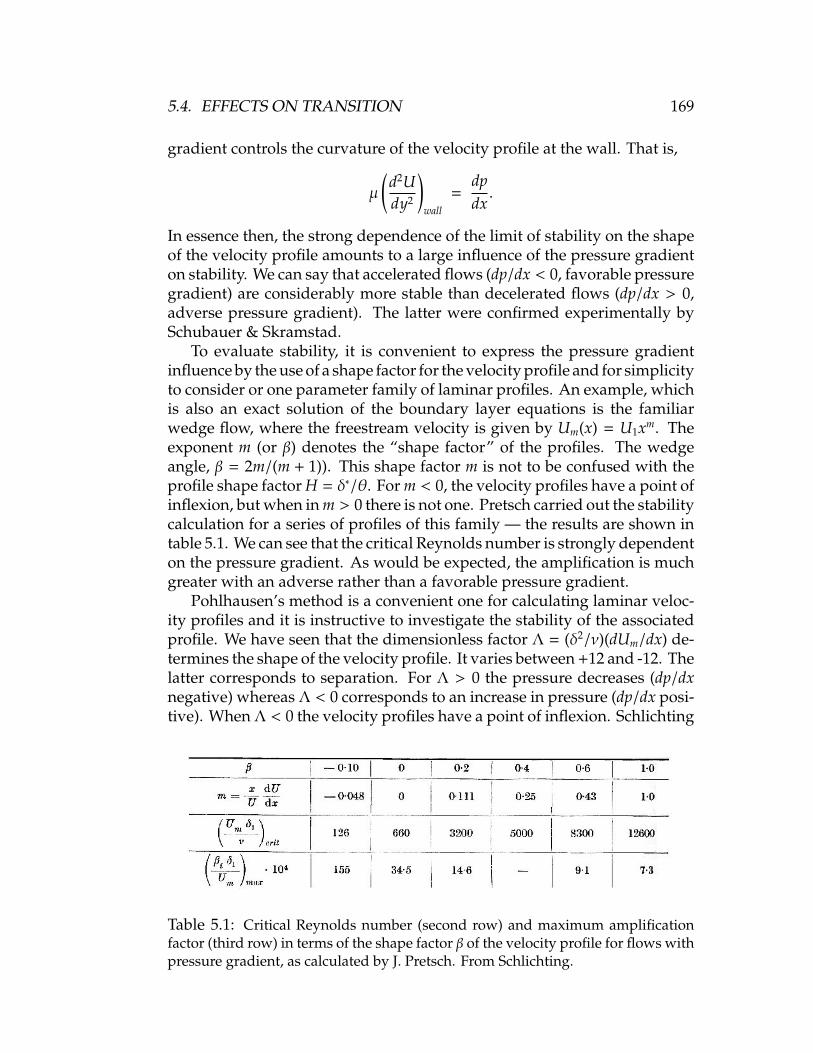
5.4. EFFECTS ON TRANSITION 169
gradient controls the curvature of the velocity profile at the wall. That is,
µ
(d2Udy2
)wall
=dpdx.
In essence then, the strong dependence of the limit of stability on the shapeof the velocity profile amounts to a large influence of the pressure gradienton stability. We can say that accelerated flows (dp/dx < 0, favorable pressuregradient) are considerably more stable than decelerated flows (dp/dx > 0,adverse pressure gradient). The latter were confirmed experimentally bySchubauer & Skramstad.
To evaluate stability, it is convenient to express the pressure gradientinfluence by the use of a shape factor for the velocity profile and for simplicityto consider or one parameter family of laminar profiles. An example, whichis also an exact solution of the boundary layer equations is the familiarwedge flow, where the freestream velocity is given by Um(x) = U1xm. Theexponent m (or β) denotes the “shape factor” of the profiles. The wedgeangle, β = 2m/(m + 1)). This shape factor m is not to be confused with theprofile shape factor H = δ∗/θ. For m < 0, the velocity profiles have a point ofinflexion, but when in m > 0 there is not one. Pretsch carried out the stabilitycalculation for a series of profiles of this family — the results are shown intable 5.1. We can see that the critical Reynolds number is strongly dependenton the pressure gradient. As would be expected, the amplification is muchgreater with an adverse rather than a favorable pressure gradient.
Pohlhausen’s method is a convenient one for calculating laminar veloc-ity profiles and it is instructive to investigate the stability of the associatedprofile. We have seen that the dimensionless factor Λ = (δ2/ν)(dUm/dx) de-termines the shape of the velocity profile. It varies between +12 and -12. Thelatter corresponds to separation. For Λ > 0 the pressure decreases (dp/dxnegative) whereas Λ < 0 corresponds to an increase in pressure (dp/dx posi-tive). When Λ < 0 the velocity profiles have a point of inflexion. Schlichting
Table 5.1: Critical Reynolds number (second row) and maximum amplificationfactor (third row) in terms of the shape factor β of the velocity profile for flows withpressure gradient, as calculated by J. Pretsch. From Schlichting.

170 CHAPTER 5. STABILITY AND TRANSITION
Figure 5.10: Left: curves of neutral stability for laminar boundary layer profileswith pressure decrease (Λ > 0) and pressure increase (Λ < 0). Right: criticalReynolds number of boundary layer profiles with pressure gradient as a functionof Λ (see equation 3.31 for a definition of Λ). From Schlichting.
& Ulrich carried out stability calculations for this family of profiles. Theneutral stability curves are shown in figure 5.10. The right hand figuresshows the plot of Rcrit versus Λ. As might have been anticipated Rcrit variesstrongly with Λ and hence with dp/dx.
We have seen that a pressure increase along a boundary layer stronglyfavors transition to turbulence. It is interesting to note that conversely, a verystrong pressure decrease, such as may be created by a centered expansion insupersonic flow, can cause a turbulent boundary layer to become laminar.Sternberg, making tests on geometry shown in figure 5.11 at a Mach numberof 3 observed this. The large favorable pressure gradient at the cornershould impresses a strong acceleration on the flow which “extinguishes”the turbulence.
Influence of suction
The effect of suction is to stabilize the boundary layer. Firstly, suctionreduces the boundary layer thickness and a thinner boundary layer is lessprone to become turbulent. Secondly, suction creates a laminar velocityprofile having a higher critical Reynolds number than a velocity profile withno suction.

5.4. EFFECTS ON TRANSITION 171
Figure 5.11: Schematic representation of the flow in a laminar boundary layer insupersonic flow around a corner, after Sternberg. From Schlichting.
Figure 5.12: Flat plate at zero incidence with homogenous suction. From Schlicht-ing.
For a flat plat at zero incidence and with uniform suction (suction velocity= −v0), as shown in figure 5.12, the velocity profile and hence the boundarylayer thickness thickness became independent of the current co-ordinate ata certain distance from the leading edge. From this location onwards we canshow that the velocity profile is given by U(y) = U∞(1−exp v0y/ν)) for whichthe critical Reynolds number is 70,000.2 Note that for the Basius profile Rcrit
is 520. Thus the critical Reynolds number of this so called “asymptotic”suction profile is more than two orders of magnitude larger than that on aflat plate with neither a pressure gradient or suction. This demonstrates thehighly stabilizing effect of suction.
Influence of roughness
The question here is how the process of transition depends on the roughnessof the wall over which the boundary layer is flowing. From a practical pointof view, the longer the flow over a wing may be kept laminar, the lower willbe the overall skin friction drag.
In a general sense, the presence of roughness favors transition. By this,we mean that under otherwise identical conditions, transition occurs at alower Reynolds number on a rough wall than on a smooth wall. This followfrom the theory of stability. Roughness elements produce additional distur-bances in the laminar stream which have to be added to those generated byturbulence and already present in the boundary layer.
2Rcrit is based on δ∗, that is Rcrit = Uδ∗/ν. Note that this is the Reynolds numberat the point of instability and will be less than the transition Reynolds number foundexperimentally.

172 CHAPTER 5. STABILITY AND TRANSITION
If the disturbances created by roughness are bigger than those due toturbulence, we would expect that a lower degree of amplification would besufficient to produce transition. Alternatively, if the roughness elements arevery small, the disturbances should lie below the “threshold” which is char-acteristic of those generated by the turbulence of the external freestream —in this case then, we would expect no effect on transition. These propositionsshow complete agreement with experiment.
When the roughness elements are large, transition occurs at the pointswhere they are actually present. Early workers in the field assumed thatthe transition point was located at the position of the roughness elementswhen they were large, or that there was no influence for small elements.However, it turns out that as roughness elements are made progressivelyhigher the point of transition moves steadily upstream until it reaches theposition of the roughness elements themselves. This prompts us to ask threebasic questions:
1. What is the maximum height of roughness elements below which noinfluence on transition exists?
2. What is the limiting height of a roughness element which causes tran-sition to occur at the element itself?
3. How do we describe the position of the transition point in the rangebetween items 1 and 2 above.
Experimentally, transition is often provoked by attaching a wire to thewall at right angles to the stream direction. This is called a “trip” wire.Goldstein deduced that the critical height (kcrit), that is, the height whichdoes not affect transition is given by
uτ,kkcrit
ν= 7,
where uτ,k =√τw,k/ρ is called the “friction” velocity, and τw,k is the shear
stress at the wall in the laminar boundary layer at the position of the rough-ness element.
The minimum height for which transition occurs at the element itselfwas proposed by Tani et al. to be uτ,kk/νcrit = 15 whereas other workersquote a value of 20. The values quoted above are all for single, cylindricalroughness elements (that is, circular wires).
Dryden developed an empirical law for the determination of the positionof the transition point, xtr, in terms of the height k of the roughness elementand its position xk. He found that in incompressible flow all the experimentalpoints for the case when transition does not occur at the roughness elementitself (that is, xtr > xk) arrange themselves on a single curve in a plot of

5.4. EFFECTS ON TRANSITION 173
Figure 5.13: Smoke picture of the flow in the boundary layer on an airfoil in thepresence of periodic disturbances, after Bergh. From Schlichting.
the Reynolds number Rtr = Uδ∗tr/ν against the ratio k/δ∗tr, where δ∗tr is thedisplacement thickness at the point of transition, and δ∗k is the displacementthickness at the position of the roughness element.
Influence of sound and vibration
Sound and vibrations usually produce disturbances over a wide spectrumof frequencies. When there exists good coupling between the boundarylayer stability characteristics and the disturbance level, sound and othertypes of vibration can have a major effect on stability. The coupling betweenfreestream turbulence and transition of the boundary layer on a smoothsphere waas used for a long time to measure the freestream turbulencelevel: the critical Reynolds number for the drag decrease on the sphere wascalibrated in terms of the level of turbulence. As an example of the effectsof sound on the boundary layer stability, figure 5.13 illustrates the stronginteraction.
Influence of heat transfer
The results given so far are valid only for flows at moderate speeds (that is,incompressible flow). In the case of compressible flows, we must considerthe rate of heat transferred from the wall and the wall, in addition to theMach number. In incompressible flows, heat can be exchanged betweenthe fluid and the wall only if the wall temperature is higher or lower thanthat of the flowing fluid. In contrast in compressible flows, heat generatedwithin the boundary layer results in an additional important influence. Ineither case, a thermal boundary layer develops in addition to the velocityboundary layer and this plays a role in the determination of the instabilityof a small disturbance. We will show in the next few pages that for thesubsonic (that is, incompressible or almost so) flow of a gas, heat transferfrom the boundary layer to the wall has a stabilizing influence whereas heat
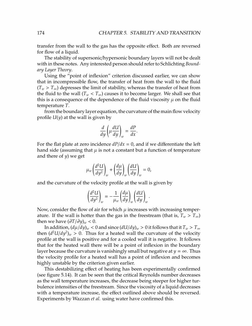
174 CHAPTER 5. STABILITY AND TRANSITION
transfer from the wall to the gas has the opposite effect. Both are reversedfor flow of a liquid.
The stability of supersonic/hypersonic boundary layers will not be dealtwith in these notes. Any interested person should refer to Schlichting Bound-ary Layer Theory.
Using the “point of inflexion” criterion discussed earlier, we can showthat in incompressible flow, the transfer of heat from the wall to the fluid(Tw > T∞) depresses the limit of stability, whereas the transfer of heat fromthe fluid to the wall (Tw < T∞) causes it to become larger. We shall see thatthis is a consequence of the dependence of the fluid viscosity µ on the fluidtemperature T.
from the boundary layer equation, the curvature of the main flow velocityprofile U(y) at the wall is given by
ddy
(µ
dUdy
)w
=dPdx.
For the flat plate at zero incidence dP/dx = 0, and if we differentiate the lefthand side (assuming that µ is not a constant but a function of temperatureand there of y) we get
µw
(d2Udy2
)w
+
(dµdy
)w
(dUdy
)w
= 0,
and the curvature of the velocity profile at the wall is given by(d2Udy2
)w
= −1µw
(dµdy
)w
(dUdy
)w.
Now, consider the flow of air for which µ increases with increasing temper-ature. If the wall is hotter than the gas in the freestream (that is, Tw > T∞)then we have (∂T/∂y)w < 0.
In addition, (dµ/dy)w < 0 and since (dU/dy)w > 0 it follows that it Tw > T∞then (d2U/dy2)w > 0. Thus for a heated wall the curvature of the velocityprofile at the wall is positive and for a cooled wall it is negative. It followsthat for the heated wall there will be a point of inflexion in the boundarylayer because the curvature is vanishingly small but negative at y = ∞. Thusthe velocity profile for a heated wall has a point of inflexion and becomeshighly unstable by the criterion given earlier.
This destabilizing effect of heating has been experimentally confirmed(see figure 5.14). It can be seen that the critical Reynolds number decreasesas the wall temperature increases, the decrease being steeper for higher tur-bulence intensities of the freestream. Since the viscosity of a liquid decreaseswith a temperature increase, the effect outlined above should be reversed.Experiments by Wazzan et al. using water have confirmed this.

5.5. THE ORIGIN OF TURBULENCE 175
Figure 5.14: The critical Reynolds number of a heated flat plate at zero incidence inan incompressible air stream. Measurements by Liepmann & Fila. From Schlicht-ing.
5.5 The Origin of Turbulence
“In flows which are originally laminar, turbulence arises frominstabilities as at large Reynolds number. Laminar pipe flow canbecome turbulent at a Reynolds number (based on mean velocityand diameter) in the neighborhood of 2,000 unless great care istaken to avoid creating small disturbances that might triggertransition from laminar to turbulent flow. Boundary layers inzero pressure gradient become unstable at a Reynolds numberUeδ∗/ν = 600 (δ∗ is the displacement thickness, Ue is the free-stream velocity, and ν is the kinematic viscosity). Free shearflows, such as the flow in a mixing layer, become unstable atvery low Reynolds numbers because of an inviscid instabilitymechanism that does not operate in boundary-layer and pipeflow. Early stages of transition can easily be seen in the smokerising from a cigarette.” (Tennekes & Lumley).
Two kinds of instability mechanisms can be identified: inviscid instabil-ities where viscosity is not important in the stability argument, and viscousinstabilities where viscosity plays a crucial role in the stability argument.Both kinds are important for the understanding of transition and turbu-lence.
5.6 Inviscid Stability Examples
The inviscid instability mechanism of thin shear layers can be demonstratedby considering a perturbed vortex sheet (figure 5.15). Initially the pressureand velocity directions are equal on the two sides of the vortex sheet, al-though the velocity magnitude is not. If a small perturbation occurs on the

176 CHAPTER 5. STABILITY AND TRANSITION
initially planar sheet, the streamlines converge on the top and diverge onthe bottom, a pressure difference is created, lift is generated, and the initiallysmall perturbation will grow, at least until non-linearities catch up with it.This is called the Kelvin-Helmholtz instability (see figure 5.16).
In a viscous fluid (but not in creeping flow), where the shear layer hasa finite thickness, the instability is still governed by the inviscid stabilityargument and the characteristic roll-up frequency is related to the shearlayer thickness and the velocity difference.
Subsequent instabilities can occur which eventually lead to the turbu-lent state. In the vortex sheet or simple shear layer case, there will alwaysexist imperfections in the flow which can lead to phase differences betweenroll-ups and eventually to vortex pairing. Three-dimensional disturbancescan also become unstable and grow, and the flow quickly takes on all char-acteristics of fully turbulent flow (see figures 5.17 and 5.18).
Interestingly, at higher Reynolds numbers, where the flow is clearlyturbulent, large-scale roll-ups are still evident which look much like theinitial Kelvin-Helmholtz roll-ups (see figure 5.19). These are sometimescalled “coherent” structures because of their organized form. Superimposedon these large-scales are all other scales, down to very small-scale motions.
Another classic, inviscid instability is Rayleigh-Benard convection, whichis buoyancy driven. A layer of fluid which is heated from below is unstableto small disturbances and convection rolls are formed (see figure 5.20).
5.7 Viscous Stability Examples
Viscous stability problems are more difficult. A good example is givenby the instability of a laminar boundary layer as the Reynolds numberincreases. What we see is that, if very small two-dimensional disturbancesare present (this is obviously a rather idealized flow situation), then belowa critical Reynolds number the disturbances will dissipate and laminar flowis recovered. Above a critical Reynolds number, the disturbances will grow,first in a two-dimensional manner (called Tollmien-Schlichting (T-S) waves
Figure 5.15: Perturbed vortex sheet.

5.7. VISCOUS STABILITY EXAMPLES 177
Figure 5.16: Kelvin-Helmholtz instability of a mixing layer.
Figure 5.17: Instability of an axisymmetric jet.
— see figure 5.21), then in a three-dimensional manner as the flow becomesunstable to three-dimensional disturbances, and then finally the flow rapidlybecomes turbulent (which in this context means that a wide range of scalesare present).
The onset of the two-dimensional instability can be analyzed as a linearproblem. The analysis was done by Tollmien in 1929 and presented in itsfinal form by Schlichting in 1933, but the experimental confirmation wasnot performed until 1947 by Schubauer & Skramstadt — mainly becausethe experiment is very difficult (see figure 5.8). Note that the most unstablefrequency is a function of Reynolds number (it can also be shown that atlow Reynolds numbers the most unstable disturbance is two-dimensionalso that it is preferentially amplified but at higher Reynolds numbers thethree-dimensional instabilities take over and grow very rapidly).
An interesting point about the analysis is that it demonstrated that vis-cosity can be destabilizing. This is contrary to expectation since we seeviscous effects as being dissipative and therefore inherently stabilizing. Inagreement with observation, the theory predicts transition in flows that are

178 CHAPTER 5. STABILITY AND TRANSITION
Figure 5.18: Instability and reconnection in the head-on collision of two vortexrings. From Lim & Nickels, 1992.
Figure 5.19: Large-scale structure in a turbulent mixing layer.
inviscidly stable (no inflection point in the velocity profile), such as channelflows and boundary layers with favorable pressure gradients. The reason is

5.7. VISCOUS STABILITY EXAMPLES 179
Figure 5.20: Buoyancy-driven convection rolls.
Figure 5.21: Instability of the boundary layer on a flat plate.
that the viscous stress fluctuations set up by a travelling wave disturbancecan shift the phase of u′ with respect to v′ so that the product u′v′ (theReynolds shear stress) is non-zero. The Reynolds shear stress interacts withthe velocity gradient to extract kinetic energy from the mean flow and feedit to the disturbance energy.
Now there are many roads to turbulence. For example, in Poiseuille flow(laminar pipe and channel flow) and Couette flow (flow between two platesin relative motion), transition does not follow these simple stages to turbu-

180 CHAPTER 5. STABILITY AND TRANSITION
Figure 5.22: Sketch of Reynolds’ dye experiment, taken from his 1883 paper.
lence. In fact, Poiseuille pipe flow is not linearly unstable at any Reynoldsnumber (neither is Couette flow), and transition must occur through theeffects of large disturbances. From recent work in DNS and experiment weknow that pipe flow shows an intermittent transition to turbulence, where“puffs” of “slugs” of turbulent flow occur between periods of laminar flow.The rather simple picture of transition presented by Osborne Reynolds orig-inal experiment (see figures 5.22 and 5.23) is not very accurate.
Transition in boundary layers can also occur in different ways. In fact, themost common road to turbulence is through the appearance of “turbulentspots” originating at points of imperfection on the surface. This is sometimescalled “bypass” transition in that it by-passes the T-S linear stage. Turbulentspots are sometimes called Emmons spots after the researcher at Harvardwho originally described them in detail — although see Schlichting for somevery early observations by Prandtl (see figures 5.5 and 5.24). They are veryregular in their appearance, grow at well-defined rates, and are separatedby regions of laminar flow (see figure 5.25). The growth process canbe described in terms of spanwise vortex tubes which experience a three-dimensional disturbance, that is, they become kinked, thereby generatinga self-induced velocity field which lifts up the kink into a region of highermean velocity, where it is then stretched. These vortex loops distort theadjacent spanwise vortex tubes, and thus the spot grows in a very ordered
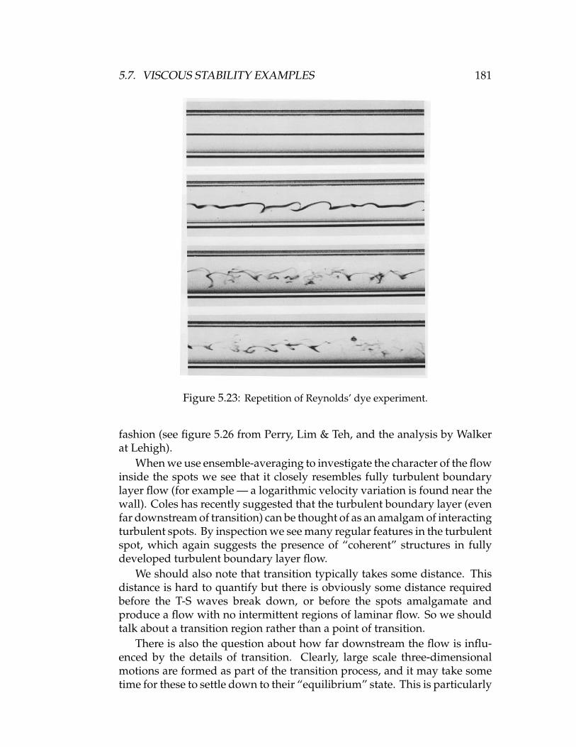
5.7. VISCOUS STABILITY EXAMPLES 181
Figure 5.23: Repetition of Reynolds’ dye experiment.
fashion (see figure 5.26 from Perry, Lim & Teh, and the analysis by Walkerat Lehigh).
When we use ensemble-averaging to investigate the character of the flowinside the spots we see that it closely resembles fully turbulent boundarylayer flow (for example — a logarithmic velocity variation is found near thewall). Coles has recently suggested that the turbulent boundary layer (evenfar downstream of transition) can be thought of as an amalgam of interactingturbulent spots. By inspection we see many regular features in the turbulentspot, which again suggests the presence of “coherent” structures in fullydeveloped turbulent boundary layer flow.
We should also note that transition typically takes some distance. Thisdistance is hard to quantify but there is obviously some distance requiredbefore the T-S waves break down, or before the spots amalgamate andproduce a flow with no intermittent regions of laminar flow. So we shouldtalk about a transition region rather than a point of transition.
There is also the question about how far downstream the flow is influ-enced by the details of transition. Clearly, large scale three-dimensionalmotions are formed as part of the transition process, and it may take sometime for these to settle down to their “equilibrium” state. This is particularly

182 CHAPTER 5. STABILITY AND TRANSITION
Figure 5.24: Growth of a turbulent spot on a flat plate as visualized by Prandtl.The photographs were taken with the aid of a slow motion camera, which traveledon a trolley along with the flow, in order to follow the same group of vortices. Theflow was made visible by sprinkling aluminum dust on the water surface. FromSchlichting.
true if the transition was initiated by some “artificial” means (although itcould be argued that all disturbances are artificial in some way). For ex-ample, in experimental work, transition is often induced by some form oftripping device, typically a circular cylinder place spanwise on the wall.This is done to speed up the transition, and fix it in place so that it doesnot occur in different places during the course of the experiment. Now ifthe tripping device is very large, it will produce a large disturbance. Sincethe disturbance will dissipate slowly (viscous dissipation is always slow) itwill affect the flow scaling for a very long distance downstream (see Coles1962 for a detailed discussion). A similar situation may exist in DNS or LESflows where disturbances are introduced to force transition — a poor choiceof disturbance environment may make the results meaningless. Of course,if these kinds of artificially introduced difficulties are avoided, there mayexist genuine effects of transition which persist downstream. Or, more tothe point perhaps, some part of the flow can be analyzed or modelled usingconcepts based on stability arguments similar to those used to describe the

5.7. VISCOUS STABILITY EXAMPLES 183
Figure 5.25: Emmons turbulent spot: (top) plan view; (middle) side view; (bottom)cross-section. Visualizations by Cantwell & Coles, and Perry, Lim & Teh.
initially laminar flow (see the large-scale structures in the turbulent mixinglayer shown in figure 5.27.
Two more things before we move on. First, we can see the important roleof Reynolds number — if the Reynolds number is low enough then there isno turbulence. We will take up this idea more formally later but for now wecan think of Reynolds number as the ratio of inertial forces to viscous forces,that is, the ratio of a typical acceleration of a fluid particle to the viscous stressgradients acting on the particle. If a typical length is L and a typical velocity isU, the Reynolds number is
(U2/L)/(νU
/L2) = UL/ν. Many different Reynolds
numbers can be defined for turbulent flow, depending on the relevant lengthand velocity scales. In terms of stability arguments, we can think of theanalogy with the role of shock absorbers in the suspension of a car. As thecar travels over a bumpy road, the shock absorber absorbs the oscillationsof the car by viscous dissipation. As the Reynolds number increases, it isas if the shock absorbers become less effective, and the oscillations become

184 CHAPTER 5. STABILITY AND TRANSITION
Figure 5.26: Schematic diagram of the sequence of events leading to the formationof a turbulent spot, in terms of vortex filaments. From Perry, Lim & Teh.
larger. At some point in fluid flow, the shock absorbers (viscosity) canactually cause the oscillations to grow and the breakdown follows.
Second, we can see how turbulence arises from a process of successiveinstability.
“On the other hand, turbulence cannot maintain itself but de-pends on its environment to obtain energy. A common sourceof energy for turbulent velocity fluctuations is shear in the meanflow; other sources, such as buoyancy, enter too. Turbulent flowsare generally shear flows. If turbulence arrives in an environ-ment where there is no shear or other maintenance mechanism,it decays: the Reynolds number decreases and the flow tends tobecome laminar again. The classic example is turbulence pro-duced by a grid in uniform flow in a wind tunnel.
Another way to make a turbulent flow laminar or to prevent alaminar flow from becoming turbulent is to provide for a mech-anism that consumes turbulent kinetic energy. This situationprevails in turbulent flows with imposed magnetic fields at low

5.7. VISCOUS STABILITY EXAMPLES 185
Figure 5.27: Shadowgraphs of mixing layer taken at random times.
magnetic Reynolds numbers and in atmospheric flows with astable density stratification, to cite two examples.” (Tennekesand Lumley).

186 CHAPTER 5. STABILITY AND TRANSITION

Chapter 6
Introduction to Turbulent Flow
6.1 The Nature of Turbulent Flow
Turbulent flow is the usual state of fluid motion at high Reynolds numbers.But what does “high Reynolds number” mean? We will deal with this ques-tion in some detail but for the moment we can start with the concept thatReynolds number measures the relative importance of inertial forces to vis-cous forces: if viscous forces are small compared to the inertial forces whenwe have a high Reynolds number. This implies that at very high Reynoldsnumbers viscosity is no longer important, and as we shall see, many aspectsof turbulent flow can be described without considering viscosity: viscos-ity is important only in setting the boundary conditions and in dissipatingmechanical energy into heat.
Turbulent flow is characterized by:
1. Three-dimensionality. Turbulence is inherently three-dimensional, al-though some people study two-dimensional turbulence (this may havesome application to geophysical flows (see figure 6.1). Note that the“stretching and tilting” term in the vorticity transport equation is ab-sent in two-dimensional flows, and therefore two-dimensional tur-bulence is considerably simpler than the real-life three-dimensionalvariety.
2. Time-dependency. That is, turbulence is characterized by unsteadyvariations in velocity, density, temperature or concentration, and thevariation occurs over a wide range of time scales. Turbulence has abroad frequency spectrum.
3. A wide range of length scales. Turbulence has a broad wavenumberspectrum.
4. Effective mixing of all fluid properties. For example, mass, velocity, tem-perature, momentum energy, etc. are all readily mixed by turbulent
187

188 CHAPTER 6. INTRODUCTION TO TURBULENT FLOW
Figure 6.1: Hurricane Fran, September 1996.
motions.
The concept of vorticity is crucial to the understanding of turbulence, andwe often talk about turbulence as consisting of an array of vortex tubesand vortex sheets, separated by fluid which is sometimes thought to beirrotational, or sometimes displaying some level of background vorticity.We also often describe turbulence in terms of “eddying” motions with agreat range of scales, without being very specific about what that means. Weusually think of these eddying motions as having some level of organizedvorticity (a mixture of vortex tubes and vortex sheets), although talkingin terms of “vortices” can be rather misleading. In fact, there has beenperennial disagreement about the definition of a vortex in turbulent flow,and it has recently been the subject of a number of scholarly papers (forexample, Kline & Robinson 1990). Nevertheless, the term eddy is widelyused, for the reasons that are made clear by figures 6.2, 6.3 and 6.4.
As a further example, consider channel flow at high Reynolds number(Re 2000, where Re = Uavh/ν. The pressure drop driving the flow isassumed to be steady (see figure 6.5). At any point in the flow, the magnitudeof the velocity in all three directions fluctuates in time. If we insert a probeinto the flow so that we can measure the velocity at a given point, wewould see the time traces shown in figure 6.6. Note that we can define a

6.1. THE NATURE OF TURBULENT FLOW 189
Figure 6.2: Satellite photo of cloud vortices downstream of Guadalupe Island (offBaja California). Courtesy National Oceanic and Atmospheric Administration
Figure 6.3: Karman vortex street behind a circular cylinder at a Reynolds numberof 140. From Taneda.

190 CHAPTER 6. INTRODUCTION TO TURBULENT FLOW
Figure 6.4: Karman vortex street behind a circular cylinder at Reynolds numbersof 200. From Koopmann.
time-averaged velocity:
U(~x) = limT→∞
1T
∫ t0+T
t0
U(~x, t)dt
and a space-averaged velocity:
Uav =1A
∫UdA =
1h
∫ +h/2
−h/2Udy.
The concept of a time-averaged velocity also leads to the concept of theflow being composed of a time-averaged field, and a fluctuating field. This iscalled the Reynolds decomposition where we write: U = U + w′, V = V + v′,W = W + w′, and p = p + p′.
Figure 6.5: Instantaneous and mean velocity profiles in fully-developed channelflow.
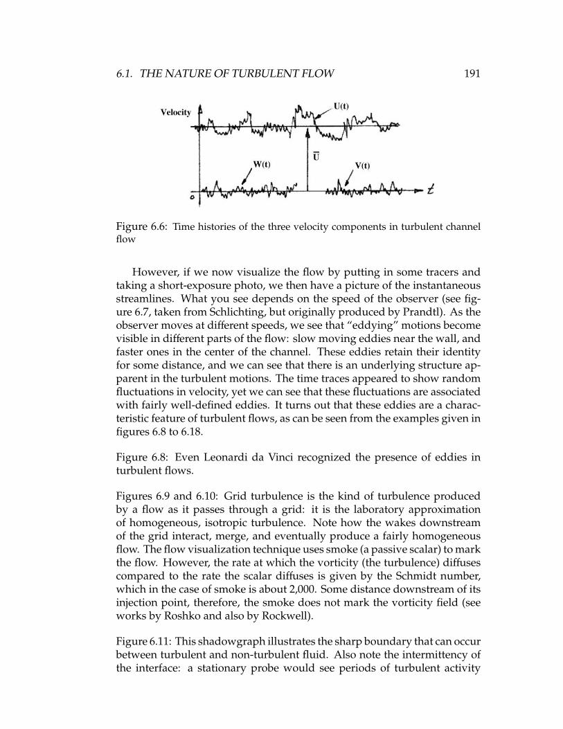
6.1. THE NATURE OF TURBULENT FLOW 191
Figure 6.6: Time histories of the three velocity components in turbulent channelflow
However, if we now visualize the flow by putting in some tracers andtaking a short-exposure photo, we then have a picture of the instantaneousstreamlines. What you see depends on the speed of the observer (see fig-ure 6.7, taken from Schlichting, but originally produced by Prandtl). As theobserver moves at different speeds, we see that “eddying” motions becomevisible in different parts of the flow: slow moving eddies near the wall, andfaster ones in the center of the channel. These eddies retain their identityfor some distance, and we can see that there is an underlying structure ap-parent in the turbulent motions. The time traces appeared to show randomfluctuations in velocity, yet we can see that these fluctuations are associatedwith fairly well-defined eddies. It turns out that these eddies are a charac-teristic feature of turbulent flows, as can be seen from the examples given infigures 6.8 to 6.18.
Figure 6.8: Even Leonardi da Vinci recognized the presence of eddies inturbulent flows.
Figures 6.9 and 6.10: Grid turbulence is the kind of turbulence producedby a flow as it passes through a grid: it is the laboratory approximationof homogeneous, isotropic turbulence. Note how the wakes downstreamof the grid interact, merge, and eventually produce a fairly homogeneousflow. The flow visualization technique uses smoke (a passive scalar) to markthe flow. However, the rate at which the vorticity (the turbulence) diffusescompared to the rate the scalar diffuses is given by the Schmidt number,which in the case of smoke is about 2,000. Some distance downstream of itsinjection point, therefore, the smoke does not mark the vorticity field (seeworks by Roshko and also by Rockwell).
Figure 6.11: This shadowgraph illustrates the sharp boundary that can occurbetween turbulent and non-turbulent fluid. Also note the intermittency ofthe interface: a stationary probe would see periods of turbulent activity

192 CHAPTER 6. INTRODUCTION TO TURBULENT FLOW
Figure 6.7: Turbulent flow in a water channel 6 cm wide, photographed withvarying camera speeds. From Schlichting.
(rotational flow), followed by periods of non-turbulent activity (irrotational,potential flow). This picture is often used to demonstrate the wide range ofscales present in turbulence. To my eye, only two scales, one based on thewake width and the other about one-fortieth of the wake width, are visible.This is a problem with the visualization technique: shadowgraphs recordall the density gradients integrated over the distance from the light source

6.1. THE NATURE OF TURBULENT FLOW 193
Figure 6.8: Shaft of water issuing from a square hole into a pool, forming bubblesand eddies (Leonardo da Vinci).
Figure 6.9: Generation of turbulence by a grid. Corke & Nagib.
to the camera (see Liepmann and Roshko for a brief explanantion). Hencethe image records the density gradients due to the eddy structures presentin the wake but it overlaps them so that the individual eddies are no longerapparent.

194 CHAPTER 6. INTRODUCTION TO TURBULENT FLOW
Figure 6.10: Homogeneous turbulence behind a grid. Corke & Nagib.
Figure 6.11: Turbulent flow far behind a projectile. Shadowgraph from BallisticResearch Laboratories, Aberdeen Proving Ground.
Figure 6.12: Here, a laser sheet illuminates a fluorescent dye, and thereforewe have an image of eddy cross-sections (the same caution about Schmidtnumber is in effect). The variety of scales, and the evident organization of theturbulence, is clearly seen. Also note that the unmarked fluid occasionallypenetrates across the centerline of the jet.

6.1. THE NATURE OF TURBULENT FLOW 195
Figure 6.12: Cross-section of a turbulent water jet, at a Reynolds number ofabout 2300, made visible by laser-induced fluorescence. From Dimotakis, Lye &Papantoniou, 1981.
Figure 6.13: Here is a really high Reynolds number jet (about 109). Note thescales of eddies are almost in a geometric progression, where each successivescale is about one-half the previous one.
Figures 6.14 and 6.15: Two views of a turbulent boundary layer at fairlylow Reynolds numbers. See how the originally non-turbulent freestreamfluid is “entrained” by the boundary layer. Occasionally, we see freestreamfluid extending almost to the wall. Presumably this fluid will be eventaully

196 CHAPTER 6. INTRODUCTION TO TURBULENT FLOW
Figure 6.13: Mount St. Helens, 18 May 1980 (US Geological Survey/Popperfoto).
engulfed and become turbulent (rotational) by viscous diffusion of vorticity.
Figure 6.16: Here is a shadowgraph of the turbulent boundary layer on acylindrical body moving to the left at about Mach 2.3 (taken in a ballistictunnel by Seiff). The integration effect is not so severe as in figure 7 becauseof the geometry, and it is now possible to distinguish structures similar tothe ones seen at subsonic speeds, as seen in figure 10.
Figure 6.17: By using Rayleigh scattering, the density variations in a stream-wise plane are made visible in a turbulent boundary layer at Mach 2.5(picture by Smith et al. at Princeton). The flow is from left to right. Thiscross section clearly shows the kind of bulges observed at subsonic speeds,as in figures 6.14 and 6.15.
Figure 6.18: Here the Rayleigh scattering technique was used to reveal thedensity variations in a plane parallel to the wall (the flow is from top tobottom) at a height of about 0.7 times the boundary layer thickness. The

6.2. EXAMPLES OF TURBULENT FLOW 197
Figure 6.14: Side view of a turbulent boundary layer at Reθ = 3500. From Corke,Guezennec & Hagib.
Figure 6.15: Turbulent boundary layer on a wall at Reθ = 4000. From Falco, 1977.
large islands are about a boundary layer thickness across. Note the three-dimensionality of the density fluctuations.
Figure 6.19: By using Rayleigh scattering, the density variations in a stream-wise plane are made visible in a turbulent boundary layer at Mach 8 (pictureby Baumgartner et al. at Princeton). The flow is from left to right. The sametype of structure is observed as at supersonic and subsonic speeds, as infigures 6.17 and 6.15.
6.2 Examples of Turbulent Flow
In the home: water issuing from a faucet, cigarette smoke, stirring a coffee

198 CHAPTER 6. INTRODUCTION TO TURBULENT FLOW
Figure 6.16: Boundary layer on a body of revolution at a Mach number of 2.3. Thebody is moving to the left. From Seiff.
Figure 6.17: Side view images of the instantaneous density field in a Mach 3turbulent boundary layer. Smith & Smits, 1996.
cup, air-conditioning ducts.
Aerodynamical flows: wake of an aircraft, flow over the wings, flow overa ship, aerodynamics of sports balls, separation.
Industrial flows: stirred reactor, pipe flow, flow through valves, constric-tions, flows in turbines, combustion furnaces, chimney outlets, pol-lutant dispersion (not bearings, lubrication applications since theseare highly viscous flows where turbulence has no role to play), flowaround buildings, internal combustion engines.
Geophysical flows: river flows, channel flows, wake behind a bridge py-lon, ocean currents, weather patterns, storms (eg. snow storms), (notsettling of small particles which is another highly viscous flow), vol-canoes, thermal plumes.

6.3. THE NEED TO STUDY TURBULENCE 199
Figure 6.18: Plan view images of the instantaneous density field in a Mach 3turbulent boundary layer at y/δ = 0.7. Smith & Smits, 1995.
Figure 6.19: Side view images of the instantaneous density field in a Mach 8turbulent boundary layer. Baumgartner, 1997.
Military flows: flight of bullets, rockets, high-speed (and low-speed) air-planes, helicopter wakes, parachute flows, submarine flows (signa-tures, noise), propellers.
6.3 The Need to Study Turbulence
Why is turbulence interesting?
If we could predict all the flow states given as examples in section 6.2, or ifwe had enough insight to develop widely applicable correlation schemes,turbulence would not be an area of research. The truth, of course, is other-wise. It comes down to this: there is no general solution to the Navier-Stokes

200 CHAPTER 6. INTRODUCTION TO TURBULENT FLOW
equations, which are the governing equations for flow of an incompressible,Newtonian, continuum fluid (for compressible flows, we need an energyequation, and equation of state and some constitutive equations). Particularsolutions exist (see Schlichting chapters XX and YY), but in the main theyare not useful for the general understanding of turbulent flow. (Sometimes,however, they can be used to give an understanding of particular mecha-nisms at work in the production, diffusion and dissipation of turbulence).
Historically, studies of turbulence have relied on a very restricted set of“tools”:
1. Approximate analysis of average properties of highly idealized turbulentflows (eg. grid turbulence);
2. Analysis of idealized linear stability problems;
3. Measurements of time-averaged properties and ensemble-average prop-erties (U, u′2, u′v′, Φ(ω), p(u), etc. );
4. Flow visualization;
5. Dimensional analysis and scaling arguments.
From this work we have obtained
1. a small set of widely accepted “facts”, for example, the logarithmicvariation of velocity in a turbulent boundary layer;
2. a small set of widely accepted correlations, for example the friction factorfor pipes as a function of Reynolds number;
3. a small set of widely accepted theories eg. Kolmogoroff’s inertial range,Batchelor’s final decay of grid turbulence;
4. a qualitative notion of energy transfer (the energy cascade);
5. the kinematics and other general features of turbulence and eddies, forexample the role of bulges, horshoe-vortices, “typical” eddies, etc.;
6. some useful but rather restricted sets of predictive tools, for example,the k-ε turbulence model;
7. a good appreciation of scaling arguments.
More recently (since late 70’s) computers have allowed LES (Large EddySimulations) and DNS (Direct Numerical Simulations) of turbulent flows.In DNS, the grid resolution is set small enough to resolve all the scales ofmotion (at least in principle), whereas in LES only the scales down to the sizeof the grid are computed, and the smaller scales are modelled in some way.

6.3. THE NEED TO STUDY TURBULENCE 201
Both types of computation give time-dependent, three-dimensional flowinformation, and they have given a great deal of insight into the dynamicsof turbulence. However, their overall impact has not been as great as wemight have hoped (at least not yet). The difficulty is that turbulence iscomplex. Extremely complex. If we consider the example of turbulent pipeflow, we have a range of scales which goes from the largest (or order D, thepipe diameter) to the smallest (of order ν/uτ, where uτ is the friction velocity,which is a velocity scale based on the wall shear stress: it is of the sameorder as a typical velocity fluctuation). For a pipe flow of water in a 10 cmpipe at 2m/sec we get Re = UDν = (2× 0.1)10−6. This is not a large Reynoldsnumber for pipe flow. Since
C f = 2 (uτ/Uav)2≈ 0.003.
Hence uτ = 0.04U, and Duτ/ν ≈ 8, 000. So the largest motions are of order 104
times the smallest. In DNS, all these scales must be resolved as a functionof time, where at least four variables (U, V, W, p) are carried for each gridpoint at each time step. In other words, a typical DNS calculation of thisrelatively simple flow will generate an enormous quantity of information:(4 (8, 000)3
)= 2 × 10¹² pieces of information at each time step. We may be
able to do calculations of this magnitude (or at least soon) but it’s anotherthing to understand it. We need to develop simpler models or concepts inturbulence which will give us some understanding and predictive power.Computations will help but in some sense the field of turbulence needsbetter ideas, not just more data.
So what are the goals of turbulence research? The main goal is:
To develop approximations to the N-S equations which embodysufficient dynamical information to allow reliable and efficientpredictions of turbulent flows.
To get there, we need to develop and test simple models of turbulence whichembody the essential physics of turbulence and its scale interactions, andcontains the correct scaling information. We need: high quality simulations,high quality experiments, and good ideas.
According to Tony Perry, our methods have evolved from the point wherewe just had good ideas (figure 6.20a), to where we experiment and theorysupported our thought processes (with a little numerics) (figure 6.20b), towhere the advent of computers was seen to add a third leg for supportfigure 6.20c), to the present situation where experiments and theory are bothsupported by computers to aid our thinking about turbulence. These arethe tools. However, there are also different ways to think about turbulence.

202 CHAPTER 6. INTRODUCTION TO TURBULENT FLOW
Figure 6.20: The evolving role of computers, experiments and theory. Accordingto Perry.
6.4 Approaches to Turbulence
As noted earlier, turbulence is extremely complex. In order to deal withthis complexity, different people take different approaches. The major va-rieties are the time-averaged approach (also called Reynolds averaged ap-proach), the ensemble-averaged approach, and the instantaneous realizationapproach. All of these ways of thinking are correct, in the sense that theycan all be represented as valid interpretations of the Navier-Stokes equa-tions, but they all give different kinds of information, they have differentapplications, and they require different kinds of input.

6.4. APPROACHES TO TURBULENCE 203
Figure 6.21: Time trace and pdf of the longitudinal velocity fluctuation
6.4.1 Reynolds-averaged approach
This is the most common approach, certainly for engineering purposes. Ithas the twin distinctions of being the most studied, and being the mostlimited in terms of understanding. In this approach, turbulence is seenpurely as a statistical phenomena. It is assumed that the time-dependentnature of turbulence is far too complicated to incorporate in a physical model(that is, a model which describes the interactions among turbulent scales ofmotion in a physical way, which could be quantitative or qualitative), or aturbulence model (that is, a model which can be incorporated quantitativelyinto a set of equations based on the Navier-Stokes (N-S) equations, and thatcan lead to useful engineering predictions). Hence, the N-S equations arewritten in terms of mean quantities by using time averages, where a timeaverage is taken over a long enough time to give a stationary mean. Hence,
U(x) = limT→∞
1T
∫ t0+T
t0
U(x, t)dt,
andU = U + u′
andu′ = 0 and v′ = 0,
etc. (see figure 6.21). But the moments are not zero:
u′2 = limT→∞
1T
∫ t0+T
t0
(U − U
)2dt,
u′v′ = limT→∞
1T
∫ t0+T
t0
(U − U
) (V − V
)dt.
When we do this, we obviously lose information. In fact, it can be shownthat we need to know all higher order moments of the turbulence (that is,

204 CHAPTER 6. INTRODUCTION TO TURBULENT FLOW
an infinite number) before we have all the information originally containedin the time-dependent equations. So now we have a subset of equations(typically for the mean velocity and then for the lower-order moments ofturbulence) which have more unknown than equations — this is known asthe “closure” problem. To close the set of equations some inspired piece ofinformation must be supplied, which may be based on experiment, theoryor simulation, or a combination of all three. We will consider this problemin some detail in a later lecture but we should note that this approach (orthe closely related pdf method, and the wave-number approach) form thebasis of all engineering calculation methods, and it is also the most commonapproach to measuring turbulence.
NOTE:
In unsteady but repeatable flows, time-averages are obviously mean-ingless. However, we can form ensemble-averages by accumulating asufficient number of samples at the same phase in the flow cycle.
6.4.2 Ensemble-averaged approach
This may not be the right name for it, but when I say “ensemble-averaged”approach I don’t mean forming the equivalent of Reynolds averages foran unsteady flow. I use the term in a more particular sense to indicate away of thinking that recognizes that turbulence has an underlying struc-ture, and that it is not just a purely random phenomena as implied by theReynolds-averaged approach. Here we say that it may be more meaningfulto recognize that the eddies which make up turbulence display some similar-ity among themselves, and that we try to determine the average propertiesof an eddy, and how these properties scale with size, position, etc..
The simplest example is given by the intermittent nature of turbulence inthe outer part of a turbulent shear layer. As we can see from the images givenin figures 6.11 to 6.18 and figure 6.22, there appear to be periods of turbulentflow (which is rotational) followed by periods of non-turbulent flow (whichis irrotational). By forming a detector function (or boxcar function) I (t)which takes the value 0 in non-turbulent flow and 1 in a turbulent flow, thenwe can form turbulence intensities based on the periods when I = 1, ratherthan over all time (see figure 6.23). That is:
u′2 = γu′2T +(1 − γ
)u′2NT.
(Note that u′2NT , 0 due to irrotational fluctuations in the external potentialflow.)
This approach can be used in more sophisticated ways to try to identifyeddies of a particular sort, or to identify contributions from two interacting

6.4. APPROACHES TO TURBULENCE 205
Figure 6.22: Streamwise cross-section of a turbulent boundary layer at Mach 3.From Smith & Smits, 1988.
Figure 6.23: The intermittency function and the distribution of the intermittencyfactor γ.
turbulent flows. A similar approach can be used if the flow has a well-defined periodicity because it is then possible to use phase-averaging toidentify the details of the large-scale structure (see Cantwell and Coles,Perry and Lim, and Perry and Tan). Of course there are many problems indefining I (t) and in interpreting the results, but this approach is an attemptto take some of the turbulent structure into account. It has been widely usedin turbulence research, for the interpretation of experimental and numericalresults (see, for example, the VITA approach of Blackwelder & Kaplan usedby Spina, Donovan & Smits 1991). Some examples of ensemble-averagedinterpretations of outer-layer structures in turbulent boundary layers aregiven in figures 6.24 and 6.25.
6.4.3 Instantaneous realization approach
Another awkward name, but here I mean the method where we try to un-derstand turbulence by looking at individual events. Of course, we tryto generalize our observations by picking out features which occur oftenenough to be important (and here we have a link to the ensemble-averagedapproach), but of necessity we are looking at a relatively small number of

206 CHAPTER 6. INTRODUCTION TO TURBULENT FLOW
Figure 6.24: Qualititative comparison between the ensemble-averaged structuresof: (a) Smith & Smits (1988) in a supersonic boundary layer (visual detection);(b) Chen & Blackwelder (1978) in a subsonic boundary layer over a heated wall(temperature probe detection).
events. We can do this in experiments by using techniques which give in-formation about the whole of the flow field, such as some forms of flowvisualization (see figure 6.26 which shows pairs of Rayleigh scattering im-ages of a Mach 2.9 turbulent boundary layer separated by intervals of 60 µs),or time-resolved PIV (Particle-Image Velocimetry), but it is particularly easyto do in numerical simulations where all the properties of turbulence oversome relatively short time period can be inspected and analyzed in greatdepth (see, for example, Robinson’s work).
6.4.4 Connections among the approaches
The boundaries between these three main approaches are not clear cut, andmost workers in turbulence move freely among them to gain the maximumof useful information. For example:
(1) the observation that turbulent flows can be intermittent has found itsway in developing Reynolds’averaged turbulence models (see, for

6.4. APPROACHES TO TURBULENCE 207
Figure 6.25: (a) Schematic of a large-scale turbulent ”bulge” in incompressibleflow. From Blackwelder & Kovasznay, 1972; (b) Ensemble-averaged flowfield in aMach 3 turbulent boundary layer. From Spina, Donovan & Smits, 1992.
example, Cebeci and Smith 1974);
(2) ensemble-averaged results are often studied in terms of their contribu-tions to the Reynolds-averaged turbulent moments (sometimes calledReynolds stresses);
(3) Individual realizations are probably only useful if they reveal somethingabout the average behavior of eddies (ensemble-average approach) orthe Reynolds stresses (Reynolds-average approach).
We should also make clear (or try to) what we mean by “structure” inturbulence. Turbulence (in one view: see Bradshaw, p.22) is the sum of alarge number of events or processes (the velocity at any point is a productof the whole field, and as a function of time will reflect all influences)that are not quite independent - like a slow hand clap superimposed on ageneral audience response. So turbulence usually displays departures from

208 CHAPTER 6. INTRODUCTION TO TURBULENT FLOW
Figure 6.26: Pair of double-pulsed Rayleigh scattering images of a Mach 2.9 tur-bulent boundary layer, separated in time by intervals of 60µs. Flow is from left toright.
Gaussian behavior - these departures may be called structure, and might beembodied in terms of the moments of the pdf’s of u′, v′ and w′.
The term structure is also used in connection with the description ofindividual eddying motions that are observed to be part of turbulence.These are sometimes called “coherent structures” if they represent some sortof entity which can be followed in time. Here we can talk about the “outer-layer bulges” for example, which can be seen in the flow visualizations ofturbulent boundary layers. These bulges evolve somewhat as they movebut we can identify some typical properties such as their angle of inclination(which is always leaning downstream), their average size, and frequency ofoccurrence.
Structure is a widely used word, and people move between its differentinterpretations, often without being precise.
6.5 Model Flows
The study of turbulence is usually restricted to rather simple model flows,such as grid turbulence (with and without a mean shear), pipe and chan-nel flows, boundary layers, jets, wakes, swirling flows, etc. From theseflows we try to extract “universal” information which we can then apply to

6.5. MODEL FLOWS 209
more complex flows such as that found in engineering applications. Even-tually, we need to know the effects on turbulence of shear, wall constraint,pressure gradient, curvature, divergence, compression, rotation, buoyancy(stratification), chemical reactions (with and without heat release), three-dimensionality, magneto-hydrodynamic effects, separately and in combina-tion.
We need to determine basic mechanisms, and find their sensitivity tochanges in boundary conditions or initial conditions. It is of little use toconstruct an edifice of understanding based on one highly particular flow(for example, the flat plate, zero pressure gradient boundary layer) andthen find that the edifice must be rebuilt everytime a boundary condition ischanged (for instance when the wall is curved, or the flow is accelerating).
210 CHAPTER 6. INTRODUCTION TO TURBULENT FLOW

Chapter 7
Reynolds-Averaged Equations
Let us begin with the straight statistical approach where we use the decom-position (in Cartesian coordinates, where V = Ui + Vj + Wk):
U (x, t) = U (x) + u′ (x, t)
(V, W and the pressure p are decomposed similarly). As before we have
a = limT→∞
∫ t0+T
t0
a dt,
where t0 is an arbitrary start sampling time, and the rules for averaging are:
a′ = 0
a + b = a + b
a = a
a · b = a · b
∂a∂s
=∂a∂s.
Start with the continuity and Navier-Stokes equations (for incompressibleflow and no body forces):
∇ ·V = 0 (7.1)
DVDt
=∂V∂t
+ V · ∇V = −1ρ∇p + ν∇2V (7.2)
or∂ui
∂t+ ui
∂ui
∂x j= −
1ρ
∂p∂xi
+ ν∂2ui
∂x2j
. (7.3)
In the momentum equation, the first term on the left hand side is the rate ofchange of momentum due to unsteady flow at a point, and the second term
211

212 CHAPTER 7. REYNOLDS-AVERAGED EQUATIONS
on the left hand side is the rate of change of momentum due to convectionof fluid particles to regions where the velocity is different. The first term onthe right hand side is the force per unit volume due to pressure differences,and the second term on the right hand side is the force per unit volume dueto differences in viscous shear stresses that drag fluid elements about.
7.1 Continuity Equation
With the Reynolds decomposition, the continuity equation becomes:
∂U∂x
+∂V∂y
+∂W∂z
+∂u′
∂x+∂v′
∂y+∂w′
∂z= 0. (7.4)
Taking the time average we obtain:
∂U∂x
+∂V∂y
+∂W∂z
= 0. (7.5)
That is,∇ · V = 0.
By subtracting equation 7.5 from 7.4 we obtain:
∂u′
∂x+∂v′
∂y+∂w′
∂z= 0. (7.6)
That is,∇ · v′ = 0.
Note that the mean and fluctuating velocities individually satisfy the conti-nuity equation.
7.2 Momentum Equation
Consider the x-component of the momentum equation. Using the Reynoldsdecomposition, we obtain:
∂U∂t
+∂u′
∂t+ U
∂U∂x
+ u′∂u′
∂x+ u′
∂U∂x
+ U∂u′
∂x
+ V∂U∂y
+ v′∂u′
∂y+ v′
∂U∂y
+ V∂u′
∂y
+ W∂U∂z
+ w′∂u′
∂z+ w′
∂U∂z
+ W∂u′
∂z
= −1ρ
∂p∂x−
1ρ
∂p′
∂x+ ν∇2U + ν∇2u′. (7.7)

7.2. MOMENTUM EQUATION 213
Now we take the time average and consider each term in turn.
(a) ∂U/∂t = 0 since by definition u is a time average. Hence to applyReynolds averaging the flow must be stationary. We can apply a morerestricted form of averaging of the time constant associated with theunsteadiness is much larger than any time constant associated withthe turbulence but we must be very careful: if ui is a function of t0,the definition of a time average is meaningless and ensemble averagesmust be used.
(b) ∂u′∂t = 0, since u′ = 0
(c) u′ ∂u′∂x = 1
2∂u′2∂x =
∂(
12 u′2
)∂x
(d) u′ ∂U∂x = v′ ∂U
∂y = w′ ∂U∂z = 0
(e) U∂u′∂x = V∂u′
∂y = W∂u′∂z = 0
(f) v′ ∂u′∂y = ∂u′v′
∂y − u′ ∂v′∂y
(g) w′ ∂u′∂z = ∂u′w′
∂z − u′ ∂w′∂z
(h) ∂p′
∂x = 0
(i) ν∇2u′ = 0.
Also note from the continuity equation 7.5 that
u′∂u′
∂x+ u′
∂v′
∂y+ u′
∂w′
∂z= 0.
That is,∂(
12u′2
)∂x
+ u′∂v′
∂y+ u′
∂w′
∂z= 0.
Hence the x-component Reynolds-averaged equation becomes:
U∂U∂x
+ V∂U∂y
+ W∂U∂z
=
−1ρ
∂p∂x−
∂u′2
∂x+∂u′v′
∂y+∂u′w′
∂z
+ ν∇2U (7.8)
where we have dropped the overbars on the mean velocities and pressure.Note that if the flow was not turbulent, we recover the x-momentum equa-tion for steady (laminar) flow.

214 CHAPTER 7. REYNOLDS-AVERAGED EQUATIONS
Similarly, we have for the y- and z-components:
U∂V∂x
+ V∂V∂y
+ W∂V∂z
=
−1ρ
∂p∂y−
∂u′v′
∂x+∂v′2
∂y+∂v′w′
∂z
+ ν∇2V (7.9)
U∂W∂x
+ V∂W∂y
+ W∂W∂z
=
−1ρ
∂p∂z−
∂u′w′
∂x+∂v′w′
∂y+∂w′2
∂z
+ ν∇2W. (7.10)
We see that the process of Reynolds averaging has given us an equationfor the mean flow. However, in so doing, terms involving time-averages ofvelocity fluctuations have appeared, and we have no information on thesenew terms. Therefore the system of time-averaged equations describing pand V is not closed. This is the fundamental difficulty of the Reynolds-averaged approach: second-order mean products of fluctuating quantitiesappear in the equation for the mean flow. This is sometimes called theclosure problem.
These second-order products are of two kinds:
(i) Mean squares, or the variances, such as u2i (no summation). The root
mean square,√
u2i , is known as the intensity of the turbulence compo-
nent i, while the intensity of the turbulence is given by:√q2 =
(u2 + v2 + w2
) 12 (
√q2 = 2k in some books).
This is related to the kinetic energy of the turbulence (per unit volume)12ρq2.
(ii) Cross-products, which can also be interpreted as the single-point cor-relations (or co-variances) between two velocity fluctuations ui and u j.The correlation coefficient is defined as:
R1,2 =u1u2√u2
1
√u2
2
≤ 1.
Note that if ui and u j are independent then the correlation uiu j = 0.

7.3. THE REYNOLDS STRESSES 215
Figure 7.1: Elemental control volume.
7.3 The Reynolds Stresses
When we write the last two terms in equation 7.8 as:
1ρ
µ∇2U − ρ
∂u′2
∂x+∂u′v′
∂y+∂u′w′
∂z
we see that the viscous terms represent a force per unit volume, becauseit involves the gradients of stresses (for example ∂
∂y
(µ∂U∂y
)). Similarly, we
always call ρu2, ρuv, ρuw, etc., the Reynolds stresses since their gradientshave the dimensions of a force per unit volume. They are, of course, onlyapparent stresses since they arose from the non-linear convective terms inthe Navier-Stokes equations.
To see this interpretation more clearly consider the mean x-momentumflux through one of the faces dydz of an elemental control volume
=(ρUdydz
)U = ρ(U + u)2 dydz = ρ
(U2 + u2
)dydz,
as shown in figure 7.1.The additional mean momentum flux due to the turbulent motion can
be interpreted as an extra stress (= ρu2). This is an extra normal stress inthat it acts normal to the face across which the transport occurs.
Now consider the mean x-momentum flux across one of the faces dxdz:
=(ρVdydz
)U = ρ
(UV + uv
)dydz,
Here ρuv represents an extra mean shear stress on the face dxdz. A similarterm will arise when we consider the mean y-momentum passing throughthe face dydz, so that the Reynolds stress sensor is symmetric.
So we can find the total x-momentum flux. What is important are thegradients of these fluxes, since these are equal to the resultant forces in the

216 CHAPTER 7. REYNOLDS-AVERAGED EQUATIONS
x-direction:
ρ
∂U2
∂x+∂UV∂y
+∂UW∂z
+∂u2
∂x+∂uv∂y
+∂uw∂z
dxdydz.
Note that the turbulent fluctuations also lead to extra fluxes of quantitiesother than momentum. For example, if there are temperature fluctuationsθ′, then there is an extra rate of enthalpy transfer ρCpθ′u in the x-direction,etc., in addition to the enthalpy transfer by molecular conduction.
Now rms velocity fluctuations of about ±10% will produce Reynoldsstresses of about ρ(0.1U)2/4. In a pipe, if we are not too close to the wall, themean velocity gradients are of order U/D, giving viscous stresses of orderµU/D. The ratio is 0.0025µU/D, or 250 if µU/D = 100, 000. So Reynoldsstresses (and other turbulent transport rates) are much larger than viscousstresses (and other molecular transport rates), outside the near-wall region.
Note, in addition, that whether a stress is a “normal” or a “shear” stressdepends solely on the axes chosen, and, as in solids, we can always finda set of principal axes with respect to which only normal stresses remain.Since q2 is the trace of the Reynolds stress tensor it is invariant with rotationof axes.
If we add up the three components of the mean momentum equation weget
U j∂Ui
∂x j=
1ρ∂∂x j
(−pδi j + 2µSi j − ρuiu j
)(7.11)
where
Si j =12
(∂Ui
∂x j+∂U j
∂xi
).
We also use
τi j = −ρuiu j = τ ji.
Two examples of turbulent stress distributions are given in figures 7.2and 7.3. Figure 7.2 gives the results of a study of a two-stream mixing layerby Mehta & Westphal (1984). Note that the mean velocity profiles collapseon a curve that looks like an error function. The maximum streamwiseturbulence intensity occurs near the centerline and it is about 18% of thevelocity difference across the layer, and the shear stress −ρuv is about one-third of the streamwise normal stress ρu2. It is particularly interesting thatthe correlation coefficient Ruv is positive (that is, negative v is correlatedwith positive u, and vice versa), and quite high (about 0.5 over most of thelayer). Figure 7.3 shows the results obtained by Alving et al. (1990) in a zeropressure gradient boundary layer. All the stress levels are lower than thecorresponding values in the mixing layer (this is the influence of the wall
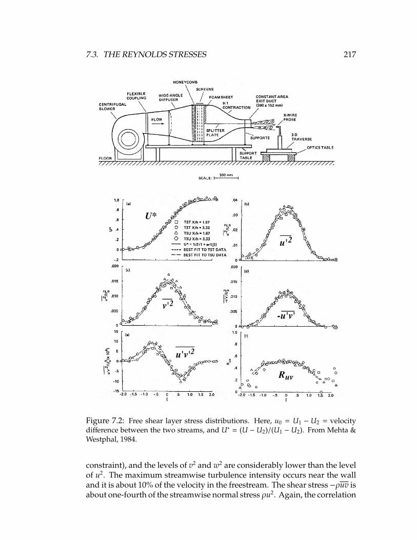
7.3. THE REYNOLDS STRESSES 217
Figure 7.2: Free shear layer stress distributions. Here, u0 = U1 − U2 = velocitydifference between the two streams, and U∗ = (U − U2)/(U1 − U2). From Mehta &Westphal, 1984.
constraint), and the levels of v2 and w2 are considerably lower than the levelof u2. The maximum streamwise turbulence intensity occurs near the walland it is about 10% of the velocity in the freestream. The shear stress −ρuv isabout one-fourth of the streamwise normal stress ρu2. Again, the correlation

218 CHAPTER 7. REYNOLDS-AVERAGED EQUATIONS
Figure 7.3: (a) Normal stresses in a zero pressure gradient boundary layer: 4,u′2/u2
τ; , v′2/u2τ; ©, w′2/u2
τ (uτ =√τw/ρ). (b) Shear stress distribution. Results
from Alving, 1988. Filled-in symbols from Erm, Smits & joubert, 1987. Solid linefrom Klebanoff, 1955.
coefficient Ruv is positive and quite high (in this case about 0.45 over mostof the layer).
7.4 Turbulent Transport of Heat
For an incompressible flow, the energy equation is given by:
ρCpDTDt
=DpDt
+ k∇2T + 2µSi j∂U j
∂xi(7.12)

7.5. THE REYNOLDS STRESS EQUATIONS 219
where k = thermal conductivity of fluid (W/mK), and
Si j =12
(∂Ui
∂x j+∂U j
∂xi
),
and 2µSi j∂U j
∂xi= Φ = dissipation function. (7.13)
Now, by an order of magnitude argument (not repeated here, but see forexample White Viscous Flow, or Schlichting, or Panton pp. 254–258), wecan show that for most purposes, as long as the Eckert number (Ec = (γ −1)Ma2T0/∆T) is small compared to one, the pressure term and the dissipationfunction are negligible compared to the other terms. Hence:
ρCpDTDt
= k∇2T
∂T∂t
+ U j∂T∂x j
= α∇2T (7.14)
where α = thermal diffusivity (with dimensions L2/T), and Pr = ν/α.Substituting T = T + θ′ etc., taking the mean, we get
U j∂T∂x j
=∂∂x j
(α∂T∂x j− θ′u j
)(7.15)
where the term in parenthesis is equal to Q j/ρCp, where Q j is the mean heatflux per unit area, that is, the rate of transport of mean heat, given by the sumof the contributions from molecular motion and turbulent motion. Note thesimilarity with equation 7.11 for the mean momentum: the transport of heatand momentum occurs in a similar way, even when the flow is turbulent.
7.5 The Reynolds Stress Equations
We can form equations for the evolution of the Reynolds stresses directlyfrom the Navier-Stokes equation. For example, if we take equation 7.7,multiply by the fluctuating velocity u, time average and subtract the mean,we get:
∂(
12u2
)∂t
+ U∂(
12u2
)∂x
+ V∂(
12u2
)∂y
+ W∂(
12u2
)∂z
=D
(12u2
)Dt
= −1ρ
u∂p′
∂x+ νu∇2u −
(u2∂U∂x
+ uv∂U∂y
+ uw∂U∂z
)
−
u2∂u∂x
+ uv∂u∂y
+ uw∂u∂z
. (7.16)
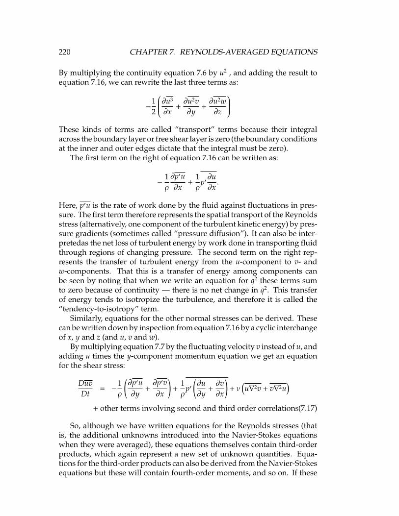
220 CHAPTER 7. REYNOLDS-AVERAGED EQUATIONS
By multiplying the continuity equation 7.6 by u2 , and adding the result toequation 7.16, we can rewrite the last three terms as:
−12
∂u3
∂x+∂u2v∂y
+∂u2w∂z
These kinds of terms are called “transport” terms because their integralacross the boundary layer or free shear layer is zero (the boundary conditionsat the inner and outer edges dictate that the integral must be zero).
The first term on the right of equation 7.16 can be written as:
−1ρ
∂p′u∂x
+1ρ
p′∂u∂x.
Here, p′u is the rate of work done by the fluid against fluctuations in pres-sure. The first term therefore represents the spatial transport of the Reynoldsstress (alternatively, one component of the turbulent kinetic energy) by pres-sure gradients (sometimes called “pressure diffusion”). It can also be inter-pretedas the net loss of turbulent energy by work done in transporting fluidthrough regions of changing pressure. The second term on the right rep-resents the transfer of turbulent energy from the u-component to v- andw-components. That this is a transfer of energy among components canbe seen by noting that when we write an equation for q2 these terms sumto zero because of continuity — there is no net change in q2. This transferof energy tends to isotropize the turbulence, and therefore it is called the“tendency-to-isotropy” term.
Similarly, equations for the other normal stresses can be derived. Thesecan be written down by inspection from equation 7.16 by a cyclic interchangeof x, y and z (and u, v and w).
By multiplying equation 7.7 by the fluctuating velocity v instead of u, andadding u times the y-component momentum equation we get an equationfor the shear stress:
DuvDt
= −1ρ
(∂p′u∂y
+∂p′v∂x
)+
1ρ
p′(∂u∂y
+∂v∂x
)+ ν
(u∇2v + v∇2u
)+ other terms involving second and third order correlations(7.17)
So, although we have written equations for the Reynolds stresses (thatis, the additional unknowns introduced into the Navier-Stokes equationswhen they were averaged), these equations themselves contain third-orderproducts, which again represent a new set of unknown quantities. Equa-tions for the third-order products can also be derived from the Navier-Stokesequations but these will contain fourth-order moments, and so on. If these

7.6. THE TURBULENT KINETIC ENERGY EQUATION 221
Reynolds-stress equations are to be useful, then at some point the equationsneed to be closed, that is, the highest-order products need to be expressedin terms of lower-order products (u2, −uv, U, for example) so that the num-ber of equations equals the number of unknowns. This is called turbulencemodelling (see below), and most attention has been focussed on the turbu-lence kinetic energy, despite the fact that q2 does not appear in any of themean momentum equations.
7.6 The Turbulent Kinetic Energy Equation
In any case, by adding up the three equations for the normal stresses, weobtain:
D(
12q2
)Dt
= −1ρ
(∂p′u∂x
+∂p′v∂y
+∂p′w∂z
)+
1ρ
p′(∂u∂x
+∂v∂y
+∂w∂z
)+ ν
(u∇2u + v∇2v + w∇2w
)−
[u2∂U∂x
+ uv∂U∂y
+ uw∂U∂z
+ uv∂V∂x
+ v2∂V∂y
+ vw∂V∂z
+ uw∂W∂x
+ vw∂W∂y
+ w2∂W∂z
]−
12
∂u3
∂x+∂u2v∂y
+∂u2w∂z
+∂v2u∂x
+∂v3
∂y+∂v2w∂z
+∂w2u∂x
+∂w2v∂y
+∂w3
∂z
(7.18)
The second term on the right is zero by continuity. In tensor notation:
D(
12q2
)Dt
=∂(
12q2
)∂t
+
1a︷ ︸︸ ︷U j
∂(
12q2
)∂x j
2a︷︸︸︷ 1b,2b︷︸︸︷= −
∂∂x j
p′u j
ρ+ 1
2u jq2
− uiu j∂Ui
∂x j︸ ︷︷ ︸3
+ νui∂2ui
∂x2j︸ ︷︷ ︸
4,5
. (7.19)
It is useful to give the physical meaning associated with the various terms.In this we follow Bradshaw An introduction to turbulence and its measurement1971 (Pergamon Press — out of print). See also figure 7.4.

222 CHAPTER 7. REYNOLDS-AVERAGED EQUATIONS
Figure 7.4: “The most general case of fluid motion, exhibiting all the complicationsallowed by the Navier-Stokes equations, is called turbulence,” Peter Bradshaw,1971.
(1) The instantaneous rate of transport of q2 is q2 times the instantaneousvelocity, for example, the rate of transport in the x-direction is q2(U+u).[Note that the “rate of transport” is nothing more than the flux per unitarea, where the flux of (something) is the amount of that (something)being transported across some surface per unit time. For example,the mass flux = (n · ρV)dA, the momentum flux = (n · ρV)VdA, theenergy flux = (n ·ρV)V2dA, etc.] The mean rate of transport of q2 in thex-direction is therefore q2U + q2u. The net rate at which q2 is leavingan elementary control volume in the x-direction is ∂
∂x (q2U +q2u)dxdydz.Summing up the contributions from the three directions gives terms(1a) + (1b), where (1a) is called the advection, or mean energy transport,and it is the rate of change of 1
2q2 along a mean streamline. [Note thatany term that can be expressed as a spatial gradient of a mean quantityis a “transport” term (its integral over the flow volume must be zero).Terms not so expressible are called “source/sink” terms. Note that term(3) is the only one involving a mean velocity gradient, and it is the onlyterm therefore that can act to take energy from the mean motion.]
(2) Terms like p′u′ can be interpreted as the rate at which work is be-ing done against the fluctuations in pressure (per unit area). Hence∂∂x (p′u)dxdydz represents the net loss of turbulent energy from an ele-mental volume by the work done in transporting the fluid through aregion of changing pressure.
The sum of terms (2a) and (2b) (also called (1b)) is sometimes calledthe turbulent energy transport, or energy diffusion.
(3) Terms like −ρu2 ∂U∂x dxdydz represent an extraction of energy from the
mean flow by the turbulence: from the point of view of the turbulence

7.6. THE TURBULENT KINETIC ENERGY EQUATION 223
these are energy production terms, and from the point of view of themean flow these are energy loss terms (we will see from the equationfor the mean flow kinetic energy derived in section 7.7 that thesesame terms appear in that equation with the opposite sign). Notethat −ρu2 ∂U
∂x dxdydz is the rate at which work is done against the x-component of the Reynolds normal stress to stretch an element of fluiddxdydz in the x-direction at a rate ∂U
∂x . Usually terms like−ρuv∂U∂y dxdydz
are more important, and these represent the work done against theshear stress −ρuv to shear an element of fluid at the rate ∂U
∂y .
(4) Now a term like(µ∂U∂y
)∂U∂y represents the product of the instantaneous
viscous stress and the instantaneous rate of strain, that is, a transferof energy between the bulk motion and the molecular motion — adissipation of bulk kinetic energy into thermal energy by viscosity.From the point of view of the temperature field it is a source of energyand is responsible for “aerodynamic” heating in high-speed flows.
The viscous term in the energy equation (the enthalpy equation) is:
Φ = 2µSi j∂U j
∂xi=∂U j
∂xi
(µ
(∂Ui
∂x j+∂U j
∂xi
))= dissipation function
(see section 7.7). If we substitute the Reynolds decomposition and takethe time average, we obtain (see Schlichting, Chapter 18 Part e):
Φ =∂U j
∂xi
(µ
(∂Ui
∂x j+∂U j
∂xi
))+∂u j
∂xi
(µ
(∂ui
∂x j+∂u j
∂xi
)). (7.20)
The first term on the right represents the dissipation of mean flowkinetic energy into thermal internal energy (= Φm, the “direct” dis-sipation function), and the second term on the right represents theviscous dissipation of turbulent kinetic energy (= ε, the “turbulent”dissipation function). Since the instantaneous velocity gradients as-sociated with the turbulence are much greater than the mean velocitygradients (except very close to a solid surface), ε Φm.
How does all this relate to the turbulent kinetic energy equation? Well,the viscous term in equation 7.19 may be written as:
ν(u∇2u + v∇2v + w∇2w
)= ν
12∇
2(u2 + v2 + w2
)−
(∂u∂x
)2
−
(∂u∂y
)2
−
(∂u∂z
)2
− · · ·
We recognize the squares of velocity gradients as elements of ε. Notall the elements are there, because cross product terms like µ ∂
2uv∂x∂y are

224 CHAPTER 7. REYNOLDS-AVERAGED EQUATIONS
missing in the turbulent kinetic energy equation. However, thesecross-product terms are usually interpreted as a diffusion term andthese can be shown to be small, except near the wall (see TownsendSection 2.7). To explain this interpretation, we also bring in the otherterm µ∇2(1
2q2). This is the viscous diffusion of q2), just as µ∇2U is theviscous diffusion of U. Similarly, µ ∂
2uv∂x∂y is the viscous diffusion of uv.
Since all diffusion terms are small at all Reynolds numbers that are nottoo low we have:
µ
(∂u j
∂xi
)2
≈ ε ≈ µ(u′∇2u′ + v′∇2v′ + w′∇2w′
)(5) Diffusion terms like µ∇2U are negligible (see Townsend Section 2.7).
Energy balances for the wake of a circular cylinder and a zero pressuregradient boundary layer are shown in figure 7.5, and for a fully developedpipe flow in figure 7.7. The wall bounded flows display large regions wherethe production term is approximately balanced by the dissipation term. Thediffusion terms become important near the wall, as expected, and they areimportant near the outer edge of the layer, since all other terms become verysmall there. The wake flow is somewhat more complicated in that all termsappear to be important everywhere.
7.7 Mean Flow Kinetic Energy Equation
To derive the equation for the mean flow kinetic energy (this is not thesame as the energy or enthalpy equation), we take the mean x-momentumequation 7.8 and multiply by U. Similarly, we take the y- and z-momentumequations and multiply by V and W respectively. Adding up the resultingequations gives:
DDt
ρU2i
2
= U j∂∂x j
ρU2i
2
= −Ui∂p∂xi
+ Ui∂∂x j
(2µSi j
)− Ui
∂∂x j
(ρuiu j
)(7.21)
The term on the left in equation 7.21 is the rate of change of the kineticenergy of the mean motion. The first term on the right of equation 7.21 isthe work done by the mean pressure forces to produce kinetic energy of themean motion. The viscous term in equation 7.21 has both a spatial transferpart and a dissipation part:
Ui∂∂x j
(2µSi j
)=
∂∂x j
(2µUiSi j
)− 2µSi j
∂Ui
∂x j
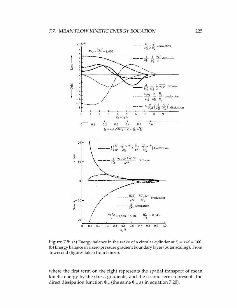
7.7. MEAN FLOW KINETIC ENERGY EQUATION 225
Figure 7.5: (a) Energy balance in the wake of a circular cylinder at ξ = x/d = 160.(b) Energy balance in a zero pressure gradient boundary layer (outer scaling). FromTownsend (figures taken from Hinze).
where the first term on the right represents the spatial transport of meankinetic energy by the stress gradients, and the second term represents thedirect dissipation function Φm (the same Φm as in equation 7.20).

226 CHAPTER 7. REYNOLDS-AVERAGED EQUATIONS
Figure 7.6: Mean flow energy balance in a zero pressure gradient boundary layer(outer scaling). From Townsend (figure taken from Hinze).
The last term on the right in equation 7.21 can be written as:
−Ui∂∂x j
(ρuiu j
)= −
∂∂x j
(Uiρuiu j
)+ ρuiu j
∂Ui
∂x j
where the first term on the right represents the spatial transport of meankinetic energy by the turbulent fluctuations, and the second term representsthe loss to turbulence: this is the extraction of turbulent energy from themean flow.
Figure 7.6 shows the energy balance of the mean motion for a zero pres-sure gradient boundary layer. Obviously the term labelled “dissipation toturbulence” is identical in magnitude to the “production” term in figure 7.7bbut with opposite sign.

7.7. MEAN FLOW KINETIC ENERGY EQUATION 227
Figure 7.7: (a) Energy balance in the wall region of a pipe flow (inner scaling).(b) Energy balance in the core region of a pipe flow (outer scaling). From Laufer(figures taken from Hinze).

228 CHAPTER 7. REYNOLDS-AVERAGED EQUATIONS

Chapter 8
Vorticity and Turbulence
8.1 Introduction
If you have ever looked over a river bridge and watched the surface patternsmove downstream of the pylons then you will have seen swirling motionswith both rotational and translational motion. Similar patterns have beenobserved in the wake of any bluff body (sharp plate, cylinder) as well asin boundary layers and free shear layers. They are generally disorganizedin that their characteristic scales vary with time and space in an apparentlyrandom fashion. Their scales are also a function of Reynolds number in thatthe range of length scales that is observed increases with Reynolds number,as does the range of time scales, or frequencies.
We know that turbulent motions are characterized by intense three- di-mensional fluctuations in velocity, even if the flow itself is nominally two-dimensional. How can we interpret these motions physically? Inherent inall thinking about turbulence is the concept of an eddy, which is regarded asa more or less coherent fluid motion and forms a subset of the larger veloc-ity field (according to Townsend, p.6: “flow patterns with spatially limiteddistributions of vorticity and comparatively simple forms”). Any interpre-tation of eddy behavior is often based on analogies with simpler swirlingmotions such as that associated with vortices, for example, the Rankine orpotential vortex, which leads to the concept of a line vortex, and the sinkvortex. Turbulence is often seen in terms of vorticity distributed in a veryintermittent fashion: the turbulent fluid is identified with fluid containingconcentrated vorticity distributed as vortex tubes or sheets, and these tubesor sheets may be contained in a background field where the vorticity is at arelatively low level (almost zero). The eddying motions associated with thisvorticity distribution interact with each other and they become distorted,they are transported and they change their intensity. There are two ways ofinterpreting eddies: as a perturbation imposed on the mean velocity field(a consequence of thinking in terms of the Reynolds-averaged equations of
229

230 CHAPTER 8. VORTICITY AND TURBULENCE
motion) or as constituting the entire velocity field, both mean and fluctuat-ing. The conceptual difference is clear: what is not usually so clear is howany particular researcher interprets the motions in terms of structure.
The concept of eddy structures arises from at least three sources:
1. Flow visualization;
2. Correlations and spectrum functions; and
3. The vorticity equation.
The concept of vorticity is crucial for a physical understanding of turbulence.Note that there is an important distinction between vorticity and vortices:for example, a laminar boundary layer has vorticity but no vortices. Inturbulent flow, vortices are difficult to define unambiguously, but eddiesare generally thought of as vortex tubes, at least qualitatively, and these aresometimes called the “muscles and sinews of turbulence.” Here, we startwith some basic definitions, then consider vortices in inviscid flow, and thenvortices in a viscous flow. We will only consider barotropic, constant densityflows.
8.2 Basic Concepts
8.2.1 Circulation
The circulation Γ is defined as
Γ =
∮V · d` (8.1)
where counterclockwise is positive. That is, the circulation contained withina closed contour in a body of fluid is defined as the integral around thecontour of the velocity vector which is locally tangential to the contour.
8.2.2 Vorticity
Vorticity is defined as the curl of the velocity:
Ω = ∇ ×V.
That is,
Ωi = εi jk∂u j
∂xk=
(∂uk
∂x j−∂u j
∂xk
). (8.2)
The vorticity is related to the instantaneous angular velocity of the fluidelement, ω, by:
Ω = 2ω.
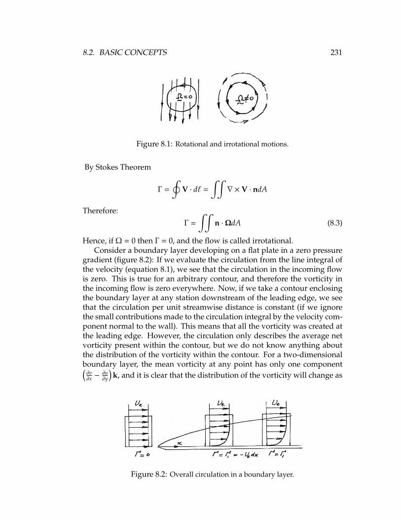
8.2. BASIC CONCEPTS 231
Figure 8.1: Rotational and irrotational motions.
By Stokes Theorem
Γ =
∮V · d` =
∫∫∇ ×V · ndA
Therefore:
Γ =
∫∫n ·ΩdA (8.3)
Hence, if Ω = 0 then Γ = 0, and the flow is called irrotational.Consider a boundary layer developing on a flat plate in a zero pressure
gradient (figure 8.2): If we evaluate the circulation from the line integral ofthe velocity (equation 8.1), we see that the circulation in the incoming flowis zero. This is true for an arbitrary contour, and therefore the vorticity inthe incoming flow is zero everywhere. Now, if we take a contour enclosingthe boundary layer at any station downstream of the leading edge, we seethat the circulation per unit streamwise distance is constant (if we ignorethe small contributions made to the circulation integral by the velocity com-ponent normal to the wall). This means that all the vorticity was created atthe leading edge. However, the circulation only describes the average netvorticity present within the contour, but we do not know anything aboutthe distribution of the vorticity within the contour. For a two-dimensionalboundary layer, the mean vorticity at any point has only one component(∂v∂x −
∂u∂y
)k, and it is clear that the distribution of the vorticity will change as
Figure 8.2: Overall circulation in a boundary layer.

232 CHAPTER 8. VORTICITY AND TURBULENCE
Figure 8.3: Circulation in a boundary layer in a favorable pressure gradient.
the layer grows. Note also that if the boundary layer is turbulent, the overalllevel of the fluctuating vorticity within the boundary layer a given volumemust sum to zero, and we can expect that within any sub-volume it muston average be zero also, so that negative and positive vorticity must nearlycancel at any time.
If the boundary layer enters a region of streamwise pressure gradient,the freestream velocity will change, and therefore the circulation around acontour enclosing the layer must change accordingly. Therefore pressuregradients can change the circulation (favorable pressure gradients will in-crease the circulation, and vice versa). It is sometimes said that the pressuregradients at the wall act as a source or sink of vorticity1.
8.2.3 Vortex tubes and filaments
Instantaneously, imagine a closed contour in the fluid. Each point on thecontour will have a streamline passing through it. These streamlines definea volume called a stream tube. If the cross-sectional area is infinitesimal, weget a stream filament.
Similarly, we define a vortex line as a line whose tangents are parallelto the vorticity vector. For a closed contour, each point on the contour willhave a vortex line passing through it. Hence, we can define a vortex tube,and a vortex filament.
For an incompressible flow, the velocity field is divergence-free, that is,∇ ·V = 0, and there are no sinks or sources of mass in the fluid. As a vectoridentity, the divergence of the curl of a vector is zero, that is, ∇ ·Ω = 0 andthere are no sinks or sources of vorticity inside the fluid. Therefore, vortextubes must terminate on themselves, at a solid boundary, or at a free surface.
We can make a formal analogy between V in an incompressible flow andΩ.
1Note that all the vorticity in the layer is due to the no-slip condition: a pressure gradientby itself will not generate vorticity in a barotropic fluid — see section 8.4
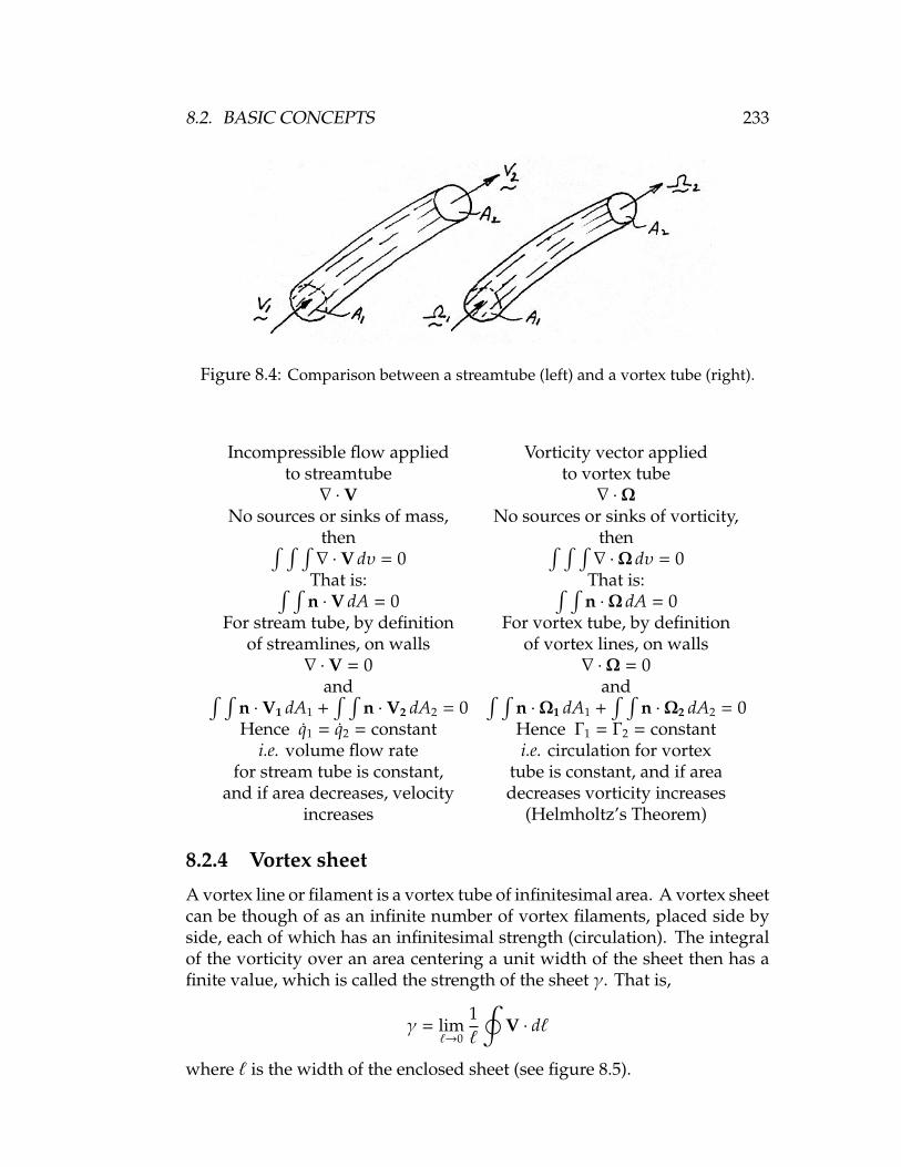
8.2. BASIC CONCEPTS 233
Figure 8.4: Comparison between a streamtube (left) and a vortex tube (right).
Incompressible flow applied Vorticity vector appliedto streamtube to vortex tube∇ ·V ∇ ·Ω
No sources or sinks of mass, No sources or sinks of vorticity,then then∫ ∫ ∫∇ ·V dυ = 0
∫ ∫ ∫∇ ·Ω dυ = 0
That is: That is:∫ ∫n ·V dA = 0
∫ ∫n ·Ω dA = 0
For stream tube, by definition For vortex tube, by definitionof streamlines, on walls of vortex lines, on walls
∇ ·V = 0 ∇ ·Ω = 0and and∫ ∫
n ·V1 dA1 +∫ ∫
n ·V2 dA2 = 0∫ ∫
n ·Ω1 dA1 +∫ ∫
n ·Ω2 dA2 = 0Hence q1 = q2 = constant Hence Γ1 = Γ2 = constant
i.e. volume flow rate i.e. circulation for vortexfor stream tube is constant, tube is constant, and if area
and if area decreases, velocity decreases vorticity increasesincreases (Helmholtz’s Theorem)
8.2.4 Vortex sheet
A vortex line or filament is a vortex tube of infinitesimal area. A vortex sheetcan be though of as an infinite number of vortex filaments, placed side byside, each of which has an infinitesimal strength (circulation). The integralof the vorticity over an area centering a unit width of the sheet then has afinite value, which is called the strength of the sheet γ. That is,
γ = lim`→0
1`
∮V · d`
where ` is the width of the enclosed sheet (see figure 8.5).

234 CHAPTER 8. VORTICITY AND TURBULENCE
Figure 8.5: Circulation in a vortex sheet.
Vortex sheets represent velocity discontinuities in the flow, such as thatwhich occurs between two uniform parallel flows of different velocity (seefigure 8.6).
Figure 8.6: Decomposition of a two-stream shear layer.
8.3 Biot-Savart Law
This “law’ gives the induced fluid velocity at any distance from an arbitraryinfinite line with circulation Γ (line vortex). That is,
dV =Γ
4πr3 d` × r. (8.4)
That is:
|dV| =Γ
4πr3 |d`| |r| sinθ,
where the direction is given by the right hand screw rule.Consider an infinite straight line vortex filament. The induced velocity
at any point may be found as follows:
V =
∫∞
−∞
Γ
4πr3 d` × r.
That is:
|V| =∫∞
−∞
Γ
4πr2 sinθd`.
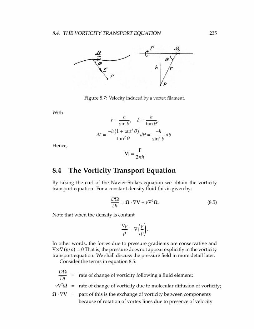
8.4. THE VORTICITY TRANSPORT EQUATION 235
Figure 8.7: Velocity induced by a vortex filament.
Withr =
hsinθ
, ` =h
tanθ,
d` =−h
(1 + tan2 θ
)tan2 θ
dθ =−h
sin2 θdθ.
Hence,
|V| =Γ
2πh.
8.4 The Vorticity Transport Equation
By taking the curl of the Navier-Stokes equation we obtain the vorticitytransport equation. For a constant density fluid this is given by:
DΩDt
= Ω · ∇V + ν∇2Ω. (8.5)
Note that when the density is contant
∇pρ
= ∇
(pρ
).
In other words, the forces due to pressure gradients are conservative and∇×∇
(p/ρ
)= 0 That is, the pressure does not appear explicitly in the vorticity
transport equation. We shall discuss the pressure field in more detail later.Consider the terms in equation 8.5:
DΩDt
= rate of change of vorticity following a fluid element;
ν∇2Ω = rate of change of vorticity due to molecular diffusion of vorticity;
Ω · ∇V = part of this is the exchange of vorticity between componentsbecause of rotation of vortex lines due to presence of velocity

236 CHAPTER 8. VORTICITY AND TURBULENCE
Figure 8.8: Illustrating the Kelvin and Helmholtz theorems.
gradients; another part gives the rate of change of vorticitydue to stretching of vortex lines. This term is non-linear,since Ω depends on V.
For inviscid flows, we see that if the vorticity was initially zero then itwill remain zero — so the vorticity of a fluid lump depends on its initialcondition, and if it was zero initially it cannot gain vorticity ever. Also, forinviscid flows we have Kelvin’s theorem, which says that the circulationaround any closed material curve is invariant.
We can make the following observations from these two theorems:
1. Since the vorticity Ω = ∇ × V, this implies ∇ · Ω = 0. Therefore, thevortex lines never end in a fluid. They either form closed loops or endat a boundary.
2. The circulation is the same for every contour enclosing the vortex line,that is, DΓ/Dt = 0.
3. If we have at some instant a flow without vorticity (such that thecirculation around any contour is zero), then Kelvin’s theorem statesthat at any future time the fluid must remain without vorticity. Inparticular, a fluid initially at rest has no vorticity, and must remainwithout vorticity.
4. Vortex tubes are in some sense permanent – a vortex tube specifiedat an initial instant by drawing the vortex-lines that intersect a givenclosed curve in the fluid has a continuing identity. We may say that ina barotropic, inviscid fluid a vortex-tube moves with the fluid and itsstrength remains constant (Batchelor p. 274).

8.5. VORTEX INTERACTIONS 237
Figure 8.9: Effect of a velocity gradient on a vortex line. (a) Tilting: vorticity ω2,velocity gradient ∂u1/∂x2. (b) Stretching: vorticity ω2, velocity gradient ∂u2/∂x2.From Bradshaw, Turbulence, 1978.
8.4.1 Vortex tilting and stretching
(For the following see Turbulence, ed. P. Bradshaw, Springer-Verlag, 1978,p.9-10).
The vorticity/velocity-gradient interaction termΩ · ∇V can be written intensor notation for the ith component as Ω j∂ui/∂x j.
1. A. When i = j, say i = 1; j = 2 (figure 8.9a). Here this term represents anexchange of vorticity between components because a velocity gradient∂u1/∂x2 tilts a vortex line which was originally in the x2-direction sothat it acquires a component in the x1-direction.
2. B. When i = j, say i = j = 2 (figure 8.9b, the vortex line is stretchedby the rate of tensile strain along the axis, without any change ofdirection of that axis. We have already seen that the circulation arounda closed path enclosing a vortex filament is constant (incompressibleflow) (equivalent to conserving angular momentum), and as the lineis stretched its vorticity will increase.
8.5 Vortex Interactions
Vortex interactions play a very important role in many flow situations. Forexample, the generation of vortex trails behind aircraft, the formation of vor-tex sheets associated with lifting surfaces, the atmospheric phenomenon oftornadoes, vortex rings (for example, smoke rings) and the vortex sheddingbehind bluff bodies (for example, the von Karman vortex street behind acylinder) all involve vortex interaction. For example, the turbulent vorticesbehind an aircraft could disturb the flight of another aircraft moving into

238 CHAPTER 8. VORTICITY AND TURBULENCE
the vortex system, and the stability and decay of the vortex system is par-ticularly important. In the field of turbulence, the understanding of vortexinteractions is crucial for the understanding of the kinematics and dynamicsof turbulence.
Turbulent flows have many random or chaotic features. However, recentevidence has demonstrated the existence of organized motions in a wide va-riety of turbulent shear flows (mixing layers, boundary layers and wakes).These so called “coherent structures” are often modelled as interacting vor-tices. Turbulent flows have often been described as a complex collectionof vortices entangled like spaghetti. The large dissipation of energy andthe high rates of mass, momentum and energy diffusion in turbulent flowsare due to the intense mixing and distortion of the interacting vortices. Anexample of such an interaction is seen in figures 5.19 and 5.27. It showshow two or three vortices in a mixing layer combine to form a larger scalestructure. Notice that the vortices (while pairing) rotate about each otherand amalgamate.
Therefore, it is easy to see why the study of vortex interaction is suchan active field of research. Some of the more recent research in this areais illustrated in Van Dyke’s Album of Fluid Motion. The study of vortexinteractions is a very large field and we will restrict the discussion to thesimplest flows, that is, inviscid, barotropic flows with conservative bodyforces. Under these conditions the vorticity field obeys Helmholtz’s rules(see section 8.4).
The vorticity equation for an inviscid, incompressible fluid reduces to:
DΩDt
= Ω · ∇V,
where the term on the right-hand side is called the vorticity stretching vector.For two-dimensional flows, this equation reduces to:
DΩDt
= 0.
We will now consider a number of examples.
8.5.1 Velocity field induced by a vortex filament
By a vortex filament, we mean a vortex tube of concentrated vorticity suchthat, as its cross-sectional area A goes to zero, Ω goes to infinity to keep theproduct ΩA = Γ = constant. Therefore the integral of the velocity vectoralong a closed path containing the filament is Γ. The aim is to find theinduced velocity field in the irrotational fluid surrounding the filament; weare interested in calculating ur and uθ. There are several methods of doing

8.5. VORTEX INTERACTIONS 239
Figure 8.10: Notation for calculating the induced velocity field.
this. The most general method involves the use of the Biot-Savart law whichcan be expressed as (see section 8.3):
4πV =
∫Γ
r3 ds × r.
The integration is carried over the length of the vortex filament. The Biot-Savart law says that each element of the vortex filament contributes to thevelocity induced at point P and the contribution is proportional to the inverseof (some) power of r. Therefore at any point P the induced velocity is largelydetermined by the elements nearest to P.
For a filament aligned with the y-axis, the velocity at the point P in thex-z plane at a distance r from the origin is given by:
V = uθeθ =Γ
2πreθ.
The induced velocity can also be found by using the complex potentialfunction for a vortex filament. The complex potential in this case is
F(z) =−iΓ2π
ln z
= φ + iψ
andV = ∇φ.
The velocity field is determined by differentiation of the velocity potentialor stream function. Hence:
uθ =Γ
2πrSo the velocity field for a vortex filament varies as l/r where r is the
distance from the center of the vortex. Note that uθ → ∞ at the center of

240 CHAPTER 8. VORTICITY AND TURBULENCE
Figure 8.11: Rankine vortex velocity distribution.
the vortex: it is a singularity. In a real (viscous) fluid, viscosity damps outthe velocity in the center of the vortex, leading to solid body rotation in thecentral region of the vortex. The pressure varies parabolically in this regionand hyperbolically outside of this region.
8.5.2 The Rankine vortex
Consider the Rankine vortex — a solid body rotation in the core, surroundedby an irrotational field of the same circulation. In the core,
∂p∂r
=ρu2
θ
rso that
p − pmin =ρu2
θ
2and the kinetic energy per unit length
E = πρ
∫ a
0u2θr dr
remains finite.The vorticity is confined to the inner core, the energy is finite, and viscos-
ity limits the energy in the irrotational flow from becoming infinite. Actualflows that approach this are the sink vortex, hurricane, cyclone, tornado.
This is our model for a line vortex. We can imagine any flow withvorticity to be made up of large numbers of infinitesimally slender vortices,or sometimes as vortex sheets which can be thought of as a layer of locallyparallel vortex lines.
8.5.3 Filaments of opposite sign and equal strength
We can solve for the velocity field by considering a complex potential of theform:
F(z) =iΓ2π
ln(z − cz + c
).

8.5. VORTEX INTERACTIONS 241
Figure 8.12: Two vortex filaments of opposite sign and equal strength.
But here we are more interested in vortex interactions. The vortex at Ainduces a velocity at point B in the y-direction and vice versa (figure 8.12).The magnitude of the velocity is
uinduced =Γ
2π(2c)=
Γ
4πc.
Therefore both vortices move downwards at the speed Γ/4πc. The velocityof the fluid at the midpoint between the vortices equals the sum of inducedvelocities from each vortex:
umidpoint =2Γ
2πc=
Γ
πc= 4
(Γ
4πc
),
which is four times the velocity of the vortex pair, so there is a jet of fluidbetween the vortices.
Note the line of symmetry between the two vortices. Since this line is astreamline, the normal velocity in the x-direction at any point on the y-axisis zero. Therefore, V · n = 0 on the y-axis, and this is the wall boundarycondition for inviscid fluids. Thus the two vortex system above is equivalentto a single vortex next to a wall (figure 8.13). Therefore a vortex next to awall will move parallel to the wall at the velocity. This fact is very usefulbecause we can see now how to account for the effect of the wall in morecomplicated situations. This technique of replacing the wall with anothervortex of the opposite sign is called the Method of Images.
Figure 8.13: Single vortex moving along a wall, with image vortex in the wall.
If the strengths of the vortices are not equal in magnitude, then the motionis not in a straight line but in concentric circles. The center of rotation is

242 CHAPTER 8. VORTICITY AND TURBULENCE
Figure 8.14: Two vortices of unequal strengths and opposite sign.
found as follows. In figure 8.14, u1 and u2 are the velocities induced by thevortices on each other and 0 is the center of rotation. Now,
u1 =Γ1
4πc, u2 =
−Γ2
4πc(Γ2 < 0).
Imposing the condition of irrotationality in the fluid surrounding the vor-tices (only solid body rotation is allowed), then by similar triangles:
u2
x=
u1
x + 2c.
Substituting for u1 and u2 leads to:
−Γ2
x=
Γ1
x + 2c.
That is,
x =(−Γ2
Γ1 + Γ2
)2c.
When Γ1 + Γ2 = 0, x = ∞, and we get motion in a straight line.
8.5.4 Filaments of the same sign and strength
By using arguments similar to the previous case, we can show that theinduced velocities are in opposite directions. Therefore it is obvious that thevortices will rotate about each other.
If the strengths of the vortices are not the same, then an analysis similarto that given earlier yields x = [Γ2/(Γ1 + Γ2)]2c and the motion is again inconcentric circles (figure 8.15).
8.5.5 Filaments not parallel to each other
Until now, we have been considering filaments which were parallel to eachother. We now consider two vortices, one along the x-axis and the otherparallel to the z-axis at a distance y from the origin (figure 8.16). Let us

8.5. VORTEX INTERACTIONS 243
Figure 8.15: Two vortices of the same sign and strength.
Figure 8.16: Two vortices not parallel to each other.
consider the induced velocities at some points on the two vortices. A vortex1 induces a velocity in the downward direction (−y). At B, it induces avelocity in the +y-direction. Similarly, the velocities induced by vortex 2 atpoints C and D are shown. At point E, there is a velocity in the +x-directionand at point F, the induced velocity is in the +z-direction. Therefore, on eachfilament there are points where the induced velocities are perpendicular toeach other. This leads to the stretching of the filaments. As time goes onthe distortions of the filaments (from straight lines) increase, leading to amess which looks like spaghetti. In this process, it is clear from recent work(for example, by Orszag, Zabruski, and Hussain) that viscosity cannot beneglected: when the vortices come close enough the velocity gradients arehigh enough to make viscous forces become predominant. As a result, wehave vortex “connection and reconnection” whereby, in the example givenabove, pieces of one vortex connect to a piece of the other vortex. This canonly happen when viscous forces are important. See also the experiment byLim & Nickels shown in figure 5.18.
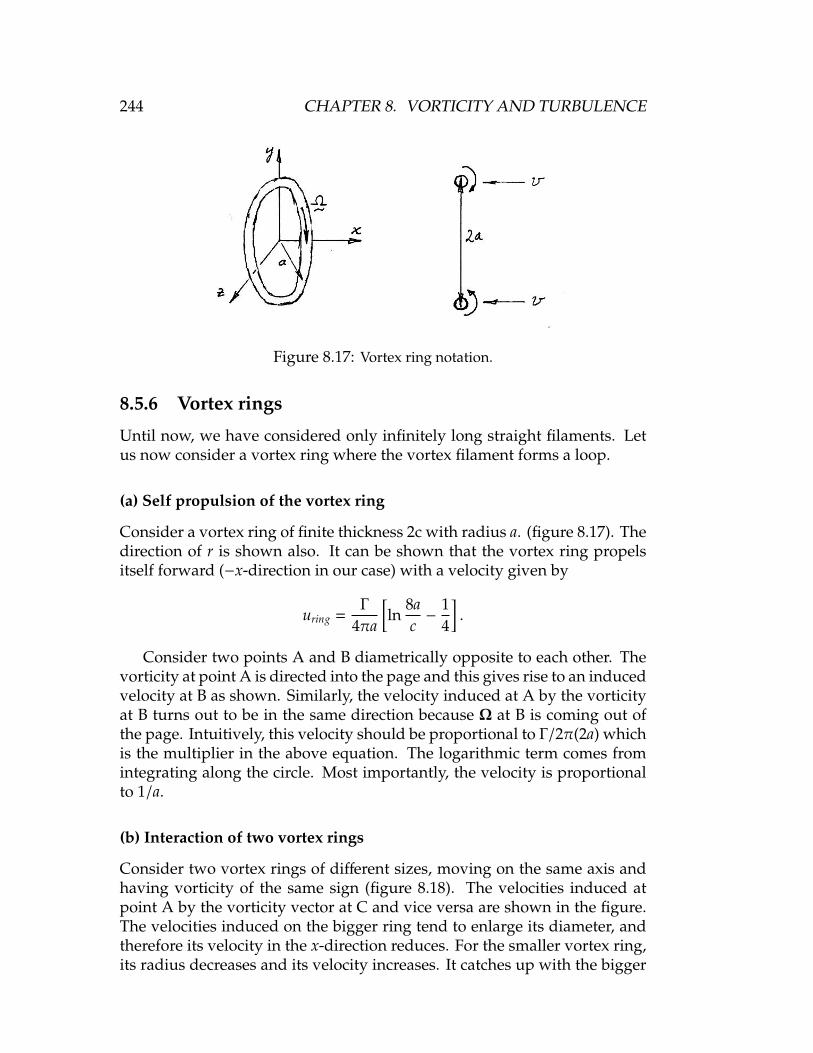
244 CHAPTER 8. VORTICITY AND TURBULENCE
Figure 8.17: Vortex ring notation.
8.5.6 Vortex rings
Until now, we have considered only infinitely long straight filaments. Letus now consider a vortex ring where the vortex filament forms a loop.
(a) Self propulsion of the vortex ring
Consider a vortex ring of finite thickness 2c with radius a. (figure 8.17). Thedirection of r is shown also. It can be shown that the vortex ring propelsitself forward (−x-direction in our case) with a velocity given by
uring =Γ
4πa
[ln
8ac−
14
].
Consider two points A and B diametrically opposite to each other. Thevorticity at point A is directed into the page and this gives rise to an inducedvelocity at B as shown. Similarly, the velocity induced at A by the vorticityat B turns out to be in the same direction because Ω at B is coming out ofthe page. Intuitively, this velocity should be proportional to Γ/2π(2a) whichis the multiplier in the above equation. The logarithmic term comes fromintegrating along the circle. Most importantly, the velocity is proportionalto 1/a.
(b) Interaction of two vortex rings
Consider two vortex rings of different sizes, moving on the same axis andhaving vorticity of the same sign (figure 8.18). The velocities induced atpoint A by the vorticity vector at C and vice versa are shown in the figure.The velocities induced on the bigger ring tend to enlarge its diameter, andtherefore its velocity in the x-direction reduces. For the smaller vortex ring,its radius decreases and its velocity increases. It catches up with the bigger

8.6. VORTICITY DIFFUSION 245
ring and passes right through it. Now the roles are reversed and the “leap-frogging” repeats itself (see figure 8.19).
What if the two vortices are of opposite circulations? In this case, whenthe vortex rigns approach each other, each induces a radial outward velocityon the other, and they grow in size and slow down.
(c) Vortex ring near a wall
This system is equivalent to the one shown in figure 8.20. The velocitiesinduced by the fictitious ring on the left tend to expand the ring. The vortexring “sees” its image or reflection in the wall and behaves accordingly.
The mirror image principle also explains the “ground effect” — the extralift an airplane experiences near the ground. An airfoil sees its mirror imageand feels the induced velocity and pressure field from the reflection (fig-ure 8.21). So the lift will be increased. The effect depends strongly on aspectratio (see, for example, Ashley & Landahl p.218, Thwaites p.527). Thereare two basic mechanisms: (1) the image of the spanwise vortex induces anupwash on the front part of the physical wing, and a downwash over therear — to counteract this, a vortex distribution is required, corresponding toa camber, which is such as to produce a force directed towards the ground;and (2) the images of the trailing vortices produce an upwash at the physicalwing, thereby reducing the induced angle of incidence, which reduces theinduced drag and increases the lift slightly.
8.6 Vorticity Diffusion
For two-dimensional, barotropic viscous flows the vorticity transport equa-tion reduces to:
DΩDt
= ν∇2Ω. (8.6)
Figure 8.18: Vortex ring interaction.

246 CHAPTER 8. VORTICITY AND TURBULENCE
Figure 8.19: Leapfrogging of two vortex rings. from Yamada & Matsui, 1978.

8.6. VORTICITY DIFFUSION 247
Figure 8.20: Vortex ring near a wall.
Now, the energy equation for constant property, low speed flow is given by:
DTDt
= α∇2T. (8.7)
Note the similarity. In fact, both equations are diffusion equations and
ν =µ
ρ= viscous diffusivity
α =kρCp
= thermal diffusivity
In addition, if C represents the proportion of marked molecules in a fluidmixture (the concentration of one component of the mixture), then the con-centration obeys a simple conservation law, where the concentration of agiven fluid particle can only change by molecular transport across the sur-face, That is:
DCDt
= ℘∇2C. (8.8)
where ℘ is the mass diffusivity.The ratio of these diffusivities give a measure of the relative diffusivity
of vorticity, heat and mass:
να
=µCp
k= Pr =
viscous diffusion ratethermal diffusion rate
Figure 8.21: Ground effect due to image wing.

248 CHAPTER 8. VORTICITY AND TURBULENCE
Figure 8.22: Relative diffusion of vorticity and temperature.
ν℘
=µ
ρ℘= Sc =
viscous diffusion ratemass diffusion rate
℘
α=
ρCp℘
k= Le =
mass diffusion ratethermal diffusion rate
Note: Pr = ScLe and some typical value for the Prandtl number are 0.024(mercury), 0.72 (air), 7.0 (water) and 3,500 (SAE 30 oil). Also, the Schmidtnumber is important for the interpretation of scalar fields: for most markers,such as smoke in air and dye in water, the Schmidt number is very large andthe vorticity is diffused at a much higher rate than the marker is diffused(see recent work by Roshko, Rockwell, Dahm). In these cases, the extentof the marked fluid does not neccessarily coincide with the extent of thevorticity, even in turbulent flows where the dominant transport process ofvorticity is by turbulent diffusion not viscous diffusion. Because of theseconsiderations, there are considerable advantages to using temperature as ascalar marker in air flows.
For example, if we were to compare the temperature and velocity profilesin the Rayleigh problem, where a heated flat plate is suddenly acceleratedfrom rest in a viscous fluid, we see that only for gases (Pr ≈ 1) do the thermaland velocity profiles almost coincide (figure 8.22). .
8.6.1 Note on vorticity diffusion
Consider the Rayleigh problem, and evaluate the circulation around a fixedcontour, of unit length in the x-direction (figure 8.23). . At t = 0, Γ =−2U/unit length. At t > 0, Γ = −2U/unit length. That is, the circulationhas remained constant, despite the action of viscosity inside the contour.However, at t 0, Γ < −2U/unit length because of viscous diffusion across

8.7. THE PRESSURE FIELD AND VORTICITY 249
the contour, out of the control volume.Of course, if the contour was large enough, then the circulation would
always remain constant, although the vorticity distribution would be con-tinually changing.
Another example is a bucket of radius R containing a viscous fluid,placed on a rotating turntable. If at t < 0, the fluid was moving with solidbody rotation, then the circulation around any contour enclosing all thefluid would be +2πR2ω. If at t = 0, the bucket was suddenly brought torest, the no-slip condition at the wall would instantaneously cancel out thiscirculation. Within the bucket, the vorticity generated at the wall diffusesout with time until the vorticity everywhere is also zero.
Another example is the behavior of a line vortex being stretched in aviscous fluid.
8.7 The Pressure Field and Vorticity
So far we have not considered the pressure fluctuations in a turbulent field.We can obtain an equation for the instantaneous pressure (mean plus fluctu-ating) by taking the divergence of the Navier-Stokes equations. We obtain:
−1ρ∇
2 (p + p′)
=∂2uv∂x∂y
+∂2vw∂y∂z
+∂2wu∂z∂x
+∂2u2
∂x2
∂2v2
∂y2 +∂2w2
∂z2 (8.9)
where u, v and w are the instantaneous velocities. Note that the viscousstresses do not constribute to the pressure field — it is completely specifiedby the instantaneous velocity field. Equation 8.9 is in the form of a Poisson’sequation ∇2p = f , so that there exists a solution:
p + p′ =ρ
4π
∫f (x′)|x − x′|
dx′dy′dz′,
Figure 8.23: Vorticity diffusion as a function of time. (a) t = 0; (a) t > 0; (a) t 0.

250 CHAPTER 8. VORTICITY AND TURBULENCE
where|x − x′|2 = (x − x′)2 +
(y − y′
)2+ (z − z′)2
(x′ is the position at which the pressure is to be found). That is
p + p′ =ρ
4π
∫∂2uiu j/∂xi∂x j
|x − x′|dx′dy′dz′. (8.10)
So the pressure is not local but it is given by the integral over the entirevelocity field.
Note that it may be shown (exercise) that
p(x′) =ρ
4π
∫ [2∂ui
∂x j
∂u j
∂xi+
∂2
∂xi∂x j
(uiu j − uiu j
)] dx′dy′dz′
|x − x′|.
Term I on the right hand side represents the contribution to p′ due to theinteraction between mean velocity gradients and turbulent velocity gradi-ents; and Term II represents the contribution to p′ due to fluctuations ofthe Reynolds stresses about their mean value (generally smaller than thecontribution due to Term I).
8.8 Splat and Spin
We can rewrite equation 8.9 (for incompressible flow) as:
−1ρ
∂2p∂x2
i
=∂2uiu j
∂xi∂x j(8.11)
=∂∂x j
(u j∂ui
∂xi+ ui
∂u j
∂xi
)=
∂ui
∂x j
∂u j
∂xi+ ui
∂∂xi
(∂ui
∂x j
)Hence
−1ρ
∂2p∂x2
i
=∂ui
∂x j
∂u j
∂xi. (8.12)
Now we have
Si j ==12
(∂ui
∂x j+∂u j
∂xi
),
and
ξi j ==12
(∂ui
∂x j−∂u j
∂xi
),

8.8. SPLAT AND SPIN 251
Figure 8.24: A straining field formed by the collision of two vortices.
where Si j and ξi j are the rate-of-strain tensor (symmetric) and the rate-of-rotation tensor (anti-symmetric), respectively, so that
∂ui
∂x j= Si j + ξi j.
Hence,
−1ρ
∂2p∂x2
i
=(Si j + ξi j
) (Si j − ξi j
)= Si jSi j − ξi jξi j
Now Si jSi j = S2 = sum of the squares of the principal strains, andξi jξi j = 12Ω2
i ,where Ωi is the ith component of the vorticity vector.
[Note: ξi j = 12εi jkΩk, where
εi jk = 1 (cyclic i jk)εi jk = −1 (anti-cyclic i jk)εi jk = 0 (otherwise)
and εi jkεi jm = 2δkm, so this result follows]
Hence
−1ρ
∂2p∂x2
i
= S2−
12Ω2
i (8.13)
where the first term on the right is called splat, and the second term is calledspin.
But so what? Here we follow Bradshaw & Koh, Phys. Fluids 24, 777, 1981.Consider a straining field caused by the collision of two vortices (figure 8.24).A small fluid element in the region of the collision will be compressed inthe y-direction and elongated in the x-direction. The rotation will be small.

252 CHAPTER 8. VORTICITY AND TURBULENCE
Figure 8.25: Visualization by Robinson of Spalart’s simulations of a low Reynoldsnumber turbulent wall layer (Reθ ≈ 640). Here the pressure minima seem to markthe vortical motions well.
From Poisson’s equation, S2≈ 0, which implies that ∂2p/∂x2
i < 0. That is,the pressure is a maximum.
Next, consider a fluid element embedded in a vortex. In this case thevorticity term dominates(
∂ui
∂x j≈ −
∂ui
∂xiand Si j ≈ 0, while ξi j , 0
)and ∂2p/∂x2
i > 0, implying that a pressure minimum will occur in the core ofa vortex (which is fairly obvious from previous considerations). Bradshaw &Koh referred to these components as “splat” and “spin” (see equation 8.13).This provides a simple physical explanation of turbulent pressure fluctua-tions: high and low pressures are caused by the collision of eddies and thepassage of eddies, respectively. This helps the interpretation of the pressurefield, and it also helps the interpretation of DNS results (for example, seefigure 8.25). .
Note that, despite this talk of vorticity, it is the pressure gradients thatdrive the flow. Pressure fluctuations can be viewed as the signatures of

8.8. SPLAT AND SPIN 253
fluid motion, but it is important to remember that the motions come aboutbecause of pressure gradients.

254 CHAPTER 8. VORTICITY AND TURBULENCE

Chapter 9
Statistical Description ofTurbulence
So far we have made extensive use of Reynolds averaging to describe turbu-lent flow behavior, especially in terms of the Reynolds-averaged equationsof motion. Here we introduce other measures, including higher order mo-ments, space-time correlations, spectra and wavelets. Parts of this presen-tation follows Tennekes & Lumley, Chapters 6 and 8.
In this chapter, we will denote the instantaneous values of the velocitycomponents by capital letters (U, V, and W), time-averaged values by over-bars (U, V, and W), and lower case letters for fluctuating velocities (u, v, andw). For the pressure p, the time-average value is p, and the fluctuating valueis p′. A capital P indicates a probability.
9.1 Probability Density
We will consider only statistically steady functions (stationary) — these havemean values which are not a function of time.
If we collect the contribution to U(t) in the range from U1 to U1 + ∆U (seefigure 9.1, over a long time T , then P(U) is the probability density where
P(U) ∆U = limT→∞
1T
Σ (∆t) = ∆F(U)
where F(U) = P(V < U), and ∆t is the amount of time spent in the interval∆U. The probability of finding U(t) between U1 and U1 + ∆U is equal to theproportion of time spent there. Also:
P(U) ≥ 0, and∫∞
−∞
P(U) dU = 1
255

256 CHAPTER 9. STATISTICAL DESCRIPTION OF TURBULENCE
Figure 9.1: A random signal and its probability density function. From Tennekes& Lumley, 1972.
Note that we can write:
f = limT→∞
1T
∫ t0+T
t0
f (U) dt
which is the definition of a mean. So:
f =
∫∞
−∞
f (U) P(U) dU,
and therefore
U =
∫∞
−∞
U P(U) dU.
If we now consider the fluctuations away from the mean, we obtain thevariance (the mean square departure from the mean):
u2 =
∫∞
−∞
u2 P(U) dU =
∫∞
−∞
u2 P(u) du
where σ =√
u2 is the standard deviation (or intensity).Now the value of u2 does not reflect the symmetry or anti-symmetry of
the u distribution. However, the third moment u3 depends only on the lackof symmetry in P(u):
u3 =
∫∞
−∞
u3 P(u) du.
For a symmetric distribution, u3 = 0 (see figure 9.2).The skewness S is defined by:
S =u3
σ3 =u3
(√
u2)3.

9.1. PROBABILITY DENSITY 257
Figure 9.2: (a) Probability density distribution of a sine wave; (b) A function withpositive skewness (3rd moment); (c) A function with small kurtosis (4th moment);(d) A function with large kurtosis; (e) bimodal probability density distributionindicating intermittent behavior. From Tennekes & Lumley, 1972.
The fourth-order moment is called the kurtosis K:
K =u4
σ4 =1σ4
∫∞
−∞
u4 P(u) du.
Some representative probability density distributions for boundary lay-ers are shown in figures 9.3 and 9.4, and some representative distributionsof skewness and kurtosis in a subsonic turbulent boundary layer are shownin figure 9.5. Bimodal distributions indicate that the signal is intermittent,that is, it is flipping between two preferred states. This is seen near the edge

258 CHAPTER 9. STATISTICAL DESCRIPTION OF TURBULENCE
Figure 9.3: (a) Probability density distributions of u′ and v′ at y/δ = 0.1 in anincompressible boundary layer (Alving, 1988); (b) As in (a) but at y/δ = 0.7.
of a shear layer where the flow is intermittently turbulent. In the examplegiven below, the relatively sharp peak would correspond to the free stream(the finite width of the peak is due to the irrotational fluctuations induced bythe turbulent field), and the broad peak would correspond to the turbulencewithin the layer.
9.2 Joint Probability Density
Consider two variables, u(t) and v(t). Then P(u, v), the joint probabilitydensity, is proportional to the fraction of time that the signals spend in awindow defined by u and u + ∆u, and v and v + ∆v. As before:
P(u, v) ≥ 0∫∫P(u, v) dudv = 1.
Note ∫P(u, v) dv = P(u)

9.3. CORRELATION COEFFICIENTS 259
Figure 9.4: (a) Probability density distributions of (ρu)′ in a Mach 2.9 undisturbedboundary layer (Hayakawa & Smits, 1983); (b) As in (a) but downstream of reat-tachment. ∫
P(u, v) du = P(v).
The most important moment is
uv =
∫∫∞
−∞
uv P(u, v) dudv.
This is called the “covariance” or the correlation between u and v (see fig-ure 9.6). It is a measure of the asymmetry of P(u, v). If P(−u, v) = P(u, v),then −uv = 0 (see figure 9.7). In boundary layers −uv > 0.
Some representative covariances for −uv are shown in figure 9.8.
9.3 Correlation Coefficients
To get an estimate of the length scales of the fluctuating motion we study thecorrelation between the same fluctuating quantity measured at two differentpoints in space (and time). In general
R (x, r) =u(x, t)u(x + r, t + τ)√
u(x, t)2
√u(x + r, t + τ)2
.

260 CHAPTER 9. STATISTICAL DESCRIPTION OF TURBULENCE
Figure 9.5: Skewness and kurtosis in a subsonic turbulent boundary layer. (a)Skewness of u; (b) Skewness of v; (c) Kurtosis of u. From Alving, 1988.
9.3.1 Space correlations: r , 0, τ = 0
Attention is usually given to correlations of the same component of velocityat points separated in a direction either parallel to or perpendicular to it(see figure 9.9). These are called the longitudinal and lateral correlations,respectively. Correlations will depend on the magnitude and direction of r.

9.3. CORRELATION COEFFICIENTS 261
Figure 9.6: Covariance of u and v. From Tennekes & Lumley, 1972.
Figure 9.7: Functions with negative and positive covariances. From Tennekes &Lumley, 1972.
Different behaviors with different directions may provide information aboutthe structure of turbulence. With r = |r| = 0, and u1 parallel to u2, then R = 1.At large enough r, u1 and u2 become independent so that R→ 0.
Townsend postulated some eddy forms (set up so that they satisfied

262 CHAPTER 9. STATISTICAL DESCRIPTION OF TURBULENCE
Figure 9.8: Contours in (u, v) space: (a) pdf; (b) contributions to −uv. Top: y/δ =0.1; Bottom : y/δ = 0.7. From Alving et al.. 1989.
Figure 9.9: Velocities at two points separated by a distance r.
continuity) and examined how the correlation function might give someinformation regarding the shape of these eddies (shown in figure 9.10). Thenotation that is often used is best illustrated by an example. For instance,R11(r2, 0, 0) is the space correlation in the y-direction of the u-componentof velocity, and R22(r1, 0, 0) is the space correlation in the x-direction of the

9.3. CORRELATION COEFFICIENTS 263
Figure 9.10: Simple eddy structures. (a) Isolated eddy; (b) Periodic array of eddies;(c) Finite row of simple eddies. From Townsend, 1976.
v-component of velocity. For Townsend’s examples, consider R11:
(a) For simple eddies, R11 decreases rapidly with r;
(b) For periodic eddies, R11 is also periodic; and
(c) For an array of eddies in line, R11 is periodic along the line but fallsoff rapidly in the normal direction.
However, if the wave number of these eddies varies around some meanthen one loses correlation. That is, the periodicity of R11 becomes difficultto detect and it takes lower values — this is often described as “jitter” (seefigure 9.11).
A negative region (curve B in figure 9.11b) implies u1 and u2 tend tobe in opposite directions, which is commonly found in lateral correlations.Longitudinal correlations tend to be more like curve A.
The correlation curve indicates the distance over which the motion atone point affects the other. This suggests a (Eulerian) length scale based onthe area of the curve called the integral scale LE:
LE =
∫∞
0R(r) dr (9.1)
Another length scale that can be defined in terms of the space-correlation is

264 CHAPTER 9. STATISTICAL DESCRIPTION OF TURBULENCE
Figure 9.11: Examples of auto correlations: (a) Typical R22(r1, 0, 0) correlation in aboundary layer at about y/δ = 0.5 (Bradshaw, 1970); (b) Other possible forms.
the microscale λE, where:
1λ2
E
= −12∂2R∂r2
∣∣∣∣∣r=0
(9.2)
In figures 9.12 and 9.13 some examples are given of space correla-tions of the density fluctuations in a supersonic turbulent boundary layer(freestream Mach number of 2.9). Two side views are shown, as well astwo plan views. The images were obtained by M.W. Smith using Rayleighscattering to make the two-dimensional instantaneous density field visible.
9.3.2 Autocorrelations: r = 0, τ , 0
An autocorrelation is the correlation of the same velocity component at asingle point but at different instants in time. Such a correlation dependson τ in a similar way the space-correlation depends on r. Note that for astationary flow
R(τ) =u(t)u(t + τ)
u2.
We can define a typical time scale of the turbulence ΛL:
ΛL =
∫∞
0R(τ) dτ (9.3)
which is called the integral time scale (or Lagrangian integral scale).1
When a turbulent motion is being transported in a flow with a relativelylarge mean velocity it is possible that the turbulence is advected past the
1Lagrangian refers to moving points or following fluid elements; Eulerian refers to fixedpoints.

9.3. CORRELATION COEFFICIENTS 265
Figure 9.12: Space correlations of density fluctuations derived from Rayleighscattering images taken in planes parallel to the wall at Mach 2.5. From Smith &Smits, 1996.
point of observation more rapidly than the pattern of fluctuation is changing(figure 9.14). An autocorrelation will then be related to the correspondingspace correlation with a separation in the mean flow direction given byr = τU, that is, u(τ) may be identified with u(r/U). Effectively this assumesthat the turbulence is “frozen:” this is valid only if u/U 1. This is knownas Taylor’s Hypothesis.
Another time scale defined in terms of the auto-correlation is the (La-grangian) micro time-scale λL, where:
1λ2
L
= −12∂2R∂τ2
∣∣∣∣∣τ=0. (9.4)
That is, λL is defined in terms of an osculating parabola fitted to the autocor-relation near zero time delay (figure 9.15). Since the autocorrelation is even,

266 CHAPTER 9. STATISTICAL DESCRIPTION OF TURBULENCE
Figure 9.13: As in figure 9.12, but plane is in streamwise direction (flow is fromright to left).
Figure 9.14: Turbulent motion (eddy) convected past the point of observation.
∂2R/∂τ2∣∣∣τ=0
= 0, and expanding the correlation in a Taylor series:
R = 1 −12τ2
λ2L
+ O(τ4) + . . . as τ→ 0.
In practice, the micro time-scale is not that different from the integral
Figure 9.15: The Lagrangian macro (ΛL) and micro (λL) time scales.

9.3. CORRELATION COEFFICIENTS 267
Figure 9.16: Variation of the longitudinal space-time correlation with increasingtime delay τ. Measured with two probes separated in the streamwise direction.From Tennekes & Lumley.
time-scale (or Lagrangian integral scale) ΛL. Also, λL is difficult to measurebecause its value depends critically on the accuracy of the measurementsfor short time delay.
Because u(t) is stationary, we can write
0 =d2u2
dt2 = 2 ud2udt2 + 2
(dudt
)2
and so we have: (dudt
)2
= 2u2
λ2L
(9.5)
9.3.3 Space-time correlations
These correlations are taken at different positions and different instants, andthey can be useful for indicating the evolution of certain features, such asthe coherence length of an “average large-scale motion.” Figure 9.16 illus-trates how the space-time correlation changes with increasing time delayτ. Figure 9.18 shows the connection with an “equivalent” space correlationusing Taylor’s hypothesis.
Another example is given in figure 9.18. Here two hot wires were usedto measure the space-time correlation curves for the streamwise componentof the velocity and a separation in the streamwise direction (that is, R11).The individual correlation curves are shown, as well as a curve drawn toconnect the maxima. This curve gives some measure of the rate at which thelarge scale motions change their character. Note that the curve decays muchmore quickly in a subsonic boundary layer than it does in the supersoniccase.

268 CHAPTER 9. STATISTICAL DESCRIPTION OF TURBULENCE
Figure 9.17: Correlation measurements showing the decay of maximum correla-tion level with increasing time delay τ.
Figure 9.19 shows some examples of space time correlations for thestreamwise component of velocity in turbulent boundary layers (taken fromKovasznay et al. 1970). Here, the correlation was measured in a threeperpendicular planes. The contour maps show the maximum value of thecorrelation at any point in these three planes, and they give some measure ofthe shape of an “average large- scale motion, although their interpretationis subject to the rate at which the structures evolve: if the structures developrapidly, such contour maps can lead to erroneous conclusions.
In figure 9.20, some comparisons are made for a subsonic and a super-sonic turbulent boundary layer. Here, two probes were used to measure thespanwise space correlation, and Taylor’s hypothesis was used to convert theautocorrelation into a streamwise space correlation. The maximum valuesof the correlations were then used to produce the contour maps. Note thatthe spanwise dimension of the contour maps is nearly constant throughoutthe layer, and it is about the same in a subsonic and a supersonic flow. Thestreamwise extent is very much larger, and it depends strongly on the dis-tance from the wall, and on the Mach number (Reynolds number also turnsout to be important).
One particular space-time correlation of interest is the correlation for op-timum time delay, R0. Consider the experiment shown in figure 9.21. Here,two hot wires were used to measure the streamwise velocity fluctuationsin a boundary layer as a function of time at two distances from the wall,that is, R12, for a separation ζ. An example of the correlation as a functionof time delay is shown. The time delay to the peak in the correlation τmax
may be used to define a “structure angle” θ, if the convection velocity of thelarge-scale motion is known. Some typical results for θ are shown in Fig-ure 9.22 for subsonic and supersonic boundary layers. The result dependson wire spacing when that is small, but for large spacing the results appearto collapse onto a single curve. The angles are small near the wall, increase

9.3. CORRELATION COEFFICIENTS 269
Figure 9.18: Correlation measurements showing the decay of maximum correla-tion level of R11 with increasing streamwise wire separation. (a) Owen & Horstman[1972], Reθ = 7, 300, Ma = 7.2 (top curve: y/δ = 0.08; middle curve: y/δ = 0.15;bottom curve: y/δ = 0.30); (b) Favre et al. [1958], Reθ = 2, 700, Ma = 0.4 (top curve:band-pass 1–2,500 Hz; middle curve: band-pass 1–275 Hz; bottom curve: along amean streamline with zero time delay).
to about 50 in the middle of the layer, and then increase further near theouter edge. The measurements are in broad qualitative agreement with theflow visualization results (see figures 6.14 to 6.19).
9.3.4 Recapitulation of correlations
The following summary has been reproduced from Hinze.

270 CHAPTER 9. STATISTICAL DESCRIPTION OF TURBULENCE
Figure 9.19: (a) Contours of constant space-time correlation of streamwise ve-locity fluctuations from Kovasznay et al.: spanwise/streamwise contours, verti-cal/streamwise contours, and spanwise/vertical contours are shown. Fixed point(wire) at y/δ = 0.5. (b) Iso-space correlation contours of R11(ζ1, ζ2, ζ3, τm) for opti-mum time delay τm. From Favre et al.. Fixed points at y/δ = 0.03 and y/δ = 0.152.

9.3. CORRELATION COEFFICIENTS 271
Figure 9.20: Left: Contours of constant space-time correlation of mass-flux fluctu-ations from spanwise separated probes in a supersonic boundary layer: from top tobottom y/δ = 0.20, y/δ = 0.51, y/δ = 0.82. From Spina & Smits. Right: Contours ofconstant space-time correlation of streamwise velocity fluctuations from spanwiseseparated probes in a subsonic boundary layer: from top to bottom y/δ = 0.22,y/δ = 0.52, y/δ = 0.80. From Alving et al..
EULERIAN SPACE CORRELATIONS
Double Correlations between a Velocity Component and Pressure or Other ScalarQuantity. First-order tensor:
(Ki,p)A,B = (ui)ApB (Ki,γ)A,B = (ui)AγB

272 CHAPTER 9. STATISTICAL DESCRIPTION OF TURBULENCE
Figure 9.21: Left: Experiment to measure structure angles. Right: Space-timecorrelation for a given probe spacing. From R. W. Smith Ph.D. Thesis.
Figure 9.22: Average structure angle profiles for several vertical wire spacings,subsonic and supersonic boundary layers. From Spina et al..
Correlation coefficient:
(Li,p)A,B =(Ki,p)A,B
(u′i)Ap′B(no summation)

9.3. CORRELATION COEFFICIENTS 273
Figure 9.23: Double correlations between two velocity components. From Hinze.
Special case when A ≡ B:
Ki,γ(0) = γui = −εγ∂Γ∂xi
(measure of “eddy” transport)
Double Correlations between Two Velocity Components (see figure 9.23. Second-order tensor:
(Qi, j)A,B = (ui)A(u j)B
Correlation coefficient:
(Ri, j)A,B =(ui)A(u j)B
(u′i)A(u′j)B
Special case when A ≡ B:
Qi, j(0) = uiu j = −(εm)ik
(∂Uk
∂x j+∂U j
∂xk
)(measure of turbulence stresses, eddy “viscosity,” or eddy-transport coefficient ofmomentum)
For the special case of homogeneous turbulence (see chapter 10):Longitudinal correlation coefficient:
f(r) =(ur)A(ur)B
u′2
Transverse correlation coefficient:
g(r) =(un)A(un)B
u′2
Integral scale:
Λ f =
∫∞
0f(r) dr = Λg =
∫∞
0g(r) dr
Dissipation scale:
λ f from1λ2
f
= −12∂2f∂r2
∣∣∣∣∣r=0

274 CHAPTER 9. STATISTICAL DESCRIPTION OF TURBULENCE
Figure 9.24: Triple correlations between velocity components in homogeneousturbulence. From Hinze.
λg from1λ2
g= −
12∂2g∂r2
∣∣∣∣∣∣r=0
Triple Correlations between Velocity Components. Third-order tensor:
(Sik, j)A,B = (ui)A(uk)A(u j)B
Correlation coefficient:
(Tik, j)A,B =(ui)A(uk)A(u j)B
(u′i)A(u′k)A(u′j)B
For the special case of homogeneous turbulence (see chapter 10 andfigure 9.24):
k(r) = Trr,r =(ur)2
A(ur)B
u′3
h(r) = Tnn,r =(un)2
A(ur)B
u′3
q(r) = Tnr,r =(un)A(ur)A(un)B
u′3
EULERIAN TIME CORRELATION
For velocity u at a fixed point:
RE(t) =u(τ)u(τ − t)
u′2
For steady flowfield, averaging with respect to time:Eulerian integral time scale:
TE =
∫∞
0RE dt

9.3. CORRELATION COEFFICIENTS 275
Eulerian dissipation time scale:
τE from1τ2
E
= −12∂2RE
∂t2
∣∣∣∣∣t=0
If the field has a uniform mean velocity U, so that U u, there is a simplerelationship between TE and Λ f : because of x = Ut,
Λ f = UTE
andf(x) ≡ RE(t)
LAGRANGIAN TIME CORRELATION
RL(t) =v(τ)v(τ − t)
v′2
for the velocity components of a fluid particle. Homogeneous flowfield.Averaging over a large number of particles:Lagrangian or diffusion integral time scale:
TL =
∫∞
0RL dt
Lagrangian dissipation time scale:
τL from1τ2
L
= −12∂2RL
∂t2
∣∣∣∣∣t=0
Lagrangian or diffusion integral length scale:
ΛL = v′TL
Coefficient of eddy diffusion for fluid particles:
ε = v′ΛL = v′2∫∞
0RL dt
Similarly, for transport on Γ by fluid particles:
εγ(α) = v′2∫∞
0f (α, t)RL(t) dt
where f (α, t) accounts for the effect of exchange during the path of theparticles.

276 CHAPTER 9. STATISTICAL DESCRIPTION OF TURBULENCE
Figure 9.25: Some frequency spectra taken in a subsonic boundary layer: (a)log-log representation; (b) pre-multiplied representation. From Alving et al..
9.4 Frequency Spectra
We define the power spectral density φ by saying that φ(ω)dω is the contribu-tion from frequencies ω− 1
2dω and ω+ 12dω (where dω is small but arbitrary)
to the mean square of the signal. Note that:∫∞
0φ(ω) dω = u2
(=
∫∞
0ωφ(ω) d(logω)
)and φ is sometimes just called the spectrum. The first representation isusually plotted on log-log coordinates, and the second one (sometimes calledthe “pre-multiplied” form) is usually plotted on linear-log coordinates (seefigure 9.25).
Now, the spectrum of a sinω1t is 12a2δ(ω−ω1), where δ is the delta function,
which is zero when ω , ω1 and goes to infinity at ω = ω1 such that δ(ω−ω1)is unity. Thus the integral of the spectrum of a sinω1t over all ω is themean square 1
2a2. The spectrum φ can be measured using a narrow band“notch” filter, that is, by measuring the mean square signal passing througha bandpass filter — the mean square of a convolution of u(t) with a filterfunction. These are illustrated in figure 9.26. Some examples taken from asubsonic boundary layer are shown in figure 9.25.
Now there is a simple connection between the auto-correlation and itsspectrum function:
u(t)u(t + τ) =
∫∞
0φ(ω) exp (iωτ) dω

9.4. FREQUENCY SPECTRA 277
Figure 9.26: Typical φ22(k1) wave number (or frequency) spectrum in boundarylayer at about y/δ = 0.5. From Bradshaw.
Remember: exp (±iωτ) = cosωτ ± i sinωτ, and complex numbers are usedsimply to identify different parts of the transform. Now φ(ω) is an evenfunction (φ(ω) = φ(−ω)), and since the time correlation is an even functionof τ, we could write:
u(t)u(t + τ) =
∫∞
0φ(ω) cosωτ dω
and so we have the inverse transform:
φ(ω) =1π
∫∞
−∞
u(t)u(t + τ) cosωτ dτ
=2π
∫∞
0u(t)u(t + τ) cosωτ dτ
Useful pairs of transforms are given in table 9.1 (source unknown).Using Taylor’s hypothesis, the autocorrelation with time delay (−r1/U)
(r1 is in the x-direction, that is, in the direction of the flow) should be nearlythe same as the space correlation with a spacing r1 in the x-direction. Thenwe can convert a frequency to a wave number using k1 = ω/U (where the

278 CHAPTER 9. STATISTICAL DESCRIPTION OF TURBULENCE
Table 9.1: Table of transforms.
frequency is in Hertz), assuming that the convection velocity of eddies withfrequency ω is the local mean velocity, U, so that:
U−1φ(ω) = φ(k1).
We usually write:
φ′(ω) =1
2π
∫∞
−∞
eiωτRuu dτ
and Ruu(τ) =1
2π
∫∞
−∞
e−iωτφ′(ω) dω.
Here we take into account positive and negative arguments in correlationand spectrum, and φ′(ω) and Ruu(τ) are non-dimensionalized by u′2 , orsomething similar.
We can also have co-spectra, such as the u′v′ co-spectrum, defined by:
φuv(ω) =1
2π
∫∞
−∞
eiωτRuv dτ
which is the sum of a real part (called the co-spectrum) and an imaginarypart (called the quadrature spectrum).

9.5. WAVE NUMBER SPECTRA 279
What about the relation between Fourier transforms and the space corre-lation? For this we need wave number spectra.
9.5 Wave Number Spectra
Another method of determining time or length scales associated with tur-bulent motion is by Fourier analysis of the velocity fluctuations into three-dimensional wave-space.2
Specifically, we define:
Φi j(x,k) =1
(2π)3
∫∞
−∞
Ri j(x, r)e−i(k·r) dV(r) (9.6)
where the integration is over all r space. The inverse relation
Ri j(x, r) =
∫∞
−∞
Φi j(x,k)ei(k·r) dV(k) (9.7)
is taken over all k space, where k is the wave number (= frequency in Hzdivided by local velocity).
Now Φi j is known as the energy spectrum function, and it gives the con-tribution from k to the energy of the turbulence (also known as the “wavenumber spectrum”). That is, Φi j gives the contribution to uiu j from Fouriercomponents of the velocity field with wave numbers in unit volume of kspace.
Since Ri j and Φi j are Fourier transforms of each other, either is, in prin-ciple, calculable from the other. In practice, it is more accurate to measuredirectly the one required. Each quantity, however, makes a separate con-tribution to the understanding of turbulent flows: namely, correlation mea-surements tend to give information about the large scales, and spectra tendto give information about the small scales.
As an example, consider the one-dimensional (x-component) wave num-ber spectrum of the v-component of velocity. The space correlation was:
R22(r1, 0, 0) =v(x)v(x + r1)√
v(x)2
√v(x + r1)2
which according to Taylor’s hypothesis is nearly the same as the v-componentauto-correlation v(t)v(t + τ)/v2 with time delay −r1/U (= τ).Then
Φ′22(k1) =1
2π
∫∞
−∞
v(x)v(x + r1)e−ik1r1 dr1
2In contrast, Fourier decomposition into component frequencies is one-dimensional.

280 CHAPTER 9. STATISTICAL DESCRIPTION OF TURBULENCE
Figure 9.27: Energy distributed in three-dimensional wave number space.
and
v(x)v(x + r1) =
∫∞
−∞
Φ′22(k1)eik1r1 dk1.
Note
(1) Φ′ is dimensional so that Φ = Φ′/
√v(x)2
√v(x + r1)2.
(2) k1 is the x-component wave number, where λ1 = 2π/k1 (the y- andz-components are k2 and k3 respectively); and
(3) By putting i = j = 2 and r2 = r3 = 0 in Equation 9.7, we have
v(x)v(x + r1) =
∫ [∫∫Φ′(k1, k2, k3) dk2dk3
]eik1r1 dk1.
so that
Φ′(k1) =
∫∫Φ′(k1, k2, k3) dk2dk3 , Φ′(k1, 0, 0)
We can think of Φ(k) as being distributed in wave number space as asolid body, whose local density is equal to the local value of Φ(k). Theenergy content of an elemental volume is:
Φ(k) dk1dk2dk3.
The energy content of a slice of thickness dk1 is:
Φ(k1) dk1 =
[∫∫Φ(k) dk2dk3
]dk1
(This analogy is spelled out more clearly by Bradshaw in ”Turbulence andIts Measurement).

9.6. WAVELET TRANSFORMS 281
Perhaps more useful than the energy spectrum function is the integratedspectrum function (or wave number magnitude spectrum):
Ei j(k) =12
∮|k|=k
Φi j (k) dS (k) (9.8)
where the integration is over a spherical surface in k space of radius |k|.This represents the contribution to uiu j from wave numbers with magnitudeequal to |k|. That is, 2E(k)dk is the weight of a spherical shell of radius |k| = k,and thickness dk , cut from the imaginary solid. Of particular interest is thesum of the diagonal components of Φii. Then:
Rii(0) = uiu j =
∫∞
−∞
Φii (k) dV (k) dk
andEii(k) =
12
sin Φii (k) dk
So12
uiu j =
∫∞
−∞
Eii(k) dk = kinetic energy per unit mass
The only practical way to measure true wave-number spectra is by takingthe Fourier transform of the corresponding correlations, which can be verytime consuming. Usually we measure φ(ω) as an approximation to φ(k1).
9.6 Wavelet Transforms
9.6.1 Introduction
Due to the well-known intermittent nature of turbulence, the traditionaluse of the Fourier decomposition for the analysis of turbulence data hassome inherent disadvantages. These disadvantages arise from the fact thatFourier modes, while being discrete in the frequency domain, are infinitein the physical domain. Thus, Fourier decomposition is not well suited forhighlighting the intermittency of the data or capturing individual localized“events ,” especially when the events occur randomly in space and time.Relatively new analysis methods, using wavelet transforms, offer the pos-sibility of overcoming some of the disadvantages associated with Fourieranalysis techniques.
The wavelet transform is the result of convolving a function, termed an“analyzing wavelet,” with a data signal. The wavelet transform is equivalentto a filter, and the characteristics of the filter depend on the characteristicsof the analyzing wavelet function. The wavelet function is localized in space

282 CHAPTER 9. STATISTICAL DESCRIPTION OF TURBULENCE
(or time) and consequently is also localized, but not discrete, in frequencyspace. Therefore, wavelet analysis offers an advantage over Fourier analysisin that wavelet decomposition of turbulence data is better able to captureany events present in the data.
Furthermore, the shape of the analyzing wavelet is arbitrary, subject onlyto a few constraints (see section 9.6.3). The shape of the wavelet functionmay be chosen to correspond to the signature of some interesting eventwhich is believed to be an important feature of the turbulent flow. Incomparison, the wavelet function may also be chosen such that it exhibitsa particular behavior in the frequency domain which also may have somephysical significance. Thus, the wavelet transform may be viewed as a filterin both physical space and frequency space, and the two representationsare intimately connected through the wavelet function (Brasseur & Wang,1991).
Finally, the wavelet transform is is performed over a range of scale.The wavelet transform for a particular scale is obtained by convolving thedata signal with a re-scaled, or dilated, version of the wavelet function (seesection 9.6.2). Thus, wavelet analysis is capable of highlighting localizedevents which may occur at many different scales (spatial or temporal) andis a useful tool for investigating the scaling of turbulent flows.
9.6.2 One-Dimensional Continuous Wavelet Transforms
Much experimental fluid mechanics research is based on the analysis of one-dimensional time-series data of particular flow variables of interest, such asvelocity, vorticity, or pressure. Therefore, the one-dimensional continuouswavelet transform is of great practical interest. This section briefly presentsthe definitions and relationships necessary to understand and compute con-tinuous wavelet transforms in one dimension. See Grossman & Morlet(1984), Kronland-Martinet et al. (1987), Smith & Smits (1991a), and Wang etal. (1991) for more detailed discussions.
The wavelet transform, denoted by T(b, a), is defined as the convolutionof a wavelet function, g(t), with a signal, s(t). The wavelet function is re-scaled by a scale factor, a, where a > 0 and a > 1 corresponds to dilations,and pre-multiplied by a weighting function, w(a), to yield w(a)g(t/a). Thus,
T(b, a) =1√
a
∫∞
−∞
g(
t − ba
)s(t)dt (9.9)
where the overbar denotes complex conjugation, b is the time-shift param-eter, and the weighting function has been chosen to be equal to 1/
√a to
ensure that the product w(a)g(t/a) has the same energy for all values of a.In general, g(t) may be complex. and thus T(b, a) may also be complex.
9.6. WAVELET TRANSFORMS 283
Equation 9.9 may be written in terms of Fourier transforms as
T(b, a) =√
a∫∞
−∞
G(aω)S(ω)e jωb dω (9.10)
where S(ω) is the Fourier transform of s(t) defined by
S(ω) =1√
2π
∫∞
−∞
s(t)e− jωt dt (9.11)
and G(ω) is the Fourier transform of g(t).The original signal may be reconstructed from its wavelet transform
using the following:
s(t) =1
C(g)
∫∞
0
∫∞
−∞
1√
ag(
t − ba
)T(b, a)
dbdaa2 (9.12)
As in equation 9.9, the factor 1/√
a arises from the weighting function. Thefactor C(g) is a constant for a given wavelet function and will be discussedin section 9.6.3. Equation 9.12 may be used to show that the total energy ofthe signal can be computed from the wavelet transform using∫
∞
−∞
s(t)s(t) dt =1
C(g)
∫∞
0
∫∞
−∞
T(b, a)T(b, a) db (9.13)
Let
Ea [s(t)] =1
C(g)a2
∫∞
−∞
T(b, a)T(b, a) db (9.14)
where Ea [s(t)] is the energy of the function s(t) at a scale a. Then, equa-tion 9.13 becomes ∫
∞
−∞
s(t)s(t) dt =
∫∞
0Ea [s(t)] da (9.15)
Equation 9.14 may be used to compute an energy spectrum of the signal s(t)in terms of wavelet scale a. Note that it has been implicitly assumed thatboth g(t) and s(t) are square-integrable functions.
9.6.3 The Admissibility Condition
The parameter C(g) in equation 9.12 is defined as
C(g) = 2π∫∞
−∞
1|ω|
G(ω)G(ω) dω (9.16)
The constraint thatC(g) < ∞ (9.17)
284 CHAPTER 9. STATISTICAL DESCRIPTION OF TURBULENCE
for both ω > 0 and ω < 0 is termed the “admissibility condition” and mustbe imposed to ensure that the reconstruction formula, equation 9.12, is well-behaved. This constraint requires that G(0) = 0, that is, the mean value ofthe function g(t) must be zero. Thus the wavelet transform, regardless ofthe scale factor, will not contain any information about the mean value ofthe signal.
It is important to remember that C(g) is a constant for a given waveletfunction g(t), and thus appears outside the integrals in equations 9.12, 9.13and 9.14. Therefore, in principle, a function which does not satisfy the ad-missibility condition may still be used as a “wavelet.” The consequence ofusing an inadmissable function as a wavelet is that the wavelet transform atall scales will carry information about the mean value of the signal. There-fore, when equation 9.12 is used to reconstruct the original signal from itswavelet transform, the result will be infinite.
Note that the formula for C(g) given by equation 9.16 is not, in general,correct for all wavelet functions. For one-dimensional wavelet functions,C(g) will be a function of the sign (positive or negative) of ω. For higher-dimensional wavelets, C(g) will, in general, be a function of the wavenumbervector k (Wang et al. 1991). Any changes in the definition of C(g) will alsoresult in changes in the reconstruction formula given in equation 9.12.
9.6.4 Choice of Wavelet Function
Many different wavelet functions are available. A common choice is theMexican Hat wavelet, which is given by
gr(t) =(1 − t2
)e−t2/2 (9.18)
This function can be considered the real part of a complex function, g(t),whose Fourier transform is given by
2ω2e−ω2/2 for ω > 00 for ω ≤ 0
(9.19)
and thus satisfies the admissibility condition. The imaginary part of thefunction g(t), denoted by gi(t), may be obtained by computing the inverseFourier transform of equation 9.19. The real part, imaginary part, andmodulus of g(t) are shown in figure 9.28, as are its Fourier transforms asgiven by equation 9.19. These representations illustrate the localized natureof the wavelet function in both physical and frequency space.
Note that we can think of the wavelet transform as a microscope, wherethe “optics” are given by the specific wavelet function g(t) that is chosen forthe analysis, the “enlargement” is given by the parameter a, and the positionis determined by the parameter b. This interpretation was first proposed byLliandrat & Moret-Bailly (1990).

9.6. WAVELET TRANSFORMS 285
Figure 9.28: Top: The Mexican Hat wavelet function, g(t), for three different scalefactors, a; zero time shift (b = 0); and w(a) = 1/
√a. Bottom: The Fourier transform,
or frequency domain representation, of the Mexican Hat wavelet function. Notethe long low-frequency tail. From Smith’s Ph.D. Thesis.
9.6.5 Examples
Figure 9.29a shows the transform coefficients for the wavelet decompositionof a one-dimensional signal, in this case the streamwise velocity fluctuationin a turbulent boundary layer. Figure 9.29b shows the reconstruction of thesignal using 13 scales; as can be seen the reconstruction is (qualitatively) very

286 CHAPTER 9. STATISTICAL DESCRIPTION OF TURBULENCE
Figure 9.29: (a) Fluctuating signal (the top trace) and associated wavelet transform.(b) Fluctuating signal (the top trace) and reconstructed signals from the wavelettransform.
good. These kind of diagrams are usually presented as shown in figure 9.30.There, the magnitude of the coefficients are represented by intensity, andthe wavelet scales increase along the vertical scale. The particular exampleshows the streamwise velocity fluctuations obtained by two probes sepa-rated in the streamwise direction. The signals were both analyzed using theMexican hat wavelet, and the change in the wavelet coefficients is a measureof the change in the correlation with streamwise evolution. It can be seenthat the large scales retain good correlation but that the smaller scales do not(the largest wavelet scale corresponds to about a boundary layer thicknessin size).
In figure 9.31 the results of a scale similarity study are given. Here, thesimilarity of the wavelet coefficients are studied, as a function of scale, byexamining their probability density distributions and their spectra. Somesimilarity is seen in these crude measures, at least for the larger scales, butit is not compelling.
Two other uses for wavelet analysis of turbulence signals have been

9.6. WAVELET TRANSFORMS 287
Figure 9.30: Subsonic boundary layer results (Reθ = 13, 200) using Mexican hatwavelet. Upstream signal is shown at top; downstream is shown below. Thehorizontal axis is time, and covers the equivalent of about 50δ.
proposed. The first is to use wavelet decomposition as a basis for conditionalsampling, and the preliminary results obtained by Poggie, Poddar & Smits(1993) look promising. The second is to use it as a basis for identifyingstructure. Here, particular wavelet families are designed to match expectedfeatures in the flow. For example, Smith & Smits (1993) have suggestedsearching for vortex tubes by matching velocity signatures characteristic ofthese features. This was first suggested by Lumley (see section 9.6.6. Seealso Chapter 10.
9.6.6 A Simple Eddy
The following material is quoted verbatim from Tennekes & Lumley, 1972.
Let us recall that an autocorrelation and the corresponding spectrum
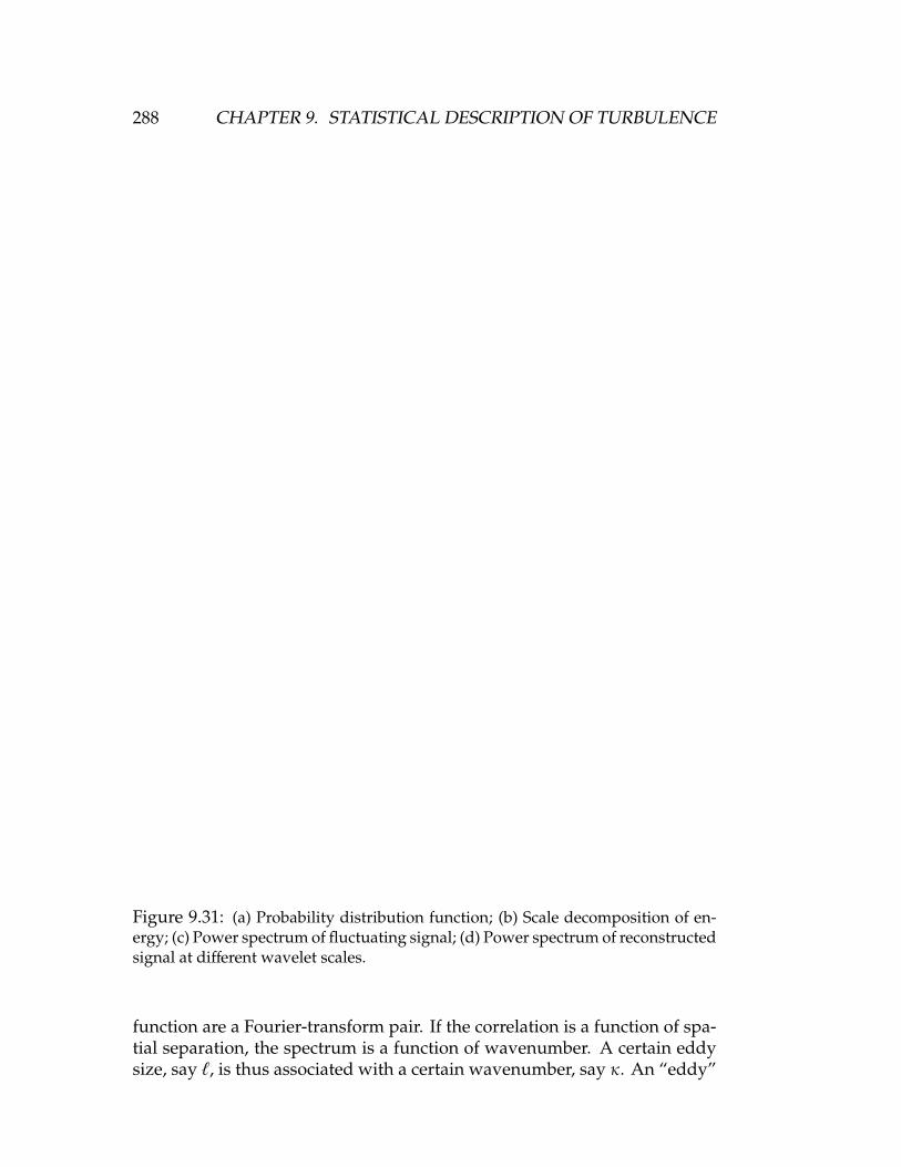
288 CHAPTER 9. STATISTICAL DESCRIPTION OF TURBULENCE
Figure 9.31: (a) Probability distribution function; (b) Scale decomposition of en-ergy; (c) Power spectrum of fluctuating signal; (d) Power spectrum of reconstructedsignal at different wavelet scales.
function are a Fourier-transform pair. If the correlation is a function of spa-tial separation, the spectrum is a function of wavenumber. A certain eddysize, say `, is thus associated with a certain wavenumber, say κ. An “eddy”

9.6. WAVELET TRANSFORMS 289
of wavenumber κmay be thought of as some disturbance containing energyin the vicinity of κ. It would be tempting to think of an eddy as a distur-bance contributing a narrow spike to the spectrum at κ. However, a narrowspike in the spectrum creates slowly damped oscillations (of wavelength2π/κ) in the correlation, as we discovered in section 6.2 (that is, section 6.2in Tennekes & Lumley). Such a correlation is characteristic of wavelikedisturbances, but not of eddies; we expect eddies to lose their identity be-cause of interactions with others within one or two periods or wavelengths.Therefore, the contribution of an eddy to the spectrum should be a fairlybroad spike, wide enough to avoid oscilatory behavior (“ringing”) in thecorrelation.
It is convenient to define an eddy of wavenumber κ as a disturbancecontaining energy between, say 0.62κ and 1.62κ. This choice centers theenergy around κ on a logarithmic scale, because ln(1.62) = ln(1/0.62) ≈ 0.5;it also makes the width of the contribution to the spectrum equal to κ(figure 9.32). We recall from section 6.2 (in Tennekes & Lumley) that thetransform of a narrow band around κ is a wave of wavelength 2π/κ, withan envelop whose width is the inverse of the bandwidth. Now, because thebandwidth selected is κ, the width of the envelop is of order 1/κ. This issketched in figure 9.32; we see that an eddy defined this way is indeed therelatively compact disturbance we want it to be. The eddy size ` is roughlyequal to 2π/κ.
The schematic eddy presented in figure 9.32 suffices for the developmentof energy-cascade concepts (see section 10.5). This model, however, cannotdeal with all of the problems associated with the distinction between wavesand eddies. The Fourier transform of a velocity field is a decompositioninto waves of different wavelengths; each wave is asociated with a singleFourier coefficient. An eddy, however, is associated with many Fouriercoefficients and the phase relations among them. Fourier transforms areused because they are convenient (spectra can be measured easily); moresophisticated transforms are needed if one wants to decompose a velocityfield into eddies instead of waves (Lumley, 1970).

290 CHAPTER 9. STATISTICAL DESCRIPTION OF TURBULENCE
Figure 9.32: An eddy of wave number κ and wavelength 2π/κ. From Tennekes &Lumley, 1972.

Chapter 10
Homogeneous IsotropicTurbulence
10.1 Introduction
The term homogeneous implies that the turbulence properties are indepen-dent of position. Here, averages such as the total energy of the fluctuations12ui(x)ui(x) are constants. More general correlations such as ui(x)u j(x + r) areindependent of x and depend only on r. The term isotropy implies that thereis no preferred direction, such that, for example, q2 = 3u2
1 = 3u22 = 3u2
3, andhence there can be no mean shearing.
In practice, most turbulent flows are not isotropic, nor are they homoge-neous but the more important features of the energy transfer process are thesame as in homogeneous flow, and it is easier to study the simpler case toobtain some physical insight.
A practical approximation to isotropic homogeneous turbulence is theturbulent flow found far downstream of a uniform grid of bars (see fig-ure 6.10). The wakes of the individual bars become turbulent close behindthe grid and interact in a complicated way so that at a large number of meshlengths from the plane of the grid (> 20) the turbulence is more or less homo-geneous (see figure 10.1) For a uniform grid the turbulence also approachesisotropy (see figure 10.2). In this case, the turbulent energy decays slowly asthe distance from the grid increases because there is no source of turbulentenergy other than the shear flow close to the grid.
For homogeneous turbulence, the turbulent kinetic energy equation be-comes (show this as an exercise):
∂∂t
(12q2
)= −uiu j
∂Ui
∂x j− ν
(∂ui
∂x j
)2
(10.1)
Note that, unless production equal dissipation, q2 varies with time and the
291

292 CHAPTER 10. HOMOGENEOUS ISOTROPIC TURBULENCE
Figure 10.1: Generation of homogenous turbulence in a wind tunnel using a grid.
flow is not stationary.Most theoretical work in homogeneous flows has concentrated on the
behavior of the correlations and spectrum functions. We will only considertwo principal observations from the study of isotropic homogeneous turbu-lence which have a larger implication for all turbulent flows: the decay ofisotropic homogeneous turbulence, and the energy cascade.
Equation 10.1 shows that energy is produced by working of the Reynoldsstresses against the mean flow, and it is dissipated as heat by workingof the viscous stresses against the turbulent velocity gradients. Since theReynolds stress tensor specifies the turbulent kinetic energy, the eddiescontaining most of the energy also contribute most to the Reynolds stressesand presumably receive most of the energy that is transferred from the meanflow. On the other hand, the rate of energy dissipation is determined byeddies which are much smaller than those containing most of the energy. Soa simple consideration of the energy budget raises two questions: the natureof the energy transfer from the mean flow to the turbulent eddies, and thenature of the transfer from the large energy-containing eddies to the muchsmaller dissipating eddies (Townsend p.46).
From the turbulent kinetic energy equation for homogeneous turbulence(equation 10.1), we see that:
1. The action of viscosity is strongest where the instantaneous velocitygradients are largest – implies small scale motions. Dissipation istherefore controlled by small eddies.
2. The production term can be interpreted as the interaction of eddieswith significant −u′v′ working against the mean shear, that is, theextraction of energy from the mean flow by the motions which containmost of the Reynolds stress. These motions must be at least comparableto the scale of the mean flow for a reasonable interaction to occur. Alsothe smaller motions will contribute little to the shear stress — if thevortex stretching makes the smaller motions lose all sense of direction

10.1. INTRODUCTION 293
Figure 10.2: Approach to isotropy of decaying turbulence generated by differentsquare biplane grids using square and round rods (from Comte-Bellot & Corrsin1966).
then their contribution to −u′v′ goes to zero. Hence the productionterm is said to be dominated by the large scale motions, and the energyis said to be transferred to the dissipating eddies by inviscid vortexstretching.
An important point to note is that the energy transfer occurs as an inviscidprocess so that the rate at which energy is transferred to the smaller eddiesis constant and it is actually independent of viscosity — viscosity simplysets the size of the smallest eddies that finally dissipate the energy.
Now in grid turbulence (which is approximately isotropic if there is nomean shear), there is no source of turbulent energy far from the grid, andthe turbulent energy decays slowly. This decay period is dominated by thedecay of high Reynolds number turbulence and it is called the “initial period
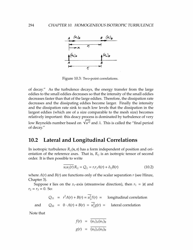
294 CHAPTER 10. HOMOGENEOUS ISOTROPIC TURBULENCE
Figure 10.3: Two-point correlations.
of decay.” As the turbulence decays, the energy transfer from the largeeddies to the small eddies decreases so that the intensity of the small eddiesdecreases faster than that of the large eddies. Therefore, the dissipation ratedecreases and the dissipating eddies become larger. Finally the intensityand the dissipation rate sink to such low levels that the dissipation in thelargest eddies (which are of a size comparable to the mesh size) becomesrelatively important: this deacy process is dominated by turbulence of very
low Reynolds number based on√
u′2 and λ. This is called the “final periodof decay.”
10.2 Lateral and Longitudinal Correlations
In isotropic turbulence Ri j(x, r) has a form independent of position and ori-entation of the reference axes. That is, Ri j is an isotropic tensor of secondorder. It is then possible to write
uiu j(r) Ri j = Qi j = rir jA(r) + δi jB(r) (10.2)
where A(r) and B(r) are functions only of the scalar separation r (see Hinze,Chapter 3).
Suppose r lies on the x1-axis (streamwise direction), then r1 = |r| andr2 = r3 = 0. So:
Q11 = r2A(r) + B(r) = u21 f (r) = longitudinal correlation
and Q22 = 0 · A(r) + B(r) = u21g(r) = lateral correlation
Note that
f (r) = (u1)A(u1)B
g(r) = (u2)A(u2)B

10.2. LATERAL AND LONGITUDINAL CORRELATIONS 295
Hence
A(r) =1r2 u2
1
(f (r) − g(r)
)B(r) = u2
1g(r)
And so equation 10.2 becomes (in this case):
Qi j = u21
[rir j
r2 ( f − g) + δi jg]
(10.3)
We can find a relationship between f and g by considering the derivativesof Ri j. Now:
Qi j = ui(0)u j(r)
∂Qi j
∂x j=
∂ui(0)u j(r)∂x j
∣∣∣∣∣∣∣r
= ui(0)∂u j(r)∂x j
∣∣∣∣∣∣∣r
+ u j(r)∂ui(0)∂x j
∣∣∣∣∣∣r
The first term on the right is zero by continuity, and the second term is zerosince ui(0) must be independent of the gradient at r. Hence
∂Qi j
∂x j=∂Qi j
∂r j= 0
and from equation 10.3 (see Hinze p. 185):
1
u21
∂Qi j
∂r j=∂∂r j
[rir j
r2 ( f − g) + δi jg]
That is,
1
u21
∂Qi j
∂r j=
3( f − g)r2 ri +
( f − g)r2 δi j −
2( f − g)r3
r jr j
r2 ri
+1r3
(d fdr−
dgdr
)r jr jri + δi j
r j
rdgdr
= 0
Hence
f (r) +r2
d fdr
= g(r) (10.4)

296 CHAPTER 10. HOMOGENEOUS ISOTROPIC TURBULENCE
Figure 10.4: Longitudinal (R11) and lateral (R22) correlations.
and we have obtained a relationship between the lateral and longitudinalcorrelations, which results basically from the continuity equation for incom-pressible flow.
Now f and g are even functions of r. Expanding f and g in a seriesexpansion for small separations we obtain:
f (r) = 1 +r2
2!∂2 f∂r2
∣∣∣∣∣∣r=0
+ · · ·
g(r) = 1 +r2
2!∂2g∂r2
∣∣∣∣∣∣r=0
+ · · ·
Together with equation 7.2.3, we obtain (Hinze p.188):
∂2g∂r2
∣∣∣∣∣∣r=0
= 2∂2 f∂r2
∣∣∣∣∣∣r=0
Therefore:λ2
f = 2λ2g (10.5)
It is now possible to express Qi j in terms of one scalar only:
Qi j
u21
= −rir j
2rd fdr
+ δi j
(f +
r2
d fdr
)(10.6)
Note that Qi j(r) = 0 if i = j and R22 = R33 by symmetry, and f and g are evenfunctions of r. So:
Qi j(r)
u21
=
f (r) 0 00 g(r) 00 0 g(r)
(see also figures 10.5, 10.6 and 10.7).

10.2. LATERAL AND LONGITUDINAL CORRELATIONS 297
Figure 10.5: Longitudinal correlation coefficient in the final period (UM/ν = 650).From Batchelor & Townsend, 1948.
Figure 10.6: Transverse correlations for grids of different shapes. From Stewart &Townsend, 1951.
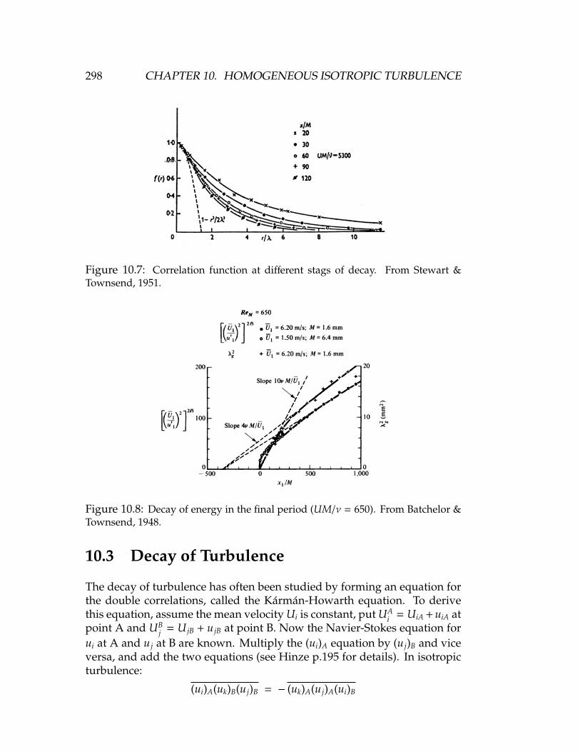
298 CHAPTER 10. HOMOGENEOUS ISOTROPIC TURBULENCE
Figure 10.7: Correlation function at different stags of decay. From Stewart &Townsend, 1951.
Figure 10.8: Decay of energy in the final period (UM/ν = 650). From Batchelor &Townsend, 1948.
10.3 Decay of Turbulence
The decay of turbulence has often been studied by forming an equation forthe double correlations, called the Karman-Howarth equation. To derivethis equation, assume the mean velocity Ui is constant, put UA
i = UiA + uiA atpoint A and UB
j = U jB + u jB at point B. Now the Navier-Stokes equation forui at A and u j at B are known. Multiply the (ui)A equation by (u j)B and viceversa, and add the two equations (see Hinze p.195 for details). In isotropicturbulence:
(ui)A(uk)B(u j)B = − (uk)A(u j)A(ui)B

10.3. DECAY OF TURBULENCE 299
Figure 10.9: Notation for k(r, t).
andpA(u j)B = − pB(ui)A = 0
(this is the only way they can be invariant under reflection). Finally weobtain an equation for the dynamic behavior of isotropic turbulence in termsof the double correlation (the Karman-Howarth (1938) equation):
∂∂t
(u2
1 f)−
(u21)3/2
r4
∂∂r
(r4k
)= 2ν
u21
r4
∂∂r
(r4∂ f∂r
)(10.7)
where k(r, t) is the correlation between two velocity components at one point,and one at another (all in the same direction; see figure 10.9), and
h(r, t) = − k(r, t)/2
Note that h and k are triple correlations, while f is a double correlation.Equation 10.7 has more unknowns than equations (not unusual in tur-
bulence theory). However, if we consider conditions where viscous effectsdominate, so that the second term in the left of equation 10.7 (the convectiveterm) can be neglected, then:
∂∂t
(u2
1 f)
= 2νu2
1
r4
∂∂r
(r4∂ f∂r
)(10.8)
This is a diffusion equation, with the solution
f (r, t) = e−r2/8νt (10.9)
This is the decay law for turbulence when viscous effects dominate – calledthe “final period of decay.”
Consider a single point result for r→ 0. Now
fr→0 = 1 −r2
2λ2 + · · ·
where λ2 =−1
∂2 f (0,t)∂r2
+ · · ·
Hence∂u2
∂t= −
10νu2
λ2 (10.10)

300 CHAPTER 10. HOMOGENEOUS ISOTROPIC TURBULENCE
(this is true regardless of f for r→ 0; Batchelor, p. 100)
Since f = e−r2/8νt
and1λ2 =
∂2 f (0, t)∂r2
∣∣∣∣∣∣r=0
=1
4νt
and sodu2
dt= −
52
u2
t
Using Taylors hypothesis we have t = x/U, and(U2
u2
)= C (x − x0) (10.11)
where x0 is the virtual origin. Experimental work supports this conclusionfor x ≥ 500M, where M is the mesh size (see figure 10.8).
Another useful result for isotropic turbulence is that a simple form canbe found for the dissipation, where:
ε ≡ ν
(∂ui
∂x j+∂u j
∂xi
)∂u j
∂xi
We note that ∂ui∂x j
∂u j
∂xiis small, so that
ε = ν
(∂ui
∂x j
)2
εν
=∂ui
∂x j
∂ui
∂x j
=∂∂x j
∂∂x′j
(uiu′i
)∣∣∣∣x→x′
=∂∂x j
∂∂x′j
u2 Rii|x→x′ = u2 ∂∂x j
∂Rii
∂x j
∣∣∣∣∣∣r→0
= −u2 ∂2Rii
∂r j∂r j
∣∣∣∣∣∣r→0
ε = −νu2(8
rf ′ + 7 f ′′ + r f ′′′
)r→0
= −νu2(
f ′′(0) + 7 f ′′(0))
= 15νu2 f ′′(0)
So, for isotropic, homogeneous turbulence,
ε = 15νu2
λ2 (10.12)

10.4. SPECTRA AND THE ENERGY CASCADE 301
Note that this agrees with equation 10.11 in that:
∂12q2
∂t= −ε = −15
νu2
λ2
and since q2 = 3u2, we obtain:
∂u2
∂t= −10
νu2
λ2
as before.Note also that in the case of isotropic homogeneous turbulence:(
∂ui
∂x j
)2
=
(∂ui
∂x j−∂u j
∂xi
) (∂ui
∂x j−∂u j
∂xi
)= ωkωk (10.13)
and therefore the viscous dissipation per unit mass is equal to the viscositytimes the mean square of the rate of strain, and to the viscosity times themean square vorticity (also called enstrophy).
10.4 Spectra and the Energy Cascade
An equation in terms of spectral functions instead of correlation functionsmay be found by taking Fourier transforms of the Karman-Howarth equa-tion. This gives:
∂E(k, t)∂t
= −∂S(k, t)∂t
− 2νk2 E(k, t) (10.14)
where E is the integrated energy spectrum defined in section 9.5. Specifically,E = E11, where
Ei j(k) =12
∫|k|=k
Φi j(k) dS(k)
and S is a related Fourier transform of the triple correlations (that is, thespectrum function of Si,i given on p.196, Hinze).
Term on left: represents the rate of change of energy associated withwave number k.
First term on right: In considering the Karman-Howarth equation, theterm with the triple correlation may be interpreted as representinga “convective” action in the spread of the double correlation f (r, t).This convective action may be caused by the interaction of eddies ofdifferent size. Hence this term represents the interaction of eddies ofdifferent wave numbers, thereby transferring energy between wavenumbers. Specifically, 3
2S(k, t) is the flux of kinetic energy from com-ponents of wave number less than k to components of wave numberlarger than k.

302 CHAPTER 10. HOMOGENEOUS ISOTROPIC TURBULENCE
Figure 10.10: Spectral distributions of turbulent intensity, energy transfer andviscous dissipation (the broken curves indicate the effect of an increase of fluidviscosity). From Townsend, 1976.
Second term on right: represents the viscous dissipation at each wavenumber k.
The distributions of the kinetic energy, viscous energy dissipation, andenergy transfer are shown in figure 10.10 for two Reynolds numbers. Thescale of the energy-containing eddies is 1/ke, and the scale of the dissipatingeddies is 1/kd. The viscous dissipation is associated with high wave num-bers, that is, small eddies. As Townsend points out, the Fourier componentsof the small wave number (large size) eddies that contribute most to theenergy,
12q2 = 3
2
∫∞
0E(k) dk = 3
2
∫∞
0kE(k) d(log k)
contribute comparatively little to the viscous dissipation,
ε = 3ν∫∞
0k2E(k) dk = 3ν
∫∞
0k3E(k) d(log k)
(this result is derived in section 10.87). That is, the sizes of the energy-containing eddies are different by orders of magnitude from the sizes ofthe dissipating eddies. Since S(k, t) transfers energy, we would expect anet transfer from the low wave number (large eddy) to the large wavenumber (small eddy) end of the spectrum. Energy fed to the turbulenceis primarily fed to the large scales (of the order of the scale of the meanvelocity gradients, or the mesh size in grid turbulence). From these largeeddies, smaller eddies are generated by eddy interactions (see section 10.5),and then still smaller ones, until the eddies are small enough for viscosityto become important (that is, when the Reynolds numbers associated withthe eddies is of order unity). We would expect that there is little direct

10.5. VORTEX STRETCHING AND THE ENERGY CASCADE 303
Figure 10.11: A vortex tube in an inviscid flow.
Figure 10.12: A vortex tube stretched by the surrounding strain field.
interaction between large energy-containing eddies and small dissipatingones. Increasing the Reynolds number (say by decreasing the viscosity), onlyextends this “energy cascade” at the small eddy end. That is, the viscosityjust sets the scaleat which the dissipation occurs. The structure of all otherscales is independent of Reynolds number — this observation is known asthe Reynolds number similarity hypothesis (section 3.5 in Townsend).
10.5 Vortex Stretching and the Energy Cascade
The following notes were adapted from the lecture notes used by ProfessorT. Wei at Rutgers, who in turn adapted them from lecture notes used byProfessor W. Wilmarth at Michigan.
Consider a vortex tube in an inviscid flow (figure 10.11). The vortex tubehas circulation Γ, a characteristic diameter λ and velocity uλ. Hence Γ ∝ uλλ.
If this tube is being stretched by the surrounding strain field (figure 10.12),the length increases but Γ is conserved (note that in a viscous fluid, ω(r) willbe different — see section 8.6). The strain rate
σ =1∆t
∆LL
=1L
dLdt
Since the volume of the tube will be constant in an incompressible inviscidflow,
L ∝volumeλ2

304 CHAPTER 10. HOMOGENEOUS ISOTROPIC TURBULENCE
Figure 10.13: The motion of a wandering point.
anddLdt∝ −
volumeλ3
dλdt
so thatσ =
1L
dLdt∝ −
1λ
dλdt
So a positive strain rate will decrease the characteristic scale (and by implica-tion increase the characteristic wave number). The concept of random walkimplies that stretching will be statistically more likely than compression.The theory states that a particle subjected to random impulses will, on theaverage, increase its distance from its starting point. Hence, as Bradshawobserves, the distance between two particles will, on the average, increase.If those two particles are situated at the ends of a given element of vortexline, then, in a flow field approximating to random disturbances, the lengthof the element will on the average increase.
What happens to the kinetic energy? Now:
KE ∝ (uλ)2∝ ω2λ2
∝Γ2
λ2
and therefore, as the scale decreases, the kinetic energy goes up. In otherwords, vortex stretching is a means of transferring energy from the sur-rounding strain field (set up primarily by eddies with scales much largerthan λ) to eddies which are smaller in scale than λ. That is, on the aver-age vortex stretching transfers energy from low wavenumbers (large λ) tohigher wavenumbers (small λ).
Consider the rate of kinetic energy transferred among wave numbers,that is, the kinetic energy flux ελ at a given wave number:
ελ ∝u2λ
τ∝
u3λ
λ
Since energy is supplied from the large eddies (where the size of largesteddies depend on the mesh size, or shear layer thickness, or pipe diameter),

10.5. VORTEX STRETCHING AND THE ENERGY CASCADE 305
the rate of energy input depends on the characteristic velocity and lengthscales of the largest eddies (say U and δ). Hence,
u3λ
λ∝
U3
δ
That is,
uλ ∝ U(λδ
)1/3
or
Reλ =uλλν∝
Uδν
(λδ
)4/3
= Reδ(λδ
)4/3
The energy transfer process is inviscid as long as Reδ 1. For ReλO(1), vis-cous dissipation will become important. If the length scale for the dissipativescales is λv, then:
λv ∝ δ (Reδ)−3/4
(λv is the Kolmogorov scale, usually denoted by η).
10.5.1 The energy transfer process
If we consider the vorticity field to be made up of a mean vorticity and afluctuating vorticity then we can see that two processes control the vortexstretching — random walk and the presence of a mean shear. The energyof the stretched vortex line increases and this must be extracted from thevelocity field which does the stretching, in particular, the strain field thatis present. Now it seems reasonable that an eddy of a given scale can onlyinteract with an eddy of comparable scale and that the greater the differencebetween two eddy length scales the smaller their interaction will be: to asmall eddy, the strain rate due to a neighboring much larger eddy will havelittle effect since the net change in velocity across the small scale eddy iscomparatively small. So large eddies will feel the effect of the mean shearmost directly and therefore will have forms which depend on the nature ofthe shear. The small eddies, formed by vortex stretching down to smaller andsmaller sizes eventually lose all influence of the boundary conditions thataffected their parents and are therefore held to be in some sense universal.That is, since the vortex-stretching process is essentially random (and three-dimensional) it does not tend to transmit directional preferences.
To summarize, if an element of fluid has rotation and it is subject to astrain rate in the z-direction ∂W/∂z then the element will be stretched in thez direction and its cross-section will get smaller in the x-y plane. If angularmomentum is conserved then ωr2 = constant, and when r decreases ωmustincrease. This means that the kinetic energyω2r2 must increase. This energymust come from the flow field that does the stretching.

306 CHAPTER 10. HOMOGENEOUS ISOTROPIC TURBULENCE
Figure 10.14: Three-dimensional perturbation in a vortex sheet.
Thus an extension in one direction decreases the length scales and in-creases the velocity components in the other two directions, which in turnstretch other elements of fluid with vorticity components in these direc-tions, and so on. If the viscosity is negligible this distortion and spreadingof length scales would go on indefinitely. The lower limit of the motionsthat survive will therefore depend on the Reynolds number, and the spreadof scales increases with Reynolds number.
10.5.2 How does this get started?
Even if we started with a field where there was no stretching whatsoevergoing on then the smallest disturbance will produce a kink in a vortex line.If the Reynolds number is high enough so that viscous damping is notimportant then this disturbance will grow under its own induced velocityfield (figure 10.14.
10.5.3 How does it continue?
A single disturbance will set up its own velocity field which interacts withother vortex lines and so on. General spatial and temporal unsteadiness,which needs to be only very small, depending on the Reynolds number,eventually produces a “continuous” distribution of length and frequencyscales. Note that the strain field which maintains vortex stretching may bethought of as the resultant strain set up by the induced velocity fields of thesurrounding motions.
So there is an energy cascade from δ down to λv. For δ > λ λv, theenergy transfer is inviscid (inertial), and the rate is governed by
εδ = ελ = ελv → heat
and ελv is fixed by U and δ:
U3
δ=
u3λv
λv= dissipation rate.

10.6. ISOTROPICITY OF THE SMALL SCALES 307
Figure 10.15: The energy cascade and the scale of the smallest motions.
As we stated before, the role of viscosity is to fix the scale λv at which thedissipation occurs (figure 10.15.
10.6 Isotropicity of the Small Scales
It is often argued that the small eddies, formed by vortex stretching down tosmaller and smaller sizes, will eventually lose all influence of the boundaryconditions that affected their parents and are therefore held to be in somesense universal. That is, since the vortex-stretching process is essentiallyrandom (and three-dimensional) it does not tend to transmit directionalpreferences. This argument is often used to justify the modelling of thesmall scales as an isotropic field, even when the energy containing eddiesare neither homogeneous nor isotropic.
Now there are several objections to the notion that the small scale eddiesare isotropic (see Bradshaw Turbulence):
1. Energy production varies across shear layer and therefore the intensityof the small eddies is likely to do likewise;
2. The instantaneous rate of energy transfer to the small eddies varieswith time and space; and
3. Averaging the instantaneous intensity of the small scale motions overperiods larger than typical time scales of smallest eddies but shorterthan those of the large eddies will also vary with space and time.
10.7 The Initial Period of Decay
By physical arguments we can say that, for isotropic homogeneous turbu-lence, the initial period of decay (x > 20M) is dominated by the decay of

308 CHAPTER 10. HOMOGENEOUS ISOTROPIC TURBULENCE
the energy containing eddies — there is a drain of energy from those ed-dies through inertial interactions towards the small eddies in the dissipationwave number range. Now a model for the dissipation may be given fromour previous consideration (as long as λ λv):
ε =u3λ
λ=
q3
Λ
where Λ is some macro-scale, and q is the velocity scale of the energy-containing eddies. The turbulent kinetic energy equation reduces to
ddt
(12q2
)= −
q3
Λ
and by using Taylor’s hypothesis:
Ud
dx
(12q2
)= −
q3
Λ
A similarity solution may be found for q2 = axn, Λ = bxm, and we find thatn = −1, and m = 1
2 . Hence:
q2∝
1x
(10.15)
Λ ∝√
x (10.16)
This is the initial period of decay law (see Batchelor Homogeneous Turbulence(1953) and Dickey & Mellor JFM Vol. 99, pp. 13-31 (1980)). Some experi-mental results are shown in figure 10.16. Note also that qΛ/ν = constant,that is, the turbulence decays so that the large-scale Reynolds number staysconstant.
10.8 Kolmogorov Hypothesis
Inertial actions do not change the energy, they just move it from one place toanother. But we expect on the basis of the previous discussion that strong in-teractions can occur only among wavenumbers with approximately similarwavenumbers (perhaps within an order of magnitude). This is so becausethe strain rates or velocity gradients associated with one eddy must havesignificant values over the size of the eddy it interacts with. We can dividethe spectrum into three ranges: the production range (low wavenumber),the inertial range (intermediate wavenumber — here little production ordissipation takes place), and the dissipation range (high wavenumber).

10.8. KOLMOGOROV HYPOTHESIS 309
Figure 10.16: Left: Decay of energy during and beyond the initial period (afterBatchelor & Townsend, 1948a). Right: Variation ofλ2 during the initial period (afterBatchelor & Townsend, 1948a; and Stewart & Townsend, 1951).
If this hypothesis is correct, these wavenumber ranges are virtually inde-pendent. So the only effect of the production range on the higher wavenum-ber part of the spectrum is to determine the total rate of production ofturbulent energy, and if the field is stationary than the rate of production =rate of dissipation ε. Therefore, the spectrum in the range where k is largeenough to be independent of production can depend, at a given k, only onε and ν. That is:
E = E(k, ν, ε) (= power per unit mass per wavenumber)
[E] =L3
T2 , [ε] =L2
T3 , [ν] =L2
T, [k] =
1L
But in the inertial subrange, the energy should be independent of ν. Hence,by dimensional analysis,
E(k)ε2/3k−5/3 = K0 = Kolmogorov constant ≈ 1.44
That is,E(k) = K0 ε
2/3 k−5/3 (10.17)
This famous result is known as the Kolmogorov (1941) -5/3 law. Experimentlends much support for this -5/3 behavior.

310 CHAPTER 10. HOMOGENEOUS ISOTROPIC TURBULENCE
Further, in the dissipating range, we find
E(k)ε2/3k−5/3 = K
(ν3/4ε−1/4k
)(10.18)
We thus have the Kolmogorov microscales which describe the characteristicsof the dissipating eddies:
η (= λv) =(ν3
ε
)1/4, τK =
(νε
)1/2, υ = (νε)1/4 (10.19)
Note that the Reynolds number formed with these quantities is unity:
ηυ
ν= 1
Now E(k) (actually Eii) is the three-dimensional integrated energy spec-trum function. There is, however, no known way of measuring Eii directly,but for isotropic flow it is related to the one-dimensional spectrum functionΦ11(k1) by the relation:
E11(k1) = k21∂2Φ11(k1)∂k2
1
− k1∂Φ11(k1)∂k1
(Hinze 1959). If Eii exhibits a power law relationship with wave number thenthe (measurable) one-dimensional spectrum function Φ(k1) also follows thesame power law relationship. Hence the “inertial subrange” defined byequation 10.17 for E(k) would be evident from measurements of Φ(k1). Infact, what is most often measured in the frequency spectrum Φ(ω), and k1 isfound by k1 = frequency/mean velocity. Strictly, we should not use the meanvelocity but the phase velocity associated with the particular wave number.This issue is discussed extensively by Perry & Abell (1977).
The dimensional reasoning that led to equations 10.17 and 10.18 hasbeen criticized by many workers on the basis of the conceptual difficul-ties of a fluctuating energy dissipation rate ε being independent of the lowwavenumber range (see for example Landau & Lifshitz 1959, Oboukhov1962, Corrsin 1962, and Kraichnan 1974, and also section 10.10). However,the experimental evidence for the existence of an inertial subrange is exten-sive, and perhaps the best example is provided by Grant et al. (1962, JFM),obtained in a tidal channel (figure 10.17). See also the results obtained byGurvich et al. (1967) in the atmospheric boundary layer (figure 10.18). (Notethat in laboratory flows, the wavenumber span of the inertial subrange isoften very small, due to the low turbulence Reynolds numbers encountered.See figure 10.19.)

10.8. KOLMOGOROV HYPOTHESIS 311
Figure 10.17: One-dimensional energy spectrum obtained in a tidal current. ——computed according to Pao. From Grant & Stewart.
Figure 10.18: Spectra for temperature and vertical velocity fluctuations obtainedfrom measurements from aircraft and from a tower. From Gurvich et al. (1967).

312 CHAPTER 10. HOMOGENEOUS ISOTROPIC TURBULENCE
Figure 10.19: Power spectral density of the streamwise velocity fluctuations in thelogarithmic law of the wall region of a turbulent boundary layer conjectured fromrecent similarity proposals. Here z = distance from the wall, k1 is the streamwisewavenumber, and δH is the boundary layer thickness. From Perry.
10.9 Form of the Spectrum in the Dissipation Range
In the dissipation range we have
E(k)ε2/3k−5/3 = K
(ν3/4ε−1/4k
)= K
(kη
)(equation 10.18) but dimensional analysis does not say anything about theform of the function K. Suppose that for wavenumbers greater than the

10.9. FORM OF THE SPECTRUM IN THE DISSIPATION RANGE 313
energy containing range we have stationary turbulence. Then equation 10.14becomes
dS(k)dk
= − 2νk2E(k) (10.20)
In the inertial range where viscous action is negligible, S ≈ constant andmust equal −ε, since energy is transferred through the inertial range byinviscid interactions. Hence
ε =
∫∞
02νk2E(k) dk (10.21)
This is a useful way to measure the dissipation (if the probe has sufficientspatial resolution).
Now, to obtain a form for the function K, suppose that we could writethat in the equilibrium range S is proportional to E (Pao, Physics of Fluids,1965):
E = E(ε, k.ν) = − σS(ε, k, ν)
whereσ is the rate at which the energy is being transported through a cascadeprocess across the wave number range. Now σ is unknown. However, inthe inertial subrange
E = E(ε, k) = K0 ε2/3k−5/3
and S ≈ −ε. So we obtain that (with σ = E/ε)
σ = σ(ε, k) = K0ε−1/3k−5/3
Pao postulated that σ was independent of ν over the entire wave numberrange, and would apply also in the dissipation range. Hence
dSdk
= − νK0 ε−1/3k1/3S
That is,
S = − ε exp
−32
K0
(ν3k4
ε
)1/3 = − ε exp(−
32
K0(kη
)4/3)
Finally
E = K0 ε2/3k−5/3 exp
(−
32
K0(kη
)4/3)
(10.22)
andK = K0 exp
(−
32
K0(kη
)4/3)
Equation 10.22 is called Pao’s form of the dissipation spectrum. For somecomparisons with experimental data see figures 10.17 and 10.20.

314 CHAPTER 10. HOMOGENEOUS ISOTROPIC TURBULENCE
Figure 10.20: One-dimensional energy spectrum E1(k11 (), and E2(k11 (××××).—— computed according to Pao. After Kistler & Vrebalovich.
10.10 The Decay of Isotropic Turbulence: Sum-mary
As time goes on, we see that the energy containing motions (low wavenum-bers) decay as their energy is drained by inertial interactions towards thehigh wavenumber dissipation range. In terms of the spectrum, there wouldbe a range of wavenumbers in which the spectral amplitudes would remaininvariant with time — the universal equilibrium range (see figure 10.21).
At later times, however, the energy transfer from the large eddies to thesmall eddies decreases (the energy-containing eddies have been depleted).Then, since the small eddies are no longer receiving energy to sustain them,they begin to disappear, and the small eddies will decay faster than thevery weak large scales that remain. The dissipation rate decreases and thedissipating eddies get larger as the smallest scales continue to disappear:
1kd∝
(ν3
ε
)1/4
, and since ε ↓,1k↑, and λ ↓
Finally, the intensity and the dissipation rate sink to such low levelsthat the energy in the largest eddies becomes relatively important: this isturbulence of very low Reynolds number and it is governed by viscouseffects — this is the final period of decay.

10.11. ISOTROPICITY IN THE DISSIPATION RANGE 315
Figure 10.21: Form of the three-dimensional energy spectrum Ek, t in the variouswavenumber ranges. Townsend, or Hinze.
So, curiously, we see that in the initial period of decay the energy con-taining motions increase their scale, and that in the final period of decay itis the large scales that are last to die because the small scales dissipate morerapidly (it looks a bit like an energy transfer from small scales to large butof course it is not).
10.11 Isotropicity in the Dissipation Range: TheConcept of Local Isotropy
The vortex-stretching “cascade” process, being essentially random and three-dimensional, tends not to transmit directional preferences from large scalesto small scales. Therefore motions at scales many times smaller than thoseof the main energy containing motions tend to be statistically isotropic. Thisnotion is often applied even in inhomogeneous flows, and it is called theconcept of “local isotropy.”
Now there are several objections to the notion that the small scale eddiesare isotropic (Bradshaw, Turbulence):
1. Energy production varies across shear layer hence intensity of smalleddies likely to do likewise;
2. Instantaneous rate of energy transfer to the small eddies varies withtime and space; and

316 CHAPTER 10. HOMOGENEOUS ISOTROPIC TURBULENCE
Figure 10.22: 3-D iso-contours for wavelet transformed enstrophy field. The peakin the wavelet filter is aligned with the peak in the dissipation rate spectrum, k = 10.The contour level is 2.5 times the r.m.s. value of the wavelet coefficients at that timestep. (a) St = 0.0, (a) St = 0.325, (a) St = 0.65, (a) St = 1.0. Brasseur & Wang, Physicsof Fluids, 1992.
3. Averaging the instantaneous intensity of the small scale motions overperiods larger than typical time scales of smallest eddies but shorterthan those of the large eddies will also vary with space and time.
In fact, simulations of homogeneous isotropic turbulence indicate thatthe regions of the flow where dissipation is high (where vorticity fluctuationsare high) are dominated by rod-like structures of random orientation, wherethe diameter scales with η but the length can be many orders of magnitudelarger (see figure 10.22). When this flow is subjected to a mean shear, thenrods line-up in a preferred direction which depends on the mean strain rate(see figure 10.22 again), and therefore it can be argued that the dissipatingstructures will reflect the influence of the large scales, as well as the historyof the strain field. For a full discussion see Brasseur (AIAA Paper 91-0230),Rogers et al. (Report TF25, Dept. Mech. Eng., Stanford 1986), and Rogallo(NASA TM 81315, 1981).
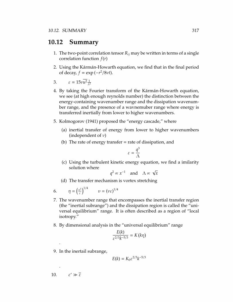
10.12. SUMMARY 317
10.12 Summary
1. The two-point correlation tensor Ri j may be written in terms of a singlecorrelation function f (r)
2. Using the Karman-Howarth equation, we find that in the final periodof decay, f = exp (−r2/8νt).
3. ε = 15νu2 1λ2
4. By taking the Fourier transform of the Karman-Howarth equation,we see (at high enough reynolds number) the distinction between theenergy-containing wavenumber range and the dissipation wavenum-ber range, and the presence of a wavnemuber range where energy istransferred inertially from lower to higher wavenumbers.
5. Kolmogorov (1941) proposed the “energy cascade,” where
(a) inertial transfer of energy from lower to higher wavenumbers(independent of ν)
(b) The rate of energy transfer = rate of dissipation, and
ε =q3
Λ
(c) Using the turbulent kinetic energy equation, we find a imilaritysolution where
q2∝ x−1 and Λ ∝
√x
(d) The transfer mechanism is vortex stretching
6. η =(ν3
ε
)1/4υ = (νε)1/4
7. The wavenumber range that encompasses the inertial transfer region(the “inertial subrange”) and the dissipation region is called the “uni-versal equilibrium” range. It is often described as a region of “localisotropy.”
8. By dimensional analysis in the “universal equilibrium” rangeE(k)
ε2/3k−5/3 = K(kη
).
9. In the inertail subrange,
E(k) = K0ε2/3k−5/3
.
10. ε′ ε

318 CHAPTER 10. HOMOGENEOUS ISOTROPIC TURBULENCE

Chapter 11
Turbulent Shear Flows
In the logical progression of topics, we should now consider sheared ho-mogeneous turbulence, then turbulent free shear flows (mixing layers, jets,wakes), and finally wall-bounded flows. However, it may actually be moreinstructive to move on to wall-bounded flows before considering otherflows, particularly when some wall-bounded flows offer a certain degreeof simplification. Such flows are “fully-developed” flows, such as pipe andchannel flow sufficiently far downstream from the entrance, and turbulentCouette flow.
11.1 Channel Flow
Here we consider fully-developed, turbulent, two-dimensional channel flow.Fully developed flow means that the flow is statistically stationary (thepressure driving the flow is steady) and homogeneous in the downstreamdirection (x-direction in figure 11.1. Hence ∂V/∂x = 0. The boundaryconditions are the no-slip conditions, so that on the top and bottom wallsU = V = W = 0, and u′ = v′ = w′ = 0. From the the continuity equa-tion (equation 7.5), we see that V = 0 everywhere. Also, since the flow istwo-dimensional, W = 0 everywhere, and w′v′ = 0.
From the mean flow Reynolds-averaged equations (equations 7.8 to 7.10):
(x-momentum) 0 = −1ρ
∂p∂x−∂u′v′
∂y+ ν
∂2U∂y2 (11.1)
(y-momentum) 0 = −1ρ
∂p∂y−∂v′2
∂y(11.2)
(z-momentum) 0 = −1ρ
∂p∂z
(11.3)
319

320 CHAPTER 11. TURBULENT SHEAR FLOWS
Figure 11.1: Notation for fully-developed turbulent, two-dimensional channelflow.
Integrate equation 11.2:
pρ
= − v′2 +pw(x)ρ
(11.4)
Substitute for the pressure in equation 11.1:
∂∂y
(−u′v′ + ν
∂U∂y
)=
1ρ
dpw
dx+∂(−v′2
)∂x
Therefore
τT ≡ −u′v′ + ν∂U∂y
=1ρ
dpw
dxy + F(x)
because ∂(−v′2
)/∂x = 0 from streamwise homogeneity. Here, τT is the
“total” stress, being the sum of the Reynolds shear stress and the viscousstress. From symmetry: (
∂U∂y
)h/2
= −
(∂U∂y
)−h/2
and so F(x) = 0, and:
−u′v′ + ν∂U∂y
=1ρ
dpw
dxy = constant × y (11.5)
at a given x. Data indicate that dp/dx < 0. The stress distribution is illustratedin figure 11.2. Note that:
τw
ρ= u2
τ =
(Sxy
)w
ρ= ν
(∂U∂y
)−h/2
If we consider the integral form of the momentum equation (x-componentonly, see Figure 37):

11.1. CHANNEL FLOW 321
Figure 11.2: Stress and turbulent kinetic energy distributions in fully-developedturbulent, two-dimensional channel flow.
Figure 11.3: Fixed control volume for fully-developed turbulent, two-dimensionalchannel flow. ∫ (
n · ρV)
VdA =
∫npdA + Fv︸ ︷︷ ︸
net outflux︸︷︷︸
resultant force︸︷︷︸
net viscousof momentum due to pressure forces
differences
For a fully-developed flow this reduces to:∫npdA = Fv
Since the pressure difference is only a function of x (remember that p2 − p1 =pw2 − pw2):
p1wh − p2wh = τwL (2w + 2h)
For a two-dimensional flow, the channel width is much greater than theheight and:
τw = −h2
dpw
dx(11.6)
So that finally:
−uv + νdUdy
= −τw
ρ
2yh
(11.7)
Now, very near the surface, we expect viscous forces to become dominantbecause the velocity gradients become very large and −uv approaches zero

322 CHAPTER 11. TURBULENT SHEAR FLOWS
Figure 11.4: Notation for the region near the wall.
as the wall is approached. If y′ is measured from the bottom surface, we areconcerned with the region where 2y′/h ≈ 0 (see figure 11.4). So for a smallregion near the wall:
νdUdy′
≈τw
ρ
(2y′
h− 1
)=
τw
ρ+ · · ·
HencedUdy′
=τw
µ+ . . .
and U =τwy′
µ+ . . .
which is usually written asUuτ
=y′uτν. (11.8)
Here we have defined a velocity scale uτ (sometimes called the frictionvelocity) based on the wall shear stress, so that uτ =
√τw/ρ.
Very near the wall, therefore, the velocity varies linearly with the distancefrom the wall. Note that the form given in equation 11.8 includes the densityalthough it strictly does not belong in an expression describing a viscous-dominated region. This distinction is only important when consideringflows with variable fluid properties, such as boundary layers in supersonicflow.
Experiments show that further out from the wall (where it is still truethat
(2y/h − 1
) 1):
U = f n(τw
ρ, ν, y′
)so that:
Uuτ
= f n(
y′uτν
). (11.9)
This is sometimes called “the law of the wall” (after Don Coles). With thenotation
y+ =y′uτν, and U+ =
Uuτ,

11.2. TURBULENT COUETTE FLOW 323
Figure 11.5: Mean flow and stress distributions in fully-developed turbulent,Couette flow.
equation 11.9 may be written as:
U+ = f n(y+) . (11.10)
11.2 Turbulent Couette Flow
Couette flow is the flow that occurs between two parallel, two-dimensionalplates when these plates have differing velocities, as will occur when thebottom plate is stationary and the top plate is moving at a constant speed,as shown in figure 11.5. In this case the flow is not driven by a pressuregradient (dp/dx = 0) but by the viscous shear on the moving wall. When theflow is fully developed the equation of motion reduces to:
−uv + νdUdy
= −τw
ρ= constant.
11.3 Turbulent Pipe Flow
Turbulent flow is characterized by unsteady eddying motions that are inconstant motion with respect to each other. At any point in the flow, theeddies produce fluctuations in the flow velocity and pressure. If we wereto measure the streamwise velocity in turbulent pipe flow, we would seea variation in time as shown in figure 11.6. We see that the velocity has atime-averaged value 〈U〉, defined by
〈U〉 = limT→∞
1T
t+T∫t
U dt
and a fluctuating value u′, so that 〈U〉 is not a function of time, but u′ is.The eddies interact with each other as they move around, and they
can exchange momentum and energy. For example, an eddy that is near the

324 CHAPTER 11. TURBULENT SHEAR FLOWS
Figure 11.6: Velocity at a point in a turbulent flow as a function of time.
centerline of the pipe (and therefore has a relatively high velocity), may movetowards the wall and interact with eddies near the wall (which typically havelower velocities). As they mix, momentum differences are smoothed out.This process is superficially similar to the action of viscosity which tends tosmooth out momentum gradients by molecular interactions, and turbulentflows are sometimes said to have an equivalent “eddy” viscosity. Becauseturbulent mixing is such an effective transport process, the eddy viscosity istypically several orders of magnitude larger than the molecular viscosity.
The important point is that turbulent flows are very effective at mixing:the eddying motions can very quickly transport momentum, energy andheat from one place to another. As a result, velocity differences get smoothedout more effectively than in a laminar flow, and the time-averaged velocityprofile in a turbulent pipe flow is much more uniform than in a laminarflow (see figure 11.7). The velocity profile is no longer parabolic, and it issometimes approximated by a power law, such as
〈U〉UCL
=
(2yD
)1/n
, (11.11)
where UCL is the velocity on the centerline, and the exponent n varies withReynolds number (for a Reynolds number of about 100,000, n = 7). Seesection 11.8.
As a result of this mixing, the velocity gradient at the wall is higher thanthat seen in a laminar flow at the same Reynolds number, so that the shearstress at the wall is correspondingly larger. This observation is in agreementwith the fact that the losses in a turbulent flow are much higher than in alaminar flow, and therefore the pressure drop per unit length will be greater,which is reflected in a larger frictional stress at the wall. Note that we cannotevaluate the wall stress from equation 11.11 since this approximation to thevelocity profile actually gives an infinite velocity gradient (and therefore an

11.4. TURBULENT BOUNDARY LAYERS 325
Figure 11.7: Velocity distributions in laminar and turbulent pipe flow.
infinite stress) at the wall. Instead, we often use the semi-empirical relation
1√f
= 2.0 log(Re
√f)− 0.8
which is known as Prandtl’s universal law of friction for smooth pipes (thisis the line corresponding to turbulent flow in a smooth pipe as given in theMoody diagram, figure 5.2). A more accurate form is given by
1√f
= 1.873 log(Re
√f)− 0.2631 −
233(Re
√f)0.90 (11.12)
which describes the friction factor to within 1 % for Reynolds numbers from10 × 103 to 35 × 106.1
11.4 Turbulent Boundary Layers
Turbulent pipe flows were discussed in section 11.3. Similar considerationsapply to turbulent boundary layer flow. Transition to turbulence in bound-ary layers can occur for Rex > 105, where Rex is the Reynolds number basedon the freestream velocity, Ue, and the distance from the leading edge, x. Themajor difference between pipe and boundary layer flows is that a boundarylayer has an outer edge. Turbulence is unsteady, and therefore the edgebetween the inner turbulent and the outer non-turbulent fluid changes withtime, and an instantaneous cross-section reveals a highly convoluted edge(figure 11.8). The boundary layer thickness δ can only be defined in a time-averaged sense. The velocity profile itself is fuller than a laminar boundarylayer (see figure 11.9), and it is sometimes approximated by a power lawsimilar to that used to describe turbulent pipe flow (see section 11.8). Thatis,
〈U〉Ue
=( yδ
)1/n, (11.13)
1M.V. Zagarola & A.J. Smits, Phys. Rev. Lett., January 1997.

326 CHAPTER 11. TURBULENT SHEAR FLOWS
where Ue is the time averaged velocity at the edge of the boundary layer, andthe exponent n varies with Reynolds number (for a Reynolds number basedon length of about 500,000, n = 7). The boundary layer grows approximatelyaccording to
δx
=0.37Re0.2
x
so that δ grows as x0.8. That is, a turbulent boundary layer grows fasterthan a laminar boundary layer. Again, this is a reflection of the fact thatturbulence diffuses momentum more efficiently than viscosity.
As in pipe flow, the velocity gradient at the wall is higher than that foundin a laminar flow at the same Reynolds number, so that the shear stress atthe wall is correspondingly larger. The wall stress is given approximatelyby the empirical relation
C f =0.0576Re0.2
x
where the local skin friction coefficient was defined in equation 3.9.Consider the case of a two-dimensional turbulent boundary layer devel-
oping on a flat wall. The external flow is steady, and since ∂W/∂z = 0, W = 0everywhere. The complete equations of motion are:
continuity∂U∂x
+∂V∂y
= 0 (11.14)
x-momentum U∂U∂x
+ V∂U∂y
= −1ρ
∂p∂x
+∂∂x
(2ν∂U∂x− u2
)+∂∂y
(ν
(∂U∂y
+∂V∂x
)− uv
)(11.15)
Figure 11.8: Streamwise section of a turbulent boundary layer. Rayleigh scatteringimage of a turbulent boundary layer at Mach 2.5, by M.W. Smith. Flow is from leftto right. Reynolds number based on momentum thickness is about 25,000.

11.4. TURBULENT BOUNDARY LAYERS 327
Figure 11.9: Mean velocity profiles in a boundary layer undergoing transition.From Munson, Young & Okiishi, Fundamentals of Fluid Mechanics.
y-momentum U∂V∂x
+ V∂V∂y
= −1ρ
∂p∂y
+∂∂x
(ν
(∂U∂y
+∂V∂x
)− uv
)+∂∂y
(2ν∂V∂y− v2
)(11.16)
These equations could be simplified if we could show that some termsare more important than others. We need to make order-of-magnitudearguments, and therefore we need to choose suitable scales.
Some more-or-less typical velocity profiles are sketched in figure 11.10. Inthe outer part of the boundary layer we assume the local freestream velocityUe will represent the order of magnitude of the mean velocity. Similarly, thestreamwise length scale is the distance from the origin of the boundary layerL (this origin does not necessarily coincide with the leading edge of the platesince there will always be a region of laminar and transitional flow), and thelength scale normal to the plate will be the boundary layer thickness δ. Fromthis, velocity gradients in the direction normal to the plate will be of orderUe/δ, which probably over-estimates the actual velocity gradient magnitude.

328 CHAPTER 11. TURBULENT SHEAR FLOWS
Figure 11.10: Typical mean velocity and Reynolds shear stress profiles in a bound-ary layer, with notation.
In the inner part of the boundary layer the mean velocity gradients are verymuch greater, and instead of the thickness of the boundary layer we shoulduse the thickness of the viscous layer δv. The velocity scale for the mean flowin this region should still be Ue, or at least some fraction of Ue (see Townsendfor a further discussion of this velocity scale, which he calls Us since it seemsto act as a slip velocity for the outer flow). For the turbulence, we assumethat for the inner and outer flow all the stresses are of equal order and that
u2 = O(u2τ), v2 = O(u2
τ), ww2 = O(u2τ),
although we should remember that all stresses must go to zero at the walland in the freestream.
From the continuity equation we have that V = O(Ueδ/L) in the outerregion, and V = O(Ueδv/L) in the inner region.
By considering the order of magnitude of the terms in the x-momentumequation, and eliminating obviously small terms, we obtain for the outerflow (assuming pressure differences are of the order of the dynamic pres-sure):
U∂U∂x
+ V∂U∂y
= −1ρ
∂p∂x
+∂∂y
(−uv) +∂∂y
(ν∂U∂y
)(11.17)︸ ︷︷ ︸
O(
U2e
L
) ︸ ︷︷ ︸O(
U2e
L
) ︸ ︷︷ ︸O(
u2τδ
) ︸ ︷︷ ︸O(νUeδ2
)
Therefore:
δL
= O(
u2τ
U2e
)= O
(C f
2
)since C f ≡
τw12ρU2
e
=2u2
τ
U2e
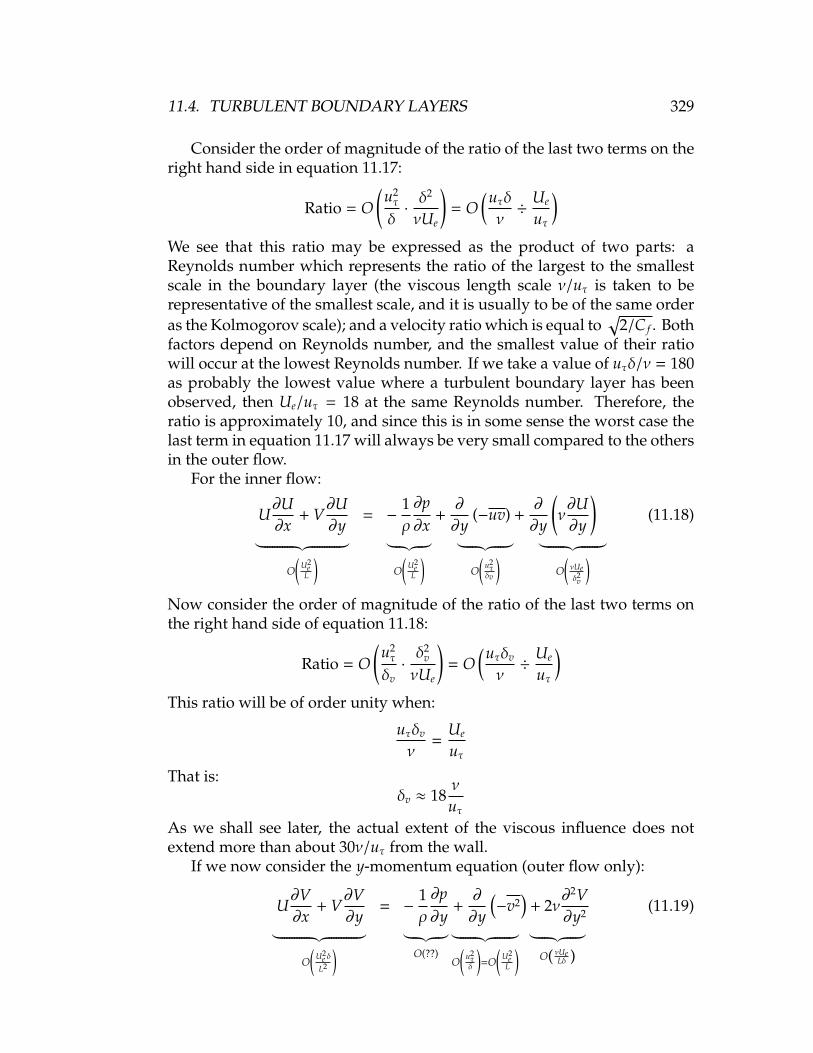
11.4. TURBULENT BOUNDARY LAYERS 329
Consider the order of magnitude of the ratio of the last two terms on theright hand side in equation 11.17:
Ratio = O(
u2τ
δ·δ2
νUe
)= O
(uτδν÷
Ue
uτ
)We see that this ratio may be expressed as the product of two parts: aReynolds number which represents the ratio of the largest to the smallestscale in the boundary layer (the viscous length scale ν/uτ is taken to berepresentative of the smallest scale, and it is usually to be of the same orderas the Kolmogorov scale); and a velocity ratio which is equal to
√2/C f . Both
factors depend on Reynolds number, and the smallest value of their ratiowill occur at the lowest Reynolds number. If we take a value of uτδ/ν = 180as probably the lowest value where a turbulent boundary layer has beenobserved, then Ue/uτ = 18 at the same Reynolds number. Therefore, theratio is approximately 10, and since this is in some sense the worst case thelast term in equation 11.17 will always be very small compared to the othersin the outer flow.
For the inner flow:
U∂U∂x
+ V∂U∂y
= −1ρ
∂p∂x
+∂∂y
(−uv) +∂∂y
(ν∂U∂y
)(11.18)︸ ︷︷ ︸
O(
U2e
L
) ︸ ︷︷ ︸O(
U2e
L
) ︸ ︷︷ ︸O(
u2τδv
) ︸ ︷︷ ︸O(νUeδ2v
)Now consider the order of magnitude of the ratio of the last two terms onthe right hand side of equation 11.18:
Ratio = O(
u2τ
δv·δ2
v
νUe
)= O
(uτδv
ν÷
Ue
uτ
)This ratio will be of order unity when:
uτδv
ν=
Ue
uτThat is:
δv ≈ 18νuτ
As we shall see later, the actual extent of the viscous influence does notextend more than about 30ν/uτ from the wall.
If we now consider the y-momentum equation (outer flow only):
U∂V∂x
+ V∂V∂y
= −1ρ
∂p∂y
+∂∂y
(−v2
)+ 2ν
∂2V∂y2 (11.19)︸ ︷︷ ︸
O(
U2e δ
L2
) ︸ ︷︷ ︸O(??)
︸ ︷︷ ︸O(
u2τδ
)=O
(U2
eL
) ︸ ︷︷ ︸O( νUe
Lδ )

330 CHAPTER 11. TURBULENT SHEAR FLOWS
The viscous term is always negligible outside the sublayer. The terms onthe left are an order of magnitude smaller than the stress gradients, and sothe pressure gradient term must be of the same order as the stress gradients.
Now consider:
dpρ
=1ρ
∂p∂x
dx +1ρ
∂p∂y
dy︸ ︷︷ ︸O(
U2e
L L) ︸ ︷︷ ︸
O(
U2e
L δ
)
Therefore∂p∂x≈
dpdx
=dpw
dxand since at the edge of the boundary layer ∂/∂y = 0, we get from x-momentum equation in the freestream:
UedUe
dx=
dpw
dx
and we speak of the pressure gradient as being “imposed” or “impressed”on the boundary layer.
Summary: Hence the two-dimensional turbulent boundary layer equationis given by:
U∂U∂x
+ V∂U∂y
= −1ρ
dpw
dx+∂∂y
(−uv + ν
∂U∂y
)(11.20)
where the wall pressure pw is now a boundary condition given by Bernoulli’sequation:
UedUe
dx=
dpw
dx(11.21)
11.4.1 Turbulence characteristics
Figure 11.11 shows measurements of u′, v′, w′ and −u′v′ in a turbulentboundary layer on a flat plate at a Reynolds number Rex = 107. Note that:(i) the scaling is not based on similarity coordinates — as we shall see later;and (ii) the normal components are shown as intensities (r.m.s. values),although the shear stress is shown in the usual way.
The fluctuations are quite large, being up to about 11-12% of Ue nearthe wall, although different components differ in magnitude, for obviousphysical reasons: u′ is largest, being unimpeded by the wall, whereas v′ isdirectly impeded by the wall and it is the smallest, and it also reaches itsmaximum value much further from the wall than u′ or w′. The w′-component

11.4. TURBULENT BOUNDARY LAYERS 331
Figure 11.11: Variation of the fluctuating turbulent velocity components in theboundary layer on a flat plate at zero incidence, as measured by P. S. Klebanoff.From Schlichting.
lies between the other two in magnitude. It is important to note that a two-dimensional (in the mean sense) turbulent boundary layer will always havea non-zero lateral component w′. The quantity u′v′, rescaled by a factor of20 in figure 11.11, is small but of crucial importance in the understanding ofthe boundary layer. Near the wall, u′, v′ and w′ all vanish due to the no-slipcondition — this is most clearly seen in the inset of the figure showing theregion y/δ < .015. Turbulence resists damping and significant fluctuationsexist as close to the wall as we are able to measure (y/δ < 0.01 in this case).
Note also that the turbulence extends outside of the boundary layer, thatis for y > δ. Of course, δ is rather arbitrary and there is some freestreamturbulence, but the main cause is “intermittency.” Measurements of the tur-bulent velocity components show that there exists a fairly sharp boundarybetween the turbulent flow in the boundary layer and the nearly turbulentfree external flow. The edge of a turbulent boundary layer consists of aninterface, called the superlayer (Corrsin), separating the fully turbulent andexternal flows (see figure 11.12). The interface evolves as it travels down-stream and irrotational fluid is “entrained” into the boundary layer, and toa stationary observer its position appears to fluctuate strongly with time.
An intermittency factor γ can be defined which is equal to 1 when theflow is fully turbulent at all times and equal to 0 when it is fully laminar.A typical distribution of γ is shown in figure 11.12. The boundary layer isobserved to be intermittent from about y/δ = 0.4 to y/δ = 1.2. The meanposition of the superlayer (where γ is 50%) is at about y/δ = 0.78. It isusual to incorporate this intermittency factor in modelling the outer layer

332 CHAPTER 11. TURBULENT SHEAR FLOWS
Figure 11.12: Left: Schematic showing the interface between turbulent and non-turbulent fluid in a boundary layer. Right: Variation of the intermittency factor ina turbulent boundary layer on a flat plate at zero incidence, as measured by P. S.Klebanoff. From Schlichting.
turbulence.
11.4.2 Stress Behavior Near the Wall
At the wall, U and V are zero, and therefore the acceleration terms are alsozero. Thus, at the wall, the pressure gradient and stress gradient termsbalance:
dpw
dx=∂∂y
(µ∂U∂y
)∣∣∣∣∣∣y=0
(11.22)
Hence we see that the order-of-magnitude argument used in the near-wallregion, which suggested that the convective terms are of the same order asthe pressure gradient term, fails in the limit at the wall. Thus, at some smalldistance from the wall, it is not true that the pressure gradient balancesthe gradient of total stress, as is sometimes stated: away from the wallthe orders- of-magnitude of the pressure gradient and convective terms areequal, and it is not clear if a simple result can be obtained by neglecting onewith respect to the others.
So for flows with arbitrary pressure gradients the order-of-magnitudeargument indicates that:
µ∂U∂y− ρu′v′ = τw (11.23)
since at y = 0, u′ = v′ = 0 and µ∂U∂y = τw.
Thus there exists a constant-stress region near the wall, where the sumof the viscous and turbulent shearing stresses is constant (see figure 11.13).If the pressure gradient is not zero, then the extent of this constant stress
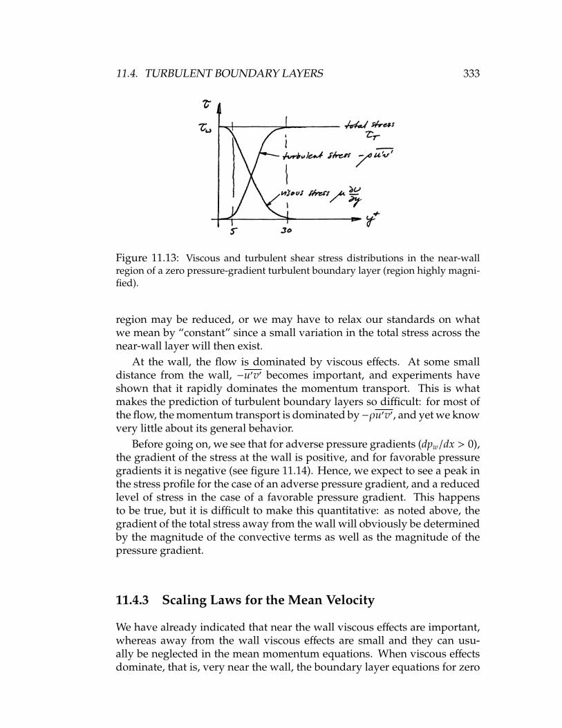
11.4. TURBULENT BOUNDARY LAYERS 333
Figure 11.13: Viscous and turbulent shear stress distributions in the near-wallregion of a zero pressure-gradient turbulent boundary layer (region highly magni-fied).
region may be reduced, or we may have to relax our standards on whatwe mean by “constant” since a small variation in the total stress across thenear-wall layer will then exist.
At the wall, the flow is dominated by viscous effects. At some smalldistance from the wall, −u′v′ becomes important, and experiments haveshown that it rapidly dominates the momentum transport. This is whatmakes the prediction of turbulent boundary layers so difficult: for most ofthe flow, the momentum transport is dominated by−ρu′v′, and yet we knowvery little about its general behavior.
Before going on, we see that for adverse pressure gradients (dpw/dx > 0),the gradient of the stress at the wall is positive, and for favorable pressuregradients it is negative (see figure 11.14). Hence, we expect to see a peak inthe stress profile for the case of an adverse pressure gradient, and a reducedlevel of stress in the case of a favorable pressure gradient. This happensto be true, but it is difficult to make this quantitative: as noted above, thegradient of the total stress away from the wall will obviously be determinedby the magnitude of the convective terms as well as the magnitude of thepressure gradient.
11.4.3 Scaling Laws for the Mean Velocity
We have already indicated that near the wall viscous effects are important,whereas away from the wall viscous effects are small and they can usu-ally be neglected in the mean momentum equations. When viscous effectsdominate, that is, very near the wall, the boundary layer equations for zero

334 CHAPTER 11. TURBULENT SHEAR FLOWS
Figure 11.14: Total stress distributions in turbulent boundary layers with zero,favorable, and adverse pressure gradients.
pressure gradient flow give:
∂∂y
(µ∂U∂y
)∣∣∣∣∣∣0
= 0
That is, (µ∂U∂y
)∣∣∣∣∣∣0
= τw
andU =
τw
µy + · · · (11.24)
Thus, for some small distance from the wall the velocity profile is linear, as itis in laminar flow. A similar result was found for channel flow in section 11.1.Note that the density does not enter this relation since the accelerationterms have been neglected. However, we often write this relationship byintroducing the friction velocity uτ =
√τw/ρ:
Uuτ
=yuτν
(11.25)
orU+ = y+ (11.26)
where U+ =Uuτ, andy+ =
yuτν
This is the linear part of the sublayer. The density is only introduced for thesake of uniform notation rather than any physical reason (this distinction isimportant in variable density flows). Experimentally, this “linear” sublayerregion is found to occupy a region where y+
≤ 5 (a very thin region in termsof y/δ, as we shall see).
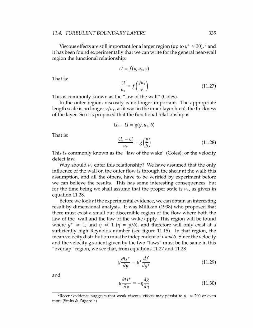
11.4. TURBULENT BOUNDARY LAYERS 335
Viscous effects are still important for a larger region (up to y+≈ 30), 2 and
it has been found experimentally that we can write for the general near-wallregion the functional relationship:
U = f (y,uτ, ν)
That is:Uuτ
= f( yuτν
)(11.27)
This is commonly known as the “law of the wall” (Coles).In the outer region, viscosity is no longer important. The appropriate
length scale is no longer ν/uτ, as it was in the inner layer but δ, the thicknessof the layer. So it is proposed that the functional relationship is
Ue −U = g(y,uτ, δ)
That is:Ue −U
uτ= g
( yδ
)(11.28)
This is commonly known as the “law of the wake” (Coles), or the velocitydefect law.
Why should uτ enter this relationship? We have assumed that the onlyinfluence of the wall on the outer flow is through the shear at the wall: thisassumption, and all the others, have to be verified by experiment beforewe can believe the results. This has some interesting consequences, butfor the time being we shall assume that the proper scale is uτ, as given inequation 11.28.
Before we look at the experimental evidence, we can obtain an interestingresult by dimensional analysis. It was Millikan (1938) who proposed thatthere must exist a small but discernible region of the flow where both thelaw-of-the- wall and the law-of-the-wake apply. This region will be foundwhere y+
1, and η 1 (η = y/δ), and therefore will only exist at asufficiently high Reynolds number (see figure 11.15). In that region, themean velocity distribution must be independent of ν and δ. Since the velocityand the velocity gradient given by the two “laws” must be the same in this“overlap” region, we see that, from equations 11.27 and 11.28
y∂U+
∂y= y+
d fdy+
(11.29)
and
y∂U+
∂y= −η
dgdη
(11.30)
2Recent evidence suggests that weak viscous effects may persist to y+≈ 200 or even
more (Smits & Zagarola)

336 CHAPTER 11. TURBULENT SHEAR FLOWS
Figure 11.15: Inner and outer regions, showing region of overlap.
By matching the velocity gradients, and by noting that the right hand sideof equation 11.29is only a function of y+, and the right hand side of equa-tion 11.30is only a function of η, then in the overlap region:
y+d fdy+
= −ηdgdη
=1κ
where κ is a constant. That is,
d fdy+
=1κy+
anddgdη
= −1κη
By integrating, we obtain two forms of the log-law:
Uuτ
=1κ
ln( yuτν
)+ B (11.31)
andUe −U
uτ= −
1κ
ln( yδ
)+ B′ (11.32)
Here κ is von Karman’s constant, and an often quoted value is 0.41.The first form (equation 11.31) is the version most commonly seen. In
this form, the additive constant B depends on the lower limit of integrationand it may depend on Reynolds number (see for example Duncan, Thom &Young, and Zagarola & Smits). However, for all practical flows it seems thatB is a constant and equal to about 5.2 (see Bradshaw & Brederode). Notethat if we were to accept the suggestion by Bill George that the outer flowin a boundary layer should scale on Ue rather than uτ, we would find thatthe velocity variation in the overlap region is then expressed as a power

11.4. TURBULENT BOUNDARY LAYERS 337
Figure 11.16: Regions of a turbulent boundary layer (inner layer coordinates).Outer-layer profile shown is for Ue = constant. From Cebeci & Bradshaw.
Figure 11.17: Universal plot of turbulent boundary layer profiles in zero pressuregradient (outer layer coordinates), after Clauser (1956). The symbols denote theexperimental data. From Cebeci & Bradshaw.
law. In practice, the differences with a logarithmic variation are small, butphilosophically it is an important distinction.
So we can plot the velocity profile in two ways: using inner-layer vari-ables (uτ, ν/uτ) (see figure 11.16), or outer-layer variables, or “velocity defectcoordinates” (uτ, δ) (see figure 11.17).
Thus we can see an important difference between laminar and turbulent

338 CHAPTER 11. TURBULENT SHEAR FLOWS
boundary layers: laminar layers scale according to a single parameter η(= y/δ), whereas turbulent layers scale according to two parameters y+ andη (for zero pressure gradient flows). We cannot write down a similaritysolution in the same way we could for the Blasius flow: the turbulentboundary layer profile is Reynolds number dependent. Before consideringthis aspect, we note the combined velocity profile representation suggestedby Coles:
Uuτ
=1κ
ln( yuτν
)+ B +
Π
κW
(yδ
)(11.33)
Here, Π is a function of Reynolds number but asymptotes to a constant ap-proximately equal to 0.55 at high Reynolds number. Note that equation 11.33does not include the viscous sublayer. The wake function W is well-fittedby a sin2 function:
W = 2 sin2(π2
yδ
)(11.34)
where π is the usual Pythagorean constant = 3.14159 . . .
11.5 Reynolds-Number Dependence of VelocityProfile
First consider the ratio of the outer-layer and inner-layer length scales (=δuτ/ν). As we shall see in section 11.8, in a zero pressure gradient turbulentboundary layer, we have, approximately:
δx
=0.37
Re1/5x
,
θx
=0.037
Re1/5x
,
and
C f =0.0592
Re1/5x
≡ 2u2τ
U2e
from which we get:
δuτν
= 0.064Re0.7x = 1.146Re7/8
θ (11.35)
So we can see that the viscous length scale becomes a decreasingly smallfraction of the boundary layer thickness as the Reynolds number increases.For example, consider the fraction of the boundary layer thickness occupiedby the viscous sublayer (y+
≤ 30). This fraction varies from 20% at the lowest

11.5. REYNOLDS-NUMBER DEPENDENCE 339
Figure 11.18: Fraction of the boundary layer thickness occupied by the viscoussublayer, as a function of momentum thickness Reynolds number Reθ. from JimBrasseur.
Reynolds number where a turbulent boundary layer is self-sustaining, tomuch less than 1% at very high Reynolds numbers (see figure 11.18.
What about the log-law? Experiments have shown that the lower limitof the log-law corresponds to about the upper limit of the viscous sublayer(y+ ≈ 30), and the upper limit of the log-law corresponds to about y/δ ≈ 0.2.3
According to these observations, a log- law can only exist when δuτ/ν > 150,which corresponds to Rex > 65, 000 and Reθ > 255. In practice, turbulentboundary layers are not observed until Reθ > 320 (Preston 1956, Smits et al.1982).
What about the wake region? Experiments have shown that the wakefactor in Coles’ “law of the wake” formulation (equation 11.33) is a functionof Reynolds number for Reθ < 5000 (see figure 11.19).
Note also that the velocity profile is plotted as U/Ue = f (y/δ) (sometimescalled “power-law” coordinates), the shape will continue to be a function ofReynolds number, even at high Reynolds numbers. When plotted in defectcoordinates, however, the profiles collapse for Reθ > 5000 (see figures 11.17and 11.20).
3Recent boundary layer and pipe flow data indicate a subtle but persistent influence ofviscosity out to y+ = 200 or even 500, so that the simple arguments adopted here concerningscaling may need to be modified.

340 CHAPTER 11. TURBULENT SHEAR FLOWS
Figure 11.19: Wake factor Π as a function of Reθ. The dotted line is the correlationderived by Coles (1962). See Smits et al. for the key to the symbols indicatingexperimental data.
Figure 11.20: Turbulent boundary layer velocity profiles plotted in “power-law”coordinates, showing effect of increasing Reynolds number.
11.6 Friction Law for Pipe and Channel Flows
For a two-dimensional channel flow, we found a linear variation of totalstress in the near-wall region. This linear variation also holds for pipe flow,where y is measured radially from the wall. Again, near the wall we canidentify a region where viscous effects are important (the viscous sublayer,where y+ < 30), and a region away from the wall where they are not (the coreregion). Here we also find a region of overlap where a logarithmic velocityvariation occurs, and also a wake region but with a smaller value of the wakefactor Π than seen in the boundary layer case. In fact, Π is so small that it isnot a bad approximation to neglect it altogether (see Tennekes and Lumley,Section 5.2, for a fuller discussion).4 If we assume that the log-law works
4As we shall see, if the wake component is independent of Reynolds number, it willintegrate to a constant so that the result obtained by neglecting it is the same as the morecomplete result except for an additive constant.

11.6. FRICTION LAW FOR PIPE AND CHANNEL FLOWS 341
all the way to the centerline, we can derive a skin- friction formulation verysimply. From the log-law:
Uuτ
=1κ
lnyuτν
+ B
Evaluating the velocity at the centerline gives:
Umax
uτ=
1κ
lnhuτ2ν
+ B
To get the skin friction coefficient (= τw/ 12ρU2
av), we need to evaluate theaverage velocity, Uav. If we further assume that the log-law holds all theway to the wall (since the thin viscous sublayer should not contribute sig-nificantly to the momentum defect, which means in effect that we are at ahigh Reynolds number), we get:
Umax
uτ=
2h
∫ h/2
0
Uuτ
dy =1κ
lnhuτ2ν
+ B −1κ
Using Re= Uavh/ν, we obtain:√2
C f=
1κ
ln
Re2
√C f
2
+ B −1κ
or, with the friction factor f = 4C f ,√8f
=1κ
ln
Re2
√f8
+ B −1κ
With κ = 0.41 and B = 5.2 , we get
1√f
= 0.862 ln(Re
√f)− 0.518 (11.36)
If we repeat this analysis for pipe flow, we obtain
Uav
uτ=
1κ
lnDuτ2ν
+ B −3
2κ
and1√
f= 0.862 ln
(Re
√f)− 1.738 (11.37)
There exists a concept of “hydraulic diameter” which is used to extendthese simple cases to conduits of more complex cross-sectional shapes (Perry,

342 CHAPTER 11. TURBULENT SHEAR FLOWS
1962). Very simply, the pipe result is used for other conduit shapes bysubstituting for the diameter D with a hydraulic diameter DH, where DH isdefined by
DH = 4 × (cross-section area)/(wetted perimeter)
It seems to work quite well, as we can see when we use the pipe result toobtain the channel result. For a channel,
DH =4hw
2(h + w)
where h is the channel height, and w is its width. When we substitute inthe pipe result the hydraulic diameter for the channel, and use the fact thatw h, we obtain:
1√f
= 0.862 ln(Re
√f)− 1.141
which is very similar to the earlier result (equation 11.37).
11.7 Momentum-Integral Methods for TurbulentBoundary Layers
The Reynolds shear-stress term−ρu′v′ in the turbulent boundary layer equa-tions is obviously a source of difficulty in solving the equations: it representsa new unknown, so that the list of unknowns has been increased from two(U and V) as in the laminar case to three without increasing the number ofequations. Trying to generate an expression for−ρu′v′ in terms of U and V iscalled the “closure” problem. We will discuss some of the more elementarymethods for “closing” the set of equations later. Here we take a simplerapproach, using the momentum integral equation and an expression for theprofile to obtain information about the “integral” parameters δ, δ∗, θ and theskin friction coefficient C f .
By integrating the boundary layer equations over the thickness of thelayer, or by using the integral form of the momentum equation applied toa control volume enclosing the full extent of the layer (see, for example,Duncan, Thom & Young), we obtain the “momentum integral equation:”
dθdx
+ θ (H + 2)1
Ue
dUe
dx=
C f
2(11.38)
for a two-dimensional, constant density, constant property, steady flow. Thisrelationship holds for laminar and turbulent flows (to the boundary layerapproximation).

11.8. POWER LAWS 343
For zero pressure gradient flow,
dθdx
=C f
2(11.39)
For these relationships to be useful, we need a representation of the velocityprofile.
11.8 Power Laws
Earlier, we mentioned the power-law velocity-profile similarity proposed byBill George (1992). Simpler power-law relations have been used for manyyears as engineering approximations. They are based on the observationthat the velocity profile in a zero pressure-gradient boundary layer can beapproximated by a relationship such as:
UUe
=( yδ
) 1n
, (11.40)
where the value of n depends weakly on the Reynolds number, varying froma value of 7 for 5 × 10⁵ < Rex < 107 to a value of 9 for 106 < Rex < 108. As aresult, we obtain
δ∗
δ=
11 + n
andθδ
=n
(1 + n) (2 + n). (11.41)
Therefore the shape factor H (= δ∗/θ) depends on n, and for n = 7, δ∗/δ = 1/8,θ/δ = 7/72, and H = 9/7 (compare these results with a laminar boundarylayer).
Experiments show that the shape factor is not constant, especially atlow Reynolds numbers, indicating to some extent the Reynolds-number-dependence of n.
Power-law approximations work reasonably well as a description forthe outer-layer velocity distribution, but at the wall ∂U
/∂y → ∞, and they
cannot be used to find the skin-friction. It is usually assumed instead thatthe Blasius relationship (derived as a curve-fit to pipe flow data) can be used,so that
Ue
uτ= Cb
(uτδν
) 1n
, (11.42)
where Cb is a constant. By using the momentum-integral equation, (Equa-tion 11.39), we obtain, for n = 7,
C f =0.0592
Re1/5x
,δx
=0.37
Re1/5x
, andθx
=0.037
Re1/5x
, (11.43)

344 CHAPTER 11. TURBULENT SHEAR FLOWS
and for n = 9,
C f =0.0375
Re1/6x
,δx
=0.27
Re1/6x
, andθx
=0.023
Re1/6x
, (11.44)
where the constants have been adjusted to fit the experimental data (seeYoung, 1989).
Despite their questionable provenance, these relationships are useful forsimple engineering estimates.
Note that equation 11.43 indicates that the growth of the turbulent bound-ary layer on a flat plate is proportional to x0.8, which is a faster rate of growththan that of a laminar layer, which grows as x0.5.
The local skin friction coefficient is C f , defined as
C f ≡τw
12ρU2
e
(11.45)
The total skin friction coefficient CF is defined as
CF ≡Drag
12ρU2
e b`
and b and ` are the width and length of the plate respectively. Hence:
CF = b∫ `
0
τw12ρU2
e b`dx =
0.72(Ue`ν
)0.2 (11.46)
This equation agrees pretty well with experiment if the constant 0.072 ischanged to 0.074. A comparison with experiment is shown in figure 11.21.
Because of the limitation on Blasius’s pipe resistance formula, the va-lidity of the equation is restricted to flows for which Ueδ/ν < 105. Usingequation 11.43, this corresponds to Ue`/ν < 6×10⁶. Since for Ue`/ν less thanabout 5 × 10⁵ the boundary layer on a plate is fully laminar, equation 11.45is valid in the range 5 × 10⁵ < Ue`/ν < 107.
Despite the fact that these power-laws do not represent the profile verywell, the correlations derived for δ, δ∗, θ and C f are quite reasonable (see,for example, Smits et al. 1983), and they are very useful for preliminarycalculations.
11.9 Mixing Length and Eddy Viscosity Concepts
In turbulent shear flows, it is usually the Reynolds shear stresses that aremost important. Consider a flow with U(y), and V = 0 = W (see fig-ure 11.22a). If fluid element A moves to position y0 by turbulent motion it
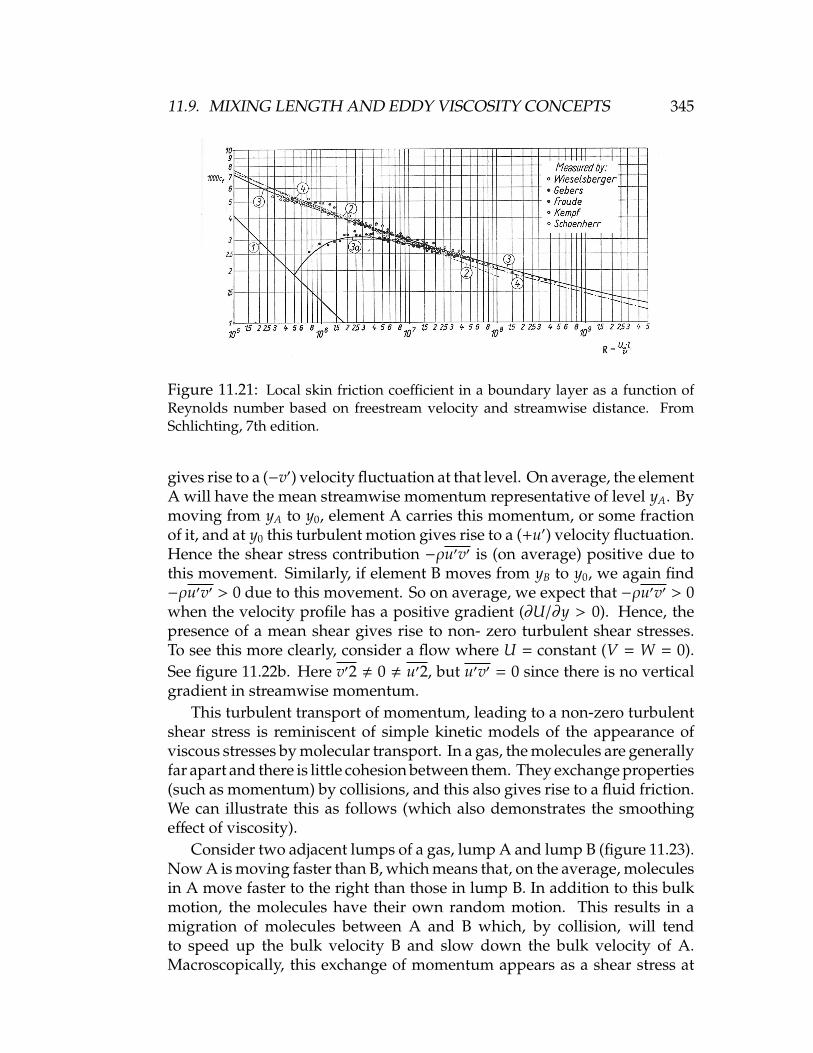
11.9. MIXING LENGTH AND EDDY VISCOSITY CONCEPTS 345
Figure 11.21: Local skin friction coefficient in a boundary layer as a function ofReynolds number based on freestream velocity and streamwise distance. FromSchlichting, 7th edition.
gives rise to a (−v′) velocity fluctuation at that level. On average, the elementA will have the mean streamwise momentum representative of level yA. Bymoving from yA to y0, element A carries this momentum, or some fractionof it, and at y0 this turbulent motion gives rise to a (+u′) velocity fluctuation.Hence the shear stress contribution −ρu′v′ is (on average) positive due tothis movement. Similarly, if element B moves from yB to y0, we again find−ρu′v′ > 0 due to this movement. So on average, we expect that −ρu′v′ > 0when the velocity profile has a positive gradient (∂U/∂y > 0). Hence, thepresence of a mean shear gives rise to non- zero turbulent shear stresses.To see this more clearly, consider a flow where U = constant (V = W = 0).See figure 11.22b. Here v′2 , 0 , u′2, but u′v′ = 0 since there is no verticalgradient in streamwise momentum.
This turbulent transport of momentum, leading to a non-zero turbulentshear stress is reminiscent of simple kinetic models of the appearance ofviscous stresses by molecular transport. In a gas, the molecules are generallyfar apart and there is little cohesion between them. They exchange properties(such as momentum) by collisions, and this also gives rise to a fluid friction.We can illustrate this as follows (which also demonstrates the smoothingeffect of viscosity).
Consider two adjacent lumps of a gas, lump A and lump B (figure 11.23).Now A is moving faster than B, which means that, on the average, moleculesin A move faster to the right than those in lump B. In addition to this bulkmotion, the molecules have their own random motion. This results in amigration of molecules between A and B which, by collision, will tendto speed up the bulk velocity B and slow down the bulk velocity of A.Macroscopically, this exchange of momentum appears as a shear stress at

346 CHAPTER 11. TURBULENT SHEAR FLOWS
Figure 11.22: (a) Turbulent momentum transport with a positive velocity gradient;(b) Transport with a zero velocity gradient.
Figure 11.23: Momentum transport on a molecular scale with a positive velocitygradient.
the interface between the lumps (remember these are surface forces whichact typically over a distance comparable to the mean free path).
Hence:
1. Viscosity tends to smooth out velocity differences between adjacentfluid lumps;
2. In a gas the viscosity must depend on the average molecular speed,the number density and the mean free path. The dimensions are[
stressvelocity gradient
]=
MLT−2L−2
LT−1L−1 =ML3 ×
LT× L
= density × velocity × length
The proportionality constant between stress and velocity gradient iscalled the viscosity µ, and so we would expect, in a gas, µ ∼ ρvΛ,where v is the mean molecular speed, and Λ is the mean free path. Infact, using a hard sphere molecular model, we find:
µ =5π32ρvΛ ≈ 1
2ρvΛ (11.47)

11.9. MIXING LENGTH AND EDDY VISCOSITY CONCEPTS 347
This relationship approximates observation, and the departures arisefrom the limitations of the hard sphere model;
3. In a gas, if we increase the temperature, the number of collisions willincrease and we would expect the viscosity to increase, which it does;
4. In a liquid the mechanism is different. If the temperature increases theintermolecular forces decrease, and hence the viscosity will decrease.
11.9.1 Prandtl’s eddy viscosity
These analogies with molecular motions lead to two simple closure schemes:the eddy viscosity and mixing length hypotheses. The eddy viscosity ap-proach says that, since
Si j = µ
(∂Ui
∂x j+∂U j
∂xi
)why not
−ρu′v′ = µt
(∂Ui
∂x j+∂U j
∂xi
)Specifically, for two-dimensional thin shear layers, we write
−ρu′v′ = µt∂U∂y
That is,
−u′v′ = νt∂U∂y
(11.48)
Here νt is known as the eddy viscosity. Its simplest form sets νt = constant,but variants such as νt = νt(y) and νt = νt(x, y) are widespread. A functionfor νt can always be formed that satisfies any set of experimental data, butit is not a universal function (see reasons given below, especially in thehandout from Bradshaw’s notes). A typical distribution for a zero pressuregradient boundary layer is shown in figure 11.25.
11.9.2 Taylor and von Karman’s mixing length method
Consider a mean flow where U = U(y), with turbulence components u′ andv′. If fluid elements at y1 will, on average, come from levels y1−`m and y2+`m,where `m is a length scale. If we assume that the fluid elements retain theirinitial velocities U(y1 − `m) and U(y1 + `m) before mixing at height y1, thenthese velocities represent, on average, the overall spread of instantaneous

348 CHAPTER 11. TURBULENT SHEAR FLOWS
Figure 11.24: Vertical turbulent momentum transport over a characteristic distance`m.
velocities at that height: U − urms and U + urms (see figure 11.24). Now if `m
is small, √u′2 = `m
∂U∂y
If we assume that u′v′ is proportional to u′2 then:
−ρu′v′ = ρ`2m∂U∂y
∣∣∣∣∣∂U∂y
∣∣∣∣∣ (11.49)
where the magnitude is used to ensure the correct sign of the shear stress.All we need now is `m, the “mixing length.” A typical distribution for a
zero pressure gradient boundary layer is shown in figure 11.26. Again wefind that there is no “universal” distribution, and the mixing length is flowdependent.
Now the kinetic arguments for the viscous stresses work because (1)∂U/∂y is small compared with the gradient of the molecular velocities whichare responsible for viscosity, and (2) memories of velocity gradients extendonly over distances comparable to the mean free path and therefore theproduction of viscous stresses is purely a local phenomenon.
Neither of these statements is true for the large eddies responsible forthe production of Reynolds stresses. While turbulent velocities are smallcompared with the mean velocity over most of the flow field, the largesteddies are as big as the whole of the turbulent field.
In short, in using these gradient diffusion models using forms of νt (the“Boussinesq” hypothesis5 or mixing length models, we’re trying to calculateturbulent flows without saying anything about the turbulence. So let’s learnmore about the turbulence.
5Boussinesq J. (1877) Theorie de l’ecoulement tourbillant, Men. Pres. Acad. Sci. XXIII, 46,Paris

11.9. MIXING LENGTH AND EDDY VISCOSITY CONCEPTS 349
Figure 11.25: Dimensionless eddy viscosity distribution (εm in this plot) across azero pressure gradient boundary layer, according to the data of Klebanoff (1954).From Cebeci & Smith, 1974.
Figure 11.26: Dimensionless mixing length distribution across a zero pressuregradient boundary layer, according to the data of Klebanoff (1954). From Cebeci &Smith, 1974.

350 CHAPTER 11. TURBULENT SHEAR FLOWS
11.10 Mixing length and eddy viscosity
(from notes by Peter Bradshaw, September 1976)We define a length ` by
`m =(−uv)1/2
∂U/∂y
and call it the “mixing length.”We also define a quantity νt, having the dimensions of kinematic viscosity,
by
νt =(−uv)∂U/∂y
and call it the “(kinematic) eddy viscosity.” These are purely the definitionsof symbols: no assumption is involved, providing that we do not supposethat the mixing length necessarily corresponds directly to an eddy lengthscale or that the eddy viscosity is a property of the fluid like the molecularviscosity.
Since our object is to find some empirical equation for −uv there is nopoint in introducing `m or νt unless their behavior is simpler than that of−uv itself. What one would like to find is that `m is just some multiple of theshear layer thickness δ (or, more reasonably, that `m/δ = f (y/δ)) or that νt issimilarly related to Ueδ). There are several methods of calculating thin shearlayers, especially boundary layers, that rely on relations like these, withempirical constants chosen to give the best agreement between calculationand experiment. What is the justification for this? The justification used bythe proprietors of these calculation methods is usually “It works, doesn’tit?” — the defense used by witch-doctors from time immemorial. A morescientific assessment is possible and, particularly in the case of the mixinglength, gives some ideas of the errors likely to be incurred by using simpleempirical relations between `m or νt and the mean properties of the shearlayer. For simplicity we consider only thin shear layers so that Reynoldsstresses other than −uv do not affect the mean flow.
11.10.1 Early ideas about turbulence
Soon after it was recognized that turbulent flow carried a much larger shearstress than a laminar flow with the same value of ∂U/∂y, Boussinesq (1877)suggested that turbulence might have a simply-behaved eddy viscosity.Any idea of a direct connection between turbulence and molecular diffusion,making νt a universal multiple of ν, was soon contradicted by experiment,but the concept of a simply-behaved νt underlay several attempts to treatturbulent flow (for instance the Ekman layer model (1905) of cyclonic motion

11.10. MIXING LENGTH AND EDDY VISCOSITY 351
in the lower atmosphere was first formulated using an eddy viscosity andonly later rewritten in the laminar-flow form usually quoted in textbooks).
In 1925 Prandtl, who had invented the boundary layer concept in 1904,postulated a more definite analogy between turbulence and molecular mo-tion. Specifically he supposed that turbulent eddies conserved their mo-mentum between collisions with other eddies, and the “mixing length” asdefined above came out as the mean free path of this imaginary process.Now the idea that eddies are separate entities that collide every so often canbe disproved simply by watching a plume of smoke; the eye of faith candistinguish eddies but their interaction is continuous, and not discrete as inthe case of molecules. Unfortunately when the mixing length idea was triedout in the inner layer of a turbulent wall flow, using the plausible assump-tion that `m was proportional to y, it successfully predicted the logarithmicprofile observed in practice if the constant of proportionality was taken as0.4. The witch doctors took over and the mixing length was in. It was 1950before the paradox was resolved.
11.10.2 Special cases where `m and νt are simple functions
In the inner layer of a wall flow, it is plausible to assume that the flowdepends only on u , y and ; the physical justification is that the eddies nearthe wall are small so that they are unconscious of the comparatively slowfluctuations of the larger eddies further out or of the even slower changes(with x) of the free stream. Dimensional analysis gives the familiar
Uuτ
= f1
(uτyν
)or
∂U∂y
=uτy
f2
(uτyν
)If we further argue that viscosity should not affect the shear-stress-carryingeddies outside the viscous sublayer then (outside the sublayer) ∂U/∂y sim-plifies to
∂U∂y
=uτκy
foruτyν< 30, say
which is the mixing length formula with (−uv)1/2= uτ and `m = κy.
In the outer layer of a boundary layer in zero pressure gradient, plausiblearguments and dimensional analysis lead to
Ue −Uuτ
= f3
( yδ
),
(−uv)1/2
uτ= f4
( yδ
)

352 CHAPTER 11. TURBULENT SHEAR FLOWS
and∂U∂y
=uτδ
f5
( yδ
)or
∂U∂y
=(−uv)1/2
δf6
( yδ
)There is no reason to suppose that f6 is a constant (implying ` = constant×δ) but obviously f6 must tend to 1/(κy/δ) in the log law region where theinner-layer and outer-layer analyses are simultaneously valid.
Now what we have done, for these special cases only, is to obtain the mixinglength formula, with `m = κy or `/δ = f6(y/δ), by dimensional analysis,based on the ideas that the inner-layer eddies are not directly affected by theouter layer eddies (“local equilibrium”) and that the outer layer flow changesonly in scales but not in behavior as the boundary layer flows downstream(“self-preservation”). The eddy viscosity formula, with νt = κuτy in theinner layer and νt = uτδ f7(y/δ) in the outer layer, can be obtained from thesame analysis. In neither case do we need any concepts borrowed from thekinetic theory of gases. The outer layer “self-preserving” results also apply,with different functions of y/δ, to other self-preserving flows like jets in stillair or wakes in zero pressure gradient (and in these two cases quite goodagreement with experiment is obtained by taking νt or `m constant acrossthe width of the shear layer). Again no physical meaning need be attachedto νt or `m. By coincidence, the function f7 in the eddy viscosity in the outerlayer of a boundary layer is nearly the same for a wide range of (constant)values of the presure-gradient parameter (δ∗/τw)dp/dx.
If we look more closely, the essential lack of physical meaning in νt and`m becomes more obvious. Near the center line of a symmetrical jet or wake,U = uτ + O(y2) so that ∂U/∂y is proportional to y. Again by symmetry, −uvis proportional to y. Therefore `m ∝ y−1/2 and `m → ∞ as y → 0! In thiscase νt is well behaved near the center line, but in an asymmetrical jet (forinstance a wall jet from a nozzle blowing tangential to a wall) ∂U/∂y and−uv change sign at different points, between which νt is negative and `m isimaginary.
If we extend the idea of eddy viscosity to the normal stresses in a turbu-lent flow and write
−u2 = νt∂U∂x
−v2 = νt∂V∂y
−w2 = νt∂W∂z
then adding these three equations and using the continuity equation
∂U∂x
+∂V∂y
+∂W∂z
= 0

11.10. MIXING LENGTH AND EDDY VISCOSITY 353
givesu2 + v2 + w2 = 0
so the turbulence vanishes altogether, a result to gladden the heart of anywitch doctor. (There are ways round this).
In three-dimensional flow it is found that the eddy viscosity for −vw,namely −vw/(∂W/∂y), is in general not equal to the eddy viscosity for −uv,namely −uv/(∂U/∂y).
11.10.3 Relation between `m and eddy length scales
If the turbulence is in local equilibrium, then, by definition, the mean andturbulent transport terms in the turbulent energy equation (or the otherexact equations for the rates of change of Reynolds stress along a meanstreamline) are negligible. Thus, in the turbulent energy equation, we get
“production” = “dissipation”
or−uv
∂U∂y
= ε
where ε stands for complicated viscous terms. Now we know that ε isreally the rate of transfer of energy to the smaller eddies from the energy-containing, shear-stress-carrying eddies, and should therefore depend ontypical scales of the latter. A dimensionally-correct form is
ε =(−uv)3/2
Lwhere L, defined by this expression, is called the “dissipation length param-eter.” Then
−uv∂U∂y
=(−uv)3/2
Lso that `m == L (= κy in the inner layer of a boundary layer). This derivationadds little to the purely dimensional arguments above. The point is that Lis defined by a relation between two turbulence qualities involved in thefundamental process of energy transfer from large eddies to small and istherefore a real eddy length scale, which should be much less dependent onthe mean flow than `m, which is a relation between one turbulence quantityand one mean flow quantity. Therefore, in cases where the flow is changingsignificantly with distance downstream, so that the transport terms in theturbulent energy equation become significant and `m is no longer equal toL, it is L and not `m that is more likely to obey simple rules. In fact acalculation method that I (peter Bradshaw) devised, assuming L/δ = F(y/δ),gives distinctly better results than `m/δ = f (y/δ) in rapidly-changing flows,and enables one to assess the errors in the latter assumption.

354 CHAPTER 11. TURBULENT SHEAR FLOWS
11.10.4 Conclusions
(i) `m and νt have no physical significance; they are just quantities definedby the equations at the beginning of this section.
(ii) `m and νt obey simple rules only in local-equilibrium layers and self-preserving flows, and only in a local-equilibrium layer, where alllength scales are proportional, can `m be identified with a true tur-bulence length scale.
(iii) By coincidence `m/δ is nearly the same function of y/δ in self- preserv-ing boundary layers over a wide range of (δ∗/τw)dp/dx (as well as beingindependent of x in any one such boundary layer). This is explicablefrom the analysis of section 11.10.3 if we note that mean transportand turbulent transport of turbulent energy are by coincidence nearlyequal and opposite throughout a self-preserving boundary layer, leav-ing production dissipation.
(iv) From (ii) and (iii) it follows that simple rules for `m or νt can give goodresults in boundary layers — or other thin shear layers — that are nottoo far from being self-preserving.
(v) In more demanding cases `m and νt do not obey simple formulae andmay exhibit ludicrously unphysical behavior.
(vi) It is frequently useful to phrase qualitative arguments in terms of mix-ing length or eddy viscosity, or even to make qualitative hypothesesabout `m or νt rather than −uv directly. This is acceptable if pathologi-cal cases (such as asymmetrical jets) are avoided but the student mustbeware being conned into forgetting conclusion (i).

Chapter 12
Engineering Calculation Methodsfor Turbulent Flows
12.1 Introduction
Here we discuss methods for calculating turbulent flows at Reynolds num-bers of engineering interest. As we have noted previously , at very lowReynolds numbers we can use Direct Numerical Simulations (DNS) wherethe smallest resolved scale is the smallest eddy of interest, that is, the gridscale ∆ is 0(η), where η is of order the Kolmogorov scale. At higher Reynoldsnumbers, we can use LES (where the smallest scales are modelled in someway but the time-dependent anisotropic large (energy-containing) scales arecomputed directly. However, turbulent flows found in engineering appli-cations have Reynolds numbers which are typically much larger than theregimes suitable for DNS or LES approaches, and calculations are usuallybased on the Reynolds-Averaged Navier-Stokes equations (RANS), togetherwith some turbulence model to close the equations. In any case, routineengineering calculations will almost certainly continue to use turbulencemodels since LES and DNS are unlikely to transcend the status of research-type calculations and become design tools (they are immensely labor andcomputer intensive, and they require highly skilled users). A good surveyof engineering calculation methods is given by Wilcox, including computerprograms and homework problems.
The early efforts in calculating turbulent boundary layers used methodsbased on the momentum integral equations. These “integral” methodswere discussed briefly in section 11.7, and a more detailed survey is givenby Cebeci in Turbulence. Here we will consider one representative example.Current calculation methods are all based directly on the partial differentialequations derived from the N-S equation by using Reynolds decomposition.According to Reynolds (in Turbulence), different levels of turbulent flow pdemodels can be identified. We can modify this hierarchy somewhat to suggest
355

356 CHAPTER 12. ENGINEERING CALCULATION METHODS
the following ordering:
1. Integral methods — these are based on the momentum integralequation which is an ode for the integral properties of the boundarylayer.
2. Zero-equation models — models using only the pde’s for the meanvelocity field, and no turbulence models (for example eddy viscosityor mixing length models). Also called “algebraic stress models.”
3. One-equation models — models involving one pde relating to aturbulence velocity scale, in addition to the mean pde’s.
4. Two-equation models — models using an additional pde related toa turbulence length scale (for example k–ε, or k–ω)).
5. Stress-equation models (Reynolds-Averaged Navier Stokes, or RANS)— models involving pde’s for all components of the Reynolds stresstensor, and in general for a length scale as well.
6. Very Large-Eddy Simulations (VLES) – c-omputations of the three-dimensional time- dependent large eddy structure and a high-levelmodel for smaller-scale turbulence (for example a Smagorinski eddy-viscosity model).
7. Large-Eddy Simulations (LES) — computations of the three-dimensionaltime- dependent large eddy structure and a low-level model for thesmall-scale turbulence (for example, k–ε).
8. Direct Numerical Simulations (DNS) — computations of the fullthree-dimensional time-dependent flow field with no modelling as-sumptions.
12.2 Integral Methods
By integrating the mean momentum equation from the wall out to theboundary layer edge for a two-dimensional incompressible flow, we ob-tain the momentum-integral equation (equations 3.29 and 3.30). If the shapefactor H and the wall stress τw, can be expressed as functions of the momen-tum thickness θ, this equation can be solved for θ. The simplest empiricalinput is to assume H = constant, and τw = f (Reθ). A more realistic versionis that by Head who used the concept of an entrainment velocity Ve, whichis a velocity scale defined in terms of the growth of the velocity deficit in theboundary layer. That is:
Ve
Ue=
1Ue
ddx
(Ue (δ − δ∗)) = F (H1) (12.1)

12.3. ZERO-EQUATION MODELS 357
Head assumed that Ve = F(H1), where H1 is a new shape parameter definedby H1 = (δ − δ∗)/θ, and also that H1 = G(H). The functions F and G can beobtained from experimental data. By additionally using some skin frictioncorrelation, such as that proposed by Ludwieg & Tillman:
C f = 0.24610−0.678HRe−0.268θ , (12.2)
a closed set of equations is obtained which can be solved for the skin frictionand other integral properties. This method was widely used and it wasextended in a number of ways by Green (who allowed F to be a functionof the streamwise distance) and Myring (who extended the method to threedimensions). The integral approach avoided the complexity of solving thepartial differential equations describing the shear layer development, but itquickly lost popularity when computers became available that made possi-ble the rapid solution of multiple pde’s.
12.3 Zero-Equation Models
Most of these methods are based on the eddy viscosity concept in some form(see also sections 11.9) and 11.10. For a boundary layer method, for a flowwith constant properties,
U∂U∂x
+ V∂U∂y
= UedUe
∂x+∂∂y
(−u′v′ + ν
∂U∂y
)(12.3)
The two most popular models for the Reynolds shear stress are
−u′v′ = νt∂U∂y
eddy viscosity
and−ρu′v′ = ρ`2
m∂U∂y
∣∣∣∣∣∂U∂y
∣∣∣∣∣ mixing length
Here νt or `m are prescribed as functions of y (see figures 11.25 and 11.26)for particular flows. The methods lack generality but are still widely used.Note that implicitly we assume that νt or `m are better behaved quantitiesthan τ and ∂U/∂y themselves – that in some sense they are more “universal.”
The notes in the next few sections are based on material in Launder $Spalding’s Mathematical Models of Turbulence, Academic Press, 1972.
12.3.1 Nature of the hypothesis
• The originator was Prandtl (1925), who used as a starting point thekinetic theory of gases, which gives:
µ ≈ 13ρvΛ

358 CHAPTER 12. ENGINEERING CALCULATION METHODS
where Λ is the mean free path, and v is the molecular velocity.
• First part of the hypothesis:τ
∂U/∂y≡ µt = ρ`mVt
where `m is the mixing length, and Vt is the turbulent velocity.
• Second part of the hypothesis:
Vt ≡ `m
∣∣∣∣∣∂U∂y
∣∣∣∣∣As a consequence,
τ ≡ µt∂U∂y
= ρ`m
∣∣∣∣∣∂U∂y
∣∣∣∣∣ ∂U∂y
so that
µt = ρ
√τρ`m
The question is: “What determines `m?”
Values of mixing length for some free turbulent flows:
For a plane mixing layer:
`m/δ = 0.07, where δ ≡ layer width
For a plane jet in stagnant surroundings:
`m/δ = 0.09, where δ ≡ width of half jet
For a “fan” jet in stagnant surroundings:
`m/δ = 0.125, where δ ≡ width of half jet
For a round jet in stagnant surroundings:
`m/δ = 0.075, where δ ≡ width of half jet
Mixing length distribution in boundary layers near a single wall:
The Escudier formula gives:
yδ≤λκ,
`m
δ= κ
yδ
yδ>λκ,
`m
δ= λ
where κ = 0.41 and λ = 0.09 (see figure 12.1). Note that this formula needsmodification very near the wall.

12.3. ZERO-EQUATION MODELS 359
Figure 12.1: Mixing length distribution in boundary layers near a single wall.
Figure 12.2: Mixing length very near a wall; van Driest’s (1956) hypothesis.
Mixing length very near a wall; van Driest’s (1956) hypothesis:
The effective viscosity, µe f f , is given by:
µe f f = µ + ρ`2m
∣∣∣∣∣∂u∂y
∣∣∣∣∣The mixing length is given by:
`m = κy[+1 − exp
(−
y√τsρ
Aµ
)]where A = 26.0. The resulting distribution is shown in figure 12.2.
12.3.2 Mixing-Length Hypothesis
Advantages
In favor of the Mixing Length Hypothesis (MLH) are three important at-tributes:
• It is simple, requiring no additional differential equations to be solved;
• Provided that good choices are made for the mixing-length distribu-tions, the MLH allows realistic predictions to be made of the velocityand shear-stress distributions, and the general behavior, of boundary-layer flows;

360 CHAPTER 12. ENGINEERING CALCULATION METHODS
Figure 12.3: The MLH implies that the effective viscosity vanishes where thevelocity gradient is zero.
• Much experience of using the MLH has been accumulated and madeavailable through publications.
Disadvantages
Against the MLH, it must however be said:
• That there is almost no successful experience of predicting recirculatingflows with its aid, for the relations between the stresses and the velocitygradients are too complicated;
• It implies that the effective viscosity vanishes where the velocity gra-dient is zero (see figure 12.3). For a finite effective Prandtl number,the effective thermal conductivity also goes to zero under these condi-tions.;
• The MLH takes no account of processes of convection or diffusion ofturbulence.
It is true that care and ingenuity can make good some of the deficienciesof the MLH; and for many practical purposes it is still the best model toemploy.
12.4 One-Equation Models
In typical one-equation turbulence models, the Turbulent Kinetic Energyequation (TKE equation — equation 7.19) forms the basis for a model equa-
tion for the turbulence velocity scale q =
√q2 =
√u2
i , following Prandtl

12.4. ONE-EQUATION MODELS 361
(1945). The velocity scale k is determined from the solution of a convectivetransport equation. The TKE equation is given by:
D(
12q2
)Dt
= −∂∂x j
p′u j
ρ+ 1
2u jq2
︸ ︷︷ ︸1,2
−uiu j∂Ui
∂x j︸ ︷︷ ︸3
+ νui∂2ui
∂x2j︸ ︷︷ ︸
4
. (12.4)
The term on the left is the advection of TKE. The first term on the right repre-sents the net loss of TKE by the work done in transporting the fluid througha region of changing pressure; the second term represents the transport ofTKE by the turbulence itself; the third term represents the production ofTKE (the extraction of energy from the mean flow by the turbulence), andthe fourth term is the dissipation, ε.
In general, the scalar eddy viscosity is defined by:
uiu j = 13q2δi j − 2νtSi j (12.5)
In one-equation models, νt is modelled by
νt = C2q`m (12.6)
which still requires the length scale distribution `m(y/δ) to be specified.We also need to do some work with the TKE equation. In particular,
we need to model the diffusion term (1 and 2) and the dissipation (4).To start with the dissipation, we found from considerations of isotropichomogeneous turbulence that in the initial period of decay the dissipationmay be modelled by:
ε = C3q3
`m(12.7)
For high Reynolds number turbulence in inhomogeneous flows, we makethe same assumption on the grounds that the dissipation will still be deter-mined by the properties of the energy containing eddies.
For the diffusion term we write:
p′u j
ρ+ 1
2u jq2 = −C4νt∂q2
∂x j(12.8)
Whenever we model a higher-order moment as being proportional to thegradient of a related lower-order moment, it is called a gradient diffusionhypothesis.
Consider the forms appropriate to thin shear layers (the boundary layerapproximation). The TKE equation becomes
D(
12q2
)Dt
= −∂∂x j
(p′v′
ρ+ 1
2q2v′)− u′v′
∂U∂y− ε (12.9)

362 CHAPTER 12. ENGINEERING CALCULATION METHODS
In the usual notation, we start with the exact boundary-layer form of thek-equation:
ρDkDt
= −∂∂y
(ρv′k′ + v′p′
)− ρu′v′
∂u∂y− µ
∑∂u′i∂x j
2
where k = 12q2. On the left we have convective flow, and on the right we
have diffusion, production, and dissipation. The various terms are modelledaccording to:
•ρv′k′ + v′p′ = constant × ρ
√
k `∂k∂y
=µt
σk·∂k∂y
•ρu′v′ = νt
∂u∂y
•
−µ∑∂u′i
∂x j
2
→ local isotropy→ cDρk3/2
`
and so:
ρDkDt
= −∂∂y
(µt
σk
∂k∂y
)+ µt
(∂u∂y
)2
− cDρk3/2
`
This is one way of developing a one equation model. A different approachwas given by Bradshaw, Ferris & Atwell in 1967.
The Bradshaw-Ferris-Atwell Method
Consider one very popular version of a one equation model in more detail –this is the model by Bradshaw, Ferris & Atwell (1967) sometimes called theBFA method.. This method was the “winner” at the 1968 Stanford Olympics,that is, the 1968 AFOSR-IFP-Stanford Conference on Computation of Turbu-lent Boundary Layers (the runner-up was Cebeci & Smith’s algebraic eddyviscosity model — a zero-equation model).
Bradshaw’s modelling of the energy equation
•
Dissipation: ∝ρk3/2
`, as before
•
Diffusion: − v′k′ = Bk√τmax
ρ, B ≡
τmax
ρu2G
g( yδ
)where τ = a · ρk, and a = 0.3.

12.4. ONE-EQUATION MODELS 363
Figure 12.4: Values of a1 measured by Alving (1988) in a boundary layer recoveringfrom a sudden application of convex curvature.
•`δ
= f( yδ
)The functions f and g are shown in figure 12.5 (where f = L, g = G).
• The diffusion assumption renders the equation hyperbolic.
BFA actually start with the equation for the turbulent kinetic energy buttransform it into an equation for the shear stress by the assumption that
−uv
q2≡ a1 = constant (= 0.15 for boundary layers)
(the constant a1 = a, where the subscript was introduced by Townsend). Thisassumption is in reasonable agreement with experiment in many boundarylayers, and it avoids the use of the turbulent viscosity concept. See fig-ure 12.4.
The treatment of the diffusion is also quite different. Instead of the“gradient diffusion” assumption, Bradshaw supposed that the diffusive fluxof energy is proportional to the energy itself times a diffusion velocity of thelarge eddies of turbulence: this is taken as
√τmax/ρ. That is:
−q2v′ = q2√τmax
ρ=
τρa1
√τmax
ρ

364 CHAPTER 12. ENGINEERING CALCULATION METHODS
Figure 12.5: Distributions of a1, L, and G according to the BFA method.
So that
−q2v′ =1a1
Gτρ
√τmax
ρ
and G is a function of y/δ.Note that the p′v′ term has been neglected on the basis that it is probably
small. Or you could argue that it has been included but modelled in thesame way as q2v′. Since p′v′ cannot be measured directly, the jury is out.
The model equation for the shear stress becomes:
DDt
(τ
2a1ρ
)=τρ∂U∂y−
(τmax
2a1ρ
)1/2∂∂y
(Gτρ
)−
(τ/ρ
)3/2
L(12.10)
where
a1 = constant = Townsend’s structure parameter
L/δ = L(y/δ) = dissipation length — prescribed
G/√τmax/ρU2
e = f (y/δ) = diffusion function — prescribed
(see figure 12.5).Now the BFA method could have started directly with the shear stress
equation (after all, it is u′v′ that we need to know). To the boundary layerapproximation the shear stress equation is given by:
Du′v′
Dt= − v′2
∂u∂y︸ ︷︷ ︸
production
−∂∂y
(u′v′2 +
p′u′
ρ
)︸ ︷︷ ︸
diffusion

12.4. ONE-EQUATION MODELS 365
+p′
ρ
(∂u′
∂y+∂v′
∂x
)︸ ︷︷ ︸redistribution
− 2ν∑
l
(∂u′
∂xl
∂v′
∂xl
)︸ ︷︷ ︸
dissipation
However, the terms in the TKE equation have been measured and studiedexperimentally much more extensively than the terms in the shear stressequation. So the advantage of the BFA approach is that a1, L, and G have allbeen measured. (A minor advantage is that with this model the set of pde’scomprising equations 12.3, 12.5 and the continuity equation is hyperbolic,and therefore ode’s can be written along the characteristic directions. Theseode’s do not contain V, so that, to the boundary layer approximation, theeffect of the V-component velocity is merely to displace the flow in they-direction, leaving the development of U and τ along a given streamlineunaltered.
Implicitly it is assumed that a1, L, and G change much more slowly thanτ and U in the x-direction, so that they can be regarded as well-behavedcoefficients rather than variables. This is probably satisfied as long as theflow remains hyperbolic in its response to disturbances.
Note that near the surface, production will equal dissipation. That is,
−uv∂U∂y
= ε
or according to BFA:
τ∂U∂y
=τ3/2
L
That is,∂U∂y
=
√τ
L
and therefore in this region, L reduces to the mixing length which is knownto be equal to κy in this region (the logarithmic region). L is not equal tothe mixing length in regions where the advection or diffusion is appreciable.Since L is a quantity relating one turbulence parameter to another it is likelyto be more universal than the mixing length which is a quantity relating aturbulence parameter to the mean velocity gradient.
Also, near the outer edge of the boundary layer, the TKE equation reducesto diffusion equals advection, so that:(
U∂∂x
+ V∂∂y
)τ
2a1= −
∂∂y
(Gτ)

366 CHAPTER 12. ENGINEERING CALCULATION METHODS
If we assume self-preservation, such that ∂/∂x = −η∂/∂y, and we integrateover a region in η where τ→ 0 (the outer edge), then we find
dQdx
=d
dx(Ue(δ − δ∗)) = entrainment rate = 2a1G(y = δ)
This helps to define the empirical function G.
Assessment of Bradshaw’s model
Advantage:
• The local shear stress is not tied to the local mean velocity gradient.
Disadvantages:
• Transport of length scale is not accounted for.
• The shear stress/kinetic energy relation is of limited validity; in prac-tice, it is applicable only to external boundary layers without velocitymaxima.
What about the performance of Bradshaw’s model? It does have oneadvantage over the energy model of Prandtl and others: the shear stressis freed from the local mean velocity gradient. However, the advantageturns out to be conceptual rather than actual. Recent surveys by Ng &Spalding (1970) and Sivasegaram & Whitelaw (1970) have concluded thereis little to choose, in the way of accuracy, between predictions obtained withBradshaw’s model and with the MLH. Like the MLH and Prandtl’s energymodel, it fails to allow for the transport of length scale.
Moreover, the assumed proportionality of τ and ρk has only limitedvalidity. Along the axis of a pipe, for example, the stress is zero but theturbulence energy is finite. In practice therefore only external boundary-layer flows can be predicted. Even then the model in its original formmay not be applied to wall-jets or natural-convection boundary layers; forin these flows the shear stress changes sign but the turbulence energy, ofcourse, cannot.
12.5 Two-Equation Models
The principal feature of two-equation models
• Two-equation models determine k, the kinetic energy of turbulence,and `, the length scale, from transport equations.
• Then, µt = ρ√
k`

12.5. TWO-EQUATION MODELS 367
Figure 12.6: Length scale variations.
Figure 12.7: (a) Recirculating flow downstream of a backward-facing step. (b)Duct with complex cross-section.
Why we need two-equation models: boundary-layer flows
• Experiments show that viscous influences alter length-scale profiles.In figure 12.6, we can guess ` at x1; but what distribution should bechosen at x2 and x3?
Why we need two-equation models: elliptic flows
• In recirculating flows (figure 12.7a), convective transport of ` may belarge.
• In fully developed duct flows (figure 12.7b), complex cross-sectionsgive rise to large difusive effects on ` that cannot be accounted for byalgebraic formulae.
A means of constructing the length-scale-determining equation
• Define a variable z ≡ km`n, with m and n constants.
• Derive an exact equation for z from the Navier-Stokes equations.
• Express unknown correlations in terms of knowable quantities, forexample,
−z′v′ ∝√
k`∂z∂y
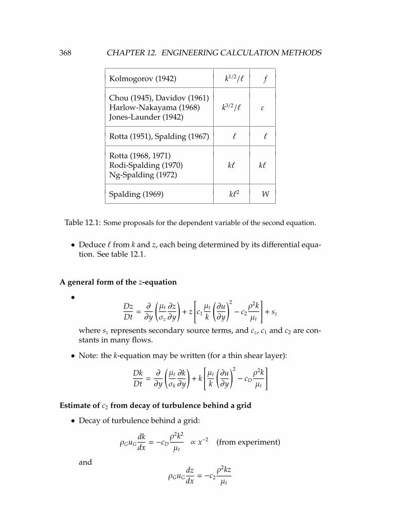
368 CHAPTER 12. ENGINEERING CALCULATION METHODS
Kolmogorov (1942) k1/2/` f
Chou (1945), Davidov (1961)Harlow-Nakayama (1968) k3/2/` εJones-Launder (1942)
Rotta (1951), Spalding (1967) ` `
Rotta (1968, 1971)Rodi-Spalding (1970) k` k`Ng-Spalding (1972)
Spalding (1969) k`2 W
Table 12.1: Some proposals for the dependent variable of the second equation.
• Deduce ` from k and z, each being determined by its differential equa-tion. See table 12.1.
A general form of the z-equation
•DzDt
=∂∂y
(µt
σz
∂z∂y
)+ z
c1µt
k
(∂u∂y
)2
− c2ρ2kµt
+ sz
where sz represents secondary source terms, and cz, c1 and c2 are con-stants in many flows.
• Note: the k-equation may be written (for a thin shear layer):
DkDt
=∂∂y
(µt
σk
∂k∂y
)+ k
µt
k
(∂u∂y
)2
− cDρ2kµt
Estimate of c2 from decay of turbulence behind a grid
• Decay of turbulence behind a grid:
ρGuGdkdx
= −cDρ2k2
µt∝ x−2 (from experiment)
and
ρGuGdzdx
= −c2ρ2kzµt
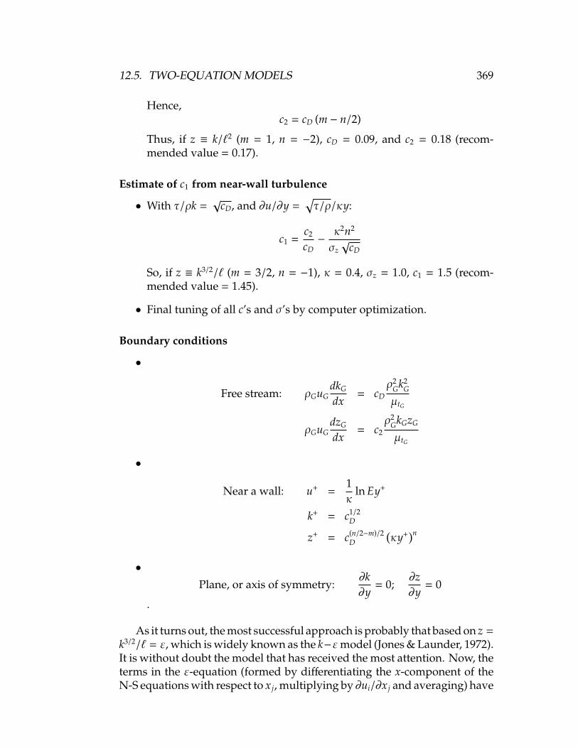
12.5. TWO-EQUATION MODELS 369
Hence,c2 = cD (m − n/2)
Thus, if z ≡ k/`2 (m = 1, n = −2), cD = 0.09, and c2 = 0.18 (recom-mended value = 0.17).
Estimate of c1 from near-wall turbulence
• With τ/ρk =√
cD, and ∂u/∂y =√τ/ρ/κy:
c1 =c2
cD−
κ2n2
σz√
cD
So, if z ≡ k3/2/` (m = 3/2, n = −1), κ = 0.4, σz = 1.0, c1 = 1.5 (recom-mended value = 1.45).
• Final tuning of all c’s and σ’s by computer optimization.
Boundary conditions
•
Free stream: ρGuGdkG
dx= cD
ρ2Gk2
G
µtG
ρGuGdzG
dx= c2
ρ2GkGzG
µtG
•
Near a wall: u+ =1κ
ln Ey+
k+ = c1/2D
z+ = c(n/2−m)/2D
(κy+)n
•Plane, or axis of symmetry:
∂k∂y
= 0;∂z∂y
= 0
.
As it turns out, the most successful approach is probably that based on z =k3/2/` = ε, which is widely known as the k−εmodel (Jones & Launder, 1972).It is without doubt the model that has received the most attention. Now, theterms in the ε-equation (formed by differentiating the x-component of theN-S equations with respect to x j, multiplying by ∂ui/∂x j and averaging) have
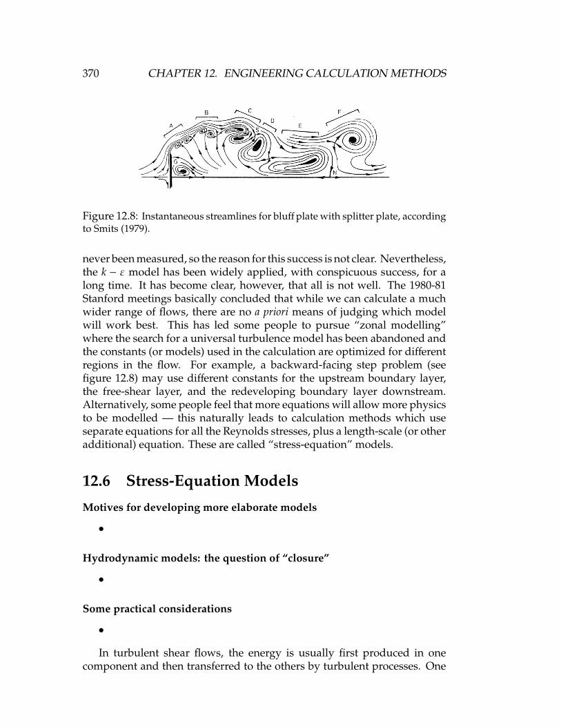
370 CHAPTER 12. ENGINEERING CALCULATION METHODS
Figure 12.8: Instantaneous streamlines for bluff plate with splitter plate, accordingto Smits (1979).
never been measured, so the reason for this success is not clear. Nevertheless,the k − ε model has been widely applied, with conspicuous success, for along time. It has become clear, however, that all is not well. The 1980-81Stanford meetings basically concluded that while we can calculate a muchwider range of flows, there are no a priori means of judging which modelwill work best. This has led some people to pursue “zonal modelling”where the search for a universal turbulence model has been abandoned andthe constants (or models) used in the calculation are optimized for differentregions in the flow. For example, a backward-facing step problem (seefigure 12.8) may use different constants for the upstream boundary layer,the free-shear layer, and the redeveloping boundary layer downstream.Alternatively, some people feel that more equations will allow more physicsto be modelled — this naturally leads to calculation methods which useseparate equations for all the Reynolds stresses, plus a length-scale (or otheradditional) equation. These are called “stress-equation” models.
12.6 Stress-Equation Models
Motives for developing more elaborate models
•
Hydrodynamic models: the question of “closure”
•
Some practical considerations
•
In turbulent shear flows, the energy is usually first produced in onecomponent and then transferred to the others by turbulent processes. One

12.6. STRESS-EQUATION MODELS 371
of the key terms in the equations of motion is the pressure strain term.The set of differential equations governing the transport of the (kinematic)Reynolds stresses uiu j may be written in the form:
Duiu j
Dt= −
[u juk
∂Ui
∂xk+ uiuk
∂U j
∂xk
]︸ ︷︷ ︸
generation
− 2ν∂ui
∂xk
∂u j
∂xk︸ ︷︷ ︸dissipation
+pρ
(∂ui
∂x j+∂u j
∂xi
)︸ ︷︷ ︸
pressure strain
−∂∂xk
[uiu juk − ν
∂uiu j
∂xk+
pρ
(δ jkui + δiku j
)]︸ ︷︷ ︸
diffusion
(12.11)
• The dissipation is handled in the usual way, that is,
2ν∂ui
∂xk
∂u j
∂xk= 2
3δi jε (12.12)
where ε comes from the dissipation (or length scale) equation. Forexample, Launder, Reece & Rodi (JFM, 1975) use:
DεDt
= Cε∂∂xk
(kε
ukul∂ε∂xl
)− Cε1ε
uiuk
k∂Ui
∂xk− Cε2
ε2
k(12.13)
• The diffusion term is usually modelled using a gradient diffusion hy-pothesis. For example, Daly & Harbour (1970) use:
uiu juk = C′skε∂ukul
∂xl(12.14)
This is an example of an isotropic effective diffusion formulation —more complicated forms are obviously possible.
• The generation term can be calculated directly.
• The pressure-strain term, or the pressure-strain redistribution tensoris a crucial element, and needs to be considered in detail.
The pressure-strain term
As in Chapter 11, we can write the pressure-strain term as:
−1ρ
u′∂p′
∂x= −
1ρ
∂p′u′
∂x+
1ρ
p′∂u′
∂x(12.15)

372 CHAPTER 12. ENGINEERING CALCULATION METHODS
The first term on the right is the spatial transport of turbulent energy bypressure gradients (sometimes called the pressure diffusion). The second termon the right represents the transfer of turbulent energy from u′ to v′ and w′
by pressure fluctuations. This process tends to isotropize turbulence, and itis part of the tendency-to-isotropy term. There is no net change of energy —when we write the equation for the rate of change of q2 these kinds of termssum to zero because of continuity. However, in stress-equation modelling,this redistribution term needs to be dealt with explicitly.
Following Chou (1945), the explicit appearance of the pressure in thecorrelation is eliminated by taking the divergence of the equation for thefluctuating velocity ui, thus obtaining a Poisson equation for p. The pressure-strain correlation may then be re-expressed in the following form for aposition x in the flow:
pρ∂ui
∂x j=
14π
∫vol
(∂2ulum
∂xl∂xm
)′∂ui
∂x j︸ ︷︷ ︸φi j,1
+ 2(∂Ul
∂xm
)′ (∂um
∂xl
)′ (∂ui
∂x j
) d vol∣∣∣x − y∣∣∣ + Si j
︸ ︷︷ ︸φi j,2
(12.16)
where capital letters indicate mean values and lower case letters indicatefluctuating quantities, and where terms with and without a prime relate tovalues at y and x respectively (the integration being carried out over y-space),and Si j is a surface integral which will be negligible away from the vicinityof a solid boundary. Equation 12.16 suggests that there are two distinctkinds of interaction giving rise to the correlation p∂ui/∂x j; one involvingjust fluctuating quantities (φi j,1) and another arising from the presence of themean rate of strain (φi j,2).
Nearly every worker who has made closure approximations for equa-tion 12.11 has adopted Rotta’s (1951) proposal forφi j,1, which may be writtenas:
φi j,1 + φ ji,1 = −c1
(εk
) (uiu j −
23δi jk
)= φi j,1, for brevity (12.17)
where c1 is supposed to be a constant (at any rate, at high Reynolds numbers)and k and ε are the time-averaged turbulence kinetic energy and energydissipation rate respectively: the quotient k/ε thus represents a characteristicdecay time of the turbulence. According to equation 12.17, the sign of φi j,1 isalways such as to promote a change towards isotropy, its magnitude beingproportional to the local level of anisotropy. Rotta (1951) originally proposed

12.7. LARGE EDDY SIMULATION 373
that c1 should be about 1.4, though later he showed (Rotta, 1962) that a valueabout twice as large provided a better fit to Uberoi’s (1957) data on the decayof highly anisotropic turbulence.
φi j,1 is called the return-to-isotropy part of the pressure strain tensor, sincein flows without any mean strain this term is responsible for the return toisotropy, and φi j,2 is called the rapid part of the pressure strain tensor, sinceunder conditions of rapid distortion the effects of far outweigh the effectsof φi j,1 (Townsend 1971). There is considerable disagreement on what thecorrect form for φi j,2 is, and it is an area of current work (see, for example,Shih & Lumley 1990, JFM).
12.7 Large Eddy Simulation
The following material was taken from the Ph.D thesis by Ugo Piomelli(Stanford, 1987.)
12.7.1 General considerations
Numerical solution of the Navier-Stokes equations is made very difficult bythe large number of grid points required to adequately resolve all the scalesof motion. It is easy to show (Tennekes & Lumley, 1972) that the ratio of thelargest and smallest scales of motion varies with the 3/4 power of the flowReynolds number. This implies that the number of grid points required forthree-dimensional Direct Numerical Simulation (DNS) of a turbulent flowincreases with the 9/4 power of the Reynolds number of the flow.
Thus only very low Reynolds number, geometrically simple flows havebeen treated by means of DNS. Only recently has simulation of wall boundedflows been successfully attempted. Moser & Moin (1984, 1987) studied theturbulent flow in a mildly curved channel, Spalart & Leonard (1985) andSpalart (1986a,b) simulated a boundary layer and Kim, Moin & Moser (1987)studied the flow in a plane channel.
These efforts are limited to very low Reynolds numbers: 3200 for thechannel (based on channel half-width and centerline velocity) and 1400for the boundary layer (based on edge velocity and momentum thickness).Even then, they require very large amounts of computer CPU time, tens ofhours on supercomputers. These limits restrict the usefulness of DNS tobasic research.
The simulation of turbulent flows for engineering application is usuallybased on the Reynolds-Averaged Navier-Stokes equations (RANS), in whichthe effect of all the turbulent structures is modelled. This approach is limitedby the fact that it is difficult, if not impossible, to model the large structureswhich differ greatly from one flow to the other. Even the most complex

374 CHAPTER 12. ENGINEERING CALCULATION METHODS
models have not been successfully applied to widely different classes offlows.
Large Eddy Simulation (LES) is an approach to the simulation of turbu-lent flows in which the large scales of motion are computed explicitly, whilethe effect of the small scales (subgrid scales or SGS) is modelled. The ratio-nale for this method is based on two experimental observations: first, thesmall scales, which are created by interactions among larger scales, are moreisotropic and universal in nature than the large scales, which are determinedby the boundary conditions; one should therefore be able to model them ina more general way. Secondly, since the small scales carry only a smal1fraction of the total turbulent energy, it may be possible to model them in afairly crude way without overly affecting the structure of the large scales.
In LES one solves the equations of motion for the large scale structures,which can be formally obtained by multiplying the Navier-Stokes equationsby a filtering function and integrating them over the computational domain.The smallest scale admitted by the filter, A, determines the cutoff betweensubgrid and resolved scales.
LES was first applied to engineering flows by Deardorff (1970), whocarried out a simulation of turbulent flow in a channel at very high Reynoldsnumber using only 6720 grid points. The effect of the subgrid scales wasmodelled by the eddy viscosity model introduced by Smagorinsky t1963).The agreement of the mean velocity profile with the experimental data wasfair, and good agreement was obtained for the Reynolds stress profiles.
Schumann (1973, 1975) extended Deardorff’s results by using more points(up to 65536), as well as a subgrid scale model which divided the subgridscale (SOS) stress into a locally isotropic and an inhomogeneous part. Hiscalculations were carried out at Reynolds number 150,000 and constitute amarked improvement over Deardorff’s.
Both Deardorff and Schumann used approximate boundary conditionsdesigned to ensure that the logarithmic law-of-the-wall is obeyed; they didnot attempt to compute the dynamics of the wall layer, in which most of theturbulence is produced.
During the period 1970–1978 LES was applied by the Stanford group tohomogeneous unbounded flows (Kwak, Reynolds & Ferziger, 1975; Shaanan,Ferziger & Reynolds, 1975; Clark, Ferziger & Reynolds, 1977, 1979 and oth-ers).
Moin, Reynolds & Ferziger (1978) were the first to attempt the simulationof a wall-bounded flow in which the wall layer was computed. In their sim-ulation they used 16 points in the streamwise and spanwise directions and63 unequally spaced points in the direction normal to the walls. They alsoused the Smagorinsky model to account for the effect of the subgrid scales.Although the grid resolution, especially in the streamwise and spanwise di-rections, was insufficient to resolve the streaky structures near the wall, the
12.7. LARGE EDDY SIMULATION 375
results of the simulation were encouraging: mean velocity, Reynolds stressand turbulent intensity profiles were in good agreement with experiments,except very near the wall.
Moin & Kim (1982) (hereafter called MK) improved on the results byMoin et al.. (1978) by using a much finer grid (64 × 63 × 128 points re-spectively in the streamwise, normal and spanwise directions). FollowingSchumann, they divided the SGS stress into a locally isotropic part and aninhomogeneous part meant to account for the poor spanwise resolution. Thesimulation was very successful; not only were the mean velocity, Reynoldsstress and turbulent intensities predicted accurately, but the higher orderstatistics agreed well with experimental results. The streaks were captured,although their spacing was too large. The poor resolution of the wall layerwas held responsible for the errors in the streak spacing and in the location ofthe peak in the streamwise turbulent intensity, as well as for discrepanciesbetween experimental and computed values of the higher order statisticsnear the wall.
Horiuti (1987) analyzed the numerical method used by Moin et al. (1978)and MK, and showed that their use of the rotational form of the Navier-Stokes equations coupled with finite differences in the normal directionproduces very large truncation errors near the wall. He suggested use of amodification of Arakawa’s (1966) scheme which is conservative and moreaccurate than MK’s approximation near the wall. Horiuti’s 1987 simulation,which used (64× 63× 64 grid points (and was therefore capable of resolvingthe wall layer) and the Smagorinsky model, showed extremely good agree-ment with experimental results, and with the DNS of Moser & Moin (1984,1987). The computed streak spacing was slightly larger than the value pre-dicted by MK, but the grid resolution was only half as fine in the spanwisedirection; the position of the peak in the streamwise turbulent intensity wascloser to the experimental value than in MK. The turbulent energy budgetswere in good qualitative agreement with those computed by Moser & Moin(1984, 1987) for a curved channel.
12.7.2 Governing equations
The equations governing the motion of an incompressible fluid in a channelare the Navier-Stokes equations and the continuity equation:
∂ui
∂t+∂uiu j
∂x j= −
1ρ
∂p∂xi
+ δi1 +1
Reτ∂2ui
∂x j∂x j(12.18)
∂ui
∂xi= 0 (12.19)
where the variables are made dimensionless using the channel half-widthδ and the friction velocity uτ = (τw/ρ)1/2. The summation rule applies to

376 CHAPTER 12. ENGINEERING CALCULATION METHODS
repeated indices. In the present work we shall use the convention that x1 orx is the streamwise direction, x2 or y the direction normal to the walls and x3
or z the spanwise or transverse direction. The velocity components in thosedirections will be denoted by u1, u2 and u3 or u, v and w.
In large eddy simulation we decompose the velocity ui in a large scalecomponent ui and a subgrid component u′i .
ui = ui + u′i (12.20)
The large scale field is defined by filtering:
u j(x1, x2, x3) =
∫D
3∏i=1
Gi(xi, x′i)u j(x′1, x′
2, x′
3)dx′1dx′2dx′3 (12.21)
where the integral is extended to the entire flow field and Gi is the filterfunction in the i-th direction. In the present simulations we have used twodifferent filters in the planes parallel to the wall: the Gaussian filter
Gi(xi, x′i) =( 6π∆i
)exp
[−6(xi − x′i)
2/∆2i
](i = 1, 3) (12.22)
and the sharp cutoff filter which is defined, in real space, by (Leonard, 1974):
Gi(xi, x′i) =2 sin
[π(xi − x′i)/∆i
]π(xi − x′i)
(i = 1, 3) (12.23)
With this filter the subgrid scales represent the effect of al1 the structureswith wavenumbers |ki| > π/ki. The sharp cutoff filter is implicitly appliedwhenever an infinite series is approximated by a finite number of modes.
In the direction normal to the wall it is desirable to use a filter withvariable width to account for the variation of the turbulence length scaleswith distance from the wall. This was accomplished by employing a boxfilter of variable width:
G2(y, y′) =
[∆+y j + ∆−y j
]−1for y − ∆−y j < y′ < y + ∆+y j,
0 for y′ < y − ∆−y j, y′ > y + ∆+y j;(12.24)
with∆+y j = 1
2 (y j+1 − y j)∆−y j = 1
2 (y j − y j−1)
for 1
2 (y j + y j−1) < y < 12 (y j+1 + y j)
where y j is the vertical coordinate of the j-th computational point. Appli-cation of the filtering function G2 defined by equation 12.24 to ui can beinterpreted as averaging ui over the grid spacing.

12.7. LARGE EDDY SIMULATION 377
When any of the filters described here is used, partial differentiation andfiltering commute (see Moin et al., 1978 and also Moin & Kim, 1982). For theGaussian and sharp cutoff filter, the linear dimension of the filter in the i-thdirection, ∆i is usually twice the grid spacing hi (see Kwak et al., 1975).
Applying the filtering operation to the non-linear term in the Navier-Stokes equations we obtain
∂∂x j
=∂∂x j
[uiu j + Li j + Ci j + Ri j
](12.25)
where Li j = uiu j − uiu j
Ci j = uiu′j + u ju′jLi j = u′iu
′
j
(12.26)
The terms in equation 12.26 are referred to as, respectively, Leonard stresses,cross (or outscatter) terms and subgrid scale Reynolds stresses (or backscat-ter). While the cross terms and SGS Reynolds stresses are invariably mod-elled, the Leonard stresses can be either modelled or computed. Whensecond-order accurate difference schemes are used, the Leonard stresses Li j
are of the same order as the truncation error (Shaanan et al., 1975). Whenhigher order difference schemes or spectral methods are employed, it is de-sirable to compute Li j exactly. If the Leonard stresses are computed (as inMK) the filtered Navier-Stokes equations assume the form
∂ui
∂t+∂uiu j
∂x j= −
∂P∂xi
+ δi1 −∂τi j
∂x j+
1Reτ
∂2ui
∂x j∂x j(12.27)
where τi j = Qi j −13Qkkδi j
P = p/ρ + 13Qkk
Qi j = Ri j + Ci j
(12.28)
The term τi j in equation 12.28 is also frequently referred to as subgrid scaleReynolds stress.
The filtered continuity equation is
∂ui
∂xi= 0 (12.29)
12.7.3 The residual stress model
The assumptions on which LES is based, such as the universality and ho-mogeneity of the small eddies and the hypothesis that the small eddies donot contribute much to the total turbulent kinetic energy, imply use of fairly

378 CHAPTER 12. ENGINEERING CALCULATION METHODS
crude models to simulate the effect of the small eddies on the large ones thatare simulated.
The model that has been used most frequently in LES of turbulent flowsis an eddy viscosity model due to Smagorinsky (1963):
τi j = −2νTSi j (12.30)
where
Si j =12
(∂ui
∂x j+∂u j
∂xi
)(12.31)
is the strain-rate tensor, and νT is an eddy viscosity. To determine the eddyviscosity we assume that, in the balance of subgrid scale turbulent kineticenergy q2 = u′iu
′
i , the two dominant effects are production and dissipation.The production ℘ is given by
℘ = −u′iu′
jSi j = 2νTSi jSi j (12.32)
while dimensional analysis suggests that the dissipation ε is given by
℘ = c1
(u′iu
′
i
)3/2
`(12.33)
in which ` is the characteristic length scale of the subgrid eddies.Equating equation 12.32 to 12.33 and assuming that the eddy viscosity
is proportional to the characteristic length and velocity scales of the smalleddies:
νT = c2`(u′iu
′
i
)1/2(12.34)
we obtain Smagorinsky’s (1963) model:
νT = `2√
2Si jSi j (12.35)
in which all the constants have been absorbed by the length scale `.Since ` is the size of a representative subgrid scale eddy, it must be related
to the filter size ∆, which is in turn related to the grid size h. If the cutoffis within the inertial sub-range of homogeneous isotropic turbulence, Lilly(1966, 1967) found that ` can be expressed as
` = CS∆ (12.36)
with CS = 0.23.For anisotropic filters no uniquely superior expression for ` has yet been
found. Near the wall the growth of turbulence structures is inhibited, and thereduction of the length scales must be taken into account. Non-uniformity

12.7. LARGE EDDY SIMULATION 379
of the computational grid in the normal direction is not usually sufficient toaccount for the variation of the length scales, and empirical corrections areused near the wall.
MK modified the formulation used by Deardorff (1970) to include thereduction of the length scales near the wall by Van Driest (1956) damping;the latter is often used in one-point closure models. This leads to
`MK = CS[1 − exp
(−y+/A+)] (∆1∆2∆3)1/3 (12.37)
where A+ = 25. The exponential damping can be added to the length scaleproposed by Bardina, Ferziger & Reynolds (1980) to yield
`BFR = CS[1 − exp
(−y+/A+)] √
∆21 + ∆2
2 + ∆23 (12.38)
An alternative formulation proposed by Mwn and Callen (1986) is
1`MC
=1
CS (∆1∆2∆3)1/3 +1
κ(1 −
∣∣∣y∣∣∣) (12.39)
in which κ is the von Karman constant. Equation 12.39 matches Deardorff’slength scale to Prandll mixing length on the assumption that, near the walls,at y = ±l, the size of the subgrid eddies scales with the distance from thewall.
Another expression for ` was proposed by Leslie (1985):
`L = CS[1 − exp
(−y+/A+)] (∆−3/4
1 + ∆−3/42 + ∆−3/4
3
)−4/3(12.40)
We suggest an expression of the form
`PFM = CS
[1 − exp
(−y+3/A+3
)]1/2(∆1∆2∆3)1/3 (12.41)
which ensures the proper behavior for the SGS Reynolds stress τ12 near thewall (τ12 ∼ y+3).
The two-part model, introduced by Schumann (1975) and employed byMK, is usually written:
τi j = −2νT
(Si j − 〈Si j〉
)− 2ν∗T〈Si j〉 (12.42)
where 〈〉 represents averaging over a plane parallel to the wall. The firstterm in equation 12.42 is a modified Smagorinsky model with
νT = `2√
2(Si j − 〈Si j〉
) (Si j − 〈Si j〉
)(12.43)

380 CHAPTER 12. ENGINEERING CALCULATION METHODS
The second term, in which
ν∗T = `∗2√
2〈Si j〉〈Si j〉 (12.44)
is supposed to account for the production of subgrid turbulent kinetic energyin the viscous sublayer, where the grid resolution is inadequate. While thelength scale ` represents an average of length scales in all directions, `∗ onlyrepresents the spanwise structures that the grid cannot resolve. The form of`∗ originally proposed by Schumann (1975) is
`∗S = min[c√
∆1∆3, κyw
](12.45)
in which yw is the distance from the nearest wall and c = 0.065.Moin & Kim (1982) used
`∗MK = c∆23
[1 − exp
(−y+3/A+3
)]2(12.46)
Another model that has been very successful for the simulation of ho-mogeneous turbulence, as well as for shear flows, is the mixed model. Thismodel, developed by Bardina et al. (1980) is based on the assumption thatthe main interaction between resolved and subgrid scale eddies takes placebetween the smallest resolved eddies and the largest subgrid scale eddies.Since filtering a velocity field removes the smallest scales of the flow, a ve-locity field that is filtered twice will contain only the very largest scales ofmotion. The difference between a filtered velocity field and one that hasbeen filtered twice, ui − ¯ui, will therefore contain predominantly interme-diate scales of motion, that is, the smallest resolved scales. On the basisof these considerations Bardina et al. (1980) introduced the scale similaritymodel, which is of the form
τi j = CB
(uiu j − ¯ui ¯u j
)(12.47)
Bardina et al. (1980) found that the scale similarity model correlateswell with the subgrid scale Reynolds stresses, but does not dissipate energy.They then proposed the mixed model, which is a linear combination ofthe scale similarity model (equation 12.47) and the Smagorinsky model(equation 12.30):
τi j = CB
(uiu j − ¯ui ¯u j
)− 2νTSi j (12.48)
The constant CB was set to 1.1 by fitting numerical results to experimentaldata.
Speziale (1985) showed that, if the Leonard stresses are computed, Galileaninvariance of the equations of motion is not preserved if either the Smagorin-sky or the two-part model is employed, but is preserved only if the mixed

12.7. LARGE EDDY SIMULATION 381
model is used with CB = 1. If the Leonard stresses are modelled, however,then either the Smagorinsky or the two-part model guarantees Galileaninvariance, and the mixed model cannot be used in the form given by (equa-tion 12.48).
It should also be noticed that when one uses either the Smagorinsky orthe two-part model, the trace of the subgrid scale stress tensor has to beadded to the pressure, since the strain tensor is trace-free. With the mixedmodel, however, such is not the case, and one can replace (equation 12.28)with
τi j = Ri j + Ci j
P = p/ρ (12.49)

382 CHAPTER 12. ENGINEERING CALCULATION METHODS

Chapter 13
Structure of Turbulence inWall-Bounded Shear Flows
13.1 Physical Models for Turbulent Boundary Lay-ers
There have been many studies of organized motions in turbulent boundarylayers. The following extract from the MSE thesis of J. Goldstein (Princeton,1991) provides a convenient summary of this work.
Hussain (1983) defines a coherent structure as “a connected large-scaleturbulent fluid mass with phase correlated vorticity over its spanwise ex-tent.” He states that organized structures are responsible for significanttransport of mass, momentum, and energy without actually being energeticthemselves, and that they must be spatially mutually exclusive. He theorizesthat it is this exclusivity that makes the interaction of coherent structures,such as pairing and tearing, a highly non-linear process. Hussain writes that“the presence of coherent structures everywhere in a turbulent shear flowsuggests a sequence of formation, evolution, and decay.” The formationof these structures seems to be due to some instability mechanism, eventhough this mechanism and the processes by which these structures evolveare not yet fully understood. Decay of coherent structures seems to be aresult of inter-structure interaction and viscous diffusion.
Yule (1980) proposed that coherent structures are “repetitive, have sur-vival distances much larger than the structure size, and contribute signif-icantly to the kinetic energy.” Hussain, however, states that the last twoconditions do not occur in general, but are dependent on where the coher-ent structure exists in the boundary layer. Brown & Thomas (1978) statethat an organized structure is “a recognizable large-scale motion which hasits own internal dynamics which of itself and through its interactions withother similar structures dominates the mechanism of the flow.”
383

384 CHAPTER 13. STRUCTURE OF TURBULENCE
Figure 13.1: Schematic of a horseshoe vortex, the dominant coherent structure ina turbulent boundary layer according to Theodorson (1952).
It was Theodorsen (1952) who first suggested the existence of organizedstructures in turbulent boundary layers. He went so far as to proposethat the dominant coherent structure in a turbulent boundary layer is ahorseshoe-shaped vortex loop inclined downstream at 45 to the wall (seefigure 13.1). Theodorsen theorized that vortex stretching is the only availablemechanism by which the concentration of vorticity can be increased to leadto turbulence. Based on his analysis of the enstrophy equation, Theodorsenconcluded that the.vortex stretching term in the equation will be a maximumon a plane inclined 45o to the wall. His physical reasoning seems to be quitesound, but it is still not known why the breakdown of laminar shear flows toturbulence should be accompanied by the formation of horseshoe vorticesinclined at 45, although the existence of horseshoe vortices in turbulentshear flows and their corresponding average angle of inclination has beenverified by large numbers of direct observations, beginning with Theodorsenhimself (working with Prof. John Weske in the early 1950’s). See figure 13.2.This structure in particular has received particular attention over the years,since the horseshoe vortex seems to serve as the dominant dynamical linkbetween the different regions of a turbulent boundary layer. This point willbe discussed further in later sections.
It is common practice to catalog organized structures depending onwhere they occur in the boundary layer. Inner-layer structures, accordingto taxonomy by Robinson (1991), consist primarily of low- and high-speedstreaks, vortical structures such as legs and arches and the burst-sweep cycle.Outer layer structures basically consist of large-scale long-lived structuressuch as bulges and backs. Other coherent structures include pockets, highpressure potatoes, near-wall shear layers, vortical structures, and wall pres-sure fluctuations. Horseshoe vortices of various scales are found in boththe inner and outer layers. Structures relevant to the present work will bediscussed further in later sections.

13.2. INNER LAYER STRUCTURES 385
Figure 13.2: Early flow visualization studies of horseshoe vortices by Theodorsonand Weske.
13.2 Inner Layer Structures
Kline et al. (1967), using hydrogen bubbles in water to visualize a turbu-lent boundary layer, found that the bubbles, when introduced very close tothe floor, collect into streamwise streaks with an average spanwise separa-tion of about 100 wall units (see figure 13.3). These streak patterns migrateslowly downstream, with a velocity less than the local mean, and are there-fore called low-speed streaks. Additional probe measurements showed thatregions where velocity is greater than the local mean exist between the low-speed streaks. These regions are known as high-speed streaks. Robinson et al.(1989) studied the low-speed and high-speed streaks in the interpretationof the Spalart (1986) turbulent boundary layer DNS data. They found thatthe length of the low-speed streaks often exceeds 1500 wall units, and werebetween 20 and 80 wall units wide. These low-speed streaks are certainlycoherent structures, but are not particularly energetic. In contrast, the lengthof high-speed streaks rarely exceeds 800 wall units, and their widths rangebetween 40 and 100 wall units (see figure 13.4).
Kline it et al. also noted that the low-speed streaks rise very slowly fromthe floor. When the streak reaches a y+ of about 10, it begins to oscillate.The oscillation increases in magnitude and the lift-up continues until a y+
of about 15 (on average), when the streak breaks up. This can occur at a y+
as high as 30. The remnants of the streak continue moving away from thewall. This streak lift-up, oscillation, and break-up is termed an ejection. One

386 CHAPTER 13. STRUCTURE OF TURBULENCE
Figure 13.3: Hydrogen bubbles marking low-speed streaks in the sublayer, fromKline et al. (1967). Wire located at (a) y+ = 3; and (b) y+ = 38. The flow direction isfrom top to bottom.
or more ejections from the same low-speed streak is termed a burst, which isusually followed by an inrush of high momentum fluid from above, called asweep. Blackwelder (1978) suggests that the upward motion of streaks ceaseupon the arrival of the sweep imposed by the outer flow field. The sweepmotion results in an inflectional velocity profile, which according to Chen &Blackwelder (1978) cause instabilities that trigger ejections. This sequenceof events is called the burst-sweep cycle, and seems to be responsible formost of the turbulent energy and instantaneous Reynolds stress (−ρu′v′)

13.2. INNER LAYER STRUCTURES 387
Figure 13.4: (a) Low- and high-speed streaks; and (b) Low-speed streaks withejections (u′v′ second quadrant) and sweeps (u′v′ fourth quadrant). From theanalysis of Spalart’s DNS of a turbulent boundary layer by Robinson et al. (1989).Flow is from left to right, Reθ = 640, y+ = 15.
production in the boundary layer, hence its importance.Hot-wire anemometry has been used extensively to study the structure
of coherent motions. However, identifying ejections and sweeps in hotwire data is a complicated task. Various conditional sampling techniqueshave been developed to cope with this problem. Wallace et al. (1972) andWilmarth & Lu (1972) introduced the quadrant technique, a method for clas-sifying u′v′ events. They labelled a burst a quadrant two (Q2) event (u′ < 0,v′ > 0), and a sweep a quadrant four (Q4) event (u′ > 0, v′ < 0). Events inthe other two quadrants (Q1 and Q3) were labelled interactions. There areother methods used to detect ejections and sweeps, such as u′v′-threshold,u′v′ slope threshold, u′ threshold (U-level), u′ slope threshold, and variable-interval time-averaging (VITA). The effectiveness of each detection criterionwere compared in Bogard & Tiederman (1986). They concluded that the

388 CHAPTER 13. STRUCTURE OF TURBULENCE
quadrant technique, with an appropriate threshold, can most readily iden-tify ejections. The VITA and U-level techniques also had low probabilitiesfor error, but were more sensitive to the threshold chosen. Identifying burstsand sweeps in visualization data is an even more complicated task, to bediscussed later.
There is considerable controversy as to what part of the burst-sweep cy-cle contributes most to turbulent energy production. Grass (1971) showedthat the production of turbulent energy is an intermittent process, and thatit occurs through contributions by both sweeps and bursts. He also con-cluded that the contribution of sweeps to turbulent energy production islimited to the wall region, while the contribution of ejections extended wellinto the outer region. Kim et al. (1971) concluded that nearly all of the tur-bulent energy production occurs during ejections in the inner layer. Corino& Brodkey (1969) concluded that bursting occurs 18% of the time and isresponsible for 50 to 70% of the total turbulence production. Kline & Corinoseparately estimated that 70% of the Reynolds stress production occurs dur-ing ejections. In contrast, Willmarth & Lu (1972) concluded that 60% ofthe Reynolds stress production occurs during the sweep cycle. Lu & Will-marth (1973) concluded that bursts account for 77% of u′v′ production, whilesweeps account for 55%. The excess over 100% is accounted for by inter-actions with negative contributions. Wallace et al. (1972) measured equalcontributions (70%) from ejections and sweeps. These values are the resultof analysis of hot wire data.
A number of investigators have attributed the existence of the high-and low-speed streaks and the bursting cycle in the viscous sublayer to thepresence of counter-rotating streamwise vortex pairs. Bakewell & Lumley(1967) found, through an eigenfunction decomposition of the fluctuatingstreamwise velocity, that the dominant coherent structure in the inner layerwas a streamwise counter-rotating vortex pair elongated in the streamwisedirection, with an average spanwise separation of 90–100 wall units (seefigure 13.5). The planes of circulation of these vortices were found to beinclined slightly upstream from wall normal. The effect of these streamwisevortices on the surrounding fluid is to sweep near-wall low-momentumfluid between them and induce an upward motion. Bakewell & Lumleysuggested the ejections result from the plane of circulation of the stream-wise vortices becoming normal to the wall, coupled with an increase incirculation. Townsend (1970) proposed that a pair of counter-rotating vor-tices inclined 30 to the floor was the dominant-coherent structure in thenear-wall region. Head & Bandyopadhyay (1981) found visual evidence forthese vortices (see figure 13.6). How are these vortices formed?
Tu (1966) hypothesized that the vortices are formed when transversevorticity undergoes local distension near the wall. The distended vortexloop is stretched and distorted into counter-rotating vortex pairs. Brown &

13.2. INNER LAYER STRUCTURES 389
Figure 13.5: A streamwise counter-rotating vortex pair, proposed by Bakewell &Lumley (1967) to be the dominant vortical structure in the inner layer: (a) proposedstructure; (b) corresponding streamlines on centerline.
Figure 13.6: Streamwise vortex pairs from the visualization by Head & Bandy-opadhyay (1981).
Thomas (1978) found that the large-scale structure streamlines are concavenear the wall (see figure 13.7). Here, the mean vorticity and the circulationare of opposite signs, which according to Rayleigh is the criterion for an

390 CHAPTER 13. STRUCTURE OF TURBULENCE
Figure 13.7: Curvature of the inner layer streamlines which may give rise toTaylor-Gortler instabilities. From Brown & Thomas (1978).
inviscid instability. In a viscous flow, if the streamline curvature is largeenough, the condition may give rise to Taylor-Gortler vortices. This, Brown& Thomas concluded, is the mechanism for the formation of the streamwisevortices. Alternatively, it has been suggested that the streamwise vorticesare actually the legs of the horseshoe vortices. However, Robinson et al.showed that not all these quasi-streamwise vortices, as they called them,are the legs of horseshoe vortices, and that whole horseshoe vortices withtwo trailing legs are very rare. In addition, the length of these legs (vorticeshaving a predominantly streamwise orientation, according to Robinson etal.) is much less than the expected length of the streamwise counter-rotatingvortex pairs according to Bakewell & Lumley.
In addition to legs, Robinson et al. classified vortices as necks, extendingupward from the floor at an angle of about 45 to the floor, and heads, havinga predominantly transverse orientation (see figure 13.8). The vortices wereextracted from the numerical data by assuming that the vortices have a low-pressure core, and setting an appropriate pressure threshold. Changing thepressure threshold alters the connectivity of the vortices, but the basic shapeof the vortices is maintained. Robinson et al. found that strong ejections,in general, occur in two locations: on the inboard sides of legs, and behindheads. This is to be expected, since the vortices there, through Biot-Savartinteractions, induce an upward velocity in the surrounding fluid. Likewise,

13.2. INNER LAYER STRUCTURES 391
Figure 13.8: Vortex taxonomy by Robinson et al. (1989).
Figure 13.9: Location of ejection (u′v′ second quadrant) and sweep (u′v′ fourthquadrant) events with respect to vortical structures. From Robinson et al. (1989).
strong sweeps are generally found on the outboard sides of legs and necks(see figure 13.9).

392 CHAPTER 13. STRUCTURE OF TURBULENCE
13.3 Outer Layer Structures
Since it was an accepted fact that most of the turbulent energy productionoccurs in the inner layer, and it appeared that the outer layer was rather pas-sive, most of the early coherent structure studies focused on the inner layer.There has been, however, renewed interest in the outer layer in recent years.Large-scale structures appear to play an important role in the dynamics ofthe turbulent boundary layer. They are responsible for large-scale mixingin the outer layer, and play a dominant role in the entrainment of high-momentum freestream fluid into the boundary layer. Large-scale structuresmay also provide the trigger for inner layer instabilities to develop.
Chen & Blackwelder (1978) used temperature tagging to study the large-scale structures in a turbulent boundary layer. They heated the wall slightlyso that low momentum, near-wall fluid would be “hot,” and high mo-mentum, outer layer fluid would be “cold” Using two vertically displacedhot-wire probes, they found the average time delay between when the hot-cold interface marking a large-scale structure reached the lower and higherprobes. They were thus able to determine the average large-scale structureangle to be approximately 45 between y/δ = 0.15 and 0.67.
The outer layer appears to be dominated by large scale vortical struc-tures, called bulges, and large scale incursions of irrotational fluid that mayreach almost all the way to the floor. These bulges have spanwise andstreamwise dimensions of the order of δ, and have long survival distances.The convection velocity of bulges was found to be between 0.8 and 0.9U∞.Kovasznay et al. (1970) found that if the flow were viewed from a coordinatesystem moving at this convection velocity, a stagnation point appears on theback of the large-scale structure at about y/δ = 0.8. This phenomenon wasalso observed by Brown & Thomas (1978) and Falco (1977) (see figure 13.10).Kovasznay et al. concluded that the upstream-facing side of the structure isthe most active. This phenomenon of increased turbulence activity on theupstream-facing region of a turbulent/non-turbulent interface is found in anumber of flows.
Head & Banyopadhyay (1981) performed an extensive survey of outerlayer coherent structures at various Reynolds numbers. The visualizationstudy consisted of seeding the turbulent boundary layer with smoke andilluminating it with a laser sheet at various orientations. These includedtransverse light planes inclined downstream at 45, the average character-istic angle of the horseshoe vortices, and upstream at 45, perpendicularto the plane of the horseshoes (see figure 13.11). The visualization withthe laser sheet oriented at 45 downstream showed a number of invertedU-shaped structures which were interpreted as being horseshoe vortices. Itwas noted that the aspect ratio of these U-shaped structures increased withReynolds number. With the laser sheet oriented at 45 upstream, the visual-

13.3. OUTER LAYER STRUCTURES 393
Figure 13.10: Streamlines in a large-scale bulge with the observer moving at 0.8U∞,showing the saddle point on the back of the structure. From Falco (1977).
Figure 13.11: Cuts along and perpendicular to the plane of the horseshoe vortices,showing (a) inverted U-shaped loops; and (b) mushrooms. Top: low Reynoldsnumber; Bottom: high Reynolds number. From Head & Bandyopadhyay (1981).
ization revealed counter-rotating vortex pairs resembling mushrooms. Thisseemed to confirm that horseshoe vortices were, in fact, the dominant coher-ent structure in the turbulent boundary layer. However, the upstream- anddownstream-facing plane cuts were never of the same structure at the sameinstant in time. Tnerefore, that these structures were horseshoe vorticescould not be proven conclusively.
When the flow was visualized using a streamwise-oriented laser sheet,

394 CHAPTER 13. STRUCTURE OF TURBULENCE
Figure 13.12: Random distribution of horseshoe vortices. From Perry & Chong’s(1982) model of a turbulent boundary layer.
it was observed that, at least occasionally, the horseshoe vortices would risefrom the floor in an ordered fashion, their heads making a 20 angle to thefloor. This, in addition to being another level of coherence, could suggestthat the formation of a horseshoe vortex and its rise from the wall createsconditions which are beneficial to the formation of a smaller horseshoebehind it.
Perry & Chong (1982) proposed a model for the turbulent boundarylayer consisting of different distributions of Λ-shaped vortices, inclined at acharacteristic angle to the floor, embedded in an irrotational flow (see fig-ure 13.12). The model assumes that all the circulation in the flow residesin these vortices. The vortices, through Biot-Savart interactions, move andstretch each other. This stretching results in an increase in the vortex’s as-pect ratio, causing the vortex legs to come closer together. This results invorticity cancellation and eventually, death by viscous dissipation. Perry& Chong used random, discrete, and continuous distributions of vortexheights in their model. They set both the discrete and continuous distribu-tions to satisfy the law of the wall, and their model in turn predicts otherknown turbulent boundary layer parameters such as spectra. Their workhelped validate the findings of many previous studies which suggested thathorseshoe vortices are the dominant structure in turbulent boundary layers.
The combined visualization and hot wire study by Palco (1977) intro-duced the notion of the “typical” eddy as the coherent structure responsiblefor a large part of the Reynolds stress production in the outer layer. Typicaleddies are highly coherent three-dimensional vortical structures, and arefound in turbulent boundary layers, wakes, jets, and mixing layers. In tur-bulent boundary layers, they are found embedded in large-scale bulges, andresemble distorted laminar vortex rings (see figure 13.13). Falco determinedthe average height and length of the typical eddies, but since his visualiza-tion study was conducted along a streamwise plane, no information about

13.3. OUTER LAYER STRUCTURES 395
Figure 13.13: (a) “Typical” eddies in a turbulent boundary layer; (b) Idealizedspanwise; and (c) cross-sections of a typical eddy. From Falco (1977). The flow isfrom left to right.
the spanwise scale of these eddies could be obtained. The average typicaleddy streamwise size was found to be constant at around 200 wall units.It is interesting that the streamwise scale of these eddies is fixed when thelength is scaled on inner layer parameters. This point will be discussedfurther in later sections. Typical eddies in the log region were found to havea convection velocity less than the convection velocity of the bulges theyappear in, and usually became part of bulges upstream that overtook them.In contrast, typical eddies in the outer layer convect downstream faster thanthe large scale structure they appear in and will move to the front of thebulge.

396 CHAPTER 13. STRUCTURE OF TURBULENCE
13.4 Interactions
When the bursting cycle was first studied, it was assumed to be a purelyinner layer phenomenon which scaled on inner layer parameters. Kline etal. (1967) proposed that the bursting period scaled on ν and uτ. However,in 1971, Rao et al. showed that, over a large range of Reynolds numbers, themean bursting period scales on U∞ and δ. They proposed a strongly interac-tive relationship between the inner and outer layers, one where large scalestructures scour the inner layer, causing intense shear which triggers localinstabilities, resulting in ejections. Laufer & Badri Narayanan (1971) notedthat the mean bursting frequency is approximately equal to the frequency ofthe passage of large scale structures in the outer layer. Blackwelder & Kaplan(1976) also concluded that the bursting frequency scales on outer variables.In contrast, Blackwelder & Haritonidis (1983) and Luchik & Tiederman(1987) concluded that the bursting frequency scales on inner variables. Thisongoing controversy suggests a complex relationship between the inner endouter layers.
There is further evidence which points to strong interactions between theinner and outer layers. Blackwelder & Kaplan (1976) examined the velocitysignals from an array of ten hotwires arranged vertically or in the spanwisedirection (see figure 13.14). They found a high degree of correlation inthe large scales in the vertical direction throughout the boundary layer,but almost none in the spanwise direction (at a y+ of 15). This is dueto the small scale of the structures at this height in the sublayer. Palcofound that the Reynolds number dependence of the typical eddy scale wasremoved by non-dimensionalizing the eddy lengths with inner variables,a strange notion since typical eddies are a turbulent phenomena, not aviscous phenomena. Over this range, the average eddy streamwise scaleis approximately constant at 200 wall units, and the average vertical scaleincreases slowly from an initial value of about 100 wall units. He reportsthat the Lu & Willmarth (1972) measurements of the duration of intenseturbulent production in the outer layer, when non-dimensionalized withinner variables, fit on the specified range. Head & Bandyopadhyay (1981)concluded that Falco’s typical eddies were actually longitudinal sections ofhorseshoe vortex tips. This seems to explain the scaling of the typical eddieson inner layer variables, and lends credence to Antonia’s (1972) conclusionthat “there seems to bc little doubt that large-scale bursts (of high shearstress) observed near the outer region of the boundary layer originate fromor at least extend through to the inner layer region of the flow.”
Praturi & Brodkey (1978) performed a stereoscopic study of a turbu-lent boundary layer (Reθ = 900) by photographing the motion of tracerparticles, using a camera moving with the flow at 70% of the freestreamvelocity. They concluded that “wall-region vortex motions are a result of in-

13.4. INTERACTIONS 397
Figure 13.14: Velocity traces from an array of ten hot wires placed in a turbulentboundary layer, arranged (a) vertically; and (b) spanwise. From Blackwelder &Kaplan (1976).
teraction between the incoming higher-speed fluid from the outer region ofthe boundary-layer and the outflowing low-speed wall-region fluid.” Thisobservation is in direct contradiction to all models which suggest that theoutflow of low-speed fluid in the near wall region is caused by counter-rotating vortex pairs. In addition, even though large numbers of frameswere studied, complete horseshoe vortices were not detected, although thevortex elements which make up horseshoes were observed. This conclusionagrees with that of Robinson et al. (1989).
Brown & Thomas (1978) correlated wall shear stress data with velocitydata at various heights in the boundary layer. They found a line of max-imum correlation tilted 18 from the horizontal, which they hypothesizedwas due to a large-scale organized structure moving at a characteristic con-vection velocity and angle producing a wall shear stress response. Offen &

398 CHAPTER 13. STRUCTURE OF TURBULENCE
Figure 13.15: Model of the interaction between a horseshoe vortex and a low-speedstreak. From Hinze (1975).
Kline (1975) suggested that structures in the logarithmic region are respon-sible for sweeps, which in turn, establish conditions which cause ejectionsfurther downstream. They also hypothesized that large scale outer layerstructures are formed as a result of vortex pairing by a number of remnantsof the vortices associated with the bursting cycle. Smith (1978) studied therelationship between inner and outer layer coherent structures using flowvisualization from a moving frame of reference. He proposed that burstingis directly related to the passage of a large-scale motion, usually a transversevortex. Logarithmic-layer typical eddies could very well be the large-scalestructure in question.
Researchers have long believed that a strong dynamical link exists be-tween horseshoe vortices and the bursting cycle. Hinze (1975) proposed thefollowing model: due to some outer-layer disturbance, he states, a horse-shoe vortex forms close to the wall (see figure 13.15). The vortex tip risesfrom the wall due to self-induction, and the velocity gradient stretches thevortex. The stretching causes the vorticity to become more concentrated,inducing an outward flow between its legs. As the horseshoe rises from thefloor, an intense shear layer with an inflection point forms, giving rise to lo-cal instabilities which produces breakdown of the vortex tip. The pressurewave of this chaotic break-up, or burst, propagate through the boundarylayer. An inrush of high-momentum fluid follows. Interactions betweenthis sweep and slower fluid may give rise to another horseshoe vortex, andthe cycle repeats itself.
Acarlar & Smith (1984) studied the formation and evolution of horse-

13.4. INTERACTIONS 399
shoe vortices using hydrogen bubbles. The viscous sublayer was trippedwith a hemispherical disturbance embedded in the tunnel floor, causingvortex-sheet roll-up and the formation of a horseshoe vortex. Based ontheir observations, they proposed a model for the burst/sweep cycle (seefigure 13.16): in a turbulent boundary layer, a disturbance, possibly fromthe outer layer, imposes an adverse pressure gradient on the near-wall fluid,causing a local deceleration. When the decelerated fluid interacts withfaster-moving fluid in the near-wall region, a highly unstable inflectionalvelocity profile results, giving rise to a roll-up of the vortex sheet into horse-shoe vortices. Due to self-induction, the horseshoe moves away from thewall, and is stretched by the action of the shear flow. This creates a lateralpressure gradient which maintains the low-speed streaks. They attributeejections to the strong streamwise pressure gradient created by the horse-shoe vortex tip. The ejection of low-speed fluid outward stops when thevortex tip rises too far from the wall. Smith also noted, as did Head &Bandyopadhyay, that as the horseshoe vortices rise from the wall, their tipsalign themselves at an angle between 15 and 30 to the wall. Moin & Kim(1985) concluded from their large-eddy-simulation of a turbulent channelflow that horseshoe vortices are formed from agglomerated vortex lineswhich coalesce into U-shaped vortex loops after having been perturbed (seefigure 13.17).
Another interesting finding of the Head & Bandyopadhyay study wasthat the average spanwise extent of the horseshoe vortices was approxi-mately 100 wall units regardless of Reynolds number (in the Reθ range 600to 9400), which coincides with the average spacing of the low-speed streaksin the viscous sublayer (see figure 13.18). This would seem to suggest thatthe spanwise scale of the horseshoe vortices is set in the inner layer, and asthey rise from the floor (Head & Bandyopadhyay showed that the horseshoevortices originate very close to the wall in a low Reynolds number turbulentboundary layer), their spanwise scale is maintained. However, by whatmechanism does a horseshoe vortex originating at the wall with an averagescale of 100 wall units get to be a δ-sized outer-layer structure? This ques-tion is more perplexing at high Reynolds numbers, where the separationof scales between the inner and outer layers is extreme. It could be thatat intermediate to high Reynolds numbers, large-scale horseshoe vorticesform in the logarithmic region due to inviscid instabilities, not at the walldue to viscous instabilities. If this is the case, Head & Bandyopadhyay’sobservation that the spanwise scale of the horseshoe vortices is maintainedat 100 wall units throughout the boundary layer is particularly perplexing.
Moin & Kim (1986) analyzed both DNS and LES turbulent channelflow data to find the connection between the bursting cycle and horse-shoe vortices. Using the VISA (Variable-Interval Space-Averaging) detec-tion technique proposed by Kim (1983), they were able to obtain the three-
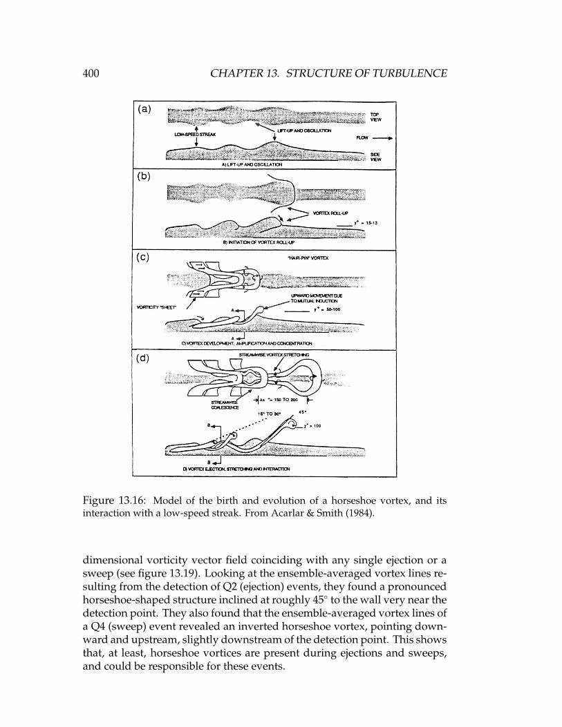
400 CHAPTER 13. STRUCTURE OF TURBULENCE
Figure 13.16: Model of the birth and evolution of a horseshoe vortex, and itsinteraction with a low-speed streak. From Acarlar & Smith (1984).
dimensional vorticity vector field coinciding with any single ejection or asweep (see figure 13.19). Looking at the ensemble-averaged vortex lines re-sulting from the detection of Q2 (ejection) events, they found a pronouncedhorseshoe-shaped structure inclined at roughly 45 to the wall very near thedetection point. They also found that the ensemble-averaged vortex lines ofa Q4 (sweep) event revealed an inverted horseshoe vortex, pointing down-ward and upstream, slightly downstream of the detection point. This showsthat, at least, horseshoe vortices are present during ejections and sweeps,and could be responsible for these events.

13.5. A STUDY OF NEAR WALL SCALING LAWS 401
Figure 13.17: Instantaneous distribution of vortex filaments in a simulated channelflow, showing a horseshoe-like structure. From DNS of turbulent channel flow byMoin & Kim (1986).
13.5 A Study of Near Wall Scaling Laws
The following section was taken from Li Jun-de “The Turbulence Structureof Wall Shear Flows,” Ph.D. Thesis, 1989, University of Melbourne, andPerry, Lim & Henbest (1985). Note that in their analysis (reproduced here),x is the streamwise direction (u′), y is the lateral direction (v′), and z is thewall-normal direction (w′). This conforms with the notation used in thegeophysical fluid dynamics community, but it is different from the notationused elsewhere in these notes.
A characteristic of the turbulent boundary layer is that there exist manydifferent length scales. These include the boundary layer thickness δH, thedistance from the wal1 z, the Kolmogorov scale η and the viscous scale ν/uτ,etc. Perry & Abell (1977), by using a dimensional analysis in conjunctionwith physical arguments, were able to show that in the turbulent wall re-gion, the turbulence spectrum in different wavenumber regions scales withdifferent length scales for the streamwise component. Their approach wasbased partly on the Townsend attached eddy hypothesis and was extendedto the spanwise and normal to the wall components by Perry, Henbest &Chong (1986).
Figure 13.20 shows a schematic of three attached eddies of different scalewith the instantaneous streamline pattern they each generate relative to thefluid at infinity. Imagine that these eddies are surrounded by fine scale
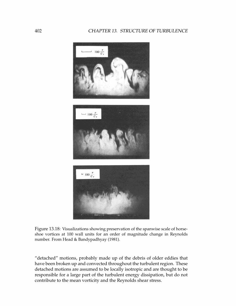
402 CHAPTER 13. STRUCTURE OF TURBULENCE
Figure 13.18: Visualizations showing preservation of the spanwise scale of horse-shoe vortices at 100 wall units for an order of magnitude change in Reynoldsnumber. From Head & Bandypadhyay (1981).
“detached” motions, probably made up of the debris of older eddies thathave been broken up and convected throughout the turbulent region. Thesedetached motions are assumed to be locally isotropic and are thought to beresponsible for a large part of the turbulent energy dissipation, but do notcontribute to the mean vorticity and the Reynolds shear stress.

13.5. A STUDY OF NEAR WALL SCALING LAWS 403
Figure 13.19: Ensemble average of vortex lines in the vicinity of an (a) ejection; and(b) a sweep, showing a horseshoe vortex and an inverted horseshoe, respectively.From DNS of turbulent channel flow by Moin & Kim (1986).
From figure 13.20 it can be seen that a hot-wire probe at a distance z fromthe wall will see contributions to u′ (longitudinal velocity fluctuations) andto v′ (lateral velocity fluctuations) from eddies of scale z and larger, whereascontributions to w′ (normal velocity fluctuations) will only be made fromeddies of height of order z.
The following analysis is applicable for z δH and for z ν/uτ (theturbulent wall region) on a smooth wall. Here, δH is the boundary layerthickness using the Hama (1954) velocity defect formulation for constant

404 CHAPTER 13. STRUCTURE OF TURBULENCE
Figure 13.20: A sketch of three attached eddies of varying scales together with theinstantaneous streamline pattern they each generate.
Figure 13.21: Wavenumber regions for the longitudinal spectrum showing regionsof overlap.
pressure layers.The behavior of the velocity fluctuation spectra in the wall region can
be separated into three different wavenumber regions. Let φ11(k1), φ22(k1)and φ33(k1) be the one-dimensional spectra for u, v and w respectively. Ac-cording to Perry & Abell (1977) and Perry et al. (1986), φ11(k1) scales withthe boundary layer thickness δH in the low wavenumber region, with theKolmogorov length scale in the higher wavenumber region and with thelocal distance z from the wall in the wavenumbers in between. Figure 13.21shows the summary of the various regions.
In the first region, we have “outer flow” scaling:
φ11(k1δH)u2τ
= g1(k1δH) =φ11(k1)δHu2
τ
(13.1)

13.5. A STUDY OF NEAR WALL SCALING LAWS 405
In the Kolmogorov region:
φ11(k1η)υ2 = g3(k1η) =
φ11(k1)ηυ2 (13.2)
where υ is the Kolmogorov velocity scale. In between, we have “inner flow”scaling:
φ11(k1z)u2τ
= g2(k1z) =φ11(k1)
zu2τ
(13.3)
In the turbulent wall region, they adopted Townsend’s assumption that thelocal energy production ℘ equals the local energy dissipation rate ε.
℘ = −u1u3∂U∂z
= ε (13.4)
By using the law of the wall in the wall region, they obtained
υ =
(νu3
τ
κz
)1/4
and
η =
(ν3κzu3τ
)1/4
(13.5)
When the Reynolds number is high enough, Perry et al. (1986) anticipatedthat there will be two overlap regions existing in the streamwise spectra.
Figure 13.21 shows these overlap regions,where F is a characteristic con-stant and P, N and M are universal constants.
In the overlap region from klδH =F to klz = ℘,
φ11(k1z)u2τ
=A1
k1z= g2(k1z) (13.6)
andφ11(k1δH)
u2τ
=A1
k1δH= g1(k1δH) (13.7)
These relations are compatible only if there exists the -1 law as shown andA1 is a universal constant. In the second overlap region, that is, from k1z =Nto k1η =M, by requiring that the spectrum is independent of viscosity ν,theyobtained:
φ11(k1η)υ2 =
K0(k1η
)5/3 = g3(k1η) (13.8)
φ11(k1z)u2τ
=K0
κ2/3
1
(k1z)5/3 = g3(k1z) (13.9)

406 CHAPTER 13. STRUCTURE OF TURBULENCE
Figure 13.22: Wavenumber regions for the normal to the wall spectrum showingregions of overlap.
where K0 is the Kolmogorov universal constant. Townsend (1976) proposedthat K0 ≈ 0.5.
By using the attached eddy hypothesis, it can be seen that the spanwisespectrumφ22(k1) is of the same functional form asφ11(k1). In the first overlapregion the universal constant becomes A2 and in the second overlap regionthere is a 4/3 factor which results from the isotropic condition.
Forφ33(k1), they argued that the only eddies that contribute to the normalto the wall component are the eddies that scale with the distance from thewall. Thus there is no outer flow scaling and only two regions exist forφ33(k1). This has been shown in figure 13.21. Again, when the Reynoldsnumber is high enough, there is one overlap region. For this region theyderived:
φ33(k1η)υ2 =
43
K0(k1η
)5/3 (13.10)
andφ33(k1z)
u2τ
=43
K0
κ2/3
1
(k1z)5/3 (13.11)
The inconvenience of the above scaling laws for spectra is that they arenot given by a single formula which is valid over the entire wavenumberrange. Perry, Li, Henbest & Marusic (1988b) derived such a formula from acurve fitting procedure for each component. Although there is no physicalbasis for these more general formulae, they are designed to give a fairly ac-

13.5. A STUDY OF NEAR WALL SCALING LAWS 407
curate indication of the shape of the spectra while preserving the asymptoticlaws such as the -1 law and the -5/3 law with all the correct scaling.
The streamwise velocity component spectrum which incorporates thesescaling laws is:
φ11(k1δH)u2τ
=A′
G1G2
1
(k1z)5/3 (13.12)
where
G1 =(1 +
[12
1 + tanh (θ(k1δH − q))
αk1δH
]2)1/2
and
G2 =
(1 +
[β
u2τ
υ2 A′1
(k1η)K11(k1η)
]m)1/m
with A′ = 2.06, α = 2.0, β = 0.500, θ = 1.8, q = 0.9 and m = 0.4.The normal to the wall velocity component spectrum is:
φ33(k1z)u2τ
= B′(1 +
[β
u2τ
υ2
zη
1(K33(k1η)
]m)−1/m
(13.13)
where B′ = 0.9, m = 0.8 and β = 0.903.The various constants in equations 13.12 and 13.13 are chosen according
to the data from Lim (1985) and Perry et al. (1987) and according to Perry etal. (1988b) “they are subject to alteration without notice.”
The terms K11(k1η) and K33(k1η) in equations 13.12 and 13.13 are the one-dimensional spectra derived by using the Kovasznay’s spectral expressionin the Kolmogorov equilibrium region (Kovasznay, 1948). They are:
K11(k1η) = 0.500(k1η)−5/3− 6.04(k1η)−1/3
− 1.8(k1η) + 0.306(k1η)2 + 7.03 (13.14)
and
K33(k1η) = 0.669(k1η)−5/3− 4.02(k1η)−1/3
− 0.153(k1η)2 + 3.51 (13.15)
Figures 13.23 and 13.25 show the results calculated from equations 13.12and 13.13 respectively and figures 13.24 and 13.26 show the pre-multipliedforms of these spectra. The figures show that the -1 law and the -5/3 law arevery pronounced only when Kτ approaches 106 (Kτ = δhuτ/ν). This Kτ valueis reached only in meteorological data.
The broadband turbulence intensities can be obtained by integrating thestreamwise spectrum over different regions, for example:
u2
u2τ
=
∫ F
0g1(k1δH)d(k1δH) +
∫ P
Fz/δH
g2(k1z)d(k1z) +
∫ N
Pg2(k1z)d(k1z)
+
∫ Mk−1/4z+3/4
Ng2(k1z)d(k1z) +
u2τ
υ2
∫∞
Mg3(k1η)d(k1η) (13.16)
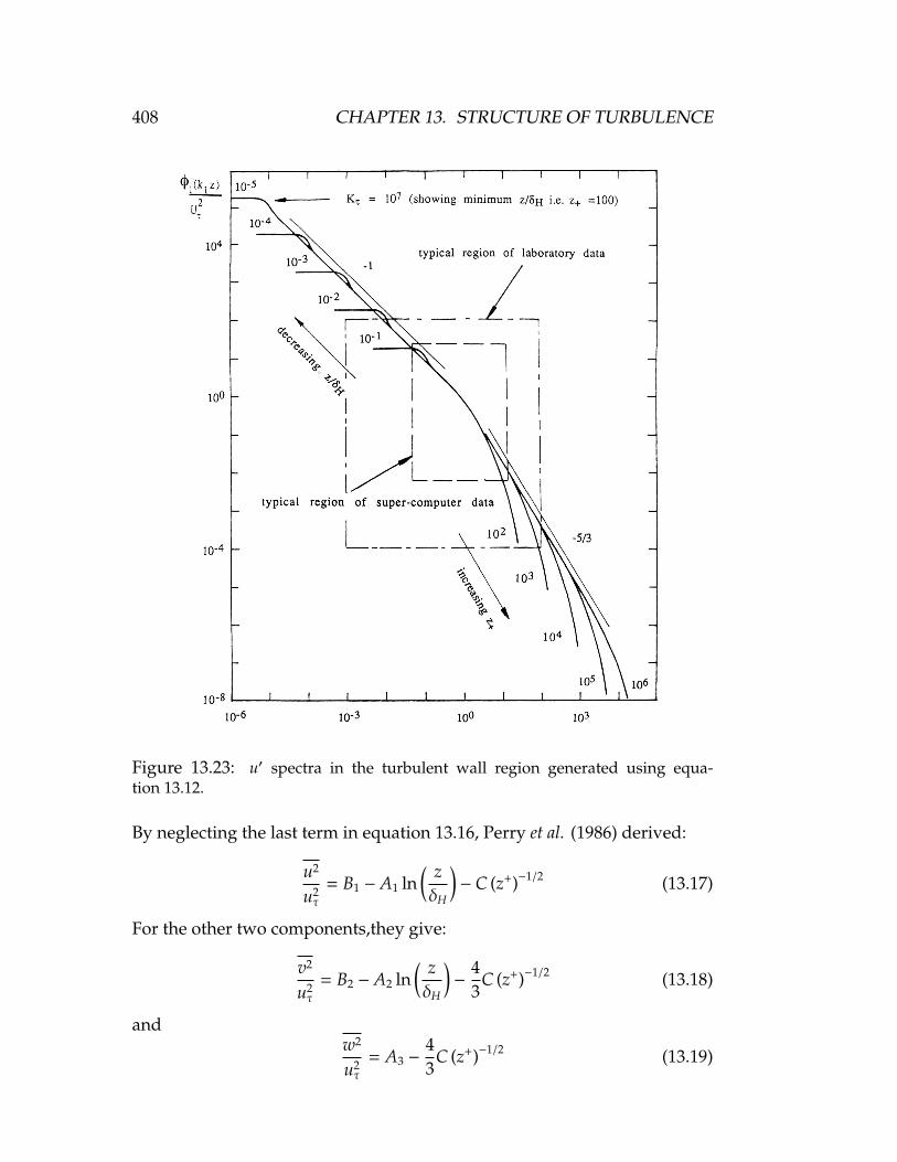
408 CHAPTER 13. STRUCTURE OF TURBULENCE
Figure 13.23: u′ spectra in the turbulent wall region generated using equa-tion 13.12.
By neglecting the last term in equation 13.16, Perry et al. (1986) derived:
u2
u2τ
= B1 − A1 ln( zδH
)− C (z+)−1/2 (13.17)
For the other two components,they give:
v2
u2τ
= B2 − A2 ln( zδH
)−
43
C (z+)−1/2 (13.18)
andw2
u2τ
= A3 −43
C (z+)−1/2 (13.19)

13.5. A STUDY OF NEAR WALL SCALING LAWS 409
Figure 13.24: Premultiplied u′ spectra. (I) Energy contribution from Kτ → ∞; (II)finite Reynolds number case.
where B1 and B2 are characteristic constants and A1, A2, A3 and C are univer-sal constants. All the formulaes in this section apply only to the turbulentwall region, that is, 100ν/uτ < z < 0.156δH.
Perry, Lim & Henbest (1987) have attempted to verify experimentallythese scaling laws and the broadband turbulence intensity profiles in theturbulent boundary layer. They showed that, in the turbulent wall region,the -1 laws exist in the u and v spectra and the -5/3 law exists in the spectraof the three components. These agree with the above scaling predictions.
Lim (1985) and Perry,Lim & Henbest (1987) have also attempted to verifythe broadband turbulence intensity formulae (equations 13.17, 13.18 and13.19) for turbulent boundary layers over smooth and rough walls. Theyfound that the broadband turbulence intensities for the streamwise and thespanwise components agree well with the equations 13.17 and 13.18. Forthe normal to the wall component, the results were inconclusive. Theyattributed this to errors in the hot-wire anemometry techniques used andfound that the data from other workers also gave inconclusive results.

410 CHAPTER 13. STRUCTURE OF TURBULENCE
Figure 13.25: Wall-normal w′ spectra in the turbulent wall region generated usingequation 13.13.
Spalart (1988) has pointed out that the factor 4/3 in equations 13.18 and13.19 should not be present and the viscous correction term in the equationsshould be isotropic because it has been assumed that the flow is isotropic inthe Kolmogorov equilibrium region.
In equation 13.16, neglecting the last term on the right hand side intro-duces two problems. Firstly, as mentioned earlier, the amount of energyneglected is not fractionally the same for the three different componentsbecause near the wall u2 > v2 > w2. For the w2 quantity the contributionmade by the last term in equation 13.16 is by no means negligible while foru2, the contribution is negligible. Secondly, for isotropic flow, the following

13.5. A STUDY OF NEAR WALL SCALING LAWS 411
Figure 13.26: Premultiplied wall-normal w′ spectra. (I) Energy contribution fromKτ →∞; (II) finite Reynolds number case.
relation exists (Batchelor, 1953, or Hinze, 1975) for one-dimensional spectra:
φ33(k1) = φ22(k1) =12
(φ11(k1) − k1
dφ11(k1)dk1
)(13.20)
Equation 13.20 shows that the sudden arbitrary cut off of the φ11(k1) atk1η = M introduces a delta function for φ22(k1) and φ33(k1). This deltafunction was erroneously excluded in Perry et al.’s (1986) analysis and withits inclusion the factor 4/3 mentioned earlier becomes unity.
To resolve these issues Perry & Li (1990) first incorporated a more generalviscous term such that
u2
u2τ
= B1 − A1 ln( zδH
)− V (z+) (13.21)
v2
u2τ
= B2 − A2 ln( zδH
)− V (z+) (13.22)
w2
u2τ
= A3 − V (z+) (13.23)

412 CHAPTER 13. STRUCTURE OF TURBULENCE
where B1 = 2.39 and B2 = 1.20 are characteristic constants and A1 = 1.03,A2 = 0.475, A3 = 1.78. V(z+) is the viscous correction and it is isotropic.Many forms have been suggested for V(z+) and they have been obtainedfrom various sources ranging from DNS to fitting the spectrum given by theKovasznay (1948) formula. The most recent algebraic form, obtained fromthe model spectra of Perry & Li (1990) at high wavenumbers, which is usedby Marusic & Perry (1995) and Marusic, Uddin & Perry (1997) is
V (z+) = 5.58(1 − z+−0.9
)z+−0.5 (13.24)
Equations 13.21 – 13.23 have the same functional forms obtained by Townsend(1976) using the attached eddy hypothesis at large Reynolds number (asz+→∞, V(z+) becomes negligible over most of the boundary layer).

Appendix A
Equations of Motion
A.1 Continuity equation
Integral forms of the continuity equation for a fixed control volume:
∂∂t
∫ρ dυ +
∫n · ρV dA = 0
∫n · ρV dA = 0 Fixed mass
∫n · ρV dA = 0 Steady flow
∫n ·VdA = 0 Incompressible flow
Differential forms of the continuity equation:
∂ρ
∂t+ ∇ · ρV = 0
∇ ·V = −1ρ
DρDt
In tensor notation:∂ρ
∂t+∂ρui
∂xi= 0
413

414 APPENDIX A. EQUATIONS OF MOTION
A.2 Linear momentum equation
Integral form of the momentum equation for a fixed control volume, wheregravity is the only body force:
Fext +
∫~Σ dA +
∫ρgdυ =
∂∂t
∫ρVdυ +
∫ (n · ρV
)VdA
For an inviscid fluid: ∫~Σ dA =
∫p dA
Differential form of the momentum equation (the Navier-Stokes equation):
ρDui
Dt= ρ
∂ui
∂t+ ρu j
∂ui
∂x j= ρgi +
∂σi j
∂x j
or∂(ρui)∂t
+∂(ρuiu j)∂x j
= ρgi +∂σi j
∂x j
whereσi j = −pδi j + di j
and di j depends on the motion of the fluid only and it is called the shear stresstensor, or the deviatoric stress tensor (= σ′i j in my notes, or τi j in Currie). Forisotropic, Newtonian fluids,
di j = λSkkδi j + 2µSi j
where λ is called the “second viscosity coefficient” (µ′′ in Batchelor),
∂ui
∂x j= Si j + Ri j
Si j = ei j and Ri j = ξi j in my notes, and
Si j = 12
(∂ui
∂x j+∂u j
∂xi
)and Ri j = 1
2
(∂ui
∂x j−∂u j
∂xi
).
With the definition of the bulk viscosity µ′′ (K in Currie, and κ in Batchelor):
µ′′ = λ + 23µ
we havedi j = µ′′Skkδi j + 2µ
(Si j −
13Skkδi j
)

A.3. ENERGY EQUATION 415
andσi j = −pδi j + µ′′Skkδi j + 2µ
(Si j −
13Skkδi j
).
Differential form of the momentum equation where only the dynamic vis-cosity is retained:
ρ∂ui
∂t+ ρu j
∂ui
∂x j= −
∂p∂xi
+∂∂x j
(µ
(∂ui
∂x j+∂u j
∂xi−
23
∂uk
∂xkδi j
))
For a constant-property fluid:
ρDVDt
= −∇p + ρg + µ∇2V
or, with ψ = altitude:
ρDVDt
= −∇p − ρg∇ψ + µ∇2V.
For an inviscid fluid we obtain Euler’s equation:
ρDVDt
= −∇p + ρg
A.3 Energy equation
Integral form of the energy equation for a fixed control volume:
∂∂t
∫ρ(e + 1
2ρV2)
dυ +
∫ (n · ρV
) (e + 1
2ρV2)
dA =
∫n · k∇T dA
+
∫σi jniu j dA +
∫ρg ·V dA.
Differential form (h = e + p/ρ):
DDt
(h + 1
2V2 + gψ)
=1ρ
∂p∂t
+∂∂t
(gψ
)+
1ρ
[∂∂xi
(σi ju j
)+ ∇ · k∇T
]Therefore, for a steady flow of an inviscid fluid where heat conduction effectsare negligible, along along a streamline (streamlines are pathlines in steadyflow):
h + 12V2 + gψ = constant

416 APPENDIX A. EQUATIONS OF MOTION
When the fluid is incompressible as well, the specific internal energy e isconstant, and
pρ
+ 12V2 + gψ = constant
which is Bernoulli’s equation.
Enthalpy equation
By using the momentum equation, we can write the energy equation as anenthalpy equation:
ρDhDt
=DpDt
+ ∇ · k∇T + di j∂u j
∂xi
where
di j∂u j
∂xi= Φ (the dissipation function)
Entropy equation
From the enthalpy equation
ρDhDt−
DpDt
= ∇ · k∇T + Φ.
Using dh − dp/ρ = Tds, we get
ρTDsDt
= ∇ · k∇T + Φ
Note: when q = 0 (adiabatic flow), and there is no dissipation, then theflow is isentropic (the rate of change of entropy following a fluid particle iszero). If this is true for all fluid particles, the flow is homentropic, that is, s isconstant everywhere.
A.4 Summary
The equations of motion for a compressible, viscous, heat conducting fluidare:
∂ρ
∂t+∂ρui
∂xi= 0, (A.1)
ρ∂ui
∂t+ ρu j
∂ui
∂x j= −
∂p∂xi
+∂di j
∂x j, (A.2)
ρ∂h∂t
+ ρu j∂h∂x j
=DpDt−∂∂xi
(k∂T∂xi
)+ di j
∂ui
∂x j, (A.3)

A.4. SUMMARY 417
which are, respectively, the continuity, momentum and energy equations.The deviatoric stress tensor di j is given by
di j = µ
(∂ui
∂x j+∂u j
∂xi−
23
∂uk
∂xkδi j
). (A.4)
With the addition of an equation of state and the known variation of vis-cosity and thermal conductivity with temperature and pressure, this is acomplete set of equations describing compressible fluid flow, provided that:the continuum hypothesis holds, the fluid particles are in local thermody-namic equilibrium, body forces can be neglected, the fluid is Newtonian,heat conduction follows Fourier’s law and radiative heat transfer can beneglected.

418 APPENDIX A. EQUATIONS OF MOTION

Appendix B
References
S.B. Pope, “Turbulent Flows,” Cambridge University Press, 2000P.S. Bernard and J.M. Wallace, “Turbulent Flow: Analysis, Measure-ment, and Prediction,” John Wiley & Sons, 2002
J. Mathieu and J. Scott, “An Introduction to Turbulent Flow,” Cam-bridge University Press, 2000
H. Tennekes and J.L. Lumley, “A First Course in Turbulence,” MITPress, 1972
Hinze, J.O., “Turbulence,” McGraw-Hill, New York, 2nd edition, 1975
P. Bradshaw, “An Introduction to Turbulence and Its Measurement,”Pergamon Press, 1971
P. A. Libby, “Introduction to Turbulence,” Taylor & Francis,1996
J. T. Davies, “Turbulence Phenomena,” Academic Press, 1972
M. Lesieur, “Turbulence in Fluids,” Kluwer, 3rd edition, 1993
H. Schlichting and K. Gersten, “Boundary-Layer Theory,” McGraw-Hill, 8th edition, 2000
D. C. Wilcox, “Turbulence Modeling for CFD,” DCW Industries, 1993
B. E. Launder and D. B. Spalding, “Mathematical Models of Turbu-lence,” Academic Press, 1972
U. Frisch, “Turbulence,” CUP paperback, 1995
Cebeci, T. and Smith, A. M. O., “Analysis of Turbulent BoundaryLayers,” Academic Press, 1974
419

420 APPENDIX B. REFERENCES
Bradshaw, P., Cebeci, T. and Whitelaw, J. H., “Engineering CalculationMethods for Turbulent Flow,” Academic Press, 1981
Cebeci, T. and Bradshaw, P., “Momentum Transfer in Boundary Lay-ers,” Hemisphere, 1977
Cebeci, T. and Bradshaw, P., “Physical and Computational Aspects ofConvective Heat Transfer,” Springer-Verlag, 1984
Smits, A.J. and Dussauge, J.P., “Turbulent Shear Layers in SupersonicFlow,” Springer Verlag, AIP Imprint, 1996