arX

iv:1

403.

0681

v1 [

gr-q

c] 4

Mar

201

4

Bounce solutions in viscous fluid cosmology

Ratbay Myrzakulov∗, Lorenzo Sebastiani†

Eurasian International Center for Theoretical Physics and Department of General

Theoretical Physics, Eurasian National University, Astana 010008, Kazakhstan

Abstract

We investigate the bounce cosmology induced by inhomogeneous viscous fluids in FRWspace-time (non necessarly flat), taking into account the early-time acceleration after thebounce. Different forms for the scale factor and several examples of fluids will be considered.We also analyze the relation between bounce and finite-time singularities and between thecorresponding fluids realizing this scenarios. In the last part of the work, the study is extendedto the framework of f(R)-modified gravity, where the modification of gravity may also beconsidered as an effective (viscous) fluid producing the bounce.

Contents

1 Introduction 1

2 Inhomogeneous viscous fluids in FRW space-time. 2

3 Bounce solutions with exponential scale factor 3

3.1 Fluids realizing the bounce with exponential scale factor . . . . . . . . . . . . . . . 5

4 Bounce solutions with power-law scale factor 5

4.1 Fluids realizing the bounce with power-law scale factor . . . . . . . . . . . . . . . . 7

5 Bounce solutions in modified theories of gravity 7

6 Conclusions 9

1 Introduction

The cosmological observations reveal that the universe is expanding in an accelerated way [1].Apart the introduction of small and positive Cosmological Constant in the framework of GeneralRelativity, where the acceleration is induced by the negative pressure of the dark energy withEquation of State parameter ω = −1, several descriptions of the cosmic acceleration have beenpresented in the recent literature, making the dark energy issue the “Mystery of the Millennium” [2],with many implications in fundamental physics. The data constrain ω to be very close to minusone, but in principle different forms of dark fluid (phantom, quintessence...), satisfying a suitableEquation of State are allowed. Moreover, the existence of an accelerated epoch also in the early-time universe, namely the inflation, which cannot be driven by standard matter/radiation, addssome new interest in the investigation of general forms, behaviours and solutions of dark fluids. Wealso observe that, despite to the fact that many macroscopic physical systems, like the large scale

∗Email address: rmyrzakulov@gmail.com†E-mail address: l.sebastiani@science.unitn.it

1

structure of matter, can be approximated like perfect fluids (with Equation of State parameterω = const), we cannot exclude non-perfect fluid representation for the dark components of theuniverse (whose origin remains unknown) like inhomogeneous and/or viscous fluid representation.Namely, the Equation of Steate paramter of the dark energy may be not a constant or its pressuremay depend on the expansion rate of the universe due to some viscosity. The investigation ofsuch a kind of fluids is motivated by several reason. For example, in the last years the interestin modified theories of gravity, where some combination of curvature invariants (Riemann tensor,Weyl tensor, Ricci tensor and so on) replaces or is added into the classical Hilbert-Einstein actionof General Relativity, has grown up (see Refs. [3] –[8] and Ref.[9]), and it is worth consideringthat this theories have a corresponding description in the fluid-like form, so that the study ofinhomogeneous viscous fluids is one of the easiest way to understand some of the general aspectsof modified theories also (for a recent review of inhomogeneous fluids as an equivalent descriptionof different theoretical models, see Ref. [10]).

When we consider universe contents different from the standard matter ones, we may findseveral interesting cosmological solutions with a great varieties of features like oscillations, singu-larities etc. Among them, the bounce solutions (where a cosmological contraction is followed by anexpansion at a finite time) are interesting to analyze (see Refs. [11] for a review). The idea that,instead from an initial singularity, the universe has emerged from a cosmological bounce furnishesan alternative scenario to the Big Bang theory. In the so-called matter bounce scenario [12], inthe initial contraction the universe is in a matter-dominated stage, after that a bounce withoutany singularity appears, and the expanding universe with the correct observed matter spectrumis generated: in such a case, the precision of the anisotropies predicted by the model are wellconfirmed by the observations of the Cosmic Microwave Background (CMB) anisotropies. Manydifferent aspects of bounce cosmology have been analyzed in the literature (see Ref. [13] for BKLinstability, Refs. [14] for the Ekpyrotic scenario, and Ref. [15] for other recent works). Finally,in the recent work of Ref. [16], the bounce solutions have been considered in the framework ofmodified gravity and massive bigravity.

The aim of this work is to investigate the bounce cosmology induced by inhomogeneous viscousfluids in Friedmann-Robertson-Walker space-time (not necessarly flat). We will discuss differentbounce solutions and the feautures of the related dark fluids, taking into account the necessityto have a cosmic (inflationary) acceleration after the bounce. In particular, we are interested inthe relation between bounce and singular solutions, and in the corresponding relation betweenthe dark fluids realizing such scenarios. In the last part of the work, we also will extend thestudy to f(R)-modified gravity, where the modification to Einstein’s gravity can be viewed as an(effective) viscous fluid: in this case, the realization of bounce solutions will be considered in flatFRW space-time.

The paper is organized as follows. In Section 2, the formalism of inhomogeneous viscous fluidsin FRW universe is presented. In Section 3, we will analyze the bounce solutions in fluid cosmologywith exponential scale factor, we will study the feauture of the models and we will analyze theappearance of singular solutions. Some explicit examples of fluid realizing such a bounce willbe presented. In section 4, the same investigation will be carried out for the bounce solutionswith power-law scale factor. Section 5 is devoted to bounce solutions in f(R)-gravity by using afluid-like representation. Conclusions and remarks are given in Section 6.

We use units of kB = c = ~ = 1 and denote the gravitational constant, GN , by κ2 ≡ 8πGN ,

such that G−1/2N = MPl, MPl = 1.2× 1019 GeV being the Planck mass.

2 Inhomogeneous viscous fluids in FRW space-time.

Let us start by recalling the Friedmann Equations of Motion (EOMs) for the Friedmann-Robertson-Walker (FRW) metric in spherical coordinates r, θ, φ,

ds2 = −dt2 + a2(t)

[

dr2

1− k2r2+ r2dΩ2

]

, dΩ2 = (dθ2 + sin2 θdφ2) , (1)

2

which read

H2 +k

a2=

κ2ρ

3, − (2H + 3H2)

κ2= p . (2)

In the above expressions, a(t) is the scale factor of the universe (r = r′/√

|a(t)|2, r′ being thephysical radial coordinate), k = −1, 0, 1 is the spatial curvature which correspons to the hyperbolic,flat or spherical space, respectively, and H = a(t)/a(t) is the Hubble paramter where the dotdenotes the derivative with respect to the cosmological time t. The cosmological parameter reads

Ω = 1 +k

a2H2, (3)

and in general can be different to one.In the Friedmann equations, p and ρ are the pressure and the energy density of the fluid

contents of the universe which must satisfy the conservation law,

ρ+ 3H(ρ+ p) = 0 . (4)

In this work, we will consider the general form for the Equation of State (EoS) of inhomogeneousviscous fluids, namely [17, 18, 19]

p = ω(ρ)ρ−B(a(t), H, H...) , (5)

where the EoS parameter, ω(ρ), may depend on the energy density, and the bulk viscosityB(a(t), H, H...) is a general function of the scale factor, the Hubble parameter and its deriva-tives. On thermodynamical grounds, in order to have the positive sign of the entropy change inan irreversible process, the bulk viscosity must be a positive quantity [20, 21]. The stress-energytensor of fluid Tµν is given by

Tµν = ρuµuν +[

ω(ρ)ρ+B(ρ, a(t), H, H...)]

(gµν + uµuν) , (6)

where uµ = (1, 0, 0, 0) is the four velocity vector. The fluid energy conservation law (4) finallyleads to

ρ+ 3Hρ(1 + ω(ρ)) = 3HB(ρ, a(t), H, H...) . (7)

In the next sections, we will revisit some simple bounce solutions discussing the general featuresof the fluids which realize them and the possibility to have an early-time acceleration after thebounce. Some explicit examples of this fluids will be furnish.

3 Bounce solutions with exponential scale factor

We start by examining the bounce scenario where the scale factor and therefore the Hubbleparameter behave as

a(t) = a0eα(t−t0)

2n

, H(t) = 2nα (t− t0)2n−1 , n = 1, 2, 3... (8)

where a0 , α are positive (dimensional) constants and n is a positive natural number from whichdepends the feature of the bouncing. Moreover, t0 > 0 is the fixed bounce time. When t < t0,the scale factor decreases and we have a contraction with negative Hubble parameter, at t = t0we have the bounce, such that a(t = t0) = a0, and when t > t0 the scale factor increases and theuniverse expands with positive Hubble parameter.

It is worth to spending some words on the case of n non positive natural number. First ofall, the special choice n = 1/2 corresponds to the de Sitter solution (H(t) = const). Then, whenn < 1/2 or n is a positive non-natural number, the bounce is changed in a finite-time singularityoccurring at t = t0. It means, that the Hubble parameter or some of its derivatives (and thereforethe curvature) diverge at that time, and we may describe two different expansion (or contraction)cosmological histories, but the two branches with t > t0 (H(t) < 0) and t < t0 (H(t) > 0) are notconnected respect to each other: in other words, the universe starts or finish with a singularity.In the specific, the finite-time singularities can be classified in the following way [22]:

3

• Type I [23]–[27]: for t → t0, a(t), H(t), H(t) → ∞, namely the scale factor, the effectiveenergy density and the effective pressure of the universe diverge. It corresponds to the casen < 0.

• Type II (sudden [28, 29]): for t → t0, a(t) → const, H(t) → const and H(t) → ∞, namelythe effective pressure of the universe diverges. It corresponds to the case 0 < n < 1/2.

• Type III [30]: for t → t0, a(t) → const, H(t) → ∞ and |H(t)| → ∞, namely the effectiveenergy density and pressure of the universe diverge. It corresponds to the case 1/2 < n < 1.

• Type IV [22]: for t → t0, only the higher derivatives of H(t) diverge. It corresponds to thecase n > 1, but n 6= m/2, where m is an integer number.

Finally, when n = m/2, m odd integer number, the scale factor possesses a saddle point at t = t0,but the bounce is absent.

The presence of an initial singularity suggests the Big Bang scenario, while the bounce solutionbrings to a contracting/expanding universe. In such a case,

a

a= H2 + H = 2nα(t− t0)

2(n−1)[

2nα(t− t0)2n + (2n− 1)

]

, (9)

and we have an acceleration. In particular, after the bounce, the universe expands in an acceleratedway and the inflationary scenario may be suggested.

Let us return to the bounce solution (8). From the first EOM in (2) we obtain

ρ =3

κ2

[

4n2α2(t− t0)2(2n−1) +

k

a20e2α(t−t0)2n

]

. (10)

It is easy to see that for the flat universe (k = 0) or for the spherical universe (k = 1), thisquantity is positive defined, but in the hyperbolic space (k = −1) we have a region where the fluidpossesses a negative energy density (in particular, ρ = −3/(a0κ)

2 at t = t0). For this reason, wewill concentrate on the first two (physical) cases.

In the flat universe, the energy density of fluid decreases with the contraction, is equal to zeroat t = t0, and increases with the subsequent expansion.

In the spherical universe, if n > 1, there is a region around the bounce where the energy densityof fluid increases during the contraction and decreases during the expansion, reaching the value ofρ = 3/(a0κ

2) at t = t0. This is clear if we analyze the time derivative of the energy density,

ρ =3

κ2

[

8n2(2n− 1)α2(t− t0)4n−3 − 4nα(t− t0)

2n−1 k

a20e2α(t−t0)2n

]

, (11)

for k = 1. Let us consider n > 1. We see that, when t ≪ t0, since (t− t0) < 0 and (t− t0)4n−3 ≫

(t− t0)2n−1, the first negative term is dominant and the energy density decreases. However, when

t approaches to t0, the second positive term becomes dominant and the energy density starts toincrease until t0 where has a local maximum. After that, energy density decrases as soon as tremains close to t0, but, when t ≫ t0, the energy density increases again. This mechanism isinteresting if we consider that after the bounce the cosmological parameter (3), namely

Ω = 1 +k

a20α2(t− t0)2(2n−1)e2α(t−t0)2n

, (12)

decreases as a consequance of the acceleration of the universe. In this way, the solution (8)with n > 1 may give rise to an accelerated universe, whose energy density decreases with thecosmological parameter. This scenario may be compatible with the inflation, whose effectiveenergy density decreases making possible the exit from this period, at the end of whose thecosmological parameter is close to one: it is clear that to reproduce such comology other fluidcontents which become dominant during this phase must be added to the model to produce asubsequent deceleration.

4

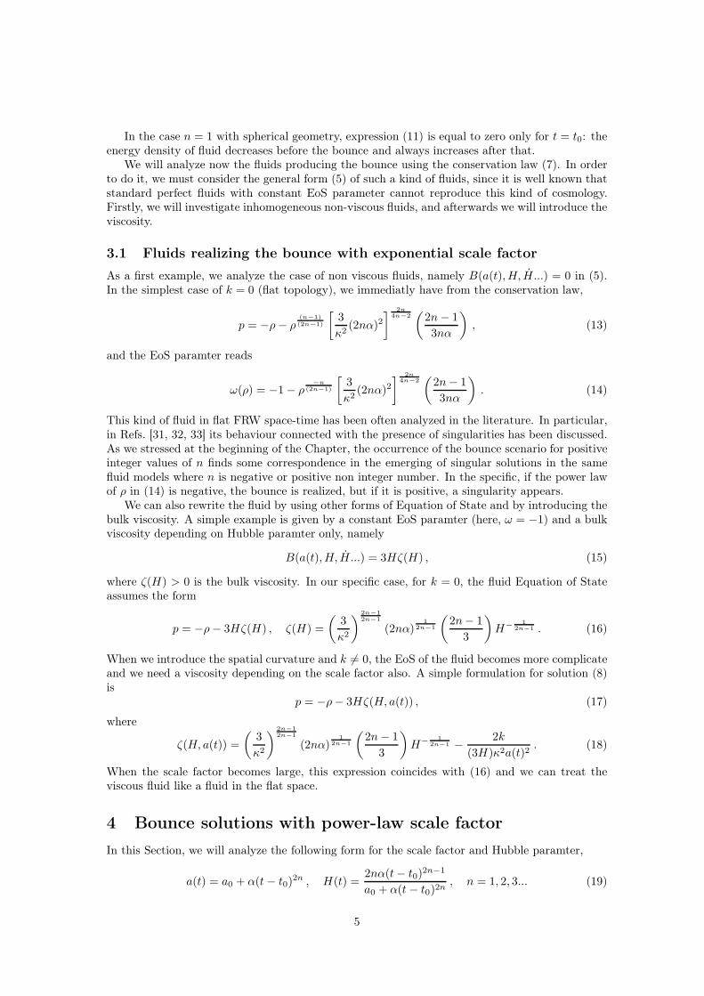
In the case n = 1 with spherical geometry, expression (11) is equal to zero only for t = t0: theenergy density of fluid decreases before the bounce and always increases after that.

We will analyze now the fluids producing the bounce using the conservation law (7). In orderto do it, we must consider the general form (5) of such a kind of fluids, since it is well known thatstandard perfect fluids with constant EoS parameter cannot reproduce this kind of cosmology.Firstly, we will investigate inhomogeneous non-viscous fluids, and afterwards we will introduce theviscosity.

3.1 Fluids realizing the bounce with exponential scale factor

As a first example, we analyze the case of non viscous fluids, namely B(a(t), H, H...) = 0 in (5).In the simplest case of k = 0 (flat topology), we immediatly have from the conservation law,

p = −ρ− ρ(n−1)(2n−1)

[

3

κ2(2nα)2

]2n

4n−2(

2n− 1

3nα

)

, (13)

and the EoS paramter reads

ω(ρ) = −1− ρ−n

(2n−1)

[

3

κ2(2nα)2

]2n

4n−2(

2n− 1

3nα

)

. (14)

This kind of fluid in flat FRW space-time has been often analyzed in the literature. In particular,in Refs. [31, 32, 33] its behaviour connected with the presence of singularities has been discussed.As we stressed at the beginning of the Chapter, the occurrence of the bounce scenario for positiveinteger values of n finds some correspondence in the emerging of singular solutions in the samefluid models where n is negative or positive non integer number. In the specific, if the power lawof ρ in (14) is negative, the bounce is realized, but if it is positive, a singularity appears.

We can also rewrite the fluid by using other forms of Equation of State and by introducing thebulk viscosity. A simple example is given by a constant EoS paramter (here, ω = −1) and a bulkviscosity depending on Hubble paramter only, namely

B(a(t), H, H...) = 3Hζ(H) , (15)

where ζ(H) > 0 is the bulk viscosity. In our specific case, for k = 0, the fluid Equation of Stateassumes the form

p = −ρ− 3Hζ(H) , ζ(H) =

(

3

κ2

)2n−12n−1

(2nα)1

2n−1

(

2n− 1

3

)

H−1

2n−1 . (16)

When we introduce the spatial curvature and k 6= 0, the EoS of the fluid becomes more complicateand we need a viscosity depending on the scale factor also. A simple formulation for solution (8)is

p = −ρ− 3Hζ(H, a(t)) , (17)

where

ζ(H, a(t)) =

(

3

κ2

)

2n−12n−1

(2nα)1

2n−1

(

2n− 1

3

)

H−1

2n−1 − 2k

(3H)κ2a(t)2. (18)

When the scale factor becomes large, this expression coincides with (16) and we can treat theviscous fluid like a fluid in the flat space.

4 Bounce solutions with power-law scale factor

In this Section, we will analyze the following form for the scale factor and Hubble paramter,

a(t) = a0 + α(t− t0)2n , H(t) =

2nα(t− t0)2n−1

a0 + α(t− t0)2n, n = 1, 2, 3... (19)

5

where a0, α are positive (dimensional) constants and n is a positive natural number. The time ofthe bounce is fixed at t = t0. When t < t0, the scale factor decreases and we have a contractionwith negative Hubble parameter, at t = t0 we have the bounce, such that a(t = t0) = a0, andwhen t > t0 the scale factor increases and the universe expands with positive Hubble parameter.

If a0 = 0 we obtain a bounce solution with singularity, namely the universe contracts untila(t = t0) = 0, where the Hubble parameter and therefore the curvature diverge. However, thescale factor does not become singular and starts to increase after t0 realizing the bounce.

When n is a negative number, the scale factor diverges at t = t0 and we can set a0 = 0without loss of generality. In this case, we encounter the so called Big Rip singularity, whereH(t) = −2n/(t0 − t), H being positive for t < t0 and diverging with the scale factor at t = t0.This is an important solution of the Friedmann equations in the case of phantom perfect fluidswith ω < −1 [23], and in fact it is a possible scenario for the dark energy epoch of the universetoday.

Let us return to the bounce solution (19). We get

a

a=

2n(2n− 1)α(t− t0)2(n−1)

a0 + α(t− t0)2n, (20)

and we have an acceleration before and after the bounce. Moreover, from the first EOM in (2) wederive

ρ =3

κ2 [a0 + α(t− t0)2n]

[

4n2α2(t− t0)4n−2 + k

a0 + α(t− t0)2n

]

. (21)

It is easy to see that in the flat (k = 0) or spherical (k = 1) universe, this quantity is positivedefined. In the hyperbolic space (k = −1), always exist a region where the fluid possesses anegative energy density (in particlular, ρ = −3/(a0κ)

2 at t = t0), and, as in the previous Section,we will concentrate on the first two cases only.

The time derivative of the fluid energy density reads

ρ = −4n(t− t0)2n−3α[2n(t− t0)

2nα(a0(1 − 2n) + (t− t0)2nα) + k(t− t0)

2]

3(a0 + α(t− t0)2n)3κ2 . (22)

When t is close to t0, this expression leads to

ρ(t → t0) ≃8n2(t− t0)

4n−3α2(2n− 1)

3a20κ2 , (23)

such that the energy density decreases before the bounce and increases after it. However, when|t| ≫ t0, one has

ρ(|t| ≫ t0) = −4n(t− t0)−4n−3[2n(t− t0)

4nα2 + k(t− t0)2]

3α2κ2 , (24)

and the energy density increases in the region before (but far from) the bounce and decreasesafter it. This behaviour could be interesting in the attempt to reproduce the inflation with analternative scenario with respect to the standard Big Bang one. In the cases of spherical or flatspatial topology, the energy density of the universe starts to decreases after some times from thebounce making possible an exit from inflation. Note that the cosmological paramter reads

Ω = 1 +k

4n2α2(t− t0)4n−2, (25)

and decreases with the acceleration.

6

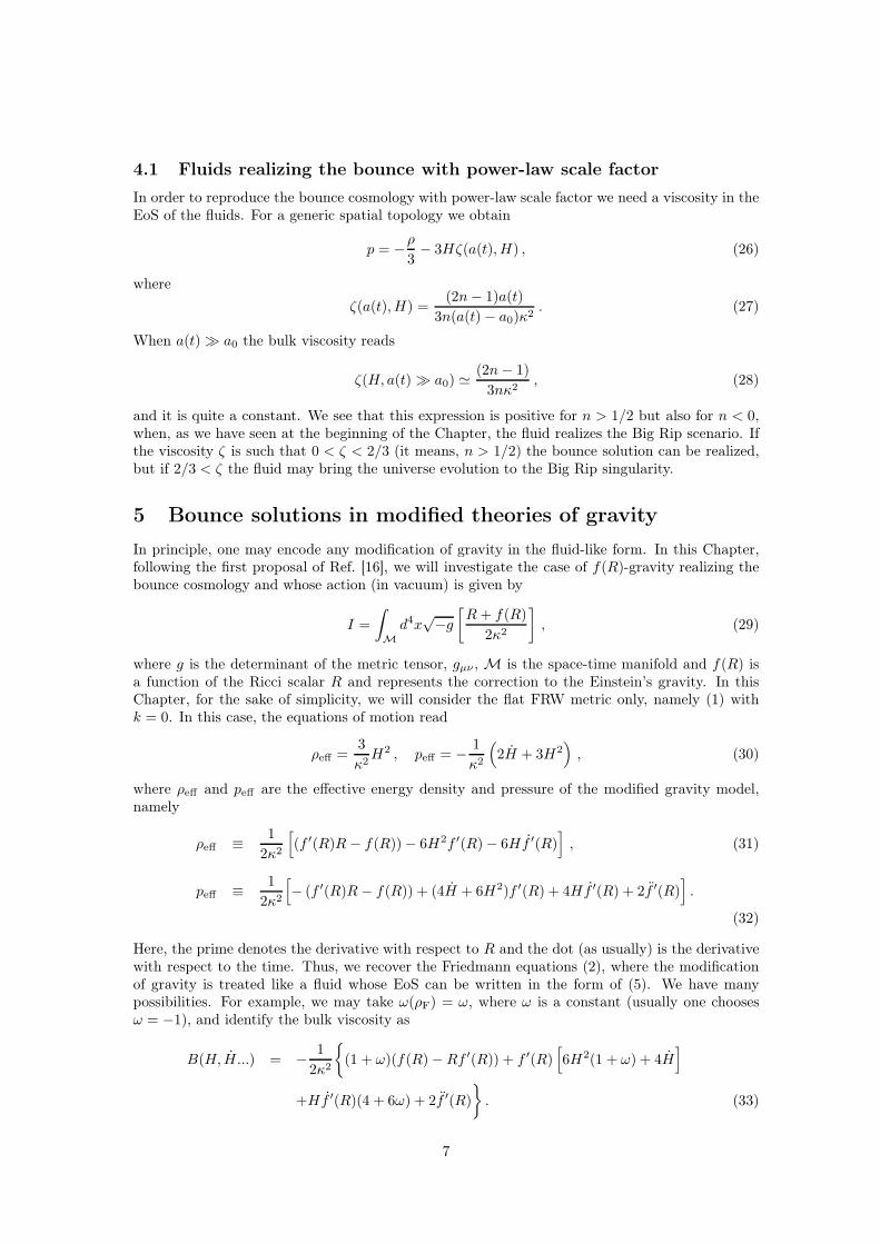
4.1 Fluids realizing the bounce with power-law scale factor

In order to reproduce the bounce cosmology with power-law scale factor we need a viscosity in theEoS of the fluids. For a generic spatial topology we obtain

p = −ρ

3− 3Hζ(a(t), H) , (26)

where

ζ(a(t), H) =(2n− 1)a(t)

3n(a(t)− a0)κ2. (27)

When a(t) ≫ a0 the bulk viscosity reads

ζ(H, a(t) ≫ a0) ≃(2n− 1)

3nκ2, (28)

and it is quite a constant. We see that this expression is positive for n > 1/2 but also for n < 0,when, as we have seen at the beginning of the Chapter, the fluid realizes the Big Rip scenario. Ifthe viscosity ζ is such that 0 < ζ < 2/3 (it means, n > 1/2) the bounce solution can be realized,but if 2/3 < ζ the fluid may bring the universe evolution to the Big Rip singularity.

5 Bounce solutions in modified theories of gravity

In principle, one may encode any modification of gravity in the fluid-like form. In this Chapter,following the first proposal of Ref. [16], we will investigate the case of f(R)-gravity realizing thebounce cosmology and whose action (in vacuum) is given by

I =

∫

M

d4x√−g

[

R+ f(R)

2κ2

]

, (29)

where g is the determinant of the metric tensor, gµν , M is the space-time manifold and f(R) isa function of the Ricci scalar R and represents the correction to the Einstein’s gravity. In thisChapter, for the sake of simplicity, we will consider the flat FRW metric only, namely (1) withk = 0. In this case, the equations of motion read

ρeff =3

κ2H2 , peff = − 1

κ2

(

2H + 3H2)

, (30)

where ρeff and peff are the effective energy density and pressure of the modified gravity model,namely

ρeff ≡ 1

2κ2

[

(f ′(R)R − f(R))− 6H2f ′(R)− 6Hf ′(R)]

, (31)

peff ≡ 1

2κ2

[

− (f ′(R)R− f(R)) + (4H + 6H2)f ′(R) + 4Hf ′(R) + 2f ′(R)]

.

(32)

Here, the prime denotes the derivative with respect to R and the dot (as usually) is the derivativewith respect to the time. Thus, we recover the Friedmann equations (2), where the modificationof gravity is treated like a fluid whose EoS can be written in the form of (5). We have manypossibilities. For example, we may take ω(ρF) = ω, where ω is a constant (usually one choosesω = −1), and identify the bulk viscosity as

B(H, H...) = − 1

2κ2

(1 + ω)(f(R)−Rf ′(R)) + f ′(R)[

6H2(1 + ω) + 4H]

+Hf ′(R)(4 + 6ω) + 2f ′(R)

. (33)

7

In order to recontsruct modified gravity models realizing the bounce solutions, one can take thetime derivative of ρeff,

ρeff =1

2κ2

[

6H2f ′(R)− 12HHf ′(R)− 6Hf ′(R)]

, (34)

and insert this expression in the derivative of the first Friedmann-like equation, such that, giventhe bounce solution, we obtain an equation for f ′(R) only,

6HH

κ2=

1

2κ2

[

6H2f ′(R)− 12HHf ′(R)− 6Hf ′(R)]

. (35)

From this equation it is possible to derive the on-shell form of f ′(R) and then, by replacing thetime with the corresponding expression of the Ricci scalar, get the model f(R) from f ′(R).

Let us see some examples of modified gravity model realizing the bounce. The Ricci scalar reads

R = 12H2 + 6H . (36)

We can start from solution (8) with n = 1. The Hubble parameter and the Ricci scalar are givenby

H(t) = 2α(t− t0) , R = 48α2(t− t0)2 + 12α . (37)

The solution of (35) is

f ′(R) = c0

[

1− 2α(t− t0)2 − 1

c0

]

, (38)

namely

f ′(R) = c0

[(

3

2− 1

c0

)

− R

24α

]

, f(R) = c0

[(

3

2− 1

c0

)

R− R2

48α

]

+ c1 , (39)

where c0, c1 are generic constants. By using the first Friedmann-like equation (30), one obtains

c1 = −3αc0 . (40)

This result is in agreement with Ref. [16]. In order to recover the Einstein gravity term in theaction, we must put

c0 =2

3, f(R) = − R2

72α− 2α . (41)

Some comments are in order. It is well know that the γR2-term with positive γ > 0 [34] orf(R) = γR2 + λ, where γ, λ > 0 [35] admit accelerated non-singular solutions and are used inthe theories for inflation. Here, we see that if the coefficient in front of R2 and the “cosmological”constant of the model are negative, we still obtain an accelerated solution, but back into the pastthe bounce appears.

An other example simple to solve is given by (19) with a0 = 0. In such a case,

H(t) =2n

(t− t0), R(t) =

48n2 − 12n

(t− t0)2, (42)

and the reconstruction leads to

f ′(R) = −1 + c0

(

R

48n2 − 12n

)λ±

, f(R) = −R+c0

(λ± + 1)

(

R

48n2 − 12n

)λ±

R+ c1 , (43)

where

λ± = −1

4

(

1 + 2n±√

1 + 20n+ 4n2)

. (44)

8

Here, c0 is a free paramter and c1 is fixed by the first Friedmann-like equation as

c1 = 0 , (45)

such that the final Lagrangian of the theory results to be a power-law of the Ricci scalar,

L = c0Rλ±+1 , (46)

where we have redefined the constant c0. If n < 0, we find a model for the Big Rip [36], such thatfor this kind of modified power law-models the appearance of the Big Rip or the bounce solutionmust be carefully investigated. Note that in our case, making the choice a0 = 0 in (19), the Hubbleparamter diverges at t = t0 like for the Big Rip: however, the scale factor does not diverge andrealizes the bounce. We also observe that λ± +1 6= 1 independently on n, according with the factthat the pure Einstein gravity is free of bounce or singularity solutions.

6 Conclusions

The study of inhomogeneous viscous fluids in Friedmann-Robertson-Walker universe is importantunder many points of view. This kind of fluids has a very general form of Equation of State andcan be used in many different contexts, like the description of current dark energy epoch or theprimordial inflation. Then, many dark energy models have a corresponding fluid-representation,and the modified theories of f(R)-gravity are an example of it.

In this paper, we have analyzed the bounce cosmology realized in Friedmann-Robertson-Walkerspace-time by viscous fluids considering two specific forms of the bounce, namely bounce withexponential scale factor, and bounce with power-law scale factor. In the both cases, we have foundsome examples of fluids which bring to such solutions. Since the bounce has been proposed as analternative scenario for the Big Bang, our investigation has taken into account the necessity to havean acceleration after the bounce in the context of inflation. For this reason, we have considereddifferent topologies (non necessarly flat) for the FRW metric and we have payed attention to theevolution of the cosmological parameter Ω also. Generally speaking, the bounce solutions bringto an accelerated universe, but the behaviour of the related fluid energy densities can be different.It is reasonable to expect a decreasing of the energy density during the contraction phase, andan increasing of it in the expanding universe: however, we have seen that in some case it mayexist a region around the bounce where this behaviour is inverted. This fact is quite interesting,since it gives the possibility to reproduce after the bounce an accelerating universe whose energydensity decreases, making possible an exit from this stage, but it is clear that to obtain a realisticinflation other universe contents must be considered in the theory in order to bring the universe toa decelerated expansion. An other interesting point analyzed in this work is the relation betweenbounce and singualar solutions: since the form of the scale factors is the same, also the relatedfluids present the same structure of Equation of State, and the occurrence of one solution insteadto the other one typically depends on the coefficients of the bulk viscosity only.

In the final part of the paper, following the first proposal of Ref. [16], we have analyzed f(R)-modified gravity realizing the bounce and some explicit examples have been derived and discussedfor flat FRW space-time.

Other relevant works on inhomogeneous viscous fluids and the dark energy issue have beenpresented in Refs. [37]–[43], in Ref. [44] for the inflationary scenario and in Ref. [45] for viscousfluids applied to the study of Little Rip cosmology.

References

[1] Komatsu, E.; Dunkley, J.; Nolta, M.R.; Bennett, C.L.; Gold, B.; Hinshaw, G.; Jarosik, N.;Larson, D.; Limon, M.; Page, L.; et al. Astrophys. J. Suppl. (2009), 180, 330–376.

[2] T. Padmanabhan, AIP Conf. Proc. 861, 179 (2006) [arXiv:astro-ph/0603114].

9

[3] S. Nojiri and S. D. Odintsov, Phys. Rept. 505, 59 (2011) [arXiv:1011.0544 [gr-qc]]; eConfC0602061, 06 (2006) [Int. J. Geom. Meth. Mod. Phys. 4, 115 (2007)] [arXiv:hep-th/0601213].

[4] S. Capozziello and V. Faraoni, Beyond Einstein Gravity: A Survey of Gravitational Theories

for Cosmology and Astrophysics (Springer, Berlin, 2010).

[5] S. Capozziello and M. De Laurentis, Phys. Rept. 509, 167 (2011) [arXiv:1108.6266 [gr-qc]].

[6] T. Clifton, P. G. Ferreira, A. Padilla and C. Skordis, Phys. Rept. 513, 1 (2012) [arXiv:1106.2476[astro-ph.CO]].

[7] A. de la Cruz-Dombriz and D. Saez-Gomez, Entropy 14, 1717 (2012) [arXiv:1207.2663 [gr-qc]].

[8] R. Myrzakulov, L. Sebastiani and S. Zerbini, Int. J. Mod. Phys. D 22, 1330017 (2013)[arXiv:1302.4646 [gr-qc]].

[9] M. R. Setare and D. Momeni, Int. J. Theor. Phys. 50, 106 (2011) [arXiv:1001.3767 [physics.gen-ph]]; S. H. Hendi and D. Momeni, Eur. Phys. J. C 71, 1823 (2011) [arXiv:1201.0061 [gr-qc]]; M. Jamil, D. Momeni, M. Raza and R. Myrzakulov, Eur. Phys. J. C 72, 1999 (2012)[arXiv:1107.5807 [physics.gen-ph]]; M. Jamil, K. Yesmakhanova, D. Momeni and R. Myrza-kulov, Central Eur. J. Phys. 10, 1065 (2012) [arXiv:1207.2735 [gr-qc]]; K. Bamba, M. Jamil,D. Momeni and R. Myrzakulov, Int. J. Mod. Phys. D 21, 1250065 (2012) [arXiv:1203.2103[gr-qc]]; M. Jamil, S. Ali, D. Momeni and R. Myrzakulov, Eur. Phys. J. C 72, 1998 (2012)[arXiv:1201.0895 [physics.gen-ph]]; M. Jamil, D. Momeni and R. Myrzakulov, Chin. Phys. Lett.29, 109801 (2012) [arXiv:1209.2916 [physics.gen-ph]].

[10] K. Bamba, S. Capozziello, S. Nojiri and S. D. Odintsov, Astrophys. Space Sci. 342 (2012)155 [arXiv:1205.3421 [gr-qc]].

[11] M. Novello and S. E. P. Bergliaffa, Phys. Rept. 463 (2008) 127 [arXiv:0802.1634 [astro-ph]].

[12] R. H. Brandenberger, arXiv:1206.4196 [astro-ph.CO]; Int. J. Mod. Phys. Conf. Ser. 01, 67(2011) [arXiv:0902.4731 [hep-th]]; AIP Conf. Proc. 1268, 3 (2010) [arXiv:1003.1745 [hep-th]];PoS ICFI 2010, 001 (2010) [arXiv:1103.2271 [astro-ph.CO]];

[13] V. A. Belinsky, I. M. Khalatnikov and E. M. Lifshitz, Adv. Phys. 19, 525 (1970).

[14] J. Khoury, B. A. Ovrut, P. J. Steinhardt and N. Turok, Phys. Rev. D 64 (2001) 123522[hep-th/0103239].

[15] B. Xue and P. J. Steinhardt, Phys. Rev. Lett. 105, 261301 (2010) [arXiv:1007.2875 [hep-th]];Phys. Rev. D 84, 083520 (2011) [arXiv:1106.1416 [hep-th]]; Y. -F. Cai, D. A. Easson and R.Brandenberger, JCAP 1208, 020 (2012) [arXiv:1206.2382 [hep-th]]; Y. -F. Cai, R. Brandenbergerand P. Peter, Class. Quant. Grav. 30, 075019 (2013) [arXiv:1301.4703 [gr-qc]]; Y. -F. Cai, E.McDonough, F. Duplessis and R. Brandenberger, arXiv:1305.5259 [hep-th]; I. Bars, P. J. Stein-hardt and N. Turok, Phys. Lett. B 726 (2013) 50 [arXiv:1307.8106]; B. Xue, D. Garfinkle,F. Pretorius and P. J. Steinhardt, Phys. Rev. D 88 (2013) 083509 [arXiv:1308.3044 [gr-qc]].

[16] K. Bamba, A. N. Makarenko, A. N. Myagky, S. Nojiri and S. D. Odintsov, JCAP01(2014)008[arXiv:1309.3748 [hep-th]].

[17] S. Capozziello, V. F. Cardone, E. Elizalde, S. Nojiri and S. D. Odintsov, Phys. Rev. D 73

(2006) 043512 [astro-ph/0508350].

[18] S. Nojiri and S. D. Odintsov, Phys. Rev. D 72 (2005) 023003 [hep-th/0505215].

[19] S. Nojiri and S. D. Odintsov, Phys. Lett. B 639 (2006) 144 [hep-th/0606025].

[20] I. H. Brevik, O. Gorbunova, Gen.Rel.Grav. 37 2039-2045 (2005) [arXiv: 0508038v1 [gr-qc]].

10

[21] I. H. Brevik, O. Gorbunova and Y. A. Shaido, Int. J. Mod. Phys. D 14 1899 (2005)[arXiv:gr-qc/0508038].

[22] S. Nojiri, S. D. Odintsov and S. Tsujikawa, Phys. Rev. D 71, 063004 (2005)[arXiv:hep-th/0501025].

[23] R. R. Caldwell, M. Kamionkowski and N. N. Weinberg, Phys. Rev. Lett. 91 (2003) 071301[astro-ph/0302506].

[24] B. McInnes, JHEP 0208 029 (2002) [arXiv:hep-th/0112066].

[25] V. Faraoni, Int. J. Mod. Phys. D 11, 471 (2002) [arXiv:astro-ph/0110067].

[26] S. Nojiri and S. D. Odintsov, Phys. Lett. B 562, 147 (2003) [arXiv:hep-th/0303117]; E.Elizalde, S. Nojiri and S. D. Odintsov, Phys. Rev. D 70, 043539 (2004) [arXiv:hep-th/0405034].

[27] P. F. Gonzalez-Diaz, Phys. Lett. B 586, 1 (2004) [arXiv:astro-ph/0312579]; S. Nesseris andL. Perivolaropoulos, Phys. Rev. D 70, 123529 (2004) [arXiv:astro-ph/0410309]; M. Sami andA. Toporensky, Mod. Phys. Lett. A 19, 1509 (2004) [arXiv:gr-qc/0312009]; H. Stefancic, Phys.Lett. B 586, 5 (2004) [arXiv:astro-ph/0310904]; L. P. Chimento and R. Lazkoz, Mod. Phys.Lett. A 19, 2479 (2004) [arXiv:gr-qc/0405020].

[28] J. D. Barrow, G. J. Galloway and F. J. Tipler, Mon. Not. Roy. astr. Soc., 223, 835- 844(1986); J. D. Barrow, Phys. Lett. B 235, 40 (1990); J. D. Barrow, Class. Quant. Grav. 21, L79(2004) [gr-qc/0403084].

[29] S. Nojiri and S. D. Odintsov, Phys. Lett. B 595, 1 (2004) [hep-th/0405078].

[30] S. Nojiri and S. D. Odintsov, Phys. Rev. D 70 (2004) 103522 [hep-th/0408170].

[31] S.Nojiri and S. D. Odintsov, Phys. Lett. B 686 (2010) 44 [arXiv:0911.2781 [hep-th]].

[32] A. V. Astashenok, S. Nojiri, S. D. Odintsov and A. V. Yurov, Phys. Lett. B 709, 396 (2012)[arXiv:1201.4056 [gr-qc]].

[33] S. Myrzakul, R. Myrzakulov and L. Sebastiani, to appear in Astrophys.Space Sci,arXiv:1311.6939 [gr-qc].

[34] A. A. Starobinsky, Phys. Lett. B 91, 99 (1980).

[35] L. Sebastiani, G. Cognola, R. Myrzakulov, S. D. Odintsov and S. Zerbini, Phys. Rev. D 89

(2014) 023518 [arXiv:1311.0744 [gr-qc]].

[36] K. Bamba, S. Nojiri and S. D. Odintsov, JCAP 0810, 045 (2008) [arXiv:0807.2575 [hep-th]]; K. Bamba, S. D. Odintsov, L. Sebastiani and S. Zerbini, Eur. Phys. J. C 67 (2010) 295[arXiv:0911.4390 [hep-th]].

[37] Cardone, V.F.; Tortora, C.; Troisi, A.; Capozziello, S. Phys. Rev. D (2006), 73, 043508:1–043508:15.

[38] S. Nojiri and S. D. Odintsov, Phys. Lett. B 649 (2007) 440 [hep-th/0702031 [HEP-TH]].

[39] I. Brevik, S. Nojiri, S. D. Odintsov and D. Saez-Gomez, Eur. Phys. J. C 69 (2010) 563[arXiv:1002.1942 [hep-th]].

[40] I. Brevik and S.D. Odintsov, Phys. Rev. D (2002), 65, 067302:1–067302:4.

[41] D. Youm, Phys. Lett. B (2002), 531, 276–280.

[42] N. Majd and D. Momeni, Int. J. Mod. Phys. E 20, 113 (2011) [arXiv:0903.2020 [gr-qc]].

11

[43] R. Myrzakulov, L. Sebastiani and S. Zerbini, Galaxies 1, no. 2, 83 (2013) [arXiv:1307.4854[gr-qc]].

[44] J. D. Barrow, Phys. Lett. B 180, 335 (1986); J. D. Barrow, Nucl. Phys. B 310 (1988) 743;J. D. Barrow, In "Cambridge 1989, Proceedings, The formation and evolution of cosmic strings"449-462.

[45] I. Brevik, E. Elizalde, S. Nojiri and S. D. Odintsov, Phys. Rev. D 84 (2011) 103508[arXiv:1107.4642 [hep-th]].

12