arX

iv:0

812.

1117

v2 [

gr-q

c] 3

1 M

ar 2

009

arXiv: 0812.1117

Phase-space analysis of interacting phantom cosmology

Xi-ming Chen∗ and Yungui Gong†

College of Mathematics and Physics,

Chongqing University of Posts and Telecommunications,

Chongqing 400065, China

Emmanuel N. Saridakis‡

Department of Physics,

University of Athens,

GR-15771 Athens, Greece

We perform a detailed phase-space analysis of various phantom cosmological models, where thedark energy sector interacts with the dark matter one. We examine whether there exist late-timescaling attractors, corresponding to an accelerating universe and possessing dark energy and darkmatter densities of the same order. We find that all the examined models, although accepting stablelate-time accelerated solutions, cannot alleviate the coincidence problem, unless one imposes a formof fine-tuning in the model parameters. It seems that interacting phantom cosmology cannot fulfillthe basic requirement that led to its construction.

I. INTRODUCTION

Recent cosmological observations support that the universe is experiencing an accelerated expansion, and that thetransition from the deceleration phase to the accelerated phase happened in the recent past [1]. In order to explainthis remarkable phenomena, one can modify the theory of gravity, such as f(R) gravity [2, 3], Dvali-Gabadadze-Porrati model [4], and string inspired models [5]. An alternative direction is to introduce the concept of dark energywhich provides the acceleration mechanism. The simplest candidate of dark energy which is consistent with currentobservations is the cosmological constant. Due to the lack of a good explanation of the small value of the cosmologicalconstant, many dynamical dark energy models were explored, such as a canonical scalar field (quintessence) model[6], a phantom model that has equation of state parameter w < −1 [7, 8, 9], or the combination of quintessence andphantom in a unified model named quintom [10]. Moreover, many theoretical studies are devoted to shed light ondark energy within some quantum gravitational principles, such as the so-called “holographic dark energy” proposal[11].

The dynamical nature of dark energy introduces a new cosmological problem, namely why are the densities ofvacuum energy and dark matter nearly equal today although they scale independently during the expansion history.To solve the problem, one would require that the matter density and dark energy density always approach their currentvalues independent of the initial conditions. The elaboration of this ’coincidence’ problem led to the considerationof generalized versions of the aforementioned models with the inclusion of a coupling between dark energy and darkmatter. Thus, various forms of “interacting” dark energy models [12, 13] have been constructed in order to fulfil theobservational requirements.

One decisive test for dark energy models is the investigation of their phase-space analysis. In particular, to examinewhether they possess attractor solutions corresponding to accelerating universes and ratio Ωdark energy/Ωdark matter ofthe order 1. If these conditions are fulfilled, then the universe will result to that solution at late times, independently ofthe initial conditions, and the basic observational requirements will be satisfied. Although non-interacting quintessence[14, 15], non-interacting phantom [16] and non-interacting quintom models [17] admit late-time accelerated attractors,they possess Ωdark energy = 1 and thus they are unable to solve the coincidence problem.

When dark energy - dark matter interaction is switched on in quintessence, then one can find accelerated attractorswhich moreover give Ωdark energy/Ωdark matter ≈ O(1) [18, 19, 20, 21], but paying the price of introducing new problemssuch as justifying a non-trivial, almost tuned, sequence of cosmological epochs [22]. In cases of interacting phantommodels [23], the existing literature remains in some special coupling forms with mainly numerical results, whichsuggest that the coincidence problem might be alleviated [13, 24].

∗Electronic address: chenxm@cqupt.edu.cn†Electronic address: gongyg@cqupt.edu.cn‡Electronic address: msaridak@phys.uoa.gr

2

In the present work we are interested in performing a detailed phase-space analysis of the interacting phantomparadigm, considering new and general forms of the interaction term Q. In addition, we go beyond the simplifiednon-local forms of the literature, considering also a local Q-form proportional to a density [21, 25, 26, 27]. Doingso we find that although late-time accelerated attractors do exist in all the models, as it is expected for phantomcosmology, almost all of them correspond to complete dark energy domination and thus they are unable to solve thecoincidence problem. Only for a narrow area of the parameter space of one particular model, can the correspondingsolution alleviate the aforementioned problem.

The plan of the work is as follows: In section II we construct the interacting phantom cosmological scenario and wepresent the formalism for its transformation into an autonomous dynamical system, suitable for a phase-space stabilityanalysis. In section III we perform the phase-space analysis for four different models, using various interaction terms,and in section IV we discuss the corresponding cosmological implications. Finally, section V is devoted to the summaryof the obtained results.

II. PHANTOM COSMOLOGY

Let us construct the interacting phantom cosmological paradigm. Throughout the work we consider a flat Robertson-Walker metric:

ds2 = dt2 − a2(t)dx2, (1)

with a the scale factor.The evolution equations for the phantom and dark matter density (considered as dust for simplicity) are:

ρm + 3Hρm = −Q (2)

ρφ + 3H(ρφ + pφ) = Q, (3)

with Q a general interaction term and H the Hubble parameter. Therefore, Q > 0 corresponds to energy transfer fromdark matter to dark energy, while Q < 0 corresponds to dark energy transformation to dark matter. For simplicity,we take the usual phantom energy density and pressure:

ρφ = −1

2φ2 + V (φ) (4)

pφ = −1

2φ2 − V (φ), (5)

where V (φ) is the phantom potential. Equivalently, the phantom evolution equation can be written as:

φ + 3Hφ − ∂V (φ)

∂φ= −Q

φ. (6)

Finally, the system of equation closes by considering the Friedmann equations:

H2 =κ2

3(ρφ + ρm), (7)

H = −κ2

2

(

ρφ + pφ + ρm

)

, (8)

where we have set κ2 ≡ 8πG. Although we could straightforwardly include baryonic matter and radiation in themodel, for simplicity reasons we neglect them.

In phantom cosmological models, the dark energy is attributed to the phantom field, and its equation of state isgiven by

wφ =pφ

ρφ. (9)

Alternatively one could construct the equivalent uncoupled model described by:

ρm + 3H(1 + wm,eff )ρm = 0 (10)

ρφ + 3H(1 + wφ,eff )ρφ = 0, (11)

3

where

wm,eff =Q

3Hρm(12)

wφ,eff = wφ − Q

3Hρφ. (13)

However, it is more convenient to introduce the “total” energy density ρtot ≡ ρm + ρφ, obtaining:

ρtot + 3H(1 + wtot)ρtot = 0, (14)

with

wtot =pφ

ρφ + ρm= wφΩφ, (15)

where Ωφ ≡ ρφ

ρtot≡ Ωdark energy. Obviously, since ρtot = 3H2/κ2, (14) leads to a scale factor evolution of the form

a(t) ∝ t2/(3(1+wtot)), in the constant wtot case. However, in the late-time stationary solutions that we are studying inthe present work, wtot has reached to a constant value and thus the above behavior is valid. Therefore, we concludethat in such stationary solutions the condition for acceleration is just wtot < −1/3.

In order to perform the phase-space and stability analysis of the phantom model at hand, we have to transformthe aforementioned dynamical system into its autonomous form [14, 15]. This will be achieved by introducing theauxiliary variables:

x =κφ√6H

,

y =κ√

V (φ)√3H

, (16)

together with M = ln a. Thus, it is easy to see that for every quantity F we acquire F = H dFdM . Using these variables

we obtain:

Ωφ ≡ κ2ρφ

3H2= −x2 + y2, (17)

wφ =−x2 − y2

−x2 + y2, (18)

and

wtot = −x2 − y2. (19)

We mention that relations (18) and (19) are always valid, that is independently of the specific state of the system (theyare valid in the whole phase-space and not only at the critical points). Finally, note that in the case of complete darkenergy domination, i.e ρm → 0 and Ωφ → 1, we acquire wtot ≈ wφ < −1, as expected to happen in phantom-dominatedcosmology.

The next step is the introduction of a specific ansatz for the interaction term Q. In this case the equations ofmotion (2), (6), (7) and (8) can be transformed to an autonomous system containing the variables x and y and theirderivatives with respect to M = ln a. The consideration of various Q-ansatzes is performed in the next section.

A final assumption must be made in order to handle the potential derivative that is present in (6). The usualassumption in the literature is to assume an exponential potential of the form

V = V0 exp(−κλφ), (20)

since exponential potentials are known to be significant in various cosmological models [14, 15]. Note that equivalently,

but more generally, we could consider potentials satisfying λ = − 1κV (φ)

∂V (φ)∂φ ≈ const (for example this relation is

valid for arbitrary but nearly flat potentials [28]).Having transformed the cosmological system into its autonomous form:

X′ = f(X), (21)

4

where X is the column vector constituted by the auxiliary variables, f(X) the corresponding column vector of theautonomous equations, and prime denotes derivative with respect to M = ln a, we extract its critical points Xc

satisfying X′ = 0. Then, in order to determine the stability properties of these critical points, we expand (21) aroundXc, setting X = Xc + U with U the perturbations of the variables considered as a column vector. Thus, for eachcritical point we expand the equations for the perturbations up to the first order as:

U′ = Ξ · U, (22)

where the matrix Ξ contains the coefficients of the perturbation equations. Thus, for each critical point, the eigenvaluesof Ξ determine its type and stability.

III. PHASE-SPACE ANALYSIS

In the previous section we constructed the interacting phantom cosmological model, with an arbitrary interactionterm Q, and we presented the formalism for its transformation into an autonomous dynamical system, suitable fora phase-space stability analysis. In this section we introduce four specific forms for Q and we perform a completephase-space analysis.

A. Interacting model 1

This specific interacting model is characterized by a coupling of the form [20, 21, 29]:

Q = αHρm. (23)

Thus, inserting the auxiliary variables (16) into the equations of motion (2), (6), (7) and (8), and using (23) we resultin the following autonomous system:

x′ = −3x +3

2x(1 − x2 − y2) −

√

3

2λ y2 − α

2x(1 + x2 − y2)

y′ =3

2y(1 − x2 − y2) −

√

3

2λxy. (24)

The critical points (xc, yc) of the autonomous system (24) are obtained by setting the left hand sides of the equationsto zero. The real and physically meaningful (i.e corresponding to y > 0 and 0 ≤ Ωφ ≤ 1) of them are presented intable I. In the same table we present the necessary conditions for their existence.

The 2 × 2 matrix Ξ of the linearized perturbation equations writes:

Ξ =

3[

−1 +(1−x2

c−y2c)

2 − x2c − α

3 + α6x2

c(1 + x2

c − y2c )

]

yc

[

−√

6λ − 3xc + αxc

]

yc

[

−√

32λ − 3xc

] [

3(1−x2c−y2

c)2 − 3y2

c −√

32λxc

]

.

Therefore, for each critical point of table I, we examine the sign of the real part of the eigenvalues of Ξ, whichdetermines the type and stability of this specific critical point. In table I we present the results of the stabilityanalysis. In addition, for each critical point we calculate the values of wtot (given by relation (19)), and of Ωφ (givenby (17)). Thus, knowing wtot we can express the acceleration condition wtot < −1/3 in terms of the model parameters.

In order to present the results more transparently, in fig. 1 we depict the range of the 2D parameter space (α, λ)that corresponds to an existing and stable critical point B of table I, i.e to negative real parts of the correspondingeigenvalues. Furthermore, we numerically evolve the autonomous system (24) for the parameters α = 0.5, λ = 1.0and α = −3.1, λ = 0.1, and the results are shown in figure 2. Depending on which region of the parameter-space dothe chosen parameter-pair belong (see table (I)), the system lies in the basin of attraction of either the critical pointA or B, and thus it is attracted by the one or the other. This is apparent in figure 2, where we present two differentparameter choices, leading respectively to point B and A.

B. Interacting model 2

In this model we consider an interaction term of the form [20]:

Q = α0κ2nH3−2nρn

m. (25)

5

Cr. P. xc yc Existence Stable for Ωφ wtot Acceleration

A − λ√6

q

1 + λ2

6all α,λ −α < λ2 + 3 1 −1 − λ2

3all α,λ

B 3+α√6λ

q

−α3− (3+α)2

6λ2 λ2 ≥ (3+α)2

−αfor 0 ≥ α ≥ −3 α < −3 − (3+α)2

3λ2 − α3

α3

α < −1

−(3 + α) ≥ λ2 ≥ (3+α)2

−αfor α ≤ −3 −(3 + α) > λ2 ≥ (3+α)2

−α

TABLE I: The real and physically meaningful critical points of interacting model 1 and their behavior.

-60 -50 -40 -30 -20 -10

-8

-4

0

4

8

FIG. 1: The range of the 2D parameter space (α, λ) that corresponds to an existing and stable critical point B of table I, that

is in the case of interacting model 1.

−1 −0.5 00

0.2

0.4

0.6

0.8

1

1.2

1.4

x

y

−1 −0.5 00.4

0.6

0.8

1

1.2

1.4

1.6

x

y

α=−3.1λ=0.1

α=0.5λ=1.0

FIG. 2: Phase-space trajectories for interacting model 1. The left panel corresponds to α = −3.1 and λ = 0.1, and thus to thestable fixed point B of table I with (xc, yc)=(-0.41, 0.93). The right panel corresponds to α = 0.5 and λ = 1.0 and thus to thestable fixed point A of table I with (xc, yc)=(-0.41, 1.08).

This ansatz corresponds to a generalization of interacting model 1. In the following, we take n = 2 for simplicity.Inserting (25) into the cosmological equations (2), (6), (7) and (8), using the auxiliary variables, we acquire thefollowing autonomous system:

x′ = −3x −√

6

2λy2 +

3

2x(1 − x2 − y2) − 3

2α0

(1 + x2 − y2)2

x

y′ = −√

6

2λxy +

3

2y(1 − x2 − y2). (26)

6

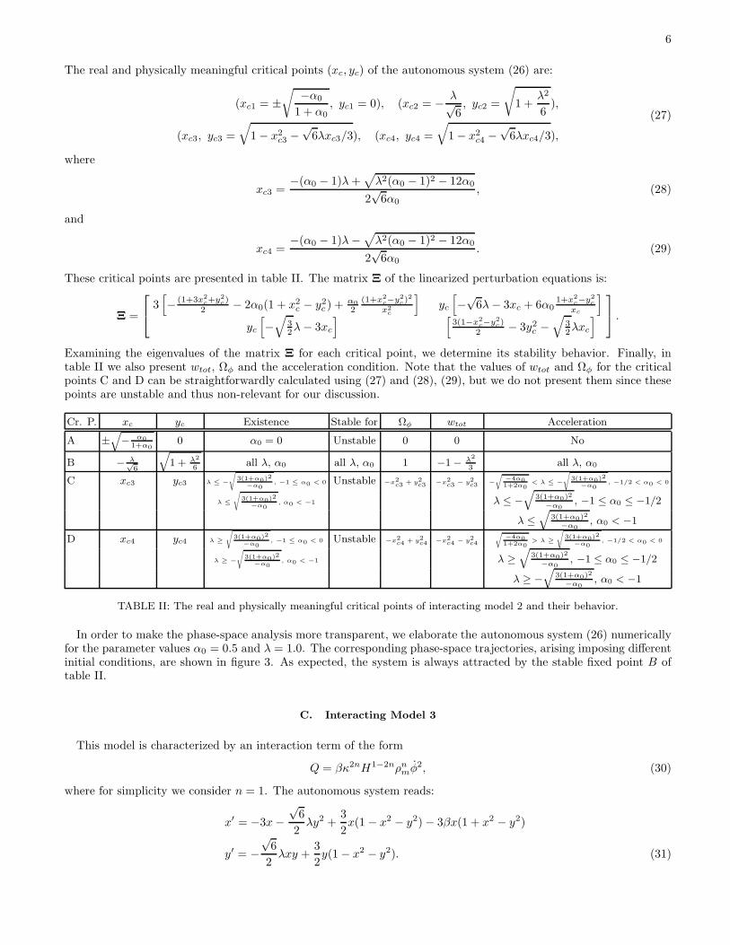
The real and physically meaningful critical points (xc, yc) of the autonomous system (26) are:

(xc1 = ±√

−α0

1 + α0, yc1 = 0), (xc2 = − λ√

6, yc2 =

√

1 +λ2

6),

(xc3, yc3 =

√

1 − x2c3 −

√6λxc3/3), (xc4, yc4 =

√

1 − x2c4 −

√6λxc4/3),

(27)

where

xc3 =−(α0 − 1)λ +

√

λ2(α0 − 1)2 − 12α0

2√

6α0

, (28)

and

xc4 =−(α0 − 1)λ −

√

λ2(α0 − 1)2 − 12α0

2√

6α0

. (29)

These critical points are presented in table II. The matrix Ξ of the linearized perturbation equations is:

Ξ =

3[

− (1+3x2c+y2

c)2 − 2α0(1 + x2

c − y2c ) + α0

2(1+x2

c−y2c)2

x2c

]

yc

[

−√

6λ − 3xc + 6α01+x2

c−y2c

xc

]

yc

[

−√

32λ − 3xc

] [

3(1−x2c−y2

c)2 − 3y2

c −√

32λxc

]

.

Examining the eigenvalues of the matrix Ξ for each critical point, we determine its stability behavior. Finally, intable II we also present wtot, Ωφ and the acceleration condition. Note that the values of wtot and Ωφ for the criticalpoints C and D can be straightforwardly calculated using (27) and (28), (29), but we do not present them since thesepoints are unstable and thus non-relevant for our discussion.

Cr. P. xc yc Existence Stable for Ωφ wtot Acceleration

A ±q

− α01+α0

0 α0 = 0 Unstable 0 0 No

B − λ√6

q

1 + λ2

6all λ, α0 all λ, α0 1 −1 − λ2

3all λ, α0

C xc3 yc3 λ ≤ −

s

3(1+α0)2

−α0, −1 ≤ α0 < 0 Unstable −x2

c3 + y2c3 −x2

c3 − y2c3 −

r

−4α01+2α0

< λ ≤ −

s

3(1+α0)2

−α0, −1/2 < α0 < 0

λ ≤

s

3(1+α0)2

−α0, α0 < −1 λ ≤ −

q

3(1+α0)2

−α0, −1 ≤ α0 ≤ −1/2

λ ≤q

3(1+α0)2

−α0, α0 < −1

D xc4 yc4 λ ≥

s

3(1+α0)2

−α0, −1 ≤ α0 < 0 Unstable −x2

c4 + y2c4 −x2

c4 − y2c4

r

−4α01+2α0

> λ ≥

s

3(1+α0)2

−α0, −1/2 < α0 < 0

λ ≥ −

s

3(1+α0)2

−α0, α0 < −1 λ ≥

q

3(1+α0)2

−α0, −1 ≤ α0 ≤ −1/2

λ ≥ −q

3(1+α0)2

−α0, α0 < −1

TABLE II: The real and physically meaningful critical points of interacting model 2 and their behavior.

In order to make the phase-space analysis more transparent, we elaborate the autonomous system (26) numericallyfor the parameter values α0 = 0.5 and λ = 1.0. The corresponding phase-space trajectories, arising imposing differentinitial conditions, are shown in figure 3. As expected, the system is always attracted by the stable fixed point B oftable II.

C. Interacting Model 3

This model is characterized by an interaction term of the form

Q = βκ2nH1−2nρnmφ2, (30)

where for simplicity we consider n = 1. The autonomous system reads:

x′ = −3x −√

6

2λy2 +

3

2x(1 − x2 − y2) − 3βx(1 + x2 − y2)

y′ = −√

6

2λxy +

3

2y(1 − x2 − y2). (31)

7

−0.9 −0.8 −0.7 −0.6 −0.5 −0.4 −0.3 −0.20.6

0.8

1

1.2

1.4

1.6

1.8

xy

α0=0.5

λ=1.0

FIG. 3: Phase-space trajectories for interacting model 2 using α0 = 0.5 and λ = 1.0. The stable fixed point is the critical pointB in table II, with (xc2, yc2)=(-0.41, 1.08).

The real and physically meaningful critical points (xc, yc) of the autonomous system (31) are:

(xc1 = 0, yc1 = 0), (xc2 = − λ√6, yc2 =

√

1 +λ2

6),

(xc3, yc3 =

√

1 − x2c3 −

√6λxc3/3), (xc4, yc4 =

√

1 − x2c4 −

√6λxc4/3),

(32)

where

xc3 =λ +

√

λ2 − 12β

2√

6β, (33)

and

xc4 =λ −

√

λ2 − 12β

2√

6β. (34)

The matrix Ξ of the linearized perturbation equations is:

Ξ =

3[

− (1+3x2c+y2

c)2 − β(1 + 3x2

c − y2c )

]

yc

[

−√

6λ − 3xc + 6βxc

]

yc

[

−√

32λ − 3xc

] [

3(1−x2c−y2

c)2 − 3y2

c −√

32λxc

]

.

The critical points are presented in table III, together with their stability behavior, wtot, Ωφ and the accelerationcondition.

Cr. P. xc yc Existence Stable for Ωφ wtot Acceleration

A 0 0 all β, λ Unstable 0 0 No

B − λ√6

q

1 + λ2

6all β, λ all λ, β ≥ −1 1 −1 − λ2

3all β, λ

λ2 < − 31+β

, β < −1

C xc3 yc3 λ ≤q

−31+β

, β < −1 Unstable −x2c3 + y2

c3 −x2c3 − y2

c3 −√−4β < λ ≤

q

−31+β

, β < −1

D xc4 yc4 −q

−31+β

≤ λ, β < −1 Unstable −x2c4 + y2

c4 −x2c4 − y2

c4 −q

−31+β

≤ λ <√−4β, β < −1

TABLE III: The real and physically meaningful critical points of interacting model 3 and their behavior.

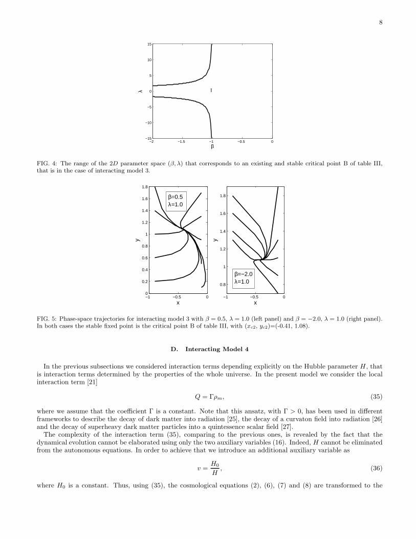
In order to present the results more transparently, in fig. 4 we depict the range of the 2D parameter space (β, λ) thatcorresponds to the existence of the stable critical point B of table III. Furthermore, we elaborate the autonomoussystem (31) numerically, for the parameter values λ = 1.0, β = 0.5 and λ = 1.0, β = −2.0 . The phase-spacetrajectories, corresponding to different initial conditions, are shown in figure 5. In these cases, the system is alwaysattracted by the stable fixed point B of table III, as expected.

8

−2 −1.5 −1 −0.5 0−15

−10

−5

0

5

10

15

βλ I

FIG. 4: The range of the 2D parameter space (β, λ) that corresponds to an existing and stable critical point B of table III,that is in the case of interacting model 3.

−1 −0.5 00

0.2

0.4

0.6

0.8

1

1.2

1.4

1.6

1.8

x

y

−1 −0.5 0

0.8

1

1.2

1.4

1.6

1.8

x

y

β=0.5λ=1.0

β=−2.0λ=1.0

FIG. 5: Phase-space trajectories for interacting model 3 with β = 0.5, λ = 1.0 (left panel) and β = −2.0, λ = 1.0 (right panel).In both cases the stable fixed point is the critical point B of table III, with (xc2, yc2)=(-0.41, 1.08).

D. Interacting Model 4

In the previous subsections we considered interaction terms depending explicitly on the Hubble parameter H , thatis interaction terms determined by the properties of the whole universe. In the present model we consider the localinteraction term [21]

Q = Γρm, (35)

where we assume that the coefficient Γ is a constant. Note that this ansatz, with Γ > 0, has been used in differentframeworks to describe the decay of dark matter into radiation [25], the decay of a curvaton field into radiation [26]and the decay of superheavy dark matter particles into a quintessence scalar field [27].

The complexity of the interaction term (35), comparing to the previous ones, is revealed by the fact that thedynamical evolution cannot be elaborated using only the two auxiliary variables (16). Indeed, H cannot be eliminatedfrom the autonomous equations. In order to achieve that we introduce an additional auxiliary variable as

v =H0

H, (36)

where H0 is a constant. Thus, using (35), the cosmological equations (2), (6), (7) and (8) are transformed to the

9

following autonomous system:

x′ = −3x +3

2x(1 − x2 − y2) −

√

3

2λ y2 − γv

2x(1 + x2 − y2)

y′ =3

2y(1 − x2 − y2) −

√

3

2λxy

v′ =3

2v(1 − x2 − y2), (37)

where we have introduced the dimensionless coupling constant

γ =Γ

H0. (38)

The 3 × 3 matrix Ξ of the linearized perturbation equations is:

Ξ =

3[

− (1+3x2c+y2

c)2 + γvc

6x2c(1 + x2

c − y2c) − γvc

3

]

yc

[

−√

6λ − 3xc + γvc

xc

]

− γ2xc

(1 + x2c − y2

c )

yc

[

−√

32λ − 3xc

] [

3(1−x2c−y2

c)2 − 3y2

c −√

32λxc

]

0

−3xcvc −3ycvc32 (1 − x2

c − y2c )

.

In this model there is only one real and physically meaningful critical point presented in table IV, together with itsstability behavior, wtot, Ωφ and the acceleration condition.

Cr. P. xc yc vc Existence Stable for Ωφ wtot Acceleration

A − λ√6

q

1 + λ2

60 all γ,λ all γ,λ 1 −1 − λ2

3all γ,λ

TABLE IV: The real and physically meaningful critical point of interacting model 4 and its behavior.

−0.9 −0.8 −0.7 −0.6 −0.5 −0.4 −0.3 −0.2 −0.1 00

0.2

0.4

0.6

0.8

1

1.2

1.4

1.6

1.8

x

y

λ=0.5

FIG. 6: Phase-space trajectories for interacting model 4 with λ = 0.5. The stable fixed points is the critical point A of tableIV, with (xc, yc)=(-0.20, 1.02).

To reveal this behavior more transparently, we solve numerically the autonomous system (37) for λ = 0.5. In orderto plot the two dimensional phase trajectories for the variables x and y, we project the system onto the v = 0 planeand the results are shown in figure 6. Finally, we mention that for the corresponding model of a canonical field,examined in [21], using the variable z = H0/(H0 +H) the authors found “critical points” for z = 1, which correspondsto v = ∞ in our case. However, as we can see, this point is not a critical point of the system.

IV. COSMOLOGICAL IMPLICATIONS

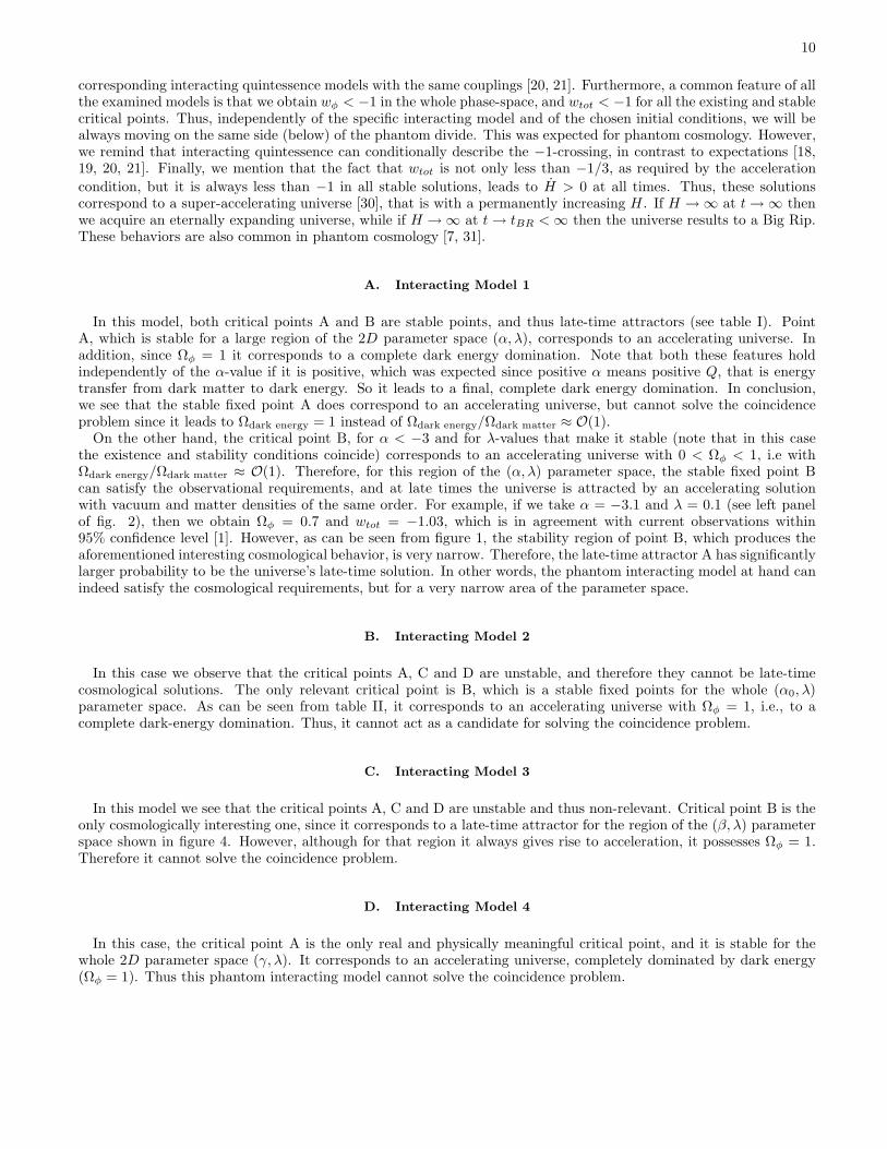
Since we have performed a complete phase-space analysis of various interacting phantom models, we can nowdiscuss the corresponding cosmological behavior. A general remark is that this behavior is radically different from the

10

corresponding interacting quintessence models with the same couplings [20, 21]. Furthermore, a common feature of allthe examined models is that we obtain wφ < −1 in the whole phase-space, and wtot < −1 for all the existing and stablecritical points. Thus, independently of the specific interacting model and of the chosen initial conditions, we will bealways moving on the same side (below) of the phantom divide. This was expected for phantom cosmology. However,we remind that interacting quintessence can conditionally describe the −1-crossing, in contrast to expectations [18,19, 20, 21]. Finally, we mention that the fact that wtot is not only less than −1/3, as required by the acceleration

condition, but it is always less than −1 in all stable solutions, leads to H > 0 at all times. Thus, these solutionscorrespond to a super-accelerating universe [30], that is with a permanently increasing H . If H → ∞ at t → ∞ thenwe acquire an eternally expanding universe, while if H → ∞ at t → tBR < ∞ then the universe results to a Big Rip.These behaviors are also common in phantom cosmology [7, 31].

A. Interacting Model 1

In this model, both critical points A and B are stable points, and thus late-time attractors (see table I). PointA, which is stable for a large region of the 2D parameter space (α, λ), corresponds to an accelerating universe. Inaddition, since Ωφ = 1 it corresponds to a complete dark energy domination. Note that both these features holdindependently of the α-value if it is positive, which was expected since positive α means positive Q, that is energytransfer from dark matter to dark energy. So it leads to a final, complete dark energy domination. In conclusion,we see that the stable fixed point A does correspond to an accelerating universe, but cannot solve the coincidenceproblem since it leads to Ωdark energy = 1 instead of Ωdark energy/Ωdark matter ≈ O(1).

On the other hand, the critical point B, for α < −3 and for λ-values that make it stable (note that in this casethe existence and stability conditions coincide) corresponds to an accelerating universe with 0 < Ωφ < 1, i.e withΩdark energy/Ωdark matter ≈ O(1). Therefore, for this region of the (α, λ) parameter space, the stable fixed point Bcan satisfy the observational requirements, and at late times the universe is attracted by an accelerating solutionwith vacuum and matter densities of the same order. For example, if we take α = −3.1 and λ = 0.1 (see left panelof fig. 2), then we obtain Ωφ = 0.7 and wtot = −1.03, which is in agreement with current observations within95% confidence level [1]. However, as can be seen from figure 1, the stability region of point B, which produces theaforementioned interesting cosmological behavior, is very narrow. Therefore, the late-time attractor A has significantlylarger probability to be the universe’s late-time solution. In other words, the phantom interacting model at hand canindeed satisfy the cosmological requirements, but for a very narrow area of the parameter space.

B. Interacting Model 2

In this case we observe that the critical points A, C and D are unstable, and therefore they cannot be late-timecosmological solutions. The only relevant critical point is B, which is a stable fixed points for the whole (α0, λ)parameter space. As can be seen from table II, it corresponds to an accelerating universe with Ωφ = 1, i.e., to acomplete dark-energy domination. Thus, it cannot act as a candidate for solving the coincidence problem.

C. Interacting Model 3

In this model we see that the critical points A, C and D are unstable and thus non-relevant. Critical point B is theonly cosmologically interesting one, since it corresponds to a late-time attractor for the region of the (β, λ) parameterspace shown in figure 4. However, although for that region it always gives rise to acceleration, it possesses Ωφ = 1.Therefore it cannot solve the coincidence problem.

D. Interacting Model 4

In this case, the critical point A is the only real and physically meaningful critical point, and it is stable for thewhole 2D parameter space (γ, λ). It corresponds to an accelerating universe, completely dominated by dark energy(Ωφ = 1). Thus this phantom interacting model cannot solve the coincidence problem.

11

V. CONCLUSIONS

In this work we performed a detailed phase-space analysis of various phantom cosmological models, where the darkenergy sector interacts with the dark matter one. Our basic goal was to examine whether there exist late-time scalingattractors, corresponding to accelerated universe and possessing Ωdark energy/Ωdark matter ≈ O(1), thus satisfying thebasic observational requirements. We investigated four different interaction models, including one with a local, i.e.H-independent, form of the interaction term (interacting model 4). We extracted the critical points, determinedtheir stabilities, and calculated the basic cosmological observables, namely the total equation-of-state parameter wtot

and Ωdark energy (attributed to the phantom field). The key point of solving the coincidence problem is that theuniverse is in the attractor now and it has normal radiation dominated and matter dominated eras before it reachedthe attractors. Note that as long as the interaction term is not too strong, the standard cosmology can be alwaysrecovered. Once it is in the attractor, the results do not depend on the initial conditions. Thus, one can switch onthe interaction and consider as initial conditions the end of the known epochs of standard Big Bang cosmology, inorder to avoid disastrous interference.

In all the examined models we found that stable late-time solutions do exist, corresponding moreover to an accel-erating universe. This feature was expected since phantom cosmology has been constructed in order to always satisfythis condition. Indeed, for all the studied models, we did not find any non-accelerating stable solution. However, inalmost all the cases the late-time solutions correspond to a complete dark energy domination and thus are unableto solve the coincidence problem. The only case in which this is possible is in interacting model 1, if we select theparameter values from a very narrow region of the 2D parameter space (see figure 1).

In conclusion, we see that the examined models of interacting phantom cosmology can produce acceleration (whichis “embedded” in phantom cosmology in general) but cannot solve the coincidence problem, unless one imposes aform of fine-tuning in the model parameters. This result has been extracted by the negative-kinetic-energy realizationof phantom, which does not cover the whole class of phantom models, but since it is a qualitative statement itshould intuitively be robust for general interacting phantom scenarios, too. An alternative direction would be toconsider more complicated interaction terms, suitably constructed in order to solve the coincidence problem. Butthe interaction term was introduced in phantom cosmology in order to solve the coincidence problem in a simpleand general way, avoiding the assumptions and fine-tunings of conventional cosmology. Although promising and withmany advantages, interacting phantom cosmology needs further investigation.

[1] A.G. Riess et al. [Supernova Search Team Collaboration], Astron. J. 116, 1009 (1998); A. G. Riess et al. [Supernova SearchTeam Collaboration], Astrophys. J. 607, 665 (2004); S. Perlmutter et al. [Supernova Cosmology Project Collaboration],Astrophys. J. 517, 565 (1999); D. N. Spergel et al., Astrophys. J. Suppl. 148, 175 (2003); S. W. Allen, et al., Mon. Not.Roy. Astron. Soc. 353, 457 (2004).

[2] S.M. Carroll, V. Duvvuri, M. Trodden, M.S. Turner, Phys. Rev. D 70, 043528 (2004); T. Chiba, Phys. Lett. B 575, 1(2003); S. Nojiri, S.D. Odintsov, Phys. Rev. D 68, 123512 (2003); C.G. Shao, R.G. Cai, B. Wang, R.K. Su, Phys. Lett. B633, 164 (2006).

[3] S. Capozziello, Int. J. Mod. Phys. D 11, 483 (2002); S. A. Appleby and R. A. Battye, Phys. Lett. B 654, 7 (2007); S.Nojiri, S.D. Odintsov, Int. J. Geom. Meth. Mod. Phys. 4, 115 (2007); A. A. Starobinsky, JETP Lett. 86, 157 (2007); W.Hu, I. Sawicki, Phys. Rev. D 76, 064004 (2007); S. Nojiri, S.D. Odintsov, [arXiv:0807.0685[hep-th]].

[4] G.R. Dvali, G. Gabadadze, M. Porrati, Phys. Lett. B 485, 208 (2000); C. Deffayet, G.R. Dvali, G. Gabadadze, Phys. Rev.D 65, 044023 (2002); Y.G. Gong, C.K. Duan, Class. Quantum Grav. 21, 3655 (2004); F. K. Diakonos and E. N. Sari-dakis, JCAP 0902, 030 (2009); Y.G. Gong, C.K. Duan, Mon. Not. Roy. Astron. Soc. 352, 847 (2004); Y.G. Gong,[arXiv:0808.1316[astro-ph]].

[5] P. Binetruy, C. Deffayet, D. Langlois, Nucl. Phys. B 565, 269 (2000); R.G. Cai, Y.G. Gong, B. Wang, JCAP 0603, 006(2006); Y.G. Gong, A. Wang, Class. Quantum Grav. 23, 3419 (2006); Y.G. Gong, A. Wang, Q. Wu, Phys. Lett. B 663,147 (2008); M. R. Setare and E. N. Saridakis, Phys. Lett. B 670, 1 (2008); M. R. Setare and E. N. Saridakis, JCAP 0903,002 (2009).

[6] B. Ratra and P. J. E. Peebles, Phys. Rev. D 37, 3406 (1988); C. Wetterich, Nucl. Phys. B 302, 668 (1988); A. R. Liddleand R. J. Scherrer, Phys. Rev. D 59, 023509 (1998); I. Zlatev, L. M. Wang and P. J. Steinhardt, Phys. Rev. Lett. 82, 896(1999); Z. K. Guo, N. Ohta and Y. Z. Zhang, Mod. Phys. Lett. A 22, 883 (2007).

[7] R. R. Caldwell, Phys. Lett. B 545, 23 (2002); R. R. Caldwell, M. Kamionkowski and N. N. Weinberg, Phys. Rev. Lett. 91,071301 (2003); S. Nojiri and S. D. Odintsov, Phys. Lett. B 562, 147 (2003); V. K. Onemli and R. P. Woodard, Phys. Rev.D 70, 107301 (2004) [arXiv:gr-qc/0406098]; M. R. Setare, Eur. Phys. J. C 50, 991 (2007); E. N. Saridakis, [arXiv:0811.1333[hep-th]].

[8] B. Boisseau, G. Esposito-Farese, D. Polarski and A. A. Starobinsky, Phys. Rev. Lett. 85, 2236 (2000); S. Nojiri,S. D. Odintsov and M. Sasaki, Phys. Rev. D 71, 123509 (2005); M. z. Li, B. Feng and X. m. Zhang, JCAP 0512,

12

002 (2005); S. Nojiri and S. D. Odintsov, Phys. Rev. D 72, 023003 (2005); S. Sur and S. Das, JCAP 0901, 007 (2009);K. Bamba, C. Q. Geng, S. Nojiri and S. D. Odintsov, arXiv:0810.4296 [hep-th].

[9] C. Armendariz-Picon, V. F. Mukhanov and P. J. Steinhardt, Phys. Rev. D 63, 103510 (2001) [arXiv:astro-ph/0006373].[10] B. Feng, X. L. Wang and X. M. Zhang, Phys. Lett. B 607, 35 (2005); Z. K. Guo, et al., Phys. Lett. B 608, 177 (2005);

M.-Z Li, B. Feng, X.-M Zhang, JCAP, 0512, 002 (2005); B. Feng, M. Li, Y.-S. Piao and X. Zhang, Phys. Lett. B 634, 101(2006); M. R. Setare, Phys. Lett. B 641, 130 (2006); W. Zhao and Y. Zhang, Phys. Rev. D 73, 123509 (2006); M. R. Setareand E. N. Saridakis, Phys. Lett. B 671, 331 (2009).

[11] A. G. Cohen, D. B. Kaplan and A. E. Nelson, Phys. Rev. Lett. 82, 4971 (1999); P. Horava and D. Minic, Phys. Rev.Lett. 85, 1610 (2000); S. D. H. Hsu, Phys. Lett. B 594, 13 (2004); M. Li, Phys. Lett. B 603, 1 (2004); Y.G. Gong, Phys.Rev. D 70, 064029 (2004); Y.G. Gong and J. Liu, JCAP 0809, 010 (2008); D. Pavon and W. Zimdahl, Phys. Lett. B628, 206 (2005); H. Li, Z. K. Guo and Y. Z. Zhang, Int. J. Mod. Phys. D 15, 869 (2006); M. R. Setare, J. Zhang and X.Zhang, JCAP 0703, 007 (2007); E. N. Saridakis, Phys. Lett. B 660, 138 (2008); E. N. Saridakis, JCAP 0804, 020 (2008);E. N. Saridakis, Phys. Lett. B 661, 335 (2008).

[12] A. P. Billyard and A. A. Coley, Phys. Rev D 61, 083503 (2000); J. P. Mimoso, A. Nunes and D.Pavon, Phys. Rev. D73, 023502 (2006); R. Lazkoz and G. Leon, Phys. Lett. B 638, 303 (2006); T. Gonzalez, G. Leon and I. Quiros, Class.Quant. Grav. 23, 3165 (2006); G. R. Farrar and P. J. E. Peebles, Astrophys. J. 604, 1 (2004); B. Wang, Y. G. Gong andE. Abdalla, Phys. Lett. B 624, 141 (2005); M. R. Setare, Phys. Lett. B 642, 1 (2006).

[13] Z. K. Guo, R. G. Cai and Y. Z. Zhang, JCAP 0505, 002 (2005); A. Nunes, J.P. Mimoso and T.C. Charters, Phys. Rev. D63, 083506 (2001); D.F. Mota and C. van de Bruck, Astron. Astrophys. 421, 71 (2004); M. Manera and D.F. Mota, Mon.Not. Roy. Astron. Soc. 371, 1373 (2006); N.J. Nunes and D.F. Mota, Mon. Not. Roy. Astron. Soc. 368, 751 (2006); J.D.Barrow and T. Clifton, Phys. Rev. D 73, 103520 (2006); T. Clifton and J.D. Barrow, Phys. Rev. D 73, 104022 (2006); T.Clifton and J.D. Barrow, Phys. Rev. D 75, 043515 (2007); M. Jamil and M.A. Rashid, arXiv: 0802.1144; M. Jamil, arXiv:0810.2896.

[14] P.G. Ferreira, M. Joyce, Phys. Rev. Lett. 79, 4740 (1997); E.J. Copeland, M. Sami, S. Tsujikawa, Int. J. Mod. Phys. D15, 1753 (2006); Y.G. Gong, A. Wang, Y.Z. Zhang, Phys. Lett. B 636, 286 (2006).

[15] E. J. Copeland, A. R. Liddle and D. Wands, Phys. Rev. D 57, 4686 (1998).[16] P. Singh, M. Sami and N. Dadhich, Phys. Rev. D 68, 023522 (2003); J. G. Hao and X. Z. Li, Phys. Rev. D 70, 043529

(2004).[17] H. Wei and S. N. Zhang, Phys. Rev. D 76, 063005 (2007); M. R. Setare and E. N. Saridakis, JCAP 0809, 026 (2008);

M. R. Setare and E. N. Saridakis, Phys. Lett. B 668, 177 (2008); M. R. Setare and E. N. Saridakis, [arXiv:0807.3807[hep-th]].

[18] C. Wetterich, Astron. Astrophys. 301, 321 (1995); L. Amendola, Phys. Rev. D 60, 043501 (1999).[19] H. Garcia-Compean, G. Garcia-Jimenez, O. Obregon and C. Ramirez, JCAP 0807, 016 (2008).[20] X. M. Chen and Y.G. Gong, [arXiv:0811.1698[gr-qc]].[21] C. G. Bohmer, G. Caldera-Cabral, R. Lazkoz and R. Maartens, Phys. Rev. D 78, 023505 (2008).[22] L. Amendola, M. Quartin, S. Tsujikawa and I. Waga, Phys. Rev. D 74, 023525 (2006).[23] Z. K. Guo and Y. Z. Zhang, Phys. Rev. D 71, 023501 (2005). T. Gonzalez and I. Quiros, Class. Quant. Grav. 25, 175019

(2008).[24] R. Curbelo, T. Gonzalez, G. Leon and I. Quiros, Class. Quant. Grav. 23, 1585 (2006).[25] R. Cen, Astrophys. J. 546, L77 (2001) [arXiv:astro-ph/0005206]; M. Oguri, K. Takahashi, H. Ohno and K. Kotake,

Astrophys. J. 597, 645 (2003).[26] K. A. Malik, D. Wands and C. Ungarelli, Phys. Rev. D 67, 063516 (2003).[27] H. Ziaeepour, Phys. Rev. D 69, 063512 (2004).[28] R. J. Scherrer and A. A. Sen, Phys. Rev. D 77, 083515 (2008); R. J. Scherrer and A. A. Sen, Phys. Rev. D 78, 067303

(2008); M. R. Setare and E. N. Saridakis, Phys. Rev. D 79, 043005 (2009).[29] L. P. Chimento, A. S. Jakubi, D. Pavon and W. Zimdahl, Phys. Rev. D 67, 083513 (2003).[30] S. Das, P. S. Corasaniti and J. Khoury, Phys. Rev. D 73, 083509 (2006); M. Kaplinghat and A. Rajaraman, Phys. Rev. D

75, 103504 (2007).[31] F. Briscese, E. Elizalde, S. Nojiri and S. D. Odintsov, Phys. Lett. B 646, 105 (2007).