Phase space analysis of interacting dark energy in f (T) cosmology
13
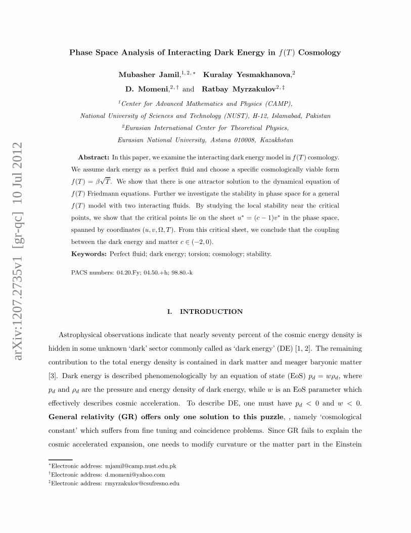
arXiv:1207.2735v1 [gr-qc] 10 Jul 2012 Phase Space Analysis of Interacting Dark Energy in f (T ) Cosmology Mubasher Jamil, 1,2, ∗ Kuralay Yesmakhanova, 2 D. Momeni, 2, † and Ratbay Myrzakulov 2, ‡ 1 Center for Advanced Mathematics and Physics (CAMP), National University of Sciences and Technology (NUST), H-12, Islamabad, Pakistan 2 Eurasian International Center for Theoretical Physics, Eurasian National University, Astana 010008, Kazakhstan Abstract: In this paper, we examine the interacting dark energy model in f (T ) cosmology. We assume dark energy as a perfect fluid and choose a specific cosmologically viable form f (T )= β √ T . We show that there is one attractor solution to the dynamical equation of f (T ) Friedmann equations. Further we investigate the stability in phase space for a general f (T ) model with two interacting fluids. By studying the local stability near the critical points, we show that the critical points lie on the sheet u * =(c − 1)v * in the phase space, spanned by coordinates (u, v, Ω,T ). From this critical sheet, we conclude that the coupling between the dark energy and matter c ∈ (−2, 0). Keywords: Perfect fluid; dark energy; torsion; cosmology; stability. PACS numbers: 04.20.Fy; 04.50.+h; 98.80.-k I. INTRODUCTION Astrophysical observations indicate that nearly seventy percent of the cosmic energy density is hidden in some unknown ‘dark’ sector commonly called as ‘dark energy’ (DE) [1, 2]. The remaining contribution to the total energy density is contained in dark matter and meager baryonic matter [3]. Dark energy is described phenomenologically by an equation of state (EoS) p d = wρ d , where p d and ρ d are the pressure and energy density of dark energy, while w is an EoS parameter which effectively describes cosmic acceleration. To describe DE, one must have p d < 0 and w< 0. General relativity (GR) offers only one solution to this puzzle, , namely ‘cosmological constant’ which suffers from fine tuning and coincidence problems. Since GR fails to explain the cosmic accelerated expansion, one needs to modify curvature or the matter part in the Einstein * Electronic address: [email protected] † Electronic address: [email protected] ‡ Electronic address: [email protected]
-
Upload
independent -
Category
Documents
-
view
2 -
download
0
Transcript of Phase space analysis of interacting dark energy in f (T) cosmology
arX
iv:1
207.
2735
v1 [
gr-q
c] 1
0 Ju
l 201
2
Phase Space Analysis of Interacting Dark Energy in f(T ) Cosmology
Mubasher Jamil,1, 2, ∗ Kuralay Yesmakhanova,2
D. Momeni,2, † and Ratbay Myrzakulov2, ‡
1Center for Advanced Mathematics and Physics (CAMP),
National University of Sciences and Technology (NUST), H-12, Islamabad, Pakistan
2Eurasian International Center for Theoretical Physics,
Eurasian National University, Astana 010008, Kazakhstan
Abstract: In this paper, we examine the interacting dark energy model in f(T ) cosmology.
We assume dark energy as a perfect fluid and choose a specific cosmologically viable form
f(T ) = β√T . We show that there is one attractor solution to the dynamical equation of
f(T ) Friedmann equations. Further we investigate the stability in phase space for a general
f(T ) model with two interacting fluids. By studying the local stability near the critical
points, we show that the critical points lie on the sheet u∗ = (c − 1)v∗ in the phase space,
spanned by coordinates (u, v,Ω, T ). From this critical sheet, we conclude that the coupling
between the dark energy and matter c ∈ (−2, 0).
Keywords: Perfect fluid; dark energy; torsion; cosmology; stability.
PACS numbers: 04.20.Fy; 04.50.+h; 98.80.-k
I. INTRODUCTION
Astrophysical observations indicate that nearly seventy percent of the cosmic energy density is
hidden in some unknown ‘dark’ sector commonly called as ‘dark energy’ (DE) [1, 2]. The remaining
contribution to the total energy density is contained in dark matter and meager baryonic matter
[3]. Dark energy is described phenomenologically by an equation of state (EoS) pd = wρd, where
pd and ρd are the pressure and energy density of dark energy, while w is an EoS parameter which
effectively describes cosmic acceleration. To describe DE, one must have pd < 0 and w < 0.
General relativity (GR) offers only one solution to this puzzle, , namely ‘cosmological
constant’ which suffers from fine tuning and coincidence problems. Since GR fails to explain the
cosmic accelerated expansion, one needs to modify curvature or the matter part in the Einstein
∗Electronic address: [email protected]†Electronic address: [email protected]‡Electronic address: [email protected]
2
field equations. Some notable examples are f(R) gravity [4], scalar-tensor gravity [5] and Lovelock
gravity [6] and more recently f(T ) gravity [7], to name a few. Other models where matter action
is modified include the bulk viscous stress [8] and the anisotropic stress [9] or some exotic fluid
like Chaplygin gas (CG) [10]. One of the crucial tests to check the viability of extended
theories of gravity is the potential detection of gravitational waves [11].
We assume a phenomenological form of interaction between matter and dark energy since these
are the dominant components of the cosmic composition, following [12]. The exact nature of this
interaction is beyond the scope of the paper and unresolved till we obtain a consistent theory of
quantum gravity. In these interacting dark energy-dark matter models, the dark energy decays
into matter at a rate proportional to Hubble length. The interacting dark energy scenario
can successfully resolve the coincidence problem then stable attractor solutions of the
Friedmann-Robertson-Walker (FRW) equations can be obtained [13].Some observa-
tional support to these models come from the astrophysical observations [14, 15]. For
motivation from field theory and particle physics of the interacting dark energy, the
interested reader is referred to [16, 17].
The present paper is devoted to the study of dynamics of interacting dark energy in f(T )
cosmology. This theory is based on torsion scalar T rather than curvature scalar R. We assume
the dark energy in the form of a perfect fluid interacting with the matter. We study this model
by the local stability method and than extend it for dark energy satisfying a more
general form of equation of state.
II. BASIC EQUATIONS
A. Basics of f(T ) gravity
General relativity is a gauge theory of the gravitational field. It is based on the equivalence
principle. However it is not necessary to work with Riemannian manifolds. There are
some extended theories such as Riemann-Cartan, in them the geometrical structure
of the theory has non-vanishing object of non-metricity. In these extensions, there are
more than one dynamical quantity (metric). For example this theory may be constructed from the
metric, non-metricity and torsion [18]. Ignoring from the non-metricity of the theory, we
can leave the Riemannian manifold and go to Weitznbock spacetime, with torsion and
zero local Riemann tensor. One sample of such theories is called teleparallel gravity in which
3
we are working in a non-Riemannian manifold.The dynamics of the metric is determined
using the scalar torsion T . The fundamental quantities in teleparallel theory are the
vierbein (tetrad) basis vectors eiµ. This basis is an orthogonal, coordinate free basis, defined
by the following equation
gµν = eiµejνηij.
This tetrad basis must be orthonormal and ηij is the Minkowski metric. It means that eiµeµj = δij .
There is a simple extension of the teleparallel gravity, which is called f(T ) gravity.
In this theories, f is an arbitrary function of the torsion T . One suitable form of action for f(T )
gravity in Weitzenbock spacetime is [19]
S =1
2κ2
∫
d4xe(T + f(T ) + Lm).
Here e = det(eiµ), κ2 = 8πG. The dynamical quantity of the model is the scalar torsion T and Lm
is the matter Lagrangian. The field equation can be derived from the action by varying
the action with respect to eiµ
e−1∂µ(eSµν
i )(1 + fT )− e λi T
ρµλS
νµρ fT
+S µνi ∂µ(T )fTT − 1
4eνi(1 + f(T )) = 4πGe ρ
i Tν
ρ , (1)
where T νρ is the energy-momentum tensor for matter sector of the Lagrangian Lm, defined by
Tµν = − 2√−g
δ∫
(√−gLmd4x)
δgµν.
Here T is defined by
T = S µνρ T ρ
µν ,
where
T ρµν = eρi (∂µe
iν − ∂νe
iµ),
S µνρ =
1
2(Kµν
ρ + δµρTθνθ − δνρT
θµθ ),
and the contorsion tensor reads Kµνρ as
Kµνρ = −1
2(T µν
ρ − T νµρ − T µν
ρ ).

4
It is straightforward to show that this equation of motion reduces to Einstein gravity
when f(T ) = 0. Indeed, it is the equivalency between the teleparallel theory and
Einstein gravity [20]. The theory has been found to address the issue of cosmic acceleration in
the early and late evolution of universe [21] but this crucially depends on the choice of suitable
f(T ), for instance exponential form containing T cannot lead to phantom crossing
[22]. Reconstruction of f(T ) models has been reported in [23] while thermodynamics of f(T )
cosmology including the generalized second law of thermodynamics has been recently
investigated [24].
B. Interacting dark energy in f(T ) cosmology
We adopt the metric in the form of a flat Friedmann-Lemaitre-Robertson-Walker metric with
metric ds2 = dt2 − a(t)2(dxidxi), i = 1, 2, 3. We start with the Friedmann equation for the
f(T ) model [7]
H2 =1
1 + 2fT
(κ2
3ρ− f
6
)
, (2)
where ρ = ρm + ρd, and ρm, ρd represent the energy densities of matter and dark energy.
The second FRW equation is
H = −κ2
2
( ρ+ p
1 + fT + 2TfTT
)
. (3)
For a spatially flat universe (k = 0), the total energy conservation equation is
ρ+ 3H(ρ+ p) = 0, (4)
where H is the Hubble parameter, ρ is the total energy density and p is the total pressure of the
background fluid. The so-called energy-balance equations corresponding to dark energy and dark
matter are [25]
ρd + 3H(ρd + pd) = −Q,
ρm + 3Hρm = Q, (5)
Here Q is the interaction term which corresponds to energy exchange between dark energy and
dark matter. The function Q has dependencies on the energy densities of the dark matter and dark
energy and the Hubble parameter, i.e. Q(Hρm), Q(Hρd) or Q(Hρm,Hρd) [26]. Since the nature
of both dark energy and dark matter is unknown, it is not possible to derive Γ from first principles.

5
To give a reasonable Q, we may expand like Q(Hρm,Hρd) ≃ αmHρm+αdHρd. Since the coupling
strength is also not known, we may adopt just one parameter for our convenience; hence we take
αm = αd = c [27]. We here choose the following coupling function Q = 3Hc(ρd + ρm).
To perform the stability analysis of the cosmological model, it is always convenient to define
dimensionless density parameters via
u ≡ κ2ρd3H2
, v ≡ κ2pd3H2
, Ωm ≡ κ2ρm3H2
. (6)
Moreover the equation of state parameter of dark energy
w ≡ pdρd
=v
u. (7)
Also the equation of state of all the fluids together is
wtot ≡pd
ρd + ρm=
v
1− ΩT
. (8)
Using (6), we can rewrite (2) in dimensionless form
Ωm = 1− u− ΩT , (9)
where ΩT ≡ f(T )T
− 2fT , is another dimensionless density parameter constructed for torsion scalar.
In f(T ) and teleparallel gravities, phase space analysis for different dark energy models
has been reported in [28, 29].
III. STABILITY ANALYSIS OF PERFECT FLUID
In this section, we treat dark energy as a perfect fluid. Physically it means that the fluid has
no viscosity or heat transfer property. Its a simple fluid which cannot be self-gravitating and has a
smooth distribution in space. A perfect fluid is represented by a phenomenological linear equation
of state connecting energy density and pressure by
pd = wρd, (10)
where w is a ‘constant’ of proportionality but can be a function of time or e-folding parameter
x = ln a. For a general dark energy paradigm, the minimum condition to be satisfied is w ≤ −1/3.
This opens a window to construct variety of theoretical models to explain cosmic
acceleration.
Some of these well-known models are cosmological constant (w = −1), quintessence (w < −1/3)
and phantom energy (w < −1).
6
The dynamical system representing the dynamics of perfect fluid’s density and pressure reads
as
du
dx= −3[u+ v + c(1− ΩT )]
+3u[ 1− ΩT + v
1 + 2TfT + fTT
]
, (11)
dv
dx= −3w[u+ v + c(1 − ΩT )]
+3v[ 1−ΩT + v
1 + 2TfT + fTT
]
. (12)
We notice that our dynamical system is under-determined: three unknown functions (u, v,ΩT ) and
two coupled equations. Thus we must choose f(T ) to solve the system. It is discussed in [30] that a
power-law form of correction term f(T ) ∼ T n (n > 1) such as T 2 can remove the finite-time future
singularity. However, when n = 0, the correction term behaves like a cosmological constant. The
model with n = 1/2 can be helpful in realizing power-law inflation, and also describes
little-rip and pseudo-rip cosmology [30]. Due to these reasons, we choose
f(T ) = β√−T ,
where β is a constant. Note that choosing β = 0 (or f(T ) = 0) leads to teleparallel gravity
which is equivalent to General Relativity. Note that this choice f(T ) = β√−T , has
correspondence with the cosmological constant EoS in f(T ) gravity [31]. This f(T )
model can be recovered via reconstruction scheme of holographic dark energy [35].
Also it can be inspired from a model for dark energy model form the Veneziano ghost
[32]. Recently Capozziello et al [33] investigated the cosmography of f(T ) cosmology
by using data of BAO, Supernovae Ia and WMAP. Following their interesting results,
we notice that if we choose β =√
3/2H0(Ωm0 − 1), than one can estimate the parame-
ters of this f(T ) model as a function of Hubble parameter H0 and the cosmographic
parameters and the value of matter density parameter.
Recently attractor solutions for the dynamical system with three fluids (dark matter, dark en-
ergy and radiation) interacting non-gravitationally have been investigated to resolve the coincidence
problem using similar f(T ) [29].
To perform the stability of the system comprising equations (11) and (12), we first calculate
the critical points (u∗, v∗) by equating
du
dx= 0,
dv
dx= 0.
7
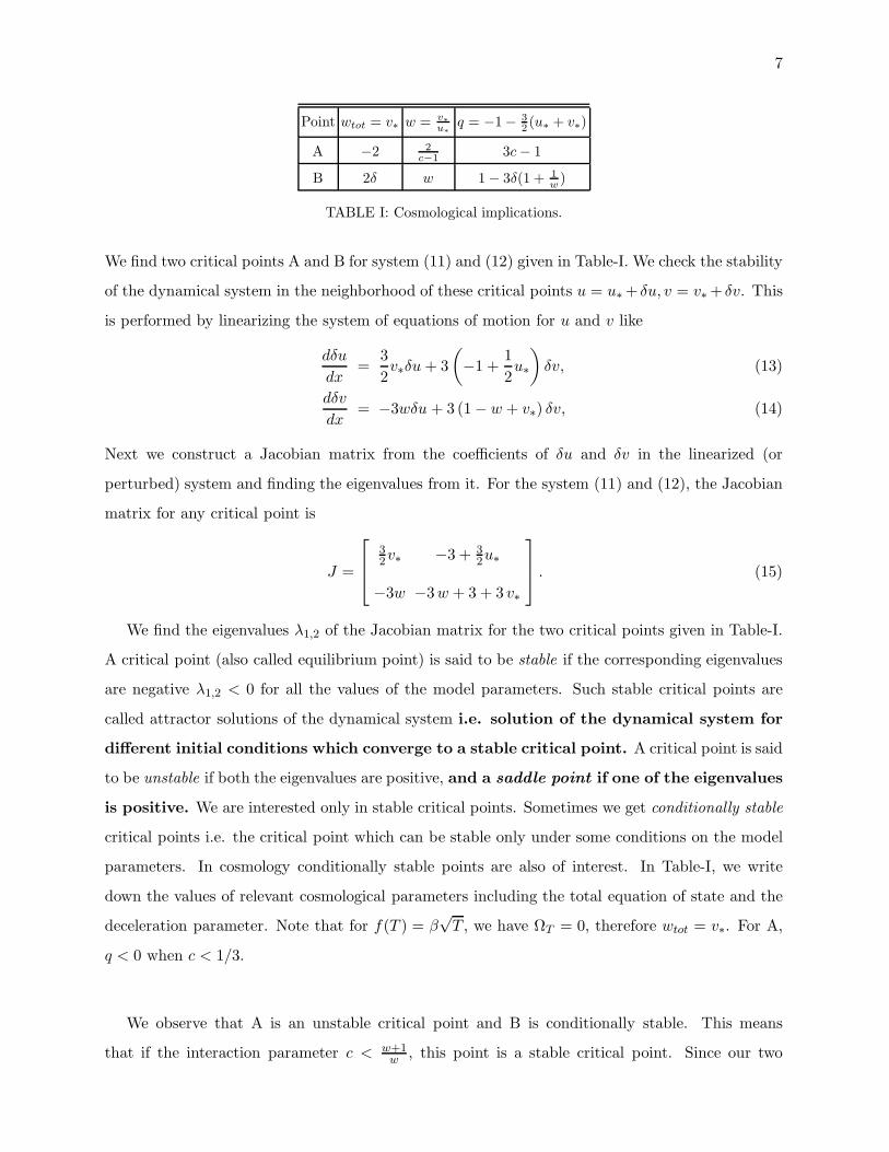
Point wtot = v∗ w = v∗
u∗
q = −1− 3
2(u∗ + v∗)
A −2 2
c−13c− 1
B 2δ w 1− 3δ(1 + 1
w)
TABLE I: Cosmological implications.
We find two critical points A and B for system (11) and (12) given in Table-I. We check the stability
of the dynamical system in the neighborhood of these critical points u = u∗+ δu, v = v∗+ δv. This
is performed by linearizing the system of equations of motion for u and v like
dδu
dx=
3
2v∗δu+ 3
(
−1 +1
2u∗
)
δv, (13)
dδv
dx= −3wδu + 3 (1− w + v∗) δv, (14)
Next we construct a Jacobian matrix from the coefficients of δu and δv in the linearized (or
perturbed) system and finding the eigenvalues from it. For the system (11) and (12), the Jacobian
matrix for any critical point is
J =
32v∗ −3 + 3
2u∗
−3w −3w + 3 + 3 v∗
. (15)
We find the eigenvalues λ1,2 of the Jacobian matrix for the two critical points given in Table-I.
A critical point (also called equilibrium point) is said to be stable if the corresponding eigenvalues
are negative λ1,2 < 0 for all the values of the model parameters. Such stable critical points are
called attractor solutions of the dynamical system i.e. solution of the dynamical system for
different initial conditions which converge to a stable critical point. A critical point is said
to be unstable if both the eigenvalues are positive, and a saddle point if one of the eigenvalues
is positive. We are interested only in stable critical points. Sometimes we get conditionally stable
critical points i.e. the critical point which can be stable only under some conditions on the model
parameters. In cosmology conditionally stable points are also of interest. In Table-I, we write
down the values of relevant cosmological parameters including the total equation of state and the
deceleration parameter. Note that for f(T ) = β√T , we have ΩT = 0, therefore wtot = v∗. For A,
q < 0 when c < 1/3.
We observe that A is an unstable critical point and B is conditionally stable. This means
that if the interaction parameter c < w+1w
, this point is a stable critical point. Since our two
8
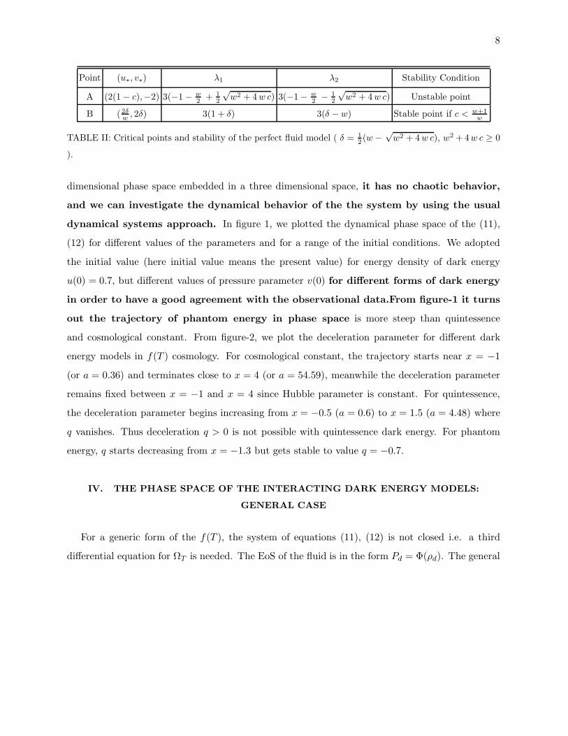
Point (u∗, v∗) λ1 λ2 Stability Condition
A (2(1− c),−2) 3(−1− w
2+ 1
2
√w2 + 4w c) 3(−1− w
2− 1
2
√w2 + 4w c) Unstable point
B (2δw, 2δ) 3(1 + δ) 3(δ − w) Stable point if c < w+1
w
TABLE II: Critical points and stability of the perfect fluid model ( δ = 1
2(w−
√w2 + 4w c), w2 +4w c ≥ 0
).
dimensional phase space embedded in a three dimensional space, it has no chaotic behavior,
and we can investigate the dynamical behavior of the the system by using the usual
dynamical systems approach. In figure 1, we plotted the dynamical phase space of the (11),
(12) for different values of the parameters and for a range of the initial conditions. We adopted
the initial value (here initial value means the present value) for energy density of dark energy
u(0) = 0.7, but different values of pressure parameter v(0) for different forms of dark energy
in order to have a good agreement with the observational data.From figure-1 it turns
out the trajectory of phantom energy in phase space is more steep than quintessence
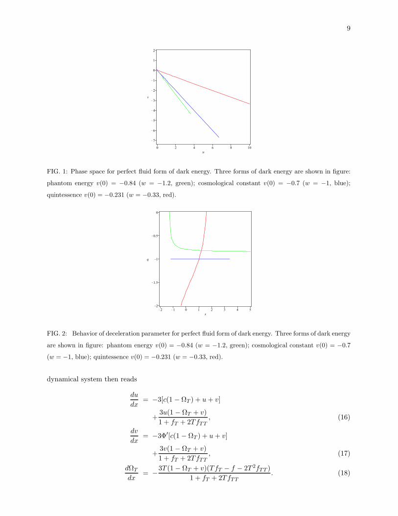
and cosmological constant. From figure-2, we plot the deceleration parameter for different dark
energy models in f(T ) cosmology. For cosmological constant, the trajectory starts near x = −1
(or a = 0.36) and terminates close to x = 4 (or a = 54.59), meanwhile the deceleration parameter
remains fixed between x = −1 and x = 4 since Hubble parameter is constant. For quintessence,
the deceleration parameter begins increasing from x = −0.5 (a = 0.6) to x = 1.5 (a = 4.48) where
q vanishes. Thus deceleration q > 0 is not possible with quintessence dark energy. For phantom
energy, q starts decreasing from x = −1.3 but gets stable to value q = −0.7.
IV. THE PHASE SPACE OF THE INTERACTING DARK ENERGY MODELS:
GENERAL CASE
For a generic form of the f(T ), the system of equations (11), (12) is not closed i.e. a third
differential equation for ΩT is needed. The EoS of the fluid is in the form Pd = Φ(ρd). The general
9
FIG. 1: Phase space for perfect fluid form of dark energy. Three forms of dark energy are shown in figure:
phantom energy v(0) = −0.84 (w = −1.2, green); cosmological constant v(0) = −0.7 (w = −1, blue);
quintessence v(0) = −0.231 (w = −0.33, red).
FIG. 2: Behavior of deceleration parameter for perfect fluid form of dark energy. Three forms of dark energy
are shown in figure: phantom energy v(0) = −0.84 (w = −1.2, green); cosmological constant v(0) = −0.7
(w = −1, blue); quintessence v(0) = −0.231 (w = −0.33, red).
dynamical system then reads
du
dx= −3[c(1 − ΩT ) + u+ v]
+3u(1 − ΩT + v)
1 + fT + 2TfTT, (16)
dv
dx= −3Φ′[c(1 − ΩT ) + u+ v]
+3v(1 − ΩT + v)
1 + fT + 2TfTT, (17)
dΩT
dx= −3T (1− ΩT + v)(TfT − f − 2T 2fTT )
1 + fT + 2TfTT
. (18)

10
Here Φ′ = dΦdρd
. The system (16-18) is non-autonomous due to presence of f and we need to add
another equation to it. From the definition of the T = −6H2 it is easy to show that the fourth
equation is
dT
dx= − 3T (1 −ΩT + v)
1 + fT + 2TfTT
. (19)
Now the system (16-19) is closed. We discussed the different possible attractors of the system
(16-19) in Table-III.
TABLE III: Critical Points of the general f(T ) model.
Critical sheet (u∗, v∗,Ω∗
T, T ∗) Stability Condition
C (u∗, v∗,Ω∗
T(0), 0) Physically unacceptable
D ((c− 1)v∗, v∗, T ∗, ,Ω∗
T) Conditionally stable
Case C is not physically viable since when T ∗ = 0 it implies H = 0. It means that the local
geometry in the neighbourhood of this point is Minkowski flat. We are not interested to such
cases since astrophysically H 6= 0. But for case D, we conclude that the critical points in the phase
space lie on the two dimensional surface
u∗ = (c− 1)v∗. (20)
Since EoS is w = vu, this equation tells us that the critical point can be written in the form
p∗d =ρ∗d
c−1 . It shows that w∗ = 1c−1 . Since −1 < w∗ < −1
3 , it shows that the interacting coupling
must be in the range c ∈ (−2, 0), which is also reported in an earlier work [36]. This is a new
constraint on the coupling constant c from the phase analysis approach. But from this analysis we
can not obtain any new information about the values of the T ∗,Ω∗T . We remember here that, this
discussion is free from any specific form of the f(T ). We conclude that for interacting dark energy
models in f(T ) gravity, there is only one physically acceptable critical point D.
V. CONCLUSION
In this paper, we investigated the stability and phase space description of a perfect
fluid form of the dark energy interacting with matter. We wrote the general dynamical
system equations for two fluids and found the critical points. We linearized the system of
equations and showed that for perfect fluid case there is only one attractor solution.
For any value of the EoS parameter w, we obtained a new bound on the coupling constant c < w+1w
.
11
It is a new constraint on c in the context of the f(T ) gravity which shows that energy is being
transferred from matter to dark energy. Thus we obtain a scenario where the universe becomes
increasingly dark energy dominated. Further for a general f(T ) model, there is only one critical
point, and this critical point lives on the surface with equation u∗ = (c − 1)v∗ in the four
dimensional phase space which is spanned by four coordinates X = (u∗, v∗,Ω∗T , T
∗).
Acknowledgment
The authors would like to thank the anonymous referees for their enlightening
comments on our paper for its improvement.
[1] A. G. Riess et al, (Supernova Search Team Collaboration), Astron. J. 116 (1998) 1009; S. Perlmutter
et al, (Supernova Cosmology Project Collaboration), Astrophys. J. 517 (1999) 565; C. L. Bennett et al,
Astrophys. J. Suppl. Ser. 148 (2003) 175; M. Tegmark et al, (Sloan Digital Sky Survey Collaboration)
Phys. Rev. D 69 (2004) 103501.
[2] R. R. Caldwell and M. Kamionkowski, arXiv:0903.0866v1 [astro-ph.CO]; T. Padmanabhan, Phys. Rep.
380 (2003) 325; P. J. E. Peebles, B. Ratra, Rev. Mod. Phys. 75 (2003) 559; V. Sahni and A. Starobinsky,
Int. J. Mod. Phys. D 15 (2006) 2105; M. Sami, Lect. Notes Phys. 72 (2007) 219; ibid, arXiv:0904.3445
[hep-th]; E. J. Copeland et al, Int. J. Mod. Phys. D 15 (2006) 1753; T. Buchert, Gen. Rel. Grav. 40
(2008) 467.
[3] N. Bachall et al, Science 284, 1481 (1999).
[4] G. Cognola, E. Elizalde, S. Nojiri, S. D. Odintsov, S. Zerbini, Phys. Rev. D 73 (2006) 084007. S.
Capozziello, M. De Laurentis, Phys. Rept. 509, 167 (2011); M.R. Setare, M. Jamil, Gen.
Relativ. Gravit. 43, 293 (2011); A. Sheykhi, K. Karami, M. Jamil, E. Kazemi, M. Haddad,
Gen. Relativ. Gravit. 44, 623 (2012); M. Jamil, D. Momeni, Chin. Phys. Lett.28,099801
(2011); M. Jamil, I. Hussain, D. Momeni ,Eur. Phys. J. Plus, 126,80(2011); M. Jamil,
S. Ali, D. Momeni, R. Myrzakulov,Eur. Phys. J. C , 72,1998 (2012) ; M. Jamil, D.
Momeni, N. S. Serikbayev, R. Myrzakulov , Astrophys. Space Sci 339,37(2012) ; M.
Jamil, D. Momeni, M. Raza, R. Myrzakulov, Eur. Phys. J. C 72,1999 (2012) ; M. Jamil,
E.N. Saridakis, M.R. Setare, JCAP 1011, 032 (2010); K. Karami, M. Jamil, N. Sehraei,
Phys. Scr. 82,045901 (2010) ; M R Setare, D Momeni, R Myrzakulov, Phys. Scr. 85
,065007(2012); M. Jamil , M. A. Rashid, D. Momeni, O. Razina, K. Esmakhanova, J. Phys.
Conf. Ser. 354 012008(2012); D Momeni, Y. Myrzakulov, P. Tsyba, K. Yesmakhanova, R.
Myrzakulov, J. Phys. Conf. Ser.354 012011(2012)
12
[5] L. Jarv, P. Kuusk, M. Saal, Phys. Rev. D 78, 083530 (2008); T. Tamaki, Phys. Rev. D 77 (2008) 124020;
H. Motavali et al, Phys. Lett. B 666 (2008) 10.
[6] C. Garraffo, G. Giribet, E. Gravanis, S. Willison, J. Math. Phys. 49 (2008) 042502; S.H. Mazharimousavi
and M. Halilsoy, Phys. Lett. B 665 (2008) 125.
[7] R.Ferraro, F.Fiorini, Phys. Rev. D 75, 084031(2007); R. Ferraro, F. Fiorini,Phys. Rev. D 78, 124019
(2008).
[8] I. Brevik and O. Gorbunova, Gen. Rel. Grav. 37 (2005) 2039; G. M. Kremer and F. P. Devecchi, Phys.
Rev. D 67 (2003) 047301; I. Brevik, Grav. Cosmol. 14 (2008) 332.
[9] K. A. Malik and D. Wands, Phys. Rept. 475, 1 (2009)
[10] A. Yu. Kamenshchik, U. Moschella, V. Pasquier, Phys. Lett. B 511 (2001) 265.
[11] C. Corda, Int. J. Mod. Phys. D 18, 2275 (2009); C. Corda, Phys. Rev. D 83, 062002
(2011); ibid, Astropart. Phys. 34, 412 (2011)
[12] H. M. Sadjadi, M. Alimohammadi, Phys. Rev. D 74 (2006) 103007; T. Clifton, J.D. Barrow, Phys. Rev.
D 73 (2006) 104022; G. M. Phys. Rev. D 68 (2003) 123507; M. R. Setare, Phys. Lett. B 648 (2007) 329;
ibid, Int. J. Mod. Phys. D 18 (2009) 419.
[13] W. Zimdahl and D. Pavon, Gen. Rel. Grav. 36 (2004) 1483; M. Jamil, M.A. Rashid, Eur. Phys. J. C
60 (2009) 141; P. Wu, H. Yu, Class. Quant. Grav. 24, 4661 (2007); M. Jamil, Int. J. Theor. Phys. 49,
62 (2010).
[14] B. Wang et al, Nuc. Phys. B 778 (2007) 69.
[15] O. Bertolami et al, Phys. Lett. B 654 (2007) 165.
[16] A. de la Macorra, Phys. Rev. D 76 (2007) 027301.
[17] S.M. Carroll et al, Phys. Rev. D 68 (2003) 023509.
[18] L. Smalley, Phys. Lett. A 61 (1977) 436.
[19] C-Q. Geng, C.-C Lee, E. N. Saridakis, Y-P Wu, Phys. Lett. B 704 (2011) 384; C-Q. Geng, C.-C. Lee,
E. N. Saridakis, JCAP 01 (2012) 002.
[20] K. Hayashi, T. Shirafuji, Phys. Rev. D 19, 3524 (1979); K. Hayashi, T. Shirafuji, Phys. Rev. D 24, 3312
(1981).
[21] D. Liu, P. Wu, H. Yu, arXiv:1203.2016 [gr-qc].
[22] P. Wu, H. Yu, Phys. Lett. B 693, 415 (2010).
[23] M. R. Setare, M. J. S. Houndjo, arXiv:1203.1315v1 [gr-qc]; M. H. Daouda, M. E. Rodrigues, M. J. S.
Houndjo, Eur. Phys. J. C 72, 1893 (2012).
[24] K. Bamba, M. Jamil, D. Momeni, R. Myrzakulov, arXiv:1202.6114v1 [physics.gen-ph].
[25] M. U. Farooq, M. Jamil, U. Debnath, Astrophys. Space Sci. 334, 243 (2011); M. U. Farooq, M. A.
Rashid, M. Jamil, Int. J. Theor. Phys. 49 (2010) 2278; ibid, Int. J. Theor. Phys. 49 (2010) 2334; M.
Jamil, A. Sheykhi, M. U. Farooq, Int. J. Mod. Phys. D 19 (2010) 1831; M. Jamil, M.U. Farooq, Int. J.
Theor. Phys. 49 (2010) 42.
[26] C. Feng, B. Wang, E. Abdalla, R-K Su, Phys. Lett. B 665, 111 (2008); ibid, Eur. Phys. J. C 58, 111
13
(2008)
[27] S. del Campo, R. Herrera, D. Pavon, JCAP 0901, 020 (2009).
[28] C. Xu, E. N. Saridakis, G. Leon, arXiv:1202.3781v1 [gr-qc].
[29] M. Jamil, D. Momeni, R. Myrzakulov, Eur. Phys. J. C 72, 1959 (2012).
[30] K. Bamba, R. Myrzakulov, S. Nojiri, S. D. Odintsov, Phys. Rev. D 85, 104036 (2012).
[31] R. Myrzakulov, Eur. Phys. J. C 71, 1752 (2011).
[32] K. Karami, A. Abdolmaleki, arXiv:1202.2278.
[33] S. Capozziello, V.F. Cardone, H. Farajollahi, A. Ravanpak, Phys. Rev. D 84, 043527
(2011).
[34] A. Naruko, M. Sasaki, Prog. Theor. Phys. 121, 193 (2009); M. Bojowald, G. Calcagni, S. Tsujikawa,
JCAP 11, 046 (2011); M. Susperregi, A. Mazumdar, Phys. Rev. D 58, 083512 (1998); A. R Liddle, A.
Mazumdar, F. E Schunck, Phys. Rev. D 58, 061301 (1998).
[35] M. H. Daouda, M. E. Rodrigues, M. J. S. Houndjo, Eur. Phys. J. C 72, 1893 (2012).
[36] M. Jamil, M.A. Rashid, Eur. Phys. J. C 60, 141 (2009).