Modified geodetic brane cosmology

arX

iv:1

109.

2332

v3 [

gr-q

c] 2

2 A

ug 2

012

Modified geodetic brane cosmology

Ruben Cordero† Miguel Cruz§Alberto Molgado∗ and Efraın

Rojas‡

† Departamento de Fısica, Escuela Superior de Fısica y Matematicas del IPN,

Unidad Adolfo Lopez Mateos, Edificio 9, 07738, Mexico, Distrito Federal, Mexico

§ Departamento de Fısica, Centro de Investigacion y de Estudios Avanzados del IPN,

Apdo Postal 14-740, 07000 Mexico DF, Mexico∗ Facultad de Ciencias, Universidad Autonoma de San Luis Potosı, Av. Salvador

Nava S/N, Zona Universitaria CP 78290 San Luis Potosı, SLP, Mexico

and Dual CP Institute of High Energy Physics, Mexico

‡ Departamento de Fısica, Facultad de Fısica e Inteligencia Artificial, Universidad

Veracruzana, 91000 Xalapa, Veracruz, Mexico

E-mail: [email protected], [email protected],

[email protected], [email protected]

Abstract. We explore the cosmological implications provided by the geodetic

brane gravity action corrected by an extrinsic curvature brane term, describing a

codimension-1 brane embedded in a 5D fixed Minkowski spacetime. In the geodetic

brane gravity action we accommodate the correction term through a linear term in

the extrinsic curvature swept out by the brane. We study the resulting geodetic-

type equation of motion. Within a Friedmann-Robertson-Walker metric, we obtain a

generalized Friedmann equation describing the associated cosmological evolution. We

observe that, when the radiation-like energy contribution from the extra dimension

is vanishing, this effective model leads to a self-(non-self)-accelerated expansion of

the brane-like universe in dependence on the nature of the concomitant parameter β

associated with the correction, which resembles an analogous behaviour in the DGP

brane cosmology. Several possibilities in the description for the cosmic evolution of

this model are embodied and characterized by the involved density parameters related

in turn to the cosmological constant, the geometry characterizing the model, the

introduced β parameter as well as the dark like-energy and the matter content on

the brane.

PACS numbers: 04.50.-h, 11.25.-w

1. Introduction

A lot of attention has been paid to explain the current accelerated expansion of the

Universe. As is well known, General Relativity (GR) cannot explain this fact unless a

type of dark energy or another sort of exotic configuration is included. Many scientists

hitherto have been captivated by this idea while others prefer to keep a skeptical

position and opt for review part of the standard lore of cosmology, wondering if there

http://arxiv.org/abs/1109.2332v3

Modified geodetic brane cosmology 2

might be viable alternative theories of gravity which avoid unusual constituents. An

active line of research towards this goal resides in braneworld cosmology where any

proposed geometrical model should be self-consistent and able to reproduce an accurate

cosmological evolution [1, 2].

In the brane scenario, the earlier model proposed by Regge and Teitelboim is an

attempt to generalize GR [3], consisting of a brane Ricci scalar in addition to a brane

cosmological constant Λ. This type of gravity is often referred to as geodetic brane

gravity (GBG) [4] when no gravitational effect from the brane into the bulk is considered.

In this stringy approach to classical gravitation, the embedding functions are alternative

field variables instead of the four-dimensional metric components. GBG is parametrized

by a conserved bulk energy, which renders a very interesting deviation from GR.

Such energy is the source of a radiation-like energy characterizing higher dimensional

cosmological models. Similarly, the Dvali-Gabadadze-Porrati (DGP) braneworld model

has been considered as one of the most promising scenarios to study viable modifications

of GR since, at low energies, it explains acceptably the late-time acceleration of our

universe [5, 6, 7, 8]. Both brane models are conjectured to belong to an unified

brane theory proposed in [9]. The main idea underlying this work is that these brane

models may be closely connected by means of a geometric aggregate: a linearly extrinsic

curvature term arising from the trajectory swept out by the brane. Indeed, this term

introduces second-order derivative correction terms into the original GBG theory leading

in turn to a robust geometrical effective model able to provide an accelerated branelike

gravity resembling in certain limit that of the DGP approach.

If we are interested in maintaining the second order nature of the equations of

motion to guarantee that no extra degrees of freedom propagate around the bulk, from

a geometrical perspective, we have restrictions on the terms that we may include in any

physically viable modification for GBG. Indeed, in addition to the first two Lovelock

terms on the (3 + 1)-dimensional worldvolume, namely the Λ and the R scalars [10],

we may only incorporate two possible boundary terms related to either a bulk Einstein-

Hilbert term or a bulk Gauss-Bonnet term‡. These terms will necessarily introduce

brane Lagrangians either proportional to K or to K3 − 3KKabKab + 2Ka

bKbcK

ca as

discussed in [11, 12, 13, 14, 15, 16] (see also below for notation). Now, as the original

prescription for GBG does not consider the bulk gravity to be dynamical, we will focus

on another (3 + 1)-dimensional worldvolume geometrical term leading to second-order

equations of motion. More specifically, in this work we consider only the linear term

in the mean extrinsic curvature swept out by the brane as a small modification to

the GBG. This fact provides an alternative mechanism to contrast the cosmological

constant effects by introducing this peculiar kind of correction into the geodetic brane

dynamics. Hence, in a FRW framework, we realize that the β parameter enforcing this

brane correction contributes as either a catalyst or a preventer of the acceleration of

this branelike universe in direct dependence of the sign of the mentioned parameter.

‡ In the (3+1)-dimensional case, the higher Lovelock terms are total derivatives and do not contribute

to the equations of motion.


As a consequence of the invariance under reparametrizations of this model, the

brane energy is conserved. This fact is important because it parametrizes the deviation

of the Einstein limit as in GBG. We thereby obtain a useful expression to get a

Friedmann-type equation, providing fingerprints of the cosmological evolution of this

sort of universes. As a byproduct, when we consider no gravitational effects on the

bulk from the brane, we reproduce the DGP cosmology accordingly where the role of

the inverse crossover scale is played now by the β parameter. This would then suggest

that in our approach, the regarded second order-correction term acts like the DGP bulk

curvature effect thus modifying the acceleration behaviour of this branelike universe,

and in addition, when we switch off the cosmological constant content, we are able to

obtain an accelerated universe behaviour similar to the one developed in [17].

This extrinsic curvature correction term has drawn attention for a long time

in several contexts. It was regarded in the study of hypersurfaces in differential

geometry [18]. This correction term was also considered in the bending and shape

determination of phospholipid membranes [19]. In the relativistic context, it appears

in the improvement for the earlier attempt by Dirac to picture the electron as a

bubble [20, 21], and more recently, it has been considered as an effective 4D field

theory yielding one of the Galileon actions pursuing applications in particle physics

and cosmology [12, 13, 22, 23, 24].

The paper is organized as follows. In Section 2, we deal with the geometrical aspects

of the modified GBG. The variation casts out crucial results for the entire discussion of

our approach. In Section 3, we specialize our model to a FRW geometry for the branelike

universe. In Section 4, we provide a Friedman type equation, and also we analyse the

effects that theK-term implements when the radiation-like energy is vanishing or is very

small. Section 5 is dedicated to show how this model reproduces the DGP cosmology

accordingly. In Section 6, we conclude and discuss our results.

2. The Geometrical Model

We consider a spacelike 3-brane Σ, propagating in a flat five-dimensional nondynamical

Minkowski background spacetime with metric ηµν , (µ, ν = 0, 1, . . . , 4). To specify

the brane trajectory, or worldvolume m, in the bulk, we set xµ = Xµ(ξa) to being

the parametrization of the four-dimensional trajectory of Σ where xµ are the local

coordinates for the background spacetime, ξa are local coordinates for m, and Xµ

the embedding functions (a = 0, 1, 2, 3). In general, the crucial derivatives of the

parametrization are those encoded in the induced metric tensor gab = ηµνeµae

νb = ea · eb

and the extrinsic curvature of m, Kab = −n · Daeb, where Da = eµaDµ and Dµ is the

bulk covariant derivative and eµa = ∂aXµ stand for the tangent vectors to m. Moreover,

nµ denotes the spacelike unit normal vector to the worldvolume. It is defined implicitly

by n · ea = 0 and we choose to normalize it as n · n = 1.


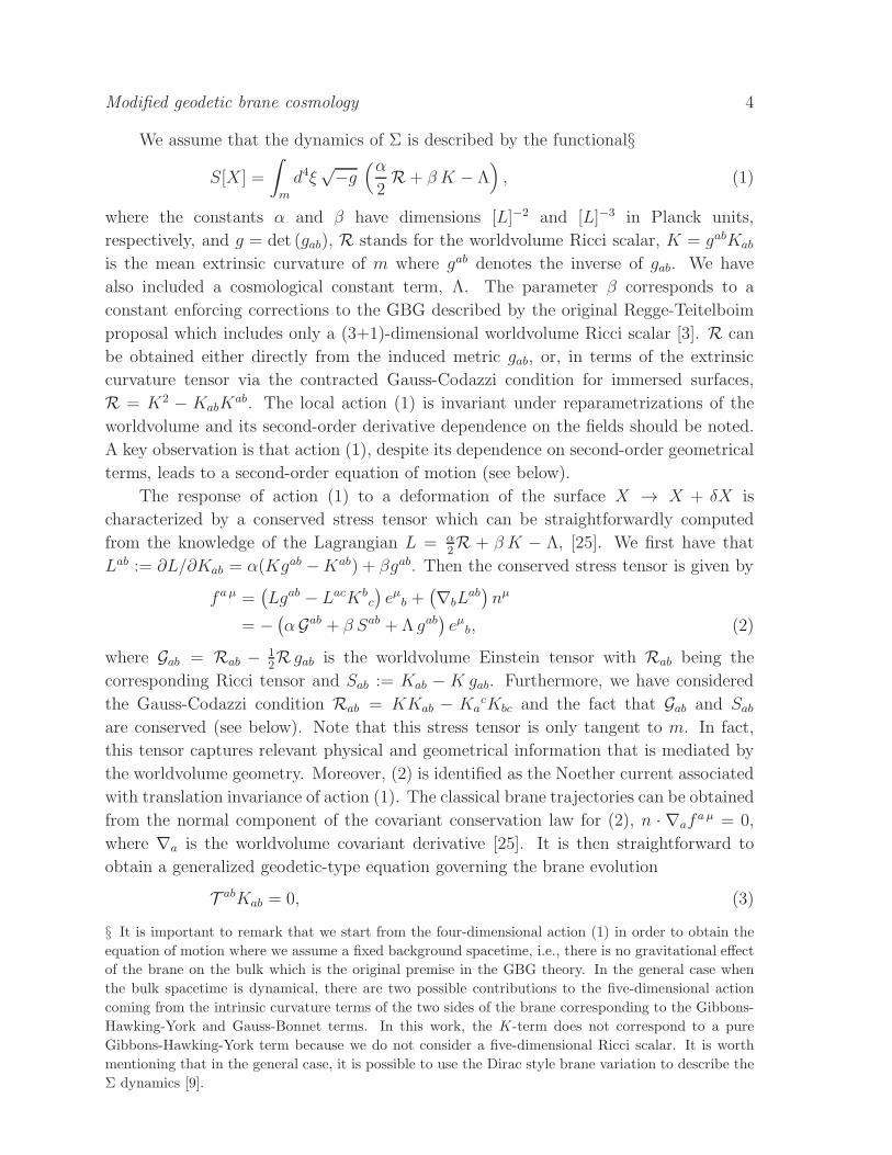
We assume that the dynamics of Σ is described by the functional§

S[X ] =

∫

m

d4ξ√−g

(α2R+ β K − Λ

), (1)

where the constants α and β have dimensions [L]−2 and [L]−3 in Planck units,

respectively, and g = det (gab), R stands for the worldvolume Ricci scalar, K = gabKab

is the mean extrinsic curvature of m where gab denotes the inverse of gab. We have

also included a cosmological constant term, Λ. The parameter β corresponds to a

constant enforcing corrections to the GBG described by the original Regge-Teitelboim

proposal which includes only a (3+1)-dimensional worldvolume Ricci scalar [3]. R can

be obtained either directly from the induced metric gab, or, in terms of the extrinsic

curvature tensor via the contracted Gauss-Codazzi condition for immersed surfaces,

R = K2 − KabKab. The local action (1) is invariant under reparametrizations of the

worldvolume and its second-order derivative dependence on the fields should be noted.

A key observation is that action (1), despite its dependence on second-order geometrical

terms, leads to a second-order equation of motion (see below).

The response of action (1) to a deformation of the surface X → X + δX is

characterized by a conserved stress tensor which can be straightforwardly computed

from the knowledge of the Lagrangian L = α2R + β K − Λ, [25]. We first have that

Lab := ∂L/∂Kab = α(Kgab −Kab) + βgab. Then the conserved stress tensor is given by

faµ =(Lgab − LacKb

c

)eµb +

(∇bL

ab)nµ

= −(α Gab + β Sab + Λ gab

)eµb, (2)

where Gab = Rab − 1

2R gab is the worldvolume Einstein tensor with Rab being the

corresponding Ricci tensor and Sab := Kab − K gab. Furthermore, we have considered

the Gauss-Codazzi condition Rab = KKab − KacKbc and the fact that Gab and Sab

are conserved (see below). Note that this stress tensor is only tangent to m. In fact,

this tensor captures relevant physical and geometrical information that is mediated by

the worldvolume geometry. Moreover, (2) is identified as the Noether current associated

with translation invariance of action (1). The classical brane trajectories can be obtained

from the normal component of the covariant conservation law for (2), n · ∇afaµ = 0,

where ∇a is the worldvolume covariant derivative [25]. It is then straightforward to

obtain a generalized geodetic-type equation governing the brane evolution

T abKab = 0, (3)

§ It is important to remark that we start from the four-dimensional action (1) in order to obtain the

equation of motion where we assume a fixed background spacetime, i.e., there is no gravitational effect

of the brane on the bulk which is the original premise in the GBG theory. In the general case when

the bulk spacetime is dynamical, there are two possible contributions to the five-dimensional action

coming from the intrinsic curvature terms of the two sides of the brane corresponding to the Gibbons-

Hawking-York and Gauss-Bonnet terms. In this work, the K-term does not correspond to a pure

Gibbons-Hawking-York term because we do not consider a five-dimensional Ricci scalar. It is worth

mentioning that in the general case, it is possible to use the Dirac style brane variation to describe the

Σ dynamics [9].


where

T ab = α Gab + β Sab + Λ gab. (4)

This tensor is conserved and its conservation is supported by the Bianchi identity,

∇aGab = 0, and the Codazzi-Mainardi condition for embedded surfaces, ∇aSab = 0.

The equation of motion (3) is of second order in derivatives of the embedding functions

because of the presence of the extrinsic curvature tensor. This is so even though we

have the presence of second-order derivative terms in our model through the scalars Rand K. Additionally, we can construct the physical quantity given by

πµ =√h ηafµ

a = −√hT abηaeµ b, (5)

where ηa denotes the timelike unit normal vector to Σ when it is viewed into m [26],

and h := det(hAB) with hAB = gabǫaAǫ

bB being the spatial metric on Σ and ǫaA are

the tangent vectors to Σ (A,B = 1, 2, 3). In other words, when Σ is considered as a

spacelike surface in the worldvolume m described by the embedding ξa = χa(uA), with

χa being the corresponding embedding functions, we can obtain an orthonormal basis

defined at each point of Σ given by ǫaA, ηa, where ηa satisfies gabηaηb = −1 (see Ref.

[27] for more details). On physical grounds, expression (5) corresponds to the conserved

linear momentum density associated with the brane Σ.

3. Modified Geodetic Brane Cosmology

A simple but interesting brane geometry is provided by a spherical configuration.

Suppose that Σ evolves in a five-dimensional Minkowski spacetime, ds25 = −dt2 + da2 +

a2 dΩ23, where dΩ2

3 = dχ2 + sin2 χ dθ2 + sin2 χ sin2 θ dφ2 denotes the metric of the unit

3-sphere. Assuming the universe to be homogeneous, isotropic and closed, it leads to

consider

xµ = Xµ(ξa) = (t(τ), a(τ), χ, θ, φ), (6)

to be a parametric representation of the worldvolume m, where τ is the proper time

for an observer at rest with respect to the brane. This is the geometry of the standard

Friedmann-Robertson-Walker (FRW) case.

The orthonormal basis adapted to m is given by the four tangent vectors eµacomplemented with the unit spacelike normal vector

nµ =1

N(a, t, 0, 0, 0), (7)

where we have introduced the function N =√

t2 − a2. The overdot denotes

differentiation with respect to τ . The metric induced from the background spacetime is

ds24 = −N2 dτ 2 + a2 dΩ23 = gabdξ

adξb. (8)

We can identify immediately the spatial metric on Σ and in consequence its determinant,

h = a6 sin4 χ sin2 θ. The coordinate system defined by (8) and (7) promotes the following


non-vanishing components of the extrinsic curvature

Kττ =

t2

N3

d

dτ

(a

t

), (9a)

Kχχ = Kθ

θ = Kφφ =

t

Na. (9b)

The Ricci scalar associated to the metric (8) and the mean extrinsic curvature are

computed accordingly,

R =6t

N4a2(aat− aat +N2t), (10)

K =1

N3

(ta− at

)+

3t

aN. (11)

Note the linear dependence in the accelerations that these geometrical scalars possess.

In addition, associated with this geometry, we have the nonvanishing components of the

worldvolume Einstein tensor,

Gττ = − 3t2

N2a2, (12)

Gχχ = Gθ

θ = Gφφ = − t2

N4a2

[2at

d

dτ

(a

t

)+N2

], (13)

and

Sττ = − 3t

Na, (14)

Sχχ = Sθ

θ = Sφφ = − t

N3a

[at

d

dτ

(a

t

)+ 2N2

]. (15)

The mechanical law governing the evolution of the brane Σ is obtained from

equation (3). After a lengthy but straightforward computation, it yields the equation

of motion

d

dτ

(a

t

)= − N2

a2(

ta

)

(t2

a2− 3ΛN2 + 6βN t

a

)

(3 t2

a2− ΛN2 + 6βN t

a

) , (16)

which involves second derivatives of the field variables a and t. Hereafter, a bar over a

letter denotes the quotient by 3α, e.g. Λ = Λ/3α, etc. The reparametrization invariance

of the model (1) dictates that for every solution for the expansion rate a(τ), we have a

gauge freedom to choose in connection with a function for t(τ). This fact will be used

repeatedly in the subsequent developments.

3.1. Inclusion of matter

As expected, action (1) is permitted to depend on additional fields, like matter

sources. Their dynamical contributions are obtained through the stress tensor Tab :=

(−2/√−g)δSm/δg

ab where Sm denotes a matter action. The form of the equation of

motion remains unchanged when we add T abm to the original one in equation (3) [4],


by modifying the tensor T ab as follows: T ab 7→ T ab − T abm . According to this line of

reasoning, the conserved stress tensor (2) gets a similar contribution from the matter

Lagrangian.

Now, a good acceptance for the energy-momentum tensor that is compatible with

the assumed homogeneity and isotropy of the universe is given by

T abm = (ρ+ P )ηaηb + P gab , (17)

where ρ = ρ(a) is the energy density of the fluid and P = P (a) its pressure. Now, by

considering (12)-(15) and the matter field content enclosed in (17), a straightforward

computation from the expression (5) for πµ, it yields the expressions for the momenta

conjugate to t, a

πt =at

N3

[a2 +N2

(1− a2 Λ− a2 ρ

)+ 3 β N a t

], (18)

πa = − aa

N3

[a2 +N2

(1− a2 Λ− a2 ρ

)+ 3 β N a t

], (19)

respectively, where we have absorbed a global constant in (18) and (19) in order to avoid

the density character of the momenta. Although we have so far restricted ourselves to

the spherical case for simplicity, it may be convenient to generalize these expressions

in order to include also the cases of hyperbolic and flat geometries. To this end, we

can choose alternative parametrizations for equation (6) (see for example [28] for a

detailed variety of embeddings) which requires analogue developments. At this stage,

we mention only that depending on the parametrization chosen, the momenta πt and

πa acquire a different form but, however, they pleasantly lead to an unaltered form for

the energy conservation law‖ (see (20) below). Hereafter, the three possible geometries

for the universe will be considered in the successive equations through the parameter k,

(k = −1, 0, 1) and the use of the cosmic gauge, N = 1.

4. Friedmann Type Equation

The first integral of equation (16) corresponds to the Friedmann equation associated

to our model (1). To find out, we proceed by considering the conserved physical

quantities arising in our model. The reparametrization invariance of model (1), in

the time coordinate t, dictates that equation (18) is conserved. For a general geometry

of the universe and by considering the cosmic gauge, equation (18) is promoted to

− E

a4:=

(a2 + k)1/2

a

[(a2 + k)

a2−

(Λ + ρ

)]+ 3β

(a2 + k)

a2, (20)

‖ For illustration, following [28] for the open Universe case, the quantities Kττ ,Gτ

τ and Sττ remain

unaltered as (9a), (12) and (14) so the term T ττ with an associated lapse function given by

N =√a2 − T 2. In such a case the only change in form lies in the quantities Gχ

χ = Gθθ = Gφ

φ

given by Gχχ = − a2

a2N 4

[2aT d

dτ

(a

T

)+N 2

]and in consequence in T χ

χ. Therefore, by repeating the

development above we obtain a momentum conjugate to T given by πy = a3T

N

[T

2

a2N 2 −(Λ + ρ

)+ 3βT

aN

]

which leads to an energy conservation law given by (20) with k = −1.


where E := −πt is the conserved brane energy and it parametrizes the deviation from the

Einstein limit in the sense that as E → 0 and β → 0 together, the Einstein cosmology

is recovered. In terms of this energy, the equation of motion (3) in the presence of a

matter configuration, results

a

a=

(t2

a2

) [Ea4

− 3β t2

a2+ 2(Λ + ρ) t

a− 3(ρ+ P ) t

a

]

[−3E

a4− 3β t2

a2+ 2(Λ + ρ) t

a

] . (21)

Now, by defining X := t/[a(Λ + ρ)1/2] = (a2 + k)1/2/[a(Λ + ρ)1/2] we are able

to rewrite the energy equation (20) as X 3 + 3 β∗X 2 − X + 2E∗ a−4 = 0 where

we have introduced the notation, β∗(a) = β/(Λ + ρ)1/2 = β/[3α(Λ + ρ)]1/2 and

E∗(a) = E/[2(Λ+ρ)3/2] = (E/2)[3α/(Λ+ρ)]3/2. Now, by considering the usual Liouville

change of variable X := Y − β∗, the cubic equation for X transforms into

Y3 − (1 + 3 β∗2)Y +

[β∗

(1 + 2 β∗2

)+

2E∗

a4

]= 0, (22)

which is an incomplete cubic equation with real coefficients. Taking into account the

identities 4 cos3 θ − 3 cos θ = cos 3θ and 4 cosh3 θ − 3 cosh θ = cosh 3θ and the fact that

(1 + 3 β∗2) > 0, the physical solution for equation (22) is given by

Y = 2

√β∗2 +

1

3F

1

3F−1

[β∗(β∗2 + 1

2) + E∗

a4

(β∗2 + 1

3)3/2

], (23)

where

F (x) =

cosh x, for |x| > 1,

cosx, for |x| ≤ 1.(24)

By considering dust, ρ = ρm 0/a3, and inserting the expression (23) into the definition

for X , we obtain

(a2 + k)1/2

a(Λ + ρm 0 a−3

)1/2 + β∗ = 2

√β∗2 +

1

3F

1

3F−1

[β∗(β∗2 + 1

2) + E∗

a4

(β∗2 + 1

3)3/2

], (25)

where ρm 0 = ρm 0/3α. Then, when we square this equation followed by a rearrangement,

we obtain the Friedmann type equation in the fashion

a2 + U(a, E) = 0, (26)

where we can identify an effective potential parametrized by the constant E through

the parameter Ωdr, as defined below,

U(a, E)

H20

= −Ωk,0 −a2

9

2

[Ω2

β,0 + 3

(ΩΛ,0 +

Ωm,0

a3

)]1/2×

×F

1

3F−1

Ωβ,0

[Ω2

β,0 +9

2

(ΩΛ,0 +

Ωm,0

a3

)]− 27Ωdr

2a4

[Ω2

β,0 + 3(ΩΛ,0 +

Ωm,0

a3

)]3/2

− Ωβ,0

2

. (27)


0! b

b! 0

a2 4 6 8

U

K20

K10

0

Figure 1. The effective potential U describing possible brane trajectories for a closed

universe and some parameter choices [Ωdr = 0.1,ΩΛ,0 = 0.2,Ωm,0 = 2.5(Ωβ,0 =

0.5,Ωk,0 = −2.59), (Ωβ,0 = −0.5,Ωk,0 = −0.93)]. The solid curve describes the

potential involving positive β. The dashed curve denotes the potential involving

negative β.

Here we have introduced the energy density parameters defined by Ωk,0 := −k/H20 ,

ΩΛ,0 := Λ/(3αH20), Ωm,0 := ρm,0/(3αH

20), Ωβ,0 := β/(αH0) and Ωdr := −E/H3

0 , the

latter being the so-called dark radiation-like energy density parameter. As customary, H0

is the Hubble constant. In what follows, we develop a standard mechanical analysis for

the motion of a single non-relativistic particle moving with zero energy in the potential

U(a, E).

In Figure (4), we depict this potential for an energy density matter configuration

in the brane of the form ρ ∝ a−3 where we have considered some parameter choices. We

infer that U(a, E) becomes singular at a → 0 and when a → ∞ then U(a, E) → −∞.

In addition, for some of the chosen parameters, the universe will expand forever at

an ever increasing rate (Big Chill) because the dashed curve does not intersect the

horizontal axis and this implies that there is no returning point with a = 0. For some

other parameters, we observe a Big Bounce behaviour because in this case the potential

intersects the horizontal axis and there is a returning point¶. These brane trajectories

for the universe are strongly in dependence of the conserved energy values. Thus, the

message is clear. Negative values of the parameter β, β < 0, cause the universe to

accelerate whereas positive values, β > 0, cause it to decelerate, i.e. the β parameter

works as a preventer or a catalyst of the acceleration of this type of universe.

¶ We follow the terminology employed in [31] to refer the term Big Chill for a universe that expands

forever and Big Bounce for a universe with no Big Bang singularity.


0! b b! 0

a

H0 t

3 6 9 12

200

400

600

Figure 2. The scale factor a as a function of H0τ for a closed universe with

the parameter choices [Ωdr = 0.1,ΩΛ,0 = 0.2,Ωm,0 = 2.5, (Ωβ,0 = 0.5,Ωk,0 =

−2.59), (Ωβ,0 = −0.5,Ωk,0 = −0.93)]. The dashed curve denotes the potential

involving positive β parameter and the doted curve involves negative β parameter.

Moreover, from equation (26), it is possible to plot the scale factor a versus H0τ

for some parameter choices in the case of a closed universe, see figure (4). Note that, in

dependence on the sign of β, the universe would have to start off in a very special form.

The scale factor behaviour depends sensitively on what the initial value is.

Another conveniently form to rewrite the Friedmann equation (26) is in terms of

the Hubble parameter H := a/a and the energy density parameters associated to the

model. Thus, equation (26) reads(H2

H20

− Ωk,0

a2

)1/2(H2

H20

− Ωk,0

a2− Ωm,0

a3− ΩΛ,0

)+ Ωβ,0

(H2

H20

− Ωk,0

a2

)=

Ωdr

a4. (28)

Clearly, one may verify that the normalization condition is obtained straightforwardly

from (28) by evaluating at the present moment, yielding

(1− Ωk,0)1/2(1− Ωk,0 − Ωm,0 − ΩΛ,0) + Ωβ,0(1− Ωk,0) = Ωdr. (29)

On the other hand, for consistency when Ωdr = Ωβ,0 = 0, it is evident that the standard

cosmology is fully recovered [1, 32].

The general behaviour of the scale factor can be obtained from the normalization

condition and the effective potential. In order to extract physical information, we have

to find the roots of the effective potential because this gives us the possible existence

of returning points for the scale factor. If there are no returning points, we have an

universe that expands forever. The other possible situation, in our case, involves two

returning points corresponding to a universe without initial singularity. The procedure

is as follows. From equation (29) we have a cubic equation for Ωk,0. Once we choose a


Wb, 0

Big Bounce

k = 0

Wm, 0

Big Chill

ClosedOpen

0 1 2 3

K3

K2

K1

1

2

3

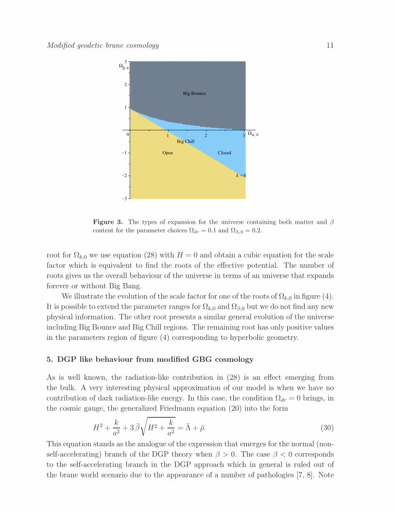
Figure 3. The types of expansion for the universe containing both matter and β

content for the parameter choices Ωdr = 0.1 and ΩΛ,0 = 0.2.

root for Ωk,0 we use equation (28) with H = 0 and obtain a cubic equation for the scale

factor which is equivalent to find the roots of the effective potential. The number of

roots gives us the overall behaviour of the universe in terms of an universe that expands

forever or without Big Bang.

We illustrate the evolution of the scale factor for one of the roots of Ωk,0 in figure (4).

It is possible to extend the parameter ranges for Ωk,0 and Ωβ,0 but we do not find any new

physical information. The other root presents a similar general evolution of the universe

including Big Bounce and Big Chill regions. The remaining root has only positive values

in the parameters region of figure (4) corresponding to hyperbolic geometry.

5. DGP like behaviour from modified GBG cosmology

As is well known, the radiation-like contribution in (28) is an effect emerging from

the bulk. A very interesting physical approximation of our model is when we have no

contribution of dark radiation-like energy. In this case, the condition Ωdr = 0 brings, in

the cosmic gauge, the generalized Friedmann equation (20) into the form

H2 +k

a2+ 3 β

√H2 +

k

a2= Λ + ρ. (30)

This equation stands as the analogue of the expression that emerges for the normal (non-

self-accelerating) branch of the DGP theory when β > 0. The case β < 0 corresponds

to the self-accelerating branch in the DGP approach which in general is ruled out of

the brane world scenario due to the appearance of a number of pathologies [7, 8]. Note


also that, when we re-organize equation (30) as in the standard relativistic form, we can

identify an effective cosmological constant given by

Λeff := Λ− 3 β

√H2 +

k

a2. (31)

Note that the β parameter plays the role of the inverse of the crossover scale rc,

responsible of the transition from 4D to 5D behaviour in the degravitation property

of the DGP approach [1, 6]. In fact, β is related to the 5D Planck mass as one can

observe from the set of purely gravitational actions that give rise to the Galileon field

theory of brane cosmology [11]. Hence, in our approach, the responsible of the (non-)

self-acceleration of the Universe is the parameter β characterizing the intrinsic properties

of the geometrical surface. In addition, for an arbitrary β, from equation (29) we can

obtain the corresponding normalization condition

√1− Ωk,0 = −Ωβ,0

2+

√(Ωβ,0

2

)2

+ Ωm,0 + ΩΛ,0 (32)

which can be recognized as the normalization condition in the DGP approach by defining

Ωrc = (Ωβ,0/2)2 = β2/(2αH0)

2 [1, 17].

The Friedmann equation acquires a non conventional form when we consider

a nonvanishing radiation-like contribution. For example, in the reasonable case of

|Ωdr| ≪ 1 [33], and Λ = 0, after a lengthy but straightforward computation, from

equation (28) the Friedmann equation reads

H2

H20

− Ωk,0

a2=

−Ωβ,0

2+

√(Ωβ,0

2

)2

+ Ωm,0

2

+ f (a,Ωβ,0,Ωm,0,Ωdr) , (33)

where f is a quite complicated function which explicitly reads

f =

3

[−Ωβ,0

2+

√(Ωβ,0

2

)2

+ Ωm,0

](D

1/3+ −D

1/3−

)Ωdr

a4√[

Ωβ,0

(Ω2

β,0 +9

2

Ωm,0

a3

)]2−

(Ω2

β,0 +3Ωm,0

a3

)3, (34)

and D± = −Ωβ,0

(Ω2

β,0 +9

2

Ωm,0

a3

)±√[

Ωβ,0

(Ω2

β,0 +9

2

Ωm,0

a3

)]2−

(Ω2

β,0 +3Ωm,0

a3

)3

. Clearly,

expression (33) specializes to the Friedmann equation found in [17] for the analysis of

an accelerated universe without cosmological constant. In addition, from equations (33)

and (34), two features should be emphasized. At large distances, a → ∞ gives rise to

f → 0 and we have a slight modification to the DGP accelerated universe behaviour.

On the other hand, however, when a → 0, the function f increases considerably and

a significant effect is expected which will strongly modify the quantum cosmology

approach for our model. Therefore, we find that when Ωdr fades away then modified

GBG leads to a late-time self-acceleration and in consequence we have an interesting

alternative effective model supporting this degravitation characteristic.


6. Concluding remarks

In this paper, we have shown that GBG modified by a curvature brane scalar defined by

a linear extrinsic curvature term leads us to reproduce under certain conditions a similar

brane cosmological behaviour as in the DGP setup. Contrarily to the DGP approach, we

considered an empty fixed bulk which, however, leads us to reproduce similar dynamical

equations. In addition, we showed that the effective potential emerging in our model

exhibits an accelerated behaviour for this universe as DGP theory does. In this modified

GBG, the inverse DGP crossover scale rc is played by the parameter related to the K-

term. We thus observe that this model mimics the dynamics of DGP approach with the

important exception that in our case such effects directly result from the geometrical

characteristics of the brane through the parameter β. Even though gravity was switched

off from the beggining in our setup all this happens so because modified GBG is enclosed

in the set of purely gravitational 4D brane theories that gives rise to the Galileon field

theory where that peculiar type of scalar fields is able to create accelerating spacetimes

similar to those of the DGP setup [11, 35], which are argued to explain also dark energy.

From another point of view, we study part of the Galileon field theory, restricted to the

first three Lovelock brane Lagrangians directly.

This prescription surely constitutes an interesting theoretical alternative to analyse

certain subjects in braneworld cosmology. In particular, we confirm that the acceleration

description of brane universes can be formulated differently from what we have been

accustomed to so far. Then, motivated by the equivalence at the effective level, with

DGP gravity, we believe that this modified GBG deserves a deep exploration at the

classical canonical level, followed by an extensive study of its quantum mechanical

aspects in order to discern on the physical viability of the brane model. Our work will not

stop here. We are interested in understanding how much an Ostrogradski-Hamiltonian

development of model (1) is sensitive to the fact that the ghost and tachyon states appear

in this scenario [21, 34]. Alternatively, we believe that our approach opens the scope

of brane theories to be included as a correction terms, like the Gauss-Bonnet counter-

term, yielding also second order equations of motion [29, 30] improving thus the GBG

framework. It is worth saying that the terms appearing in the present model belong to a

wide range of effective field brane models related to the so-called Galileons which possess

interesting symmetry properties that also deserve an exhaustive investigation in view

of their potential applications to particle physics and cosmology [11, 12, 13, 22, 23, 24].

The results of these points will be presented elsewhere.

Acknowledgments

E.R. and R.C. acknowledge support from CONACYT (Mexico) research Grant No. J1-

60621-I. ER and MC are grateful to E. Ayon-Beato for fruitful discussions. ER cordially

thanks A. Cervantes and B. Tapia-Santos for their contributions towards the numerical

analysis. Also, ER and MC acknowledge partial support from grant PROMEP, CA-


UV: Algebra, Geometrıa y Gravitacion. MC acknowledges support from a CONACyT

scholarship (Mexico). This work was partially supported by SNI (Mexico). RC also

acknowledges support from EDI, COFAA-IPN and SIP-20111070. AM acknowledges

financial support from PROMEP through grant UASLP-PTC-402.

References

[1] R. Maartens and K. Koyama, Liv. Rev. Rel. 13:5 (2010), arXiv: 1004.3962v2 [hep-th]

[2] V. Sahni and Y. Shtanov, JCAP 0311 014 (2003).

[3] T. Regge and C. Teitelboim, in Proceedings of the Marcel Grossman Meeting, Trieste, Italy, 1975,

edited by R. Ruffini (North-Holland, Amsterdam, 1977), p.77.

[4] A. Davidson and D. Karasik, Mod. Phys. Lett. A 13, 2187 (1998); Phys. Rev. D 67, 064012 (2003);

arXiv: gr-qc/9901004v1 and arXiv: gr-qc/0207061v2

[5] G.R. Dvali, G. Gabadadze and M. Porrati, Phys. Lett. B 484 112 (2000); Phys. Lett. B485 208

(2000); arXiv: hep-th/0002190v2 and arXiv: hep-th/0005016v2.

[6] C. Deffayet, Phys. Lett. B502, 199 (2001), arXiv: hep-th/0010186v2

[7] R. Gregory, N. Kaloper, R. C. Myers and A. Padilla, JHEP 10, 069 (2007), arXiv: 0707.2666v2

[hep-th].

[8] A. Nicolis and R. Ratazzi, JHEP 06, 059 (2004), arXiv: hep-th/0404159v1

[9] A. Davidson and I. Gurwich, Phys. Rev. D 74, 044023 (2006), arXiv: gr-qc/0606098v1

[10] D. Lovelock, J. Math. Phys. 12 498 (1971)

[11] C. de Rham and A. J. Tolley, JCAP 05, 015 (2010), arXiv: 1003.5917v2 [hep-th].

[12] G. Goon, K. Hinterbichler and M. Trodden, Phys. Rev. Lett. 106, 231102 (2011), arXiv:

1103.6029v2 [hep-th].

[13] G. Goon, K. Hinterbichler and M. Trodden, JCAP, 07, 017, (2011).

[14] A. Davidson and S. Rubin, Class. Quantum Grav. 26, 235006 (2009).

[15] R. Dick, Phys. Lett. B 491, 333 (2000), arXiv:[hep-th/0007063].

[16] R. Dick, Class. Quantum Grav. 18, R1 (2001), arXiv:[hep-th/0105320].

[17] C. Deffayet, G. Dvali and G. Gabadadze, Phys. Rev. D 65, 044023 (2002), arXiv: astro-

ph/0105068v1

[18] B-Y Chen, J. London Math. Soc. 6, 321 (1973).

[19] S. Svetina and B. Zeks, Eur. Biophys. J, 17, 101 (1989);

[20] M. Onder and R. Tucker, J. Phys. A: Math. Gen. (1988)

[21] R. Cordero, A. Molgado and E. Rojas, Class. Quantum Grav. 28, 065010 (2011), arXiv:

1012.1379v2 [gr-qc].

[22] M. Trodden and K. Hinterbichler, Class. Quantum Grav. 28 204003 (2011), arXiv:1104.2088v1[hep-

th].

[23] C. de Rham and L. Heisenberg, Phys. Rev. D 84 043503 (2011).

[24] C. Burrage, C. de Rham and L. Heisenberg, JCAP 1105 025 (2011).

[25] G. Arreaga, R. Capovilla and J. Guven, Ann. Phys., NY 279, 126 (2000), arXiv: hep-

th/0002088v1

[26] R. Capovilla and J. Guven, Phys. Rev. D 55, 2388 (1997), arXiv: math-ph/9804001v1

[27] R. Capovilla, J. Guven and E. Rojas, Class. Quantum Grav. 21, 5563 (2004), arXiv: hep-

th/0404178v1

[28] J. Rosen, Rev. Mod. Phys. 37, 204 (1965).

[29] R. C. Myers, Phys. Rev. D 36, 392 (1987).

[30] S. C. Davis, Phys. Rev. D 67, 024030 (2003), arXiv: gr-qc/0208205v3

[31] B. Ryden, Introduction to cosmology, Addison-Wesley, San Francisco, (2006).

[32] A. Davidson, D. Karasik and Y. Lederer, Class. Quantum Grav. 16, 1349 (1999), arXiv:

gr-qc/9901003

http://arxiv.org/abs/hep-th/0007063

http://arxiv.org/abs/hep-th/0105320

http://arxiv.org/abs/gr-qc/9901003


[33] R. Maartens, Liv. Rev. Rel., 7:7 (2004) arXiv: gr-qc/0312059v2.

[34] M. Ostrogradski, Mem. Ac. St. Petersbourg 1 385 (1850).

[35] A. Nicolis, R. Rattazzi and E. Trincherini, Phys. Rev. D 79 064036 (2009).

http://arxiv.org/abs/gr-qc/0312059

Modified geodetic brane cosmology

Documents

Transcript of Modified geodetic brane cosmology