arX

iv:h

ep-t

h/03

0707

2v1

8 J

ul 2

003

KCL-MTH-03-13

ITP-UU-03-11

February 1, 2008

The deformed M2-brane

P.S. Howe 1, S.F. Kerstan 1, U. Lindstrom 2 and D. Tsimpis 1

1 Department of Mathematics, King’s College, London, UK

2 Department of Theoretical Physics Uppsala University, Sweden

Abstract

The superembedding formalism is used to study correction terms to the dynamics of the M2brane in a flat background. This is done by deforming the standard embedding constraint.It is shown rigorously that the first such correction occurs at dimension four. Cohomologicaltechniques are used to determine this correction explicitly. The action is derived to quadraticorder in fermions, and the modified κ-symmetry transformations are given.

1 Introduction

An interesting problem in string/M theory is to consider higher-order corrections to the effective

dynamics of various branes. A number of results have been obtained in the purely bosonic sector,

particularly for D-branes, [1, 2, 3, 4, 5, 6, 7].1 Some of these have been supersymmetrised, for

example the ∂4F 4 and other terms in D-brane actions [10, 11], but it has so far proven difficult

to obtain Lagrangians or equations of motion with fully-fledged kappa-symmetry. Some kappa-

symmetric results have been obtained for higher-derivative terms for superparticles [12, 13, 14]

and superstrings [15], for coincident D0-branes in [16], and for branes in lower-dimensional

spacetimes in [18, 19]. The last two papers made use of the superembedding formalism [20, 21]

which offers a systematic way of incorporating kappa-symmetry whilst maintaining manifest

target space supersymmetry. In this paper we shall examine the leading correction terms for the

M2-brane using this formalism. We shall derive the action up to terms quadratic in the fermions

as well as the modified kappa-symmetry transformations.

The two examples studied in [18, 19], namely a membrane in four dimensions and a set of

coincident membranes in three dimensions, were relatively easy to analyse because the world-

volume multiplets in both cases are off-shell. This means that the standard superembedding

constraints do not need to be altered - one only needs to find higher-order Lagrangians which

can be constructed using standard methods. However, for the 1/2 BPS branes in string theory

and M-theory the worldvolume multiplets are maximally supersymmetric matter or gauge mul-

tiplets and it is not known how to find auxiliary fields for these or even if they exist. Indeed, the

standard superembedding constraint leads directly to the equations of motion of the brane in

most cases [22, 23]. This means that we need to find new techniques to discuss higher-derivative

interactions for these branes. The purpose of the present paper is to show how this can be car-

ried out in a perturbative fashion for the case of the M2-brane. The basic idea is to deform the

superembedding constraint in such a way that the field content of the brane theory is unchanged.

The torsion identities, which we describe in detail below, then impose consistency requirements

on the deformation which can be analysed order by order in a parameter ℓ which has the dimen-

sions of length and which could be the Planck length or the string length√α′. In fact, what we

end up with is a cohomology problem which is similar in spirit to the cohomological problems

encountered in the analysis of higher-order corrections to maximally supersymmetric field the-

ories including supergravity [24, 25, 26, 27, 28]. However, the cohomology problem considered

here is manifestly covariant with respect to target space supersymmetry and local worldvolume

supersymmetry (κ-symmetry); if we were to work in the static gauge the formalism would au-

tomatically have “N = 2” worldvolume supersymmetry (actually d = 3, N = 16) non-linearly

realised.

We shall limit ourselves to the case of a flat target superspace in this paper for simplicity,

although there will also be corrections involving the target space curvature. We show rigorously

that supersymmetry does not allow any deformations with three or fewer powers of ℓ, a result

which is to be expected in view of the results that have been obtained for D-branes. We

then analyse in some detail the lowest-order non-trivial deformation at ℓ4. This turns out to

1For some earlier work on higher derivative corrections see [8, 9].

1

be rather complicated and involves up to seven powers in fields. We show that there is a

unique deformation with at most three fields. We believe that it is unlikely that there are other

independent deformations, because of the number of constraints that have to be satisfied, but we

have not completed the proof of this assertion. Knowledge of the cubic terms in the deformation

is sufficient to determine the modified Lagrangian to quadratic order in fermions, and thus to

determine the full purely bosonic part of the action at order ℓ4. The result is, as expected, a

Lagrangian which is quartic in the extrinsic curvature.

The organisation of the paper is as follows. In the next section we briefly review the superem-

bedding formalism and the relation of worldvolume supersymmetry to κ-symmetry. In section

three we solve the torsion identities for the membrane to first order in the deformation field ψ

and summarise the lowest order results which give the standard dynamics. In section four we

introduce the relevant spinorial cohomology groups for deformed superembeddings. In section

five we discuss the constraints on the deformation and solve the relevant cohomology problem

up to order ℓ4 in section six. In section seven we construct the action, up to terms quadratic in

the fermions, and in section eight we discuss the modified κ-symmetry transformations.

2 Superembeddings

The superembedding formalism was pioneered in the context of superparticles in three and four

dimensions by Sorokin, Tkach, Volkov and Zheltukhin [20], and has been applied by these and

other authors to various other branes; for a review see [21].2 In [22] it was shown that the

formalism can be applied to arbitrary branes including those with various types of worldvolume

gauge fields, and it was then used to construct the full non-linear equations of motion of the

M-theory 5-brane in an arbitrary supergravity background [23].

We consider a superembedding f : M → M , where M is the worldvolume of the brane and M

is the target space. Our index conventions are as follows: coordinate indices are taken from the

middle of the alphabet with capitals for all, Latin for bosonic and Greek for fermionic, M =

(m,µ), tangent space indices are taken in a similar fashion from the beginning of the alphabet

so that A = (a, α). We denote the coordinates of M by zM = (xm, θµ). The distinguished

tangent space bases are related to coordinate bases by means of the supervielbein, EMA, and its

inverse EAM . We use exactly the same notation for the target space but with all of the indices

underlined. Indices for the normal bundle are denoted by primes, so that A′ = (a′, α′). We shall

occasionally group together tangent and normal indices and denote them by a bar, a = (a, a′)

etc.

The embedding matrix is the derivative of f referred to the preferred tangent frames, thus

EAA := EA

M∂MzMEMA (1)

In addition, we can specify a basis EA′ for the normal bundle in terms of the target space

basis by means of the normal matrix EA′A.

2For an earlier attempt to use source and target superspaces, see, e.g., [29].

2

The basic embedding condition is

Eαa = 0 (2)

Geometrically this states that the odd tangent space of the brane is a subspace of the odd

tangent space of the target superspace at any point on the brane. To see the content of this

constraint we can consider a linearised embedding in a flat target space in the static gauge. This

gauge is specified by identifying the coordinates of the brane with a subset of the coordinates of

the worldvolume, so that

xa =

xa

xa′

(x, θ)(3)

θα =

θα

θα′

(x, θ)(4)

Since

Ea = dxa − i

2dθα(Γa)αβθ

β (5)

in flat space, it is easy to see, to first order in the transverse fields, that the embedding condition

implies that

DαXa′

= i(Γa′

)αβ′θβ′

(6)

where

Xa′

= xa′

+i

2θα(Γa′

)αβ′θβ′

(7)

From this equation the nature of the worldvolume multiplet specified by the embedding condition

can be determined. Depending on the dimensions involved, this multiplet can be one of three

types: (i) on-shell, i.e. the multiplet contains only physical fields and these fields satisfy equations

of motion, (ii) Lagrangian off-shell, meaning that the multiplet also contains auxiliary fields (in

most cases), and that the equations of motion of the physical fields are not satisfied, although

they can be derived from a superfield action, and (iii) underconstrained, which means that

further constraints are required to obtain multiplets of one of the first two types. For thirty-two

target space supersymmetries, the multiplets are always of type (i) or of type (iii), whereas for

sixteen or fewer supersymmetries all three types of multiplet can occur, with type (iii) arising

typically for cases of low even codimension.

In this paper we shall be concerned with the membrane in D = 11 superspace, i.e. the M2-

brane. This has been discussed as a superembedding in [30]. The worldvolume is d = 3, N = 8

superspace, and the worldvolume multiplet is an on-shell scalar multiplet (type (i)). This can be

3

seen from (7). The leading component of the superfield Xa′

describes eight scalar fields on the

worldvolume, while the leading component of θα′

describes eight spin one-half fields. Equation

(7) implies that there are no further independent component fields and that the scalars and

spinors satisfy the usual equations of motion for free massless fields.

In order to determine the consequences of the superembedding condition in the non-linear case,

and to find the induced supergeometry on the brane, one uses the torsion equation which is the

pull-back of the equation defining the target space torsion two-form. This reads

2∇[AEB]C + TAB

CECC = (−1)A(B+B)EB

BEAATAB

C (8)

In this equation the covariant derivative acts on both worldvolume and target space tensor

indices. The latter are taken care of by the pull-back of the target space connection, while the

worldvolume connection can be chosen in a variety of different ways. One also has to parametrise

the embedding matrix. Having done all this, one can work through the torsion equation starting

at dimension zero. In this way the consequences of the embedding condition (2) can be worked

out in a systematic and covariant fashion.

The equations of the component or Green-Schwarz formalism can be obtained by taking the

leading (θ = 0) components of the various equations that describe the brane multiplet. A key

feature of the formalism is that these component equations are guaranteed to be κ-symmetric

because κ-symmetry can be identified with the leading term in a worldvolume local supersymme-

try transformation. We recall briefly how this works [20]. Let vM be a worldvolume vector field

generating an infinitesimal diffeomorphism. If we write the superembedding in local coordinates

as fM = zM (X), then the effect of such a transformation on z(z) is

δzM = vM∂MzM (9)

If we express this in the preferred bases we find

δzA := δzMEMA = vAEA

A (10)

Now if we take an odd worldvolume diffeomorphism, va = 0, and use the embedding condition

(2) we get

δza = 0 (11)

δzα = vαEαα (12)

This can be brought to the more usual κ-symmetric form if we define

κα := vαEαα (13)

and note that it satisfies

4

κα = κβPβα :=

1

2κβ(1 + Γ)β

α (14)

where P is the projection operator onto the worldvolume subspace of the odd tangent space

of the target superspace. We can always write P = 1/2(1 + Γ), and so Γ is computable in

terms of the embedding matrix. Substituting this into (12) we recover the normal form of κ-

symmetry transformations. (Strictly, we should evaluate this equation at θ = 0 to get the correct

component form.) The explicit form of P is

Pαβ = (E−1)α

γEγβ (15)

where the inverse is taken in the fermionic tangent space (of M).

For the case of the supermembrane in D = 11, this procedure yields the equations of motion

found in [31]. To find higher derivative corrections to these equations it follows that we shall

need to amend the basic embedding condition (2). We note that a simple consequence of this

is that the κ-symmetry transformations will no longer have the standard characteristic form for

which δza = 0.

3 The torsion identities

In this section we shall study the torsion identities in the case that the embedding condition is

relaxed. We shall take the target space to be flat so that the only non-vanishing component of

the target space torsion is

Tαβa = −i (Γa)αβ , (16)

We can parametrise the embedding matrix as follows:

Eαa = ψα

a′

ua′a Eα

α = uαα + hα

α′

ua′α (17)

Eaa = ua

a, Eaα = Λa

α′

uα′α (18)

while the normal matrix can be chosen to have the form

Eα′a = 0, Eα′

α = uα′α (19)

Ea′a = ua′

a, Ea′α = 0 (20)

Here, the 32 × 32 matrix uαα := (uα

α, uα′α) is an element of Spin(1, 10) while the matrix

uaa := (ua

a, ua′a) is the corresponding element of SO(1, 10). The dimensions, in units of mass,

of the various components of the embedding matrix are given by

5

[Eαα] = [Ea

a] = 0, [Eαa] = −[Ea

α] = −12 (21)

and similarly for the normal matrix. We can always bring these matrices into the above forms

by a suitable choice of the bases of the even and odd tangent spaces on the worldvolume. We

can now plug this form of the embedding matrix into the torsion identity

∇AEBC − (−)AB∇BEA

C + TABCEC

C = (−)A(B+B)EBBEA

ATABC (22)

and work out the consequences. As we noted earlier, the covariant derivative here acts on

both target space and worldvolume indices, but since the target space is flat we only need a

worldvolume connection. This can be specified either by imposing some constraints on the

worldvolume torsion tensor or by choosing a connection which is natural in the superembedding

context. We shall use the latter. Given the matrix u we can define the set of one-forms

XA := (∇Au)u−1 (23)

If we set

XA,bc = XA,b′

c′ = 0 (24)

then we fix connections for the tangent and normal bundles in a standard fashion. Note that

XA,βγ =

1

4(Γbc)β

γXA,bc (25)

The torsion identities yield the following results for a flat target superspace:

dim 0

Tαβc = −i(Γc)αβ + 2ψ(α

d′Xβ),d′c (26)

∇(αψβ)c′ = −ih(α

γ′

(Γc′)β)γ′ +(

−Tαβγψγ

c′)

(27)

dim 1/2

Tαbc = ψα

d′Xb,d′c + iΛb

β′

hαγ′

(Γc)β′γ′ (28)

Xαbc′ = ∇bψα

c′ + iΛbβ′

(Γc′)αβ′ (29)

Tαβγ = −2h(α

δ′Xβ),δ′γ (30)

2∇(αhβ)γ′

= −2X(α,β)γ′ − Tαβ

cΛcγ′ −

(

Tαβδhδ

γ′)

(31)

dim 1

6

Tabc = iΛa

α′

Λbβ′

(Γc)α′β′ (32)

2X[ab]c′ = −Tab

γψγγ′

(33)

Taβγ = −Λa

δ′Xβ,δ′γ − hβ

δ′Xa,δ′γ (34)

Xa,βγ′

= ∇βΛaγ′ −∇ahβ

γ′

(35)

dim 3/2

Tabγ = 2Λ[a

δ′Xb],δ′γ (36)

2∇[aΛb]γ′

= −TabcΛc

γ′ − Tabδhδ

γ′

(37)

The terms in brackets will be irrelevant in what follows because they will turn out to be zero at

first order in the deformation parameter as we shall shortly see.

3.1 Zeroth order

In the zeroth order theory the standard embedding condition Eαa = 0 holds, so that ψα

c′ = 0.

If we substitute this into the above equations we find that hαβ′

= 0 while the induced torsion is

Tαβc = −i(Γc)αβ (38)

at dimension zero and vanishes at dimension one-half. The dimension one and three-halves

components are given by the corresponding equations above.

For X we find, at dimension one-half,

Xα,bc′ = iΛb

β′

(Γc′)αβ′ (39)

2X(αβ)γ′

= i(Γc)αβΛcγ′

(40)

It is easy to show that these equations imply that

(Γa)α′β′Λaβ′

= 0 (41)

In the linearised theory Λaβ′ ∼ ∂aθ

β′

, so that we can identify (41) as the equation of motion of

the fermion field in the worldvolume multiplet. At dimension one we have

X[ab]c′ = 0 (42)

Xa,βγ′

= ∇βΛaγ′

(43)

7

Using the fermion equation of motion we find the scalar equation of motion

ηabXa,bc′ = 0 (44)

Indeed, in the linearised theory, Xabc′ ∼ ∂a∂bX

c′ , so we get the massless Klein-Gordon equation.

Finally, a short calculation gives the supersymmetry variation of Xabc′ :

∇αiXb,cd′ = −i(σd′∇(bΛc))αi +

1

2(Λbγ

e ⊗ σf ′d′Λc)(σf ′Λe)αi (45)

3.2 First order

A first order deformation of the theory will involve the presence of a non-vanishing ψ field which

we can take to be of the form of a dimensionful parameter β, say, multiplied by a function of

the physical fields Λaβ′

and Xabc′ as well as derivatives. We shall write this schematically as

ψ = βf(Λ,X, ∂) (46)

Furthermore, ψ is subject to the constraint

∇(αψβ)c′ = −ih(α

γ′

(Γc′)β)γ′ (47)

Note that, since ψ, h and Tαβγ are all of order β we are allowed to drop the Tαβ

γψγc′ term from

(27). The problem is then to analyse equation (47). This can be done systematically in powers

of the length parameter ℓ. Note that, given an explicit expression for ψ in terms of the physical

fields, equation (47) allows us to solve for h.

4 Spinorial cohomology for branes

The notion of spinorial cohomology [24, 26] is useful for studying both the space of physical

fields in certain supersymmetric theories and also for studying deformations of the equations

of motion. In the simplest case one studies spinorial p-forms, i.e. totally symmetric p-spinors

which are γ-traceless, together with a differential operator which is obtained by acting with Dα

followed by symmetrisation and removal of the γ-trace. This defines a cohomology which is

isomorphic to pure spinor cohomology [32, 33]. The relevance of the latter to theories in ten and

eleven dimensions is explained by the fact that the equations of motion can be interpreted in

terms of pure spinor integrability [34, 35]. The formalism has been applied to D = 10 Yang-Mills

theory and supergravities in ten and eleven dimensions [24, 25, 26, 27, 28]. Moreover, one can

also consider vector-valued spinorial cohomology [26]. For branes, the appropriate cohomology

is a variant on the latter.

Since we are interested in first-order deformations, it is sufficient to work on a worldvolume

whose induced supergeometry is given by the zeroth order theory. We then consider the spaces

8

ΩpB′ and Ωp

F ′ . The objects in these spaces are spinorial p-forms on M which take their values

either in the even normal bundle B′ or the odd normal bundle F ′. There is a natural map

Γ : Ωp−1F ′ → Ωp

B′ given by

hα1...αp−1γ′ 7→ −ih(α1...αp−1

γ′

(Γc′)αb)γ′ (48)

We can therefore form the quotient space ΩpB′ := Ωp

B′/Γ(Ωp−1F ′ ) and construct a derivative ds :

ΩpB′ → Ωp+1

B′ which squares to zero. This derivative is defined by acting with the spinorial

covariant derivative ∇α and symmetrising modulo equivalences of the form of equation (48). In

other words, if h ∈ ΩpB′ represents an equivalence class [h] ∈ Ωp

B′ , then ds[h] = [∇h] ∈ Ωp+1B′

where

(∇h)α1...αp+1c′ := ∇(α1

hα2...αp+1)c′ (49)

It is easy to see that this definition is independent of the choice of representative h. To see that

d2s = 0 we observe that

∇(α1∇α2hα3...αp+2)

c′ = −1

2R(α1α2,α3

γh|γ|α4...αp+2)c′ +

1

2R(α1α2,d′

c′hα3...αp+2)d′ (50)

Now, from the first Bianchi identity, we have

R(α1α2α3)γ = ∇(α1

Tα2α3)γ + T(α1α2

BTBα3)γ

= −i(Γb)(α1α2Tbα3)

γ (51)

so that the first term on the RHS of (50) is of the form

−i(Γb)(α1α2kbα3...αp+2)

c′ (52)

for some k. However, this can be written as

−ih(α1...αp+1

γ′

(Γc′)αp+2)γ′ (53)

where

hα1...αp+1γ′

= (Γbc′)(α1

γ′

kbα2...αp+2)c′ (54)

and so this term maps to zero in the quotient space. The second term on the RHS of (50) can

be evaluated with the aid of the Gauss-Codazzi equation which can, in turn, be derived from

the definition of XA. One finds that

Rαβc′d′ = 2X(αc′

eXβ)ed′ (55)

9

Since Xαbc′ = iΛb

β′

(Γc′)β′α we have

Rαβc′d′ = 2Λeγ′

Λeδ′(Γc′)γ′(α(Γd′)β)δ′ (56)

from which it is easy to see that the second term also gives zero in the quotient space. This

shows that d2s = 0 so that we can define the cohomology groups Hp

B′ := ker ds ∩ ΩpB′/imdsΩ

p−1B′ .

We claim that a first-order deformation of the dynamics of the membrane is given by an ele-

ment of H1B′(phys), where the notation indicates that the coefficients should be given by fields

constructed from the physical fields.

To see that this is the appropriate group we need to consider redefinitions. We shall find the

effect of a field redefinition of the embedding coordinates

zM → zM + (δz)M (57)

on the field ψαc′ . The transformation (57) of the embedding coordinates with the background

geometry fixed may be viewed equivalently as a diffeomorphism of the background geometry with

the embedding coordinates fixed. Taking the latter point of view, we find that the target-space

vielbein transforms as

δEMA = (δz)NTNM

A + ∇M(δz)A,

up to a Lorentz transformation on the flat index. The transformation of the embedding matrix

reads

δEAA = EA

M∂MZMδEM

A

= ∇A(δz)A + EAC(δz)BTBC

A

Setting A = α, A = a in the above and expressing Eαa in terms of ψα

c′ , we obtain

δψαc′ = ∇α(δz)c

′

+ (δz)bXαbc′ − i(δz)γ

′

(Γc′)γ′α (58)

where (δz)c := (δz)cucc, etc. Since δz is of order β we can use the zeroth order expression for

X and so we obtain

δψαc′ = ∇α(δz)c

′ − ihγ′

(Γc′)γ′α (59)

where

hγ′

:= (δz)γ′ − (δz)bΛb

γ′

(60)

Together with the fact that ψ satisfies the constraint (47), this proves the contention that the

first-order deformation is indeed given by an element of H1B′(phys).

We observe that the zeroth order group H0B′ can be interpreted as the space of physical fields,

since a deformation of the form of (59) such that the left-hand side vanishes will leave the basic

10

embedding constraint unchanged. Indeed, the linearised embedding equation (2) can also be

viewed as defining an element of this group in flat space.

The discussion given here is pertinent to the M2-brane but can be generalised to other branes.

This may require some technical modifications since the field hαγ′

does not vanish at zeroth

order in the presence of worldvolume gauge fields; in particular, this is the case for D-branes

and the M5-brane.

5 Constraints on ψ

We now derive the constraints on ψαa′

implied by the dimension–0 torsion identity at linear

order in β,

∇(αψc′

β) = −ih(αγ′

(Γc′)β)γ′ (61)

Note that in the above we have taken into account that T γαβ is of order β as implied by the

dimension–1/2 torsion identity.

The field ψαia′

(switching to two-step notation) transforms under the (1)×((0001)⊗(1000)) rep-

resentation of Spin(1, 2)×Spin(8). (See the appendix for representation-theoretic conventions.)

Decomposing ψ into irreducible representations, we find

ψαia′ ∼ (1) × (1001) ⊕ (1) × (0010)

Explicitly:

ψαia′

= Σαia′

(1) × (1001)

+ (σa′

)ij′Σj′

α (1) × (0010) (62)

From (59) it follows that the trace part in the decomposition of ψa′

αi above can be eliminated

using field redefinitions of the embedding coordinates. We shall therefore set Σi′

α = 0.

Similarly, the field hαβ′ → hαi

βj′ (in two-step notation) transforms under the ((1) ⊗ (1)) ×((0001) ⊗ (0010)) representation of Spin(1, 2) × Spin(8). Decomposing in irreducible represen-

tations, we have

hαiβj′ ∼ (0) × (1000) ⊕ (0) × (0011) ⊕ (2) × (1000) ⊕ (2) × (0011)

Explicitly

hαiβj′ = δα

β(σa′

)ij′ha′ (0) × (1000)

+1

6δα

β(σa′b′c′)ij′ha′b′c′ (0) × (0011)

+ (γa)αβ(σa′

)ij′haa′ (2) × (1000)

+1

6(γa)α

β(σa′b′c′)ij′haa′b′c′ (2) × (0011) (63)

In order to analyse (61) we need to decompose ∇αiΣβja′

into irreducible representations of

Spin(1, 2) × Spin(8), (remember we have set Σi′

α to zero). This field transforms under the

11

((1)⊗ (1))× ((0001)⊗ (1001)) representation. Decomposing into irreducible representations, we

have

∇αiΣβja′ ∼ (0) × (1000) ⊕ (0) × (0011) ⊕ (0) × (1100)

⊕ (2) × (1000) ⊕ (2) × (0011) ⊕ (2) × (1002)

Explicitly,

∇αiΣa′

βj = εαβδijYa′

+1

7εαβ(σa′b′)ijYb′ (0) × (1000)

+1

2εαβ(σb′c′)ijY

a′b′c′ +1

10εαβ(σa′b′c′d′)ijYb′c′d′ (0) × (0011)

+1

2εαβ(σb′c′)ijY

b′c′;a′

(0) × (1100)

+1

120εαβ(σb′c′d′e′)ijY

b′c′d′e′;a′

(0) × (1002)

+ (γa)αβδijYaa′

+1

7(γa)αβ(σa′b′)ijYab′ (2) × (1000)

+1

2(γa)αβ(σb′c′)ijYa

a′b′c′ +1

10(γa)αβ(σa′b′c′d′)ijYab′c′d′ (2) × (0011)

+1

2(γa)αβ(σb′c′)ijYa

b′c′;a′

(2) × (1100)

+1

120(γa)αβ(σb′c′d′e′)ijYa

b′c′d′e′;a′

(2) × (1002) (64)

The semi-colon notation here denotes “hook” representations, e.g a′b′; c′ denotes a traceless

tensor which is antisymmetric on a′b′, but not on all three indices. Using (63,64) in (61) we can

solve for hαiβj′ in terms of the Y s:

ha′ = − i

7Ya′

ha′b′c′ = −iYa′b′c′

haa′ = iYaa′

haa′b′c′ = −3i

5Yaa′b′c′ .

In addition we find two constraints

Ya′b′;c′ = 0

Yaa′b′c′d′;e′ = 0. (65)

Finally, the fields Yaa′b′;c′ , Ya′b′c′d′;e′ drop out of (61) and are therefore left undetermined.

6 Solving the spinorial cohomology problem

Let us recapitulate: the deformations of the supersymmetric M2 theory are parametrised by the

object Σ a′

αi in the (1)× (1001) of Spin(1, 2)×Spin(8). Σαia′

is not arbitrary, but has to satisfy

the two constraints (65). In the language of section 4, such a Σ a′

αi determines an element of

12

the spinorial cohomology group H1B′ . These constraints tell us that the projection of the spinor

derivative of Σ a′

αi onto the (0) × (1100) ⊕ (2) × (1002) part should vanish. This gives us the

explicit form of the spinorial derivative ds for this case:

ds(Σαia′

) → (σa′1a′

2)ijǫαβ∇αiΣb′

βj|(1100) ⊕ (σa′1...a′

5)ijγαβa ∇αiΣ

b′

βj|(1002), (66)

where the bars denote the projections onto the indicated irreducible Spin(8) representations.

In addition one has to take into account the field redefinitions. As explained in the previous

section, these are given by the projection of the spinor derivative of (δz)a′

onto the (1)× (1001)

part. Explicitly,

ds(δz)a′ → ∇αi(δz)

a′ |(1001), (67)

Our strategy is to view Σ a′

αi , (δZ)a′

as composite operators, given in terms of the world-volume

fields Xabc′ , Λa

αi′ . At any given order of ℓ, one writes down the most general expressions for

Σ a′

αi , (δz)a′

allowed by dimensional analysis and representation theory. In determining the

most general expressions at a given order in ℓ one can assume that the worldvolume fields obey

the lowest-order equations. This is because Σa′

αi, (δz)a′

are already of order β. In terms of

irreducible representations of Spin(1, 2) × Spin(8),

Λaαi′ ∼ (3) × (0010)

Xc′

ab ∼ (4) × (1000)

∇aΛαi′

b ∼ (5) × (0010), up to terms of the form Λ3

∇aXbcd′ ∼ (6) × (1000), up to terms of the form XΛ2

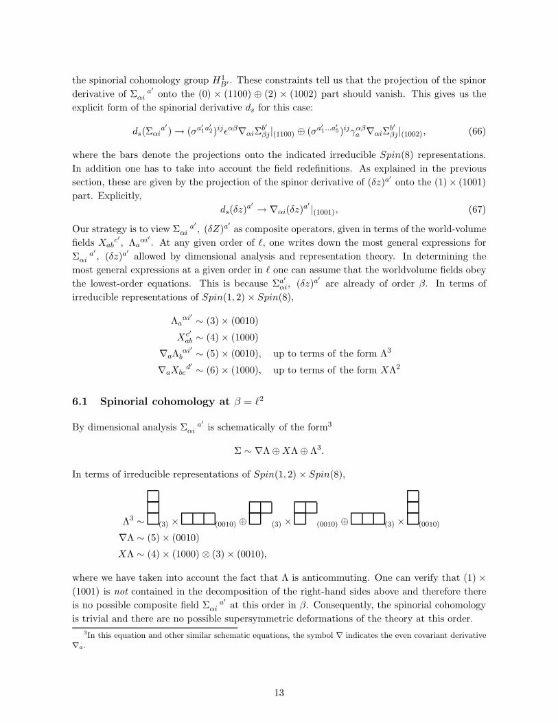
6.1 Spinorial cohomology at β = ℓ2

By dimensional analysis Σ a′

αi is schematically of the form3

Σ ∼ ∇Λ ⊕XΛ ⊕ Λ3.

In terms of irreducible representations of Spin(1, 2) × Spin(8),

Λ3 ∼ (3) × (0010) ⊕ (3) × (0010) ⊕ (3) × (0010)

∇Λ ∼ (5) × (0010)

XΛ ∼ (4) × (1000) ⊗ (3) × (0010),

where we have taken into account the fact that Λ is anticommuting. One can verify that (1) ×(1001) is not contained in the decomposition of the right-hand sides above and therefore there

is no possible composite field Σ a′

αi at this order in β. Consequently, the spinorial cohomology

is trivial and there are no possible supersymmetric deformations of the theory at this order.

3In this equation and other similar schematic equations, the symbol ∇ indicates the even covariant derivative∇a.

13

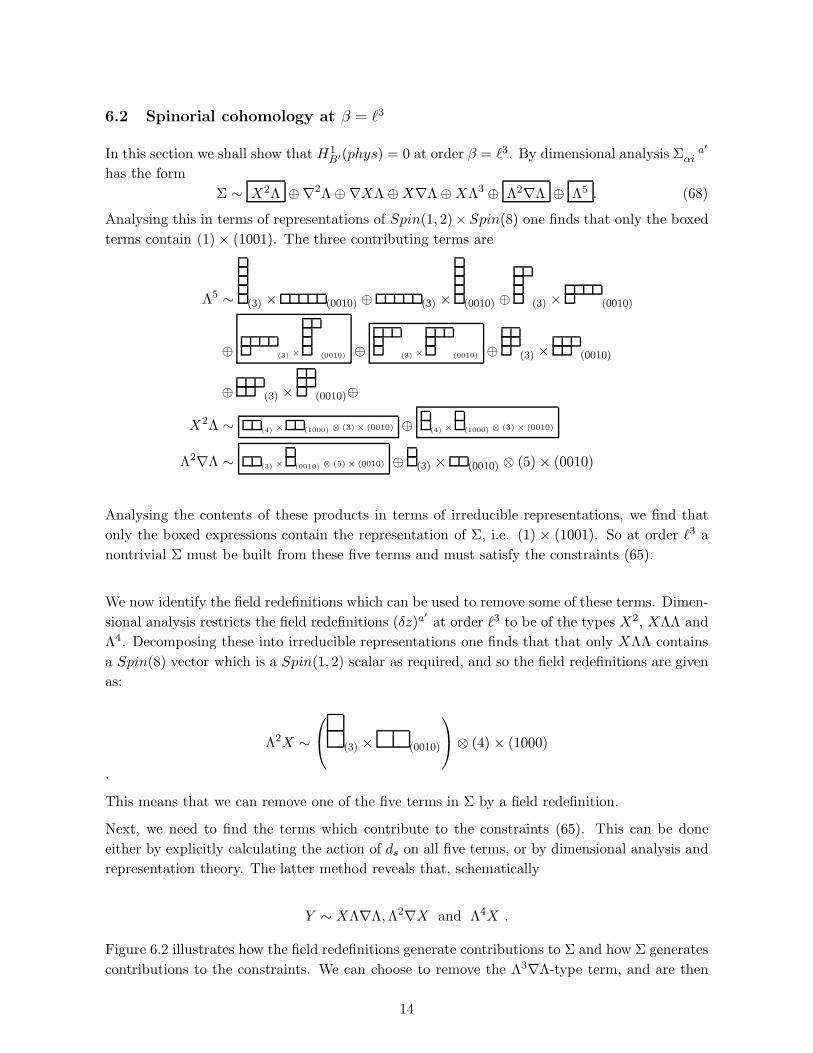
6.2 Spinorial cohomology at β = ℓ3

In this section we shall show that H1B′(phys) = 0 at order β = ℓ3. By dimensional analysis Σ a′

αi

has the form

Σ ∼ X2Λ ⊕∇2Λ ⊕∇XΛ ⊕X∇Λ ⊕XΛ3 ⊕ Λ2∇Λ ⊕ Λ5 . (68)

Analysing this in terms of representations of Spin(1, 2)×Spin(8) one finds that only the boxed

terms contain (1) × (1001). The three contributing terms are

Λ5 ∼ (3) × (0010) ⊕ (3) × (0010) ⊕ (3) × (0010)

⊕ (3) × (0010) ⊕ (3) × (0010) ⊕ (3) × (0010)

⊕ (3) × (0010)⊕

X2Λ ∼ (4) × (1000) ⊗ (3) × (0010) ⊕ (4) × (1000) ⊗ (3) × (0010)

Λ2∇Λ ∼ (3) × (0010) ⊗ (5) × (0010) ⊕ (3) × (0010) ⊗ (5) × (0010)

Analysing the contents of these products in terms of irreducible representations, we find that

only the boxed expressions contain the representation of Σ, i.e. (1) × (1001). So at order ℓ3 a

nontrivial Σ must be built from these five terms and must satisfy the constraints (65).

We now identify the field redefinitions which can be used to remove some of these terms. Dimen-

sional analysis restricts the field redefinitions (δz)a′

at order ℓ3 to be of the types X2, XΛΛ and

Λ4. Decomposing these into irreducible representations one finds that that only XΛΛ contains

a Spin(8) vector which is a Spin(1, 2) scalar as required, and so the field redefinitions are given

as:

Λ2X ∼

(3) × (0010)

⊗ (4) × (1000)

.

This means that we can remove one of the five terms in Σ by a field redefinition.

Next, we need to find the terms which contribute to the constraints (65). This can be done

either by explicitly calculating the action of ds on all five terms, or by dimensional analysis and

representation theory. The latter method reveals that, schematically

Y ∼ XΛ∇Λ,Λ2∇X and Λ4X .

Figure 6.2 illustrates how the field redefinitions generate contributions to Σ and how Σ generates

contributions to the constraints. We can choose to remove the Λ3∇Λ-type term, and are then

14

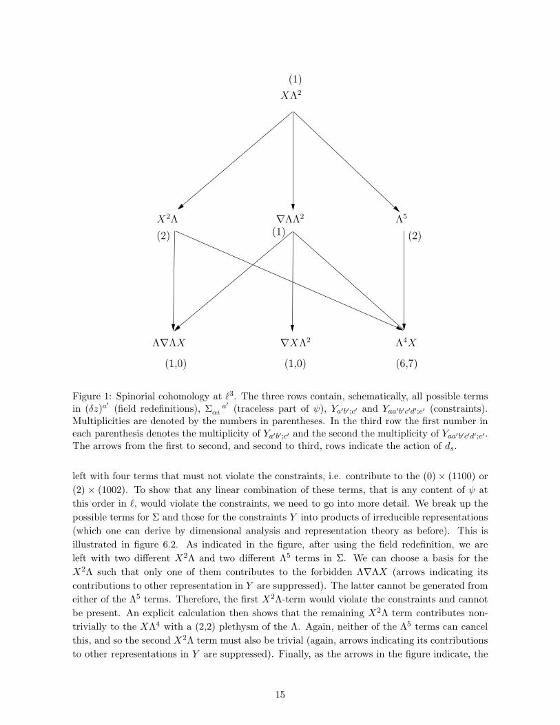
(1) (2)(2)

(1,0) (1,0) (6,7)

(1)

∇XΛ2 Λ4X

∇ΛΛ2 Λ5X2Λ

Λ∇ΛX

XΛ2

Figure 1: Spinorial cohomology at ℓ3. The three rows contain, schematically, all possible termsin (δz)a

′

(field redefinitions), Σ a′

αi (traceless part of ψ), Ya′b′;c′ and Yaa′b′c′d′;e′ (constraints).Multiplicities are denoted by the numbers in parentheses. In the third row the first number ineach parenthesis denotes the multiplicity of Ya′b′;c′ and the second the multiplicity of Yaa′b′c′d′;e′ .The arrows from the first to second, and second to third, rows indicate the action of ds.

left with four terms that must not violate the constraints, i.e. contribute to the (0) × (1100) or

(2) × (1002). To show that any linear combination of these terms, that is any content of ψ at

this order in ℓ, would violate the constraints, we need to go into more detail. We break up the

possible terms for Σ and those for the constraints Y into products of irreducible representations

(which one can derive by dimensional analysis and representation theory as before). This is

illustrated in figure 6.2. As indicated in the figure, after using the field redefinition, we are

left with two different X2Λ and two different Λ5 terms in Σ. We can choose a basis for the

X2Λ such that only one of them contributes to the forbidden Λ∇ΛX (arrows indicating its

contributions to other representation in Y are suppressed). The latter cannot be generated from

either of the Λ5 terms. Therefore, the first X2Λ-term would violate the constraints and cannot

be present. An explicit calculation then shows that the remaining X2Λ term contributes non-

trivially to the XΛ4 with a (2,2) plethysm of the Λ. Again, neither of the Λ5 terms can cancel

this, and so the second X2Λ term must also be trivial (again, arrows indicating its contributions

to other representations in Y are suppressed). Finally, as the arrows in the figure indicate, the

15

xx

xxxx

Λ4XΛ4X Λ4XΛ∇ΛX

X2Λ X2Λ Λ5 Λ5

Λ4X

Figure 2: The first row represents possible terms for Σ and the second row those for Y . Thearrows indicate the action of ds (the spinorial derivative). Some arrows are suppressed. Theproducts of Young-Tableaux represent plethysms of Λ, so that the left factor is a tableau of the(3) of Spin(1,2) and the right factor is a tableau of the (0010) of Spin(8).

Λ5 terms cannot remove each other’s contributions towards Y . This shows that there is no linear

combination of the potential terms which obey the constraints.

6.3 Spinorial cohomology at β = ℓ4

By dimensional analysis Σ a′

αi is, schematically,

Σ ∼ X3Λ ⊕X∇XΛ ⊕X2∇Λ ⊕X∇2Λ ⊕∇2XΛ ⊕∇X∇Λ ⊕∇3Λ

⊕X2Λ3 ⊕∇XΛ3 ⊕X∇ΛΛ2 ⊕ Λ2∇2Λ ⊕ (∇Λ)2Λ ⊕XΛ5 ⊕∇ΛΛ4 ⊕ Λ7 (69)

In terms of irreducible representations of Spin(1, 2) × Spin(8), we can decompose the above

contributions as

Λ7 ∼ 7 (1) × (1001) ⊕ . . .

Λ4∇Λ ∼ 12 (1) × (1001) ⊕ . . .

X2Λ3 ∼ 28 (1) × (1001) ⊕ . . .

X2∇Λ ∼ 2 (1) × (1001) ⊕ . . .

Λ2∇2Λ ∼ 1 (1) × (1001) ⊕ . . .

(∇Λ)2Λ ∼ 1 (1) × (1001) ⊕ . . .

X∇XΛ ∼ 4 (1) × (1001) ⊕ . . .

16

In addition one can verify that there are no more contributions coming from the rest of the

terms on the right-hand side of (69). There are therefore fifty-five possible terms.

We shall now make the assumption that there is a non-trivial cohomology element cubic in the

fields. This is what we expect from string theory calculations in ten dimensions. In order to

determine the cubic part (Σ(cub)a′

αi ) of the cohomology, we shall only require the explicit form of

the cubic terms. These are eight in total,

Σ(1)a′

αi = Xb;ca′∇bXcab′(σb′Λa)αi|(1001)

Σ(2)a′

αi = Xbcb′∇bXcaa′

(σb′Λa)αi|(1001)Σ

(3)a′

αi = Xbca′∇bXadb′(γcd ⊗ σb′Λa)αi|(1001)

Σ(4)a′

αi = Xbcb′∇bXada′

(γcd ⊗ σb′Λa)αi|(1001)Σ

(5)a′

αi = (σb′∇bΛc)αiXbda′

Xdcb′ |(1001)

Σ(6)a′

αi = (γbc ⊗ σb′∇dΛe)αiXbda′

Xceb′ |(1001)

Σ(7)a′

αi = (Λbγd ⊗ σa′b′Λc)(σb′∇b∇cΛd)αi|(1001)Σ

(8)a′

αi = (Λbγd ⊗ σa′b′∇bΛc)(σb′∇cΛd)αi|(1001),

so that

Σ(cub)a′

αi =8

∑

I=1

cIΣ(I)a′

αi . (70)

The coefficients cI will be determined, up to an overall factor, in the following.

Carrying out a similar analysis for the redefinitions (δz)a′

at this order in β we conclude that

the only possible contributions are of the form,

Λ4X ∼ 5 (0) × (1000) ⊕ . . .

Λ2∇X ∼ 1 (0) × (1000) ⊕ . . .

XΛ∇Λ ∼ 2 (0) × (1100) ⊕ . . .

X3 ∼ 1 (0) × (1100) ⊕ . . .

There are nine terms in total, but we shall only need the explicit form of the following cubic

terms,

(δz)(1)a′

= Xbca′

Xbdb′Xcdb′

(δz)(2)a′

= (Λbγd ⊗ σa′b′Λc)∇bXcdb′

(δz)(3)a′

= (Λbγd ⊗ σa′b′∇bΛc)Xcdb′

(δz)(4)a′

= (Λdγb∇cΛd)Xbca′

. (71)

Finally, we need to repeat the analysis for the constraints Ya′b′;c′ and Yaa′b′c′d′;e′ . We find the

17

following contributions,

X2∇X ∼ 1 (0) × (1100) ⊕ . . .

∇X∇ΛΛ ∼ 1 (0) × (1100) ⊕ . . .

X∇2ΛΛ ∼ 1 (0) × (1100) ⊕ . . .

X3Λ2 ∼ 12 (0) × (1100) ⊕ 13 (2) × (1002) ⊕ . . .

X∇ΛΛ3 ∼ 26 (0) × (1100) ⊕ 38 (2) × (1002) ⊕ . . .

∇XΛ4 ∼ 6 (0) × (1100) ⊕ 7 (2) × (1002) ⊕ . . .

XΛ6 ∼ 22 (0) × (1100) ⊕ 35 (2) × (1002) ⊕ . . .

We shall only need the explicit form of the following terms,

Y (1)a′b′;c′ = Xbca′

Xad[b′|∇bX

ae|c′]εcde|(1100)Y (1)a′b′;c′ = (∇bΛcσb′c′Λa)∇bXca

a′ |(1100)Y (1)a′b′;c′ = (∇b∇cΛaσ

b′c′Λa)Xbca′ |(1100).

All the above is summarised in the following diagram. The coefficients cI in (70) are determined,

up to an overall factor, as follows. First note that the redefinitions (71) can be used to eliminate

Σ(I)a′

αi ; I = 5 . . . 8. Indeed an explicit calculation gives

ds(δz)(2)a′ → Σ

(7)a′

αi + . . .

ds(δz)(3)a′ → iΣ

(8)a′

αi + . . . ,

so that (δz)(2,3)a′

can be used to eliminate Σ(7,8)a′

αi . Moreover,

ds(δZ)(1)a′ → 2iΣ

(5)a′

αi + . . .

ds(δZ)(4)a′ → −1

2Σ

(5)a′

αi +1

2Σ

(6)a′

αi + . . . ,

and so (δz)(1,4)a′

can be used to eliminate Σ(5,6)a′

αi . In the following we set

cI = 0; I = 5 . . . 8.

Next we evaluate the action of ds on the remaining cubic terms,

dsΣ(1)a′

αi → −4iY (3)a′b′;c′ + . . .

dsΣ(2)a′

αi → −4iY (2)a′b′;c′ + . . .

dsΣ(3)a′

αi → −16iY (1)a′b′;c′ − 4iY (3)a′b′;c′ + . . .

dsΣ(4)a′

αi → −32iY (1)a′b′;c′ + 4iY (2)a′b′;c′ + . . . ,

where the ellipses stand for terms with more than three fields. Demanding the vanishing of ds

fixes the remaining coefficients to be

c2 =1

2c1

c3 = −c1

c4 =1

2c1.

18

(12)(1)(2)(4) (28)ΛX∇X (∇Λ)2 Λ Λ7∇2ΛΛ2

(7)

X2∇X(22,35)(6,7)(26,38)(12,13)(1,0)(1,0)(1,0)

Λ∇Λ∇X Λ∇2ΛX Λ2X3 Λ3∇ΛX ∇XΛ4 XΛ6

Λ3X2∇ΛX2 ∇ΛΛ4

(1)

(5)(2) (1)(1)

Λ∇ΛX Λ2∇XX3 Λ4X

Figure 3: Spinorial cohomology at ℓ4.

We conclude that the part of the spinorial cohomology cubic in the fields at order ℓ4 is determined

up to an overall factor to be represented by

Σ a′

αi = Xbca′∇bXcab′(σb′Λa)αi|(1001) +

1

2Xbcb′∇bXc

aa′

(σb′Λa)αi|(1001)−Xbca′∇bX

adb′(γcd ⊗ σb′Λa)αi|(1001)+

1

2Xbcb′∇bX

ada′

(γcd ⊗ σb′Λa)αi|(1001) (72)

7 Action

There are various ways of deriving the action corresponding to the deformed embedding con-

straint. One is to compute the modified equations of motion by solving the torsion constraints

at dimensions one-half and one, and then to work back to the Lagrangian. This is a systematic

approach, but is fairly tedious in practice. Another possibility is to use the action principle for

19

branes. We shall discuss this below, but it turns out that one is required to solve another spino-

rial cohomology problem. In order to avoid this we shall find the key part of the Lagrangian

up to quadratic order in fermions by brutal force. Nevertheless, the action principle does shed

light on the structure of the component action.

7.1 Action principle

We recall that supersymmetric Lagrangians in D-dimensional spacetime can be constructed from

closed superspace D-forms [36, 37]. Given such a form, L, the spacetime action is

S =

∫

ǫm1...mDLm1...mD(x, 0) (73)

Under an infinitesimal superspace diffeomorphism generated by a vector field v, δL = LvL =

ivdL + d(ivL) = d(ivL) because L is closed. By evaluating this variation at θ = 0 on the

spacetime part of the D-form one can see that the action (73) is invariant under spacetime

diffeomorphisms and local supersymmetry transformations, these being identified as the leading

components of the even and odd superspace diffeomorphisms.

In the context of branes one can construct a Lagrangian form starting from the (closed) Wess-

Zumino (d + 1)-form W on the super worldvolume, where d is the dimension of the bosonic

worldvolume. This can be written in terms of an explicit potential Z, W = dZ, but it can also

be written in terms of a globally-defined d-form, W = dK. The d-form L = K − Z is closed

by construction. It is uniquely defined up to the exterior derivative of a (d − 1)-form which is

irrelevant in the action. When the standard embedding constraint Eαa = 0 is imposed (in the

on-shell or Lagrangian off-shell cases) this procedure gives the Green-Schwarz action, including

the Born-Infeld contribution in the case of D-branes [38]. At higher orders, it must still be

possible to write W as dK, but we shall also require Lagrangian forms satisfying dL = 0.

For the M2-brane W is the pull-back of the target space four-form H on to the brane, W =

f∗H := H. The components of the pullback are (up to signs)

HABCD = EDDEC

CEBBEA

AHABCD.

The only non-vanishing component of H in flat superspace is

Hab, γδ = −i(Γab)γδ (74)

To order β we therefore have

dim. -1

Hαβγδ = 0 (75)

dim. -1/2

Haβγδ = 0 (76)

dim. 0

Habγδ = −i(Γab)γδ − 4iΛ[aα′

(Γb]c′)α′(γψδ)c′ (77)

20

dim. 1/2

Habcδ = −3i(Γ[ab|)γ′δ′Λ|c]γ′

hδδ′ (78)

dim. 1

Habcd = 0 (79)

We can now solve H = dK. In components,

HABCD = 4∇[AKBCD] + 6TF[AB|KF |CD]

Note that for β = 0, all the components of K are zero, except for the highest-dimension com-

ponent Kabc. To order β we have, taking (75–79) into account ,

dim. -1

0 = −3i

2(Γf )(αβ|Kf |γδ) + ∇(αKβγδ)

This is solved by

Kαβγ = 0; Kaβγ = 0.

dim. -1/2

0 = (Γf )(βγ|Kfa|δ)

This implies

Kabγ = 0.

dim. 0

−i(Γab)γδ − 4iΛ[aα′

(Γb]c′)α′(γψδ)c′ =

(

− i(Γe)γδ − 2iΛeα′

(Γc′)α′(γψδ)c′)

Keab

where we have taken into account the expression for Tαβe to order β, given in section three. The

above equation is satisfied when

Kabc = εabc.

This is identical to the solution for KABC in the β = 0 case. This does not necessarily mean that

there is no correction to the Green-Schwarz action because the induced Green-Schwarz metric

may change. However, one can check that there is no such change to first order in β although

corrections of this type will arise at higher orders.

This means that the Lagrangian form we are looking for must satisfy dL = 0, and, furthermore,

that Lαβγ cannot be zero. Since the Lagrangian form can be changed by an exact form without

affecting the action (73), it follows that this gives rise to a new spinorial cohomology problem.

This is more complicated than the one treated in section six in that the representations involved

are larger. On dimensional grounds, the order β contribution to Lαβγ which is quartic in fields

has the schematic form Λ3X but we have not attempted to compute it explicitly. However, it is

useful to observe that this method of constructing actions tells us something about the structure

of the component Lagrangian. From (73) we have

ǫmnpLmnp = ǫmnp(

EpcEn

bEmaLabc + 3Ep

cEnbEm

αLαbc + . . .)

(80)

21

The non-leading terms on the right-hand side all involve the induced worldvolume “gravitino”

field Emα. This is related to ∂mθ

α but it is not expressible in terms of Λ. The components LABC

will all be constructed from manifest tensors, namely Λ and X; the gravitino terms reflect the

fact that the Lagrangian is a density.

7.2 Component approach

In the component approach we write the action as S = S0 + S1, where S0 is the usual Green-

Schwarz action for the supermembrane [31], and similarly for the worldvolume supersymmetry

variations, so that at first order we have

δ1S0 + δ0S1 = 0 (81)

We can ignore the first term if we calculate S1 using the lowest-order field equations. The ne-

glected terms correspond to field redefinitions. We are therefore looking for an on-shell invariant

at order β.

From the discussion above we have seen that the first-order Lagrangian density L will have the

form

L =√−gL+ ǫmnp

(

3EpcEn

bEmαLαbc + . . .

)

(82)

where g is the determinant of the Green-Schwarz metric, L := ǫabcLabc and where the right-hand

side is understood to be evaluated at θ = 0. Under a worldvolume supersymmetry variation we

find

δL = ∂m(vαLmα )

= δ(√−g)L+

√−g δL+ǫmnp

(

3EpcEn

bEmαδLαbc + 6Ep

c(δEnb)Em

αLαbc + 3EpcEn

b(δEmα)Lαbc . . .

)

(83)

for some Lmα . To quadratic order in fermions the terms represented by the dots in (82), which

have two or more powers of Emα, can be disregarded. The schematic form of the Lagrangian

terms are

L ∼ X4 + Λ2∇X2 + O(Λ4)

Lαbc ∼ ΛX3 + O(Λ3) (84)

while

δEma = ivβ(Γa)βγEm

γ

δEmα = ∇mv

α + vβEmcTβc

α . (85)

22

We shall focus on the terms in the variation of L which are linear in fermions. In the variation

of Emα we can use the lowest-order expression for the induced torsion Tβc

α. As this is quadratic

in Λ the corresponding term in δEmα can be ignored. The term involving the variation of the

world-volume vielbein Ema can also be ignored as it leads to terms which are cubic in fermions.

The terms which are linear in fermions involve either Λ or Emα, and these must cancel separately.

Thus we see that the term arising from the variation of the determinant of the metric multiplied

by the X4 term in L must be cancelled by the leading term coming from the variation of Lαbc.

The terms linear in Λ arise from varying both the Λ0 and Λ2 terms in L and from the ∇vvariation term in Em

α multiplied by Lαbc. It therefore follows that the terms linear in Λ in

the variation of L will cancel up to a covariant divergence if the parameter vα is taken to be

covariantly constant. The terms involving the derivative of v in the variation of L must cancel

against similar terms arising from the variation of Emα. In fact, demanding that these terms

cancel determines Lαbc at first order in Λ. We shall therefore concentrate on computing L up

to quadratic order in the fermions. In what follows we shall refer to L as the Lagrangian.

It follows from the analysis in section six that, up to and including terms quadratic in the

fermions, there is a unique supersymmetric invariant at order l4. Indeed, we have shown that at

order cubic in the fields there is a unique nontrivial element in the relevant spinorial cohomology

group and this implies that there is a unique deformation of the equations of motion. We

conclude that in the action there is a unique supersymmetric invariant at order quartic in the

fields. In particular, there can be no terms in the action of order cubic, or less, in the fields.

There are also no terms of the form Λ2X3 as can be seen by the fact that there is no scalar in

the decomposition of the tensor product

[(3) × (0010)]2⊗a ⊗ [(4) × (1000)]3⊗s , (86)

The bosonic part of the Lagrangian at l4, is a linear combination of the following three X4 terms

t1 := Xaba′

Xcda′Xabb′Xcdb′

t2 := Xaba′

Xcdb′Xab

a′Xcdb′

t3 := Xaba′

Xcdb′Xac

a′Xbdb′ . (87)

A fourth structure

t4 := Xaba′

Xcda′Xacb′Xbdb′ (88)

can be shown to be linearly dependent

t4 = t1 +1

2t2 − 2t3, (89)

by using the identity

4X[a[b|a′

Xc]|d]b′ =

(

δefX

gha′

Xghb′ −Xf

ga′

Xgeb′ −Xf

gb′Xgea′

)

εeacεfbd. (90)

At quadratic order in the fermions, the Lagrangian at l4 contains terms of the form Λ2X∇Xand Λ∇ΛX2. A lengthy calculation, the details of which are given in appendix B, yields the

following result for L:

23

L =1

4Xab

a′

Xcda′Xabb′Xcdb′ −

1

4Xab

a′

Xcdb′Xac

a′Xbdb′

+i(Λaγb∇cΛd)Xaba′

Xcda′ − 2i

3(Λfγa ⊗ σa′b′∇fΛb)X

aea′Xb

eb′

− i

3(Λaγb ⊗ σa′b′∇cΛd)X

aba′Xcd

b′ + O(Λ4). (91)

The Lagrangian above is determined up to a total derivative and up to terms vanishing by virtue

of the lowest-order equations of motion. The latter can always by removed by appropriate field

redefinitions.

We shall now compare our result to that of [2]. In this paper the bosonic CP-even part of the

O(l4) Lagrangian of a D-p brane was determined to be

1

16

(

(RT )abcd(RT )abcd − 2(RT )ab(RT )ab − (RN )abc′d′(RN )abc′d′ + 2Ra′b′Ra′b′

)

, (92)

see equation (2.14) of that reference. In the above we have omitted an overall multiplicative

constant involving α′ and the string coupling.

Let us view (92) as the world-volume Lagrangian of a D2-brane and consider its lift to eleven

dimensions. The various curvatures in (92) are given, in the notation of the present paper and

for flat target-space, by

(RT )abcd = Xaca′Xbda′ −Xada′Xbc

a′

(RN )abc′d′ = Xaec′Xebd′ −Xbec′X

ead′

(RT )ab = −Xaea′

Xeba′

Ra′b′ = Xaba′Xabb′ . (93)

Substituting (93) into (92) on gets precisely the bosonic part of (91).

The Lagrangian (92) was determined, as is the case with (91), modulo total derivatives 4 and

terms which vanish by virtue of the lowest-order equations of motion. In [3] the investigation of

these ambiguities was considered, see equation (5.4) therein. It was shown that there is a total

of five ambiguous terms, two of which vanish by virtue of the lowest-order equations of motion

and therefore cannot be determined perturbatively. Two of the other three terms vanish for

flat target-space, whereas the remaining third term vanishes by virtue of equation (89) of the

present paper.

8 Kappa symmetry

Although we have not used the modified worldvolume supersymmetry transformations in de-

termining the Lagrangian, it is perhaps of interest to see how the usual κ-symmetry variations

are altered. To lowest order the κ-symmetry transformations were derived, starting from world-

volume supersymmetry transformations, in equations (9-14). These will be amended when we

4the coefficient of the Gauss-Bonnet term was fixed to zero in [2] by an indirect argument.

24

deform the embedding condition. In general, a worldvolume supersymmetry transformation

gives the following transformations

δza = vαEαa (94)

δzα = vαEαα . (95)

We can convert the second of these into κ-symmetry form as before:

δzα = κβPβα =

1

2κβ(1 + Γ)β

α . (96)

where κα = vαEαα and

Pαβ = (E−1)α

γEγβ (97)

where the inverse refers to inverting the square matrix formed from (Eαα, Eα′

α). Explicitly

Pαβ = (u−1)α

γuγβ + (u−1)α

γhγδ′uδ′

β (98)

The first term here has the same structure as in the undeformed theory. The bosonic projection

of δzM can be written

δza = καΨαa = δzαΨα

a , (99)

where

Ψαa = (E−1)α

γEγa

= (E−1)αγψγ

a′

ua′a (100)

satisfies Ψ = PΨ.

In the undeformed theory the matrix Γ is given by

Γ = −1

6ǫabcua

aubbuc

cΓabc . (101)

This can easily be seen to be the same as

Γαβ = (u−1)α

γuγβ − (u−1)α

γ′

uγ′β (102)

In the deformed theory we can write

25

Γ = Γ0 +1

2u−1(1 + Γ0)h(1 − Γ0)u (103)

where Γ0 has the same form as in (101) and (102) and where h is regarded as a 32 × 32 matrix

satisfying h = P0hQ0, with P0 = 1/2(1 + Γ0), Q = 1/2(1 − Γ0).

The formulae above are valid for an arbitrary deformation ψ. To obtain the order β term we

merely have to substitute into the expressions the explicit forms for ψ and h.

9 Conclusions

In this paper we have discussed the first correction to the dynamics of the M2-brane in the

superembedding formalism which we have shown to occur at order ℓ4. We have seen that

the allowed modifications of the constraints are specified by an element of a certain spinorial

cohomology group. There is a unique solution cubic in the fields and we believe that there are

no other independent terms at quartic or higher orders. In principle one could continue this

analysis for higher powers of ℓ. We would expect to find both corrections induced by iterating

the first correction and new cohomological terms. However, the computations are difficult, even

at ℓ4.

The formalism developed here could be applied straightforwardly to other branes such as the

M5-brane and D-branes. Indeed, we could obtain the equivalent terms in the D2-brane action

by dimensional reduction. In particular, this would shed some light on the κ-symmetric ef-

fective action including ∂4F 4 terms. Another extension of the formalism would be to include

non-trivial supergravity backgrounds. In D = 11 it is expected that the first correction to super-

gravity occurs at ℓ6, so that this complication could be ignored. It should therefore be relatively

straightforward to compute the corrections at the same order, which involve the background su-

pergravity fields. In the case of the M5-brane these results could again be dimensionally reduced

to ten dimensions, either to give results for the NS5-brane, or the D4-brane. In the latter case

one would expect to see some sign of the A-genus terms discussed in [39, 40, 41]. In principle,

we should therefore be able to obtain some information about the supersymmetrisation of these

terms.

Acknowledgements

This work was supported in part by EU contracts HPRN-2000-00122 (which includes Queen

Mary, London as a subcontractor) and HPRN-CT-2000-00148 and PPARC grants PPA/G/S/

1998/00613 and PPA/G/O/2000/00451. SFK thanks the German National Merit Foundation

for financial support. UL acknowledges support in part by VR grant 650-1998368.

26

Appendix A

Notation

The following index conventions are used: plain (underlined) indices refer to worldsurface and

target space quantities respectively and primed indices refer to normal spaces; indices from the

beginning of the alphabet refer to preferred bases, indices from the middle of the alphabet to

coordinate bases; Latin (Greek) indices are used for even (odd) indices, while capital indices

run over the whole space. Thus a worldsurface preferred basis index could be A = (a, α) while

a target space coordinate index could be M = (m,µ). Tensor quantities with indices are not

underlined, but if the indices are omitted or if a target space tensor is projected on some of its

indices we underline the tensor.

For the spinor indices a two step notation is used. Initially the target space index α, running

from 1 to 32 is split in two, α → (α,α′), where both the worldsurface index α and the normal

index α′ run from 1 to 16. For some purposes this is adequate but sometimes one wishes to

recognise explicitly that these indices transform under Spin(1, 2) × Spin(8). We set

ψα → ψαi

ψα′ → ψαi′ (104)

where the spinor index on the right takes on two values while i and i′ both run from 1 to 8.

We use space-favoured metrics throughout, ηab = (−1,+1, . . . ,+1), and the spacetime ǫ-tensors

have ǫ0123... = +1.

We use the following representation of the D = 11 Γ-matrices:

Γa = γa ⊗ γ9

Γa′

= 1 ⊗ γa′

(105)

where the d = 3 γ-matrices are 2 × 2 and the d′ = 8 γ-matrices are 16 × 16. The charge

conjugation matrix is

C = ǫ⊗ γ9 (106)

In indices

(Γa)αβ = (γa)α

β

(

δij 0

0 −δi′ j′

)

(Γa′

)αβ = δα

β

(

0 (σa′

)ij′

(σa′

)i′j 0

)

(107)

and

Cαβ = ǫαβ

(

δij 00 −δi′j′

)

(108)

where the 8 × 8 σ-matrices are related to the eight-dimensional γ-matrices by

γa′

=

(

0 (σa′

)ij′

(σα′

)i′j 0

)

(109)

27

Eleven-dimensional spinor indices are raised or lowered according to the rule

ψα = Cαβψβ ↔ ψα = ψ βCβα (110)

where C with upper indices is the same matrix as C with lower indices. Three-dimensional

spinor indices are similarly raised or lowered using ǫ. Eight-dimensional indices, whether spinor

or vector, are raised and lowered with the standard Euclidean metric. The Γ-matrices with

lowered indices are

(Γa)αβ = (γa)αβ

(

δij 00 δi′j′

)

(Γa′

)αβ = ǫαβ

(

0 −(σa′

)ij′

(σa′

)i′j 0

)

(111)

It is straightforward to decompose any of the eleven-dimensional Γ-matrices with multi-vector

indices in this way. We give the two-index Γ-matrices as they are used most in the text:

(Γab)αβ = (γab)αβ

(

δij 00 δi′j′

)

(Γab′)αβ = −(γa)αβ

(

0 −(σb′)ij′

(σb′)i′j 0

)

(Γa′b′)αβ = ǫαβ

(

(σa′b′)ij′ 0

0 −(σa′b′)i′j

)

(112)

The three-dimensional γ-matrices are real, symmetric with lowered indices, and satisfy

γaγb = ηab + γab (113)

where

γab = ǫabcγc ↔ γa = −1

2ǫabcγ

bc (114)

For the eight-dimensional σ-matrices one may take

σa′

= (1, iτr)

σa′

= (1,−iτr) (115)

where r = 1, . . . 7, and where the τr are seven-dimensional Dirac matrices which are purely

imaginary and antisymmetric. The matrices σa′b′c′d′ and σa′b′c′d′ are symmetric, the former

being self-dual, the latter anti-self-dual, σa′b′ and σa′b′ are antisymmetric.

Group theoretic conventions

Consider a Lie groupG and aG-module V . The n-th tensor product V ⊗n admits a decomposition

∑

R

VR ×R

under G× Sn, where R runs over all irreducible representations of the symmetric group Sn and

VR is a G-module. As is well known, the irreducible representations of Sn can be parametrised

28

by partitions of n or, equivalently, by the associated Young diagrams. If R is associated to the

partition λ of n, VR is the plethysm of V with respect to λ.

In this paper, we are using a notation referring to the product group Spin(1, 2) × Spin(8).

The highest weight of the standard module (i.e. of the vector representation) of Spin(8) is

given by (1000) on the basis of fundamental weights. A two-form is (0100) and a three-form is

(0011). The self-dual and anti-self-dual four-forms are represented by (0002), (0020) respectively.

The chiral and anti-chiral spinors are (0001), (0010). Moreover, the highest weight of the k-

form-spinor is given by the sum of the highest weight of the k-form and the highest weight

of the spinor. Recall that by a k-form-spinor we refer to the projection onto the irreducible

(gamma-traceless) part. For example (1001) is a chiral vector-spinor, (0110) is an anti-chiral

two-form-spinor, etc. We can also consider the projection onto the highest-weight representation

of the plethysm associated to the partition [2, . . . , 2, 1, . . . , 1] of n+ k, with k entries equal to 2

and n− k entries equal to 1. This is one way to view the irreducible (n, k)-tensors of section 5.

For example, a (2,1)-tensor is a two-form and a one-form and is represented by (1100). A (3,1)-

tensor is a three-form and a one-form and is represented by (1011), etc. The highest-weights

of irreducible (gamma-traceless) (n, k)-tensor-spinors are represented in the obvious way. For

example (1101) is the highest weight of a (2, 1)-tensor-(chiral) spinor. This discussion generalizes

straightforwardly to representations corresponding to more general partitions.

In the case of Spin(1, 2) the situation is simpler, in that the representation denoted by (n) is

of dimension n + 1. Hence, the spinor representation is denoted by (1), the vector by (2), the

vector spinor by (3) and so on.

Appendix B

In this appendix we give some details of the derivation of the action in section seven. At

quadratic order in the fermions the Lagrangian at ℓ4 contains terms of the form Λ2X∇X and

Λ∇ΛX2. We have the following structures:

Λ2X∇X:

u1 := (Λfγa ⊗ σa′b′Λf )Xcda′∇aXcdb′

u2 := (Λaγb ⊗ σa′b′Λc)Xafa′∇fXbc

b′

u3 := (ΛaγbΛc)Xafa′∇fXbca′

u4 := (Λaγb ⊗ σa′b′Λc)Xbfa′∇fXac

b′ (116)

Λ∇ΛX2:

s1 := (Λfγa∇fΛb)Xaea′

Xbea′

s2 := (Λaγb∇cΛd)Xaba′

Xcda′

s3 := (Λfγa ⊗ σa′b′∇fΛb)Xae

a′Xbeb′

s4 := (Λaγb ⊗ σa′b′∇cΛd)Xab

a′Xcdb′

s5 := (Λaγb ⊗ σa′b′∇cΛd)Xac

a′Xbdb′

s6 := (Λaγb∇cΛd)Xaca′

Xbda′ . (117)

29

Not all of the above are independent. Only three of the u and four of the s-terms are, as can be

seen by counting the number of scalars in the decomposition of the tensor products

[(3) × (0010)]2⊗a ⊗ [(4) × (1000)] ⊗ [(6) × (1000)] (118)

and

[(3) × (0010)] ⊗ [(5) × (0010)] ⊗ [(4) × (1000)]2⊗s . (119)

Indeed on has

0 = u2 − u4 −1

2u1

0 = s6 − s2 + s1

0 = 3s5 − s4 + s3. (120)

The first line of (120) is derived using the identity

εegh(Λgγh ⊗ σa′b′Λc) =1

2εdec(Λ

fγd ⊗ σa′b′Λf ). (121)

The second line of (120) can be shown by taking (90) into account. Finally, to derive the third

line of (120) one notes that

0 = (Λeγ[aeγb ⊗ σa′b′∇cΛd)Xa

c|a′

X |b]db′ . (122)

In addition one has to take into account the fact that some terms are related to each other by

integration by parts. Indeed, up to total derivatives, one has the following relations

u1 = 2s3

u2 = s4 − s5

u2 = u4 + s3

u3 = s2 − s6

u3 = s1

u4 = 2s5

u4 = u2 − s3. (123)

Only six of the equations (120,123) above are independent. It is perhaps interesting to note that

the group-theoretic relations (120) are all implied by the partial integration equations (123).

The solution may be given in terms of four independent variables which we take to be s1−4,

u1 = 2s3

u2 =1

3s3 +

2

3s4

u3 = s1

u4 = −2

3s3 +

2

3s4

s5 = −1

3s3 +

1

3s4

s6 = −s1 + s2. (124)

30

Therefore, the lagrangian at l4 can be written as

L =

3∑

i=1

Aiti +

4∑

i=1

Bisi + O(Λ4), (125)

where the constant coefficients A,B are determined by the requirement that the supersymmetric

variation of L be a total derivative, up to ∇v terms.

At linear order in the fermions, the supersymmetric variation of the correction to the Lagrangian,

igoniring the ∇v terms, consists of terms of the form ∇ΛX3, Λ∇XX2. Explicitly, one can write

down the following structures (suppressing spinor indices and the supersymmetry parameter v)

∇ΛX3:

w1 := (γab ⊗ σa′b′c′∇cΛd)Xaea′Xeb

b′Xcd

c′

w2 := (γab ⊗ σa′∇cΛd)Xaea′Xeb

b′Xcdb′

w3 := (γab ⊗ σa′∇cΛd)Xac

a′Xebb′Xe

db′

w4 := (σa′∇aΛb)Xaea′Xeg

b′Xgbb′

w5 := (σa′∇aΛb)Xabb′Xeg

a′Xegb′

w6 := (σa′∇aΛb)Xab

a′Xegb′Xeg

b′

w7 := (γab ⊗ σa′∇cΛd)Xac

b′Xeb

a′Xedb′

w8 := (γab ⊗ σa′∇cΛd)Xac

b′Xed

a′Xebb′

w9 := (σa′∇aΛb)Xaeb′X

ega′Xg

bb′

w10 := (γab ⊗ σa′b′c′∇cΛd)Xcb

a′Xaeb′X

edc′ (126)

31

Λ∇XX2:

z1 := (σa′

Λa)∇aXbca′Xbdb′Xcdb′

z2 := (γab ⊗ σa′

Λc)∇dXbca′Xaeb′Xdeb′

z3 := (σa′

Λa)∇bXcda′Xabb′Xcdb′

z4 := (γab ⊗ σa′

Λc)∇bXdea′Xcdb′Xe

ab′

z5 := (σa′

Λa)∇aXbcb′Xbd

a′Xcdb′

z6 := (γab ⊗ σa′

Λc)∇dXbcb′Xaea′Xdeb′

z7 := (γab ⊗ σa′

Λc)∇bXdeb′Xaca′Xdeb′

z8 := (σa′

Λa)∇bXcdb′Xaba′

Xcdb′

z9 := (γab ⊗ σa′

Λc)∇dXbcb′Xaeb′Xd

ea′

z10 := (γab ⊗ σa′

Λc)∇cXdeb′Xd

aa′Xebb′

z11 := (γab ⊗ σa′

Λc)∇bXdeb′Xacb′X

dea′

z12 := (γab ⊗ σa′b′c′Λc)∇dXbca′Xaeb′Xde

c′

z13 := (γab ⊗ σa′b′c′Λc)∇cXdea′Xdab′X

ebc′

z14 := (γab ⊗ σa′b′c′Λc)∇bXdea′Xacb′Xde

c′

z15 := (γab ⊗ σa′

Λc)∇bXdeb′Xaea′Xcdb′

z16 := (γab ⊗ σa′

Λc)∇bXdeb′Xaeb′Xcda′

z17 := (γab ⊗ σa′b′c′Λc)∇bXde

a′Xaeb′Xcdc′

z18 := (σa′

Λa)∇bXcdb′Xabb′Xcda′

z19 := (γab ⊗ σa′

Λc)∇bXdea′Xdeb′Xacb′

z20 := (σa′b′c′Λa)∇bXcda′Xabb′X

cdc′ . (127)

As before, not all of these structures are linearly independent. Only six of the w and fourteen

of the z-terms are, as one can see by counting the number of spinors [(1) × (0001)] in the

decomposition of the tensor products

[(5) × (0010)] ⊗ [(4) × (1000)]3⊗s (128)

and

[(3) × (0010)] ⊗ [(6) × (1000)] ⊗ [(4) × (1000)]2⊗s . (129)

Indeed, taking into account (90) and the identity

γ[abΛc] = 0, (130)

one can derive the following relations

w7 = −w2 + w3 − w4 +1

2w6

w8 = w2 + w7

w9 = −2w4 + w5 +1

2w6

w10 =1

2w1 (131)

32

and

z15 + z16 = 2z5 − z6 + z7 − z9 + z11

z15 − z16 = z10

z17 =1

2z13

z19 = −z1 + z2 + z4

z18 = −z5 + z8 + z9 + z10 − z11 + z15

2z20 = z12 − z13 − z14 − z17. (132)

The last two lines in equation (132) above are derived by noting that

(γ[eaσa′Λe)∇bXcd|b′Xa

ba′

X |c]db′ = 0 (133)

and

(γ[ea|σa′b′c′Λe)∇bXc|d|

a′Xabb′X

|c]dc′ = 0. (134)

In addition one has to allow for integrations by parts. Up to total derivatives, one has the

following relations

w1 = 2z17

w2 = z4 − z15

w3 = z2 − z7

w4 = −z1 − z8

w5 = −z3 − z18

w6 = −2z8

w7 = z6 − z19

w8 = z9 − z11

w9 = −z3 − z5

w10 = −z12 − z14 (135)

33

and

z1 = −2z5

z2 = z6 + z10

z2 = w4 − z16

z4 = w9 − z9

z4 = −w7 + z10

z5 = −w4 − z18

z6 = w4 − z15

z7 =1

2w6

z10 = −w3 − z15

z11 = w5 − z19

z12 = z17

z13 = 2z12

z13 = w10 + z17

z16 = −w8

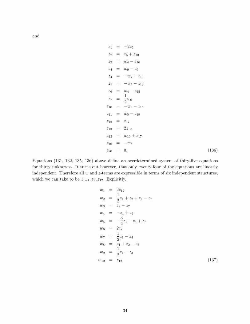
z20 = 0. (136)

Equations (131, 132, 135, 136) above define an overdetermined system of thiry-five equations

for thirty unknowns. It turns out however, that only twenty-four of the equations are linearly

independent. Therefore all w and z-terms are expressible in terms of six independent structures,

which we can take to be z1−4, z7, z12. Explicitly,

w1 = 2z12

w2 =1

2z1 + z2 + z4 − z7

w3 = z2 − z7

w4 = −z1 + z7

w5 = −3

2z1 − z3 + z7

w6 = 2z7

w7 =1

2z1 − z4

w8 = z1 + z2 − z7

w9 =1

2z1 − z3

w10 = z12 (137)

34

and

z5 = −1

2z1

z6 = −1

2z1 + z2

z8 = −z7z9 =

1

2z1 − z3 − z4

z10 =1

2z1

z11 = −1

2z1 − z2 − z3 − z4 + z7

z13 = 2z12

z14 = −2z12

z15 = −1

2z1 − z2 + z7

z16 = −z1 − z2 + z7

z17 = z12

z18 =3

2z1 − z7

z19 = −z1 + z2 + z4

z20 = 0. (138)

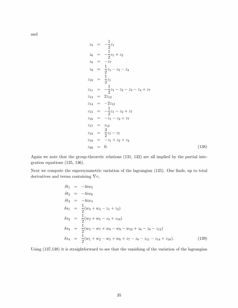
Again we note that the group-theoretic relations (131, 132) are all implied by the partial inte-

gration equations (135, 136).

Next we compute the supersymmetric variation of the lagrangian (125). One finds, up to total

derivatives and terms containing ∇v,

δt1 = −4iw5

δt2 = −4iw6

δt3 = −4iw4

δs1 =1

2(w3 + w4 − z1 + z2)

δs2 =1

2(w2 + w5 − z3 + z19)

δs3 =1

2(w4 − w7 + w8 − w9 − w10 + z6 − z9 − z12)

δs4 =1

2(w1 + w2 − w5 + w6 + z7 − z8 − z11 − z14 + z18). (139)

Using (137,138) it is straightforward to see that the vanishing of the variation of the lagrangian

35

implies the following relations for the coefficients in (125),

A1 =3i

4B4

A2 = 0

A3 = −3i

4B4

B1 = 0

B2 = −3B4

B3 = 2B4. (140)

These results lead to the Lagrangian (91).

References

[1] O. D. Andreev and A. A. Tseytlin, “Partition Function Representation For The Open

Superstring Effective Action: Cancellation Of Mobius Infinities And Derivative Corrections

To Born-Infeld Lagrangian,” Nucl. Phys. B 311 (1988) 205.

[2] C. P. Bachas, P. Bain and M. B. Green, “Curvature terms in D-brane actions and their

M-theory origin,” JHEP 9905 (1999) 011 [arXiv:hep-th/9903210].

[3] A. Fotopoulos, “On α′2 corrections to the D-brane action for non-geodesic world-volume

embeddings,” JHEP 0109 (2001) 005 [arXiv:hep-th/0104146].

[4] N. Wyllard, “Derivative corrections to D-brane actions with constant background fields,”

Nucl. Phys. B 598 (2001) 247 [arXiv:hep-th/0008125].

[5] A. Bilal, “Higher-derivative corrections to the non-abelian Born-Infeld action,” Nucl. Phys.

B 618 (2001) 21 [arXiv:hep-th/0106062].

[6] N. Wyllard, “Derivative corrections to the D-brane Born-Infeld action: Non-geodesic em-

beddings and the Seiberg-Witten map,” JHEP 0108 (2001) 027 [arXiv:hep-th/0107185].

[7] P. Koerber and A. Sevrin, “The non-abelian D-brane effective action through order α′4,”

JHEP 0210 (2002) 046 [arXiv:hep-th/0208044].

[8] U. Lindstrom, M. Rocek and P. van Nieuwenhuizen, “A Weyl Invariant Rigid String,” Phys.

Lett. B 199 (1987) 219.

[9] U. Lindstrom and M. Rocek, “Bosonic And Spinning Weyl Invariant Rigid Strings,” Phys.

Lett. B 201 (1988) 63.

[10] A. Collinucci, M. de Roo and M. G. Eenink, “Derivative corrections in 10-dimensional

super-Maxwell theory,” JHEP 0301 (2003) 039 [arXiv:hep-th/0212012].

[11] J. M. Drummond, P. J. Heslop, P. S. Howe and S. F. Kerstan, “Integral invariants in N =

4 SYM and the effective action for coincident D-branes,” [arXiv:hep-th/0305202].

36

[12] E. A. Ivanov and A. A. Kapustnikov, “Gauge Covariant Wess-Zumino Actions For Super

P-Branes In Superspace,” Int. J. Mod. Phys. A 7 (1992) 2153.

[13] J. P. Gauntlett, “A kappa symmetry calculus for superparticles,” Phys. Lett. B 272 (1991)

25 [arXiv:hep-th/9109039].

[14] E. A. Ivanov and A. A. Kapustnikov, “Towards A Tensor Calculus For Kappa Supersym-

metry,” Phys. Lett. B 267 (1991) 175.

[15] T. Curtright and P. van Nieuwenhuizen, “Supersprings,” Nucl. Phys. B 294 (1987) 125.

[16] D. P. Sorokin, “Coincident (super)-Dp-branes of codimension one,” JHEP 0108 (2001) 022

[arXiv:hep-th/0106212].

[17] S. Panda and D. Sorokin, “Supersymmetric and kappa-invariant coincident D0-branes,”

JHEP 0302 (2003) 055 [arXiv:hep-th/0301065].

[18] P. S. Howe and U. Lindstrom, “Kappa-symmetric higher derivative terms in brane actions,”

Class. Quant. Grav. 19 (2002) 2813 [arXiv:hep-th/0111036].

[19] J. M. Drummond, P. S. Howe and U. Lindstrom, “Kappa-symmetric non-Abelian Born-

Infeld actions in three dimensions,” Class. Quant. Grav. 19 (2002) 6477 [arXiv:hep-

th/0206148].

[20] D. Sorokin, V. Tkach and D.V. Volkov, “Superparticles, twistors and Siegel symmetry,”

Mod. Phys. Lett. A4 (1989) 901; D. Sorokin, V. Tkach, D.V. Volkov and A. Zheltukhin,

“From the superparticle Siegel symmetry to the spinning particle proper time supersym-

metry,” Phys. Lett. B216 (1989) 302; D.V. Volkov and A. Zheltukhin, “Extension of the

Penrose representation and its use to describe supersymmetric models,” Sov. Phys. JETP

Lett. 48 (1988) 63-66.

[21] D. Sorokin, “Superbranes and superembeddings,” Phys. Report 239 (2000) 1.

[22] P. S. Howe and E. Sezgin, “Superbranes,” Phys. Lett. B 390 (1997) 133 [arXiv:hep-

th/9607227].

[23] P. S. Howe and E. Sezgin, “D = 11, p = 5,” Phys. Lett. B 394 (1997) 62 [arXiv:hep-

th/9611008].

[24] M. Cederwall, B. E. Nilsson and D. Tsimpis, “The structure of maximally supersymmet-

ric Yang-Mills theory: Constraining higher-order corrections,” JHEP 0106 (2001) 034

[arXiv:hep-th/0102009].

[25] M. Cederwall, B. E. Nilsson and D. Tsimpis, “D = 10 super-Yang-Mills at O(α′2),” JHEP

0107 (2001) 042 [arXiv:hep-th/0104236].

[26] M. Cederwall, B. E. Nilsson and D. Tsimpis, “Spinorial cohomology and maximally super-

symmetric theories,” JHEP 0202 (2002) 009 [arXiv:hep-th/0110069].

37

[27] M. Cederwall, B. E. Nilsson and D. Tsimpis, “Spinorial cohomology of abelian d = 10

super-Yang-Mills at O(α′3),” JHEP 0211 (2002) 023 [arXiv:hep-th/0205165].

[28] P. S. Howe and D. Tsimpis, “On higher-order corrections in M theory,” [arXiv:hep-

th/0305129].

[29] S. J. Gates and H. Nishino, “D = 2 Superfield Supergravity, Local (Supersymmetry)2 And

Nonlinear Sigma Models,” Class. Quant. Grav. 3 (1986) 391.

[30] I. A. Bandos, D. P. Sorokin, M. Tonin, P. Pasti and D. V. Volkov, “Superstrings and

supermembranes in the doubly supersymmetric geometrical approach,” Nucl. Phys. B 446

(1995) 79 [arXiv:hep-th/9501113].

[31] E. Bergshoeff, E. Sezgin and P. K. Townsend, “Supermembranes And Eleven-Dimensional

Supergravity,” Phys. Lett. B 189 (1987) 75.

[32] N. Berkovits, “Super-Poincare covariant quantization of the superstring,” JHEP 0004

(2000) 018 [arXiv:hep-th/0001035].

[33] N. Berkovits, “Covariant quantization of the superparticle using pure spinors,” JHEP 0109

(2001) 016 [arXiv:hep-th/0105050].

[34] P. S. Howe, “Pure Spinors Lines In Superspace And Ten-Dimensional Supersymmetric

Theories,” Phys. Lett. B 258 (1991) 141 [Addendum-ibid. B 259 (1991) 511].

[35] P. S. Howe, “Pure spinors, function superspaces and supergravity theories in ten-dimensions

and eleven-dimensions,” Phys. Lett. B 273 (1991) 90.

[36] R. D’Auria, P. Fre, P. K. Townsend and P. van Nieuwenhuizen, “Invariance Of Actions,

Rheonomy And The New Minimal N=1 Supergravity In The Group Manifold Approach,”

Annals Phys. 155 (1984) 423.

[37] S.J. Gates, M. Grisaru, M. Knutt-Wehlau and W. Siegel, “Component actions from

curved superspace: normal coordinates and ectoplasm,” Phys.Lett. B421 (1998) 203-210,

[arXiv:hep-th/9711151].

[38] P.S. Howe, O. Raetzel and E. Sezgin, “On brane actions and superembeddings,” JHEP

9808 (1998) 011, [arXiv:hep-th/9804051].

[39] M. B. Green, J. A. Harvey and G. W. Moore, “I-brane inflow and anomalous couplings on

D-branes,” Class. Quant. Grav. 14 (1997) 47 [arXiv:hep-th/9605033].

[40] Y. K. Cheung and Z. Yin, “Anomalies, branes, and currents,” Nucl. Phys. B 517 (1998)

69 [arXiv:hep-th/9710206].

[41] R. Minasian and G.W. Moore, “K theory and Ramond-Ramond charge,” JHEP 9711 (1997)

002 [arXiv:hep-th/9710230].

38