arX

iv:h

ep-t

h/98

1113

9v3

20

May

199

9

hep-th/9811139

IASSNS-HEP-98/95

TIFR/TH/98-43

Brane Constructions, Conifolds and M-Theory

Keshav Dasgupta1

School of Natural Sciences, Institute for Advanced Study

Olden Lane, Princeton NJ 08540, U.S.A.

Sunil Mukhi2

Tata Institute of Fundamental Research,

Homi Bhabha Rd, Mumbai 400 005, India

ABSTRACT

We show that a set of parallel 3-brane probes near a conifold singularity can be mapped

onto a configuration of intersecting branes in type IIA string theory. The field theory on

the probes can be explicitly derived from this formulation. The intersecting-brane metric

for our model is obtained using various dualities and related directly to the conifold metric.

The M-theory limit of this model is derived and turns out to be remarkably simple. The

global symmetries and counting of moduli are interpreted in the M-theory picture.

November 1998

1 E-mail: keshav@ias.edu2 E-mail: mukhi@tifr.res.in

1. Introduction

Recently, a system of parallel 3-branes in the presence of a conifold singularity has

received some attention[1]. The N = 1 supersymmetric gauge theory on the 3-branes has

been deduced indirectly from properties of the conifold. For a large number N of 3-branes,

the system is conjectured to be dual to a certain IIB string compactification, extending

the AdS-CFT correspondence[2] in an interesting way. One of the notable features of this

system is that the compact space which occurs on the string theory side of the duality is

not even locally S5.

This system has been investigated further in Refs.[3,4], where baryon-like chiral oper-

ators built out of products of N chiral superfields were identifies with D3 branes wrapped

over the three cycle of the compact space T 1,1. Also a D5 brane wrapped over a two cycle

of T 1,1 was identified with a domain wall in AdS5. Upon crossing it, the gauge group is

argued to change from SU(N) × SU(N) to SU(N) × SU(N + 1).

Our goal in what follows will be to derive the conformal field theory on 3-branes at

the conifold singularity using a version of the brane construction pioneered by Hanany and

Witten[5]. This construction will enable us to explicitly read off the spectrum and other

properties of the conformal field theory on 3-branes at a conifold.

It has been argued some time ago that the conifold singularity (in the absence of a

transverse 3-brane) is dual to a system of perpendicular NS 5-branes intersecting over a

3 + 1 dimensional world volume[6]. In this formulation, a 3-brane wrapped over a 3-cycle

that shrinks as one approaches the conifold limit from the “deformation” side is replaced

by an open D-string connecting the two NS branes. By an S-duality, this can be replaced

by a fundamental open string connecting perpendicular D 5-branes, and one can now see

in perturbation theory the famous massless hypermultiplet whose presence “cures” the

conifold singularity[7]. However this picture, though it provided initial inspiration for the

present work, will not be directly useful for us.

Starting from a slightly different viewpoint, we will argue that the conifold singularity

is represented by a configuration of two type IIA NS 5-branes that are rotated with respect

to one another, and located on a circle, with D 4-branes stretched between them from

both sides. The result is an elliptic version of a model studied in Refs.[8,9,10], where

it was used to analyse pure N = 1 supersymmetric QCD. In particular, this clarifies

the relationship between the AdS duals to branes at quotient singularities and branes at

conifolds, explaining why the latter is a relevant deformation of the former.

1

After deriving our model, we will use the supergravity solution for intersecting branes

to give a heuristic but more explicit map from brane configurations to conifolds. This will

allow us to make many identifications more precise, and also to argue that the separation of

the NS and NS’ 5-branes along one of the common transverse directions can be interpreted

as turning on a constant flux of the NS-NS B-field on the type IIB side.

Finally, we investigate the M-theory limit of our model[11]. This has been useful in

the past in studying the solution of two kinds of nontrivial models, those with nonzero

beta function and those which are conformally invariant. Our model falls in the latter

class, but unlike its N = 2 supersymmetric counterpart, it has a surprisingly simple lift

to M-theory as we will show. Some of the continuous and discrete global symmetries of

the model, and the counting of moduli, come out naturally in the M-theory picture. In

particular the RR B-field will make its appearance symmetrically with the NS-NS B-field,

describing separation of branes along the x10 direction.

This construction allows several interesting generalizations, which will not be anal-

ysed here. A class of conifold-like singularities parametrized by two integers (n, n′) was

investigated, for example, in Ref.[6]. In this case we expect to find several rotated NS

5 branes arranged around a circle, a model recently investigated by Uranga[12]. More

general conical and other singularities have been addressed from the AdS viewpoint in

Ref.[13] and more recently in Ref.[14].

2. Conifolds and Intersecting Branes

Let us review the basic idea in Ref.[6] to map a conifold or generalization thereof to

a set of intersecting NS and NS’ 5-branes. The equation of a conifold,

(z1)2 + (z2)

2 + (z3)2 + (z4)

2 = 0 (2.1)

can be rewritten(z1)

2 + (z2)2 = ζ

(z3)2 + (z4)

2 = −ζ(2.2)

which describes two degenerating tori varying over a P 1 base. By performing two T-

dualities, one over a cycle of each torus, one ends up with a pair of NS 5-branes which

are locally along the directions x1, x2, x3, x4, x5 and x1, x2, x3, x8, x9 respectively, where x4

and x8 are the directions along which T-duality was performed. The D3-brane that shrinks

2

at the conifold singularity becomes a D-string stretching between these NS 5-branes in this

language.

If we place N D3-branes transverse to the conifold singularity (i.e., along the

(x1, x2, x3) directions), then after these dualities they turn into D5-branes covering the

2-torus along the 4 − 6 directions. The result is identical to a “brane box”[15,16], but

unfortunately this does not seem to be a useful description of the model in which we are

interested.

According to Ref.[16], such a model should have gauge group U(N) and N = 4

supersymmetry, unless the brane box is “twisted”. In the latter case it would have the

desired gauge group U(N)×U(N) but still N = 2 supersymmetry rather than N = 1 which

we expect. We will return to this point in a subsequent section. Presumably this model is

not actually incorrect, but rather the standard techniques to analyse brane configurations

are less useful in this description. The model that we construct in the next section will turn

out to be easy to analyse and to describe all qualititative features of branes at conifolds

rather well.

3. Branes at Conifolds and Fibred Brane Configurations

Let us write Eq.(2.1) above as

(z1)2 + (z2)

2 + (z3)2 = −(z4)

2 (3.1)

In this form it describes the Z2 ALE space R4/Z2 blown up by a P 1 of size |z4|. Thus it

can be thought of as a fibration where the base is the z4 plane and the fibre is an ALE

(Eguchi-Hanson) space of linearly varying scale size.

Let us choose conventions in which z4 = x4 + ix5 and the directions x6, x7, x8, x9 de-

scribe the ALE space embedded in z1, z2, z3. The ALE space is centred at (x6, x7, x8, x9) =

(0, 0, 0, 0). Moreover, at (x4, x5) = (0, 0) the scale size shrinks to zero and there is a sin-

gularity, the node of the conifold.

Suppose we are very close to this singularity. Then the ALE space can be replaced

with a positive-mass two-centre Taub-NUT space. The scale size of the ALE space is

traded for the distance separating the two centres in the Taub-NUT space, hence this

distance also varies linearly as a function of x4, x5.

This means that we have a pair of 5-brane Kaluza-Klein monopoles filling the x1, x2, x3

directions and separating from each other linearly along x6, x7, x8, x9 as a function of

3

x4, x5. This function must be holomorphic in suitable complex coordinates in order to

produce a supersymmetric model. Hence we can choose the two KK 5-branes to lie at

(x6, x7, x8, x9) = α(0, 0, x4, x5). As a result, they intersect over a 3-brane in the x1, x2, x3

directions, at the point x4 = x5 = 0. Thus we will replace the conifold by this configuration

of intersecting KK monopoles.

A T-duality along the x6 direction converts these KK monopoles to a pair of NS 5-

branes aligned in the same way. More generally, we can separate the two NS5-branes along

the x6 and x7 directions. The x6 coordinates of these branes are actually determined by

the background B-field if there is one. Turning on such a B-field causes the x6 separation

to be proportional to the integral of the B-field over the (vanishing) 2-cycle of the original

ALE space. Hence the branes are also separated in the x6 direction if the B field is nonzero.

This will be confirmed in a subsequent section.

Now, if N D3-branes are placed transverse to the conifold then upon performing

the T-duality described above, they turn into D4-branes stretched along the compact x6

direction. These 4-branes are “broken” twice, once on each NS 5-brane, so there are really

two independent segments for each 4-brane on the x6 circle.

Let us now look at the limit in which the number N of D3-branes (which are now

D4-branes) becomes large. For parallel NS5-branes, the spacetime becomes AdS5 ×S5/Z2

with a total of 16 supersymmetries. For our rotated branes, the transverse space is similar

except that the singular circle on S5 is blown up by a P 1. This P 1 is in fact present all

over the 4, 5 plane, but its size is varying with distance away from the centre. However,

since the fixed circle of S5/Z2 arises when

(x6, x7, x8, x9) → −(x6, x7, x8, x9) (3.2)

it lies at the origin of 6, 7, 8, 9 and along a circle in the 4, 5 plane. Along this circle, the

P 1 has a constant size.

It has been noted that precisely this blowup of S5/Z2 gives rise to the smooth Einstein

manifold T1,1. This blowup has some unusual properties relative to conventional blowups

of ALE spaces: (i) it is a relevant and not a marginal deformation in the brane field theory,

(ii) it breaks 16 supersymmetries down to 8. At this stage we can see roughly how these

arise. The P 1 actually varies in size over the full spacetime, hence one may expect that it

is not just a marginal perturbation, even though it is a constant-size blowup of the fixed

locus in S5/Z2. The branes are not parallel, but rotated in a definite way. This makes the

4

adjoint fields massive, inducing precisely the correct relevant perturbation to break N = 2

supersymmetry to N = 1. We will see that the induced mass terms in the superpotential

are antisymmetric under exchange of gauge groups, as expected from Ref.[1].

4. Analysis of the Model

In order to draw a figure of the model that we will be discussing, it is convenient

to suppress certain directions. The x1, x2, x3 directions are always suppressed as they

correspond to the noncompact dimensions in which the field theory lives. It is convenient

also to think of the coordinates x4+ix5 and x8+ix9 as representing one complex dimension

each. We also suppress the x7 direction. The configuration relevant to the conifold is then

as in Fig. 1.

x6

4x , x 5

0 2πR

θ

Fig. 1: Brane configuration for the conifold theory

The gauge group of this configuration is straightforward to read off. To start off, we

had N D3-branes transverse to the conifold. By T-duality these have turned into N D4-

branes, and moreover they stretch from the first NS5-brane to the second and back around

the x6 circle to the first. Thus they have “broken” into two segments, and from standard

arguments we expect one U(N) gauge group from each segment. This naive U(N)×U(N)

gauge group contains two U(1) factors, one of which is the pure centre of mass motion

and the other decouples by standard reasoning as in Ref.[11]. Thus the gauge group is

SU(N) × SU(N) × U(1), exactly as desired.

Next let us look for the matter multiplets. Open strings stretching across the

two points where the D4-brane is split by the NS5-branes correspond as usual to bi-

fundamentals. In the language of N = 2 supersymmetry we get two bi-fundamental

5

hypermultiplets, which decompose under N = 1 supersymmetry as two chiral multiplets

A1, A2 in the (N,N) of SU(N) × SU(N) and two more chiral multiplets B1, B2 in the

(N,N).

This is precisely the postulated field content of the model ofN D3-branes at a conifold.

However, so far we have just reproduced fields which arose already in the N = 2 model.

One difference now becomes apparent: there are no moduli for the centre of mass of the

D4-branes to move in the 4, 5 or 8, 9 directions. This is well-known to imply that the

adjoint has acquired a mass. Moreover, there is no way to separate the N D4-branes from

each other and go to the Coulomb branch of SU(N) × SU(N). But this is exactly what

we expect from the analysis of Ref.[1].

Moreover, because of their immobility, the D4-branes on opposite sides of each NS5-

brane cannot split off from each other. This means that the bi-fundamental matter mul-

tiplets cannot acquire a mass, so they must always be massless.

The final aspect of the theory that we need to reproduce is the superpotential. Before

the twisting, the N = 2 theory had, in N = 1 language, two pairs of chiral bi-fundamentals

Ai, Bi and two adjoints Φ, Φ, one for each factor of the gauge group. They were coupled

by a standard cubic superpotential as dictated by N = 2 supersymmetry:

W (Ai, Bi,Φ, Φ) = g1 tr Φ (A1B1 + A2B2) + g2 tr Φ (B1A1 +B2A2) (4.1)

Now the twisting clearly assigns a mass to the adjoints. The mass parameter m is actually

known[8] to be proportional to µ = tan θ where θ is the rotation angle. Because the model

is compactified on x6, it is clear that if the relative rotation angle between NS 5-brane

1 and 2 is θ, then the angle between 2 and 1 (going the other way around the circle) is

−θ. Hence the mass parameter is equal and opposite for the two adjoints, therefore it is

antisymmetric under exchange of the two gauge groups.

This needs a slight qualification. Physically, the amount of twisting experienced by

4-branes which are not at the origin will depend inversely on the separation between the

5-branes, which in turn is inversely proportional to the square of the gauge coupling[11].

Hence the mass perturbation actually takes the form

Wm(Φ, Φ) =1

2m((g1)

2tr Φ2 − (g2)2tr Φ2

)(4.2)

Integrating out the adjoints then gives a quartic superpotential:

W (Ai, Bi) =1

2mtr ((A1B1A2B2) − tr (B1A1B2A2)) (4.3)

6

Note that the superpotential is finite as long as θ 6= π/2, it goes smoothly to zero as the

branes become exactly orthogonal1. In what follows, we will mainly analyse the case of

orthogonal branes as it is pictorially simpler.

This superpotential has a nonabelian global symmetry which becomes visible if we

write it as:

W (Ai, Bi) =1

2mǫijǫkltr (AiBkAjBl) (4.4)

This has manifest global SU(2)×SU(2) symmetry, under which the Ai and the Bj trans-

form separately as doublets under the first and second factors respectively. We will identify

parts of this symmetry after obtaining the M-theory limit of the model.

5. Brane Configurations and Geometric Singularities in various Dimensions

We now give an alternative derivation of the relationship between branes at conifolds

and intersecting brane configurations, which will help us to see more clearly how the various

geometrical data of the conifold fit together in the brane picture. Although the discussion

will be somewhat qualitative and some constants have to be fixed by hand, this will provide

us a definite map between coordinates in the brane configuration and in the conifold.

We will proceed in the reverse direction to the previous section, in the sense that we

will start with particular brane configurations and use U-duality transformations to map

them to D3 branes near geometric singularities.

Let us consider two NS5 branes in type IIA oriented along some directions. There are

three interesting cases:

(i) The 5-branes have all five directions common,

(ii) The 5-branes have three of their directions common, and

(iii)The 5-branes have only one common direction.

The first one gives rise to ALE spaces with Ak−1 singularity (here we will focus mainly

on A1 singularities, the general case arises from having more than two NS5 branes). The

second case is the subject of this paper. It gives rise to conifold singularities. The third

case will give rise to toric Hyper-Kahler manifolds[18,19]. We will see that a certain set of

U-duality transformations relate the various cases.

1 Even though the identification µ = tanθ gives correct answer for many cases, it is actually

valid only for small θ[17]. So for our case at θ = π/2 we can still have some superpotential. We

are grateful to A. Uranga for pointing this out.

7

ALE space with Ak−1 singularity

Let us start with a configuration of a D3-brane suspended between two parallel D5-

branes. The situation can be represented as follows:

D5 : 1 2 3 4 5 − − − −D3 : 1 2 − − − 6 − − −

This will be used, as in Ref.[20], to obtain the metric for D4-branes suspended between

NS 5-branes.

The first step is easy since it is known[21] how to write down metrics for general

configurations of intersecting D-branes2 For NS-branes, certain scalings need to be done

as we will see.

Let Hi = 1 + Qi/rdi be the relevant harmonic functions for the D3 and D5-branes

respectively. Qi is proportional to the charge of the brane, and r is the transverse distance.

The metric for the above configuration is:

ds2 =(H5H3)−1/2ds2

012+ (H3/H5)

1/2ds2345

+

+ (H5/H3)1/2ds26 + (H3H5)

1/2ds2789(5.1)

In this case, the Hi are harmonic functions in the three directions (x7, x8, x9) since these

are the “overall transverse” directions in the problem. Hence each of them is of the form

1 + 1/r where r = ((x7)2 + (x8)2 + (x9)2)1

2 .

2 Consider a system of N intersecting Dp branes with harmonic functions Hi for each of them.

The metric for such a system follows a general formula. Choose the maximal set of common

directions, say n1, and write the metric for that part with a factor (H1H2...Hm)−1. m is the

number of D branes which have n1 common directions. Now choose the next set. And so on. In

the end the directions along which no branes lie appear in the metric without a prefactor. Finally

the whole metric is multiplied with (H1H2H3.....HN)1/2. As an example let n1, n2, n3 be the set

of common directions and m1, m2,m3 be the number of D branes with those common directions,

then the metric will be

ds2 =(H1...HN)1/2[(H1..Hm1)−1ds2

012..n1+ (H1...Hm2

)−1ds2n1+1,..,n1+n2

+ .... + ds2no common directions]

For reviews, see for example Refs.[22,23].

8

Under a S-duality transformation the system becomes a D3 brane between two NS5

branes. The metric for this configuration is just the previous one multiplied by a factor of

H1/2

5:

ds2 = (H3)−1/2ds2

012+ (H3)

1/2ds2345

+H5H−1/2

3ds2

6+H5H

1/2

3ds2

789(5.2)

A T-duality along x3 will now bring the theory to IIA with a configuration of a D4 brane

between two NS5 branes. The metric for this configuration will be:

ds2 = (H3)−1/2ds2

0123+ (H3)

1/2ds245

+H5H−1/2

3ds2

6+H5H

1/2

3ds2

789(5.3)

At this point we go to IIB via T-duality along x6. The resulting configuration turns out to

be a bunch of D3 branes on a geometric singularity. This geometry is basically the T-dual

manifestation of the NS5-branes.

The duality relations that we need can be found, for example, in Ref.[24]. We quote

the relevant formulae below (g and B are the metric and the antisymmetric fields of type

IIA and G is the metric of type IIB, x6 is the compact direction).

Gmn = gmn − (g6mg6n −B6mB6n)/g66, G66 = 1/g66, G6m = B6m/g66 (5.4)

Here m,n take all values from 0 to 9 except 6. For the IIA metric in Eq.(5.3), we have the

following metric components:

gµν =H−1/2

3ηµν , g44 = g55 = H

1/2

3, g66 = H5H

−1/2

3,

g77 = g88 = g99 = H5H1/2

3

(5.5)

µ, ν = 0, 1, 2, 3 are the spacetime coordinates. The transformation formulae in eq.(5.4)

will give the following metric components for the IIB case:

Gµν =gµν , G44 = G55 = g44, G66 = (g66)−1,

G6i = B6i/g66, Gii = gii +B2

6i/g66(5.6)

i = 7, 8, 9 and B6i = ωi is the antisymmetric background in the type IIA picture. ωi solves

the B-field equation

~∇ × ~ω = ~∇H5 (5.7)

Therefore the IIB metric arising from T-duality on Eq.(5.3) will look like

ds2 = Gµν ds2

0123+Gij ds

2

ij , i, j = 6, 7, 8, 9 (5.8)

9

which after putting in all factors becomes:

ds2 = H−1/2

3ds2

0123+H

1/2

3[ds2

45+H−1

5(dx6 + ω.dx789)

2 +H5ds2

789] (5.9)

We observe that the metric describes a D3 brane with world-volume along (0123)-directions

as well as a Taub-NUT space in the transverse directions (6789). The harmonic functions

H5 and H3 are given by 1 + 1/r. Here, however, we face a problem. H5 (which is still

1 + 1/r) is as desired for the Taub-NUT metric. But H3 should have been the harmonic

function of a 3-brane with 6 noncompact transverse directions, namelyH3 = 1+1/r4 where

r = ((x4)2+. . . (x9)2) to get the correct behaviour. The problem occurs when we demand a

“localised” 3-brane, as opposed to the “delocalised” one that occurs in Eq.(5.1). Therefore

by following the standard T-duality rules (and assuming some delocalised directions) we

do not recover the exact metric of a D3 brane near an Ak−1 singularity. A more general

analysis wherein no delocalisation is assumed may lead to a better result.

From Ref.[24] it is easy to check that in the IIB case, no other background will be

excited under the above transformations.

At this point, as shown in [20], we can examine the near horizon geometry of this

system, which turns out to describe type IIB theory on AdS5 × S5/Z2 (Zk if there are k

NS5 branes). To see this we first go near the center of the Taub-NUT space. For distances

very close to this point, we can neglect the constant part in the H5 harmonic function.

This way the D3 brane is localised at the Ak−1 singularity. Now in the near horizon region

one can neglect the constant part of H3 also. This way the geometry resembles S5/Zk.

The gauge theory on the D4 brane can be read off explicitly from this model. We have

a configuration of k parallel NS5 branes arranged on a circle x6. The D4 brane is cut at k

points to give a gauge group of U(1)k (or U(N)k if there are N D4 branes). The matter

multiplets will come from strings joining two D4 branes across an NS5 brane. These will

be hypermultiplets in bi-fundamental representations. We will return to this later.

Conifold singularity

Now we proceed in the same way but for the case relevant to the N = 1 model that

we have presented in the preceding sections. As before, we start with a configuraton of

two orthogonal D5 branes and a D3 brane between them. The configuration is

D5 : 1 2 3 4 5 − − − −D5′ : 1 2 3 − − − − 8 9D3 : 1 2 − − − 6 − − −

10

Let Hi be the relevant harmonic functions for the D5, D5′ and D3 branes. This time, the

Hi are harmonic functions in one overall transverse direction, x7. Hence they behave as

Hi = 1 + r where r = |x7|.Under a S-duality this will turn into two NS5 branes and a D3 between them. A

further T-duality along x3 will give us our configuration, for the special case where the

rotation parameter α discussed earlier is equal to 1. This situation is similar to the previous

case of an ALE singularity. Therefore a further T-duality along x6 should give us a bunch

of D3 branes near a conifold singularity.

The metric for the above configurations of D branes can be written down following

standard prescriptions as explained in the previous section. The result is:

ds2 =(H5H′

5H3)−1/2ds2012 +H

1/2

3(H5H

′

5)−1/2ds23 + (H3H

′

5)1/2H

−1/2

5ds245+

+ (H3H5)1/2H

′−1/2

5ds289 + (H5H

′

5)1/2H

−1/2

3ds26 + (H5H

′

5H3)1/2ds27

(5.10)

The metric after a S and a T3 duality will give a configuration of a D4 brane between

two orthogonal NS5 branes. The metric for this configuration is easy to write down from

eq.(5.10). The result is:

ds2 =H−1/2

3ds20123 +H ′

5H1/2

3ds245 +H5H

1/2

3ds289+

+H5H′

5H

−1/2

3ds2

6+H5H

′

5H

1/2

3ds2

7

(5.11)

At this point we use the duality map Eq.(5.4)On the type IIA side there can be a nontrivial

Bµν background. We assume the non zero values are B46, B68 and Bij for i, j ∈ (4, 5, 8, 9).

x6 is the compact circle3. We get the following metric components for the IIB case:

Gµν =gµν , G66 = g−1

66, G6i = B6i/g66,

Gii = gii +B2

6i/g66, G77 = g77, G48 = B64B68/g66(5.12)

where i = 4, 8 and µ, ν = 0, 1, 2, 3 (if we want to get the rotated case then i = 4, 5, 8, 9).

The IIB metric therefore becomes:

ds2 =H−1/2

3ds20123 +H

1/2

3[H ′

5ds2

45 +H5ds2

89 +H5H′

5ds2

7+

+ (H5H′

5)−1(ds6 +B64ds4 +B68ds8)

2](5.13)

3 If we were doing the reverse procedure, starting with a conifold geometry and using the

T-duality relations to get to our brane picture, then the configuration would come out as two

intersecting branes at an angle to both 45 and 89 planes. However we can rotate the configuration

so that the two branes are along 45 and 89 respectively, for α = 1. At a general value of α we

would keep the NS5-brane fixed along 45 and rotate the NS5’ brane in the (45,89) planes

11

In addition to B46, B68, whose roles will be explained below, we have chosen to excite

constant nonzero B-fields, Bij where i, j ∈ (4, 5, 8, 9), on the IIB side[24]. This will be the

nontrivial B background on a conifold. As we will see, this will parametrise the separation

of the NS5-branes, or equivalently the difference of gauge couplings in the two factors, a

quantity that is not encoded in the geometry of the problem in the type IIB description.

Now we will argue that the above metric is locally that of a 3-brane at a conifold.

First of all, as in the previous discussion, we must take H3 to be the harmonic function of

a 3-brane localised in 6 transverse directions, while H5 and H ′

5continue to be (1 + |x7|).

Now since H5, H′

5are nonsingular for all finite x7, we can absorb them into the coordinates

x4, x5 and x8, x9. In any case, near the point |x7| = 0 we can take the harmonic functions

to be effectively constant.

Now we see that Eq.(5.13) resembles the form of the metric for a 3-brane at a geomet-

rical conifold singularity. However, in Eq.(5.13), the (4, 5) and (8, 9) directions are planar,

while for a genuine conifold they need to combine into the direct product of round spheres

with a definite radius. In other words, we need to make the replacement:

ds245 + ds289 → C

i=2∑

i=1

(dθ2

i + sin2θi dφ2

i ) (5.14)

where C is a constant. This amounts to the substitution:

dx4 →√C sinθ1 dφ1, dx5 →

√C dθ1 (5.15)

and similarly for (x8, x9) and (θ2, φ2). As we will see again in later sections, the fact that

our procedure does not quite reproduce a conifold, but rather something similar where two

2-spheres are replaced by 2-planes, is responsible for the fact that only the U(1) subgroups

of the global SU(2) symmetries are manifest.

Next, in analogy with the Taub-NUT case, we define ω4 = B64 and determine it by

solving the equation

~∇ × ~ω = constant (5.16)

where ~ω = (ω4, 0, 0), and the right side is constant (unlike for the Taub-NUT case) because

of the fact that the harmonic function H5 is linear in x7. In polar coordinates this becomes:

1

sin θ1

∂

∂θ1(sin θ1 ω4) = constant (5.17)

12

This equation is solved by ω4 = cot θ1. The same procedure gives ω8 = B68 = cot θ2.

With the replacement x6 → ψ, we have:

(dx6 +B64dx4 +B68dx

8)2 = (dψ + cos θ1dφ1 + cos θ2dφ2)2 (5.18)

Finally we make the conformal transformation x7 = log r, after which (suitably rescaling

coordinates and making an appropriate choice of the constant C) the term in square

brackets in Eq.(5.13) becomes the conifold metric:

ds2conifold = dr2 + r2

(1

6

2∑

i=1

(dθ2

i + sin2θi dφ2

i ) +1

9(dψ + cosθ1dφ1 + cosθ2dφ2)

2

)(5.19)

This metric still solves the supergravity equations of motion, as was shown in Refs.[25,26].

This completes our map from the metric of a configuration of intersecting branes to

that of 3-branes at a conifold (modulo the heuristic step of replacing two 2-planes by

2-spheres):

ds2 = (H3)−1/2ds20123 + (H3)

1/2[ds2conifold] (5.20)

We make the following observations:

(i) From eq.(2.1) we can calculate the base of the conifold by intersecting the space

of solutions of (2.1) with a sphere of radius r in C4,

4∑

i=1

|zi|2 = r2 (5.21)

If we now break up z into its real and imaginary parts, zi = xi + iyi, then we have from

(2.1) and (5.21)

xixi = r2/2, yiyi = r2/2, xiyi = 0 (5.22)

The first of these defines an S3 with radius r/√

2. The other two equations define an S2

bundles over S3. Since all such bundles are trivial the base has a topology of S2 × S3[27].

(ii) If the (4, 5) and (8, 9) directions were planar, then we would have a U(1) symmetry

associated to individual rotations of each of them. Taking them to be round spheres should

enhance these symmetries to SU(2) × SU(2). It appears that the enhanced symmetries

are not directly visible in the brane construction, but the above manipulations (and the

discussion to follow) nevertheless illuminate what they should geometrically correspond

to. The coordinates zi transform as a vector of SO(4), giving rise to a global symmetry

13

SO(4) ∼ SU(2) × SU(2). Since the zi also parametrises the N = 1 chiral multiplets

Ai, Bi; i = 1, 2, these multiplets transform as a doublet of SU(2). As we will see in the

following section, the lift of this model to M-theory is consistent with the appearance of

this global symmetry, in contrast to the non-elliptic case studied in Refs.[8,9,10] where

these symmetries cannot appear.

(iii) This mapping of a brane configuration to a geometric manifold actually alows us

to identify locally all the directions of the conifold in the brane picture. For the previous

case of an ALE space we found that an S2 and the transverse distance r lie in the (789)

direction. In the present case, there are two S2 factors which play a symmetrical role,

these are associated to the (45) and (89) directions. Therefore, as we have seen above,

they are two supersymmetric cycles in the two NS5 branes. The transverse distance is

again x7. The U(1) fibre of the conifold base is the x6 direction. Finally, the S2 factor

in the direct product S2 × S3, over which the U(1) part does not vary, is parametrised

locally by two combinations of the coordinates (x4, x5, x8, x9) that are symmetric under

the exchange (4, 5) ↔ (8, 9). The S3 factor is therefore parametrised by the other two

combinations along with x6.

(iv) From Eqs.(5.20) and (5.19) we have:

ds2 = H−1/2

3ds20123 +H

1/2

3[dr2 +Gijds

2

ij ] (5.23)

where i, j = 4, 5, 6, 8, 9 and H3 = 1 + L4/r4 with L4 = 4πgsN(α′)2. Following[1] we see

that the near horizon limit (r → 0) of the geometry is AdS5 × T 1,1. At this point we can

make the connection between S5/Z2 and T 1,1 clear. From Ref.[1] we expect that when one

blows up the fixed circle of S5/Z2 one gets the Einstein space T 1,1. This simply amounts

to rotating the brane configurations from being parallel to orthogonal.

AdS5 × T 1,1 has the explicit form:

ds2 = (r2/L2)ds20123

+ L2[dr2 +Gijds2

ij ]/r2 (5.24)

The factor of L2 implies that now the two S2 do not shrink to zero size. In the brane

picture, if the number of D4 branes is very large then in their near-horizon region, the S2’s

have a definite size.

(v) We have seen that a single T-duality along the isometry direction of a conifold

(i.e. the x6 direction) gives us a configuration of two orthogonal NS5 branes in type IIA

theory having a common 3 + 1 dimensions. It is natural to ask how this picture is related

14

to the one proposed by BSV[6]. To make this connection we use the fact that the S3 of

the base can be written as a U(1) fibration over S2. The U(1) and the S2 have already

been identified from the brane picture.

Now, this S2 can be thought of as a degenerating torus, one of whose cycles is shrinking

to zero size. The point where the cycle degenerates can be removed and the manifold

becomes topologically a sphere. One can similarly treat the other S24. One can T-dualise

along the two directions of the degenerating torus. This will take the theory back to type

IIB and the configuration will be two orthogonal NS5 branes having a common 3 + 1

dimensions. This is the BSV picture. As we saw earlier, the brane construction of this

maps to a “brane box” but as far as we can see, it does not provide the straightforward

interpretation of the system that the type IIA picture gives.

(vi) We can also see the relation between ALE spaces and conifold a bit more clearly

from the brane analysis. For the case of parallel branes (without the D4 in between) the

orthogonal space is ALE×R6. As we rotate the branes from the parallel to the orthogonal

configuration, we see that an R2 in R6 starts becoming a P 1. This would imply that the

orthogonal space is an ALE fibration over a P 1 which from eq.(3.1) is precisely a conifold.

Toric Hyper-Kahler manifolds

Although not directly related to the main theme of this paper, we digress briefly to

discuss this case. Here it is more economical to study the reverse map, namely given a

hyper-Kahler manifold, we can use eq.(5.4) to see what kind of brane construction this

gives rise to. We will find that it is a set of intersecting NS5-branes along a string. This

part will be mainly a review of Refs.[18,19].

The toric eightfold that we are interested in will have T 2 isometry. A generic toric

eightfold has the following local form of the metric:

ds2 = Uijdxidxj + U ij(dφi +Ai)(dφj + Aj) (5.25)

where Uij are the entries of a positive definite symmetric n×n matrix function U of the n

set of coordinates xi. And Ai = dxjωji where ω is a n×n matrix. φi are the two isometry

directions.

4 The two degenerating tori of Eq.(2.2) can be identified with the tori formed by taking one

cycle from each of the S2. This is because from Ref.[6] we know that the S3 of the base come

from x6 and one cycle from each of the two fibre torus.

15

Therefore we have a configuration of type IIA theory on a eightfold with a metric

ds2 = ds201 + Uijdxidxj + U ij(dφi + Ai)(dφj +Aj) (5.26)

If we T-dualise twice along the two isometry directions using the relations given in Eq.(5.4)

we get a model back in IIA which can be interpreted as an arbitrary number of NS5-branes

intersecting on a string[18] (for subsequent developments, see Refs.[28]).

Starting with M-theory on the toric fourfold, we compactify along one isometry direc-

tion and then T-dualise along other, which takes us to type IIB theory with a configuration

of one NS5-brane and a D5 brane having 2 + 1 common directions. A 2-brane probe in

M-theory will now become a D3-brane suspended between the two 5-branes. This picture,

as argued in[18], is not the Hanany-Witten model because we get N = 3 in d = 3 from

this model. A generalisation of this model and other questions related to the near horizon

geometry etc. will be addressed in a future paper[29].

6. The M-theory Description

Remarkable insight can be gained into the dynamics of theories constructed via type

IIA branes by taking the strong-coupling limit and going to M-theory. This approach

was pioneered by Witten in Ref.[11] for N = 2 theories, where it yields an amazing new

derivation of the Seiberg-Witten curves and their generalizations for various gauge groups,

and also gives rise to the solution found in Ref.[30] of the conformal N = 2 models related to

integrable systems. It was generalised to N = 1 models in Refs.[8,9,10], and subsequently

studied by many other authors.

The common feature of these solutions is that a configuration of D4-branes ending

on NS5-branes in type IIA string theory has to turn into a configuration purely made up

of 5-branes in the M-theory limit, since there are no 4-branes in M-theory. Indeed, since

M5-branes cannot actually “end” on each other because of charge conservation, so what

actually happens is that there is a single smooth M5-brane at the end, whose weak-coupling

(small M-circle radius) limit looks like branes ending on branes. On the other hand, the

gauge theory that is being realised via brane configurations has coupling constants that

depend only on the ratio of brane separations to the string coupling, so by scaling both of

these up together, we can keep the gauge theory coupling finite and still justify the use of

M-theory.

16

Clearly it is an interesting problem to understand what is the solution of our model

using this M-theory limit. For clarity, let us list the four different models that we will be

comparing in our discussion:

(i) Non-elliptic N = 2: A model of 2 parallel NS5-branes with N D4-branes stretched

between them (where the NS5-branes fill the directions (x1, x2, x3, x4, x5) and are separated

along x6, while the D4-branes fill (x1, x2, x3) and are stretched along x6, see Fig. 2),

4x , x 5

x6

Fig. 2: Model (i): Non-elliptic N = 2

(ii) Elliptic N = 2: A model of 2 parallel NS5-branes located on a compact direction,

with N D4-branes stretched between them from both sides (the directions are precisely as

for model (i) but x6 is compact, see Fig. 3),

4x , x 5

x60

Fig. 3: Model (ii): Elliptic N = 2

(iii) Non-elliptic N = 1: A model of 2 orthogonal NS5-branes with N D4-branes

stretched between them (where first NS5-branes fills the directions (x1, x2, x3, x4, x5) and

is separated along x6 from the second NS5’-brane, which fills (x1, x2, x3, x8, x9), while the

D4-branes fill (x1, x2, x3) and are stretched along x6, see Fig. 4),

17

x6

4x , x 5

0

θ

x8 x9,

Fig. 4: Model (iii): Non-elliptic N = 1

(iv) Elliptic N = 1: A model of 2 orthogonal NS5-branes located on a compact

direction, with N D4-branes stretched between them from both sides (the directions are

precisely as for model (iii) but x6 is compact, this model has already been illustrated in

Fig. 1).

Models (i) and (iii) are not conformally invariant – they can be thought of as the

N = 2 and N = 1 supersymmetric versions of pure SU(N) QCD. The elliptic models (ii)

and (iv) are the ones dual to 3-branes at a Z2 ALE singularity and a conifold, respectively,

that have been the subject of previous sections.

Models (i) and (ii) were solved in the M-theory limit in Ref.[11]. The solutions can

be summarised as follows: in model (i), the M-theory brane is wrapped on R4 × Σ where

R4 is described by the coordinates (x0, x1, x2, x3) and Σ is a complex curve (Riemann

surface) holomorphically embedded in R3 × S1 parametrised by the complex coordinates

(v, t) where v = x4 + ix5 and t = exp(−(x6 + ix10)). The curve Σ is given by the equation

t2 + t(vN + u2vN−2 + . . .+ uN ) + 1 = 0 (6.1)

This curve has (N − 1) complex parameters. This fits with the fact that it has Euler

characteristic χ = 4− 2N which, via χ = 2− 2g, determines the genus g to be N − 1. The

Euler characteristic is computed by noting that within each of the NS5-branes we have a

2-sphere or P 1 (in the (4, 5) directions) with N little tubes joining the two P 1’s. Each P 1

has χ = 2 and each tube takes away 2 from χ. The situation is illustrated in Fig. 5.

18

x6

x , x 54

Fig. 5: Solution of model (i): genus = N − 1

The genus of the curve is the number of massless photons in the Coulomb branch of

the field theory. We can check this by noting that in the present case, the gauge group is

SU(N) which has a Coulomb branch of dimension N − 1.

Model (ii) requires a slightly different approach. This time the spectrum is a

U(1) × SU(N) × SU(N) gauge theory with 2 bi-fundamental hypermultiplets (the U(1)

is decoupled). The theory is conformally invariant. The M5-brane to which the brane

configuration tends in the limit of large type IIA coupling is again wrapped on R4 × Σ

where R4 is the same as for model (i), but now Σ is a complex curve holomorphically

embedded in R2 ×T 2. The torus T 2 is described by the coordinates x6, x10, both of which

are compact.

If the (6, 10) torus is parametrised by two complex coordinates (x, y) satisfying a

Weierstrass equation

y2 = x3 + fx+ g (6.2)

then the curve Σ is described by the equation

vN +N∑

i=1

fi(x, y)vN−i = 0 (6.3)

where fi(x, y) are N meromorphic functions, each of which has a simple pole at two points

(X, Y ) and (X ′, Y ′) (with equal and opposite residues).

Each of the functions depends on two complex parameters, one being the common

residue at the poles and the other a constant shift. Thus we have 2N real parameters, but

one of them describes the masses of the two hypermultiplets, which are equal and opposite.

This parameter has been identified in Ref.[11]to be the residue of f1. The remaining 2N−1

19

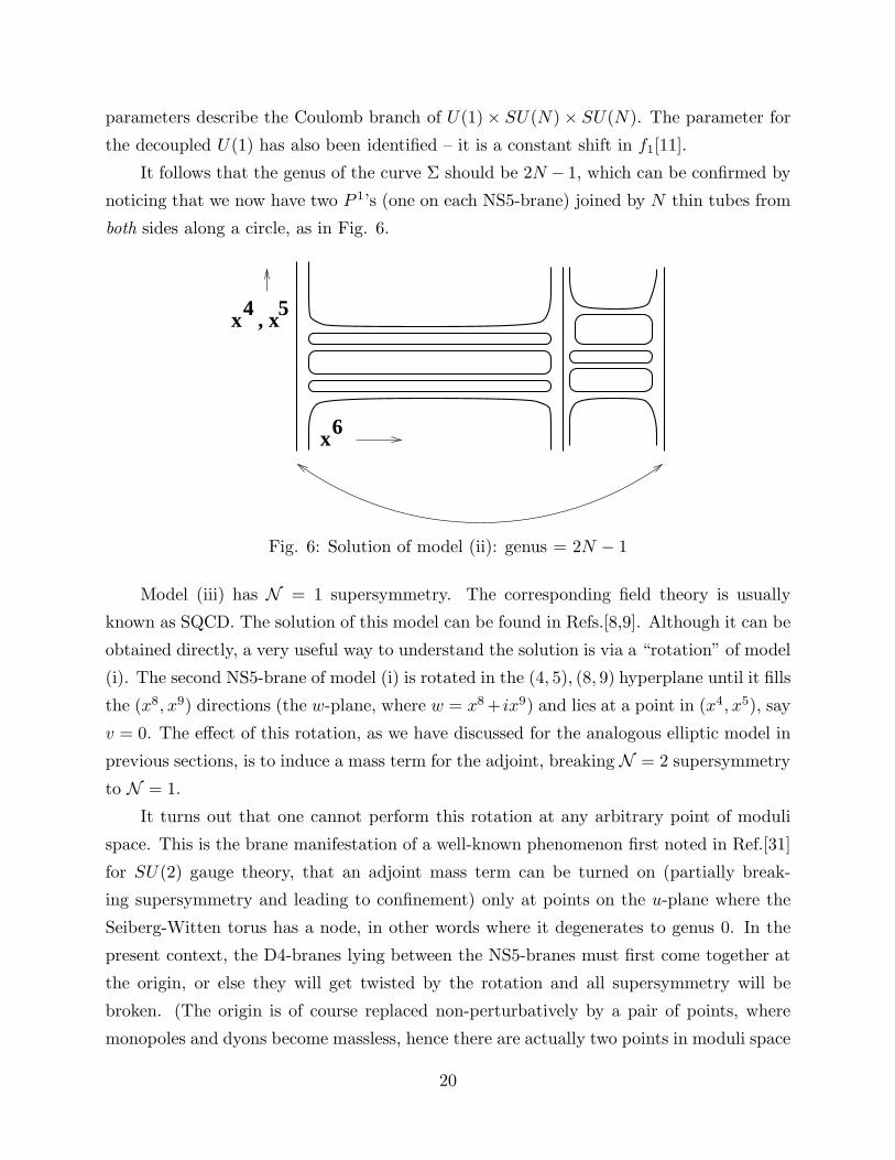
parameters describe the Coulomb branch of U(1) × SU(N) × SU(N). The parameter for

the decoupled U(1) has also been identified – it is a constant shift in f1[11].

It follows that the genus of the curve Σ should be 2N − 1, which can be confirmed by

noticing that we now have two P 1’s (one on each NS5-brane) joined by N thin tubes from

both sides along a circle, as in Fig. 6.

x6

x , x 54

Fig. 6: Solution of model (ii): genus = 2N − 1

Model (iii) has N = 1 supersymmetry. The corresponding field theory is usually

known as SQCD. The solution of this model can be found in Refs.[8,9]. Although it can be

obtained directly, a very useful way to understand the solution is via a “rotation” of model

(i). The second NS5-brane of model (i) is rotated in the (4, 5), (8, 9) hyperplane until it fills

the (x8, x9) directions (the w-plane, where w = x8 + ix9) and lies at a point in (x4, x5), say

v = 0. The effect of this rotation, as we have discussed for the analogous elliptic model in

previous sections, is to induce a mass term for the adjoint, breaking N = 2 supersymmetry

to N = 1.

It turns out that one cannot perform this rotation at any arbitrary point of moduli

space. This is the brane manifestation of a well-known phenomenon first noted in Ref.[31]

for SU(2) gauge theory, that an adjoint mass term can be turned on (partially break-

ing supersymmetry and leading to confinement) only at points on the u-plane where the

Seiberg-Witten torus has a node, in other words where it degenerates to genus 0. In the

present context, the D4-branes lying between the NS5-branes must first come together at

the origin, or else they will get twisted by the rotation and all supersymmetry will be

broken. (The origin is of course replaced non-perturbatively by a pair of points, where

monopoles and dyons become massless, hence there are actually two points in moduli space

20

where rotation is allowed.) In short, rotation of an NS5-brane breaking N = 2 to N = 1

is possible only when the curve Σ has degenerated to genus 0.

The resulting model, in the M-theory limit, is described by an M5-brane wrapped

over R4 × Σ where again R4 is spanned by (x0, x1, x2, x3) but this time Σ is a certain

complex curve holomorphically embedded in R4 × T 2. Thus in the N = 1 models, the

curve is a holomorphic embedding in a non-compact complex Calabi-Yau 3-fold rather

than a complex surface (2-fold) as was the case for N = 2.

The 3-fold is parametrised by the complex coordinates v, w (for the R4 part which is

made up of the (4, 5) and (8, 9) directions) and (x, y) which describe the 2-torus T 2. The

fact that Σ in this model has genus 0 is evident both from the simple fact that the Coulomb

branch has disappeared, and from the brane construction in which the two P 1’s (one in

each 5-brane) are connected by a single “tube” consisting of all the 4-branes bunched

together. The situation is depicted in Fig. 7.

x8 x9,

x , x4 5

x60

Fig. 7: Solution of model (iii): genus = 0

Now let us come to model (iv), the one which is the main subject of this paper. We

can try to see it as a rotation of model (ii). Indeed, this rotation is just the relevant

perturbation which in geometric language takes D3-branes transverse to ALE×R2 to D3-

branes at a conifold. Let us ask now what is the condition for the model (ii) to admit a

rotation breaking N = 2 supersymmetry to N = 1. In this case it is easy to see that the

Seiberg-Witten curve only has to degenerate to genus 1 to permit the rotation. However,

there is another constraint, that the hypermultiplet mass parameter must also go to zero.

This is shown as follows.

Geometrically, in order to rotate one 5-brane we need that the 4-branes connecting

the 5-branes (from both sides) coalesce completely. This correponds to going to the origin

of the Coulomb branch for the SU(N) × SU(N) part of the gauge group (this collapses

21

each of the two bunches of 4-branes), and also making the single hypermultiplet mass

parameter zero (this makes the two bunches of 4-branes coincide where they touch the

5-branes). This process freezes altogether 2N − 1 parameters, leaving only the constant

shift in f1. as a result, the curve Σ relevant to this model has genus 1.

This is of course confirmed by the fact that the Coulomb branch of this model just

corresponds to the free decoupled U(1). Moreover, geometrically, we have again N D4-

branes joining the NS5-branes from both sides, as in model (ii), but now that they are all

collapsed, there is only a single tube connecting a pair of P 1’s from both sides, with the

result again that the genus is equal to 1.

Now we can ask, in the spirit of Refs.[11,8,9], what is the description of the genus

1 curve Σ on which the M 5-brane is wrapped. The answer is rather remarkable and is

related to a phenomenon recently discussed by Dorey and Tong in Ref.[32]5. The situation

considered in Ref.[32] is a pair of NS5-branes with some D4-branes stretched between them,

and with additional semi-infinite 4-branes on either side. The particular configuration of

interest arises when some of D4-branes “line up” on opposite sides of the NS5-brane (Fig.

8).

x6

4 5x , x

0

Fig. 8: 4-branes “lined up” across a 5-brane

One can ask what describes the M-theory limit of this configuration, which correponds

to special regions of moduli space. The answer turns out to be that while the NS5-brane

turns into an M5-brane as usual, the D4-branes that are lined up on opposite sides of it

turn into M5-branes that go through it. In other words, in the M-theory limit, the charge

carried by the type IIA D4-branes does not flow onto the 5-brane on which they end from

both sides, but goes right through. The situation is illustrated in Fig. 9.

5 We are grateful to David Tong for explaining these results to us before publication.

22

x6

4 5x , x

0

Fig. 9: Cylindrical M5-branes going through transverse M5-branes

In our model, called model (iv) above, this situation is indeed realised. As explained

above, in order to allow rotation of an NS5-brane and break supersymmetry from N = 2

to N = 1, the D4-branes of model (ii) must all collect at the origin. Hence by the above

argument, in the M-theory limit we will have a bunch of N coincident toroidal M5-branes

wrapped on the (x6, x10), going through a pair of M5-branes: one aligned in the (x4, x5)

direction and the other rotated in the (x4, x5), (x8, x9) hyperplane (Fig. 10).

x , x4

x0

5

6

Fig. 10: Solution of model (iv): genus = 1

This can be seen starting from the M-theory curve for model (ii). Recall that this

model is described by Eq.(6.3), specified by a set of N complex meromorphic functions

fi(x, y) on the (x6, x10) torus. We want to consider the special point in moduli space where

we are at the origin of the Coulomb branch and the hypermultiplet mass parameter is zero.

From the discussion above, it follows that f1(x, y) = 0 (the constant part is zero since the

centre-of-mass U(1) parameter is fixed at the origin, and the residue vanishes because the

hypermultiplet mass is zero). Similarly, since the constant and residue parts of the other

23

fi(x, y) describe the VEV’s associated to going to the Coulomb branch of the two SU(N)

factors of the gauge group (before rotation), to go to the origin of the Coulomb branch

these must also be set to zero, as a result of which all the fi’s vanish identically. Hence

we get the curve

vN = 0 (6.4)

corresponding to N coincident M5-branes wrapped on the (x6, x10) torus. After rotation,

the curve is no longer given by a single equation in R2×T 2 but rather by two equations in

R4 × T 2. By the symmetry that was present between the two NS5-branes before rotation,

the equations must be

vN = 0

wN = 0(6.5)

where w labels the coordinate on the rotated brane. If the rotation is by 90 degrees then

w = x8 + ix9, otherwise it is a suitable linear combination of the (x4, x5) and (x8, x9)

coordinates.

These equations precisely describe the N toroidal branes, which are located at the

origin of the v and w planes. One has to supplement these by hand with the requirement

that the transverse planar branes are still present, at two points p1, p2 on the (x6, x10)

torus. Hence the M-theory limit has three separate and disconnected 5-brane components,

two of which are the original NS and NS’ 5-branes and the third is the torus which has N

coincident M5-branes wrapped on it, described by Eq.(6.5).

The above description has important implications for the global symmetries and other

properties of the model, as we will now see.

7. Global Symmetries and Moduli

The fact that the stretched branes are decoupled from the transverse ones makes it

clear that rotations of the v-plane and w-plane can be carried out independently of each

other and of shifts in the x6 and x10 directions. This is in contrast to model (iii), where the

the v and w-plane rotations and the rotation along x10 were linked together into a single

U(1) symmetry by the constraint that all the branes merge into a genus-0 curve[9]. We will

identify some of these transformations as factors of the global SU(2)× SU(2) symmetries

associated to the conifold and discussed at length in Ref.[1], and another one as the U(1)

R-symmetry.

24

As we already briefly pointed out, the U(1)’s rotating the v and w planes will act on

the chiral multiplets coming from “short strings” connecting the 4-branes across a 5-brane.

Across the first 5-brane, we will get a pair of chiral fields, one in the (N,N) representation

of the gauge group and the other in the (N,N). Let us label these as A1 and B2. Similarly

the chiral fields arising across the second 5-brane are B1, A2, transforming in the (N,N)

and (N,N) representation respectively.

Now rotation of the 4, 5 plane by an angle α induces a transformation on the chiral

fields as follows. The short strings living on the D4-brane would give rise to an N = 4

multiplet if no NS5-branes were present. The NS5-branes break this to a hypermultiplet.

From the geometry of the problem, it is clear that this hypermultiplet is the one which

parametrised motion of the 4-brane in the (x4, x5, x8, x9) directions. It decomposes after

breaking to N = 1 (which is induced by a different NS5-brane located some distance away)

into the two chiral multiplets A1 and B2, hence these two fields can be thought of as being

associated to the (x4, x5) and (x8, x9) directions respectively. It follows that under rotation

of the (x4, x5) plane by an angle α, A1 picks up a phase eiα while B2 is unchanged. On the

NS5’-brane, the situation is reversed. There the chiral multiplets are B1 and A2, but this

brane is also rotated at 90 degrees to the previous one, hence we find that A2 is charged

under (x4, x5) rotations. Moreover, because A2 comes from a “left-pointing” short string

(this is clear since it is an (N,N) of the gauge group), it picks up a phase e−iα under this

rotation.

Combining, we find that under rotations of the (x4, x5) plane, the chiral fields trans-

form as

A1 → eiαA1, A2 → e−iαA2, B1 → B1, B2 → B2 (7.1)

This shows that these rotations define the U(1) Cartan subalgebra of the global SU(2)

that is expected in this field theory. This in turn lends support to our earlier observation

that SU(2) arises by “enhancement” of this U(1) rotation, if the (x4, x5) directions are

compactified on a round 2-sphere.

Similar considerations can be used to show that rotations of the (x8, x9) plane generate

a U(1) lying in the second SU(2).

Finally, a shift along x6 generates an identical phase on all the chiral fields.

A1 → eiγA1, A2 → eiγA2, B1 → eiγB1, B2 → eiγB2 (7.2)

25

This must therefore be the U(1) R-symmetry of the theory. Notice that we have already

identified x6 with the conifold coordinate that is usually called ψ, whose shift precisely

generates the R-symmetry.

Next, let us consider the discrete symmetries. According to Ref.[1], there is supposed

to be a global Z2 symmetry that acts on the conifold as z4 → −z4 and, in field theory

language, exchanges the two SU(N) factors in the gauge group. Hence it also exchanges

the chiral fields Ai and Bi. This symmetry emerges very neatly from our construction.

Recall that in the beginning of the argument, we had treated the conifold as a fibration of

ALE spaces over a base, which was chosen to be parametrised by z4. The result of various

dualities gave a pair of intersecting NS5-branes where the base z4 was equal to the sum

and difference of the brane coordinates. Thus, inversion of z4 is nothing but exchange

of the two NS5-branes. This obviously exchanges the factors of the gauge group and the

chiral multiplets associated to each 5-brane.

Another interesting discrete symmetry is the element w of the centre of SL(2,Z) in

the type IIB description:

w =

(−1 00 −1

)(7.3)

This was argued in Ref.[1] to exchange the two factors of the gauge group, while not

exchanging Ai and Bi, but instead exchanging the fundamental representation N of the

first SU(N) with the anti-fundamental N of the second, and vice-versa. In our picture

this symmetry is just the geometrical inversion of both the torus directions:

x6 → −x6, x10 → −x10 (7.4)

which clearly performs the required tasks.

Finally, we turn to the moduli. The M-theory solution of our model has a set of N

M5-branes wrapped on a 2-torus parametrised by x6, x10. We will now examine this point

more closely. As is well-known, type IIB theory arises from M-theory by compactifying

on a 2-torus and performing T-duality along one of the cycles. In the present case, x6

is precisely the direction along which we performed T-duality to obtain our model from

its type IIB description as 3-branes at a conifold. Hence this torus holds the key to

understanding the relation to type IIB.

26

In the type IIA theory, the two NS5-branes are located at definite values of x6, which

we may call 0 and a. The gauge coupling constants g1 and g2 of the two SU(N) factors

are then determined, by standard arguments[11] to be:

1

(g1)2=R6 − a

gst

1

(g2)2=

a

gst

(7.5)

This can be recast in a useful form as

1

(g1)2+

1

(g2)2=R6

gst

1

(g1)2− 1

(g2)2=R6 − 2a

gst

(7.6)

It follows that the difference in couplings is determined by a, the brane separation, while

the sum of the couplings is determined only by the string coupling gst (for fixed R6).

In the M-theory limit, the two planar M5-branes are located at definite points on the

(x6, x10) torus. Hence we have two complex parameters. One of these generalises a, and we

will call it φ, while the other generalises 1

gst

and is in fact the complex structure parameter

of the 2-torus, which in IIB becomes the dilaton-axion parameter τIIB . At the same time

on the field theory side, g1 and g2 are part of complex parameters (by incorporating the

θ-angles) which we will call τY M1

and τY M2

. The obvious holomorphic generalization of the

above equations to the M-theory limit is:

τY M1 + τY M

2 ∼ τIIB

τY M1 − τY M

2 ∼ φτIIB

(7.7)

It follows that the sum of the gauge theory parameters is determined by the (complex) type

IIB string coupling, while the difference is determined by φ. This is identical to relations

derived in Sec.3 of Ref.[1] (where they were derived using very different reasoning) if we

make the identification:

φ = 2

∫

S2

(BNS + iBRR) − 1 (7.8)

where the S2 is one of the factors in the conifold base S2 × S3. Here, BNS and BRR are

the two 2-form fields in the type IIB theory, and their appearance in this context is related

to considerations in Ref.[33].

27

This remarkable agreement moreover clarifies the meaning of the x6 separation be-

tween the branes in conifold language, as was promised in Sec. 5 when we allowed constant

B-fluxes in the (4, 5, 8, 9) directions. Indeed, we now see the more general result that φ,

the complex distance between the two planar 5-branes, is determined by the value of the

NS-NS and RR B-fields in the dual type IIB theory. Its real part∫

S2 BNS is the separation

in x6. Apparently∫BNS = 1

2corresponds to 5-branes located symmetrically at opposite

points of the 2-torus, hence identical couplings and theta angles in the two gauge factors.

In the type IIA description, BNS remains a 2-form while BRR turns into the RR

3-form with one index along the 6 direction (we T-dualised along a direction orthogonal

to the S2, namely x6). In the M-theory limit, BNS also becomes the M-theory 3-form,

with one index in the “10” direction. So finally, in the M-theory picture there are two

constant 3-form backgrounds, with the 3-form having one index in a toroidal direction and

the other two indices outside. This is of course the familiar way in which the two B-fields

of type IIB originate from M-theory.

Acknowledgements: We are especially grateful to Angel Uranga for detailed discussions

and for sharing the results of Ref.[12] before publication, and to Shishir Sinha for intensive

discussions on aspects of this work. We are also happy to acknowledge useful conversations

with Gottfried Curio, Atish Dabholkar, Debashis Ghoshal, Steve Gubser, Dileep Jatkar,

Albion Lawrence, Shiraz Minwalla, Matt Strassler, David Tong, Cumrun Vafa and Edward

Witten. The work of K.D. was supported in part by DOE grant No. DE-FG02-90ER40542.

S.M. acknowledges financial support and hospitality from Andy Strominger and the Physics

Department at Harvard University, where part of this work was performed.

28

References

[1] I. Klebanov and E. Witten, “Superconformal Field Theory on Threebranes at a Calabi-

Yau Singularity”, (1998); hep-th/9807080.

[2] J. Maldacena, “The Large N Limit of Superconformal Field Theories and Supergrav-

ity”, Adv. Theor. Math. Phys. 2 (1998) 231; hep-th/9711200.

[3] S. S. Gubser, “Einstein Manifolds and Conformal Field Theories”, (1998); hep-

th/9807164.

[4] S. S. Gubser and I. R. Klebanov, “Baryons and Domain Walls in an N = 1 Super-

conformal Gauge Theory”, (1998); hep-th/9808075.

[5] A. Hanany and E. Witten, “Type IIB Superstrings, BPS Monopoles, and Three-

Dimensional Gauge Dynamics”, Nucl. Phys. B492 (1997) 152; hep-th/9611230.

[6] M. Bershadsky, V. Sadov and C. Vafa, “D-strings on D-manifolds”, Nucl. Phys. B463

(1996) 398; hep-th/9510225.

[7] A. Strominger, “Massless Black Holes and Conifolds in String Theory”, Nucl. Phys.

B451 (1995) 96; hep-th/9504090.

[8] K. Hori, H. Ooguri and Y. Oz, “Strong Coupling Dynamics of Four-dimensional N = 1

Gauge Theories from M-theory Fivebranes”, Adv. Theor. Math. Phys. 1 (1997) 1; hep-

th/9706082.

[9] E. Witten, “Branes and the Dynamics of QCD”, Nucl. Phys. B507 (1997) 658; hep-

th/9706109.

[10] A. Brandhuber, N. Itzhaki, V. Kaplunovsky, J. Sonnenschein and S. Yankielow-

icz, “Comments on the M Theory Approach to N=1 SQCD and Brane Dynamics”,

Phys.Lett. B410 (1997) 27; hep-th/9706127.

[11] E. Witten, “Solutions of Four Dimensional Field Theories via M-Theory, Nucl. Phys.

B500 (1997) 3; hep-th/9703166.

[12] A. Uranga, “Branes configurations for Branes at Conifolds”, (1998); hep-th/9811004.

[13] B.S. Acharya, J.M. Figueroa-O’Farrill, C.M. Hull and B. Spence, “Branes at Conical

Singularities and Holography”, hep-th/9808014.

[14] D. Morrison and R. Plesser, “Non- Spherical Horizons-I” , (1998); hep-th/9810201.

[15] A. Hanany and A. Zaffaroni, “On The Realisation of Chiral Four Dimensional Gauge

Theories using Branes”, JHEP 05 (1998) 001; hep-th/9801134.

[16] A. Hanany and A. Uranga, “Brane boxes and Branes on Singularities”, JHEP 05

(1998) 013; hep-th/9805139.

[17] O. Aharony and A. Hanany, “Branes, Superpotentials and Superconformal Fixed

Points”, Nucl. Phys. B504 (1997) 239; hep-th/9704170.

[18] J. P. Gauntlett, G. W. Gibbons, G. Papadopoulos and P.K. Townsend, “Hyperkahler

Manifolds and Multiply Intersecting Branes”, Nucl. Phys. B500 (1997) 133; hep-

th/9702202.

29

[19] N. C. Leung and C. Vafa, “Branes and Toric Geometry” , Adv. Theor. Math. Phys.

2 (1998) 91; hep-th/9711013.

[20] B. Andreas, G. Curio and D. Lust, “The Neveu-Schwarz Five Brane and its dual

Geometries”, hep-th/9807008.

[21] A.A. Tseytlin, “Harmonic Superpositions of M-branes”, Nucl. Phys. B475 (1996) 149;

hep-th/9604035.

[22] A.A. Tseytlin, “Composite BPS Configurations of p-branes in Ten Dimensions and

Eleven Dimensions”, Class. Quant. Grav. 14 (1997) 2085; hep-th/9702163.

[23] J. P. Gauntlett, “Intersecting Branes”, hep-th/9705011.

[24] E. Bergshoeff, C. Hull and T. Ortin, “ Duality in the Type II Superstring Effective

Action”, Nucl. Phys. B451 (1995) 547; hep-th/9504081.

[25] A. Kehagias, “New Type IIB Vacua and Their F-theory Interpretation”, Phys. Lett.

B435 (1998) 337; hep-th/9805131.

[26] O. Aharony, A. Fayyazuddin and J. Maldacena, “The Large-N Limit of N = 2, N = 1

Field Theories from Threebranes in F-theory”, JHEP 07 (1998) 013; hep-th/9806159.

[27] P. Candelas and X. C. de la Ossa, “Comments on Conifolds”, Nucl. Phys. B342 (1990)

246.

[28] G. Papadopoulos and A. Teschendorff, “Multiangle Five-brane Intersections”, hep-

th/9806191;

G. Papadopoulos and A. Teschendorff, “Grassmannians, Calibrations and Five-brane

Intersections”, hep-th/9811034.

[29] Work in progress.

[30] R. Donagi and E. Witten, “Supersymmetric Yang-Mills Theory and Integrable Sys-

tems”, Nucl. Phys. B460 (1996) 296; hep-th/9510101.

[31] N. Seiberg and E.Witten, “Electric-Magnetic duality, Monopole Condensation and

Confinement in N = 2 Supersymmetric Yang- Mills Theory”, Nucl. Phys. B426

(1994) 19; hep-th/9407087.

[32] N. Dorey and D. Tong, “The BPS Spectra of Gauge Theories in Two and Four Di-

mensions”, to appear.

[33] A. Lawrence, N. Nekrasov and C. Vafa, “On Conformal Field Theories in Four Di-

mensions”, Nucl. Phys. B533 (1998) 199; hep-th/9803015.

30