arX

iv:1

311.

6798

v1 [

astr

o-ph

.CO

] 2

6 N

ov 2

013

New exact cosmologies on the brane

Artyom V. Astashenok1 and Artyom V. Yurov1,

Sergey V. Chervon1,2 and Evgeniy V. Shabanov2,

M. Sami31I. Kant Baltic Federal University, Kaliningrad 236041, Russia

2Ilya Ulyanov State Pedagogical University, Ulyanovsk 432700, Russia3Centre of Theoretical Physics, Jamia Millia Islamia, New Delhi 110025, India

We develop a method for constructing exact cosmological solutions in brane world cosmology. Newclasses of cosmological solutions on Randall – Sandrum brane are obtained. The superpotential andHubble parameter are represented in quadratures. These solutions have inflationary phases undergeneral assumptions and also describe an exit from the inflationary phase without a fine tuning ofthe parameters. Another class solutions can describe the current phase of accelerated expansionwith or without possible exit from it.

I. INTRODUCTION

Brane world scenario have been proposed more then decade ago and this scenario attracted many attention. Thereason of such attention includes the hope to describe observed accelerated expansion of the Universe.To our knowledge the work by Binetrruy, Deffaet and Langlois [1] was the first work where brane cosmology,

different from standard Friedmann cosmology, have been proposed. It is interesting to mention that in the first workon brane cosmology at once it was much attention to searching of exact solutions. This situation is a diametricallyopposite to that in cosmological inflation theory where about a decade approximated solution have been under studytill the works [2, 3]. Further development of the brane cosmology scenarios was performed in works [4–8] where fewexact solutions have been found. In in the work [9] it was shown the relation between exact solutions in [7, 8] and[4, 5]. Namely it was given the explicit coordinate transformation which proved the equivalence between this twosolutions,i.e. both solutions represent the same spacetime in different coordinate systems.In consideration of inflation scenario in brane cosmology it is important to analyze scalar field solutions with

self-interacting potential. There are number of works devoted to this issue. We will mention few of them whereinvestigation of exact solutions was carried out. In the article [10] it was found exact solution at high energy limitwhen H2 proportional to ρ2; canonical and tachyon fields were analyzed there. A general thick brane with a scalarfield was analysed in the work [11], where restrictions on the scalar potential was obtained and exact solutions forstepwise potentials of different shapes was found. A general scalar field and barotropic fluid during the early stageof a brane-world where the Friedmann constraint is dominated by the square of the energy density was studied inthe work [12]. In this article we present the method of exact solution construction and new classes of exact solutionsobtained by superpotential method (see [13] and literature cited therein). Fist application of this method for Randal– Sandrum brane cosmology was perfomed in the work [25].The article is organized as follow. In section II we present the model and method of exact solution construction for

it. Section III devoted to solutions obtained for given superpotential. In section IV we present new exact solutionsbased on given evolution of the scalar field. In section V we discuss viable cosmological models obtained in the article.

II. COSMOLOGICAL MODELS ON THE FRW BRANE: METHODS OF SOLUTIONS CONSTRUCTION

As an alternative to the FRW cosmology let us consider the simplest brane model in which spacetime is homogeneousand isotropic along three spatial dimensions, being our 4-dimensional universe an infinitesimally thin wall, withconstant spatial curvature, embedded in a 5-dimensional spacetime ([15],[16]). In the Gaussian normal coordinatesystem, for the brane which is located at y = 0, one gets

ds2 = −n2dt2 + a2(t, y)γijdxidxj + dy2, (1)

where γij is the maximally 3-dimensional metric. Let t be the proper time on the brane (y = 0), then n(t, 0) = 1.Therefore, one gets the FRW metric on the brane

ds2|y=0 = −dt2 + a2(t, 0)γijdxidxj . (2)

The 5-dimensional Einstein equations have the form

RAB − 1

2gABR = χ2TAB + Λ4gAB, (3)

2

where Λ4 is the bulk cosmological constant, χ2 = 8πG(5)/c4, G(5) is the gravitational constant in 5-dimensionalspacetime. The next step is to write the total energy momentum tensor TAB on the brane as

TAB = SA

Bδ(y), (4)

with SAB = diag(−ρb, pb, pb, pb, 0), where ρb and pb are the total brane energy density and pressure, respectively.

One can now calculate the components of the 5-dimensional Einstein tensor which solve Einstein’s equations. Oneof the crucial issues here is to use appropriate junction conditions near y = 0. These reduce to the following tworelations:

dn

ndy |y=0+

=χ2

3ρb +

χ2

2pb,

da

ady |y=0+

= −χ2

6ρb. (5)

After some calculations, one obtains the following result

H2 = χ4 ρ2b

36+

Λ4

6− k

a2+

Ea4

. (6)

This expression is valid on the brane only. Here H = a(t, 0)/a(t, 0) and E is an arbitrary integration constant. Theenergy conservation equation is correct, too,

ρb + 3a

a(ρb + pb) = 0. (7)

Now, let ρb = ρ+ λb, where λb is the brane tension. Further we consider the fine-tuned brane with Λ4 = λ2bχ

4/6 andthe case of flat spacetime (k = 0):

a2

a2=

λχ4

6

ρ

3

(

1 +ρ

2λb

)

+Ea4

. (8)

In what follows we will consider a single brane model which mimics GR at present but differs from it at late times.We set M−2

p = 8πG = σχ4/6. For simplicity, we set E = 0 (the term with E is usually called “dark radiation”). Infact, setting E 6= 0 does not lead to additional solutions on a radically new basis, in the framework of our approach.Eq. (8) can be simplified to

a2

a2=

ρ

3M2p

(

1 +ρ

2λb

)

. (9)

One can see that Eq. (9), for ρ << |λb|, differs insignificantly from the FRW equation. The brane model with apositive tension has been discussed in [17],[18],[19] in the context of the unification of early- and late-time accelerationeras. The braneworld model with a negative tension and a time-like extra dimension can be regarded as being dualto the Randall-Sundrum model ([20],[21],[22]). Note that, for this model, the Big Bang singularity is absent. Andthis fact does not depend upon whether or not matter violates the energy conditions ([23]). This same scenario hasalso been used to construct cyclic models for the universe [24].One can assume that in our epoch the ρ/2λ << 1 and so there is no significant difference between the brane model

and FRW cosmology. But the universe evolution in the future or in past, for brane cosmology, can in fact differ fromsuch convenient cosmology, due to the non-linear dependence of the expansion rate on the energy density.One can reduce the field equation to the slow-roll form

3HU = −W ′φ, (10)

with substitution

W = V +1

2U2, U(φ) = φ (11)

Then Friedmann equation (9) one can write down in terms of the superpotential W

H2 =1

3M2p

W

(

1 +W

2λb

)

. (12)

Considering H as positive and inserting (12) into (10) one can obtain

3

√3

MpU(φ)

√

W

(

1 +W

2λb

)

= −W ′φ. (13)

This is the key equation for further progress. For givenW (φ) as function of scalar field one can define the dependenceof scalar field from time inversing the following relation:

t− t0 = −√3

Mp

∫

dφ

W ′φ

√

W

(

1 +W

2λb

)

(14)

In frames of this approach the physical potential is

V (φ) = W (φ)−M2

p

6W ′2

φ

(

W (φ)

(

1 +W (φ)

2λb

))−1

(15)

One can also define U(φ) as function of scalar field. In this case the integration (13) via separation of W and φleads to the superpotential and Hubble parameter presentation in quadratures

√W =

√

2λb sinh

(

−√

3

2λb

1

2MP

∫

U(φ)dφ

)

, W > 0, (16)

√−W =

√

2λb cosh

(

−√

3

2λb

1

2MP

∫

U(φ)dφ

)

, W < 0, (17)

H =

√

λb

6

1

MPsinh

(

−√

3

2λb

1

MP

∫

U(φ)dφ

)

(18)

Note that the argument in (18) should be positive. Therefore∫

U(φ)dφ should be always negative.The physical potential V can be obtained from the superpotential definition (11)

V (φ) = 2λb sinh2

(

−√

3

2λb

1

2MP

∫

U(φ)dφ

)

− 1

2U(φ)2. (19)

Thus to obtain the examples of exact solutions one can suggest the functional dependence a scalar field φ on cosmictime t and evaluate the integral

∫

U(φ)dφ:

∫

U(φ)dφ =

∫

U2(t)dt.

Standard calculation leads to the following formula for N(φ):

N(φ) = −√

λb

2M−2

P

∫

√

W

(

1 +W

2λb

)

√

(

W

λb+ 1

)2

+ 1dφ

W ′(20)

To understand the period with accelerating Universe expansion let us calculate aa = H +H2. For given W (φ) we

have the following simple relation for acceleration parameter:

a

a= −1

6

W ′2φ

W+

W

3M2P

+W

6λb

(

W

M2P

− 1

2

W ′2φ

W (1 +W/2λb)

)

(21)

The first two terms corresponds to the case of usual FRW cosmology. The last appears due to the brane tension.Combining (21) with (14) one can analyze the behavior a/a as function of time.If we define the function U(φ) it is convenient to use the result

a

a= − U2

2M2P

cosh

(

−√

3

2λb

1

MP

∫

U(φ)dφ

)

+λb

6M2P

sinh2

(

−√

3

2λb

1

MP

∫

U(φ)dφ

)

(22)

4

To investigate changing of the acceleration sign let us represent (22) in the following form

6M2P

λb

a

a= Z2 − 3U2

λbZ − 1, Z = cosh

(

−√

3

2λb

1

MP

∫

U(φ)dφ

)

(23)

Taking into account that Z > 1 we omit the the root

Z2 =3U2

2λb−√

9U4

4λ2b

+ 1 (24)

as it is less then unity. For the next root

Z1 =3U2

2λb+

√

9U4

4λ2b

+ 1 (25)

it is easy to check that Z1 > 1 for any value of U2. Therefore we can imply that there is only one point during theevolution when deceleration have been changed to acceleration. So in the framework of scalar field cosmology on thebrane we have only one inflationary period. If it is early inflation then once again as in FRW cosmology we need tosolve the problem of exit from inflation (for example using generation of the particle after inflation ends). On theother hand, if it is later inflation, we may suggest existence one more additional specie at the early stage of Universeevolution which will be responsible for early inflation.

III. SOLUTIONS WITH GIVEN W (φ)

Let’s consider two simple superpotentials. The first case is

W =m2φ2

2(26)

One can easy derive the dependence t(φ). The result is

t− t0 = −√6λb

2m2M−1

P

arcsinh

(

mφ

2√λb

)

+mφ

2√λb

√

1 +m2φ2

4λb

For simplicity we put φ(t0) = 0. At t → ∞ scalar field φ → −∞. One can consider the moment t < t0 for thismoment φ > 0. The universe acceleration is

a

a= −m2

12+

m2φ2

6M2P

+m2φ2

12λb

(

m2φ2

2M2P

− 1

2

m2

1 +m2φ2/4λb

)

(27)

For scale factor as function of scalar field we have

a = a0 exp

(

± φ2

8M2P

(

2 +m2φ2

4λb

))

(28)

One can choose the sign − for t < 0 (i.e. φ > 0) and + for t > 0 (φ < 0). The moment t = −∞ corresponds toBig Bang singularity then universe expands so that a > 0 then non-inflationary phase follows. Then universe againexpands with acceleration. The asymptotic of solution is

a(t) ∼ a0 exp

(

λbm2

2M2P

(t− t0)2

)

. (29)

The potential of scalar field can be obtained from (15):

V (φ) =m2φ2

2− M2

Pm2

3

(

1 +m2φ2

4λb

)−1

. (30)

At t → ∞ this potential corresponds to free scalar field with mass m.

5

For case of φ− 4 superpotential

W (φ) =λφ4

4(31)

we have the following link between time and scalar field:

t− t0 = −√3

2MP

√λ

(

cosh η − cosh η0 + ln tanhη

2− ln tanh

η02

)

, (32)

η = arcsinh

(

(

λ

8λb

)1/2

φ2

)

.

The scalar field at the moment t = t0 is φ0 =(

8λb

λ

)1/4sinh1/2 η0 where η0 is arbitrary constant. At t → ∞ the scalar

field φ → 0. From expression for universe acceleration

a

a= −2λ

3φ2 +

λ

12M2P

φ4 +λ2φ6

24λb

(

1

4M2P

φ2 − 2

1 + λφ4/8λb

)

(33)

one can see that exit from inflation occurs. The scale factor as function of scalar field

a = a0 exp

(

± φ2

8M2P

(

1 +λφ4

24λb

))

(34)

The negative sign corresponds to universe starting from a = 0 (φ = ∞ at t = −∞) and expanding with accelerationprior to some moment of time when exit from inflation occurs.

IV. SOLUTIONS WITH GIVEN φ(t)

To obtain exact solutions we can use the dynamics of the scalar field considered in many works. Let us start fromthe simplest ones.

A. Logarithmic evolution of the scalar field

Let

φ = A ln(λt).

The solutions are

√W =

√

2λb sinh

(

−√

3

2λb

1

2MP

(

C1 −A2

t

))

, W > 0, (35)

√−W =

√

2λb cosh

(

−√

3

2λb

1

2MP

(

C1 −A2

t

))

, W < 0, (36)

H =

√

λb

6

1

MPsinh

(

−√

3

2λb

1

MP

(

C1 −A2

t

))

. (37)

The superpotential’s and physical potential’s presentation in terms of scalar field can be obtained using givendependance φ = A ln(λt).

√W =

√

2λb sinh

(

−√

3

2λb

1

2MP

(

C1 −A2λ exp(−φ/A))

)

, W > 0, (38)

√−W =

√

2λb cosh

(

−√

3

2λb

1

2MP

(

C1 −A2λ exp(−φ/A))

)

, W < 0, (39)

V (φ) = 2λb sinh2

(

−√

3

2λb

1

2MP

(

C1 −A2λ exp(−φ/A))

)

− A2λ2

2e−2φ/A. (40)

6

U(φ)

φ

Figure 1: The potential of scalar field for logarithmic evolution of scalar field.

The potential V (φ) is depicted on Fig. 1. Thus we have obtained the exact formulas for given evolution of thescalar field. We know that for solutions under consideration we may have only one inflection point for scalar factor aassociated with the equation (25). Using the definition for Z (23) one can obtain the equation for time correspondingto inflection point:

3A2

2λbt2+

√

9A4

4λ2bt

4+ 1 = cosh

(√

3

2λb

A2

MP t

)

(41)

It is easy to see that this equation will be true when t → ∞. We can analyze this equation numerically to find thefinite time t < ∞ which will correspond to deceleration changes to acceleration. One can state that this time is about

ti ≈ 0.286λ−1/2b in the units with MP = 1 and for A = 1. Therefore we can use this approximate result to set this

time equal to beginning of (early or later) inflation. From the other hand we can analyze the transition from branecosmology to Friedmann one by tending the brane tension to infinity λb → ∞. The results are:

√

λb → ∞ :√W = −

√3

1

2Mp

(

C1 −A2

t

)

= −√3

1

2Mp

(

C1 −A2λe−φ/A)

, (42)

√−W = ∞, (43)

H = − 1√6Mp

(

√

3

2

1

Mp

(

C1 −A2

t

)

)

, (44)

V (φ) = ∞. (45)

Here we can define the scale factor with power law – exponential behavior

a(t) = exp

(

− C1t

2M2P

)

t2A

2λ2

2M2

P . (46)

We carefully analyzed the solution in this section. To simplify presentation of the next solutions let us represent

7

equations (16)-(19) in the following way

√W =

√

2λb sinh

(

−√

3

2λb

1

2MP[F (φ) + C1]

)

, W > 0, (47)

√−W =

√

2λb cosh

(

−√

3

2λb

1

2MP[F (φ) + C1]

)

, W < 0, (48)

H =

√

λb

6

1

MPsinh

(

−√

3

2λb

1

MP[F (φ(t)) + C1]

)

(49)

V (φ) = 2λb sinh2

(

−√

3

2λb

1

2MP[F (φ) + C1]

)

− 1

2[U(φ)]2. (50)

Using the general formulas (47)-(50) we will display new solutions by putting values for F (φ) and U(φ). Also wewill use general formulas for transition to Friedmann Universe (by setting λb → ∞ ) below

√

λb → ∞ :

√W = −

√3

2Mp(F (φ) + C1) , (51)

√−W = ∞, (52)

H = − 1

2M2p

(F (φ(t)) + C1) , (53)

V (φ) = − 3

4MP(F (φ) + C1)

2 − 1

2[U(φ)]2 (54)

B. Power law evolution

Let

φ = Ats, s 6= 0, s 6= 1/2.

The solutions are represented by functions

F (φ) =A−1/ss2

2s− 1φ2−1/s =

A2s2

2s− 1t2s−1, U2(φ) = A2s2

[

φ

A

]2s−2

s

. (55)

The equation for the time corresponding to inflection point is

3A2s2

2λbt2s−2 +

√

9A4s4

4λbt4s−4 + 1 = cosh

(

−√

3

2λb

A2s2

(2s− 1)MPt2s−1

)

(56)

By tending the brane tension to infinity λb → ∞ we obtain

√

λb → ∞ :

√W = −

√3

2Mp

(

A2s2

2s− 1

[

φ

A

]

2s−1

s

+ C1

)

, (57)

√−W = ∞, (58)

H = − 1√6Mp

(

√

3

2

1

Mp

(

C1 +A2s2

2s− 1t2s−1

s

)

)

, (59)

V (φ) = ∞. (60)

In the case when s = 1/2 we have

8

U(φ)

φ

Figure 2: The potential of scalar field for φ = At1/2.

F (φ) =A2

2ln

φ

A, U2(φ) =

A4

4φ2(61)

The potential of scalar field in this case is depicted on Fig. 2.The equation for the time corresponding to inflection point is

3A2

8tλb+

√

9A4

32t2λ2b

+ 1 =1

2

(

t−B + tB)

, B =

√

3

2λb

A2

4MP(62)

This time is about t ≈ 4.11λ−1/2b in units MP = A = 1. In this moment the deceleration begins.

C. Exponential evolution

Let

φ = Ae−λt.

The solutions represented by functions

F (φ) = −φ2λ

2= −A2λ

2e−2λt, U2(φ) = λ2φ2 (63)

The potential of scalar field is presented on Fig. 3.The equation for the time corresponding to inflection point is

3A2λ2

2λbe−2λt +

√

9A4λ4

4λ2b

e−4λt + 1 = cosh

(√

3

2λb

A2λ

MPe−2λt

)

, (64)

For inflection time we have two different solutions: i) when λ > 0 a → 0 at t → ∞ (and a > 0 at 0 < t < ∞); ii)

when λ = −√λb < 0 a = 0 at t ≈ 0.879λ

−1/2b (Mp = A = 1). At this time acceleration changes to deceleration i.e. we

have the inflation phase during finite time.

9

U(φ)

φ

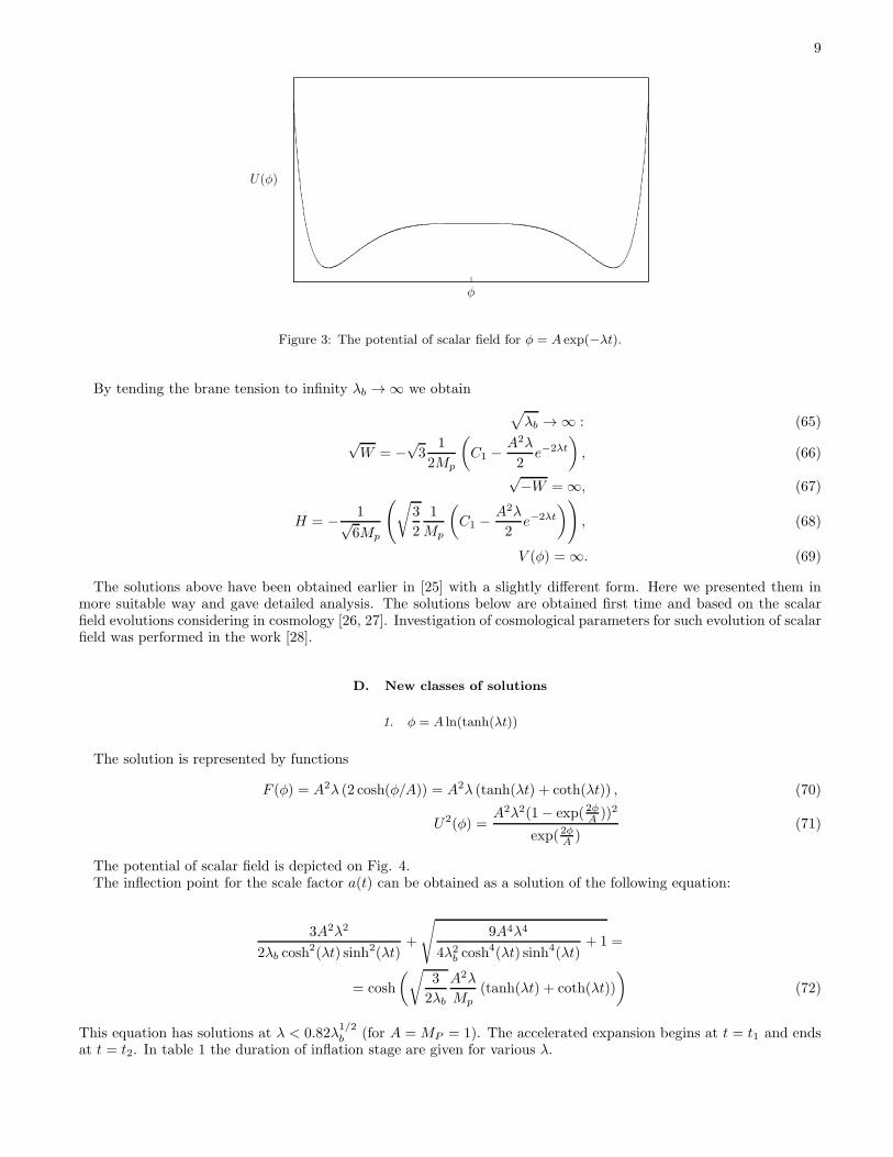
Figure 3: The potential of scalar field for φ = A exp(−λt).

By tending the brane tension to infinity λb → ∞ we obtain

√

λb → ∞ : (65)√W = −

√3

1

2Mp

(

C1 −A2λ

2e−2λt

)

, (66)

√−W = ∞, (67)

H = − 1√6Mp

(

√

3

2

1

Mp

(

C1 −A2λ

2e−2λt

)

)

, (68)

V (φ) = ∞. (69)

The solutions above have been obtained earlier in [25] with a slightly different form. Here we presented them inmore suitable way and gave detailed analysis. The solutions below are obtained first time and based on the scalarfield evolutions considering in cosmology [26, 27]. Investigation of cosmological parameters for such evolution of scalarfield was performed in the work [28].

D. New classes of solutions

1. φ = A ln(tanh(λt))

The solution is represented by functions

F (φ) = A2λ (2 cosh(φ/A)) = A2λ (tanh(λt) + coth(λt)) , (70)

U2(φ) =A2λ2(1− exp(2φA ))2

exp(2φA )(71)

The potential of scalar field is depicted on Fig. 4.The inflection point for the scale factor a(t) can be obtained as a solution of the following equation:

3A2λ2

2λb cosh2(λt) sinh2(λt)

+

√

9A4λ4

4λ2b cosh

4(λt) sinh4(λt)+ 1 =

= cosh

(√

3

2λb

A2λ

Mp(tanh(λt) + coth(λt))

)

(72)

This equation has solutions at λ < 0.82λ1/2b (for A = MP = 1). The accelerated expansion begins at t = t1 and ends

at t = t2. In table 1 the duration of inflation stage are given for various λ.

10

U(φ)

φ

Figure 4: The scalar field potential for φ = A ln(tanh(λt))

λ/λ1/2

0.8 0.38 < tλ1/2b < 0.53

0.6 0.315 < tλ1/2b < 0.382

0.4 0.295 < tλ1/2b < 1.2

0.2 0.286 < tλ1/2b < 2.31

Table I: The duration of accelerated expansion for model φ = A ln(tanh(λt)) for various λ.

2. φ = A ln(tan(λt))

The solution is represented by formulas

F (φ) = A2λ(2 sinh(φ/A)) = A2λ(tan(λt) − cot(λt)), (73)

U2(φ) =A2λ2(1 + exp(2φA ))2

exp(2φA )(74)

On Fig. 5 one can see the dependence of potential from scalar field.

U(φ)

φ

Figure 5: The scalar field potential for φ = A ln(tan(λt))

11

λ/λ1/2

0.6 0.265 < tλ1/2b < 2.355

0.8 0.251 < tλ1/2b < 1.712

1.0 0.239 < tλ1/2b < 1.335

1.2 0.225 < tλ1/2b < 1.083

1.4 0.215 < tλ1/2b < 0.907

Table II: The duration of accelerated expansion for model φ = A ln(tan(λt)) for various λ.

U(φ)

φ

Figure 6: The scalar field potential for φ = A/ sinh(λt)

The time for inflection point can be found as a solution of equation:

3A2λ2

2λb cos2(λt) sin2(λt)

+

√

9A4λ4

4λ2b cos

4(λt) sin4(λt)+ 1 =

= cosh

(√

3

2λb

A2λ

Mp(tan(λt) − cot(λt))

)

(75)

We have the same situation as in previous case. For various values of λ we have two roots corresponding to momentof beginning of inflation and to moment of exit from inflation. In table 2 these results are given for various values ofλ.

3. φ = A/ sinh(λt)

The solution is described by the functions

F (φ) = A2λ coth(λt)1

3

[

φ2

A2− 1

]

= A2λ coth(λt)1

3

[

1

sinh2(λt)− 1

]

, (76)

U2(φ) =λ2

A2φ4

(

1 +

(

A

φ

)2)

(77)

The potential of scalar field is depicted on Fig. 6.The inflection point can be found from corresponding equation

3A2λ2 cosh2(λt)

2λb sinh4(λt)

+

√

9A4λ4 cosh4(λt)

4λ2b sinh

8(λt)+ 1 =

= cosh

(√

3

2λb

A2λ cosh(λt)

3Mp

[

1

sinh2(λt)− 1

])

(78)

12

λ/λ1/2

0.6 0.665 < tλ1/2b < 3.5

0.8 0.545 < tλ1/2b < 2.63

1.0 0.468 < tλ1/2b < 2.11

1.2 0.414 < tλ1/2b < 1.765

1.4 0.374 < tλ1/2b < 1.52

Table III: The duration of accelerated expansion for model φ = A/ sinh(λt) for various λ (A = MP = 1).

U(φ)

φ

Figure 7: The scalar field potential for φ = A arctan(exp(λt))

Once again for various values of λ we have phase of accelerated expansion during finite time. In table 3 one can seeresults for various values of λ.

4. φ = A arctan(exp(λt))

The solution is represented by functions

F (φ) = −A2λ cos2(φ/A)

2= − A2λ

2(1 + exp(2λt), (79)

U2(φ) =A2λ2 tan2( φ

A )

(1 + tan2( φA ))

. (80)

The potential of scalar field is presented on Fig. 7.From the equation

3A2λ2 exp(2λt)

2λb(1 + exp(2λt))2+

√

9A4λ4 exp(4λt)

4λ2b(1 + exp(2λt))4

+ 1 =

= cosh

(√

3

2λb

A2λ

2Mp(1 + exp(2λt))

)

(81)

one can find that for λ > 0 a > 0 (0 < t < ∞) and for λ < 0 we have the moment when deceleration begins. For

example for λ = −λ1/2b we have t ≈ 0.093λ

−1/2b .

5. φ = A sin−1(λt)

The solution is described by formulas

13

U(φ)

φ

Figure 8: The scalar field potential for φ = A sin−1(λt)

F (φ) = A2λ cot(λt)1

3

[

1− 1

sin2(λt)

]

= A2λ cot(λt)1

3

[

1− 1

sin2(λt)

]

, (82)

U2(φ) =λ2

A2φ4

(

1−(

A

φ

)2)

. (83)

On Fig. 8 one can see the potential of scalar field.The inflection point can be found from equation

3A2λ2 cos2(λt)

2λb sin4(λt)

+

√

9A4λ4 cos4(λt)

4λ2b sin

8(λt)+ 1 =

= cosh

(√

3

2λb

A2λ cot(λt)

3Mp

[

1− 1

sin2(λt)

])

. (84)

For λ = λ1/2b we have the phase of accelerated expansion for t > 0.4λ

−1/2b .

V. DISCUSSIONS

In this paper we have discussed a simple method of construction of exact solutions for cosmological equations onRS brane. Despite simplicity, the method allows for acquirement of solutions characterized by interesting properties.These solutions have inflationary phases under quite general assumptions. This is an indication that inflationaryregime seems a common occurrence in cosmology not requiring any special initial conditions. We have the followingcases:(i) accelerated expansion begins at some moment of time and lasts forever (logarithmic evolution of scalar field,

φ ∼ sin−1(λt)). In principle current observed acceleration can be described by this case.(ii) acceleration take place before t < tf when deceleration starts (power and exponential evolution of scalar field

or φ ∼ arctan(exp(λt))). These solutions may correspond to inflation in beginning of cosmological evolution and exitfrom inflation phase.(iii) acceleration occurs during interval ti < t < tf (φ ∼ ln(tanh(λt)), φ ∼ ln(tan(λt)), φ ∼ 1/ sinh(λt)). The

interpretation of such solutions is obvious: we have the possible exit from inflation or current accelerated expansionor initial inflation rolling to later slow inflation (with further exit from it).Therefore these models can not only describe inflation but also describe an exit from the inflationary phase without

a fine tuning of the parameters. This fact can be seen as evidence of the existence of a realistic model that contains

14

an inflationary phase in the early universe stage and a current phase of accelerated expansion.

[1] P. Binetruy, C. Deffayet, D. Langlois, Nucl. Phys. B 565, 269 (2000) [hep-th/9905012].[2] J.D. Barrow, Phys. Lett. B 187, 12 (1987).[3] A.G. Muslimov, Class. Quant. Grav. 7, 231 (1990).[4] P. Binetruy, C. Deffayet, U. Ellwanger, D. Langlois, Phys. Lett. B 477, 285 (2000).[5] S. Mukohyama, Phys. Lett. B 473, 241 (2000).[6] Dan N. Vollick, Class. Quant. Grav. 18, 1 (2001).[7] P. Kraus, JHEP 9912, 011 (1999) [hep-th/9910149].[8] D. Ida, JHEP 0009, 014 (2000).[9] S. Mukohyama, T. Shiromizu, K. Maeda, Phys. Rev. D 62, 024028 (2000); Erratum-ibid. D63, 029901 (2001).

[10] B.C. Paul, D. Paul, [arXiv:0708.0897[hep-th]].[11] K.A. Bronnikov, B.E. Meierovich, Grav. Cosmol. 9, 4, 313 (2003).[12] S. Mizuno, S.-J. Lee, and E.J. Copeland, [astro-ph/0405490].[13] A.V. Yurov, V.A. Yurov, S.V. Chervon, M. Sami, Theor. Math. Phys., 166, 258 (2011).[14] E.J. Copeland, M. Sami and S. Tsujikawa, hep-th/0603057.[15] V. Sahni and Yu. Shtanov, [arXiv:0811.3839[astro-ph]].[16] D. Langlois, Prog. Teor. Phys. Suppl., 148, 181 (2003).[17] E.J. Copeland, A.R. Liddle, and J.E. Lidsey, Phys. Rev. D 64, 023509 (2001).[18] V. Sahni, M. Sami and T. Souradeep, Phys. Rev. D 65, 023518 (2002).[19] M. Sami and V. Sahni, Phys. Rev. D 70, 083513 (2004).[20] Yu. Shtanov and V. Sahni, Phys. Lett. B 557, 1 (2003).[21] L. Randall and R. Sundrum, Phys. Rev. Lett., 83, 3370 (1999).[22] E.J. Copeland, S.-J. Lee, J.E. Lidsey and S. Mizuno, Phys. Rev. D 71, 023526 (2005).[23] A. Ashtekar, T. Pawlowski and P. Singh, Phys. Rev. D 74, 084003 (2006).[24] N. Kanekar, V. Sahni and Yu. Shtanov, Phys. Rev. D 63, 083520 (2001).[25] S.V. Chervon, M. Sami, Electronnyi Zhurnal “Issledovano v Rossii”, http://zhurnal.ape.relarn.ru/articles/2009/088.pdf

088/091009, p. 1151, 2009 [In Russian].[26] J.D. Barrow, Phys.Rev. D 49, 3055 (1994).[27] S.V. Chervon, Gen. Rel. Grav., 36, 1547 (2004).[28] S.V. Chervon, I.V. Fomin, Grav. Cosmol., 14, 163 (2008).