arX

iv:0

809.

1284

v2 [

gr-q

c] 2

5 Se

p 20

08

Thin accretion disks onto brane world black holes

C. S. J. Pun1,∗ Z. Kovacs2,3,† and T. Harko1‡

1Department of Physics and Center for Theoretical and Computational Physics,

The University of Hong Kong, Pok Fu Lam Road, Hong Kong

2Max-Planck-Institut fur Radioastronomie,

Auf dem Hugel 69, 53121 Bonn, Germany and

3Department of Experimental Physics,

University of Szeged, Dom Ter 9, Szeged 6720, Hungary

(Dated: September 25, 2008)

Abstract

The braneworld description of our universe entails a large extra dimension and a fundamental

scale of gravity that might be lower by several orders of magnitude as compared to the Planck scale.

An interesting consequence of the braneworld scenario is in the nature of the vacuum solutions of

the brane gravitational field equations, with properties quite distinct as compared to the standard

black hole solutions of general relativity. One possibility of observationally discriminating between

different types of black holes is the study of the emission properties of the accretion disks. In the

present paper we obtain the energy flux, the emission spectrum and accretion efficiency from the

accretion disks around several classes of static and rotating brane world black holes, and we compare

them to the general relativistic case. Particular signatures can appear in the electromagnetic

spectrum, thus leading to the possibility of directly testing extra-dimensional physical models by

using astrophysical observations of the emission spectra from accretion disks.

PACS numbers: 04.50.+h, 04.20.Jb, 04.20.Cv, 95.35.+d

∗Electronic address: jcspun@hkucc.hku.hk†Electronic address: zkovacs@mpifr-bonn.mpg.de‡Electronic address: harko@hkucc.hku.hk

1

I. INTRODUCTION

The idea, proposed in [1, 2], that our four-dimensional Universe might be a three-brane,

embedded in a five-dimensional space-time (the bulk), has attracted a considerable interest

in the past few years. According to the brane-world scenario, the physical fields (electro-

magnetic, Yang-Mills etc.) in our four-dimensional Universe are confined to the three brane.

These fields are assumed to arise as fluctuations of branes in string theories. Only gravity can

freely propagate in both the brane and bulk space-times, with the gravitational self-couplings

not significantly modified. This model originated from the study of a single 3-brane embed-

ded in five dimensions, with the 5D metric given by ds2 = e−f(y)ηµνdxµdxν + dy2, which,

due to the appearance of the warp factor, could produce a large hierarchy between the scale

of particle physics and gravity. Even if the fifth dimension is uncompactified, standard

4D gravity is reproduced on the brane. Hence this model allows the presence of large, or

even infinite non-compact extra dimensions. Our brane is identified to a domain wall in a

5-dimensional anti-de Sitter space-time. For a review of the brane world models see [3].

The braneworld description of our universe entails a large extra dimension and a funda-

mental scale of gravity that might be lower by several orders of magnitude compared to the

Planck scale [1, 2]. Due to the correction terms coming from the extra dimensions, signifi-

cant deviations from the Einstein theory occur in brane world models at very high energies

[4, 5]. Gravity is largely modified at the electro-weak scale of 1 TeV. The cosmological and

astrophysical implications of the brane world theories have been extensively investigated in

the physical literature [6, 7].

Several classes of spherically symmetric solutions of the static gravitational field equations

in the vacuum on the brane have been obtained in [8, 9, 10, 11]. As a possible physical

application of these solutions the behavior of the angular velocity vtg of the test particles

in stable circular orbits has been considered [9, 10, 11]. The general form of the solution,

together with two constants of integration, uniquely determines the rotational velocity of

the particle. In the limit of large radial distances, and for a particular set of values of

the integration constants the angular velocity tends to a constant value. This behavior is

typical for massive particles (hydrogen clouds) outside galaxies, and is usually explained by

postulating the existence of the dark matter. The exact galactic metric, the dark radiation,

the dark pressure and the lensing in the flat rotation curves region in the brane world scenario

2

has been obtained in [11].

For standard general relativistic spherical compact objects the exterior space-time is

described by the Schwarzschild metric. In the five dimensional brane world models, the high

energy corrections to the energy density, together with the Weyl stresses from bulk gravitons,

imply that on the brane the exterior metric of a static star is no longer the Schwarzschild

metric [12]. The presence of the Weyl stresses also means that the matching conditions do

not have a unique solution on the brane; the knowledge of the five-dimensional Weyl tensor

is needed as a minimum condition for uniqueness.

It is known that the Einstein field equations in five dimensions admit more general spher-

ically symmetric black holes on the brane than four-dimensional general relativity. Hence

an interesting consequence of the braneworld scenario is in the nature of the spherically

symmetric vacuum solutions to the brane gravitational field equations, which could repre-

sent black holes with properties quite distinct as compared to ordinary black holes in four

dimensions. Such black holes are likely to have very diverse cosmological and astrophysi-

cal signatures. Static, spherically symmetric exterior vacuum solutions of the brane world

models have been proposed first in [12] and in [13]. The first of these solutions, obtained in

[12], has the mathematical form of the Reissner-Nordstrom solution of the standard general

relativity, in which a tidal Weyl parameter plays the role of the electric charge of the general

relativistic solution. The solution has been obtained by imposing the null energy condition

on the 3-brane for a bulk having non zero Weyl curvature, and it can be matched to the

interior solution corresponding to a constant density brane world star. A second exterior

solution, which also matches a constant density interior, has been derived in [13].

Two families of analytic solutions of the spherically symmetric vacuum brane world model

equations (with gtt 6= −1/grr), parameterized by the ADM mass and a PPN parameter β

have been obtained in [14]. Non-singular black-hole solutions in the brane world model

have been considered in [15], by relaxing the condition of the zero scalar curvature but

retaining the null energy condition. The four-dimensional Gauss and Codazzi equations for

an arbitrary static spherically symmetric star in a Randall–Sundrum type II brane world

have been completely solved on the brane in [16]. The on-brane boundary can be used to

determine the full 5-dimensional space-time geometry. The procedure can be generalized to

solid objects such as planets.

A method to extend into the bulk asymptotically flat static spherically symmetric brane-

3

world metrics has been proposed in [17]. The exact integration of the field equations along

the fifth coordinate was done by using the multipole (1/r) expansion. The results show that

the shape of the horizon of the brane black hole solutions is very likely a flat “pancake” for

astrophysical sources.

The general solution to the trace of the 4-dimensional Einstein equations for static, spher-

ically symmetric configurations has been used as a basis for finding a general class of black

hole metrics, containing one arbitrary function gtt = A(r), which vanishes at some r = rh > 0

(the horizon radius) in [18]. Under certain reasonable restrictions, black hole metrics are

found, with or without matter. Depending on the boundary conditions the metrics can

be asymptotically flat, or have any other prescribed asymptotic. The exact stationary and

axisymmetric solutions describing charged rotating black holes localized on a 3-brane in the

Randall-Sundrum braneworld were studied in [19]. By taking the metric on the brane to be

of the Kerr-Schild form it can be shown that the Kerr-Newman solution of ordinary general

relativity in which the electric charge is superseded by a tidal charge satisfies a closed system

of the effective gravitational field equations on the brane. The negative tidal charge may

provide a mechanism for spinning up the black hole so that its rotation parameter exceeds

its mass. For a review of the black hole properties and of the lensing in the brane world

models see [20].

It is generally expected that most of the astrophysical objects grow substantially in mass

via accretion. Recent observations suggest that around most of the active galactic nuclei

(AGN’s) or black hole candidates there exist gas clouds surrounding the central compact

object, and an associated accretion disc, on a variety of scales from a tenth of a parsec to a

few hundred parsecs [21]. These clouds are assumed to form a geometrically and optically

thick torus (or warped disc), which absorbs most of the ultraviolet radiation and the soft

X-rays. The gas exists in either the molecular or the atomic phase. The most powerful

evidence for the existence of super massive black holes comes from the very-long baseline

interferometry (VLBI) imaging of molecular H2O masers in the active galaxy NGC 4258

[22]. This imaging, produced by Doppler shift measurements assuming Keplerian motion

of the masering source, has allowed a quite accurate estimation of the central mass, which

has been found to be a 3.6× 107M⊙ super massive dark object, within 0.13 parsecs. Hence,

important astrophysical information can be obtained from the observation of the motion of

the gas streams in the gravitational field of compact objects.

4

The determination of the accretion rate for an astrophysical object can give a strong

evidence for the existence of a surface of the object. A model in which Sgr A*, the 3.7 ×106M⊙ super massive black hole candidate at the Galactic center, may be a compact object

with a thermally emitting surface was considered in [23]. For very compact surfaces within

the photon orbit, the thermal assumption is likely to be a good approximation because

of the large number of rays that are strongly gravitationally lensed back onto the surface.

Given the very low quiescent luminosity of Sgr A* in the near-infrared, the existence of a

hard surface, even in the limit in which the radius approaches the horizon, places a severe

constraint on the steady mass accretion rate onto the source, M ≤ 10−12M⊙ yr−1. This

limit is well below the minimum accretion rate needed to power the observed submillimeter

luminosity of Sgr A*, M ≥ 10−10M⊙ yr.

Thus, from the determination of the accretion rate it follows that Sgr A* does not have a

surface, that is, it must have an event horizon. Therefore the study of the accretion processes

by compact objects is a powerful indicator of their physical nature.

The first comprehensive theory of accretion disks around black holes was constructed in

[24]. This theory was extended to the general relativistic models of the mass accretion onto

rotating black holes in [25]. These pioneering works developed thin steady-state accretion

disks, where the accreting matter moves in Keplerian orbits. The hydrodynamical equilib-

rium in the disk is maintained by an efficient cooling mechanism via radiation transport.

The photon flux emitted by the disk surface was studied under the assumption that the disk

emits a black body radiation. The properties of radiant energy flux over the thin accretion

disks were further analyzed in [26] and in [27], where the effects of the photon capture by

the hole on the spin evolution were presented as well. In these works the efficiency with

which black holes convert rest mass into outgoing radiation in the accretion process was also

computed.

The emissivity properties of the accretion disks have also been investigated for exotic

central objects recently, such as quark, boson or fermion stars for both rotating and non-

rotating cases [28, 29, 30], as well as for the modified f(R) type theories of gravity [31]. The

radiation power per unit area, the temperature of the disk and the spectrum of the emitted

radiation were given, and compared with the case of a Schwarzschild black hole of an equal

mass.

It is the purpose of the present paper to study the matter accretion by brane world black

5

holes. By using the general formalism of accretion we analyze the accretion process for

several black hole type solutions of the gravitational field equations on the brane, both non-

rotating and rotating, which have been previously obtained. Particular signatures can appear

in the electromagnetic spectrum, thus leading to the possibility of directly testing extra-

dimensional physical models by using astrophysical observations of the emission spectra

from accretion disks.

The present paper is organized as follows. We review the field equations of the brane

world models and the static, spherically symmetric solutions of the field equations as well as

the rotating ones in Section II. The thin accretion disks onto black holes are briefly described

in Section III. In Section IV we consider the radiation flux, spectrum and efficiency of thin

accretion disks onto several classes of brane world black holes. We discuss and conclude our

results in Section V.

II. THE GRAVITATIONAL FIELD EQUATIONS IN THE BRANE WORLD

MODELS

In the present Section we briefly describe the basic mathematical formalism of the brane

world models, and we present the spherically symmetric static vacuum field equations. The

solutions of the vacuum field equations on the brane physically describe the brane world

black holes.

A. The gravitational field equations on the brane

We start by considering a five dimensional (5D) spacetime (the bulk), with a single four-

dimensional (4D) brane, on which matter is confined. The 4D brane world ((4)M, gµν) is

located at a hypersurface(B(XA

)= 0

)in the 5D bulk spacetime ((5)M, gAB), of which

coordinates are described by XA, A = 0, 1, ..., 4. The induced 4D coordinates on the brane

are xµ, µ = 0, 1, 2, 3. In the present paper the capital Latin indices A, B, ..., I, J, ... take

values in the range 0, 1, ..., 4, while the Greek indices run in the range 0, ..., 3.

The action of the system is given by S = Sbulk + Sbrane, where

Sbulk =∫

(5)M

√−(5)g

[1

2k25

(5)R + (5)Lm + Λ5

]d5X,

6

and

Sbrane =∫

(4)M

√−(5)g

[1

k25

K± + Lbrane (gαβ, ψ) + λb

]d4x, (1)

where k25 = 8πG5 is the 5D gravitational constant, (5)R and (5)Lm are the 5D scalar curvature

and the matter Lagrangian in the bulk, Lbrane (gαβ , ψ) is the 4D Lagrangian, which is given

by a generic functional of the brane metric gαβ and of the matter fields ψ, K± is the trace of

the extrinsic curvature on either side of the brane, and Λ5 and λb (the constant brane tension)

are the negative vacuum energy densities in the bulk and on the brane, respectively [4].

The Einstein field equations in the bulk are given by [4]

(5)GIJ = k25(5)TIJ ,

(5)TIJ = −Λ5(5)gIJ + δ(B)

[−λb

(5)gIJ + TIJ

], (2)

where (5)TIJ ≡ −2δ(5)Lm/δ(5)gIJ+(5)gIJ

(5)Lm, is the energy-momentum tensor of bulk matter

fields, while Tµν is the energy-momentum tensor localized on the brane and which is defined

by Tµν ≡ −2δLbrane/δgµν + gµν Lbrane.

The delta function δ (B) denotes the localization of brane contribution. In the 5D space-

time a brane is a fixed point of the Z2 symmetry. The basic equations on the brane are

obtained by projections onto the brane world. The induced 4D metric is gIJ = (5)gIJ −nInJ ,

where nI is the space-like unit vector field normal to the brane hypersurface (4)M . The unit

vector field satisfies the condition nInI = −1. In the following we assume (5)Lm = 0. In the

brane world models only gravity can probe the extra dimensions.

Assuming a metric of the form ds2 = (nInJ + gIJ)dxIdxJ , with nIdxI = dχ the unit

normal to the χ = constant hypersurfaces and gIJ the induced metric on χ = constant

hypersurfaces, the effective 4D gravitational equation on the brane takes the form [4]:

Gµν = −Λgµν + k24Tµν + k4

5Sµν −Eµν , (3)

where Sµν is the local quadratic energy-momentum correction

Sµν =1

12TTµν −

1

4Tµ

αTνα +1

24gµν

(3T αβTαβ − T 2

), (4)

and Eµν is the non-local effect from the free bulk gravitational field, the transmitted pro-

jection of the bulk Weyl tensor CIAJB, EIJ = CIAJBnAnB, with the property EIJ →

EµνδµI δ

νJ as χ → 0. We have also denoted k2

4 = 8πG, with G the usual 4D gravitational

constant.

7

The 4D cosmological constant, Λ, and the 4D coupling constant, k4, are related by

Λ = k25(Λ5 + k2

5λ2b/6)/2 and k2

4 = k45λb/6, respectively. In the limit λ−1

b → 0 we recover

standard general relativity [4].

The Einstein equation in the bulk and the Codazzi equation also imply the conservation

of the energy-momentum tensor of the matter on the brane, DνTµν = 0, where Dν denotes

the brane covariant derivative. Moreover, from the contracted Bianchi identities on the

brane it follows that the projected Weyl tensor obeys the constraint DνEµν = k4

5DνSµν .

The symmetry properties of Eµν imply that in general we can decom-

pose it irreducibly with respect to a chosen 4-velocity field uµ as Eµν =

−k4[U(uµuν + 1

3hµν

)+ Pµν + 2Q(µuν)

], where k = k5/k4, hµν = gµν + uµuν projects or-

thogonal to uµ, the “dark radiation” term U = −k−4Eµνuµuν is a scalar, Qµ = k−4hα

µEαβuβ

is a spatial vector and Pµν = −k−4[h(µ

αhν)β − 1

3hµνh

αβ]Eαβ is a spatial, symmetric and

trace-free tensor [3].

In the case of the vacuum state we have ρ = p = 0, Tµν ≡ 0, and consequently Sµν ≡ 0.

Therefore the field equation describing a static brane takes the form

Rµν = −Eµν + Λgµν , (5)

with the trace R of the Ricci tensor Rµν satisfying the condition R = Rµµ = 4Λ.

In the vacuum case Eµν satisfies the constraint DνEµν = 0. In an inertial frame at any

point on the brane we have uµ = δµ0 and hµν = diag(0, 1, 1, 1). In a static vacuum Qµ = 0

and the constraint for Eµν takes the form [13]

1

3DµU +

4

3UAµ +DνPµν + AνPµν = 0, (6)

where Aµ = uνDνuµ is the 4-acceleration. In the static spherically symmetric case we

may chose Aµ = A(r)rµ and Pµν = P (r)(rµrν − 1

3hµν

), where A(r) and P (r) (the “dark

pressure”) are some scalar functions of the radial distance r, and rµ is a unit radial vector [12].

B. Static and spherically symmetric brane world black holes

Static black holes are described by the static and spherically symmetric metric given by

ds2 = −eν(r)dt2 + eλ(r)dr2 + r2(dθ2 + sin2 θdφ2

). (7)

8

With the metric given by (7) the gravitational field equations and the effective energy-

momentum tensor conservation equation in the vacuum take the form [8, 9]

− e−λ

(1

r2− λ′

r

)+

1

r2= 3αU + Λ, (8)

e−λ

(ν ′

r+

1

r2

)− 1

r2= α (U + 2P ) − Λ, (9)

1

2e−λ

(ν ′′ +

ν ′2

2+ν ′ − λ′

r− ν ′λ′

2

)= α (U − P ) − Λ, (10)

ν ′ = −U′ + 2P ′

2U + P− 6P

r (2U + P ), (11)

where ′ = d/dr, and we have denoted α = 16πG/k4λb.

The field equations (8)–(10) can be interpreted as describing an anisotropic ”matter

distribution”, with the effective energy density ρeff , radial pressure P eff and orthogonal

pressure P eff⊥ , respectively, so that ρeff = 3αU + Λ, P eff = αU + 2αP − Λ and P eff

⊥ =

αU − αP − Λ, respectively, which gives the condition ρeff − P eff − 2P eff⊥ = 4Λ = constant.

This is expected for the ‘radiation’ like source, for which the projection of the bulk Weyl

tensor is trace-less, Eµµ = 0.

Eq. (8) can immediately be integrated to give

e−λ = 1 − C1

r− GMU (r)

r− Λ

3r2, (12)

where C1 is an arbitrary constant of integration, and we denoted GMU (r) = 3α∫ r0 U(r)r2dr.

The function MU is the gravitational mass corresponding to the dark radiation term

(the dark mass). For U = 0 the metric coefficient given by Eq. (12) must tend to the

standard general relativistic Schwarzschild metric coefficient, which gives C1 = 2GM , where

M = constant is the baryonic (usual) mass of the gravitating system.

By substituting ν ′ given by Eq. (11) into Eq. (9), and with the use of Eq. (12), we obtain

the following system of differential equations satisfied by the dark radiation term U , the

dark pressure P and the dark mass MU , describing the vacuum gravitational field, exterior

to a massive body, in the brane world model [8]:

dMU

dr=

3α

Gr2U. (13)

dU

dr= −

(2U + P )[2GM +GMU − 2

3Λr3 + α (U + 2P ) r3

]

r2(1 − 2GM

r− MU

r− Λ

3r2) − 2

dP

dr− 6P

r, (14)

9

To close the system a supplementary functional relation between one of the unknowns U ,

P and MU is needed. Generally, this equation of state is given in the form P = P (U). Once

this relation is known, Eqs. (13)–(14) give a full description of the geometrical properties of

the vacuum on the brane.

In the following we will restrict our analysis to the case Λ = 0. Then the system of

equations (13) and (14) can be transformed to an autonomous system of differential equations

by means of the transformations q = 2GM/r + GMU/r, µ = 3αr2U , p = 3αr2P , θ = ln r

where µ and p are the “reduced” dark radiation and pressure, respectively. With the use of

the new variables, Eqs. (13) and (14) become

dq

dθ= µ− q, (15)

dµ

dθ= −

(2µ+ p)[q + 1

3(µ+ 2p)

]

1 − q− 2

dp

dθ+ 2µ− 2p. (16)

Eqs. (13) and (14), or, equivalently, (15) and (16), are called the structure equations of

the vacuum on the brane [8]. In order to close the system of equations (15) and (16) an

“equation of state” p = p (µ), relating the reduced dark radiation and the dark pressure

terms, is needed. Once the equation of state is known, exact vacuum solutions of the

gravitational field equations on the brane can be obtained. The opposite procedure can

also be followed, that is, by specifying the functional form of the metric tensor, the dark

radiation and the dark pressure can be obtained from the field equations. Therefore, several

exact solutions of the gravitational field equations on the brane can be obtained [12, 14, 18].

C. Rotating brane world black holes

In order to study rotating black hole solutions on the brane it is convenient to assume

that the axisymmetric and stationary metric is of the Kerr-Schild form, and can be expressed

in the form of its linear approximation around the flat metric, ds2 = (ds2)flat +H (lµdxµ)2,

where lµ is a null, geodesic vector field in both the flat and full metrics, and H is an

arbitrary scalar function. By introducing a set of coordinates yµ = u, r, θ, φ, the metric

can be written in the alternative form [19]

ds2 =[− (du+ dr)2 + dr2 + Σdθ2 +

(r2 + a2

)sin2 θdφ2 + 2a sin2 θdrdφ+H

(du− a sin2 θdφ

)2],

(17)

10

where H = H (r, θ), the parameter a is related to the angular momentum of the black hole,

and the quantity Σ is defined as Σ = r2 + a2 cos2 θ. The condition R = 0 gives for H the

differential equation

(∂2

∂r2+

4r

Σ

∂

∂r+

2

Σ

)H = 0, (18)

with the general solution H = (2Mr − β) /Σ, where M and β are arbitrary integration

constants. By applying the Boyer-Lindquist transformation du = dt− (r2 + a2) dr/∆, dφ =

dϕ − adr/∆, where ∆ = r2 + a2 − 2Mr + β, the induced metric for a rotating black hole

on the brane takes the form of the Kerr-Newman solution of standard general relativity,

describing a stationary and axisymmetric charged black hole. The parameter M can be

interpreted as the mass of the black hole, but since there is no electric charge on the brane,

the parameter β, the tidal charge parameter, which can take both positive and negative

values, carries the imprints of a non-local, Coulomb type interaction from the bulk. The

components of the projections of the Weyl tensor from the bulk are given by Ett = −Eϕ

ϕ =

−β [Σ − 2 (r2 + a2)] /Σ3, Err = −Eθ

θ = β/Σ2, and Etϕ = −2βa (r2 + a2) sin2 θ/Σ3, which

shows a clear analogy with the energy-momentum tensor of a charged rotating black hole in

standard general relativity [19].

III. THIN ACCRETION DISKS ONTO BLACK HOLES

The theory of mass accretion around rotating black holes was developed for the general

relativistic case by Novikov and Thorne [25]. They extended the steady-state thin disk

models introduced by Shakura and Sunyaev [24] to the curved space-time, by adopting the

equatorial approximation for the stationary and axisymmetric geometry. The time- and

space-like Killing vector fields (∂/∂t)µ and (∂/∂φ)µ describe the symmetry properties of

this type of space-time, where t and r are the Boyer-Lyndquist time and radial coordinates,

respectively.

The horizontal size of the thin disk is negligible as compared to its vertical extension, i.e,

the disk height H , defined by the maximum half thickness of the disk, is much smaller than

any characteristic radii r of the disk, H << r. In the steady-state accretion disk models,

the mass accretion rate M0 is supposed to be constant in time, and the physical quantities

of the accreting matter are averaged over a characteristic time scale, e.g. ∆t, and over the

11

azimuthal angle ∆φ = 2π, for a total period of the orbits and for the height H . The plasma

moves in Keplerian orbits around the black hole, with a rotational velocity Ω, and the plasma

particles have a specific energy E, and specific angular momentum L, which depend only

on the radii of the orbits. The particles are orbiting with the four-velocity uµ in a disk

having an averaged surface density Σ. The accreting matter is modeled by an anisotropic

fluid source, where the density ρ0 (the specific heat is neglected), the energy flow vector qµ

and the stress tensor tµν are measured in the averaged rest-frame. The energy-momentum

tensor describing this source takes the form

T µν = ρ0uµuν + 2u(µqν) + tµν ,

where uµqµ = 0, uµt

µν = 0. The four-vectors of the energy and of the angular momentum

flux are defined by

− Eµ ≡ T µν(∂/∂t)

ν Jµ ≡ T µν(∂/∂φ)ν , (19)

respectively. The four dimensional conservation laws of the rest mass, of the energy and of

the angular momentum of the plasma provide the structure equations of the thin disk. By

integrating the equation of the rest mass conservation, ∇µ(ρ0uµ) = 0, it follows that the

time averaged accretion rate M0 is independent of the disk radius:

M0 ≡ −2πrΣur = const , (20)

where a dot represents the derivative with respect to the time coordinate [26]. The averaged

rest mass density is defined by

Σ(r) =∫ H

−H〈ρ0〉dz, (21)

where 〈ρ0〉 is the rest mass density averaged over ∆t and 2π. The conservation law ∇µEµ = 0

of the energy can be written in an integral form as

[M0E − 2πrΩWφr],r = 4π

√−gF E , (22)

where a comma denotes the derivative with respect to the radial coordinate r. Eq. (22)

shows the balance between the energy transported by the rest mass flow, the dynamical

stresses in the disk, and the energy radiated away from the surface of the disk, respectively.

The torque Wφr in Eq. (22) is given by

Wφr =

∫ H

−H〈tφr〉dz, (23)

12

where 〈tφr〉 is the φ − r component of the stress tensor, averaged over ∆t and over a 2π

angle. The law of the angular momentum conservation, ∇µJµ = 0, states in its integral

form the balance of the three forms of the angular momentum transport,

[M0L− 2πrWφr],r = 4π

√−gF L . (24)

By eliminating Wφr from Eqs. (22) and (24), and by applying the universal energy-

angular momentum relation dE = ΩdJ for circular geodesic orbits in the form E,r = ΩL,r,

the flux of the radiant energy over the disk can be expressed in terms of the specific energy,

angular momentum and the angular velocity of the black hole. Then the flux integral leads

to the expression of the energy flux F (r), which is given by

F (r) = − M0

4π√−g

Ω,r

(E − ΩL)2

∫ r

rms

(E − ΩL)L,rdr , (25)

where the no-torque inner boundary conditions were also prescribed [26]. This means that

the torque vanishes at the inner edge of the disk, since the matter at the marginally stable

orbit rms falls freely into the black hole, and cannot exert considerable torque on the disk.

The latter assumption is valid as long as strong magnetic fields do not exist in the plunging

region, where matter falls into the hole.

Once the geometry of the space-time is known, we can derive the time averaged radial

distribution of photon emission for accretion disks around black holes, and determine the

efficiency of conversion of the rest mass into outgoing radiation. After obtaining the radial

dependence of the angular velocity Ω, of the specific energy E and of the specific angular

momentum L of the particles moving on circular orbits around the black holes, respectively,

we can compute the flux integral (25).

Let us consider an arbitrary stationary and axially symmetric geometry,

ds2 = gttdt2 + gtφdtdφ+ grrdr

2 + gθθdθ2 + gφφdφ

2 , (26)

where in the equatorial approximation (|θ − π/2| ≪ 1)the metric functions gtt, gtφ, grr, gθθ

and gφφ depend only on the radial coordinate r. The geodesic equations take the form

(dt

dτ

)2

=Egφφ + Lgtφ

g2tφ − gttgφφ

, (27)

(dφ

dτ

)2

= −Egtφ + Lgtt

g2tφ − gttgφφ

, (28)

13

and

grr

(dr

dτ

)2

= V (r), (29)

respectively, where τ is the affine parameter, and the potential term V (r) is defined by

V (r) ≡ −1 +E2gφφ + 2ELgtφ + L2gtt

g2tφ − gttgφφ

. (30)

For circular orbits in the equatorial plane the following conditions must hold

V (r) = 0, V,r(r) = 0. (31)

These conditions give the specific energy E, the specific angular momentum L and the

angular velocity Ω of particles moving on circular orbits around spinning general relativistic

stars as

E = − gtt + gtφΩ√−gtt − 2gtφΩ − gφφΩ2

, (32)

L =gtφ + gφφΩ√

−gtt − 2gtφΩ − gφφΩ2, (33)

Ω =dφ

dt=

−gtφ,r +√

(gtφ,r)2 − gtt,rgφφ,r

gφφ,r. (34)

The marginally stable orbit around the central object are determined by the condition

V,rr(r) = 0. (35)

Let us represent the effective potential in the form V (r) ≡ −1+ f/g, where f ≡ E2gφφ +

2ELgtφ + L2gφφ and g ≡ g2tφ − gttgφφ, respectively. Then from the condition V (r) = 0 we

obtain first −1+f/g = 0, which implies f = g. From V,r(r) = 0 we obtain (f,rg − fg,r) /g2 =

0, while V,rr(r) = 0 gives g−1(f,rr − g,rr) = 0, since V (r) = 0 and V,r(r) = 0. If g 6= 0 we

have

E2gφφ,rr + 2ELgtφ,rr + L2gtt,rr − (g2tφ − gttgφφ),rr = 0 . (36)

By inserting Eqs. (32)-(33) into Eq. (36), and solving the resulting equation for r, we

obtain the marginally stable orbits, once the metric coefficients gtt, gtφ and gφφ are explicitly

given.

In the case of a static and spherically symmetric geometry, given by Eq. (7), the geodesic

equations for particles orbiting in the equatorial plane take the form

e2ν

(dt

dτ

)2

= E2, e(ν+λ)

(dr

dτ

)2

+ Veff(r) = E2, r4

(dφ

dτ

)2

= L2, (37)

14

and the effective potential can be written as

V (r) ≡ eν

1 +

L

r2

2 . (38)

The conditions for a stable particle orbit are again V (r) = 0 and V,r(r) = 0. From these

conditions we obtain

Ω =

√ν,reν

2r, (39)

E =eν

√eν − r2Ω2

, (40)

L =r2Ω√

eν − r2Ω2. (41)

At the marginally stable orbit (or the innermost stable circular orbit) rms the condition

V,rr(r) = 0 holds, condition from which we can derive the value of rms for a specified

function ν(r).

After inserting Eqs. (39)-(41) into the integral (25), and taking into account that√g =

r2e(ν+λ)/2 for θ = π/2, we can compute the flux F (r) over the whole disk surface for each

brane black hole geometry given by the metric functions ν(r) and λ(r).

The accreting matter in the steady-state thin disk model is supposed to be in thermody-

namical equilibrium. Therefore the radiation emitted by the disk surface can be considered

as a perfect black body radiation, where the energy flux is given by F (r) = σT 4(r) (σ is the

Stefan-Boltzmann constant), and the luminosity L (ω) has a black body spectrum [29]:

L (ω) = 4πd2I (ω) =4

πcos γω3

∫ rf

ri

rdr

exp (ω/T )− 1. (42)

Here d is the distance to the source, I(ω) is the Planck distribution function, γ is the

disk inclination angle, and ri and rf indicate the position of the inner and outer edge of the

disk, respectively. We take ri = rms and rf → ∞, since we expect the flux over the disk

surface vanishes at r → ∞ for any kind of brane black hole geometry.

The flux and the emission spectrum of the accretion disks around black holes satisfy

some simple scaling relations, with respect to the simple scaling transformation of the radial

coordinate, given by r → r = r/M , where M is the mass of the black hole. Generally,

the metric tensor coefficients are invariant with respect of this transformation, while the

specific energy, the angular momentum and the angular velocity transform as E → E,

L → ML and Ω → Ω/M , respectively. The flux scales as F (r) → F (r)/M4, giving the

15

simple transformation law of the temperature as T (r) → T (r) /M . By also rescaling the

frequency of the emitted radiation as ω → ω = ω/M , the luminosity of the disk is given by

L (ω) → L (ω) /M . On the other hand, the flux is proportional to the accretion rate M0,

and therefore an increase in the accretion rate leads to a linear increase in the radiation

emission flux from the disc.

The efficiency ǫ with which the central object converts rest mass into outgoing radiation

is the other important physical parameter characterizing the properties of the accretion

disks. The efficiency is defined by the ratio of two rates measured at infinity: the rate of

the radiation of the energy of the photons escaping from the disk surface to infinity, and

the rate at which mass-energy is transported to the black hole. If all the emitted photons

can escape to infinity, the efficiency depends only on the specific energy measured at the

marginally stable orbit rms,

ǫ = 1 − Ems . (43)

For Schwarzschild black holes the efficiency is about 6%, no matter if we consider the photon

capture by the black hole, or not. Ignoring the capture of radiation by the black hole, ǫ is

found to be 42% for rapidly rotating black holes, whereas the efficiency is 40% with photon

capture in the Kerr potential.

IV. THIN DISK ACCRETION ONTO BRANE WORLD BLACK HOLES

In the present Section we consider the accretion properties of several classes of brane world

black holes, which have been obtained by solving the vacuum gravitational field equations

for the metrics given by Eqs. (7) and (17), respectively, where the metric functions ν and

λ depend only on r. There are many black hole type solutions on the brane, and in the

following we analyze only four particular example, including three static black hole solutions,

described by various metric potentials ν(r) and λ(r), and the rotating generalization of

the Kerr black hole. All the corresponding metric functions satisfy the gravitational field

equations on the brane. The energy flux F (r) and the disk emission spectrum is obtained

for supermassive brane world black holes, with a total mass of 2.5 × 106M⊙ and by using a

mass accretion rate of 2× 10−6M⊙ yr−1. The inclination angle γ used for the calculation of

the spectra is set to cos γ = 1.

16

A. The DMPR brane black hole

The first brane black hole we consider is a solution of the vacuum field equations, obtained

by Dadhich, Maartens, Papadopoulos and Rezania in [12], which represent the simplest

generalization of the Schwarzschild solution of general relativity. We call this type of brane

black hole as the DMPR black hole. For this solution the metric tensor components are

given by

eν = e−λ = 1 − 2M

r+Q

r2, (44)

where Q is the so-called tidal charge parameter. In the limit Q → 0 we recover the

usual general relativistic case. The metric is asymptotically flat, with limr→∞ exp (ν) =

limr→∞ exp (λ) = 1. There are two horizons, given by

r±h = M ±√M2 −Q. (45)

Both horizons lie inside the Schwarzschild horizon rs = 2M , 0 ≤ r−h ≤ r+h ≤ rs. In the

brane world models there is also the possibility of a negative Q < 0, which leads to only one

horizon rh+ lying outside the Schwarzschild horizon,

rh+ = M +√M2 +Q > rs. (46)

In this case the horizon has a greater area than its general relativistic counterpart, so that

bulk effects act to increase the entropy and decrease the temperature, and to strengthen the

gravitational field outside the black hole.

DMPR brane black holes are characterized by the metric functions (44). If we insert eν

from these equations into Eq. (38), we obtain the effective potential V (r) for this type of

black hole for any particle with a specific angular momentum L, orbiting around the black

hole, as a function of the total mass M , and of the tidal charge Q of the black hole. In Fig. 1

we present the radial profile of V (r) for M/L = 4, and different values of the tidal charge

Q, running between −M2 and M2. For comparison we have also plotted the Schwarzschild

potential, corresponding to Q = 0.

By increasing Q from zero to M2 we also increase the potential barrier, as compared to

the Schwarzschild case, whereas negative tidal charges lowers the barrier, as expected for the

potential of the Reissner-Nordstrom type black holes. The variation of Q also modifies the

position of the marginally stable orbit, as shown by the shift of the cut-off in the left hand

17

0.95

1.00

1.05

1.10

1.15

0 5 10 15 20 25 30 35 40

V(r

)

r/M

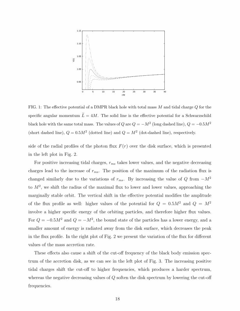
FIG. 1: The effective potential of a DMPR black hole with total mass M and tidal charge Q for the

specific angular momentum L = 4M . The solid line is the effective potential for a Schwarzschild

black hole with the same total mass. The values of Q are Q = −M2 (long dashed line), Q = −0.5M2

(short dashed line), Q = 0.5M2 (dotted line) and Q = M2 (dot-dashed line), respectively.

side of the radial profiles of the photon flux F (r) over the disk surface, which is presented

in the left plot in Fig. 2.

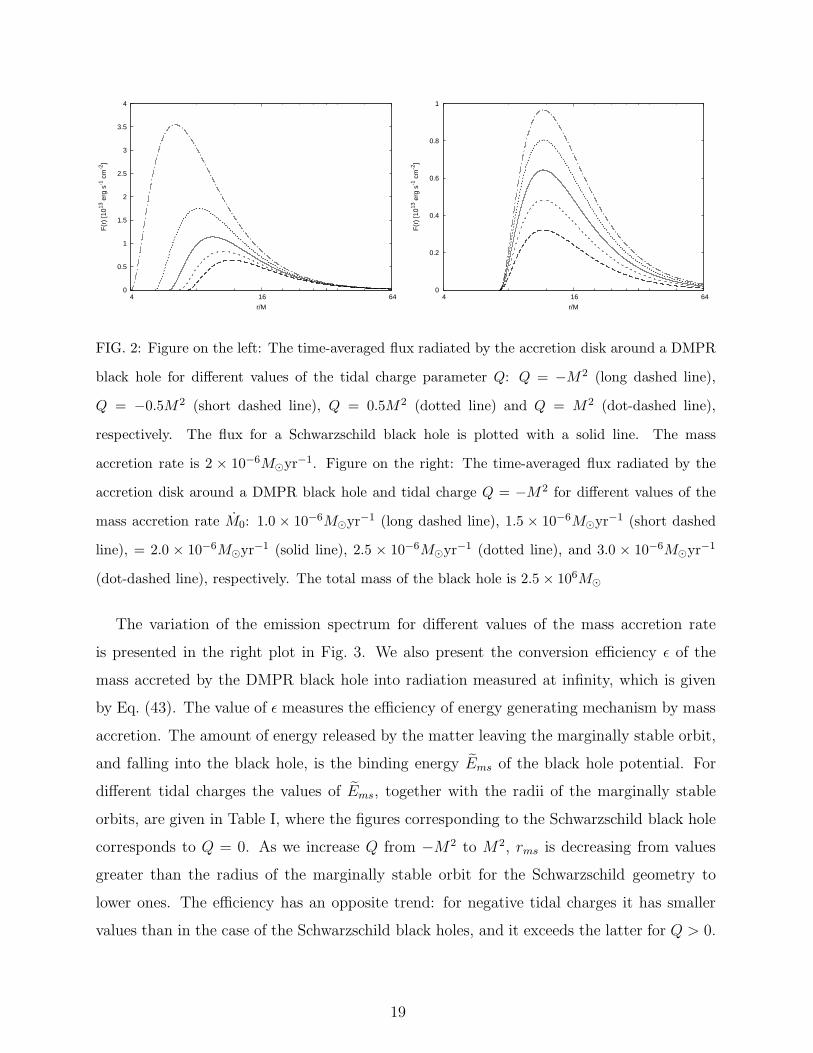
For positive increasing tidal charges, rms takes lower values, and the negative decreasing

charges lead to the increase of rms. The position of the maximum of the radiation flux is

changed similarly due to the variations of rms. By increasing the value of Q from −M2

to M2, we shift the radius of the maximal flux to lower and lower values, approaching the

marginally stable orbit. The vertical shift in the effective potential modifies the amplitude

of the flux profile as well: higher values of the potential for Q = 0.5M2 and Q = M2

involve a higher specific energy of the orbiting particles, and therefore higher flux values.

For Q = −0.5M2 and Q = −M2, the bound state of the particles has a lower energy, and a

smaller amount of energy is radiated away from the disk surface, which decreases the peak

in the flux profile. In the right plot of Fig. 2 we present the variation of the flux for different

values of the mass accretion rate.

These effects also cause a shift of the cut-off frequency of the black body emission spec-

trum of the accretion disk, as we can see in the left plot of Fig. 3. The increasing positive

tidal charges shift the cut-off to higher frequencies, which produces a harder spectrum,

whereas the negative decreasing values of Q soften the disk spectrum by lowering the cut-off

frequencies.

18

0

0.5

1

1.5

2

2.5

3

3.5

4

4 16 64

F(r

) [1

013 e

rg s

-1 c

m-2

]

r/M

0

0.2

0.4

0.6

0.8

1

4 16 64

F(r

) [1

013 e

rg s

-1 c

m-2

]

r/M

FIG. 2: Figure on the left: The time-averaged flux radiated by the accretion disk around a DMPR

black hole for different values of the tidal charge parameter Q: Q = −M2 (long dashed line),

Q = −0.5M2 (short dashed line), Q = 0.5M2 (dotted line) and Q = M2 (dot-dashed line),

respectively. The flux for a Schwarzschild black hole is plotted with a solid line. The mass

accretion rate is 2 × 10−6M⊙yr−1. Figure on the right: The time-averaged flux radiated by the

accretion disk around a DMPR black hole and tidal charge Q = −M2 for different values of the

mass accretion rate M0: 1.0 × 10−6M⊙yr−1 (long dashed line), 1.5 × 10−6M⊙yr−1 (short dashed

line), = 2.0 × 10−6M⊙yr−1 (solid line), 2.5 × 10−6M⊙yr−1 (dotted line), and 3.0 × 10−6M⊙yr−1

(dot-dashed line), respectively. The total mass of the black hole is 2.5 × 106M⊙

The variation of the emission spectrum for different values of the mass accretion rate

is presented in the right plot in Fig. 3. We also present the conversion efficiency ǫ of the

mass accreted by the DMPR black hole into radiation measured at infinity, which is given

by Eq. (43). The value of ǫ measures the efficiency of energy generating mechanism by mass

accretion. The amount of energy released by the matter leaving the marginally stable orbit,

and falling into the black hole, is the binding energy Ems of the black hole potential. For

different tidal charges the values of Ems, together with the radii of the marginally stable

orbits, are given in Table I, where the figures corresponding to the Schwarzschild black hole

corresponds to Q = 0. As we increase Q from −M2 to M2, rms is decreasing from values

greater than the radius of the marginally stable orbit for the Schwarzschild geometry to

lower ones. The efficiency has an opposite trend: for negative tidal charges it has smaller

values than in the case of the Schwarzschild black holes, and it exceeds the latter for Q > 0.

19

1020

1025

1030

1035

1040

1045

1016 1017

ωL(

ω)

[erg

s-1

]

ω [Hz]

1020

1025

1030

1035

1040

1045

1016 1017

ωL(

ω)

[erg

s-1

]

ω [Hz]

FIG. 3: Figure on the left: The emission spectrum of the accretion disk around a DMPR black hole

for different values of the tidal charge parameter Q: Q = −M2 (long dashed line), Q = −0.5M2

(short dashed line), Q = 0.5M2 (dotted line) and Q = M2 (dot-dashed line), respectively. The

solid line represents the disk spectrum for a Schwarzschild black hole. The mass accretion rate

is 2 × 10−6M⊙yr−1. Figure on the right: The emission spectrum of the accretion disk around a

DMPR black hole with tidal charge Q = −M2 for different values of the mass accretion rate M0:

1.0 × 10−6M⊙yr−1 (long dashed line), 1.5 × 10−6M⊙yr−1 (short dashed line), 2.0 × 10−6M⊙yr−1

(solid line), 2.5×10−6M⊙yr−1 (dotted line), and 3.0×10−6M⊙yr−1 (dot-dashed line), respectively.

The total mass of the black hole is 2.5 × 106M⊙

Q [M2] rms [M ] ǫ

-1 7.3100 0.0476

-0.5 6.6949 0.0517

0 6.0000 0.0572

0.5 5.1695 0.0655

1 4.0019 0.0814

TABLE I: The marginally stable orbit and the efficiency for different DMPR black hole geometries.

The case Q = 0 corresponds to the standard general relativistic Schwarzschild black hole.

B. The CFM brane black hole

Two families of analytic solutions in the brane world model, parameterized by the ADM

mass and the PPN parameters β and γ, and which reduce to the Schwarzschild black hole

20

for β = 1, have been found by Casadio, Fabbri and Mazzacurati in [14]. We call the

corresponding brane black holes as the CFM black holes.

The first class of solutions is given by

eν = 1 − 2M

r, (47)

and

eλ =1 − 3M

r(1 − 2M

r

) [1 − 3M

2r

(1 + 4

9η)] , (48)

respectively, where η = γ − 1 = 2 (β − 1). As in the Schwarzschild case the event horizon

is located at r = rh = 2M . The solution is asymptotically flat, that is limr→∞ eν ≡ eν∞ ≡limr→∞ eλ ≡ eλ∞ = 1.

The second class of solutions corresponding to brane world black holes obtained in [14]

has the metric tensor components given by

eν =

η +

√1 − 2M

r(1 + η)

1 + η

2

, (49)

and

eλ =[1 − 2M

r(1 + η)

]−1

, (50)

respectively. The metric is asymptotically flat. In the case η > 0, the only singularity in the

metric is at r = r0 = 2M (1 + η), where all the curvature invariants are regular. r = r0 is a

turning point for all physical curves. For η < 0 the metric is singular at r = rh = 2M/ (1 − η)

and at r0, with rh > r0. rh defines the event horizon.

The first and second class of the CFM brane black holes are characterized by the metric

potentials (47) and (49). Since for the first class of solutions the metric function eν coincides

with the one of the Schwarzschild black hole, their effective potentials V (r) are the same

for equal total masses and fixed L. As a consequence, the specific energy, specific angular

momentum and angular velocity of the particles orbiting around the first class of CFM

black holes are equal to those of the particles moving at the same Keplerian orbit in the

Schwarzschild potential.

However, the radiation flux from the accretion disk shows considerable differences as

compared to the Schwarzschild case when the parameter η is varied. This behavior, shown

in the left plot of Fig. 4, is due to the fact that the proper volume used in the calculation of

21

any integral in this spacetime depends on both the metric functions ν(r) and λ(r), and in

the flux integral given by Eq. (25) we have

√−g = r

[1 − 3M

r

1 − 3M2r

(1 + 49η)

]1/2

. (51)

Since the left hand side of Eq. (51) is decreasing for negative values of η, we obtain higher

and higher flux values by decreasing this metric parameter for η < 0. We have the opposite

effect for η > 0, where the increase of this parameter causes the proper volume to also

increase, and, in turn, the amplitudes of the flux profile to decrease. Because the effective

potential does not depend on η, there is no variation in the radius of the marginally stable

orbit. However, a cut-off appears in the left hand side of the flux profiles for η > 0, where

the denominator in Eq. (51) becomes negative. This gives the criterion

r

M<

3

2

(1 +

4M

9

). (52)

As one can see in left plot of Fig. 4, for η = 5 this criterion is true for any radii greater than

rms, but we obtain a cut-off in the left hand side of the flux profile by setting η equal to

η = 10.

Although the position of the marginally stable orbit does not change for different values

of η, the maximum of the radial distribution of the flux is located at higher and higher radii

as we increase η. The right plot in Fig. 4 presents the variation of the flux for a fixed mass

and parameter η, and for different values of the accretion rate.

The variation in the shape and the amplitude of the flux profile for different values of η

has a clear effect of shifting the cut-off frequency in the disk spectra. The left plot of Fig. 5

shows that the cut-off value shifts to higher frequencies when η is negative, hardening the

spectra. For η > 0 the disk spectrum becomes softer, with lower cut-off frequencies. The

effect of the variation of the mass accretion rate on the emission spectra for a fixed mass

and η is presented in the right plot of Fig. 5.

Since the effective potential of the CFM black holes of the first class is the same as the

one of the Schwarzschild geometry, their conversion efficiencies ǫ of the mass accreted by the

black hole into radiation measured at infinity are also the same.

If we consider the second class of the CFM black holes, given by Eqs. (49) and (50),

respectively, the variation of the parameter η causes similar effects in the behavior of the

photon flux emitted by the accretion disk and its spectrum. However, the metric function

22

0

0.2

0.4

0.6

0.8

1

1.2

1.4

1.6

1.8

4 16 64

F(r

) [1

013 e

rg s

-1 c

m-2

]

r/M

0

0.5

1

1.5

2

2.5

3

4 16 64

F(r

) [1

013 e

rg s

-1 c

m-2

]

r/M

FIG. 4: Figure on the left: The time-averaged flux radiated by an accretion disk around a first

class CFM black holes for various values of η: η = −10 (long dashed line), η = −5 (short dashed

line), η = 5 (dotted line) and η = 10 (dot-dashed line). The flux for a Schwarzschild black hole

is plotted with a solid line. The mass accretion rate is 2 × 10−6M⊙ yr−1. Figure on the right:

The time-averaged flux radiated by the accretion disk around a first class CFM black hole for

η = −10 and for different values of the mass accretion rate M0: 1.0 × 10−6M⊙yr−1 (long dashed

line), 1.5 × 10−6M⊙yr−1 (short dashed line), 2.0 × 10−6M⊙yr−1 (solid line), 2.5 × 10−6M⊙yr−1

(dotted line), and 3.0 × 10−6M⊙yr−1 (dot-dashed line), respectively. The total mass of the black

hole is 2.5 × 106M⊙.

ν(r) now differs from the Schwarzschild black hole case, and we obtain different effective

potentials for different values of the η. The radial profiles of V (r) are shown in Fig. 6, where

η is set to values between −0.8 and 0.8.

By decreasing the values of η from zero to small negative values, we can increase the

potential barrier around the black hole, and decrease the radius of the marginally stable

orbit. The minimum of the effective potential is also increased. Any increment in η from

zero to small positive values causes the opposite effects for V (r). Then the parameters η < 0

increase the flux values and shift rms to lower radii, while negative values of η give lower

fluxes with a cut-off at higher values of rms, as shown in the left plot of Fig. 7.

The variation of the numerical value of the radial coordinate r at the position where

the radiation flux takes its maximum value follows the tendency of rms: with increasing η

we obtain higher and higher orbits for Fmax. These effects result in similar shifts in the

disk spectrum as in the case of the CFM black holes of the first class: in the left plot of

23

1020

1025

1030

1035

1040

1045

1016 1017

ωL(

ω)

[erg

s-1

]

ω [Hz]

1020

1025

1030

1035

1040

1045

1016 1017

ωL(

ω)

[erg

s-1

]

ω [Hz]

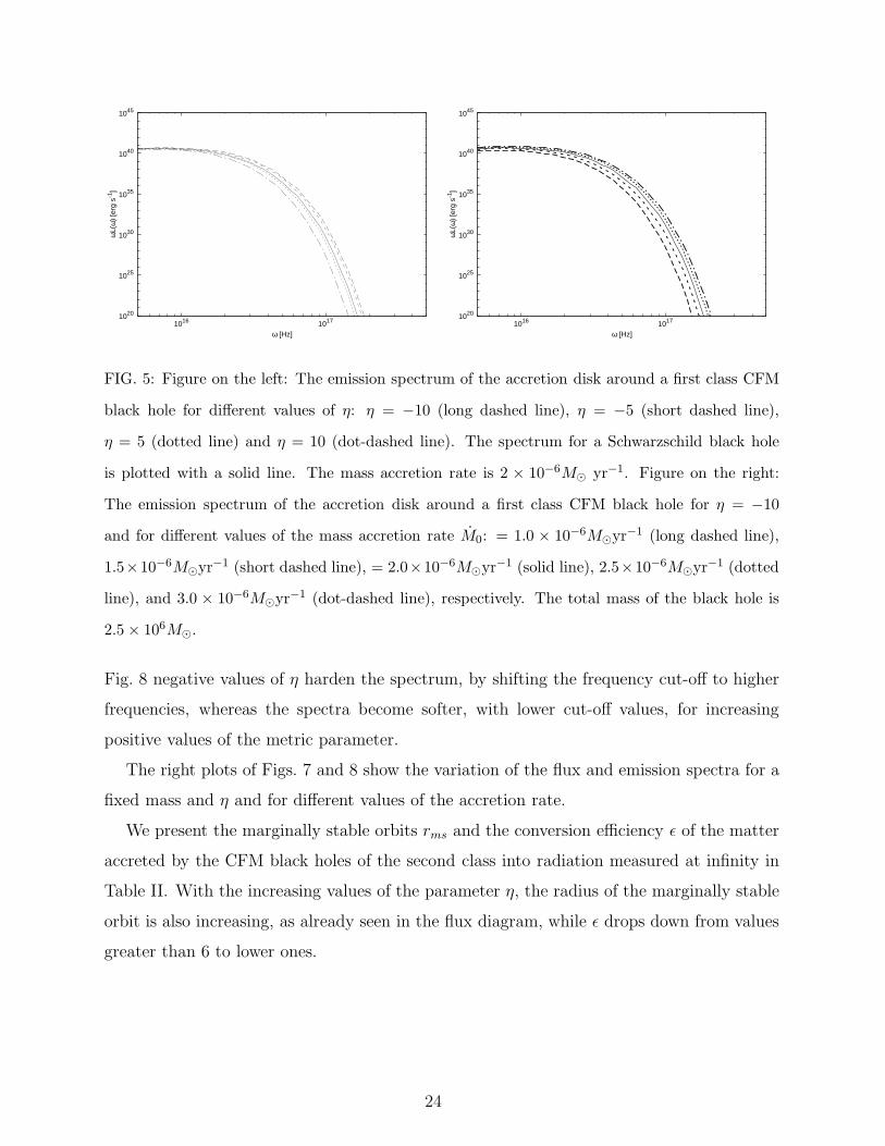
FIG. 5: Figure on the left: The emission spectrum of the accretion disk around a first class CFM

black hole for different values of η: η = −10 (long dashed line), η = −5 (short dashed line),

η = 5 (dotted line) and η = 10 (dot-dashed line). The spectrum for a Schwarzschild black hole

is plotted with a solid line. The mass accretion rate is 2 × 10−6M⊙ yr−1. Figure on the right:

The emission spectrum of the accretion disk around a first class CFM black hole for η = −10

and for different values of the mass accretion rate M0: = 1.0 × 10−6M⊙yr−1 (long dashed line),

1.5×10−6M⊙yr−1 (short dashed line), = 2.0×10−6M⊙yr−1 (solid line), 2.5×10−6M⊙yr−1 (dotted

line), and 3.0 × 10−6M⊙yr−1 (dot-dashed line), respectively. The total mass of the black hole is

2.5 × 106M⊙.

Fig. 8 negative values of η harden the spectrum, by shifting the frequency cut-off to higher

frequencies, whereas the spectra become softer, with lower cut-off values, for increasing

positive values of the metric parameter.

The right plots of Figs. 7 and 8 show the variation of the flux and emission spectra for a

fixed mass and η and for different values of the accretion rate.

We present the marginally stable orbits rms and the conversion efficiency ǫ of the matter

accreted by the CFM black holes of the second class into radiation measured at infinity in

Table II. With the increasing values of the parameter η, the radius of the marginally stable

orbit is also increasing, as already seen in the flux diagram, while ǫ drops down from values

greater than 6 to lower ones.

24

0.94

0.96

0.98

1.00

1.02

1.04

1.06

1.08

1.10

0 5 10 15 20 25 30 35 40

V(r

)

r/M

FIG. 6: The effective potential of the thin accretion disk around a CFM black hole of the second

class with a total mass of M and L = 4M for different values of the parameter η. The potential

V (r) corresponding to the Schwarzschild black hole is plotted with a solid line. The values of η

are η = −0.8 (long dashed line), η = −0.4 (short dashed line), η = 0.4 (dotted line) and η = 0.8

(dot-dashed line), respectively.

η rms [M ] ǫ

-0.8 4.3445 0.0795

-0.4 5.1165 0.0657

0 6.0000 0.0572

0.4 6.9722 0.0501

0.8 8.0091 0.0444

TABLE II: The marginally stable orbit and the efficiency for CFM black holes of the second kind.

The case η = 0 corresponds to the standard general relativistic Schwarzschild black hole.

C. The BMD brane world black hole

Several classes of brane world black hole solutions have been obtained by Bronnikov,

Melnikov and Dehnen in [18] (for short the BMD black holes). In the following we analyze

the accretion properties of a particular class of these models, with metric given by

eν =(1 − 2M

r

)2/s

, eλ =(1 − 2M

r

)−2

, (53)

25

0

0.5

1

1.5

2

2.5

3

3.5

4 16 64

F(r

) [1

013 e

rg s

-1 c

m-2

]

r/M

0

0.1

0.2

0.3

0.4

0.5

0.6

0.7

0.8

0.9

4 16 64

F(r

) [1

013 e

rg s

-1 c

m-2

]

r/M

FIG. 7: Figure on the left: The time-averaged flux radiated by an accretion disk around a second

class CFM black hole for different values of η: η = −0.8 (long dashed line), η = −0.4 (short dashed

line), η = 0.4 (dotted line) and η = 0.8 (dot-dashed line). The flux for a Schwarzschild black hole

is plotted with a solid line. The mass accretion rate is 2× 10−6M⊙ yr−1. Figure on the right: The

time-averaged flux radiated by the accretion disk around a second class CFM black hole with the

parameter η = 0.8 for different values of the mass accretion rate M0: 1.0×10−6M⊙yr−1 (long dashed

line), 1.5 × 10−6M⊙yr−1 (short dashed line), 2.0 × 10−6M⊙yr−1 (solid line), 2.5 × 10−6M⊙yr−1

(dotted line), and 3.0 × 10−6M⊙yr−1 (dot-dashed line), respectively. The total mass of the black

hole is 2.5 × 106M⊙.

where s ∈N. The metric is asymptotically flat, and at r = rh = 2M these solutions have a

double horizon.

Eqs. (53) determine the geometry of the BMD brane black holes, which have the effective

potential plotted in Fig. 9. In the figure we have plotted V (r) for values of s between s = 5

and s = 20.

With increasing s the potential barrier increases as well, but we obtain smaller and smaller

radii for the marginally stable orbits. Although the higher values of s increase the potential

over the region of the stable Keplerian orbits, and the energy of the orbiting particles, as

compared to the case of the Schwarzschild potential, the value of√−g used to calculate the

flux integral increases more rapidly. Therefore Eq. (25) gives smaller fluxes for higher values

of s. This effect is shown in the left plot of Fig. 10, where we present the plots of the photon

flux emitted by the accretion disk in the BMD brane black hole geometry.

The relative shift of rms to lower orbits for increasing s can also be well studied in the

26

1020

1025

1030

1035

1040

1045

1016 1017

ωL(

ω)

[erg

s-1

]

ω [Hz]

1020

1025

1030

1035

1040

1045

1016 1017

ωL(

ω)

[erg

s-1

]

ω [Hz]

FIG. 8: Figure on the left: The emission spectrum of the thin accretion disk around a second class

CFM black hole for different values of η: η = −0.8 (long dashed line), η = −0.4 (short dashed

line), η = 0.4 (dotted line), and η = 0.8 (dot-dashed line). The spectrum for a Schwarzschild black

hole is plotted with a solid line. The mass accretion rate is 2× 10−6M⊙ yr−1. Figure on the right:

The emission spectrum of the accretion disk around a second class CFM black hole with parameter

η = 10 for different values of the mass accretion rate M0: 1.0 × 10−6M⊙yr−1 (long dashed line),

1.5 × 10−6M⊙yr−1 (short dashed line), 2.0 × 10−6M⊙yr−1 (solid line), 2.5 × 10−6M⊙yr−1 (dotted

line), and 3.0 × 10−6M⊙yr−1 (dot-dashed line), respectively. The total mass of the black hole is

2.5 × 106M⊙.

1.00

1.10

1.20

1.30

1.40

1.50

1.60

1.70

1.80

1.90

0 5 10 15 20 25 30 35 40

V(r

)

r/M

FIG. 9: The effective potential for BMD black holes of a fixed total mass M for L = 4M and

different values of s. The solid line is the effective potential for a Schwarzschild black hole with

the same total mass M . The parameter s is set to s = 5 (long dashed line), s = 10 (short dashed

line), s = 15 (dotted line) and s = 20 (dot-dashed line).

27

0

0.2

0.4

0.6

0.8

1

1.2

4 16 64

F(r

) [1

013 e

rg s

-1 c

m-2

]

r/M

0

0.05

0.1

0.15

0.2

0.25

0.3

0.35

0.4

0.45

4 16 64

F(r

) [1

013 e

rg s

-1 c

m-2

]

r/M

FIG. 10: Figure on the left: The time-averaged flux radiated by an accretion disk around a BMD

black hole for different values of s: s = 5 (long dashed line), s = 10 (short dashed line), s = 15

(dotted line) and s = 20, respectively. The flux for a Schwarzschild black hole is plotted with a

solid line. The mass accretion rate is 2×10−6M⊙ yr−1. Figure on the right: The time-averaged flux

radiated by the accretion disk around a BMD black hole with s = 20 for different values of the mass

accretion rate M0: 1.0 × 10−6M⊙yr−1 (long dashed line), 1.5 × 10−6M⊙yr−1 (short dashed line),

2.0×10−6M⊙yr−1 (solid line), 2.5×10−6M⊙yr−1 (dotted line), and 3.0×10−6M⊙yr−1 (dot-dashed

line), respectively. The total mass of the black hole is 2.5 × 106M⊙.

plot. The maximum of the flux value has the same shift: by increasing s the maximum of

F (r) is obtained at lower and lower radii. This behavior of the radiation flux results in the

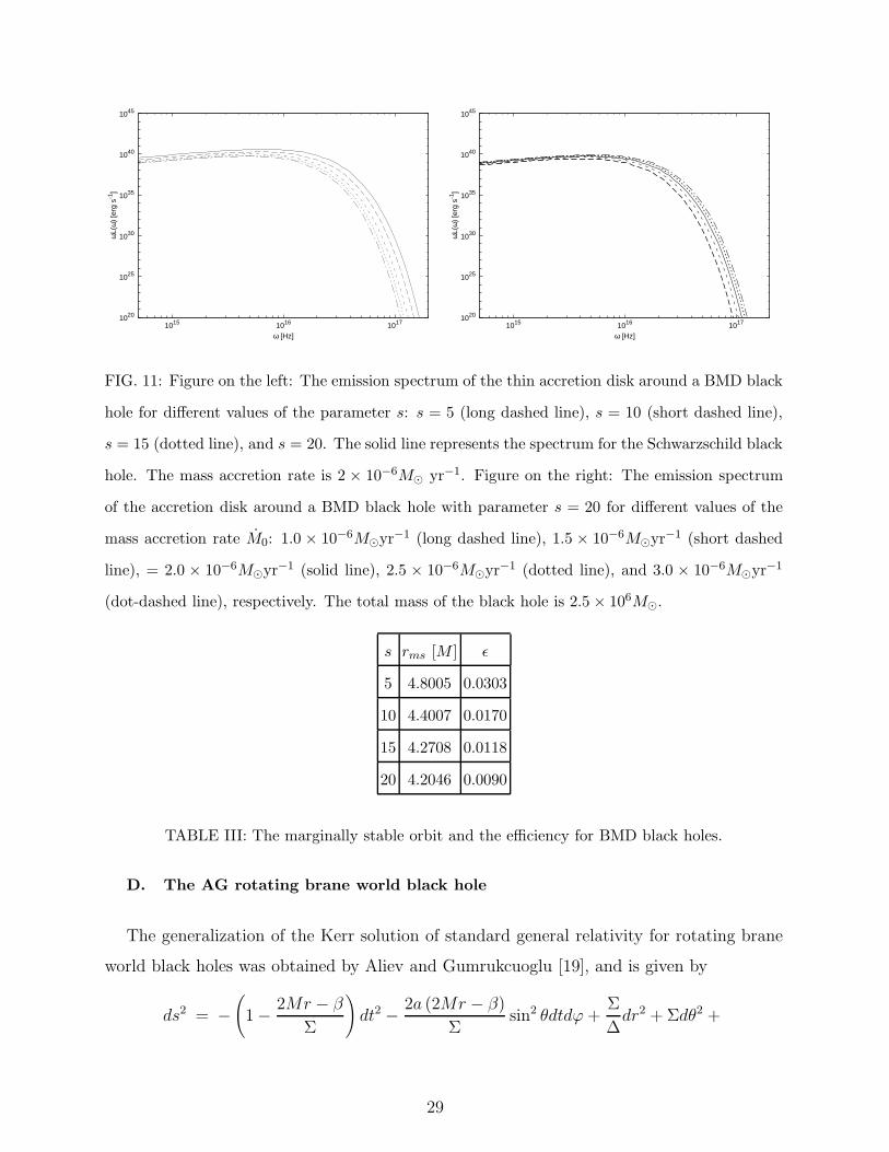
softening of the emission spectrum of the disk. As seen in the left plot of Fig. 11, the cut-off

of the disk spectrum shifts to lower frequencies for increasing values of s, as compared to

the ones obtained in the case of the Schwarzschild geometry. The right plots in Figs. 10 and

11 show the effect of the change of the accretion rate for a BMD brane world black hole for

a fixed mass an s.

The marginally stable orbit and the conversion efficiency ǫ of the accreted mass into

radiation measured at infinity for the BMD black holes are presented in Table III. Both

rms and ǫ have values less than those derived in the Schwarzschild geometry, and they exhibit

a decreasing tendency as we increase the values of the parameter s.

28

1020

1025

1030

1035

1040

1045

1015 1016 1017

ωL(

ω)

[erg

s-1

]

ω [Hz]

1020

1025

1030

1035

1040

1045

1015 1016 1017

ωL(

ω)

[erg

s-1

]

ω [Hz]

FIG. 11: Figure on the left: The emission spectrum of the thin accretion disk around a BMD black

hole for different values of the parameter s: s = 5 (long dashed line), s = 10 (short dashed line),

s = 15 (dotted line), and s = 20. The solid line represents the spectrum for the Schwarzschild black

hole. The mass accretion rate is 2 × 10−6M⊙ yr−1. Figure on the right: The emission spectrum

of the accretion disk around a BMD black hole with parameter s = 20 for different values of the

mass accretion rate M0: 1.0 × 10−6M⊙yr−1 (long dashed line), 1.5 × 10−6M⊙yr−1 (short dashed

line), = 2.0 × 10−6M⊙yr−1 (solid line), 2.5 × 10−6M⊙yr−1 (dotted line), and 3.0 × 10−6M⊙yr−1

(dot-dashed line), respectively. The total mass of the black hole is 2.5 × 106M⊙.

s rms [M ] ǫ

5 4.8005 0.0303

10 4.4007 0.0170

15 4.2708 0.0118

20 4.2046 0.0090

TABLE III: The marginally stable orbit and the efficiency for BMD black holes.

D. The AG rotating brane world black hole

The generalization of the Kerr solution of standard general relativity for rotating brane

world black holes was obtained by Aliev and Gumrukcuoglu [19], and is given by

ds2 = −(

1 − 2Mr − β

Σ

)dt2 − 2a (2Mr − β)

Σsin2 θdtdϕ+

Σ

∆dr2 + Σdθ2 +

29

(r2 + a2 +

2Mr − β

Σa2 sin2 θ

)sin2 θdϕ2. (54)

We call this solution the AG rotating brane world black hole. The event horizon of the

black hole is determined by the solution of the equation ∆ = 0, with the largest root given

by r+ = M +√M2 − a2 − β. The event horizon does exist if the condition M2 ≥ a2 + β is

fulfilled. For a negative tidal charge, as a → M , r+ → M +√−β > M , a condition that

is not allowed in standard general relativity. On the other hand for a negative tidal charge

the extreme horizon r+ = M corresponds to a black hole with rotation parameter a greater

than its mass M .

Near to the equatorial plane, |θ − π/2| ≪ 1, by introducing the coordinate z = r cos θ ≈r(θ− π/2), the approximate form for the geometry of the AG rotating brane black hole can

be written as

ds2 = −DA−1dt2 + r2

A (dφ− ωdt)2 + D−1dr2 + dz2 (55)

with the metric functions

A = 1 + a2∗/r

2∗ + 2a2

∗/r3∗ − a2

∗β∗/r4∗ , (56)

D = 1 − 2/r∗ + a2∗/r

2∗ − β∗/r

2∗ (57)

ω = 2Mar−3A

−1, (58)

where we denoted a∗ = a/M , r∗ = r/M , and β∗ = β/M2, respectively. The effective

potential per unit mass for the radial motion is given by

V (r) =[(r2 + a2

)r2 + (2Mr − β) a2

]E2 −

(r2 − 2Mr + β

)L2 − 2a (2Mr − β) EL− r2∆.

(59)

The variation of the potential V (r) is represented, as a function of r/M , and for different

values of the tidal charge parameter β, in Fig. 12. By increasing β from zero to 2M2 we

also increase the potential barrier as compared with the standard general relativistic Kerr

black hole case, whereas negative tidal charges lowers the potential barrier. The changes in

the value of β also modify the positions of the marginally stable orbits.

In Fig. 13 we present the flux profiles of the accretion disk in the modified Kerr geometry

(55) as a function of r/M and for different values of the tidal charge β (left plot) and of

the accretion rate M0 (right plot). The variation of the numerical value of the tidal charge

determines similar modifications for the flux values as in the case of the accretion disk around

30

1022

1022

1021

100

1021

1022

1022

0.01 0.1 1 10

V(r

)

r/M

FIG. 12: The effective potential of a rotating AG brane world black hole of a total mass 2.5×106M⊙

and with spin a = 0.9982 for the specific energy E = 0.8 and the specific angular momentum

L = 4M . The solid line is the effective potential for a rotating Kerr black hole (β = 0) with the

same total mass. The different values of β are β = −2M2 (long dashed line), β = −M2 (short

dashed line), β = M2 (dotted line) and β = 2M2 (dot-dashed line), respectively.

the DMPR black holes, which can be considered as the static limit (a = 0) of the rotating

AG black hole. The left hand plots in Figs. 13 and 2, respectively, show the same variation

of the flux profiles as a function of the tidal charge. We note that since Q corresponds to

−β, an increase in the numerical values of β from negative values to positive ones decreases

the magnitude of the flux, and increases the radius of the marginally stable orbits. The right

hand plots in Figs. 2 and 13, respectively, also exhibit the same tendency: for higher mass

accretion rates the flux will be amplified as well. In Figs. 2 and 13 the cut-off values of the

spectra decrease with the increasing values of β and −Q, respectively. The same analogy is

valid for disk spectra for the static and the rotating cases. The emission spectra in the case

of the rotating AG brane world black holes are represented, for different values of the spin

parameter and of the accretion rate, in Figs. 14.

By comparing Tables I and IV we can see the same effect of the variation of the tidal

charge on the efficiency ǫ for the static DMPR and for the rotating AG brane black hole,

respectively. As β and −Q increase from negative values to positive ones, the marginally

stable orbits shift to higher radii, and the efficiency of the conversion of the accreting mass

to radiant energy decreases, from values higher than 0.3241 (the efficiency for the standard

Kerr black hole with a∗ = 0.9982) to lower ones.

31

0

100

200

300

400

500

600

1 2 4

F(r

) [1

013 e

rg s

-1 c

m-2

]

r/M

0

100

200

300

400

500

600

700

800

900

1 2 4

F(r

) [1

013 e

rg s

-1 c

m-2

]

r/M

FIG. 13: Figure on the left: The time-averaged flux radiated by the accretion disk around a rotating

AG brane world black hole with spin a = 0.8892 for different values of the tidal charge parameter β:

β = −2×10−3M2 (long dashed line), β = −10−3M2 (short dashed line), β = 10−3M2 (dotted line),

and β = 2× 10−3M2 (dot-dashed line), respectively. The flux for a Kerr black hole with the same

total mass and spin is plotted with a solid line. The mass accretion rate is 2×10−6M⊙yr−1. Figure

on the right: The time-averaged flux radiated by the accretion disk around a rotating AG brane

world black hole with spin a = 0.8892 and tidal charge β = −2×10−3M2 for different values of the

mass accretion rate M0: 1.0 × 10−6M⊙yr−1 (long dashed line), 1.5 × 10−6M⊙yr−1 (short dashed

line), = 2.0 × 10−6M⊙yr−1 (solid line), 2.5 × 10−6M⊙yr−1 (dotted line), and 3.0 × 10−6M⊙yr−1

(dot-dashed line), respectively. The total mass of the black hole is 2.5 × 106M⊙.

β [10−3M2] rms [M ] ǫ

-2 1.1677 0.3449

-1 1.2019 0.3329

0 1.2277 0.3241

1 1.2511 0.3169

2 1.2716 0.3109

TABLE IV: The marginally stable orbit and the efficiency for different rotating AG black hole

geometries for a∗ = 0.9982. The case β = 0 corresponds to the standard general relativistic Kerr

black hole.

32

1020

1025

1030

1035

1040

1045

1017 1018

ωL(

ω)

[erg

s-1

]

ω [Hz]

1020

1025

1030

1035

1040

1045

1016 1017 1018

ωL(

ω)

[erg

s-1

]

ω [Hz]

FIG. 14: Figure on the left: The emission spectrum of the accretion disk around a rotating AG

brane world black hole with spin a = 0.8892 for different values of the tidal charge parameter:

β = −2 × 10−3M2 (long dashed line), β = −10−3M2 (short dashed line), β = 10−3M2 (dotted

line), and β = 2× 10−3M2 (dot-dashed line), respectively. The flux for a Kerr black hole with the

same total mass and spin is plotted with a solid line. The mass accretion rate is 2× 10−6M⊙yr−1.

Figure on the right: The emission spectrum of the accretion disk around a rotating AG brane

world black hole with spin a = 0.8892 and tidal charge β = −2×10−3M2 for different values of the

mass accretion rate M0: 1.0 × 10−6M⊙yr−1 (long dashed line), 1.5 × 10−6M⊙yr−1 (short dashed

line), = 2.0 × 10−6M⊙yr−1 (solid line), 2.5 × 10−6M⊙yr−1 (dotted line), and 3.0 × 10−6M⊙yr−1

(dot-dashed line), respectively. The total mass of the black hole is 2.5 × 106M⊙.

V. DISCUSSIONS AND FINAL REMARKS

In the present paper we have considered the basic physical properties of matter forming

a thin accretion disk in the space-time metric of the brane world black holes. The physical

parameters of the disk-effective potential, flux and emission spectrum profiles have been

explicitly obtained for several classes of black holes, and for several values of the parameters

characterizing the vacuum solution of the generalized field equations in the brane world

models. All the astrophysical quantities related to the observable properties of the accretion

disk can be obtained from the black hole metric.

There are many effective 4D solutions of the vacuum field equations on the brane, with

arbitrary parameters which depend on properties of the bulk, or are simply put in by using

general physical considerations. At the present moment it is theoretically not known whether

33

these parameters should be universal over all brane world black holes, or whether each

separate black hole may have different values of them. Conversely, there is not a single

complete solution, in the sense that the metric in the bulk is uniquely known. This situation

is unsatisfactory from a purely theoretical point of view, and a solution of this problem

seems to be very difficult to be found. Therefore it may be useful to solve the problem of

the existence and nature of the brane world black holes by investigating more closely the

existing observational evidence of the black hole properties, and try to discriminate between

different black hole models by using the data provided by the observational study of the

astrophysical processes around black holes.

Testing strong field gravity and the detections of the possible deviations from standard

general relativity, signaling the presence of new physics, remains one of the most important

objectives of observational astronomy. Due to their compact nature, black holes provide an

ideal environment to do this. Presently, the best constraints on the brane world black hole

parameters can be obtained from the classical tests of general relativity (perihelion preces-

sion, deflection of light, and the radar echo delay, respectively). The existing observational

solar system data on the perihelion shift of Mercury, on the light bending around the Sun

(obtained using long-baseline radio interferometry), and ranging to Mars using the Viking

lander, as applied to the DMPR black hole, can constrain the numerical values of both

the bulk tidal parameter Q and of the brane tension [32]. The stronger limit is obtained

from the perihelion precession, |Q| ≤ 6 × 107 − 5 × 108 cm2. An improvement of one order

of magnitude in the observational data on Mercury’s perihelion shift could provide a very

precise estimate of the bulk tidal parameter, as well as of the brane tension λ.

Observations in the near-infrared (NIR) or X-ray bands have provided important infor-

mation about the spin of the black holes, or the absence of a surface in stellar type black hole

candidates. In the case of the source Sgr A∗, where the putative thermal emission due to the

small accretion rate peaks in the near infrared, the results are particularly robust. However,

up to now, these results have confirmed the predictions of the general relativity mainly in

a qualitative way, and the observational precision achieved cannot distinguish between the

different proposed theories of gravitation. However, important technological developments

may allow to image black holes directly [33]. A background illuminated black hole will

appear in a silhouette with radius√

27GM/c2, with an angular size of roughly twice that

of the horizon, and may be directly observed. With an expected resolution of 20 µas, sub-

34

millimeter very-long baseline interferometry (VLBI) would be able to image the silhouette

cast upon the accretion flow of Sgr A∗, with an angular size of ∼ 50 µas, or M87, with an

angular size of ∼ 25 µas. For a black hole embedded in an accretion flow, the silhouette will

generally be asymmetric regardless of the spin of the black hole. Even in an optically thin

accretion flow asymmetry will result from special relativistic effects (aberration and Doppler

shifting). In principle, detailed measurements of the size and shape of the silhouette could

yield information about the mass and spin of the central black hole, and provide invaluable

information on the nature of the accretion flows in low luminosity galactic nuclei.

Due to the differences in the space-time structure, the brane world black holes present

some important differences with respect to their disc accretion properties, as compared to

the standard general relativistic Schwarzschild and Kerr cases. Therefore, the study of

the accretion processes by compact objects is a powerful indicator of their physical nature.

Since the conversion efficiency, as well as the flux and the spectrum of the black body

radiation in the case of the brane world black holes is different as compared to the standard

general relativistic case, the astrophysical determination of these physical quantities could

discriminate, at least in principle, between the different gravity theories, and give some

constrains on the existence of the extra dimensions.

Acknowledgments

The work of T. H. is supported by an RGC grant of the government of the Hong Kong

SAR.

[1] L. Randall and R. Sundrum, Phys. Rev. Lett., 83, 3370 (1999).

[2] L. Randall and R. Sundrum, Phys. Rev. Lett. 83 4690 (1999).

[3] R. Maartens, Living Reviews in Relativity 7, 1 (2004).

[4] T. Shiromizu, K. Maeda and M. Sasaki, Phys. Rev. D62, 024012 (2000).

[5] M. Sasaki, T. Shiromizu and K. Maeda, Phys. Rev. D62, 024008 (2000).

[6] R. Maartens, Phys. Rev. D62, 084023 (2000); A. Campos and C. F. Sopuerta, Phys. Rev.

D63, 104012 (2001); A. Campos and C. F. Sopuerta, Phys. Rev. D64, 104011 (2001); C.-M.

Chen, T. Harko and M. K. Mak, Phys. Rev. D64, 044013 (2001); D. Langlois, Phys. Rev.

35

Lett. 86, 2212 (2001); C.-M. Chen, T. Harko and M. K. Mak, Phys. Rev. D64, 124017 (2001);

J. D. Barrow and R. Maartens, Phys. Lett. B532, 153 (2002); C.-M. Chen, T. Harko, W. F.

Kao and M. K. Mak, Nucl. Phys. B636, 159 (2002); M. Szydlowski, M. P. Dabrowski and A.

Krawiec, Phys. Rev. D66, 064003 (2002); T. Harko and M. K. Mak, Class. Quantum Grav.

20, 407 (2003); C.-M. Chen, T. Harko, W. F. Kao and M. K. Mak, JCAP 0311, 005 (2003);

T. Harko and M. K. Mak, Class. Quantum Grav. 21, 1489 (2004); A. N. Aliev and A. E.

Gumrukcuoglu, Class. Quantum Grav. 21, 5081, (2004); M. Maziashvili, Phys. Lett. B627,

197 (2005); S. Mukohyama, Phys. Rev. D72, 061901 (2005); M. K. Mak and T. Harko, Phys.

Rev. D71, 104022 (2005); L. A. Gergely, Phys. Rev. D74 024002, (2006); N. Pires, Zong-

Hong Zhu, J. S. Alcaniz, Phys. Rev. D73, 123530 (2006); G. M. Szabo, L. A. Gergely and

Z. Keresztes, PMC Physics A1, 8 (2007); Z. Keresztes, L. A. Gergely, B. Nagy and G. M.

Szabo, PMC Physics A1, 4 (2007); L. A. Gergely and I. Kepiro, JCAP 0707, 007 (2007); Z.

Kovacs and L. A. Gergely, Phys. Rev. D77, 024003 (2008); T. Harko and V. S. Sabau, Phys.

Rev. D77, 104009 (2008); T. Harko, W. F. Choi, K. C. Wong and K. S. Cheng, JCAP 06,

002 (2008); G. De Risi, T. Harko, F. S. N. Lobo and C. S. J. Pun, arXiv:0807.3066 (2008).

[7] G. Kofinas, E. Papantonopoulos and V. Zamarias, Phys. Rev. D 66, 104028 (2002); G. Kofinas,

E. Papantonopoulos and I. Pappa, Phys. Rev. D 66, 104014 (2002); D. Stojkovic, JHEP 0409,

061, 2004; D. Karasik, C. Sahabandu, P. Suranyi and L. C. R. Wijewardhana, Phys. Rev.

D70, 064007 (2004); V. P. Frolov, D. V. Fursaev and D. Stojkovic, JHEP 0406, 057 (2004);

R. Whisker, Phys. Rev. D71, 064004 (2005); A. S. Majumdar and N. Mukherjee, Int. J. Mod.

Phys. D14, 1095 (2005); A. L. Fitzpatrick, L. Randall and T. Wiseman, JHEP 0611, 033

(2006); G. A. S. Dias, S. Gao and J. P. S. Lemos, Phys. Rev. D 75, 024030 (2007); J. Ponce

de Leon, Class. Quantum Grav. 25, 075012 (2008); S. Gao and J. P. S. Lemos, Int. J. Mod.

Phys. A 23, 2943 (2008).

[8] T. Harko and M. K. Mak, Phys. Rev. D69, 064020 (2004).

[9] M. K. Mak and T. Harko, Phys. Rev. D70, 024010 (2004).

[10] T. Harko and M. K. Mak, Annals of Physics 319, 471 (2005).

[11] T. Harko and K. S. Cheng, Astrophys. J. 636, 8 (2006).

[12] N. Dadhich, R. Maartens, P. Papadopoulos and V. Rezania, Phys. Lett. B487, 1 (2000).

[13] C. Germani and R. Maartens, Phys. Rev. D64, 124010 (2001).

[14] R. Casadio, A. Fabbri and L. Mazzacurati, Phys. Rev. D65, 084040 (2002).

36

[15] S. Shankaranarayanan and N. Dadhich, Int. J. Mod. Phys. D13, 1095 (2004).

[16] M. Visser and D. L. Wiltshire, Phys. Rev. D67, 104004 (2003).

[17] R. Casadio and L. Mazzacurati, Mod. Phys. Lett. A18, 651 (2003).

[18] K. A. Bronnikov, V. N. Melnikov and H. Dehnen, Phys. Rev. D68, 024025 (2003).

[19] A. N. Aliev and A. E. Gumrukcuoglu, Phys. Rev. D71, 104027 (2005).

[20] A. S. Majumdar and N. Mukherjee, Int. J. Mod. Phys. D14, 1095 (2005).

[21] C. M. Urry and P. Padovani, Publ. Astron. Soc. of the Pacific 107, 803 (1995).

[22] M. Miyoshi, J. Moran, J. Herrnstein, L. Greenhill, N. Nakai, P. Diamond and M. Inoue, Nature

373, 127 (1995).

[23] A. E. Broderick and R. Narayan, Astrophys. J. 638, L21 (2006).

[24] N. I. Shakura and R. A. Sunyaev, Astron. Astrophys. 24, 33 (1973).

[25] I. D. Novikov and K. S. Thorne, in Black Holes, ed. C. DeWitt and B. DeWitt, New York:

Gordon and Breach (1973).

[26] D. N. Page and K. S. Thorne, Astrophys. J. 191, 499 (1974).

[27] K. S. Thorne, Astrophys. J. 191, 507 (1974).

[28] S. Bhattacharyya, A. V. Thampan and I. Bombaci, Astron. Astrophys. 372, 925 (2001).

[29] D. Torres, Nucl. Phys. B 626, 377 (2002); F. S. Guzman, Phys. Rev. D73, 021501 (2006).

[30] Y. F. Yuan, R. Narayan and M. J. Rees, Astrophys. J. 606, 1112 (2004).

[31] C. S. J. Pun, Z. Kovacs and T. Harko, Phys. Rev. D78, 024043 (2008).

[32] C. G. Boehmer, T. Harko, F. S. N. Lobo, Class. Quantum Grav. 25, 045015 (2008)

[33] A. E. Broderick and A. Loeb, Astrophys. J. 636, L109 (2006).

37