arX

iv:h

ep-t

h/01

0612

7v2

21

Jun

2001

hep-th/0106127

NUB-3215/Th-01

HUPT-01/A031

CTP-MIT-3152

LA-PLATA-TH-01-06

Brane Worlds, String Cosmology, and AdS/CFT

Luis Anchordoquia,1, Jose Edelsteinb,2, Carlos Nunezb,3, Santiago Perez Bergliaffac,4,

Martin Schvellingerd,5, Marta Troboe,6, and Fabio Zysermane,7

aDepartment of Physics, Northeastern University

Boston, MA 02115, USA

b Department of Physics, Harvard University

Cambridge, MA 02138, USA

c Centro Brasileiro de Pesquisas Fisicas,

Rua Xavier Sigaud, 150, CEP 22290-180, Rio de Janeiro, Brazil

d Center for Theoretical Physics, Massachusetts Institute of Technology

Cambridge, MA 02139, USA

e Departamento de Fısica, Universidad Nacional de La Plata

CC67 La Plata (1900), Argentina

Abstract

Using the thin-shell formalism we discuss the motion of domain walls in de Sitter and

anti-de Sitter (AdS) time-dependent bulks. This motion results in a dynamics for

the brane scale factor. We show that in the case of a clean brane the scale factor

describes both singular and non-singular universes, with phases of contraction and

expansion. These phases can be understood as quotients of AdS spacetime by a discrete

symmetry group. We discuss this effect in some detail, and suggest how the AdS/CFT

correspondence could be applied to obtain a non perturbative description of brane-

world string cosmology.

1doqui@hepmail.physics.neu.edu2edels@lorentz.harvard.edu3nunez@lorentz.harvard.edu4sepb@cbpf.br5martin@ctpbeaker.mit.edu6trobo@venus.fisica.unlp.edu.ar7zyserman@venus.fisica.unlp.edu.ar

1

Contents

1 Introduction 2

2 Brane worlds from the connected sum of (A)dS 4

2.1 Field equations . . . . . . . . . . . . . . . . . . . . . . . . . . . . . . . 4

2.2 dS . . . . . . . . . . . . . . . . . . . . . . . . . . . . . . . . . . . . . . 6

2.3 AdS . . . . . . . . . . . . . . . . . . . . . . . . . . . . . . . . . . . . . 12

3 Non-perturbative string cosmology via AdS/CFT 15

A Appendix: Flatland dynamics 23

1 Introduction

The intriguing idea that fundamental interactions could be understood as manifesta-

tions of the existence of extra dimensions in our 4-dimensional world can be traced

back at least to the work of Kaluza and Klein (KK) [1], with revivals of activity that

one generically refers to as KK theories [2]. Over the last two years, a fresh interest

in the topic has been rekindled, mainly due to the realization that localization of mat-

ter [3] and localization of gravity [4] may drastically change the commonly assumed

properties of such models.

From the phenomenological perspective the so-called “brane worlds” provide an eco-

nomic explanation of the hierarchy between the gravitational and electroweak mass

scales. In the canonical example of Arkani-Hamed, Dimopoulos and Dvali (ADD) [5],

spacetime is a direct product of ordinary 4-dimensional manifold (“our universe”) and a

(flat) spatial n-torus of common linear size rc and volume vn = rnc . Of course, Standard

Model (SM) fields cannot propagate a large distance in the extra dimensions without

conflict with observations. This is avoided by trapping the fields in a thin shell of thick-

ness δ ∼ M−1s [6]. The only particles propagating in the (4 + n)-dimensional bulk are

the (4 + n) gravitons. Thus, gravity becomes strong in the entire (4 + n)-dimensional

spacetime at a scale Ms ∼ a few TeV, which is far below the conventional Planck scale,

Mpl ∼ 1018 GeV. Strictly speaking, the low energy effective 4-dimensional Planck scale

Mpl is related to the fundamental scale of gravity M∗ via Gauss’ Law M2pl = M2+n

∗ vn.

For n extra dimensions one finds that rc ≈ 1030/n−19 m, assuming M∗ ∼ 1 TeV [7].

This relation immediately suggests that n = 1 is ruled out, because rc ∼ 1011 m and,

the gravitational interaction would thus be modified at the scale of our solar system.

However, already for n = 2, rc ∼ 1 mm - just the scale where our present day experi-

mental knowledge about gravity ends [8]. Furthermore, one can imagine more general

2

scenarios termed asymmetric compactifications, where, e.g., there are p “small” di-

mensions with sizes of ∼ 1/TeV and the effective number of large extra dimensions

being neff = n− p. Here, the expected number of extra dimensions should be 6 or 7 as

suggested by string theory [9]. Naturally, there is a strong motivation for immediate

phenomenological studies to assess the experimental viability of such a radical depar-

ture from previous fundamental particle physics. Leaving aside table-top experiments

and astrophysics (which requires that Ms > 110 TeV for n = 2, but only around a

few TeV for n > 2 [10]), there are two ways of probing this scenario. Namely, via

the KK–graviton emission in scattering processes, or else through the exchange of KK

towers of gravitons among SM particles [11]. The search for extra-dimension footprints

in collider data has already started. However, as yet no observational evidence has

been found [12].

The ADD scenario is based on the fact that the 4-dimensional coordinates are in-

dependent of the coordinates of the extra n dimensions. Giving up this assumption

can lead to a number of other interesting models with completely different gravita-

tional behaviors. Perhaps the most compelling model along these lines can be built

by considering a 5-dimensional anti-de Sitter (AdS) space with a single 4-dimensional

boundary [4]. This boundary is taken to be a p-brane with intrinsic tension σ. In the

Randall-Sundrum (RS) world, there is a bound state of the graviton confined to the

brane, as well as a continuum of KK modes. At low energies, the bound state domi-

nates over the KK states to give an inverse square law if the AdS radius is sufficiently

small. Therefore, Newton’s law is recovered on the brane, even with an infinitely large

fifth dimension. The number of papers discussing variants of this scenario is already

very large [13]. Some key papers are [14]. For a comprehensive review the reader is

referred to [15].

The presence of large extra dimensions modifies the Friedmann equation on the brane

by the addition of non-linear terms [16] which yield new cosmological scenarios [17].

Fortunately, a world that undergoes a phase of inflation could be long lived by a universe

like our own at low energies [18]. Specifically, brane-world scenarios are good candidates

to describe our world as long as the normal rate of expansion has been recovered by

the epoch of nucleosynthesis [19]. We remind the reader that the universe has to be

re-heated up to a temperature O(MeV) so as to synthethize light elements, because

the entropy produced during a cold inflationary phase red-shifts away. Therefore, any

significant departure from the standard Friedmann-Robertson-Walker (FRW) scenario

could only arise at very high energies. A broader study of these ideas is currently

under way (for an incomplete list of references, see [20]). In this regard, we initiate

here the analysis of new inflationary brane-worlds that arise from surgically modified

evolving spacetimes. The dynamics of the bulk in our framework is originated in the

symmetries of the dS and AdS spacetimes, without the need of extra fields in the bulk,

3

as in the models discussed in reference [21].

The article is divided in two main parts. In Section 2 we derive the equation of

motion of a brane using the thin shell formalism [22], in which the field equations

are re-written as junction conditions relating the discontinuity in the brane extrinsic

curvature to its vacuum energy. Then, we discuss the evolution of a single brane

falling into dS and AdS spaces. As a result of its non interaction with the environment

producing the gravitational field, the brane tension obeys an internal conservation law.

Therefore, the motion of the brane can be treated as a closed system, or alternatively

as a continuous collection of such branes. The evolution yields a dynamics for the

scale factor. We show that in the case of a clean brane (i.e., without matter in the

form of stringy excitations) the scale factor describes both singular and non-singular

universes, with phases of contraction and expansion. Section 3 contains a general

discussion (and some speculations) on the applications of our results in the light of

the AdS/CFT correspondence. Quotients of AdS space by discrete symmetry groups

describe dynamical AdS bulks. Indeed, it has been suggested [23] that this is the

way in which AdS/CFT correspondence must be formulated in the case of dynamical

spacetimes. However, since we consider a p-brane instead of the AdS boundary itself,

for our purposes, the AdS/CFT correspondence should be considered when gravity is

coupled to the conformal theory.

2 Brane worlds from the connected sum of (A)dS

2.1 Field equations

In spite of the fact that dS space does not seem to be obtainable from stringy back-

grounds, there has been a growing interest in dS bulks in recent times [24]. In view of

these developments we will discuss the motion of spherical branes in both dynamical

dS and AdS bulks. The following discussion will refer mostly to branes of dimension

d = 4, but the relevant equations will be written for arbitrary d ≥ 2.

In order to build the class of geometries of interest, we consider two copies of (d+1)-

dimensional dS (AdS) spaces M1 and M2 undergoing expansion. Then, we remove

from each one identical d-dimensional regions Ω1 and Ω2 [25]. One is left with two

geodesically incomplete manifolds with boundaries given by the hypersurfaces ∂Ω1 and

∂Ω2. Finally, we identify the boundaries up to homeomorphism h : ∂Ω1 → ∂Ω2 [26].

Therefore, the resulting manifold that is defined by the connected sum M1#M2, is

geodesically complete. The classical action of such a system can be cast in the following

form

S =L(3−d)

p

16π

∫

M

dd+1x√

g(R − 2Λ) +L(3−d)

p

8π

∫

∂Ωddx

√γK + σ

∫

∂Ωddx

√γ. (1)

4

The first term is the usual Einstein-Hilbert action with a cosmological constant Λ.

The second term is the Gibbons-Hawking boundary term, necessary for a well-defined

variational problem [27]. In our convention, the extrinsic curvature is defined as KMN =

∇(M nN), where nM is the outward pointing normal vector to the boundary ∂Ω.1 Here

R stands for the (d + 1)-dimensional Ricci scalar in terms of the metric gMN , while γ

is the induced metric on the brane, and σ is the brane tension.

For definiteness, the spatial coordinates on ∂Ω can be taken to be the angular vari-

ables φi, which for a spherically symmetric configuration are always well defined up to

an overall rotation. Generically, the line element of each patch can be written as

ds2 = −dt2 + A2(t) [ r2 dΩ2(d−1) + (1 − kr2)−1 dr2 ], (2)

where k takes the values 1 (-1) for dS (AdS), dΩ(d−1) is the corresponding metric on

the unit (d− 1)-dimensional sphere, and t is the proper time of a clock carried by any

raider of the extra dimension. The homeomorphism h entails a proper matching of

the metric across the boundary layer [22]. The required junction conditions are most

conveniently derived by introducing Gaussian normal coordinates in the vicinity of the

brane,

ds2 = (n · n)−1dη2 + γµν(η, xµ)dxµdxν , (3)

where n = ∂η, (n · n) = 1, (-1) if ∂Ω is space-like (time-like). The coordinate η

parameterizes the proper distance perpendicularly measured from ∂Ω. Associating

negatives values of η to one side of the shell and positive values to the other side, the

energy momentum tensor TMN can be written as,

TMN(x) = σ ηµν δ Mµ δ N

ν δ(η) +3 Λ L(3−d)

p

2 π d (d − 1)gMN [Θ(η) + Θ(−η)], (4)

where Θ is the step function, and ηµν is the Minkowski metric. The integration of the

field equations

G NM =

4 π

L(3−d)p

T NM (5)

across the boundary ∂Ω yields,

∆Kν

µ − δ νµ ∆K =

4 π

L(3−d)p

σ δ νµ , (6)

where

∆Kµ

ν ≡ limǫ→0

Kµ(−)

ν − Kµ(+)

ν , (7)

1Throughout the article capital Latin subscripts run from 1 to (d+1), lower Greek subscripts from1 to d, and lower Latin subscripts from 1 to (d − 1). As usual, parenthesis denote symmetrization,∇ is the (d + 1)-dimensional covariant derivative. We adopt geometrodynamic units so that G ≡ 1,c ≡ 1 and h ≡ L2

p≡ M2

p, where Lp and Mp are the Planck length and Planck mass, respectively.

5

is the jump in the second fundamental form of the brane in going from −ǫ to +ǫ side.

For the case at hand ∆Kν

µ = 2K ν(−)

µ .

In order to analyze the dynamics of the system, the brane is allowed to move radially.

Let the position of the brane be described by xµ(τ, φi) ≡ (t(τ), a(τ), φi), with τ the

proper time (as measured by co–moving observers on the brane) that parameterizes

the motion, and the velocity of a piece of stress energy at the brane satisfying uMuM =

−1. Note that, with these assumptions the brane will have an “effective scale factor”

A2(t) = a2(t)A2(t).

The unit normal to the brane reads

nM =

[

a′ A

(1 − ka2)1/2, 0, . . . , 0,

1

A[1 − k a2 + (a′ A)2]1/2

]

. (8)

Using the identity ∂η = nµ∂µ, plus the standard relation

Kτ

τ =∂xM

∂xτ

∂xτ

∂xNK

MN , (9)

the non-trivial components of the extrinsic curvature are given by

Kφi

φi=

A a′

(1 − ka2)1/2+

1

aA[1 − ka2 + (a′A)2]1/2, (10)

and

Kτ

τ =a′′ A

[1 − ka2 + (a′A)2]1/2+

2a′A

[1 − ka2]1/2+

2 a′2 k a A

[1 − ka2 + (a′A)2]1/2 [1 − ka2], (11)

where a′ ≡ da/dτ , and A ≡ dA/dt. The proper time is related to the coordinate time

by

dτ

dt= ±

√

1 − (A a)2

1 − ka2. (12)

Thus, one can always eliminate one in favor of the other by using a′ = a dt/dτ . With

this constraint Eqs. (5) and (6) become two sets of differential equations relating

unknown functions of t: A, a. In the following subsections we find out particular

solutions of this system.

2.2 dS

Let us consider two patches of dS spacetimes undergoing expansion. This implies

setting A(t) = ℓ cosh(t/ℓ) and k = 1 in Eq.(2), where ℓ2 = d(d − 1)/|Λ| is the dS

radius. Fig. 1 shows the Penrose diagram of the model considered in this subsection.

6

χ χ= π = 0 χ = π

Figure 1: Penrose diagram of dS spacetime with a spherical domain wall. Double arrowstands for identification. Horizontal (vertical) inner lines are t– (χ–) constant surfaces.The t = ±∞ surfaces correspond to the top and bottom horizontal lines, respectively.Vertical dashed lines represent the coordinate singularities χ = 0 and χ = π, typical ofpolar coordinates. We have used the transformation r = sin(χ).

As usual, there is a redundancy between the field equations and the covariant con-

servation of stress-energy. A straightforward calculation shows that the equation of

motion of the brane reads,

4 π

L(3−d)p (d − 1)

σ =±a sinh(t/ℓ) + [a ℓ cosh(t/ℓ)]−1 (1 − a2)

1 − a2 − [ℓ cosh(t/ℓ) a]21/2. (13)

We study first the case σ = 0. Integration of Eq.(13) yields,

a(t) =√

C tanh2(t/ℓ) + 1, (14)

and

a(t) =√

C coth2(t/ℓ) + 1, (15)

for positive and negative sign in Eq.(13), respectively. C is an integration constant

which we will set to 1 in what follows. Note that the proper time is always real for

both solutions.

Let us consider first Eq.(14). A plot of the effective scale factor for this case, Fig. 2(i),

shows that it corresponds to an eternal non-singular universe that undergoes a phase

of accelerated contraction up to a minimum volume at t = 0, and then expands again.

Note that, for all t the expansion of the bulk dominates the cosmological evolution of

the brane.

7

-3 -2 -1 0 1 2 30

20

40

60

80

-4 -2 0 2 41

1.2

1.4

1.6

1.8

2

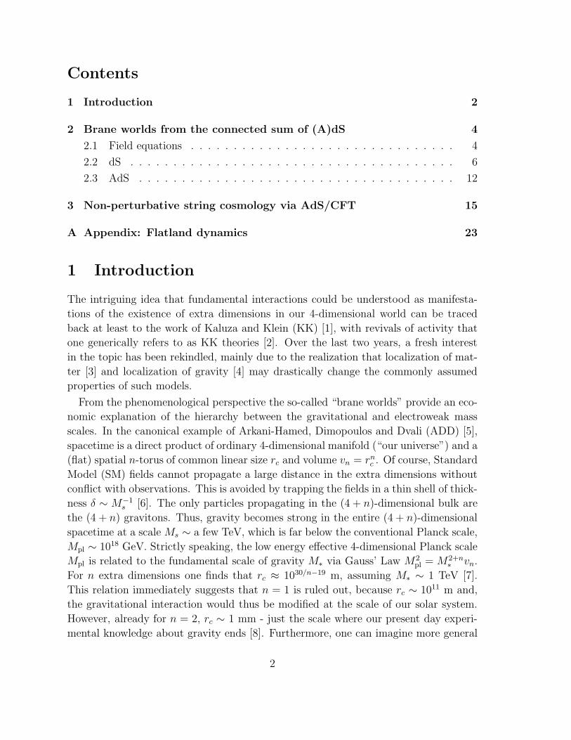
tt(i) (ii)Figure 2: (i) Brane (solid-line) and bulk (dashed-line) scale factors. (ii) Ratio betweenthe brane and bulk expansions, Υ(t). We set ℓ = 1 and σ = 0.

If we define the Hubble parameters Hbrane = 2 [a/a + A/A] and Hbulk = 2 A/A, we

can compare the rates of expansion by plotting Υ = Hbrane/Hbulk. This is shown in

Fig. 2(ii). For t → −∞, both the brane and the bulk are infinitely large and start

contracting at equal rates. Later, the contraction of the brane is faster than the one of

the bulk, until the minimum is reached. The subsequent evolution is the mirror image of

the evolution from −∞ to 0. The weighted rate of evolution (expansion or contraction)

is larger on the brane for all t. For |t| ≪ 1 the rate of expansion on the brane Hbrane is

decoupled from that on the bulk with a behavior given by Υ ∼ 2−2 t2+10 t4/3+O(t5).

For large values of t, Υ = 2 cosh2(t) sech(2t).

Now, we turn to the analysis of the second solution given by Eq.(15). As in the

previous case, both the bulk and the brane have infinite volume at t → −∞, see

Fig. 3(i). Due to the fact that a(t) is finite for limt→±∞, asymptotically the expansion of

the bulk will dominate again the evolution of the spacetime. However, as t approaches

to zero, coth(t) diverges, so that a(t) drives the evolution of the brane. The behavior

of Υ is plotted in Fig. 3(ii). This universe is composed of two disconnected branches,

symmetric with respect to t = 0. The branch on the left starts with an infinite volume,

contracts up to a minimum, and then re-expands back to infinite volume. It should be

stressed that near t = 0, a finite interval of the coordinate time t is associated to an

infinite interval of proper time.

Notice that both solutions exhibit a bounce. They can be understood also as a

special class of wormhole, a Tolman wormhole [28], which entails a violation of the

strong energy condition on the brane.

In order to obtain a solution for any σ > 0 we must solve Eq.(13) numerically. For

8

-3 -2 -1 0 1 2 30

50

100

150

200

-10 -5 0 5 10

-1.5

-1

-0.5

0

0.5

1

1.5

tt(i) (ii)Figure 3: (i) Brane (solid-line) and bulk (dashed-line) scale factors. (ii) Ratio betweenthe brane and bulk expansions, Υ(t). We chose ℓ = 1 and σ = 0, as in the previouscase.

simplicity we set ℓ = 1. After a brief calculation, Eq.(13) (keeping only the + sign)

can be casted as

A(a, t) a2 + B(a, t) a + C(a, t) = 0, (16)

where

A(a, t) = a2 cosh2(t) (σ2 cosh2(t) + sinh2(t)), (17)

B(a, t) = (1 − a2) a sinh(2t), (18)

C(a, t) = (1 − a2)2 − σ2 cosh2(t) a2 (1 − a2), (19)

and the factor 4 π/ [L(3−d)p (d− 1)] has been absorbed in σ. From Eq.(16) it is straight-

forward to write

a =−B(a, t) ±

√

B2(a, t) − 4A(a, t)C(a, t)

2A(a, t), a(t0) = a0. (20)

It must be noted here that Eq.(20) represents two different initial value problems due

to the ± sign in front of the square root. From the discussion above, one would wish

that a(0) = 1, when σ → 0. However, this does not lead to a well defined problem. In

order to overcome this step, we take t0 close to 0 (positive or negative). This yields a0

near 1 as desired. For the sake of numerical accuracy [29] the right hand side of the

above equation must be written in a different – but equivalent – way. Assuming that

a is a complex-valued function, we get the following initial value problems

a =−B(a, t) − q

√

B2(a, t) − 4A(a, t)C(a, t)

2A(a, t), a(t0) = a0, (21)

9

100

101

102

-3 -2 -1 0 1 2 3t

A21

1.1

1.2

1.3

1.4

1.5

-2 -1 0 1 2t

a

σ_

=0

σ_

=10-5

σ_

=10-4

σ_

=10-3

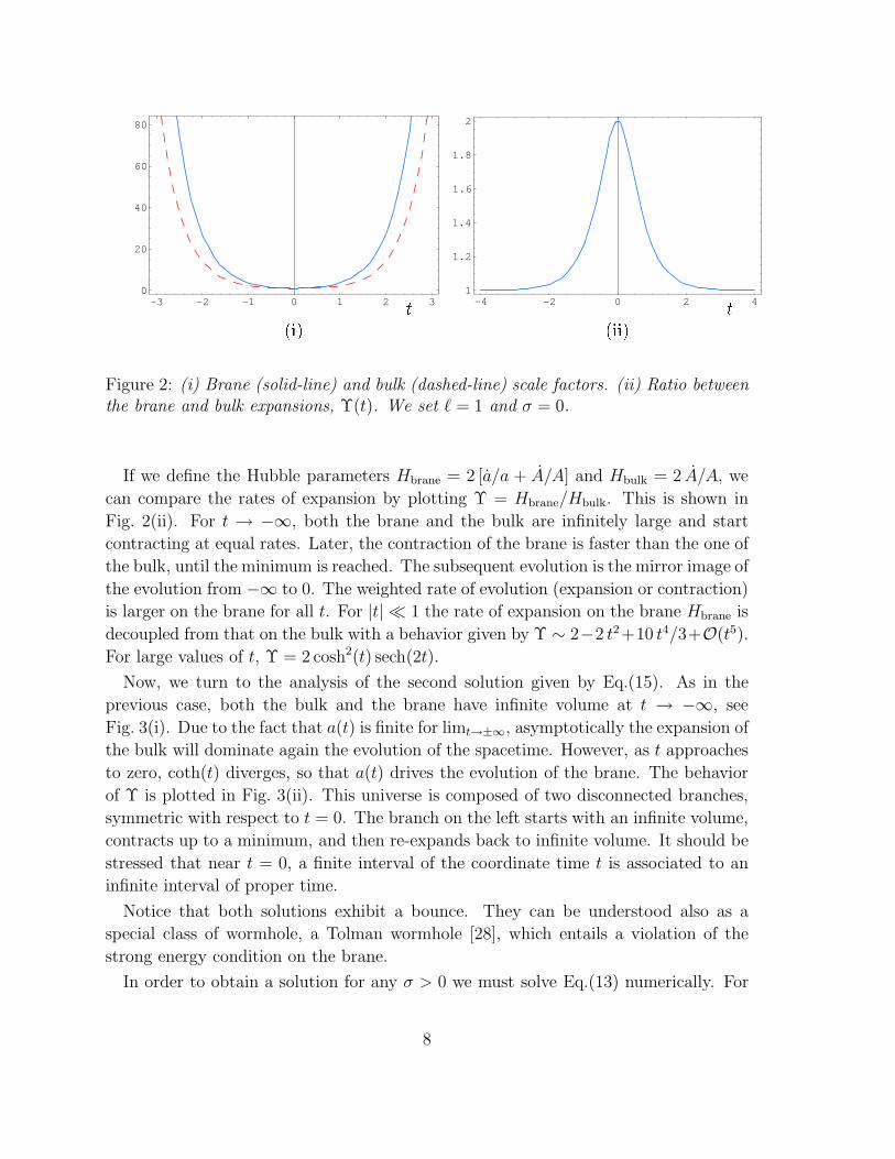
Figure 4: The “effective scale factor” A2(t) is plotted for σ = 10−4. The embeddedfigure displays the dependence of a(t) with σ (the imaginary part is zero).

and

a =−2C(a, t)

B(a, t) + q√

B2(a, t) − 4A(a, t)C(a, t), a(t0) = a0, (22)

where q = 1 if

Re

B∗(a, t)√

B2(a, t) − 4A(a, t)C(a, t)

≥ 0, (23)

or q = −1 otherwise.

Solutions of Eq.(22) for different values of σ are shown in Fig. 4. They were obtained

using the well-known fourth-order Runge-Kutta method [30]. In order to check the

results obtained numerically, we consider the expansion a(t) = a0 +a1 t+O(t2) around

t = 0. By replacing it on Eq.(13) we get

a20 =

1

2 σ2

(√

1 + 4 σ2 − 1)

,

a21 = 1 − 2a2

0 + a40 . (24)

For instance, it is straightforward to see that if σ = 10−3, the slope goes to zero.

As in the case σ = 0, the model describes an eternal non-singular universe. By

progressively increasing the tension of the brane we obtain slower “cosmological” de-

velopments. The effective cosmological constant on the brane is given by

λeff =2

3

d − 1

dΛ +

1

8(d − 2) (d − 1) σ2. (25)

10

-4 -2 0 2 41

1.1

1.2

1.3

1.4

Figure 5: Comparison of a(t) for different dS radius. The solid line stands for ℓ = 1,whereas the dashed line ℓ = 2. σ was set to zero.

It is interesting to remark that by modifying the vacuum energy of the bulk, one can

obtain a similar evolution for a. In other words, by increasing the dS radius ℓ, a(t)

becomes smoother as depicted in Fig. 5. Thus, one can say that Λ and σ have opposite

effects.

At this stage, it is worth noting that the tidal acceleration in the nM direction as

measured by observers on the brane with velocity uN is given by −nM RMNOP uN nO uP ,

where RMNOP is the Riemann tensor. Recalling that we are dealing with a conformally

flat bulk,

tidal acceleration in off − brane direction ∝ Λ . (26)

Consequently, a positive Λ furnishes an acceleration away from the brane, giving rise to

a non-localized gravity model [31]. This situation may change when considering models

with non-local bulk effects (through a nonzero Weyl tensor in the bulk [16]), or with

the incorporation of moduli fields [32] (see Appendix). Note that one can compactify

the spacetime by adding a second brane. In order to do this, one must redefine the

jump in the second fundamental form (in going from −ǫ to ǫ) between the two new

disjoint boundaries ∂Ωi ≡ ri = b < a as

∆Kµ

ν ≡ limǫ→0

Kµ(+)

ν − Kµ(−)

ν , (27)

and then repeat mutatis mutandis the entire computation [33].

Minkowski or dS compactifications seem to be ruled out by some results from low

energy string theory [34]. However, all the “no go” arguments rely on the low energy

11

i ii

Figure 6: (i) Penrose diagram of AdS space with a dS-RS-type domain wall. Thearrows denote identifications. The vertical solid lines represent timelike infinity. (ii)AdS space with a dS domain wall and pre-surgery regions inside the light-cone. Thevertical dashed-lines denote spacelike infinity.

limit of type II string theory (or M theory), where negative tension objects do not

exist. The full string theory could provide objects such as orientifold planes [35], and

compactification to RS set ups after including string-loop corrections to the gravity

action. In addition, massive type II A supergravity could be an alternative arena for

realizing dS compactifications or RS models on manifolds with boundary. Steps in this

direction were presented elsewhere [36]. A different approach was discussed in [37].

All in all, if the bulk is conformally flat, then it is the sign of the bulk cosmological

constant that determines whether there is gravity trapping or not. Henceforth, we

study AdS bulks.

2.3 AdS

By setting A(t) = sin(t), k = −1, ℓ = 1 in Eq.(2), it is obtained

ds2 = −dt2 + sin2(t) [r2 dΩ2(d−1) + (1 + r2)−1 dr2] . (28)

This is the metric associated to the universal covering space of AdS. The above metric

only covers a part of the universal covering space, even when all the intervals t ∈[(nπ, (n+1)π] (for any integer n) are included. Let us consider only one of the possible

patches for the coordinate t ranged between 0 to π. At t = π there is a Cauchy horizon

connecting to a new spacetime that is physically unreachable. This horizon is the

light-cone emanating from the center of symmetry of the solution. Before proceeding

12

0 1 2 3 4 5

0.25

0.5

0.75

1

1.25

1.5

1.75

2

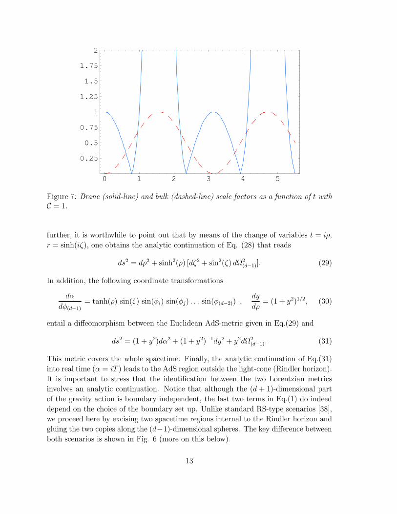
Figure 7: Brane (solid-line) and bulk (dashed-line) scale factors as a function of t withC = 1.

further, it is worthwhile to point out that by means of the change of variables t = iρ,

r = sinh(iζ), one obtains the analytic continuation of Eq. (28) that reads

ds2 = dρ2 + sinh2(ρ) [dζ2 + sin2(ζ) dΩ2(d−1)]. (29)

In addition, the following coordinate transformations

dα

dφ(d−1)= tanh(ρ) sin(ζ) sin(φi) sin(φj) . . . sin(φ(d−2)) ,

dy

dρ= (1 + y2)1/2, (30)

entail a diffeomorphism between the Euclidean AdS-metric given in Eq.(29) and

ds2 = (1 + y2)dα2 + (1 + y2)−1dy2 + y2dΩ2(d−1). (31)

This metric covers the whole spacetime. Finally, the analytic continuation of Eq.(31)

into real time (α = iT ) leads to the AdS region outside the light-cone (Rindler horizon).

It is important to stress that the identification between the two Lorentzian metrics

involves an analytic continuation. Notice that although the (d + 1)-dimensional part

of the gravity action is boundary independent, the last two terms in Eq.(1) do indeed

depend on the choice of the boundary set up. Unlike standard RS-type scenarios [38],

we proceed here by excising two spacetime regions internal to the Rindler horizon and

gluing the two copies along the (d−1)-dimensional spheres. The key difference between

both scenarios is shown in Fig. 6 (more on this below).

13

0

0.5

1

1.5

1 1.1 1.2 1.3 1.4 1.5

σ_

=2

RealImag

t

a(t)

Figure 8: Real and imaginary parts of a(t) for σ = 2.

1 1.1 1.2 1.3 1.4 1.5

0

1

2

3

4

5

t

a(t)

Figure 9: Analytical solution for σ = 0 from Eq.(33) for t ∈ (π/4, π/2]. We haveconsidered C = 5 × 10−2, so as to approximately reproduce the initial condition of thenumerical solution depicted in Fig. 8.

14

With this in mind, the equation of motion of a clean brane sweeping AdS is given

by4 π σ

L(3−d)p (d − 1)

=±a cos(t) + [a sin(t)]−1 (1 + a2)

1 + a2 − [sin(t) a]21/2. (32)

For σ = 0, straightforward integration yields,

a(t) =

√

C cot2(t) − 1 for t ∈ (0, π/4]

√

C tan2(t) − 1 for t ∈ (π/4, π/2].

(33)

To obtain this solution we have exchanged the ± sign in the equation of motion at

t = π/4. In Fig. 7 we show the evolution of the bulk and brane scale factors for

t ∈ [0, 7/4π]. Note however, that Eq.(33) does not describe a physical solution because

the proper time is not real. By checking the Jacobian in Eq.(12) one can immediately

realize that the intervals where the proper time is real are shifted in π/2 with respect to

the corresponding solutions of Eq.(33). To understand what is going on, let us re-write

the effective cosmological constant on the brane,

λeff = (d − 1)

[

1

8(d − 2)σ2 − 2

3

(d − 1)

ℓ2

]

. (34)

It is easily seen that in order to obtain λeff > 0 (condition that arises from imposing

that the sections t = constant and a = constant are (d − 1) spheres), we must impose

σ2 >16

3

(d − 1)

(d − 2)

1

ℓ2. (35)

Thus, the existence of a well behaved solution of a spherical domain wall sweeping the

internal region to the Rindler horizon has an explicit dependence on the dimension of

the spacetime through the brane tension.

In order to find the solution for σ > 0 we follow the procedure sketched before for

the case of a dS bulk. In Fig. 8 we show the solution of Eq.(32) (considering again only

the plus sign) for σ = 2. It has been obtained by setting ℓ = 1, and with the initial

condition a(1) = 1. For comparison in Fig. 9 we display the corresponding analytical

solution of Eq.(33), for t ∈ (π/4, π/2]. One can check by inspection that a(t) becomes

smoother with increasing σ. This implies that the denominator on the r.h.s. of Eq.(32)

is real, rendering a well defined proper time. Putting all this together, a non-vanishing

brane tension leads to the suitable shifting on a(t).

3 Non-perturbative string cosmology via AdS/CFT

A, seemingly different, but in fact closely related subject we will discuss in this section

is the AdS/CFT correspondence [39]. This map provides a “holographic” projection

15

of string theory (or M theory) in AdS space, to a conformal field theory (CFT) living

on its boundary [40]. Actually, more general spaces with certain smooth restrictions

would typically lead to non conformal field theories on their boundary. For asymptot-

ically AdS spaces the bulk excitations do indeed have a correspondent state/operator

in the boundary [41]. The duality between the “strongly coupled gauge theory/weakly

coupled gravity” is the face-off of the well known computation of black hole quantities

via a field theory [42] that naturally yields a non-perturbative stringy background.

In the standard non-compact AdS/CFT set up, gravity is decoupled from the dual

boundary theory. However, any RS-like model should properly be viewed as a coupling

of gravity to whatever strongly coupled conformal theory the AdS geometry is dual to

[43]. The holographic description has been recently invoked to discuss phenomenologi-

cal and gravitational aspects of RS-models [44]. Here, we try to take advantage of this

duality to describe cosmological set ups.

There exist a “new lore” that convinces us that if our universe is five-dimensional, it

should have evolved to the present situation from M theory [45]. If this is the case, it

is reasonable to describe the evolution of the AdS5 sector (up to stabilization at some

scale) by

ds2 = −dt2 + sin2(t) [sinh2(ζ) dΩ2(d−1) + dζ2]. (36)

In other words, the metric in Eq.(36) with SO(d, 1) isometries (which is in fact a

subgroup of the full SO(d, 2) symmetry group of AdS) is expected to characterize the

dynamics of the system that has “stationary” phases governed by

ds2 = −(1 + y2) dT 2 + (1 + y2)−1 dy2 + y2dΩ2(d−1) . (37)

Recall that we set ℓ = 1, and the discussion refers to d = 4. This overall picture is

actually related to the notion of black holes threaded with collapsing matter, stabilized

as static objects. Particularly, in such a limit the dual non-perturbative description

for maximally extended Schwarzschild-AdS spacetimes has been recently put forward

[46]. Applying Maldacena’s conjecture in the whole dynamical scenario, however, is not

straightforward. Basically, because the well known correspondence between correlation

functions in a field theory and string theory backgrounds with AdS subspace [41]

does not have a clear counterpart. We are not going to present here a prescription

for such a generalization, which is beyond the scope of the present article. Instead,

we content ourselves assuming the existence of a subset of operators/states satisfying

certain discrete symmetries, and sketch a CFT dual of the dynamical gravitational

system discussed in the previous section.

In order to do so, we should first draw the reader’s attention to some generic features

of the metrics in Eqs.(36) and (37). The (p+2)-dimensional AdS space, can be obtained

16

by taking a hyperboloid (for instance see [47])

− x20 − x2

p+2 +p+1∑

j=1

x2j = −1, (38)

embedded in (p + 3)-dimensional space with metric

ds2 = −dx20 − dxp+2 +

p+1∑

j=1

dx2j . (39)

By construction, the spacetime contains “anomalies” in the form of closed time-like

curves, corresponding to the S1 sector of the hyperboloid. However, by unwrapping

that circle one can eliminate the causal “anomalies”, and obtain the so called “universal

covering space of AdS”. A convenient parametrization sets xp+2 = cos(t), so that a

constant t surface is a constant negative curvature hyperboloid of radius sin(t), with

the metric given in Eq.(36). One can alternative solve Eq.(38) by setting

x0 = cosh(y) sin(T ), xp+2 = cosh(y) cos(T ), xj = sinh(y) Ωj, (40)

where j = 1, . . . , p + 1, and∑

j Ω2j = 1. By inspection of Fig. 10, it is easily seen that

the universal AdS space is conformal to half of the Einstein static universe. While

the coordinate system (t, ζ, φi), with apparent singularities at t = nπ (n ∈ Z), covers

only diamond-shaped regions, coordinates (T, y, φi) cover the whole space. The surface

corresponding to t = −∞ (solid line) emanates from T = 0 bouncing at T = π/2

towards T = π. After reflection, the solid line represents a hypersurface at t = ∞. The

vertical thin solid lines (with end points T = 0, T = π) stand for hypersurfaces y =

constant, whereas the corresponding horizontal lines are T= constant curves. Notice

that every timelike geodesic emanating from any point in the space (to either pass or

future) reconverges to an image point, diverging again to refocus at a second image

point, and so on [48]. Therefore, the sets of points which can be reached by future

directed timelike lines starting at a point p, is the set of points lying beyond the future

null cone of p, i.e., the infinite chain of diamond shaped regions similar to the one

characterized by (t, ζ, φi). Since the total space is non-singular, it should be expected

that the other regions that are outside the diamond-shaped domain can be included.

All points in the Cauchy development of the surface T = 0 can be reached by a unique

geodesic normal to the surface, whereas points lying outside the Cauchy development

cannot be reached by this kind of geodesics.

The infinitely sequence of diamond-shaped regions can also be understood as quo-

tients with respect to the universal covering space [23]. If we consider a quotient of the

form Hd/Γ (with a discrete group of invariances Γ) such that we get a finite volume

region out of Hd, we could interpret this as a cosmological model with a big bang

17

T

κ=π/2κ=0

κ=−π/2

T=

T=

T= 0

π/2

π

Figure 10: A chain of diamond-shaped regions of the universal covering of the AdS.Here, κ = 2 arctan[exp(ρ)] − π/2.

18

and a big crunch [49]. This cosmological model is a quotient space constructed by

identification of points in FRW space under the action of a discrete subgroup Γ of the

manifold’s isometry group G. Intuitively, we divide the space in different regions such

that for any observer placed at x0, the so-called Dirichlet domain is defined as the set

of all points closer to x0 than to γ x0, being γ an element of the group Γ. Notice that

the action of γ’s shifts the outskirts of each point in a given diamond-shaped region to

another diamond-shaped domain. With this in mind, one can describe the universe we

live in by a Dirichlet domain. Then, we can see the importance of the Cauchy surface

mentioned above at T = 0 in Eq.(36), since after imposing initial data on this surface

we can cover the complete AdS space.

A particular example of this sort of phenomenon occurs in the extended RS-universe

discussed in Section 2. The envisaged surgery, shown in Fig. 11, starts with two

asymptotic AdS regions, each one with two outer and inner horizons, that are then

repeated an infinite number of times in the maximal analytic extension. The brane

expansion starts out in the downmost AdS region, falling through the future outer

horizon to the next incarnation of the universe. This process occurs in a finite time

t. Since we have an AdS space and a quotient on it, one can naturally ask, what

is the effect of this quotient on the CFT. This question is of great interest since the

resulting CFT would be a non-perturbative description of string cosmology. The idea

is to construct a CFT with a Hilbert space invariant under Γ. These states would in

principle describe linearized gravity modes in the cosmological background [50]. The

main problem with this construction is that finding such a CFT would involve to take

a quotient on the space on which the CFT lives. The interesting point discovered in

[23] is that one can take a quotient on the operator and state spaces leading to a subset

invariant under Γ. Before proceeding further, it is instructive to recall that instead of

a CFT living in a flat Minkowski space, we handle a gauge theory coupled to gravity

on the brane.

When considering the near horizon geometry of D3 branes, AdS5×S5, one deals with

a four dimensional N = 4 supersymmetric Yang Mills theory as its holographic dual.

The symmetries on the brane side, SL(2, Z) and SO(6) are present on the gravity side

as type IIB symmetries. An enormous amount of tests on the above relation have been

done. Many of them involve correlation functions. Others refer to the matching of the

weight of chiral primaries on the CFT side with the masses of the KK modes on the

compact part of the geometry. In the case of M theory, we deal with AdS4 × S7 (and

also with AdS7 × S4) and 3-dimensional supersymmetric CFT with 16 charges or the

(0,2) little string theory in each case (they correspond to M2/M5 branes). In these

cases the existence of a matching between chiral primaries and KK states was also

checked in detail. The AdS6×S4 (that appears when we consider the D4-D8 system in

massive IIA theory [36]) leads to five-dimensional CFT. Again, the same matching and

19

Figure 11: Maximally extended Penrose diagram. The past and future RS horizons,are replaced by the past and future light-cones obtained after analytical continuation.

20

correspondence was achieved. Besides, there exits compactifications of M theory with

an AdS5 sector (for instance AdS5 × H2 × S4 [51]), where all the previous mentioned

features work in pretty much the same way. The subtlety of these compactifications

is that they lead to 4-dimensional CFT’s with 4 or 8 supercharges, thus making closer

contact with the supersymmetric SM-like theories.

In order to describe a method that can hopefully be applied to any of the products

discussed above, let us restrict to the case of AdS3×S3×T 4 (the background geometry

that appears considering D1-D5 system). The gravity system has a dual description

in terms of a 2-dimensional supersymmetric CFT, with N = (4, 4) supersymmetry.

The isometries, given by SL(2, R) × SL(2, R), coincide with the symmetry generated

on the 2-dimensional boundary by the Virasoro generators L0,±, L0,±. A scalar field

satisfying the Klein-Gordon equation in AdS3, will have eigenmodes in correspondence

with the masses of the chiral primaries on the field theory side. These states, like

all their descendants, are protected and in correspondence with the KK states on the

S3 × T 4 of the geometry. Once we have applied the quotient operation, the proposed

way to obtain the correspondence is lifting the gravity mode to the uncompactified AdS

space. This is carried out by considering a periodic function defined on each Dirichlet

domain, covering the complete space. The correspondence is between the cosmological

gravity mode, and the state given by the sum of individual states on each domain (on

the CFT side). It is important to point out that this sum is not convergent. Therefore,

methods dealing with rigged Hilbert spaces have been applied to define the sum (the

CFT state) properly. In addition, as it has been point out in [23] the quotients required

to obtain the cosmology break down all the supersymmetries. One can understand this

considering that a spacetime where some of the supersymmetries remain unbroken must

be stationary (or sort of “null-stationary”). However, our quotient spacetime has no

Killing fields whatsoever. Note that such a Killing field would have to be an element of

the AdS symmetry group that commutes with the group we used to take the quotient.

However, there are not such elements. Another way of saying this is that, after the

quotient, one will not be able to return (globally) to the static coordinate system [52].

It implies that there are not protected quantities in the cosmological scheme. Other

ways of doing the quotient could in principle, be find. This opens the possibility of

different definitions of this theory in the boundary, which would be very interesting to

explore further. Moreover, it is also important to address whether there could exist

scenarios in which the above mentioned quotients describing the cosmological evolution

do preserve some of the supersymmetries. We hope to return to these topics in future

publications.

21

Acknowledgements

We have benefitted from discussions with Juan Maldacena, Stephan Stieberger, and

Mike Vaughn. We are grateful to Gia Dvali and Tetsuya Shiromizu for a critical

reading of the manuscript and valuable comments. We would like to especially thank

Gary Horowitz and Don Marolf for sharing with us their expertise on this subject and

teaching us about their work. This article was partially supported by CONICET (Ar-

gentina), FAPERj (Brazil), Fundacion Antorchas, IFLP, the Mathematics Department

of the UNLP, the National Science Foundation (U.S.), and the U.S. Department of

Energy (D.O.E.) under cooperative research agreement #DF-FC02-94ER40818.

22

Figure 12: Penrose diagram of Minkowski spacetime with a spherical domain wall.Double arrow stands for identification. Horizontal (vertical) inner lines are t– (r–)constant surfaces. The t = ±∞ surfaces correspond to the top and bottom horizontallines, respectively. Vertical dashed line represents the coordinate singularities r = 0,that occur with polar coordinates.

A Appendix: Flatland dynamics

In this appendix we will briefly discuss the main features of a novel scenario which

contains fields in the bulk with Lagrangian L. We start by considering a rather general

action,

S =L3−d

p

16π

∫

M

dd+1x√

gR +L3−d

p

8π

∫

∂Ωddx

√γK +

∫

M

dd+1x√

gL + σ∫

∂Ωddx

√γ . (41)

The standard approach to solve the equations of motion would be to assume some

specific type of fields descibed by L, and from the physics of that source to derive

an equation of state, which together with the field equations would determine the

behavior of the (d + 1)-dimensional scale factor. In deriving our model, however, the

philosophy of solving Einstein’s equation must be altered somewhat from the usual one:

We concentrate on the geometrical properties of the spacetime, without specifying L.

We are interested here in (d+1)-dimensional Ricci-flat spacetime undergoing expansion.

Thus, we set k = 0 in Eq.(2) and we replace the metric in the field equations to obtain

the curvature constraint

R = 2 dA

A+ d (d − 1)

A2

A2. (42)

23

-3 -2 -1 0 1 2 30

2

4

6

8

10

Figure 13: Brane (solid-line) and bulk (dashed-line) scale factors, for σ = 0.

Now, it is easily seen that

A(t) =(K0

2

)α

[(1 + d)(t −K1)]α (43)

describes a flat solution undergoing expansion, with equation of state (in terms of the

bulk energy density ρ and pressure p),

d α (α − 1) t−2 = − 4π

L3−dp

(ρ + d p) , (44)

provided that α = 2/(d + 1). For simplicity, we have set the integration constants

K0 = α, K1 = 0. Note that the fields threading the spacetime violate the (d + 1)

strong energy condition. After recalling that we are dealing with a clean brane and a

conformally flat bulk, it is straightforward to obtain the equation of motion of a brane

in this background,

4π

L3−dp (d − 1)

σ =±a α tα−1 + (a tα)−1

[1 − (a tα)2]1/2. (45)

Figure 12 shows the Penrose diagram for this brane-surgery. For the case σ = 0, d = 4

the solution reads,

a(t) = ± 5√6

t3/5 , (46)

where a0 is an integration constant. In Fig. 13, we show the evolution of A(t) and

A(t) for a0 = 0. The solution (brane and bulk scales factor) describes to separate

symmetric patches of contraction and expansion with a shrinkage down to zero at

24

t = 0. From Eq.(12) one can easily see that the solution does not represent a physical

system because (Aa)2 > 1.

It is interesting to point out that in a most general action, the last world-volume

term in Eq.(41) would depend on the d-dimensional Ricci scalar. Such term can not

be excluded by any symmetry reason and in fact is expected to be generated on the

brane. Inclusion of this term often dramatically modifies the situation (e.g. can induce

4-dimensional gravity even if extra space is 5-dimensional Minkowskian [53]). Thus,

it would be interesting to explore dynamical scenarios without fixing the shape of the

brane.

25

References

[1] T. Kaluza, Sitzungsber. Preuss. Akad. Wiss. Berlin (Math. Phys. ) K1, 966 (1921);O. Klein, Z. Phys. 37, 895 (1926) [Surveys High Energ. Phys. 5, 241 (1926)].

[2] Variations of Kaluza Klein theory that motivated the renaissance of higher dimensionalmodels are discussed in, K. Akama, Lect. Notes Phys. 176, 267 (1982) [hep-th/0001113];V. A. Rubakov and M. E. Shaposhnikov, Phys. Lett. B 125 (1983) 136; M. Pavsic, Class.Quant. Grav. 2, 869 (1985); M. Pavsic, Phys. Lett. A 107, 66 (1985); M. Visser, Phys.Lett. B 159, 22 (1985) [hep-th/9910093]; G. W. Gibbons and D. L. Wiltshire, Nucl.Phys. B 287, 717 (1987); I. Antoniadis, Phys. Lett. B 246, 377 (1990).

[3] G. Dvali and M. Shifman, Phys. Lett. B 396, 64 (1997) [Erratum-ibid. B 407, 452(1997)] [hep-th/9612128]; M. Gogberashvili, Mod. Phys. Lett. A 14, 2025 (1999)[hep-ph/9904383]; B. Bajc and G. Gabadadze, Phys. Lett. B 474, 282 (2000) [hep-th/9912232].

[4] L. Randall and R. Sundrum, Phys. Rev. Lett. 83, 4690 (1999) [hep-th/9906064].

[5] N. Arkani-Hamed, S. Dimopoulos and G. Dvali, Phys. Lett. B 429, 263 (1998) [hep-ph/9803315]; I. Antoniadis, N. Arkani-Hamed, S. Dimopoulos and G. Dvali, Phys. Lett.B 436, 257 (1998) [hep-ph/9804398]; N. Arkani-Hamed, S. Dimopoulos and G. Dvali,Phys. Rev. D 59, 086004 (1999) [hep-ph/9807344].

[6] Assuming that the higher dimensional theory at short distance is a string theory, oneexpects that the fundamental string scale Ms and M∗ are not too different. A perturba-tive expectation is that Ms ∼ gsM∗, where g2

s is the gauge coupling at the string scale,of order g2

s/4π ∼ 0.04. S. Nussinov and R. Shrock, Phys. Rev. D 59, 105002 (1999)[hep-ph/9811323].

[7] This scale emerge from supersymmetry breaking, see for instance, L. Randall and R. Sun-drum, Nucl. Phys. B 557, 79 (1999) [hep-th/9810155], and references therein.

[8] Specifically, no deviations from Newtonian physics are expected at separations rang-ing down to 218 µm. C. D. Hoyle, U. Schmidt, B. R. Heckel, E. G. Adelberger,J. H. Gundlach, D. J. Kapner and H. E. Swanson, Phys. Rev. Lett. 86, 1418 (2001)[hep-ph/0011014].

[9] For an alternative approach to both large and small extra dimensions with asymmetriccompactifications, see J. Lykken and S. Nandi, Phys. Lett. B 485, 224 (2000) [hep-ph/9908505].

[10] See for instance, S. Cullen and M. Perelstein, Phys. Rev. Lett. 83, 268 (1999) [hep-ph/9903422]; N. Arkani-Hamed, S. Dimopoulos, G. Dvali and N. Kaloper, JHEP 0012,010 (2000) [hep-ph/9911386]; V. Barger, T. Han, C. Kao and R. J. Zhang, Phys. Lett.B 461, 34 (1999) [hep-ph/9905474]; G. C. McLaughlin and J. N. Ng, Phys. Lett. B 470,157 (1999) [hep-ph/9909558]; S. Cassisi, V. Castellani, S. Degl’Innocenti, G. Fiorentiniand B. Ricci, Phys. Lett. B 481, 323 (2000) [astro-ph/0002182].

26

[11] See for instance, G. F. Giudice, R. Rattazzi and J. D. Wells, Nucl. Phys. B 544, 3 (1999)[hep-ph/9811291]; T. Han, J. D. Lykken and R. Zhang, Phys. Rev. D 59, 105006 (1999)[hep-ph/9811350]; J. L. Hewett, Phys. Rev. Lett. 82, 4765 (1999) [hep-ph/9811356];E. A. Mirabelli, M. Perelstein and M. E. Peskin, Phys. Rev. Lett. 82, 2236 (1999)[hep-ph/9811337]; T. G. Rizzo, hep-ph/9910255; S. Cullen, M. Perelstein and M. E. Pe-skin, Phys. Rev. D 62, 055012 (2000) [hep-ph/0001166]; L. Anchordoqui, H. Goldberg,T. McCauley, T. Paul, S. Reucroft and J. Swain, Phys. Rev. D 63, 124009 (2001) [hep-ph/0011097].

[12] M. Acciarri et al. (L3 Collaboration), Phys. Lett. B 470, 281 (1999); C. Adloff et al. (H1Collaboration), Phys. Lett. B 479, 358 (2000); B. Abbott et al. (DØ Collaboration),Phys. Rev. Lett. 86, 1156 (2001).

[13] Of particular phenomenological interest is the set–up with the shape of a gravitationalcondenser in which two branes of opposite tension (which gravitationally repel eachother) are stabilized by a slab of AdS. In this model the extra dimension is stronglycurved, and the distance scales on the brane with negative tension are exponentiallysmaller than those on the positive tension brane. Such exponential suppression can thennaturally explain why the observed physical scales are so much smaller than the Plankscale. L. Randall and R. Sundrum, Phys. Rev. Lett. 83, 4690 (1999) [hep-th/9906064].

[14] W. D. Goldberger and M. B. Wise, Phys. Rev. Lett. 83, 4922 (1999) [hep-ph/9907447];J. Garriga and T. Tanaka, Phys. Rev. Lett. 84, 2778 (2000) [hep-th/9911055]; N. Arkani-Hamed, S. Dimopoulos, G. Dvali and N. Kaloper, Phys. Rev. Lett. 84, 586 (2000)[hep-th/9907209]; J. Lykken and L. Randall, JHEP 0006, 014 (2000) [hep-th/9908076];I. I. Kogan, S. Mouslopoulos, A. Papazoglou, G. G. Ross and J. Santiago, Nucl. Phys. B584, 313 (2000) [hep-ph/9912552]; N. Arkani-Hamed, S. Dimopoulos, N. Kaloper andR. Sundrum, Phys. Lett. B 480, 193 (2000) [hep-th/0001197]; I. I. Kogan, and G. G.Ross, Phys. Lett. B 485, 255 (2000) [hep-th/0003074]; R. Gregory, V. A. Rubakov,and S. M. Sibiryakov Phys. Rev. Lett. 84 5928 (2000) [hep-th/0002072]; I. I. Kogan,S. Mouslopoulos, A. Papazoglou, G. G. Ross, Nucl. Phys. B 595, 249 (2001) [hep-th/0006030]; I. I. Kogan, S. Mouslopoulos, A. Papazoglou, Phys. Lett. B 501, 140(2001) [hep-th/0011141]; K. A. Meissner and M. Olechowski, Phys. Rev. Lett. 86, 3708(2001) [hep-th/0009122]; C. Csaki, M. L. Graesser and G. D. Kribs, Phys. Rev. D63, 065002 (2001) [hep-th/0008151]; A. Karch and L. Randall, JHEP 0105, 008 (2001)[hep-th/0011156]; A. Karch and L. Randall, [hep-th/0105108]; A. Karch and L. Randall,[hep-th/0105132]. See also N. Arkani-Hamed, A. G. Cohen and H. Georgi, Phys. Rev.Lett. 86, 4757 (2001) [hep-th/0104005], for a discrete extra dimension framework, andG. Dvali, G. Gabadadze, M. Kolanovic and F. Nitti, [hep-th/0106058] for a model withlow energy quantum gravity scale.

[15] V. A. Rubakov, [hep-ph/0104152].

[16] T. Shiromizu, K. Maeda and M. Sasaki, Phys. Rev. D 62, 024012 (2000) [gr-qc/9910076].

[17] M. Cvetic, S. Griffies and H. H. Soleng, Phys. Rev. D 48, 2613 (1993) [gr-qc/9306005];N. Arkani-Hamed, S. Dimopoulos, N. Kaloper and J. March-Russell, Nucl. Phys. B 567,

27

189 (2000) [hep-ph/9903224]; P. Binetruy, C. Deffayet and D. Langlois, Nucl. Phys. B565, 269 (2000) [hep-th/9905012]; N. Kaloper, Phys. Rev. D 60, 123506 (1999) [hep-th/9905210]; C. Csaki, M. Graesser, C. Kolda and J. Terning, Phys. Lett. B 462, 34(1999) [hep-ph/9906513]; J. M. Cline, C. Grojean and G. Servant, Phys. Rev. Lett. 83,4245 (1999) [hep-ph/9906523]; D. J. Chung and K. Freese, Phys. Rev. D 61, 023511(2000) [hep-ph/9906542]; H. B. Kim and H. D. Kim, Phys. Rev. D 61, 064003 (2000)[hep-th/9909053]; P. Kanti, I. I. Kogan, K. A. Olive and M. Pospelov, Phys. Lett. B468, 31 (1999) [hep-ph/9909481]; J. Cline, C. Grojean and G. Servant, Phys. Lett. B472, 302 (2000) [hep-ph/9909496]; P. Kraus, JHEP 9912, 011 (1999) [hep-th/9910149];E. E. Flanagan, S. H. Tye and I. Wasserman, Phys. Rev. D 62, 044039 (2000) [hep-ph/9910498]; C. Csaki, M. Graesser, L. Randall and J. Terning, Phys. Rev. D 62, 045015(2000) [hep-ph/9911406]; D. Ida, JHEP 0009, 014 (2000) [gr-qc/9912002]; M. Cveticand J. Wang, Phys. Rev. D 61, 124020 (2000) [hep-th/9912187]; P. Kanti, I. I. Kogan, K.A. Olive, and M. Pospelov, Phys. Rev. D 61, 106004 (2000) [hep-ph/9912266] S. Muko-hyama, T. Shiromizu and K. Maeda, Phys. Rev. D 62, 024028 (2000) [Erratum-ibid. D63, 029901 (2000)] [hep-th/9912287].

[18] R. Maartens, D. Wands, B. A. Bassett and I. Heard, Phys. Rev. D 62, 041301 (2000)[hep-ph/9912464]; S. Nojiri and S. D. Odintsov, Phys. Lett. B 484, 119 (2000) [hep-th/0004097]; S. Nojiri and S. D. Odintsov, JHEP 0007, 049 (2000) [hep-th/0006232];S. Nojiri, O. Obregon and S. D. Odintsov, Phys. Rev. D 62, 104003 (2000) [hep-th/0005127]; T. Hertog and H. S. Reall, Phys. Rev. D 63, 083504 (2001); S. Nojiri,S. D. Odintsov and K. E. Osetrin, Phys. Rev. D 63, 084016 (2001); R. Maartens, V.Sahni and T. D. Saini, Phys. Rev. D 63, 063509 (2001); R. M. Hawkins and J. E. Lidsey,Phys. Rev. D 63, 041301 (2001); S. Kobayashi, K. Koyama and J. Soda, Phys. Lett. B501, 157 (2001).

[19] D. Tilley and R. Maartens, Class. Quant. Grav. 17, 287 (2000); E. Papantonopoulosand I. Pappa, Phys. Rev. D 63, 103506 (2001); S. Tsujikawa, K. Maeda, S. Mizuno,Phys. Rev. D 63 123511 (2001); L. Anchordoqui and K. Olsen, [hep-th/0008102]; K.Maeda [astro-ph/0012313]; J. Yokoyama and Y. Himemoto, [hep-ph/0103115]; G. Hueyand J. E. Lidsey [astro-ph/0104006]; B. Chen and F. Lin, [hep-th/0106054].

[20] C. Barcelo and M. Visser, Phys. Lett. B 482, 183 (2000); H. Stoica, S. H. Henry Tyeand I. Wasserman, Phys. Lett. B 482, 205 (2000); R. Maartens, Phys. Rev. D 62,084023 (2000); C. van de Bruck, M. Dorca, R. H. Brandenberger and A. Lukas, Phys.Rev. D 62, 123515 (2000); P. Bowcock, C. Charmousis and R. Gregory, Class. Quant.Grav. 17, 4745 (2000); N. J. Kim, H. W. Lee and Y. S. Myung, Phys. Lett. B 504,323 (2001); A. Hebecker and J. March -Russell, [hep-ph/0103214]; J. Khoury, B. A.Ovrut, P. J. Steinhardt and N. Turok, [hep-th/0103239]; C.-M Chen, T. Harko andM. K. Mak, [hep-th/0103240]; Y. S. Myung, [hep-th/0103241]; S. Bhattacharya, D.Choudhury, D. P. Jatkar, A. A. Sen [hep-th/0103248]; D. H. Coule [gr-qc/0104016]; N.Sago, Y. Himemoto and M. Sasaki [gr-qc/0104033]; N. J. Kim, H. W. Lee, Y. S. Myungand G. Kang [hep-th/0104159]; R.-G. Cai, Y. S. Myung, N. Ohta [hep-th/0105070]; M.Ito [hep-th/0105186]; R.-G. Cai, and Y.-Z. Zhang [hep-th/0105214]

28

[21] H. A. Chamblin and H. S. Reall, Nucl. Phys. B 562, 133 (1999); K. Enqvist, E. Keski-Vakkuri, S. Rasanen [hep-th/0007254]; Y. Himemoto and M. Sasaki, Phys. Rev. D 63,044015 (2001); N. Sago, Y. Himemoto and M. Sasaki, [gr-qc/0104033]

[22] W. Israel, Nuovo Cimento 44B, 1 (1966); erratum–ibid. 48B, 463 (1967). See also: S.K. Blau, E. I. Guendelman and A. H. Guth, Phys. Rev. D 35, 1747 (1987); D. Hochbergand T. W. Kephart, Phys. Rev. Lett. 70, 2665 (1993); M. Cvetic and H. H. Soleng,Phys. Rept. 282, 159 (1997) [hep-th/9604090]; B. Carter, [gr-qc/0012036]; M. Visser,Lorentzian Wormholes, (AIP Press, Woodbury, N.Y. 1995).

[23] G. T. Horowitz and D. Marolf, JHEP 9807, 014 (1998) [hep-th/9805207].

[24] P. Horava, de Sitter Entropy and String Theory; E. Witten, Quantum Gravity in de Sit-

ter space. http://theory.theory.tifr.res.in/strings/Proceedings/; R. Bousso,JHEP 0104, 035 (2001) [hep-th/0012052]; A. Chamblin and N. D. Lambert, [hep-th/0102159]; V. Balasubramanian, P. Horava and D. Minic, JHEP 0105, 043 (2001)[hep-th/0103171]; E. Witten, [hep-th/0106109].

[25] In more general cases one can take this two copies to be different. R. A. Battye and B.Carter, [hep-th/0101061]; R. A. Battye, B. Carter, A. Mennim, and J.-P Uzan, [hep-th/0105091]; B. Carter, J. -P. Uzan, R. A. Battye, A. Mennim, [gr-qc/0106038].

[26] See, e.g., W. S. Massey, Algebraic Topology (Springer, Berlin 1977). The cut and pastediscuss here result from the trivial homeomorphism, h ≡identity.

[27] G. W. Gibbons and S. W. Hawking, Phys. Rev. D 15, 2752 (1977).

[28] D. Hochberg, C. Molina-Paris and M. Visser, Phys. Rev. D 59, 044011 (1999) [gr-qc/9810029].

[29] W. H. Press, S. A. Teukolsky, W. T. Vetterling, B. P. Flannery, Numerical Recipies inFortran, Cambridge University Press, 1993.

[30] J. Stoer, R. Bullirsch, Introduction to Numerical Analysis, Springer, 1991.

[31] R. Maartens, [gr-qc/0101059].

[32] C. Barcelo and M. Visser, Phys. Rev. D 63, 024004 (2001) [gr-qc/0008008]; C. Barceloand M. Visser, JHEP 0010, 019 (2000) [hep-th/0009032].

[33] L. A. Anchordoqui and S. E. Perez Bergliaffa, Phys. Rev. D 62, 067502 (2000) [gr-qc/0001019].

[34] J. Maldacena and C. Nunez, Int. J. Mod. Phys. A 16, 822 (2001) [hep-th/0007018].

[35] S. B. Giddings, S. Kachru and J. Polchinski, hep-th/0105097.

[36] C. Nunez, I. Y. Park, M. Schvellinger and T. A. Tran, JHEP 0104, 025 (2001) [hep-th/0103080].

29

[37] M. J. Duff, J. T. Liu and K. S. Stelle, [hep-th/0007120]; M. Cvetic, M. J. Duff, T. J.Liu, C. N. Pope and K. S. Stelle, [hep-th 0011167].

[38] J. Garriga and M. Sasaki, Phys. Rev. D 62, 043523 (2000) [hep-th/9912118].P. F. Gonzalez-Diaz, [hep-th/0105088].

[39] J. Maldacena, Adv. Theor. Math. Phys. 2, 231 (1998) [Int. J. Theor. Phys. 38, 1113(1998)] [hep-th/9711200].

[40] The prime example here being the duality between type IIB on AdS5 × S5 and N = 4supersymmetric U(N) Yang-Mills in d = 4 with coupling gY M (the t’Hooft coupling isdefined as λ = g2

Y MN). See [39].

[41] E. Witten, Adv. Theor. Math. Phys. 2, 253 (1998) [hep-th/9802150]; S. S. Gubser,I. R. Klebanov and A. M. Polyakov, Phys. Lett. B 428, 105 (1998) [hep-th/9802109].

[42] A. Strominger and C. Vafa, Phys. Lett. B 379, 99 (1996) [hep-th/9601029]. J. M. Mal-dacena, Ph.D. Thesis, [hep-th/9607235].

[43] S. S. Gubser, Phys. Rev. D 63, 084017 (2001) [hep-th/9912001]; S. Nojiri, S. D. Odintsovand S. Zerbini, Phys. Rev. D 62, 064006 (2000) [hep-th/0001192]; S. W. Hawking,T. Hertog and H. S. Reall, Phys. Rev. D 62, 043501 (2000) [hep-th/0003052]; L. An-chordoqui, C. Nunez and K. Olsen, JHEP 0010, 050 (2000) [hep-th/0007064].

[44] B. T. McInnes, Nucl. Phys. B 602, 132 (2001) [hep-th/0009087]; N. S. Deger andA. Kaya, JHEP 0105, 030 (2001) [hep-th/0010141]; S. de Haro, K. Skenderis andS. N. Solodukhin, hep-th/0011230; K. Koyama and J. Soda, JHEP 0105, 027 (2001)[hep-th/0101164]; I. Savonije and E. Verlinde, Phys. Lett. B 507, 305 (2001) [hep-th/0102042]; T. Shiromizu and D. Ida, [hep-th/0102035]; K. Ghoroku and A. Nakamura,[hep-th/0103071]; S. Nojiri and S. D. Odintsov, [hep-th/0103078]; M. Mintchev, [hep-th/0103259]; M. Perez-Victoria, JHEP 0105, 064 (2001) [hep-th/0105048]; S. Nojiri,S. D. Odintsov and S. Ogushi, [hep-th/0105117]; T. Shiromizu, T. Torii and D. Ida,[hep-th/0105256]; I. Z. Rothstein, [hep-th/0106022].

[45] Within this framework the universe can be thought of as a compactification of M the-ory on AdS5. There are several compactifications of string/ M theory that satisfy thiscondition appart from the very well known compactifications of II B on AdS5 × S5/Γwe can mention the ones studied in, A. Fayyazuddin and D. J. Smith, JHEP 0010, 023(2000) [hep-th/0006060]. See also [34].

[46] J. M. Maldacena, [hep-th/0106112].

[47] O. Aharony, S. S. Gubser, J. Maldacena, H. Ooguri and Y. Oz, Phys. Rept. 323, 183(2000) [hep-th/9905111].

[48] S. W. Hawking and G. F. R. Ellis, The large scale structure of the space-time, (CambridgeUniversity Press), 1973.

30

[49] Quotients between geometries are also used to describe black holes (like in the caseof AdS3 the BTZ black hole) M. Banados, C. Teitelboim and J. Zanelli, Phys. Rev.Lett. 69, 1849 (1992) [hep-th/9204099]. M. Banados, M. Henneaux, C. Teitelboim andJ. Zanelli, Phys. Rev. D 48, 1506 (1993) [gr-qc/9302012].

[50] Notice that the influence of the KK modes should be important near the big-bang/big-crunch, but more or less negligible in the middle of the evolution.

[51] Although H2 is not a compact space, the low energy degrees of freedom cannot beexcited on this manifold because they have much larger wave-lengths when comparedto the characteristic length of H2.

[52] D. Marolf, private communication.

[53] G. Dvali, G. Gabadadze and M. Porrati, Phys. Lett. B 485, 208 (2000) [hep-th/0005016];G. Dvali and G. Gabadadze, Phys. Rev. D 63, 065007 (2001) [hep-th/0008054]. See also,Dvali–Gabadadze–Kolanovic–Nitti on Ref. [14].

31