arX

iv:h

ep-t

h/01

0815

2v2

25

Sep

2001

hep-th/0108152RUNHETC-2001-25

D-brane charges

in

Five-brane backgrounds

Juan Maldacena1,2, Gregory Moore3, Nathan Seiberg1

1 School of Natural Sciences,

Institute for Advanced Study

Einstein Drive

Princeton, New Jersey, 08540

2 Department of Physics, Harvard University

Cambridge, MA 02138

3 Department of Physics, Rutgers University

Piscataway, New Jersey, 08855-0849

We discuss the discrete Zk D-brane charges (twisted K-theory charges) in five-brane back-

grounds from several different points of view. In particular, we interpret it as a result of

a standard Higgs mechanism. We show that certain degrees of freedom (singletons) on

the boundary of space can extend the corresponding Zk symmetry to U(1). Related ideas

clarify the role of AdS singletons in the AdS/CFT correspondence.

August 14, 2001

1. Introduction

D-brane charges and RR fluxes are classified by K-theory, at weak coupling [1,2,3].

It is important to bear in mind that all the arguments in favor of this rely on a picture

of type II strings valid at weak coupling and on smooth spaces. Moreover, there is some

tension between the K-theoretic classification of charges and fluxes and both U-duality

(which mixes RR and NSNS degrees of freedom), and with the AdS/CFT correspondence

(which treats charges and fluxes more democratically).

An important open problem is finding a more broadly applicable homotopy classifica-

tion of both charges with fluxes. Even stating this open problem in a precise and useful

way would constitute some progress.

With this motivation in mind the present paper studies the physical meaning of the

K-theoretic charge group K∗H(X) in the presence of nontorsion H-flux, more specifically

in backgrounds associated with 5-branes1. We will find that in some situations the K-

theoretic classification can be slightly misleading, and we will show (in our examples) how

to correct it.

One of the hallmarks of K-theoretic charges is that they naturally include torsion

charges, and this is often cited as an important distinction from more traditional viewpoints

on charges. Nevertheless, one should not lose sight of the fact that torsion charges also

can arise naturally in standard gauge theories. It is true that the charges of a U(1) gauge

group label the different representations and take values in Z. But, if the U(1) gauge

symmetry is broken to the integers modulo k, denoted here by Zk, through a standard

Higgs mechanism via a charged scalar field of charge k > 1, then the unbroken gauge

symmetry is Zk. The dual group of representations is again Zk leading to a torsion group

of charges. We will see that this is precisely what happens in some examples of K-theoretic

torsion charges. We will also see in these examples that there are often physical modes,

zero-modes of RR potentials, which effectively restore the U(1) symmetry. In the context

of string theory on AdS spaces these modes reside at the boundary and are sometimes

called “singletons” (or “doubletons”). We will extend the terminology to a wider context

and refer to these boundary modes as “singletons.”

In appendix A we discuss general properties of p-forms with Chern Simons couplings

and in appendix B we explain how the singleton is related to the U(1) subgroup of the

gauge group in the AdS/CFT correspondence.

1 It is an interesting question whether any background with cohomologically nontrivial H-flux

can be regarded as one created by 5-branes.

1

1.1. The general class of backgrounds

We will now be more precise about the class of backgrounds under consideration. We

will focus on type IIA string theory with the action

S =1

(2π)7α′4

∫

√

−det ge−2φ(

R + 4(∇φ)2)

− 1

2(2π)3α′2

∫

e−2φH ∧ ∗H

− 1

2(2π)7α′3

∫

R2 ∧ ∗R2 −1

2(2π)3α′

∫

R4 ∧ ∗R4 +1

4π

∫

C3 ∧ dC3 ∧ H

(1.1)

Here g is the string metric, φ is the dilaton, R2 := dC1 is the RR 2-form fieldstrength, and

R4 := dC3 − H ∧ C1.2 3

We take spacetime to be a product of time and 9-dimensional space IRt × X9, where

X9 can be compact or noncompact. Let us assume we have a IIA geometry with a static

metric on IRt×X9 such that near infinity we have X9 = IR×X8 (IR is the radial direction),

where X8 is fibered by S3 → X8 → X5. Moreover, we assume that S3 is not a contractible

cycle in X9. The NS three form fieldstrength H = kξ3 for some 3-form ξ3 with integral

periods such that ξ3 → ω3(1 + O(1/r)) at infinity, where ω3 is the volume form of S3,

normalized to have period = 1. The Bianchi identity and the equation of motion imply

that dξ3 = 0 and d(∗e−2φξ3) = 0. At infinity H → kω3.

The quintessential background with cohomologically nontrivial H-flux is the NS5-

brane of Callan, Harvey and Strominger:

ds2IIA = (dx)2 + U(dy⊥)2

e2φ−2φ∞ = U = 1 +kα′

r2

H = −kω3

(1.2)

where ω3 is the integral class on S3 and r := |y⊥|. We will sometimes restrict attention

to the throat region e2φ∞α′ ≪ r2 ≪ kα′. While this is the motivating example we often

2 When the M-theory circle is a non-trivial fibration, or C3 is not globally well-defined, or

there is a Romans mass then the above expression must be modified.3 The topological terms in this action and in the M-theory action lead to a natural normal-

ization convention for differential forms: The fieldstrength of the 4-form flux in M -theory should

be dimensionless and should have periods which are 2π times an integral class (more precisely, an

integral class plus 14p1(TX) [4]). This fixes most of the conventions for the IIA Lagrangian. In

particular the H-flux has integral periods. In other words, our normalizations for RR fields differ

from [5] in the following way: Cusp+1 = µpCP olchinski

p+1 , where µ−2p = (4π2α′)pα′. Similarly, for the

NS three form we have (2π)2α′Hus3 = HP olchinski

3 .

2

have in mind, the strong coupling singularity can lead to difficulties and ambiguities in

our conclusions. We therefore wish to consider other examples where the string coupling is

bounded above, although it can become zero as we approach the boundary of the spacetime.

Examples

1. The doubly Wick rotated near-extremal NS5-brane [6,7] 4

ds2string =(1 − r2

0/r2)dφ2 + (1 +Q5

r2)

[

dr2

1 − r20/r2

+ r2ds2S3

]

+ (−dt2 + ds24)

e2φ−2φ∞ =1 +Q5

r2

Q5 =r20 sinh2 β , α′k = r2

0

sinh 2β

2

(1.3)

2. The solution describing k NS5 branes wrapped on S2 × R3,1 [8]. In this solution the

structure of the spacetime near the boundary is the radial direction times R1,3 ×X5,

where X5 is a (topologically trivial, but metrically nontrivial) S3 fibration over S2.

The full geometry is topologically R1,3 × S3 × B3. In other words, the S2 is filled by

a three ball in the full geometry. The radius of S3 is constant and there is a constant

H flux equal to k over the three sphere. Even though in [8] the type IIB version was

mainly considered, we can similarly consider the type IIA version of this background.

This is a supersymmetric background preserving four supercharges.

3. Geometries of the form AdS3 × S3 × M4, where M4 can be K3, T 4 or S3 × S1 with

NS H fields on AdS3 and S3.

Unfortunately, it is not obvious how to incorporate the interesting solutions of Kle-

banov and Strassler [9] since they have RR fields and we do not know what replaces

K-theory in the presence of RR fields.

In order to measure the RR charge present in these backgrounds we should measure

the flux of the RR fields at infinity, i.e. at the boundary ∂X9. As argued in [3,10,11,12]

RR fieldstrengths are topologically classified by K-theory, so the fields at the boundary

are classified by

QRRIIA = K0

H(∂X9)

QRRIIB = K1

H(∂X9)(1.4)

4 This background has a tachyonic mode due to the negative specific heat of the Euclidean

black hole. It will be clear that this is not important for our discussion.

3

where QRR are the charges defined by measuring the RR fluxes at the boundary. In the

geometries we have considered the IIA fluxes at infinity are

K0H(X8) = K1(X5) ⊗ K1

H(SU(2)) ∼= K1(X5) ⊗ Zk (1.5)

and are therefore k-torsion. In (1.5) we used that K0H(SU(2)) = 0, K1

H(SU(2)) = Zk.

Let us now focus on the group of D0 charges as measured by fluxes at infinity. Ac-

cording to (1.5) this group is Zk. In this paper we show that this Zk conservation law can

be understood as a the result of a Higgs mechanism. A field with charge k gets a vacuum

expectation value and therefore we only have a Zk conservation law. We will also show that

this answer can be misleading in some cases. In those cases there are “singleton” modes

that can keep track of k units of charge and therefore the full charge group measured at

infinity is really Z. Whether this happens or not depends on the behaviour of the metric

and dilaton near the boundary and it is not captured by K-theory which depends only on

the topology of the boundary.

It is important to bear in mind that in this paper we are defining the charge group

as the possible fluxes that we can measure at infinity. This should be distinguished from

the topological classification of D-brane sources (which is sometimes called the group of

D-brane charges). This latter group is given by the sets of topologically distinct (in string

field theory sense) D-brane configurations. This is given by the K-theory of the whole

space (as opposed to the K-theory of the boundary, which classifies the RR fluxes). In fact

one can connect the two by saying that [3]

QDIIA = K0

H(∂X9)/j(K0H(X9))

QDIIB = K1

H(∂X9)/j(K1H(X9))

(1.6)

where j is the inclusion map. The essential idea is that this is a form of Gauss’ law:

Charges are measured by fluxes at infinity. Thus the K1H(X9) charges usually associated

with IIA theory are measured by K0H(∂X9). In accounting for the charges of D-branes we

should mod out by those classes which extend smoothly inside since such classes can exist

without a D-brane source.

2. IIA spacetime interpretation

In this section we explain how one can understand the Zk D0 charge group in terms

of IIA supergravity. We then explain how the restoration of the U(1) symmetry fits in.

4

2.1. Higgs mechanism

We will consider spacetimes X10 which are fibered over 7-dimensional spacetimes X7

by S3, where S3 carries k units of H-flux. We will perform a Kaluza-Klein reduction along

the S3 and keep only the lowest energy modes. In this section we only keep the most

important terms for the physical discussion. Thus, the RR 3-form potential is reduced by

C3 = χ(x)ω3 + c3 (2.1)

where χ(x) is a scalar in X7 and c3 is pulled back from X7. Similarly, the RR 1-form

C1 → c1 is assumed to be pulled back from X7.

As for the other fields in the theory, the H-flux is frozen to be H = kξ3, and we

neglect metric perturbations. This ansatz can be justified in supersymmetric backgrounds

such as the throat geometry of the extremal fivebrane since these have no tachyons. In

other examples, a more careful analysis is needed. Even if there are tachyons we believe

that our discussion captures the main physics.

The RR sector of the IIA supergravity Lagrangian reduces to

S =

∫

X7

|dχ + kc1|2 + |dc1|2 + |dc3|2 + kc3dc3. (2.2)

The RR U(1) gauge symmetry acts on χ because it acts on C3 in ten dimensions δC =

DHΛ ≡ (d−H∧)Λ. This gauge transformation law shows that χ shifts in the appropriate

way so that the order parameter

Φ = eiχ = exp[

i

∫

S3

C3

]

(2.3)

has charge k.

From (2.2) it is clear that the U(1) RR gauge symmetry is spontaneously broken by

the standard Higgs mechanism. Furthermore, since it is broken by the charge k order

parameter Φ = eiχ, the U(1) symmetry is spontaneously broken down to Zk. Since the

dual group of Zk is again Zk, the Zk group of D0 charges is explained by a completely

standard physical mechanism.

Remarks:

1. There are three distinct and independent sources of mass terms in the 7 dimensional

theory which should not be confused with one another. First, the linear dilaton gives

5

mass to some NS fields. Second there is a gauge invariant mass term for the 3-form

C3 in 7-dimensions giving this field a mass of order 1/k see (2.2). This mass term

does not break the U(1) RR gauge symmetry associated with c1. Neither does it

break the gauge symmetry of the c3 field. Indeed, note that (2.2) is a sum of two

decoupled systems. Third, there is a Higgs type Lagrangian for the coupling of χ to

the RR vector field c1. This is the term responsible for the symmetry breaking and the

consequent torsion charge. In appendix A we will review several general facts about

Chern-Simons/BF theories, and in particular show that the Higgs-type couplings are

dual to the Chern-Simons-like terms.

2. Several authors have discussed several definitions of charge [13-17]. In the viewpoint

advocated in this section, there is in fact no U(1) charge simply because a charged field

has obtained an expectation value, and we cannot define a charge in a spontaneously

broken vacuum.

3. In the usual discussion of the Higgs mechanism a potential is responsible for fixing the

modulus of the Higgs field. It is possible to make the modulus of Φ in (2.3) dynamical

and have a Lagrangian in which the U(1) gauge symmetry is realized linearly. In

such a Lagrangian a potential must fix the expectation value of |Φ| to one and then

this massive field can be integrated out. One would have to perform a more detailed

Kaluza-Klein analysis to learn about this potential. For our purposes it is enough to

consider the simpler problem without a dynamical |Φ| which is based on (2.2).

2.2. How to measure torsion charges

One interesting question is whether we can measure torsion charges at long distances.

It seems clear that if a charge is conserved in a quantum theory of gravity there should be

a way to measure it at long distances, otherwise the charge can fall into a black hole and

disappear. In the present case we can measure these charges by measuring Aharonov-Bohm

phases in the following way. For simplicity consider the NS-5 brane, but the same could

be repeated for the other backgrounds mentioned above. Suppose we want to measure the

D0 brane Zk charge. We consider a D4 brane that is a point on S3. This implies that

in the extra seven dimensions the D4 brane has codimension two. Then we take the D4

brane around the D0 branes and we produce a phase

ei2πn/k (2.4)

6

where n is defined as the D0 brane charge. Clearly this charge is defined modulo k and

furthermore, we can measure it at long distances. This phase comes from the Chern

Simons couplings of the RR gauge potentials. More explicitly, in the ten dimensional IIA

supergravity Lagrangian there is a coupling of the form∫

dC5 ∧ A ∧ H ∼ k∫

dC5 ∧ A,

where C5 dual to C3. (In terms of C3 this coupling comes from the kinetic term which is

of the form (dC3 +A∧H)2). At long distances we can neglect the kinetic terms for C5 and

A. In the presence of a D4 brane the equation of motion for C5 implies that the field A

around the fourbrane is of the form Aϕ ∼ 1/k where ϕ is the angle around the fourbrane.

So when we take the D0 brane around the fourbrane we get the phase (2.4). One can

similarly measure D2 brane charges by taking them around other D2 branes oriented in

different directions. In principle it should be possible to compute this directly from the one

loop open string diagrams. This has indeed been done in [18] for type I torsion charges.

It seems that one should be able to measure NS torsion charges via similar Aharonov-

Bohm phases. There are several interesting open problems related to these questions. For

example, it would be nice to have a simple K-theory formula for such phases. 5

3. M-theory picture

All the type IIA backgrounds described in this paper have a simple M-theory lift. We

just need to add the M-theory circle using the standard formulas for the uplifting. Our

conventions for the relation of IIA theory and M theory are the following. 11-dimensional

spacetime is a circle bundle with a globally well-defined 1-form

Θ = dϕM + C1,µdxµ (3.1)

5 A natural proposal for such an expression is the following. Consider IIA theory on X9 ×Rt.

Suppose a brane produces a torsion flux. (It must be a torsion flux in order to be able to speak

of Aharonov-Bohm phases in the first place.) Accordingly, we get an element of K0tors(X8) where

X8 = ∂X9. We are going to measure the phase at infinity. Using the exact coefficient sequence we

lift the torsion element to an element of K−1(X8; U(1)). Now, the test brane defines an element

of K0(X8). There is a natural pairing K0(X8) × K−1(X8; U(1)) → K−1(X8; U(1)). Thus, to a

torsion flux and test brane charge we get an element of K−1(X8; U(1)). Now let us consider the

Aharonov-Bohm phase for transport along a element of H1(X8). We lift this to an element of

K-homology and consider the pairing K1(X)×K1(X; U(1)) → U(1). While this pairing exists on

purely topological grounds it can also be defined in terms of eta invariants of Dirac operators [19],

and these likewise enter in discussions of Aharonov-Bohm phases. Thus, it is natural to guess

that this is the Aharonov-Bohm phase. We thank E. Witten for a discussion on this matter.

7

We have 0 ≤ ϕM ≤ 2π so that Θ is normalized to∫

S1 Θ = 2π along the fiber. Denote the

fieldstrength by R2 = dC(1). The metric is taken to be

ds2(11) = e4φ/3Θ2 + e−2φ/3ds2

IIA (3.2)

with φ independent of the the fiber coordinate. Thus there is a U(1) isometry of the metric.

We will decompose the G-field as follows:

GM−theory = π∗(R4) + π∗(H) ∧ Θ (3.3)

We have written the explicit pullback by π : X11 → X10 for emphasis, but will henceforth

drop it. This defines R4. Note that dΘ = π∗(R2) is a basic form so the last term is just

part of the definition of R4. From (3.3) we get the Bianchi identities:

dR4 − H ∧ R2 = 0

dH = 0(3.4)

If the line bundle is trivial we have a globally well-defined 1-form C1. Then we can write

R4 = dC3 − H ∧ C1 (3.5)

It follows from (3.3) that in the backgrounds under consideration we have k units of

flux of G4 on S1 × S3. The circle size is bounded above and the geometry is non-singular.

From this perspective the U(1) D0 symmetry becomes translation along the 11th direction.

The metric and the field strength are translation invariant, so it might come as a surprise

that translation symmetry is broken. To understand this phenomenon consider an M2

brane whose worldvolume wraps the S3. Its phase is given by

ei∫

S3C3 = eik(ϕM−ϕ0

M ) (3.6)

where ϕ0M is an arbitrary constant 6. The fact that we cannot define the phase in a U(1)

invariant fashion breaks the symmetry from U(1) → Zk. This effect is very familiar in

6 One should be more accurate here. The M -theory 3-form can be viewed as a Cheeger-Simons

3-character. It is a group homomorphism from the group of 3-cycles in 11 dimensions to U(1) such

that, if Σ3 = ∂B4 then exp[i∫

Σ3C3] = exp[i

∫

B4G4], where G4 is a closed form with (2π)-integral

periods. The formula (3.6) is really the ratio of characters for the 3-cycles S3× P and S3

× P0,

where P,P0 are two points on the M-theory circle. In the extremal 5-brane one could also fill in

the 3-sphere in which case one would find eikϕM up to exponential corrections in the radius from

the core of the 5-brane.

8

the context of a two-torus with a magnetic field where the translation group is similarly

broken.7 The fact that such M2 brane instantons break the U(1) symmetry is intimately

related to the picture advocated in [20].

Since we have a background with G4 flux we would be tempted to interpret it in terms

of M5 branes. Notice however that the background is non-singular, so it is not obvious

where the branes are located. Nevertheless we can think of these backgrounds as being

the dual gravity description of a system of M5 branes with a small transverse circle8 S1M .

The U(1) symmetry associated with D0 charge corresponds to translations along the circle

S1M . Since the fivebranes are transverse to this circle, it is clear that we will break the

U(1) symmetry. What is a bit surprising is that a Zk seems preserved, as would be the

case if the branes were equally spaced. In general we can say that there is no evidence

that the Zk is broken from the gravity perspective, suggesting that the branes are equally

spaced. Furthermore, in the gravity backgrounds we are considering, there are no zero

modes corresponding to the motion of individual branes.

In example 2 above we can go even further and make an argument showing that

the branes are dynamically restricted to be equally spaced. The argument is as follows.

Example 2 can be thought of as arising from IIA NS5 branes wrapped on the S2 of the small

resolution of the conifold giving rise to an effective d = 4 N = 1 theory in the IR. When

the radius of the 11th dimension is large this theory seems to have moduli corresponding to

the position of the NS fivebrane on xM (which together with the expectation value of the

dynamical two form field b2 on the 5-branes on S2 gives a chiral multiplet). It was shown

in [21] that M2 branes stretched between the fivebranes give rise to a superpotential. For

large radius of S1M , RM , this superpotential has a minimum when the branes are equally

spaced. We conclude therefore that the theory has a massive vacuum with a Zk symmetry.

By holomorphy we expect that this will be the case also for small RM when the dual

gravity description is valid. In summary, for example 2 the Zk symmetry should be an

exact symmetry. In example 1 we do not know of an argument that will tell us that the

7 One might ask whether in a case where we have flux on S4 the symmetry is broken. In this

case it is possible to define the phase in an SO(5) invariant fashion by choosing a four- manifold

inside S4 whose boundary is the M2 brane, as it is done in the familiar case of the SU(2) WZW

model, which has the full symmetry of S3.8 The condition of the circle being small is really the condition that the decoupling limit (or

nearly decoupling limit) is that of the IIA NS fivebrane, which has an M-theory lift in the IR.

9

Zk symmetry survives all possible non-perturbative effects. In fact example 1 is already

perturbatively unstable.

Finally let us discuss the case of the usual extremal fivebranes that preserve 16 super-

charges. In this case we can move all the fivebranes independently and there is no reason

for expecting a Zk symmetry. Indeed, in the IIA gravity solution that describes this system

there is a strong coupling region. D0 branes can fall into this region and disappear. If

the branes are equally spaced, then we expect a Zk symmetry in the full non-perturbative

theory. The precise symmetry group depends on what the theory is doing at the IIA strong

coupling singularity.

4. D-brane probes

D-brane probes are very useful in assessing the symmetries of a background. Gauge

symmetries of the background become global symmetries of the probe theory. So an

interesting perspective on the symmetry breaking U(1) → Zk is provided by considering a

D2-brane probe in the 5-brane background. To be definite, consider a probe in examples

1 or 2 whose worldvolume is along the directions where the IIA metric is trivial. So the

probe will be a point on S3.

The probe theory is a 3-dimensional U(1) gauge theory. As is standard, we dualize

the photon by

F = dA = ∗dϕM (4.1)

We can interpret the scalar field ϕM as the position of the M2 brane on the 11th circle [22],

and identify our global U(1) symmetry as dual to the gauge U(1). Since the gauge group

is U(1), and not IR, there are instantons for the U(1) gauge field, dF ∼ ∑

i δ3(σ − Pi),

which break the global U(1) symmetry [23].

The duality (4.1) is valid in the IR for the probe field theory regardless of whether

the radius of the M -theory circle is large or not, i.e. regardless of whether we can use the

eleven dimensional description for the whole background. The instantons which correct

the 3 dimensional theory are obtained by considering the full theory. They consist of D2

brane world volumes wrapping S3. The H field on S3 gives them magnetic charge under

F . In the M-theory description, they are M2 brane world volumes wrapping S3 which

have an amplitude

∼ exp[

−TM2vol(S3) + i

∫

S3

CM3

]

(4.2)

10

where CM3 is the M -theory RR 3-form potential.9 Since G4 = dCM

3 = kω3 ∧ dϕM , the

phase of the instanton amplitude (4.2) becomes eik(ϕM−ϕ0M ). Consequently, the instantons

generate terms in the low energy effective action which are proportional to

e−TM2vol(S3)eik(ϕM−ϕ0M ) (4.3)

demonstrating an explicit breaking U(1) → Zk.

Remark: We have focused on the instantons relevant for writing the low energy effective

action on the brane. Nevertheless, it is interesting to ask about the effects of instantons

which simultaneously wrap both the fiducial worlvolume of the probe together with the S3.

Such instantons have zero scale size because of a certain “bubbling phenomenon” present

for the harmonic map problem in dimensions larger than two. Briefly, suppose we have a

map F : M → M ×M where M is an n-dimensional manifold equipped with metric g and

B-field. Consider the action

I[F ] :=

∫

M

vol(F ∗(E ⊕ E)) (4.4)

where E = g + B. If F has degree (1, 1) then for n > 2 there is a bubbling instability.

Indeed, let h(x) be a test function mapping the ball ‖ xµ ‖≤ 1 (in some metric, in some

coordinate patch) onto M with degree 1. Moreover, suppose that on the boundary h maps

to a single point P0. We can then extend h to the rest of M simply by letting everything

outside the ball ‖ xµ ‖≤ 1 map to P0. Now we define hλ(x) := h(xµ/λ) for ‖ x ‖≤ λ and

hλ maps everything outside this ball to P0. It is not difficult to see that the configuration

is unstable to shrinking λ → 0 when n > 2. This leads to the bubbled configuration where

F (x) = (x, f(x)) with f(x) wrapping once around M at x = 0 and f(x) = constant for

x 6= 0.

5. Restoration of the U(1)

Let us return to the general backgrounds of section 1.1. We have explained how K-

theory predicts that the D0 charge group in such backgrounds is Zk. Equivalently, the U(1)

gauge symmetry of the RR 1-form of IIA theory is broken to Zk. We have explained this

9 Note that in our examples the amplitude of (4.2) is small only if k/gs is large, i.e. only if

we are in the perturbative IIA regime.

11

in terms of the Higgs mechanism, brane probes, and dynamically generated symmetries in

M-theory. We will now explain that these arguments can be wrong. More charitably, we

will show that they present a limited point of view.

More precisely, we will explain that, in certain circumstances, the unbroken group

should really be regarded as U(1), and not Zk, and consequently the group of D0 charges

is Z, and not Zk. The apparent contradiction with the K-theoretic formulation is resolved

when one understands that the “symmetry restoration” to U(1) involves degrees of freedom

ignored in the K-theory analysis.

5.1. RR collective coordinates

One viewpoint on the symmetry restoration is that there is a collective coordinate of

the RR fields, which arises since “large RR gauge transformations” which do not vanish

at infinity should be considered as global symmetries, and not gauge symmetries.

Recall that H = kξ3 for some 3-form ξ3 with integral periods such that ξ3 → ω3(1 +

O(1/r)) at infinity. The equations of motion imply that dξ3 = 0 and d(∗e−2φξ3) = 0.

Moreover, we assume that ξ3 is normalizable, which implies that the fivebrane has finite

volume.

Under these conditions there exists a normalizable collective coordinate for the RR

fields:C3 = χ(t)ξ3

C1 = −1

kχ(t)(1 − e−2(φ−φ∞))dt

(5.1)

Thus, R4 = −χ(t)e−2φξ3 ∧ dt satisfies the Bianchi identity dR4 − H ∧ R2 = 0. The

zeromode of χ(t) provides a solution of the RR equations of motion. The normalizability

of the zeromode of χ(t) is determined by that of ξ3.

Large global gauge transformations show that χ(t) is a periodic variable, with period

χ ∼ χ + 2π. In the quantum mechanical theory, this periodic coordinate has a spectrum

of discrete momenta, each unit of momentum carries k units of D0 charge, which together

with the previous Zk form the D0 charge group which is Z. A more detailed analysis of

this point will be given in section 6.

Now we can see what was missing in the analysis of the previous sections. First, in the

discussion of the Higgs mechanism, in section 2.1 the zeromode of the Goldstone boson for

the RR 1-form is normalizable and hence does not induce spontaneous symmetry breaking

U(1) → Zk. Second, in the M2 probe analysis of section 4, the zeromode ϕM0 in (4.3), must

12

be integrated over, so the mode becomes dynamical and the symmetry is unbroken. This

mode is like an axion since it appears in the instanton amplitudes (4.3) as a θ parameter.

In the M-theory description we are allowing a motion of the M-fivebranes along the

11th dimension. In fact, the easiest way to get the zero modes (5.1) by uplifting the IIA

background and considering an infinitesimal boost ϕM → ϕM + vt, t → t + vϕM . The

4-form transforms as G4 = kξ3 ∧ dϕM + vkξ3dt. The metric becomes

ds211 ∼e4φ/3(dϕM + vt)2 + e−2φ/3

[

−(dt + vdϕM )2 + · · ·]

∼e4φ/3[

dϕM + v(1 − e−2φ)dt]2

+ e−2φ/3

[

−(dt)2 + · · ·] (5.2)

up to O(v2). This fixes C1 and we can now obtain C3 from (3.3) to obtain the new RR

potentials. These are just those given in (5.1) above. To the extent that we can think of

this geometry as a wrapped 5-brane, the 5-brane is wrapped on the 5-manifold X5 and

propagates in time. Therefore, its mass is finite iff vol(X5) is finite at r = ∞. If there are

k M5 branes transverse to the M-theory circle with coordinate ϕM , and the branes have

a finite mass (e.g., because they wrap a finite volume space) then these five-branes can

absorb momentum and move in the ϕM direction.

What is a bit surprising from this point of view is that the quantization of the singleton

mode gives us k units of momentum. The reason is that the transformation χ → χ+2π in

the IIA variables corresponds to motion of all the branes by ∆ϕM = 2π/k along the 11th

circle. The fact that this is a symmetry is more evidence that the fivebranes are equally

spaced. More precisely, we should consider the wavefunction for the system including the

position of all 5-branes x1, . . . , xk around the M-theory circle. We can separate the center

of mass degree of freedom xcm = 1k

∑

i xi and accordingly separate the wavefunction

Ψ(x1, . . . , xk) = e2πiqxcmΨrelq (xi − xj) (5.3)

where we have written a state in an eigenstate of total momentum around the M-theory

circle of momentum q ∈ Z. The relative wavefunction only depends on qmodk, through

the phases that appear when we change one of the coordinates xi → xi + 2π. Therefore,

when we change q → q + k there is no change in the relative wavefunction and this mode

is captured by a simple collective coordinate as above. On the other hand if we change q

by another amount we need more information about the system to determine the relative

wavefunction.

13

5.2. Some U-dual descriptions: KK-monopoles and H-monopoles

An interesting perspective on the phenomena discussed in this paper is provided by the

story of unwinding strings in the presence of Kaluza-Klein monopoles [24]. This example

also illustrates the need for interpreting (1.4) with care.

Consider first type IIB on R1,4 × X5 with flat metric on R1,4 and zero H-field. Then

∂X9 = S3 × X5. The reader may set X5 = T 5 without much loss of generality. Let us

consider the RR fluxes in such a background. For IIB we should compute the flux group

at infinity

K1(∂X9) = K1(S3) ⊗ K0(X5) ⊕ K0(S3) ⊗ K1(X5). (5.4)

We are interested in fluxes associated to D1 branes in R1,4. These are measured (in

cohomology) by a degree seven class on the boundary (dual to HRR3 in cohomology) which

is of degree five on X5 and of degree two on S3. There is no such class in (5.4). This is not

at all surprising since there are no one cycles in R4 where the D1 branes can be wrapped.

Now let us consider R1,4 × X5 but with a KK monopole, or Taub-NUT metric on

R4, and with zero H-field. Since the metric is smooth and since we can take the string

coupling to be arbitrarily weak, the K-theory analysis is valid. The topology of this space

is the same as in the example above so that the RR fluxes are again (5.4). In particular,

if we view the sphere S3 at infinity as an S1 Hopf fibration over S2, (5.4) predicts there is

no charge associated with the winding number of D1 strings around the fiber coordinate.

Fluxes associated with such strings would be degree 7 classes associated with elements of

K0(S3) ⊗ K1(X5) which are degree two in K0(S3), but there are no such classes.

In fact, there is a nontrivial RR charge associated with the winding of D1 strings

around the Hopf fiber at infinity. The apparent contradiction with K-theory is resolved by

noting that the analysis leading to (1.4)(5.4) neglects the collective coordinate degrees of

freedom in the RR potentials explained in section 5.1. The collective coordinate for the

KK monopole and the fact that it carries RR charge was discussed in [24]10. The collective

coordinate of the KK monopole comes from BRR2 = α(t)Ω2 where Ω2 is a normalizable

harmonic 2-form on TN [25]. This collective coordinate carries D1 string charge and the

charge measured at infinity is indeed Z, signaling an unbroken U(1) gauge group. Again,

it is important that X5 is compact, otherwise this collective coordinate would not be

10 In [24] fundamental strings were considered, here we want to consider D-strings. The

discussion is exactly the same after exchanging BNS2 → BRR

2

14

normalizable. In conclusion, it seems that to determine the physically relevant group of

charges, as measured by RR fluxes at infinity, one needs more information than just the

topology of the space. As we explained above, flat R1,4 and the KK monopole have the

same topology, but we expect different physical charges at infinity. It would be nice to

understand how to correct (1.4) in a general background, so that it gives the physically

appropriate answer.

As discussed in [24] it is also quite interesting to consider the T-dual description of the

above phenomenon. Now we have type-IIA theory on an H-monopole. A wound D1 string

becomes a D0-brane, in the presence of an NS5 brane. The transverse space is R3 × S1.

At long distances H ∼ ω2 ∧ dθ where ω2 is the unit volume form on the sphere S2 ⊂ R3.

Therefore, the D0 can end on a D2-instanton wrapping S2 × S1. Should we conclude

that D0 brane charge, as measured by the corresponding RR flux, will be undefined? As

we have seen in section 5, the answer is “no”: There is a mode of the IIA RR potential

C3 ∼ χω2 ∧ dθ, for which our standard story applies: χ is the Goldstone boson eaten

by the RR 1-form C1. Using the explicit form of the metric one checks that ω2 ∧ dθ is

normalizable in the weak coupling region of the H-monopole.11 This closes the circle of

ideas.

In the above discussion we pointed out that the RR fluxes are not properly classified

by (1.4). On the other hand we have no complaints against (1.6) as a group of D-brane

sources. In our case (1.6) together with (5.4) gives us the source charge group QD ∼=K1(S3) ⊗ K0(X5) ∼= K0(X5). This again vanishes for D1 branes wrapping the fiber of

the Hopf fibration, but this is not surprising since they can shrink to nothing. So there

is no problem in the interpretation of (1.6) as the group of topologically distinct sets of

D-branes that we can have in a given background.

The above discussion has been carried out for a singly charged KK monopole. The

generalization to charge k monopoles is rather interesting. Let us therefore consider a

smooth Taub-NUT space TNk corresponding to k KK monopoles. The boundary at in-

finity is topologically a Lens space S3/Zk, and metrically the fiber of S3/Zk → S2 is

asymptotically of constant radius. There appears to be a conserved Zk winding charge

since two strings winding n and n + Nk times around the fiber can be smoothly deformed

11 The above form is non-normalizable in the strong coupling region of an extremal H-monopole.

In the philosophy of this paper we should consider a smooth background with this strong coupling

singularity removed. Then the mode will be normalizable.

15

to one another at infinity. Moreover, for the resolved TN space the fundamental group is

π1(TNk) = 0, suggesting that there is no winding charge at all. Note that the unwinding

of k strings can be done far away from the cores of the KK monopoles, but in order to

unwind a smaller number of strings we need to go to the cores of the KK monopoles.

Let us now consider the RR charge in the K-theoretic description. The K-theory of

3-dimensional Lens spaces is easily computed [26]:

K0(S3/Zk) = Z + Zk

K1(S3/Zk) = Z(5.5)

The nontrivial classes in K0 can be represented by the flat line bundles associated to the

unitary representations of π1(S3/Zk) = Zk. These line bundles extend to the full space

TNk as tautological line bundles in the hyperkahler quotient construction. Thus, the group

of RR fluxes at infinity is

(Z + Zk) ⊗ K1(X5) ⊕ K0(X5) (5.6)

The factor Zk ⊗ K1(X5) is the group of fluxes associated to strings winding around the

nontrivial elements of π1(S3/Zk). So we would conclude from this that the RR fluxes

associated to D1 branes wrapping the fiber is Zk-valued. As we explained above the

collective coordinate degrees of freedom imply that this flux is actually Z-valued. In fact,

in this case there are many normalizable harmonic two forms Ω2, which lead to RR zero

modes. There is essentially one for each KK monopole.

It is interesting also to compute the group of D-brane source charges by modding out

by the image of j in (1.6). In this case the image of j is nontrivial since, as we mentioned

above, the Zk fluxes can be extended to the interior. This implies that the group of source

charges is again K0(X5), so that there is no source-charge coming from D1 branes wrapping

the fiber. This is consistent with what we said above, since a D1 brane wrapping the fiber

can shrink to nothing.

The T-dual of this charge k situation brings us back to the D0 charge group. The

unwinding of the D1 strings at infinity is T-dual to the decay of k D0 branes due to a D2

brane instanton. From the K-theoretic viewpoint we compute (e.g. via the AHSS)

K0H(S2 × S1) = Z

K1H(S2 × S1) = Z + Zk

(5.7)

16

with H = kω2 ∧ dθ. The Zk summand in the second line corresponds to D0 charge, and

the Z summand in the second line corresponds to D2 branes wrapping S2. In this T-dual

picture we see the Zk group in the weakly coupled region, but the fact that it can be

broken to nothing depends on the behaviour of the theory in the strong coupling region,

where K-theory is not valid. However, by duality we know that in the strong coupling

region we should think in terms of M fivebranes and that the Zk group is broken if we

put the fivebranes at generic positions in the 11 dimensional circle. It is also broken if we

separate the 5-branes in the transverse three dimensional space. Separating them in the

three dimensional space is U-dual to resolving the the singular charge k KK monopole into

the smooth Taub-NUT space described above.

Finally, we note that one could combine the stories and consider k2 H-monopoles

together with k1 KK monopoles. The relevant K-theory group is computed from

K0H(S3/Zk1

) = Zk1

K1H(S3/Zk1

) = Zk2.

(5.8)

Here k1k2 = k 6= 0 and H = k2x3 is normalized so that∫

S3/Zk1

x3 = 1. Note that (5.8) is

nicely compatible with T-duality.

6. A detailed analysis of the singleton mode and U(1) symmetry restoration

In this section we focus on the background given in example 1 and we compactify

the five directions along the fivebrane. We dimensionally reduce to the r, t directions and

retain only the RR potentials χ and C1 (and we rename the latter potential to be A in

this section). The resulting Lagrangian is

S =1

4π

∫

dt

∫ ∞

r0

dr

[

β(r)(

χ + kA0

)2 − γ(r)(

χ′ + kA1

)2+

1

α(r)F 2

0r

]

(6.1)

where1

α=

v5

(2π)6α′3 2π2r3(1 +Q5

r2)(1 − r2

0

r2)

β =v5

(2π)2α′1

2π2r3(1 + Q5

r2 )

γ =v5

(2π)2α′(1 − r2

0

r2 )

2π2r3(1 + Q5

r2 )2

(6.2)

17

where v5 is the volume of the directions along the fivebrane at large r, and (α′k)2 =

Q5(Q5 + r20).

Before proceeding we do a duality transformation in χ to the variable χ so that the

lagrangian becomes

S =1

2π

∫

dt

∫ ∞

r0

dr

[

1

2αF 2

r0 +1

2γ( ˙χ)2 − 1

2β(χ′)2 + kχF0r

]

+k

2π

∫

dtA0χ(r = r0) (6.3)

where χ is defined as C5 = χξv5where ξv5

is fiveform along the volume of the fivebrane

normalized so that its integral is one. Both χ and χ are periodic with periods 2π. C5

is the field dual to C3 in ten dimensions, dC5 ∼ ∗(dC3 + HA). The last term in (6.3) is

a boundary term necessary in order to have the appropriate boundary conditions at the

origin (r = r0). More precisely, we want to have boundary conditions at the origin such

that A0 is free, therefore we need the boundary term to cancel a boundary contribution

in the variation of the action. We also impose that χ(r = r0) =constant. When the time

direction is a circle, large gauge transformations determine this constant

χ(r = r0) = 2πn/k. (6.4)

n can be interpreted as the number of D0 branes at the origin. For simplicity we will

not put any D0 branes at the origin. In this case the boundary condition is χ ∈ 2πZ.

With these boundary conditions the full ten dimensional solution is non-singular at the

origin. The reason for this is that the five-form must be smoothly extendible to the entire

geometry. In examples 1 and 3 of section 1.1 there is a circle along the brane worldvolume

which is contractible to a point at r = r0. In example 2 the there is a 2-sphere along the

worldvolume contractible to a point.

We add to the system a number of Wilson line observables which are D0 worldlines

of charges qi which we take for simplicity to be purely temporal. Then the A0 equation of

motion is

∂r(1

αF0r) + k∂rχ + 2π

∑

qiδ(r − ri) = 0 (6.5)

where qi are integers.

We define the D0 brane charge to be the RR flux measured at infinity:

Q ≡ 1

2παFr0

∣

∣

r=+∞. (6.6)

18

By integrating (6.5) we conclude that the total charge is

Q = k(χ(∞) − χ(0))

2π+

∑

i

qi (6.7)

The value of χ(∞) is a theta angle and it gives a fractional value to the D0 brane

charge of a fivebrane by the usual Witten effect. Without much loss of generality we can

set it to zero, since it is just an overall shift in the charge. Note that even though χ is

only defined modulo 2π, the difference χ(∞) − χ(0) is a well-defined real number if χ is

continuous. We then identify k(χ(∞)− χ(0))/(2π) as the contribution to the charge from

the singleton.

In order to gain a bit more insight notice that we could think of spacetime as divided

into two regions, the region where the photon is massive, which is the throat region and

the region where it is massless which is the asymptotic region far away from the brane.

In order to get some intuition on the behaviour of the system let us understand the

dynamics in the massive region. So let us set, α, β, γ to constants β = 1, γ = γ0 and

α = α0. Moreover, we introduce a spatial variable ρ, with −∞ < ρ < ∞. Let us find the

fields produced by a Wilson line of charge q in the time direction inserted at ρ = 0. The

equation of motion for χ, for a time independent configuration, is

∂2ρχ + kF0ρ = 0 (6.8)

We can solve (6.5) by setting

1

α0F0ρ + kχ + 2πqθ(ρ) = 0 (6.9)

The solution is

χ =2πq

k(1

2e−κρ − 1) ,

1

α0F0ρ = −2πq

1

2e−κρ ρ > 0

χ = − 2πq

k

1

2e−κ|ρ| ,

1

α0F0ρ = 2πq

1

2e−κ|ρ| ρ < 0

(6.10)

where κ = k√

α0.

So we see that as we cross the Wilson line from ρ < 0 to ρ > 0 the value of χ jumps

by −2πq/k. We can obtain the long distance version of this result by considering the long

distance version of the lagrangian (6.3)

S ≈ 1

2π

∫

kχF (6.11)

19

which is a “BF” theory in two dimensions. (See appendix A for some relevant facts about

such theories.)

In conclusion, we find that even though the electric field produced by a point charge

decays exponentially, the χ field “remembers” how much charge there was. Since χ has

period 2π the charge is defined modulo k in the massive region.

In order to get some insight for the singleton, let us consider a simplified system with

a boundary at ρ = 0. We need some boundary conditions at ρ = 0. We impose boundary

conditions A0(ρ = 0) = χ(ρ = 0) = 0. The first boundary condition implies that the U(1)

gauge transformation parameter is independent of time at the boundary. The constant

part is a global symmetry, i.e. we only divide the path integral by gauge transformations

where the gauge parameter goes to zero at the boundary. The condition that χ = 0 will

be more fully justified later. Time independent solutions of the resulting equations are of

the form

χ = χ(−∞)(−e−κ|ρ| + 1) ,1

α0F0ρ = kχ(−∞)ekρ ρ < 0 (6.12)

where χ(−∞) is the value of χ as ρ → −∞. This is the singleton mode that carries the

charge. The total charge is given by (6.6) evaluated at the boundary, and this can be

read off from (6.12). If there are no other charges in the interior, we should use that

χ(−∞)/(2π) is an integer and then we get that the singleton carries charge k. More

precisely, in situations where the fivebrane geometry is cut off at some finite value of

r = r0 we argued above that it should be an integer.

This simplified model appears naturally in the theory of the extremal fivebrane as

follows. In that case, β = α/α0 with α0 = (2π)8α′4/v25 . After defining a new variable ξ

through the equation dξ = βdr we find that we get a theory like (6.3) with β → 1, γ → γ2,

α → α0. Explicitly,

ξ − ξ0 =v5

(2π)4α′Q5log

r2

r2 + Q5(6.13)

and we choose ξ0 so that the physical range of ξ is −∞ < ξ < 0. The region of ξ ∼ 0

corresponds to the asymptotically flat region far from the fivebrane. The fact that γ is

nonzero does not modify any of the time independent equations we considered above. It

does, however, have an important consequence. First it implies that χ is massless in the

region ξ ∼ 0. Second it implies that the only reasonable boundary condition we can

impose on χ at ξ = 0 is a Dirichlet boundary condition. As we explained above this

constant value of χ(ξ = 0) = χ(r = ∞) is like a theta angle in the full theory. Setting

20

χ = 0 at ξ = 0 we can compute the energy contained in the singleton mode by inserting

(6.12) with χ(−∞) = 2πn into the Hamiltonian. We find that the energy is

E =1

2kn22π

√α0 =

1

2kn2 M2

0

M5(6.14)

where M0 and M5 are the masses of one D0 and one NS5 brane. This is, of course, the

expected answer based on BPS bounds and it can be thought of as the energy of k M5

branes with nk units of momentum in the 11th dimensional circle, in perfect accord with

the M -theoretic interpretation of the singleton degree of freedom of section 5.1.

So- we can at last answer the question: “What happens when k D0 branes disappear?”

Since χ is a periodic variable we have no physical effect if along some trajectory χ shifts by

2π. Let us call such a configuration a “Dirac string.” If we have k coincident D0 branes,

we also have this shift by 2π if we are far away from the D0 trajectories. This suggests

that k D0-brane lines could be replaced by a Dirac string, as in Fig. 1. In the low energy

theory (6.11) both are equivalent. In the original Lagrangian (6.3), they are not. In fact k

D0-brane lines cannot terminate due to current conservation, which in turn follows from

gauge invariance. This problem can be solved if we add a new object to the theory which

is the baryon vertex [27], where k D0 lines can end. This object acts as a magnetic source

for χ; it implies the equation

ddχ = 2πδ2(x) (6.15)

where x = (r, t). Note that the winding of χ around the point where it is inserted is

precisely the periodicity of χ. Equation (6.15) also makes sure that the current conservation

condition is microscopically obeyed (so that we preserve gauge invariance). The simplest

way to understand this is to go back to the original variable χ. If k Wilson lines are

ending at the point x = 0 there is a term of the form eikǫ(x=0) when we perform a gauge

transformation C1 → C1 + dǫ. This is cancelled if the baryon vertex couples to χ as

eiχ(x=0) (6.16)

so as to make the whole configuration gauge invariant. (Recall that the covariant derivative

is dχ + kc1. ) Then the equation of motion of χ will be of the form ∇2χ = 2πδ2(x) which

maps under the duality to (6.15).12 We can also see from the full string theory that the

baryon vertex couples to χ as in (6.16). In this case the baryon vertex is a D2 brane

worldvolume wrapping the S3. Since χ is related to the three form on S3 as in (2.1) the

coupling of the three form to the D2 brane translates into (6.16).

In conclusion, the singleton mode is responsible for the conservation of the U(1) charge.

12 The Laplacian is not that of flat space but involves the functions β, γ when these are not 1.

21

Fig. 1: Here we see k D0 lines ending on a baryon vertex. A “Dirac string” for

the χ field, indicated by the dotted line, emanates from the baryon vertex.

Remarks:

1. It is crucial, for the U(1) to be restored, that the worldvolume of the fivebrane is

finite, otherwise the 3-form would not be normalizable.

2. The presence of the singleton mode is also related to the fact that Chern Simons

theories have physical propagating modes on the boundary when spacetime has a

boundary and we impose local boundary conditions for the gauge fields. This is the

relation to the general theory outlined in appendix A.

7. U-Duality in AdS3 × S3 × T 4

First let us start with a flat space compactification of IIB string theory on R6 × T 4.

The charges of particle like excitations in six dimensions form a lattice P ∼= Z16. There

are 8 NS charges and 8 RR charges. Similarly there is a lattice of string like charges in six

dimensions S ∼= Z10 ∼= II5,5 . As representations of SO(5, 5; Z) the particles are spinors

and the strings are a vector. When we have a BPS string carrying some charge we can

take its near horizon limit, which will generically be AdS3 × S3 × T 4. This system has

been much studied. A partial list of relevant references includes [28-34].

A choice of near-horizon limit is a choice of string charge S. We regard the 10 as a

symmetric bispinor

(16 ⊗ 16)symm ⊃ 10 ⊕ · · · (7.1)

and denote it by Sαβ = Sβα. The gamma matrices acting on the spinor representation Z16

are integral, so (7.1) can holds for representations of SO(5, 5; Z).

22

On AdS3 we will have 16 vector fields corresponding to the sixteen vector fields that

we had in six dimensions. These vector fields have a Chern-Simons coupling given by

S = Sαβ

∫

AαdAβ (7.2)

The gauge group for the Chern-Simons fields is U(1)16. Singular gauge transforma-

tions such as those described in appendix A induce nontrivial Wilson loops. The group of

charges for Wilson loops may be elegantly expressed as follows. From (7.1) we see that a

choice of string charge Qαβ determines a map ΛQ : P → (P)∗ by pα → gαβQβγpγ (where

gαβ is the lattice metric). The group of charges is

(P)/ΛQ(P) (7.3)

This is the finite group (Z 12S2)8 and carries a signature (4, 4) quadratic form. In general

there is no invariant meaning to the level of the WZW model, and one obtains different

levels by going to different asymptotic regions. The only invariant combination is S2.

One particular asymptotic region makes the nature of the group particularly transparent.

Consider Q5 NS5 branes and Q1 parallel fundamental strings. Thus, in some basis the

string charge is S = (Q1, Q5, 0, . . .). We assume this is a primitive vector, or there are

other complications. Thus Q1, Q5 are relatively prime. Then we can interpret the charge

group as follows: 13

1. The 4 D1 charges are broken to ZQ5by Euclidean D3’s wrapping S3 × T 1.

2. The 4 D3 charges are broken to ZQ5by Euclidean D5’s wrapping S3 × T 3.

3. The 4 F1 charges are broken to ZQ1by KK monopoles with T 1 ⊂ T 4 as the Hopf

circle.

4. The 4 momentum charges are broken to ZQ1by NS5-branes wrapping S3 × T 3, with

T 3 orthogonal to the circle carrying the momentum.

The above gives a presentation of the finite group (7.3) as (ZQ1)8⊕(ZQ5

)8 ∼= (ZQ1Q5)8.

Nevertheless, the true charge group is still Z16, by the considerations above. Note that

the finite group (ZQ5)8 is the one deduced from KH(∂X9). This example should provide

a useful test case for understanding the proper formulation of the classification of fluxes

together with charges.

13 We thank E. Witten for a useful discussion on this subject.

23

8. Discussion

In some discussions of charges of D-branes the issue of torsion charges takes on an

aura of mystery, especially in the K-theoretic context. We would like to emphasize that

there is nothing terribly mysterious or exotic about torsion charges. They are present in

ordinary laboratory physics in, for example, superconductivity. We have seen that the

mechanism by which such torsion charges arise in 5-brane backgrounds is simply through

Higgs condensation of a charged field which does not carry the fundamental unit of charge.

We can measure these torsion charges by measuring Aharonov-Bohm phases at infinity.

We further pointed out that the physical charge measured at infinity seems to be

different from the expression naively deduced from the K-theory of the boundary of the

space. The reason is that the definition of the charge far away depends on the metric

and not just on the topology of the space. This is clearly illustrated by the KK monopole

example. RR charges as measured by RR fields at infinity can be carried by RR zero

modes as well as by D-branes. We believe this will be an important point in answering the

open problem mentioned in the introduction.

Many interesting issues remain open to future investigation. It would be nice to have

a clear and systematic criterion for deciding when the U(1) symmetries are, or are not,

restored. In example 2 of section 1.1 we believe the U(1) symmetry is not restored, since

the relevant harmonic three form turns out to be non-normalizable. The D0 charge group

is then Zk and not Z.

The issues we have discussed are intimately related to the topological classification

of branes together with fluxes, a subject which has not yet been adequately understood.

Finally, the issues we have discussed are related to the relation between U -duality and

K-theory. The relation of K-theory to D-brane instantons described in [20] suggests a

formulation of an SL(2, Z) invariant version of the AHSS which is relevant to that problem,

but we will leave a detailed description of this to another occasion.

Acknowledgements

We would like to thank E. Diaconescu, M. Douglas, and E. Witten for many conver-

sations on topics related to this paper over the past few years.

GM and JM would like to thank the ITP at Santa Barbara for hospitality during the

writing of part of this manuscript. This research was supported in part by the National

Science Foundation under Grant No. PHY99-07949 to the ITP.

24

GM is supported by DOE grant #DE-FG02-96ER40949 to Rutgers. He also thanks

the Aspen Center for Physics for hospitality during the conclusion of this work.

JM and NS were supported in part by DOE grant #DE-FG02-90ER40542, JM was

also supported in part by DOE grant #DE-FGO2-91ER40654, NSF grants PHY-9513835

and the David and Lucile Packard Foundation.

Appendix A. Some comments on Higher-Dimensional Chern Simons/BF the-

ories, and their role in supergravity

At several points in this paper we have relied on Chern-Simons and BF type theories,

which are generalizations of the basic paradigm of three-dimensional Chern-Simons theory

[35]. Here we collect a few relevant remarks on these theories useful for following the main

text. Much of what we say is well-known to those who know it well, and can be found in

an extensive literature.

A.1. Duality of Chern Simons and Higgs Lagrangians

In equation (2.2) we encountered the two types of systems we would like to study.

These Lagrangians are easily generalized, and we will study the more general systems.

Let us begin with the general Higgs-type Lagrangion for p-form gauge potentials in

D-dimensions. The Minkowskian action is

exp

[

−i

∫

XD

1

2κ1(dλp + kAp+1) ∧ ∗(dλp + kAp+1) +

1

2κ2dAp+1 ∧ ∗dAp+1

]

(A.1)

where κ1, κ2 are some positive constants. The Euclidean theory has the same action

without the overall factor of i.

Consider first the local physics of (A.1). The classical equations of motion of the

theory (A.1) are:

d[

∗(dλp + kAp+1)]

= 0

d(∗dAp+1) + (−1)p kκ1

κ2∗ (dλp + kAp+1) = 0

(A.2)

The local gauge symmetry includes Ap+1 → Ap+1 + dΛp, λp → λp − kΛp. After a gauge

transformation removing λp we recognize the formulae of a massive field with mass-squared

k2κ1/κ2. In Minkowski space, wavefunctions are in the induced representation from the

antisymmetric tensor of rank (D − p − 2) (equivalently, rank p + 1) of SO(D − 1).

25

We will now dualize λp to λD−p−2 to obtain an equivalent formulation (A.1) in terms

of BF theory, but before doing so we should discuss the global nature of the fields.

The global nature of the fields in this theory is of the utmost importance to its

proper interpretation. 14 Although we write gauge potentials Ap+1 and λp, when XD is

topologically nontrivial we wish to allow field configurations where they are not globally

well-defined. Thus we allow the fieldstrengths Fp+2 = dAp+1 and fp+1 = dλp to be closed

forms with nonzero periods. These periods are 2π times an integer, and any integer can

appear. Thus the integral constant k appearing in (A.1) is meaningful. 15

Global aspects are also crucial in the choice of the gauge group. When XD is compact,

the choice most suitable to physics appears to be to allow large gauge transformations

Ap+1 → Ap+1 + ζp+1 where ζp+1 is any closed form with (2π)-integral periods. We will

denote the space of such forms by Zp+12πZ(XD). Similarly, we take as gauge symmetry

λp ∼ λp +Zp2πZ(XD). It is for this reason that we cannot simply shift away λp by a gauge

transformation in (A.1).

We are now ready to dualize λp to λD−p−2. At the classical level we can dualize λp

into λD−p−2 by interchanging equations of motion with Bianchi identities. The equations

of motion are solved for

∗(dλp + kAp+1) = − 1

2πκ1dλD−p−2

∗dAp+1 = (−1)p k

2πκ2λD−p−2 + ζD−p−2

(A.3)

where ζD−p−2 is a closed form (this is the constant q of section 6).

We perform the dualization quantum mechanically by following a standard procedure:

We introduce an auxiliary (p + 1)-form Bp+1 with no restriction that it be closed or have

integral periods, together with a new gauge potential λD−p−2 whose fieldstrength has

(2π)-integral periods, and consider the action

exp

[

−i

∫

XD

1

2κ1(Bp+1 + kAp+1) ∧ ∗(Bp+1 + kAp+1) +

1

2κ2dAp+1 ∧ ∗dAp+1

− i

2π

∫

XD

Bp+1dλD−p−2

] (A.4)

14 At this point the reader might wish to rotate to Euclidean space and take XD to be compact.15 Some readers will therefore declare that our fields should really be considered to be Cheeger-

Simons differential characters [36]. Useful expositions in the physics literature can be found in

[37,38,39].

26

Integrating out λD−p−2 forces Bp+1 to be closed with (2π)-integral periods, and we recover

the theory (A.1) together with its solitonic sectors. On the other hand, we could also shift

Bp+1 by kAp+1 and perform the Gaussian integral on Bp+1 to obtain the theory

exp

[

−i

∫

XD

1

8π2κ1dλD−p−2 ∧ ∗dλD−p−2 +

1

2κ2dAp+1 ∧ ∗dAp+1

− ik

2π

∫

XD

Ap+1dλD−p−2

] (A.5)

The new theory has a topological BF-type coupling. In the Euclidean signature the first

term is real but the BF coupling remains imaginary. In both theories (A.1) and (A.5) the

number of degrees of freedom is the same, it is that of a massive Ap+1 form. In this sense

the Higgs mechanism and Chern-Simons couplings are dual to each other.

An important special case of the above theory occurs in odd dimensions D = 2n + 1

with p + 1 = n. In this case we get a Chern-Simons selfcoupling and further discussion is

required.

In the present paper the most important examples are

1. D = 7, p = 0. The Higgs system is replaced by the BF system with λ5, A1.

2. D = 7, p = 2. This is the self-dual 3-form.

3. D = 2, p = 0. This is the 1+1 dimensional theory analyzed in detail in section 6.

A.2. Topological theory in the long-distance limit

The long-distance/low-energy dynamics of the theory (A.1) is dominated by the BF

coupling in the formulation (A.5). This is most easily seen by simply noting that in (A.5)

the BF coupling has only one derivative. 16 Thus we obtain a topological field theory of

BF type:

exp

[

− ik

2π

∫

XD

Ap+1dAD−p−2

]

(A.6)

where we have renamed λD−p−2 → AD−p−2 in this subsection.

Another example of this phenomenon was studied in detail by Witten in [40] in the

context of the AdS/CFT correspondence on AdS5 × S5. In that case, the large N limit

16 At this point some readers might get confused. Usually, in justifying the dominance of

topological terms in an action one introduces a family of metrics gµν = t2g(0)µν and takes a t → ∞

limit. In our case we must also scale the potential Ap+1, or, better, its gauge coupling κ2.

27

jutified the condensation of∫

S5 G5 = N leading to a 5-dimensional TFT of BF type. While

the mathematics is rather similar to what we are discussing in this paper, the physics is

slightly different, since we obtain a topological field theory by freezing a Neveu-Schwarz

sector field.

The topological field theory (A.6) is more subtle than might at first appear. Once

again, it is absolutely crucial to specify the global nature of the fields and their gauge

symmetries. We allow the on-shell fieldstrengths to be closed forms with (2π)-integral

periods. What should we take to be the gauge group? Let Bp be the space of exact p-

forms and Zp the space of closed p-forms. There are three natural choices of gauge group

for the field Ai:

1. Ai ∼ Ai + Bi(XD).

2. Ai ∼ Ai + Zi2πZ(XD).

3. Ai ∼ Ai + Zi(XD).

Accordingly, there are six theories with Lagrangian (A.6). These theories are distinct.

For example, if both potentials are of type 1, k is not quantized. If both are of type

2, k is quantized and integral. This is the choice which appears to be most relevant to

supergravity. 17 If both are of type 3, we must restrict the periods of A or of λ to be zero.

The nature of the gauge group similarly restricts the possible observables (“Wilson

surfaces”) and the identifications imposed between different observables by gauge symme-

try. In theory 1, any function of∫

γAi, where γ are any closed cycles, is gauge invariant.

In theory 2, the observables are

W (γ) = exp[i

∫

γ

Ai] (A.7)

where γ is a cycle defining an integral homology class. The cycle γ generalizes the electric

coupling of the gauge field, and some readers will prefer to write γ = eγ0 where e is an

integer and γ0 defines a primitive integral homology class. In theory 3, there are no gauge

invariant observables.

The correlation functions of these observables are easily computed. Let γ1, . . . , γn be

integral (p + 1)-cycles and σ1, . . . , σm be integral (D − p − 2)-cycles. Then

⟨

W (γ1) · · ·W (γn) · W (σ1) · · ·W (σm)

⟩

= exp

[

2πi

k

∑

r,s

L(γr, σs)

]

(A.8)

17 Thus, some readers will insist that the theory (A.6) is the gauge invariant product of a dual

pair of Cheeger-Simons characters. For a careful description of such products see [41].

28

where L(γ, σ) is the integral linking number. 18 One way to interpret this formula is that

the insertion of a Wilson line along eγ0 creates a holonomy 2πe/k for the field AD−p−2

around γ0.

In theory 2, the Wilson surface observables are subject to an important identification

rule, namely

W (γ) ∼ W (γ + kγ′) (A.9)

where γ′ is any cycle defining an integral homology class. This is plainly compatible

with the explicit correlators (A.8) but it can also be derived by the technique of making

a “singular gauge transformation,” familiar from discussions of 3D Chern-Simons gauge

theory, as well as from the fractional quantum Hall system. In this case, one can see that

the effect of inserting a Wilson line of charge k is just performing a gauge transformation

A → A + 2πdθ where θ is an angle around the Wilson line to be inserted. These singular

gauge transformations are allowed in the theory, they are unobservable Dirac strings.

We now describe these singular gauge transformations in the general case. Let σ be

a closed integral cycle in XD of dimension D − p − 2. Let ζp+1 be a trivialization of the

poincare dual of σ on XD − σ, i.e. a solution of dζp+1 = η(σ → XD) on XD − σ. Thus,

near XD, ζp+1 is a global angular form on the normal bundle of σD−p−2. In 3D Chern

Simons theory we have ζp+1 = dθ where θ is the angle around the Dirac string. If we have a

Wilson surface observable of the form eik

∫

σAD−p−2 we can see from the equations of motion

of (A.6) that the field configuration for Ap+1 around it is the same as that of a singular

gauge transformation of the type we have just described. Therefore the insertion of such

a Wilson surface operator is unobservable, since it is equivalent to performing a singular

gauge transformation, i.e. it is the same as adding an unobservable “Dirac surface.”

A.3. Theory on a manifold with boundary: The singleton degrees of freedom

Let us now introduce a boundary into the theories (A.1) and (A.6).

We begin with the theory (A.1) with local degrees of freedom. Let us also begin with

a “cylindrical spacetime” by which we mean a spacetime of the form XD = IRt × MD−1

where MD−1 is a manifold with boundary ∂MD−1 = ΣD−2. One should have in mind

the example of the cylinder with MD−1 the ball of dimension D − 1. Let r be a normal

18 The reader who is still awake might notice that we have neglected self-intersection terms.

These require a choice of framing of the normal bundle. In the situations of interest in this paper

the normal bundle will be trivial so we can take the self-intersections to be zero.

29

coordinate near the boundary so that ∂∂r is a unit normal vector. A system of boundary

conditions such that (A.1) is a well-posed variational problem is

δAp+1|∂XD= 0

ι(∂

∂r)[dλp + kAp+1]

|∂XD= 0

(A.10)

(the second line is simply the normal covariant derivative). The boundary condition in the

first line fixes the gauge symmetries. We can no longer make gauge transformations by

Λp on the the boundary, and consequently, in addition to the massive degrees of freedom

propagating in the bulk, there is a massless p-form field propagating along the boundary.

This is closely related to the singleton degree of freedom. An analogous story holds in the

dual formulation (A.5).

Let us now turn to the topological theory. In this case there are two conceptually

different choices for the manifold XD with boundary. 19

First, if ∂XD is compact then the path integral defines a vector in a Hilbert space.

That Hilbert space is the quantization of a finite-dimensional phase space. In general the

phase space is a quotient of Hp+1(∂XD; R) ⊕ HD−p−2(∂XD; R). When D = 2n + 1 and

p = n − 1 the phase space is a quotient of Hn(∂XD; R). 20 Different vectors in the phase

space are obtained by including different operators W (γ) in the interior of XD. Nontrivial

operators on the Hilbert space are obtained from Wilson surface operators associated to

cycles γ piercing the boundary ∂XD.

Second, we can consider (A.6) on a cylindrical spacetime XD = IRt × MD−1. In this

case the theory is holographically dual to a quantum field theory living on the boundary.

These dynamical degrees of freedom on the boundary are sometimes referred to as “single-

ton” degrees of freedom, because of their role in AdS theories. Now, the “singular gauge

transformations” act nontrivially on the Hilbert space of these theories, and should not

be considered to be gauge transformations. Rather they produce modes with nontrivial

fluxes for the singleton degrees of freedom. The Hilbert space includes a sum over these

19 Cheeger-Simons characters for manifolds with boundary have been studied in [42]. In the

context of theories of self-dual forms they have been studied by Witten in [43,40,44]. In the

context of M-theory with boundary they have been studied in detail in [45].20 In the K-theoretic quantization of fluxes this phase space is replaced by the K-theory torus,

as studied in [44,3,11].

30

flux sectors. There are also new operators in the theory arising from Wilson surface op-

erators for surfaces which pierce the boundary. These can be interpreted as insertions of

charged operators in the boundary theory.

One chooses boundary conditions so that variations satisfy

k

2π

∫

IRt×ΣD−2

Ap+1δAD−p−2 = 0. (A.11)

A convenient boundary condition which satisfies (A.11) is

ι(∂

∂t)Ap+1 = ι(

∂

∂t)AD−p−2 = 0 (A.12)

where these are the components of the gauge fields which have an overlap with the “time

direction” IRt. These boundary conditions break some of the gauge symmetry leaving

unbroken the subgroup of gauge transformations which are zero on the boundary ΣD−2 ×IRt.

In order to identify the spectrum on the boundary we follow a procedure used in

[35,46]. We note that the time components of the gauge fields in (A.6) are Lagrange

multipliers, so integrating over these we impose the constraints

d(Ap+1|MD−1) = 0

d(AD−p−2|MD−1) = 0

(A.13)

If Hp+1(MD−1) = 0, HD−p−2(MD−1) = 0, we can globally solve

Ap+1|M = d(D−1)Φp, AD−p−2|M = d(D−1)ΦD−p−3

and substitute back into the Lagrangian.21 The result is a total derivative, leading to a

theory on the boundary of the form

∫

IRt×ΣD−2

dt(∂

∂tΦp) ∧ dΦD−p−3 (A.14)

(There are several different versions of (A.14) differing by various integrations by parts.)

We see that we should identify Φp and dΦD−p−3 as conjugate variables in the sense of

21 We are skating over several technical issues at this point. One should really introduce the

entire panoply of ghosts-for-ghosts. Moreover, there are Jacobian factors from the change of

variables. We expect that these all cancel, but have not checked the details.

31

Hamiltonian dynamics. The global nature of the gauge group is therefore the global topol-

ogy of the phase space, and will affect the values that can be taken by coordinates and

momenta. Canonical quantization of the theory based on the action (A.14) leads to the

Hilbert space of the theory of a p form gauge field (which is the same as the theory of a

D − p − 3 form gauge field).

We can generalize the theory (A.6) by adding a surface term to the action. This term

can depend on the metric on the boundary. For example, we can add to the action

i

4g2

∫

IRt×ΣD−2

AD−p−2 ∧ ∗AD−p−2 (A.15)

where ∗AD−p−2 is the dual in the boundary. The i =√−1 in front of (A.15) shows that we

view the time direction IRt as having Lorentzian signature. Now (A.11) is replaced with

∫

IRt×ΣD−2

(k

2πAp+1 −

1

2g2∗AD−p−2)δAD−p−2 = 0. (A.16)

Free boundary conditions lead in this case to the condition

kg2

πAp+1 = ∗AD−p−2 . (A.17)

We can integrate over Ap+1 in the bulk to find a delta functional of dAD−p−2 which

means that AD−p−2 is a flat connection. Therefore, the bulk action (A.6) vanishes and the

boundary action (A.15) can be written as

i

4g2

∫

IRt×ΣD−2

dΦD−p−3 ∧ ∗dΦD−p−3 (A.18)

This is the standard theory of a D − p − 3 form gauge field which can be dualized to the

theory of a massless p form gauge field.

What is the difference between the theory based on (A.14) and the theory based on

(A.18)? The Hilbert space of the boundary theory is that of a p form gauge field in both

cases, but the Hamiltonian which acts on this Hilbert space is different in the two theories.

The latter depends on the details of the boundary interactions.

The case D = 4n + 3, p = 2n is particularly interesting. Since p + 1 = D − p − 2

the two different gauge fields in (A.6) are of the same degree and we can consider two

linear combinations of them A2n+1 and C2n+1 such that the action (A.6) can be written

as a difference of two terms∫

A2n+1dA2n+1 − C2n+1dC2n+1. The spectrum of the theory

32

on the boundary is that of a 2n form gauge field. It splits into two contributions. The

selfdual part originates from A and the antiselfdual part originates from C. Therefore, we

can consider the theory which is based on A only. The spectrum on the boundary of this

theory is a chiral 2n form gauge field.

This discussion suggests a way to define an action for a chiral gauge field on a 4n + 2

dimensional space N4n+2.22 All we need to do is consider the Chern-Simons action of

a 2n + 1 dimensional gauge fields in a manifold M4n+3 such that ∂M4n+3 = N4n+2. By

adding various boundary interactions we can study different Hamiltonians acting on the

Hilbert space of the chiral gauge field.

More explicitly, consider N4n+2 = IRt × Σ4n+1 with Lorentzian signature and study

the action

S(A, B) = − ik

2π

∫

M4n+3

A2n+1 ∧ dA2n+1

+ik

4π

∫

N4n+2

(A2n+1 − B2n+1) ∧ ∗(A2n+1 − B2n+1) + 2A2n+1 ∧ B2n+1

=S(A, B = 0) +ik

4π

∫

N4n+2

(A + ∗A) ∧ (B − ∗B) + B ∧ ∗B

=S(A, B = 0) +ik

4π

∫

N4n+2

A(+) ∧ B(−) + B ∧ ∗B

(A.19)

where B2n+1 is a nondynamical 2n + 1 form background field (source) on N4n+2. Its anti-

selfdual part B(−) couples to the selfdual part of the dynamical field A(+). The boundary

variation including the surface term from the bulk is [(A−B)− ∗(A−B)]δA = 0 which for

free boundary conditions sets A−B to a selfdual field. Performing the functional integral

over A the answer is exp[Γ(B)] where Γ(B) is a functional of B . Since under the gauge

transformation which does not vanish on N4n+2 and acts also on the sources δA = δB = dλ

the action transforms as δS(A, B) = ik2π

∫

N4n+2dλ ∧ B,

δΓ(B) =ik

2π

∫

N4n+2

dλ ∧ B (A.20)

Therefore, Γ is a sum of a gauge invariant term and a Chern-Simons term for B on M4n+3.

22 The following discussion is closely related to Witten’s analysis of selfdual fields in [43,44].

Related ideas have also been considered by S. Shatashvili.

33

A.4. Examples

Let us flesh out this abstract discussion with some particular examples.

1. D = 2 and p = 0. We now have action S = k∫

Ad℘ where A is a 1-form and ℘ is

a 0-form. Let us suppose that the gauge group is such that we identify A ∼ A + ω

where ω is a closed 1-form with 2πZ periods. Let us work on the strip [−L, L] × Rt.

If we integrate over ℘(x, t) for x ∈ (−L, L) then A = dq, and substituting back into

the action we get the basic action of quantum mechanics

S = k

∫

dtq1℘1 − k

∫

dtq2℘2 (A.21)

where q1 = q(x = L, t), ℘1 = ℘(x = L, t), ℘2 = ℘(x = −L, t), q2 = q(x = −L, t). If we

insert a “Wilson line” exp[ie∫

Atdt] then we can shift it away by a “singular gauge

transformation”

℘ → ℘ − e

kθ(x) (A.22)

Related to this, if we declare the gauge group of ℘ to be ℘ ∼ ℘+Z then ℘ → ℘+Nθ(x)

is a gauge transformation which shifts the charge of a Wilson line by q → q + Nk.

Our choice of gauge group for A means q ∼ q +2πZ. So, if we also identify ℘ ∼ ℘+Z

then we are quantizing the compact phase space S1 × S1. Then the momentum is

indeed valued in Zk. On the other hand, we could choose not to identify ℘. Then we

are quantizing the phase space S1q ×R℘. Now the momenta are indeed quantized, but

can take any integral value.

2. D = 3 and p = 0. Since D = 4n + 3 and p = 2n here we can have a single gauge

field A1. This is the famous example of 3d Abelian Chern-Simons theory, which is

holographically dual to the level k U(1) chiral algebra. The Wilson loop operators on

the cylinder create holonomy n/k for the gauge field. The singular gauge transfor-

mations shift n → n + k. These act nontrivially on the Hilbert space associated with

the boundary theory, amounting to an insertion of the extending chiral field ei√

2kφ

of charge k with respect to the current. The different chiral sectors are labelled by

nmodk, and the symmetry of the fusion rules is Zk. Nevertheless, the conformal field

theory has a U(1) symmetry.

3. D = 5, p = 1. We have two 2-forms B(1), B(2). The boundary theory has a U(1)

photon, B(1) = dA, while B(2) gives the dual photon. The action (A.14) for this case

was studied in [47].

4. D = 7, p = 2. This example is similar to (2) and can have a single gauge field A4.

34

Appendix B. U(N) vs SU(N) in the AdS/CFT correspondence

String theory on AdS5 ×S5 is related to U(N) Yang Mills theory [48]. The U(1) part

of this U(N) theory is free. In [49] and [50], it was emphasized that bulk gravity in AdS

is dual to the SU(N) part of the gauge theory. It is clear from the arguments in [49,50]

that the U(1) degree of freedom cannot live in the bulk of AdS.

The theories in examples 2,3,4 in appendix A appear in the low energy description of

string theory on AdS spaces. The singleton degrees of freedom play an important role in

determining the precise structure of the gauge group in the holographically dual theory.

As explained in appendix A, a Chern-Simons theory with a boundary leads to a degree of

freedom living at the boundary. In the case of AdS5 we have a Chern-Simons action in

the bulk for the RR and NS 2-form potentials. These lead to a single U(1) gauge field on

the boundary, which arises from the “gauge freedom” of the 2-form BNS . (The gauge field

arising from BRR is the magnetic dual, see (A.17). )

Let us consider the Wilson line in representation R along a closed curve C in the

boundary theory, WR,C := TrRPexp∫

CA, Here A is the U(N) gauge field. It is an

N ×N antihermitian matrix-valued 1-form. Recall that an irreducible representation R of

U(N) is labelled by a pair (q, λ) where q is the integral charge specifying the representation

of the U(1), and λ is an irrep of SU(N) such that qmodN is the N -ality of λ.

In the AdS/CFT correspondence the computation of the expectation values of WR,C

in the boundary theory is replaced by the string theory correlators of Wilson surfaces

whose worldsheets Σ end on C. Such worldsheets couple to BNS as exp[i∫

ΣBNS ] and

therefore depend on the singleton gauge field A in the same way as a Wilson line for the

U(1) subgroup of charge q = 1.

When C is a contractible cycle in the boundary we are computing the Wilson line

associated to the creation/annihilation of a quark/antiquark pair. This was computed via

AdS/CFT in [51,52]. On the other hand, if the boundary manifold is of the form S1 ×M3

then we can instead consider a Wilson loop for C = S1 × P where P ∈ M3 is a point.

Expectation values of

W(P1, . . . , PN ) := TrN

(

Pexp

∫

S1×P1

A

)

· · ·TrN

(

Pexp

∫

S1×PN

A

)

(B.1)

where Pi, i = 1, .., N , are N points on M3, measures the coupling to a “baryon” made

out of the antisymmetric combination of N external quarks. In [27] and [50] it was argued

that the existence, in the gauge theory, of a “baryon vertex,” namely a gauge invariant

35

coupling of N external quarks with nonzero expectation value, implies that the bulk physics

is described by the SU(N) part of the gauge theory. We now can see that if we include

the singleton mode that lives at the boundary we can also account for the U(1) degree of

freedom.

At first sight the baryon vertex seems to preclude the existence of a U(1) degree

of freedom living at the boundary. One argument for this is that in the path integral

evaluation of (B.1) the integral over the zeromode of∫

S1×PTrA would set expectation

values of (B.1) and its products to zero. 23 The apparent contradiction is resolved as

follows. 24 For definiteness, take M3 = S3 and fill it in with the disk D4. The gravity dual

for expectation values of (B.1) involves an insertion in the bulk of a D5-brane wrapped on

Q×S1 ×S5, where Q ∈ D4 is a point [27]. As explained in [27] charge conservation forces

us to attach N Wilson surfaces coupling to BNS . However, we must also include a “Dirac

string” singularity of the field BRR. This “Dirac string” is actually a two dimensional

surface in the five-dimensional manifold D4 ×S1, and a 7-dimensional manifold in the full

spacetime, but we will refer to it as a “Dirac string.” While the Dirac string for BRR has

no physical effect in the bulk, it does have a physical effect when it intersects the boundary

on S1 × P0, where P0 is a point on S3. Indeed, it acts as a source of charge −N for the

singleton mode holographically dual to BNS. The reason for this is the following. The RR

field around this Dirac surface is such that∫

S2 BRR = 2π, where S2 is the sphere linking

the Dirac surface in five dimensions. As we explained above BNS on the boundary is the

field strength of the singleton gauge field, while BRR is the field strength of the electric-

magnetic dual singleton field. Then, one can either use singular gauge transformations in

the BF theory S = N∫

dBRR ∧BNS , or, alternatively, invoke boundary conditions (A.17)

to conclude that there is an electric field for the singleton field of strength −N .

The conclusion from the above reasoning is that the holographic dual of the insertion

of a wrapped D5 brane is the expectation value of

exp[

−∫

C×P0

TrA]

W(P1, . . . , PN ). (B.2)

That is, in terms of the gauge theory, we have N U(N) quarks inserted where the funda-

mental strings intersect the boundary, and we have a Wilson line which couples only to the

23 This issue did not arise in the computation of [51,52], because, for a contractible C, there is

no zeromode to integrate over.24 A second, essentially equivalent, resolution proceeds by studying the U(1) gauge invariance

of an operator related to (B.1) but involving open Wilson lines.

36

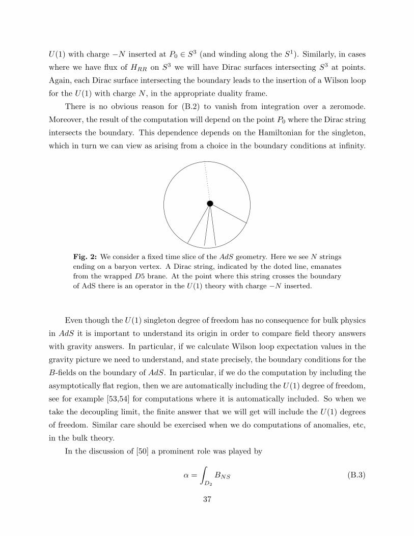
U(1) with charge −N inserted at P0 ∈ S3 (and winding along the S1). Similarly, in cases

where we have flux of HRR on S3 we will have Dirac surfaces intersecting S3 at points.

Again, each Dirac surface intersecting the boundary leads to the insertion of a Wilson loop

for the U(1) with charge N , in the appropriate duality frame.

There is no obvious reason for (B.2) to vanish from integration over a zeromode.

Moreover, the result of the computation will depend on the point P0 where the Dirac string

intersects the boundary. This dependence depends on the Hamiltonian for the singleton,

which in turn we can view as arising from a choice in the boundary conditions at infinity.

Fig. 2: We consider a fixed time slice of the AdS geometry. Here we see N strings

ending on a baryon vertex. A Dirac string, indicated by the doted line, emanates

from the wrapped D5 brane. At the point where this string crosses the boundary

of AdS there is an operator in the U(1) theory with charge −N inserted.

Even though the U(1) singleton degree of freedom has no consequence for bulk physics

in AdS it is important to understand its origin in order to compare field theory answers

with gravity answers. In particular, if we calculate Wilson loop expectation values in the

gravity picture we need to understand, and state precisely, the boundary conditions for the

B-fields on the boundary of AdS. In particular, if we do the computation by including the

asymptotically flat region, then we are automatically including the U(1) degree of freedom,

see for example [53,54] for computations where it is automatically included. So when we

take the decoupling limit, the finite answer that we will get will include the U(1) degrees

of freedom. Similar care should be exercised when we do computations of anomalies, etc,

in the bulk theory.

In the discussion of [50] a prominent role was played by

α =

∫

D2

BNS (B.3)

37

in cases where the five dimensional geometry was D2 × S3 or D2 × R3. It is important

to understand the field theory interpretation of this variable. Consider a Wilson line

W = Tr(Pe

∫

S1A

), we define α through W = |W |eiα. When we introduce this Wilson loop

operator in the path integral, via the AdS prescription, we indeed get a phase equal to (B.3).

The phase eiα depends on both the SU(N) degrees of freedom and on the U(1) degrees

of freedom. If we are considering an infinite volume system, the field theory on S1 × R3

for example, then α is fixed as a vev. In [50] the behaviour of various quantities under the

SU(N) dependence of α was studied. In particular, it was argued that α → α + 2π/N

should be a symmetry, but α → α + β should not be a symmetry for arbitrary β. If

we perform a gauge transformation on the B field that does not vanish at infinity we see

that we change α → α + β, and this is equivalent to introducing a Wilson line for the

singleton. In [50] these gauge transformations were not allowed so that the singleton mode

was effectively frozen to zero, so that only the dependence of the physical answers on the

SU(N) dependence of α were studied.

It is amusing to note that in the Klebanov-Witten [55] solution there is only one

obvious set of B fields with Chern Simons terms, the same we had above, and therefore

only one U(1). From the field theory point of view we could imagine starting with a

U(N) × U(N) theory so that we would naively expect two U(1)’s. The relative U(1) is

truly decoupled in the IR by the renormalization group flow while the overall U(1) is the

one we still see living at the boundary and coming from the B−fields in AdS. Baryons

that come from D3 branes in the bulk [56] are not charged under this overall U(1). The

question of whether the relative U(1) appears or not seems hard to answer.

What we have said above regarding the singleton mode in the case of AdS5 × S5, can

also be generalized to other dimensions. In the case of AdS7 × S4 there is a three form

potential C3 in seven dimensions with a coupling N4π

∫

AdS7C3 × dC3. This C3 leads to a

self dual two form on the boundary. In the AdS3 case, gauge fields in AdS3, with Chern

Simons couplings lead to chiral scalar fields on the boundary. In the AdS4 × S7 case all

modes living on the boundary are expected to be scalar fields and they should be modes

with SO(8) quantum numbers. It would be interesting to see them.

38

References

[1] R. Minasian and G. Moore,“K-Theory and Ramond-Ramond Charge,” JHEP 9711

:002, 1997; hep-th/9710230.

[2] E. Witten, “D-Branes And K-Theory,” JHEP 9812:019, 1998; hep-th/9810188.

[3] G. Moore and E. Witten, “Self-duality, RR fields and K-Theory,” hep-th/9912279.

[4] E. Witten, “On Flux Quantization in M -Theory and the Effective Action,” hep-

th/9609122; Journal of Geometry and Physics, 22 (1997) 1.

[5] J. Polchinski, “String theory”, Cambridge Univ. Press, 1998.

[6] G. T. Horowitz and A. Strominger, “Black strings and P-branes,” Nucl. Phys. B 360,

197 (1991).

[7] G.W. Gibbons and K. Maeda, “Black holes and membranes in higher dimensional

theories with dilaton fields,” Nucl.Phys.B298:741,1988

[8] J. M. Maldacena and C. Nunez, “Towards the large n limit of pure N = 1 super Yang

Mills,” Phys. Rev. Lett. 86, 588 (2001) [hep-th/0008001].

[9] I. R. Klebanov and M. J. Strassler, “Supergravity and a confining gauge theory: Du-

ality cascades and chiSB-resolution of naked singularities,” JHEP 0008, 052 (2000)

[hep-th/0007191].

[10] D.S. Freed and M.J. Hopkins, “On Ramond-Ramond fields and K-theory,” hep-

th/0002027 JHEP 0005 (2000) 044

[11] E. Diaconescu, G. Moore, and E. Witten, “E8 Gauge Theory, and a Derivation of

K-Theory from M -Theory,” hep-th/0005090

[12] D. Freed,“Dirac Charge Quantization and Generalized Differential Cohomology,” hep-

th/0011220

[13] C. Bachas, M. Douglas and C. Schweigert, “Flux stabilization of D-branes,” JHEP

0005, 048 (2000) [hep-th/0003037].

[14] J. Pawelczyk, “SU(2) WZW D-branes and their noncommutative geometry from

DBI action,” JHEP 0008, 006 (2000) [hep-th/0003057]; J. Pawelczyk and S. Rey,

“Ramond-Ramond flux stabilization of D-branes,” Phys. Lett. B 493, 395 (2000)

[hep-th/0007154].

[15] D. Marolf, “Chern-Simons terms and the three notions of charge,” hep-th/0006117

[16] J.M. Figeroa-O’Farrill and S. Stanciu, “D-brane charge, flux quantization and relative

(co)homology,” hep-th/0008038

[17] W. Taylor, “D2-branes in B fields,” JHEP 0007, 039 (2000) [hep-th/0004141].

[18] S. Gukov, “K-theory, reality, and orientifolds,” Commun. Math. Phys. 210, 621 (2000)

[hep-th/9901042].

[19] J. Lott, “R/Z Index Theory,” Comm. Anal. Geom. 2, p. 279

[20] J. Maldacena, G. Moore, and N. Seiberg, “D-brane instantons and K-theory charges,”

hep-th/0108100.

39

[21] J. A. Harvey and G. Moore, “Superpotentials and Membrane Instantons,” hep-

th/9907026; G. Moore, G. Peradze and N. Saulina, “Instabilities in heterotic M-

theory induced by open membrane instantons,” hep-th/0012104; E. Lima, B. Ovrut

and J. Park, “Five-brane superpotentials in heterotic M-theory,” hep-th/0102046.

[22] P. K. Townsend, “D-branes from M-branes,” Phys. Lett. B 373, 68 (1996) [hep-

th/9512062].

[23] A.M. Polyakov, PLB59 (1975)82; “Quark confinement and topology of gauge fields,”

Nucl. Phys. B120 (1977) 429 ; Gauge Fields and Strings Harwood Academic Publish-

ers, 1987, ch. 4

[24] R. Gregory, J. Harvey, and G. Moore, “Unwinding strings and T-duality of Kaluza-

Klein and H-Monopoles,” hep-th/970808; Adv.Theor.Math.Phys. 1 (1997) 283-297

[25] A. Sen, “Kaluza-Klein Dyons in String Theory,” hep-th/9705212, Phys.Rev.Lett. 79

(1997) 1619-1621; “Dynamics of Multiple Kaluza-Klein Monopoles in M- and String

Theory,” hep-th/9707042, Adv.Theor.Math.Phys. 1 (1998) 115-126

[26] M. Atiyah, K-theory, Addison-Wesley, 1989.

[27] E. Witten, “Baryons and Branes in Anti de Sitter Space, JHEP 9807 (1998) 006,

hep-th/9805112.

[28] J. Maldacena, “The large N limit of superconformal field theories and supergravity,”

Adv. Theor. Math. Phys. 2, 231 (1998) [Int. J. Theor. Phys. 38, 1113 (1998)] [hep-

th/9711200].

[29] J. Maldacena and A. Strominger, “AdS(3) black holes and a stringy exclusion princi-

ple,” JHEP 9812, 005 (1998) [hep-th/9804085].

[30] R. Dijkgraaf, “Instanton strings and hyperKaehler geometry,” Nucl. Phys. B 543, 545

(1999) [hep-th/9810210].

[31] J. Maldacena, G. Moore and A. Strominger, “Counting BPS black holes in toroidal

type II string theory,” hep-th/9903163.

[32] D. Kutasov and N. Seiberg, “More comments on string theory on AdS(3),” JHEP

9904, 008 (1999) [hep-th/9903219].

[33] N. Seiberg and E. Witten, “The D1/D5 system and singular CFT,” JHEP 9904, 017

(1999) [hep-th/9903224].

[34] F. Larsen and E. Martinec, “U(1) charges and moduli in the D1-D5 system,” JHEP

9906, 019 (1999) [hep-th/9905064].

[35] E. Witten, “Quantum field theory and the Jones polynomial,” Commun.Math.Phys.

121:351, 1989

[36] J. Cheeger and J. Simons, “Differential Characters and Geometric Invariants,” in

Geometry and Topology, J. Alexander and J. Harer eds., LNM 1167.

[37] K. Gawedzki, “Topological actions in two-dimensional quantum field theories,” in

Nonperturbative quantum field theory Procedings of the 1987 Cargese meeting, pp.

101-141.

40

[38] R. Dijkgraaf and E. Witten, “Topological gauge theories and group cohomology,”

Commun.Math.Phys.129:393,1990

[39] M. Hopkins and I.M. Singer, unpublished, but to appear.

[40] E. Witten, “AdS/CFT Correspondence and Topological Field Theory”,

JHEP 9812 (1998) 012, hep-th/98120112.

[41] B. Harris, “Differential Characters and the Abel-Jacobi Map”, in Algebraic K-theory:

Connections with Geometry and Topology, J.F. Jardine and V.P. Snaith eds., Nato ASI

Series C: Mathematical and Physical Sciences – Vol. 279, Kluwer Academic Publishers,

1989.

[42] R. Zucchini, “Relative topological integrals and relative Cheeger-Simons differential

characters,” hep-th/0010110

[43] E. Witten, “Five-Brane Effective Action In M -Theory”, J. Geom. Phys. 22 (1997)

103, hep-th/9610234.

[44] E. Witten, “Duality relations among topological effects in string theory,” JHEP 0005,

031 (2000) [hep-th/9912086].

[45] E. Diaconescu and G. Moore, unpublished.

[46] S. Elitzur, G. Moore, A. Schwimmer and N. Seiberg, “Remarks On The Canonical

Quantization Of The Chern-Simons-Witten Theory,” Nucl. Phys. B 326, 108 (1989).

[47] J. H. Schwarz and A. Sen, “Duality symmetric actions,” Nucl. Phys. B 411, 35 (1994)

[hep-th/9304154].

[48] O. Aharony, S. S. Gubser, J. Maldacena, H. Ooguri and Y. Oz, “Large N field theories,

string theory and gravity,” Phys. Rept. 323, 183 (2000) [hep-th/9905111].

[49] E. Witten, “Anti-de Sitter space and holography,” Adv. Theor. Math. Phys. 2, 253

(1998) [hep-th/9802150].

[50] O. Aharony and E. Witten, “Anti-de Sitter space and the center of the gauge group,”

JHEP 9811, 018 (1998) [hep-th/9807205].

[51] J. Maldacena, “Wilson loops in large N field theorieds,” Phys. Rev. Lett. 80(1998)

4859; hep-th/9803002

[52] S.-J. Rey and J. Yee, “Macroscopic strings as heavy quarks in large N gauge theories

and Anti-de Sitter supergravity,” hep-th/9803001

[53] A. Bilal and C. Chu, “Testing the AdS/CFT correspondence beyond large N,” hep-

th/0003129.

[54] M. Marino and C. Vafa, “Framed knots at large N” hep-th/0108064.

[55] I. R. Klebanov and E. Witten, “Superconformal field theory on threebranes at a

Calabi-Yau singularity,” Nucl. Phys. B 536, 199 (1998) [hep-th/9807080].

[56] S. S. Gubser and I. R. Klebanov, “Baryons and domain walls in an N = 1 supercon-

formal gauge theory,” Phys. Rev. D 58, 125025 (1998) [hep-th/9808075].

41