arX

iv:h

ep-p

h/00

0108

3v2

24

Jan

2000

FTUAM-2000/001; IFT-UAM/CSIC-00-02, DAMTP-2000-001

hep-th/0001083

A D-brane Alternative to the MSSM

G. Aldazabal1, L. E. Ibanez2 and F. Quevedo3

1 Instituto Balseiro, CNEA, Centro Atomico Bariloche,

8400 S.C. de Bariloche, and CONICET, Argentina.

2 Departamento de Fısica Teorica C-XI and Instituto de Fısica Teorica C-XVI,

Universidad Autonoma de Madrid, Cantoblanco, 28049 Madrid, Spain.

3 D.A.M.T.P., Wilberforce Road, Cambridge, CB3 0WA, England.

Abstract

The success of SU(5)-like gauge coupling unification boundary conditions g23 =

g22 = 5/3g2

1 has biased most attempts to embed the SM interactions into a uni-

fied structure. After discussing the limitations of the orthodox approach, we

propose an alternative that appears to be quite naturally implied by recent de-

velopments based on D-brane physics. In this new alternative: 1) The gauge

group, above a scale of order 1 TeV, is the minimal left-right symmetric exten-

sion SU(3)×SU(2)L ×SU(2)R ×U(1)B−L of the SM; 2) Quarks, leptons and Higgs

fields come in three generations; 3) Couplings unify at an intermediate string scale

Ms = 9 × 1011 GeV with boundary conditions g23 = g2

L = g2R = 32/3 g2

B−L. This

corresponds to the natural embedding of gauge interactions into D-branes and is

different from the standard SO(10) embedding which corresponds to kB−L = 8/3.

Unification only works in the case of three generations; 4) Proton stability is au-

tomatic due to the presence of Z2 discrete R-parity and lepton parities. A specific

Type IIB string orientifold model with the above characteristics is constructed. The

existence of three generations is directly related to the existence of three complex

extra dimensions. In this model the string scale can be identified with the intermedi-

ate scale and SUSY is broken also at that scale due to the presence of anti-branes in

the vacuum. We discuss a number of phenomenological issues in this model includ-

ing Yukawa couplings and a built-in axion solution to the strong-CP problem. The

present framework could be tested by future accelerators by finding the left-right

symmetric extension of the SM at a scale of order 1 TeV.

1 Introduction

The success of coupling unification extrapolations based on the massless spectrum of

the MSSM has greatly conditioned the search for a realistic string vacuum. This search

has been shaped, to a great extent, by the fact that SM couplings seem to join at a

scale MX = 2 × 1016 GeV, not far from the Planck mass Mp and by the necessity

of identifying the string scale Ms essentially with the Planck scale in heterotic model

building.

In this situation, it appears natural to look for perturbative heterotic vacua in

which, below a scale of order MX , essentially only the MSSM remains.

Recent p-brane developments have changed our view of the possible ways to embed

SM physics into string theory. To start with, it has been realized that the string/M-

theory scale may be much below the Planck and unification scales [1, 2, 3, 4, 5, 6, 7,

8, 9, 10, 11, 12]. This is because in the presence of p-branes (like D-branes in Type II

and Type I string theory) gauge interactions can be localized in the world-volume of

D-branes (e.g., a 3-brane), whereas gravitational interactions in general live in the full

ten (or eleven) dimensions. Then the largeness of the Planck mass may be obtained

even if Ms << Mp if there are large compact dimensions.

Now, if Ms << MX , gauge coupling unification should in principle take place at

the string scale Ms and thus the nice unification of MSSM couplings is lost. Of course,

this unification problem appearing for string models if Ms << MX , could be taken as

an argument against them. However, we think that we should first try to answer the

following question: Is there any simple alternative framework which is consistent with

unification at a string scale Ms << MX ? After all, the MSSM+big desert orthodoxy

is not free of problems. In fact, some unattractive features of the standard scenario are

the following:

i) The quark/lepton generations come in three chiral copies whereas the Higgs fields

come only in one copy and are non-chiral. The fact that there is a single Higgs set is cru-

cial to obtain correct unification predictions. This asymmetry among quarks/leptons

on one side and Higgs fields on the other looks quite ad hoc.

ii) The MSSM needs to be supplemented by additional symmetries like R-parity in

order to ensure proton stability from dimension four operators. It also needs additional

symmetries beyond R-parity to get stability against dimension five operators.

iii) To obtain a viable heterotic string unification, whose massless sector is just the

MSSM and includes the above symmetries, turns out to be a very difficult task, if not

impossible. All the models studied up to now require a complicated study of possible

1

scalar flat directions and only very particular ones lead to something of that sort [13] .

The reason why dynamics should prefer such vacua with only one set of Higgsses and

built-in discrete symmetries to suppress too fast proton decay is unclear.

Given the above limitations of the orthodox approach, it seems sensible to look

for (if possible, elegant) alternatives. But to be really competitive with the MSSM

scenario such alternatives need to 1) improve some of the above problematic aspects

of the standard scenario and 2) have a nice and consistent unification of coupling

constants. By the latter we mean that couplings unify at the string scale without

forcing the structure of the model by adding, for instance, unjustified extra mass scales

or ad-hoc extra massless particles.

In the present paper we want to propose such an alternative to the standard MSSM+

big desert scenario. We propose that above a scale of order 1 TeV or so, the gauge

group is that of the minimal left-right symmetric extension of the supersymmetric

standard model, i.e.,SU(3) × SU(2)L × SU(2)R × U(1)B−L [14, 15, 16]. In addition

all quarks, leptons and Higgs fields come in three generations. Interestingly enough,

this simple structure leads to very precise unification of gauge coupling constants at

an intermediate scale of order 1012 GeV as long as the normalization of the U(1)B−L

coupling is the one expected if such gauge group is associated to a collection of D-

branes. It is important to remark that this normalization differs from the one predicted

by standard GUT left-right symmetric scenarios like SO(10).

We also construct an explicit Type IIB orientifold string compactification leading to

the desired massless spectrum and normalization of coupling constants. In this model

there is a simple explanation for the family replication: there are three quark-lepton

generations because there are three complex compact dimensions and an underlying

Z3 orbifold. These features resemble the first three-generation perturbative heterotic

string models built, those of ref.[17]. Furthermore, this model has the interesting prop-

erty of having natural discrete symmetries including R-parity and Z2 lepton numbers.

Thus guaranteeing in a natural way the stability of the proton, although allowing for

other baryon number violation processes, such as neutron-antineutron oscillations, suf-

ficiantly suppressed to be consistent with current experimental bounds. Finally, the

structure of the model allows for candidate axion fields with the right couplings to

gauge fields needed to solve the strong CP problem.

The structure of this paper is as follows. In chapter 2 we present this alternative

scenario which we call D-brane left-right symmetric model. We also discuss the uni-

fication of coupling constants and show how, if this model is correct, new Z’ and W ’

2

gauge bosons corresponding to left-right symmetry should be found at future or present

colliders. In chapter 3 we present a particular Type IIB orientifold model realizing the

above scenario and study the cancellation of U(1) anomalies and generation of Fayet-

Iliopoulos terms. In this realization the unification scale is identified with a string

scale Ms ∝ 1012 GeV. The model has also some anti-branes in the bulk which provide

for hidden-sector supersymmetry breaking at the same scale of order Ms. We study

a number of phenomenological issues of this particular orientifold model in chapter 4.

This includes some aspects of the structure of Yukawa couplings, SU(2)R × U(1)B−L

symmetry breaking and the presence of natural candidates for invisible axions. In

chapter 5 we present an outlook and some final comments.

2 The D-brane left-right symmetric model and cou-

pling unification

As we discussed above, it has become recently clear that the string scale could well

be much below the Planck mass. But, is there any indication or advantage from a

lowered string scale? A particularly interesting alternative to the unification at MX

close to the Planck scale is getting unification close to the geometric intermediate scale

MI =√

MWMp. Indeed, if the string scale is of order Ms =∝ MI , gauge couplings

should unify at that scale. Now, as argued in ref.[10] , if there are non supersymmetric

brane configurations, the scale of supersymmetry breaking would also be of order of

Ms = MI . This is interesting because hidden sector supersymmetry breaking models

also need to have SUSY-breaking at the intermediate scale. Thus in this case the

string, unification and SUSY-braking scales would be one and the same.

We would like to argue in what follows that the intermediate scale idea is equally

good than the standard one in what concerns coupling unification, at least for a model

with the following structure:

i) The gauge group above a L-R symmetric scale MR slightly above the weak scale

is the minimal left-right symmetric extension of the SM: SU(3)× SU(2)L × SU(2)R ×U(1)B−L.

ii) All quarks, leptons and Higgs fields come in three generations. Thus the chi-

ral multiplet content is three copies of (3, 2, 1, 1/3) + (3, 1, 2,−1/3) +(1, 2, 1,−1) +

(1, 1, 2,+1) +(1, 2, 2, 0).

iii) The boundary conditions at the unification (i.e,.string) scale are g23 = g2

L = g2R =

32/3g2B−L. This corresponds to a weak angle with sin2θ(Ms) = 3/14 = 0.215.

3

In a model with the above characteristics one finds that gauge couplings naturally

unify at a scale of order the intermediate scale Ms ∝ 1012 GeV as long as the left-

right scale MR is not far from the weak scale MW . An important point to remark

is that the unification boundary conditions are different from those found in GUT

schemes. Indeed in SO(10)-like schemes the boundary conditions at unification are

g23 = g2

L = g2R = 8/3g2

B−L yielding the canonical sin2θW = 3/8. A remarkable point we

find is that the new boundary conditions we are proposing are precisely the ones which

are natural from the point of view of the embedding of the gauge group in a D-brane

scheme.

Let us discuss in some more detail how coupling unification takes place. The above

mentioned boundary conditions g23 = g2

L = g2R = 32/3g2

B−L have a simple group theo-

retical interpretation. They correspond to the embedding of the left-right symmetric

gauge group into a non-semisimple structure:

U(3) × U(2)L × U(2)R (2.1)

with unified coupling constants g23 = g2

L = g2R at some mass scale (to be identified later

on with the string scale Ms ). This is in fact the structure one gets in models with

gauge groups living on D-branes, as we will discuss in the specific string model below.

As we said, the model contain three identical generations under U(3)×U(2)L ×U(2)R

with quantum numbers (3, 2, 1)(1,−1,0) + (3, 1, 2)(−1,0,1) +(1, 2, 1)(0,−1,0) + (1, 1, 2)(0,0,1)

+(1, 2, 2)(0,1,−1), where the subindices denote the charges with respect to the three

U(1)’s. We denote the U(1) generators by Q3, QL and QR respectively. It is easy to

check that two of them are anomalous and only one of them, the linear combination

QB−L = −2

3Q3 − QL − QR (2.2)

is anomaly free 1 . This is just the familiar (B − L) of left-right symmetric models

which is related to weak hypercharge by Y = −T 3R + QB−L/2. Now, notice that, if

we normalize the original U(n) generators in the fundamental representation Ta to

TrT 2a = 1, the normalization of the U(1)’s are TrQ2

3 = 3, TrQ2L = TrQ2

R = 2. Then,

the normalization of U(1)B−L compared to that of the non-Abelian generators is kB−L =

2TrQ2B−L = 32/3, as remarked above. Notice this implies a hypercharge normalization

k1 = kR + 1/4kB−L = 11/3, and hence a tree level weak angle sin2θW = 3/14 = 0.214.

Let us study now the one-loop corrections to the couplings. In between the scales

MR and Ms the gauge group is SU(3) × SU(2)L × SU(2)R × U(1)B−L and the above1In string theory the other two (anomalous) U(1)’s become massive and decouple due to a gener-

alized Green-Schwarz mechanism. See the discussion in chapter 3.

4

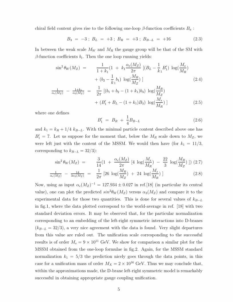
chiral field content gives rise to the following one-loop β-function coefficients Ba :

B3 = −3 ; BL = +3 ; BR = +3 ; BB−L = +16 (2.3)

In between the weak scale MW and MR the gauge group will be that of the SM with

β-function coefficients bi. Then the one loop running yields:

sin2 θW (MZ) =1

1 + k1(1 + k1

αe(MZ)

2π[(BL − 1

k 1B′

1) log(Ms

MR)

+ (b2 −1

k 1b1) log(

MR

MZ) ] (2.4)

1αe(MZ )

− 1+k1

α3(MZ )=

1

2π[(b1 + b2 − (1 + k1)b3) log(

MR

MZ)

+ (B′

1 +BL − (1 + k1)B3) log(Ms

MR) ] (2.5)

where one defines

B′

1 = BR +1

4BB−L (2.6)

and k1 = kR + 1/4 kB−L. With the minimal particle content described above one has

B′

1 = 7. Let us suppose for the moment that, below the MR scale down to MZ , we

were left just with the content of the MSSM. We would then have (for k1 = 11/3,

corresponding to kB−L = 32/3):

sin2 θW (MZ) =3

14(1 +

αe(MZ)

2π[4 log(

Ms

MR

) − 22

3log(

MR

MZ

) ]) (2.7)

1αe(MZ)

− 143α3(MZ )

=1

2π[26 log(

MR

MZ

) + 24 log(Ms

MR

) ] (2.8)

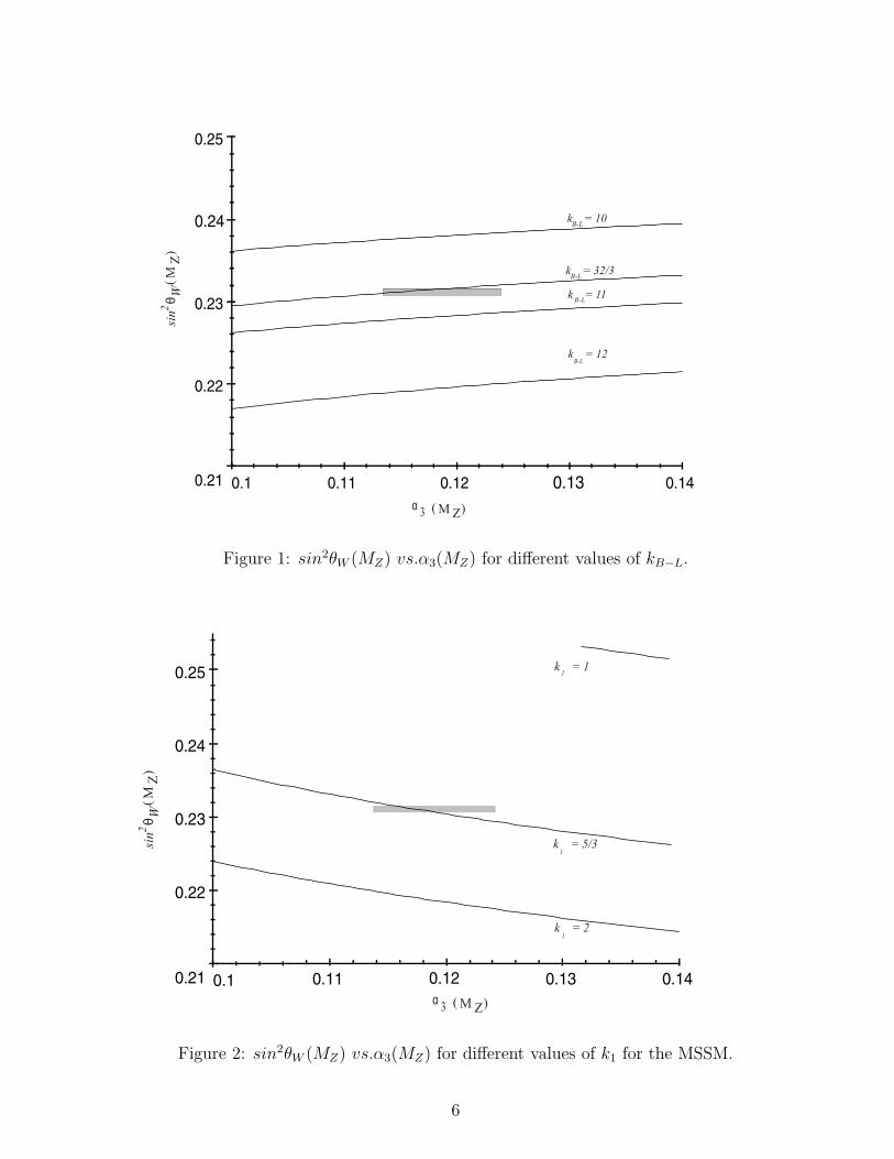
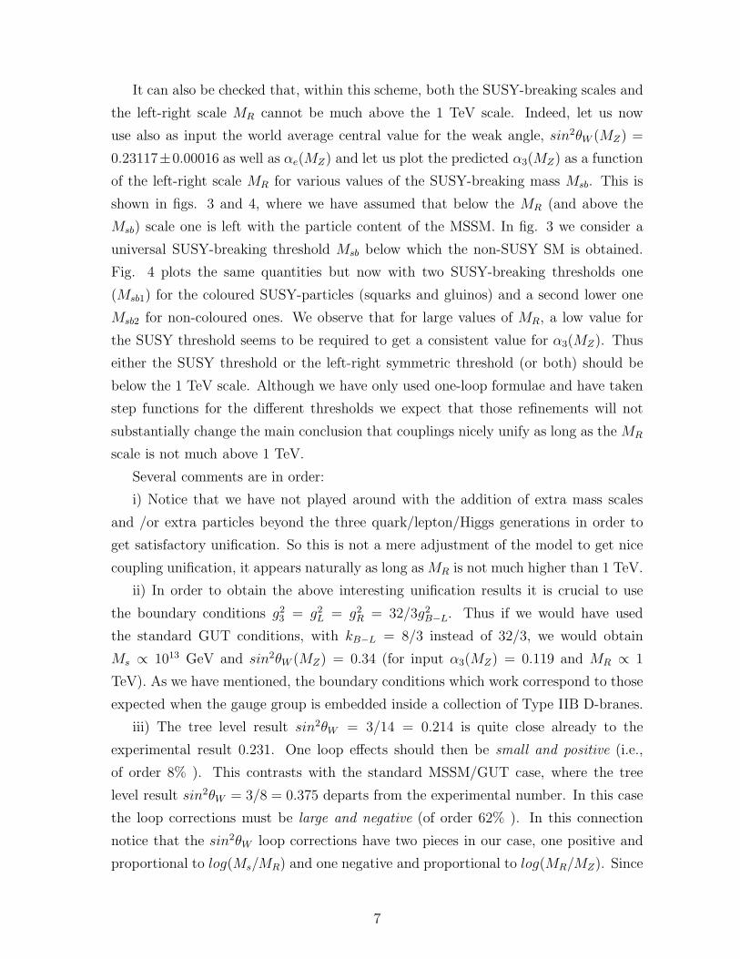
Now, using as input αe(MZ)−1 = 127.934 ± 0.027 in ref.[18] (in particular its central

value), one can plot the predicted sin2θW (MZ) versus α3(MZ) and compare it to the

experimental data for those two quantities. This is done for several values of kB−L

in fig.1, where the data plotted correspond to the world-average in ref. [18] with two

standard deviation errors. It may be observed that, for the particular normalization

corresponding to an embedding of the left-right symmetric interactions into D-branes

(kB−L = 32/3), a very nice agreement with the data is found. Very slight departures

from this value are ruled out. The unification scale corresponding to the successful

results is of order Ms = 9 × 1011 GeV. We show for comparison a similar plot for the

MSSM obtained from the one-loop formulae in fig.2. Again, for the MSSM standard

normalization k1 = 5/3 the prediction nicely goes through the data points, in this

case for a unification mass of order MX = 2 × 1016 GeV. Thus we may conclude that,

within the approximations made, the D-brane left-right symmetric model is remarkably

successful in obtaining appropriate gauge coupling unification.

5

0.140.130.120.110.1

0.25

0.24

0.23

0.22

0.21

k = 12B-L

α 3 M Z ( )

MZ

()

sin θ

W2

B-Lk = 11B-Lk = 32/3

B-Lk = 10

Figure 1: sin2θW (MZ) vs.α3(MZ) for different values of kB−L.

0.140.130.120.11

k = 21

k = 5/31

k = 11

0.1

0.25

0.24

0.23

0.22

0.21

MZ

()

sin θ

W2

α 3 M Z ( )

Figure 2: sin2θW (MZ) vs.α3(MZ) for different values of k1 for the MSSM.

6

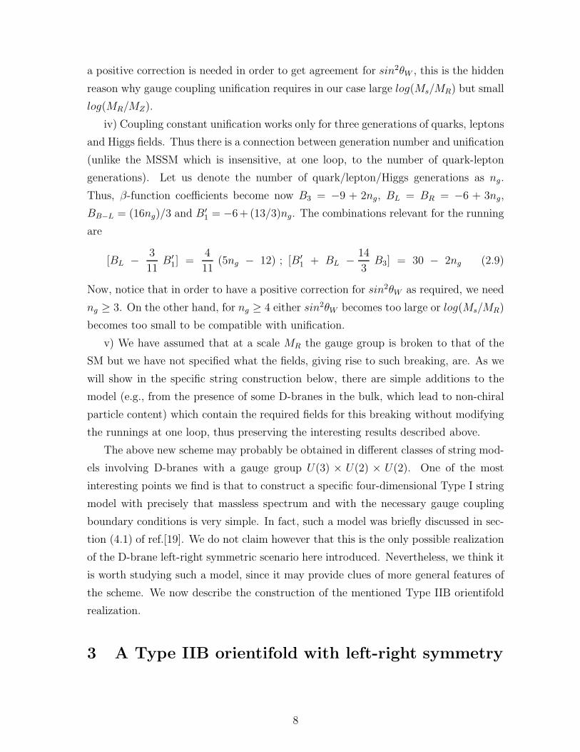
It can also be checked that, within this scheme, both the SUSY-breaking scales and

the left-right scale MR cannot be much above the 1 TeV scale. Indeed, let us now

use also as input the world average central value for the weak angle, sin2θW (MZ) =

0.23117±0.00016 as well as αe(MZ) and let us plot the predicted α3(MZ) as a function

of the left-right scale MR for various values of the SUSY-breaking mass Msb. This is

shown in figs. 3 and 4, where we have assumed that below the MR (and above the

Msb) scale one is left with the particle content of the MSSM. In fig. 3 we consider a

universal SUSY-breaking threshold Msb below which the non-SUSY SM is obtained.

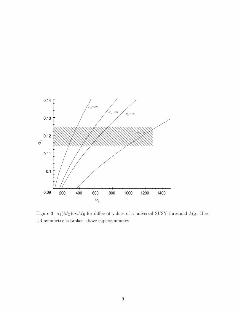
Fig. 4 plots the same quantities but now with two SUSY-breaking thresholds one

(Msb1) for the coloured SUSY-particles (squarks and gluinos) and a second lower one

Msb2 for non-coloured ones. We observe that for large values of MR, a low value for

the SUSY threshold seems to be required to get a consistent value for α3(MZ). Thus

either the SUSY threshold or the left-right symmetric threshold (or both) should be

below the 1 TeV scale. Although we have only used one-loop formulae and have taken

step functions for the different thresholds we expect that those refinements will not

substantially change the main conclusion that couplings nicely unify as long as the MR

scale is not much above 1 TeV.

Several comments are in order:

i) Notice that we have not played around with the addition of extra mass scales

and /or extra particles beyond the three quark/lepton/Higgs generations in order to

get satisfactory unification. So this is not a mere adjustment of the model to get nice

coupling unification, it appears naturally as long as MR is not much higher than 1 TeV.

ii) In order to obtain the above interesting unification results it is crucial to use

the boundary conditions g23 = g2

L = g2R = 32/3g2

B−L. Thus if we would have used

the standard GUT conditions, with kB−L = 8/3 instead of 32/3, we would obtain

Ms ∝ 1013 GeV and sin2θW (MZ) = 0.34 (for input α3(MZ) = 0.119 and MR ∝ 1

TeV). As we have mentioned, the boundary conditions which work correspond to those

expected when the gauge group is embedded inside a collection of Type IIB D-branes.

iii) The tree level result sin2θW = 3/14 = 0.214 is quite close already to the

experimental result 0.231. One loop effects should then be small and positive (i.e.,

of order 8% ). This contrasts with the standard MSSM/GUT case, where the tree

level result sin2θW = 3/8 = 0.375 departs from the experimental number. In this case

the loop corrections must be large and negative (of order 62% ). In this connection

notice that the sin2θW loop corrections have two pieces in our case, one positive and

proportional to log(Ms/MR) and one negative and proportional to log(MR/MZ). Since

7

a positive correction is needed in order to get agreement for sin2θW , this is the hidden

reason why gauge coupling unification requires in our case large log(Ms/MR) but small

log(MR/MZ).

iv) Coupling constant unification works only for three generations of quarks, leptons

and Higgs fields. Thus there is a connection between generation number and unification

(unlike the MSSM which is insensitive, at one loop, to the number of quark-lepton

generations). Let us denote the number of quark/lepton/Higgs generations as ng.

Thus, β-function coefficients become now B3 = −9 + 2ng, BL = BR = −6 + 3ng,

BB−L = (16ng)/3 and B′

1 = −6+ (13/3)ng. The combinations relevant for the running

are

[BL − 3

11B′

1] =4

11(5ng − 12) ; [B′

1 + BL − 14

3B3] = 30 − 2ng (2.9)

Now, notice that in order to have a positive correction for sin2θW as required, we need

ng ≥ 3. On the other hand, for ng ≥ 4 either sin2θW becomes too large or log(Ms/MR)

becomes too small to be compatible with unification.

v) We have assumed that at a scale MR the gauge group is broken to that of the

SM but we have not specified what the fields, giving rise to such breaking, are. As we

will show in the specific string construction below, there are simple additions to the

model (e.g., from the presence of some D-branes in the bulk, which lead to non-chiral

particle content) which contain the required fields for this breaking without modifying

the runnings at one loop, thus preserving the interesting results described above.

The above new scheme may probably be obtained in different classes of string mod-

els involving D-branes with a gauge group U(3) × U(2) × U(2). One of the most

interesting points we find is that to construct a specific four-dimensional Type I string

model with precisely that massless spectrum and with the necessary gauge coupling

boundary conditions is very simple. In fact, such a model was briefly discussed in sec-

tion (4.1) of ref.[19]. We do not claim however that this is the only possible realization

of the D-brane left-right symmetric scenario here introduced. Nevertheless, we think it

is worth studying such a model, since it may provide clues of more general features of

the scheme. We now describe the construction of the mentioned Type IIB orientifold

realization.

3 A Type IIB orientifold with left-right symmetry

8

140012001000800600400200

0.14

0.13

0.12

0.11

0.1

0.09

M = 90sb

M = 300sb

M = 150sb

3α

MR

M = 200sb

Figure 3: α3(MZ)vs.MR for different values of a universal SUSY-threshold Msb. Here

LR symmetry is broken above supersymmetry

9

140012001000800600400200

0.14

0.13

0.12

0.11

0.1

0.09

α 3

MR

M = 100sb 1

M = 300sb 1

M = 500sb 1

M = 800sb 1

Figure 4: α3(MZ)vs.MR for a non-colored SUSY particle threshold Msb2 = 100 and

different values of a coloured SUSY threshold Msb1.

10

3.1 The LR orientifold model

The model we are interested in is a Z3 Type IIB orientifold with both D-branes and

anti -D-branes. A general discussion of such kind of models is given in Ref. [20, 19]

where we refer the reader for notation and details of the construction 2. Here we only

present a brief description in order to settle the general framework.

A Z3 Type IIB orbifold, in four dimensions [22], is obtained by dividing closed Type

IIB string theory compactified on a six dimensional torus T 6, by the discrete symmetry

group Z3. The orientifold model is obtained by further dividing the orbifoldized string

by world sheet orientation reversal symmetry [23]. The twist eigenvalues, associated

to complex coordinates Ya a = 0, 1, 2 are chosen as v = 13(1, 1,−2) in order to leave

N = 1 supersymmetry in four dimensions.

The general picture is that the above procedure leads to a Klein-Bottle unoriented

world sheet. Amplitudes computed on such a surface contain unphysical tadpole like

divergences which can be interpreted as unbalanced charges carried by RR form poten-

tials. Thus, in order to cancel such divergences, D9-branes, carrying opposite charges

must be introduced. Moreover, D5-branes and anti-D5-branes can be consistently in-

cluded. Even if they are not required (in this Z3 case) for tadpole cancellation, they

open the way for achieving interesting supersymmetry breaking patterns and at the

same time provide new possibilities for model building.

Let us be more explicit. An open string state is denoted by |Ψ, ab〉λpqab where Ψ refers

to world-sheet degrees of freedom whereas a, b are Chan-Paton indices associated to the

open string endpoints lying on Dp-branes and Dq-branes respectively [22, 24, 25] . λpq is

the Chan-Paton, hermitian matrix, containing the gauge group structure information.

Analogously, λpq (λpq) is introduced for open strings ending at Dp, Dq-antibranes ( Dp

antibrane, Dq-brane, etc.).

The Z3 action (denoted by θ) that twists the internal complex coordinates has

a corresponding action on Chan Paton matrices represented by unitary matrix γθ,p,

namely θ : λpq → γθ,pλpqγ−1

θ,q . Moreover, Wilson lines, wrapping along internal tori

directions can also be included and also have a matrix representation when acting on

Chan-Paton factors.

Consistency under group algebra operations and the requirement of cancellation of

RR tadpoles leads to constraints on the possible twist matrices. Tadpole cancellation,

in the Z3 case we are discussing, imposes the number of nine branes to be 32 and

the requirement that the number of D5-branes and anti-D5-branes must be equal.

2For other constructions involving anti-branes see [21]

11

Moreover, cancellation of twisted tadpoles requires

Tr (W)aγθ,9 + 3(Tr γθ,5,a,i − Tr γθ,5,a,i) = −4 (3.1)

for a = 0, 1, 2.

Here we have allowed for the possibility of having a Wilson line, represented by the

matrix W on Chan -Paton matrices, wrapping along the direction e1. We denote with

a, i with a, i = 0, 1, 2 the nine orbifold fixed points in the first and second complex

planes. For a given a, i = 0, 1, 2 label the subset of fixed points that feels the twist

(W)aγθ,9.

Generic solutions to these equations are discussed in [19]. Here we consider the

specific model characterized by γθ,9 = (γθ,9, γ∗

θ,9), and W = (W, W∗) where ∗ denotes

the complex conjugate and

γθ,9 = diag (αI3, α2I2, I2, I2, αI7) (3.2)

W = diag (I3, I2, I2, I2, I7) (3.3)

Also,

γθ,5,2,i = diag (α, α2) (3.4)

where α = e2iπ/3.

It can be easily checked that such a choice satisfies the tadpole cancellation con-

straint 3.1. Notice that there are two 5-branes (Tr γθ,5,2,i = −1) stuck at each of the

three fixed points of the type (2, i) ≡ (−1, i). The effective twist is thus W−1γθ,9.

There are no 5-branes at the other six fixed points (Tr (γθ,9) = Tr (W)γθ,9 = −4).

Since we must have the same number of branes and antibranes, six anti-5-branes must

be present in the bulk.

It is always possible to add an extra Wilson line in the third complex plane in such

a way that anti-brane sector is gauge decoupled from the 9, 5-branes sectors. In this

way, anti-branes in the bulk, which lead to a non-supersymmetric spectrum, provide

a“hidden sector” which will transmit supersymmetry breaking through gravitational

interactions to the “observable” brane sector. An alternative description of such a

decoupling situation can be achieved by performing a T-duality transformation in the

third complex dimension. Thus, 9-branes become 7-branes located at the origin (Y3 =

0) in the third complex plane with their world volume including the first two complex

planes. 5-branes (antibranes) turn into 3-branes (antibranes) which can be located

12

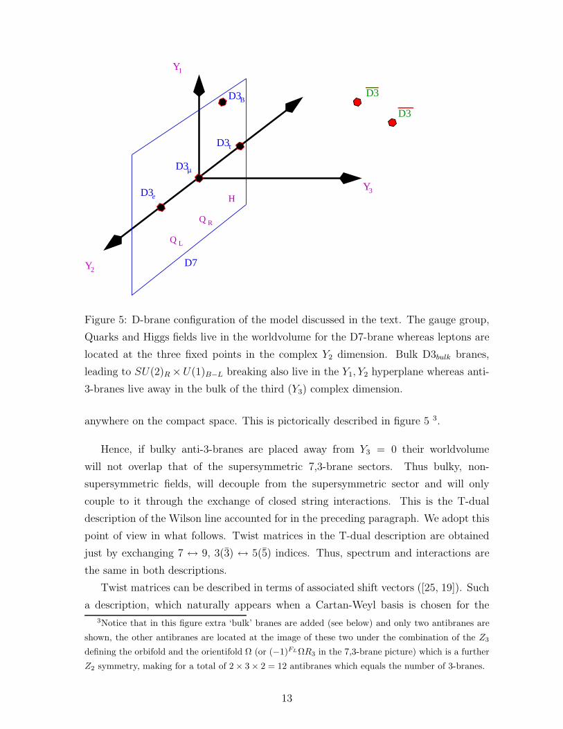
Y D7

D3

D3

D3

D3 D3

D3

Y3

2

e

µ

τ

Q

Q

H

L

R

Y1

B

Figure 5: D-brane configuration of the model discussed in the text. The gauge group,

Quarks and Higgs fields live in the worldvolume for the D7-brane whereas leptons are

located at the three fixed points in the complex Y2 dimension. Bulk D3bulk branes,

leading to SU(2)R ×U(1)B−L breaking also live in the Y1, Y2 hyperplane whereas anti-

3-branes live away in the bulk of the third (Y3) complex dimension.

anywhere on the compact space. This is pictorically described in figure 5 3.

Hence, if bulky anti-3-branes are placed away from Y3 = 0 their worldvolume

will not overlap that of the supersymmetric 7,3-brane sectors. Thus bulky, non-

supersymmetric fields, will decouple from the supersymmetric sector and will only

couple to it through the exchange of closed string interactions. This is the T-dual

description of the Wilson line accounted for in the preceding paragraph. We adopt this

point of view in what follows. Twist matrices in the T-dual description are obtained

just by exchanging 7 ↔ 9, 3(3) ↔ 5(5) indices. Thus, spectrum and interactions are

the same in both descriptions.

Twist matrices can be described in terms of associated shift vectors ([25, 19]). Such

a description, which naturally appears when a Cartan-Weyl basis is chosen for the

3Notice that in this figure extra ‘bulk’ branes are added (see below) and only two antibranes are

shown, the other antibranes are located at the image of these two under the combination of the Z3

defining the orbifold and the orientifold Ω (or (−1)FLΩR3 in the 7,3-brane picture) which is a further

Z2 symmetry, making for a total of 2 × 3 × 2 = 12 antibranes which equals the number of 3-branes.

13

group algebra, is especially adapted for computing the spectrum [25, 19]. Thus, twist

matrices above (now for 7,3-branes) correspond to

V7 =1

3(1, 1, 1;−1,−1; 0, 0; 0, 0; 1, 1, 1, 1, 1, 1, 1) (3.5)

W =1

3(1, 1, 1; 1, 1; 1, 1; 0, 0; 0, 0, 0, 0, 0, 0, 0) (3.6)

and simply V3,(2,i) = 13

for matrices in 3.4.

We then have for (W)γθ,9 and W−1γθ,9

V7 +W =1

3(2, 2, 2; 0, 0; 1, 1; 0, 0; 1, 1, 1, 1, 1, 1, 1) (3.7)

V7 −W =1

3(0, 0, 0; 1, 1; 2, 2; 0, 0; 1, 1, 1, 1, 1, 1, 1) (3.8)

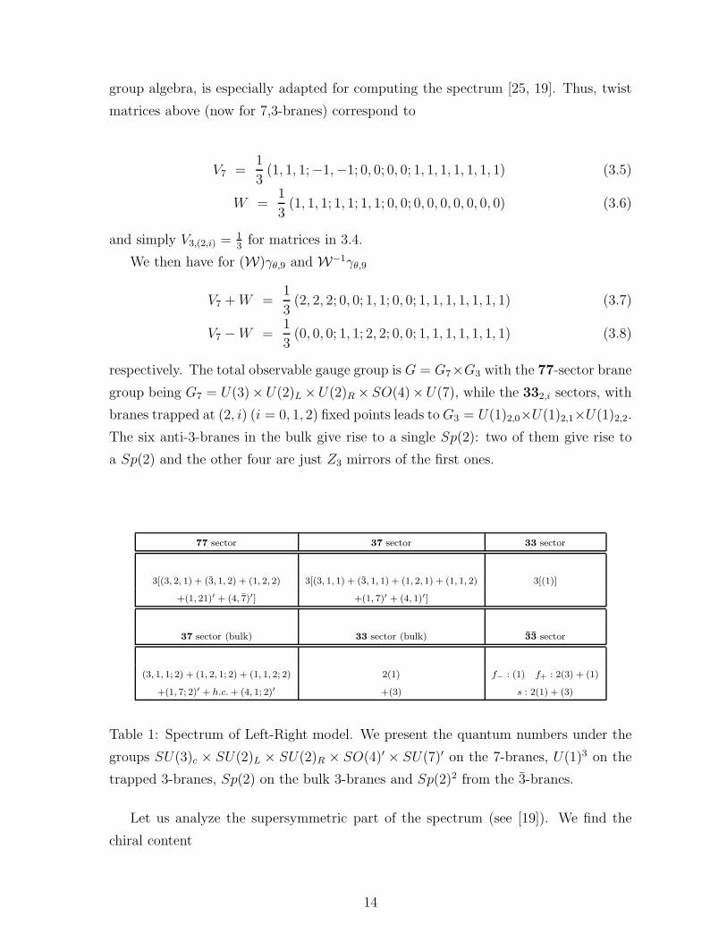
respectively. The total observable gauge group is G = G7×G3 with the 77-sector brane

group being G7 = U(3)×U(2)L ×U(2)R × SO(4)×U(7), while the 332,i sectors, with

branes trapped at (2, i) (i = 0, 1, 2) fixed points leads toG3 = U(1)2,0×U(1)2,1×U(1)2,2.

The six anti-3-branes in the bulk give rise to a single Sp(2): two of them give rise to

a Sp(2) and the other four are just Z3 mirrors of the first ones.

77 sector 37 sector 33 sector

3[(3, 2, 1) + (3, 1, 2) + (1, 2, 2) 3[(3, 1, 1) + (3, 1, 1) + (1, 2, 1) + (1, 1, 2) 3[(1)]

+(1, 21)′ + (4, 7)′] +(1, 7)′ + (4, 1)′]

37 sector (bulk) 33 sector (bulk) 33 sector

(3, 1, 1; 2) + (1, 2, 1; 2) + (1, 1, 2; 2) 2(1) f− : (1) f+ : 2(3) + (1)

+(1, 7; 2)′ + h.c. + (4, 1; 2)′ +(3) s : 2(1) + (3)

Table 1: Spectrum of Left-Right model. We present the quantum numbers under the

groups SU(3)c × SU(2)L × SU(2)R × SO(4)′ × SU(7)′ on the 7-branes, U(1)3 on the

trapped 3-branes, Sp(2) on the bulk 3-branes and Sp(2)2 from the 3-branes.

Let us analyze the supersymmetric part of the spectrum (see [19]). We find the

chiral content

14

77sector : (3.9)

3[(3, 2, 1, 1/3 ) + (3, 1, 2,−1/3 ) + (1, 2, 2, 0 )] + 3[(1, 21 )′ + (4, 7 )′]

where we have indicated the representations under the Left-Right groupGLR = SU(3)×SU(2)L × SU(2)R × U(1)B−L and G′ = SO(4)′ × U(7)′. The Abelian factor U(1)B−L

is generated by QB−L = −23Q3 −QL −QR introduced in 2.2 where Q3, QL, QR are the

generators of the Abelian factor in the corresponding unitary groups. As mentioned,

QB−L is identified with B − L symmetry generator and it can be shown (see next sec-

tion) to be non anomalous. The Standard Model hypercharge Y and electromagnetic

charge are thus obtained as

Y =QB−L

2− T 3

R (3.10)

Qem = Y + T 3L (3.11)

where T 3R,L are the diagonal generators of SU(2)R,L.

We observe that the 77 sector contains the standard three quark generations plus

a set of three chiral Higgs fields (1, 2, 2, 0). The factor three here is associated to the

three compact complex dimensions Ya (a = 0, 1, 2) each one of them feeling the same

orbifold twist.

372,isector : (3.12)

(3, 1, 1,−2/3)−1 + (3, 1, 1, 2/3)−1 + (1, 2, 1,−1)1 + (1, 1, 2,+1)1 + [(1, 7)′1 + (4, 1)′1]

A subindex indicates the charge with respect to the U(1)3,(2,i) 3-brane group. Since

i = 0, 1, 2, we will have three identical copies. Hence, these sectors provide three

generations of standard leptons.

We display the summary of the massless spectrum of the model in Table 1 4. Each

of the three 33 sectors contain a singlet chiral field (1)2. As we will see in the next

chapter, these three singlets generically get vacuum expectation values of the order of

the string scale, giving masses to the extra colour triplets in the 37 sector of the model.

In this way, the massless spectrum of the model coupling to the SU(3) × SU(2)L ×SU(2)R × U(1)B−L group is indeed the one proposed in chapter 2. Thus, the results

for gauge coupling unification obtained there directly apply to the present model.

4 In Tables 1,2,3 we also display the extra massless fields which might appear if, in addition to

the branes discussed above, there are further 3-branes living in the bulk (see fig. 5) of the first two

complex dimensions (but at Y3 = 0). These 3-branes may be used to break the left-right symmetry

down to the SM, as we discuss in next chapter. They do not modify one-loop coupling unification,

though.

15

3.2 Anomalous U(1)’s and Fayet-Iliopoulos terms

The LR model contains seven Abelian U(1) factors. Four of these terms, namely

Q3, QL, QR and Q7, appear in the unitary groups of the 77 sector, whereas the other

three Q(2,i) come from each of the 332,i sectors. As we know, some of these U(1)’s are

anomalous. The spectrum of the model with the corresponding U(1) charges is given

in Table 2. ¿From there the matrix of mixed U(1)-non-Abelian anomalies [19] can be

computed to be

T αβIJ =

0 9 −9 0 0

−6 0 6 0 0

6 −6 0 0 0

0 0 0 21 −21

−2 1 1 1 −1

(3.13)

The rows correspond to the seven factors Q3, QL, QR, Q7 and Q(2,i) (same structure

repeats for i = 0, 1, 2). The columns correspond to the nonabelian groups: SU(3),

SU(2)L, SU(2)R, SU(7) and SO(4) respectively.

There are two linear independent combinations of above generators which are free

of anomalies whereas the other five have triangle anomalies. 5

A possible choice for the non anomalous generators is 6

QB−L = −2

3Q3 −QL −QR

QX = QR −QL − 2

7Q7 + 2

∑

i

Qni

2

(3.14)

while anomalous ones can be chosen as

QA1 = Qn02−Qn1

2

QA2 = Qn02+Qn1

2− 2Qn2

2

QA3 = Q3 −QL +Q7

QA4 = Q3 −QR −Q7

5This is a generic feature of this type of models with 5-branes at just one (a, i) (a fixed) set of fixed

points. If branes are stuck at two different a’s then there are ten U(1)’s and three of them are non

anomalous. If there are branes at the three sets a = 0, 1, 2 then four of the thirteen Abelian factors

are anomaly free.6It is amusing that if one looks at the QX charges of quarks, leptons and Higgs fields, they are

identical to the ones such fields have under the U(1) contained in the branching E6 → SO(10)×U(1).

Here, though, there is no E6 nor SO(10) symmetry present.

16

Matter fields Q3 QL QR Q7 Q(2,i)

77 sector

(3, 2, 1) 1 -1 0 0 0

(3, 1, 2) -1 0 1 0 0

(1, 2, 2) 0 1 -1 0 0

(4, 7)′ 0 0 0 -1 0

(1, 21)′ 0 0 0 2 0

37 sector

(3, 1, 1) 1 0 0 0 -1

(3, 1, 1) -1 0 0 0 -1

(1, 2, 1) 0 1 0 0 1

(1, 1, 2) 0 0 -1 0 1

(4, 1)′ 0 0 0 0 -1

(1, 7)′ 0 0 0 1 1

33 sector

(1) 0 0 0 0 2

37 bulk

(3, 1, 1; 2) 1 0 0 0 0

(3, 1, 1; 2) -1 0 0 0 0

(1, 2, 1; 2) 0 1 0 0 0

(1, 2, 1; 2) 0 -1 0 0 0

(1, 1, 2; 2) 0 0 1 0 0

(1, 1, 2; 2) 0 0 -1 0 0

(1, 7; 2)′ 0 0 0 1 0

(1, 7; 2)′ 0 0 0 -1 0

(4, 1; 2)′ 0 0 0 0 0

Table 2: Spectrum of Left-Right model. We present the quantum numbers under

the U(1)7 groups. The first 4 U(1)’s come from the 7-brane sector. The next three

come from the 3-brane sector, these we have written as a single column with the

understanding that for instance in the 37 sector, each of the three copies have that

charge under one of the three U(1)’s and zero under the other two.

17

Matter fields QB−L QX QA1 QA2 QA3 QA4 QA5

77 Sector

(3, 2, 1) 1/3 1 0 0 2 1 0

(3, 1, 2) -1/3 1 0 0 -1 -2 0

(1, 2, 2) 0 -2 0 0 -1 1 0

(4, 7)′ 0 2/7 0 0 -1 1 -3

(1, 21)′ 0 -4/7 0 0 2 -2 6

37 sector

(3, 1, 1) -2/3 -2 (-1,1,0) (-1,-1,2) 1 1 -1

(3, 1, 1) 2/3 -2 (-1,1,0) (-1,-1,2) -1 -1 -1

(1, 2, 1) -1 1 (1,-1,0) (1,1,-2) -1 0 1

(1, 1, 2) 1 1 (1,-1,0) (1,1,-2) 0 1 1

(4, 1)′ 0 -2 (-1,1,0) (-1,-1,2) 0 0 -1

(1, 7)′ 0 12/7 (1,-1,0) (1,1,-2) 1 -1 4

33 sector

(1) 0 4 (2,-2,0) (2,2,-4) 0 0 2

37 bulk

(3, 1, 1; 2) -2/3 0 0 0 1 1 0

(3, 1, 1; 2) 2/3 0 0 0 -1 -1 0

(1, 2, 1; 2) -1 -1 0 0 -1 0 0

(1, 2, 1; 2) 1 1 0 0 1 0 0

(1, 1, 2; 2) -1 1 0 0 0 -1 0

(1, 1, 2; 2) 1 -1 0 0 0 1 0

(1, 7; 2)′ 0 -2/7 0 0 1 -1 3

(1, 7; 2)′ 0 2/7 0 0 -1 1 -3

(4, 1; 2)′ 0 0 0 0 0 0 0

Table 3: Spectrum of Left-Right model. We present the quantum numbers under the

4 anomaly free U(1) groups and the three anomalous U(1)’s. Some of the fields in the

37 sector have several entries for QY and QZ , the reason being that the fields come in

three copies which differ by those charges.

18

QA5 =∑

i

Qni

2+ 3Q7 (3.15)

Notice that even though QA1 and QA2 present no mixed U(1)-non-Abelian anomalies,

they have cubic and mixed U(1) anomalies. Under these new combinations, the charges

of the particles in the spectrum are displayed in Table 3.

As usual in Type I theory [26], U(1) anomalies are cancelled by a generalized

Green-Schwarz mechanism through the coupling to twisted close string RR fields [27] .

Anomalous U(1)s become massive [29] . At the same time, because of supersymmetry,

a Fayet-Iliopoulos term, associated to each of the anomalous groups, appears [27, 28,

29, 30, 31]. The corresponding D-term potential is

Vr =1

2

(

ξr +∑

l

qlr|φl|2

)2

(3.16)

where φl is the scalar field with charge qrl under the anomalous group U(1)Ar. The ξr

r = 1, . . . 5 terms can be explicitly computed (see eq. 3.20 in Ref. [19]) in terms of the

fields M(a,i), the Neveu-Schwarz partners of the RR antisymmetric forms mentioned

above. We find

ξ1 =3√

3

2( M02 −M12 )

ξ2 =3√

3

2( M02 +M12 − 2M22 )

ξ3 =

√3

2

∑

i

(12M0i + 4M1i + 5M2i)

ξ4 = −√

3

2

∑

i

(4M0i + 12M1i + 5M2i)

ξ5 =

√3

2

∑

i

(7M0i + 7M1i + 8M2i) (3.17)

Notice that all the FI-terms ξr are linearly independent combinations of the NS−NS

twisted moduli. This means that, unlike what usually happens in the perturbative

heterotic vacua [32] , there is no need to check for D-flatness of the scalar potentials

eq.(3.16). This is because for any field direction of the scalars φl charged under each

anomalous U(1)r, there will be vevs for the twisted moduli yielding ξr’s compensating

them. Furthermore, this indicates, in general, a departure of the orbifold limit and also

that the anomalous U(1)’s do not remain as effective global symmetries, as it would

have happened if all twisted moduli were vanishing [33] .

19

3.3 The structure of mass scales

The unification of coupling constants in this model takes place at a scale of order 9×1011

GeV which should then be identified with the string scale Ms. In addition that is also

the order of magnitude of the compactification scales M1, M2 of the radii of the first

two complex dimensions. This is desirable for two reasons: 1) Since the worldvolume

of 7-branes includes the first two complex dimensions, if M1,2 were much smaller there

would be charged Kaluza-Klein fields which might spoil gauge coupling unification; 2)

Some phenomenologically interesting non-renormalizable Yukawa couplings involve (see

next chapter) 3-branes living at different locations in the first two compact directions.

Such couplings would be considerably suppressed if M1,2 were much smaller than Ms.

On the other hand, the compactification scale M3 along the third complex plane (which

is transverse to the 7-branes worldvolume) is unconstrained by these considerations.

The Planck mass is related to the string scale Ms and the compactification scales Mi

by (see e.g. [11] ) :

Mp =2√

2M4s

λM1M2M3=

√2

α7

M1M2

M3(3.18)

where α7 =λM2

1M2

2

2M4s

is the unified coupling of the group coming from 7-branes, which

includes the standard model group. Thus, for M1,2 ∝ Ms = 9 × 1011 GeV, one can

obtain the measured Mp for M3 ∝ (100)/α7 TeV. In this scheme (see fig. 5) the size of

the Y3 coordinate would be thus very large compared to Y1,2.

The present class of models contain anti-3-branes in the bulk in transverse space.

As depicted in fig. 5, their worldvolume does not have overlap with that of the “visible

world” of 3-branes and 7-branes once the latter are located at the origin in the third

compact dimension. Anti-3-branes are instead in the bulk in that dimension. The

global configuration of the model is non-supersymmetric, since the supersymmetries

preserved by branes are broken by the anti-branes and viceversa7. Closed string states

living in the bulk of space will generically communicate supersymmetry breaking from

the anti-3-brane sector to the visible sector of 3-branes and 7-branes. We will assume

that the presence of SUSY-breaking anti-3-branes in the bulk constitutes a SUSY-

breaking hidden sector for this model. Since these anti-3-branes live far away in the

bulk of the (very large) third complex dimension, SUSY-breaking effects in the 7-branes

and 3-branes where the SM resides will be Planck mass suppressed. Thus one expects

7It is worth pointing out that even though the presence of the anti-branes explicitly break super-

symmetry, the number of massless bosonic degrees of freedom still matches the number of massless

fermionic degrees of freedom as can be easily seen in all models of this type, following the general

spectrum of reference [19].

20

SUSY-breaking soft terms of order:

Msoft = ǫM2

s

Mp(3.19)

where the value of the fudge factor ǫ will depend on the details of how SUSY-breaking

effects in the antibranes are transmitted to the branes by the massless closed string

fields. Since gauge coupling unification predicts Ms = 9 × 1011 GeV, in order to get

soft terms of order, say 1 TeV, we need 8 ǫ ∝ 10−2.

The above assumption of a very large Y3 dimensions is a possible simple explanation

for the observed large size ofMp compared to our predictedMs = 9×1011 GeV. Recently

an alternative explanation has been proposed [36] to obtain such an effect which may

occur (in some simple models) even if the extra dimensions are infinite. This occurs

due to the presence of warp factors in the space-time metric exponentially depending

on the extra dimensions. Furthermore, it has also been argued [37] that a localized

set of D3 branes does indeed induce a warped geometry around its location. It would

be interesting to explore whether this kind of arguments extend to configurations like

the one discussed here which involve intersections of both 3-branes and 7-branes 9. An

exponential warp factor depending on the dimension Y3 transverse to both 3-branes

and 7-branes could in this case be a possible alternative origin for the Mp/Ms hierarchy

in a model like the one studied here.

3.4 Yukawa couplings and conservation rules

The general structure of renormalizable couplings in this class of orientifolds was al-

ready discussed in ref.[19] . Let us review the couplings involving the supersymmetric

sector for the present model, leaving their phenomenological implications for the next

section.

i) (77)3 couplings

These have the form:

φ77i φ

77j φ

77k , i 6= j 6= k 6= i (3.20)

where φ77i , i = 1, 2, 3 are any of the charged chiral fields in the 77 sector associated to

the complex plane i. These type of couplings give rise for example to quark Yukawa

8This seems to suggest a one-loop transmission of SUSY-breaking to the observable D-brane sectors,

as occurs for example in moduli dominated [34] and/or anomaly mediated [35] scenarios.9For recent studies of the Randall-Sundrum scenario in the presence of brane intersections see [38].

21

couplings, as we discuss below. The coupling is proportional to the gauge coupling con-

stant for the 77 gauge interactions g7, which is the one associated to the physical gauge

fields. Recall that the latter is related to the string scale Ms and the compactification

scales M1,2 of the first two complex planes by:

α7 =g27

4π=

λM21M

22

2M4s

(3.21)

where λ is the Type IIB dilaton coupling. It is this α7 which provides the boundary

conditions for the running of the gauge couplings of the left-right symmetric model.

ii) (73)(73)(77) couplings

These in principle only involve the 77 sector associated to the third complex plane

[19] :

ψ73i ψ

73i φ

773 (3.22)

where i = 0, 1, 2 labels the fixed points where the 3-brane is localized. Notice that

these couplings are diagonal in the i label, i.e., there are no renormalizable couplings

involving different fixed points. These Yukawa couplings are also proportional to the

77 gauge coupling constant g.

iii) (73)(73)(33) couplings

In a similar manner there are superpotential couplings of the form

ψ73i ψ

73i φ

333,i (3.23)

in which again i labels the fixed point. Again, only the 33 chiral fields in the third

complex plane appear in the coupling. For example, we already mentioned that there

is a coupling of this type between the singlets (1)2 in the 33i sectors and the coloured

triplets in the 73i sectors. Notice however that the gauge coupling g is now different,

with α = λ/2.

Several comments concerning the above couplings are in order. From the string

point of view, these couplings are obtained from a disk-shaped worldsheet at which

boundaries three open string vertex operators are attached. The boundaries of the disk

represent the relevant p-branes, 3-branes and 7-branes in our case. Thus an insertion of

a vertex operator of a particle in a 73i sector turns a 7-brane boundary into a 3i-brane

boundary (and viceversa). This implies that, for the disk worldsheet to make sense,

73i vertex insertions (for each different i) have to come in pairs (see figure 6). Thus

22

....

....

(73)

(77)

(77)

(77)(37)

7

7

7

733

3

3

3

3

(33)

(33)

(33)

(33)

3

Figure 6: Disk couplings of vertex operators of massless fields from (33), (37), (77)

sectors. Vertices of (37), (73) particles must come in pairs in order to get a consistent

D-brane boundary on the disk.

23

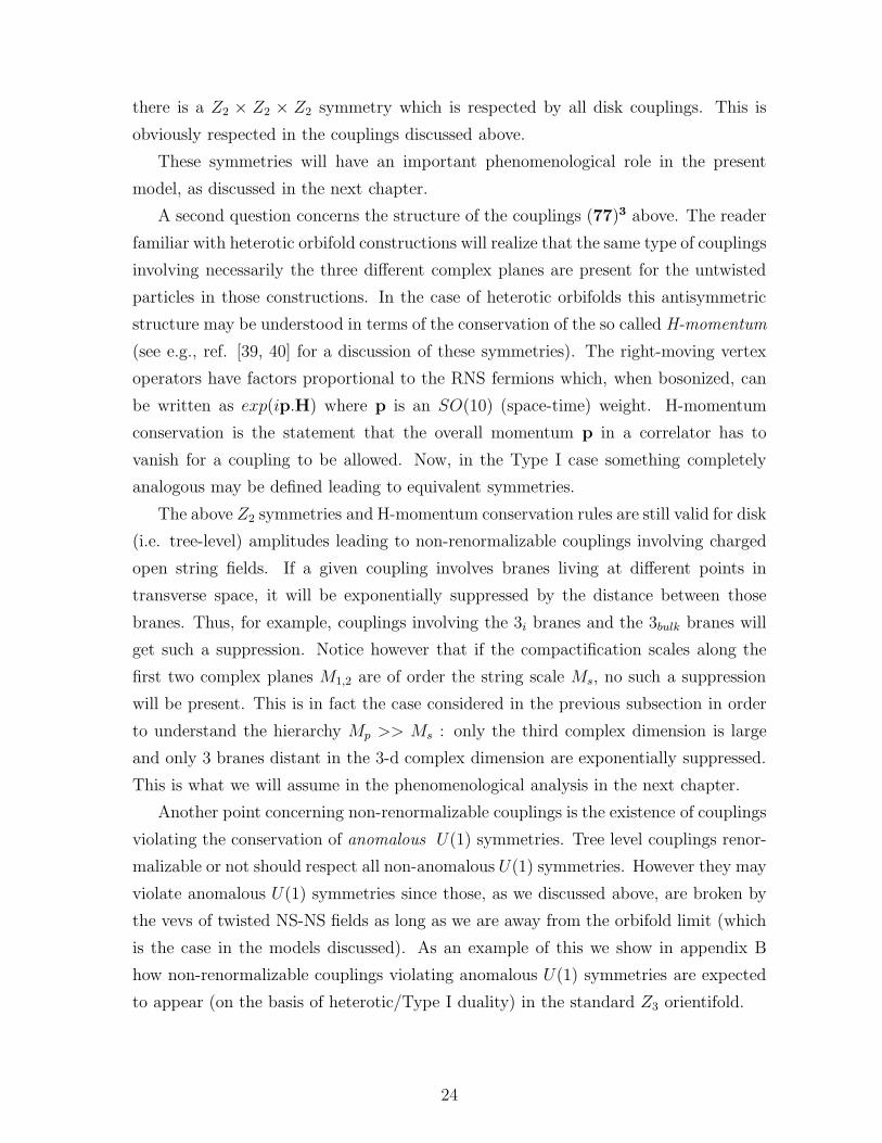
there is a Z2 × Z2 × Z2 symmetry which is respected by all disk couplings. This is

obviously respected in the couplings discussed above.

These symmetries will have an important phenomenological role in the present

model, as discussed in the next chapter.

A second question concerns the structure of the couplings (77)3 above. The reader

familiar with heterotic orbifold constructions will realize that the same type of couplings

involving necessarily the three different complex planes are present for the untwisted

particles in those constructions. In the case of heterotic orbifolds this antisymmetric

structure may be understood in terms of the conservation of the so called H-momentum

(see e.g., ref. [39, 40] for a discussion of these symmetries). The right-moving vertex

operators have factors proportional to the RNS fermions which, when bosonized, can

be written as exp(ip.H) where p is an SO(10) (space-time) weight. H-momentum

conservation is the statement that the overall momentum p in a correlator has to

vanish for a coupling to be allowed. Now, in the Type I case something completely

analogous may be defined leading to equivalent symmetries.

The above Z2 symmetries and H-momentum conservation rules are still valid for disk

(i.e. tree-level) amplitudes leading to non-renormalizable couplings involving charged

open string fields. If a given coupling involves branes living at different points in

transverse space, it will be exponentially suppressed by the distance between those

branes. Thus, for example, couplings involving the 3i branes and the 3bulk branes will

get such a suppression. Notice however that if the compactification scales along the

first two complex planes M1,2 are of order the string scale Ms, no such a suppression

will be present. This is in fact the case considered in the previous subsection in order

to understand the hierarchy Mp >> Ms : only the third complex dimension is large

and only 3 branes distant in the 3-d complex dimension are exponentially suppressed.

This is what we will assume in the phenomenological analysis in the next chapter.

Another point concerning non-renormalizable couplings is the existence of couplings

violating the conservation of anomalous U(1) symmetries. Tree level couplings renor-

malizable or not should respect all non-anomalous U(1) symmetries. However they may

violate anomalous U(1) symmetries since those, as we discussed above, are broken by

the vevs of twisted NS-NS fields as long as we are away from the orbifold limit (which

is the case in the models discussed). As an example of this we show in appendix B

how non-renormalizable couplings violating anomalous U(1) symmetries are expected

to appear (on the basis of heterotic/Type I duality) in the standard Z3 orientifold.

24

4 Phenomenology of the D-brane left-right sym-

metric orientifold

In this chapter we discuss several phenomenological aspects of this model. We will not

attempt a detailed description of all possible aspects like fermion masses or spontaneous

gauge symmetry breaking, rather we will only discuss some possible avenues enabling

to address the gross phenomenological issues in this model.

i) A nearby vacuum

As we mentioned in the previous chapter, apart from the three left-right symmetric

generations and Higgs fields, this particular string model has three copies of vector-like

colour triplets form the (37) sectors. However, these states are generically massive.

Indeed, looking at Table 3 one sees that all gauge interactions allow for a coupling

between the three singlets 14 from the (33) sectors to the three pairs (3, 1, 1,−2/3)−2 +

(3, 1, 1,+2/3)−2, where the subindices denote the QX charge. These Yukawa couplings

do indeed exist, as discussed in previous chapter. Thus, if the three singlets 14 get a

vev of order Ms, the colour triplets will disappear from the low-energy spectrum and

we will be left at low energies with precisely the massless spectrum discussed in chapter

2, leading to very good predictions for gauge coupling unification 10

If we give a vev < 14 >a∝Ms, a = 1, 2, 3 to these (33) singlets, we have to ensure D-

flatness and F-flatness for this direction. In fact we should not care too much about the

D-terms of the anomalous U(1)’s because they can be easily cancelled for appropriate

values of the blowing-up fields M discussed in chapter 3. On the other hand, the

D-term corresponding to the anomaly-free QX generator has to cancel, which requires

giving a vev to some fields with negative QX charge. A natural option seems to be

giving vevs to the antisymmetric Aij of SU(7) present in the (77)3 sector as follows 11

:

A12 = A23 = A34 = A45 = A56 = A67 = A71 = v (4.1)

with v ∝Ms. This direction can be easily seen to be D-flat and F-flat. Below MR the

only U(1) interaction left is now QB−L since QX is broken by the above vevs.

10Notice that, on the other hand, equivalent couplings to the Higgs doublets (1, 2, 2, 0) in the (77)

sector do not exist. Thus a doublet-triplet splitting mechanism is built-in in the symmetries of the

model.11This also turns out to give rise to the required masses for right-handed neutrinos.

25

ii) The breaking of the left-right symmetry and bulk 3-branes

The chiral multiplet content of our model below Ms includes just thee generations

of quarks/leptons/Higgs fields. Some additional fields (particularly, SU(2)R doublets)

are needed if we want to break our theory down to the SM gauge group. Probably

there is more than one way to modify the model in such a way that one has additional

massless SU(2)R doublets for symmetry breaking while the good coupling unification

predictions are not spoiled 12. The simplest possibility seems to add some additional

3-branes moving in the bulk in the first two compact directions but at the origin in

the third compact direction (so that their worldvolume overlaps with that of 7-branes).

The simplest set of 3-branes that one can add in the bulk are 6 of them (one 3-brane

and their orbifold and orientifold mirrors). They lead to a SU(2) gauge group in the

(33)bulk sector and massless chiral fields in the (73bulk) sector transforming like:

[(3, 1, 1,−2/3; 2) + (1, 2, 1,−1; 2) + (1, 1, 2,+1; 2) +h.c.] + (1, 7; 2)′+h.c. + (4, 1; 2)′ .

(4.2)

In addition there are chiral fields in the (33)bulk sector transforming like 2(1) + (3)

under the SU(2) group on the 3-branes. We will see later on when we discuss neutrino

masses that the SU(2) group coming from this bulky 3-branes should be broken close

to the Ms scale by vacuum expectation values of the fields (1, 7; 2)′ + h.c. above.

The chiral fields in eq.(4.2) include SU(2)R doublets which can in principle get a vev

and break the symmetry. Thus we will assume that some of the fields in (1, 1, 2,+1; 2)+

(1, 1, 2,−1; 2) will get vacuum expectation values of order MR ∝ 1TeV and break the

symmetry to that of the SM. We will briefly discuss below how that could take place

due to a radiative symmetry breaking mechanism.

One interesting point of the extra particle content provided by the addition of these

“bulky 3-branes” is that they give a net vanishing contribution to the combinations

(B′

1 + BL − 143B3) and (BL − 3

11B′

1) which control the joining of coupling constants.

Indeed we can easily check that extra contributions to the β-functions are obtained:

∆BL = ∆BR = ∆B3 = +2 ; ∆B′

1 = ∆BR +1

4∆BL =

22

3(4.3)

so that unification of couplings is not modified 13at one loop.12In particular, the variant left-right symmetric model displayed in table 1 of ref.[19] is another

possibility. That model has additional matter but one can check that gauge coupling unification along

similar lines to those of the present model takes place. A discussion of this variant model is presented

in appendix A13This is analogous to the well known fact that complete SU(5) representations do not modify the

one-loop conditions for unification in the MSSM.

26

iii) Quark and charged lepton masses

In this model renormalizable quark Yukawa couplings of type (77)3 exist with the

structure:

g ǫijk(3, 2, 1, 1/3)i(3, 1, 2,−1/3)j(1, 2, 2, 0)k (4.4)

where i, j, k = 1, 2, 3 label the three complex planes and g is the (77) gauge coupling

constant. With this simple structure, there would be a massless quark generation

and two degenerate generations with masses of order g√

∑

i | < Hi > |2. However, this

structure is modified by various effects. To start with, the Kahler metric for the

(77) matter fields in a model like this one needs not be diagonal. There are Kahler

untwisted moduli which mix the different complex planes. Furthermore, other effects

mixing different complex planes may come from non-renormalizable D-terms like, e.g.

< 21i21∗j > QiRQ

jR∗. In addition to these, there are mixing terms with the color triplets

from the bulky branes. In particular there are renormalizable Yukawa couplings of the

form (77)(73bulk)2:

(3, 1, 2,−1/3)3 × (3, 1, 1,−2/3; 2)× < (1, 1, 2, 1; 2) > (4.5)

(3, 2, 1, 1/3)3 × (3, 1, 1, 2/3; 2)× < (1, 2, 1,−1; 2) >

and hence the right-handed D-quarks of the (77) sector mix with the colour triplets

from the (73bulk) sector once the SU(2)R doublets in that sector get a vev. This means

that generically two physical right-handed D-quarks (the three of them in the variant

model of the appendix) will be SU(2)R singlets and the other will be contained in

a doublet 14. The second Yukawa coupling above will give masses to the first two

D-quarks and the couplings in (4.4) will give masses to the third.

Concerning the possible Yukawa couplings for the leptons, the following couplings

in the disk are allowed by all non-anomalous gauge symmetries:

g (1, 2, 2, 0)3 × (1, 2, 1,−1)a × (1, 1, 2,+1)a × fa(Mγ) a = 1, 2, 3 (4.6)

i.e., the Higgs fields along the third complex plane in the (77) sector couple diago-

nally to the lepton generations. Looking at Tables 2 and 3 we can observe that these

couplings are indeed allowed by all non-anomalous symmetries, including the QX gen-

erator. However they are in principle forbidden by the anomalous U(1)’s which are

spontaneously broken at the string scale. The twisted moduli fields discussed in the

14This is analogous to the alternate left-right models considered in refs.[41, 42] . Those models are

interesting from the point of view of supression of FCNC, as we comment below.

27

previous section are charged (non-linearly) under these anomalous U(1)’s so one ex-

pects that upon the insertion of coherent sets of twisted vertex Mγ operators the above

couplings will be allowed, as discussed in previous chapter and exemplified in appendix

B. This we denote by the addition of the factor fa(Mγ) in the above expression. No-

tice that this factor does not necessarily mean an exponential suppression, since the

physical gauge couplings of the SM gauge interactions are given by the couplings on

the (77) sector which are proportional to λ/(M4sR

21R

22), but not to the dilaton λ itself.

Thus λ need not be too small a number (see also the discussion in appendix B). The

precise size of the obtained lepton masses depends on the size of the vev for (1, 2, 2, 0)3

and on the value of fa(Mγ) for each a.

iv) Neutrino masses

In this model there is no right-handed SU(2)R triplet which might give a large

Majorana mass to the right-handed neutrinos. However there are fields Na which are

singlets under the SU(3)× SU(2)L × SU(2)R ×U(1)B−L group and can combine with

the right-handed neutrinos which then get a Dirac mass of order MR. Specifically,

those singlets are contained in the (1, 7′) representations in the three (37) sectors. For

the relevant couplings to appear we have to give vevs of order the string scale to the

(1, 7; 2)′ + (1, 7; 2) chiral fields in the (73bulk) sector. In particular there is a D-flat and

F-flat direction along Ψ26 = Ψ

16 = u and Ψ2

7 = Ψ17 = iu, where in Ψs

r (Ψsr) the index

r runs over SU(7) and s over the SU(2). Then an effective renormalizable Yukawa

coupling is induced at low energies of the form:

(1, 1, 2,−1)a × (1, 1, 2,+1; 2)× (1, 7)′a < (1, 21′)6 × (1, 7; 2)h(Mγ) > (4.7)

where the (1, 1, 2,+1; 2) are SU(2)R doublets from the 3-branes in the bulk. One can

check that this coupling is allowed by all anomaly-free gauge interactions of the model.

As happened with the masses of charged leptons, insertions of twisted moduli fields

will be required, which we parameterize by the factor h(Mγ). Notice that this coupling,

since it is non-renormalizable, is in principle suppressed by powers of Ms. It is of the

general form (73)2(73bulk)2(77)6 and hence involves 3-branes located at different points

which will also mean exponential suppression in the distance between the location of the

3-branes at the fixed points and those in the bulk. Notice however that, as we discussed

in the previous chapter, we have chosen the first two complex compact directions with

sizes of order 1/Ms and hence there is not necessarily any extra suppression, only the

third compact complex dimension is assumed to be very large.

28

Once the fields (1, 1, 2,+1; 2) get a vev breaking spontaneously the SU(2)R sym-

metry, the right handed neutrinos inside the three (1, 1, 2,−1)a fields will get a mass

of order MR combining with some singlets inside the (1, 7)′a. Notice in this connection

that generically the SU(7) gauge symmetry is broken and those fields behave indeed

like singlet partners of the right-handed neutrinos. In this situation the left-handed

neutrinos remain massless. However there are mixing terms from analogous couplings

involving SU(2)L doublets of the form:

(1, 2, 1,+1)a × (1, 2, 1,−1; 2)× (1, 7)′a < (1, 21′)6 × (1, 7; 2)h(Mγ) > (4.8)

Then the left handed neutrinos get induced Majorana masses of order mνL∝ ml × (<

(1, 2, 1,−1; 2) > / < (1, 1, 2,+1; 2) >). The particular sizes depend on the vev of

< (1, 2, 1,−1; 2) >, since < (1, 1, 2,+1; 2) > we know is of order MR ∝ 1 TeV. One

thus gets neutrino masses of order:

maν ∝ ma

l ×< (1, 2, 1,−1; 2) >

MR(4.9)

For < (1, 2, 1,−1; 2) >∝ ml a seesaw-like formula is obtained but the precise sizes

depend on the unknown values of the vevs of the SU(2)L doublets < (1, 2, 1,−1; 2) >.

Notice however that these mass contributions are flavour diagonal, there is no mixing

between different lepton families. Thus oscillations can only take place into some inert

sterile massless neutrino contained in the original (1, 7)′a fields. This is not a generic

property of the present scenario. One can check that in the variant model described in

the appendix mixing between different neutrino flavors can take place, since there are

no Z2 lepton parities.

v) Discrete symmetries and proton stability

The couplings in this orientifold model respect a number of discrete Z2 symmetries:

i) There is a Z2 symmetry associated to each of the three (37) sectors. Under it

all (73) particles are odd and the rest are even. Indeed, if we consider the couplings

of (37) particles on the boundary of the disk, they have to appear in multiplets of two

(see fig.6). Since in these sectors live the leptons (and some singlets coming from the

(1, 7′)’s which, as we saw above behave like neutrino-like fields), this corresponded to

a discrete Z2 lepton number parity. There is one Z2 symmetry for each of the three

flavours.

ii) The flat direction considered gives vevs to the fields (1, 7; 2)′ + (1, 7; 2)′ and also

to some SU(7) antisymmetric fields. Thus this direction respects a Z2 symmetry under

29

which 7-plets and SU(2) doublets (with respect to the (33bulk) group) are odd. Under

this symmetry all quarks and leptons are even but the (1, 7′) fields in the (73) sectors

are odd. The fields in the (73bulk) are odd, since all are SU(2) doublets.

In fact , after breaking of the SU(2)R symmetry by the (1, 1, 2,±1; 2) fields and of

the SU(2)L by the (1, 2, 2, 0) (or, in addition, the (1, 2, 1,±1; 2) fields), the diagonal

Z2 which is the combination of the original Z2 and the center of SU(2)R and SU(2)L

remains still unbroken. Thus, even after electroweak breaking a Z2 symmetry remains

under which

* All quarks and leptons are odd.

* Higgs fields breaking SU(2)L are even.

* Singlets combining with right-handed neutrinos are odd.

* SU(2)R and SU(2)L doublets in the (73bulk) sector are even.

* Colour triplets in the (73bulk) sector are odd.

Note that this residual symmetry can be identified with the standard R-parity of

supersymmetric models.

In summary, the effective lagrangian has a residual R-parity symmetry 15 and in

addition three lepton parities, one per lepton flavour. It is well known that R-parity

may be considered as a discrete Z2 subgroup of the B-L symmetry. Thus combining

it with the lepton parities we thus have a Z2 symmetry associated to baryon number.

This means that nucleons are stable, since a Z2 baryon parity has to be conserved under

which baryons are odd and leptons and mesons are even. Thus protons are absolutely

stable. On the other hand baryon number can be violated in two units, since there

is a Z2 symmetry. This means that in principle there can be neutron-antineutron

transitions allowed. However those transitions violate B-L symmetry and hence are

suppressed by high powers of (MR/Ms) and the rate in this model is negligible. Notice

on the contrary that discrete symmetries allow for the neutrino masses discussed in the

previous subsection.

vi) Gauge symmetry breaking and the low energy spectrum

As we discussed in the previous chapter, due to the presence of anti-3-branes in

the bulk, one expects the generation of SUSY-breaking soft terms in the effective

action. Once soft SUSY-breaking terms appear, SU(2)L × SU(2)R × U(1)B−L gauge

15It is well known that a residual R-parity remains in left-right symmetric models if the SU(2)R ×U(1)B−L symmetry is broken by SU(2)R triplets (1, 1, 3,−2). Notice that this is not the case here

and the origin of the residual R-parity is different.

30

symmetry breaking can occur due to loop corrections. We will not perform a complete

analysis of the (quite involved) scalar potential, but will just study what scalar fields are

likely to get vevs once loop corrections are included. As usual they will be the SU(3)

colour singlets with Yukawa couplings to coloured fields. These include the SU(2)L

and SU(2)R doublets in the model, as well as the fields in the (33bulk) sector which

are triplets (1; 3) under the SU(2)bulk gauge group. The following Yukawa couplings

appear at the renormalizable level:

(3, 2, 1, 1/3)i × (3, 1, 2,−1/3)j × (1, 2, 2, 0)k (4.10)

(3, 1, 2,−1/3)3 × (3, 1, 1,−2/3; 2)× (1, 1, 2,+1; 2)

(3, 2, 1, 1/3)3 × (3, 1, 1, 2/3; 2)× (1, 2, 1,−1; 2)

(3, 1, 1,−2/3; 2)× (3, 1, 1,+2/3; 2)× (1; 3) .

The first of these couplings is the (77)3 quark Yukawa coupling that we mentioned

above. The second and third couplings are of type (77)3(73bulk)2 and the fourth of

type (33bulk)(73bulk)2. All these four Yukawa couplings tend to give negative mass2 to

the above colour singlet scalars from one-loop diagrams in which the colour triplets

circulate in the loop.

In addition one also expects generically the presence of trilinear scalar couplings

( ”A-terms”) involving the colour singlet scalars. They are proportional to the scalar

couplings

(1; 3) × (1, 2, 1,−1; 2)× (1, 2, 1,+1; 2) + h.c. (4.11)

(1; 3) × (1, 1, 2,+1; 2)× (1, 1, 2,−1; 2) + h.c.

(1, 2, 2, 0)3 × (1, 2, 1,−1; 2)× (1, 1, 2,+1; 2) + h.c.

(1, 2, 2, 0)3 × (1, 2, 1,+1; 2)× (1, 1, 2,−1; 2) + h.c.

The first two have couplings proportional to the (33bulk) gauge coupling constant

whereas the last two are proportional to the (77) gauge coupling. The corresponding

A-terms are proportional to Msoft and only involve the corresponding scalars. These

contributions to the scalar potential are not positive definite and will favor all SU(2)R

and SU(2)L doublets (and the scalars in (1, 3)) to get a non-vanishing vev at some

level. We will assume that a stable minimum of the scalar potential exists for vevs of

the order of magnitude:

< (1, 1, 2,+1; 2) >∝< (1, 1, 2,−1; 2) >∝< (1; 3) >∝MR ∝ 1TeV (4.12)

< (1, 2, 2, 0)i >∝MZ << MR

31

so that the required hierarchy between the left and right gauge symmetries is obtained.

Notice that in principle all interactions respect an explicit parity left↔right symmetry

and it is the vacuum which will explicitly break parity symmetry and decide who is

left-handed and who is right-handed. Whatever SU(2) survives to lower energies we

will call SU(2)L by definition.

Another relevant question is what is the mass of the extra Higgs and Higgsino fields

that this model has both from the (77) and (73bulk) sectors. This is a complicate issue

which will depend on the detailed structure of vevs. Looking at the first, third and

fourth couplings in eqs.(4.11) we see that vevs of order MR for (1; 3) and (1, 1, 2,±1; 2)

will make massive some of the SU(2)L doublets in the (73bulk) sector and also the

(1, 2, 2, 0)3 fields in the (77) third complex plane. In this situation we would be left

at low energies with the fields (1, 2, 2, 0)1 and (1, 2, 2, 0)2 corresponding to the first

two complex planes. However, as we mentioned when we discussed quark Yukawa

couplings, there are different effects which will generically mix the particles living in

different complex planes in (77) sectors. Thus one also expects that these other doublets

could become massive. We will thus assume that at a scale of order MR only one set of

SM doublets remains relatively light, so that they are available for SU(2)L spontaneous

symmetry breaking.

In addition there are the extra right-handed chiral fields (1, 1, 2,±1; 2) from the

(73bulk) sector. Some of these where eaten in the process of SU(2)R breaking. The

remaining may acquire a mass of orderMR from the second equation in (4.11) , once the

scalars (1; 3) get a vev. The same applies to the extra colour triplets (3, 1, 1, 1/3; 2)+h.c.

from the (73bulk) sector. We already mentioned that some combination of them mixes

with the right-handed quarks from the (77) sector. The orthogonal combination will

get a mass of order MR once the scalars (1; 3) get a vev. All in all, the spectrum

below the MR would thus be similar to that of the MSSM: three quark-lepton chiral

multiplets and one set of Hu +Hd Higgs fields.

vii) Ramond-Ramond fields and invisible axions

We already mentioned in chapter 3 that in this class of orientifold models there are

twisted Ramond-Ramond singlet scalars which couple to FF . As already discussed in

ref.[10] , they are natural candidates to play the role of invisible axions in a model like

this. Notice however that, in the absence of other charged scalar vevs, the combina-

tions of twisted Ramond-Ramond fields coupling to the gauge groups get in fact large

masses of order the string scale Ms by providing the longitudinal degrees of freedom

32

of anomalous U(1)’s when the latter become massive. This can be easily seen from

eq.(3.16).

Now, again from eq.(3.16), since ξr 6= 0, in the presence of other charged fields

from the open string sector acquiring a vev and contributing to the anomalous U(1)

breaking, there will be a linear combination of RR-field plus the charged field, which

will be swallowed by the U(1) to become massive. The orthogonal combination will

remain massless. This massless linear combination will in general couple to the gauge

fields (and in particular, to QCD) in the standard axionic fashion with the gauge kinetic

function taking the general form fα = S + s(ai)α M(ai) with s(ai)

α constant computable

coefficients [28, 31] and with a decay constant of order the string scale Ms ∝ 1012 GeV,

well within astrophysical limits.

viii) Experimental signatures

The most obvious experimental implication of the present scheme is the existence

of extra WR, Z ′

0 gauge bosons corresponding to the left-right symmetric gauge inter-

actions at a scale of order 1 TeV or below. The phenomenology of SU(3) × SU(2)L ×SU(2)R × U(1)B−L models has been extensively studied in the past, although most of

the studies have tacitly assumed an SO(10) embedding of such gauge symmetry leading

to the canonical value for the weak angle [15] . In addition, many studies have concen-

trated on a scheme in which SU(2)R chiral triplets transforming like (1, 1, 3,−2)+h.c.

break the left right symmetry. At the same time these vevs could give rise to large

Majorana masses for the right-handed neutrinos, leading to a see-saw structure for

neutrino masses. This kind of Higgs fields do not appear in the class of models that we

construct, and right-handed neutrinos are expected to become massive by combining

with other singlet chiral fields, as explained above. Thus many previous studies do not

directly apply to the present model.

There are a number of experimental limits on the masses of the extra gauge bosons

[16] . If right-handed neutrinos are lighter than the WR mass, the channel WR → lRνR

is open leading to clean signatures at the Tevatron. From searches in that channel D0

has set [43] the limit MWR> 720 GeV and CDF MWR

> 650 [44] . If right-handed

neutrinos are heavier than the WR, this signature disappears and weaker limits coming

from dijet production are obtained. D0 excludes the range 340 < MWR< 680 GeV [45]

whereas CDF excludes 300 < MWR< 420 [46] . UA2 had excluded the energy range

100 < MWR< 251 also from the dijet signature [47] . There are stronger constraints

on the WR mass from the KL − KS mass difference but those are much more model

33

dependent [18]. On the other hand, for left-right symmetric models with gL = gR like

this, one can obtain limits from precision LEP-I measurements and low-energy neutral

current data yielding MZ′

0> 900 GeV, implying MWR

> 780 GeV in this class of

models [48] . In summary, the extra gauge bosons appearing in a left-right symmetric

model like this should weight more than around 800 GeV or so 16 Masses of this size

or a bit higher are compatible with the gauge coupling unification results in chapter 2.

However those coupling unification results seem to prefer not very high masses for WR

and Z ′

0.17Thus the extra left-right symmetric degrees of freedom could perhaps soon

be discovered.

In addition in this class of models there is a triplication of the number of Higgs

fields transforming like (1, 2, 2, 0). Thus one also expects to find at energies of order 1

TeV, charged and neutral Higgs and Higgsino fields. In fact these fields are potentially

dangerous. Indeed, it is well known that in generic models with multiple Higgs SU(2)L

doublets, the unitary transformations which diagonalize the quark mass matrices do

not necessarily diagonalize the Yukawa interactions and FCNC can in principle appear.

This FCNC problem is generically present in left-right symmetric models with a lowMR

scale like this. Thus to suppress sufficiently such kind of transitions, the extra Higgs

fields have to be sufficiently heavy and/or the Yukawa couplings will need to have some

symmetries. The question of how to evade the problem of FCNC in supersymmetric

left-right models with MR ∝ 1 TeV has been adressed in ref.[42, 41] . There it is

shown that this problem can be avoided if there are present some extra SU(2)R singlet

D-type quarks mixing with the right-handed doublet quarks in the model in such a way

that the physical D-quarks are mostly SU(2)R singlets. In addition extra SU(2)R and

SU(2)L doublets with non-vanishing B-L charge are also required [42] . Interestingly

enough this type of extra fields and mixings are also present in the D-brane model here

discussed. It would be interesting to see whether in a D-brane type of model a similar

mechanism as in ref.[42] could be made operative.

Finally, there are also extra fields from the sector which is in charge of the breaking

of the SU(2)R symmetry. In order not to spoil gauge coupling unification we have seen

that the required SU(2)R doublets should come along with the same number of SU(2)L

16If the right-handed D-quarks are mostly SU(2)R singlets as discussed above, WR production is

very much supressed and direct limits on the WR mass are much weakened [41]. However that is not

the case for the Z’ and hence mass limits of that order are expected to still apply.17 It has been recently pointed out [49] that a small amount of missing invisible width in Z decays

at LEP I as well as atomic parity violation experiments could perhaps indicate already the existence

of some extra Z’ with mass of order 500-1000 GeV.

34

doublets and coloured SU(3) triplets. In the D-brane explicit constructions presented

in this paper such structure of extra particles is very natural and corresponds to the

addition of some extra 3-branes in the bulk of the first two complex dimensions. All

these extra particles are expected to have masses also aroundMR or the SUSY-breaking

scale. Thus new extra heavy lepton-like and quark-like extra fermions and scalars are

expected to be produced at future accelerators corresponding to this sector.

In this chapter we have given an overall discussion of phenomenological aspects of

the particular orientifold model introduced in chapter 3. We believe that the particular

Z3 orientifold here discussed is tantalizingly close to the general new scheme proposed

in chapter 2. Analogous models based on the same orientifold can be constructed

which will lead to somewhat different phenomenological properties. For example, one

can construct similar models by adding a second discrete Wilson line breaking e.g.

the original SU(7) symmetry further. Another possibility is to consider the variant

left-right symmetric discussed in the appendix .

5 Final comments and outlook

During more than 15 years the minimal supersymmetric standard model has been

thoroughly studied as the best motivated extension of the standard model. During the

past 10, this study became more intense due to the realization that gauge coupling

unification works very well in the MSSM as compared to the standard model. In this

article we have proposed an interesting alternative to the MSSM mostly motivated

by the structure of D-brane models. This alternative scenario matches the success of

gauge coupling unification of the MSSM, with the interesting feature that unification

works only if there are three families of quarks, leptons and Higgs fields. In the present

scheme several physical mass scales are unified: the string unification, susy-breaking

and axion scales are one and the same and of order Ms = 9 × 1011 GeV. As it has

been noted in several occasions, [9, 10], this intermediate scale may have important

physical implications regarding neutrino masses, the strong CP problem, ultra high-

energy cosmic rays, non thermal dark matter candidates, inflation, etc.

We have also presented a concrete D-brane model satisfying most of the general

properties of the proposed scenario. The existence of three quark-lepton generations

has an elegant explanation in these constructions: there are three generations because

there are three complex compact dimensions and a Z3 orbifold structure18. The proton

18This simple explanation, first encountered in the heterotic models in [17] , is to be compared with

35

is stable due to a combination of discrete symmetries including lepton and R-parities

and Yukawa couplings are obtained for quarks, charged leptons and neutrinos. To

our knowledge this is the first example where R-parity appears so naturally in string

theoretical models. This guarantees the existence of an LSP and most of the standard

searches for supersymmetry. Being a left-right symmetric model, it shares many of the

good properties that have been realized over several years about LR models [14, 15].

Recall, however, that the Higgs structure we find differs from the standard treatment

in the sense that the fields responsible for breaking the LR group to the standard model

are doublets that belong to the spectrum of the corresponding string model instead of

SU(2) triplets, as often assumed in the literature [15] .

One may ask if going to a left-right symmetric model is unavoidable in this class

of theories. Indeed, one can construct explicit three generation Z3 orientifold models

with the gauge group of the standard model and some examples of this type were

presented in ref.[19] . However gauge coupling unification does not appear as naturally

as in the left-right symmetric models here described. Furthermore, the absence of

the B − L gauged symmetry makes difficult to find field directions with a sufficiently

stable proton. We believe that this is probably a generic property and both coupling

unification and proton stability seem to point towards a left-right symmetric extension

of the SM above a TeV scale.

Since the LR scale, MR, has to be relatively close to the TeV scale in order for

gauge unification to work, this scenario can be experimentally tested very soon. In

the first place, the existence of new massive gauge fields for which the experimental

constraints are becoming very strong can be explored. The scenario can also be tested

by looking at the existence of new Higgs particles at the TeV scale, which in principle

can give rise to flavour changing neutral currents, and of course with the production

of supersymmetric particles.

There are several aspects that remain to be understood in this scenario. First,

the Higgs scalar potential needs to be studied in order to understand the possible

patterns of gauge symmetry breaking. This is also important in order to address the

issue of possible FCNC transitions coming from the multi-Higgs structure. Then, the

detailed structure of soft supersymmetry breaking terms needs to be addressed. This is

important in order to have more information about the possible experimental signals of

supersymmetry. Other issues, such as the origin of baryogenesis, may depend crucially

that in Calabi-Yau compactifications of perturbative or non-perturbative heterotic vacua in which the

net number of generations minus antigenerations is related to the Hodge numbers of the CY. Those

tend to be quite large in general and only for very particular manifolds is small.

36

on this knowledge. A through analysis of the general structure of neutrino masses and

oscilations in this kind of scenario would also be important.

As for the explicit string model constructed, it would be interesting to study dif-

ferent variations e.g. with further symmetry breaking (Wilson lines) or locations of

3-branes which may lead to different phenomenological details. Also interesting would

be to look for similar left-right symmetric models using other constructions like Type

IIA orientifolds or non-perturbative heterotic orbifolds [50] leading to similar spectra.

In addition the standard issues of moduli stabilization 19 and the cosmological constant20 remain open.

It is highly remarkable that in this string model, the unification scale coincides with

the preferred fundamental string scale determined by supersymmetry breaking, since

a priori the two scales did not have to be related. If this turns out to be true, we

might say that nature has been misleading us for many years into the belief that the

unification scale was much higher. In any case, we believe the present new scenario

has many appealing properties and deserves to be considered as a serious alternative

to the MSSM.

Acknowledgements

We acknowledge useful conversations with B. Allanach, M. Klein, R. Rabadan and

A. Uranga. This work has been partially supported by CICYT (Spain), the Euro-

pean Commission (grant ERBFMRX-CT96-0045) and PPARC. G.A work is partially

supported by APCyT grant 03-03403.

19For some recent attempts to understand the stabilization of large radii see e.g. ref.[51, 19].20For some recent ideas about the cosmological constant problem in the D-brane context see e.g.

refs. [37, 52] .

37

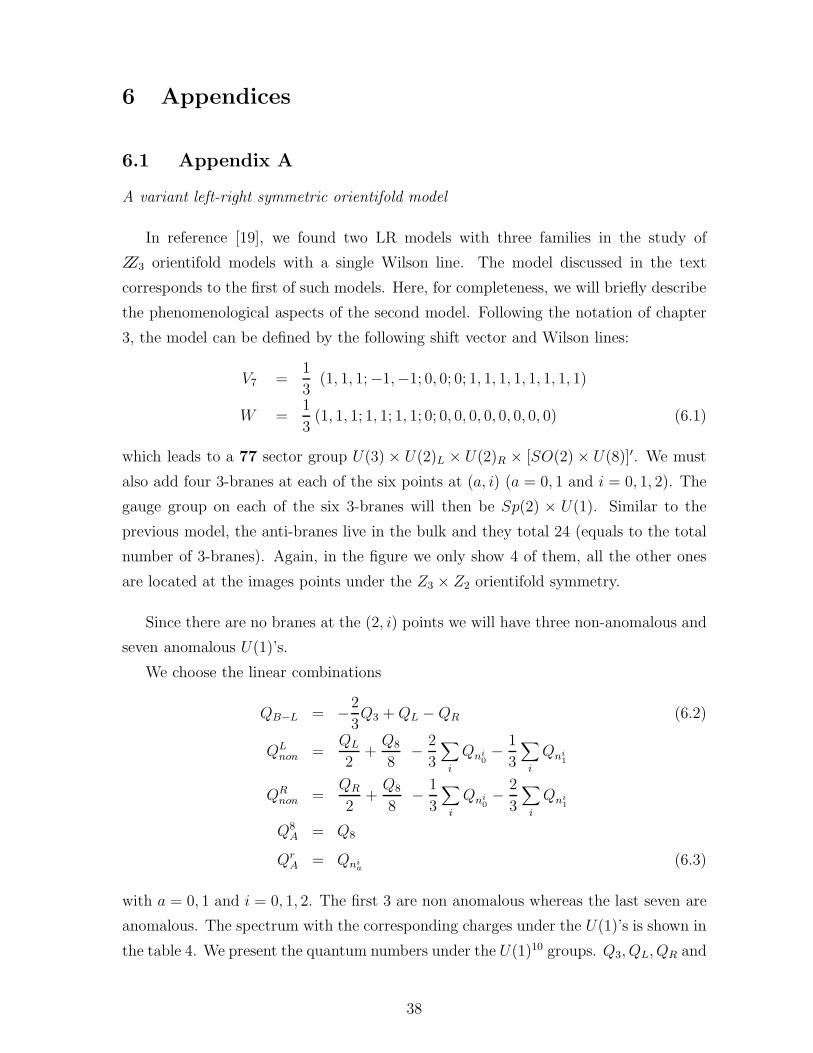
6 Appendices

6.1 Appendix A

A variant left-right symmetric orientifold model

In reference [19], we found two LR models with three families in the study of

ZZ3 orientifold models with a single Wilson line. The model discussed in the text

corresponds to the first of such models. Here, for completeness, we will briefly describe

the phenomenological aspects of the second model. Following the notation of chapter

3, the model can be defined by the following shift vector and Wilson lines:

V7 =1

3(1, 1, 1;−1,−1; 0, 0; 0; 1, 1, 1, 1, 1, 1, 1, 1)

W =1

3(1, 1, 1; 1, 1; 1, 1; 0; 0, 0, 0, 0, 0, 0, 0, 0) (6.1)

which leads to a 77 sector group U(3) × U(2)L × U(2)R × [SO(2) × U(8)]′. We must

also add four 3-branes at each of the six points at (a, i) (a = 0, 1 and i = 0, 1, 2). The

gauge group on each of the six 3-branes will then be Sp(2) × U(1). Similar to the

previous model, the anti-branes live in the bulk and they total 24 (equals to the total

number of 3-branes). Again, in the figure we only show 4 of them, all the other ones

are located at the images points under the Z3 × Z2 orientifold symmetry.

Since there are no branes at the (2, i) points we will have three non-anomalous and

seven anomalous U(1)’s.

We choose the linear combinations

QB−L = −2

3Q3 +QL −QR (6.2)

QLnon =

QL

2+Q8

8− 2

3

∑

i

Qni

0− 1

3

∑

i

Qni

1

QRnon =

QR

2+Q8

8− 1

3

∑

i

Qni

0− 2

3

∑

i

Qni

1

Q8A = Q8

QrA = Qni

a(6.3)

with a = 0, 1 and i = 0, 1, 2. The first 3 are non anomalous whereas the last seven are

anomalous. The spectrum with the corresponding charges under the U(1)’s is shown in

the table 4. We present the quantum numbers under the U(1)10 groups. Q3, QL, QR and

38

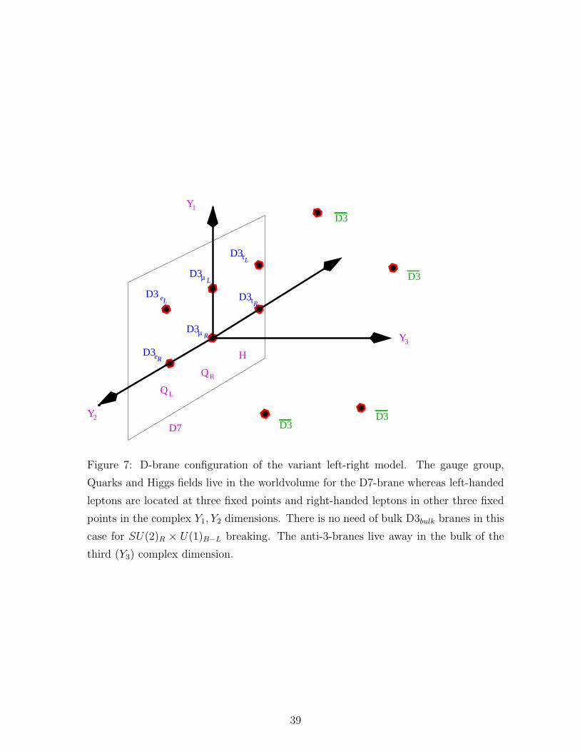
D3D3

D3

D3

D3

D3

D3

D3

D7

Y

Y

Y3

1

2

Q

Q

H

L

R

µ

τ

τ

µD3

e

L

R

RL

L

D3Re

Figure 7: D-brane configuration of the variant left-right model. The gauge group,

Quarks and Higgs fields live in the worldvolume for the D7-brane whereas left-handed

leptons are located at three fixed points and right-handed leptons in other three fixed

points in the complex Y1, Y2 dimensions. There is no need of bulk D3bulk branes in this

case for SU(2)R × U(1)B−L breaking. The anti-3-branes live away in the bulk of the

third (Y3) complex dimension.

39

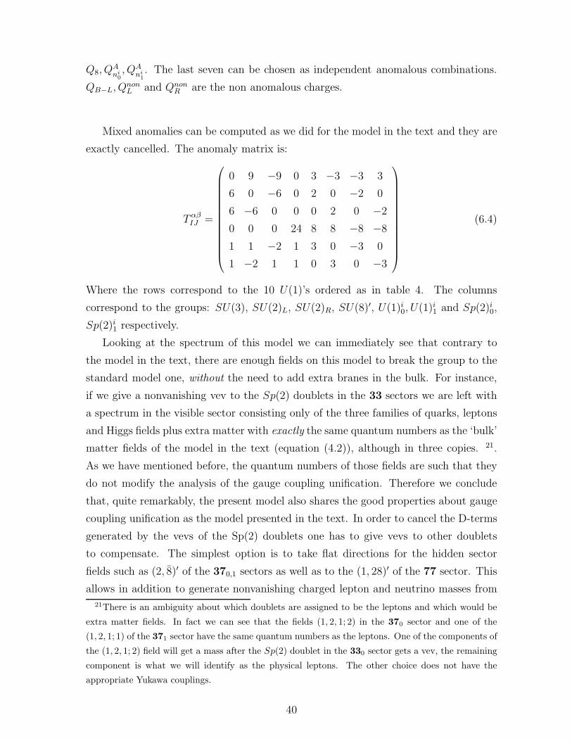
Q8, QAni

0

, QAni

1

. The last seven can be chosen as independent anomalous combinations.

QB−L, QnonL and Qnon

R are the non anomalous charges.

Mixed anomalies can be computed as we did for the model in the text and they are

exactly cancelled. The anomaly matrix is:

T αβIJ =

0 9 −9 0 3 −3 −3 3

6 0 −6 0 2 0 −2 0

6 −6 0 0 0 2 0 −2

0 0 0 24 8 8 −8 −8

1 1 −2 1 3 0 −3 0

1 −2 1 1 0 3 0 −3

(6.4)

Where the rows correspond to the 10 U(1)’s ordered as in table 4. The columns

correspond to the groups: SU(3), SU(2)L, SU(2)R, SU(8)′, U(1)i0, U(1)i

1 and Sp(2)i0,

Sp(2)i1 respectively.

Looking at the spectrum of this model we can immediately see that contrary to

the model in the text, there are enough fields on this model to break the group to the

standard model one, without the need to add extra branes in the bulk. For instance,

if we give a nonvanishing vev to the Sp(2) doublets in the 33 sectors we are left with

a spectrum in the visible sector consisting only of the three families of quarks, leptons

and Higgs fields plus extra matter with exactly the same quantum numbers as the ‘bulk’

matter fields of the model in the text (equation (4.2)), although in three copies. 21.

As we have mentioned before, the quantum numbers of those fields are such that they

do not modify the analysis of the gauge coupling unification. Therefore we conclude

that, quite remarkably, the present model also shares the good properties about gauge

coupling unification as the model presented in the text. In order to cancel the D-terms

generated by the vevs of the Sp(2) doublets one has to give vevs to other doublets

to compensate. The simplest option is to take flat directions for the hidden sector

fields such as (2, 8)′ of the 370,1 sectors as well as to the (1, 28)′ of the 77 sector. This

allows in addition to generate nonvanishing charged lepton and neutrino masses from

21There is an ambiguity about which doublets are assigned to be the leptons and which would be

extra matter fields. In fact we can see that the fields (1, 2, 1; 2) in the 370 sector and one of the

(1, 2, 1; 1) of the 371 sector have the same quantum numbers as the leptons. One of the components of

the (1, 2, 1; 2) field will get a mass after the Sp(2) doublet in the 330 sector gets a vev, the remaining

component is what we will identify as the physical leptons. The other choice does not have the

appropriate Yukawa couplings.

40

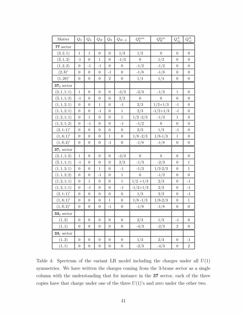
Matter Q3 QL QR Q8 QB−L QnonL Qnon

R QAni

0

QAni

1

77 sector

(3, 2, 1) 1 1 0 0 1/3 1/2 0 0 0

(3, 1, 2) -1 0 1 0 -1/3 0 1/2 0 0

(1, 2, 2) 0 -1 -1 0 0 -1/2 -1/2 0 0

(2, 8)′ 0 0 0 -1 0 -1/8 -1/8 0 0

(1, 28)′ 0 0 0 2 0 1/4 1/4 0 0

370 sector

(3, 1, 1; 1) 1 0 0 0 -2/3 -2/3 -1/3 1 0

(3, 1, 1; 2) -1 0 0 0 2/3 0 0 0 0

(1, 1, 2; 1) 0 0 1 0 -1 2/3 1/2+1/3 -1 0

(1, 1, 2; 1) 0 0 -1 0 1 2/3 -1/2+1/3 -1 0

(1, 2, 1; 1) 0 1 0 0 1 1/2 -2/3 -1/3 1 0

(1, 2, 1; 2) 0 -1 0 0 -1 -1/2 0 0 0

(2, 1; 1)′ 0 0 0 0 0 2/3 1/3 -1 0

(1, 8; 1)′ 0 0 0 1 0 1/8 -2/3 1/8-1/3 1 0

(1, 8; 2)′ 0 0 0 -1 0 -1/8 -1/8 0 0

371 sector

(3, 1, 1; 2) 1 0 0 0 -2/3 0 0 0 0

(3, 1, 1; 1) -1 0 0 0 2/3 -1/3 -2/3 0 1

(1, 1, 2; 1) 0 0 1 0 -1 -1/3 1/2-2/3 0 1

(1, 1, 2; 2) 0 0 -1 0 1 0 -1/2 0 0

(1, 2, 1; 1) 0 1 0 0 1 1/2 +1/3 2/3 0 -1

(1, 2, 1; 1) 0 -1 0 0 -1 -1/2+1/3 2/3 0 -1

(2, 1; 1)′ 0 0 0 0 0 1/3 2/3 0 -1

(1, 8; 1)′ 0 0 0 1 0 1/8 -1/3 1/8-2/3 0 1

(1, 8; 2)′ 0 0 0 -1 0 -1/8 -1/8 0 0

330 sector

(1, 2) 0 0 0 0 0 2/3 1/3 -1 0

(1, 1) 0 0 0 0 0 -4/3 -2/3 2 0

331 sector

(1, 2) 0 0 0 0 0 1/3 2/3 0 -1

(1, 1) 0 0 0 0 0 -2/3 -4/3 0 2

Table 4: Spectrum of the variant LR model including the charges under all U(1)

symmetries. We have written the charges coming from the 3-brane sector as a single

column with the understanding that for instance in the 37 sector, each of the three

copies have that charge under one of the three U(1)’s and zero under the other two.

41

couplings such as22

(1, 2, 2)(1, 2, 1; 2)∗(1, 1, 2; 2)∗ < (1, 8; 2)′(1, 8; 2)′(1, 28)′ > < (1, 28)′4 >

(1, 1, 2; 2)∗(1, 1, 2)(1, 1)0,i < (1, 2)0,i(1, 8; 2)′(1, 8; 2)′(1, 28)′ > (6.5)

where the ∗ on the Sp(2) doublets stand for the component of the doublet that remains

massless after the doublet in the 33 sector got a nonvanishing vev and the subindex a, i

indicates that these are fields from the 37a sector. Notice that in this case the right-

handed neutrinos become massive by combining with singlets in the 33 sectors. These

couplings are allowed by all the gauge symmetries including the anomalous U(1)’s,

therefore, contrary to the model in text, there is no need to introduce insertions of

twisted vertex operators in order to generate lepton masses.

Interestingly enough, this flat direction leaves a remaining Z2 symmetry consisting

in changing sign to all SU(8) octets and simultaneously changing sign to all particles

in sectors 37. It is easy to see that this discrete symmetry combined with the two

Z2’s remaining after breaking the LR SU(2)’s imply a residual discrete baryon Z2

parity making the proton absolutely stable, similar to the model in the text. Unlike

that model however, lepton number is not conserved since couplings like QDL are

permitted, although suppressed by powers of (MR/Ms) since they violate B − L.

Combining these SU(8) flat directions with those of the Sp(2) doublets does not

preserve gauge coupling unification since couplings such as

(3, 1, 1; 2)∗(3, 1, 1; 2)∗ < (1, 8; 2)(1, 8; 2)(1, 28) > (6.6)

will in principle give masses to the extra triplets. Thus an alternative which does

preserve gauge coupling unification would be combining the SU(8) flat directions with

those of singlets in the 33 sectors (not giving vevs to the Sp(2) doublets). This main-

tains gauge coupling unification with the good properties for lepton masses. In this

case giving a mass to all the extra triplets needs the insertion of twisted vertex opera-

tors. In summary this model is very similar to the one presented in the text (although

probably a bit more complicated) and may deserve further exploration.

22Yukawa couplings giving rise to quark masses are identical to the model in the text since they

only include couplings among fields of the 77 sector.

42

6.2 Appendix B

Anomalous U(1)’s and non-renormalizable couplings in the Z3 orientifold

In this appendix we will argue that non-renormalizable couplings violating anoma-

lous U(1) charges are in general expected in orientifolds similar to the ones considered

in the present article. More specifically heterotic/Type I duality seems to indicate that

this is the case. Consider in particular the standard D = 4, N = 1, Z3 orientifold first

constructed in ref.[22]. The underlying orbifold is exactly the same than the one con-

sidered in the present paper, the only difference being the absence of anti-branes and

Wilson lines. The model has 32 9-branes and a gauge group SU(12)×SO(8)×U(1)A.

In the open string (99) sector there are charged fields transforming like:

3(66, 1)+2 + 3(12, 8)−1 (6.7)

where the subindex denotes the U(1)A charge. It is easy to check that the U(1)A in-

teraction is anomalous. In addition there are 27 chiral singlets (1, 1)0 coming from

the twisted closed string sector. The latter are singlets under U(1)A but transform

non-linearly under that anomalous symmetry, and it is this transformation which can-

cels the U(1)A anomalies by means of a generalized Green-Schwarz mechanism. At

the same time the U(1)A becomes massive. Now, SU(12) invariance allows for a non-

renormalizable superpotential coupling of the type (66, 1)6+2 by contraction with the

12-index antisymmetric tensor. However, such a coupling would violate U(1)A conser-

vation in 12 units. Since this U(1)A symmetry is broken one may suspect that such

non-renormalizable coupling may however exist if one moves away from the orbifold

limit, i.e., if the twisted NS-NS singlet fields get a vev.

Heterotic/Type I duality seems to indicate that is the case. The above orientifold

has a heterotic dual [22, 53, 25] which is a Z3 orbifold compactification of the SO(32)

heterotic string. This model has the same gauge group and the charged particles in the

untwisted sector are identical to those in the (99) sector of the Type I model. There

are also 27 twisted chiral fields transforming like (1, 1)−4 under the gauge group, which

should be identified as duals of the 27 twisted fields of the Type I dual. Notice however

that, unlike their Type I counterparts, the heterotic singlets are charged under the

anomalous U(1)A. Now, one can convince oneself that in this heterotic Z3 orbifold the

following non-renormalizable couplings do in general exist:

(1, 1)3−4 × (66, 1)6

+2 (6.8)

43

This coupling preserves the U(1)A symmetry. One can also check that this coupling

preserves the necessary selection rules in order to be present. In particular, it respects

the Z3 point group symmetry (the twisted fields appear to the third power). Also the

H-momentum conservation is obeyed. To check this it is enough to consider the vertex

operators associated to the (66, 1)+2 written in the ” 0-picture”. In addition, as pointed

out in ref.[53] , the FI-term present in this heterotic model forces the singlets (1, 1)−4

to get non-vanishing vevs. Thus away from the orbifold point the heterotic model will

present (66, 1)6+2 couplings, effectively violating the anomalous U(1)A symmetry. This

strongly suggests that similar couplings will also be present in the dual Type I model

as long as one stays away from the orbifold point, i.e., as long as the twisted NS−NS

closed string singlets have non-vanishing vevs. This is indeed the case considered in

the models in the present article.

44

References

[1] E. Witten, Nucl. Phys. B471 (1996) 135

[2] J.D. Lykken, Phys. Rev. D54 (1996) 3693, hep-th/9603133.

[3] I. Antoniadis, N. Arkani-Hamed, S. Dimopoulos, G. Dvali Phys. Lett. B436 (1999)

257.

[4] K. Dienes, E. Dudas and T. Gherghetta, hep-ph/9803466; hep-ph/9806292; hep-

ph/9807522.

[5] R. Sundrum, hep-ph/9805471; hep-ph/9807348.

[6] G. Shiu and S.H. Tye, hep-th/9805157.

[7] C. Bachas, hep-ph/9807415.

[8] Z. Kakushadze and S.H. Tye, hep-th/9809147.

[9] K. Benakli, hep-ph/9809582.

[10] C.P. Burgess, L.E. Ibanez and F. Quevedo, hep-ph/9810535, Phys. Lett. B447

(1999) 257.

[11] L.E. Ibanez, C. Munoz and S. Rigolin, hep-ph/9812397.

[12] A. Donini and S. Rigolin, hep-ph/9901443.

[13] For recent discussions of quasirealistic perturbative heterotic models see e.g.

G.K. Leontaris and J. Rizos, hep-th/9901098;

G.E. Cleaver, A. Faraggi and D. Nanopoulos, hep-ph/9904301;

M. Cvetic, J. Everett, P. Langacker and J. Wang, hep-ph/9902247. r

[14] J.C. Pati and A. Salam, Phys. Rev. D10 (1974) 275;

R. Mohapatra and J.C. Pati, Phys. Rev. D11 (1974) 566;

G. Senjanovic and R. Mohapatra, Phys. Rev. D12 (1975) 1502.

[15] See e.g. R. Mohapatra, hep-ph/9707518 and hep-ph/9911272 for a recent discus-

sion and some references about left-right symmetric models.

[16] K. Babu, C. Kolda and J. March-Russell, in Review of Particle Properties (1998),

( http://pdg.lbl.gov/) .

45

[17] L.E. Ibanez, Jihn E. Kim, H.P. Nilles, F. Quevedo, Phys. Lett. B191 (1987) 282

L.E. Ibanez, J. Mas, H.P. Nilles and F. Quevedo, Nucl. Phys. B301 (1988) 157

A. Font, L.E. Ibanez, F. Quevedo and A. Sierra, Nucl. Phys. B331 (1990) 421.

[18] C. Caso et al, The European Physical Journal C3 (1998) 1.( http://pdg.lbl.gov/).

[19] G. Aldazabal, L. Ibanez, F. Quevedo, hep-th/ 9909172.

[20] G. Aldazabal and A. M. Uranga, JHEP 9910 (1999) 24, hep-th/9908072.

[21] I. Antoniadis, E. Dudas and A. Sagnotti, hep-th/9908023;

C. Angelantonj, I. Antoniadis, G. D’Apollonio, E. Dudas and A. Sagnotti, hep-

th/9911081.

[22] C. Angelantonj, M. Bianchi, G. Pradisi, A. Sagnotti and Ya.S. Stanev, Phys. Lett.

B385 (1996) 96, hep-th/9606169.

[23] A. Sagnotti, in Cargese 87, Strings on Orbifolds, ed. G. Mack et al. (Pergamon

Press, 1988) p. 521;

P. Horava, Nucl. Phys. B327 (1989) 461; Phys. Lett. B231 (1989) 251;

J. Dai, R. Leigh and J. Polchinski, Mod.Phys.Lett. A4 (1989) 2073;

R. Leigh, Mod.Phys.Lett. A4 (1989) 2767;

G. Pradisi and A. Sagnotti, Phys. Lett. B216 (1989) 59 ;

M. Bianchi and A. Sagnotti, Phys. Lett. B247 (1990) 517 ;

E. Gimon and J. Polchinski, Phys.Rev. D54 (1996) 1667, hep-th/9601038.

E. Gimon and C. Johnson, Nucl. Phys. B477 (1996) 715, hep-th/9604129;

A. Dabholkar and J. Park, Nucl. Phys. B477 (1996) 701, hep-th/9604178.

[24] M. Berkooz and R. G. Leigh, Nucl. Phys. B483 (1997) 187, hep-th/9605049;

Z. Kakushadze, Nucl. Phys. B512 (1998) 221, hep-th/9704059;

Z. Kakushadze and G. Shiu, Phys. Rev. D56 (1997) 3686, hep-th/9705163;

Z. Kakushadze and G. Shiu, hep-th/9706051;

L.E. Ibanez, hep-th/9802103;

G. Zwart, hep-th/9708040;

J. Lykken, E. Poppitz and S. Trivedi, hep-th/9806080.

[25] G. Aldazabal, A. Font, L.E. Ibanez and G. Violero, Nucl. Phys. B536 (1998) 29,

hep-th/9804026.

46

[26] A. Sagnotti, Phys. Lett. B294 (1992) 196, hep-th/9210127;

M. Berkooz, R. G. Leigh, J. Polchinski, J. H. Schwarz, N. Seiberg, E. Witten,

Nucl. Phys. B475 (1996) 115, hep-th/9605184.

[27] L. E. Ibanez, R. Rabadan and A. Uranga, Nucl. Phys. B542 (1999) 112, hep-

th/9808139 .

[28] L.E. Ibanez, R. Rabadan and A. Uranga, hep-th/9905098.

[29] E. Poppitz, hep-th/9810010;

Z. Lalak, S. Lavignac, H.-P. Nilles, hep-th/9903160;

M. Cvetic, L. Everett, P. Langacker and J. Wang, hep-th/9903051.

[30] M. Klein, hep-th/9910143.

[31] I. Antoniadis, C. Bachas and E. Dudas, hep-th/9906039;

C. Scrucca and M. Serone, hep-th/9912108.

[32] M. Dine, N. Seiberg and E. Witten, Nucl. Phys. B289 (1987) 585;

J. Atick, L. Dixon and A. Sen, Nucl. Phys. B292 (1987) 109;

M. Dine, I. Ichinose and N. Seiberg, Nucl. Phys. B293 (1987) 253.

[33] L.E. Ibanez and F. Quevedo, hep-ph/9908305.

[34] A. Font, L.E. Ibanez, D. Lust and F. Quevedo, Phys. Lett. B245 (1990) 401;

L.E. Ibanez and D. Lust, Nucl. Phys. B382 (1992) 305;

A. Brignole, L.E. Ibanez and C. Munoz Nucl. Phys. B422 (1994) 125 ;

A. Brignole, L. E. Ibanez, C. Munoz and C. Scheich, Z.f. Phys. C 74, (1997) 157,

hep-ph/9508258.

[35] L. Randall and R. Sundrum, hep-th/9810155;

G. Giudice, M. Luty, H. Murayama and R. Rattazzi, hep-ph/9810442;

J. Bagger, T. Moroi and E. Poppitz, hep-th/9911029.

[36] L. Randall and R. Sundrum, Phys. Rev. Lett. 83 (1999) 4922, hep-ph/9905221.

[37] H. Verlinde, hep-th/9906182;

E. Verlinde and H. Verlinde, hep-th/9912018.

[38] N. Arkani-Hamed, S. Dimopoulos, G. Dvali and N. Kaloper, hep-th/9907209 ;

C. Csaki and Y. Shirman, hep-th/9908186;

47

A.E. Nelson, hep-th/9909001;

M. Carroll, S. Hellerman and M. Trodden, hep-th/9911083.

[39] A. Font, L.E. Ibanez, F. Quevedo, A. Sierra, Nucl. Phys. B331 (1990) 421-474;

A. Font, L.E. Ibanez, H.P. Nilles, F. Quevedo, Nucl. Phys. B307 (1988) 109.

Erratum-ibid.B310:764,1988.

[40] L. Dixon, unpublished (1987);

M. Cvetic, Phys. Lett. B59 (1987) 1795.

[41] E. Ma, Phys. Rev. D36 (1987) 274;

K. Babu, X.-G. He and E. Ma, Phys. Rev. D36 (1987) 878;

E. Ma and D. Ng, Phys. Rev. D39 (1989) 1986.

[42] E. Ma, hep-ph/9405329; hep-ph/9411408.

[43] S. Abachi et al. (D0 Collaboration), Phys. Rev. Lett. 76 (1996) 3271 .

[44] F. Abe et al. (CDF Collaboration), Phys. Rev. Lett. 74 (1995) 2900

[45] B. Abbott et al. (D0 Collaboration), International Europhysics Conference on

High Energy Physics, August 1997, Jerusalem, Israel .

[46] F. Abe et al. (CDF Collaboration), Phys. Rev. D55 (1997) 5263 .

[47] J. Alitti et al. (UA2 Collaboration), Nucl. Phys. B400 (1993) 3 .

[48] J. Chay, K.Y. Lee and S-h. Nam, hep-ph/9809298 .

[49] J. Erler and P. Langacker, hep-ph/9910315.

[50] G. Aldazabal, A. Font, L.E. Ibanez, A. Uranga and G. Violero, Nucl. Phys. B519

(1998) 239 , hep-th/9706158.

[51] N. Arkani-Hamed, S. Dimopoulos and J. March-Russell, hep-th/9809124;

K. Dienes, E. Dudas, T. Gherghetta and A. Riotto, hep-ph/9809406;

G. Dvali and S.H. Tye , hep-ph/9812483;

T. Banks, M. Dine and A. Nelson, hep-th/9903019;

Z. Kakushadze, hep-th/9906222;

N. Arkani-Hamed, S. Dimopolous, N. Kaloper, J. March-Russell, hep-ph/9903224

E. Flanagan, S.H. Tye and I. Wasserman, hep-ph/9909373;

W. Goldberger and M. Wise, hep-ph/9907447;

48

C. Angelantonj, I. Antoniadis, G. D’Apollonio, E. Dudas and A. Sagnotti, hep-

th/9911081;

Z. Chacko and A. Nelson, hep-th/9912186;

M. Chaichian and A. Kobakhidze, hep-th/9912193.

[52] C.Burgess, R. Myers and F. Quevedo, hep-th/9911164.

[53] Z. Kakushadze, Nucl. Phys. B512 (1998) 221, hep-th/9704059;

Z. Kakushadze and G. Shiu, Phys. Rev. D56 (1997) 3686, hep-th/9705163;

Z. Kakushadze and G. Shiu, hep-th/9706051.

49