arX

iv:0

812.

0536

v1 [

hep-

ph]

2 D

ec 2

008

IFT-UAM/CSIC-08-81

Bayesian approach and Naturalness in MSSManalyses for the LHC

M. E. Cabrera a1, J. A. Casas a2 and R. Ruiz de Austri b3

a Instituto de Fısica Teorica, IFT-UAM/CSIC,U.A.M., Cantoblanco, 28049 Madrid, Spain

b Instituto de Fısica Corpuscular, IFIC-UV/CSIC, Valencia, Spain

Abstract

The start of LHC has motivated an effort to determine the relative probability ofthe different regions of the MSSM parameter space, taking into account the present,theoretical and experimental, wisdom about the model. Since the present experimentaldata are not powerful enough to select a small region of the MSSM parameter space,the choice of a judicious prior probability for the parameters becomes most relevant.Previous studies have proposed theoretical priors that incorporate some (conventional)measure of the fine-tuning, to penalize unnatural possibilities. However, we show thatsuch penalization arises from the Bayesian analysis itself (with no ad hoc assumptions),upon the marginalization of the µ−parameter. Furthermore the resulting effective priorcontains precisely the Barbieri-Giudice measure, which is very satisfactory. On the otherhand we carry on a rigorous treatment of the Yukawa couplings, showing in particularthat the usual practice of taking the Yukawas “as required”, approximately correspondsto taking logarithmically flat priors in the Yukawa couplings. Finally, we use an efficientset of variables to scan the MSSM parameter space, trading in particular B by tan β,giving the effective prior in the new parameters. Beside the numerical results, we giveaccurate analytic expressions for the effective priors in all cases. Whatever experimentalinformation one may use in the future, it is to be weighted by the Bayesian factors workedout here.

1maria.cabrera@uam.es2alberto.casas@uam.es3rruiz@ific.uv.es

1 Introduction

The imminent start of LHC has motivated an interesting effort (see refs. [1–8]) to antici-pate which kind of supersymmetric model is more likely to be there, or, in more precisewords, which region of the parameter space of the minimal supersymmetric standardmodel (MSSM) is more probable, taking into account the present (theoretical and ex-perimental) wisdom about the model. This wisdom includes theoretical constraints (andperhaps prejudices) and experimental constraints, such as electroweak precision tests.The idea is to use this information to determine the relative probability of the differentregions of the MSSM parameter space, thus the frequent expression “LHC forecasts”.The appropriate framework to evaluate this probability is the Bayesian approach, whichallows to separate in a neat way the objective and subjective pieces of information.

In the Bayesian analysis one tries to make inferences about the relative probability ofdifferent ”states of nature” (corresponding to different values of the parameters definingthe model, say pi) upon the observation of different data which are determined4 completelyby pi.

The probability density of a particular point {p0i } in the parameter space, given a

certain set of data, is the so-called posterior probability density function (pdf), p(p0i |data),

which is given by the fundamental Bayesian relation (for a review see ref. [9])

p(p0i |data) = p(data|p0

i ) p(p0i )

1

p(data). (1.1)

Here p(data|p0i ) is the likelihood (sometimes denoted by L), i.e. the probability density of

measuring the given data for the chosen point in the parameter space. E.g. for observablesmeasured within a gaussian uncertainty, L is proportional to e−

12χ2

, where χ2 is theconventional chi-squared. p(p0

i ) is the prior, i.e. the “theoretical” probability density thatwe assign a priory to the point in the parameter space. Finally, p(data) is a normalizationfactor which plays no role unless one wishes to compare different classes of models, so forthe moment it can be dropped from the previous formula.

One can say that in eq. (1.1) the first factor (the likelihood) is objective, while thesecond (the prior) is subjective, since it contains our prejudices about which regions ofthe parameter space are more “natural” or “expectable”. It is desirable that the resultsof the analysis are as independent as possible of the chosen prior. This happens if thedata are powerful enough to select a very small region of the parameter space, so thateq. (1.1) is dominated by the likelihood, i.e. essentially the pdf is non-zero just in thenarrow region of non-vanishing p(data|pi). However, in many instances this is not thecase, as it happens for the MSSM.

The somewhat subjective character of the prior, p(p0i ), has often motivated to ignore its

presence, identifying in practice p(p0i |data) with p(data|p0

i ). However, it must be noticedthat this procedure implicitly implies a choice for the prior, namely a completely flat priorin the parameters. This is not necessarily the most reasonable or ”free of prejudices”

4Normally this determination takes the form of a probability distribution since the theoretical com-putations and the experimental data are affected by different kinds of errors and uncertainties.

1

attitude. Note for example that using p2i as initial parameters instead of pi the previous

flat prior becomes non-flat. So one needs some theoretical basis to establish, at least, theparameters whose prior can be reasonably taken as flat.

If we are interested in the most probable value of one (or several) of the initial pa-rameters, say pi, i = 1, ..., N1, but not in the others, pi, i = N1 + 1, ..., N , we have tomarginalize the latter, i.e. integrate in the parameter space:

p(pi, i = 1, ..., N1|data) =

∫

dpN1+1, ..., dpN p(pi, i = 1, ..., N |data) . (1.2)

This procedure is very useful and common to make predictions about the values of partic-ularly interesting parameters. It must be noticed that, in order to perform the marginal-isation, we need an input for the prior functions and for the range of allowed values ofthe parameters, which determines the range of the definite integration (1.2). A choice forthese ingredients is therefore inescapable in trying to make LHC forecasts.

Let us now particularize these general statements to the MSSM (for a review see[10]). Beside the Standard Model (SM) –like parameters (to be discussed below), theMSSM contains a great number of parameters associated with the unknown process ofsupersymmetry (SUSY) breaking, the so-called soft SUSY-breaking terms. Assuminguniversality of these terms at a given high scale (namely the scale at which the SUSYbreaking is transmitted to the observable sector), these parameters are reduced to four:the universal scalar mass, m, the universal gaugino mass, M , the universal trilinear scalarcoupling, A, and the bilinear scalar coupling, B. The universality assumption is in partjustified by the need of keeping the FCNC processes under control and it does come outnaturally in several schemes of SUSY breaking mediation, e.g. minimal SUGRA or gauge-mediated models (for a review see [11] and [12] respectively). Beside these four parametersone has to include the µ-parameter (i.e. the Higgs mass term in the superpotential) asan additional independent parameter, presumably with a magnitude similar to the softbreaking terms, as it is demanded by a successful electroweak breaking (see below). Thenotation used here is consistent with refs. [10, 13].

The SM-like parameters of the MSSM include the SU(3) × SU(2) × U(1)Y gaugecouplings, g3, g, g′, and the Yukawa couplings, which in turn determine the fermion massesand mixing angles. An important difference from the SM is that the MSSM contains twoHiggs doublets, H1, H2, with expectation values vi = 〈H0

i 〉 determined by the parametersof the model upon minimization of the scalar potential, V (H1, H2). They have to fulfill2(v2

1+v22) = v2 = (246 GeV)2. The down-type-quark masses go like md ∼ ydv1 = ydv cos β,

where tanβ ≡ v2/v1. Similarly for the up-type-quarks mu ∼ yuv2 = yuv sin β, and for thecharged leptons, me ∼ yev1 = yev cos β. Hence the values of the Yukawa couplings whichgive the observed fermion masses depend on the derived parameter tanβ, a fact that willbe relevant later in our discussion.

In sect. 2 we address some basic aspects of the Bayesian approach for the MSSM,showing in particular that a penalization of the fine-tuning arises from the Bayesiananalysis itself (with no ad hoc assumptions as in previous analyses), upon the marginal-ization of the µ−parameter (subsect. 2.1). We also present a rigorous treatment of theYukawa couplings, showing that the usual practice of taking the Yukawas “as required”,

2

approximately corresponds to taking logarithmically flat priors in the Yukawa couplings(subsect. 2.2). In sect. 3 we use an efficient set of variables to scan the MSSM parameterspace, trading in particular B by tan β, giving the effective prior in the new parameters.Finally, in sect. 4 we summarize our results and conclusions.

2 Some basic aspects

2.1 Connection between the Bayesian approach and the fine-

tuning measure

It is common lore that the parameters of the MSSM, {m, M, A, B, µ}, should not be farfrom the electroweak scale in order to avoid unnatural fine-tunings to obtain the correctscale of the electroweak breaking. This can be easily appreciated from the minimization ofthe tree-level form of the scalar potential, V (H1, H2), which gives the expectation valuesof the Higgses, and thus the value of M2

Z = 12(g2 + g′2)(v2

1 + v22); namely

M2Z = 2

m2H1

− m2H2

tan2 β

tan2 β − 1− 2µ2 . (2.1)

Unless the µ−term and the soft masses mHi(which upon the renormalization running

depend also on the other soft terms) are close to the electroweak scale, a funny cancellationamong the various terms in the right hand side of (2.1) is necessary to get the experimentalMZ .

A conventional measure of the degree of fine-tuning is given by the Barbieri-Giudicefine-tuning parameters [14]:

ci =

∣

∣

∣

∣

∂ lnM2Z

∂ ln pi

∣

∣

∣

∣

, (2.2)

which weigh up the sensitivity of MZ with respect to the parameters of the model, pi.The global measure of the fine-tuning is taken as c ≡ max{ci} or c ≡

√

∑

c2i [14–17].

Previous studies have attempted to incorporate this fine-tuning measure to the Bayesianapproach through the prior p(pi). In particular, in refs. [2, 18] a prior p(pi) ∝ 1/c wasproposed5. In principle this is not unreasonable since 1/c approximately indicates theprobability of a cancellation among the various terms contributing to M2

Z to give a result<∼ (M exp

Z )2. This can be intuitively seen as follows. Expanding M2Z(pi) around a point

in parameter space that gives the desired cancellation, say P0 ≡ {p0i }, up to the linear

term in the parameters, one finds that only a small neighborhood δP ∼ P0/c around thispoint gives a value of M2

Z smaller or equal to the experimental value [15]. Hence, if oneassumes that P could reasonably have taken any value of the order of magnitude of P0,then only for a small fraction ∼ 1/c of this region one gets M2

Z<∼ (M exp

Z )2, thus the roughprobabilistic meaning of c.

5Another prior designed to catch the naturalness criterion has been proposed in ref. [4].

3

However, though reasonable, the above-mentioned proposals for priors are rather arbi-trary, as the very measure of the fine-tuning is. On the other hand, since the naturalnessarguments are deep down statistical arguments, one might expect that an effective pe-nalization of fine-tunings should arise from the Bayesian analysis itself, with no need ofintroducing ”naturalness priors” ad hoc. This is in fact the case, as we are about to see.

Let us consider MZ as an experimental data, on a similar foot to the rest of physicalobservables. Then the total likelihood reads

p(data|s, m, M, A, B, µ) = NZ e−12χ2

Z Lrest , (2.3)

where s represents the SM-like parameters, Lrest is the likelihood associated to all thephysical observables, except MZ , and

χ2Z =

(

MZ − M expZ

σZ

)2

, (2.4)

where σZ ≪ M expZ is the experimental uncertainty in the Z mass; finally NZ = 1/

√2πσZ

is a normalization constant. Let us now use this sharp dependence on MZ to marginalizethe pdf in the µ−parameter, performing a change of variable µ → MZ :

p(s, m, M, A, B| data) =

∫

dµ p(s, m, M, A, B, µ|data)

= NZ

∫

dMZ

[

dµ

dMZ

]

e−χ2Z Lrest p(s, m, M, A, B, µ)

≃ Lrest

[

dµ

dMZ

]

µ0

p(s, m, M, A, B, µ0) . (2.5)

where µ0 is the value of µ that reproduces the experimental value of MZ for the givenvalues of {s, m, M, A, B}. In the last line of (2.5) we have approximated NZ e−

12χ2

Z ≃δ(MZ − M exp

Z ). Essentially the same result is obtained by performing the µ−integrationin the stationary point approximation. Now, comparing (2.5) to the definition of fine-tuning parameters (2.2), we can write

p(s, m, M, A, B| data) = 2 Lrestµ0

MZ

1

cµp(s, m, M, A, B, µ0) . (2.6)

Several comments are in order here. First, the presence of the fine-tuning parameter, 1/cµ,penalizes the regions of the parameter space with large fine-tuning, as desired. Actuallyeq. (2.6) is very similar to multiply by hand the initial prior in the parameters by a factor1/c, as in ref. [2]. The difference is that here the factor 1/cµ has not been put by hand:it comes out from the marginalization in µ. Moreover the prior p(s, m, M, A, B, µ0) isstill undefined. If one takes it as flat, then one gets the same as in ref. [2], but withone factor µ in the numerator (still the regions of large fine-tuning are penalized since cµ

goes parametrically as ∼ µ2). If one takes logarithmically flat priors, i.e. p(µ) ∝ 1/µ,then eq. (2.6) would formally coincide with the procedure of multiplying the theoreticalprior p(s, m, M, A, B) by a factor 1/c. This is reasonable: the usual naturalness criteria

4

implicitly assume that for a given value of one parameter, say µ = µ0, the prior probabilityis distributed around µ0 [15,17] with a width ∼ µ0 [see the brief discussion in the paragraphafter eq. (2.2)]. This is equivalent to assume that the value µ = µ0 has a prior probability∝ 1/µ0. Actually this is the reason why, according to usual fine-tuning arguments, largesoft parameters are more unlikely than small ones: for the former the region of theparameter space that produces the observed electroweak scale is much narrower than forthe latter, not in absolute value, but compared to the size of the soft parameters in eachcase. Assuming flat priors there would be no reason to prefer soft parameters of theelectroweak size instead of e.g. order MGUT. The fact that even for flat priors we still geta penalty factor µ/cµ comes from the assumption of a prior flat in µ instead of µ2, whichis the quantity that appears in the cancellation [see e.g. eq. (2.1)].

We find very satisfactory that the usual parameter to quantify the degree of fine-tuningemerges from the Bayesian approach “spontaneously”, not upon subjective assumptions,especially taking into account that there has been much discussion in the literature aboutits significance and suitability, see e.g. refs. [15–19]. Actually, one gets simply cµ insteadc, as defined in eq. (2.2). Of course there is nothing special with the µ−parameter, exceptthe fact that we have chosen to marginalize it using the experimental information aboutMZ , which is the usual practice. Had we chosen to marginalize another parameter, sayM , we would have got cM , but of course at the end the results would be the same.

A convenient way to view eq. (2.6) is to imagine that we start with an MSSM parameterspace {s, m, M, A, B} where µ has been eliminated using the experimental value of MZ .Then the pdf appears as the likelihood associated to the experimental information (exceptM exp

Z ) times an effective prior

peff(s, m, M, A, B) = 2µ0

MZ

p(µ0)

cµ

p(s, m, M, A, B) , (2.7)

where for simplicity we have assumed that the prior in µ factorizes from the rest. Thismeans that the initial prior gets multiplied by a factor 2 µ0

MZ

p(µ0)cµ

that carries the fine-

tuning penalty. In Fig. 1 we have plotted this factor in representative slices of the{s, m, M, A, B} parameter space (using the two basic choices p(µ) ∝ const., p(µ) ∝ 1/µ)for some illustrative and physically relevant cases. In all of them large soft parameters getpenalized (except partially for focus-point regions [20,21]). There are no ad hoc assump-tions for this result, it just comes out from the value of M exp

Z and the marginalization ofµ.

For practical calculations it is useful to have an approximate expression for cµ. Fromthe tree-level condition (2.1) we see that cµ ∼ 2µ2/M2

Z . Nevertheless, using the approx-imate analytic formulas discussed in sect. 3, it is possible to write a much more refinedexpression for cµ, which we postpone to that section.

2.2 Nuisance variables and the role of the Yukawa couplings

It is common in statistical problems that not all the parameters that define the system areof interest. In the problem at hand we are interested in determining the probability regions

5

Figure 1: Values of the factor µ p(µ)/(MZcµ) (in logarithmic units and up to a convenientproportionality constant) in the {m, M} plane for µ > 0, A = 0, B = 0 (upper plots), andfor µ < 0, A = 0 and the minimal SUGRA relation B = A − m (lower plots), using thetwo basic initial priors, p(µ) ∝ const. (left plots), p(µ) ∝ 1/µ (right plots). The plottedfactor appears in the effective prior given in eq. (2.7).

6

for the MSSM parameters that describe the new physics, i.e. {m, M, A, B, µ}, but not (ornot at the same level) in the SM-like parameters, denoted by {s}. However, the nuisanceparameters {s} play an important role in extracting experimental consequences from theMSSM. The usual technique to eliminate nuisance parameters is simply marginalizingthem, i.e. integrating the pdf (2.6) in the {s} variables (for a review see ref. [22]).When the value of a nuisance parameter is in one-to-one correspondence to a high-qualityexperimental piece of information (included in Lrest), this integration simply selects the“experimental” value of the nuisance parameter, which thus becomes (basically) a constantwith no further statistical significance in the analysis. In particular, the prior on suchnuisance parameter becomes irrelevant. In the MSSM, nuisance parameters of this classare the gauge couplings, {g3, g, g′}6, which thus can be extracted from the analysis.

In the pure SM a similar argument can be used to eliminate the Yukawa couplings,since they are in one-to-one correspondence to the quark and lepton masses. However, asdiscussed in sect. 1, in the MSSM these masses depend also on the value of tanβ ≡ v2/v1,which is a derived quantity that takes different values at different points of the MSSM pa-rameter space. This means that two viable MSSM models (with the same fermion masses)will have in general very different values of the Yukawa couplings, and thus the theoreticalprior, p(y), will play a relevant and non-ignorable role in their relative probability. AnyBayesian analysis of the MSSM amounts to an explicit or implicit assumption about theprior in the Yukawa couplings.

In order to make these points more explicit, let us temporarily simplify the discussionapproximating the experimental likelihood related to the fermion masses as

Lfermion masses = δ(mt − mexpt ) δ(mb − mexp

b ) .... (2.8)

(which is a fair approximation). This is a factor of the global likelihood, Lrest. Likewise,let us approximate the theoretical values of the fermion masses as

mt =1√2ylow

t vsβ, mb =1√2ylow

b vcβ, etc. (2.9)

where sβ ≡ sin β, cβ ≡ cos β and ylowi are the low-energy Yukawa couplings. As it is well-

known these expressions correspond to the running masses. The physical (pole) massesinclude a radiative correction that we have ignored here, but not in our full analysis.A further simplification is to assume ylow

i = Riyi, where yi are the high-energy Yukawacouplings (and thus the input parameters) and the renormalization-group factor Ri doesnot depend on yi itself (this is not a good approximation for the top Yukawa coupling,but we will assume it momentarily for the sake of clarity). Now, the marginalization inthe Yukawa couplings can be readily done, integrating the pdf given by eq. (2.6) in the yi

6Strictly speaking, the initial theoretical inputs are the gauge couplings at high energy, which are re-lated to the experimental (low-energy) ones by the renormalization-group running. This running dependson the other MSSM parameters through the position of thresholds associated with different particles.Hence, two viable MSSM models have slightly different values of the gauge couplings at high energy,and thus the theoretical prior on the couplings would play an (almost insignificant) role in the statisticalcomparison of the two models.

7

variables. Writing just the relevant terms we get∫

[dyt dyb · · · ] p(y, m, M, A, B| data) =

∫

[dyt dyb · · · ] p(y)δ(mt − mexpt ) δ(mb − mexp

b ) · · ·

∼ p(y)

∣

∣

∣

∣

dyt

dmt

∣

∣

∣

∣

∣

∣

∣

∣

dyb

dmb

∣

∣

∣

∣

· · · = p(y) s−1β c−1

β · · · (2.10)

where p(y) denotes the prior in the Yukawa couplings (which we assume that factorizesfrom the other priors). Eq. (2.10) represents the footprint of the Yukawa couplings in thepdf. Note that the factors s−1

β c−1β · · · arise from the change of variables yi → mi, even if

the likelihood is not approximated by deltas. There are as many such factors as quarksand leptons. This amounts to a dramatic modulation of the relative probability of MSSMregions with different tan β if one chooses a flat prior, p(y) = const. If, instead, one takeslogarithmically flat priors, i.e. p(yi) ∝ 1/yi, then the s−1

β c−1β · · · factors get cancelled, so

that the elimination of the Yukawa couplings does not leave a footprint in the probabilitydensity of the (non-nuisance) MSSM parameter space, {m, M, A, B, µ}.

In previous Bayesian analyses of the MSSM the role of the Yukawa couplings was notconsidered to this extent. Essentially, their values were taken as needed to reproduce theexperimental fermion masses, within uncertainties. As we have seen, this practice approx-imately corresponds to assuming logarithmically flat priors in the Yukawa couplings7.

The above discussion is however oversimplified. As already mentioned, the marginal-ization in the top Yukawa coupling (and sometimes the bottom one) produces extra factorsdue to the dependence of Rt on yt. Actually, since one is marginalizing simultaneouslyin the Yukawa couplings and the µ−parameter one has to evaluate the full Jacobianof the transformation {µ, yt} → {MZ , mt}, which introduces additional contributions.Furthermore, the picture gets more complicated due to the fact that, for a given choiceof {m, M, A, B}, there may be several values of µ leading to the correct value of MZ

with different values of tan β and thus of the Yukawa couplings. This means that in themarginalization one has to sum over all these possibilities. This is technically annoyingand reduces the clarity of the approach. These drawbacks can be eliminated by tradingin the statistical analysis the initial B−parameter by the derived tan β parameter, as wediscuss in the next section.

Let us finally mention that in the analysis of ref. [2] the fermion masses themselves,rather than the Yukawa couplings, were taken as SM-like variables. The advantage of suchprocedure is that these nuisance variables are in obvious one-to-one correspondence to theexperimental data. Then the priors on the masses become almost irrelevant, and they canbe integrated out, almost without leaving any footprint. However, this has two problems.First, the fermion masses are obviously derived quantities and should not be taken asinitial input variables, even if this makes life easier. Second, such procedure introducescompletely artificial factors, as it will become clear at the end of the next section.

7Actually, for independent reasons, we find the logarithmically flat prior for Yukawa couplings a mostsensible choice. Certainly there is no convincing origin for the experimental pattern of fermion masses,and thus of Yukawa couplings. However it is a fact that these come in very assorted orders of magnitude(from O(10−6) for the electron to O(1) for the top), suggesting that the underlying mechanism mayproduce Yukawa couplings of different orders with similar efficiency.

8

3 Efficient variables to scan the MSSM parameter

space

In MSSM analyses it is normally very advantageous, both for theoretical and phenomeno-logical reasons, to trade the initial B−parameter by the derived tan β parameter. On thephenomenological side, tanβ is a parameter that appears explicitly in the predictions formany physical processes, such as cross sections, branching ratios, etc. (this is unlike B,that enters only in a very indirect way). Thus it is convenient to get the probability densityof the MSSM parameter space as a function of tanβ. On the theoretical side, for a givenviable choice of {m, M, A, tanβ}, there are exactly two values of µ (with opposite sign andthe same absolute value at low energy) leading to the correct value of MZ . Thus workingin one of the two (positive and negative) branches of µ, each point in the {m, M, A, tanβ}space corresponds exactly to one model, whereas a point in the {m, M, A, B} space maycorrespond to several models, introducing a conceptual and technical complication in theanalysis, as mentioned in the previous section.

Changing variables B → tanβ amounts to a factor dB/d tanβ in the pdf. On theother hand, we have seen in sect. 2 that it is convenient to trade µ and yt by MZ and mt,as this makes the marginalization of these variables easier and more transparent. Thuswe should compute the whole Jacobian, J , of the transformation

{µ, yt, B} → {MZ , mt, t}, t ≡ tanβ , (3.1)

so that, in the new variables, the pdf reads

p(gi, mt, m, M, A, tanβ| data) = Lrest J |µ=µ0p(gi, yt, m, M, A, B, µ = µ0) . (3.2)

Here we have made explicit the dependence on the gauge couplings, and the top Yukawacoupling and mass, but not on the other fermions’. In this equation we have alreadymarginalized MZ using the associated likelihood ∼ δ(MZ − M exp

Z ) (recall that µ0 is thevalue of µ that reproduces the experimental MZ .) The combination

peff(gi, mt, m, M, A, tan β) ≡ J |µ=µ0p(gi, yt, m, M, A, B, µ = µ0) (3.3)

can be viewed as the effective prior in the new, more convenient, variables to scan theMSSM. Note that, as discussed in subsect. 2.2, the gauge couplings are fairly irrelevant forthe statistical analysis, so we will drop them in what follows. In order to work out J weneed the dependence of the old variables on the new ones, which can be derived from theminimization equations of the scalar potential, V (H1, H2), and from the expression of thetop pole mass. For the numerical analysis we have used the SOFTSUSY code [13] whichimplements the full one-loop contributions and leading two-loop terms to the tadpolesfor the electroweak symmetry breaking conditions with parameters running at two-loops.This essentially corresponds to the next-to-leading log approximation. However, in orderto highlight the most relevant facts it is useful to write down the expressions arising fromthe minimization of the tree-level potential with parameters running at one-loop (i.e.essentially the leading log approximation):

µ2low =

m2H1

− m2H2

t2

t2 − 1− M2

Z

2(3.4)

9

Blow =s2β

2µlow

(m2H1

+ m2H2

+ 2µ2low) (3.5)

ylow =mt

v sβ. (3.6)

Here the “low” subscript indicates that the quantity is evaluated at low scale (moreprecisely, at a representative supersymmetric mass, such as the geometric average ofthe stop masses). The soft masses m2

Hiare also understood at low scale. For notational

simplicity, we have dropped the subscript t from the Yukawa coupling. We are not makingexplicit the role of the bottom Yukawa coupling, which is treated in a similar foot to thetop one. Note that all these low-energy quantities contain an implicit dependence on thetop Yukawa coupling through the corresponding renormalization-group equations (RGEs).The effect of the one-loop corrections on the effective potential to the previous expressionsis incorporated by correcting the soft masses m2

Hiwith one-loop tadpole effects along the

lines of ref. [23]. Similarly the pole top mass is given by the running top mass, appearingin eq. (3.6), plus a radiative correction ∆radmt. Eqs. (3.4–3.6), even when corrected withthe mentioned radiative effects, have the structure

µ = f(MZ , y, t), y = g(MZ , mt, t), B = h(µ, y, t) , (3.7)

where we only make explicit the dependence on the variables involved in the change ofvariables (3.1). Note that y depends on MZ since v ∝ MZ . Notice also that, unlikeeqs. (3.4–3.6), eqs. (3.7) are defined in terms of the the high-energy parameters.

From eqs. (3.7) it is straightforward to evaluate the Jacobian J of the transformation(3.1), and thus the effective prior (3.3). J gets simply

J =

∣

∣

∣

∣

∣

∣

∣

∣

∣

∣

∣

∂µ∂MZ

∂µ∂t

∂µ∂mt

∂B∂MZ

∂B∂t

∂B∂mt

∂y∂MZ

∂y∂t

∂y∂mt

∣

∣

∣

∣

∣

∣

∣

∣

∣

∣

∣

=∂f

∂MZ

∂g

∂mt

∂h

∂t, (3.8)

where the factor ∂f/∂MZ carries essentially the fine-tuning penalization discussed insubsect. 2.1.

We can give an analytical and quite accurate expression of J by using the approximateequations (3.4–3.6), and expressing the low-energy values of µ, B, y in terms of the high-energy ones through the integrated 1-loop RGEs. Schematically,

µlow = Rµ(y)µ, Blow = B + ∆RGB(y) , (3.9)

where Rµ(y), ∆RGB(y) are definite functions of y (and other parameters, but not µ andB) [24]. Similarly,

ylow ≃ yE(Qlow)

1 + 6yF (Qlow), (3.10)

10

where Q is the renormalization scale, F =∫ Qlow

QhighE ln Q, and E(Q) is a definite function

that depends just on the gauge couplings [25]. Plugging (3.9) and (3.10) into eqs. (3.4–3.6) we get explicit expressions for the f, g, h functions. The relevant derivatives, to beplugged in (3.8), read

∂f

∂MZ= −MZ

µ

1

2R2µ

= −MZ

µlow

1

2Rµ(3.11)

∂h

∂t= Blow

1 − t2

t(1 + t2)(3.12)

∂g

∂mt

=E

v sβ

(

y

ylow

)2

. (3.13)

Let us comment briefly on these expressions. As mentioned above, eq. (3.11) is essentiallythe fine-tuning factor 2µ/(MZcµ) obtained in subsect. 2.1 [eq. (2.6)]. It penalizes largescales for µ. Eq. (3.12) counts the volume conversion from dB to dt and it is proportionalto a soft mass just for dimensional reasons. Note that this factor penalizes low scales.This is easy to understand looking at eq. (3.5): for a given interval in tan β, the largerthe values of the soft masses and µ, the larger the corresponding interval in B is. Solarger B is favoured. Note, however, that the size of the interval of B relative to thevalue of B itself (which is statistically meaningful) is essentially constant. Indeed, theB-factor in eq. (3.12) will be cancelled in the pdf if one uses logarithmic flat priors forthe soft terms, p(B) ∝ 1/B. This reasoning is similar to that after eq. (2.6). Finally,eq. (3.13) corresponds to eq. (2.10) of our preliminar discussion. In particular, the 1/sβ

factor corresponds to the same factor in (2.10).

The Jacobian of the transformation (3.1) is given by the product of the three factorsof eqs. (3.11–3.13),

J =1

4(g2 + g′2)1/2

[

E

R2µ

]

Blow

µ

t2 − 1

t(1 + t2)

(

y

ylow

)2

s−1β . (3.14)

In the previous derivation we have considered just the top Yukawa coupling in thechange of variables (3.1). Once the others fermions are taken into account, the Jacobiangets a s−1

β factor for each u−type quark and a c−1β factor for each d−type quark and

charged lepton, as discussed in subsect. 2.2. Now, recall that the effective prior in thenew variables is the product of J by the initial prior, as expressed in eqs. (3.2, 3.3); sotaking a logarithmically flat prior for the Yukawa couplings (i.e. p(yi) ∝ y−1

i ) the s−1β , c−1

β

factors get cancelled in the effective prior and the pdf. For the top Yukawa coupling(and sometimes for the bottom one) this cancellation still leaves a residual dependence

on tan β since

(

y

ylow

)2

s−1β × 1

y∝ y

ylow, which through (3.10) depends on y itself and thus

on tan β.

11

Therefore, the effective prior defined by eq. (3.3) takes the approximate form

peff(mt, m, M, A, tanβ) ∝[

E

R2µ

]

y

ylow

t2 − 1

t(1 + t2)

Blow

µ0p(m, M, A, B, µ = µ0) . (3.15)

The most basic priors for the initial variables are the flat and the logarithmic ones, i.e.

p(m, M, A, B, µ) = const. , p(m, M, A, B, µ) ∼ 1

mMABµ. (3.16)

Some comments are in order here. First, the normalization factors in (3.16) are determinedby the integrated probability and thus depend on the bounds one establishes for theparameters. Since we are discussing here relative probabilities in the parameter space, theyare not relevant at this stage, but they become more important when some parametersare marginalized. Second, as argued in subsect. 2.1, the logarithmic prior is physicallysensible and is the one that can catch the intuition that fine-tunings are statisticallyunlikely. Actually, when plugged in (3.15), the logarithmic prior gives rise to the fine-tuning penalization 1/µ2 ∼ 1/cµ. However, the simple logarithmic prior of eq. (3.15)is clearly too simple, since it cannot be normalized due to low-energy and high-energydivergences. These are easily cured by taking reasonable upper and lower bounds on theparameters, e.g. [10 GeV, MX ]. In fact, this choice can be refined. From the 1-loop RGEof the initial parameters, it is clear that very small values for m, A, B are not radiativelystable, due to sizeable contributions proportional to the gaugino mass M . Therefore, it isnot very sensible to assume that values of these parameters smaller than say O(10−1M)at precisely MX can have a particular statistical meaning. Thus we can take flat priorsat this region of small values. On the other hand, the experimental lower bounds on thegluino, charginos and neutralinos imply that M and µ cannot be smaller than O(100)GeV.

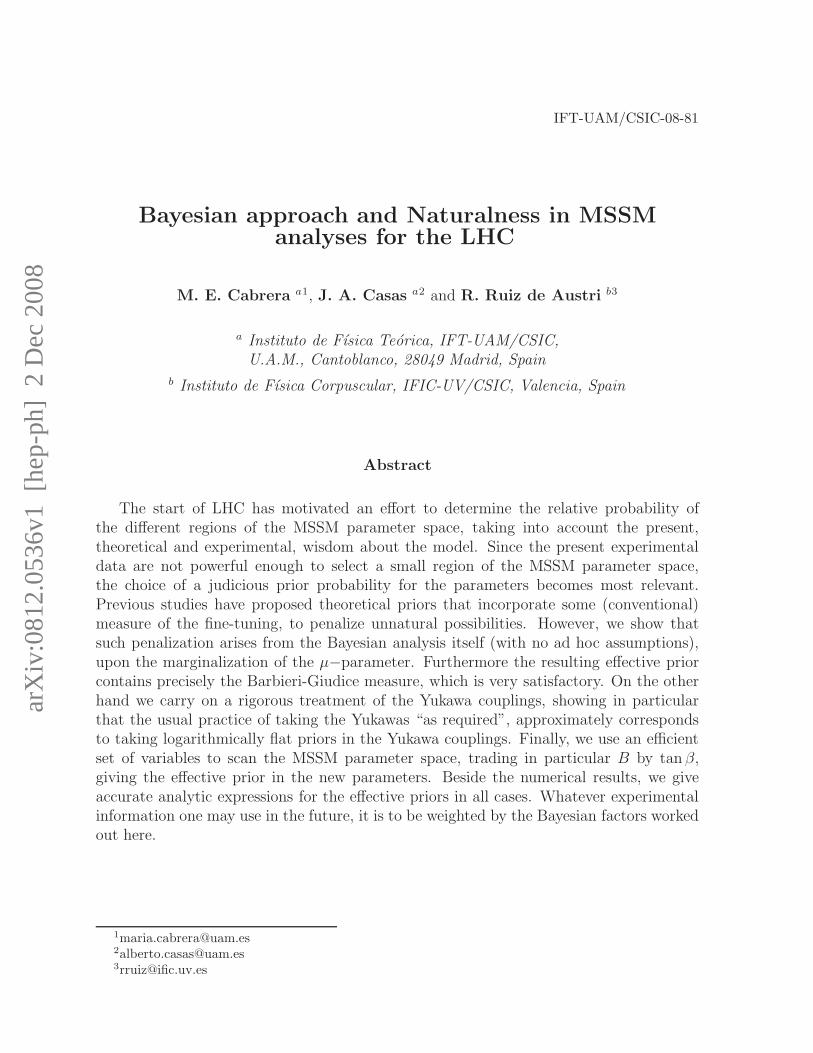
In Fig. 2 we show the effective prior defined in (3.3) and computed using eq. (3.8) [withthe full one-loop expressions of eqs. (3.4–3.6)] for the two priors discussed after eq. (3.16),i.e. flat and logarithmically flat. The plots show, up to a constant of proportionality,the effective priors in the {m, M} plane (with constant tanβ, A) for some representativecases8. We have assumed in the figures that the soft terms are initially given at the scale ofgauge unification, MX ∼ 1016 GeV, as essentially happens in scenarios of gravity–mediatedSUSY breaking, but of course our formulas are also applicable to e.g. gauge–mediatedSUSY breaking scenarios. The penalization of large scales is clear for the logarithmicallyflat case, as expected from our discussion. The fact that using a logarithmic prior penalizeslarge values of the parameters could seem quite obvious. However, this is not so clearwhen one compares the integrated probability that the the parameters are within differentranges of scales. For instance, the logarithmic prior alone would give more probability to

8The proportionality constant is simply the normalization constant of the initial prior, eqs. (3.16),times the normalization constant of the Yukawa prior. However, these factors play no role in the examof the relative probabilities of the points in the parameter space. Obviously, the absolute values of theleft plots cannot be compared to those of the right plots, as they are affected by a different normalizationconstant. We prefer not to include these normalization factors, as they depend on the upper limit assumedfor the soft terms, and do not shed any additional light on the relative probabilities inside the parameterspace.

12

Figure 2: Values of the effective prior, peff , in logarithmic units as defined in eq. (3.3) (upto a normalization constant), in the {m, M} plane for A = 0 and tanβ = 3 (upper plots),tan β = 10 (central plots), tan β = 30 (lower plots). The left and right plots correspondrespectively to the two basic choices of priors (flat and logarithmically flat) discussed ineq. (3.16) and below. See text for further details.

13

Figure 3: The same as Fig. 2, but in the {M, tanβ} plane, for A = 0, m = M .

the [100 TeV, MX ] range than to the [100 GeV, 100 TeV] one. However, the presence ofthe mentioned fine-tuning factor, 1/µ2, in the effective prior still penalizes the high-energyregions.

Fig. 3 is similar to Fig. 2, but showing now slices in the {M, tanβ} plane (with thecondition m = M). The plots illustrate the tanβ dependence of the effective prior, whichcan be essentially extracted from the approximate expression (3.15). [Note that, besidesthe explicit dependence, eq. (3.15) contains an implicit dependence on tan β through theRµ, Blow and y/ylow factors.] We can appreciate from the plots that the prior probabilitydecreases with tan β.

The effective prior computed and shown in the figures corresponds to the last twofactors of the pdf (3.2). The first factor, i.e. the likelihood, carries the experimentalinformation (fermion masses, electroweak precision tests, g-2 of the muon, dark matterconstraints, etc.). Whatever experimental information (and thus likelihood) we may use,it will be always weighted by the same effective prior factor shown here.

In this section we have argued so far that the sensible initial choice of independentparameters of the MSSM is {gi, yt, m, M, A, B, µ}, while for practical reasons it is mostconvenient to work with the set {gi, mt, m, M, A, tanβ, MZ} (and signµ). MZ is eliminatedfrom the analysis using its extremely sharp likelihood. The effective prior in the newvariables is then given by eqs. (3.3, 3.8), for which we gave explicit approximate expressionsin eqs. (3.14, 3.15).

It is interesting to wonder what would have been the result if one had insisted intaking directly mt as an initial (nuisance) variable, so that the transformation (3.1) wouldhave just involved {µ, B} → {MZ , t}, as has been done e.g. in ref. [4]. As argued insubsect. 2.2, it is theoretically bizarre to take mt as a fundamental variable, instead of yt.However, one may gain the bonus of almost no sensitivity to the prior in mt, since this is

14

essentially fixed by the experiment. This is true, but this procedure introduces extremelycounter-intuitive contributions to the Jacobian, as we will see briefly. The new 2-variableJacobian is given by

J2 =

∣

∣

∣

∣

∣

∣

∣

∣

∂µ∂MZ

∣

∣

∣

t,mt

∂µ∂t

∣

∣

MZ ,mt

∂B∂MZ

∣

∣

∣

t,mt

∂B∂t

∣

∣

MZ ,mt

∣

∣

∣

∣

∣

∣

∣

∣

, (3.17)

where the subscripts emphasize which variables have to be kept frozen in the partialderivations. Now, using the definitions (3.7), it is straightforward to obtain

J2 =∂f

∂MZ

∂h

∂t+

∂g

∂MZ

(

∂f

∂y

∂h

∂t− ∂f

∂t

∂h

∂y

)

+∂f

∂MZ

∂h

∂y

∂g

∂t. (3.18)

It is amusing that this expression is more complicated than in the 3-variable case, eq. (3.8).This comes from the fact that the derivatives in (3.17) contain contributions coming fromthe dependence of µ and B on y, which is in turn a function of t and MZ , eq. (3.6).These contributions were cancelled inside the 3-variable Jacobian thanks to the third rowin the matrix of eq. (3.8), but they are not cancelled here and give rise to the second andthird terms in eq. (3.18). Note that the first term in (3.18) is similar to the 3-variableJacobian given by eq. (3.8), whose physical significance (including the information aboutfine-tuning) was discussed after eq. (3.13). This term goes parametrically as B/µ and wasthe only one quoted in ref. [4], thus the resemblance of their result to our approximateexpression (3.14), except for the RG and s−1

β factors. However the second term goesparametrically as Bm2/µM2

Z , and thus is much more important for large soft terms,which then become strongly favoured (contrary to the intuitive expectatives). Thereforethere is no reason to have ignored such term. In consequence, the expressions used inref. [4] are much closer to using yt as a fundamental variable with logarithmically flatprior than to using mt.

Let us finish this section by using the approximate expressions discussed above togive, as advanced at the end of subsect. 2.1, an approximate expression for the fine-tuningparameter cµ. Recall that this parameter was defined as

cµ =

∣

∣

∣

∣

∂ ln M2Z

∂ lnµ

∣

∣

∣

∣

y,B

, (3.19)

where the subscript indicates that the partial derivative must be performed at y, B con-stant. Using eqs. (3.7), cµ can be written as

cµ =2µ

MZ

(

∂f

∂MZ

)

−1[

1 +∂f

∂t

∂h

∂µ

(

∂h

∂t

)

−1]

, (3.20)

where the right hand side has to be understood in absolute value. As above, using (3.9)and (3.10) we obtain explicit approximated expressions for the f, g, h functions. Theneq. (3.20) reads

cµ = 4R2µ

µ2

M2Z

[

1 − t2(1 + t2)

(t2 − 1)3

m2H1

− m2H2

Blowµlow

(

Blow

µlow

− 4t2

1 + t2

)]

. (3.21)

15

Note that the combination m2H1

−m2H2

can be easily written in terms of B, µ using eqs. (3.4,3.5).

4 Conclusions

The start of LHC has motivated an effort to determine the relative probability of thedifferent regions of the MSSM parameter space, taking into account the present (theoret-ical and experimental) wisdom about the model. These attempts are often called “LHCforecasts” [1–4, 6–8]. The central equation to extract this valuable information is thefundamental Bayesian relation

p(s, m, M, A, B, µ|data) ∝ L(s, m, M, A, B, µ) p(s, m, M, A, B, µ) , (4.1)

which gives this probability in terms of the usual experimental likelihood, L, and the priorp(s, m, M, A, B, µ), i.e. the “theoretical” probability density assigned a priory to pointsin the space spanned by the MSSM parameters {m, M, A, B, µ} and the SM-like ones (s).

Since the present experimental data are not powerful enough to select a small region ofthe MSSM parameter space, the choice of a judicious prior becomes most relevant. Indeed,ignoring this amounts to an implicit choice for the prior (which is not always sensible).On the other hand, it is common lore that the parameters of the MSSM, {m, M, A, B, µ},should not be far from the electroweak scale in order to avoid unnatural fine-tunings toobtain the correct scale of the electroweak breaking. Previous studies have attempted toincorporate this reasonable intuition to the Bayesian approach, by choosing a prior thatcounted (more or less explicitly) a conventional measure of the fine-tuning, typically theBarbieri-Giudice parameter, c, defined in eq. (2.2).

However, though reasonable, these kinds of proposals are rather arbitrary, as the verymeasure of the fine-tuning is. On the other hand, since the naturalness arguments aredeep down statistical arguments, one might expect that an effective penalization of fine-tunings should arise from the Bayesian analysis itself. One of the main results of thispaper has been to show that this is really so: using the fact that the likelihood associatedto the experimental MZ is essentially a Dirac delta, ∼ δ(MZ − M exp

Z ), one can easilymarginalize the µ-parameter (i.e. integrate the density of probability in this variable).Then one gets an effective prior for the remaining parameters

peff(s, m, M, A, B) = 2µ0

MZ

1

cµp(s, m, M, A, B, µ0) , (4.2)

which exhibits the fine-tuning penalization. (µ0 is the value of µ that reproduces theexperimental MZ for the given values of {s, m, M, A, B}.) Of course this effective prior hasto be combined with the experimental likelihood, except the part associated to the Z mass.The initial prior, p(s, m, M, A, B, µ), can be taken as flat or (preferably) logarithmicallyflat, as usual. We find very satisfactory that precisely the usual parameter to quantifythe degree of fine-tuning emerges in the Bayesian approach “spontaneously”, not uponsubjective assumptions, especially taking into account that there has been much discussion

16

in the literature about its significance and suitability. We have completed this analysisby giving an explicit and quite accurate expression for cµ, see eq. (3.21).

Our second result concerns the treatment of the Yukawa couplings. In previousBayesian analyses the Yukawas were essentially taken as needed to reproduce the ex-perimental fermion masses, within uncertainties. However, unlike the pure SM, in theMSSM the Yukawa couplings are not in one-to-one correspondence to the quark and lep-ton masses: they depend also on the value of tan β, which is a derived quantity that takesdifferent values at different points of the MSSM parameter space. This means that twoviable MSSM models (with the same fermion masses) will have in general very differentvalues of the Yukawa couplings, and thus the theoretical prior, p(y), will play a relevantand non-ignorable role in evaluating their relative probability. Any Bayesian analysis ofthe MSSM amounts to an explicit or implicit assumption about the prior in the Yukawacouplings. We have made explicit the dependence of the results on such prior and shownthat the easiest and usual practice of taking the Yukawas “as required”, approximatelycorresponds to taking logarithmically flat priors in the Yukawa couplings, which on theother hand is not an unreasonable choice at all.

Finally we have repeated this analysis, using a more efficient set of variables to scanthe MSSM parameter space. Besides trading µ by MZ and the Yukawa couplings (inparticular the top one) by the fermion masses, it is known that trading B by tan β ishighly advantageous. Following similar steps one can arrive to an effective prior in thenew parameters:

peff(gi, mt, m, M, A, tanβ) ≡ J |µ=µ0p(gi, yt, m, M, A, B, µ = µ0) , (4.3)

where J is the Jacobian of the transformation

{µ, yt, B} → {MZ , mt, t}, t ≡ tanβ (4.4)

(MZ does not appear in the right hand side of (4.3) since it is marginalized as explainedabove.) Note that still the initial choice of independent parameters is {yt, m, M, A, B, µ}(on which the initial priors are defined). It is the change of variables plus the marginaliza-tion of MZ what leads to the above effective prior. We have calculated J both numericallyand analytically (in an approximate but quite accurate fashion). The relevant formulasare eqs. (3.8) and(3.14). The last expression is very handful and leads to the effectiveprior given in eq. (3.15). Whatever experimental information (and thus likelihood) onemay use, it will be always weighted by the same effective prior factor calculated (andshown in plots for illustrative cases) here.

We have also discussed the results in comparison with other approaches in the litera-ture, arguing that the present one is conceptually more satisfactory.

Acknowledgements

We thank D. Garcıa-Cerdeno and R. Trotta for interesting discussions and suggestions.This work has been partially supported by the MICINN, Spain, under contract FPA

17

2007–60252, the Comunidad de Madrid through Proyecto HEPHACOS S-0505/ESP–0346,and by the European Union through the UniverseNet (MRTN–CT–2006–035863). M. E.Cabrera acknowledges the financial support of the CSIC through a predoctoral researchgrant (JAEPre 07 00020). R. Ruiz de Austri is supported by the project PARSIFAL(FPA2007-60323) of the Ministerio de Educacion y Ciencia of Spain . The use of theciclope cluster of the IFT-UAM/CSIC is also acknowledged.

References

[1] B. C. Allanach and C. G. Lester, Phys. Rev. D 73 (2006) 015013[arXiv:hep-ph/0507283].

[2] B. C. Allanach, Phys. Lett. B 635 (2006) 123 [arXiv:hep-ph/0601089].

[3] R. R. de Austri, R. Trotta and L. Roszkowski, JHEP 0605 (2006) 002[arXiv:hep-ph/0602028].

[4] B. C. Allanach, K. Cranmer, C. G. Lester and A. M. Weber, JHEP 0708 (2007) 023[arXiv:0705.0487 [hep-ph]].

[5] L. Roszkowski, R. Ruiz de Austri and R. Trotta, JHEP 0707, 075 (2007)[arXiv:0705.2012 [hep-ph]].

[6] O. Buchmueller et al., JHEP 0809 (2008) 117 [arXiv:0808.4128 [hep-ph]].

[7] R. Trotta, F. Feroz, M. P. Hobson, L. Roszkowski and R. Ruiz de Austri,arXiv:0809.3792 [hep-ph].

[8] J. Ellis, arXiv:0810.1178 [hep-ph].

[9] R. Trotta, Contemp. Phys. 49 (2008) 71 [arXiv:0803.4089 [astro-ph]].

[10] S. P. Martin, arXiv:hep-ph/9709356.

[11] H. P. Nilles, Phys. Rept. 110 (1984) 1.

[12] C. F. Kolda, Nucl. Phys. Proc. Suppl. 62 (1998) 266 [arXiv:hep-ph/9707450].

[13] B. C. Allanach, SOFTSUSY: a C++ program for calculating supersymmetric spectra,Comput. Phys. Commun. 143 (2002) 305 [arXiv:hep-ph/0104145].

[14] R. Barbieri and G. F. Giudice, Nucl. Phys. B 306 (1988) 63.

[15] P. Ciafaloni and A. Strumia, Nucl. Phys. B 494 (1997) 41 [arXiv:hep-ph/9611204].

[16] J. A. Casas, J. R. Espinosa and I. Hidalgo, JHEP 0411 (2004) 057[arXiv:hep-ph/0410298].

18

[17] J. A. Casas, J. R. Espinosa and I. Hidalgo, JHEP 0503 (2005) 038[arXiv:hep-ph/0502066].

[18] L. Giusti, A. Romanino and A. Strumia, Nucl. Phys. B 550 (1999) 3[arXiv:hep-ph/9811386].

[19] B. de Carlos and J. A. Casas, Phys. Lett. B 309 (1993) 320 [arXiv:hep-ph/9303291];G. W. Anderson and D. J. Castano, Phys. Lett. B 347 (1995) 300[arXiv:hep-ph/9409419]; P. Athron and D. J. Miller, Phys. Rev. D 76 (2007) 075010[arXiv:0705.2241 [hep-ph]].

[20] J. L. Feng, K. T. Matchev and T. Moroi, Phys. Rev. Lett. 84 (2000) 2322[arXiv:hep-ph/9908309].

[21] J. L. Feng, K. T. Matchev and T. Moroi, Phys. Rev. D 61 (2000) 075005[arXiv:hep-ph/9909334].

[22] J. O. Berger, B. Liseo and R. L. Wolpert, “Integrated likelihood methods for elimi-nating nuisance variables” Statistical Science 1999, Vol. 14, No. 1, 1-28

[23] D. M. Pierce, J. A. Bagger, K. T. Matchev and R. j. Zhang, Nucl. Phys. B 491

(1997) 3 [arXiv:hep-ph/9606211].

[24] See e.g. ref. [10] above.

[25] L. E. Ibanez and C. Lopez, Nucl. Phys. B 233 (1984) 511.

19