Black Hole Remnants at the LHC

L. Bellagambab∗, R. Casadioa,b†, R. Di Sipioa,b‡ and V. Viventia§

aDipartimento di Fisica, Universita di Bolognavia Irnerio 46, 40126 Bologna, Italy

bIstituto Nazionale di Fisica Nucleare, Sezione di Bolognavia Irnerio 46, 40126 Bologna, Italy

January 17, 2012

Abstract

We investigate possible signatures of black hole events at the LHC in the hypothesis thatsuch objects will not evaporate completely, but leave a stable remnant. For the purpose ofdefining a reference scenario, we have employed the publicly available Monte Carlo generatorCHARYBDIS2, in which the remnant’s behavior is mostly determined by kinematic constraintsand conservation of some quantum numbers, such as the baryon charge. Our findings show thatelectrically neutral remnants are highly favored and a significantly larger amount of missingtransverse momentum is to be expected with respect to the case of complete decay.

1 Introduction

Models with large extra dimensions [1, 2] allow for the fundamental scale of gravity MG to beas low as the electro-weak scale (MG ' 1 TeV), and microscopic black holes (BH) may thereforebe produced in our accelerators (for reviews, see, e.g., Refs. [3]). Once a BH is formed, and thebalding phase is over, the Hawking radiation [4] sets off. The standard description of this effect isbased on the canonical Planckian distribution for the emitted particles, which implies the life-timeof microscopic BHs is very short, of the order of 10−26 s [5]. This picture (restricted to the ADDscenario [1]) has been implemented in several numerical codes [6, 7, 8, 9, 10, 11, 12], which havebeen mainly designed to extract information that will allow us to identify BH events at the LargeHadron Collider (LHC) (see Ref. [13] for a search of BH signatures with the first data collected bythe LHC).

It is important to recall that the end-stage of the BH evaporation remains an open issue (see,e.g., Refs. [14, 15, 16]), because we do not yet have a confirmed theory of quantum gravity. In fact,the semiclassical Hawking temperature grows without bound, as the BH mass decreases, which can

∗lorenzo.bellagamba@bo.infn.it†roberto.casadio@bo.infn.it‡riccardo.disipio@bo.infn.it§vi.strawberry@gmail.com

1

arX

iv:1

201.

3208

v1 [

hep-

ph]

16

Jan

2012

be viewed as a sign of the lack of predictability of perturbative approaches 1. This is an importantissue also on a purely experimental side, since deviations from the Hawking law for small BH mass(near the fundamental scale MG) could actually lead to detectable signatures.

Our ignorance of the late stages of the BH evaporation is usually bypassed in the numericalcodes by letting the microscopic BH decay into a few standard model particles as an (arbitrary)lower mass is reached, but the possibility of ending the evaporation by leaving a stable remnanthas also been considered [19, 20]. The purpose of this report is precisely to study the case in whichBHs stop emitting and leave a long-lived (or even stable) remnant of mass M 'MG.

For this purpose, we have employed the Monte Carlo code CHARYBDIS2 [12], which is presentlythe only generator which natively supports remnant BHs, as we shall describe in Section 3. InSection 4, we report results from test runs and describe in details both the primary emission andfinal output obtained using Pythia [21]. We shall use units with c = ~ = 1 and the Boltzmannconstant kB = 1.

2 Black hole production and evolution

In the ADD scenario [1], a microscopic BH with horizon radius shorter than the typical size of theextra dimensions is usually approximated by a (4 +d)-dimensional solution of the vacuum Einsteinequations. In the simplest case of a non-rotating BH, this leads to the following expression for thehorizon radius,

RH =1√πMG

(M

MG

) 1d+1

(8 Γ(d+3

2

)d+ 2

) 1d+1

, (2.1)

where M is the BH mass, Γ the Gamma function, and the temperature associated with the horizonis given by

TH =d+ 1

4π RH. (2.2)

At the LHC, a BH could form by colliding two protons. The total BH cross section can beestimated from the geometrical hoop conjecture [22] as

σ(M) ≈ π RH . (2.3)

In order to determine the total production cross section, this expression must be rescaled accordingto the parton luminosity approach as

dσ

dM

∣∣∣∣pp→BH+X

=dL

dMσ(ab→ BH; s = M2) , (2.4)

where a and b represent the partons which form the BH,√s is their centre-mass energy and

dL

dM=

2M

s

∑a,b

∫ 1

M2/s

dxaxa

fa(xa) fb

(M2

s xa

), (2.5)

1For reviews of the more consistent microcanonical description of BH evaporation in which energy conservation isgranted, see Refs. [17, 18].

2

where fi(xi) are parton distribution functions (PDF) and√s the LHC centre-mass collision energy

(up to 7 TeV presently, with a planned maximum of 14 TeV).Once formed, the BH begins to evolve. In the standard picture, the decay process can be

divided into three characteristic stages:

Balding phase: the BH radiates away the multipole moments inherited from the initial config-uration and reaches a hairless state. A fraction of the initial mass will also be radiated asgravitational radiation.

Evaporation phase: the BH loses mass via the Hawking effect. It first spins down by emitting theinitial angular momentum, after which it proceeds with the emission of thermally distributedquanta. The radiation spectrum contains all the Standard Model (SM) particles, (emitted onour brane), as well as gravitons (also emitted into the extra dimensions).

Planck phase: the BH has reached a mass close to the effective Planck scale MG and falls into theregime of quantum gravity. It is generally assumed that the BH will either completely decayinto SM particles [5] or a (meta-)stable remnant is left, which carries away the remainingenergy [19].

We will here focus on the possibility that the third phase ends by leaving a stable remnant.

3 Remnants and a Monte Carlo code

Several Monte Carlo codes which simulate the production and decay of micro-BHs are now available(see, e.g. Refs. [6, 7, 8, 9, 10, 11, 12]). The only code which presently implements the descriptionof a remnant is CHARYBDIS2 [12]. Such a description is mostly based on kinematic and quantumnumber constraints, so that the remnant will necessarily have zero baryon number. The productionand evaporation phases are better modeled, from a theoretical point of view, although they couldstill be improved. For example, the production phase is described using bounds from trappedsurface formation, which might lead to overestimate the amount of missing energy in gravitationalradiation [23]. Further refinements have also been investigated for the Hawking spectra [24, 10].

A list of the relevant adjustable parameters in the code and the values we used in the simulations,is given in Table 1. In the study we present here, we simulated the different scenarios in pp collisionswith total centre-mass energy of both

√s = 7 TeV and 14 TeV.

Parameter Description Used values

MG Fundamental gravitational scale 2− 4 TeV

D Total number of dimensions 6, 8

MINMSS minimum initial BH mass 2×MG

MAXMSS maximum initial BH mass√s

RMSTAB main switch for stable BH remnant TRUE/FALSE

KINCUT kinematic condition for BH remnant TRUE/FALSE

Table 1: Most relevant parameters of CHARYBDIS2 and their values for the different simulatedsamples used in this study.

It is particularly important to describe in details the role of one of the kinematic constraints,namely KINCUT. When set to TRUE, the generator will not allow the emission of Hawking quanta

3

[GeV]remnantM0 500 1000 1500 2000 2500 3000 3500 4000

Eve

nts

/80

Gev

0

200

400

600

800

1000

1200

1400

1600

1800

2000

-1LHC @ 7 TeV - Integrated luminosity=1fb

=2 TeV, D=6, KINCUT=TRUEGM

=2 TeV, D=6, KINCUT=FALSEGM=2 TeV, D=8, KINCUT=TRUEGM

=2 TeV, D=8, KINCUT=FALSEGM

Figure 1: Remnant mass for different values of the KINCUT parameters.

that reduce the BH mass M below MG, whereas KINCUT=FALSE will allow the last decay particleto have an energy as large as the BH’s (but no more). Let us then see what will likely happenfor the last emission, when the BH has already evaporated down to a mass MLE & MG. Thegenerator will try to simulate an Hawking particle with energy ω determined by the Planckiandistribution with a temperature TH = TH(MLE) and small enough to ensure energy conservation.Roughly speaking (that is, neglecting the BH kinetic energy), this means TH(MLE) ' ω < MLE.Since the temperature (2.2) increases for decreasing M , it is likely the attempted last ω will carryaway enough energy to reduce M below MG. If KINCUT=TRUE, this process is forbidden andthe generator simply stops and leaves a remnant of mass MLE > MG. If KINCUT=FALSE, theprocess is allowed and the remnant mass will be M ' MLE − ω < MG. The effect of KINCUTis clearly visible in Fig. 1, which shows the remnant mass distributions for samples generated at√s = 7 TeV with MG = 2 TeV, in D = 6 and 8. If KINCUT=FALSE the last decay step, which

allows the remnant to access masses lower than MG, typically releases a lot of energy, producinglow mass remnants. On the other hand KINCUT=TRUE forbids remnant masses below MG, thusproducing an increase of events as the remnant mass approaches MG and long tails towards highervalues. These scenarios are in agreement with the results we shall show in the next Section.

From a theoretical point of view, one expects a remnant mass around MG (see, e.g., Ref. [26]).The above scenarios are therefore, in a sense, complementary, with the KINCUT=FALSE caseperhaps less sound.

4

pp collision√s = 7 TeV

Process MG [TeV] D σ [pb] remnant P lepT > 0.5 TeV Pmiss

T > 0.5 TeV ET > 2 TeVBH 2.0 6 0.017 KINCUT=TRUE 0.18± 0.02 11.8± 0.1 0.39± 0.03BH 2.0 6 ” KINCUT=FALSE 0.51± 0.03 14.9± 0.2 7.1± 0.1BH 2.0 6 ” no remnant 0.94± 0.04 1.74± 0.05 15.8± 0.2BH 2.0 8 0.052 KINCUT=TRUE 0.49± 0.05 33.9± 0.4 1.69± 0.09BH 2.0 8 ” KINCUT=FALSE 1.57± 0.09 43.0± 0.5 22.9± 0.3BH 2.0 8 ” no remnant 3.2± 0.1 5.4± 0.2 46.5± 0.5BH 2.5 8 1.74× 10−2 KINCUT=TRUE 0.0023± 0.0002 0.130± 0.001 0.0169± 0.0005BH 2.5 8 ” KINCUT=FALSE 0.0070± 0.0003 0.151± 0.002 0.112± 0.001BH 2.5 8 ” no remnant 0.0119± 0.0005 0.0225± 0.0006 0.162± 0.002tt - - 84 - 0 2.0± 1.2 5.4± 1.9

pp collision√s = 14 TeV

Process MG [TeV] D σ [pb] remnant P lepT > 1 TeV Pmiss

T > 1 TeV ET > 4 TeVBH 3.5 6 0.040 KINCUT=TRUE 0.30± 0.03 24.8± 0.3 0.47± 0.04BH 3.5 6 ” KINCUT=FALSE 1.01± 0.06 32.7± 0.4 10.4± 0.2BH 3.5 6 ” no remnant 1.82± 0.08 3.67± 0.12 33.5± 0.4BH 4.0 6 3.6× 10−3 KINCUT=TRUE 0.037± 0.004 2.45± 0.03 0.089± 0.006BH 4.0 6 ” KINCUT=FALSE 0.102± 0.006 3.02± 0.03 1.44± 0.02BH 4.0 6 ” no remnant 0.198± 0.008 0.36± 0.01 3.18± 0.03tt - - 469 - 0 0 0.75± 0.75

Table 2: List of generated Monte Carlo samples. Also reported are the expected numbers of eventsproduced at the LHC for an integrated luminosity of 1 fb−1 at

√s = 7 TeV and 14 TeV after basic

selection cuts on the PT of the leading lepton (electron or muon), missing PT and visible transverseenergy, for different values of MG and D. The expected events for one of the most relevant SMprocess, the tt production, are also reported.

4 Simulations

The standard setting for CHARYBDIS2 simulates the evaporation of a microscopic BH accordingto Hawking’s law, until the black hole mass M reaches the minimum value, which is assumedequal to the fundamental scale of gravity MG. The BH subsequently decays into a few bodies(Nf = 2, . . . , 6) simply according to phase space. As described in the previous Section, we areinstead interested in the study of scenarios with a residual stable BH remnant in the final state.

In order to compare the output of the different scenarios (no stable remnant, stable remnantwith KINCUT=TRUE/FALSE) we have generated Monte Carlo samples varying the parameterslisted in Table 1 and assuming two different centre mass energy for the LHC, namely 7 and 14 TeV.As pointed out in Table 1, the mass of the produced BH has been required to be at least 2MG inorder to avoid the region where the classical theory, used to evaluate the production cross section, isno longer valid. The other parameters have been fixed to the CHARYBDIS2 default values. Table 2summarizes the characteristics of the generated samples, including the tt production process whichis one of the most relevant backgrounds. The table also contains the event yields normalized toan integrated luminosity of 1 fb−1 for few basic selection requirements applied at the hadronizationlevel, as described in details in Section 5.

4.1 Primary Emission

Let us first examine the “primary” BH emission, namely the particles produced by direct BHevaporation, before parton evolution and hadronization are taken into account. This emission isthe direct output of CHARYBDIS2. Fig. 2 shows the produced final state particles and the particlemultiplicity for

√s = 7 TeV, MG = 2 TeV, in D = 8 and for the different remnant conditions. The

5

final state particles, listed in Fig. 2, panels a), c) and e), are grouped in SM particles (the firstthree blocks contain quarks, leptons and bosons, respectively), gravitons (G), neutral (R0) andcharged (R±) BH remnants. The remnants are neutral in the large majority of the cases, with onlya few percent of the events ending in a charged remnant. The neutral remnants behave as weaklyinteracting massive particles (WIMPs), producing a striking signal of missing transverse energyand a topology quite different from the usual case of total BH evaporation.

4.2 Final Output

The primary output includes unstable particles, along with quarks and gluons that have to beprocessed by a parton shower Monte Carlo in order to produce the final state observables (hadronlevel). We used PYTHIA [21] to model the parton evolution and hadronization of quarks andgluons emitted during the BH evaporation, as well as to treat the unstable particle decays andthe proton remnants. This produced the final features of the events as would be seen by the LHCdetectors. Besides the signal BH samples, also one of the most relevant SM backgrounds for suchtopologies, the process pp → ttX, has been generated using the NLO generator POWHEG [25],interfaced with PYTHIA for the parton shower, hadronization and particle decays. At least one ofthe two top quarks was requested to decay in either e, µ or τ .

5 Results and outlook

In order to point out the main characteristics of the different scenarios under study and the possi-bility to observe a signal over the SM background, we have applied a basic selection to the hadronlevel Monte Carlo samples using the following event variables:

• P lepT , defined as the transverse momentum of the leading lepton (e or µ) with |ηlep| < 2.5,

where ηlep is the lepton pseudorapidity;

• the missing transverse momentum,

PmissT =

√√√√(∑i

Pxi

)2

+

(∑i

Pyi

)2

, (5.1)

where Pxi and Pyi are the cartesian x and y components of the momentum of the ith particle,and i runs over all the undetectable final state particles: neutrinos, gravitons and neutral BHremnant;

• the visible transverse energy,

EvisT =

∑k

(√P 2xk

+ P 2yk

), (5.2)

where k runs over all the detectable final state particles.

The choice of the above simple variables is motivated by the fact that the observation of final stateparticles with transverse momentum of several hundreds of GeV’s is the typical signal for the decayof a large mass state. In particular, the requirement of high-energy leptons and/or high missing

6

transverse momentum allows to cope with the huge QCD background at the LHC. Since BHs decaydemocratically to all SM particles, the search for extremely energetic leptons is, in this context,one of the most direct way to look for deviations from the SM predictions.

However, in case of stable neutral remnants, the lepton signal can be depressed by the fact thata relevant fraction of the BH mass is not available in the decay. On the other hand, the neutralremnant, behaving as a WIMP, will carry away a lot of energy and enhance the missing transverseenergy signal. This is clearly visible in Figs. 3 and 4, where we show, for two representative cases at√s = 7 and 14 TeV, the PT of the leading lepton, the Pmiss

T and the EvisT for the different scenarios.

The tt background is also displayed.

The main characteristics of the different cases are further clarified in Fig. 5, which shows,for a representative case at

√s = 7 TeV, the event distribution in the Evis

T -PmissT plane for the

different remnant scenarios and for the tt background. If the BH decays completely, the events areconcentrated at relatively low Pmiss

T and very high EvisT , whereas, in the case of a stable remnant,

a shift towards much higher values of PmissT and consequently lower Evis

T is clearly visible. Asalready stressed in Section 3, the control parameter KINCUT sets two extreme and probably notrealistic descritpions of the stable remnant. Nevertheless, given the large uncertainties in thetheoretical picture, these two borderline scenarios allow to quantify the possible spread of therelevant experimental observables.

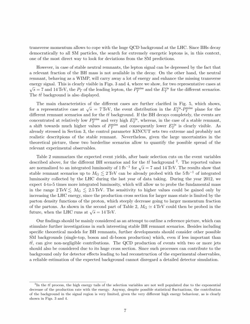
Table 2 summarizes the expected event yields, after basic selection cuts on the event variablesdescribed above, for the different BH scenarios and for the tt background 2. The reported valuesare normalized to an integrated luminosity of 1 fb−1 for

√s = 7 and 14 TeV. The results show that

stable remnant scenarios up to MG . 2 TeV can be already probed with the 5 fb−1 of integratedluminosity collected by the LHC during the last year of data taking. During the year 2012, weexpect 4-to-5 times more integrated luminosity, which will allow us to probe the fundamental massin the range 2 TeV. MG . 2.5 TeV. The sensitivity to higher values could be gained only byincreasing the LHC energy, since the production cross section for larger mass state is limited by theparton density functions of the proton, which steeply decrease going to larger momentum fractionof the partons. As shown in the second part of Table 2, MG ' 4 TeV could then be probed in thefuture, when the LHC runs at

√s = 14 TeV.

Our findings should be mainly considered as an attempt to outline a reference picture, which canstimulate further investigations in such interesting stable BH remnant scenarios. Besides includingspecific theoretical models for BH remnants, further developments should consider other possibleSM backgrounds (single-top, boson and di-boson production) which, even if less important thantt, can give non-negligible contributions. The QCD production of events with two or more jetsshould also be considered due to its huge cross section. Since such processes can contribute to thebackground only for detector effects leading to bad reconstruction of the experimental observables,a reliable estimation of the expected background cannot disregard a detailed detector simulation.

2In the tt process, the high energy tails of the selection variables are not well populated due to the exponentialdecrease of the production rate with the energy. Anyway, despite possible statistical fluctuations, the contributionof the background in the signal region is very limited, given the very different high energy behaviour, as is clearlyshown in Figs. 3 and 4.

7

Acknowledgements

We would like to thank the CHARYBDIS2 developers, in particular M.O.P. Sampaio and B.R. Web-ber, for very useful suggestions and comments.

References

[1] N. Arkani-Hamed, S. Dimopoulos and G. Dvali, Phys. Lett. B 429, 263 (1998); Phys. Rev.D 59, 0806004 (1999); I. Antoniadis, N. Arkani-Hamed, S. Dimopoulos and G. Dvali, Phys.Lett. B 436, 257 (1998).

[2] L. Randall and R. Sundrum, Phys. Rev. Lett. 83, 4690 (1999); Phys. Rev. Lett. 83, 3370(1999).

[3] M. Cavaglia, Int. J. Mod. Phys. A 18, 1843 (2003); P. Kanti, Int. J. Mod. Phys. A 19, 4899(2004).

[4] S.W. Hawking, Nature 248, 30 (1974); Comm. Math. Phys. 43, 199 (1975).

[5] S. Dimopoulos and G. Landsberg, Phys. Rev. Lett. 87, 161602 (2001).

[6] C. M. Harris, P. Richardson and B.R. Webber, JHEP 0308, 033 (2003).

[7] S. Dimopoulos and G. Landsberg, Black hole production at future colliders, in Proc. of theAPS/DPF/DPB Summer Study on the Future of Particle Physics (Snowmass 2001), editedby N. Graf, eConf C010630, P321 (2001).

[8] E.J. Ahn and M. Cavaglia, Phys. Rev. D 73, 042002 (2006).

[9] M. Cavaglia, R. Godang, L. Cremaldi and D. Summers, Comput. Phys. Commun. 177 (2007)506.

[10] G.L. Alberghi, R. Casadio, A. Tronconi, J. Phys. G G34 (2007) 767; G.L. Alberghi, R. Casa-dio, D. Galli, D. Gregori, A. Tronconi and V. Vagnoni, “Probing quantum gravity effects inblack holes at LHC,” hep-ph/0601243.

[11] D.-C. Dai, G. Starkman, D. Stojkovic, C. Issever, E. Rizvi, J. Tseng, Phys. Rev. D77 (2008)076007.

[12] J.A. Frost, J.R. Gaunt, M.O.P. Sampaio, M. Casals, S.R. Dolan, M.A. Parker, B.R. Webber,JHEP 0910 (2009) 014; M.O.P. Sampaio, “Production and evaporation of higher dimensionalblack holes,” Ph.D. thesis, http://www.dspace.cam.ac.uk/handle/1810/226741.

[13] CMS Collaboration, V. Khachatryan et al., Phys. Lett. B 697 (2011) 434.

[14] G. Landsberg, J. Phys. G 32, R337 (2006).

[15] C.M. Harris, M.J. Palmer, M.A. Parker, P. Richardson, A. Sabetfakhri and B. R. Webber,JHEP 0505, 053 (2005).

[16] A. Casanova and E. Spallucci, Class. Quant. Grav. 23, R45 (2006).

8

[17] R. Casadio, B. Harms and Y. Leblanc, Phys. Rev. D 57, 1309 (1998); R. Casadio and B. Harms,Phys. Rev. D 58, 044014 (1998) and Mod. Phys. Lett. A14, 1089 (1999).

[18] R. Casadio, B. Harms, Entropy 13 (2011) 502-517.

[19] B. Koch, M. Bleicher and S. Hossenfelder, JHEP 0510, 053 (2005).

[20] S. Hossenfelder, Nucl. Phys. A 774, 865 (2006).

[21] T. Sjostrand, S. Mrenna and P. Skands, JHEP 0605, 026 (2006).

[22] K.S. Thorne, in Magic without magic, edited by J. Klauder (Freeman, 1972).

[23] C. Herdeiro, M.O.P. Sampaio and C. Rebelo, JHEP 1107 (2011) 121.

[24] C. Herdeiro, M.O.P. Sampaio and M. Wang, Phys. Rev. D 85 (2012) 024005; M.O.P. Sampaio,JHEP 1002 (2010) 042; JHEP 0910 (2009) 008.

[25] P. Nason, JHEP 11, 040 (2006); S. Frixione, P. Nason and C. Oleari, JHEP 11, 070 (2007).S. Frixione, P. Nason, and G. Ridolfi, JHEP 09, 126 (2007).

[26] G. L. Alberghi, R. Casadio, O. Micu, A. Orlandi, JHEP 1109 (2011) 023.

9

d u s c b t e eν µ µν τ τν g γ 0Z ±W 0h

G

0R ±R

par

ticl

e m

ult

iplic

ity

-310

-210

-110

1

a)No stable remnant

Multiplicity0 1 2 3 4 5 6 7 8 9 10

0

0.1

0.2

0.3

0.4

0.5

0.6

0.7

0.8

0.9

1

b)No stable remnant

d u s c b t e eν µ µν τ τν g γ 0Z ±W 0h

G

0R ±R

par

ticl

e m

ult

iplic

ity

-310

-210

-110

1

c)KINCUT=FALSE

Multiplicity0 1 2 3 4 5 6 7 8 9 10

0

0.1

0.2

0.3

0.4

0.5

0.6

0.7

0.8

0.9

1

d)KINCUT=FALSE

d u s c b t e eν µ µν τ τν g γ 0Z ±W 0h

G

0R ±R

par

ticl

e m

ult

iplic

ity

-310

-210

-110

1

e)KINCUT=TRUE

Multiplicity0 1 2 3 4 5 6 7 8 9 10

0

0.1

0.2

0.3

0.4

0.5

0.6

0.7

0.8

0.9

1

f)KINCUT=TRUE

Figure 2: Primary decay products of the BH (panels a, c, e) and multiplicity (panels b, d, f) forno remnant, KINCUT=FALSE and KINCUT=TRUE, respectively. The plots have been obtainedusing Monte Carlo samples generated at 7 TeV, with MG = 2 TeV in D = 8.

10

[GeV]lepTP

0 200 400 600 800 1000 1200 1400 1600 1800 2000

Eve

nts

/50

Gev

-210

-110

1

10

210

310

410-1LHC @ 7 TeV - Integrated luminosity=1fb

Charybdis2 no remnantCharybdis2 stable remnant, KINCUT=FALSECharybdis2 stable remnant, KINCUT=TRUEt-tbar powheg+Pythia

[GeV]missTP

0 200 400 600 800 1000 1200 1400 1600 1800 2000

Eve

nts

/50

Gev

-210

-110

1

10

210

310

410

[GeV]visTE

0 500 1000 1500 2000 2500 3000 3500 4000 4500 5000

Eve

nts

/50

Gev

-210

-110

1

10

210

310

410

Figure 3: Distributions of P lepT , Pmiss

T and EvisT for BH events with different remnant scenarios and

for the tt background. The BH distributions have been obtained using the simulated samples at√s = 7 TeV with MG = 2 TeV in D = 8.

11

[GeV]lepTP

0 500 1000 1500 2000 2500 3000 3500 4000

Eve

nts

/50

Gev

-310

-210

-110

1

10

210

310

410

510 -1LHC @ 14 TeV - Integrated luminosity=1fbCharybdis2 no remnantCharybdis2 stable remnant, KINCUT=FALSECharybdis2 stable remnant, KINCUT=TRUEt-tbar powheg+Pythia

[GeV]missTP

0 500 1000 1500 2000 2500 3000 3500 4000

Eve

nts

/50

Gev

-310

-210

-110

1

10

210

310

410

510

[GeV]visTE

0 1000 2000 3000 4000 5000 6000 7000 8000 9000 10000

Eve

nts

/50

Gev

-310

-210

-110

1

10

210

310

410

510

Figure 4: Distributions of P lepT , Pmiss

T and EvisT for BH events with different remnant scenarios and

for the tt background. The BH distributions have been obtained using the simulated samples at√s = 14 TeV with MG = 4 TeV in D = 6.

12

[GeV]missTP

0 200 400 600 800 1000 1200 1400 1600 1800 2000

[G

eV]

vis

TE

0

500

1000

1500

2000

2500

3000

3500

4000

4500

5000

[GeV]missTP

0 200 400 600 800 1000 1200 1400 1600 1800 2000

[G

eV]

vis

TE

0

500

1000

1500

2000

2500

3000

3500

4000

4500

5000

[GeV]missTP

0 200 400 600 800 1000 1200 1400 1600 1800 2000

[G

eV]

vis

TE

0

500

1000

1500

2000

2500

3000

3500

4000

4500

5000

CHARYBDIS2 no remnant

CHARYBDIS2 stable remnant, KINCUT=FALSE

CHARYBDIS2 stable remnant, KINCUT=TRUE

ttbar POWHEG+PYTHIA

Figure 5: Distributions of signal and background events in the EvisT -Pmiss

T plane for the differentremnant scenarios. The BH distributions have been obtained using the simulated samples at√s = 7 TeV with MG = 2 TeV in D = 8.

13