WHOI-94-21

Woods Hole Oceanographic Institution

Massachusetts Institute of Technology

Joint Program in Oceanography/

Applied Ocean Science and Engineering

-c^CHOo

1930

4.

DOCTORAL DISSERTATION

Variations in the Paniculate Flux of 230Th and 231Pa and Paleoceanographic Applications of the 231Pa/230Th Ratio

by

Ein-Fen Yu

May 1994

19950120 031

,..*<£% *$&§&■ $£;■:■■&

pi^'ZZ

DTIf QUALITY INSPECTED 8

*v>

WHOI-94-21

Variations in the Particulate Flux of ^Th and ^Pa and Paleoceanographic Applications of the ^Pa/230!!! Ratio

by

Ein-Fen Yu

Woods Hole Oceanographic Institution Woods Hole, Massachusetts 02543

and

The Massachusetts Institute of Technology Cambridge, Massachusetts 02139

May 1994

DOCTORAL DISSERTATION

Funding was provided by the National Science Foundation under Grants OCE-8817836, OCE-8922707, OCE-9016494, and OCE-9200780.

Reproduction in whole or in part is permitted for any purpose of the United States Government. This thesis should be cited as: Ein-Fen Yu, 1994. Variations in the Particulate Flux of 230Th and 23lPa and

Paleoceanographic Applications of the 23,Pa/230Th Ratio. Ph.D. Thesis. MIT/WHOI, WHOI-94-21.

Approved for publication; distribution unlimited.

Approved for Distribution:

Michael P. Bacon, Chair Department of Marine Chemistry and Geochemistry

John W. Farrinj Dean of Graduate Studies

VARIATIONS IN THE PARTICIPATE FLUX OF 230 TH AND 231 PA AND PALEOCEANOGRAPHIC APPLICATIONS OF THE 231PA/230TH RATIO

by

Ein-Fen Yu B.S., Marine Sciences, Chinese Culture University, 1983 M.S., Oceanography, National Taiwan University, 1985

Submitted in partial fulfillment of the requirements for the degree of Doctor of Philosophy

at the MASSACHUSETTS INSTITUTE OF TECHNOLOGY

and the WOODS HOLE OCEANOGRAPHIC INSTITUTION

May, 1994

Copyright Ein-Fen Yu 1994. All rights reserved.

The author hereby grants to MIT and WHOI permission to reproduce and distribute copies of this thesis document in whole or in part.

Signature of author. ^V* ~£-v-n

Joint Program in Oceanography Massachusetts Institute of Technology/ Woods Hole Oceanographic Institution

Certified by **c Dr. Michael P. Bacon Thesis Supervisor

Accepted by. ().£,.%- Dr. Daniel J. Repeta Chair

Joint Committee for Chemical Oceanography

VARIATIONS IN THE PARTICULATE FLUX OF 230TH AND 231PA AND PALEOCEANOGRAPHIC APPLICATIONS OF THE 231PA/230TH RATIO

by

Ein-Fen Yu

ABSTRACT

Fractionation between 230xh (ti/2 = 7.5xl()4yr) and 231pa (tj/2 = 3.2x1 O^yr), the two longest-lived radionuclides produced from the decay of natural uranium, is found widely within the oceans. This large scale fractionation was investigated in samples of sinking particulate matter collected with sediment traps and in deep-sea sediment cores. New analytical methods for uranium, thorium, and protactinium isotopes by Inductively-Coupled Plasma Spectrometry (ICP-MS) with a conventional Meinhard concentric glass nebulizer were developed. Composite samples from sediment traps deployed a year or longer in diverse geographic regions of the ocean were analyzed to examine assumptions underlying the use of the 230Th_norrnaii2eci f]ux method and the 231pa/230xh ratio for reconstruction of the fluxes of sedimentary components in the present and past ocean. The compiled results demonstrated that over most of the ocean, the flux of 2301^ mt0 the sediments balances approximately its production rate in the overlying water column, with an accuracy better than 30%; whereas 231pa tends to migrate towards the margins or other regions of high particle flux. Thus the 231pa/230jh ratio is sensitive to regional differences in the scavenging intensity. In addition to this, the influence of particle composition on the 231pa/230xh ratio was investigated, but it was not possible to reach a definitive conclusion. The thesis describes aspects of the large scale geochemical fractionation between the two elements within the Atlantic Ocean during the Holocene and the Last Glacial Maximum and attempts to answer questions concerning the causes of the large scale fractionation resulting from a differential partitioning of the two elements between a vertical flux with sinking particles and a horizontal flux to boundaries due to ocean circulation. A quantification of the influence on the fractionation of the two nuclides by advection resulting from the thermohaline circulation was made, and it is shown that almost half of the 231pa production in the water column is exported from the Atlantic Ocean to the Southern Ocean. This export is important in the budget of 231pa in deep-sea sediments of the Southern Ocean. This suggests that the variations in 231pa/230rrn rati0 reflect variations not only in particle flux, but also in the intensity or pattern of the thermohaline circulation. Reconstruction of the 230ih- normalized biogenic opal and carbonate paleo-fluxes suggests no significant changes in surface production in the southern Indian Ocean between the Last Glacial Maximum and the Holocene period.

Acknowledgments

This work would not be complete without support and aid from

numerous people. I would especially like to thank to my thesis advisor, Dr. Mike

Bacon, for his constant advice, guidance, support, encouragement, patience, and understanding throughout my years in the Joint Program. Dr. Roger Francois

also contributed greatly throughout this work. I would also like to thank the other members of my thesis committee, Drs. Ed. Boyle and Bill Curry, for their generous offering of their expertise and scientific advice throughout this thesis

work.

I would like to thank Alan Fleer in particular for teaching all he knows

about deep-sea sediment sample preparation procedures, and his constant assistance in the lab. Terry for assistance in problem shooting of counting system is also appreciated. I am grateful to Dr. Ron Pflaum for his regular assistance in setting up the ICP-MS at Harvard, Prof. Stein Jacobsen for providing access to the instrument. I am grateful to Tim Shaw, Debbie Colodner, Rob Sherrell, and Kelly Falkner for teaching me about ICP-MS during the beginning stage of my development of analytical techniques by ICP-MS.

A special thanks to Dr. Ken Buesseler, who has kindly allowed me to use one of his counting systems while the major counter system in Mike's lab was out of order. Mary Hartman offered help in routine changing my samples. Special thanks go to Drs. Bill Curry and Mark Altabet for their kindness to allow me to use equipments in their lab.

This work benefitted from the supplies of year or longer collections of

sediment trap materials that were kindly provided by Dr. Susumu Honjo and his

colleague Dr. Steve Manganini. Appreciation goes to Steve who assisted in

splitting all sediment trap materials.

This work also benefitted greatly from the supplies of deep-sea sediments

from the Deep-Sea Sample Repository in Lamont-Doherty Earth Observatory

(LDEO) (Supported by National Science Foundation through Grant OCE91-01689 and the Office of Naval research through Grant N00014-90-J-1060), Antarctic Research Facility of Florida State University, and Deep-Sea Sample repository in Woods Hole Oceanographic Institution. Thanks to Ms. Rusty Lotti in LDEO and Mr. Dennis Cassidy in Antarctic Research Facility for their continuous aid in sampling. Sample materials of a downcore from the Southern Indian Ocean

were kindly provided by Dr. Laurent D. Labeyrie at Gif-sur-Yvette, France. The Holocene and Last Glacial Maximum sections of three cores in the North Atlantic Ocean were kindly provided by Dr. Eystein Jansen through the connection of Dr.

Delia Oppo.

I would like to acknowledge MIT Research Reactor which is supported

from the U. S. DOE Reactor Sharing Grant No. DE-FG07-80ER10770. A015 for providing facilities to make 233pa tracer.

Special thanks go to Greg Ravizza. I learned a great deal from his always

bright questions or comments. He continuously offered encouragement and help

in many ways, and shared his tremendous experiences.

I am also indebted to my other two pre-general examine committee, Drs. Ed. Sholkovitz and Phil. Gschwend along with Mike for their guidance in taking courses and encouragement throughout my first two most difficult years in the Joint Program. I also want to thank Dr. Mark Kurz who generously offered me an opportunity to learn some about mass spectrometry.

Many thanks go to Marcia Davis for improving my writing in English for years, and her great favor in editing. Thanks to Ms. Laura Praderio for her very efficient helps in editing this thesis as well.

Thanks to my friends and colleagues during these academia years in the Joint Progam, Nathalie Waser, Debbie Colodner, Jenny Lee, Greg Ravizza, Catherine Goyet, Frank Yang, Ed. Brook, and Mike DeGrandpre. I am especially grateful to Nancy Hayward for her warm heart in smoothing and comforting my difficult life in a foreign country.

Finally, I wish to thank my family for supporting me through this crazy endeavor.

Funding for this research was provided by the National Science Foundation (Grants OCE-8817836, OCE-8922707, OCE-9016494, and OCE- 9200780). Funds from the Woods Hole Oceanographic Institution and from the Gordon Research Conferences for travel to scientific meetings are also gratefully acknowledged. Accession For

BTIS GRA&I DTIC TAB Unannounced Justification.

a D

By Distribution/

Availability Codes

list Avail and/or

Special

-«fe

Table of Contents

Title page 1

Abstract 3

Acknowledgments 4

Table of contents 6

List of figures H

List of tables 14

Chapter 1 Introduction 17

1.1 Background 17 1.1.1 In situ production of 231pa and 230xh in sea water 17 1.1.2 Large-scale fractionation of 231pa and 230jh yj

1.2 Goals of the thesis 19 1.3 Outline of the thesis 20

Chapter 2 The new methods for uranium, thorium, and protactinium isotopes by inductively coupled plasma-mass spectrometry — 23

2.1 Introduction 23 2.2 Apparatus 24 2.3 Reagents, spikes, and working references 26

2.4 Radiochemical techniques 28 2.4.1 Sample preparation 29 2.4.2 Sample dissolution 29 2.4.3 Subsampling for 238u and 232-fti 32 2.4.4 Coprecipitation with Fe and Al hydroxides 33 2.4.5 Ion exchange procedure for separation and purification

of U, Th and Pa 33 2.4.6 Chemical yield determination of Pa 34

2.4.7 Final analyte preparation for ICP-MS 35

2.5 ICP-MS analysis 35 2.5.1 ICP-MS operation parameters 35

2.5.1-a Sample introduction 35 2.5.1-b Optimized conditions and features for Pa, U and

Th isotopes analysis 36 2.5.1-c Resolution, sensitivity and stability 36 2.5.1-d Background, memory effect, and detection limits — 41

2.5.1-e Linearity and dynamic: range 42 2.5.2 Analytical procedures 43

2.6 Determination of 231Pa by ICP-MS 44 2.6.1 Degree of ionization of 23*Pa 44

2.6.2 Abundance sensitivity 44 2.6.3 Quantitative analysis of 231pa/ 230jh isotope ratio and

instrument fractionation 45

2.6.4 Matrix effects 47

2.6.5 Precision and accuracy 55 2.7 Simultaneous determination of 230xh+234u+235u/ and

232Th+238U by isotope dilution-ICPMS 59 2.7.1 Abundance sensitivity 59 2.7.2 Mass fractionation 59 2.7.3 Precision and accuracy 60

2.8 Calculations 60 2.8.1 Isotope dilution calculation 60

2.8.1-a Background correction 63 2.8.1-b Blank correction 66 2.8.1-c Contribution from spikes 66

2.8.2 Sources of error 67 2.9 Conclusions 68

Chapter 3 Fractionation between 23lPa and 230Th in the settling particles: Can we use both as tools for reconstruction of paleo-particle flux 71

3.1 Introduction 71

3.1.1 Background 71 3.1.2 Questions and aims 76

3.2 Sampling strategy 77 3.3 Sample collection, handling and distribution 78

3.3.1 NABE 78 3.3.2 Arabian sea 81 3.3.3 PAPA : 81

3.4 Methods 82

3.4.1 Preparation of composite sediment trap samples 82

3.4.2 Radiochemical procedures 83

3.4.3 Carbonate content 83 3.4.4 Data processing 84

3.5 Results 84 3.5.1 Unsupported isotope activities 86

3.5.2 Authigenic uranium and particulate uranium 90

3.6 Discussion 91 3.6.1 Quantification of sediment trap efficiency with 231pa

and 230-rh 95

3.6.2 Quantification of particulate radioisotope flux 104

3.6.2-a The value of V/P for 230Th 105

3.6.2-b Is 230Th flux constant 107

3.6.2-c The V/P values for 231Pa 111 3.6.3 Particulate 231Paex/ 230Thex ratios in sediment traps — 112

3.6.4 Does the composition of particles affect the relationship between particle flux and the 23*Paex/ 23<^Thex ratio?-114

3.6.5 Implications for the 230Th-normalized flux method — 124 3.6.5-a The method and its assumptions 124 3.6.5-b Advantages and problems 125

3.7 Conclusions and Future Study 129

Chapter 4 Basin-wide variations in chemical scavenging of 23lPa and 230Th within the Atlantic Ocean since the Last Glacial Maximum 131

4.1 Introduction 131 4.2 Methods 133 4.3 Results 134 4.4 Discussion 141

4.4.1 Chemical fractionation between 23lPa and 230Th in the Holocene Atlantic sediments 141

4.4.2 Export of 231Pa and 230Th from the North Atlantic

across 25°N 154

4.4.3 The mass balance of 23^Pa in Holocene Antarctic

sediments 164 4.4.4 LGM/Holocene changes in the Pa/Th distribution in

Atlantic sediments 167

4.4.5 Changes in the flux of sedimentary components

between LGM and Holocene 179 4.5 Conclusions 188

Chapter 5 Variations in 231p3/ 230xh and sediment fluxes across the

frontal zones in the southern Indian Ocean and changes

since the Last Glacial Maximum 191 5.1 Introduction — 191

5.1.1 Why do we care to reconstruct past changes in particle fluxes in the Southern Ocean? 191

5.1.2 Why do 231Pa/ 230^ (231Pa/ 230rh)exo

measurements? 192 5.2 Deep-sea sediment samples 193

5.2.1 Core locations and physical setting in the region 194 5.2.2 Stratigraphy and sample selection 197 5.2.3 Downcore profile on the APF in the southeastern

Indian Ocean 197 5.3 Results 199

5.3.1 Uranium contents of the transect samples 199 5.3.2 Unsupported activities of 231pa and 230xh 0f the

transect samples 207 5.3.3 Radionuclide results from MD88-773 208

5.4 Discussion 208 5.4.1 230xh-normalized paleoflux 208

5.4.1-a The 230xh-normalized total flux for the Holocene transect samples 210

5.4.1-b The changes in the 230xh-normalized total flux between the Holocene and the LGM of the transect samples 214

5.4.1-c The latitudinal variations in extent of sediment focusing 214

5.4.1-d Change in the focusing factor with time 219 5.4.2 Variations in (231pa/ 230xh)ex

o ratio 220 5.4.2-a Latitudinal variations in (231pa/ 230jh)exo ratios

from the Holocene sections of the transect sediments - 222

10

5.4.2-b The causes for the latitudinal variations in (231pa/ 230xh)ex° ratio of the Holocene transect

samples 225 5.4.2-c A downcore profile of (231Pa/ 230Th)ex° ratios

and particle fluxes south of the APF 230

5.4.3 Interpretation of the latitudinal variations in 230xh_normaiize£j opal flux 232

5.4.3-a Latitudinal distribution patterns of opal content and 230Th-normalized opal flux during the Holocene -233

5.4.3-b The conditions and processes responsible for the

latitudinal distribution patterns of opal 236

5.4.3-c Interpretation of 230Th-normalized opal flux

changes between the LGM and the Holocene 238

5.4.3-d Impact of APF northward migration on the latitudinal

distribution and magnitude of changes in chemical properties and particle flux :—241

5.4.3-e Did biological production change during the LGM? 243 5.4.4 Interpretation of 230xh-normalized carbonate flux 245

5.4.4-a Latitudinal variations of carbonate record, and changes between the LGM and the Holocene 245

5.4.4-b MD88-773 carbonate profiles provide evidence of carbonate production changes 248

5.4.4-c The effect of CaC03: Corg rain ratio on the

interpretation of carbonate records 250

References 253

11

List of Figures

Figure 2.1 A schematic flow chart for separation and purification of U,

Th, and Pa isotopes for ICP-MS analysis 30

Figure 2.2 Variations of instrument tuning sensitivity over a long

time period 38 Figure 2.3 An example of medium-term stability of the instrument — 40 Figure 2.4 Example of sample matrix effect on a 231pa standard analyte 49 Figure 2.5 Extent of matrix effect 50 Figure 2.6 Example of reduction in sample matrix effect on the

231pa signal 54

Figure 3.1 Comparison of estimated mean annual flux (g/m^/y) 94 Figure 3.2 Summary of some available 230xh/231pa activity ratios

measured in the water column 99 Figure 3.3 The estimated trapping efficiency [E(230Th)] versus

trap depth 102 Figure 3.4 (V/P)230xh and (V/P)231pa versus trap efficiency-corrected

mass flux; (F/P)230Th and (F/P)231Pa versus mass flux 108 Figure 3.5 (Pa/Th)/0.093 vs. trap efficiency-corrected mass flux 113 Figure 3.6 The vertical flux/production ratio of 230Th and 231pa

versus trap efficiency-corrected flux 117 Figure 3.7 The 231pa/230jh activity ratio versus trap efficiency-

corrected flux 119 Figure 3.8 Deviation of the 231pa/230xh ratio over 0.093 versus

%opal, %carbonate, %Corg and %terrigenous material 120

Figure 4.1 The map of selected cores of the Atlantic Ocean 135 Figure 4.2 The map of decay-corrected unsupported 231pa/230rrn of the

Holocene Atlantic Ocean 142 Figure 4.3 Summary of unsupported 231pa/230xh ratios in the Holocene

Atlantic sediments 147 Figure 4.4 230jh distributions measured in ocean-water profiles by

alpha-counting 157 Figure 4.5 231pa distributions measured in ocean-water profiles by

alpha-counting 158 Figure 4.6 Diagram of the mass balance of 231pa m the Holocene

Southern Ocean 166

12

Figure 4.7 The map of decay-corrected unsupported 231pa/230xh of the

LGM Atlantic Ocean 172 Figure 4.8 Summary of unsupported 231pa/230xh ratios in the LGM

Atlantic sediments 174

Figure 4.9 The map of LGM/Holocene ratio of the decay-corrected unsupported 231pa/230xh ratios (Pa/Thex

0) in the Atlantic

Ocean 177

Figure 4.10 Diagram of the mass balance of 231Pa in the LGM Southern Ocean 178

Figure 4.11 Carbonate (%) for both the LGM and Holocene in the

Atlantic sediments 181

Figure 4.12 Non-carbonate (%) for both the LGM and Holocene in

the Atlantic sediments 182 Figure 4.13 The LGM/Holocene ratio of the 230Th-normalized

carbonate and non-carbonate flux for the Atlantic sediments 183

Figure 5.1 Map of selected cores in the southern Indian Ocean 196 Figure 5.2 Oxygen isotope chronology of core MD88-773 198 Figure 5.3 Total uranium and authigenic uranium versus age in core

MD88-773 209 Figure 5.4 230xh-normalized total flux of the Holocene section 211 Figure 5.5 LGM/Holocene ratio of 230Th-normalized total flux versus

latitude for the transect samples in the southern Indian

Ocean 216 Figure 5.6 Comparison between the 230Th-normalized total flux and

the sediment accumulation rate for the Holocene transect samples in the southern Indian Ocean 218

Figure 5.7 The (231Pa/230Th)ex° activity ratio of the Holocene

sections and LGM sections of the transect sediments from the southern Indian Ocean 223

Figure 5.8 %Opal and %carbonate versus latitude for the Holocene transect sections in the southern Indian Ocean 227

Figure 5.9 230xh-normalized opal and carbonate flux for the Holocene

transect sections in the southern Indian Ocean 228 Figure 5.10 (23lPa/230Th)exO and 230Th-normalized total flux versus

age in core MD88-773 231

13

Figure 5.11 LGM/Holocene ratios of 230xh-normalized opal flux, carbonate flux, and (231pa/230xh)exo versus latitude for the

transect samples in the southern Indian Ocean 239

Figure 5.12 The water depth and %carbonate (both the LGM and the Holocene) of the transect cores in the southern Indian Ocean-246

Figure 5.13 The water depth and carbonate flux (both the LGM and the

Holocene) of the transect cores in the southern Indian Ocean-249

Figure 5.14 230xh-normalized carbonate and non-carbonate flux versus

age in core MD88-773 251

14

List of Tables

Table 2.1 Information on the production of 233pa by neutron

activation of 232xh 27

Table 2.2 ICP-MS operation conditions 39

Table 2.3 Example of background levels (in ACPS) for Th, Pa, and

U isotopes 41 Table 2.4 Abundance sensitivity for 231pa 45

Table 2.5 Example of calibration for quantitative analysis of 231Pa/229Th ratio 46

Table 2.6 Examples of instrument stability on 231pa/229xh atom ratio

and instrument mass fractionation 47

Table 2.7 The experimental results of matrix effects on the measurement of 231pa/229xh ratio 52

Table 2.8 Precision and accuracy of 231pa/229xh measurement by

ICP-MS 58 Table 2.9 Comparison of ICP-MS to a-spectrometry for 231pa

measurements 58 Table 2.10 Examples of stabilities on isotope ratio and the instrumental

mass fractionation 61 Table 2.11 Reproducibility of Th, U isotope measurement on a

uraninite standard 62 Table 2.12 Comparison of a-spectrometry results and ICP-MS results

for Th and U isotopes in marine sediments 64 Table 2.13 Examples of procedural blanks 66

Table 3.1 Locations and collection information of the compiled sediment trap samples 79

Table 3.2 Analytical results of radionuclides for sediment trap

samples 85 Table 3.3 Calculated results of radionuclides for sediment trap

samples 87 Table 3.4 Complied data for sediment trap samples 93

Table 3.5 Model results of the sediment trap efficiency 100 Table 3.6 Concentration and flux of components for sediment trap

samples 116

15

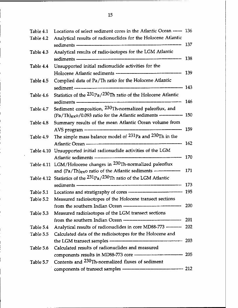
Table 4.1 Locations of select sediment cores in the Atlantic Ocean 136 Table 4.2 Analytical results of radionuclides for the Holocene Atlantic

sediments 137 Table 4.3 Analytical results of radio-isotopes for the LGM Atlantic

sediments 138

Table 4.4 Unsupported initial radionuclide activities for the

Holocene Atlantic sediments 139

Table 4.5 Complied data of Pa/Th ratio for the Holocene Atlantic

sediment 143 Table 4.6 Statistics of the 231pa/230xh ratio of the Holocene Atlantic

sediments 146 Table 4.7 Sediment composition, 230xh-normalized paleoflux, and

(Pa/Th)exo/0.093 ratio for the Atlantic sediments 150

Table 4.8 Summary results of the mean Atlantic Ocean volume from

AVS program 159 Table 4.9 The simple mass balance model of 231pa and 230xh in the

Atlantic Ocean 162 Table 4.10 Unsupported initial radionuclide activities of the LGM

Atlantic sediments 170 Table 4.11 LGM/Holocene changes in 230xh-normalized paleoflux

and (Pa/Th)exO ratio of the Atlantic sediments 171

Table 4.12 Statistics of the 23lPa/230Th ratio of the LGM Atlantic

sediments 173 Table 5.1 Locations and stratigraphy of cores 195 Table 5.2 Measured radioisotopes of the Holocene transect sections

from the southern Indian Ocean 200

Table 5.3 Measured radioisotopes of the LGM transect sections from the southern Indian Ocean 201

Table 5.4 Analytical results of radionuclides in core MD88-773 202 Table 5.5 Calculated data of the radioisotopes for the Holocene and

the LGM transect samples 203 Table 5.6 Calculated results of radionuclides and measured

components results in MD88-773 core 205

Table 5.7 Contents and 230xh-normalized fluxes of sediment components of transect samples 212

16

Table 5.8 Changes of composition and 230Th-normalized

fluxes between Holocene and LGM of transect section 215

Table 5.9 Calculation of focusing factor for core MD88-773 221

Table 5.10 Average values of 230Th-normalized total flux and (231pa/230xh)ex° ratio for transect samples 224

Table 5.11 Estimations of the biogenic opal flux 235

17

CHAPTER 1

INTRODUCTION

1.1 BACKGROUND

1.1.1. In situ production of 231pa and 230-rh m sea Water

Naturally occurring protactinium-231 (ti/2 = 3.2x1 O^yr) and thorium-230 (ti/2 = 7.5xl()4yr) have in-situ sources in sea water resulting from the decay of uranium. 231pa ^ the alpha decay daughter of 235{j, and 2307h is the alpha

decay daughter of 234{j. In the open ocean, uranium is essentially conservative, its concentration varies only with salinity (Cochran, 1992). Since the residence time of uranium is much longer (approximately 4.5xl05yr, Chen et al, 1986) than the stirring time of the oceans (approximately lxl()3yr; Broecker and Peng, 1982), the distribution of uranium in the ocean is essentially uniform. Consequently, 231pa and 230xh are produced at a constant rate throughout the ocean, and their rates of supply to the sediment are directly proportional to the depth of the water column. Once produced, both 231pa and 230xh are removed rapidly to the

sediment on a time scale of ~40 to 200 yr (Anderson et al, 1983a and b) and ~20 to 40 yr (Moore and Sackett, 1964; Bhat et al, 1969; Matsumoto, 1975; Brewer et al,

1980; Li et al, 1980; Anderson et al, 1983a and b), respectively; 23lPa and 230rh will be removed to sediments by a rigidly fixed 231pa/230xh activity ratio of 0.093 (or 10.8 if 230xh/231pa activity ratio is used) determined by the

235u/234u ratio in seawater, if there is no fractionation between the two

nuclides (Anderson et al, 1983a). Actual measurements in the ocean, however, give results that diverge considerably from this value.

1.1.2 Large-scale fractionation of 23lpa and 230xh

Depth profiles of 230jh in seawater often show a linearly increasing trend

as expected from the in situ production from uranium and reversible uptake by

18

sinking particles (Bacon and Anderson, 1982; Anderson et al, 1983a; Nozaki and

Nakanishi, 1985; Cochran et al, 1987; Nozaki et ah, 1987; Bacon, unpublished data). In comparison with the profiles of 230xh j^ the open ocean, 231pa shows a

very different pattern with increasing in total 231pa aoncentration to a mid-depth

maximum, and decreasing concentration toward the bottom (Nozaki and Nakanishi, 1985). In consequence, the activity ratio 230xh/231pa obtained from

open-ocean water shows an increasing trend toward the bottom, and the activity ratio of 230xh/231pa [$ generally less than the supply rate ratio which is 10.8. This implies that a large fraction of 231pa relative to 230Th ^ transported a

longer distance away from its source. The capability of large horizontal transport of Pa results from its longer residence time relative to that 230Th.

Studies of sinking particles with sediment traps provide important information about the fractionation between 231pa and 230xh. The works of

Anderson et al (1983) and later Lao (1991) confirmed that the 230Th/231Pa

activity ratio is fractionated with values higher than 10.8 at the mid-ocean sites, and lower than 10.8 at the ocean margins. The significant horizontal 231pa

concentration gradients from the mid-ocean sites toward the margins clearly indicate a net transport of 231pa (Anderson et al., 1983 a and b). Many investigations of surface sediment have also shown an ocean basin scale fractionation between 231pa an£j 230jh. Surface sediments around the margins of the ocean tend to have higher 231pa/230xh ratio than the production rate ratio of 0.093, in contrast with the abyssal sediments underlying the interior regions.

This is found to be commonly in the Pacific Ocean (DeMaster, 1981; Yang et al.,

1986; Shimmield et al, 1986; Anderson et al, 1990; Lao, 1991). However, it is not

true for the Atlantic Ocean, as will be shown in this thesis.

Important information regarding the large-scale fractionation of scavenged elements like 231 pa ancj 230rh has been reviewed with box models (Bacon, 1988). As Bacon pointed out, the large fractionation between 230 jh and

231pa within a basin comes about because of the partitioning of the two elements between two transport pathways, i.e., vertical scavenging or horizontal transport, for removal. On one hand 230xh, because of its high particle reactivity and short residence time, is predominately removed with the downward flux of particles. On the other hand 231pa/ which is relatively less particle-reactive, with a

residence time about 2 to 3 times longer than that of 230xh, can be laterally

19

transported longer distances away from its production site before it is removed. Consequently, over most of the ocean, the flux of 230xh mt0 the sediments

balances approximately its production rate in the overlying water column;

whereas 231pa tends to migrate towards the margins or regions of high particle

flux. As a result, competition between vertical scavenging and horizontal

transport determines the fractionation between the two elements. Thus, regional

differences in the scavenging intensity and the ocean mixing rate will influence the distribution of 231pa and 2307h on a basin-wide scale. The differential

chemical reactivity of 231pa ancj 230xh on different particle surfaces is another

factor that can modify the fractionation between the two elements.

1.2 GOALS OF THE THESIS

In this thesis, the goal is to examine all those factors (particle scavenging intensity, particle reactivities, and ocean mixing rate) as described above for causing the large-scale fractionation of scavenged elements like 231pa and 230xh.

Such examination has included investigations of sediment trap samples and

deep-sea sediments. Then I pursue applications based on the fractionation between the two elements in the ocean. Such applications have been included in this thesis for studies of paleoceanography, boundary scavenging, and ocean mixing.

In these areas, I can pursue two lines of investigation. First, the nearly uniform deposition of 230rh over the whole seafloor can allow us to predict 230xh flux, which is nearly equal to the rate of production from the decay of uranium in the water column. This allows us to use decay-corrected excess 230jh activity in sediments as a reference against which variations in the flux of other sediments can be evaluated. This is the so called "230xh-normalized flux

method", an idea first proposed by Bacon (1984). I can apply this idea to examine the variations in sedimentary flux between the LGM and the Holocene.

The second area of research is based on the ratio of 231pa/230xh. The

scavenging efficiency of these nuclides and the fractionation between the two nuclides can be an indicator of intensity of particle flux. Chemical composition of the settling particles could also influence the relative distribution of the two

20

nuclides. From the distribution of boundary scavenging of 231pa and 230^ we

may gain insights on the distribution or flux of other reactive elements or trace

metals. This is particularly focused on the distribution patterns in the Atlantic Ocean. Some questions like where the boundary scavenging of 231pa or 230xh

occurs in the Atlantic Ocean, what factors control the distribution patterns of chemical fractionation between 230jh and 231pa in the Atlantic Ocean, and how

the distribution pattern changes with time are examined in this thesis.

Besides the particle flux and chemical composition of a particle, the potential importance of the influence of advection by ocean circulation is

underscored by the findings of this thesis work and opens up the possible use of

231pa and 230jh as tracers for examining ocean advection.

Since a basin scale fractionation between 231pa and 230jh is pursued, a

large number of samples would be required to obtain complete representation of different scavenging conditions (for this thesis work, the whole Atlantic Ocean is studied). Given the limitations of time, a fast and precise analytical technique was pursued to replace the conventional oc-spectrometry counting method, a precise but time consuming technique. Inductively-Coupled Plasma Spectrometry (ICP-MS) was initially pursued for this purpose. Methods by Inductively-Coupled Plasma Spectrometry (ICP-MS) with a conventional Meinhard concentric glass nebulizer for measuring 231 p3/ and simultaneous

measurement of U and Th isotopes in sediment samples were developed. The technique has been used routinely for Th and U isotopes measurements for

sediments; unfortunately, given the limitation of amount of sample materials, routine measurements for 231pa by this technique were not often made for this

thesis work. However, I have shown that routine measurements for 231pa by

this technique can be promised if a more efficient sample introduction is available.

1.3 OUTLINE OF THE THESIS

The thesis consists of five chapters. The next chapter describes the newly developed analytical methods for uranium, thorium, and protactinium isotopes by Inductively-Coupled Plasma Spectrometry (ICP-MS) with a conventional

21

Meinhard concentric glass nebulizer. Chapter three address the fractionation between 231pa and 230jh ^ the settling particles (more emphasis on the

influences of scavenging intensity and the particle composition on the

fractionation between the two elements) and ideas to use both as tools for reconstruction of paleo-particle flux. Chapter four opens up the question of the advection by ocean circulation causing the basin wide fractionation between 231pa and 230xh. Chapter five focuses on the variations in 231pa/230jh ratio

and sediment fluxes across the frontal zones in the southern Indian Ocean and changes since the Last Glacial Maximum.

22

23

CHAPTER 2

THE NEW METHODS FOR URANIUM, THORIUM, AND PROTACTINIUM

ISOTOPES BY INDUCTIVELY COUPLED PLASMA-MASS SPECTROMETRY

2.1 INTRODUCTION

The potential of uranium, thorium, and protactinium isotopes as tools

in geochemistry and oceanography has been appreciated for a long time.

Determination of these isotopes in marine sediments has generally been

performed by a-spectrometry. The method has been widely used but tends to

be very time consuming or requires elaborate laboratory facilities. With

recent developments in mass spectrometry, atom-based techniques have now

become superior for the analysis of long-lived radionuclides in seawater,

marine deposits, and deep-sea sediments. Like fixed-magnetic thermal

ionization mass spectrometry (TIMS) which provides superior sensitivity and

precision to counting-techniques, inductively-coupled plasma spectrometry

(ICP-MS) offers several advantages over both TIMS and ex-counting: superior

ionization, fast analysis, multi-element capabilities, and simple sample

preparation. Methods for the determination of 238JJ (Klinkhammer and

Palmer, 1991) and 230Th (Shaw and Francois, 1991) by isotope- dilution ICP-

MS have recently been reported. Measurement of 231pa by ICP-MS is more

difficult because of the low amounts of 231pa (its concentration is about 20

times less than that of 230xh in sediment samples) and because there is no

suitable Pa isotope for isotope dilution. Initial work for this dissertation

involved the development of techniques for quantitative measurement of

24

231pa m marine sediments by ICP-MS with a conventional Meinhard

concentric glass nebulizer. As the work progressed, because of the multi-

element capabilities of ICP-MS, methods were also developed to allow

simultaneous determination of 230xh, 234y, and 235{j on the same aliquot,

and simultaneous determination of 232xh and 238u on another aliquot by

isotope dilution. Simultaneous measurements by ICP-MS provide analyses

that are not only faster and less laborious but also more precise than those

provided by the a-counting technique. The success of the procedure for U

isotope determinations is important, because decay-correction of 230xh ancj

231pa m sediment samples requires knowledge of 234y (or 238jj) and 235y

content.

The cc-spectrometry technique was also used in this thesis for sediment

trap samples, spikes and working-reference calibrations for ICP-MS work and

for 231 pa measurement in sediments of small size or low concentration.

2.2 APPARATUS

Analyses were performed on a model VG PQ2 Plus quadrupole ICP-MS

at Harvard University. ICP-MS involves the introduction of ions from an

argon gas plasma through a specialized sampling interface (= 1 mm diameter

high purity Ni sampling cone and a skimmer cone with ~ 0.75 mm diameter)

into a high vacuum region, where a quadrupole mass analyzer separates

them for detection on the basis of their charge-to-mass ratio. Sample aliquots

are introduced into the plasma with a peristaltic pump (Gilson Minipuls 22)

and a Meinhard concentric glass nebulizer. The sample aerosol created in the

nebulizer is directed through a spray chamber, which acts as a filter allowing

25

aerosol droplets < 10 microns in diameter to enter the plasma. Such small

droplets can be efficiently desolvated, atomized and ultimately ionized in the

plasma but constitute only about 1-5% of the original aerosol, with the rest of

the sample directed to a waste bottle.

Chemical yield for Pa was determined by beta-counting of 233pa tracer

added at the beginning of the analysis and was performed on two 2n

proportional counters (Nuclear Measurements Corporation Model PCC-11T

proportional counter coupled to NMC Model DS-1T decade

scaler/timer/higher voltage supply). Both counters use 10% methane/90%

argon as the counting gas. The operating voltage for ß -counting is at 1800V.

Background for ß counting is 12-20 counts/min. The counting efficiency of

both proportional counters is around 50%.

Chemical yield monitoring for Pa was also done with a GeLi gamma

counter during the early stages of this work. The 311.89keV photopeak was

used.

Three a-counting systems were used during the course of this work:

Canberra Quad alpha spectrometer model 7404 with a Canberra 8180 pulse-

height analyzer; EG&G Ortec 576A with a model 918A CADCAM

multichannel buffer and a 476-16 multiplexer; and a 16-detector system

consisting of Kicksort 504 N Quad bias supplies and 211Q Quadamps and a

Northern NS-700 series (Northern Econ II Series) pulse-height analyzer.

Silicon surface-barrier detectors are used in all of these systems. Energy

resolution, expressed as full peak width at half-maximum height, is 20-40

keV. Counting efficiency of the detectors ranges between 25 and 35%.

26

Teflon lab-ware was cleaned in soap and was then boiled twice in 50%

HN03. Polyethylene and polypropylene vessels (bottles, columns, centrifigue

tubes) were leached in soap and 2N HC1 acid baths. The major concern is

carry-over of residual 233pa from previous samples. 8-mm x 10-cm

polyethylene columns with polyethylene frits were used for ion exchange

chromatography. The use of any glassware was avoided to prevent

adsorption of Pa (Sill, 1978; Anderson and Fleer, 1982).

2.3 REAGENTS, SPIKES, AND WORKING REFERENCES

Reagent grade acids and distilled deionized water were used in all

procedures. Dowex AG1-X8 anion exchange resin, 100-200 mesh (Bio Rad

Laboratories), was used for all ion exchange columns.

Spikes of 236y and 229fji were calibrated against standard solutions of

238u and 232Th prepared from high-purity oxides: U3O8, NBS 950A; Th02,

Lindsay Code 116, 99.99% minimum purity, American Potash and Chemical

Co.).

Preparation of 233pa was by neutron activation of Th(N03)4-4H20 that

had been deposited on a Nuclepore aerosol filter and pressed into a pellet

(Anderson and Fleer, 1982). Irradiation was performed at the Massachusetts

Institute of Technology nuclear reactor. Detailed information about the

irradiation of 232xh to produce 233pa js given in Table 2.1. After irradiation,

the pellet was soaked in concentrated NH4OH for several hours, the excess

ammonia was evaporated, and the filter was destroyed by oxidation in

concentrated HNO3. 233pa tracer was separated from the 232ih on a Dowex

27

AG1-X8 Cl- column. Solutions of 233pa were repurified periodically to

remove accumulated 233u decay product.

A reference solution of 231pa for establishing the analytical procedures

was milked from a Harwell uraninite solution (Huh, personal

communication), and calibrated with an a-counter of known efficiency and

with 233pa as yield monitor. A reference solution of 230xh was directly

diluted from a stock standard solution (standard solution catalog #7230 from

Isotope Products Laboratories) and calibrated against a weighed amount of

232jh by a-counting. Stock 238u solution was made gravimetrically from an

oxide U3O8 (NBS 950A), and the working reference solution was

gravimetrically diluted from it.

Table 2.1 Information on the production of 233pa by neutron activation of

232Th

Chemical form Th(N03)4-4H20, mol. wt.= 552 Physical form Solid Number of 2327h atoms (N) 1.09 x 10l8 Production and decay processes of 233pa 232xh (n, Y) 233xh-> 233Pa_> 233u Irradiation time (t) 8 hours Neutron flux (F) 5 x 10l3 n/cm2.sec Cross section of target (CJTh) 7.4 x 10-24 cm2

233ih half-life 22 minutes 233Pa half-life 27 days= 648 hours

Activity (233pa)= NF(aTh)(l-exp(-XPat))

= (1.09 x 10l8)(5 x 10l3)(7.4 x 10-24)(l-exp(Xpat)) = 92.86 [iCi 233pa per mg 0f Th(N03)4.4H20

28

2.4 RADIOCHEMICAL TECHNIQUES

Radiochemical techniques were designed to prepare sample for two

measurement techniques: one was the conventional oc-spectrometry

technique, and the other was the ICP-MS technique. Sediment trap samples

and some sediments of small sample size or low concentration were prepared

according to the standard procedure that Anderson and Fleer (1982) and Fleer

and Bacon (1991) used for cc-spectrometry. Sample preparation procedures for

most sediment sample determinations by ICP-MS were similar to those

procedures used in a-spectrometry but with some modifications. In brief,

sediment samples were prepared for analysis by means of acid dissolution.

Separation and purification by of Pa, Th and U fractions were done by

coprecipitation with Fe and Al hydroxides and by anion exchange

chromatography of the chloro-complexes and nitrate-complexes. The solvent

extraction and electroplating to prepare sources for counting were omitted in

the preparation for ICP-MS.

Determination of Pa, Th, and U isotopes in sediment samples by ICP-

MS requires three separate runs: (1) taking small aliquots of the dissolved

sample, after appropriate dilution but without chemical separation, and

spiking these small aliquots with 236{j and 229xh for isotope-dilution

analysis for simultaneous measurements of 238y and 232xfy (2) using a two-

stage spike with 233pa as a tracer for chemical yield and 229jh as an internal

standard for measurement of 231pa; and (3) isotope dilution analysis for

simultaneous determinations of 234y, 235JJ, and 230Th on the same aliquot

being spiked with 236JJ, and 229xh 231pa measurement by ICP-MS is much

more difficult because of the low aboundance of 231pa m nature (its

29

concentration is about 20 times less than that of 230xh ^ sediments) and

because of the fact that no suitable Pa isotopes exist for the isotope-dilution

procedure. For radiation safety, 233pa was avoided, because its short half-life

would require very large amount of activity (> 10*> dpm). 229xh was chosen

as a substitute for several reasons: (1) the activity required for isotope dilution

is not high (at least four orders less radiation), (2) its mass is close to mass 231,

and (3) it causes no interference with mass 231. The preparation procedure

for these separation runs is outlined schematically in Figure 2.1 and is

described in the following sub-sections.

2.4.1 Sample preparation

Sediment samples are dried at 110°C to a constant weight, ground with

an agate mortar and pestle, and stored in air-tight vials. Before the day for

weighing, the sample is heated in an oven a few hours or overnight at 60°C to

remove moisture.

2.4.2 Sample dissolution

Dried sediment is weighed and placed in a Teflon FEP beaker, and

236u and 229jh spikes as yield monitors are added in amounts approximately

equal to the expected amount of 235JJ ancj 230xh in the sample. The 233pa

spike is added in an amount that will yield approximately 100 cpm (counts

per minute). Samples are subjected to total dissolution with mixtures of

30

Weigh dried sediment and spike sample with 236u, 229^ and 233pa

li Digest the sediment with mixtures of concentrated FINO3, HCIO4, HF

U Take a small aliquot and add in spikes of 236y and 229xh Make up the solution to 5% HNO3. This is the solution for simultaneous measurements of 232xh+229xh+238u+236u by isotope dilution ICP-MS

\l Coprecipitate the remaining samples with Fe and Al hydroxides

It Centrifuge and wash precipitates

Anion exchange column #1 Redissolve precipitates with concentrated HC1, and pass through a Cl-form anion exchange column to separate Th, U, and Pa from others U Elute Th (Am, Ac, Pa) with concentrated HC1

to column #2

li Elute Pa with concentrated HC1+0.13NHF

to column #3

U Elute U (Fe) with 0.1NHC1

Combine U and Th solutions, then go to column #2

Figure 2.1 A schematic flow chart for separation and purification of U, Th,

and Pa isotopes for ICP-MS analyses

31

Figure 2.1 (continue)

Anion exchange column #2: Nitrate-form ion exchange column for Th+U purification Washing out most of the sample impurities with 3 column volumes of 8N HNO3

It Elute Th with 9N HC1 li Elute Pa with concentrated HC1+0.13N HF, and combine it with the first Pa fraction 4 Elute U with 0. IN HC1 u Combine U and Th fraction in a beaker, and make up to 2-2.5 ml 5% HNO3 solution. This is the solution for simultaneous measurement of 230xh+229Th+235u+234u+236u by isotope dilution-ICP-MS

Anion exchange column #3: Nitrate-form ion exchange column for Pa purification washing out most of the sample impurities with 3 column volumes of8NHN03

li Elute Th with 9N HC1 U Elute Pa with concentrated HC1+0.13N HF U Boil off HC1+0.1N HF solution, and convert to ~1 ml solution in 5% HNO3 U Weigh precisely both before and after taking a small aliquot (-50 |xl) of Pa solution for chemical yield determination U Add the second stage of 229jh into the Pa solution after yield determination, and dilute to 2-2.5 ml 5% HNO3 solution. This is the solution for 231pa/229xh analysis

32

HN03, HF, and HCIO4 along with the first set of 236U, 229Th, and 233Pa

spikes. The sample is first treated with enough 2N HC1 to dissolve CaC03,

then 5-15 ml 70% HCIO4,1-5 ml 48% HF and 5-15 ml concentrated HNO3 is

added, and the sample is loosely covered with a lid and heated on a hotplate

to break down the aluminosilicate. The sample solution is covered tightly

with a lid and fuming is continued until all organic matter is destroyed by

HCIO4. The sample is removed from the hot plate and cooled briefly, the lid

is removed from the beaker, and a few more drops of 48% HF are added to the

sample. Then the HCIO4 is allowed to fume to insure complete dissolution

of floating or suspended aluminosilicate. Beaker walls are then rinsed down

two or three times with concentrated HNO3 to remove traces of HF, and the

solution is further heated until it becomes a semi-solid. The trace of HF must

be removed; otherwise Pa will be eluted along with Th with the 9N HC1. 2N

HC1 and a few ml of distilled water are then added, after which the solution is

heated for few more minutes. A subsample for 238u and 232xh js taken at

this point.

2.4.3 Subsampling for 238U and 232Th

After the sample is completely dissolved, the final fumed residue is

taken up in 2N HC1 into a pre-weighed centrifuge tube; then the digested

solution, along with the tube, is weighed. A 50 p.1 aliquot is removed at this

point, put into another pre-weighed centrifuge tube, and spiked a second time

with 229Th and 236U for simultaneous analysis of 232Th+229Th+238U+236U

by isotope dilution-ICP-MS. Spikes must be precisely weighed.

33

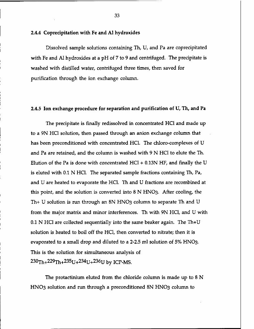
2.4.4 Coprecipitation with Fe and Al hydroxides

Dissolved sample solutions containing Th, U, and Pa are coprecipitated

with Fe and Al hydroxides at a pH of 7 to 9 and centrifuged. The precipitate is

washed with distilled water, centrifuged three times, then saved for

purification through the ion exchange column.

2.4.5 Ion exchange procedure for separation and purification of U, Th, and Pa

The precipitate is finally redissolved in concentrated HC1 and made up

to a 9N HC1 solution, then passed through an anion exchange column that

has been preconditioned with concentrated HC1. The chloro-complexes of U

and Pa are retained, and the column is washed with 9 N HC1 to elute the Th.

Elution of the Pa is done with concentrated HC1 + 0.13N HF, and finally the U

is eluted with 0.1 N HC1. The separated sample fractions containing Th, Pa,

and U are heated to evaporate the HC1. Th and U fractions are recombined at

this point, and the solution is converted into 8 N HNO3. After cooling, the

Th+ U solution is run through an 8N HNO3 column to separate Th and U

from the major matrix and minor interferences. Th with 9N HC1, and U with

0.1 N HC1 are collected sequentially into the same beaker again. The Th+U

solution is heated to boil off the HC1, then converted to nitrate; then it is

evaporated to a small drop and diluted to a 2-2.5 ml solution of 5% HNO3.

This is the solution for simultaneous analysis of

230Th+229Th+235U+234U+236U by ICP-MS.

The protactinium eluted from the chloride column is made up to 8 N

HNO3 solution and run through a preconditioned 8N HNO3 column to

34

separate Pa from other impurities. The Pa fraction is eluted with

concentrated HC1 + 0.13 N HF after sequential washings with 8 N HNO3 and 9

N HC1. The cleanup is essential to ensure a pure Pa solution and thus to

avoid possible matrix effects or interferences when measuring by ICP-MS.

After this final purification, the Pa fraction is converted to nitrate form by

successive washings with concentrated HNO3 followed by evaporation to

ensure complete removal of HF, and it is evaporated to one small drop

(-50^1) in a FEP-Teflon vial. The solution is then brought to ~ 5% HNO3 by

dilution. A small aliquot for plating on a stainless steel disc for yield

determination is taken. The solution is weighed precisely both before and

after taking this aliquot.

2.4.6 Chemical yield determination of Pa

Determining the chemical yield of Pa is done by ß-counting the 233pa

tracer. This is done by taking a subaliquot (~50 ul of ~ 2 ml) sample solution

and manually plating onto a stainless steel disc. Sample solutions are

weighed precisely before and after taking the subaliquot. All experiments are

designed so that counts are acquired on a relative basis for a given counting

geometry, negating the necessity for determining the absolute efficiencies of

the detector. Several standard 233pa plates are made from each batch of 233pa

working solutions. The solutions are pipetted directly into an electroplating

cell and are plated. All the plates usually agree within counting statistics.

Any that do not agree are discarded. Several standard 233pa plates are also

plated by evaporation to compare with those are electroplated to make sure

that the electroplating efficiency is 100%. The decay rate of standard 233pa [s

35

occasionally checked to ensure that no other interferences are included in the

tracer. It is desirable that enough 233pa Spike for both standards and samples

to obtain good precision (better than 2%) within a short time period (<20

minutes).

2.4.7 Final analyte preparation for ICP-MS

After determination of the chemical yield, a known concentration of

229xh spike is added to the Pa solution. The solution is then diluted to 2-2.5

ml analyte volume and the whole analyte solution is weighed; finally, the

combined solution of 231pa + 229jh m 5»/,, HNO3 is ready for introduction

into the ICP-MS. It is important to add the 229xh Spike after, not before,

determination of chemical yield to avoid interference during the counting of

233pa from 229jh and its decay products.

2. 5 ICP-MS ANALYSIS

2.5.1 ICP-MS operation parameters

Analyses were performed on a model VG PQ2 Plus quadrupole ICP-MS

at Harvard University. ICP-MS operating parameters are listed in Table 2. 2.

2.5.1-a Sample introduction

All three batches (230Th+229Th+235U+234U+236U; 231Pa+229Th; and

238u+236u+232xh+229xh) of sample in 1-5% HNO3 are used as a final

36

analyte, and are separately introduced into the ICP-MS with a peristaltic

pump (Gilson Minipuls 22) and a Meinhard concentric glass nebulizer. The

length of the Teflon tubing between the valve and the nebulizer is

minimized, and the pump is set at a constant speed. The sample volume is

optimized to obtain maximum sample signal relative to background without

being too high in sample viscosity. With a flow rate of 0.8 ml/min, a 48-

second uptake time, and 33-second running time for each of three runs per

sample, the required sample volume is 2-2.5 ml.

2.5.1-b Optimized conditions and features for Pa, U, and Th isotopes analysis

One "tuning cocktail", which contains the same concentration of

different elements in the mass range from 9ße to 238u, is usually made up in

order to optimize the operating condition of the instrument. Resolution,

sensitivity, and instrument stability need to be optimized each running day;

sometimes it is also necessary to adjust the instrument after a half day. Mass

calibration also needs to be verified occasionally, but it is not necessary to re-

calibrate it every running day.

2.5.2-c Resolution, Sensitivity, and Stability

Different resolution settings are tested to obtain one proper resolution

setting without the loss of too much sensitivity. The mass spectrometer is set

to provide 0.5-1.0 a.m.u. resolution over the entire mass range. 0.8 a.m.u.

peak area is usually integrated. The operating conditions for the ICP-MS

system are optimized by maximizing the ion intensity for 238u. After tuning,

37

an example of the instrument mean intensity is 2.37 ± 0.03 MHz for a 50 ppb

238u tuning solution. However, optimal tuning sensitivity varies from day

to day. It has been recorded over a long time period (Figure 2.2). The

variability in sensitivity is caused by changes in the lens voltages, the plasma

operating conditions, or the flow rate of the nebulizer. Sometimes, the

sensitivity loss is caused by deposition of material on the sampler or skimmer

or on the orifice of the nebulizer. It is always possible to recover the original

sensitivity simply by removing and cleaning these parts.

One instrument operation feature observed from Figure 2.2 is that the

signal intensities fluctuated from low mass to high mass ranges on the tuning

solution containing the same concentration of different elements. This

feature of non-uniform elemental responses across the mass range is due to

the performance of the interface. However, this feature does not affect

measurements, because corrections are always made for mass fractionation

with a monitor, which contains known concentrations of isotopes of interest.

The percent relative standard deviation (% RSD) is calculated for 10

successive scans in 10-20 minute intervals. Short-term stability is in the

range of 1.3% RSD for a 25 ppb 238y solution. For comparison, a working

reference solution of 231pa with a much lower concentration (0.0155 ppb)

gave a precision of 5%, which is limited mostly by counting statistics due to

the low count rate. An example of a medium-term shift for a 231pa working

reference is measured over 4 hours (Figure 2.3). The average difference of

each run from the first run is in the range of [-(5.6 ± 2.3)]% (la). The medium-

term stability for a standard solution of a 238y or 230jh is obtained as a range

of <1 to 3% over 4 hours. The experiment indicates that the PQ can operate

stably for a few hours but has some shift over a working day. Instability

38

CM ON ON

in

IN ON ON

CM ON ON

CO

CO

^ vo a ^

PH <

ON CM CM Ov ON ON ON

NO l-H 1H

i—1 *tf CM fc. >N > n, « O

< 2 2

en ON ON

in i-H

G «

cn ON ON

CM

(0

► II <► -- I] 'I

N

"T3 C3 o o> 1- lH 0) «8 (X - 01

*J .s ^ 4-> U W) o c u o on

l-H c m u 0> 3 > r* O O"

£ .S

C» CN|

bo O c *• •a o> S co 5ON

Sä .8 0» . CJOXI c 0< g OH

— « 10 o <§£

.2 « S

.2

> fN

"Ö 01 oi y

0) J5 u

O0a I •*■< ^J C3

(s/sjimoD) sJDV »»N

39

Table 2. 2 ICP-MS operating conditions

Instrument component Conditions

Pneumatic Pump Pump uptake rate: 0.8 ml/min

Uptake time: 48 seconds

ICP unit Forward power: 1.35 kwatt

Reflected power: <5 watt

Coolant Ar flow: 14.5 ml/min

Auxiliary Ar flow: 0.6 ml/min

Nebulizer Ar flow: 0.73 ml/min

Nebulizer Meinhard glass concentric nebulizer

Mass spectrometer Interface pressure: 1.5 mbar

Quadrupole chamber pressure: 2.9 x 10~6 mbar

Analytical procedure Analytical solution: 2-2.5 ml 5% HNO3

Run mode: mass scan mode

Resolution setting: coarse scale: 5.0

fine scale: 5.0

40

c o u 0) 93 »«. Vi

a o u

CD Pu, u

z

600

550

500-

450"

400-

350-

300

"° Pa-231 medium-term stability

1 1 1 1 1 1 1 1 1 1 1

13:05 13:27 14:12 14:58 15:42 16:30

Time (hr: min)

Figure 2.3 An example of medium-term stability of the instrument which is demonstrated by measuring a 231pa working solution over four hours. The concentration of the 231pa working solution is 0.0155 ppb.

41

manifests itself both as a gradual shift and in sporadic fluctuations. Factors

that contribute to instability include a non-constant temperature in the spray

chamber, inhomogeneous aerosol flow from the nebulizer, damaged or worn

sampling and skimmer cones, air leakage through worn O-rings in the

nebulizer mounting block, and room temperature fluctuations (Price Russ IE

& Bazan, 1987; Falkner, 1989,1991). The stability of the instrument can be

corrected for by periodic monitoring of a working reference solution when

measurements last longer than a few hours. Therefore, the sequence of a

background and a working reference interspersed with samples is applied

routinely.

2.5.1-d Background, Memory Effect, and Detection Limits

Background spectra were examined for potential interferences.

Deionized, distilled water, 1% and 5% HNO3, and 2N HC1 were checked, and

no significant background features were observed in the mass range 228 to

240. Background levels were uniform almost all the time, and typically were

in the range of 15 to 25 ACPS (counts in area peak per second) for mass 228 to

240 by mass scan mode. The average background spectra over a long period of

several running days are shown in Table 2. 3. The number in parentheses is

the numbers of replicate analyses.

Table 2.3 Example of background levels (in ACPS) for Th, Pa, and U isotopes

229Th 230Th 231Pa 232Th 234u 235u 236u 238u

23±4

(n=23)

22±4

(n=ll)

25±6

(n=25)

16±2

(n=6)

12±3

(n=26)

18±5

(n=21)

16±5

(n=22)

19±1

(n=6)

42

A memory effect from previous samples can occur for high

concentration runs (in particular for Th because it has a very strong tendency

to adsorb on surfaces), but it can be eliminated by a combination of a one-

minute rinse with deionized water and a 1.5-minute rinse with 5% HNO3.

Longer washing time may be required depending on the concentration and

viscosity of the previous sample. The required washing time can be checked

by continuously uptaking different washing solutions such as dilute HC1 or

HN03 (1% - 5%) or deionized water and monitoring the background signal.

This step is particularly necessary to insure that low concentrations of a

sample will not be contaminated by a previous sample with a suspected high

concentration; otherwise, the error could be significant.

The detection limit in ICP-MS is determined by the background noise

and the sensitivity for the element of interest. The detection limit for 231pa [s

calculated by taking 3 a of the noise in the signal against a known

concentration of working reference 231p3/ and its value is ~0.5 pg/g (i.e. ~ 1 x

1()9 atom/g = ~ 0.05 dpm/g) on the VG PQ2 Plus instrument. The following

formula is used (Hulmston and Hutton, 1991):

LOD(i) (pg/g) = 3c x IB/IA x CA

where LOD = the limit of detection, Iß = integrated peak area of the blank (5.58

ACPS in this example), IA = integrated peak area of the analyte (= 677 ACPS),

and CA = concentration of the analyte (pg/g) (= 20 pg/g = 2.093 dpm/g).

2.5.1-e Linearity and dynamicrange

43

The pulse counting systems that are used have an effective dynamic

range of 6 to 7 orders of magnitude from 1 to 10? counts per second (cps) for

analyte concentrations from 1 ppt to 1 ppm. The analog detector has a

concentration range of 10 ppb to 100 ppm for the linear dynamic range.

2.5.2 Analytical procedures

From the results of the experiments discussed above, the following

analytical procedures are used for routine analysis of Pa, Th, and U isotopes in

sediments. A mass scan mode is chosen, and isotope ratios are acquired for

all three separated batches of solutions containing different isotopes. Mass

scan ranges are from 228.5 to 239 amu. For Pa analysis, raw data on masses

229, 231, and 232 are obtained, and the isotope ratio 231/229 is calculated. The

mass 232 is included for checking the abundance sensitivity. For

230xh+234u+235u determination, masses 231 and 237 are also acquired to

check for effects of tailing or hydride formation (see below), but mass 232 is

skipped to avoid detector overload. For analytical procedures of the

232Th+238u analysis, the masses 231, 237, and 239 are scanned to monitor the

abundance sensitivity on 232xh and 238u spectra respectively, and possible

formation of hydride. A monitor solution containing the isotopes of interest

is interspersed with samples to correct for mass fractionation. All spikes and

standards used for the determination of samples are examined in association

with samples on each individual running day in order to make interference

corrections for any contributions from spikes and standards.

44

2.6 DETERMINATION OF 23!PA BY ICP-MS

The major effort was to establish an adequate procedure for 231pa

analysis using 229-jh as an internal standard and taking into account (1)

abundance sensitivity, (2) quantitative analysis and instrumental

fractionation, (3) matrix effects and matrix elimination, and (4) accuracy and

reproducibility. In addition, efforts were made to establish procedures (as

shown in the next section) for simultaneous isotope dilution analysis of U

and Th isotopes.

2.6.1 Degree of ionization of 231pa

One advantage of ICP-MS over thermal ionization mass spectrometry

(TIMS) is its superior ionization efficiency. Most elements are efficiently

ionized in a high temperature range of 7500 to 8000K (Houk and Thompson,

1988). Ionization efficiency of Pa by ICP-MS has never been reported before

simply because we do not know its plasma chemistry very well. It was

estimated by assuming the same transport efficiency as Th, and by taking the

ionization efficiency of Th which is known to be 100%. The ionization of Pa

was found to be almost the same as that of Th, i.e., 100%.

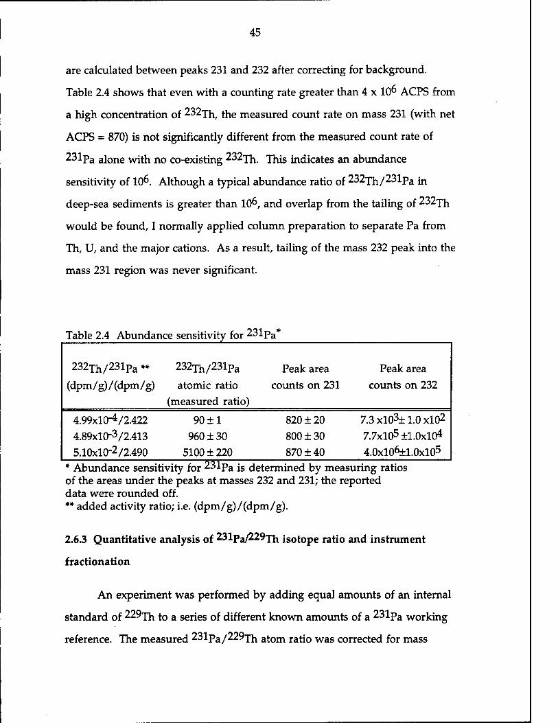
2.6.2 Abundance sensitivity

Abundance sensitivity for 231pa js measured as the ratio of the areas

under the peaks at masses 232 and 231. 0.8 amu (atomic mass unit), the width

normally used in the data analysis, is used as the width over which the areas

45

are calculated between peaks 231 and 232 after correcting for background.

Table 2.4 shows that even with a counting rate greater than 4 x 10^ ACPS from

a high concentration of 232^ the measured count rate on mass 231 (with net

ACPS = 870) is not significantly different from the measured count rate of

231pa alone with no co-existing 232xh jhis indicates an abundance

sensitivity of 10^. Although a typical abundance ratio of 232jil/231pa m

deep-sea sediments is greater than 10^, and overlap from the tailing of 232xh

would be found, I normally applied column preparation to separate Pa from

Th, U, and the major cations. As a result, tailing of the mass 232 peak into the

mass 231 region was never significant.

Table 2.4 Abundance sensitivity for 231p a*

232Th/231Pa **

(dpm/g)/(dpm/g)

232Th/231pa

atomic ratio (measured ratio)

Peak area counts on 231

Peak area counts on 232

4.99x10-4/2.422 4.89x10-3/2.413 5.10x10-2/2.490

90 ±1 960 ± 30

5100 ± 220

820 ± 20 800 + 30 870 ±40

7.3 xl03± 1.0 xlO2

7.7x105 ±1.0x104 4.0xl06±1.0xl05

* Abundance sensitivity for 231pa is determined by measuring ratios of the areas under the peaks at masses 232 and 231; the reported data were rounded off. ** added activity ratio; i.e. (dpm/g)/(dpm/g).

2.6.3 Quantitative analysis of 231pa/229xh isotope ratio and instrument

fractionation

An experiment was performed by adding equal amounts of an internal

standard of 229xh to a series of different known amounts of a 231pa working

reference. The measured 231pa/229jh atom ratio was corrected for mass

46

fractionation using a "monitor". The results (Table 2.5) show that the

calculated 231pa/229yh ratios are identical with expected 231pa/229jh ratios

from the working references within analytical errors. These results illustrate

the quantitative capabilities of 231pa/229xh isotope ratio measurement by

using 229Th as an internal standard.

Table 2.5 Example of calibration for quantitative analysis of 231pa/229jh

ratio* 231Pa/229Th 231Pa/229Th 231Pa/229Th Measured

Expected Measured Calculated

Expected

0.14 0.14 ± 0.01 0.15 1.00

0.20 0.22 ±0.01 0.21 1.10

0.27 0.27 + 0.01 0.29 1.00

0.33 0.37 ± 0.02 0.35 1.12

0.56 0.59 ± 0.03 0.60 1.05

Calibration parameters: y = mx +c Slope (m) = 1.069 Intercept (c) = -3.027 E -3 Correlation coefficient (r) = 0.997 * atom ratio ** the measured ratio was corrected for background and for mass fractionation *** calculated ratio was obtained with the regression line and the expected 231pa/229xh atomic ratio

Mass fractionation corrections are required because the observed

isotope ratios usually deviate from "true" values (Campana, 1980;

Klinkhammer and Palmer, 1991; Shaw and Francois, 1991). Corrections are

made by comparing the measured isotope ratio to a "monitor" solution

47

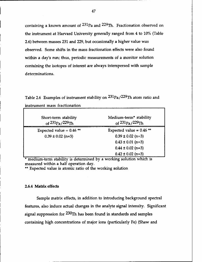
containing a known amount of 231pa and 229xh. Fractionation observed on

the instrument at Harvard University generally ranged from 4 to 10% (Table

2.6) between masses 231 and 229, but occasionally a higher value was

observed. Some shifts in the mass fractionation effects were also found

within a day's run; thus, periodic measurements of a monitor solution

containing the isotopes of interest are always interspersed with sample

determinations.

Table 2.6 Examples of instrument stability on 231pa/229xh atom ratio and

instrument mass fractionation

Short-term stability Medium-term* stability of231Pa/229Th of231pa/229Th

Expected value = 0.46 ** Expected value = 0.46 **

0.39 ± 0.02 (n=3) 0.39 ± 0.02 (n=3) 0.43 ± 0.01 (n=3) 0.44 ± 0.02 (n=3) 0.42 ± 0.02 (n=3)

* medium-term stability is determined by a working solution which is measured within a half operation day. ** Expected value is atomic ratio of the working solution

2.6.4 Matrix effects

Sample matrix effects, in addition to introducing background spectral

features, also induce actual changes in the analyte signal intensity. Significant

signal suppression for 230*rh has been found in standards and samples

containing high concentrations of major ions (particularly Fe) (Shaw and

48

Francois, 1991); in the following experiments, evidence of signal suppression

for Pa is also found.

Experiment 1 Detection of matrix effects: a series of known amounts of 231pa

aqueous standards (see Table 2.7) are added to several aliquots of equal

amounts (Table 2.7) of sediment solution to make standards in the presence

of sample matrix. Various sediments were used in order to examine effects of

different kinds of sample matrix.

The data shown in Figure 2.4 illustrate how the interfering materials

present in samples shift the slopes of calibration curves away from that of

aqueous standards. The solid line represents a typical calibration line for a set

of aqueous standards. As standard concentration increases, a linear increase

in signal intensity is observed. When aliquots of a standard are added to

portions of the samples, the signal intensity for all the solution still falls

within the linear portion of the working curves, but because of the

interference, the slopes of aqueous standards in the presence of sample matrix

are different from that observed for the aqueous standards. The discrepancy

between the slope of standards and the slopes of the aliquots with different

kind of sediment sample matrices are decreasing 5% and 9.8% (± 1 a) for

opaline sediment and calcareous silicate sediment respectively.

Experiment 2 Extent of matrix effect: various concentrations (Table 2.7) of one

sediment (calcareous clay) matrix were added to the same amount of 231pa

aqueous standard.

Figure 2.5 clearly shows that when the concentration of sample matrix

is increased by 5 times, there is a suppression of signal intensity of

49

u < 4-1

z

3000

2500

2000 i

1500

1000

500"

y = 14.600 + 212.48x RA2 = 0.999 (opaline)

y = 23.287 + 222.22X RA2 = 0.998 (standard)

y = - 2.6000 + 243.30x RA2 = 1.000 (calcareous)

Pa231 (dpm)

Figure 2.4 Example of sample matrix effects on a 231Pa standard analyte. Circles represent standard in absence of sample matrix; triangles represent standard in presence of opaline sediment sample matrix; crosses represent standard in presence of calcareous silicate sediment sample matrix.

50

1000- 1 i

950"

900- a

850- C/5 PH u 800-

750-

700-

650"

600 "1 !

0. 0 0.1

y = 964.29-571.14X RA2 = 0.984

0.2 —i ' 1—

0.3 0.4 0.5 —i

0.6

Analyte (ml)

Figure 2.5 Extent of matrix effect. A set of different concentration sediment matrix with adding equal amount (2.16 dpm/g) of a 231pa

working solution. The concentration of sediment is ~3g/ml.

51

approximately 7% to 28%. The effect is not well understood at this time; in

general, a high concentration of any matrix element essentially suppresses the

signal of Pa in sample analytes. Semi-quantitative scans of the sample with

significant matrix effects and the sample without matrix effects were made by

spiking ll^In as an internal standard. Results suggest that ÜB and 1HB group

elements in the periodic table are suspected interferences because their

concentrations were 3 to 10 times higher in the sample with the matrix effects

than in the 231pa standard and the sample without the matrix effects.

Spectral overlaps (i.e., isobaric interferences) and /or signal intensity

depression/enhancement from contained impurities in analyzing samples

have also been checked for the determination of 231pa /229Th ratio. Three

sets of experiments were examined. The first set of experiments used a series

of working solutions containing known amounts of both 231pa an(j 229jh in

the solution with no presence of any sediment matrix. The second set

involved adding the same series of working solutions to an equal amount of

a sediment matrix. The third set of experiments required addition of the

same series of working solutions to different amounts of a sediment matrix.

Table 2.7 shows the experimental results. The average measured

231pa/229-jh atomic ratios of the second set of experiments and the third set

of experiments are 10% ± 6% and 26% ± 11% higher than the average ratio of

the first set of experiments. In the third set of experiments, the average result

gives a ~ 8% ± 10% higher value for a solution containing the sediment

matrix than the value of a solution containing no sediment matrix (III-A

solution). These results suggested that there is sample matrix effect on the

measurement of the 231pa/229ih rati0/ but the measured data showed a

relatively high standard deviation. The effect may not be significant if one

52

Table 2.7 The experimental results of matrix effects on the measurement of

231pa/229xh ratio

Experiment Amount of Initial mount of Measured atomic

# working solution* sediment matrix ** ratio

I-A 0/0 0/0 N.D. ***

I-B 1.03/10.30 0/0 0.40 ± 0.04

I-C 2.00/20.01 0/0 0.42 ± 0.04

I-D 3.00/29.99 0/0 0.44 ±0.01

I-E 4.00/40.00 0/0 0.41 ± 0.01

Average = 0.42 ± 0.01

H-A 0/0 0 N.D. ***

II-B 1.03/10.30 2g/2.5 ml 0.46 ±0.01

n-c 2.00/20.01 2g/2.5 ml 0.42 ± 0.01

E-D 3.00/29.99 1.8g/2.5ml 0.48 ± 0.01

n-E 4.00/40.02 2g/2.5 ml 0.47 ±0.01 Average = 0.46 ± 0.01

m-A 2.00/20.01 0 0.48 ± 0.01 III-B 2.00/20.01 lg/2.5 ml 0.53 ± 0.02 m-c 1.03/10.30 2g/2.5 ml 0.49 ± 0.01

m-D 1.03/10.30 3g/2.5 ml 0.63 ± 0.01

m-E 1.03/10.30 4g/2.5 ml 0.52 ± 0.01 Average = 0.53±0.05

the activity ratio (in unit (dpm/g)/(dpm/g)) of 231pa/ 229yh in 2.5 ml weighed working solution. The expected atomic ratio of 231pa/ 229xh in the working solution is ~0.45 for each individual analyte. ** the amount (in unit gram of sediment) of sediment matrix used in the analytical solution (in unit ml of analyte). *** there is no calculation data since no significant peak area counts after subtraction from the background levels.

53

takes counting statistics and instrumental stability into account. Efforts were

also made for reducing the matrix problem, if any, by applying ion-exchange

column purification procedures, as indicated above, for the separation of Pa

(and Th, U) from the major cations. The result has been observed from the

data in Figure 2.6, which demonstrates that when a sample has been cleaned

by an additional 8N HNO3 column, major interference materials can be

properly cleaned out, and the slope of the working curve is identical with that

of the aqueous standard.

The standard addition method was thought to be a useful technique

that might correct possible matrix interferences present in the sample rather

than eliminating the interference itself. This method was developed for the

correction of matrix effects in the beginning of this thesis; however, the

method of standard addition could not be applied to many of the samples in

this thesis work, since the amount of available sample material was not

enough for acceptable precision by this method.

After sample purification, the final solution is introduced into ICP-MS,

and as the following section shows, there is no significant matrix effect to

bias the determination of the 231pa/229xh ratio, and precise and accurate

measurement for 231pa can be made by using 229xh as an internal standard.

The problem arising from spectral overlap is also eliminated by column-

preparation. Isobaric interferences at mass 231 have never been found, since

no significant background features have been observed above mass 84, and no

significant MO+ or MOH forms of elements in the periodic table could

interfere with the 231 and 229 mass peaks after our chemical preparation is

applied. The possible chance of 230xhH formation at mass 231 is also

54

e o u <u 03

*«> d s o u

(/)

U ■w

z

2000 1800

1600 1400

1200 1000 800 600 400 200

0

y = 23.287+ 222.22x RA2 = 0.998

■ y = 16.400+ 223.45x RA2 = 0.995 *

0 T

2 10

Pa-231 (dpm)

Figure 2.6 Example of reduction in sample matrix effect on the 231pa

signal by applying one ion-exchange column purification. Squares represent a set of different concentration of a 231pa working solution; crosses represent the same set 231Pa working solution in the presence of the sediment sample after one more step of 8N HNO3 column purification.

55

unlikely to interfere significantly with the 231pa peak after column

separation.

On the other hand, the "residual" of the first addition of the 229Th

spike might have a chance to leak into the Pa fraction during the column

separation; therefore, the procedure is to add a higher amount of 229jh on

the second stage spike.

2.6.5 Precision and Accuracy

Precision and accuracy of 231pa determination by ICP-MS were assessed

by replicate analyses of the Harwell uraninite (Congo pitchblende), which is a

well-characterized reference material. It has been used for extensive inter-

laboratory comparisons by a-spectrometry, and it has been shown that all

uranium series isotopes approach the secular equilibrium values (a

distributed note from M. Ivanovich, 1979). The equilibrium value of 235y

activity is proportional to 238u activity (i.e., 235y activity=0.046 238|j

activity); the equilibrium value of 231pa js thus expected to equal its parent

value which is 5.56 dpm/g. Several Harwell uraninite aliquots with

concentrations in the range 0.18 to 0.24 dpm per gram of solution (i.e., 0.38

dpm to 0.50 dpm of Pa from Harwell uraninite solution for a 2.1 ml analyte

volume) were prepared following the same preparation procedure as for the

sediment sample and with the same amount of 229xh was added as an

internal standard. The 231pa /2297h ratios of the Harwell uraninite aliquots

were then determined. Precision and accuracy are shown in Table 2.8. The

same uraninite reference material, with a concentration in the range of 1 to

1.5 dpm of Harwell uraninite solution, was measured by a-spectrometry, and

56

the results are also presented on Table 2.8 for comparison. As shown in Table

2.8, the analytical results of 231pa analyses by ICP-MS are given as a mean

value of 5.65 dpm/g with 4% deviation (± 1 o), and the oc-spectrometry results

are given as 5.99 dpm/g with 4% deviation (± 1 a). The standard deviation of

ICP-MS results includes errors from the analytical procedure, the calibration

of added spikes and working references, the chemical yield determination by

beta counting, the atom ratio determination, the "monitor" solution for

instrumental mass fractionation, and background subtraction of ICP-MS. The

standard deviation of results by cc-spectrometry includes errors from the

analytical procedure, chemical yield determination by beta counting, and

counting error by cc-counter. Apparently, the measurements of smaller 231pa

samples by ICP-MS technique have precision (0.38 dpm to 0.50 dpm of

Harwell uraninite solution) comparable to that of a-spectrometry on a larger

sample size (1 to 1.5 dpm), but the ICP-MS technique obtained a 231pa average

value with smaller deviations from a real value (i.e., 5.56 dpm/g) of Harwell

uraninite than those samples done by a-spectrometry. On the other hand, if

the solutions being measured by ICP-MS have the same amount (-0.4 dpm) of

analyte, days to weeks of cc-counting time would be needed to obtain the

same precision of ~4%.

A comparison between the internal standard-ICP-MS technique and

the a-counting technique was aslo made for a series of sediment samples

having a range of 231pa concentrations of ~0.29 to 1.5 dpm/g. The analytical

results are shown in Table 2.9. To indicate the comparison between the two

techniques, the ratio of the results of each was taken, and it shows that the

correlation between the two techniques is high, with an average ratio of 0.94 ±

0.06 (la, n =9). The standard deviations include a partial error derived from

57

the a-counting technique and a partial error derived from the ICP-MS

technique. The error for low concentration samples measured by ICP-MS is

large because of the large background correction.

The experiments' results clearly show that the dependence of isotope

ratios on the concentration or on the presence of concomitant elements

existing in different type sediment samples can be eliminated by the method

developed here. Apparently, from the results shown in Table 2.8 and Table

2.9, in terms of precision, accuracy, and the time requirement for obtaining a

data point, the ICP-MS analytical technique of 231pa measurements, based on

isotope ratios spiked with 229xh as an internal standard, are preferable to the

a-counting technique. The analytical method reported here for 231pa

determination should be considered a stepping-stone to future advances. In

future, we expect to obtain much better precision and to be able to apply the

technique to a much smaller sample size using other kinds of sample

introduction techniques than that with the conventional nebulizer. These

sample introduction techniques may include ultrasonic-nebulizer, direct-flow

injection, or electro-thermal volatilization (ETV), because it is believed that

these techniques might improve sensitivity by 10 to 100-fold over that

demonstrated by the conventional nebulizer.

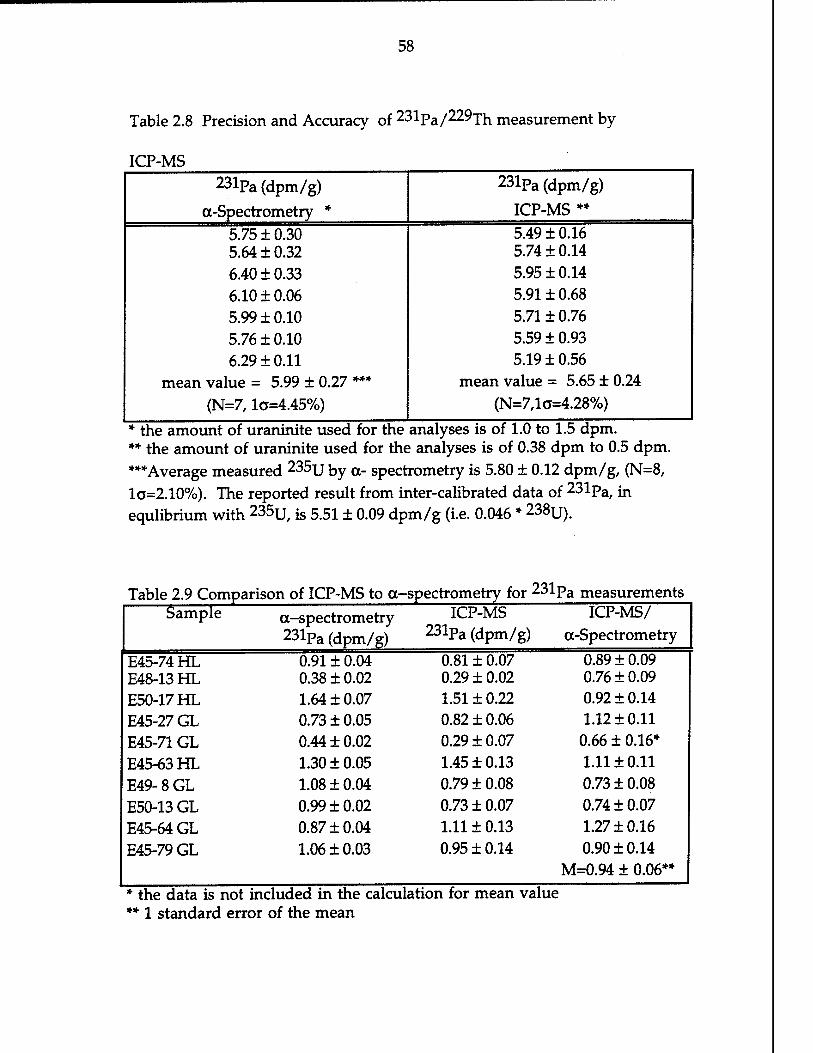
58

Table 2.8 Precision and Accuracy of 231Pa/229Th measurement by

ICP-MS 231Pa (dpm/g) 23lPa (dpm/g)

cc-Spectrometry * ICP-MS **

5.75 ±0.30 5.49 ± 0.16 5.64 ±0.32 5.74 ± 0.14 6.40 ±0.33 5.95 ± 0.14 6.10 ±0.06 5.91 ± 0.68 5.99 ±0.10 5.71 ± 0.76 5.76 ± 0.10 5.59 ±0.93 6.29 ± 0.11 5.19 ± 0.56

mean value = 5.99 ± 0.27 *** mean value = 5.65 ± 0.24

(N=7, 1CT=4.45%) (N=7,la=4.28%)

* the amount of uraninite used for the analyses is of 1.0 to 1.5 dpm. ** the amount of uraninite used for the analyses is of 0.38 dpm to 0.5 dpm. ***Average measured 235u by a- spectrometry is 5.80 ± 0.12 dpm/g, (N=8, la=2.10%). The reported result from inter-calibrated data of 231pa, in equlibrium with 235u, is 5.51 ± 0.09 dpm/g (i.e. 0.046 * 238u).

Table 2.9 Comparison of ICP-MS to cc- -spectrometry for 231pa measurements Sample oc-spectrometry

231pa (dpm/g)

ICP-MS 23lpa (dpm/g)

ICP-MS/ a-Spectrometry

E45-74 HL E48-13 HL

0.91 ± 0.04 0.38 ± 0.02

0.81 ± 0.07 0.29 ± 0.02

0.89 ± 0.09 0.76 ± 0.09

E50-17HL 1.64 ± 0.07 1.51 ± 0.22 0.92 ± 0.14 E45-27GL 0.73 ± 0.05 0.82 ± 0.06 1.12 ±0.11 E45-71GL 0.44 ± 0.02 0.29 ± 0.07 0.66 ± 0.16* E45-63HL 1.30 ±0.05 1.45 ±0.13 1.11 ±0.11 E49-8GL 1.08 ± 0.04 0.79 ± 0.08 0.73 ±0.08 E50-13 GL 0.99 ± 0.02 0.73 ± 0.07 0.74 ± 0.07 E45-64 GL 0.87 ±0.04 1.11 ± 0.13 1.27 ±0.16 E45-79 GL 1.06 ±0.03 0.95 ±0.14 0.90 ±0.14

M=0.94 ± 0.06** * the data is not included in the calculation for mean value ** 1 standard error of the mean

59

2.7 SIMULTANEOUS DETERMINATION OF 23°TH+234U+235U, AND

232TH+238U BY ISOTOPE DILUTION-ICPMS

2.7.1 Abundance sensitivity

After optimization, coarse scale is set at 5.0 and fine scale is set at 5.0. A

band of 0.6 a.m.u. is used for each peak integration, and mass-scan mode is

chosen. For 230Th+234u+235u, isotope ratios 230/229, 234/236 and 235/236

are measured. For 232jh+238u the ratios 232/229, 238/236 are measured.

Masses 231 and 237 are also scanned during 230xh+234u+235u analysis to

monitor any possible tailing from the 232xh at mass 230 or 235JJH

interference at mass 236. The consideration is that if 236uH can interfere

with mass 237, then 235UH would interfere with mass 236 in the same

proportion because samples are always spiked to give approximately equal

amounts of 236JJ ancj 235]j Therefore, an approximate correction for 235UH

interference can be made. Usually the correction is insignificant.

2.7.2 Mass fractionation

Mass fractionations are also found in the analyses of

230jh+234u+235u and 232xh+238u (Table 2.10). The mean values of the

observed 230xh/229xh ratio are about 3% to 9% lower than the expected

value. The235U/236Uand234U/236U

ratios are about 0.3% to 5% and 0.6% to 8% lower than the expected values.

Sensitivities seem to be lower for lighter isotopes than for heavier isotopes.

60

Some shifts in mass fractionation were also examined with a mixture

of known isotope ratio standards to monitor the stabilities within a day's run.

Results show medium-term stability to be approximately in the range of 1%

to 4% for 230/229,234/236,235/236 (Table 2.10).

No evidence that the isotopes are dependent on concentrations of

sample or on the presence of concomitant elements was observed in

measurements on marine sediments. Even at a solution concentration of

~ 0.2 dpm/g for 230Th, it is possible to measure the isotope ratios with a

precision of 2% or better by the isotope dilution technique.

2.7.3 Precision and accuracy

Reproducibility checks with uraninite reference solutions are indicated

in Table 2.11. The accuracy of the isotope ratios was examined by comparing

results from a variety of deep-sea samples from different sites with both

isotope dilution-ICP-MS and alpha-spectrometry. Both methods give the

same results (Table 2.12). For precision and speed, isotope-dilution ICP-MS

analysis of 230Th, 232Th, 234U, 235U, and 238U is favored over the a-

counting technique.

2.8 CALCULATIONS

2.8.1 Isotope dilution calculation

61

Table 2.10 Examples of stabilities on isotope ratio and the instrumental mass

fractionation

Isotope ratio Short-term stability Medium-term stability *

230Th/229Th Expected value = 0.90 ** Expected value = 0.68 **

0.85 ± 0.03 (n=4) 0.64 ± 0.02 (n=4)

0.61 ± 0.04 (n=4)

0.62 ± 0.02 (n=4) 234u/236u Expected value = 0.78 ** Expected value = 0.78 **

0.72 ± 0.02 (n=4) 0.72 ± 0.02 (n=4) 0.75 ± 0.03 (n=4) 0.78 ± 0.03 (n=4) 0.75 ± 0.02 (n=4)

235u/236u Expected value=103.16** Expected value = 103.16 * *

98.14 ± 0.48 (n=4) 98.14 ± 0.48 (n=4) 100.10 ± 0.01 (n=4) 101.05 ± 5.81 (n=4) 99.79 ± 3.23 (n=4)

238u/236u Expected value = 1.56 ** Expected value = 1.56 ** 1.43 ± 0.05 (n=3) 1.43 ± 0.05 (n=3)

1.40 ± 0.02 (n=3) 1.48 ± 0.02 (n=3) 1.45 ± 0.07 (n=3)

232^/229^ Expected value = 1.57 ** Expected value = 1.57 ** 1.68 ± 0.005 (n=3) 1.68 ± 0.005 (n=3)

1.63 ± 0.02 (n=3) 1.70 ± 0.06 (n=3) 1.71 ± 0.06 (n=3)

Medium-term stability is determined by a working solution which is measured within a half operation day.

Expected value is atomic ratio of the working solution **

62

rH tv /«N £> ON "<* NO CM © be cfl o ON © CM II CM D 1 2

CO ">* NO rH e +i

■<* +1 +1 +1 +1 co co © CO IN $ g§ "O

CM 00 NO

© ©

CM <*

CM NO C vo

CN CO CM CM CM rH rH rH rH rH

/•—. * in

0) 5 (50 CQ CM o CO o rH

ON ©

II P

1 +l

B c-> in

if) CO ©

NO

© +1

Ö ©

1 l-l

V4H

LO in in in

o <c .5

CM O 00 CM CM CM CM CM II °. CO

CO CM

»H J3 o © o O ©

RS +1 >-. s d © © © © j>> D 1 8 +1 +1 +1 +1 +1 13 "tf 00 ON T-i CO ON c CO ON ON © p ON rH rt R3 Ö Ö rH rH Ö

o ^ WD CO 00 CM CM ON 00

4-» o en D to .5 ©

CO NO CO

CM CM

NO CM

II CM C +1 •^* 00 6 §

OH O

w Ö

+1 +1 +1 +1 £ V

£ CO CM

in in © CO

ON 00 NO CM

CO in CM CN|

in CO in CM

C NO CM

"■M 1—1 rH rH r—< rH

o £* © tN © "%

NO tN

PH

rH

CM

+1

in CM +1 T-H

in CM rH

+1 00

II CM

s +l S Si 3

O »H

QJ o

^ u

S <N rH

m 00 rH rH

o in CM rH

NO Ö CM rH

C CM CM rH

Ä CO CM

%

rH in NO Tf CM CO NO rH

II rH rH 1—1

CM CM

© CM CM

© rH

in rH in rH rH rH

CM +1 CM1

+1 +1 +1 +1 +1 01

£d NO ON oo ON tN in S iG o CM ON 00 «* NO O Tf P ^ £ 00 in rl? NO IN ON 00

t*? 1 CM CM CM CM CM CM CM CM H Ö rH

63

Radioisotope concentrations in sediments are usually reported in

activity units (e.g., dpm/g). The following quantities are used to calculate the

activities:

Rs=measured ratio of the sample (net ACPS ratio)

Rmt=nieasured ratio of the monitor tracer (net ACPS ratio)

Rt=known ratio of the monitor (atom ratio)

F=conversion factor, atom ratio to activity ratio

Aspk=activity of calibrated spike (dpm/g)

WSpk=weight of spike (grams)

Ws=weight of sample (grams)

Isotope ratios contain the unknown (sample) isotope in the numerator,

and the known (spike) isotope in the denominator. Thus the measured ratios

230/229,232/229,234/236,235/236, and 238/236 refer to 230xh, 232^, 234u,

235u and 238y in the numerators, and 229^ 236y in the denominator.

One can calculate the activities of isotope compositions of interest in a

sediment sample as follows:

A (dpm/g)=Rmt/Rt * Rs * F * Aspk * Wspk /Ws

2.8.1-a Background correction

During each day's run, deionized distilled water is interspersed

periodically within the sequence of sample and monitor solutions, and then

all the raw data from the samples and the monitor are arranged as a "blank

subtraction" from the average raw data of the deionized distilled water.

Background levels for deionized distilled water are usually in the same range

as for 1-5% HNO3. Background levels are average in the uniform

64

Table 2.12 Comparsion of a- spectrometry results and ICP-MS results for Th

and U isotopes in marine sediments by ICP-MS

Table 2.12a

230xh (dpm/g) 230jh (dpm/g)

Sample a- counting ICP-MS ICP-MS

a

KN64-05 GL 3.40 ± 0.10 3.5210.10 1.04

AÜ 107-22 HL 5.5810.22 6.0010.07 1.08

An 107-65 HL 8.69 ±0.44 8.4510.13 0.97

All 107-65 GL 7.8010.42 7.8210.41 1.00

CHN 82-4 HL 6.5610.31 6.4210.10 0.98

CHN 82-11 HL 5.6310.45 5.9210.14 1.05

38 GGC GL 6.4310.32 5.7910.20 0.90

91 GGC-0 8.7510.17 8.8910.17 1.02

91 GGC 72 6.3510.19 6.1210.10 0.96

TR 163- 9.5 6.5610.23 6.4210.14 0.98

TR 163- 72 5.7510.21 5.5810.10 0.97

TR 163- 94.5 5.2310.20 5.2410.07 1.00

TR 163-131.5 5.7810.33 5.2810.35 0.91

TR 163-145 5.2610.20 5.7110.10 1.09

E 48-13 HL 15.1010.57 15.1410.21 1.00 E 45-74 HL 11.6310.64 11.9410.19 1.03

E 50-8 HL 4.2610.12 4.1610.09 0.98 E 45-27 GL 12.1710.36 13.2710.22 1.09

E 45-71 GL 8.3810.44 7.8210.06 0.93

E 48-27 GL 8.2210.27 7.9110.22 0.96

E48-3GL 3.0410.15 2.9610.07 0.97

mean = 1.001 0.05

65

Table 2.12b

Sample 234u 234u 234u 235u 235u

(dpm/g) (dpm/g) ICP-MS (dpm/g) (dpm/g)

a-aaunting ICBMS a-counting a-aninting ICP-MS

KN64-05 GL 0.70 ± 0.04 0.63 0.90 0.03 0.031 ± 0.001

AH 107-22 HL 0.49 ± 0.03 0.41 0.84 0.02 0.029 ±0.001

AH 107-22 GL 0.55 ±0.03 0.57 1.04 0.03 0.029 ± 0.001

An 107-65 HL 0.43 ± 0.02 0.43 1.00 0.02 0.019 ±0.001

AE107-65 GL 0.62 ± 0.02 0.69 1.11 0.03 0.032 ± 0.001

E 48-13 HL 0.24 ± 0.03 0.21 0.88

M=O.96±0.04

Table 2.12c

Sample 2321h 232rh 232rh Sample 238u 238u 238u

(dpm/g) (dpm/g) (dpm/g) (dpm/g) ICP-lvB

a- ICP-MS ICP-VS a-autirg ICP-MS ja-

axithg a-

E49-29bag 136±0.07 1.47±0.03 1.08 CHN82-11HL O26±0.01 0.29+D.00 1.12

E48-11GL 0.15±0.01 0.18±0.00 1.20 290XHL 055±0.03 0.46±0.01 0.84

CHN82-11HL 05H0.03 0.45±0.01 0.88 550XHL 0.97±0.06 0.84±0.02 0.87

55QXHL 155±0.09 1ÄM0.01 1.16 CHN82-15HL 037±0.01 028±0.00 0.76

CHN82-15HL 03HO.01 035±0.01 1.13 38QXC1 0.89+0.03 0.91±0.03 1.02

CHN82-11GL 135±0.71 133±0.03 0.99 550XGL 156±0.Q3 1.47±0.02 0.94

CHN82-15GL l.O2±0.O4 1.18±0.01 1.16 82QXGL L28±0.Q5 152±0.04 1.19

VM22-197-133 21HÖ.06 ??1-K).04 1.05

M=

1.08+Ü10

CHN82-1XL 0.78±0.02 0.63±0.02 0.81

M=

osmu

66

range, but with a little sporadic fluctuation. For those samples with low

concentrations, a factor in all of the Pa analyses in this study, the background

subtraction can be significant. The effect of variable background levels can

influence the precision significantly.

2.8.1-b Blank correction

Procedural blanks were occasionally run parallel to samples, and no

signals significantly different from the background level were found (Table

2.13). Blank corrections are seldom more than few percent. However, count

rates on the procedure blanks are subtracted from those of the samples before

applying the calculation if a significant blank is found.

Table 2.13 Examples of procedural blanks (in ACPS) for 231Pa and Th and U

isotopes

231Pa 229Th 230Th 232Th 235u 236u 234u 238u

(ACPS) (ACPS) (ACPS) (ACPS) (ACPS) (ACPS) (ACPS) (ACPS)

3±3 5±3 2±2 10±9 4±0 0±1 1±0 4±7

0±0 7±2 4±4 4±6 7±6 2±3 1±0 4±6

5±5 7±4 1±1 1±1 7±4 1±0 1±1 1±0

3±3 11 ±10 3±3 1±1 13 ±1 1±0 1±0 3±2

2.8.1-c Contribution from spikes

Contributions of the spike and working references are examined at the

same time with samples on each instrument running day, and are subtracted

67

from all the raw data of the sample, standard, and monitor solution. A spike

of 236U made a 10% contribution to mass 235 (i.e., 235U).

The 236u spike (Oak Ridge National Laboratory) used in this work

contains some impurities that have been found to interfere with peaks on

masses 234 and 235. The 236TJ contained 234JJ m an amount equal to 12.4% of

the 236y activity, but this causes an atomic ratio of 234U/236TJ in the

impurity in value equal only to 0.0013. On the other hand, the 236y spike

contains a significant amount of 235]j that is suspected to come from the

residual of production process of 236TJ by 235]j (n,y) neutron irradiation. The

monitoring of the 236TJ spike by ICP-MS analyses showed that the 235U/236TJ

ratio of impurity is 0.10 (atom ratio).

2.8.2 Sources of error

Sources of errors include the measurement of isotope ratios by ICP-MS,

the calibration of spikes and working references with alpha-counting, the

determination of chemical yield for Pa by beta-counting, and the weighing of

the samples. Isotope ratio measurements involve precision of triplicate runs,

mass fractionation correction from a monitor, and the effects of the variable

background level. The accuracy of the calibrated results for all spikes and

working references involve the counting statistics and the detector efficiency

of the alpha counter. The latter error is only for 231pa counting since there is

no other suitable a-emitting Pa isotope that can be used for isotope dilution

by the alpha counting technique. The chemical yield monitor for Pa with

beta-counting of a 233pa tracer involves a decay correction due to the short

half-life of 233pa an£j the arrangement of geometric factors in counting both

68

the standard and the sample. Unexpected changes in the humidity of the

weighing room air also cause errors in the weights of small-sized samples.

Propagation of measurement errors in a derived results, f(x, y), is made by use

of the following equations:

G2f (x, y) = (df/dx)2 Gx2 + (3f/dy)2 Gy

2

Ox/y = x/y (oxVx2 + OyVy2)1^

2.9 CONCLUSIONS

Methods were developed to measure 2^lpa and uranium and thorium

isotopes in sediments by ICP-MS. The procedure involves three separate

runs: (1) a two-stage spike for 2^lpa measurement with 233pa as a tracer for

chemical yield and 22^Th as an internal standard; (2) isotope dilution analysis

for simultaneous determinations of 2^U, 2^5u, and 230xh on the same

aliquot with spikes of 236u, and 229Th; and (3) simultaneous measurements

of 238u and 232Th by isotope-dilution analysis of a separate small aliquot

removed just after sample dissolution. The precision for a 231pa

measurement, at present, is ~4% on ~0.2 dpm per gram of solution. Accurate

determination of the amount of 2^lpa in a sediment sample can be achieved

at a level of greater than 0.3 dpm. The method has a detection limit of

approximately 0.5 pg/g (i.e., 0.05 dpm/g of solution) 231Pa. In addition,

accurate, simultaneous measurements of 230lh, 234u, and 235u on one

aliquot and 232Th and 2^8u on a separate aliquot by isotope dilution ICP-MS

has been established for a routine sediment analysis. The whole technique

69

offers the following advantages when compared with a- spectrometry: (1)

shorter measurement time (less than 5 minutes vs. days to weeks); (2) higher

analytical precision for the same range of sample concentration (better than

5% vs. 5->10% for 231Pa, and <l-3% vs. 3->10% for uranium and thorium

isotopes); and (3) smaller sample size requirement for Th and U isotopes. A

more efficient sample introduction method would provide a better precision

and is necessary for the analysis of small samples or for samples with lower

concentration such as sediment trap or water samples.

70

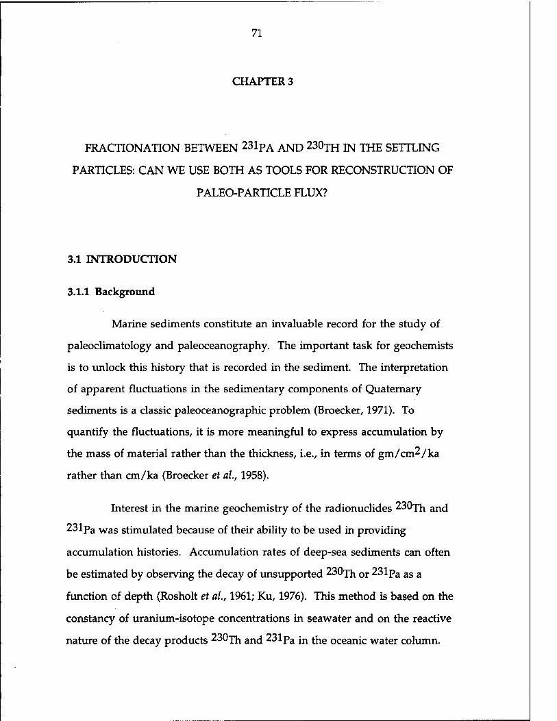
71

CHAPTER 3

FRACTIONATION BETWEEN 231pA AND 230TH IN THE SETTLING

PARTICLES: CAN WE USE BOTH AS TOOLS FOR RECONSTRUCTION OF

PALEO-PARTICLE FLUX?

3.1 INTRODUCTION

3.1.1 Background

Marine sediments constitute an invaluable record for the study of

paleoclimatology and paleoceanography. The important task for geochemists

is to unlock this history that is recorded in the sediment. The interpretation

of apparent fluctuations in the sedimentary components of Quaternary

sediments is a classic paleoceanographic problem (Broecker, 1971). To

quantify the fluctuations, it is more meaningful to express accumulation by

the mass of material rather than the thickness, i.e., in terms of gm/cm^/ka

rather than cm/ka (Broecker et ah, 1958).

Interest in the marine geochemistry of the radionuclides 230Th and

231pa was stimulated because of their ability to be used in providing

accumulation histories. Accumulation rates of deep-sea sediments can often

be estimated by observing the decay of unsupported 230xh or 231pa as a

function of depth (Rosholt et ah, 1961; Ku, 1976). This method is based on the

constancy of uranium-isotope concentrations in seawater and on the reactive

nature of the decay products 230xh and 231pa jn the oceanic water column.

72

The estimation is based on two important assumptions: that the initial values

of 230Th and 231pa are constant through time, and that the sedimentation

rate is constant as well. Successful examples were found in a Caribbean core

(Broecker and Van Donk, 1970). However, geological processes which focus

or erode material from specific sites decrease our ability to understand past

variations in the sedimentation rate; thus, sediment dating using 230xh and

231pa does not always provide satisfactory chronologies, because large

downcore variations of initial 230jh and 231pa activity in sediments can

result in large uncertainties.

Two contradictory ideas have been proposed to interpret the large

downcore variations of 230xh activity in sediments. The debate arises from

different interpretations of the relationship between unsupported 230xh (the

term 230jhex will be used in the following text) flux and the overall particle

flux, which is usually driven by surface ocean productivity (Fisher et ah, 1988;

Nozaki, 1991).

In a core section with an unusually high 230xhex° level, one model,

called the productivity model by Thomson et. ah, (1993), would infer

unusually high production and presumably a higher overall accumulation

rate, whereas the other model, called the constant 230xhex flux model by

Bacon and Rosholt (1982), would infer a period of unusually low sediment

accumulation rate. Bacon and Rosholt (1982) and Bacon (1984) suggested a

uniform rain rate of 230jh, equal to production, occurs over the entire

seafloor; thus, 230xhex flux is independent of total mass flux. As a

consequence, there is an inverse relationship between particle rain rate to the

seafloor and the excess 230jh activity in the settling particles. Variations in

fluxes of other nuclides, trace metals, and sediment components can thus be

73

quantified by normalization to 230xhex flux. This is the so-called "230xh-

normalized flux method".

In contrast, a production model has been proposed in several

workers (Mangini and Diester-Haass, 1983; Yang et al, 1990; Shimmield et al,

1986; Schölten et al, 1990) to interpret large variations in the sediment

profiles as showing much larger departure from a vertical flux balance than is

likely to occur. It was argued, however, that in their conclusion they have

not considered the possibility of variable sediment focusing (Bacon, 1984;

Suman and Bacon, 1989; Francois et. al, 1990; Francois and Bacon, 1991). The

constant 230xhex flux model suggests that variability in sediment

redistribution rates could be removed by normalizing all component fluxes to

that of 230xhex- The magnitude of sediment redistribution is then just a

factor adjusting the expected production in the water column to observed

230xh concentrations. To illuminate the debate between the two concepts, I

carried out sediment trap studies to examine the dependence of the

scavenging efficiency of 230xh (and 231pa) on the particle rain rates, and to

examine the crucial hypothesis of constant 230xhex° flux in the 230xh-

normalized flux method in the thesis.

Besides using the 230xh-normalized flux model, I propose in this

thesis to use decay-corrected unsupported 231pa/230xh Ta^0 ( me term

(231pa/230xh)ex° will be used in the following text) as an index of particle

flux in the present ocean and past time, which I call the "(231pa/230xh)ex°

ratio index".

Uranium decay supplies 231pa ancj 230xh in the ocean at a fixed ratio

of 0.093 if there is no fractionation between the two isotopes. Many

74

observations of water columns, sediment traps, and sediments from previous

works have shown that fractionation between 230Th and 231pa occurs

everywhere within an ocean basin (DeMaster, 1981; Anderson et al, 1983 a&b;

Bacon et al, 1985; Yang et al, 1986; Taguchi et al, 1989; Francois et. al, 1990;

Francois and Bacon, 1991; Anderson et al, 1991; Lao, 1991; Rutgers Van Der

Loeff and Berger, 1993).

Evidence shows that a region with a removal ratio of

(231pa/230Th)exo that is greater than the value of 0.093 represents a

preferential scavenging of 231pa, Such evidence comes from the Antarctic

and the margins of the Pacific (i.e., the Panama Basin, Guatemala Basin, the

northern North Pacific; Anderson et al, 1983b, 1990; Yang et al, 1986; Taguchi

et al, 1989; Lao et al, 1992; DeMaster, 1979; Rutgers Van Der Loeff and Berger,

1993). Conversely, a region with a ratio of less than 0.093 represents a

preferential lateral transport of a portion of 231pa to somewhere else. Such

regions can be seen in the open ocean (Anderson et al, 1983a; Bacon et al,

1989; Lao et al, 1992; Chapter 4 of this thesis).

The large fractionation between 230jh and 231pa within a basin

comes about because of the partitioning of the two elements between two

transport pathways, i.e., vertical scavenging or horizontal transport, for

removal. The differential partitioning is caused by differences in reactivity

between the two elements. On one hand 230^ due to its high particle

reactivity with a range of residence time between 10 and 40 years (Nozaki et

al, 1981; Anderson et al, 1983a&b), is predominately removed with the

downward flux of particles. On the other hand, 231pa is \ess patrticle-reactive,

with a residence time about 2 to 3 times longer than that for 230xh (Anderson

et al, 1983a&b), and can be laterally transported longer distances away from its

75

production site before it is removed. As a result, over most of the ocean the

flux of 230xh into the sediments approximately balances its production rate in

the overlying water column, whereas 231pa tends to migrate towards the

margins or regions of high particle flux. Consequently, the (231pa/230xh)exo

ratio of the material falling to the seafloor reflects the particle rain rate of the

overlying water column. A high value of the (231pa/230xh)ex° ratio reflects

higher particle fluxes in a region, and a lower value reflects lower particle flux

in a region. By further extrapolation of the concept into the past ocean, one

expects that the variations of the (231pa/230Th)exo ratio in a down-core

sediment profile would reflect the fluctuations of the particle rain rate in the

overlying water column. The advantage of this approach is that since the

231pa content is normalized to the 230jh content, the bias of sediment

redistribution processes can be removed. In addition, most biogenic

particulate carriers are easily degraded by diagenesis and reminerization

processes in sediments, but both 231pa an£j 230^ which are adsorbed onto

the particles, are not significantly affected by these processes. Thus, even

though particles have suffered from dissolution, both 231pa ancj 230jn

should still faithfully record the fluxes of their particulate carriers. A higher

(231pa/230xh)exo ratio thus confirms a higher flux based on the 230xh-

normalized flux method and reflects a higher particle rain or higher

production from the overlying water column.

The idea of using the (231pa/230Th)exo rati0 as a tool for

reconstruction of particle flux in the present and past ocean comes from the

strong ratio-dependence on the particle flux. The idea can be proved

straightforwardly by performing analyses of both isotopes on material

collected in sediment traps. Spatial variations in the (231pa/230x]1)exo rati0

76

would reflect contrasts in the different flux of regions, and the temporal

variations in the (231pa/230xh)ex° ratio at a site would reflect changes in the

relative flux intensity in the region.

A particle reactive chemical substance is introduced into the ocean in

dissolved form, and it is partitioned by particle dynamic processes that

include adsorption, complexation and biological uptake (Anderson et ah,

1991) during the chemical substance's scavenging pathway through the water

column. While the flux of particulate matter through the water column

seems to be the principle factor regulating the overall intensity of scavenging,

it may not be the unique process responsible for the phenomenon of

fractionation between 230xh and 231pa. The fractionation might arise from

the differential particle composition, or "quality" of particle changes in

different regions as well (Anderson et ah, 1983a&b; Anderson et ah, 1990 and

1991; Taguchi et ah, 1989; Lao, 1991; Anderson et al., 1992). To examine

whether the particle composition controls the fractionation of 231pa an£j

230xh, I added the analyses of bulk particle compositions in sediment trap

materials to this study in addition to the 230xh and 231pa analyses.

3.1.2 Questions and Aims

The tasks of the sediment trap studies as indicated above are to

examine (1) whether the assumption of a constant 230xh flux holds for the

230xh-normalization flux method; (2) whether the fractionation between

231pa and 230xh depends predominately on total particle flux, i.e., the

scavenging rate; (3) whether particle compositions affect the relationships

between particle flux and the nuclide fluxes; (4) whether we can apply both

77

the "230xh-normalized flux method" and the "(231pa/230Th)exo ratio index"

to infer the geographic variability of particle flux and the way it varies with

time; and (5) whether we are able to apply 230Th an(j 231pa as tools for

reconstruction of particle flux in the past ocean. The task, in essence, will be to

examine the relationships between particle flux and the various indicators.

3.2 SAMPLING STRATEGY

The aims of this study are (1) to determine whether the 230xh flux is

constant, (2) whether the (231pa/230xh)ex° ratio is a function of total particle

flux, and (3) how particle composition would control the relationship

between nuclide fluxes and particle flux. This work was done by carrying out

radiochemical analyses of composited material from sediment traps that were

deployed for approximately a year or longer. Seasonal variations in the flux

of 230jh collected in sediment traps have been observed in the Sargasso Sea

(Bacon, et. dl., 1985). The variations are correlated with variations in particle

flux and are due to short-term, local departures from a steady state. The

variations in the upper water column were found to be rapidly reflected in

the deeper water column. The purpose of this study is to better understand

the processes in today's ocean so that we may then begin to develop an

understanding of the processes in the past ocean. Records of one year or

longer of sediment trap samples have thus been chosen to remove any short-

period unsteady condition and to average over the annual cycle of mass flux.

The sediment trap materials were kindly provided by S. Honjo and his

coworkers of the Woods Hole Oceanographic Institution.

78

While several oceanic sites were sampled and analyzed in this work,

there were also several years-long data sets available in the literature that I

include in the discussion of the relationship between the 231pa and 230jh

flux and particle flux to make the geographic coverage as wide as possible.

Once the relations between isotopes and flux of particulate materials are

established, I hope to be able to state some fundamental principles about the

scavenging of 231pa and 230jh for paleoceanography applications.

3.3 SAMPLE COLLECTION, HANDLING AND DISTRIBUTION

The samples used in this study were collected with a large, conical

sediment trap of the PARFLUX design (Honjo, 1980). Upon recovery, the

samples were washed through stainless-steel sieves to separate particles into

the following size fractions: >1 mm, 63 p.m ~ 1 mm, and <63 Jim. The

radionuclide analyses were done on the <1 mm fractions. Table 3.1 gives

detailed information on mooring locations, trap depths, and trap types. The

following details about trap deployments and sample handling at each

individual site are largely drawn from technical reports of Honjo and his

coworkers (Honjo et ah, 1989; Takahashi et ah, 1989; Honjo and Manganini,

1992; Nair et al, unpublished).

3.3.1 NABE

Automated, time-series sediment traps were deployed at three

bathypelagic depths on bottom-tethered arrays in the North Atlantic at 34°N

21°W and 48°N 21°W for about a year (spring 1989-1990). The arrays were

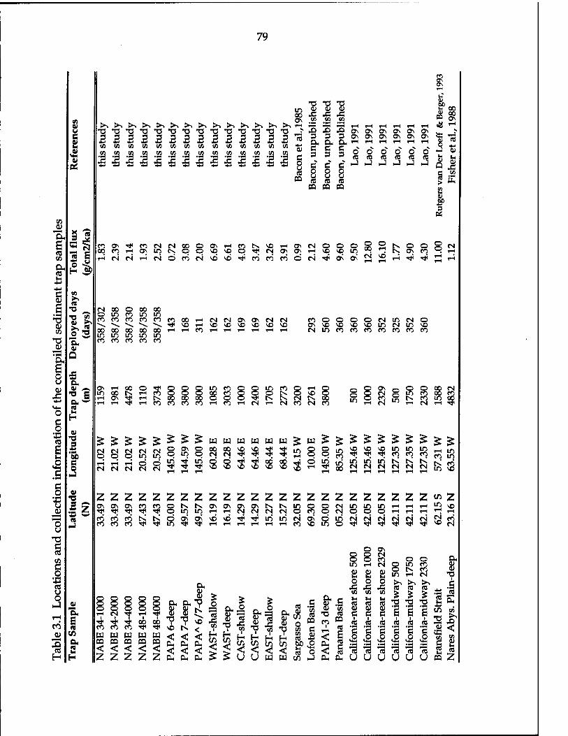
79

CO en &, CB

to

0)

(A C o

•J3 cc u O

CO

I

0) V w C a

s

t» >-.

t» ^

5 S a tv

D

u a OJ cv „m^,

s s «4H fS O IN

c H o

33 0) •a I 2

»H 60 £ e ^ o •I-*

c o cv T. •o

5 z •w

o n mi

6 « CO a 2 H

5S rH

•o *o •o 4> &0 „

If) QJ OJ tu Si °° 00 ON CO

X! CO CO Ä 8

X >> rS >, >s >. >s >. >> >, >^ >. >, >, 1-H »^ «r4 •1—i

r-i rH rH rH rH T-t <a <-■ T3 *0 "O "O TJ •ö •o T3 ■o •o "0 "O "O "O V 23 ig 23 ON ON ON ON ON ON V

5 5 5 5 5 5 5 5 5 5 B B B B 13 3 3 3 ON ON ON ON ON ON its *-j 8 *

rJ til •-I 1-

a 3 5 w

co W (A (A 10 CO CO CO CO CO CO CO to to 0)

§ u CO

3 V V N v *. ^>

1 .2 .2 .55 £ £ <5 1 l .a

5 1 1 1 CO CO CO to • ?H »|H «*H 'rH

e o co

o co

o co

o co

O CO

rJ

O

2 o O o

CO ä u ce

u co

CQ CQ CQ B

£

CO ON *f CO CM CM 00 o ON rH n S * H ON CM o o o o 00

o tv o © §2 00 CO rH ON m IX o O NO \o O ^ N ON ON rH NO NO in T*H tv ON CO

rH tN N ri CM d CO CM NÖ NO "* CO CO CO © CM ■* ON ON tN 7-1

NO r-1

r-i TJH ■>* rH rH rH r"1

Os

00 O 00 00 in co in in CO CO CO CO CO

S <J *0 H 00 NO

CM CM ON ON CM CM NO NO NO NO NO NO

OOOOOOOOrHrHCOrHrHrHrHrHrH in m in in co co co co

CO o o ON NO NO CM in co

o o CM in CM o NO NO m CN in NO CO CO CO CO CO CO

rHoooTt*oooincoooincoorHO OOt-vrHCOOOOOOCOOOOKONOO ~ lX000000OOOTt<tNKcMt^00

COCOCOCOrHfOrHtSrHCMCOCSCO ON 3| rH ^

o o o o CM

O O 00 CM in co oo co

^^^^^i^^WWWWWW^W^^ "3 3 J5 CM CM CM CM

o o m in O ON o in

CM CM CM CM CM PPS^ "*

O 00 00 NO NO O CM CM "<* ■*

in o •«t NO

© NO 3 NS

00 00 oo on HI NO NO 3

o o Ö

rKOcoiK^coinoo

£ £ £ £ £ £ J>£ H co

NO NO NO in in m ^ ^ rf CO CO CO in in in ix tv CM CM CM CM CM CM

rH m co in tv CO in NO

COCOON.tN.ONONONONtv^inOOCM Hl^OinifiHHNNMNOnOtN

ON ON

n n N N CO CO ** Th

oN.r>.ONONONONtv^inoo OininrHrHCMCMCMCMOCOO 6oN»NÖ*'oi'jiiriiriN(j;diri in^h^rHrHrHrHrHrHCONOinO

222222^2 iflinifiiHHH^e OOOrHrHrH^rH

o o o o

CO CO

H tN ^

*r ^ **r oo

WWW CQ CQ CQ < < 2 2

< 2 U CQ

80

deployed in March and April 1989, recovered and redeployed in September

1989, and totally recovered in April 1990. The total deployment time for the

sediment traps was 378 days, including a 20-day hiatus in the middle. The

34°N station is in the North Atlantic Subtropical Zone whereas the 48°N

station is in the North Atlantic Transition Zone (Honjo and Manganini,

1992); thus the two stations represent different physical and biogeographic

areas. This trap experiment included synchronization of the open/close

timing of all six traps, thus providing a time-space matrix in depth (1, 2, and

4.5 or 5 km) and latitude (1,256 km apart). Current meters and thermistors

that were deployed 1.2 m below each of the three sediment traps at the 48°N

21 °W station recorded no significant turbulence, and the currents were

generally less than 5 cm/sec throughout the year-long deployment.

Each sediment trap was deployed with 13 rotary collectors. Each trap

was opened and closed 26 times, providing continuous time-series sampling

at 14-day intervals, except for two periods. An independent monitoring

mechanism installed with each trap (Honjo and Doherty, 1988) confirmed

that the entire program was executed correctly and on schedule. Before the

deployment of a trap, analytical grade formalin was added to the sample

containers to make a 3% solution buffered with 0.1% sodium borate. After

recovery of the traps, no swimmers were identified in any samples.

Particle samples were wet-sieved through a 1-mm Nitex mesh. This

was necessary to maintain precision during splitting of the major portion of

the sediment, which was <1 mm. Common particles in the >l-mm fraction

were large aggregates and fragmented gelatinous Zooplankton.

81

3.3.2 Arabian Sea

Three moored arrays consisting of a total of six time-series sediment

traps were continuously deployed at locations in the western (16°15N, 60°28E),

central (14°29N, 64°46E)/ and eastern (15°28N, 68°45E) part of the northern

Arabian Sea. Each mooring system consisted of two time-series sediment

traps: one 1000 m below the surface and the other 1000 m above sea bottom.

Prior to deployment, collecting cups were poisoned with mercuric chloride.

The sediment traps were programmed to measure the flux of sinking particles

at intervals of 12 to 13 days over a duration of six months per deployment.

The traps were recovered and redeployed three times betwen May 1986 and

1987. Upon recovery of the traps, the samples were wet-sieved and split using

a precise rotary splitter. One quarter of the <1 mm size fraction was filtered

through preweighed Nuclepore filters (0.4 micron) and dried at 40°C.

3.3.3 PAPA

PARFLUX Mark 5, time-series sediment traps (Honjo and Doherty,

1988) were moored at 1000 m and 3800 m at station PAPA (50°N, 145°W; water

depth 4200 m) over a four-year period from September 1982 to August 1986.

The sediment traps were deployed, recovered, and redeployed about every six

months. Twelve cups located in a rotating carousel provided time-series

sampling during trap deployments. Sampling intervals were 12 to 14.5 days.

Samples were wet-sieved through 1-mm and 63-micron stainless steel

screens. The greater than 1-mm size fraction contained a negligible amount

of siliceous phytoplankton.

82

The sediment trap samples from the PAPA site used for this study were

from the traps deployed from December 3,1984, to April 20,1985 (PAPA6);

and from May 10,1985, to October 11,1985 (PAPA7), almost a complete annual

cycle of seasonal flux changes.

Collection cups were filled prior to deployment with 10% sodium azide

to retard bacterial decomposition. Procedures for handling samples at sea and

for processing samples in the lab are described in detail elsewhere (Honjo and

Manganini, 1992; Nair et ah, unpublished; and Takahashi et al., 1989).

Because of the need to avoid any seasonal bias, time-series samples

were combined, using amounts of material from each sample proportional to

the mass flux during the collection interval, to produce composite samples.

Composite samples were then analyzed for radionuclides following the

procedure described in Chapter 2. Sediment trap samples were analyzed for

major sedimentary components such as carbonate, biogenic opal, and the rest

of each sample was assumed to be the terrigenous fraction.

3.4 METHODS

3.4.1 Preparation of Composite Sediment Trap Samples

The procedure I used to prepare the composited sediment trap material

for analysis involved the following: preparation of 20 ml scintillation vials

for use in precise rotary splitting by soaking vials and rinsing them in acid,

then distilled deionized water; use of a precise rotary splitter to split the

materials; use of a washing solution during splitting of 3% formaldehyde +

83

0.1% sodium borate in ESL seawater (treated for 1-2 days with 3%

formaldehyde + 0.1% sodium borate and then filtered).

Samples were filtered on 0.45 urn Nuclepore filters, rinsed with

deionized, distilled water three times, then dried for 24 hours at 50°C. The

dried samples were cooled in a desiccator and weighed. After cooling, the

dried samples were peeled from the filters, and ground with an agate mortar

pestle; then the samples were stored in plastic vials in desiccators.

3.4.2. Radiochemical Procedures

Aliquots of <200 to 500 mg of dried sediment trap material were used

for radiochemical analyses. All samples were subjected to total dissolution

with mixtures of HNO3, HF, and HCIO4 in the presence of 236U, 229Th, and

233pa added as yield monitors. The radiochemical analysis procedures were

followed in a sequence as shown in Figure 2.1, which included separation,

purification, and electroplating. Th, U and Pa isotopes were determined by

counting alpha-emitted particles with silicon surface-barrier detectors. The

yields of the beta-emitting 233pa tracer were measured with a windowless 2-rc

proportional counter.

3.4.3 Carbonate Content

Carbonate content was determined by a method based on a vacuum-

gasometric technique which was reported by Ostermann, et al. (1990). A

preweighed sample was introduced into a sealed reaction vessel containing

84

concentrated phosphate acid. The pressure due to the evolution of CO2 gas is

proportional to the carbonate content when calibrated with an appropriate

standard and was recorded by a transducer. The results were calculated and

reported as carbonate percent in the total sample.

3.4.4 Data processing

Most of the radiochemical analyses were performed on the <l-mm size

fraction, which is close to the total sample weight. The analytical results are

shown in Table 3.2. Radionuclide fluxes in the <l-mm fraction were

calculated, and total flux was taken on the <l-mm fraction as shown in Table

3.3. For convenient comparison of the measured fluxes with longer-term

averages, I use mean annual flux units in the tables and figures. The

formulae for calculation of the flux are as follows:

1. Average flux (mg/m^/day) =

Total weight (mg)/(sample collection time x aperture of trap (0.5 m^))

2. Average annual total flux (g/m^/y) =

I Average flux * open days of each cup*365/[(total open days)*1000]

3.5 RESULTS

Analytical results of radionuclides are shown in Table 3.2. All analyses

were performed on the < 1 mm size fraction except the PAPA6 deep trap. Pa

and Th isotopes were measured by the alpha-counting technique. Except for

85

> 0)

•a •o *J tn

£3 1ft f to CM •a

>

*d 44 I»

f to CM

>'

•a 44 (ft

!3 00 f to CM 0.

i •a •a 4ri

Cf) tn cu

1 re

1H

00

1 re to a to CM *o OH

> 4-> "O c •o a; en E

T3 0) V)

H f (H CO &. o CM •a

«4-1

CD CU >

T» V A •o U TJ 2 ** c o

"0 re i 60

fr4 eo u V4H CM •c o

CO 4-4 g 3 0, en P .c <tf hi *> b H OH

PM4 V re u "O

XJ >■,

re V

u 4 0- &

CM re

en £ eo D. ON cu re V

■s H T3

«CMCOCMtNrHCMCM gggggggg 00000000

oooooooo dddddddd

N N * n o o o o s o o o o o

i—: rH hs «* T* in m Tf n n d> ö d> ö d>

Sv N 0\ CD rH rH ö ö d

t CO Ifl N n ^

CM vo CO rH Ö Ö

« 5 00

NNinNN*f$tnif)P)*a ooooooooooooo ööööööööööciöö

S N S ^ ^ ^ dodo

3 3 ON cN O CO CO 00 O rH

O rH rH rH r-i

VO * M O* O N n ts n n

' H O rl ri

ID IT)

s § Ö Ö

CM "* 00 O O

§3i30HNnnoN ©©CMrHpQOrHp OOOOOOOOO

dciöödööcJöd

O O O O O O

n » vo in N m m

d in m * co n ^ T-i o o in CD o R en

8 d d

co en CO o rH O

o o o o o o o

55 9 o o d d

CM 3 S ^ S H 5 § S B o rH A CM ° 5 ° ö ö ö d ° ö §§

N^irjrlNNrHnNnin^lfjO ddddddddddddd0?

©rHrH0fv|rHrH0CM,_,00g dddi-jdddcädt-jdddcj

rH m in "* - -. M H n *o If) N

»tNino^HNvocom ■" t cN N If) vO ^ O

HNlfJONCO^dridcNHNd

O H M O 't in 00 K rH CO

o o in co O O 00 CO § § O h» HO'ifHNaiCOOOO'O'NN

rHrH«*rHCOCOCOrHCOrHCMrHCM

O O O O o £ s> OQOQOOHOHO K £ OOOOO 0> OJ-H f^O P, 0 rHCMfrnrt* a; cy 'S STa H^ H/ ^t x X T i >a in i n CO CO it t VD N ? i «5

OH =3 UH cu 1)

•n

< < < U w w

!

1 0) u o

01

(0 u a,

86

the data otained from the NABE station, which were obtained by the alpha

counting technique, the rest of the 234y and 235y data were obtained by ICP-

MS, and 238JJ was calculated by the natural 235u/238u activity ratio of 0.046.

A range of 0.3 to 0.8 grams of dry weight composited sediment trap material

was analyzed. The analytical uncertainty of each measurement with

propagated uncertainties in the 1-sigma counting statistics is in the range of

3% (235U by ICP-MS technique) to 12% (Pa and Th isotopes by alpha counting

technique, and 234JJ by ICP-MS technique). The uncertainty is primarily due

to small sample size and low concentration, and the practical limits of

counting time. Procedural blank corrections are also included in Table 3.2.

The blank corrections are between 0.5% to 9% for 230Th, and 0.5% to 10% for

231pa. Uncertainties reported in each table were obtained by using a standard

propagation of error calculation, including ± lo counting statistics and

uncertainities in blank correction and detector efficiencies.

Table 3.3 lists the calculated results of this study. It includes the

unsupported 230xh ancj 231pa activities, the specific activities and fluxes of

detrital uranium and authigenic uranium, and calculated 238u/232jh,

234u/238u and 230Th/232Th activity ratios.

3.5.1. Unsupported Isotope Activities

Unsupported 230Th and 2^lpa are those amounts of the 230xh and

231pa that were scavenged directly from the water column. To be able to

calculate the unsupported 230lh and 2^lpa activities (designated by the

notations 230lrtexr ^Paex for convenience), i.e., scavenged 230Th and 231pa

activities, it is necessary to correct for the supported activities from uranium

87

QJ

t «0 en OH « *H

•4-1 c QJ

OJ

en 0)

g O

?0

1—1

3 (A

e T3

3 u I—H « U co co 0)

5§

«I w B tt> g •a OM

3 ^ 3

tu

<*N*NNNNNS»0\001f) NHONr;\oo;rj(j\qqp;q(iq ÖÖÖÖÖrHÖrHÖrHrHÖi-50

CM 00 ON

NO NO

CO CO ON

t-> CO O ON H Ö

IN T-H o o

tvtNOOONCOOvOCOCN Ni/jqifiifjNonoon NHtsOOvÖlfi^rHtNtN

CM o

co NO IN ^ © o O ON CO o

in oo 00 CO

r-s H r-t lO tx ON CM CM 2 » ON 00 ©

O CO

CO ON o K in TH

00 co CM CM

r-H ON in

s

o o o o o o CM ^

CO CO W [XI pa co < < Z Z

CM

o © o o o © T-H Tf

I I oo oo ■«* Tt*

w w CO CO < < 2 £

OONNONOOTjfCMON

OH QJ

OH OJ 0)

OH "O ST1 .1

NO tV

< < &H

IN H CO

en

<

NO

I £ £

OH O QJ QJ

T*

CD <

fO OHS OH

QJ -a f-< t* t* f< <£ <3 <*> K < < < < U U W W

cMco^inNotvoooN O T-i CM CO "*

88

en CO

1 H

X V

H o re

OH rH CD CM

^ N N \£) N o o o o o o © o o o o d © © d +1 +1 +1 +1 +1 {> VD tN rH T}< S n N If) N o o o © o o d d d d

ro o o

o o o o

in o o

o o in o o

in o o

o o

CO o o

o o o o o o o o o +1 +1 +1 +1 +1 +1 +1 +1 +1 00 o

CM CO o R o

T—1 o t—1

R o o IN o o ON

o in in o

o o o o o o o o o

X CD

tu CO -Ö CM w

f O X V

JS H o CO CM

I

o T-i ON in co © in co K oo T-H t^ in ^1 N n in IH © H CM © r-5 TJH

feovintNO\rvT-iT-H SosoooirjHO

.rfvOCMCMinONCO Pt\Nif)Hiric<i^

00 Tf rH rv tN r-5

R CM as

© CM in H ON rH in vo

R CM

rH tss in o in rjn ON CM

00 CO CO tN r-i K tN rH

IN ©

R ON rv co co rH ON

c

s <

»9»

B a,

o 2

CONOCOCMvOOOCO^'HHOOCOvOCMrH OOrHOOincO^OOOrHrHrH d>öciöcic5d>ööciciciöö

-*if)0»vooir)0*»'tifiNro

OrH'^dcMOÖTt'vDdrHdcMrHCM

Hin^lfiaO\rlOO\OOHN^ incMrHVCT^00ON000000'«ftNvO

comrHCMtNCMOvocooorNCMONin CMCO^rHrHrMrHrHrHrHCM'^CO'* ööd>ööd>ööd>ööööö

HNn^lTj^N»»^ CM CO "tf

89

in the detrital minerals and from authigenic uranium derived from seawater

from the measured 230jh and 231pa activities (Table 3.2) in the sediment trap

material. Since 238u/232xh activity ratios for most major minerals and

pelagic marine sediments vary over a narrow range (0.8±0.2), the detrital

uranium content is usually estimated by measuring 232xh and 238u/232jj1

activity ratios (Anderson, 1982; and Anderson et al, 1990 and 1992). The

authigenic uranium content is usually calculated from the difference between

the measured total uranium content and the detrital uranium content. For

sediment trap samples analyzed here, authigenic uranium concentrations

range from 0.06 to 1.67 dpm/g, which are approximately 14% to 91% of the

total, measured uranium activity in the samples. Although most of the

sediment trap materials contain a significant amount of authigenic U (Table

3.3) that is derived from seawater, the contributions of the decay products

230jh ancj 231pa are always negligible because the samples are always too

"young" to be corrected for any significant amount of the decay products of

authigenic U (Anderson et. al, 1990). The detrital components of 230xh an£j

231pa Were calculated by assuming their activities to be in secular equilibrium

with their U parents; thus, scavenged 230jh and 231pa activities were

calculated by using the difference between total 231pa ancj 230xh activities and

the activities of their respective parents. The estimations can be done with

the following equations (Lao, 1991; and Anderson et al, 1990):

230Thex = 23°Thm - (0.8±0.2)232Thm/ (3-l)

231Paex = 231Pam . 0.046(0.8±0.2)232Thm, and (3_2)

Authigenic U = Um - (0.8±0.2)232xhm (3.3)

90

where all values are in activity units, "m" is the measured total activity in the

sample, (0.8±0.2) is the ratio of 238U/232Th, and 0.046 is the natural

235u/238u activity ratio. From the above equations, I calculated the

uncertainties of unsupported activities of 230xh and 231pa, and their

propagated uncertainties are approximately 20%. Large uncertainties of

calculated 230Thex and 231paex are derived from the large uncertainty of the

assumed 238u/232xh ratio.

Depth profiles of unsupported activities of 230Th and 231pa at different

stations always showed a similar pattern: lower activity levels for the

shallower trap and higher activity levels for the deeper trap. The pattern of

increasing activities with depth is expected, since both 230jh and 231pa are

produced throughout the water depth.

3.5.2. Authigenic Uranium and Particulate Uranium

The concentrations of detrital uranium (calculated by measuring 232xh

and assuming a constant 238|j/232xh ratio of 0.8 ± 0.2 for the detrital phase),

show an increase with depth for all stations. The authigenic uranium

concentration in the samples from the PAPA and all the Arabian Sea stations,

with the exception of the deep CAST trap, remarkably enough dominates

almost 70% to 90% of the total uranium measured (Table 3.2). For three

mooring sites from the Arabian Sea stations, the concentrations of authigenic

U are higher in the shallowest trap sample and have lower concentrations in

the deep trap samples. The NABE stations show a similar trend of decreasing

in seawater-derived uranium activity with depth. This feature was observed

at other stations in the open ocean (Anderson, 1982). The flux of authigenic

91

uranium decreases with depth, a trend clearly shown in the data from the

stations of NABE. This decrease with depth is suggested as a reflection of the

formation of authigenic uranium that must occur in surface water, then is

remineralized in the water column; this authigenic uranium must be

associated with very labile particle phases that would not remain for long

periods of time when they reach the sediment surface (Anderson, 1982;

Anderson et ah, 1990). The possible carrier phase of particulate authigenic

uranium is believed to be organic matter. The 234u/238y ratios (Table 3.3)

scatter compared to the seawater value for most of the samples; it is not

possible to demonstrate whether there is a significant correlation between the

234u/238u ratios and the authigenic U contents because of the large counting

errors that result from the low counting rate of 234y by ICP-MS. In addition

to the 234u/238u activity ratio, the 238u/232Th ratio is clearly greater than

the value in the detrital phase (i.e., 0.6 to 1.0) (Table 3.3). This demonstrates

that the particulate U at most sites is dominated by the authigenic source.

3.6 DISCUSSION

The essential tasks of this chapter are to examine the relationships

between particle flux and the various indicators. How is the nuclide

scavenging influenced by mean annual particle flux? Is the spatial variation

in nuclide scavenging within an ocean basin (i.e., stronger scavenging at the

ocean margins than in the open ocean) largely a result of the spatial variation

in annual particle flux? How does scavenging removal compete with

horizontal transport to cause fractionation between 231pa an£j 230xh? Does

the spatial contrast in the value of the (231pa/230xh)ex ratio in the sediment

92

indicate a contrast in the scavenging rate in the overlying water column? To

examine these questions, the correlation between mean annual particle flux

and mean annual nuclide flux was examined. Compilation of all available

data obtained from year-long deployment of sediment traps from this thesis

work and other previous studies are included to establish better the influence

of particulate material on nuclide scavenging. The mean annual total particle

fluxes recorded in the sediment traps varied by a large range from ~1 to -17

g/cm^/ka. The geographic distributions cover a wide spatial range from an

oligotrophic ocean to a margin ocean and the polar ocean. The locations and

collection periods of all sediment traps are provided in Table 3.4. Fluxes of

particulate material, fluxes of particulate radionuclides, and (231pa/230xh)ex

ratios are also shown in Table 3.4. The stations from NABE, the Arabian Sea,

and PAPA were done within the scope of this thesis. For most of stations, all

of the radionuclides were determined on the size fractions < 1 mm, and the

flux of <1 mm material is taken to represent the total particulate flux. It is

assumed that the concentrations of nuclides are negligible on the >1 mm

particles. The flux of <1 mm particles are dominates total mass flux, ranging

from 85% to 100% of the total mass flux (Figure 3.1).

The collections of sediment traps for PAPA6 and PAPA7 each covered

one half of a year, and they were analyzed for nuclides and sedimentary

components separately. The mean annual total mass flux, and the mean

annual fluxes of nuclides and compositions at the PAPA station thus

calculated based on the time-weighed fraction for each collection period. The

reason for the calculation was to remove the effects of seasonal variations in

nuclides and particle fluxes. This calculation is also done for the stations off

the California coast (Lao, 1991) and the Nares Abyssal Plain (Fisher et ah,

93

Table 3.4 Compiled data for sediment trap samples

Trap Sample Total flux 230Th)F/P 231Pa)F/P 231Pa/230Th)exo/0.093 depth (cm) (g/cm2/ka)

NABE 34-1000 1.83 0.56 0.20 0.31 NABE 34-2000 2.39 0.80 0.30 0.38 NABE 34-4000 2.14 0.89 0.26 0.29 NABE 48-1000 1.93 0.32 0.14 0.55 NABE 48-4000 2.52 0.61 0.17 0.26 PAPA 6-deep 0.72 0.61 0.45 0.73 PAPA 7-deep 3.08 1.25 1.11 0.88 PAPAA 6/7-deep 2.00 0.96 0.81 0.78 WAST-shallow 6.69 0.84 1.02 1.08 WAST-deep 6.61 0.89 0.72 0.84 CAST-shallow 4.03 0.67 0.50 0.75 CAST-deep 3.47 1.11 0.96 0.78 EAST-shallow 3.26 0.92 0.95 1.01 EAST-deep 3.91 1.09 0.64 0.59 Sargasso Sea 0.99 0.71 0.36 0.51 Lofoten Basin 2.12 0.81 PAPAl-3 deep 4.60 0.98 Panama Basin 9.60 1.50 2.49 1.66 Califonia-near shore 500 9.50 1.49 3.13 2.10 Califonia-near shore 1000 12.80 1.80 3.99 2.22 Califonia-near shore 2329 16.10 1.60 3.71 2.32 Califonia-midway 500 1.77 0.31 0.66 2.13 Califonia-mid way 1750 4.90 0.71 1.72 2.42 Califonia-midway 2330 4.30 0.61 1.48 2.43 Bransfield Strait 11.00 1.32 Nares Abys. Plain-deep 0.91 0.71 Nares Abys. Plain 1.12 0.68

94

<foap-lSVH

Mon^HS-ISVa

MOipHs-isvD

daap-lSVM

MoncHS-xsVM

daap-Z V JVJ

daap-g yjVd

*-w aavN

x-8? aavN

irtt aavN

Z-K aavN

i-*e aavN

x «a »—I

CO 3

0)

T3

CO

CO

c O

• 1-H CO u CO

O u

CO

0) M

(X/zin/8) xnu

95

1988). In addition, PAPA1-3 data were taken from Bacon (unpublished data)

and given in Table 3.4 for comparison. Sample materials from the Arabian

Sea stations were only from half-year collections, but they were taken to

represent the mean annual records and are included in the compiled data

plots for discussion. The mean annual flux range (3 to 7 g/cm^/ka) of these

half-year collections is apparently higher than the mean annual flux (2.3 to 3.4

g/cm^/ka) reported from the whole year collection (Nair et ah, unpublished);

therefore, the fluxes might be under- or over-estimated because of seasonal

variations.

3.6.1 Quantification of sediment trap efficiency with 230jh and 231pa

For more than a decade, sediment traps have aided scientists in

developing insights into the functioning of ocean systems. The trapping

efficiency of a sediment trap is essential to know for quantifying the flux of

particulate materials. The production of 230jh in the water column occurs at

a known rate because it is produced from the decay of uranium, an element

with nearly constant concentration and uniform distribution in the ocean, at

least through the Quaternary (Anderson, 1982); in addition, the residence

time of 230xh in the ocean is very short, in a range of -20 to 40 years

(Anderson et al.f 1983a and 1983b), as compared to its half-life of 75,200 years.

Thus, 230-jn has been suggested as the best candidate for quantifying trapping

efficiency (Brewer et al., 1980).

By comparing the flux (F) of Th measured in collected sediment trap

material to its production rate (P) from the overlying water column, the

trapping efficiency would be determined (i.e., the trapping efficiency equals

96

F/P). The production (P) of 230xh can be calculated by the formula p230jh

=0.0026*Z, where Z is the water depth in meters, and P is in dpm/cm^/ka. If

there is no trapping error, F/P=l.

The above is based on the assumption that V=P, where V is the vertical

flux of 230xh scavenged from seawater, but this is subject to some

uncertainties (Bacon et ah, 1985). The uncertainties arise from (1) the possible

partitioning of 230xh scavenging between vertical and horizontal pathways

and (2) temporal variations in scavenging rate of 230Th due, for example, to

the seasonal variations in total particle flux. From the total fluxes of 230xh

collected in a PARFLUX-design sediment trap at 3200m in the Sargasso Sea,

Bacon et al (1985) showed that the apparent trapping efficiency obtained for

different two-month intervals varied from 25% to 101%. The data indicate,

for the short term, that the production and removal of 230^ are clearly not

in balance. However, the seasonal bias may be removed, as suggested by

Bacon et al. (1985), by averaging over annual, or longer, records of 2307h in

the trap to obtain the mean annual flux F of 230xh. This is what I have done

in the following.

Horizontal transport of 230xh may occur; thus, the net horizontal

transport (H) of 230Th needs to be evaluated. It then becomes a problem to

use the mass balance of 230^ to examine both the trapping efficiency and the

extent of the horizontal transport of 230xh, which can not be solved uniquely.

As previously suggested (Anderson et ah, 1983b; and Bacon et al, 1985), to

evaluate absolute trapping efficiency, one needs to combine information on

230Th/231pa activity ratio both in the water column and in settling

particulate matter at the site; then one can calculate both the vertical flux V

97

and horizontal transport flux H by simultaneously satisfying oceanic material

balances for 230Th and 231Pa (Bacon et al., 1985):

HTh + VTh = PTh (34)

HPa + VPa = PPa (3-5)

HTh = Rh HPa (3-6)

VTh = RvVPa (3-7)

This method was designed to estimate V and H that are independent of

the fluxes measured by traps. The equations are based on mass balance,

assuming that H is the horizontal flux from the ocean interior toward the

margins of the basin, which causes an intensified scavenging at the margins.

A flux of 230xh, however, might occur in a particulate form from the

opposite direction at the margins due to sediment resuspension at the

margins and lateral spreading toward the ocean interior. In other words, the

flux H should be evaluated to take into account all net effects of horizontal

redistribution of the 230jh production.

In equation (3-6), Rh is the 230xh/231pa activity ratio in seawater

(governing the horizontal transport), and Ru (equation 3-7) is the

230xh/231pa activity ratio in the settling particulate matter. The net flux H is

taken to be positive for transport away from the ocean interior. The absolute

trapping efficiency E is then given by

E = F/V = F/(P-H). (3-8)

The Rh of the NABE 47-shallow and -deep stations were calculated

from the measured values of 230jh/231pa activity ratios in the water column

98

at depth of 1550 m and 2700 m. The measurements were done by A. Fleer

(unpublished data). The value for the Sargasso Sea was taken from

unpublished data of Bacon. Measurements are not available for the other

stations in Table 3.4, so Rh was estimated by a best-fit of a third- order

polynomial regression line (Figure 3.2) to the measured 231pa/230jh ratio

data from other stations where measurements were available. As shown in

Figure 3.2, the 230xh/231pa rati0 increases with depth, and the ratio shows

only slight variations, within a narrow envelop, at a given depth, even when

the data are from different regions. The values of R\> and F for all stations

were taken from the measured values in Table 3.4. The sources of the

compiled data for R\> are indicated in Table 3.4. The required parameters to

solve for both H and V for the 230jh and 231pa Df all traps, and the calculated

results are summarized in Table 3.5. The sources of error are largely from the

analytical errors of both 230Th ancj 231pa measurements in the water column

and in the particulate material. Since the concentrations of both nuclides in

the two phases are low, the analytical results would therefore have a large

error.

The calculated values of trapping efficiency E (i.e. F/V of 230Th) range

from 0.3 to 1.4 (Table 3.5 and Figure 3.3). If E values is close to 1, it can be

concluded that the sediment trap performed well in measuring the flux of

particulate materials. Within a deviation of ±30%, this result was found for

all of the PARFLUX sediment traps at the deeper depths for the NABE 34 and

48, PAPA, Sargasso Sea, and all Arabian Sea stations. The shallow traps

(-1000 m or shallower) showed a tendency toward undertrapping. Most of

the shallow traps, even as deep as ~1000 m, show clearly the imbalance

between production and removal of 230jh The sediment traps used for this

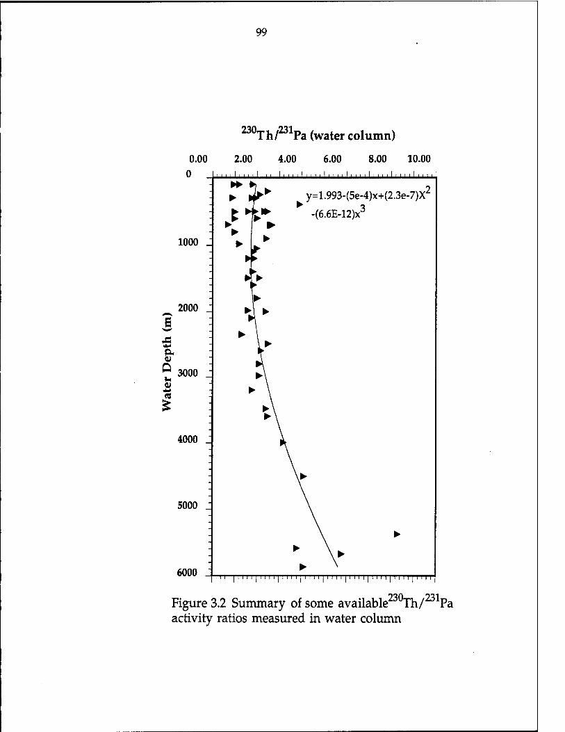
99

230Th/231pa (water column)

0.00 2.00 4.00 6.00 8.00 10.00 0 i

1000 J ►

!►* y=1.993-(5e-4)x+(2.3e-7)X2

V* -(6.6E-12)x3

►

►

- V

Wat

er D

epth

(m

) o

o

o

o

o

o

V ►1 ►

► \ \ ►

►\ ► \

►\

4000 J \

- \>

5000 J \

- \ ►

- * V 6000 " ► \

Figure activity

1 1 1 1 I 1 1 1 1 1 M 1 1 I 1 1 1 1 1 1 1 1 1 I i 1 1 1 1 1 1 1 1 I 1 1 1 1 1 1 1 1 1 I 1 1 1 1

3.2 Summary of some available Th/ ratios measured in water column

xPa

100

o>

u C <v

01 OH

I 0) en

<*H o

3 o

'33 -d o

in co l-H

r **

M .«H

CL, fi OH •a

£ B El

a ■° S OH W

2 H

OH

S «

OH

SS H

d Z

H in N . .. ts M N N 0\ i-H rH CO i-i

aiif)HHNntcnnnoNO\oao\ NnHNHNHriridHrirJi-lriH

oo oo "* r-i IN o ._>.,_. _. , Tttv.OvOvOK^00r>J00\0

$ t-x ts ON r-i CM CO r-t "#

CO 00 r-5 i-H CM ^S3 co o ^ H a N q ^ ^

* iri .^ ^ iri ^ >* 5 N

OOvS!o\ONOCO'<!f<CMTHCOr-l-ttsNi-iCM'>*T-lTt<'*

CM rjt N»0\NNMlfi'<f*N\OHNlf)H<tlf)

oo o "*t T-t

Ö CM* co in

IN ON H r(" Tf CO ON LH

IN O CM CO

rfn*Minoinif)foif) r-lOOONi-HT-Hr-ICOCM O CM

o\ »-I oo Ifi » N rH ON

o-^omcoooincooo COOOOCOOOOINOON

rfrHt^OOOOO-^JNlNCMin ^rHCOCOrHCOrHCMT-ICMCOCM in

ON CM CO CM

O O in

O ON

tv CO 1-1 CM

o o o o o o o o o o o o 1-H CM "tf i—I

-tf -st« ** 00 CO co CO "^ w W W W M pa CO pa < < < < z Z Z 2

0)

o T?

00 N£>

w < fc co S c£2

■5

■"to

•s

■5 OH .2 0> 01

CO

•s to

'S co co en < < < ►^ ^ > > > rs -s, 's, nj to

ST ^ pa QJ O

«3 «1 CO 00 «H

to e to C to

o o o o o in l-H o> 01 »H »H o o ^ *k

(-1 JH RJ to 0) o> C C i i to to

C C .o .o

ON

CO O O

^ S !£ 23 n, O tN CO g in rH CM o >^ >, >^

»C fO tO fO

I s £ s & T3 T3 TJ V* .9-4 »rH «*H

S 6 6 £ i i i i tQ t0 tO to

• ^H «l-H »^H »»H c c c c .o o .o o

HNn^n^Nco» CM CO Tf

to to to to to to U U U U U U

in NO tN 00 ON O H H H rl H N

101

o Z

X "0 01

3 *■*

53 S fc m 0 *4 u o H

XJ H ON

MH

J3 H H

1 B

J3 H a; > rt

cu DH

>

"£> 2 H >

c3

i 3

^-v ^"N *J >% c ,*»> r* o (0

CH

! in > en "O 0)

-g O

£ 2

|H (4 01 o> a» 0)

I-H 1—1

WH UH

< < £ £ o © hs in IN in cs T—1

£ £ o o £ £

s s T3 T5

01 0) i- s- 3 3 vi [fi « (C a; o>

T3 T) O) 01

SS c 3

C O tö

CO CO

0Ü 03 04

C o u «a

ON ON ON ON ON ON ON ON ON ON ON ON rH rH T-( T—1 T-H r-t ^ V

O O O 0 0 o fB « CO tc to to

HJ HJ HJ HJ HJ HJ

> > > > > OS 04 04 04 04

2S2 £ £22SSKK2SSSSK22C§

ON in LO v£> cs 00 * N If) N H cvi H in ri

tN ON 3 NO 00 VO in rH v^ O

N 5\ in N N * N rHOONinNfltOnNOl

oo JS o in °£ ts ^ ^ VO ^ ON 3 IN ON" S

vOOONCNrHvO'.tfOtv.rH LnCOCOCO^OONOOONNßrH ÖÖÖÖÖÖÖÖÖrH

CNOsrHOONOOi—I rH rH ONptNinnjoqNqcotNvq ÖrHÖrHrHrHrHÖÖÖ

cnocsinooT}HcS'«^otvCNiorginNOooco^rHrH \q^NnNqooo)NrHO\NooNr;nHNifii't ©ÖrHÖÖT^ÖOÖrHÖT-HOrHrHrHrHOÖ©

ONO\corjoococNNONOino OOOOt^ONtNONOONONONO öööööÖT-5ööÖT-H

l-Hf>OON©CNOOON ONOOCNCNCO'^CO"^'* ÖÖrHTHrHrHrHrHrH

00 in r-l T-H O CO CN N t<5 N If) N N H Ö Ö Ö Ö Ö Ö rH

H n in N Tf T« 00 N N O If) ^

rH CO CO IN ON CN v£> O N OS N N •* \C

OOOrHOOCSrNCMCOeSCOCO

H(s|^ONOON»BNNN\OON^NNONin\ON ----- ■■ — — — iNinoNcovopcop

<j \Ö ts <* ri CO CO rH vO ON

CO.-, , _.__.._ _ OCOVOONCO'^P'^rHrHpP NvcirivoiriNONvöiridifivonH*"*^ N^OOMSONNNNVO^VON» — —

00 tN rH tN VO CO nooNONONNn(N*'*ir!no"n™^

- • • • • • ' N fÄ K" 00 ff! <* q ,-H ^ ^ rH ^ rH CN CMrHrHVOCNlinrH-^rtcOCO

HNn^m^NK^S^^^^NoooNO

102

0.00 0

Trapping efficiency [E( Th)]

0.50 1.00 1.50

1000 _

£ 2000

3000

4000 _

5000

Figure 3.3 The estimated trapping efficiency

[E( Th)] versus trap depth. The numbers are same as those in Table 3.5

103

study show a tendency of increasing in trapping efficiency with water depth

for almost of stations. The potential problems due to swimmers and

hydrodynamic bias have been suggested to influence significantly the records

in shallow trap collections, but to influence to a lesser degree records in

deeper traps (Gardner, 1980; 1985; Lee et al, 1988; U. S. JGOFS Report, 1989;

Busseler, 1991).

The trapping efficiency of the off-California nearshore deepest trap

indicates overtrapping. Sediment traps deployed in margin areas might have

collected some resuspended and laterally advected slope sediments, thus

providing another source of 230xh m addition to that scavenged from the

overlying water column. From the calculations shown from equation (3-4) to

(3-8), the data clearly suggest that the sediment trap performed unreliably in

measuring the particle fluxes in the NABE 34 and 48-shallow traps, and the

station off-California midway.

The data from the PAPA station was derived from time-weighted

mean annual flux from two half-year collections PAPA6 and PAPA7.

Comparing this time-weighed mean annual 230jh flux p to its production

rate P yields 0.96, a value comparable to a previous analysis result of 0.98 from

the same site (Bacon, unpublished data). The two estimates come from

different time periods that showed different values of total mass flux (two-

fold difference in total mass flux between the two periods). This indicates that

the scavenging efficiency of 230xh is so strong that its scavenging rate is

independent of total mass flux from the overlying water column. This

indicates also that the interannual variations in the 230xh flux may be small

even though the variations in mass flux can be large. The absolute trapping

efficiency of the traps, however, during the collection period of PAPA1-3 is

104

not known. Finally, the trapping efficiency of the traps off the California coast

was estimated independently by comparing the F/P of 230xh for the deepest

trap to the F/P data of the core top (Lao, 1991); their data (0.66 for the traps of

the off-California nearshore, and 0.17 for the trap off the California midway)

were significantly lower than the calculations shown here. The average E

value for all traps is 0.87 ± 0.32 (n=20), but the average E for all deep

PARFLUX traps is 1.00 ± 0.05 (1 standard error of the mean, n=9). This

indicates that the PARFLUX traps deployments are very reliable for the deep

water particle collection.

As mentioned earlier, F/P of 230jh was initially used for the

estimation of apparent trapping efficiency (Brewer et al., 1980). By comparing

the measured flux of ^Oyh integrated over collection period to the rate of

production in the overlying water column, the apparent trapping efficiency

for all traps were calculated. The F/P values of 230jn are listed in Table 3.5

also for comparison with the absolute trapping efficiency based on F/V values

of ^Ofh ^ general, the apparent trapping efficiency based on F/P values of

230ih shows similar patterns for all traps used for this study.

3.6.2 Quantification of Particulate Radioisotope Flux

Since the F/P ratio is used to examine the scavenging efficiency of

radionuclides by the settling particles, corrections for trapping error must be

made to provide better quantification of the scavenging efficiency of

radionuclides and their adsorbers and better understanding of the scavenging

behaviors of both 230jh and 231pa. The trapping efficiency corrected-mass

flux will be used in the following discussion.

105

As indicated in Table 3.5, after correction for trapping efficiency, the

total mass fluxes of particulate material at the NABE 34 station showed a

smaller mass range than those at the NABE 48 station. The range of mass

fluxes in the NABE stations and both the CAST and EAST stations varies

from ~2 to ~6 g/cm^/ka, whereas the total mass fluxes of the two WAST traps

range from 7 to 8 g/cm^/ka. There is a decreasing trend in the corrected- total

mass flux with depth for stations in the open ocean, but an increasing trend

with depth for those stations at the margins. Total mass flux of open ocean

stations such as the NABE, Arabian EAST and CAST, PAPA, Sargasso Sea,

and Nares Abyssal Plain stations ranges from 1 to 6 g/cm^/ka, and in the

ocean margin area and high production regions such as Panama Basin and off

California nearshore stations it is a few times higher. A station from the

polar ocean, the Lofoten Basin (not corrected for trapping efficiency), has a

total mass flux similar to the open ocean stations. The lowest flux shown in

Table 3.4 occurs at shallow depth over the Nares Abyssal Plain, and the

highest flux is in the deepest trap at the margin site off California nearshore.

The total mass flux of the sediment traps corrected for trapping efficiency in

Table 3.5 ranges from ~1 to ~14 g/cm^/ka.

3.6.2-a The value of V/P for 230Th

The ratio of vertical flux of 230jh (and 231pa) to its production rate

(V/P) is used to quantify the scavenging efficiency of radionuclides by the

settling particles. Although V/P provides better quantification of the

scavenging efficiency of radionuclides and their adsorbers, F/P values were

calculated and listed in Table 3.5 for comparison. The V/P values for 230jh

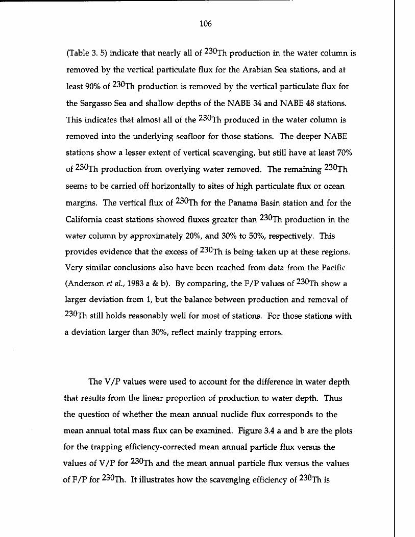
106

(Table 3. 5) indicate that nearly all of 230xh production in the water column is

removed by the vertical particulate flux for the Arabian Sea stations, and at

least 90% of 230xh production is removed by the vertical particulate flux for

the Sargasso Sea and shallow depths of the NABE 34 and NABE 48 stations.

This indicates that almost all of the 2307h produced in the water column is

removed into the underlying seafloor for those stations. The deeper NABE

stations show a lesser extent of vertical scavenging, but still have at least 70%

of 230xh production from overlying water removed. The remaining 230jh

seems to be carried off horizontally to sites of high particulate flux or ocean

margins. The vertical flux of 230jh for the Panama Basin station and for the

California coast stations showed fluxes greater than 2307h production in the

water column by approximately 20%, and 30% to 50%, respectively. This

provides evidence that the excess of 2307h is being taken up at these regions.

Very similar conclusions also have been reached from data from the Pacific

(Anderson et al., 1983 a & b). By comparing, the F/P values of 230xh show a

larger deviation from 1, but the balance between production and removal of

230jh still holds reasonably well for most of stations. For those stations with

a deviation larger than 30%, reflect mainly trapping errors.

The V/P values were used to account for the difference in water depth

that results from the linear proportion of production to water depth. Thus

the question of whether the mean annual nuclide flux corresponds to the

mean annual total mass flux can be examined. Figure 3.4 a and b are the plots

for the trapping efficiency-corrected mean annual particle flux versus the

values of V/P for 230xh ancj the mean annual particle flux versus the values

of F/P for 230xh. It illustrates how the scavenging efficiency of 2307h jg

107

related to particulate flux for both plots. The mean annual fluxes of 230^ are

well correlated with mean annual total mass fluxes. A simple linear

relationship of V/P ratios for 230^ with trapping efficiency-corrected total

mass flux was found (Figure 3.4-a). The regression line can be represented by

the following equation for the total mass flux from <1 g/cm^/ka up to 14

g/cm2/ka: Y = 0.73 + 0.06 X; where Y is the V/P ratio for 230xh, and X is the

total mass flux. The correlation coefficient R is 0.88. A similar regression line

for the relationship between mean annual particle flux versus the values of

F/P for 230Th was also found (Figure 3.4-b).

When the fluxes of 230xhex and 231paex in sediment traps are less

than their rates of production in the overlying water column, lateral

transport or other processes may be removing portions of the 230xh and

231pa (Anderson, et ah, 1983a). Since each data point in Table 3.4 represents a

year-long composited record at a site, and the trap deployments covered a

large range in total mass flux, a global-average mass balance of 230xh can be

estimated by averaging all available V/P data. The result gives an average

value of 1.06 ± 0.05 (1 standard error of the mean, n=20), indicating that, on a

global scale, there is a good balance between production and removal.

3.6.2-b Is 250Th flux constant?

Although there is a definite trend in the composited data of V/P ratios

(also F/P ratios in Figure 3.4-b) for 230xh with total mass flux, with V/P <1 in

areas of low mass flux and V/P > 1 in areas of high mass flux, the slope of the

regression line is shallow (Figure 3.4-a). The data indicate that while total

mass flux varies 14 fold between low- and high-productivity regions, the

108

5.00

§ 4.00 -j

u S

S 3-°° H

3 E 2.00

> 1.00

0.00

(a) m V/P)Pa Y=-0.3+0.3X R=0.87 ------- V/P)Th Y=0.7+0.06X R=0.88

10 15

Trap efficiency corrected-Mass Flux (g/cm /ka)

20

5.00

4.00 H

s= o t5 3.00 H

o PH

"x 9

2.00 -

1.00

0.00

(b)..#.. p/P)Pa Y=-0.15+0.27X R=0.93 —B— F/P)Th Y=0.51+0.08X R=0.83

0 5 10 15 20 Mass Flux (g/cm /ka)

Figure 3.4 (a) V/P)230Th and V/P)231Pa versus trap efficiency-corrected x230. 231T mass flux; (b) F/P)^uTh and F/P)^Ta versus mass flux

109

accompanying flux of ^^Th. varies only two times. A V/P ratio greater than

one is an expression of the so-called "boundary scavenging" phenomenon.

For most of the V/P values for 230xh, which are close to one, the effect of

"boundary scavenging" on 230jh appears comparatively small as shown in

Tables 3.4 and 3.5, and Figure 3.4-a. At the lowest mass fluxes of ~ 1 g/cm^/ka

(Sargasso Sea), close to 90% of 230xh production was found in the vertical

flux. At the site of the lowest scavenging efficiency of 230xh, more than 70%

of 230xh production was still sedimented out to the underlying seafloor,

whereas in the higher flux regions (Panama Basin and California margin), the

230jh flux exceeds production rate by no more than 50%, and even this value

may be biased toward the high side because of resuspension.

A similar conclusion has been derived from theoretical considerations.

The extent of boundary scavenging depends primarily on the relative time

scales of scavenging and lateral mixing (Bacon, 1988; Anderson et ah, 1990).

The time scale for lateral mixing depends on the rate of lateral mixing and the

distance over which lateral transport occurs. Using a one-dimensional

horizontal diffusion model, Anderson et ah, (1990) pointed out that for a

typical ocean basin with a half width of 3000 km and an isopycnal diffusivity

of 3x10? cm^/s, the boundary scavenging effect will be minor for elements

with residence times of less than 95 years. The residence time of 230fh with

respect to chemical scavenging has been estimated at 30 to 50 years (Brewer et

ah, 1980; Anderson et ah, 1983), which suggests that boundary scavenging

should have a minor impact on what is measured in the open ocean and

margin areas. From a simple box model, Bacon (1988) concluded that less

than 15% of the 230xh produced in open ocean waters is scavenged in margin

areas.

110

The extent of "horizontal transport" of 230xh might be used to "fine-

tune" the 230Th fluxes; the data shown in Tables 3.4 and 3.5, and Figure 3.4-a

indicated that the effect of particle flux variations on the 230xh flux might be

at most 30%. The 230Th data from Table 3.5 and Figure 3.4-a, therefore,

suggest that the assumption of a 230xh rain rate equal to the integrated

production in the overlying water column is, in most instances, correct

within about 30%, and probably better. Thomson and his colleagues (1993)

reported a similar conclusion recently.

In conclusion, the assumption that 230Th fjux t0 fae seafloor is

constant and close to the rate of production in the overlying water column is

well supported by annual flux measurements obtained from sediment traps

deployed in areas spanning a wide range of total settling fluxes. For most of

the deep-sea, the sedimentation flux has been estimated within a range of 1 to

3 g/cm^/ka; the application of the "230xh-normalized flux method" to

estimate the variation of the paleo-particle rain rate can be used perfectly well

since the entire flux of 230jh production is scavenged downward vertically in

such a mass flux range. In regions with extremely high particle flux, although

the absolute values of paleoflux might be underestimated by as much as 10%

to 30%, the application of the 230xh_normaiizatiOn flux method to obtain the

variation of paleoflux with time should be distorted less by this effect.

I conclude, therefore, that the large variations of F/P of 230fh reported

from sediments from one up to as much as ten in those margin sediments

(Mangini and Diester-Haass, 1983), in SEEP-I &II (Anderson et al.f 1991), and

the western and the eastern equatorial Atlantic sediments (Francois, et al.,

1991) must be due to sediment redistribution.

Ill

3.6.2-c The V/P values for 2^Pa

The V/P values show a strong tendency for significant horizontal

transport of 231pa fr0m the open ocean to regions of higher particle flux

(Table 3.5). For 231p3/ the partitioning of the removal flux is the reverse in

comparison to that of 230^ with only one-fifth of the production in open

ocean sites being carried downward by settling particles and the rest being

taken up at the ocean margins or other regions with high particulate flux.

The relationship between the V/P and trapping efficiency-corrected

total mass flux for 231pa can aiso be represented by a linear regression (Figure

3.4-a). It is clearly indicated in Figure 3.4 that there is a strong dependence of

the V/P values of 231pa Dn total mass flux. In low particle flux regions, traps

collected flux with a much lower value than production rate for 231pa m the

overlying water column; while in areas of higher mass flux or margins, traps

collected flux with a much higher value of F/P. While total mass flux

collected by traps varies 14-fold between low- and high-productivity regions,

the accompanying flux of 231pa varies up to more than one order of

magnitude, from a deficit of as low as about 30% in oligotrophic regions to an

excess of more than 4 times greater in high particle regions and margin areas.

This shows that the extent of horizontal transport for 231pa is much greater

than it is for 230Th.

Results of the compiled data set suggest that particle flux is the major

factor influencing removal of the nuclides 230jh and 231 pa from seawater.

The scavenging rate of 230xh apparently fluctuates less in relation to the flux

of particulate materials; whereas 231pa js verv sensitive in relation to the flux

112

of participate materials. The hypothesis of a constant flux of 230jh therefore

holds as a good approximation for the 230jh-normalized flux model.

3.6.3. Particulate (231Pa/230Th)ex ratios in sediment traps

Since the vertical flux of 230jh fluctuates much less than the vertical

flux of 231pa in response to variations in the particle flux (Figure 3.4), a

higher ratio of (231pa/230Th)ex should reflect the higher particle rain rates.

Data from sediment traps deployed for a year or longer in the deep sea do

show this phenomenon (Figure 3.5 a and b). Higher unsupported

(231pa/230jh)ex ratios, more than two times higher than the theoretical

production ratio of 0.093 (Table 3.5 and Figure 3.5a), occurred in regions of

higher particle flux such as ocean margins and high production areas (e.g., the

Panama Basin and off the California coast); whereas lower ratios, as low as

one-fourth of the theoretical ratio, occurred in regions of lower particle flux

such as open ocean gyres (e.g., the Sargasso Sea, the northern Atlantic Ocean).

The dependence of (231pa/230,rn)ex ratios on the total flux is strong, as

indicated by the slope of the regression line (Figure 3.5a). The slope shows

the(231pa/230xh)ex ratiG to be approximately 14 times with the variations in

total particle flux. While total mass flux collected by traps varies 16-fold

between low- and high-productivity regions, the accompanying ratio of

(231pa/230xh)ex varies from as low as 30% of the theoretical ratio in

oligotrophic regions to an excess of about 2.5 times of 0.093 in high particle

flux regions. This reflects the large amount of horizontal transport of 231pa

from low flux regions to high flux regions.

113

3.00

2.50 -

© 2.00 H

H 1.50 H o

«2 I.OO

0.50 H

0.00

(a) y= 0.02+0.20X R=0.86

0 5 10

Trap efficiency corrected-Mass Flux (g/cm /ka)

15

3.00

2.50 -

© 2.00 H

j2 1.50

£ I.OO

0.50 H

0.00

(b)

o o

1 ' '

D

D y= 0.18+0.14X R=0.94

_L

0 5 10 15 20 Mass Flux (g/cm /ka)

Figure 3.5 Pa/Th)/0.093 versus (a) trap efficiency corrected-mass flux and (b) mass flux. Symbols (o) on figure (b) are data from the California-midway traps, which are not included in the regression line.

114

3.6.4 Does the composition of particles affect the relationship between particle

flux and nuclide flux and the (231Pa/230Th)ex ratio?

Boundary scavenging is the term used to describe the phenomenon of

more enhanced chemical scavenging at the ocean margins than in the ocean

interior (Spencer et al, 1981). Although many previous workers have found

this phenomenon to occur for particle reactive chemical substances in

different regions (Bacon et al., 1976; Nozaki et al, 1981; Spencer et al, 1981;

Anderson et al, 1983 a&b; Lao et al, 1993), the controlling mechanisms are

not well understood. Higher total flux of particular matter certainly

contributes to a higher (231pa/230jh)ex ratio, as demonstrated above (Table

3.5 and Figure 3.5) and in other works (Taguchi et al, 1989; Anderson et al,

1990; Lao, 1991). Other factors such as the chemical composition of particulate

matter, ocean mixing rate, and residence time of the scavenged elements

(Anderson et al, 1983b; Bacon, 1988; and Anderson et al, 1990) have also been

suggested as potentially important factors. In the following section, I discuss

how the particle composition may cause deviations from the simple

relationship of (231pa/230Th)ex ratio to total particle flux. The quality of

particles, and whether the change in quality of particles during their

transportation and transformation, controls the fractionation between 231pa

and 230xh in different ocean regions are important issues to examine.

Partitioning of particle-reactive metals between particles and solutions

is often described by a distribution coefficient (Kd), defined as

Kd=[M]p/[M]d,

where [M]p is the activity in the solid phase (in dpm/g of particle) and [M]d is

the activity in the solution (in dpm/g of solution). In an attempt to identify

115

possible differences in the scavenging properties of different particulate

carrier phases for both 231pa an£j 230xh, the Kds of 230jh an£j 231pa for each

of these phases should be examined. Unfortunately, field data is very limited.

For now, I will provide two types of indirect ways to examine the empirical

relations of V/P of both 231Pa and 230Th, and of the (231pa/230Th)ex ratio,

with the deposition rate of a component of interest in particulate material.

First, the empirical relation of the nuclides with the four major components

of settling particles, carbonate, biogenic opal, organic carbon, and terrigenous

materials, were examined and the results are shown in Table 3.6. Figure 3.6 a-

d shows the correlation of V/P of both 231pa and 230xh with the trap

efficiency corrected-flux of carbonate, organic carbon, opal, and terrigenous

carrier phases. Figure 3.7 a-d gives the correlation of the (231Pa/230Th)ex

ratio compared with the flux of the major carrier phases. No significant

correlations are observed, suggesting that no carrier phase of carbonate, opal,

organic matter, or terrigenous material alone can control chiefly the affinity

of both 230lh and 231pa to settling particles. These observations show

inconsistent patterns compared with previous studies. The previous studies

(as described below) on particulate materials or on surface sediments,

however, did not obtain a uniform conclusion about the effect of particle

composition on scavenging behavior of nuclides.

Secondly, since the flux of each particle component in Figure 3.7

represents the variation in its concentration and the total particle flux at the

site, the control by composition can not be decoupled entirely from the

influence of total flux as used in Figures 3.6 and 3.7. The logical idea is to

examine whether the concentration of sedimentary components for those

data points with a higher particle flux range in the Figure 3.5 do show any

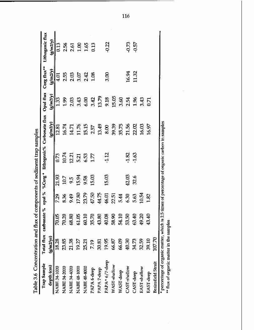
116

C/3 0)

"EH

en OH IB S-l

O)

(A

o C-H

o u

<*H o X

13

C O •a a c QJ u

§ U vo CO QJ

P-H

CO rH

vo in

rH vO O o

ID vO

CO 1—1

o tN CN rH rH o

fN tN

CO IN ID

O i

O i O

i

H If) CO N N 00 q in q q rf q <j N N fi N i-i

O O CO*

"* tN as co VD rH

CO ON CO CO O _ . CO ON O "<* O "* ° \D in ON 'f N rH rH fN CO VD CO CO

c o

o U

AS a o

e o

■e M U

X s c

o H

e- 6 <z> -S

2 H

a»

00 "^ rH vp in

tN rH ts \o ■* H in

IN in CM

ON

co

T* rH IN CM ö CM

H n N CM in IN

ON

o o 00

CM

in CO CM CO o

ON in N£> CM CO IN CO IN in p p ON ON in r-5 CM vö vö CO CO CM CM rH rH

tN CO 00 v©

O ^ ^ in VO rH

CO ON rH CM

ON CM IN

in o

00 IN 00

o o o rH

w CO < z

in ON

NO ON CO rj* o6 ON

o o CM 00 ö oc5 tv vo

in oo oq co CO rH CM CM

o o o o o o ■<* CO

^* en CO CO °) in *= P in o< in in 53 8

** o co ^ n *

O ON O in rH rH oq N in is q in Nrn'N^^CN.fi^.fi

in o O rH

in CM 00

VO NO CO

R o 00 00 o

o OS o rH o m

o O tN O

in CO

co o 00 in in

CO in

CO VO

ON co •<*

ON . . . r„rHlfilNONOCOON© tNCM^oqoNoqpcoiNinrH ONinhjÖONNüvoörl'cMON

CO co < < z z

o o o o o o rH ^

I I oo oo

03 01 CO CO < < z z

OH 0> 4) Ol

0- 01 01

"O tv. S3

VO K

< <

C-, CH

vD < < < CH

as rC

<

OH 0) 01

•O I

H

<

13

rs Ü en

Oi S 01 01

TJ U3

^ ** H H »] i« « tfl < < < < s> r^> r^ ^< ^ »- i£ U U m w co

*S "a. I B * S In" 01

8 - u 01 'S *

6P 6

o .y ^ 2 0 (C

c 'S 01 v U s u 3 oi -a cur

117

uoipnpaid/xnij jBajpaA uopDnpoij/xnu jBDijiaA

re o

o X

<S i

TJ Si <J cu VH

O u >>

u

en

en CD >

CH

CO tN

^. '— > > ♦•

-

♦ • -

• ♦ •

• ♦ ■

• ♦

CO «♦♦

-

to ■

g •*• • ♦

-♦ ■

i i i i l i i i l i i i i l i i i i l

IN

W °?

ID d

o in cs

o o ri

o in

o q ri

O in

o o ©

uotpnpojj/xnjj jcapwA

tN

o o

•J3

en

O

s too •^* VH

uoipnpoij/xnu pop» A

2 Ä

•8! O H »X 0) OH£!

«a .a *«3 5 .a So £ S tu ü

>'C

(0

go"

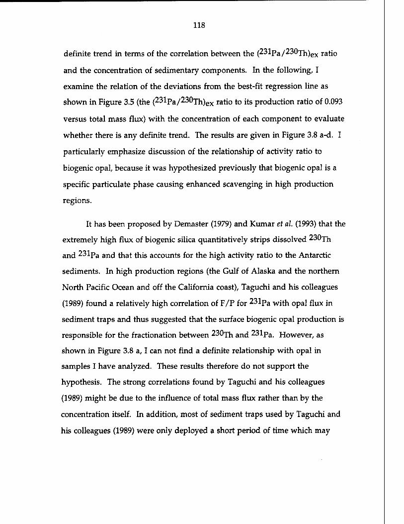
118

definite trend in terms of the correlation between the (231Pa/230Th)ex ratio

and the concentration of sedimentary components. In the following, I

examine the relation of the deviations from the best-fit regression line as

shown in Figure 3.5 (the (231Pa/230Th)ex ratio to its production ratio of 0.093

versus total mass flux) with the concentration of each component to evaluate

whether there is any definite trend. The results are given in Figure 3.8 a-d. I

particularly emphasize discussion of the relationship of activity ratio to

biogenic opal, because it was hypothesized previously that biogenic opal is a

specific particulate phase causing enhanced scavenging in high production

regions.

It has been proposed by Demaster (1979) and Kumar et al. (1993) that the

extremely high flux of biogenic silica quantitatively strips dissolved 230xh

and 231pa and that this accounts for the high activity ratio to the Antarctic

sediments. In high production regions (the Gulf of Alaska and the northern

North Pacific Ocean and off the California coast), Taguchi and his colleagues

(1989) found a relatively high correlation of F/P for 231pa with opal flux in

sediment traps and thus suggested that the surface biogenic opal production is

responsible for the fractionation between 230xh and 231pa. However, as

shown in Figure 3.8 a, I can not find a definite relationship with opal in

samples I have analyzed. These results therefore do not support the

hypothesis. The strong correlations found by Taguchi and his colleagues

(1989) might be due to the influence of total mass flux rather than by the

concentration itself. In addition, most of sediment traps used by Taguchi and

his colleagues (1989) were only deployed a short period of time which may

119

in

'S

s

t o u

in ©

01 a 2 H

(Hloa/^xcz) <HW*«W

C co bo

u

0) In

3 O m o £> «H e l-i

01 « 60 u

'S 01

/-^ e +* "0 .—«*

rH oi CO OH

01 o

o X 3 I

u ai <H

o u >■> u C

(0 ts. CO

a 3 60 E

□ %

1 i I i i i i I i i i

o m o -P-

in

Q I « ' ' i I ' o in TH O d d

«s

in S ri "Jo

s •a a o

E o

I in c

01

« hi H

o o d

rs

s u

s

01 u ES o y c oi

OI

a 2 H

«WB*xa> OU^ej^)

OH TO

to

QJ >

> X! u

CO

t—' tß O 3 CO o <N g

«J bO

co S

co '-

bO f8 E 6

120

.

D -

□ •

Q

•

D •

•o 00 n ■

s 60

D ■

1 i i i D | i i 1 '

in

es

«

«3 s o c 01 60

tr>

o o o in

o m o o

£60-0/(HJLoa/Bdl£Z) V £6<rO/OLW*«WV

□ - □

.

□ ■

□ □

•

□ . D .

TO 00

□ Q _ rt ■

D -

in es

o es

_ in

■a a O

o S5

m

. D

-j

□ -

□

□ -_

G

%

□ -

u 00

E

%

, , , . , T-r-i-i-T-T-T-T-

© o o m o © 6

o in

o o © o o in

o m

e«ro/<»iwB«Wv eeo-oAm^/ea^v

IM

O

tu «s C o

•e ns u

>p

O

tß

> ro ON o

in o o

TS O «3 >* «H

^ in > m

4-> u fÖ

© £ o

m es

CO CM —

P « o U es vo co

^ «5 in

o of th

e ge

nou

rH

O cj '■0 ^ in ra S5

> r^r- 0J "o

o o^ oo C ro *

QJ !rt & 0J S tJ b0 «ö e e

121

cause a largely seasonal bias to the records; also there were no estimations or

corrections of their traps for the trapping efficiency. On the other hand, there

only a subset of the sediment trap samples used in Figure 3.5 have biogenic

opal data; thus the data may not be completely representive. In addition,

since the materials of sediment traps were composited for all annual

collections, I perhaps average in actually observing relationships that exist.

However, these results seem to agree with an direct measurement of

the adsorption of 230jh and 231pa Qn the silica phase which was performed

recently in a laboratory experiment by Anderson et al. (1992). In their

laboratory study, batch experiments were conducted by adding spikes of 234jh

and 233pa radiotracers to suspensions (~0.5 mg/1) of various particle types in

synthetic seawater and in 0.2-p.m-filtered coastal seawater at constant

temperature, salinity and pH. Solid phases in the experiments were hematite

(oc-Fe203), MnC>2-coated XRD resin, Y-AI2O3, silica gel and interfacial

sediments from Buzzards Bay, MA. At predetermined times, aliquots of the

suspensions were flitered (0.2-jxm Nucleopore), and 234rn1 ancj 233pa

activities were measured in the filter-retained particles and in the filtrate.

Their experiment results showed that the measured Kd values for Th and Pa

on different particle types ranged from 10^ to 10^, indicating that different

solid phases have different affinities for the two elements. Of particular

importance, the ratio of the Kd values for Th and Pa, defined as the

fractionation factor f =Kd^1/KdPa, also varied significantly for the different

phases. Fractionation factors of f for hematite (2.1), silica (1.1), and Mn02 (0.8)

indicate these phases do not fractionate substantially for Th and Pa. By

comparison, large fractionation factors were observed for AI2O3 (12.5) and

natural sediments (8.9), indicating that these phases preferentially adsorb Th

122

over Pa (Anderson et al, 1992). Of particular interest, the relation between

the deviations of activity ratio over 0.093 versus the percentage of terrigenous

materials for my samples (Figure 3.8 b) do show some degree of correlation

between the two parameters, indicating that the terrigenous materials might

cause some degree of the fractionation between 230jh and 231pa/ in

agreement with the results shown by Anderson et al (1992), but this concept

needs to be refined.

Other particle phases were also examined. Taguchi et al, (1989) found a

weak correlation between F/P for 231pa of the settling particles and organic

carbon and clay r=0.6 for both), but no correlation with Mn02 and CaC03

phases (r<0.5). In Figure 3.8, my data also do not show any correlation of the

deviations of (231pa/230xh)ex ratio over 0.093 with CaC03 and organic carbon

phases. Any of these observations include in this study, however, may be

insufficient to discuss the fractionation factor because the interaction between

particle composition and nuclide scavenging behavior is very complicated,

and because the data set is limited. In addition to these complexities, the

effect scavenging efficiency will need to compete against the effect of

horizontal transport, and the effect of mass redistribution within an ocean

basin for both 230Th and 231Pa.

The role of the specific particulate phase Mn02 coating on particles in

preferential scavenging of 231pa over 230xh in ocean margins was strongly

suggested in previous works (Spencer et al, 1981; Anderson et al. 1983b). In

the Panama and Guatemala Basins, a value of fractionation factor of fxh/Pa ~1

was found, whereas a value of frh/Pa ~ 10 was found in the open ocean gyres

in the North Atlantic Ocean. It was concluded that particles at ocean margins

may be different from open ocean particles so that the adsorption no longer

123

favors 230xh over 231pa (Anderson et al, 1983b). Conversely, the boundary

scavenging phenomenon due to the specific particulate phase MnC»2 was not

found in the Middle-Atlantic Bight (MAB) (Anderson et al, 1992), and the

fractionation between 231pa and 230jh was not found in the laboratory studys

(Anderson et al, 1992) either.

Other particulate phases such as Ba (barite) and Al (AI2O3) were also

suggested as important carriers of 231pa and 230jh, and they may be factors

causing the fractionation between 231pa ancj 230xh (Lao ei a\ 11993). Given

the correlation between the (231pa/230xh)ex rati0 with the opal or Ba

concentration in the surface sediments or in settling particulates, some

authors have thus suggested that we can use the (231pa/230Th)ex ratio as an

index of surface production (Taguchi et al., 1989; Lao et al., 1992).

Apparently, we expect that the quality and quantity of settling particles

to be related to the fractionation between 231pa and 230^ but a\\ me fieid

and laboratory studies discussed above do not give a definite conclusion in

terms of the particle composition controlling the fractionation between 231pa

and 230xh. Caution should be extended to suggestion that the

(231pa/230xh)ex° ratio can be used as a primary production index. More data

is needed to confirm the hypothesis. To be able to examine whether the

particle composition, or which particle composition, causes the fractionation

of 231pa and 230jh, and causes the enhanced scavenging in the high

production and ocean margins, further work needs to be done to fully

understand the role of individual particulate phases. Until then, it is

impossible to predict a fundamental principle from which to derive how the

extent of scavenging of 231pa and 230xh wj]i be affected by a particular

element or composition. At least, however, we do demonstrate that the total

124

mass flux certainly affects the scavenging rates of 231pa and 230xh, but to a

much weaker extent for 230xh, and that the mass flux strongly controls the

fractionation between 231pa and 230xh.

3.6.5 Implications for the 230xh-nonnalized flux method

3.6.5-a The method and its assumptions

As mentioned previously, the production of 230jh m the water

column occurs at an exactly known rate and its residence time is very short.

This allows us to make two assumptions: negligible amounts of 230ih decay

before sedimentation, and all of the 230xh produced in a basin is sedimented

out in that basin, not advected away to be preferentially scavenged at

boundaries or ocean margins. The latter is proved in a basin wide data set in

the Atlantic Ocean sediments (Chapter 4 in this thesis). There is, moreover, a

large fraction of total 230xh that is scavenged in situ from the overlying water

column, and only contains a small fraction of detrital 230jh, which can be

corrected by simply subtracting the concentration of U. As a consequence,

excess 230jh activity in settling particulates is related inversely to total mass

flux, and excess 2307h can \,e used as a reference against which the flux of

other sedimentary components can be estimated:

230Thex°=ß.z/F. (3-9)

To be able to apply this method, the concentration of U and the

sediment chronology are required for correction of detrital 230jh and for

decay correction. In an independently dated sediment (using ^O or l^C

chronologies), decay-corrected 230jh activity profiles can be used then to

125

provide high resolution, point-by-point estimates of past rain rates (Bacon,

1984) by rearranging (3-9), i.e.,

F=ß.z/230Thex°. f3"10)

From (3-10), the 230xh-normalized flux of any sedimentary component

can be obtained after multiplying F by the weight fraction of the sediment

constituent of interest (fi), ie.,

Fi=fiß.z/230Thexo (3-11)

Fi can be interpreted as a record of the pelagic rain rate of the

sedimentary constituent i. ß is the production rate from the uranium decay

in the water column, i.e. 0.00263 dpm/cm^/ka.

3.6.5-b Advantages and problems

Since the accumulation of 230xh m the sediments is dependent only

on the depth of the overlying water column (P(230jh) =0.0026*Z), this simple

relationship enables one to evaluate the rate at which other species are

removed from the water column and to distinguish pelagic rain rates from

sediment accumulation rates. The latter is controlled by bottom current

activity as well as by the primary pelagic settling flux reaching the seafloor. In

other words, the procedure tends to correct for post-deposition sediment

redistribution and focusing. This is the major advantage of the 230xh_

normalized flux method. The redistribution of the sediments after

deposition will affect the flux of 230jh in a particular sediment core. If a

bottom current focuses sediments eroded from a large area to a single site, the

126

measured surface inventory of 230jh will be larger than the water column

source. Suman and Bacon (1989) argued that even in drift deposits, where

sediment accumulation is dominated by bottom current transport, the ^-^Th-

normalized flux still retains information on regional pelagic fluxes.

Downslope transport may, however, present a greater problem, because it

carries sediment initially deposited at significantly shallower depths. This

problem can be significant at a site under a rise. Even in the unrealistic

"worse case" in which all the material originated from the top of the rise, it

was argued that the normalized fluxes would overestimate the true pelagic

fluxes by only ~10%, and even less if more sediment came from the lower

part of the rise (Francois et al., 1990). Following the reasonably similar model

calculation as that for downslope transportation, lateral transport would bring

the material which characteristized high concentration of 230xh, then the

normalized fluxes would underestimate the true pelagic rate (Francois et al.,

1990). These two processes as discussed above would have less of an affect on

the (231Pa/230Th)ex ratio, since both 231pa anci 230xh are produced under the

same proportion of ß.z.

Sediment focusing is a common redistribution process on the seafloor.

If sediment drifts consist of redeposited material eroded from other sites, the

records would be mixtures of materials of all ages; therefore, sediment

focusing could lead to misinterpretation of the removal of the nuclides and

their adsorbers in the overlying water column. If the focusing material is

fresh, the material may have little effect on the normalized fluxes (and the

(231pa/230xh)ex ratio) if the foreign material has a similar constitution as the

sediment in the host site. Another type of sediment redistribution process is

the result of transport of aged, eroded sediment to a site. On one hand, this

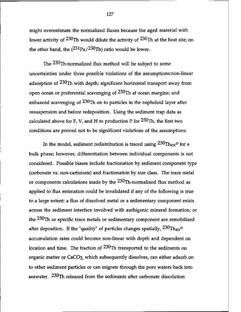
127

might overestimate the normalized fluxes because the aged material with

lower activity of 230xh WOuld dilute the activity of 230-]^ at the host site; on

the other hand, the (231pa/230jh) ratio would be lower.

The 230Th-normalized flux method will be subject to some

uncertainties under three possible violations of the assumptions:non-linear

adsorption of 2307h with depth; significant horizontal transport away from

open ocean or preferential scavenging of 230xh at ocean margins; and

enhanced scavenging of 230xh on to particles in the nepheloid layer after

resuspension and before redeposition. Using the sediment trap data as

calculated above for F, V, and H to production P for 230xh, the first two

conditions are proved not to be significant violations of the assumptions.

In the model, sediment redistribution is traced using 230Thex° for a

bulk phase; however, differentiation between individual components is not

considered. Possible biases include fractionation by sediment component type

(carbonate vs. non-carbonate) and fractionation by size class. The trace metal

or components calculations made by the 230Th_normaiizec| flux method as

applied to flux estimation could be invalidated if any of the following is true

to a large extent: a flux of dissolved metal or a sedimentary component exists

across the sediment interface involved with authigenic mineral formation; or

the 230jh or specific trace metals or sedimentary component are remobilized

after deposition. If the "quality" of particles changes spatially, 230Thex°

accumulation rates could become non-linear with depth and dependent on

location and time. The fraction of 230xh transported to the sediments on

organic matter or CaC03r which subsequently dissolves, can either adsorb on

to other sediment particles or can migrate through the pore waters back into

seawater. 230xh released from the sediments after carbonate dissolution

128

causes the model to overestimate the non-carbonate flux while redeposition

of 230jh results in the model underestimating the absolute carbonate flux.

The 230xh-normalized flux method will only provide information of a net

rain rate after dissolution; thus, for sediments that contain variable carbonate

concentrations, or sediment cores below lysocline, the records of the

normalized flux of carbonate can not be interpreted simply in terms of

production. A higher 231paex/230Thex ratio may add confirmation of higher

rain rates (and thus higher efficiency for the scavenging of particle-reactive

metals) from the overlying water column even though the biogenic adsorbers

are subject to dissolution.

The second possibility is that 230xh should be preferentially adsorbed

to smaller particles because of their larger surface to volume ratio. In such

case, winnowing of fine particles would change 230xh activity of the site for

resuspension and deposition independent of the rain rate of particles at these

sites. Does winnowing create district redeposition regions, those with more

large particles depleted in 230xh and those with predominately smaller

particles enriched in 230jh? Recently, Thomson et al., (1993), compared the

activities of 230xhex and the weight percentages of different size classes in the

surface mixed layers of core tops. Size fractions (four size classes: >400,400-20,

20-5, and <5 urn) of the surface mixed layer material showed that the two

cores experienced similar fluxes of the material in the 400- to 20-p.m size

range, but the more rapidly accumulated core had a much larger fine (<5 |im)

component. The specific activities of the four different size fractions of the

two cores are identical, so that the greater mass and 230xh fluxes to the more

rapidly accumulating core are predominately due to its greater <5 |xm flux.

129

Size fraction might fractionate the 231p3/ ancj it might fractionate differently

for 231pa than for 230jh Further work need to be done.

3.7 CONCLUSIONS AND FUTURE STUDIES

The investigations of sediment traps, including 26 traps which had

been deployed for approximately one year or longer and providing diverse

geographic coverage, provided information about the variations of

radionuclides 230xh and 231pa m the particulate materials, and the

fractionation between 230xh and 231 pa.

By applying the available measured data of (231pa/230jh)ex in the

water columns to all of those trap stations and using the measured data from

the collected materials from the sediment traps, I have provided quantitative

estimates of trapping efficiency for all deployed sediment traps used for this

study. The results demonstrated that all of the deeper traps are reliable for the

particle flux; while all of the shallow traps showed undertrapping. The

sediment traps used for this study showed a tendency of increasing in

trapping efficiency with water depth for almost all of stations.

The results of the investigations of the sediment trap materials shows

two major facts: 1) particle flux is the major factor influence removal of the

nuclides 230xh and 231pa from seawater; 2) the scavenging rate of 230jh

apparently fluctuate less in relation to the flux of particulate materials;

whereas 231pa js verv sensitive in relation to the flux of particulate materials.

These results demonstrated two important concepts: 1) the assumption of a

constant flux of 230jh holds as a good approximation for the 230xh-

130

normalized flux methods; 2) particulate (231Pa/230Th)ex ratio is strongly

dependent on the mass flux. Thus the two concepts can be used together for

reconstruction of paleo-particle flux in the past ocean, and applied for

paleoceanographic studies.

The particle components could influence the fractionation between

230xh and 231pa; however, all field and laboratory studies do not reach a

universal conclusion. Biogenic opal was hypothesized as an important factor

causing the preferential scavenging of 231pa OVer 230lh in ocean margins

and high production regions; however, the trap results in this study do not

support the scenario. Further studies either through field data or laboratory

experiments in determinations of the fractionation factor are needed to

confirm. Different fractionation between 23lPa an(j 230xh results from

different size fraction should also be examined in future study.

131

CHAPTER 4

BASIN-WIDE VARIATIONS IN CHEMICAL SCAVENGING OF 23!pA AND

230XH WITHIN THE ATLANTIC OCEAN SINCE THE LAST GLACIAL

MAXIMUM

4.1 INTRODUCTION

Yang et al. (1986) published a map of the Pacific Ocean in which contours

of the unsupported 230xh/231pa ratios of surface sediment suggested that all

margins are important boundary sinks for 231pa. However, many of the 231pa

values used to construct their map were assumed or inferred, from 231pa

contents of sediments in other regions. Additional information about which

margins actually act as important boundary sinks was provided by Anderson et

al. (1991) and Lao (1991) who recently published their 231Pa/230Th data from

ocean margin sediments collected off North and South America, from the Bering

Sea, and from the northwest Pacific. Their data eliminates some of the

uncertainty in the Pacific map by Yang et al. (1986). The combined data sets

illustrate which margins are important boundary sinks for 231pa and 230Th ^

the Pacific Ocean.

A similar map has not been constructed for the Atlantic Ocean. For this

chapter, I measured 231pa an£j 230xh m a number of well-dated deep-sea

sediment cores collected from the Atlantic Ocean. I also compiled all available

data in the literature from Atlantic cores with reasonably well-defined

132

stratigraphy and combined it with my data to construct a map similar to the one

available for the Pacific. The purpose, first of all, is to examine questions for the

Holocene Atlantic Ocean similar to those asked about the Pacific Ocean data

(Anderson et al., 1983a and b, 1990,1991; Yang et ah, 1986; Shimmield and Price,

1988,1989; Lao, 1991): Where does the boundary scavenging of 231Pa or 230Th

occur in the Atlantic Ocean? What factors control the distribution patterns of

chemical fractionation between 230Th ancj 231pa ^ the Atlantic Ocean? From

the distribution of boundary scavenging of Pa and Th, we may gain insights on

the distribution or flux of other reactive elements or trace metals .

The second purpose is to compare the distribution patterns of

(231pa/230xh)ex° ratio between the Atlantic and Pacific. It is interesting to make

such a comparison, because the ocean processes are considered to be dynamically

different between the two oceans. As I will show later by a simple mass balance

model, the advection by ocean circulation, which in previous studies is usually

assumed to have a negligible effect, is an important factor to cause the

fractionation between 231pa and 230fh in the Atlantic Ocean. I also quantify the

influence by advection resulting from the thermohaline circulation on the

fractionation of the two nuclides. Furthermore, I provide a simple box model to

demonstrate that export flux from the Atlantic by ocean advection is an

important role to account for the budget of 231pa in deep sea sediments located

beneath the Southern Ocean.

I have also constructed a 231pa /2307h map for the Last Glacial Maximum

(LGM) in the Atlantic Ocean to examine the differences between the LGM and

the Holocene. By comparing these two maps, I hope to answer the following

questions: Has the intensity of scavenging changed significantly with time,

particularly between extreme conditions represented by the LGM and the

133

Holocene? What changes in ocean conditions and processes can respond to

changes in the redistribution patterns of 231Pa/23°Th between these extremes?

What is the effect of the climatically controlled variations in the sedimentation?

Furthermore, variations in sedimentation rate have been known for a long

time to be related to climate changes. For instance, the biogenic components of

deep-sea sediments can record changes in production and oceanic circulation

related to climate changes; the terrigenous input might record changes in sea-

level, humidity and aridity, and intensity and direction of winds. These are two

major components in the Atlantic pelagic sediments; thus, we need to examine

what the distribution patterns of the sedimentary components in the Atlantic

Ocean are, and how their changes in flux relate to variations in climate.

4.2 METHODS

All sorts of lateral transport processes may influence the removal of 231pa

and cause the fractionation between it and 2307h within an ocean basin;

therefore, a large number of cores would be required to obtain complete

representation of different scavenging conditions in the whole Atlantic Ocean.

Given the limitations of stratigraphic databases, time and funding, however, a

modest number of cores were selected and previously reported data with good

quality of their stratigraphic data were compiled together for Holocene and LGM

distribution maps of unsupported 231pa/230Th activity ratio in the Atlantic

Ocean. The data discussed in this chapter should be considered to serve for an

initial investigation into the scavenging characteristics of 230jh and 231pa in the

Atlantic Ocean. These cores were selected because of their quality and available

data on stratigraphy.

134

For my experiments, I selected twenty-eight deep sea cores from the

Atlantic Ocean for analysis of uranium-series nuclides in order to accomplish the

goals as proposed above. The core locations are given in Figure 4.1 and listed in

Table 4.1. The cores that I selected are a subset of those used for mapping Cd/Ca

and isotope b^C by Boyle (1992), who lists the original sources of the

stratigraphic information. Since the differences between LGM and the Holocene

are specifically my interests in this study, I sampled only the two sections of the

sediments corresponding to these two time intervals for the uranium-series

radionuclide analyses. I also determined carbonate content in these two sections.

4.3 RESULTS

In order to examine the chemical scavenging of 231pa and 230xh, which is

a reflection of the flux of particulate materials in the ocean, I used many well-

dated deep-sea cores distributed over the Atlantic Ocean basin. The analytical

results of 23lPa, Th and U isotopes for the Holocene and LGM sections are

shown in Tables 4.2 and 4.3. The unsupported initial (decay-corrected)

concentrations of 23*Pa and 230Th (Table 4.4) were calculated as follows.

230xhexo ={230xhm -1.14* (0.810.2) 232Thm - [1.14* (238Um-

(0.8±0.2)232Thm (1- e" ^230*)]} * e X230* (4-1)

231paexo = {231pam -0.046* (0.8±0.2) 232Thm - 0.046* [(238Um -

(0.8±0.2)232Thm (1- e" ^M)]} e ^3lt (4.2)

The equations above, which estimate the quantities of 23^Th and 23lPa

scavenged from seawater (denoted as 230Thex and 23^Paex)/ were drived by

subtracting the supported components from the decay of the detrital uranium

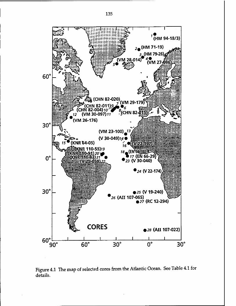
135

Figure 4.1 The map of selected cores from the Atlantic Ocean. See Table 4.1 for details.

136

Table 4.1 Locations of selected sediment cores in the Atlantic Ocean Core Latitude Longitude Water Depth of Depth of Core No.

Depth(m) LGM(cm) Holocene (cm) on Map High Latitude Northern Atlantic

HM 94-18/3 73.30N 05.41E 2469 35.5 0 1 HM 71-19 69.29N 09.31W 2210 50 0 2 HM 79-26 66.54N 05.56W 3312 70 0 3 VM 27-086 66.36N 01.07E 2900 60 9 4 VM 28-014 64.47N 29.34W 1855 190 13 5

The Northern Atlantic (20 - 60N) VM 29-179 44.00N 24.32W 3371 80 16 6 CHN 82-020 43.30N 29.52W 3070 62 ~ 69.5 4-6 7 CHN 82-015 43.22N 28.14W 2153 29-37 3-4 8 CHN 82-011 42.23N 31.48W 3209 69.5 - 71.5 3.5-5 9 CHN 82-004 41.43N 32.51W 3427 56-71 2-4 10 VM 30-097 41.00N 33.56W 3371 130-169 5-16 11 VM 26-176 36.00N 72.00W 3942 358 8-10 12 VM 23-100 22.41N 21.18W 4579 35-60 10-20 13

Equatorial Atlantic (20N - 20S) VM 30-049 18.26N 21.05W 3093 62-84 10-15 14 KNR 64-051 16.31N 74.48W 3047 38-42 6-7.5 15 VM 22-197 14.10N 18.35W 3167 133 25 16 EN 66-29 02.28'N 19.46W 5104 34-47 2-12 17 EN 66-38 04.55N 20.30W 2931 24.5 ~ 34.5 2.5 - 9.5 18 KNR110-55 04.57N 42.54W 4556 51 ~ 58.5 4-17 19 KNR110-91 04.46N 43.18W 3810 72 0 20 KNR110-82 04.20N 43.29W 2816 53-64 0-13 21 VM 25-059 01.22N 39.29W 3824 60 8 22 VM 30-040 00.12S 23.08W 3706 45 10 23 VM 22-174 10.04S 12.49W 2630 49 8 24

The Southern Atlantic (20S - 60S) VM 19-240 30.35S 13.17W 3103 80 20 25 AH 107-065 32.02S 36.11W 2795 33-45 3-4 26 RC 12-294 37.16S 10.06W 3308 45 10 27 All 107-022 54.48S 3.20W 2768 66-70 3-4 28

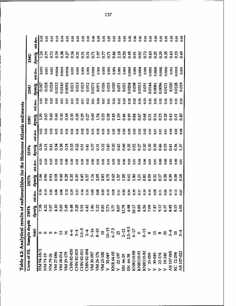
137

> « K K o o o 8 3 1-H o r— O

1-H o S 8 $ in

o in If) (M o o o 3 CO CM

o o s s 3 o 8 o o s rH CO o o

2 O © O d d d d d d d d d odd d d d d d d d d d d d d d

1 t N N N K N

ON 00 tv S rH rH rH rH IN N H * K N «i

00 © in rH CM CM co in ON in CO CO ON

D in co CM co co co tv ON rH in rf ON 00 tN ■<* CM CM co «* CO <tf

HOO d d d d d d d d rH odd CM © © d d d d © © © © d © a *0

CM 1-1 rH 3! S3 8 S 3

g rH 1-H 1-H 1-H CO rH m rH rH rH 1-H PI rH ^ 1-H 1-H CO CM CM T^ CO rH > o o o o o o O O

o o o o g o O

o o o o o 5 g 8 § g g g g o g g g g

•o odd o o d d d d p d odd d d P d P d O p P d P d 2 d d d o o o O O o d o

f N 00 00 CM co CM rH co co CM CM rH NO in © IH rH «*

CM O 00 co rH 5 1-H NO rH © 00 ON

D in CO

s ©s r-i -* ON rH rH rH ^-i tN IN CM CM CM t>. co rH CO 00 CM CM CM rH CM rH o O o O © CM o o o © O © CM © co © rH g o T-i o rH ©

ö d ö o o © d d d d o d odd d d P d o d O © O © P. © (M d d o d © © © © © © o

« N N r« I-* 1-H y^i co 1-H CM t-H 3 rn rH CS CN 8 S CM m 8 rH 1-H rH 1-H CM rH CM > O O O o o o O o o o o o o o O O d O o O o O o o « T3

d Ö Ö d d d d d d d d d odd d d d d d d d d d d d d d G 2 0) s «

f OMfl O

^ CO oo o 00 °) tv o 3 co oo in ON NO ON 3 ts 00 1-H NO co oo co rH O "3

oo O NO NO rH CO CM CM CM VO in in t in ■* ■<* NO NO CO rH CM CM ■* CO ^

V i-5 ö ö d d d d d d d d r-5 do© rH d d © © © © © d © © d d en co a u CM TJ •** C CM CM CM CJ 1- 1-H 1-H 1-H S co ^ CN| 1-H 1-H 1-H CM 8 S to s CM 1-H rH rH 1-H 8 CM 00 > o o o o o O O o o o o o o o O O o o o O O o o CS

*4 odd d d d d d d d d d odd d d d d d d d d d d d d d

< 2 a

e f vO rH rH

co co •«* co CM rH 1-H tN rH CM in © CM © in CM N. © © o NO in rH NO tN IB co to "* CM CO CM CO "* CO CO CO Tt< CM ^ NO CO m CM CO CO co "* CM -* co co

w d ö ö d d d d d d d d d ©do d © © © © d © d © © d © r-i ^ co a. "o CM •a X >' ffi 23 23 o o o o o g s 1-H o

rH o s CM

o rH o

rH rH CO o o o S S 8 1-*

o 3 s rH O

rH O 8 8 CM

O 8 S 9i 4) odd d d d d d d d d d odd d d d d d d d d d d d d d

2 00

60 1

»DO n oo o oo m in in tN NO m co in o IN m CM © rH 7-f ON rH ts 00 ON oo oo tn

co

vo o\ o> m ** CM co co ■* in rH © 00 ts NO in © NO oq CM oo m co rH co CO CO rH 01 r-i © O d d d d d d d rH CM ©do rH r-i O rH CO © d d © © d © © •o a

•*4 CM •o s . co in in S § CM ON 3 ^i o in 00 CT. CT) 00

(S rn O r-i O vc ON tN ON ON 00 t-i s CO CM Cv

o •IN

> CM i-" o 1-H CM I-H r— o o 1-H CO CM CO T^t i—i 1-H o 1-H 1-H 1-H O

•q odd d d d d d d d d d odd d d d d d d d d d d d d d H3

S fa

f »MS O ON ON 00 00 CM CM NO

c^ 8 R f^ t>. ON 00 tN ON NO £ tN CM tN in in © T-< © <*H X ON CO ON 1-H VO •>* ^< CM ON •* 00 © r>» ON 1-H 00 in «* rH CM ■* o

en IN rfi in <tf cö in NO cö in NO r-i in oo in co CO CM Nfi

rH © rH

00 NO IN t< ON vÖ 00 00 NO

"3 es •c en X V ** u a

u •r*

•a

'S. I

6 o o o ON 2 NO rH

NO I 1

CO

in i

in CO CM

NO TH

J m

© 1-H

1 00

in m o 1 t< ^ o I rH NO

in CM

CM "5 CM

1-H 1 ©

co rH !

O 00 in

rH 00 © CM t

co ^ co

C <

tn

NJ CD o m rH —i

MM o IB

00 ON NO rH rH CM i i i

NO Tjt 00 r-l o o rH

s 1 CM

1-H O

1 CM

1-H ©

1 CM

i CM

^ S

NO

1-H MS CO 0 NO

5 m *

ON rH

ON 00 CM CO

m in o

rH ON

1 ©

00 1

© ON

in CM

©

o co

R rH

©

CM

58 o .1 a 9

2 *# rH ON W N N

III

tN 00 CM CM

ON CM

00 00 oo 00 o co

NÖ CM Ö NO NO

NO NO

rH rH

rH rH

1-H 1-H

i CM CM

ON rH

© 1-H rH ° " rH

£ o U U U U U >

2 2 w tu > > > > NH

< U B s <

138

05

c v E •m

T3 u «3 u

•r*

e

U V

m u -o "w 3 C O

2

n C <

3

f

f >

•a

•-1 *°

>'

0)

ft ^

^1 N s CO OH es TJ

IS -f ® s CM TJ

a. 4)

ft, w

«5

O U S o

oooooooooooo

Nooif)Nin*»n OOOOtvOvpCOrHVO rHrHrHrHrHOrHOO©

O O 00 ^ ts vo m eo

cNcNrsirHrHrHCJ^'r^rH^r«

888888888888

CN ■<*< t-. K N * O O O OOOOCNOOrHO o o o o o o o Ö o o o

oooooooooooo

Ov in

CM lf>

VO K rH Ov o en

en rH s 2 o CO ON

i—i rH rH l-H O o rH o O © CO r-l

T-l o O 1-H o o o 5 o r« O o o 3

o o o o o Ö

o o o o Ö

VO rH o CN a ON

00 CM

CM S o © o O o o O o o o

mcMtNi-Htnooc-jr-i oooooooo

ÖÖOOÖÖÖÖÖOÖÖ

voin^oq^^eNrHcoeorHoq NNNNrirlNHHrirtN

O O O O O O O O O O O

smNNNO<*Non»» ^eö^cNeNrveNrH<a<co'vc'eN

"5 o iß ft

p o rv vo

Ov -.• i—' » s « in

! 1 ov m

Ov CM in

oo . in CO CO CO

00 Ov VO rH CN

522 XXX

vO Tf 00 rH o o

o s I

CM 00

in

OOOOOOOOOOOOOOOO

nNO^HNflOBNHÄIHHNMts oo^tNrHrHOvcoincooqincopvocoin Öi-HÖvOrHÖrHrHrHÖÖCSrHÖÖÖ

tN.CNlrH\Cr-ir-<CNr"ir-i

888888888 i-H *-( en i-H

8 8 8 8

Ov OV rH

838 vO Ov

8 S © © © d d d

NNNONJvONin COinOOrHOOCOCNCOCN OOCNCM©OOrHO o o o o

ddo o o

OOOOOOOOOOOOOO bdo'dödö ööo'öSo©

o

s in oo O VO 5 CV rH K p CN CN tx

o ov TT tv in vo ^ VO tv tv in

CO t-s CM in

-i co OrHOTtir-HOrHOrHOO^iOO

OOOOOOOOOOOOOOOO

q «* CN CM d

s COrH^inOvrHVOCNrvCNCNrHCN TjirvvOOCNeOeOCOCNCNeNeNOO

©r-idddddodooodod

tM(Nie^00Ovr-|tv^CMr;Mr;rHr«OD oooooopppppopr-pp r-^i-sr-ii-^r^(Sr^<H<-i<fioOeiOese>

OCOtNrHOVrHinvOVOVOOOC^VOCNCOin OvrH00CNrHvOOvCMC0COO\pin«*vop dr-idcMCNr-JcNCNCNr-id CO O rH O rH

CM>«Ot>.0>Or>.fMt-»iHTt't.Or-;tNCM r-r-1-HOtxCMCMNcMr«iHpr-<»!l;r-.m ÖÖbbÖÖÖÖbdobdÖb©

N»NooHp\(viHinnffiOririBe <JiKinHHK\6BNNtsiClft»0vN vd^riirirsifiNve^ininoöifiKinod

o m

in O Ov 00 CO CO

1 1 CO in

CO

PS in

2 |5 ^ S ^ rH cN m

I t Ov CO >* m

O O Ov vo m ■>*

m IN CO

t in in CO

g g CV VO rH © ov CN CM S rH © rH 2J K K - vi 4 -1 '

8 S

Ov 00 CN CO

in rH CN _ m ov oo ov o o o

^ OH OH «

s in _ CM CO

O rf rH

6 ' CN Ov O CN rH rH

o (i o

> > > > < g

139

T3 V (A

QJ C V u

"3 S JS IN

01

> u n v

S 6 O

■ M 'V S

0) "B o a. u, s 05 e D

3

CM co

o «I

CM CO IN

D CO co N

9 00 co

D tr> CM

ee

e 60

s

CM

If u

•a

to

a

I 60

•a

t-t r-H t-H i-H i-HrH iH N Ifl rH N IN n

ÖÖÖÖÖÖÖÖÖÖÖÖÖÖÖi-iÖÖÖÖÖÖÖT^Oi^Öfsi

HrHNrtNK)HHOHrtN*NOnoaONO«lflNNOON

-tf tv Tfi CM CM CM O i-H O O O © © © Q

o o o o © © © © ©

no*Nfnooooo«ie»ONNp* COI-HI-HO©COCO©VOCJ\OI-I©I-IO'-I©CM cf^oocpocjidcfriddtfr^""^ o o o

R R 3* \o CM CM CO CM

00 CO * * n t CO ** o\ v£> \0 o on vO r% "tfl CM CM VO VD ■* CM

H O o o o o o o O O O i-H o O o 1-1

So in 3 tx ■* LT) s

© O i-t CM

tN ID Tf O 1-H 1-H m "tf CM i-H CO CO CO i-t

ÖÖÖÖÖÖÖÖ

inc^i-irNCO^tcMONComcMvomcMTtii-ir^i-icMff\»ccMOOOcoini-H ©OOI-HOOÖOOCMÖOOOOOOOOOOOOOOOCM

ÖÖÖÖÖÖÖÖÖÖÖÖÖÖÖÖÖÖÖÖÖÖÖCJÖÖÖÖ

C0CMC0C0C0CMC0CMC0^COCMCM'*i-iCOincOTj<CMCMCMC0^CMC0COC0 ÖÖÖÖÖÖÖÖÖÖÖÖÖÖC3ÖÖ'^'-:'-;'-;'^^;'-;~^;~-: oooooooo

vocöiricöcöin'vdcöuSvdi^cöo6iricövdcMvdcy\cdirivot>ic©iricdrNiri

c?!rN©3'pcyvCTvcolVH OI-II-IO4,T-<CMC0OC

$ £ § a ^ 9 9 JH

ass U U

140

and from the ingrowth of the authigenic uranium. The activities of the

scavenged 230xh and 231pa components then were corrected for their decay loss.

The constant 0.8± 0.2 is the value of the 238u/232jh ratio of the average crust

(Anderson, 1982; Anderson et ah, 1990), i.e., the 238jj/232xh ratio of the sediment

detrital phase. The constant 1.14 is the seawater isotopic composition of

234u/238u, and 0.046 is the natural abundance of 235u/238u in activity units.

The decay constants of 230xh and 23lpa are Ä.230 and Ä.231- The ages (t) of the

sediment samples used for decay-correction of 230xh and 231pa were based on

the chronologies of the cores given in Table 4.1 for the transect samples. The ages

of the core-top sediments were assumed zero age, and the LGM samples were

assigned an age of 18 ka.

Since the variations in Pa/Th ratio between the Holocene and the LGM are

specific interests for this study, one section within each of these two time

intervals of the cores was carefully sampled for analyses of radioisotopes and

sediment components. The stratigraphic framework is essential to this work, and

has been on careful handling in the samples' selections. As mentioned, the

stratigraphic data were provided in Boyle (1992). However, as Boyle (1992)

pointed out "because many cores have been heavily sampled, it is not always

possible to make paleochemical analyses at the glacial maximum because of the

lack of core sample. For this reason, one should not over-interpret fine points of

this data set; only large-scale signals confirmed by nearby samples and sites

should be considered seriously." To resolve this complication for fine scale

discussion, a subcore within each core should be drilled (Broecker, personal

communication); however, this is not plactically possible to request sample

materials.

141

For convenience, hereafter, "Pa/Th" will be used throughout the text to

designate the ratio (231pa/230lh)ex° except when further differentiation is

necessary. This decay-corrected ratio is truly representative of the scavenging

fractionation between 230jh and 231pa at the time they deposit onto the seafloor.

The Holocene Pa/Th ratios of the cores from the whole Atlantic Ocean are

shown in a map (Figure 4.2). The data includes measurements from this thesis

work (Table 4.4) and those available in the literature (Table 4.5). The cores cover

geographic regions from the open ocean abyssal sediments to the Mid-Atlantic

Ridge (MAR) sediments, to the flanks of the MAR sediments, to the high

latitudes in both the northern and southern Atlantic oceans, and to ocean

margins with different characteristics (strictly speaking, the margins referred to

here and previously in the literature mean the areas of the edges of the ocean

basins). The data from 63 cores are included in the Holocene Atlantic map.

4.4 DISCUSSION

4.4.1. Chemical fractionation between 231.Pa and 230xh in the Holocene

Atlantic sediments

In this section, first, I show the distribution patterns of 231pa relative to

230jh (presented by the Pa/Th ratio) for the Holocene Atlantic sediments;

second, I discuss the "boundary scavenging" within the Atlantic basin; then, I

discuss those anomalous features in terms of deposition conditions. This study

emphasizes the process of locating the regions of enrichment or depletion of

231pa relative to the uniform scavenging efficiency of 230*jh on a basin-wide

scale. The geographic distribution of this enrichment or depletion reflects the

142

60c

30e

Oe

30°

60c

i^ _,_.. (0.052)7 <^> S^LJ0$5G)5K *«»> *>lß* ,(0.053)9 (£O51)%9(0.071)\o.O6i7O^ »9^1^n ,n «^(0.272)77 I»l4f^(0.063)(0.272) (0^071H^ . (0.047

38 (0.054) «t/fett,, 4 (0.047)45149(0.055) (0.066)72 ,0*,nncM 4S (0.057)

♦_... J°;03%#4 (0.102) ^.(0.039)55^ ^(0023)

L ^^60(0.077)4 , (0.082)74« Im 75 #^ü . f T59 (0.053) ;' W54)^i-P^)67T \ ' 16

|ö;ö46)2T% ♦ Ä*7,7(° , (0.042)22 \ 923 (0.040) '™™~— 57(0.084)

<0.051)

>24 (0.050)

26 (0.048)

30 (0.094) f ♦ < Pa/Thex°HL

>25 (0.040)

#27 (0.045) (0.048)29^

(0.090) 31 A

(0.143)35^44 (0.21-0.29)

25 (0.231) (0.193)

90° 60c 30c 0< 30'

Figure 4.2 The map of decay-corrected unsupported 231Pa/230Th ratio

(Pa/Thex°) of the Holocene Atlantic Ocean.

143

Table 4.5 Compiled data of 231Pa/230Th ratios of Holocene Atlantic sediments

Core Latitude Longitude Pa/Th Pa/Th # on the data sources Notes Holocene LGM map HL sample

AH 76-3 41o33'S 20ol2'E 0.048 #29 DeMaster, 1979 0-1 cm

RC15-101 42o59'S 41o34W 0.094 #30 DeMaster, 1979 4-7 cm

VM 29-105 48o05'S 18o41'E 0.090 0.084 #31 DeMaster, 1979 3-6 cm

AH 76-16 53o00'S 35o38E 0.123 #32 DeMaster, 1979 0-1 cm

RC 17-58 53o31'S 36o38'E 0.111 #33 DeMaster, 1979 7-9 cm

RC 13-259 53o33'S 04o56'E 0.294 #34 DeMaster, 1979 5-8 cm

RC 11-76 54o23'S 22o08"W 0.193 0.169 #35 DeMaster, 1979 10-13 cm

RC 13-255 54o35'S 02o54*E 0.143 0.294 #36 DeMaster, 1979 4-7 cm

RC 13-271 59o39'S 04o31'E 0.127 0.127 #37 DeMaster, 1979 14-16 cm

GPC5 33o41'N 57o37'W 0.054 0.049 #38 Bacon&Rosholt, 1982 32 cm

OCE152-BC8 39o46.5'N 70o58W 0.071 #39 Anderson et al, 1991 0-0.5 cm

OCE152-BC5 39o08'N 70O56W 0.063 #40 Anderson et al, 1991 0-0.5 cm

EN 179-BC7 37o25'N 73o49.4'W 0.051 #41 Anderson et al, 1991 0-1 cm

EN 179-BC4 37o32'N 74o02W 0.071 #42 Anderson et al, 1991 1-2 cm

EN 187-BC6 37o24'N 73o50W 0.055 #43 Anderson et al, 1991 0-1 cm

RC 13-259 53o33'S 04o56'E 0.21-0.29 0.12-0.13 #44 Kumar et al, 1993

CHN 82-23 41o38*N 27o20*W 0.057 #45 Kuetal.,1972 0-5 cm

CHN 82-24 41o43'N 320511^ 0.047 #46 Kuetal.,1972 0-5 cm

CHN 82-25 42ol9'N 28o35"W 0.041 #47 Kuetal.,1972 0-6 cm

CHN 82-26 42olO'N 31038W 0.057 #48 Kuetal.,1972 0-10 cm

CHN 82-28 42o00'N 29o54"W 0.055 #49 Kuetal.,1972 0-10 cm

CHN 82-30 41o51'N 26o28"W 0.065 #50 Kuetal.,1972 0-10 cm

CHN 82-31 42o23*N 31048W 0.050 #51 Kuetal.,1972 0-10 cm

CHN 82-32 43o45'N 27o47"W 0.058 #52 Kuetal.,1972 0-10 cm

CHN 82-33 42o29'N 28o40"W 0.070 #53 Kuetal.,1972 0-10 cm

CHN 82-41 43o22'N 28014W 0.093 #54 Kuetal.,1972 0-10 cm

CHN82-42 43o20'N 28o05*W 0.061 #55 Kuetal.,1972 0-10 cm

AH 42-41 22ol4'N 56o39W 0.039 #56 Kuetal.,1972 0-5 cm

V9-97 00o23'N 29o52W 0.084 #57 Ku 1966 5-8 cm

V10-95 26o31'N 51o47*W 0.023 #58 Ku 1966 0-6 cm

V16-21 17ol7N 48o28W 0.053 #59 Ku 1966 2-10 cm

V12-122 17o00'N 74o24W 0.077 #60 Kul966 10-15 cm

CH 75-2-8 14ol'N 54ol'W 0.031 #61 Anderson et al.,1983 2-4 cm

Core 12310 23o30'N 18o43'w 0.102 #62 Mangini & Diester-H

144

combined effects of the geographic variations in the extent of particle flux (i.e.,

scavenging intensity) and the extent of horizontal transport of 231pa in the

Atlantic Ocean during the Holocene.

The Pa/Th activity ratio of production from uranium in the water column

is at a fixed value of 0.093 because of the fixed abundance of 235TJ/238U (the

progenitors of 231pa and 230xhr respectively) in the ocean. Sediment values

deviating from this value imply differential deposition of the two nuclides from

the water column to the seafloor. Since the deposition rate of 230jh in most of

the ocean is balanced by its production from the overlying water column, the

Pa/Th ratio is used to evaluate the extent of the fractionation between these two

elements, thus revealing the regions of the enrichment or depletion of 231pa

relative to 230xh. In sediments, if a Pa/Th ratio is greater than the production

rate ratio of 0.093, this implies the site is a "enriched" 231pa relative to 230xh, i.e.,

the site receives an extra amount of 231pa in addition to production from the

overlying water column. Conversely, if the ratio is less than 0.093, the site is

"depleted", i.e., a certain fraction of 231pa produced in the overlying water

column is laterally transported to other areas in the ocean.

Boundary scavenging is the phenomenon influencing the distribution and

flux of chemically reactive substances in the oceanic water column (Anderson et

al, 1983,1990; Nozaki and Nakanishi, 1985; Yang et al, 1986; Lao, 1991). Within

an ocean basin, boundary scavenging occurs due to regional differences in

scavenging intensity, particle composition, the residence time of the element, and

the rate of lateral mixing in the deep sea (Bacon, 1988). Since 231pa ^ a

"boundary scavenging"- sensitive element, the distribution pattern of the Pa/Th

ratio should reflect the regional extent of "boundary scavenging". In the

following, the statistics of the compiled Atlantic core top data are calculated and

145

shown in Table 4.6. For discussion in the following, "enriched", "depleted", and

"boundary scavenging" will represent a region of Pa/Th ratio greater than

production rate ratio of 0.093, less than 0.093, and a Pa/Th ratio above the mean

value of the grouped region.

First of all, the map presented in Figure 4.2 clearly indicates that

fractionation of 230rh and 231pa occurs within the whole Atlantic Ocean. The

real variability is seen as "scatter" within the basin-wide distributions (Figure

4.2), so I could not contour the Pa/Th ratio for the Atlantic map as was done for

the Pacific map by Yang et al. (1986). In general, the Atlantic map of Pa/Th ratio

is featureless in the distribution patterns. The one striking fact is that most of the

Pa/Th ratios in the Holocene Atlantic Ocean are lower than the production rate

ratio of 0.093, implying that most of the ocean floor in the Atlantic is Pa depleted.

The Southern Ocean (Atlantic sector) is the only region that displays higher

values of Pa/Th ratio than the production rate ratio. The extensive areas of

Pa/Th ratios that exceed the production rate ratio seen in ocean margins on the

Pacific map (Yang et al, 1986; Anderson et al, 1990; Lao, 1991) are not observed in

the Atlantic.

Within different geographic divisions, the nature of boundary scavenging

of 231pa can be revealed by comparing the Pa/Th ratio at each single site to the

arithmetic mean (m) of the division as shown in Table 4.6. In Table 4.6, the

Atlantic Ocean is divided into several geographic divisions by latitude: the North

Atlantic (north of 20°N), the Tropical Atlantic (20°N to 20°S), the South Atlantic

(20°S to 45°S), and the Antarctic Atlantic sector (south of 45°S). The compiled

data is plotted as a histogram graph and shown in Figure 4.3. The figure

illustrates the large-scale mass imbalance between 231pa and 230 jh in sediments

north of 45°S.

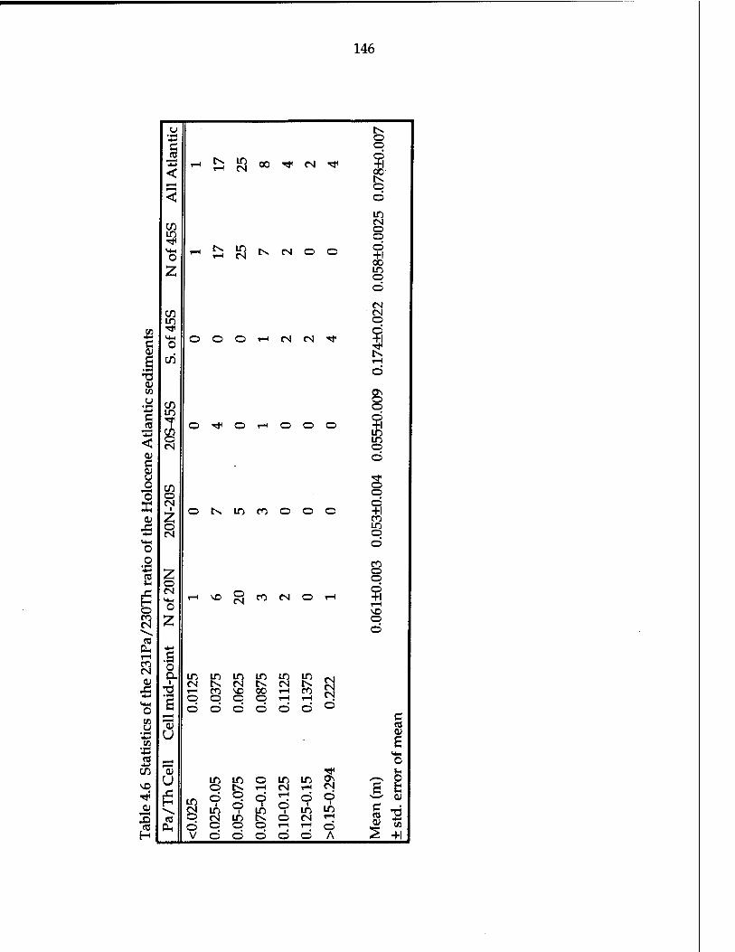
146

u K ©

s <

rH T—1 JQ oo ■<* CM >*

©

?! ;—< ©

< Ö

in 03 CM o ID o

o i—1 rH ^j N N O O I 2 in

© ©

CM 03 CM m ©

(A

c V4H o o O rH CM CM «*< ?l 0 ■^

Ü , K 6 03 r-t

• »*4 ©

0) «3 Ov

C 4->

03 in

o "<* © rH O © ©

O o ?l in

< o in ©

0) © C a> u **

03 O

© o ffi o tx in co © © © ?! cu CO X © in 53 CN o V4H o d O

•X3 ffl 2

CO © o

»H o

£ CM "4-1 O

rH NO °, CO CM © rH ?! O NO CO CM Z o

© as

PH 4->

i—i •S o a.

CO CM m in in in in in -^

N N (N N Ö SO 00 rH CO Ej O O rH rH ^

o CM tv •B T3 rH CO • I'M o o o Ö Ö O © © © °

g "33 U £

X3 <4-C « f-H o +J 03 oj "tf u

(j in in © in in 2^ -p S NO o tN rH CM rH CM & e Tj5 in d 9 o £ © o

Ä Ö 1

in 9 in 9 in in

S +1 3 CO o CM If) N O N >1

Co CH ö © © © rH rH o H V © © © Ö © A

147

o u

1

231pa/230Th activity ratio

231 230 Figure 4.3 Summary of unsupported Pa/ Th ratios measured in the Holocene Atlantic sediments

148

The arithmetic mean Pa/Th ratio from cores north of 45°S in the Atlantic

was calculated to identify regions of boundary scavenging of 231pa in the

Atlantic Ocean. The mean value is 0.058 ± 0.005 (2 sigma of the standard error of

the mean); it is close to each mean value (m) of the three divisions (the North, the

Tropical, and the South Atlantic). By taking two sigma, the "normal" range of the

Pa/Th ratio can be defined as 0.053 to 0.063. Values north of 45°S that are higher

than this range may indicate regions of the boundary scavenging of Pa, and such

areas are discussed below.

Significant boundary scavenging of 231pa is found in the polar region.

Four cores (numbers 2-5 on the map) between 64°N and 70°N show Pa/Th ratios

ranging from ~0.07 to ~0.11, significantly higher than the mean. The excess

230xh activities range from 3.39 to 5.37 dpm/g (Table 4.4) in the Holocene

sections of these cores, which is in agreement with the reported data in the

sediments of the Norwegian Sea by Schölten et ah, (1990). The 230xh-normalized

total flux is higher in this region compared to some other regions in the Atlantic

Ocean (Table 4.7), supporting the relatively higher Pa/Th ratios as a result of the

higher flux of particles in the water column. It is interesting that the inventories

of normalized-excess 210pfc (j_6v normalized to the 210pb scavenging from the

overlying water column), an element with similar particle reactivity to 231pa in

the water column (Bacon, 1988), also shows higher values for surface sediments

in the region (Cochran et ah, 1990). The normalized excess 210pb inventories, on

average, were found to be considerably greater than or equal to 100 per cent in

the high-latitude sediments (north of 50°N). This suggests the enhanced

boundary scavenging effect of reactive elements in this region. The higher

inventories of normalized-excess 210pb were interpreted as the result of high

productivity and particle flux (Cochran et ah, 1990). The Pa/Th ratios in the

149

region, however, still remain slightly less than the production ratios, implying

that even here some 231pa from the production in the overlying water column

has been transported elsewhere.

Higher values than the mean (0.058± 0.005) are found in two cores (#14

and #62) from the eastern Atlantic margin off northwest Africa, an area that has

extremely high primary production in today's surface ocean (>100 gC/m^/yr,

according to Berger et ah, 1989). This suggests that the high production resulting

from the higher upwelling intensity in the region (Mangini and Diester-Haass,

1983) may be responsible for the significant boundary scavenging of Pa. The core

# 62(M12310) shows a Pa/Th ratio even higher than 0.093. The values of other

cores in the region, however, are close to the mean value, so the picture of

boundary scavenging effect even here is not entirely consistent.

For the cluster of cores from the MAR and its flanks (numbers 6 to 11, and

45 to 55 in Figure 4.2), the average Pa/Th ratio is 0.059+ 0.006. This is close to the

mean value and suggests that boundary scavenging is not significant for the

MAR and its flanks. However, the range is fairly large (0.041 to 0.093). It was

found to be a deficit area also for normalized-excess 210pb inventories of the

surface sediments in the mid-latitude North Atlantic (Cochran et ah, 1990). In

this region, the primary production is characterized by a large spring bloom

triggered by thermal stratification (Sancetta, 1992). According to Berger et ah

(1987), primary production is within the 45 gC/m^/yr contour. This is a

moderate to high primary production in the Atlantic Ocean.

One core (number ll:V30-97) showed extremely abnormal Pa/Th ratio

almost three times higher than the production rate ratio. The data seems odd

compared to other data nearby in the region, but it does not seem to be the result

150

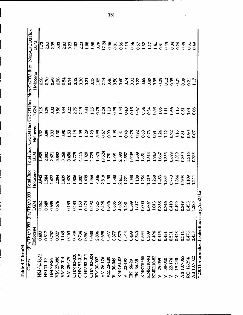
151

X 3

CM coincocococNcooo 00 ON CN NO rH NO CD NO IN CN tN rH rH m Tt ■^ in rH ON

u J tN «nnooNONO in fN m 00 00 T-t m NO CD rH ■*t NO ■* o CN CD CD NO

r-i (SNinNO'tNH r-i d IN rH d d d CN d d r-i I-i r-i d d d d d d d

§

X 3 « „, 0 8 00 OONOOrtTtCNOrH tN in «* NO o o "* rH tx in ON in in CN in rH ON rH fN

in N^NiniHrinN rH q rH ■* in NO tN CD CM NO ■* CD CN rH o CN O CN rH (0 rt ö ©000000© d rH CN d d d d d d d d d d d d d d O r-i

iE 2 s

C0

3 f

t L

GM

o\ Nnin'INNnOO

m S° 00 ON 00 CD CD in t-s <# <* CD NO rH NO m rH rH NO rH rH fN CN rH ON in <tf r-i NO CD CD m q rH NO rH m O O Ö ddodoNNo rH d CN r-i d r-i d d d d d d r-i r-i d r-i d r-i Ö

<0 U X 3 aj

0) CO u 0° U O

tN ONCDOOCOCCONON ON ON IN ON 00 rH 00 00 CN CD CD rH Tt* ä CN NO rH O fN co oqanoNinHinN cs ON NO ON q 00 ■<* ts ON NO fN ON CN fN rH 00 ON O Ö Odr-idrHrHrHr-5 rH in d d rH rH d d d d d d T-i r-i d 1-i d d d

re I

X

äs ON NHNoooinino ON IP CN in

rH rH O tx s ON rH •* CD fN CD 00 ON o NO CD O

OONOOOCN^tN^ON r^ tN m ON ON m CD in r^ Tf NO m ON 00 NO rH IfN

re U ON tv. in tN IN. CD m tN CD NO in ON NO in NO CD 00 CD fN rH cvicviiricödvd'^rH CN rH ON

rH rH r-i CN CN d rH r-i r-i r-i T-i r-i d rH d r-i O

X 0) 3 C

CM OOCNOOCOfNOOOON

NO NO 00 O O rH rH 00 CO s ON O CD 3 o 3 CD ON "* O ^

V4-1 o t NO CD rH in 00 rH CN

00 CO rH NO 3 tN d « ^ ON in^q^ionoq^ ■* O 00 •>* in "* o rH CN CN CN CD CD ON rH CM

g£ Ö

1 re r*

Ss fN oo in vo « n n t CN in 00 >P in CN l-H ON tN Q fN CD 00 $ o ON ON CD in s NO f n N NO op in fN NO NO NO I-H 3j TH TJ; a CM ON tN 00 00 00 CD y-t c5 8 r-l in rH ON Tf in oo Q

iSS •* ■<* in ■<t CD NO NO "t in NO o q CO fN ">* Tf CD ">* CN \ o odd d d rH d d d d d d •>* rH d rH d d r-i d d d d d O r-i 00

re .S CO

£5 s O aj «a

CD NNN^flON^rl 00 NO 00 fN fN ON -, ON O -* 8 Tt m rH rH 00 ** NO CD 2 ^ o 00 rtinN**^«* 00 ON ON tN «q* ON "tf in ON 5 CD CD 01 rH fN in "re

OH

a/T

h

Hol

o "* KNO\n<Jilf)Nir) NO 00 NO CD 00 m in ■* in in CD ■"* r* in in >* it d dddrndddd d CN d d d d d d d d d d d d d d d O CN

OJ © fe. -3 e o u

"re CO O in rH «* E

s O U

00 rH

ON

vc ^i o\ C! i i ONVOoOrH^OOO -r^ooHfij^t!,

o ©

i CM 00

z

tN ON o

1 o CD

rH

NÖ CN

o o rH

l CD CN

Si ? © CD

in ©

OH

ON rH

CN

CN

NO NO

00 CD NO NO

in in

i o rH rH

rH

s rH rH

CM

00

6 rH rH

ON in o

i in CN

o

? Ö CD

R rH

CNJ CN

ON rH

in NO o fN o rH 12

-294

10

7-02

2 o c 1

o g«sssESS X s 5 5 2 2 2 z 1=1 U Ö CN H II>>>UUU U > > > > 2 > m w 2 s 2 > > > > < s < *

152

of an artificial effect. Core top loss or a mix-up of the aged section of the core

should cause the Pa/Th ratio to be lower rather than higher because the half-life

of 231Pa (32.5 ka) is shorter than that of 230Th (75.2 ka). The proximity to the

Mid-Atlantic Ridge suggests the possibility that this sample might reflect

enhanced scavenging by metalliferous particles, as observed in the Pacific

(Shimmield and Price, 1988 and 1989); however, the Mg/Fe ratio was not found

to be abnormal for the core top sample by Boyle (personal communication). Thus

at the moment, I can not provide a reasonable explanation.

In the Middle-Atlantic Bight, the data from core V26-176 (core #12, this

study) and several cores from Anderson et al, (1992) have Pa/Th ratio ranging

from 0.05 to 0.07, with an average value of 0.063 + 0.016 (2 times of standard error

of the mean). This is indistinguishable from the Atlantic mean north of 45°S,

indicating that the Middle Atlantic Bight is not a margin for the enhanced

boundary scavenging of 231pa. This was found to be true for 210pfc, also

(Anderson et al, 1988; Biscaye et al, 1988). The consistently lower unsupported

Pa/Th activity ratio than their production ratio is in contrast to the typical feature

found at other margins in the Pacific, where Pa/Th ratio ranges from 0.2 to 0.3

(Anderson et al, 1992).

Cores from the margins of the western tropical Atlantic also are abnormal

because their Pa/Th ratios range from -0.03 to -0.05, which is much lower than

the production rate ratio of 0.093, and also significantly lower than the mean

value. The lowest value for the Pa/Th ratio is seen in the region of the central

subtropical Atlantic Ocean where the lowest primary production occurs (Berger

et al, 1987). A lower 230xh-normalized total flux in these cores is also seen and

supports the low-level particle flux through the water column, causing the

inefficiency of scavenging of the radionuclides in the region. The lower Pa/Th

153

ratio is a typical open ocean value, and Pa must be laterally transported to other

regions.

The northern-most core (#1, HM 94-18/3,74°N) exhibits a lower Pa/Th

ratio than the mean value for the Holocene section. It appears that 231pa m the

polar region is removed to the seafloor by downward sinking particle flux at the

site at a rate that is only half of its production in the overlying water column, so

the remaining 231pa should have been transported laterally to elsewhere in the

ocean. A lower scavenging efficiency in the polar region might be seen as a

consequence of unusually low levels of organic production and flux of particles

through the water column because of ice cover and the long polar night. The

lower scavenging efficiency is also supported by the lower 230xh_normahZed

total flux in the sample (Table 4.7), and the low content of opal in a nearby core.

The inefficiency of scavenging of reactive elements is also observed from

sediments in the Arctic Ocean by Ku and Broecker (1967), and in a later work

from the same basin by Finkel et al. (1977). It was also demonstrated by the

relatively high 231pa ancj 230xh isotope activities in water column profiles over

the Alpha ridge in the Arctic Ocean by Bacon et al. (1989). The observations of

lower scavenging efficiency may imply a net export of these reactive

radionuclides to the North Atlantic (Ku and Broecker, 1967; Bacon et al, 1989).

In contrast, the arithmetic mean is 0.174 ± 0.044 (2 sigma) for the cores

from the Antarctic Ocean (Atlantic sector) (Table 4.6). The Pa/Th ratio is on

average three-fold higher than the mean value of the cores from north of 45°S in

the Atlantic Ocean. Thus the Southern Ocean (Atlantic sector) is the only region

where the Pa/Th ratio appears consistently higher than the production ratio

0.093. This is consistent in all the observations in the Southern Ocean around

today's Polar Front (DeMaster, 1979; Kumar et al, 1993; Yu, et al, 1990; Chapter 5

154

in this thesis). High siliceous productivity and opal burial rate is associated

clearly with the Polar Front in the Antarctic (DeMaster, 1979; Burckle and Cirilli,

1987; Charles et al, 1991; Mortlock et ah, 1991; Chapter 5 in this thesis); however,

north of the front, the siliceous production and burial rates drop greatly.

Whether the higher ratios indicating enhanced scavenging of 231pa over 230jh

from the water column are due to extremely high siliceous production in the

overlying water column or other mechanisms is still unconfirmed. In any case

the Southern Ocean sediments seem to act as a major sink for 231pa which is

otherwise deficient in the whole Atlantic north of 45°S.

In conclusion, even though significant boundary scavenging of 231pa

resulting from a higher particle flux, either lithogenic or biogenic, or both within

the Atlantic Ocean north of 45°S may occur, the Pa/Th ratio from most regions is

lower than the production rate ratio. This implies 231pa depletion in the North

Atlantic sediments. The question is:where does the "missing" 231pa end up?

Since the Antarctic sediments are the only region of 231pa enrichment, it must be

that the 231pa m the North Atlantic Ocean has been exported by advection to the

South Atlantic Ocean, and then to the Antarctic. This is the first report of this

striking feature. In the following, a simple mass balance of 231pa across 25°N of

the Atlantic Ocean is pursued to examine whether the circulation is indeed

sufficient to account for this inferred export.

4.4.2 Export of 231Pa and 230Th from the North Atlantic across 25°N

The statistics in Figure 4.3 show that the Pa/Th ratio in Atlantic Ocean

surface sediments north of 45°S is usually little more than half the production

rate ratio. This implies that the balance between oceanic production and

155

deposition of 231pa does not hold for this ocean. The question isnvhere could the

"missing 231pa" g0?

The North Atlantic Ocean has been widely regarded as an important

region in terms of its large-scale circulation, consisting of both horizontal, wind-

driven gyre circulation and vertically overturning thermohaline-driven

circulation. Both circulations act in concert to transport heat (Hall and Bryden,

1982), and CO2 (Brewer et al, 1989) to latitudes where disequilibrium with the

atmosphere occurs. Considering this same driving force of the ocean advection, I

hypothesize that the "missing 231pa" m the North Atlantic Ocean is exported

from the North Atlantic to the South Atlantic; eventually, it must also be further

exported from the South Atlantic to the Southern Ocean to accumulate in the

Antarctic sediments.

In what follows, I examine the mass balance between the production rate

and the sedimentation plus the net export for both 231pa ancj 230jh in the North

Atlantic Ocean. I chose 25°N as the boundary because estimation of the variation

of mean meridional volume transport with depth has been computed at the 25°N

section by Hall and Bryden (1982; data source listed in their Table 5) to estimate

the net heat transport in the 25°N latitude section. I make specific use of these

mean meridional volume transports of water and combine the total 230jh and

231pa activity profiles (Figures 4.4 and 4.5) in the water column from the North

Atlantic Ocean to calculate the northward and southward advective flux of

nuclides across this section. For simplification, I divide the 231pa and 230jh

activity depth profiles, and water mass transport profile into only two layers:

shallow (0 to 1050 m) and deep (>1050 m to bottom). Each layer has an average

tracer concentration C and net depth-integrated water transport.

156

The steady-state mass balances of 231pa and 230xh are as follows:

IP = S + E, (4-3)

where IP is the integrated production rate from the decay of uranium for the

entire ocean north of 25°N for each tracer, S is the sedimentation rate for each

tracer, and E is the net export flux of each tracer across the 25°N boundary

section. Integrated production can be calculated as follows:

Z P (in dpm/s)

= P*V

= Cu*X*i*V (4-4)

where Qj =uranium concentration in seawater, i.e., 3.3 jxg/1 (Turekian and Chan, 1971;

Chen et ah, 1986);

X = decay constant of tracer;

f = activity ratio of 234u/238jj jn seawater, i.e., 1.15 for 230xh calculations, or

f = activity ratio of 235u/238u in seawater, i.e., 0.046 for 231pa calculations,

V = total water volume between 25°N and 90°N latitude of the Atlantic Ocean

(Table4.8).

The water volume of the Atlantic Ocean was calculated using the "AVS"

program provided by Dr. Bill Jenkins of the Woods Hole Oceanographic

Institution. The volume estimates were made by discrete integration of 5 minute

resolution topographic data base dbdb5 for the Atlantic. The program results

and sums are listed on Table 4.8.

Export is computed from the volume transports and concentration, as

indicated previously.

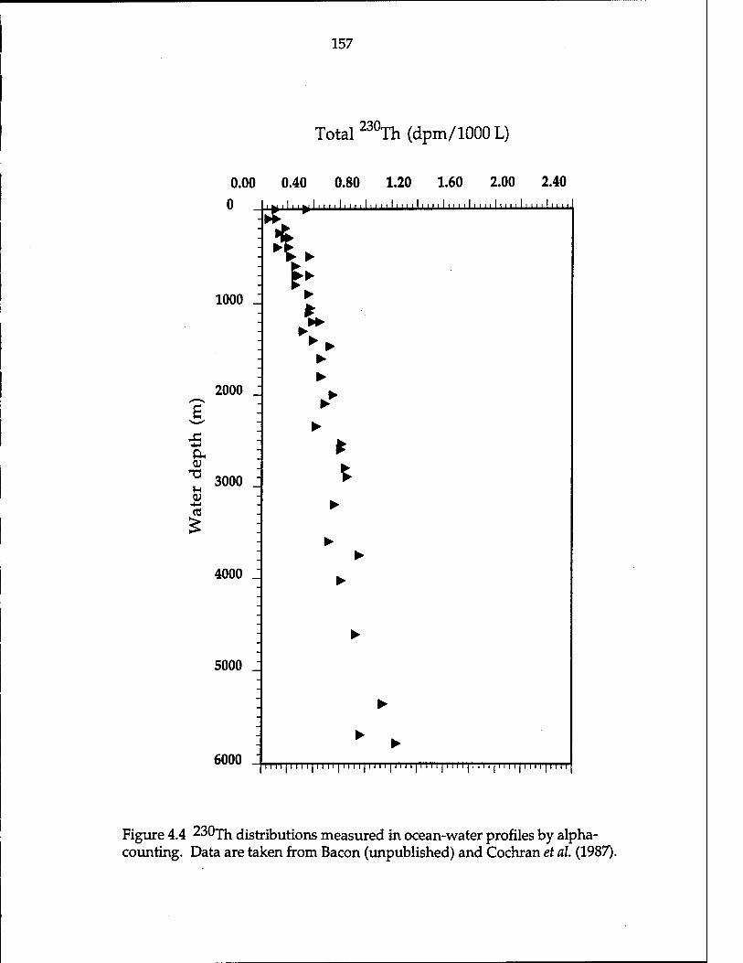
157

230, Total **Th(dpm/1000L)

u 0)

0.00

0

0.40 0.80 1.20 1.60 2.00 2.40

*, ►

- A U - h

1000 1 ►

► - ►

2000 1 ► - ► : ►

*

3000 _I t - ► - ►

► 4000 _I ►

- ►

5000 J

- ►

► ► 6000 ~

Figure 4.4 230Th distributions measured in ocean-water profiles by alpha- counting. Data are taken from Bacon (unpublished) and Cochran et al. (1987).

158

231 Total ^Ta(dpm/1000L)

0.00 0.10 0.20 0.30 0.40 0.50 0.60 0.70

1000 J

2000 _I

u 0)

3000 J

4000 _I

5000 2

6000

Figure 4.5 231Pa distributions measured in ocean-water profiles by alpha- counting. Data are taken from Bacon (unpublished).

159

g g 0 >

CD

g in

o 00 R 00

rH tN in vO

ON 00

8 W o rH

vO vö CM

CO co

in CN

CO CN

rH

&N

«5 > (0 <

g 2

IN

< 1 CN

CO rH o CN 00 "^ rH in

rH tN oö tN in cö

V V o 6 2 1—1

s 1"N

o > c 0)

in in "2 in in o i-H

5 C/> CO Tj< in vo ON to U o i ' 1 1 ' 1 o 0 ***

«8 o in CN

in co

in in in

in vo H

w HJ •PX **

•w «< V co ß 0)

g a

g in

ON CD

o\ ON

tN CN

vO CN CO

in CN in CO oö co rH g IBM

o rH tu

rH vO

ö CO

CN CN

rH rH VO vo

> o rH

** MH o tß (0

fr

(-1 < 1 CN tN CNl rH <«* o CN tN

rH W o

tN* vö "<* ^ «tf ö

6 2 rH

& 3 W5 « •o in

CN i

o

in in in in o 1

2 o CO

1 in CN

i

in co

in i

in in in

ON 1

3 NJ A» H

160

E =Cs*vs + Cd*vd (4-5)

In equation 4-5, Cs and Cd are average concentrations of the shallow and

deep layers, and vs and vd are mean meridional volume transports in the

shallow and deep layers. The concentrations C are all measurable quantities.

The data of total 230xh and 231pa m the water column were taken from the

unpublished data of Bacon and Fleer (Figures 4.4 and 4.5) and data of Cochran et

ah (1987). The mean meridional volume transport with depth is taken from the

estimation by Hall and Bryden (1982). Broad features of the volume transports

with depth have indicated that there are a net volume transport to the south in

the deep layer and to the north in the shallow layer. The activities of 231pa and

230xh in the water column show higher concentrations at deeper depth and

lower concentrations at shallower depth; thus, a net flux of 231pa and 230xh

must be transported southward in the Atlantic Ocean. Table 4.9 summarizes the

quantities used in the calculations.

The results (Table 4.9) support my proposed hypothesis of the advective

flux of 231pa and 230jh from the North to the South Atlantic, indicating that as

much as 50% of the 23lpa production, but only about 10% of the 230xh

production, is exported by ocean circulation from the North Atlantic Ocean

across 25°N. The estimated magnitude of export for 231pa js close to the amount

of 231 pa deficit in the open ocean water column, which was previously

considered laterally transported from the open ocean to the ocean margin. If

these estimations of export of both 231pa and 230xh are right, then there will be

about 50% of 231pa and 90% of 230Th production remaining for deposition to

sediments. The Pa/Th ratio in the North Atlantic sediments should be expected

to average 0.053 ± 0.016 (1 sigma). This is very close to the actually observed

arithmetic mean Pa/Th ratio of 0.061 ± 0.006 (2 sigma) north of 25°N. The large

161

error (-30%) of estimation is seen as the result of the estimation error from the

water mass transport (~25%, according to Hall and Bryden, 1982), the water

volume north of 25°N based on the topographic data (-6%), and the analytical

error of concentrations of tracers (ranging from <10% to 15%). It is obvious that

the database is very small, and the assumption of homogeneous distribution for

each tracer within a single box would be oversimplication; so the quantitative

conclusion based on it must be regarded as a first approximation. However, it

seems there can be little doubt about the basic conclusion.

As we can see in Figure 4.2, within the estimation error (1 sigma), the

estimation result for the sedimentation ratio of Pa/Th is consistent with the

observations of the deposition rate ratio of Pa/Th in the North Atlantic

sediments, which range from 0.3 to 0.7 for most of the sediments covering the

Atlantic Ocean seafloor. The above calculation, most emphatically, does not

mean that the ocean marginal boundary scavenging effect is negligible. The

internal-basin redistribution still must be found within the basin north of 25°N in

the Atlantic Ocean; however, the exported fractions of 231pa ancj 230xh are

shown to be important contributions to the final redistribution of Pa/Th

deposition ratios as seen for all Atlantic sediments. This result is important

evidence that the advection effect by ocean circulation in the North Atlantic

significantly influences the mass balance of nuclides within an ocean basin, and

significantly influences the ratio observed in the sediments. The effect can not be

ignored when sediment data are interpreted.

One question can be asked now: the export of 231pa from the Atlantic

Ocean to the Southern Ocean result in horizontal gradient of 231pa in water

column from the North Atlantic to the Southern Ocean?

162

a; u o

<

.S

o CO cs T3 c «

rH CO CM

»H a *o3 •a o

CD 05

_5>

05

ON

a;

1

H o CO CS

CO CM

a,

O 9 DM fi

J» u o s

o co Ö Ö

in NO

CS Ö

CO CO

6 S s OH

NO IN <—) CS T-H K ON ON NO

05

OH W -Ö O

6 ■«

05

CO CO

S 6 NO NO

in CO NO

LO ON

s °°

CS -1 fe gg ON T-.

2 Ä ^ in ^ ^

05

e OH

rH rH P

S OH

VO NO

O in o

o

in o

05 13 U U

NO rH O

co o o

O o +1 +1 co in o

1—1 NO o

o o

«

0) T-t CS

163

The only available data for 230Th and 231Pa in the water column of the Southern

Ocean were reported recently by Rutgers Van Der Loeff and Berger (1993);

however, the data are stiking. Vertical profiles of dissolved and particulate

230Th and 231Pa were obtained across the Antarctic Circumpolar Current (ACC)

in the southern Atlantic. North of the Polar Front, dissolved and total 230Th

increase with depth; 230Th concentrations increase three-fold across the Polar

Front; while the concentrations of 231Pa change little with depth and latitude

across the ACC (Rutgers Van Der Loeff and Berger, 1993). As a consequence, the

Pa/Th ratio in the water column decreases toward the south, but it remains far

above the production ratio of 0.093. Although the Pa/Th ratio higher than the

production rate ratio, the range of ratios falls within the same range as we typical

observed in Figure 3.2. The concentrations of 230Th and 231Pa are in the same

ranges of those observed in Figures 4.4 and 4.5, suggesting there is no significant

horizontal gradient in 230Th and 23*Pa concentration in the water column.

These data suggested a controversial feature that I would expect regarding to the

export flux of 231Pa from the Atlantic OCean. One possible explanation is that

the export 231Pa from the Atlantic Ocean is stripped very rapidly when it reaches

to the region of the Polar Front Zone (PFZ) because of highly scavenging

efficiency due to either the intensity of particle flux or due to biogenic silicate

phase or due to combination of both. In other word, the residence time of 23*Pa

must be very short in this specific region across the Subtropical Convergence

(STC, ~45°S) to the Polar Front Zone (PFZ). Future study of measuring Pa and

Th in water column and in collected materials with sediment trap across the STC

to the PFZ must be performed to confirm the scavenging phenomena of both

nuclides. Before that, I propose the following explanation. To be able to obtain a

large contrast in preferential deposition of 23*Pa between north and south in the

Atlantic sediments, two principle factors must be involved. Firstly, there must be

164

more intense scavenging from the water in the Southern Ocean. Secondly, there

must be sufficient time available for the transport from north to south Atlantic to

take place before the reactive elements are scavenged, i.e., the scavenging

residence time must be larger than the mixing time from the north to the south

Atlantic Ocean. Although the exact residence times for both 231pa and ocean

mixing are not known in the Atlantic Ocean, the average residence time of water

in the deep Atlantic is probably longer than that of 230xh and shorter than that of

231pa to be able to export 231pa from the north Atlantic to the Southern Ocean.

Once reaching the Southern Ocean, the residence time of 231pa must be very

short due to the possible reasons as discussed above. The large difference in

distribution patterns of Pa/Th ratio between the Atlantic and Pacific Oceans is

probably a result of the largely relative residence time of deep water within the

Pacific and its larger size compared to that within Atlantic Ocean.

4.4.3 The mass balance of 231Pa in Holocene Antarctic sediments

The above calculation demonstrated that transport of 231pa by the

meridional circulation in the Atlantic is sufficient to account for the 231pa deficit

observed in North Atlantic sediments. Because the South Atlantic sediments

north of 45°S are also 231pa depleted, there must be additional export from the

South Atlantic, and all of this 231pa mUst enter the circumpolar region. Now, the

question is left whether the budget can be balanced between the deposition rate

of 231pa in the Antarctic sediments and the production rate of 231pa in the

Antarctic overlying water plus the export of 231pa from the Atlantic Ocean. In

other words, is the Southern Ocean the only site to trap all of this excess 231pa, 0r

165

is a portion of it further transport northward into the Pacific and Indian Oceans

after it enters the Antarctic Circumpolar Current.

A simple box model serves for the first order approximation in examining

the mass balance of 231pa in the Antarctic sediments. The diagram is shown in

Figure 4.6. In the model, for simplification, I assume that the system of the

Southern Ocean has stabilized so that gain just balances loss. The decay loss of

231pa m the water is negligible. The input of 231pa into the Southern Ocean

box is assumed to be the production from the uranium decay in the overlying

water column plus the export from the North Atlantic Ocean. The output is

deposition to the seafloor and the further export north into the Indian or Pacific

Ocean.

I further assume that the export flux of 230xh toward to the Southern

Ocean is negligible. Then, since the depositon rate of 230-jh almost equals to the

production rate from the uranium decay in the overlying water column, the

deposition rate of 231pa m the Antarctic sediments can be estimated by taking

the mean value of Pa/Th in the entire Antarctic sediments multiplied by the sum

of the production rate of 230xh in the entire Southern Ocean.

The mass balance of 231pa for the Holocene is given in Figure 4.6. The

results show clearly that, within the uncertainties, the deposition of 231pa in

Antarctic sediments is sufficient to balance both the Antarctic production and

231pa which is exported from the Atlantic Ocean. Within the uncertainties, there

is no further export into the Indian or Pacific Ocean. This indicates that the

Pa/Th deposited ratio in the Antarctic sediments should be controlled not only

by the scavenging rate but also by the advective transport from the Atlantic. It is

166

Export Flux (E)

(235 ± 34)xl0 dpm/ka

15

Mass balance of Pa in the Southern Ocean (Holocene)

in situ Production (P)

295xl015 dpm/ka

>• to further north

~(37±86) xlO15

dpm/ka

Deposition Flux (S)

15 (493 ± 80) xlO" dpm/ka

Input/Output North of 45°S Atlantic Southern Ocean

Production231Pa (dpm/ka) 631xl015 295 xlO15

Production ^Th (dpm/ka) 6813xl015 3186xl015

Deposition (dpm/Ka) (395 ± 68)xl015

(2 sigma) (493 ± 80)xl015*

(2 sigma)

Volume (nr) 263xl015 123xl015**

Export flux (dpm/ka) (235±68)xl015

(2 sigma) (37±86)xl015

(2 sigam)

Mean Pa/Th ratio 0.058 ±0.005

(n=52, 2 sigma) 0.155 ± 0.024 # (n=21,2 sigma)

»Deposition of23 Pa in the Southern Ocean=(Pa/Th) xProductionC230!!!) xVolume ** from Warren and Wunsch (1987) # Mean Pa/Th from all available data in the Holocene Southern Ocean

231T Figure 4.6 Diagram of the mass balance of Pa in,the Holocene Southern Ocean

167

important to keep this in mind when variations in the Pa/Th ratio in the

Antarctic sediments with time are interpreted.

4.4.4 LGM/Holocene changes in the Pa/Th distribution in Atlantic sediments

During the Late Quaternary climate cycles, the ocean system has been

affected in many ways. For instance, dramatic changes in oceanic circulation

patterns and extent, and carbon system chemistry have been found to occur

(Boyle and Keigwin, 1982,1987; Curry and Lohman, 1983,1990; Duplessy et al,

1988; Curry et al, 1988; Broecker et al, 1990). The fluctuations in sea level must

have changed the input of terrigenous materials (Damuth, 1977; Milliman et al,

1975); the ice sheets at high latitudes must have varied the discharge of the ice-

rafted debris (Ruddiman, 1971); and the changes in wind intensity and direction

must have changed the transport of the eolian materials into the ocean (Kolla et

al, 1979). Because oceanic distribution of reactive nuclides is largely governed by

scavenging by sinking particles and lateral transport within an ocean basin, these

factors are reflected in the nuclide distributions in the sediments. Ultimately, it

may become possible to use the nuclide distribution to deduce changes in

particle flux or lateral transport from the sedimentary record.

In Chapter 3,1 demonstrated from the results of year-long deployment of

sediment traps that the scavenging efficiency of these nuclides and the

fractionation between the two nuclides are largely controlled by the intensity of

particle flux. Chemical composition of the settling particles could also influence

the relative distribution of the two nuclides (e.g., due to preferential uptake of

231pa by Mn oxide or biogenic opal), but this factor is still poorly understood.

Besides the particle flux and chemical composition of a particle, a simple steady-

168

state one box model, as shown in section 4.4.2, suggested another mechanism to

influence the fractionation of 23*Pa and 230Th. The model examined the mass

balance of 231Pa and 230Th north of the 25°N, and it was shown that the reactive

nuclides (in particular 231pa) are influenced strongly by oceanic advection. The

dramatic changes in oceanic circulation patterns during the glacial - interglacial

climate cycles, as many works have suggested, thus may affect the distribution

pattern and boundary scavenging of these reactive nuclides as well. For these

reasons, I focus in this section and in the following section on how changes in

oceanic condition (particularly under extremely different conditions

representative of the LGM and the Holocene) might have impacted the

fractionation between 23lPa and 230lrt. Careful mapping of the Pa/Th ratio

from the Holocene and LGM over the entire Atlantic Ocean may provide insight

into how the ocean system has changed.

LGM data for 231Pa, Th and U isotopes are listed in Table 4.3, and the

calculated results are given in Table 4.10. A map of Pa/Th ratio for the LGM

sediments, similar to the Holocene map of the Pa/Th ratios, was constructed

(Figure 4.7). For easier comparison of the changes in Pa/Th ratios and other

sediment components between the LGM and the Holocene, the notation

(Pa/Th)G/H ratio is introduced:

(Pa/Th)G/H = (Pa/Th)LGM/(Pa/Th)HL, (4-6)

where (Pa/Th)LGM and (Pa/Th)HL are the Pa/Th ratios in the LGM and the

Holocene sediments. The (Pa/Th)LGM ratios and (Pa/Th)HL ratios are taken

from Tables 4.4 and 4.10. Table 4.11 summarizes the (Pa/Th)G/H ratios. These

ratios are decay-corrected to the time of deposition.

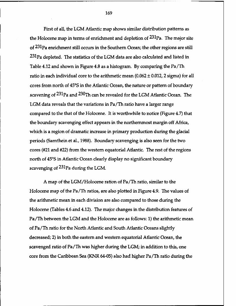
169

First of all, the LGM Atlantic map shows similar distribution patterns as

the Holocene map in terms of enrichment and depletion of 231pa. The major site

of 231pa enrichment still occurs in the Southern Ocean; the other regions are still

231pa depleted. The statistics of the LGM data are also calculated and listed in

Table 4.12 and shown in Figure 4.8 as a histogram. By comparing the Pa/Th

ratio in each individual core to the arithmetic mean (0.062 ± 0.012,2 sigma) for all

cores from north of 45°S in the Atlantic Ocean, the nature or pattern of boundary

scavening of 231pa and 230xh can \,e revealed for the LGM Atlantic Ocean. The

LGM data reveals that the variations in Pa/Th ratio have a larger range

compared to the that of the Holocene. It is worthwhile to notice (Figure 4.7) that

the boundary scavenging effect appears in the northernmost margin off Africa,

which is a region of dramatic increase in primary production during the glacial

periods (Sarnthein et al., 1988). Boundary scavenging is also seen for the two

cores (#21 and #22) from the western equatorial Atlantic. The rest of the regions

north of 45°S in Atlantic Ocean clearly display no significant boundary

scavenging of 231pa during the LGM.

A map of the LGM/Holocene ration of Pa/Th ratio, similar to the

Holocene map of the Pa/Th ratios, are also plotted in Figure 4.9. The values of

the arithmetic mean in each division are also compared to those during the

Holocene (Tables 4.6 and 4.12). The major changes in the distribution features of

Pa/Th between the LGM and the Holocene are as follows: 1) the arithmetic mean

of Pa/Th ratio for the North Atlantic and South Atlantic Oceans slightly

decreased; 2) in both the eastern and western equatorial Atlantic Ocean, the

scavenged ratio of Pa/Th was higher during the LGM; in addition to this, one

core from the Caribbean Sea (KNR 64-05) also had higher Pa/Th ratio during the

170

00 tv i-H 00 Oi CO o * H n oo N ri 6 ri O O H

^»OCOOHinijiNN doNN'i'didrinri t<cr5(SfSi-ifriir)t>.'oöuSo6t<

CM

*ine*NTfif)uirfS\oNo\NO'),ininn ON in ö ö ö ö OOOOOOCMOOOOCSI ööööödddrHodd

i-icsicNr-ir-irHooooNcncMcMcnocoooCTNfMoocop>i"«fcnot-iON o CM o

cot-iOTf ininooin^aNintoovrtN OOO OOr^SoOOOo5r-iOr-ic5ÖÖOÖC5ÖC5

o d do öööööööööööööcsööööcsöööci

NIDHOJiNClrtrt

60

ID *H in in d d

N»^"*ON^Ninr)OOSN^»NO\nNNri<*»yO»N ifimN»Nnn**noooN»nBrtn^nooir)HN 99999999d99°9ö999TT999c?c5999

^nsoi'fnifiNo *—lOOSCOrHr-I 00 Ov © i—(

mtvcMopfv\oovortO\ON BO W K) Tf o N (N * rt If) 3

CMCSr1CMr-lrHrH©>-Ht-lOCM©OOr-lr-l»-ICMi-lrH»-lOO©i-<©0

in CM o\ op 1—I 1-H I—I © ©do©

©in^oineecMTfovooinotv ftOHNHNOMN^'jaiB ©©dooododrHd©©

oc ve » 3 CO CO Tt< *T © © © d d d ©

00 00 00 00 N CO CM CM CM rH

O l-l

ON*OiO\rt»B oococooo^in^ocMmvocMT-icooorHooini-ivo **covoinoomcocMONt,-cM\ooo©cMC/\oom\ovo

cocMcor-it-io\T-(r-itcomovO'<*'cocoooinr>.vcco\ovoo\inoovoo\

© oo co \o © r-l O

o © © d

00 i-H vo O B N N H

i-H"*ocooosc:!txOi-iT-i\r!© CMOi-Hi-Hf-iT-l©i-lCMO "" '" "" ©©oooooo©

CO VO vo <-H d © ©

»inno«o\ffi»o CMCMCOCOCMi-lT-lr-100 dddddoddd

tv O .-H NNO

SCO © r-s oq

I-H CO CM

ov sinnin^^tBinHnHN K^OOOOOONOOOHVCNrtn ^©iricocMcMvo^voiriro'iriirioo^Kirioo

© oo in © ■* OS CM VO

2 S 2

feS82vf^oj«i?^9? dvoco©5i.vovi^^^ui

o s CM

171

x s

O u ra u I c o 2

ON 00ON^vO'fE>00vOCOvOrJ*cO'fP3vOp\

—• —• .^ .^ _: CM ^* .-• -j —: —; _: ^J; _; _: _J en en vo in r-! pj in

1-H O vo oo rn en O ^ 00 00

Mf)0\O00HHrtNHNNN<tiNnOH

00 * m N ^ in «r5 r-5 ö

X 3

IS CB 3 , O e • u t 60«

00 ON

oo\OH\cinn'*n»»^rt'**ooc)'foino\o\ .._.„.. _ .fH*NHN*t»NNqino*MoqiNoq'*in nnvcifiH^NinoNdodHHHNHnNN^NndrinHO 00 ^ ■* N ^ tv in oo K vo

en O u rs U

ts oo<*nainNoomo\na>ooifiOo\nnN»inHH»n«N intNA<!t|')|HnnvO»riniNo\»^nNif)'*inooo;o\o\vOri» OÖÖÖOOCJT^ÖÖÖtnrHÖÖÖÖÖOÖÖÖÖOÖÖrHÖ

O U a U S5

*D\OHifiH^ino\ri»»9io>oin(<)oinHo:»io»HN\oifno NriNHNin^iriin^in*o\»»'*n>o^tnnNNOO\*o*n ÖOÖÖÖÖÖÖÖÖÖÖÖÖOÖÖÖÖÖÖÖÖrHÖÖcSrH

I* rs X

s Nif)nNNON*»«(snnna\5iinno('t*N*OriNioo*H oq*«jNNHnNMNO;Nr|0>q\qHNNiv;r(HO;qo;rt\q T^T^fNr^CJlriHrHrHOVOr4rHÖr4ÖrHTHrHTHrHrHÖTHÖrHÖ

ON ON ^ m N B N

o o o o

inootsini-HOOi-HOooooeNoooo __. mooinootNrHtvoiNorNOOoo\o OÖrHÖddÖrHÖOÖtNi-HtÖ'OrHtNrH

«innnNNooiniN - -O>NKH\OOMTI

1-H O 1-H O O O

a o u

172

Figure 4.7 The map of decay-corrected unsupported 231pa/230yh ratio (Pa/Thex°) of the Last Glacial Maximum (LGM) Atlantic Ocean.

173

u K X! o C o

< H Jj N n t N (M i

.—I VO o

< d

CM C/5 rH LO O

o H ^| N N N H O 1 2

cn "2

VO o d

CM O

Cß •4—) o O O © rH CM rH CM

$ C 01 c/i in

rH

£ d • »H

cn co o o u in

X

1 ob o O CO o o o o o ?l

rH

4-i CM o < d s

o

CM rH O

0) CM d X t

2 O rH T* CM rH H O +1 •4-1 CO V4-I o 00 o CM o o d

XI eo rH

o CD

2 o CM U-4 rH fs CO O rH O O

CM O

?l in

CM O rH

2 & PH d rH CO 4-1

CM .5 SJ o £ OH in in in in in m -o

N N N N N N ö rH CO VO 00 rH CO i0 O O O O rH rH «N

1

O 6 u

X! 0 0 0 0 0 0°

3 w o> QJ XS (0

U £ 43 <4H CD

CM rH

i—H

U in in o in in S> O K rH CM rH CM

O

£ P SS

0) J5 ß x

m Ö °. ö r"! c5 O S in 9 uS 9 in in

3 p CM in ts. o CM <-< ? O O O O rH rH Q *5 tß

•* +1 H V c> d ö d d A

174

S 2

231pa/230Th activity fatio

231 230 Figure 4.8 Summary of unsupported Pa/ Th ratios measured in the Last Glacial Maximum Atlantic sediments

175

LGM; and 3) the preferential scavenging of 231Pa over 230Th in the Antarctic

Ocean was less during the LGM.

If advection has truly affected the 231pa and 230rh mass balance as the

model has shown (section 4.4.2) in the Holocene Atlantic, the changes in ocean

circulation patterns and intensity during the glacial time might have

accompanied variations in the distribution of (Pa/Th)G/H- Now, the question

can be asked whether the sluggishness of the southward-flowing NADW (North

Atlantic Deep Water) decreased the export of 231pa and 230rh from the Atlantic

to the Southern Ocean.

In the following, I use the same box model used for the Holocene to

examine the mass balance of 231 pa m the Southern Ocean during the LGM. The

purpose is to examine the question whether the sluggish advection of NADW

during the LGM (Boyle and Keigwin, 1982,1987; Oppo and Fairbanks, 1987;

Duplessy et dl., 1988; Curry and Lohman, 1983,1990) would decrease the export

of 231pa from the North Atlantic, and it would be an important cause of the

variations in Pa/Th ratio in the Antarctic sediments. The estimation is based on

the same production rate of 231pa and 230^ m both the North Atlantic and the

Southern Ocean, and the deposition rate of 231pa for both divisions are

determined by the Pa/Th deposition ratios during the LGM. Following the same

calculation as that for the Holocene box model, the results indicated in Figure

4.10 suggest that the export flux of 231pa and the deposition rate of 231pa m the

Antarctic sediments are almost the same within the 2 times of standard devision

of the mean during the LGM. The result shows that the depostion of 231pa into

the Antarctic sediments is still enough to account for all excess 231pa exported

from the North Atlantic, and there is no significant amount of 231pa exported

further northward. However, the result is somehow striking, because the export

176

of 231Pa from the Atlantic and deposition rate of 231Pa in the Southern Ocean

sediments suffer no changes even though the ocean conditions are thought to be

extremely different between the glacial and interglacial climates. The higher

production during the LGM induced by the increasing intensity of upwelling

(Samthein et al, 1987,1988; Mix, 1988) might have resulted in higher surface

scavenging intensity and thus been strong enough to cause higher scavenging

efficiency of 23*Pa in the equatorial Atlantic where 23*Pa was supposed to

increase in the glacial North Atlantic. All of these variations in intensity and

patterns of ocean circulation along with the internal basin redistribution (i.e.,

open ocean gyre and the margins) might have caused the decreased Pa/Th ratios

in the North Atlantic, increased Pa/Th in the tropical Atlantic, and decreased

Pa/Th ratio in the Southern Atlantic Ocean during the LGM (Figure 4.9). Since

the export to the Southern Ocean is a net effect of scavenging by particles and

advection by different patterns of water circulations in the Atlantic Ocean, the

small difference between the LGM and the Holocene in terms of the 23*Pa mass

balance in the Southern Ocean may indicate that combination of those effects are

a real reflection of little change in terms of the 23iPa budget in the Southern

Ocean, or it may indicate that the rough scale of mass balance I calculated would

not be able to decouple the effects. A fine scale of budget must be examined to

not erase the signal of boundary scavenging in the Southern Ocean. In any case,

this implies that the downcore variations in Pa/Th ratio reflect variations not

only in particle flux (i.e., production), but also in the intensity or pattern of the

thermohaline circulation.

In conclusion, the advection effect seems to be a very important factor

controlling the fractionation between 231Pa and 230Th in the Southern Ocean

177

Figure 4.9 The map of LGM/Holocene ratio of the decay-corrected unsupported 231pa/230xh ratio (Pa/Thex°) in the Atlantic Ocean.

178

Export Flux (E)

(208±82)xl0 dpm/ka

15

Mass balance of Fa in the Southern Ocean (LGM)

in situ Production (P)

295xl015 dpm/ka

► to further north

(38±117) xlO dpm/ka

15

Deposition Flux (S)

15 (465±80) xlO" dpm/ka

Input/Output North of 45°S Atlantic Southern Ocean

231 Production Pa (dpm/ka) 631 xlO15 295 xlO15

Production 230Th (dpm/ka) 6813xl015 3186xl015

Deposition (dpm/Ka) (423±82)xl015

(2 sigma) (465±80)xl015

(2 sigma)

Volume (mj 263 xlO15 123xl015**

Export flux (dpm/ka) (208±82)xl015

(2 sigma) (38±117)xl015

(2 sigam)

Mean Pa/Th ratio 0.062 ±0.006 (n=52, 2 sigma)

0.146±0.013 # (n=16, 2 sigma)

231 230 * Deposition of Pa in the Southern Ocean=(Pa/Th) xProduction( Th) x Volume ** from Warren and Wunsch (1987) # Mean Pa/Th from all available data in the LGM Southern Ocean

231T Figure 4.10 Diagram of the mass balance of Pa in the LGM Southern Ocean

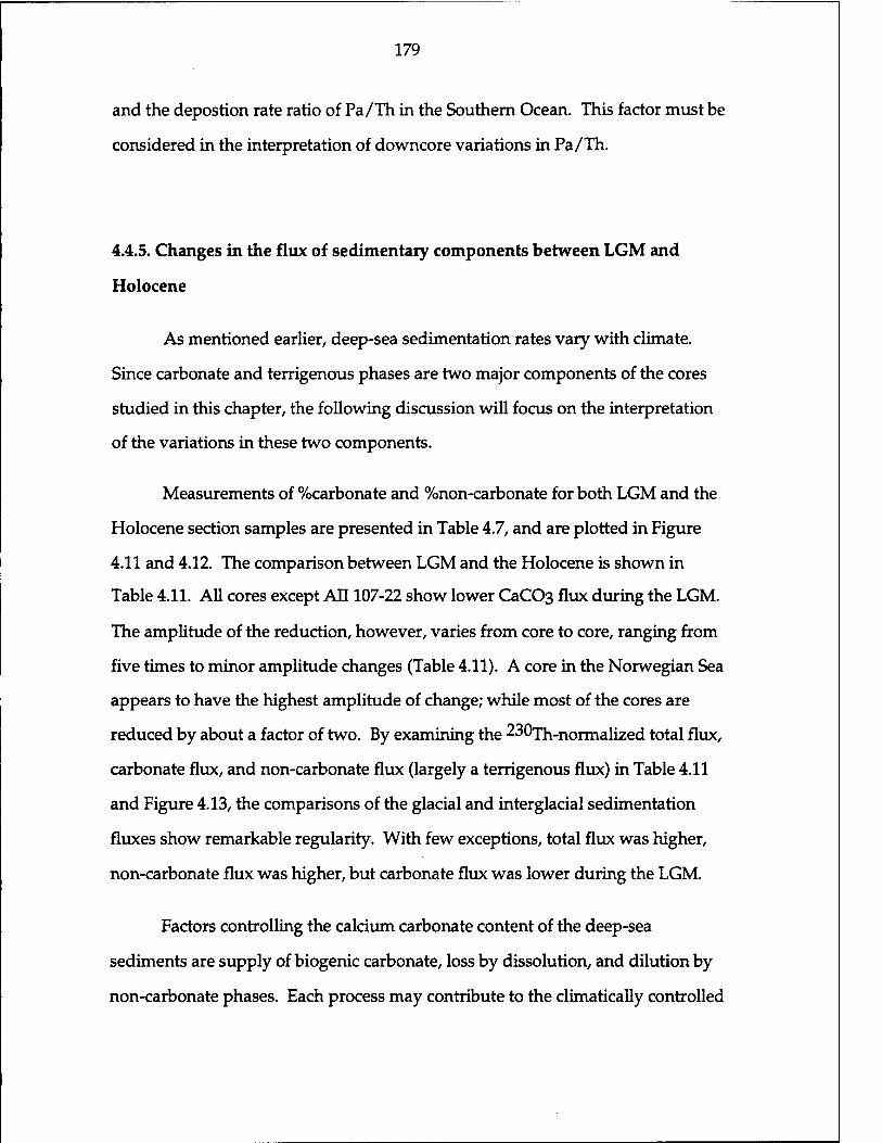
179

and the depostion rate ratio of Pa/Th in the Southern Ocean. This factor must be

considered in the interpretation of downcore variations in Pa/Th.

4.4.5. Changes in the flux of sedimentary components between LGM and

Holocene

As mentioned earlier, deep-sea sedimentation rates vary with climate.

Since carbonate and terrigenous phases are two major components of the cores

studied in this chapter, the following discussion will focus on the interpretation

of the variations in these two components.

Measurements of %carbonate and %non-carbonate for both LGM and the

Holocene section samples are presented in Table 4.7, and are plotted in Figure

4.11 and 4.12. The comparison between LGM and the Holocene is shown in

Table 4.11. All cores except AH 107-22 show lower CaCG*3 flux during the LGM.

The amplitude of the reduction, however, varies from core to core, ranging from

five times to minor amplitude changes (Table 4.11). A core in the Norwegian Sea

appears to have the highest amplitude of change; while most of the cores are

reduced by about a factor of two. By examining the 230xh-normalized total flux,

carbonate flux, and non-carbonate flux (largely a terrigenous flux) in Table 4.11

and Figure 4.13, the comparisons of the glacial and interglacial sedimentation

fluxes show remarkable regularity. With few exceptions, total flux was higher,

non-carbonate flux was higher, but carbonate flux was lower during the LGM.

Factors controlling the calcium carbonate content of the deep-sea

sediments are supply of biogenic carbonate, loss by dissolution, and dilution by

non-carbonate phases. Each process may contribute to the climatically controlled

180

fluctuations in the carbonate content of deep-sea sediments at individual sites.

Based on measurements during the GEOSECS expeditions, the relationship

between the carbonate ion content of deep water and the depth of the lysoclines

for calcite and aragonite in the open ocean were established by Broecker and

Takahashi (1978). The regional average lysocline depths drawn from their data

occur at 4800 m, 4700 m, 4800 m, and 4300 m for the 42°N MAR, 20°N MAR, the

North American Basin, and the equatorial Atlantic, respectively (the data was

taken from Table 1 of Bacon, 1984). Atlantic waters at present become

undersaturated with respect to calcite between 4,000 and 5,000 m (Takahashi,

1975). Luz and Shackleton (1975), on the basis of their study of eastern equatorial

Pacific cores, concluded that for depths at or above the regional lysocline,

dissolution does not play an important role in the glacial/interglacial fluctuations

of carbonate content. Since most cores used for this study were collected from

2000 m to 4000 m, which is above the lysocline, the fluctuation in carbonate

content for most cores used in this study should be the least affected by carbonate

dissolution. This conclusion was substantiated in many previous works (Bacon,

1984; Curry and Lohaman, 1986; Francois et al, 1990).

Although recent works have indicated that even at depths well above the

lysocline a significant amount of carbonate dissolution may occur by reaction of

the carbonate in the sediment with metabolically produced CC»2 (Emerson and

Bender, 1981), the percent carbonate plots for the cores selected in this thesis

were considered to be principally due to variation in supply of carbonate or

dilution by non-carbonate. In order to evaluate the effect of each process, I

calculated the rain rates of the carbonate and terrigenious materials in sediments.

For several cores, I also determined the content of biogenic opal, but for the rest

of the cores I took non-carbonate to consist entirely of terrigenous phase.

181

100.00

e o ■fi « u

80.00 -

60.00 -

40.00 -

20.00

0.00

S carb%)H

■ carb%)G

■UB

SSSSSSaasacacSSS z zzzzz aus

Figure 4.11 %Carbonate for both the LGM and Holocene sections in the Atlantic sediments

182

100.00

« C o

u I c o

2

80.00 "

60.00

40.00 -

20.00

0.00 £1 ^1

S non-carb%)H

■ non-carb%)G

*S 3

as 8s> >> u uu u >>>>*> Ess ««« >»><cc <

Figure 4.12 %Non-carbonate for both the LGM and Holocene sections in the Atlantic sediments

183

c QJ U o o

§

10.00

8.00-

6.00 -.

4.00

2.00

0.00

S3 Carbonate flux

■ Non-carbonate flux

..hill I mimmnniiiiiiiiiiiHr oo »■H

i

a:

O 1/irH ^»i

~~~~~zzzz:2~2a«a££ggg8SassSs SSSSSSJBKSCSSS z zzzzz BUB

230 Figure 4.13 The LGM/Holocene ratio of the Th-normalized carbonate and non-carbonate flux for the Atlantic sediments

184

The fluxes of sediment components are normalized to the 230jh activity in

the sediment (i.e., 230xh-normalized flux method).

Carbonate flux = ß (f /230xhex°) (4-7)

and

Non-carbonate flux = ß [(1-f) /230Thex°], (4-8)

where 230xheXo is in excess and has been decay-corrected; f is the fraction of

carbonate; ß is the known flux of 230^ which is controlled by the uranium

content of seawater and is a linearly increasing function of water depth Z:

ß (dpm/cm2/ka) = 0.00263 Z (m). (4-9)

As pointed out in Chapter 3, the 230xh-normalization method is used to

obtain the vertical settling of particulates and tends to corrrect for redistribution

of sediment on the bottom. Since it is not possible to rule out dissolution (e.g.,

carbonate dissolution for carbonate flux) entirely, carbonate flux refers to the net

carbonate production minus dissolution.

Both 230xh-normalized carbonate and non-carbonate flux for the

Holocene and the LGM samples from the Atlantic Ocean are presented in Table

4.7. Comparisons of the LGM and the Holocene changes are plotted in Figure

4.13. The changes in carbonate flux (Figure 4.13) between LGM and the Holocene

bear some similarities to those patterns observed in changes in carbonate content

(Figure 4.11). Most cores show a lower in carbonate flux during the LGM. This

finding is consistent with previously reported carbonate accumulation rates in

the Atlantic sediments by Turekian (1965), Bacon (1984), and Curry and Lohman

(1986,1990). The changes in 230xh-normalized non-carbonate flux, however,

185

appear to be several times higher during the LGM (Figure 4.13). This finding is

also in agreement with previous observations by Bacon (1984), Curry and

Lohmann (1986,1990), and Francois and Bacon (1991). Results from both the

230xh-normalized carbonate and non-carbonate flux thus suggest that the

carbonate content in all the cores I selected from the Atlantic Ocean have been

altered to a large extent by changes in the input rate of non-carbonate

components (Figures 4.11 and 4.12). In addition, the reduction in 230xh_

normalized carbonate flux suggests a decrease in carbonate production from the

surface water.

The dilution effect of the non-carbonate input on the carbonate content

shows that during the Holocene, the non-carbonate input contributes less to the

dilution of the carbonate content than during LGM. This supports the conclusion

of a number of authors that the carbonate fluctuations in Atlantic cores are

controlled largely by the variable dilution effect of non-carbonate input (Broecker

et al, 1958; Ruddiman, 1971; Bacon, 1984; Curry and Lohamn, 1986,1990).

Although the variations of carbonate and non-carbonate flux exhibit

regularity of changes between the LGM and the Holocene for most of the cores

from the Atlantic Ocean for this study, the fluctuation varies from region to

region. For individuate sites, I discuss the variations in fluxes between glacial

and Holocene periods in the following paragraphs.

The cores from the high latitudes in the North Atlantic have a large

amplitude changes in carbonate flux that is a factor of two between the LGM and

the Holocene. Since the cores are well above the average lysocline depth and

within the region of low production due to ice cover, their lower carbonate flux

in the LGM relative to the Holocene could imply a much lower carbonate input.

186

The non-carbonate flux, conversely, was much greater during the LGM. If the

carbonate flux contains a fraction of detrital carbonate, then the increase in the

non-carbonate phase could contribute to the increase in carbonate flux. This

obviously is not the case in these cores. Thus, the lower carbonate flux implies a

lower biogenic carbonate production in the overlying water column. If this

suggestion is right, then the increase in carbonate production during glacial time

would cause lower alkalinity and lower CO2 in the atmosphere during the LGM.

Several possible mechanisms could account for the higher non-carbonate flux

during the LGM. It could be the result of an increase in ice-rafted debris (as

suggested by Ruddiman, 1971), increase in terrigenous input due to a lower sea

level lower, increase in eolian transport due to wind patterns (as suggested by

Kolla et al, 1979 and Leinen et al, 1985), or all of these possibilities together.

Four cores selected show patterns of LGM/Holocene changes in carbonate

flux that are anomalous compared to the general patterns seen in most of the

other cores. Two cores (CHN 82-20 and CHN 82-15) are from about 42°N to 43°N

in the Atlantic, where is a region found to have massive discharges of ice-rafted

debris due to iceberg melting (when the ice front reaches its maximum seaward

position), which are called "Heinrich layers" (Bond et al, 1992; Broecker et al,

1992; Heinrich, 1988). The first two "Heinrich layers", from radiocarbon dating,

occurred at -14,300 and -21,000 years ago (Bond et al, 1992; Broecker et al, 1992;

Heinrich, 1988). These two layers may have been picked up in some of the

selected cores between the latitude 43°N to 55°N, which is the region where these

events are distributed, for the LGM sections used for nuclide measurements. The

bioturbation by benthic organisms can increase the possibility of mixing of the

different time zones in the sediment sections. The extremely low concentrations

of 230xh and 231pa activities in samples may be indicative of these layers,

187

because their scavenging activities in the water column can be diluted due to

massive discharges of detrital material. I suspect that this may be the case for the

LGM sections of the two cores from about 42°N Atlantic, resulting in the higher

carbonate and non-carbonate LGM flux compared to the Holocene flux. To be

able to prove this explanation, additional measurements such as Mg/Ca ratios of

the samples would need to be carried out (Francois and Bacon, 1994).

One core off Chesapeake bay (V26-176) also exhibited an increase of both

carbonate and non-carbonate flux during the LGM, which may result from the

increasing terrigenous input during the LGM, which may also input large

amounts of detrital carbonate.

In this work, results of variations in the changes of non-carbonate flux

between the LGM and the Holocene in the Atlantic show a consistent unique

trend of the LGM having higher input flux compared to the flux during the

Holocene. The terrigenous materials are the major phase of the non-carbonate

sedimentary component since biogenic silica makes up only a few percent of the

non-carbonate phase. The observations of higher input of terrigenous materials

into the deep sea during the LGM are in agreement with other works in the

Atlantic Ocean (Bacon, 1984; Curry and Lohman, 1986; Francois and Bacon,

1991). The high input of terrigenous materials into the deep sea during the LGM

most likely indicates that when the sea level was low, rivers flowed across the

continental shelves, which were above sea level, and discharged their load

directly into deep water. Higher erosion rates in the northern latitudes must

have also increased the load of many rivers fed directly by glaciers, whereas at

low latitudes, intensification of the trade winds and more arid conditions in

western tropical Africa resulted in large amounts of eolian transport.

188

4.5 CONCLUSIONS

A Pa/Th map for the Holocene in the Atlantic Ocean has revealed that

large-scale fractionation between 231pa and 230rh occurs in sediments. A

unique feature of the Pa/Th distribution pattern is that the Southern Ocean

(Atlantic sector) is the only region that displays consistently higher values of

Pa/Th ratio than the production rate ratio of 0.093, i.e. 231pa enrichment; while

the rest of the seafloor north of 45°S in the Atlantic shows depletion of 231pa.

Although boundary scavenging is hinted at in some places, the Atlantic Ocean

does not show the stong pattern of scavenging of 231pa relative to 230jh on the

ocean margins seen in the Pacific Ocean.

A simple mass balance model across the North Atlantic Ocean north of

25°N has quantified the influence of advection resulting from the thermohaline

circulation on the fractionation of 231pa and 230xh. This is an important factor

controlling the distribution patterns of Pa/Th in the Atlantic Ocean. The model

result shows that almost half of 231p3/ while only 10% of 230xh, produced from

uranium decay in the water column in the North Atlantic Ocean is exported

toward the South Atlantic and accumulates in the Southern Ocean sediments.

A simple box model also has demonstrated that the amount of exported

231pa from the North Atlantic Ocean plus in situ 231pa production in the water

column can balance the deposition rate of 231pa in the sediments of the Southern

Ocean. This is found for both the Last Glacial Maximum and the Holocene. In

other words, the export of 231pa from the North Atlantic Ocean play an

important role to control the budget of 231pa in the Southern Ocean.

Consequently, this implies that the variations in Pa/Th ratio reflect variations not

189

only in particle flux (i.e., production), but also in the intensity or pattern of the

thermohaline circulation. This is found to be true for the changes in Pa/Th ratios

of the sediments beneath the Southern Ocean between the Last Glacial Maximum

and the Holocene.

Finally, the changes in distribution patterns of Pa/Th ratio and the flux or

the distribution patterns of the sedimentary components (carbonate and

terrigenous materials) in the Atlantic Ocean are found to relate to variations in

the glacial-interglacial climate cycle.

190

191

CHAPTER 5

VARIATIONS IN 231PA, 230TH, AND SEDIMENT FLUXES ACROSS THE

FRONTAL ZONES IN THE SOUTHERN INDIAN OCEAN AND CHANGES

SINCE THE LAST GLACIAL MAXIMUM

5.1 INTRODUCTION

In this chapter, I present the characteristics of the 231pa/230xh ratio, and

sedimentary particle flux in the southern Indian Ocean, and discuss how these

characteristics might have changed between the Last Glacial Maximum (LGM)

and the Holocene. The reasons for doing such work are discussed below.

5.1.1 Why do we care to reconstruct past changes in particle fluxes in the

Southern Ocean?

Since the discovery of that atmospheric pC02 during the last glacial

maximum was approximately 80 |iatm lower than the pre-industrial level (Berner

et al, 1979; Delmas et ah, 1980; Neftel et al, 1982), extensive efforts have been

directed towards understanding which alternations in the biogeochemistry or

circulation of the ocean were responsible for this change in atmospheric

composition. Many models or scenarios have focussed on the role of high-

latitude surface waters. The studies of Sarmiento and Toggweiler (1984),

Siegenthaler and Wenk (1984), and Knox and McElory (1984) suggest that

increased nutrient utilization by plankton or reduced vertical mixing in high-

latitude surface waters could have lowered their surface water ECO2, and thus

192

have lowered the pC02 of the glacial atmosphere. Geochemical indicators of

overall productivity and nutrient utilization efficiency are equivocal about

glacial-interglacial changes. Several such indicators, including b^C, Cd/Ca

ratio, SlSjsj, Ge/Si ratio, and opal burial rate have been applied. The change in

calcium carbonate chemistry, by altering the distribution of carbonate ion in the

ocean or changes in carbonate productivity, also attracted attention because it

contributes to the changes in alkalinity in the ocean and would affect the pC02

(Broecker and Peng, 1989; Curry and Lohmann, 1990; Howard and Prell, 1992).

In this chapter, both carbonate and biogenic opal were thus determined in

selected cores to examine the changes in carbonate and biogenic opal

preservation between the LGM and the Holocene.

Additional motivation is to evaluate the latitudinal variability in biogenic

and non-biogenic particle fluxes in the southern Indian Ocean. Several dynamic

oceanographic fronts extend roughly east-west across the southern Indian Ocean

separating various water masses in this region. The main hydrographic fronts,

the Subtropical Convergence (STC), the Subantarctic Front (SAF), and the

Antarctic Polar Front (APF), are well-defined in the surface water of this region.

At present, APF is a boundary with steep temperature, nutrient, and productivity

gradients in the upper ocean column. There are also a marked lithogenic changes

associated with the front, with calcareous oozes to the north and biosiliceous

oozes to the south (Burckle and Cirilli, 1987; Morley, 1989; Froelich et al, 1991).

Thus, the sediment functions as an indicator of the latitudinal migration of the

APF in the past.

5.1.2 Why do 231Pa, 230Th, (^Pa/^OlhJex0 measurements?

193

The investigations from sediment traps and water columns (see Chapter 3)

have shown that first, 230xh flux to the sefloor nearly equals the production rate

in the overlying water column for entire ocean; thus it can be a reference for

particle rain rate. Secondly, the extent of fractionation between 231pa and 230jh

could reflect a broad distribution pattern of particle flux and provide insight into

changes in relative particle fluxes in different regions; thus, the

(231pa/230jil)exo rati0 ^n provide an additional tool to confirm the pattern

from ^^Thex^noTmalized flux at a site.

In addition, since redistribution of 231pa in an ocean basin is also

controlled by the extent of its lateral transport as well as by scavenging intensity,

(231pa/230xh)exo ratio can reveal the regional contrasts of deficit and excess of

231pa in terms of mass balance. It is of special interest to examine

(231pa/230-jh)exo fluctuation at fronts corresponding to large variations in the

flux of particles. Are high scavenging rates of 231pa and 230jh ^ue j0 high

surface production? Can they provide us tools to identify and even quantify past

changes in productivity? In this chapter, a transect cores in the region were

selected to observe the response to the variations; core MD88-773 (52° 90'S, 109.8°

E, water depth of 2460 m) was chosen to observe the variation with time.

Moreover, since MD88-773 core is beneath immediately south of today's APF, the

records of the variations in sedimentary fluxes and nuclide ratios can avoid

systematic variations in glacial-interglacial cycles of movements in front position

and their impact on the interpretation of the time variations in the chemical

properties and biogenic particle records (see the text in the later sections).

5.2 DEEP-SEA SEDIMENT SAMPLES

194

5.2.1 Core locations and physical setting in the region

The samples analyzed in this study came from trigger cores and piston

cores (Eltanin cores, Antarctic Core Facility, Department of Geology, Florida State

University) from a region between 28° and 62° S. Core locations are listed in

Table 5.1 and shown in Figure 5.1. Waters between 40° S and the Antarctic

continent can be divided into several well-defined circumpolar zones. North of

the STC is the characteristic oligotrophic subtropical water, and the STC acts as a

boundary to separate it from the subantarctic water. The APF is the boundary

between the subantarctic water and the Antarctic water. The Subantarctic Front

Zone (SAFZ) is defined as the region between the STC and APF. The PFZ (Polar

Front Zone) is defined as the region which includes the APF and immediately

south of the APF. The locations of the fronts are identified by their steep

temperature or salinity gradients. During austral summer, the APF in the Indian

Ocean sector of the Southern Ocean generally coincides with the 5° C surface

isotherm, and during the austral winter, it coincides with the position of the 2-4°

C surface isotherms. The position of the STC is marked at the surface by the 10° C

to 14° C surface isotherms in winter, and the 14 °C to 18° C isotherms in summer

(Deacon, 1982; Gordon, 1972; Gordon et al, 1974; Edwards and Emery, 1982). The

locations of the fronts in the Indian sector, according to Gordon (1972) and

Edwards and Emery (1982), are 42° S (varying from 42° S to 44° S), 46° S (varying

from 46° S to 48°S) and 51.7° S (varying from 50° S to 53° S) for the STC, SAF, and

APF, respectively. The range of variation is due to the seasonal variations.

Generally, the nutrient concentration is high and uniform in the waters south of

the APF, but north of APF, the water shows greater variation in nutrients and

temperature.

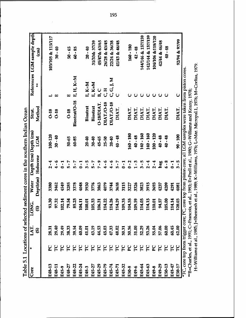
195

■3" «*J ts ON ON o a rH in in es u JH ON in m CO CO JH rH rH CO ON

ON

IN ON

•a in ^2 JO 3! en 51 o tN IN CO 5 cu rH o in m o tN en en VO VO CO CO m m rH VO CO

—H a E n

Ü

rH ^ ve CO ^< en VO fl< en *a< rH 1« rH rH rH X* X*

«a 1 ■ «a «a «a «a ^ «a «a «a «a ■ «a ID O rH

en o 1-H

o en

o in

o v©

o CM

en en rH

IN

m

CO

VO s eM

en 51 rH

O VO rH

9 VO

rH

<*<

S rH

VO O

s o rH

->*

o

ON

cu u e 1-

* *

s II

II II

8 »"

.2 U cu

es E tt X u £ O 0*co «

£ ON "^ P ^ VO- * ON c ET2

•^ Ä ^ •2 ^ -j Ml Wtf *W

-J tu tu tuK tuv tu pa o J u u U u u u u U u

c <M o 00 CO CO

CO rH

i

§ ra

(S )H k.

< CO rH

i 0

CO

0 H H' H H H H' H" H H 2 i

1H rH «1 B3 i

rH 5 Pm4

< < < -< < <: < < <

Ö •** o 6 0 hi

05 o KM

D Q 5 Q 5 Q NX

Q 0 l-x

D 2 c fr ? * u

C 2

s 6 D D

T3 E W ^^

X!

Q

E u

ex, ä <-;

£ H-»

o (A

J3

s o CM rH

o m VO

in CO

o o m o m

o CO o CO rH

CO o VO rH

o VO rH

o es rH

CO CO o o rH

E 3 5 1/5 n ii

-J

cu C cu u o

i o 1-H

1

o en

NO i

rH

Ö in i SO

1 rH

© CM

m

o en

■

in

0\ 1

in es

VO ■

VO i

o <*

rH i

O VO rH

i

o

en i

O

rH

in

O

rH

i

O O rH

x* i

o ^<

60 «0

o

CO 1

rH i

i o ON

m

S ü J

;-, ON Jin

& -a E

.s CO CU

D "o S

E

CS ** '© in m O en in tN ^ ^ in O O rH en M N X VO O en

H- *H *TT 52 Cu II "a, II ^!

0 k. E -v £; o cu ^^ O CS ON in CO CO o vfi en ON 5 CO in t-s VO ?i m en IN ON rH rH

A4 X CO VO ^< CO IN TJ< en ts vo f> in rH CM CM rH ON a o ON CO

NC ON rH 0)

n 4ri

a* en «* in CS en o ON b> co O Is ve rH es en CO ON VO eM es o

£ en CD ** en en *tf en en en t en en en en en en en en ■<* x* t **

g 0

0) CO

o «M ** s in rH rH en r^ 3 VO ON in in ON m m rH tN O x* en M« CO ^-»

2^ * * • en W rH eS rH O en en CM CM en in in o rH O in o rH o 0 w IN *S 5^ iri «rf d in vd «t «* "*' ON ^5 ON >*' x* d *' iri **' d o <" Xi

CU z B

ON er» O rH

t«. CO O o o o rH rH rH O o O rH rH rH ON o rH cs W M? W rf.2 s

o y o g ÖS u 1-1 PH e S

% r2 * "53 o fe II en b II ^

V*H

< i-i o ON en 3

OS

ON rH ON en m en fS rH VO O ON VO «* NO o m o in U in gJ .v CO bO rH ON

0 CO C

w en GO ON OS

en CO d

© i-5

rH en

m

3' o iri IN

q CO

en d

in d

q rH CM en

O in

o ts

o d d

o es'

-J CM (S CS en en rf «* "* Tf "<* <* in in m m m m in VO VO VO bO ON rH •fi ON v J3 rH ^H 0

re £ -s * * u U U U U u U U u U U U U U U U U U U U U u O S J)

04 H H H H H H H H H H H H cu H H H D- H H H H OH > K o$5

1-t cu "5 3 in

en 1H r-> es >* tN ON ON ^t 7-i es TJ< en ON m tN t> O JS > U (J ||

H * * *

u 1H rH OS CM es fS en cs es t^ IN tN en CO VO VO VO CO es rH 1< rH

1 1 CO

i CO

i m

i CO CO

1 in

i CO

i in in

i in

I m

1 in in

1 o

i ON m in

1 ON ON

i O

1 m

i O o ** «* ** <tf -ef T* «* ** <* <* "* ** i* m «* «* ** ** x* in <* m

H U tu tu tu tu tU tu tu w w tu tu tu tu tu tu tu u tu tu tu tu tu

196

30°N

Oc

30° —

60°S —

30°E

Figure 5.1 The map of selected cores from the southern Indian Ocean. The locations of the fronts (STC=Subtropical Convergence, SAF=Subantarctic Front, and APF=Antarctic Polar Front) in this study region are also indicated.

197

5.2.2 Stratigraphy and sample selection

Twenty-two deep-sea cores in the Southern Indian Ocean were selected

for this study. Sediment samples were taken from core tops and last glacial

maximum (LGM) levels to assess changes in the intensity and latitudinal

distribution of radionuclides and particle rain rates during two time intervals.

Core tops were assumed to be Holocene in age. Two depths of samples within

the LGM level (17 ka to 23 ka) were taken and made up into a homogeneous

sample to represent the LGM level in each core. LGM depths in cores, also

indicated in Table 5.1, were established either from their 81&0 records or diatom

stratigraphies (Burckle and Cooke, 1982; Burckle, 1982; Burckle et at, 1987). The

stratigraphies of these samples were provided mainly by Dr. Burckle at LDEO.

Many of these cores were also analyzed for 5 1$N by Francois and Altabet (1992);

the micropaleontological techniques for identifying the Holocene and LGM ages

were described in detail in a published paper by Francois and Altabet (1992). In

these samples, I analyzed 231p3/ and xh and U isotopes. Percentages of opal and

carbonate in the sediment samples were also determined; I calculated their

fluxes, including terrigenous flux, by normalizing their contents to the

unsupported initial 230xh concentration.

5.2.3 Downcore profile on the APF in the southeastern Indian Ocean

The percentage of carbonate was measured in addition to the radionuclide

contents. The core is from the location underlying immediately south of the

present-day Polar Front (APF) in the southeastern Indian Ocean. The sample

materials and the chronology data of core MD88-773 were kindly provided by

198

P* V

0)

o u

u

CO ■<-> fÖ

Q

R I

SI 2 2 In v

lid I

* 3

I" g *

o a; 0 «9 o J

•52 D C i a; i—J bO •

O >,

iriU 0) 13

.Is PH OH

°8,8

199

Dr. Laurent D. Labeyrie of Gif-sur-Yvette, France. The chronology of MD88-773

was determined by Labeyrie from 8 ^O stratigraphy (Figure 5.2). There were

eighteen samples from the core top through the LGM sections, which I analyzed.

The results are discussed in association with data from the transect to examine

the latitudinal variations and time variations of Th and U isotopes, 231pa/ and

fluxes of major sedimentary components. The depth-time model results for

establishing ages of MD88-773 were obtained by assigning the core depths 0 cm,

260 cm, and 350 cm as ages of 0 ka, 9 ka, and 18 ka, respectively. Between these

depth, linear interpolation was used.

5.3. RESULTS

Radiochemical data are given in Tables 5.2 through 5.4. Decay-corrected

unsupported radioactivities and the radioactive disequilibrium relationships for

these samples are shown in Tables 5.5 and Table 5.6. The features of the

radionuclide results are described as follows.

5.3.1 Uranium contents of the transect samples

As shown in Table 5.2, for the Holocene sections of the samples near the

Antarctic continent, uranium concentrations are remarkably high. Lithogenic

materials contribute a large fraction of the detrital uranium present in these

samples, since their 238u/232xh activity ratios displayed an average crustal

abundance of 238y and 232xh. The component of uranium which derived from

seawater is estimated by measuring 232-rh and 238u/232xjl activity ratios; the

200

c « OJ u o c to

£ I O co

g O

C o

•J3 u QJ CO 4J <J QJ

(0 a OJ c QJ u

"o

OJ

co 0) OH o

4-1 o co

»H

OJ »H

3 co ns OJ

CN in

OJ

oc «Xr to c ^ 9

iß ■£> co e N 9 a o<

co a N 9 S OH

rH .»

es M SI •C OH

o .fee co -i 2 s

OH g

D ~

z O

5

2 o U

ißo^tNnHnHnificcnHHOvoooHNnoco rH*rtHrHrHrHrHrHT—IrHrHCNr-I^C^^^^inNNnH ödöööoööööööööööööööi-Hr-5

mtNnnnnnmnntNnNtNNcNtNNNNNN pppppoopppppooppppoppp

^-^ ■ ^. ^—i i ^, v ^ ^»v i ^ ^*», ^»» ^"s *s^\ ^^ ^> ^»n. #«^ ^*\ —i ir\ i rs \.r*\ ^^ ^N.1 b in o « \c o\ B » *

ovoooooooo OOOOOOscNOsOs

ON CO 00

. . in IT) vo Ö (N CN co in o o »*

*OHcoin*ifivcininvOHir)H^rtNNtNnrt>üif)

CN Ö

^ in oo CN T-H T-H

<tf CO rt T-H rH in ts vo , . T-H rH CO T-j CO P

ÖÖÖÖÖÖÖÖÖÖÖrHÖÖCJÖÖ

in rH O tX 00 Tf in so vo K

vo vo O OS rH Ö

ooinvoinvoocNooovovrHsoo'^incDOrHCMOin^ COVDCOtNinTrOOinvOOqON^rHCvjrHCOCOOVrHrHCNVO ÖÖÖÖÖÖÖÖÖÖÖÖrHOrHrHrHÖrHÖCJrH

moNmootNOvocNeovotvoot^vocorHvotvtN. CNrvCNrHrHCOCNrHrHCOrHOrHSOrHrHrHinTJJ ÖÖÖÖÖÖÖÖÖÖÖÖÖÖÖÖÖÖrH

^t< ON CO ^i vo in Ö CO CO

^ONOnOivDH

in^^dco^NOTfN

in O "5* rH \o vo 00 K Os t-s rH rH

rH IN

OOvOCOtN.cOtNO inN^NH^Nr)

^OvOSOVvÖrHTjH'HHOV

ocNosinooooovocops ^coinN^otomnN». ^inHcNNNH^nooi«) M \D 1* M N ^ tO N \C N M' u, r, v, v, i, r. w. v, w », w

CO^incNCOOOsKoOOlNvOrHCNCOOOOSvOCNCNCNO COCOrt*COCO^COCOCO^COCOCOCOCOCOCOCO'!*<r}*rJ<'«^

o co

CN CO in CM

CO Ov OS R in

oo

O CO CO

y-\ CO a vO

CN OS CN

in in

OS in g in rH

o in o o

CO o o o

in o

vo o rH rH

<* o

OS o rH <* o

T-H •^ in o

o CN

rHOOsCO^OSrHOSCOCOCOCNrHsO co -^ ■<* co in p p -- — — — — -- od os os oo os o

in ö co ö co TJH in t< oo

_ OOsvOrJHsOOinO coinptNCNjppp^p ÖÖrHCNCOin'tNOOCN

[NNNtnn^tni^^HiHiininmininmin^vovo

ft H N N ^ N CT\ CTi if H N <t « Oi « t> N rtrt^NNNnNNNtsS«K**C*BNrt«IH i i i i i i i i i i i i i i i i i

löooiöiöioioioiooosmioososoioo ■ it i i oo oo m oo oo ^ ^ ^ ^ wwwwwwwwwwwwwwwwwwwwmw

201

s 1-1 "Ö

0 w'

• *■* in $ co d N 9

0»

£ ^^ 3 O (A 8 B OJ 5s 5 a o ,*■*,

* rH ^0

C o

a g « cm

&4 -rj *■> u o; tß

U ai

CM 60

9^ c r*3 & (0 H -Ö Ü ^^

s o o ^p ij 9 1 1 ££ M-l ^^ o

X! OH 8* s o Q (A

• 1-H o •

3

0) 0

lH fl CD «3 H 0) < s J

co in « 0) j-

•9 o U

H

_ co NO —j-^cj—.^jTHOoooo^jtSfOcDcoooN.^—; CM ^* en co

do Cod Cööööd ö CcModdddd fi rl

co o

co o •d CO o

CO o TJ CO o co

o CM O

CM O

CM o CO o

tu o o

tu 1—1 -<*

c w ON CO

tu CM ON

C W CM rH

w o in

w ON CO

w ON CO

w o CM

W o

vo ts NO If) NO ON r-I T-1 CM ON

c CM CM CM CM CM CM o o o o o p ■'- w w w w O 00 p ß w o _

CO ON ON CO in rH rH CM CO ■«* CM CO

S oo TJ c

CM O

i w ON in in

Tf _; \o co _; ^ rH T3 rH rH ^3 rH d Cod

HHHnifl-iOinoONONNJN ..CMC0C0C0CMy00'«ittN.NOCMin0qyrH

C O O O O O O CcMOOOrHOd C rl

CM CM _: O O T3 d d C

ON CO CO CO d d

in CO ON NO CM ^ _: O O. ON O fN •* ^?

C d d) ö r-i ö ö C COCö^öKöNOS;

ONtvinooooN—jco

dddrHod Co

NOoD^j^o-jinoocof^—jNotxoo-^minoN-jNO

do Cod G d> ö ö d> ö d> CCMOOOOOCM C ^

CMOO—JrHON-JNOtSON inco^?ONo"oNCMNO do C ts t% C CM co co K cö K

O O CM —: rH rH . . Ov000^?NCtNCM00C0

C ON TJ5 ocj vö oo 3 oo in ^J ^

T# rH C NO

o CM ON in 00 on o NO CO ON 3 00 in fN NO co in CO ts. ON rH rH on NO "tf 00 rs "tf CO

fc NO hs in rH CM CM CM T-i ON co O ON 00

CO 3 irS CM CO o ON 00 O IV NO rH CM CO 00 ON NO fsj £! CM o co -tf CO co ^ CO CO co rf co CO CO CO co co CO co

** "<* "* ■^

O ro

CM CO in "1 CM

r-i CO rH CM NO ON in ON in in rH

in o CO

O CO CO CM CM CM in in o rH o o o co ON ON R in

oo O Ln NO ■<* •«* T* Tj< ON «tf Tf o s in o o o o rH rH rH O o rH rH rH o CM

co o ON

00 ON ON CM CM CM

CO rH rH rH ON

I i i oo oo in ^3* "9' ^3* WWW

CO "^ co in 00* ON CO CO

?M CM I i

X 00

W W

ON rH O O O rH

CM CO in co

W W

o\ co co co CM rH m o co o co 3j in tN oo ■<* ^ ^ *^

ts ON & T* rH CM CM tN IS ts

I i i i 1 in in in in in ^^w ^^p ^^P ^^r ^^P w w w w w

rH v£> O co m o O O rH in m in

CM to ao vc in O ON r* in x* WWW

ON NO "^ CM CM O CM co in in in in

3 CO SO

if» in ^* ^ WWW

CO I

ON

NO O o o t< d in NO

ON CO CM rH ■ i ON O «* in W W

in o rf O d CM NO NO

ts ts x* rH

in 6 rf in w w

202

ts. 00 00 Q

C o «

3 (A 01 t-l

u •J3

13

>

3* in

co ^

>

03

I OH

CO H NO CO CM o o o o o © © © © O

i—IT-IT-ITHCNONOON''*£S poooo»-<pppp ©©ddoddod©

^^O^OO^T-H.THHcOOO^tsOcOCNin

GGdddoded©

P©©0.Po©©oH OrSrSOOr-Ji-^r-^r^O

>

•d H*

00 g

>

•d CO

f OH

•d *•* CO

f •a

Si •d

f o*

73

f-a

0

■* in o oo o o

CN n\ <M 2 oo

o o

o o

<tf 00 Tt< NO in m

CN fN o o o o

o o I-H l-H fN ro co CM

r-i o o

1-H

8 CM O o

T-H

s fsl O

CM o o CM o o

O Ö o o o o o o

oo T-l

o

NO T-H fN <—>

en CO o

Cs. in o

00 o

ON o 1—1

NC ON o

T-l

00 o

Oi-joOOoocJeoOOcJOOOoo©

v£> CO ON ts lO 00 «* O O O O O Q O o o o o o o p d © © d ö ö ö

O © ON NO NO TH H O © Q O O O O O ö ö d ö ö

O ON T-I ts ts O rH i-< CM CO "* CO o o o o p p ö ci ö ö ö ö

O00tsN000ts.T-Hi-Hi-l coONONfNcooNvocorN '^cocoTjH'^cococoin ÖÖÖÖÖÖÖÖÖ

ts. O - . VO ON co ^ NO

dodo

oo NO ts 53

co Tf in o in in NO in Fs ON ^ ON CS rl d H H

S H If T( lO g © © o © ,-4 Ö © © Ö

in CM

NO 00

CM ">tf CO O CM T-H

ON CM ©

d

CM in

N N Tf N O © © O odd©

H CO © ©

CN t-l CN CN o © s CN CO

© o © o ©

O ON i-H O ON CM

O l—i t-l

in ■*- <tf in oo g ts ON

O i—i O »—I o o

8 a ^ ^ * ON 00 ON ON

o o l-H O O

O\tstsTi<'«tfc0''S,'"tfiO S©o©©oo©© ©oo©oooo ddödödödö

cNt^NooinovONOtv NococoNoin^NocM'* T—IT—IT—IT—IT—IT—IrHi—ICM

000000000

CO T-H CO ND ts Ov CN rH CM i-i TH CN © TH ©©odd©©

CM co in oo rH o oo TjH © P © "tf NO ■<*

NO IN NO NO NO ^t NO

CO If) ON CO ts 00 © « « m t flt m »

ON I-H

ON l—l

O o

NO o 00

NO in

in ts CO ON © d HNntlfi^CfftJj

vO'tlßT-iCONOT-iCNts ©©rHCNi-H^CNi-l© ©©ooooppp dicicidöciödc)

oooocMtsNocoinoNin Tf00i-HC0i-HC0ts,T-lO Nrin<!|ia\oo»o\N d>öd>d>d>dööö

O\tslT)00C000NONDcN P00©l-I0l-HT-<T-J cidööciciöcidi

coT-HfMinT-HcocMinT-i 0)<*(Nj^q'toqtOiH COCÖTjHinNOtsNONONO

ooooooooo ONONONOooooininin cj n ui X » H ^i 00 ri

rt H H N N N «

O 00 ts 00 oo HN^**SHS

ooooooooNO^ONOoooomiftin -- -- ONNCONOfMlftvcoOrHlTOO CM ID

203

D V

I OH

*H •o 0 <

o X 0)

W X V H O- Fi

o CO

rt fS (A OH H-l u QJ V)

rH to

C m «H ji

5 H

o to l-J •-J ^ ffi

oo to

T3

<u p ri 00 0> CD

NJ O 3 E Ü «1« X CO

01

5 VH JB £ ft «3 ro (U r>i Oi o o NJ 4-> o X X w J3 O H

• 1-4

T3 o ro

2 cs cu X o 73 X bO <HH o «

CM

fO

1 OH

TJ CM

4-> o X fcO

3 u o CO 1

OH « X •o u H ID in V 0) o

■*! U

H

OCMoc?c?r"Jc$©©'"1'-iOCNlCOrN|COCOO,*r^v0.v*? ©od©o©d©©dd©ddd©d©ot:?T?rr

in "* <N O O r-l

CM ©

rf n N N 00 \C o N \o ■* * in ^ in © o © © © ©

o © © © © © © o o © o

t^in^OOOCslOOOvCNtSrHCOrH t^vOLnintsrororfOcsioo-^ ©©T-tOrHrHrHi-4rH©OCN ödöööööööööö

OriOOffiNNOOi\CNN >cinN\CNnina)0\t^ ööödd>d>d>c5öö

^N»o\innoNNinn (*nnoinqo;inif)nn

HHNrHN^ciddddd

o Tt<cot-ioscMi-ioscooNO\in cMCNcoc\l©Oi-ii-icMOtv

es ts in i-H i-i H TH N « O 00 00

d d

ON in

grHrHirjNÄtN^tsvD^n^vcinoqqgg^^ ■^oovooT^inrH^ooooSHOw^Oi-ioor-i^o-:,-^^: r^ m m ■« »*\ vr\ iv\ *^ •* m ~ »* «3 K. nv in ^ * W U n oo oo o °. '""' °° T—l SJ5 <T\ » in H * w

tscNin'^voo\rHooo\oo©voo\TH n^p)Ninn»if)^»»NON ©dddddddddddrHd

tnCOOsOsrvO'vrHr-l HnNMOOHlfj rHT-HrH©r-5d©r-5

OS ON

IN \o CO © Os in

t^ CM in Csl

SiftSSwös^c*

CO rH tNN^t N » ffi * H N « n ' * « N N iHTHaiCN|csirjmfNiNt>.tNrxfr)oov©vDvCoocNliH^<r-i I I I I I I I I I I I I I I I I I I I I I I aocoinaoaowoomwmmmin©ONWina\os©mo ^ ^ ^ ^ ^ ^ ^ *^ ^ ^ ^ ^ ^ m *<*»* ^ ^ ^ ^ in ^ in wwwwwwwwwwwwtuwwwwwwwtuw

204

2 u

bC

JC »rt i-J

C o U in in 0)

I

o X

XJ H o CO

lH CO CM

ft co CM

D oo to CM

5 oo co CM

to CM

A H CM to

H o to CM

to CM

o X o en CM

H

2 o U

2

2 u i-j

X MM

O (S o o ö Ö

co co rH O ö d • i

in t^ rH CM

d d

o o co K rH CM O O d d d d III!

NO i 5\ CM N R ^ H O (N ^O ° ^

Ö9ddd9

in co oi

1

t"N ON l—i 00 in NO NO in 0 O O 0 O o o o

IN ON T-H 00 NO O TH NO ON t-s NO r^. OOOOOO ö ö d di ö ö

00 Cv TH NO O NO CO CO 00 NO NO rH T—I rH rH rH O rH

d d d d d d £

rH ON 00 00

rH NO

O O O O

00 in o 00 in o co co NO -«a« tv NO ö ö d> ö ö ö

CN ^ co in in NO ON O NO ON rH rH tN CN H O O ri N O O

CM d

K o o o rH O

CN O o

in CM co co ON CM P p p p NO CM r-5 rH rH rH O rH

ON in CO rH CO ON CO ON p CM ON CM ON p O rH rH O rH O rH

CM ON

O

O NO ON in CM rH

ON "3<

00 NO CO

0 CO CO

NO CO

CM 00

ON CM

CM

NO CM 0 ON in

CM rH co

0 CO CM

NO CM

m o N in 00 CO NO NO

CO IN CO rH O rH rH CM

ON NO in 00 in co

CO CM o o d d

in K in ist« d d

m ^t CM CM CM co p p nj in p NO O rH rH r-i rH O

00 CM

rH 00 O rH

O O ON 00

NO

co

o 00 NO in _^ H vc <* ^ 5; in in ON in no _* —i __i _^ »*-'

00 rf NO NO in o NO CM co in CM co

^ n in N » N 3 tN ON O Tf CO CM ^1 00 Tji ON t< ON Tf £j

in d

in rH

co"

CO r-l H H ffi

1 ■ 1 00 00 in "^ ^ "3* WWW

ts CM <# N W Oi <* H N «* fO » « N N

QoaomoominininmmooNirtinoNONOifio wwwwwwwwwwwwwwwwwww

205

I 00 00 Q

3 CO QJ VH

i3 C QJ c o OH

o U

QJ

to « QJ

*0 c C8 co QJ

T3

g o

cc i-i

3 to S

T3 Ä «3 3 « U NO iri QJ

I

O X QJ

H e co

En rH co CM

o X QJ «8

pH rH CD CM

O X QJ

JS H o co

X QJ «

rH co CM

X QJ

H o co «M

60

60

.60

OH

60

OH T3

D u

60 g •a o* 4M w

<

X!

QJ U

Q

N CO 0\ O O O o o o

ifi (N n n H vo tN tN tN

ÖÖÖÖÖÖÖÖÖÖ

oo in IN oo tv oo oo o o o o o o o o o © o o o o

co so NO co oo NO NO o o o o o o o © o o o o o o

00 ON

CM 3 s CO tv 00 OS o T-H 1-1 CM

IN NO

ON CO Iß HMO CM CM CM © © ©

S ?! ?l ?l © ON tN co ID CO rH Tf rH CM CM CM © © © ©

SO CM

IN in ON © in © 00 © CM CM CM rH

© rH rH rH rH r-i

CM in ON rH ^ O

O CM 00 ON rH ON ON © CO CM rH tN rt< NO

T}< O in © © ON tN «# O rH CM in

N 3 N S IN 00 rH VO

NO in in ON

CM rf NO oo in CM ON rH 00 ON

NOinNOrNNONONOTfNO^*CO"!j*inNOtNINNONO

in CM

in CM co CM in ON 00 © CM rH rH ON © rH rH rH rH C5

00 © Tt< ON CM 00 Ö T-i Ö

CO CO NO K t-v ON 00 tN

NO in rH © 00 ON

© O O © rH O ©

ON rH ON rH in tx NO CO 00 ON ON CM

NO in NO NO in m NO

ON in CM r= CO

CM ON o 00 © in rH tN

ON CM © CM

■^ NO co CO co in in NO in in in

© ON ON O CO CM CM CO do©©

rHOOCOCOtsincOCMrfONONtvrHrH COCMCMCMCOCMCMCMCO^CMINCMCM ©OÖ©Ö©Ö©©ÖrHrHrHrH

in IN to in CO ON N© CO © © rH CM

O CO IN CO rH CM »* NO

ON CO IN GO © co ^ ^ w oo frj ^5 |ft VO ON

o o ON ON

© © © © © © © ON © GO CO m in ID

Nfnin«ONrt<*»H HrtrtrtHNNtN«

»»coocooNONONOcocoinmin 0,iHiHiHtNNnnn«f)<»«*^

206

c o U

in

I

m o

•e

o H

S ■6

fr S

Q

d d d d d d d ooi-HiDinvoKomcN

rHOrHrHrHOdOOdd

CO tv co r\i oo IT) in 00 rt* v£> in IN T»H 00 in o ON rH rH rH rH rH rH rH rH co CN ■<* rH rH o o rH O rH

o O o O O o O o O o o O o o O o O

OOtvrHVOrHT^VOin'^Ln CNJTfcocÖKrt'incovpvDin

-* 00 00 ^ ^ VD IN

rH CO rH CM rH rH IN in rH IN

CS CO rH fsj Vß T* P rH O O) © p rH rH rH O rH rH

oo*minvONO\"!fHOtn ONcoo\int>'«*ppoqo\o\o\ OrHOrHrHrHrHrHOOdd

O GO b» 00 00 noooK««9iO«nifliflin

207

formula to compute the authigenic uranium is same as used in Chapter 3. The

authigenic uranium activity is relatively higher in most of the sediment cores

underlying the present-day position of the Polar Front Zone (Table 5.5). The

authigenic uranium makes up 40% to 80% of the total uranium for the Holocene

sections for these samples in PFZ.

For LGM sections, a higher value of total uranium is still found in the

southernmost core; slightly higher values of total uranium are found in the LGM

sections relative to the Holocene sections of the cores in the PFZ and SAFZ. The

authigenic uranium of samples in the PFZ, however, shows a large scatter in the

changes between the LGM and the Holocene.

5.3.2 Unsupported Activities of ^Th and 231Pa Df the transect samples

The unsupported initial (decay-corrected) concentrations of 231pa and

230jh were calculated using equations 4-1 and 4-2 in Chapter 4. The ages of

sediment samples used for decay-correction of 230xh and 231pa were based on

the chronologies of the cores given in Table 5.1. The ages of the core-top were

assigned as 0 ka, and the LGM level sediments were assigned 18 ka. Table 5.5

provides calculated results of decay/ingrowth-corrected scavenged 230Th and

231pa, based on the above calculations for both Holocene and LGM sections.

These values are the activity of these nuclides at the time the sediments were

deposited. The unsupported activities of radionuclides on both Holocene and

LGM transect samples display a random variation. The lower activity of

230Thex° is found at the PFZ for the Holocene transect. In contrast, the 231paexo

activity is relatively higher in the cores from the PFZ for the Holocene sections.

A peak of the 230xhexo activity is found to be coincidentally at the position of

208

SAFZ during the LGM; while peaks of 231Paex° are found in both SAFZ and PFZ

regions.

5.3.3 Radionuclide results from MD88-773

Total uranium and authigenic uranium of MD88-773 are plotted in Figure

5.3. A pronounced increase in total uranium is found starting at the LGM (18 ka)

and still remains high during the late isotopic stage 3, while much lower

activities are found during the deglacial and the Holocene. Detrital uranium in

isotopic stage 2 and late stage 3 also show higher values than those during the

Holocene; however, detrital uranium has contributed to only a small fraction of

the total uranium, while the rest is authigenic, implies that uranium may have

been added to the sediment as a result of reducing condition in the sediment

(Cochran and Krishnaswami, 1980; Barnes and Cochran, 1990; Klinkhammer and

Palmer, 1991). The calculated results of 230Thex° and 231Paex° for MD88-773

are based on the chronologies given in Table 5.4 and the data shown in Table 5.6.

5.4 DISCUSSION

5.4.1 230xh-normalized paleoflux

5.4.1-a The ^^Th-normalized total flux for the Holocene transect samples

The 230Th-normalized flux method is applied to reconstruct the particle

flux in the present and past ocean. The equations (3-10 and 3-11) are used to

compute the flux.

209

i i i i

o

G « u

13 O

3 en « 0)

2

e s c to

c 0)

4-1

«« CD

i i i i i i i i

D

/ □

/

cf \

\ Ck

* □

: /

in

_ o

i i i i i i i i 11 "i" i i

in

o to

in

_ o

o o

o in

o o

o o

IS 00 00 Q

o u

0) be

CO 3 Cß

_ co

3 •i—i

C «5

3

C

3 in —H

to 0 H

CO

c o •»-I 4->

cr .a a*

bo 0 ££ 3^

'S JS RS u

| w .3 cß

c to 3 u

0) bo 3 * bC 3

S/indp

210

The method tends to correct for post-depositional sediment redistribution,

and provide information on net rain rate after dissolution. The flux, therefore, is

interpretated as net rain rate after dissolution. These fluxes, it should be

emphasized, are representative of pelagic rain rate rather than sediment

accumulation rate; each data point represents a measurement of flux at that

particular time. The latitudinal variations in 230xh-normalized total flux for the

Holocene and LGM sections of the transect samples selected for this study are

plotted in Figures 5.4 a and b.

The values of total flux range from 0.6 to an extremely high value of 8.56

g/cm2/ka (Figure 5.4a). The extremely high value occurs in the E45-47 core top,

which contains low activities of both 230jh and 231pa, The core top was taken

from a trigger core, which is believed to provide minimal disturbance, so

contamination by older materials from the deeper sections of the core is a less

plausible explanation for the extremely low activities of 230xh and 231pa.

Sediment composition in the E45-47 core top (Table 5.7) indicates that the high

flux of this sample is mainly due to an extremely high flux of terrigenous

materials; the flux values of opal and carbonate remain very low. The low

concentrations of 230xh and 231pa and extremely high terrigenous flux suggest a

massive input of ice-rafted material from the continent. Comparatively high

230xh_normaiized t0tai flux is also noticed in two other core tops (E50-8 and E50-

13). The high flux seen in E50-13 might also be due to dilution by massive ice-

rafted debris as seen in E45-47. Unlike the cores E45-47 and E50-13, the opal

component of the E50-8 core top (immediately south of the APF at ca. 52° S,

Gordon, 1982) constitutes a large portion of the sample. These two core tops

(E50-8 and E50-13) were taken from piston cores, so they might be contaminated

with older materials from the deeper core sections, however.

211

10.00 - i i i i i i i i > i > i i

'_ a. Total Flux (HL) STC T

SAF

i i i i i i i i

7 APF i

i

i

8.00- /1

£ 6.00 - Ng

u DO

4.00-

/

2.00- : A

(o)

i i i i i i i lL ä

0.00- i i i i i i i i i i i i i r—i iii i i i i r r in i i i i i —i—i—i—i—i—i—i—i—

25 30 35 40 45 50 55 60 65 Latitude (°S)

"ab

10.00

8.00

6.00

4.00

2.00-

: b. Total Flux (LGNI)

0.00

_l I l_l I I I I I ',''' I I I 1 I I I 1 I I I I 1_J I I I I I I I I I I I L

STC SAF APF

I I I I 1 I I I I | I I 1 I | FT ] I "| ' I I I I | I 111 | I-"I I I "| I I "I I""

25 30 35 40 45 50 55 60 65 Latitude (°S)

230, Figure 5.4 Th-normalized total flux of the Holocene sections (a) and LGM sections (b) of the transect sediments from the southern Indian Ocean.

212

H &

c o

■e U

O 5?

Si o u

US

O CO CO SO TH \o in 00 00 q ö r-5 ö Ö rH

in o o H \c q rH © rH

ON CM CO CO sO SO 00 00 Ö Ö Ö Ö rH CM

ro co in o CO ON © rH © rH

in in

CM CM SO rH H N If) N

rH rH rH CM 00 rH

^oifiin^oo^Nifjin^aingjvcsgjinvo qHOOoqqriqqqqHooHNq^rj Ö©Ö©'©©©Ö©©ÖÖ©'Ö©©©©©

00 00 sO o tN* rH

tN CO CO _ ___ _. SO CO ON ©in00NOinKbN^^C0rHrH©©rHrH©

©ÖÖrHÖ©©©©©'©©©ÖÖÖ©©©©

00 in CO SO rH in CNI 00 ON TJH in •* tN tN ON

sOONOOONSOsDtNrHfMCMCOOOgN inTJJSOCM^SOinvOrHrHCMCM©

o o o

Ttf<rHOOON©CMinONOrHtx.COOOCMin3;ls£> ©rHOrHrHrHrHrHC0C0inc0ininC0003 ppppppppppinp^tfsqoqoqoq ©ÖÖÖÖÖÖÖÖOÖrHÖ©©©©

CM CM so

rH tN <tf ON

00 00 N o in so in in so so so

CM CM CM

so in in in in CM in so SO 00 ^ T}H CM 00

rH CO

0 ^ !5 rH CM 00

CM

00 rH 00"

tN CO CM CM CM CO Tf CM

00 so Tf CO tN in O Ö

rH O tN CM ON CO 00 so

oooooooonoinooino tNcorHtNrHoqsqsqcMsqoqsqinsqin cÖcÖ^l'cMCÖrHrHSOrH00rHrHO\tNCO ONONONOsONONONOOONOOONONCOrHCO

R © SO © in in in in so ON rH in Tf

J^ J^ © © SO rH in

00 ONCOCMCMCOOOrHinOin O 'H^COOOsOlN.rHCMrHvqtS.

i ÖrHÖrHrHrHCMCOCÖCO

IN ts. ts!

in co CM CM CM

5 o

O^ CM © T}< SO 00

CM CO CM 00

K in in tN

?*

00

so CO rH CO

rH © ON CO "3* co "tf ^t co in 06O\ON00ON©rHC0^

OONSO"<tsD©in© OCMCMO©©^©

irisoodÖHNPJiritsödN ■^•«tf^ininininmininsososo

ONrHONCOCOCOCMrHSO ©©rHinocoocoin

CO iH ts CM «* K 6N 9> <* H N CO 00 VO

I I 3 HrtONNNNMNNNN^

ooooinoooomooiAinmininifto

CO ON co t> bs VO » CM rH ** iH

• 1 1 1 1 1 ~ O ift o

ir> ^ iß ON Ift W ON ON ^ji ^51 ^sp ^J ^Ji

213

w "«3

in

NO vO o CM ON CM r-t CO

NO ON

ON O CM

NO NO

in NO

in in 3 00

o ON oo tx

rH rH

00 Tf CO o 3 ON

ON rH

O rH CO o o o o rH O r-l l-H rH r-l CM O co

rH ON ON

00 O

00 o O rH o o

CM 00 <* in rH CM 00 Ö rH CO

ON rH "tf ON 00 ON Ö C>

00 o o ON CM O

CM O

rH O

o O o O

ON rH IN rH rji NO

CO t% NO CM 00 t<

IN O 00

in cö ON ON

■^ ON O O Ö Ö

O ON CO "«JJ *T 00 ON ON CM CM CM

CO rH rH rH ON

oö ob in *ur ,|5* *^ www

tN O in CM 00 rH 00 ON

O CO oo in CM rH

ts o in rH o in rH rH rH rH rH rH Ö Ö © © © Ö

CM CM ON rH rH O Tf -<* co in oo in © d ö d ö ©

© oo CM

00 NO "tf CO rH «ef O rH O NO CO O o in •<*« co ■<* tx cö © © d d d

ON CO rH CO "t Tjt O §h Tt rH CO CM ON CM © O O O O O O ö ö ö ö d> d> ö

NO 00

NO in co rH o in ON ^ ON 00 rH CM O O O O rH CM ©odd©©

CM CO 00 CO ^ rH rH CM rH tN in O Tt* N. ON CO NO ON in IN. *t © rH O O O rH ©

CM

d

co ,,, in co in in rH £4 NO CM in r-j © I»; ^ (•) ff> m 't "^ rH CM rH rH rH

NO _ 31 o o NO o in _

_ ON 00 © in in

co" 00 00" ON d d CM co CM •* co in

00 rH CM 00

in o co o o o ON in Tij 00 NO CM rH 06 CM in rs in ON tx vO NO NO NO

«vj tr> "^ in m ON S g CO NO CM IX

o o in CM

o in in o in rtf co in p TJJ CM CM CO CM iri

ON 00 CM NO 21 3 b

O O

Tt* NO ON ON

O CM

in co ON hs

in NO CM tx NO 00 «* CO

d ON oö in IN CM NO NO "St1 NO ^ rH

, _• rHONCOCOCOCMrHNOOONNO COinOOrHinOCOOCOinOCMCM 06 ON d

co "^M 0\ o m o 3 NO _ _. _ O O O Tf o

CO mbsOOOOrHCMCOintvOOCM nft^^^^^y^iHKKininKinNOvDvd

N N ^ tN » * * rl N >*CO » « N N IIIIIIIIIIIIIIIIIII oooomooinininmininooNinmoNONomo

wwwwwwwwwwwwwwwwwww

214

The ^SOxh.jrojmaiJzecl total flux in Holocene samples from the Polar Front

Zone on average are higher than those in the SAFZ. The range of total flux (0.93

to 1.55 g/cm2/ka, if I exclude two extremely high values from the samples near

the continent as mentioned above) in the PFZ is higher than that in the SAFZ and

north of the STC (0.6 to 1.13 g/cm2/ka). Sediment composition in the PFZ

indicates that biogenic opal contributes most of the total flux; while in the SAFZ

and north of the STC, carbonate is the dominant component.

5.4.1-b The differences in the ^^Th-normalized total flux between the Holocene and the

LGM of the transect samples

Data from LGM sections (Figure 5.4b) show that latitudinal features in all

distribution patterns of total flux are similar to those in the Holocene data. The

two northernmost LGM sections (cores E48-13 and E48-11) have abnormally high

values of total flux. The two cores have no associated trigger cores (D. S.

Cassidy, personal communication), as their recovery was not successful; thus, the

two core tops were taken from the piston cores, so the values may be false

because either an older sample was selected or the sample was contaminated

with older material. These data will thus not be included in the discussion. The

changes of 230xh-normalized flux between LGM and Holocene samples are

expressed as a ratio of LGM/Holocene (Table 5.8) and are plotted in Figure 5.5.

With few exceptions, I found that the extent and patterns of total flux show no

significant changes between the two time intervals.

5.4.1-c The latitudinal variations in extent of sediment focusing

215

o X eu

H o

NJ

s o

ffi 00 ts. CM CM tv ON in in NO oo co ON rH tv NO CO rH co

9 § CM

CM

NO

Ö co © Ö

co d

rH

r-5 ON

r-5 in r-5

00

©

p rH

rH r-5

ON

Ö co rH

1-H

r-5 in ö

in tv in c5

•J3 u u BH NJ 0) rH tc CO

4-1 CM u ^^ 0) to

g is V4H O

1?

a u

NJ

s E K o

CM CM CO NO N£> "* ON NO rH CM rH NO in tv. tv bs ON d 1-H I-H p Tf NO ON CO tN CO ■* ON P CM NO co CO ON

4-> o H

0 CM co

1-5 CM 1-5 r-5 in Ö ö ö Ö r-5 Ö r-5 r-5 r-5 d CM Ö r-5

rt O" c X 0) fl u

J3 C U NJ

"o X »3 ffi >* CO

CM K m co o 3 NO NO CO CM ■^ ON NO CM in CM ON

« e M in p p ^ NO NO in ON rH rH O CM NO 00 rH OS

£ o _y CM CO

r-5 CM

1-H r-5 in Ö d Ö ö Ö Ö Ö Ö Ö CM 00 Ö r-5 o> 01 -s S> o>

(0 U

-Q (A 01 X 3

CO

*Ö 0>

.a

X 1« NJ

5 "«3

O

s K CM o NO 1—1

m rH rH rH o NO NO in ON NO ■* 00 tv NO ON

$

co CM

O

CM

CM ON

CO

CO

rH

NO

rH NO CO

CM 00 Ö

00

CM

p r-5

p r-5

in ö

o CM

Cv

d

ta cv hJ o C

C O 4™j CM rH NO co o rH oo ■<* ■* rH oo ts. ON 1-H CM ^ co o i

o CO

.£> ö p p ON ON p ON NO tN CV tv CM o O CM ON tv CO o u «a U

1-4 T-5 Ö Ö r-5 Ö Ö Ö © Ö Ö Ö Ö Ö cö co O r-5

CM ^ *Ö

g — NJ

g a. 0

s o i—i IN 0\ r-t ON in ON «* in o 00 NO in rv ON o Ö in rH CO NO 00 ■^ NO tN in rH in ON oo 00 00 CO

Ü ö CM r-5 r-5 in NO Tj5 "* in CM r-5 Ö ö ö Ö d

t« o CM

hJ

£ o u

H 1—1 o co <<*< 1-H ON CO CO co CM NO O ON NO <* NO o o

o CO •<*< CO in P rH in o CO o in P CM CM o o o o •< OCJ ON CO ON r-5 CO ■* in Cv 00 ö r-5 CM CO in t< d CM

(A »J CM CM CO CO T* "* <tf ■^ <* Tf< in in in in in in NO NO

So S

£> u CO

in CO rH ts $

tv ON ON 1< rH s CO ON CO ts o>

IN

rH 1H CM CO CM CM tN t> IN op so NO CO CM rH rH

3 i CO

I CO

1 CO 00

1 CO

i lf>

i ID

1 I in

i ifi i ON to

1 in

■ ON

i ON

i i O O

fC o ^ 1< *tf rf ^ r* *# ^ ** ^ m «* "# <* <* *tf in in H U W w w W W W w w w W w w w u tu w w w

216

auaDoioH/WOl

217

Sediment redistribution by bottom currents is common and can lead to

errors in flux estimates based on sediment accumulation rates. As proposed,

230xh-normalized flux estimation can correct the error which results from such

sediment redistribution processes. In the following, I will compare the sediment

mass accumulation rate with the 230Th-normalized total flux to examine whether

sediment redistribution significantly affects the traditional estimation of

sediment accumulation rate in this region.

Sediment mass accumulation rate (MAR) can be calculated from the

assigned chronology and bulk sediment density. I used the average

sedimentation rate between the Holocene and LGM sections, assuming the time

interval to be 18 ka. Dry bulk sediment density (p) is estimated from the

following relationship between %CaC03 and dry bulk density as determined by

Froelich et al. (1991) for southern ocean sediments:

p = 5.313e-5[CaC03]2 + 9.346e-4[CaC03] + 0.3367 (5-4)

The comparison between MAR and ^^Th-noTmähzed total flux is shown

in Figure 5.6. Although there is a large uncertainty from the estimation of

sedimentation rate, it is still obvious that the two records of MAR and 230xh-

normalized total flux show a dramatic difference in the area between 48° S and

57° S. Sediment mass accumulation rate is 1.5- to 2.5-fold higher than 230xh-

normalized total flux in this region. The neighboring areas north of the PFZ and

further southward did not show significant differences between the two records.

This same feature has been seen in the SW Indian Ocean by Francois et al. (1993)

and in the Equatorial Atlantic (Francois et al., 1990). Based on same approach as I

have shown above, Francois et al., (1993) argue that the sediment redistribution

218

(vy[/zmoß)

B}vi uoi;Fminri3DB SSBUI juauirpas

in o in es

© in o in o

o o

(vyi/woß)

xriu p?joj pazipJuuou-iJi

0)

in VO

and

ple

s

o V©

tota

l fl

ux

nsec

t sa

m

in in

aliz

ed

ne t

ra

o 6 & in »H 0 ^^

L-no

H

ol

CD o ̂^ * „,

m 0> H £

2 V 0 • IN X ^ ftf ■M Q

o NJ et

wee

n ti

on r

at

in.

in Ja cö tu m

iso

n

um

ul

n O

a

a u cö 15 U -H DH tö TJ

o

B « £ o cn

.6 G

t

ma

her

n

in

if) c -a «1 W 3 & S ° bßT3 Qj

r7< ^ J=!

oez

219

processes are especially significant in the Southern Ocean because of the presence

normalized total flux show a dramatic difference in the area between 48° S and

57° S. Sediment mass accumulation rate is 1.5- to 2.5-fold higher than 230xh-

normalized total flux in this region. The neighboring areas north of the PFZ and

further southward did not show significant differences between the two records.

This same feature has been seen in the SW Indian Ocean by Francois et al. (1993)

and in the Equatorial Atlantic (Francois et al., 1990). Based on same approach as I

have shown above, Francois et al., (1993) argue that the sediment redistribution

processes are especially significant in the Southern Ocean because of the presence

of relatively strong abyssal currents associated with the Antarctic Circumpolar

Current and Antarctic Bottom Water. High bottom water velocities responsible

for the presence of scour zones was suggested by Watkins and Kennett (1972)

and Anderson (1990). Sediment winnowed from these areas is eventually

deposited in regions of lower current intensity, where sediment accumulation

must be in excess of the vertical particle flux originating from surface water. This

example illustrates the value of normalizing the accumulation rate of elements,

nuclides, or solid phases to a tracer such as 230xh whose known source permits

lateral redistribution to be identified and regional burial rates to be evaluated.

5.4.1-d Change in the focusing factor with time

With the MD88-773 core, I can examine variations of sediment focusing

with time. Suman and Bacon (1989) define a focusing factor (\|/) as the ratio of

230jh accumulated on the seafloor to 230ph produced in the overlying water

column during a time interval:

220

r1 V= 1 ex[230Th]cp dr (5-5)

ß Z (tl-t2Jr2

where ex[230Th]o is the activity of the decay- and ingrowth-corrected excess

230rh in the sediment, r is depth in the core, and t is the age of horizon r. The

values p, ß, and z are dry bulk density, production factor of 230 jh in the

overlying water column, and water depth, respectively.

Application of equation (5-5) to different sections of core MD88-773 (Table

5.9) indicates that the amount of 230xh which accumulated at the coring location

exceed that which was produced in the overlying water column by a factor four

during isotopic stage 3 and by as much as a factor about ten during the Holocene,

confirming that a large fraction of the sediment reaching the coring site during

these periods was brought by syndepositional redistribution processes. This

observation in MD88-773 from the southeastern Indian Ocean is in agreement

with those in the southwestern Indian Ocean by Francois et al. (1993). During

isotopic stage 2, \|/ is relatively less than during isotopic stage 3 and the Holocene.

5.4.2 Variations in (231Pa/230Th)ex° ratio

In this section, the latitudinal variations in the (231pa/230Th)ex° ratio

from the Holocene and LGM sections of the transect samples are discussed. First,

I will describe variation in (231pa/230xh)exo and discuss the factors causing the

fractionation between the two reactive nuclides in this study region. The changes

in (231pa/230xh)ex° ratio between LGM and the Holocene and the possible

reasons for the change will be discussed. Finally, I offer the study of a downcore

221

t-i o ri->

CD CO •<* o

bO c m

ON 1 co

s £

3 co u O fe

C O

•w4 *J u CM 3 & o rH ON o 1 •* rH CM

H

CO NO

IT) ON

in

o to CM

c o +d ffl NO NO

rH

s in

r"N s & u u

1 1

CM

Ö

p

ON CM

H

a. rH o NO

CM o CO

r-5 rH

o to CM

00 00 o s s bO

rH CM

ON in IN P

I-i O

H o CO

1 CO 1 §

u CM "O CM "<* o o ^^ NO in r<

«Ä »H

£> CO fC • «■* S NO 00 in

«4Ü en CO CO CO bO e ■a Ö Ö Ö

tt> 3 u £ o o o V4-H 00 in in "4-C

O c o

bC <

ON 1

o CM

o 00

rA

o in

fC ON "* 3 CM

^ "(3 U ON

in J5

s 00 NO CM

1

in rH

in 00

u u o oo m 01 D NO

CM rH

222

profile (MD88-773) immediately south of the APF in the southeastern Indian

Ocean to examine the time variations in the (231pa/230'jh)exo.

5.4.2-a Latitudinal variations in 0^-Vaß^Th)ejP ratios from the Holocene sections of

the transect sediments

Results of (231pa/230xh)exo ratios for transect samples are presented in

Table 5.5. In Figures 5.7a and b are latitudinal variations for both the Holocene

and LGM sections. One particularly interesting feature I found was that the

ratios from north and south of the APF show a contrasting pattern. The

(231pa/230xh)ex° ratios of the Holocene transect samples on the APF and south

of the APF (ca. 50° S to 57° S in latitude) are substantially higher than the

production ratio (0.093), and range from 0.107 to 0.156, with two exceptions from

the uncertain core tops (E50-8 and E50-13). The (231Pa/230Th)exo ratios of the

Holocene transect samples north of the APF (0.024 to 0.077), including sediments

north of the STC and in the SAFZ, are lower than the production ratio of 0.093.

One exception is found in the E48-11 core top but the value is only slightly

higher. On average, the (231pa/230xh)exo ratio of the cores (average ratio is

0.134 ± 0.006,1 standard deviation of the mean) on the APF and south of the APF

is about 2.6-fold higher than that of the cores (average ratio is 0.052 ± 0.005,1

standard deviation of the mean) north of the APF (Table 5.10). One extremely

high value is also found in the southernmost core E50-17 (Table 5.5).

The low values of the (231pa/230xh)exo ratios from the sediments north

of the STC and the SAFZ (Figure 5.7a) are comparable to those found in the

sediments from the central equatorial Pacific and Atlantic oceans, the East Pacific

Rise, the Mid-Atlantic Ridge, and the typical open ocean gyres (Anderson et ah,

223

0.25

0.20-

2 0.15

>

< w 0.10

0.05-

0.00

_l I I I I I I I I I I I I I L

a. Pa/Th(HL)

' I ' ' ' I ■ ■''■«'

STC SAF APF

J I I I l_*J I I I I 1—I 1 1—I L.

-1—i—i—i—i—i—i—i—i—i—i—i—i—i—i—i—i—i—i—i—i—i—i—i—|—i—i—i—i—i—i—i—i—i—|—i—i—i—r

25 30 35 40 45 50 55 60 65 Latitude (°S)

0.25

0.20

2 0.15 A

>

4S o.io-

0.05

0.00

J I l I I I I I I L l„ ,i I,, i \ ill',1 I l ■' ' ' J h i i i l i t i i

b. Pa/Th (LGM)

<- 0.093

STC SAF APF

i—i—i—i—|—i—i—i—i—i—i—i—i—i—|—i—i—i—i—|—i—i—i—i—i—i—i—i—i—i—i—i—i—i—i—i—i—i—r

25 30 35 40 45 50 55 60 65 Or Latitude ("S)

,231T, ,230 Figure 5.7 The ( Pa/ Th) ° activity ratio of the Holocene sections (a) and

LGM sections (b) of the transect samples from the southern Indian Ocean.

224

to

OH

to

u

(0 ±3

I O

«0 l-l

o>

o X a;

Is IS P* co CM

« e o

•e cs U ■ c o Z

o CO CM

ft l—i CO CM

to 01

N

6 u O c

o CO CN

to 0)

> OJD (0 iH

> <

o H o X 0i

H o co

ft rH co CN

X 3 C *^ a G a

•e n U ■ C o 2

x 3 C

o H

in

a; u

o

8 01 u « 5 o

X

c o • P*

00 o O "^ +1 JL oo sb- in

vO o o Ö +1 CO

vO

o +1 CO o

00 o

vO

o +1 II

in ~£-

ft ft

o o ^ ö oo ■H £ in w vo o d

CNI

CM

K CO o o o "* o 00 +1 II +1 II rH C rH

CM Ul

rH O

CM in

in o rH CO o TH o 00 -H II +1 II CM CO

c rH rH

ul

o o d +1 TH

O

a

in o o S-*.

o T—1 00 +1 II in CM c CM in '^^' o o

c 5

in o ^-^ o O +l II "tf CM c rH

00 >—'

o

N ft

N -^ ft N < to en ft

225

1983a and 1990; Yang et al, 1986; Lao, 1991; the Atlantic data in Chapter 4).

Higher (231pa/230xh)exo ratios in samples on the APF and south of the APF are

similar to those found in recently reported data of the Holocene sediments from

the Atlantic sectors in the Southern Ocean (Kumar et al, 1993) and from the SW

Indian Ocean (Francois et al, 1993), but the (231pa/230xh)ex0 ratios are relatively

lower than those reported data from the Atlantic sector in the Southern Ocean by

DeMaster (1979) and the typical Pacific Ocean margins by Anderson, et al, (1983b

and 1990), and Lao (1991).

5.4.2-b The causes for the latitudinal variations in (^^Paß^Th)ex0 ratio of the

Holocene transect samples

The conditions and processes that lead to the fractionation between 231pa

and 230jh have been discussed extensively in Chapters 3 and 4. In general, the

reactivity of each element toward scavenging by particles (often expressed as

residence time with respect to scavenging), the magnitude of the particle flux in

each region, and the lateral mixing rate in the ocean are believed to be the major

controlling factors. The question thus is whether a contrast in (231pa/230xh)exo

ratios between SAFZ and PFZ implies the different magnitude of particulate flux

between the two regions.

By examining the 230xh-normalized total flux from the Holocene sections

of the transect data in this study, I found that the average total flux north of the

APF is 0.82 ± 0.05 g/cm2/ka, while south of the APF, it is 1.15 ± 0.08 g/cm2/ka

(Table 5.10). This indicates that the total flux in the PFZ is only 40% higher that

in the SAFZ; while the (231Pa/230Th)exo ratio in the PFZ is a factor of 2.6 times

higher than that to the north of the APF. It appears clearly that the difference of

226

230xh-normalized total flux between north of the APF and PFZ is small, which

presumably indicates that the particle fluxes in the overlying water column in

both regions are of similar magnitude. In addition, a sample with higher total

flux does not always, as one would expect, correspond to a higher

(231pa/230jh)exo ratio. These suggest that the oceanic conditions in this study

region are complicated, and the total particle flux in the water column is not the

only factor which controls (231Pa/230Th)ex° ratio. Factors such as particle

composition or other processes might play key roles in causing the contrast

between the two regions (Figure 5.7a).

Particle composition is believed to control some degree of the fractionation

between 231pa and 230Th, although a unique conclusion is yet to be reached. An

obvious change in composition of sediments across the APF in the Southern

Ocean is the southward increase in opal content and decrease in carbonate

content (Figures 5.8 and 5.9). In the Holocene sections of the transect cores, opal

dominates in the PFZ samples, whereas carbonate dominates composition in

samples north of the APF. This implies that under relatively constant 230xh-

normalized total flux in both regions, the opal component seems responsible for

the preferential scavenging of 231pa than 230xh in the PFZ; on the other hand,

the carbonate seems unlikely to influence the fractionation between the two

nuclides. On the other hand, it is clearly shown in Table 5.10 that the difference

in average non-carbonate flux between north of the APF and PFZ is large while

the fractionation between 231pa and 230xh is great.

An affinity of 231pa for biogenic opal was suggested by Taguchi et al.

(1989). DeMaster (1979) also suggested that biogenic opal might effectively strip

the reactive nuclides such as 231p3/ 230]^^ ancj 210pb/ causing high inventories

of these nuclides to deposit onto the seafloor. In addition, the result from one

227

1111111111 111111111111111111111111111111111111111 if)

HJ

£ CJ cu E to

o •e

o u ^5 0^ 0^

« 1 1

• 1

1

o

L in

o CD

3

1111111111111111111111111111111111111111111111111

u cu CO

C «Ö j-i +j

cu C cu u

*o

cu X, 4-»

u

cu

• »-< *J tö

1—I

CO

CO

cu > cu cc c o

•e CO u

C to

OH

O

o o • o o

O o o 00

o o • o SO

o o • o

o © o

o o

in

cu

■s, u O

4-» H-> MH

J£

B o c cu

CO

O <

C to

§< cu C/}

U H

CU

C to

• i-H

0 CO

CU

%

00 in cu

00

CO O OH

C 2

«•a o 5-1

CU OH

o

PH co to

228

O

QJ

• »-I •4-»

JS CO

CO

QJ >

X

0) >J

C CO 0) u o c to

• l—I

C to C o

■fi CO u

£ 'S

QJ

o co

QJ

CC OH O

QJ N

13

CO C o 4-* u QJ CO

6 ti

B?[/ ina/S

O C

H o CO CN

ON

in a;

P-H +3

u 0) CO C CO M

QJ C QJ U O o

QJ

229

laboratory experiment showed that the AI2O3 phase gave a higher fractionation

factor between 231pa and 230jh (Anderson et al., 1992). Although a conclusion

that is globally consistent about how the particle composition affects the affinity

of reactive radionuclides such as 230xh and 231pa can not be reached from

sediment trap experiments and other sediment observations, the biogenic silica

might be an important phase for stripping 230xh and 231pa in the PFZ, since the

opal is a dominant component in terms of total bulk sediment or surface particle

material. Now, the question we are left with is: where do es excess 231pa in the

PFZ come from?

The lateral transport of 231pa may be the explanation for the contrast in

(231pa/230x]1)exo ratios of the sediments between north of the APF and the PFZ.

Model results have suggested that the lateral transport of 230jh is comparatively

small, but large for 23lpa (Bacon, 1988; Anderson et al., 1990; Chapter 4.4.3 in this

thesis). A (231pa/230xh)ex° ratio that is lower than the production rate ratio

implies that some fraction of 231pa in the water column has been laterally

transported to another region; whereas, a (231pa/230jh)exo higher than its

production rate ratio implies addition of 231pa from another region. The

(231pa/230xh)ex° ratio lower than 0.093 north of the APF, but the ratio higher

than 0.093 south of the APF thus indicates that a portion of the 231pa production

in the SAF and the STC is laterally transported out, thus causing the deficit in

these regions. The laterally transported 231pa would then be deposited to the

seafloor underlying the sediments of the present-day APF and south of the APF,

and cause the excess 231pa in that region. An additional source is the export flux

of Pa from Atlantic Ocean (Chapter 4.4.3).

Data from LGM sections show latitudinal features in distribution patterns

of the (231pa/230xh)exo ratios similar to those in the Holocene sections (Figures

230

5.7a and b). The amplitude of the variations for the average (231pa/230jh)exo

ratios in the PFZ and SAFZ are almost the same (within the error of 1 standard

deviation) as for those in the Holocene sections (Table 5.10). This suggests that

scavenging efficiency of both nuclides and the extent of fractionation between

231pa and 230jh were of the same magnitude during the LGM as during the

Holocene. This implies that the intensity of particle flux along with the degree of

the lateral transportation of 231pa from SAFZ and north of the STC to the PFZ

remains similar for both time intervals.

5.4.2 -c A downcore profile ofß^Paß^Th)ex° ratios and particle fluxes south of the

APF

The downcore (231pa/230Th)ex° ratio profile from MD88-773 (Figure

5.10) provides insight about temporal variations in the extent of fractionation

between 23lpa and 230Th. Theoretically, the (23lpa/230Th)exo ratio should be

a function of age only because of the constancy of the 235u/238u ratio in

seawater (Rosholt et al., 1961; Sackett, 1964), and it should show an exponential

decrease corresponding to a 57,200-year half-life. As seen in the downcore

profile, however, there are several maxima and minima throughout the core from

the Holocene to late isotopic stage 3, indicating variations in the degree of

differential transport of the nuclides in the marine environment. Maximum

(231pa/230xh)exo ratios are found in the deglaciation (12.9 ka to 15.9 ka), while

the lowest values are found during isotopic stage 2 (~21.8 ka) and late Holocene.

In these results, the first striking feature I noticed is that the

(231pa/230xh)exo ratios for all points in the profile are well above the seawater

231

B^UID/8

© to

in CM

O

CM

in in ©

o ©

i i i TT

D i

l

I

\ * □ /

E

i ' i i i i

/

[X ^

\

El o x X 3

\ *■» (0 o

* m

/

d

I I I I I I I I I

... «4

□

_j1II~

ID CO

o CO

ID CM

o CM

w

_ o

- Iß

o CO

o CM

in 1-1

o lH

in o o o o © o O o o o

PQ

P 60 CO

CO

CO f-i 0) > X

<s *cö o *J

*0 QJ N

•.-I i—■i

o

X H o

CO CM

73

§ 0

X cu ^^v

Ä H o co

CM \ JÖ &H m

rH K co CM IN

oo o 00 T—1 Ü in s

O 3 £ bC 4->

•iH .s (§/radp)/(8/mdp)

232

production ratio of 0.093, even the minimum values. The highest value of 0.28 is

three times higher than the production rate ratio. This implies a much higher

particle flux in the PFZ of the Antarctic Ocean. The minimum value is at least

60% higher than the production rate ratio. All of these (231Pa/230Th)ex° ratios

of the downcore profile are within the range of values from the near-by transect

samples. The comparison in (231Pa/230Th)exo between the Holocene and

isotopic stage 2 is similar to that reported from a core north of the APF in the

southwest Indian Ocean (Francois et al., 1993) but is in contrast to that data from

a core south of the APF in the Atlantic sector (Kumar, et al, 1993) which shows a

glacial reduction in (23lPa/230Th)ex° ran° by almost two times compared to the

late Holocene. The variations in the (231Pa/230Th)ex° ratio are correlated well

with the downcore variations in 230Th-normalized total flux (Figure 5.10). Since

the opal content dominants the total flux in this region, the time variations in

(231pa/230jh)exo ratio and 230 Th-normalized total flux imply the variations of

the biogenic opal production in the surface water as well (see discussion in 5.4.3

also). The relative constancy of (231Pa/230Th)ex° ratios and 230Th-normalized

total flux between the Holocene and the isotopic stage 2 supports the

observations in the Holocene and LGM sectios of the transect samples, which

suggest that there was no significant change in particle flux in this region during

the LGM. In contrast, the higher (231Pa/230Th)exo ratio associates with a higher

230xh-normalized total flux during the deglaciation (ca. 15 ka) could reflect

either a higher particle flux in the overlying water column or a higher degree of

horizontal transport.

5.4.3 Interpretation of the latitudinal variations in 230Th-normalized opal flux

233

Measured percentages of opal and carbonate, and results for the 230rh_

normalized total, opal, carbonate, and terrigenious fluxes in the Holocene and

LGM sections of the cores from the transect are presented in Tables 5.7 and 5.8.

The Holocene results are plotted in Figures 5.8 and 5.9.

5.4.3-a Latitudinal distribution patterns of opal content and ^^Th-normalized opal flux

during the Holocene

The Holocene opal content distribution (Figure 5.8) shows two contrasting

regions. Core tops from the present Antarctic Polar Front (APF) and from south

of the APF to 60° S have substantially higher opal content (45 to 80% opal) than

those immediately north of the APF, which have almost minor levels (<5% opal).

Latitudinal variations in 230Th_normaiizecl opal flux (Figure 5.9) show the same

distribution pattern. The high opal flux for the Holocene sections in the PFZ

ranges from -0.5 to -1.0 g/cm^/ka, whereas the low opal flux for the Holocene

sections north of the APF is <0.03 g/cm^/ka.

Previously published opal accumulation rates in the Atlantic sector of the

Southern Ocean by Mortlock et al. (1991) and Charles et al. (1991), and in the

Indian sector by Charles et al. (1991) parallel the pattern of latitudinal variations

in this study, but are higher by as much as 10 times both north and south of the

APF. This discrepency is also seen in other works (van Bennekom, 1988; Bareille,

et al., 1991) when compared to 230xh-normalized opal flux. The estimated

results of 230Th-normalized opal flux in this study are in agreement with the

results from samples in the Atlantic sector by DeMaster (1979), who estimated

the opal accumulation rate based on the sedimentation rates derived from a

uranium series disequilibrium method. Under such magnitude of the biogenic

234

opal accumulation rate, DeMaster (1979) has concluded that the Antarctic Ocean

seafloor is an important site in terms of the biogenic opal mass budget in the

ocean.

Table 5.11 compares opal fluxes estimated by normalization to 230xh with

those by others based on the mass accumulation rate of opal. The disagreement

between these estimates is largely the result of the syndepositional redistribution

effects due to the influence of strong abyssal currents in the APF region, as

discussed previously (Figure 5.6). As shown in Figure 5.6, the sediment focusing

effect is significant.

From the sediment trap investigations of biogenic opal flux in the

Southern Ocean (Atlantic sector), Abelmann and Gersonde (1991) estimated the

annual flux of opal at 700 m in the PFZ to be 1.53 g/cm2/ka, and at a 4454-m trap

in the Weddell sea to be about 0.4 g/cm2/ka. By comparing their trap results, it

is clear that an order of magnitude difference in opal accumulation rates (data

from Mortlock et ah, 1991 and Charles et ah, 1991) recorded in the sediments

could not possiblly be due to biogenic opal production in the surface water;

however, the 230xh-normalized opal flux that I estimated for the cores across the

APF in the Indian sector showed the same amount of opal flux as seen from the

trap data. This indicates that ^^^-xiorcnsXa&di opal flux provides a better

record of the magnitude of the biogenic opal production rate from the water

column. The application of the rate of opal accumulation history in the

sediments, thus, could have led to incorrect conclusions about the productivity

changes between glaciation and interglaciation.

235

32 QJ C 0) 0) c <u 0) c c 0) c S 0) u

o S "o £ O O jD s (0 £ "o O X r3 'S

X <J

o »H £ X

»H rJ

z o u QJ

»HS

5 u O u

2 u tu

o 4H u OJ

»H o u

«H o +■> U CO 0) <u (A CO OJ 0) u CO CO CJ U (A to

•J3 C ce co •J3 XI

S c co § S to «3 • iH

■M '"& % 4H 4J T3 'S < & & < < £ £

* PH < V

JC MM « o ^ in o

rH

CO M5 CO p

£ «3 r-5 00 rH in 1 1

"3 w I i 1 1

vO tv

CA tob vO rH o in ON "* ■<*

CO* Ö NO CM d Ö r-i

* PH

X PH 3

es "3 £ CO a, o u in o p CM

o Ö

CO cs ö

'1 rH 1 1

rH 1

CO 1

rH O rH

bO O u Z ^b

v£> y~< o rH T-t Ö O O CO Ö CM Ö O V Ö

IB 0) /—V

£ X >, T3

o G- 2 en C oo* /_v

*«3 CH

10

CO

O

CO

s oo rH

cF" o\ ON rH

rH ON ON

o T3 0) .a CM

ON • rH tv ^J r-H ON

Cß o ON . CO (Ö r-t

w rH r-1 u

rH

U

'S 4H 0) H*;

g JH

O

v

% in 0)

4H en •a u

o c 4H

OJ

0)

1 «H V

«H 0)

pa

>

to

1 Q

OJ *H «0

PD

rH 4-1

o o CO CM

d >

*H PH >H «s

r-H o

PH CJ

•si u (H CO

■s <! PH

236

5.4.3-b The conditions and processes responsible for the latitudinal distribution patterns

of opal

The record of the percentage of opal in the sediments is controlled by its

production from the surface waters, its survival from dissolution in the water

column and on the seafloor, and the dilution effect by other sedimentary

components. The strong global undersaturation of the ocean with respect to opal

implies that its dissolution rate should be unaffected by circulation changes-

unlike calcium carbonate dissolution which is governed by a variable depth-

dependent distribution of saturation states. The latitudinal variations in opal

content of the transect samples are affected by all these factors, but to different

extents in the different regions.

The contrast in opal content of sediments between PFZ and north of the

APF is obvious. The low opal content north of the APF is largely due to the

dilution by carbonates. In contrast, the extremely high opal content found in the

PFZ sediments is a result of the high surface diatom production. First of all, the

low diatom production in the SAFZ seems to be limited by available silica supply

Qacques, 1983). From the culture studies, Neori and Holm-Hansen (1982) and

Fenner et al., (1976) also found that the low optimum diatom growth rate is

caused by inefficient phytosynthensis due to the effect of temperature. They

found that most Antarctic phytoplankton enjoy optimum growth rates only

within a narrow temperature range between 0.8 -1.0° C and about 8° C; at

temperature greater than 8° C, the rates dropped off sharply. Neori and Holm-

Hansen (1982) concluded that in the presence of adequate light intensity and

nutrient supply, Antarctic phytoplankton photosynthesis is limited by

thermodynamic effects on metabolic processes.

237

The high diatom production in the PFZ is the result of a combination of

features such as: 1) a large supply of silicate and other nutrients transported to

the surface by vertical mixing (Gordon, 1986); 2) the melting ice, which lowers

salinity and density of the surface water layer, producing a stratified water

column; and 3) increased penetration of light into the water column which

promotes surface water productivity for the PFZ (Smith and Nelson, 1985;

Nelson et al., 1987). The stabilization of the surface layer has been suggested as a

necessary precondition for intense diatom blooms, so high diatom production is

often associated with the front system in the PFZ (Lutjeharms et al., 1985).

To have opal preserved in sediments, the signal of surface production

needs to be able to survive dissolution. The opal dissolution rate is difficult to

quantify. The question of whether or not variations in opal dissolution rate affect

significantly the contrast between north of the APF and PFZ is also difficult to

answer. The results from measurements of dissolved silica in pore water

(Ledford-Hoffman et al, 1986; van Bennekom et al, 1988; DeMaster et al., 1990)

and from incubation experiments (DeMaster et al., 1990) indicates that opal

dissolution rate is highly variable in the surface sediments. These studies suggest

that about one-third of the biogenic silica arriving at the seafloor in the Bransfield

Strait is dissolved, and that more than 60% of the silica in the abyssal sediments

and less than 60% of the silica beneath the PFZ within the Atlantic sector are

dissolved. One estimation from a factor analysis of the Southern Ocean by

Bareille et al. (1991) also suggests that about 40 to 70% of biogenic opal

production is dissolved for the surface sediments north of 40° S. Although the

extent of dissolution is apparently different in sediments from the PFZ and north

of the APF, there is little doubt that surface-water diatom production is high in

the PFZ compared to that north of the APF. The contrasting records of the

238

230xh-normalized opal flux of the Holocene samples between the PFZ and north

of the APF (Figure 5.9) also support this fact. Furthermore, the contrasting

records from the (231pa/230Th)ex° ratios between the two regions provide

another evidence to confirm the observations in records of the 230xh-normalized

opal flux.

Relatively low opal content is noticed also in the selected cores further

south which are believed also to be due to lower diatom production. Treguer et

al., (1983), however, have argued that low diatom productivity in the waters

poleward can not be explained by a lack of silica only. The reasons for such low

diatom productivity are not obvious, but it has been suggested that the

availability of other micronutrients such as iron limits the growth of diatoms

(Martin, 1990). Sea ice cover might play an important role in suppressing diatom

productivity in the Southern Ocean (Krebs, 1977; Whitaker, 1982).

5.4.3-c Interpretation of^^Th-normalized opal flux changes between LGM and the

Holocene:

The changes of the (231Pa/230Th)ex° ratio, and 230xh-normalized fluxes

(opal and carbonate) between LGM and the Holocene are presented as a

(LGM/HL) ratio, and are plotted in Figures 5.11. A major feature observed in the

transect samples is the much higher 230xh_normaüzec} 0pai flux north of the APF

during the LGM (Figure 5.11). These results from the Indian sector parallel those

observations made in the Atlantic and the Pacific sectors of the Southern Ocean

(Froelich et al, 1989; Mortlock et al, 1991; Charles et al, 1991). South of the APF,

however, the differences are small and not systematic (Figure 5.11). Thus, I can

239

25 30 35 40 45 50 55 60 65

Latitude (°S)

Figure 5.11 LGM/Holocene ratios of 230Th-normalized opal flux, carbonate flux, and 231pa/230jh ratio for the transect samples from the southern Indian Ocean.

240

not make the same conclusion as from previous works, which suggested a

decrease in the glacial opal productivity south of the PFZ (Mortlock et al., 1991;

Charles et al., 1991). My ^OTh-nonnaiized 0pai flux data, however, should offer

a better representation of the pelagic rain rate of opal, since the records of

accumulation rate of opal in the sediments could be biased by sediment

redistribution (as discussed in sections 5.4.1-c and 5.4.1-d).

Since the opal dissolution effect can modify the production record, and

since the change of dissolution rate between the LGM and the Holcoene in this

study region is not known, it is hard to draw a conclusion in terms of the LGM-

Holocene changes of these opal records in the PFZ. In the following and later

section (5.4.6), however, I hope to use the data of the (231Pa/230Th)ex° ratios in

MD88-773 downcore and transect sediments (Figures 5.10 and 5.11), and 230ph-

normalized total flux of the MD88-773 downcore (Figure 5.10) to comment on the

question whether the production increased during the LGM.

From the Holocene data (Figures 5.7 and 5.9, sections 5.4.2-a and b, and

5.4.3-a), we have found that higher (231pa/230xh)ex° ratios correspond to higher

230Th-normalized 0pa\ flux in the samples south of the APF. The data suggest

that a portion of 231pa in the SAFZ and north of the STC might be transported

laterally to the PFZ, where scavenging is enhanced by dominant biogenic opal

phase. By examining the (231pa/230xh)ex° ratios in the samples, most of them

(between the latitudes of 50°S to 55°S) show no significant change in the

(231pa/230xh)ex° ratio between the LGM and the Holocene if I take the

measurement errors into account (Figure 5.11). Although it is hard to estimate

how much 231pa can be laterally transported from the SAFZ to the PFZ due to

possible enhancement of scavenging when the silica front shifted northward,

carbonate still dominates the bulk sediments in the SAFZ, indicating that the

241

shifting silica would not significantly change the scavenging efficiency of 231pa

in PFZ during the LGM. The relative constancy of the (231pa/230Th)exo ratios

between the LGM and Holocene samples from the PFZ thus support the relative

constancy of opal production during the LGM compared to the Holocene (Figure

5.11). Consequently, the inconsistent variations of 230xh-normalized opal flux

might be due to differential opal dissolution between LGM and the Holocene in

each sample from the PFZ.

On the other hand, the changes I observed between the LGM and the

Holocene sections of the cores from the SAFZ and north of the STC characterize

higher percentages of opal, but lower percentages of carbonate during the LGM

(Table 5.7). The 230xh-normalized opal flux also shows higher glacial values in

this region (Figure 5.11); this implies that the opal production in the surface

water was higher in the region during the LGM. Since the opal content only

contributes a minor component in the sediments of the SAFZ and north of the

STC, the glacial age increase in 230jh-normalized opal flux in the SAFZ might

have resulted in little net production change when integrated over the whole

Southern Ocean. In addition, today the 'silica front' where surface water silica

concentrations (and opal burial in the underlying sediments) fall precipitously,

coincides closely with the dynamic APF; thus the glacial-age northward shift of

the "silica front" is the possible explanation for the changes of productivity to the

south and north of the APF (see discussion in section 5.4.6).

5.4.3-d Impact of APF northward migration on the latitudinal distribution and

magnitude of changes in opal flux

242

In the present-day Southern Ocean, higher levels of chlorophyll and

plankton biomass are often associated with fronts (Steyaert, 1973; Plancke, 1977;

Jacques and Minas, 1981; Allanson et al., 1981; Lutjeharms et al., 1985; Francois et

al, 1993). The Antarctic Polar Front (APF) is the most stationary among the three

ocean fronts in the Southern Ocean. Phytoplankton pigments are enhanced at

these fronts (Lutjeharms et al., 1985; Bidigare et al, 1986) which possibly as a

result of increased water column stability from sloping, isopycnal, or injection of

nutrients into well-stratified subtropical waters and mixing by cross-frontal

eddies (Pingree, 1978). As a consequence, the fronts create a region of enhanced

flux to the seafloor in comparison to neighboring regions. The high

(231pa/230jh)exo rat^ coincidentally high 230xh-normalized 0paj flux, and

relatively high 230xh-normalized total flux provide evidence for the enhanced

flux to the seafloor.

Whether the 230Th_normaiized biogenic opal flux is directly related to the

variations in hydrological conditions is not proved yet. However, the major

producers of biogenic opal, diatoms and radiolarian, survive within a

constrained environmental condition because of in addition to food supply,

light, ice cover, and water stability, their metabolic processes are strongly

controlled by temperature. As consequence, the "opal front" (a front acts like a

transition between a diatomaceous-domain and a calcareous domain) is

coincidendtal with today's APF position. Comparing the position of low-high

transitions in opal and carbonate contents or 230xh-normalized opal flux in both

Holocene and LGM sections (Figures 5.8,5.9, and 5.11) might indicate the

migration of the fronts. Data in Figures 5.8,5.9, and 5.11 show that the positions

of the transition zone of high-low % opal or % carbonate or their 230xh-

normalized flux might vary from 3° to 5°. This is comparable to results deduced

243

from micropaleontological studies. Several micropaleontological studies have

suggested that the position of the fronts in the southeastern Indian Ocean shifted

northward by 4-10° latitude for STC, and 4-6° for APF (e.g. Be' and Duplessy,

1976; Prell et al., 1980; Burckle, 1984; Morley, 1989). Although there are some

disagreements between different studies regarding the amplitude of the

migration, they all show a significant glacial shift northward in the position of

the fronts.

If northward migration of the hydrographic front system of the APF

during the glacial times is true, the glacial opal flux increases in the SAFZ would

not be due to the opal production changes, but it may be the result of the

migration of the opal front. As seen in Table 5.7, however, the increase in glacial

opal flux in the SAFZ due to the migration of the APF is small. In whole, the

small increase in opal flux in the SAFZ accompanied with the inconsistent

variations in glacial opal flux in the PFZ (Figure 5.11) imply little change in opal

flux in the Southern Ocean.

5.4.3-e Did biological production change during LGM?

As discussed above, the 230Th-normalized opal flux for transect samples

give little evidence for production changes during the LGM compared to the

Holocene in the Indian Sector in the Southern Ocean (see detail discussion in

section 5.4.3-c). The downcore profile of the (231pa/230xj1)exo parallels perfectly

with the time variation of the 230xh-normalized total flux in the MD88-773

(Figure 5.10), and both profiles clearly show the relatively small changes between

the isotopic stage 2 and the late Holocene. There profiles strongly suggest that

the production changes between LGM (isotopic stage 2) and the late Holocene

244

must have been small in the Southern Ocean. Moreover, since the MD88-773 core

already is situated underlying immediately south of the present-day APF, the

complication due to the migration of the APF would not affect the conclusion. In

conclusion, the production show little change during the LGM. In contrast, the

pronounced high values of the (231Pa/230Th)ex° ratio and coincidentally the

pronounced high values of the 230xh-normalized total flux were observed for

the period during the deglaciation (ca.l4ka to 15 ka) in the region.

Geochemical indicators of overall productivity are equivocal about net

glacial-interglacial changes. The more depleted planktonic b^C of the glacial

Antarctic sediments implies lower productivity (Labeyrie and Duplessy, 1985;

Keigwin and Boyle, 1985; Charles and Fairbank, 1990); whereas planktonic

Cd/Ca ratios suggest no net glacial-interglacial change (Boyle, 1988b; Keigwin

and Boyle, 1989). Another line of evidence about the change in production comes

from the transect tiß-^N data. Analytical results of SßSN were measured (by

Francois and Altabet, 1992) for many of the same cores from the same transect

samples I selected for the analyses of radionuclides and sedimentary components

for this work. The available data for both LGM and the core tops, while

principally from the samples between 45° S and 55° S, indicate that there was

relatively little change in the magnitude of the decrease from b^N nutrient-

depleted regions to the S^N nutrient -rich region. As proposed by Altabet and

Francois (submitted, 1992), and Francois and Altabet (1992), the 815N of

planktonic organic matter in surface water will increase with increasing nitrate

depletion due to the preferential uptake of NO3" during photosynthesis process.

Thus the small change in the latitudinal 5^N gradient observed in core tops and

glacial sediment sections also strongly argue against an increase in biological

uptake of nitrate in the Southern Ocean as the main mechanism for lowering

245

glacial atmospheric CO2. As a whole, both data from 230xh-normalized opal

flux and (231Pa/230Th)ex° ratio for the transect samples and for the MD88-773

downcore, the b^N gradient observed in the Holocene and LGM transect

samples, and Cd/Ca data in planktonic foraminifera would strongly argue

against increased biological production in the Southern Ocean as the main

mechanism for lowering glacial atmospheric CO2.

5.4.4 Interpretations of 230rh-normalized Carbonate flux

5.4.4-a Latitudinal variations of carbonate record, and changes between LGM and

Holocene

The transect samples show that the %CaCC»3 in LGM sections is in general

lower than that in the Holocene sections for the cores between 42° S and 55° S

(Table 5.7 and Figure 5.12). The difference varies from 62% to 91% in the SAFZ

and from 1% to 33% in the PFZ. With a precision in %CaCC>3 of about ± 1-5%, a

difference of 30% carbonate is significant.

The pattern of %CaC03 recorded in sediments is a result of the balance of

carbonate production, accumulation of non-carbonate sediments, and dissolution

of carbonate. The systematic LGM-Holocene variations in the ^SOTh.j-KHmaH^cl

carbonate flux, which is a quantitative value for the rain rate after accounting for

the carbonate dissolution effect, do show the same patterns as the variations of

carbonate content (Table 5.7 and Figures 5.11,5.12, and 5.13). Although the

percentage of non-carbonate also was higher during the LGM for the SAFZ and

PFZ cores, the variations in 230xh_normaiizecj carbonate flux indicate that the

%CaCC»3 cycles of the Southern Indian Ocean are not simply the result of

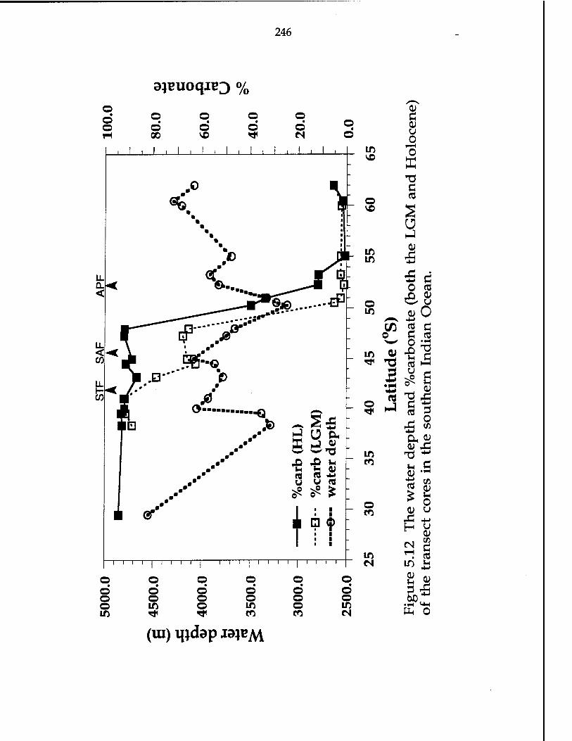
246

ajeuoquQ <>/o

o o

© 00

o o o o o

o o o in

© • o o in

o o o

© • o o m

o • o o o CO

o • o o in n

in

o v©

in in

o in

C U 0

1—1

0 X

CJ (0

U

•s ■5 c 0 «Ö es <u o

en 5 c o £ to ^^ 0 12 in

CO »-H

2 d

%c

her

n

o HJ ep

th a

n he

sou

t

in TO ~ en ^ s

o wat

or

es

en a» u

in ^ CO in ij

ft 0

(in) ipdap iajBA\

247

dilution by terrigenious and biogenic opal sediments; they must be driven by

changes in carbonate productivity or in preservation, or a combination of both.

The data of those cores from SAFZ between 42° S and 50°S or even more

northward to 28° S shows %CaC03 for the Holocene sections >90% (Figure 5.12),

even though all these cores are from water depths between 3200 m and 4550 m.

For cores from 50°S to 55°S, even though they are from shallower depths

(between 3100 m and 3900 m, in particular core E50-8 at 3100 m), %CaC03 is

lower than in those cores from deeper depths. These patterns suggest two things.

Firstly, carbonate production is higher in the region of 28°S to 50°S than in the

region of 50°S to 55°S. Secondly, most of cores are above the lysocline depth

which may be as deep as ~4000 m. The latter has been suggested by previous

reports from Holocene profiles of calcium carbonate which indicated that the top

of the calcite lysocline, a distinct decrease in %CaC03 with increasing water

depth, lies at about 4300 m in this region (Kolla et al, 1976; Lozano and Hay,

1976). Holocene core top distributions of forminiferal fragmentation also suggest

that a distinct increase occurs from 4000 m down, placing the top of the

forminiferal lysocline at this depth (Williams et al., 1985).

The high %CaC03 remains in the LGM sections in this region (62% to 95%

for cores from 40° S to 50° S, see Figure 5.12), the lysocline depths should have

been little variations, from the LGM to the Holocene. This seems to agree with

the conclusion from Hay and his colleagues (1976) who have suggested that the

site would have been above the lysocline continuously during at least the past

300,000 years. Since most of the cores (with the exception of E45-9, depth 4549m,

and/or E45-79, E45-24, and those cores south 57° S) from the southern Indian

Ocean for this study are above the regional sedimentary lysocline and the

lysocline depth remains unchange over glacial to interglacial, the data of the

248

glacial reduction in carbonate content and 230xh-normalized carbonate flux

(ranging from 0.01 to 1.4 g/cm^/ka for the Holocene sections, and 0.01 to 0.99

g/cm^/ka for the LGM sections of the cores from 42° S to 50° S (Table 5.7 and

Figure 5.13) thus are independent of the cores' depth. This implies that the

reduction is the result of reductions in carbonate productivity. However, this

suggestion is based on an assumption that there exists little carbonate dissolution

above the lysocline depth, and the lysocline depth is at same depth for all of cores

in this study region.

The similarity of glacial reduction in carbonate accumulation rate was also

suggested as a reduction in carbonate productivity by Howard and Prell (1992)

from the data in approximately the same region. They have argued that their

cores are well-positioned to sense change of the regional lysocline through time,

and lysocline depth during the isotopic stage 2 was about 600 m shallower than

at present. They thus thought that the carbonate MAR variations in their records

may be partly due to chemistry-driven lysocline variations, not changes in

carbonate productivity in surface waters. If the carbonate dissolution increased

during the LGM, as suggested by Howard and Prell (1992), the "true" carbonate

rain rate from the surface water column must have exceeded those records based

on the 230Th_normaHZed carbonate flux (because the method only provides the

records of the net rain rate after dissolution effect); thus, decrease in glacial

carbonate production should be more than observed from the 230xh-normalized

carbonate flux.

5.4.4-b MD88-773 carbonate profiles provide evidence of carbonate production changes:

249 -

(B>[/zui3/S) xnij a;euoqjB3

"aT Ift CN ff\ \© CO © rH IH d d d c> U

jD 1 1 1 1 1 1 1 1 1 1 1 1 1 1 «ft 'S

£ .o Q-P - 13

^ fa • \

o

■ \ ■ • \ • - 0 - ■J

L 1ft r~ 1ft

a;

u <2f WU JS Q <

li <

LL h

1

«

<*--©

Pr ^ ^^t^ ft

K^ ra* ^ ^

1

1

1

1

1

1

1

1

1 +

-*

45

50

5J 0

arbo

nate

flu

x (b

ot

n I

nd

ian O

cean

.

'* ■ C/ 1 fii -^B ^^ ^^ rt

'——«Q § 3 © HJ -I w

"OP JS> «53 5 SI .* 0> 0» &

.- © ° S ift

~ CO

dep

th

the

s<

..• x> ,p .2

X — c

ar

-- c

ar

—

wa

o CO

e w

ater

co

res

in

T : ♦ 1 i i Ift es

• 5.13

Th

ran

sect

C

1 1

•

1 1 1 1 1 1 1 1 1 1 1 1 1 1 1 1 1 1 1 1 1 1

o o o o c • • • • o o o o o c 5 •*-> o o o o o c D & a> o ift © in o u 0 Ift ^t* ^ CO cO c M

(ui) ipdap J9)BM •y-t <«H HH 0

250

It is possible to deduce whether the 230xh-normalized carbonate flux or

carbonate accumulation rate during glaciation is due to reduction of carbonate

production or partly due to lysocline variations. This is done by examining the

downcore ^OTh-ncHmaiizecl carbonate flux profile of core MD88-773 to LGM-

Holocene changes in carbonate flux in the northern APF. Core MD88-773 is from

a water depth 2460 m, were above the lysocline and poleward of the present-day

APF. Hay and his colleagues (1976) have suggested that the site would have

been above the lysocline continuously during at least the past 300,000 years.

Estimates of changes in carbonate flux over the isotopic stage 3 for MD88-

773 (Figure 5.14) show that isotopic stage 2 has an average carbonate flux of 0.08

g/cm2/ka, half the average for the late Holocene 0.16 g/cm2/ka, and almost six

times less than the maximum peak for the deglaciation (15 ka, 0.48 g/cm2/ka).

The similarity of the glacial-Holocene change in this shallow core to those from

greater depths on the southern Indian Ocean (230xh-normalized carbonate flux

from this study or carbonate MAR from the cores of the Southern Indian Ridge

by Howard and Prell, 1992) suggests that part of the glacial reduction in

carbonate flux is independent of depth, thus implying in reductions in carbonate

productivity. In addition, because MD88-773 is underline immediately south of

today's APF, the effect of northward shifting (as discussed in the following

section) opal-rich productivity regimes on carbonate records during the LGM is

minimized.

5.4.4-c The effect of CaCOfrCorgrain ratio on the interpretation of carbonate records

As discussed above, my data from the Southern Ocean indicate that

calcium carbonate preservation, and probably carbonate production, were

251

o in © 1ft q ri fi fi 6 d

1 I . 1 in

- c o>

D H _ o

« en 3 CO

I

I

<*

in

t-r 0» >

«a 0)

9 i

ii N C3 c o

□ M / • C

? 4 _ o •

o c

T3

E 4 &H

/ ■ CQ

P < in

_ f*

c o

CD <

X 3

'■<

- 0) N

C ^ , . • i—i

X 1—4 «5

^ B M o *«

b £ 0

\ O c 1 (0

■fi

u 0

□r' < * <

- ifi -<* 00 *-< 00 in Q f m

i

...tf.

< 2iS

•PI O 1 1

o

i ( 1 O o

1 1 '

o « 3

p*^ w

o 1ft © in c 5 ri fi fi

B>[/ UI3/8 V

© e 6

252

diminished during glacial intervals. The carbonate preservation, however, may

be ambiguous because the glacial reduction in the CaC03:C0rg ratio of the

particle rain may drive changes in dissolution within the sediments (Archer,

1991). The 230xh-normalized opal flux records (Figure 5.11) suggest a glacial

increase of opal between the present day's APF and the SAF, impling a higher

glacial opal production and thus a higher glacial surface productivity in the

SAFZ. These data, coupled with the significantly lower carbonate flux (Figure

5.11) imply that glacial CaC03:C0rg rain rate was lower than at present.

Consequently, the reduction of the glacial carbonate flux (discussion in 5.4.4-c) or

carbonate accumulation rate (Howard and Prell, 1992) might not be necessarily

due to the reduction of carbonate productivity but due to the increase of

dissolution. The decrease in the CaCC»3:Corg ram ratio and enhanced dissolution

would affect the shallow depth core the same as (or even more than) deeper

cores; this could be the reason we have the same carbonate flux variations for the

shallow MD88-773 core and for those deeper cores as well.

The APF position is believed to have migrated northward over the study

sites during the glacial stages of the past 500,000 years (See section 5.4.6). This

migration would add another complication to the variation of the carbonate

system, because today's APF position is also a boundary between a carbonate-

enriched and opal-enriched region; the shifting of the position of the boundary

might have caused a change in the CaCC»3:Corg ratio, which may be a result of

the shifting of the domains from calcareous to siliceous sediments. Since the APF

sediments might have sifted northward during the glacial, the CaC03:C0rg rain

ratio might have decreased, resulting in an increase in the dissolution of

carbonate during the glacial intervals rather than a change in carbonate

production.

253

REFERENCES

Abelmann A. and R. Gersonde (1991) Biosiliceous particle flux in the Southern Ocean. Mar. Chem., 35, 503-536.

Anderson, R. F. (1982) Concentration, vertical flux, and remineralization of particlate uranium in seawater. Geochitn. Cosmochim. Acta, 46, 1293- 1299.

Anderson, R. F., and A. P. Fleer (1982) Determination of natural actinides and plutonium in marine particulate material. Analy. Chem., 54, 1142-1147.

Anderson, R. F., M. P. Bacon, and P. G. Brewer (1983a) Removal of 230Th and 231Pa at ocean margins. Earth Planet. Sei. Lett., 66, 73-90.

Anderson, R. F., M. P. Bacon, and P. G. Brewer (1983b) Removal of 230Th and 231pa from the open ocean. Earth Planet. Sei. Lett, 62, 7-23.

Anderson R. F., M. Q. Fleisher, P. E. Biscaye and N. Kumar (1991) Anomalous boundary scavenging in the Middle Atlantic Bight:evidence from 230Th, 231Pa, 10Be, and 210Pb. Contin. Shelf Res. SEEP-II volume.

Anderson, R. F., Y. Lao, W. S. Broecker, S. E. Trumore, H. J. Hofmann, and W. Wolfli (1990) Boundary scavenging in the Pacific Ocean: a comparison of !0Be and 231Pa. Earth Planet. Sei. Lett., 96, 287-304.

Anderson, R. F., A. P. LeHuray, M. Q. Fleisher, and J. W. Murray (1989) Uranium deposition in Saanich Inlet sediments, Vancouver Island. Geochitn. Cosmochim. Acta, 53, 2205-2213.

Bacon, M. P. (1984) Glacial to interglacial changes in carbonate and clay sedimentation in the Atlantic Ocean estimated from 230Th measure- ments. Isotope Geosci., 2, 97-111.

Bacon, M. P. (1988) Tracers of chemical scavenging in the ocean: boundary effects and large-scale chemical fractionation. Philosoph. Trans. Roy. Soc. London A, 320, 187-200.

Bacon, M. P., and J. N. Rosholt (1982) Accumulation rates of Th-230, Pa-231, and some trasition metals on the Bermuda Rise. Geochim. Cosmochim. Acta, 46.

254

Bacon, M. P., C.-A. Huh, A. P. Fleer, and W. G. Deuser (1985) Seasonality in the flux of natural radionuclides and plutonium in the deep Sargasso Sea. Deep-Sea Res., 32, 273-286.

Bacon M. P., D. W. Spencer, and P. G. Brewer (1976) 210Pb/226Ra and 210Po/210Pb disequilibria in seawater and suspended particulate matter. Earth Planet. Sei. Lett, 32, 277-296.

Bard, E., L.D. Labeyrie, M.Arnold, M. Labracherie, J.-J. Pichon, J. Duprat and J.- C. Duplessy (1989) AMS C-14 ages measured in deep-sea cores from the southern ocean: implications for sedimentation rates during isotope stage 2. Quat. Res., 31, 309-317.

Bareille, G., M. Labracherie, L. Labeyrie, J.-J. Pichon, and J.-L. Turon (1991) Biogenic silica accumulation rate during the Holicene in the southeastern Indian Ocean. Mar. Chem., 35, 537-551.

Barnola, J. M, D. Raynaud, Y. S. Korotkevich, and C. Lorius (1987) Vostok ice core provides 160,000-year record of atmospheric CO2. Nature, 329, 408- 414.

Be, A.W.H. and J.-C. Duplessy (1976) Subtropical convergence fluctuations and Quaternary climates in the middle latitudes of the Indian Ocean. Science, 194, 419-422.

Berger, A. (1978) Long-term variationsof caloric insolation resulting from the Earth's orbital elemetns. Quat. Res., 9, 139-167.

Berger, W. H., and R. S. Keir (1984) Glacial-Holocene changes in atmosphere CO2 and the deep-see record, pp. 337-351, In: J. E. Hanse, and T. Takahashi (eds), Climate Processes and Climate Sensitivity (Geophy. Monogr. Ser. 29). AGU, Washington, D. C.

Berger, W. H., V. S. Smetacek, G. Wefer (1989) Ocean productivity and paleoproductivity-An overview. In: Productivity of the Ocean:Present and Past. John Wiley and Sons.

Biscaye, P. E., and S. Eittreim (1977) Suspendedparticulate loads and transport in the nepheloid layer of the abysal Alantic Ocean. Mar. Geol., 23, 155-172.

Bond G., W. Broecker, S. Johnsen, J. McManus, L. Labeyrie, J. Jouzel and G. Bonani (1993) Correlations between climate records from North Atlantic sediments and Greenland ice. Nature, 365, 143-147.

Boyle, E. A. (1988) Vertical oceanic nutrient fractionation and glacial/ interglacial CO2 cycles. Nature, 331, 55-56.

255

Boyle, E. A. (1988) The role of vertical chemical fractionation in controlling late Quaternary atmospheric carbon dioxide. /. Geophys. Res., 93, 15701- 15715.

Boyle, E.A. (1992) Cadmium and 813C paleochemical ocean distributions during the stage 2 glacial maximum. Anuu. Rev. Earth Planet. Sei., 20, 245-287.

Boyle, E. A., S. S. Huested and S. P. Jones (1981) On the distribution of copper, nickel and cadmium in surface waters of the North Atlantic and North Pacific oceans. /. Geophys. Res., 86, 8048-8066.

Boyle, E. A., and L. Keigwin (1987) North Atlantic thermohaline circulation during the past 20,000 years linked to high-latitude surface temperature. Nature, 330, 35-40.

Boyle, E. A., and L.D. Keigwin (1982) Deep circulation of the North Atlantic over the last 200,000 years: geochemical evidence. Science, 218, 784-787.

Brewer, P. G., C. Goyet, and D. Dyrssen (1989) Carbon dioxide transport by ocean currents at 25°N latiude in the Atlantic Ocean. Science, 246, 477-479.

Brewer, P. G., Y. Nozaki, D. W. Spencer, A. P. Fleer (1980) Sediment trap experiment in the deep north Atlantic and elemental fluzes. J. Mar. Res., 38, 703-728.

Broecker, W. S. (1971) Glacial accumulation rates and glacial to interglacial changes in oceanic mixiing. In: K. K. Turekian (ed.), The late Cenozoic glacial ages. Yale University Press, New Haven, Conn., pp.239-265.

Broecker, W.S., G. Bond, M. Klas, G. Bonani and W. Wolfli (1990) Paleoceanogr., 5, 469-478.

Broecker, W. S., G. Bond, M. Klas, E. Clark and J. McManus (1992) Origin of the northern Atlantic's Heinrich events. Climate Dynamics, 6, 265-273.

Broecker, W. S., and T.-H. Peng (1982) Tracers in the Sea. Palisades, New York: Lamont-Doherty Geological Observatory.

Broecker, W. S., and T.-H. Peng (1989) The cause of the glacial to interlacial atmospheric CO2 change: A polar alkalinity hypothesis. Global Biogeochem.Cycles 3, 215-240.

Broecker, W.S. and T. Takahashi (1978) The relationship between lysocline depth and in situ carbonate ion concentration. Deep-Sea Res., 25, 65-95.

256

Broecker, W.S., K.K. Turekian and B.C. Heezen (1958) The relation of deep sea sedimentation rates to variations in climate. Am. J. Sei., 256, 503-517.

Broecker, W. S., and J. Van Donk (1970) Insolation changes, ice volumes, and the 180 record in deep-sea cores. Rev. Geophys., 8, 169-198.

Busseler K. (1991) Do upper ocean sediment traps accurately record particle flux? Nature, 353, 420-423.

Buesseler, K. O., and J. E. Halverson (1987) The mass spectrometric determination of fallout 239Pu and 240Pu in marine samples. /. Environ. Radioact., 5, 425-444.

Burckle, L.H. (1984) Diatom distribution and paleoceanographic reconstruc- tion in the southern ocean-present and last glacial maximum. Mar. MicropaleontoL, 9, 241-261.

Burckle, L. D., and D. W. Cooke (1983) Late Pleistocene Eucampia antarctica abundance stratigraphy in the Atlantic sector of the Southern Ocean. MicropaleontoL, 29, 6-10.

Burckle, L. D., D. B. Clarke, and N. J. Shackleton (1978) Isochronous last- abundant-appearance datum (LAAD) of the diatom Hemidiscus karstenii in the Subantarctic. Geology, 6, 243-246.

Burckle, L. D., D. Robinson, and D. Cooke (1982) Reappraisal of sea-ice distribution in Atlantic and Pacific sectors of the Southern Ocean at 18,000 yr. B.P. Nature, 299, 435-437.

Burckle, L.H. and J. Cirilli (1987) Origin of diaton ooze belt in the southern ocean: implications for late Quaternary paleoceanography. Micropaeontol, 33, 82-86.

Campana, J.E. (1980) Elementary theory of the quadrupole mass filter. Intl. J. Mass Spectrom. 33, 101-117.

Charles, C. D., and R. G. Fairbanks (1990) Glacial to interglacial changes in the isotopic gradients of southern ocean surface water. In: U. Bleil and J. Thiede (eds.) Geological History of the Polar Oceans: Arctic Versus Antarctic. Kluwer Academic, Boston, Mass., 519-538.

Charles, C. D., R. G. Fairbanks (1992) Evidence from Southern Ocean sediments for the effect of North Atlantic Deep Water flux on climate. Nature, 335, 416-419.

Charles, C. D., P. N. Froelich, M. A. Zibello, r. A. Mortlock, and J. J. Morley (1991) Biogenic opal in Southern Ocean sediments over the last 450,000

257

years: Implications for surface water chemisry and circulation. Paleoceanogr., 6, 697-728.

Chen, J. H., R. L. Edwarddwards, and G. J. Wasserburg (1986) 238U, 234U and 232Th in seawater. Earth Planet. Sei. Lett., 80, 241-251.

CLIMAP Project Members (1976) The surface of the ice-age earth. Science, 191, 1131-1137.

CLIMAP Project Members (1981) Maps of northern and southern hemisphere continental ice, sea ice and sea surface temperatures in Auguast for the modern and the last glacial maximun. Geol. Soc. Am. Map Chart Ser., MC-36.

Cochran, J.K. (1992) The oceanic chemistry of the uranium- and thorium- series nuclides. In: Ivanovich, M. and R.S. Harmon (eds.) Uranium-Series Disequilibrium. 2nd edition, Oxford, Clarendon Press, 334-395.

Cochran, J.K. and S. Krishnaswami (1980) Radium, thorium, uranium and Pb-210 in deep-sea sediments and sediment pore waters from the North Equatorial Pacific. Am. J. Sei., 280, 849-889.

Cochran, J. K., H. D. Livingston, d. J. Hirschberg, and L. D. Surprenant (1987) Natural and anthropogenic radionuclide distributions in the northwest Atlantic Ocean. Earth Planet. Sei. Lett., 84, 135-152.

Cochran, J. K., and J. K. Osmond (1976) Sedimentation patterns and accumulation rates in the Tasman Basin. Deep-Sea Res., 23, 193-210.

Cooke, D. W., and J. D. Hays (1982) Estimates of Antarctic ocean seasonal sea- ice cover during glacial inervals, In: C. Craddock (ed.) Antarctic Geoscience, pp. 1017-1025, University of Wisconsin Press, Madison.

Curry, W. B., and G. P. Lohmann (1983) Reduced advection into Atlantic Ocean deep eastern basins during last glaciation maximum. Nature, 306, 577-580.

Curry, W. B., and G. P. Lohmann (1986) Late Quaternary carbonate sedimentation at the Sierra Leone Rise (eastern equatorial Atlantic Ocean). Mar. Geol, 70, 223-250.

Curry, W. B., and G. P. Lohmann (1990) Reconstructing past particle fluxes in the tropical Atlantic Ocean. Paleoceanogr., 5, 487-505.

Curry, W. B., J. C. Duplessy, L. D. Labeyrie and N. J. Shackleton (1988) Changes in the distribution of 813C of deep water ZCO2 between the last glaciation and the Holocene. Paleoceaogr., 3, 317-341.

258

Curry, W.B. and G.P. Lohmann (1990) Reconstructing past particle fluxes in the tropical Atlantic Ocean. Paleoceanogr., 5, 487-505.

Damuth, J. E. (1977) Late Quaternary sedimentation in the western equatorial Atlantic. Geol. Soc. Amer. Bull, 88, 695-710.

Date A. R. and A. L. Grey (1989) Applications of Inductively Coupled Plasma Mass Spectromerry. Blackie.

DeMaster, DJ. (1979) The marine budgets of silica and 32-S.. Ph.D. Thesis, Yale Univ., New Haven, 308pp.

DeMaster, D. J. (1981) The suppy and accumulation of silica in the marine environment. Geoch. Cosmoch. Acta,45, 1715-1732.

DeMaster, DJ., T.M. Nelson, S.L. Harden and C.A. Nittrouer (1991) The cycling and accumulation of silica in Antarctic deep-sea and continental shelf environments. Mar. Chem., 35, 489-502.

Duplessy, J. C, N. J. Shackleton, R. G. Fairbanks, L. Labeyrie, D. Oppo, and N. Kallel (1988) Deep water source variations during the last climatic variations andtheir impact on the global deep water circlation. Paleoceanogr., 3, 343-360.

Edwards, R. J., and W. J. Emery (1982) Australian Southern Ocean frontal structure during summer 1976-77, Aust. /. Mar. Freshwater Res., 33, 3-22.

Edwards R. L., J. H. Chen, T.-L. Ku, and G. J. Wasserburg (1987) Precise timing of the last interglacial period from mass spectrometric determination of Thorium-230 in corals. Science, 236, 1547-1553.

Emreson, S. and Bender, M. (1981) Carbon fluxes at the sediment-water interface of the deep sea: calcium carbonate presrevation. /. Mar. Res., 39, 139-162.

Falkner K. K. (1989) An investigation of the marine geochemistry of gold. Doc. dissertation.

Falkner K. K. (1991) Characterization of marine particulate material by ICPMS.

Finkel, R, S. Krishnaswami and D.L. Clark (1977) 10Be in Arctic Ocean sediments. Earth Planet. Sei. Lett, 35, 199-204.

Fisher, N. S., J. L. Cochran, S. Krishnaswami, and H. D. Livingston (1988) Predicting the oceanic flux of radionuclides on sinking biogenic debris. Nature, 335, 622-625.

259

Fleer, A. P. (1992) Updated determination of particulate and dissolved thorium-234. pp. 227-228, In: D. C. Hurd and D. W. Spencer (eds.), Marine Particles: Analysis and Characterization (Geophy. Monogr. Ser. 63). AGU, Washington, D. C.

Fleer, A. P., and M. P. Bacon (1984) Determination of lead-210 and polonium- 210 in seaater and marine particulate matter. Nucl. Instru. Methods Physics Res., 223, 243-249.

Francois, R. and M.P. Bacon (1994) Heinrich events in the North Atlantic: radiochemical evidence. Deep-Sea Res. (in press)

Francois R., M. P. Bacon, M. Altabet, and L. D. Labeyrie (1993) Glacial/Interglacial changes in sediment rain rate in the SW Indian sector of subantarctic waters as recorded by 230Th, 231Pa, U and 815N. Plaeoceanogr., 8, 611-629.

Froelich, P. N., R. A. Morlock, and A. Shemesh (1989) Inorganic germanium and silica in the Indian Ocean: biological fractionation during (Ge/Si) opal formation. Global Biogeochem. Cycles 3, 79-88.

Froelich, P. N., et al. (1991) Biogenic opal and carbonate accumulation rates in the subantarctic South Alantic: the Late Neogene of Meteor Rise Site 704. Proc. Ocean Drill. Program, Sei. Results, 120, 515-549.

Francois, R., M.A. Altabet and L.D. Burckle (1992) Glacial to interglacial changes in surface nitrate utilization in the Indian sector of the southern ocean as recorded by sediment 815N. Paleoceanogr., 7, 589-606.

Francois, R., M. P. Bacon, and D. O. suman (1990) Thorium-230 profiling in deep-sea sediments: high-resolution records of flux and dissolution of carbonate in the equatorial Atlantic during the last 24,000 years. Paleoceanogr., 5, 761-787.

Francois, R., and M. P. Bacon (1991) Variations in terrigenous input into the deep equatorial Atlantic during the past 24,000 years. Science, 251, 1473- 1476.

Francois, R., M. P. Bacon, M. A. Altabet, and L. d. Labeyrie (1994) Glacial/interglacial changes in sediment rain rate in the S. W. Indian sector of subantarctic waters as recorded by 230Th, 231Pa, U and 815N. Paleoceanogr. (accepted).

Francois R., M. P. Bacon, M. Altabet, and L. D. Labeyrie (1993) Glacial/interglacial changes in sediment rain rate in the SW Indian sector

260

of subantarctic waters as recorded by 230^, 231pa/ u and S^N. Plaeoceanogr., 8, 611-629.

Gardner, W. D. (1980) Sediment trap dynamics and calibration: a laboratory evaluation. /. Mar. Res., 38:17-39.

Gardner, W. D. (1985) The effect of tilt on sediment trap efficiency. Deep-Sea Res., 32, 349-361.

Goldberg E. D. and M. Koide (1962) Geochronological studies of deep sea sediments by the ionium-thorium method. Geichim. Cosmochim. Acta, 26,417-450.

Gordon, A. L. (1972a) Introduction : Physical oceanography of the Southeast Indian Ocean. In: D. E. Hayes (ed.) Anarctic Oceanology II: The Australian- New Zealand Sector, Antarct. Res. Ser., vol. 19, 3-10, AGU, Washington D. C.

Gordon, A. L. (1972b) On the interaction of the Antarctic circmpolar current and the Macquarie ridge, In: D. E. Hayes (ed.) Anarctic Oceanology II: The Australian-New Zealand Sector, Antarct. Res. Ser., vol. 19, 71-78, AGU, Washington D. C.

Gordon, A. L. (1981) Seasonality of Southern Ocean sea ice. /. Geophys. Res., 85,4193-4197.

Grousset, F., P. Buat-Menard, D. Boust, R.-C. Tian, S. Baudel, C. Pujol, C. Vergnaud-Grazzini (1989) Temporal changes of aeolian Saharan input in the Cape Verde abyssal plain since the last Glacial period. Oceanologica Ada, 11,177-185.

Grousset, F. E., L. Labeyrie, J. A. Sinko, M. Cremer, G. Bond, J. Duprat, E. Cortijo, and S. Huon (1993) Patterns of ice-rafted detritis in the glacial north Atlantic (40-55°N). Paleoceanogr., 8, 175-192.

Hall, M. M, and H. L. Bryden (1982) Direct setmates and mechanisms of ocean heat transport. Deep-Sea Res., 29, 339-359.

Hays, J. D. (1978) A review of the Late Quaternary climatic history of Antarctic sea. In: E. M. van Zinderen Bakker (ed.) Antarctic Glacial History and World Paleoenvironments, 57-71.

Hays, J. D., J. A. Lozano, N. J. Shackleton, and G. Irving (1976) Reconsturction of the Atlantic and western Indian Ocean sectors of the 18,000 B.P. Antarctic Ocean. In: R. M. Clines and J. D. Hays (eds.) Investigation of Late Quaternary Paleoceanography and Paleoclimatology. Mem. Geol. Soc. Am., 145, 337-372.

261

Heinrich, H. (1988) Origin and consequences of cyclic ice rafting in the northeast Atlantic Ocean during the past 130,000 years. Quat. Res., 29,142- 152.

Honjo S. (1980) Material fluxes and modes of sedimenatation in teh mesopelagic and bathpelagic zones. /. Mar. Res., 38, 53-97.

Honjo S and K. W. Doherty (1988) Large aperture time-series sediment traps; design objectives, construction and application. Deep-Sea Res., 35, 133- 149.

Honjo S., S. J. Manganini, R. Krishfield (1989) Cruise report: JGOFS leg 1 International study of the North Atlantic Bloom. Technical Report, Woods Hole Oceanographic Institution.

Honjo S. and S. J. Manganini (1992) Biogenic particle fluxes at the 34N21W and 48N21W stations, 1989-1990: Methods and analytical data compilation. Technical Report, Woods Hole Oceanographic Institution.

Houk R. S. and J. J. Thompson (1988) Inductively Coupled Plasma Mass spectrometry. Mass Spectrom Rev., 7,425-461.

Howard, W. R, and W. L. Prell (1992) Late Quaternary surface circulation of the southern ocean and its relationship to orbital variations. Paleoceanogr., 7, 79-117.

Hulmston P. and R. C. Hutton (1991) Analytical capabilities of electrothermal vaporization-Inductively Coupled Plasma Mass Spectrometry. Spectroscopy, 6, 35-38.

Hurd, D. C, and F. Theyer (1975) Changes in the physical and chemical properties of biogenic silica. In: T. R. P. Gibbs (ed.) Analy. Methods Oceanography, Adv. in Chem. Ser. 147, 211-239.

Jacques, G. (1983) Some ecophysiological aspects of the Antarctic phytoplankton. Polar Biol, 2, 27-33.

Jones, G. A., and P. Kaiteris (1983) A vacuum-gasometric technique for rapid and precise analysis of calcium carbonate in sediments and soils. /. Sed. Petrol, 53, 655-660.

Kallel, N., L. D. Labeyrie, A. Juillet-Leclerc, and J.-C. Duplessy (1988) A deep hydrological front between intermediate and deep-water masses in the glacial Indian Ocean. Nature, 333, 651-655.

Keigwin, L. D., and E. A. Boyle (1989) Late Quaternary paleochemistry of high-laitude surface waters. Palaeogeogr. Palaeoclimatol. Palaeoecol, 73, 85-106.

262

Keir, R. S. (1988) On the late Pleistocene ocean geochemistry and circulation. Paleoceonogr., 3, 413-445.

Klinkhammer, G. and M. R. Palmer (1991) Uranium in the oceans: Where it goes and why? Geochim. Cosmochim. Ada, 55, 1799-1806.

Knox, F. E., and M. McElroy (1984) Changes in atmospheric CO2; influence of marine biota at high latitudes. /. Geophys. Res., 89, 4629-4637.

Koczy, F. F. (1961) Ratio of thorium-230 to thorium-232 in deep-sea sedimets. Science, 134, 1978-1979.

Kolla, V., A.W.H. Be and P. Biscaye (1976) Calcium carbonate distribution in the surface sediments of the Indian Ocean. /. Geophys. Res., 81, 2605-2616.

Kolla, V., P. E. Biscaye, and A. F. Hartley (1979). Distribution of quartz in late Quaternary Atlantic sediments in relation to climate. Quat. Res., 11, 261- 277.

Krebs, W.N. (1977) Ecology and preservation of neritic marine diatoms, Arthur Harbor, Antarctica. Ph.D. thesis, Univ. of California, Davis, 1-234.

Ku, T.-L. (1966) Uranium Series Disequilibrium in Deep-sea Sediments, Unpublished docoral dissertation, Columbia University, New York.

Ku, T.-L. (1976) The uranium-series methods of age determination. Ann. Rev. Earth Planet. Sei, 4, 347-379.

Ku, T.-L. and Broecker, W.S. (1967) Rates of sedimentation in the Arctic Ocean. Prog. Oceanogr., 4, 95-104.

Ku, T.-L., W.S. Broecker, and N. Opdyke (1968) Comparison of sedimentation rates measured by paleomagnetic and the ionium methods of age determination. Earth Planet. Sei. Lett., 1-16.

Labeyrie, L.D., and J. C. Duplessy (1985) Changes in the oceanic 13C/12C ratio during the last 140,000 years: high-latitude surface water records. Palaeogeogr., Palaeoclimatol, Palaeoecol, 50, 217-240.

Lao, Y. (1991) Transport and Burial Rates of 10Be and 231Pa in the Pacific Ocean. Unpublished doctoral dissertation, Columbia University, New York.

Lao, Y., R. F. Anderson, W. S. Broecker (1992) Boundary scavenging and deep-sea sediment dating: constraints from excess 230Th and 231Pa. Plaeoceanogr. 8:

263

Lao, Y., R. F. Anderson, W. S. Broecker, H. J. Hofmann, and W. Wolfli (1993) Particulate fluxes of 230Th, 231Pa, and 10Be in the northeastern Pacific Ocean. Geochim. Cosmochim. Acta, 57, 205-217.

Ledford-Hoffman, P. A., DeMaster, D. J., and Nittrouer, C. A. (1986) Biogenic silica accumulation in the Ross Sea and the importance of Antarctic continental shelf deposits in the marine silica budget. Geochim. Cosmochim. Acta, 50, 2099-2110.

Lee, c, S. G. Wakeham and J. I. Hedges (1988) The measurement of oceanic particle flux- Are "swimmers" a problem? Oceanogr., 2, 34-36.

Leinen, M., D. Cwienk, G. H. Heath, P. E. Biscaye, V. Kolla, J. Thiede, and J. Dauphin (1986). Distribution of biogenic silica and quartz in recent deep sea sediments. Geology, 14, 199-203.

Lisitzin, A. P. (1971) Sedimentation in the world ocean. SEPM Spec. Pub., 17, 218-241.

Lozano, J.A. and J.D. Hays (1976) Relationship of radiolarian assemblages to sediment types and physical oceanography in the Atlantic and western Indian Ocean sectors of the Antarctic Ocean, in R.M. Cline and J.D. Hays (eds.) Investigation of Late Quaternary Paleoceanography and Paleoclimatology, Geol. Soc. Am. Mem., 145, 303-336.

Lutjeharms, J. R. E., N. M. Walters, and B. R. Allanson (1985) Oceanic frontal systems and biological enhancement, In: W. R. Siegfried, P. R. Condy, and R. M. Laws (eds) Antarctic nutrient cycles and food webs, pp. 11-21, Springer-Verlag, New York.

Luz, B. and N.J. Shackleton (1975) CaC03 solution in the tropical East Pacific during the past 130,000 years. In: W.V. Sliter, A.W.H. Be and W.H. Berger (eds.), Dissolution of deep-sea Carbonates. Sushman Found. Foram. Res., Spec. Publ., 13,142-150.

Mangini, A. and L. Diester-Haas (1983) Excess Th-230 in sediments off NW Africa traces upwelling in the past. In: Coastal upwelling: its sedimentary records, (ed. E. Suess and J. Thiede), pp:455-470. Plenum, New York.

Martin, J. H. (1990). Glacial-interglacial CO2 change: the iron gypothesis. Paleoceanogr., 5, 1-15.

Melkert, M., G. Ganssen, W. Helder, and S. R. Troelstra (1992) Episodic preservatioin of pterood oozes in the deep Northeast Atlantic Ocean: Climatic change and hydrothermal activity. Mar. Geol, 103, 407-422.

264

Milliman, J. D., C. P. Summerhayes, and H. T. Barretto (1975) Quaternary sedimentation of the Amazon continental margin: a model. Geol. Soc. Amer. Bull, 86, 610-614.

Mix, A.C. (1989) Influence of productivity variations on long-trem atmospheric CO2. Nature, 337, 541-544.

Morlock, R. A., and P. N. Froelich (1989) A simple method for the rapid determination of biogenic opal in pelagic marine sediments. Deep Sea Res., 36,1415-1426.

Morley, J. J. (1989). Variations in high-latitude oceanographic frontsin the southern Indian Ocean: An estimation based on faunal changes. Paleoceanogr., 4, 547-554.

Morley, J. J., and J. D. Hays (1983) Oceanographic conditions associated with high abundances of Radiolarian Cyclodophora davisiana. Earth Planet. Set Lett., 66, 63-72.

Mortlock, R. A., C. D. Charles, P. N. Froelich, M. A. Zibello, J. Saltzman, J. D. Hays, and L. H. Burchle (1991) Evidence for lower productivity in the Antarctic Ocean during the last glaciation. Nature, 351, 220-223.

Müller P. J., and E. Suess (1979) Productivity, sedimentation rate and sedimentary organic matter in the oceans—I: organic carbon preservation. Deep-sea Res., 26, 1347-1362.

Nair R. R., V. Ittekkot, S. J. Manganini, V. Ramaswamy, B. Haake, E. T. Degens, B. N. Desal, and S. Honjo (unpublished?) Monsoon related particle fluxes to the deep Arabian Sea.

Neftel, A., H. Oeschger, T. Staffelbach, and B. Stauffer (1988) CO2 record in the Byrd ice core 50,000-5,000 years BP. Naure, 331, 609-611.

Nelson, D. M., and L. I. Gordon (1982) Production and pelagic dissolution of biogenic silica in the Southern Ocean. Geochim Cosmochim. Ada, 46, 491-501.

Nelson, D. M., W. O. Smith, Jr., L. I. Gordon, and B. A. Huber (1987) Spring distributions of density, nutrients, and phytoplankton biomass in the ice edge zone of the Weddell-Scotia Sea. /. Geophys. Res., 92, 7181-7190.

Neori, A. and O. Holm-Hansen (1982) Effect of temperature on rate of photosynthesis in Antarctic phytoplankton. Polar Biology, 1, 33-38.

Nozaki, Y. (1991) The systematic and kinetics of U/Th decay series nuclides in ocean water. Rev. Aquat. Sei., 4:75-105.

265

Nozaki, Y., T. Nakanishi (1985) 231Pa and 230Th profiles in the open ocean water column. Deep-Sea Res., 32, 1209-1220.

Nozaki, Y. H., and H. Tsubota (1981) The water column distributions of thorium in the western North Pacific. Earth Planet. Sei. Lett., 54, 203-216.

Nozaki, Y., H.-S. Yang and M. Yamada (1987) Scavenging of thorium in the ocean. /. Geophys. Res., 92, 772-778.

Oppo, D. W., and R. G. Fairbanks (1987) Variability in the deep and intermediate water circulation of the Atlantic Ocean during the past 25,000 years: Northern hemisphere modulation of the Southern Ocean. Earth Planet. Sei. Lett, 86,1-15.

Oppo, D. W., R. G. Fairbanks, A. L. Gordon, and N. J. shackleton (1990) Late Pleistocene Southern Ocean 13C variability. Paleoceanogr., 5, 43-54.

Ostermann D. R, D. Karbott, and W. B. Curry (1990) Automated system to measure the carbonate concentration of sediments. Technical Report, Woods Hole Oceanographic Institution.

Park, Y.-H., L. Gamberoni, and E. Charriaud (1991) Frontal sturcture and transport of the Antarctic circumpolar current in the South Indian Ocean sector, 40-80°E. Mar. Chem., 35, 45-62.

Pichon, J.-J., L. D. Labeyrie, G. Bareille, M. Labracherie, J. Duprat, and J. Jouzel (1992) Surface water temperature changes in the high latitude of the southern hemisphere ovre the last glacial-interglacial cycle. Paleoceanogr., 7, 289-318.

Pingree, R.D. (1978) Cyclonic eddies and cross-frontal mixing. /. Mar. Biol. Assoc. U.K., 58, 955-963.

Plancke, J. (1977) Phytoplankton biomass and productivity in the subtropical convergence area and shelves of the western Indian subantactic islands, in Adoptations within Antarctic Ecosystems, Proceedings of the third SCAR Symposium on Antartic biology, 51-73.

Plank T. and J. Ludden (1994) Geochemistry of sediments in the argo Abyssal Plain at ODPSite 765: a continental margin reference section for sediment recycling in subduction zones. Proc. ODP Sei. Results, 123: College Stateion, Texas, (in press)

Prell, W. L., W. H. Hutson, D. F. Williams, A. W. H. Be, K. Geitzenquer, and B. Molfino (1980) Surface circulation of the Indian Ocean during the last glacial maximum, approximately 18,000 yr B.P. Quat. Res., 14, 309-336.

266

Price Russ III G. and J. M. Bazan (1987) Isotopic ratio measurements with an inductively coupled plasma source mass spectrometer. Spectrochimica Ada. 42B, 49-62.

Rosholt, J. N., C. Emiliani, J. Geiss, F. F. Koczy, and P. J. Wangersky (1961) Absolute dating of deep-sea cores by the 231Pa/230Th method. /. Geol, 69, 162-185.

Ruddiman, W. F. (1977) Late Quaternary deposition of ice-rafted sand in the subpolar North Atlantic (lat 40 to 65°N). Geol. Soc. Amer. Bull, 88, 1813- 1827.

Rutgers Van Der Loeff, M. M. and G. W. Berger (1993) Scavenging of 230Th and 231pa near the Antarctic Polar Front in the South Atlantic. Deep-Sea Res., 40, 339-357.

Sachs, P.L., T.R. Hammar, and M.P. Bacon (1989) A Larg-volume, deep-sea submersible pumping system. (WHOI-89-55). (Technical Report). Woods Hole, Massachusetts: Woods Hole Oceanographic Institution.

Sackett, W. M. (1960) Protactinium-231 content of ocean water and sediments. Science, 132, 1761-1762.

Sarmiento, J. L., and R. Toggweiler (1984) A new model for the role of the oceans in determining atmospheric pC02- Nature, 308, 621-624.

Sarnthein M. and K. Winn (1988) Global variations of surface ocean productivity in low and mid latitudes: influence on C02 reservoirs of the deep ocean and atmosphere during the last 21,000 years. Paleoceanogr., 3, 361-399.

Sarnthein, M., K. Winn, and R. Zahn (1987) Paleoproductivity of oceanic upwelling and the effect on atmospheric C02 and climatic change during deglaciation times, pp. 311-337, In: W. H. Berger and L. D. Labeyrie (eds.), Abrupt Climatic Change, Proceedings of the NATO/NSF A. R. W. Symposium at Biiers/Grenoble 1985. Dordrecht, Holland: D. Reidel.

Sancetta, C. (1992) Primary production in the glacial North Atlantic and North Pacific oceans. Nature, 360, 249-251.

Schölten J. C., R. Botz, A. Mangini, H. Paetsch, P. Stoffers, and E. Vogelsang (1990) High resolution 230Thex stratigraphy of sediments from high- latitude areas (Norweigan Sea, Fram Strait). Earth Planet. Sei. Lett., 101, 54-62.

267

Shaw T. J. and R. Francois (1991) A fast and sensitive ICP-MS assay for the determination of 230Th in marine sediments. Geochim. Cosmochim. Ada, 55, 2075-2078.

Shimmield, G. B., J. W. Murray, J. Thomson, M. P. Bacon, R. F. Anderson, and N. B. Price (1988) The distribution and behaviour of 230Th and 231Pa at an ocean margin, Baha California, Mexico. Geoch. Cosmochim. Ada, 50,2499-2507.

Shimmield, G. B., and N. B. Price (1988) The scavenging of U, 230Th and 231Pa during pulsed gydrothermal activity at 20°S, East Pacific Rise. Geochim. Cosmochim. Ada, 52, 669-677.

Siegenthaler, U., and T. Wenk (1984) Rapid atmospheric CO2 variations and ocean circulation. Nature, 308, 624-626.

Sill C. W. (1978) Radiochemical determination of protactinium-231 in envirornmental and biological materials. Analy. Chem., 50, 1559-1571.

Smith, W.O. and D.M. Nelson (1985) Phytoplankton blooms produced by a receeding ice edge in the Ross Sea: spatial coherence with the density fields. Science, 227, 163-166.

Spencer, D. W. (1972) GEOSECS II, the North Atlantic station: hydrographic features of oxygen and nutrients. Earth Planet. Sei. Lett., 16, 91-102.

Spencer, D. E., M. P. Bacon, P. G. Brewer (1981) Models of the distribution of 21°Pb in a section across the north equatorial Atlantic Ocean. /. Mar. Res., 39,119-138.

Steyaert, J. (1973) Distribution of plankton diatoms along an African- Antarctic transect. Invest. Pesq., 37, 295-328.

Suman, D. O., and M. P. Bacon (1989) Variations, in Holocene sedimentation in the North American Basin determined from Th-230 measurements. Deep-Sea Res., 36, 869-878.

Taguchi, K., K. Harada, and S. Tsunogai (1989) Particulate removal of 230Th and 231Pa in the biologically productive northern North Pacific. Earth Planet. Sei. Lett., 93, 223-232.

Takahashi K. and S. Honjo (1989) Siliceous phytoplankton flux: interannual variability and response to hydrographic changes in the northeastern Pacific. In: Aspects of climate variability in the Pacific and western Americas, Peterson D. H. (ed.), Geophy. Monogr. 55, Amer. Geophys. Union, 151-160.

268

Thomson, J., S. Colley, R. Anderson, G. T. Cook, A. B. MacKenzie, and D. D. Harkness (1993) Holocene sediment fluxes in the Northeast Atlantic from 230Thexcess and radiocarbon measurements. Plaeoceanogr. 8, 631- 650.

Thomson, J. and K.K. Turekian (1965) Some aspects of the geochemistry of marine sediments. In: J.P. Riley and G. Skirrow (eds.) Chem. Oceanogr., vol. 2. Academic Press, New York, N.Y., pp. 81-126.

Toggweiler, J. R., and J. Sarmiento (1985) Glacial to interglacial changes in atmospheric carbon dioxide: the critical role of ocean surface water in high latitudes, In: E. T. Sundquist and W. S. Broecker (eds.) The Carbon Cycle and Atmospheric C02: Natural Variations Archean to Present., Geophys. Monogr. Ser., 32, AGU, Washington, D. C, p.163-184.

Treguer, P., S. Gueneley and A. Kamatani (1988) Biogenic silica and particulate organic matter from the Indian sector of the Southern Ocean. Mar. Chem., 23, 167-180.

Turekian, K. K., and J. K. Cochran (1978) Marine chronologies with natural radionuclides. In: J. P. Riley and R. Chester (eds.), Chemical Oceanography, vol. 7, New York: Academic Press.

U. S. Global Ocean Flux Study (1989) Sediment trap technology and sampling.

U.S. JGOFS (1990). Isotopic Tracers in U.S. JGOFS. Reprot of a U.S. JGOFS workshop on radiochemistry held at Woods Hole, Massachusetts, 3 May-2 June, 1988. U.S. JGOFS Planning Report, No. 12, 116 pp.

Van Bennekom, A. J., G. W. Berger, S. J. Van der Gaast, and R. T. P. De Vries (1988) Primary productivity and the silica cycle in the Southern Ocean (Atlantic sector). Palaeoeogr., Palaeoclimatol., Palaeoecol., 67, 19-30.

Van der Loeff, M. M. R, and G. W. Berger (1991) Scavenging and particle flux: seasonal and regional variations in the Southern Ocean (Atlantic sector). Mar. Chem., 35, 553-568.

Wefer, G., E. Suess, W. balzer, G. Liebezeit, P. J. Müller, C. A. Ungerer, and W. Zenk (1982) Fluzesof biogenic components from sediment trap deployment in circumpolar waters of the Drake Passage. Nature, 299,145- 147.

Wefer, G., G. Fischer, D. K. Futterer, and R. Gersonde (1988) Seasonal particle flux in the Bransfield Strait, Antarctica. Deep-Sea Res., 35, 891-898.

269

Whitaker, T.M. (1982) Primary production of phytoplankton off Sigey Island, South Orkneys, the Antarctic. Proceedings of the Royal Society of London, B, 214,169-189.

Willians, D.f., D. Gribble, N. Healy-Williams and P. Leschak (1985) Dissolution and water-mass patterns in the Southeast Indian Ocean, Part II: the Pleistocene record from Brunhes to Matuyama age sediments. Geol. Soc. Am. Bull, 96, 190-202.

Yang, H.-S., Y. Nozaki, H. Sakai, and A. Masuda (1986) The distribution of 230Th and 231Pa in the deep-sea surface sediments of the Pacific Ocean. Geochim. Cosmochim. Ada, 50, 81-99.

Yang, Y.-L., H. Elderfield, and M. Ivanovich (1990) Glacial to Holocene changes in carbonate and clay sedimentation in the equatorial Pacific Ocean estimated from thorium-230 profiles. Paleoceanogr., 5, 789-809.

DOCUMENT LIBRARY Distribution List for Technical Report Exchange - July 1,1993

SIO Library (serials) 0175C Scripps Institution of Oceanography 9500 Gilman Drive Lajolla, CA 92093-0175

Hancock Library of Biology & Oceanography Alan Hancock Laboratory University of Southern California University Park Los Angeles, CA 90089-0371

Gifts & Exchanges Library Bedford Institute of Oceanography P.O. Box 1006 Dartmouth, NS, B2Y 4A2, CANADA

Commander International Ic e Patrol 1082 Shennecossett Road Groton, CT 06340-6095

NOAA/EDIS Miami Library Center 4301 Rickenbacker Causeway Miami, FL 33149

Library Skidaway Institute of Oceanography 10 Ocean Science Circle Savannah, GA 31411

Institute of Geophysics University of Hawaii Library Room 252 2525 Correa Road Honolulu, HI 96822

Marine Resources Information Center Building E38-320 MIT Cambridge, MA 02139

Library Lamont-Doherty Geological Observatory Columbia University Palisades, NY 10964

Library Serials Department Oregon State University Corvallis, OR 97331

Pell Marine Science Library University of Rhode Island Narragansett Bay Campus Narragansett, RI 02882

Working Collection Texas A&M University Dept. of Oceanography College Station, TX 77843

Fisheries-Oceanography Library 151 Oceanography Teaching Bldg. University of Washington Seattle, WA 98195

Library R.S.M.A.S. University of Miami 4600 Rickenbacker Causeway Miami, FL 33149

Maury Oceanographic Library Naval Oceanographic Office Building 1003 South 1002 Balch Blvd. Stennis Space Center, MS, 39522-5001

Library Institute of Ocean Sciences P.O. Box 6000 Sidney, B.C. V8L 4B2 CANADA

Library Institute of Oceanographic Sciences Deacon Laboratory Wormley, Godalming Surrey GU8 5UB UNITED KINGDOM

The Librarian CSIRO Marine Laboratories G.P.O. Box 1538 Hobart, Tasmania AUSTRALIA 7001

Library Proudman Oceanographic Laboratory Bidston Observatory Birkenhead Merseyside L43 7 RA UNITED KINGDOM

IFREMER Centre de Brest Service Documentation - Publications BP 70 29280 PLOUZANE FRANCE

50272-101

REPORT DOCUMENTATION PAGE

1. REPORT NOWHOI9421 2 3. Recipient's Accession No.

4. Title and Subtitle Variations in the Paniculate Flux of 230Th and 23lPa and Paleoceanographic Applications of

the 23lPa/230Th Ratio

5. Report Date May 1994

6.

7.Author(s) Ein.FenYu 8. Performing Organization Rept. No.

9. Performing Organization Name and Address

Woods Hole Oceanographic Institution Woods Hole, Massachusetts 02543

10. Project/Task/Work Unit No. WHOI-94-21

11. Contract(C) or Grant(G) No. OCE-8817836

(C) OCE-8922707 OCE-9016494

(G) OCE-9200780

12. Sponsoring Organization Name and Address

National Science Foundation

13. Type of Report & Period Covered

Ph.D. Thesis

14.

15. Supplementary Notes

This thesis should be cited as: Ein-Fen Yu, 1994. Variations in the Paniculate Flux of 230Th and 23lPa and Paleoceanographic Applications of the 231Pa/230Th Ratio. Ph.D. Thesis. MIT/WHOI, WHOI-94-21.

16. Abstract (Limit: 200 words) Fractionation between 23(Th (tl/2=7.5xl04yr) and 23IPa (tl/2=3.2xl0 4yr) is found widely within the oceans. This large scale

fractionation was investigated in samples of sinking paniculate matter collected with sediment traps and in deep-sea sediment

cores. The compiled sediment trap results demonstrated that over most of the ocean, the flux of 230Th into the sediments balances

approximately its production rate in the overlying water column, whereas 23lPa tends to migrate towards the margins or other

regions of high particle flux. Thus the 23lPa/230Th ratio is sensitive to regional differences in the scavenging intensity. The thesis

describes aspects of the large scale geochemical fractionation between the two elements within the Atlantic Ocean during the

Holocene and the Last Glacial Maximum. A quantification of the influence on the fractionation of the two nuclides by advection

resulting from the thermohaline circulation was made, and it is shown that almost half of the 23lPa production in the water

column is exported from the Atlantic Ocean to the Sourthern Ocean. This export is important in the budget of 23lPa in deep-sea

sediments of the Southern Ocean. This suggests that the variations in 231Pa/230Th ratio reflect variations not only in particle flux,

but also in the intensity or pattern of the thermohaline circulation. Reconstruction of the 230Th-normalized biogenic opal and carbonate paleo-fluxes suggests no significant changes in surface production in the southern Indian Ocean between the Last

Glacial Maximum and the Holocene period.

17. Document Analysis a. Descriptors 23lPa/230Th ratio particle paleoceanography

b. Identifiers/Open-Ended Terms

c. COSATI Field/Group

18. Availability Statement 19. Security Class (This Report)

UNCLASSIFIED 21. No. of Pages

273

20. Security Class (This Page) 22. Price

(See ANSI-Z39.18) See Instructions on Reverse OPTIONAL FORM 272 (4-77) (Formerly NTIS-35) Department of Commerce