arX

iv:g

r-qc

/020

3049

v3 1

4 Fe

b 20

03

Reissner-Nordstrom black hole lensing

Ernesto F. Eiroa1,∗, Gustavo E. Romero2,†, and Diego F. Torres3,‡

1 Instituto de Astronomıa y Fısica del Espacio, C.C. 67, Suc. 28, 1428, Buenos Aires, Argentina2Instituto Argentino de Radioastronomıa, C.C.5, 1894 Villa Elisa, Buenos Aires, Argentina

3 Physics Department, Princeton University, NJ 08544, USA

February 7, 2008

Abstract

In this paper we study the strong gravitational lensing scenario where the lens is a Reissner-Nordstrom black hole. We obtain the basic equations and show that, as in the case of Schwarzschildblack hole, besides the primary and secondary images, two infinite sets of relativistic images areformed. We find analytical expressions for the positions and amplifications of the relativistic images.The formalism is applied to the case of a low-mass black hole placed at the galactic halo.

PACS numbers: 04.70.-s, 04.70.Bw, 97.60.Lf

1 Introduction

The theory of General Relativity predicts the deflection of light in presence of a mass distribution.A. Einstein in 1936 [1] noted that an image due to the deflection of the light of a background starby another star can have a great magnification if the observer, the lens, and the source are highlyaligned. He also pointed out that the angular separation of the images was too small to be resolvedby the optical telescopes available at that time.

It was the discovering of quasars in 1963 which opened the possibility of really observing gravita-tional lensing effects. Quasars are very bright objects, located at cosmological distances, and have acentral compact optical emitting region. When a galaxy is interposed in the line of sight to them, theresulting gravitational magnification can be large and the images are well separated in some particularcases. In 1979 the first example of gravitational lensing was discovered (the quasar QSO 0957+561A,B).

The weak field theory of gravitational lensing, developed, among others, by Y. G. Klimov, S.Liebes, S. Refsdal, R. R. Bourassa, and R. Kantowski, has been successful in explaining the astronom-ical observations up to now. This theory is based on a first order expansion of the small deflectionangle (for a detailed treatment see [2], and references therein).

∗e-mail: eiroa@iafe.uba.ar†e-mail: romero@irma.iar.unlp.edu.ar. Member of CONICET‡e-mail: dtorres@princeton.edu

1

When the lens is a very compact object (e.g. a black hole) the weak field approximation is nolonger valid. Virbhadra and Ellis recently studied the strong field situation [3]. They obtained the lensequation using an asymptotically flat background metric and analyzed the lensing by a Schwarzchildblack hole in the center of the Galaxy using numerical methods. Besides the primary and secondaryimages, they found that there exist two infinite sets of faint relativistic images. Fritelli et al. [4] foundan exact lens equation without any reference to a background metric and compared their results withthose of Virbhadra and Ellis for the Schwarzchild black hole case. Bozza et al. [5] obtained analyticalexpressions for the positions and magnification of the relativistic images using the strong field limitapproximation.

In this paper we study the lensing situation when the lens is a slowly rotating Kerr-Newman blackhole. The introduction of charged bodies in the strong-field lensing theory is justified since chargedblack holes are thought to be final result of the catastrophic collapse of very massive (M > 35 M⊙)magnetized stars. Although selective accretion from the surroundings would neutralize the chargedblack hole if it is located in a high-density medium, there remains the possibility that if the Kerr-Newman hole is surrounded by a co-rotating, opposite charged magnetosphere, it might not dischargeso quickly. Such a configuration would present zero net charge from infinity and consequently it couldsurvive for a significant time span (103−105 yr) if located in a low density environment [6]. Moreover,the magnetosphere would have observational effects due to particle acceleration in electrostatic polargaps, similar to those presented by pulsars [6]. The relativistic wind created by the Kerr-Newmanblack hole could be responsible for detectable gamma-ray emission [7]. Hence, the study of otherpossible observational signatures from charged black holes presents particular interest.

In Sec. 2 of this paper we introduce the basic equations using the Reissner-Nordstrom’s metricfor the black hole and a flat background metric. The Reissner-Nordstrom case can be used also tostudy slowly rotating Kerr-Newman black holes. Highly rotating objects break the spherical symmetryintroducing unnecessary complications in the lensing calculations, which do not lead to qualitativelydifferent results. In Sec. 3 we use the strong field limit approximation to obtain analytical expressionsfor the positions and amplifications of the relativistic images. In Sec. 4 we calculate the positions andmagnifications of the primary and secondary images using the weak field approximation. In Sec. 5 weapply the formalism to a small black hole (7 solar masses) in the galactic halo. We close with Sec. 6,where some conclusions are drawn.

2 Basic equations

In this paper we use geometrized units (speed of light in vacuum c = 1 and gravitational constantG = 1).

Black holes are characterized uniquely by M (mass), Q (charge) and S (intrinsic angular momen-tum) [8]. Written in the t, r, θ,ϕ coordinates of Boyer and Lindquist, the Kerr-Newman geometry hasthe form:

ds2 =−∆

ρ2(dt − a sin2 θdϕ)2 +

sin2 θ

ρ2[(r2 + a2)dϕ − adt]2 +

ρ2

∆dr2 + ρ2dθ2, (1)

where∆ = r2 − 2Mr + a2 + Q2, (2)

ρ2 = r2 + a2 cos2 θ, (3)

2

Dol

Dls

Dos

S I

O

L

J

J

β

θ

α

Figure 1: Lens diagram. The observer (O), the lens (L), the source (S) and the image (I) positionsare shown. Dol, Dos, Dls are, respectively, the observer-lens, the observer-source and the lens-sourcedistances. α is the deflection angle and J is the impact parameter.

a =S

M. (4)

The Kerr-Newman geometry is axially symmetric around z axis. The horizon of events is placedat

rH = r+ = M +√

M2 − Q2 − a2. (5)

A non-rotating black hole corresponds to an isotropic black hole with charge Q. The metric is theReissner-Nordstrom’s one:

ds2 = −(

1 − 2M

r+

Q2

r2

)

dt2 + r2(

sin2 θdϕ2 + dθ2)

+

(

1 − 2M

r+

Q2

r2

)−1

dr2. (6)

The horizon is located atrH = M +

√

M2 − Q2, (7)

and the photon sphere radius is at

rps =3

2M

(

1 +

√

1 − 8

9

Q2

M2

)

. (8)

We study the lens situation shown in Fig. 1. The background space-time is considered asymp-totically flat, with the observer and the source immersed in the flat space-time region, which can be

3

embedded, if necessary, in a Robertson-Walker expanding Universe. From Fig. 1 we see that the lensequation can be expressed [3]

tan β = tan θ − Dls

Dos(tan θ + tan(α − θ)) , (9)

where β and θ are respectively the angular source and image positions and α is the deflection angledue to the black hole.

Following Sec. 8.5 of [9], we have that the deflection angle for a light ray is

α(r0) = 2

∫ ∞

r0

dr

r

√

(

rr0

)2 (

1 − 2Mr0

+ Q2

r20

)

−(

1 − 2Mr + Q2

r2

)

− π, (10)

where r0 is the closest distance of approach. The impact parameter is

J(r0) = r0

(

1 − 2M

r0+

Q2

r20

)− 12

. (11)

From the lens diagram (Fig. 1) we see that

J(r0) = Dol sin θ. (12)

Defining the distances and the charge in terms of the Schwarzschild radius (2M):

x =r

2M, x0 =

r0

2M, b =

J

2M,

dol =Dol

2M, dos =

Dos

2M, dls =

Dls

2M,

q =Q

2M,

we have that

α(x0) = 2

∫ ∞

x0

dx

x

√

(

xx0

)2 (

1 − 1x0

+ q2

x20

)

−(

1 − 1x + q2

x2

)

− π, (13)

b(x0) = x0

(

1 − 1

x0+

q2

x20

)− 12

= dol sin θ, (14)

xH =1

2+

√

1

4− q2, (15)

xps =3

4

(

1 +

√

1 − 32

9q2

)

. (16)

The deflection angle α for a light ray passing at the right of the black hole is plotted as a functionof the closest approach distance x0 in Fig. 2. We see that when x0 takes values near xps the angle of

4

1 1.2 1.4 1.6 1.8 2x0

0

5

10

15

20

α

Figure 2: Deflection angle α (in radians) plotted as a function of the closest approach distance x0.The solid line corresponds to Q = 0, the dash-dot line to |Q| = 0.5M and the dot line to |Q| = M .In each curve the vertical asymptote is placed at x0 = xps.

deflection α is greater than 2π , so the light ray can take several turns around the black hole beforereaching the observer. In this way, besides the primary and secondary images (with |α| < 2π), wehave two infinite sets of relativistic images, one produced by clockwise winding around the black hole(α > 0 ) and the other by counter-clockwise winding (α < 0). These images are located, respectively,at the same side and at the opposite side of the source. This is qualitatively shown in Fig. 3.

For a given source position β , we must solve Eq. (9) with Eqs. (13) and (14) to obtain thepositions of the images. The trascendental equation (9) is hard to solve even numerically.

The magnification for a circular symmetric lens is given by

µ =

∣

∣

∣

∣

sin β

sin θ

dβ

dθ

∣

∣

∣

∣

−1

. (17)

Differentiating both sides of Eq. (9) and with some algebra, we have

dβ

dθ=

(

cos β

cos θ

)2{

1 − dls

dos

[

1 +

(

cos θ

cos(α − θ)

)2(dα

dθ− 1

)

]}

, (18)

wheredα

dθ=

dα

dx0

dx0

dθ, (19)

5

Is Ir Ir Ip

Source

Observer

Optical Axis

Lens Plane

Source Plane

Figure 3: The primary(Ip) and secondary (Is) images are formed when the deflection angle is (inmodulus) smaller than 2π. The relativistic images (IR) are obtained when the deflection angle is(in modulus) greater than 2π (the first with clockwise winding and the first with counter-clockwisewinding are shown).

withdα

dx0=

∫ ∞

x0

−x4(

x0 − 2q2)

+ x40

(

x − 2q2)

x50x

3

[

(

xx0

)2 (

1 − 1x0

+ q2

x20

)

−(

1 − 1x + q2

x2

)

]32

dx, (20)

obtained by differentiating Eq. (13) and

dx0

dθ=

x20

(

1 − 1x0

+ q2

x20

)32

√

1 −(

x0

dol

)2 (

1 − 1x0

+ q2

x20

)−1

12dol

(

2x20 − 3x0 + 2q2

) , (21)

obtained by differentiating both sides of Eq. (14) and doing some extra algebraic tricks.

6

3 Strong field limit

In this section we shall do some approximations. The first one is that when the source and thelens are almost aligned we can replace tan θ by θ and tan β by β. For the relativistic images withclockwise winding of the rays around the black hole, we can write α = 2nπ + ∆αn with n integer and0 < ∆αn << 1, so that tan(α − θ) can be approximated by ∆αn − θ. As in the case of Schwarzschildblack hole lensing, if a ray of light emitted by the source S is going to reach the observer after turningaround the black hole, α must be very close to a multiple of 2π.

Then the lens equation takes the form [5]:

β = θ − Dls

Dos∆αn = θ − dls

dos∆αn, (22)

and the impact parameter is

b ≈ Dol

2Mθ = dolθ. (23)

The relativistic images are formed when the light rays pass very close to the photon sphere. So itis convenient to write the closest approach distance x0 as

x0 = xps + ε, (24)

where 0 ≤ ε << 1. Bozza et al [5] have shown for the Schwarzschild black hole that the deflectionangle can be approximated by:

α = −2 ln

(

2 +√

3

18ε

)

− π. (25)

From Fig. 2 we see that the curves representing the deflection angle have similar form for thedifferent values of Q. Therefore, we shall also look for a similar approximation

α = −A ln(Bε) − π, (26)

where A and B are to-be-defined positive numbers which will depend only on q = Q/2M .

A and B are chosen to satisfy

limx0→xps

(αexact − αapprox.) = 0, (27)

with αexact given by Eq. (13)1 and αapprox. is given by Eq. (26). Eq. (27) can be written in the form

limx0→xps

[

αapprox.

(

αexact

αapprox.− 1

)]

= 0. (28)

A necessary (but not sufficient) condition for this limit is:

limx0→xps

αexact

αapprox.= 1. (29)

As α → ∞ when x0 → xps, using the L’Hospital’s rule in the limit of Eq. (29), it is easy to find A:

A = limx0→xps

[

−(x0 − xps)dαexact

dx0

]

, (30)

1The integral of Eq. (13) can be calculated in terms of elliptic integrals and it is done in the Appendix, Eq. (73).

7

with dαexact

dx0given by Eq. (20)2.

To obtain B, we replace Eq.(26) in Eq. (27):

limx0→xps

[αexact + A ln B(x0 − xps) + π] = 0, (31)

which, using properties of logarithms can be expressed as

limx0→xps

A ln

[

B(x0 − xps) exp

(

αexact + π

A

)]

= 0, (32)

so

limx0→xps

B(x0 − xps) exp

(

αexact + π

A

)

= 1, (33)

then

B = limx0→xps

exp[

−(αexact+π)A

]

(x0 − xps). (34)

A and B are given in Table 1 for some values of Q.

Table 1: Numerical values for the coefficients A and B. See text for explanation.|Q| 0 0.1M 0.25M 0.5M 0.75M 1M

A 2.00000 2.00224 2.01444 2.06586 2.19737 2.82843B 0.207338 0.207979 0.21147 0.225997 0.262085 0.426782

The ratio αexact/αapprox. is plotted in Fig. 4 for 0 ≤ ε ≤ 0.05. The error using αapprox. is verysmall, less than 1.5 percent for |Q| ≤ 0.5M and less than 2 percent for 0.5M ≤ |Q| ≤ M .

The impact parameter given by Eq. (14) can be approximated, using a second order Taylorexpansion in ε, by

b = C + Dε2, (35)

with

C =

(

3 +√

9 − 32q2)2

4

√

6 − 16q2 + 2√

9 − 32q2

, (36)

and

D =72 − 256q2

(

9 − 32q2 +√

9 − 32q2)

√

6 − 16q2 + 2√

9 − 32q2

, (37)

where we have made use of Eqs. (16, 24). Inverting the Eq. (35) to obtain ε

ε =

√

b − C

D, (38)

replacing Eqs. (23) and (38) in Eq. (26) we have

α ≈ −A ln

(

B

√

dolθ − C

D

)

− π. (39)

2Or, in terms of elliptic integrals, by Eq. (79) of the Appendix.

8

0 0.01 0.02 0.03 0.04 0.05ε

1

1.0025

1.0050

1.0075

1.0100

1.0125

1.0150

1.0175

αexact/

αapprox

Figure 4: The ratio αexact/αapprox. plotted as a function of ε = x0 − xps. The solid line corresponds toQ = 0, the dash-dot line to |Q| = 0.5M and the dot line to |Q| = M .

The position of the n-th relativistic image can be approximated by a first order Taylor expansionaround α = 2nπ

θn ≈ θ0n − ρn∆αn, (40)

withθ0n = θ(α = 2nπ), (41)

and

ρn = − dθ

dα

∣

∣

∣

∣

α=2nπ

. (42)

Inverting Eq. (39) we have that

θ =1

dol

{

D

B2exp

[

−2

A(α + π)

]

+ C

}

, (43)

then

θ0n =

1

dol

{

D

B2exp

[

−2

A(2n + 1)π

]

+ C

}

, (44)

and

ρn =2D

dolAB2exp

[

−2

A(2n + 1)π

]

. (45)

From Eq. (40)

∆αn ≈ θn − θ0n

−ρn, (46)

9

replacing it in the lens equation, Eq. (22):

β = θn +dls

dos

θn − θ0n

ρn

=

(

1 +dls

dosρn

)

θn +dls

dosρnθ0n. (47)

Using that ρn ∝1

dol, then dls

dosρn∝

dlsdol

dos>> 1, we can neglect the 1 inside the parentheses to obtain

the approximate positions of the relativistic images:

θn = θ0n +

dosρn

dlsβ. (48)

Note that the second term in the last equation is a small correction on θ0n. When the source and

the lens are aligned, β = 0 and we obtain the relativistic Einstein rings with angular radius θEn = θ0

n.

The amplification of the n-th image is given by

µn ≈∣

∣

∣

∣

β

θn

dβ

dθn

∣

∣

∣

∣

−1

, (49)

which, using Eq. (48), gives

µn =

∣

∣

∣

∣

(

θ0n +

dosρn

dlsβ

)

dosρn

βdls

∣

∣

∣

∣

, (50)

neglecting the term with(

dosρn

dls

)2we have

µn ≈ 1

|β|dos

dlsθ0nρn. (51)

We see that µn ∝ d0S

βdlsd2ol

, so the amplification of the relativistic images is very small unless the observer,

the lens and the source are highly aligned.

With a similar treatment for the images formed with counter-clockwise winding of light rays aroundthe black hole, the positions of the relativistic images are

θn = −θ0n +

dosρn

dlsβ, (52)

and the amplifications are given again by Eq. (51), but with opposite parity.

To obtain the total magnification of the relativistic images, we must take into account both setsof relativistic images, and sum

µR = 2

∞∑

n=1

µn =2

|β|dos

dls

∞∑

n=1

θ0nρn, (53)

which, using that the sum of a geometrical series is∞∑

n=1an = a

1−a for |a| < 1, gives

µR ≈ 1

|β|dos

dlsd2ol

4D

AB2

(

D

B2

e−12π/A

1 − e−8π/A+ C

e−6π/A

1 − e−4π/A

)

. (54)

10

4 Primary and secondary images

We saw in the last section that relativistic images have a very small amplification unless the aligmentis high. Now we shall obtain the positions and amplifications for the primary and secondary imagesin the aproximation of very small source angle (β).

Very small β implies, from the lens equation, that α is very small too for the primary (P ) andsecondary images (S), so we can use the weak field aproximation to obtain the positions and amplifi-cations. The first step is to calculate the deflection angle α. Expanding the integrand of Eq. (13) anddoing the integration we have that

α =2

x0+

[(

15

16π − 1

)

− 3

4πq2

]

1

x20

+ O(

1

x30

)

. (55)

The charge only introduces a small correction in the second order term of the deflection angle. As usualin the weak field aproximation, we shall use a first order expansion, taking α ≈ 2/x0 and b ≈ x0 ≈ dolθ.Introducing α in the lens equation and inverting it to obtain the positions of the images, we have:

θp =1

2

(

β +√

β2 + 4θ2E

)

≈ θE +1

2β, (56)

θs =1

2

(

β −√

β2 + 4θ2E

)

≈ −θE +1

2β, (57)

where θE =√

2dls

dosdolis the Einstein ring angular radius. Using Eq. (17), the amplifications are given

by:

µp =

(

βθE

)2+ 2

2∣

∣

∣

βθE

∣

∣

∣

√

(

βθE

)2+ 4

+1

2≈ θE

2 |β| , (58)

µs =

(

βθE

)2+ 2

2∣

∣

∣

βθE

∣

∣

∣

√

(

βθE

)2+ 4

− 1

2≈ θE

2 |β| . (59)

So, the total amplification µwf of the weak field images is

µwf = µp + µs ≈θE

|β| =1

|β|

√

2dls

dosdol. (60)

Dividing Eq. (54) by (60) we have that

µR

µwf=

(

dos

dlsdol

)32

f(q), (61)

where

f(q) =4D√2AB2

(

D

B2

e−12π/A

1 − e−8π/A+ C

e−6π/A

1 − e−4π/A

)

. (62)

f(q) takes values between 1 × 10−2 and 3 × 10−2, for |q| ∈ [0, 0.5], so the relativistic images are muchless amplified than the weak field images. To give an example, the prefactor multiplying f(q) is(D/2M)−3/2, if the lens is halfway between the observer and the source, D ≈ Dos/4 which, unless theblack hole is very massive and or near the Earth makes the amplification extremely small.

11

5 An example: black hole in the galactic halo

In this section we consider as a lens a black hole with mass M = 7M⊙ , negligible angular momentum(S ≈ 0) and charge Q placed at the galactic halo (Dol = 4kpc) [10]. The source is a star with radiusRs = R⊙ located in the galactic bulge (Dos = 8kpc). This provides a model for lensing by black holecandidates similar to the case discussed in Ref. [7] and is only intended to give some feeling of thenumerical values implied in the strong field lensing of charged compact objects.

The positions and magnifications of the relativistic images for a point source are given, respectively,by Eqs. (48, 52) and (51). The weak field images are formed near the Einstein angular radiusθE ≈ 2.669mas (milliarc second). The relativistic images have angular radius of the order of therelativistic Einstein rings, the outer one is θE

1 and the others approach to θE∞. In Table 2 the angular

positions of the horizon, the photon sphere, the outer Einstein ring and the limiting value of theEinstein rings are given for different values of Q.

Table 2: Angular positions of the horizon, the photon sphere, the outer Einstein ring (θE1 ) and the

limiting value of the Einstein rings (θE∞) for different values of Q.

|Q| 0 0.1M 0.5M M

θH (mas) 3.455 × 10−8 3.447 × 10−8 3.224 × 10−8 1.727 × 10−8

θps (mas) 5.181 × 10−8 5.171 × 10−8 4.876 × 10−8 3.455 × 10−8

θE1 (mas) 8.987 × 10−8 8.973 × 10−8 8.595 × 10−8 6.957 × 10−8

θE∞ (mas) 8.977 × 10−8 8.960 × 10−8 8.581 × 10−8 6.910 × 10−8

The source is extended, so we have to integrate over its luminosity profile to obtain the magnifi-cation:

µ =

∫∫

S IµpdS∫∫

S IdS(63)

where I is the surface intensity distribution of the source and µp is the magnification correspondingto each point of the source. We take the source as uniform, so

µ =

∫∫

S µpdS∫∫

S dS. (64)

For both the relativistic and the weak field cases, the amplifications for a point source are proportionalto 1/β:

µ ∝ I =

∫∫

S1β dS

∫∫

S dS. (65)

To obtain I we use polar coordinates (R,ϕ) in the source plane, with R = 0 in the optical axis, andtake the source as a disk D(RC, RS) of radius RS centered in RC. Then

I =

∫∫

D(RC ,RS)1β RdRdϕ

πR2S

, (66)

and, using that β = R/Dos is the angular position of each point of the source, we have

I =

∫∫

D(βC ,βS)1β βdβdϕ

πβ2S

=

∫∫

D(βC ,βS) dβdϕ

πβ2S

. (67)

12

-10 -5 0 5 10time(hours)

0

2000

4000

6000

8000

Amplification

-10 -5 0 5 10time(hours)

0

1·10-22

2·10-22

3·10-22

4·10-22

5·10-22

6·10-22

Amplification

-10 -5 0 5 10time(hours)

0

1·10-22

2·10-22

3·10-22

4·10-22

5·10-22

6·10-22

7·10-22

Amplification

-10 -5 0 5 10time(hours)

0

2.5·10-22

5·10-22

7.5·10-22

1·10-21

1.25·10-21

1.5·10-21

Amplification

Figure 5: Light curves for a lensing event by a black hole with mass M = 7M⊙ and charge Q placedat the galactic halo. The source is a star of radius Rs = R⊙ placed at the galactic bulge. Upperpanel, left: total amplification of the primary and secondary images. Upper panel, right: Q = 0,total amplification of the relativistic images. Lower panel, left: |Q| = 0.5M , total amplification ofthe relativistic images. Lower panel, right: |Q| = M , total amplification of the relativistic images.In all plots, the solid line corresponds to β0 = 0, the dash-dot line to β0 = 0.8βs and the dot line toβ0 = 2βs.

where D(βc, βs) is the disk with angular radius βs = 5.8 × 10−4mas centered in βc. The last integralcan be calculated in terms of elliptic functions [5]:

I =2Sign[βs − βc]

πβ2s

[

(βs − βc)E

(

π

2,− 4βsβc

(βs − βc)2

)

+

+ (βs + βc)F

(

π

2,− 4βsβc

(βs − βc)2

)]

, (68)

13

where

F (φ0, λ) =

∫ φ0

0

(

1 − λ sin2 φ)− 1

2 dφ, (69)

E(φ0, λ) =

∫ φ0

0

(

1 − λ sin2 φ)

12 dφ, (70)

are elliptic integrals of the the first and second kind respectively, with the arguments φ0 and λ.

In Fig. 5 the light curves for a transit event are shown. The relative velocity between the lensand the source is v = 300 km/s. The angular position of the center of the source is given by βc =√

β20 +

(

vtDos

)2, where β0 is the minimum angular position of the center of the source corresponding

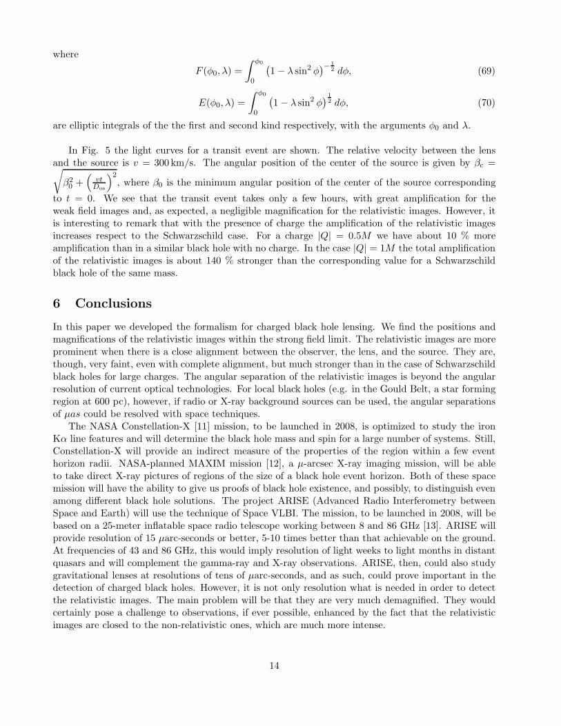
to t = 0. We see that the transit event takes only a few hours, with great amplification for theweak field images and, as expected, a negligible magnification for the relativistic images. However, itis interesting to remark that with the presence of charge the amplification of the relativistic imagesincreases respect to the Schwarzschild case. For a charge |Q| = 0.5M we have about 10 % moreamplification than in a similar black hole with no charge. In the case |Q| = 1M the total amplificationof the relativistic images is about 140 % stronger than the corresponding value for a Schwarzschildblack hole of the same mass.

6 Conclusions

In this paper we developed the formalism for charged black hole lensing. We find the positions andmagnifications of the relativistic images within the strong field limit. The relativistic images are moreprominent when there is a close alignment between the observer, the lens, and the source. They are,though, very faint, even with complete alignment, but much stronger than in the case of Schwarzschildblack holes for large charges. The angular separation of the relativistic images is beyond the angularresolution of current optical technologies. For local black holes (e.g. in the Gould Belt, a star formingregion at 600 pc), however, if radio or X-ray background sources can be used, the angular separationsof µas could be resolved with space techniques.

The NASA Constellation-X [11] mission, to be launched in 2008, is optimized to study the ironKα line features and will determine the black hole mass and spin for a large number of systems. Still,Constellation-X will provide an indirect measure of the properties of the region within a few eventhorizon radii. NASA-planned MAXIM mission [12], a µ-arcsec X-ray imaging mission, will be ableto take direct X-ray pictures of regions of the size of a black hole event horizon. Both of these spacemission will have the ability to give us proofs of black hole existence, and possibly, to distinguish evenamong different black hole solutions. The project ARISE (Advanced Radio Interferometry betweenSpace and Earth) will use the technique of Space VLBI. The mission, to be launched in 2008, will bebased on a 25-meter inflatable space radio telescope working between 8 and 86 GHz [13]. ARISE willprovide resolution of 15 µarc-seconds or better, 5-10 times better than that achievable on the ground.At frequencies of 43 and 86 GHz, this would imply resolution of light weeks to light months in distantquasars and will complement the gamma-ray and X-ray observations. ARISE, then, could also studygravitational lenses at resolutions of tens of µarc-seconds, and as such, could prove important in thedetection of charged black holes. However, it is not only resolution what is needed in order to detectthe relativistic images. The main problem will be that they are very much demagnified. They wouldcertainly pose a challenge to observations, if ever possible, enhanced by the fact that the relativisticimages are closed to the non-relativistic ones, which are much more intense.

14

Acknowledgements

We gratefully acknowledge discussions with Salvatore Capozziello and Valerio Bozza (U. of Salerno,Italy). This work has been partially supported by UBA (UBACYT X-143, EFE), CONICET (DFT,and PIP 0430/98, GER), ANPCT (PICT 98 No. 03-04881, GER), and Fundacion Antorchas (separategrants to GER and DFT).

Appendix: Deflection angle in terms of elliptic integrals

It is convenient for the calculations to express the integrals of Eqs. (13) and (20) in terms of standardelliptic integrals.Eq. (13) can be put in the form

α(x0) =2x0

√

1 − 1x0

+ q2

x20

∫ ∞

x0

dx√

P (x)− π, (71)

where

P (x) = x4 + x20

(

1 − 1

x0+

q2

x20

)−1

(−x2 + x − q2), (72)

is a fourth degree polynomial. The four roots of P (x) depend only on x0 and q and they are real forx0 > xps and |Q| ≤ M . Calling these roots r1 > r2 > r3 > r4 , the first one is r1 = x0 and the othershave long expressions (not given here for lack of space) that can be obtained with standard software.Then we can write the exact integral of Eq. (13) as

α(x0) = G(x0)F (φ0, λ) − π, (73)

with

G(x0) =4x0

√

1 − 1x0

+ q2

x20

1√

(r1 − r3)(r2 − r4), (74)

and

F (φ0, λ) =

∫ φ0

0

(

1 − λ sin2 φ)− 1

2 dφ, (75)

an elliptic integral of the first kind with arguments

φ0 = arcsin

√

(r2 − r4)

(r1 − r4), (76)

λ =(r1 − r4)(r2 − r3)

(r1 − r3)(r2 − r4). (77)

The derivative of the deflection angle can be expressed:

dα

dx0= F (φ0, λ)

dG

dx0+ G(x0)

∂F

∂λ

dλ

dx0+ G(x0)

∂F

∂φ0

dφ0

dx0, (78)

and can be written as

dα

dx0= F (φ0, λ)

dG

dx0+ G(x0)

(

− E(φ0, λ)

2(λ − 1)λ− F (φ0, λ)

2λ+

sin(2φ0)

4(λ − 1)√

1 − λ sin2 φ0

)

dλ

dx0+

+G(x0)

√

1 − λ sin2 φ0

dφ0

dx0, (79)

15

where

E(φ0, λ) =

∫ φ0

0

(

1 − λ sin2 φ)

12 dφ, (80)

is an elliptic integral of the second kind with the arguments φ0 and λ given above.

References

[1] A. Einstein, Science 84, 506 (1936).

[2] P. Schneider, J. Ehlers, E. E. Falco, Gravitational Lenses (Springer Verlag, Berlin, 1992).

[3] K. S. Virbhadra, G. F. R. Ellis, Phys. Rev. D 62, 084003 (2000). [arXiv:astro-ph/9904193].

[4] S. Frittelli, T. P. Kling, E. T. Newman, Phys. Rev. D 61, 064021 (2000).

[5] V. Bozza, S. Capozzielo, G. Iovane, G. Scarpetta, Gen. Rel. Grav. 33, 1535 (2001).[arXiv:gr-qc/0102068].

[6] B. Punsly, Astrophys. J. 498, 640 (1998).

[7] B. Punsly, G. E. Romero, D. F. Torres, J. A. Combi, Astron. Astrophys. 364, 552 (2000).[arXiv:astro-ph/0007465].

[8] C. W. Misner, K. S. Thorne, J. A. Wheeler, Gravitation (Freeman, New York, 1973).

[9] S. Weinberg, Gravitation and Cosmology: Principles and Applications of the General Theory ofRelativity (Wiley, New York, 1972).

[10] B. Punsly, Black Hole Gravitohydromagnetics (Springer Verlag, Heidelberg, 2001).

[11] Constellation-X web page: http://constellation.gsfc.nasa.gov/

[12] Maxim web page: http://maxim.gsfc.nasa.gov/

[13] Ulvestad J. S., 1999, arXiv:astro-ph/9901374.

16