Approximation of the vibration modes of a plate by Reissner-Mindlin equations

MATHEMATICS OF COMPUTATIONVolume 68, Number 228, Pages 1447–1463S 0025-5718(99)01094-7Article electronically published on May 19, 1999

APPROXIMATION OF THE VIBRATION MODESOF A PLATE BY REISSNER-MINDLIN EQUATIONS

R. G. DURAN, L. HERVELLA-NIETO, E. LIBERMAN,

R. RODRIGUEZ, J. SOLOMIN

Abstract. This paper deals with the approximation of the vibration modes ofa plate modelled by the Reissner-Mindlin equations. It is well known that, inorder to avoid locking, some kind of reduced integration or mixed interpolationhas to be used when solving these equations by finite element methods. Inparticular, one of the most widely used procedures is the mixed interpolationtensorial components, based on the family of elements called MITC. We usethe lowest order method of this family.

Applying a general approximation theory for spectral problems, we obtain

optimal order error estimates for the eigenvectors and the eigenvalues. Undermild assumptions, these estimates are valid with constants independent of theplate thickness. The optimal double order for the eigenvalues is derived froma corresponding L2-estimate for a load problem which is proven here. Thisoptimal order L2-estimate is of interest in itself.

Finally, we present several numerical examples showing the very good be-havior of the numerical procedure even in some cases not covered by our theory.

1. Introduction

Finite element discretization of Reissner-Mindlin equations is, to date, the usualway to approximate the bending of an elastic plate of moderate or small thickness(see for instance [4, 13, 19]).

For load problems, because of the ellipticity of these equations, the classical the-ory ensures the convergence of standard finite element approximations. Howeverthese elements lead to wrong results when the thickness is small with respect tothe other dimensions of the plate. This is because of the so-called locking phenom-enon, which is now well understood (see for instance [7]). In order to avoid thisdrawback, reduced integration or mixed methods are usually applied. To performtheir mathematical analysis, a family of problems, one for each thickness t > 0,is considered and approximation results valid uniformly on t are sought (see forinstance [2, 7, 10]).

Received by the editor November 13, 1997.1991 Mathematics Subject Classification. Primary 65N25, 65N30.Key words and phrases. Mixed methods, Reissner-Mindlin, plates, eigenvalues.The first author was partially supported by UBA through grant EX-071. Member of CONICET

(Argentina).The fourth author was partially supported by FONDECYT (Chile) through grant No.

1.960.615 and FONDAP-CONICYT (Chile) through Program A on Numerical Analysis.The fifth author was partially supported by SECYT through grant PIP-292. Member of

CONICET (Argentina).

c©1999 American Mathematical Society

1447

License or copyright restrictions may apply to redistribution; see http://www.ams.org/journal-terms-of-use

1448 R. G. DURAN, ET AL.

Among these methods, the so-called MITC ones, introduced by Bathe andDvorkin in [6], are very likely the most used in practice. Their application toload problems has also drawn much attention from the mathematical point of view([5, 8, 10, 15, 16]). The aim of this paper is to analyze one of these methods, thatof lowest order, when used to approximate the free vibration bending modes ofa plate. Being non-conforming, the spectral theory based on minimum-maximumprinciples (see Section 8 of [3]) cannot be directly applied to this method. Instead,our analysis will be based on the abstract spectral theory for compact operators asstated in Section 7 of [3].

Optimal order of convergence in H1 norm is known for the application of thelowest order MITC method to load problems ([8, 10, 16]). This, combined withknown regularity results ([2, 7]), allow us to prove analogous estimates for theapproximation of the eigenfunctions in vibration problems. Let us remark that thiswould not be the case for higher order methods, since the eigenfunctions are ingeneral not regular enough for us to attain similar results.

For conforming methods (which is not our case) the convergence of the eigen-functions in H1 directly yields a double order of convergence for the eigenvalues(Lemma 9.1 in [3]). Alternatively, when such double order holds for the L2 con-vergence in the corresponding load problem without further assumptions on theregularity of the solution, abstract spectral theory can be used to prove a similarresult even for non-conforming methods (see for instance Section 7 of [3]).

We prove such optimal (in order and regularity) L2 error estimates for the lowestorder MITC method, valid uniformly on the thickness t. This kind of estimates havebeen proved before for higher order MITC methods in [8, 15], but the argumentstherein do not apply to our case. Thus, our results complete the analysis of theMITC elements.

In Section 2 we present the mathematical setting and state the spectral ap-proximation results. The analysis carried out yields t-independent optimal errorestimates for the approximation of eigenfunctions and eigenvalues. The proofs arevalid for eigenvalues remaining uniformly separated from the rest of the spectrum asthe thickness becomes small. These results rely on properties of the associated loadproblems, which are proved in Section 3. Finally, in Section 4, we present numericalexperiments confirming the theoretical results and showing the good performance ofthe method. We also exhibit the potential applicability of this method to problemsnot covered by the theoretical analysis.

2. Approximation of the eigenvalue problem

Consider an elastic plate of thickness t with reference configuration Ω×(− t

2 ,t2

),

where Ω ∈ R2 is a convex polygonal domain. The deformation of the plate isdescribed by means of the Reissner-Mindlin model in terms of the rotations βt =(β1

t , β2t ) of its midplane Ω and the transverse displacement wt (see for example [7]).

Assuming that the plate is clamped, its free vibration modes are solutions of thefollowing problem:

Find a non-trivial (βt, wt) ∈ H10 (Ω)2 ×H1

0 (Ω) and ωt > 0 such that

t3a(βt, η) + κt

∫Ω

(∇wt − βt) · (∇v − η) = ω2t

[t

∫Ω

ρwtv +t3

12

∫Ω

ρ βt · η],

∀(η, v) ∈ H10 (Ω)2×H1

0 (Ω),(2.1)


APPROXIMATION OF THE VIBRATION MODES 1449

where ωt is the angular vibration frequency, a is the H10 (Ω)2-elliptic bilinear form

defined by

a(β, η) :=E

12(1− ν2)

∫Ω

2∑i,j=1

(1− ν)εij(β)εij(η) + ν div β div η

,εij(β) being the linear strain tensor, E the Young modulus and ν the Poisson ratio,κ := Ek/2(1 + ν) is the shear modulus, with k being a correction factor usuallytaken as 5/6, and ρ is the density.

The lowest vibration frequencies ωt correspond to bending modes of the plate,and for each of them λt := ρω2

t /t2 attains a finite limit as t goes to zero, as is

shown below. Therefore it is convenient for the mathematical analysis to considerthe following rescaled eigenvalue problem:

a(βt, η) +κ

t2(∇wt − βt,∇v − η) = λt

[(wt, v) +

t2

12(βt, η)

],(2.2)

∀(η, v) ∈ H10 (Ω)2 ×H1

0 (Ω),

where (·, ·) denotes the standard L2 inner product. Note that all the eigenvalues in(2.2) are strictly positive, because of the symmetry of the bilinear forms and theellipticity of its left hand side (see [7]).

Introducing the shear strain γt :=κ

t2(∇wt − βt), problem (2.2) can be written

as

a(βt, η) + (γt,∇v − η) = λt

[(wt, v) +

t2

12(βt, η)

], ∀(η, v) ∈ H1

0 (Ω)2 ×H10 (Ω),

γt =κ

t2(∇wt − βt).

(2.3)

In order to analyze the approximation of this eigenvalue problem it is convenientto introduce the operator

Tt : L2(Ω)2 × L2(Ω) → L2(Ω)2 × L2(Ω),

defined by Tt(θ, f) := (βt, wt), where (βt, wt) ∈ H10 (Ω)2 ×H1

0 (Ω) is the solution of

a(βt, η) + (γt,∇v − η) = (f, v) +t2

12(θ, η), ∀(η, v) ∈ H1

0 (Ω)2 ×H10 (Ω),

γt =κ

t2(∇wt − βt).

(2.4)

We denote by (·, ·)t the weighted L2(Ω)2 × L2(Ω) inner product in the right handside of the first equation of (2.4) and by | · |t its corresponding norm. Clearly Tt iscompact and selfadjoint with respect to (·, ·)t. Then, apart from µ = 0, its spectrumconsists of a sequence of finite multiplicity real eigenvalues converging to zero. Notethat λt is an eigenvalue of (2.3) if and only if µt := 1/λt is an eigenvalue of Tt withthe same multiplicity and corresponding eigenfunctions.

It is known (see [7]) that, when t → 0, the solution of problem (2.4) convergesto (β0, w0) ∈ H1

0 (Ω)2 ×H10 (Ω) such that there exists γ0 ∈ H0(rot,Ω)′ satisfying

a(β0, η) + 〈γ0,∇v − η〉 = (f, v), ∀(η, v) ∈ H10 (Ω)2 ×H1

0 (Ω),∇w0 − β0 = 0,

(2.5)



where 〈·, ·〉 stands for the duality pairing in H0(rot,Ω) := ψ ∈ L2(Ω)2 : rotψ ∈L2(Ω) and ψ · τ = 0 on ∂Ω (τ being a unit vector tangent to ∂Ω). This is a mixedformulation of the Kirchhoff model for the deflection of clamped thin plates:

w0 ∈ H20 (Ω) and

E

12(1− ν2)∆2w0 = f, in Ω.

Moreover, defining T0(θ, f) := (β0, w0) for (θ, f) ∈ L2(Ω)2 × L2(Ω), we will showin the next section that for 0 ≤ t ≤ tmax

‖(Tt − T0)(θ, f)‖H1(Ω)2×H1(Ω) ≤ Ct |(θ, f)|t.(2.6)

In particular, since | · |t ≤ tmax‖ · ‖H1(Ω)2×H1(Ω) for t ∈ (0, tmax), it follows thatTt|H1(Ω)2×H1(Ω) converges to T0|H1(Ω)2×H1(Ω) in norm. Then, standard propertiesof separation of isolated parts of the spectrum (see for instance [14]) yield thefollowing result:

Lemma 2.1. Let µ0 > 0 be an eigenvalue of T0 of multiplicity m. Let D be anydisc in the complex plane centered at µ0 and containing no other element of thespectrum of T0. Then, for t small enough, D contains exactly m eigenvalues of Tt

(repeated according to their respective multiplicities). Consequently, each eigenvalueµ0 > 0 of T0 is a limit of eigenvalues µt of Tt, as t goes to zero.

Mixed finite elements for the load problem (2.4) have been introduced and ana-lyzed in several papers (see for example [6, 8, 10, 15, 16]). The method that we willuse here can be seen as the lowest degree member of the so-called MITC elements,which are based on relaxing the second equation of (2.3). In order to recall thismethod let us introduce some notation.

Assume that we have a family of triangulations Th satisfying the usual mini-mum angle condition. The finite element space for the rotations consists of piecewiselinear functions augmented in such a way that they have quadratic tangential com-ponents on the boundary of each element. Namely, for each K ∈ Th, let n be a unitnormal on ∂K and define

Q(K) := η ∈ P2(K)2 : η · n|` ∈ P1(`), for each edge ` of K;

then, the finite element space for the rotations is defined by

Hh := η ∈ H10 (Ω)2 : η|K ∈ Q(K), ∀K ∈ Th.

For the transverse displacements we take standard piecewise linear elements,namely,

Wh := v ∈ H10 (Ω) : v|K ∈ P1(K), ∀K ∈ Th.

In order to define the method, we also need the reduction operator

R : H1(Ω)2 ∩H0(rot,Ω) −→ Γh,

where Γh is the lowest order rotated Raviart-Thomas space, namely,

Γh := ψ ∈ H0(rot,Ω) : ψ|K ∈ P20 ⊕ (−x2, x1)P0, ∀K ∈ Th,

and R is the operator locally defined for each ψ ∈ H1(Ω)2 by (see [7, 17])∫`

Rψ · τ =∫

`

ψ · τ,(2.7)



for every edge ` of the triangulation (τ being a unit tangent vector along `). It iseasy to see that the operator R satisfies∫

K

rot(ψ −Rψ) = 0, ∀ψ ∈ H1(Ω)2,(2.8)

for any element K ∈ Th, and it is also known ([7, 17]) that

‖ψ −Rψ‖0 ≤ Ch‖ψ‖1;(2.9)

here and hereafter ‖ · ‖k denotes the standard norm of Hk(Ω) or Hk(Ω)2 (whichone will be obvious).

Now, the finite element approximate solution (βth, wth) ∈ Hh ×Wh of the loadproblem (2.4) is defined by

a(βth, η) + (γth,∇v −Rη) = (f, v) +t2

12(θ, η), ∀(η, v) ∈ Hh ×Wh,

γth =κ

t2(∇wth −Rβth).

(2.10)

The method is nonconforming, since consistency terms arise because of the reduc-tion operator. Existence and uniqueness of the solution of (2.10) follow easily (see[10]). As in the continuous case, we introduce the operator

Tth : L2(Ω)2 × L2(Ω) −→ L2(Ω)2 × L2(Ω)

given by Tth(θ, f) := (βth, wth). Tth is also selfadjoint with respect to (·, ·)t.The corresponding eigenvalue problem reads a(βth, η) + (γth,∇v −Rη) = λth

[(wth, v) +

t2

12(βth, η)

], ∀(η, v) ∈ Hh ×Wh,

γth =κ

t2(∇wth −Rβth).

Once more λth is an eigenvalue of this problem if and only if µth := 1/λth is astrictly positive eigenvalue of Tth with the same multiplicity and correspondingeigenfunctions.

For t > 0 fixed, the spectral theory for compact operators in [3] can be directlyapplied to prove convergence of the eigenpairs of Tth to those of Tt. However, furtherconsiderations are needed to show that the error estimates do not deteriorate as tbecomes small.

To this goal we will make use of the following result, which means that optimalerror estimates in the H1 norm for the rotations and the transverse displacementhold for the approximations given by (2.10):

‖(Tt − Tth)(θ, f)‖H1(Ω)2×H1(Ω) ≤ Ch |(θ, f)|t,(2.11)

with a constant C independent of t and h. This has been proved for instance in[10] for pure transversal loads (i.e., θ = 0), but the proofs therein extend triviallyto our case.

As a consequence of (2.11), if µt is an eigenvalue of Tt with multiplicity m, thenexactly m eigenvalues µ(1)

th , . . . , µ(m)th of Tth (repeated according to their respective

multiplicities) converge to µt as h goes to zero (see [14]). The following theoremshows that, under mild assumptions, optimal t-independent error estimates in theH1 norm are valid for the eigenfunctions:



Theorem 2.1. Let µt be an eigenvalue of Tt converging to a simple eigenvalue µ0

of T0, as t goes to zero. Let µth be the eigenvalue of Tth that converges to µt,as h goes to zero. Let (βt, wt) and (βth, wth) be the corresponding eigenfunctionsnormalized in the same manner. Then, for t and h small enough,

‖(βt, wt)− (βth, wth)‖H1(Ω)2×H1(Ω) ≤ Ch,(2.12)

with a constant C independent of t and h.

Proof. For any fixed t ∈ (0, tmax), | · |t ≤ tmax‖ · ‖H1(Ω)2×H1(Ω). Hence, becauseof (2.11), Tth|H1(Ω)2×H1(Ω) converges to Tt|H1(Ω)2×H1(Ω) in norm. Then (2.12) is adirect consequence of the estimate (2.11) and Theorem 7.1 in [3], with a constant Cdepending on the constant in (2.11) (which is independent of t) and on the inverseof the distance from µt to the rest of the spectrum of Tt. Now, according to Lemma2.1, (2.6) implies that for t small enough this distance can be bounded below interms of the distance from µ0 to the rest of the spectrum of T0, which obviouslydoes not depend on t.

In the next section we will prove the following higher order L2 error estimate forthe aproximate solution of the load problem (2.4):

‖(Tt − Tth)(θ, f)‖L2(Ω)2×L2(Ω) ≤ Ch2|(θ, f)|t,(2.13)

with a constant C independent of t and h. By using it we are able to prove a doubleorder of convergence for the eigenvalues:

Theorem 2.2. Let µt and µth be as in Theorem 2.1. Then, for t and h smallenough,

|µt − µth| ≤ Ch2,


Proof. Let (βt, wt) be an eigenfunction corresponding to µt normalized in |·|t. SinceTt and Tth are selfadjoint with respect to (·, ·)t, we may apply Remark 7.5 in [3],which in our case reads

|µt − µth|≤C[(

(Tt − Tth)(βt, wt), (βt, wt))t+|(Tt − Tth)(βt, wt)|2t

],(2.14)

with a constant C depending only on the inverse of the distance from µt to therest of the spectrum of Tt. By repeating the arguments in the proof of Theorem2.1 we observe that, for t small enough, this constant can be chosen independentof t. Thus, since | · |t ≤ tmax‖ · ‖L2(Ω)2×L2(Ω), by using estimate (2.13) in (2.14) weconclude the proof.

Another consequence of estimate (2.13) is a double order of convergence in theL2 norm for the eigenfunctions:

Theorem 2.3. Let µt, µth, (βt, wt) and (βth, wth) be as in Theorem 2.1. Then,for t and h small enough,

‖(βt, wt)− (βth, wth)‖L2(Ω)2×L2(Ω) ≤ Ch2,


Proof. Since | · |t ≤ tmax‖ · ‖L2(Ω)2×L2(Ω), the arguments in the proof of Theorem2.1 can be repeated using ‖ · ‖L2(Ω)2×L2(Ω) instead of ‖ · ‖H1(Ω)2×H1(Ω) and estimate(2.13) instead of estimate (2.11).



The three theorems of this section are stated for those eigenvalues of Reissner-Mindlin equations converging to simple eigenvalues of the Kirchhoff model. Amultiple eigenvalue of the latter arises usually because of symmetries of the geom-etry of the plate; in such a case, the eigenvalue of the former converging to it hasthe same multiplicity. The proofs of these theorems extend trivially to cover thiscase.

Instead, if the Kirchhoff equations had a multiple eigenvalue not due to symmetryreasons, it could split into different eigenvalues in the Reissner-Mindlin model. Inthis case, the proofs of the theorems above do not provide estimates independentof the thickness. In fact, the constants therein blow up as the distance between theReissner-Mindlin eigenvalues becomes smaller.

For conforming methods, the minimum-maximum principles yield estimates notinvolving this distance (see, for instance, Section 8 of [3]). However, to the bestof our knowledge, estimates of this kind have not been proved for non-conformingmethods like ours. Nevertheless, the numerical experiments in Section 4 show thatsuch estimates also hold in this case for our method.

3. Proofs

The optimal spectral convergence results in the previous section rely on proper-ties (2.6), (2.11) and (2.13). The proof of the first one is standard, but we includeit for the sake of completeness. The second one is an H1 norm estimate for the loadproblem including shear loads, and its proof is an immediate extension of those in[8, 10, 16]. On the other hand, property (2.13), regarding the approximation withoptimal order in the L2 norm, was not previously known. Similar L2 estimateshave been proved for higher order methods (see [8, 15]), but with proofs relying onarguments which do not apply to the lowest order case we are considering.

In what follows we will make use of the known a priori estimates for the solutionsof problems (2.4) and (2.5) (see for instance [2]):

‖βt‖2 + ‖wt‖2 + ‖γt‖0 + t ‖γt‖1 ≤ C(t2‖θ‖0 + ‖f‖0

)≤ C |(θ, f)|t,

(3.1)

valid for 0 ≤ t ≤ tmax, with a constant C independent of t.We begin with the proof of property (2.6).

Lemma 3.1. There exists a constant C, independent of t, such that

‖(Tt − T0)(θ, f)‖H1(Ω)2×H1(Ω) ≤ Ct |(θ, f)|t,

for all (θ, f) ∈ L2(Ω)2 × L2(Ω).

Proof. Subtracting (2.5) from (2.4), we have a(βt − β0, η) + (γt − γ0,∇v − η) =t2

12(θ, η), ∀(η, v) ∈ H1

0 (Ω)2 ×H10 (Ω),

γt =κ

t2

[∇(wt − w0)− (βt − β0)

],

and taking η = βt − β0 and v = wt − w0, we obtain

a(βt − β0, βt − β0) =t2

12(θ, βt − β0)−

t2

κ(γt − γ0, γt).



Now, using the coerciveness of a and the a priori estimate (3.1) for ‖γt‖0 and ‖γ0‖0,we have

‖βt − β0‖21 ≤ Ct2‖θ‖0 ‖βt − β0‖0 + Ct2 (‖γt‖0 + ‖γ0‖0) ‖γt‖0

≤ Ct |(θ, f)|t ‖βt − β0‖0 + Ct2|(θ, f)|2t ,and therefore

‖βt − β0‖1 ≤ Ct |(θ, f)|t.(3.2)

Finally, observe that

∇(wt − w0) = (βt − β0) +t2

κγt,

and so, using again the a priori estimate (3.1) for ‖γt‖0, we obtain

‖wt − w0‖1 ≤ C(‖βt − β0‖0 + t2|(θ, f)|t

)which together with (3.2) allow us to conclude the proof.

The arguments to prove the remaining properties are based on the fact that thereexists an operator

Π : H10 (Ω)2 ×

[H1

0 (Ω) ∩H2(Ω)]−→ Hh ×Wh

such that, if (η, w) := Π(η, w), then

R(∇w − η) = ∇w −Rη(3.3)

(R being the reduction operator satisfying (2.7), (2.8) and (2.9)) and

‖η − η‖1 ≤ Ch ‖η‖2.(3.4)

The construction of such an operator is based on known properties of the spacesHh, Wh and Γh (see [10] for details). It is worth observing that (3.3) correspondsto a commutative diagram property, usual in the analysis of mixed methods. Infact, introducing the operators B and Bh such that B(η, v) := ∇v − η, for (η, v) ∈H1

0 (Ω)2 × H10 (Ω), and Bh(η, v) := ∇v − Rη, for (η, v) ∈ Hh ×Wh, that property

can be summarized in the following commutative diagram:

H10 (Ω)2 ×

[H1

0 (Ω) ∩H2(Ω)] B

//

Π

H1(Ω)2 ∩H0(rot,Ω)

R

Hh ×WhBh

// Γh

Note that, if R were an L2 projection, this commutative diagram would corre-spond to Fortin’s well-known property (which in its turn implies that an inf-supcondition, analogous to that proved in [7] for the continuous problem, holds for thediscrete case). Of course, R is not an L2 projection, and so the commutative dia-gram property given above can be seen as a generalization of Fortin’s one. In fact,optimal error estimates in H1 for the rotations and the transverse displacementyielding (2.11) follow from this generalized property:

Lemma 3.2. There exists a constant C, independent of t and h, such that

‖(Tt − Tth)(θ, f)‖H1(Ω)2×H1(Ω) ≤ Ch |(θ, f)|t,

for all (θ, f) ∈ L2(Ω)2 × L2(Ω).



Proof. Arguments identical to those in [10], combined with the a priori estimate(3.1), yield in our case

‖βt − βth‖1 + t ‖γt − γth‖0 ≤ Ch(‖βt‖2 + t ‖γt‖1 + ‖γt‖0

)≤ Ch |(θ, f)|t,

(3.5)

and, as a consequence,

‖wt − wth‖1 ≤ Ch(‖βt‖2 + t ‖γt‖1 + ‖γt‖0

)≤ Ch |(θ, f)|t,

therefore concluding the proof.

We will use a duality argument to show that, under the same conditions, optimalL2 error estimates for the rotations and the transverse displacement also hold. Firstwe will prove a lemma which will be useful to bound the consistency terms arisingfrom the reduced integration of the shear strain.

For ψ ∈ H10 (Ω)2, we denote by ψI ∈ H1

0 (Ω)2 a piecewise linear average inter-polant as defined in [9, 18], satisfying

‖ψI‖1 ≤ C‖ψ‖1(3.6)

and

‖ψ − ψI‖1 ≤ Ch‖ψ‖2.(3.7)

The following estimate holds:

Lemma 3.3. Given ζ ∈ H(div,Ω) and ψ ∈ H10 (Ω)2, we have

|(ζ, ψI −RψI)| ≤ Ch2‖ div ζ‖0 ‖ψ‖1.

Proof. From property (2.8) it follows that

rotRψI = P (rotψI),

where P is the L2 projection onto the piecewise constant functions. Now, since(rotψI)|K ∈ P0, then (rotψI) = P (rotψI). Hence rot(ψI −RψI) = 0, and so thereexists r ∈ H1(Ω) such that

∇r = ψI −RψI ;(3.8)

actually, we can take r ∈ H10 (Ω) because the tangential component of (ψI − RψI)

vanishes on ∂Ω. Then, we have

|(ζ, ψI −RψI)| = |(ζ,∇r)| = |(div ζ, r)| ≤ ‖ div ζ‖0 ‖r‖0.(3.9)

On the other hand, from property (2.7) defining R it follows that, for every edge` with end points A and B, we have

r(A) − r(B) =∫

`

∇r · τ =∫

`

(ψI −RψI) · τ = 0.

Therefore, since r vanishes on ∂Ω we conclude that r vanishes at all the nodes ofthe triangulation. Hence, since r|K ∈ P2, a standard scaling argument on eachelement K yields

‖r‖0 ≤ Ch‖∇r‖0,

which together with (2.9), (3.6), (3.8) and (3.9) allows us to conclude the proof.



Finally, we will prove the main result of this section, property (2.13), concerningL2 error estimates optimal in order and regularity. Let us remark that this resultcompletes the analysis of the MITC elements carried out in [8, 15] for the higherorder methods. (To simplify the notation, in this lemma we will drop the subscriptt from βt, wt, γt and from their discrete approximations.)

Lemma 3.4. Given (θ, f) ∈ L2(Ω)2 × L2(Ω), let (β,w) = Tt(θ, f) and (βh, wh) =Tth(θ, f). Then there exists a constant C, independent of t and h, such that

‖β − βh‖0 + ‖w − wh‖0 ≤ Ch2|(θ, f)|tor, equivalently,

‖(Tt − Tth)(θ, f)‖L2(Ω)2×L2(Ω) ≤ Ch2|(θ, f)|t.

Proof. Subtracting (2.10) from (2.4), we obtain the error equation

a(β − βh, η) + (γ − γh,∇v −Rη) = (γ, η −Rη), ∀(η, v) ∈ Hh ×Wh,

(3.10)

with γ =κ

t2(∇w − β) and γh =

κ

t2(∇wh −Rβh).

We will use a duality argument: let (ϕ, u) ∈ H10 (Ω)2 ×H1

0 (Ω) be the solution of

a(η, ϕ) + (∇v − η, δ) = (v, w − wh) + (η, β − βh), ∀(η, v) ∈ H1

0 (Ω)2 ×H10 (Ω),

δ =κ

t2(∇u− ϕ).

(3.11)

An a priori estimate analogous to (3.1) is valid for this problem, namely,

‖ϕ‖2+‖u‖2+‖δ‖0+t ‖δ‖1≤C(‖β−βh‖0+‖w−wh‖0

),(3.12)

and by taking η = 0 in (3.11) we have

− div δ = w − wh.(3.13)

By taking v = w − wh and η = β − βh in the dual problem (3.11) we have

‖w − wh‖20 + ‖β − βh‖2

0

= a(β − βh, ϕ) +(∇(w − wh)− (β −Rβh), δ

)+ (βh −Rβh, δ)

= a(β − βh, ϕ) +t2

κ(γ − γh, δ) + (βh −Rβh, δ),

and using the error equation (3.10) with (η, v) = (ϕ, u) := Π(ϕ, u) we obtain

‖w − wh‖20 + ‖β − βh‖2

0

= a(β − βh, ϕ− ϕ) +t2

κ(γ − γh, δ)− (γ − γh,∇u−Rϕ)

+ (βh −Rβh, δ) + (γ, ϕ−Rϕ).(3.14)

= a(β − βh, ϕ− ϕ) +t2

κ(γ − γh, δ −Rδ)

+ (βh −Rβh, δ) + (γ, ϕ−Rϕ),



where we have used the commutative diagram property (3.3), Rδ =κ

t2(∇u−Rϕ),

for the last equality. Now it only remains to estimate the four terms in the lastexpression.

The first two can be easily bounded. In fact, using the error estimates (3.4) and(3.5) and the a priori estimate (3.12) we have

|a(β − βh, ϕ− ϕ)| ≤ C‖β − βh‖1 ‖ϕ− ϕ‖1 ≤ C‖β − βh‖1 h ‖ϕ‖2

≤ Ch2|(θ, f)|t(‖β − βh‖0 + ‖w − wh‖0

)(3.15)

and, from (2.9), (3.5) and (3.12),

t2

κ

∣∣∣(γ − γh, δ −Rδ)∣∣∣

≤ Ct2‖γ − γh‖0 ‖δ −Rδ‖0 ≤ Ct2‖γ − γh‖0 h ‖δ‖1

≤ Ch2|(θ, f)|t(‖β − βh‖0 + ‖w − wh‖0

).

(3.16)

For the third term in (3.14) we have

(βh −Rβh, δ) =((βh − βI)−R(βh − βI), δ

)+ (βI −RβI , δ).

Now, using successively (2.9), (3.5), (3.7), (3.12) and (3.1), we obtain∣∣∣((βh − βI)−R(βh − βI), δ)∣∣∣

≤ C‖δ‖0 h ‖βh − βI‖1 ≤ C‖δ‖0 h(‖βh − β‖1 + ‖β − βI‖1

)≤ Ch2

(‖β − βh‖0 + ‖w − wh‖0

)|(θ, f)|t,

whereas by using Lemma 3.3, (3.13) and (3.1) we have

|(βI −RβI , δ)| ≤ Ch2‖β‖1 ‖ div δ‖0

≤ Ch2|(θ, f)|t ‖w − wh‖0

Therefore

|(βh −Rβh, δ)| ≤ Ch2|(θ, f)|t(‖β − βh‖0 + ‖w − wh‖0

).(3.17)

The last term in (3.14) can be bounded in an almost identical way, by using (3.4)to estimate ‖ϕ− ϕ‖1 and the fact that

− div γt = f, in Ω

which follows by taking η = 0 in problem (2.4) and (2.5).By so doing we obtain

|(γ, ϕ−Rϕ)| ≤ Ch2|(θ, f)|t(‖β − βh‖0 + ‖w − wh‖0

).(3.18)

Finally, from (3.14), (3.15), (3.16), (3.17) and (3.18), simple algebra allows us toconclude the proof.



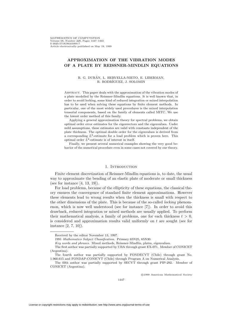
Figure 1. Finite element mesh for the square plate: N = 8

4. Numerical experiments

In this section we summarize the numerical experimentation carried out with ourmethod. The aim of these computations was two-fold: to study the performance ofthe method and to discuss the pertinence of the assumptions made in Section 2 toprove error estimates.

To validate our codes and to test the effectiveness of the method to deal with dif-ferent boundary conditions, we have first considered a typical benchmark problem:the computation of the lowest frequency vibration modes of a square plate. Wehave applied our codes to thin and moderately thick plates and compared the re-sults with those reported in [1], in which the same problems were treated by meansof a method introduced by Huang and Hinton in [12] that is based on biquadraticrectangular finite elements with enhanced shear interpolation.

We have considered a square plate of side length L and two thickness-to-span(t/L) ratios of 0.1 (moderately thick) and 0.01 (thin). In each case we have alsoconsidered four different types of boundary conditions:

• a clamped plate (as described in Section 2);• a hard simply supported plate (i.e., with transversal displacements and rota-

tions tangential to the boundary, both vanishing on each edge);• a plate with mixed boundary conditions (with two opposite edges being hard

simply supported and the other two clamped);• a plate with a free edge (with three clamped edges and the fourth being free,

i.e., no constraints either on the transversal displacements or on the rotationsalong this edge).

We denote each case by C-C-C-C, S-S-S-S, S-C-S-C and C-C-C-F, respectively (Cstands for clamped, S for hard simply supported and F for free edges).

We have used succesive refinements of a uniform mesh like that in Figure 1, therefinement parameter N being the number of element edges on each side of thesquare (hence, h =

√2L/N).

We have applied our codes to the original unscaled problems analogous to (2.1).Thus we have computed approximations of the free vibration angular frequenciesωt = t

√λt/ρ. In order to compare our results with those in [1] we present the

computed frequencies ωhmn in the following non-dimensional form:

ωmn := ωhmnL

(2(1 + ν)ρ

E

)1/2

,

m and n being the numbers of half-waves occurring in the modes shapes in the xand y directions, respectively.



Table 1. Lowest non-dimensional vibration frequencies for mod-erately thick square plates: t/L = 0.1

Bound. cond. Mode N = 10 N = 20 N = 40 H-H D-RC-C-C-C ω11 1.5947 1.5921 1.5913 1.591 1.594

ω21 3.1181 3.0595 3.0441 3.039 3.046ω12 3.1181 3.0595 3.0441 3.039 3.046ω22 4.4477 4.3106 4.2746 4.263 4.285

S-S-S-S ω11 0.9384 0.9323 0.9308 0.930 0.930ω21 2.2893 2.2366 2.2236 2.219 2.219ω12 2.2893 2.2366 2.2236 2.219 2.219ω22 3.5657 3.4450 3.4153 3.405 3.406

S-C-S-C ω11 1.3060 1.3016 1.3005 1.300 1.302ω21 2.4664 2.4120 2.3984 2.394 2.398ω12 2.9617 2.9043 2.8895 2.885 2.888ω22 4.0126 3.8830 3.8500 3.839 3.852

C-C-C-F ω 12 1 1.0959 1.0848 1.0814 1.081 1.089

ω 32 1 1.7759 1.7525 1.7454 1.744 1.758

ω 12 2 2.7413 2.6787 2.6612 2.657 2.673

ω 52 1 3.3186 3.2282 3.2035 3.197 3.216

Tables 1 and 2 show the four lowest vibration frequencies computed by ourmethod with three different meshes (N = 10, 20, 40) and each set of boundaryconditions for each thickness-to-span ratio (t/L = 0.1 and t/L = 0.01, respectively).Each table includes the results obtained by Huang and Hinton’s method in [12](column H-H) and also by an analytical approximation obtained by Dawe andRoufaeil in [11] (column D-R), both as reported in [1]. In every case we have useda Poisson ratio ν = 0.3 and different correction factors depending on the boundaryconditions, but always the same as those used in [1] to allow for the comparison:k = 0.8601 for C-C-C-C and C-C-C-F, k = 0.8333 for S-S-S-S and k = 0.822 for S-C-S-C. The reported non-dimensional frequencies are independent of the remaininggeometrical and physical parameters, except for the thickness-to-span ratio.

Both tables show that the method can be safely used for any of these boundaryconditions and for thin as well as moderately thick plates.

The goal of our second experiment was to test if the hypothesis on the uniformseparation of the spectrum assumed throughout Section 2 is actually necessary.For any convex clamped plate, according to Theorem 2.2, the convergence for eacheigenvalue is quadratic. However, the constants in the error estimates arising in itsproof blow up with the inverse of the distance from the approximated eigenvalueto the rest of the spectrum.

In order to test if this assumption is essential or if it only arises because of thetechniques used to prove the theorems, we have considered a clamped rectangularsteel plate with two very close vibration frequencies, but not exactly coincident.We have chosen the following values of the physical and geometric parameters: sidelengths: 2 m and 1 m; Young modulus: E = 1.43×1011 Pa; Poisson ratio: ν = 0.35;density: ρ = 7.7× 103 Kg; and correction factor k = 5/6.



Table 2. Lowest non-dimensional vibration frequencies for thinsquare plates: t/L = 0.01

Bound. cond. Mode N = 10 N = 20 N = 40 H-H D-RC-C-C-C ω11 0.1754 0.1754 0.1754 0.1754 0.1754

ω21 0.3668 0.3599 0.3580 0.3574 0.3576ω12 0.3668 0.3599 0.3580 0.3574 0.3576ω22 0.5487 0.5323 0.5279 0.5264 0.5274

S-S-S-S ω11 0.0972 0.0965 0.0963 0.0963 0.0963ω21 0.2486 0.2426 0.2411 0.2406 0.2406ω12 0.2486 0.2426 0.2411 0.2406 0.2406ω22 0.4035 0.3893 0.3859 0.3847 0.3848

S-C-S-C ω11 0.1417 0.1413 0.1412 0.1411 0.1411ω21 0.2748 0.2688 0.2673 0.2668 0.2668ω12 0.3474 0.3402 0.3383 0.3377 0.3377ω22 0.4814 0.4657 0.4617 0.4604 0.4608

C-C-C-F ω 121 0.1182 0.1170 0.1167 0.1166 0.1171

ω 321 0.1977 0.1956 0.1950 0.1949 0.1951

ω 122 0.3193 0.3109 0.3086 0.3080 0.3093

ω 521 0.3874 0.3771 0.3744 0.3736 0.3740

We have considered again two plates of different thickness: one moderately thick(t = 0.1m) and the other thin (t = 0.01m). For each of them we have computedthe lowest frequency vibration modes with different successively refined uniformmeshes analogous to that in Figure 1, the parameter N being now the number ofedge elements on the shortest side of the plate.

We have observed that the relative error of the approximated angular frequenciesωh

mn roughly behaves like

ωhmn − ωmn

ωmn≈ Cmnh

α,

with an order of convergence α very close to 2 and constants Cmn which depend onthe numbers of half-waves m and n, but which are almost independent of the thick-ness of the plate. We have also observed that these constants remain remarkablystable even for very close eigenvalues.

Then, for each mode, we have estimated the exact vibration frequencies ωmn,the value of the constants Cmn and the order of convergence α by means of a leastsquare fitting of the model

ωhmn ≈ ωmn (1 + Cmnh

α)

to the approximate frequencies computed on highly refined meshes (N = 16, 32,48, 64, 80).

We summarize our results in Table 3 for the moderately thick plate and in Table 4for the thin one.

It can be observed that the fourth and the fifth eigenvalues in both tables arevery close (approximately 1% of difference). However the corresponding constantsCmn are not larger than those for other eigenvalues. This fact suggests that the



Table 3. Lowest vibration frequencies (in rad/s) of a clampedmoderately thick rectangular plate: 2 m×1m, t = 0.1m

Mode N = 8 N = 16 N = 32 α ωmn Cmn

ωh11 3035.212 3025.827 3023.214 1.97 3022.317 0.071ωh

21 3918.755 3875.817 3864.488 1.98 3860.631 0.242ωh

31 5441.309 5351.958 5328.053 1.97 5319.841 0.365ωh

12 7536.399 7333.836 7280.257 1.98 7262.144 0.616ωh

41 7630.812 7399.422 7338.489 1.98 7317.795 0.689ωh

22 8340.381 8076.061 8006.128 1.98 7982.469 0.731ωh

32 9673.715 9326.597 9233.320 1.97 9201.449 0.830

Table 4. Lowest vibration frequencies (in rad/s) of a clampedthin rectangular plate: 2 m×1m, t = 0.01m

Mode N = 8 N = 16 N = 32 α ωmn Cmn

ωh11 328.760 327.663 327.347 1.99 327.240 0.086ωh

21 429.627 425.210 424.050 2.00 423.665 0.239ωh

31 607.831 598.992 596.605 1.98 595.794 0.336ωh

41 878.302 851.895 844.852 1.98 842.468 0.702ωh

12 888.126 860.941 853.510 1.98 850.980 0.727ωh

22 991.486 957.454 948.250 1.98 945.136 0.819ωh

32 1162.198 1121.967 1110.801 1.97 1106.970 0.828

assumption on the separation of the spectrum made in Section 2 is not reallynecessary.

Finally, we have made a stringent test of this hypothesis and, at the same time,of the stability of the method as t goes to zero. The eigenvalues of Kirchhoffequations for a rectangular plate with simply supported boundary conditions areexactly known:

λmn0 :=

Eπ4

12(1− ν2)

(m2

a2+n2

b2

)2

, m, n = 1, 2, 3, . . . ,

where a and b are the side lengths of the plate. If we consider the same lengths asin the previous experiment (a = 2 m, b = 1m) the fifth and the sixth eigenvaluesexactly coincide: λ41

0 = λ220 .

In Reissner-Mindlin equations, this double eigenvalue splits into two differentones, both converging to this common value and hence getting closer and closerto each other as t goes to zero. This phenomenon occurs for both hard and softsimply supported plates. We have chosen the latter (i.e., with vanishing transversaldisplacements but no constraint imposed on the rotations along the edges) in orderto test our method also for these boundary conditions, but similar results are validfor hard simply supported plates too.

We have considered the same values of the physical parameters and successivelyrefined uniform meshes like those of the previous experiment. We have computedapproximations λ41

th and λ22th on the meshes corresponding to N = 8, 16, 32, 64, for

decreasing values of the thickness t = 0.1, 0.01, 0.001, 0.0001m.



Table 5. Fifth eigenvalue λ41th (multiplied by 10−10) of Reissner-

Mindlin equations for a soft simply supported rectangular plate:2 m×1m

Thickness N = 8 N = 16 N = 32 N = 64 α λ41t C41

t = 0.1 3032.768 2801.861 2736.523 2718.535 1.83 2711.216 2.817t = 0.01 3670.259 3407.412 3341.052 3322.356 1.96 3316.899 3.180t = 0.001 3678.556 3416.164 3351.528 3335.415 2.02 3330.245 3.459t = 0.0001 3678.639 3416.253 3351.638 3335.572 2.02 3330.405 3.464

t = 0 (extrap.) 3678.640 3416.254 3351.640 3335.574 2.02 3330.406 3.464

Table 6. Sixth eigenvalue λ22th (multiplied by 10−10) of Reissner-

Mindlin equations for a soft simply supported rectangular plate:2 m×1m

Thickness N = 8 N = 16 N = 32 N = 64 α λ22t C22

t = 0.1 3039.576 2802.288 2736.243 2718.268 1.85 2711.174 2.994t = 0.01 3676.006 3407.927 3341.083 3322.346 1.98 3317.021 3.322t = 0.001 3684.276 3416.686 3351.582 3335.421 2.04 3330.376 3.613t = 0.0001 3684.359 3416.775 3351.693 3335.579 2.04 3330.536 3.618

t = 0 (extrap.) 3684.359 3416.776 3351.694 3335.581 2.04 3330.537 3.618

We have observed that the relative error of the computed eigenvalues roughlybehaves again like

λmnth − λmn

t

λmnt

≈ Cmnhα

with constants Cmn depending neither on the thickness t nor on the mesh size hand orders of convergence α close to 2.

For each thickness t and both vibration modes, we have estimated the ordersof convergence α, the constants Cmn and the exact eigenvalues λmn

t by a leastsquare fitting of the computed approximate eigenvalues λmn

th , similar to that of theprevious experiment. Finally we have also estimated by extrapolation the limitvalues λmn

0h = limt→0 λmnth .

We summarize these results for λ41th in Table 5 and for λ22

th in Table 6.

Two conclusions arise immediately from these tables. First, the constants donot deteriorate as the thickness becomes small (and consequently the eigenvaluesof Reissner-Mindlin equations get closer). Secondly, the method is locking free andprovides very accurate approximations of the eigenvalues of the Kirchhoff equations,in this case, λ41

0 = λ220 = 3330.225× 1010.

References

1. B.S. Al Janabi and E. Hinton, A study of the free vibrations of square plates with various edgeconditions, in Numerical Methods and Software for Dynamic Analysis of Plates and Shells,E. Hinton, ed., Pineridge Press, Swansea, 1987.

2. D.N. Arnold and R.S. Falk, A uniformly accurate finite element method for the Reissner-

Mindlin plate, SIAM J. Numer. Anal., 26 (1989) 1276–1290. MR 91c:650683. I. Babuska and J. Osborn, Eigenvalue problems, in Handbook of Numerical Analysis, Vol.

II, P. G. Ciarlet and J. L. Lions, eds., North Holland, Amsterdam, 1991, pp. 641–787. MR92f:65001



4. K.J. Bathe, Finite Element Procedures in Engineering Analysis, Prentice-Hall, EnglewoodCliffs, NJ, 1982.

5. K.J. Bathe and F. Brezzi, On the convergence of a four-node plate bending element based onMindlin/Reissner plate theory and a mixed interpolation, in Mathematics of Finite Elementsand Applications V, J.R. Whiteman, ed., Academic Press, London, 1985, pp. 491–503. MR87f:65125

6. K.J. Bathe and E.N. Dvorkin, A four-node plate bending element based on Mindlin/Reissnerplate theory and a mixed interpolation, Internat. J. Numer. Methods Eng. 21 (1985) 367–383.

7. F. Brezzi and M. Fortin, Mixed and Hybrid Finite Element Methods, Springer-Verlag, NewYork, 1991. MR 92d:65187

8. F. Brezzi, M. Fortin and R. Stenberg, Quasi-optimal error bounds for approximation of shear-stresses in Mindlin-Reissner plate models, Math. Models Methods Appl. Sci. 1 (1991) 125–151.MR 92e:73030

9. P. Clement, Approximation by finite element functions using local regularization. RAIRO

Anal. Numer., 9 (1975) 77–84. MR 53:456910. R. Duran and E. Liberman, On mixed finite element methods for the Reissner-Mindlin plate

model, Math. Comp., 58 (1992) 561–573. MR 92f:6513511. D. J. Dawe and O. L Roufaeil, Rayleigh-Ritz vibration analysis of Mindlin plates, J. Sound.

Vib., 12 (1980) 345–359.12. H.C. Huang and E. Hinton, A nine node Lagrangian Mindlin plate element with enhanced

shear interpolation, Eng. Comput., 1 (1984) 369–379.13. T.J.R Hughes, The Finite Element Method: Linear Static and Dinamic Finite Element Anal-

ysis, Prentice-Hall, Englewood Cliffs, NJ, 1987. MR 90i:6500114. T. Kato, Perturbation Theory for Linear Operators, Grandlehren Math. Wiss. 132, Springer

Verlag, Berlin, 1966. MR 34:332415. P. Peisker and D. Braess, Uniform convergence of mixed interpolated elements for Reissner-

Mindlin plates, RAIRO Model. Math. Anal. Numer., 26 (1992) 557–574. MR 93j:7307016. J. Pitkaranta and M. Suri, Design principles and error analysis for reduced-shear plate-

bending finite elements, Numer. Math., 75 (1996) 223-266. MR 98c:7307817. P.A. Raviart and J.M. Thomas, A mixed finite element method for second order elliptic

problems, in Mathematical Aspects of Finite Element Methods, Lecture Notes in Mathematics606, Springer Verlag, Berlin, Heidelberg, New York, 1977, pp. 292–315. MR 58:3547

18. L.R. Scott and S. Zhang, Finite element interpolation of nonsmooth functions satisfyingboundary conditions, Math. Comp. 54 (1990) 483–493. MR 90j:65021

19. O.C. Zienkiewicz and R.L. Taylor, The Finite Element Method, Vol. 2, McGraw-Hill, 1989.

Departamento de Matematica, Facultad de Ciencias Exactas y Naturales, Universi-

dad de Buenos Aires, 1428 Buenos Aires, Argentina

E-mail address: [email protected]

Departamento de Matematica Aplicada, Universidade de Santiago de Compostela,

15706 Santiago de Compostela, Spain


Comision de Investigaciones Cientıficas de la Provincia de Buenos Aires and De-

partamento de Matematica, Facultad de Ciencias Exactas, Universidad Nacional de La

Plata, C.C. 172., 1900 La Plata, Argentina


Departamento de Ingenierıa Matematica, Universidad de Concepcion, Casilla 4009,

Concepcion, Chile


Departamento de Matematica, Facultad de Ciencias Exactas, Universidad Nacional

de La Plata, C.C. 172., 1900 La Plata, Argentina



Approximation of the vibration modes of a plate by Reissner-Mindlin equations

Documents

Transcript of Approximation of the vibration modes of a plate by Reissner-Mindlin equations