Numerical approximation for Brillouin fiber ring resonator

Numerical approximation for Brillouinfiber ring resonator

Cristina Elena Preda,1,∗ Andrei A. Fotiadi,1,2,3 and Patrice Megret1

1 University of Mons, 31 Boulevard Dolez, B-7000 Mons, Belgium2 Ulyanovsk State University, 42 Leo Tolstoy St., Ulyanovsk, 432970, Russia

3 Ioffe Physico-Technical Institute of Russian Academy of Sciences, Politekhnicheskaya 26,St.Petersburg, 194021, Russia

*[email protected]

Abstract: A new method for describing the Stimulated BrillouinScattering (SBS) generated in a fiber ring resonator in dynamic regimeis presented. Neglecting the time derivatives of the fields amplitudes, ourmodeling method describes the lasers steady-state operations as well astheir transient characteristics or pulsed emission. The developed approachhas shown a very good agreement between the theoretical predictions givenby the SBS model and the experimental results.

© 2012 Optical Society of AmericaOCIS codes: (140.3510) Lasers, fiber; (140.3560) Lasers, ring; (290.5900) Scattering, stimu-lated Brillouin.

References and links1. A. A. Fotiadi and P. Megret, “Self-Q-switched Er-Brillouin fiber source with extra-cavity generation of a raman

supercontinuum in a dispersion shifted fiber,” Opt. Lett. 31, 1621–1623 (2006).2. Z. Pan, L. Meng, Q. Ye, H. Cai, Z. Fang, and R. Qu, “Repetition rate stabilization of the SBS Q-switched fiber

laser by external injection,” Opt. Express 17, 3124–3129 (2009).3. L. Chen and X. Bao, “Analytical and numerical solutions for steady state stimulated Brillouin scattering in a

single-mode fiber,” Opt. Commun. 152, 65–70 (1998).4. Z. Ou, J. Li, L. Zhang, Z. Dai, and Y. Liu, “An approximate analytic solution of the steady state Brillouin

scattering in single mode optical fiber without neglecting the attenuation coefficient,” Opt. Commun. 282, 3812–3816 (2009).

5. V. Babin, A. Mocofanescu, V. I. Vlad, and M. J. Damzen, “Analytical treatment of laser-pulse compression instimulated Brillouin scattering,” J. Opt. Soc. Am. B 16, 155–163 (1999).

6. I. Velchev and W. Ubachs, “Statistical properties of the Stokes signal in stimulated Brillouin scattering pulsecompressors,” Phys. Rev. A 71, 043810–043814 (2005).

7. H. Li and K. Ogusu, “Instability of stimulated brillouin scattering in a fiber ring resonator,” Opt. Rev. 7, 303–308(2000).

8. A. L. Gaeta and R. W. Boyd, “Stochastic dynamics of stimulated Brillouin scattering in an optical fiber,” Phys.Rev. A 44, 3205–3209 (1991).

9. S. Le Floch and P. Cambon, “Theoretical evaluation of the Brillouin threshold and the steady-state Brillouinequations in standard single-mode optical fibers,” J. Opt. Soc. Am. A 20, 1132–1137 (2003).

10. N. Vermeulen, C. Debaes, A. A. Fotiadi, K. Panajotov, and H. Thienpont, “Stokes-anti-Stokes iterative resonatormethod for modeling Raman lasers,” IEEE J. Quantum Electron. 42, 1144–1156 (2006).

11. I. Velchev, D. Neshev, W. Hogervorst, and W. Ubachs, “Pulse compression to the subphonon lifetime region byhalf-cycle gain in transient stimulated Brillouin scattering,” IEEE J. Quantum Electron. 35, 1812–1816 (1999).

12. L. F. Stokes, M. Chodorow, and H. J. Shaw, “All-single-mode fiber resonator,” Opt. Lett. 7, 288–290 (1982).13. F. E. Seraji, “Steady-state performance analysis of fiber-optic ring resonator,” Prog. Quantum. Electron. 33, 1–16

(2009).14. A. Debut, S. Randoux, and J. Zemmouri, “Experimental and theoretical study of linewidth narrowing in Brillouin

fiber ring lasers,” J. Opt. Soc. Am. B 18, 556–567 (2001).15. V. V. Spirin, C. A. Lopez, P. Megret, and A. A. Fotiadi, “Single-mode Brillouin fiber laser passively stabilized at

resonance frequency with self-injection locked pump laser,“ Laser Phys. Lett. (to be published), 1–4 (2012).

#161511 - $15.00 USD Received 13 Jan 2012; revised 11 Feb 2012; accepted 14 Feb 2012; published 24 Feb 2012(C) 2012 OSA 27 February 2012 / Vol. 20, No. 5 / OPTICS EXPRESS 5783

1. Introduction

The Stimulated Brillouin Scattering (SBS) is one of the most dominant nonlinear effects in op-tical fibers. This is a process initiated by spontaneous scattering of a pump wave on occasionalhypersound waves caused by thermal noise. In the last years, the interest for Brillouin fiberring lasers has significantly increased due to the large spectrum of their applications. The largescale of their peak power, the ultra-narrow linewidth and the low threshold power are the mostexploited features. In spite of their high-power delivery, their application is limited because ofthe pulse-to-pulse peak-power fluctuations [1, 2]. Therefore, it is of great interest to developnew models and methods for controlling such amplitude fluctuations which are mainly due tothe stochastic nature of the spontaneous Brillouin scattering that initiates the SBS. For instance,the general form of the non-linear rate equations system of the SBS is difficult to solve. In [3,4]are provided analytical and numerical solutions for steady state stimulated Brillouin scatteringin single mode optical fibers and in continuous-wave pumping. The SBS, used for compressinglasers pulse duration, is studied also in dynamic regime, but in linear cavity in [5,6]. Simulationand approximation tools are proposed. For a fiber ring resonator, theoretical investigations ofthe transient SBS instability which follow a switch-on of the pump signal are addressed in [7].

In this paper we present an iterative method for solving the SBS rate equations system. Thistechnique allows to understand and to explain the behavior of the fiber ring resonator whenit serves as generator for the SBS and thus, it has the role of a mirror for self-Q-switchinglaser operation. More precisely, we propose an iterative method for estimating the outputs:transmitted pump and Stokes waves power from the ring resonator, as well as the enhancementof pump power inside the resonator when an optical pulse is incident into it through a fiberdirectional coupler. Furthermore, we present experimental results that match the theoreticalresults obtained with our iterative method.

2. Theory and computational method

SBS is a nonlinear interaction between a laser pump wave and first-order Stokes wave throughthe intermediary of the sound wave. The coupling of the optical waves can be written as [8, 9]:

∂Ep

∂ z+

nc

∂Ep

∂ t=−α

2Ep + i

γωp

4ρ0ncρEs,

∂Es

∂ z− n

c∂Es

∂ t=

α2

Es − iγωs

4ρ0ncρ∗Ep, (1)

∂ρ∂ t

+Γ2

ρ = iγq2

16πΩEpE∗

s + f ,

where Ep(z, t) represents the slowly-varying complex field amplitude of the pump wave withthe frequency ωp and the wave number κp. Es(z, t) represents the slowly-varying complex fieldamplitude of Stokes wave with the frequency ωs and the wave number κs. ρ(z, t) is the com-plex amplitude of the variation of the material density from the mean value ρ0. We have intro-duced the acoustic frequency Ω = ωp −ωs and the acoustic wave number q = κp +κs. Thevarious constants used are: α the linear fiber loss coefficient, n the refraction index, c thespeed of the light in a vacuum, γ the electrostrictive constant and Γ = 1/τp the phonon de-cay rate with τp the photon life time. Here, f(z, t) is a Langevin noise source that describes thethermal fluctuations in the density of the fiber that leads to spontaneous Brillouin scattering.This noise source is modeled as a centered Gaussian noise having the auto-correlation func-tion of type 〈f(z, t), f∗(z′, t′)〉= Yδ (z− z′)δ (t− t′). As in [8], the noise intensity is given by:Y = 2κBTρ0/(τpv2

ASeff), where κB is Boltzmann’s constant, T is the temperature, Seff is theeffective core area and vA is the acoustic velocity in this material.


The methodology that we use is similar as that employed in [10]. We simplify the spatio-temporal system of the coupled rate equations by neglecting the time derivatives of the complexfield amplitudes and thus by considering, for the acoustic wave, an expression no depending ontime [11]:

ρ(z) =2Γ

(iγq2

16πΩEp(z)Es(z)

∗+ f(z)

). (2)

Thus, the classical system (1) which couples, through the electrostriction process, the evolutionof two optical fields Ep and Es with acoustic field ρ , is reduced from three to two coupledequations for the complex field amplitudes of the pump and the Stokes wave:

dEp(z)

dz=−α

2Ep(z)−gE |Es(z)|2 Ep(z)+ ibEs(z) f (z), (3)

dEs(z)dz

=α2

Es(z)−gE∣∣Ep(z)

∣∣2 Es(z)− ibEp(z) f ∗(z),

where the gain coefficient is given by gE = (nc/16π)gB and the constant b by b =√gBcvA/ρnΓ/gE, with gB the standard Brillouin gain coefficient of the medium.The obtained approximation is generally valid for a continuous-wave pumping but it works

as well for a regime where the incident pulse duration is much longer than the round-trip time(tr) in the ring cavity and superior to the phonon life time in this environment. Such a model,usually used to obtain the solutions in the steady-state regime, can be also used in the transientor pulsed regime when the time scales are longer than the round-trip time.

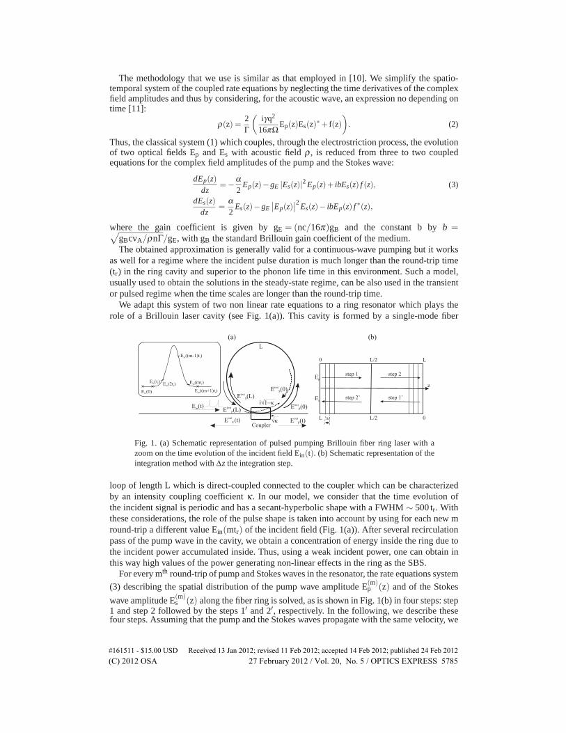
We adapt this system of two non linear rate equations to a ring resonator which plays therole of a Brillouin laser cavity (see Fig. 1(a)). This cavity is formed by a single-mode fiber

Fig. 1. (a) Schematic representation of pulsed pumping Brillouin fiber ring laser with azoom on the time evolution of the incident field Ein(t). (b) Schematic representation of theintegration method with Δz the integration step.

loop of length L which is direct-coupled connected to the coupler which can be characterizedby an intensity coupling coefficient κ . In our model, we consider that the time evolution ofthe incident signal is periodic and has a secant-hyperbolic shape with a FWHM ∼ 500 tr. Withthese considerations, the role of the pulse shape is taken into account by using for each new mround-trip a different value Ein(mtr) of the incident field (Fig. 1(a)). After several recirculationpass of the pump wave in the cavity, we obtain a concentration of energy inside the ring due tothe incident power accumulated inside. Thus, using a weak incident power, one can obtain inthis way high values of the power generating non-linear effects in the ring as the SBS.

For every mth round-trip of pump and Stokes waves in the resonator, the rate equations system

(3) describing the spatial distribution of the pump wave amplitude E(m)p (z) and of the Stokes

wave amplitude E(m)s (z) along the fiber ring is solved, as is shown in Fig. 1(b) in four steps: step

1 and step 2 followed by the steps 1′ and 2′, respectively. In the following, we describe thesefour steps. Assuming that the pump and the Stokes waves propagate with the same velocity, we


can consider that during the forward-propagation of the pump on the first half of the resonator(step 1), the Stokes wave is backward-propagated on the second half of the resonator (step 1′).These two steps are followed by the forward-propagation (backward-propagated) of the pump(Stokes) on the second half (step 2 (2′)) by using the values of the Stokes (pump) field alreadyfound in the first part of the integration (step 1′ (1)). In this way, the system (3) of the coupledequations is decoupled: the first equation is used to numerically propagate the pump, whereasthe second one, to propagate the Stokes wave. These ordinary differential equations can be nowindependently integrated using a numerical approximation method such as the fourth-orderRunge-Kutta. Let denote by ℜEp, ℑEp, ℜEs and ℑEs the real and imaginary part of the pumpand Stokes fields. Then, the pump propagation is described by the following two equations,

coupled through the values of Stokes field ℜE(m)s (z) and ℑE(m)

s (z):

dℜE(m)p (z)

dz=−α

2ℜE(m)

p (z)−gE

∣∣∣E(m)s (z)

∣∣∣2 ℜE(m)p (z)−bℑE(m)

s (z) f (z), (4)

dℑE(m)p (z)dz

=−α2

ℑE(m)p (z)−gE

∣∣∣E(m)s (z)

∣∣∣2 ℑE(m)p (z)+bℜE(m)

s (z) f (z),

with the boundary conditions for each new m round-trip calculated as a superposition [12, 13]between the value of the incident field at the moment m× tr and the circulating field of theprecedent round-trip which are transmitted through the coupler (Fig. 1(a)):

E(m)p (0) = i

√1−κEin(mtr)+

√κE(m−1)

p (L)e−iΔφp , (5)

where Δφp is detuning from resonance which replaces the linear phase shift for the pump waveφp and is defined by: Δφp = 2πnL/λp −2pπ , p being an integer. We may observe that, for thefirst pass, the boundary conditions depend only on the value of the incident field of the pump.

In order to obtain the spatial distribution of the Stokes field, we use the second equationof the system (3) in which the pump and Stokes fields are counterpropagating. As these twopropagations are decoupled, we impose a change of the sign in this equation. Put z′ = L− zwith z′ ∈ [0,L] and one obtains the following two equations coupled through the values of

pump ℜE(m)p (z) and ℑE(m)

p (z):

dℜE(m)s (z′)dz′

=−α2

ℜE(m)s (z′)+gE

∣∣∣E(m)p (z′)

∣∣∣2 ℜE(m)s (z′)−bℑE(m)

p (z′) f ∗(z′), (6)

dℑE(m)s (z′)dz′

=−α2

ℑE(m)s (z′)+gE

∣∣∣E(m)p (z′)

∣∣∣2 ℑE(m)s (z′)+bℜE(m)

p (z′) f ∗(z′),

with the boundary condition:

E(m)s (0) =

√κE(m−1)

s (L)e−iΔφs , (7)

where Δφs is the linear phase shift per round-trip of the Stokes wave. The linear phase shift ofthe Stokes wave is different of the pump linear phase shift Δφp and it is defined according tothe following expression [7]: Δφs = Δφp −2πνBnL/c, where νB is the acoustic frequency.

Based on these observations, for each m round trip in the ring, the values of the Stokes (pump)field appearing in the previous Eqs. (4) and (6), respectively, are calculated as fallows: for thepropagation on the first half of the round trip they are given according to the values obtained and

stored in the previous round trip (using Eqs. (6) and (4), respectively) : E(m)s (z) = E(m−1)

s (z′),E(m)

p (z′) = E(m−1)p (z) and, for the second part of the resonator they are given by those found

in the first step integration of the Stokes (pump) field: E(m)s (z) = E(m)

s (z′), E(m)p (z′) = E(m)

p (z).From these last relations and from the boundary conditions (7) let observe that for the firstround trip, the Stokes field will never appear without the contribution of the noise f(z). Thatjustifies the introduction of the noise source term in the initial system (1).

After each complete tour of the resonator of tr duration, we obtain the spatial distribution offields and the new initial conditions computed using Eqs. (5) and (7). Simultaneously we obtain


the expressions for the output fields after mth round-trip:

Eoutp (mtr) =

√κEin(mtr)+ i

√1−κEp(L,mtr)e

−iΔφp , (8)

Eouts (mtr) = i

√1−κEs(0,mtr)e

−iΔφs . (9)

By Eq. (8) one computes the time evolution (at each mtr) of the resonator transmission as :T(mtr) = |Eout

p (mtr)/E0|2 and by Eq. (5) one calculates the time evolution of the enhancement

coefficient Q inside the resonator : Q(mtr) = |E(m)p (0,mtr)/E0|2. Finally, the relation (9) allows

to obtain the Stokes power in the output of the laser : PS(mtr) = (n/2)ε0cSeff|EoutS (mtr)|2. The

round-trip number is fixed at the beginning of the simulation such that it covers several periodsof the incident signal.

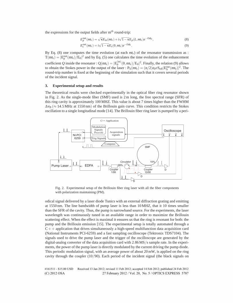
3. Experimental setup and results

The theoretical results were checked experimentally in the optical fiber ring resonator shownin Fig. 2. As the single-mode fiber (SMF) used is 2 m long, the free spectral range (SFR) ofthis ring cavity is approximately 100 MHZ. This value is about 7 times higher than the FWHMΔνB (≈ 14.5 MHz at 1550 nm) of the Brillouin gain curve. This condition restricts the Stokesoscillation to a single longitudinal mode [14]. The Brillouin fiber ring laser is pumped by a peri-

Fig. 2. Experimental setup of the Brillouin fiber ring laser with all the fiber componentswith polarization maintaining (PM).

odical signal delivered by a laser diode Tunics with an external diffraction grating and emittingat 1550 nm. The line bandwidth of pump laser is less than 10 MHZ, that it 10 times smallerthan the SFR of the cavity. Thus, the pump is narrowband source. For the experiments, the laserwavelength was continuously tuned in an available range in order to maximize the Brillouinscattering effect. When the effect is maximal it ensures us that the ring is resonant for both: thepump and the Brillouin emission [15]. The experimental setup is totally automated through aC++ application that drives simultaneously a high-speed multifunction data acquisition card(National Instruments PCI-6259) and a fast sampling oscilloscope (Tektronix TDS7104). Thesignals used to drive the pump laser and the trigger of the oscilloscope are generated by thedigital-analog converter of the data acquisition card with 2.86 MS/s sample rate. In the experi-ments, the power of the pump laser is directly modulated by the current driving the pump diode.This periodic modulation signal, with an average power of about 20 mW, is applied on the ringcavity through the coupler (10/90). Each period of the incident signal (the black signals on


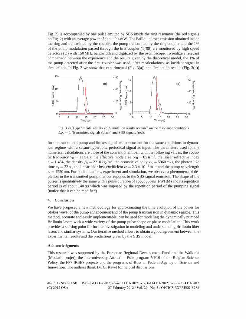
Fig. 2) is accompanied by one pulse emitted by SBS inside the ring resonator (the red signalson Fig. 2) with an average power of about 0.4 mW. The Brillouin laser emission obtained insidethe ring and transmitted by the coupler, the pump transmitted by the ring coupler and the 1%of the pump modulation passed through the first coupler (1/99) are monitored by high speeddetectors (D) with 150 MHz bandwidth and digitized by the oscilloscope. To realize a relevantcomparison between the experience and the results given by the theoretical model, the 1% ofthe pump detected after the first coupler was used, after recalculations, as incident signal insimulations. In Fig. 3 we show that experimental (Fig. 3(a)) and simulation results (Fig. 3(b))

Fig. 3. (a) Experimental results. (b) Simulation results obtained on the resonance conditionsΔφp = 0. Transmitted signals (black) and SBS signals (red).

for the transmitted pump and Stokes signal are concordant for the same conditions in dynam-ical regime with a secant-hyperbolic periodical signal as input. The parameters used for thenumerical calculations are those of the conventional fiber, with the following values: the acous-tic frequency νB = 11 GHz, the effective mode area Seff = 85 μm2, the linear refractive indexn = 1.454, the density ρ0 = 2210 kg/m3, the acoustic velocity vA = 5960 m/s, the photon livetime τp = 22 ns, the linear fiber loss coefficient α = 2.3×10−5 m−1 and the pump wavelengthλ = 1550 nm. For both situations, experiment and simulation, we observe a phenomena of de-pletion in the transmitted pump that corresponds to the SBS signal emission. The shape of thepulses is qualitatively the same with a pulse duration of about 350 ns (FWHM) and its repetitionperiod is of about 140 μs which was imposed by the repetition period of the pumping signal(notice that it can be modified).

4. Conclusion

We have proposed a new methodology for approximating the time evolution of the power forStokes wave, of the pump enhancement and of the pump transmission in dynamic regime. Thismethod, accurate and easily implementable, can be used for modeling the dynamically pumpedBrillouin lasers with a wide variety of the pump pulse shape or phase modulation. This workprovides a starting point for further investigation in modeling and understanding Brillouin fiberlasers and similar systems. Our iterative method allows to obtain a good agreement between theexperimental results and the predictions given by the SBS model.

Acknowledgments

This research was supported by the European Regional Development Fund and the Wallonia(Mediatic projet), the Interuniversity Attraction Pole program VI/10 of the Belgian SciencePolicy, the FP7 IRSES projects and the programs of Russian Federal Agency on Science andInnovation. The authors thank Dr. G. Ravet for helpful discussions.


Numerical approximation for Brillouin fiber ring resonator

Documents

Transcript of Numerical approximation for Brillouin fiber ring resonator