Computational and Applied MathematicsVol. 22, N. 1, pp. 99–121, 2003Copyright © 2003 SBMAC

Finite element approximation of bipolar viscous fluids

H. MANOUZI1, A. BRAHMI2 and M. FARHLOUL2

1Département de Mathématiques et de Statistique

Université Laval, Québec, G1K7P4, Canada2Département de Mathématiques et de Statistique

Université de Moncton, Moncton, NB, E1A 3E9, Canada

E-mail: hm@mat.ulaval.ca

Abstract. A bipolar viscous fluid model is assumed to regularise the solution of Newtonian

and quasi-Newtonian flows. In this article, a mixed finite element approximation of the bipolar

viscous fluids is proposed. In this approximation the velocity of the fluid together with its laplacian

are the most relevant unknowns. An existence and uniqueness results are proved. A mixed finite

element approximation is derived and numerical results are presented.

Mathematical subject classification: 65N30, 76M10.

Key words: finite element, bipolar fluids, Navier-Stokes, mixed finite element, PDE.

1 Introduction

Mathematical model for fluid motion play an important role in theoretical and

computational studies in the aeronautics, meteorological, plasma physics, etc.

The Navier-Stokes equations are generally accepted as providing an accurate

model for the incompressible motion of viscous fluids in many practical situa-

tions. In the classical Navier-Stokes equations theory, the viscosity of the fluid

is modeled by the dependence of the stress on the first gradient of velocity. It is

well known that the corresponding mathematical theory contains a number of un-

solved problems. One of the fundamental open problems for the Navier-Stokes

equations in 3-dimensional space is that of the uniqueness of the solution of

the Cauchy-Dirichlet problem, which is not guaranteed in the functional classes

in which global existence holds. These problems have led many authors that

#551/02.

100 BIPOLAR VISCOUS FLUIDS

a stronger mechanism of dissipation and viscosity, namely the dependence of

the stress on the higher gradients of velocity, must occur in the flows of viscous

fluids. In materials in which the higher gradients of velocity and the higher gra-

dients of deformation influence the response, the rate of work of internal forces

cannot be expected to be only the product of the usual second order stress tensor

with the first gradient of velocity. Instead of this, a more general expression

must be assumed containing additionally the sum of products of higher order

multipolar stress tensors with the higher gradients of velocity. Otherwise such

materials cannot be compatible with the Clausius-Duhem inequality. In [13]a thermodynamics theory of constitutive equations of multipolar viscous fluids

within the framework of the theory of Green and Rivlin [9] has been developed.

This paper is organized as follows. In section 2 we formulate the problem, we

introduce some notations and we give some preliminary results. In section 3 we

formulate the bipolar Navier-Stokes problem and we prove the existence and the

unicity of the solution. In section 4 we study a mixed variational formulation

and its approximation. Finally in section 5 we give some numerical results.

2 Problem formulation and preliminary results

2.1 Problem formulation

We will use the standard notation for gradient, divergence and curl operators, i.e.

for a scalar function p and a vector function v, we write ∇q, div v and curl vfor the gradient, divergence and the curl respectively. We further recall that the

vector-valued Laplace operator, �, is defined by

�v = (�v1, �v2), v = (v1, v2)

and we have the vector identity

curl (curl v) = −�v, ∀ v such that div v = 0. (1)

Next we let � be an open bounded domain of R2, with smooth boundary �. We

consider the stationary flow of an incompressible nonlinear bipolar fluid. This

Comp. Appl. Math., Vol. 22, N. 1, 2003

H. MANOUZI, A. BRAHMI and M. FARHLOUL 101

problem is modeled by the following system of equations:{(u · ∇)u = f + div σ in �

div u = 0 in �(2)

where u is the velocity field, σ the stress tensor and f represents the external

forces. The stress tensorσ = (σij )has the form (see [4], [8], [9], [10], [11], [13])

σ = −p I + 2ν �r(ε(u)) ε(u) − 2µ�ε(u) (3)

where

�r(τ) = (λ+ | τ |2) r−2

2 , τ ∈ R2×2

εij (u) = 1

2

(∂ui

∂xj

+ ∂uj

∂xi

), 1 ≤ i, j ≤ 2

and r, ν , λ and µ are positive constants with r > 1. Since div u = 0, the

divergence of the stress tensor takes the form

div σ = −∇p + 2ν div (�r(ε(u)) ε(u)) − µ�2u.

Correspondingly, the bipolar Navier-Stokes equations become

µ�2u − 2ν div[(λ+ | ε(u) |2) r−2

2 ε(u)]

+∇p + (u · ∇)u = f in �

div u = 0 in �.

(4)

By choosing the appropriate constants r, µ, ν and λ we find these classical mod-

els of fluids:

• Carreau’s law model (see [15]): µ = 0.

• Power law model (see [15]): µ = 0, λ = 0.

• Classical Navier-Stokes: r = 2, µ = 0.

• Regularized Navier-Stokes equations (see [14]): r = 2, µ �= 0.

Comp. Appl. Math., Vol. 22, N. 1, 2003

102 BIPOLAR VISCOUS FLUIDS

These laws occur in many mathematical models of physical processes of polymer,

of visco-elastic and visco-plastic fluids or of fluids with large stresses (See [10]).

We will study the system of equations (4) with the boundary conditions{u = 0 on �

�u · τ = 0 on �(5)

where τ is the unit tangent to �.

2.2 Preliminary results

Let Hm(�) and Hm(�) denote the usual Sobolev spaces of order m defined

on � and �, respectively; also Hm(�) and Hm(�) denote their vector-valued

countreparts. The inner product on Hm(�) or Hm(�) is defined by (., .)m. The

space Hm(�) is equipped with the norm

‖v‖m,� ={∑

k≤m

| v |2k,�

} 12

where

| v |k,�={ ∑

|α|=k

∫�

| ∂αv |2 dx

} 12

.

For vector valued functions the above norm extends naturally as follows: for

v = (v1, v2)

‖v‖m,� =(

2∑i=1

‖vi‖2m,�

) 12

.

We also define the Hilbert spaces

H(div , �) = {v | v ∈ L2(�), div v ∈ L2(�)

}H(curl , �) = {

v | v ∈ L2(�), curl v ∈ L2(�)}.

These spaces are equipped with their natural hilbertian norms.

LetD(�)denote the space of infinitely differentiable functions having compact

support and let Hm0 (�) be the closure ofD(�) with respect to the norm ‖ . ‖m,�

and H−m(�) the dual space of Hm0 (�). The duality pairing between H

12 (�),

H12 (�) and their dual spaces H− 1

2 (�), H− 12 (�) is denoted by 〈., .〉− 1

2 , 12 ,�.

We also have the following trace results (see, e. g., [6], [16])Comp. Appl. Math., Vol. 22, N. 1, 2003

H. MANOUZI, A. BRAHMI and M. FARHLOUL 103

Theorem 2.1. Let � be a bounded open set of R2 with a Lipschitz continuous

boundary �. We have the following properties:

1. There exists a unique linear continuous map γ0 : H 1(�) −→ H12 (�) such

that

γ0v = v| �, ∀v ∈ H 1(�).

2. There exists a unique linear continuous map γn : H(div , �) −→ H− 12 (�)

such that

γnv = (v · n)| �, ∀v ∈ H(div , �)

where n denotes the unit outward normal to �.

3. There exists a unique linear continuous map γτ : H(curl , �)−→ H− 12 (�)

such that

γτ v = (v · τ)| �, ∀v ∈ H(curl , �).

We use the convention H 0(�) = L2(�), H0(�) = L2(�), (., .)0 = (., .).

Also we introduce some function spaces which are related to the study of our

problem:

H 10 (�) = {v ∈ H 1(�) : γ0(v) = 0 on � }

H 20 (�) = {v ∈ H 2(�) : γ0(v) = 0 and γn(∇v) = 0 on � }

X = H10(�) ∩ H2(�) = {v | v ∈ H2(�), γ0(v) = 0 on �}

V = {v ∈ (D(�))2; div v = 0}

V = {v | v ∈ X, div v = 0}

M = {q ∈ L2(�),

∫�

q dx = 0}

H = {v ∈ L2(�), curl v ∈ H 1(�), div v = 0}.For details concerning Sobolev spaces consult [1], [5], [6].Comp. Appl. Math., Vol. 22, N. 1, 2003

104 BIPOLAR VISCOUS FLUIDS

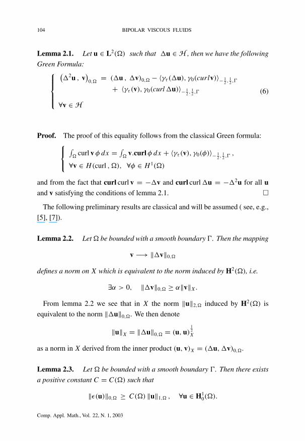
Lemma 2.1. Let u ∈ L2(�) such that �u ∈ H , then we have the following

Green Formula:

(�2u , v

)0,�

= (�u , �v)0,� − 〈γτ (�u), γ0(curlv)〉− 12 , 1

2 ,�

+ 〈γτ (v), γ0(curl �u)〉− 12 , 1

2 ,�

∀v ∈ H(6)

Proof. The proof of this equality follows from the classical Green formula:∫�

curl v φ dx = ∫�

v.curl φ dx + 〈γτ (v), γ0(φ)〉− 12 , 1

2 ,� ,

∀v ∈ H(curl , �), ∀φ ∈ H 1(�)

and from the fact that curl curl v = −�v and curl curl �u = −�2u for all uand v satisfying the conditions of lemma 2.1. �

The following preliminary results are classical and will be assumed ( see, e.g.,

[5], [7]).

Lemma 2.2. Let � be bounded with a smooth boundary �. Then the mapping

v −→ ‖�v‖0,�

defines a norm on X which is equivalent to the norm induced by H2(�), i.e.

∃α > 0, ‖�v‖0,� ≥ α‖v‖X.

From lemma 2.2 we see that in X the norm ‖u‖2,� induced by H2(�) is

equivalent to the norm ‖�u‖0,�. We then denote

‖u‖X = ‖�u‖0,� = (u, u)12X

as a norm in X derived from the inner product (u, v)X = (�u, �v)0,�.

Lemma 2.3. Let � be bounded with a smooth boundary �. Then there exists

a positive constant C = C(�) such that

‖ε(u)‖0,� ≥ C(�) ‖u‖1,� , ∀u ∈ H10(�).

Comp. Appl. Math., Vol. 22, N. 1, 2003

H. MANOUZI, A. BRAHMI and M. FARHLOUL 105

3 The bipolar Navier-Stokes problem

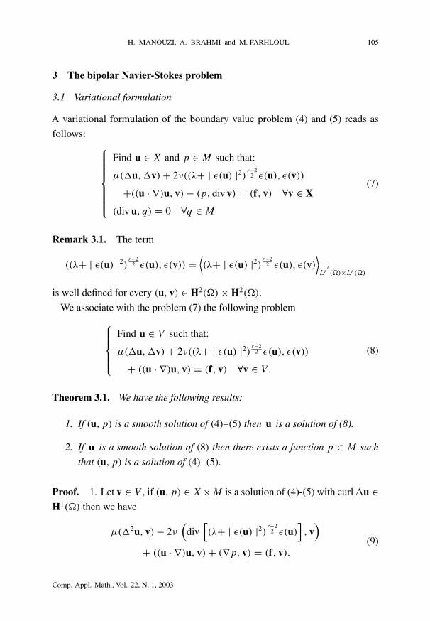
3.1 Variational formulation

A variational formulation of the boundary value problem (4) and (5) reads as

follows:

Find u ∈ X and p ∈ M such that:

µ(�u, �v) + 2ν((λ+ | ε(u) |2) r−22 ε(u), ε(v))

+((u · ∇)u, v) − (p, div v) = (f, v) ∀v ∈ X

(div u, q) = 0 ∀q ∈ M

(7)

Remark 3.1. The term

((λ+ | ε(u) |2) r−22 ε(u), ε(v)) =

⟨(λ+ | ε(u) |2) r−2

2 ε(u), ε(v)⟩Lr

′(�)×Lr(�)

is well defined for every (u, v) ∈ H2(�) × H2(�).

We associate with the problem (7) the following problem

Find u ∈ V such that:

µ(�u, �v) + 2ν((λ+ | ε(u) |2) r−22 ε(u), ε(v))

+ ((u · ∇)u, v) = (f, v) ∀v ∈ V.

(8)

Theorem 3.1. We have the following results:

1. If (u, p) is a smooth solution of (4)–(5) then u is a solution of (8).

2. If u is a smooth solution of (8) then there exists a function p ∈ M such

that (u, p) is a solution of (4)–(5).

Proof. 1. Let v ∈ V , if (u, p) ∈ X ×M is a solution of (4)-(5) with curl �u ∈H1(�) then we have

µ(�2u, v) − 2ν(

div[(λ+ | ε(u) |2) r−2

2 ε(u)], v)

+ ((u · ∇)u, v) + (∇p, v) = (f, v).

(9)

Comp. Appl. Math., Vol. 22, N. 1, 2003

106 BIPOLAR VISCOUS FLUIDS

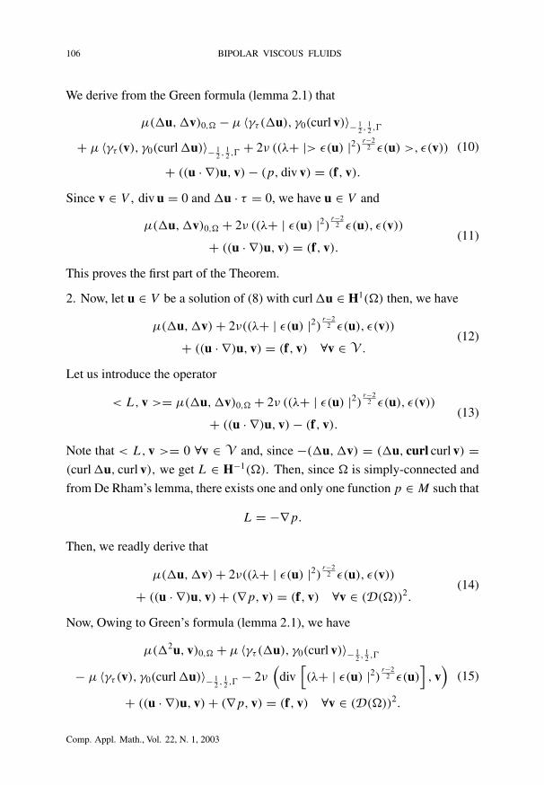
We derive from the Green formula (lemma 2.1) that

µ(�u, �v)0,� − µ 〈γτ (�u), γ0(curl v)〉− 12 , 1

2 ,�

+ µ 〈γτ (v), γ0(curl �u)〉− 12 , 1

2 ,� + 2ν ((λ+ |> ε(u) |2) r−22 ε(u) >, ε(v))

+ ((u · ∇)u, v) − (p, div v) = (f, v).

(10)

Since v ∈ V , div u = 0 and �u · τ = 0, we have u ∈ V and

µ(�u, �v)0,� + 2ν ((λ+ | ε(u) |2) r−22 ε(u), ε(v))

+ ((u · ∇)u, v) = (f, v).(11)

This proves the first part of the Theorem.

2. Now, let u ∈ V be a solution of (8) with curl �u ∈ H1(�) then, we have

µ(�u, �v) + 2ν((λ+ | ε(u) |2) r−22 ε(u), ε(v))

+ ((u · ∇)u, v) = (f, v) ∀v ∈ V .(12)

Let us introduce the operator

< L, v >= µ(�u, �v)0,� + 2ν ((λ+ | ε(u) |2) r−22 ε(u), ε(v))

+ ((u · ∇)u, v) − (f, v).(13)

Note that < L, v >= 0 ∀v ∈ V and, since −(�u, �v) = (�u, curl curl v) =(curl �u, curl v), we get L ∈ H−1(�). Then, since � is simply-connected and

from De Rham’s lemma, there exists one and only one function p ∈ M such that

L = −∇p.

Then, we readly derive that

µ(�u, �v) + 2ν((λ+ | ε(u) |2) r−22 ε(u), ε(v))

+ ((u · ∇)u, v) + (∇p, v) = (f, v) ∀v ∈ (D(�))2.(14)

Now, Owing to Green’s formula (lemma 2.1), we have

µ(�2u, v)0,� + µ 〈γτ (�u), γ0(curl v)〉− 12 , 1

2 ,�

− µ 〈γτ (v), γ0(curl �u)〉− 12 , 1

2 ,� − 2ν(

div[(λ+ | ε(u) |2) r−2

2 ε(u)], v)

+ ((u · ∇)u, v) + (∇p, v) = (f, v) ∀v ∈ (D(�))2.

(15)

Comp. Appl. Math., Vol. 22, N. 1, 2003

H. MANOUZI, A. BRAHMI and M. FARHLOUL 107

Hence, it follows that

µ�2u − 2ν div[(λ+ | ε(u) |2) r−2

2 ε(u)]

+ (u · ∇)u

+ ∇p = f in (D′(�))2.

(16)

Since f ∈ L2(�), we have

µ�2u − 2ν div[(λ+ | ε(u) |2) r−2

2 ε(u)]

+ (u · ∇)u + ∇p = f

in L2(�).

(17)

Moreover, as u ∈ V , we have

µ�2u − 2ν div[(λ+ | ε(u) |2) r−2

2 ε(u)]

+ (u · ∇)u

+∇p = f in �

div u = 0 in �

u = 0 on �.

(18)

Now, by using the Green’s formula (lemma 2.1), we have on the one hand:

µ(�u, �v)0,� − µ 〈γτ (�u), γ0(curl v)〉− 12 , 1

2 ,�

+ 2ν ((λ+ | ε(u) |2) r−22 ε(u), ε(v)) + ((u · ∇)u, v) = (f, v) ∀v ∈ V

(19)

and, by (8), we get

〈γτ (�u), γ0(curl v)〉− 12 , 1

2 ,� = 0 ∀v ∈ V.

Finally, from [2], we have

γτ (�u) = 0 on �. �

3.2 Existence and unicity of the solution

In order to show the existence and the unicity of the the solution of problem (8)

we need to state some intermediate results.

Comp. Appl. Math., Vol. 22, N. 1, 2003

108 BIPOLAR VISCOUS FLUIDS

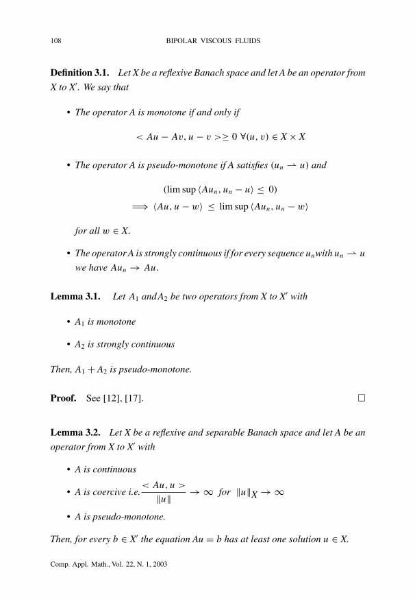
Definition 3.1. Let X be a reflexive Banach space and let A be an operator from

X to X′. We say that

• The operator A is monotone if and only if

< Au − Av, u − v >≥ 0 ∀(u, v) ∈ X × X

• The operator A is pseudo-monotone if A satisfies (un ⇀ u) and

(lim sup 〈Aun, un − u〉 ≤ 0)

�⇒ 〈Au, u − w〉 ≤ lim sup 〈Aun, un − w〉

for all w ∈ X.

• The operator A is strongly continuous if for every sequence unwith un ⇀ u

we have Aun → Au.

Lemma 3.1. Let A1 and A2 be two operators from X to X′ with

• A1 is monotone

• A2 is strongly continuous

Then, A1 + A2 is pseudo-monotone.

Proof. See [12], [17]. �

Lemma 3.2. Let X be a reflexive and separable Banach space and let A be an

operator from X to X′ with

• A is continuous

• A is coercive i.e.< Au, u >

‖u‖ → ∞ for ‖u‖X → ∞

• A is pseudo-monotone.

Then, for every b ∈ X′ the equation Au = b has at least one solution u ∈ X.

Comp. Appl. Math., Vol. 22, N. 1, 2003

H. MANOUZI, A. BRAHMI and M. FARHLOUL 109

Proof. See [12], [17]. �

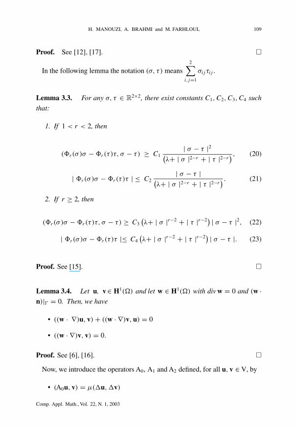
In the following lemma the notation (σ, τ ) means2∑

i,j=1

σij τij .

Lemma 3.3. For any σ, τ ∈ R2×2, there exist constants C1, C2, C3, C4 such

that:

1. If 1 < r < 2, then

(�r(σ )σ − �r(τ)τ, σ − τ) ≥ C1| σ − τ |2(

λ+ | σ |2−r + | τ |2−r) , (20)

| �r(σ )σ − �r(τ)τ | ≤ C2| σ − τ |(

λ+ | σ |2−r + | τ |2−r) . (21)

2. If r ≥ 2, then

(�r(σ )σ − �r(τ)τ, σ − τ) ≥ C3(λ+ | σ |r−2 + | τ |r−2

) | σ − τ |2, (22)

| �r(σ )σ − �r(τ)τ |≤ C4(λ+ | σ |r−2 + | τ |r−2

) | σ − τ |. (23)

Proof. See [15]. �

Lemma 3.4. Let u, v ∈ H1(�) and let w ∈ H1(�) with div w = 0 and (w ·n)|� = 0. Then, we have

• ((w · ∇)u, v) + ((w · ∇)v, u) = 0

• ((w · ∇)v, v) = 0.

Proof. See [6], [16]. �

Now, we introduce the operators A0, A1 and A2 defined, for all u, v ∈ V, by

• (A0u, v) = µ(�u, �v)

Comp. Appl. Math., Vol. 22, N. 1, 2003

110 BIPOLAR VISCOUS FLUIDS

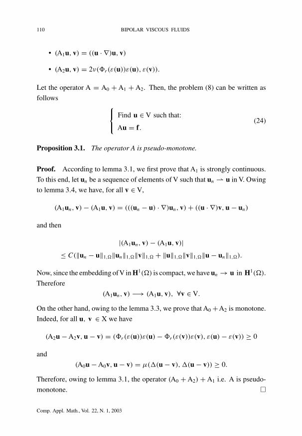
• (A1u, v) = ((u · ∇)u, v)

• (A2u, v) = 2ν(�r(ε(u))ε(u), ε(v)).

Let the operator A = A0 + A1 + A2. Then, the problem (8) can be written as

follows Find u ∈ V such that:

Au = f .(24)

Proposition 3.1. The operator A is pseudo-monotone.

Proof. According to lemma 3.1, we first prove that A1 is strongly continuous.

To this end, let un be a sequence of elements of V such that un ⇀ u in V. Owing

to lemma 3.4, we have, for all v ∈ V,

(A1un, v) − (A1u, v) = (((un − u) · ∇)un, v) + ((u · ∇)v, u − un)

and then

|(A1un, v) − (A1u, v)|≤ C(‖un − u‖1,�‖un‖1,�‖v‖1,� + ‖u‖1,�‖v‖1,�‖u − un‖1,�).

Now, since the embedding ofV in H1(�) is compact, we have un → u in H1(�).

Therefore

(A1un, v) −→ (A1u, v), ∀v ∈ V.

On the other hand, owing to the lemma 3.3, we prove that A0 +A2 is monotone.

Indeed, for all u, v ∈ X we have

(A2u − A2v, u − v) = (�r(ε(u))ε(u) − �r(ε(v))ε(v), ε(u) − ε(v)) ≥ 0

and

(A0u − A0v, u − v) = µ(�(u − v), �(u − v)) ≥ 0.

Therefore, owing to lemma 3.1, the operator (A0 + A2) + A1 i.e. A is pseudo-

monotone. �

Comp. Appl. Math., Vol. 22, N. 1, 2003

H. MANOUZI, A. BRAHMI and M. FARHLOUL 111

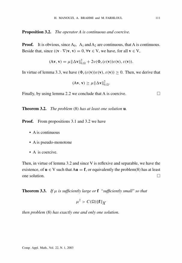
Proposition 3.2. The operator A is continuous and coercive.

Proof. It is obvious, since A0, A1 andA2 are continuous, that A is continuous.

Beside that, since ((v · ∇)v, v) = 0, ∀v ∈ V, we have, for all v ∈ V,

(Av, v) = µ‖�v‖20,� + 2ν(�r(ε(v))ε(v), ε(v)).

In virtue of lemma 3.3, we have (�r(ε(v))ε(v), ε(v)) ≥ 0. Then, we derive that

(Av, v) ≥ µ‖�v‖20,�.

Finally, by using lemma 2.2 we conclude that A is coercive. �

Theorem 3.2. The problem (8) has at least one solution u.

Proof. From propositions 3.1 and 3.2 we have

• A is continuous

• A is pseudo-monotone

• A is coercive.

Then, in virtue of lemma 3.2 and since V is reflexive and separable, we have the

existence, of u ∈ V such that Au = f , or equivalently the problem(8) has at least

one solution. �

Theorem 3.3. If µ is sufficiently large or f “sufficiently small" so that

µ2 > C(�)‖f‖X′

then problem (8) has exactly one and only one solution.

Comp. Appl. Math., Vol. 22, N. 1, 2003

112 BIPOLAR VISCOUS FLUIDS

Proof. We assume that there are two solutions u1 and u2 in V of (8) then we

have

(Au1 − Au2, v) = 0 ∀v ∈ V.

Then, for all v ∈ V, we have

µ(�u1 − �u2, �v) + 2ν(�r(ε(u1))ε(u1) − �r(ε(u2))ε(u2),

ε(v)) + ((u1 · ∇)u1, v) − ((u2 · ∇)u2, v) = 0.

By taking v = u1 − u2, we get

µ‖�(u1 − u2)‖20,� + 2ν(�r(ε(u1))ε(u1) − �r(ε(u2))ε(u2),

ε(u1) − ε(u2)) = −(((u1 − u2) · ∇)u1, u1 − u2).

Since, owing to lemma 3.3,

2ν(�r(ε(u1))ε(u1) − �r(ε(u2))ε(u2), ε(u1) − ε(u2)) ≥ 0,

we readily derive that

µ‖�(u1 − u2)‖20,� ≤ |(((u1 − u2) · ∇)u1, u1 − u2)|.

Now, for some positive constant C1 depending on �, we have

|(((u1 − u2) · ∇)u1, u1 − u2)| ≤ C1‖u1 − u2‖21,�‖u1‖1,�.

By using lemma 2.2, we get

µα2‖u1 − u2‖21,� ≤ C1‖u1 − u2‖2

1,�‖u1‖1,�. (25)

On the other hand, since u1 is a solution of (8) and by taking v = u1 in (8), we

get

µ‖�u1‖20,� + 2ν(�r(ε(u1))ε(u1), ε(u1)) = (f, u1).

Therefore,

µ‖�u1‖20,� ≤ |(f, u1)|.

We easily derive that u1 satisfies

µα2‖u1‖21,� ≤ ‖f‖X′‖u1‖1,�.

Comp. Appl. Math., Vol. 22, N. 1, 2003

H. MANOUZI, A. BRAHMI and M. FARHLOUL 113

and then

‖u1‖1,� ≤ 1

µα2‖f‖X′ . (26)

As a consequence of (25) and (26), we obtain

µα2‖u1 − u2‖21,� ≤ C1‖u1 − u2‖2

1,�

1

µα2‖f‖X′ .

Therefore

(µα2 − C1

µα2‖f‖X′)‖u1 − u2‖2

1,� ≤ 0.

Finally, we readily derive the uniqueness of the solution when the condition

µ2 >C1

α4‖f‖X′ .

holds. �

4 The mixed finite element formulation

In order to approximate numerically problem (7) we introduce the mixed for-

mulation which allows us to reduce the order of problem (7). That makes the

numerical approximation easier. Let us take w = −�u as a new variable. Then,

since div (�u) = 0 and owing to the identity (1), we may recast problem (4) as

second order system for u and w:

µcurl curl w − 2νdiv[(λ+ | ε(u) |2) r−2

2 ε(u)]

+ (u · ∇)u

+∇p = f in �

w = −�u in �

div u = 0 in �

u = 0 on �

w · τ = 0 on �.

(27)

In order to study the last problem we introduce the following space

Q = H0(curl , �) = {v ∈ H(curl , �) and (v · τ)|� = 0}.

Comp. Appl. Math., Vol. 22, N. 1, 2003

114 BIPOLAR VISCOUS FLUIDS

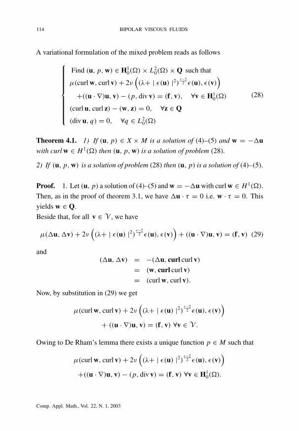
A variational formulation of the mixed problem reads as follows

Find (u, p, w) ∈ H10(�) × L2

0(�) × Q such that

µ(curl w, curl v) + 2ν((λ+ | ε(u) |2) r−2

2 ε(u), ε(v))

+((u · ∇)u, v) − (p, div v) = (f, v), ∀v ∈ H10(�)

(curl u, curl z) − (w, z) = 0, ∀z ∈ Q

(div u, q) = 0, ∀q ∈ L20(�)

(28)

Theorem 4.1. 1) If (u, p) ∈ X × M is a solution of (4)–(5) and w = −�uwith curl w ∈ H 1(�) then (u, p, w) is a solution of problem (28).

2) If (u, p, w) is a solution of problem (28) then (u, p) is a solution of (4)–(5).

Proof. 1. Let (u, p) a solution of (4)–(5) and w = −�u with curl w ∈ H 1(�).

Then, as in the proof of theorem 3.1, we have �u · τ = 0 i.e. w · τ = 0. This

yields w ∈ Q.

Beside that, for all v ∈ V , we have

µ(�u, �v) + 2ν((λ+ | ε(u) |2) r−2

2 ε(u), ε(v))

+ ((u · ∇)u, v) = (f, v) (29)

and(�u, �v) = −(�u, curl curl v)

= (w, curl curl v)

= (curl w, curl v).

Now, by substitution in (29) we get

µ(curl w, curl v) + 2ν((λ+ | ε(u) |2) r−2

2 ε(u), ε(v))

+ ((u · ∇)u, v) = (f, v) ∀v ∈ V .

Owing to De Rham’s lemma there exists a unique function p ∈ M such that

µ(curl w, curl v) + 2ν((λ+ | ε(u) |2) r−2

2 ε(u), ε(v))

+((u · ∇)u, v) − (p, div v) = (f, v) ∀v ∈ H10(�).

Comp. Appl. Math., Vol. 22, N. 1, 2003

H. MANOUZI, A. BRAHMI and M. FARHLOUL 115

On the other hand by using the new variable w = −�u and the fact that div u = 0,

we get for all z ∈ Q

(w, z) = −(�u, z)= (curl curl u, z)= (curl u, curl z)− < z · τ, curl u >− 1

2 , 12 ,� .

Then, taking into account that z · τ = 0 and u ∈ X, we find

(w, z) − (curl u, curl z) = 0 ∀z ∈ Q.

Finally, from div u = 0, we get

(div u, q) = 0 ∀q ∈ M.

2. Conversely, suppose that (u, p, w) is a solution of (28) such that u ∈ H2(�)

and curl �u ∈ H 1(�). First, since (div u, q) = 0, ∀q ∈ M and u ∈ H10(�), we

have div u = 0. Now, since div u = 0, we have

(w, z) = (curl u, curl z) ∀z ∈ (D(�))2

= (curl curl u, z) ∀z ∈ (D(�))2

= −(�u, z) ∀z ∈ (D(�))2.

Thus w = −�u, and �u ∈ Q since w ∈ Q. Therefore,

(curl w, curl v) = −(curl �u, curl v) ∀v ∈ V= −(�u, curl curl v) ∀v ∈ V= (�u, �v) ∀v ∈ V .

Thus, by the fact that div �u = �div u = 0 , �u ∈ Q, curl �u ∈ H 1(�) and

by using the lemma 2.1, we have

(curl w, curl v) = (�2u, v) ∀v ∈ V .

Therefore,

µ(�2u, v) − 2ν(

div[(λ+ | ε(u) |2) r−2

2 ε(u)], v)

+ ((u · ∇)u, v) = (f, v) ∀v ∈ V .

Comp. Appl. Math., Vol. 22, N. 1, 2003

116 BIPOLAR VISCOUS FLUIDS

Owing to De Rham’s lemma and like in the proof of theorem 3.1, there exists

one and only one function p ∈ M such that:

µ�2u − 2ν div[(λ+ | ε(u) |2) r−2

2 ε(u)]

+ (u · ∇)u − f = −∇p.

Finally, by gathering, we get

µ�2u − 2ν div[(λ+ | ε(u) |2) r−2

2 ε(u)]

+ ∇p

+ (u · ∇)u = f in �

div u = 0 in �

u = 0 on �

�u · τ = 0 on �

(30 �)

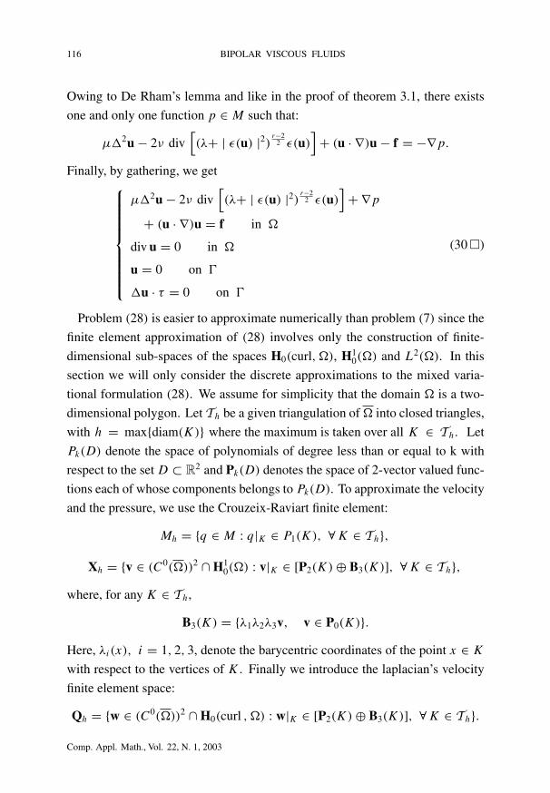
Problem (28) is easier to approximate numerically than problem (7) since the

finite element approximation of (28) involves only the construction of finite-

dimensional sub-spaces of the spaces H0(curl, �), H10(�) and L2(�). In this

section we will only consider the discrete approximations to the mixed varia-

tional formulation (28). We assume for simplicity that the domain � is a two-

dimensional polygon. Let Th be a given triangulation of � into closed triangles,

with h = max{diam(K)} where the maximum is taken over all K ∈ Th. Let

Pk(D) denote the space of polynomials of degree less than or equal to k with

respect to the set D ⊂ R2 and Pk(D) denotes the space of 2-vector valued func-

tions each of whose components belongs to Pk(D). To approximate the velocity

and the pressure, we use the Crouzeix-Raviart finite element:

Mh = {q ∈ M : q|K ∈ P1(K), ∀ K ∈ Th},

Xh = {v ∈ (C0(�))2 ∩ H10(�) : v|K ∈ [P2(K) ⊕ B3(K)], ∀ K ∈ Th},

where, for any K ∈ Th,

B3(K) = {λ1λ2λ3v, v ∈ P0(K)}.Here, λi(x), i = 1, 2, 3, denote the barycentric coordinates of the point x ∈ K

with respect to the vertices of K . Finally we introduce the laplacian’s velocity

finite element space:

Qh = {w ∈ (C0(�))2 ∩ H0(curl , �) : w|K ∈ [P2(K) ⊕ B3(K)], ∀ K ∈ Th}.Comp. Appl. Math., Vol. 22, N. 1, 2003

H. MANOUZI, A. BRAHMI and M. FARHLOUL 117

Now, let

a((u, p), (v, q)) = 2ν

∫�

�r(ε(u))ε(u) : ε(v) dx

+∫

�

(u · ∇)u. v dx −∫

�

p div v dx +∫

�

q div u dx

b(z, (v, q)) = µ

∫�

curl z curl v dx

c(w, z) =∫

�

w.z dx

Then (28) is discretized by the following problem

Find (uh, ph, wh) ∈ Xh × Mh × Qh such that

a((uh, ph), (vh, qh)) + b(wh, (vh, qh))) = (f, vh),

∀(vh, qh) ∈ Xh × Mh

b(zh, (uh, ph)) − c(wh, zh) = 0, ∀zh ∈ Qh.

(31)

5 Numerical results

The performance of the numerical method described above has been tested on

three examples of a comparative nature: the Poiseuille flow, the flow over a

backward-facing step and the driven cavity flow.

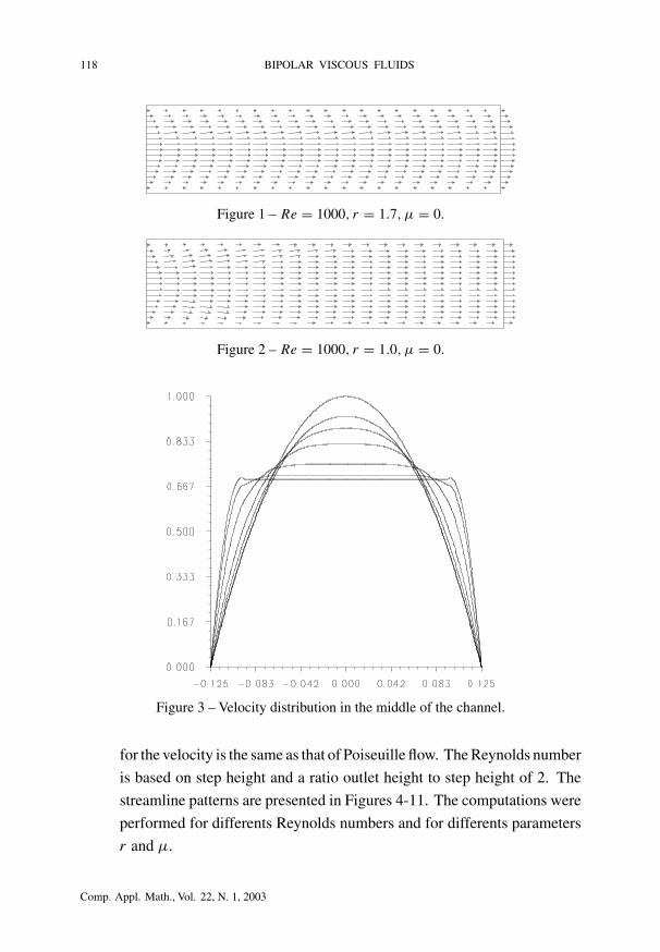
• Poiseuille flow

At inlet of the channel, a parabolic profile for the velocity is used. Figures

1, 2 give the velocity fields for the Reynolds number Re = 1000 and for

r = 1.7 and r = 1 respectively. The velocity distribution in the middle

of the channel is shown in Figure 3 for different values of the parameter

r = 1.8, 1.6, 1.4, 1.2, 1.1, 1.

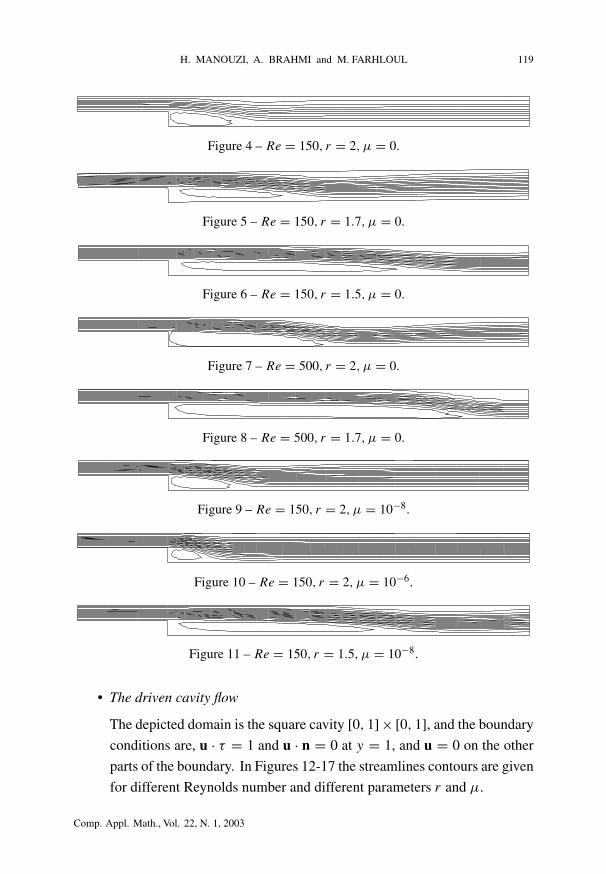
• Backward-facing step flow

With flow in channels of constant geometry such as the Poiseuille flow, a

predominant flow direction prevails. Instead, where the geometry changes

abruptly, the flow separates and develops a recirculation region. Inlet value

Comp. Appl. Math., Vol. 22, N. 1, 2003

118 BIPOLAR VISCOUS FLUIDS

Figure 1 – Re = 1000, r = 1.7, µ = 0.

Figure 2 – Re = 1000, r = 1.0, µ = 0.

Figure 3 – Velocity distribution in the middle of the channel.

for the velocity is the same as that of Poiseuille flow. The Reynolds number

is based on step height and a ratio outlet height to step height of 2. The

streamline patterns are presented in Figures 4-11. The computations were

performed for differents Reynolds numbers and for differents parameters

r and µ.

Comp. Appl. Math., Vol. 22, N. 1, 2003

H. MANOUZI, A. BRAHMI and M. FARHLOUL 119

Figure 4 – Re = 150, r = 2, µ = 0.

Figure 5 – Re = 150, r = 1.7, µ = 0.

Figure 6 – Re = 150, r = 1.5, µ = 0.

Figure 7 – Re = 500, r = 2, µ = 0.

Figure 8 – Re = 500, r = 1.7, µ = 0.

Figure 9 – Re = 150, r = 2, µ = 10−8.

Figure 10 – Re = 150, r = 2, µ = 10−6.

Figure 11 – Re = 150, r = 1.5, µ = 10−8.

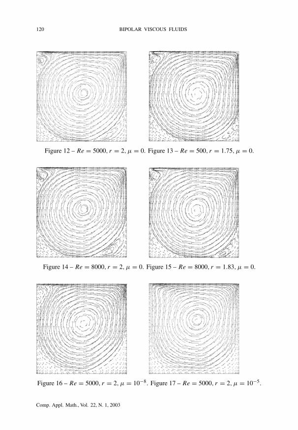
• The driven cavity flow

The depicted domain is the square cavity [0, 1]× [0, 1], and the boundary

conditions are, u · τ = 1 and u · n = 0 at y = 1, and u = 0 on the other

parts of the boundary. In Figures 12-17 the streamlines contours are given

for different Reynolds number and different parameters r and µ.

Comp. Appl. Math., Vol. 22, N. 1, 2003

120 BIPOLAR VISCOUS FLUIDS

Figure 12 – Re = 5000, r = 2, µ = 0. Figure 13 – Re = 500, r = 1.75, µ = 0.

Figure 14 – Re = 8000, r = 2, µ = 0. Figure 15 – Re = 8000, r = 1.83, µ = 0.

Figure 16 – Re = 5000, r = 2, µ = 10−8. Figure 17 – Re = 5000, r = 2, µ = 10−5.

Comp. Appl. Math., Vol. 22, N. 1, 2003

H. MANOUZI, A. BRAHMI and M. FARHLOUL 121

For all the above numerical tests the value of the parameter λ has been

fixed to the value λ = 10−11.

REFERENCES

[1] R.A. Adams, Sobolev spaces, Academic Press, New York, (1975).

[2] C. Amrouche and V. Girault, Problèmes généralisés de Stokes, Publication du Laboratoire

d’Analyse Numérique R91001, Université Pierre et Marie Curie, Paris.

[3] H. Bellout, R. Bloom and J. Necas, Phenomenological behavior of multipolar viscous fluids,

Quarterly of Applied Mathematics, Volume IX, Number 4 (1991), 687–728.

[4] A. Brahmi, Simulation numérique des fluides bipolaires, Mémoire de maîtrise, Université

Laval, Québec, (1994).

[5] P.G. Ciarlet, The Finite Element Method for Elliptic Problems, North-Holland, Amsterdam,

1978.

[6] V. Girault and P.A. Raviart, Finite element for Navier-Stokes equations, theory and algorihms,

Springer Ser. Comput. Math., 5, Springer-Verlag, Berlin, New Tork, (1986).

[7] R. Glowinski and O. Pironneau, Numerical methods for the first biharmonic equation and for

the two-dimensional Stokes problem, SIAM Rev., 21, 2 (1979), 167–212.

[8] K.K. Golovkin, New Equations Modeling the Motion of a Viscous Fluid, and their Unique

Solvability, Proc. Steklov Inst. Math., 102 (1967).

[9] A.E. Green and R.S. Rivlin, Simple force and stress multipoles, Arch. Rat. Mech. Anal.,

17 (1964), 325–353.

[10] O.A. Ladyzhenskaya, Modification of the Navier Stokes Equations for Large Velocity Gradi-

ents, in Boundary Value Problems of Mathematical Physics and Related Aspects of Function

Theory II, Consultants Bureau, New York, (1970).

[11] O.A. Ladyzhenskaya, Nonstationary Navier-Stokes equations, Amer. Math. Soc. Transl.

(2) 25 (1962), 151–160.

[12] J.L. Lions, Quelques méthodes de résolution des problèmes aux limites non linéaires, Dunod,

Paris, (1969).

[13] J. Necas and M. Silhavy, Multipolar viscous fluids, Quart. Appl. Math., 49 (1991), 247–265.

[14] Y.U. Ou and S.S. Sritharan, Analysis of regularized Navier-Stokes equations I, Quart. Appl.

Math., 49 (1991), 651–685.

[15] D. Sandri, Sur l’approximation numérique des écoulements quasi-newtoniens dont la vis-

cosité suit la loi puissance ou la loi de Carreau, M2AN 27 (1993), 131–155.

[16] R. Temam, Navier-Stokes equations, North-Holland, Amsterdam, (1977).

[17] E. Zeidler, Nonlinear functional analysis and its applications II, Springer-Verlag, (1985).

Comp. Appl. Math., Vol. 22, N. 1, 2003