Citation: Rushd, S.; Gazder, U.;

Qureshi, H.J.; Arifuzzaman, M.

Advanced Machine Learning

Applications to Viscous Oil-Water

Multi-Phase Flow. Appl. Sci. 2022, 12,

4871. https://doi.org/10.3390/

app12104871

Academic Editors: Tag Gon Kim and

Seon Han Choi

Received: 8 February 2022

Accepted: 19 April 2022

Published: 11 May 2022

Publisher’s Note: MDPI stays neutral

with regard to jurisdictional claims in

published maps and institutional affil-

iations.

Copyright: © 2022 by the authors.

Licensee MDPI, Basel, Switzerland.

This article is an open access article

distributed under the terms and

conditions of the Creative Commons

Attribution (CC BY) license (https://

creativecommons.org/licenses/by/

4.0/).

applied sciences

Article

Advanced Machine Learning Applications to Viscous Oil-WaterMulti-Phase FlowSayeed Rushd 1 , Uneb Gazder 2, Hisham Jahangir Qureshi 3 and Md Arifuzzaman 3,*

1 Chemical Engineering, College of Engineering, King Faisal University, P.O. Box 380,Al Ahsa 31982, Saudi Arabia; mrushd@kfu.edu.sa

2 Civil Engineering, College of Engineering, University of Bahrain, Isa Town P.O. Box 32038, Bahrain;ugazder@uob.edu.bh

3 Civil Engineering, College of Engineering, King Faisal University, P.O. Box 380, Al Ahsa 31982, Saudi Arabia;hqureshi@kfu.edu.sa

* Correspondence: marifuzzaman@kfu.edu.sa

Abstract: The importance of heavy oil in the world oil market has increased over the past twentyyears as light oil reserves have declined steadily. The high viscosity of this kind of unconventional oilresults in high energy consumption for its transportation, which significantly increases productioncosts. A cost-effective solution for the long-distance transport of viscous crudes could be water-lubricated flow technology. A water ring separates the viscous oil-core from the pipe wall in such apipeline. The main challenge in using this kind of lubricated system is the need for a model that canprovide reliable predictions of friction losses. An artificial neural network (ANN) was used in thisstudy to model pressure losses based on 225 data sets from independent sources. The seven inputvariables used in the current ANN model are pipe diameter, average velocity, oil density, oil viscosity,water density, water viscosity, and water content. The ANN developed using the backpropagationtechnique with seven processing neurons or nodes in the hidden layer demonstrated to be the optimalarchitecture. A comparison of ANN with other artificial intelligence and parametric techniquesshows the promising precision of the current model. After the model was validated, a sensitivityanalysis determined the relative order of significance of the input parameters. Some of the inputparameters had linear effects, while other parameters had polynomial effects of varying degrees onthe friction losses.

Keywords: water-assisted flow; backpropagation neural network; pressure gradient; friction loss;modeling; unconventional oil

1. Introduction1.1. Background

Incompatible biphasic flow often occurs in the petrochemical and oil industries. Whentwo liquids with different densities touch one another in a horizontal tube, they incline tobe affected by gravitational force. The heaviest phase generally stays below and the lightestphase flows as a separate layer over the top, creating a stratified flow regime. Controlledprocess conditions can also yield a core annular flow (CAF) regime when the differencein densities of the fluids is not very high. The heavier liquid (usually water) forms a thinlubricating annulus that sheathes the viscous core so that the core cannot touch the pipe wall.This is an alternative pipeline transportation technology that is beneficial for highly viscousfluids like unconventional heavy oils and viscous petrochemicals. The lubricating watercan significantly reduce the requirement of pumping energy when compared to similarrequirements for pumping viscous fluid alone through the pipe. In fact, it is comparable tothe power consumption for pumping only water. A considerable amount of research hasbeen undertaken to find a reliable method for designing such multiphase pipe flows.

Appl. Sci. 2022, 12, 4871. https://doi.org/10.3390/app12104871 https://www.mdpi.com/journal/applsci

Appl. Sci. 2022, 12, 4871 2 of 24

In practice, sufficient knowledge of pressure gradients or frictional pressure losses inpipes is needed to develop an energy-efficient transportation system (e.g., to determine theoptimal size of pipes and pumps that can control various flow conditions throughout thelifetime in the field). Arney et al. [1] introduced a friction loss model for pumping heavyoils in a lab-scale horizontal pipeline with the application of an idealized CAF technology.Although this model could predict a large CAF dataset with acceptable precision, it failed todo so for the self-lubricated flow (SLF) of bitumen froth (which represented a commercial-scale application of this water-lubricated flow technology). Joseph et al. [2] investigatedthe SLF phenomenon to develop their own empirical model based on data generatedfrom the lab- and pilot-scale experiments. A 35-km long SLF pipeline was designed,commissioned, and operated based on this model in Athabasca by Syncrude Canada Ltd.The SLF involved intermittent water lubrication with the oil-rich core frequently touchingthe pipe wall. Meanwhile, for CAF, this kind of contact was negligible, and the lubricationwas continuous. Rodriguez et al. [3] applied CAF in a pilot-scale pipeline. Althoughproper attention was paid to eliminating wall-fouling, it was a natural consequence ofwater lubrication and could not be excluded from the large-scale water-lubricated pipelinetransportation of viscous oils. Based on the data produced from CAF experiments, both withand without wall-fouling, a new semi-mechanistic two-parameter model was proposed toassist with friction losses. The model was claimed to perform better than similar models.However, it failed to provide satisfactory results for the water-assisted flow (WAF) ofunconventional heavy oils [4–6]. WAF refers to large-scale applications of CAF that involvewall-fouling (Figure 1). It is a commercially applicable mode of the flow technology. Oneof the most significant technical challenges facing the industrial application of WAF isthe necessity of a model that can reliably predict frictional pressure losses. Previouslyproposed models for various modes of water lubrication are not necessarily applicableto WAF pipelines. Applications of existing analytical models to different WAF datasetsproduce unreliable results, with errors as high as 500% [5]. This is because most of thesemodels are empirical and were developed using system-specific data. An exception is thephenomenological model proposed by McKibben et al. [7]. It is probably the best analyticalmodel for WAF systems. A concise description of the model is included in Section 3.1.

Figure 1. Schematic presentation of water-assisted flow regime [8].

1.2. Soft Computing Approaches

The flexible computing approaches are useful and powerful tools that play an es-sential part in analyzing and solving problems in various fields related to engineeringand technology. These computational approaches demonstrate superior performance bydefining highly accurate hypothesis functions for approximate solutions when comparedto many published analytical and empirical models [9–11]. Although different computa-tional models are applied abundantly in the field of multiphase pipeline flow, the literaturecontains only a limited number of attempts to apply these soft techniques to model WAFpressure losses.

Osman and Aggour [12] propose an artificial neural network (ANN) model to estimatepressure gradients in horizontal and quasi-horizontal multiphase pipes. The model wasconstructed and then tested on more than 450 field-derived test data samples. Its accuracy

Appl. Sci. 2022, 12, 4871 3 of 24

was then compared with the available correlations as well as mechanistic models to showthe superiority of the used ANN technique. Similarly, Adhikari and Jindal [13] alsodeveloped an ANN to estimate the pressure gradient losses for the non-Newtonian fluidfood which was passing through a tube. The proposed model was able to predict themeasured values of pressure gradients with an absolute average error of less than 5.44%.Ozbayoglu and Yuksel [14] used ANN instead of a traditional modeling approach toinvestigate the flow types and also the frictional pressure losses of a mixture of two phases(gas and liquid) flowing within a horizontal ring-shaped conduit. The outcome showed thatthe ANN can predict flow patterns with errors of less than ±5% and friction losses with anaccuracy of ±30%. Salgado et al. [15] tried to estimate the volume fractions of triphasic flowsby applying ANN and the nuclear technique. From the three investigated flow regimes ofoil-water-gas (stratified, annular, and homogeneous), the ANN model could adequatelyrelate the measurements which simulate the MCNP-X aided code that uses volume fractionfor each of the components in the three-phase flow system. Nasseh et al. [16] also usedANN in genetic algorithms to estimate the pressure gradients in multiple flows under aVenturi scrubber based on a two-phase ring flow model. Successful implementations suchas those described above strongly indicate that ANN approaches can be extended to othermultiphase flow systems. Dubdub et al., (2020) [17] applied a feed-forward neural networkwith a backpropagation technique to model water-lubricated flow of non-conventionalcrude. Even though it was a pioneering study, the authors used more than 20 nodes. TheANN model was complex and vulnerable to overfitting.

Another soft computing approach involves the use of support vector machines (SVMs).This kind of model is commonly applied to problems related to prediction and classification.The use of SVMs is prevalent in the medical sciences for the prediction of illnesses anddeficiencies [18]. SVMs can also categorize data into clusters or zones to identify problemareas. This ability has led to their application for leakage detection and monitoring inpipe networks [19]. Different SVMs have also been used in combination with ANNs inprevious studies to predict pipe pressure [20]. Recently, Rushd et al., (2021) [21] utilizedSVM along with other ML algorithms including ANN to model the pressure losses inWAF pipelines. It was a scenario-based exploratory study. Although they found ANNand SVM to perform better compared to other ML models, the nonlinear nature of thedataset did not allow those artificial intelligence tools to be pertained with self-reliance.They emphasized the requirement of further analysis. Following this, our current studyaimed to employ easier and simpler ANN and SVM models for cost-effective solutions inlong-distance transport of viscous crudes which will serve to enhance the water-lubricatedflow technology knowledge area.

To better control the ANN, a trial-and-error process was used to optimize the ANN’sparameters, e.g., neuron numbers in the respective hidden layer, the rate of exercise, andthe pulse. ANN models are usually preferred because they are inherently more flexiblethan traditional analytical models and have historical evidence to fit with experimentalmeasurements. Based on the success of using ANNs to solve many technical problems, weattempted to apply these models for modeling pressure gradients in biphasic WAF pipelines.This study aims to develop a model using soft calculations to accurately determine theWAF pressure gradients in horizontal pipes under various flow conditions.

2. Dataset

The experimental dataset used in this study consists of 225 samples, which werecollected from Shi [22] and Rushd [8]. They used the data for two independent studieson WAF. The experiments were conducted using horizontal flowloops located in SRCand Cranfield University (CU), Cranfield, England. The measured parameters were flowrate, fluid property, pipe diameter, water fraction, and pressure gradient. PVC and steelpipes were used at CU and SRC, respectively. It should be noted that, even though PVCand steel may produce significantly different hydrodynamic roughness, the material ofconstruction of a WAF pipeline is not likely to have an appreciable impact on the flow

Appl. Sci. 2022, 12, 4871 4 of 24

hydraulics. As mentioned earlier, the inner wall of such a pipeline is naturally coated orfouled with viscous oil. The hydrodynamic roughness in a WAF pipeline is, thus, controlledby the wall-coating layer of the oil, rather than the pipe’s material of construction, and theequivalent sand-grain roughness produced by a layer of viscous oil is dependent on theflow properties [2–8,22].

A total of 169 samples were used for model training/development, while the remain-ing 56 samples were used for testing the model, resulting in a ratio of 3:1. The trainingand testing samples were chosen randomly from the available data to avoid bias. Eightparameters were either measured or estimated as part of the wet experiments. Among theseparameters, the pressure gradient was considered as the output parameter. Other variables,such as pipe diameter, average velocity, respective fluid properties, and the fraction of thewater in the mixture, were used as the input parameters. Some of the basic descriptivestatistics related to the dataset and each experimental parameter are provided in Table 1.

Table 1. Experimental Parameters.

Parameter Value Short Notation

Number of samples 225 N.A.

Pipe diameter (m)

Average: 0.091Min: 0.026Max: 0.265

Standard deviation: 0.070

Dia

Average velocity (m/s)

Average: 0.952Min: 0.107Max: 2.000

Standard deviation: 0.591

Vel

Oil density (kg/m3)

Average: 921Min: 871Max: 987

Standard deviation: 38

ODen

Oil viscosity (Pa.s)

Average: 5.50Min: 0.16

Max: 28.45Standard deviation: 6.79

OVisc

Water density (kg/m3)

Average: 995Min: 985Max: 999

Standard deviation: 3.43

WDen

Water viscosity (Pa.s) × 10−3

Average: 0.829Min: 0.496Max: 1.138

Standard deviation: 0.184

WVisc

Water fraction

Average: 0.370Min: 0.070Max: 0.844

Standard deviation: 0.163

Frac

Pressure gradient (kPa/m) *

Average: 1.19Min: 0.04Max: 5.37

Standard deviation: 1.26

PressGrad

* Output parameter.

3. Modeling Methods

Three different types of modeling techniques were studied as part of the currentinvestigation: multivariate linear regression (MLR), SVM-based techniques, and ANN-based techniques. Among these methods, MLR is a traditional parametric technique, while

Appl. Sci. 2022, 12, 4871 5 of 24

SVM and ANN techniques are non-parametric machine learning (ML) techniques. Besides,the conventional model proposed by McKibben et al. [7], was also applied to the availabledataset to compare its accuracy with the models of the present study.

3.1. McKibben Model

It was the product of extensive research carried out by the Saskatchewan ResearchCouncil (SRC) (Saskatoon, SK, Canada) on WAF. The experiments were conducted usingflowloops comprised of 25, 100, and 260 mm steel pipes. The thicknesses of the wall-foulinglayers were quantified using a double-pipe heat exchanger and a hot-film probe. Theranges of oil viscosities and input water fractions were 0.62–91.6 Pa·s and 30–50%. It wasdemonstrated that the model could consider the most significant factors, such as inertia,gravity, water fraction, the additional shear caused by wall-fouling, and viscosity ratio. Themodel’s inputs are pipe diameter, average velocity, densities, viscosities, and water fraction.One of the key factors that was addressed by McKibben et al. [7] was the contribution ofthe wall-fouling layer to the effective hydrodynamic roughness of the WAF regime. Thestrong performance of the SRC model has been recognized by other investigators, suchas Shi et al. [4] and Rushd et al. [6]. Both of these independent groups of researchersdemonstrated the superiority of the McKibben model over other analytical models inpredicting the WAF pressure losses. Even though it is more accurate, its predictions stillinvolve up to ±100% error. Probably, the most significant limitation of the model is theambiguous and labor-intensive trial and error procedure used to optimize its performance.It includes a multivariate power-law function for friction factor (f ) with five coefficients,the values of which were established without any rigorous statistical analysis. The model isconcisely presented with Equation (1), while a detailed description of the model is availablein Shi [22].

∆PL

(WAF) = fρwV2

2D= 30

(V√gD

)−0.5(0.079Re0.25

w

)1.3( 16Reo

)0.32

(Cw)−1.2

(ρwV2

D

)(1)

where, f : equivalent friction factor; Re: Reynolds number; Rew: water equivalent Reynoldsnumber (Rew = DVρw

µw); Reo: oil equivalent Reynolds number (Reo =

DVρoµo

); ∆P/L: pressure

gradient (Pa/m); ρ: density (kg/m3); V: average velocity (m/s); D: pipe’s internal diameter(m); g: gravitational force (m/s2); Cw: water fraction (-); µ: dynamic viscosity (Pa.s); w:water; o: oil.

3.2. Multivariate Linear Regression

MLR is a curve-fitting approach that utilizes the criteria of minimizing the ordinaryleast square errors. The basic form of the function to predict a variable ‘Y’ can be expressedas in Equation (2).

Y = a + ∑ bixi (2)

where a is the intercept for the equation, b is the vector of regression coefficients, and xis the vector of independent variables [23]. It is a statistical technique, hence, selection ofparameters in vector x depends upon their effect on the model. A t-statistic is used for thisselection process [23].

3.3. Support Vector Machine

SVM is a popular supervised machine learning method of AI, particularly in the field ofclassification. However, it is also commonly used to predict real-values in regression prob-lems [24]. This technique works on defining hyperplanes of maximum variation/marginwithin the datasets using a kernel function, as shown in Figure 2. The basic equation foran SVM is similar to that of any regression (as shown in Equation (2)), apart from the

Appl. Sci. 2022, 12, 4871 6 of 24

application of a kernel function in the regression model. Hence, the resulting model takesthe form of Equation (3).

Y = σ · f (x) + b (3)

where σ and b are the weight and constant of the model, and f (x) is the function used tomap the vector of input variables into a higher dimensional feature space. The weights andconstants of the model for each data point are calculated, and the points with statisticallysignificant coefficients are considered support vectors [25,26]. The distance from the nearesthyperplane to the nearest expression vector is referred to as a “margin”. The success andaccuracy of SVM lie in maximizing the argin when selecting the hyperplane [27].

Figure 2. Hyperplanes for SVMs.

3.4. Artificial Neural Networks

ANNs have gained a lot of acceptance among researchers due to their generalizationcapabilities, especially in prediction problems. They represent a network of multipleprocessing units (referred to as neurons), which estimate weights and biases for each inputparameter to minimize the partial least square of error. For each neuron, the weightsand coefficients are calculated for the entire dataset without the restriction of statisticalsignificance [28]. The weights for neurons depend upon the equations which are chosen asactivation function for the neuron. These neurons serve as parallel processing units andhave the ability to capture unknown complex variations in the output variables. Due to this,ANNs are used as unsupervised learning algorithms [29]. ANN models can be representedas networks, as shown in Figure 3.

In the illustration above, Yi is the output for each processing neuron, and an ANN maycontain several neurons. The final output, ‘Y’, is the combination of outputs from all hiddenneurons. The numbers of hidden layers and neurons were not known beforehand. Thesewere determined by observing the accuracy of predictions for multiple combinations [30].

For the current study, seven neurons arranged in a single hidden layer were identifiedto produce most optimum results. To achieve this result, number of neurons in the hiddenlayers was changed from 1 to 10 and its effects on MSE for validation dataset were observed,which is shown in Figure 4. Validation dataset comprises of randomly selected samplesfrom the available dataset which is used for determining the appropriateness of modelarchitecture. The model architecture is not selected on the basis of accuracy for trainingdataset to ensure that the model can be robustly used for unknown values. It was observedthat MSE with seven neurons produced the optimum results. It should be noted that MSEis used as the default for determining weights and biases for hidden neurons and this isthe reason it was used for determining optimum number of hidden neurons. This number

Appl. Sci. 2022, 12, 4871 7 of 24

depends upon the complexity and nature of modeling problem and the the trial-and-errormethod, as described, is generally used to determine the appropriate number of hiddenneurons [31].

Figure 3. Structure of ANN Process.

Figure 4. Performance of ANN with different number of hidden neurons.

4. Results and Discussions4.1. Comparative Model Outputs

As mentioned earlier, models using SVM, ANN, and MLR were tested in the currentstudy to predict pressure gradients (Tables 2–4). The parameters for these models werefixed as per the judgement of the authors, except for weights and coefficients of SVM andANN and the hidden neurons for ANN. Weights and coefficients were calculated as part ofthe learning process of the models. Hidden neurons for ANNs were determined on thebasis of trial and error by comparison accuracy attained with a different number of neurons.Other parameters were fixed because of the fact that optimizing all parameters was notpractically feasible for a single study. For each model, the mean square error (MSE), MeanAbsolute Percent Error (MAPE) and coefficient of determination (R-square) between thepredicted and experimental values were calculated to assess the accuracy of the model.MSE is an indicator of the magnitude of error, MAPE is a measure relative to the scale

Appl. Sci. 2022, 12, 4871 8 of 24

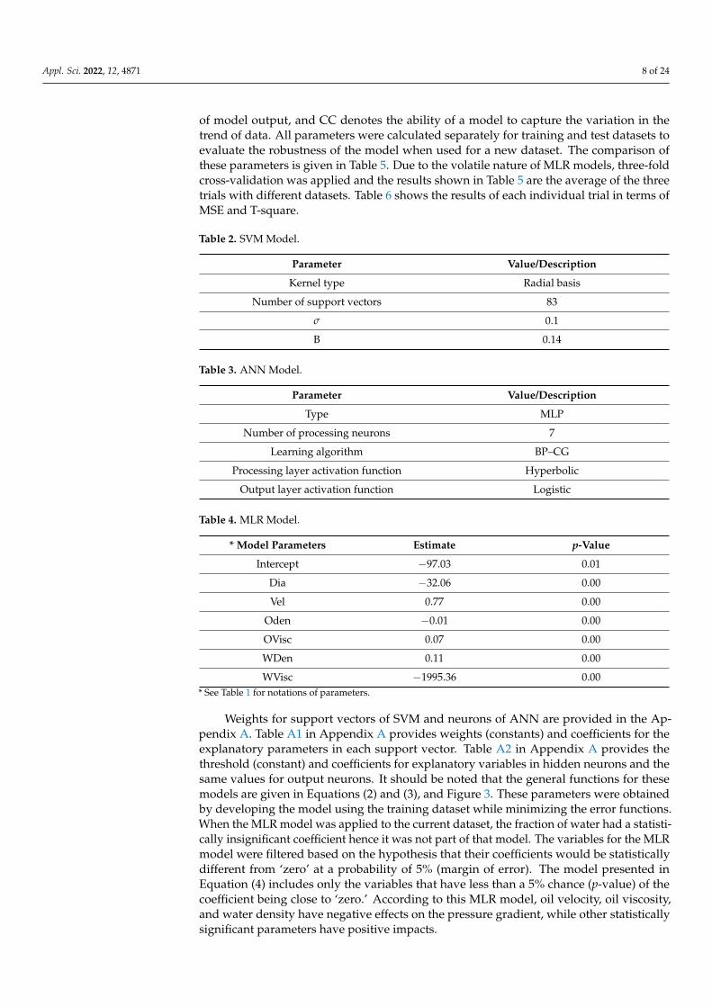
of model output, and CC denotes the ability of a model to capture the variation in thetrend of data. All parameters were calculated separately for training and test datasets toevaluate the robustness of the model when used for a new dataset. The comparison ofthese parameters is given in Table 5. Due to the volatile nature of MLR models, three-foldcross-validation was applied and the results shown in Table 5 are the average of the threetrials with different datasets. Table 6 shows the results of each individual trial in terms ofMSE and T-square.

Table 2. SVM Model.

Parameter Value/Description

Kernel type Radial basis

Number of support vectors 83

σ 0.1

B 0.14

Table 3. ANN Model.

Parameter Value/Description

Type MLP

Number of processing neurons 7

Learning algorithm BP–CG

Processing layer activation function Hyperbolic

Output layer activation function Logistic

Table 4. MLR Model.

* Model Parameters Estimate p-Value

Intercept −97.03 0.01

Dia −32.06 0.00

Vel 0.77 0.00

Oden −0.01 0.00

OVisc 0.07 0.00

WDen 0.11 0.00

WVisc −1995.36 0.00* See Table 1 for notations of parameters.

Weights for support vectors of SVM and neurons of ANN are provided in the Ap-pendix A. Table A1 in Appendix A provides weights (constants) and coefficients for theexplanatory parameters in each support vector. Table A2 in Appendix A provides thethreshold (constant) and coefficients for explanatory variables in hidden neurons and thesame values for output neurons. It should be noted that the general functions for thesemodels are given in Equations (2) and (3), and Figure 3. These parameters were obtainedby developing the model using the training dataset while minimizing the error functions.When the MLR model was applied to the current dataset, the fraction of water had a statisti-cally insignificant coefficient hence it was not part of that model. The variables for the MLRmodel were filtered based on the hypothesis that their coefficients would be statisticallydifferent from ‘zero’ at a probability of 5% (margin of error). The model presented inEquation (4) includes only the variables that have less than a 5% chance (p-value) of thecoefficient being close to ‘zero.’ According to this MLR model, oil velocity, oil viscosity,and water density have negative effects on the pressure gradient, while other statisticallysignificant parameters have positive impacts.

Appl. Sci. 2022, 12, 4871 9 of 24

Table 5. Comparison of Accuracy Parameters.

Accuracy Parameter ModelDataset

Training Test

MSE (kPa/m)

SVM 0.24 0.28

ANN 0.03 0.04

MLR 0.74 0.66

R-square

SVM 0.83 0.83

ANN 0.98 0.98

MLR 0.61 0.53

MAPE (%)

SVM 61 68

ANN 16 20

MLR 38 59

Table 6. Comparison of Accuracy Parameters for Cross-Validation of MLR.

Accuracy Parameter ModelDataset

Training Test

MSE (kPa/m)

Trial 1 0.52 0.46

Trial 2 0.55 0.44

Trial 3 0.56 0.40

R-square

Trial 1 0.58 0.56

Trial 2 0.62 0.55

Trial 3 0.61 0.49

MAPE (%)

Trial 1 35 58

Trial 2 39 61

Trial 3 35 59

PressGrad = −97.03 − 32.06(Dia) +0.77(Vel) − 0.01(Oden) + 0.07(OVisc) + 0.11(Wden) − 1995.36(WVisc) (4)

The respective performances of the models developed in this study are presented inFigures 5–7. The analytical model proposed by McKibben et al. [7] was also applied to thedataset, and its accuracy measures are also included in the comparison.

Figure 5. Comparison of MSE.

Appl. Sci. 2022, 12, 4871 10 of 24

Figure 6. Comparison of R-square.

Figure 7. Comparison of MAPE.

The comparison of accuracy measures presented in Figures 6 and 7 demonstrates thatthe ANN model performs much better than the other models, providing the least MSEand MAPE, and highest CC. Also, all models have shown negligible differences betweentraining and test datasets in terms of MSE and CC values. However, the difference inMAPE was very significant for SVM and MLR while it was very low for ANNs. Thiscould be an indication of the better robustness of ANN as compared to other models. Incomparison to the soft techniques investigated in the current study, the model used byMcKibben et al. Study [7] does not perform well, although it is most likely better thanother analytical models for the WAF of unconventional oils [4,6,22]. This observation wasconfirmed for the training as well as the test datasets. The test dataset was not used for thedevelopment of models in this study hence comparison of their accuracy is deemed fairwith the analytical model that was developed using a different dataset. This finding justifiesthe need to employ AI-based models for designing WAF pipeline systems. The analyticalmodel seems to have inadequate generalization capability, although it was developed basedon an in-depth analysis of the physics. As a result, the application of an analytical model,such as Equation (1) for designing a WAF system results in a high degree of uncertaintythat is unfavorable to both the economic and technical feasibility of an engineering project.

Appl. Sci. 2022, 12, 4871 11 of 24

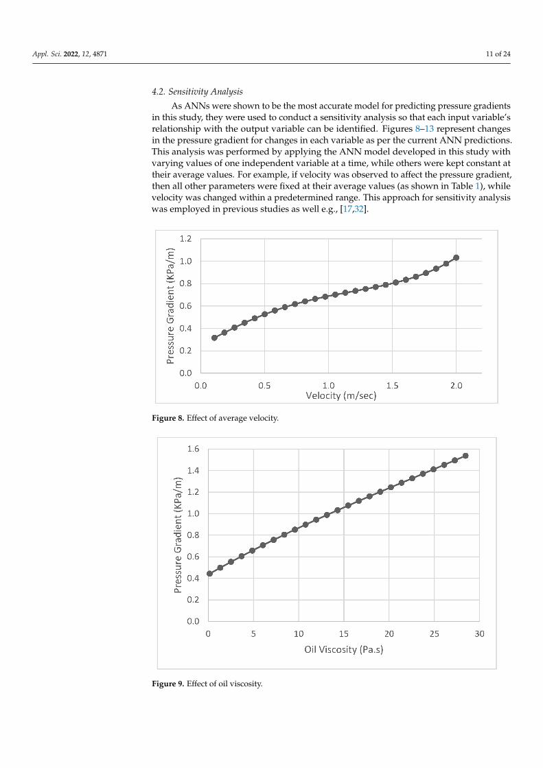
4.2. Sensitivity Analysis

As ANNs were shown to be the most accurate model for predicting pressure gradientsin this study, they were used to conduct a sensitivity analysis so that each input variable’srelationship with the output variable can be identified. Figures 8–13 represent changesin the pressure gradient for changes in each variable as per the current ANN predictions.This analysis was performed by applying the ANN model developed in this study withvarying values of one independent variable at a time, while others were kept constant attheir average values. For example, if velocity was observed to affect the pressure gradient,then all other parameters were fixed at their average values (as shown in Table 1), whilevelocity was changed within a predetermined range. This approach for sensitivity analysiswas employed in previous studies as well e.g., [17,32].

Figure 8. Effect of average velocity.

Figure 9. Effect of oil viscosity.

Appl. Sci. 2022, 12, 4871 12 of 24

Figure 10. Effect of water density.

Figure 11. Effect of oil density.

Figure 12. Effect of water viscosity.

Appl. Sci. 2022, 12, 4871 13 of 24

Figure 13. Effect of water fraction.

As shown in Figures 8–14, average velocity and oil viscosity have positive effects onthe pressure gradient. Specifically, increasing the magnitudes of these variables tends toincrease friction losses. The boosting effect of velocity is highly evident in fluid dynamicsstudies. It should be mentioned that ∆P/L is proportional to V2 for a single-phase pipe flow.The impact of oil viscosity is a WAF-specific phenomenon. Higher oil viscosity most likelyincreases the degree of wall-fouling, thereby increasing ∆P/L [4,5,7].

Figure 14. Effect of pipe diameter.

Water density and oil density have opposite effects on pressure losses. Varying thefluid density tends to affect the core eccentricity. Although the effect of eccentricity in WAFis not a well-studied phenomenon [8], the current study sheds some light on the topic.Water density seems to have a linear effect, whereas oil density has an inverse influence onfriction losses. Oil density increases the pressure gradient within the lower range, whilethe gradient decreases as the density exceed 900 kg/m3. A more practical investigation isrequired in this field.

Appl. Sci. 2022, 12, 4871 14 of 24

Water viscosity did not have a significant impact on pressure losses, as its magnitudewas essentially constant (~1 mPa.s). Similar to water viscosity, water fraction was found tohave a negligible effect on friction losses. A detailed analysis of the experimental measure-ments also demonstrated comparable results [30]. Pipe diameter had an inverse influenceon the WAF pressure gradient, which was expected since there is a nearly proportionalcorrelation between ∆P/L and D−1 for the single-phase flow in a pipeline.

The outcome of this sensitivity analysis highlights another advantage of using ANN, asthe same model can capture varying degrees of relationships between variables. Traditionalparametric and analytical models lack this ability or require prior information about theproblem that needs to be customized in a specific way to fit the model. On the other hand,the ANN model was developed in the present study without using any priory information.

5. Conclusions

The current study investigated the machine learning approach to model frictionallosses in a pipeline transmitting a mixture of water and heavy oil. Lab- and pilot-scale datawere analyzed with different machine learning algorithms and a MLR model. The resultsof the analysis are summarized below.

Traditional parametric or analytical models—for example, the model developed byMcKibben et al.,—lack the ability of generalization, therefore producing inferior predictionsof actual measurements when compared to AI-based machine learning algorithms (e.g.,MLR, SVM, and ANN).

Among the four modeling approaches examined in this research, ANN performedthe best. It produced the least MSE (~0) and the highest CC (~1), both for the training andtest datasets.

In addition to predicting frictional pressure losses, the ANN model could also analyzethe respective sensitivities of the input parameters to the output parameter. Oil density,water viscosity, and pipe diameter were negatively related to the pressure gradient. Oildensity and water viscosity caused the friction loss to increase at the lower range, whilethe gradient decreased as the parametric values crossed threshold limits. Oil viscosityand water density had linear effects on the output variable, whereas other parametershad polynomial effects. This kind of analysis is to play a significant role in operatingwater-assisted pipelines.

The validated AI framework developed in this study is flexible and scalable. Effortsare underway to apply it to other flow conditions.

Author Contributions: Conceptualization, S.R. and U.G.; methodology, U.G.; software, U.G.; valida-tion, S.R. and U.G.; formal analysis, S.R. and U.G.; investigation, S.R., M.A. and U.G.; resources, S.R.,M.A. and U.G.; data curation, S.R. and U.G.; writing—original draft preparation, S.R., M.A. and U.G.;writing—review and editing, S.R., M.A., H.J.Q. and U.G.; visualization, S.R. and U.G.; supervision,S.R., M.A. and U.G.; project administration, S.R., M.A. and U.G.; funding acquisition, S.R., M.A. andH.J.Q. All authors have read and agreed to the published version of the manuscript.

Funding: Deanship of Scientific Research, Vice Presidency for Graduate Studies and ScientificResearch, King Faisal University, Saudi Arabia [Project No. AN000246].

Institutional Review Board Statement: Not applicable.

Informed Consent Statement: Not applicable.

Data Availability Statement: The data were collected from [19,20]. The data used for the currentstudy are included in the Appendix A (Table A3).

Acknowledgments: This work was supported through the Annual Funding track by the Deanshipof Scientific Research, Vice Presidency for Graduate Studies and Scientific Research, King FaisalUniversity, Saudi Arabia [Project No. AN000246]. The authors would like to acknowledge thetechnical and instrumental support they received from King Faisal University and University ofBahrain. We also acknowledge the contributions of Saskatchewan Research Council and CranfieldUniversity, where the data used for the current study were generated.

Appl. Sci. 2022, 12, 4871 15 of 24

Conflicts of Interest: We would like to declare no conflict of interest.

Appendix A

Table A1. SVM Full Model.

Weights 1 Dia Vel ODen OVisc WDen WVisc Frac

1 −10.00 0.32 0.74 0.20 0.07 0.88 0.65 0.12

2 −10.00 0.32 0.74 0.20 0.04 0.86 0.61 0.28

3 −10.00 0.32 0.74 0.20 0.04 0.82 0.55 0.45

4 −10.00 0.32 1.00 0.20 0.04 0.80 0.58 0.28

5 −10.00 0.32 1.00 0.20 0.04 0.84 0.52 0.45

6 −8.33 0.32 0.47 0.20 0.02 0.67 0.37 0.43

7 −10.00 0.32 0.74 0.20 0.04 0.64 0.35 0.43

8 10.00 0.32 1.00 0.20 0.04 0.62 0.33 0.01

9 −7.00 0.32 0.74 1.00 0.86 0.80 0.52 0.31

10 −1.97 0.32 0.21 1.00 1.00 0.88 0.65 0.48

11 −10.00 0.32 0.74 1.00 0.86 0.80 0.52 0.45

12 10.00 0.32 1.00 1.00 0.53 0.59 0.30 0.16

13 1.69 0.32 0.21 1.00 0.68 0.69 0.39 0.44

14 −2.00 0.32 0.74 0.78 0.07 0.82 0.55 0.25

15 −10.00 0.32 0.47 0.78 0.10 0.86 0.61 0.45

16 −10.00 0.32 0.74 0.78 0.09 0.78 0.50 0.47

17 −10.00 0.32 1.00 0.78 0.07 0.82 0.55 0.47

18 2.42 0.32 0.47 0.78 0.01 0.31 0.09 0.36

19 −10.00 0.00 0.05 0.33 0.20 1.00 1.00 0.41

20 −10.00 0.00 0.04 0.33 0.20 1.00 1.00 0.56

21 −10.00 0.00 0.10 0.33 0.20 1.00 1.00 0.73

22 −10.00 0.00 0.21 0.33 0.20 1.00 1.00 0.93

23 −10.00 0.00 0.32 0.33 0.20 1.00 1.00 1.00

24 −10.00 0.00 0.09 0.33 0.20 1.00 1.00 0.22

25 −10.00 0.00 0.12 0.33 0.20 1.00 1.00 0.40

26 −10.00 0.00 0.36 0.33 0.20 1.00 1.00 0.87

27 −10.00 0.00 0.48 0.33 0.20 1.00 1.00 0.94

28 10.00 0.00 0.22 0.33 0.20 1.00 1.00 0.22

29 −10.00 0.00 0.25 0.33 0.20 1.00 1.00 0.31

30 9.61 0.00 0.46 0.33 0.20 1.00 1.00 0.69

31 10.00 0.00 0.43 0.33 0.20 1.00 1.00 0.45

32 10.00 0.00 0.64 0.33 0.20 1.00 1.00 0.66

33 10.00 0.00 0.75 0.33 0.20 1.00 1.00 0.75

34 10.00 0.00 0.85 0.33 0.20 1.00 1.00 0.79

35 −10.00 0.00 0.08 0.29 0.12 0.93 0.75 0.16

36 −8.40 0.00 0.11 0.29 0.12 0.93 0.75 0.35

37 −10.00 0.00 0.16 0.29 0.12 0.93 0.75 0.54

Appl. Sci. 2022, 12, 4871 16 of 24

Table A1. Cont.

Weights 1 Dia Vel ODen OVisc WDen WVisc Frac

38 10.00 0.00 0.33 0.29 0.12 0.93 0.75 0.24

39 10.00 0.00 0.44 0.29 0.12 0.93 0.75 0.45

40 10.00 0.00 0.67 0.29 0.12 0.93 0.75 0.68

41 10.00 0.00 0.86 0.29 0.12 0.93 0.75 0.79

42 9.46 0.00 0.05 0.42 0.13 0.86 0.61 0.57

43 10.00 0.00 0.06 0.42 0.13 0.86 0.61 0.37

44 10.00 0.00 0.08 0.42 0.13 0.86 0.61 0.44

45 10.00 0.00 0.10 0.42 0.13 0.86 0.61 0.56

46 10.00 0.00 0.13 0.42 0.13 0.86 0.61 0.65

47 −10.00 0.00 0.07 0.42 0.13 0.86 0.61 0.16

48 −10.00 0.00 0.09 0.42 0.13 0.86 0.61 0.25

49 −10.00 0.00 0.10 0.42 0.13 0.86 0.61 0.33

50 0.70 0.00 0.36 0.42 0.13 0.86 0.61 0.88

51 10.00 0.00 0.27 0.42 0.13 0.86 0.61 0.02

52 10.00 0.00 0.28 0.42 0.13 0.86 0.61 0.06

53 10.00 0.00 0.30 0.42 0.13 0.86 0.61 0.10

54 10.00 0.00 0.33 0.42 0.13 0.86 0.61 0.17

55 10.00 0.00 0.35 0.42 0.13 0.86 0.61 0.25

56 10.00 0.00 0.41 0.42 0.13 0.86 0.61 0.35

57 10.00 0.00 0.46 0.42 0.13 0.86 0.61 0.44

58 10.00 0.00 0.52 0.42 0.13 0.86 0.61 0.52

59 10.00 0.00 0.62 0.42 0.13 0.86 0.61 0.62

60 3.04 0.00 0.05 0.55 0.48 1.00 1.00 0.85

61 7.24 0.00 0.08 0.55 0.48 1.00 1.00 0.68

62 10.00 0.00 0.16 0.55 0.48 1.00 1.00 0.86

63 4.35 0.00 0.10 0.55 0.48 1.00 1.00 0.58

64 10.00 0.00 0.18 0.55 0.48 1.00 1.00 0.80

65 −10.00 0.00 0.02 0.33 0.20 1.00 1.00 0.33

66 −1.70 0.11 0.47 1.00 0.60 0.64 0.35 0.27

67 10.00 0.11 0.47 1.00 0.71 0.72 0.42 0.00

68 10.00 0.11 0.47 1.00 0.42 0.51 0.24 0.00

69 10.00 0.11 0.47 1.00 0.28 0.39 0.17 0.00

70 −10.00 0.11 0.21 1.00 0.64 0.67 0.37 0.27

71 −10.00 0.11 0.21 1.00 0.60 0.64 0.35 0.22

72 −10.00 0.11 0.21 1.00 0.42 0.51 0.24 0.27

73 −10.00 0.11 0.21 1.00 0.17 0.30 0.12 0.00

74 −10.00 0.32 1.00 0.14 0.04 0.85 0.58 0.28

75 −1.88 0.32 0.74 0.06 0.01 0.43 0.19 0.31

76 −10.00 0.32 0.47 0.14 0.04 0.86 0.61 0.43

78 −10.00 0.32 1.00 0.14 0.04 0.86 0.61 0.43

79 10.00 1.00 0.21 0.14 0.04 0.85 0.58 0.26

Appl. Sci. 2022, 12, 4871 17 of 24

Table A1. Cont.

Weights 1 Dia Vel ODen OVisc WDen WVisc Frac

80 2.78 1.00 1.00 0.14 0.04 0.83 0.55 0.25

81 10.00 1.00 0.21 0.14 0.04 0.86 0.61 0.45

82 10.00 1.00 1.00 0.14 0.04 0.85 0.58 0.40

83 10.00 1.00 1.00 0.10 0.02 0.64 0.35 0.40

Table A2. ANN Weights.

Neuron 2.1 2.2 2.3 2.4 2.5 2.6 2.7 3.1

Thresh −0.83 0.17 0.75 0.23 −0.62 0.69 0.65 −0.44

1.1 −0.01 0.04 0.81 0.14 1.65 −2.05 −5.55

1.2 1.83 −0.86 −0.77 −0.34 0.77 −0.52 1.56

1.3 −0.97 0.31 −0.89 −0.27 3.01 −1.59 −0.38

1.4 0.34 1.22 −0.51 −0.31 2.03 0.27 0.40

1.5 0.17 0.81 0.31 0.73 −0.12 0.66 −0.14

1.6 −0.10 0.68 −0.83 0.44 −1.36 0.05 −0.10

1.7 −0.41 −0.41 −0.35 0.68 −0.60 1.59 −1.13

2.1 1.11

2.2 0.47

2.3 0.04

2.4 −0.33

2.5 2.39

2.6 1.81

2.7 3.88

Table A3. Data set.

Reference NominalDiameter (Inch) ρo/ρw (-) µo/µw (-) Reo (-) Rew (-) Cw (-) Pressure Gradient

Ratio (WAF/Heavy Oil)Temperature

(◦C)

Shi [22] 1

0.911 4923 0.8 4407 0.39 1.2% 12

0.911 4923 0.8 4293 0.51 1.5% 12

0.911 4923 1.2 6622 0.63 1.2% 12

0.911 4923 2.2 11,623 0.79 1.1% 12

0.911 4923 3.0 16,098 0.84 1.1% 12

0.911 4923 1.2 6439 0.24 1.4% 12

0.911 4923 1.4 7627 0.38 1.3% 12

0.911 4923 1.6 8837 0.49 1.5% 12

0.911 4923 2.5 13,518 0.66 1.1% 12

0.911 4923 3.4 18,199 0.74 1.1% 12

0.911 4923 4.3 22,994 0.80 1.0% 12

0.911 4923 2.2 11,782 0.24 1.7% 12

0.911 4923 2.5 13,404 0.31 1.2% 12

0.911 4923 3.4 18,130 0.51 1.3% 12

Appl. Sci. 2022, 12, 4871 18 of 24

Table A3. Cont.

Reference NominalDiameter (Inch) ρo/ρw (-) µo/µw (-) Reo (-) Rew (-) Cw (-) Pressure Gradient

Ratio (WAF/Heavy Oil)Temperature

(◦C)

Shi [22] 1

0.911 4923 4.1 22,332 0.60 1.3% 12

0.911 4923 4.9 26,693 0.67 1.1% 12

0.911 4923 3.0 16,258 0.26 1.2% 12

0.911 4923 3.9 21,167 0.42 1.3% 12

0.911 4923 5.6 30,210 0.58 1.2% 12

0.911 4923 6.5 34,959 0.65 1.2% 12

0.911 4923 7.3 39,252 0.68 1.2% 12

0.907 3376 1.9 7008 0.19 2.4% 21

0.907 3376 2.3 8415 0.34 2.8% 21

0.907 3376 2.9 10,910 0.49 2.5% 21

0.907 3376 4.4 16,299 0.66 1.9% 21

0.907 3376 5.3 19,590 0.25 2.3% 21

0.907 3376 6.7 25,085 0.42 2.1% 21

0.907 3376 9.7 36,261 0.60 1.9% 21

0.907 3376 12.3 45,870 0.68 2.0% 21

0.923 4270 1.1 5184 0.45 5.9% 25

0.923 4270 1.3 5854 0.51 5.6% 25

0.923 4270 1.6 7281 0.60 4.4% 25

0.923 4270 2.5 11,650 0.75 3.1% 25

0.923 4270 1.4 6582 0.35 4.8% 25

0.923 4270 1.6 7252 0.41 5.1% 25

0.923 4270 1.9 8680 0.50 4.7% 25

0.923 4270 2.2 10,107 0.58 3.7% 25

0.923 4270 2.8 13,048 0.67 3.0% 25

0.923 4270 1.5 7165 0.19 2.8% 25

0.923 4270 1.7 7922 0.26 2.5% 25

0.923 4270 1.9 8680 0.33 2.4% 25

0.923 4270 2.2 10,398 0.44 2.8% 25

0.923 4270 2.5 11,592 0.50 2.9% 25

0.923 4270 3.2 14,621 0.60 2.7% 25

0.923 4270 3.8 17,679 0.67 2.4% 25

0.923 4270 4.4 20,388 0.72 2.2% 25

0.923 4270 5.0 23,213 0.75 2.1% 25

0.923 4270 3.9 18,116 0.09 2.7% 25

0.923 4270 4.1 18,815 0.11 2.5% 25

0.923 4270 4.2 19,660 0.15 2.9% 25

0.923 4270 4.6 21,058 0.20 3.1% 25

0.923 4270 4.6 21,291 0.22 3.0% 25

0.923 4270 4.9 22,660 0.26 2.8% 25

Appl. Sci. 2022, 12, 4871 19 of 24

Table A3. Cont.

Reference NominalDiameter (Inch) ρo/ρw (-) µo/µw (-) Reo (-) Rew (-) Cw (-) Pressure Gradient

Ratio (WAF/Heavy Oil)Temperature

(◦C)

Shi [22] 1

0.923 4270 5.5 25,456 0.34 2.6% 25

0.923 4270 6.1 28,427 0.41 2.2% 25

0.923 4270 6.8 31,660 0.47 2.0% 25

0.923 4270 8.0 37,223 0.55 1.9% 25

0.923 4270 8.7 40,106 0.58 1.8% 25

0.923 4270 9.3 43,135 0.61 1.7% 25

0.923 4270 9.9 45,786 0.63 1.7% 25

0.936 11,604 0.2 2443 0.46 3.1% 11

0.936 11,604 0.2 2672 0.50 3.0% 11

0.936 11,604 0.2 2946 0.54 2.7% 11

0.936 11,604 0.3 3722 0.64 2.6% 11

0.936 11,604 0.4 4750 0.73 2.3% 11

0.936 11,604 0.5 5937 0.77 1.9% 11

0.936 11,604 0.4 4704 0.50 1.9% 11

0.936 11,604 0.5 5777 0.59 1.8% 11

0.936 11,604 0.8 9316 0.74 1.4% 11

0.936 11,604 0.4 5480 0.42 1.5% 11

0.936 11,604 0.5 6553 0.52 1.6% 11

0.936 11,604 0.6 7901 0.60 1.5% 11

0.936 11,604 0.8 10,275 0.69 1.3% 11

0.911 4923 0.6 3334 0.32 2.8% 12

0.911 4923 0.7 3699 0.40 3.3% 12

0.911 4923 0.8 4407 0.42 3.0% 12

0.911 4923 0.9 4772 0.48 2.2% 12

Rushd [8] 2

0.992 25,600 2.7 69,072 0.09 0.9% 32

0.992 25,600 2.7 69,072 0.28 0.6% 32

0.993 23,097 3.2 73,315 0.28 0.6% 35

0.995 17,928 4.5 80,691 0.28 0.8% 40

0.992 25,600 2.7 69,072 0.07 1.1% 32

0.995 17,928 4.5 80691 0.07 1.4% 40

0.996 12,797 6.7 86,657 0.07 1.7% 44

0.993 23,998 1.5 35,969 0.28 0.1% 34

0.993 23,097 1.6 36,657 0.24 0.2% 35

0.993 23,998 3.0 71,938 0.24 0.8% 34

0.995 17,928 2.2 40,345 0.28 0.3% 40

0.997 11,381 3.9 44,110 0.17 0.6% 45

0.998 8358 5.4 45,605 0.07 0.9% 47

0.998 8358 8.2 68,408 0.28 1.5% 47

Appl. Sci. 2022, 12, 4871 20 of 24

Table A3. Cont.

Reference NominalDiameter (Inch) ρo/ρw (-) µo/µw (-) Reo (-) Rew (-) Cw (-) Pressure Gradient

Ratio (WAF/Heavy Oil)Temperature

(◦C)

Rushd [8] 4

0.897 1910 26.0 55,274 0.19 6.0% 23

0.897 1697 28.5 53,999 0.28 8.2% 22

0.898 1461 35.6 57,860 0.41 10.3% 25

0.897 2130 47.7 113,123 0.19 7.7% 24

0.897 1910 51.9 110,548 0.28 7.3% 23

0.898 1431 74.3 118,342 0.40 10.7% 26

0.897 2130 71.5 169,684 0.16 6.9% 24

0.898 1461 106.7 173,579 0.29 9.6% 24

0.898 1399 116.5 181,464 0.42 10.8% 27

0.898 1431 148.5 236,542 0.29 9.8% 26

0.898 1364 162.9 247,404 0.42 10.1% 28

0.900 1149 53.8 68,611 0.13 31.0% 33

0.900 1043 61.6 71,395 0.30 31.1% 35

0.900 1149 53.8 68,611 0.41 23.3% 33

0.900 1043 123.3 142,790 0.14 20.0% 35

0.901 1001 131.0 145,602 0.29 15.6% 36

0.900 1097 114.8 140,005 0.40 13.7% 34

0.901 1766 111.4 218,403 0.09 17.0% 36

0.901 1721 116.5 222,641 0.29 9.3% 37

0.900 1808 106.7 214,185 0.40 8.4% 35

0.901 1766 148.5 291,203 0.08 18.1% 36

0.901 1766 148.5 291,203 0.30 8.3% 36

0.900 1808 142.2 285,580 0.41 8.0% 35

0.989 30,518 1.8 55,274 0.14 0.9% 23

Rushd [8] 4

0.990 29,749 3.9 115,719 0.15 1.3% 25

0.993 29,298 6.0 177,014 0.13 1.2% 26

0.993 28,802 8.3 241,345 0.08 1.2% 27

0.990 29,749 1.9 57,860 0.31 1.0% 25

0.990 29,298 4.0 118,342 0.31 0.9% 26

0.991 28,259 6.5 185,441 0.31 0.9% 28

0.991 27,671 9.0 252,613 0.26 0.9% 29

0.990 30,154 1.9 56,561 0.44 0.7% 24

0.990 28,802 4.2 120,976 0.43 0.7% 27

0.991 28,259 6.5 185,441 0.42 0.7% 28

0.991 27,671 9.0 252,613 0.41 0.8% 29

0.993 24,008 2.9 70002 0.08 1.6% 34

0.993 22,192 6.5 145,602 0.09 1.4% 36

0.994 20,171 11.2 226,940 0.17 1.2% 38

0.994 21,207 13.9 296,855 0.19 1.4% 37

Appl. Sci. 2022, 12, 4871 21 of 24

Table A3. Cont.

Reference NominalDiameter (Inch) ρo/ρw (-) µo/µw (-) Reo (-) Rew (-) Cw (-) Pressure Gradient

Ratio (WAF/Heavy Oil)Temperature

(◦C)

Rushd [8] 4

0.993 24,008 2.9 70,002 0.14 1.2% 34

0.993 22,192 6.5 145,602 0.17 1.2% 36

0.994 21,207 10.4 222,641 0.28 0.9% 37

0.994 19,079 16.1 308,285 0.32 1.0% 39

0.992 24,839 2.7 68,611 0.41 0.8% 33

0.993 23,126 6.1 142,790 0.41 0.8% 35

0.993 22,192 9.8 218,403 0.42 0.8% 36

0.994 19,079 16.1 308,285 0.42 1.0% 39

0.964 3199 17.4 57,860 0.25 3.3% 25

0.964 3085 37.0 118,342 0.26 3.9% 26

0.964 2581 67.8 181,464 0.26 4.6% 27

0.965 3096 78.7 252,613 0.26 3.4% 29

0.964 3304 16.5 56,561 0.42 2.0% 24

0.964 3199 34.9 115,719 0.42 2.1% 25

0.965 3096 59.1 189,459 0.43 2.6% 27

0.964 2581 90.4 241,952 0.43 3.8% 29

0.966 2064 32.1 68,611 0.27 3.9% 33

0.966 1885 71.8 140,005 0.25 5.8% 34

0.967 1661 127.1 218,403 0.24 8.0% 36

0.966 2064 128.5 274,446 0.25 5.8% 33

0.966 2064 32.1 68,611 0.39 1.7% 33

Rushd [8] 4

0.966 1885 71.8 140,005 0.39 5.5% 34

0.967 1661 127.1 218,403 0.39 7.0% 36

0.966 2064 128.5 274,446 0.39 5.6% 33

0.972 969 92.1 91,827 0.20 6.2% 49

0.973 896 202.6 186,582 0.20 7.5% 50

0.973 896 303.9 279,873 0.20 10.9% 50

0.972 1038 338.0 360,966 0.20 12.5% 48

0.972 969 92.1 91,827 0.35 12.4% 49

0.971 969 184.3 183,841 0.35 6.2% 49

0.970 969 276.4 276,040 0.35 7.8% 49

0.972 1038 338.0 360,966 0.35 9.4% 48

0.891 1538 13.4 23,144 0.32 32.9% 25

0.891 1538 33.5 57,860 0.30 9.7% 25

0.891 1538 67.0 115,719 0.28 11.0% 25

0.890 1475 107.1 177,347 0.29 11.6% 26

0.890 1475 142.7 236,463 0.29 8.2% 26

0.887 884 29.2 29,120 0.31 42.8% 36

0.887 884 73.1 72801 0.30 34.3% 36

Appl. Sci. 2022, 12, 4871 22 of 24

Table A3. Cont.

Reference NominalDiameter (Inch) ρo/ρw (-) µo/µw (-) Reo (-) Rew (-) Cw (-) Pressure Gradient

Ratio (WAF/Heavy Oil)Temperature

(◦C)

Rushd [8] 4

0.887 884 146.2 145,602 0.29 19.3% 36

0.887 884 219.3 218,403 0.28 19.6% 36

0.886 645 45.5 33133 0.33 46.0% 43

0.886 645 113.7 82,832 0.31 46.8% 43

0.886 645 227.4 165,664 0.31 26.8% 43

0.886 645 341.1 248,497 0.31 20.6% 43

0.886 645 454.8 331,329 0.31 22.2% 43

0.885 430 79.3 38,551 0.32 51.3% 52

0.884 349 255.9 101,015 0.29 87.2% 55

0.884 320 566.8 205,184 0.29 60.9% 56

0.885 430 594.6 289,133 0.29 31.3% 52

0.885 430 792.8 385,510 0.29 37.4% 52

0.890 1475 14.3 23,646 0.41 26.0% 26

0.891 1538 33.5 57,860 0.40 9.7% 25

0.891 1538 67.0 115,719 0.40 10.5% 25

0.891 1538 100.5 173,579 0.40 10.9% 25

0.891 1538 134.0 231,438 0.40 7.9% 25

0.887 884 29.2 29,120 0.41 29.4% 36

0.887 884 73.1 72,801 0.42 33.2% 36

0.887 884 146.2 145,602 0.41 18.7% 36

Rushd [8]

4

0.887 884 219.3 218,403 0.40 17.5% 36

0.887 884 292.4 291,203 0.40 18.2% 36

0.886 584 52.1 34,325 0.43 33.5% 45

0.886 584 130.2 85,812 0.42 46.0% 45

0.886 584 260.3 171,624 0.42 29.7% 45

0.886 615 364.1 252,872 0.42 21.4% 44

0.886 615 485.5 337,163 0.42 27.2% 44

0.885 404 85.7 39,123 0.44 39.6% 53

0.884 320 283.4 102,592 0.42 67.2% 56

0.884 320 566.8 205,184 0.41 48.3% 56

0.884 320 850.2 307,776 0.42 39.2% 56

0.884 349 1023.4 404,059 0.42 55.9% 55

10

0.890 1475 91.5 151,538 0.27 54.6% 26

0.890 1475 183.0 303,076 0.24 23.9% 26

0.890 1475 274.4 454,614 0.26 27.3% 26

0.890 1409 391.4 619,483 0.26 29.2% 27

0.888 917 177.0 182,804 0.27 79.7% 35

0.887 884 374.8 373,237 0.26 80.9% 36

0.887 884 562.2 559,855 0.28 44.6% 36

0.887 884 749.6 746,473 0.26 45.7% 36

Appl. Sci. 2022, 12, 4871 23 of 24

Table A3. Cont.

Reference NominalDiameter (Inch) ρo/ρw (-) µo/µw (-) Reo (-) Rew (-) Cw (-) Pressure Gradient

Ratio (WAF/Heavy Oil)Temperature

(◦C)

Rushd [8] 10

0.886 584 333.6 219,971 0.32 75.6% 45

0.886 584 667.3 439,941 0.27 94.4% 45

0.886 584 1000.9 659,912 0.24 96.5% 45

0.886 584 1334.6 879,882 0.24 63.0% 45

0.891 1538 85.9 148,318 0.42 38.4% 25

0.891 1538 171.8 296,636 0.39 20.8% 25

0.891 1538 257.7 444,953 0.39 24.5% 25

0.890 1475 365.9 606,152 0.38 28.1% 26

0.888 977 163.0 179,371 0.40 55.0% 34

0.888 977 325.9 358,743 0.38 70.3% 34

0.888 977 488.9 538,114 0.39 38.7% 34

0.888 917 708.1 731,216 0.38 44.8% 35

0.886 645 291.5 212,333 0.43 54.9% 43

0.886 645 583.0 424,666 0.40 82.4% 43

0.886 645 874.4 636,998 0.37 91.6% 43

0.886 615 1244.5 864,286 0.36 64.6% 43

References1. Arney, M.; Bai, R.; Guevara, E.; Joseph, D.; Liu, K. Friction factor and holdup studies for lubricated pipelining—I. Experiments

and correlations. Int. J. Multiph. Flow 1993, 19, 1061–1076. [CrossRef]2. Joseph, D.D.; Bai, R.; Mata, C.; Sury, K.; Grant, C. Self-lubricated transport of bitumen froth. J. Fluid Mech. 1999, 386, 127–148.

[CrossRef]3. Rodriguez, O.; Bannwart, A.; de Carvalho, C. Pressure loss in core-annular flow: Modeling, experimental investigation and

full-scale experiments. J. Pet. Sci. Eng. 2009, 65, 67–75. [CrossRef]4. Shi, J.; Lao, L.; Yeung, H. Water-lubricated transport of high-viscosity oil in horizontal pipes: The water holdup and pressure

gradient. Int. J. Multiph. Flow 2017, 96, 70–85. [CrossRef]5. Rushd, S.; McKibben, M.; Sanders, R.S. A new approach to model friction losses in the water-assisted pipeline transportation of

heavy oil and bitumen. Can. J. Chem. Eng. 2019, 97, 2347–2358. [CrossRef]6. Rushd, S.; Sultan, R.A.; Mahmud, S. Modeling Friction Losses in the Water-Assisted Pipeline Transportation of Heavy Oil. In

Processing of Heavy Crude Oils: Challenges and Opportunities; Gounder, R.M., Ed.; IntechOpen: London, UK, 2019. [CrossRef]7. McKibben, M.; Gillies, R.; Sanders, S. A New Method for Predicting Friction Losses and Solids Deposition during the Water-

Assisted Pipeline Transport of Heavy Oils and Co-Produced Sand. In Proceedings of the SPE Heavy Oil Conference-Canada,Calgary, AB, Canada, 11 June 2013. [CrossRef]

8. Rushd, M.M.A.S. A New Approach to Model Friction Losses in The Water-Assisted Pipeline Transportation of Heavy Oil andBitumen. Ph.D. Thesis, University of Alberta, Edmonton, AB, Canada, 2016. [CrossRef]

9. Hassan, M.R.; Mamun, A.A.; Hossain, M.I.; Arifuzzaman, M. Hybrid computational intelligence and statistical measurements formoisture damage modeling in lime and chemically modified asphalt. Computational Intelligence and Neuroscience. Comput.Intell. Neurosci. 2018, 2018, 7525789. [CrossRef] [PubMed]

10. Arifuzzaman Advanced ANN Prediction of Moisture Damage in CNT Modified Asphalt Binder. Soft Comput. Civ. Eng. 2017, 1,1–11.

11. Alam, S.; Gazder, U. Shear strength prediction of FRP reinforced concrete members using generalized regression neural network.Neural Comput. Appl. 2019, 32, 6151–6158. [CrossRef]

12. Osman, E.-S.A.; Aggour, M.A. Artificial neural network model for accurate prediction of pressure drop in horizontal andnear-horizontal-multiphase flow. Pet. Sci. Technol. 2002, 20, 1–15. [CrossRef]

13. Adhikari, B.; Jindal, V. Artificial neural networks: A new tool for prediction of pressure drop of non-Newtonian fluid foodsthrough tubes. J. Food Eng. 2000, 46, 43–51. [CrossRef]

14. Ozbayoglu, M.; Yuksel, H.E. Analysis of gas—Liquid behavior in eccentric horizontal annuli with image processing and artificialintelligence techniques. J. Pet. Sci. Eng. 2012, 81, 31–40. [CrossRef]

Appl. Sci. 2022, 12, 4871 24 of 24

15. Salgado, C.M.; Pereira, C.M.; Schirru, R.; Brandão, L.E. Flow regime identification and volume fraction prediction in multiphaseflows by means of gamma-ray attenuation and artificial neural networks. Prog. Nucl. Energy 2010, 52, 555–562. [CrossRef]

16. Nasseh, S.; Mohebbi, A.; Sarrafi, A.; Taheri, M. Estimation of pressure drop in venturi scrubbers based on annular two-phase flowmodel, artificial neural networks and genetic algorithm. Chem. Eng. J. 2009, 150, 131–138. [CrossRef]

17. Dubdub, I.; Rushd, S.; Al-Yaari, M.; Ahmed, E. Application of ANN to the water-lubricated flow of non-conventional crude.Chem. Eng. Commun. 2020, 209, 47–61. [CrossRef]

18. Huang, M.-W.; Chen, C.-W.; Lin, W.-C.; Ke, S.-W.; Tsai, C.-F. SVM and SVM Ensembles in Breast Cancer Prediction. PLoS ONE2017, 12, e0161501. [CrossRef]

19. Panda, A.K.; Rapur, J.S.; Tiwari, R. Prediction of flow blockages and impending cavitation in centrifugal pumps using SupportVector Machine (SVM) algorithms based on vibration measurements. Measurement 2018, 130, 44–56. [CrossRef]

20. Nasir, M.T.; Mysorewala, M.; Cheded, L.; Siddiqui, B.; Sabih, M. Measurement error sensitivity analysis for detecting and locatingleak in pipeline using ANN and SVM. In Proceedings of the 2014 IEEE 11th International Multi-Conference on Systems, Signals &Devices (SSD14), Barcelona, Spain, 11–14 February 2014; pp. 1–4.

21. Rushd, S.; Rahman, M.; Arifuzzaman; Ali, S.A.; Shalabi, F. Aktaruzzaman Predicting pressure losses in the water-assisted flow ofunconventional crude with machine learning. Pet. Sci. Technol. 2021, 39, 926–943. [CrossRef]

22. Shi, J. A Study on High-Viscosity Oil-Water Two-Phase Flow in Horizontal Pipes. Ph.D. Thesis, Cranfield University,Cranfield, UK, 2015. Available online: http://dspace.lib.cranfield.ac.uk/handle/1826/9654 (accessed on 1 September 2015).

23. Alexopoulos, E.C. Introduction to multivariate regression analysis. Hippokratia 2010, 14, 23.24. Yu, H.; Kim, S. SVM Tutorial-Classification, Regression and Ranking. Handb. Nat. Comput. 2012, 1, 479–506.25. Tabari, H.; Kisi, O.; Ezani, A.; Talaee, P.H. SVM, ANFIS, regression and climate based models for reference evapotranspiration

modeling using limited climatic data in a semi-arid highland environment. J. Hydrol. 2012, 444–445, 78–89. [CrossRef]26. Sahoo, A.; Xu, H.; Jagannathan, S. Neural network-based adaptive event-triggered control of nonlinear continuous-time systems.

In Proceedings of the 2013 IEEE International Symposium on Intelligent Control (ISIC), Hyderabad, India, 28–30 August 2013;pp. 35–40.

27. Noble, W.S. What is a support vector machine? Nat. Biotechnol. 2006, 24, 1565–1567. [CrossRef]28. Rezaeianzadeh, M.; Tabari, H.; Yazdi, A.A.; Isik, S.; Kalin, L. Flood flow forecasting using ANN, ANFIS and regression models.

Neural Comput. Appl. 2014, 25, 25–37. [CrossRef]29. Yegnanarayana, B. Artificial Neural Networks; PHI Learning Pvt. Ltd.: New Delhi, India, 2009.30. Sobie, E.A. Parameter Sensitivity Analysis in Electrophysiological Models Using Multivariable Regression. Biophys. J. 2009, 96,

1264–1274. [CrossRef]31. Sheela, K.G.; Deepa, S.N. Review on Methods to Fix Number of Hidden Neurons in Neural Networks. Math. Probl. Eng. 2013,

2013, 425740. [CrossRef]32. Wang, J.; Li, X.; Lu, L.; Fang, F. Parameter sensitivity analysis of crop growth models based on the extended Fourier Amplitude

Sensitivity Test method. Environ. Model. Softw. 2013, 48, 171–182. [CrossRef]