A Coupled Inviscid-Viscous Airfoil Analysis Solver,Revisited∗

Krzysztof J. Fidkowski †

University of Michigan, Ann Arbor, MI 48109

This paper presents a self-contained, comprehensive exposition and newelements of a classic airfoil analysis technique: an integral boundary layer solvercoupled to a vortex-panel potential-flow method. The resulting solver mfoil,implemented in Matlab and made freely available, builds on the XFOIL codeand documentation, which serve as the inspiration, reference, and standardof comparison. Modifications made in the present implementation include anaugmented-state coupled solver for more control in limiting the state update,a new stagnation-point formulation to reduce leading-edge oscillations in theboundary layer variables, and amore robust treatment of the amplification ratenear transition. Several results highlight these modifications and demonstratecapabilities of the code.

Nomenclature

2 = airfoil chord length2air = speed of sound23 = drag coefficient2� = dissipation coefficient, 1/(d4D3

4)∫g(mD/m[)3[

2 5 = skin-friction coefficient, 2gwall/(d4D24)

2g = shear stress coefficient, gmax/(d4D24)

2ℓ = lift coefficient2< = moment coefficient2? = pressure coefficient38 = edge velocity direction factor on node 8�0 = stagnation enthalpy� = shape parameter, X∗/\�: = kinematic shape parameter, � computed with d = 1�∗ = kinetic energy shape parameter, \∗/\�∗∗ = density shape parameter, X∗∗/\�F = wake shape parameter, ℎF/\

∗Manuscript accepted by the AIAA Journal in November, 2021†Professor, Aerospace Engineering, kfid@umich.edu, AIAA Associate Fellow

ℎF = wake gap/dead-air thickness8, : = unit direction vectors along G, I< = mass (area) flow" = Mach number= = amplification factor for transitionASu = Sutherland’s law temperature ratio'4 = chord-based Reynolds number, d∞+∞2/`∞'4\ = local momentum-thickness Reynolds number, dD4\/`B = arc-length distance on airfoil and wakeBstag = stagnation point B valueSu(·) = Sutherland’s law function) = temperatureu = boundary-layer state vectorD4 = boundary-layer edge velocity*B = normalized wall slip velocityD@ = equilibrium value of (1/D4)3D4/3b+∞ = free-stream speed®G = spatial coordinate, G8 + I:U = angle of attackW = vortex sheet strengthWair = ratio of specific heats for airX = combined momentum and displacement thicknessX∗ = displacement thickness,

∫[1 − (dD)/(d4D4)] 3[

X∗∗ = density thickness\ = momentum thickness,

∫(dD)/(d4D4) [1 − D/D4] 3[

\∗ = kinetic energy thickness,∫(dD)/(d4D4) [1 − D2/D2

4] 3[` = dynamic viscosityb = surface distance from leading edged = densityf = source sheet strengthg = shear stressΨ = streamfunctionl = Newton-Raphson under-relaxation factor

I. IntroductionThe XFOIL code [1] has dominated airfoil analysis and design for over thirty years. It has

been used in the design of airfoils for wind turbines [2–4], small UAVs [5, 6], marine turbines [7],aeroacoustics [8], and other applications. It has also been wrapped in scripts for analysis/designframeworks [9], and its methods have been ported to academic [10, 11] and industry codes [12].The original publication has over 2400 citations.

Developed at a similar time as the ISES code [13–15], now a part of MISES, which features anEuler method for the outer flow, the panel code XFOIL shares the same integral boundary layer (IBL)

2

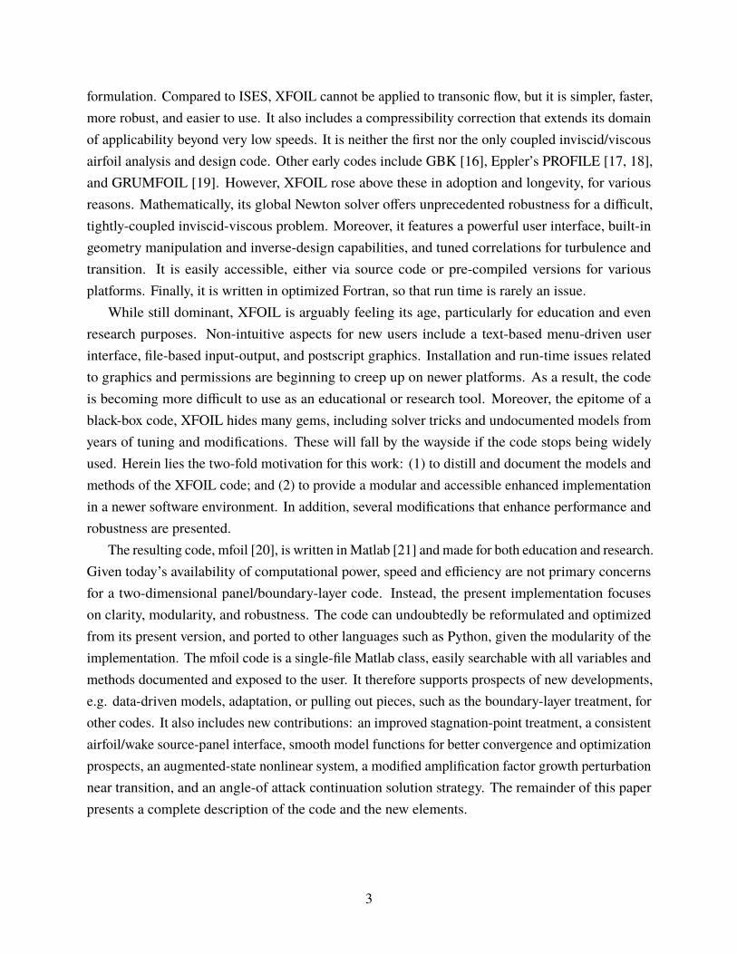
formulation. Compared to ISES, XFOIL cannot be applied to transonic flow, but it is simpler, faster,more robust, and easier to use. It also includes a compressibility correction that extends its domainof applicability beyond very low speeds. It is neither the first nor the only coupled inviscid/viscousairfoil analysis and design code. Other early codes include GBK [16], Eppler’s PROFILE [17, 18],and GRUMFOIL [19]. However, XFOIL rose above these in adoption and longevity, for variousreasons. Mathematically, its global Newton solver offers unprecedented robustness for a difficult,tightly-coupled inviscid-viscous problem. Moreover, it features a powerful user interface, built-ingeometry manipulation and inverse-design capabilities, and tuned correlations for turbulence andtransition. It is easily accessible, either via source code or pre-compiled versions for variousplatforms. Finally, it is written in optimized Fortran, so that run time is rarely an issue.

While still dominant, XFOIL is arguably feeling its age, particularly for education and evenresearch purposes. Non-intuitive aspects for new users include a text-based menu-driven userinterface, file-based input-output, and postscript graphics. Installation and run-time issues relatedto graphics and permissions are beginning to creep up on newer platforms. As a result, the codeis becoming more difficult to use as an educational or research tool. Moreover, the epitome of ablack-box code, XFOIL hides many gems, including solver tricks and undocumented models fromyears of tuning and modifications. These will fall by the wayside if the code stops being widelyused. Herein lies the two-fold motivation for this work: (1) to distill and document the models andmethods of the XFOIL code; and (2) to provide a modular and accessible enhanced implementationin a newer software environment. In addition, several modifications that enhance performance androbustness are presented.

The resulting code, mfoil [20], is written inMatlab [21] and made for both education and research.Given today’s availability of computational power, speed and efficiency are not primary concernsfor a two-dimensional panel/boundary-layer code. Instead, the present implementation focuseson clarity, modularity, and robustness. The code can undoubtedly be reformulated and optimizedfrom its present version, and ported to other languages such as Python, given the modularity of theimplementation. The mfoil code is a single-file Matlab class, easily searchable with all variables andmethods documented and exposed to the user. It therefore supports prospects of new developments,e.g. data-driven models, adaptation, or pulling out pieces, such as the boundary-layer treatment, forother codes. It also includes new contributions: an improved stagnation-point treatment, a consistentairfoil/wake source-panel interface, smooth model functions for better convergence and optimizationprospects, an augmented-state nonlinear system, a modified amplification factor growth perturbationnear transition, and an angle-of attack continuation solution strategy. The remainder of this paperpresents a complete description of the code and the new elements.

3

II. Equations and DiscretizationThe velocity field, ®E(®G) in incompressible and irrotational flow satisfies ∇ · ®E = 0 and ∇ × ®E = ®0,

respectively. A velocity potential Φ(®G) models irrotational velocity fields via ®E = ∇Φ, and, intwo dimension, a streamfunction Ψ(®G) models incompressible velocity fields via ®E = ∇ × (∇Ψ).In a flow that is both incompressible and irrotational, the velocity potential and streamfunctionsatisfy Laplace’s equation, ∇2Φ = ∇2Ψ = 0. A general potential flow can therefore be modeledby superimposing elementary solutions to Laplace’s equations, which include vortex and sourcedistributions. Placing these distributions on panels in two dimensions yields a potential flow panelmethod for modeling the entire flowfield [22].

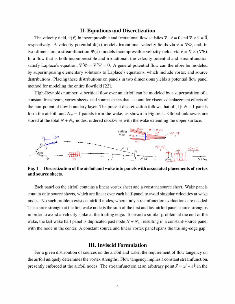
High-Reynolds number, subcritical flow over an airfoil can be modeled by a superposition of aconstant freestream, vortex sheets, and source sheets that account for viscous displacement effects ofthe non-potential flow boundary layer. The present discretization follows that of [1]: # − 1 panelsform the airfoil, and #F − 1 panels form the wake, as shown in Figure 1. Global unknowns arestored at the total # + #F nodes, ordered clockwise with the wake extending the upper surface.

,fTE WTE

13 2

#

8

9

# +2 . . .B

bD

b;

Bstag. . .

# −1

# +#F# +:

f1

fF1

fF1 +f

F2

2

f#−1 f1 + f#−1trailingedge

f8

W 9W 9+1

fF:

fF:+fF

:+12

fF:+fF

:−12

Fig. 1 Discretization of the airfoil and wake into panels with associated placements of vortexand source sheets.

Each panel on the airfoil contains a linear vortex sheet and a constant source sheet. Wake panelscontain only source sheets, which are linear over each half-panel to avoid singular velocities at wakenodes. No such problem exists at airfoil nodes, where only streamfunction evaluations are needed.The source strength at the first wake node is the sum of the first and last airfoil panel source strengthsin order to avoid a velocity spike at the trailing edge. To avoid a similar problem at the end of thewake, the last wake half panel is duplicated past node # + #F, resulting in a constant-source panelwith the node in the center. A constant source and linear vortex panel spans the trailing-edge gap.

III. Inviscid FormulationFor a given distribution of sources on the airfoil and wake, the requirement of flow tangency on

the airfoil uniquely determines the vortex strengths. Flow tangency implies a constant streamfunction,presently enforced at the airfoil nodes. The streamfunction at an arbitrary point ®G = G8 + I: in the

4

domain is

Ψ(®G) = +∞(I cosU − G sinU)︸ ︷︷ ︸Ψ∞ (®G)=freestream contribution

+#−1∑:=1

(W

:(®G) [W: , W:+1]) +Ψf: (®G)f:

)︸ ︷︷ ︸

airfoil panel :

+#F−1∑:=1

(F: (®G) [f

F:−1, f

F: , f

F:+1]

))

︸ ︷︷ ︸wake panel :

+TE(®G) [W# , W1])︸ ︷︷ ︸TE gap panel

(1)

On a wake panel, the source strength varies piecewise linearly on the two panel halves, as shown inFigure 1 and denoted by :− and :+, so that wake panel : contributes

F: (®G) [f

F:−1, f

F: , f

F:+1]

) = f:−

[12(fF:−1 + f

F: ), f

F:

]+ f

:+

[fF: ,

12(fF: + f

F:+1)

](2)

The appendix provides expressions for the vortex and source panel streamfunction influencecoefficients that appear in these two equations. In the presence of a trailing-edge gap, a constantsource panel of strength fTE = 1

2 (W# − W1) |CTE × ?TE |, and a constant vortex panel of strengthWTE =

12 (W# − W1) CTE · ?TE, where CTE is the unit trailing-edge bisector vector and ?TE is the unit

vector along the TE panel from node # to node 1, ensure no net flow through the gap and smoothstreamlines off the upper and lower surfaces [1], as shown in Figure 2. TE(®G) accounts for thecontributions of both of these TE panels.

(a) No source or vortex panel (b) Only source panel (c) Both source and vortex panels

Fig. 2 Effect of trailing-edge source and vortex panels on flow near the trailing edge. Thebranch cut perpendicular from the constant-source panel creates the concentration of stream-lines in (b) and (c).

Both the linear vortex and constant source panels have bounded streamfunction values at thepanel endpoints. Constant source panels exhibit branch cuts across which the streamfunctionis discontinuous. Making the cuts point outward from the airfoil on each panel prevents thediscontinuities from affecting the streamfunction calculation at the airfoil nodes, as illustrated inFigure 3.

5

(a) Panel-aligned branch cuts (incorrect k) (b) Panel-perpendicular branch cuts (correct k)

Fig. 3 Use of a standard arctangent in panel-aligned coordinates causes branch cuts ofconstant-source panels, here only across the trailing-edge gap, to interfere with the stream-function calculation on airfoil nodes. Panel-perpendicular cuts, obtained by a simple shift ofstreamfunction values, prevent this problem.

Evaluating Eq. 1 at the airfoil nodes gives a vector of # streamfunction values,

= ∞ + A$ + B2 A ∈ R#×# , B ∈ R#×(#+#F−2) , (3)

where $ ∈ R# contains the airfoil node vortex strengths and 2 ∈ R#+#F−2 contains both the airfoiland wake panel source strengths. The Kutta condition of smooth flow off the trailing edge providesan additional equation, W1 + W# = 0. Setting the streamfunction equal to Ψ0, an additional unknown,at each airfoil node yields a (# + 1) × (# + 1) system of equations for $ and Ψ0. Solving this systemgives

$ = −A−1(∞ + B2

)(4)

where $ = [$,Ψ0]) , A is A augmented with the Kutta condition and effects of Ψ0, and B is Bpadded with an extra row of zeros. Without viscous sources, Eq. (4) constitutes the inviscid solution,which can be separated into 0 and 90◦ reference solutions as $8 = −A−1

∞= $0 cosU + $90 sinU.

Since the flow inside the airfoil is stagnant, W equals the tangential velocity at the airfoil surface.For an airfoil without a trailing-edge gap, nodes 1 and # coincide, so that the # th row of the

system in Eq. (3) duplicates the first. The # th row is then replaced by an extrapolation of the changein W between the lower and upper surfaces: W# − W1 = 2(W2 − W#−1) − (W3 − W#−2) [1].

IV. Viscous Formulation

A. Boundary-Layer EquationsThe integral boundary layer equations model the viscous flow and affect the inviscid solution

through displacement effects. In turn, the inviscid solution affects the boundary layer through theedge velocity. Separate boundary layer solutions exist on the upper and lower surfaces, and in

6

the wake. Let b be the distance from the leading edge stagnation point for one such surface. Thegoverning boundary layer equations on that surface read [1, 13, 22].

1\

3\

3b+ (2 + � + �F − "2

4 )1D4

3D4

3b=

2 5

2\(momentum) (5)

1�∗

3�∗

3b+

(2�∗∗

�∗+ 1 − � − �F

)1D4

3D4

3b=

22�\�∗−2 5

2\(shape parameter) (6)

3=

3b=

3=

3'4\

3'4\

3b(amplification) (7)

X

21/2g

321/2g

3b−

lag

�V (1 +*B)(21/2g,eq − [�21/2

g ) = 2X(D@ −

1D4

3D4

3b

)(turbulent shear lag) (8)

The amplification equation pertains to the growth of the amplitude of the most amplified Tollmien-Schlichting wave and applies only in laminar regions. The turbulent shear lag equation modelsthe evolution of the maximum shear stress coefficient, 2g, to account for deviations of outer layerdissipation from its local equilibrium value. It only applies in the turbulent region, which includesthe entire wake.

The boundary layer equations are discretized by finite differences on the airfoil and wake nodes.At each node 8, the state vector consists of four quantities, u8 = [\, X∗, = or 21/2

g , D4]) . To interpretthe third state, a separate flag indicates whether a node is laminar or turbulent.

B. Boundary-Layer ResidualsConsidering adjacent nodes 1 and 2, the discretized equations read

'mom ≡ ln\2\1+ (2 + � + �F − "2

4 ) lnD42D41− 1

2lnb2b1

2 5 b

\(9)

'shape ≡ ln�∗2�∗1+

(2�∗∗

�∗+ 1 − � − �F

)lnD42D41+ ln

b2b1

(122 5 b

\− 2�b\�∗

)(10)

'amp ≡ [2 − [1 −3=

3bΔb (11)

'lag ≡ 2X ln2

1/2g2

21/2g1−

lag

�V (1 +*B)(21/2g,eq − [�21/2

g )Δb − 2X(D@Δb − ln

D42D41

)(12)

The derivation of these equations uses finite differences of logarithms for terms such as 1\3\3b= 3

3\ln \.

Including b with the 2 5 and 2� terms in the momentum and shape equations, i.e. 2 5\= 1

b

2 5 b

\=

33b(ln b) 2 5 b

\, improves accuracy and stability near stagnation, as 2 5 and 2� depend inversely on D4,

which depends directly on b at stagnation.The appendix presents closure relations for the quantities that appear in the residuals. In the

discretized equations, quantities without a subscript of 1 or 2 are determined by symmetrical

7

averaging from the nodes, consistent with trapezoidal integration, or upwinding, which improvesstability with a bias towards backward Euler. The upwinding factor between nodes 1 and 2, used ase.g. � = (1 − [up)�1 + [up�2, depends on the kinematic shape parameter,

[up = 1 − 12

exp

(−(ln | 5�D |)2

�up

�2:2

), 5�D =

�:2 − 1�:1 − 1

(13)

where �up equals 1 on the airfoil and 5 in the wake. The larger value in the wake derives from theoriginal XFOIL implementation and improves stability of the solver. In the momentum equation, allquantities are averaged and the term 2 5 b

\is treated together. Further averaging 2 5 b

\with an evaluation

at the midpoint state improves accuracy of the drag calculation. In the shape parameter equation, theskin friction and dissipation terms, 2 5 b

\and 2�b

\�∗ , are upwinded, while the other terms are averaged.In the amplification equation, 3=

3bis averaged. In the shear lag equation, 21/2

g and 21/2g,eq are upwinded,

X is averaged, and D@ is computed using an upwinded 2 5 and �: , and an averaged X∗ and '4\ .

C. Stagnation-Point TreatmentThe leading-edge stagnation point, defined as the location on the airfoil surface at which D4 = 0,

separates the upper and lower surfaces of the airfoil. The distance from the leading edge of a pointon the airfoil surface or wake is then b ≡ |B − Bstag |, where B is the spline arclength. The B-value ofthe stagnation point, Bstag is determined by linearly interpolating the edge velocity and B values ofthe nodes adjacent to the stagnation interval, Bstag = (D42B1 + D41B2)/(D41 + D42). The sign of theedge velocity is positive away from the stagnation point, and hence a negative D41 or D42 in thecourse of a calculation indicates that the stagnation interval must move. A direction factor, 38 ± 1,at each airfoil and wake node aids in mapping the clockwise node ordering direction to the localdownstream direction: i.e. 38 = −1 on the lower surface nodes.

The discretized equations apply between two nodes on a given surface or wake. These equationschange for the interval between stagnation and the first node, as only one state is available. Themodified equations dictate the value of variables at stagnation and pertain to momentum and shapeparameter, as the amplification rate is assumed to be zero on the first interval. At stagnation,b, D4 → 0, so the first terms in Eqs. (5) and (6) become negligible relative to the others, which haveD4 in the denominator. Thus, ln \2

\1and ln �∗2

�∗1drop out of the discretized equations. Also, writing

D4 ≈ b (first term in Taylor series) at stagnation means that ln D42D41

= ln b2b1, and without loss of

generality, both of these terms can be set to 1. The resulting two equations are closed and yield thestagnation values of \ and X∗. Applying this equation to the first node state makes the assumptionthat the first node and stagnation point are the same, which can cause inaccuracy and unstableoscillations in the variables. At a cost of slightly higher bandwidth in the residual Jacobian matrix, a

8

more accurate and stable solution follows from applying the stagnation point equations to a statelinearly extrapolated from the first two nodes to b = 0. For further accuracy improvement, the edgevelocity slope at stagnation, = 3D4

3b, is calculated from a quadratic fit of D4 at stagnation and the

first two nodes. In the unlikely case that the stagnation point coincides, to machine precision, with apanel node, the stagnation equations apply to that node.

D. Wake Discretization and InitializationAn accurate viscous flow approximation requires solution of the boundary layer variables in the

airfoil wake. The inviscid solution defines the wake geometry as the streamline emanating from themidpoint of the trailing edge, as shown in Figure 1. Starting with the first wake point a distance nF2downstream of the trailing edge midpoint, a predictor-corrector method produces the subsequentwake nodes, totalling #F = [#/10 + 103F] and spaced geometrically until a total wake length of3F2.

A separate set of three equations defines the first wake node state in terms of the airfoil trailingedge states 1 and # ,

'Fmom ≡ \F1 − \1 − \# , 'Fshape ≡ X∗F1 − X

∗1 − X

∗# − ℎTE, 'Flag ≡ 2

1/2Fg1 −

\121/2g1 + \#2

1/2g#

\1 + \#(14)

If the state at node 1 or # is laminar, transition to turbulence is forced and 21/2g is calculated using

the transition equation, Eq. (17). The wake displacement thickness includes the trailing edge gap,which starts at ℎF1 = ℎ)� for the first wake node and decreases to zero at a distance !F = 5 Fℎ)�

away from the trailing edge according to [23]

ℎF (bF) = ℎ)�[1 +

(2 + 5 F 3C

3b

)bF

!F

] (1 − b

F

!F

)2(15)

where bF is the distance along the wake from the trailing edge, and 3C3b

is the TE airfoil thicknessslope, clipped to lie between ±3/ 5 F. The value ℎF is subtracted from the displacement thicknessat the affected wake nodes for use in the boundary layer equations. The momentum and shapeequations explicitly add ℎF back into X∗ to obtain the shape parameter with the true displacementthickness, � + �F, where �F = ℎF/\.

E. Transition PredictionTo predict transition, the present approach uses the 49 method [13, 24], as in XFOIL. The

amplification factor, =, starts at zero at the leading-edge stagnation point and evolves downstreamaccording to Eq. (7). Once = exceeds =crit, the boundary layer transitions to turbulent and the shear

9

lag equation, Eq. (8) replaces the amplification factor equation. The discrete interval over whichtransition occurs requires special treatment to predict the transition location.

=

laminar

turbulent

21/2g

b1 b2bC

u+Cu2

u1

u−C

Fig. 4 Transition interval definitions.

Figure 4 illustrates the quantities used in analyzing a transition interval. The switch in equationsand variables occurs at the transition location, bC . The discrete boundary layer equations appliedseparately over the laminar interval, b1 to bC , and the turbulent interval, bC to b2, yield two sets ofresiduals, which are summed together in the global system,

Rtran ≡ R(u1, b1; u−C , bC)︸ ︷︷ ︸laminar

+R(u+C , bC ; u2, b2)︸ ︷︷ ︸turbulent

(16)

where R ≡ ['mom, 'shape, 'amp or 'lag]) and the arguments indicate the endpoint states andcoordinates for the particular subinterval. The state variables \, X∗, and D4 at transition, uC , areobtained by linearly interpolating the states from nodes 1 and 2 to bC . On the laminar side oftransition, u−C , the amplification factor is = = =crit, whereas on the turbulent side, u+C , the shear stresscoefficient is initialized to

21/2g = �g4

−�g/(�:−1)21/2g,eq (17)

The discretized amplification equation, Eq. (11), on the laminar subinterval implicitly defines thetransition location via the residual

'C ≡ 'amp(u1, b1; u−C , bC) = 0 (18)

For given endpoint states u1, u2, a Newton-Raphson solver yields bC and its derivatives with respectto the state variables and node coordinates for addition to the global system. The requirement thatthe transition residual remain zero constrains the derivatives. For example, the calculation of thederivative of bC with respect to the state at node 1 proceeds as follows:

0 = X'C =m'C

mu1Xu1 +

m'C

mbCXbC ⇒ mbC

mu1= −

(m'C

mbC

)−1m'C

mu1(19)

10

A similar calculation yields derivatives with respect to u2, b1, and b2. These derivatives then appearin the linearization of the transition residual, Eq. (16), for the global system.

On the way to the converged solution, the location of transition can move within a panel or acrosspanels, with the latter more likely in the initial solver iterations. Following each state update in thesolver, the transition location is recalculated on both airfoil surfaces by marching the amplificationequation from the stagnation point, using the updated state. This marching further updates theamplification factor at the laminar nodes∗ and stops upon reaching the transition interval, identifiedwhen = exceeds =crit. If the new interval is upstream of the previous one, the previously laminarnodes between the two intervals are initialized to turbulent, with 21/2

g linearly interpolated from thetransition value, Eq. (17), to the first turbulent node after the original transition interval. If thetransition interval moves downstream, the amplification factor on the newly identified laminar nodesis already set from marching, and no further re-initialization is required. Similarly, no action isrequired if the transition interval remains the same, as the transition residual calculation accountsfor movements of bC within an interval.

V. Coupled Solver

A. InitializationThe coupled inviscid-viscous Newton solver requires an initial guess for the boundary layer

variables. A segregated solution provides this guess: solving the inviscid problem first, withoutviscous sources, yields the wake shape and a baseline edge velocity D4 at each node. A marchingprocedure on each airfoil surface follows, starting at the first point after the leading edge, which isset to the stagnation state. On each subsequent interval, the residuals from Eqs. (9)-(12) providethree implicit equations for the three unknown states, \, X∗, = or 21/2

g , at the next node. This “direct”marching mode can fail, however, particularly close to separation [25]. When the Newton-Raphsonsolver fails to converge, or when the kinematic shape parameter exceeds �:,max, 3.8 for laminar and2.5 for turbulent flow, an “inverse” mode is attempted. In the inverse mode, D4 returns as a statevariable, and a prescribed �: change provides the fourth equation that closes the system. Betweennodes 1 and 2, this change is

�:2 = max(�:1 + .03Δ�: , �: max,lam) (laminar) (20)

�:2 = max(�:1 − .15Δ�: , �: max,turb) (turbulent) (21)

�:2 = �:2 −�:2 + .03Δ�: (�:2 − 1)3 − �:

1 + .09Δ�: (�:2 − 1)2(wake) (22)

∗The amplification factor does not directly affect the other residuals, so updating it again in an additional segregatedstep does not destroy the quadratic convergence of the Newton-Raphson solver.

11

where Δ�: ≡ (b2 − b1)/\1. The wake definition is implicit and six iterations are performed startingfrom �:2 = �:1. The inverse mode can also fail, although much less frequently than the directmode. In the event of failure, the state at node 2 is constructed by scaling \ and X∗ from node 1 by(b2/b1) .5 (on the airfoil), and by using the inviscid edge velocity. In the wake, the extrapolation is\2 = \1 and X∗2 = (X

∗1 + \1A)/(1 + A), where A = (b2 − b1)/(10X∗1). While heuristic, these equations

generally provide adequate initialization for the Newton-Raphson solver.During initialization of the boundary layer on the airfoil, if the updated amplification factor,

=2, exceeds =crit, that interval is solved again using the transition residual, Eq. 16, in place of theoriginal residual. The subsequent nodes are then marked as turbulent. If the flow remains laminar atthe airfoil trailing edge, transition is forced at the start of the wake, and the wake residuals, Eqs. 14,define the first wake state.

B. Coupling with the Inviscid SolutionThe boundary layer displacement thickness affects the potential flow solution through a

transpiration boundary condition [22], modeled by source sheets on the wake and airfoil panels,as shown in Figure 1. Defining the missing “mass” flow, density excluded, as < ≡ D4X∗, the localsource sheet strength is f = 3<

3b[1]. The discretized version of this equation on the panel between

nodes 8 and 8 + 1 reads

f8 =<8+138+1 − <838

B8+1 − B8⇒ 2 = D′m (23)

where 2 consists of sources on both the airfoil and wake panels, and D′ ∈ R(#+#F−2)×(#+#F ) mapsthe mass flow vector at the nodes, m, to 2. Eq. 23 remains valid across the stagnation interval,where the sum of the mass flows dictates the source strength, due to the presence of the directionfactors 38 and 38+1.

The potential flow solution affects the boundary layer equations through the edge velocity, D4.On the airfoil nodes, W8 equals the clockwise tangential velocity, so D48 = 38W8. On the wake nodes,the velocity is calculated by summing contributions from the freestream and all vortex and sourcesheets,

uF4 = uF,∞4 + CW$ + Cf2 (24)

where DF,∞4,8

= +∞(cosU8 + sinU:) · CF8is the freestream contribution, CF

8is the unit tangent vector

along the wake at node 8, CW ∈ R#F×# accounts for the effect of the airfoil vortex sheet strengths,and Cf ∈ R#F×(#+#F−2) accounts for the effect of the airfoil and wake source strengths.

From Eq. (4), the vector of vortex strengths on the airfoil nodes can be written as $ =

12

$0 cosU + $90 sinU + B′2, where B′ ∈ R#×(#+#F−1) . Substituting this expression into theexpressions for the edge velocity on the airfoil and wake gives

airfoil: u04 = diag(d0)[$0 cosU + $90 sinU + B′2

]= u0,inv4 + D0m

wake: uF4 = uF,∞4 + CW[$0 cosU + $90 sinU + B′2

]+ Cf2 = uF,inv4 + DFm

(25)

where in the second steps, Eq. (23) replaced 2 in terms of m, resulting in the matrices D0 =

diag(d)B′D′ ∈ R#×(#+#F ) and DF = (CWB′ + Cf)f ∈ R#F×(#+#F ) . The vector d0 contains the #direction factors 38 on the airfoil.

Combining these expressions yields the potential flow edge velocity on all nodes, airfoil andwake,

u4 = uinv4 + Dm (26)

where D = [D0; DF] ∈ R(#+#F )×(#+#F ) depends only on the airfoil and wake geometry, and theinviscid solution is stored as two reference vectors, so that uinv

4 = uinv4,0 cosU + uinv

4,90 sinU. In aconverged coupled solution, this potential-flow expression for the edge velocity must match the edgevelocity stored in the boundary-layer state vector. Enforcing this equality at each airfoil and wakenode yields the residual vector

RD ≡ u4 −[uinv4 + D(u4 .%∗)

](27)

where in the mass flow expression, the product between u4 and %∗ is element-wise. This is the fourthset of equations that closes the global system.

C. Global System SolutionThe global system contains 4# tot unknowns, where # tot = # + #F, consisting of state vectors

on every airfoil and wake node. Marching through the panels on the three surfaces (lower, upper,wake) yields three residuals per panel, Eqs. (9)-(12). The stagnation point system and the wakeinitialization provide the starting-node residuals on the airfoil and wake surfaces. Finally, Eq. (27)provides the additional fourth residual for each node.

Most of the sparse residual Jacobianmatrix is populated concurrently with the residual calculationat each panel. To account for movement of the stagnation point, derivatives of the three panelresiduals with respect to b, which is measured from the stagnation point coordinate Bstag, are alsocalculated and stored in the sparse matrix mR′

m/ ∈ R(3# tot)×# tot , where R′ ∈ R3# tot contains the panel

residuals, and / ∈ R# tot stores the surface b coordinate of each node. As the stagnation point locationdepends on the edge velocity, the required addition to the residual Jacobian matrix occurs in the u4

13

columns,

mR′

mu4+= mR′

m/

m/

mBstag

mBstag

mu4(28)

where m/mBstag

= −d is the opposite of the nodal direction vector, and mBstagmu4 ∈ R

1×(#+#F ) contains onlytwo nonzero entries corresponding to the edge velocities adjacent to the stagnation interval. Hence,the step in Eq. 28 increments only two columns of the residual Jacobian matrix.

In a lift-constrained run with a target lift coefficient 2ℓ,tgt, an extra residual, '2ℓ ≡ 2ℓ (u) − 2ℓ,tgt,augments the global system to allow solution for the unknown angle of attack, U. Derivatives of'2ℓ with respect to the state and angle of attack are computed during the 2ℓ calculation. In theadditional column of the Jacobian matrix, mR′

mU= 0 for the three boundary-layer residuals, and, by

Eq. 27, mRDmU

= − muinv4

mU= uinv

4,0 sinU − uinv4,90 cosU.

At each Newton iteration, a sparse linear solver yields the state update, Δu ∈ R# tot , and theangle of attack update ΔU in lift-constrained mode. Limiting this update with an under-relaxationfactor, l, prevents non-physical states and divergence of the solver. A single global value of l iscalculated such that: \ and X∗ do not decrease by more than 50%; = and 21/2

g values greater than0.2 and 0.1 max(21/2

g ), respectively, do not decrease by more than 80% (very small values are notlimited); = does not increase by more than 2; 21/2

g does not increase by more than .05; D4 does notchange by more than 20%; U does not change by more than 2◦. In addition, after the update, negative2

1/2g values are clipped to 0.1 max(21/2

g ), and the value of X∗ on each node is increased to ensure that�: > �:,min, where �:,min = 1.00005 on the airfoil and 1.02 in the wake. Changes in the angle ofattack require rebuilding the inviscid solution and potentially the wake, although an option exists tokeep the wake fixed at the inviscid-trimmed angle of attack.

VI. Compressibility CorrectionThe potential flow solution presented thus far applies to incompressible flow. A compressibility

correction extends its applicability to subcritical compressible flow. As in XFOIL, the present workuses the Kármán-Tsien compressibility correction [26], which consists of nonlinear corrections tothe incompressible speed, +inc, and pressure coefficient, 2?,inc,

+ =+inc(1 − _)

1 − _(+inc/+∞)2, 2? =

2?,inc

V + _(1 + V)2?,inc/2, _ =

"2∞

(1 + V)2, V =

√1 − "2

∞ (29)

Although the boundary-layer equations apply as written in compressible flow, notably through theinclusion of the edge Mach number, "4, in Eq. 5, the velocity correction has several widespread,albeit subtle, effects. First, the edge velocity computed from the potential flow solution and stored

14

as a boundary layer state corresponds to the incompressible edge velocity, D4,inc. Applying thecorrection yields the compressible edge velocity, D4, as a function of D4,inc and "∞. The edge Machnumber calculation, "4 = D4/2air requires the local speed of sound, 2air, which depends on thetemperature and hence the corrected speed through

22air = (Wair − 1)

(�0 −

D24

2

), �0 =

+2∞

(Wair − 1)"2∞

(1 + Wair − 1

2"2∞

)(30)

where�0 is the constant stagnation enthalpy. Themomentum-thickness Reynolds number calculation'4\ = dD4\/` also requires the local density, d, and dynamic viscosity, `. Isentropic relations yieldthe density,

d = d0

(1 + Wair − 1

2"24

)−1/(Wair−1), d0 = d∞

(1 + Wair − 1

2"2∞

)1/(Wair−1)(31)

and Sutherland’s law yields the dynamic viscosity,

` = `0Su()

)0

), `0 = `∞Su

()∞)0

), Su

()

)0

)=

()

)0

)1.5 1 + ASu))0+ ASu

,)

)0= 1 − 1

2+2∞�0

(32)

VII. Post-ProcessingOutputs of interest include coefficients of lift, moment, and drag, separated into skin-friction and

pressure components. A summation over the airfoil panels, including the trailing-edge gap, yieldsthe lift, moment, and near-field pressure drag coefficients,

2ℓ =12

∫airfoil

2? = · ! 3B ≈12

#∑8=1

2?,8 (− sinUΔI8 − cosUΔG8) (33)

23,inv =12

∫airfoil

2? = · � 3B ≈12

#∑8=1

2?,8 (cosUΔI8 − sinUΔG8) (34)

2< =122

∫airfoil

2? [(®G − ®G0) × =] · 9 3B ≈122

#∑8=1[2?,8, 2?,8+1]M

Δ®G8 · (®G8 − ®G0)

Δ®G8 · (®G8+1 − ®G0)

(35)

where ! = − sinU8+cosU: , � = cosU8+sinU: , 2?,8 = (2?8+2?,8+1)/2, Δ®G8 = ®G8+1−®G8 = ΔG8 8+ΔI8 : ,®G0 is the moment reference location, and M = [2, 1; 1, 2]/6. The approximation that the pressurecoefficient varies linearly across a panel underlies these integrals.

In viscous simulations, the Squire-Young relation [27] provides an accurate approximation of thetotal drag coefficient by extrapolating the final wake momentum thickness, 23 = 2\ (D4/+∞) (5+�)/2.

15

The quantities \, D4, and � in this expression are taken from the final wake node. An integration ofthe skin friction coefficient over the airfoil lower and upper surfaces yields the skin friction dragcoefficient,

235 =� 5 1 + � 5 2

12d∞+

2∞2

, � 5 9 =

∫surface 9

gF 3 ®b · � ≈# 9∑8=1

12(gF,8−1 + gF,8)Δ®G 9 · �, gF =

12d2 5 D

24 (36)

where # 9 is the number of nodes on surface 9 , and node 0 corresponds to the stagnation point,where D4 = 0. The difference of the total and skin friction drag coefficients yields the pressure dragcoefficient, 23? = 23 − 235 .

VIII. ResultsUnless otherwise noted, the following set of results is based on a NACA 2412 airfoil at chord

Reynolds number '4 = 106, angle of attack U = 2◦, and free-stream Mach number "∞ = 0.4. Thedefault number of airfoil points is # = 200.

A. Outputs and DistributionsTable 1 presents the outputs computed from the present code, mfoil, in comparison to those

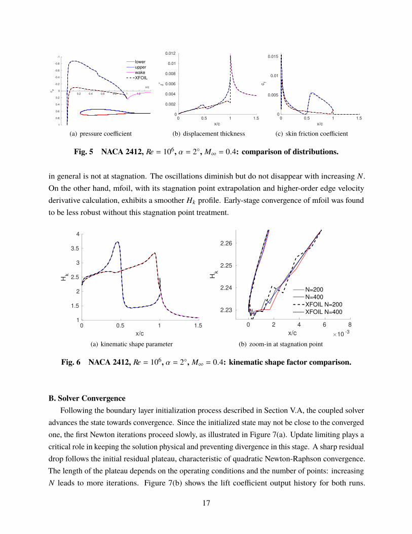
obtained from XFOIL. Differences in panel distributions and models cause slight differences in theresults, but the overall agreement is very good. Likewise, the distribution quantities in Figure 5exhibit excellent agreement.

Table 1 NACA 2412, '4 = 106, U = 2◦, "∞ = 0.4: output comparisons to XFOIL

output mfoil XFOILlift coefficient 0.4889 0.4910

quarter-chord moment coefficient -0.0501 -0.0506drag coefficient 0.00617 0.00618

skin friction drag coefficient 0.00421 0.00421upper surface transition 0.49082 0.49012lower surface transition 0.94872 0.94862

The present modifications in the stagnation point treatment, described in Section IV.C, causenoticeable differences in the solution behavior near the stagnation point. Figure 6 shows thekinematic shape factor, which for most of the airfoil and the wake matches that of XFOIL very well.However, a zoom-in at the leading edge shows oscillations in the XFOIL results. These oscillationsare due to an inconsistency in the equation for the first boundary layer point on each surface, which

16

0 0.2 0.4 0.6 0.8 1 1.2

x/c

-1

-0.8

-0.6

-0.4

-0.2

0

0.2

0.4

0.6

0.8

1

cp

lower

upper

wake

XFOIL

(a) pressure coefficient

0 0.5 1 1.5

x/c

0

0.002

0.004

0.006

0.008

0.01

0.012

*

(b) displacement thickness

0 0.5 1 1.5

x/c

0

0.005

0.01

0.015

cf

(c) skin friction coefficient

Fig. 5 NACA 2412, '4 = 106, U = 2◦, "∞ = 0.4: comparison of distributions.

in general is not at stagnation. The oscillations diminish but do not disappear with increasing # .On the other hand, mfoil, with its stagnation point extrapolation and higher-order edge velocityderivative calculation, exhibits a smoother �: profile. Early-stage convergence of mfoil was foundto be less robust without this stagnation point treatment.

0 0.5 1 1.5

x/c

1

1.5

2

2.5

3

3.5

4

Hk

(a) kinematic shape parameter

0 2 4 6 8

x/c 10-3

2.23

2.24

2.25

2.26

Hk

N=200

N=400

XFOIL N=200

XFOIL N=400

(b) zoom-in at stagnation point

Fig. 6 NACA 2412, '4 = 106, U = 2◦, "∞ = 0.4: kinematic shape factor comparison.

B. Solver ConvergenceFollowing the boundary layer initialization process described in Section V.A, the coupled solver

advances the state towards convergence. Since the initialized state may not be close to the convergedone, the first Newton iterations proceed slowly, as illustrated in Figure 7(a). Update limiting plays acritical role in keeping the solution physical and preventing divergence in this stage. A sharp residualdrop follows the initial residual plateau, characteristic of quadratic Newton-Raphson convergence.The length of the plateau depends on the operating conditions and the number of points: increasing# leads to more iterations. Figure 7(b) shows the lift coefficient output history for both runs.

17

Accurate 2ℓ values do not occur until close to residual convergence.

0 10 20 30

Newton iteration

10-10

10-5

100

L2 r

esid

ua

l n

orm

N=200

N=400

(a) residual norm

0 10 20 30

Newton iteration

0.3

0.4

0.5

0.6

lift c

oeffic

ient

(b) lift coefficient

Fig. 7 NACA 2412, '4 = 106, U = 2◦, "∞ = 0.4: residual and output convergence.

The amplification factor rate of increase equation contains an extra term, Eq. 76, that ensuresthat the rate does not stagnate as = → =crit. This term differs from a similar one in XFOIL, inits smoother form and positive values after =crit. Without this term, the amplification factor maynot cross the critical value when expected, particularly at high Reynolds numbers and on coarsepanelings. Figure 8 shows this lack of convergence for the NACA 2412 airfoil at U = 2◦, " = 0.4,'4 = 107. Including the extra term in 3=

3byields rapid convergence instead.

0 10 20 30 40 50

Newton iteration

10 -10

10 -5

10 0

L2 r

esid

ual norm

with extra amplification

no extra amplification

(a) residual norm

0 0.2 0.4 0.6 0.8 1

x/c

-2

0

2

4

6

8

10

am

plif

ication facto

r

(b) upper-surface amplification factor

Fig. 8 NACA 2412, '4 = 107, U = 2◦, "∞ = 0.4: lack of convergence without extraamplification rate.

18

C. Geometry Manipulation and Newton ContinuationThe code supports airfoil geometry import and manipulation, including camber modification

and flap deployment. Built-in splining functions redistribute panel nodes based on surface curvature.High angle of attack simulations with flaps can cause convergence problems due to the near separatednature of the flowfield. Figure 9 illustrates this problem for an U = 5◦, '4 = 106, " = 0.2 simulationof a NACA 2412 airfoil with a 10◦ flap at 80% chord. A direct solution attempt fails due toseparation on the upper surface flap hinge, as shown in Figure 9(a). The residual stagnates at a largevalue and severe update limiting due to a near non-physical state prevents solution advancement.An angle-of-attack continuation strategy aids in such a case: a solution at U = 0◦ initializes theboundary-layer solution at U = 2.5◦, which in turn initializes the solution at U = 5◦, shown inFigure 9(c). Figure 9(b) shows the combined residual history: after the first angle of attack,subsequent solutions proceed more quickly due to a good starting guess. This process can beautomated inside or outside the code, using different starting angles of attack and fixed or adaptiveincrements.

0 0.2 0.4 0.6 0.8 1 1.2

x/c

-2.5

-2

-1.5

-1

-0.5

0

0.5

1

cp

lower

upper

wake

(a) unconverged 2? , no continuation

0 20 40 60 80

Newton iteration

10-10

10-5

100

105

L2 r

esid

ua

l n

orm

= 0 = 2.5 = 5

continuation

no continuation

(b) residual convergence

0 0.2 0.4 0.6 0.8 1 1.2

x/c

-3

-2.5

-2

-1.5

-1

-0.5

0

0.5

1

cp

lower

upper

wake

(c) converged 2? with continuation

Fig. 9 NACA 2412, '4 = 106, U = 5◦, "∞ = 0.2, 10◦ flap : angle-of-attack continuation.

IX. ConclusionThe speed, robustness, and ease-of-use of the XFOIL airfoil analysis and design code have

made it the program of choice for many research studies and educational purposes. Its longevity of

19

over thirty years and counting is a testament to its methods, implementation, and maintenance. Assoftware and hardware have advanced, however, XFOIL is feeling its age with regard to accessibilityand understanding beyond a black-box level. In this work, the XFOIL code has been re-implemented,with certain modifications, in a modular, documented Matlab class, with the purpose of (1) distillingand documenting the models and methods; and (2) providing an accessible implementation in anewer software framework. This paper presents a self-contained and comprehensive exposition ofthe methods used, as an accompaniment to the code. The results section serves to show agreementwith XFOIL, which has undergone multiple previous validations, and performance and robustnessenhancements due to several modifications.

Appendix

A. Panel Influence CoefficientsThis appendix presents the influence coefficients of linear/constant vortex/source panels that

appear in Eqs. (1) and (2). Figure 10 defines the quantities used in calculating the streamfunctionand velocity at an arbitrary evaluation point.

G

A1

\2

\1

ℎ

0

3

A2

I

evaluation point

2

1

=

C

Fig. 10 Geometry definition for a panel of length 3.

Vortex panel: Given vortex strengths W1 and W2 at the two nodes, the streamfunction at theevaluation point is Ψ = W [W1, W2]) , where W = [ΨW − ΨW, ΨW], and

ΨW =1

2c(ℎ(\2 − \1) − 3 + 0 ln A1 − (0 − 3) ln A2) , (37)

ΨW =0

3ΨW + 1

4c3

(A2

2 ln A2 − A21 ln A1 −

12A2

2 +12A2

2

)(38)

When the evaluation point lies on a panel endpoint, setting the corresponding ln A1 or ln A2 to zeroavoids a mathematical exception (the streamfunction remains well-defined due to multiplicativefactors on these terms that go to zero). The velocity at the evaluation point is ®E = EC C + E==, where

20

EC = (EC − EC)W1 + ECW2, E= = (E= − E=)W1 + E=W2, and

EC =1

2c(\2 − \1), EC =

12c3

(ℎ ln

A2A1+ 0(\2 − \1)

), (39)

E= =1

2clnA2A1, E= =

12c3

(0 ln

A2A1+ 3 − ℎ(\2 − \1)

)(40)

Setting W1 = W2 = W gives the constant vortex panel result, Ψ = ΨWW, where ΨW = ΨW, and®E = (EC C + E==)W.

Source panel: Given source strengths f1 and f2 at the two nodes, the streamfunction at theevaluation point is Ψ = f [f1, f2]) , where f = [Ψf − Ψf, Ψf], and

Ψf =1

2c(0(\1 − \2) + 3\2 + ℎ ln A1 − ℎ ln A2) , (41)

Ψf =0

3Ψf + 1

4c3

(A2

2\2 − A21\1 − ℎ3

)(42)

The streamfunction is singular at the panel endpoints, except in the case of a constant source,f1 = f2 = f, in which case Ψ = Ψff = Ψff. Setting the appropriate ln A1 or ln A2 to zero avoids amathematical exception. For a constant source panel, offsetting the streamfunction calculation by−3/4 or 33/4, depending on the sign of \1 + \2 − c, positions the branch cut in the = direction.

The velocity at the evaluation point is ®E = EC C + E==, where EC = (EC − EC)f1 + ECf2, E= =(E= − E=)f1 + E=f2, and

EC =1

2clnA1A2, EC =

12c3

(0 ln

A1A2− 3 + ℎ(\2 − \1)

), (43)

E= =1

2c(\2 − \1), E= =

12c3

(−ℎ ln

A1A2+ 0(\2 − \1)

)(44)

Setting f1 = f2 = f gives the constant source panel result ®E = (EC C + E==)f.

B. Closure EquationsThis appendix presents the closure relations used in mfoil, which in large part follow those of

XFOIL and have previously been documented [1, 13, 23]. Deviations from these references aremainlydue to updates to the XFOIL code from the original publications, and present additional modifications,in Eqs. (58), (74), (76), have been made for improved robustness of the Newton-Raphson solver.

21

The shape parameter closures are

�: = (� − 0.29"24 )/(1 + 0.113"2

4 ) (45)

�∗∗ = 0.064"24 /(�: − 0.8) (46)

�∗lam =

(0.0111�2

:− .0278�3

:)/(�: − 1) + 1.528 − 0.002(�:�: )2 if �: < 4.35

0.015�2:/�: + 1.528 otherwise

(47)

�: = �: − 4.35 (48)

�∗turb = (�∗turb,inc + 0.028"24 )/(1 + 0.014"2

4 ) (49)

�∗turb,inc =

1.5 + 4/'4\ + 1.5(.5 − 4/'4\)�2

A /(�: + .5) if �: < �0

1.5 + 4/'4\ + (�: − �0)2(0.007 ln '4\/�2�∗ + 0.015/�: ) otherwise

(50)

�A = (�0 − �: )/(�0 − 1) (51)

�0 = min(3 + 400/'4\ , 4) (52)

'4\ = max('4\ , 200) (53)

��∗ = �: − �0 + 4/ln '4\ (54)

X = min (3.15 + 1.72/(�: − 1) + X∗, 12\) (55)

The skin-friction coefficient is zero in the wake. In laminar and turbulent regions, it is

2 5 ,lam =1'4\

0.0727(5.5 − �: )3/(�: + 1) − 0.07 if �: < 5.5

0.015(1 − 1/(�: − 4.5))2 − 0.07 otherwise(56)

2 5 ,turb = 0.34�2 5 �−1.74−0.31�:2 5

+ 0.00011(tanh(4 − �:/.875) − 1) (57)

�2 5 = −1.33�: ; if �2 5 < −17, �2 5 = −20 + 34(�2 5 +17)/3 (58)

�2 5 = max(log10('4\/�2), 1.303) (59)

�2 =

√1 + 0.5(Wair − 1)"2

4 (60)

22

The dissipation coefficient closures are

2�8,lam =1'4\

0.00205(4 − �: )5.5 + 0.207 if �: < 4

−0.0016(�: − 4)2/(1 + 0.02(�: − 4)2) + 0.207 otherwise(61)

2�8,turb = min(2�8,wall + 2�8,outer + 2�8,stress, 2�8,lam) (62)

2�8,wall =122 5*B (2/�∗)0.5 [1 + tanh((�: − 1) ln('4\)/2.1)] (63)

2�8,outer = 2g (0.995 −*B)2/�∗ (64)

2�8,stress = 0.3(0.995 −*B)2/(�∗'4\) (65)

2�8,wake = min(2�8,outer + 2�8,stress, 2�8,lamwake) (66)

2�8,lamwake = 2.2(1 − 1/�: )2(1/�: )/(�∗'4\) (67)

*B =12�∗(1 − (�: − 1)/(��V)) (max 0.98 on airfoil, 0.99995 in wake) (68)

The rate of increase of the amplification factor is

3=

3b= (A= 5=6= + n=)/\ (69)

5= = −.05 + 2.7� − 5.5�2 + 3�3 + 0.14−20� (70)

6= = 0.028/� − 0.0345 exp[−(3.87� − 2.52)2] (71)

A= =

0 if B= < 0

1 if B= > 1

3B2=− 2B3

=otherwise

(72)

B= = (log10 '4\ − (!0 − 0.1))/0.2 (73)

!0 = 2.492�0.43 + 0.7(1 + tanh(14� − 9.24) (74)

� = 1/(�: − 1) (75)

n= = 0.001(1 + tanh(5(= − =crit)) (76)

The equilibrium values of D@ = 1D4

3D43b

and the root shear stress coefficient are

D@ = (0.52 5 − (�:2/(��[��: ))2)/(�VX∗) (77)

�:2 = �: − 1 − ��/'4\ , �� = 0 in wake, else �� (78)

2g,eq = �∗(�: − 1)�2:2/[(2�

2��V (1 −*B)��2

: ] (79)

In the above equations, small �: values are limited to 1.00005 in the wake and 1.05 on theairfoil.

23

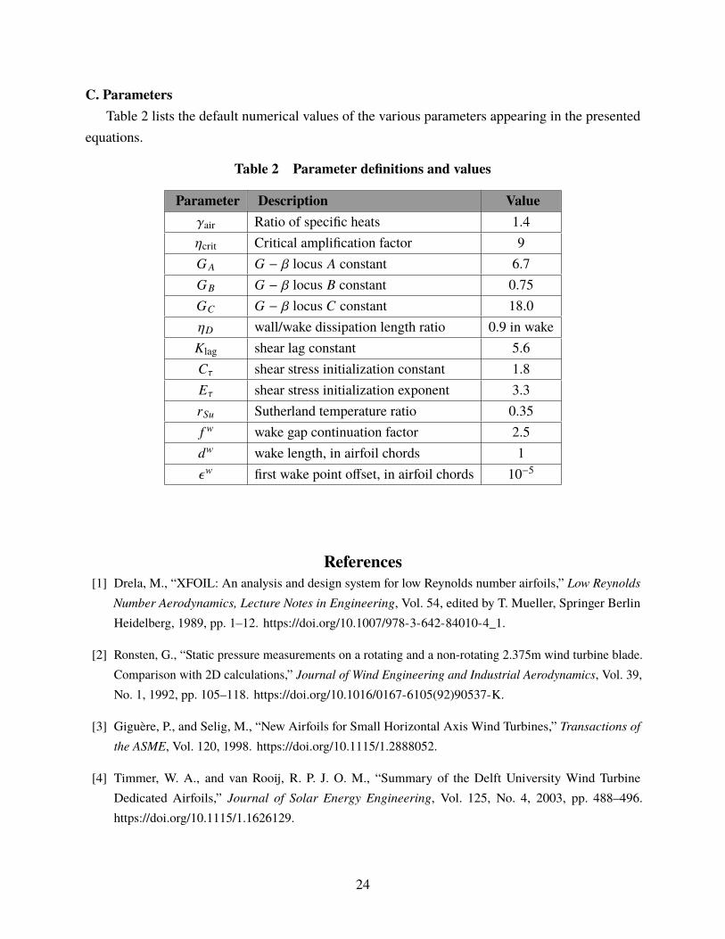
C. ParametersTable 2 lists the default numerical values of the various parameters appearing in the presented

equations.

Table 2 Parameter definitions and values

Parameter Description ValueWair Ratio of specific heats 1.4[crit Critical amplification factor 9�� � − V locus � constant 6.7�� � − V locus � constant 0.75�� � − V locus � constant 18.0[� wall/wake dissipation length ratio 0.9 in wake lag shear lag constant 5.6�g shear stress initialization constant 1.8�g shear stress initialization exponent 3.3A(D Sutherland temperature ratio 0.355 F wake gap continuation factor 2.53F wake length, in airfoil chords 1nF first wake point offset, in airfoil chords 10−5

References[1] Drela, M., “XFOIL: An analysis and design system for low Reynolds number airfoils,” Low Reynolds

Number Aerodynamics, Lecture Notes in Engineering, Vol. 54, edited by T. Mueller, Springer BerlinHeidelberg, 1989, pp. 1–12. https://doi.org/10.1007/978-3-642-84010-4_1.

[2] Ronsten, G., “Static pressure measurements on a rotating and a non-rotating 2.375m wind turbine blade.Comparison with 2D calculations,” Journal of Wind Engineering and Industrial Aerodynamics, Vol. 39,No. 1, 1992, pp. 105–118. https://doi.org/10.1016/0167-6105(92)90537-K.

[3] Giguère, P., and Selig, M., “New Airfoils for Small Horizontal Axis Wind Turbines,” Transactions ofthe ASME, Vol. 120, 1998. https://doi.org/10.1115/1.2888052.

[4] Timmer, W. A., and van Rooij, R. P. J. O. M., “Summary of the Delft University Wind TurbineDedicated Airfoils,” Journal of Solar Energy Engineering, Vol. 125, No. 4, 2003, pp. 488–496.https://doi.org/10.1115/1.1626129.

24

[5] Mueller, T. J., and DeLaurier, J. D., “Aerodynamics of Small Vehicles,” Annual Review of FluidMechanics, Vol. 35, 2003, pp. 89–111. https://doi.org/10.1146/annurev.fluid.35.101101.161102.

[6] Lafountain, C., Cohen, K., and Abdallah, S., “Use of XFOIL in design of camber-controlled morphingUAVs,” Computer Applications in Engineering Education, Vol. 20, No. 4, 2012, pp. 673–680.https://doi.org/10.1002/cae.20437.

[7] Batten, W., Bahaj, A., Molland, A., and Chaplin., J., “Hydrodynamics of Marine Current Turbines,”Renewable Energy, Vol. 31, No. 2, 2006, pp. 249–256. https://doi.org/10.1016/j.renene.2005.08.020.

[8] Jones, B. R., Crossley, W. A., and Lyrintzis, A. S., “Aerodynamic and aeroacoustic optimizationof rotorcraft airfoils via a parallel genetic algorithm,” Journal of Aircraft, Vol. 37, No. 6, 2000, pp.1088–1096. https://doi.org/10.2514/2.2717.

[9] Marten, D., Wendler, J., Pechlivanoglou, G., Nayeri, C. N., and Paschereit, C. O., “QBLADE: an opensource tool for design and simulation of horizontal and vertical axis wind turbines,” InternationalJournal of Emerging Technology and Advanced Engineering, Vol. 3, No. 3, 2013, pp. 264–269.https://doi.org/10.1115/GT2016-57184.

[10] van Rooij, R. P. J. O. M., “Modification of the boundary layer calculation in RFOIL for improved airfoilstall prediction,” Delft University of Technology Report IW-96087R, 1996.

[11] Ramanujam, G., and Özdemir, H., “Improving Airfoil Lift Prediction,” AIAA Paper 2017-1999, 2017.https://doi.org/10.2514/6.2017-1999.

[12] Johnson, F. T., Tinoco, E. N., and Yu, N. J., “Thirty Years Of Development And ApplicationOf CFD At Boeing Commercial Airplanes, Seattle,” Computers and Fluids, 2005, pp. 115–1151.https://doi.org/10.1016/j.compfluid.2004.06.005.

[13] Drela, M., and Giles, M. B., “Viscous-Inviscid Analysis of Transonic and Low Reynolds NumberAirfoils,” AIAA Journal, Vol. 25, No. 10, 1987, pp. 1347–1355. https://doi.org/10.2514/3.9789.

[14] Giles, M. B., and Drela, M., “Two-Dimensional Transonic Aerodynamic Design Method,” AIAA Journal,Vol. 25, No. 9, 1987, pp. 1199–1206. https://doi.org/10.2514/3.9768.

[15] Drela, M., and Giles, M., “ISES: A Two-Dimensional Viscous Aerodynamic Design and Analysis Code,”AIAA Paper 87-0424, 1987. https://doi.org/10.2514/6.1987-424.

[16] Bauer, F., Garabedian, P., Korn, D., and Jameson, A., “Supercritical Wing Sections II,” Lecture Notes inEconomics and Mathematical Systems, Vol. 108, Springer-Verlag Berlin Heidelberg New York, 1975.https://doi.org/10.1007/978-3-642-48912-9.

[17] Eppler, R., and Somers, D. M., “A Computer Program for the Design and Analysis of Low-SpeedAirfoils,” NASA Technical Memorandum 80210, 1980.

25

[18] Eppler, R., and Somers, D. M., “Supplement to: A Computer Program for the Design and Analysis ofLow-Speed Airfoils,” NASA Technical Memorandum 81862, 1980.

[19] Melnik, R., Brook, J., and Mead, H., “GRUMFOIL: A Computer Code for the Computation of ViscousTransonic Flow over Airfoils,” AIAA Paper 87-0414, 1987. https://doi.org/10.2514/6.1987-414.

[20] Fidkowski, K. J., “mfoil,” , 2021. URL http://websites.umich.edu/~kfid/codes.html, accessed: 2021-10-01.

[21] MATLAB, version 7.10.0 (R2021b), The MathWorks Inc., Natick, Massachusetts, 2021.

[22] Drela, M., Flight Vehicle Aerodynamics, MIT Press, Cambridge, MA, 2014.

[23] Drela, M., “Integral boundary layer formulation for blunt trailing edges,” AIAA Paper 89-2166-CP,1989. https://doi.org/10.2514/6.1989-2166.

[24] Smith, A., and Gamberoni, N., “Transition, Pressure Gradient, and Stability Theory,” Douglas AircraftCompany Report ES 26388, 1956.

[25] Goldstein, S., “On Laminar Boundary-Layer Flow Near a Position of Separation,” The Quarterly Journalof Mechanics and Applied Mathematics, Vol. 1, 1948, pp. 43–69. https://doi.org/10.1093/qjmam/1.1.43.

[26] Shapiro, A. H., The Dynamics and Thermodynamics of Compressible Fluid Flow, Volume I, John Wiley& Sons, 1953.

[27] Squire, H., and Young, A., “The Calculation of the Profile Drag of Aerofoils,” R.A.E. Report 1838,November 1937.

26