
TECHNICAL REFERENCE GUIDE FOR MiX99 SOLVER - Jukuri
92
MiX99 Solving Large Mixed Model Equations Release XI/2019 TECHNICAL REFERENCE GUIDE FOR MiX99 SOLVER Last update: Nov 2019 ©Copyright 2019
-
Upload
khangminh22 -
Category
Documents
-
view
0 -
download
0
Transcript of TECHNICAL REFERENCE GUIDE FOR MiX99 SOLVER - Jukuri

MiX99Solving Large Mixed Model Equations
Release XI/2019
TECHNICAL REFERENCE GUIDEFOR
MiX99 SOLVER
Last update: Nov 2019©Copyright 2019

TECHNICAL REFERENCE GUIDE FOR MiX99 SOLVER
PrefaceDevelopment of MiX99 was initiated to allow more sophisticated models in estimationof breeding values for dairy cattle. In the first versions the emphasis was on computa-tional efficiency and the target users were experts on genetic evaluations. Thereforethe logic of model definitions were more from an animal breeding perspective. Theforemost application of this software is solving of large-scale genetic and genomicevaluations for national dairy cattle evaluations. Nevertheless, we have tried to keepthe software as a general tool, where many models can be used. As a result, besidescattle, MiX99 is used in genetic evaluation of other species like pig, horse, sheep,goats, fish, foxes, poultry, and for many types of research work.
DisclaimerMiX99 software is owned by Natural Resources Institute Finland (Luke). When usingthis program you agree with the following terms. You are not allowed to distribute,copy, give or transfer MiX99, neither under the same nor under a different name. Anydecisions based on information given by MiX99 are made at your own responsibilityand risk. Only limited technical support can be provided, but vital questions on its usecan be directed to the authors ([email protected]). Please report any bugs to the authors.MiX99 can be referenced by (MiX99 Development Team, 2019). If you would like touse MiX99, please contact Animal Genetics at Natural Resources Institute Finland1.
MiX99 new (NEW) and development (DEV) featuresNEWNew MiX99 features are indicated in the documentation by a colored vertical bar and
note “NEW” on the right margin.
DEVSome of the newest MiX99 features currently in development are not yet available inthe official MiX99 release. These new MiX99 development features are indicated inthe documentation by a colored vertical bar and note “DEV” on the right margin.
AuthorsMartin Lidauer, Kaarina Matilainen, Esa Mäntysaari, Timo Pitkänen, Matti Taskinen,Ismo StrandénNatural Resources Institute Finland (Luke),FI-31600 Jokioinen, [email protected]://www.luke.fi/mix99
1MiX99 Development Team, Animal Genetics, Natural Resources Institute Finland (Luke), FI-31600Jokioinen, Finland.
ii

TECHNICAL REFERENCE GUIDE FOR MiX99 SOLVER
Contents
1 Introduction . . . . . . . . . . . . . . . . . . . . . . . . . . . . . . . . . . 12 Computing Methods . . . . . . . . . . . . . . . . . . . . . . . . . . . . . 2
2.1 Preconditioned conjugate gradient method . . . . . . . . . . . . 22.2 Iteration on data technique . . . . . . . . . . . . . . . . . . . . . 22.3 Data work file reduction . . . . . . . . . . . . . . . . . . . . . . . 22.4 Equation family blocks . . . . . . . . . . . . . . . . . . . . . . . . 3
3 How to run MiX99 solver programs . . . . . . . . . . . . . . . . . . . . . 43.1 Computing environment . . . . . . . . . . . . . . . . . . . . . . . 43.2 MiX99 solver programs . . . . . . . . . . . . . . . . . . . . . . . 43.3 Multi-threaded MiX99 solvers . . . . . . . . . . . . . . . . . . . . 43.4 Running the solver . . . . . . . . . . . . . . . . . . . . . . . . . . 5
4 The MiX99 solver option file . . . . . . . . . . . . . . . . . . . . . . . . . 64.1 Solver option lines . . . . . . . . . . . . . . . . . . . . . . . . . . 64.2 Command line options . . . . . . . . . . . . . . . . . . . . . . . . 154.3 Determining convergence . . . . . . . . . . . . . . . . . . . . . . 16
4.3.1 Choosing a suitable convergence criterion . . . . . . . 174.3.2 Effect of preconditioning on convergence . . . . . . . . 18
4.4 External STOP file: stopping iteration . . . . . . . . . . . . . . . 194.5 External PEEK file: intermediate solutions during iteration . . . . 194.6 External ITER file: changing parameters during iteration . . . . . 20
5 Output files of the MiX99 solvers . . . . . . . . . . . . . . . . . . . . . . 225.1 Standard output . . . . . . . . . . . . . . . . . . . . . . . . . . . 225.2 Successful execution of MiX99 solver . . . . . . . . . . . . . . . 235.3 Solution files . . . . . . . . . . . . . . . . . . . . . . . . . . . . . 24
5.3.1 Formatted solution files . . . . . . . . . . . . . . . . . . 245.3.2 Unformatted solution files . . . . . . . . . . . . . . . . . 24
5.4 Files for model validation purposes . . . . . . . . . . . . . . . . . 256 Reliabilities . . . . . . . . . . . . . . . . . . . . . . . . . . . . . . . . . . 27
6.1 Approximate reliabilities using ApaX . . . . . . . . . . . . . . . . 276.1.1 Differences of reliability calculation and breeding value
estimation . . . . . . . . . . . . . . . . . . . . . . . . . 286.1.2 ApaX instruction file . . . . . . . . . . . . . . . . . . . . 296.1.3 Guidelines for determining blocking and JFilter . . . . . 326.1.4 ApaX Output files . . . . . . . . . . . . . . . . . . . . . 336.1.5 Example of ApaX instruction file . . . . . . . . . . . . . 33
6.2 Exact reliabilities using exa99 . . . . . . . . . . . . . . . . . . . . 366.2.1 Option file for exa99 . . . . . . . . . . . . . . . . . . . . 366.2.2 Exa99 output files . . . . . . . . . . . . . . . . . . . . . 38
iii

TECHNICAL REFERENCE GUIDE FOR MiX99 SOLVER
6.3 Reversed reliability approximation . . . . . . . . . . . . . . . . . 397 Daughter Yield Deviations . . . . . . . . . . . . . . . . . . . . . . . . . . 41
7.1 Calculation of daughter yield deviations . . . . . . . . . . . . . . 417.1.1 Pedigree file . . . . . . . . . . . . . . . . . . . . . . . . 417.1.2 MiX99 instruction file . . . . . . . . . . . . . . . . . . . 417.1.3 MiX99 solver option file . . . . . . . . . . . . . . . . . . 42
7.2 Solution files for daughter yield deviations . . . . . . . . . . . . . 427.3 Example . . . . . . . . . . . . . . . . . . . . . . . . . . . . . . . . 42
8 Non-linear models . . . . . . . . . . . . . . . . . . . . . . . . . . . . . . 458.1 Threshold-model . . . . . . . . . . . . . . . . . . . . . . . . . . . 45
8.1.1 Instruction file for mix99i . . . . . . . . . . . . . . . . 458.1.2 Stopping criterion file for mix99s . . . . . . . . . . . . 458.1.3 Solution files . . . . . . . . . . . . . . . . . . . . . . . . 468.1.4 Example . . . . . . . . . . . . . . . . . . . . . . . . . . 46
8.2 Gompertz-model . . . . . . . . . . . . . . . . . . . . . . . . . . . 468.2.1 Instruction file for mix99i . . . . . . . . . . . . . . . . 468.2.2 Stopping criterion file for mix99s . . . . . . . . . . . . 478.2.3 Solution files . . . . . . . . . . . . . . . . . . . . . . . . 478.2.4 Example . . . . . . . . . . . . . . . . . . . . . . . . . . 48
9 Estimation of variance components . . . . . . . . . . . . . . . . . . . . . 499.1 Running MC EM REML . . . . . . . . . . . . . . . . . . . . . . . 499.2 File with starting values of (co)variance components . . . . . . . 509.3 MiX99 instruction file . . . . . . . . . . . . . . . . . . . . . . . . . 509.4 MiX99 solver option file . . . . . . . . . . . . . . . . . . . . . . . 51
9.4.1 Number of data samples . . . . . . . . . . . . . . . . . 519.4.2 Determining convergence of REML parameter estimates 519.4.3 Keeping certain variance components fixed . . . . . . . 529.4.4 MC EM REML for MACE . . . . . . . . . . . . . . . . . 52
9.5 Standard errors for REML parameter estimates . . . . . . . . . . 539.6 Solution files for variance components . . . . . . . . . . . . . . . 549.7 Example . . . . . . . . . . . . . . . . . . . . . . . . . . . . . . . . 55
10 Accounting for heterogeneous variance . . . . . . . . . . . . . . . . . . 6010.1 Computation environment . . . . . . . . . . . . . . . . . . . . . . 6010.2 Models for the heterogeneity of variances . . . . . . . . . . . . . 60
10.2.1 Currently supported variance models by MiX99 . . . . 6010.3 Input data for the variance model . . . . . . . . . . . . . . . . . . 63
10.3.1 Input data for mix99hv . . . . . . . . . . . . . . . . . . 6310.3.2 Instruction file for mix99hv . . . . . . . . . . . . . . . . 6310.3.3 Output files from mix99hv . . . . . . . . . . . . . . . . 65
10.4 Instruction file for the variance model . . . . . . . . . . . . . . . . 6610.5 Variance components for the variance model . . . . . . . . . . . 69
10.5.1 Files with information for the variance component esti-mation . . . . . . . . . . . . . . . . . . . . . . . . . . . 69
10.6 Standardization of the multiplicative adjustment factors . . . . . . 7010.6.1 Files for the standardization procedure . . . . . . . . . 7010.6.2 Standardization process . . . . . . . . . . . . . . . . . 7110.6.3 Multiple residual variance-covariance matrices . . . . . 71
10.7 Running a model with heterogeneous variance . . . . . . . . . . 72
iv

TECHNICAL REFERENCE GUIDE FOR MiX99 SOLVER
10.7.1 Implementation on shared memory platforms . . . . . . 7210.8 Workflow and needed files for running multiplicative mixed model 7310.9 Example . . . . . . . . . . . . . . . . . . . . . . . . . . . . . . . . 7510.10 Output files . . . . . . . . . . . . . . . . . . . . . . . . . . . . . . 77
10.10.1 Mi.log and Ms.log . . . . . . . . . . . . . . . . . . . . . 7710.10.2 HVd.log . . . . . . . . . . . . . . . . . . . . . . . . . . . 7810.10.3 CYC.log . . . . . . . . . . . . . . . . . . . . . . . . . . 7810.10.4 Lambda.log . . . . . . . . . . . . . . . . . . . . . . . . . 79
11 Acknowledgement . . . . . . . . . . . . . . . . . . . . . . . . . . . . . . 8012 References . . . . . . . . . . . . . . . . . . . . . . . . . . . . . . . . . . 80Index . . . . . . . . . . . . . . . . . . . . . . . . . . . . . . . . . . . . . . . . 83
v

TECHNICAL REFERENCE GUIDE FOR MiX99 SOLVER
1 IntroductionDairy cattle breeders around the world have moved to so called test-day models fromplain animal models for 305d data. Usually this model upgrade leads to a manifoldincrease in computations. This is because test-day models have more effects thantraditional models based on 305d data, and also because number of records increaseabout ten times. In a national evaluation, number of test-day records and number ofunknowns in the mixed model equations (MME) are easily more than 100 million.
Computational techniques and algorithms that were found useful for solving animalmodels may take weeks to obtain solution to large random regression test day modelMME. Consequently, faster solving algorithms had to be developed. Strandén and Li-dauer (1999) and Lidauer et al. (1999) advocated the use of preconditioned conjugategradient (PCG) method. Lidauer and Strandén (1998) and Strandén (1999) showedthe usefulness of parallel computing. These techniques have been found to reducecomputing time considerably.
MiX99 development work focused on incorporation of these new techniques into an it-eration on data BLUP-program (Lidauer and Strandén, 1999). We have also extendedthe software with programs for different needs: a general program that approximatereliabilities of bulls’ estimated breeding values (EBV), as required by the Interbull; ageneral program that calculates exact reliabilities of EBVs via inversion of the coeffi-cient matrix; and programs, which are required when accounting for heterogeneousvariance. Although the programs have been designed primarily for genetic evaluationof dairy cattle, the programs can and are used for other species that use other typesof statistical models.
The MiX99 package consists of two main programs: pre-processor and solver. Thepre-processor program mix99i reads model instructions, examines input data, andcomputes data sets for the solver program mix99s, which solves the MME by iterationon data. The MME can also be solved by the program mix99p, which is designed touse several CPUs in parallel. In addition, the pre-processed data can be analyzed withadditional programs (apax99, apax99p and exa99) to compute accuracies of thebreeding values. For giving instructions to mix99i please see the manuals CommandLanguage Interface for MiX99 and Technical reference guide for MiX99 pre-processor .In this reference guide we describe the solver options and instructions for mix99s,mix99p, apax99, apax99p, and exa99.
1

TECHNICAL REFERENCE GUIDE FOR MiX99 SOLVER
2 Computing Methods2.1 Preconditioned conjugate gradient methodThe method of conjugate gradient (CG) is an iterative method to solve a linear systemCs = r. It is based on a geometric approach (Shewchuk, 1994). In breeding valueestimation, the C matrix corresponds to the coefficient matrix of mixed model equations(MME), the s vector contains the solutions, and the r vector is the right-hand side ofMME.
Preconditioned conjugate gradient method (PCG) uses conjugate gradient method ona transformed problem. Preconditioning is equivalent to solving M-1Cs = M-1r, where Mis a symmetric positive definite preconditioner matrix that approximates C. Togetherwith a suitable preconditioner matrix, convergence rate of the CG method is superiorto other commonly used algorithms for solving MME (Lidauer et al., 1999).
MiX99 program creates the preconditioner matrix M, which comprises of diagonalblocks of the coefficient matrix. Implementation of the PCG algorithm using iterationon data (IOD) technique requires keeping four vectors, of size equal to the number ofunknowns in the MME, in memory and to read the data and the preconditioner matrixonce per iteration round. The algorithm does not require any pre-set tuning parameterslike relaxation factors.
2.2 Iteration on data techniqueThe major computational task in PCG is the multiplication of the coefficient matrixwith a vector each round of iteration. Therefore, in IOD all data records must beread and processed. IOD technique requires for each record a certain amount (N)of floating point operations to calculate the product coefficient matrix times a vectorcorresponding to the record. In MiX99, N increases almost linearly with increasingcomplexity of the statistical model; N=2(2f+t2), where f is the number of effects in themodel, and t is the number of traits in the model.
2.3 Data work file reductionComplex models with many effects may yield large iteration work files, which increasesdisk input/output (I/O) work. Iteration work files were made smaller by a data reductiontechnique. Data file reduction in MiX99 is based on the concept of avoiding redundantinformation. The following strategies were considered useful when complex statisticalmodels were used for a typical dairy cattle data:
1) Pedigree information and observation data are stored in separate files.
2) If several effects in the model have the same class code, only one equation iden-tification number is stored in the iteration data file. This is possible by properlyordering the equations. For example, all random effects on animal like additivegenetic and none-additive environment effect have the same class code.
3) All regression covariables or a part of them may be placed in a small table ratherthan read from the data file. The table is accessed by an index. For example,functions of days in milk can be put to a table and the connected covariate valuesare found by days in milk index.
2

TECHNICAL REFERENCE GUIDE FOR MiX99 SOLVER
4) When different traits are measured at different time (e.g. different lactation), ob-servations of the traits may be grouped by the time component to avoid storinglarge amount of dummy variables for missing information.
2.4 Equation family blocksIn MiX99, equations are ordered by equation families. An equation family block com-prises of closely linked equations in the MME. For example in dairy cattle fixed andrandom effects that belong to the same herd (herd test-day effects, cows’ non-geneticand genetic effects, etc.) are closely linked to each other and therefore form a blockof equations. Equations of fixed and random effects which are present in differentherds, e.g. age effect or sire effect, are combined into common blocks. The equationfamily order increases data locality in the computations, which enhances computingspeed, and is essential when using parallel computing (Strandén and Lidauer, 1999).For more information see equation family blocks in the Technical reference guide forMiX99 pre-processor .
3

TECHNICAL REFERENCE GUIDE FOR MiX99 SOLVER
3 How to run MiX99 solver programs3.1 Computing environmentMiX99 is written in standard Fortran 90 and is self-contained. It is developed inUNIX and Linux environment. The program has been tested to compile under manyUNIX and Linux Fortran 90/95 compilers as well as Windows compilers. When par-allel computing is used, a Message Passing Interface (MPI) library must be avail-able. For the development of the parallel processing using MPI, Open MPI (http://www.open-mpi.org) or MPICH (http://www.mpich.org) were used.
3.2 MiX99 solver programsExecuting the MiX99 pre-processor program mix99i (see Technical reference guidefor MiX99 pre-processor ) will create all necessary files for the solver programs. Thereis a single process and a parallel program available for solving the MME. Both pro-grams use iteration on data technique and solve the MME by the PCG method:
mix99s Uses one process for solving. During the iteration process it reads the workfiles Tmp4.pedi0, Tmp5.clas0, Tmp6.diab0, and Tm10.trco0 everyround of iteration. After convergence, final solutions are written to solutionfiles.
mix99p Uses several MPI processes in parallel for solving. Number of parallel pro-cesses is defined in the MiX99 instruction file for mix99i. An additional pre-processing program, named imake99 needs to be executed before runningmix99p. The imake99 program makes a file called Index.bin. Duringthe iteration, each process (i) reads its own work files Tmp4.pedi(i),Tmp5.clas(i), Tmp6.diab(i), and Tm10.trco(i) every round of it-eration. After convergence, one process writes the final solution to the so-lution files.
3.3 Multi-threaded MiX99 solversNEWIn addition to the normal MiX99 solver executables, specially compiled multi-threaded
versions of MiX99 solvers are also included. Multi-threaded MiX99 executablesparallelize some of the calculations, especially large dense matrix computations. Thesemulti-threaded MiX99 executables are located in mp subdirectory of the MiX99 binarydistribution. The name of the multi-threaded MiX99 executable is the same as thesingle-threaded counterpart, only the location (directory) is different.
Number of computational threads (not to be confused with number of MPI processes)used by the multi-threaded MiX99 executable is controlled by one or more environmentvariables depending on how the dense matrix libraries are compiled in the executables.To cover most of the cases, the following environment variables need to be set:
export MKL_NUM_THREADS=10export OPENBLAS_NUM_THREADS=10export GOTO_NUM_THREADS=10export OMP_NUM_THREADS=10
Both the “single process” (mix99s) and the parallel solvers (mix99p) have the multi-threaded version of the executable included and both multi-threaded solvers parallelize
4

TECHNICAL REFERENCE GUIDE FOR MiX99 SOLVER
some of the dense matrix operations using the multi-threading. The multi-threaded“single process” solver spawns given number of computational threads (ten in the ex-ample above) when calculating the multi-threaded operations.
The multi-threaded parallel MPI solver (mix99p) parallelizes calculations, thus, usingboth MPI and the multi-threading. Depending on the operation, either one or all of theMPI solver processes utilize the multi-threading. This means that the overall numberof computational threads is up to number of MPI processes times the given number ofthreads.
3.4 Running the solverSolving mixed model equations using MiX99 involves execution of at least two pro-grams. First, the pre-processing program mix99i is executed. In order to execute thisprogram, two alternatives about how to give model information are available: either byproviding a CLIM command file on the command line or by directing a MiX99 instruc-tion file to the standard input (see Command Language Interface for MiX99; Technicalreference guide for MiX99 pre-processor ). After this pre-processing step, the solverprogram mix99s is executed. The solver reads a solver option file from the standardinput and writes information about the iteration process to standard output.
mix99s < solver_option_file
Some of the MiX99 solver options can be specified from the command line also (seeCommand line options). The easiest way to execute solver is to give option -s whichuses default values in solving breeding values, and produces standard output files.
mix99s -s
When parallel computing is used, instead of executing mix99s you have to executeimake99 and mix99p after the mix99i run has finished:
imake99mpiexec99 -np 4 mix99p < solver_option_file
During the execution of the solver programs, mix99s and mix99p, they can be in-structed to stop the iteration, store intermediate solutions to files, and change some ofthe iteration parameters by creating external files STOP, PEEK, and DEVITER, respectively.
After successful completion of the solver, file OK_mix99s or OK_mix99p will be cre-ated. The file will have the completion time. When this file is missing, the solverwas terminated due to some error. When using MiX99 through a script, please checkexistence of the OK_mix99s or OK_mix99p file.
5
TECHNICAL REFERENCE GUIDE FOR MiX99 SOLVER
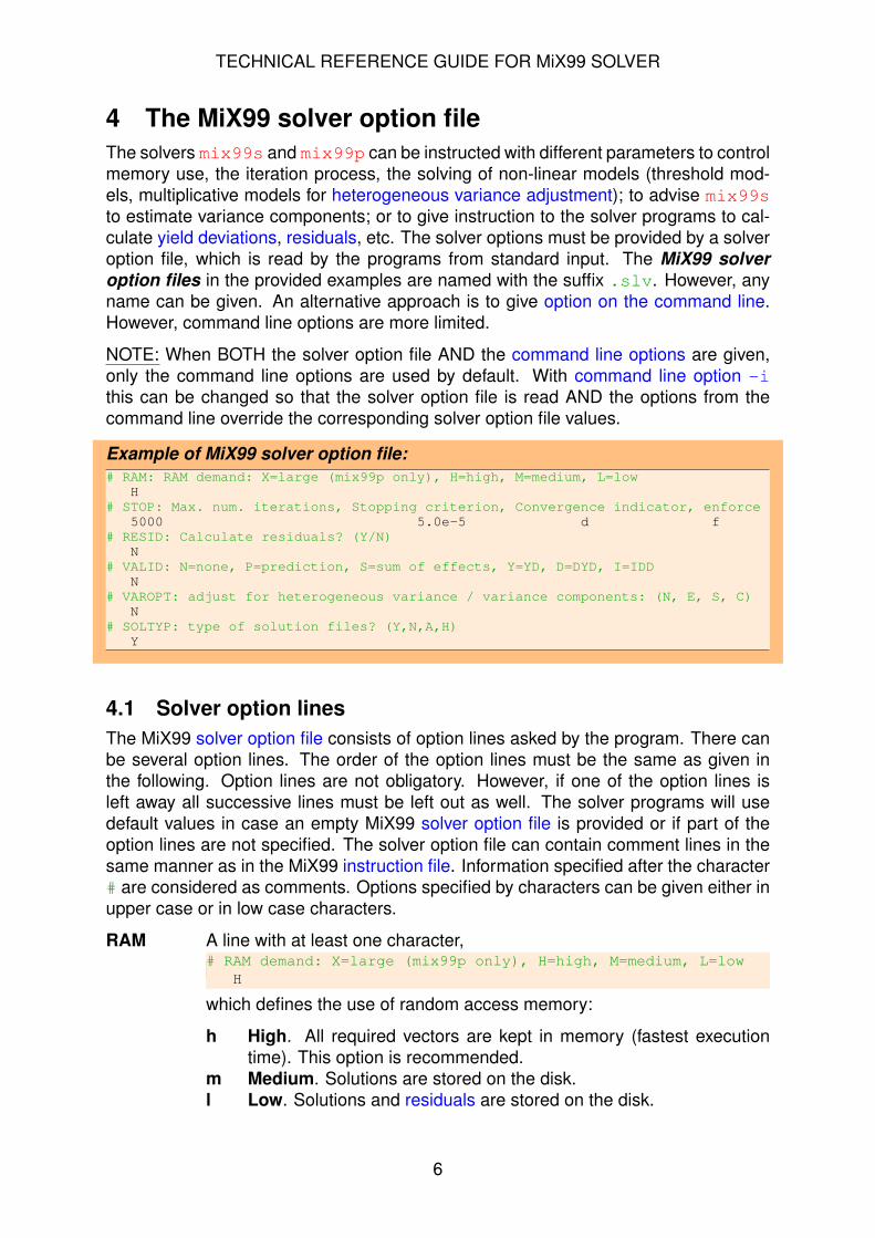
4 The MiX99 solver option fileThe solvers mix99s and mix99p can be instructed with different parameters to controlmemory use, the iteration process, the solving of non-linear models (threshold mod-els, multiplicative models for heterogeneous variance adjustment); to advise mix99sto estimate variance components; or to give instruction to the solver programs to cal-culate yield deviations, residuals, etc. The solver options must be provided by a solveroption file, which is read by the programs from standard input. The MiX99 solveroption files in the provided examples are named with the suffix .slv. However, anyname can be given. An alternative approach is to give option on the command line.However, command line options are more limited.
NOTE: When BOTH the solver option file AND the command line options are given,only the command line options are used by default. With command line option -ithis can be changed so that the solver option file is read AND the options from thecommand line override the corresponding solver option file values.
Example of MiX99 solver option file:# RAM: RAM demand: X=large (mix99p only), H=high, M=medium, L=low
H# STOP: Max. num. iterations, Stopping criterion, Convergence indicator, enforce
5000 5.0e-5 d f# RESID: Calculate residuals? (Y/N)
N# VALID: N=none, P=prediction, S=sum of effects, Y=YD, D=DYD, I=IDD
N# VAROPT: adjust for heterogeneous variance / variance components: (N, E, S, C)
N# SOLTYP: type of solution files? (Y,N,A,H)
Y
4.1 Solver option linesThe MiX99 solver option file consists of option lines asked by the program. There canbe several option lines. The order of the option lines must be the same as given inthe following. Option lines are not obligatory. However, if one of the option lines isleft away all successive lines must be left out as well. The solver programs will usedefault values in case an empty MiX99 solver option file is provided or if part of theoption lines are not specified. The solver option file can contain comment lines in thesame manner as in the MiX99 instruction file. Information specified after the character# are considered as comments. Options specified by characters can be given either inupper case or in low case characters.
RAM A line with at least one character,# RAM demand: X=large (mix99p only), H=high, M=medium, L=low
H
which defines the use of random access memory:
h High. All required vectors are kept in memory (fastest executiontime). This option is recommended.
m Medium. Solutions are stored on the disk.l Low. Solutions and residuals are stored on the disk.
6

TECHNICAL REFERENCE GUIDE FOR MiX99 SOLVER
The option m and l will reduce memory requirements by 25% and 50%,respectively, with the penalty to increase I/O-operations. However, in caseof memory limitations, the option m and l may yield shortest executiontime.
There is an extra memory option, named x, for parallel solver (mix99p).The option can also be enabled by using parallel solver command lineoption -x. This memory option uses even more memory than option hbut can speed up the computations significantly in some cases. The extramemory is used to access the linked list (see imake99 output) faster.Each process will allocate a vector of size number of unknowns. Thus,when there are 100 million unknowns and 10 processors, this will lead toan extra memory allocation of 10 × 100 × 106 × 4 bytes, i.e., less than 4giga bytes.
There are additional options than can be given after the definition of RAMuse. These must be given on the same line in the order below:
N/Y N = no checking of release information, Y = check it
IOP/IM/CHM in single-step, product of A−1gg times vector is performed us-ing one of three approaches. Approach IOP uses iteration on pedi-gree, IM uses iteration in memory, and CHM uses CHOLMOD li-brary. Use of memory from lowest to most: IOP, IM, CHM, wherememory need by IOP and IM is quite close but CHM much more.Computing time from highest to lowest: IOP, IM, CHM, where thereis substantial difference between all approaches. The CHM optioncan use multiple threads.
MEL NEWin single-step, reads G−1 or T matrix from file to memory. TheMEL option uses efficient matrix multiplication during PCG iteration.The multiplication can use many computational threads by the multi-threaded versions of MiX99 solvers. Note that when the number ofgenotyped animals is large the matrix to read is large, and con-sumes a lot of RAM memory.
MEM is like option MEL but slower and uses slightly less memory, whenT matrix is used.
ω value for the ω multiplier of matrix A−1gg . In practice, value of ω istypically about 0.6− 0.8.
Defaults: h for high memory, Y for check release information, IM for inmemory iteration, and ω value of 1.
The following will change to use CHM, MEL, and multiplier 0.8:H CHM MEL 0.8
STOP One line with three (mix99p) or four (mix99s) entries:# maxiter, tolerance, criterion (A/R/M/D), [enforce (F)]:5000 5.0e-5 D F
The first entry is an integer number that specifies the maximum num-ber of iterations. The second entry is a real value that specifies the
7
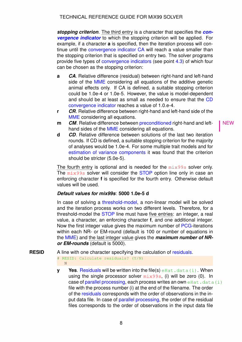
TECHNICAL REFERENCE GUIDE FOR MiX99 SOLVER
stopping criterion. The third entry is a character that specifies the con-vergence indicator to which the stopping criterion will be applied. Forexample, if a character a is specified, then the iteration process will con-tinue until the convergence indicator CA will reach a value smaller thanthe stopping criterion that is specified on entry two. The solver programsprovide five types of convergence indicators (see point 4.3) of which fourcan be chosen as the stopping criterion:
a CA. Relative difference (residual) between right-hand and left-handside of the MME considering all equations of the additive geneticanimal effects only. If CA is defined, a suitable stopping criterioncould be 1.0e-4 or 1.0e-5. However, the value is model-dependentand should be at least as small as needed to ensure that the CDconvergence indicator reaches a value of 1.0.e-4.
r CR. Relative difference between right-hand and left-hand side of theMME considering all equations.
m NEWCM . Relative difference between preconditioned right-hand and left-hand sides of the MME considering all equations.
d CD. Relative difference between solutions of the last two iterationrounds. If CD is defined, a suitable stopping criterion for the majorityof analyses would be 1.0e-4. For some multiple trait models and forestimation of variance components it was found that the criterionshould be stricter (5.0e-5).
The fourth entry is optional and is needed for the mix99s solver only.The mix99s solver will consider the STOP option line only in case anenforcing character f is specified for the fourth entry. Otherwise defaultvalues will be used.
Default values for mix99s: 5000 1.0e-5 d
In case of solving a threshold-model, a non-linear model will be solvedand the iteration process works on two different levels. Therefore, for athreshold-model the STOP line must have five entries: an integer, a realvalue, a character, an enforcing character f, and one additional integer.Now the first integer value gives the maximum number of PCG-iterationswithin each NR- or EM-round (default is 100 or number of equations inthe MME) and the last integer value gives the maximum number of NR-or EM-rounds (default is 5000).
RESID A line with one character specifying the calculation of residuals.# RESID: Calculate residuals? (Y/N)
N
y Yes. Residuals will be written into the file(s) eHat.data(i). Whenusing the single processor solver mix99s, (i) will be zero (0). Incase of parallel processing, each process writes an own eHat.data(i)file with the process number (i) at the end of the filename. The orderof the residuals corresponds with the order of observations in the in-put data file. In case of parallel processing, the order of the residualfiles corresponds to the order of observations in the input data file
8

TECHNICAL REFERENCE GUIDE FOR MiX99 SOLVER
beginning with file zero (0) up to number of processes minus one.The eHat.data(i) files have as many columns with residuals asthe maximum number of traits in the largest trait group. This is equalto the mxntra parameter given in the Parlog file. The Parlog fileis produced by mix99i. The residual columns are ordered in thesame sequence as the traits in the trait groups. For missing obser-vations the corresponding value in the residual files are set to themissing value -8192.0.
n No. No residuals are written.h This option is only available in mix99p and will create the file(s)
ARsiwi.data(i), which contain information about the heterogene-ity of variance in the residuals. These files are needed only whenaccounting for heterogeneous variance (see chapter Accounting forheterogeneous variance).
Default value: n
VALID A line with one entry,# VALID: N=none,P=prediction,S=sum of effects,Y=YD,D=DYD,I=IDD
N
which instructs the solver to calculate for each observation a correspond-ing, here specified, sub-quantity of the applied model line, or to instructthe solver to simulate observations based on the specified model. Thecalculated quantities are written to binary files after the iteration processhas ended. Missing values will be specified with -8192.0. The structureof the files will be explained in the chapter 5:
n None. None of the options are requested.p Predictions. For each observations the predicted value (y) is writ-
ten to the file(s) yHat.data(i).s Selected Model Factors’ Sum. For each observation the sum of
selected model factors is written to the file(s) sHat.data(i). Theselected factors must be specified on a following line.
y Yield Deviations (YD). For each observation the corresponding YDwill be written to the file(s) named YD.data(i). The factors in-cluded into the YD must be specified on a following line.
i Individual Daughter Deviations (IDD). For each observation thecorresponding IDD will be written into the file(s) named IDD.data(i).The factors included into the IDD must be specified on a followingline.
d Daughter Yield Deviations (DYD). The solver will calculate for eachobservation the corresponding IDD and will use it for the calculationof DYDs based on the approach of Mrode and Swanson (2004).For this option the calculated DYD will be written to a formatted file-named Soldyd. (see chapter Calculation of daughter yield devia-tions). The factors included into the DYD must be specified on afollowing line.
g Generate Observations. This option is available in mix99s only.The mix99s solver will not solve the model, but instead will gen-
9

TECHNICAL REFERENCE GUIDE FOR MiX99 SOLVER
erate for each observation in the data a simulated observation (y).Therefore, for all effects in the model true solutions will be simulatedbased on the provided variance components. Fixed effect solutionswill be set to zero. The true solutions are written to the MiX99 stan-dard solution files. The generated observations will be written intothe file named ySim.data0. This file can be used in a future MiX99run to replace real observation by simulated observations. See theVAR instruction line in the Technical reference guide for MiX99 pre-processor for reading and using of the generated observations in-stead of the real observations.When specifying g a SEED option line must be included after theVAROPT option line. The SEED option line has one entry, whichmust be one of those given in the SEED option description below(see VAROPT).
r Deregression. (See chapter: “Deregression” in Command Lan-guage Interface for MiX99).
The options y, i, d and g are not supported when solving non-linear mod-els.
The options s, y,i, or d will require adding of a second line, which spec-ifies which factors of the model are included into the calculation of thespecified quantity.
FACTOR One line with as many integers as there are factor columnsdefined in the REGRESS instruction line. This is equal to the firstinteger value of the REGRESS instruction line (see Technical ref-erence guide for MiX99 pre-processor ). The order of the integervalues on the FACTOR line corresponds to the order of the factorsspecified on the REGRESS instruction line. Each integer specifieswhether or not the corresponding factor of the model is included intothe calculation of the desired quantity.
1 The factor will be included into the specified quantity0 The factor will be excluded from the specified quantity
Specification of the factors for the desired quantities will be asfollowing:
Let’s assume a model, for which the solver will have the followingmodel terms available after the model has been solving:
y = Xb+Zp+Za+ e,
where y contains the observations, b the estimates for the fixed ef-fect factors, p the estimates for the non-genetic animal effect fac-tors, a the estimates for the additive genetic animal factors and ethe residuals.
Selected Model Factors’ Sum. Any factor included in b, p, or acan be included into the sum. All factors included into the sum haveto be specified with ones (1); all factors excluded have to be set tozero (0).
10

TECHNICAL REFERENCE GUIDE FOR MiX99 SOLVER
Yield Deviations (Y D = y−Xb−Zp). All factors associated withb and p have to be set to zero (0); all factors associated with a haveto be specified with ones (1).
Individual Daughter Deviations (IDD) and Daughter Yield Devia-tions (DYD). The IDD is a quantity which is need also for the calcu-lation of the DYD. Thus, for both options the same quantity is needed(IDD = y−Xb−Zp− 1/2adam). All factors associated with b andp have to be set to zero (0); all factors associated with a have to bespecified with ones (1).
VAROPT A line with one entry that specifies different options related to the adjust-ment for heterogeneous variance or to the estimation of variance compo-nents.# VAROPT: adjust for heterogeneous variance /# variance components: (N,E,S,C)
N
n None. None of the options are requested.
e <f n> Estimation of Variance Components. The option e will instructmix99s to estimate variance components by a stochastic MonteCarlo Expectation Maximization REML (MC EM REML) algorithm(for more information please see chapter 9). NEWA special case is op-tion ei for estimation of variance components of a MACE model (seeMC EM REML for MACE). An additional (optional) instruction canbe given after the e (or ei) character. This instruction has two en-tries; the character f and an integer number n. The optional instruc-tions are needed in case certain variance component parametersare meant to be fixed. This option will be explained in chapter 9.4.3.
When an e (or ei) is defined on the VAROPT option line, threeadditional instruction lines have to be given.
STOPE The first line contains three entries, two integers followedby one real valued number. The first integer number specifiesthe maximum number of MC EM REML rounds. NEWIf the givennumber of REML rounds has a negative sign (e.g. -60), pre-viously run REML estimation is to be continued using this newtotal number of rounds. The second integer number specifiesthe number of data samples generated and analyzed within aREML round. The real valued number is the stopping crite-rion for the REML analysis. After the convergence indicatorreaches a value smaller than the specified convergence crite-rion, the REML analysis will perform a sequence of final 30MC EM REML rounds, which will reduce the Monte Carlo errorfrom the parameter estimates.
Default values: 1000 5 1.0e-9
SEED The second line contains one entry, which defines the type ofthe seed used by the random number generator for generatingthe data samples.
11

TECHNICAL REFERENCE GUIDE FOR MiX99 SOLVER
d Default initialization by call to random_seed.r The random number generator is initialized base on the
system clock.g The user can specify the seeds for the random number
generator. If option g is specified j integers must be pro-vided in the next line.
Default value: d
MIX99PATH The third line contains the path for the directory wherethe mix99i pre-processor executable is located. In certain in-tervals the mix99s solver will make a system call to mix99ito update the preconditioner matrices as explained in chap-ter 9. This will also cause an update of the MiX99.lst file.Variance components listed are not anymore the starting val-ues used, but the intermediate estimates that were applied forthe most recent preconditioner matrix update. If the given di-rectory name is empty (either a pair of quotation marks ("") orminus sign (-)) the pre-processor is assumed to be located ina directory that is included in the search PATH.
s Start-up cycle for heterogeneous variance adjustment. Aftermix99p has performed a maximum number of 20 iterations (spec-ified on the STOP option line) it will write heterogeneity of varianceestimates to files named SiWi.data(i). These files will be usedby mix99hv to create the input data files for the applied variancemodel that describes the heterogeneity of variance in the data.
c Cycle between models for solving the multiplicative mixed model.The option is needed for the heterogeneous variance adjustmentand will instruct mix99p to discontinue in certain intervals the itera-tion process and make system calls for solving the variance modelby a second, simultaneous MiX99 analysis. The process will con-tinue until both models have converged.
ADJUST In case s or c is defined on the VAROPT option line, anadditional line needs to be specified with as many integers asthere are factor columns defined in the REGRESS instructionline. This is equal to the first integer value of the REGRESSinstruction line (see Technical reference guide for MiX99 pre-processor ). The order of the integer values on the ADJUSTline corresponds to the order of the factors specified on theREGRESS instruction line. Each integer specifies whether ornot the corresponding factor of the model is included into theadjustment of heterogeneous variance.
1 The factor will be included into the HV adjustment.0 The factor will be excluded from the HV adjustment.
Including all factors corresponds to the method by Meuwissenet al. (1996). When excluding some factors from the HV ad-
12

TECHNICAL REFERENCE GUIDE FOR MiX99 SOLVER
justment a restricted multiplicative mixed model will be applied.Excluding the fixed effect factors from the example model givenin VALID will perform a restricted multiplicative mixed modeladjustment for heterogeneous variance of the form:
yi = Xib+ (Zip+Zia+ ei) γi,
where γi = 1λi
and λi is the heterogeneous variance adjust-ment factor for stratum i.
STOPC In case c is defined on the VAROPT option line, a secondadditional line with two entries must be given. The first entryis an integer value giving the maximum number of heteroge-neous variance adjustment cycles; i.e. the maximal numberthat the variance model will be updated and solved. The sec-ond entry is a real value and is the required stopping crite-rion. The updating and solving of the variance model will stopwhen the convergence indicator for the heterogeneity adjust-ment factors has reached a value smaller than the specifiedstopping criterion. The convergence indicator for the hetero-geneity adjustment factors is calculated as:
cd(k) =
(l(k) − l(k−1)
)T (l(k) − l(k−1)
)(l(k))
T(l(k))
,
where cd(k) is the value of the convergence indicator in adjust-ment cycle k and l is the vector of multiplicative adjustmentfactors (lambda values).
Default values: 1000 1.0e-7
SOLTYP A line with one character,# SOLTYP: type of solution files? (Y,N,A,H)
Y
which specifies the way solutions are handled. This option became nec-essary when modules for solving different non-linear models were imple-mented in the MiX99 package. For solving standard linear models a ymust be specified. All other options are related to adjustment of hetero-geneous variance or to non-linear Gompertz models.
y Yes, give standard solution files. Solution files are written in textformat.
n No. No solutions are written. This is useful when specifying options on the VAROPT option line.
d DMUINPformat. Option will produce binary and ASCII files with thepseudo data. See 8.2.2. This option is needed only for a simultane-ous estimation of variance components for the non-linear Gompertzfunction model by, for example, using the DMU package for the vari-ance component estimation.
One of the two options (a, h) must be defined when using MiX99 forsolving the variance model for adjustment of heterogeneous variance The
13

TECHNICAL REFERENCE GUIDE FOR MiX99 SOLVER
option will instruct mix99p to accelerate the solutions of the variancemodel between consecutive heterogeneous variance adjustment cycles.The solutions are written to binary files (SolfixB for strata of the firsteffect and SolaniB for strata of the second effect in the variance model).
a Accelerated solutions using Aitken acceleration. This option is suit-able, if convergence is dominated by a single large eigenvalue. Formany models it yields fast convergence (between 40 to 60 cycles).
h Accelerated solutions using a Half-Chebychev golden ratio proce-dure (Hesterberg, 2005). This step-lengthening method follows agolden ratio procedure. For large and complex models it was foundmore reliable but it requires between 80 to 100 cycles. The optionis robust and therefore recommend for routine evaluations.
14

TECHNICAL REFERENCE GUIDE FOR MiX99 SOLVER
4.2 Command line optionsSome of the MiX99 solver options can be alternatively specified from the commandline. List of available command line options of the MiX99 programs, such as the (non-parallel) solver mix99s, can be obtained with
mix99s -h
This will print the following instructions:Usage:
mix99s [-s] [-i] [-p|-pt|-pb] [-r|-rt|-rb] [-m][-n NITER] [-n0 N0ITER] [-c{a,d,r,m} TOL][-IOP|-CHM] [-o VAL] [-t tau] [-MEM|-MEL][-peek [-]PITER] [-peek_step PSTEP][-h|--help] [-v|--verbose] [-V|--version][--bindir BINDIR] [--datadir DATADIR] [--tmpdir TMPDIR]
where-s: use defaults, solve and produce standard solution files.-i: use both input file and command line options.-p or -pt: use defaults, solve and produce predictions.-pb: same as -p but produce binary files.-r or -rt: use defaults, solve and produce residuals.-rb: same as -r but produce binary files.-m: Generate MME.dat and rhs.dat of the problem.-n NITER: number of iterations.-n0 N0ITER: minimum number of iterations.
Default: 20 if Cd criterion and old solutions, 1 otherwise.-ca TOL: Ca convergence stopping criterion.-cd TOL: Cd convergence stopping criterion.-cr TOL: Cr convergence stopping criterion.-cm TOL: Cm convergence stopping criterion.-IOP: use iteration on pedigree in inv(A11) of single-step.-CHM: use cholmod in inv(A11) of single-step.-o: coefficient VAL multiplies inv(A22) in ssGBLUP.-t: coefficient TAU multiplies inv(G)/inv(H) in ssGBLUP.-MEM: read T/inv(G) matrix to memory.-MEL: read T/inv(G) matrix to memory and use efficient multiplication.-peek [-]PITER: Write intermediate solutions at iteration PITER.
If negative, file extension _PEEK instead of _<ITER>.-peek_step PSTEP: Write solutions every PSTEP iterations.
If PITER negative, file extension _<ITER> instead of _PEEK.-peekcr CRTOL Write intermediate solutions at Cr==CRTOL-continue_reml: Continue previous REML iteration.-h or --help : Show usage.-v or --verbose: Show additional information.-V or --version: Show version information.--bindir BINDIR:
Directory for MiX99 binaries. Default: (empty)--datadir DATADIR:
Data directory. Default: (empty)--tmpdir TMPDIR:
Directory for temporary files. Default: (empty)Corresponding environment variables:
MIX99_BINDIR, MIX99_DATADIR, MIX99_TMPDIRNote: Environment variables are used first, then command line options.
Note: If solver command line options given input file is notused unless option -i is given in which case command lineoptions override the input file values.
Example: -n 100 -cd 1e-5will set number iterations to 100, and willuse Cd stopping criterion with 1e-5 as stopping value.
Note that if any solver command line options are given, the solver option file (or thestandard input) is not read by default and the default values are used for options notspecified on the command line.
15

TECHNICAL REFERENCE GUIDE FOR MiX99 SOLVER
By specifying command line option -i the solver option file is read first AND optionsfrom the command line override the corresponding solver option file values:
mix99s -s -n 200 -cr 1e-5 -i < solver_option_file.slv
4.3 Determining convergenceThe solver programs mix99s and mix99p provide five different convergence indica-tors. The convergence indicators are calculated after each round of iteration and arewritten to the standard output:
Iteration Statistics--------------------
Convergence Indicators-----------------------------------------------------------------------------ROUND CA CR CM CD MAX.CHA.------- ------------ ------------ ------------ ------------ ------------
Solution vector will be initialized to be zerorhs’ * rhs = 734663911244.259
animal rhs’ * rhs = 160746417.003415------------------------------------------------------0 1.000 1.000 1.000 0.000 0.0001 0.1138 0.2698E-01 0.8155E-01 1.000 7.1662 0.4657E-01 0.1977E-01 0.3428E-01 0.2083 -2.9153 0.2944E-01 0.1569E-01 0.2513E-01 0.1235 1.8214 0.2365E-01 0.1201E-01 0.2276E-01 0.1552 2.3075 0.2375E-01 0.5799E-02 0.2014E-01 0.1615 2.1286 0.1754E-01 0.4293E-02 0.1565E-01 0.2247 3.1507 0.1336E-01 0.2695E-02 0.1228E-01 0.1155 -1.9048 0.9771E-02 0.3307E-02 0.8834E-02 0.8621E-01 1.3359 0.7163E-02 0.2451E-02 0.6747E-02 0.6375E-01 -1.016
10 0.5710E-02 0.2095E-02 0.5442E-02 0.5017E-01 -1.219
The first four convergence indicators are norms that can be selected as the stoppingcriterion of the iteration. For describing these norms we define that C represents thecoefficient matrix of MME, s(k) the vector of solutions at round k, r the right hand sideof the MME, and M−1 the inverse of the preconditioner matrix, which approximatesthe inverse of C. The four norms are:
ca(k) =
√(r −Ca(k))
T(r −Ca(k))
(ra)T (ra)
,
cr(k) =
√(r −Cs(k))T (r −Cs(k))
(r)T (r),
cm(k) =
√(r −Cs(k))T M−1 (r −Cs(k))
(r)T M−1 (r),
cd(k) =
√(s(k) − s(k−1))T (s(k) − s(k−1))
(s(k))T
(s(k)),
where ca(k) is the relative differences (residuals) between left-hand side and right-hand side of the part of the MME which includes the equations of the additive geneticanimal effects; cr(k) is the relative residuals of all effects of the MME; NEWcm(k) is the pre-
16

TECHNICAL REFERENCE GUIDE FOR MiX99 SOLVER
conditioned relative residuals of the MME; and cd(k) is the relative differences betweensolutions of consecutive iteration rounds.
The norms ca(k) and cr(k) are the most reliable convergence indicators. Convergencebehaviour when solving a model, where these both norms are getting smaller eachround of iteration indicates that estimates are converging towards the true solutions ofthe MME. By definition of the conjugate gradient methods, every additional conjugategradient step will move the estimates closer to the true solutions of the MME and thusboth norms are getting smaller. However, for some models especially cr(k) can showan erratic behaviour. This is because preconditioning M−1 is not included into thecalculation of the two norms. Moreover, the size of the norm varies between models.Because of the latter two characteristics it is necessary to find for each model theappropriate stopping criterion in case the stopping criterion is applied to norm ca(k) ornorm cr(k).
NEWThe norm cm(k) is preconditioned form of the norm cr(k). It is closer to what the PCGiteration is minimizing and therefore, at least in theory, has less erratic behaviour. Theperformance, however, depends on the properties of the preconditioning. If there is nopreconditioning (see PRECON instruction), cm(k) is equal to cr(k).
The norm cd(k) is widely used because it’s easy to calculate and has very smoothconvergence behaviour. The norm is almost independent from the applied model andit has been found that a value smaller than 1×10⁻⁴ indicates sufficient convergence forthe vast majority of models solved by MiX99. However, a disadvantage of the norm isthat a small value of the norm is no guaranty that real convergence has been achieved.
The fifth convergence indicator gives the largest change of an estimate between thelast two iterations out of all estimates. A large value at the end of the iteration processusually indicates that some fixed effect classes have very few observations and nounique estimate is found for some effect levels. For many models it has been foundthat this indicator should converge to a value smaller than 1×10⁻¹.
In case of solving the multiplicative mixed model for the heterogeneous variance ad-justment (option c at the VAROPT line) only one convergence indicator is providedduring the HV cycling process. For computational ease this criterion is cm(k).
4.3.1 Choosing a suitable convergence criterion
Each of the three available norms for indicating progress of convergence has its owncharacteristics as described above. Based on the experiences which we and theMiX99 users gained by solving very different models of very different size, we rec-ommend the following alternatives ways to secure sufficiently accurate converged so-lutions:
Alternative 1: Apply a convergence criterion of 1×10⁻⁴ (or between 1×10⁻⁴ and 1×10⁻⁵)to the convergence indicator CD and check that the convergence indicators CA andCR show progress of convergence during the whole iteration process.
Alternative 2: Apply the convergence criterion to the convergence indicator CA anddefine a convergence criterion, which will ensure that the convergence criterion CDwill have reached a value smaller than 1×10⁻⁴ at the end of the iteration process.
17

TECHNICAL REFERENCE GUIDE FOR MiX99 SOLVER
For some large routine evaluations solving time might be critical, and the solvershould carry out only the least number of required iteration rounds to achieve sufficientconvergence of the solutions. For such evaluations the most suitable convergencecriterion is found by comparing solutions of several test runs, where different strictconvergence criterion were applied, with “quasi-true” solutions from a test run with avery strict convergence criterion (e.g. cd(k) norm between 1×10⁻⁵ and 1×10⁻⁶). Formany models it was found that a correlation of ≥0.995 of the genetic animal effectsolutions with the “quasi-true” genetic animal effect solutions indicate that sufficientconvergence has been achieved (Lidauer and Strandén, 1999).
4.3.2 Effect of preconditioning on convergence
The choice of preconditioner matrices can have significant effect on speed of con-vergence when solving complex models. Generally, the better the inverse of the pre-conditioner matrix approximates the inverse of the coefficient matrix of the MME, thefaster convergence of the solutions is achieved. However, specifying large precondi-tioner matrices may cause a considerable increase in computations at the cost of totalsolving time.
The following example demonstrates that the specified preconditioning can signifi-cantly affect the solving time. For specifying the preconditioner matrices, please seePRECON instruction line in the Technical reference guide for MiX99 pre-processor .
The example data included 374007 test-day records from 19709 cows of 130 herds.The data was modeled with a multiple trait random regression model including ninetraits. The model including four fixed effects, a random herd-test-day effect and func-tions for the within-herd lactation curve, the non-genetic animal effect, and the additivegenetic animal effect. To make the solving of the model as demanding as possible, norank reduction was applied. This yielded (co)variance matrices of size 9, 27, 36, 36,and 9 (for the residual), respectively. The MME included over 2 million equations.
Here, the effect of three different preconditioning alternatives will be demonstrated:Alt.1) a diagonal preconditioner for all effects; this is equal to the diagonal of C. Alt.2)a block diagonal preconditioner for all effects; the bock size varied between 9 and 36depending on the effects. Alt.3) a block diagonal preconditioner for all random effectsand one full block preconditioner matrix including all fixed effect equations, which wasof size 7401×7401.
Solving was continued until the convergence indicator cd(k) was smaller than 3.16×10⁻⁵.
Preconditioner alternative Number of Solving Size of Pre-Iterations Time (min) conditioner
(Mb)Alt 1) Diagonals 3725 56.3 8Alt 2) Block diagonal 584 13.6 140Alt 3) Block diagonal + full block 598 24.0 25
Applying a block diagonal preconditioner matrix for all effects yielded the shortest solv-ing time, whereas apply a diagonal preconditioner matrix for all effects yielded thesmallest preconditioner matrix. Experiences showed that a block diagonal precondi-tioner is a good choice for many different models. For very large models the size of
18

TECHNICAL REFERENCE GUIDE FOR MiX99 SOLVER
the preconditioner matrices might be critical. Then, a diagonal preconditioner needsto be applied for some of the effects in the model.
Figure 1: Logarithm of the convergence indicator norms CA, CR, and CD by round ofiteration, given for different preconditioning alternatives when solving a complex model.
4.4 External STOP file: stopping iterationIn some situations it might be useful that the iteration process is stopped in a con-trolled fashion before one of the specified stopping criterion has been fulfilled. Thesolver programs can be instructed to stop after the current round of iteration by creat-ing a file named STOP in the directory where the solver is executed. Then, the solverwill write the most recent solutions to the standard solution files. When parallel com-puting is applied, the STOP file has to be accessible by the master process. In caseheterogeneous variance is accounted, a STOP file can be used to stop the cycling be-tween mean model and variance model. Then, after the current adjustment cycle isfinished, the program will continue with iterations on the mean model until a stoppingcriterion is reached or the STOP file is provided a second time. The solvers will erasethe STOP file from the directory to avoid trouble in future analysis.
4.5 External PEEK file: intermediate solutions during iterationThe MiX99 solver programs can also be instructed to store the intermediate solutionsduring the iteration by creating a file named PEEK in the directory where the solver isexecuted. The existence of the PEEK file is recognized by the solver at run time, thecontent of the file is read to memory, and the PEEK file is then removed.
The PEEK file may be either empty or contain one or two integers:
19

TECHNICAL REFERENCE GUIDE FOR MiX99 SOLVER
[-]PITER PSTEP
If the PEEK file is empty, the solutions of the current iteration are stored once to solutionfiles named with a _<ITER> suffix, where <ITER> is the iteration number of the currentiteration. If the PEEK file contains one integer (PITER), a target iteration number, thesolutions of that iteration is stored to files with a _<ITER> suffix. Solutions of thecurrent iteration are also stored if the target iteration has been passed, i.e. currentiteration number is larger than the target iteration specified in the PEEK file. If thetarget iteration number is negative (-PITER), the file name suffix is constant _PEEKinstead of the changing iteration number (_<ITER>).
If the PEEK file contains two integers ([-]PITER PSTEP), for example20 100
the solutions are stored starting from the iteration PITER (20 in the example) andrepeating after every PSTEP iterations (100). The default file suffix is constant _PEEKso that the possible large solution files do not fill the file space. With a negative startingiteration number (-PITER) the file suffix contains the iteration number (_<ITER>) butthis must be used carefully.
The starting iteration (PITER), iteration step (PSTEP), and the choice of the file suffixcan also be specified by using the command line options.
4.6 External ITER file: changing parameters during iterationDEVIt may also be useful to be able to modify the parameters of the iterative method
during the iteration. This can happen, for example, if the original maximum numberof iterations is found to be too low or stopping criterion too tight during the iteration.
The solver programs can be instructed to update some of the iteration parameters bycreating a file named ITER during the execution in the directory where the solver isexecuted. When parallel computing is applied, the ITER file has to be accessible bythe master process. The ITER file is read in the beginning of each PCG iteration andaffect the iterations henceforth.
Content of ITER is either one or two lines similar to solver option file lines with optionalcomment lines. The first line contains the same parameters as the STOP line of thesolver option file with four:# STOP: maxiter, tolerance, criterion (A/R/M/D), [enforce (F)]:
6000 1.0e-6 M F
or five parameters on the line:# STOP: maxiter, tolerance, criterion (A/R/M/D), [enforce (F)]:
6000 1.0e-6 M F 1000
The fifth parameter is used by threshold-models and deregression. Parameters on theSTOP line control the normal PCG iterations of the solvers.
For estimating variance components, optional second line similar to STOPE line of thesolver option file can be specified:# STOP: maxiter, tolerance, criterion (A/R/M/D), [enforce (F)]:
6000 1.0e-6 M F# STOPE: REMLrounds, nSamples, stopCritVCE
200 10 1.0e-10
20

TECHNICAL REFERENCE GUIDE FOR MiX99 SOLVER
Parameters on the STOPE line control the MC EM REML iteration.
Alternatively, in the case of heterogeneous variance, the second line of ITER file issimilar to STOPC line of the solver option file:# STOP: maxiter, tolerance, criterion (A/R/M/D), [enforce (F)]:
6000 1.0e-6 M F# STOPC: Maximum_number_of_cycles, Stopping_criterion for lambdas (CD)
100 1.0e-8
In order to create the ITER file safely without the danger of the solver program concur-rently reading possibly incomplete file content, a lock file ITER.LOCK can be created:
touch ITER.LOCKcp -f ITER.NEW ITERrm -f ITER.LOCK
The solver does not read an existing ITER file as long as the lock file ITER.LOCK ex-ists. After reading and accepting the ITER file successfully, it is renamed to ITER.OLD.
Reading of the ITER file is notified by a message listing the changed parameters:************************ M i X 9 9 s M e s s a g e ************************Message: Time: 13:30:10.7 02.07.2019
Updating iteration parameters from ITER file:- Solver STOP line in ITER file:
>> 6000 1.0e-6 M F- Max. number of iterations changed from 5000 to 6000.- Stopping criterion value changed from .5e-6 to .1E-7.- Stopping criterion changed from D to M.
- Renaming ITER file to ITER.OLD.
*******************************************************************************
21

TECHNICAL REFERENCE GUIDE FOR MiX99 SOLVER
5 Output files of the MiX99 solvers5.1 Standard outputThe solver programs mix99s and mix99p will write information about the specifiedsolver options, about the iteration process as well as a sample of solutions and thedescription of the solution files to standard output.
Example of MiX99 solver output:...
___________________ Parameters ___________________________________________
Memory requirements : high.Checking of release information in files : yes
Maximum Number of PCG Iterations .................... 10Stopping Criterion ............................. CR < 0.1000E-07
Calculate residuals : No.
Standard solution files.___________________________________________________________________________
MiX99_SOLVE: Start of Iteration Time: 12:21:40.5 14.11.2019___________________________________________________________________________
Iteration Statistics--------------------
Convergence Indicators-----------------------------------------------------------------------------ROUND CA CR CM CD MAX.CHA.------- ------------ ------------ ------------ ------------ ------------
Solution vector will be initialized to be zerorhs’ * rhs = 0.185225002431870
animal rhs’ * rhs = 5.070000081062319E-002------------------------------------------------------0 1.000 1.000 1.000 0.000 0.0001 0.4842 0.2575 0.2207 1.000 3.4302 0.1754 0.9276E-01 0.7472E-01 0.1539 0.36923 0.1104 0.6328E-01 0.5308E-01 0.8938E-01 -0.32944 0.7422E-01 0.4172E-01 0.3741E-01 0.1179 0.34915 0.8466E-01 0.4494E-01 0.3465E-01 0.6819E-01 -0.20296 0.3030E-01 0.1594E-01 0.1380E-01 0.6376E-01 0.19437 0.1739E-01 0.9124E-02 0.7221E-02 0.2382E-01 -0.9714E-018 0.6203E-02 0.3774E-02 0.3381E-02 0.8615E-02 -0.2129E-019 0.9535E-03 0.4991E-03 0.4089E-03 0.4604E-02 0.1745E-01
10 0.1174E-14 0.6218E-15 0.5045E-15 0.9120E-03 -0.3014E-02
CR convergence criterion 0.1E-7 achieved in 10 iterations.___________________________________________________________________________
MiX99_SOLVE: End of Iteration Time: 12:21:40.5 14.11.2019___________________________________________________________________________
Solutions for First 20 Levels of Across-Block Fixed Effect: 1 sex-----------------------------------------------------------------------Fact.Trt _____Level_____ N-Obs Eq-No Solution Factor
1 1 1 3 9 4.35850 sex1 1 2 2 10 3.40443 sex
First 20 Animal Solutions---------------------------------------------------------------------------Fact.Trt __Animal-ID____ N-Desc N-Obs Eq-No Solution Factor
1 1 1 2 0 1 0.984446E-01 animal1 1 2 2 0 2 -0.187701E-01 animal
22

TECHNICAL REFERENCE GUIDE FOR MiX99 SOLVER
1 1 3 2 0 3 -0.410842E-01 animal1 1 4 1 1 4 -0.866312E-02 animal1 1 5 1 1 5 -0.185732 animal1 1 6 1 1 6 0.176872 animal1 1 7 0 1 7 -0.249459 animal1 1 8 0 1 8 0.182615 animal
---------------------------------------------------------------------------Description of Solution Files:---------------------------------------------------------------------------
"Solfix"-File: Solutions for Across-Block Fixed Effects
Column | Description----------------------
1 Factor Number2 Trait Number3 Level Code4 Number of Observations5 Solution6 Name of Factor7 Name of Trait
"Solani"-File: Solutions for Genetic Animal Effect
Column | Description----------------------
1 Animal ID2 Number of Descendants3 Number of Observations4 Solution for Trait 1 weaningW and Factor animal
___________________________________________________________________________
MiX99_SOLVE: --- D O N E --- Time: 12:21:40.5 14.11.2019___________________________________________________________________________
5.2 Successful execution of MiX99 solverSuccessful execution of MiX99 program is indicated with a line containing
--- D O N E ---
in the end of the output of the program. Before finishing an error-free execution MiX99program will also create an OK-file named OK_<program>, i.e. OK_mix99s or OK_-mix99p for the solvers. If this file is missing, the program was terminated due to someerror. When using MiX99 through a script, please check existence of the OK-file.
NEWConvergence of the PCG iteration process is reported with one or more lines of infor-mation depending on the values of the convergence indicators, how the iteration wasended, and the number of iterations.
If the iteration process was stopped using an external STOP file, this is indicated with:Iteration process has been stopped externally!
As the main convergence information, if the user given stopping criterion was achievedduring the iteration, this is indicated with a line containing, for example:
CR convergence criterion 0.1E-7 achieved in 10 iterations.
Otherwise, opposite result is indicated with:CR convergence criterion 0.1E-7 was _NOT_ achieved in 10 iterations.
In addition to the user chosen stopping criterion, the convergence of the cd conver-gence indicator is reported depending on its last value with lines:
23

TECHNICAL REFERENCE GUIDE FOR MiX99 SOLVER
Solutions have converged according to CD criterion.
Solutions most likely have converged sufficiently according to CD criterion.
Solutions are poorly converged according to CD criterion.Some solutions may be unreliable.
orSolutions are very poorly converged according to CD criterion.Some solutions are unreliable.Please check your data, pedigree, (co)variance components, and the model.
Additional lines are also shown if the last largest change indicator was very large:Very big largest round to round change for solution (MAX.CHA.):Size of change: 249849832.9823978Equation number: 12998
Please check fixed effect classes.
Lastly, if the number of iterations was very high, this is indicated with:Model showed poor iteration convergence characteristics.
orModel showed very poor iteration convergence characteristics.Please check your data, model, and pre-conditioning!
5.3 Solution files5.3.1 Formatted solution files
The structure of the standard solution files depends on the model. Therefore, thesolvers write for each solution file an explanation to the standard output after the solv-ing procedure has finished.
Solani Solutions for additive genetic animal effects.
Solfix Solutions for all across blocks fixed effects.
Solfnn Solutions for the nth within blocks fixed effect. E.g., Solf02 is the solutionfile for the 2nd within block fixed effect.
Solrnn Solutions for the nth random effect in the model. E.g., Solr03 is the solu-tion file for the random effects with the random effect number 3. Solutionfiles for the random effects are optional (see RANSOLFILE instructionline in Technical reference guide for MiX99 pre-processor .
Solreg Solutions for the regression effects applied across the whole data. (Spec-ified on the REGRESS instruction line. see Technical reference guide forMiX99 pre-processor .
Soldyd Solution files with daughter yield deviation for sires.
Sol_mn For some LS-models only. Solution file with the estimate for the mean.
5.3.2 Unformatted solution files
The MiX99 solvers write solutions to unformatted files which will allow a restart of thesolvers with the solutions given in these files.
24

TECHNICAL REFERENCE GUIDE FOR MiX99 SOLVER
Solvec The mix99s solver writes a copy of the solution vector to this file afterthe end of the iteration process. At each start of mix99s the programwill check whether a Solvec file is provided, and if so, it will initializethe solution vector with solutions given in Solvec. Thus mix99s can berestarted without running the pre-processor.
Note, the pre-processor mix99i will erase an old Solvec file. In casethe mix99i pre-processor is instructed to include old solutions, it willcreate a Solvec, which will be read by the solver. For instructing MiX99to read old solutions please see SOLUNF instruction line in the Technicalreference guide for MiX99 pre-processor .
Solpriv(i), Solcommon These files contain the solutions private to each processand common to each process. These files allow restart of the mix99psolver. The files have the same meaning as the Solvec file for themix99s solver.
Solunf Contains all solutions to the MME and the original ids of all effect levels.This file is optional (see SOLUNF instruction line in the Technical refer-ence guide for MiX99 pre-processor ) and can be rather large. The file canbe used to initialize, in a future evaluation when more data has accumu-lated, the solution vector with old solutions. For a future evaluation the filemust be renamed to Solold to be read by the mix99i pre-processor.
5.4 Files for model validation purposesThe solver programs can be instructed to provide information useful for model valida-tion purposes or information need for other type of analyses. The specified option onthe RESID and VALID option lines will instruct which of the following unformatted filesare created:
eHat.data(i) File(s) with residuals.
yHat.data(i) File(s) with predicted observations.
sHat.data(i) File(s) with a sum of selected model factors.
YD.data(i) File(s) with yield deviations.
IDD.data(i) File(s) with individual daughter deviations.
The mix99s solver will create one file only with a zero character (0) added at the endof the filename. The parallel solver mix99p will create as many files as there areprocesses specified for the parallel run. The files are numbered by (i), where (i) goesfrom zero to number of processes minus one and the number is added at the end ofthe filename.
The file(s) contain strictly as many rows as there are data rows in the input data file,regardless whether some input data is missing or not used in an analysis. The orderof the rows is consistent with the order of the data rows in the input data file. Each rowconsists of a fixed number of real values, which depends on the applied model. Thenumber of real values is the same on all rows and is equal to the number of traits inthe largest trait group. This number is equal to the mxntra parameter in the Parlog file.
25

TECHNICAL REFERENCE GUIDE FOR MiX99 SOLVER
The Parlog file is produced by mix99i pre-processor. The real values in a particularrow correspond to the trait group that is specified on the corresponding data row in theinput data file. The order of the values within a row corresponds to the order of thetraits within a trait group as specified on the MODEL instruction lines (see Technicalreference guide for MiX99 pre-processor . In case an observation is missing in thedata file or it is not used in the analysis, a missing value variable will be written for thecorresponding real value. This missing value variable is -8192.0. In case the SCALEoption is used, all information will be transformed back to the original scale beforewriting to the files.
All values on a row are stored as single precision real values and simple Fortran pro-grams can be written to transfer the files to text files. However, the MiX99 pack-ages provides MiXtools programs, which allows simple analyses of the information(means and SD by classification), or merging of the files with the input data file. SeeMiXtoolmerge.f90 and MiXtoolms.f90 in the MiXtools directory of the pack-age.
26

TECHNICAL REFERENCE GUIDE FOR MiX99 SOLVER
6 Reliabilities6.1 Approximate reliabilities using ApaXSometimes reliabilities or accuracies of estimated breeding values are needed, e.g.,Interbull requires reliabilities for the evaluated bulls. Reliabilities need elements of in-verse of the mixed model equations (MME). Exact inverse of MME cannot be computedin most cases due to computing time or memory limitations. Thus, approximationsneed to be used. A separate program named apax99 has been made to calculateapproximations to reliabilities. A parallel computing version has been written as well,named apax99p.
In general, ApaX was made to handle linear animal models. However, even here thereare restrictions. Some new features are not supported. For example, no additionalcorrelation files (needed by MAS BLUP), or regression design matrices (needed bygenomic BLUP) are accounted by ApaX.
Four approximation methods to calculate reliabilities have been implemented withsome additional ones being variations of these four methods. The approximation meth-ods have two steps (Strandén et al., 2000). The first step accounts for data design,and the second step accounts for relationship information. The first step is the samefor all approximation methods and is computationally most demanding. This step usesparallel computing in apax99p.
The following calculation methods are base to all available methods:
1) Interbull reliabilities (Strandén et al., 2000)2) Misztal and Wiggans approach (Misztal and Wiggans, 1988)3) Jamrozik et al. approach (Jamrozik et al., 2000)4) Tier and Meyer approach (Tier and Meyer, 2004)
DEVReliabilities by method 4, i.e., Tier and Meyer approach, are available in the singleprocessor apax99 and parallel apax99p versions of the development feature versionof MiX99, but the other version has method 4 only in the single processor program.
Some notes on the base methods:
Method 1. Calculations are based loosely on the guidelines set by Interbull, andhave been accepted by Interbull to be used in the Finnish dairy cattleevaluations. There is a post-processing program called BR2.f90 thatproduces the information required by Interbull from the output given byapax99 or apax99p.
Method 2. Approximation has two steps. The first step calculates information amountdue to observations by model design. The second step uses the methodof Misztal and Wiggans (1988) to incorporate relationship information.
Method 3. Similar to method 2, except that the method by Jamrozik et al. (2000) isused in the second step to account for relationship information.
Method 4. The first step is the same as in the other approximation methods 1-3.However, all subsequent calculations use matrices unlike the other ap-proximations that rely on scalar computations for multiple trait cases as
27

TECHNICAL REFERENCE GUIDE FOR MiX99 SOLVER
well. Because of matrix computations, method 4 often uses more mem-ory than the other approximation methods, especially when many traitsand/or random regression test day models are analyzed.
6.1.1 Differences of reliability calculation and breeding value estimation
In general, reliability calculation by the MiX99 package is similar to solving MME bymix99s/mix99p. The apax99 and apax99p programs accept data prepared bymix99i. There are, however, some restrictions and modifications to the regular direc-tive files:
1) Only effects that are defined to be within block are considered when approximatereliabilities are calculated.
2) Animal genetic effects need to the first effect in the within block equations.
3) No heterogeneous variance modeling is accounted (multiple residual variancematrices are, however, used in the first step when calculating cow reliabilities butnot in the second step where the residual is taken from the standard variancecomponent file).
4) Preconditioner matrix information is ignored. Thus, computationally lightest pre-conditioner, i.e., no preconditioner, is best.
5) Phantom parent groups can exist in the data and model but are not accounted inthe reliability calculations. Hence, results are the same with or without phantomparent groups.
6) Extra correlation matrices for random effects are not accounted except in single-step model parts of the additional matrix needed by single-step are used.
7) Regression coefficient matrices are not accounted.
In practice, the first restriction relates to memory use. Although it is possible to havelarge herd blocks in breeding value estimation without problems (especially in singleprocessor case), here such large blocks may use too much memory. It is advisableto have blocks with contemporaries in the same block as herd. If there are manyanimals that have observations in several blocks (e.g., herd changing cows), memorymay become a limiting factor.
After running the preprocessor program mix99i, a program called imake4apaxneeds to be executed before running the parallel version apax99p. When breed-ing values are estimated, number of common blocks need to be defined. Here it doesnot matter how many common blocks have been given because imake4apax will resetthis to zero.
28

TECHNICAL REFERENCE GUIDE FOR MiX99 SOLVER
6.1.2 ApaX instruction file
The ApaX reliability approximation programs apax99 and apax99p require informa-tion, which is read by the standard input of the programs.
Example of ApaX instruction file:# Reliability method (AccurType):2
# Number of non-zeros in sparse matrix (MaxNonZ):10000
# Original dir file (OriginalDir): "-" = MiX99_IN.DIR and MiX99_IN.OPT:-
# Absorption level effect (JFilter):2
The information is given on instruction lines in the same order as presented below.Information that is model dependent is given in italics:
AccurType Number of approximation method:
1 Interbull2 Misztal & Wiggans3 Jamrozik et al. approach4 Interbull Tier and Meyer approach (available only in apax99)
20 Reversed reliability approximation
For parallel computing there is option 1d for the Interbull method that isfor distributed memory computers. In 1d the second step of the Interbullmethod uses parallel computing as well. The main advantage is distribu-tion of memory where each parallel job uses less memory than a singleprocessor version but combined memory use is greater.
Several additional options can be given on this line:
O Write PEV.bin file after the 1st approximation step.I Read PEV.bin. Thus, no need to perform the 1st step.M Maternal trait assumption in calculation of phenotypic variance. Thus,
when additive genetics has both direct and maternal effects, it isnecessary to inform the program that correct formula is used in cal-culation of phenotypic variance:
var(gdirect) + var(gmaternal) + cov(gdirect, gmaternal) + var(residual).
R Maternal genetic reliabilities. This option informs that maternal traitreliabilities should be calculated instead of direct genetic reliabilities.Please use option M as well to have phenotypic variance calculatedproperly.
L Long output listing. Default is short output listing.C Cancel checking of pedigree loops (in apax99).P Pedigree filename given instead of original directive filename (for
reversed reliability approximation).
Options O and I allow quicker execution when multiple approximationmethods need to be executed. For example, method 1 and 2 reliabili-ties need to be calculated. First, make method 1 reliabilities and write
29

TECHNICAL REFERENCE GUIDE FOR MiX99 SOLVER
file PEV.bin. Then, PEV.bin is read (input) and used in a subsequentrun to calculate method 2 reliabilities without the time consuming 1st step.Note that the directive files (for mix99i and apax99) need to be ex-actly the same in the two runs except for change in first command line toapax99 where reliability calculation method and options can be changed.
MaxNonZ Maximum number of non-zeros in the sparse matrix of the largest block.The program will process data block by block, and build coefficient matrixof the mixed model equations (MME) for the equations within block. MMEof each block is stored as a sparse matrix, and, here, maximum numberof non-zeros element in the sparse matrix is given.
It is not necessary to know exactly this value because dynamic memoryallocation approach is used to increase size of the sparse matrix. How-ever, it may be good to have a reasonable value for the required size. Theimplemented dynamic memory allocation approach increases sparse ma-trix by 50% when the matrix becomes full. Consequently, memory maybe reserved more than actually required (at most 50% more).
In shared memory parallel computers this may be very important. Notethat if memory is increased above available memory, less than 50% isadded. Eventually, no memory can be added to increase sparse matrixsize, and then disk is used through file Sparse_Matrix.DMPz where zis the process number. Note that this will slow computations considerably.Naturally, the sparse matrix cannot grow beyond size of available diskmemory.
StartDIM OPTIONAL: asked only when a covariable table was given in the di-rective file. Starting index value of the first line in the covariable table,if covariable file is present. The data file has index values (see 7.3) thatcorrespond to lines in the covariable file. Each line of the covariable lineis stored internally in MiX99 compactly such that the starting index valueis lost. This information has to be given again here. In dairy cattle, this isoften the lowest value for days in milk.
CovarInfo OPTIONAL: asked only when a covariable table was given in the di-rective file. One line for each model line in the directive file for mix99i,if covariable file is present. Each line has 3 numbers: Smallest covari-able table index value used for the breeding value index using randomregressions, number of covariable table calculation points, and distancebetween the points. For example, if breeding value is defined by calculat-ing random regressions from days in milk every day from 8 to 312 (to get305 day breeding values), then a triplet 8 305 1 is given (StartDIM abovemust be 8 or lower). If the days are from day 15 every 30th day for 10points, then the triplet is 15 10 30.
OriginalDir Name of the original directive file given to the pre-processor programmix99i. NEWIf dash (-), uses the input directives and command line optionsstored in files MiX99_IN.DIR and MiX99_IN.OPT by the last run of thepre-processor.
30

TECHNICAL REFERENCE GUIDE FOR MiX99 SOLVER
NumBVs OPTIONAL: Asked only when there are more than one trait in themodel. Number of breeding values to be calculated. Zero (0) indicatesbreeding values for all traits with default Weights. Zero is allowed only formodels for which the default weights can be deduced. NOTE: the valuecan be at most number of traits.
Weights OPTIONAL: Asked only when NumBVs is greater than 1. A line foreach breeding value index (NumBVs). Each line gives weights accordingto the breeding value index wanted. Number of weight values on eachline is equal to the number of traits in the model. For example, there arethree traits in the model. Now, an index weight line has three values, eachinforming how the traits are weighted in a breeding value index. A validline would be like ‘1 1 0’ where the first two traits are weighted equallybut last one is not accounted.
H2calc OPTIONAL: Asked only when there are more than 2 random effects,i.e., more than just genetic and residual random effects. Randomeffect numbers included in the calculation of phenotypic variance in heri-tability, if more than 2 random effects (i.e. additive genetics and residual)in the model. The two last random effects (genetic and residual) are auto-matically included in the calculation of phenotypic variance of heritability.However, when there are other random effects as well, their inclusion isasked here. The random effects are numbered as in the parameter file forvariance components. For example, there are five random effects: herdtest month (number 1), first permanent environment (2), second perma-nent environment (3), additive genetic (4), and residual (5). If all but herdtest day is wanted in the heritability then a line ‘2 3’ is given indicating thatsecond and third random effect are included in the phenotypic variance.
JFilter Calculation of reliabilities is programmed such that all within block effectsare absorbed to the animal genetic effects. They can be absorbed ei-ther exactly or approximately. JFilter describes which effects are approxi-mately absorbed. If the exact absorption is done, the sparse matrix maybe filled and exhaust available memory. In addition, the computationsmay be slow. Therefore, some effects can be only approximately ab-sorbed with no additional fill-in to the sparse matrix. In order to minimizememory use in absorption, ordering of the effects within block should besuch that the smallest number is given to an effect with observations froma single animal and larger numbers to the effects with observations fromseveral animals. Effects are ordered as given in the within block ordering.Exact absorption is commonly done for the effects that are within animalssuch as permanent environmental effects. For example, let’s consider acase in which we have three within block effects: 1) genetic, 2) perma-nent environment, and 3) herd year. If we want to absorb the herd effectapproximately, the JFilter value of 3 is given. Thus, only the permanentenvironment effect (effect 2) is exactly absorbed to the genetic effects. Ina situation, in which we want to exactly absorb all other within block ef-fects to the genetic effects (n within block effects), a value of n+1 shouldbe given to the JFilter. In the example given above, JFilter would be 4.
31

TECHNICAL REFERENCE GUIDE FOR MiX99 SOLVER
6.1.3 Guidelines for determining blocking and JFilter
Two of the most difficult variables affecting reliability calculations are blocking (SORT_-R and absorption level (JFilter). Some guidelines for reliability calculations:
1) Start model building for reliability calculations from a simple to a more complexmodel.The simplest model for reliability calculations should have the genetic effects and non-genetic animal effects (e.g., permanent environment). Then, some kind of manage-ment effect can be tested in the model. Management effects are commonly approxi-mately absorbed (see next comment) and can create problems in absorption process.Look at the output. Perhaps, there are many management effects or alternatives. Testthem separately. The less there are messages of type ‘ABSORB: Singularity in row’the better from numerical calculation point of view.
2) Have only one effect per trait absorbed approximately.When several effects are absorbed approximately, they tend to double count informa-tion, and may lead to negative information which is seen as messages of singularitygiven by the absorption procedure. Approximate absorption does not account possibleco-linearity or other correlations in design between effects. As an extreme case, as-sume an effect being twice in the model and both effects are absorbed approximately.Then, the other effect will lead to double accounting of the effect, because approximateabsorption does not notice that the same effect is twice in the model. This means thatprediction error variance left for an individual can become negative. In general, this isthe more likely the less there are number of observations in an effect class, e.g., smallherd and herd-year classes.
The approximately absorbed effect from the full model should be the one with mostlevels for the model to account best management effect from modelling point of view.This effect is typically a herd management effect by time effect like herd-year. Unfortu-nately, this can be numerically the worst effect. Sometimes it is possible to have morethan one effect per trait if all approximately absorbed effects are random. However,this is very rare due to likely increase in numerical problems.
3) All effects close to animal (e.g., permanent environment) should be absorbed ex-actly. These effects do not result in additional fill-in, if order of observations for ananimal can be such that they are close to each other. If observations of an animal arein different blocks, then memory is used more.
4) Blocking should be used to group animals by the herd management effect in themodel (management without time) for efficient memory management.
• If there are too many blocks, then memory is used too much because manyanimals tend to become block/herd changers.
• If there are not enough blocks, memory is again used too much, because allinformation for a block is read to memory.
5) If there is a maternal effect in the model, try to have dam in the same block as itsoffspring with observations. When dam is in a different block than any of its offspring,the two blocks are connected, and there are block changer equations. ApaX willmake a separate block from these block changers. The block should be kept as smallas possible for memory reasons by ordering as many dams as possible to the same
32

TECHNICAL REFERENCE GUIDE FOR MiX99 SOLVER
blocks as their offspring with observations.
If there are problems with reliability calculations, it is best to start with a simple modelwhich has only animal genetic effect. Then increase level of complexity in the model.Problems in reliability calculations involve: long computing time, unusual reliabilities(close to one without reason), diminishing reliability with increased data. Changes inblocking strategy, absorption level or effects in the reliability calculations model aremost likely to cure any problems.
Finally, one useful strategy in understanding reliability calculations is to have a dummypedigree where all animals have unknown parents. Reliabilities using such pedigreecan be compared with reliabilities by complete pedigree information (using methods 2and 3). Comparison shows if the problems are due to pedigree, and not due to abovementioned variables. In addition, it gives information on which animals are the oneswith most problems.
6.1.4 ApaX Output filesOnce apax99 or apax99p has been executed, the reliabilities will be written to asolution file, called PEVani. The solution file has similar structure to the solution fileSolani produced by the solver programs. However, the PEVani file has a differentformat depending on the computing method used. When the Interbull method is usedeach line has both effective daughter contributions (EDC) and reliabilities. When anyother method is used then only reliabilities are given, and the format of the file is exactlythe same as Solani.
The PEVani file produced by the Interbull method can be made more accessible byprogram BR2.f90. This program expects that files PEVani and BR2.dat written byapax99/apax99p are available. In addition, names of two files are asked:
SireFile This file has id numbers of all the sires for which the sire reliabilities werecalculated. The file should be a regular text file with each line having abull id number as the first number.
OutFile This is the output file that will be generated.
Each line of the output file has the following information:
1) Id number of a bull.2) Effective daughter contributions (EDC) for each breeding value requested.3) Reliability for each sire breeding value requested.
6.1.5 Example of ApaX instruction file
ApaX99 instruction file:# Type of analysis: 1= Interbull accuracies1# Maximum number of non-zeros in the sparse matrix600000# Start DIM in covariable table file,1# For each model line: First DIM, Number of DIMS, DIM step8 305 18 305 18 305 1
# Original directive file given to mix99i (or -):
33
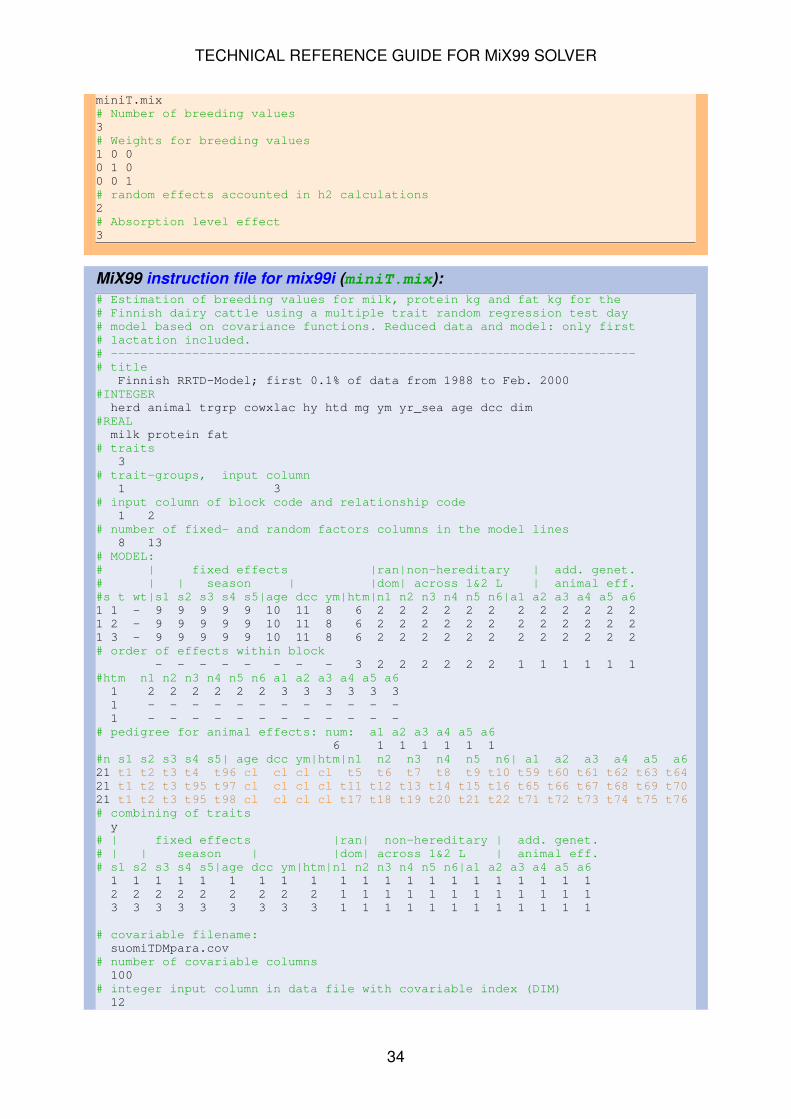
TECHNICAL REFERENCE GUIDE FOR MiX99 SOLVER
miniT.mix# Number of breeding values3# Weights for breeding values1 0 00 1 00 0 1# random effects accounted in h2 calculations2# Absorption level effect3
MiX99 instruction file for mix99i (miniT.mix):# Estimation of breeding values for milk, protein kg and fat kg for the# Finnish dairy cattle using a multiple trait random regression test day# model based on covariance functions. Reduced data and model: only first# lactation included.# -----------------------------------------------------------------------# title
Finnish RRTD-Model; first 0.1% of data from 1988 to Feb. 2000#INTEGERherd animal trgrp cowxlac hy htd mg ym yr_sea age dcc dim
#REALmilk protein fat
# traits3
# trait-groups, input column1 3
# input column of block code and relationship code1 2
# number of fixed- and random factors columns in the model lines8 13
# MODEL:# | fixed effects |ran|non-hereditary | add. genet.# | | season | |dom| across 1&2 L | animal eff.#s t wt|s1 s2 s3 s4 s5|age dcc ym|htm|n1 n2 n3 n4 n5 n6|a1 a2 a3 a4 a5 a61 1 - 9 9 9 9 9 10 11 8 6 2 2 2 2 2 2 2 2 2 2 2 21 2 - 9 9 9 9 9 10 11 8 6 2 2 2 2 2 2 2 2 2 2 2 21 3 - 9 9 9 9 9 10 11 8 6 2 2 2 2 2 2 2 2 2 2 2 2# order of effects within block
- - - - - - - - 3 2 2 2 2 2 2 1 1 1 1 1 1#htm n1 n2 n3 n4 n5 n6 a1 a2 a3 a4 a5 a61 2 2 2 2 2 2 3 3 3 3 3 31 - - - - - - - - - - - -1 - - - - - - - - - - - -
# pedigree for animal effects: num: a1 a2 a3 a4 a5 a66 1 1 1 1 1 1
#n s1 s2 s3 s4 s5| age dcc ym|htm|n1 n2 n3 n4 n5 n6| a1 a2 a3 a4 a5 a621 t1 t2 t3 t4 t96 cl cl cl cl t5 t6 t7 t8 t9 t10 t59 t60 t61 t62 t63 t6421 t1 t2 t3 t95 t97 cl cl cl cl t11 t12 t13 t14 t15 t16 t65 t66 t67 t68 t69 t7021 t1 t2 t3 t95 t98 cl cl cl cl t17 t18 t19 t20 t21 t22 t71 t72 t73 t74 t75 t76# combining of traitsy
# | fixed effects |ran| non-hereditary | add. genet.# | | season | |dom| across 1&2 L | animal eff.# s1 s2 s3 s4 s5|age dcc ym|htm|n1 n2 n3 n4 n5 n6|a1 a2 a3 a4 a5 a61 1 1 1 1 1 1 1 1 1 1 1 1 1 1 1 1 1 1 1 12 2 2 2 2 2 2 2 2 1 1 1 1 1 1 1 1 1 1 1 13 3 3 3 3 3 3 3 3 1 1 1 1 1 1 1 1 1 1 1 1
# covariable filename:suomiTDMpara.cov
# number of covariable columns100
# integer input column in data file with covariable index (DIM)12
34

TECHNICAL REFERENCE GUIDE FOR MiX99 SOLVER
# method used for relationshipam
# input fileTer.dat
# int-col. real-col. form12 3 f
# code for missing real values0.0
# scaling (y/n)n
# pedigree fileminiTDM.pedi
# parameter filesuomiTDMpara.in
# directory for the temporary files.
# solution files for random effects: htm non-ac animaln n y
# binary solution filen
# block preconditioner WpW, XpX (=D_M)d d d d
35

TECHNICAL REFERENCE GUIDE FOR MiX99 SOLVER
6.2 Exact reliabilities using exa99Approximate reliabilities can be calculated using apax99. However, MiX99 containsanother program, which allows the exact calculation of accuracies via inversion of thecoefficient matrix. The program is named exa99, has dynamic memory allocation,and is executed after running the pre-processor mix99i. exa99 is only useful forsmall problems (up to 200 000 equations). When specifying the model in the MODELline(s) of the MiX99 instruction file for mix99i, it is important to order the effects bynumber of levels. For within block effects, the effect with the most levels should get thelowest block ordering number and the effect with the least levels the highest. Similarly,for across block fixed effects, the effect with most levels should be specified first andthe effect with the least levels should be specified last. This is important to keep thememory requirements as low as possible when inverting the coefficient matrix.
6.2.1 Option file for exa99
Execution of exa99 requires an option file, which is read by standard input. The firstinformation asked by exa99 are internal storage format used for making coefficientmatrix of the mixed model equations. There are three formats:
F Full dense storageF
Internally the program stores the coefficient matrix in a rectangular dou-ble precision matrix. In practice, this storage format will give the fastestcomputations but may require a lot of computer RAM memory.
A number can be given after the ’F’ letter. This number is used to multiplediagonal elements of the coefficient matrix to make it full rank. Defaultvalue is 1.0001. The format is
F 1.0001
V Packed vector storageV
Internally the program stores the coefficient matrix in a packed upper tri-angle vector format. Thus, the RAM memory need is about half of the fulldense storage. However, computationally this storage form can be muchslower.
A number can be given after the ’V’ letter. This number is used to multiplediagonal elements of the coefficient matrix to make it full rank. Defaultvalue is 1.0001. The format is
V 1.0001
S Sparse matrix storageS
Internally the program store the coefficient matrix as a sparse matrix.Number of non-zeros is set to be 15 times the size of the coefficient ma-trix. A number can be given after the ’S’ letter which is initial guess for thenumber of non-zeros in the coefficient matrix. Thus, then the format is
S 1234567
36

TECHNICAL REFERENCE GUIDE FOR MiX99 SOLVER
Only the lower triangle of the matrix is stored. Thus, memory need canbe much less than for the packed vector storage. If the number non-zeros given is not enough, the program will increase sparse matrix size.However, this will use more memory than is optimal. Computationally thesparse matrix storage form is the slowest. In addition, total memory needdepends on the order of equations and can be even higher than for thefull dense storage.
The sparse matrix storage allows numerical filtering of low values in or-der to preserve some sparsity. After the format line, a line having threenumbers (these numbers are examples) is given:
1E-5 1E-6 1E-7
where the first number (1E-5) is for the operational zero of diagonal val-ues, the second number (1E-6) is for the operational zero of off-diagonalvalues, and the last value (1E-7) is matrix sparsity value. Often thesevalues are the same.
The three values have two purposes. First, these values are used todetect singularities in the coefficient matrix, i.e., dependencies. Singu-larity detection can help making the computations more reliable becauserounding errors due to almost zero values are not propagated. Second,the values allow preserving some sparsity in the matrix. The operationalvalues mean that when during inversion calculations absolute value ofadded element is less than operational value,´ the value is not added tothe coefficient matrix. Too high operational value leads to too high ap-proximation of computations. The matrix sparsity value is used to make amatrix element value zero when absolute value of an element is less thanthe sparsity value. Thus, the operational zero values are used to effec-tively zero values calculated during inversion calculations but the sparsityvalue is used to neglect elements for these computations even beforethese computations are made.
The operational zero and sparsity values are ways to increase sparsity inthe coefficient matrix during computations. The higher the values giventhe more approximations are used in the computations. Note that noneof these values affect during making of the coefficient matrix.
After the matrix format information has been given, name of the file having diagonalvalues of the genetic relationship matrix is asked. The file has format:
<ID code> <Diagonal value>
For example, diagonal of the pedigree based relationship matrix for animal i is 1 + Fiwhere Fi is inbreeding coefficient of animal i.
An example of an exa99 option file:FAdiag.dat
Full dense storage format and diagonal of relationship matrix is in file Adiag.dat.
For sparse matrix storage the command lines can be:
37

TECHNICAL REFERENCE GUIDE FOR MiX99 SOLVER
S 12345671E-5 1E-6 1E-7Adiag.dat
6.2.2 Exa99 output files
The output files have the same setup as when solving the mixed model equations.Structure of the output files depends on the model. Therefore, explanation of thecontent of those files is given in the printout of the particular run of exa99.
ACCani PEV and accuracies for animal effects.
SEfix Standard errors for all across blocks fixed effects.
SEfnn Standard errors for the nth within blocks fixed effect. E.g., SEf02 is thesolution file for the 2nd within block fixed effect.
PEVrnn Prediction error variance for the nth random effect in the model. E.g.,PEVr03 is the solution file for the random effects with the random effectnumber 3.
SEreg Standard errors for the across whole data regression effects.
38

TECHNICAL REFERENCE GUIDE FOR MiX99 SOLVER
6.3 Reversed reliability approximationThe reliability calculation can be reversed so that from given reliabilities it is possible tocalculate approximately weights that would lead back to the same reliabilities. Theseweights, considered as effective record contributions (ERC), can be derived fromreliabilities, pedigree, and heritability of the considered trait using reversed Harris andJohnson algorithm (Harris and Johnson, 1998).
The reversed reliability approximation can be calculated with apax99 (but not apax99p)using AccurType 20. The main input parameters, the reliabilities, are given to apax99in a separate file containing two or more columns: identification numbers and one ormore reliabilities:
File containing reliabilities for reversed reliability approximation:
Id1 Reliability1
2 0.15809E-014 0.144645 0.143796 0.115438 0.15527...
...
Note that the ERCs will be calculated just for those animals that are listed in the file.ERCs of other animals in the pedigree will be set to zero.
A slightly modified ApaX instruction file is used to calculate the ERCs from the givenreliabilities. Other input information, i.e. pedigree and heritability, are either given usingthe original MiX99 preprocessor directive file or given directly without the need to usethe MiX99 preprocessor.
• AccurType 20 without option p indicates that the original preprocessor directivefile name is given as OriginalDir:
Example apax99 input file of Reversed reliability approximation:# Reliability method (AccurType): Reversed reliability approximation20
# Filename of the reliability information (id and r2s):id_r2s.dat
# Original dir file (OriginalDir): "-" = MiX99_IN.DIR and MiX99_IN.OPT:-
# ERC parameters: tol maxit smallest [h2]1e-8 100 0.0001
whereas option p indicates that the pedigree filename is given instead of theoriginal directive filename:
Example of Reversed reliability approximation using pedigree file directly:# Reliability method (AccurType): Reversed reliability approximation,# p = pedigree file given, no mix99i needed:20 p
39
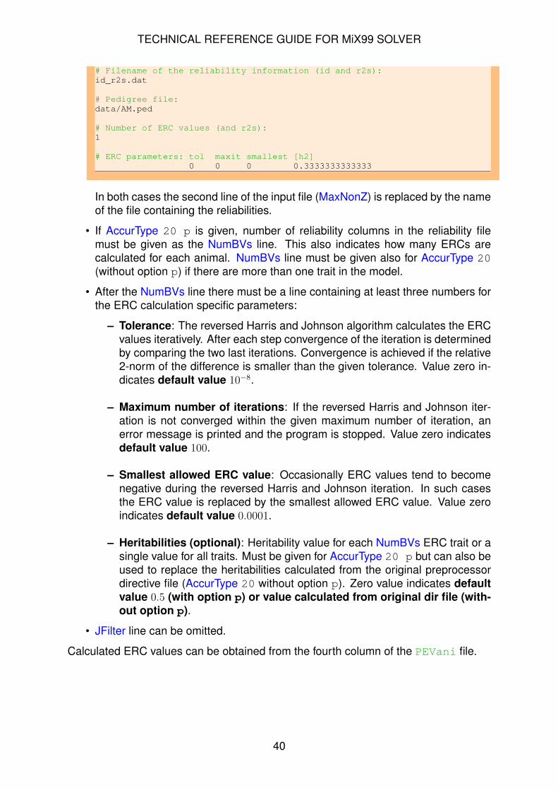
TECHNICAL REFERENCE GUIDE FOR MiX99 SOLVER
# Filename of the reliability information (id and r2s):id_r2s.dat
# Pedigree file:data/AM.ped
# Number of ERC values (and r2s):1
# ERC parameters: tol maxit smallest [h2]0 0 0 0.3333333333333
In both cases the second line of the input file (MaxNonZ) is replaced by the nameof the file containing the reliabilities.
• If AccurType 20 p is given, number of reliability columns in the reliability filemust be given as the NumBVs line. This also indicates how many ERCs arecalculated for each animal. NumBVs line must be given also for AccurType 20(without option p) if there are more than one trait in the model.
• After the NumBVs line there must be a line containing at least three numbers forthe ERC calculation specific parameters:
– Tolerance: The reversed Harris and Johnson algorithm calculates the ERCvalues iteratively. After each step convergence of the iteration is determinedby comparing the two last iterations. Convergence is achieved if the relative2-norm of the difference is smaller than the given tolerance. Value zero in-dicates default value 10−8.
– Maximum number of iterations: If the reversed Harris and Johnson iter-ation is not converged within the given maximum number of iteration, anerror message is printed and the program is stopped. Value zero indicatesdefault value 100.
– Smallest allowed ERC value: Occasionally ERC values tend to becomenegative during the reversed Harris and Johnson iteration. In such casesthe ERC value is replaced by the smallest allowed ERC value. Value zeroindicates default value 0.0001.
– Heritabilities (optional): Heritability value for each NumBVs ERC trait or asingle value for all traits. Must be given for AccurType 20 p but can also beused to replace the heritabilities calculated from the original preprocessordirective file (AccurType 20 without option p). Zero value indicates defaultvalue 0.5 (with option p) or value calculated from original dir file (with-out option p).
• JFilter line can be omitted.
Calculated ERC values can be obtained from the fourth column of the PEVani file.
40
TECHNICAL REFERENCE GUIDE FOR MiX99 SOLVER
7 Daughter Yield DeviationsThe request of daughter yield deviation (DYD) for different dairy cattle studies andfor model validation purposes made it necessary to implement adequate calculationprocedures into MiX99. A general approach for the calculation of DYD is implementedinto MiX99. The calculations follow the method presented in Mrode and Swanson(2004). For simple models, like single trait animal models, the approach will yieldDYD, which are calculated in the same manner as given in VanRaden and Wiggans(1991). In case of random regression models, DYD coefficients will be given. Thesecoefficients can be used in a post-processing procedure to obtain DYD for certainintervals of the time trajectory, like 305-day yield DYD.
DYDs can be obtained for each bull that has daughters with records. Furthermore, it ispossible to classify within each bull the DYDs by a classification variable. This is usefulfor model validation purposes.
In some situations it might be useful to obtain yield deviations (YD) or individual daugh-ter deviations (IDD). Here, an IDD is defined as the YD minus half of the dam’s additivegenetic animal effect. MiX99 provides an option to calculate for each observation thatis included in the analysis the corresponding YD or IDD. The YDs and IDDs will be writ-ten to unformatted files. For instructing MiX99 to calculate YDs or IDDs please seethe explanations given for the VALID option in chapter 4, and about Files for modelvalidation purposes in chapter 5.
7.1 Calculation of daughter yield deviationsThis chapter will explain how MiX99 can be instructed to calculate DYD. Instructionshave to be given for the pre-processing and for the solver programs. In case it isdesired to classify the DYDs within sires, additional information will be needed in thepedigree file.
7.1.1 Pedigree file
The additional information in the pedigree file is required only if DYD should be clas-sified within sires (optional). A column with the classification variable has to be addedto the pedigree file. This column must be given after the pedigree information (i.e,column 4 or higher) or after the blocking variable code in case blocking of the data isdesired (i.e, in this case column 5 or higher). The classification code will indicate towhich within-sire class the daughter will be grouped; e.g., the classification code couldcorrespond with the calving years of the daughters. The classification codes need tobe numbered from one (1) to n within a sire. Some classes may be missing within asire. For animals without observations in the data file a zero (0) is given.
7.1.2 MiX99 instruction file
Instructions specific to the calculation of DYD have to be given on two instruction lines.First, on the PEDFILE instruction line an integer value has to be provided after thepedigree filename. There are two alternatives available. Alternative 1: specifying azero (0) will instruct MiX99 to calculate DYDs for each bull with daughters that haveobservations. Alternative 2: Specifying the column number of the pedigree file thatcontains a within-sire classification will instruct MiX99 to calculate for DYD for each
41

TECHNICAL REFERENCE GUIDE FOR MiX99 SOLVER
class within sire. Second, on the PRECON instruction line a block diagonal precondi-tioner matrix (option b) must be defined for the additive genetic animal effect.
7.1.3 MiX99 solver option fileInstruction specific to the calculation of DYD have to be given on two option lines. Theoption d must be specified on the VALID option line. This is followed by a FACTORoption line which specifies the model factors that are included into the DYD. Pleasesee Daughter Yield Deviations in chapter 4.1, for specifying the FACTOR option line.
7.2 Solution files for daughter yield deviationsDaughter yield deviations are written to a file named Soldyd. The structure of the fileis similar to that one of the file Solani. The structure of the file is model-specific andthe solver will write an explanation to standard output. In case of a random regressionmodel, DYD regression coefficients are given. Number and order of the coefficientsis the same as for the animal effect coefficients in Solani. The DYD coefficients arefollowed by as many integers as there are coefficients for a particular DYD function.The order of these integers is the same as the order of the DYD coefficients, and theintegers may have a value of one or zero. Ones indicate that the corresponding coef-ficients were estimable. This is important for multi-trait or random regression models,where it might be not possible that some DYD functions are not defined. For instance,given a model specifies that first and second lactation observations are different traitsand all daughters of a sire have first lactation observations only. Then, there is no DYDfunction available for the second lactation.
For random regression models the same covariables as applied for the additive geneticanimal effect apply also to the DYDs. Note: A bull’s DYD function is only defined forthe time interval in which the bull’s daughters have observations. An extrapolation ofthe function beyond this time interval may yield absurd results.
7.3 ExampleThe example explained in chapter 7.3 of the Technical reference guide for MiX99 pre-processor will be modified for the calculation of DYD. Modifications are in bold.
MiX99 instruction file:# TITLE:
RANDOM REGRESSION, L.Schaeffer & J.Dekkers (1994)# INTEGER:
HTD Animal# REAL:
Covar_1 Covar_2 Milk# TRAITS:
1# TRGRP:
1 -# DATASORT: block_code, relationship_code (single residual var.)
1 2# FIXRAN: number of fixed and random factors in the model
1 3# MODEL: trait_group trait weight herd-test-day gamma0 gamma1 gamma2
1 3 - 1 2 2 2# WITHINBLOCKORDER: order of effects within blocks
2 1 1 1# RANDOM: gamma0 gamma1 gamma2
42

TECHNICAL REFERENCE GUIDE FOR MiX99 SOLVER
1 1 1# RELATIONSHIPS: number: gamma0 gamma1 gamma2
3 1 1 1# REGRESS: number beta1 beta2 herd-test-day gamma0 gamma1 gamma2
6 1 2 cl cl 1 2# COMBINE:
n# PEDIGREE:
am# DATAFILE:
example3.dat# VAR:
2 3 f# MISSVA:
0.0# SCALE:
n# PEDFILE: filename, a zero for calculation of DYD
example3.ped 0# PARFILE:
variance_comp.ex3# TMPDIR:
.# RANSOLFILE: animal effect
y# SOLUNF:
n# PRECON: block diagonal preconditioner for the animal effect in WpW
b d f# PARALLEL: number of processors used by the solver program
1# COMMONBLOCKS:
0
MiX99 solver option file:# RAM RAM demand: H=high, M=medium, L=low
H# STOP Maximum_number_of_iterations, Stopping_criterion (CR)
1000 1.0e-7 r f# RESID Calculate residuals? (Y/N)
N# VALID D for calculation of DYDs
D# FACTOR: beta1 beta2 herd-test-day gamma0 gamma1 gamma2
0 0 0 1 1 1# VAROPT (N, S, C, E, G)
N# SOLTYP Type of solution files? (N,Y,A,H)
Y
Description of the Soldyd file written by the solver to standard output:..
Daughter Yield Deviations-------------------------
First 50 Solutions-------------------------------------------------
Sire Class N-Daug. N-Rec. Effect Trait Solution Def.9 1 2 9 1 1 -2.98764 19 1 2 9 2 1 0.488173E-01 19 1 2 9 3 1 0.284341 1
10 1 2 9 1 1 3.74280 110 1 2 9 2 1 -0.433969E-01 110 1 2 9 3 1 -0.516160 1
43

TECHNICAL REFERENCE GUIDE FOR MiX99 SOLVER
11 1 2 5 1 1 -1.03777 111 1 2 5 2 1 0.841567E-02 111 1 2 5 3 1 0.498087E-01 1
"Soldyd"-File: Daughter Yield Deviations for Sires
Column | Description----------------------
1 Code of Sire2 Within Sire Classification3 Number of Daughters4 Total Number of Records5 DYD Solution / Coefficient : Factor 1 Trait 16 DYD Solution / Coefficient : Factor 2 Trait 17 DYD Solution / Coefficient : Factor 3 Trait 18 DYD is defined (yes=1,no=0): Factor 1 Trait 19 DYD is defined (yes=1,no=0): Factor 2 Trait 1
10 DYD is defined (yes=1,no=0): Factor 3 Trait 1..
44

TECHNICAL REFERENCE GUIDE FOR MiX99 SOLVER
8 Non-linear modelsTwo non-linear models are implemented into MiX99. Estimation of categorical vari-ables is implemented by the generalized linear mixed model with the probit link func-tion, and estimation of the growth curve models is implemented by linearization ofnon-linear Gompertz function model using second order Taylor series expansion. Useof these models is still exiguous and extensions of the MiX99 program for these mod-els are therefore considered as test-versions. There is no possibility to give the CLIMcommand file for these models yet. Instead, the MiX99 instruction file should be made.
8.1 Threshold-modelPrediction of breeding values is possible for models with one categorical and severallinear traits. Models are allowed to have missing traits and unequal design matricesfor traits. Thresholds can be estimated or set to be known. (Co)variance componentshave to be known and residual variance of the categorical trait should be set to one.
8.1.1 Instruction file for mix99i
The categorical trait is defined by giving Tn, where n is a number of thresholds, on itsown column between first and second parameters in the MODEL line. For example,for a binary trait (recorded as 1 and 2) option T1 needs to be marked. In case of amultiple trait model, the linear traits are defined first (see example 7.9). When thethreshold model is defined, one or two additional instruction lines must be given rightafter the MODEL line.
First additional line defines the method that is used to analyze the threshold mod-els. There are two options: em option defines the Expectation Maximization algorithm(EM) (Gilmour and Thompson, 1998) and nr option defines the Newton-Raphson algo-rithm (NR) (Janss and Foulley, 1993; Hoeschele, Tier, and Graser, 1995). By default,thresholds are estimated simultaneously. Optionally, additional characters “ft” can bespecified to indicate fixed threshold values. Thus, a new line must follow, where thethreshold values for categorical trait are defined. This line should contain as many realnumbers as defined for the categorical trait in the MODEL line.
8.1.2 Stopping criterion file for mix99s
Solving of the threshold-model is a non-linear problem and iterative in two levels.Therefore, the STOP line changes to have five entries: an integer, a real value, acharacter, an enforcing character “f” and an integer. Now the first integer value givesthe maximum number of PCG-iterations within each NR- or EM-round (default is 100or number of equations in the MME) and the last integer value gives the maximumnumber of NR- or EM-rounds (default is 5000). Analyze is set to be converged whenonly one PCG iteration round is needed within the NR round, or less than 10 PCGiteration rounds are needed within the EM round.
There should be insignificant differences in solutions between two algorithms, but theEM algorithm is generally slower to converge than NR algorithm. NR algorithm iscritical to attain good solutions within the rounds. Increasing the maximum number ofPCG-iterations within each round may lead to fewer NR rounds and in that way fasterconvergence finally. Instead, EM algorithm will need reasonable solutions to certain
45

TECHNICAL REFERENCE GUIDE FOR MiX99 SOLVER
extent within each EM round, after which increase in accuracy will not improve the totalconvergence.
8.1.3 Solution files
Solution files are equal to the linear mixed model case. When thresholds are esti-mated, these are printed in the output and in the end of the Solfix-file (with factorname Threshold and factor number 0).
8.1.4 Example
Example 7.9 in Technical reference guide for MiX99 pre-processor contains the in-struction file for bivariate model with one binary trait.
8.2 Gompertz-modelA multiplicative Gompertz model (i.e. ln(y) = ln(a) − b ∗ exp(−k ∗ t) + e) as demon-strated in Vuori et al. (2006a); Vuori et al. (2006b) is implemented in MiX99. Thus,log-transformation is needed for original observations y, although solutions are forthree parameters a, b and k. All traits introduced in the analysis must currently havethe non-linear Gompertz form. Models are allowed to have missing traits and unequaldesign matrices for traits. (Co)variance components could be known or estimated si-multaneously between each round by the covariance component estimation programwhich allows linear random regression models.
8.2.1 Instruction file for mix99i
Model specification for non-linear model reminds the specification of regression mod-els, although few additional features and restrictions compared to model specificationfor linear random regression traits exist. The two most important lines in the instructionfile therefore are MODEL and REGRESS lines which will be discussed below.
Non-linear Gompertz-model traits are defined in the MODEL line by giving the charac-ter G on its own column between first and second parameters. Effects in the MODELlines are defined as many times as number of parameters of the Gompertz functionthe effect is related to (i.e. 1-3 times for Gompertz function, see example 7.8). How-ever, for all traits, at least one common fixed effect needs to be related to all threeparameters. This effect is defined first in the MODEL line, and further, is defined tobe across-block effect (see WITHINBLOCKORDER). I.e., dash (-) must be specifiedfor the first effect in WITHINBLOCKORDER line. If many such effects occur, you maydefine effect with smallest number of levels first.
All factors in the MODEL line must be considered as covariables read from the sep-arate file, i.e., covariable columns have to be specified with a preceding "t" on theREGRESS line(s). Real input column for covariable indicates the parameter of theGompertz function the effect is related to: t1 for mature weight, t2 for relative initialweight and t3 for maturation rate. An additional column for time is needed at the endof each REGRESS line. This is not counted in the number of regression effects speci-fied first in the REGRESS line.
In consequence, a covariable file is always needed. The index connecting an obser-vation and a set of covariables is usually time of measurement but the rest of the file
46

TECHNICAL REFERENCE GUIDE FOR MiX99 SOLVER
differs from those to linear random regression models. Because the Gompertz functionhas three parameters, first three covariable columns should contain only ones. Afterthese, a column with the time variable is set. This can also be a scaled time if needed.E.g. select time scaling so that estimate for maturation rate is approximately one. Thenumber of columns needed in covariable table is therefore at least 4, i.e., number ofparameters in the non-linear Gompertz function plus one for the time dependent.
Addition to MODEL and REGRESS lines, restrictions on PRECON and DATASORTlines should be mentioned: (1) Diagonal (d) must be defined for all preconditioners and(2) multiple residual (co)variance matrices are not possible for non-linear Gompertzfunction models.
Note: The iterative algorithm for non-linear Gompertz function model is implementedso that a restart of analysis is needed. For this reason the user must define the conver-gence of the iterative process by itself. However, this enables the possible update ofnew variance components for each iteration round by calling mix99i first. Thereforeboth options in the SOLUNF line are possible, but restart of mix99s is possible withoption n as well in case the covariance components are known and won’t change fromround to round. The case when estimation of variance components is done simultane-ously is covered in the section of stopping criterion file.
8.2.2 Stopping criterion file for mix99s
Stopping criterion file is defined as for linear traits. Now the stopping criterion is forBLUP solutions within each round. To decide the final convergence of the iterativeprocess, user must define the convergence by itself over repeated BLUP analysis.One option would be to append the solutions after each round to another file which isstudied for converge of solutions.
It is possible to estimate variance components simultaneously between each round byanother analysis. This is allowed by the option d in SOLTYP line, which will producebinary and ascii files named DMUINP and DMUINP.dat, respectively. There is a his-torical reason for naming files according to DMU, but any other suitable program canbe used also. These files include the pseudo data, i.e., linearized observations andcovariables, among others. Missing observations and covariables in DMUINP andDMUINP.dat files are coded as -99999. First within these files are integer columnsand then real columns. Integer columns contain within and across block fixed effectsand random non-genetic and genetic effects, in this order. After these there is the col-umn with zeros. First real columns contain linearized observations for each trait, afterwhich linearized covariables for each three Gompertz function parameters by traits fol-low. Last real column contain ones. Note: Good knowledge and carefulness is neededto estimate the covariance components accurately.
8.2.3 Solution files
Program gives solutions for Gompertz-model parameters (i.e. a, b and k) defined foreach effect. Because model mimics linear random regression model, solutions filesare equal to the linear random regression model case.
47

TECHNICAL REFERENCE GUIDE FOR MiX99 SOLVER
8.2.4 Example
Example 7.8 in Technical reference guide for MiX99 pre-processor contains the in-struction file for Gompertz function.
48

TECHNICAL REFERENCE GUIDE FOR MiX99 SOLVER
9 Estimation of variance componentsFor prediction of breeding values, variance components need to be known. An imple-mentation of the Monte Carlo (MC) Expectation Maximization (EM) Restricted Maxi-mum Likelihood (REML) (MC EM REML) algorithm for the estimation of variance com-ponents (Matilainen et al., 2012) is available in the mix99s solver. The algorithmapplies a resampling procedure to estimate prediction error variances (PEV) neededin the EM REML equations. Estimates of location parameters are obtained from thereal data within each REML round, whereas PEV is obtained within each REML roundby repeatedly simulating data and estimating the location parameters of the simu-lated data. This enables calculation of PEV without inversion of the coefficient matrix,leading to memory requirements equal to the solving of the mixed model equations.Although EM algorithm is known to be slow in convergence, the MC EM REML makesREML feasible for large data sets and complex models for which the inversion of thecoefficient matrix would be too memory and time consuming.
The implementation for the variance component estimation supports the majority ofmodels possible in MiX99. However, analysis of models which include an externalcorrelation structure matrix (e.g. an IBD matrix), or which include an effect with anautoregressive correlation structure as well as threshold models and Gompertz modelsare not supported yet.
The current implementation has been developed and tested to serve a research co-operation between Luke (former MTT) and Rothamsted Research (UK). We considerthis implementation ready to be tested by MiX99 users as well. Any feedback aboutyour experiences is very much appreciated.
9.1 Running MC EM REMLEstimation of variance components requires execution of two programs. First, thepre-processor program mix99i is executed either by using CLIM command file orMiX99 instruction file with initial values for the variance components. Then, the solverprogram mix99s is executed with specific instructions in the solver option file (seeVAROPT option line in chapter 4.1).
DEVBecause models used in MC EM REML estimation are usually complex and analysestime consuming, it is also possible to change some of the iteration parameters to bemore suitable during the execution of the solver mix99s. This can be done by usingexternal file ITER. Both the parameters regarding breeding value estimation and theparameters regarding variance component estimation can be updated.
If the estimation is wanted to be stopped beforehand, external STOP file will do it in acontrolled way.
NEWIn case the estimation has stopped or ended, but more REML rounds is needed,the estimation can be continued by starting solver mix99s without running the pre-processor mix99i first. In that case maximum number of iterations for variance com-ponent estimation is marked as negative value in the STOPE line of the solver optionfile. This value is the new total number of REML rounds, i.e., value should be largerthan the REML rounds in the previous run. For example, when estimation has stoppedon the REML round 1000 but you want to make another 1000 rounds, then the new
49
TECHNICAL REFERENCE GUIDE FOR MiX99 SOLVER
maximum number of iterations for estimation of variance components is -2000. Theestimation, including REML rounds, will start from what they ended (last row in theREMLlog file) and estimates from the new REML rounds will be appended to REMLlogfile as well. Other PCG and REML iteration parameters can also be changed for thecontinued estimation.
The variance component estimation can also be restarted by performing another esti-mation using the previously estimated variance components as the initial values. Theestimated variance components from the parfile need to be first copied to the filespecified in PARFILE line of the instruction file (and possibly resfile to RESFILE).Remember also to save the old REMLlog file to another name to keep old estimatesavailable. Other estimation parameters can be modified at this stage, too. Then, thepre-processor program mix99i is run to restart the estimation from the new initial val-ues of the variance components before running the solver mix99s for the restartedestimation.
How MiX99 works to estimate variance components will be explained in more detail inthe following.
9.2 File with starting values of (co)variance componentsThe file with the starting values for the (co)variance components must be in the sameformat as described in the chapter File with (co)variance components of the Technicalreference guide for MiX99 pre-processor . The file will be specified in the PARFILEinstruction line of the CLIM command file or MiX99 instruction file. The same rulesapply also for a file with starting values for the multiple residual (co)variance matricesin the case that a model with multiple residual (co)variances is applied (optional).
9.3 MiX99 instruction fileThere is no need to give a specific instruction regarding variance component estima-tion neither in the MiX99 instruction file, nor in the CLIM command file. Becausepre-processor mix99i will at the beginning form preconditioner matrices with theinitial values for the variance components, updating of the matrices with the mostcurrent variance component estimates was found crucial to enhance convergence.In the currently implemented version of the variance estimation module the mix99ssolver will automatically, in certain REML round intervals, make a system call to starta mix99i pre-processing run. NEWTherefore MiX99 pre-proprocessor stores its instruc-tions directives (.DIR) and possible command line options (.OPT) automatically tofiles MiX99_IN.DIR and MiX99_IN.OPT, respectively. So, during the preconditionerupdate these files need to be available and contain the information from the originalpre-processor run. Alternatively, MiX99 instruction file named as MiX99_DIR.DIRcan be used to specify the pre-processor directives for the preconditioner update. Thisfile is automatically created by the pre-processor when a CLIM command file is usedfor the model. File MiX99_DIR.DIR contains the same information in instruction fileformat.
Updating of the preconditioner matrices is done every 10th REML round during the first100 REML rounds and on every 100th REML round thereafter. If the updating did notsucceed, the text
50

TECHNICAL REFERENCE GUIDE FOR MiX99 SOLVER
Updating of preconditioner failed!
is printed to the standard output and further instructions are given to check for addi-tional error intormation:
See files MiX99_DIR.LOG and WARNING.log.
If pre-processor directives for the preconditioner update could not be found, this inindicated by error message:
Either MiX99_IN.DIR or MiX99_DIR.DIR file is needed as directive filefor mix99i.
9.4 MiX99 solver option fileThe solver mix99s is instructed to estimate variance components by specifying optione on the VAROPT option line and by giving information on three additional optionlines STOPE, SEED and MIX99PATH thereafter. Specifying the information on threeadditional option lines is explained in chapter 4.1 regarding the option e. If some of thegiven parameters for the STOPE line are found to be poor during the execution of MCEM REML, see Running MC EM REML for different possibilities to change these.
9.4.1 Number of data samples
The second parameter given on the STOPE line is number of data samples. This isa number of data samples generated and analyzed within a one round of stochasticMC EM REML. The number of analyzed data samples within a REML round will affectthe accuracy of the prediction error variance estimates. Increasing the number of sam-ples will reduce the Monte Carlo error associated with the prediction error variances.However, the size of Monte Carlo error depends also on the model specified and onthe amount of data and animals included in the analysis.
We observed that convergence of the MC EM REML algorithm is not affected by thenumber of samples specified and for many models even one sample per REML roundis sufficient. The number of specified data samples is critical, because each additionaldata sample will require one additional BLUP model to be solved within a REML round,which increases the total time of the REML analysis.
Our experiences so far suggest that analysis with large amount of data and sufficientnumber of animals (e.g. test-day data with observation from over 10 000 animals)needs only one Monte Carlo sample per REML round. When amount of data is rathersmall in relation to the number of parameters to be estimated, a higher number of sam-ples (5, 10 or 20) might be more appropriate. For some analyses with small amount ofdata, software using non Monte Carlo REML implementation can be more suitable.
9.4.2 Determining convergence of REML parameter estimates
There is a need for a convergence indicator which accounts for the characteristicsthat parameter estimates are associated with Monte Carlo noise. The currently im-plemented convergence indicator is calculated from the vectors containing predictedvariance component estimates at two points x − 1 and x ( s(x − 1) and s(x)), wherethe prediction is based on estimated variance components obtained during the latestx EM rounds (θ(k−x+1), . . ., θ(k)), and where a predicted estimate for each variance pa-rameter is calculated as si(x) = αi+ βix. The size of x is chosen to be large enough to
51
TECHNICAL REFERENCE GUIDE FOR MiX99 SOLVER
minimize the Monte Carlo noise in the convergence indicator, which is calculated forREML round k:
cc(k)E =
(s(k)(x)− s(k)(x− 1)
)T (s(k)(x)− s(k)(x− 1)
)(s(k)(x))
T(s(k)(x))
After cc(k)E has reached a value smaller than the specified convergence criterion (seeSTOPE option line), the REML analysis will perform a sequence of 30 additional MCEM REML rounds, which will reduce the Monte-Carlo error from the parameter es-timates by using weighted average with decreasing weights for latest solutions. Sofar, depending on the analysis, it was found that values between 1.0e-8 to 1.0e-9 aresuitable convergence criterion.
9.4.3 Keeping certain variance components fixed
For some analyses it might be desired that certain pre-defined variance components(starting values) remain unchanged during the MC EM REML analysis. The instruc-tions about which variance component parameters are kept fixed are given in theMiX99 solver option file.
For this option the three entries e f n have to be specified on the VAROPT option line,where f instructs mix99s to keep some parameters unchanged and the third entryn is an integer value which tells how many parameters should remain unchanged.This option will require the inserting of n additional lines right after the VAROPT line.Each line specifies one parameter that should remain unchanged. A line consists ofthree integers, where the first integer is the random effect number followed by therow-column combination. In practice, you can copy the corresponding line from theparameter file excluding the variance component parameter itself.
In case multiple residual variance matrices are applied, four integers need to be de-fined for residual variance component parameters to be unchanged. The first integernumber is equal to the random effect number of the residual effect. The second inte-ger gives the residual variance class number. This is equal to the first number on thecorresponding parameter line in the file with multiple residual (co)variances (see chap-ter 3.4 in Technical reference guide for MiX99 pre-processor ). The last two integersspecify the row-column combination.
9.4.4 MC EM REML for MACE
NEWAs a special case is the estimation of variance components for a MACE model. Vari-ance component estimation of the MACE model can be done by keeping the residualvariance fixed at unity and applying weights, wij = EDCij/(λjσ
2gj
) with λj = (4−h2j)/h2j ,for deregressed breeding values for bull i in different countries j (Tyrisevä et al., 2011).However, estimation of variance components will change genetic variances σ2
gjthat
were originally used in the calculation of the weights. Therefore, it will be more ac-curate to update the weights after new estimates of genetic variances are available.MiX99 can do this updating of weights for the MACE model automatically after eachREML round when option ei instead of just e is specified for estimation of variancecomponents on the VAROPT option line.
52

TECHNICAL REFERENCE GUIDE FOR MiX99 SOLVER
9.5 Standard errors for REML parameter estimatesMiX99 is capable to calculate standard errors for the variance component estimatesat the last REML round. Approximated standard errors are based on variances oversampled gradients as explained for NR-method in Matilainen et al. (2013). They arecalculated automatically when the number of data samples is at least 10. Adequatenumber of samples depends on the data and model, but 50 or more samples is rec-ommended.
As using number of data samples less than 10, even a single one, is much faster, onecan first start the estimation using the smaller number of samples. Then, after the con-vergence of the variance components, one additional REML round can be executedafterwards. This can be done in different ways. Either the estimation of variance com-ponents can be continued or another variance component estimation can be startedusing the estimated variance components as the initial values. In both cases the num-ber of samples can be set to larger than 10, for example 50, in the solver option file sothat the standard errors are calculated.
Approximated standard errors, as well as all covariances of REML estimates in theinformation matrix, are printed after the last REML round. Standard errors are printedto the vceSE, and information matrix is printed to the vceI. The vceSE has fourcolumns. It resembles the parfile, but has approximated standard errors in thefourth column. If model has multiple residual variance matrices, standard errors for allresidual classes are printed after the first residual class (like in REMLlog). Exampleabout vceSE is for one trait with two random effects and residual:
vceSE:1 1 1 208.1342 1 1 272.5083 1 1 59.4737
The vceI has seven columns. First three integers indicates the first parameter andthe next three integers indicates the second parameter. Seventh column has the co-variance between the two parameters. For example above, vceI is
vceI:1 1 1 1 1 1 43319.72 1 1 1 1 1 -44735.82 1 1 2 1 1 74260.43 1 1 1 1 1 -1222.083 1 1 2 1 1 485.0083 1 1 3 1 1 3537.12
The information matrix contains a value for each combination of the (co)varianceparameters and so it becomes large very soon. For example, for model with six(co)variance parameters, the information matrix contains 21 elements.
vceSE:1 1 1 98919.71 2 1 3534.951 2 2 155.8952 1 1 82881.32 2 1 2914.912 2 2 126.006
53

TECHNICAL REFERENCE GUIDE FOR MiX99 SOLVER
vceI:1 1 1 1 1 1 0.978512E+101 2 1 1 1 1 0.310664E+091 2 1 1 2 1 0.124959E+081 2 2 1 1 1 0.987140E+071 2 2 1 2 1 483421.1 2 2 1 2 2 24303.12 1 1 1 1 1 -0.755926E+102 1 1 1 2 1 -0.238666E+092 1 1 1 2 2 -0.741774E+072 1 1 2 1 1 0.686931E+102 2 1 1 1 1 -0.236382E+092 2 1 1 2 1 -0.937649E+072 2 1 1 2 2 -355953.2 2 1 2 1 1 0.216383E+092 2 1 2 2 1 0.849670E+072 2 2 1 1 1 -0.737152E+072 2 2 1 2 1 -356791.2 2 2 1 2 2 -17917.62 2 2 2 1 1 0.667658E+072 2 2 2 2 1 319118.2 2 2 2 2 2 15877.5
For model with 42 (co)variance parameters, the information matrix contains as muchas 903 elements.
9.6 Solution files for variance componentsREMLlog Contains the estimates of variance components at every REML round.
The first column in the file specifies the REML round and the NEWsecondcolumn the convergence criterion value of that round. After the secondcolumn as many columns follow as there are variance component param-eters to be estimated. The order of the lines is as following. The firstthree lines in the REMLlog describe the order of the parameter columnsof which the first line contains the random effect number and the secondand third lines the row-column combination for the particular parameterof a random effect. Hence, the first three lines are identically with the firstthree columns in the file with the (co)variance components. If multipleresidual variance matrices are defined, then their variance class numberis added to the end of the file. The fourth line contains the initial param-eter values used. The following lines contain the estimates of variancecomponents at each REML round.
parfile Contains the latest solutions of variance component estimates. The struc-ture of the file is the same as in the parameter file of the PARFILE instruc-tion line.
resfile Contains the latest solutions of residual variance component estimateswhen multiple residual variance matrices are defined. The structure ofthe file is the same as in the multiple residual variance matrices file of theRESFILE instruction line.
vceSE This file will be produced when approximated standard errors for REMLparameter estimates are calculated. Resembles parfile. First threeintegers indicates the random effect number and row-column combinationof that matrix. Fourth column contains the real value and is approximated
54

TECHNICAL REFERENCE GUIDE FOR MiX99 SOLVER
standard error. If the model has multiple residual variance matrices, theseare numbered as in REMLlog and printed right after the standard errorsfor other random effects.
vceI This file will be produced when approximated standard errors for REMLparameter estimates are calculated. The file has seven columns. Sev-enth column has the value of the information matrix for each pairwiseparameter combination. The first parameter is indicated by the first threeintegers as in vceSE, and the second parameter is indicated by the nextthree integers as in vceSE.
9.7 ExampleSchaeffer has written a technical note on maximum likelihood estimation of variancecomponents (Journal of Dairy Science, 1976). It contains a small example data inTable 1 for milk yields of first lactation daughters of five dairy sires in two herds. Themodel contains sire groups and herds as fixed effects and uncorrelated sires as ran-dom effects. In the following the CLIM command file for the mix99i pre-processorand the MiX99 solver option file for the mix99s solver program, as well as the listingin the standard output of the solver are given.
CLIM command file:TITLE data in technical note of Schaeffer (Table 1, J. Dairy Sci., 1976)
DATAFILE data.datINTEGER group herd sireREAL yield
PARFILE data.par
PEDFILE data.pedPEDIGREE sire sm
MODELyield = group herd sire
The “MiX99_DIR.DIR” file created for mix99i:# TITLE data in technical note of Schaeffer (Table 1, J. Dairy Sci., 1976)data in technical note of Schaeffer (Table 1, J. Dairy Sci., 1976)# INTEGER group herd siregroup herd sire# REAL yieldyield# TRAITS
1# TRAITGRP1 -
# datasort: Block_code, Relationship_code- -
# FIXRAN: Numbers of fixed and random factors in the model2 1 0 0# MODEL: Subgr. Trait Weight ... model factors ...1 1 - 1 2 3
# WITHINBLOCKORDER: Order of effects within blocks- - 1
# RANDOM1
# RELATIONSHIPS1 1
55

TECHNICAL REFERENCE GUIDE FOR MiX99 SOLVER
# REGRESS3 cl cl cl
# COMBINEn# PEDIGREEsm# DATAFILE data.datdata.dat# VAR
3 1 f# MISSVA0
# SCALEn# PEDFILE data.peddata.ped# PARFILE data.pardata.par# tmpdir.
# noransoly
# SOLUNFn# preconb b # Default is block
# parallel: Number of processors used by the solver program1 # Default: no parallel computing
# COMMONBLOCKS: Number of blocks in common area for parallel computing0
MiX99 solver option file:# RAM: RAM demand: H=high, M=medium, L=low
H# STOP: Max. num. iterations, Stopping criterion, Convergence indicator, enforce
5000 5.0e-5 d f# RESID: Calculate residuals? (Y/N)
N# VALID: N=none, P=prediction, S=sum of effects, Y=YD, D=DYD, I=IDD
N# VAROPT: adjust for heterogeneous variance (N, E, S, C)
E# STOPE: REMLrounds, nSamples, stopCritVCE
1000 5 1.0e-9# SEED: Type of seed for the random number generator
R# MIX99PATH:
/share/apps/# SOLTYP: type of solution files? (Y,N,A,H)
Y
At the following are three excerpts of standard output of MC EM REML evaluation: atthe beginning, when the convergence criterion of MC EM REML is reached, and at theend. Comments after # are added.
Parts of standard output file of the solver:...
___________________________________________________________________________
MiX99_SOLVE: Start of MC EM REML iteration Time: 13:11:00.3 18.11.2019___________________________________________________________________________
56

TECHNICAL REFERENCE GUIDE FOR MiX99 SOLVER
___________________________________________________________________________
MiX99_SOLVE: Start of Iteration Time: 13:11:00.3 18.11.2019___________________________________________________________________________
Iteration Statistics--------------------
Convergence Indicators-----------------------------------------------------------------------------ROUND CA CR CM CD MAX.CHA.
------- ------------ ------------ ------------ ------------ ------------Solution vector will be initialized to be zero
rhs’ * rhs = 14014.6999754906animal rhs’ * rhs = 2345.34000116348
------------------------------------------------------0 1.000 1.000 1.000 0.000 0.0001 0.8156E-01 0.4002E-01 0.4602E-01 1.000 1.6752 0.4518E-01 0.2589E-01 0.3458E-01 0.2209 -0.65453 0.3199E-01 0.2202E-01 0.2617E-01 0.5391 -1.0814 0.8213E-02 0.9357E-02 0.9692E-02 0.8242E-01 -0.30685 0.1470E-02 0.7315E-03 0.1014E-02 0.3065E-01 -0.8918E-016 0.6997E-03 0.4073E-03 0.4696E-03 0.4586E-02 -0.2069E-017 0.4954E-10 0.2027E-10 0.2669E-10 0.1223E-01 -0.3061E-018 0.4274E-12 0.3967E-12 0.4006E-12 0.8750E-10 -0.2393E-099 0.1452E-16 0.1267E-16 0.1258E-16 0.3625E-12 0.6506E-12
CD convergence criterion 0.5E-4 achieved in 9 iterations.Solutions have converged according to CD criterion. # Convergence of real data
___________________________________________________________________________
MiX99_SOLVE: End of Iteration Time: 13:11:00.3 18.11.2019___________________________________________________________________________
9 0.1185E-15 0.9644E-16 0.1095E-15 0.4962E-13 0.2709E-139 0.4008E-15 0.5995E-15 0.5419E-15 0.3275E-14 0.1915E-149 0.2205E-15 0.1849E-15 0.1966E-15 0.2568E-13 0.1618E-139 0.2994E-15 0.3145E-15 0.2893E-15 0.7103E-14 -0.5329E-149 0.7586E-16 0.1449E-15 0.1133E-15 0.1982E-15 -0.3053E-15
# Convergences of five simulated data setsREML ROUND 1 CONV Cd 0.000 # REML convergence indicator
.
.
.___________________________________________________________________________
MiX99_SOLVE: Start of Iteration Time: 13:11:02.7 18.11.2019___________________________________________________________________________
Iteration Statistics--------------------
Convergence Indicators-----------------------------------------------------------------------------ROUND CA CR CM CD MAX.CHA.
------- ------------ ------------ ------------ ------------ ------------
Solution vector will be initialized with old solutions # Solutions from the# previous round used
rhs’ * rhs = 2477845.52138173animal rhs’ * rhs = 414663.904911524
------------------------------------------------------0 0.1222E-02 0.5000E-03 0.8504E-03 0.000 0.0001 0.3017E-04 0.1590E-03 0.1578E-03 0.3780E-02 -0.1741E-012 0.5373E-04 0.4800E-04 0.5064E-04 0.4383E-03 -0.1848E-023 0.3687E-04 0.2310E-04 0.2650E-04 0.9638E-04 -0.3164E-034 0.9305E-04 0.5960E-04 0.6905E-04 0.4135E-03 0.1130E-025 0.8204E-04 0.4137E-04 0.5711E-04 0.8518E-03 0.2677E-02
57

TECHNICAL REFERENCE GUIDE FOR MiX99 SOLVER
6 0.3515E-05 0.2416E-05 0.2596E-05 0.6819E-03 0.2034E-027 0.8988E-05 0.3690E-05 0.5059E-05 0.1978E-03 -0.5310E-038 0.1870E-16 0.1799E-16 0.1791E-16 0.3922E-04 -0.1523E-039 0.1120E-17 0.9135E-18 0.1009E-17 0.1369E-16 0.5551E-16
CD convergence criterion 0.5E-4 achieved in 9 iterations.Solutions have converged according to CD criterion. # Convergence of real data
___________________________________________________________________________
MiX99_SOLVE: End of Iteration Time: 13:11:02.7 18.11.2019___________________________________________________________________________
9 0.3023E-15 0.2992E-15 0.2675E-15 0.1355E-12 0.3701E-139 0.4977E-14 0.7166E-14 0.6355E-14 0.7685E-13 0.4430E-139 0.8280E-15 0.1071E-14 0.1022E-14 0.1668E-12 -0.3136E-139 0.8386E-14 0.1256E-13 0.1209E-13 0.3144E-13 -0.8604E-149 0.6958E-15 0.1165E-14 0.8450E-15 0.5171E-12 -0.2358E-12
# Convergences of five simulated data setsREML ROUND 321 CONV Cd 0.9572E-09 # REML convergence indicator
REML convergence criterion 0.1E-8 achieved on round: 321- Additional 30 REML rounds will be performed to reduce variationin variance component estimates.
.
.
.___________________________________________________________________________
MiX99_SOLVE: Start of Iteration Time: 13:11:02.9 18.11.2019___________________________________________________________________________
Iteration Statistics--------------------
Convergence Indicators-----------------------------------------------------------------------------ROUND CA CR CM CD MAX.CHA.
------- ------------ ------------ ------------ ------------ ------------
Solution vector will be initialized with old solutions # Solutions from the# previous round used
rhs’ * rhs = 2691132.89311232animal rhs’ * rhs = 450357.241589269
------------------------------------------------------0 0.1545E-03 0.6321E-04 0.1075E-03 0.000 0.0001 0.1501E-05 0.2075E-04 0.2054E-04 0.4940E-03 -0.2280E-022 0.7044E-05 0.5680E-05 0.5891E-05 0.5764E-04 -0.2421E-033 0.2437E-05 0.2368E-05 0.2522E-05 0.9361E-05 0.2672E-044 0.6524E-05 0.3228E-05 0.4053E-05 0.1273E-04 -0.4024E-045 0.8385E-05 0.4114E-05 0.5907E-05 0.7934E-04 0.2502E-036 0.3123E-06 0.2126E-06 0.2289E-06 0.1667E-03 0.5088E-037 0.1162E-05 0.4770E-06 0.6565E-06 0.2334E-04 -0.6286E-048 0.1057E-16 0.1040E-16 0.1045E-16 0.7990E-05 -0.2768E-049 0.4813E-18 0.2255E-17 0.2079E-17 0.6230E-17 0.2776E-16
CD convergence criterion 0.5E-4 achieved in 9 iterations.Solutions have converged according to CD criterion. # Convergence of real data
___________________________________________________________________________
MiX99_SOLVE: End of Iteration Time: 13:11:02.9 18.11.2019___________________________________________________________________________
9 0.1635E-15 0.1646E-15 0.1680E-15 0.2608E-12 -0.8683E-139 0.1652E-13 0.1800E-13 0.1810E-13 0.6993E-12 -0.3253E-129 0.9189E-15 0.1077E-14 0.1097E-14 0.7176E-12 0.2352E-129 0.1516E-14 0.1914E-14 0.1454E-14 0.2583E-13 -0.1557E-139 0.9651E-15 0.8771E-15 0.9718E-15 0.5607E-13 -0.2165E-13
# Convergences of five simulated data setsREML ROUND 351 CONV Cd 0.1705E-07 (321+30/30 rounds)# REML convergence indicator
58

TECHNICAL REFERENCE GUIDE FOR MiX99 SOLVER
___________________________________________________________________________
MiX99_SOLVE: End of MC EM REML iteration Time: 13:11:02.9 18.11.2019___________________________________________________________________________
REML convergence criterion (0.1E-8) was achieved in 321 roundsand additional 30 rounds were performed to reduce variation in variancecomponent estimates.
First 10 MC EM REML estimates:------------------------------1 1 1 0.388419201 1 1 0.71836584E-01
---------------------------------------------------------------------------...
59

TECHNICAL REFERENCE GUIDE FOR MiX99 SOLVER
10 Accounting for heterogeneous varianceThe need to account for heterogeneous variances (HV) in several dairy cattle evalua-tions led to the implementation of this possibility into MiX99. The applied method isbased on the multiplicative mixed model (MMM) approach given in Meuwissen et al.(1996). The approach requires to solve simultaneously the model for breeding valueestimation (mean model) and a model for dispersion parameters (variance model).For our needs, to accommodate multiple trait test-day models, we have modified theapproach of Meuwissen et al. (1996). The most important modifications are: scalingfactors are standardized to keep the across trait covariance structure unchanged; lossin degrees of freedom due to the estimation of fixed effects in the mean model is ac-counted (by an approximation) for the estimation of residual variances within strata;variance components for the mean model are not re-estimated; and the solving algo-rithm was modified to allow large test-day models. A description of the implementedmethod is given in Lidauer et al. (2008).
The implementation was targeted towards test-day models for dairy cattle. This re-quired some restrictions on the variety of variance models that can be fitted. How-ever, the current implementation should allow accounting for heterogeneous variancein many other models beside test-day models. However, non-linear models are notsupported.
For future versions of MiX99 we target on a larger variety of variance models andsimplified implementation.
10.1 Computation environmentThe current implementation works only for the parallel solver in MiX99. Therefore, aMPI (message passing interface) environment is required on the computing platform.The HV method was implemented having shared memory computer architecture inmind. However, meanwhile we have implemented the HV method also on distributedmemory platforms. An example of the required scripts for setting up the HV methodon a distributed memory platform (Linux-cluster) may be requested from the authors.
10.2 Models for the heterogeneity of variancesIn the multiplicative mixed model approach two models have to be solved simultane-ously, the mean model (the model with the breeding values) and the variance model(the model, which describes the heterogeneity of variances). By definition of the mul-tiplicative mixed model approach, the mean model must be nested within the variancemodel. This is because scaling of observations of a particular stratum will change themean of these observations, which requires that the mean model is able to account forthis change.
10.2.1 Currently supported variance models by MiX99
For large models, like random regression test-day model, solving a multiplicative modelis a challenging task. Therefore, some restrictions were necessary on the type ofvariance models that can be fitted. The possibility for a larger variety of variancemodels would lower computation speed, and therefore, is not implemented yet. For aneasier understanding, a short explanation of the computations is given:
60
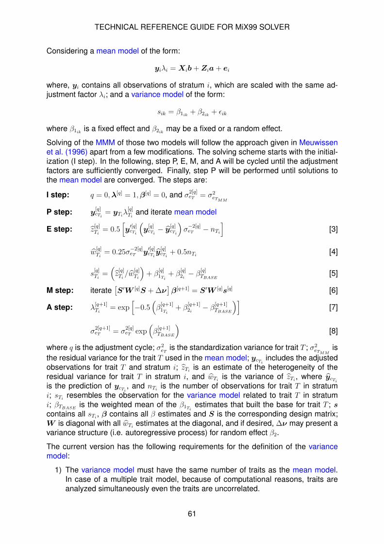
TECHNICAL REFERENCE GUIDE FOR MiX99 SOLVER
Considering a mean model of the form:
yiλi = Xib+Zia+ ei
where, yi contains all observations of stratum i, which are scaled with the same ad-justment factor λi; and a variance model of the form:
sik = β1ik + β2ik + εik
where β1ik is a fixed effect and β2ik may be a fixed or a random effect.
Solving of the MMM of those two models will follow the approach given in Meuwissenet al. (1996) apart from a few modifications. The solving scheme starts with the initial-ization (I step). In the following, step P, E, M, and A will be cycled until the adjustmentfactors are sufficiently converged. Finally, step P will be performed until solutions tothe mean model are converged. The steps are:
I step: q = 0,λ[q] = 1,β[q] = 0, and σ2[q]eT = σ2
eTMM
P step: y[q]cTi
= yTiλ[q]Ti
and iterate mean model
E step: z[q]Ti
= 0.5[y′[q]cTi
(y[q]cTi− y[q]
cTi
)σ−2[q]eT − nTi
][3]
w[q]Ti
= 0.25σ−2[q]eT y
′[q]cTiy[q]cTi
+ 0.5nTi [4]
s[q]Ti
=(z[q]Ti/w
[q]Ti
)+ β
[q]1Ti
+ β[q]2i− β[q]
TBASE[5]
M step: iterate[S′W [q]S + ∆ν
]β[q+1] = S′W [q]s[q] [6]
A step: λ[q+1]Ti
= exp[−0.5
(β[q+1]1Ti
+ β[q+1]2i− β[q+1]
TBASE
)][7]
σ2[q+1]eT = σ
2[q]eT exp
(β[q+1]TBASE
)[8]
where q is the adjustment cycle; σ2eT
is the standardization variance for trait T ; σ2eTMM
isthe residual variance for the trait T used in the mean model; ycTi includes the adjustedobservations for trait T and stratum i; zTi is an estimate of the heterogeneity of theresidual variance for trait T in stratum i, and wTi is the variance of zTi, where ycTiis the prediction of ycTi , and nTi is the number of observations for trait T in stratumi; sTi resembles the observation for the variance model related to trait T in stratumi; βTBASE
is the weighted mean of the β1Ti estimates that built the base for trait T ; scontains all sTi, β contains all β estimates and S is the corresponding design matrix;W is diagonal with all wTi estimates at the diagonal, and if desired, ∆ν may present avariance structure (i.e. autoregressive process) for random effect β2.
The current version has the following requirements for the definition of the variancemodel:
1) The variance model must have the same number of traits as the mean model.In case of a multiple trait model, because of computational reasons, traits areanalyzed simultaneously even the traits are uncorrelated.
61
TECHNICAL REFERENCE GUIDE FOR MiX99 SOLVER
2) If traits are grouped by trait groups, traits must be grouped in the same order inboth models.
3) Two effects must be specified for each trait.
⇒ Fixed across block strata: The first effect must be a fixed effect. Usuallythis effect will describe heterogeneity of variance between strata, which iscommon across the whole data; for instance, strata like years, seasons,parities, etc.
⇒ Fixed/random within block strata: The second effect may be a fixed or arandom effect. In case of a fixed effect, please see MODEL instructions,about how to specify LS-models. In case that the second effect is random,optionally, a first order autoregressive process for strata within same en-vironments (blocks) is supported. For the latter, a program (mix99hv) isprovided, which sets up the autocorrelation structure.
The previous three requirements for the variance model should be easy to accommo-date. However, there is one more restriction on how the strata for the two effects inthe variance model must be defined. These restriction are because of computationalconstrains only. For an easier understanding of this restriction it is worth to know thatmix99p performs all calculations of step E for one data block at the time. For theneed of fast computations all required information is stored in vectors, rather than inlinked lists. To avoid exhaustion of computer memory only the segment of the stratathat relates to one data block is made accessibly during processing of a particular datablock. This causes the following two restrictions:
1) The second effect (β2), regardless whether it is defined as fixed or as random,must include a block interaction. The block structure must correspond with theblock structure of the mean model. Note: The blocking variable of the meanmodel will be included as interaction in the second effect of the variance modelin the form block × within-block classes (see 10.3.1). Therefore, it is importantthat the blocking variable in the mean model is the same for all observations withthe same production environment. For instance in dairy cattle, the blocking vari-able may be herd of production, but it must not be herd of birth, if heterogeneousvariance due to different production environments should be adjusted. Calcula-tions are performed in block-wise manner, where a data block in the mean modelhas a corresponding data block in the variance model. This requires, that eachstratum of the second effect can only be present in one block.
2) Strata of the first effect (β1) can be associated with data of different blocks. How-ever, because of computational restrictions, within each data block a strata of thefirst effect (β1) can only be associated with one strata of the second effect (β2).Thus, the levels of the first effects must be nested within the levels of the secondeffect. (This is because within each block only one pointer to the second effectstrata is stored for each first effect strata. The restriction could be relaxed if apointer to the second effect strata would be stored for each observation. How-ever, this would be currently computationally too expensive). Different strata ofthe first effect can be associated with the same stratum of the second effect.For instance, if the first effect in the variance model is a region×year×seasoneffect, then the second effect may be a herd effect, a herd×year effect, or a
62

TECHNICAL REFERENCE GUIDE FOR MiX99 SOLVER
herd×year×season effect. However, if the first effect is a year effect only, thenthe second effect may not be a herd×year×season effect.
10.3 Input data for the variance modelThe program mix99hv sets up the required input data files for the variance model. Inorder to get first heterogeneity observations, a few iterations have to be made on themean model prior to the mix99hv run.
10.3.1 Input data for mix99hv
Three integer columns of the input data file for the mean model are read by mix99hvwhen setting up the data file for the variance model. These three columns are: the col-umn for the blocking variable, a column with the strata of the first effect of the variancemodel, and a column with the within block strata for the second effect of the variancemodel. The blocking variable must be consistent with the production environment inwhich the observations were made. For instance, herd of production but not herd ofbirth. This is important because mix99hv uses the blocking variable for coding thesecond effect of the variance model. For the same reason, the third column mustcontain a within-block stratification only (without block interaction).
Both columns, that one with the blocking variable and the other one with the within-block stratification, are used to set up information for the first order autoregressiveprocess (Wade and Quaas, 1993) and to set up the strata for the second effect in thevariance model. To accommodate the autocorrelation structure, coding of the within-block classes must be consistent with the distances between classes. When codingstarts from n and goes up to k, then k - n is equal to the largest possible distancebetween classes of the block. Usually, classes are defined by the time when observa-tions were recorded, e.g., year, month, week. Class codes have to be defined that thedistance between consecutive classes is one, i.e, class_code n+1 - class_code n = 1.In case, there is a missing class between consecutive classes, the distance must be 2.It is advisable to number all possible classes consecutively from 1 to k and then givefor each class the corresponding code. This way, mix99hv will automatically calculatethe right distances between classes.
If the second effect in the variance model is considered as fixed effect or as a normalrandom effect, coding of the within block strata can be relaxed. However, in order tosave memory requirements we recommend that within block, coding should be con-secutively starting with one. Remember, that the actual class code for the secondeffect will be formed by the program mix99hv from the block sorting variable and thewithin block class code.
10.3.2 Instruction file for mix99hv
Execution of mix99hv requires an instruction file, which is read by standard input.Editing rules for this file are the same as for the MiX99 instruction file. The file containsseveral instruction lines, which have to be in the same order as given in the following.The file can contain as many comment lines as wanted.
DATAFILE The name of the input data file for the mean model. If the data file is in adifferent directory, the whole path must be specified.
63

TECHNICAL REFERENCE GUIDE FOR MiX99 SOLVER
VAR_I One line with one integer and one character. The integer is the numberof integer columns in the data file. The character is a code for the type ofthe file.
f Formatted free format (columns are separated by at least one space).u Unformatted format, i.e., a binary file.
TRGRP One integer value that indicates the integer column with the trait groupcode in the data file. If trait groups are not needed the number must beset to zero (0).
SORT_B One integer, which indicates the integer data column of the block sortingvariable in the input data file for the mean model. The variables in thiscolumn will be use to set up the autocorrelation structure and to form theclass codes for the second effect in the variance model (see also 10.3.1).
MODVAR One line with two integers. The first integer indicates the integer datacolumn with the class variables of the first effect in the variance model(fixed across block strata). The second integer indicates the integer datacolumn with the within-block class variables for the second effect in thevariance model (within block strata).
ARFILE A line with one character. This character defines, whether a file(AR.pedi.reml) with information about the autocorrelation structure iscreated. This file is only useful for the estimation of variance componentsfor the variance model, using our tailored software, which is not includedin MiX99.
n No. No file created.y Yes. File created.
STAND A line with one character. This character defines, whether or not stan-dardization variances (provided in the file HVbase_ResVar, for the cal-culation of the heterogeneity observations), should be scaled to resultstandardized adjustment factors, which are on average 1.0 for observa-tions of the defined base strata. For more details, see Standardization ofthe multiplicative adjustment factors. The Standardization process has tobe done only once for a specific model. The obtained scaled standard-ization variances can then be used as parameters for future analyses.
y Yes. Standardization of multiplicative adjustment factors.n No. No standardization process.
BASEFILE If y is defined, an additional line with the name of the file,that contains the class codes for the base classes must begiven (see Standardization of the multiplicative adjustmentfactors).
APPROX A line with one character for each trait. This character defines, whether ornot rank approximation, to account for loss in degrees of freedom due tothe estimation of fixed effects in the mean model, should be consideredfor the estimation of within strata residual variances. This option was
64
TECHNICAL REFERENCE GUIDE FOR MiX99 SOLVER
included for the need to avoid an underestimation of within strata residualvariances when size of strata is small. This approximation can only beused if within block fixed effect classes in the mean model match with thestrata of the second effect in the variance model. For instance, a fixedherd×year effect in the mean model and herd×year strata for the secondeffect of the variance model. Otherwise, the loss in degrees of freedomwill be underestimated.
y Yes. Consider rank approximation.n No. Do not consider rank approximation.
SETLOSS One line with as many real values as there are traits in themodel. This line is only given if d is specified at the end ofthe previous APPROX instruction line. Then, for each trait,for which rank approximation is not applied, a preset lossin degrees of freedom may be given. The value must bebetween 0.0 and 1.0.
MERGE2 One line with as many integers as there are traits in the model. The inte-gers tell whether or not strata of the second effect in the variance modelare combined across traits. For the specification of the integers samerules apply as for one column in the MERGE instruction for mix99i. Thespecified integers must be consistent with the MERGE specification in thevariance model instruction file. If combining is not desired integers from1 up to n are given, where n is equal to number of traits.
TMPHV The directory where the HV information files HV.data, HV.pedi,Lambda.data(i), HV.info(i), and optional ARsiwi.data(i) willbe created. These files are rather large and will be created during theexecution of the script runMMM. If the HV information files should be inthe same directory where the script is executed, a dot (.) is given.
10.3.3 Output files from mix99hv
The program mix99hv creates a file named HV.data, which is the input data filefor the variance model; a file named HV.pedi, which contains information about theautocorrelation structure; the files named AR.block, and Hetlog, which are readby mix99i and mix99p; as well as the files HV.info(i), which are needed duringupdating of the adjustment factors.
HV.data
The file HV.data is created by mix99hv and is the input data file for the variancemodel. The file is in unformatted (binary) format and contains integer and real datacolumns. First there are four integer data columns, followed by the real data columns,where the number of real data columns depends on the specified model.
65

TECHNICAL REFERENCE GUIDE FOR MiX99 SOLVER
Integer data column Description1 renumbered block sorting variable2 renumbered class variables for the second effect3 trait group code4 renumbered class variables for the first effect
There are two groups of real data columns. The first group contains heterogeneityobservations and the second group the corresponding weights for the heterogeneityobservations. Each group has as many columns as there are number of traits in thelargest trait group. E.g., if the first trait group includes two traits and the second traitgroup three trait, then there will be three columns for the heterogeneity observationsand three columns for the weights. The order of the heterogeneity observations andof the weights follows the order of the traits within trait group. If there are fewer traitsin a trait group, remaining columns are set to missing. If an observation is missing orif a column is not used for a certain trait group, a code for missing values will be given.This code is set to -8192.0 and has to be given in the instruction file for the variancemodel.
HV.pedi
The file HV.pedi is created by mix99hv as well. The file is needed to provide theblocking information for the variance model and to set up the autocorrelation structurefor second effect in the variance model, if latter is desired. For the variance model, theHV.pedi file replaces the normal pedigree file. The file has four integer columns:
Integer column Description1 renumbered class variables for the second effect2 distance to the next classes3 information about class position within block (1=first class in block;
2=class between; 0=last class in block; 3=first and last class inblock)
4 renumbered block sorting variable
In case it is desired to define the second effect as a fixed effect (LS-models), informa-tion on column 2 and 3 will be not used. If the second effect should be a normal randomeffect, the autocorrelation parameters on the RHO instruction line should be set to zero(0.0) in the instruction file for the variance model. This makes information on 2 and 3redundant. Alternatively, it is possible to define instead of ar (autoregressive model)am (animal model) in the instruction file for the random model and set the values incolumn 2 and 3 to zero.
10.4 Instruction file for the variance modelSetting up the instruction file for the variance model follows the same rules as given forthe mean model. However, a large part of the instructions are already defined by the
66

TECHNICAL REFERENCE GUIDE FOR MiX99 SOLVER
general setup for the HV-adjustment. These pre-defined instructions are as following:
TITLE
INT-VAR Block BlockxCl Trg Fix
REAL-VAR Name of traits followed by weights for the traits. Names are in same orderas given in the mean model.
TRAITS Number of traits must be the same as in the mean model.
TRGRP Number of trait groups must be the same as in the mean model. Integerinput column for the trait group code is 3.
SORT_R 1 2The value 1 for the integer column with block code, followed by the value2 for the integer input column of the second effect in the variance model.
FIXRAN 1 1Two integers with the value 1, for the number of fixed and random factors.
MODEL As many model lines as there are traits in the model. Ordering of thetraits within trait groups must be the same as in the mean model. Forthe variance model, all observations are weighted (see Meuwissen etal. (1996)). This requires defining of the real columns with the weights.In HV.data, the real columns with the weights start after the columnswith the observations and have the same order as the columns for theobservations. Note, if trait groups are defined, for any trait group, thecolumn with the observations for the first trait within trait group is alwaysthe first real column. For each trait, the corresponding column with theweights is on position “size of largest trait group plus trait column”.
For the first effect in the variance model column 4 has to be defined, forthe second effect column 2 (see Example 10.9).
WITHINBLOCKORDER - 1A dash (-) is given followed by the integer value 1.
RANDOM The second effect in the model has to be defined always as random (alsofor a LS-model; see defining of LS-models).
RELATIONSHIPS 1 1Two integers with the value of 1.
REGRESS Only class variables (cl) are allowed.
COMBINE (n/y). In case y is given, then last column of the MERGE instructionlines must be consistent with the MERGE2 line in the instruction file formix99hv.
PEDIGREE ar for autoregressive model, am for random effect, ls for LS-model.
RHO In case ar is defined in PEDIGREE , one line with as manyautocorrelation values as there are traits in the model mustbe given. Order of the values must be the same as the orderof traits. In case some traits are combined, the order of the
67

TECHNICAL REFERENCE GUIDE FOR MiX99 SOLVER
autocorrelations must follow the order of the correspondingvariances that are applied for the last random effect.
DATAFILE The HV.data file is placed in the same directory as was defined for thework files in the instruction file for mix99hv: /path for the workfiles/HV.data.
VAR An integer value of 4 for the number of integer columns in HV.data fol-lowed by the number of real columns in HV.data and the character u forunformatted file. The number of real columns is two times the size of thelargest trait group.
MISSVA -8192.0The code for missing heterogeneity observations is -8192.0.
SCALE nA n for no scaling.
PEDFILE The HV.pedi file is placed in the same directory as was defined for thework files in the instruction file for mix99hv: /path for the workfiles/HV.pedi.
PARFILE The name of the file with the variance components for the variance model.
TMPDIR The directory where the temporary files for the variance model are placed.The directory must be a sub-directory of the directory with the temporaryfiles for the mean model and must be named B1: /path for the meanmodel temporary files/B1.
RANSOLFILE yA y for the second effect in the model. In case of a LS-model a y must begiven as well.
SOLUNF nA n for no unformatted solution files.
PRECON d dA d for the WpW and d for the XpX part, since all traits are uncorrelated.
PARALLEL Same number of processes as for the mean model.
COMMONBLOCKS 0An integer value of 0, because there is no common pedigree block in themodel.
From release XII/2014 onwards the variance model can be given also with CLIM syn-tax. The following illustrates CLIM syntax needed to build variance model.
Variance model CLIM:TITLE Variance Model
DATAFILE BINARY path/to/HV.dataINTEGER BLCK HERDxYR TRGRP MONTHREAL HET_OBS WGHT
MISSING -8192.0TRAITGROUP TRGRP
68

TECHNICAL REFERENCE GUIDE FOR MiX99 SOLVER
DATASORT BLOCK=BLCK PEDIGREECODE=HERDxYR
PEDFILE path/to/HV.pediPEDIGREE HERDxYR ar
PARFILE variance_model.varAR 0.7 # If pedigree type is ar then autocorrelation values
# for each trait must be given in AR statement
MODEL # As many model lines as there are traits in the model# Ordering of traits must follow mean model!
HET_OBS(1) = MONTH HERDxYR ! WEIGHT=WGHT# The first effect of the model is fourth integer column# and the second effect is second integer column
PRECON d dPARALLEL 2 0WITHINBLOCKORDER HERDxYR
10.5 Variance components for the variance modelIn case the second effect of the variance model is defined as a random effect, vari-ance components are required. Estimation of the variance components depends onthe specified model, and therefore, only a brief explanation about how variance compo-nents for the variance model may be estimated is provided. Generally, the estimationprocedure requires first solving of the multiplicative mixed model followed by the esti-mation of variance components for the variance model. The new variance componentsare updated in the multiplicative mixed model and the whole process is repeated untilvariance components do not change any more. MiX99 authors will provide support forestimating VC for multiplicative mixed models.
At the moment the MiX99 variance component estimation module does not supportmodels with an auto-regressive correlation structure.
10.5.1 Files with information for the variance component estimation
For the estimation of the variance components, a file with the heterogeneity observa-tions for the variance model is needed. MiX99 provides the files named ARsiwi.data(i),which contain the most recent heterogeneity observations plus the correspondingweights. The file is an unformatted file with real columns only. The order of thecolumns is the same as the order of the real columns in the HV.data file. The integercolumns of the HV.data file and the real columns of the ARsiwi.data(i) files maybe merged to create an input data file for the variance component estimation. In orderto obtain the ARsiwi.data(i) files, an h must be specified in the RESID option lineof the MiX99 solver option file for the mean model (Mean_model.slvM in the HVdirectory).
In case, an autocorrelation structure is applied for the second effect in the variancemodel, MiX99 may provide two different files with the required information to set upthe autocorrelation structure. The first is named HV.pedi, which contains the requiredinformation as needed for MiX99. The second is named AR.pedi.reml, and is cre-ated if a y is specified in the ARFILE instruction line of the instruction file for mix99hv(see 10.3.2). The AR.pedi.reml file contains the following five integer columns:
69

TECHNICAL REFERENCE GUIDE FOR MiX99 SOLVER
Integer column Description1 renumbered class variables for the random effect (within block
strata)2 renumbered class variable for the next class of the random effect;
this variable is zero (0) in case the class in the first column is thefirst or the last class of a block.
3 renumbered class variable for the next class of the random effect,in case the class in the first column is the first class of a block; andotherwise zero (0).
4 a column with zeros5 a column with zeros
10.6 Standardization of the multiplicative adjustment factorsIn the method presented by Meuwissen et al. (1996), variance components for themean model are re-estimated, because accounting for HV has some effect on the her-itability. However, re-estimation of variance components is hardly feasible for largemodels. Further, even it would be possible to extend the approach of Meuwissen et al.(1996) to multiple trait models, it would be computationally demanding. Therefore, inthe current implementation, heterogeneity observations of different traits are consid-ered to be uncorrelated in the variance model. For all these reasons, a standardizationprocedure was implemented, which should assure that the covariance structure acrosstraits remains unchanged.
The idea of the standardization procedure is to find for each trait a standardizationvariance var(s), for which the quantity “ [(y′ieiλ
2i )/var(s)] − ni“ becomes zero and the
adjustment factors for observations in the base classes are on average 1.0; yi andei are of size ni and contain observations and residuals of stratum i, respectively; λiis the adjustment factor for stratum i. In a perfect world, the standardization variancevar(s) would become same as the residual variance of the mean model. The standard-ization variances have to be provided in a file named HVbase_ResVar. The file withconverged standardization variances must be provided for any future (routine) runs.
10.6.1 Files for the standardization procedure
File with class codes of the base
The standardization base should include a part of the data for which it is reasonableto assume that standardization factors should be on average 1.0 for all traits. Thispart of the data must include observation from all traits (if this is not possible seeStandardization process). Corresponding strata of the first fixed effect in the variancemodel need to be provided in the base class file. The file will be renumbered bymix99hv and original and renumbered class codes are written to ID.Base. Theprovided file may contain additional columns. The file ID.Base is repeatedly read bymix99p during the standardization process.
File with the residual variances
70

TECHNICAL REFERENCE GUIDE FOR MiX99 SOLVER
A file named HVbase_ResVar with as many rows as there are traits in the model.Each row corresponds to the trait in the model and contains the standardization vari-ance. During the standardization process, the file will be updated after each adjust-ment cycle. The residual variances of the mean model can be given as starting valuesfor the standardization process. The HVbase_ResVar file must be provided in thedirectory where mix99p is executed any time when adjustment for HV is considered.
10.6.2 Standardization process
The standardization process is specified in the instruction file for mix99hv. A y mustbe specified in the STAND instruction line, and on the BASEFILE line the filename ofthe file with the base class codes must be provided. To ensure converged standardiza-tion variances, we recommended a minimum of 150 adjustment cycles. Cycle to cyclechanges in the standardization variances can be checked from the standard outputfile. The line marked with “Re:” contains the currently used standardization variances.
The provided standardization method might not work for very complicated models.For instance, if not all traits have observations in the same time period or in somecases where genetic effects are combined over traits. For such situations it is pos-sible to keep the variance ratios between standardization variances of different traitsunchanged. Providing the file HVbase_ResVarLEVEL will allow this task. The filehas the same form as HVbase_ResVar but additionally a second column with inte-ger values is included. The first column contains standardization variances and theintegers in the second column specify which standardization variances should be al-tered and which should have a fixed ratio to another standardization variance. If thestandardization variance is allowed to be altered, the own trait number is given. If thestandardization variance should have a fixed ratio with the standardization varianceof another trait, then the trait number of the other trait is given. For instance, if thestandardization variance for trait two should be altered and the ratio between stan-dardization variance for trait four and trait two should be fixed, than a 2 is specified fortrait two and also for trait four.
10.6.3 Multiple residual variance-covariance matrices
Multiple residual variance-covariance matrices (see Multiple residual (co)variances(RESFILE) in Technical reference guide for MiX99 pre-processor ) for the mean modelare automatically considered for the calculation of observations for the variance model.However, for the standardization process one needs to be aware that provided stan-dardization variances in the HVbase_ResVar file correspond to the residual variance-covariance matrix of the first residual variance class in the mean model. The baseclasses need to contain observations that go into the first residual variance class. Dur-ing the standardization process, standardization variances for all other residual vari-ance classes are automatically changed if the standardization variances for the firstresidual variance class are changed. The ratios between standardization variances ofdifferent residual variance classes are kept constant.
If it is desired that ratios between standardization variances of different residual vari-ances classes are different from those between residual variances of different residualvariance classes in the mean model, a file named HVbase_ResVarCLASS can beprovided. The file has as many rows as there are multiple residual variance classes
71

TECHNICAL REFERENCE GUIDE FOR MiX99 SOLVER
and a many columns as there are traits in the model. Each row should contain thecorresponding residual variances. For classes where higher or lower standardizationvariances are desired, the variances should be changed accordingly.
10.7 Running a model with heterogeneous varianceThe applied multiplicative mixed model approach, to account for heterogeneous vari-ance, requires a simultaneous solving of two linear models, namely the mean modeland the variance model. Both models are solved by two different MiX99 runs, whichinteract with each other. To facilitate these interactions between the models a certaindirectory structure is required when setting up the models.
The heterogeneous_variance directory of the MiX99 package includes all re-quired to set up to run a model with heterogeneous variances. For distributed memoryplatforms, implementations are more complicated and we recommend a good under-standing of the implementation for shared memory platforms before an implementationis done for a distributed memory platform.
10.7.1 Implementation on shared memory platforms
The mean model must be set up in an own directory. The variance model must beset up in a sub-directory of the mean model directory and must be named B1. Thedirectory with the temporary files for the mean model must be specified in the instruc-tion file for the mean model. The temporary files for the variance model must be ina sub-directory of the mean model temporary file directory and it must be named B1.Additionally a third directory with heterogeneous variance information must be spec-ified in the instruction file for mix99hv. The input data files for the variance modelwill be placed into this directory. For large model, these three directories may requireconsiderable amount of disk space.
The whole solving process is controlled by the script runMMM provided with MiX99package. The script controls all required MiX99 runs for solving the multiplicativemixed model. The only required modifications in the script are to set the parameter forthe number of processes (PARALLEL) and the calls to mpirun. The program mix99pcalls the script solve_HVmodel during iteration process to start solving of the vari-ance model. Output from this script is written to CYC.log
Three different solver option files are needed for multiplicative mixed model. The filesin example provided are named as Mean_model_init.slvI, which is used to ini-tialize mean model, solver option file Variance_model.slvV (in directory B1) forthe variance model, and Mean_model.slvM for running the mean model. The con-vergence criterion for the adjustment procedure is given in the STOPC instruction lineof the stopping criterion file Mean_model.slvM. From our experiences, a stoppingcriterion of 1.0e-7 for the relative change between adjustment factors of consecutivecycles or at least 80 adjustment cycles was found useful. However, a less conservativecriterion may yield already sufficiently converged adjustment factors.
72

TECHNICAL REFERENCE GUIDE FOR MiX99 SOLVER
10.8 Workflow and needed files for running multiplicative mixedmodel
The following table shows all necessary files and directories needed to set up andrun multiplicative mixed effects model. The filenames are the same as in HV exampleshipped with MiX99. Files that have to be named with a certain name are marked witha star (*).
Directory and file setup for multiplicative mixed model
Directories within mean model directory*B1 Directory for variance modeltmpMiX Directory for temporary files (Mean model)
*tmpMiX/B1 Directory for temporary files (Variance model).Should be a subfolder of mean model temporary files
tmpHV Directory for HV information files (see TMPHV)
FilesrunMMM Script that does all steps
*B1/solve_variance_model Script that runs variance model. Created by runMMMscript.
*solve_HVmodel Script called from mix99p to run variance model.An example script is shipped with MiX99. Scriptruns B1/solve_variance_model
Files for Mean modelmean_model.[clm|mix] Definition for the mean modelmean_model.dat Datamean_model.ped Pedigreemean_model.var Variance components for mean modelmean_model.resvar Optional: Variance components for residuals if more
than one residual classmean_model_init.slvI Solver option file to initialize the mean modelmean_model.slvM Solver option file for the mean model
Files for variance modelhvdata.dir Instruction file for mix99hv (see section 10.3.2)B1/variance_model.[clm|mix] Model definition for the variance model (see section
10.4)B1/variance_model.slvV Solver option file to variance modelB1/variance_model.var Variance components for the variance model
*B1/HVbase_ResVar Standardization variances for traits*B1/HVbase_ResVarCLASS Optional: Ratios of standardization variances
between different residual classes
Additional files for standardization of adjustment factorsHVbaseclasses Standardization base (see section 10.6.1)
*HVbase_ResVarLEVEL Optional: Control standardization varianceestimation for traits
*Name can not be changed
73

TECHNICAL REFERENCE GUIDE FOR MiX99 SOLVER
Solving multiplicative mixed effect model requires several steps. To help users weprovide an example script runMMM located in examples/heterogeneous_variance di-rectory that can be used as a starting point when solving larger models with HV cor-rection. Workflow of running MMM is presented in the following table. Input files arethe same as in previous table.
Workflow for running MMM
In mean model directory1 mix99i mean_model.clim Initialize mean model2 imake99 Additional pre-processing program mean model3 mix99p < mean_model_init.slvI Run couple of iterations of mean model to get
initial values for variance model4 mix99hv < hvdata.dir Create data for variance model
In B1 directory5 mix99i variance_model.clim Initialize variance model6 imake99 Additional pre-processing program for variance
model7 mix99p < variance_model.slvV Solve variance model
In mean model directory8 mix99p < mean_model.slvV Solve MMM. Mean model solver calls script
solve_HVmodel. That runs step 7 in eachcycle and updates lambda values.
In addition to files created by standard MiX99 solver the HV solving process createsfiles to exchange information between mean and variance model and provide informa-tion to user. The following table lists the most important files. Filenames containingstandard output from MiX99 software follows the script runMMM shipped with MiX99package.
Files created by MiX99hvtmpHV/HV.data Data for variance modeltmpHV/HV.pedi Pedigree file for variance model
Optional files created by mean model solverARsiwi.data(i) Heterogeneity observations and weights for variance model.
Used when estimating VC for variance model. See section(10.5.1)
AR.pedi.reml Information about AR correlation structure
Log files created by runMMMMi.log Mean model initialization (mix99i)imake99.log Mean model imake99
74

TECHNICAL REFERENCE GUIDE FOR MiX99 SOLVER
Ma.log Log for first iterations on mean model (mix99p)HVd.log Log from variance model data creation (mix99hv)B1/Vi.log Variance model initialization (mix99i)B1/imake99.log Variance model imake99B1/Vs.log Variance model solving. All cycles. (mix99p)Ms.log Log for solving multiple mixed model
Log files created by MiX99CYC.log Output from solve_HVmodel. (see section 10.10.3)Lambda.log Lambda values. (see section 10.10.4
10.9 ExampleAccounting for heterogeneous variance in a small test-day model. This example is alsoshipped with MiX99 package and can be run with script runMMM. The script carefullyverifies that all the steps are performed without errors.
Mean model is a random regression model. Variance model includes fixed monthstrata and autocorrelation structure is applied between consecutive years within herd.
Instruction file for mean model (mean_model.clm):TITLE Heterogeneous variance adjustment by Meuwissen approach: a demonstration
DATAFILE mean_model.datINTEGER Month Animal Herd HerdYear YearREAL Covar_1 Covar_2 MilkDATASORT BLOCK=Herd PEDIGREECODE=Animal
PEDFILE mean_model.pedPEDIGREE G am
PARFILE mean_model.var
TMPDIR tmpMiXMISSING 0.0
MODELMilk = Covar_1 Covar_2 Month HerdYear G( 1 Covar_1 Covar_2 | Animal )
WITHINBLOCKORDER G HerdYear
PRECON d d bPARALLEL 2 1
Instruction file for mix99hv hvdata.dir :# Instruction file for mix99hv# This is needed to allow mix99hv to create a data and pedigree file# for the variance model#----------------------------------------------------------------------## Name of the data file
mean_model.dat# Number of integer columns; type of file (f/u)
5 f# Column with the trait group code
0
75

TECHNICAL REFERENCE GUIDE FOR MiX99 SOLVER
# Column with the block variable for the auto regress. proc.# (HERD)
3# Heterogeneity Model:# Fixed across block strata; random within block strata# (Month) (Year within Herd)
1 5# Create pedigree file for REML-analysis? (y/n)
n# Standardisation of multiplicative adjustment factors? (y/n)
n# Name of file with the class codes of the base# ID.Base.Classes
# Approximation of rank across traits (y/n)y
# Random HY effect: Combining of second and third lactation in the variance model1
# Directory for the temporary files./tmpHV
Instruction file for the variance model (variance_model.clm):TITLE Variance Model
DATAFILE BINARY ../tmpHV/HV.dataINTEGER BLCK HERDxYR TRGRP MONTHREAL HET_OBS WGHTMISSING -8192.0TRAITGROUP TRGRP
DATASORT BLOCK=BLCK PEDIGREECODE=HERDxYR
PEDFILE ../tmpHV/HV.pediPEDIGREE HERDxYR ar
PARFILE variance_model.varAR 0.7
MODELHET_OBS(1) = MONTH HERDxYR ! WEIGHT=WGHT
PRECON d dPARALLEL 2 0WITHINBLOCKORDER HERDxYRTMPDIR ../tmpMiX/B1
File with standardization variances HVbase_ResVar:1.089320
MiX99 solver option file mean_model_init.slvI:# RAM RAM demand: H=high, M=medium, L=low
H# STOP Maximum_number_of_iterations, Stopping_criterion (CR)
20 1.0e-7# RESID Calculate residuals? (Y/N/H)
N# VALID Information for model validation
N# VAROPT Adjust for heterogeneous variance (N, E, S, C, G)
S# SOLTYP Type of solution files? (N,Y,A,H)
N
76

TECHNICAL REFERENCE GUIDE FOR MiX99 SOLVER
MiX99 solver option file variance_model.slvV:# RAM RAM demand: H=high, M=medium, L=low
H# STOP Maximum_number_of_iterations, Stopping_criterion (CR)
25 1.0e-7# RESID Calculate residuals? (Y/N/H)
N# VALID Information for model validation
N# VAROPT Adjust for heterogeneous variance (N, S, C)
N# SOLTYP Type of solution files? (N,Y,A,H)
H
MiX99 solver option file mean_model.slvM:# RAM RAM demand: H=high, M=medium, L=low
H# STOP Maximum_number_of_iterations, Stopping_criterion (CR)
1000 1.0e-7# RESID Calculate residuals? (Y/N/H)
N# VALID Information for model validation
N# VAROPT Adjust for heterogeneous variance (N, S, C)
C# STOPC Maximum_number_of_cycles, Stopping_criterion for lambdas (CD)80 1.0e-7
# SOLTYP Type of solution files? (N,Y,A,H)Y
File with variance components for the variance model variance_model.var:1 1 1 0.0784852 1 1 0.590860
10.10 Output filesThere are several sources to follow the progress of the heterogeneous variance ad-justment process: information written to standard output, HVd.log, CYC.log andLambda.log.
10.10.1 Mi.log and Ms.log
Standard output from mix99i and mix99p are written to the files I.log and S.logfor the mean model, respectively, and for the variance model it is written to Vi.log,Vs.log, respectively. Each cycle, mix99p output from the variance model will beappended to Vs.log.
Standard output from the main script runMMM contains general information about theprogress of the HV adjustment and is explained in more detail. The output informsabout the current stage of calculation: INITIALIZATION, START ADJUSTMENT CY-CLES, CYCLE END, FINAL ITERATION ON MEAN MODEL.
During each cycle the following information is provided (for a simple single trait model):.Solve Variance-Model
Last HV cycle: 2
77

TECHNICAL REFERENCE GUIDE FOR MiX99 SOLVER
Lambda criterion CD = 4.59369973910834D-0068.85770073643941D-004
# convergence of the adjustment factors
# for lambda values of first and second
# effect in the variance model
rhs’ M^-1 * rhs = 318.854161366479------------------------------------------------------
8 0.6804E-02 0.000 0.000 0.0009 0.3163E-02 0.000 0.000 0.00010 0.3698E-02 0.000 0.000 0.00011 0.3698E-02 0.000 0.000 0.000
# iteration on mean model
Re: 56.1916 # Standardization variance
Residual class: 1NStrata 22.0000 # number of strata for each trait
zHatMean 0.3248 # average absolute value of z(z is minimized)
wHatMean 2.4492 # average weight associate with z’s
.
10.10.2 HVd.log
This output provides information about the data and model structure for the variancemodel.
For instance:Number of Blocks in the Data: 57949Largest Class in Blocks found: 21Largest Class in Fixed Strata: 675Shift variable: 100Largest Random Stratum Code: 5794921
For routine evaluations it might give a large amount of warnings of the following form:Block without si and wi values: renum.block code= 3771Current number of blocks: 3713
This means that the block (herd) has not enough information to calculate residualvariances for the strata in the block. For instance if the strata are herd test-days andthere is only one cow in a herd.
For such a block a second warning will be written:Warning!!! Block without HV-obs. in AR classes.Block= 3713 ignored.
For such a case the adjustment factors will be set to 1.0. If the number of such blockis rather large one might consider a different variance model.
10.10.3 CYC.log
Every cycle mix99p calls the script solve_HVmodel. Output form this script as wellas a sample of adjustment factors it written to CYC.log.
During each cycle the following information is provided (for a simple single trait model):.Tue Apr 20 11:11:23 EEST 2004Variance_model-iterations: 12 Convergence crit (Cr): 0.3716E-07Lambda convergence (Cd):5.25599751543677D-006 0.00000000000000D+000Beta convergence (Cr): 2.21850223850421D-002Acceleration = 16.0800328372335 2 Used = 1.25000000000000
78

TECHNICAL REFERENCE GUIDE FOR MiX99 SOLVER
Lambda values for first 30 fixed strata:----------------------------------------Code, Trait 1, 2, 3, ...
1 0.91302 0.94163 0.96744 1.05245 1.1232
Lambda values for random strata:-------------------------------Block, AR_class, Traits: 1, 2, 3, ...
1 1 1.01521 2 1.01402 1 1.01732 2 1.01423 1 0.97693 2 0.98494 1 0.99114 2 0.9874
.
The sample of adjustment factors allows visual inspection (by plotting the adjustmentfactor of one class) of convergence.
10.10.4 Lambda.log
This file is created every cycle by the master process of mix99p. On distributed mem-ory platforms the file will be written to the directory of the master node. Lambda.logcontains the lambda values of all strata of the first effect and a sample of lambda val-ues of strata of the second effect in the variance model. It also provides informationabout the standardization of variances. From the Lambda.log file one can checkwhether the lambda values are within a reasonable range. Normally between 0.6 and1.9. Some values might be smaller or larger. In case a large amount of values is0.37 (exp(-1)) or 2.72 (exp(1)) something might go wrong. The latter values are themaximum allowed deviations of adjustment factors from 1.0.
79

TECHNICAL REFERENCE GUIDE FOR MiX99 SOLVER
11 AcknowledgementThe Biometrical Genetics Team at Natural Resources Institute Finland is kindly ac-knowledged for the valuable suggestions, comments and for being the beta tester ofnew MiX99 versions.
12 ReferencesGilmour, A. R. and Thompson, Robin (1998). ”Reformulated generalised linear (mixed)
model aids multiple trait genetic evaluation with polychotomous calving ease”. In:Proc. 6th World Congr. Genet. Appl. Livest. Prod. Vol. 20, pp. 613–616 (cit. onp. 45).
Harris, B. and Johnson, D. (1998). ”Approximate Reliability of Genetic EvaluationsUnder an Animal Model”. In: J. Dairy Sci. 81.10, pp. 2723–2728. DOI: 10.3168/jds.S0022-0302(98)75829-1 (cit. on p. 39).
Hesterberg, T. (2005). ”Staggered Aitken Acceleraton for EM”. In: Proc. of the Ameri-can Stat. Assoc. Minneapolis, Minnesota, USA, 2101––2110. URL: http://home.comcast.net/~timhesterberg/articles/JSM05-accelerateEM.pdf (cit. on p. 14).
Hoeschele, I., Tier, B., and Graser, H. U. (1995). ”Multiple-trait genetic evaluationfor one polychotomous trait and several continuous traits with missing data andunequal models”. In: J. Anim. Sci. 73.6, pp. 1609–1627. URL: http : / / www .
journalofanimalscience.org/content/73/6/1609 (cit. on p. 45).Jamrozik, J., Schaeffer, L. R., and Jansen, G. B. (2000). ”Approximate accuracies of
prediction from random regression models”. In: Livest. Prod. Sci. 66.1, pp. 85–92.DOI: 10.1016/S0301-6226(00)00158-5 (cit. on p. 27).
Janss, L. L. G. and Foulley, J. L. (1993). ”Bivariate analysis for one continuous andone threshold dichotomous trait with unequal design matrices and an application tobirth weight and calving difficulty”. In: Livest. Prod. Sci. 33.3–4, pp. 183–198. DOI:10.1016/0301-6226(93)90001-X (cit. on p. 45).
Lidauer, M. and Strandén, I. (1998). ”Experience on using parallel computing to solvelarge test-day models”. In: Proc. 49th Ann. Meeting EAAP. 4. Warsaw, Poland, p. 46(cit. on p. 1).
Lidauer, M. and Strandén, I. (1999). ”Fast and flexible program for genetic evaluation indairy cattle”. In: INTERBULL Bulletin. 20. Tuusula, Finland, pp. 20–25. URL: https://journal.interbull.org/index.php/ib/article/view/468/466 (cit. on pp. 1,18).
Lidauer, M., Strandén, I., Mäntysaari, E. A., Pösö, J., and Kettunen, A. (1999). ”Solvinglarge test-day models by iteration on data and preconditioned conjugate gradient”.In: J. Dairy Sci. 82.12, pp. 2788–2796. DOI: 10.3168/jds.S0022-0302(99)75536-0(cit. on pp. 1, 2).
Lidauer, M., Emmerling, R., and Mäntysaari, E. A. (2008). ”Multiplicative random re-gression model for heterogeneou variance adjustment in genetic evaluation for milkyield in Simmental”. In: J. Anim. Breed. Genet. 125.3, pp. 147–159. DOI: 10.1111/j.1439-0388.2008.00728.x (cit. on p. 60).
Lidauer, M., Matilainen, K., Mäntysaari, E. A., Pitkänen, T., Taskinen, M., and Strandén,I. (2019). Technical reference guide for MiX99 pre-processor. Release XI/2019.Natural Resources Institute Finland (Luke) (cit. on pp. 1, 3–5, 10, 12, 18, 24–26,42, 46, 48, 50, 52, 71).
80

TECHNICAL REFERENCE GUIDE FOR MiX99 SOLVER
Matilainen, K., Mäntysaari, E. A., Lidauer, M., Strandén, I., and Thompson, R (2012).”Employing a Monte Carlo algorithm in expectation maximization restricted maxi-mum likelihood estimation of the linear mixed model”. In: J. Anim. Breed. Genet.129.6, pp. 457–468. DOI: 10.1111/j.1439-0388.2012.01000.x (cit. on p. 49).
Matilainen, K., Mäntysaari, E. A., Lidauer, M., Strandén, I., and Thompson, R. (2013).”Employing a Monte Carlo algorithm in Newton-type methods for restricted max-imum likelihood estimation of genetic parameters”. In: PLoS ONE 8.12. e80821.DOI: 10.1371/journal.pone.0080821 (cit. on p. 53).
Meuwissen, T. H. E., De Jong, G., and Engel, B. (1996). ”Joint estimation of breedingvalues and heterogeneous variances of large data files”. In: J. Dairy Sci. 79.2,pp. 310–316. DOI: 10.3168/jds.S0022-0302(96)76365-8 (cit. on pp. 12, 60, 61,67, 70).
MiX99 Development Team (2019). MiX99: A software package for solving large mixedmodel equations. Release XI/2019. Natural Resources Institute Finland (Luke).Jokioinen, Finland. URL: http://www.luke.fi/mix99 (cit. on p. ii).
Misztal, I. and Wiggans, G. R. (1988). ”Approximation of prediction error variance inlarge-scale animal models”. In: J. Dairy Sci. 71, Supplement 2.0, pp. 27–32. DOI:10.1016/S0022-0302(88)79976-2 (cit. on p. 27).
Mrode, R. A. and Swanson, G. J. T. (2004). ”Calculating cow and daughter yield devia-tions and partitioning of genetic evaluations under a random regression model”. In:Livest. Prod. Sci. 86.1–3, pp. 253–260. DOI: 10.1016/j.livprodsci.2003.09.001(cit. on pp. 9, 41).
Shewchuk, J. R. (1994). An introduction to the conjugate gradient method without theagonizing pain. URL: http://www.eletrica.ufpr.br/artuzi/te804/arquivos/cg.pdf (cit. on p. 2).
Strandén, I. (1999). ”Parallel benefits in test-day evaluations”. In: INTERBULL Bulletin.20. Tuusula, Finland, pp. 26–32. URL: https://journal.interbull.org/index.php/ib/article/view/469/467 (cit. on p. 1).
Strandén, I. (2019). Command Language Interface for MiX99. Release XI/2019. Natu-ral Resources Institute Finland (Luke) (cit. on pp. 1, 5, 10).
Strandén, I. and Lidauer, M. (1999). ”Solving large mixed linear models using precon-ditioned conjugate gradient iteration”. In: J. Dairy Sci. 82.12, pp. 2779–2787. DOI:10.3168/jds.S0022-0302(99)75535-9 (cit. on pp. 1, 3).
Strandén, I., Lidauer, M., Mäntysaari, E. A., and Pösö, J. (2000). ”Calculation of Inter-bull weighting factors for the Finnish test day model”. In: INTERBULL Bulletin. 26.Verden, Germany, pp. 78–79. URL: https://journal.interbull.org/index.php/ib/article/view/366/366 (cit. on p. 27).
Tier, B. and Meyer, K. (2004). ”Approximating prediction error covariances among addi-tive genetic effects within animals in multiple-trait and random regression models”.In: J. Anim. Breed. Genet. 121.2, pp. 77–89. DOI: 10.1111/j.1439-0388.2003.00444.x (cit. on p. 27).
Tyrisevä, A.-M. et al. (2011). ”Principal component approach in variance componentestimation for international sire evaluation”. In: Genet. Sel. Evol. 43.21. DOI: 10.1186/1297-9686-43-21 (cit. on p. 52).
VanRaden, P. M. and Wiggans, G. R. (1991). ”Derivation, Calculation, and Use ofNational Animal Model Information”. In: J. Dairy Sci. 74.8, pp. 2737–2746. DOI:10.3168/jds.S0022-0302(91)78453-1 (cit. on p. 41).
81

TECHNICAL REFERENCE GUIDE FOR MiX99 SOLVER
Wade, K. M. and Quaas, R. L. (1993). ”Solutions to a system of equations involvinga first-order autoregressive process”. In: J. Dairy Sci. 76.10, pp. 3026–3032. DOI:10.3168/jds.S0022-0302(93)77642-0 (cit. on p. 63).
Vuori, K., Strandén, I., Lidauer, M., and Mäntysaari, E. A. (Aug. 2006a). ”MiX99 –Effective solver for large and complex linear mixed models”. In: Proc. 8th WorldCongr. Genet. Appl. Livest. Prod. Belo Horizonte, MiG, Brazil, pp. 27–33 (cit. onp. 46).
Vuori, K., Strandén, I., Sevón-Aimonen, M.-L., and Mäntysaari, E. A. (June 2006b).”Estimation of non-linear growth models by linearization: a simulation study usinga Gompertz function”. In: Genet. Sel. Evol. 38, pp. 343–358. DOI: 10.1186/1297-9686-38-4-343 (cit. on p. 46).
82
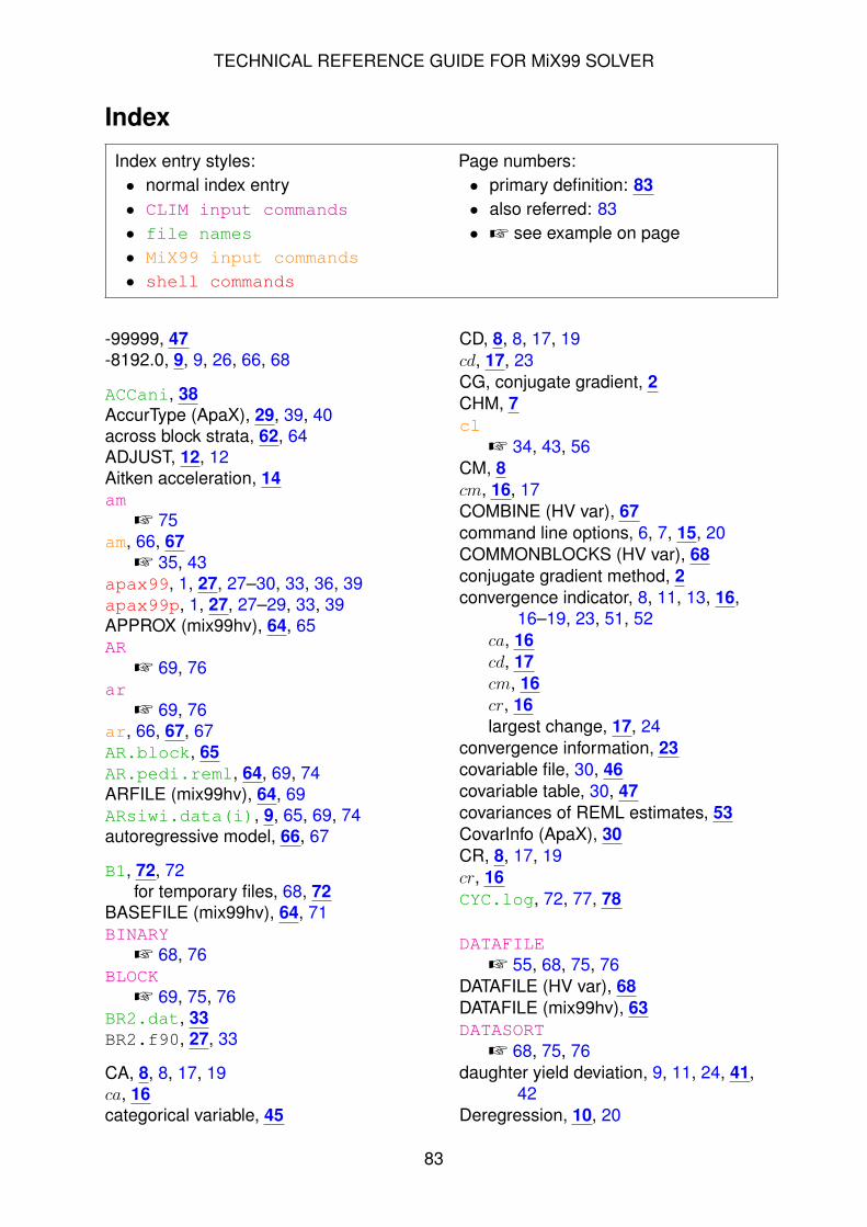
TECHNICAL REFERENCE GUIDE FOR MiX99 SOLVER
Index
Index entry styles: Page numbers:• normal index entry • primary definition: 83• CLIM input commands • also referred: 83• file names • Z see example on page• MiX99 input commands
• shell commands
-99999, 47-8192.0, 9, 9, 26, 66, 68
ACCani, 38AccurType (ApaX), 29, 39, 40across block strata, 62, 64ADJUST, 12, 12Aitken acceleration, 14am
Z 75am, 66, 67
Z 35, 43apax99, 1, 27, 27–30, 33, 36, 39apax99p, 1, 27, 27–29, 33, 39APPROX (mix99hv), 64, 65AR
Z 69, 76ar
Z 69, 76ar, 66, 67, 67AR.block, 65AR.pedi.reml, 64, 69, 74ARFILE (mix99hv), 64, 69ARsiwi.data(i), 9, 65, 69, 74autoregressive model, 66, 67
B1, 72, 72for temporary files, 68, 72
BASEFILE (mix99hv), 64, 71BINARY
Z 68, 76BLOCK
Z 69, 75, 76BR2.dat, 33BR2.f90, 27, 33
CA, 8, 8, 17, 19ca, 16categorical variable, 45
CD, 8, 8, 17, 19cd, 17, 23CG, conjugate gradient, 2CHM, 7cl
Z 34, 43, 56CM, 8cm, 16, 17COMBINE (HV var), 67command line options, 6, 7, 15, 20COMMONBLOCKS (HV var), 68conjugate gradient method, 2convergence indicator, 8, 11, 13, 16,
16–19, 23, 51, 52ca, 16cd, 17cm, 16cr, 16largest change, 17, 24
convergence information, 23covariable file, 30, 46covariable table, 30, 47covariances of REML estimates, 53CovarInfo (ApaX), 30CR, 8, 17, 19cr, 16CYC.log, 72, 77, 78
DATAFILEZ 55, 68, 75, 76
DATAFILE (HV var), 68DATAFILE (mix99hv), 63DATASORT
Z 68, 75, 76daughter yield deviation, 9, 11, 24, 41,
42Deregression, 10, 20
83

TECHNICAL REFERENCE GUIDE FOR MiX99 SOLVER
Development features (DEV), ii, 5, 20,27, 49
DYD, daughter yield deviation, 9, 11,41, 41, 42
EDC, effective daughter contribution,33, 33
effective daughter contribution, 33effective record contributions, 39eHat.data(i), 8, 25EM REML, 49EM, Expectation Maximization
for estimation of variancecomponents, 49
for Threshold-model, 45ERC, 39estimation of variance components, 8,
11, 20, 49changing parameters during
estimation, 20, 49continuing estimation, 11, 49, 53restarting estimation, 50, 53stopping evaluation, 49
exa99, 1, 36, 36–38
F, 36FACTOR, 10, 10, 42first order autoregressive process, 62,
63, 64, 66fixed variance components, 11, 52FIXRAN (HV var), 67
generating observations, 9genomic BLUP, 27Gompertz-model, 13, 45, 46, 49
H2calc (ApaX), 31Half-Chebychev, 14heterogeneous variance, 1, 9, 19, 21,
28, 60, 60, 62, 72, 75heterogeneous variance adjustment, 6,
11, 12–14, 17, 77heterogeneous_variance, 72Hetlog, 65HV, heterogeneous variance, 60HV.data, 65, 65, 67–69, 74HV.info(i), 65, 65HV.pedi, 65, 66, 66, 68, 69, 74HVbase_ResVar, 64, 70, 71, 71, 73,
76
HVbase_ResVarCLASS, 71, 73HVbase_ResVarLEVEL, 71, 73HVd.log, 78
I.log, 77ID.Base, 70, 70IDD, 9, 11, 41IDD.data(i), 9, 25IM, 7imake4apax, 28imake99, 4, 4, 5, 74, 75Index.bin, 4individual daughter deviation, 9, 11, 25,
41information matrix, 53instruction file
ApaX, 29, 33, 39CLIM command file, 5, 45, 49, 50,
55Exa, 36HV var, 66, 66mix99hv, 63, 67–69, 71, 72preprocessor directive file, 4, 5, 6,
34, 45, 46, 49, 50, 63solver option file, 5, 6, 6, 15, 20, 21,
49, 52, 53, 55, 69INT-VAR (HV var), 67INTEGER
Z 55, 68, 75, 76IOD, iteration on data, 2IOP, 7ITER, 5, 20, 20, 21, 49ITER.LOCK, 21, 21ITER.OLD, 21iteration on data, 1, 1, 2, 4iterative method, 2, 20
changing parameters duringiteration, 5, 20
convergence indicator, 8, 16determining convergence, 16intermediate results, 5, 19interrupting, 5, 19maximum number of iterations, 7,
20nested iterations, 45restarting, 24stopping criterion, 8, 20
JFilter (ApaX), 31, 32, 40
84
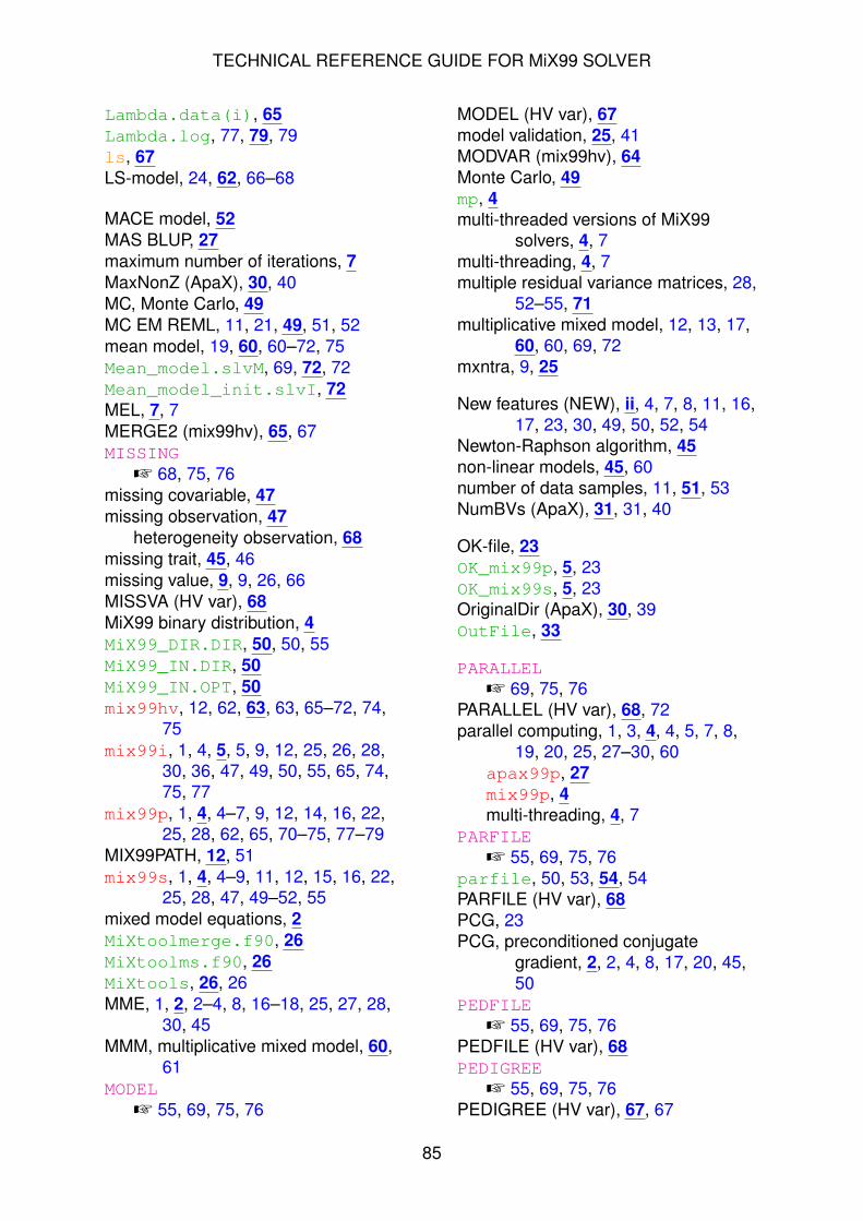
TECHNICAL REFERENCE GUIDE FOR MiX99 SOLVER
Lambda.data(i), 65Lambda.log, 77, 79, 79ls, 67LS-model, 24, 62, 66–68
MACE model, 52MAS BLUP, 27maximum number of iterations, 7MaxNonZ (ApaX), 30, 40MC, Monte Carlo, 49MC EM REML, 11, 21, 49, 51, 52mean model, 19, 60, 60–72, 75Mean_model.slvM, 69, 72, 72Mean_model_init.slvI, 72MEL, 7, 7MERGE2 (mix99hv), 65, 67MISSING
Z 68, 75, 76missing covariable, 47missing observation, 47
heterogeneity observation, 68missing trait, 45, 46missing value, 9, 9, 26, 66MISSVA (HV var), 68MiX99 binary distribution, 4MiX99_DIR.DIR, 50, 50, 55MiX99_IN.DIR, 50MiX99_IN.OPT, 50mix99hv, 12, 62, 63, 63, 65–72, 74,
75mix99i, 1, 4, 5, 5, 9, 12, 25, 26, 28,
30, 36, 47, 49, 50, 55, 65, 74,75, 77
mix99p, 1, 4, 4–7, 9, 12, 14, 16, 22,25, 28, 62, 65, 70–75, 77–79
MIX99PATH, 12, 51mix99s, 1, 4, 4–9, 11, 12, 15, 16, 22,
25, 28, 47, 49–52, 55mixed model equations, 2MiXtoolmerge.f90, 26MiXtoolms.f90, 26MiXtools, 26, 26MME, 1, 2, 2–4, 8, 16–18, 25, 27, 28,
30, 45MMM, multiplicative mixed model, 60,
61MODEL
Z 55, 69, 75, 76
MODEL (HV var), 67model validation, 25, 41MODVAR (mix99hv), 64Monte Carlo, 49mp, 4multi-threaded versions of MiX99
solvers, 4, 7multi-threading, 4, 7multiple residual variance matrices, 28,
52–55, 71multiplicative mixed model, 12, 13, 17,
60, 60, 69, 72mxntra, 9, 25
New features (NEW), ii, 4, 7, 8, 11, 16,17, 23, 30, 49, 50, 52, 54
Newton-Raphson algorithm, 45non-linear models, 45, 60number of data samples, 11, 51, 53NumBVs (ApaX), 31, 31, 40
OK-file, 23OK_mix99p, 5, 23OK_mix99s, 5, 23OriginalDir (ApaX), 30, 39OutFile, 33
PARALLELZ 69, 75, 76
PARALLEL (HV var), 68, 72parallel computing, 1, 3, 4, 4, 5, 7, 8,
19, 20, 25, 27–30, 60apax99p, 27mix99p, 4multi-threading, 4, 7
PARFILEZ 55, 69, 75, 76
parfile, 50, 53, 54, 54PARFILE (HV var), 68PCG, 23PCG, preconditioned conjugate
gradient, 2, 2, 4, 8, 17, 20, 45,50
PEDFILEZ 55, 69, 75, 76
PEDFILE (HV var), 68PEDIGREE
Z 55, 69, 75, 76PEDIGREE (HV var), 67, 67
85

TECHNICAL REFERENCE GUIDE FOR MiX99 SOLVER
PEDIGREECODEZ 69, 75, 76
PEEK, 5, 19, 19, 20PEV.bin, 29, 29, 30PEVani, 33, 33, 40PEVrnn, 38PRECON
Z 69, 75, 76PRECON (HV var), 68preconditioned conjugate gradient
method, 1, 2preconditioner matrix, 2, 2, 12, 18, 19preconditioning, 2, 8, 16–19, 28, 47, 50
block diagonal, 18, 18, 42diagonal, 18, 18full block, 18updating, 12
predicted observations, 9, 25
RAM, 6RANDOM (HV var), 67random_seed, 12RANSOLFILE (HV var), 68REAL
Z 55, 68, 75, 76REAL-VAR (HV var), 67REGRESS (HV var), 67RELATIONSHIPS (HV var), 67reliability
approximation, 1, 27exact, 1, 36reversed, approximation, 39
REML, 11, 49, 50–52, 54REMLlog, 50, 53, 54, 54, 55resfile, 50, 54RESID, 8, 25, 69residuals, 6, 8, 9, 10, 25restart iteration, 24reversed reliability approximation, 29,
39RHO (HV var), 67runMMM, 65, 72, 73–75, 77
S, 36S.log, 77SCALE (HV var), 68SEED, 10, 11, 51SEfnn, 38SEfix, 38
SEreg, 38SETLOSS (mix99hv), 65sHat.data(i), 9, 25simulating observations, 10SireFile, 33SiWi.data(i), 12sm
Z 55sm
Z 56Sol_mn, 24Solani, 24, 33, 42SolaniB, 14Solcommon, 25Soldyd, 9, 24, 42, 43Solfnn, 24Solfix, 24, 46SolfixB, 14Solold, 25Solpriv(i), 25Solrnn, 24Solreg, 24SOLTYP, 13, 47Solunf, 25SOLUNF (HV var), 68solve_HVmodel, 72–75, 78Solvec, 25, 25SORT_B (mix99hv), 64SORT_R (HV var), 32, 67Sparse_Matrix.DMPz, 30STAND (mix99hv), 64, 71standard errors
for fixed effects, 38for variance components, 53
standard output, 22, 42, 77StartDIM (ApaX), 30STOP, 7, 8, 12, 20, 45STOP, 5, 19, 19, 23, 49STOPC, 13, 21, 72STOPE, 11, 20, 21, 49, 51, 52stopping criterion, 8, 16, 23
CA, 8CD, 8CM, 8CR, 8
stopping iteration, 19, 23sum of selected model factors, 9, 25
threshold-model, 8, 20, 45, 45, 49
86

TECHNICAL REFERENCE GUIDE FOR MiX99 SOLVER
TITLEZ 55, 68, 75, 76
TITLE (HV var), 67Tm10.trco(i), 4Tm10.trco0, 4Tmp4.pedi(i), 4Tmp4.pedi0, 4Tmp5.clas(i), 4Tmp5.clas0, 4Tmp6.diab(i), 4Tmp6.diab0, 4TMPDIR
Z 75, 76TMPDIR (HV var), 68TMPHV (mix99hv), 65, 73TRAITGROUP
Z 68, 76TRAITS (HV var), 67TRGRP (HV var), 67TRGRP (mix99hv), 64
V, 36VALID, 9, 13, 25, 41, 42VAR (HV var), 68
VAR_I (mix99hv), 64variance model, 12–14, 19, 60, 60–72,
75, 77–79Variance_model.slvV, 72VAROPT, 10, 11, 11–13, 17, 49, 51, 52vceI, 53, 55vceSE, 53, 54, 55Vi.log, 77Vs.log, 77, 77
WEIGHTZ 69, 76
Weights (ApaX), 31, 31within block strata, 62, 63, 64, 70WITHINBLOCKORDER
Z 69, 75, 76WITHINBLOCKORDER (HV var), 67work files, 2, 4, 4
YD, yield deviation, 9, 41YD.data(i), 9, 25yHat.data(i), 9, 25yield deviation, 6, 9, 11, 25, 41ySim.data0, 10
87