
STAAD.Pro V8i (SELECTseries 4) Technical Reference Manual
775
STAAD.Pro V8i (SELECTseries 4) Technical Reference Manual DAA037780-1/0005 Last updated: 19 November 2012
Transcript of STAAD.Pro V8i (SELECTseries 4) Technical Reference Manual

STAAD.Pro
V8i (SELECTseries 4)
Technical Reference ManualDAA037780-1/0005
Last updated: 19 November 2012


Copyright InformationTrademark NoticeBentley, the "B" Bentley logo, STAAD.Pro are registered or nonregisteredtrademarks of Bentley Systems, Inc. or Bentley Software, Inc. All other marks arethe property of their respective owners.
Copyright Notice© 2012, Bentley Systems, Incorporated. All Rights Reserved.
Including software, file formats, and audiovisual displays; may only be usedpursuant to applicable software license agreement; contains confidential andproprietary information of Bentley Systems, Incorporated and/or third partieswhich is protected by copyright and trade secret law and may not be provided orotherwise made available without proper authorization.
AcknowledgmentsWindows, Vista, SQL Server, MSDE, .NET, DirectX are registered trademarks ofMicrosoft Corporation.
Adobe, the Adobe logo, Acrobat, the Acrobat logo are registered trademarks ofAdobe Systems Incorporated.
Restricted Rights LegendsIf this software is acquired for or on behalf of the United States of America, itsagencies and/or instrumentalities ("U.S. Government"), it is provided withrestricted rights. This software and accompanying documentation are"commercial computer software" and "commercial computer softwaredocumentation," respectively, pursuant to 48 C.F.R. 12.212 and 227.7202, and"restricted computer software" pursuant to 48 C.F.R. 52.227-19(a), as applicable.Use, modification, reproduction, release, performance, display or disclosure ofthis software and accompanying documentation by the U.S. Government aresubject to restrictions as set forth in this Agreement and pursuant to 48 C.F.R.12.212, 52.227-19, 227.7202, and 1852.227-86, as applicable.Contractor/Manufacturer is Bentley Systems, Incorporated, 685 Stockton Drive,Exton, PA 19341- 0678.
Unpublished - rights reserved under the Copyright Laws of the United States andInternational treaties.
End User License Agreements
Technical Reference Manual — i

Table of Contents
To view the End User License Agreement for this product, review: eula_en.pdf.
ii — STAAD.Pro

Table of ContentsAbout this Manual 1
Document Conventions 2
Section 1 General Description 51.1 Introduction 6
1.2 Input Generation 7
1.3 Types of Structures 7
1.4 Unit Systems 9
1.5 Structure Geometry and Coordinate Systems 9
1.6 Finite Element Information 21
1.7 Member Properties 37
1.8 Member/ Element Release 46
1.9 Truss and Tension- or Compression-Only Members 47
1.10 Tension, Compression - Only Springs 47
1.11 Cable Members 47
1.12 Member Offsets 50
1.13 Material Constants 52
1.14 Supports 52
1.15 Master/Slave Joints 53
1.16 Loads 53
1.17 Load Generator 60
1.18 Analysis Facilities 63
1.19 Member End Forces 87
1.20 Multiple Analyses 93
1.21 Steel, Concrete, and Timber Design 94
1.22 Footing Design 94
1.23 Printing Facilities 94
1.24 Plotting Facilities 94
1.25 Miscellaneous Facilities 94
Technical Reference Manual — iii

Table of Contents
1.26 Post Processing Facilities 95
Section 2 American Steel Design 972.1 Design Operations 97
2.2 Member Properties 98
2.3 Steel Design per AISC 360 Unified Specification 102
2.4 Steel Design per AISC 9th Edition 112
2.5 Steel Design per AASHTO Specifications 175
2.6 Design per American Cold Formed Steel Code 209
Section 3 American Concrete Design 2173.1 Design Operations 217
3.2 Section Types for Concrete Design 218
3.3 Member Dimensions 219
3.4 Design Parameters 220
3.5 Slenderness Effects and Analysis Consideration 224
3.6 Beam Design 225
3.7 Column Design 231
3.8 Designing elements, shear walls, slabs 236
Section 4 American Timber Design 2474.1 Design Operations 247
4.2 Allowable Stress per AITC Code 250
4.3 Input Specification 252
4.4 Naming Conventions for Sections 254
4.5 Design Parameters 257
4.6 Member Design Capabilities 262
4.7 Orientation of Lamination 263
4.8 Tabulated Results of Member Design 263
4.9 Examples 265
Section 5 Commands and Input Instructions 2715.1 Command Language Conventions 275
5.2 Problem Initiation and Model Title 280
iv — STAAD.Pro

Table of Contents
5.3 Unit Specification 282
5.4 Input/Output Width Specification 284
5.5 Set Command Specification 284
5.6 Data Separator 294
5.7 Page New 295
5.8 Page Length/Eject 295
5.9 Ignore Specifications 296
5.10 No Design Specification 296
5.11 Joint Coordinates Specification 296
5.12 Member Incidences Specification 300
5.13 Elements and Surfaces 303
5.14 Plate Element Mesh Generation 309
5.15 Redefinition of Joint and Member Numbers 317
5.16 Entities as Single Objects 318
5.17 Rotation of Structure Geometry 324
5.18 Inactive/Delete Specification 324
5.19 User Steel Table Specification 326
5.20 Member Property Specification 339
5.21 Element/Surface Property Specification 368
5.22 Member/Element Releases 370
5.23 Axial Member Specifications 375
5.24 Element Plane Stress and Ignore Inplane Rotation Specification 382
5.25 Member Offset Specification 383
5.26 Specifying and Assigning Material Constants 385
5.27 Support Specifications 405
5.28 Rigid Diaphragm Modeling 420
5.29 Draw Specifications 427
5.30 Miscellaneous Settings for Dynamic Analysis 427
5.31 Definition of Load Systems 429
5.32 Loading Specifications 539
Technical Reference Manual — v

Table of Contents
5.33 Reference Load Cases - Application 669
5.34 Frequency Calculation 670
5.35 Load Combination Specification 672
5.36 Calculation of Problem Statistics 676
5.37 Analysis Specification 676
5.38 Change Specification 709
5.39 Load List Specification 711
5.40 Load Envelope 712
5.41 Section Specification 713
5.42 Print Specifications 714
5.43 Stress/Force output printing for Surface Entities 722
5.44 Printing Section Displacements for Members 724
5.45 Printing the Force Envelope 726
5.46 Post Analysis Printer Plot Specifications 727
5.47 Size Specification 727
5.48 Steel and Aluminum Design Specifications 728
5.49 Code Checking Specification 731
5.50 Group Specification 734
5.51 Steel and Aluminum Take Off Specification 736
5.52 Timber Design Specifications 737
5.53 Concrete Design Specifications 739
5.54 Footing Design Specifications 742
5.55 Shear Wall Design 742
5.56 End Run Specification 745
Index of Commands 759A, B 759
C 759
D 759
E 760
F 760
vi — STAAD.Pro

Table of Contents
G 760
H 760
I 760
J, K 760
L 760
M 760
N 761
O 761
P, Q 761
R 761
S 761
T 762
U, V, W, X, Y, Z 762
Technical Support 763
Technical Reference Manual — vii

About this ManualSection 1 of the manual contains a general description of the analysis and designfacilities available in the STAAD engine.
Specific information on steel, concrete, and timber design is available in Sections2, 3, and 4 of this manual, respectively.
Detailed STAAD engine STD file command formats and other specific userinformation is presented in Section 5.
About this Manual
Technical Reference Manual — 1

Document ConventionsThe following typographical and mathematical conventions are used throughoutthis manual. It is recommended you spend some time to familiarize yourself withthese as to make comprehension of the content easier.
Notes, Hints, and Warnings
Items of special note are indicated as follows:
Note: This is an item of general importance.
Hint: This is optional time-saving information.
Warning: This is information about actions that should not beperformed under normal operating conditions.
File Path/File Name.extension
A fixed width typeface is used to indicate file names, file paths, and fileextensions (e.g., C:/SPROV8I/STAAD/STAADPRO.EXE)
Interface Control
A bold typeface is used to indicate user controls. Menu and sub-menu itemsare indicated with a series of > characters to distinguish menu levels. (e.g.,File > Save As…).
User Input
A bold, fixed width typeface is used to indicate information which must bemanually entered. (e.g., Type DEAD LOAD as the title for Load Case 1).
STAAD Page Controls
A " | " character is used to represent the page control levels between pagesand sub-pages. (e.g., Select the Design | Steel page).
Terminology
l Click - This refers to the action of pressing a mouse button to "click" an onscreen interface button. When not specified, click means to press the leftmouse button.
2— STAAD.Pro V8i (SELECTseries 4)
Document Conventions

l Select - Indicates that the command must be executed from a menu ordialog (synonymous with Click). Used when referring to an action in amenu, drop-down list, list box, or other control where multiple options areavailable to you.
l pop-up menu - A pop-up menu is displayed typically with a right-click ofthe mouse on an item in the interface.
l Window - Describes an on screen element which may be manipulated inde-pendently. Multiple windows may be open and interacted with simul-taneously.
l Dialog - This is an on screen element which (typically) must be interactedwith before returning to the main window.
l Cursor - Various selection tools are referred to as "cursors" in STAAD.Pro.Selecting one of these tools will change the mouse pointer icon to reflectthe current selection mode.
Mathematical ConventionsSimilar to spelling conventions, American mathematical notation is usedthroughout the documentation.
l Numbers greater than 999 are written using a comma (,) to separate everythree digits. For example, the U.S. value of Young's Modulus is taken as 29,000,000 psi.
Warning: Do not use commas or spaces to separate digits within anumber in a STAAD input file.
l Numbers with decimal fractions are written with a period to separatewhole and fraction parts. For example, a beam with a length of 21.75 feet.
l Multiplication is represented with a raised, or middle, dot (·). For example,P = F·A.
l Operation separators are used in the following order:
1. parenthesis ( )
2. square brackets [ ]
3. curly brackets (i.e., braces) { }
For example, Fa= [1 - (Kl/r)2/(2·C
c2)]F
y/ {5/3 + [3(Kl/r)/(8·C
c)] - [(Kl/r)3/
(8·Cc3)]}
Document Conventions
Technical Reference Manual — 3

4— STAAD.Pro V8i (SELECTseries 4)
Document Conventions

Section 1
General Description
1.1 Introduction 6
1.2 Input Generation 7
1.3 Types of Structures 7
1.4 Unit Systems 9
1.5 Structure Geometry and Coordinate Systems 9
1.6 Finite Element Information 21
1.7 Member Properties 37
1.8 Member/ Element Release 46
1.9 Truss and Tension- or Compression-Only Members 47
1.10 Tension, Compression - Only Springs 47
1.11 Cable Members 47
1.12 Member Offsets 50
1.13 Material Constants 52
1.14 Supports 52
Technical Reference Manual — 5

1.15 Master/Slave Joints 53
1.16 Loads 53
1.17 Load Generator 60
1.18 Analysis Facilities 63
1.19 Member End Forces 87
1.20 Multiple Analyses 93
1.21 Steel, Concrete, and Timber Design 94
1.22 Footing Design 94
1.23 Printing Facilities 94
1.24 Plotting Facilities 94
1.25 Miscellaneous Facilities 94
1.26 Post Processing Facilities 95
1.1 IntroductionThe STAAD.Pro V8i Graphical User Interface (GUI) is normally used to create allinput specifications and all output reports and displays (See the GraphicalEnvironment manual). These structural modeling and analysis input specificationsare stored in STAAD input file – a text file with extension, .STD. When the GUIopens an existing model file, it reads all of the information necessary from theSTAAD input file. You may edit or create this STAAD input file and then the GUIand the analysis engine will both reflect the changes.
The STAAD input file is processed by the STAAD analysis “engine” to produceresults that are stored in several files (with file extensions such as ANL, BMD, TMH,etc.). The STAAD analysis text file (file extension .ANL) contains the printableoutput as created by the specifications in this manual. The other files contain theresults (displacements, member/element forces, mode shapes, sectionforces/moments/displacements, etc.) that are used by the GUI in the postprocessing mode.
This section of the manual contains a general description of the analysis anddesign facilities available in the STAAD engine. Specific information on steel,concrete, and timber design is available in Sections 2, 3, and 4 of this manual,respectively. Detailed STAAD engine STD file command formats and otherspecific input information is presented in Section 5.
6— STAAD.Pro V8i (SELECTseries 4)
Section 1 General Description
1.1 Introduction

The objective of this section is to familiarize you with the basic principlesinvolved in the implementation of the various analysis/design facilities offered bythe STAAD engine. As a general rule, the sequence in which the facilities arediscussed follows the recommended sequence of their usage in the STAAD inputfile.
1.2 Input GenerationThe GUI (or you, the user) communicates with the STAAD analysis enginethrough the STAAD input file (file extension .STD). That input file is a text fileconsisting of a series of commands in the STAAD command language which areexecuted sequentially. The commands contain either instructions or datapertaining to analysis and/or design. The elements and conventions of theSTAAD command language are described in Section 5 of this manual.
The STAAD input file can be created through a text editor or the Graphical UserInterface (GUI) modeling facility. In general, any plain-text editor may be utilizedto edit or create the STAAD input file. The GUI Modeling facility creates theinput file through an interactive, menu-driven graphics oriented procedure.
Note: Some of the automatic generation facilities of the STAAD commandlanguage will be re-interpreted by the GUI as lists of individual modelelements upon editing the file using the GUI. A warning message ispresented prior to this occurring. This does not result in any effectivedifference in the model or how it is analyzed or designed.
It is important to understand that STAAD.Pro is capable of analyzing a widerange of structures. While some parametric input features are available in theGUI, the formulation of input is the responsibility of you, the user. The programhas no means of verifying that the structure input is that which was intended bythe engineer.
1.3 Types of StructuresA STRUCTURE can be defined as an assemblage of elements. STAAD is capable ofanalyzing and designing structures consisting of both frame, plate/shell and solidelements. Almost any type of structure can be analyzed by STAAD.
SPACE
A3D framed structure with loads applied in any plane. This structure type isthe most general.
PLANE
Section 1 General Description
1.2 Input Generation
Technical Reference Manual — 7

This structure type is bound by a global X-Y coordinate system with loadsin the same plane.
TRUSS
This structure type consists of truss members which can have only axialmember forces and no bending in the members.
FLOOR
A 2D or 3D structure having no horizontal (global X or Z) movement of thestructure [FX, FZ, and MY are restrained at every joint]. The floor framing(in global X-Z plane) of a building is an ideal example of a this type of struc-ture. Columns can also be modeled with the floor in a FLOOR structure aslong as the structure has no horizontal loading. If there is any horizontalload, it must be analyzed as a SPACE structure.
Specification of the correct structure type reduces the number of equations to besolved during the analysis. This results in a faster and more economic solution forthe user. The degrees of freedom associated with frame elements of differenttypes of structures is illustrated in the following figure.
Figure 1-1: Degrees of freedom in each type of Structure
8— STAAD.Pro V8i (SELECTseries 4)
Section 1 General Description
1.3 Types of Structures

1.4 Unit SystemsYou are allowed to input data and request output in almost all commonly usedengineering unit systems including MKS1, SI2, and FPS3. In the input file, the usermay change units as many times as required. Mixing and matching betweenlength and force units from different unit systems is also allowed.
The input unit for angles (or rotations) is degrees. However, in JOINTDISPLACEMENT output, the rotations are provided in radians.
For all output, the units are clearly specified by the program.
1.5 Structure Geometry and Coordinate SystemsA structure is an assembly of individual components such as beams, columns,slabs, plates etc.. In STAAD, frame elements and plate elements may be used tomodel the structural components. Typically, modeling of the structure geometryconsists of two steps:
A. Identification and description of joints or nodes.
B. Modeling of members or elements through specification of connectivity(incidences) between joints.
In general, the term MEMBER will be used to refer to frame elements and the termELEMENT will be used to refer to plate/shell and solid elements. Connectivity forMEMBERs may be provided through the MEMBER INCIDENCE command whileconnectivity for ELEMENTs may be provided through the ELEMENT INCIDENCEcommand.
STAAD uses two types of coordinate systems to define the structure geometryand loading patterns. The GLOBAL coordinate system is an arbitrary coordinatesystem in space which is utilized to specify the overall geometry & loadingpattern of the structure. A LOCAL coordinate system is associated with eachmember (or element) and is utilized in MEMBER END FORCE output or local loadspecification.
1Metre, Kilogram, and Second - A physical system of units with thesefundamental units of measurement.2International System of Units - From the French "Système internationald'unités", which uses metres, kilograms, and seconds and the fundamental unitsof measurement.3Foot, Pound, and Second - A physical system of units with these fundamentalunits of measurement.
Section 1 General Description
1.4 Unit Systems
Technical Reference Manual — 9

1.5.1 Global Coordinate SystemThe following coordinate systems are available for specification of the structuregeometry.
Conventional Cartesian Coordinate System
This coordinate system is a rectangular coordinate system (X, Y, Z) whichfollows the orthogonal right hand rule. This coordinate system may be usedto define the joint locations and loading directions. The translationaldegrees of freedom are denoted by u1, u2, u3 and the rotational degrees offreedom are denoted by u4, u5 & u6.
Figure 1-2: Cartesian (Rectangular) Coordinate System
Cylindrical Coordinate System
In this coordinate system, the X and Y coordinates of the conventionalCartesian system are replaced by R (radius) and Ø (angle in degrees). The Zcoordinate is identical to the Z coordinate of the Cartesian system and itspositive direction is determined by the right hand rule.
Figure 1-3: Cylindrical Coordinate System
10— STAAD.Pro V8i (SELECTseries 4)
Section 1 General Description
1.5 Structure Geometry and Coordinate Systems

Reverse Cylindrical Coordinate System
This is a cylindrical type coordinate system where the R- Ø planecorresponds to the X-Z plane of the Cartesian system. The right hand rule isfollowed to determine the positive direction of the Y axis.
Figure 1-4: Reverse Cylindrical Coordinate System
1.5.2 Local Coordinate SystemA local coordinate system is associated with each member. Each axis of the localorthogonal coordinate system is also based on the right hand rule. Fig. 1.5 showsa beam member with start joint 'i' and end joint 'j'. The positive direction of thelocal x-axis is determined by joining 'i' to 'j' and projecting it in the samedirection. The right hand rule may be applied to obtain the positive directions ofthe local y and z axes. The local y and z-axes coincide with the axes of the twoprincipal moments of inertia. Note that the local coordinate system is alwaysrectangular.
Section 1 General Description
1.5 Structure Geometry and Coordinate Systems
Technical Reference Manual — 11

A wide range of cross-sectional shapes may be specified for analysis. Theseinclude rolled steel shapes, user specified prismatic shapes etc.. Fig. 1.6 showslocal axis system(s) for these shapes.
Figure 1-5: When Global-Y is Vertical
Figure 1-6: When Global-Z is Vertical (that is, SET Z UP is specified)
12— STAAD.Pro V8i (SELECTseries 4)
Section 1 General Description
1.5 Structure Geometry and Coordinate Systems

Wide Flange -ST
WideFlange - TB
Wide Flange- CM
Angle - STAngle - RA
Angle - LD
(Long legsback-to-back)
Angle - SD
(Short legsback-to-back)
WideFlange - T
Channel - ST
Channel - D Prismatic Tube - ST
Table 1-1: Local axis system for various cross sec-tions when global Y axis is vertical
Figure 1-7: Local axis system for a single angle as defined in standard publications, whichdiffers from the local axis of STAAD Angle - ST or Angle - RA sections.
Section 1 General Description
1.5 Structure Geometry and Coordinate Systems
Technical Reference Manual — 13

WideFlange - ST
Wide Flange- TB
Wide Flange -CM
Angle - LDAngle - SD
Channel - ST
WideFlange - T
Channel - D Prismatic
Tube - ST Angle - ST
Angle - RA
Table 1-2: Local axis system for various cross sec-tions when global Z axis is vertical (SET Z UP is
specified).
Note: The local x-axis of the above sections is going into the paper
14— STAAD.Pro V8i (SELECTseries 4)
Section 1 General Description
1.5 Structure Geometry and Coordinate Systems

1.5.3 Relationship Between Global & Local CoordinatesSince the input for member loads can be provided in the local and globalcoordinate system and the output for member-end-forces is printed in the localcoordinate system, it is important to know the relationship between the localand global coordinate systems. This relationship is defined by an angle measuredin the following specified way. This angle will be defined as the beta (β) angle.For offset members the beta angle/reference point specifications are based on theoffset position of the local axis, not the joint positions.
Beta Angle
When the local x-axis is parallel to the global Vertical axis, as in the case of acolumn in a structure, the beta angle is the angle through which the local z-axis(or local Y for SET Z UP) has been rotated about the local x-axis from a positionof being parallel and in the same positive direction of the global Z-axis (global Yaxis for SET Z UP).
When the local x-axis is not parallel to the global Vertical axis, the beta angle isthe angle through which the local coordinate system has been rotated about thelocal x-axis from a position of having the local z-axis (or local Y for SET Z UP)parallel to the global X-Z plane (or global X-Y plane for SET Z UP)and the localy-axis (or local z for SET Z UP) in the same positive direction as the globalvertical axis. Figure 1.7 details the positions for beta equals 0 degrees or 90degrees. When providing member loads in the local member axis, it is helpful torefer to this figure for a quick determination of the local axis system.
Reference Point
An alternative to providing the member orientation is to input the coordinates(or a joint number) which will be a reference point located in the member x-yplane (x-z plane for SET Z UP) but not on the axis of the member. From thelocation of the reference point, the program automatically calculates theorientation of the member x-y plane (x-z plane for SET Z UP).
Figure 1-8: Relationship between Global and Local axes
Section 1 General Description
1.5 Structure Geometry and Coordinate Systems
Technical Reference Manual — 15

Reference Vector
This is yet another way to specify the member orientation. In the reference pointmethod described above, the X,Y,Z coordinates of the point are in the global axissystem. In a reference vector, the X,Y,Z coordinates are specified with respect tothe local axis system of the member corresponding to the BETA 0 condition.
A direction vector is created by the program as explained in section 5.26.2 of thismanual. The program then calculates the Beta Angle using this vector.
Figure 1-9: Beta rotation of equal & unequal legged 'ST' angles
16— STAAD.Pro V8i (SELECTseries 4)
Section 1 General Description
1.5 Structure Geometry and Coordinate Systems

Note: The order of the joint numbers in the MEMBER INCIDENCES commanddetermines the direction of the member's local x-axis.
Figure 1-10: Beta rotation of equal & unequal legged 'RA' angles
Section 1 General Description
1.5 Structure Geometry and Coordinate Systems
Technical Reference Manual — 17

Figure 1-11: Member orientation for various Beta angles when Global-Y axis is vertical
18— STAAD.Pro V8i (SELECTseries 4)
Section 1 General Description
1.5 Structure Geometry and Coordinate Systems

Figure 1-12: Member orientation for various Beta angles when Global-Z axis is vertical (that is,SET Z UP is specified)
Section 1 General Description
1.5 Structure Geometry and Coordinate Systems
Technical Reference Manual — 19

Figure 1-13: Member orientation for various Beta angles when Global-Y axis is vertical
20— STAAD.Pro V8i (SELECTseries 4)
Section 1 General Description
1.5 Structure Geometry and Coordinate Systems

1.6 Finite Element InformationSTAAD.Pro is equipped with a plate/shell finite element, solid finite element andan entity called the surface element. The features of each is explained in thefollowing sections.
1.6.1 Plate and Shell ElementThe Plate/Shell finite element is based on the hybrid element formulation. Theelement can be 3-noded (triangular) or 4-noded (quadrilateral). If all the fournodes of a quadrilateral element do not lie on one plane, it is advisable to modelthem as triangular elements. The thickness of the element may be different fromone node to another.
"Surface structures" such as walls, slabs, plates and shells may be modeled usingfinite elements. For convenience in generation of a finer mesh of plate/shellelements within a large area, a MESH GENERATION facility is available. See "PlateElement Mesh Generation" on page 309 for details.
Section 1 General Description
1.6 Finite Element Information
Technical Reference Manual — 21

You may also use the element for PLANE STRESS action only (i.e., membrane/in-plane stiffness only). The ELEMENT PLANE STRESS command should be used forthis purpose.
Geometry Modeling Considerations
The following geometry related modeling rules should be remembered whileusing the plate/shell element.
1. The program automatically generates a fictitious, center node "O" (see thefollowing figure) at the element center.
Figure 1-14: Fictitious center node (in the case of triangular elements, a fourth node; inthe case of rectangular elements, a fifth node)
2. While assigning nodes to an element in the input data, it is essential thatthe nodes be specified either clockwise or counter clockwise (see thefollowing figure). For better efficiency, similar elements should benumbered sequentially.
Figure 1-15: Examples of correct and incorrect numbering sequences
3. Element aspect ratio should not be excessive. They should be on the orderof 1:1, and preferably less than 4:1.
4. Individual elements should not be distorted. Angles between two adjacent
22— STAAD.Pro V8i (SELECTseries 4)
Section 1 General Description
1.6 Finite Element Information

element sides should not be much larger than 90 and never larger than 180.
Figure 1-16: Some examples of good and bad elements in terms of the angles
Load Specification for Plate Elements
Following load specifications are available:
1. Joint loads at element nodes in global directions.
2. Concentrated loads at any user specified point within the element in globalor local directions.
3. Uniform pressure on element surface in global or local directions.
4. Partial uniform pressure on user specified portion of element surface inglobal or local directions.
5. Linearly varying pressure on element surface in local directions.
6. Temperature load due to uniform increase or decrease of temperature.
7. Temperature load due to difference in temperature between top andbottom surfaces of the element.
Theoretical Basis
The STAAD plate finite element is based on hybrid finite element formulations.An incomplete quadratic stress distribution is assumed. For plane stress action,the assumed stress distribution is as follows.
Figure 1-17: Assumed stress distribution
Section 1 General Description
1.6 Finite Element Information
Technical Reference Manual — 23

The incomplete quadratic assumed stress distribution:
σ
σ
τ
x y x xy
x y y xy
y x xy y x
a
a
a
a
=
1 0 0 0 0 2 0
0 0 0 1 0 0 2
0 − 0 0 0 − 1 −2 − −
…
x
y
xy
2
2
2 2
1
2
3
10
a1through a
10= constants of stress polynomials
The following quadratic stress distribution is assumed for plate bending action:
Figure 1-18: Quadratic stress distribution assumed for bending
The incomplete quadratic assumed stress distribution:
M
M
M
Q
Q
x y x xy
x y xy y
x y xy xy
x y xy
y x y
a
a
a
a
a
=
1 0 0 0 0 0 0 0 0
0 0 0 1 0 0 0 0 0
0 0 0 0 0 0 1 − 0 0 −
0 1 0 0 0 0 0 0 1 0 −
0 0 0 0 0 1 0 1 0 − 0
…
x
y
xy
x
y
2
2
1
2
3
12
13
a1through a
13= constants of stress polynomials
24— STAAD.Pro V8i (SELECTseries 4)
Section 1 General Description
1.6 Finite Element Information

The distinguishing features of this finite element are:
1. Displacement compatibility between the plane stress component of oneelement and the plate bending component of an adjacent element which isat an angle to the first (see the following figure) is achieved by theelements. This compatibility requirement is usually ignored in most flatshell/plate elements.
Figure 1-19: Adjacent elements at some angle
2. The out of plane rotational stiffness from the plane stress portion of eachelement is usefully incorporated and not treated as a dummy as is usuallydone in most commonly available commercial software.
3. Despite the incorporation of the rotational stiffness mentioned previously,the elements satisfy the patch test absolutely.
4. These elements are available as triangles and quadrilaterals, with cornernodes only, with each node having six degrees of freedom.
5. These elements are the simplest forms of flat shell/plate elements possiblewith corner nodes only and six degrees of freedom per node. Yet solutionsto sample problems converge rapidly to accurate answers even with a largemesh size.
6. These elements may be connected to plane/space frame members with fulldisplacement compatibility. No additional restraints/releases are required.
7. Out of plane shear strain energy is incorporated in the formulation of theplate bending component. As a result, the elements respond to Poissonboundary conditions which are considered to be more accurate than thecustomary Kirchoff boundary conditions.
8. The plate bending portion can handle thick and thin plates, thus extendingthe usefulness of the plate elements into a multiplicity of problems. Inaddition, the thickness of the plate is taken into consideration incalculating the out of plane shear.
9. The plane stress triangle behaves almost on par with the well known linearstress triangle. The triangles of most similar flat shell elements incorporatethe constant stress triangle which has very slow rates of convergence. Thus
Section 1 General Description
1.6 Finite Element Information
Technical Reference Manual — 25

the triangular shell element is very useful in problems with doublecurvature where the quadrilateral element may not be suitable.
10. Stress retrieval at nodes and at any point within the element.
Plate Element Local Coordinate System
The orientation of local coordinates is determined as follows:
1. The vector pointing from I to J is defined to be parallel to the local x- axis.
2. For triangles: the cross-product of vectors IJ and JK defines a vector parallelto the local z-axis, i.e., z = IJ x JK.
For quads: the cross-product of vectors IJ and JL defines a vector parallel tothe local z-axis, i.e., z = IJ x JL.
3. The cross-product of vectors z and x defines a vector parallel to the local y-axis, i.e., y = z x x.
4. The origin of the axes is at the center (average) of the four joint locations(three joint locations for a triangle).
Figure 1-20: Element origin
Output of Plate Element Stresses and Moments
For the sign convention of output stress and moments, please see figures below.
ELEMENT stress and moment output is available at the following locations:
A. Center point of the element.
B. All corner nodes of the element.
C. At any user specified point within the element.
Following are the items included in the ELEMENT STRESS output.
26— STAAD.Pro V8i (SELECTseries 4)
Section 1 General Description
1.6 Finite Element Information

Title Description
SQX, SQY Shear stresses (Force/ unit length/thickness)
SX, SY Membrane stresses (Force/unit length/thickness)
SXY Inplane Shear Stress (Force/unit length/thickness)
MX, MY,MXY
Moments per unit width (Force xLength/length)
(For Mx, the unit width is a unitdistance parallel to the local Y axis. ForMy, the unit width is a unit distanceparallel to the local X axis. Mx and Mycause bending, while Mxy causes theelement to twist out-of-plane.)
SMAX,SMIN
Principal stresses in the plane of theelement (Force/unit area). The 3rdprincipal stress is 0.0
TMAX Maximum 2D shear stress in the planeof the element (Force/unit area)
VONT,VONB
3D Von Mises stress at the top andbottom surfaces, where:
VM = 0.707[(SMAX - SMIN)2+ SMAX2 + SMIN2]1/2
TRESCAT,TRESCAB
Tresca stress, where TRESCA = MAX[ |(Smax-Smin)| , |(Smax)| , |(Smin)| ]
Table 1-3: Items included in the Stress Element output
Notes
1. All element stress output is in the local coordinate system. The directionand sense of the element stresses are explained in the following section.
2. To obtain element stresses at a specified point within the element, you
Section 1 General Description
1.6 Finite Element Information
Technical Reference Manual — 27

must provide the location (local X, local Y) in the coordinate system for theelement. The origin of the local coordinate system coincides with the centerof the element.
3. The 2 nonzero Principal stresses at the surface (SMAX & SMIN), themaximum 2D shear stress (TMAX), the 2D orientation of the principalplane (ANGLE), the 3D Von Mises stress (VONT & VONB), and the 3DTresca stress (TRESCAT & TRESCAB) are also printed for the top andbottom surfaces of the elements. The top and the bottom surfaces aredetermined on the basis of the direction of the local z-axis.
4. The third principal stress is assumed to be zero at the surfaces for use inVon Mises and Tresca stress calculations. However, the TMAX and ANGLEare based only on the 2D inplane stresses (SMAX & SMIN) at the surface.The 3D maximum shear stress at the surface is not calculated but would beequal to the 3D Tresca stress divided by 2.0.
Sign Convention of Plate Element Stresses and Moments
See "Print Specifications " on page 714 for definitions of the nomenclature used inthe following figures.
Figure 1-21: Sign conventions for plate stresses and moments
Figure 1-22: Sign convention for plate bending
28— STAAD.Pro V8i (SELECTseries 4)
Section 1 General Description
1.6 Finite Element Information

Mx is the Bending Moment on the local x face and the local x-face is the faceperpendicular to the local x-axis.
My is the Bending Moment on the local y face and the local y-face is the faceperpendicular to the local y-axis.
Figure 1-23: Stress caused by Mx
Figure 1-24: Stress caused by My
Section 1 General Description
1.6 Finite Element Information
Technical Reference Manual — 29

Figure 1-25: Torsion
Figure 1-26: Membrane stress Sx and Sy
30— STAAD.Pro V8i (SELECTseries 4)
Section 1 General Description
1.6 Finite Element Information
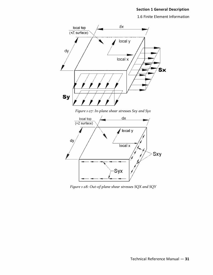
Figure 1-27: In-plane shear stresses Sxy and Syx
Figure 1-28: Out-of-plane shear stresses SQX and SQY
Section 1 General Description
1.6 Finite Element Information
Technical Reference Manual — 31

Members, plate elements, solid elements and surface elements can all be part of asingle STAAD model. The MEMBER INCIDENCES input must precede theINCIDENCE input for plates, solids or surfaces. All INCIDENCEs must precedeother input such as properties, constants, releases, loads, etc. The selfweight ofthe finite elements is converted to joint loads at the connected nodes and is notused as an element pressure load.
Plate Element Numbering
During the generation of element stiffness matrix, the program verifies whetherthe element is same as the previous one or not. If it is same, repetitivecalculations are not performed. The sequence in which the element stiffnessmatrix is generated is the same as the sequence in which elements are input inelement incidences.
Therefore, to save some computing time, similar elements should be numberedsequentially. The following figure shows examples of efficient and non-efficientelement numbering.
However, you have to decide between adopting a numbering system whichreduces the computation time versus a numbering system which increases theease of defining the structure geometry.
Figure 1-29: Examples of efficient and inefficient element numbering
32— STAAD.Pro V8i (SELECTseries 4)
Section 1 General Description
1.6 Finite Element Information

1.6.2 Solid ElementSolid elements enable the solution of structural problems involving general threedimensional stresses. There is a class of problems such as stress distribution inconcrete dams, soil and rock strata where finite element analysis using solidelements provides a powerful tool.
Theoretical Basis
The solid element used in STAAD is of eight-noded, isoparametric type. Theseelements have three translational degrees-of-freedom per node.
Figure 1-30: eight-noded, isoparametric solid element
By collapsing various nodes together, an eight noded solid element can bedegenerated to the following forms with four to seven nodes. Joints 1, 2, and 3must be retained as a triangle.
Figure 1-31: Forms of a collapsed eight-noded solid element
Section 1 General Description
1.6 Finite Element Information
Technical Reference Manual — 33

The stiffness matrix of the solid element is evaluated by numerical integrationwith eight Gauss-Legendre points. To facilitate the numerical integration, thegeometry of the element is expressed by interpolating functions using naturalcoordinate system, (r,s,t) of the element with its origin at the center of gravity.The interpolating functions are shown below:
X h x= ∑i i i=18
, y h y= ∑ i i i=18
, z h z= ∑i i i=18
where x, y and z are the coordinates of any point in the element and xi, yi, zi,i=1,..,8 are the coordinates of nodes defined in the global coordinate system. Theinterpolation functions, hi are defined in the natural coordinate system, (r,s,t).Each of r,s and t varies between -1 and +1. The fundamental property of theunknown interpolation functions hi is that their values in natural coordinatesystem is unity at node, i, and zero at all other nodes of the element. Theelement displacements are also interpreted the same way as the geometry. Forcompleteness, the functions are given below:
u h u= ∑i i i=18
, v h v= ∑i i i=18
, w h w= ∑i i i=18
where u, v and w are displacements at any point in the element and ui,vi, w
i, i=1,
8 are corresponding nodal displacements in the coordinate system used todescribe the geometry.
Three additional displacement "bubble" functions which have zero displacementsat the surfaces are added in each direction for improved shear performance toform a 33x33 matrix. Static condensation is used to reduce this matrix to a 24x24matrix at the corner joints.
34— STAAD.Pro V8i (SELECTseries 4)
Section 1 General Description
1.6 Finite Element Information

Local Coordinate System
The local coordinate system used in solid element is the same as the globalsystem.
Figure 1-32: Local coordinate system for a solid element
Properties and Constants
Unlike members and shell (plate) elements, no properties are required for solidelements. However, the constants such as modulus of elasticity and Poisson’sratio are to be specified. Also, density needs to be provided if selfweight isincluded in any load case.
Output of Element Stresses
Element stresses may be obtained at the center and at the joints of the solidelement. The items that are printed are :
l Normal Stresses : SXX, SYY and SZZ
l Shear Stresses : SXY, SYZ and SZX
l Principal stresses : S1, S2 and S3
l Von Mises stresses: SIGE = 0.707[(S1 - S2)2 + (S2 - S3)2 + (S3 - S1)2]1/2
Direction cosines : six direction cosines are printed, following the expression DC,corresponding to the first two principal stress directions.
Section 1 General Description
1.6 Finite Element Information
Technical Reference Manual — 35

1.6.3 Surface ElementFor any panel type of structural component, modeling requires breaking it downinto a series of plate elements for analysis purposes. This is what is known instress analysis parlance as meshing. When you choose to model the panelcomponent using plate elements, you are then taking on the responsibility ofmeshing. Thus, what the program sees is a series of elements. It is yourresponsibility to ensure that meshing is done properly. Examples of these areavailable in example problems 9, 10, 23, 27, etc. (Refer to the Examples manual)where individual plate elements are specified.
By using the Surface type of entity, the burden of meshing is shifted from you tothe program to some degree. The entire wall or slab is hence represented by justa few "Surface" entities, instead of hundreds of elements. When the program goesthrough the analysis phase, it will then automatically subdivide the surface intoelements. Therefore, you do not have to instruct the program in what manner tocarry out the meshing.
The attributes associated with the surface element, and the sections of thismanual where the information may be obtained, are listed below:
AttributesRelatedSections
Surfaces Incidences 5.13.3
Openings in surface 5.13.3
Local Coordinates system forsurfaces
1.6.3
Specifying sections for stress/forceoutput
5.13.3
Property for surfaces 5.21.2
Material constants 5.26.3
Surface loading 5.32.3.4
Stress/Force output printing 5.42
Shear Wall Design 3.8.2, 5.55
36— STAAD.Pro V8i (SELECTseries 4)
Section 1 General Description
1.6 Finite Element Information

Local Coordinate system for surfaces
The origin and orientation of the local coordinate system of a surface elementdepends on the order in which the boundary nodal points are listed and positionof the surface element in relation to the global coordinate system.
Let X, Y, and Z represent the local and GX, GY, and GZ the global axis vectors,respectively. The following principles apply.
a. Origin of X-Y-Z is located at the first node specified.
b. Direction of Z may be established by the right hand corkscrew rule, wherethe thumb indicates the positive Z direction, and the fingers point alongthe circumference of the element from the first to the last node listed.
c. X is a vector product of GY and Z (X = GY x Z). If GY and Z are parallel, Xis taken as a vector parallel to GX.
d. Finally, Y is a vector product of Z and X (Y = Z x X).
The diagram below shows directions and sign convention of local axes and forces.
Figure 1-33: Local axis & sign convention of surface forces
1.7 Member PropertiesThe following types of member property specifications are available in STAAD:
Section 1 General Description
1.7 Member Properties
Technical Reference Manual — 37

Shear Area for members refers to the shear stiffness effective area. Shear stiffnesseffective area is used to calculate shear stiffness for the member stiffness matrix.
As an example: for a rectangular cross section, the shear stiffness effective area isusually taken as 0.83 (Roark) to 0.85 (Cowper) times the cross sectional area. Ashear area of less than the cross sectional area will reduce the stiffness. A typicalshearing stiffness term is
(12EI/L3)/(1+Φ)
Where:
Φ = (12 EI) / (GAs L2)
As= the shear stiffness effective area.
Phi (Φ) is usually ignored in basic beam theory. STAAD will include the PHI termunless the SET SHEAR command is entered.
Shear stress effective area is a different quantity that is used to calculate shearstress and in code checking. For a rectangular cross section, the shear stresseffective area is usually taken as two-thirds (0.67x) of the cross sectional area.
Shear stress in STAAD may be from one of three methods.
1. (Shear Force)/(Shear stress effective area)
This is the case where STAAD computes the area based on the cross sectionparameters.
2. (Shear Force)/(Shear stiffness effective area)
This is the case where STAAD uses the shear area entered.
3. (V Q)/(I t)
In some codes and for some cross sections, STAAD uses this method.
The values that STAAD uses for shear area for shear deformation calculation canbe obtained by specifying the command PRINT MEMBER PROPERTIES.
The output for this will provide this information in all circumstances: when AYand AZ are not provided, when AY and AZ are set to zero, when AY and AZ areset to very large numbers, when properties are specified using PRISMATIC, whenproperties are specified through a user table, when properties are specifiedthrough from the built-in-table, etc.
1.7.1 Prismatic PropertiesThe following prismatic properties are required for analysis:
38— STAAD.Pro V8i (SELECTseries 4)
Section 1 General Description
1.7 Member Properties

l AX = Cross sectional area
l IX = Torsional constant
l IY = Moment of inertia about y-axis.
l IZ = Moment of inertia about z-axis.
In addition, the user may choose to specify the following properties:
l AY = Effective shear area for shear force parallel to local y-axis.
l AZ = Effective shear area for shear force parallel to local z-axis.
l YD = Depth of section parallel to local y-axis.
l ZD = Depth of section parallel to local z-axis.
For T-beams, YD, ZD, YB & ZB must be specified. These terms, which are shownin the next figure are:
l YD = Total depth of section (top fiber of flange to bottom fiber of web)
l ZD = Width of flange
l YB = Depth of stem
l ZB = Width of stem
For Trapezoidal beams, YD, ZD & ZB must be specified. These terms, which tooare shown in the next figure are:
l YD = Total depth of section
l ZD = Width of section at top fiber
l ZB = Width of section at bottom fiber
Top & bottom are defined as positive side of the local Z axis, and negative side ofthe local Z axis respectively.
STAAD automatically considers the additional deflection of members due to pureshear (in addition to deflection due to ordinary bending theory). To ignore theshear deflection, enter a SET SHEAR command before the joint coordinates. Thiswill bring results close to textbook results.
The depths in the two major directions (YD and ZD) are used in the program tocalculate the section moduli. These are needed only to calculate member stressesor to perform concrete design. You can omit the YD & ZD values if stresses ordesign of these members are of no interest. The default value is 253.75 mm (9.99inches) for YD and ZD. All the prismatic properties are input in the local membercoordinates.
Section 1 General Description
1.7 Member Properties
Technical Reference Manual — 39

Figure 1-34: Prismatic property nomenclature for a T and Trapezoidal section
To define a concrete member,you must not provide AX, but instead, provide YDand ZD for a rectangular section and just YD for a circular section. If no momentof inertia or shear areas are provided, the program will automatically calculatethese from YD and ZD.
Table 1.1 is offered to assist the user in specifying the necessary section values. Itlists, by structural type, the required section properties for any analysis. For thePLANE or FLOOR type analyses, the choice of the required moment of inertiadepends upon the beta angle. If BETA equals zero, the required property is IZ.
Structure Type Required Properties
TRUSS structure AX
PLANE structure AX, IZ, or IY
FLOOR structure IX, IZ or IY
SPACE structure AX, IX, IY, IZ
Table 1-4: Required Section Properties
1.7.2 Built-In Steel Section LibraryThis feature of the program allows you to specify section names of standard steelshapes manufactured in different countries. Information pertaining to theAmerican steel shapes is available in section 2.
For information on steel shapes for other countries, please refer to theInternational Codes manual.
STAAD.Pro comes with the non-composite castellated beam tables supplied bythe steel products manufacturer SMI Steel Products. Details of the manufacture
40— STAAD.Pro V8i (SELECTseries 4)
Section 1 General Description
1.7 Member Properties

and design of these sections may be found athttp://www.smisteelproducts.com/English/About/design.html
Figure 1-35: Castellated beam elevation
Since the shear areas of the sections are built into the tables, shear deformationis always considered for these sections.
1.7.3 User Provided Steel TableYou can provide a customized steel table with designated names and propercorresponding properties. The program can then find member properties fromthose tables. Member selection may also be performed with the programselecting members from the provided tables only.
These tables can be provided as a part of a STAAD input or as separately createdfiles from which the program can read the properties. If you do not use standardrolled shapes or only use a limited number of specific shapes, you can createpermanent member property files. Analysis and design can be limited to thesections in these files.
See "User Steel Table Specification" on page 326 and See "Property Specificationfrom User Provided Table" on page 350 for additional details.
1.7.4 Tapered SectionsProperties of tapered I-sections may be provided through MEMBER PROPERTYspecifications. Given key section dimensions, the program is capable ofcalculating cross-sectional properties which are subsequently used in analysis.
Tapered I-sections have constant flange dimensions and a linearly varying webdepth along the length of the member.
See "Tapered Member Specification" on page 349 for details.
1.7.5 Assign CommandIf you want to avoid the trouble of defining a specific section name but ratherleave it to the program to assign a section name, the ASSIGN command may beused. The section types that may be assigned include BEAM, COLUMN, CHANNEL,ANGLE and DOUBLE ANGLE.
Section 1 General Description
1.7 Member Properties
Technical Reference Manual — 41

When the keyword BEAM is specified, the program will assign an I-shaped beamsection (Wide Flange for AISC, UB section for British).
For the keyword COLUMN also, the program will assign an I-shaped beam section(Wide Flange for AISC, UC section for British).
If steel design-member selection is requested, a similar type section will beselected.
See "Assign Profile Specification" on page 350 for details.
1.7.6 Steel Joist and Joist GirdersSTAAD.Pro includes facilities for specifying steel joists and joist girders. The basisfor this implementation is the information contained in the 1994 publication ofthe American Steel Joist Institute called “Fortieth edition standard specifications,load tables and weight tables for steel joist and joist girders”. The following arethe salient features of the implementation.
Member properties can be assigned by specifying a joist designation contained intables supplied with the program. The following joists and joist girder types havebeen implemented:
l Open web steel joists – K series and KCS joists
l Longspan steel joists – LH series
l Deep Longspan steel joists – DLH series
l Joist Girders – G series
The pages in the Steel Joist Institute publication where these sections are listedare shown in the following table.
Joist type Beginning page number
K series 24
KCS 30
LH series 54
DLH series 57
Joist girders 74
Table 1-5: SJI joist types
42— STAAD.Pro V8i (SELECTseries 4)
Section 1 General Description
1.7 Member Properties

The designation for the G series Joist Girders is as shown in page 73 of the SteelJoist Institute publication. STAAD.Pro incorporates the span length also in thename, as shown in the next figure.
Figure 1-36: STAAD nomenclature for SJI joist girders
Theoretical basis for modeling the joist
Steel joists are prefabricated, welded steel trusses used at closely spaced intervalsto support floor or roof decking. Thus, from an analysis standpoint, a joist is nota single member in the same sense as beams and columns of portal frames thatone is familiar with. Instead, it is a truss assembly of members. In general,individual manufacturers of the joists decide on the cross section details of themembers used for the top and bottom chords, and webs of the joists. So, joisttables rarely contain any information on the cross-section properties of theindividual components of a joist girder. The manufacturer’s responsibility is toguarantee that, no matter what the cross section details of the members are, thejoist simply has to ensure that it provides the capacity corresponding to itsrating.
The absence of the section details makes it difficult to incorporate the true trussconfiguration of the joist in the analysis model of the overall structure. InSTAAD, selfweight and any other member load applied on the joist is transferredto its end nodes through simply supported action. Also, in STAAD, the joistmakes no contribution to the stiffness of the overall structure.
As a result of the above assumption, the following points must be noted withrespect to modeling joists:
1. The entire joist is represented in the STAAD input file by a single member.Graphically it will be drawn using a single line.
2. After creating the member, the properties should be assigned from the joistdatabase.
3. The 3D Rendering feature of the program will display those members usinga representative Warren type truss.
Section 1 General Description
1.7 Member Properties
Technical Reference Manual — 43

4. The intermediate span-point displacements of the joist cannot bedetermined.
Figure 1-37: Example rendering of a joist member in STAAD.Pro
Assigning the joists
The procedure for assigning the joists is explained in the Graphical User Interfacemanual.
The STAAD joists database includes the weight per length of the joists. So, forselfweight computations in the model, the weight of the joist is automaticallyconsidered.
Example
An example of a structure with joist (command file input data) is shown below.
STAAD SPACE EXAMPLE FOR JOIST GIRDER
UNIT FEET KIP
JOINT COORDINATES
1 0 0 0; 2 0 10 0
3 30 10 0; 4 30 0 0
MEMBER INCIDENCES
1 1 2; 2 2 3; 3 3 4;
MEMBER PROPERTY AMERICAN
44— STAAD.Pro V8i (SELECTseries 4)
Section 1 General Description
1.7 Member Properties

1 3 TABLE ST W21X50
MEMBER PROPERTY SJIJOIST
2 TABLE ST 22K6
CONSTANTS
E STEEL ALL
DENSITY STEEL ALL
POISSON STEEL ALL
SUPPORTS
1 4 FIXED
UNIT POUND FEET
LOAD 1
SELFWEIGHT Y -1
LOAD 2
MEMBER LOAD
2 UNI GY -250
LOAD COMB 3
1 1 2 1
PERF ANALY PRINT STAT CHECK
PRINT SUPP REAC
FINISH
1.7.7 Composite Beams and Composite DecksThere are two methods in STAAD for specifying composite beams. Compositebeams are members whose property is comprised of an I-shaped steel crosssection (like an American W shape) with a concrete slab on top. The steel sectionand concrete slab act monolithically. The two methods are:
1. The EXPLICIT definition method – In this method, the member geometry isfirst defined as a line. It is then assigned a property from the steel database,with the help of the ‘CM’ attribute. See "Assigning Properties from SteelTables" on page 341 for details on using this method. Additional parameterslike CT (thickness of the slab), FC (concrete strength), CW (effective widthof slab), CD (concrete density), etc., some optional and some mandatory,
Section 1 General Description
1.7 Member Properties
Technical Reference Manual — 45

are also provided.
Hence, the responsibility of determining the attributes of the compositemember, like concrete slab width, lies upon you, the user. If you wish toobtain a design, additional terms like rib height, rib width, etc. must alsobe separately assigned with the aid of design parameters. Hence, someamount of effort is involved in gathering all the data and assigning them.
2. The composite deck generation method – The laboriousness of the previousprocedure can be alleviated to some extent by using the program’scomposite deck definition facilities. The program then internally convertsthe deck into individual composite members (calculating attributes likeeffective width in the process) during the analysis and design phase. Thedeck is defined best using the graphical tools of the program since adatabase of deck data from different manufacturers is accessible from easy-to-use dialogs. Since all the members which make up the deck areidentified as part of a single object, load assignment and alterations to thedeck can be done to just the deck object, and not the individual membersof the deck.
See "Composite Decks" on page 351 for details.
1.7.8 Curved MembersMembers can be defined as being curved. Tapered sections are not permitted.The cross-section should be uniform throughout the length.
The design of curved members is not supported.
See "Curved Member Specification" on page 355 for details.
1.8 Member/ Element ReleaseSTAAD allows releases for members and plate elements.
One or both ends of a member or element can be released. Members/Elementsare assumed to be rigidly framed into joints in accordance with the structuraltype specified. When this full rigidity is not applicable, individual forcecomponents at either end of the member can be set to zero with member releasestatements. By specifying release components, individual degrees of freedom areremoved from the analysis. Release components are given in the local coordinatesystem for each member. Note that PARTIAL moment release is also allowed.
Only one of sections 1.8 and 1.9 properties can be assigned to a given member.The last one entered will be used. In other words, a MEMBER RELEASE should not
46— STAAD.Pro V8i (SELECTseries 4)
Section 1 General Description
1.8 Member/ Element Release
be applied on a member which is declared TRUSS, TENSION ONLY, orCOMPRESSION ONLY.
See "Member/Element Releases" on page 370 for details
1.9 Truss and Tension- or Compression-Only MembersFor analyses which involve members that carry axial loads only (i.e., trussmembers) there are two methods for specifying this condition. When all themembers in the structure are truss members, the type of structure is declared asTRUSS whereas, when only some of the members are truss members (e.g.,bracings of a building), the MEMBER TRUSS command can be used where thosemembers will be identified separately.
In STAAD, the MEMBER TENSION or MEMBER COMPRESSION command can beused to limit the axial load type the member may carry.
See "Member Tension/Compression Specification" on page 377 for details.
1.10 Tension, Compression - Only SpringsIn STAAD, the SPRING TENSION or SPRING COMPRESSION command can beused to limit the load direction the support spring may carry. The analysis will beperformed accordingly.
See "Axial Member Specifications" on page 375 for details.
1.11 Cable MembersSTAAD supports two types of analysis for cable members:
1.11.1 Linearized Cable MembersCable members may be specified by using the MEMBER CABLE command. Whilespecifying cable members, the initial tension in the cable must be provided. Thefollowing paragraph explains how cable stiffness is calculated.
The increase in length of a loaded cable is a combination of two effects. The firstcomponent is the elastic stretch, and is governed by the familiar springrelationship:
F = Kx
Where:
Kelastic = EA/L
The second component of the lengthening is due to a change in geometry (as acable is pulled taut, sag is reduced). This relationship can be described by
Section 1 General Description
1.9 Truss and Tension- or Compression-Only Members
Technical Reference Manual — 47

F = Kx
but here,
K =sag
T
w L
12
α
3
2 3 1
cos2
Where:
w = weight per unit length of cable
T = tension in cable
α = angel that the axis of the cable makes with a horizontal plane (=0, cable is horizontal; = 90, cable is vertical).
Therefore, the "stiffness" of a cable depends on the initial installed tension (orsag). These two effects may be combined as follows:
K = =combK K
EA L
( )1
1 / + 1 /
( / )
1 +sag elastic w L EA α
T
( )2 2cos2
123
Note:When T = infinity, Kcomb
= EA/L and that when T = 0, Kcomb
= 0. Itshould also be noted that as the tension increases (sag decreases) thecombined stiffness approaches that of the pure elastic situation.
The following points need to be considered when using the cable member inSTAAD :
1. The linear cable member is only a truss member whose propertiesaccommodate the sag factor and initial tension. The behavior of the cablemember is identical to that of the truss member. It can carry axial loadsonly. As a result, the fundamental rules involved in modeling truss membershave to be followed when modeling cable members. For example, when twocable members meet at a common joint, if there isn't a support or a 3rdmember connected to that joint, it is a point of potential instability.
2. Due to the reasons specified in 1) above, applying a transverse load on acable member is not advisable. The load will be converted to twoconcentrated loads at the 2 ends of the cable and the true deflectionpattern of the cable will never be realized.
3. A tension only cable member offers no resistance to a compressive forceapplied at its ends. When the end joints of the member are subjected to acompressive force, they "give in" thereby causing the cable to sag. Under
48— STAAD.Pro V8i (SELECTseries 4)
Section 1 General Description
1.11 Cable Members

these circumstances, the cable member has zero stiffness and this situationhas to be accounted for in the stiffness matrix and the displacements haveto be recalculated. But in STAAD, merely declaring the member to be acable member does not guarantee that this behavior will be accounted for.It is also important that you declare the member to be a tension onlymember by using the MEMBER TENSION command, after the CABLEcommand. This will ensure that the program will test the nature of theforce in the member after the analysis and if it is compressive, the memberis switched off and the stiffness matrix re-calculated.
4. Due to potential instability problems explained in item 1 above, you shouldalso avoid modeling a catenary by breaking it down into a number ofstraight line segments. The cable member in STAAD cannot be used tosimulate the behavior of a catenary. By catenary, we are referring to thosestructural components which have a curved profile and develop axial forcesdue their self weight. This behavior is in reality a non-linear behaviorwhere the axial force is caused because of either a change in the profile ofthe member or induced by large displacements, neither of which are validassumptions in an elastic analysis. A typical example of a catenary is themain U shaped cable used in suspension bridges.
5. The increase of stiffness of the cable as the tension in it increases underapplied loading is updated after each iteration if the cable members arealso declared to be MEMBER TENSION. However, iteration stops when alltension members are in tension or slack; not when the cable tensionconverges.
See "Second Order Analysis" on page 67, See "Axial Member Specifications" onpage 375, and See "Analysis Specification" on page 676 for details.
1.11.2 Nonlinear Cable and Truss MembersCable members for the Nonlinear Cable Analysis may be specified by using theMEMBER CABLE command. While specifying cable members, the initial tension inthe cable or the unstressed length of the cable must be provided. you shouldensure that all cables will be in sufficient tension for all load cases to converge.Use selfweight in every load case and temperature if appropriate; i.e., don’t entercomponent cases (e.g., wind only).
The nonlinear cable may have large motions and the sag is checked on every loadstep and every equilibrium iteration.
In addition there is a nonlinear truss which is specified in the Member Trusscommand. The nonlinear truss is simply any truss with pretension specified. It is
Section 1 General Description
1.11 Cable Members
Technical Reference Manual — 49

essentially the same as a cable without sag. This member takes compression. If allcables are taut for all load cases, then the nonlinear truss may be used to simulatecables. The reason for using this substitution is that the truss solution is morereliable.
Points 1, 2, and 4 in the previous section will not apply to nonlinear cable analysisif sufficient pretension is applied, so joints may be entered along the shape of acable (in some cases a stabilizing stiffness may be required and entered for thefirst loadstep). Point 3 above: The Member Tension command is unnecessary andignored for the nonlinear cable analysis. Point 5 above: The cable tensions areiterated to convergence in the nonlinear cable analysis.
See "Nonlinear Cable/Truss Analysis" on page 78, See "Axial MemberSpecifications" on page 375, and See "Nonlinear Cable Analysis" on page 683 fordetails.
1.12 Member OffsetsSome members of a structure may not be concurrent with the incident jointsthereby creating offsets. This offset distance is specified in terms of global or localcoordinate system (i.e., X, Y and Z distances from the incident joint). Secondaryforces induced, due to this offset connection, are taken into account in analyzingthe structure and also to calculate the individual member forces. The new offsetcentroid of the member can be at the start or end incidences and the newworking point will also be the new start or end of the member. Therefore, anyreference from the start or end of that member will always be from the newoffset points.
Figure 1-38: Example of working points (WP)
50— STAAD.Pro V8i (SELECTseries 4)
Section 1 General Description
1.12 Member Offsets

In the figure above, WP refers to the location of the centroid of the starting orending point of the member.
Example
MEMBER OFFSET
1 START 7
1 END -6
2 END -6 -9
MEMBER OFFSET
1 START 7
1 END -6
2 END -6 -9
See "Member Offset Specification" on page 383 for details.
Section 1 General Description
1.12 Member Offsets
Technical Reference Manual — 51

1.13 Material ConstantsThe material constants are: modulus of elasticity (E); weight density (DEN);Poisson's ratio (POISS); co-efficient of thermal expansion (ALPHA), CompositeDamping Ratio, and beta angle (BETA) or coordinates for any reference (REF)point.
E value for members must be provided or the analysis will not be performed.Weight density (DEN) is used only when selfweight of the structure is to be takeninto account. Poisson's ratio (POISS) is used to calculate the shear modulus(commonly known as G) by the formula,
G = 0.5⋅E/(1 + POISS)
If Poisson's ratio is not provided, STAAD will assume a value for this quantitybased on the value of E. Coefficient of thermal expansion (ALPHA) is used tocalculate the expansion of the members if temperature loads are applied. Thetemperature unit for temperature load and ALPHA has to be the same.
Composite damping ratio is used to compute the damping ratio for each mode ina dynamic solution. This is only useful if there are several materials with differentdamping ratios.
BETA angle and REFerence point are discussed in Section 1.5.3 and are input aspart of the member constants.
Note: Poisson's Ratio must always be defined after the Modulus of Elasticityfor a given member/element.
1.14 SupportsSTAAD allows specifications of supports that are parallel as well as inclined to theglobal axes.
Supports are specified as PINNED, FIXED, or FIXED with different releases. Apinned support has restraints against all translational movement and noneagainst rotational movement. In other words, a pinned support will havereactions for all forces but will resist no moments. A fixed support has restraintsagainst all directions of movement.
The restraints of a fixed support can also be released in any desired direction asspecified.See "Global Support Specification" on page 405 for details.
Translational and rotational springs can also be specified. The springs arerepresented in terms of their spring constants. A translational spring constant is
52— STAAD.Pro V8i (SELECTseries 4)
Section 1 General Description
1.13 Material Constants

defined as the force to displace a support joint one length unit in the specifiedglobal direction. Similarly, a rotational spring constant is defined as the force torotate the support joint one degree around the specified global direction. See"Multilinear Spring Support Specification" on page 414 for details.
For static analysis, Multi-linear spring supports can be used to model the varying,non-linear resistance of a support (e.g., soil). See "Automatic Spring SupportGenerator for Foundations" on page 409 for descriptions of the elastic footingand elastic foundation mat facilities.
The Support command is also used to specify joints and directions where supportdisplacements will be enforced.
1.15 Master/Slave JointsThe master/slave option is provided to enable the user to model rigid links in thestructural system. This facility can be used to model special structural elementslike a rigid floor diaphragm. Several slave joints may be provided which will beassigned same displacements as the master joint. The user is also allowed theflexibility to choose the specific degrees of freedom for which the displacementconstraints will be imposed on the slaved joints. If all degrees of freedom (Fx, Fy,Fz, Mx, My and Mz) are provided as constraints, the joints will be assumed to berigidly connected.
See "Master/Slave Specification" on page 420 for details.
1.16 LoadsLoads in a structure can be specified as joint load, member load, temperatureload and fixed-end member load. STAAD can also generate the self-weight of thestructure and use it as uniformly distributed member loads in analysis. Anyfraction of this self-weight can also be applied in any desired direction.
1.16.1 Joint LoadJoint loads, both forces and moments, may be applied to any free joint of astructure. These loads act in the global coordinate system of the structure.Positive forces act in the positive coordinate directions. Any number of loadsmay be applied on a single joint, in which case the loads will be additive on thatjoint.
See "Joint Load Specification" on page 540 for details.
Section 1 General Description
1.15 Master/Slave Joints
Technical Reference Manual — 53

1.16.2 Member LoadThree types of member loads may be applied directly to a member of a structure.These loads are uniformly distributed loads, concentrated loads, and linearlyvarying loads (including trapezoidal). Uniform loads act on the full or partiallength of a member. Concentrated loads act at any intermediate, specified point.Linearly varying loads act over the full length of a member. Trapezoidal linearlyvarying loads act over the full or partial length of a member. Trapezoidal loadsare converted into a uniform load and several concentrated loads.
Any number of loads may be specified to act upon a member in any independentloading condition. Member loads can be specified in the member coordinatesystem or the global coordinate system. Uniformly distributed member loadsprovided in the global coordinate system may be specified to act along the full orprojected member length. See "Global Coordinate System" on page 10 to find therelation of the member to the global coordinate systems for specifying memberloads. Positive forces act in the positive coordinate directions, local or global, asthe case may be.
Uniform moment may not be applied to tapered members. Only uniform loadover the entire length is available for curved members.
Figure 1-39: Member Load Configurations for A) linear loads, B) concentrated loads, C) linearloads, D) trapezoidal load, E) triangular (linear) loads, and E) uniform load
54— STAAD.Pro V8i (SELECTseries 4)
Section 1 General Description
1.16 Loads

See "Member Load Specification" on page 541 for details.
1.16.3 Area Load, One-way, and Floor LoadsOften a floor is subjected to a uniform pressure. It could require a lot of work tocalculate the equivalent member load for individual members in that floor.However, with the AREA, ONEWAY or FLOOR LOAD facilities, you can specify thepressure (load per unit square area). The program will calculate the tributary areafor these members and calculate the appropriate member loads. The Area Loadand Oneway load are used for one way distribution and the Floor Load is usedfor two way distribution.
The following assumptions are made while transferring the area/floor load tomember load:
a. The member load is assumed to be a linearly varying load for which thestart and the end values may be of different magnitude.
b. Tributary area of a member with an area load is calculated based on halfthe spacing to the nearest approximately parallel members on both sides. Ifthe spacing is more than or equal to the length of the member, the areaload will be ignored. Oneway load does not have this limitation.
Section 1 General Description
1.16 Loads
Technical Reference Manual — 55
c. These loading types should not be specified on members declared asMEMBER CABLE, MEMBER TRUSS, MEMBER TENSION, MEMBER COMPRESSION,or CURVED.
Note: Floor Loads and One-way Loads can be reduced when included in aload case defined as “Reducible” according to the UBC/IBC rules.
An example:
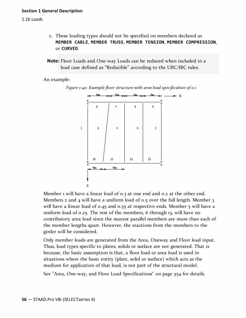
Figure 1-40: Example floor structure with area load specification of 0.1
Member 1 will have a linear load of 0.3 at one end and 0.2 at the other end.Members 2 and 4 will have a uniform load of 0.5 over the full length. Member 3will have a linear load of 0.45 and 0.55 at respective ends. Member 5 will have auniform load of 0.25. The rest of the members, 6 through 13, will have nocontributory area load since the nearest parallel members are more than each ofthe member lengths apart. However, the reactions from the members to thegirder will be considered.
Only member loads are generated from the Area, Oneway and Floor load input.Thus, load types specific to plates, solids or surface are not generated. That isbecause, the basic assumption is that, a floor load or area load is used insituations where the basic entity (plate, solid or surface) which acts as themedium for application of that load, is not part of the structural model.
See "Area, One-way, and Floor Load Specifications" on page 554 for details.
56— STAAD.Pro V8i (SELECTseries 4)
Section 1 General Description
1.16 Loads

1.16.4 Fixed End Member LoadLoad effects on a member may also be specified in terms of its fixed end loads.These loads are given in terms of the member coordinate system and thedirections are opposite to the actual load on the member. Each end of a membercan have six forces: axial; shear y; shear z; torsion; moment y, and moment z.
See "Fixed-End Load Specification" on page 579 for details.
1.16.5 Prestress and Poststress Member LoadMembers in a structure may be subjected to prestress load for which the loaddistribution in the structure may be investigated. The prestressing load in amember may be applied axially or eccentrically. The eccentricities can beprovided at the start joint, at the middle, and at the end joint. Theseeccentricities are only in the local y-axis. A positive eccentricity will be in thepositive local y-direction. Since eccentricities are only provided in the local y-axis, care should be taken when providing prismatic properties or in specifyingthe correct BETA angle when rotating the member coordinates, if necessary. Twotypes of prestress load specification are available; PRESTRESS, where the effectsof the load are transmitted to the rest of the structure, and POSTSTRESS, wherethe effects of the load are experienced exclusively by the members on which it isapplied.
1. The cable is assumed to have a generalized parabolic profile. The equationof the parabola is assumed to be
y = ax2 + bx + c
Where:
a = 1/L2 (2es - 4em + 2ee)
b = 1/L (4em - ee - 3es)
c = es
es = eccentricity of the cable at the start of the member (in localy-axis)
em = eccentricity of the cable at the middle of the member (inlocal y-axis)
ee = eccentricity of the cable at the end of the member (in localy-axis)
L = Length of the member.
Section 1 General Description
1.16 Loads
Technical Reference Manual — 57

2. The angle of inclination of the cable with respect to the local x-axis (astraight line joining the start and end joints of the member) at the start andend points is small which gives rise to the assumption that
sinθ = θ = dy/dx
Hence, if the axial force in the cable is P, the vertical component of theforce at the ends is P(dy/dx) and the horizontal component of the cableforce is,
P[1 - (dy/dx)2]1/2
Users are advised to ensure that their cable profile meets this requirement.An angle under 5 degrees is recommended.
3. The member is analyzed for the prestressing / poststressing effects using theequivalent load method. This method is well documented in most reputedbooks on Analysis and Design of Prestressed concrete. The magnitude of theuniformly distributed load is calculated as
udl = 8⋅Pe/L2
Where:
P = Axial force in the cable
e = (es + ee)/2 - em
L = Length of the member
4. The force in the cable is assumed to be same throughout the memberlength. No reduction is made in the cable forces to account for friction orother losses.
5. The term MEMBER PRESTRESS as used in STAAD signifies the followingcondition. The structure is constructed first. Then, the prestressing force isapplied on the relevant members. As a result, the members deform anddepending on their end conditions, forces are transmitted to othermembers in the structure. In other words, "PRE" refers to the time ofplacement of the member in the structure relative to the time of stressing.
6. The term MEMBER POSTSTRESS as used in STAAD signifies the followingcondition. The members on which such load is applied are first cast in thefactory. Following this, the prestressing force is applied on them.Meanwhile, the rest of the structure is constructed at the construction site.Then, the prestressed members are brought and placed in position on thepartially built structure. Due to this sequence, the effects of prestressing are
58— STAAD.Pro V8i (SELECTseries 4)
Section 1 General Description
1.16 Loads

"experienced" by only the prestressed members and not transmitted to therest of the structure. In other words, "POST" refers to the time of placementof the member in the structure relative to the time of stressing.
7. As may be evident from Item (6) above, it is not possible to compute thedisplacements of the ends of the POSTSTRESSED members for the effects ofpoststressing, and hence are assumed to be zero. As a result, displacementsof intermediate sections (See SECTION DISPLACEMENT command) aremeasured relative to the straight line joining the start and end joints of themembers as defined by their initial JOINT COORDINATES.
See "Prestress Load Specification" on page 573 for details.
1.16.6 Temperature and Strain LoadUniform temperature difference throughout members and elements may bespecified. Temperature differences across both faces of members and through thethickness of plates may also be specified (uniform temperature only for solids)..The program calculates the axial strain (elongation and shrinkage) due to thetemperature difference for members. From this it calculates the induced forces inthe member and the analysis is done accordingly. The strain intervals ofelongation and shrinkage can be input directly.
See "Temperature Load Specification for Members, Plates, and Solids" on page578 for details.
1.16.7 Support Displacement LoadStatic Loads can be applied to the structure in terms of the displacement of thesupports. Displacement can be translational or rotational. Translationaldisplacements are provided in the specified length while the rotationaldisplacements are always in degrees. Note that displacements can be specifiedonly in directions in which the support has an "enforced" specification in theSupport command.
See "Support Joint Displacement Specification" on page 580 for details.
1.16.8 Loading on ElementsOn Plate/Shell elements, the types of loading that are permissible are:
1. Pressure loading which consists of loads which act perpendicular to thesurface of the element. The pressure loads can be of uniform intensity ortrapezoidally varying intensity over a small portion or over the entire
Section 1 General Description
1.16 Loads
Technical Reference Manual — 59

surface of the element.
2. Joint loads which are forces or moments that are applied at the joints in thedirection of the global axes.
3. Temperature loads which may be constant throughout the plate element(causing only elongation / shortening) or may vary across the depth of aplate element causing bending on the plate element.. The coefficient ofthermal expansion for the material of the element must be provided inorder to facilitate computation of these effects.
4. The self-weight of the elements can be applied using the SELFWEIGHTloading condition. The density of the elements has to be provided in orderto facilitate computation of the self-weight.
On Solid elements, the loading types available are:
1. The self-weight of the solid elements can be applied using the SELFWEIGHTloading condition. The density of the elements has to be provided in orderto facilitate computation of the self-weight.
2. Joint loads which are forces or moments that are applied at the joints in thedirection of the global axes.
3. Temperature loads which may be constant throughout the solid elements(causing only elongation / shortening). The coefficient of thermal expansionfor the material of the element must be provided in order to facilitatecomputation of these effects.
4. Pressure on the faces of solids.
Only translational stiffness is supported in solid elements. Thus, at joints wherethere are only solid elements, moments may not be applied. For efficiency,rotational supports should be used at these joints.
See "Element Load Specifications" on page 544 for details.
1.17 Load GeneratorLoad generation is the process of taking a load causing unit such as windpressure, ground movement or a truck on a bridge, and converting it to a formsuch as member load or a joint load which can be then be used in the analysis.
For seismic loads, a static analysis method or a dynamic analysis method can beadopted. The static analysis method, which is the one referred to here, is basedon codes such as UBC, IBC, AIJ, IS1893 etc. For dynamic analysis, see the sectionsin this chapter on response spectrum and time history analysis.
Input for the load generation facility consists of two parts:
60— STAAD.Pro V8i (SELECTseries 4)
Section 1 General Description
1.17 Load Generator

1. Definition of the load system(s).
2. Generation of primary load cases using previously defined load system(s).
1.17.1 Moving Load GeneratorThis feature enables the user to generate static loads on members due to vehiclesmoving on a structure. Moving load system(s) consisting of concentrated loads atfixed specified distances in both directions on a plane can be defined by the user.A user specified number of primary load cases will be subsequently generated bythe program and taken into consideration in analysis. American Association ofState Highway and Transportation Officials (AASHTO) vehicles are availablewithin the program and can be specified using standard AASHTO designations.
See "Definition of Moving Load System" on page 429 and See "Generation ofMoving Loads" on page 651 for details.
1.17.2 Seismic Load GeneratorThe STAAD seismic load generator follows the procedure of equivalent lateralload analysis explained in UBC, IBC and several other codes. It is assumed thatthe lateral loads will be exerted in X and Z (or X and Y if Z is up) directions(horizontal) and Y (or Z if Z is up) will be the direction of the gravity loads. Thus,for a building model, Y (or Z if Z is up) axis will be perpendicular to the floorsand point upward (all Y (or Z if Z is up) joint coordinates positive). The user isrequired to set up his model accordingly. Total lateral seismic force or base shearis automatically calculated by STAAD using the appropriate equation from thecode. IBC 2003, IBC 2000, UBC 1997, 1994, or 1985, IS:1893, Japanese, Colombianand other specifications may be used.
For load generation per the codes, the user is required to provide seismic zonecoefficients, importance factors, soil characteristic parameters, etc. See "UBC 1997Load Definition" on page 434 for the detailed input required for each code.
Instead of using the approximate code based formulas to estimate the buildingperiod in a certain direction, the program calculates the period using Rayleighquotient technique. This period is then utilized to calculate seismic coefficient C.
After the base shear is calculated from the appropriate equation, it is distributedamong the various levels and roof per UBC specifications. The distributed baseshears are subsequently applied as lateral loads on the structure. These loads maythen be utilized as normal load cases for analysis and design.
See "Generation of Seismic Loads" on page 653 for details.
Section 1 General Description
1.17 Load Generator
Technical Reference Manual — 61

1.17.3 Wind Load GeneratorThe Wind Load Generator is a utility which takes as input wind pressure andheight ranges over which these pressures act and generates nodal point andmember loads.
This facility is available for two types of structures.
l Panel type or Closed structures
l Open structures
Closed structures are ones like office buildings where non-structural entities likea glass facade, aluminum sheets, timber panels or non-load bearing walls act as anobstruction to the wind. If these entities are not included in the structural model,the load generated as a result of wind blowing against them needs to becomputed. So, the steps involved in load generation for such structures are:
i. Identify the panels – regions circumscribed by members so that a polygonalclosed area is formed. The area may also be formed between the groundlevel along one edge and members along the other.
ii. Calculate the panel area and multiply it by the wind pressure.
iii. Convert the resulting force into nodal point loads.
Plates and solids are not considered in the calculation of the panel area. Openingswithin the panels may be modeled with the help of exposure factors. An exposurefactor is associated with each joint of the panel and is a fractional number bywhich the area affecting a joint of the panel can be reduced or increased.
The automated load generator should only be used for vertical panels. Panels notparallel to the global Y axis (for Y UP) should be loaded separately.
Open structures are those like transmission towers, in which the region betweenmembers is “open” allowing the wind to blow through. The procedure for loadgeneration for open structures is i) Calculate the exposed area of the individualmembers of the model. ii) Multiply that exposed area by the wind pressure toarrive at the force and apply the force on individual members as a uniformlydistributed load. It is assumed that all members of the structure within thespecified ranges are subjected to the pressure and hence, they will all receive theload. The concept of members on the windward side shielding the members inthe inside regions of the structure does not exist for open structures. Membersloaded as an open structure need not be vertical.
See "Definition of Wind Load" on page 503 and See "Generation of Wind Loads"on page 660 for details.
62— STAAD.Pro V8i (SELECTseries 4)
Section 1 General Description
1.17 Load Generator

1.17.4 Snow LoadSTAAD.Pro is capable of generating snow loading on a structure in accordancewith the provisions of the ASCE-7-02 code. The feature is currently implementedfor structures with flat or sloping roofs. Snow load generation for members ofopen lattice structures like electrical transmission towers is currently not part ofthis facility. Hence, the feature is based on panel areas, not the exposed width ofindividual members.
See "Definition of Snow Load" on page 530 and See "Generation of Snow Loads" on page 664 for details.
1.18 Analysis FacilitiesSalient features of each type of analysis are discussed in the following sections.Detailed theoretical treatments of these features are available in standardstructural engineering textbooks.
1.18.1 Stiffness AnalysisThe stiffness analysis implemented in STAAD is based on the matrixdisplacement method. In the matrix analysis of structures by the displacementmethod, the structure is first idealized into an assembly of discrete structuralcomponents.
Structural systems such as slabs, plates, spread footings, etc., which transmit loadsin two directions (frame members or finite elements). Each component has anassumed form of displacement in a manner which satisfies the force equilibriumand displacement compatibility at the joints. have to be discretized into anumber of three or four noded finite elements connected to each other at theirnodes. Loads may be applied in the form of distributed loads on the elementsurfaces or as concentrated loads at the joints. The plane stress effects as well asthe plate bending effects are taken into consideration in the analysis.
Assumptions of the Analysis
For a complete analysis of the structure, the necessary matrices are generated onthe basis of the following assumptions:
1. The structure is idealized into an assembly of beam, plate and solid typeelements joined together at their vertices (nodes). The assemblage is loadedand reacted by concentrated loads acting at the nodes. These loads may be
Section 1 General Description
1.18 Analysis Facilities
Technical Reference Manual — 63

both forces and moments which may act in any specified direction.
2. A beam member is a longitudinal structural member having a constant,doubly symmetric or near-doubly symmetric cross section along its length.Beam members always carry axial forces. They may also be subjected toshear and bending in two arbitrary perpendicular planes, and they may alsobe subjected to torsion. From this point these beam members are referredto as "members" in the manual.
3. A plate element is a three or four noded planar element having variablethickness. A solid element is a four-to-eight- noded, three dimensionalelement. These plate and solid elements are referred to as "elements" in themanual.
4. Internal and external loads acting on each node are in equilibrium. Iftorsional or bending properties are defined for any member, six degrees offreedom are considered at each node (i.e., three translational and threerotational) in the generation of relevant matrices. If the member is definedas truss member (i.e., carrying only axial forces) then only the three degrees(translational) of freedom are considered at each node.
5. Two types of coordinate systems are used in the generation of the requiredmatrices and are referred to as local and global systems.
Local coordinate axes are assigned to each individual element and are orientedsuch that computing effort for element stiffness matrices are generalized andminimized. Global coordinate axes are a common datum established for allidealized elements so that element forces and displacements may be related to acommon frame of reference.
Basic Equation
The complete stiffness matrix of the structure is obtained by systematicallysumming the contributions of the various member and element stiffness. Theexternal loads on the structure are represented as discrete concentrated loadsacting only at the nodal points of the structure.
The stiffness matrix relates these loads to the displacements of the nodes by theequation:
Aj = aj + Sj⋅DjThis formulation includes all the joints of the structure, whether they are free todisplace or are restrained by supports. Those components of joint displacementsthat are free to move are called degrees of freedom. The total number of degreesof freedom represent the number of unknowns in the analysis.
64— STAAD.Pro V8i (SELECTseries 4)
Section 1 General Description
1.18 Analysis Facilities

Method to Solve for Displacements There are many methods to solve the unknowns from a series of simultaneousequations.
In STAAD.Pro, the element stiffness matrices are assembled into a global stiffnessmatrix by standard matrix techniques used in FEA programs. The technique usedby STAAD was copied from SAP IV. The global stiffness matrix is thendecomposed as
[ K ] = [LT] [D] [L]
which is a modified Gauss method.
[K] {d} = {F}
becomes
[LT] [D] [L] {d} = {F}
which can be manipulated into a forward and a backward substitution step toobtain {d}. STAAD can detect singular matrices and solve then via a techniquecopied from Stardyne.
Basic Solver
An approach which is particularly suited for structural analysis is called themethod of decomposition. This method has been selected for use inSTAAD. Since the stiffness matrices of all linearly elastic structures arealways symmetric, an especially efficient form of the decomposition calledModified Cholesky's method may be applied to these problems. Thismethod is reasonably accurate and well suited for the Gaussian eliminationprocess in solving the simultaneous equations.
Advanced Solver
(Available effective 2007 Build 01): An approach is used that is math-ematically equivalent to the modified Choleski method. However the orderof operations, memory use, and file use is highly optimized. Run times areoften 10 to 100 (even 1000) times faster.
Consideration of Bandwidth
For the Basic Solver only. The method of decomposition is particularly efficientwhen applied to a symmetrically banded matrix. For this type of matrix fewercalculations are required due to the fact that elements outside the band are allequal to zero.
Section 1 General Description
1.18 Analysis Facilities
Technical Reference Manual — 65

STAAD takes full advantage of this bandwidth during solution, as it is importantto have the least bandwidth to obtain the most efficient solution. For thispurpose, STAAD offers features by which the program can internally rearrangethe joint numbers to provide a better bandwidth.
For the Advanced Solver only. Internal storage order is automatically calculated tominimize time and memory.
Multiple Structures & Structural Integrity
The integrity of the structure is a very important requirement that must besatisfied by all models. You must make sure that the model developed representsone or more properly connected structures.
An "integral" structure may be defined as a system in which proper "stiffnessconnections" exist between the members/elements. The entire model functions asone or more integrated load resisting systems. STAAD checks structural integrityusing a sophisticated algorithm and reports detection of multiple structureswithin the model. If you did not intend for there to be multiple structures, thenyou can fix it before any analysis. There are several additional model checkingoptions within the Tools and Geometry menus.
Modeling and Numerical Instability Problems
Instability problems can occur due to two primary reasons.
1. Modeling problem
There are a variety of modeling problems which can give rise to instabilityconditions. They can be classified into two groups.
a. Local instability - A local instability is a condition where the fixityconditions at the end(s) of a member are such as to cause aninstability in the member about one or more degrees of freedom.Examples of local instability are:
i. Member Release: Members released at both ends for any of thefollowing degrees of freedom (FX, FY, FZ and MX) will besubjected to this problem.
ii. A framed structure with columns and beams where the columnsare defined as "TRUSS" members. Such a column has no capacityto transfer shears or moments from the superstructure to thesupports.
66— STAAD.Pro V8i (SELECTseries 4)
Section 1 General Description
1.18 Analysis Facilities

b. Global Instability - These are caused when the supports of thestructure are such that they cannot offer any resistance to sliding oroverturning of the structure in one or more directions. For example, a2D structure (frame in the XY plane) which is defined as a SPACEFRAME with pinned supports and subjected to a force in the Zdirection will topple over about the X-axis. Another example is thatof a space frame with all the supports released for FX, FY or FZ.
2. Math precision
A math precision error is caused when numerical instabilities occur in thematrix inversion process. One of the terms of the equilibrium equationtakes the form 1/(1-A), where A=k1/(k1+k2); k1 and k2 being the stiffnesscoefficients of two adjacent members. When a very "stiff" member isadjacent to a very "flexible" member, viz., when k1>>k2, or k1+k2 k1, A=1and hence, 1/(1-A) =1/0. Thus, huge variations in stiffnesses of adjacentmembers are not permitted. Artificially high E or I values should be reducedwhen this occurs.
Math precision errors are also caused when the units of length and force arenot defined correctly for member lengths, member properties, constants etc.
Users also have to ensure that the model defined represents one singlestructure only, not two or more separate structures. For example, in aneffort to model an expansion joint, you may end up defining separatestructures within the same input file. Multiple structures defined in oneinput file can lead to grossly erroneous results.
See "Analysis Specification" on page 676 for details.
1.18.2 Second Order AnalysisSTAAD offers the capability to perform second order stability analyses.
See "Analysis Specification" on page 676 for details.
1.18.2.1 P-Delta Analysis
Structures subjected to lateral loads often experience secondary forces due to themovement of the point of application of vertical loads. This secondary effect,commonly known as the P-Delta effect, plays an important role in the analysis ofthe structure.
In textbooks this secondary effect is typically referred to as stress stiffening formembers in tension (or softening for compression). The stiffness changes due to
Section 1 General Description
1.18 Analysis Facilities
Technical Reference Manual — 67

P-Delta are known as geometric stiffness, [Kg]. There are two types of P-Deltaeffects for members. P-∆ which is due to the displacement of one end of amember relative to the other end (e.g., story drift of column members). A secondeffect is P-δ which is due to the bending of the member.
P-δ due to the bending of the member not only affects the local & global stiffness,nodal displacements, and member end forces; it also has an additional effect onthe section displacements and section moments. The (axial compressive memberforce) times (the local relative to the ends section displacement) gives a sectionmoment in addition to the flexural moment. This additional section moment willcause an additional sectional displacement; and so on. Normally this process willconverge after 5-20 iterations if the member buckling load is not exceeded.STAAD uses up to 20 iterations unless convergence or divergence occurs.
P-δ due to the bending of the member can also occur with tension if the memberhas sufficient bending. STAAD only iterates once for tension.
STAAD does not include the effects of geometric stiffness for solids. If the part ofthe structure that deforms involves non-trivial motions of solids, then the resultswill be erroneous for P-Delta analysis (as well as for buckling analysis).
1.18.2.1.1 Large Delta and Small Delta
In STAAD, a procedure has been adopted to incorporate the P-Delta effect intothe analysis without re-forming and factorizing the global stiffness matrix oneach iteration. Actually, only the global stiffness matrix is formed and factorized;which must be done for any analysis. Only the relatively fast forward andbackward substitution step for typically five to 25 iterations must be performed.This step is done simultaneously for however many cases are being solved. Seesection 1.18.2.1.2 for an alternate formulation of P-Delta that may be used indynamics.
Note: This feature is available in STAAD.Pro 2007 Build 01 and greater.
If a structure is heavily loaded it may become unstable for some load cases. Itmay take 10 to 30 iterations for this instability to become obvious by themaximum displacements or bending moment envelope values becoming verylarge or infinite or reported as NaN.
The procedure consists of the following steps:
1. First, the primary deflections are calculated based on the provided externalloading.
68— STAAD.Pro V8i (SELECTseries 4)
Section 1 General Description
1.18 Analysis Facilities
2. Primary deflections are used to calculate member axial forces and platecenter membrane stresses. By default the small delta effects are calculated.To include only the large delta effects, enter the LARGEDELTA option on thePDELTA command. These forces and stresses are used to calculate geometricstiffness terms. These terms times the displacement results from the prioriteration create the P-Delta secondary loading. This secondary loading isthen combined with the originally applied loading to create the effectiveload vector for the next iteration.
The lateral loading must be present concurrently with the vertical loadingfor proper consideration of the P-Delta effect. The REPEAT LOAD facility(see Section 5.32.11) has been created with this requirement in mind. Thisfacility allows you to combine previously defined primary load cases tocreate a new primary load case.
3. The revised load vector is used with the static triangular factorized matrixto generate new deflections.
4. Element/Member forces and support reactions are calculated based on thenew deflections.
Repeat steps 2 to 4 for several iterations. Three to 30 iterations arerecommended. This procedure yields reasonably accurate results with smalldisplacement problems. You are allowed to specify the number of iterations. Ifthe Converged option is used, then set the displacement convergence toleranceby entering a SET PDELTATOL i9 command before the Joint Coordinates. If allchanges in displacement dof from one iteration to the next is less than thespecified tolerance value, i
9, then that case is converged.
The P-Delta analysis is recommended by several design codes such as ACI 318,LRFD, IS456-1978, etc. in lieu of the moment magnification method for thecalculation of more realistic forces and moments.
P-Delta effects are calculated for frame members and plate elements only. Theyare not calculated for solid elements. P-Delta has the most effect in structureswhere there are vertical and horizontal loads in the same load case.
The maximum displacement should be reviewed for P-Delta analyses because thisanalysis type permits large buckling displacements if the loads make the structureunstable. You may need to repeat the analysis with only one to five iterations inorder to get a pre-collapse solution in order to view the large displacementareas.
Section 1 General Description
1.18 Analysis Facilities
Technical Reference Manual — 69

The section moment due to tension and the section displacements due toshear/bending are added to the moment diagram, if small delta is selected. Thisis no iteration performed for this step.
1.18.2.1.2 P-Delta Kg Analysis
In STAAD, an alternate procedure has been adopted to incorporate the P-Deltaeffect into the analysis by combining the global stiffness matrix and the globalgeometric stiffness matrix [K+Kg].
Note: This feature is available in STAAD.Pro 2007 Build 01 and greater.
1. First, the primary deflections are calculated by linear static analysis basedon the provided external loading.
2. Primary deflections are used to calculate member axial forces and platecenter membrane stresses. These forces and stresses are used to calculategeometric stiffness terms. Both the large delta effects and the small deltaeffects are calculated. These terms are the terms of the Kg matrix which areadded to the global stiffness matrix K.
The lateral loading must be present concurrently with the vertical loadingfor proper consideration of the P-Delta effect. The REPEAT LOAD facility(see Section 5.32.11) has been created with this requirement in mind. Thisfacility allows the user to combine previously defined primary load cases tocreate a new primary load case.
This procedure yields reasonably accurate results with small displacementproblems. STAAD allows the user to specify multiple iterations of this P-Delta-KGprocedure; however one iteration is almost always sufficient.
The P-Delta analysis is recommended by several design codes such as ACI 318,LRFD, IS456-1978, etc. in lieu of the moment magnification method for thecalculation of more realistic forces and moments.
P-Delta effects are calculated for frame members and plate elements only. Theyare not calculated for solid elements.
The maximum displacement should be reviewed for P-Delta analyses because thisanalysis type permits buckling. You may need to repeat the analysis with onlyone to five iterations or as a static case in order to get a pre-collapse solution inorder to view the large displacement areas.
Buckling may also cause the analysis to fail with a negative definite matrixfailure. In this case, a message is printed and the results of the case are set to
70— STAAD.Pro V8i (SELECTseries 4)
Section 1 General Description
1.18 Analysis Facilities

zero. (In this case, repeat the analysis using PDELTA 30 ANALYSIS SMALLDELTAinstead).
1.18.2.1.3 P-Delta K+Kg Dynamic Analysis
In STAAD, an alternate procedure has been adopted to incorporate the P-Deltaeffect into dynamic analysis by combining the global stiffness matrix and theglobal geometric stiffness matrix [K+Kg].
Note: This feature is available in STAAD.Pro 2007 Build 01 and greater.
This method uses the resulting [K+Kg] matrices from the last static case beforethe PDELTA KG command in the dynamic cases that precede the PDELTA KGcommand.
LOAD n
Static case input
LOAD n+1
Dynamic case input
PDELTA KG ANALYSIS
1. First, the primary deflections are calculated by linear static analysis basedon the provided external loading for case n.
2. Primary deflections are used to calculate member axial forces and platecenter membrane stresses. These forces and stresses are used to calculategeometric stiffness terms. Both the large delta effects and the small deltaeffects are calculated. These terms are the terms of the Kg matrix which areadded to the global stiffness matrix K.
The final triangular factorization for case n is then used in the dynamic case n+1along with the masses specified in case n+1 to solve the dynamic analysis.
Lateral loading must be present concurrently with the vertical loading for properconsideration of the P-Delta effect. The REPEAT LOAD facility (See "Repeat LoadSpecification" on page 647) has been created with this requirement in mind. Thisfacility allows the user to combine previously defined primary load cases tocreate a new primary load case.
P-Delta effects are calculated for frame members and plate elements only. Theyare not calculated for solid elements. P-Delta is restricted to structures wheremembers and plate elements carry the vertical load from one structure level tothe next.
Section 1 General Description
1.18 Analysis Facilities
Technical Reference Manual — 71

The maximum displacement should be reviewed for P-Delta analyses because thisanalysis type permits buckling. You may need to repeat the analysis with onlyone to five iterations or as a static case in order to get a pre-collapse solution inorder to view the large displacement areas.
Buckling may also cause the analysis to fail with a negative definite matrixfailure. In this case a message is printed and the results of the case are set tozero. The dynamic results should be ignored if this type of failure should occur.
1.18.2.1.4 AISC 360-05 Direct Analysis
From STAAD.Pro 2007 Build 03 onwards, the ANSI/AISC 360-05 Direct Analysisprocedure has been adopted to incorporate the P-Delta effect into a staticanalysis by combining the global stiffness matrix and the global geometricstiffness matrix [K+Kg]; plus flexural stiffness reduction; plus axial stiffnessreduction; plus an additional flexure reduction if member axial compressionforces are above 50% of yield; plus the addition of notional loads.
Note: This feature is available in STAAD.Pro 2007 Build 03 and greater.
1. First, the primary deflections are calculated by linear static analysis basedon the provided external loading for case n. The stiffness reductions andnotional loads are included here.
2. Primary deflections are used to calculate member axial forces and platecenter membrane stresses. These forces and stresses are used to calculategeometric stiffness terms. Both the large delta effects and the small deltaeffects are calculated. These forces and stresses are used to calculategeometric stiffness terms. These terms times the displacement results fromthe prior iteration create the P-Delta secondary loading. This secondaryloading is then combined with the originally applied loading to create theeffective load vector for the next iteration.
3. The final triangular factorization for case n is then used to calculatedisplacements and member forces.
Lateral loading must be present concurrently with the vertical loading forproper consideration of the P-Delta effect. The REPEAT LOAD facility (See"Repeat Load Specification" on page 647) has been created with thisrequirement in mind. This facility allows the user to combine previouslydefined primary load cases to create a new primary load case.
4. The axial force is compared to yield force to calculate τb (see Appendix 7 of
72— STAAD.Pro V8i (SELECTseries 4)
Section 1 General Description
1.18 Analysis Facilities

AISC 360-05). Flexure stiffness of selected members is set to (0.8 * τb * EI)
5. Steps 2 to 4 are repeated until convergence or the iteration limit is reached.
See "Notional Loads" on page 665 for details on adding notional loads for a directanalysis.
1.18.2.2 Buckling Analysis
In STAAD, two procedures have been adopted to incorporate the calculation ofthe Buckling Factor for a load case. The buckling factor is the amount by whichall of the loadings in a load case must be factored to cause global buckling of thestructure.
Note: This feature is available in STAAD.Pro 2007 Build 01 and greater.
STAAD does not include the effects of geometric stiffness for solids. If the part ofthe structure that deforms during buckling involves non-trivial motions of solids,then the results will be erroneous for buckling (as well as for P-Delta analysis).
1.18.2.2.1 Basic Solver
In STAAD, a simple procedure has been adopted to incorporate the calculation ofthe Buckling Factor for any number of primary load cases. The buckling factor isthe amount by which all of the loadings in a load case must be factored to causeglobal buckling of the structure.
1. First, the primary deflections are calculated by linear static analysis basedon the provided external loading.
2. Primary deflections are used to calculate member axial forces and platecenter membrane stresses. These forces and stresses are used to calculategeometric stiffness terms. Both the large delta effects and the small deltaeffects are calculated. These terms are the terms of the Kg matrix which aremultiplied by the estimated BF (buckling factor) and then added to theglobal stiffness matrix K.
Buckling Kg matrix effects are calculated for frame members and plateelements only. They are not calculated for solid elements. So bucklinganalysis is restricted to structures where members and plate elements carrythe vertical load from one structure level to the next.
3. For compressive cases, the Kg matrix is negative definite. If the bucklingfactor is large enough, then [ [K]+BF*[Kg] ] will also be negative definite
Section 1 General Description
1.18 Analysis Facilities
Technical Reference Manual — 73

which indicates that BF times the applied loads is greater than the loadingnecessary to cause buckling.
4. STAAD starts an iterative procedure with a BF estimate of 1.0. If that BFcauses buckling, then a new, lower BF estimate is used in the next trial. Ifthe BF does not cause buckling, then a higher BF estimate is used. On thefirst iteration, if the determinant of the K matrix is positive and lower thanthe determinant of the K+Kg matrix, then the loads are in the wrongdirection to cause buckling; and STAAD will stop the buckling calculationfor that case.
5. After a few iterations, STAAD will have the largest BF that did not causebuckling (lower bound) and the lowest BF that did cause buckling (upperbound). Then each trial will use a BF estimate that is halfway between thecurrent upper and lower bounds for BF.
6. After the default iteration limit is reached or the user specified iterationlimit, MAXSTEPS, is reached or when two consecutive BF estimates arewithin 0.1% of each other; then the iteration is terminated.
7. Results for this load case are based on the last lower bound BF calculated.
l Only primary load cases may be solved
l Any number of buckling cases may be solved.
l Only the first buckling mode (lowest BF) is calculated.
l The buckling shape may not be as expected even though thebuckling factor is OK. To enhance the mode shape result, apply smallloads in the locations and directions where you expect the largedisplacements.
1.18.2.2.2 Advanced Solver
In STAAD, a second procedure has been adopted to incorporate the calculation ofthe Buckling Factor for one primary load case. The buckling factor is the amountby which all of the loadings in a load case must be factored to cause globalbuckling of the structure. This procedure is an eigenvalue calculation to getbuckling factors and buckling shapes.
1. First, the primary deflections are calculated by linear static analysis basedon the provided external loading.
2. Primary deflections are used to calculate member axial forces and platecenter membrane stresses. These forces and stresses are used to calculate
74— STAAD.Pro V8i (SELECTseries 4)
Section 1 General Description
1.18 Analysis Facilities
geometric stiffness terms. Both the large delta effects and the small deltaeffects for members are calculated. These terms are the terms of the Kgmatrix.
3. An eigenvalue problem is formed. | [ K ] - BFi*[ Kg ] | = 0
There will be up to 4 buckling factors (BF) and associated buckling mode shapescalculated. The buckling factor is the amount by which the static load case needsto be multiplied by to just cause buckling (Euler buckling). BF less than 1.0 meansthat the load causes buckling; greater than 1.0 means buckling has not occurred. IfBF is negative, then the static loads are in the opposite direction of the bucklingload.
Notes
l Solid elements do not contribute to Kg in STAAD.
l Buckling shapes for the last buckling case only may be displayed in thepostprocessor. If there are several buckling cases, then all will have theirbuckling factors printed.
l The displacement and member/element results are not calculated for theload case times the buckling factor.
1.18.2.3 Static Geometrically Nonlinear Analysis
In STAAD, a procedure has been adopted to incorporate the geometricnonlinearities into the analysis by updating the global stiffness matrix and theglobal geometric stiffness matrix [K+Kg] on every step based on the deformedposition. The deformations significantly alter the location or distribution ofloads, such that equilibrium equations must be written with respect to thedeformed geometry, which is not known in advance.
Note: This feature is available in STAAD.Pro 2007 Build 05 and greater.
1. First, the primary deflections are calculated by linear static analysis basedon the provided external loading.
2. Primary deflections are used to calculate member axial forces and platecenter membrane stresses. These forces and stresses are used to calculategeometric stiffness terms. Both the large delta effects and the small deltaeffects are calculated. These terms are the terms of the Kg matrix which areadded to the global stiffness matrix K.
Section 1 General Description
1.18 Analysis Facilities
Technical Reference Manual — 75

3. Next the deflections are re-calculated. Now equilibrium is computed in thedeformed position to get out of balance forces. The tangential stiffnessmatrix is determined from each members new position; the Kg matrix isupdated; and the out of balance forces are applied to get the next iterationresult.
4. Repeat until converged. If displacements are much too large, then try usingARC 5 to limit displacements on the first linear static step to 5 inches orsome suitable value. The STEP 10 parameter may help by loading the struc-ture over many steps.
5. The options for Newton-Raphson, Kg, Steps = 1 are usually taken; but theseoptions are available for some difficult cases.
6. Offset beams, curved beams, cables are not permitted. Tension/compressionis not permitted.
Nonlinear effects are calculated for springs, frame members and plate elementsonly. They are not calculated for solid elements.
The maximum displacement should be reviewed for Nonlinear analyses becausethis analysis type may result in buckling or large displacements.
The following limitations should be noted regarding static, geometricallynonlinear analyses:
l Large rotations in one step should be avoided by using more steps.
l Very large displacements, unstable structures, and/or post-buckling shouldbe avoided.
l Geometrically nonlinear only. No tension/compression or contact is con-sidered. No yield, plastic moment hinges or bilinear behavior is considered.
l Solids cannot be used for this analysis method.
Note: The nonlinear analysis command requires the Advanced Analysis Enginepackage.
See "Geometric Nonlinear Analysis" on page 703 for details.
1.18.2.4 Imperfection Analysis
Structures subjected to vertical and lateral loads often experience secondaryforces due to curvature imperfections in the columns and beams. This secondaryeffect is similar to the P-Delta effect. In STAAD the procedure consists of thefollowing steps:
76— STAAD.Pro V8i (SELECTseries 4)
Section 1 General Description
1.18 Analysis Facilities

1. First, the deflections and the axial forces in the selected imperfect membersare calculated based on the provided external loading.
2. The axial forces and the input imperfections are then used to compute anadditional loading on the selected imperfect members that are incompression. These additional loads are combined with the originallyapplied loading.
3. The static analysis is performed with the combined loading to obtain thefinal result.
The section moment due to tension and the section displacements due toshear/bending are added to the moment diagram, if small delta is selected. Thisis no iteration performed for this step.
See "Imperfection Analysis" on page 706 for details.
1.18.2.5 Multilinear Analysis
When soil is to be modeled as spring supports, the varying resistance it offers toexternal loads can be modeled using this facility, such as when its behavior intension differs from its behavior in compression. Stiffness-Displacementcharacteristics of soil can be represented by a multi-linear curve. Amplitude ofthis curve will represent the spring characteristic of the soil at differentdisplacement values. The load cases in a multi-linear spring analysis must beseparated by the CHANGE command and PERFORM ANALYSIS command. The SETNL command must be provided to specify the total number of primary load cases.There may not be any PDELTA, dynamic, or TENSION/ COMPRESSION membercases. The multi-linear spring command will initiate an iterative analysis whichcontinues to convergence.
1.18.2.6 Tension / Compression Only Analysis
When some members or support springs are linear but carry only tension (or onlycompression), then this analysis may be used. This analysis is automaticallyselected if any member or spring has been given the tension or compression onlycharacteristic. This analysis is an iterative analysis which continues toconvergence. Any member/ spring that fails its criteria will be inactive (omitted)on the next iteration. Iteration continues until all such members have the properload direction or are inactive (default iteration limit is 10).
This is a simple method that may not work in some cases because members areremoved on interim iterations that are needed for stability. If instabilitymessages appear on the second and subsequent iterations that did not appear on
Section 1 General Description
1.18 Analysis Facilities
Technical Reference Manual — 77

the first cycle, then do not use the solution. If this occurs on cases where onlysprings are the tension/compression entities, then use multi-linear spring analysis.
The load cases in a tension/compression analysis must be separated by theCHANGE command and PERFORM ANALYSIS command. The SET NL commandmust be provided to specify the total number of primary load cases. There maynot be any Multi-linear springs, NONLINEAR, or dynamic cases.
1.18.2.7 Nonlinear Cable/Truss Analysis
Note: This feature is available in limited form.
When all of the members, elements and support springs are linear except forcable and/or preloaded truss members, then this analysis type may be used. Thisanalysis is based on applying the load in steps with equilibrium iterations toconvergence at each step. The step sizes start small and gradually increase (15-20steps is the default). Iteration continues at each step until the change indeformations is small before proceeding to the next step. If not converged, thenthe solution is stopped. You can then select more steps or modify the structureand rerun.
Structures can be artificially stabilized during the first few load steps in case thestructure is initially unstable (in the linear, small displacement, static theorysense).
The user has control of the number of steps, the maximum number of iterationsper step, the convergence tolerance, the artificial stabilizing stiffness, and theminimum amount of stiffness remaining after a cable sags.
This method assumes small displacement theory for all members/trusses/elementsother than cables & preloaded trusses. The cables and preloaded trusses can havelarge displacement and moderate/large strain. Cables and preloaded trusses maycarry tension and compression but cables have a reduced E modulus if not fullytaut. Pretension is the force necessary to stretch the cable/truss from itsunstressed length to enable it to fit between the two end joints. Alternatively,you may enter the unstressed length for cables.
The current nonlinear cable analysis procedure can result in compressive forces inthe final cable results. The procedure was developed for structures, loadings, andpretensioning loads that will result in sufficient tension in every cable for allloading conditions. The possibility of compression was considered acceptable inthe initial implementation because most design codes strongly recommend cablesto be in tension to avoid the undesirable dynamic effects of a slack cable such as
78— STAAD.Pro V8i (SELECTseries 4)
Section 1 General Description
1.18 Analysis Facilities

galloping, singing, or pounding. The engineer must specify initial preloadingtensions which will ensure that all cable results are in tension. In addition thisprocedure is much more reliable and efficient than general nonlinear algorithms.To minimize the compression the SAGMIN input variable can be set to a smallvalue such as 0.01, however that can lead to a failure to converge unless manymore steps are specified and a higher equilibrium iteration limit is specified.SAGMIN values below 0.70 generally requires some adjustments of the otherinput parameters to get convergence.
Currently the cable and truss are not automatically loaded by selfweight, but theuser should ensure that selfweight is applied in every load case. o not entercomponent load cases such as wind only; every case must be realistic. Memberloads will be lumped at the ends for cables and trusses. Temperature load mayalso be applied to the cables and trusses. It is OK to break up the cable/truss intoseveral members and apply forces to the intermediate joints. Y-up is assumed andrequired.
The member force printed for the cable is Fx and is along the chord line betweenthe displaced positions of the end joints.
The analysis sequence is as follows:
1. Compute the unstressed length of the nonlinear members based on jointcoordinates, pretension, and temperature.
2. Member/Element/Cable stiffness is formed. Cable stiffness is from EA/L andthe sag formula plus a geometric stiffness based on current tension.
3. Assemble and solve the global matrix with the percentage of the totalapplied load used for this load step.
4. Perform equilibrium iterations to adjust the change in directions of theforces in the nonlinear cables, so that the structure is in static equilibriumin the deformed position. If force changes are too large or convergencecriteria not met within 15 iterations then stop the analysis.
5. Go to step 2 and repeat with a greater percentage of the applied load. Thenonlinear members will have an updated orientation with new tension andsag effects.
6. After 100% of the applied load has converged then proceed to computemember forces, reactions, and static check. Note that the static check is notexactly in balance due to the displacements of the applied static equivalentjoint loads.
The load cases in a nonlinear cable analysis must be separated by the CHANGEcommand and PERFORM CABLE ANALYSIS command. The SET NL command
Section 1 General Description
1.18 Analysis Facilities
Technical Reference Manual — 79

must be provided to specify the total number of primary load cases. There maynot be any Multi-linear springs, compression only, PDelta, NONLINEAR, ordynamic cases.
Also for cables and preloaded trusses:
1. Do not use Member Offsets.
2. Do not include the end joints in Master/Slave command.
3. Do not connect to inclined support joints.
4. Y direction must be up.
5. Do not impose displacements.
6. Do not use Support springs in the model.
7. Applied loads do not change global directions due to displacements.
8. Do not apply Prestress load, Fixed end load.
9. Do not use Load Combination command to combine cable analysis results.Use a primary case with Repeat Load instead.
1.18.3 Dynamic AnalysisAvailable dynamic analysis facilities include solution of the free vibrationproblem (eigenproblem), response spectrum analysis and forced vibrationanalysis.
1.18.3.1 Solution of the Eigenproblem
The eigenproblem is solved for structure frequencies and mode shapesconsidering a diagonal, lumped mass matrix, with masses possible at all actived.o.f. included. Two solution methods may be used: the subspace iterationmethod for all problem sizes (default for all problem sizes), and the optionaldeterminant search method for small problems.
1.18.3.2 Mass Modeling
The natural frequencies and mode shapes of a structure are the primaryparameters that affect the response of a structure under dynamic loading. Thefree vibration problem is solved to extract these values. Since no external forcingfunction is involved, the natural frequencies and mode shapes are direct functionsof the stiffness and mass distribution in the structure. Results of the frequencyand mode shape calculations may vary significantly depending upon the massmodeling. This variation, in turn, affects the response spectrum and forced
80— STAAD.Pro V8i (SELECTseries 4)
Section 1 General Description
1.18 Analysis Facilities

vibration analysis results. Thus, extreme caution should be exercised in massmodeling in a dynamic analysis problem.
In STAAD, all masses that are capable of moving should be modeled as loadsapplied in all possible directions of movement. Even if the loading is known to beonly in one direction there is usually mass motion in other directions at some orall joints and these mass directions (applied as loads, in weight units) must beentered to be correct. Joint moments that are entered will be considered to beweight moment of inertias (force-length2 units).
Please enter selfweight, joint, and element loadings in global directions with thesame sign as much as possible so that the representative masses do not canceleach other.
Member/Element loadings may also be used to generate joint translationalmasses. Member end joint moments that are generated by the member loading(including concentrated moments) are discarded as irrelevant to dynamics. Entermass moments of inertia, if needed, at the joints as joint moments.
STAAD uses a diagonal mass matrix of six lumped mass equations per joint. Theselfweight or uniformly loaded member is lumped 50% to each end joint withoutrotational mass moments of inertia. The other element types are integratedbut—roughly speaking—the weight is distributed equally amongst the joints ofthe element.
The members/elements of finite element theory are simple mathematicalrepresentations of deformation meant to apply over a small region. The finiteelement analysis (FEA) procedures will converge if you subdivide the elementsand rerun; then subdivide the elements that have significantly changed resultsand rerun; an so on, until the key results are converged to the accuracy needed.
An example of a simple beam problem that needs to subdivide physical membersto better represent the mass distribution (as well as the dynamic response andthe force distribution response along members) is a simple floor beam betweentwo columns will put all of the mass on the column joints. In this example, avertical ground motion will not bend the beam even if there is a concentratedforce (mass) at mid span.
Masses that are assigned to slave degrees of freedom (dof) are moved to themaster node with a rotatory mass moment of inertia applied at the master. Thiswill be an approximation if the master node is not at the center of gravity (CG,i.e., center of mass) of the slave masses.
In addition, the dynamic results will not reflect the location of a mass within amember (i.e., the masses are lumped at the joints). This means that the motion,of a large mass in the middle of a member relative to the ends of the member, is
Section 1 General Description
1.18 Analysis Facilities
Technical Reference Manual — 81

not considered. This may affect the frequencies and mode shapes. If this isimportant to the solution, split the member into two. Another effect of movingthe masses to the joints is that the resulting shear/moment distribution is basedas if the masses were not within the member.
Note: If one end of a member is a support, then half of the member mass islumped at the support and will not move during the dynamic response.Use ENFORCED supports to minimize this limitation.
1.18.3.3 Damping Modeling
Damping may be specified by entering values for each mode, or using a formulabased on the first two frequencies, or by using composite modal damping.Composite modal damping permits computing the damping of a mode from thedifferent damping ratios for different materials (steel, concrete, soil). Modes thatdeform mostly the steel would have steel damping ratio, whereas modes thatmostly deform the soil, would have the soil damping ratio.
Composite Damping
Composite modal damping is based on a weighted average of strain energies ineach material, (or element), for each mode (eigenvector). The critical compositedamping term D
Jfor mode J is computed by:
⋅
⋅
⋅
⋅D =i
ϕ b k ϕ
ϕ K ϕ{ }{ }
{ }
{ }Σi
n
i
T
i i
j
T
j
=1
Where:
n = total number of degrees of freedom
bi= equivalent percent of critical damping associated with component
i
{φJ} = mode shape vector for mode J
[k]i= stiffness associated with component i
[K] = stiffness matrix for the system
1.18.3.4 Response Spectrum
This capability allows the user to analyze the structure for seismic loading. Forany supplied response spectrum (either acceleration vs. period or displacement
82— STAAD.Pro V8i (SELECTseries 4)
Section 1 General Description
1.18 Analysis Facilities
vs. period), joint displacements, member forces, and support reactions may becalculated. Modal responses may be combined using one of the square root of thesum of squares (SRSS), the complete quadratic combination (CQC), the ASCE4-98(ASCE), the Ten Percent (TEN) or the absolute (ABS) methods to obtain theresultant responses. Results of the response spectrum analysis may be combinedwith the results of the static analysis to perform subsequent design. To accountfor reversibility of seismic activity, load combinations can be created to includeeither the positive or negative contribution of seismic results.
1.18.3.5 Response Time History
STAAD is equipped with a facility to perform a response history analysis on astructure subjected to time varying forcing function loads at the joints and/or aground motion at its base. This analysis is performed using the modalsuperposition method. Hence, all the active masses should be modeled as loads inorder to facilitate determination of the mode shapes and frequencies. Please referto the previous section on "mass modeling" for additional information on thistopic. In the mode superposition analysis, it is assumed that the structuralresponse can be obtained from the "p" lowest modes. The equilibrium equationsare written as
[m]{x''} + [c]{x'} + [k]{x} = {P(t)}
Note: The double-prime notation ('') designates the second derivative (i.e.,acceleration) and a prime notation (') designates the first derivative(i.e., velocity).
Using the transformation
x ϕ q{ } = ∑ { }ip
i i=1
The equation for {P(t)} reduces to "p" separate uncoupled equations of the form
q''i + 2 ξiωiq'i + ωi2qi = Ri(t)
where:
ξ = the modal damping ration
ω = the natural frequency for the ith mode.
These are solved by the Wilson- θ method which is an unconditionally stable stepby step scheme. The time step for the response is entered by you or set to adefault value, if not entered. The qis are substituted in equation 2 to obtain thedisplacements {x} at each time step.
Section 1 General Description
1.18 Analysis Facilities
Technical Reference Manual — 83

Time History Analysis for a Structure Subjected to a Harmonic Loading
A Harmonic loading is one in which can be described using the followingequation
F(t) = F0sin(ωt + φ)
Where:
F(t) = Value of the forcing function at any instant of time "t"
F0= Peak value of the forcing function
ω = Frequency of the forcing function
φ = Phase angle
A plot of the above equation is shown in the figure below.
Figure 1-41: Harmonic loading function
The results are the maximums over the entire time period, including start-uptransients. So, they do not match steady-state response.
Definition of Input in STAAD for the above Forcing Function
As can be seen from its definition, a forcing function is a continuous function.However, in STAAD, a set of discrete time-force pairs is generated from theforcing function and an analysis is performed using these discrete time-forcingpairs. What that means is that based on the number of cycles that you specify forthe loading, STAAD will generate a table consisting of the magnitude of the forceat various points of time. The time values are chosen from this time '0' to n*tc insteps of "STEP" where n is the number of cycles and tc is the duration of onecycle. STEP is a value that you may provide or may choose the default value thatis built into the program. STAAD will adjust STEP so that a ¼ cycle will be evenlydivided into one or more steps. See "Definition of Time History Load" on page507 for a list of input parameters that need to be specified for a Time HistoryAnalysis on a structure subjected to a Harmonic loading.
84— STAAD.Pro V8i (SELECTseries 4)
Section 1 General Description
1.18 Analysis Facilities

The relationship between variables that appear in the STAAD input and thecorresponding terms in the equation shown above is explained below.
F0= Amplitude
ω = Frequency
φ = Phase
Forces applied at slave dof will be ignored; apply them at the master instead.
1.18.3.6 Steady State and Harmonic Response
A structure [subjected only to harmonic loading, all at a given forcing frequencyand with non-zero damping] will reach a steady state of vibration that willrepeat every forcing cycle. This steady state response can be computed withoutcalculating the transient time history response prior to the steady statecondition.
R(t) = R0sin(ωt + φ)
The result, R, has a maximum value of R0 and a phase angle φ . These two valuesfor displacement, velocity, and acceleration at each joint may be printed ordisplayed.
This analysis is performed using the modal superposition method. Hence, all theactive masses should be modeled as loads in order to facilitate determination ofthe mode shapes and frequencies. See "Mass Modeling" on page 80 for additionalinformation on this topic. In the mode superposition analysis, it is assumed thatthe structural response can be obtained from the "p" lowest modes.
A Harmonic loading is one in which can be described using the followingequation
F(t) = F0sin(ωt + φ)
Where:
F(t) = Value of the forcing function at any instant of time "t"
F0= Peak value of the forcing function
ω = Frequency of the forcing function
φ = Phase angle
A plot of the above equation is shown in Section 1.18.3.5.
Section 1 General Description
1.18 Analysis Facilities
Technical Reference Manual — 85

The results are the steady-state response which is the absolute maximum ofdisplacement (and other output quantities) and the corresponding phase angleafter the steady state condition has been reached.
In addition, a Harmonic response can be calculated. This response consists of aseries of Steady State responses for a list of frequencies. The joint displacement,velocity, or acceleration can be displayed as the response value versus frequency.Load case results are the maximums over all of the frequencies.
All results are positive as in the Response Spectrum and Time history analyses.This means section results should be ignored (BEAM 0.0 in Parameters for codechecking). Because of this, you may want to add the steady state response toDead & Live loads for one combination case and subtract the steady stateresponse from those loads for another combination case.
Ground motion or a joint force distribution may be specified. Each globaldirection may be at a different phase angle.
Output frequency points are selected automatically for modal frequencies and fora set number of frequencies between modal frequencies. There is an option tochange the number of points between frequencies and an option to addfrequencies to the list of output frequencies.
The load case that defines the mass distribution must be the case just before thePERFORM STEADY STATE ANALYSIS command. Immediately after that commandis a set of data starting with BEGIN STEADY and ending with END STEADY. Thelist of additional frequencies and the steady state load cases with joint loads orground accelerations and phasing data are entered here. The optional printcommand for the maximum displacement and associated phase angle for selectedjoints must be at the end of this block of input.
Note: Stardyne-Dynre2 data beginning with START2 and ending with ALLDONE may substitute for the BEGIN to END STEADY data if the STRESSdata is omitted.
Note: A license for the advanced analysis module is required to access thisfeature.
1.18.3.7 Pushover Analysis
Pushover analysis is a static, nonlinear procedure using simplified nonlineartechnique to estimate seismic structural deformations. It is an incremental static
86— STAAD.Pro V8i (SELECTseries 4)
Section 1 General Description
1.18 Analysis Facilities

analysis used to determine the force-displacement relationship, or the capacitycurve, for a structure or structural element.
In STAAD, the basis for this analysis is the information published in thedocuments FEMA 356 : 2000 and ATC 40.
Please contact Bentley's Technical Support Group for a separate documentcontaining the details of the implementation.
Note: A license for the advanced analysis module is required to access thisfeature.
1.19 Member End ForcesMember end forces and moments in the member result from loads applied to thestructure. These forces are in the local member coordinate system. The followingfigures show the member end actions with their directions.
Figure 1-42: Member end forces when Global Y is vertical
Figure 1-43: Member end moments when Global Y is vertical
Section 1 General Description
1.19 Member End Forces
Technical Reference Manual — 87

Figure 1-44: Member end forces when Global Z is vertical (that is, SET Z UP is specified)
Figure 1-45: Member end moments when Global Z is vertical (that is, SET Z UP is specified)
88— STAAD.Pro V8i (SELECTseries 4)
Section 1 General Description
1.19 Member End Forces

Stress Zones Due to BendingFigure 1-46: Stress zones due to bending about the Y axis (MY) for various section types
Section 1 General Description
1.19 Member End Forces
Technical Reference Manual — 89

Note: Local X axis goes into the page; Global Y is vertically upwards; Shadedarea indicates zone under compression; Non-shaded area indicates zoneunder tension
90— STAAD.Pro V8i (SELECTseries 4)
Section 1 General Description
1.19 Member End Forces

Figure 1-47: Stress zones due to bending about the Z axis (MZ) for various section types
Note: Local X axis goes into the page; Global Y is vertically upwards; Shadedarea indicates zone under compression; Non-shaded area indicates zoneunder tension.
See "Section Specification" on page 713 for details.
Section 1 General Description
1.19 Member End Forces
Technical Reference Manual — 91

1.19.1 Secondary AnalysisSolution of the stiffness equations yield displacements and forces at the joints orend points of the member. STAAD is equipped with the following secondaryanalysis capabilities to obtain results at intermediate points within a member.
1.19.1.1 Member Forces at Intermediate Sections
With the SECTION command, you may choose any intermediate section of amember where forces and moments need to be calculated. These forces andmoments may also be used in design of the members. The maximum number ofsections specified may not exceed five, including one at the start and one at theend of a member. If no intermediate sections are requested, the program willconsider the start and end member forces for design. However, of the sectionsprovided, they are the only ones to be considered for design.
1.19.1.2 Member Displacements at Intermediate Sections
Like forces, displacements of intermediate sections of members can be printed orplotted. This command may not be used for truss or cable members.
1.19.1.3 Member Stresses at Specified Sections
Member stresses can be printed at specified intermediate sections as well as atthe start and end joints. These stresses include:
a. Axial stress, which is calculated by dividing the axial force by the crosssectional area,
b. Bending-y stress, which is calculated by dividing the moment in local-ydirection by the section modulus in the same direction,
c. Bending-z stress, which is the same as above except in local-z direction,
d. Shear stresses (in y and z directions), and
e. Combined stress, which is the sum of axial, bending-y and bending-zstresses.
All the stresses are calculated as the absolute value.
1.19.1.4 Force Envelopes
Force envelopes of the member forces FX (axial force), FY (Shear-y), and MZ(moment around local z-axis, i.e., strong axis) can be printed for any number of
92— STAAD.Pro V8i (SELECTseries 4)
Section 1 General Description
1.19 Member End Forces

intermediate sections. The force values include maximum and minimum numbersrepresenting maximum positive and maximum negative values. The following isthe sign convention for the maximum and minimum values:
l FX A positive value is compression, and negative tension.
l FY A positive value is shear in the positive y-direction, and negative inthe negative y-direction.
l FZ Same as above, except in local z-direction.
l MZ A positive moment will mean a moment causing tension at the top ofthe member. Conversely, a negative moment will cause tension at the bot-tom of the member. The top of a member is defined as the side towardspositive local y-axis.
l MY Same as above, except about local z axis.
1.20 Multiple AnalysesStructural analysis/design may require multiple analyses in the same run. STAADallows you to change input such as member properties, support conditions etc. inan input file to facilitate multiple analyses in the same run. Results from differentanalyses may be combined for design purposes.
For structures with bracing, it may be necessary to make certain membersinactive for a particular load case and subsequently activate them for another.STAAD provides an INACTIVE facility for this type of analysis.
Inactive Members
With the INACTIVE command, members can be made inactive. These inactivemembers will not be considered in the stiffness analysis or in any printout. Themembers made inactive by the INACTIVE command are made active again withthe CHANGE command. This can be useful in an analysis where stage constructionis modeled due to which, a set of members should be inactive for certain loadcases. This can be accomplished by:
a. making the desired members inactive
b. providing the relevant load cases for which the members are inactive
c. performing the analysis
d. using the CHANGE command to make all the inactive members active
e. making another set of members inactive and providing the proper load
Section 1 General Description
1.20 Multiple Analyses
Technical Reference Manual — 93

cases for which the members are meant to be inactive, performing theanalysis and repeating the procedure as necessary.
1.21 Steel, Concrete, and Timber DesignDetailed information on the extensive design capabilities in STAAD for steel,concrete and timber is presented in Sections 2, 3 and 4 respectively.
Detailed information on the extensive design capabilities in STAAD for Americansteel, concrete, and timber codes is presented in the Technical Reference Manual.Detailed information on codes from other countries and regions, as well asspecialized American codes and Aluminum design is presented in the InternationlDesign Codes manual.
1.22 Footing Design
Note: This section has been removed.
Contact Bentley's Technical Support Group for further information.
1.23 Printing FacilitiesAll input data and output may be printed using PRINT commands available inSTAAD. The input is normally echoed back in the output. However, if required,the echo can be switched off.
Extensive listing facilities are provided in almost all PRINT commands to allowyou to specify joints, members and elements for which values are required.
1.24 Plotting FacilitiesPlease refer to the STAAD.Pro Graphical Environment Manual for a completedescription of the extensive screen and hardcopy graphical facilities available andinformation on using them.
1.25 Miscellaneous FacilitiesSTAAD offers the following miscellaneous facilities for problem solution.
Perform Rotation
This command can be used to rotate the structure shape through any desiredangle about any global axis. The rotated configuration can be used for further
94— STAAD.Pro V8i (SELECTseries 4)
Section 1 General Description
1.21 Steel, Concrete, and Timber Design

analysis and design. This command may be entered after the Joint Coordinates orbetween two Joint Coordinate commands or after all Member/Element Incidencesare specified.
See "Rotation of Structure Geometry" on page 324 for details.
Substitute
Joint and member numbers may be redefined in STAAD through the use of theSUBSTITUTE command. After a new set of numbers are assigned, input andoutput values will be in accordance with the new numbering scheme. This facilityallows the user to specify numbering schemes that will result in simple inputspecification as well as easy interpretation of data.
See "Redefinition of Joint and Member Numbers" on page 317 for details.
Calculation of Center of Gravity
STAAD is capable of calculating the center of gravity of the structure. The PRINTCG command may be utilized for this purpose.
See "Print Specifications " on page 714 for details.
1.26 Post Processing FacilitiesAll output from the STAAD engine may be utilized for further processing by theSTAAD.Pro Graphical Interface. Please refer to the STAAD.Pro GraphicalEnvironment Manual for a complete description of the extensive screen andhardcopy graphical facilities available and for information on how to use them.
Section 1 General Description
1.26 Post Processing Facilities
Technical Reference Manual — 95

96— STAAD.Pro V8i (SELECTseries 4)
Section 1 General Description

Section 2
American Steel Design
2.1 Design Operations 97
2.2 Member Properties 98
2.3 Steel Design per AISC 360 Unified Specification 102
2.4 Steel Design per AISC 9th Edition 112
2.5 Steel Design per AASHTO Specifications 175
2.6 Design per American Cold Formed Steel Code 209
2.1 Design OperationsSTAAD contains a broad set of facilities for designing structural members asindividual components of an analyzed structure. The member design facilitiesprovide the user with the ability to carry out a number of different designoperations. These facilities may be used selectively in accordance with therequirements of the design problem. The operations to perform a design are:
l Specify the members and the load cases to be considered in the design.
l Specify whether to perform code checking or member selection.
Technical Reference Manual — 97

l Specify design parameter values, if different from the default values.
These operations may be repeated by the user any number of times dependingupon the design requirements.
Steel Design may be performed according to several codes such as AISC-ASD (9thedition), AISC-LRFD, AISC 13th edition, AISI, AASHTO, etc. A brief description ofeach is presented in the following pages.
Currently, STAAD supports steel design of wide flange, S, M, HP shapes, tees,angle, double angle, channel, double channel, pipes, tubes, beams with cover plateand composite beams (I shapes with concrete slab on top).
2.2 Member PropertiesFor specification of member properties of standard American steel sections, thesteel section library available in STAAD may be used. The syntax for specifyingthe names of built-in steel shapes is described in the next section.
2.2.1 Built-in Steel Section LibraryThe following sections describe specification of steel sections from the AISC SteelTables.
2.2.1.1 AISC Steel Table
Almost all AISC steel shapes are available for input. Following are thedescriptions of all the types of sections available:
Wide Flanges (W shapes)
All wide flange sections as listed in AISC are available the way they are written,e.g., W10X49, W21X50, etc.
20 TO 30 TA ST W10X49
33 36 TA ST W18X86
C, MC, S, M, HP Shapes
The above shapes are available as listed in AISC (9th Edition) without decimalpoints. For example, C8X11.5 will be input as C8X11 and S15X42.9 will be input asS15X42, omitting the fractional portion of the weight past the decimal.
98— STAAD.Pro V8i (SELECTseries 4)
Section 2 American Steel Design
2.2 Member Properties

Note: Exception: MC6X151 for MC6X15.1 and MC6X153 for MC6X15.3.
10 TO 20 BY 2 TA ST C15X40
1 2 TA ST MC8X20
Double Channels
Back to back double channels, with or without spacing between them, areavailable. The letter D in front of the section name will specify a double channel.
21 22 24 TA D MC9X25
55 TO 60 TA D C8X18
Front to front channel steel sections can be defined by using the FR (DoubleChannel – Front to Front) option and any spacing required between the channelsare specified with the SP designation.
61 62 TABLE FR C4X5 SP 0.5
Note: The SP parameter is optional, but if it is not set, the section will not beassumed to be a closed box for torsional calculations.
Angles
Angle specifications in STAAD are different from those in the AISC manual. Thefollowing example illustrates angle specifications.
Similarly, L505010 = L 5 x 5 x 5/8 and L904016 = L 9 x 4 x 1
Section 2 American Steel Design
2.2 Member Properties
Technical Reference Manual — 99

At present, there are two ways to define the local y and z-axes for an anglesection. To make the transition from the AISC Manual to the program data easy,the standard section for an angle is specified:
51 52 53 TA ST L40356
This specification has the local z-axis (i.e., the minor axis) corresponding to theZ-Z axis specified in the steel tables. Many engineers are familiar with aconvention used by some other programs in which the local y-axis is the minoraxis. STAAD provides for this convention by accepting the command:
54 55 56 TA RA L40356
Note: RA denotes reverse angle
Double Angles
Short leg back to back or long leg back to back double angles can be specified byinputting the word SD or LD, respectively, in front of the angle size. In case of anequal angle either LD or SD will serve the purpose.
14 TO 20 TA LD L35304 SP 0.5
Long leg back to back L3-1/2x3x1/4 with 0.5 space.
23 27 TA SD L904012
Short leg back to back L 9x4x3/4
Tees
Tees are not input by their actual names, as they are listed in the AISC manual,but instead by designating the beam shapes (W and S) from which they are cut.For example
1 2 5 8 TA T W8X24
Tee cut from W8x24, or a TW4x12
100— STAAD.Pro V8i (SELECTseries 4)
Section 2 American Steel Design
2.2 Member Properties

Pipes
Two types of specifications can be used for pipe sections. In general pipes may beinput by their outer and inner diameters. For example,
1 TO 9 TA ST PIPE 0D 2.0 ID 1.875
Will mean a pipe with an outer diameter of 2.0 and inner diameter of 1.875 incurrent input units.
Pipe sections listed in the AISC manual can be specified as follows.
5 TO 10 TA ST PIPX20
Tubes
Tubes from the AISC tables can be specified as follows.
5 TO 10 TA ST TUB120808
Tubes, like pipes, can be input by their dimensions (Height, Width andThickness) as follows.
6 TA ST TUBE DT 8.0 WT 6.0 TH 0.5
Section 2 American Steel Design
2.2 Member Properties
Technical Reference Manual — 101

Is a tube that has a height of 8, a width of 6, and a wall thickness of 0.5 in thecurrent input units.
Note:Member Selection cannot be performed on tubes specified in the latterway. Only code checking can be performed on these sections.
2.2.1.2 Welded Plate Girders
The AISC welded plate girder shapes (pages 2-230 and 2-231 – AISC 9th edition)are available in the Steel Section library of the program.
1 TO 10 TA ST B612010
15 16 TA ST B682210
Nomenclature
2.2.1.3 Castellated Beams
STAAD.Pro incorporates the non-composite castellated beam tables supplied bythe steel products manufacturer SMI Steel Products. See "Castellated Beams" onpage 151 for details.
2.3 Steel Design per AISC 360 Unified SpecificationSteel member design per ANSI/AISC 360-05 and 360-10, Specifications forStructural Steel Buildings, has been implemented in STAAD.Pro. Thesespecifications are published as part of the AISC Steel Construction Manual. Sincethe ASD and the LRFD method are both addressed in those specifications, theyare referred to as UNIFIED.
102— STAAD.Pro V8i (SELECTseries 4)
Section 2 American Steel Design
2.3 Steel Design per AISC 360 Unified Specification

To use the 2010 edition (default), specify the command:
CODE AISC UNIFIED
or
CODE AISC UNIFIED 2010
To use the 2005 edition, specify the command:
CODE AISC UNIFIED 2005
Hint: Either method may be selected in the user interface using the SteelDesign - Whole Structure dialog.
Design can be performed according to the provisions for Load and ResistanceFactor Design (LRFD) or to the provisions for Allowable Strength Design(ASD), as per section B3 of the code. This selection of the design methodologycan be done through the METHOD parameter. The full list of parameters is givenin section 2.3.8.
2.3.1 General Comments on Design as per AISC Unified CodeBoth Allowable Stress Design and Load Resistance Factor Design methods areimplemented in STAAD. The selection of the method can be done through theMETHOD parameter explained in the parameter list. This Unified Code allows thedesigner to design the member as per LRFD as well as ASD method.
Design for Strength Using Load and Resistance Factor Design(LRFD)
Design according to the provisions for Load and Resistance Factor Design (LRFD)satisfies the requirements of the AISC 360 Unified Code Specification, when thedesign strength of each structural component equals or exceeds the requiredstrength determined on the basis of the LRFD load combinations.
Design shall be performed in accordance with Equation B3-1 of the Code:
Ru ≤ φRn
Where:
Ru = Required Strength (LRFD)
Rn = Nominal Strength,
φ = Resistance Factor,
φRn = Design Strength
Section 2 American Steel Design
2.3 Steel Design per AISC 360 Unified Specification
Technical Reference Manual — 103

Design for Strength Using Allowable Strength Design (ASD)
Design according to the provisions for Allowable Strength Design (ASD) satisfiesthe requirements of the AISC 360 Unified Code Specification when the allowablestrength of each structural component equals or exceeds the required strengthdetermined on the basis of the ASD load combinations.
Design shall be performed in accordance with Equation B3-2 of the Code:
Ra ≤ Rn/Ω
Where:
Ra = Required Strength (ASD)
Rn = Nominal Strength,
Ω = Safety Factor,
Rn/Ω = Allowable Strength
2.3.2 Section ClassificationThe LRFD specification allows inelastic deformation of section elements. Thuslocal buckling becomes an important criterion. Steel sections are classified ascompact, non-compact or slender element sections depending upon their localbuckling characteristics. This classification is a function of the geometricproperties of the section. The design procedures are different depending on thesection class. STAAD.Pro is capable of determining the section classification forthe standard shapes and design accordingly.
The Section Classification is done as per section B4 and Table B4.1, for Stiffenedand Un-Stiffened Elements of a section.
2.3.3 Limit States
2.3.3.1 Axial Tension
The criteria governing the capacity of tension members are based on:
l Tensile Yielding in Gross Section and
l Tensile Rupture of Net Section.
The limit state of yielding in the gross section is intended to prevent excessiveelongation of the member, and the corresponding check is done as per sectionD2-(a) of the code.
104— STAAD.Pro V8i (SELECTseries 4)
Section 2 American Steel Design
2.3 Steel Design per AISC 360 Unified Specification

The second limit state involves fracture at the section with the minimumeffective net area, and the corresponding check is done as per section D2-(b) ofthe code.
STAAD calculates the tension capacity of a given member based on these twolimit states.
The Net Section Area may be specified by the user through the use of theparameter NSF (see Table 2.1). The Effective Net Area of tension members can bedetermined by using the Shear Lag Factor. You can also input the shear lag factorthrough the use of the parameter SLF.
2.3.3.2 Axial Compression
The Design Compressive Strength (LRFD), φc.Pn, and the Allowable CompressiveStrength (ASD), Pn/Ωc, are calculated by the program.
The Nominal Compressive Strength, Pn, shall be the minimum value obtainedaccording to the Limit States of -
l Flexural Buckling,
l Torsional Buckling, and
l Flexural-Torsional Buckling.
The Nominal Compressive Strength, Pn, for a particular member is calculated bySTAAD according to the procedure outlined in Chapter E, section E3 to E5, of theunified code specifications. For slender elements, the procedure described insection E7 is used.
Effective length for calculation of compression resistance may be providedthrough the use of the parameters KY, KZ. If not provided, the entire memberlength will be taken into consideration.
In addition to the compression resistance criterion, compression members arerequired to satisfy slenderness limitations which are a function of the nature ofuse of the member (main load resisting component, bracing member, etc.). Inboth the member selection and code checking process, STAAD immediately doesa slenderness check on appropriate members before continuing with otherprocedures for determining the adequacy of a given member.
2.3.3.3 Flexural Design Strength
The Design Flexural Strength (LRFD), φb·M
n, and the Allowable Flexural Strength
(ASD), Mn/Ω
b, are being calculated by the program.
Section 2 American Steel Design
2.3 Steel Design per AISC 360 Unified Specification
Technical Reference Manual — 105

The Nominal Flexural Strength, Mn, is determined according to Sections F2
through F12 of unified code specifications, for different types of rolled sections.
The Nominal Flexural Strength of a member is determined by the limit states ofYielding (Y), Lateral-Torsional Buckling (LTB), Flange Local Buckling (FLB), WebLocal Buckling (WLB), Tension Flange Yielding (TFY), Leg Local Buckling (LLB),and Local Buckling (LB).
The program internally calculates the Lateral-Torsional Buckling ModificationFactor (C
b) for non-uniform moment diagrams when both ends of the
unsupported segment are braced. The purpose of this factor is to account for theinfluence of the moment gradient on lateral-torsional buckling.
To specify laterally unsupported length, the parameter UNF can be used, bydefault which takes the value of the member length.
2.3.3.4 Design for Shear
The Design Shear Strength (LRFD), φv·Vn, and the Allowable Shear Strength
(ASD), Vn/Ω
v, are calculated by the program, as per section G2 of the unified
code specifications.
The Nominal Shear Strength, Vn, of un-stiffened or stiffened webs, is calculated
taking care of limit states of shear yielding and shear buckling. The sections G4to G7 of the code specifications are used to evaluate Nominal Shear Strength, V
nfor different types of rolled sections.
2.3.3.5 Design for Combined Forces and Torsion
The interaction of flexure and axial forces in singly and doubly symmetric shapesis governed by sections H1 and H3. These interaction formulas cover the generalcase of biaxial bending combined with axial force and torsion. They are also validfor uniaxial bending and axial force.
Note: STAAD.Pro only performs checks for torsion per formula H3 for closedHSS sections. Open sections—such as wide flanges—which may besubject warping stresses are not checked.
2.3.4 Design ParametersDesign per AISC 360-05 and 360-10 (Unified) specifications is requested by usingthe CODE parameter. Other applicable parameters are summarized in thefollowing Table. These parameters communicate design decisions from the
106— STAAD.Pro V8i (SELECTseries 4)
Section 2 American Steel Design
2.3 Steel Design per AISC 360 Unified Specification

engineer to the program and thus allow the user to control the design process tosuit an application's specific needs.
The default parameter values have been selected such that they are frequentlyused numbers for conventional design. Depending on the particular designrequirements, some or all of these parameter values may be changed to exactlymodel the physical structure.
ParameterName
DefaultValue
Description
CODE AISC UNIFIED Used to designate this code(default is the 2010 edition).
CODE AISC UNIFIED 200-5
CODE AISC UNIFIED 201-0
AXIS 1 1 = Design single angles forbending based on principle axis.
2 = Design single angles forbending based on geometricaxis.
BEAM 1.0 0.0 = design at ends and thoselocations specified by theSECTION command.
1.0 = design at ends and at every1/12th point along memberlength.
CAN 0 0 = deflection check based onthe principle that maximumdeflection occurs within thespan between DJ1 and DJ2.
1 = deflection check based onthe principle that maximumdeflection is of the cantilevertype (see note 2 on Table 2.1)
Table 2-1: AISC 360-05 and 360-10 Design Parameters
Section 2 American Steel Design
2.3 Steel Design per AISC 360 Unified Specification
Technical Reference Manual — 107

ParameterName
DefaultValue
Description
CB** 1.0 Coefficient Cbper Chapter F. If
Cbis set to 0.0, it will be cal-
culated by the program. Anyother value will be directly usedin the design.
DFF none (man-datory fordeflectioncheck)
"Deflection Length" / Maximumallowable local deflection
DJ1 Start Joint ofmember
Joint No. denoting starting pointfor calculation of "DeflectionLength" (see note 1 on Table 2.1)
DJ2 End Joint ofmember
Joint No. denoting end point forcalculation of "DeflectionLength" (see note 1 on Table 2.1)
DMAX 1000.0 mm Maximum allowable depth formember selection.
DMIN 0.0 mm Minimum allowable depth formember selection.
FU 400 MPa Ultimate strength of steel.
FYLD 250 MPa Yield strength of steel.
KX 1.0 K value for flexural-torsionalbuckling.
KY 1.0 K value in local y-axis.
KZ 1.0 K value in local z-axis.
LX MemberLength
Length for flexural-torsionalbuckling
LY MemberLength
Length to calculate slendernessratio for buckling about local y-axis.
108— STAAD.Pro V8i (SELECTseries 4)
Section 2 American Steel Design
2.3 Steel Design per AISC 360 Unified Specification

ParameterName
DefaultValue
Description
LZ MemberLength
Length to calculate slendernessratio for buckling about local z-axis.
MAIN 200 Allowable slenderness limit forcompression members.
METHOD LRFD Used to specify LRFD or ASDdesign methods.
NSF 1.0 Net Section Factor for tensionmembers.
PROFILE Used in member selection. Referto Section 5.48.1 for details.
RATIO 1.0 Permissible ratio of actual loadto allowable strength.
SLF 1.0 Shear Lag Factor for deter-mination of Net Effective Areaof tension members.
STP 1.0 Section Type to determine Fr
(compression residual stress inflange)
1.0 = Rolled section(Fr= 10 ksi)
2.0 = Welded section(Fr= 16.5 ksi)
TMAIN 300 Allowable slenderness limit fortension members.
Section 2 American Steel Design
2.3 Steel Design per AISC 360 Unified Specification
Technical Reference Manual — 109

ParameterName
DefaultValue
Description
TRACK 0 Specifies the amount of detailincluded in design output
0 = Suppress allmember capacities
1 = Print all membercapacities
2 = Print full memberdesign details
UNB MemberLength
Unsupported length of the bot-tom* flange for calculating flex-ural strength. Will be used onlyif compression is in the bottomflange.
UNT MemberLength
Unsupported length of the top*flange for calculating flexuralstrength. Will be used only ifcompression is in the top flange.
* Top and Bottom represent the positive and negative side of the local Y axis(local Z axis if SET Z UP is used).
** Non-default values of CB must be re-entered before every subsequent CHECKCODE or SELECT command.
Notes
1. For a description of the deflection check parameters DFF, DJ1, DJ2 see theNotes section of Table 2.1 of this manual.
2. NSF is the Net Section Factor as used in most of the Steel Design Codes ofSTAAD. It is defined as the Ratio of ‘Net cross section area’ / ‘Gross sectionarea’ for tension member design. The default value is 1.0. For the AISC 360code, it is described in section D.3.2.
3. SLF is the Shear Lag Factor, as used in Section D.3.3 of the AISC 360-05code. This factor is used to determine the Effective Net Area by multiplying
110— STAAD.Pro V8i (SELECTseries 4)
Section 2 American Steel Design
2.3 Steel Design per AISC 360 Unified Specification

this factor with Net Area of the cross section. Please refer to Table D3.1 ofthe 360 code for a list of acceptable SLF values. In STAAD, the default valuefor SLF is 1.0. The Effective Net Area is used to determine the TensileStrength for Tensile rupture in the Net Section, as per equation D.2.2.
4. To summarize, the “Gross Area” (Ag) is multiplied by NSF to get the “NetArea” (An) of the section. The “Net Area” (An) is again multiplied by SLFto get the “Effective Net Area” (Ae) of the section.
2.3.5 Code Checking and Member SelectionCode Checking and Member Selection options are both available in the AISC 360Unified Code implementation in STAAD.Pro. See "Code Checking" on page 131and See "Member Selection" on page 132 for general information on theseoptions. See "Code Checking Specification" on page 731 and See "MemberSelection Specification" on page 732 for information on specification of thesecommands.
2.3.6 Tabulated Results of Steel DesignResults of Code Checking and Member Selection are presented in the output file.The output is clearly marked for the selected specification (ASIC 360), editionused (2010 or 2005), and the design method (LRFD or ASD).
The following details are presented on Code Checking of any member:
l Result of Code Checking (Pass / Fail) for the member Number.
l Critical Condition which governed the design and the corresponding Ratioand Location.
l Loads corresponding to the Critical Condition at the Critical Location.
l Section Classification
l Slenderness check report
l Section Capacities in Axial Tension, Axial Compression, Bending and Shearin both the directions.
Section 2 American Steel Design
2.3 Steel Design per AISC 360 Unified Specification
Technical Reference Manual — 111

2.4 Steel Design per AISC 9th Edition
2.4.1 Working Stress Design
2.4.1.1 Allowables per AISC Code
For steel design, STAAD compares the actual stresses with the allowable stressesas defined by the American Institute of Steel Construction (AISC) Code. Theninth edition of the AISC Code, as published in 1989, is used as the basis of thisdesign (except for tension stress). Because of the size and complexity of the AISCcodes, it would not be practical to describe every aspect of the steel design in thismanual. Instead, a brief description of some of the major allowable stresses aredescribed herein.
2.4.1.1.1 Tension Stress
Allowable tensile stress on the net section is calculated as;
Ft = 0.60 Fy
2.4.1.1.2 Shear Stress
Allowable shear stress on the gross section,
Fv = 0.4 Fy
2.4.1.1.3 Stress Due To Compression
Allowable compressive stress on the gross section of axially loaded compressionmembers is calculated based on the formula E-1 in the AISC Code, when thelargest effective slenderness ratio (Kl/r) is less than C
c. If Kl/r exceeds C
c,
allowable compressive stress is decreased as per formula 1E2-2 of the Code.
C =cπ E
F
2
y
2
2.4.1.1.4 Bending Stress
Allowable bending stress for tension and compression for a symmetrical memberloaded in the plane of its minor axis, as given in Section 1.5.1.4 is:
Fb = 0.66FyIf meeting the requirements of this section of:
112— STAAD.Pro V8i (SELECTseries 4)
Section 2 American Steel Design
2.4 Steel Design per AISC 9th Edition

a. bf/2t
f≤ 65/√(F
y)
b. bf/tf≤ 190/√(F
y)
c. d/t ≤ 640(1 - 3.74 (fa/Fy))/√(F
y) when (f
a/Fy) < 0.16, or than 257/√(F
y) if
(fa/Fy) > 0.16
d. The laterally unsupported length shall not exceed 76.0 bf/Fy(except for
pipes or tubes), nor 20,000/(d Fy/Af)
e. The diameter:thickness ratio of pipes shall not exceed 3,300/√(Fy)
If for these symmetrical members, bf/2t
fexceeds 65/√(F
y), but is less than 95/√
(Fy), F
b= F
v(0.79 - 0.002(b
f/2t
f)√(F
y)
For other symmetrical members which do not meet the above, Fb is calculated asthe larger value computed as per AISC formulas F1-6 or F1-7 and F1-8 asapplicable, but not more than 0.60Fy. An unstiffened member subject to axialcompression or compression due to bending is considered fully effective when thewidth-thickness ratio is not greater than the following:
l 76.0/√(Fy), for single angles or double angles with separators
l 95.0/√(Fy), for double angles in contact
l 127.0/√(Fy), for stems of tees
When the actual width-thickness ratio exceeds these values, the allowable stressis governed by B5 of the AISC code.
Tension and compression for the double symmetric (I & H) sections with bf/2t
fless than 65/√(F
y) and bent about their minor axis, F
b= 0.75 F
y. If b
f/2t
fexceeds
65/√(Fy), but is less than 95/√(F
y), F
b= F
y(1.075 - 0.005(b
f/2t
f)√(F
y).
For tubes, meeting the subparagraphs b and c of this Section, bent about theminor axis, F
b= 0.66F
y; failing the subparagraphs B and C but with a
width:thickness ration less than 238/√(Fy), F
b= 0.6F
y.
2.4.1.1.5 Combined Compression and Bending
Members subjected to both axial compression and bending stresses areproportioned to satisfy AISC formula H1-1 and H1-2 when fa/Fa is greater than0.15, otherwise formula H1-3 is used. It should be noted that during code checkingor member selection, if fa/Fa exceeds unity, the program does not compute thesecond and third part of the formula H1-1, because this would result in amisleadingly liberal ratio. The value of the coefficient Cm is taken as 0.85 forsidesway and 0.6 - 0.4 (M1/M2), but not less than 0.4 for no sidesway.
Section 2 American Steel Design
2.4 Steel Design per AISC 9th Edition
Technical Reference Manual — 113

2.4.1.1.6 Singly Symmetric Sections
For double angles and Tees which have only one axis of symmetry, the KL/r ratioabout the local Y-Y axis is determined using the clauses specified on page 3-53 ofthe AISC ASD 9th ed. Manual.
2.4.1.1.7 Torsion per Publication T114
The AISC 89 code of specifications for steel design currently does not have anyprovisions specifically meant for design of sections for Torsion. However, AISChas published a separate document called “Torsional Analysis of Steel Members”which provides guidelines on transforming torsional moments into normalstresses and shear stresses which can then be incorporated into the interactionequations explained in Chapter H of the AISC 89 code. The guidelines of thepublication have now been incorporated into the AISC-89 steel design modulesof STAAD.
To consider stresses due to torsion in the code checking or member selectionprocedure, specify the parameter TORSION with a value of 1.0. See Table 2.1 formore details.
Methodology
If the user were to request design for torsion, the torsional properties requiredfor calculating the warping normal stresses, warping shear stresses and pure shearstresses are first determined. These depend of the "boundary" conditions thatprevail at the ends of the member. These boundary conditions are defined as"Free", "Pinned" or "Fixed". They are explained below:
Free
represents the boundary condition such as that which exists at the free endof a cantilever beam. It means that there is no other member connected tothe beam at that point.
Pinned
represents the condition that corresponds to either a pinned supportdefined at the joint through the Support command or a release of any ofthe moments at the joint through a Member Release Specification.
Fixed
114— STAAD.Pro V8i (SELECTseries 4)
Section 2 American Steel Design
2.4 Steel Design per AISC 9th Edition

represents the condition where a fixed support exists at the joint. In theabsence of a support at that joint, it represents a condition where a rigidframe connection exists between the given member and at least one othermember connected to that joint. Also, no member releases should bepresent at that joint on the given member.
After the boundary conditions are determined, the normal and shear stresses aredetermined. The guidelines specified in the publication T114 for concentratedtorsional moments acting at the ends of the member are used to determine thesestresses.
The warping normal stresses are added to the axial stresses caused by axial load.These are then substituted into the interaction equations in Chapter H of theAISC 89 code for determining the ratio. The plane shear and warping shearstresses are added to the shear stresses causes by actual shear forces andcompared against the allowable shear stresses on the cross section.
Torsional boundary conditions at a joint where a FIXED BUT type ofsupport is specified
If the end of a the member is declared a FIXED BUT type of support, thetorsional boundary conditions at that end are determined in the followingmanner.
If the member framing into that support does not have any "member releases"specified at that node, then,
a. If all of the 3 translational degrees of freedom at that support are either freeto displace, or have a spring, then, that end of the member is consideredtorsionally FREE.
Example:
45 FIXED BUT MX MY MZ KFX 75 KFY 115
In this example, at joint 45, a spring has been specified along KFX and KFY,and, no restraint is provided for translation along global Z. So, the memberwhich has joint 45 as one of its nodes is considered torsionally free at joint45.
b. If any of the 3 translational degrees of freedom at that support arerestrained, and, any of the moment degrees of freedom are unrestrained orhave a spring, then, that end of the member is considered torsionallyPINNED.
Section 2 American Steel Design
2.4 Steel Design per AISC 9th Edition
Technical Reference Manual — 115
Examples:
78 FIXED BUT FX MZ
In this example, joint 78 is prevented from translation along global Y and Z,and free to rotate about global Z. So, the member which has joint 78 as oneof its nodes is considered torsionally PINNED at joint 78.
17 FIXED BUT MX MY
In this example, joint 17 is prevented from translation along global X, Y andZ, and free to rotate about global X and Y. So, the member which has joint17 as one of its nodes is considered torsionally PINNED at joint 17.
85 FIXED BUT FZ MZ KFY 1.0E8 KMX 1.6E6
In this example, the joint is prevented from translation along global X, has arotational spring for resisting moments about global X and is free to rotateabout global Z. So, the member which has joint 85 as one of its nodes isconsidered torsionally PINNED at joint 85.
Restrictions
This facility is currently available for Wide Flange shapes (W, M & S), Channels,Tee shapes, Pipes and Tubes. It is not available for Single Angles, Double Angles,members with the PRISMATIC property specification, Composite sections (WideFlanges with concrete slabs or plates on top), or Double Channels. Also, thestresses are calculated based on the rules for concentrated torsional momentsacting at the ends of the member.
2.4.1.1.8 Design of Web Tapered Sections
Appendix F of AISC-89 provides specifications for design of Web-Taperedmembers. These specifications have been incorporated into STAAD to performcode checking on web tapered wide flange shapes. Please note that memberselection cannot be performed on web-tapered members.
2.4.1.1.9 Slender Compression Elements
For cross sections with elements which fall in the category of slender as per TableB5.1 of the AISC ASD code (the others being compact and non-compact), therules of Appendix B of the code have been implemented. For stiffenedcompression elements, the effective cross section properties are calculated andused. For unstiffened compression elements, the allowable stresses are reducedper the Appendix.
116— STAAD.Pro V8i (SELECTseries 4)
Section 2 American Steel Design
2.4 Steel Design per AISC 9th Edition

2.4.1.2 Design Parameters
The program contains a large number of parameter names which are needed toperform designing and code checking. These parameter names, with their defaultvalues, are listed in Table 2-3. These parameters communicate design decisionsfrom the engineer to the program.
The default parameter values have been selected such that they are frequentlyused numbers for conventional design. Depending on the particular designrequirements of an analysis, some or all of these parameter values may have tobe changed to exactly model the physical structure. For example, by default theKZ (k value in local z-axis) value of a member is set to 1.0, while in the realstructure it may be 1.5. In that case, the KZ value in the program can be changedto 1.5, as shown in the input instructions. Similarly, the TRACK value of a memberis set to 0.0, which means no allowable stresses of the member will be printed. Ifthe allowable stresses are to be printed, the TRACK value must be set to 1.0.
The parameters PROFILE, DMAX, and DMIN are only used for member selection.
ParameterName
DefaultValue
Description
AXIS 1 Select axis about which singleangles are design
1 = Design singleangles for bendingabout their principleaxis.
2 = Design singleangles for bendingabout their geometricaxis.
Table 2-2: AISC (9th Ed.) Design Parameters
Section 2 American Steel Design
2.4 Steel Design per AISC 9th Edition
Technical Reference Manual — 117

ParameterName
DefaultValue
Description
BEAM 1.0 Used to specify the number ofsections at which the memberdesign is evaluated.
0.0 = design at endsand those locationsspecified by theSECTION command.
1.0 = design at endsand at every 1/12th
point along memberlength.
BMAX 83.3333 ft Maximum allowable width of theflange. Used in the design oftapered sections.
CAN 0 Specifies the method used fordeflection checks
0 = deflection checkbased on the principlethat maximumdeflection occurswithin the spanbetween DJ1 and DJ2.
1 = deflection checkbased on the principlethat maximumdeflection is of thecantilever type (seenote 1)
118— STAAD.Pro V8i (SELECTseries 4)
Section 2 American Steel Design
2.4 Steel Design per AISC 9th Edition

ParameterName
DefaultValue
Description
CB 1.0 Cb value as used in Section 1.5 ofAISC. Use 0.0 to direct the pro-gram to calculated Cb. Any othervalue be used in lieu of the pro-gram calculated value.
CDIA 0.0 The diameter of circular open-ings. If a member has more thanone circular opening, they canhave different diameters.
CHOLE NONE Section locations of circularopenings along the length of themember. Maximum threelocations can be specified foreach member when there is norectangular opening.
Section 2 American Steel Design
2.4 Steel Design per AISC 9th Edition
Technical Reference Manual — 119

ParameterName
DefaultValue
Description
CMP 0 Composite action withconnectors
0 = design as non-composite beam
1 = design as acomposite beam if theslab is in bendingcompressionthroughout the span,design as a non-composite beam if theslab is in tensionanywhere along thespan
2 = design as acomposite beam only.Ignore momentswhich cause tension inthe slab.
CMYCMZ
0.85 for side-sway and cal-culated forno sidesway
Cm value in local y and z axes,respectively.
CYC 500,000 Cycles of maximum stress towhich the shear connectors aresubject.
DFF none (man-datory fordeflectioncheck)
"Deflection Length" / Maximumallowable local deflection
DIA 0.625 in. Diameter of the shear connectors
120— STAAD.Pro V8i (SELECTseries 4)
Section 2 American Steel Design
2.4 Steel Design per AISC 9th Edition
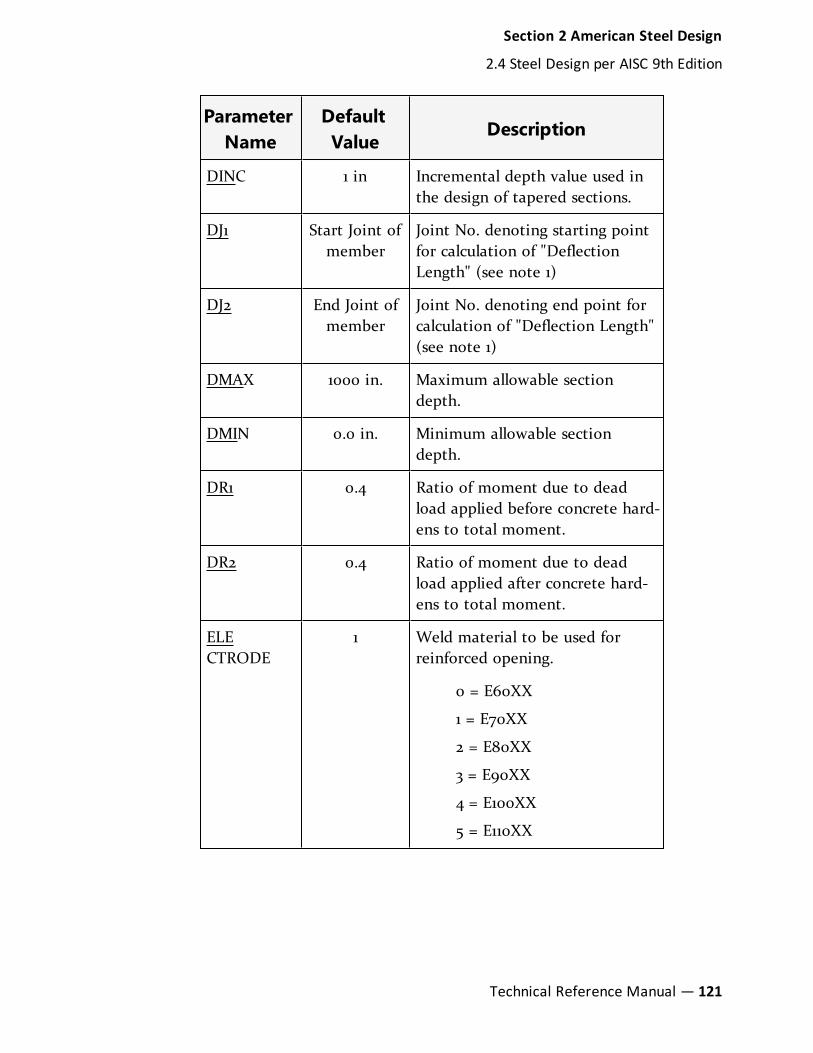
ParameterName
DefaultValue
Description
DINC 1 in Incremental depth value used inthe design of tapered sections.
DJ1 Start Joint ofmember
Joint No. denoting starting pointfor calculation of "DeflectionLength" (see note 1)
DJ2 End Joint ofmember
Joint No. denoting end point forcalculation of "Deflection Length"(see note 1)
DMAX 1000 in. Maximum allowable sectiondepth.
DMIN 0.0 in. Minimum allowable sectiondepth.
DR1 0.4 Ratio of moment due to deadload applied before concrete hard-ens to total moment.
DR2 0.4 Ratio of moment due to deadload applied after concrete hard-ens to total moment.
ELECTRODE
1 Weld material to be used forreinforced opening.
0 = E60XX
1 = E70XX
2 = E80XX
3 = E90XX
4 = E100XX
5 = E110XX
Section 2 American Steel Design
2.4 Steel Design per AISC 9th Edition
Technical Reference Manual — 121

ParameterName
DefaultValue
Description
FBINC 0 Incremental bottom flange widthused in the design of tapered sec-tions. In this case, the top flangewidth will remain unchanged.
FLX 1 Single angle member bracing
1 = Single anglemember is not fullybraced against lateraltorsional buckling.
2 = Single anglemember is fully bracedagainst lateraltorsional buckling.
3 = Single anglemember is bracedagainst lateraltorsional buckling atthe point of maximummoment.
FPC 3.0 ksi Compressive strength of concreteat 28 days
FSS 1 Is the full section to be used forshear design?
0 = No (False)
1 = Yes (True)
FTBINC 0 Incremental flange width (topand bottom) used in the designof tapered sections.
122— STAAD.Pro V8i (SELECTseries 4)
Section 2 American Steel Design
2.4 Steel Design per AISC 9th Edition

ParameterName
DefaultValue
Description
FTINC 0 Incremental top flange widthused in the design of tapered sec-tions. In this case, the bottomflange width will remainunchanged.
FU Depends onFYLD
Ultimate tensile strength of steelin current units.
l If FYLD < 40 KSI, then FU =58 KSI
l If 40 KSI ≤ FYLD ≤ 50 KSI,then FU = 60 KSI
l If FYLD > 50 KSI, then FU =65 KSI
FYLD 36 KSI Yield strength of steel in currentunits.
HECC 0.0 Eccentricity of opening withrespect to the centerline of themember.
KX 1.0 K value used in computing KL/rfor flexural torsional buckling fortees and double angles.
KY 1.0 K value in local y-axis. Usually,this is the minor axis.
KZ 1.0 K value in local z-axis. Usually,this is the major axis.
LX MemberLength
Length value used in computingKL/r for flexural torsional buck-ling for tees and double angles.
Section 2 American Steel Design
2.4 Steel Design per AISC 9th Edition
Technical Reference Manual — 123
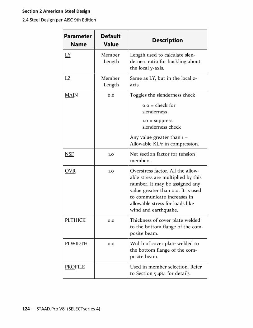
ParameterName
DefaultValue
Description
LY MemberLength
Length used to calculate slen-derness ratio for buckling aboutthe local y-axis.
LZ MemberLength
Same as LY, but in the local z-axis.
MAIN 0.0 Toggles the slenderness check
0.0 = check forslenderness
1.0 = suppressslenderness check
Any value greater than 1 =Allowable KL/r in compression.
NSF 1.0 Net section factor for tensionmembers.
OVR 1.0 Overstress factor. All the allow-able stress are multiplied by thisnumber. It may be assigned anyvalue greater than 0.0. It is usedto communicate increases inallowable stress for loads likewind and earthquake.
PLTHICK 0.0 Thickness of cover plate weldedto the bottom flange of the com-posite beam.
PLWIDTH 0.0 Width of cover plate welded tothe bottom flange of the com-posite beam.
PROFILE Used in member selection. Referto Section 5.48.1 for details.
124— STAAD.Pro V8i (SELECTseries 4)
Section 2 American Steel Design
2.4 Steel Design per AISC 9th Edition

ParameterName
DefaultValue
Description
RATIO 1.0 Permissible ratio of actual toallowable stress.
RDIM 0.0 Dimensions of rectangularopenings (at each section, RDIMhas a length term and a depthterm – see syntax below). If amember has more than onerectangular opening they canhave different dimensions.
RHOLE None Section locations of rectangularopenings along the length of themember. Maximum threelocations can be specified foreach member when there is nocircular opening.
RBHEIGHT 0.0 Height of ribs in the form steeldeck.
RBWIDTH 2.5 in. Width of ribs in the form steeldeck.
SHE 0 Option for calculating actualshear stress.
0 = Compute theshear stress usingVO/Ib
1 = Computer theshear stress based onthe area of the sectionelement.
Section 2 American Steel Design
2.4 Steel Design per AISC 9th Edition
Technical Reference Manual — 125

ParameterName
DefaultValue
Description
SHR 0 Indicates use of temporaryshoring during construction.
0 = Without shoring
1 = With shoring
SSY 0.0 Sidesway
0.0 = Sidesway in localy-axis.
1.0 = No sidesway
SSZ 0.0 Same as SSY, but in local z-axis.
STIFF MemberLength ordepth of
beam, which-ever isgreater
Spacing of stiffeners for plategirder design.
STP 1 Section type as defined inASD Manual table.
1 = Rolled
2 = Welded
126— STAAD.Pro V8i (SELECTseries 4)
Section 2 American Steel Design
2.4 Steel Design per AISC 9th Edition

ParameterName
DefaultValue
Description
TAPER 1.0 Design basis for tapered members
0.0 = Design taperedI-section based onrules of Chapter F andAppendix B of AISConly. Due not use therules in Appendix F ofAISC-89.
1.0 = Design tapered I-sections based on therules of Appendix F ofAISC-89.
THK 4.0 in. Thickness of concrete slab or thethickness of concrete slab abovethe form steel deck.
TMAIN 300 Any value greater than 1 = Allow-able KL/r in tension.
TORSION 0.0 Toggles the check for torsion
0.0 = No torsion checkis performed
1.0 = Perform torsioncheck based on rulesof AISC T114.
TRACK 0.0 Controls the level of detail towhich results are reported:
0 = minimum detail
1 = intermediate detail
2 = maximum detail(see Figure 2.1)
Section 2 American Steel Design
2.4 Steel Design per AISC 9th Edition
Technical Reference Manual — 127

ParameterName
DefaultValue
Description
UNB MemberLength
Unsupported length of the bot-tom* flange for calculating allow-able bending compressive stress.Will be used only if flexural com-pression is on the bottom flange
UNT MemberLength
Unsupported length of the top*flange for calculating allowablebending compressive stress. Willbe used only if flexural com-pression is on the top flange.
WELD 1 for closedsections, 2for open sec-
tions
Weld type, as explained in Sec-tion 2.12. A value of 1 will meanwelding is on one side onlyexcept for wide-flange or tee sec-tions, where the web is alwaysassumed to be welded on bothsides. A value of 2 will mean weld-ing on both sides. For closed sec-tions like a pipe or tube, thewelding will be on one side only.
WIDTH 0.25 timesthe memberlength
Effective width of the concreteslab.
WMAX See Section2.12
Maximum welding thickness.
WMIN See Section2.12
Minimum welding thickness.
WSTR 0.4 x FYLD Allowable weld stress.
*Top and Bottom represent the positive and negative side of the local Y axis(local Z axis if SET Z UP is used).
128— STAAD.Pro V8i (SELECTseries 4)
Section 2 American Steel Design
2.4 Steel Design per AISC 9th Edition

Notes
1. When performing the deflection check, you can choose between twomethods. The first method, defined by a value 0 for the CAN parameter, isbased on the local displacement. See "Printing Section Displacements forMembers" on page 724 for details on local displacement.
If the CAN parameter is set to 1, the check will be based on cantilever styledeflection. Let (DX1, DY1,DZ1) represent the nodal displacements (in globalaxes) at the node defined by DJ1 (or in the absence of DJ1, the start nodeof the member). Similarly, (DX2, DY2, DZ2) represent the deflection valuesat DJ2 or the end node of the member.
Compute Delta = (DX2 − DX1) + (DY2 − DY1) + (DZ2 − DZ1)2 2 2
Compute Length = distance between DJ1 and DJ2 or, between start nodeand end node, as the case may be.
Then, if CAN is specified a value 1, dff = L/Delta
Ratio due to deflection = DFF/dff
2. If CAN = 0, deflection length is defined as the length that is used forcalculation of local deflections within a member. It may be noted that formost cases the “Deflection Length” will be equal to the length of themember. However, in some situations, the “Deflection Length” may bedifferent.
For example, refer to the figure below where a beam has been modeledusing four joints and three members. The “Deflection Length” for all threemembers will be equal to the total length of the beam in this case. Theparameters DJ1 and DJ2 should be used to model this situation. Also thestraight line joining DJ1 and DJ2 is used as the reference line from whichlocal deflections are measured. Thus, for all three members here, DJ1 shouldbe "1" and DJ2 should be "4".
D is equal to the maximum local deflection for members 1, 2, and 3.
PARAMETERS
Section 2 American Steel Design
2.4 Steel Design per AISC 9th Edition
Technical Reference Manual — 129
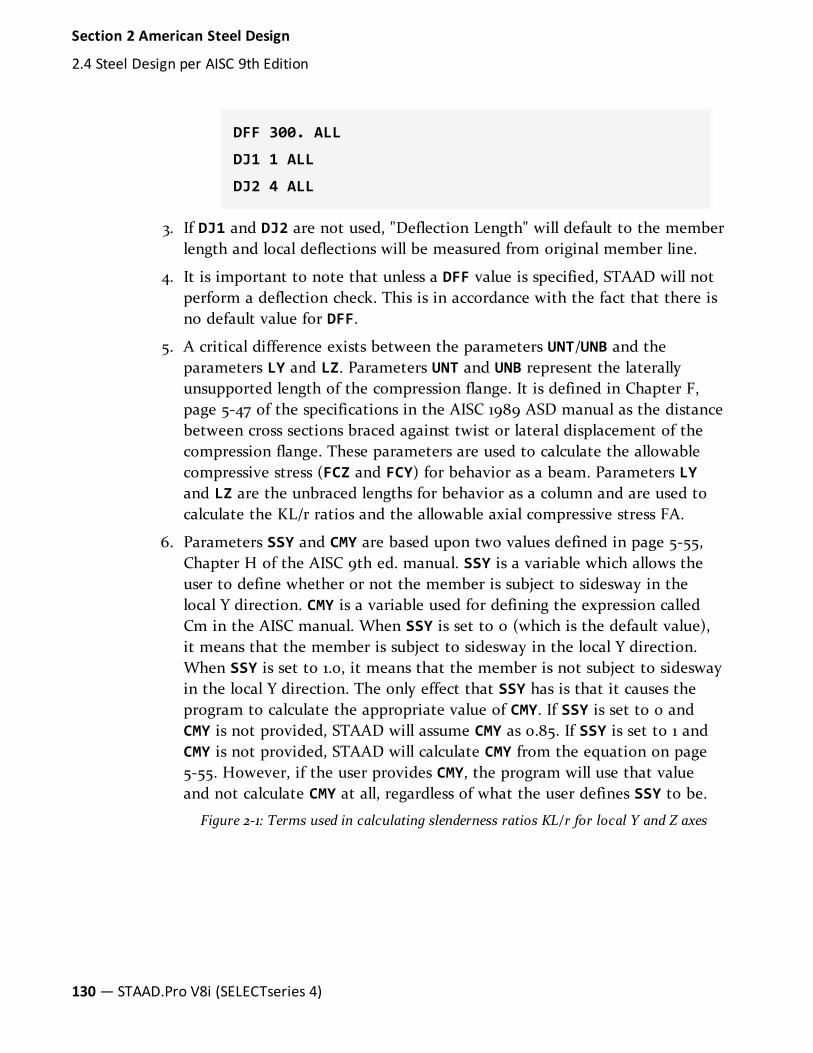
DFF 300. ALL
DJ1 1 ALL
DJ2 4 ALL
3. If DJ1 and DJ2 are not used, "Deflection Length" will default to the memberlength and local deflections will be measured from original member line.
4. It is important to note that unless a DFF value is specified, STAAD will notperform a deflection check. This is in accordance with the fact that there isno default value for DFF.
5. A critical difference exists between the parameters UNT/UNB and theparameters LY and LZ. Parameters UNT and UNB represent the laterallyunsupported length of the compression flange. It is defined in Chapter F,page 5-47 of the specifications in the AISC 1989 ASD manual as the distancebetween cross sections braced against twist or lateral displacement of thecompression flange. These parameters are used to calculate the allowablecompressive stress (FCZ and FCY) for behavior as a beam. Parameters LYand LZ are the unbraced lengths for behavior as a column and are used tocalculate the KL/r ratios and the allowable axial compressive stress FA.
6. Parameters SSY and CMY are based upon two values defined in page 5-55,Chapter H of the AISC 9th ed. manual. SSY is a variable which allows theuser to define whether or not the member is subject to sidesway in thelocal Y direction. CMY is a variable used for defining the expression calledCm in the AISC manual. When SSY is set to 0 (which is the default value),it means that the member is subject to sidesway in the local Y direction.When SSY is set to 1.0, it means that the member is not subject to sideswayin the local Y direction. The only effect that SSY has is that it causes theprogram to calculate the appropriate value of CMY. If SSY is set to 0 andCMY is not provided, STAAD will assume CMY as 0.85. If SSY is set to 1 andCMY is not provided, STAAD will calculate CMY from the equation on page5-55. However, if the user provides CMY, the program will use that valueand not calculate CMY at all, regardless of what the user defines SSY to be.
Figure 2-1: Terms used in calculating slenderness ratios KL/r for local Y and Z axes
130— STAAD.Pro V8i (SELECTseries 4)
Section 2 American Steel Design
2.4 Steel Design per AISC 9th Edition

7. For a T shape which is cut from a parent I, W, S, M or H shapes, thePROFILE parameter should be assigned a value corresponding to the parentshape. For example, if the T desired is an American WT6, specify W12 forthe PROFILE parameter.
2.4.1.3 Code Checking
The purpose of code checking is to check whether the provided sectionproperties of the members are adequate. The adequacy is checked as per AISC-89. Code checking is done using the forces and moments at specified sections ofthe members. If no sections are specified, the program uses the start and endforces for code checking.
When code checking is selected, the program calculates and prints whether themembers have passed the code or have failed; the critical condition of the AISCcode (like any of the AISC specifications or compression, tension, shear, etc.); thevalue of the ratio of the critical condition (overstressed for a value more than 1.0or any other specified RATIO value); the governing load case, and the location(distance from the start of the member) of forces in the member where thecritical condition occurs.
Code checking can be done with any type of steel section listed in Section 2.2.1 ofthis manual.
Section 2 American Steel Design
2.4 Steel Design per AISC 9th Edition
Technical Reference Manual — 131

2.4.1.4 Member Selection
STAAD is capable of performing design operations on specified members. Oncean analysis has been performed, the program can select the most economicalsection (i.e., the lightest section) which fulfills the code requirements for thespecified member. The section selected will be of the same type section asoriginally designated for the member being designed. A wide flange will beselected to replace a wide flange, etc. Several parameters are available to guidethis selection. If the PROFILE parameter is provided, the search for the lightestsection is restricted to that profile. Up to three (3) profiles may be provided forany member with a section being selected from each one. Member selection canalso be constrained by the parameters DMAX and DMIN which limit the maximumand minimum depth of the members. If the PROFILE parameter is provided forspecified members, DMAX or DMIN parameters will be ignored by the program inselecting these members.
Member selection can be performed with all the types of steel sections listed inSection 2.2.1 of this manual. Note that for beams with cover plates, the sizes ofthe cover plate are kept constant while the beam section is iterated.
Selection of members, whose properties are originally input from a user createdtable, will be limited to sections in that table.
Member selection cannot be performed on members whose section properties areinput as prismatic.
2.4.1.4.1 Member Selection by Optimization
Steel table properties of an entire structure can be optimized by STAAD. Thisoptimization method involves the following steps.
1. CHECK CODE ALL
2. Modify the ratios
3. SELECT ALL
4. PERFORM ANALYSIS
5. SELECT ALL
An additional step of grouping may be performed if the FIXED GROUP and GROUPcommands are provided (See "Group Specification" on page 734). After the laststep, a re-analysis is not automatically performed, so users must ensure that theyspecify the analysis command following the SELECT OPTIMIZE command.
132— STAAD.Pro V8i (SELECTseries 4)
Section 2 American Steel Design
2.4 Steel Design per AISC 9th Edition

2.4.1.4.2 Deflection Check With Steel Design
This facility allows the user to consider deflection as a criteria in the CODE CHECKand MEMBER SELECTION processes. The deflection check may be controlled usingthe three parameters DJ1, DJ2, and DFF which are described in Table 2.1.Deflection is used in addition to other strength and stability related criteria. Thelocal deflection calculation is based on the latest analysis results.
2.4.1.5 Truss Members
As described in Section 1.9, a truss member is capable of carrying only axialforces. So during the design phase, no calculation time (or, matrix bandwidth) iswasted determining the allowable bending or shear stresses. Therefore, if there isany truss member in an analysis (such as a bracing or a strut, etc.), it is advisableto declare it as a truss member rather than as a regular frame member with bothends pinned.
2.4.1.6 Unsymmetric Sections
For unsymmetric sections like single angles, STAAD considers the smaller sectionmodulus for calculating bending stresses.
For single angles, the “specification for allowable stress design of single-anglemembers”, explained in pages 5-309 to 5-314 of the AISC-ASD 9th edition manualhas been incorporated.
2.4.1.7 Composite Beam Design as per AISC-ASD
In Section 1.7.7 of this manual, two methods of specifying the properties of abeam as a composite section (I-shaped beam with concrete slab on top) aredescribed. Those members can be designed as composite beams in accordancewith the AISC ASD code provisions. If the properties are assigned using theexplicit method as defined in Section 1.7.7, the design parameters must beseparately assigned. The CMP parameter in particular must be set a value of 1 or2. If the properties are derived from the composite decks, the design parametersare automatically generated during the deck creation phase, and hence noseparate parameters need to be assigned.
Other parameters used in the design of composite members are: DIA, DR1, DR2,FPC, HGT, PLTHICK, PLWIDTH, RBHEIGHT, RBWWIDTH, SHR, THK, and WIDTH. Referto Table 2-3 for details on design parameters.
Section 2 American Steel Design
2.4 Steel Design per AISC 9th Edition
Technical Reference Manual — 133
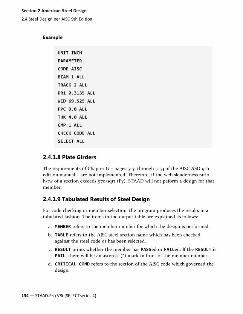
Example
UNIT INCH
PARAMETER
CODE AISC
BEAM 1 ALL
TRACK 2 ALL
DR1 0.3135 ALL
WID 69.525 ALL
FPC 3.0 ALL
THK 4.0 ALL
CMP 1 ALL
CHECK CODE ALL
SELECT ALL
2.4.1.8 Plate Girders
The requirements of Chapter G – pages 5-51 through 5-53 of the AISC ASD 9thedition manual – are not implemented. Therefore, if the web slenderness ratioh/tw of a section exceeds 970/sqrt (Fy), STAAD will not peform a design for thatmember.
2.4.1.9 Tabulated Results of Steel Design
For code checking or member selection, the program produces the results in atabulated fashion. The items in the output table are explained as follows:
a. MEMBER refers to the member number for which the design is performed.
b. TABLE refers to the AISC steel section name which has been checkedagainst the steel code or has been selected.
c. RESULT prints whether the member has PASSed or FAILed. If the RESULT isFAIL, there will be an asterisk (*) mark in front of the member number.
d. CRITICAL COND refers to the section of the AISC code which governed thedesign.
134— STAAD.Pro V8i (SELECTseries 4)
Section 2 American Steel Design
2.4 Steel Design per AISC 9th Edition
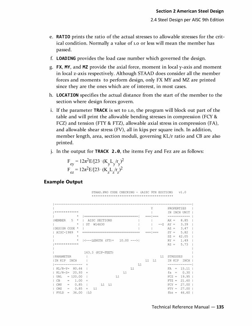
e. RATIO prints the ratio of the actual stresses to allowable stresses for the crit-ical condition. Normally a value of 1.0 or less will mean the member haspassed.
f. LOADING provides the load case number which governed the design.
g. FX, MY, and MZ provide the axial force, moment in local y-axis and momentin local z-axis respectively. Although STAAD does consider all the memberforces and moments to perform design, only FX MY and MZ are printedsince they are the ones which are of interest, in most cases.
h. LOCATION specifies the actual distance from the start of the member to thesection where design forces govern.
i. If the parameter TRACK is set to 1.0, the program will block out part of thetable and will print the allowable bending stresses in compression (FCY &FCZ) and tension (FTY & FTZ), allowable axial stress in compression (FA),and allowable shear stress (FV), all in kips per square inch. In addition,member length, area, section moduli, governing KL/r ratio and CB are alsoprinted.
j. In the output for TRACK 2.0, the items Fey and Fez are as follows:
Fey = 12π2E/[23⋅(KyLy/ry)
2
Fez = 12π2E/[23⋅(KzLz/rz)
2
Example Output
STAAD.PRO CODE CHECKING - (AISC 9TH EDITION) v1.0********************************************
|--------------------------------------------------------------------------|| Y PROPERTIES ||************* | IN INCH UNIT || * |=============================| ===|=== ------------ ||MEMBER 5 * | AISC SECTIONS | | AX = 8.85 || * | ST W14X30 | | --Z AY = 3.39 ||DESIGN CODE * | | | AZ = 3.47 || AISC-1989 * =============================== ===|=== SY = 5.82 || * SZ = 42.05 || * |<---LENGTH (FT)= 10.00 --->| RY = 1.49 ||************* RZ = 5.73 || || 163.3 (KIP-FEET) ||PARAMETER | L1 STRESSES ||IN KIP INCH | L1 L1 IN KIP INCH ||--------------- + L1 -------------|| KL/R-Y= 80.64 | L1 FA = 15.11 || KL/R-Z= 20.93 + L1 fa = 0.30 || UNL = 120.00 | L1 FCZ = 19.95 || CB = 1.00 + FTZ = 21.60 || CMY = 0.85 | L1 L1 FCY = 27.00 || CMZ = 0.85 + L1 FTY = 27.00 || FYLD = 36.00 |L0 fbz = 46.60 |
Section 2 American Steel Design
2.4 Steel Design per AISC 9th Edition
Technical Reference Manual — 135

| NSF = 0.85 +---+---+---+---+---+---+---+---+---+---| fby = 0.00 || DFF = 0.00 -9.1 Fey = 22.97 || dff= 0.00 ABSOLUTE MZ ENVELOPE Fez = 340.99 || (KL/R)max = 80.64 (WITH LOAD NO.) FV = 14.40 || fv = 4.78 || || MAX FORCE/ MOMENT SUMMARY (KIP-FEET) || ------------------------- || || AXIAL SHEAR-Y SHEAR-Z MOMENT-Y MOMENT-Z || || VALUE -2.7 16.5 0.0 0.0 163.3 || LOCATION 0.0 0.0 0.0 0.0 10.0 || LOADING 1 1 0 0 1 || ||**************************************************************************||* *||* DESIGN SUMMARY (KIP-FEET) *||* -------------- *||* *||* RESULT/ CRITICAL COND/ RATIO/ LOADING/ *|| FX MY MZ LOCATION || ====================================================== || FAIL AISC- H2-1 2.335 1 || 2.66 T 0.00 -163.32 10.00 ||* *||**************************************************************************|| ||--------------------------------------------------------------------------|
2.4.2 Steel Design per AISC/LRFD SpecificationThe 2nd and 3rd editions of the American LRFD code have been implemented.The commands to access those respective codes are:
For the 3rd edition code:
PARAMETER
CODE LRFD
or
PARAMETER
CODE LRFD3
For the 2nd Edition:
PARAMETER
CODE LRFD2
2.4.2.1 General Comments
The design philosophy embodied in the Load and Resistance Factor Design(LRFD) Specification is built around the concept of limit state design, the currentstate-of-the-art in structural engineering. Structures are designed and
136— STAAD.Pro V8i (SELECTseries 4)
Section 2 American Steel Design
2.4 Steel Design per AISC 9th Edition

proportioned taking into consideration the limit states at which they wouldbecome unfit for their intended use. Two major categories of limit-state arerecognized--ultimate and serviceability. The primary considerations in ultimatelimit state design are strength and stability, while that in serviceability isdeflection. Appropriate load and resistance factors are used so that a uniformreliability is achieved for all steel structures under various loading conditions andat the same time the chances of limits being surpassed are acceptably remote.
In the STAAD implementation of LRFD, members are proportioned to resist thedesign loads without exceeding the limit states of strength, stability andserviceability. Accordingly, the most economic section is selected on the basis ofthe least weight criteria as augmented by the designer in specification ofallowable member depths, desired section type, or other such parameters. Thecode checking portion of the program checks that code requirements for eachselected section are met and identifies the governing criteria.
The following sections describe the salient features of the LRFD specifications asimplemented in STAAD steel design. A detailed description of the design processalong with its underlying concepts and assumptions is available in the LRFDmanual. However, since the design philosophy is drastically different from theconventional Allowable Stress Design (ASD), a brief description of thefundamental concepts is presented here to initiate the user into the designprocess.
2.4.2.2 LRFD Fundamentals
The primary objective of the LRFD Specification is to provide a uniformreliability for all steel structures under various loading conditions. Thisuniformity can not be obtained with the allowable stress design (ASD) format.
The ASD method can be represented by the inequality
ΣQi < Rn/F.S.
The left side is the required strength, which is the summation of the load effects,Qi (forces and moments). The right side, the design strength, is the nominalstrength or resistance, Rn, divided by a factor of safety. When divided by theappropriate section property (area or section modulus), the two sides of theinequality become the actual stress and allowable stress respectively. ASD, then,is characterized by the use of unfactored "working" loads in conjunction with asingle factor of safety applied to the resistance. Because of the greater variabilityand, hence, unpredictability of the live load and other loads in comparison withthe dead load, a uniform reliability is not possible.
Section 2 American Steel Design
2.4 Steel Design per AISC 9th Edition
Technical Reference Manual — 137

LRFD, as its name implies, uses separate factors for each load and resistance.Because the different factors reflect the degree of uncertainty of different loadsand combinations of loads and of the accuracy of predicted strength, a moreuniform reliability is possible. The LRFD method may be summarized by theinequality
yiQi < RnØ
On the left side of the inequality, the required strength is the summation of thevarious load effects, Qi, multiplied by their respective load factors, yi. The designstrength, on the right side, is the nominal strength or resistance, Rn, multipliedby a resistance factor, Ø.
In the STAAD implementation of LRFD, it is assumed that the user will useappropriate load factors and create the load combinations necessary for analysis.The design portion of the program will take into consideration the load effects(forces and moments) obtained from analysis. In calculation of resistances ofvarious elements (beams, columns etc.), resistance (nominal strength) andapplicable resistance factor will be automatically considered.
2.4.2.3 Analysis Requirements
The types of construction recognized by AISC specification have not changed,except that both "simple framing" (formerly Type 2) and "semi-rigid framing"(formerly Type 3) have been combined into the same category, Type PR (partiallyrestrained). "Rigid Framing" (formerly Type 1) is now Type FR (fully restrained).Type FR construction is permitted unconditionally. Type PR construction maynecessitate some inelastic, but self-limiting, deformation of a structural steelelement. Thus, when specifying Type PR construction, the designer should takeinto consideration the effects of partial restraint on the stability of the structure,lateral deflections and second order bending moments. As stated in Sect. C1 ofthe LRFD specification, an analysis of second order effects is required. Thus,when using LRFD code for steel design, the user must use the P-Delta analysisfeature of STAAD.
2.4.2.4 Section Classification
The LRFD specification allows inelastic deformation of section elements. Thuslocal buckling becomes an important criterion. Steel sections are classified ascompact, noncompact or slender element sections depending upon their localbuckling characteristics. This classification is a function of the geometricproperties of the section. The design procedures are different depending on the
138— STAAD.Pro V8i (SELECTseries 4)
Section 2 American Steel Design
2.4 Steel Design per AISC 9th Edition

section class. STAAD is capable of determining the section classification for thestandard shapes and user specified shapes and design accordingly.
2.4.2.5 Limit States
2.4.2.5.1 Axial Tension
The criteria governing the capacity of tension members is based on two limitstates. The limit state of yielding in the gross section is intended to preventexcessive elongation of the member. The second limit state involves fracture atthe section with the minimum effective net area. The net section area may bespecified by the user through the use of the parameter NSF (see Table 2.6).STAAD calculates the tension capacity of a given member based on these twolimit states and proceeds with member selection or code check accordingly.
2.4.2.5.2 Axial Compression
The column strength equations have been revised in LRFD to take into accountinelastic deformation and other recent research in column behavior. Twoequations governing column strength are available, one for inelastic buckling andthe other for elastic or Euler buckling. Both equations include the effects ofresidual stresses and initial out-of-straightness. Compression strength for aparticular member is calculated by STAAD according to the procedure outlined inChapter E of the LRFD specifications. For slender elements, the proceduredescribed in Appendix B5.3 is used.
Singly symmetric and unsymmetric compression members are designed on thebasis of the limit states of flexural-torsional and torsional buckling. Theprocedure of Appendix E3 is implemented for the determination of designstrength for these limit states.
Effective length for calculation of compression resistance may be providedthrough the use of the parameters KY, KZ and/or LY, LZ. If not provided, theentire member length will be taken into consideration.
In addition to the compression resistance criterion, compression members arerequired to satisfy slenderness limitations which are a function of the nature ofuse of the member (main load resisting component, bracing member, etc.). Inboth the member selection and code checking process, STAAD immediately doesa slenderness check on appropriate members before continuing with otherprocedures for determining the adequacy of a given member.
Section 2 American Steel Design
2.4 Steel Design per AISC 9th Edition
Technical Reference Manual — 139

2.4.2.5.3 Flexural Design Strength
In LRFD, the flexural design strength of a member is determined by the limitstate of lateral torsional buckling. Inelastic bending is allowed and the basicmeasure of flexural capacity is the plastic moment capacity of the section. Theflexural resistance is a function of plastic moment capacity, actual laterallyunbraced length, limiting laterally unbraced length, buckling moment and thebending coefficient. The limiting laterally unbraced length Lr and bucklingmoment Mr are functions of the section geometry and are calculated as per theprocedure of Chapter F. The purpose of bending coefficient Cb is to account forthe influence of the moment gradient on lateral-torsional buckling. Thiscoefficient can be specified by the user through the use of parameter CB (seeTable 2.6) or may be calculated by the program (if CB is specified as 0.0). In theabsence of the parameter CB, a default value of 1.0 will be used. The procedurefor calculation of design strength for flexure also accounts for the presence ofresidual stresses of rolling. To specify laterally unsupported length, either of theparameters UNB and UNT (see Table 2.6) can be used.
2.4.2.5.4 Combined Axial Force and Bending
The interaction of flexure and axial forces in singly and doubly symmetric shapesis governed by formulas H1-1a and H1-1b. These interaction formulas cover thegeneral case of biaxial bending combined with axial force. They are also valid foruniaxial bending and axial force.
2.4.2.5.5 Design for Shear
The procedure of Sect. F2 of the LRFD Specification is used in STAAD to designfor shear forces in members. Shear strength as calculated in LRFD is governed bythe following limit states: Eq. F2-1a by yielding of the web; Eq. F2-2a by inelasticbuckling of the web; Eq. F2-3a by elastic buckling of the web. Shear in wideflanges and channel sections is resisted by the area of the web, which is taken asthe overall depth times the web thickness.
2.4.2.6 Design Parameters
Design per LRFD specifications is requested by using the CODE parameter. Otherapplicable parameters are summarized in Table 2-4. These parameterscommunicate design decisions from the engineer to the program and thus allowthe engineer to control the design process to suit an application's specific needs.
140— STAAD.Pro V8i (SELECTseries 4)
Section 2 American Steel Design
2.4 Steel Design per AISC 9th Edition

The default parameter values have been selected such that they are frequentlyused numbers for conventional design. Depending on the particular designrequirements, some or all of these parameter values may be changed to exactlymodel the physical structure.
The parameters DMAX and DMIN are applicable for member selection only.
ParameterName
DefaultValue
Description
AXIS 1 1 = Design single angles for bendingabout their principle axis.
2 = Design single angles forbending about their geometric axis.
BEAM 1.0 0.0 = design at ends and thoselocations specified by the SECTIONcommand.
1.0 = design at ends and at every1/12th point along member length.
CAN 0 0 = deflection check based on theprinciple that maximum deflectionoccurs within the span between DJ1and DJ2.
1 = deflection check based on theprinciple that maximum deflectionis of the cantilever type (see note 2of Table 2.1)
CB** 1.0 Coefficient Cb per Chapter F ofAISC LRFD. If Cb is set to 0.0, itwill be calculated by the program.Any of value will be used directlyin design.
DFF None (Man-datory fordeflectioncheck)
"Deflection Length" / Maximumallowable local deflection
Table 2-3: AISC LRFD (2nd and 3rd Ed.) Design Parameters
Section 2 American Steel Design
2.4 Steel Design per AISC 9th Edition
Technical Reference Manual — 141

ParameterName
DefaultValue
Description
DJ1 Start Jointof Member
Joint No. denoting starting pointfor calculation of "DeflectionLength" (see note 1 of Table 2.1)
DJ2 End Jointof Member
Joint No. denoting end point forcalculation of "Deflection Length"(see note 1 of Table 2.1)
DMAX 45.0 in. Maximum allowable section depth.
DMIN 0.0 in. Minimum allowable section depth
FLX 1 1 = Single angle member is not fullybraced against lateral torsionalbuckling.
2 = Single angle member is fullybraced against lateral torsionalbuckling.
3 = Single angle member is bracedagainst lateral torsional buckling atthe point of maximum moment.
FYLD 36.0 ksi Yield strength of steel.
FU 60.0 ksi Ultimate tensile strength of steel.
KX 1.0 K value for flexural-torsional buck-ling.
KY 1.0 K value in the local y-axis. Usuallythis is the minor axis.
KZ 1.0 K value in the local z-axis. Usuallythis is the major axis.
LX MemberLength
Length used for flexural-torsionalbuckling.
142— STAAD.Pro V8i (SELECTseries 4)
Section 2 American Steel Design
2.4 Steel Design per AISC 9th Edition

ParameterName
DefaultValue
Description
LY MemberLength
Length to calculate the slendernessratio for buckling about the local y-axis.
LZ MemberLength
Length to calculate the slendernessratio for buckling about the local z-axis.
MAIN 0.0 0.0 = check for slenderness
1.0 = suppress slenderness check
Any value greater than 1 =Allowable KL/r in compression.
NSF 1.0 Net section factor for tensionmembers.
PROFILE Used in member selection. Refer toSection 5.48.1 for details.
RATIO 1.0 Permissible ratio of actual loadeffect to design strength.
STIFF MemberLength ordepth,
whicheveris greater
Spacing of stiffeners for beams forshear design.
STP 1 Section type to determine Fr
(compressive residual stress inflange) per 3rd Ed. LRFD spec., p16.1-97.
1 = Rolled section (Fr=
10 ksi)
2 = Welded section (Fr
= 16.5 ksi)
Section 2 American Steel Design
2.4 Steel Design per AISC 9th Edition
Technical Reference Manual — 143
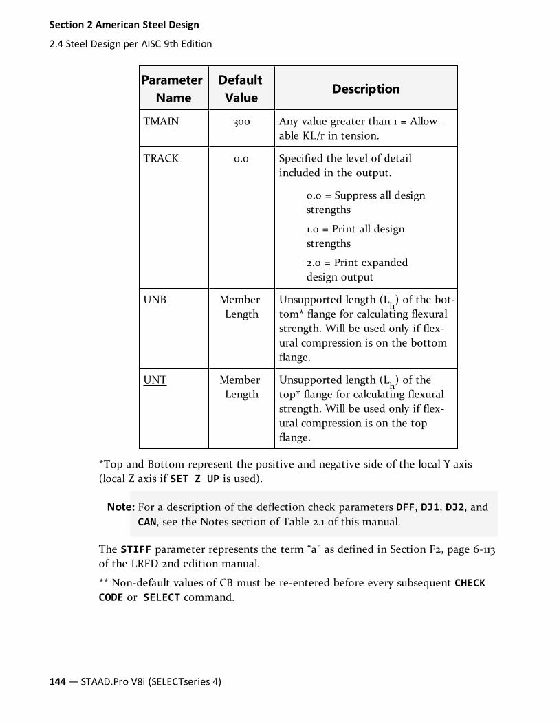
ParameterName
DefaultValue
Description
TMAIN 300 Any value greater than 1 = Allow-able KL/r in tension.
TRACK 0.0 Specified the level of detailincluded in the output.
0.0 = Suppress all designstrengths
1.0 = Print all designstrengths
2.0 = Print expandeddesign output
UNB MemberLength
Unsupported length (Lh) of the bot-
tom* flange for calculating flexuralstrength. Will be used only if flex-ural compression is on the bottomflange.
UNT MemberLength
Unsupported length (Lh) of the
top* flange for calculating flexuralstrength. Will be used only if flex-ural compression is on the topflange.
*Top and Bottom represent the positive and negative side of the local Y axis(local Z axis if SET Z UP is used).
Note: For a description of the deflection check parameters DFF, DJ1, DJ2, andCAN, see the Notes section of Table 2.1 of this manual.
The STIFF parameter represents the term “a” as defined in Section F2, page 6-113of the LRFD 2nd edition manual.
** Non-default values of CB must be re-entered before every subsequent CHECKCODE or SELECT command.
144— STAAD.Pro V8i (SELECTseries 4)
Section 2 American Steel Design
2.4 Steel Design per AISC 9th Edition

2.4.2.7 Code Checking and Member Selection
Both code checking and member selection options are available in STAAD LRFDimplementation. See "Code Checking" on page 131 and See "Member Selection" onpage 132 for general information on these options. See "Code CheckingSpecification" on page 731 and See "Member Selection Specification" on page 732for information on specification of these commands.
Example for the LRFD-2001 code
UNIT KIP INCH
PARAMETER
CODE LRFD
FYLD 50 ALL
UNT 72 MEMBER 1 TO 10
UNB 72 MEMB 1 TO 10
MAIN 1.0 MEMB 17 20
SELECT MEMB 30 TO 40
CHECK CODE MEMB 1 TO 30
Example for the LRFD-1994 code
UNIT KIP INCH
PARAMETER
CODE LRFD2
FYLD 50 ALL
UNT 72 MEMBER 1 TO 10
UNB 72 MEMB 1 TO 10
MAIN 1.0 MEMB 17 20
SELECT MEMB 30 TO 40
CHECK CODE MEMB 1 TO 30
Section 2 American Steel Design
2.4 Steel Design per AISC 9th Edition
Technical Reference Manual — 145

2.4.2.8 Tabulated Results of Steel Design
Results of code checking and member selection are presented in a tabular format.A detailed discussion of the format is provided in Section 2.11. Followingexceptions may be noted: CRITICAL COND refers to the section of the LRFDspecifications which governed the design.
If the TRACK is set to 1.0, member design strengths will be printed out.
2.4.2.9 Composite Beam Design per the American LRFD 3rdedition code
The design of composite beams per the 3rd edition of the American LRFD codehas been implemented. The salient points of this feature are as follows:
Figure 2-2: Nomenclature of composite beams
Theoretical Basis
1. Find the maximum compressive force carried by concrete as:
0.85 fc⋅b⋅t
2. Find the maximum tensile force carried by the steel beam as:
As . fy
146— STAAD.Pro V8i (SELECTseries 4)
Section 2 American Steel Design
2.4 Steel Design per AISC 9th Edition

Tensile strength of concrete is ignored.
3. If step 1 produces a higher value than step 2, plastic neutral axis (PNA) is inthe slab. Else, it is in the steel beam.
Location of the Plastic Neutral Axis (PNA) defines the moment capacity:
l Case 1: PNA in the slab
Find the depth of the PNA below the top of the slab as:
0.85fc⋅b⋅a = As⋅fyRearranging terms:
a = As⋅fy/(0.85fc⋅b)
Figure 2-3: Plastic neutral axis in the concrete slab
Lever arm
e = d/2 + hr + t - a/2
Moment Capacity
φb(As⋅fy)e
l Case 2: PNA in Steel Beam
Define:
Cs= Compressive force in slab = 0.85f
c⋅b⋅t
Cb= Compressive force in steel beam
Tb= Tensile force in steel beam
Section 2 American Steel Design
2.4 Steel Design per AISC 9th Edition
Technical Reference Manual — 147

Cs + Cb = TbSince the magnitude of C
b+ magnitude of T
b= A
s⋅fy
Substituting for Tb as (As⋅fy- C
b) gives:
Cs+ Cb = As⋅fy - CbRearranging terms:
Cb= (As⋅fy - Cs)/2
Determine whether the PNA is within the top flang of the steel beam orinside the web:
Cf= Maximum compressive force carried by the flange = A
f⋅fy
Where:
Af= Area of the flange
If Cf≥ C
b, the PNA lies within the flange (Case 2A)
If Cf< C
b, the PNA lies within the web (Case 2B)
l Case 2A: PNA in Flange of Steel Beam
Calculate:
y = Cf/(bf⋅fy)
Where:
bf= width of the flange
The point of action of the tensile force is the centroid of the steel are belowthe PNA. After find that point, e
1and e
2can be calculated.
Figure 2-4: Plastic neutral axis falls within the top flange
148— STAAD.Pro V8i (SELECTseries 4)
Section 2 American Steel Design
2.4 Steel Design per AISC 9th Edition

Moment Capacity
φb(Cf⋅e1 + Cs⋅e2)
l Case 2B: PNA in Web of Steel Beam
Figure 2-5: Plastic neutral axis falls within the web
Cw= Compressive force in the web = C
b- C
fg = Cw/(tw⋅fy)
Where:
tw= thickness of the web
Section 2 American Steel Design
2.4 Steel Design per AISC 9th Edition
Technical Reference Manual — 149

The point of action of the tensile force is the centroid of the steel areabelow the PNA. After finding that point, e
1, e2, and e
3can be calculated.
Moment Capacity
φb(Cs⋅e2 + Cf⋅e1 + Cw⋅e3)
Utilization Ratio = Applied Moment / Moment Capacity
Notes
1. Rib Height is the distance from top of flange of steel beam to lower surfaceof concrete.
2. If the slab is flush on top of the steel beam, set the Rib Height to zero.
Figure 2-6: Steel deck form ribs
3. For moments which cause tension in the slab (called positive moments inSTAAD convention), design of the beam is presently not carried out.
4. Shear connectors are presently not designed.
5. Member selection is presently not carried out.
6. In order to design a member as a composite beam, the member propertyspecification during the analysis phase of the data must contain the “CM”attribute. See "Assigning Properties from Steel Tables" on page 341 fordetails.
150— STAAD.Pro V8i (SELECTseries 4)
Section 2 American Steel Design
2.4 Steel Design per AISC 9th Edition

ParameterName
DefaultValue
Description
RBH 0.0 in. Rib height for steel form deck.
EFFW Value used inanalysis
Effective width of the slab.
FPC Value used inanalysis
Ultimate compressive strengthof the concrete slab.
Table 2-4: Composite Beam Design Parameters for AISC-LRFD
Example
STAAD SPACE
…
MEMBER PROPERTY
1 TA CM W12X26 CT 6.0 FC 4.0 CW 40.0
…
PERFORM ANALYSIS
…
PARAMETER
CODE LRFD
RBH 5.0 MEMB 1
CHECK CODE MEMB 1
FINISH
2.4.3 Castellated BeamsSTAAD.Pro comes with the non-composite castellated beam tables supplied bythe steel products manufacturer SMI Steel Products. Details of the manufactureand design of these sections may be found at the SMI Steel Product's web site.
Figure 2-7: Castellated beam elevation
Section 2 American Steel Design
2.4 Steel Design per AISC 9th Edition
Technical Reference Manual — 151

According to the manufacturer, castellated beams are manufactured by cutting awide flange along the web in a zig-zag pattern, offsetting the two halves, andwelding the two halves together, as shown in the next figure. As a result, theunderlying steel section is a wide flange (W shapes) in the AISC table or a Bshape. STAAD currently supports only the ones derived from W shapes.
Figure 2-8: Manufacturing process for castellated beams: A) Cut hexagonal line, B) Stagger topand bottom sections, and C) discard waste at ends
STAAD.Pro’s design of castellated beams is based on the information gatheredfrom the following sources:
l Design of Welded Structures -- Omer W. Blodget, published by The JamesLincoln Arc Welding Foundation, pages 4.7-8 and 4.7-9
l AISC 9th edition manual – Allowable stress design
l ASCE Journal of Structural Engineering 124:10, October 1998 – castellatedbeam web buckling in shear, R.G. Redwood and S. Demirdjian
2.4.3.1 Analysis and Design Criteria
The local axis system (local X, local Y and local Z) of a castellated beam isidentical to that for a wide flange, and is shown in Section 1.5.2.
152— STAAD.Pro V8i (SELECTseries 4)
Section 2 American Steel Design
2.4 Steel Design per AISC 9th Edition
It is important recognize that there are two basic issues to be understood withregard to these members a) analysis b) steel design
First, the design issues because only then will their relationship with the analysisissues become apparent. Design of a castellated beam is done only for FY (shearalong the web) and MZ (moment about the major axis which is the Z axis). If atthe start of the design process, the program detects that the beam has axial force(FX), shear along local-Z (FZ), torsion (MX) or moment about the minor axis(MY), design of that member will be terminated.
Next is how these design limitations have a bearing on the analysis issues. If youintend to design these members, as a result of the above restrictions, he/she mustmodel it in such a way that none of the 4 unacceptable degrees of freedom endup with a non-zero value anywhere along the length of the member. That means,if the member ends are defined as supports, the support conditions must bedefined with the above in mind. Similarly, if the castellated member is attachedto other members, its end conditions (MEMBER RELEASES) must be modeledtaking the above facts into consideration.
The design limitations also have a bearing on the type of loads that are appliedto the member. Loads which cause any of the above-mentioned four degrees offreedom to end up with a non-zero value will cause the member design to beterminated.
However, if you wish to only analyze the structure, and are not interested inperforming a steel design, the above described restrictions for supports, memberend conditions or loading are not applicable.
The design method is the allowable stress method, using mainly the rules statedin the AISC ASD 9th edition code. Only code checking is currently available forcastellated beams. Member selection is not.
Note: STAAD does not multiply the analysis moment by 1.7 for ASD method.It is upto you to multiply the dead and live loads by 1.7 in loadcombination and using this load case in design. The reason is that ifprogram internally multiplies the analysis moment by 1.7 for ASDmethod (it is 1.2 for dead and 1.6 for live loads for LRFD method) thenyou must ensure that the analysis moment is the unfactored moment. Ifby mistake the 1.7 factor is used during load combination and the I-beam with web opening is designed with this load, the program willfurther increase the load by 1.7. Hence, it has been intentionally left toyour engineering judgement to use whatever load factor you see fitbefore designing I-beam with opening with that factored load case.
Section 2 American Steel Design
2.4 Steel Design per AISC 9th Edition
Technical Reference Manual — 153

2.4.3.2 Design Parameters
The following table contains a list of parameters and their default values.
ParameterName
DefaultValue
Description
CB 1.0 Cb value used for computing allow-able bending stress per Chapter F ofthe AISC specifications.
CMZ 0.85 Cm value in local z-axis. Used in theinteraction equations in Chapter H ofthe AISC specifications.
EOPEN 1.5e + b Distance from the ecenter of the lasthole to the end of the member.
1.5e + b is the minimum allowablevalue. Any value greater than or equalto this minimum will be used by theprogram.
See Figure 2.13 for the definition of eand b.
FYLD 36 ksi Yield stress of steel.
RATIO 1.0 Permissible maximum ratio of actualload to section capacity. Any inputvalue will be used to change the righthand side of the governing interactionequations in Chapter H and elsewherein the AISC specifications.
Table 2-5: American Castellated Beam Design Parameters
154— STAAD.Pro V8i (SELECTseries 4)
Section 2 American Steel Design
2.4 Steel Design per AISC 9th Edition

ParameterName
DefaultValue
Description
SOPEN 1.5e + b Distance from the start of themember to the center of the firsthole.
1.5e + b is the minimum allowablevalue. Any value greater than or equalto this minimum will be used by theprogram.
See Figure 2.13 for the definition of eand b.
TRACK 0 Used to control the level ofdescription of design output.
0 = Detailed output suppressed
1 = Detail output included
UNL MemberLength
Unsupported length of compressionflange for calculating allowable bend-ing stress.
2.4.3.3 Design Procedure
Cross-Section Checks
The first check that is carried out is a verification whether the memberproperties satisfy certain basic requirements. If the member fails these checks,the remainder of the checks are not performed.
The cross section checks are the following:
Figure 2-9: Castellated beam nomenclature
Section 2 American Steel Design
2.4 Steel Design per AISC 9th Edition
Technical Reference Manual — 155

1. Web Post Width ( e ) should be at least 3.0 inches
2. Tee Depth ( dT-top and d
T-bot ) should be greater than the thickness of
flange plus one inch.
3. Angle θ should be between 45 and 70 degrees.
4. In order for the program to determine the number of holes which areadmissible for the beam, the parameters SOPEN and EOPEN need to beassigned. In the figure above, there is a term shown as S. This value is partof the section tables supplied with STAAD.Pro, so it retrieves that valuefrom there. It then computes the number of holes, and the remainder of theterms shown in the above diagram.
5. SOPEN and EOPEN (see the parameter table shown earlier) have to be atleast 1.5e + b, with “e” and “b” as shown in the earlier figure. If you inputs avalue less than these minima, the minimum values are used.
Checking the member for adequacy in carrying the applied loading
This consists of five different checks:
1. Global Bending
2. Vierendeel Bending
3. Horizontal Shear
4. Vertical Shear
5. Web Post Buckling
156— STAAD.Pro V8i (SELECTseries 4)
Section 2 American Steel Design
2.4 Steel Design per AISC 9th Edition

DesignFor
Section Considered in theDesign
(shown with the verticaldotted lines)
Vier-endeelBending
GlobalBending
VerticalShear
Hor-izontalShear
Web PostBuckling
Table 2-6: Cross section considered for limitstates
1. Global Bending:
Global bending check is done at the web post section. This is the region ofthe member where the full cross section is active, without interference ofthe holes.
The actual bending stress is computed at the middle of the web postlocation and is obtained by dividing the moment by the section modulus ofthe full section.
For computing the allowable bending stress, the compactness of the sectionis first determined in accordance with Table B5.1 in the Chapter B of theAISC 9th edition specifications. The rules applicable to I-shaped sections are
Section 2 American Steel Design
2.4 Steel Design per AISC 9th Edition
Technical Reference Manual — 157

used for this. Following this, the allowable bending stress is computed perchapter F of the same.
The ratio is computed by dividing the actual stress by the allowable stress.
2. Vierendeel Bending:
This is checked at the middle of the hole locations. The effective crosssection at these locations is a Tee. The overall moment (Mz) at the spanpoint corresponding to the middle of the hole is converted to an axial forceand a moment on the Tee.
The actual stress is computed at the top and bottom of each Tee section.
fa = M / ( deffect * At )
where At is the area of the Tee section
fb = V * e * a / ( 2 S )
where a is the area factor. For the top Tee section, a = Area of Top Tee / ( Area of Top Tee + Area of Bottom Tee )
Allowable Stresses for vierendeel bending:
l Axial Stress: The allowable axial stress is computed as per theChapter E of the AISC specifications. The unsupported length forcolumn buckling is equal to e.
l Bending Stress: The allowable bending stress is computed for thetop and bottom Tee section as per the Chapter F of the AISC manual.
The axial stress plus bending stress is computed at the top and bottom ofeach tee section. If it is compressive then it is checked against equationsH1-1 and H1-2 of Chapter H of the AISC manual. If it is tensile then it ischecked against equation H2-1
3. Horizontal Shear
Allowable Shear stress is computed as 0.4 Fy.
Actual Stress: Please refer to pages 4.7-8 and 4.7-9 of the reference book onwelded structures mentioned under Item (a) earlier.
4. Vertical Shear
Allowable Shear stress is computed as 0.4 Fy.
The actual shear stress is computed at the middle of the web post location.
5. Web Post buckling
158— STAAD.Pro V8i (SELECTseries 4)
Section 2 American Steel Design
2.4 Steel Design per AISC 9th Edition

Please refer to pages 1202-1207 of the ASCE journal mentioned under Item(c) earlier.
2.4.3.4 General Format
The command syntax in the STAAD input file for assigning castellated beams is:
MEMBER PROPERTY AMERICAN
Member-list TABLE ST section-name
Example
MEMBER PROPERTY AMERICAN
2 TABLE ST CB12X28
Assigning Design parameters
Under the PARAMETERS block on input, the code name must be specified as:
CODE AISC CASTELLATED
Example
PARAMETER
CODE AISC CASTELLATED
UNL 0.01 MEMB 25 31
FYLD 50 MEMB 25 31
SOPEN 11.124 MEMB 25 31
…
CHECK CODE MEMB 25 31
2.4.3.5 Steel Design Output
The following is a typical TRACK 2 level output page from a STAAD output file.STAAD.PRO CODE CHECKING - (AISC CASTELLATED) v1.0********************************************
ALL UNITS ARE - Kip and Inches (UNLESS OTHERWISE NOTED)
Castellated Steel Design for Member 2
Section 2 American Steel Design
2.4 Steel Design per AISC 9th Edition
Technical Reference Manual — 159

==========================================
Section Name ST CB27X40
Design Results--------------Design Status: Pass Critical Ratio: 0.96
Check for Global Bending-------------------------Load = 3 Section = 260.874Fy = 0.76 Mz = -3020.39Fb top = 33.00 Fb Bot = 33.00fb = 26.83Ratio = 0.81
Check for Vierendeel Bending----------------------------Load = 3 Section = 214.624Fy = 4.61 Mz = -2894.76Fa = 29.91 Fb = 30.00Klr = 1.46 Fe = 69606.88fa = 26.08 fb = 2.79Ratio = 0.96
Check for Vertical Shear-------------------------Load = 3 Section = 0.000Fy = 22.50 Mz = 0.00Fv = 20.00 fv = 2.62Ratio = 0.13
Check For Horizontal Shear ( Web Post )---------------------------------------Load = 3 Section = 519.874Fy = -20.82 Mz = -415.10Fv = 20.00 fv = 14.73Ratio = 0.74
Check for Web Post Buckling---------------------------Load = 3 Section = 519.874Fy = -20.82 Mz = -415.10Mallow = 141.32 Mact = 189.47Ratio = 0.75
Viewing the design results in the GUI
1. After the analysis and design is completed, double click on the castellatedmember in the STAAD.Pro View window.
The Beam dialog box.
2. Select the Castellated Beam Design tab.
Figure 2-10: Beam dialog box Castellated Beam Design tab
160— STAAD.Pro V8i (SELECTseries 4)
Section 2 American Steel Design
2.4 Steel Design per AISC 9th Edition

3. (Optional) Click Print to create a hard copy of the Castellated Beam datafor this beam.
4. Click Close.
The dialog closes.
2.4.3.6 Example
The following is an example STAAD Input for a portal frame with a castellatedbeam.
Figure 2-11: 3D Rendering of the example structure
Section 2 American Steel Design
2.4 Steel Design per AISC 9th Edition
Technical Reference Manual — 161

Hint: You can copy the input code below and paste into the STAAD Editor orinto a plain text editor program and save as an .STD file for use inSTAAD.Pro.
STAAD PLANE EXAMPLE PROBLEM FOR
*CASTELLATED BEAM DESIGN
UNIT FT KIP
JOINT COORDINATES
1 0. 0. ; 2 45 0
3 0 15 ; 4 45 15
MEMBER INCIDENCE
1 1 3; 2 3 4; 3 4 2
MEMBER PROPERTY AMERICAN
2 TA ST CB27X40
1 3 TA ST W21X50
UNIT INCH
CONSTANTS
E STEEL ALL
DEN STEEL ALL
POISSON STEEL ALL
162— STAAD.Pro V8i (SELECTseries 4)
Section 2 American Steel Design
2.4 Steel Design per AISC 9th Edition

MEMBER RELEASE
2 START MX MY MZ
2 END MY MZ
UNIT FT
SUPPORT
1 2 FIXED
LOADING 1 DEAD AND LIVE LOAD
MEMB LOAD
2 UNI Y -0.4
LOADING 2 WIND FROM LEFT
MEMBER LOAD
2 UNI Y -0.6
LOAD COMB 3
1 1.0 2 1.0
PERFORM ANALYSIS
LOAD LIST 3
PRINT MEMBER FORCES
PRINT SUPPORT REACTION
UNIT KIP INCH
PARAMETER
CODE AISC CASTELLATED
UNL 0.01 MEMB 2
FYLD 50 MEMB 2
CMZ 0.85 MEMB 2
CB 1.1 MEMB 2
TRACK 2.0 ALL
SOPEN 11.124 MEMB 2
EOPEN 11.124 MEMB 2
CHECK CODE MEMB 2
FINISH
Section 2 American Steel Design
2.4 Steel Design per AISC 9th Edition
Technical Reference Manual — 163

2.4.4 Design of Beams with Web OpeningsDesign of steel members with web openings per AISC Steel Design Guide 2 - ASDspecifications may be performed in STAAD for members whose yield strength is65 ksi or less.
Note: The web openings are given consideration only during the design phase.The reduction in section properties caused by the presence of theopenings is not considered automatically during the analysis phase.Hence, the analysis is performed as if the full section properties areeffective for such members.
During the design process, the program first determines the utilization ratio(U.R.) at the location of the opening as though it is an unreinforced opening. Ifthe U.R. is less than 1.0, the member is presumed to have passed therequirements at that location. If the U.R. exceeds 1.0, then it determines the U.R.as though it is a reinforced opening. If it fails this too, the cause of the failurealong with the associated numerical values is reported.
2.4.4.1 Description
The following are the salient points of the design process.
A. Only a code check operation is permitted on members with web openings.The MEMBER SELECTION process will not be performed if a web opening isspecified for the member.
B. The CODE CHECK operation is performed at the following locations alongthe member span:
a. The 13 equally spaced points along the member span customary withthe BEAM 1 parameter
OR
The section locations specified using the SECTION command, if theBEAM parameter is set to 0.0
OR
The 2 member ends if BEAM parameter is set to 0, and the SECTIONcommand is not specified.
b. At the web openings locations defined using the RHOLE and CHOLEparameters (Refer to Table 2.18-1 below).
164— STAAD.Pro V8i (SELECTseries 4)
Section 2 American Steel Design
2.4 Steel Design per AISC 9th Edition

If any of the locations defined under (a) above happen to coincide withthose in (b), such locations are designed as places where openings arelocated, and not as an unperforated section location.
The utilization ratio (U.R.) is determined for all the locations in (a) above,as well as all the locations in (b) above. The highest value among theselocations is deemed critical from the design standpoint.
The design output consists of the critical value obtained from checking thelocations under (a), and each of the locations under (b).
The critical location among those in (b) is not displayed in the post-processing pages of the program such as the Beam-Unit Check page, or theMember Query-Steel Design tab.
Members declared as TRUSS (trusses) or TENSION (tension-only) are not designedfor web openings.
2.4.4.2 Design steps for Steel Beam with Web Opening
At the location of web holes, the capacity of the section is determined using therules explained below.
Figure 2-12: Opening configurations for steel beams, (a) unreinforced opening, (b) reinforcedopening
(a)
(b)
Section Properties Required:
As= Cross-sectional area of steel in the unperforated member (at a
Section 2 American Steel Design
2.4 Steel Design per AISC 9th Edition
Technical Reference Manual — 165

section along the beam where there is no opening)
d = Depth of beam
tw= Thickness of web
bf= Width of flange
tf= Thickness of flange
Z = Plastic section modulus of member without opening
J = Torsional constant of the beam
L = Length of the member
Lb= Unbraced length of compression flange
Opening Information Required:
e = Eccentricity of opening, specified using the HECC parameter(distanced from mid-depth of beam to mid-depth of the opening) = |e |
sign convention for eccentricity: upward eccentricity + e, downwardeccentricity - e
Loading:
Vu= Factored shear at different opening locations
Mu= Factored bending moment at different opening locations
Calculated Parameters
Circular Opening Properties:
Unreinforced Opening Properties:
ho= D
ofor bending
ho= 0.9 D
ofor shear
ao= 0.45 D
o
Reinforced Opening Properties:
ho= D
ofor bending and shear
ao= 0.45 D
o
Tee Properties:
Refer to Figure 2.17(a), above
166— STAAD.Pro V8i (SELECTseries 4)
Section 2 American Steel Design
2.4 Steel Design per AISC 9th Edition

st= Depth of top tee = d/2 – (h
o/ 2 + e)
sb= Depth of bottom tee = d/2 – (h
o/ 2 - e)
Reinforcement Properties:
Ar= Area of reinforcement on each side of the opening
tr= Thickness of reinforcement bar
br= Width of reinforcement bar
Dr= Depth of reinforcement bar
2.4.4.3 Calculation Steps
1. Check for local buckling of compression flange and reinforcement (if any)
(AISC Design Guide 2 for Web Openings: section 3.7.a.1)
Width to thickness ratio of compression flange, F1= b
f/ 2t
fWidth to thickness ratio of web reinforcement, F
2= b
r/ tr
Limiting width to thickness ratio, B1= 65 / √F
yF1and F
2must not exceed B
1.
2. Check for web buckling
(AISC Design Guide 2 for Web Openings: section 3.7.a.2)
Width to thickness ratio of web, W1= (d – 2t
f) / t
wW1must not exceed 520/√F
y
3. Check for opening dimensions to prevent web buckling
(AISC Design Guide 2 for Web Openings: section 3.7.a.2 & section 3.7.b.1)
a. Limit on ao/ h
oas given below,
If W1is ≤ 420/√F
ythen web qualifies as stocky,
ao/ h
omust not exceed 3.0,
If W1is > 420/√F
ybut ≤ 520/√F
ythen
ao/ h
omust not exceed 2.2,
b. ho/ d must not exceed 0.7
c. The opening parameter, po= (a
o/ h
o) + (6 h
o/ d) must not exceed
5.6
Section 2 American Steel Design
2.4 Steel Design per AISC 9th Edition
Technical Reference Manual — 167

4. Check for tee dimensions
(AISC Design Guide 2 for Web Openings: section 3.7.b.1)
a. The maximum depth of the web opening is governed by the followingrules:
Depth st≥ 0.15d, s
b≥ 0.15d
b. Aspect ratios of the tees (v = a0/ s) should not be greater than 12
a0/ sb≤ 12, a
0/ st≤ 12
5. Check for buckling of tee-shaped compression zone
(AISC Design Guide 2 for Web Openings: section 3.7.a.3)
The tee, which is in compression, is investigated as an axially loadedcolumn. For unreinforced members this is not done when the aspect ratioof the tee is less than or equal to four:
Fytwd/√3 ≤ 4
For reinforced openings, this check is only done for large openings inregions of high moment.
6. Calculation for Maximum Moment Capacity, Mm
(AISC Design Guide 2 for Web Openings: section 3.5.a)
For unperforated section
Mp = FyZ
ΔAs = hotw - 2ArUnreinforced Opening:
M M= 1 −m p
A e
Z
( )∆ +sh o
4
Reinforced Opening:
a. If twe < A
r
M M M= 1 − ≤m p
t h e e A h
Z p
+ − −wh o
o r o
2
4
2
168— STAAD.Pro V8i (SELECTseries 4)
Section 2 American Steel Design
2.4 Steel Design per AISC 9th Edition

b. If twe ≥ A
r
M M M= 1 − ≤m p
A e
Z p
∆ + −sh o A r
tw4 2
7. Calculation for Maximum Shear Capacity, Vm
(AISC Design Guide 2 for Web Openings: section 3.6.a)
Vpband V
pt= Plastic shear capacity of the web of the tee
Vpb = Fy tw sb / √3
Vpt = Fy tw st / √3
The values of aspect ratios νband ν
tand factors μ
band μ
t(which appear in
the equations shown below) are different for reinforced and unreinforcedopenings.
Unreinforced Opening:
For the bottom tee, νb= a
o/ sband μ
b= 0
For the top tee, νt= a
o/ stand μ
t= 0
Reinforced Opening:
st1and s
b1are used to calculate for n reinforced opening.
st1 = st - Ar / (2bf)
sb1 = sb - Ar / (2bf)
Pr= Force in reinforcement along edge of opening = F
yAr≤
Fytwao/ (2√3)
drtand d
rb= Distance from outside edge of flange to centroid of
reinforcement.
drt = st - ½ trdrb = sb - ½ tr
For the bottom tee, νb= a
o/ sb1and μ
b= 2P
rdrb/ (V
pbsb)
For the top tee, νt= a
o/ st1and μ
t= 2P
rdrt/ (V
ptst)
General Equations:
Using equations given below for αvband α
vt
Section 2 American Steel Design
2.4 Steel Design per AISC 9th Edition
Technical Reference Manual — 169

αvb= Ratio of nominal shear capacity of bottom tee, V
mbto
plastic shear capacity of the web of the tee = (√6 + μb) / (ν
b+
√3) ≤ 1
αvt= Ratio of nominal shear capacity of top tee, V
mtto plastic
shear capacity of the web of the tee = (√6 + μt) / (ν
t+ √3) ≤ 1
Vmb = VpbavbVmt = Vptavt
Vm= Maximum nominal shear capacity at a web opening = V
mb+ V
mt8. Check against Maximum Shear Capacity V
m(AISC Design Guide 2 for Web Openings: section 3.7.a.2)
Vp= Plastic shear capacity of unperforated web = F
ytwd /√3
If W1≤ 420/√F
y, V
mmust not exceed 2/3 V
pIf W
1> 420/√F
ybut ≤ 520/√F
y, V
mmust not exceed 0.45 V
p
9. Check against Moment Shear Interaction
AISC Design Guide 2 for Web Openings: section 3.2 & section 3.4)
R1 = Vu / Vm ≤ 1.0
R2 = Mu / Mm ≤ 1.0
R13 + R23 ≤ R3, R ≤ 1.0
10. Corner Radii (for reinforced opening only)
(AISC Design Guide 2 for Web Openings: section 3.7.b.2)
Minimum radii = the greater of 2twor 5/8 inch
11. Calculation of length of fillet weld (for reinforced opening only)
(AISC Design Guide 2 for Web Openings: section 3.7.b.5)
For reinforcing bars on both sides / on one side of the web:
Fillet welds should be used on both sides of the reinforcement onextensions past the opening. The required strength of the weld within thelength of the opening is,
Rwr = 2PrWhere:
170— STAAD.Pro V8i (SELECTseries 4)
Section 2 American Steel Design
2.4 Steel Design per AISC 9th Edition

Rwr= Required strength of the weld
The reinforcement should be extended beyond the opening by a distance
L1 = ao / 4 or L1 = Ar√3 / (2tw)
whichever is greater, on each side of the opening. Within each extension,the required strength of the weld is
Rwr = Fy ArAdditional requirements for reinforcing bars on one side of the web:
Af= area of flange = b
f⋅tf
a. Ar≤ A
f/ 3
b. ao/ h
o≤ 2.5
c. V1 = st/ twor V2 = s
b/ tw
V1 and V2 ≤ 140 / √Fy
d. Mu / (Vu d) ≤ 20
12. Calculation for spacing of openings
(AISC Design Guide 2 for Web Openings: section 3.7.b.6)
Rectangular Opening:
S ≥ hoS ≥ ao (Vu / Vp) / [1 - (Vu / Vp)]
Circular Opening:
S ≥ 1.5 DoS ≥ Do (Vu / Vp) / [1 - (Vu / Vp)]
13. Check for deflection
The deflection check is performed using the approximate proceduredescribed in section 6.2 of the AISC Design Guide 2 for Web Openings.
2.4.4.4 General Format
RHOLE r1 r2 r3 Memb <list>
CHOLE c1 c2 c3 Memb <list>
Where:
r1, r2 and r3 and c1, c2 and c3 are the section locations of three
Section 2 American Steel Design
2.4 Steel Design per AISC 9th Edition
Technical Reference Manual — 171

rectangular and three circular openings respectively, along the lengthof the member in ascending order from the start of the member (i.e.,r1< r2<r3 and c1< c2<c3)
Notes
The maximum number of openings allowed for each member is three. Thus therecan be three rectangular openings, three circular openings, or a combination ofthree rectangular and circular openings for each member.
RDIM [l1 d1] [l2 d2] [l3 d3] Memb <list>
Where l1, l2 and l3 are the three different lengths and d1, d2 and d3 are the threedifferent depths of the rectangular openings.
CDIA d1 d2 d3 Memb <list>
Where d1, d2 and d3 are the three different diameters of the circular openings.
HECC e1 e2 e3 Memb <list>
If the eccentricity of the opening is in the negative local Y-axis of the memberthe sign should be negative.
ELECTRODE f Memb <list>
Where f is the weld material used to calculate size and length of fillet weldrequired to connect reinforcing bars on beam web at opening.
Example
UNIT INCH PARAMETER RHOLE 0.4 0.6 MEMB 5
RDIM 10.0 5.0 20.0 10.0 MEMB 5 CHOLE 0.8 MEMB 5 CDIA 10.0MEMB 5 ELECTRODE 3 MEMB 5
The above example shows that member 5 contains two rectangular openings atsections 0.4 and 0.6 whereas one circular opening is located at section 0.8 of themember. The dimensions of rectangular openings are 10.0 X 5.0 and 20.0 X 10.0inch respectively whereas diameter of circular opening is 10.0 inch.
Note: Refer to "AD.2005.3.1 Designing I-beams with web openings per AISCASD" in the STAAD.Pro 2005 Release Report for verification examplesusing this feature.
172— STAAD.Pro V8i (SELECTseries 4)
Section 2 American Steel Design
2.4 Steel Design per AISC 9th Edition

2.4.4.5 Example
Note: Refer to "AD.2005.3.1 Designing I-beams with web openings per AISCASD" in the STAAD.Pro 2005 Release Report for verification examplesusing this feature.
STAAD PLANE EXAMPLE PROBLEM NO. 1
START JOB INFORMATION
ENGINEER DATE 18-MAY-05
END JOB INFORMATION
UNIT FEET KIP
JOINT COORDINATES
1 0 0 0; 2 30 0 0; 3 0 20 0; 4 10 20 0; 5 20 20 0; 6 3020 0; 7 0 35 0;
8 30 35 0; 9 7.5 35 0; 10 22.5 35 0; 11 15 35 0; 12 5 380; 13 25 38 0;
14 10 41 0; 15 20 41 0; 16 15 44 0;
MEMBER INCIDENCES
1 1 3; 2 3 7; 3 2 6; 4 6 8; 5 3 4; 6 4 5; 7 5 6; 8 7 12;9 12 14;
10 14 16; 11 15 16; 12 13 15; 13 8 13; 14 9 12; 15 9 14;16 11 14;
17 11 15; 18 10 15; 19 10 13; 20 7 9; 21 9 11; 22 10 11;23 8 10;
MEMBER PROPERTY AMERICAN
1 3 4 TABLE ST W14X90
2 TABLE ST W10X49
5 6 7 TABLE ST W21X50
8 TO 13 TABLE ST W18X35
14 TO 23 TABLE ST L40404
MEMBER TRUSS
14 TO 23
MEMBER RELEASE
Section 2 American Steel Design
2.4 Steel Design per AISC 9th Edition
Technical Reference Manual — 173

5 START MZ
UNIT INCHES KIP
DEFINE MATERIAL START
ISOTROPIC MATERIAL1
E 29000
POISSON 0.3
DENSITY 0.000283
ISOTROPIC STEEL
E 29732.7
POISSON 0.3
DENSITY 0.000283
ALPHA 1.2E-005
DAMP 0.03
END DEFINE MATERIAL
CONSTANTS
BETA 90 MEMB 3 4
MATERIAL MATERIAL1 MEMB 1 TO 4 6 TO 23
MATERIAL STEEL MEMB 5
UNIT FEET KIP
SUPPORTS
1 FIXED
2 PINNED
PRINT MEMBER INFORMATION LIST 1 5 14
PRINT MEMBER PROPERTIES LIST 1 2 5 8 14
LOAD 1 DEAD AND LIVE LOAD
SELFWEIGHT X 1
SELFWEIGHT Y -1
JOINT LOAD
4 5 FY -15
11 FY -35
MEMBER LOAD
174— STAAD.Pro V8i (SELECTseries 4)
Section 2 American Steel Design
2.4 Steel Design per AISC 9th Edition

8 TO 13 UNI Y -0.9
6 UNI GY -1.2
CALCULATE RAYLEIGH FREQUENCY
LOAD 2 WIND FROM LEFT
MEMBER LOAD
1 2 UNI GX 0.6
8 TO 10 UNI Y -1
* 1/3 RD INCREASE IS ACCOMPLISHED BY 75% LOAD
LOAD COMB 3 75 PERCENT DL LL WL
1 0.75 2 0.75
LOAD COMB 4 75 PERCENT DL LL WL
1 2.75 2 2.75
PERFORM ANALYSIS
LOAD LIST 4
UNIT INCHES KIP
PARAMETER
CODE AISC
*WEB OPENINGS
*********************
RHOLE 0.6 MEMB 5
RDIM 20.0 10.0 MRMB 5
ELECTRODE 3
*********************
CHECK CODE MEMB 5 6
FINISH
2.5 Steel Design per AASHTO SpecificationsDesign to AASHTO Standard Specifications for Highway Bridges utilizing theASD and LRFD approaches is implemented in STAAD. These are described in thefollowing two sections.
To utilize the ASD method, specify the commands
PARAMETER
Section 2 American Steel Design
2.5 Steel Design per AASHTO Specifications
Technical Reference Manual — 175

CODE AASHTO
Or
PARAMETER
CODE AASHTO ASD
To utilize the LRFD method, specify the commands
PARAMETER
CODE AASHTO LRFD
2.5.1 AASHTO (ASD)The design of structural steel members in accordance with the AASHTO StandardSpecifications for Highway Bridges, 17th edition has been implemented.
2.5.1.1 General
The section of the above code implemented in STAAD is Chapter 10, Part C –Service Load design Method, Allowable Stress design. Sections 10.32.1.A and 10.36are implemented. As per the AASHTO committee, this is the last edition for thiscode (the ASD approach) and only technical errors will be fixed in the future forthis code.
In general, the concepts followed in MEMBER SELECTION and CODE CHECKINGprocedures are similar to that of the AISC based design. It is assumed that theuser is familiar with the basic concepts of steel design facilities available inSTAAD. Please refer to Section 2 of the STAAD Technical Reference Manual fordetailed information on this topic. This section specifically addresses theimplementation of steel design based on the AASHTO specifications.
Design is available for all standard sections listed in the AISC ASD 9th editionmanual, namely, Wide Flanges, S, M, HP, Tees, Channels, Single Angles, DoubleAngles, Tubes and Pipes. The design of HSS sections (those listed in the 3rd
edition AISC LRFD manual) and Composite beams (I shapes with concrete slabon top) are not supported.
2.5.1.2 Allowable Stresses
The member design and code checking in STAAD is based upon the allowablestress design method. It is a method for proportioning structural members usingdesign loads and forces, allowable stresses, and design limitations for theappropriate material under service conditions. It is beyond the scope of thismanual to describe every aspect of structural steel design per AASHTO
176— STAAD.Pro V8i (SELECTseries 4)
Section 2 American Steel Design
2.5 Steel Design per AASHTO Specifications

specifications because of practical reasons. This section will discuss the salientfeatures of the allowable stresses specified by the AASHTO code. Table 10.32.1Aof the AASHTO code specifies the allowable stresses.
Axial Stress
Allowable tension stress, as calculated in AASHTO is based on the net section.This tends to produce a slightly conservative result. Allowable tension stress onthe net section is given by,
Ft = 0.55⋅FyAllowable compressive stress on the gross section of axially loaded compressionmembers is calculated based on the following formula:
Fa = Fy/FS⋅[1-(Kl/r)2Fy]/(4π
2E)
when (Kl/r) ≤ Cc
Fa = π2E/[FS⋅(Kl/r)2]
when (Kl/r) > Cc
Where:
Cc = (2π2E/Fy)
1/2
It should be noted that AASHTO does not have a provision for increase inallowable stresses for a secondary member and when 1/r exceeds a certain value.
Bending Stress
Allowable stress in bending compression for rolled shape girders and built-upsections whose compression flanges are supported laterally through their fulllength by embedment in concrete is given by:
Fb = 0.55⋅FyFor similar members with unsupported or partially supported flange lengths, theallowable bending compressive stress is given by
Fb = 0.55⋅Fy[1 - (1/r)2Fy/(4π
2E)]
Where:
r2 = b2/12
Due to inadequate information in the AASHTO Code, the allowable tensilestresses due to bending for both axes are set to be the same as the correspondingallowable bending compressive stresses.
Section 2 American Steel Design
2.5 Steel Design per AASHTO Specifications
Technical Reference Manual — 177

Shear Stress
Allowable shear stress on the gross section is given by:
Fv = 0.33 FyFor shear on the web, the gross section is defined as the product of the totaldepth and the web thickness. The AASHTO code does not specify any allowablestress for shear on flanges. The program assumes the same allowable for shearstress (0.33Fy) for both shear on the web and shear on the flanges. For shear onthe flanges, the gross section is taken as 2/3 times the total flange area.
Bending-Axial Stress Interaction
Members subjected to both axial and bending stresses are proportioned accordingto section 10.36 of the AASHTO steel code. All members subject to bending andaxial compression are required to satisfy the following formula:
fa/Fa + Cmx⋅fbx/[(1 - fa/Fex)⋅Fbx] + Cmy⋅fby/[(1 - fa/Fey)⋅Fby] < 1.0
at intermediate points, and
fa/(0.472⋅Fy) + fbx/Fbx + fby/Fby < 1.0
at the ends of the member.
The start and end nodes of a member are treated as support points.
For members subject to axial tension and bending, the following equations arechecked:
fa/Fa + fbx/Fbx + fby/Fby < 1.0
at intermediate points, and
fa/(0.472⋅Fy) + fbx/Fbx + fby/Fby < 1.0
at the ends of the member.
2.5.1.3 AASHTO (ASD) Design Parameters
The following table outlines the parameters that can be used with the AASHTO(ASD) code along with the default values used if not explicitly specified.
178— STAAD.Pro V8i (SELECTseries 4)
Section 2 American Steel Design
2.5 Steel Design per AASHTO Specifications

ParameterName
Default Value Description
BEAM 1.0 0.0 = Design at endsand thoselocations specifiedby the SECTIONcommand.
1.0 = Design at endsand every 1/12th
point along themember length.
CB 1.0 Cb value as used in thecalculation of Fb
0.0 = Cb value to becalculated
Any other value will beused in thecalculations.
CMY
CMZ
0.85 for sideswayand calculatedfor no sidesway
Cm value in local y & zaxes
DFF None. (Mandatory for adeflection check)
“Deflection length” /Maximum allowablelocal axis deflection.
DJ1 Start joint of member Joint No. denotingstarting point forcalculating “DeflectionLength”.
DJ2 End joint of member Joint No. denotingending point forcalculating “DeflectionLength”.
Table 2-7: AASHTO (ASD) Design Parameters
Section 2 American Steel Design
2.5 Steel Design per AASHTO Specifications
Technical Reference Manual — 179

ParameterName
Default Value Description
DMAX 1000.0 Maximum allowedsection depth (incurrent length units)for a section to beselected with theSELECT command.
DMIN 0.0 Minimum allowedsection depth (incurrent length units)for a section to beselected with theSELECT command.
FYLD 36 KSI Yield strength of steelin current units.
KY 1.0 K value in local y-axis.Usually, this is minoraxis.
KZ 1.0 K value in local z-axis.Usually, this is majoraxis.
LY Member Length Length to calculateslenderness ratio forbuckling about local Yaxis.
LZ Member Length Same as above exceptin local z-axis.
MAIN 0.0 0.0 =check forslenderness
1.0 =suppressslenderness check
180— STAAD.Pro V8i (SELECTseries 4)
Section 2 American Steel Design
2.5 Steel Design per AASHTO Specifications

ParameterName
Default Value Description
NSF 1.0 Ratio of ‘Net crosssection area’ / ‘Grosssection area’ fortension memberdesign.
PROFILE None Used in memberselection. Refer toSection 5.48.1 fordetails.
PUNCH 1.0 = K-Overlap2.0 = K-Gap3.0 = T and Y4.0 = Cross with
diaphragms5.0 = Cross without
diaphragms
RATIO 1.0 Permissible ratio of theactual to allowablestresses.
SSY 0.0 0.0 =Sidesway in localy-axis.
1.0 =No sidesway inlocal y-axis
SSZ 0.0 0.0 =Sidesway in localz-axis.
1.0 =No sidesway inlocal z-axis.
STIFF Greater of memberlength or depth of
beam.
Spacing of stiffeners forplate girder design incurrent length units.
Section 2 American Steel Design
2.5 Steel Design per AASHTO Specifications
Technical Reference Manual — 181

ParameterName
Default Value Description
TRACK 0 Level of detail inOutput File:
0 = Printthe designoutput attheminimumdetail level.
1 = Print thedesignoutput attheinter-mediatedetail level.
2 = Printthe designoutput atmaximumdetail level.
UNF 1.0 Unsupported lengthfactor of thecompression flange forcalculating theallowable bendingcompressive strength.
UNL Member Length Unsupported length ofcompression flange forcalculating allowablebending compressivestress.
WSTR 0.4 x FYLD Allowable weldingstress
182— STAAD.Pro V8i (SELECTseries 4)
Section 2 American Steel Design
2.5 Steel Design per AASHTO Specifications

2.5.1.4 AASHTO (ASD) Verification Problem
The following compares the solution of a design performed using STAAD.Proagainst a hand calculation. This problem is included as.../SPROV8I/STAAD/EXAMP/US/AASHTO_VER.STD with the program.
Type
Allowable Stress Steel Design per the AASHTO Standard Specifications forHighway Bridges, 17th Edition (2002)
Reference
Following step by step hand calculation as per AASHTO code.
Problem
Determine the allowable stresses (AASHTO code) for the members of thestructure as shown in figure. Also, perform a code check for these members basedon the results of the analysis.
Figure 2-13: AASHTO ASD verification problem
Members 1, 2 = W12X26, Members 3, 4 = W14X43
Members 5, 6, 7 = W16X36, Memb8= L40404,
Member 9 = L50506
The frame is subject to the following load cases:
1. a uniform, gravity load along the beam of 2 kips/ft
2. a lateral, wind load of 15 kips
Section 2 American Steel Design
2.5 Steel Design per AASHTO Specifications
Technical Reference Manual — 183

3. a combination of 75% of load 1 and 75% of load 2
Comparison
MemberNumber
STAAD.ProResults
Hand Cal-culation
Difference
1 1.218 1.217 none
2 1.093 1.092 none
3 1.204 1.203 none
4 1.126 1.126 none
5 0.690 0.689 none
6 1.052
(0.832 whenslenderness checkis suppressed)
0.732 none*
7 0.809 0.808 none
8 1.091 1.091 none
9 0.928 0.927 none
Table 2-8: Comparison of governing ratios for members in theAASHTO ASD verification example
Solution
Only the AASHTO steel design elements are check here. No structural analysiscalculations are included in these hand verifcations.
Though the program does check shear per the AASHTO specifications, thosecalculations are not reflected here. Only the controlling stress ratios arepresented.
As all members are grade 36 steel, the following critical slenderness parameterapplies to each:
C = = = 126.1cπ E
F
π2 2 29,000
36y
2 2
184— STAAD.Pro V8i (SELECTseries 4)
Section 2 American Steel Design
2.5 Steel Design per AASHTO Specifications

1. Member 1
Size W 12X26, L = 10 ft., a = 7.65 in2, Sz= 33.39 in3
From observation, Load case 1 will govern
l Fx = 25.0 kip (compression)
l Mz= 56.5 k-ft
Calculate the allowable stress as per Table 10.32.1A.
Bending Minor Axis
Allowable minor axis bending stress:
FTY = FTZ = 0.55 · FY = 19.8 ksi
Bending Major Axis
F F( )= 0.772 + 9.87 ≤ 0.55cz
C
S
I
l
J
I
d
l y50(10) 2
b
xc
yc
yc
6
Where:
Cb = 1.75 + 1.05(M1/M2)+0.3x(M1/M2)2
M1 = 0, so Cb= 1.75
Szc= Section modulus with respect to the compression flange
=204/(0.5 · 12.22) = 33.38789 in3
IYC = tb3/12 = 0.38 · 6.493/12 = 8.6564 in4
J = (2 x 6.49 · 0.383+ (12.22 – 2 · 0.38) · 0.233)/3 = 0.28389 in4
F ksi( )= 0.772 + 9.87 10 = 64.375cz
50(10) 1.75
33.38789
8.6564
120
0.28389
8.6564
11.46
120
2−3
6
which is larger than 0.55 · FY= 19.8 ksi, so F
CZ= 19.8 ksi
Axial Compression
Critical (kL/r) = 1.0 · 120/1.5038 = 79.7978
As (kL/r) < Cc, the allow axial stress in compression is given by:
Section 2 American Steel Design
2.5 Steel Design per AASHTO Specifications
Technical Reference Manual — 185

F ksi= 1 − = 1 − = 13.58a
F
F S
kL r F
π E π. .
( / )
4
36
2.12
(79.79) 36
4 29, 000
y y2
2
2
2
Actual Stress
Actual axial stress, fa= 25/7.65 = 3.26 ksi
The critical moment occurs at the end node of the beam. So we use theAASHTO equation 10.42 in section 10-36 to calculate the design ratio.
Actual bending stress = fbz= 56.5 · 12/33.4 = 1.692 · 12 = 20.3 ksi
F ksi= = = 250.6ez
π E
F S kL r
π
. .( / )
29, 000
2.12(120 / 5.17)
2
2
2
2
From Table 10-36A, Cmz
= 0.85
Equation 10-42
⋅+ + = + + 0 = 1.122
f
F
C f
F
C f
F ( )1 − 1 −
3.26
13.58
0.58 20.3
1 − 19.8
a
a
mz bz
fa
F ezbz
my by
fa
F eyby′ ′
3.26
250.6
For the end section, use Equation 10.43:
+ + = + + 0 = 1.217f
F
f
F
f
F0.472
3.26
0.472(36)
20.3
19.8
a
y
bz
bz
by
by
The critical stress ratio is thus 1.217. The value calculated by STAAD is 1.218
2. Member 2
Size W 12X26, L = 5 ft., a = 7.65 in2, Sz = 33.4 in3
From observation Load case 1 will govern, Forces at the midspan are
l Fx = 8.71 kip (compression)
l Mz= 56.5 k-ft
Calculate the allowable stress as per Table 10.32.1A.
Bending Minor Axis
Allowable minor axis bending stress:
FTY = FTZ = 0.55 · FY = 19.8 ksi
186— STAAD.Pro V8i (SELECTseries 4)
Section 2 American Steel Design
2.5 Steel Design per AASHTO Specifications

Bending Major Axis
F F( )= 0.772 + 9.87 ≤ 0.55cz
C
S
I
l
J
I
d
l y50(10) 2
b
xc
yc
yc
6
Where:
Cb = 1.75 + 1.05(M1/M2)+0.3x(M1/M2)2
M1 = 39.44 and M2 = 677.96, so Cb= 1.69
Szc= Section modulus with respect to the compression flange
=204/(0.5 · 12.22) = 33.38789 in3
IYC = tb3/12 = 0.38 · 6.493/12 = 8.6564 in4
J = (2 x 6.49 · 0.383+ (12.22 – 2 · 0.38) · 0.233)/3 = 0.28389 in4
F ksi( )= 0.772 + 9.87 10 = 227.34cz
50(10) 1.69
33.38789
8.6564
60
0.28389
8.6564
11.46
60
2−3
6
which is larger than 0.55 · FY= 19.8 ksi, so F
CZ= 19.8 ksi
Axial Compression
Critical (kL/r) = 1.0 · 60/1.504 = 39.92
As (kL/r) < Cc, the allow axial stress in compression is given by:
F ksi= 1 − = 1 − = 16.13a
F
F S
kL r F
π E π. .
( / )
4
36
2.12
(39.92) 36
4 29, 000
y y2
2
2
2
Actual Stress
Actual axial stress, fa= 8.71 / 7.65 = 1.138 ksi
The critical moment occurs at the end node of the beam. So we use theAASHTO equation 10.42 in section 10-36 to calculate the design ratio.
Actual bending stress = fbz= 56.5 · 12/33.4 = 1.691 · 12 = 20.3 ksi
(KL/r)z = 1 · 60/5.16 = 11.618
F ksi= = = 998.5ez
π E
F S kL r
π
. .( / )
29, 000
2.12(11.618)
2
2
2
2
From Table 10-36A, Cmz
= 0.85
Equation 10-42
Section 2 American Steel Design
2.5 Steel Design per AASHTO Specifications
Technical Reference Manual — 187

⋅+ + = + + 0 = 0.942
f
F
C f
F
C f
F ( )1 − 1 −
1.138
16.13
0.58 20.3
1 − 19.8
a
a
mz bz
fa
F ezbz
my by
fa
F eyby′ ′
1.138
998.5
For the end section, use Equation 10.43:
+ + = + + 0 = 1.092f
F
f
F
f
F0.472
1.138
0.472(36)
20.3
19.8
a
y
bz
bz
by
by
The critical stress ratio is thus 1.092. The value calculated by STAAD is1.093.
3. Member 3
Size W 14X43, L = 11 ft., a = 12.6 in2, Sz = 62.7 in3
From observation Load case 3 will govern, Forces at the end are
n Fx= 25.5 kip (compression)
n Mz= 112.17 k-ft
Calculate the allowable stress as per Table 10.32.1A.
Bending Minor Axis
Allowable minor axis bending stress:
FTY = FTZ = 0.55 · FY = 19.8 ksi
Bending Major Axis
F F( )= 0.772 + 9.87 ≤ 0.55cz
C
S
I
l
J
I
d
l y50(10) 2
b
xc
yc
yc
6
Where:
Cb = 1.75 + 1.05(M1/M2)+0.3x(M1/M2)2
M1 = 0, so Cb= 1.75
Szc= Section modulus with respect to the compression flange =
428/(0.5 · 13.66) = 62.7 in3
IYC = tb3/12 = 0.53 · 8.03/12 = 22.61in in4
J = (2 · 8.0 · 0.533+ (13.66 – 2 · 0.53) · 0.3053)/3 = 0.913 in4
188— STAAD.Pro V8i (SELECTseries 4)
Section 2 American Steel Design
2.5 Steel Design per AASHTO Specifications

F ksi( )= 0.772 + 9.87 10 = 83.19cz
50(10) 1.75
62.7
22.61
132
0.917
22.61
12.6
132
2−3
6
which is larger than 0.55 · FY= 19.8 ksi, so F
CZ= 19.8 ksi
Axial Compression
Critical (kL/r) = 1.0 · 132/1.894 = 69.69
As (kL/r) < Cc, the allow axial stress in compression is given by:
F ksi= 1 − = 1 − = 14.39a
F
F S
kL r F
π E π. .
( / )
4
36
2.12
(69.69) 36
4 29, 000
y y2
2
2
2
Actual Stress
Actual axial stress, fa= 25.5 / 12.6 = 2.024 ksi
The critical moment occurs at the end node of the beam. So we use theAASHTO equation 10.42 in section 10-36 to calculate the design ratio.
Actual bending stress = fbz= 112.17 · 12/62.7 = 1.789 · 12 = 21.467 ksi
(KL/r)z = 1 · 132/5.828 = 22.649
F ksi= = = 263.18ez
π E
F S kL r
π
. .( / )
29, 000
2.12(22.648)
2
2
2
2
From Table 10-36A, Cmz
= 0.85
Equation 10-42
⋅+ + = + + 0 = 1.069
f
F
C f
F
C f
F ( )1 − 1 −
2.024
14.39
0.58 21.467
1 − 19.8
a
a
mz bz
fa
F ezbz
my by
fa
F eyby′ ′
2.024
263.21
For the end section, use Equation 10.43:
+ + = + + 0 = 1.203f
F
f
F
f
F0.472
2.024
0.472(36)
21.467
19.8
a
y
bz
bz
by
by
The critical stress ratio is thus 1.203. The value calculated by STAAD is 1.204.
4. Member 4
Size W 14X43, L = 4 ft., a = 12.6 in2, Sz = 62.6 in3
From observation Load case 3 will govern, Forces at the end are
Section 2 American Steel Design
2.5 Steel Design per AASHTO Specifications
Technical Reference Manual — 189

n Fx= 8.75 kip (tension)
n Mz= 112.17 k-ft
Calculate the allowable stress as per Table 10.32.1A.
Bending Minor Axis
Allowable minor axis bending stress:
FTY = FTZ = 0.55 · FY = 19.8 ksi
Bending Major Axis
F F( )= 0.772 + 9.87 ≤ 0.55cz
C
S
I
l
J
I
d
l y50(10) 2
b
xc
yc
yc
6
Where:
Cb = 1.75 + 1.05(M1/M2)+0.3 · (M1/M2)2
M1 = -191.36 Kip-in , M2 = -1346.08 Kip-in so Cb = 1.606
IYC = tb3/12 = 0.53 · 8.03/12 = 22.61 in4
J = (2 · 8.0 · 0.533+ (13.66 – 2 · 0.53) · 0.3053)/3 = 0.913 in4
F ksi( )= 0.772 + 9.87 10 = 508.8cz
50(10) 1.606
62.6
22.61
48
0.911
22.61
12.6
48
2−3
6
which is larger than 0.55 · FY= 19.8 ksi, so F
CZ= 19.8 ksi
Axial Tension
Note: No connection information is specified and no reduction ofsection is assumed.
Ft = 0.55 · FY = 19.8 ksi
Actual Stress
Actual axial stress, fa= 8.75 / 12.6 = 0.694 ksi
Actual bending stress = fbz= 112.17 · 12/62.7 = 1.789 · 12 = 21.47 ksi, which
exceeds FCZ.
fbz/FCZ = 21.47/19.8 = 1.084
190— STAAD.Pro V8i (SELECTseries 4)
Section 2 American Steel Design
2.5 Steel Design per AASHTO Specifications

The critical moment occurs at the end node of the beam. So we use theAASHTO equation 10.43 in section 10-36 to calculate the design ratio forthe end section.
+ + = + + 0 = 1.125f
F
f
F
f
F0.472
0.694
0.472(36)
21.467
19.8
a
y
bz
bz
by
by
The critical stress ratio is thus 1.125. The value calculated by STAAD is 1.126.
5. Member 5
Size W 16X36, L = 5 ft., a = 10.6 in2, Sz = 56.5 in3
From observation Load case 3 will govern, Forces at the end are
l Fx = 14.02 kip (compression)
l Mz= 57.04 k-ft
Calculate the allowable stress as per Table 10.32.1A.
Bending Minor Axis
Allowable minor axis bending stress:
FTY = FTZ = 0.55 · FY = 19.8 ksi
Bending Major Axis
F F( )= 0.772 + 9.87 ≤ 0.55cz
C
S
I
l
J
I
d
l y50(10) 2
b
xc
yc
yc
6
Where:
Cb = 1.75 + 1.05(M1/M2)+0.3 · (M1/M2)2
M1 = 40.14, M2 = -684.4 so Cb = 1.81
Szc= Section modulus with respect to the compression flange =
448/(0.5 · 15.86) = 56.5 in in3
IYC = tb3/12 = 0.43 · 6.993/12 = 12.238 in4
J = (2 · 6.99 · 0.433+ (15.86 – 2 · 0.43) · 0.293)/3 = 0.5 in4
F ksi( )= 0.772 + 9.87 10 = 263.1cz
50(10) 1.81
56.5
12.238
60
0.5
12.238
15
60
2−3
6
Section 2 American Steel Design
2.5 Steel Design per AASHTO Specifications
Technical Reference Manual — 191

which is larger than 0.55 · FY= 19.8 ksi, so F
CZ= 19.8 ksi
Axial Compression
Critical (kL/r) = 1.0 · 60/1.52 = 69.69
As (kL/r) < Cc, the allow axial stress in compression is given by:
F ksi= 1 − = 1 − = 16.15a
F
F S
kL r F
π E π. .
( / )
4
36
2.12
(39.474) 36
4 29, 000
y y2
2
2
2
Actual Stress
Actual axial stress, fa= 14.02 / 10.6 = 1.323 ksi
The critical moment occurs at the end node of the beam. So we use theAASHTO equation 10.42 in section 10-36 to calculate the design ratio.
Actual bending stress = fbz= 57.04 · 12/56.5 = 1.001 · 12 = 12.115 ksi
(KL/r)z = 1 · 60/6.5= 9.231
F ksi= = = 1, 584.4ez
π E
F S kL r
π
. .( / )
29, 000
2.12(9.231)
2
2
2
2
From Table 10-36A, Cmz
= 0.85
Equation 10-42
⋅+ + = + + 0 = 0.602
f
F
C f
F
C f
F ( )1 − 1 −
1.323
16.149
0.85 12.115
1 − 19.8
a
a
mz bz
fa
F ezbz
my by
fa
F eyby′ ′
1.323
1, 584.4
For the end section, use Equation 10.43:
+ + = + + 0 = 0.689f
F
f
F
f
F0.472
1.323
0.472(36)
12.115
19.8
a
y
bz
bz
by
by
The critical stress ratio is thus 0.689. The value calculated by STAAD is0.690.
6. Member 6
Size W 16X36, L = 16 ft., a = 10.6 in2, Sz = 56.5 in3
From observation Load case 3 will govern, Forces at the end are
l Fx = 10.2 kip (compression)
l Mz= 62.96 k-ft
192— STAAD.Pro V8i (SELECTseries 4)
Section 2 American Steel Design
2.5 Steel Design per AASHTO Specifications

Calculate the allowable stress as per Table 10.32.1A.
Bending Minor Axis
Allowable minor axis bending stress:
FTY = FTZ = 0.55 · FY = 19.8 ksi
Bending Major Axis
F F( )= 0.772 + 9.87 ≤ 0.55cz
C
S
I
l
J
I
d
l y50(10) 2
b
xc
yc
yc
6
Where:
Cb = 1.75 + 1.05(M1/M2)+0.3 · (M1/M2)2
M1 = 8.947 M2 = 183.05 so Cb = 1.69
Szc= Section modulus with respect to the compression flange =
448/(0.5 · 15.86) = 56.5 in in3
IYC = tb3/12 = 0.43 · 6.993/12 = 12.238 in4
J = (2 · 6.99 · 0.433+ (15.86 – 2 · 0.43) · 0.293)/3 = 0.5 in4
F ksi( )= 0.772 + 9.87 10 = 287.9cz
50(10) 1.81
56.5
12.238
192
0.5
12.238
15
192
2−3
6
which is larger than 0.55 · FY= 19.8 ksi, so F
CZ= 19.8 ksi
Axial Compression
Critical (kL/r) = 1.0 · 192/1.52 = 126.3
As (kL/r) > Cc, the allow axial stress in compression is given by:
F ksi= = = 8.46a
π E
F S kL r
π
. .( / )
29, 000
2.12(126.3)
2
2
2
2
Actual Stress
Actual axial stress, fa= 10.2 /10.6 = 0.962 ksi
The critical moment occurs at the end node of the beam. So we use theAASHTO equation 10.42 in section 10-36 to calculate the design ratio.
Section 2 American Steel Design
2.5 Steel Design per AASHTO Specifications
Technical Reference Manual — 193

Actual bending stress = fbz= 62.96 · 12/56.5 = 1.114 · 12 = 13.37 ksi
(KL/r)z = 1 · 192/6.51= 29.49
F ksi= = = 155.2ez
π E
F S kL r
π
. .( / )
29, 000
2.12(29.49)
2
2
2
2
From Table 10-36A, Cmz
= 0.85
Equation 10-42
⋅+ + = + + 0 = 0.691
f
F
C f
F
C f
F ( )1 − 1 −
0.962
8.46
0.85 13.37
1 − 19.8
a
a
mz bz
fa
F ezbz
my by
fa
F eyby′ ′
0.926
155.2
For the end section, use Equation 10.43:
+ + = + + 0 = 0.732f
F
f
F
f
F0.472
0.962
0.472(36)
13.37
19.8
a
y
bz
bz
by
by
The critical stress ratio is thus 0.732. The value calculated by STAAD is0.732
Note: The program gives this value when the slenderness check issuppressed (MAIN 1.0 for member 6); otherwise the member failsas a compression member with a slenderness parameter greaterthan 120).
7. Member 7
Size W 16X36, L = 4 ft., a = 10.6 in2, Sz = 56.5 in3
From observation Load case 3 will govern, Forces at the midspan are
l Fx = 24.05 kip (tension)
l Mz= 62.96 k-ft
Calculate the allowable stress as per Table 10.32.1A
Bending Minor Axis
Allowable minor axis bending stress:
FTY = FTZ = 0.55 · FY = 19.8 ksi
194— STAAD.Pro V8i (SELECTseries 4)
Section 2 American Steel Design
2.5 Steel Design per AASHTO Specifications

Bending Major Axis
FCZ = 0.55 · FY = 19.8 ksi
Axial Tension
Note: No connection information is specified and no reduction ofsection is assumed.
Fa = 0.55 · FY = 19.8 ksi
Actual Stress
Actual axial stress, fa= 24.05 /10.6 = 2.268 ksi, hence, ok.
Actual bending stress = fbz= 62.96 · 12/56.5 = 1.114 · 12 = 13.37 ksi
So the combined ratio is
fa/Fa + fbz/FTZ + fby/FTY = 2.268/19.8 + 13.37/19.8 + 0 = 0.790
The critical moment occurs at the end node of the beam. So we use theAASHTO equation 10.43 in section 10-36 to calculate the design ratio forthe end section.
+ + = + + 0 = 0.809f
F
f
F
f
F0.472
2.268
0.472(36)
13.37
19.8
a
y
bz
bz
by
by
The critical stress ratio is thus 0.809. The value calculated by STAAD is0.809 .
8. Member 8
Size L4x4x1/4, L = 7.07 ft., a = 1.938 in2
From observation Load case 1 will govern, Forces
Fx= 23.04 kip (compression)
Calculate the allowable stress as per Table 10.32.1A
Axial Compression
Critical (KL/r)y= 1.0 · 7.07 · 12/0.795 = 106.7
As (kL/r) < Cc, the allow axial stress in compression is given by:
Section 2 American Steel Design
2.5 Steel Design per AASHTO Specifications
Technical Reference Manual — 195

F ksi= 1 − = 1 − = 10.89a
F
F S
kL r F
π E π. .
( / )
4
36
2.12
(106.7) 36
4 29, 000
y y2
2
2
2
Actual Stress
Actual axial stress, fa= 23.04 /1.938 = 11.88 ksi
fa/Fa = 11.88/10.89 = 1.091
The value calculated by STAAD is 1.091.
9. Member 9
Size L5x5x3/8, L = 5.657 ft, A = 3.61 in2
From observation Load case 1 will govern, Forces
Fx= 48.44 kip (compression)
Calculate the allowable stress as per Table 10.32.1A
Axial Compression
Critical (KL/r)y= 1.0 · 5.567 · 12/0.99 = 68.57
As (kL/r) < Cc, the allow axial stress in compression is given by:
F ksi= 1 − = 1 − = 14.47a
F
F S
kL r F
π E π. .
( / )
4
36
2.12
(68.57) 36
4 29, 000
y y2
2
2
2
Actual Stress
Actual axial stress, fa= 48.44 /3.61 = 13.42 ksi
fa/Fa = 13.42/14.47 = 0.927
The value calculated by STAAD is 0.928.
2.5.2 AASHTO (LRFD)The following outlines the implementation of the AASHTO StandardSpecifications for Highway Bridges (LRFD, 1998) which has been implemented inSTAAD.Pro.
196— STAAD.Pro V8i (SELECTseries 4)
Section 2 American Steel Design
2.5 Steel Design per AASHTO Specifications

2.5.2.1 General
The design philosophy embodied in the Load and Resistance Factor Design(LRFD) Specification is built around the concept of limit state design, the currentstate-of-the-art in structural engineering. Structures are designed andproportioned taking into consideration the limit states at which they wouldbecome unfit for their intended use. Two major categories of limit-state arerecognized ultimate and serviceability. The primary considerations in ultimatelimit state design are strength and stability, while that in serviceability isdeflection. Appropriate load and resistance factors are used so that a uniformreliability is achieved for all steel structures under various loading conditions andat the same time the chances of limits being surpassed are acceptably remote.
In the STAAD implementation of AASTHO-LRFD, members are proportioned toresist the design loads without exceeding the limit states of strength, stabilityand serviceability. Accordingly, the most economic section is selected on thebasis of the least weight criteria as augmented by the designer in specification ofallowable member depths, desired section type, or other such parameters. Thecode checking portion of the program checks that code requirements for eachselected section are met and identifies the governing criteria.
The following sections describe the salient features of the AASTHO-LRFDspecifications as implemented in STAAD steel design.
2.5.2.2 Capacities per AASHTO (LRFD) Code
Axial Strength
The criteria governing the capacity of tension members is based on two limitstates. The limit state of yielding in the gross section is intended to preventexcessive elongation of the member. The second limit state involves fracture atthe section with the minimum effective net area. The net section area may bespecified through the use of the parameter NSF. STAAD calculates the tensioncapacity of a given member based on these two limit states and proceeds withmember selection or code check accordingly
Pr = φyPny = φyFyAgPr = φuPnu = φuFuAnU
Where:
Pny= Nominal tensile resistance for yielding in gross section (kip)
Section 2 American Steel Design
2.5 Steel Design per AASHTO Specifications
Technical Reference Manual — 197

Fy= Yield strength (ksi)
Ag= Gross cross-sectional area of the member (in2)
Pnu= Nominal tensile resistance foe the fracture in the net section
(kip)
Fu= Tensile strength (ksi)
An= Net area of the member
U = reduction factor to account for shear lag.
φy= resistance factor for yielding of tension member
φu= resistance factor for fracture of tension members
Allowable compressive stress on the gross section of axially loadedcompression members is calculated based on the following formula:
λ =K
r π
F
E
2
z
y
if λ ≤ 2.25
Nominal compressive resistance,
Pn = 0.66λFyAs
if λ > 2.25
Nominal compressive resistance
Pn = 0.88FyAs/λ
Where:
As = Gross sectional area
The Factored resistance
Pr = φc Pn
Bending Strength
The flow to calculate the allowable bending strength for rolled shape girders andbuilt-up sections is given by the flowing flow chart.
Figure 2-14: Flow used to calculate the allowable bending strength for rolled shape girders andbuilt-up sections
198— STAAD.Pro V8i (SELECTseries 4)
Section 2 American Steel Design
2.5 Steel Design per AASHTO Specifications

Shear Strength
The nominal shear resistance of un-stiffened webs of homogeneous girders shallbe calculated as.
If D/tw≤ 2.46√(E/F
y), then
Vn = Vp =0.58FywDtwIf 2.46√(E/F
y) < D/t
w≤ 3.07√(E/F
y), then
Section 2 American Steel Design
2.5 Steel Design per AASHTO Specifications
Technical Reference Manual — 199

Vn = 1.48·tw2√(E·Fy)
If D/tw> 3.07√(E/F
y), then
Vn = 4.55·tw3·E/D
Bending-Axial Interaction
Members subjected to both axial forces and bending moments are proportionedaccording to section 6.9.2.2 of the AASHTO steel code. All members subject tobending and axial compression or axial tension are required to satisfy thefollowing formula:
If Pu/Pr< 0.2, then
+ + ≤ 1.0P
P
M
M
M
M2.0
u
r
ux
rx
uy
ry
If Pu/Pr≥ 0.2, then
+ + ≤ 1.0P
P
M
M
M
M
8
9
u
r
ux
rx
uy
ry
2.5.2.3 AASHTO (LRFD) Design Parameters
The following table outlines the parameters that can be used with the AASHTO(LRFD) code along with the default values used if not explicitly specified.
200— STAAD.Pro V8i (SELECTseries 4)
Section 2 American Steel Design
2.5 Steel Design per AASHTO Specifications

ParameterName
DefaultValue
Description
BEAM 1.0 Identify where beam checksare performed:
0 = Perform designat ends and thoselocations specifiedin the SECTIONcommand.
1 = Perform designat ends and 1/12thsection locationsalong memberlength.
DMAX 1000 Maximum allowed sectiondepth (in current lengthunits) for a section to beselected with the SELECTcommand.
DMIN 0 Minimum allowed sectiondepth (in current lengthunits) for a section to beselected with the SELECTcommand.
DFF 0 “Deflection Length”/Maxallowable local deflection
If set to 0, (default) then nodeflection check is performed.
DJ1 Start joint ofmember
Joint No. denoting startingpoint for calculating“Deflection Length”.
Table 2-9: AASHTO (LRFD) Design Parameters
Section 2 American Steel Design
2.5 Steel Design per AASHTO Specifications
Technical Reference Manual — 201

ParameterName
DefaultValue
Description
DJ2 End joint ofmember
Joint No. denoting endingpoint for calculating“Deflection Length”.
GRADE 1 Grade of Steel:
1: Grade 362: Grade 503 Grade 50W4: Grade 70W5: Grade 100/100W
Refer to AASHTO LRFD,Table 6.4.1-1
KY 1.0 K value in local y-axis.Usually, this is the minoraxis.
KZ 1.0 K value in local z-axis.Usually, this is the majoraxis.
LY MemberLength
Length to calculateslenderness ratio forbuckling about the local Yaxis.
LZ MemberLength
Same as above except in localz-axis.
MAIN 0.0 Flag for checking slendernesslimit:
0.0 =check forslenderness
1.0 =suppressslenderness check
202— STAAD.Pro V8i (SELECTseries 4)
Section 2 American Steel Design
2.5 Steel Design per AASHTO Specifications

ParameterName
DefaultValue
Description
NSF 1.0 Net Section Factor. Ratio of (Net Area)/(GrossArea)
NSF 1.0 Net section factor for tensionmembers.
TRACK 0 Level of detail in Output File:
0 = Print thedesign output atthe minimumdetail level.1 = Print thedesign output atthe intermediatedetail level.2 = Print thedesign output atmaximum detaillevel..
UNB MemberLength
Unsupported length ofbottom flange. Used forcalculating the moment ofresistance when the bottomof beam is in compression.
UNT MemberLength
Unsupported length of topflange. Used for calculatingthe moment of resistancewhen top of beam is incompression.
2.5.2.3.1 AASHTO (LRFD) Verification Problem
The following compares the solution of a design performed using STAAD.Proagainst a hand calculation.
Section 2 American Steel Design
2.5 Steel Design per AASHTO Specifications
Technical Reference Manual — 203

Type
AASHTO (LRFD) Steel Design.
Reference
The following step by step hand calculation as per AASHTO_LRFD(1998) code.
Problem
Determine the allowable resistances (AASHTO_LRFD, 1998 code) for the memberof the structure as shown in figure. Also, perform a code check for the memberbased on the results of the analysis.
A 48 foot long, non-composite girder is assumed to be simply supported. Thesection is a plate girder with 16" x 1" plate flanges and a 34" x 3.6" plate web (36in. total depth). All plates are grade 36 steel.
The beam is subject to a 9.111 kip/ft uniform load.
Figure 2-15: AASHTO LRFD verification example
Comparison
ValueSTAAD.ProResults
Hand Cal-culations
Difference
Critical Inter-action Ratio
1.654 1.657 none
Table 2-10: Comparison of results for AASHTO LRFD verificationexample
204— STAAD.Pro V8i (SELECTseries 4)
Section 2 American Steel Design
2.5 Steel Design per AASHTO Specifications

Solution
A = 154.4 in2, Iz = 21,594 in4, Iy = 814.9 in
4
Sz = 21,594(2)/36 = 1,200 in3
r in= = = 2.30y
I
A
814.9
154.4
y
r in= = = 11.83z
I
A
21,594
154.4
z
From observation Load case 1 will govern,
Mz = 2,624 kip-ft
Axial Compression Capacity
Refer Clause 6.9.4 of the code.
(kL/r)y = 0.333 × 576/ 2.297 = 83.50
(kL/r)z = 1 × 576/ 11.826 = 48.71
(kL/r)crit = 83.50 < 120, ok.
Calculation of Width/Thickness ratio for axial compression
Plate buckling coefficients taken from Table 6.9.4.2-1:
kw = 1.49, kf = 0.56
Slenderness ratio for the web:
(d - 2·tf)/tw = (36 - 2 · 1) / 3.6 = 9.444
Slenderness ratio for the 1/2 flange:
bf/(2·tf) = 16/(2 · 1) = 8.0
Critical ratio for web:
k = 1.49 = 42.29 > 9.444wE
F
29, 000
36y
Critical ratio for flange:
k = 0.56 = 15.89 > 8.0fE
F
29, 000
36y
Thus, OK [AASHTO LRFD Cl. 6.4.9.2]
Slenderness ratio about major and minor axis:
Section 2 American Steel Design
2.5 Steel Design per AASHTO Specifications
Technical Reference Manual — 205

⋅λ ( )= = = 0.298z
K
r π
F
E π
21.0 576
11.83
2 36
29, 000z
y
⋅λ ( )= = = 0.877y
K
r π
F
E π
20.333 576
2.30
2 36
29,000y
y
λygoverns, thus λ = 0.877
λ < 2.25, so Equation 6.9.4.1-1 is used to determine the nominal compressiveresistance
Pn = 0.66λFyAs = 0.66
0.877·36·154.4 = 3,861 kips
The factored compressive resistance, Pr= φ
cPn= 0.9 · 3,861 = 3,475 kips
Major Axis Bending Capacity
The compression flange moment of inertia:
Iyc = 1(16)3/12 = 341.3 in4
Iyc/Iy = 341.3/814.9 = 0.419, > 0.1 and < 0.9
Thus, OK [AASHTO LRFD Cl. 6.10.2.1]
= = 9.445 < 6.77 = 6.77 = 192.1D
t
E
F
2 2(17)
3.6
29,000
36
o
w y
Thus, OK [AASHTO LRFD Cl. 6.10.2.2]
Calculation of depth of the web in compression at the plastic moment, Dcp
(Clause 6.10.3.3.2)
Area of Web, Aw= (36 – 2 × 1) × 3.6 = 122.4 in2
Area of flange area in tension, Aft= Area of flange in compression, A
fc= 16 × 1 =
16 in2
⋅ ⋅
D Fy A A A in= + − = 36 16 + 122.4 − 16 = 17cpD
A F ft w fc2
34
2 122.4 36
w
w y
= = 9.445 < 3.76 = 3.76 = 108.1D
t
E
F
2 2(17)
3.6
29,000
36
cp
w y
Thus, OK [AASHTO LRFD Cl. 6.10.4.1.2]
= = 8.0 < 0.382 = 0.382 = 10.98b
t
E
F
16.0
2(1.0
29,000
36
f
f y
Thus, OK [AASHTO LRFD Cl. 6.10.4.3]
Check clause 6.10.4.1.6a
206— STAAD.Pro V8i (SELECTseries 4)
Section 2 American Steel Design
2.5 Steel Design per AASHTO Specifications

(B/t)flange < 0.75 × (B/t)flange_limit = 0.75 ×10.978
(D/T)web < 0.75 × (D/T)web_limit =0.75×108.057
Check clause 6.10.4.1.7
Mpz = Pz × Fy= 1,600 in3(36 ksi) = 57,614 in-k
L M M in= 0.124 − 0.0759 / = 0.124 − 0.0759 0 / 57, 614 = 229.5b l pz
r E
F
2.30(29, 000)
36
y
y
Unsupported length, Lu= 576 in > L
b.; section is non-compact.
Check clause 6.10.4.1.9
A notional section comprised of the compression flange and one-third of thedepth of the web in compression, taken about the vertical axis.
A A t in( ) ( )= + = 16 + 3.6 = 36.4rt cf
c t
w
−
3
18 − 1.0
3
2f
I t in= = 1 = 363.4rt f
c t t−
3 12
18 − 1
3
3.6
12
4f w3 3
r in= = 3.149rt
363.4
36.4
L in= 1.76 3.159 = 159.8p29, 000
36
Lb > Lp
Clause 6.10.4.2.6
L in= 4.44 = 4.44 = 403.3r
I d
S
E
F
341.3(36)
1, 200
29,000
36
yc
xc y
Minimum radius of gyration of the compression flange taken about thevertical axis:
r in= = = 4.619t
I
A
341.3
16
yc
cf
Hybrid factor, Rh = 1.0 (For Homogeneous sections, Hybrid factors shall be takenas 1.0 per clause 6.10.4.3.1)
As per clause 6.10.4.3.2, Load-shedding factor, Rb
If area of the compression flange, Acf≥ the area of the tension flange, A
tflb= 5.76
Dc = 17.00
Section 2 American Steel Design
2.5 Steel Design per AASHTO Specifications
Technical Reference Manual — 207

L= = 9.445 < = 5.76 = 163.5D
t bE
F
2 2(17)
3.6
29,000
36
c
w y
Thus:
Rb,comp = Rb,ten = 1.0
Lr < Lb
Cb = 1.75 + 1.05(M1/M2)+0.3x(M1/M2)2
Here M1 = 0, M2 = 0 so Cb= 1.75
⋅M C R R kip in( )= = 1.75 1.0 1.0 = 19, 000nz comp bz b comp h
M L
L, , 2
236(1, 200)
2
408.4
576
2y r
b
⋅M R R F Z kip in( )( )( )= = 1.0 1.0 36 1, 200 = 43, 188nz ten b ten h y, ,
Mnz = 19,000 kip·in
Resisting Moment
Mr = Qf · Mn= 1.0 (19,000) = 19,000 kip·in
Actual Moment = 31,488 kip·in
Interaction ratio = 31,488 / 19,000 = 1.657
STAAD Input File
The following input is used in this verification example.
STAAD SPACESTART JOB INFORMATIONENGINEER DATE 23-MAY-11END JOB INFORMATIONINPUT WIDTH 79UNIT FEET KIPJOINT COORDINATES1 0 0 0; 2 38 0 0;MEMBER INCIDENCES1 1 2;START USER TABLETABLE 1UNIT INCH KIPWIDE FLANGEAASHTOGIRDER154.4 36 3.6 16 1 21593.85 814.86 539.4 129.6 32.0ENDDEFINE MATERIAL STARTISOTROPIC STEELE 29000POISSON 0.3
208— STAAD.Pro V8i (SELECTseries 4)
Section 2 American Steel Design
2.5 Steel Design per AASHTO Specifications

DENSITY 0.000283ALPHA 6E-006DAMP 0.03TYPE STEELSTRENGTH FY 36 FU 58 RY 1.5 RT 1.2END DEFINE MATERIALMEMBER PROPERTY AMERICAN1 UPTABLE 1 AASHTOGIRDERCONSTANTSMATERIAL STEEL ALLUNIT FEET KIPSUPPORTS1 PINNED2 FIXED BUT FX MY MZUNIT INCHES KIPLOAD 1 LOADTYPE NONE TITLE LOAD CASE 1MEMBER LOAD1 UNI GY -0.76PERFORM ANALYSISPARAMETER 1CODE AASHTO LRFDTRACK 2 ALLCHECK CODE ALLFINISH
2.6 Design per American Cold Formed Steel CodeProvisions of the AISI Specification for the Design of Cold-Formed SteelStructural Members, 1996 Edition have been implemented. The program allowsdesign of single (non-composite) members in tension, compression, bending,shear, as well as their combinations using the LRFD Method. For flexuralmembers, the Nominal Section Strength is calculated on the basis of initiation ofyielding in the effective section (Procedure I). Strength increase from Cold Workof Forming is a user selectable option.
2.6.1 Cross-Sectional Properties you specifies the geometry of the cross-section by choosing one of the sectionshape designations from the STAAD Steel Tables for cold-formed sections, whichmirror the Gross Section Property Tables published in the "Cold- Formed SteelDesign Manual", AISI, 1996 Edition.
The Tables are currently available for the following shapes:
l Channel with Lips
l Channel without Lips
l Angle with Lips
Section 2 American Steel Design
2.6 Design per American Cold Formed Steel Code
Technical Reference Manual — 209

l Angle without Lips
l Z with Lips
l Z without Lips
l Hat
Shape selection may be done using the member property pages of the graphicaluser interface (GUI) or by specifying the section designation symbol in the inputfile. Details of the latter are explained below.
2.6.2 The AISI Steel Section LibraryThe command-line syntax for assigning steel sections from the AISI library is asexplained below:
C-Section with Lips
20 TO 30 TA ST 14CS3.75X135
33 36 TA ST 12CS1.625X102
42 43 TA ST 4CS4X060
C-Section with Lips
50 TO 60 TA ST 10 CU1.25X071
32 33 TA ST 3CU1.25X057
21 28 TA ST 1.5CU1.25X035
Z-Section with Lips
1 3 4 TA ST 12ZS3.25X135
33 45 TA ST 10ZS3X060
12 13 TA ST 6ZS2X048
Z-Section without Lips
2 3 TA ST 12ZU1.25X105
4 5 TA ST 4ZU1.25X036
6 7 TA ST 1.5ZU1.25X048
Equal Leg Angles without Lips
210— STAAD.Pro V8i (SELECTseries 4)
Section 2 American Steel Design
2.6 Design per American Cold Formed Steel Code

8 9 TA ST 4LS4X105
10 11 TA ST 3LS3X060
12 13 TA ST 2LS2X075
Equal Leg Angles without Lips
1 5 TA ST 4LU4X135
7 8 TA ST 2.5LU2.5X105
4 9 TA ST 2LU2X060
Hat Sections without Lips
4 8 TA ST 10HU5X075
5 6 TA ST 6HU9X105
1 7 TA ST 3HU4.5X135
2.6.3 Current LimitationsAt the present time, only standard single sections are available for specification.Options such as double angles, double channels, and user provided sectionsincluding pipes and tubes will be available at a later date. Additionally,combination sections, such as an angle placed on top of a channel, or a platewelded to the top, bottom or side of one of the above shapes, are not availableat this time.
STAAD.Pro uses unreduced section properties in the structure analysis stage.Both unreduced and effective section properties are used in the design stage, asapplicable.
2.6.4 Design ProcedureThe following two design modes are available:
1. Code Checking
The program compares the resistance of members with the applied loadeffects, in accordance with the LRFD Method of the AISI code. Codechecking is carried out for locations specified by the user via the SECTIONcommand or the BEAM parameter. The results are presented in a form of aPASS/FAIL identifier and a RATIO of load effect to resistance for each
Section 2 American Steel Design
2.6 Design per American Cold Formed Steel Code
Technical Reference Manual — 211

member checked. The user may choose the degree of detail in the outputdata by setting the TRACK parameter.
2. Member Selection
You may request that the program search the cold formed steel shapesdatabase (AISI standard sections) for alternative members that pass thecode check and meet the least weight criterion. In addition, a minimumand/or maximum acceptable depth of the member may be specified. Theprogram will then evaluate all database sections of the type initiallyspecified (i.e., channel, angle, etc.) and, if a suitable replacement is found,present design results for that section. If no section satisfying the depthrestrictions or lighter than the initial one can be found, the program leavesthe member unchanged, regardless of whether it passes the code check ornot.
The program calculates effective section properties in accordance with thefollowing Sections:
l B2.1, Uniformly Compressed Stiffened Elements
l B2.3, Webs and Stiffened Elements with Stress Gradient
l B3.1, Uniformly Compressed Unstiffened Elements
l B3.2, Unstiffened Elements and Edge Stiffeners with Stress Gradient
l B4.2, Uniformly Compressed Elements with an Edge Stiffener
Cross-sectional properties of members are checked for compliance with thefollowing Sections:
l B1.1(a), Maximum Flat-Width-to-Thickness Ratios, and
l B1.2, Maximum Web Depth-to-Thickness Ratio
The program checks member strength in accordance with Chapter C of thespecification as follows:
1. Tension Members
Resistance is calculated in accordance with Section C2.
2. Flexural Members
a. C3.1, Strength for bending only:
l C3.1.1, Nominal Section Strength, Procedure I
l C3.1.2, Lateral Buckling Strength
212— STAAD.Pro V8i (SELECTseries 4)
Section 2 American Steel Design
2.6 Design per American Cold Formed Steel Code

b. C3.2, Strength for Shear Only
c. C3.3, Strength for Combined Bending and Shear
3. Concentrically Loaded Compression Members.
a. C4.1, Sections not subject to Torsional or Torsional-Flexural Buckling,and
b. C4.2, Doubly or Singly Symmetric sections subject to Torsional or Tor-sional-Flexural Buckling.
4. Combined Axial Load and Bending.
a. C5.1, Combined Tensile Axial Load and Bending, and
b. C5.2, Combined Compressive Axial Load and Bending.
2.6.5 Design ParametersThe following table contains the input parameters for specifying values of designvariables and selection of design options.
ParameterName
DefaultValue
Description
BEAM 1.0 0.0 = design at ends and thoselocations specified by the SECTIONcommand.
1.0 = design at ends and at every 1/12th
point along member length.
CMZ 1.0 End moment coefficient for bendingabout z-axis. See AISI C5.2.2. Used forcombined axial load and bendingdesign. Values range from 0.4 to 1.0.
CMY 0.0 End moment coefficient for bendingabout y-axis. See AISI C5.2.2. Used forcombined axial load and bendingdesign. Values range from 0.4 to 1.0.
Table 2-11: AISI Cold Formed Steel Design Parameters
Section 2 American Steel Design
2.6 Design per American Cold Formed Steel Code
Technical Reference Manual — 213

ParameterName
DefaultValue
Description
CWY 0 Specifies whether the cold work offorming strengthening effect shouldbe included in resistancecomputation. See AISI A7.2.
0 = effect not included
1 = effect included
DMAX 1000.0 Maximum depth permissible for thesection during member selection, incurrent units.
DMIN 0.0 Minimum depth required for the sec-tion during member selection, in cur-rent units.
FLX 1 Specifies whether torsional-flexuralbuckling restraint is provided or isnot necessary for the member. SeeAISI C4.1
0 = Section subject totorsional-flexural bucklingand restraint not provided
1 = Restraint provided orunnecessary
FU 58 ksi Ultimate tensile strength of steel incurrent units.
FYLD 36 ksi Yield strength of steel in current units.
KT 1.0 Effective length factor for torsionalbuckling used to compute the KL/rratio for determining the capacity inaxial compression. Values range from0.01 (for a column completelyrestrained against torsional buckling)to any large value.
214— STAAD.Pro V8i (SELECTseries 4)
Section 2 American Steel Design
2.6 Design per American Cold Formed Steel Code

ParameterName
DefaultValue
Description
KY 1.0 Effective length factor for overall col-umn buckling about the local y-axis;used to compute the KL/r ratio fordetermining the capacity in axial com-pression. Values can range from 0.01(for a column completely restrainedagainst buckling) to any large value.
KZ 1.0 Effective length factor for overall col-umn buckling about the local z-axis;used to compute the KL/r ratio fordetermining the capacity in axial com-pression. Values can range from 0.01(for a column completely restrainedagainst buckling) to any large value.
LT MemberLength
Unbraced length used in computingKL/r for twisting, in current units oflength.
LY MemberLength
Length used to calculate slendernessratio for buckling about the local y-axis.
LZ MemberLength
Same as LY, but in the local z-axis.
NSF 1.0 Net section factor for tensionmembers. See AISI C2.
STIFF MemberLength
Spacing in the longitudinal directionof shear stiffeners for reinforced webelements, in current units of length.See AISI C3.2.
Section 2 American Steel Design
2.6 Design per American Cold Formed Steel Code
Technical Reference Manual — 215

ParameterName
DefaultValue
Description
TRACK 0 Used to control the level of detail inwhich the design output is reportedin the output file.
0 = Prints only themember number, sectionname, ration, andPASS/FAIL status.
1 = Prints the designsummary in addition tothat printed by TRACK 0
2 = Prints member andmaterial properties inaddition to that printed byTRACK 1
TSA 1 Specifies whether the bearing andintermediate transverse stiffeners arepresent. If set to 1, the program usesmore liberal set of interactionequations found in AISI C3.3.2.
0 = Beams withunreinforced webs
1 = Beams with transverseweb stiffeners
216— STAAD.Pro V8i (SELECTseries 4)
Section 2 American Steel Design
2.6 Design per American Cold Formed Steel Code

Section 3
American Concrete Design
3.1 Design Operations 217
3.2 Section Types for Concrete Design 218
3.3 Member Dimensions 219
3.4 Design Parameters 220
3.5 Slenderness Effects and Analysis Consideration 224
3.6 Beam Design 225
3.7 Column Design 231
3.8 Designing elements, shear walls, slabs 236
3.1 Design OperationsSTAAD has the capabilities for performing concrete design. It will calculate thereinforcement needed for the specified concrete section. All the concrete designcalculations are based on the current edition of ACI 318 (unless a previous versionis specified).
Technical Reference Manual — 217
Four versions of the code are currently implemented: the 1999, 2002, 2005, and2008 editions.
To access the 1999 edition, specify the commands:
START CONCRETE DESIGN
CODE ACI 1999
To access the 2002 edition, specify the commands:
START CONCRETE DESIGN
CODE ACI 2002
To access the 2005 edition, specify the commands:
START CONCRETE DESIGN
CODE ACI 2005
To access the 2008 edition, specify the commands:
START CONCRETE DESIGN
CODE ACI
or
CODE ACI 2008
Note: Only the latest version of the code, ACI 318-08, is available for selectionthrough the User Interface. For design per older editions, you mustspecify the code year manually in the STAAD input file through theSTAAD Editor.
3.2 Section Types for Concrete DesignThe following types of cross sections can be defined for concrete design.
l For Beams Prismatic (Rectangular & Square), Trapezoidal and T-shapes
l For Columns Prismatic (Rectangular, Square and Circular)
l For Slabs Finite element with a specified thickness.
l Walls/Plates
Figure 3-1: Section types for concrete design
218— STAAD.Pro V8i (SELECTseries 4)
Section 3 American Concrete Design
3.2 Section Types for Concrete Design

3.3 Member DimensionsConcrete members which will be designed by the program must have certainsection properties input under the MEMBER PROPERTY command. The followingexample shows the required input:
UNIT INCH
MEMBER PROPERTY
1 3 TO 7 9 PRISM YD 18. ZD 12. IZ 2916 IY 1296
11 13 PR YD 12.
14 TO 16 PRIS YD 24. ZD 48. YB 18. ZB 12.
17 TO 19 PR YD 24. ZD 18. ZB 12.
In the above input, the first set of members are rectangular (18 inch depth and 12inch width) and the second set of members, with only depth and no widthprovided, will be assumed to be circular with 12 inch diameter. Note that no area(AX) is provided for these members. For concrete design, this property must notbe provided. If shear areas and moments of inertias are not provided, theprogram calculates these values from YD and ZD. Notice that in the aboveexample the IZ and IY values provided are actually 50% of the values calculatedusing YD and ZD. This is a conventional practice which takes into considerationrevised section parameters due to cracking of section.
The third and the fourth set of members in the above example represent a T-shape and a TRAPEZOIDAL shape respectively. Depending on the properties (YD,ZD, YB, ZB, etc.) provided, the program will determine whether the section isrectangular, trapezoidal or T-shaped and the BEAM design will be doneaccordingly.
Section 3 American Concrete Design
3.3 Member Dimensions
Technical Reference Manual — 219

3.4 Design ParametersThe program contains a number of parameters which are needed to performdesign by the ACI code. Default parameter values have been selected such thatthey are frequently used numbers for conventional design requirements. Thesevalues may be changed to suit the particular design being performed. Table 3.1 isa complete list of the available parameters and their default values.
Section 5.53.2 of this manual describes the commands required to provide theseparameters in the input file. For example, the values of SFACE and EFACE(parameters that are used in shear design), the distances of the face of supportsfrom the end nodes of a beam, are assigned values of zero by default but may bechanged depending on the actual situation. Similarly, beams and columns aredesigned for moments directly obtained from the analyses without anymagnification. The factor MMAG may be used for magnification of columnmoments. For beams, the user may generate load cases which contain loadsmagnified by the appropriate load factors.
ParameterName
DefaultValue
Description
CLB 1.5 in. forbeams*
0.75 in.for plateelements*
Clear cover for bottom rein-forcement.
CLS 1.5 in.* Clear cover for side reinforcement.
See 'Note a' below.
CLT 1.5 in. forbeams*
0.75 in.for plateelements*
Clear cover for top reinforcement.
DEPTH YD* Depth of concrete member. Thisvalue defaults to YD as providedunder MEMBER PROPERTIES.
Table 3-1: ACI 318 Design Parameters
220— STAAD.Pro V8i (SELECTseries 4)
Section 3 American Concrete Design
3.4 Design Parameters

ParameterName
DefaultValue
Description
EFACE 0.0* Face of support location at end ofbeam. If specified, the shear force atend is computed at a distance ofEFACE + d from the end joint of themember.
Note: See "Design for Shear" onpage 225 for additionalinformation.
FC 4,000psi*
Compressive strength of concrete.
FYMAIN 60,000psi*
Yield stress for main reinforcing steel.
FYSEC 60,000psi*
Yield stress for secondary steel.
LWF 1.0 Modification factor, λ, for light-weight concrete as specified in ACI318-08, cl. 8.6.1. Valid entries arebetween 0.75 and 1.0, inclusive. Usedas a reduction factor for the mechan-ical properties of lightweight con-crete.
MAXMAIN #18 bar Maximum main reinforcement barsize.
Note: See 'Note b' below.
MINMAIN #4 bar Minimum main reinforcement barsize (Number 4 - 18)
Note: See 'Note b' below.
Section 3 American Concrete Design
3.4 Design Parameters
Technical Reference Manual — 221
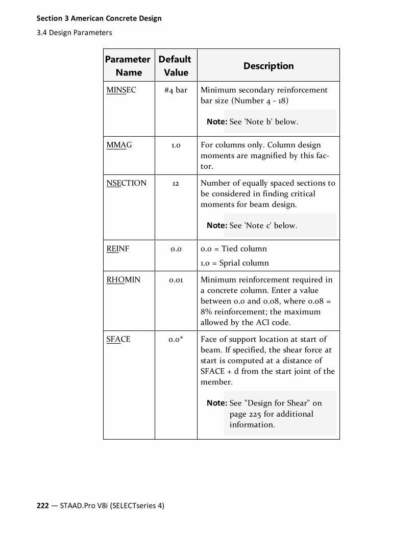
ParameterName
DefaultValue
Description
MINSEC #4 bar Minimum secondary reinforcementbar size (Number 4 - 18)
Note: See 'Note b' below.
MMAG 1.0 For columns only. Column designmoments are magnified by this fac-tor.
NSECTION 12 Number of equally spaced sections tobe considered in finding criticalmoments for beam design.
Note: See 'Note c' below.
REINF 0.0 0.0 = Tied column
1.0 = Sprial column
RHOMIN 0.01 Minimum reinforcement required ina concrete column. Enter a valuebetween 0.0 and 0.08, where 0.08 =8% reinforcement; the maximumallowed by the ACI code.
SFACE 0.0* Face of support location at start ofbeam. If specified, the shear force atstart is computed at a distance ofSFACE + d from the start joint of themember.
Note: See "Design for Shear" onpage 225 for additionalinformation.
222— STAAD.Pro V8i (SELECTseries 4)
Section 3 American Concrete Design
3.4 Design Parameters

ParameterName
DefaultValue
Description
TRACK 0.0 Beam Design:
0.0 = Critical moment willnot be printed out withbeam design report.
1.0 = Critical moment willbe printed out with beamdesign report
2.0 = Print out requiredsteel areas for allintermediate sectionsspecified by NSECTION.
Column Design:
0.0 = Prints out detaileddesign reports
1.0 = Prints out columninteraction analysis resultsin addition to TRACK 0.0output.
2.0 = Prints out aschematic interactiondiagram and intermediateinteraction values inaddition to TRACK 2.0results.
WIDTH ZD* Width of concrete member. Thisvalue defaults to ZD as providedunder MEMBER PROPERTIES.
Note: * These values must be provided in the current unit system being used.
Section 3 American Concrete Design
3.4 Design Parameters
Technical Reference Manual — 223
Notes
a. The value used when specifying the CLS parameter for column design istaken to be the clear cover for the longitudinal bars in a column. It is nottaken as the clear cover for the tie bars. Therefore, the distance from theedge of the column to the centerline of the first row of longitudinal bars isCLS plus half the diameter of the main bar.
b. When using metric units for ACI design, provide values for these param-eters in actual 'mm' units instead of the bar number. The following metricbar sizes are available: 6 mm, 8 mm, 10 mm, 12 mm, 16 mm, 20 mm, 25mm, 32 mm, 40 mm, 50 mm and 60 mm.
c. NSECTION should have no member list since it applies to all members. Theminimum value allowed is 12, the maximum is 20. If more than one NSEC-TION entered, then highest value is used.
3.5 Slenderness Effects and Analysis ConsiderationSlenderness effects are extremely important in designing compression members.The ACI-318 code specifies two options by which the slenderness effect can beaccommodated (Section 10.10 & 10.11 ACI-318). One option is to perform an exactanalysis which will take into account the influence of axial loads and variablemoment of inertia on member stiffness and fixed-end moments, the effect ofdeflections on moments and forces, and the effect of the duration of loads.Another option is to approximately magnify design moments.
STAAD uses both these options. To perform the first type of analysis, use thecommand PDELTA ANALYSIS instead of PERFORM ANALYSIS. This analysismethod will accommodate the requirements as specified in Section 10.10 of theACI-318 Code, except for the effects of the duration of the loads. It is felt that thiseffect may be safely ignored because experts believe that the effects of theduration of loads are negligible in a normal structural configuration. If it isdesired, STAAD can also accommodate any arbitrary moment magnificationfactor (second option) as an input, in order to provide some safety due to theeffects of the duration of loads.
Although ignoring load duration effects is somewhat of an approximation, itmust be realized that the approximate evaluation of slenderness effects is also anapproximate method. In this method, moment-magnification is based onempirical formula and assumptions on sidesway.
Considering all this information, it is our belief, that a PDELTA ANALYSIS, asperformed by STAAD, is most appropriate for the design of concrete members.
224— STAAD.Pro V8i (SELECTseries 4)
Section 3 American Concrete Design
3.5 Slenderness Effects and Analysis Consideration

However,you should note that to take advantage of this analysis, allcombinations of loadings must be provided as primary load cases and not as loadcombinations. This is due to the fact that load combinations are just algebraiccombinations of forces and moments, whereas a primary load case is revisedduring the PDelta analysis based on the deflections. Also note that the properfactored loads (e.g., 1.4 for DL etc.) should be provided by the user. STAAD doesnot factor the loads automatically.
3.6 Beam DesignBeams are designed for flexure, shear and torsion. For all these forces, all activebeam loadings are prescanned to locate the possible critical sections. The totalnumber of sections considered is 12 (twelve) unless this number is redefined withan NSECTION parameter. All of these equally spaced sections are scanned todetermine moment and shear envelopes.
3.6.1 Design for FlexureReinforcement for positive and negative moments are calculated on the basis ofthe section properties provided by the user. If the section dimensions areinadequate to carry the applied load, that is if the required reinforcement isgreater than the maximum allowable for the cross section, the program reportsthat beam fails in maximum reinforcement. Effective depth is chosen as Totaldepth - (Clear cover + diameter of stirrup + half the dia. of main reinforcement),and a trial value is obtained by adopting proper bar sizes for the stirrups andmain reinforcements. The relevant clauses in Sections 10.2 to 10.6 of ACI 318 areutilized to obtain the actual amount of steel required as well as the maximumallowable and minimum required steel. These values are reported as ROW,ROWMX, and ROWMN in the output and can be printed using the parameterTRACK 1.0 (see Table 3.1). In addition, the maximum, minimum and actual barspacing are also printed.
It is important to note that beams are designed for flexural moment MZ only.The moment MY is not considered in the flexural design.
3.6.2 Design for ShearShear reinforcement is calculated to resist both shear forces and torsionalmoments. Shear forces are calculated at a distance (d+SFACE) and (d+EFACE)away from the end nodes of the beam. Parameters SFACE and EFACE have defaultvalues of zero unless provided under parameters (see Table 3.1). The value of theeffective depth, d, used for this purpose is the updated value and accounts for the
Section 3 American Concrete Design
3.6 Beam Design
Technical Reference Manual — 225

actual center of geometry of the main reinforcement calculated under flexuraldesign.
Note: If a beam cross section is very deep but the span length is relativelyshort, an error may result from the start of the shear design occurringbeyond the beam's midpoint. In these cases, a negative value of SFACEand EFACE can be used to start the shear design at reasonable distance.For example, a negative value of d may be used to start the design atthe start and end nodes.
Clauses 11.1 through 11.6 of ACI 318 are used to calculate the reinforcement forshear forces and torsional moments. Based on the total stirrup reinforcementrequired, the size of bars, the spacing, the number of bars and the distance overwhich they are provided are calculated. Stirrups are always assumed to be two-legged.
The reduction factor for lightweight concrete, λ, introduced in ACI 318-08 can bemanually specified through the LWF parameter. This value us used to reduce theshear strength provided by concrete, V
c, in equations 11-3, 11-4, and 11-5.
3.6.3 Design for AnchorageIn the output for flexural design, the anchorage details are also provided. At anyparticular level, the START and END coordinates of the layout of the mainreinforcement is described along with the information whether anchorage in theform of a hook or continuation is required or not at theseSTART and END points.Note that the coordinates of theseSTART and END points are obtained aftertaking into account the anchorage requirements. Anchorage length is calculatedon the basis of the Clauses described in Chapter 12 of ACI 318.
Example
Beam design per the ACI 318-2002 code
UNIT KIP INCH
START CONCRETE DESIGN
CODE ACI 2002
FYMAIN 58 ALL
MAXMAIN 10 ALL
CLB 2.5 ALL
226— STAAD.Pro V8i (SELECTseries 4)
Section 3 American Concrete Design
3.6 Beam Design

DESIGN BEAM 1 7 10
END CONCRETE DESIGN
Note: The command CODE ACI can also be used to initiate the ACI 318-2002design code.
Example
Beam design per the ACI 318-1999 code
UNIT KIP INCH
START CONCRETE DESIGN
CODE ACI 1999
FYMAIN 58 ALL
MAXMAIN 10 ALL
CLB 2.5 ALL
DESIGN BEAM 1 7 10
END CONCRETE DESIGN
3.6.4 Description of Output for Beam DesignThe following is a sample output of an actual reinforcement pattern developed bythe program. The following annotations apply to the output:
LEVEL
Serial number of bar level which may contain one or more bar group
HEIGHT
Height of bar level from the bottom of beam
BAR INFO
Reinforcement bar information specifying number of bars and bar size
FROM
Distance from the start of the beam to the start of the reinforcement bar
TO
Distance from the start of the beam to the end of the reinforcement bar
Section 3 American Concrete Design
3.6 Beam Design
Technical Reference Manual — 227
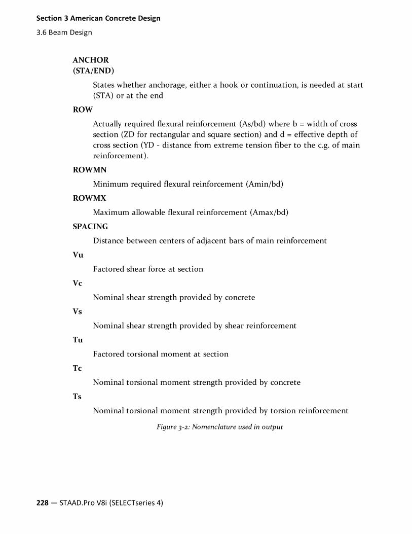
ANCHOR(STA/END)
States whether anchorage, either a hook or continuation, is needed at start(STA) or at the end
ROW
Actually required flexural reinforcement (As/bd) where b = width of crosssection (ZD for rectangular and square section) and d = effective depth ofcross section (YD - distance from extreme tension fiber to the c.g. of mainreinforcement).
ROWMN
Minimum required flexural reinforcement (Amin/bd)
ROWMX
Maximum allowable flexural reinforcement (Amax/bd)
SPACING
Distance between centers of adjacent bars of main reinforcement
Vu
Factored shear force at section
Vc
Nominal shear strength provided by concrete
Vs
Nominal shear strength provided by shear reinforcement
Tu
Factored torsional moment at section
Tc
Nominal torsional moment strength provided by concrete
Ts
Nominal torsional moment strength provided by torsion reinforcement
Figure 3-2: Nomenclature used in output
228— STAAD.Pro V8i (SELECTseries 4)
Section 3 American Concrete Design
3.6 Beam Design

The following is a sample TRACK 1.0 output from concrete beam design per ACI(from the file .../SPROV8I/STAAD/EXAMP/US/EXAMP08.STD):
=====================================================================BEAM NO. 14 DESIGN RESULTS - FLEXURE PER CODE ACI 318-05
LEN - 20.00FT. FY - 60000. FC - 4000. SIZE - 16.00 X 21.00 INCHESLEVEL HEIGHT BAR INFO FROM TO ANCHOR
FT. IN. FT. IN. FT. IN. STA END_____________________________________________________________________1 0 + 2-3/8 8-NUM.5 2 + 2-5/8 20 + 0-0/0 NO YES
|----------------------------------------------------------------|| CRITICAL POS MOMENT= 191.70 KIP-FT AT 11.67 FT, LOAD 1|| REQD STEEL= 2.47 IN2, RHO=0.0083, RHOMX=0.0214 RHOMN=0.0033 || MAX/MIN/ACTUAL BAR SPACING= 10.00/ 1.62/ 1.62 INCH || REQD. DEVELOPMENT LENGTH = 27.37 INCH ||----------------------------------------------------------------|Cracked Moment of Inertia Iz at above location = 4320.43 inch^42 1 + 6-1/8 4-NUM.11 0 + 0-0/0 16 + 2-0/0 YES NO
|----------------------------------------------------------------|| CRITICAL NEG MOMENT= 371.81 KIP-FT AT 0.00 FT, LOAD 1|| REQD STEEL= 5.39 IN2, RHO=0.0184, RHOMX=0.0214 RHOMN=0.0033 || MAX/MIN/ACTUAL BAR SPACING= 10.00/ 2.82/ 3.53 INCH || REQD. DEVELOPMENT LENGTH = 80.14 INCH ||----------------------------------------------------------------|Cracked Moment of Inertia Iz at above location = 8050.77 inch^43 1 + 6-3/8 3-NUM.6 16 +10-1/4 20 + 0-0/0 NO YES
|----------------------------------------------------------------|| CRITICAL NEG MOMENT= 104.94 KIP-FT AT 20.00 FT, LOAD 1|| REQD STEEL= 1.30 IN2, RHO=0.0044, RHOMX=0.0214 RHOMN=0.0033 || MAX/MIN/ACTUAL BAR SPACING= 10.00/ 1.75/ 5.62 INCH || REQD. DEVELOPMENT LENGTH = 21.35 INCH ||----------------------------------------------------------------|Cracked Moment of Inertia Iz at above location = 2602.81 inch^4
B E A M N O. 14 D E S I G N R E S U L T S - SHEARAT START SUPPORT - Vu= 84.31 KIP Vc= 35.77 KIP Vs= 76.64 KIPTu= 0.23 KIP-FT Tc= 5.70 KIP-FT Ts= 0.00 KIP-FT LOAD 1NO STIRRUPS ARE REQUIRED FOR TORSION.REINFORCEMENT IS REQUIRED FOR SHEAR.PROVIDE NUM. 5 2-LEGGED STIRRUPS AT 4.7 IN. C/C FOR 102. IN.AT END SUPPORT - Vu= 57.62 KIP Vc= 35.77 KIP Vs= 41.06 KIPTu= 0.23 KIP-FT Tc= 5.70 KIP-FT Ts= 0.00 KIP-FT LOAD 1NO STIRRUPS ARE REQUIRED FOR TORSION.REINFORCEMENT IS REQUIRED FOR SHEAR.PROVIDE NUM. 4 2-LEGGED STIRRUPS AT 9.3 IN. C/C FOR 102. IN.
___ 11J____________________ 240.X 16.X 21_____________________ 12J____| |||============================================================ ===========||| 4#11H |18.| |0.TO |194. | | | | | | | | | | | | |3#6 H| 18. 202.TO| 240. || 23#5 C/C 5 | | | | | | | | | | | | | | | | | | | | | |12#4 C/C 9| || |8#5|H| |2. |27.TO| 240.| | | | | | | | | | | | | | | | || ===================================================================||| ||___________________________________________________________________________|___________ ___________ ___________ ___________ ___________
Section 3 American Concrete Design
3.6 Beam Design
Technical Reference Manual — 229

| | | | | | | | | || OOOO | | OOOO | | OOOO | | OOOO | | ooo || 4#11 | | 4#11 | | 4#11 | | 4#11 | | 3#6 || | | | | | | | | || | | 8#5 | | 8#5 | | 8#5 | | 8#5 || | | oooooooo | | oooooooo | | oooooooo | | oooooooo || | | | | | | | | ||___________| |___________| |___________| |___________| |___________|
3.6.5 Cracked Moment of Inertia - ACI Beam DesignWhen beam design is done per ACI 318, STAAD will report the moment of inertiaof the cracked section at the location where the design is performed. The crackedsection properties are calculated in accordance with the equations shown below.
Rectangular Sections
Figure 3-3: Gross section (A) and cracked transform section (B) for rectangular shapes
Without compression steel
n = EI/EcB = b/(nAI)
Ig = b⋅h3/12
kd = [(2d⋅B + 1)1/2 - 1]/B
Icr = b(kd)3/3 + nAs(d - kd)
2
230— STAAD.Pro V8i (SELECTseries 4)
Section 3 American Concrete Design
3.6 Beam Design

Tee Shaped Sections
Figure 3-4: Gross and cracked transform sections for tee shapes without compression steel
Without compression steel
C = bw/nAsf = hf(b - bw)/(nAs)
yt = h - 1/2[(b - bw)⋅hf2 + bwh
2]/[(b - bw)⋅hf + bwh]
kd = {[C⋅(2d + hf⋅f) + (1 + f)2]1/2 - (1 + f)}/C
Icr = (b - bw)⋅hf3/12 + bw(kd)
3/3 + (b - bw)⋅hf⋅(kd - hf/2)2 + nAs⋅(d - kd)
2
See "Description of Output for Beam Design" on page 227 for an example ofoutput including the calculated cracked moment of inertia.
3.7 Column DesignColumns design in STAAD per the ACI code is performed for axial force anduniaxial as well as biaxial moments. All active loadings are checked to computereinforcement. The loading which produces the largest amount of reinforcementis called the critical load. Column design is done for square, rectangular andcircular sections. For rectangular and circular sections, reinforcement is alwaysassumed to be equally distributed on all faces. This means that the total numberof bars for these sections will always be a multiple of four (4). If the MMAGparameter is specified, the column moments are multiplied by the MMAG valueto arrive at the ultimate moments on the column. Since the ACI code no longerrequires any minimum eccentricity conditions to be satisfied, such checks are notmade.
Section 3 American Concrete Design
3.7 Column Design
Technical Reference Manual — 231
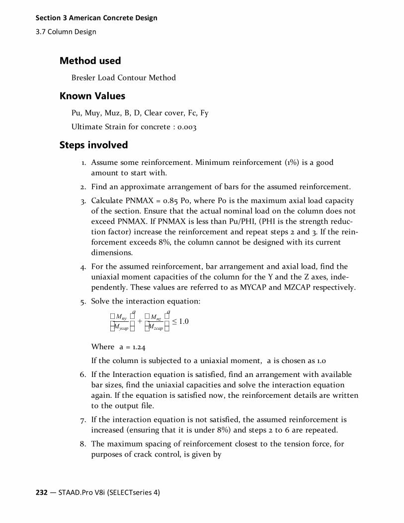
Method usedBresler Load Contour Method
Known ValuesPu, Muy, Muz, B, D, Clear cover, Fc, Fy
Ultimate Strain for concrete : 0.003
Steps involved
1. Assume some reinforcement. Minimum reinforcement (1%) is a goodamount to start with.
2. Find an approximate arrangement of bars for the assumed reinforcement.
3. Calculate PNMAX = 0.85 Po, where Po is the maximum axial load capacityof the section. Ensure that the actual nominal load on the column does notexceed PNMAX. If PNMAX is less than Pu/PHI, (PHI is the strength reduc-tion factor) increase the reinforcement and repeat steps 2 and 3. If the rein-forcement exceeds 8%, the column cannot be designed with its currentdimensions.
4. For the assumed reinforcement, bar arrangement and axial load, find theuniaxial moment capacities of the column for the Y and the Z axes, inde-pendently. These values are referred to as MYCAP and MZCAP respectively.
5. Solve the interaction equation:
+ ≤ 1.0M
M
aM
M
any
ycap
nz
zcap
Where a = 1.24
If the column is subjected to a uniaxial moment, a is chosen as 1.0
6. If the Interaction equation is satisfied, find an arrangement with availablebar sizes, find the uniaxial capacities and solve the interaction equationagain. If the equation is satisfied now, the reinforcement details are writtento the output file.
7. If the interaction equation is not satisfied, the assumed reinforcement isincreased (ensuring that it is under 8%) and steps 2 to 6 are repeated.
8. The maximum spacing of reinforcement closest to the tension force, forpurposes of crack control, is given by
232— STAAD.Pro V8i (SELECTseries 4)
Section 3 American Concrete Design
3.7 Column Design

s cc= 15 40, 000 − 2.5 ≤ 12f f
40,000 40, 000
s s
with fsin psi and is permitted to be taken equal to (2/3) f
y, rather than 60
percent of fy, as in ACI 318-02.
9. Section 10.9.3 has been modified to permit the use of spiral reinforcementwith specified yield strength of up to 100,000 psi. For spirals with fytgreater than 60,000 psi, only mechanical or welded splices may be used.
Column Interaction
The column interaction values may be obtained by using the design parameterTRACK 1.0 or TRACK 2.0 for the column member. If a value of 2.0 is used for theTRACK parameter, 12 different Pn-Mn pairs, each representing a different pointon the Pn-Mn curve are printed. Each of these points represents one of theseveral Pn-Mn combinations that this column is capable of carrying about thegiven axis, for the actual reinforcement that the column has been designed for. Inthe case of circular columns, the values are for any of the radial axes. The valuesprinted for the TRACK 1.0 output are:
P0 = Maximum purely axial load carrying capacity of the column(zero moment).
Pnmax = Maximum allowable axial load on the column (Section 10.3.5of ACI 318).
P-bal = Axial load capacity at balanced strain condition.
M-bal = Uniaxial moment capacity at balanced strain condition.
e-bal = M-bal / P-bal = Eccentricity at balanced strain condition.
M0 = Moment capacity at zero axial load.
P-tens = Maximum permissible tensile load on the column.
Des. Pn = Pu/PHI where PHI is the Strength Reduction Factor and Puis the axial load for the critical load case.
Des. Mn = Mu*MMAG/PHI where PHI is the Strength ReductionFactor and Mu is the bending moment for the appropriate axis for thecritical load case. For circular columns,
M M M= +u uy uz2 2
e/h = (Mn/Pn)/h
Section 3 American Concrete Design
3.7 Column Design
Technical Reference Manual — 233

Where:
h is the length of the column.
Example
Column design per the ACI 318-2005 code
UNIT KIP INCH
START CONCRETE DESIGN
CODE ACI 2005
FYMAIN 58 ALL
MAXMAIN 10 ALL
CLB 2.5 ALL
DESIGN COLUMN 23 25
END CONCRETE DESIGN
Example
Column design per the ACI 318-2002 code
UNIT KIP INCH
START CONCRETE DESIGN
CODE ACI 2002
FYMAIN 58 ALL
MAXMAIN 10 ALL
CLB 2.5 ALL
DESIGN COLUMN 23 25
END CONCRETE DESIGN
Example
Column design per the ACI 318-1999 code
UNIT KIP INCH
START CONCRETE DESIGN
234— STAAD.Pro V8i (SELECTseries 4)
Section 3 American Concrete Design
3.7 Column Design

CODE ACI 1999
FYMAIN 58 ALL
MAXMAIN 10 ALL
CLB 2.5 ALL
DESIGN COLUMN 23 25
END CONCRETE DESIGN
Column Design OutputThe samples illustrate different levels of the column design output. The followingoutput is generated without any TRACK definition (i.e., using the default ofTRACK 0.0):
====================================================================COLUMN NO. 5 DESIGN PER ACI 318-05 - AXIAL + BENDING
FY - 60000 FC - 4000 PSI, SQRE SIZE - 12.00 X 12.00 INCHES, TIEDAREA OF STEEL REQUIRED = 7.589 SQ. IN.
BAR CONFIGURATION REINF PCT. LOAD LOCATION PHI----------------------------------------------------------8 - NUMBER 9 5.556 2 STA 0.650
(PROVIDE EQUAL NUMBER OF BARS ON EACH FACE)TIE BAR NUMBER 4 SPACING 8.00 IN
TRACK 1.0 generates the following additional output:COLUMN INTERACTION: MOMENT ABOUT Z -AXIS (KIP-FT)
--------------------------------------------------------P0 Pn max P-bal. M-bal. e-bal.(inch)942.40 753.92 179.59 170.75 11.41M0 P-tens. Des.Pn Des.Mn e/h
148.52 -480.00 350.15 10.47 0.00249--------------------------------------------------------
COLUMN INTERACTION: MOMENT ABOUT Y -AXIS (KIP-FT)--------------------------------------------------------P0 Pn max P-bal. M-bal. e-bal.(inch)942.40 753.92 179.59 170.75 11.41M0 P-tens. Des.Pn Des.Mn e/h
148.52 -480.00 350.15 136.51 0.03249--------------------------------------------------------
TRACK 2.0 generates the following output in addition to the above examples:Pn Mn Pn Mn (@ Z )
| 695.93 77.23 347.96 148.53P0 |* 637.93 93.16 289.97 157.71
| * 579.94 107.06 231.98 164.41Pn,max|__* 521.94 118.23 173.98 170.18
| * 463.95 129.01 115.99 163.66Pn | * 405.96 139.03 57.99 156.37NOMINAL| * Pn Mn Pn Mn (@ Y )AXIAL| * 695.93 77.23 347.96 148.53
COMPRESSION| * 637.93 93.16 289.97 157.71Pb|-------*Mb 579.94 107.06 231.98 164.41| * 521.94 118.23 173.98 170.18
___________|____*_______ 463.95 129.01 115.99 163.66| * M0 Mn, 405.96 139.03 57.99 156.37| * BENDING
Section 3 American Concrete Design
3.7 Column Design
Technical Reference Manual — 235

P-tens|* MOMENT|
3.8 Designing elements, shear walls, slabsSTAAD currently provides facilities for designing 3 types of entities associatedwith surface type of structures.
a. Individual plate elements – these are designed from the standpoint that oneelement is independent of the next element. See Section 3.8.1 for details.
b. Shear Walls – Structural components modeled using the SURFACEINCIDENCE command can be designed as shear walls. See Section 3.8.2 fordetails.
3.8.1 Element DesignElement design will be performed only for the moments MX and MY at thecenter of the element. Design will not be performed for SX, SY, SXY, SQX, SQY orMXY. Also, design is not performed at any other point on the surface of theelement.
A typical example of element design output is shown in Table 3.4. Thereinforcement required to resist Mx moment is denoted as longitudinalreinforcement and the reinforcement required to resist My moment is denoted astransverse reinforcement (Figure 3.1). The parameters FYMAIN, FC, and CLEARlisted in Table 3.1 are relevant to slab design. Other parameters mentioned inTable 3.1 are not applicable to slab design. Please note that the default value ofclear cover - parameters CLT and CLB - for plate elements is 0.75 inches, asshown in Table 3.1.
Figure 3-5: Sign convention of loaded plate element
236— STAAD.Pro V8i (SELECTseries 4)
Section 3 American Concrete Design
3.8 Designing elements, shear walls, slabs

Example Element Design OutputELEMENT DESIGN SUMMARY----------------------ELEMENT LONG. REINF MOM-X /LOAD TRANS. REINF MOM-Y /LOAD
(SQ.IN/FT) (K-FT/FT) (SQ.IN/FT) (K-FT/FT)FY: 60.000 KSI FC: 4.000 KSI COVER (TOP): 0.750 INCOVER (BOTTOM): 0.750 IN TH: 6.000 IN
47 TOP : Longitudinal direction - Only minimum steel required.47 TOP : Transverse direction - Only minimum steel required.47 TOP : 0.130 0.00 / 0 0.130 0.00 / 0
BOTT: 0.562 11.60 / 1 0.851 14.83 / 1
Example
Element design per the ACI 318-2002 code
UNIT KIP INCH
START CONCRETE DESIGN
CODE ACI 2002
FYMAIN 58 ALL
MAXMAIN 10 ALL
CLB 2.5 ALL
DESIGN ELEMENT 43
END CONCRETE DESIGN
Example
Element design per the ACI 318-1999 code
UNIT KIP INCH
START CONCRETE DESIGN
CODE ACI 1999
FYMAIN 58 ALL
MAXMAIN 10 ALL
CLB 2.5 ALL
DESIGN ELEMENT 43
END CONCRETE DESIGN
Section 3 American Concrete Design
3.8 Designing elements, shear walls, slabs
Technical Reference Manual — 237

3.8.2 Shear Wall DesignDesign of shear walls in accordance with ACI 318-02 has been implemented. Shearwalls have to be modeled using the Surface element. The program implementsprovisions of chapters 10, 11 and 14 of ACI 318-02.
The attributes associated with the surface element, and the sections of thismanual where the information may be obtained, are listed below:
AttributesRelatedSections
Surfaces Incidences 5.13.3
Openings in surface 5.13.3
Local Coordinates system forsurfaces
1.6.3
Specifying sections for stress/forceoutput
5.13.3
Property for surfaces 5.21.2
Material constants 5.26.3
Surface loading 5.32.3.4
Stress/Force output printing 5.42
Shear Wall Design 3.8.2, 5.55
Description
The program implements the provisions of ACI 318-02, except Chapter 21, for thedesign of shear walls. It performs in-plane shear, compression, as well as in-planeand out-of-plane bending design of reinforcing. The shear wall is modeled by asingle or a combination of Surface elements. The use of the Surface elementenables the designer to treat the entire wall as one entity. It greatly simplifies themodeling of the wall and adds clarity to the analysis and design output. The
238— STAAD.Pro V8i (SELECTseries 4)
Section 3 American Concrete Design
3.8 Designing elements, shear walls, slabs

results are presented in the context of the entire wall rather than individual finiteelements thereby allowing users to quickly locate required information.
The definition of the shear wall starts with specification of the Surface element(s). The boundary of the wall should include all corner joints as well as anyadditional joints required for connections with other elements of the building,such as beams. All geometry and material properties must be specified for surfaceelements separately from specifications for other element types.
The wall may be loaded indirectly through members/elements attached to it, ordirectly by application of nodal or uniformly distributed loads. All wall elementsmust be of constant thickness.
The program reports shear wall design results for each load case/combination fora user specified number of sections given by the SURFACE DIVISION (defaultvalue is 10) command. The wall is designed at these horizontal sections. Theoutput includes the required horizontal and vertical distributed reinforcing, theconcentrated (in-plane bending) reinforcing, and the links required to resist out-of-plane shear.
General Format
START SHEARWALL DESIGN
CODE ACI
FYMAIN f1
FC f2
HMIN f3
HMAX f4
VMIN f5
VMAX f6
EMIN f7
EMAX f8
LMIN f9
LMAX f10
CLEAR f11
TWOLAYERED f12
KSLENDER f13
DESIGN SHEARWALL LIST shearwall-list
Section 3 American Concrete Design
3.8 Designing elements, shear walls, slabs
Technical Reference Manual — 239

END
The following table explains parameters used in the shear wall design commandblock above. All reinforcing bar sizes are English designation (#).
ParameterName
DefaultValue
Description
FYMAIN 60.0 ksi Yield strength of steel, in currentunits.
FC 4.0 ksi Compressive strength of concrete, incurrent units.
HMIN 3 Minimum size of horizontal rein-forcing bars (range 3 -18).
HMAX 18 Maximum size of horizontal rein-forcing bars (size 3 - 18).
VMIN 3 Minimum size of vertical reinforcingbars (range 3 - 18).
VMAX 18 Maximum size of vertical reinforcingbars (range 3 - 18).
EMIN 3 Minimum size of vertical reinforcingbars located in edge zones (range 3 -18).
EMAX 18 Maximum size of vertical reinforcingbars located in edge zones (range 3 -18).
LMIN 3 Minimum size of links (range 3 - 18).
LMAX 18 Maximum size of links (range 3 - 18).
CLEAR 3.0 in. Clear concrete cover, in current units.
TWOLAY-ERED
0 Reinforcement placement mode:
0. single layer, each direction
1. two layers, each direction
Table 3-2: Shear Wall Design Parameters
240— STAAD.Pro V8i (SELECTseries 4)
Section 3 American Concrete Design
3.8 Designing elements, shear walls, slabs

ParameterName
DefaultValue
Description
KSLENDER 1.5 Slenderness factor for finding effectiveheight.
Example
…
SET DIVISION 12
SURFACE INCIDENCES
2 5 37 34 SUR 1
19 16 65 68 SUR 2
11 15 186 165 SUR 3
10 6 138 159 SUR 4
…
SURFACE PROPERTY
1 TO 4 THI 18
SUPPORTS
1 7 14 20 PINNED
2 TO 5 GEN PIN
6 TO 10 GEN PIN
11 TO 15 GEN PIN
19 TO 16 GEN PIN
…
SURFACE CONSTANTS
E 3150
POISSON 0.17
DENSITY 8.68E-005
ALPHA 5.5E-006
…
START SHEARWALL DES
Section 3 American Concrete Design
3.8 Designing elements, shear walls, slabs
Technical Reference Manual — 241

CODE ACI
FC 4
FYMAIN 60
TWO 1
VMIN 5
HMIN 5
EMIN 8
DESIGN SHEA LIST 1 TO 4
END
Notes regarding the above example:
1. Command SET DIVISION 12 indicates that the surface boundary node-to-node segments will be subdivided into 12 fragments prior to finite elementmesh generation.
2. Four surfaces are defined by the SURFACE INCIDENCES command.
3. The SUPPORTS command includes the support generation routine. Forinstance, the line 2 TO 5 GEN PIN assigns pinned supports to all nodesbetween nodes 2 and 5. As the node-to-node distances were previouslysubdivided by the SET DIVISION 12 command, there will be an additional11 nodes between nodes 2 and 5. As a result, all 13 nodes will be assignedpinned supports. Please note that the additional 11 nodes are notindividually accessible to the user. They are created by the program toenable the finite element mesh generation and to allow application ofboundary constraints.
4. Surface thickness and material constants are specified by the SURFACEPROPERTY and SURFACE CONSTANTS, respectively.
5. The shear wall design commands are listed between lines STARTSHEARWALL DES and END. The CODE command selects the design code thatwill be the basis for the design. The DESIGN SHEARWALL LIST command isfollowed by a list of previously defined Surface elements intended as shearwalls and/or shear wall components. Refer to the beginning of this sectionfor references to all related commands.
242— STAAD.Pro V8i (SELECTseries 4)
Section 3 American Concrete Design
3.8 Designing elements, shear walls, slabs

Technical Overview
The program implements provisions of Chapter 14 of ACI-318-02 and relevantprovisions from Chapters 10 and 11, as referenced therein, for all active load cases.The wall is designed as an unbraced reinforced wall. The following steps areperformed for each of the horizontal sections of the wall set using the SURFACEDIVISION command whose default value is 10.
Design for in-plane shear (denoted using Fxy in the shear wall force output) perSection 11.10 of ACI 318
l Extreme compression fiber to centroid of tension (concentrated)reinforcement distance, d, is taken as 0.8 horizontal length of the wall (ACI- 11.10.4),
l Limit on the nominal shear strength, Vn, is calculated (ACI - 11.10.3),
l Nominal shear strength of concrete is computed (11.10.6),
l If the factored shear force does not exceed ½ of the design strength ofconcrete, the minimum ratios of shear (distributed) reinforcing arereported, in accordance with 14.3.2 and 14.3.3. Otherwise, the reinforcingratios are established in accordance with 11.10.9.
l If the factored shear force is greater than ½ but does not exceed the designstrength of concrete, the ratios reported are the minima calculated inaccordance with 11.10.9.2 and 11.10.9.4.
l If the factored shear force exceeds the design strength of concrete, thedistributed reinforcing is calculated based on 11.1.1 and 11.10.9.
l Number of distributed reinforcing layers and reinforcing allocation betweenlayers reflect requirements of 14.3.4.
l Rebar spacing is given c/c and meets the requirements of 14.3.5, 11.10.9.3,and 11.10.9.5 of ACI 318, as applicable.
Design for in-plane bending (denoted by Mz in the shear wall force output) perSection 14.4 of ACI 318
l Walls are assumed to be cantilever beams fixed at their base and carryingloads to the foundation.
l Strength reduction factor is established in accordance with Section 9.3.2.
l Minimum reinforcing is calculated in accordance with 10.5.1 or 10.5.3,whichever produces a smaller ratio.
Section 3 American Concrete Design
3.8 Designing elements, shear walls, slabs
Technical Reference Manual — 243

l Extreme compression fiber to centroid of tension reinforcement distance, d,is taken as 0.8 horizontal length of the wall (11.10.4 of ACI 318).
l Flexural design of the wall is carried out in accordance with provisions ofChapter 10.
l The flexural (concentrated) reinforcing is located at both ends (edges) ofthe length of the wall. Rebar layout conforms to the spacing requirementsof Section 7.6.
Design for compression and out-of-plane bending (Section 14.8)
l The design is based on the Alternative Design of Slender Walls procedure.
l The procedure requires that the wall panel be designed as simply supported(at top and bottom), axially loaded with out-of-plane uniform lateral load,with maximum moments and deflections occurring at mid-height.
l Minimum distributed reinforcing ratio is controlled by the in-plane sheardesign calculations.
l The reinforcing amount required by 14.8 is over and above any reinforcingrequired due to in-plane shear.
3.8.3 Slabs and RC DesignerContact the Bentley Technical Support Group for further information.
3.8.4 Design of I-shaped beams per ACI-318I-shaped sections can be designed as beams per the ACI 318 code. The propertyfor these sections must be defined through a user table, I-section, or using thetapered specification. Information on assigning properties in this manner isavailable in sections 5.19 (I-section type) and 5.20.3 (Tapered I shape) of theTechnical Reference manual.
From the standpoint of the analysis – determining member forces, nodaldisplacements and support reactions – the same set of facilities and rules whichare applicable for any normal reinforced concrete frames or other structures canbe used when I-sections or tapered concrete members are specified. In otherwords, there isn’t anything unique or special to account for in the analysis modelsimply because I-shaped concrete beams are part of it.
From the standpoint of design, the following rules are applicable:
1. The member can be designed as a beam using the general principlesexplained in Chapter 3 of the Technical Reference manual. It currently
244— STAAD.Pro V8i (SELECTseries 4)
Section 3 American Concrete Design
3.8 Designing elements, shear walls, slabs

cannot be designed as a column. Design as a beam is done for flexure (MZ),shear (FY) and torsion (MX) just like that for rectangular, tee or trapezoidalbeams. Axial forces (FX) are used during the capacity computations in shearand torsion. At each section along the length that the member is designedat, the depth at that section location is used for effective depthcomputation.
2. The program performs the following tests on the section dimensions beforestarting the design:
l If the thickness of the web is the same as the width of the top andbottom flanges, the member is designed as a rectangular section.
l If the thickness of the web is the same as the width of one of theflanges but not the other, the member is designed as a T-section or arectangular section, depending on which side the compression due tobending is at.
l If the web thickness does not match the width of either flange, designis done using the rules applicable for T-beams – one flange is incompression, the other in tension, and tensile capacity of concrete onthe tensile side of the neutral axis is ignored.
l The program is also able to design the beam as a doubly reinforcedsection if it is unable to design it as a single-reinforced section.
3. The parameters for designing these members are as shown in Table 3.1 ofthis manual. Detailed output on design at individual section locations alongthe member length may be obtained by setting the TRACK parameter to 3.0.
An example for I-beam design is shown below.
STAAD PLANE I BEAM CONCRETE DESIGN PER ACI-318
UNIT FEE KIP
JOINT COORDINATES
1 0 0 0; 2 10 0 0
MEMBER INCIDENCES
1 1 2
UNIT INCHES KIP
MEMBER PROPERTY
1 TAPERED 18 10 18 15 2.5
CONSTANTS
Section 3 American Concrete Design
3.8 Designing elements, shear walls, slabs
Technical Reference Manual — 245

E 3300 ALL
DENSITY CONCRETE ALL
POISSON CONCRETE ALL
SUPPORTS
1 2 PINNED
UNIT FEET KIP
LOAD 1 DEAD LOAD
MEMBER LOAD
1 UNI GY -5.76
LOAD 2 LIVE LOAD
1 UNI GY -7.04
LOAD COMB 3 ACI 318-02
1 1.4 2 1.7
PERFORM ANALYSIS
LOAD LIST 3
START CONCRETE DESIGN
CODE ACI 2002
UNIT INCHES KIP
MINMAIN 9 ALL
FC 4 ALL
FYMAIN 60 ALL
TRACK 2.0 ALL
DESIGN BEAM ALL
END CONCRETE DESIGN
FINISH
246— STAAD.Pro V8i (SELECTseries 4)
Section 3 American Concrete Design
3.8 Designing elements, shear walls, slabs

Section 4
American Timber Design
4.1 Design Operations 247
4.2 Allowable Stress per AITC Code 250
4.3 Input Specification 252
4.4 Naming Conventions for Sections 254
4.5 Design Parameters 257
4.6 Member Design Capabilities 262
4.7 Orientation of Lamination 263
4.8 Tabulated Results of Member Design 263
4.9 Examples 265
4.1 Design OperationsSTAAD.Pro supports timber design per two versions of the AITC code: 1985 and1994. The implementation of both the codes is explained below.
To access the 1994 edition, specify the commands:
Technical Reference Manual — 247

CODE AITC
or
CODE AITC 1994
To access the 1984 edition, specify the commands:
CODE AITC 1984
or
CODE TIMBER
4.1.1 1994 AITC code implementationThe salient aspects of design in accordance with the 4th edition (1994) of theTimber Construction Manual published by the American Institute of TimberConstruction are:
1. Design can be performed for two types of timber sections: dimensionaltimber sections (i.e., sawn lumber) and glulaminated sections.
2. The program includes a database of dimensional timber sections with thiscode.
Implementation of Dimensional Lumber Properties
The database of sawn lumber sections, listed in Table 8.1 of the 1994 AITCManual, is implemented in the program. Some of the key aspects of thisimplementation are:
In the property tables in the AITC manual, one will find that, for any particularspecies of timber, the Modulus of Elasticity (E) and allowable stresses may varywith the cross-section size. For example, a 2x4 Douglas Fir-Larch, SelectStructural member has an E of 1900 ksi and an allowable bending stress, F
b, of
1450 psi. A 5x5 Douglas Fir-Larch, Select Structural, Beam or Stringer memberhas an E of 1600 ksi and an allowable bending stress, F
b, of 1600 psi. And a 5x5
Douglas Fir-Larch, Select Structural, Post or Timbers member has an E of 1600 ksiand an allowable bending stress, F
b, of 1750 psi.
So, in the STAAD timber database for sawn lumber, for each species and grade oftimber, the section size, or properties are associated with the Modulus ofElasticity and allowable stresses for the cross-section. When a section is assigned,its E and allowable stresses are automatically fetched along with its properties.The material properties of Southern Pine members were taken from Table 8.4 ofthe 1994 AITC manual. For all other species with section sizes 2”-4” wide, thematerial properties have been taken from Table 8.3. For all non-Southern Pine
248— STAAD.Pro V8i (SELECTseries 4)
Section 4 American Timber Design
4.1 Design Operations

species with section sizes greater than 5”x5”, the material properties are obtainedfrom Table 8.6 of the 1994 AITC Manual.
Please note that not all section sizes listed in Table 8.1 are available in everyspecies. Some sizes are not produced for particular species. For example, theAspen species only produces sizes from 2”-4” wide. It does not produce sizes5”x5” and larger. This can be observed by comparing Table 8.3, where Aspen islisted as an available species, to Table 8.6, where Aspen is not listed as anavailable species. Also note that although 1” wide members are listed in Table8.1, there are no values available in the species properties tables; Table 8.4, Table8.5, and Table 8.6. AITC does not allow for the structural design of these smallmembers.
4.1.2 1985 AITC code implementationSTAAD’s Timber design module per the 1985 AITC code (Timber ConstructionManual, 3rd. Edition, 1985) allows design of Glulam timber sections. It alsoconforms to the National Design Specification for Wood Construction andSupplement (NDS) and building codes like Uniform Building Code (UBC),Basic/National Building Code and Standard Building Code. Some of the mainfeatures of the program are:
1. This feature is for Glulam Timber only (design of dimensional lumber areavailable for 1994 AITC only).
2. Code check and design of members as per TCM - AITC.
3. Design values for Structural Glued Laminated Timber tables are in-builtinto the program. The program accepts Table no., Combination and Speciesspecifications as inputs (e.g., 1:16F-V3-SP/SP) and reads design values fromin-built tables.
4. Incorporates all the following Allowable stress modifiers:
i. Duration of Load Factor
ii. Size Factor
iii. Form Factor
iv. Lateral stability of Beams and Columns
v. Moisture Content Factor
vi. Temperature and Curvature factors.
The allowable stresses for bending, tension, compression, shear and Moduliof elasticities are modified accordingly.
Section 4 American Timber Design
4.1 Design Operations
Technical Reference Manual — 249

5. Determines slenderness for beams and columns (Short, intermediate andlong) and checks for min. eccentricity, lateral stability, buckling, bendingand compression, bending and tension and horizontal shear against bothaxes.
6. The output results show sections provided or chosen, actual and allowablestresses, governing condition and ratios of interaction formulae and the rel-evant AITC clause nos. etc for each individual member.
4.2 Allowable Stress per AITC CodeExplanation of terms and symbols used in this section
Symbols Description
fa
Actual compression or tension stress (in PSI). Fortension, the axial load is divided by net sectionalarea (i.e, NSF x X-area).
FA Allowable design value for compression or tension(in PSI) modified with applicable modifiers or cal-culated based on slenderness in case of com-pression.
fbzfby
Actual bending stresses about local Z and Y axis (inPSI).
FBZ
FBY
Allowable design values for bending stresses aboutlocal Z and Y axis (in PSI) modified by the appli-cable modifiers.
JZ
JY
Modifier for P-DELTA effect about the Z and Y axisrespectively as explained in formula 5-18 of TCM.
fvzfvy
Actual horizontal shear stresses.
FVZ
FVY
Allowable horizontal shear stresses.
Table 4-1: Timber design nomenclature
250— STAAD.Pro V8i (SELECTseries 4)
Section 4 American Timber Design
4.2 Allowable Stress per AITC Code

Symbols Description
VZ
VY
Shear in local Z and local Y direction.
ZD
YD
Depth of section in local Z and Y axis.
EZ
EY
Minimum eccentricity along Z and Y axis.
CFZ
CFY
Values of the size factors in the z-axis and y-axis,respectively.
CLZ
CLY
Represent the factors of lateral stability for beamsabout the z-axis and y-axis, respectively.
RATIO Permissible ratio of stresses. The default value is1.0.
Combined Bending and Axial Tension
The following interaction formulae are checked :
fa/FA + fbz/(FBZ x CFZ) + fby/(FBY x CFY) ≤ RATIO
Lateral stability check with Net compressive stress:
fa/FA + fbz/(FBZ x CLZ) + fby/(FBY x CLY) ≤ RATIO
Combined Bending and Axial Compression
fa/FA + fbz/(FBZ-JZ x fa) + fby/(FBY-JY x fa) ≤ RATIO
Applicability of the size factor:
a. When CF < 1.00,
if fa > FBZ x (1-CFZ), FBZ is not modified with CFZ. if fa > FBY x (1-CFY),FBY is not modified with CFY.
if fa < FBZ x (1-CFZ) FBZ is taken as FBZ x CFZ + fa but shall not exceedFBZ x CLZ
Section 4 American Timber Design
4.2 Allowable Stress per AITC Code
Technical Reference Manual — 251

if fa < FBY x (1-CFY) FBY is taken as FBY x CFY + fa but shall not exceedFBY x CLY
b. When CF ≥ 1.00, the effect of CF and CL are cumulative FBZ is taken as FBZx CFZ x CLZ FBY is taken as FBY x CFY x CLY
Minimum Eccentricity
The program checks against min. eccentricity in following cases:
a. The member is a FRAME member and not a truss member and under com-pression.
b. The value of actual axial compressive stress does not exceed 30% of theallowable compressive stress.
c. The actual moments about both axes are less than moments that would becaused due to min. eccentricity. In this approach, the moment due to min.eccentricity is taken as the compressive load times an eccentricity of 1 in. or0.1 x depth whichever is larger.
In case of min. eccentricity,
fbz = fa x (6+1.5 x JZ)/(EZ/ZD)
fby = fa x (6+1.5 x JY)/ (EY/YD)
the following conditions are checked :
fa/FA + fbz/(FBZ-JZ x fa) ≤ RATIO
fa/FA + fby/(FBY-JY x fa) ≤ RATIO
Shear Stresses
Horizontal stresses are calculated and checked against allowable values:
fvz = 3 x VY /(2 x Area x NSF) ≤ FVZ
fvy = 3 x VZ /(2 x Area x NSF) ≤ FVY
4.3 Input SpecificationA typical set of input commands for STAAD.Pro timber design per AITC 1984 islisted below:
UNIT KIP INCH
PARAMETER
252— STAAD.Pro V8i (SELECTseries 4)
Section 4 American Timber Design
4.3 Input Specification

CODE TIMBER
GLULAM 1:16F-V3-DF/DF MEMB 1 TO 14
GLULAM 1:24F-V5-SP/SP MEMB 15 TO 31
GLULAM 20F-V1-DF/WW MEMB 32 TO 41
LAMIN 1.375 LY 168.0 MEMB 5 9 15 TO 31
LZ 176.0 MEMB 1 TO 4 6 7 8 10 TO 14
LUZ 322.6 ALL
LUY 322.6 ALL
WET 1.0 ALL
CDT 1.33
NSF 0.85
BEAM 1.0 ALL
CHECK CODE 1 TO 14
SELECT MEMB 15 TO 31
4.3.1 Explanation of Input Commands and ParametersSpecify PARAMETER and then CODE TIMBER to start TIMBER DESIGN beforespecifying the input parameters. The user must provide the timber grade(GLULAM GRADE) for each member he intends to design. The parameters can bespecified for all or specified list of members. If a parameter is not specified, thedefault value is assigned to it. See following INPUT PARAMETERS LIST TABLEfor description and default values of the parameters.
4.3.2 Glulam Grade and Allowable Stresses from TableThe allowable stresses for GLULAM members are read in from Table-1 and Table-2of AITC for design values for Structural Glued Laminated Timber. The structuralmembers are to be specified in the following manner:
Section 4 American Timber Design
4.3 Input Specification
Technical Reference Manual — 253
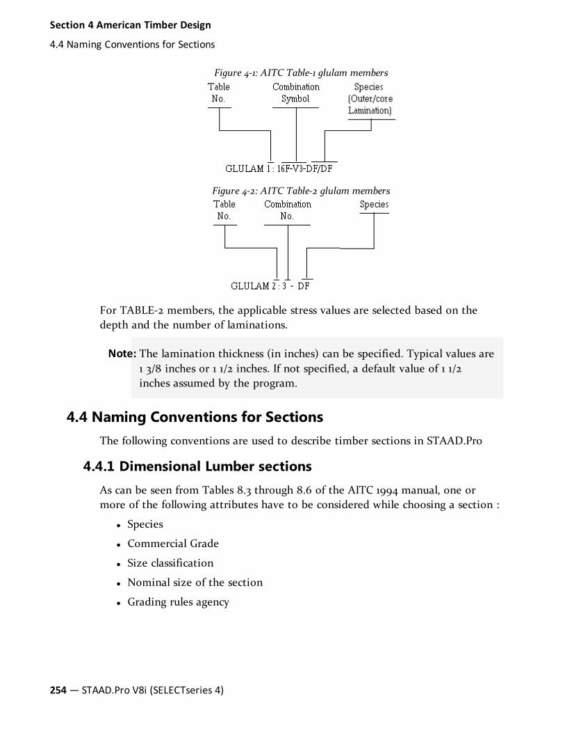
Figure 4-1: AITC Table-1 glulam members
Figure 4-2: AITC Table-2 glulam members
For TABLE-2 members, the applicable stress values are selected based on thedepth and the number of laminations.
Note: The lamination thickness (in inches) can be specified. Typical values are1 3/8 inches or 1 1/2 inches. If not specified, a default value of 1 1/2inches assumed by the program.
4.4 Naming Conventions for SectionsThe following conventions are used to describe timber sections in STAAD.Pro
4.4.1 Dimensional Lumber sectionsAs can be seen from Tables 8.3 through 8.6 of the AITC 1994 manual, one ormore of the following attributes have to be considered while choosing a section :
l Species
l Commercial Grade
l Size classification
l Nominal size of the section
l Grading rules agency
254— STAAD.Pro V8i (SELECTseries 4)
Section 4 American Timber Design
4.4 Naming Conventions for Sections

STAAD uses a naming convention that incorporates all of the above. Shownbelow is the name of a section that has characteristics as shown. It may be foundon page 8-637 of the AITC 1994 manual.
Species: Douglas Fir Larch
Commercial Grade: Dense Select Structural
Size Classification: Beams
Nominal size: 5”x 5”
Grading Rules Agency: WCLIB
Figure 4-3: Timber naming conventions
Implementation of Glulam Properties
For Glulam sections, each glulam designation has an associated value of Modulusof Elasticity and a set of allowable stresses. However, these values are notdependent on the size of the cross section. For example, a 3-1/8”x 6” 24F-V8DF/DF beam and a 6-3/4” x 30” 24F-V8 DF/DF beam both have an E of 1,600 ksiand an allowable bending stress in the tension zone, F
bx, of 2,400 psi.
Therefore, in STAAD’s glulam database, the section sizes are not linked to theglulam type. Users may specify any cross-section size they choose and pick thedesired glulam type. The Modulus of Elasticity and allowable stresses associatedwith that glulam are assigned to the member. The material properties for theGlulam database are taken from Table 1 of AITC 117-93 – Design StandardSpecifications for Structural Glued Laminated Timber of Softwood Species. Thispublication has been reproduced in the AITC 1994 manual starting from page 8-843.
Example for Dimensional Timber
UNIT FEET KIP
DEFINE MATERIAL START
ISOTROPIC DFLN_SS_4X4
E 273600
POISSON 0.15
Section 4 American Timber Design
4.4 Naming Conventions for Sections
Technical Reference Manual — 255
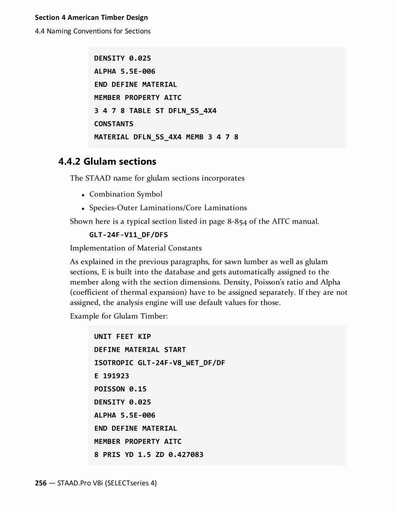
DENSITY 0.025
ALPHA 5.5E-006
END DEFINE MATERIAL
MEMBER PROPERTY AITC
3 4 7 8 TABLE ST DFLN_SS_4X4
CONSTANTS
MATERIAL DFLN_SS_4X4 MEMB 3 4 7 8
4.4.2 Glulam sectionsThe STAAD name for glulam sections incorporates
l Combination Symbol
l Species-Outer Laminations/Core Laminations
Shown here is a typical section listed in page 8-854 of the AITC manual.
GLT-24F-V11_DF/DFS
Implementation of Material Constants
As explained in the previous paragraphs, for sawn lumber as well as glulamsections, E is built into the database and gets automatically assigned to themember along with the section dimensions. Density, Poisson’s ratio and Alpha(coefficient of thermal expansion) have to be assigned separately. If they are notassigned, the analysis engine will use default values for those.
Example for Glulam Timber:
UNIT FEET KIP
DEFINE MATERIAL START
ISOTROPIC GLT-24F-V8_WET_DF/DF
E 191923
POISSON 0.15
DENSITY 0.025
ALPHA 5.5E-006
END DEFINE MATERIAL
MEMBER PROPERTY AITC
8 PRIS YD 1.5 ZD 0.427083
256— STAAD.Pro V8i (SELECTseries 4)
Section 4 American Timber Design
4.4 Naming Conventions for Sections

CONSTANTS
MATERIAL GLT-24F-V8_WET_DF/DF MEMB 8
4.5 Design ParametersThe timber design parameters for the AITC codes.
4.5.1 AITC 1994 Parameters
ParameterName
DefaultValue
Description
STAADAITC1994Code
CB Cb
1.0 Bearing Area Factor, Table4.13
CFB CF
1.0 Size Factor for AllowableBending Stress, see Table 8.3,8.4, 8.5, 8.6, 8.7
CFC CF
1.0 Size Factor for AllowableCompression Parallel toGrain, see Table 8.3, 8.4, 8.5,8.6, 8.7
CFT CF
1.0 Size Factor for AllowableTension Parallel to Grain, seeTable 8.3, 8.4, 8.5, 8.6, 8.7
CFU Cfu
1.0 Flat Use Factor, see Table 4.9
CSS CH
1.0 Shear Stress Factor, Section4.5.14
Table 4-2: AITC 1994 Timber Design Properties
Section 4 American Timber Design
4.5 Design Parameters
Technical Reference Manual — 257

ParameterName
DefaultValue
Description
STAADAITC1994Code
CMB CM
1.0 Wet service Factor forAllowable Bending Stress, seeTable 4.8
CMC CM
1.0 Wet service Factor forAllowable CompressionParallel to Grain, see Table4.8
CME CM
1.0 Wet service Factor forModulus of Elasticity, seeTable 4.8
CMP CM
1.0 Wet service Factor forAllowable CompressionPerpendicular to Grain, seeTable 4.8
CMT CM
1.0 Wet service Factor forAllowable Tension Parallel toGrain, see Table 4.8
CMV CM
1.0 Wet service Factor forAllowable Shear StressParallel to Grain, see Table4.8
CR Cr
1.0 Repetitive Member Factor,see Section 4.5.10
CSF CF
1.0 Form Factor, see Section4.5.12
CTM Ct
1.0 Temperature Factor, seeTable 4.11
258— STAAD.Pro V8i (SELECTseries 4)
Section 4 American Timber Design
4.5 Design Parameters
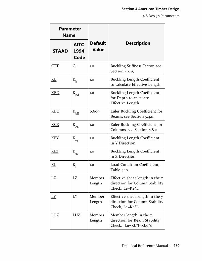
ParameterName
DefaultValue
Description
STAADAITC1994Code
CTT CT
1.0 Buckling Stiffness Factor, seeSection 4.5.15
KB Kb
1.0 Buckling Length Coefficientto calculate Effective Length
KBD Kbd
1.0 Buckling Length Coefficientfor Depth to calculateEffective Length
KBE KbE
0.609 Euler Buckling Coefficient forBeams, see Section 5.4.11
KCE KcE
1.0 Euler Buckling Coefficient forColumns, see Section 5.8.2
KEY Key
1.0 Buckling Length Coefficientin Y Direction
KEZ Kez
1.0 Buckling Length Coefficientin Z Direction
KL Kl
1.0 Load Condition Coefficient,Table 4.10
LZ LZ MemberLength
Effective shear length in the zdirection for Column StabilityCheck, Le=Ke*L
LY LY MemberLength
Effective shear length in the ydirection for Column StabilityCheck, Le=Ke*L
LUZ LUZ MemberLength
Member length in the zdirection for Beam StabilityCheck, Lu=Kb*l+Kbd*d
Section 4 American Timber Design
4.5 Design Parameters
Technical Reference Manual — 259

ParameterName
DefaultValue
Description
STAADAITC1994Code
LUY LUY MemberLength
Member length in the ydirection for Beam StabilityCheck, Lu=Kb*l+Kbd*d
CDT CDT 1.0 Load Duration Factor
CCR CCR 1.0 Curvature factor (Section4.5.11)
INDEX INDEX 10 Exponent value in theVolume Factor Equation(Section 4.5.6)
CV CV 1.0 Volume Factor (Section 4.5.6)
CC CC 0.8 Variable in Column StabilityFactor, Cp (Section 5.8.2, Eqn5-14)
SRC SRC 1.0 Slenderness ratio ofCompression member
SRT SRT 1.0 Slenderness ratio of Tensionmember
RATIO 1.0 Permissible ratio of actual toallowable stress
BEAM 1.0 0 = Design for end forces orlocations specified by sectioncommand. 1 = Calculatemoments at 12 pts along thebeam and use the maximumfor design.
260— STAAD.Pro V8i (SELECTseries 4)
Section 4 American Timber Design
4.5 Design Parameters

4.5.2 AITC 1984 Parameters
ParameterName
DefaultValue
Description
BEAM 1.0 0.0 = design for end forces or atlocations specified by sectioncommand.
1.0 = calculate moments at twelfthssections along the beam and use themax. for design.
CCR 1.0 Curvature factor
CDT 1.0 Duration of load factor
CSF 1.0 Form factor
CTM 1.0 Temp. factor
LAMINATION
1.50 inch Thickness of lamination in inch (1.50or 1.375)
LUZ 1.92*L Unsupported effective length forbeam in z.
LUY 1.92*L Unsupported effective length forbeam in y.
LY MemberLength
Same as above in y-axis.
LZ MemberLength
Effective length of the column in z-axis.
NSF 1.0 Net section factor for tensionmembers. (both shear and tensionstresses are based on sectional area xnsf )
RATIO 1.0 Permissible ratio of actual toallowable stresses.
Table 4-3: AITC 1985 Timber Design Parameters
Section 4 American Timber Design
4.5 Design Parameters
Technical Reference Manual — 261

ParameterName
DefaultValue
Description
WET 0.0 0.0 - dry condition
1.0 - wet condition
wet use factors are in-built
4.6 Member Design CapabilitiesSTAAD.Pro is capable of performing member design functions for both 1984 and1994 editions of AITC.
Hint: The User Interface can be used to easily assign design commands tomembers.
4.6.1 Code CheckingThe CHECK CODE command enables the user to check the adequacy of the size ( YD X ZD ) provided in the MEMBER PROPERTIES for the most critical forces andmoments. The program prints whether the member has passed or failed, thecritical conditions and the value of the ratio.
4.6.2 Member SelectionMember selection is limited to AITC 1984.
The SELECT MEMBER command starts with the min. permissible depth (or min.depth provided thru DMIN parameter) and checks the code. If the member failswith this depth, the thickness is increased by one lamination thickness and thecode requirements are checked again. The process is continued till the sectionpasses all the code requirements. This ensures the least weight section for themember. If the depth of the section reaches max. allowable or available depthand the member still fails, you can have the following options for redesign:
a. Change the width or increase the max. allowable depth (DMAX)
b. Change the timber grade
c. Change the design parameters
262— STAAD.Pro V8i (SELECTseries 4)
Section 4 American Timber Design
4.6 Member Design Capabilities

4.7 Orientation of LaminationLaminations are always assumed to lie along the local Z-plane of the member. Inthe MEMBER PROPERTIES section, YD always represents the depth of the sectionacross the grain and ZD represents the width along the grain. This is inaccordance with the sign convention conforming to SET Y UP (default).
Figure 4-4: Orientation of lamination
4.8 Tabulated Results of Member DesignFor CODE CHECKING and/or MEMBER SELECTION the output results are printedas shown in the previous section. The items are explained as follows:
a. MEMBER refers to the member number for which the design is performed.
b. TABLE refers to the size of the PRISMATIC section (B X D or ZD X YD).
c. RESULT prints whether the member has PASSed or FAILed.
d. CRITICAL COND refers to the CLAUSE or FORMULA NO. from theTIMBER CONSTRUCTION MANUAL (3rd. Edition, AITC-1985) whichgoverned the design. See following table:
CriticalCondition
Governing Criteria
Clause 5-19 Axial Compression and Bend-ing with MINIMUM ECCEN-TRICITY.
Table 4-4: Critical conditions evaluated perAITC code
Section 4 American Timber Design
4.7 Orientation of Lamination
Technical Reference Manual — 263

CriticalCondition
Governing Criteria
Clause 5-18 Axial Compression and Bend-ing
Clause 5-42 Axial Tension and Bending
Clause 5-24 Horizontal Shear
Clause 5.40 Lateral stability for net com-pressive stress in case of Ten-sion and Bending.
e. RATIO prints the ratio of the actual stresses to allowable stresses for thecritical condition. This ratio is usually the cumulative ratio of stresses in theinteraction formula. In case of shear governing the design, it means theratio of the actual shear stress to allowable shear stress. If this value exceedsthe allowable ratio (default 1.0) the member is FAILed.
f. LOADING provides the load case number that governed.
g. FX, MY and MZ provide the design axial force, moment in local Y axes andmoment in local Z axes respectively. FX value is followed by a letter C or Tto denote COMPRESSION or TENSION.
h. LOCATION specifies the actual distance from the start of the member tothe section where design forces govern in case BEAM command or SEC-TION command is specified.
OUTPUT parameters that appear within the box are explained as follows:
a. MEMB refers to the same member number for which the design is per-formed.
b. GLULAM GRADE refers to the grade of the timber.
c. LAM refers to lamination thickness provided in the input or assumed bythe program. See INPUT PARAMETERS section.
d. LZ, LY, LUZ and LUY are the effective lengths as provided or calculated. SeeINPUT PARAMETERS section.
e. JZ and JY are the modifiers for the P-DELTA effect about Z-axis and Y-axisrespectively. These are calculated by the program.
264— STAAD.Pro V8i (SELECTseries 4)
Section 4 American Timber Design
4.8 Tabulated Results of Member Design

f. CDT, CSF, WET, CCR, CTM are the allowable stress modifiers explained inthe INPUT PARAMETERS section.
g. CFZ and CFY are values of the size factors in the Z-axis and Y-axis respec-tively. CLZ and CLY represent the factors of lateral stability for beams aboutZ-axis and Y-axis respectively. These values are printed to help the user seethe intermediate design values and re-check the design calculations.
h. fa, fbz, fby, fvzand f
vyare the actual axial stress, bending stresses about Z and
Y axes and horizontal shear stresses about Z and Y axes respectively. If thebending moments about both axes are less then the eccentric momentsbased on min. eccentricity then bending stresses are calculated based on themin. eccentricity . Refer DESIGN OPERATIONS section for details.
i. FA, FBZ, FBY, FVZ, and FVY are the final allowable axial, bending (Z and Yaxes) and horizontal shear (Z and Y axes) stresses. See "Allowable Stress perAITC Code" on page 250 for details.
4.8.1 Example Glulam Member DesignSTAAD.Pro CODE CHECKING - (AITC)***********************
ALL UNITS ARE - POUN FEET (UNLESS OTHERWISE NOTED)MEMBER TABLE RESULT/ CRITICAL COND/ RATIO/ LOADING/
FX MY MZ LOCATION=======================================================================
1 10.750X16.500 GLULAM GRADE:GLT-24F-V8_DF/DFPASS CL.5.9.2 0.014 3
4583.17 C 0.00 1310.87 12.0000|--------------------------------------------------------------------------|| LEZ = 144.000 LEY = 144.000 LUZ = 144.000 LUY = 144.000 INCHES || || CD = 1.000 CMB = 1.000 CMT = 1.000 CMC = 1.000 CMP = 1.000 || CMV = 1.000 CME = 1.000 CFB = 1.000 CFT = 1.000 CFC = 1.000 || CFU = 1.000 CR = 1.000 CTT = 1.000 CC = 1.000 CF = 1.000 || CT = 1.000 CH = 1.000 CB = 1.000 CI = 1.000 CV = 0.000 || CLY = 0.999 CLZ = 0.997 CP = 0.934 c = 0.900 E' = 1600000.122 PSI || || ACTUAL STRESSES : (POUND INCH) || fc = 25.839 ft = 0.000 || f_cby = 0.000 f_cbz = 32.249 || fv = 0.000 || ALLOWABLE STRESSES: (POUND INCH) || FC = 1541.320 FT = 0.000 || FCBY = 1448.972 FCBZ = 2340.789 || FCEY = 0.000 FCEZ = 8780.903 || FBE = 3727.248 || FTB = 0.000 F**TB = 0.000 || FV = 0.000 SLENDERNESS = 50.000 ||--------------------------------------------------------------------------|
4.9 ExamplesThe following conventions are used to describe timber sections in STAAD.Pro
Section 4 American Timber Design
4.9 Examples
Technical Reference Manual — 265

4.9.1 Example for dimensional lumber
STAAD PLANE EXAMPLE FOR DIMENSIONAL LUMBER
UNIT FEET POUND
JOINT COORDINATES
1 0 0 0; 2 6 0 0; 3 12 0 0; 4 18 0 0;
5 24 0 0; 6 6 3 0; 7 12 6 0; 8 18 3 0;
MEMBER INCIDENCES
1 1 2; 2 2 3; 3 3 4; 4 4 5; 5 1 6; 6 6 7; 7 7 8; 8 8 5;
9 2 6; 10 3 7; 11 4 8; 12 6 3; 13 3 8;
UNIT FEET POUND
DEFINE MATERIAL START
ISOTROPIC DFLR_SS_2X4
E 2.736E+008
POISSON 0.15
DENSITY 25
ALPHA 5.5E-006
ISOTROPIC DFLR_SS_3X6
E 2.736E+008
POISSON 0.15
DENSITY 25
ALPHA 5.5E-006
END DEFINE MATERIAL
MEMBER PROPERTY AITC
1 TO 4 9 TO 11 TABLE ST DFLR_SS_2X4
5 TO 8 12 13 TABLE ST DFLR_SS_3X6
CONSTANTS
MATERIAL DFLR_SS_2X4 MEMB 1 TO 4 9 TO 11
MATERIAL DFLR_SS_3X6 MEMB 5 TO 8 12 13
MEMBER RELEASE
9 TO 13 START MP 0.99
266— STAAD.Pro V8i (SELECTseries 4)
Section 4 American Timber Design
4.9 Examples

9 TO 13 END MP 0.99
6 END MP 0.99
7 START MP 0.99
SUPPORTS
1 PINNED
5 FIXED BUT FX MZ
UNIT FEET POUND
LOAD 1 DEAD+LIVE LOAD
SELFWEIGHT Y -1
MEMBER LOAD
1 TO 4 UNI GY -30
5 TO 8 UNI GY -40
LOAD 2 SNOW LOAD
MEMBER LOAD
5 TO 8 UNI GY -50
LOAD 3 WIND LOAD
MEMBER LOAD
5 6 UNI Y -30
7 8 UNI Y 25
LOAD COMB 11 D+L+SNOW
1 1.0 2 1.0
LOAD COMB 12 D+L+SNOW+WIND
1 1.0 2 1.0 3 1.0
PERFORM ANALYSIS PRINT STATICS CHECK
PARAMETER
CODE AITC
BEAM 1.0 ALL
CHECK CODE ALL
FINISH
Section 4 American Timber Design
4.9 Examples
Technical Reference Manual — 267

4.9.2 Example for Glulaminated lumber
STAAD PLANE EXAMPLE FOR GLULAM DESIGN
INPUT WIDTH 79
UNIT FEET KIP
JOINT COORDINATES
1 0 0 0; 2 12 0 0; 3 24 0 0; 4 36 0 0; 5 0 12 0; 6 6 100; 7 18 6 0; 8 30 2 0;
MEMBER INCIDENCES
1 1 2; 2 2 3; 3 3 4; 4 5 6; 5 6 7; 6 7 8; 7 8 4; 8 1 5; 92 6; 10 3 7; 11 1 6;
12 2 7; 13 3 8;
UNIT INCHES KIP
DEFINE MATERIAL START
ISOTROPIC GLT-24F-V8_DF/DF
E 1600
POISSON 0.15
DENSITY 1.44676E-005
ALPHA 5.5E-006
END DEFINE MATERIAL
MEMBER PROPERTY
1 TO 7 PRIS YD 16.5 ZD 10.75
8 TO 13 PRIS YD 10.5 ZD 8.75
CONSTANTS
MATERIAL GLT-24F-V8_DF/DF MEMB 1 TO 13
SUPPORTS
1 4 PINNED
UNIT POUND FEET
LOAD 1 DEAD
SELFWEIGHT Y -1
LOAD 2 LIVE
MEMBER LOAD
268— STAAD.Pro V8i (SELECTseries 4)
Section 4 American Timber Design
4.9 Examples

1 TO 3 UNI GY -100
4 TO 7 UNI GY -100
LOAD COMB 3
1 1.0 2 1.0
PERFORM ANALYSIS PRINT STATICS CHECK
PARAMETER
CODE AITC
CMT 1 ALL
RATIO 0.9 ALL
CHECK CODE ALL
FINISH
Section 4 American Timber Design
4.9 Examples
Technical Reference Manual — 269

270— STAAD.Pro V8i (SELECTseries 4)
Section 4 American Timber Design

Section 5
Commands and InputInstructions
5.1 Command Language Conventions 275
5.2 Problem Initiation and Model Title 280
5.3 Unit Specification 282
5.4 Input/Output Width Specification 284
5.5 Set Command Specification 284
5.6 Data Separator 294
5.7 Page New 295
5.8 Page Length/Eject 295
5.9 Ignore Specifications 296
5.10 No Design Specification 296
5.11 Joint Coordinates Specification 296
Technical Reference Manual — 271

5.12 Member Incidences Specification 300
5.13 Elements and Surfaces 303
5.14 Plate Element Mesh Generation 309
5.15 Redefinition of Joint and Member Numbers 317
5.16 Entities as Single Objects 318
5.17 Rotation of Structure Geometry 324
5.18 Inactive/Delete Specification 324
5.19 User Steel Table Specification 326
5.20 Member Property Specification 339
5.21 Element/Surface Property Specification 368
5.22 Member/Element Releases 370
5.23 Axial Member Specifications 375
5.24 Element Plane Stress and Ignore Inplane Rotation Specification 382
5.25 Member Offset Specification 383
5.26 Specifying and Assigning Material Constants 385
5.27 Support Specifications 405
5.28 Rigid Diaphragm Modeling 420
5.29 Draw Specifications 427
5.30 Miscellaneous Settings for Dynamic Analysis 427
5.31 Definition of Load Systems 429
5.32 Loading Specifications 539
5.33 Reference Load Cases - Application 669
5.34 Frequency Calculation 670
5.35 Load Combination Specification 672
5.36 Calculation of Problem Statistics 676
5.37 Analysis Specification 676
5.38 Change Specification 709
5.39 Load List Specification 711
5.40 Load Envelope 712
5.41 Section Specification 713
272— STAAD.Pro V8i (SELECTseries 4)
Section 5 Commands and Input Instructions

5.42 Print Specifications 714
5.43 Stress/Force output printing for Surface Entities 722
5.44 Printing Section Displacements for Members 724
5.45 Printing the Force Envelope 726
5.46 Post Analysis Printer Plot Specifications 727
5.47 Size Specification 727
5.48 Steel and Aluminum Design Specifications 728
5.49 Code Checking Specification 731
5.50 Group Specification 734
5.51 Steel and Aluminum Take Off Specification 736
5.52 Timber Design Specifications 737
5.53 Concrete Design Specifications 739
5.54 Footing Design Specifications 742
5.55 Shear Wall Design 742
5.56 End Run Specification 745
This section of the manual describes in detail various commands and relatedinstructions for STAAD. The user utilizes a command language format tocommunicate instructions to the program. Each of these commands eithersupplies some data to the program or instructs it to perform some calculationsusing the data already specified. The command language format and conventionsare described in Section 5.1. This is followed by a description of the availablecommands.
Although the STAAD input can be created through the Modeling mode, it isimportant to understand the command language. With the knowledge of thislanguage, it is easy to understand the problem and add or comment data asnecessary. The general sequence in which the commands should appear in aninput file should ideally follow the same sequence in which they are presented inthis section. The commands are executed in the sequence entered. Obviouslythen the data needed for proper execution of a command must precede thecommand (e.g., Print results after Perform Analysis). Otherwise, the commandscan be provided in any order with the following exceptions.
i. All design related data can be provided only after the analysis command.
ii. All load cases and load combinations must be provided together, except in
Section 5 Commands and Input Instructions
Technical Reference Manual — 273

a case where the CHANGE command is used (refer to section 5.38).Additional load cases can be provided in the latter part of input.
All input data provided is stored by the program. Data can be added, deleted ormodified within an existing data file.
In STAAD.Pro 2006 and earlier, all analytical calculations such as jointdisplacements, eigenvalues and eigenvectors were calculated using an analysisengine which for identification purposes is known as the Basic Solver. Thisengine has been able to handle the analytical requirements for a vast majority ofSTAAD models that users have created in the recent years.
As computer resources such as processor speed, memory and disk space havegrown, STAAD users are also creating larger models. As a result, numericallyfaster algorithms and solution techniques have become necessary. Also, newfeatures such as pushover analysis and buckling analysis which are outside thescope of the standard engine have made it necessary to introduce a new enginewhich is known as the Advanced Solver. This new Solver is available as analternative engine effective from STAAD.Pro 2007, Build 1001.
The Advanced Solver
As described above, the Advanced solver is a new addition to the STAADAnalysis Engine (note 1) which can be used for solving both static and dynamicproblems. It is part of the STAAD engine with no special command required torun it. It is automatically activated if a suitable license is available (note 2),however, this can be turned off and the Basic Solver used by including theoption:
SET STAR 0
This command must be included in the header information block at the start ofthe file and before the first JOINT command block.
The engine can operate in two modes, in-core and out-of-core. The in-coresolver will be used for models with under 20000 joints and the out-of-core solverfor models over 20000 joints. In most situations, the in-core mode will providethe quickest solution, but where there is insufficient memory available, then theengine will use the out-of-core mode. Again, selection of the mode isautomatically chosen by the analysis, but can be over-ridden.
The full set of overrides for the advanced engine is:
SET STAR -3 use in-core solver regardless of size
SET STAR 4 use out-of-core solver regardless of size
274— STAAD.Pro V8i (SELECTseries 4)
Section 5 Commands and Input Instructions

SET STAR 3 default
SET STAR 0 use Basic STAAD solver
Notes
1. The Advanced Solver is not available for use with a Stardyne Analysis.
2. To use this feature requires access to a STAAD Advanced license. If youdo not currently have this feature, please contact your account manager.
3. Global Euler Buckling analysis is different between the two solvers.
5.1 Command Language ConventionsThis section describes the command language used in STAAD. First, the variouselements of the language are discussed and then the command format isdescribed in details.
5.1.1 Elements of STAAD Commands
Integer Numbers
Integer numbers are whole numbers written without a decimal point. Thesenumbers are designated as i
1, i2, etc., and should not contain any decimal point.
Negative signs (-) are permitted in front of these numbers. Omit the sign forpositive. No spaces between the sign and the number.
Floating Point Numbers
These are real numbers which may contain a decimal portion. These numbers aredesignated as f
1, f2... etc.. Values may have a decimal point and/or exponent.
When specifying numbers with magnitude less than 1/100, it is advisable to usethe E format to avoid precision related errors. Negative signs (-) are permitted infront of these numbers. Omit the sign for positive. No spaces between the signand the number. Limit these to 24 characters.
Example
5055.32 0.73 -8.9 732
5E3 -3.4E-6
etc.
The decimal point may be omitted if the decimal portion of the number is zero.
Section 5 Commands and Input Instructions
5.1 Command Language Conventions
Technical Reference Manual — 275

Alphanumeric
These are characters, which are used to construct the names for data, titles orcommands. Alphabetic characters may be input in upper or lower case letters. Noquotation marks are needed to enclose them.
Example
MEMBER PROPERTIES
1 TO 8 TABLE ST W8X35
Repetitive Data
Repetitive numerical data may be provided in some (but not all) input tablessuch as joint coordinates by using the following format:
n*f
Where:
n = number of times data has to be repeated
f = numeric data, integer and floating point
Example
JOINT COORDINATES
1 3*0.
This joint coordinate specification is same as:
1 0. 0. 0.
5.1.2 Command Formats
Free-Format Input
All input to STAAD is in free-format style. Input data items should be separatedby blank spaces (not commas) from the other input data items. Quotation marksare never needed to separate any alphabetic words such as data, commands ortitles. Limit a data item to 24 characters.
276— STAAD.Pro V8i (SELECTseries 4)
Section 5 Commands and Input Instructions
5.1 Command Language Conventions

Commenting Input
For documentation of a STAAD data file, the facility to provide comments isavailable. Comments can be included by providing an asterisk (*) mark as thefirst non-blank character in any line. The line with the comment is "echoed" inthe output file but not processed by the program.
Example
JOINT LOAD
* THE FOLLOWING IS AN EQUIPMENT LOAD
2 3 7 FY 35.0
ETC.
Meaning of Underlining in the Manual
Exact command formats are described in the latter part of this section. Manywords in the commands and data may be abbreviated. The full word intended isgiven in the command description with the portion actually required (theabbreviation) underlined.
For example, if the word MEMBER is used in a command, only the portion MEMBneed be input. It is clearer for others reading the output if the entire word isused, but an experienced user may desire to use the abbreviations.
Meaning of Braces and Parenthesis
In some command formats, braces enclose a number of choices, which arearranged vertically or separated by a | character. One and only one of the choicescan be selected. However, several of the listed choices may be selected if anasterisk (*) mark is located outside the braces.
Example
{XY | YZ | XZ}
In the above example, you must make a choice of XY or YZ or XZ.
Note: In some instances, the choices will be explicitly defined using "or" forclarification.
Example
Section 5 Commands and Input Instructions
5.1 Command Language Conventions
Technical Reference Manual — 277

*{FX | FY | FZ}
Here, you can choose one or all of the listing (FX, FY and FZ), in any order.
Parentheses, ( ), enclosing a portion of a command indicate that the enclosedportion is optional. The presence or absence of this portion affects the meaningof the command, as is explained in the description of the particular command.
Example
PRINT (MEMBER) FORCES
PERFORM ANALYSIS (PRINT LOAD DATA)
In the first line, the word MEMBER may be omitted with no change of themeaning of the command. In the second line, the PRINT LOAD DATA commandmay also be omitted, in which case the load data will not be printed.
Multiple Data Separator
Multiple data can be provided on a single line, if they are separated by asemicolon (;) character. One restriction is that a semicolon can not separateconsecutive commands. They must appear on separate lines.
Example
MEMBER INCIDENCES
1 1 2; 2 2 3; 3 3 4
etc.
Possible Error:
PRINT FORCES; PRINT STRESSES
In the above case, only the PRINT FORCES command is processed and the PRINTSTRESSES command is ignored.
Listing Data
In some STAAD command descriptions, the word "list" is used to identify a list ofjoints, members/elements, or loading cases. The format of a list can be defined asfollows:
list = *{ i1 i2 i3 … | i1 TO i2 (BY i3) | X or Y or Z }
278— STAAD.Pro V8i (SELECTseries 4)
Section 5 Commands and Input Instructions
5.1 Command Language Conventions

TO means all integers from the first (i1) to the second (i
2) inclusive. BY means that
the numbers are incremented by an amount equal to the third data item (i3). If
BY i3is omitted, the increment will be set to one. Sometimes the list may be too
long to fit on one line, in which case the list may be continued to the next lineby providing a hyphen preceded by a blank. Also, only a list may be continuedand not any other type of data.
Instead of a numerical list, a single group-name may be entered if that group waspreviously defined.
Instead of a numerical list, the specification X ( or Y or Z) may be used. Thisspecification will include all MEMBERs parallel to the global direction specified.Note that this is not applicable to JOINTs or ELEMENTs.
Note: ALL, BEAM, PLATE, SOLID. Do not use these unless thedocumentation for a command specifically mentions them as availablefor that command. ALL means all members and elements, BEAM meansall members, etc.
Continuing a command to the next line
Only lists may be continued to the next line by ending the line with a blank andhyphen (see above) with few exceptions: Multilinear spring supports, Supports,Master/Slave. Others have special types of continuations. Please follow thecommand descriptions.
Example
2 4 7 TO 13 BY 2 19 TO 22 -
28 31 TO 33 FX 10.0
This list of items is the same as:
2 4 7 9 11 13 19 20 21 22 28 31 32 33 FX 10.0
Possible Error:
3 5 TO 9 11 15 -
FX 10.0
Section 5 Commands and Input Instructions
5.1 Command Language Conventions
Technical Reference Manual — 279

In this case, the continuation mark for list items is used when list items are notcontinued. This will result in an error message or possibly unpredictable results.
5.1.3 Listing of Objects by Specification of Global RangesUsed to specify lists of objects (e.g., joints, members, and/or elements) byproviding global ranges. The general format of the specification is as follows.
General Format
{ XRANGE | YRANGE | ZRANGE } f1, f2
Where:
XRANGE, YRANGE, ZRANGE = direction of range (parallel to globalX, Y, Z directions respectively)
f1, f2 = values (in current unit system) that defines the specifiedrange.
Notes
1. Only one range direction (XRANGE, YRANGE etc.) is allowed per list.(Exceptions:Area/Floor load and Master/Slave).
2. No other items may be in the list.
3. The values defining the range (f1, f2) must be in the current unit system.
Example
MEMBER TRUSS
XRANGE 20. 70.
CONSTANTS
E STEEL YRANGE 10. 55.
In the above example, a XRANGE is specified with values of 20. and 70. Thisrange will include all members lying entirely within a range parallel to the globalX-axis and limited by X=20 and X=70.
5.2 Problem Initiation and Model TitleThis command initiates the STAAD run and is also used to specify the type of thestructure and provide an optional title.
280— STAAD.Pro V8i (SELECTseries 4)
Section 5 Commands and Input Instructions
5.2 Problem Initiation and Model Title
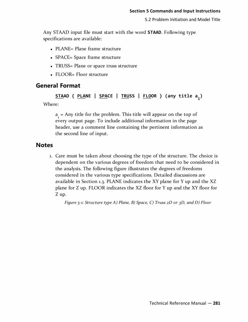
Any STAAD input file must start with the word STAAD. Following typespecifications are available:
l PLANE= Plane frame structure
l SPACE= Space frame structure
l TRUSS= Plane or space truss structure
l FLOOR= Floor structure
General FormatSTAAD { PLANE | SPACE | TRUSS | FLOOR } (any title a1)
Where:
a1= Any title for the problem. This title will appear on the top of
every output page. To include additional information in the pageheader, use a comment line containing the pertinent information asthe second line of input.
Notes
1. Care must be taken about choosing the type of the structure. The choice isdependent on the various degrees of freedom that need to be considered inthe analysis. The following figure illustrates the degrees of freedomsconsidered in the various type specifications. Detailed discussions areavailable in Section 1.3. PLANE indicates the XY plane for Y up and the XZplane for Z up. FLOOR indicates the XZ floor for Y up and the XY floor forZ up.
Figure 5-1: Structure type A) Plane, B) Space, C) Truss 2D or 3D, and D) Floor
Section 5 Commands and Input Instructions
5.2 Problem Initiation and Model Title
Technical Reference Manual — 281

2. The optional title provided by you are printed on top of every page of theoutput. You can use this facility to customize his output.
LimitsThe following limits to model size are effective for STAAD.Pro V8i (SELECTseries2) (release 20.07.07).
1. Joint number 1 to 999999
2. Number of joints: 200000*
3. Member/Element numbers: 1 to 999999
4. Number of Members, Plates, and Solids: 225000*
5. Load Case numbers: 1 to 99999
6. Number of primary and combination cases: 10101
7. Number of modes and frequencies: 2700
8. Number of load cases that may be combined by a Repeat Load or LoadCombination command: 550
* Some STAAD copies are available with much smaller limits, please check whatlimits you have purchased.
5.3 Unit SpecificationThis command allows you to specify or change length and force units for inputand output.
282— STAAD.Pro V8i (SELECTseries 4)
Section 5 Commands and Input Instructions
5.3 Unit Specification

General FormatUNIT *{ length-unit, force-unit}
length-unit = { INCHES | FEET or FT or FO | CM | METER | MMS| DME | KM }
force-unit = { KIP | POUND | KG | MTON | NEWTON | KNS | MNS| DNS }
Note: DME denotes Decimeters. MNS denotes mega Newtons (1000KiloNewtons) and DNS denotes DecaNewtons (10 Newtons). MTONdenotes Metric Ton (1000 kilograms). All other units are selfexplanatory.
DescriptionThe UNIT command can be specified any number of times during an analysis. Alldata is assumed to be in the most recent unit specification preceding that data.Also, the input-unit for angles is always degrees. However, the output unit forjoint rotations (in joint displacement) is radians. For all output, the units areclearly specified by the program.
Example
UNIT KIP FT
UNIT INCH
UNIT METER KNS
UNIT CM MTON
Notes
a. This command may be used as frequently as needed to specify data or gen-erate output in the desired length and/or force units. Mixing of differentunit systems (Imperial, Metric, SI etc.) is allowed.
b. This command may be anywhere a primary level command (e.g., JOINTCOORD, MEMBER INCIDENCE, etc.) can be. In addition, it may also bewherever a first level load command may be.
Section 5 Commands and Input Instructions
5.3 Unit Specification
Technical Reference Manual — 283

c. Exceptions: The second level load commands (MEMBER LOAD, JOINTLOAD and FLOOR LOAD), allow the UNIT command to be entered on aseparate line, not within a continuation or between semi-colons.
5.4 Input/Output Width SpecificationThese commands may be used to specify the width(s) of the lines of output file(s).
For INPUT width, 79 is always used. The program can create output using twodifferent output widths - 72 (default) and 118. The 72-character width may beused for display on most CRTs and for printing on “portrait” wide paper. The 118-character width may be used for printing on “landscape” wide paper.
Note: This is a customization facility that may be used to improve thepresentation quality of the output documents.
General Format{INPUT | OUTPUT} WIDTH i1
Where:
i1= 72 or 118 depending on narrow or wide output. 72 is the default
value.
5.5 Set Command SpecificationThis command allows the user to set various general specifications for theanalysis/design run.
General FormatSET { NL i1 | {DISPLACEMENT i2 | PDELTA TOL i9} | SDAMP i3 |WARP i4 | ITERLIM i5 | PRINT i7 | NOPRINT DIRECT | SHEAR |ECHO { ON | OFF } | GUI i6 | Z UP | DEFLECTION CUTOFF f1 |FLOOR LOAD TOLERANCE F2 }
Where:
i1 = Maximum number of primary load cases (NL)
i3 = Damping ratio to be used for all springs in computing the modalcomposite damping in dynamics.
284— STAAD.Pro V8i (SELECTseries 4)
Section 5 Commands and Input Instructions
5.4 Input/Output Width Specification

i4 = Warping restraint ratio to be used for I section members incomputing the torsional rigidity. If 0.0 then no warping restraint,normal default option; If 1.0 then full warping restraint. Cw, thewarping constant, will be computed and used in the torsional rigiditycalculation. Values between 0.0 and 1.0 will result in a partial warpingrestraint.
i5 = Maximum number of tension/compression iterations.
i6 = 1, Bypass forming data and files needed for post-processing.
i7 = Used to suppress some warning messages or to include additionaloutput. Refer to table 5-1 for values.
Note: The following SET commands contain values with associated units andshould appear after a UNIT command and before the firstJOINT command.
Note: Both i2and i
9are the P-Delta Convergence criteria input. There are
two methods available, enter SET DISPLACEMENT i2 or SET PDELTATOL i9 . Enter only one.
i2 = If the change in the Euclidean norm of the displacement vectorfrom one PDELTA iteration to the next is less than this convergencetolerance value; then the iteration has converged for the case beinganalyzed.
i9= If the maximum absolute change in displacement of each dof
from one PDELTA iteration to the next is less than this convergencetolerance value; then the iteration has converged for the case beinganalyzed.
f1= If the absolute value of the maximum section displacement is less
than f1after two iterations; then it is converged. Rapidly diverging
minor axis displacement will not occur until after two iterations. f1is
in current length units.
f2= tolerance value used
Section 5 Commands and Input Instructions
5.5 Set Command Specification
Technical Reference Manual — 285

Description
Command Description
SET NL The SET NL command is used ina multiple analysis run if the userwants to add more primary loadcases after one analysis has beenperformed. Specifically, for thoseexamples, which use the CHANGEcommand (section 5.38), if theuser wants to add more primaryload cases, the NL value shouldbe set to the maximum number(or slightly more) with the SETNL command. The program willthen be able to set aside addi-tional memory space for infor-mation to be added later. Thiscommand should be providedbefore any joint, member or loadspecifications. The value for i1should not be much greater thanthe maximum number of primaryload cases.
Table 5-1: Commonly used SET commands
286— STAAD.Pro V8i (SELECTseries 4)
Section 5 Commands and Input Instructions
5.5 Set Command Specification

Command Description
SET
DISPLACEMENT
or
PDELTA TOL
For PDELTA ANALYSIS withCONVERGE option there are twoconvergence methodologies tochoose from (refer to section5.37.2 for additional information)
1. The SET DISPLACEMENT i2command is used to specifythe convergence tolerance.If the Euclidean norm RMSdisplacement of two con-secutive iterations changesless than the value entered,then that load case is con-verged. This commandshould be placed before theJOINT COORDINATE spec-ification. The default tol-erance value, i
2, is equal to
the maximum span of struc-ture divided by 120. Theconvergence tolerance forthe Euclidean norm is dif-ficult to know, so using thisoption is not rec-ommended.
2. The SET PDELTA TOL i9command selects this sec-ond method. Default tol-erance value, i
9, is 0.01 inch.
If the maximum change ineach displacement dof fromtwo consecutive iterationsis less than ftol, then thatload case is converged. Thiscommand should be placedbefore the JOINT COOR-DINATE specification andafter a UNIT command.
Section 5 Commands and Input Instructions
5.5 Set Command Specification
Technical Reference Manual — 287

Command Description
SET SDAMP The SET SDAMP command willallow the damping of springs tobe considered in computing thecomposite modal damping foreach mode in a dynamic solution.This command is not used unlessCDAMP ratios are also enteredfor the members and elements inthe CONSTANTS command. Com-posite damping is generally onlyused if there are many modes inthe dynamic solution and thereare a wide range of dampingratios in the springs, members, orelements.
SET WARP The SET WARP command willallow the I section member endwarping restraint to be con-sidered in calculating the tor-sional stiffness rigidity. Full orpartial or no warping restraintare allowed.
288— STAAD.Pro V8i (SELECTseries 4)
Section 5 Commands and Input Instructions
5.5 Set Command Specification

Command Description
SET ITERLIM The SET ITERLIM command isfor raising the maximumiteration limit above the defaultof 10 in tension/compressioniterations. Since this iterativeprocedure will not necessarilyconverge, this option of moreiterations may not help andshould be used with caution. Theminimum iteration limit thatmay be entered is 3.
After any tension/compressionanalysis, the output file (fileextension .ANL) should bescanned for warnings of non-convergence. Do not use resultsfrom non-converged cases.
Section 5 Commands and Input Instructions
5.5 Set Command Specification
Technical Reference Manual — 289
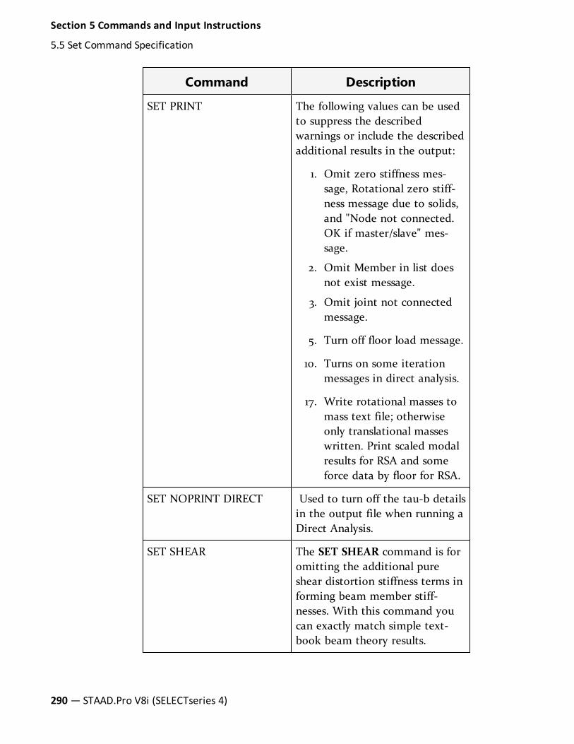
Command Description
SET PRINT The following values can be usedto suppress the describedwarnings or include the describedadditional results in the output:
1. Omit zero stiffness mes-sage, Rotational zero stiff-ness message due to solids,and "Node not connected.OK if master/slave" mes-sage.
2. Omit Member in list doesnot exist message.
3. Omit joint not connectedmessage.
5. Turn off floor load message.
10. Turns on some iterationmessages in direct analysis.
17. Write rotational masses tomass text file; otherwiseonly translational masseswritten. Print scaled modalresults for RSA and someforce data by floor for RSA.
SET NOPRINT DIRECT Used to turn off the tau-b detailsin the output file when running aDirect Analysis.
SET SHEAR The SET SHEAR command is foromitting the additional pureshear distortion stiffness terms informing beam member stiff-nesses. With this command youcan exactly match simple text-book beam theory results.
290— STAAD.Pro V8i (SELECTseries 4)
Section 5 Commands and Input Instructions
5.5 Set Command Specification

Command Description
SET ECHO The SET ECHO ON commandwill activate and the SET ECHOOFF command will deactivate theechoing of input file commandsin the output file. In the absenceof the SET ECHO command,input file commands will beechoed back to the output file.
SET GUI After the calculations are com-pleted, and before the Analysiswindow is closed, the programcreates several files for the pur-pose of displaying results in thepost processing mode. In largemodels, this can be a time con-suming process. If the user's goalis to look at results in the outputfile only (file extension .ANL) anddoes not intend to go into thepost-processing mode, he/shecould instruct the program toskip the process of creating thosefiles. The SET GUI 1 may bespecified immediately before theFINISH command, or some-where near the beginning of thefile after STAAD SPACE.
Section 5 Commands and Input Instructions
5.5 Set Command Specification
Technical Reference Manual — 291

Command Description
SET Z By default, the Y-axis is thevertical axis. However, the SET ZUP command may be used tomodel situations where Z-axisrepresents the vertical axis(direction of gravity load) of thestructure. This situation mayarise if the input geometry iscreated through some CADsoftware. This command willaffect the default BETA anglespecification. However, BETA canbe set to a certain value for allmembers parallel to a particularglobal axis by using the MEMBERX (or Y or Z) type of listing. Foradditional information, see theCONSTANTs specification(Section 5.26).
The SET Z UP Command directlyinfluences the values of thefollowing input:
a. JOINT COORDINATE
b. Input for the PERFORMROTATION Command
c. BETA ANGLE
The following features of STAADcannot be used with the SET ZUP command:
Automatic Generation of SpringSupports for Mat Foundations
292— STAAD.Pro V8i (SELECTseries 4)
Section 5 Commands and Input Instructions
5.5 Set Command Specification

Command Description
SET STAR n Instructs the program whichsolver to use. Refer to Section 5.for additional information onusing the Advanced Solver.
SET DEFLECTION CUTOFF Used to arrest huge dis-placements in minor axis due tosmall delta effects.
SET FLOOR LOAD TOL-ERANCE
Used to specify the tolerance forout of plane nodes in a floor load.
The following table contains a list of other rarely used SET commands
Command Description
SET DATA CHECK Ignored
SET RUN Ignored
SET COMPRESS Turn OFF file compression
SET SOLUTION INCORE Use determinant search forfrequencies for small prob-lems.
SET SOLVER should ignore
SET EXM should ignore (ExtendedMemory)
SET NJ should ignore
SET MN should ignore
SET CONNECTIVITY should ignore
SET MASS = 1, Use generated momentsat masses.
SET MODAL should ignore
Table 5-2: Infrequently used SET commands
Section 5 Commands and Input Instructions
5.5 Set Command Specification
Technical Reference Manual — 293

Command Description
SET THISTORY =2, Use exact force inte-gration in time history.
SET INTERPOLATION LIN or LOG for spectra
SET DISPLACEMENT METHOD should ignore
SET s1 s1 = file extension for L43
SET BUBBLE = 1, Do not use bubble fnsin solids
SET NOSECT No section results will becalculated
SET TMH should ignore
SET SSVECT To instruct the program touse a different initial set oftrial vectors for eigen-solution. May be used ifeigen extraction fails.
SET INCLINED REACTION To obtain reactions atinclined supports in theinclined axis system.
SET GROUP DUPLICATES Followed by an integervalue which is used to spec-ify the number of groups towhich one model entity(node, member, plate, orsolid object) may belong.Must be in the range of fourto 100, inclusive. Thedefault value is 10 groups.
5.6 Data SeparatorThis command may be used to specify the desired separator character that can beused to separate multiple lines of data on a single line of input.
The semicolon (;) is the default character which functions as the separator for
294— STAAD.Pro V8i (SELECTseries 4)
Section 5 Commands and Input Instructions
5.6 Data Separator

multiple line data on one line. However, this separator character can be changedby the SEPARATOR command to any character.
Note: Comma (,) or asterisk (*) may not be used as a separator character.
General FormatSEPARATOR a1
5.7 Page NewThis command may be used to instruct the program to start a new page ofoutput.
With this command, a new page of output can be started. This commandprovides the flexibility, the user needs, to design the output format.
Note: The presentation quality of the output document may be improved byusing this command properly.
General FormatPAGE NEW
5.8 Page Length/EjectThese commands may be used to specify the page length of the output and thedesired page eject character.
General FormatPAGE { LENGTH i | EJECT a1 }
Where:
i = The page length in STAAD output is based on a default value of 60lines . However, the user may change the page length to any number i(number of lines per page) desired.
a1= Standard page eject character (CNTRL L for PCs and 1 for
Mini/Mfrm) is embedded in the STAAD program. The PAGE EJECTcommand with the input of the character a1 will alter the default pageeject character in the program. A blank character will suppress pageejection.
Section 5 Commands and Input Instructions
5.7 Page New
Technical Reference Manual — 295

5.9 Ignore SpecificationsThis command allows you to provide member lists in a convenient way withouttriggering error messages pertaining to non-existent member numbers.
The IGNORE LIST command may be used if you want the program to ignore anynonexistent member(s) that may be included in a member list specification. Forexample, for the sake of simplicity, a list of members may be specified as MEMB3 TO 40 where members 10 and 11 do not exist. An error message can be avoidedin this situation by providing the IGNORE LIST command anywhere in thebeginning of input. A warning message, however, will appear for eachnonexistent member.
General formatIGNORE LIST
5.10 No Design SpecificationThis command allows you to declare that no design operations will be performedduring the run. The memory reserved for design will be released to accommodatelarger analysis jobs.
STAAD always assumes that at some point in the input, you may want toperform design for steel, concrete, etc. members. These design processes requiremore computer memory. If memory availability is a problem, the abovecommand may be used to eliminate extra memory requirements.
General FormatINPUT NODESIGN
5.11 Joint Coordinates SpecificationThese commands allow the user to specify and generate the coordinates of thejoints of the structure. The JOINT COORDINATES command initiates thespecification of the coordinates. The REPEAT and REPEAT ALL commands alloweasy generation of coordinates using repetitive patterns.
General FormatJOINT COORDINATES (CYLINDRICAL (REVERSE)) (NOCHECK)band-spec
i1, x1, y1, z1, ( i2, x2, y2, z2, i3 )
296— STAAD.Pro V8i (SELECTseries 4)
Section 5 Commands and Input Instructions
5.9 Ignore Specifications

REPEAT n, xi1, yi1, zi1, (xi2, yi2, zi2,..., xin, yin, zin)
REPEAT ALL n, xi1, yi1, zi1, (xi2, yi2, zi2,..., xin, yin,zin)
n is limited to 150
JTORIG xOrigin yOrigin zOrigin
band-spec = (NOREDUCE BAND)
Where:
NOCHECK = Do not perform check for multiple structures or orphanjoints.
DescriptionThe command JOINT COORDINATES specifies a Cartesian Coordinate System.Joints are defined using the global X, Y and Z coordinates. The command JOINTCOORDINATES CYLINDRICAL specifies a Cylindrical Coordinate System. Jointsare defined using the r, q and z coordinates. JOINT COORDINATES CYLINDRICALREVERSE specifies a Reverse Cylindrical Coordinate system. Joints are definedusing the r, y and q coordinates. See "Global Coordinate System" on page 10 fordetails and figures.
JTORIG causes the program to use a different origin than (0, 0, 0) for all of thejoints entered with this JOINT COORDINATES command. It is useful in instancessuch as when the center of cylinder is not at (0, 0, 0) but at a different point inspace. The JTORIG command should be entered on a separate command line.Basically after the joint coordinates are entered or generated, then the xOrigin,yOrigin, and zOrigin values are added to the coordinates. For example a cylindercould be generated about the Y axis then moved by this command to its properplace. To create multiple offset structural parts, enter additional JOINTCOORDINATES commands, each one followed by its JTORIG command. Anexample showing the use of this command is provided later in this section.
The multiple JOINT COORDINATES command concept allows UNIT changes andPERFORM ROTATION commands in between; such that these commands wouldapply to a selected portion of the joints. However, the PERFORM ROTATIONcommand applies to all prior defined joints, not just those in the previous JOINTCOORDINATE command.
NOREDUCE BAND causes the program to execute without performing a bandwidthreduction.
Example
Section 5 Commands and Input Instructions
5.11 Joint Coordinates Specification
Technical Reference Manual — 297

JOINT COORDINATES NOREDUCE BAND
The REPEAT command causes the previous line of input to be repeated ‘n’number of times with specified coordinate increments. The REPEAT ALLcommand functions similar to the REPEAT command except that it repeats allpreviously specified input back to the most recent REPEAT ALL command, or alljoint data if no previous REPEAT ALL command has been given.
Note: Use REPEAT ALL 0 to start a section of data to be repeated ifnecessary. When using the REPEAT and REPEAT ALL commands, jointnumbering must be consecutive and should begin with 1.
* i1= The joint number for which the coordinates are provided. Any
integer number (maximum 6 digits) within the limit (see section 5.2for limit) is permitted.
x1, y1and z
1= X, Y & Z (R, & Z for cylindrical or R, Y & for cylindrical
reverse) coordinates of the joint.
For PLANE analyses z1is an optional data item when defining input for
individual joints. z1is always required for joint generation. The following are used
only if joints are to be generated.
* i2= The second joint number to which the joint coordinates are
generated.
x2, y2, and z
2= X, Y & Z (R, & Z for cylindrical or R, Y & for cylindrical
reverse) coordinates of the joint i2.
i3= Joint number increment by which the generated joints will be
incremented. Defaults to 1 if left out.
n = Number of times repeat is to be carried out. Note that “n” cannotexceed 150 in any one single REPEAT command.
xik, yi
k& zi
k= X, Y & Z (R, & Z [R, Y & ]) coordinate increments for
k th repeat.
The X, Y and Z (R, & Z [R, Y & ]) coordinates will be equally spaced between i1
and i2.
* The REPEAT command uses the highest joint number entered so far plus one forthe intermediate generated joint numbers.
298— STAAD.Pro V8i (SELECTseries 4)
Section 5 Commands and Input Instructions
5.11 Joint Coordinates Specification

Example 1
JOINT COORDINATES
1 10.5 2.0 8.5
2 0.0 0.0 0.0
3 5.25 0.0 8.5 6 50.25 0.0 8.5
In this example, X Y Z coordinates of joints 1 to 6 are provided. Note that thejoints between 3 & 6 will be generated with joints equally spaced from 3 to 6.Hence, joint 4 will have coordinates of 20.25 0.0 8.5 and joint 5 will havecoordinates of 35.25 0.0 8.5.
Example 2
JOINT COORDINATES
1 0.0 0.0 0.0 4 45 0.0 0.0
REPEAT 4 0.0 0.0 15.0
REPEAT ALL 10 0.0 10.0 0.0
Here, the 220 joint coordinates of a ten story 3 X 4-bay structure are generated.The REPEAT command repeats the first input line 4 times, incrementing each Zcoordinate by 15. Thus, the first 2 lines are sufficient to create a "floor" of twentyjoints.
1 0. 0. 0. ; 2 15. 0. 0. ; 3 30. 0. 0. ; 4 45. 0. 0.
5 0. 0. 15. ; 6 15. 0. 15. ; 7 30. 0. 15. ; 8 45. 0. 15.
..... ..... ..... .....
17 0. 0. 60. ; 18 15. 0. 60. ; 19 30. 0. 60. ; 20 45. 0. 60.
The REPEAT ALL command repeats all previous data (i.e., the 20 joint "floor")ten times, incrementing the Y coordinate by 10 each time. This creates the 200remaining joints of the structure.
Section 5 Commands and Input Instructions
5.11 Joint Coordinates Specification
Technical Reference Manual — 299

Example 3
21 0.0 10.0 0.0 ; 22 15.0 10.0 0.0 ; ... ;
40 45.0 10.0 60.0 ; 41 0.0 20.0 0.0 ; ... ;
200 45.0 90.0 60.0 ; 201 0.0 100.0 0.0 ; ... ;
219 30.0 100.0 60.0 ; 220 45.0 100.0 60.0
The following examples illustrate various uses of the REPEAT command.
REPEAT 10 5. 10. 5.
The above REPEAT command will repeat the last input line 10 times using thesame set of increments (i.e., x = 5., y = 10., z = 5.)
REPEAT 3 2. 10. 5. 3. 15. 3. 5. 20. 3.
The above REPEAT command will repeat the last input line three times. Eachrepeat operation will use a different increment set.
REPEAT 10 0. 12. 0. 15*0 0. 10. 0. 9*0
The above REPEAT command will repeat the last input line 10 times; six timesusing x, y and z increments of 0., 12. and 0., and four times using increments of0., 10. and 0. Each x, y and z value of 0 represents no change from the previousincrement. To create the 2nd through 6th repeats, five sets of 0., 0. and 0. (15*0)are supplied. The seventh repeat is done with increments of 0., 10. and 0. The 8ththrough 10th repeats are done with the same increments as 7, and is representedas 9*0.
Note: The PRINT JOINT COORDINATE command may be used to verify thejoint coordinates provided or generated by REPEAT and REPEAT ALLcommands. Also, use the Post Processing facility to verify geometrygraphically.
5.12 Member Incidences SpecificationThis set of commands is used to specify members by defining connectivitybetween joints. REPEAT and REPEAT ALL commands are available to facilitate
300— STAAD.Pro V8i (SELECTseries 4)
Section 5 Commands and Input Instructions
5.12 Member Incidences Specification

generation of repetitive patterns.
The member/element incidences must be defined such that the model developedrepresents one single structure only, not two or more separate structures. STAADis capable of detecting multiple structures automatically.
General FormatMEMBER INCIDENCES
i1, i2, i3, ( i4, i5, i6 )
REPEAT n, mi, jiREPEAT ALL n, mi, ji
DescriptionThe REPEAT command causes the previous line of input to be repeated ‘n’number of times with specified member and joint increments. The REPEAT ALLcommand functions similar to the REPEAT command except that it repeats allpreviously specified input back to the most recent REPEAT ALL command or tothe beginning of the specification if no previous REPEAT ALL command has beenissued.
Note:When using REPEAT and REPEAT ALL commands, member numberingmust be consecutive.
i1
= Member number for which incidences are provided. Anyinteger number (maximum six digits) is permitted.
i2
= Start joint number.
i3
= End joint number.
Note: Use REPEAT ALL 0 to start a set of members that will be repeated ifyou don’t want to repeat back to the last REPEAT ALL.
The following data are used for member generation only:
i4
= Second member number to which members will begenerated.
i5
= Member number increment for generation.
Section 5 Commands and Input Instructions
5.12 Member Incidences Specification
Technical Reference Manual — 301

i6
= Joint number increment which will be added to the incidentjoints. (i
5and i
6will default to 1 if left out.)
n = Number of times repeat is to be carried out.
mi= Member number increment
ji
= Joint number increment
The PRINT MEMBER INFO command may be used to verify the memberincidences provided or generated by REPEAT and REPEAT ALL commands.
Hint: Use the Post Processing facility to verify geometry graphically.
Example 1
MEMBER INCIDENCES
1 1 2
2 5 7 5
7 11 13 13 2 3
In this example, member 1 goes from joint 1 to 2. Member 2 is connected betweenjoints 5 and 7. Member numbers from 3 to 5 will be generated with a membernumber increment of 1 and a joint number increment 1 (by default). That is,member 3 goes from 6 to 8, member 4 from 7 to 9, member 5 from 8 to 10.Similarly, in the next line, member 7 will be from 11 to 13, member 9 will be from14 to 16, 11 from 17 to 19 and 13 from 20 to 22.
Example 2
MEMBER INCIDENCES
1 1 21 20
21 21 22 23
REPEAT 4 3 4
36 21 25 39
REPEAT 3 4 4
REPEAT ALL 9 51 20
302— STAAD.Pro V8i (SELECTseries 4)
Section 5 Commands and Input Instructions
5.12 Member Incidences Specification

This example creates the 510 members of a ten story 3 X 4-bay structure (this is acontinuation of the example started in Section 5.12). The first input line createsthe twenty columns of the first floor:
1 1 21 ; 2 2 22 ; 3 3 23 ; ... ; 19 19 39 ; 20 20 40
The two commands (21 21 22 23 and REPEAT 4 3 4) create 15 members which arethe second floor "floor" beams running, for example, in the east-west direction:
21 21 22; 22 22 23; 23 23 24
24 25 26; 25 26 27; 26 27 28
... ... ...
33 37 38; 34 38 39; 35 39 40
The next two commands (36 21 25 39 and REPEAT 3 4 4) function similar to theprevious two commands, but here create the 16 second floor "floor" beamsrunning in the north-south direction:
36 21 25; 37 22 26; 38 23 27; 39 24 28
40 25 29; 41 26 30; 42 27 31; 43 28 32
... ... ... ...
48 33 37; 49 34 38; 50 35 39; 51 36 40
The preceding commands have created a single floor unit of both beams andcolumns, a total of 51 members. The REPEAT ALL now repeats this unit ninetimes, generating 459 new members and finishing the ten story structure. Themember number is incremented by 51 (the number of members in a repeatingunit) and the joint number is incremented by 20, (the number of joints on onefloor).
5.13 Elements and SurfacesThis section describes the commands used to specify plates (i.e., shells), surfaces,and solids.
5.13.1 Plate and Shell Element Incidence SpecificationThis set of commands is used to specify ELEMENTs by defining the connectivitybetween JOINTs. REPEAT and REPEAT ALL commands are available to facilitate
Section 5 Commands and Input Instructions
5.13 Elements and Surfaces
Technical Reference Manual — 303

generation of repetitive patterns.
The element incidences must be defined such that the model developedrepresents one single structure only, not two or more separate structures. STAADis capable of detecting multiple structures automatically.
General format
ELEMENT INCIDENCES (SHELL)
i1, i2, i3, i4, (i5), ( TO i6, i7, i8 )
REPEAT n, ei, jiREPEAT ALL n, ei, ji
Description
ELEMENT INCIDENCES SHELL must be provided immediately after MEMBERINCIDENCES (if any) are specified. The REPEAT command causes the previousline of input to be repeated ‘n’ number of times with specified element and jointincrements. The REPEAT ALL command functions similar to the REPEATcommand, except that it repeats all previously specified input back to the mostrecent REPEAT ALL command; or to the beginning of the specification if noprevious REPEAT ALL command had been issued. Use “REPEAT ALL 0 0 0” tostart a set of elements that will be repeated if you don’t want to repeat back tothe last REPEAT ALL.
i1= Element number (any number up to six digits). If MEMBER
INCIDENCE is provided, this number must not coincide with anyMEMBER number.
i2...i5= Clockwise or counterclockwise joint numbers which represent
the element connectivity. i5is not needed for triangular (3 noded)
elements.
The following data is needed if elements are to be generated:
i6= Last element number to which elements are generated.
i7= Element number increment by which elements are generated.
Defaults to 1 if omitted.
i8= Joint number increment which will be added to incident joints.
Defaults to 1 if omitted.
304— STAAD.Pro V8i (SELECTseries 4)
Section 5 Commands and Input Instructions
5.13 Elements and Surfaces

The following data is needed if REPEAT or REPEAT ALL commandsare used to generate elements:
n = Number of times repeat is to be carried out.
ei= Element number increment.
ji= Joint number increment.
Example
ELEMENT INCIDENCE
1 1 2 7 6
2 3 4 8
3 8 9 11 10 TO 8
9 1 3 7 TO 14
Notes
The PRINT ELEMENT INFO command may be used to verify the elementincidences provided or generated by REPEAT and REPEAT ALL commands.
Also, use the Post Processing facility to verify geometry graphically.
5.13.2 Solid Element Incidences Specification4- through 8-noded elements, also known as solid elements, are described usingthe commands described below. Technical information on these elements isavailable in section 1.6.2 of this manual.
General Format
The element incidences for solid elements are to be identified using theexpression SOLID to distinguish them from PLATE/SHELL elements.
ELEMENT INCIDENCES SOLID
i1, i2, i3, i4, i5, i6, i7, i8, i9, ( TO i10, i11, i12 )
REPEAT n, ei, jiREPEAT ALL n, ei, ji
Section 5 Commands and Input Instructions
5.13 Elements and Surfaces
Technical Reference Manual — 305

Description
ELEMENT INCIDENCES SOLID must be provided immediately after MEMBERINCIDENCES (if any) are specified as well as after the ELEMENT INCIDENCESSHELL (if any).
i1= Element number
i2… i
9= Joint number of the solid element
i10= Last element number to be generated
i11= Element number increment
i12= Joint number increment
n = Number of times REPEAT is be to be carried out
ei= Element number increment
ji= Joint number increment
Specify the four nodes of any of the faces of the solid element in a counter-clockwise direction as viewed from the outside of the element and then go to theopposite face and specify the four nodes of that face in the same direction usedin specifying the nodes of the first face. The opposite face must be behind thefirst face, as defined by the right hand rule, i.e., the opposite (back) face pointsto the first (front) face, which points to the viewer.
Use REPEAT ALL 0 to start a set of solids that will be repeated if you don’t wantto repeat back to the last REPEAT ALL.
Example
ELEMENT INCIDENCES SOLID
1 1 5 6 2 21 25 26 22 TO 3
4 21 25 26 22 41 45 46 42 TO 6
5.13.3 Surface Entities SpecificationIn order to facilitate rapid modeling of complex walls and slabs, a type of entitycalled Surface is available. At the modeling level, it corresponds to the entirestructural part, such as a wall, floor slab or bridge deck. At the analysis level, it isfirst decomposed into a number of quadrilateral plate elements. Thus the Surfaceis a superelement for modeling purposes (it is composed from a number of plate
306— STAAD.Pro V8i (SELECTseries 4)
Section 5 Commands and Input Instructions
5.13 Elements and Surfaces

elements). Consequently, the user has the convenience of specifying only onelarge structural component per wall or slab, yet may maintain full control overthe computational accuracy by setting the desired number of finite elementdivisions. Surfaces may include rectangular openings.
The attributes associated with the surface element, and the sections of thismanual where the information may be obtained, are listed below:
AttributesRelatedSections
Surfaces Incidences 5.13.3
Openings in surface 5.13.3
Local Coordinates system forsurfaces
1.6.3
Specifying sections for stress/forceoutput
5.13.3
Property for surfaces 5.21.2
Material constants 5.26.3
Surface loading 5.32.3.4
Stress/Force output printing 5.42
Shear Wall Design 3.8.2, 5.55
General FormatSET DIVISION m
SURFACE INCIDENCE n1, … , ni SURFACE s
DIVISION sd1, … , sdj -
RECOPENING x1 y1 z1 x2 y2 z2 x3 y3 z3 x4 y4 z4
DIVISION od1, … , odk
Where:
m - number of segments to be generated between each pair of
Section 5 Commands and Input Instructions
5.13 Elements and Surfaces
Technical Reference Manual — 307

adjacent nodes
n1, … , ni - node numbers defining the perimeter of the surface,
s - surface ordinal number,
sd1, … , sdj - number of divisions for each of the node-to-nodedistance on the surface perimeter,
x1 y1 z1 (...) - coordinates of the corners of the opening,
od1, … , odk - divisions along edges of the opening.
The SET DIVISION command specifies a default number of generated meshingdivisions for all node to node segments. In its absence, that number is taken as10.
If the sd1, … , sdj or the od1, … ,odk list does not include all node-to-nodesegments, or if any of the numbers listed equals zero, then the correspondingdivision number is set to the default value of 10, or as previously input by theSET DIVISION command).
The SURFACE INCIDENCES command start the specifications of the elements.Commands SUR 1 and SUR 2 define Surface elements No. 1 and 2 with defaultboundary divisions and no openings. The SUR 3 command defines Surface No. 3with non-default edge divisions and one opening. The DIV command followingSUR 3 defines Surface element edge divisions. Non-default opening edgedivisions are defined by the DIV command following the RECO command.
Notes
1. The surface definition must comprise a minimum of four nodal pointsforming corners of a rectangle. However, any number of additional nodesmay be incorporated into the surface boundaries provided the nodes arecollinear on edges they belong to. In addition, the user specifies the numberof edge divisions that will be the basis for mesh generation. A singlecommand per wall is used for this purpose. The program will subdivide alledges into the requested number of fragments and each of these fragmentswill become an edge of a plate element. However, if the original surfaceedges have additional nodal points between the corners, all node-to-nodelengths of the surface edge will be divided into the same number offragments.
308— STAAD.Pro V8i (SELECTseries 4)
Section 5 Commands and Input Instructions
5.13 Elements and Surfaces

2. Surface thickness and material constants are specified in a manner similarto that for plate elements, except that, currently, only a constant surfacethickness is supported.
3. A support generation function allows quick assignment of supportspecifications to multiple nodal points.
4. Surface elements may be loaded by uniformly distributed loads in anyglobal direction or by loads normal to the plane.
5. It is possible to obtain in-plane bending moments as well as stresses alongany arbitrary line cutting the surface.
Example
SET DIVISION 12
SURFACE INCIDENCES
2 5 37 34 SUR 1
34 37 54 51 SUR 2
19 16 65 68 SUR 3 DIV 10 16 10 16 -
RECO 5.8 1.5 6.9 6.4 1.5 .6.9 6.4 0.5 6.9 5.8 0.5 6.9 DIV5 10 5 10
This example illustrates definition of three Surface elements. The SET DIVISION12 command establishes a default number of boundary divisions for automaticmesh generation. This command will apply to outer edges of the elements as wellas to the edges of openings, if present.
5.14 Plate Element Mesh GenerationThere are several methods available in STAAD to model panel type entities likewalls or slabs as an assembly of plate elements. This process is called meshing.
Two of those methods have a set of commands which can be provided in theSTAAD input file. The first method, which is described in section 5.14.1 is basedentirely on commands in the input file alone, and does not have any graphicalinterface for creation or modification.
Section 5 Commands and Input Instructions
5.14 Plate Element Mesh Generation
Technical Reference Manual — 309

The second method is referred to as the Parametric mesh generator and is bestused from STAAD's graphical screens. The aspect of this method, which enablescommands to be written into the input file, is described in section 5.14.2.
5.14.1 Element Mesh GenerationThis set of commands is used to generate finite element meshes. The procedureinvolves the definition of super-elements, which are subsequently divided intosmaller elements.
Description
This is the second method for the generation of element incidences. If you needsto divide a big element into a number of small elements, he may use this facilitywhich generates the joint numbers and joint coordinates, the element numbersand the element incidences automatically. Use of this feature consists of twoparts:
1. Definition of the super-element boundary points: A super-element may bedefined by either 4 boundary points or 8 boundary points ( see figurebelow). A boundary point is denoted by a unique alphabet (A-Z in uppercase or a-z in lower case) and its corresponding coordinates. Hence, any 4or 8 of the 52 characters may be used to define the super-element bound-ary. If 4 points are used to define the super-element, each side of the super-element will be assumed to have a straight edge connecting the 2 pointsdefining that side. If 8 points are used, each side will be a smooth curve con-necting the 3 points defining that side.
2. Generation of sub-elements: define the super-element using boundarypoints (4 or 8 as explained above) and specify the total number of sub-ele-ments required.
General Format
DEFINE MESH
Ai xi yi zi ( { CYL, RCYL } ( x0, y0, z0 ) )
…
Aj xj yj zj ( { CYL, RCYL } ( x0, y0, z0 ) )
GENERATE ELEMENT { (QUADRILATERAL), TRIANGULAR }
MESH Ai Aj … n1 (n2)
MESH Am An … n3 (n4)
310— STAAD.Pro V8i (SELECTseries 4)
Section 5 Commands and Input Instructions
5.14 Plate Element Mesh Generation

…
(up to 21 MESH input lines)
Where:
Ai, A
j= Alphabets A - Z or alphabets a - z. That is max 52.
xi,yi,zi= Coordinates for boundary point A
i.
If CYL or RCYL is defined, above coordinates will be in cylindrical or reversecylindrical coordinates system. Optional coordinates x
o, yoand z
owill be the
Cartesian coordinates for the origin of the cylindrical coordinates. Defaults to 0,0, 0 if not provided. The 3 fields (x,y,z) may be replaced by a joint numberwhose coordinates have been defined in the JOINT COORDINATE command byentering A
iJOINT jn instead.
Ai,Aj,Ak... = A rectangular super-element defined by four or eight
boundary points.
n1= Number of elements along the side A
iAjof the super-element.
(Must not exceed 28).
n2= Number of elements along the side A
jAkof the super-element.
(Must not exceed 28).
If n2is omitted, that is, only n
1is provided, then n
1will indicate the total number
of elements within the super-element. In this case, n1must be the square of an
integer.
Limits
There is a limit of 21 Mesh commands. Up to 33000 joints may be generated andup to 67000 elements. Total number of joints in the model after this command iscompleted may not exceed 100,000.
Notes
All coordinates are in current unit system. While using this facility you has tokeep the following points in mind:
1. All super-elements must be 4-noded or 8-noded. Generated elements for 4-noded super-elements will retain the straight-line edges of the super-elements, while joints of elements generated from 8-noded super-elementswill lie on a curved trajectory.
Section 5 Commands and Input Instructions
5.14 Plate Element Mesh Generation
Technical Reference Manual — 311

Figure 5-2: Mesh generation for super elements
Mesh gen-erated for a4-nodedsuper-ele-ment
Mesh gen-erated foran 8-nodedsuper-ele-ment
2. Two super-elements, which have a common boundary, must have the samenumber of elements along their common boundary.
3. Sequence of super-elements - MESH commands define the super-elements.The sequence of this MESH command should be such that once one isdefined, the next super-elements should be the ones connected to this.Therefore, for convenience, the first super-element should be the one,which is connected by the largest number of super-elements. In the exampleshown here for the tank, the bottom super-element is specified first.
4. This command must be used after the MEMBER INCIDENCE and ELEMENTINCIDENCE section and before the MEMBER PROPERTIES and ELEMENTPROPERTIES section. The elements that are created internally are num-bered sequentially with an increment of one starting from the lastmember/element number plus one. Similarly the additional joints createdinternally are numbered sequentially with an increment of one startingfrom the last joint number plus one. It is advisable that users keep the jointnumbers and member/element numbers in a sequence with an increment ofone starting from one.
5. If there are members embracing a super-element which is being meshed,you must take care of the required additions/modifications in the MEMBERINCIDENCE section themselves since a few more new joints might appear
312— STAAD.Pro V8i (SELECTseries 4)
Section 5 Commands and Input Instructions
5.14 Plate Element Mesh Generation

on the existing common boundary as a result of meshing the super-element.See the following figure:
Figure 5-3: Additional joints on a super element
Note: If a member exists between points A and B, the user mustbreakup this member into 4 parts. Members will not be meshedautomatically.
6. The sub-elements will have the same direction (Clockwise or Anti-clock-wise) as the super-elements. For a super-element bounded by four points A,B, C and D, if ABCD, BCDA etc. are in clockwise direction, CBAD or DCBAetc. are in anti-clock wise direction. If the particular super-element isdenoted as ABCD, all the sub-elements in it will have a clockwise elementincidence in this example.
7. Element incidences of the generated sub-elements may be obtained by pro-viding the command 'PRINT ELEMENT INFORMATION' after the 'MESH...'command in the input file.
8. If the STAAD input file contains commands for JOINT COORDINATES,MEMBER INCIDENCES, ELEMENT INCIDENCES, and MESH GENERATION, theyshould be specified in the following order:
STAAD SPACE
UNIT . . .
JOINT COORDINATES
…
MEMBER INCIDENCES
…
ELEMENT INCIDENCES
…
DEFINE MESH
Section 5 Commands and Input Instructions
5.14 Plate Element Mesh Generation
Technical Reference Manual — 313

…
GENERATE ELEMENT
…
9. Newly created joints will be merged with existing joints if they are within0.001 inches of each other.
Example
The following section of input illustrates the use of MESH GENERATION facility,the user may compare this with the geometry inputs for Example Prob. No. 10 inthe STAAD example manual:
Figure 5-4: Mesh generation used in Example Problem 10
STAAD SPACE TANK STRUCTURE WITH
* MESH GENERATION
UNIT . . .
DEFINE MESH
A 0 0 0 ; B 0 20 0 ; C 20 20 0
D 20 0 0 ; E 0 0 -20 ; F 0 20 -20
G 20 20 -20 ; H 20. 0. -20
GENERATE ELEMENT
MESH AEHD 16
MESH EABF 16
MESH ADCB 16
MESH HEFG 16
314— STAAD.Pro V8i (SELECTseries 4)
Section 5 Commands and Input Instructions
5.14 Plate Element Mesh Generation

MESH DHGC 16
Figure 5-5: Typical generated elements
Typical gen-erated Quadelements
Typical gen-erated Tri-angularelements
5.14.2 Persistency of Parametric Mesh Models in the STAADInput File
There is a feature in STAAD.Pro’s graphical model generation facilities called theParametric Model. It is meant for creating a plate element mesh and is describedin Section 2.2.2.5 of the STAAD Graphical Environment manual.
When a STAAD model has portions generated from a parametric mesh model,the parametric input (which is not otherwise part of the STAAD input data) issaved within a specially designated section of the STAAD input file. This givesyou the flexibility to save mesh models at any time and make modifications at alater time, such as adding an opening or a density line.
It is important that this data not be modified or removed so as to preserve theparametric model. Any changes to the portions of the model marked betweenthe <! and !> marks may have unintended consequences to the model.
ExampleSpecial tag based commands have been introduced to support saving ofparametric mesh models as part of the STAAD input file as shown below.
2072 1114 1113 1160; 2073 1045 1160 1113;
ELEMENT PROPERTY
Section 5 Commands and Input Instructions
5.14 Plate Element Mesh Generation
Technical Reference Manual — 315

810 TO 1779 1821 TO 2073 THICKNESS 1
THIS ENTIRE SECTION OF THE INPUT FILE MUST NOT BE EDITED.<! STAADPRO GENERATED DATA DO NOT MODIFY!!!
PARAMETRIC MODEL SECOND_FLOOR
MESH PARAM 0 3
MESH ORG 3 5 8
BOUNDARY 10
11 1 93 1 94 1 95 1 83 1 71 1 70 1 69 1 41 1 26 1
OPENING CIRC 72 360 96 43.2666 12
OPENING POLY 5
216 360 67.2 1 270 360 33.6 2 324 360 67.2 2 270 360100.8 2 216 360 100.8 2
DENSITY POINTS 2
180 360 168 1 360 360 168 1
DENSITY LINE 0 360 168 100 180 360 168 200
DENSITY LINE 180 360 168 1 360 360 168 1
DENSITY LINE 360 360 168 1 540 360 168 1
DENSITY LINE 180 360 0 1 180 360 168 1
DENSITY LINE 180 360 168 1 180 360 336 1
DENSITY LINE 360 360 0 1 360 360 168 1
DENSITY LINE 360 360 168 1 360 360 336 1
DENSITY LINE 54 360 302.4 1 162 360 201.6 1
DENSITY LINE 216 360 201.6 1 324 360 235.2 1
GENERATED PLATES ALL
END
<! STAAD PRO GENERATED DATA DO NOT MODIFY!!!
PARAMETRIC MODEL ROOF
MESH PARAM 60 3
MESH ORG 2 3 5
BOUNDARY 6
36 1 65 1 66 1 53 1 52 1 51 1
316— STAAD.Pro V8i (SELECTseries 4)
Section 5 Commands and Input Instructions
5.14 Plate Element Mesh Generation

GENERATED PLATES ALL
END
!> END GENERATED DATA BLOCK
!> END GENERATED DATA BLOCK
DEFINE MATERIAL START
ISOTROPIC STEEL
5.15 Redefinition of Joint and Member NumbersThis command may be used to redefine JOINT and MEMBER numbers. OriginalJOINT and MEMBER numbers are substituted by new numbers.
General FormatSUBSTITUTE { { JOINT | MEMBER } { XRANGE | YRANGE | ZRANGE } | COLUMN } f1, f2 START i
Where:
f1and f
2are two range values of x, y, or z
i is the new starting number.
DescriptionJoint and member numbers can be redefined in STAAD through the use of theSUBSTITUTE command. After a new set of numbers is assigned, input and outputvalues will be in accordance with the new numbering scheme. You can designnumbering schemes that will result in simple input specification as well as easyinterpretation of results. For example, all joints in first floor of a building may berenumbered as 101, 102 ...., all second floor joints may be renumbered as 201, 202....., etc.
Meaningful re-specification of JOINT and MEMBER numbers may significantlyimprove ease of interpretation of results.
This command may be in between incidence commands:
MEMBER INCIDENCE
SUBSTITUTE
ELEMENT INCIDENCE
Section 5 Commands and Input Instructions
5.15 Redefinition of Joint and Member Numbers
Technical Reference Manual — 317

Example
UNIT METER
SUBST JOINT YR 9.99 10.0 START 101
SUBST COLUMN START 901
Joints with Y coordinates ranging from 9.99 to 10 meters will have a new numberstarting from 101. Columns will be renumbered starting with the new number901.
5.16 Entities as Single ObjectsIn the mathematical model, beams, columns, walls, slabs, block foundations, etc.are modeled using a collection of segments, which are known by the namesmembers, plate elements, solid elements, etc. Hence, the bottom chord of a trussmay be modeled using 5 members, with each member representing the segmentbetween points where diagonals or vertical braces meet the bottom chord.
Often, it is convenient to cluster these segments under a single name so thatassignment of properties, loads, design parameters. etc. is simplified. There arepresently two options in STAAD for clustering entities - Group names andPhysical members.
5.16.1 Listing of Entities (Members / Elements / Joints, etc.) bySpecifying Groups
This command allows the user to specify a group of entities (e.g., members,joints, elements, etc.) and save the information using a 'group-name'. The 'group-name' may be subsequently used in the input file instead of a member/joint listto specify other attributes. This very useful feature allows avoiding of multiplespecifications of the same member/joint list. Following is the general formatrequired for the GROUP command.
General Format
START GROUP DEFINITION
followed by
(GEOMETRY)
_(group-name) member/element/solid-list
…
318— STAAD.Pro V8i (SELECTseries 4)
Section 5 Commands and Input Instructions
5.16 Entities as Single Objects

or
JOINT
_(group-name) joint-list
…
MEMBER
_(group-name) member-list
…
ELEMENT
_(group-name) element-list
SOLID
_(group-name) solid-list
…
FLOOR
_(group-name) member-list
…
followed by
END GROUP DEFINITION
Where:
joint-list = the list of joints belonging to the group. TO, BY, and ALLare permitted.
group-name = an alphanumeric name specified by the user to identifythe group. The group-name must start with the '_' (underscore)character and is limited to 24 characters.
member-list = the list of members/joints belonging to the group TO,BY, ALL, BEAM, PLATE, and SOLID are permitted.
ALL means all members, plates, and solids; BEAM means all beams;PLATE all plates; and SOLID all solids.
Notes
1. The GROUP definition must start with the START GROUP DEFINITIONcommand and end with the END command.
2. More than one GROUP name may be specified within the same definition
Section 5 Commands and Input Instructions
5.16 Entities as Single Objects
Technical Reference Manual — 319
specification.
3. The words JOINT, MEMBER, ELEMENT, FLOOR, or SOLID may be provided ifthe you wish to identify the group name and lists with those specific items.However, if the group name and list is merely a means of grouping togethermore than one type of structural component under a single heading, theword GEOMETRY may be provided. In the absence of any of those words(GEOMETRY, JOINT, MEMBER, ELEMENT, FLOOR, or SOLID), the list is assumedto be that for GEOMETRY.
4. The same joint or member/element number may be included in up to fourgroups. Multiple definitions are useful for output but can be ambiguous forinput data such as constants, section property, release, etc.
5. If two or more consecutively entered groups have the same name, then theywill be merged. If not consecutive, the second entry of the same name willbe ignored.
6. A member group may be used in lieu of a member-list with virtually anycommand which requires member lists, such as MEMBER LOADS, steel andconcrete parameters, etc. There is one place however where a MEMBERGROUP will not suffice, and that is for defining panels during a FLOOR LOADassignment.
In Section 5.32.4 of this manual, as explained under the topic “Applyingfloor load on members grouped under a FLOOR GROUP name”, a panel hasto be specified using a FLOOR GROUP, not a MEMBER GROUP. A FLOORGROUP is not accepted in lieu of a member-list for any other command.
7. The maximum number of group allowed in an input file is equal to thetotal number of member, plates, solid, and nodes times the number ofduplicate entities allowed to be in different group, which is by default 10(may be changed using the SET GROUP DUPLICATE i command in Section5.5).
For example, if a model has 10 members, 3 plates and 2 solids, and 100nodes. The maximum number of groups could be 10 · (10 + 3 + 2 + 100) =1150.
Example 1
START GROUP DEFINITION
_TRUSS 1 TO 20 25 35
320— STAAD.Pro V8i (SELECTseries 4)
Section 5 Commands and Input Instructions
5.16 Entities as Single Objects

_BEAM 40 TO 50
END
MEMBER PROPERTIES
_TRUSS TA LD L40304
_BEAM TA ST W12X26
Example 2
START GROUP DEFINITION
JOINT
_TAGA 1 TO 10
MEMBER
_TAGB 40 TO 50
GEOMETRY
_TAGC 101 TO 135
END
MEMBER PROPERTIES
_TAGB TA LD L40304
_TAGC TA ST W12X26
5.16.2 Physical MembersSTAAD allows grouping analytical predefined members into physical membersusing a special member group PMEMBER. This command defines a group ofanalytical, collinear members with same cross section and material property.
To model using PMEMBER, you need to model regular analytical members andthen, group those together.
While creating a PMEMBER, the following pre-requisites apply:
1. Existence of the analytical members in the member-list.
2. Selected members should be interconnected.
3. The selected individual members must be collinear (adjacent analytical
Section 5 Commands and Input Instructions
5.16 Entities as Single Objects
Technical Reference Manual — 321

members must lie within 5°).
4. Local axis of the individual members comprising the physical membershould be identical (i.e., x, y and z are respectively parallel and in samesense).
Hint: You may select Tools > Redefine Incidence in the STAAD.ProGraphical Environment for modifying analytical members whichare pointing in the wrong direction
5. A member in one Physical Member Group should not be part of any otherPhysical Member Group.
Description
PMEMBER can be created either in the modeling mode or in the Steel Designermode. Modeling mode and Steel Designer mode PMEMBERs will be labeled as Mand D, respectively. Modeling mode PMEMBER will allow variable cross-sections.Steel Designer mode will allow importing of PMEMBERs created in the modelingmode.
To define a Physical Member, the following command is used after the MEMBERINCIDENCE command:
DEFINE PMEMBER
{Member list} PMEMBER (pmember-no)
Example
JOINT COORDINATE
1 0 0 0 6 10.0 0 0
MEMBER INCIDENCE
1 1 2 5
DEFINE PMEMBER
1 TO 5 PMEMB 1
To define the member property of a Physical Member, the following command isused:
PMEMBER PROPERTY
{Pmember-list} PRIS …
322— STAAD.Pro V8i (SELECTseries 4)
Section 5 Commands and Input Instructions
5.16 Entities as Single Objects

The Physical Member supports all types of member properties available inSTAAD.
If multiple definitions of member properties for a particular analytical member isencountered (e.g., analytical member properties is defined twice, once viaPMEMBER PROP command and again via the MEMBER PROP command, thenthe MEMBER PROP command will override the PMEMBER PROP definition.
To define the Material constants of a Physical Member, the following command isused:
PMEMBER CONSTANT
E CONCRETE pmember-list
DEN CONCRETE pmember-list
……
Any member, which is a part of any PMEMBER is not allowed to be assignedconstants explicitly.
A Physical Member can be loaded with Uniformly Distributed Load and Moment,Concentrated Load and Moment, and Trapezoidal Load. The command syntax isas follows:
PMEMBER LOAD
{Pmember List} UNI / CON / UMOM / UCON / TRAP f1 f2 f3 f4
Design parameters are available for use with PMEMBERS by using the PMEMBlist. The following syntax is used:
{parameter} {value} PMEMB {Pmember-list}
Example
RATIO 1.05 PMEMB 1 2
Note: There is not option to specify ALL for a PMEMB list, except for CODECHECK or SELECT commands.
After the analysis, the Post Analysis results of a PMEMBER can be seen by usingthe following command:
PRINT PMEMBER FORCE
This command will produce member forces for all the analytical members in thegroup.
Section 5 Commands and Input Instructions
5.16 Entities as Single Objects
Technical Reference Manual — 323

5.17 Rotation of Structure GeometryThis command may be used to rotate the currently defined joint coordinates(and the attached members/elements) about the global axes. The rotatedconfiguration is used for analysis and design. While specifying this command, thesense of the rotation should conform to the right hand rule.
General FormatPERFORM ROTATION *{ X d1 | Y d2 | Z d3 }
Where:
d1, d
2, d
3are the rotations (in degrees) about the X, Y, and Z global
axes, respectively.
Example
PERFORM ROTATION X 20 Z -15
5.18 Inactive/Delete SpecificationThis set of commands may be used to temporarily inactivate or permanentlydelete specified JOINTs or MEMBERs.
General FormatINACTIVE { MEMBERS member-list | ELEMENTS element-list }
DELETE { MEMBERS member-list | JOINTS joint-list }
DescriptionThese commands can be used to specify that certain joints or members bedeactivated or completely deleted from a structure. The INACTIVE commandmakes the members and elements temporarily inactive; the user must re-activatethem during the later part of the input for further processing. The DELETEcommand will completely delete the members/elements from the structure; youcannot re-activate them. The Delete Joint command must be immediately afterthe Joint Coordinates. The DELETE commands must be provided immediatelyafter all member/element incidences are provided and before any INACTIVEcommands.
324— STAAD.Pro V8i (SELECTseries 4)
Section 5 Commands and Input Instructions
5.17 Rotation of Structure Geometry

Notes
a. The DELETE MEMBER command will automatically delete all jointsassociated with deleted members, provided the joints are not connected byany other active members or elements.
b. This command will also delete all the joints, which were not connected tothe structure in the first place. For example, such joints may have beengenerated for ease of input of joint coordinates and were intended to bedeleted. Hence, if a DELETE MEMBER command is used, a DELETE JOINTcommand should not be used.
c. The DELETE MEMBER command is applicable for deletion of members aswell as elements. If the list of members to be deleted extends beyond oneline, it should be continued on to the next line by providing a blank spacefollowed by a hyphen (-) at the end of the current line.
d. The INACTIVE MEMBER command cannot be used in situations whereinactivating a member results in joints becoming unconnected in space.
e. The inactivated members may be restored for further processes (such as ananalysis or design for a 2nd set of load cases) by using the CHANGEcommand. See Section 5.37 and Example 4 for more information.
f. The DELETE MEMBER command should be used to delete elements too.Specify the command as DELETE MEMBER j, where j is the element numberof the element you wish to delete. In the example shown below, 29 to 34and 43 are element numbers.
g. Loads that have been defined on members declared as INACTIVE memberswill not be considered in the analysis. This applies to SELFWEIGHT, MEMBERLOADS, PRESTRESS, and POSTSTRESS LOADS, TEMPERATURE LOADs, etc.
h. The DELETE JOINT command must be specified before all incidencecommands such as MEMBER INCIDENCE, ELEMENT INCIDENCE, etc.
Example
INACTIVE MEMBERS 5 7 TO 10
DELETE MEMBERS 29 TO 34 43
Section 5 Commands and Input Instructions
5.18 Inactive/Delete Specification
Technical Reference Manual — 325

5.19 User Steel Table SpecificationSTAAD allows the user to create and use customized Steel Section Table (s) forProperty specification, Code checking and Member Selection. This set ofcommands may be used to create the table(s) and provide necessary data.
General FormatSTART USER TABLE
TABLE i1 (fn)
section-type
section-name
property-spec
END
Where:
i1= table number (1 to 99). During the analysis process, the data in
each user provided table is stored in a corresponding file with anextension .U0?. For example, the data of the 5th table is stored in.U05. The first part of the input file name is the same as that of theSTAAD input file. These files are located in the same workingdirectory as the input file. Hence, they may later be used as externaluser provided tables for other input files.
fn= vexternal file name containing the section name and
corresponding properties (up to 72 characters).
section-type = a steel section name including: WIDE FLANGE,CHANNEL, ANGLE, DOUBLE ANGLE, TEE, PIPE, TUBE, GENERAL,ISECTION & PRISMATIC.
section-name = Any user designated section name, use 1 to 36characters. First three characters of Pipes and Tubes must be PIP andTUB respectively. Only alphanumeric characters and digits areallowed for defining section names. (Blank spaces, asterisks, questionmarks, colon, semi-colon etc. are not permitted.)
property-spec = Properties for the section. The requirements aredifferent for each section type as follows. Shear areas AY and AZ mustbe provided to ensure proper shear stress or shear strengthcalculations during design.
326— STAAD.Pro V8i (SELECTseries 4)
Section 5 Commands and Input Instructions
5.19 User Steel Table Specification

The default length units for properties are the current units. If UNIT command isentered within the User Table in the input file then those units become thecurrent units. However, a UNIT command on an external file only affects that fileand has no effect on the units in subsequent input file commands. The user mayspecify the desired length unit by using the UNIT command as the first commandin the table (see example following this description).
If data is from input file, then use up to 3 lines of input per property-spec (end allbut last with a hyphen, - ). If data is from external file, then use only one line,but it can be up to 250 characters long.
Example
START USER TABLE
TABLE 1
UNIT INCHES KIP
WIDE FLANGE
P24X55-ABCDEFGHIJKLMNOPQRSTUVWXYZ111
16.2 23.57 0.375 7.005 0.505 1350 29.1 1.00688 8.838757.07505
P24X56
18.3 20.99 .4 8.24 .615 1330 57.5 1.83 0.84 7.0
MEMBER PROPERTY
27 UPTABLE 1 P24X55-ABCDEFGHIJKLMNOPQRSTUVWXYZ111
39 UPTABLE 1 P24X56
5.19.1 Wide Flange
AX
Cross section area
D
Depth of the section
TW
Thickness of web
WF
Width of the top flange (or both flanges when WF1 is not specified)
Section 5 Commands and Input Instructions
5.19 User Steel Table Specification
Technical Reference Manual — 327

TF
Thickness of top flange (or both flanges when WF1 is not specified)
IZ
Moment of inertia about local z-axis (usually strong axis)
IY
Moment of inertia about local y-axis
IX
Torsional constant
AY
Shear area in local y-axis. If zero, shear deformation is ignored in the anal-ysis
AZ
Same as above except in local z-axis
WF1
Width of the bottom flange
TF1
Thickness of bottom flange
The following option parameters are used to include a composite concrete slab. Ifincluded, these must be on a separate line following a dash, -, line end on the endof the required section parameters.
CFR
Width of the composite slab to the left of the web center line
CFL
Width of the composite slab to the right of the web center line
CFT
Thickness of the composite slab
MR
Modular ratio of the concrete in the composite slab
The following option parameters are used to include a bottom flange cover plate.
328— STAAD.Pro V8i (SELECTseries 4)
Section 5 Commands and Input Instructions
5.19 User Steel Table Specification

Hint: Bottom cover plates can only be added in association with a compositeslab.
BPR
Width of the additional bottom flange plate to the left of the web centerline
BPL
Width of the additional bottom flange plate to the right of the web centerline
BPT
Thickness of the additional bottom flange plate
Example
START USER TABLETABLE 1UNIT MMSWIDE FLANGEUNEQUAL_FLANGE_I16855 600 10 405 15 1.10087E+009 1.21335E+008 1.13626E+006 6000 7450 30017UNEQUAL_FLANGE_COMP_I-16855 600 10 405 15 1.10087E+009 1.21335E+008 1.13626E+006 6000 7450 -300 17250 350 75 9.1UNEQUAL_FLANGE_COMP_BOTPLT_I-16855 600 10 405 15 1.10087E+009 1.21335E+008 1.13626E+006 6000 7450 -300 17-250 350 75 9.1120 100 25END
5.19.2 ChannelFigure 5-6: Channel section
Section 5 Commands and Input Instructions
5.19 User Steel Table Specification
Technical Reference Manual — 329

AX
Cross section area
D
TW
WF
TF
IZ
IY
IX
CZ
AY
AZ
5.19.3 Angle
D
Depth of angle
WF
Width of angle
TF
Thickness of flanges
R
Radius of gyration about principal axis, shown as r(Z-Z) in the AISC manual(this must not be zero)
AY
330— STAAD.Pro V8i (SELECTseries 4)
Section 5 Commands and Input Instructions
5.19 User Steel Table Specification

Shear area long Y axis
AZ
Shear area along Z axis
5.19.4 Double AngleFigure 5-7: Double angle section
D
WF
TF
SP
IZ
IY
IX
CY
AY
AZ
Note: The parameter RVV is defined as the radius of gyration about the minorprincipal axis for single angles - z-z axis for “TA ST” angles, and y-y axisfor “TA RA” angles.
5.19.5 TeeFigure 5-8: Tee section
Section 5 Commands and Input Instructions
5.19 User Steel Table Specification
Technical Reference Manual — 331
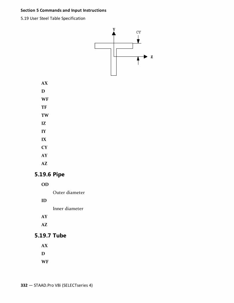
AX
D
WF
TF
TW
IZ
IY
IX
CY
AY
AZ
5.19.6 Pipe
OD
Outer diameter
ID
Inner diameter
AY
AZ
5.19.7 Tube
AX
D
WF
332— STAAD.Pro V8i (SELECTseries 4)
Section 5 Commands and Input Instructions
5.19 User Steel Table Specification

TF
IZ
IY
IX
AY
AZ
5.19.8 GeneralThe following cross-sectional properties should be used for this section-type. Thisfacility allows the user to specify a built-up or unconventional steel section.Provide both the Y and Z parameters for design or code checking.
AX
Cross section area
D
Depth of the section
TD
Thickness associated with section element parallel to depth (usually web).To be used to check depth/thickness ratio
B
Width of the section
TB
Thickness associated with section element parallel to flange. To be used tocheck width/thickness ratio
IZ
Moment of inertia about local z-axis
IY
Moment of inertia about local y-axis
IX
Torsional Constant
SZ
Section modulus about local z-axis
Section 5 Commands and Input Instructions
5.19 User Steel Table Specification
Technical Reference Manual — 333

SY
Section modulus about local y-axis
AY
Shear area for shear parallel to local y-axis
AZ
Shear area for shear parallel to local z-axis
PZ
Plastic modulus about local z-axis
PY
Plastic modulus about local y-axis
HSS
Warping constant for lateral torsional buckling calculations
DEE
Depth of web. For rolled sections, distance between fillets should be pro-vided
Note: Properties PZ, PY, HSS and DEE must be provided for codechecking/member selection per plastic and limit state based codes(AISC LRFD, British, French, German and Scandinavian codes). Forcodes based on allowable stress design (AISC-ASD, AASHTO, Indiancodes), zero values may be provided for these properties.
Note: STAAD.Pro can perform some code checks on a General section whereas a Prismatic section (Section 5.20.2) is for analysis only.
5.19.9 I SectionThis section type may be used to specify a generalized I-shaped section. Thecross-sectional properties required are listed below. This section can be used tospecify tapered I-shapes.
Figure 5-9: I section and tapered web
334— STAAD.Pro V8i (SELECTseries 4)
Section 5 Commands and Input Instructions
5.19 User Steel Table Specification
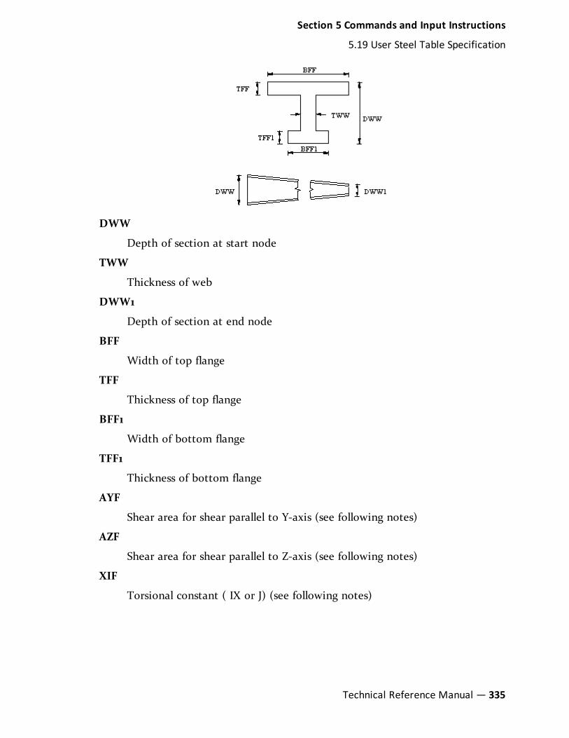
DWW
Depth of section at start node
TWW
Thickness of web
DWW1
Depth of section at end node
BFF
Width of top flange
TFF
Thickness of top flange
BFF1
Width of bottom flange
TFF1
Thickness of bottom flange
AYF
Shear area for shear parallel to Y-axis (see following notes)
AZF
Shear area for shear parallel to Z-axis (see following notes)
XIF
Torsional constant ( IX or J) (see following notes)
Section 5 Commands and Input Instructions
5.19 User Steel Table Specification
Technical Reference Manual — 335

Notes
DWW should never be less than DWW1. Therefore, you must provide themember incidences accordingly.
You are allowed the following options for the values AYF, AZF and XIF.
If positive values are provided, they are used directly by the program.
If zero is provided, the program calculates the properties using the followingformula.
AYF = D x TWW
Where:
D = Depth at section under consideration
AZF = 0.66 ((BFF x TFF) + (BFF1 x TFF1))
XIF = 1/3 ((BFF x TFF3) + (DEE x TWW3) + (BFF1 x TFF13))
Where:
DEE = Depth of web of section
If negative values are provided, they are applied as factors on the correspondingvalue(s) calculated by the program using the above formula. The factor applied isalways the absolute of the value provided, i.e., if the user provides the value ofXIF as -1.3, then the program will multiply the value of XIF, calculated by theabove formula, by a factor of 1.3.
5.19.10 PrismaticThe property-spec for the PRISMATIC section-type is as follows:
AX
Cross-section area
IZ
Moment of inertia about the local z-axis
IY
Moment of inertia about the local y-axis
IX
Torsional constant
336— STAAD.Pro V8i (SELECTseries 4)
Section 5 Commands and Input Instructions
5.19 User Steel Table Specification

AY
Shear area for shear parallel to local y-axis.
AZ
Shear area for shear parallel to local z-axis.
YD
Depth of the section in the direction of the local y-axis.
ZD
Depth of the section in the direction of the local z-axis
Note:When listing multiple shapes, those section names must be provided inascending order by weight since the member-selection process usesthese tables and the iteration starts from the top.
Example
START USER TABLE
TABLE 1
UNIT . . .
WIDE FLANGE
W14X30
8.85 13.84 .27 6.73 .385 291. 19.6 .38 0 0
W21X50
14.7 20.83 .38 6.53 .535 984 24.9 1.14 7.92 0
W14X109
32. 14.32 .525 14.605 .86 1240 447 7.12 7.52 0
TABLE 2
UNIT . . .
ANGLES
L25255
2.5 2.5 0.3125 .489 0 0
L40404
Section 5 Commands and Input Instructions
5.19 User Steel Table Specification
Technical Reference Manual — 337

4. 4. .25 .795 0 0
END
5.19.11 Using Reference Table FilesThe above example can also be input as follows:
START USER TABLE
TABLE 1 TFILE1
TABLE 2 TFILE2
END
Where TFILE1 and TFILE2 are names of files which must be created prior torunning STAAD, and where the file TFILE1 will contain the following:
UNIT . . .
WIDE FLANGE
W14X30
8.85 13.84 .27 6.73 .385 291. 19.6 .38 0 0
W21X50
14.7 20.83 .38 6.53 .535 984 24.9 1.14 7.92 0
W14X109
32. 14.32 0.525 14.605 .86 1240 447 7.12 7.52 0
and the file TFILE2 will contain:
UNIT . . .
ANGLES
L25255
2.5 2.5 .3125 .489 0 0
L40404
4. 4. .25 .795 0 0
338— STAAD.Pro V8i (SELECTseries 4)
Section 5 Commands and Input Instructions
5.19 User Steel Table Specification

Note: The User-Provided Steel Table(s) may be created and maintained asseparate file(s). The same files may be used for all models using sectionsfrom these tables. These files should reside in the same directory wherethe input file is located. On each file the first table should contain aUNITS command.
5.20 Member Property SpecificationThis set of commands may be used for specification of section properties forframe members.
The options for assigning properties come under two broad categories:
1. Those which are specified from built-in property tables supplied with theprogram, such as for steel, aluminum and timber.
2. Those which are not assigned from built-in tables, but instead are specifiedon a project-specific basis, such as for concrete beams and columns, or cus-tom-made sections for industrial structures.
Properties which are specified from built-in property tables
1. General format for standard steel (hot rolled):
MEMBER PROPERTIES { AMERICAN | AUSTRALIAN | BRITISH |CANADIAN | CHINESE | DUTCH | EUROPEAN | FRENCH | GERMAN| INDIAN | JAPANESE | KOREAN | MEXICAN | RUSSIAN| SAFRICAN | SPANISH | VENEZUELAN }
member-list { TABLE type-spec section-name-in-table(additional-spec) | ASSIGN profile-spec }
AMERICAN, BRITISH, EUROPEAN (etc.) option will instruct the program toread properties from the appropriate steel table. The default depends onthe country of distribution.
l See "Assigning Properties from Steel Tables" on page 341 for type-specsand additional-specs.
l See "Assign Profile Specification" on page 350 for ASSIGN profile-spec.
l Section 2 of this manual and the sections on steel design for variouscountries in the International Codes manual contain information onthe section types which can be assigned for the various countriesnamed in the above list.
Section 5 Commands and Input Instructions
5.20 Member Property Specification
Technical Reference Manual — 339

l See "Examples of Member Property Specification" on page 351 forexamples.
The MEMBER PROPERTY command may be extended to multiple lines byending all lines but the last with a space and hyphen (-).
2. General format for cold formed steel:
MEMBER PROPERTIES { BUTLER | COLD AMERICAN | COLDBRITISH | COLD INDIAN | KINGSPAN | LYSAGHT | RCECO }
member-list TABLE ST section-name-in-table
Section 2 of this manual and the sections on steel design for variouscountries in the International Codes manual contain information on thesection types which can be assigned for the various countries/organizationsnamed in the above list.
3. General format for steel joist:
MEMBER PROPERTIES SJIJOIST
member-list TABLE ST section-name-in-table
Section 1 of this manual contains information on the joist types which canbe assigned from the Steel Joist Institute’s tables.
4. General format for Aluminum:
MEMBER PROPERTIES ALUMINUM
member-list TABLE ST section-name-in-table
The section on aluminum design in the International Codes manual containinformation on the section types which can be assigned for the aluminumtable in the above list.
5. General format for Timber:
MEMBER PROPERTIES { AITC | TIMBER CANADIAN }
member-list TABLE ST section-name-in-table
Section 4 of this manual and the sections on timber design in theInternational Codes manual contain information on the section types whichcan be assigned for the above list.
Properties that are not specified from built-in property tablesMEMBER PROPERTIES
member-list { PRISMATIC property -spec | TAPERED argument-list | UPTABLE i1 section-name }
340— STAAD.Pro V8i (SELECTseries 4)
Section 5 Commands and Input Instructions
5.20 Member Property Specification

l See "Prismatic Property Specification" on page 346 for specification of PRIS-MATIC properties.
l See "Tapered Member Specification" on page 349 for specification ofTAPERED members.
l See "Property Specification from User Provided Table" on page 350 for spec-ification from UPTABLES.
l See "Examples of Member Property Specification" on page 351 for examples.
The MEMBER PROPERTY command may be extended to multiple lines by endingall lines but the last with a space and hyphen (-).
5.20.1 Assigning Properties from Steel TablesThe following commands are used for specifying section properties from built-insteel table(s). The section type specification is followed by additionalspecifications as needed.
General Format
type-spec . table-name additional-spec.
type-spec = { ST | RA | D | LD | SD | T | CM | TC | BC | TB| FR }
Where:
type-spec
Description Diagram
ST single section from the stand-ard built-in tables
Table 5-3: Type-specs for various profile types
Section 5 Commands and Input Instructions
5.20 Member Property Specification
Technical Reference Manual — 341

type-spec
Description Diagram
RA single angle with reverse Y-Zaxes (see Section 1.5.2)
D double profile. In the case ofchannels, back-to-back
LD double angle with long legsback-to-back
SD double angle with short legsback-to-back
T tee section cut from I shapedsection
CM composite section, availablefor I shaped sections
TC section with top cover plate
342— STAAD.Pro V8i (SELECTseries 4)
Section 5 Commands and Input Instructions
5.20 Member Property Specification

type-spec
Description Diagram
BC section with bottom coverplate
TB section with both top andbottom cover plate
top plate dimensions aredescribed using WP and THparameter values and bottomplate dimensions aredescribed using BW and BTparameter values
FR front-to-front (i.e., toe-to-toe)channels.
Note: Spacing between thechannels must beprovided using theSP optionmentioned in theadditional specspecificationdescribed below.
SA double angle in a star arrange-ment (heel to heel)
table-name = Table section name like W8X18, C15X33 etc.
The documentation on steel design per individual country codes containsinformation regarding their steel section specification also. For details onspecifying sections from the American steel tables, see Section 2.2.1 of thismanual.
Section 5 Commands and Input Instructions
5.20 Member Property Specification
Technical Reference Manual — 343

additional-spec = * {SP f1 | WP f2 | TH f3 | WT f4 | DT f5 |OD f6 | ID f7 | CT f8 | FC f9 | CW f10 | CD f11 | BW f12| BT f13 }
Where:
Variable Description
f1 Spacing between double angles ordouble channels (default is 0.0)
Rib height for composite sections
f2 Width of top cover plate for Ishaped sections with cover plate.
f3 Thickness of plates or tubes (topplate for I shaped sections)
f4 Width of tube.
f5 Depth of tube.
f6 Outer diameter of pipe.
f7 Inside diameter of pipe.
f8 Concrete thickness of the concretefor composite sections.
f9 Compressive strength of concretefor composite sections.
f10 Concrete width for composite sec-tions.
f11 Concrete density for composite sec-tions (default is 150 pounds percubic ft.)
f12 With of bottom cover plate for Ishaped sections with cover plates
f13 Thickness of cover plates for Ishaped sections with cover
Table 5-4: Additional specifications for steel sec-tions
See "Built-In Steel Section Library" on page 40 for more information.
344— STAAD.Pro V8i (SELECTseries 4)
Section 5 Commands and Input Instructions
5.20 Member Property Specification
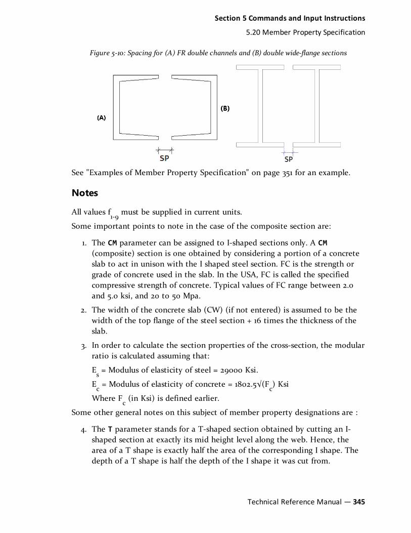
Figure 5-10: Spacing for (A) FR double channels and (B) double wide-flange sections
See "Examples of Member Property Specification" on page 351 for an example.
Notes
All values f1-9must be supplied in current units.
Some important points to note in the case of the composite section are:
1. The CM parameter can be assigned to I-shaped sections only. A CM(composite) section is one obtained by considering a portion of a concreteslab to act in unison with the I shaped steel section. FC is the strength orgrade of concrete used in the slab. In the USA, FC is called the specifiedcompressive strength of concrete. Typical values of FC range between 2.0and 5.0 ksi, and 20 to 50 Mpa.
2. The width of the concrete slab (CW) (if not entered) is assumed to be thewidth of the top flange of the steel section + 16 times the thickness of theslab.
3. In order to calculate the section properties of the cross-section, the modularratio is calculated assuming that:
Es= Modulus of elasticity of steel = 29000 Ksi.
Ec= Modulus of elasticity of concrete = 1802.5√(F
c) Ksi
Where Fc(in Ksi) is defined earlier.
Some other general notes on this subject of member property designations are :
4. The T parameter stands for a T-shaped section obtained by cutting an I-shaped section at exactly its mid height level along the web. Hence, thearea of a T shape is exactly half the area of the corresponding I shape. Thedepth of a T shape is half the depth of the I shape it was cut from.
Section 5 Commands and Input Instructions
5.20 Member Property Specification
Technical Reference Manual — 345

What we refer to as I shaped sections are sections which look like theEnglish alphabet I. The American Wide Flange, the British UB and UCsections, Japanese H sections, etc., all fall under this category. Consequently,the 'T' shape cut from a Japanese H shape is one obtained by cutting the Hshape at exactly its mid-height level of the web.
Not all I shaped sections have a corresponding T. This may be inferred bygoing through the section libraries of individual countries andorganizations. In such cases, if a user were to specify such a T section, theprogram will terminate with the message that the section does not exist.
5. Steel Cover plates also can be added only to I shaped sections. Thus, the TC,BC, and TB are not applicable to any shape other than an I shape.
5.20.2 Prismatic Property SpecificationThe following commands are used to specify section properties for prismaticcross-sections.
General FormatFor the PRISMATIC specification, properties are provided directly (End each linebut last with a hyphen “-”) as follows:
property-spec = * { AX f1 | IX f2 | IY f3 | IZ f4 | AY f5 |AZ f6 | YD f7 | ZD f8 | YB f9 | ZB f10 }
Figure 5-11: Prismatic property nomenclature for a T and Trapezoidal section
Where:
AX f1
= Cross sectional area of the member. Set to zero for TEE,Rectangular, Trapezoid, or circular.
IX f2
= Torsional constant.
346— STAAD.Pro V8i (SELECTseries 4)
Section 5 Commands and Input Instructions
5.20 Member Property Specification

IY f3
= Moment of inertia about local y-axis.
IZ f4
= Moment of inertia about local z-axis (usually major).
AY f5
= Effective shear area in local y-axis.
AZ f6
= Effective shear area in local z-axis.
If any of the previous six parameters are omitted, it will be calculated from theYD, ZD, YB, and/or ZB dimensions.
YD f7
= Depth of the member in local y direction. Used as thediameter of section for circular members.
ZD f8
= Depth of the member in local z direction. If ZD is notprovided and YD is provided, the section will be assumed to becircular.
YB f9
= Depth of stem for T-section.
ZB f10= Width of stem for T-section or bottom width for
TRAPEZOIDAL section.
The values that STAAD calculates for the omitted terms can be obtained byspecifying the command PRINT MEMBER PROPERTIES.
The values of many of the derived properties like shear areas (AY, AZ), sectionmodulii (SY, SZ), etc. will be shown in the output file.
This command can be used regardless of the manner in which the properties arespecified (e.g., PRISMATIC, user table, built-in table).
5.20.2.1 Prismatic Tapered Tube Property Specification
The following commands are used to specify section properties for prismatictapered tube cross-sections. For the property types shown below, additionalinformation can be obtained from Table 2.1 of the ASCE 72 document, 2ndedition.
General Format
property-spec = * { ROUND | HEXDECAGONAL | DODECAGONAL |OCTAGONAL | HEXAGONAL | SQUARE } START d1 END d2 THICK t
Where:
d1= Depth of section at start of member.
d2= Depth of section at end of member.
Section 5 Commands and Input Instructions
5.20 Member Property Specification
Technical Reference Manual — 347

t = Thickness of section (constant throughout the member length).
Figure 5-12: Prismatic tapered tube shapes
SquareHexagonal (6 sides)
Octagonal (8 sides) Dodecagonal (12sides)
Hexdecagonal (16sides) Round
Note: Section properties are calculated using the rules applicable for thin-walled sections.
348— STAAD.Pro V8i (SELECTseries 4)
Section 5 Commands and Input Instructions
5.20 Member Property Specification

Example
UNIT …
MEMBER PROPERTY
1 PRIS ROUND STA 10 END 8 THI 0.375
2 PRIS HDC STA 15 END 10 THI 0.375
3 PRIS DOD STA 12 END 12 THI 0.375
5.20.3 Tapered Member SpecificationThe following commands are used to specify section properties for tapered I-shapes.
General Formatargument-list = f1 f2 f3 f4 f5 (f6 f7)
Where:
f1= Depth of section at start node.
f2= Thickness of web.
f3= Depth of section at end node.
f4= Width of top flange.
f5= Thickness of top flange.
f6= Width of bottom flange. Defaults to f
4if left out.
f7= Thickness of bottom flange. Defaults to f
5left out
Example
MEMBER PROPERTY
1 TO 5 TAPERED 13.98 0.285 13.98 6.745 .455 6.745 .455
Section 5 Commands and Input Instructions
5.20 Member Property Specification
Technical Reference Manual — 349

Notes
a. All dimensions (f1, f2, .....f
7) should be in current units.
b. f1(Depth of section at start node) should always be greater than f
3(Depth
of section at end node). You must provide the member incidences accord-ingly.
5.20.4 Property Specification from User Provided TableThe following commands are used to specify section properties from a previouslycreated USER-PROVIDED STEEL TABLE.
General Formatmember-list UPTABLE I1 section-name
Where:
UPTABLE stands for User-Provided TABLE
i1= table number as specified previously (1 to 20)
section-name = section name as specified in the table.
See "Examples of Member Property Specification" on page 351 for an example.
5.20.5 Assign Profile SpecificationThe ASSIGN command may be used to instruct the program to assign a suitablesteel section to a frame member based on the profile-spec shown below.
General Formatprofile-spec = { BEAM | COLUMN | CHANNEL | ANGLE (DOUBLE) }
See "Examples of Member Property Specification" on page 351 for an example.
Note: Sections are always chosen from the relevant built-in steel table. Tofind out the details of the sections that are chosen, the commandPRINT MEMBER PROPERTIES should be provided after specification ofall member properties. These commands may not work with certaintables such as cold-formed steel, Timber, Aluminum, and even some ofthe standard steel tables.
350— STAAD.Pro V8i (SELECTseries 4)
Section 5 Commands and Input Instructions
5.20 Member Property Specification

5.20.6 Examples of Member Property SpecificationThis section illustrates the various options available for MEMBER PROPERTYspecification.
UNIT …
MEMBER PROPERTIES
1 TO 5 TABLE ST W8X31
9 10 TABLE LD L40304 SP 0.25
12 TO 15 PRISMATIC AX 10.0 IZ 1520.0
17 18 TA ST PIPE OD 2.5 ID 1.75
20 TO 25 TA ST TUBE DT 12. WT 8. TH 0.5
27 29 32 TO 40 42 PR AX 5. IZ 400. IY 33. -
IX 0.2 YD 9. ZD 3.
43 TO 47 UPT 1 W10X49
50 51 UPT 2 L40404
52 TO 55 ASSIGN COLUMN
56 TA TC W12X26 WP 4.0 TH 0.3
57 TA CM W14X34 CT 5.0 FC 3.0
This example shows each type of member property input. Members 1 to 5 arewide flanges selected from the AISC tables; 9 and 10 are double angles selectedfrom the AISC tables; 12 to 15 are prismatic members with no shear deformation;17 and 18 are pipe sections; 20 to 25 are tube sections; 27, 29, 32 to 40, and 42 areprismatic members with shear deformation; 43 to 47 are wide flanges selectedfrom the user input table number 1; 50 and 51 are single angles from the userinput table number 2; 52 through 55 are designated as COLUMN members usingthe ASSIGN specification. The program will assign a suitable I-section from thesteel table for each member.
Member 56 is a wideflange W12X26 with a 4.0 unit wide cover plate of 0.3 unitsof thickness at the top. Member 57 is a composite section with a concrete slab of5.0 units of thickness at the top of a wide flange W14X34. The compressivestrength of the concrete in the slab is 3.0 force/length2.
5.20.7 Composite DecksA composite deck generation facility is available in the program.
Section 5 Commands and Input Instructions
5.20 Member Property Specification
Technical Reference Manual — 351

General FormatThe command syntax for defining the deck within the STAAD input file is asshown below.
START DECK DEFINITION
_DECKdeck-name
PERIPHERYmember-list
DIRECTIONd1 d2 d3COMPOSITEmember-list
OUTERmember-list
VENDOR name
FCf1CTf2CDf3RBHf4RBWf5PLTf6PLWf7DIAf8HGTf9DR1f10SHRf11CMPf12CW ;f13MEMB cw-member-list
END DECK DEFINITION
Where:
deck-name = an alphanumeric name specified by the user toidentify the deck. The deck-name line must start with '_DEC'. Thedeck-name is the second word and is limited to 23 characters. Thisname must not be the same as any group name.
352— STAAD.Pro V8i (SELECTseries 4)
Section 5 Commands and Input Instructions
5.20 Member Property Specification

member-list = the list of members belonging to the deck. TO, BY,ALL, and BEAM are permitted. ALL means all members in structure;BEAM means all beams.
d1 = x component of the direction of the deck.
d2 = y component of the direction of the deck.
d3 = z component of the direction of the deck.
The following parameters may be in any order or omitted. They only apply to thecomposite members listed above. Do not enter a member list for theseparameters.
f1 = compressive strength of the concrete for all compositemembers listed above for this composite deck.
f2 = concrete thickness.
f3 = concrete density.
f4 = height of rib of form steel deck. This is the distance from
the top of the I beam to the bottom of the concrete deck.
f5 = width of rib of form steel deck.
f6 = thickness of cover plate welded to bottom flange of
composite beam.
f7 = width of cover plate welded to bottom flange of composite
beam.
f8 = diameter of shear connectors.
f9 = height of shear connectors after welding.
f10 = ratio of moment due to dead load applied before concrete
hardens to the total moment.
f11 = temporary shoring during construction.
0 = no shoring1 = with shoring
f12 = composite action with connectors.
0 = no composite action in design1 = composite action2 = ignore positive moments during design
The following parameter may be specified by member list. They only apply to thecomposite members listed above.
Section 5 Commands and Input Instructions
5.20 Member Property Specification
Technical Reference Manual — 353

f13 = concrete width for each composite member listed. cw-
member-list = the list of composite members in this deck that havethis width.Enter as many CW lines as necessary to define the width ofall composite members of this deck.
This Deck definition data should be entered after the member properties havebeen entered.
Notes
1. The DECK definition must start with the START DECK DEFINITION com-mand and end with the END command.
2. More than one DECK may be specified between the START and END.
3. The same member number may be included in up to 4 deck/groups. Mul-tiple definitions are useful for output but can be ambiguous for input datasuch as constants, section property, release, etc.
4. If two or more consecutively entered decks have the same name, then theywill be merged. If not consecutive, the second entry of the same name willbe ignored.
5. The _deck-name must be unique within the Deck definitions and theGroup definitions.
6. PER, DIR, OUT are data created by the GUI. Do not edit this data.
7. This Deck definition data should be entered after the member propertieshave been entered.
Example
START DECK DEFINITION
_DECK DEC-1
PERIPHERY 4 1640 18 38 56 50 49
DIRECTION 0.0000000.000000 -1.000000
COMPOSITE 41 74 38
OUTER 7 8 3130
VENDOR USSTEEL
DIA 0.700
354— STAAD.Pro V8i (SELECTseries 4)
Section 5 Commands and Input Instructions
5.20 Member Property Specification

HGT 2.75
CT 11.0
FC 3.1
RBW 2.6
RBH 0.1
CMP 1.0
SHR 1
CD 0.0000870
CW 123.000000 MEMB41
CW 123.000000 MEMB7
CW 61.500000 MEMB4
CW 61.500000 MEMB38
END DECK DEFINITION
See "Composite Beams and Composite Decks" on page 45 for additional details.
5.20.8 Curved Member SpecificationThe following commands are used to specify that a member is curved. The curvemust be a segment of a circle and the internal angle subtended by the arc mustbe less than 180 degrees. Any non-tapered cross-section is permitted.
General Format
MEMBER CURVED
member-list RADIUS r GAMMA g PRESS p
Where:
r = radius in length units
g = The angle in degrees used to define the plane of the circle. Theangle is defined using the same set of rules used to define theorientation (beta angle) of a straight member connected between thetwo nodes.
p = Pressure/Flexibility parameter for pipe bends. See notes.
Section 5 Commands and Input Instructions
5.20 Member Property Specification
Technical Reference Manual — 355

Notes
1. The radius should be in current units.
2. Certain attributes like releases, TENSION/COMPRESSION flags, and severalmember load types are currently not available. Section forces too arecurrently not available.
3. The design of curved members is not supported.
Pressure/Flexibility Parameter
This applies only to pipe bend (elbow) members (OD and ID entered). Thesemembers will flex more due to ovalization depending on internal pressure. TheASME Boiler and Pressure Vessel Code, Section III, NB-3687.2, 1971, for Class Icomponents is used to calculate the flexibility reduction factor.
l Set p = 0 or omit for this flexibility increase calculation to occur with inter-nal pressure equal to zero.
l Set p > 0 to specify internal pressure to use in this flexibility calculation.Pressure reduces the flexibility increase.
l Set p = -9999 to ignore this additional flexibility calculation and use onlybeam theory.
l Set p = flexibility reduction factor (-FLEXF below); which must be a neg-ative number less than –1.0 .
ASME Pipe Elbow flexability factors theory [ASME Section NB-3687.3]
This section only applies if (Bend Radius/Mean Radius) ≥ 1.70 or if (Arclength) >(2x Mean Radius)
Flexibility Factor, FLEXF = (1.65x (Mean Radius)2)/[t⋅(Bend Radius)] x1/[1 + (Press)(Mean Radius)(FACT.)]
Where:
FACT. = 6⋅(MR/t)4/3⋅(BR/MR)1/2/(Et)
MR = Mean Radius of elbow wall
BR = Bend Radius
Press = Internal Pressure
356— STAAD.Pro V8i (SELECTseries 4)
Section 5 Commands and Input Instructions
5.20 Member Property Specification

t = elbow wall thickness
E = Modulus of Elasticity
If the Flexibility Factor computed is less than 1.0, then STAAD will use 1.0 . TheFlexibility Factor directly multiplies or contributes to most non-shear terms inthe elbow flexibility matrix.
Notes
1. The input for defining the curved member involves 2 steps. The first is themember incidence, which is the same as that for a straight line member.The second is the command described above, which indicates that thesegment between the 2 nodes of the member is curved, and not a straightline.
2. Any non-tapered cross section property currently available in STAAD can beassigned to these members.
3. Currently, two load types are permitted on curved members. One is theSELFWEIGHT load type, described in Section 5.32.9 of the STAAD.ProTechnical Reference manual. The other is the uniformly (UNI) distributedload type of the MEMBER LOAD options explained in Section 5.32.2 of thesame manual. The uniformly distributed load has to be applied over the fullspan of the member. Other member loads such as LINEAR, TRAP,CONCENTRATED force or moment, UNIFORM moment, etc. are not currentlysupported. These options are expected to become available in futureversions of the program.
4. Some of the other member load types such as PRESTRESS, TEMPERATURE,STRAIN loads, etc. are also not currently supported. These options too areexpected to become available in future versions of the program.
5. The results of the analysis currently consist of the nodal displacements ofthe ends of the curved member, and the member end forces. The nodaldisplacements are in the global coordinate system. The member end forcesare in the local coordinate system, with each end of the member having itsown unique local axis system. Results at intermediate sections, such assectional displacements, and sectional forces will be available in futureversions of the program.
Gamma Angle
The plane of the circle defines the plane formed by the straight line joining thetwo ends of the arc, and the local Y axis of an imaginary straight member
Section 5 Commands and Input Instructions
5.20 Member Property Specification
Technical Reference Manual — 357

between those two points. The positive value of the GAMMA angle is obtainedusing the same sense as the positive value of the beta angle of that imaginarystraight line member whose local Y axis points towards the vertex of the arc.
Several diagrams intended to show the GAMMA angle for various segments lying inthe three global planes are shown.
Figure 5-13: Gamma angle for various configurations of the circular arc lying in the global XYplane
Figure 5-14: Gamma angle for various configurations of the circular arc lying in the global XYplane
358— STAAD.Pro V8i (SELECTseries 4)
Section 5 Commands and Input Instructions
5.20 Member Property Specification

Figure 5-15: Gamma angle for various configurations of the circular arc lying in the global YZplane
Figure 5-16: Gamma angle for various configurations of the circular arc lying in the global YZplane
Section 5 Commands and Input Instructions
5.20 Member Property Specification
Technical Reference Manual — 359

Figure 5-17: Gamma angle for various configurations of the circular arc lying in the global XZplane
Figure 5-18: Gamma angle for various configurations of the circular arc lying in the global XZplane
360— STAAD.Pro V8i (SELECTseries 4)
Section 5 Commands and Input Instructions
5.20 Member Property Specification

Member local axis system
The local axis directions for curved members are dependent on the point ofinterest along the curve. The general rules for local axis, as laid out in Section1.5.2 of this manual are applicable. The figure shown later for member end forcesindicates the directions of axes at the start and end nodes.
Rotation of local axis
There is a limited facility available to change the orientation of a curved membercross section. The cross-section may be at the default position where the strongaxis (local y) is normal to the plane of the curve and the weak axis is in thatplane.
The BETA ANGLE and REFERENCE POINT options, explained in section 1.5.3 and5.26.2 of this manual, are not available for curved members.
Sign conventions
The displacements of the nodes of the curved member are along the global axissystem just as in the case of straight members.
The member end forces for curved members are quite similar to that for straightmembers. The only distinguishing item is that they are normal and tangential tothe local axis at the corresponding ends. For example, FX at the start is
Section 5 Commands and Input Instructions
5.20 Member Property Specification
Technical Reference Manual — 361

tangential to the curve at the start node, and FX at the end is tangential to thecurve at the end node. Similarly, FZ is along the radial direction at the two ends.
Member releases, offsets, tension/compression, truss and cable may not bespecified for curved beams.
Figure 5-19: Sign conventions for member end actions; Global Y is vertical
Example
STAAD SPACE
UNIT KIP FEET
JOINT COORD CYL REVERSE
1 150 0 0 13 150 0 90
REPEAT 1 30 0 0
REPEAT ALL 1 0 15 0
MEMBER INCIDENCES
1 1 27 26
101 27 28 112
113 40 41 124
201 27 40 213
START GROUP DEFINITION
362— STAAD.Pro V8i (SELECTseries 4)
Section 5 Commands and Input Instructions
5.20 Member Property Specification

MEMBER
_COLUMN 1 TO 26
_CIRCUMFERENTIAL 101 TO 124
_RADIAL 201 TO 213
END GROUP DEFINITION
MEMBER PROPERTIES
_COLUMN PRIS YD 3.0
_CIRCUMFERENTIAL PRIS YD 3.0
_RADIAL PRIS YD 3.0
CONSTANT
E CONCRETE ALL
DENSITY CONCRETE ALL
POISSON CONCRETE ALL
MEMBER CURVED
101 TO 112 RADIUS 150 GAMMA 90.0
113 TO 124 RADIUS 180 GAMMA 90.0
SUPPORTS
1 TO 26 PINNED
LOAD 1
SELF Y -1.0
PERFORM ANALYSIS PRINT STAT CHECK
PRINT MEMBER FORCE LIST 101 113
FINISH
5.20.9 Applying Fireproofing on membersSTAAD.Pro now includes a method to automatically consider the weight offireproofing material applied to structural steel.
Two types of fireproofing configurations are currently supported. They are:
Section 5 Commands and Input Instructions
5.20 Member Property Specification
Technical Reference Manual — 363

Block Fireproofing (BFP)The next figure shows this configuration. The fire-protection material forms arectangular block around the steel section.
The area of fireproofing material (Afp) at any section along the member length is
calculated in the following manner.
For Wide Flanges (I-shaped sections), Channels and Tees,
Afp = [(Bf + 2T)*(D+2T)] - AsteelFor single angles,
Afp= [(Bf + 2T)*(D+2T)] - AsteelWhere:
Bfis the flange width
D the overall depth of the steel section
T is the thickness of the fireproofing material beyond the outer edgesof the cross section as shown in the next figure.
Asteel
= Area of the steel section
Figure 5-20: Block fireproofing (BFP) on various shapes
Contour Fireproofing (CFP)In this configuration, the fire-protection material forms a coating around thesteel section as shown in the next figure. The area of fireproofing material (A
fp)
for this case is calculated in the following manner.
For Wide Flanges (I-shaped sections)
Afp = [(Bf + 2T)*(Tf+2T)]*2 + [(D-2T-2Tf)*(Tw+2T)] - AsteelFor single angles,
Afp = [(L1+2T)*(2T+Ta) + (L2-Ta)*(2T+Ta)] - Asteel
364— STAAD.Pro V8i (SELECTseries 4)
Section 5 Commands and Input Instructions
5.20 Member Property Specification

For Tees,
Afp = [(Bf + 2T)*(Tf+2T)] + [(D-Tf)*(Tw+2T)] - AsteelWhere:
Bfis the flange width
D the overall depth of the steel section
T is the thickness of the fireproofing material beyond the outer edgesof the cross section as shown in the next figure.
Tfis the thickness of the flange for the I shape and Tee
Tais the thickness of the leg of the angle
Twis the thickness of the web for the I shape and Tee
Asteel
= Area of the steel section
Figure 5-21: Contour fireproofing (CFP) on various shapes
The number of input items required to apply this attribute is four – a) the typeof fireproofing b) the thickness T shown in the above figures c) the density of thefireproofing material d) the members on which it is to be applied.
For each such member, Afpis calculated and multiplied by the density of the
fireproofing material to obtain the weight per unit length of the member. This isadded to the weight per unit length of the steel section itself and the total isused in calculating selfweight. Hence, SELFWEIGHT must be one of the loadcomponents of load cases if the weight of the fireproofing material should beconsidered as part of those load cases.
General FormatMEMBER FIREPROOFING
Member-list FIRE { BFP | CFP } THICKNESS f1DENSITY f2
Section 5 Commands and Input Instructions
5.20 Member Property Specification
Technical Reference Manual — 365

Where:
f1= thickness (T in the figures above) in length units
f2= density of fireproofing material in (force / length3) units
In the actual load case itself, nothing besides the SELFWEIGHT command isnecessary to instruct the program to include the weight of the fireproofingmaterial in the selfweight calculation.
Notes
1. STAAD calculates the fire proofing weight only for the following sections:
For block fireproofing - I-shaped sections like those from the built-in tables(American W,S,M,HP, British UC and UB, etc.), tapered I shaped sections,single channels, angles and Tees.
For CFP-contour fireproofing - the sections are I-beam straight or tapered,angle, Tee.
I-shaped sections like those from the built-in tables (American W,S,M,HP,British UC and UB, etc.), tapered I shaped sections, angles and Tees..
2. Fire proofing weight is not calculated for the following section types: Pipe,tube, composite I beams with slab on top, double channel, double angle,HSS, I-beam with cover plates, prismatic, solid circle or rectangle,castellated, cold formed sections, wood, aluminum, tapered poles, etc.
Example Problem
STAAD SPACE
UNIT KIP FEET
JOINT COORDINATES
1 0. 0. ;2 0. 15. ; 3 20. 15. ;4 20. 0.
MEMBER INCIDENCE
1 1 2 ; 2 2 3 ; 3 3 4
MEMBER PROPERTY AMERICAN
1 3 TABLE ST W12X26
2 TABLE ST W14X34
CONSTANTS
E STEEL ALL
366— STAAD.Pro V8i (SELECTseries 4)
Section 5 Commands and Input Instructions
5.20 Member Property Specification

POISSON STEEL ALL
DENSITY STEEL ALL
SUPPORT
1 FIXED ; 4 PINNED
UNIT POUND INCH
MEMBER FIREPROOFING
1 3 FIRE BFP THICK 2.0 DENSITY 40
2 FIRE CFP THICK 1.5 DENSITY 40
UNIT KIP FT
LOADING 1 DEADWEIGHT OF STEEL + FIREPROOFING
SELF Y -1.0
LOAD 2 LIVE
MEMBER LOAD
2 UNI GY -0.8
LOAD COMBINATION 3
1 0.75 2 0.75
PERFORM ANALYSIS
PRINT MEMBER FORCES
PRINT SUPPORT REACTIONS
FINISH
5.20.10 Member Property Reduction FactorsConcrete design specifications recommend the use of cracked section propertiesfor the analysis and design of concrete sections. Though the methodology tohandle cracked section properties is Nonlinear in nature (i.e., the sectioncapacities should be checked and modified depending upon the section forces thesection is handling). The model should then be re-analyzed with modifiedreduced section properties and redesigned. This iteration should be continueduntil the forces in all sections designed are below the allowable limit of ultimatestrength.
In STAAD.Pro, you can specify a set of reduction factors to be applied on thecalculated section properties such as Area, Moments of Inertia, and TorsionalConstant. If a you want to adopt this approach to account for cracking of
Section 5 Commands and Input Instructions
5.20 Member Property Specification
Technical Reference Manual — 367

concrete sections, refer to Section 10.11.1 of ACI 318 for a set of values to use forthese reduction factors depending upon the nature of forces and moments themember is subjected to.
Similarly, the specifications in the AISC 13th edition manual suggest reducing thestiffness of the member during the analysis. The REDUCEDEI parameter may alsobe used when the PERFORM DIRECT ANALYSIS command is used. See "DirectAnalysis" on page 686 for additional information.
General Format
The format of the command is:
MEMBER CRACKED
<Member List> REDUCTION *{ RAX | RIX | RIY | RIZ } factor
The reduction factor should be a fraction of unity.
Also, this is a multiplication factor on the property value. It does not signify theamount by which the property is reduced, but, it is simply a value by which theunreduced property is multiplied by. Thus, the calculated (or the user specifiedvalue) of the property will be multiplied by the reduction factor to arrive at thevalue used in the analysis.
For example, a factor of 0.45 defined for RAX will mean that if the cross sectionalarea of the gross section is 0.8 ft2, the value used in the analysis will be 0.8 X0.45 = 0.36 ft2.
Multiple factors can be assigned on the same line.
The reduction factor is considered only for analysis but not for design.
Example
MEMBER CRACKED
1 REDUCTION RAX 0.35 RIX 0.40 RIY 0.45 RIZ 0.45
5.21 Element/Surface Property SpecificationIndividual plate elements, and the Surface element need to have their thicknessspecified before the analysis can be performed. The commands for specifying thisinformation are explained in this section. No similar properties are required forsolid elements. However, constants such as modulus of elasticity, Poisson’s Ratio,etc. are required.
368— STAAD.Pro V8i (SELECTseries 4)
Section 5 Commands and Input Instructions
5.21 Element/Surface Property Specification

5.21.1 Element Property SpecificationThis set of commands may be used to specify properties of plate finite elements.Elements of uniform or linearly varying thickness may be modeled using thiscommand. The value of the thickness must be provided in current units.
Unlike members and plate/shell elements, no properties are required for solidelements. However, constants such as modulus of elasticity and Poisson’s ratio areto be specified.
General Format
ELEMENT PROPERTY
element-list THICKNESS f1 (f2, f3, f4)
Where:
f1= Thickness of the element.
f2...f4= Thicknesses at other nodes of the element, if different from f
1.
Example
UNIT . . .
ELEMENT PROPERTY
1 TO 8 14 16 THI 0.25
5.21.2 Surface Property SpecificationThis set of commands may be used to specify properties of surface entities.
General Format
SURFACE PROPERTY
surface-list THICKNESS t
Where:
t = Thickness of the surface element, in current units.
Example
Section 5 Commands and Input Instructions
5.21 Element/Surface Property Specification
Technical Reference Manual — 369

SURFACE PROPERTY
1 TO 3 THI 18
The attributes associated with the surface element, and the sections of thismanual where the information may be obtained, are listed below:
AttributesRelatedSections
Surfaces Incidences 5.13.3
Openings in surface 5.13.3
Local Coordinates system forsurfaces
1.6.3
Specifying sections for stress/forceoutput
5.13.3
Property for surfaces 5.21.2
Material constants 5.26.3
Surface loading 5.32.3.4
Stress/Force output printing 5.42
Shear Wall Design 3.8.2, 5.55
5.22 Member/Element ReleasesSTAAD allows specification of releases of degrees of freedom for frame membersand plate elements.
5.22.1 Member Release SpecificationThis set of commands may be used to fully release specific degrees of freedom atthe ends of frame members. They may also be used to describe a mode ofattachment where the member end is connected to the joint for specific degreesof freedom through the means of springs.
370— STAAD.Pro V8i (SELECTseries 4)
Section 5 Commands and Input Instructions
5.22 Member/Element Releases

General Format
MEMBER RELEASES
member-list {START | END | BOTH } { *{ FX | FY | FZ | MX |MY | MZ } | *{KFX f1 | KFY f2 | KFZ f3 | KMX f4 | KMY f5| KMZ f6 } | {MP f7 | *{ MPX f8 | MPY f9 | MPZ f10 }} }
Where:
FX … MZ = represent force-x through moment-z degrees of freedomin the member local axes
KFX … KMZ f1 … f6 = spring constants for these degrees of freedom, incurrent units.
f7 = release factor for all three moments
f8, f9, f10 = release factors for each moment separately. The momentrelated stiffness co-efficient will be multiplied by a factor of (1 - fn) atthe specified end. Release factors must be in the range of 0.001through 0.999.
Note: If FX through MZ is used, it signifies a full release for that degree offreedom and if KFX through KMZ is used, it signifies a springattachment.
Notes
a. Member releases are a means for describing a type of end condition formembers when the default condition, namely, fully moment and force resist-ant, is not applicable. Examples are bolted or riveted connections. Partialmoment releases are a way of specifying bending and torsional momentcapacity of connections as being a fraction of the full bending and torsionalstrength.
b. It is important to note that the factor f1indicates a reduction in the stiff-
ness corresponding to the rotational degrees of freedom MX, MY, and MZ.In other words, you should not expect the moment on the member toreduce by a factor of f
1. It may be necessary to perform a few trials in order
to arrive at the right value of f1that results in the desired reduction in
moment.
Section 5 Commands and Input Instructions
5.22 Member/Element Releases
Technical Reference Manual — 371

c. The START and END are based on the MEMBER INCIDENCE specification.The BOTH specification will apply the releases at both ends.
d. At any end of the member—for any particular DOF—full, partial, andspring release cannot be applied simultaneously. Only one out of the threeis permitted.
e. If MY (or MZ) is fully released at both ends, then VZ (or VY) cannot betransmitted through the member. The final shears in the member will beentirely due to loads applied directly to the member.
Example
MEMBER RELEASE
1 3 TO 9 11 12 START KFX 1000.0 MY MZ
1 10 11 13 TO 18 END MZ KMX 200.0
In this example, for members 1, 3 to 9, 11 and 12, the moments about the local Yand Z axes are released at their start joints (as specified in MEMBER INCIDENCES).Further, these members are attached to their START joint along their local x axisthrough a spring whose stiffness is 1000.0 units of force/length. For members 1, 10,11 and 13 to 18, the moment about the local Z axis is released at their end joint.Also, the members are attached to their END joint about their local x axisthrough a moment-spring whose stiffness is 200.0 units of force-length/Degree.Members 1 and 11 are released at both start and end joints, though not necessarilyin the same degrees of freedom.
Partial Moment Release
Moments at the end of a member may be released partially using the MP option(to provide the same partial release in all . This facility may be used to modelpartial fixity of connections. The following format may be used to provide apartial moment release. This facility is provided under the MEMBER RELEASEoption and is in addition to the existing RELEASE capabilities.
Example
MEMBER RELEASE
15 TO 25 START MP 0.25
372— STAAD.Pro V8i (SELECTseries 4)
Section 5 Commands and Input Instructions
5.22 Member/Element Releases

The above RELEASE command will apply a factor of 0.75 on the moment relatedstiffness coefficients at start node of members 15 to 25.
5.22.2 Element Release SpecificationThis set of commands may be used to release specified degrees of freedoms atthe corners of plate finite elements.
General Format
ELEMENT RELEASE
element-list { J1 | J2 | J3 | J4 } *{ FX | FY | FZ | MX | MY| MZ }
Where:
J1, J2, J3 and J4 = signify joints in the order of the specification of theelement incidence. For example, if the incidences of the elementwere defined as 35 42 76 63, J1 represents 35, J2 represents 42, J3represents 76, and J4 represents 63.
FX through MZ = represents forces/moments to be released per localaxis system.
Note: Element releases at multiple joints cannot be specified in a single line.Those must be specified separately as shown below.
Examples
Example of Correct Usage
ELEMENT RELEASE
10 TO 50 J1 MX MY
10 TO 50 J2 MX MY
10 TO 50 J3 MY
10 TO 50 J4 MY
Example of Incorrect Usage
ELEMENT RELEASE
10 TO 50 J1 J2 MX MY
Section 5 Commands and Input Instructions
5.22 Member/Element Releases
Technical Reference Manual — 373

10 TO 50 J3 J4 MY
Notes
a. All releases are in the local axis system. See Figure 1.13 for the variousdegrees of freedom. Fx and Fy have the same sense as Sx and Sy in Figure1.13. Fz has the same sense as SQx or SQy. Generally, do not over release.The element must still behave as a plate after the releases.
b. Selfweight is applied at each of the nodes as if there were no releases.
c. Thermal stresses will include the fixed-end thermal pre-stress as if therewere no release.
d. May not be used with the Element Plane Stress or Element Ignore InplaneRotation commands on the same element.
e. Note that the usual definitions of local Mx and My are reversed here. SeeFigure 1.13 for the definitions of Mx and My. Releasing Fz, Mx, My willrelease all bending capability. Releasing Fx, Fy, Mz will release all in-planestiffness.
5.22.3 Element Ignore StiffnessStructural units like glass panels or corrugated sheet roofs are subjected to loadslike wind pressures or snow loads. While these units are designed to carry thoseloads and transmit those loads to the rest of the structure, they are not designedto provide any additional stiffness to the structure. One way to handle thesituation is to not input the unit as part of the structural model, and apply theload using load generation techniques like AREA LOAD or FLOOR LOAD.
STAAD provides another way of handling such units. This is through the help ofthe ELEMENT IGNORE STIFFNESS command. To use this feature, the glass panelor roof unit must be defined using plate elements. The IGNORE STIFFNESScommand enables one to consider the unit just for the purpose of application ofELEMENT LOAD commands, while its stiffness will not be considered during theassembly of the stiffness matrix. In other words, it is like an INACTIVE memberwhich is active for ELEMENT LOAD command application but INACTIVE forstiffness. Like the INACTIVE command, the plates listed here will become activeat the next CHANGE command. To keep them inactive, re-enter this data aftereach CHANGE.
The SELFWEIGHT, ELEMENT WEIGHT, TEMPERATURE, and mass of the plates listedhere will still be ignored.
374— STAAD.Pro V8i (SELECTseries 4)
Section 5 Commands and Input Instructions
5.22 Member/Element Releases

General Format
IGNORE STIFFNESS {ELEMENT} element-list
Example
IGNORE STIFFNESS ELEMENT 78 TO 80
5.23 Axial Member SpecificationsA member can have only one of the following specifications:
l Truss
l Tension-only
l Compression-only
l Cable
If multiple specifications are applied to the same member, only the last enteredwill be used (Warnings will be printed).
Note:MEMBER TRUSS, MEMBER TENSION, MEMBER COMPRESSION, andMEMBER CABLE are axial-only for stiffness. MEMBER CABLE are specialtruss members that may also be specified as tension-only.
5.23.1 Member Truss SpecificationThis command may be used to model a specified set of members as TRUSSmembers.
This specification may be used to specify TRUSS type members in a PLANE,SPACE or FLOOR structure. The TRUSS members are capable of carrying onlyaxial forces. Typically, bracing members in a PLANE or SPACE frame will be ofthis nature.
General Format
MEMBER TRUSS
member-list TENSION f1Where:
Section 5 Commands and Input Instructions
5.23 Axial Member Specifications
Technical Reference Manual — 375

f1= optional Initial Tension in truss member, in current units.
Note: For Nonlinear CABLE ANALYSIS Only: The Tension parameter isignored except in Nonlinear Cable Analysis. For that analysis type, atruss with pretension is considered to be nonlinear (largedisplacement). In this analysis type, trusses without preload areassumed to be linear members that carry both tension and compressionregardless of this command.
This command is superfluous when a TRUSS type structure has already beenspecified using the command STAAD TRUSS.
Example
MEMB TRUSS
1 TO 8 10 12 14 15
Notes
a. The TRUSS member has only one degree of freedom-the axial deformation.Note also that Member Releases are not allowed. Selfweight and transverseloads may induce shear/moment distributions in the member.
b. Member loads are lumped at each end, whereas a frame member withmoment releases only retains the axial component of the applied memberload.
5.23.2 Member Cable SpecificationThis command may be used to model a specified set of members as CABLEmembers.
Cable members, in addition to elastic axial deformation, are also capable ofaccommodating the stiffness effect of initial tension and tension due to staticloads. When used in a nonlinear cable analysis, cable members are capable ofaccommodating large displacements. See "1.11 Cable Members" on page 47 for atheoretical discussion of cable members.
General Format
MEMBER CABLE
376— STAAD.Pro V8i (SELECTseries 4)
Section 5 Commands and Input Instructions
5.23 Axial Member Specifications

member-list { TENSION f1 | LENGTH f2 }
Where:
f1= Initial Tension in cable member(in current units)
f2= Unstressed cable length (in current units)
Notes
1. The tension specified in the cable member is applied on the structure as anexternal load as well as is used to modify the stiffness of the member. Thetension value must be positive to be treated as a cable otherwise it is atruss (See "1.11 Cable Members" on page 47). If the TENSION parameter orthe value is omitted, a minimum tension will be used.
2. This is a truss member but not a tension-only member unless you alsoinclude this member in a MEMBER TENSION input (See "5.23.3 Member Ten-sion/Compression Specification" on page 377). Note also that MemberReleases are not allowed.
3. The tension is a preload and will not be the final tension in the cable afterthe deformation due to this preload.
4. The tension is used to determine the unstressed length. That length will beshorter than the distance between the joints by the distance that the ten-sion will stretch the cable.
Example
MEMB CABLE
20 TO 25 TENSION 15.5
5.23.3 Member Tension/Compression SpecificationThis command may be used to designate certain members as Tension-only orCompression-only members.
Tension-only members are truss/cable members that are capable of carryingtensile forces only. Thus, they are automatically inactivated for load cases thatcreate compression in them.
General Format
MEMBER TENSION
member-list
Section 5 Commands and Input Instructions
5.23 Axial Member Specifications
Technical Reference Manual — 377

MEMBER COMPRESSION
member-list
MEMBER TENSION 0
(no list required)
Linear Tension/ Compression Analysis
Compression-only members are truss members that are capable of carryingcompressive forces only. Thus, they are automatically inactivated for load casesthat create tension in them. Member Releases are not allowed on members withthis attribute.
The procedure for analysis of Tension-only or Compression-only membersrequires iterations for every load case and therefore may be quite involved. youmay also consider using the INACTIVE specification (instead ofTension/Compression) if the solution time becomes unacceptably high.
If a CHANGE command is used (because of a change in the list of tensionmembers, cable tension, supports, etc.), then the SET NL command must be usedto convey to STAAD that multiple analyses and multiple structural conditions areinvolved.
Note: For Nonlinear cable analysis, this command is unnecessary and ignored.Cables are automatically assumed to be partially to fully tension only(except that there should always be selfweight) without this command.In this analysis type, trusses without preload are assumed to be linearmembers that carry both tension and compression regardless of thiscommand.
a. Loads that have been defined on members declared as MEMBER TENSION orMEMBER COMPRESSION will be active even when the member becomesINACTIVE during the process of analysis. This applies to SELFWEIGHT,MEMBER LOADS, PRESTRESS & POSTSTRESS LOADS, TEMPERATURE LOAD,etc.
b. A member declared as a TENSION only member or a COMPRESSION onlymember will carry axial forces only. It will not carry moments or shearforces. In other words, it is a truss member.
c. Do not use Load Combination to combine these cases.Tension/Compression cases are Nonlinear and should not be linearly
378— STAAD.Pro V8i (SELECTseries 4)
Section 5 Commands and Input Instructions
5.23 Axial Member Specifications

combined as in Load Combination. Use a primary load case with theRepeat Load command.
Example
MEMBER TENSION
12 17 19 TO 37 65
MEMBER COMPRESSION
5 13 46 TO 53 87
Member Tension 0
This command switches off ALL tension/compression only specifications for loadcases which are specified subsequent to this command, usually entered after aCHANGE command. There is no list associated with this command. Hence, forany further primary load cases, the tension/compression only attributed isdisabled for ALL members.
Example
The following is the general sequence of commands in the input file if theMEMBER TENSION or MEMBER COMPRESSION command is used. This example isfor the MEMBER TENSION command. Similar rules are applicable for the MEMBERCOMPRESSION command. The dots indicate other input data items.
STAAD …
SET NL …
UNITS …
JOINT COORDINATES
…
MEMBER INCIDENCES
…
ELEMENT INCIDENCES
…
CONSTANTS
Section 5 Commands and Input Instructions
5.23 Axial Member Specifications
Technical Reference Manual — 379

…
MEMBER PROPERTY
…
SUPPORTS
…
MEMBER TENSION
…
LOAD 1
…
LOAD 2
…
LOAD 3
…
LOAD 4
…
LOAD 5
REPEAT LOAD
…
PERFORM ANALYSIS
CHANGE
LOAD LIST ALL
PRINT …
PRINT …
PARAMETER
…
CHECK CODE …
FINISH
380— STAAD.Pro V8i (SELECTseries 4)
Section 5 Commands and Input Instructions
5.23 Axial Member Specifications

Notes
a. See "5.5 Set Command Specification" on page 284 for explanation of theSET NL command. The number that follows this command is an upperbound on the total number of primary load cases in the file.
b. STAAD performs up to 10 iterations automatically, stopping if converged. Ifnot converged, a warning message will be in the output. Enter a SETITERLIM i command (i > 10) before the first load case to increase thedefault number of iterations. Since convergence may not be possible usingthis procedure, do not set the limit too high.
c. The principle used in the analysis is the following.
l The program reads the list of members declared as MEMBERTENSION and/or COMPRESSION.
l The analysis is performed for the entire structure and the memberforces are computed.
l For the members declared as MEMBER TENSION / COMPRESSION,the program checks the axial force to determine whether it is tensileor compressive. If the member cannot take that load, the member is"switched off" from the structure.
l The analysis is performed again without the switched off members.
l Up to 10 iterations of the above steps are made for each load case,unless a higher value is set using the command ITERLIM.
l This method does not always converge and may become unstable.Check the output for instability messages. Do not use results if thelast iteration was unstable.
d. A revised MEMBER TENSION / COMPRESSION command and itsaccompanying list of members may be provided after a CHANGE command.If entered, the new MEMBER TENSION/COMPRESSION commands replaceall prior such commands. If these commands are not entered after aCHANGE, then the previous commands will still be applicable.
e. The MEMBER TENSION command should not be used if the following loadcases are present : Response Spectrum load case, Time History Load case, orMoving Load case. If used, the MEMBER TENSION /COMPRESSION will beignored in all load cases.
f. If UBC Load cases are included, then follow each UBC load case with anAnalysis command, then a Change command.
Section 5 Commands and Input Instructions
5.23 Axial Member Specifications
Technical Reference Manual — 381

5.24 Element Plane Stress and Ignore Inplane RotationSpecification
These commands allow the user to model the following conditions on plateelements
a. PLANE STRESS condition
b. In-plane rotation stiffness reformulated to be rigid or to be zero.
General FormatELEMENT { PLANE STRESS | RIG ID ( INPLANE ROTATION )| IGNORE ( INPLANE ROTATION) }
element-list
The PLANE STRESS specification allows the user to model selected elements forPLANE STRESS action only [No bending or transverse shear stiffness].
The RIGID INPLANE ROTATION command causes the program to connect thecorner Mz "in-plane rotation" action to the other corner Mz rotations rigidly. TheSTAAD plate element formulation normally produces a very soft Mz stiffness thatimproves the inplane shear deformation. However when the plate Mz isconnected to a beam bending moment as the only load path for that moment,then the RIGID INPLANE option may be used to have that element carry the Mzmoment to the other joints rigidly to avoid the instability at the beam end.Usually only the elements connected to beams in this manner would have thisspecification.
The IGNORE INPLANE ROTATION command causes the program to ignore "in-plane rotation" actions. The STAAD plate element formulation normally includesthis important action automatically. However, it may be noted that someelement formulations ignore this action by default. The user may utilize thisoption to compare STAAD results with solutions from these programs.
These options are exclusive of each other and also exclusive of element releases.No single element may have more than one of these options.
Example
ELEMENT PLANE STRESS
1 TO 10 15 20 25 35
ELEMENT IGNORE
382— STAAD.Pro V8i (SELECTseries 4)
Section 5 Commands and Input Instructions
5.24 Element Plane Stress and Ignore Inplane Rotation Specification

30 50 TO 55
5.25 Member Offset SpecificationThis command may be used to rigidly offset a frame member end from a joint tomodel the offset conditions existing at the ends of frame members.
General FormatMEMBER OFFSETS
member-list { START | END } ( LOCAL ) f1, f2, f3Where:
f1, f2, and f3 = correspond to the distance, measured in LOCALized orGlobal coordinate system, from the joint (START or END as specified)to the centroid of the starting or ending point of the members listed.
LOCAL = optional parameter, if not entered then f1, f2, f3 are assumedto be in global. LOCAL means that the distances f1, f2, f3 are in thesame member coordinate system that would result if the memberwere not offset and BETA = 0.0.
DescriptionThe MEMBER OFFSET command can be used for any member whose starting orending point is not concurrent with the given incident joint. This commandenables the user to account for the secondary forces, which are induced due tothe eccentricity of the member. Member offsets can be specified in any direction,including the direction that may coincide with the member x-axis.
Figure 5-22: Example of working point (WP) represented by member end offsets
Section 5 Commands and Input Instructions
5.25 Member Offset Specification
Technical Reference Manual — 383

In the figure above, WP refers to the location of the centroid of the starting orending point of the member.
Example
MEMBER OFFSET
1 START 7
1 END -6
2 END -6 -9
Notes
a. If a MEMBER LOAD (see MEMBER LOAD specification) is applied on amember for which MEMBER OFFSETS have been specified, the location ofthe load is measured not from the coordinates of the starting joint. Instead,it is measured from the offset location of the starting joint.
b. START and END is based on the user's specification of MEMBERINCIDENCE for the particular member.
384— STAAD.Pro V8i (SELECTseries 4)
Section 5 Commands and Input Instructions
5.25 Member Offset Specification

5.26 Specifying and Assigning Material ConstantsMaterial constants are attributes like Modulus of Elasticity and Density which arerequired for operations like generating the stiffness matrix, computing selfweight,and for steel and concrete design.
In STAAD, there are two ways in which this data may be specified :
a. A two-step process that involves:
1. Creating the material data by defining MATERIAL tags specified underthe heading DEFINE MATERIAL (See "5.26.1 Define Material" on page386)
2. Assigning them to individual members, plates and solids under theheading CONSTANTS (See "Specifying Constants for Members and Ele-ments" on page 388)
This will create commands as shown below :
PART 1DEFINE MATERIAL
... NAME
...
...
END MATERIAL
PART 2CONSTANTS
MATERIAL NAME ...
b. Assign material attributes explicitly by specifying the individual constants(See "Specifying Constants for Members and Elements" on page 388).
CONSTANTS
E ...
POISSON .
See "Surface Constants Specification" on page 394 for an explanation for thecommands required to assign material data to Surface elements.
Section 5 Commands and Input Instructions
5.26 Specifying and Assigning Material Constants
Technical Reference Manual — 385

5.26.1 Define MaterialThis command may be used to specify the material properties by material name. You will then assign the members and elements to this material name in theCONSTANTS command (See "Specifying Constants for Members and Elements" onpage 388 for details and an example).
Note: ISOTROPIC materials can be assigned to all element types,2DORTHOTROPIC materials should only be assigned to plate elements.
General Format
DEFINE MATERIAL
then
ISOTROPIC name
E f1G f3POISSON f6DENSITY f7ALPHA f8DAMPING f10
or
2DORTHOTROPIC name
E f1 (f2)
G f3 (f4) (f5)
POISSON f6DENSITY f7ALPHA f8 (f9)
DAMPING f10Repeat ISOTROPIC or 2DORTHOTROPIC name and values for as many materials asdesired then:
END MATERIAL (DEFINITION)
Where:
386— STAAD.Pro V8i (SELECTseries 4)
Section 5 Commands and Input Instructions
5.26 Specifying and Assigning Material Constants

name = material name (name of up to 36 characters).
f1, f2= specifies Young's Modulus (E). (f
2in local Y for 2DOthotropic
materials)
f3, f4, f5= specifies Shear Modulus (G). For plates, the following are G
values in local directions: f3is the G for in-plane shear; f
4is the G for
transverse shear in the local Y-Z direction; f5is the G for transverse
shear in the local Z-X direction. (Enter only for beams when Poisson isnot in the range of 0.01 to 0.499.)
f6= specifies Poisson's Ratio. If G is not entered, then this value is
used for calculating the Shear Modulus (G = 0.5xE/(1+POISSON)). Thisvalue must be in the range of 0.01 to 0.499. Poisson's ratio must beentered for orthotropic plates or when Poisson cannot be computedfrom G.
f7= specifies weight density.
f8, f9= Co-efficient of thermal expansion. (f
9in local Y for
2DOthotropic materials)
f10 = Damping ratio to be used in computing the modal damping by
the composite damping method. Damping must be in the range of0.001 to 0.990.
Note: Any material property which you do not explicitly specify is assumed tobe the default value.
lf1defaults to 0.0 but a positive value must be entered or an error will
ensue
lf2defaults to f
1lf
3defaults to 0.5xE/(1+POISSON)
lf4defaults to f
3lf
5defaults to f
4.
lf6defaults to a sliding scale value based on E (that is: 0.30 when E is
near that of steel, 0.33 when E is near that of aluminum, 0.17when E is near that of concrete) .
lf7defaults to 0.0
lf8defaults to 0.0
Section 5 Commands and Input Instructions
5.26 Specifying and Assigning Material Constants
Technical Reference Manual — 387

lf9defaults to f
8lf
10defaults to 0.0
Hint: If one or more of the material properties is not explicitly specified, theresults may be unpredictable or even incorrect with respect to theintended behavior. Therefore, it is best practice to always specify eachmaterial property for each defined material.
5.26.2 Specifying Constants for Members and ElementsThis command may be used to specify the material properties (Modulus ofElasticity, Poisson's ratio, Density, Coefficient of linear expansion, and materialdamping) of the members and elements. In addition, this command may also beused to specify the member orientation (BETA angle or reference point/vector).
General Format
CONSTANTS
MATERIAL name { MEMBER member/element-list | (ALL) }
Where:
name = material name as specified in the DEFINE MATERIALcommand (See "Define Material" on page 386 ).
or
{ E f1 | G f2 | POISSON f3 | DENSITY f4 | BETA { f5 | ANGLE| RANGLE } | ALPHA f6 | CDAMP f7 } { MEMBER memb/elem-list |BEAM | PLATE | SOLID | (ALL) }
{ REF f8, f9, f10 | REFJT f11 | REFVECTOR f12 f13 f14 } MEMBERmemb/elem-list
Where:
memb/elem-list = MEM, BEA, PLA, SOL, ALL. Only MEM may befollowed by a list. If none are specified, the default is to use ALL,which means all members and elements; BEA means all members;PLA, all plates; SOL, all solids.
388— STAAD.Pro V8i (SELECTseries 4)
Section 5 Commands and Input Instructions
5.26 Specifying and Assigning Material Constants

f1= Specifies Young's Modulus (E). This value must be provided before
the POISSON for each member/element in the Constants list.
f2= specifies Shear Modulus (G). Enter only for beams when Poisson
would not be 0.01 to 0.499.
f3= specifies Poisson's Ratio. This value is used for calculating the
Shear Modulus (G = 0.5xE/(1+POISSON)).
f4= specifies weight density.
f5= Specifies member rotation angle in degrees (See "Relationship
Between Global & Local Coordinates" on page 15 ).
f6= Co-efficient of thermal expansion.
f7= Damping ratio to be used in computing the modal damping.
The following values are used in various methods to define the BETA angle basedon geometry:
f8, f9, f10 = Global X, Y, and Z coordinates for the reference point
f11= use location of joint f
11for the reference point, from which the
BETA angle will be calculated by STAAD.
f12, f13, f14 = Establishes a Reference Vector along which the local y-axis
is aligned. From the start node of the member, move by a distance off12along the beam's local X axis, f
13along the local Y axis, and f
14along
the local Z axis to define the end node of the reference vector. (TheBETA angle is thus the angel between the local y-axis and thereference vector)
Using BETA ANGLE and RANGLE
Single angle sections are oriented according to their principal axes by default. If itis necessary to orient them such that their legs are parallel to the global axes, theBETA specification must be used. STAAD offers the following additionalspecifications for this purpose:
l BETA ANGLE
l BETA RANGLE
Both of the above options will result in an orientation with the legs parallel tothe global axis. The ANGLE option rotates the section through the angle (90° - α)(where α = angle between the principal axis system and the geometric axis
Section 5 Commands and Input Instructions
5.26 Specifying and Assigning Material Constants
Technical Reference Manual — 389

system of the angle). The RANGLE option rotates the section through an angleequal to (180° - α). For unequal angles, the right option must be used based onthe required orientation.
BETAvalue=
Zero (0) ANGLE RANGLE
"BT"Angle
"RA"Angle
Table 5-5: Effect of BETA ANGLE and BETA RAN-GLE commands
Note: In the figures in the proceeding table, the local x-axis goes into thepage/screen. Global Y-axis is vertical.
Figure 5-23: Orientation of a column (vertical member) corresponding to A) BETA = 0 and B)BETA = ANGLE
390— STAAD.Pro V8i (SELECTseries 4)
Section 5 Commands and Input Instructions
5.26 Specifying and Assigning Material Constants

Note: In the proceeding figures, the local x-axis and Global Y-axis come out ofthe page/screen (i.e., the local x-axis is parallel to the Global Y-axis).
Built-In Material Constants
For E, G, POISSON, DENSITY, ALPHA and CDAMP, built-in material names canbe entered instead of a value for f
1. The built-in names are STEEL, CONCRETE, &
ALUMINUM. Appropriate values will be automatically assigned for the built-innames.
Con-stant
SteelCon-crete
Alu-minum
Unit-s
E (US) 29,000
3,150 10,000 Kip/i-n2
Table 5-6: Constants (in Kip, inch, Fahrenheitunits)
Section 5 Commands and Input Instructions
5.26 Specifying and Assigning Material Constants
Technical Reference Manual — 391

Con-stant
SteelCon-crete
Alu-minum
Unit-s
Poisson’s 0.30 .17 .33
Density .0002-83
.000086-8
.000098 Kip/i-n3
Alpha 6.5E-6 5.5E-6 12.8E-6 L/L/°F
CDAMP .03 .05 .03 Rati-o
E(nonUS)
29,732.73-6
Kip/i-n2
Con-stant
Ste-el
Con-crete
Alu-minum
Unit-s
E (US) 199,947,960
21,718,455
68,947,573 kN/-m2
Poisson’s 0.30 .17 .33
Density 76.81-9 541
23.561612 26.601820 kN/-m3
Alpha 12.0-E-6
10.0E-6 23.0E-6 L/L/°C
CDAMP .03 .05 .03 Rati-o
E(nonUS)
205,000,000
kN/-m2
Table 5-7: Constants (in MKS, Celsius units)
392— STAAD.Pro V8i (SELECTseries 4)
Section 5 Commands and Input Instructions
5.26 Specifying and Assigning Material Constants

Note: E (US) is used if US codes were installed or if Member PropertiesAmerican is specified for an analysis; otherwise E (nonUS) is used.
Example 1
DEFINE MATERIAL
ISOTROPIC CFSTEEL
E 28000.
POISSON 0.25
DENSITY 0.3E-3
ALPHA 11.7E-6
DAMP 0.075
END MATERIAL
CONSTANTS
MATERIAL CFSTEEL MEMB 1 TO 5
CONSTANTS
E 2.1E5 ALL
BETA 45.0 MEMB 5 7 TO 18
DENSITY STEEL MEMB 14 TO 29
BETA 90 MEMB X
Example 2
The REFVECTOR command is used as in the following example:
REFVECTOR 0 2 1 MEMBER 27 TO 32
This command will set BETA as 90° for all members parallel to the X-axis andinstructs the program to do the following procedure:
1. Establish the beam's local X,Y and Z axis corresponding to Beta = 0
2. Set the start node of the reference vector to be the same as the start nodeof the member.
Section 5 Commands and Input Instructions
5.26 Specifying and Assigning Material Constants
Technical Reference Manual — 393

3. From the start node of the reference vector, move by a distance of 0 alongthe beam's local X axis, 2 along the local Y axis, and 1 along the local Z axis.This establishes the end node of the reference vector.
4. At the end of step 3, the start node as well as the end node of the referencevector are known. That is the now the final direction of the member's localY axis.
Since the local Y axis corresponding to Beta 0 is known, and the local-Y axiscorresponding to the beam's final position has been established in step 4, Betaangle is calculated as the angle between these two vectors.
In this example, the angle is Tan-1(1/2) = 26.5651 degrees
Notes
a. The value for E must always be given first in the Constants list for eachmember/element.
b. All numerical values must be provided in the current units.
c. It is not necessary or possible to specify the units of temperature orALPHA. The user must ensure that the value provided for ALPHA isconsistent in terms of units with the value provided for temperature (seeSection 5.32.6).
d. If G is not specified, but Poisson is specified, G is calculated from E/[2 (1+ Poisson)] .
e. If neither G nor Poisson is specified, Poisson is assumed based on E, and Gis then calculated.
f. If G and Poisson are both specified, the input value of G is used, G is notcalculated in this situation.
g. If G and Poisson are both required in the analysis, such as for the stiffnessmatrix of plate elements, and G is specified, but Poisson is not, then,Poisson is calculated from [(E/2G) –1].
h. To obtain a report of the values of these terms used in the analysis, specifythe command PRINT MATERIAL PROPERTIES.
5.26.3 Surface Constants SpecificationExplained below is the command syntax for specifying constants for surfaceentities.
394— STAAD.Pro V8i (SELECTseries 4)
Section 5 Commands and Input Instructions
5.26 Specifying and Assigning Material Constants

The attributes associated with the surface element, and the sections of thismanual where the information may be obtained, are listed below:
AttributesRelatedSections
Surfaces Incidences 5.13.3
Openings in surface 5.13.3
Local Coordinates system forsurfaces
1.6.3
Specifying sections for stress/forceoutput
5.13.3
Property for surfaces 5.21.2
Material constants 5.26.3
Surface loading 5.32.3.4
Stress/Force output printing 5.42
Shear Wall Design 3.8.2, 5.55
General Format
SURFACE CONSTANTS
{ E f1 | G f2 | POISSON f3 | DENSITY f4 | ALPHA f5 } { LISTsurface-list | ALL }
Where:
f1= specifies Young's Modulus (E)
f2= specifies Modulus of Rigidity (G)
f3= specifies Poisson's Ratio
f4= specifies weight density
f5= Co-efficient of thermal expansion
Section 5 Commands and Input Instructions
5.26 Specifying and Assigning Material Constants
Technical Reference Manual — 395

In lieu of numerical values, built-in material names may be used for the abovespecification of constants. The built-in names are STEEL, CONCRETE andALUMINUM. See "Specifying Constants for Members and Elements" on page 388for the values used in the built-in materials.
Example
SURFACE CONSTANTS
E 3150 1 TO 4
POISSON 0.17 ALL
DENSITY 8.68E-005 1 TO 4
ALPHA 5.5E-006 1 TO 4
Notes
a. If G is not specified, but Poisson is specified, G is calculated from E/ [2 (1+ Poisson)] .
b. If neither G nor Poisson is specified, Poisson is assumed based on E, and Gis then calculated.
c. If G and Poisson are both specified, the input value of G is used, G is notcalculated in this situation.
d. If G and Poisson are both required in the analysis, such as for the stiffnessmatrix of plate elements, and G is specified, but Poisson is not, then,Poisson is calculated from [(E/2G) –1].
e. To obtain a report of the values of these terms used in the analysis, specifythe command PRINT MATERIAL PROPERTIES.
5.26.4 Modal Damping InformationTo define unique modal damping ratios for every mode. STAAD.Pro allows youto specify modal damping either directly or by using Rayleigh damping (thealgebraic combination of mass-proportional damping and stiffness-proportionaldamping).
If all modes have the same damping, then enter damping with the Define TimeHistory Load or with the Dynamic Loading commands.
Damping may be entered here
396— STAAD.Pro V8i (SELECTseries 4)
Section 5 Commands and Input Instructions
5.26 Specifying and Assigning Material Constants

l by specifying that STAAD EVALUATE each mode’s damping based on thefrequency of the mode and the minimum and maximum damping enteredhere. The formula used to evaluate the damping is given below.
l by specifying that STAAD CALCULATE each mode’s damping based on thefrequency of the mode and the mass factor, ALPHA, and the STIFFNESSfactor, BETA. The formula used to calculate the damping is given below.
l explicitly for some or all modes (EXPLICIT).
The damping entered will be used in Time History load cases; and in ResponseSpectrum load cases that use the CQC or ASCE4 methods and/or Spectra vs.Period curves versus damping.
General Format
DEFINE DAMPING INFORMATION
{ EVALUATE dmin (dmax) | CALC ALPHA c1 BETA c2 (MAX c3 MINc4) | EXPLICIT d1 (d2 d3 d4 … dn ) }
END
Where:
dmin, dmax = the minimum and maximum damping ratiosrespectively to be used in the EVALUATE damping formula below.
c1, c2 = The mass-proportional damping coefficient (α) and thestiffness-proportional damping coefficient (β), respectively. Used inthe CALCULATE damping formula below.
c3, c4 = specified minimum and maximum damping ratios,respectively, to be used in the CALCULATE damping formula below.
d1, d2, … dn . = the damping ratios for each mode.
Note: Damping ratios must be in the range 0.0 through 1.0.
Evaluate Damping
The formula used for EVALUATE (to evaluate the damping per modal frequency)is:
Damping for the first 2 modes is set to dmin from input.
Section 5 Commands and Input Instructions
5.26 Specifying and Assigning Material Constants
Technical Reference Manual — 397
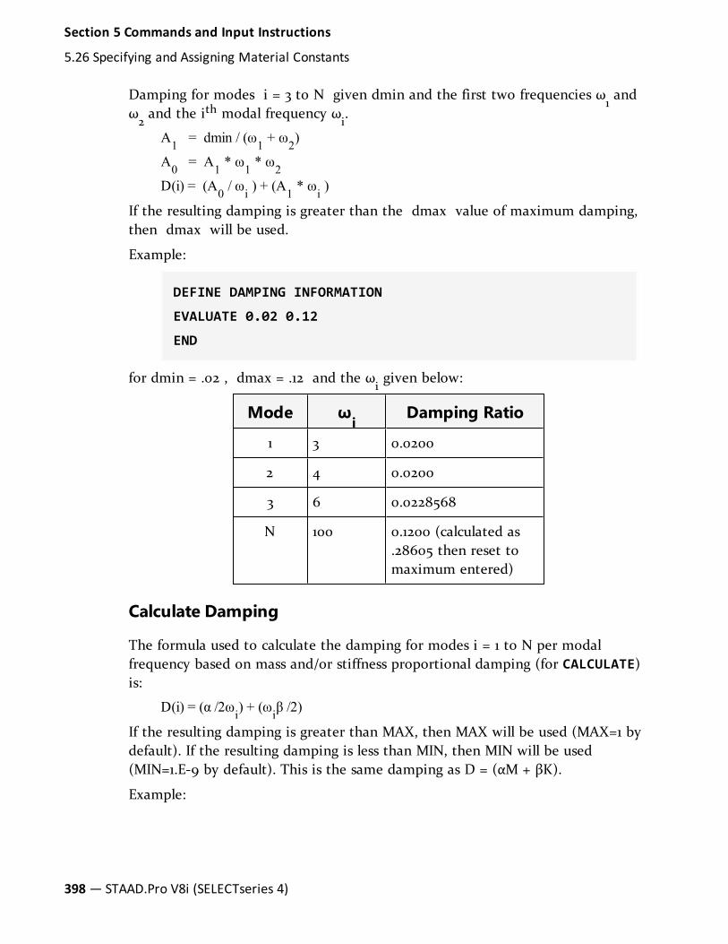
Damping for modes i = 3 to N given dmin and the first two frequencies ω1and
ω2and the ith modal frequency ω
i.
A1 = dmin / (ω1 + ω2)
A0 = A1 * ω1 * ω2D(i) = (A0 / ωi ) + (A1 * ωi )
If the resulting damping is greater than the dmax value of maximum damping,then dmax will be used.
Example:
DEFINE DAMPING INFORMATION
EVALUATE 0.02 0.12
END
for dmin = .02 , dmax = .12 and the ωigiven below:
Mode ωi
Damping Ratio
1 3 0.0200
2 4 0.0200
3 6 0.0228568
N 100 0.1200 (calculated as.28605 then reset tomaximum entered)
Calculate Damping
The formula used to calculate the damping for modes i = 1 to N per modalfrequency based on mass and/or stiffness proportional damping (for CALCULATE)is:
D(i) = (α /2ωi) + (ωiβ /2)
If the resulting damping is greater than MAX, then MAX will be used (MAX=1 bydefault). If the resulting damping is less than MIN, then MIN will be used(MIN=1.E-9 by default). This is the same damping as D = (αM + βK).
Example:
398— STAAD.Pro V8i (SELECTseries 4)
Section 5 Commands and Input Instructions
5.26 Specifying and Assigning Material Constants

DEFINE DAMPING INFORMATION
CALC ALPHA 1.13097 BETA 0.0013926
END
To get 4% damping ratio at 4 Hz and 6% damping ratio at 12 Hz
Mode Hz Rad/sec Damp Ratio
1 4.0 25.133 0.04
3 12.0 75.398 0.06
D(i) = (α /2ωi) + (ωiβ /2)
0.04 = α / 50.266 + 12.567 β
0.06 = α / 150.796 + 37.699 β
α = 1.13097
β = 0.0013926
However they are determined, the α and β terms are entered in the CALC dataabove. For this example calculate the damping ratio at other frequencies to seethe variation in damping versus frequency.
Mode Hz Rad/sec Damp Ratio
1 4.0 25.133 0.040
3 12.0 75.398 0.060
2 12.0664 0.05375
8 50.2655 0.04650
20 120.664 0.09200
4.5 28.274 0.03969
The damping, due to β times stiffness, increases linearly with frequency; and thedamping, due to alpha times mass, decreases parabolicly. The combination of thetwo is hyperbolic.
Figure 5-24: Graph of Damping Ration, D(i), versus Natural Frequency, ω with Max. and Min.values applied.
Section 5 Commands and Input Instructions
5.26 Specifying and Assigning Material Constants
Technical Reference Manual — 399

Explicit DampingWith the EXPLICIT option, you must provide unique modal damping values forsome or all modes. Each value can be preceded by a repetition factor (rf*damp)without spaces.
Example
DEFINE DAMPING INFORMATION
EXPLICIT 0.03 7*0.05 0.04 -
0.012
END
In the above example, mode 1 damping is .03, modes 2 to 8 are .05, mode 9 is.04, mode 10 (and higher, if present) are 0.012.
If there are fewer entries than modes, then the last damping entered will apply tothe remaining modes. This input may be continued to 10 more input lines with
400— STAAD.Pro V8i (SELECTseries 4)
Section 5 Commands and Input Instructions
5.26 Specifying and Assigning Material Constants

word EXPLICIT only on line 1; end all but last line with a space then a hyphen. There may be additional sets of EXPLICIT lines before the END.
5.26.5 Composite Damping for SpringsThis command may be used to designate certain support springs as contributingto the computation of modal damping by the composite damping method. TheResponse Spectrum or Time History dynamic response analyses must selectcomposite damping for this data to have any effect on results.
General Format
SPRING DAMPING
joint-list *{ KFX f1 | KFY f2 | KFZ f3 }
Where:
f1, f2, f3= damping ratios (0.001 to 0.990) in the local X, Y, and Z
directions, respectively.
Note: At least one of KFX, KFY, or KFZ must be entered and each one enteredmust have a spring damp value following it.
Description
If this Spring Damping command is entered, then all springs in the structure areincluded in the composite damping calculation, otherwise no spring is consideredin that calculation.
This input command does not create a spring. Rather, if a support spring exists atthe joint in the specified direction, then it will be assigned the damping ratio.See "5.27 Support Specifications" on page 405 to define springs.
Note: This is not a discrete damper definition.
5.26.6 Member Imperfection InformationTo define camber and drift specifications for selected members. Drift is usuallyfor columns and camber for beams.
General Format
DEFINE IMPERFECTION
Section 5 Commands and Input Instructions
5.26 Specifying and Assigning Material Constants
Technical Reference Manual — 401

CAMBER { Y | Z } (f1) RESPECT (f2) *{ XR f4 f5 | YR f4 f5| ZR f4 f5 | MEM memb-list | LIST memb-list | ALL }
DRIFT { Y | Z } (f3) *{ XR f4 f5 | YR f4 f5 | ZR f4 f5 |MEM memb-list | LIST memb-list | ALL }
Where:
f1= Camber value. Default = 300.
f2= Respect value. Default = 1.6 .
f3= Drift value. Default = 200.
f4, f5= global coordinate values to specify X, Y, or Z range for member
selection.
Imperfections will be simulated by loads. These loads will be generated for thespecified members if there is an Imperfection Analysis specified and if thespecified members are active, in compression, and are not truss ortension/compression only members.
Please refer to sections 1.18.2.4 and 5.37 for more details.
Notes
Camber is the maximum offset of the neutral axes in the defined direction froma vector that passes through the ends of the beam (i.e., the local X axis) definedas the ratio of offset/member length.
Figure 5-25: Camber definition
402— STAAD.Pro V8i (SELECTseries 4)
Section 5 Commands and Input Instructions
5.26 Specifying and Assigning Material Constants

Drift is the offset of the end a member from its specified location defined as aratio of offset/member length.
Figure 5-26: Drift definition
Section 5 Commands and Input Instructions
5.26 Specifying and Assigning Material Constants
Technical Reference Manual — 403

RESPECT is a non dimensional constant used to skip the camber imperfectioncalculation if the compressive load is small or EI is great or length is short. Acombination of these terms is calculated and called EPSILON. If EPSILON is lessthan RESPECT, then the imperfection calculation is skipped for that localdirection, for that case, for that member. The imperfection calculation is alsoskipped for any member that is in tension.
EPSILONy = Length * SQRT[ (abs(axial load)) / EIz]
EPSILONz = Length * SQRT[ (abs(axial load)) / EIy]
Example
SUPPORTS
1 FIXED
2 FIXED BUT FX
DEFINE IMPERFECTION
CAMBER Y 300 RESPECT 0.4 ALL
LOAD 1 GRAVITY + LATERAL
404— STAAD.Pro V8i (SELECTseries 4)
Section 5 Commands and Input Instructions
5.26 Specifying and Assigning Material Constants

MEMBER LOAD
1 UNI GY -1
JOINT LOAD
2 FX -10
PERFORM IMPERFECTION ANALYSIS PRINT STATICS CHECK
5.27 Support SpecificationsSTAAD support specifications may be either parallel or inclined to the globalaxes. See "Global Support Specification" on page 405 for specification of supportsparallel to the global axes. See "5.27.2 Inclined Support Specification" on page 407for specification of inclined supports.
5.27.1 Global Support SpecificationThis set of commands may be used to specify the SUPPORT conditions forsupports parallel to the global axes.
For SURFACE elements, if nodes located along a straight line are all supportedidentically, as in the case of the base of a wall, support generation can beperformed for assigning restraints to those nodes. See the “GENERATE” option inthe command syntax below. You only need to provide the starting and endingnodes of the range, and the type of restraint.
General FormatSUPPORTS
{ joint-list | ni TO nj GENERATE } { PINNED | FIXED ( BUTrelease-spec (spring-spec) ) | ENFORCED ( BUT release-spec)}
release-sepc = { FX | FY | FZ | MX | MY | MZ }
spring-spec = *{KFX f1 | KFY f2 | KFZ f3 | KMX f4 | KMY f5| KMZ f6 }
Where:
ni, nj = Start and end node numbers, respectively, for generatingsupports along a SURFACE element edge.
f1… f
6= Spring constants corresponding to support spring directions
X, Y, and Z and rotations about X, Y, and Z, repsectively.
Section 5 Commands and Input Instructions
5.27 Support Specifications
Technical Reference Manual — 405

Description of Pinned and FixedA PINNED support is a support that has translational, but no rotational restraints.In other words, the support has no moment carrying capacity. A FIXED supporthas both translational and rotational restraints. A FIXED BUT support can bereleased in the global directions as described in release-spec (FX for force-Xthrough MZ for moment-Z). Also, a FIXED BUT support can have spring constantsas described in spring-spec (translational spring in global X-axis as KFX throughrotational spring in global Z-axis as KMZ). Corresponding spring constants are f1through f6. The rotational spring constants are always per degree of rotation. Allsix releases may be provided as may be required when using the CHANGEcommand. If both release specifications and spring specifications are to besupplied for the same support joint, release specifications must come first.
1. See "Change Specification" on page 709 for information on specification ofSUPPORTS along with the CHANGE command specifications.
2. Spring constants must be provided in the current units.
3. All spring DOF must be entered after the last non-spring DOF is specified,if both are on the same line.
4. If there are two entries for the same joint, then:
a. any direction that is pinned/fixed on either will be fixed in thatdirection.
b. any direction released on one and is a spring on the other will use thespring.
c. any direction that is pinned/fixed on one and a spring on the otherwill use the spring.
d. any direction that is a spring on two or more entries will have thespring constants added.
Example 1
SUPPORTS
1 TO 4 7 PINNED
5 6 FIXED BUT FX MZ
8 9 FIXED BUT MZ KFX 50.0 KFY 75.
18 21 FIXED
406— STAAD.Pro V8i (SELECTseries 4)
Section 5 Commands and Input Instructions
5.27 Support Specifications

27 FIXED BUT KFY 125.0
In this example, joints 1 to 4 and joint 7 are pinned. No moments are carried bythose supports. Joints 5 and 6 are fixed for all DOF except in force-X andmoment-Z. Joints 8 and 9 are fixed for all DOF except moment-Z and havesprings in the global X and Y directions with corresponding spring constants of 50and 75 units respectively. Joints 18 and 21 are fixed for all translational androtational degrees of freedom. At joint 27, all the DOF are fixed except the FYDOF where it has a spring with 125 units spring constant.
Description of EnforcedEnforced Support defines which translational and rotational directions, at a joint,may have a support displacement imposed. The support displacements aredefined for each load case in section 5.32.8. If no support displacement isentered, then zero displacement will be imposed, as if that direction was FIXED. The enforced displacement directions will be fixed for dynamic load cases.
If there are two entries for the same joint, then any direction that is enforced oneither will be enforced in that direction, overriding any other supportspecification for that joint-direction.
Currently the support generation command can only be used in conjunction withthe Surface element support specifications.
Example 2
SUPPORTS
3 TO 7 GENERATE PIN
The above command will generate pinned supports for all joints located betweennodes No. 3 and 7 along a straight line. This may include joints explicitly definedby the user or joints generated by the program for internal use only (e.g., as aresult of SET DIVISION and SURFACE INCIDENCES commands).
5.27.2 Inclined Support SpecificationThese commands may be used to specify supports that are inclined with respectto the global axes.
General FormatSUPPORT
Section 5 Commands and Input Instructions
5.27 Support Specifications
Technical Reference Manual — 407
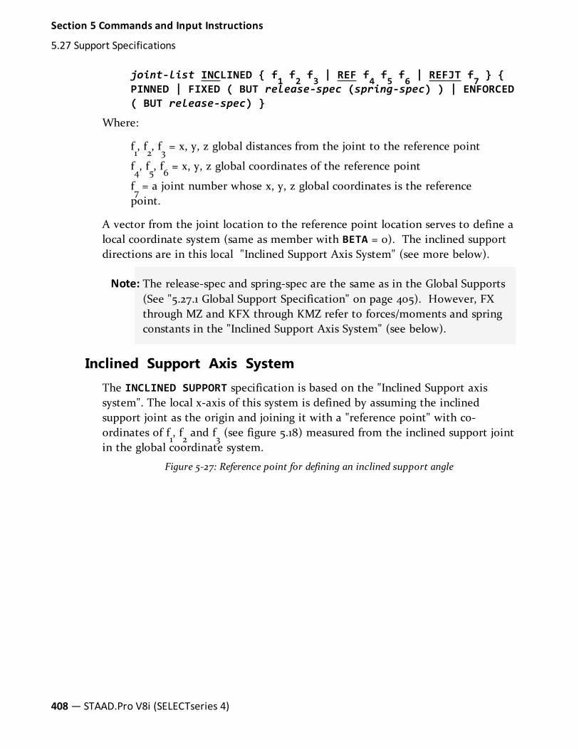
joint-list INCLINED { f1 f2 f3 | REF f4 f5 f6 | REFJT f7 } { PINNED | FIXED ( BUT release-spec (spring-spec) ) | ENFORCED( BUT release-spec) }
Where:
f1, f2, f3= x, y, z global distances from the joint to the reference point
f4, f5, f6= x, y, z global coordinates of the reference point
f7= a joint number whose x, y, z global coordinates is the reference
point.
A vector from the joint location to the reference point location serves to define alocal coordinate system (same as member with BETA = 0). The inclined supportdirections are in this local "Inclined Support Axis System" (see more below).
Note: The release-spec and spring-spec are the same as in the Global Supports(See "5.27.1 Global Support Specification" on page 405). However, FXthrough MZ and KFX through KMZ refer to forces/moments and springconstants in the "Inclined Support Axis System" (see below).
Inclined Support Axis SystemThe INCLINED SUPPORT specification is based on the "Inclined Support axissystem". The local x-axis of this system is defined by assuming the inclinedsupport joint as the origin and joining it with a "reference point" with co-ordinates of f
1, f2and f
3(see figure 5.18) measured from the inclined support joint
in the global coordinate system.
Figure 5-27: Reference point for defining an inclined support angle
408— STAAD.Pro V8i (SELECTseries 4)
Section 5 Commands and Input Instructions
5.27 Support Specifications

The Y and Z axes of the inclined support axis system have the same orientationas the local Y and Z axes of an imaginary member whose BETA angle is zero andwhose incidences are defined from the inclined support joint to the referencepoint. See "Relationship Between Global & Local Coordinates" on page 15 of thismanual for more information on these concepts.
Note: Inclined support directions are assumed to be same as global whencomputing some dynamic and UBC intermediate results (e.g., globalparticipation factors). If masses and/or forces in the free directions atinclined supports are a relatively small portion of the overall forces,then the effect should be very small.
Example
SUPPORT
4 INCLINED 1.0 -1.0 0.0 FIXED BUT FY MX MY MZ
5.27.3 Automatic Spring Support Generator for FoundationsSTAAD has a facility for automatic generation of spring supports to modelfootings and foundation mats. This command is specified under the SUPPORTcommand.
Section 5 Commands and Input Instructions
5.27 Support Specifications
Technical Reference Manual — 409

General Format
SUPPORT
{ joint-list ELASTIC FOOTING f1 (f2) | joint-list ELASTICMAT | plate-list PLATE MAT } DIR { X | XONLY | Y | YONLY |Z | ZONLY } SUBGRADE f3(PRINT) ( {COMP | MULTI } )
or
plate-list PLATE MAT DIR ALL SUBGRADE f4 (f5 f6)
(PRINT) ( {COMP | MULTI } )
Where:
f1, f2= Length and width of the ELASTIC footing. If f
2is not given, the
footing is assumed to be a square with sides f1
X,Y,Z = Global direction in which soil springs are to be generated
f3= Soil sub-grade modulus in current force/area/length units
f4, f5, f6= Soil sub-grade modulus for use with ALL option in current
force/area/length units in Y, X, Z directions respectively. f4, f5 defaultto f3 if omitted. Note the order in which the Y value is specified first,followed by X and then Z.
Figure 5-28: Correct and Incorrect order for specifying subgrade modulus values
Warning: Do not use this command with SET Z UP.
Description
If you want to specify the influence area of a joint yourself and have STAADsimply multiply the area you specified by the sub-grade modulus, use the
410— STAAD.Pro V8i (SELECTseries 4)
Section 5 Commands and Input Instructions
5.27 Support Specifications

ELASTIC FOOTING option. Situations where this may be appropriate are such aswhen a spread footing is located beneath a joint where you want to specify aspring support. A value for f
1(and f
2if its a non-square footing) is required for
the FOOTING option.
If you want to have STAAD calculate the influence area for the joint (instead ofyou specifying an area yourself) and use that area along with the sub-grademodulus to determine the spring stiffness value, use the ELASTIC MAT option.Situations where this may be appropriate are such as when a slab is on soil andcarries the weight of the structure above. You may have modeled the entire slabas finite elements and wish to generate spring supports at the nodes of theelements.
The PLATE MAT option is similar to the Elastic Mat except for the method usedto compute the influence area for the joints. If your mat consists of plateelements and all of the influence areas are incorporated in the plate areas, thenthis option is preferable. Enter a list of plates or YRANGE f1 f2 at the beginning ofthe command, the joint influence areas are then calculated using the sameprinciples as joint forces would be from uniform pressure on these plates. Thismethod overcomes a major limitation of the Delaunay triangle method used inthe ELASTIC MAT option, which is that the contour formed by the nodes of themat must form a convex hull.
The PLATE MAT DIR ALL option is similar to the Plate Mat except that thespring supports are in 3 directions. If the compression only option is alsospecified, then the compression direction will be assumed to be in the Ydirection. If the Y spring at a joint goes slack (lift off), then the X and Z springstiffnesses for that joint will also be set to zero. Otherwise the X and Z springsact in both directions. The influence area for the X and Z springs is the same asused for the Y spring. Three values of subgrade reaction may be entered, the firstis for the Y direction, the second for X and the third for Z.
The keyword DIR is followed by one of the alphabets X, Y or Z (or XONLY,YONLY, or ZONLY) which indicate the direction of resistance of the springsupports. If X or Y or Z is selected then a spring support is generated in thatdirection plus 3 other directions receive a fixed support, e.g., if Y is selected, thenFY is supported by a spring; FX and FZ and MY are fixed supports; and MX andMZ are free. If XONLY, YONLY, or ZONLY are selected then only a spring supportin that direction is generated.
The keyword SUBGRADE is followed by the value of the subgrade reaction. Thevalue should be provided in the current unit system signified by the most recentUNIT statement prior to the SUPPORT command.
The PRINT option prints the influence area of each joint.
Section 5 Commands and Input Instructions
5.27 Support Specifications
Technical Reference Manual — 411
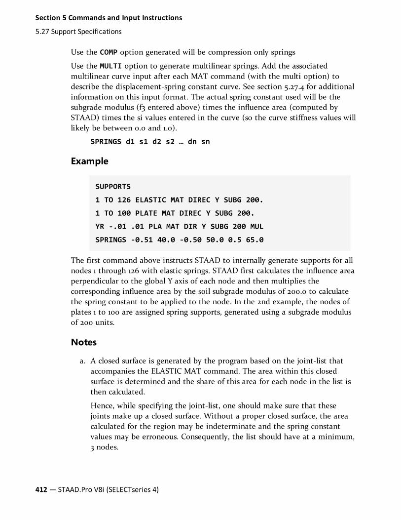
Use the COMP option generated will be compression only springs
Use the MULTI option to generate multilinear springs. Add the associatedmultilinear curve input after each MAT command (with the multi option) todescribe the displacement-spring constant curve. See section 5.27.4 for additionalinformation on this input format. The actual spring constant used will be thesubgrade modulus (f3 entered above) times the influence area (computed bySTAAD) times the si values entered in the curve (so the curve stiffness values willlikely be between 0.0 and 1.0).
SPRINGS d1 s1 d2 s2 … dn sn
Example
SUPPORTS
1 TO 126 ELASTIC MAT DIREC Y SUBG 200.
1 TO 100 PLATE MAT DIREC Y SUBG 200.
YR -.01 .01 PLA MAT DIR Y SUBG 200 MUL
SPRINGS -0.51 40.0 -0.50 50.0 0.5 65.0
The first command above instructs STAAD to internally generate supports for allnodes 1 through 126 with elastic springs. STAAD first calculates the influence areaperpendicular to the global Y axis of each node and then multiplies thecorresponding influence area by the soil subgrade modulus of 200.0 to calculatethe spring constant to be applied to the node. In the 2nd example, the nodes ofplates 1 to 100 are assigned spring supports, generated using a subgrade modulusof 200 units.
Notes
a. A closed surface is generated by the program based on the joint-list thataccompanies the ELASTIC MAT command. The area within this closedsurface is determined and the share of this area for each node in the list isthen calculated.
Hence, while specifying the joint-list, one should make sure that thesejoints make up a closed surface. Without a proper closed surface, the areacalculated for the region may be indeterminate and the spring constantvalues may be erroneous. Consequently, the list should have at a minimum,3 nodes.
412— STAAD.Pro V8i (SELECTseries 4)
Section 5 Commands and Input Instructions
5.27 Support Specifications

b. The internal angle formed by 2 adjacent segments connecting 3 consecutivenodes in the list should be less than 180 degrees. In other words, the regionshould have the shape of a convex polygon. The example below explains themethod that may be used to get around a situation where a convex polygonis not available.
c. For the model comprised of plate elements 100 to 102 in the figure below,one wishes to generate the spring supports at nodes 1 to 8. However, asingle ELASTIC MAT command will not suffice because the internal anglebetween the edges 1-8 and 8-7 at node 8 is 270 degrees, which violates therequirements of a convex polygon.
So, you should break it up into two commands:
1 2 3 8 ELASTIC MAT DIREC Y SUBG 200.
3 4 5 6 7 8 ELASTIC MAT DIREC Y SUBG 200.
Figure 5-29: Example for elastic mat generation for a convex polygonal shape
Joints 3 and 8 will hence get the contribution from both of the abovecommands.
The command works only when the plane of the closed region is parallel toone of the global planes X-Y, Y-Z or X-Z. For regions that are inclined to
Section 5 Commands and Input Instructions
5.27 Support Specifications
Technical Reference Manual — 413

one of the global planes, the spring constant will have to be evaluatedmanually and specified using the FIXED BUT type of spring support.
5.27.4 Multilinear Spring Support SpecificationWhen soil is modeled as spring supports, the varying resistance it offers toexternal loads can be modeled using this facility, such as when its behavior intension differs from its behavior in compression.
General Format
MULTILINEAR SPRINGS
joint-list SPRINGS d1 s1 d2 s2 … dn snWhere:
disipairs represent displacement and spring constant pairs (si is zero
or positive), starting from the maximum negative displacement to themaximum positive displacement.
The first pair defines the spring constant from negative infinity displacement upto the displacement defined in the second pair. The second pair define the springconstant when the support displaces in the range from the displacement definedin the second pair, up to the displacement defined in the third pair. Thiscontinues for each displacement and spring constant pair until the last pair whichdefines the spring constant for displacements greater than the displacement inthe last pair to positive infinity.
Each load case in a multi-linear analysis must be separated by a CHANGEcommand and have its own PERFORM ANALYSIS command. There may not beany PDELTA, NONLIN, dynamics, CABLE, or TENSION/COMPRESSION analysisincluded. The multi-linear spring command will initiate an iterative analysis andconvergence check cycle. The cycles will continue until the root mean square(RMS) of the effective spring rates used remain virtually the same for twoconsecutive cycles.
Example
UNIT …
SUPPORT
1 PINNED; 2 4 FIXED BUT KFY 40.0
414— STAAD.Pro V8i (SELECTseries 4)
Section 5 Commands and Input Instructions
5.27 Support Specifications

MULTILINEAR SPRINGS
2 4 SPRINGS -1 40.0 -0.50 50.0 0.5 65.0
Load-Displacement characteristics of soil can be represented by a multi-linearcurve. Amplitude of this curve will represent the spring characteristic of the soilat different displacement values. A typical spring characteristic of soil may berepresented as the step curve as shown in the figure below. In the above example,the multi-linear spring command specifies soil spring at joints 2 and 4. (Note thatthe amplitude of the step curve does not change after the first point.)
Notes
a. SUPPORT springs must have previously been entered for each springentered here. For the first cycle, the spring value used will be the supportspring value (not the zero displacement value here). Use a realistic andstable value.
b. All directions that have been defined with an initial spring stiffness in theSUPPORT command will become multi-linear with this one curve.
c. This command can be continued to up to 11 lines by ending all but last witha hyphen. The semi-colons and the XRANGE, YRANGE, ZRANGE list itemsmay not be used.
d. This command needs a minimum of two displacement and spring constantpairs.
Figure 5-30: Spring constant is always positive or zero. F = Force Units, L = Length
Section 5 Commands and Input Instructions
5.27 Support Specifications
Technical Reference Manual — 415

Units
5.27.5 Spring Tension/Compression SpecificationThis command may be used to designate certain support springs as Tension-onlyor Compression-only springs.
General Format
SPRING TENSION
joint-list (spring-spec)
SPRING COMPRESSION
joint-list (spring-spec)
spring-spec = *{ KFX | KFY | KFZ | ALL }
Description
Tension-only springs are capable of carrying tensile forces only. Thus, they areautomatically inactivated for load cases that create compression in them.Compression-only springs are capable of carrying compressive forces only. Thus,they are automatically inactivated for load cases that create tension in them.
416— STAAD.Pro V8i (SELECTseries 4)
Section 5 Commands and Input Instructions
5.27 Support Specifications

If no spring spec is entered or ALL is entered then all translational springs at thatjoint will be tension (or compression) only. This input command does not createa spring, only that if a support spring exists at the joint in the specified directionthen it will also be tension (or compression) only. See "Support Specifications" onpage 405 to define springs.
For compression only springs the ALL parameter has special meaning. Thecompression only spring is in the Y direction; the X and Z direction springs arebi-directional. However when the Y direction spring goes slack, the X and Zsprings at the same joint are made inactive as well.
Note: The procedure for analysis of Tension-only or Compression-only springsrequires iterations for every load case and therefore may be quiteinvolved.
Since this command does not specify whether the spring is in the positive ornegative direction from the joint, it is assumed in STAAD to be in the negativedirection. For negative displacement the spring is in compression and for positivethe spring is in tension.
If a CHANGE command is used (because of a change in list of tension springs,supports, etc.), then the SET NL command must be used to convey to STAADthat multiple analyses and multiple structural conditions are involved.
1. See "5.5 Set Command Specification" on page 284 for explanation of theSET NL command. The number that follows this command is an upperbound on the total number of primary load cases in the file.
2. STAAD performs up to 10 iterations automatically, stopping if converged. Ifnot converged, a warning message will be in the output. Enter a SETITERLIM i command (with i > 10) before the first load case to increase thedefault number of iterations. Since convergence may not be possible usingthis procedure, do not set the limit too high. If not converged, a messagewill be in the output.
3. The principle used in the analysis is the following.
l The program reads the list of springs declared as SPRING TENSIONand/or COMPRESSION.
l The analysis is performed for the entire structure and the spring forcesare computed.
l For the springs declared as SPRING TENSION / COMPRESSION, theprogram checks the axial force to determine whether it is tensile or
Section 5 Commands and Input Instructions
5.27 Support Specifications
Technical Reference Manual — 417

compressive. Positive displacement is TENSION. If the spring cannottake that load, the spring is "switched off" from the structure.
l The analysis is performed again without the switched off springs.
l Up to ITERLIM iterations of the above steps are made for each loadcase.
l This method does not always converge and may become unstable.Check the output for instability messages. Do not use results if thelast iteration was unstable. You may need to include some support ineach global direction that is not tension (or compression) only to bestable on every iteration.
4. A revised SPRING TENSION / COMPRESSION command and itsaccompanying list of joints may be provided after a CHANGE command. Ifentered, the new SPRING commands replace all prior SPRING commands. Ifnot entered after a CHANGE, then the previous spring definitions are used.
5. The SPRING TENSION command should not be used if the following loadcases are present: Response Spectrum load case, Time History Load case,Moving Load case. If used, the SPRING TENSION / COMPRESSION will beignored in all load cases.
6. If the SPRING TENSION / COMPRESSION command is used in a model withUBC, IBC or other such seismic load cases, each such load case must befollowed by an ANALYSIS and CHANGE command.
Notes
a. A spring declared as tension-only or compression-only will carry axial forcesonly. It will not carry moments.
b. The SPRING TENSION / COMPRESSION commands should not be specified ifthe INACTIVE MEMBER command is specified.
c. Do not use Load Combination to combine these cases.Tension/Compression cases are non-linear and should not be linearlycombined as in Load Combination. Use a primary load case with theRepeat Load command.
Example
SPRING TENSION
418— STAAD.Pro V8i (SELECTseries 4)
Section 5 Commands and Input Instructions
5.27 Support Specifications

12 17 19 TO 37 65
SPRING COMPRESSION
5 13 46 TO 53 87 KFY
The following is the general sequence of commands in the input file if theSPRING TENSION or COMPRESSION command is used. This example is for theSPRING TENSION command. Similar rules are applicable for the SPRINGCOMPRESSION command. The dots indicate other input data items.
STAAD …
SET NL …
UNITS …
JOINT COORDINATES
…
MEMBER INCIDENCES
…
ELEMENT INCIDENCES
…
CONSTANTS
…
MEMBER PROPERTY
…
ELEMENT PROPERTY
…
SUPPORTS
…
SPRING TENSION
…
LOAD 1
…
LOAD 2
…
LOAD 3
Section 5 Commands and Input Instructions
5.27 Support Specifications
Technical Reference Manual — 419

REPEAT LOAD
…
PERFORM ANALYSIS
CHANGE
LOAD LIST ALL
PRINT …
PRINT …
PARAMETER
…
CHECK CODE …
FINISH
5.28 Rigid Diaphragm ModelingSTAAD.Pro has two methods for defining rigid floor diaphragms. Both arefunctionally equivalent but the Master-Slave joint requires that an analytical nodebe located and specified as the master node. For most models, the simpler FloorDiaphragm option is preferred.
5.28.1 Master/Slave SpecificationThis set of commands may be used to model specialized linkages (displacementtying, rigid links) through the specification of MASTER and SLAVE joints. Pleaseread the notes for restrictions.
General Format
SLAVE *{ XY | YZ | ZX | RIGID | FX | FY | FZ | MX | MY | MZ} MASTER j JOINT joint-spec
Where:
joint-spec = { joint-list or *{ XRANGE | YRANGE | ZRANGE }f1, f2 }
Description
The master/slave option provided in STAAD allows the user to model specializedlinkages (displacement tying, rigid links) in the system. For example, SLAVE FY …
420— STAAD.Pro V8i (SELECTseries 4)
Section 5 Commands and Input Instructions
5.28 Rigid Diaphragm Modeling

connects the two joints such that the Y displacement at the slave will be the sumof Y displacement at the master plus the rigid rotation,
R sin θ
Notice that instead of providing a joint list for the slaved joints, a range ofcoordinate values (in global system) may be used. All joints whose coordinatesare within the range are assumed to be slaved joints. For convenience, thecoordinate range specified for slaved joints in this entry may include the masterjoint for this entry. However, master and slave joints of other entries must not beincluded in the coordinate range. All 2 or 3 ranges can be entered to form a“tube” or “box” for selecting joints in the tube or box region.
Fx, Fy etc. are the directions in which they are slaved (any combination may beentered).
If two or more entries have the same master, the slave lists will be merged. Pleaseensure that the same direction specs are used.
The direction specifiers (XY, YZ, ZX) are combinations of the basic directions, XYis the same as entering FX, FY, MZ; etc. Any combination of direction specifiersmay be entered. An example of the use of this format is: a rigid diaphragm floorthat still retains bending flexibility entered as SLA ZX … .
If RIGID or if all directions are provided, the joints are assumed to be rigidlyconnected as if SLA DIA RIG were entered, even if DIA is omitted.
Restrictions
l Solid elements may not be connected to slave joints.
l Master joints may not be master or slaves in another entry.
l Slave joints may not be master or slaves in another entry.
l Slave directions at joints may not be supported directions or havedisplacements imposed.
l Master and/or slave joints may not be inclined supports.
l The master / slave specification is only intended for linear static anddynamic analysis.
l Multilinear springs are not permitted.
Example
Fully Rigid and Rigid Floor Diaphragm
Section 5 Commands and Input Instructions
5.28 Rigid Diaphragm Modeling
Technical Reference Manual — 421

SLAVE RIGID MASTER 22 JOINT 10 TO 45
SLAVE RIGID MASTER 70 JOINT YRANGE 25.5 27.5
SLA ZX MAS 80 JOINT YR 34.5 35.5
In STAAD.Pro 2007 Build 1001, the internal processing of any Master Slavecommand was enhanced to allow an automatic bandwidth reduction to takeplace.
The analysis engine now performs a bandwidth reduction on files that includeMaster/Slave commands which must occur in the input file after the definition ofsupports. In previous versions of STAAD.Pro, for the bandwidth reduction to takeplace, the data of Master/Slave would need to be repeated before the supportdefinitions. This requirement is now no longer required.
5.28.2 Floor DiaphragmThis command is used to create rigid floor diaphragms without the need tospecify a master joint at each. When specified, this command directs the engineto perform the following:
a. calculate the center of mass for each rigid diaphragm (where master joint isto be located) considering the mass model of the structure. The mass mustbe modeled using mass reference load. See "Mass Modeling Using ReferenceLoads" on page 533
b. create, internally, an analytical node at the center of mass location to beincluded during analysis (unless a master node is specified) if an existinganalytical node exists at this point, then the existing joint is used in lieu ofcreating a new joint.
c. search all nodes available within a diaphragm and add them as slave nodes;with the master node located at the center of mass for the diaphragm (or atthe specified master node)
Note: This feature requires STAAD.Pro V8i (SELECTseries 3) (release20.07.08) or higher.
General Format
FLOOR DIAPHRAGM
DIAPHRAGM i1 TYPE RIGID diaphragm-spec
After all diaphragms are defined, then:
422— STAAD.Pro V8i (SELECTseries 4)
Section 5 Commands and Input Instructions
5.28 Rigid Diaphragm Modeling
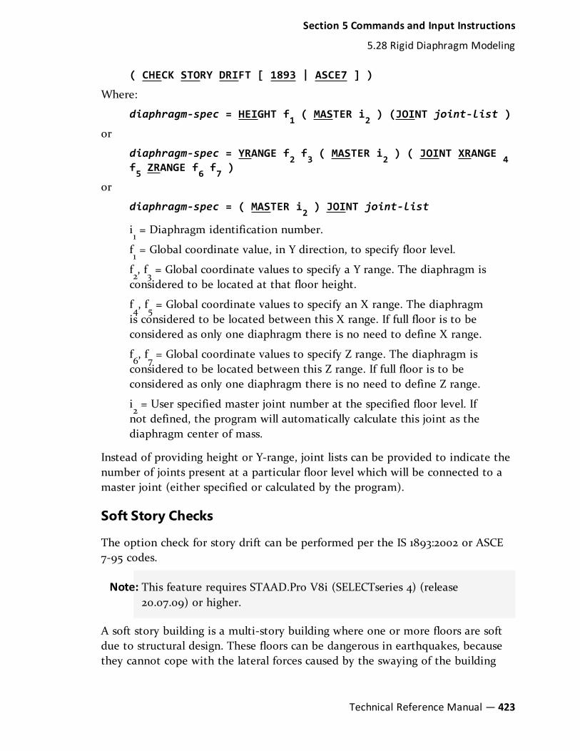
( CHECK STORY DRIFT [ 1893 | ASCE7 ] )
Where:
diaphragm-spec = HEIGHT f1 ( MASTER i2 ) (JOINT joint-list )
or
diaphragm-spec = YRANGE f2 f3 ( MASTER i2 ) ( JOINT XRANGE 4f5 ZRANGE f6 f7 )
or
diaphragm-spec = ( MASTER i2 ) JOINT joint-list
i1= Diaphragm identification number.
f1= Global coordinate value, in Y direction, to specify floor level.
f2, f3= Global coordinate values to specify a Y range. The diaphragm is
considered to be located at that floor height.
f4, f5= Global coordinate values to specify an X range. The diaphragm
is considered to be located between this X range. If full floor is to beconsidered as only one diaphragm there is no need to define X range.
f6, f7= Global coordinate values to specify Z range. The diaphragm is
considered to be located between this Z range. If full floor is to beconsidered as only one diaphragm there is no need to define Z range.
i2= User specified master joint number at the specified floor level. If
not defined, the program will automatically calculate this joint as thediaphragm center of mass.
Instead of providing height or Y-range, joint lists can be provided to indicate thenumber of joints present at a particular floor level which will be connected to amaster joint (either specified or calculated by the program).
Soft Story Checks
The option check for story drift can be performed per the IS 1893:2002 or ASCE7-95 codes.
Note: This feature requires STAAD.Pro V8i (SELECTseries 4) (release20.07.09) or higher.
A soft story building is a multi-story building where one or more floors are softdue to structural design. These floors can be dangerous in earthquakes, becausethey cannot cope with the lateral forces caused by the swaying of the building
Section 5 Commands and Input Instructions
5.28 Rigid Diaphragm Modeling
Technical Reference Manual — 423

during a quake. As a result, the soft story may fail, causing what is known as asoft story collapse.
Soft story buildings are characterized by having a story which has a lot of openspace. Parking garages, for example, are often soft stories, as are large retailspaces or floors with a lot of windows. While the unobstructed space of the softstory might be aesthetically or commercially desirable, it also means that thereare less opportunities to install shear walls, specialized walls which are designedto distribute lateral forces so that a building can cope with the swayingcharacteristic of an earthquake.
If a building has a floor which is 70% less stiff than the floor above it, it isconsidered a soft story building. This soft story creates a major weak point in anearthquake, and since soft stories are mostly associated with retail spaces andparking garages, they are often on the lower stories of a building, which meansthat when they collapse, they can take the whole building down with them,causing serious structural damage which may render the structure totallyunusable.
Notes
a. Full diaphragm definition should be provided in one line. Seconddiaphragm definition should be provided in second line. However, if thereis joint-list, the list can extend to the second line with a continuation sign("-".
DIA F1 TYP RIG YR F2 F3 JOI XR F4 F5 ZR F6 F7
DIA F11 TYP RIG YR F21 F31 JOI XR F41 F51 ZR F61 F71
DIA F12 TYP RIG JOI 35 45 51 TO 57 59 TO 83 -
90 TO 110
where f1, f11 and f12 are three rigid diaphragms located at floor heightranging between f2 and f3, f21 and f31 and the joints lying in the plane asindicated by their global Y coordinates respectively.
b. Diaphragms should be specified in ascending order (i.e., diaphragms at firstfloor level should be specified first before specifying that on 2nd floor leveland so on).
c. If user defined master joint is specified in one diaphragm, user definedmaster joints should be specified for all diaphragms. Combination of user
424— STAAD.Pro V8i (SELECTseries 4)
Section 5 Commands and Input Instructions
5.28 Rigid Diaphragm Modeling

defined master joint for one diaphragm and program calculated masterjoint for another diaphragm is not supported.
d. Before specifying floor diaphragm mass model (in terms of reference load)must be specified.
e. Floor diaphragm can be specified only once in an input file.
f. Floor diaphragm cannot be specified along with FLOOR HEIGHT command.
g. Floor diaphragm cannot be specified along with MASTER-SLAVE command.
h. Floor diaphragm cannot be specified with SET Z UP command.
i. Sloped diaphragms are not supported.
j. Base level (or ground floor level or support level) is taken as the minimumof Y coordinates defined. Different base level can be specified usingfollowing syntax.
FLOOR DIAPHRAGM
DIA f1 TYPE RIG YR f2 f3 JOI XR f4 f5 ZR f6 f7
DIA f11 TYPE RIG YR f21 f31 JOI XR f41 f51 ZR f61 f71
…
BASE b1Where:
b1= base/ground floor level of the structure
k. The maximum number of diaphragms allowed by the program (defaultvalue) is 150. If more than 150 diaphragms need to be specified, then SETRIGID DIAPHRAGM n must be specified before specifying joint incidence,where n = total number of diaphragms in the structure.
Example
*********************************************************-**
UNIT FEET KIP
DEFINE REF LOAD
LOAD R1 LOADTYPE MASS
* MASS MODEL
Section 5 Commands and Input Instructions
5.28 Rigid Diaphragm Modeling
Technical Reference Manual — 425

SELFWEIGHT X 1
SELFWEIGHT Y 1
SELFWEIGHT Z 1
JOINT LOAD
17 TO 48 FX 2.5 FY 2.5 FZ 2.5
49 TO 64 FX 1.25 FY 1.25 FZ 1.25
*
LOAD R2
SELFWEIGHT Y -1
JOINT LOAD
17 TO 48 FY -2.5
49 TO 64 FY -1.25
END DEF REF LOAD
*********************************************************-*******
FLOOR DIAPHRAGM
DIAPHRAGM 1 TYPE RIGID YR 4.1 4.3 JOI XR -0.1 21.3 ZR -0.1 31.9
DIAPHRAGM 2 TYPE RIGID YR 8.3 8.5 JOI XR -0.1 21.3 ZR -0.1 31.9
DIAPHRAGM 3 TYPE RIGID YR 12.5 12.7 JOI XR -0.1 21.3 ZR -0.1 31.9
DIAPHRAGM 4 TYPE RIGID YR 16.7 16.9 JOI XR -0.1 21.3 ZR -0.1 31.9
DIAPHRAGM 5 TYPE RIGID YR 20.9 21.1 JOI XR -0.1 21.3 ZR -0.1 31.9
DIAPHRAGM 6 TYPE RIGID YR 25.1 25.3 JOI XR -0.1 21.3 ZR -0.1 31.9
DIAPHRAGM 7 TYPE RIGID YR 29.3 29.5 JOI XR -0.1 21.3 ZR -0.1 31.9
DIAPHRAGM 8 TYPE RIGID YR 33.5 33.7 JOI XR -0.1 21.3 ZR -0.1 31.9
426— STAAD.Pro V8i (SELECTseries 4)
Section 5 Commands and Input Instructions
5.28 Rigid Diaphragm Modeling

DIAPHRAGM 9 TYPE RIGID YR 37.7 37.9 JOI XR -0.1 21.3 ZR -0.1 31.9
BASE 0.5
*********************************************************-**
5.29 Draw SpecificationsThis command has been discontinued in STAAD.Pro. Please use the GraphicalUser Interface for screen and hard copy graphics.
5.30 Miscellaneous Settings for Dynamic AnalysisWhen dynamic analysis such as frequency and mode shape calculation, responsespectrum analysis and time history analysis is performed, it involves eigenvalueextraction and usage of a certain number of modes during the analysis process.These operations are built around certain default values. This section explains thecommands required to override those defaults.
5.30.1 Cut-Off Frequency, Mode Shapes, or TimeThese commands are used in conjunction with dynamic analysis. They may beused to specify the highest frequency or the number of mode shapes that need tobe considered.
General Format
CUT (OFF) { FREQUENCY f1 | MODE SHAPE i1 | TIME t1 }
Where:
f1= Highest frequency (cycle/sec) to be considered for dynamic
analysis.
i1= Number of mode shapes to be considered for dynamic analysis. If
the cut off frequency command is not provided, the cut off frequencywill default to 108 cps. If the cut off mode shape command is notprovided, the first six modes will be calculated. These commandsshould be provided prior to the loading specifications.
t1= Ending time for a time history analysis. If zero (default), the time
history will end when the last forcing function ends.
Section 5 Commands and Input Instructions
5.29 Draw Specifications
Technical Reference Manual — 427

A maximum of i1mode shapes will be computed regard-less of f
1. If during
convergence testing, the 0 through f1frequencies are converged, then the modal
calculation will be completed before i1mode shapes are calculated.
If the CUT OFF FREQ f1 and CUT OFF MODE i1 commands are both entered,then after completing each iteration step in the Subspace iteration, convergencetesting is performed. If every frequency from 0.0 to f
1meets the convergence
tolerance, then the Subspace iteration is done. Similarly, if every mode from 0 toi1meets the convergence tolerance, then the Subspace iteration is done. If the cut
off frequency f1results in fewer modes than i
1, then only those frequencies up to
the cut off are used. If the cut off frequency would result in more modes than i1,
then only the first i1modes are used. That is, the modes cut off takes precedence
over the frequency cut off.
5.30.2 Mode SelectionThis command allows specification of a reduced set of active dynamic modes. Allmodes selected by this command remain selected until a new MODE SELECT isspecified.
This command is used to limit the modes used in dynamic analysis to the modeslisted in this command and deactivate all other modes that were calculated butnot listed in this command. If this command is not entered, then all modescalculated are used in the dynamic analysis.
General Format
MODE SELECT mode-list
Example
CUT OFF MODES 10
MODE SELECT 1 TO 3
In this example, 10 modes will be calculated but only modes 1 and 3 will be usedin dynamic analysis.
Notes
a. Do not enter this command within the loads data (from the first Load com-mand in an analysis set down to the associated Analysis command).
428— STAAD.Pro V8i (SELECTseries 4)
Section 5 Commands and Input Instructions
5.30 Miscellaneous Settings for Dynamic Analysis
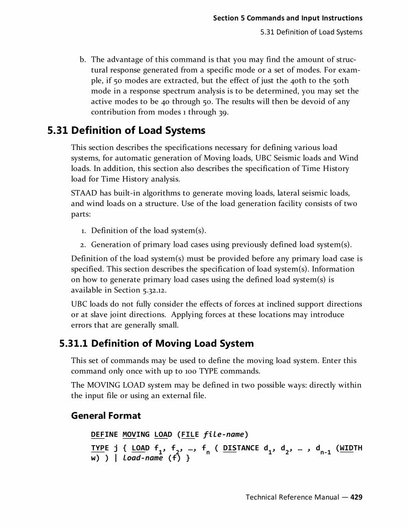
b. The advantage of this command is that you may find the amount of struc-tural response generated from a specific mode or a set of modes. For exam-ple, if 50 modes are extracted, but the effect of just the 40th to the 50thmode in a response spectrum analysis is to be determined, you may set theactive modes to be 40 through 50. The results will then be devoid of anycontribution from modes 1 through 39.
5.31 Definition of Load SystemsThis section describes the specifications necessary for defining various loadsystems, for automatic generation of Moving loads, UBC Seismic loads and Windloads. In addition, this section also describes the specification of Time Historyload for Time History analysis.
STAAD has built-in algorithms to generate moving loads, lateral seismic loads,and wind loads on a structure. Use of the load generation facility consists of twoparts:
1. Definition of the load system(s).
2. Generation of primary load cases using previously defined load system(s).
Definition of the load system(s) must be provided before any primary load case isspecified. This section describes the specification of load system(s). Informationon how to generate primary load cases using the defined load system(s) isavailable in Section 5.32.12.
UBC loads do not fully consider the effects of forces at inclined support directionsor at slave joint directions. Applying forces at these locations may introduceerrors that are generally small.
5.31.1 Definition of Moving Load SystemThis set of commands may be used to define the moving load system. Enter thiscommand only once with up to 100 TYPE commands.
The MOVING LOAD system may be defined in two possible ways: directly withinthe input file or using an external file.
General Format
DEFINE MOVING LOAD (FILE file-name)
TYPE j { LOAD f1, f2, …, fn ( DISTANCE d1, d2, … , dn-1 (WIDTHw) ) | load-name (f) }
Section 5 Commands and Input Instructions
5.31 Definition of Load Systems
Technical Reference Manual — 429

( DISTANCE d1, d2, … , dn-1 (WIDTH w) ) < optionally as 2ndset >
The FILE option should be used only in the second case when the data is to beread from an external file. The filename should be limited to 24 characters.
Note:Moving Loads can be generated for frame members only. They will notbe generated for finite elements.
Note: All loads and distances are in current unit system.
Define Moving Load Within the Input File
Use the first TYPE specification. Input Data must be all in one line (as shownabove) or two sets of lines. If two sets, then the second set must begin with DISas shown above. If two sets, then Load and Dist lines may end each line but lastof each set with a hyphen (See example).
TYPE j LOAD f1, f2, …, fnDISTANCE d1, d2, … , dn-1 (WIDTH w)
Where:
j = moving load system type number (integer limit of 200 types)
n = number of loads (e.g., axles), 2 to 200.
fi= value of conc. i th load
di= distance between the (i+1) th load and the ith load in the
direction of movement
w = spacing between loads perpendicular to the direction ofmovement. If left out, one dimensional loading is assumed. (e.g., thewidth of vehicle). This parameter will double the total load since thefiis applied to each wheel.
Note: For a single moving load use: TYPE j LOAD f1 DIST 0
Define Moving Load Using an External File
Use the second TYPE specification.
TYPE j load-name (f)
Where:
430— STAAD.Pro V8i (SELECTseries 4)
Section 5 Commands and Input Instructions
5.31 Definition of Load Systems

j = moving load system type no. (integer).
load-name = the name of the moving load system (maximum of 24characters).
f = Optional multiplying factor to scale up or down the value of theloads. (default = 1.0)
Following is a typical file containing the data.
CS200NAME OF LOAD SYSTEM (LOAD-NAME, MUST START IN COLUMN 1)50.
80. 90. 100.LOADS (ALL ON ONE 79 CHAR INPUT LINE)7. 7. 9.
DISTANCE BETWEEN LOADS (ONE LINE)6.5WIDTH
Figure 5-31: Graphical representation of the previous load system
Several load systems may be repeated within the same file.
The STAAD moving load generator assumes:
1. All positive loads are acting in the negative global vertical (Y or Z)direction. The user is advised to set up the structure model accordingly.
2. Resultant direction of movement is determined from the X and Z (or Y if Zis up)increments of movements as provided by the user.
Reference Load
The first specified concentrated load in the moving load system is designated asthe reference load. While generating subsequent primary load cases, the initialposition of the load system and the direction of movement are defined withrespect to the reference load location. Also, when selecting the reference loadlocation with a positive value of Width specified, then the following two viewsdefine the reference load location.
Figure 5-32: Movement parallel to global X axis; Movement parallel to global Z axis
Section 5 Commands and Input Instructions
5.31 Definition of Load Systems
Technical Reference Manual — 431

Notice that in the left view, the reference point is on the positive Z wheel trackside; whereas in the right view, the reference point is on the least positive Xwheel track side.
Specifying Standard AASHTO Loadings
Truck loads specified in AASHTO specifications are also built in to STAAD.
TYPE i { HS20 | HS15 | H20 | H15 } (f) ( vs )
Where:
i = moving load system type no. (integer).
f = optional multiplying factor (default = 1.0)
vs = variable spacing as defined by AASHTO, for HS series trucks(default = 14 ft.)
Example 1
DEFINE MOVING LOAD
TYPE 1 LOAD 10.0 20.0 –
15.0 10.0
DISANCE 5.0 7.5 –
6.5 WIDTH 6.0
TYPE 2 HS20 0.80 22.0
432— STAAD.Pro V8i (SELECTseries 4)
Section 5 Commands and Input Instructions
5.31 Definition of Load Systems

Example 2
When data is provided through an external file called MOVLOAD
Data in input file
UNIT …
DEFINE MOVING LOAD FILE MOVLOAD
TYPE 1 AXLTYP1
TYPE 2 AXLTYP2 1.25
Data in external file MOVLOAD
AXLTYP1
10 20 15
5.0 7.5
6.0
AXLTYP2
20 20
10
7.5
5.31.2 Definitions for Static Force Procedures for SeismicAnalysis
STAAD offers facilities for determining the lateral loads acting on structures dueto seismic forces, using the rules available in several national codes and widelyaccepted publications. The codes and publications allow for so called equivalentstatic force methods to be used in place of more complex methods like responsespectrum and time history analysis. Among the several such codes supported bySTAAD are UBC, IBC, IS 1893, AIJ, etc.
Once the lateral loads are generated, the program can then analyze the structurefor those loads using the applicable rules explained in the code documents.
Section 5 Commands and Input Instructions
5.31 Definition of Load Systems
Technical Reference Manual — 433

5.31.2.1 UBC 1997 Load Definition
This feature enables one to generate horizontal seismic loads per the UBC 97specifications using a static equivalent approach. Depending on this definition,equivalent lateral loads will be generated in horizontal direction(s).
The seismic load generator can be used to generate lateral loads in the X & Zdirections for Y up or X & Y for Z up. Y up or Z up is the vertical axis and thedirection of gravity loads (See the SET Z UP command in Section 5.5). Allvertical coordinates of the floors above the base must be positive and the verticalaxis must be perpendicular to the floors.
Methodology
The design base shear is computed in accordance with Section 1630.2.1 of theUBC 1997 code. The primary equation, namely, 30-4 of UBC 1997, as shownbelow, is checked.
V = CvI/(RT)⋅W
In addition, the following equations are checked :
Equation 30-5 – The total design base shear shall not exceed
V = 2.5⋅CaI/R⋅W
Equation 30-6 - The total design base shear shall not be less than
V = 0.11⋅CaIW
Equation 30-7 – In addition, for Seismic Zone 4, the total base shear shall also notbe less than
V = 0.8⋅ZNvI/R⋅W
For an explanation of the terms used in the above equations, please refer to theUBC 1997 code.
There are two stages of command specification for generating lateral loads. Thisis the first stage and is activated through the DEFINE UBC LOAD command.
Procedure Used by the Program
Steps to calculate base shear are as follows:
1. Time Period of the structure is calculated based on clause 1630.2.2.1(Method A) and 1630.2.2.2 (Method B).
434— STAAD.Pro V8i (SELECTseries 4)
Section 5 Commands and Input Instructions
5.31 Definition of Load Systems

2. The user may override the period that the program calculates using MethodB by specifying a value for PX or PZ (Items f9 and f10) depending on thedirection of the UBC load. The specified value will be used in place of theone calculated using Method B.
3. The governing Time Period of the structure is then chosen between theabove-mentioned two periods on the basis of the guidance provided inclause 1630.2.2.2.
4. From Table 16-Q and 16-R, Ca and Cv coefficients are calculated.
5. The Design Base Shear is calculated based on clause 1630.2.1 and distributedat each floor using the rules of clause 1630.5.
6. If the ACCIDENTAL option is specified, the program calculates theadditional torsional moment. The lever arm for calculating the torsionalmoment is obtained as 5% of the building dimension at each floor levelperpendicular to the direction of the UBC load (clause 1630.6). At each jointwhere a weight is located, the lateral seismic force acting at that joint ismultiplied by this lever arm to obtain the torsional moment at that joint.
7. If the value of Ct is not specified, the program scans the Modulus ofElasticity (E) values of all members and plates to determine if the structureis made of steel, concrete or any other material. If the average E is smallerthan 2000 ksi, Ct is set to 0.02. If the average E is between 2000 & 10000ksi, Ct is set to 0.03. If the average E is greater than 10,000 ksi, Ct is set to0.035. If the building material cannot be determined, Ct is set to 0.035. Ct isin units of seconds/feet¾ or in units of seconds/meter¾. Ct < 0.42 if theunits are in feet, and Ct > 0.42 if the units are in meter.
8. Due to the abstractness of the expression "Height above foundation", inSTAAD, height "h" is measured above supports. If supports are staggered allover the vertical elevations of the structure, it is not possible to calculate"h" if one doesn't have a clear elevation level from where to measure "h".Also, the code deals with distributing the forces only on regions above thefoundation. If there are lumped weights below the foundation, it is notclear as to how one should determine the lateral forces for those regions.
General Format
DEFINE UBC (ACCIDENTAL) LOAD
ZONE f1 ubc-spec
SELFWEIGHT
JOINT WEIGHT
Section 5 Commands and Input Instructions
5.31 Definition of Load Systems
Technical Reference Manual — 435

joint-list WEIGHT w
…
Note: See "UBC 1994 or 1985 Load Definition" on page 438 for completeweight input definition.
Where:
ubc-spec = {I f2, RWX f3, RWZ f4, STYP f5, NA f6, NV f7, (CTf8), (PX f9), (PZ f10)}
f1 = Seismic zone coefficient. Instead of using an integer value like 1, 2,3 or 4, use the fractional value like 0.075, 0.15, 0.2, 0.3, 0.4, etc.
f2 = Importance factor
f3 = Numerical coefficient R for lateral load in X direction
f4 = Numerical coefficient R for lateral load in Z direction
f5 = Soil Profile type
f6 = Near source factor Na
f7 = Near source factor Nv
f8 = Optional CT value to calculate time period based on Method A(see Note 7)
f9 = Optional Period of structure (in sec) in X-direction to be used inMethod B
f10 = Optional Period of structure (in sec) in Z-direction to be used inMethod B
The Soil Profile Type parameter STYP can take on values from one to f. These arerelated to the values shown in Table 16-J of the UBC 1997 code in the followingmanner :
STAAD ValueUBC 199-7 codevalue
1 SA
2 SB
3 SC
Table 5-8: Soil profile types (STYP) for UBC 1997
436— STAAD.Pro V8i (SELECTseries 4)
Section 5 Commands and Input Instructions
5.31 Definition of Load Systems

STAAD ValueUBC 199-7 codevalue
4 SD
5 SE
Note: The soil profile type SFis not supported.
The seismic zone factor (ZONE) in conjunction with the soil profile type (STYP),Near source factor (Na), and the Near source factor (Nv), is used to determinethe values of seismic coefficients Ca and Cv from Tables 16-Q and 16-R of theUBC 1997 code.
If the ACCIDENTAL option is specified, the accidental torsion will be calculatedper the UBC specifications. The value of the accidental torsion is based on the"center of mass" for each level. The "center of mass" is calculated from theSELFWEIGHT, JOINT WEIGHTs and MEMBER WEIGHTs you have specified.
Example 1
DEFINE UBC LOAD
ZONE 0.38 I 1.0 STYP 2 RWX 5.6 RWZ 5.6 NA 1.3 NV 1.6 CT0.037
SELFWEIGHT
JOINT WEIGHT
51 56 93 100 WEIGHT 1440
101 106 143 150 WEIGHT 1000
151 156 193 200 WEIGHT 720
MEMBER WEIGHT
12 17 24 UNI 25.7
FLOOR WEIGHT
YRA 9 11 FOOR 200 XRA -1 21 ZR -1 41
ELEMENT WEIGHT
234 TO 432 PR 150
Section 5 Commands and Input Instructions
5.31 Definition of Load Systems
Technical Reference Manual — 437

Example 2
The following example shows the commands required to enable the program togenerate the lateral loads. See "Generation of Loads" on page 651 for thisinformation.
LOAD 1 ( SEISMIC LOAD IN X DIRECTION )
UBC LOAD X 0.75
LOAD 2 ( SEISMIC LOAD IN Z DIRECTION )
UBC LOAD Z 0.75
The UBC / IBC input can be provided in two or more lines using thecontinuation mark (hyphen) as shown in the following example :
DEFINE UBC ACCIDENTAL LOAD
ZONE 3.000 -
I 1.00 RWX 1.100 -
RWZ 1.200 STYP 5.000 NA 1.40 NV 1.50 CT -
1.300 PX 2.100 PZ 2.200
5.31.2.2 UBC 1994 or 1985 Load Definition
This set of commands may be used to define the parameters for generation ofUBC-type equivalent static lateral loads for seismic analysis. Depending on thisdefinition, equivalent lateral loads will be generated in horizontal direction(s).
Philosophy
The seismic load generator can be used to generate lateral loads in the X & Zdirections for Y up or X & Y for Z up. Y up or Z up is the vertical axis and thedirection of gravity loads (See the SET Z UP command in Section 5.5). Allvertical coordinates of the floors above the base must be positive and the verticalaxis must be perpendicular to the floors.
Total lateral seismic force or base shear is automatically calculated by STAADusing the appropriate UBC equations (All symbols and notations are per UBC).
UBC 1994: Equation 1
V = ZIC W
438— STAAD.Pro V8i (SELECTseries 4)
Section 5 Commands and Input Instructions
5.31 Definition of Load Systems

Rw
UBC 1984: Equation 2
V = ZIK · CS · W
Base shear V may be calculated by STAAD using either the 1994 procedure(equation 1) or the 1985 procedure (equation 2). The user should use theappropriate "ubc-spec" (see General Format below) to instruct the programaccordingly.
Procedure Used by the Program
STAAD utilizes the following procedure to generate the lateral seismic loads.
1. You must specify seismic zone co-efficient and desired ubc-spec (1985 or1994) following the DEFINE UBC LOAD command.
2. Program calculates the structure period T.
3. Program calculates C from appropriate UBC equation(s) utilizing T.
4. Program calculates V from appropriate equation(s). W is obtained fromSELFWEIGHT, JOINT WEIGHT, MEMBER WEIGHT, ELEMENT WEIGHT, FLOORWEIGHT, and ONEWAY WEIGHT commands specified following the DEFINEUBC LOAD command. The weight data must be in the order shown.
Note: If both mass table data (SELFWEIGHT, JOINT WEIGHT, MEMBERWEIGHT, etc. options) and a REFERENCE LOAD are specified, thesewill be added algebraically for a combined mass.
5. The total lateral seismic load (base shear) is then distributed by theprogram among different levels of the structure per UBC procedures.
General Format
DEFINE UBC (ACCIDENTAL) LOAD
ZONE f1 ubc-spec
SELFWEIGHT (f11)
JOINT WEIGHT
joint-list WEIGHT w
MEMBER WEIGHT
mem-list { UNI v1 v2 v3 | CON v4 v5 }
ELEMENT WEIGHT
Section 5 Commands and Input Instructions
5.31 Definition of Load Systems
Technical Reference Manual — 439

plate-list PRESS p1FLOOR WEIGHT
floor-weight-spec
ONEWAY WEIGHT
oneway-weight-spec
REFERENCE LOAD { X | Y | Z }
Ri1 f11Where:
ubc-spec for UBC 1994 = *{ I f2 RWX f3 RWZ f4 S f5 (CT f8)(PX f9) (PZ f10) }
ubc-spec for UBC 1985 = *{K f6 I f2 (TS f7) }
floor-weight-specSee "Floor Load Specification" on page 562 forfloor weight specification.
oneway-weight-specSee "One-way Load Specification" on page 556for One-way load specification.
Note: The weight definitions must be in the order specified above. That is,selfweight, joint weight, member weight, element weight, and thenfloor weights. If one or more is not present, it can be skipped as long asthe general order is preserved.
Where:
ParameterDefaultValue
Description
f1
- The seismic zone coefficient (0.2, 0.3etc.). Instead of using an integer valuelike 1, 2, 3 or 4, use the fractionalvalue like 0.075, 0.15, 0.2, 0.3, 0.4, etc.
f2
- The importance factor. Used for both1985 and 1994 specifications.
f3
- (UBC 1994 spec only) Numerical co-efficient R
wfor lateral load in X-direc-
tion.
440— STAAD.Pro V8i (SELECTseries 4)
Section 5 Commands and Input Instructions
5.31 Definition of Load Systems
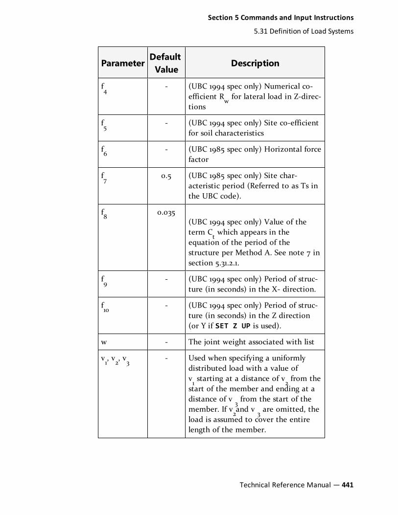
ParameterDefaultValue
Description
f4
- (UBC 1994 spec only) Numerical co-efficient R
wfor lateral load in Z-direc-
tions
f5
- (UBC 1994 spec only) Site co-efficientfor soil characteristics
f6
- (UBC 1985 spec only) Horizontal forcefactor
f7
0.5 (UBC 1985 spec only) Site char-acteristic period (Referred to as Ts inthe UBC code).
f8
0.035(UBC 1994 spec only) Value of theterm C
twhich appears in the
equation of the period of thestructure per Method A. See note 7 insection 5.31.2.1.
f9
- (UBC 1994 spec only) Period of struc-ture (in seconds) in the X- direction.
f10
- (UBC 1994 spec only) Period of struc-ture (in seconds) in the Z direction(or Y if SET Z UP is used).
w - The joint weight associated with list
v1, v2, v3
- Used when specifying a uniformlydistributed load with a value ofv1 starting at a distance of v
2 from the
start of the member and ending at adistance of v
3 from the start of the
member. If v2and v
3 are omitted, the
load is assumed to cover the entirelength of the member.
Section 5 Commands and Input Instructions
5.31 Definition of Load Systems
Technical Reference Manual — 441

ParameterDefaultValue
Description
v4, v5
- Used when specifying a concentratedforce with a value of v
4applied at a
distance of v5from the start of the
member. If v5is omitted, the load is
assumed to act at the center of themember.
p1
- The weight per unit area for theplates selected. Assumed to beuniform over the entire plate.
Element Weight is used if plateelements are part of the model, anduniform pressures on the plates are tobe considered in weight calculation.
Ri1
- Identification number of a previouslydefined reference load case.
See "Defining Reference Load Types"on page 531
f11
1.0 Magnification factor (required for ref-erence loads).
Floor Weight is used if the pressure is on a region bounded by beams, but theentity which constitutes the region, such as a slab, is not defined as part of thestructural model. It is used in the same sort of situation in which you would useFLOOR LOADS (See "Floor Load Specification" on page 562 for details). Similarly,you can use the Oneway Weight command to specify a load path direction forthe pressure on a region.
Notes
a. If the option ACCIDENTAL is used, the accidental torsion will be calculatedper UBC specifications. The value of the accidental torsion is based on thecenter of mass for each level. The center of mass is calculated from theSELFWEIGHT, JOINT WEIGHT, MEMBER WEIGHT, ELEMENT WEIGHT, FLOORWEIGHT, and ONEWAY WEIGHT commands you have specified.
442— STAAD.Pro V8i (SELECTseries 4)
Section 5 Commands and Input Instructions
5.31 Definition of Load Systems

b. In ubc-spec for 1985 code, specification of TS is optional. If TS is specified,resonance co-efficient S is determined from the building period T and userprovided TS using UBC equations. If TS is not specified, the default value of0.5 is assumed.
c. By providing either PX or PZ or both, you may override the periodcalculated by STAAD for Method B of the UBC Code. The user definedvalue will then be used instead of the one recommended by UBC perequation 28.5 of UBC 94. If you do not define PX or PZ, the period forMethod B will be calculated by the program per equation 28.5.
d. Some of the items in the output for the UBC analysis are explained below.
CALC / USED PERIOD
The CALC PERIOD is the period calculated using the Rayleigh method(Method B as per UBC code). For UBC in the x-direction, the USEDPERIOD is PX. For the UBC in the z-direction, the USED PERIOD is PZ. IfPX and PZ are not provided, then the used period is the same as thecalculated period for that direction. The used period is the one substitutedinto the critical equation of the UBC code to calculate the value of C.
e. In the analysis for UBC loads, all the supports of the structure have to be atthe same level and have to be at the lowest elevation level of the structure.
Example
DEFINE UBC LOAD
ZONE 0.2 I 1.0 RWX 9 RWZ 9 S 1.5 CT 0.032
SELFWEIGHT
JOINT WEIGHT
17 TO 48 WEIGHT 2.5
49 TO 64 WEIGHT 1.25
LOAD 1
UBC LOAD X 0.75
SELFWEIGHT Y -1.0
JOINT LOADS
17 TO 48 FY -2.5
FLOOR WEIGHT
Section 5 Commands and Input Instructions
5.31 Definition of Load Systems
Technical Reference Manual — 443

_SLAB1 FLOAD 0.045
ONEWAY LOAD
_ROOF ONE 0.035 GY
5.31.2.3 Colombian Seismic Load
The purpose of this command is to define and generate static equivalent seismicloads as per Colombian specifications using a static equivalent approach similarto those outlined by UBC. Depending on this definition, equivalent lateral loadswill be generated in horizontal direction(s).
The seismic load generator can be used to generate lateral loads in the X & Zdirections for Y up or X & Y for Z up. Y up or Z up is the vertical axis and thedirection of gravity loads (See the SET Z UP command in Section 5.5). Allvertical coordinates of the floors above the base must be positive and the verticalaxis must be perpendicular to the floors.
Methodology
Seismic zone coefficient and parameter values are supplied by the user throughthe DEFINE COLOMBIAN LOAD command.
Program calculates the natural period of building T utilizing clause 1628.2.2 ofUBC 1994.
Design spectral coefficient, Sa, is calculated utilizing T as:
S
A I T T
A I T
A S T
A I T
=
(1.0 + 5.0 ) 0 ≤ ≤ 0.3 sec
2.5 0.3 < ≤ 0.48 sec
1.2 0.48 < < 2.4 sec
/ 2 2.4 sec <
a
a
a
a
I
T
a
when
when
when
when
Where:
Aa= Seismic Risk factor
S = Soil Site Coefficient
I = Coefficient of Importance
Base Shear, Vs is calculated as
Vs = W * Sa
444— STAAD.Pro V8i (SELECTseries 4)
Section 5 Commands and Input Instructions
5.31 Definition of Load Systems

W = Total weight on the structure
The total lateral seismic load, Vs, is then distributed by the program among
different levels as:
Fx = Cvx * VsWhere:
C =vx
W h K
W h K( )∑
x x
i
nx x=1
Wx= Weight at the particular level
hx= Height of that particular level
K
T
T T
T
=
1.0 ≤ 0.5 sec
0.75 + 0.5 0.5 < ≤ 2.5 sec
2.0 2.5 sec <
when
when
when
General Format
DEFINE COLUMBIAN (ACCIDENTAL) LOAD
ZONE f1 col-spec
SELFWEIGHT
JOINT WEIGHT
joint-list WEIGHT w
…
Note: See "UBC 1994 or 1985 Load Definition" on page 438 for completeweight input definition.
Where:
col-spec = ( I f2 S f3)
f1= Seismic Risk factor
f2= Soil Site Coefficient
f3= Coefficient of Importance
General format to provide Colombian Seismic load in any load case:
LOAD i
COLMBIAN LOAD {X | Y | Z} (f4) (ACC f5)
Section 5 Commands and Input Instructions
5.31 Definition of Load Systems
Technical Reference Manual — 445

Where:
i = load case number
f4 = factor to multiply horizontal seismic load
f5 = multiplying factor for Accidental Torsion, to be used to multiplythe accidental torsion load (default = 1.0). May be negative (otherwise,the default sign for MY is used based on the direction of thegenerated lateral forces).
If the ACCIDENTAL option is specified, the accidental torsion will be calculatedper the specifications. The value of the accidental torsion is based on the "centerof mass" for each level. The "center of mass" is calculated from the SELFWEIGHT,JOINT WEIGHTs and MEMBER WEIGHTs you have specified.
Example
DEFINE COLOMBIAN LOAD
ZONE 0.38 1.0 S 1.5
JOINT WEIGHT
51 56 93 100 WEIGHT 1440
101 106 143 150 WEIGHT 1000
151 156 193 200 WEIGHT 720
LOAD 1 ( SEISMIC LOAD IN X DIRECTION )
COLOMBIAN LOAD X
5.31.2.4 Japanese Seismic Load
The purpose of this command is to define and generate static equivalent seismicloads as per Japanese specifications using a static equivalent approach similar tothose outlined by UBC. Depending on this definition, equivalent lateral loads willbe generated in horizontal direction(s). The implementation is as per Article 88in the ‘Building Codes Enforcement Ordinance 2006’.
The seismic load generator can be used to generate lateral loads in the X & Zdirections for Y up or X & Y for Z up. Y up or Z up is the vertical axis and thedirection of gravity loads (See the SET Z UP command in Section 5.5). Allvertical coordinates of the floors above the base must be positive and the verticalaxis must be perpendicular to the floors.
446— STAAD.Pro V8i (SELECTseries 4)
Section 5 Commands and Input Instructions
5.31 Definition of Load Systems

Methodology
Seismic zone coefficient and parameter values are supplied by the user throughthe DEFINE AIJ LOAD command.
Program calculates the natural period of building Tutilizing the followingequation:
T = h(0.02 + 0.01α)
Where:
h = height of building (m)
α = Alpha, ratio of steel height for overall height
Design spectral coefficient, Rt, is calculated utilizing T and Tc as follows:
R
T T
T T T T T
T T T T
=
1.0 <
1 − 0.2( / − 1) ≤ ≤ 2
1.6 / 2 <
t
c
c c c
c c
2
when
when
when
Tc = Period defined by ground support specification for Rt.
αiis calculated from the weight values provided in the Define AIJ
Load command.
αi = Wi / W
Where:
Wi= sum of weight from a top to floor i.
W = all weight
The seismic coefficient of floor, Ci, is calculated using:
Ci = Z Rt Ai CoWhere:
Z = zone factor
Co= normal coefficient of shear force
A = 1 +i
T a a
T
( )2 1 / −
1 + 3
i i
Seismic load shear force, Qi, of each floor is calculated by C
iand W
i:
Qi = CiWiWhere:
Section 5 Commands and Input Instructions
5.31 Definition of Load Systems
Technical Reference Manual — 447
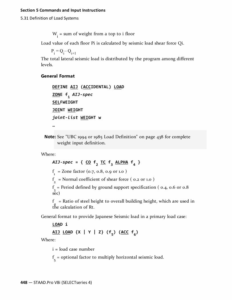
Wi= sum of weight from a top to i floor
Load value of each floor Pi is calculated by seismic load shear force Qi.
Pi = Qi– Qi+1The total lateral seismic load is distributed by the program among differentlevels.
General Format
DEFINE AIJ (ACCIDENTAL) LOAD
ZONE f1 AIJ-spec
SELFWEIGHT
JOINT WEIGHT
joint-list WEIGHT w
…
Note: See "UBC 1994 or 1985 Load Definition" on page 438 for completeweight input definition.
Where:
AIJ-spec = { CO f2 TC f3 ALPHA f4 }
f1= Zone factor (0.7, 0.8, 0.9 or 1.0 )
f2= Normal coefficient of shear force ( 0.2 or 1.0 )
f3 = Period defined by ground support specification ( 0.4, 0.6 or 0.8
sec)
f4= Ratio of steel height to overall building height, which are used in
the calculation of Rt.
General format to provide Japanese Seismic load in a primary load case:
LOAD i
AIJ LOAD {X | Y | Z} (f5) (ACC f6)
Where:
i = load case number
f5= optional factor to multiply horizontal seismic load.
448— STAAD.Pro V8i (SELECTseries 4)
Section 5 Commands and Input Instructions
5.31 Definition of Load Systems

f6= multiplying factor for Accidental Torsion, to be used to multiply
the AIJ accidental torsion load (default = 1.0). May be negative(otherwise, the default sign for MY is used based on the direction ofthe generated lateral forces).
Choose horizontal directions only.
If the ACCIDENTAL option is specified, the accidental torsion will be calculatedper the AIJ specifications. The value of the accidental torsion is based on the"center of mass" for each level. The "center of mass" is calculated from theSELFWEIGHT, JOINT WEIGHTs and MEMBER WEIGHTs you have specified
Example
DEFINE AIJ LOAD
ZONE 0.8 CO 0.2 TC 0.6 ALPHA 1.0
JOINT WEIGHT
51 56 93 100 WEIGHT 1440
101 106 143 150 WEIGHT 1000
151 156 193 200 WEIGHT 720
LOAD 1 ( SEISMIC LOAD IN X)
AIJ LOAD X
5.31.2.5 Indian IS:1893 (Part 1) 2002 Code - Lateral Seismic Load
This feature enables one to generate seismic loads per the IS:1893 specificationsusing a static equivalent approach.
The seismic load generator can be used to generate lateral loads in the X and Zdirections only. Y is the direction of gravity loads. This facility has not beendeveloped for cases where the Z axis is set to be the vertical direction (See theSET Z UP command in Section 5.5).
Methodology
The design base shear is computed by STAAD in accordance with the IS: 1893(Part 1)-2002 equation 7.5.3.
V = Ah.W
Where:
Section 5 Commands and Input Instructions
5.31 Definition of Load Systems
Technical Reference Manual — 449

Ah = Z/2⋅I/R⋅Sa/g
Note: All symbols and notations in the above equation are as per IS: 1893(Part1)-2002.
STAAD utilizes the following procedure to generate the lateral seismic loads:
1. You provide seismic zone coefficient and desired "1893(Part 1)-2002 specs"through the DEFINE 1893 LOAD command.
2. Program calculates the structure period (T).
3. Program calculates Sa/g utilizing T.
4. Program calculates V from the above equation. W is obtained from masstable data entered via SELFWEIGHT, JOINT WEIGHT(s), MEMBER WEIGHT(S),and/or REFERENCE LOAD you provide through the DEFINE 1893 LOADcommand.
5. The total lateral seismic load (base shear) is then distributed by theprogram among different levels of the structure per the IS: 1893 procedures.
See "Generation of Loads" on page 651 for additional information.
General Format
DEFINE 1893 (ACCIDENTAL) LOAD
ZONE f1 1893-spec
SELFWEIGHT
JOINT WEIGHT
joint-list WEIGHT w
MEMBER WEIGHT
mem-list { UNI v1 v2 v3 | CON v4 v5 }
REFERENCE LOAD { X | Y | Z }
Ri1 f11(CHECK SOFT STORY)
Where:
1893-spec = RF f2 I f3 SS f4 (ST f5) DM f6 (PX f7) (PZ f8)( { DT f9 | GL f10 } )
450— STAAD.Pro V8i (SELECTseries 4)
Section 5 Commands and Input Instructions
5.31 Definition of Load Systems

Note: If both mass table data (SELFWEIGHT, JOINT WEIGHT, and MEMBERWEIGHT options) and a REFERENCE LOAD are specified, these will beadded algebraically for a combined mass.
Where:
f1= Seismic zone coefficient. Refer to Table 2 of IS:1893 (Part 1)-2002.
f2= Response reduction factor. Refer Table 7 of IS: 1893 (Part 1) -2002.
f3= Importance factor depending upon the functional use of the
structures, characterized by hazardous consequences of its failure,post-earthquake functional needs, historical value, or economicimportance. Refer Table 6 of IS: 1893(Part 1)-2002.
f4= Rock or soil sites factor (=1 for hard soil, 2 for medium soil, 3 for
soft soil). Depending on type of soil, average response accelerationcoefficient S
a/g is calculated corresponding to 5% damping. Refer
Clause 6.4.5 of IS: 1893 (Part 1) -2002.
f5= Optional value for type of structure (= 1 for RC frame building, 2
for Steel frame building, 3 for all other buildings). If this parameter ismentioned the program will calculate natural period as per Clause 7.6of IS:1893(Part 1)-2002.
f6= Damping ratio to obtain multiplying factor for calculating Sa/g
for different damping. If no damping is specified 5% damping (defaultvalue 0.05) will be considered corresponding to which multiplyingfactor is 1.0. Refer Table 3 of IS:1893(Part 1)-2002.
f7= Optional period of structure (in sec) in X direction. If this is
defined this value will be used to calculate Sa/g for generation of
seismic load along X direction.
f8
= Optional period of structure (in sec) in Z direction. If this isdefined this value will be used to calculate Sa/g for generation ofseismic load along Z direction.
f9= Depth of foundation below ground level. It should be defined in
current unit. If the depth of foundation is 30 m or more, the value ofAhis taken as half the value obtained. If the foundation is placed
between the ground level and 30 m depth, this value is linearlyinterpolated between A
hand 0.5A
h.
Section 5 Commands and Input Instructions
5.31 Definition of Load Systems
Technical Reference Manual — 451

f10= Y coordinate of ground level (or global Z coordinate for SET Z
UP). A reduced lateral force is applied to levels below this height, perClause 6.4.4.
f11= Magnification factor (required for reference loads). Default is 1.0.
Ri1= Identification number of a previously defined reference load
case. See "Defining Reference Load Types" on page 531
w = joint weight associated with joint list
v1, v2, v3= Used when specifying a uniformly distributed load with a
value of v1 starting at a distance of v
2 from the start of the member
and ending at a distance of v3 from the start of the member. If v
2and
v3 are omitted, the load is assumed to cover the entire length of the
member.
v4, v5= Used when specifying a concentrated force with a value of v
4applied at a distance of v
5from the start of the member. If v
5is
omitted, the load is assumed to act at the center of the member.
Notes
a. If the ACCIDENTAL option is specified, the accidental torsion will be cal-culated per the IS 1893 specifications. The value of the accidental torsion isbased on the center of mass for each level. The center of mass is calculatedfrom the SELFWEIGHT, JOINT WEIGHT, and MEMBER WEIGHT commandsyou have specified.
b. By default STAAD calculates natural periods of the structure in both X andZ directions respectively which are used in calculation for base shear. If,however, PX and PZ are mentioned the program will consider these valuesfor calculation of average response acceleration coefficient. If instead of PXand PZ values ST is mentioned the program will calculate natural perioddepending upon the empirical expression given in IS: 1893 (Part 1)-2002.
c. Either the DT or GL parameter is to be specified in the input. If bothparameters are specified, the DT value will be ignored
5.31.2.5.1 Soft Story Checking
STAAD will perform this check when the option CHECK SOFT STORY commandis used. If omitted, no soft story check is performed. Soft Story checking is onlyvalid for structures having vertical elements in the form of columns and shear
452— STAAD.Pro V8i (SELECTseries 4)
Section 5 Commands and Input Instructions
5.31 Definition of Load Systems

wall (without opening). At present the program will exclude the effect of anyother forms of lateral force resisting structural elements.
As per the IS1893-2002 code Clause 7.1, to perform well during an earthquake abuilding must have simple and regular configuration, adequate lateral strength,stiffness and ductility. This is because a building with simple regular geometryand uniformly distributed mass and stiffness in plan as well as in elevation, willsuffer much less damage than buildings with irregular configurations.
According to this standard, a building can be considered irregular, if at least oneof the conditions given in Table 4 - Plan Irregularities and Table 5 - VerticalIrregularities, of IS1893-2002 is applicable.
STAAD has implemented the methodology to find vertical stiffness irregularities,as given in Table 5 Sl No. (1) i) a) and Sl No. (1) i) b), in the form of soft storychecking.
Stiffness Irregularities: Soft Story
As per this provision of the code, a soft story is one in which the lateral stiffnessis less than 70 percent of that in the story above or less than 80 percent of theaverage lateral stiffness of the three story above.
Stiffness Irregularities: Extreme Soft Story
As per this provision of the code, a extreme soft story is one in which the lateralstiffness is less than 60 percent of that in the story above or less than 70 percentof the average lateral stiffness of the three story above.
Thus, if any story of a building is found to be soft or extremely soft, the buildingis likely to suffer much damage in an earthquake than a similar type of buildingbut has more regular vertical stiffness.
Note: STAAD identifies column and shear wall (without opening) as verticalcomponent for the purpose of computing lateral stiffness of the story.The vertical stiffness of a column is calculated as 12EI / L3 where E is theYoung’s modulus, I is the moment of inertia and L is the length of thecolumn respectively and that for a shear wall (without opening) iscalculated as Ph3/3EI + 1.2Ph/AG (i.e., summation of flexural stiffnessand shear stiffness, obtained as deflection of a cantilever wall under asingle lateral load P at its top) where h is the height, A is the cross-sectional area and G is the shear modulus of the wall (E and I carryusual meaning). The summation of lateral stiffness of all columns and
Section 5 Commands and Input Instructions
5.31 Definition of Load Systems
Technical Reference Manual — 453
shear walls at a particular floor level constitute the total lateral stiffnessof that particular story or floor level. The program checks soft story of abuilding along both global X and Z directions respectively. Thiscomputation is valid only for those structures whose floors are treatedas rigid diaphragm.
5.31.2.5.2 Identification of Floor Level
The following two ways can identify floor level:
l Program calculated
l User defined
For regular building which has well defined floors (i.e., does not contain shearwall, staggered flooring, etc), STAAD can identify floor level on its own. However,if floor level is not so well defined, it is better to define floor height to have moreaccurate result for the purpose of torsion and soft story checking.
Program calculated
In general, STAAD identifies floor levels in order of increasing magnitude of Y-coordinates of joints. The program sorts different values of Y-coordinates, fromminimum to maximum values, in ascending order and consider each Y-coordinate value as each floor level. This is the method used by the DEFINE UBCor similar load generation features.
This feature has been enhanced to identify the beam-column junctions at eachfloor level, as identified by the method above. If no beam-column junctions areidentified at that level, a floor level will not be considered at that level in thestructure. Where beam-column junctions are found, the program identifies twobeams, at the same level which span in two different directions from the samebeam-column junction. If this true, this identified floor level will be consideredas truly existing floor level in the structure.
The enhanced feature for finding floor level is being used by lateral loadgeneration feature for response spectrum analysis and soft story checking as perIS1893-2002 code. For response spectrum analysis, story drift and soft storychecking is performed only when floor heights are specified.
454— STAAD.Pro V8i (SELECTseries 4)
Section 5 Commands and Input Instructions
5.31 Definition of Load Systems

User defined
Floor heights should be defined before using the DEFINE command for anyprimary response spectrum load case. The following general format is used for auser-defined floor height:
FLOOR HEIGHT
h1; h2; h3; …;hi -
hi+1; …;hn(BASE hb)
Where:
h1… h
n= the different floor heights in current length unit and n is the
number of floor levels.
hb= the base level with respect to which 1st story height will be
calculated. If hbis not defined, the minimum Y-coordinate value
present in the model will be taken as base level.
User defined floor heights are used by lateral load generation for responsespectrum analysis and soft story checking as per IS1893-2002 code.
See "Generation of Seismic Loads" on page 653 for an example of the correctusage of this command.
5.31.2.6 IBC 2000/2003 Load Definition
The specifications of the IBC 2000, and 2003 codes for seismic analysis of abuilding using a static equivalent approach have been implemented as describedin this section. Depending on this definition, equivalent lateral loads will begenerated in horizontal direction(s).
The seismic load generator can be used to generate lateral loads in the X & Zdirections for Y up or X & Y for Z up. Y up or Z up is the vertical axis and thedirection of gravity loads (See the SET Z UP command in Section 5.5). Allvertical coordinates of the floors above the base must be positive and the verticalaxis must be perpendicular to the floors.
The implementation details of the respective codes are as follows:
Section 5 Commands and Input Instructions
5.31 Definition of Load Systems
Technical Reference Manual — 455

IBC 2000
On a broad basis, the rules described in section 1617.4 of the IBC 2000 codedocument have been implemented. These are described in pages 359 thru 362 ofthat document. The specific section numbers, those which are implemented, andthose which are not implemented, are as follows:
Implemented sec-tions of IBC 2000
Omitted sectionsof IBC 2000
1617.4.1
1617.4.1.1
1617.4.2
1617.4.2.1
1617.4.3
1617.4.4
1617.4.4.4
1617.4.4.1
1617.4.4.2
1617.4.4.3
1617.4.4.5
1617.4.5
1617.4.6
Table 5-9: Sections of IBC 2000 implementedand omitted in the program
IBC 2003
On a broad basis, the rules described in section 1617.4 of the IBC 2003 codedocument have been implemented. This section directs the engineer to Section9.5.5 of the ASCE 7 code. The specific section numbers of ASCE 7-2002, thosewhich are implemented, and those which are not implemented, are shown in thetable below. The associated pages of the ASCE 7-2002 code are 146 thru 149.
456— STAAD.Pro V8i (SELECTseries 4)
Section 5 Commands and Input Instructions
5.31 Definition of Load Systems
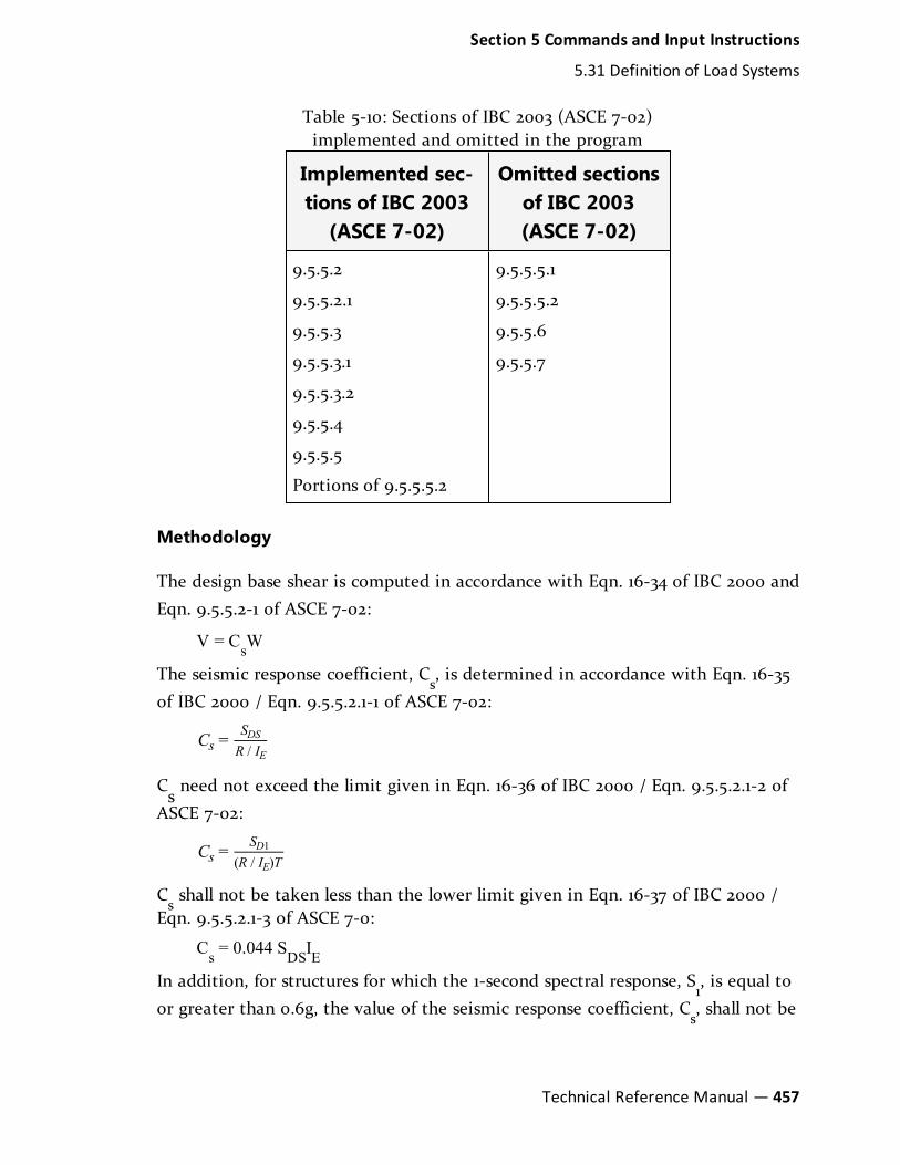
Implemented sec-tions of IBC 2003(ASCE 7-02)
Omitted sectionsof IBC 2003(ASCE 7-02)
9.5.5.2
9.5.5.2.1
9.5.5.3
9.5.5.3.1
9.5.5.3.2
9.5.5.4
9.5.5.5
Portions of 9.5.5.5.2
9.5.5.5.1
9.5.5.5.2
9.5.5.6
9.5.5.7
Table 5-10: Sections of IBC 2003 (ASCE 7-02)implemented and omitted in the program
Methodology
The design base shear is computed in accordance with Eqn. 16-34 of IBC 2000 andEqn. 9.5.5.2-1 of ASCE 7-02:
V = CsW
The seismic response coefficient, Cs, is determined in accordance with Eqn. 16-35
of IBC 2000 / Eqn. 9.5.5.2.1-1 of ASCE 7-02:
C =sS
R I/
DS
E
Cs need not exceed the limit given in Eqn. 16-36 of IBC 2000 / Eqn. 9.5.5.2.1-2 ofASCE 7-02:
C =sS
R I T( / )
D
E
1
Csshall not be taken less than the lower limit given in Eqn. 16-37 of IBC 2000 /
Eqn. 9.5.5.2.1-3 of ASCE 7-0:
Cs = 0.044 SDSIEIn addition, for structures for which the 1-second spectral response, S
1, is equal to
or greater than 0.6g, the value of the seismic response coefficient, Cs, shall not be
Section 5 Commands and Input Instructions
5.31 Definition of Load Systems
Technical Reference Manual — 457

taken less than the limit given in Eqn. 16-38 of IBC 2000 / Eqn. 9.5.5.2.1-4 ofASCE 7-02:
C =sS
R I
0.5
/ E
1
For an explanation of the terms used in the above equations, please refer to therelevant IBC and ASCE 7-02 codes.
Procedure Used by the Program
Steps used to calculate and distribute the base shear are as follows:
1. The Time Period of the structure is calculated based on section 1617.4.2 ofIBC 2000, and section 9.5.5.3 of ASCE 7-02 (IBC 2003) This is reported inthe output as T
a.
2. The period is also calculated in accordance with the Rayleigh method. Thisis reported in the output as T.
3. you may override the Rayleigh based period by specifying a value for PX orPZ (Items f7 and f8) depending on the direction of the IBC load.
4. The governing Time Period of the structure is then chosen between theabove two periods, and the additional guidance provided in clause 1617.4.2of IBC 2000, section 9.5.5.3 of ASCE 7-02 (IBC 2003) or section 12.8.2.1 ofASCE 7-05 (IBC 2006). The resulting value is reported as "Time Periodused".
5. The Design Base Shear is calculated based on equation 16-34 of IBC 2000,equation 9.5.5.2-1 of ASCE 7-02 (IBC 2003) or equation 12.8-1 of ASCE 7-05(IBC 2006). It is then distributed at each floor using the rules of clause1617.4.3, equations 16-41 and 16-42 of IBC 2000. For IBC 2003, using clause9.5.5.4, equations 9.5.5.4-1 & 9.5.5.4-2 of ASCE 7-02.
6. If the ACCIDENTAL option is specified, the program calculates theadditional torsional moment. The lever arm for calculating the torsionalmoment is obtained as 5% of the building dimension at each floor levelperpendicular to the direction of the IBC load (clause 1617.4.4.4 of IBC 2000,and section 9.5.5.5.2 of ASCE 7-02 for IBC 2003 ). At each joint where aweight is located, the lateral seismic force acting at that joint is multipliedby this lever arm to obtain the torsional moment at that joint.
458— STAAD.Pro V8i (SELECTseries 4)
Section 5 Commands and Input Instructions
5.31 Definition of Load Systems

General Format
There are 2 stages of command specification for generating lateral loads. This isthe first stage and is activated through the DEFINE IBC 2000 or 2003 LOADcommand.
DEFINE IBC ( { 2000 | 2003 } ) (ACCIDENTAL) LOAD
SDS f1 ibc-spec
SELFWEIGHT
JOINT WEIGHT
joint-list WEIGHT w
…
Note: See "UBC 1994 or 1985 Load Definition" on page 438 for completeweight input definition.
Where:
ibc-spec = { SD1 f2 S1 f3 IE f4 RX f5 RZ f6 SCLASS f7 (CTf8) (PX f9) (PZ f10) }
f1 = Design spectral response acceleration at short periods. Seeequation 16-18, Section 1615.1.3 of IBC 2000 and equation 9.4.1.2.5-1 ofASCE7-02
f2 = Design spectral response acceleration at 1-second period. Seeequation 16-19, Section 1615.1.3. of IBC 2000 and equation 9.4.1.2.5-2 ofASCE7-02
f3 = Mapped spectral acceleration for a 1-second period. See equation16-17 of IBC 2000, and 9.4.1.2.4-2 of ASCE 7-02
f4 = Occupancy importance factor determined in accordance withSection 1616.2 of IBC 2000 and 2003, and section 9.1.4 (page 96) ofASCE 7-02
f5 = The response modification factor for lateral load along the Xdirection. See Table 1617.6 of IBC 2000 (pages 365-368) and Table1617.6.2 of IBC 2003 (page 334-337). It is used in equations 16-35, 16-36& 16-38 of IBC 2000
f6 = The response modification factor for lateral load along the Zdirection. See Table 1617.6 of IBC 2000 (pages 365-368) and Table
Section 5 Commands and Input Instructions
5.31 Definition of Load Systems
Technical Reference Manual — 459

1617.6.2 of IBC 2003 (page 334-337). It is used in equations 16-35, 16-36& 16-38 of IBC 2000.
f7 = Site class as defined in Section 1615.1.1 of IBC 2000 (page 350) &2003 (page 322). Enter 1 through 6 in place of A through F, see tablebelow).
f8 = Optional CT value to calculate time period. See section 1617.4.2.1,equation 16-39 of IBC 2000 and section 9.5.5.3.2, equation 9.5.5.3.2-1of ASCE 7-02.
If the value of Ct is not specified, the program scans the Modulus of Elasticity (E)values of all members and plates to determine if the structure is made of steel,concrete or any other material. If the average E is smaller than 2000 ksi, Ct is setto 0.016(0.044) [0.016 is the value in FPS units, 0.044 is the value in Metric units].If the average E is between 2000 & 10000 ksi, Ct is set to 0.02(0.055). If theaverage E is greater than 10000 ksi, Ct is set to 0.028(0.068). If the buildingmaterial cannot be determined, Ct is set to 0.02(0.055).
In Table 9.5.5.3.2 on page 147 of ASCE 7-02, a structure type called "Eccentricallybraced steel frames" is listed, with a Ct of 0.03(0.07). STAAD does not choose thisCt on its own presently. If one wishes to use this value, Ct should be specified asan input accordingly.
f9 = Optional Period of structure (in sec) in X-direction to be used asfundamental period of the structure instead of the value derived fromsection 1617.4.2 of IBC 2000, and section 9.5.5.3 of ASCE 7-02.
f10 = Optional Period of structure (in sec) in Z or Y direction to beused as fundamental period of the structure instead of the valuederived from section 1617.4.2 of IBC 2000, and section 9.5.5.3 of ASCE7-02.
The Soil Profile Type parameter SCLASS can take on values from 1 to 6. These arerelated to the values shown in Table 1615.1.1, Site Class Definitions of the IBC2000/2003 code in the following manner :
460— STAAD.Pro V8i (SELECTseries 4)
Section 5 Commands and Input Instructions
5.31 Definition of Load Systems

STAAD ValueIBCValu-e
1 A
2 B
3 C
4 D
5 E
6 F
Table 5-11: Values of IBC soilclass (SCLASS) used in STAAD
Example 1
DEFINE IBC 2003 LOAD
SDS 0.6 SD1 0.36 S1 0.31 I 1.0 RX 3 RZ 4 SCL 4 CT 0.032
SELFWEIGHT
JOINT WEIGHT
51 56 93 100 WEIGHT 1440
101 106 143 150 WEIGHT 1000
151 156 193 200 WEIGHT 720
Example 2
The following example shows the commands required to enable the program togenerate the lateral loads. Users may refer to Section 5.32.12 of the TechnicalReference Manual for this information.
LOAD 1 ( SEISMIC LOAD IN X DIRECTION )
IBC LOAD X 0.75
Section 5 Commands and Input Instructions
5.31 Definition of Load Systems
Technical Reference Manual — 461

LOAD 2 ( SEISMIC LOAD IN Z DIRECTION )
IBC LOAD Z 0.75
The Examples manual contains examples illustrating load generation involvingIBC and UBC load types.
5.31.2.7 CFE (Comisión Federal De Electricidad) Seismic Load
The purpose of this command is to define and generate static equivalent seismicloads as per MANUAL DE DISEÑO POR SISMO - SEISMIC DESIGN HANDBOOKCOMISIÓN FEDERAL DE ELECTRICIDAD - ELECTRIC POWER FEDERALCOMMISSION - October 1993 (Chapters 3.1, 3.2, 3.3 and 3.4) specifications.Depending on this definition, equivalent lateral loads will be generated inhorizontal direction(s). This is a code used in the country of Mexico.
The seismic load generator can be used to generate lateral loads in the X & Zdirections for Y up or X & Y for Z up. Y up or Z up is the vertical axis and thedirection of gravity loads (See the SET Z UP command in Section 5.5). Allvertical coordinates of the floors above the base must be positive and the verticalaxis must be perpendicular to the floors.
Methodology
Seismic zone coefficient and parameter values are supplied by the user throughthe DEFINE CFE LOAD command.
Program calculates the natural period of building T utilizing Rayleigh-Quotientmethod. If time period is provided in the input file, that is used in stead ofcalculated period.
The acceleration a is calculated according to the following:
a
a c a T T
c T T T
c T T T T
=
+ − <
≤ ≤
( / ) <
T
Ta
a b
br
b
0 0a
when
when
when
Where:
c = Seismic coefficient is extracted from table 3.1
a0, T
a, T
b, and r are obtained form table 3.1
The ductility reduction factor Q’ is calculated according to section 3.2.5.
462— STAAD.Pro V8i (SELECTseries 4)
Section 5 Commands and Input Instructions
5.31 Definition of Load Systems

Q
Q T T
Q T T′ =
≥
1 + − 1 <
a
T
T aa
when
when
If not regular, then Q’ = Q’ x 0.8
If the period Tsof the soil is known and the soil type II or III T
aand T
bwill be
modified according to section 3.3.2.
Lateral loads for each direction are calculated for:
When T ≤ Tb, Eq. 4.5. Section 3.4.4.2 is used:
P W h=n n n
W a
W h Q
Σ
Σ ′
n
N
n
n
N
n n
=1
=1
When T > Tb, Eq. 4.6/7/8. Section 3.4.4.2 is used:
P W a Q K h K h( )( )= / +n n i i1 22
Where:
K =q r q W
W h1[1 − (1 − )]Σ
Σ( / )
i
i i
K =rq q W
W h( )21.5 (1 − )Σ
Σ /
i
i i2
q = (Tb /T)r
The base shear are distributed proportionally to the height if T ≤ Tb
or with thequadratic equation mentioned if T > T
b.
The distributed base shears are subsequently applied as lateral loads on thestructure.
General Format
DEFINE CFE (ACCIDENTAL) LOAD
ZONE f1 cfe-spec
SELFWEIGHT
JOINT WEIGHT
joint-list WEIGHT w
…
Section 5 Commands and Input Instructions
5.31 Definition of Load Systems
Technical Reference Manual — 463

Note: See "UBC 1994 or 1985 Load Definition" on page 438 for completeweight input definition.
Where:
cfe-spec = { QX f2 QZ f3 GROUP f4 STYP f5 (REGULAR) (TS f6)(PX f7) (PZ f8) }
f1 = Zone number specified in number such as 1, 2, 3 or 4
f2 = seismic behavior factor of the structure along X direction as aparameter according 3.2.4.
f3 = seismic behavior factor of the structure along Z direction as aparameter according 3.2.4.
f4 = Group of structure entered as A or B
f5 = Soil type entered as 1 or 2 or 3
The optional parameter REGULAR is entered to consider the structureas a regular structure. By default, all structures are considered asirregular.
f6 = site characteristic period
f7 = Optional Period of structure (in sec) in X-direction to be used asfundamental period of the structure instead of the value calculated bythe program using Rayleigh-Quotient method
f8 = Optional Period of structure (in sec) in Z direction (or Y if SET ZUP is used) to be used as fundamental period of the structure insteadof the value calculated by the program using Rayleigh-Quotientmethod
To provide a CFE Seismic load in any load case:
LOAD i
CFE LOAD {X | Y | Z} (f)
Where:
i = the load case number
f = factor to multiply horizontal seismic load. Choose horizontaldirections only.
464— STAAD.Pro V8i (SELECTseries 4)
Section 5 Commands and Input Instructions
5.31 Definition of Load Systems

Example
UNIT KGS METER
DEFINE CFE LOAD
ZONE 2 QX .5 QZ 0.9 STYP 2 GROUP B TS 0.2
SELFWEIGHT
MEMBER WEIGHT
1 TO 36 41 TO 50 UNI 300
JOINT WEIGHT
51 56 93 100 WEIGHT 1440
101 106 143 150 WEIGHT 1000
FLOOR WEIGHT
YRA 11.8 12.2 FLOAD 400 -
XRA -1 11 ZRA -1 21
LOAD 1 ( SEISMIC LOAD IN X DIRECTION )
CFE LOAD X 1.0
LOAD 2 ( SEISMIC LOAD IN -Z DIRECTION )
CFE LOAD Z -1.0
5.31.2.8 NTC (Normas Técnicas Complementarias) Seismic Load
The purpose of this command is to define and generate static equivalent seismicloads as per Code of the México Federal District (Reglamento de Construccionesdel Distrito Federal de México) and Complementary Technical Standards forSeismic Design (y Normas Técnicas Complementarias (NTC) para Diseño porSismo -Nov. 1987) (Chapters 8.1 8.2 8.6 and 8.8) specifications. Depending on thisdefinition, equivalent lateral loads will be generated in horizontal direction(s).
The seismic load generator can be used to generate lateral loads in the X & Zdirections for Y up or X & Y for Z up. Y up or Z up is the vertical axis and thedirection of gravity loads (See the SET Z UP command in Section 5.5). Allvertical coordinates of the floors above the base must be positive and the verticalaxis must be perpendicular to the floors.
Section 5 Commands and Input Instructions
5.31 Definition of Load Systems
Technical Reference Manual — 465

Methodology
The design base shear is computed in accordance with Sections 8.1 or 8.2 of the NTC as decided by the user.
A. Base Shear is given as
Vo / Wo = c / Q
Where:
Seismic Coefficient, c, is obtained by the program from thefollowing table
SeismicCoef-ficient,
c
Gro-upA
Gro-upB
I 0.24 0.16
II notshaded 0.48 0.32
III (and IIwhereshaded) 0.60 0.40
Table 5-12: Seismic coef-ficient per NTC
Q: is entered by the user as a parameter.
B. Base shear is given as
Vo / Wo = a / Q’
Where Reduction of Shear Forces are requested
Time Period T of the structure is:calculated by the program based on usingRayleigh quotient technique.
you may override the period that the program calculates by specifyingthese in the input
466— STAAD.Pro V8i (SELECTseries 4)
Section 5 Commands and Input Instructions
5.31 Definition of Load Systems
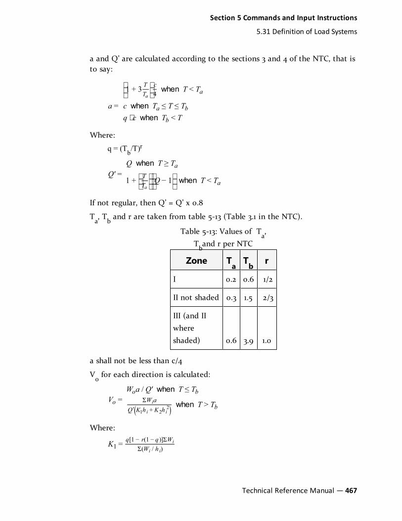
a and Q’ are calculated according to the sections 3 and 4 of the NTC, that isto say:
when
when
when
⋅a
T T
c T T T
q c T T
=
1 + 3 <
≤ ≤
<
T
T
ca
a b
b
4a
Where:
q = (Tb/T)r
when
when
Q
Q T T
Q T T′ =
≥
1 + − 1 <
a
T
T aa
If not regular, then Q’ = Q’ x 0.8
Ta, T
band r are taken from table 5-13 (Table 3.1 in the NTC).
Zone TaTb
r
I 0.2 0.6 1/2
II not shaded 0.3 1.5 2/3
III (and IIwhereshaded) 0.6 3.9 1.0
Table 5-13: Values of Ta,
Tband r per NTC
a shall not be less than c/4
Vofor each direction is calculated:
V
W a Q T T
T T=
/ ′ ≤
>o
o b
W a
Q K h K hb( )
Σ
′ +
i
i i1 22
when
when
Where:
K =q r q W
W h1[1 − (1 − )]Σ
Σ( / )
i
i i
Section 5 Commands and Input Instructions
5.31 Definition of Load Systems
Technical Reference Manual — 467

K =rq q W
W h( )21.5 (1 − )Σ
Σ /
i
i i2
Wiand h
ithe weight and the height of the ith mass over the soil or
embedment level.
The base shear are distributed proportionally to the height if T ≤ Tb
orwith the quadratic equation mentioned if T > T
b. The distributed base
shears are subsequently applied as lateral loads on the structure.
General Format
DEFINE NTC LOAD
ZONE f1 ntc-spec
SELFWEIGHT
JOINT WEIGHT
joint-list WEIGHT w
…
Note: See "UBC 1994 or 1985 Load Definition" on page 438 for completeweight input definition.
Where:
ntc-spec = { QX f2 QZ f3 GROUP f4 (SHADOWED) (REGULAR)(REDUCE) (PX f6) (PZ f7) }
f1 = Zone number specified in number such as 1, 2, 3 or 4
f2 = seismic behavior factor of the structure along X direction as aparameter according 3.2.4.
f3 = seismic behavior factor of the structure along Z direction as aparameter according 3.2.4.
f4 = Group of structure entered as A or B
REGULAR optional parameter is entered to consider the structure as aregular structure. By default, all structures are considered as irregular.
SHADOWED optional parameter is used to define the shaded zone II asthe site of the structure. By default regular zone II is used.
468— STAAD.Pro V8i (SELECTseries 4)
Section 5 Commands and Input Instructions
5.31 Definition of Load Systems

REDUCE optional parameter allows to reduce the seismic factors asdescribed above. Otherwise the following formula is used to calculatebase shear,
V W= ∑c
Q nN
n′ =1
f6 = Optional Period of structure (in sec) in X-direction to be used asfundamental period of the structure instead of the value calculated bythe program using Rayleigh-Quotient method
f7 = Optional Period of structure (in sec) in Z-direction to be used asfundamental period of the structure instead of the value calculated bythe program using Rayleigh-Quotient method
To provide NTC Seismic load in any load case:
LOAD i
NTC LOAD {X/Y/Z} (f)
where i and f are the load case number and factor to multiply horizontal seismicload respectively.
Example
UNIT KGS METER
DEFINE NTC LOAD
ZONE 2 QX .5 QZ 0.9 GROUP B
SELFWEIGHT
ELEMENT WEIGHT
1577 TO 1619 PRESSURE 275
LOAD 1 ( SEISMIC LOAD IN X DIRECTION )
NTC LOAD X 1.0
LOAD 2 ( SEISMIC LOAD IN Z DIRECTION )
NTC LOAD Z 1.0
5.31.2.9 RPA (Algerian) Seismic Load
The purpose of this command is to define and generate static equivalent seismicloads as per RPA specifications using a static equivalent approach similar to those
Section 5 Commands and Input Instructions
5.31 Definition of Load Systems
Technical Reference Manual — 469

outlined by RPA. Depending on this definition, equivalent lateral loads will begenerated in horizontal direction(s).
The seismic load generator can be used to generate lateral loads in the X & Zdirections for Y up or X & Y for Z up. Y up or Z up is the vertical axis and thedirection of gravity loads (See the SET Z UP command in Section 5.5). Allvertical coordinates of the floors above the base must be positive and the verticalaxis must be perpendicular to the floors.
Methodology
The design base shear is computed in accordance with section 4.2.3 of the RPA 99code. The primary equation, namely 4-1, as shown below, is checked.
V = (A D Q)W / R
Where:
W = total weight on the structure
A = zone coefficient
D = average dynamic amplification factor
R = lateral R factor
Q = structural quality factor
Seismic zone coefficient and parameter values are supplied by the user throughthe DEFINE RPA LOAD command.
Program calculates the natural period of building T utilizing clause 4.2.4 of RPA99.
Design spectral coefficient (D) is calculated utilizing T as,
D = 2.5η when 0 ≤ T ≤ T2= 2.5η(T2/T)
2/3 when T2 ≤ T ≤ 0.3 sec.
= 2.5η(T2/3)2/3(3/T)5/3 when T > 0.3 sec.
Where:
η = factor of damping adjustment (Eq. 4.3)
T2= specific period (Table 4.7)
Total lateral seismic load, V is distributed by the program among different levels.
There are 2 stages of command specification for generating lateral loads. This isthe first stage and is activated through the DEFINE RPA LOAD command.
470— STAAD.Pro V8i (SELECTseries 4)
Section 5 Commands and Input Instructions
5.31 Definition of Load Systems

General Format
DEFINE RPA (ACCIDENTAL) LOAD
A f1 rpa-spec
SELFWEIGHT
JOINT WEIGHT
joint-list WEIGHT w
…
Note: See "UBC 1994 or 1985 Load Definition" on page 438 for completeweight input definition.
Where:
rpa-spec = { Q f2 RX f3 FZ f4 STYP f5 CT f6 CRDAMP f7 (PXf8) (PZ f9) }
f1 = Seismic zone coefficient. Instead of using an integer value like 1, 2,3 or 4, use the fractional value like 0.08, 0.15, 0.2, 0.3, 0.05, etc.
f2 = Importance factor
f3 = Coefficient R for lateral load in X direction – table 4.3
f4 = Coefficient R for lateral load in Z direction – table 4.3
f5 = Soil Profile Type
f6 = Coefficient from table 4.6 of RPA 99
f7 = Damping factor
f8 = Optional Period of structure (in sec) in X direction
f9 = Optional Period of structure (in sec) in Z direction (or Y if SET ZUP is used) to be used as fundamental period of the structure insteadof the value calculated by the program using Rayleigh method
General format to provide RPA Seismic load in any load case:
LOAD i
RPA LOAD {X | Y | Z} (f10) (ACC f11)
Where:
i = the load case number
f10 = factor to multiply horizontal seismic load.
Section 5 Commands and Input Instructions
5.31 Definition of Load Systems
Technical Reference Manual — 471

f11 = multiplying factor for Accidental Torsion, to be used to multiplythe RPA accidental torsion load (default = 1.0). May be negative(otherwise, the default sign for MY is used based on the direction ofthe generated lateral forces).
Note: If the ACCIDENTAL option is specified, the accidental torsion will becalculated per the RPA specifications. The value of the accidentaltorsion is based on the "center of mass" for each level. The "center ofmass" is calculated from the SELFWEIGHT, JOINT WEIGHTs andMEMBER WEIGHTs you have specified.
Example
DEFINE RPA LOAD
A 0.15 Q 1.36 STYP 2 RX 3 RZ 4 CT 0.0032 –
CRDAMP 30 PX .027 PZ 0.025
JOINT WEIGHT
51 56 93 100 WEIGHT 1440
101 106 143 150 WEIGHT 1000
151 156 193 200 WEIGHT 720
LOAD 1 ( SEISMIC LOAD IN X DIRECTION )
RPA LOAD X 1.0
5.31.2.10 Canadian Seismic Code (NRC) - 1995
This set of commands may be used to define the parameters for generation ofequivalent static lateral loads for seismic analysis per National Building Code(NRC/CNRC) of Canada- 1995 edition. Depending on this definition, equivalentlateral loads will be generated in horizontal direction(s).
The seismic load generator can be used to generate lateral loads in the X & Zdirections for Y up or X & Y for Z up. Y up or Z up is the vertical axis and thedirection of gravity loads (See the SET Z UP command in Section 5.5). Allvertical coordinates of the floors above the base must be positive and the verticalaxis must be perpendicular to the floors.
472— STAAD.Pro V8i (SELECTseries 4)
Section 5 Commands and Input Instructions
5.31 Definition of Load Systems
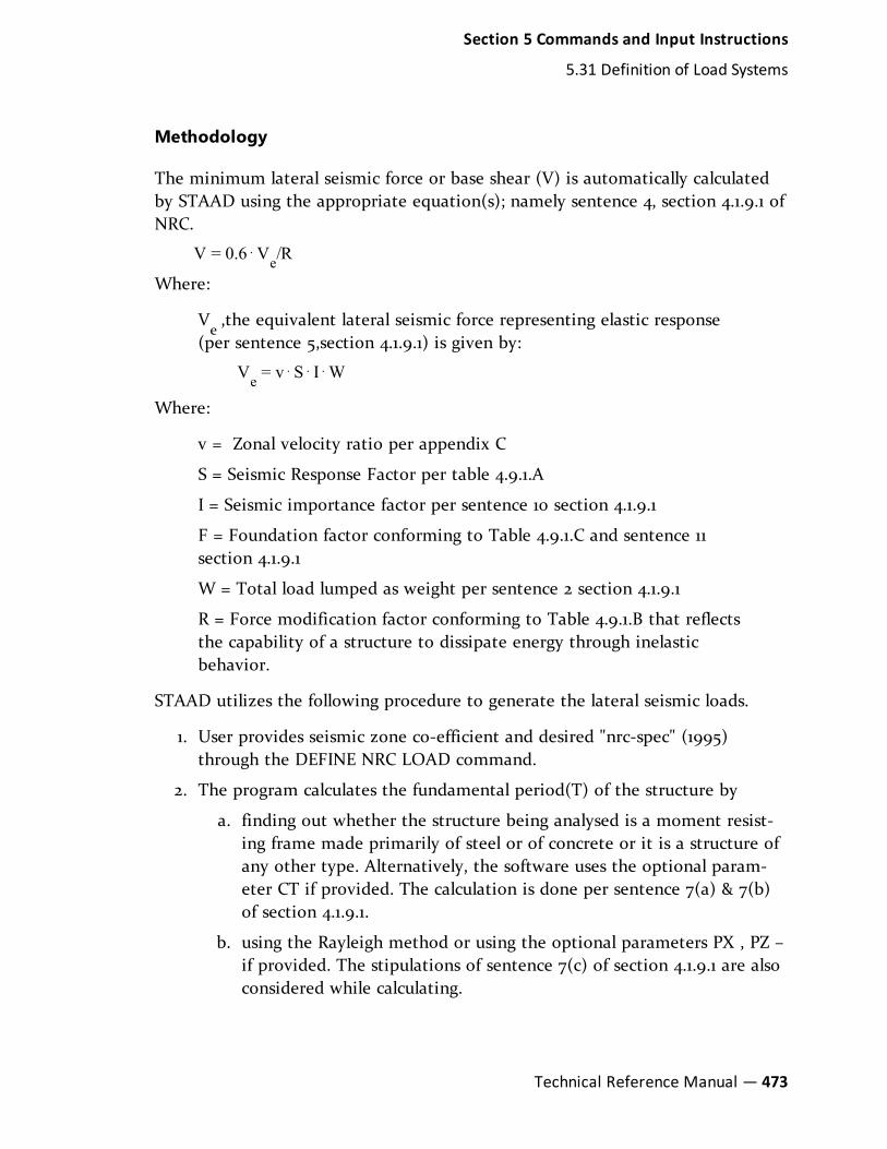
Methodology
The minimum lateral seismic force or base shear (V) is automatically calculatedby STAAD using the appropriate equation(s); namely sentence 4, section 4.1.9.1 ofNRC.
V = 0.6⋅Ve/R
Where:
Ve,the equivalent lateral seismic force representing elastic response
(per sentence 5,section 4.1.9.1) is given by:
Ve = v⋅S⋅I⋅W
Where:
v = Zonal velocity ratio per appendix C
S = Seismic Response Factor per table 4.9.1.A
I = Seismic importance factor per sentence 10 section 4.1.9.1
F = Foundation factor conforming to Table 4.9.1.C and sentence 11section 4.1.9.1
W = Total load lumped as weight per sentence 2 section 4.1.9.1
R = Force modification factor conforming to Table 4.9.1.B that reflectsthe capability of a structure to dissipate energy through inelasticbehavior.
STAAD utilizes the following procedure to generate the lateral seismic loads.
1. User provides seismic zone co-efficient and desired "nrc-spec" (1995)through the DEFINE NRC LOAD command.
2. The program calculates the fundamental period(T) of the structure by
a. finding out whether the structure being analysed is a moment resist-ing frame made primarily of steel or of concrete or it is a structure ofany other type. Alternatively, the software uses the optional param-eter CT if provided. The calculation is done per sentence 7(a) & 7(b)of section 4.1.9.1.
b. using the Rayleigh method or using the optional parameters PX , PZ –if provided. The stipulations of sentence 7(c) of section 4.1.9.1 are alsoconsidered while calculating.
Section 5 Commands and Input Instructions
5.31 Definition of Load Systems
Technical Reference Manual — 473

c. taking the conservative value of T between those calculated by meth-ods (a) and (b) above.
3. The program finds out the value of Seismic Response Factor(S) per table4.9.1.A utilizing the values of T as calculated above and the values of ZA &ZV input by the user.
4. The program calculates V per sentence 4 section 4.1.9.1. W is obtained fromthe weight data (SELFWEIGHT, JOINT WEIGHT(s), etc.) provided by theuser through the DEFINE NRC LOAD command. The weight data must bein the order shown.
5. The total lateral seismic load (base shear) is then distributed by the pro-gram among different levels of the structure per applicable NRC guidelineslike sentence 13(a) section 4.1.9.1.
General Format
There are two stages of command specification for generating lateral loads. Thisis the first stage and is activated through the DEFINE NRC LOAD command.
DEFINE NRC LOAD
nrc-spec
SELFWEIGHT
JOINT WEIGHT
joint-list WEIGHT w
…
Note: See "UBC 1994 or 1985 Load Definition" on page 438 for completeweight input definition.
Where:
nrc-spec = *{ V f1 ZA f2 ZV f3 RX f4 RZ f5 I f6 F f7 (CT f8)(PX f9) (PZ f10) }
f1
= Zonal velocity ratio per Appendix C
f2
= Factor for acceleration related seismic zone per Appendix C
f3
= Factor for velocity related seismic zone per Appendix C
474— STAAD.Pro V8i (SELECTseries 4)
Section 5 Commands and Input Instructions
5.31 Definition of Load Systems

f4
= Force modification factor along X-direction that reflects thecapability of a structure to dissipate energy through inelasticbehavior. Please refer Table 4.1.9.1B
f5
= Force modification factor along Z-direction that reflects thecapability of a structure to dissipate energy through inelasticbehavior. Please refer Table 4.1.9.1B
f6
= Seismic importance factor per sentence 10 section 4.1.9.1
f7
= Foundation factor conforming to Table 4.1.9.1C and sentence11 section 4.1.9.1
f8
= Factor to be used to calculate the fundamental period ofstructure .This is an optional parameter.
f10
= Period of structure (in seconds) in the X- direction. This is anoptional parameter.
f11 = Period of structure (in seconds) in the Z- direction (or Y if SET ZUP is used). This is an optional parameter.
w = joint weight associated with list
v1, v2, v3= Used when specifying a uniformly distributed load with a
value of v1 starting at a distance of v
2 from the start of the member
and ending at a distance of v3 from the start of the member. If v
2and
v3 are omitted, the load is assumed to cover the entire length of the
member.
v4, v5= Used when specifying a concentrated force with a value of v
4applied at a distance of v
5from the start of the member. If v
5is
omitted, the load is assumed to act at the center of the member.
p1= weight per unit area for the plates selected. Assumed to be
uniform over the entire plate.
Element Weight is used if plate elements are part of the model, and uniformpressures on the plates are to be considered in weight calculation.
Floor Weight is used if the pressure is on a region bounded by beams, but theentity which constitutes the region, such as a slab, is not defined as part of thestructural model. It is used in the same sort of situation in which one usesFLOOR LOADS (see Section 5.32.4 of STAAD Technical Reference Manual fordetails of the Floor Load input).
The weights have to be input in the order shown.
Section 5 Commands and Input Instructions
5.31 Definition of Load Systems
Technical Reference Manual — 475

Generation of NRC Load
The load so defined as above is applied on the structure in the NRC loadcases.These loadcases have to be the first loadcases in the input file. Built-in algorithmswill automatically distribute the base shear among appropriate levels and theroof per the relevant code specifications.
The following general format should be used to generate loads in a particulardirection.
LOAD i
NRC LOAD { X | Y | Z } (f1)
Where:
i = load case number
f1= factor to be used to multiply the NRC Load (default = 1.0). May be
negative.
Notes
1. By providing either PX or PZ or both, you may override the period cal-culated by STAAD using Rayleigh method. If you do not define PX or PZ,the period for Method 2(b) above will be calculated by the program usingRayleigh method and the stipulations of sentence 7(c) of section 4.1.9.1
2. Some of the items in the output for the NRC analysis are explained below.
Ta = Time period calculated per sentence 7(a) or 7(b) of section
4.1.9.1
Tc = Time period calculated per sentence 7(c) of section 4.1.9.1
CALC / USED PERIOD
The CALC PERIOD is the period calculated using the Rayleigh method. ForNRC in the x-direction, the USED PERIOD is PX. For the NRC in the z-direction (or Y direction if SET Z UP is used), the USED PERIOD is PZ. IfPX and PZ are not provided, then the used period is the same as thecalculated period for that direction. The used period is the one utilized tofind out the value of S.
3. In the analysis for NRC loads, all the supports of the structure have to be atthe same level and have to be at the lowest elevation level of the structure.
476— STAAD.Pro V8i (SELECTseries 4)
Section 5 Commands and Input Instructions
5.31 Definition of Load Systems

Example
DEFINE NRC LOAD
V 0.2 ZA 4 ZV 4 RX 4 RZ 4 I 1.3 F 1.3 CT 0.35 PX 2 PZ 2
SELFWEIGHT
JOINT WEIGHT
17 TO 48 WEIGHT 7
49 TO 64 WEIGHT 3.5
LOAD 1 EARTHQUAKE ALONG X
NRC LOAD X 1.0
PERFORM ANALYSIS PRINT LOAD DATA
CHANGE
See also Example Problem EXAMP14_NRC.STD
5.31.2.11 Canadian Seismic Code (NRC) – 2005 Volume 1
This set of commands may be used to define the parameters for generation ofequivalent static lateral loads for seismic analysis per National Building Code(NRC/CNRC) of Canada- 2005 Volume 1 edition. Depending on this definition,equivalent lateral loads will be generated in horizontal direction(s).
The seismic load generator can be used to generate lateral loads in the X & Zdirections for Y up or X & Y for Z up. Y up or Z up is the vertical axis and thedirection of gravity loads (See the SET Z UP command in Section 5.5). Allvertical coordinates of the floors above the base must be positive and the verticalaxis must be perpendicular to the floors.
Methodology
The minimum lateral seismic force or base shear (V) is automatically calculatedby STAAD using the appropriate equation (s).
V =S T M I W
R R
( )a v E
d o
as per section 4.1.8.11(2) of NBC of Canada 2005, Volume 1
Except that V shall not be less than:
Section 5 Commands and Input Instructions
5.31 Definition of Load Systems
Technical Reference Manual — 477

V =S M I W
R Rmin
(2.0) v E
d o
and for an Rd= 1.5, V need not be greater than:
V =S I W
R Rmax
2
3
(0.2) E
d o
(i.e., the upper limit of V)
Description of the terms of the equation to calculate V:
l Tais the fundamental lateral period in the direction under consideration
and is determined as:
a. For moment-resisting frames that resist 100% of the required lateralforces and where the frame is not enclosed by or adjoined by morerigid elements that would tend to prevent the frame from resistinglateral forces, and is calculated by the empirical formulae as describedbelow provided hn is in meter
i. 0.085(hn)3/4for steel moment frames,
ii. 0.075(hn)3/4for concrete moment frames, or
b. The period is also calculated in accordance with the Rayleigh methodbut could be overridden by user specified time period (PX, PZ).
If design spectral acceleration, S(Ta),calculated considering structural
time period calculated based on method (b) is greater than 0.8 timethe same calculated considering structural time period calculatedbased on method (a), the former is used for further calculation.Otherwise, the later time period is used.
c. Other established methods of mechanics using a structural model thatcomplies with the requirements of Sentence 4.1.8.3.(8), except that
i. for moment resisting frames, Ta shall not be greater than 1.5times that determined in Clause (a).
ii. for braced frames, Ta shall not be greater than 2.0 times thatdetermined in Clause (b).
iii. for shear wall structures, Ta shall not be greater than 2.0 timesthat determined in Clause (c), and
iv. for the purpose of calculating the deflections, the period withoutthe upper limit specified is referred from Appendix A.
l S(Ta) is the design spectral acceleration and is determined as follows, using
478— STAAD.Pro V8i (SELECTseries 4)
Section 5 Commands and Input Instructions
5.31 Definition of Load Systems

linear interpolation for intermediate values of Ta:
S(Ta) = FaSa(0.2) for Ta ≤ 0.2s
= FvSa(0.5) or F
aSa(0.2), whichever is smaller for T
a= 0.5s
= FvSa(1.0) for T
a= 1.0s
= FvSa(2.0) for T
a= 2.0s
= FvSa(2.0)/2 for T
a≥ 4.0s
The above terms Sa(0.2), S
a(0.5), S
a(1.0) and S
a(2.0) are the Seismic Data
and are obtained as user input from the Table C-2.
Based on the above values of Sa(Ta), F
aand F
v,the acceleration- and
velocity based site coefficients are determined from the Tables 4.1.8.4.B and4.1.8.4.C, using linear interpolation for intermediate values of S
a(0.2) and S
a(1.0). It is to be mentioned that, these are the user inputs based on the siteclasses from A to E and the desired S
a(0.2) and S
a(1.0) values as required as
per the above equations.
l Mvis the factor to account for higher mode effect on base shear and the
associated base overturning moment reduction factor is J which areobtained as user input from the Table 4.1.8.11. To get this higher modefactor (M
v) and numerical reduction coefficient for base overturning
moment (J), user has to get the ratios of Sa(0.2)/S
a(2.0) as also the “Type of
Lateral Resisting System”.
For values of Mv between fundamental lateral periods, Ta of 1.0 and 2.0 s,the product S(Ta). Mv shall be obtained by linear interpolation.
Values of J between fundamental lateral periods, Ta of 0.5 and 2.0 s shall beobtained by linear interpolation.
l IEis the earthquake importance factor of the structure and is determined
from the Table 4.1.8.5. This is an user input depending on Importance Cat-egory and ULS / SLS
l W is the weight of the building and shall be calculated internally using thefollowing formula:
W W= ∑in
i=1
Where Wiis the portion of W that is located at or assigned to level i.
l Rdis the ductility-related force modification factor reflecting the capability
of a structure to dissipate energy through inelastic behavior as described inarticle 4.1.8.9.
Section 5 Commands and Input Instructions
5.31 Definition of Load Systems
Technical Reference Manual — 479

l Rois the over-strength-related force modification factor accounting for the
dependable portion of reserve strength in a structure designed according tothe provision of the Article 4.1.8.9.
These Rdand R
ovalues are the user inputs depending on the type of SFRS
As per 4.1.8.11(6), the total lateral seismic force, V, shall be distributed such that aportion, F
tshall be concentrated at the top of the building, where,
Ft= 0.07T
aV
but Ftis not greater than 0.25V and F
t= 0 when T
ais not greater than 0.7s.
The remainder (V- Ft), shall be distributed along the height of the building,
including the top level, in accordance with the following formula [as per section4.1.8.11(6)]:
F =xV F W h
W h
( − )
∑
t x x
i
ni i=1
Where:
Fxis the lateral force applied to level x.
Ftis the portion of V to be concentrated at the top of the structure.
Wi,Wx are the portion of W that is located at or assigned to level i orx respectively.
hi,hx are the height above the base(i=0) to level i or x respectively.
level i is any level in the building, i=1 for first level above the base.
level n is uppermost in the main portion of the structure.
General Format
STAAD utilizes the following format to generate the lateral seismic loads.
DEFINE NRC2005LOAD
nrc-spec
SELFWEIGHT
JOINT WEIGHT
joint-list WEIGHT w
…
480— STAAD.Pro V8i (SELECTseries 4)
Section 5 Commands and Input Instructions
5.31 Definition of Load Systems
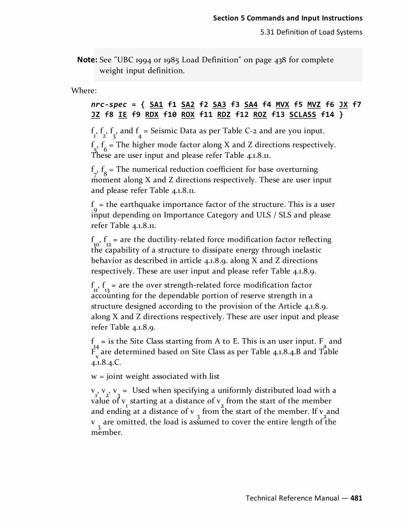
Note: See "UBC 1994 or 1985 Load Definition" on page 438 for completeweight input definition.
Where:
nrc-spec = { SA1 f1 SA2 f2 SA3 f3 SA4 f4 MVX f5 MVZ f6 JX f7JZ f8 IE f9 RDX f10 ROX f11 RDZ f12 ROZ f13 SCLASS f14 }
f1, f2, f3, and f
4= Seismic Data as per Table C-2 and are you input.
f5, f6= The higher mode factor along X and Z directions respectively.
These are user input and please refer Table 4.1.8.11.
f7, f8= The numerical reduction coefficient for base overturning
moment along X and Z directions respectively. These are user inputand please refer Table 4.1.8.11.
f9= the earthquake importance factor of the structure. This is a user
input depending on Importance Category and ULS / SLS and pleaserefer Table 4.1.8.11.
f10, f12= are the ductility-related force modification factor reflecting
the capability of a structure to dissipate energy through inelasticbehavior as described in article 4.1.8.9. along X and Z directionsrespectively. These are user input and please refer Table 4.1.8.9.
f11, f13= are the over strength-related force modification factor
accounting for the dependable portion of reserve strength in astructure designed according to the provision of the Article 4.1.8.9.along X and Z directions respectively. These are user input and pleaserefer Table 4.1.8.9.
f14= is the Site Class starting from A to E. This is an user input. F
aand
Fvare determined based on Site Class as per Table 4.1.8.4.B and Table
4.1.8.4.C.
w = joint weight associated with list
v1, v2, v3= Used when specifying a uniformly distributed load with a
value of v1 starting at a distance of v
2 from the start of the member
and ending at a distance of v3 from the start of the member. If v
2and
v3 are omitted, the load is assumed to cover the entire length of the
member.
Section 5 Commands and Input Instructions
5.31 Definition of Load Systems
Technical Reference Manual — 481

v4, v5= Used when specifying a concentrated force with a value of v
4applied at a distance of v
5from the start of the member. If v
5is
omitted, the load is assumed to act at the center of the member.
p1= weight per unit area for the plates selected. Assumed to be
uniform over the entire plate.
Element Weight is used if plate elements are part of the model, and uniformpressures on the plates are to be considered in weight calculation.
Floor Weight is used if the pressure is on a region bounded by beams, but theentity which constitutes the region, such as a slab, is not defined as part of thestructural model. It is used in the same sort of situation in which one usesFLOOR LOADS (See "Floor Load Specification" on page 562 for details). Theweights have to be input in the order shown.
Example
DEFINE NRC 2005 LOAD
SA1 .33 SA2 .25 SA3 .16 SA4 .091 MVX 1.2 MVZ 1.5 JX .7 JZ.5 IE 1.3 -
RDX 4.0 ROX 1.5 RDZ 3.0 ROZ 1.3 SCLASS 4
SELFWEIGHT
JOINT WEIGHT
17 TO 48 WEIGHT 7
49 TO 64 WEIGHT 3.5
LOAD 1 EARTHQUAKE ALONG X
NRC LOAD X 1.0
PERFORM ANALYSIS PRINT LOAD DATA
CHANGE
See Example Problem EXAMP14_NRC_2005.STD
5.31.2.12 Turkish Seismic Code
This set of commands may be used to define the parameters for generation ofequivalent static lateral loads for seismic analysis per the specifications laid out inSpecification for Structures to be Built in Disaster Areas Part – III – Earthquake
482— STAAD.Pro V8i (SELECTseries 4)
Section 5 Commands and Input Instructions
5.31 Definition of Load Systems

Disaster Prevention Amended on 2.7.1998, Official Gazette No. 23390 (EnglishTranslation). This is referred to as the Turkish Seismic Provisions.
The seismic load generator can be used to generate lateral loads in the X & Zdirections for Y up or X & Y for Z up. Y up or Z up is the vertical axis and thedirection of gravity loads (See the SET Z UP command in Section 5.5). Allvertical coordinates of the floors above the base must be positive and the verticalaxis must be perpendicular to the floors.
Base Shear
The minimum lateral seismic force or base shear, Vt, is automatically calculated
per equation 6.4 in section 6.7.1:
V =tWA T
R T
( )
( )a
1
1
Where:
T1 is the fundamental time period of the structure.
Except that Vt shall not be less than:V A IW= 0.10t ,min 0
Seismic Load Reduction Factor, Ra (T1), in above equation is determined basedon the following equations 6.3a and 6.3b in the code:
R T
R T T
R T T
( ) =1.5 + − 1.5 0 ≤ ≤
>
a
T
Ta
a
11
1
a
1when
when
The Structural Behavior Factor in either direction, RX and RZ, are providedthrough user input (variables f5 and f5) along the direction of calculation.Spectrum Characteristics Period, TA and TB, are also provided by user throughthe parameters (variables f2 and f3).
Where:
Rais the Structural Behavior Factor in either direction, RX and RZ,
are provided through user input (variables f5 and f5) along thedirection of calculation.
Ta, T
bare the Spectrum Characteristics Period are provided by user
through the parameters (variables f2 and f3).
Section 5 Commands and Input Instructions
5.31 Definition of Load Systems
Technical Reference Manual — 483

T1is the fundamental Lateral period in the direction under
consideration and is determined as:
a. Calculated by the empirical formulae as described belowprovided hn is in meter:
T1= C
T[hn] ¾
Where CTis assumed to be 0.075 for steel moment frames,
0.085 for concrete moment frames, or any user specified value.
b. The period is also calculated in accordance with the Rayleighmethod but could be overridden by user specified time period(PX, PZ).
The time period calculated based on method (a) is used in furthercalculation unless it is greater than 1.0 sec and 1.3 times of this isgreater than the same calculated based on method (b). In that casetime period calculated based on method (b) is used.
A(T1) is the Spectral Acceleration Coefficient is determined as follows
as per eq. 6.1,
A(T1) = Ao I S(T1)
Aoand I in above equation are Effective Ground Acceleration
Coefficient and Building Importance Factor are provided by the userthrough the load definition parameter and could be found in table 6.2and 6.3 respectively in the code.
S(T1) is the Spectrum Coefficient is found by following equations,could be found in eq. 6.2a, 6.2b and 6.3c in original code.
when
when
when
S T
T T
T T T
T T
( ) =
1 + 1.5 0 ≤ <
2.5 ≤ ≤
2.5 <
T
TA
A B
T
TB
1
0.8
A
B
1
1
W is the weight of the building and shall be calculated internally usingthe following formula:
W W= ∑in
i=1
Wiis the portion of W that is located at or assigned to level i.
484— STAAD.Pro V8i (SELECTseries 4)
Section 5 Commands and Input Instructions
5.31 Definition of Load Systems

Vertical Distribution
As per 4.1.8.11(6), the total lateral seismic force, Vt, shall be distributed such thata portion, Ft shall be concentrated at the top of the building, where,
ΔFN = 0.07 T1 Vtbut ΔFN is not greater than 0.20Vtand ΔFN = 0 when HN ≤ 25 m.
The remainder (V- ΔFN), shall be distributed along the height of the building,including the top level, in accordance with the following formula (per equation6.9:
Fi = (Vt - ΔFN ) wi Hi / Σ wj Hj
Where:
Fi is the lateral force applied to level i.
ΔFN is the portion of Vt to be concentrated at the top of thestructure.
Wi,Wj are the portion of W that is located at or assigned to level i orj respectively.
level i is any level in the building, i = 1 for first level above the base.
level N is uppermost in the main portion of the structure.
General Format
STAAD utilizes the following format to generate the lateral seismic loads.
DEFINE TURKISH LOAD
tur-spec
SELFWEIGHT
JOINT WEIGHT
joint-list WEIGHT w
…
Note: See "UBC 1994 or 1985 Load Definition" on page 438 for completeweight input definition.
Where:
Section 5 Commands and Input Instructions
5.31 Definition of Load Systems
Technical Reference Manual — 485

tur-spec = { A f1 TA f2 TB f3 I f4 RX f5 RZ f6 (CT f7) (PXf8) (PZ f9) }
f1 = Effective Ground Acceleration Coefficient, Ao. Refer table 6.2
f2, f3 = Spectrum Characteristic Periods, TA and TB. These are userinput and found in Table 6.4
f5 and f6 = Structural Behavior Factors (R) along X and Z directionsrespectively. These are user input and please refer Table 6.5
f4 = the earthquake importance factor of the structure.
f10, f12 = are the ductility-related force modification factor reflectingthe capability of a structure to dissipate energy through inelasticbehavior as described in article 4.1.8.9. along X and Z directionsrespectively. These are user input and please refer Table 4.1.8.9.
f8 = Optional CT value to calculate time period. See section 1617.4.2.1,equation 16-39 of IBC 2000 and section 9.5.5.3.2, equation 9.5.5.3.2-1of ASCE 7-02.
f9 = Optional Period of structure (in sec) in X-direction to be used asfundamental period of the structure instead of the value derived fromsection 1617.4.2 of IBC 2000, and section 9.5.5.3 of ASCE 7-02.
f10 = Optional Period of structure (in sec) in Z-direction to be used asfundamental period of the structure instead of the value derived fromsection 1617.4.2 of IBC 2000, and section 9.5.5.3 of ASCE 7-02.
w = joint weight associated with list
v1, v2, v3= Used when specifying a uniformly distributed load with a
value of v1 starting at a distance of v
2 from the start of the member
and ending at a distance of v3 from the start of the member. If v
2and
v3 are omitted, the load is assumed to cover the entire length of the
member.
v4, v5= Used when specifying a concentrated force with a value of v
4applied at a distance of v
5from the start of the member. If v
5is
omitted, the load is assumed to act at the center of the member.
p1= weight per unit area for the plates selected. Assumed to be
uniform over the entire plate.
Element Weight is used if plate elements are part of the model, and uniformpressures on the plates are to be considered in weight calculation.
486— STAAD.Pro V8i (SELECTseries 4)
Section 5 Commands and Input Instructions
5.31 Definition of Load Systems

Floor Weight is used if the pressure is on a region bounded by beams, but theentity which constitutes the region, such as a slab, is not defined as part of thestructural model. It is used in the same sort of situation in which one usesFLOOR LOADS (See "Floor Load Specification" on page 562 for details).
Example
DEFINE TUR LOAD
A 0.40 TA 0.10 TB 0.30 I 1.4 RX 3.0 RZ 3.0
SELFWEIGHT
JOINT WEIGHT
17 TO 48 WEIGHT 7
49 TO 64 WEIGHT 3.5
LOAD 1 EARTHQUAKE ALONG X
TUR LOAD X 1.0
PERFORM ANALYSIS PRINT LOAD DATA
CHANGE
See Example Problem EXAMP14_TURKISH.STD
5.31.2.13 IBC 2006/2009 Seismic Load Definition
The specifications of the seismic loading chapters of the International CodeCouncil’s IBC 2006 & 2009 code and the ASCE 7-05 (including Supplement #2)code for seismic analysis of a building using a static equivalent approach havebeen implemented as described in this section. Depending on the definition,equivalent lateral loads will be generated in the horizontal direction(s).
Note: This feature requires STAAD.Pro 2007 (Build 03) or higher. Refer toAD.2007-03.1.6 of the What's New section for additional information onusing this feature.
The seismic load generator can be used to generate lateral loads in the X & Zdirections for Y up or X & Y for Z up. Y up or Z up is the vertical axis and thedirection of gravity loads (See the SET Z UP command in Section 5.5). Allvertical coordinates of the floors above the base must be positive and the verticalaxis must be perpendicular to the floors.
Section 5 Commands and Input Instructions
5.31 Definition of Load Systems
Technical Reference Manual — 487

The rules described in section 1613 of the ICC IBC-2006 code (except 1613.5.5)have been implemented. This section directs the engineer to the ASCE 7-2005code. The specific section numbers of ASCE 7— those which are implemented,and those which are not implemented—are shown in the table below.
Implementedsections of
IBC 2006/2009(ASCE 7-2005)
Omitted sectionsof
IBC 2006/2009(ASCE 7-2005)
11.4 12.8.4.1
11.5 12.8.4.3 and onwards
12.8
Table 5-14: Sections of IBC 2006 implementedand omitted in the program
Additionally, Supplement #2 of ASCE 7-05—as referenced by IBC 2009—specifiesa different equation to be used for the lower bound of the seismic responsecoefficient, which has also been implemented.
Steps used to calculate and distribute the base shear are as follows:
1. The Time Period of the structure is calculated based on section 12.8.2.1 ofASCE 7-05 (IBC 2006/2009). This is reported in the output as Ta.
2. The period is also calculated in accordance with the Rayleigh method. Thisis reported in the output as T.
3. you may override the Rayleigh based period by specifying a value for PX orPZ (Items f7 and f8) depending on the direction of the IBC load.
4. The governing Time Period of the structure is then chosen between theabove two periods, and the additional guidance provided in section 12.8.2of ASCE 7-05 (IBC 2006). The resulting value is reported as "Time Periodused" in the output file.
5. The Design Base Shear is calculated based on equation 12.8-1 of ASCE 7-05(IBC 2006). It is then distributed at each floor using the rules of clause12.83, equations 12.8-11, 12.8-12 and 12.8-13 of ASCE 7-05.
6. If the ACCIDENTAL option is specified, the program calculates the additionaltorsional moment. The lever arm for calculating the torsional moment isobtained as 5% of the building dimension at each floor level perpendicular
488— STAAD.Pro V8i (SELECTseries 4)
Section 5 Commands and Input Instructions
5.31 Definition of Load Systems

to the direction of the IBC load (section 12.8.4.2 of ASCE 7-05 for IBC2006). At each joint where a weight is located, the lateral seismic forceacting at that joint is multiplied by this lever arm to obtain the torsionalmoment at that joint.
7. The amplification of accidental torsional moment, as described in Section12.8.4.3 of the ASCE 7-05 code, is not implemented.
8. The story drift determination as explained in Section 12.8.6 of the ASCE 7-05 code is not implemented in STAAD.
Methodology
The design base shear is computed in accordance with the following equation(equation 12.8-1 of ASCE 7-05):
V = CsW
The seismic response coefficient, Cs, is determined in accordance with the
following equation (equation 12.8-2 of ASCE 7-05):
Cs = SDS/[R/IE]
For IBC 2006, Csneed not exceed the following limits defined in ASCE 7-05
(equations 12.8-3 and 12.8-4):
Cs= S
D1/[T⋅(R/I)] for T ≤ T
LCs= S
D1· T
L/[T2(R/I)] for T > T
L
However, Csshall not be less than (equation 12.8-5 of ASCE 7-05, supplement #2):
Cs = 0.044 · SDS · I ≥ 0.01
In addition, per equation 12.8-6 of ASCE 7-05, for structures located where S1is
equal to or greater than 0.6g, Cs shall not be less than
Cs = 0.5 · S1/(R/I)
For an explanation of the terms used in the above equations, please refer to theIBC 2006/2009 and ASCE 7-05 codes.
General Format
There are two stages of command specification for generating lateral loads. Thisis the first stage and is activated through the DEFINE IBC 2006 LOADcommand.
DEFINE IBC 2006 (ACCIDENTAL) LOAD
Section 5 Commands and Input Instructions
5.31 Definition of Load Systems
Technical Reference Manual — 489

map-spec ibc06-spec
SELFWEIGHT
JOINT WEIGHT
joint-list WEIGHT w
…
Note: See "UBC 1994 or 1985 Load Definition" on page 438 for completeweight input definition.
Where:
map-spec = { ZIP f1 | LAT f2 LONG f3 | SS f4 S1 f5 }
ibc06-spec = { RX f6 RZ f7 I f8 TL f9 SCLASS f10 (CT f11) (PXf12) (PZ f13) (K f14) (FA f15) (FV f16) }
f1= The zip code of the site location to determine the latitude and
longitude and consequently the Ss and S1 factors. (ASCE 7-05 Chapter22).
f2, f3= The latitude and longitude, respectively, of the site used with
the longitude to determine the Ss and S1 factors. (ASCE 7-05 Chapter22).
f4= The mapped MCE for 0.2s spectral response acceleration. (IBC
2006/2009 Clause 1613.5.1, ASCE 7-05 Clause 11.4.1).
f5= The mapped MCE spectral response acceleration at a period of 1
second as determined in accordance with Section 11.4.1 ASCE7-05
f6= The response modification factor for lateral load along the X
direction, (ASCE Table 12.2.1). This is the value used in “R” in theequations shown above for calculating Cs.
f7= The response modification factor for lateral load along the Z
direction, (ASCE Table 12.2.1) This is the value used in “R” in theequations shown above for calculating Cs.
f8= Occupancy importance factor. (IBC 2006/2009 Clause 1604.5,
ASCE 7-05 Table 11.5-1)
f9= Long-Period transition period in seconds. (ASCE 7-05 Clause 11.4.5
and Chapter 22).
f10= Site class. Enter 1 through 6 in place of A through F, see table
below. (IBC 2006/2009 Table 1613.5.2, ASCE 7-05 Section 20.3)
490— STAAD.Pro V8i (SELECTseries 4)
Section 5 Commands and Input Instructions
5.31 Definition of Load Systems

The Soil Profile Type parameter SCLASS can take on values from 1 to6. These relate to the values shown in Site Class Definitions Table inthe following manner:
IBC ClassSCLASS value
A 1
B 2
C 3
D 4
E 5
F 6
Table 5-15: Values ofIBC soil class (SCLASS) used
in STAAD
f11= Optional CT value to calculate time period. (ASCE 7-05 Table
12.8-2).
f12= Optional Period of structure (in sec) in X-direction to be used as
fundamental period of the structure. If not entered the value iscalculated from the code. (ASCE 7-05 Table 12.8-2).
f13= Optional Period of structure (in sec) in Z-direction to be used as
fundamental period of the structure. If not entered the value iscalculated from the code. (ASCE 7-05 Table 12.8-2).
f14= Exponent value, x, used in equation 12.8-7, ASCE 7. (ASCE 7-2005
table 12.8-2 page 129).
f15= Optional Short-Period site coefficient at 0.2s. Value must be
provided if SCLASS set to F (i.e., 6). (IBC 2006/2009 Clause 1613.5.3,ASCE 7-05 Section 11.4.3).
f16= Optional Long-Period site coefficient at 1.0s. Value must be
provided if SCLASS set to F (i.e., 6). (IBC 2006/2009 Clause 1613.5.3,ASCE 7-05 Section 11.4.3).
Section 5 Commands and Input Instructions
5.31 Definition of Load Systems
Technical Reference Manual — 491

Example 1
DEFINE IBC 2006
LAT 38.0165 LONG -122.105 I 1.25 RX 2.5 RZ 2.5 SCLASS 4 -
TL 12 FA 1 FV 1.5
SELFWEIGHT
JOINT WEIGHT
51 56 93 100 WEIGHT 650
MEMBER WEIGHT
151 TO 156 158 159 222 TO 225 324 TO 331 UNI 45
Example 2
The following example shows the commands required to enable the program togenerate the lateral loads. Refer to Section 5.32.12 of the Technical ReferenceManual for this information.
LOAD 1 (SEISMIC LOAD IN X DIRECTION)
IBC LOAD X 0.75
LOAD 2 (SEISMIC LOAD IN Z DIRECTION)
IBC LOAD Z 0.75
5.31.2.14 Chinese Static Seismic per GB50011-2001
This set of commands may be used to define and generate static equivalentseismic loads as per Chinese specifications GB50011-2001. This load uses a staticequivalent approach, similar to that found in the UBC. Depending on thisdefinition, equivalent lateral loads will be generated in the horizontal direction(s).
Note: This feature is available in STAAD.Pro V8i (SELECTseries 1) (release20.07.06) and later.
The seismic load generator can be used to generate lateral loads in the X and Zdirections for Y up and the X and Y directions for Z up; where Y up or Z up is the
492— STAAD.Pro V8i (SELECTseries 4)
Section 5 Commands and Input Instructions
5.31 Definition of Load Systems

vertical axis parallel to the direction of gravity loads (See the SET Z UPcommand in Section 5.5).
Note: All vertical coordinates of the floors above the base must be positiveand the vertical axis must be perpendicular to the floors.
This method of seismic load generation is limited in use to buildings not tallerthan 40 meters, with deformations predominantly due to shear, and a ratheruniform distribution of mass and stiffness in elevation. Alternately, for buildingsmodeled as a single-mass system, a simplified method such as this base shearmethod, may be used.
Gravity Loads for Design
In the computation of seismic action, the representative value of gravity load ofthe building shall be taken as the sum of characteristic values of the weight ofthe structure and members plus the combination values of variable loads on thestructure. The combination coefficients for different variable loads shall be takenfrom the following table.
Type of Variableland Combination
coefficient
Snow load 0.5
Dust load on roof 0.5
Live load on roof Not considering
Live load on the floor, calculatedaccording to actual state
1.0
Live load on the floor, calculatedaccording to equivalent uniform state
Library,archives
0.8
Othercivilbuild-ings
0.5
Table 5-16: Combinations of different load effects per GB50011-2001
Section 5 Commands and Input Instructions
5.31 Definition of Load Systems
Technical Reference Manual — 493

Type of Variableland Combination
coefficient
Gravity for hanging object of crane Hardhooks
0.3
Softhooks
Not con-sidering
Seismic influence coefficient
This shall be determined for building structures according to the Intensity, Site-class, Design seismic group, and natural period and damping ratio of thestructure. The maximum value of horizontal seismic influence coefficient shall betaken from Table 2.2; the characteristic period shall be taken as Table 2.3according to Site-class and Design seismic group, that shall be increased 0.05s forrarely earthquake of Intensity 8 and 9.
Earthquakeinfluence
Intensity6
Intensity7
Intensity8
Intensity9
Frequent earthquake 0.04 0.08 (0.12) 0.16(0.24) 0.32
Rarely earthquake - 0.50(0.72) 0.90(1.20) 1.40
Table 5-17: Earthquake influence per GB50011-2001
Note: The values in parenthesis are separately used for where the design basicseismic acceleration is 0.15g and 0.30g.
Earthquake GroupSite class
I II III IV
1 0.2-5
0.3-5
0.4-5
0.6-5
2 0.3-0
0.4-0
0.5-5
0.7-5
Table 5-18: Earthquake group per GB50011-2001
494— STAAD.Pro V8i (SELECTseries 4)
Section 5 Commands and Input Instructions
5.31 Definition of Load Systems

Earthquake GroupSite class
I II III IV
3 0.3-5
0.4-5
0.6-5
0.9-0
Calculation of seismic influence coefficient
The design base shear is computed in accordance with the equations shownbelow.
The damping adjusting and forming parameters on the building seismic influencecoefficient curve (Fig.2.1) shall comply with the following requirements:
1. The damping ratio of building structures shall select 0.05 except otherwiseprovided, the damping adjusting coefficient of the seismic influencecoefficient curve shall select 1.0, and the coefficient of shape shall conformto the following provisions:
1. Linear increase section, whose period (T) is less than 0.1 s;
2. Horizontal section, whose period form 0. is thought to characteristicperiod, shall select the maximum value (α
max);
3. Curvilinear decrease section, whose period from characteristic periodthought to 5 times of the characteristic period, the power index (γ)shall choose 0.9.
4. Linear decrease section, whose period from 5 times characteristicperiod thought to 6s, the adjusting factor of slope (η
1) shall choose
0.02.
Figure 5-33: Seismic influence coefficient curve
Section 5 Commands and Input Instructions
5.31 Definition of Load Systems
Technical Reference Manual — 495

2. When the damping adjusting and forming parameters on the seismicinfluence coefficient curve shall comply with the following requirements:
1. The power index of the curvilinear decreased section shall bedetermined according to the following equation E2.1
r = 0.9 +ζ
ζ
0.05 −
0.5 + 5 E2.1Where:
γ- the power index of the curvilinear decrease section;
ξ- the damping ratio.
2. The adjusting factor of slope for the linear decrease section shall bedetermined from following equation:
η1 = 0.02+(0.05-ζ)/8 E2.2
Where:
η1- the adjusting factor of slope for the linear decrease
section, when it is less than 0, shall equal 0.
3. The damping adjustment factor shall be determined according to thefollowing equation:
η = 1 +ζ
ζ2
0.05 −
0.06 + 1.7 E2.3Where:
η2- the damping adjustment factor, when it is smaller than
0.55 shall equal 0.55.
Calculation of horizontal seismic action
When the base shear force method is used, only one degree of freedom may beconsidered for each story; the characteristic value of horizontal seismic action ofthe structure shall be determined by the following equations (Fig. 2.2):
FEk = a1Geq E2.4
F F δ= (1 − )iG H
G H Ek n∑
i i
jn
j j=1 E2.5ΔFn = δnFEkE2.6
Figure 5-34: Calculation of horizontal seismic action
496— STAAD.Pro V8i (SELECTseries 4)
Section 5 Commands and Input Instructions
5.31 Definition of Load Systems
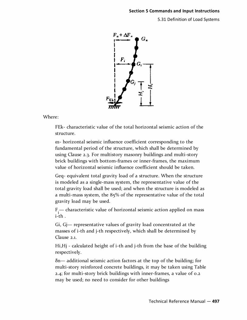
Where:
FEk- characteristic value of the total horizontal seismic action of thestructure.
α1- horizontal seismic influence coefficient corresponding to thefundamental period of the structure, which shall be determined byusing Clause 2.3. For multistory masonry buildings and multi-storybrick buildings with bottom-frames or inner-frames, the maximumvalue of horizontal seismic influence coefficient should be taken.
Geq- equivalent total gravity load of a structure. When the structureis modeled as a single-mass system, the representative value of thetotal gravity load shall be used; and when the structure is modeled asa multi-mass system, the 85% of the representative value of the totalgravity load may be used.
Fi— characteristic value of horizontal seismic action applied on mass
i-th .
Gi, Gj— representative values of gravity load concentrated at themasses of i-th and j-th respectively, which shall be determined byClause 2.1.
Hi,Hj - calculated height of i-th and j-th from the base of the buildingrespectively.
δn— additional seismic action factors at the top of the building; formulti-story reinforced concrete buildings, it may be taken using Table2.4; for multi-story brick buildings with inner-frames, a value of 0.2may be used; no need to consider for other buildings
Section 5 Commands and Input Instructions
5.31 Definition of Load Systems
Technical Reference Manual — 497

ΔFn - additional horizontal seismic action applied at top of thebuilding.
Table 2.4 Additional seismic action factors at top of the building
Note: T, is the fundamental period of the structure.
The horizontal seismic shear force at each floor level of the structure shall complywith the requirement of the following equation:
V λ G> ∑Eki jn
j=1 E2.7
Where:
VEki- the floor i-th shear corresponding to horizontal seismic action
characteristic value.
λ- Shear factor, it shall not be less than values in Table 2.5; for theweak location of vertical irregular structure, these values shall bemultiplied by the amplifying factor of 1.15.
Gj- the representative value of gravity load in floor j-th of the
structure.
StructuresIntensity
7Intensity
8Intensity
9structures with obvious torsioneffect or fundamental period isless than 3.5s
0.16(0.024)
0.032(0.048)
0.064
Structures with fundamentalperiod greater than 5.0s
0.012(0.018)
0.024(0.032)
0.040
Table 5-19: Minimum seismic shear factor value of the floor levelper GB50011-2001
Note:1.The values may be selected through interpolation method for structureswhose fundamental period is between 3. 5s and 5s.
2.Values in the brackets are used at the regions with basic seismicacceleration as 0.15g and 0.30g respectively.
498— STAAD.Pro V8i (SELECTseries 4)
Section 5 Commands and Input Instructions
5.31 Definition of Load Systems

Calculation of vertical seismic action
For tall buildings for Intensity 9, the characteristic value of vertical seismic actionshall be determined by the following equations (figure 2.3). The effects of verticalseismic action at floor level may be distributed in proportion of representativevalue of gravity load acting on the members, which should multiply with theamplified factor 1.5:
FEvk = αvmaxGeq E2.8
F F=iG H
G H Evk∑
i i
jn
j j=1 E2.9
Where:
FEvk
= characteristic value of the total vertical seismic actions of thestructure.
Fv= characteristic value of vertical seismic action at the level of mass
i-th.
αvmax
= maximum value of vertical seismic influence coefficient,which may be taken as 65% of the maximum value of the horizontalseismic influence coefficient.
Geq= equivalent total gravity load of the structure, which may be
taken as 75% of the representative value of the total gravity load ofthe structure.
Figure 5-35: Sketch for the computation of vertical seismic action
Section 5 Commands and Input Instructions
5.31 Definition of Load Systems
Technical Reference Manual — 499

Complementarities
1. Structures having the oblique direction lateral-force-resisting members andthe oblique angel to major orthogonal axes is greater than 150, the hor-izontal seismic action along the direction of each lateral-force-resistingmember shall he considered respectively. So we could consider this thoughthe item, the action of the oblique member could be multiplied by this fac-tor as design force.
2. Eccentricity: similar to UBC code. The eccentricity value of gravity centeron each floor should be e
i= ±0.05L
i,
where:
ei- Eccentricity value of gravity center on i-th floor.
Li- maximum width of calculated story of the building.
3. Structures having obviously asymmetric mass and stiffness distribution, thetorsion effects caused by both two orthogonal horizontal direction seismicaction shall be considered; and other structures, it is permitted that a sim-plified method, such as adjusting the seismic effects method, to considertheir seismic torsion effects.
So we may use the to decide which whether torsion effects should be considered.
General Format
The following general format should be used to generate loads in a particulardirection.
DEFINE GB (ACCIDENTAL) LOAD
INTENSITY s1 { FREQUENT | RARE } GROUP i1 SCLASS i2 (DAMP f1)(DELN f2) (SF f3) (AV f4) (PX f5) (PZ f6)
Where:
l s1= the Fortification Intensity (ref. table 5.1.4-1). Acceptable values are 6, 7,
7A, 8, 8A, or 9.
l i1= Design Seismic Group (ref. table 5.1.4-2). Acceptable values are 1,2, or 3.
l i2= Site-Class (ref. table 5.1.4-2). Acceptable values are 1, 2, 3, or 4.
l f1= damping ratio (default = 0.05 for 5% damping)
500— STAAD.Pro V8i (SELECTseries 4)
Section 5 Commands and Input Instructions
5.31 Definition of Load Systems

l f2= δ
n, Additional seismic action factor at the top of the building (default
as calculated from Table 5.2.1)
l f3= Shear Factor λ, Minimum seismic shear factor of the floor (default as
calculated from Table 5.2.5)
l f4= maximum value of vertical seismic influence coefficient α
(v,max)(default=0.0) (ref. section 5.3)
Frequency of seismic action, as specified by either FREQUENT or RARE (ref.table 5.1.2-2)
As a fraction of total vertical load is to be considered such as 0.75Geq, specify theproduct of the factor on maximum horizontal seismic influence factor and factorof total gravity load as f4. For instance,
l α(v,max)
= 0.65αmax
And
l Gv,eq = 0.75Geq
l Specify f4as (0.65*0.75) i.e., equal to 0.4875
l f5and f
6= optional time period along two horizontal direction (X and Y,
respectively).
Steps described in section 5.1.4, 5.1.5, 5.2.1, 5.2.5, 5.3.1 will be used in generatingload due to seismic action.
To apply the load in any load case, following command would be used
LOAD CASE i
GB LOAD X (f7) (ACC f8)
Where:
i = load case number
f7= optional factor to multiply horizontal seismic load.
f8= multiplying factor for Accidental Torsion, to be used to multiply
the accidental torsion load (default = 1.0). May be negative (otherwise,the default sign for MY is used based on the direction of thegenerated lateral forces).
Note: If the ACCIDENTAL option is specified, the accidental torsion will becalculated per the GB specifications. The value of the accidental torsionis based on the "center of mass" for each level. The "center of mass" is
Section 5 Commands and Input Instructions
5.31 Definition of Load Systems
Technical Reference Manual — 501

calculated from the SELFWEIGHT, JOINT WEIGHTs and MEMBERWEIGHTs you have specified.
Example Output
*****************************************************************************
* *
* EQUIV. SEISMIC LOADS AS PER SEISMIC DESIGN CODE FOR BUILDINGS *
* (GB50011-2001) OF CHINA ALONG X *
* T CALCULATED = 0.252 SEC. T USER PROVIDED = 1.200 SEC. *
* T USED = 1.200 SEC. *
* MAX. HORIZONTAL SEISMIC INFLUENCE COEFFICIENT = 0.240 *
* CHARACTERISTIC PERIOD = 0.750 SEC. *
* DAMPING RATIO = 0.030 POWER INDEX (GAMMA) = 0.931 *
* DAMPING ADJUSTMENT FACTOR (ETA2) = 1.180 *
* ADJUSTING FACTOR (ETA1) = 0.022 *
* HORIZONTAL SEISMIC INFLUENCE COEFFICIENT (ALPHA1) = 0.183 (18.288%) *
* MINIMUM SHEAR FACTOR AS PER SEC. 5.2.5 (LAMBDA) = 0.050 ( 5.000%) *
* TOTAL HORIZONTAL SEISMIC ACTION = *
* = 0.183 X 285.529 = 52.218 KIP *
* DESIGN BASE SHEAR = 0.750 X 52.218 *
* = 39.164 KIP *
* ADDITIONAL SEISMIC ACTION FACTOR (DELTAN) = 0.020 *
* VERTICAL SEISMIC INFLUENCE COEFFICIENT (ALPHA,VMAX) = -0.108 *
* TOTAL VERTICAL SEISMIC ACTION = *
* = -0.108 X 285.529 = -30.837 KIP *
* TOTAL DESIGN VERTICAL LOAD = 0.750 X -30.837 *
* = -23.128 KIP *
* *
*****************************************************************************
CHECK FOR MINIMUM LATERAL FORCE AT EACH FLOOR [GB50011-2001:5.2.5]
LOAD - 1 FACTOR - 0.750
FLOOR LATERAL GRAVITY LAMBDA LAMBDA ADJUSTMENT
HEIGHT (KIP ) LOAD (KIP ) LOAD (KIP ) (%) MIN (%) FACTOR
------------- ----------- ------------ ------ ------ -----------
30.000 23.406 79.045 29.61 5.00 1.00
20.000 19.208 180.888 10.62 5.00 1.00
10.000 9.604 282.731 3.40 5.00 1.47
JOINT LATERAL TORSIONAL VERTICAL LOAD - 1
LOAD (KIP ) MOMENT (KIP -FEET) LOAD (KIP ) FACTOR - 0.750
502— STAAD.Pro V8i (SELECTseries 4)
Section 5 Commands and Input Instructions
5.31 Definition of Load Systems
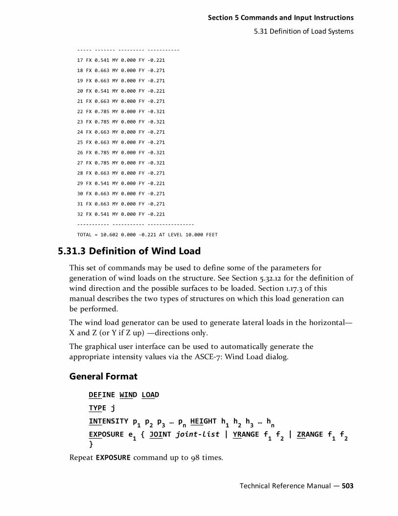
----- ------- --------- -----------
17 FX 0.541 MY 0.000 FY -0.221
18 FX 0.663 MY 0.000 FY -0.271
19 FX 0.663 MY 0.000 FY -0.271
20 FX 0.541 MY 0.000 FY -0.221
21 FX 0.663 MY 0.000 FY -0.271
22 FX 0.785 MY 0.000 FY -0.321
23 FX 0.785 MY 0.000 FY -0.321
24 FX 0.663 MY 0.000 FY -0.271
25 FX 0.663 MY 0.000 FY -0.271
26 FX 0.785 MY 0.000 FY -0.321
27 FX 0.785 MY 0.000 FY -0.321
28 FX 0.663 MY 0.000 FY -0.271
29 FX 0.541 MY 0.000 FY -0.221
30 FX 0.663 MY 0.000 FY -0.271
31 FX 0.663 MY 0.000 FY -0.271
32 FX 0.541 MY 0.000 FY -0.221
----------- ----------- ----------------
TOTAL = 10.602 0.000 -0.221 AT LEVEL 10.000 FEET
5.31.3 Definition of Wind LoadThis set of commands may be used to define some of the parameters forgeneration of wind loads on the structure. See Section 5.32.12 for the definition ofwind direction and the possible surfaces to be loaded. Section 1.17.3 of thismanual describes the two types of structures on which this load generation canbe performed.
The wind load generator can be used to generate lateral loads in the horizontal—X and Z (or Y if Z up) —directions only.
The graphical user interface can be used to automatically generate theappropriate intensity values via the ASCE-7: Wind Load dialog.
General Format
DEFINE WIND LOAD
TYPE j
INTENSITY p1 p2 p3 … pn HEIGHT h1 h2 h3 … hnEXPOSURE e1 { JOINT joint-list | YRANGE f1 f2 | ZRANGE f1 f2}
Repeat EXPOSURE command up to 98 times.
Section 5 Commands and Input Instructions
5.31 Definition of Load Systems
Technical Reference Manual — 503

Where:
j = wind load system type number (integer)
p1,p2,p3… p
n = wind intensities (pressures) in force/area. Up to 100
different intensities can be defined in the input file per type.
h1,h2,h3… h
n = corresponding heights in global vertical direction,
measured in terms of actual Y (or Z for Z UP ) coordinates up towhich the corresponding intensities occur.
e1, e2… e
m = exposure factors. A value of 1.0 means that the wind
force may be applied on the full influence area associated with thejoint(s) if they are also exposed to the wind load direction. Limit: 99factors.
joint-list = Joint list associated with Exposure Factor (joint numbers or“TO” or “BY”) or enter only a group name.
f1and f
2= global coordinate values to specify Y (or Z if Z UP) vertical
range for Exposure Factor. Use YRANGE when Y is Up and ZRANGEwhen Z is Up (See the SET Z UP command in Section 5.5).
If the command EXPOSURE is not specified or if a joint is not listed in anExposure, the exposure factor for those joints is chosen as 1.0.
Description
All intensities and heights are in current unit system. The heights specified are interms of actual Y coordinate ( or Z coordinates for Z UP ) and not measuredrelative to the base of the structure. The first value of intensity (p
1) will be
applied to any part of the structure for which the Y coordinate ( or Z coordinatefor Z UP ) is equal to or less than h
1. The second intensity ( p
2) will be applied to
any part of the structure that has vertical coordinates between the first twoheights (h
1and h
2) and so on. Any part of the structure that has vertical
coordinates greater than hnwill be loaded with intensity p
n.
Only exposed surfaces bounded by members (not by plates or solids) will be used.The joint influence areas are computed based on surface member selection dataentered in section 5.32.12 and based on the wind direction for a load case. Onlyjoints actually exposed to the wind and connected to members will be loaded.The individual bounded areas must be planar surfaces, to a close tolerance, orthey will not be loaded.
504— STAAD.Pro V8i (SELECTseries 4)
Section 5 Commands and Input Instructions
5.31 Definition of Load Systems

Exposure factor (e) is the fraction of the influence area associated with the joint(s) on which the load may act if it is also exposed to the wind load. Total load ona particular joint is calculated as follows.
Joint load = (Exposure Factor) X (Influence Area) X (Wind Intensity)
The exposure factor may be specified by a joint-list or by giving a vertical rangewithin which all joints will have the same exposure. If an exposure factor is notentered or not specified for a joint, then it defaults to 1.0 for those joints; inwhich case the entire influence area associated with the joint(s) will beconsidered.
For load generation on a closed type structure defined as a PLANE FRAME,influence area for each joint is calculated considering unit width perpendicular tothe plane of the structure. You can accommodate the actual width byincorporating it in the Exposure Factor as follows.
Exposure Factor (User Specified) = (Fraction of influence area) X (influence widthfor joint)
Notes
a. All intensities, heights and ranges must be provided in the current unit sys-tem.
b. If necessary, the INTENSITY, EXPOSURE command lines can be continuedon to additional lines by ending all but last line with a space and hyphen(-). Use up to 11 lines for a command.
Example
UNIT FEET
DEFINE WIND LOAD
TYPE 1
INTENSITY 0.1 0.15 HEIGHT 12 24
EXPOSURE 0.90 YRANGE 11 13
EXPOSURE 0.85 JOITN 17 20 22
LOAD 1 WIND LOAD IN X-DIRECTION
WIND LOAD X 1.2 TYPE 1
Section 5 Commands and Input Instructions
5.31 Definition of Load Systems
Technical Reference Manual — 505

For additional examples, see section 5.32.12 and example 15 in the Examplesmanual.
The Intensity line can be continued in up to 12 lines.
So the following
INT 0.008 0.009 0.009 0.009 0.01 0.01 0.01 0.011 0.011 0.0120.012 0.012 HEIG 15 20 25 30 40 50 60 70 80 90 100 120
could be split as
INT 0.008 0.009 0.009 0.009 0.01 0.01 0.01 0.011 0.011 0.0120.012 0.012 –
HEIG 15 20 25 30 40 50 60 70 80 90 100 120
or
INT 0.008 0.009 0.009 0.009 0.01 0.01-
0.01 0.011 0.011 0.012 0.012 0.012 HEIG 15 20 25 -
30 40 50 60 70 80 90 100 120
etc.
Persistency of Parameters used to Generate ASCE Wind Loads
Note: This feature is effective STAAD.Pro 2006
In the graphical environment, under the General-Load-Definitions-WindDefinitions page, there is a facility to generate the pressure versus height tableper the ASCE 7 wind load specifications per the 1995, 2002, or 2010 editions. Theparameters which go into the derivation of this table are not retained by thegraphical environment but rather added into the STAAD input file so they maybe edited as needed. These values are not read by the STAAD engine directlyand, therefure, are not directly processed as a load but are rather used togenerate the wind intensity values which are used by the engine. An example ofit is shown below.
Example
DEFINE WIND LOAD
TYPE 1
<! STAAD PRO GENERATED DATA DO NOT MODIFY !!!
506— STAAD.Pro V8i (SELECTseries 4)
Section 5 Commands and Input Instructions
5.31 Definition of Load Systems

ASCE-7-2002:PARAMS 85.000 MPH 0 1 0 0 0.000 FT 0.000 FT0.000 FT 1 -
1 40.000 FT 30.000 FT 25.000 FT 2.000 0.010 0 -
0 0 0 0 0.761 1.000 0.870 0.850 0 -
0 0 0 0.866 0.800 0.550
!> END GENERATED DATA BLOCK
INT 0.0111667 0.0111667 0.0113576 0.0115336 0.01169720.0118503 0.0119944 -
0.0121307 0.0122601 0.0123834 0.0125012 0.01261410.0127226 0.012827 0.0129277 -
HEIG 0 15 16.9231 18.8461 20.7692 22.6923 24.6154 26.538528.4615 -
30.3846 32.3077 34.2308 36.1538 38.0769 40
5.31.4 Definition of Time History LoadThis set of commands may be used to define parameters for Time Historyloading on the structure. The time history data may be specified using eitherexplicit definition, function specification, a spectrum specification, or timehistory data provided in an external file.
General Format
DEFINE TIME HISTORY (DT x)
TYPE i { ACCELERATION | FORCE | MOMENT } (SCALE f7) (SAVE)
{ t1 p1 t2 p2 … tn pn | function-spec | spectrum-spec | READfilename (f8) }
Repeat TYPE and Amplitude vs Time sets until all are entered, then:
ARRIVAL TIME
a1 a2 a3 … an{ DAMPING d | CDAMP | MDAMP }
The time history data can be explicitly defined using pairs of time and values ofacceleration, force, or moment, where:
l ACCELERATION indicates that the time varying load type is a groundmotion.
Section 5 Commands and Input Instructions
5.31 Definition of Load Systems
Technical Reference Manual — 507

l FORCE indicates that it is a forcing function.
l MOMENT indicates that it is a moment forcing function.
Variableor Com-mand
DefaultValue
Description
x - Solution time step used in the step-by-step integration of the uncoupledequations. Values smaller than0.00001 will be reset to the default DTvalue of 0.0013888 seconds.
i - Type number of time varying load(integer). Up to 136 types may beprovided. This number should besequential.
SCALE f7
1.0 The scale factor option multiplies allforces, accelerations, and amplitudesentered, read or generated within thisType. Primarily used to convert accel-eration in g’s to current units(9.80665, 386.08858, etc.).
SAVE - The save option results in thecreation of two files (input file namewith .TIM and .FRC file extensions).
The .TIM file contains the history ofthe displacements of every node.
The .FRC file contains the history ofthe 12 end forces of every member ofthe structure at every time step, andthe 6 reactions at each support atevery step.
Syntax: TYPE 1 FORCE SAVE
Table 5-20: Parameters for explicitly defined time history load
508— STAAD.Pro V8i (SELECTseries 4)
Section 5 Commands and Input Instructions
5.31 Definition of Load Systems

Variableor Com-mand
DefaultValue
Description
t1 p1t2 p2
- Values of time (in sec.) andcorresponding force (current forceunit) or acceleration (current lengthunit/sec2) depending on whether thetime varying load is a forcing functionor a ground motion. If the data isspecified through the input file, up to499 pairs can be provided for eachtype in the ascending value of time.More than one line may be used ifnecessary. However, if the data isprovided through an external file, anunlimited number of time-force pairsmay be specified.
If the first point is not at zero time,then the forces before the first time(but after the arrival time) will bedetermined by extrapolation usingthe first two points entered. If thefirst point has a nonzero force, therewill be a sudden application of thatforce over a single integration step(DT) at that time. Zero force will beassumed for all times after the lastdata point.
Section 5 Commands and Input Instructions
5.31 Definition of Load Systems
Technical Reference Manual — 509

Variableor Com-mand
DefaultValue
Description
a1a2a3... a
n- Values of the various possible arrival
times (seconds) of the variousdynamic load types. Arrival time isthe time at which a load type beginsto act at a joint (forcing function) orat the base of the structure (groundmotion). The same load type mayhave different arrival times fordifferent joints and hence all thosevalues must be specified here.
The arrival times and the times fromthe time-force pairs will be added toget the times for a particular set ofjoints in the TIME LOAD data (seesection 5.32.10.2). The arrival timesand the time-force pairs for the loadtypes are used to create the loadvector needed for each time step ofthe analysis. Refer to Section 5.32.10.2for information on input specificationfor application of the forcing functionand/or ground motion loads. Up to999 arrival time values may bespecified.
510— STAAD.Pro V8i (SELECTseries 4)
Section 5 Commands and Input Instructions
5.31 Definition of Load Systems

Variableor Com-mand
DefaultValue
Description
d 0.05 Modal damping ratio.
To enter different damping for eachmode, enter a DEFINE DAMPcommand elsewhere and MDAMP here;or for composite damping, enterCDAMP here and CDAMP ratios for all ofthe members / elements/ springs inthe Constants and Set commands.
The default value of 0.05 is used if novalue is entered, if 0.0 is entered, or ifless than 0.0000011 is entered. Use0.0000011 to get exactly 0.0 fordamping.
The function-spec option can be used to specify harmonic loads. Both sine andcosine harmonic functions may be specified. The program will automaticallycalculate the harmonic load time history based on the following specifications.
For the function and amplitude option (:
function-spec =
{ SINE | COSINE }
AMPLITUDE f0 { FREQUENCY | RPM } f2 (PHASE f3) CYCLES f4 { SUBDIV f5 | STEP f6 }
Note: Please be aware that if a Cosine function or Sine with nonzero phaseangle is entered, the force at the arrival time will be nonzero; there willbe a sudden application of force over a single integration step (DT) atthat time.
Where:
Section 5 Commands and Input Instructions
5.31 Definition of Load Systems
Technical Reference Manual — 511

Variable or Com-mand
DefaultValue
Description
x - Solution time step usedin the step-by-step inte-gration of the uncoupledequations. Valuessmaller than 0.00001 willbe reset to the defaultDT value of 0.0013888seconds.
i - Type number of timevarying load (integer).Up to 136 types may beprovided. This numbershould be sequential.
SCALE f7
1.0 The scale factor optionmultiplies all forces,accelerations, and ampli-tudes entered, read orgenerated within thisType. Primarily used toconvert acceleration ing’s to current units(9.80665, 386.08858,etc.).
Table 5-21: Parameters for use with function time history load
512— STAAD.Pro V8i (SELECTseries 4)
Section 5 Commands and Input Instructions
5.31 Definition of Load Systems
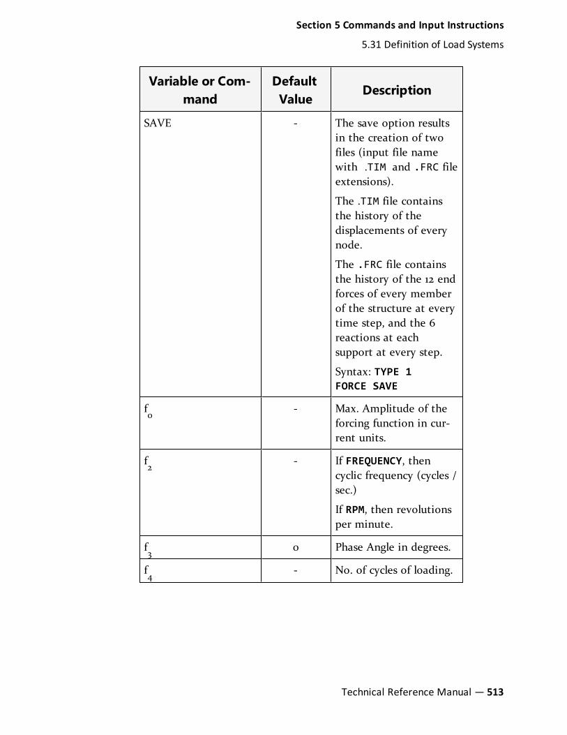
Variable or Com-mand
DefaultValue
Description
SAVE - The save option resultsin the creation of twofiles (input file namewith .TIM and .FRC fileextensions).
The .TIM file containsthe history of thedisplacements of everynode.
The .FRC file containsthe history of the 12 endforces of every memberof the structure at everytime step, and the 6reactions at eachsupport at every step.
Syntax: TYPE 1FORCE SAVE
f0
- Max. Amplitude of theforcing function in cur-rent units.
f2
- If FREQUENCY, thencyclic frequency (cycles /sec.)
If RPM, then revolutionsper minute.
f3
0 Phase Angle in degrees.
f4
- No. of cycles of loading.
Section 5 Commands and Input Instructions
5.31 Definition of Load Systems
Technical Reference Manual — 513

Variable or Com-mand
DefaultValue
Description
f5
3 Used to subdivide a ¼cycle into this manyinteger time steps.
Note: Only used todigitize theforcingfunction. It isnot the DTused tointegrate forthe responses. Moresubdivisionswill make thedigitized forcecurve moreclosely match asine wave. Thedefault isusuallyadequate.
514— STAAD.Pro V8i (SELECTseries 4)
Section 5 Commands and Input Instructions
5.31 Definition of Load Systems

Variable or Com-mand
DefaultValue
Description
f6
(p/12) Time step of loading.Default is equal to onetwelfth of the periodcorresponding to thefrequency of theharmonic loading. (It isbest to use the default)
Note: Only used todigitize theforcingfunction. It isnot the DTused tointegrate forthe responses. Moresubdivisions orsmaller stepsize will makethe digitizedforce curvemore closelymatch a sinewave.
Section 5 Commands and Input Instructions
5.31 Definition of Load Systems
Technical Reference Manual — 515

Variable or Com-mand
DefaultValue
Description
a1a2a3... a
n- Values of the various
possible arrival times(seconds) of the variousdynamic load types.Arrival time is the timeat which a load typebegins to act at a joint(forcing function) or atthe base of the structure(ground motion). Thesame load type mayhave different arrivaltimes for different jointsand hence all thosevalues must be specifiedhere.
The arrival times andthe times from thetime-force pairs will beadded to get the timesfor a particular set ofjoints in the TIMELOAD data (see section5.32.10.2). The arrivaltimes and the time-forcepairs for the load typesare used to create theload vector needed foreach time step of theanalysis. Refer to Section5.32.10.2 for informationon input specificationfor application of theforcing function and/orground motion loads.Up to 999 arrival timevalues may be specified.
516— STAAD.Pro V8i (SELECTseries 4)
Section 5 Commands and Input Instructions
5.31 Definition of Load Systems

Variable or Com-mand
DefaultValue
Description
d 0.05 Modal damping ratio.
To enter differentdamping for each mode,enter a DEFINE DAMPcommand elsewhere andMDAMP here; or forcomposite damping,enter CDAMP here andCDAMP ratios for all ofthe members /elements/ springs in theConstants and Setcommands.
The default value of 0.05is used if no value isentered, if 0.0 isentered, or if less than0.0000011 is entered.Use 0.0000011 to getexactly 0.0 for damping.
The spectrum-spec option can be used to specify a synthetic ground motionacceleration time history based statistically on a user supplied accelerationspectrum.
The program will automatically calculate the acceleration time history based onthe following specifications. Enter f
12, f13, and f
14to indicate the rise, steady, &
decay times, respectively.
For the spectrum option:
spectrum-spec =
SPECTRUM TMAX f9 DTI f10 DAMP f11 T1 f12 T2 f13 T3 f14 SEED f15OPTIONS NF f16 NITR f17 ( THPRINT f18 ) ( SPRINT f19 ) ( FREQ)
Starting on the next line, enter Spectra in the following input form:
P1, V1; P2, V2; … ; Pn, VnWhere:
Section 5 Commands and Input Instructions
5.31 Definition of Load Systems
Technical Reference Manual — 517
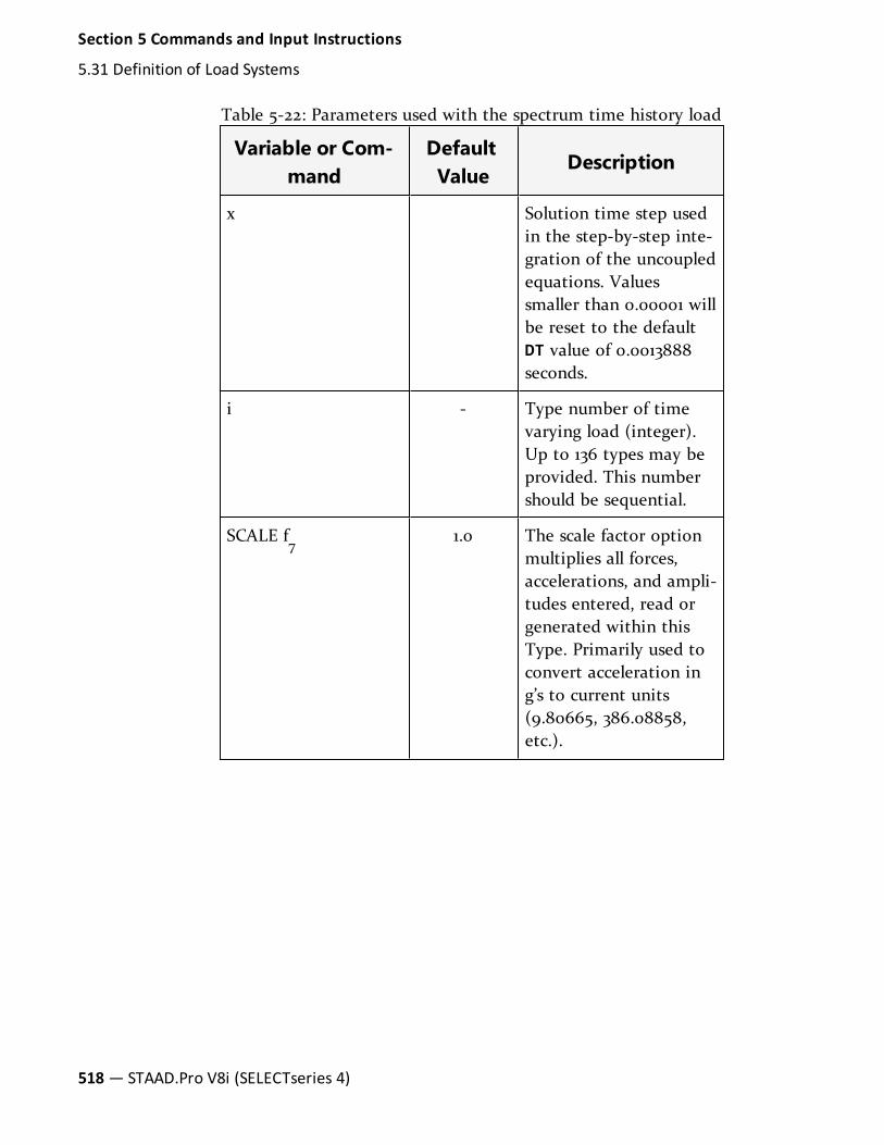
Variable or Com-mand
DefaultValue
Description
x Solution time step usedin the step-by-step inte-gration of the uncoupledequations. Valuessmaller than 0.00001 willbe reset to the defaultDT value of 0.0013888seconds.
i - Type number of timevarying load (integer).Up to 136 types may beprovided. This numbershould be sequential.
SCALE f7
1.0 The scale factor optionmultiplies all forces,accelerations, and ampli-tudes entered, read orgenerated within thisType. Primarily used toconvert acceleration ing’s to current units(9.80665, 386.08858,etc.).
Table 5-22: Parameters used with the spectrum time history load
518— STAAD.Pro V8i (SELECTseries 4)
Section 5 Commands and Input Instructions
5.31 Definition of Load Systems

Variable or Com-mand
DefaultValue
Description
SAVE The save option resultsin the creation of twofiles (input file namewith .TIM and .FRC fileextensions).
The .TIM file containsthe history of thedisplacements of everynode.
The .FRC file containsthe history of the 12 endforces of every memberof the structure at everytime step, and the 6reactions at eachsupport at every step.
Syntax: TYPE 1FORCE SAVE
f9
20 seconds The Max. time (in sec-onds) in the generatedtime history.
f10
0.2 Delta time step (in sec-onds) in the generatedtime history.
f11
0.05 Damping ratio (5% isentered as 0.05) asso-ciated with the inputspectrum.
f12
4 seconds Ending time of theacceleration rise time.
f13
9 seconds Ending time of thesteady acceleration.
Section 5 Commands and Input Instructions
5.31 Definition of Load Systems
Technical Reference Manual — 519

Variable or Com-mand
DefaultValue
Description
f14
14 seconds Ending time of the accel-eration decay.
f15
Random Seed. Enter apositive integer (1 to2147483647) to be usedas a unique randomnumber generation“seed”. A unique timehistory will be producedfor each seed value.Change this value whenyou want to produce a“different (from thetime history generatedwith the prior seedvalue)” but statisticallyequivalent time history.Omit this entry to getthe default value (nor-mal option).
f16
The input shockspectrum will be re-digitized at NF equallyspaced frequencies byinterpolation. Default isthe greater of 35 or thenumber of points in theinput spectrum.
f17
10 The number of iter-ations which will beused to perfect the com-puted time history.
520— STAAD.Pro V8i (SELECTseries 4)
Section 5 Commands and Input Instructions
5.31 Definition of Load Systems

Variable or Com-mand
DefaultValue
Description
f18
1 Print the time historythat is generated. Omitthe THPRINT parameterto avoid printing.
1 = printbeginning 54values andlast 54 values
2 = Printentire curve.
>10 = printbeginning f
18values andlast f
18values
f19
1 Print the spectrum gen-erated from the time his-tory that is generated.Omit the SPRINT param-eter to avoid printing
FREQ If entered, thenfrequency-spectra pairsare entered rather thanperiod-spectra pairs.
Section 5 Commands and Input Instructions
5.31 Definition of Load Systems
Technical Reference Manual — 521
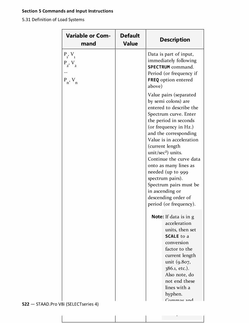
Variable or Com-mand
DefaultValue
Description
P1, V
1P2, V
2…
Pn, V
n
Data is part of input,immediately followingSPECTRUM command.Period (or frequency ifFREQ option enteredabove)
Value pairs (separatedby semi colons) areentered to describe theSpectrum curve. Enterthe period in seconds(or frequency in Hz.)and the correspondingValue is in acceleration(current lengthunit/sec2) units.Continue the curve dataonto as many lines asneeded (up to 999spectrum pairs).Spectrum pairs must bein ascending ordescending order ofperiod (or frequency).
Note: If data is in gaccelerationunits, then setSCALE to aconversionfactor to thecurrent lengthunit (9.807,386.1, etc.).Also note, donot end theselines with ahyphen.Commas andsemi-colonsare optional.
522— STAAD.Pro V8i (SELECTseries 4)
Section 5 Commands and Input Instructions
5.31 Definition of Load Systems

Variable or Com-mand
DefaultValue
Description
a1a2a3... a
nValues of the variouspossible arrival times(seconds) of the variousdynamic load types.Arrival time is the timeat which a load typebegins to act at a joint(forcing function) or atthe base of the structure(ground motion). Thesame load type mayhave different arrivaltimes for different jointsand hence all thosevalues must be specifiedhere.
The arrival times andthe times from thetime-force pairs will beadded to get the timesfor a particular set ofjoints in the TIMELOAD data (see section5.32.10.2). The arrivaltimes and the time-forcepairs for the load typesare used to create theload vector needed foreach time step of theanalysis. Refer to Section5.32.10.2 for informationon input specificationfor application of theforcing function and/orground motion loads.Up to 999 arrival timevalues may be specified.
Section 5 Commands and Input Instructions
5.31 Definition of Load Systems
Technical Reference Manual — 523
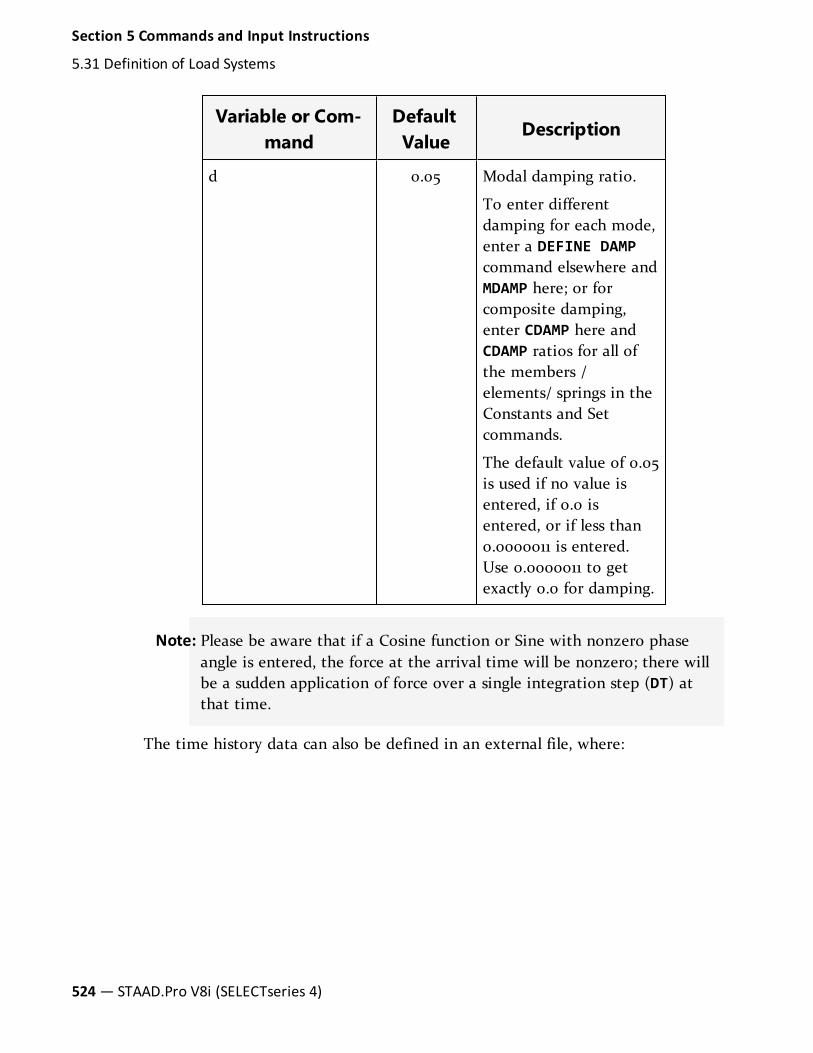
Variable or Com-mand
DefaultValue
Description
d 0.05 Modal damping ratio.
To enter differentdamping for each mode,enter a DEFINE DAMPcommand elsewhere andMDAMP here; or forcomposite damping,enter CDAMP here andCDAMP ratios for all ofthe members /elements/ springs in theConstants and Setcommands.
The default value of 0.05is used if no value isentered, if 0.0 isentered, or if less than0.0000011 is entered.Use 0.0000011 to getexactly 0.0 for damping.
Note: Please be aware that if a Cosine function or Sine with nonzero phaseangle is entered, the force at the arrival time will be nonzero; there willbe a sudden application of force over a single integration step (DT) atthat time.
The time history data can also be defined in an external file, where:
524— STAAD.Pro V8i (SELECTseries 4)
Section 5 Commands and Input Instructions
5.31 Definition of Load Systems

Variableor Com-mand
DefaultValue
Description
x - Solution time step used in the step-by-step integration of the uncoupledequations. Values smaller than0.00001 will be reset to the default DTvalue of 0.0013888 seconds.
i - Type number of time varying load(integer). Up to 136 types may beprovided. This number should besequential.
SCALE f7
1.0 The scale factor option multiplies allforces, accelerations, and amplitudesentered, read or generated within thisType. Primarily used to convert accel-eration in g’s to current units(9.80665, 386.08858, etc.).
SAVE - The save option results in thecreation of two files (input file namewith .TIM and .FRC file extensions).
The .TIM file contains the history ofthe displacements of every node.
The .FRC file contains the history ofthe 12 end forces of every member ofthe structure at every time step, andthe 6 reactions at each support atevery step.
Syntax: TYPE 1 FORCE SAVE
filename Filename for an external file con-taining time varying load historydata.
Table 5-23: Parameters for a time history load defined in anexternal file
Section 5 Commands and Input Instructions
5.31 Definition of Load Systems
Technical Reference Manual — 525

Variableor Com-mand
DefaultValue
Description
f8
The delta time spacing used for theexternal file data
a1a2a3... a
nValues of the various possible arrivaltimes (seconds) of the variousdynamic load types. Arrival time isthe time at which a load type beginsto act at a joint (forcing function) orat the base of the structure (groundmotion). The same load type mayhave different arrival times fordifferent joints and hence all thosevalues must be specified here.
The arrival times and the times fromthe time-force pairs will be added toget the times for a particular set ofjoints in the TIME LOAD data (seesection 5.32.10.2). The arrival timesand the time-force pairs for the loadtypes are used to create the loadvector needed for each time step ofthe analysis. Refer to Section 5.32.10.2for information on input specificationfor application of the forcing functionand/or ground motion loads. Up to999 arrival time values may bespecified.
526— STAAD.Pro V8i (SELECTseries 4)
Section 5 Commands and Input Instructions
5.31 Definition of Load Systems

Variableor Com-mand
DefaultValue
Description
d 0.05 Modal damping ratio.
To enter different damping for eachmode, enter a DEFINE DAMPcommand elsewhere and MDAMP here;or for composite damping, enterCDAMP here and CDAMP ratios for all ofthe members / elements/ springs inthe Constants and Set commands.
The default value of 0.05 is used if novalue is entered, if 0.0 is entered, or ifless than 0.0000011 is entered. Use0.0000011 to get exactly 0.0 fordamping.
Examples
Using Force and Acceleration options:
UNIT …
DEFINE TIME HISTORY
TYPE 1 FORCE
0.0 1.0 1.0 1.2 2.0 1.8 3.0 2.2
4.0 2.6 5.0 2.8
TYPE 2 ACCELERATION SCALE 9.80665
0.0 1.0 1.0 1.2 2.0 1.8 3.0 2.2
4.0 2.6 5.0 2.8
ARRIVAL TIME
0.0 1.0 1.8 2.2 3.5 4.4
DAMPING 0.075
Using the Spectrum option:
Section 5 Commands and Input Instructions
5.31 Definition of Load Systems
Technical Reference Manual — 527

UNIT …
DEFINE TIME HISTORY
TYPE 1 ACCELERATION SCALE 9.80665
SPECTRUM TMAX 19 DTI 0.01 DAMP 0.03
OPTIONS NF 40
0.03 1.00 ; 0.05 1.35
0.1 1.95 ; 0.2 2.80
0.5 2.80 ; 1.0 1.60
ARRIVAL TIME
0.0 1.0 1.8 2.2 3.5 4.4
DAMPING 0.075
Using the Harmonic Loading Generator:
UNIT …
DEFINE TIME HISTORY
TYPE 1 FORCE
*FOLLOWING LINES FOR HARMONIC LOADING GENERATOR
FUNCTION SINE
AMPLITUDE 6.2831 FREQUENCY 60 CYCLES 100 STEP 0.02
ARRIVAL TIME
0.0
DAMPING 0.075
To define more than one sinusoidal load, the input specification is as follows:
DEFINE TIME HISTORY
TYPE 1 FORCE
FUNCTION SINE
AMPLITUDE 1.925 RPM 10794.0 CYCLES 1000
TYPE 2 FORCE
FUNCTION SINE
AMPLITUDE 1.511 RPM 9794.0 CYCLES 1000
528— STAAD.Pro V8i (SELECTseries 4)
Section 5 Commands and Input Instructions
5.31 Definition of Load Systems
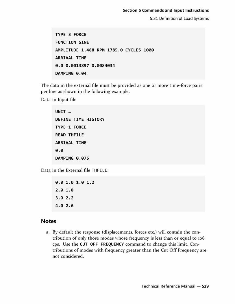
TYPE 3 FORCE
FUNCTION SINE
AMPLITUDE 1.488 RPM 1785.0 CYCLES 1000
ARRIVAL TIME
0.0 0.0013897 0.0084034
DAMPING 0.04
The data in the external file must be provided as one or more time-force pairsper line as shown in the following example.
Data in Input file
UNIT …
DEFINE TIME HISTORY
TYPE 1 FORCE
READ THFILE
ARRIVAL TIME
0.0
DAMPING 0.075
Data in the External file THFILE:
0.0 1.0 1.0 1.2
2.0 1.8
3.0 2.2
4.0 2.6
Notes
a. By default the response (displacements, forces etc.) will contain the con-tribution of only those modes whose frequency is less than or equal to 108cps. Use the CUT OFF FREQUENCY command to change this limit. Con-tributions of modes with frequency greater than the Cut Off Frequency arenot considered.
Section 5 Commands and Input Instructions
5.31 Definition of Load Systems
Technical Reference Manual — 529

b. Results are the individual maximums over the time period. Thus, derivedquantities such as section forces and stresses, plate surface stresses and prin-cipal stresses should not be used.
c. Results from harmonic input are the maximum over the time period includ-ing the start-up transient period. These results are not the steady-stateresults.
d. By default, the results do not include the time period after the time loadsend. Use the CUT OFF TIME command to lengthen (or shorten) the timeperiod. If an intense short-term loading is used, the loading should be con-tinued until after the expected peak response is reached.
e. The READ filename command is to be provided only if the history of thetime varying load is to be read from an external file. filename is the filename and may be up to 72 characters long. If the data on the file consistsonly of amplitudes, then enter f
8as the delta time spacing.
5.31.5 Definition of Snow LoadThis set of commands may be used to define some of the parameters forgeneration of snow loads on the structure. See section 5.32.13, Generation of SnowLoads, for the definition of additional parameters and the surfaces to be loaded.
General FormatDEFINE SNOW LOAD
TYPE f1 PG f2 CE f3 CT f4 IM f5Where:
f1- Type No: (limit of 100). The “Type No.” is an integer value (1, 2, 3,
etc.) which denotes a number by which the snow load type will beidentified. Multiple snow load types can be created in the samemodel. Include as many types as needed.
f2- Ground Snow Load (Default = 0.0). The pressure or, weight per
unit area, to be used for the calculation of the design snow load. Use anegative value to indicate loading acting towards the roof (upwards)as per section 7.2 of SEI/ASCE 7-02.
f3- Exposure Factor (Default = 1.0). Exposure factor as per Table 7-2
of the SEI/ASCE-7-02 code. It is dependent upon the type of exposure
530— STAAD.Pro V8i (SELECTseries 4)
Section 5 Commands and Input Instructions
5.31 Definition of Load Systems

of the roof (fully exposed/partially exposed/sheltered) and the terraincategory, as defined in section 6.5.6 of the code.
f4- Thermal Factor (Default = 0.0). Thermal factor as per Table 7-3 of
the SEI/ASCE-7-02 code. It is dependent upon the thermal condition.
f5- Importance Factor (Default = 1.0). Importance factor as per Table
7-4 of the SEI/ASCE-7-02 code. This value depends on the categorythe structure belongs to, as per section 1.5 and Table 1-1 of the code.
Example
START GROUP DEFINITION
FLOOR
_ROOFSNOW 102 TO 153 159 160 TO 170 179 195 TO 197
END GROUP DEFINITION
UNIT FEET POUND
DEFINE SNOW LOAD
TYPE 1 PG 50 CE 0.7 CT 1.1 IM 1.1
5.31.6 Defining Reference Load TypesLarge models can include multiple load cases which do not require analysis intheir own right and are simply the building blocks for inclusion in primary loadcases. Thus Reference Loads may be defined for this purpose. This is similar to aREPEAT LOAD command (See Section 5.32.11), but has the added benefit of notbeing solved in its own right.
This converts a real load case to something similar to a load case definition. Areference load case is solved only when it is later called in a load case. Thebenefit is that it enables you to define as many load cases as you wish, butinstruct the program to actually solve only a limited number of "real" load cases,thus limiting the amount of results to be examined.
Note: This feature requires STAAD.Pro 2007 Build 01 or higher.
See "Reference Load Cases - Application" on page 669 for a description of theprocedure for specifying the reference load information in active load cases.
Section 5 Commands and Input Instructions
5.31 Definition of Load Systems
Technical Reference Manual — 531

General Format
DEFINE REFERENCE LOADS
LOAD R(i) LOADTYPE (type) TITLE load_title
(Load items)
…
END DEFINE REFERENCE LOADS
Example
DEFINE REFERENCE LOADS
LOAD R1 LOADTYPE DEAD TITLE REF DEAD
SELFWEIGHT Y -1
JOINT LOAD
4071 4083 4245 4257 FY -4.04
4090 FY -0.64
ELEMENT LOAD
378 TO 379 406 TO 410 422 TO 426 PR GY -1.44
MEMBER LOAD
5006 TO 5229 UNI GY -0.64
PMEMBER LOAD
1 TRAP GY -0.347 -0.254 35.5 42
LOAD R2 LOADTYPE LIVE TITLE REF LIVE
JOINT LOAD
4209 FY -6.63
4071 4083 4245 4257 FY -1.71
LOAD R3 LOADTYPE SNOW TITLE REF SNOW
JOINT LOAD
4109 FY -8.69
4071 4083 4245 4257 FY -3.29
LOAD R4 LOADTYPE SOIL TITLE REF SOIL
ELEMENT LOAD
532— STAAD.Pro V8i (SELECTseries 4)
Section 5 Commands and Input Instructions
5.31 Definition of Load Systems

1367 TO 1394 1396 1398 1522 1539 TO 1574 -
1575 TRAP JT -0.78 -0.78 -0.719167 -0.719167
LOAD R4 LOADTYPE MASS TITLE MASS MODEL
SELFWEIGHT X 1
SELFWEIGHT Y 1
SELFWEIGHT Z 1
JOINT LOAD
17 TO 48 FY -2.5
49 TO 64 FY -1.25
END DEFINE REFERENCE LOADS
Mass Modeling Using Reference Loads
A reference load case of type MASS can be created which can then be used todefine the structure mass used for all dynamic analyses (i.e., seismic, responsespectrum, time history, etc.). Some analysis methods require you to createseparate weight tables in the form of SELFWEIGHT, MEMBER WEIGHT, JOINTWEIGHT, etc. for each analysis, thus resulting in repetition of the sameinformation. Using a LOADTYPE MASS reduces the repetitive data entry and theneed for manually creating a weight table.
A mass model using this method is defined once and then used for all dynamicanalyses.
Note: This feature requires STAAD.Pro V8i (SELECTseries 3) (release20.07.08) or higher.
If the LOADTYPE MASS is missing and no mass is defined in the correspondingseismic or dynamic analysis load cases, the program will report error as mass ismissing. If a mass model using reference load type MASS is defined and also aseismic weight table is defined within a dynamic load (i.e., static equivalentseismic load, time history, response spectrum, etc.) command, the program willsimply add the seismic weight table with mass model already defined. This willincrease the masses of the structure for equivalent seismic static analysis. Theprogram will issue a warning message. Precaution should be taken so that massmodel is not defined twice.
Section 5 Commands and Input Instructions
5.31 Definition of Load Systems
Technical Reference Manual — 533

5.31.7 Definition of Direct Analysis MembersThis set of commands may be used to define the members whose flexuralstiffness or axial stiffness is considered to contribute to the lateral stability of thestructure. Also the initial value of τ
bfor each member can be set here. See
Appendix 7 ANSI/AISC 360-05.
Note: This feature is available effective STAAD.Pro 2007 Build 03 and greater.
Members listed with FLEX will have their EI factored by 0.80 times τb whileperforming the global solution. The final member forces and code check will bewith 100% of the flexural stiffness. Members listed with AXIAL will have their EAfactored by 0.80 while performing the global solution. The final member forcesand code check will be with 100% of the axial stiffness.
The FYLD value here will only be used for the calculation of τb.
General Format
DEFINE DIRECT
FLEX (f1) list-spec
AXIAL list-spec
FYLD (f2) list-spec
NOTIONAL LOAD FACTOR (f3)
list-spec = * { XR f4 f5 | YR f4 f5 | ZR f4 f5 | MEMBERS mem-list | LIST memb-list | ALL }
Where:
f1= τ
bvalue. Default is 1.0. See Appendix 7 ANSI/AISC 360-05
f2= Yield Strength in current units. Default is 36.0 KSI.
f3= Notional Load Factor. Default is 0.002. If 0.003 or greater is
entered, then τbwill be set to 1.0 and no iterations will be performed.
f4,f5= Upper and lower range values, respectively, used when
specifying a range for FLEX or FYLD.
For specifying NOTIONAL LOADs, please see section 5.32.14. The notional loads andthe factor used is specified entirely in the loading data.
534— STAAD.Pro V8i (SELECTseries 4)
Section 5 Commands and Input Instructions
5.31 Definition of Load Systems

Notes
a. The NOTIONAL LOAD FACTOR f3 command does not instruct the programto create Notional Loads. Instead, it is a control parameter used solely tomake the following decision :
l If f3is 0.002, the program calculates Tau-b on an iterative basis, as
described in section 1.18.2.1.4 of this manual.
l If f3is greater than 0.00299, the program sets the iteration limit to 1
and does not perform any additional iterations.
b. τbis the value entered in the FLEX command. τ
bdefaults to 1.0 if not
entered.
5.31.8 Mass Model Using Reference LoadIn STAAD.Pro, there is a facility to create mass model which will be used for alltypes of analysis, including seismic, response spectrum, time history, and anyother dynamic analysis.
Note: This feature requires STAAD.Pro V8i (SELECTseries 3) (release20.07.08) or higher.
When a rigid floor diaphragm is present in the model, the program follows thefollowing logic:
a. If a reference load type MASS is present, then the mass model is formed bycombining all MASS reference loads.
b. If reference load type MASS is not present, then the mass model is formedby combining all gravity reference loads. Warnings are displayed in the anal-ysis output to alert you to this fact.
c. If neither reference load types MASS nor gravity are present, then the massmodel is formed by combining all DEAD reference loads. If any LIVE ref-erence loads are present, then they will also be combined to this massmodel. Warnings are displayed in the analysis output to alert you to thisfact.
Mass model will be formed from Gravity or Dead/Live reference loads in caseMass reference load types are not present, only when rigid floor diaphragm ispresent in the model.
Section 5 Commands and Input Instructions
5.31 Definition of Load Systems
Technical Reference Manual — 535

General Format
DEFINE REFERENCE LOADS
LOAD Ri title
…
Load header and items
…
LOAD Rj LOADTYPE MASS title
…
Load header and items
…
END DEFINE REFERENCE LOADS
DEFINE UBC/1893/… LOAD
ZONE …
LOAD 1 title
UBC/1893/… LOAD X f1
LOAD 2 title
UBC/1893/… LOAD Z f2
LOAD 3 title
SPECTRUM …
The mass model is defined using the LOADTYPE MASS command. This massmodel will be used for all types of analysis, including static equivalent, responsespectrum, time history, and simply Eigen solution. If the load type MASS ismissing and also no mass is defined in the corresponding seismic or dynamicanalysis load cases, the program will report error as mass is missing
If a mass model using reference load type MASS is defined and also a seismicweight table is defined in DEFINE UBC/1893/… DEFINITION, the program willsimply add seismic weight table with mass model already defined. This willincrease the masses of the structure for equivalent seismic static analysis. Theprogram will issue a warning message in the analysis output. Precaution shouldbe taken so that the mass model is not defined twice. Similar warnings are issuedin the cases of response spectrum and time history analysis.
536— STAAD.Pro V8i (SELECTseries 4)
Section 5 Commands and Input Instructions
5.31 Definition of Load Systems

Example
UNIT FEET KIP
DEFINE REF LOAD
LOAD R1 LOADTYPE MASS
* MASS MODEL
SELFWEIGHT X 1
SELFWEIGHT Y 1
SELFWEIGHT Z 1
JOINT LOAD
17 TO 48 FX 2.5 FY 2.5 FZ 2.5
49 TO 64 FX 1.25 FY 1.25 FZ 1.25
*
LOAD R2
SELFWEIGHT Y -1
JOINT LOAD
17 TO 48 FY -2.5
49 TO 64 FY -1.25
END DEF REF LOAD
*********************************************************-***
DEFINE UBC LOAD
ZONE 0.38 I 1 RWX 5.6 RWZ 5.6 STYP 2 CT 0.032 NA 1.3 NV1.6
*********************************************************-**
DEFINE TIME HISTORY
TYPE 1 FORCE
0.0 -0.0001 0.5 0.0449 1.0 0.2244 1.5 0.2244 2.0 0.67312.5 -0.6731
TYPE 2 ACCELERATION
Section 5 Commands and Input Instructions
5.31 Definition of Load Systems
Technical Reference Manual — 537

0.0 0.001 0.5 -7.721 1.0 -38.61 1.5 -38.61 2.0 -115.822.5 115.82
ARRIVAL TIMES
0.0
DAMPING 0.05
*********************************************************-**
LOAD 1
UBC LOAD X 0.75
*********************************************************-**
LOAD 2
UBC LOAD Z 0.75
*********************************************************-**
LOAD 3
SPECTRUM CQC X 0.174075 ACC DAMP 0.05 SCALE 32.2
0.03 1.00 ; 0.05 1.35 ; 0.1 1.95 ; 0.2 2.80 ; 0.5 2.80 ;1.0 1.60
*********************************************************-**
LOAD 4
SPECTRUM CQC Z 0.174075 ACC DAMP 0.05 SCALE 32.2
0.03 1.00 ; 0.05 1.35 ; 0.1 1.95 ; 0.2 2.80 ; 0.5 2.80 ;1.0 1.60
*********************************************************-**
LOAD 5
TIME LOAD
53 57 37 41 21 25 FX 1 1
GROUND MOTION X 2 1
*********************************************************-**
538— STAAD.Pro V8i (SELECTseries 4)
Section 5 Commands and Input Instructions
5.31 Definition of Load Systems
5.32 Loading SpecificationsThis section describes the various loading options available in STAAD. Thefollowing command may be used to initiate a new load case.
General FormatLOADING i1 ( LOADTYPE a1 ) ( REDUCIBLE ) ( TITLE any_load_title )
Where:
i1= any unique integer number (up to five digits) to identify the load
case. This number need not be sequential with the previous loadnumber.
a1= one of the following:
Dead Rain Water/Ice
Wind on Ice
Live Ponding Crane Hook
Roof Live Dust Mass
Wind Traffic Gravity
Seismic Temperature Push
Snow Accidental None
Fluids Flood
Soil Ice
The words LOADTYPE a are necessary only if you intend to use the AutomaticLoad Combination generation tool in the graphic interface. For details, refer tothe User Interface Manual.
The keyword REDUCIBLE should be used only when the loadtype is LIVE. Itinstructs the program to reduce—according to the provisions of UBC 1997, IBC2000, or IBC 2003 codes—a floor live load specified using FLOOR LOAD or ONEWAYLOAD commands. For details, see Section 5.32.4 of this manual.
Under this heading, all different loads related to this loading number can beinput. These different kinds of loads are described in the remaining sub-sectionsbelow.
Section 5 Commands and Input Instructions
5.32 Loading Specifications
Technical Reference Manual — 539

Notes
a. For Mass Model Loading in Dynamics, it is strongly recommended that youread Section 1.18.3.2. For the purpose of entering the mass distribution forthe first dynamic load case, use the following sections: 5.32.1 through 5.32.4plus 5.32.9. A reference load can be used to create a mass model for alldynamic analyses.
The purpose of the mass modeling step is to create lumped masses at thejoints that the eigensolution can use. The member/element loading is only aconvenience in generating the joint masses. Analytically the masses are notin the elements but are lumped at the joints.
b. The absolute value of joint loads or loads distributed to joints frommember/element loadings will be treated as weights. The moments appliedto member/elements or computed at joints as a result of member/elementloadings will be ignored. Only moments (actually weight moment of inertia,force-length2 units) applied in the Joint.
c. The load command will be used in defining the weight moment of inertiasat joints. For slave joint directions, the associated joint weight or weightmoment of inertia will be moved to the master. In addition, thetranslational weights at slave joint directions will be multiplied by thesquare of the distance to the master to get the additional weight momentof inertia at the master. Cross product weight moment of inertias at themaster will be ignored.
5.32.1 Joint Load SpecificationThis set of commands may be used to specify joint loads on the structure. Fordynamic mass modeling see sections 5.32 and 1.18.3.
General Format
JOINT LOAD
joint-list *{ FX f7 | FY f8 | FZ f9 | MX f10 | MY f11 | MZ f12}
Where:
f7, f8, f9= force values in the corresponding global direction (even at
inclined support joints).
f10, f11, f12= moment values in the corresponding global direction.
540— STAAD.Pro V8i (SELECTseries 4)
Section 5 Commands and Input Instructions
5.32 Loading Specifications

Example
UNIT FEET KIP
…
JOINT LOAD
3 TO 7 9 11 FY -17.2 MZ 180.0
5 8 FX 15.1
UNIT INCH KIP
12 MX 180.0 FZ 6.3
Notes
a. Joint numbers may be repeated where loads are meant to be additive inthe joint.
b. A UNIT command may be on lines in between joint-list lines.
c. If moments are for dynamic mass, then the units are assumed to be force-length2.
5.32.2 Member Load Specification
This set of commands may be used to specify member loads on frame members
General Format
MEMBER LOAD
member-list { { UNI | UMOM } dir-spec f1 f2 f3 f4 | { CON |CMOM } dir-spec f5 f6 f4 | LIN dir-spec f7 f8 f9 | TRAP dir-spec f10 f11 f12 f13 }
Where:
dir-spec = { X | Y | Z | GX | GY | GZ | PX | PY | PZ }
X, Y, & Z specify the direction of the load in the local (member) x, yand z-axes.
GX, GY, & GZ specify the direction of the load in the global X, Y, andZ-axes.
Section 5 Commands and Input Instructions
5.32 Loading Specifications
Technical Reference Manual — 541

PX, PY and PZ may be used if the load is to be along the projectedlength of the member in the corresponding global direction.
Note: Load start and end distances are measured along themember length and not the projected length.
f1 = value of uniformly distributed load (UNI) or moment (UMOM).
f2, f3 = distance of from the start of the member to the start of theload, and distance from the start of the member to the end of theload, respectively. The load is assumed to cover the full memberlength if f2 and f3 are omitted.
Note: Uniformly distributed moments can not be assigned totapered members for analysis.
f4 = Perpendicular distance from the member shear center to the localplane of loading. The value is positive in the general direction of theparallel (or close to parallel) local axis. If global or projected load isselected, then the local Y component of load is offset the f4 distance;the local Z component is offset the f4 distance; and the local Xcomponent is not offset.
542— STAAD.Pro V8i (SELECTseries 4)
Section 5 Commands and Input Instructions
5.32 Loading Specifications

Note: The local x component of force is not offset (i.e., nosecondary moment is caused by axial load).
f5 = value of concentrated force (CON) or moment (CMOM)
f6 = distance of from the start of the member to concentrated force ormoment. f6 will default to half the member length if omitted.
f7, f8 = LIN specifies a linearly decreasing or increasing, or a triangularload. If the load is linearly increasing or decreasing then f7 is the valueat the start of the member and f8 is the value at the end.
f9 = If the load is triangular, then f7 and f8 are input as zero and f9 isthe value of the load in the middle of the member.
f10, f11= The starting and ending load value for a trapezoidal linearly
varying load (TRAP), respectively. The TRAP load may act over the fullor partial length of a member and in a local, global or projecteddirection.
f12, f13= the loading starting point and stopping point, respectively.
Both are measured from the start of the member. If f12and f
13are not
given, the load is assumed to cover the full member length.
Notes
a. In earlier versions of STAAD, the LINear type of member load could beapplied only along the local axis of the member. It has been modified toallow for global and projected axes directions also.
b. If the member being loaded has offset distances (see MEMBER OFFSET spec-ification), the location of the load is measured not from the coordinates ofthe starting node but from the offset distance.
c. Trapezoidal loads are converted into a uniform load and 8 or more con-centrated loads.
d. A UNIT command may be on lines in between member-list lines.
e. If a load location is less than zero, it is reset to 0.0.
f. If a load location is greater than the length, it is reset to the length.
Section 5 Commands and Input Instructions
5.32 Loading Specifications
Technical Reference Manual — 543

Example
MEMBER LOAD
619 CON GY -2.35 5.827
68 TO 72 UNI GX -0.088 3.17 10.0
186 TRAP GY -0.24 -0.35 0.0 7.96
3212 LIN X -5.431 -3.335
41016 UNI PZ -0.075
3724 LIN GY -6.2 -7.8
5.32.3 Element Load SpecificationsThis set of commands may be used to specify various types of loads on plate andsolid elements.
5.32.3.1 Element Load Specification - Plates
This command may be used to specify various types of ELEMENT LOADS forplates. Plate element loads must be applied following the expression
ELEMENT LOAD (PLATE)
using the format explained under the following options.
Option 1
element-list {PRESSURE {GX | GY | GZ} p1 (x1 y1 x2 y2) }
This is for specifying a pressure of magnitude p1 in one of the global axisdirections on the full element or a small rectangular part of an element. If appliedon a small part, (x1,y1,x2 and y2) define the corners of the rectangular regionwhere the load is applied. If only x1, y1 is provided, the load is assumed as aconcentrated load applied at the specified point defined by (x1,y1). If (x1,y1,x2,y2)is not provided, the load is assumed to act over the full area of the element. (x1,y1, x2 and y2) are measured from the center of the element in the local axissystem (see figure later in this section). There is no option to apply the load overa projected area.
p1 has units of force per square of length for pressure and units of force forconcentrated load.
GX, GY and GZ represent the global axis directions.
544— STAAD.Pro V8i (SELECTseries 4)
Section 5 Commands and Input Instructions
5.32 Loading Specifications

Option 2
element-list PRESSURE (Z) p1 (x1 y1 x2 y2)
This is for specifying a constant pressure of magnitude p1 acting perpendicular tothe plane of the element on the full element or a small rectangular part of anelement. This coincides with the element’s local Z axis. If applied on a small part,(x1,y1,x2 and y2) define the corners of the rectangular region where the load isapplied. If only x1, y1 is provided, the load is assumed as a concentrated loadapplied at the specified point defined by (x1,y1). If (x1,y1,x2,y2) is not provided,the load is assumed to act over the full area of the element. (x1,y1, x2 and y2) aremeasure from the center of the element in the local axis system (see figure laterin this section). There is no option to apply the load over a projected area.
p1 has units of force per square of length for pressure and units of force forconcentrated load.
Figure 5-36: Coordinate values, x1,y1 & x2,y2, in the local coordinate system used in options 1and 2
Option 3
element-list PRESSURE {LX | LY} {p2}
This is for specifying a constant pressure of magnitude p2 along the local X (LX)or Y (LY) axis of the element (parallel to the element surface). An example of thistype of load is friction load. With this option, a load can be applied only on thefull area of the element.
p2 has units of force per square of length.
Section 5 Commands and Input Instructions
5.32 Loading Specifications
Technical Reference Manual — 545

Option 4
element-list TRAP {GX | GY | GZ | LX | LY} {X | Y} f1 f2
This is for applying a trapezoidally varying load with the following characteristics:
a. The direction of action of the load is global (GX, GY or GZ), parallel to thesurface (LX or LY as in friction type loads), or normal to the elementsurface (local Z). The last becomes the automatic direction of action if theglobal or tangential directions are not specified).
b. The load varies along the local X or Y directions (imagine the wall of a tankwith hydrostatic pressure where pressure at the lower nodes is higher thanat the upper nodes, and hence the load varies as one travels from thebottom edge of the elements to the top edge.)
This type of load has to be applied over the full area of the element. f1 isthe intensity at the I-J (or J-K) edge, and f2 is the intensity at the K-L (orL-I) edge depending on whether the load varies along "X" or "Y".
Figure 5-37: Center of the element is the origin defining the rectangular area on which thepressure is applied in option 4
The TRAP option should be used when a linearly varying pressure needs to bespecified. The variation must be provided over the entire element.
X or Y - Direction of variation of element pressure. The TRAP X/Y optionindicates that the variation of the Trapezoid is in the local X or in the local Ydirection. The load acts in the global or local direction if selected, otherwisealong the local Z axis.
f1 - Pressure intensity at start.
f2 - Pressure intensity at end.
Option 5
element-list TRAP {GX | GY | GZ | LX | LY} JT f3 f4 f5 f6
546— STAAD.Pro V8i (SELECTseries 4)
Section 5 Commands and Input Instructions
5.32 Loading Specifications

This is for specifying a trapezoidally varying load over the full area of theelement where one happens to know the intensity at the joints (JT) of theelement. The load is defined by intensities of f3, f4, f5 and f6 at the 4 corners of a4-noded element. For triangular elements, f6 is not applicable. The load can actalong the global directions (GX, GY and GZ) or along the local X and Y directions(LX and LY, like a friction load).
Notes
a. “Start” and “end” defined above are based on positive directions of the localX or Y axis.
b. Pressure intensities at the joints allows linear variation of pressure in boththe X and Y local directions simultaneously.
c. The TRAP load with global directions may be used to apply a volumetrictype of pressure. For example, consider a grain silo with a sloping wall. Inthe event of modeling it using non-uniform elements, by which we meanelements whose 3 or 4 nodes are all at different elevations, the grain heightat each node will depend on the elevation of the node. One can apply thepressure by specifying the intensity at each node of each element.
Example
LOAD 4
ELEMENT LOAD
1 7 TO 10 PR 2.5
11 12 PR 2.5 1.5 2.5 5.5 4.5
15 TO 25 TRAP X 1.5 4.5
15 TO 20 TRAP GY JT 1.5 4.5 2.5 5.5
34 PR 5.0 2.5 2.5
35 TO 45 PR -2.5
15 25 TRAP GX Y 1.5 4.5
29 95 TRAP LX Y 3.7 8.7
5.32.3.2 Element Load Specification - Solids
The following types of loads can be assigned on the individual faces of solidelements:
Section 5 Commands and Input Instructions
5.32 Loading Specifications
Technical Reference Manual — 547

l A uniform pressure
l A volumetric type of pressure on a face where the intensity at one node ofthe face can be different from that at another node on the same face.
An example of such a load is the weight of water on the sloping face of adam. If the dam is modeled using solids, for the individual elements, thewater height at the lower elevation nodes will be larger than those at thehigher elevation nodes.
The syntax is as follows.
General Format
ELEMENT LOAD SOLIDS
elem-list FACE i1 PRESSURE { GX | GY | GZ } f1 f2 f3 f4Where:
f1f2f3f4= Pressure values at the joints for each 3 or 4 joint face
defined. Only f1needs to be specified for uniform pressure. In any case
the pressure is provided over the entire face.
i1= one of six face numbers to receive the pressure for the solidsselected. See figure in section 1.6.2 for the following face definitions.Enter a pressure on all 4 joints even if the face is collapsed to 3points.
Description
The first option above loads the solid by specifying one or more of the 6 faces toreceive pressure.
The PRESSURE may be provided either in GLOBAL (GX, GY, GZ) directions or inlocal Z direction (normal to the element). If the GLOBAL direction is omitted,the applied loading is assumed to be normal to the face and a positive pressure isinto the solid. The loads are proportional to the area, not the projected area.
Face NumberSurface Joints
f1 f2 f3 f4
1 front Jt 1 Jt 4 Jt 3 Jt 2
548— STAAD.Pro V8i (SELECTseries 4)
Section 5 Commands and Input Instructions
5.32 Loading Specifications

Face NumberSurface Joints
f1 f2 f3 f4
2 bottom Jt 1 Jt 2 Jt 6 Jt 5
3 left Jt 1 Jt 5 Jt 8 Jt 4
4 top Jt 4 Jt 8 Jt 7 Jt 3
5 right Jt 2 Jt 3 Jt 7 Jt 6
6 back Jt 5 Jt 6 Jt 7 Jt 8
Example
LOAD 4
ELEMENT LOAD SOLIDS
11 12 FACE 3 PR 2.5 1.5 2.5 5.5
5.32.3.3 Element Load Specification - Joints
This command may be used to specify various types of element like loads forjoints. Three or four joints are specified that form a plane area; pressure isspecified for that area; then STAAD computes the equivalent joint loads. Thiscommand may be used as an alternative or supplement for the Area Load, FloorLoad, and the other Element Load commands.
The PRESSURE may be provided either in GLOBAL (GX, GY, GZ) directions or inlocal Z direction (normal to the element). If the GLOBAL direction is omitted,the applied loading is assumed to be in the local Z direction as if the jointsdefined a plate. The loads are proportional to the area, not the projected area.
General Format
ELEMENT LOAD JOINTS
i1 (BY i2) i3 (BY i4) i5 (BY i6) i7 (BY i8) -
FACETS j1 PRESSURE { GX | GY | GZ } f1 f2 f3 f4
Section 5 Commands and Input Instructions
5.32 Loading Specifications
Technical Reference Manual — 549

Note: If this data is on more than one line, the hyphens must be within thejoint data.
Where:
f1f2f3f4= Pressure values at the joints for each 3 or 4 joint facet
defined. Only f1needs to be specified for uniform pressure. In any case
the pressure is provided over the entire element.
j1= number of facets loaded.
i1, i3, i5, i7= Joint numbers that define the first facet.
i2, i4, i6, i8= each joint number is incremented by the BY value (1 if
omitted).
Example
LOAD 4
ELEMENT LOAD JOINT
1 BY 1 2 BY 1 32 BY 1 31 BY 1 -
FACETS 5 PR GY 10 10 15 15
The above data is equivalent to the following:
LOAD 4
ELEMENT LOAD JOINT
1 2 32 31 FACETS 1 PRESSURE GY 10 10 15 15
2 3 33 32 FACETS 1 PRESSURE GY 10 10 15 15
3 4 34 33 FACETS 1 PRESSURE GY 10 10 15 15
4 5 35 34 FACETS 1 PRESSURE GY 10 10 15 15
5 6 36 35 FACETS 1 PRESSURE GY 10 10 15 15
So, the value following the word FACETS is like a counter for generation,indicating how many element faces the load command must be created for. Thusa value of 5 for facets means, a total of 5 imaginary element faces have beenloaded.
550— STAAD.Pro V8i (SELECTseries 4)
Section 5 Commands and Input Instructions
5.32 Loading Specifications

BY is the value by which the individual corner node number is being incrementedduring the generation. In this example, the value is 1, which is same as thedefault. Instead, if it had been say,
1 BY 22 BY 2 32 BY 1 31 BY 1 -
FACETS 5 PRESSURE GY 10 10 15 15
we would have obtained
1 2 32 31 FACETS 1 PRESSURE GY 10 10 15 15
3 5 33 32 FACETS 1 PRESSURE GY 10 10 15 15
5 8 34 33 FACETS 1 PRESSURE GY 10 10 15 15
8 11 35 34 FACETS 1 PRESSURE GY 10 10 15 15
9 14 36 35 FACETS 1 PRESSURE GY 10 10 15 15
Notes
If a pressure or volumetric load is acting on a region or surface, and the entitywhich makes up the surface, like a slab, is not part of the structural model, onecan apply the pressure load using this facility. The load is defined in terms of thepressure intensity at the 3 or 4 nodes which can be treated as the corners of thetriangular or quadrilateral plane area which makes up the region. This commandmay be used as an alternative or supplement for the Area Load, Floor Load,Wind Load, and other pressure load situations.
In other words, the element pressure load can be applied along a global directionon any surface, without actually having elements to model that surface. Thus, fora sloping face of a building, if one wants to apply a wind pressure on the slopingface, one can do so by specifying the joints which make up the boundary of thatface. Three or four joints are specified that form a plane area; pressure isspecified for that area; then STAAD computes the equivalent joint loads.
5.32.3.3.1 Surface Loads Specification
The following loading options are available for surface entities:
General Format
LOAD n
SURFACE LOAD
Section 5 Commands and Input Instructions
5.32 Loading Specifications
Technical Reference Manual — 551

surface-list PRESSURE { GX | GY | GZ } load-spec
Where:
GX, GY, and GZ = Global X, Y and Z directions. If the direction isomitted, the load will act along the local Z axis of the surface.
load-spec is provided for the following types of surface loads:
l Uniform pressure across the entire surface
load-spec = w
Where:
w = Value of pressure. Negative value indicates loadacts opposite to the direction of the axis specified.
l Pressure load on a partial area of the surface:
load-spec = w x1 y1 x2 y2Where:
w = Value of pressure. Negative value indicates loadacts opposite to the direction of the axis specified.
x1, y1= Local X and Y coordinates of the corner
nearest to the surface origin of the loaded region.Measured from the origin of the surface, in the localcoordinate system of the surface.
x2, y2= Local X and Y coordinates of the corner
farthest from the surface origin of the loaded region.Measured from the origin of the surface, in the localcoordinate system of the surface.
l Concentrated force anywhere on the surface:
load-spec = p x y
Where:
p = Value of the concentrated force. Negative signindicates load acts opposite to the direction of theaxis specified.
x, y = Local X and Y coordinates of the point ofaction of the force. Measured from the origin of thesurface, in the local coordinate system of the surface.
552— STAAD.Pro V8i (SELECTseries 4)
Section 5 Commands and Input Instructions
5.32 Loading Specifications

Example
LOAD 1 UNIFORM PRESSURE ON FULL SURFACE
SURFACE LOAD
1 2 PRESS GX 0.002
3 GX -0.0025
*
LOAD 2 CONCENTRATED FORCE
SURFACE LOAD
10 12 PRE GZ 400 3.5 4.5
*
LOAD 3 PARTIAL AREA LOAD
SURFACE LOAD
23 25 PRE FY -250 4 4.3 8 9.5
The attributes associated with the surface element, and the sections of thismanual where the information may be obtained, are listed below:
AttributesRelatedSections
Surfaces Incidences 5.13.3
Openings in surface 5.13.3
Local Coordinates system forsurfaces
1.6.3
Specifying sections for stress/forceoutput
5.13.3
Property for surfaces 5.21.2
Material constants 5.26.3
Section 5 Commands and Input Instructions
5.32 Loading Specifications
Technical Reference Manual — 553

AttributesRelatedSections
Surface loading 5.32.3.4
Stress/Force output printing 5.42
Shear Wall Design 3.8.2, 5.55
5.32.4 Area, One-way, and Floor Load SpecificationsThese commands may be used to specify loading over an area enclosed by beammembers and the program will distribute the loading onto the perimeter beamsas either a one way or two-way system. They are used mostly when the entitytransmitting the load, such as a slab, is not part of the structural model. TheAREA LOAD or ONEWAY LOAD may be used for modeling one-way distribution andthe FLOOR LOAD may be used for modeling two-way distribution. There are threecommands which should be used in the following way:
Area Load
The program will establish the direction of the shorter span and load thebeams in that direction. This command is used for distributing a pressureload onto the beams that define a closed loop.
Floor Load
This command is used for distributing a pressure load onto all beams thatdefine a closed loop assuming a two way distribution of load.
One-way
This may appear similar to the AREA LOAD command, but this commanddefines an area from which the program will search out closed loops ofbeams, similar to the FLOOR LOAD command and also has the option todefine the direction of span. This command is an development of the prin-cipals defined in the FLOOR LOAD command, but the load is defined to spanin a single direction.
Note: Floor Load and One-Way Load can be made reducible according to theUBC/IBC rules if included in a Live Load case which is specified asReducible.
554— STAAD.Pro V8i (SELECTseries 4)
Section 5 Commands and Input Instructions
5.32 Loading Specifications

5.32.4.1 Area Load Specification
Used for distributing a pressure load onto the beams that define a closed loop.The program will establish the direction of the shorter span and load the beamsin that direction.
Note: The AREA LOAD command has been deprecated in favor of the favor ofthe ONEWAY LOAD or FLOOR LOAD commands.
General Format
AREA LOAD
memb-list ALOAD f1 { GX | GY | GZ }
Where:
f1= The value of the area load (units of weight over square length
unit). If Global direction is omitted, then this load acts along thepositive local y-axis [for the members of a floor analysis, the local ydirection will coincide with global vertical axis in most cases]. IfGlobal direction is included, then the load acts in that direction. Themagnitude of the loads calculated is the same as if the positive local yaxis option was selected. (For detailed description, refer to Section 1.)
Note: Area load should not be specified on members declared as MEMBERCABLE, MEMBER TRUSS or MEMBER TENSION.
Example
AREA LOAD
2 4 TO 8 A LOAD - 0.250
12 16 ALOAD -.0500
Notes
a. The structure has to be modeled in such a way that the specified global axisremains perpendicular to the floor plane(s).
Section 5 Commands and Input Instructions
5.32 Loading Specifications
Technical Reference Manual — 555

b. For the FLOOR LOAD specification, a two-way distribution of the load isconsidered. For the ONEWAY and AREA LOAD specification, a one-wayaction is considered. For ONE WAY loads, the program attempts to find theshorter direction within panels for load generation purposes. So, if any ofthe panels are square in shape, no load will be generated for those panels.For such panels, use the FLOOR LOAD type.
c. The global horizontal direction options (GX and GZ) enables one to con-sider AREA LOADs, ONEWAY LOADSs, and FLOOR LOADs for massmatrix for frequency calculations.
5.32.4.2 One-way Load Specification
Defines an area from which the program will search out closed loops of beams,similar to the FLOOR LOAD command and also has the option to define thedirection of span. This command is a development of the principals defined inthe FLOOR LOAD command, but the load is defined to span in a single direction(similar to AREA LOAD).
The One-way Load specification be applied to groups and can also use live loadreduction per IBC or UBC codes.
General Format
ONEWAY LOAD
{ YRANGE f1 f2 ONELOAD f3 (XRA f4 f5 ZRA f6 f7) { GX | GY |GZ } (INCLINED) (TOWARDS f8)
or
YRANGE f1 f2 ONELOAD f3 (XRA f4 f5 ZRA f6 f7) { GX | GY | GZ} (INCLINED) (TOWARDS f8)
or
YRANGE f1 f2 ONELOAD f3 (XRA f4 f5 ZRA f6 f7) { GX | GY | GZ} (INCLINED) (TOWARDS f8)
or
_FloorGroupName ONELOAD f3 { GX | GY | GZ } (INCLINED)(TOWARDS f8)
Where:
f1 f2 = Global coordinate values to specify Y, X, or Z range. The load
556— STAAD.Pro V8i (SELECTseries 4)
Section 5 Commands and Input Instructions
5.32 Loading Specifications

will be calculated for all members lying in that global plane within thefirst specified global coordinate range.
f3 = The value of the load (unit weight over square length unit). Ifthe global direction is omitted, then this load acts parallel to thepositive global Y if command begins with YRA and based on the areaprojected on a X-Z plane. Similarly, for commands beginning withXRA, the load acts parallel to the positive global X and based on thearea projected on a Y-Z plane. Similarly, for commands beginning withZRA, the load acts parallel to the positive global Z and based on thearea projected on a X-Y plane.
f4 – f7 = Global coordinate values to define the corner points of thearea on which the specified floor load (f3) acts. If not specified, thefloor load will be calculated for all members in all floors within thefirst specified global coordinate range.
GX,GY,GZ = If a Global direction is included, then the load is re-directed to act in the specified direction(s) with a magnitude of theloads which is based on the area projected on a plane as if the Globaldirection was omitted. The Global direction option is especially usefulin mass definition.
FloorGroupName = See "Listing of Entities (Members / Elements /Joints, etc.) by Specifying Groups" on page 318 for the procedure forcreating FLOORGROUPs. The member-list contained in this namewill be the candidates that will receive the load generated from thefloor pressure.
f8 = Defines a member onto which the loading is directed anddefines the span direction for the one way loading. If the TOWARDSoption is not used, the program will default to distributing a one-wayload to the longest side.
INCLINED - This option must be used when a ONEWAY LOAD is applied on a set ofmembers that form a panel(s) which is inclined to the global XY, YZ, or ZXplanes.
Hint: The SET FLOOR LOAD TOLERANCE command may be used to specify aspecify the tolerance for out-of-plane nodes to be included in a floorload. See "Set Command Specification" on page 284
Section 5 Commands and Input Instructions
5.32 Loading Specifications
Technical Reference Manual — 557

Notes
a. The structure has to be modeled in such a way that the specified global axisremains perpendicular to the floor plane(s).
b. For the FLOOR LOAD specification, a two-way distribution of the load is con-sidered. For the ONEWAY and AREA LOAD specification, a one-way actionis considered. For ONE WAY loads, the program attempts to find theshorter direction within panels for load generation purposes. So, if any ofthe panels are square in shape, no load will be generated for those panels.For such panels, use the FLOOR LOAD type.
c. The load per unit area may not vary for a particular panel and it is assumedto be continuous and without holes.
d. If the floor has a shape consisting of a mixture of convex and concaveedges, then break up the floor load command into several parts, each for acertain region of the floor. This will force the program to localize the searchfor panels and the solution will be better. See illustrative example at theend of this section.
e. At least one quadrilateral panel bounded on at least 3 sides by "complete"members has to be present within the bounds of the user-defined range ofcoordinates (XRANGE, YRANGE and ZRANGE) in order for the program tosuccessfully generate member loads from the FLOOR/ONEWAY LOADspecification. A "complete" member is defined as one whose entire lengthbetween its start and end coordinates borders the specified panel.
The load distribution pattern depends upon the shape of the panel. If thepanel is Rectangular, the distribution will be Trapezoidal and triangular asexplained in the following diagram.
Figure 5-38: Trapezoidal and triangular load distribution for rectangular panels
558— STAAD.Pro V8i (SELECTseries 4)
Section 5 Commands and Input Instructions
5.32 Loading Specifications

For a panel that is not rectangular, the distribution is described in followingdiagram.
First, the CG of the polygon is calculated. Then, each corner is connected tothe CG to form triangles as shown. For each triangle, a vertical line is drawnfrom the CG to the opposite side. If the point of intersection of the verticalline and the side falls outside the triangle, the area of that triangle will becalculated and an equivalent uniform distributed load will be applied onthat side. Otherwise a triangular load will be applied on the side.
Live Load Reduction per UBC and IBC Codes
The UBC 1997, IBC 2000 and IBC 2003 codes permit reduction of floor live loadsunder certain situations. The provisions of these codes have been incorporated inthe manner described further below.
To utilize this facility, the following conditions have to be met when creating theSTAAD model.
i. The live load must be applied using the FLOOR LOAD or ONEWAY LOADoption. This option is described earlier in this section of this manual, and
Section 5 Commands and Input Instructions
5.32 Loading Specifications
Technical Reference Manual — 559

an example of its usage may be found in example problem 15 of the Exam-ples manual.
ii. As shown in section 5.32, the load case has to be assigned a Type called Liveat the time of creation of that case. Additionally, the option called Reduc-ible, also has to be specified as shown.
LOAD n LOADTYPE Live REDUCIBLE
Where:
n is the load case number
The following figures show the load generated on members for the twosituations.
Figure 5-39: Load generated for the previously described cases
i)
ii)
560— STAAD.Pro V8i (SELECTseries 4)
Section 5 Commands and Input Instructions
5.32 Loading Specifications

CodeName
Section of codewhich
has beenimplemented
Applicable Equa-tions
UBC 1997 1607.5, page Equation 7-1
R = r(A-150) for FPSunits
R = r(A-13.94) for SIunits
IBC 2000 1607.9.2, page 302 Equation 16-2
R = r(A-150) for FPSunits
R = r(A-13.94) for SIunits
IBC 2003 1607.9.2, page 277 Equation 16-22
R = r(A-150) for FPSunits
R = r(A-13.94) for SIunits
Table 5-24: Table - Details of the code implementation
In the above equations,
A = area of floor supported by the member
R = reduction in percentage
R = rate of reduction equal to 0.08 for floors.
Notes
a. Only the rules for live load on Floors have been implemented. The rules forlive load on Roofs have not been implemented.
b. Since the medium of application of this method is the FLOOR LOAD orONEWAY LOAD feature, and since STAAD performs load generation onbeams only, the rules of the above-mentioned sections of the code for
Section 5 Commands and Input Instructions
5.32 Loading Specifications
Technical Reference Manual — 561

vertical members (columns) has not been implemented. The distributedload on those members found to satisfy the requirements explained in thecode would have a lowered value after the reduction is applied.
c. Equation (7-2) of UBC 97, (16-3) of IBC 2000 and (16-23) of IBC 2003 havenot been implemented.
d. In the IBC 2000 and 2003 codes, the first note says “A reduction shall not bepermitted in Group A occupancies.” In STAAD, there is no direct methodfor conveying to the program that the occupancy type is Group A. So, it isthe user’s responsibility to ensure that when he/she decides to utilize thelive load reduction feature, the structure satisfies this requirement. If itdoes not, then the reduction should not be applied. STAAD does not checkthis condition by itself.
e. In the UBC 97 code, the last paragraph of section 1607.5 states that “Thelive load reduction shall not exceed 40 percent in garages for the storage ofprivate pleasure cars having a capacity of not more than nine passengersper vehicle.” Again, there is no method to convey to STAAD that the struc-ture is a garage for storing private pleasure cars. Hence, it is the user’sresponsibility to ensure that the structure satisfies this requirement. If itdoes not, then the reduction should not be applied. STAAD does not checkthis condition by itself.
f. Because all the three codes follow the same rules for reduction, no provisionis made available in the command syntax for specifying the code nameaccording to which the reduction is to be done.
5.32.4.3 Floor Load Specification
Used to distribute a pressure load onto all beams that define a closed loopassuming a two way distribution of load.
The Floor Load specification be applied to groups and can also use live loadreduction per IBC or UBC codes.
General Format
FLOOR LOAD
{ YRANGE f1 f2 FLOAD f3 (XRA f4 f5 ZRA f6 f7) { GX| GY | GZ } (INCLINED)
or
562— STAAD.Pro V8i (SELECTseries 4)
Section 5 Commands and Input Instructions
5.32 Loading Specifications

YRANGE f1 f2 FLOAD f3 (XRA f4 f5 ZRA f6 f7) { GX |GY | GZ } (INCLINED)
or
YRANGE f1 f2 FLOAD f3 (XRA f4 f5 ZRA f6 f7) { GX |GY | GZ } (INCLINED)
or
_FloorGroupName FLOAD f3 { GX | GY | GZ } (INCLINED) }
Where:
f1f2= Global coordinate values to specify Y, X, or Z range. The load
will be calculated for all members lying in that global plane within thefirst specified global coordinate range.
f3= The value of the load (unit weight over square length
unit). If the global direction is omitted, then this load acts parallel tothe positive global Y if command begins with YRA and based on thearea projected on a X-Z plane. Similarly, for commands beginningwith XRA, the load acts parallel to the positive global X and based onthe area projected on a Y-Z plane. Similarly, for commands beginningwith ZRA, the load acts parallel to the positive global Z and based onthe area projected on a X-Y plane.
f4- f7= Global coordinate values to define the corner points of the
area on which the specified floor load (f3) acts. If not specified, thefloor load will be calculated for all members in all floors within thefirst specified global coordinate range.
GX,GY,GZ = If a Global direction is included, then the load is re-directed to act in the specified direction(s) with a magnitude of theloads which is based on the area projected on a plane as if the Globaldirection was omitted. The Global direction option is especiallyuseful in mass definition.
FloorGroupName = Please see section 5.16 of this manual for theprocedure for creating FLOORGROUPs. The member-list contained inthis name will be the candidates that will receive the load generatedfrom the floor pressure.
INCLINED - This option must be used when a FLOOR LOAD is applied on a set ofmembers that form a panel(s) which is inclined to the global XY, YZ, or ZXplanes.
Section 5 Commands and Input Instructions
5.32 Loading Specifications
Technical Reference Manual — 563

Hint: The SET FLOOR LOAD TOLERANCE command may be used to specify aspecify the tolerance for out-of-plane nodes to be included in a floorload. See "Set Command Specification" on page 284
Notes
a. The structure has to be modeled in such a way that the specified global axisremains perpendicular to the floor plane(s).
b. For the FLOOR LOAD specification, a two-way distribution of the load isconsidered. For the ONEWAY and AREA LOAD specification, a one-wayaction is considered. For ONE WAY loads, the program attempts to find theshorter direction within panels for load generation purposes. So, if any ofthe panels are square in shape, no load will be generated for those panels.For such panels, use the FLOOR LOAD type.
c. FLOOR LOAD from a slab is distributed on the adjoining members astrapezoidal and triangular loads depending on the length of the sides asshown in the diagram. Internally, these loads are converted to multiplepoint loads.
Figure 5-40: Members 1 and 2 get full trapezoidal and triangular loads respectively.Members 3 and 4 get partial trapezoidal loads and 5 and 6 get partial triangular load.
d. The load per unit area may not vary for a particular panel and it is assumedto be continuous and without holes.
e. The FLOOR LOAD facility is not available if the SET Z UP command isused (See Section 5.5.)
f. If the floor has a shape consisting of a mixture of convex and concaveedges, then break up the floor load command into several parts, each for acertain region of the floor. This will force the program to localize the searchfor panels and the solution will be better. See illustrative example at theend of this section.
g. At least one quadrilateral panel bounded on at least 3 sides by "complete"members has to be present within the bounds of the user-defined range of
564— STAAD.Pro V8i (SELECTseries 4)
Section 5 Commands and Input Instructions
5.32 Loading Specifications

coordinates (XRANGE, YRANGE and ZRANGE) in order for the program tosuccessfully generate member loads from the FLOOR/ONEWAY LOADspecification. A "complete" member is defined as one whose entire lengthbetween its start and end coordinates borders the specified panel.
The load distribution pattern depends upon the shape of the panel. If thepanel is Rectangular, the distribution will be Trapezoidal and triangular asexplained in the following diagram.
Figure 5-41: Trapezoidal and triangular loading patterns for rectangular panels
For a panel that is not rectangular, the distribution is described in followingdiagram.
First, the CG of the polygon is calculated. Then, each corner is connected tothe CG to form triangles as shown. For each triangle, a vertical line is drawnfrom the CG to the opposite side. If the point of intersection of the verticalline and the side falls outside the triangle, the area of that triangle will becalculated and an equivalent uniform distributed load will be applied onthat side. Otherwise a triangular load will be applied on the side.
Figure 5-42: Triangular and uniform dead load for a non-rectangular polygon
Section 5 Commands and Input Instructions
5.32 Loading Specifications
Technical Reference Manual — 565

Example
The input for FLOOR LOAD is explained through the following example.Consider the following floor plan at y = 12:
Figure 5-43: Example floor plan to be loaded
If the entire floor has a load of 0.25 (force/unit area), then the input will beas follows:
…
LOAD 2
FLOOR LOAD
YRA 12.0 12.0 FLOAD -0.25
566— STAAD.Pro V8i (SELECTseries 4)
Section 5 Commands and Input Instructions
5.32 Loading Specifications

…
If in the above example, panel A has a load of 0.25 and panels B and C havea load of 0.5, then the input will be as follows:
Hint: Note the usage of XRANGE, YRANGE, and ZRANGE specifications.
…
LOAD 2
FLOOR LOAD
YRA 11.9 12.1 FLOAD -0.25 XRA 0.0 11.0 ZRA 0.0 16.0
YRA 11.9 12.1 FLOAD -0.5 XRA 11.0 21.0 ZRA 0.0 16.0
LOAD 3
…
The program internally identifies the panels (shown as A, B, and C in thefigure). The floor loads are distributed as trapezoidal and triangular loads asshown by the dotted lines in the figure. The negative sign for the loadsignifies that it is applied in the downward global Y direction.
Illustration of Notes Item (f) for FLOOR LOAD
The attached example illustrates a case where the floor has to be sub-divided into smaller regions for the floor load generation to yield properresults. The internal angle at node 6 between the sides 108 and 111 exceeds180 degrees. A similar situation exists at node 7 also. As a result, thefollowing command:
LOAD 1
FLOOR LOAD
YRANGE 11.9 12.1 FLOAD -0.35
will not yield acceptable results. Instead, the region should be subdivided asshown in the following example
LOAD 1
FLOOR LOAD
Section 5 Commands and Input Instructions
5.32 Loading Specifications
Technical Reference Manual — 567

YRANGE 11.9 12.1 FLOAD -0.35 XRA -.01 15.1 ZRA -0.18.1
YRANGE 11.9 12.1 FLOAD -0.35 XRA 4.9 10.1 ZRA 7.916.1
Figure 5-44: Sub-divide floor area to avoid convex angles
h. The global horizontal direction options (GX and GZ) enables one to con-sider AREA LOADs, ONEWAY LOADSs and FLOOR LOADs for mass matrixfor frequency calculations.
i. For ONE WAY loads, the program attempts to find the shorter directionwithin panels for load generation purposes. So, if any of the panels aresquare in shape, no load will be generated on the members circumscribingthose panels. In such cases, one ought to use the FLOOR LOAD type.
Applying FLOOR LOAD onto a Floor Group
When applying a floor load using XRANGE, YRANGE and ZRANGE, there are twolimitations that one may encounter:
a. If panels consist of members whose longitudinal axis cross each other in anX type, and if the members are not connected to each other at the point ofcrossing, the panel identification and hence the load generation in thatpanel may fail. A typical such situation is shown in the plan drawing shownin the next figure.
Figure 5-45: Load generation on a panel with members not connected at a point of
568— STAAD.Pro V8i (SELECTseries 4)
Section 5 Commands and Input Instructions
5.32 Loading Specifications

crossing (members 24 and 24)
b. After the load is specified, if the user decides to change the geometry of thestructure (X, Y or Z coordinates of the nodes of the regions over which thefloor load is applied), she/he has to go back to the load and modify its datatoo, such as the XRANGE, YRANGE and ZRANGE values. In other words, the2 sets of data are not automatically linked.
The above limitations may be overcome using a FLOOR GROUP. A GROUPname is a facility which enables us to cluster a set of entities – nodes, members,plates, solids, etc. into a single moniker through which one can address them.Details of this are available in section 5.16 of this manual.
The syntax of this command, as explained earlier in this section is:
FLOOR LOAD
Floor-group-name FLOAD f3 { GX | GY | GZ }
Where:
f3 = pressure on the floor
To create equal loads in all 3 global directions for mass definition or otherreasons, then enter direction labels for each direction desired; GY first then GXand/or GZ.
Example
START GROUP DEFINITION
FLOOR
_PNL5A 21 22 23 28
Section 5 Commands and Input Instructions
5.32 Loading Specifications
Technical Reference Manual — 569
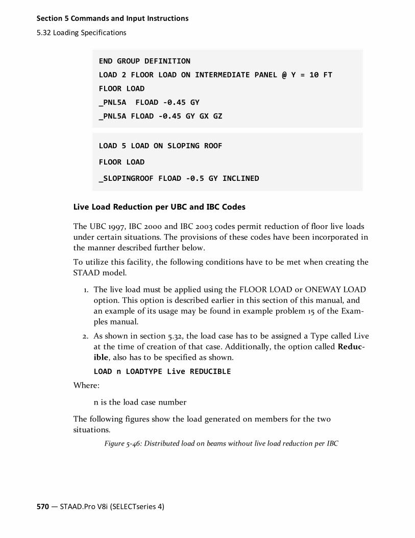
END GROUP DEFINITION
LOAD 2 FLOOR LOAD ON INTERMEDIATE PANEL @ Y = 10 FT
FLOOR LOAD
_PNL5A FLOAD -0.45 GY
_PNL5A FLOAD -0.45 GY GX GZ
LOAD 5 LOAD ON SLOPING ROOF
FLOOR LOAD
_SLOPINGROOF FLOAD -0.5 GY INCLINED
Live Load Reduction per UBC and IBC Codes
The UBC 1997, IBC 2000 and IBC 2003 codes permit reduction of floor live loadsunder certain situations. The provisions of these codes have been incorporated inthe manner described further below.
To utilize this facility, the following conditions have to be met when creating theSTAAD model.
1. The live load must be applied using the FLOOR LOAD or ONEWAY LOADoption. This option is described earlier in this section of this manual, andan example of its usage may be found in example problem 15 of the Exam-ples manual.
2. As shown in section 5.32, the load case has to be assigned a Type called Liveat the time of creation of that case. Additionally, the option called Reduc-ible, also has to be specified as shown.
LOAD n LOADTYPE Live REDUCIBLE
Where:
n is the load case number
The following figures show the load generated on members for the twosituations.
Figure 5-46: Distributed load on beams without live load reduction per IBC
570— STAAD.Pro V8i (SELECTseries 4)
Section 5 Commands and Input Instructions
5.32 Loading Specifications

Figure 5-47: Distributed load on beams of a floor after live load reduction per IBC 2003
CodeName
Section of codewhich
has beenimplemented
Applicable Equa-tions
UBC 1997 1607.5, page Equation 7-1
R = r(A-150) for FPSunits
R = r(A-13.94) for SIunits
IBC 2000 1607.9.2, page 302 Equation 16-2
R = r(A-150) for FPSunits
R = r(A-13.94) for SIunits
Table 5-25: Details of the code implementation
Section 5 Commands and Input Instructions
5.32 Loading Specifications
Technical Reference Manual — 571

CodeName
Section of codewhich
has beenimplemented
Applicable Equa-tions
IBC 2003 1607.9.2, page 277 Equation 16-22
R = r(A-150) for FPSunits
R = r(A-13.94) for SIunits
In the above equations,
A = area of floor supported by the member
R = reduction in percentage
R = rate of reduction equal to 0.08 for floors.
Notes
a. Only the rules for live load on Floors have been implemented. The rules forlive load on Roofs have not been implemented.
b. Since the medium of application of this method is the FLOOR LOAD orONEWAY LOAD feature, and since STAAD performs load generation onbeams only, the rules of the above-mentioned sections of the code for ver-tical members (columns) has not been implemented. The distributed loadon those members found to satisfy the requirements explained in the codewould have a lowered value after the reduction is applied.
c. Equation (7-2) of UBC 97, (16-3) of IBC 2000 and (16-23) of IBC 2003 havenot been implemented.
d. In the IBC 2000 and 2003 codes, the first note says “A reduction shall not bepermitted in Group A occupancies.” In STAAD, there is no direct methodfor conveying to the program that the occupancy type is Group A. So, it isthe user’s responsibility to ensure that when he/she decides to utilize thelive load reduction feature, the structure satisfies this requirement. If itdoes not, then the reduction should not be applied. STAAD does not checkthis condition by itself.
572— STAAD.Pro V8i (SELECTseries 4)
Section 5 Commands and Input Instructions
5.32 Loading Specifications

e. In the UBC 97 code, the last paragraph of section 1607.5 states that “Thelive load reduction shall not exceed 40 percent in garages for the storage ofprivate pleasure cars having a capacity of not more than nine passengersper vehicle.” Again, there is no method to convey to STAAD that the struc-ture is a garage for storing private pleasure cars. Hence, it is the user’sresponsibility to ensure that the structure satisfies this requirement. If itdoes not, then the reduction should not be applied. STAAD does not checkthis condition by itself.
f. Because all the three codes follow the same rules for reduction, no provisionis made available in the command syntax for specifying the code nameaccording to which the reduction is to be done.
5.32.5 Prestress Load SpecificationThis command may be used to specify PRESTRESSloads on members of thestructure.
General Format
MEMBER {PRESTRESS | POSTSTRESS } (LOAD)
memb-list FORCE f1 *{ ES f2 | EM f3 | EE f4 }
Where:
f1= Prestressing force. A positive value indicates precompression in
the direction of the local x-axis. A negative value indicatespretension.
f2= specifies eccentricity (from the centroid) of the prestress force at
the start of the member.
f3= specifies eccentricity (from the centroid) of the prestress force at
the mid-point of the member.
f4= specifies eccentricity (from the centroid) of the prestress force at
the end of the member.
Description
The first option, (MEMBER PRESTRESS LOAD), considers the effect of theprestressing force during its application. Thus, transverse shear generated at theends of the member(s) subject to the prestressing force is transferred to theadjacent members.
Section 5 Commands and Input Instructions
5.32 Loading Specifications
Technical Reference Manual — 573

The second option, (MEMBER POSTSTRESS LOAD), considers the effect of theexisting prestress load after the prestressing operation. Thus, transverse shear atthe ends of the member(s) subject to the prestressing force is not transferred tothe adjacent members.
Example
MEMBER PRESTRESS
2 TO 7 11 FORCE 50.0
MEMBER POSTSTRESS
8 FORCE 30.0 ES 3.0 EM -6.0 EE 3.0
In the first example, a prestressing force of 50 force units is applied through thecentroid (i.e., no eccentricity) of members 2 to 7 and 11. In the second example, apoststressing force of 30 force units is applied with an eccentricity of 3 lengthunits at the start, -6.0 at the middle, and 3.0 at the end of member 8.
One of the limitations in using this command is that under any one load case, onany given member, a prestress or poststress load may be applied only once. If thegiven member carries multiple stressed cables or has a PRESTRESS andPOSTSTRESS load condition, such a situation will have to be specified throughmultiple load cases for that member. See example below.
Incorrect Input:
LOAD 1
MEMBER PRESTRESS
6 7 FORCE 100 ES 2 EM -3 EE 2
6 FORCE 150 ES 3 EM -6 EE 3
PERFORM ANALYSIS
Correct aInput:
LOAD 1 MEMBER PRESTRESS
6 7 FORCE 100 ES 2 EM -3 EE 2
LOAD 2
MEMBER PRESTRESS
6 FORCE 150 ES 3 EM -6 EE 3
574— STAAD.Pro V8i (SELECTseries 4)
Section 5 Commands and Input Instructions
5.32 Loading Specifications

LOAD COMBINATION 3
1 1.0 2 1.0
PERFORM ANALYSIS
Examples for Modeling Techniques
The following examples describe the partial input data for the members andcable profiles shown below.
Figure 5-48: Example 1
JOINT COORD
1 0 0 ; 2 10 0
MEMBER INCI
1 1 2
…
UNIT …
LOAD 1
MEMBER POSTSTRESS
1 FORCE 100 ES 3 EM -3 EE 3
PERFORM ANALYSIS
Figure 5-49: Example 2
Section 5 Commands and Input Instructions
5.32 Loading Specifications
Technical Reference Manual — 575

JOINT COORD
1 0 0 ; 2 20 0
MEMBER INCI
1 1 2
…
UNIT …
LOAD 1
MEMBER PRESTRESS
1 FORCE 100 ES -3 EM -3 EE -3
PERFORM ANALYSIS
Figure 5-50: Example 3
JOINT COORD
1 0 0 ; 2 5 0 ; 3 15 0 0 ; 4 20 0
MEMBER INCI
1 1 2 ; 2 2 3 ; 3 3 4
…
UNIT …
LOAD 1
576— STAAD.Pro V8i (SELECTseries 4)
Section 5 Commands and Input Instructions
5.32 Loading Specifications

MEMBER PRESTRESS
1 FORCE 100 ES 3 EM 0 EE -3
2 FORCE 100 ES -3 EM -3 EE -3
3 FORCE 100 ES -3 EM 0 EE 3
PERFORM ANALYSIS
Figure 5-51: Example 4
JOINT COORD
1 0 0 ; 2 10 0 ; 3 20 0 0
MEMBER INCI
1 1 2 ; 2 2 3
…
UNIT …
LOAD 1
MEMBER PRESTRESS
1 FORCE 100 ES 3 EM 0 EE -3
2 FORCE 100 ES -3 EM 0 EE 3
PERFORM ANALYSIS
Figure 5-52: Example 5
JOINT COORD
1 0 0 ; 2 10 0 ; 3 20 0 0
Section 5 Commands and Input Instructions
5.32 Loading Specifications
Technical Reference Manual — 577

MEMBER INCI
1 1 2 ; 2 2 3
…
UNIT …
LOAD 1
MEMBER PRESTRESS
1 FORCE 100 ES 3 EM -3 EE 3
2 FORCE 100 ES 3 EM -3 EE 3
PERFORM ANALYSIS
5.32.6 Temperature Load Specification for Members, Plates,and Solids
This command may be used to specify TEMPERATURE loads or strain loads onmembers, plates, and solids; or strain loads on members.
General Format
TEMPERATURE LOAD
memb/elem-list { TEMP f1 f2 f4 | STRAIN f3 | STRAINRATE f5 }
Where:
f1= The change in temperature which will cause axial elongation in
the members or uniform volume expansion in plates and solids. Thetemperature unit is the same as the unit chosen for the coefficient ofthermal expansion ALPHA under the CONSTANT command.(Members/Plates/Solids)
f2= The temperature differential from the top to the bottom of the
member or plate (Ttop surface-Tbottom surface). If f2 is omitted, nobending will be considered. (Local Y axis) (Members/Plates). Sectiondepth must be entered for prismatic.
f4= The temperature differential from side to side of the member.
(Local Z axis) (Members). Section or flange width must be entered forprismatic.
578— STAAD.Pro V8i (SELECTseries 4)
Section 5 Commands and Input Instructions
5.32 Loading Specifications

f3= Initial axial elongation (+)/ shrinkage (-) in member due to misfit,
etc. in length unit (Members only).
f5= Initial axial elongation (+)/ shrinkage (-) per unit length, of
members only.
Example
UNIT MMS
TEMP LOAD
1 TO 9 15 17 TEMP 70.0
18 TO 23 TEMP 90.0 66.0
8 TO 13 STRAIN 3.0
15 27 STRAINRATE 0.4E-4
Notes
a. It is not necessary or possible to specify the units for temperature or forALPHA. The user must ensure that the value provided for ALPHA isconsistent in terms of units with the value provided for the temperatureload. (See "Specifying and Assigning Material Constants" on page 385).
If ALPHA was provided by a material name (STEEL, CONCRETE, ALUMINUM)then the temperature here must be in degree Fahrenheit units (if Englishlength units were in effect when Alpha was defined) or degree Celsius units(if metric length units were in effect when Alpha was defined).
5.32.7 Fixed-End Load SpecificationThis command may be used to specify FIXED END loads on members (beamsonly) of the structure.
General Format
FIXED ( END ) LOAD
memb-list FXLOAD f1, f2, ..... f12Where:
member_list = normal STAAD member list rules (TO and BY for
Section 5 Commands and Input Instructions
5.32 Loading Specifications
Technical Reference Manual — 579

generation; and - to continue list to next line).
f1... f
6= Force-x, shear-y, shear-z, torsion, moment-y, moment-z (all in
local coordinates) at the start of the member.
f7... f
12= Same as above except at the end of the member.
If less than 12 load values are entered, zero values will be added to the end. Theloads may be extended to one additional line by ending the first load line with a- (hyphen).
These loads are given in the member local coordinate system and the directionsare opposite to the actual load on the member.
5.32.8 Support Joint Displacement SpecificationThis command may be used to specify displacements (or generate loads to inducespecified displacements) in supported directions (pinned, fixed, enforced, orspring).
General Format
SUPPORT DISPLACMENT
support-joint-list { FX | FY | FZ | MX | MY | MZ } f1Where:
f1 = Value of the corresponding displacement. For translationaldisplacements, the unit is in the currently specified length unit, whilefor rotational displacements the unit is always in degrees.
FX, FY, FZ specify translational displacements in X, Y, and Z directionsrespectively. MX, MY, MZ specify rotational displacements in X, Y, and Zdirections.
Description
There are two distinct modes of usage for this command. If any “Enforced”specifications were used in the Support command then the “Displacement mode”is used; otherwise the “Load mode” is used. Despite the name of this command,if displacements are specified in spring directions, the displacement is at the jointnot at the grounded end of the support spring. Displacement cannot be specifiedin a direction that does not have a support or a spring.
580— STAAD.Pro V8i (SELECTseries 4)
Section 5 Commands and Input Instructions
5.32 Loading Specifications

1. DISPLACEMENT MODE - With this mode, the support joint displacementis modeled as an imposed joint displacement. The joint directions wheredisplacement may be specified must be defined (same for all cases) in theSUPPORT command, see section 5.27.1. Any beam members, springs or finiteelements will be considered in the analysis. Other loading, inclinedsupports, and master/slave are all considered. Any number of cases mayhave displacements entered. However, all cases will have zerodisplacements at the enforced directions if no displacement values areentered for that case. At inclined supports the displacement specification isassumed to be in the inclined direction. Displacements may not bespecified at slave directions.
If some cases are to have spring supports and others enforced displacementsat the same joint directions, then two PERFORM ANALYSES must be usedwith the CHANGE command in between. The first perform analysis couldhave the SUPPORTS with springs, no enforced directions, and with the loadcases without displacements. The second perform analysis would then haveSUPPORTS without springs but with enforced directions and the cases withdisplacements.
Displacement Mode Restrictions:
l The Support Displacement command may be entered only once percase.
l Spring directions and Enforced directions may not both be specifiedat the same joint direction in the same Perform Analysis step.
2. LOAD MODE - With this mode, the support joint displacement ismodeled as a load. Only beam members (not springs or finite elements)are considered in computing the joint load distribution necessary to causethe displacement. Other loading, inclined supports, and master/slave arealso not considered. These unconsidered factors, if entered, will result indisplacements other than those entered (results are superimposed). Onlythose cases with displacements entered will be affected.
Load Mode Restrictions:
l Support Displacements can be applied in up to four load cases only.
l The Support Displacement command may be entered only once percase.
l Finite elements should not be entered.
l Inclined supports must not be entered.
Section 5 Commands and Input Instructions
5.32 Loading Specifications
Technical Reference Manual — 581

l Spring supports are not considered in calculating the load so their usewill lead to displacements different from the input values.
Example
UNIT …
SUPPORT DISPL
5 TO 11 13 FY -0.25
19 21 TO 25 MX 15.0
In this example, the joints of the first support list will be displaced by 0.25 unitsin the negative global Y direction. The joints of the second support list will berotated by 15 degrees about the global X-axis.
5.32.9 Selfweight LoadUsed to calculate and apply the self weight of structural elements for analysis.
This command may be used to calculate and apply the SELFWEIGHT of thestructure for analysis.
General Format
SELFWEIGHT ( { X | Y | Z } f1) ( LIST member-list | ALL | _groupname )
Where:
f1
The factor to be used to multiply the selfweight. The defaultvalue is -1.0.
X, Y, & Z
represent the global direction in which the selfweight acts. Thedefault direction is along the Y axis.
member-list
member, plate and/or solid list or group. All list specificationssuch as explicit list including TO and BY, range (XR, YR, ZR), par-allel to (X, Y, Z) and groups are supported. If a group is used, the
582— STAAD.Pro V8i (SELECTseries 4)
Section 5 Commands and Input Instructions
5.32 Loading Specifications

selfweight command must be repeated for each group. If list isnot provided, all structural components are used for body weightcalculation unless those are inactive either by INACTIVE com-mand specification or internally set due to TEN-SION/COMPRESSION ONLY specification.
Description
This command is used if the self-weight of the members, plates, and solids withinthe structure is to be considered. The self-weight of every active element iscalculated and applied as a uniformly distributed member load.
Note: Surfaces are not included in the selfweight command. The SSELFWTmust be used to include the selfweight for surface elements. See"Surface Selfweight Load" on page 585
This command may also be used without any direction and factor specification.Thus, if specified as SELFWEIGHT, loads will be applied in the negative global Ydirection with a factor of unity.
Notes
a. Density must be provided for calculation of the self weight.
b. The selfweight of finite elements is converted to joint loads at the con-nected nodes and is not used as an element pressure load.
c. The selfweight of a plate is placed at the joints, regardless of plate releases.
d. The SELFWEIGHT specification for definition of static method of seismicload generator also is capable of accepting a list. Only there is no directionspecification for this command.
e. Similarly, the SELFWEIGHT specification when used in a Reference Load isalso capable of handling a list.
Example
LOAD 1 DEAD AND LIVE LOAD
* FACTORED WEIGHT FOR MEMBERS, PLATES, AND SOLIDS 4THROUGH 10 ALONG GLOBAL X DIRECTION
SELF WEIGHT X 1.4 LIST 4 TO 10
Section 5 Commands and Input Instructions
5.32 Loading Specifications
Technical Reference Manual — 583
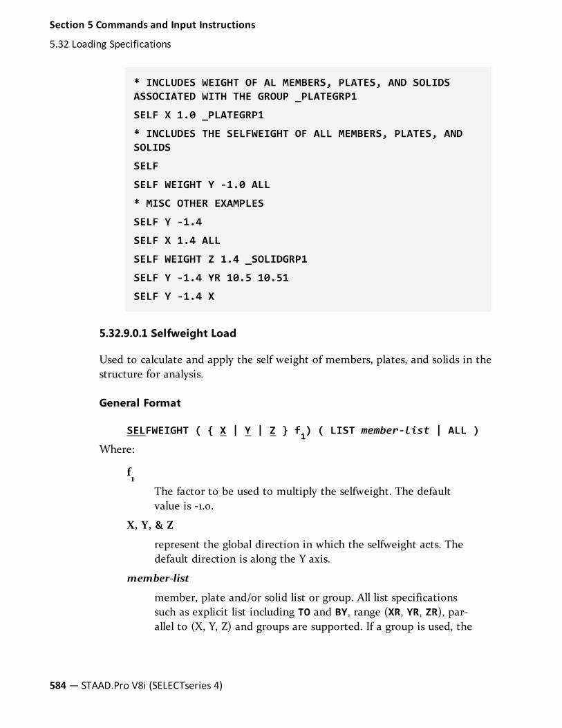
* INCLUDES WEIGHT OF AL MEMBERS, PLATES, AND SOLIDSASSOCIATED WITH THE GROUP _PLATEGRP1
SELF X 1.0 _PLATEGRP1
* INCLUDES THE SELFWEIGHT OF ALL MEMBERS, PLATES, ANDSOLIDS
SELF
SELF WEIGHT Y -1.0 ALL
* MISC OTHER EXAMPLES
SELF Y -1.4
SELF X 1.4 ALL
SELF WEIGHT Z 1.4 _SOLIDGRP1
SELF Y -1.4 YR 10.5 10.51
SELF Y -1.4 X
5.32.9.0.1 Selfweight Load
Used to calculate and apply the self weight of members, plates, and solids in thestructure for analysis.
General Format
SELFWEIGHT ( { X | Y | Z } f1) ( LIST member-list | ALL )
Where:
f1
The factor to be used to multiply the selfweight. The defaultvalue is -1.0.
X, Y, & Z
represent the global direction in which the selfweight acts. Thedefault direction is along the Y axis.
member-list
member, plate and/or solid list or group. All list specificationssuch as explicit list including TO and BY, range (XR, YR, ZR), par-allel to (X, Y, Z) and groups are supported. If a group is used, the
584— STAAD.Pro V8i (SELECTseries 4)
Section 5 Commands and Input Instructions
5.32 Loading Specifications

selfweight command must be repeated for each group. If list isnot provided, all structural components are used for body weightcalculation unless those are inactive either by INACTIVE com-mand specification or internally set due to TEN-SION/COMPRESSION ONLY specification.
Example
LOAD 1 DEAD AND LIVE LOAD
* INCLUDES THE SELFWEIGHT OF ALL MEMBERS, PLATES, ANDSOLIDS. THE FOLLOWING TWO COMMANDS ARE FUNCTIONALLYIDENTICAL
SELF
SELF WEIGHT Y -1.0 ALL
* FACTORED WEIGHT FOR MEMBERS, PLATES, AND SOLIDS 4THROUGH 10 ALONG GLOBAL X DIRECTION
SELF WEIGHT X 1.4 LIST 4 TO 10
* INCLUDES WEIGHT OF AL MEMBERS, PLATES, AND SOLIDSASSOCIATED WITH THE GROUP _PLATEGRP1
SELF X 1.0 _PLATEGRP1
5.32.9.0.2 Surface Selfweight Load
Used to calculate and apply the self weight of surface elements in the structurefor analysis.
Note: This feature requires STAAD.Pro V8i (SELECTseries 3) or higher.
General Format
SSELFWEIGHT ( { X | Y | Z } f1) ( LIST surface-list | ALL )
Where:
f1
Section 5 Commands and Input Instructions
5.32 Loading Specifications
Technical Reference Manual — 585

The factor to be used to multiply the selfweight. The defaultvalue is -1.0.
X, Y, & Z
represent the global direction in which the selfweight acts. Thedefault direction is along the Y axis.
surface-list
surface element list or group. All list specifications such asexplicit list including TO and BY, range (XR, YR, ZR), parallel to(X, Y, Z) and groups are supported. If a group is used, the self-weight command must be repeated for each group. If list is notprovided, all structural components are used for body weight cal-culation unless those are inactive either by INACTIVE commandspecification or internally set due to TENSION/COMPRESSIONONLY specification.
See "Selfweight Load" on page 584 for Description and Notes pertaining to selfweight.
Example
LOAD 1 LOADTYPE NONE TITLE DEAD LOAD
SURFACE LOAD
1 PR 1 0 0
SSELFWEIGHT Y -1
5.32.10 Dynamic Loading SpecificationThe command specification needed to perform response spectrum analysis andtime-history analysis is explained in the following sections.
5.32.10.1 Response Spectrum Analysis
Various methods for performing response spectrum analysis have beenimplemented in STAAD. They include a generic method that is described in mosttext books, as well as code based methods like those required by the Eurocode 8,IS 1893, etc. These are described in the following sections.
586— STAAD.Pro V8i (SELECTseries 4)
Section 5 Commands and Input Instructions
5.32 Loading Specifications
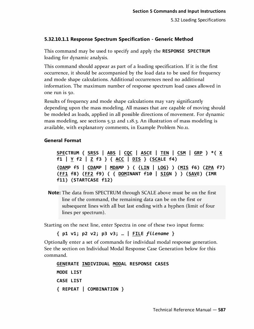
5.32.10.1.1 Response Spectrum Specification - Generic Method
This command may be used to specify and apply the RESPONSE SPECTRUMloading for dynamic analysis.
This command should appear as part of a loading specification. If it is the firstoccurrence, it should be accompanied by the load data to be used for frequencyand mode shape calculations. Additional occurrences need no additionalinformation. The maximum number of response spectrum load cases allowed inone run is 50.
Results of frequency and mode shape calculations may vary significantlydepending upon the mass modeling. All masses that are capable of moving shouldbe modeled as loads, applied in all possible directions of movement. For dynamicmass modeling, see sections 5.32 and 1.18.3. An illustration of mass modeling isavailable, with explanatory comments, in Example Problem No.11.
General Format
SPECTRUM { SRSS | ABS | CQC | ASCE | TEN | CSM | GRP } *{ Xf1 | Y f2 | Z f3 } { ACC | DIS } (SCALE f4)
{DAMP f5 | CDAMP | MDAMP } ( {LIN | LOG} ) (MIS f6) (ZPA f7)(FF1 f8) (FF2 f9) ( { DOMINANT f10 | SIGN } ) (SAVE) (IMRf11) (STARTCASE f12)
Note: The data from SPECTRUM through SCALE above must be on the firstline of the command, the remaining data can be on the first orsubsequent lines with all but last ending with a hyphen (limit of fourlines per spectrum).
Starting on the next line, enter Spectra in one of these two input forms:
{ p1 v1; p2 v2; p3 v3; … | FILE filename }
Optionally enter a set of commands for individual modal response generation.See the section on Individual Modal Response Case Generation below for thiscommand.
GENERATE INDIVIDUAL MODAL RESPONSE CASES
MODE LIST
CASE LIST
{ REPEAT | COMBINATION }
Section 5 Commands and Input Instructions
5.32 Loading Specifications
Technical Reference Manual — 587

END
Where:
ParameterDefaultValue
Description
f1, f2, f3 0.0 Factors for the input spectrum tobe applied in X, Y, & Z directions.Any one or all directions can beinput. Directions not providedwill default to zero.
f4 Linear scale factor by which thespectra data will be multiplied.Usually used to factor g’s tolength/sec2 units. This input isthe appropriate value of accel-eration due to gravity in the cur-rent unit system (thus, 9.81 m/s2
or 32.2 ft/s2).
f5 0.05 Damping ratio for all modeswhen DAMP is used. Default valueis 0.05 (5% damping if 0 or blankentered).
Table 5-26: Parameters used for generic model response spectrum
588— STAAD.Pro V8i (SELECTseries 4)
Section 5 Commands and Input Instructions
5.32 Loading Specifications

ParameterDefaultValue
Description
f6 Use Missing Mass method toinclude the static effect of themasses not represented in themodes. The spectral accelerationlength/sec2 for this missing massmode is the f6 value entered inlength per second squared units(this value is not multiplied bySCALE). If f6 is zero, then thespectral acceleration at the ZPA f7frequency is used. If f7 is zero ornot entered, then the spectralacceleration at 33Hz is used. Theresults of this calculation areSRSSed with the modalcombination results.
For SRSS, CQC, and TEN theresults of this calculation areSRSSed with the modalcombination results. For ABS,missing mass is ignored. ForASCE, the missing mass result isalgebraically added with the rigidparts of the extracted modes. ForASCE, the MIS option is assumedto be on. If any of f6, f7, f8, or f9are not entered, the defaults willbe used. Missing mass does notinclude the effect of masseslumped at the supports unless thesupport is a stiff spring or anEnforced support.
Note: If the MIS parameter isentered on anyspectrum case it will beused for all spectrumcases.
Section 5 Commands and Input Instructions
5.32 Loading Specifications
Technical Reference Manual — 589

ParameterDefaultValue
Description
f7 33 [Hz] For use with MIS option only.Defaults to 33 Hz if not entered.Value is printed but not used ifMIS f6 is entered.
f8 2 [Hz] The f1 parameter defined in theASCE 4-98 standard in Hz units.For ASCE option only.
f9 33 [Hz] The f2 parameter defined in theASCE 4-98 standard in Hz units.For ASCE option only.
f10 1 (1st Mode) Dominant mode method. Allresults will have the same sign asmode number f10 alone wouldhave if it were excited then thescaled results were used as astatic displacements result.Defaults to mode 1 if no valueentered. If a 0 value entered, thenthe mode with the greatest %participation in the excitationdirection will be used (only onedirection factor may be nonzero).
Note: Do not enter the SIGNparameter with thisoption. Ignored for theABS method ofcombining spectralresponses from eachmode.
590— STAAD.Pro V8i (SELECTseries 4)
Section 5 Commands and Input Instructions
5.32 Loading Specifications

ParameterDefaultValue
Description
f11 1 The number of individual modalresponses (scaled modes) to becopied into load cases. Defaultsto one. If greater than the actualnumber of modes extracted(NM), then it will be reset to NM.Modes one through f11 will beused. Missing Mass modes are notoutput.
f12 HighestLoad CaseNo. + 1
The primary load case number ofmode 1 in the IMR parameter.Defaults to the highest load casenumber used so far plus one. If f12is not higher than all prior loadcase numbers, then the defaultwill be used. For modes 2 throughNM, the load case number is theprior case no. plus one.
SRSS , ABS , CQC, ASCE4-98, CSM, GRP, & TEN Percent are methods ofcombining the responses from each mode into a total response. The CQC&ASCE4methods require damping, ABS, SRSS, CRM, GRP, and TEN do not use dampingunless Spectra-Period curves are made a function of damping (see File optionbelow). CQC, ASCE, CRM, GRP, and TEN include the effect of responsemagnification due to closely spaced modal frequencies. ASCE includes morealgebraic summation of higher modes. ASCE & CQC are more sophisticated andrealistic methods and are recommended.
SRSS
Square Root of Summation of Squares method.
CQC
Complete Quadratic Combination method (Default). This method is rec-ommended for closely spaced modes instead of SRSS..
ASCE
Section 5 Commands and Input Instructions
5.32 Loading Specifications
Technical Reference Manual — 591

NRC Regulatory Guide Rev. 2 (2006) Gupta method for modal com-binations and Rigid/Periodic parts of modes are used. The ASCE4-98 def-initions are used where there is no conflict. ASCE4-98 Eq. 3.2-21 (modifiedRosenblueth) is used for close mode interaction of the damped periodic por-tion of the modes.
ABS
Absolute sum. This method is very conservative and represents a worst casecombination.
CSM
Closely Spaced Method as per IS:1893 (Part 1)-2002 procedures.
GRP
Closely Spaced Modes Grouping Method. NRC Reg. Guide 1.92 (Rev. 1.2.1,1976).
TEN
Ten Percent Method of combining closely spaced modes. NRC Reg. Guide1.92 (Rev. 1.2.2, 1976).
ACC or DIS indicates whether Acceleration or Displacement spectra will beentered.
DAMP, MDAMP, and CDAMP Select source of damping input:
l DAMP indicates to use the f2value for all modes.
l MDAMP indicates to use the damping entered or computed with theDEFINE DAMP command if entered, otherwise default value of 0.05 will beused.
l CDAMP indicates to use the composite damping of the structure calculatedfor each mode. One must specify damping for different materials under theCONSTANT specification.
LIN or LOG: Select linear or logarithmic interpolation of the input Spectra versusPeriod curves for determining the spectra value for a mode given its period. LINis default. Since Spectra versus Period curves are often linear only on Log-Logscales, the logarithmic interpolation is recommended in such cases; especially ifonly a few points are entered in the spectra curve.
For LIN or LOG , when FILE filename is entered, the interpolation along thedamping axis will be linear. The last LIN-LOG parameter entered on all of thespectrum cases will be used for all spectrum cases.
592— STAAD.Pro V8i (SELECTseries 4)
Section 5 Commands and Input Instructions
5.32 Loading Specifications

SAVE : This option results in the creation of a file (file name with .ACCextension) containing the joint accelerations in g’s and radians/sec2
SIGN : This option results in the creation of signed values for all results. The sumof squares of positive values from the modes are compared to sum of squares ofnegative values from the modes. If the negative values are larger, the result isgiven a negative sign. This command is ignored for ABS option.
Warning: Do not enter DOMINANT parameter with this option.
Spectra data is input in one of these two input forms:
1. p1, v1; p2, v2; …. ; pn, vn. Data is part of input, immediately fol-lowing SPECTRUM command. Period – Value pairs (separated by semicolons) are entered to describe the Spectrum curve. Period is in seconds andthe corresponding Value is either acceleration (current length unit/sec2) ordisplacement (current length unit) depending on the ACC or DIS chosen.Continue the curve data onto as many lines as needed (up to 500 spectrumpairs). Spectrum pairs must be in ascending order of period. Note, if data isin g acceleration units, then set SCALE to a conversion factor to the currentlength unit (9.81, 386.4, etc.). Also note, do not end these lines with ahyphen (-). Each SPECTRUM command must be followed by Spectra data ifthis input form is used.
2. FILE filename data is in a separate file.
When the File filename command has been provided, then you musthave the spectra curve data on a file named FILENAME prior to starting theanalysis. The format of the FILE spectra data allows spectra as a function ofdamping as well as period.
Note: If the FILE fn command is entered, it must be with the firstspectrum case and will be used for all spectrum cases.
No File filename command needs to be entered with the remainingspectrum cases. The format is shown below. FILENAME may not be morethan 72 characters in length.
Example
LOAD 2 SPECTRUM IN X-DIRECTION
SELFWEIGHT X 1.0
Section 5 Commands and Input Instructions
5.32 Loading Specifications
Technical Reference Manual — 593

SELFWEIGHT Y 1.0
SELFWEIGHT Z 1.0
JOINT LOAD
10 FX 17.5
10 FY 17.5
10 FZ 17.5
SPECTRUM SRSS X 1.0 ACC SCALE 32.2
0.20 0.2 ; 0.40 0.25 ; 0.60 0.35 ; 0.80 0.43 ; 1.0 0.47
1.2 0.5 ; 1.4 0.65 ; 1.6 0.67 ; 1.8 0.55 ; 2.0 0.43
LOAD 2 SPECTRUM IN X-DIRECTION
SELFWEIGHT X 1.0
SELFWEIGHT Y 1.0
SELFWEIGHT Z 1.0
JOINT LOAD
10 FX 17.5
10 FY 17.5
10 FZ 17.5
SPECTRUM SRSS X 1.0 ACC SCALE 32.2
0.20 0.2 ; 0.40 0.25 ; 0.60 0.35 ; 0.80 0.43 ; 1.0 0.47
1.2 0.5 ; 1.4 0.65 ; 1.6 0.67 ; 1.8 0.55 ; 2.0 0.43
Multiple Response Spectra
If there is more than one response spectrum defined in the input file, the loaddata (representing the dynamic weight) should accompany the first set ofspectrum data only. In the subsequent load cases, only the spectra should bedefined. See example below.
LOAD 1 SPECTRUM IN X-DIRECTION
SELFWEIGHT X 1.0
SELFWEIGHT Y 1.0
594— STAAD.Pro V8i (SELECTseries 4)
Section 5 Commands and Input Instructions
5.32 Loading Specifications

SELFWEIGHT Z 1.0
JOINT LOAD
10 FX 17.5
10 FY 17.5
10 FZ 17.5
SPECTRUM SRSS X 1.0 ACC SCALE 32.2 IMR 2 STARTCASE 11
0.20 0.2 ; 0.40 0.25 ; 0.60 0.35 ; 0.80 0.43 ; 1.0 0.47
1.2 0.5 ; 1.4 0.65 ; 1.6 0.67 ; 1.8 0.55 ; 2.0 0.43
PERFORM ANALYSIS
CHANGE
*
LOAD 2 SPECTRUM IN Y-DIRECTION
SPECTRUM SRSS Y 1.0 ACC SCALE 32.2
0.20 0.1 ; 0.40 0.15 ; 0.60 0.33 ; 0.80 0.45 ; 1.00 0.48
1.20 0.51 ; 1.4 0.63 ; 1.6 0.67 ; 1.8 0.54 ; 2.0 0.42
File Format for Spectra Data
The format of the FILE spectra data allows spectra as a function of damping aswell as period. The format is:
Dataset 1 MDAMPCV NPOINTCV (no of values = 2)
Dataset 2 Damping Values in ascending order (no of values = Mdampcv)
Dataset 3a Periods (no of values = Npointcv)
3b Spectra (no of values = Npointcv)
For ASCE, the MIS option is assumed to be on. If any of f6, f7, f8, f9 are notentered the defaults will be used.
Repeat Data set 3 Mdampcv times (3a,3b , 3a,3b , 3a,3b , etc.) (i.e., for eachdamping value).
Data sets 2, 3a and 3b must have exactly Npointcv values each. Blanks or commasseparate the values. The data may extend to several lines. Do not end lines with ahyphen (-). No comment lines (*) or semi-colons. Multiple values may be enteredper line.
Section 5 Commands and Input Instructions
5.32 Loading Specifications
Technical Reference Manual — 595

l MDAMPCV= Number of damping values for which there will be separateSpectra vs. Period curves.
l NPOINTCV= Number of points in each Spectra vs. Period curve. IfNPOINTCV is negative, then the period-spectra values are entered as pairs.
Individual Modal Response Case Generation
Individual modal response (IMR) cases are simply the mode shape scaled to themagnitude that the mode has in this spectrum analysis case before it is combinedwith other modes. If the IMR parameter is entered, then STAAD will create loadcases for the first specified number of modes for this response spectrum case (i.e.,if five is specified then five load cases are generated, one for each of the first fivemodes). Each case will be created in a form like any other primary load case.
The results from an IMR case can be viewed graphically or through the printfacilities. Each mode can therefore be assessed as to its significance to the resultsin various portions of the structure. Perhaps one or two modes could be used todesign one area/floor and others elsewhere.
You can use subsequent load cases with Repeat Load combinations of thesescaled modes and the static live and dead loads to form results that are all withinternally consistent signs (unlike the usual response spectrum solutions). Themodal applied loads vector will be omega squared times mass times the scaledmode shape. Reactions will be applied loads minus stiffness matrix times thescaled mode shape.
With the Repeat Load capability, you can combine the modal applied loadsvector with the static loadings and solve statically with P-Delta or tension only.
Note:When the IMR option is entered for a Spectrum case, then a PerformAnalysis & Change must be entered after each such Spectrum case.
Input for using individual modal response cases is as follows:
GENERATE INDIVIDUAL MODAL RESPONSE CASES
MODE LIST mode_list
CASE LIST case_list
{ REPEAT | ( COMBINATION )}
END
Where:
596— STAAD.Pro V8i (SELECTseries 4)
Section 5 Commands and Input Instructions
5.32 Loading Specifications

MODE LIST =list of mode numbers that will have a corresponding IMRload case generated. Enter mode numbers separated by spaces and/oruse the “ii to jj” form or ALL. Default is mode 1. This data can becontinued on multiple lines by entering a hyphen at the end of eachline but the last. If the MODE LIST is entered more than once the datawill be concatenated.
CASE LIST = list of load case numbers that matches the mode list.These case numbers must not have been used for any other case. Ifmore cases than modes, the unused numbers will be ignored andremain available. If there are more modes than cases, then unusedcase numbers will be selected. Default will use unused case numbersfor all of the modes selected. This data can be continued on multiplelines by entering a hyphen at the end of each line but the last. If theCASE LIST is entered more than once the data will be concatenated..
REPEAT or COMBINATION = If COMBINATION is chosen then thesecases must not be entered in a REPEAT LOAD command. If REPEAT ischosen then the equivalent applied loads will be saved in a file. Inaddition, a static analysis of this case will be solved; and the case canthen be used in a REPEAT LOAD command. The default isCOMBINATION.
END = Used to end this data.
Example
LOAD 1 SPECTRUM IN X-DIRECTION
SELFWEIGHT X 1.0
SELFWEIGHT Y 1.0
SELFWEIGHT Z 1.0
JOINT LOAD
10 FX 17.5
10 FY 17.5
10 FZ 17.5
SPECTRUM CQC X 1.0 ACC SCALE 32.2
0.20 0.2 ; 0.40 0.25 ; 0.60 0.35 ; 0.80 0.43 ; 1.0 0.47
1.2 0.5 ; 1.4 0.65 ; 1.6 0.67 ; 1.8 0.55 ; 2.0 0.43
Section 5 Commands and Input Instructions
5.32 Loading Specifications
Technical Reference Manual — 597

GENERATE IND MOD RES
MODE LIST 1 2 TO 5
CASE LIST 11 12 TO 15
REPEAT
END
LOAD 2 SPECTRUM IN Y-DIRECTION
SPECTRUM SRSS Y 1.0 ACC SCALE 32.2
0.20 0.1 ; 0.40 0.15 ; 0.60 0.33 ; 0.80 0.45 ; 1.00 0.48
1.20 0.51 ; 1.4 0.63 ; 1.6 0.67 ; 1.8 0.54 ; 2.0 0.42
5.32.10.1.2 Response Spectrum Specification in Conjunction with the IndianIS: 1893 (Part 1)-2002
This command may be used to specify and apply the RESPONSE SPECTRUMloading as per IS: 1893 (Part 1)-2002 for dynamic analysis.
The seismic load generator can be used to generate lateral loads in the X and Zdirections only. Y is the direction of gravity loads.
Note: This facility has not been developed for cases where the Z axis is set tobe the vertical direction using the SET Z UP command.
Methodology
The design lateral shear force at each floor in each mode is computed by STAADin accordance with the Indian IS: 1893 (Part 1)-2002 equations 7.8.4.5c and7.8.4.5d.
Qik = Ak⋅φik⋅Pk⋅Wkand
V Q= Σiki i
n
ik= +1
Note: All symbols and notations in the above equation are as per IS: 1893(Part 1)-2002.
STAAD utilizes the following procedure to generate the lateral seismic loads.
598— STAAD.Pro V8i (SELECTseries 4)
Section 5 Commands and Input Instructions
5.32 Loading Specifications
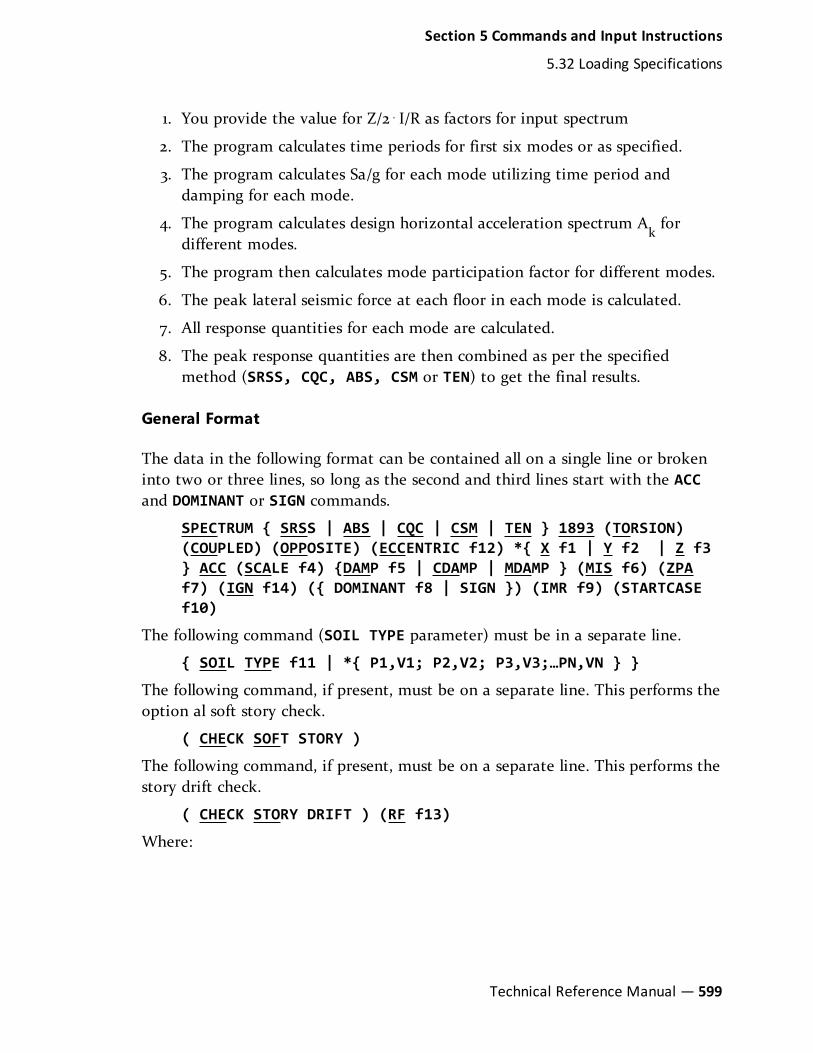
1. You provide the value for Z/2⋅I/R as factors for input spectrum
2. The program calculates time periods for first six modes or as specified.
3. The program calculates Sa/g for each mode utilizing time period anddamping for each mode.
4. The program calculates design horizontal acceleration spectrum Akfor
different modes.
5. The program then calculates mode participation factor for different modes.
6. The peak lateral seismic force at each floor in each mode is calculated.
7. All response quantities for each mode are calculated.
8. The peak response quantities are then combined as per the specifiedmethod (SRSS, CQC, ABS, CSM or TEN) to get the final results.
General Format
The data in the following format can be contained all on a single line or brokeninto two or three lines, so long as the second and third lines start with the ACCand DOMINANT or SIGN commands.
SPECTRUM { SRSS | ABS | CQC | CSM | TEN } 1893 (TORSION)(COUPLED) (OPPOSITE) (ECCENTRIC f12) *{ X f1 | Y f2 | Z f3} ACC (SCALE f4) {DAMP f5 | CDAMP | MDAMP } (MIS f6) (ZPAf7) (IGN f14) ({ DOMINANT f8 | SIGN }) (IMR f9) (STARTCASEf10)
The following command (SOIL TYPE parameter) must be in a separate line.
{ SOIL TYPE f11 | *{ P1,V1; P2,V2; P3,V3;…PN,VN } }
The following command, if present, must be on a separate line. This performs theoption al soft story check.
( CHECK SOFT STORY )
The following command, if present, must be on a separate line. This performs thestory drift check.
( CHECK STORY DRIFT ) (RF f13)
Where:
Section 5 Commands and Input Instructions
5.32 Loading Specifications
Technical Reference Manual — 599

ParameterDefaultValue
Description
f1, f2, f3 0.0 Factors for the input spectrum tobe applied in X, Y, & Z directions.These must be entered as theproduct of Z/2⋅I/R. Any one orall directions can be input. Direc-tions not provided will default tozero.
f4 1.0 Linear scale factor by whichdesign horizontal accelerationspectrum will be multiplied. Thisfactor signifies that the structuresand foundations, at which levelbase shear will be calculated, areplaced below the ground level.
Note: If site specific spectracurve is used then f4value is to bemultiplied by the scalefactor by which spectradata will be multiplied.Usually to factor g’s tolength/sec2 units.
f5 0.05 Damping ratio for all modeswhen DAMP is used. Default valueis 0.05 (5% damping if 0 or blankentered).
Table 5-27: Parameters used for IS: 1893 (Part 1) 2002 responsespectrum
600— STAAD.Pro V8i (SELECTseries 4)
Section 5 Commands and Input Instructions
5.32 Loading Specifications

ParameterDefaultValue
Description
f6 Use Missing Mass method. Thestatic effect of the masses notrepresented in the modes isincluded. The spectralacceleration for this missing massmode is the f6 value entered inlength/sec2 (this value is notmultiplied by SCALE).
If f6 is zero, then the spectralacceleration at the ZPA f7frequency is used. If f7 is zero ornot entered, the spectralacceleration at 33Hz (Zero PeriodAcceleration, ZPA) is used. Theresults of this calculation areSRSSed with the modalcombination results.
Note: If the MIS parameter isentered on anyspectrum case it will beused for all spectrumcases.
f7 33 [Hz] For use with MIS option only.Defaults to 33 Hz if not entered.Value is printed but not used ifMIS f6 is entered.
Section 5 Commands and Input Instructions
5.32 Loading Specifications
Technical Reference Manual — 601

ParameterDefaultValue
Description
f8 1 (1st Mode) Dominant mode method. Allresults will have the same sign asmode number f8 alone wouldhave if it were excited then thescaled results were used as astatic displacements result.Defaults to mode 1 if no valueentered. If a 0 value entered,then the mode with the greatest% participation in the excitationdirection will be used (only onedirection factor may be nonzero).
Note: Do not enter the SIGNparameter with thisoption. Ignored for theABS method ofcombining spectralresponses from eachmode.
f9 1 The number of individual modalresponses (scaled modes) to becopied into load cases. Defaultsto one. If greater than the actualnumber of modes extracted(NM), then it will be reset toNM. Modes one through f9 willbe used. Missing Mass modes arenot output.
602— STAAD.Pro V8i (SELECTseries 4)
Section 5 Commands and Input Instructions
5.32 Loading Specifications

ParameterDefaultValue
Description
f10 HighestLoad CaseNo. + 1
The primary load case number ofmode 1 in the IMR parameter.Defaults to the highest load casenumber used so far plus one. Iff10 is not higher than all priorload case numbers, then thedefault will be used. For modes 2through NM, the load casenumber is the prior case no. plusone.
f11 The soil type present. Dependingupon time period, types of soiland damping, average responseacceleration coefficient, S
a/g is
calculated.
1 = for rocky or hardsoil
2 = medium soil
3 = soft soil sites
P1,V1; P2,V2;P3,V3; … Pn,Vn
Data is part of input immediatelyfollowing spectrum command.Period - Value pairs (pairs sep-arated by semicolons) areentered to describe the spectrumcurve. Period is in seconds andthe corresponding Value is accel-eration (current length unit/sec2). If data is in g accelerationunits then the factor by whichspectra data will be multiplied isg to the current length unit (9.81,386.4, etc). Do not enter if a SoilType value is specified.
Section 5 Commands and Input Instructions
5.32 Loading Specifications
Technical Reference Manual — 603

ParameterDefaultValue
Description
f12 0.05 It is a factor which indicates theextent of accidental eccentricity.For all buildings this factor is tobe provided as 0.05. However,for highly irregular buildings thisfactor may be increased to 0.10.This factor is to be externally pro-vided to calculate design eccen-tricity.
f13 The response reduction factor. Ifnot specified, the program willlook for the factor defined underDEFINE 1893 LOAD (See "IndianIS:1893 (Part 1) 2002 Code -Lateral Seismic Load" on page449). If none is provided thereeither, a factor of 1.0 is assumed.
The response reduction factorrepresents ratio of maximumseismic force on a structureduring specified ground motion ifit were to remain elastic to thedesign seismic force. Actualseismic force is reduced by afactor RF to obtain design force.)
604— STAAD.Pro V8i (SELECTseries 4)
Section 5 Commands and Input Instructions
5.32 Loading Specifications

ParameterDefaultValue
Description
f14 0.009 It indicates the massparticipation (in percent) ofthose modes to be excludedwhile considering torsionprovision of IS-1893. Dependingupon the model it may be foundthat there are many local modesand torsional modes whose massparticipation is practicallynegligible. These modes can beexcluded without much change inthe final analysis result. If notprovided all modes will beconsidered. If none provided thedefault value of 0.009% will beconsidered. If IGN is entered onany one spectrum case it will beused for all spectrum cases.(Optional input)
Note: If the value of f14 isconsiderable it maylead to considerablevariation of analysisresult from the actualone. Hence cautionmust be taken whileusing IGN command.
SAVE: This option results in the creation of an Acceleration data file (.ACC fileextension) containing the joint accelerations in g's and radians/sec2. These filesare plain text and may be opened and viewed with any text editor (e.g.,Notepad).
SRSS , CQC, ABS, CSM and TEN are methods of combining the responses fromeach mode into a total response.
Section 5 Commands and Input Instructions
5.32 Loading Specifications
Technical Reference Manual — 605

l SRSS stands for square root of summation of squares,
l CQC for complete quadratic combination
l ABS for Absolute method.
l CSM is a closely-spaced modes grouping method where the peak responsequantities for closely spaced modes (considered to be within 10 percent ofeach other) are combined by Absolute method. This peak response quantityfor closely spaced modes is then combined with those of widely spacedmodes by SRSS method.
l TEN percent method combines modal responses as published in US NuclearRegulatory Guide 1.92 Revision 1 of February 1976.
Note: CQC, SRSS and CSM Grouping methods are recommended by IS:1893(Part 1) –2002.
1893 indicates the analysis as per IS:1893(Part 1)-2002 procedures.
TORSION indicates that the torsional moment (in the horizontal plane) arisingdue to eccentricity between the center of mass and center of rigidity needs to beconsidered. See "Torsion" on page 610 for additional information.
Note: If TOR is entered on any one spectrum case it will be used for allspectrum cases.
Lateral shears at story levels are calculated in global X and Z directions. Forglobal Y direction the effect of torsion will not be considered.
COUPLED indicates that the dynamic analysis had been performed for torsionallycoupled system. Only application of torsion from accidental eccentricity issufficient (i.e., the program will exclude torsion from dynamic eccentricity).(Optional input)
OPPOSITE indicates to consider horizontal torsional moment arising due toaccidental eccentricity in opposite direction. Since accidental eccentricity can beon either side one must consider lateral force acting at a floor level to beaccompanied by a clockwise or an anticlockwise accidental torsion moment.
Note: To provide accidental torsion in both clockwise and anticlockwisedirection, you must create two separate response spectrum load cases:one with only TORSION and the other with TORSION OPPOSITE.
ACC indicates Acceleration spectra will be entered.
606— STAAD.Pro V8i (SELECTseries 4)
Section 5 Commands and Input Instructions
5.32 Loading Specifications

DAMP, MDAMP, and CDAMP Select source of damping input:
l DAMP indicates to use the f2value for all modes.
l MDAMP indicates to use the damping entered or computed with theDEFINE DAMP command if entered, otherwise default value of 0.05 will beused.
l CDAMP indicates to use the composite damping of the structure calculatedfor each mode. One must specify damping for different materials under theCONSTANT specification.
SIGN = This option results in the creation of signed values for all results. The sumof squares of positive values from the modes are compared to sum of squares ofnegative values from the modes. If the negative values are larger, the result isgiven a negative sign. This option is ignored for ABS option for combiningresponses.
Warning: Do not enter DOMINANT parameter with the SIGN option.
If the MODE SELECT command is provided along with the IGN command, thenumber of modes excluded from the analysis will be those deselected by the MODESELECT command and also those deselected by the IGN command.
CHECK SOFT STORY indicates that soft story checking will be performed. Ifomitted from input, there will be no soft story checking. For additional details,See "Indian IS:1893 (Part 1) 2002 Code - Lateral Seismic Load" on page 449 inSection 5.31.2.5.
Individual Modal Response Case Generation
Individual modal response (IMR) cases are simply the mode shape scaled to themagnitude that the mode has in this spectrum analysis case before it is combinedwith other modes. If the IMR parameter is entered, then STAAD will create loadcases for the first specified number of modes for this response spectrum case (i.e.,if five is specified then five load cases are generated, one for each of the first fivemodes). Each case will be created in a form like any other primary load case.
The results from an IMR case can be viewed graphically or through the printfacilities. Each mode can therefore be assessed as to its significance to the resultsin various portions of the structure. Perhaps one or two modes could be used todesign one area/floor and others elsewhere.
You can use subsequent load cases with Repeat Load combinations of thesescaled modes and the static live and dead loads to form results that are all with
Section 5 Commands and Input Instructions
5.32 Loading Specifications
Technical Reference Manual — 607

internally consistent signs (unlike the usual response spectrum solutions). Themodal applied loads vector will be omega squared times mass times the scaledmode shape. Reactions will be applied loads minus stiffness matrix times thescaled mode shape.
With the Repeat Load capability, you can combine the modal applied loadsvector with the static loadings and solve statically with P-Delta or tension only.
Note:When the IMR option is entered for a Spectrum case, then a PerformAnalysis & Change must be entered after each such Spectrum case.
See "Response Spectrum Specification - Generic Method" on page 587 foradditional details on IMR load case generation.
Notes
a. The design base shear VB, calculated from the Response Spectrum method,
is compared with the base shear Vb, calculated by empirical formula for the
fundamental time period. If VBis less than V
b, all of the response quantities
are multiplied by Vb/VBas per Clause 7.8.2.
For this, the following input is necessary before defining any primary loadcase.
DEFINE 1893 LOAD
ZONEf1 1893-spec
SELFWEIGHT
JOINT WEIGHT
joint-list WEIGHT w
MEMBER WEIGHT
UNI v1 v2 v3
mem-list
CONv4 v5
CHECK SOFT STORY
608— STAAD.Pro V8i (SELECTseries 4)
Section 5 Commands and Input Instructions
5.32 Loading Specifications

1893-Spec= {RF f2, I f3, SS f4, (ST f5), DM f6, (PXf7), (PZ f8), (DT f9)}
Refer to Section 5.31.2.5 for full details on this command structure.
Note: STAAD does not calculate the fundamental frequency of thestructure needed for the empirical base shear Vb. calculation; soyou must enter either the ST parameter or the PX and PZparameters in the DEFINE 1893 LOAD data.
b. The following interpolation formula is adopted for interpolation betweendamping values as given in Table 3.
Interpolation and/or extrapolation of ground response acceleration for aparticular mode has been made for determining the spectrum ordinatescorresponding to the modal damping value for use in Response Spectrumanalysis. The relationship that shall be used for this purpose is defined by:
Sa = Ae-ξ + B/ξ
Where:
Sa = Spectrum ordinate
ξ = damping ratio
Constants A and B are determined using two known spectrum ordinates Sa1
and Sa2corresponding to damping rations ξ
1and ξ
2, respectively, for a
particular time period and are as follows:
A =S a ξ S a ξ
ξ e ξ e
−
−ξ ξ
1 1 2 2
1
− 12
− 2
B =ξ ξ S a e S a e
ξ e ξ e
( )−
−
ξ ξ
ξ ξ
1 2 2− 1
1− 2
1− 1
2− 2
Where:
ξ1 < ξ < ξ2c. The story drift in any story shall not exceed 0.004 times the story height asper Clause 7.11.1. To check this, the following command should be givenafter the analysis command.
PRINT STOREY DRIFT
A warning message will be printed if story drift exceeds this limitation.
d. If any soft story (as per definition in Table 5 of IS:1893-2002) is detected, awarning message will be printed in the output.
Section 5 Commands and Input Instructions
5.32 Loading Specifications
Technical Reference Manual — 609

Torsion
The torsion arising due to dynamic eccentricity (i.e., static eccentricity multipliedby dynamic amplification factor) between center of mass and center of rigidity isapplied along with accidental torsion, as per the recommendations of Cl. 7.9.2 ofthe IS 1893 code. The dynamic eccentricity is automatically calculated by the pro-gram (in both cases of TOR and TOR OPP options), while the amount of acci-dental eccentricity can be specified through the ECC option (if not specified,default of 5% of lateral dimension of the floor in the direction of the earthquakewill be considered).
Non-symmetric or torsionally unbalanced buildings are prone to earthquake dam-age due to coupled lateral and torsional movements (i.e., the translational vibra-tion of the building couples with its torsional vibrations within elastic range).The level of coupling between lateral and torsional vibrations of the building canbe larger, thus leading to significantly higher lateral-torsional coupling than thatpredicted by elastic analysis.
l Cl. 7.8.4.5 of IS 1893 (Part 1) : 2002 is valid for buildings with regular or nom-inally irregular plan configurations. For buildings which are irregular in plan,it is better to consider torsion from dynamic eccentricity into analysis; evenif torsionally coupled vibration is considered during response spectrum anal-ysis.
l Cl. 7.9.2 Note 2 of Amendment No. 1 January 2005 states that, in the casethat a 3D dynamic analysis is carried out, the dynamic amplification factor1.5—as given by Cl. 7.9.2—can be replaced by 1.0. This implies that the codealso recommends to use Cl. 7.9.2 for all types of buildings by including tor-sion from both dynamic and accidental eccentricity in the response spec-trum analysis.
Methodology
As per IS1893-2002 code, provision shall be made in all buildings for increase inshear forces on the lateral force resisting elements resulting from the horizontaltorsional moment arising due to eccentricity between the center of mass and thecenter of rigidity.
In response spectrum analysis all the response quantities (i.e. joint displacements,member forces, support reactions, plate stresses, etc) are calculated for eachmode of vibration considered in the analysis. These response quantities fromeach mode are combined using a modal combination method (either by CQC,
610— STAAD.Pro V8i (SELECTseries 4)
Section 5 Commands and Input Instructions
5.32 Loading Specifications
SRSS, ABS, TEN PERCENT, etc) to produce a single positive result for the givendirection of acceleration. This computed result represents a maximum magnitudeof the response quantity that is likely to occur during seismic loading. The actualresponse is expected to vary from a range of negative to positive value of thismaximum computed quantity.
No information is available from response spectrum analysis as to when thismaximum value occurs during the seismic loading and what will be the value ofother response quantities at that time. As for example, consider two joints J2 andJ3 whose maximum joint displacement in global X direction come out to be X1and X2 respectively. This implies that during seismic loading joint J1 will have Xdirection displacement that is expected to vary from -X1 to +X1 and that for jointJ2 from -X2 to +X2. However, this does not necessarily mean that the point oftime at which the X displacement of joint J1 is X1, the X displacement of joint J2will also be X2.
For the reason stated above, torsional moment at each floor arising due todynamic eccentricity along with accidental eccentricity (if any) is calculated foreach mode. Lateral story shear from this torsion is calculated forming global loadvectors for each mode. Static analysis is carried out with this global load vectorto produce global joint displacement vectors for each mode due to torsion. Thesejoint displacements from torsion for each mode are algebraically added to theglobal joint displacement vectors from response spectrum analysis for each mode.The final joint displacements from response spectrum along with torsion for allmodes are combined using specified modal combination method to get finalmaximum possible joint displacements. Refer to the steps explained below.
Steps
For each mode following steps are performed to include Torsion provision.
1. Lateral storey force at each floor is calculated. Refer Cl. 7.8.4.5c of IS 1893(Part 1) : 2002. (Q
ikat floor i for mode k)
2. At each floor design eccentricity is calculated. Refer Cl. 7.9.2 and Cl. 7.9.2Note 2 of Amendment No. 1 January 2005 of IS 1893 (Part 1) : 2002.
Section 5 Commands and Input Instructions
5.32 Loading Specifications
Technical Reference Manual — 611
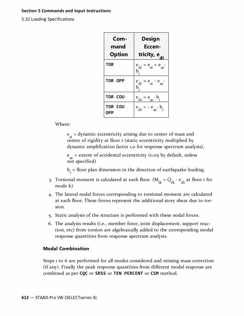
Com-mandOption
DesignEccen-
tricity, edi
TOR edi= e
si+ e
ac·
bi
TOR OPP edi= e
si- e
ac·
bi
TOR COU edi= e
ac· b
i
TOR COUOPP
edi= - e
ac· b
i
Where:
esi= dynamic eccentricity arising due to center of mass and
center of rigidity at floor i (static eccentricity multiplied bydynamic amplification factor 1.0 for response spectrum analysis),
eac= extent of accidental eccentricity (0.05 by default, unless
not specified)
bi= floor plan dimension in the direction of earthquake loading.
3. Torsional moment is calculated at each floor. (Mik= Q
ik· ediat floor i for
mode k)
4. The lateral nodal forces corresponding to torsional moment are calculatedat each floor. These forces represent the additional story shear due to tor-sion.
5. Static analysis of the structure is performed with these nodal forces.
6. The analysis results (i.e., member force, joint displacement, support reac-tion, etc) from torsion are algebraically added to the corresponding modalresponse quantities from response spectrum analysis.
Modal Combination
Steps 1 to 6 are performed for all modes considered and missing mass correction(if any). Finally the peak response quantities from different modal response arecombined as per CQC or SRSS or TEN PERCENT or CSM method.
612— STAAD.Pro V8i (SELECTseries 4)
Section 5 Commands and Input Instructions
5.32 Loading Specifications

Notes
After the analysis is complete following files are generated.
a. Story shear for each mode for each load case is given in the file <FILE-NAME>_RESP1893.TXT.
b. Rotational stiffness of each floor is given in the file <FILENAME>_ROT1893.TXT.
c. Center of mass, center of rigidity, design eccentricity at each floor level andadditional shear due to torsion at each floor level for each mode for eachload case is given in the file <FILENAME>_TOR1893.TXT.
5.32.10.1.3 Response Spectrum Specification per Eurocode 8 1996
This command may be used to specify and apply the RESPONSE SPECTRUMloading as per the 1996 edition of Eurocode 8 (EC8) for dynamic analysis.
General Format
SPECTRUM { SRSS | ABS | CQC | ASCE | TEN } EURO {ELASTIC| DESIGN} *{ X f1 | Y f2 | Z f3 } ACC
{DAMP f4 | CDAMP | MDAMP } ( {LIN | LOG} ) (MIS f5) (ZPA f6)({ DOMINANT f7 | SIGN }) (SAVE) (IMR f8) (STARTCASE f9)
Note: The data from SPECTRUM through ACC must be on the first line of thecommand, the remaining data can be on the first or subsequent lineswith all but last ending with a hyphen (limit of four lines perspectrum).
Starting on the next line, the response spectra is input using following standardinput parameters:
SOIL TYPE { A | B | C} ALPHA f10 Q f11
Where:
Section 5 Commands and Input Instructions
5.32 Loading Specifications
Technical Reference Manual — 613

ParameterDefaultValue
Description
f1, f2, f3 0.0 Factors for the input spectrum tobe applied in X, Y, & Z directions.Any one or all directions can beinput. Directions not providedwill default to zero.
f4 0.05 Damping ratio for all modeswhen DAMP is used. Default valueis 0.05 (5% damping if 0 or blankentered).
f5 Use Missing Mass method toinclude the static effect of themasses not represented in themodes. The spectral accelerationfor this missing mass mode is thef5 value entered in length persecond squared units (this valueis not multiplied by SCALE).
If f5 is zero, then the spectralacceleration at the ZPA f6frequency is used. If f6 is zero ornot entered, then the spectralacceleration at 33Hz is used. Theresults of this calculation areSRSSed with the modalcombination results.
Note: If the MIS parameter isentered on anyspectrum case it will beused for all spectrumcases.
Table 5-28: Parameters used for Eurocode 8 1996 response spec-trum
614— STAAD.Pro V8i (SELECTseries 4)
Section 5 Commands and Input Instructions
5.32 Loading Specifications

ParameterDefaultValue
Description
f6 33 [Hz] For use with MIS option only.Defaults to 33 Hz if not entered.Value is printed but not used ifMIS f5 is entered.
f7 1 (1st Mode) Dominant mode method. Allresults will have the same sign asmode number f7 alone wouldhave if it were excited then thescaled results were used as astatic displacements result.Defaults to mode 1 if no valueentered. If a 0 value entered,then the mode with the greatest% participation in the excitationdirection will be used (only onedirection factor may be nonzero).
Note: Do not enter the SIGNparameter with thisoption. Ignored for theABS method ofcombining spectralresponses from eachmode.
f8 1 The number of individual modalresponses (scaled modes) to becopied into load cases. Defaultsto one. If greater than the actualnumber of modes extracted(NM), then it will be reset to NM.Modes one through f8 will beused. Missing Mass modes are notoutput.
Section 5 Commands and Input Instructions
5.32 Loading Specifications
Technical Reference Manual — 615

ParameterDefaultValue
Description
f9 HighestLoad CaseNo. + 1
The primary load case number ofmode 1 in the IMR parameter.Defaults to the highest load casenumber used so far plus one. Iff12 is not higher than all priorload case numbers, then thedefault will be used. For modes 2through NM, the load casenumber is the prior case no. plusone.
f10 Alpha is defined to be designground acceleration expressed interms of acceleration due to grav-ity(g). For most of the appli-cation of Eurocode 8, the hazardis described in terms of a singleparameter (i.e., the value of effec-tive peak ground acceleration inrock or firm soil). This accel-eration is termed as the designground acceleration.
f11 Q is the behavior factor used toreduce the elastic response spec-tra to the design response spec-tra. The behavior factor is anapproximation of the ratio of theseismic forces, that the structurewould experience, if its responsewas completely elastic with 5%viscous damping, to the mini-mum seismic forces that may beused in design- with a con-ventional linear model still ensur-ing a satisfactory response of thestructure.
616— STAAD.Pro V8i (SELECTseries 4)
Section 5 Commands and Input Instructions
5.32 Loading Specifications

Unlike the custom defined response spectra, the EC 8 response spectra is notinput using frequency-acceleration pairs. Based on the type of Response Spectra(Elastic/Design), Soil Type, Alpha and Q the software generates the applicableresponse spectra curve using the guidelines of section 4.2.2 or 4.2.4 of Eurocode 8as applicable.
SRSS, ABS, CQC, CSM, & TEN Percent are methods of combining the responsesfrom each mode into a total response. CQC and TEN include the effect ofresponse magnification due to closely spaced modal frequencies. CQC is a moresophisticated and realistic method and is recommended.
l SRSS- Square Root of Summation of Squares method.
l CQC - Complete Quadratic Combination method. (Default).
l ABS - Absolute sum. (Very conservative worst case)
l TEN - Ten Percent Method of combining closely spaced modes. NRC Reg.Guide 1.92 (1976).
l CSM - Closely-Spaced Modes grouping method where the peak responsequantities for closely spaced modes (considered to be within 10 percent ofeach other) are combined using the Absolute method. This peak responsequantity for closely spaced modes is then combined with those of widelyspaced modes by SRSS method.
The specifier EURO is mandatory to denote that the applied loading is as per theguidelines of Eurocode 8.
The response spectrum loading can be based on either ELASTIC or DESIGNresponse spectra.
Within the scope of Eurocode 8 the earthquake motion at a given point of thesurface is generally represented by an elastic ground acceleration responsespectrum termed as “Elastic Response Spectrum”. STAAD generates the ElasticResponse Spectra using the guidelines of section 4.2.2 and Table 4.1 of Eurocode8.
The capacity of structural systems to resist seismic actions in the nonlinear rangegenerally permits their design for forces smaller than those corresponding to alinear elastic response. To avoid explicit nonlinear structural analysis in design,the energy dissipation capacity of the structure through mainly ductile behaviorof its elements and/or other mechanisms, is taken into account by performing alinear analysis based on a response spectrum which is a reduced form of thecorresponding elastic response spectrum. This reduction is accomplished by introducing the behavior factor Q and the reduced response spectrum is termed
Section 5 Commands and Input Instructions
5.32 Loading Specifications
Technical Reference Manual — 617

as “Design Response Spectrum”. STAAD generates the Elastic Response Spectrausing the guidelines of section 4.2.4 and Table 4.2 of Eurocode 8.
So, if the structure is supposed to resist seismic actions in the nonlinear range theDesign Response Spectra is to be used.
ACC indicates that the Acceleration spectra will be entered. Eurocode 8 does notprovide displacement response spectra.
DAMP, CDAMP, MDAMP: Select source of damping input.
l DAMP indicates to use the f4 value for all modes.
l CDAMP indicatesto use Composite modal damping if entered, otherwisesame as MDAMP.
l MDAMP indicates to use the damping entered or computed with theDEFINE DAMP command if entered, otherwise default value of 0.05 will beused.
LIN or LOG. Select linear or logarithmic interpolation of the input Spectraversus Period curves for determining the spectra value for a mode given itsperiod. LIN is default. Since Spectra versus Period curves are often linear onlyon Log-Log scales, the logarithmic interpolation is recommended in such cases;especially if only a few points are entered in the spectra curve.For LIN or LOG , when FILE fn is entered, the interpolation along thedamping axis will be linear.
Note: The last LIN-LOG parameter entered on all of the spectrum cases willbe used for all spectrum cases.
SAVE = The save option results in the creation of a file (file name with "Acc"extension) containing the joint accelerations in g’s and radians/sec2
SIGN = This option results in the creation of signed values for all results. The sumof squares of positive values from the modes are compared to sum of squares ofnegative values from the modes. If the negative values are larger, the result isgiven a negative sign. Do not enter DOMINANT parameter with the SIGNoption. SIGN option is ignored for ABS option.
SOIL TYPE parameter is used to define the subsoil conditions based on whichthe response spectra will be generated. Based on the subsoil conditions the soiltypes may be of three kinds
618— STAAD.Pro V8i (SELECTseries 4)
Section 5 Commands and Input Instructions
5.32 Loading Specifications
l Type A :for Rock or stiff deposits of sand
l Type B :for deep deposits of medium dense sand,gravel or medium stiffclays.
l Type C:Loose cohesionless soil deposits or deposits with soft to mediumstiff cohesive soil.
Please refer section 3.2 of Eurocode 8 for detailed guidelines regarding the choiceof soil type.
Individual Modal Response Case Generation
Individual modal response (IMR) cases are simply the mode shape scaled to themagnitude that the mode has in this spectrum analysis case before it is combinedwith other modes. If the IMR parameter is entered, then STAAD will create loadcases for the first specified number of modes for this response spectrum case (i.e.,if five is specified then five load cases are generated, one for each of the first fivemodes). Each case will be created in a form like any other primary load case.
The results from an IMR case can be viewed graphically or through the printfacilities. Each mode can therefore be assessed as to its significance to the resultsin various portions of the structure. Perhaps one or two modes could be used todesign one area/floor and others elsewhere.
You can use subsequent load cases with Repeat Load combinations of thesescaled modes and the static live and dead loads to form results that are all withinternally consistent signs (unlike the usual response spectrum solutions). Themodal applied loads vector will be omega squared times mass times the scaledmode shape. Reactions will be applied loads minus stiffness matrix times thescaled mode shape.
With the Repeat Load capability, you can combine the modal applied loadsvector with the static loadings and solve statically with P-Delta or tension only.
Note:When the IMR option is entered for a Spectrum case, then a PerformAnalysis & Change must be entered after each such Spectrum case.
See "Response Spectrum Specification - Generic Method" on page 587 foradditional details on IMR load case generation.
Section 5 Commands and Input Instructions
5.32 Loading Specifications
Technical Reference Manual — 619

Description
This command should appear as part of a loading specification. If it is the firstoccurrence, it should be accompanied by the load data to be used for frequencyand mode shape calculations. Additional occurrences need no additionalinformation. Maximum response spectrum load cases allowed in one run is 4.
Results of frequency and mode shape calculations may vary significantlydepending upon the mass modeling. All masses that are capable of moving shouldbe modeled as loads, applied in all possible directions of movement. For dynamicmass modeling, see sections 5.32 and 1.18.3 of STAAD Technical Reference Manual.An illustration of mass modeling is available, with explanatory comments, inExample Problem No.11_EC8.
Example
LOAD 2 SPECTRUM X-DIRECTION
SELFWEIGHT X 1.0
SELFWEIGHT Y 1.0
SELFWEIGHT Z 1.0
JOINT LOAD
10 FX 17.5
10 FY 17.5
10 FZ 17.5
MEMBER LOADS
5 CON GX 5.0 6.0
5 CON GY 5.0 6.0
5 CON GX 7.5 10.0
5 CON GY 7.5 10.0
5 CON GX 5.0 14.0
5 CON GY 5.0 14.0
SPECTRUM SRSS EURO ELASTIC X 1 ACC DAMP 0.05 –
LIN MIS 0 ZPA 40
SOIL TYPE A ALPHA 2 Q 1.5
620— STAAD.Pro V8i (SELECTseries 4)
Section 5 Commands and Input Instructions
5.32 Loading Specifications

Multiple Response Spectra
For special conditions more than one spectrum may be needed to adequatelyrepresent the seismic hazard over an area. This happens when the earthquakeaffecting the area are generated by sources varying widely in location and otherparameters. In those cases different values of ALPHA as well as Q may be requiredto indicate the different shapes of response spectrum for each type ofearthquake.
5.32.10.1.4 Response Spectrum Specification per Eurocode 8 2004
This command may be used to specify and apply the RESPONSE SPECTRUMloading as per the 2004 edition of Eurocode 8, ‘General Rules, seismic actions andrules for buildings’, BS EN 1998-1:2004. The graph of frequency – accelerationpairs are calculated based on the input requirements of the command and asdefined in the code.
General Format
SPECTRUM { SRSS | ABS | CQC | ASCE | TEN } EURO 2004{ELASTIC | DESIGN} {RS1 | RS2} *{ X f1 | Y f2 | Z f3 } ACC
{DAMP f4 | CDAMP | MDAMP } ( {LIN | LOG} ) (MIS f5) (ZPA f6)({ DOMINANT f7 | SIGN }) (SAVE) (IMR f8) (STARTCASE f9)
Note: The data SPECTRUM through ACC must be on the first line of thecommand, the remaining data can be on the first or subsequent lineswith all but last ending with a hyphen (limit of four lines perspectrum).
Starting on the next line, the response spectra is input using following standardinput parameters:
SOIL TYPE { A | B | C | D | E } ALPHA f10 Q f11
Where:
Section 5 Commands and Input Instructions
5.32 Loading Specifications
Technical Reference Manual — 621

ParameterDefaultValue
Description
f1, f2, f3 0.0 Factors for the input spectrum tobe applied in X, Y, & Z directions.Any one or all directions can beinput. Directions not providedwill default to zero.
f4 0.05 Damping ratio for all modeswhen DAMP is used. Default valueis 0.05 (5% damping if 0 or blankentered).
f5 Use Missing Mass method toinclude the static effect of themasses not represented in themodes. The spectral accelerationfor this missing mass mode is thef5 value entered in length persecond squared units (this valueis not multiplied by SCALE).
If f5 is zero, then the spectralacceleration at the ZPA f6frequency is used. If f6 is zero ornot entered, then the spectralacceleration at 33Hz is used. Theresults of this calculation areSRSSed with the modalcombination results.
Note: If the MIS parameter isentered on anyspectrum case it will beused for all spectrumcases.
Table 5-29: Parameters used for Eurocode 8 2004 response spec-trum
622— STAAD.Pro V8i (SELECTseries 4)
Section 5 Commands and Input Instructions
5.32 Loading Specifications

ParameterDefaultValue
Description
f6 33 [Hz] For use with MIS option only.Defaults to 33 Hz if not entered.Value is printed but not used ifMIS f5 is entered.
f7 1 (1st Mode) Dominant mode method. Allresults will have the same sign asmode number f7 alone wouldhave if it were excited then thescaled results were used as astatic displacements result.Defaults to mode 1 if no valueentered. If a 0 value entered,then the mode with the greatest% participation in the excitationdirection will be used (only onedirection factor may be nonzero).
Note: Do not enter the SIGNparameter with thisoption. Ignored for theABS method ofcombining spectralresponses from eachmode.
f8 1 The number of individual modalresponses (scaled modes) to becopied into load cases. Defaultsto one. If greater than the actualnumber of modes extracted(NM), then it will be reset to NM.Modes one through f8 will beused. Missing Mass modes are notoutput.
Section 5 Commands and Input Instructions
5.32 Loading Specifications
Technical Reference Manual — 623

ParameterDefaultValue
Description
f9 HighestLoad CaseNo. + 1
The primary load case number ofmode 1 in the IMR parameter.Defaults to the highest load casenumber used so far plus one. If f9is not higher than all prior loadcase numbers, then the defaultwill be used. For modes 2through NM, the load casenumber is the prior case no. plusone.
f10 Alpha is the ‘Ground AccelerationOn Type A Ground’ and definedin Eurocode 8 as a
g, as used in
equations 3.2 – 3.5. Refer to theEurocode for further information.
f11 Q is the ‘Behaviour Factor’ and isan approximation of the ratio ofthe seismic forces that the struc-ture would experience if itsresponse was completely elasticwith 5% viscous damping, to theseismic forces that may be usedin design, with a conventionalelastic analysis model, still ensur-ing a satisfactory response of thestructure.
Unlike the custom defined response spectra the EC 8 response spectra is notinput using frequency-acceleration pairs. Based on the type of Response Spectra(Elastic/Design), Soil Type, Alpha and Q the software generates the applicableresponse spectra curve using the guidelines of section 3.2.2.2 or 3.2.2.3 or 3.2.2.5 ofEurocode 8: 2004 as applicable.
SRSS, ABS, CQC, CSM, & TEN Percent are methods of combining the responsesfrom each mode into a total response. CQC and TEN include the effect ofresponse magnification due to closely spaced modal frequencies. CQC is a moresophisticated and realistic method and is recommended.
624— STAAD.Pro V8i (SELECTseries 4)
Section 5 Commands and Input Instructions
5.32 Loading Specifications

l SRSS - Square Root of Summation of Squares method.
l CQC - Complete Quadratic Combination method. (Default).
l ABS - Absolute sum. (Very conservative worst case)
l TEN - Ten Percent Method of combining closely spaced modes. NRC Reg.Guide 1.92 (1976).
l CSM - Closely-Spaced Modes grouping method where the peak responsequantities for closely spaced modes (considered to be within 10 percent ofeach other) are combined using the Absolute method. This peak responsequantity for closely spaced modes is then combined with those of widelyspaced modes by SRSS method.
See Sections 1.18.3, 5.30, and 5.34 of STAAD Technical Reference Manual
The keywords EURO 2004 is mandatory to denote that the applied loading is asper the guidelines of Eurocode 8.
The response spectrum loading can be based on either ELASTIC or DESIGNresponse spectra.
Two types of response spectra curve can be generated based on either RS1 (forresponse spectra type 1 curve) or RS2 (for response spectra type 2 curve) for eachELASTIC and DESIGN option.
Within the scope of Eurocode 8 the earthquake motion at a given point of thesurface is generally represented by an elastic ground acceleration responsespectrum termed as “Elastic Response Spectrum”. STAAD generates the ElasticResponse Spectra using the guidelines of section 4.2.2 and Table 4.1 of Eurocode8.
The capacity of structural systems to resist seismic actions in the nonlinear rangegenerally permits their design for forces smaller than those corresponding to alinear elastic response. To avoid explicit nonlinear structural analysis in design,the energy dissipation capacity of the structure through mainly ductile behaviorof its elements and/or other mechanisms, is taken into account by performing alinear analysis based on a response spectrum which is a reduced form of thecorresponding elastic response spectrum. This reduction is accomplished by introducing the behavior factor Q and the reduced response spectrum is termedas “Design Response Spectrum”. STAAD generates the Elastic Response Spectrausing the guidelines of section 4.2.4 and Table 4.2 of Eurocode 8. Therefore, ifthe structure is supposed to resist seismic actions in the nonlinear range theDesign Response Spectra should be specified.
Section 5 Commands and Input Instructions
5.32 Loading Specifications
Technical Reference Manual — 625

ACC indicates that the Acceleration spectra will be entered. Eurocode 8 does notprovide displacement response spectra.
DAMP , CDAMP , MDAMP. Defines the method of damping to be employed.
l DAMP signifies use of single damping factor f4 for all modes.
l CDAMP signifies use of Composite Modal Damping. This evaluates the damp-ing from that defined in the material or constant definitions. If there is nodamping information entered in the material or constant definitions, thebehavior is the same as MDAMP.
l MDAMP signifies the use of Modal Damping. If this option is selected, then aDEFINE DAMP command is required. If this has not been defined, then adefault value of 0.05 will be used. See Technical Reference Manual section5.26.4 Modal Damping Information for more information on this command.
LIN or LOG. Select linear or logarithmic interpolation of the input Spectra versusPeriod curves for determining the spectra value for a mode given its period. LINis default. Since Spectra versus Period curves are often linear only on Log-Logscales, the logarithmic interpolation is recommended in such cases; especially ifonly a few points are entered in the spectra curve.
SIGN = This option results in the creation of signed values for all results. The sumof squares of positive values from the modes are compared to sum of squares ofnegative values from the modes. If the negative values are larger, the result isgiven a negative sign.
Warning: Do not enter DOMINANT parameter with the SIGN option. SIGNoption is ignored for ABS option.
SAVE = The save option results in the creation of a file (file name with an .ACCextension) containing the joint accelerations in g’s and radians/sec2)
SOIL TYPE parameter is used to define the subsoil conditions based on whichthe response spectra will be generated as defined in Table 3.1 Ground Types.Based on the subsoil conditions the soil types may be of five kinds:
l Type A: rock or other rock-like geographical formation.
l Type B: very dense sand, gravel or very stiff clay.
l Type C: Deep deposits of dense or medium dense sand, gravel or stiff clay.
l Type D: Deposits of loose-to-medium cohesionless soil or of predominantlysoft to firm cohesive soil.
l Type E: Surface alluvium layer
626— STAAD.Pro V8i (SELECTseries 4)
Section 5 Commands and Input Instructions
5.32 Loading Specifications

Please refer section 3.2 of Eurocode8 for detailed guidelines regarding the choiceof soil type.
Individual Modal Response Case Generation
Individual modal response (IMR) cases are simply the mode shape scaled to themagnitude that the mode has in this spectrum analysis case before it is combinedwith other modes. If the IMR parameter is entered, then STAAD will create loadcases for the first specified number of modes for this response spectrum case (i.e.,if five is specified then five load cases are generated, one for each of the first fivemodes). Each case will be created in a form like any other primary load case.
The results from an IMR case can be viewed graphically or through the printfacilities. Each mode can therefore be assessed as to its significance to the resultsin various portions of the structure. Perhaps one or two modes could be used todesign one area/floor and others elsewhere.
You can use subsequent load cases with Repeat Load combinations of thesescaled modes and the static live and dead loads to form results that are all withinternally consistent signs (unlike the usual response spectrum solutions). Themodal applied loads vector will be omega squared times mass times the scaledmode shape. Reactions will be applied loads minus stiffness matrix times thescaled mode shape.
With the Repeat Load capability, you can combine the modal applied loadsvector with the static loadings and solve statically with P-Delta or tension only.
Note:When the IMR option is entered for a Spectrum case, then a PerformAnalysis & Change must be entered after each such Spectrum case.
See "Response Spectrum Specification - Generic Method" on page 587 foradditional details on IMR load case generation.
Description
This command should appear as part of a loading specification. If it is the firstoccurrence, it should be accompanied by the load data to be used for frequencyand mode shape calculations. Additional occurrences need no additionalinformation.
Results of frequency and mode shape calculations may vary significantlydepending upon the mass modeling. All masses that are capable of movingshould be modeled as loads, applied in all possible directions of movement. For
Section 5 Commands and Input Instructions
5.32 Loading Specifications
Technical Reference Manual — 627

dynamic mass modeling, see sections 5.32 and 1.18.3 of STAAD TechnicalReference Manual.
Example
LOAD 2 SPECTRUMIN X-DIRECTION
SELFWEIGHT X 1.0
SELFWEIGHT Y 1.0
SELFWEIGHT Z 1.0
JOINT LOAD
10 FX 17.5
10 FY 17.5
10 FZ 17.5
MEMBER LOADS
5 CON GX 5.0 6.0
5 CON GY 5.0 6.0
5 CON GX 7.5 10.0
5 CON GY 7.5 10.0
5 CON GX 5.0 14.0
5 CON GY 5.0 14.0
SPECTRUM SRSS EURO ELASTIC X 1 ACC DAMP 0.05 –
LIN MIS 0 ZPA 40
SOIL TYPE A ALPHA 2 Q 1.5
Multiple Response Spectra
For special conditions more than one spectrum may be needed to adequatelyrepresent the seismic hazard over an area. This happens when the earthquakeaffecting the area is generated by sources varying widely in location and otherparameters. In such cases different values of ALPHA as well as Q may be requiredto indicate the different shapes of response spectrum for each type ofearthquake.
628— STAAD.Pro V8i (SELECTseries 4)
Section 5 Commands and Input Instructions
5.32 Loading Specifications

5.32.10.1.5 Response Spectrum Specification per IBC 2006
This command may be used to specify and apply the RESPONSE SPECTRUMloading as per the 2006 edition of the ICC specification International BuildingCode (IBC), for dynamic analysis. The graph of frequency – acceleration pairs arecalculated based on the input requirements of the command and as defined inthe code.
Methodology
The methodology for calculating the response spectra is defined in ASCE-7-2005,section 11.4. The following is a quick summary:
a. Input Ssand S
1(this could have been searched from database or entered
explicitly)
b. Calculate
Sms= Fa x Ssand
Sm1 = Fv x S1Where:
Faand F
vare determined from the specified site classes A – E and using
tables 11.4-1 and 11.4-2. For site class F, the values must be supplied. Theseare required to be provided by the user. You may also specify values for F
aand F
vin lieu of table values.
c. Calculate
Sds = (2/3) Smsand
Sd1 = (2/3) Sm1The spectrum is generated as per section 11.4.5.
General Format
SPECTRUM { SRSS | ABS | CQC | ASCE | TEN } IBC 2006 *{ X f1| Y f2 | Z f3 } ACC
{DAMP f5 | CDAMP | MDAMP } ( {LIN | LOG} ) (MIS f6) (ZPA f7)({ DOMINANT f8 | SIGN }) (SAVE) (IMR f9) (STARTCASE f10)
Section 5 Commands and Input Instructions
5.32 Loading Specifications
Technical Reference Manual — 629

Note: The data from SPECTRUM through ACC must be on the first line of thecommand. The data shown on the second line above can be continuedon the first line or one or more new lines with all but last ending with ahyphen (limit of four lines per spectrum).
The command is completed with the following data which must be started on anew line:
{ZIP f11 | LAT f12 LONG f13 | SS f14 S1 f15 } SITE CLASS(f16) (FA f17 FV f18) TL f19
Where:
ParameterDefaultValue
Description
f1, f2, f3 0.0 Factors for the input spectrum tobe applied in X, Y, & Z directions.Any one or all directions can beinput. Directions not providedwill default to zero.
f5 0.05 Damping ratio for all modeswhen DAMP is used. Default valueis 0.05 (5% damping if 0 or blankentered).
Table 5-30: Parameters used for IBC 2006 response spectrum
630— STAAD.Pro V8i (SELECTseries 4)
Section 5 Commands and Input Instructions
5.32 Loading Specifications

ParameterDefaultValue
Description
f6 Optional parameter to use‘Missing Mass’ method. Thestatic effect of the masses notrepresented in the modes isincluded. The spectralacceleration for this missing massmode is the f6 value entered inlength/sec2 (this value is notmultiplied by SCALE).
If f6 is zero, then the spectralacceleration at the ZPA f7frequency is used. If f7 is zero ornot entered, the spectralacceleration at 33Hz (Zero PeriodAcceleration, ZPA) is used. Theresults of this calculation areSRSSed with the modalcombination results.
Note: If the MIS parameter isentered on anyspectrum case it will beused for all spectrumcases.
f7 33 [Hz] For use with MIS option only.Defaults to 33 Hz if not entered.Value is printed but not used ifMIS f6 is entered.
Section 5 Commands and Input Instructions
5.32 Loading Specifications
Technical Reference Manual — 631

ParameterDefaultValue
Description
f8 1 (1st Mode) Dominant mode method. Allresults will have the same sign asmode number f8 alone wouldhave if it were excited then thescaled results were used as astatic displacements result.Defaults to mode 1 if no value isentered. If a 0 value entered,then the mode with the greatest% participation in the excitationdirection will be used (only 1direction factor may be nonzero).
Note: Do not enter the SIGNparameter with thisoption. Ignored for theABS method ofcombining spectralresponses from eachmode.
f9 33 [Hz] The number of individual modalresponses (scaled modes) to becopied into load cases. Defaultsto one. If greater than the actualnumber of modes extracted(NM), then it will be reset to NM.Modes one through f9 will beused. Missing Mass modes are notoutput.
632— STAAD.Pro V8i (SELECTseries 4)
Section 5 Commands and Input Instructions
5.32 Loading Specifications

ParameterDefaultValue
Description
f10 HighestLoad CaseNo. + 1
The primary load case number ofmode 1 in the IMR parameter.Defaults to the highest load casenumber used so far plus one. Iff10 is not higher than all priorload case numbers, then thedefault will be used. For modes 2through NM, the load casenumber is the prior case no. plusone.
f11 The zip code of the site locationto determine the latitude andlongitude and consequently the S
sand S
1factors. (IBC 2006, ASCE
7-02 Chapter 22)
f12 The latitude of the site used withthe longitude to determine the S
sand S
1factors. (IBC 2006, ASCE
7-02 Chapter 22)
f13The longitude of the site usedwith the latitude to determinethe S
sand S
1factors. (IBC 2006,
ASCE 7-02 Chapter 22)
f14 Mapped MCE for 0.2s spectralresponse acceleration. (IBC 2006,ASCE 7-02 Chapter 22)
f15 Mapped spectral acceleration fora 1-second period. (IBC 2000,equation 16-17. IBC 2003, ASCE7-02 section 9.4.1.2.4-2. IBC2006, ASCE 7-05 Section 11.4.1)
Section 5 Commands and Input Instructions
5.32 Loading Specifications
Technical Reference Manual — 633

ParameterDefaultValue
Description
f16 Enter A through F for the SiteClass as defined in the IBC code. (IBC 2000, Section 1615.1.1 page350. IBC 2003, Section 1615.1.1page 322. IBC 2006 ASCE 7-05Section 20.3)
f17 Optional Short-Period site coef-ficient at 0.2s. Value must be pro-vided if SCLASS set to F (i.e., 6). (IBC 2006, ASCE 7-05 Section11.4.3)
f18 Optional Long-Period site coef-ficient at 1.0s. Value must be pro-vided if SCLASS set to F (i.e., 6). (IBC 2006, ASCE 7-05 Section11.4.3)
f19 Long-Period transition period inseconds. (IBC 2006, ASCE 7-02Chapter 22)
SRSS, ABS, CQC, CSM, & TEN Percent are methods of combining the responsesfrom each mode into a total response. CQC and TEN include the effect ofresponse magnification due to closely spaced modal frequencies. CQC is a moresophisticated and realistic method and are recommended.
l SRSS- Square Root of Summation of Squares method.
l CQC - Complete Quadratic Combination method. (Default).
l ABS - Absolute sum. (Very conservative worst case)
l TEN - Ten Percent Method of combining closely spaced modes. NRC Reg.Guide 1.92 (1976).
l CSM - Closely-Spaced Modes grouping method where the peak responsequantities for closely spaced modes (considered to be within 10 percent ofeach other) are combined using the Absolute method. This peak response
634— STAAD.Pro V8i (SELECTseries 4)
Section 5 Commands and Input Instructions
5.32 Loading Specifications

quantity for closely spaced modes is then combined with those of widelyspaced modes by SRSS method.
Note: If SRSS is selected, the program will internally check whether there areany closely spaced modes or not. If it finds any such modes, it willswitch over to the CSM method. In the CSM method, the program willcheck whether all modes are closely spaced or not. If all modes areclosely spaced, it will switch over to the CQC method.
IBC2006 indicates that the spectrum should be calculated as defined in the IBC2006 specification.
ACC indicates that an acceleration spectrum is defined.
Source of damping input:
l MDAMP indicates to use the damping entered or computed with the DEFINEDAMP command if entered, otherwise default value of 0.05 will be used.
l CDAMP is the composite damping of the structure calculated for each mode.One must specify damping for different materials under CONSTANT spec-ification.
LIN, LOG The interpolation method of the spectrum curves for determining thespectrum value for modes intermediate points. LIN is default option if notspecified.
SIGN = This option results in the creation of signed values for all results. The sumof squares of positive values from the modes are compared to sum of squares ofnegative values from the modes. If the negative values are larger, the result isgiven a negative sign. Do not enter DOMINANT parameter with the SIGNoption. SIGN option is ignored for ABS option.
SAVE = Optional parameter to save the results in a file (file name with .ACCextension) containing the joint accelerations in g’s and radians/sec2)
Individual Modal Response Case Generation
Individual modal response (IMR) cases are simply the mode shape scaled to themagnitude that the mode has in this spectrum analysis case before it is combinedwith other modes. If the IMR parameter is entered, then STAAD will create loadcases for the first specified number of modes for this response spectrum case (i.e.,if five is specified then five load cases are generated, one for each of the first fivemodes). Each case will be created in a form like any other primary load case.
Section 5 Commands and Input Instructions
5.32 Loading Specifications
Technical Reference Manual — 635

The results from an IMR case can be viewed graphically or through the printfacilities. Each mode can therefore be assessed as to its significance to the resultsin various portions of the structure. Perhaps one or two modes could be used todesign one area/floor and others elsewhere.
You can use subsequent load cases with Repeat Load combinations of thesescaled modes and the static live and dead loads to form results that are all withinternally consistent signs (unlike the usual response spectrum solutions). Themodal applied loads vector will be omega squared times mass times the scaledmode shape. Reactions will be applied loads minus stiffness matrix times thescaled mode shape.
With the Repeat Load capability, you can combine the modal applied loadsvector with the static loadings and solve statically with P-Delta or tension only.
Note:When the IMR option is entered for a Spectrum case, then a PerformAnalysis & Change must be entered after each such Spectrum case.
See "Response Spectrum Specification - Generic Method" on page 587 foradditional details on IMR load case generation.
5.32.10.1.6 Response Spectrum Specification per SNiP II-7-81
This command may be used to specify and apply the RESPONSE SPECTRUMloading as per SNiP II-7-81 for dynamic analysis.
Note: This feature requires STAAD.Pro 2007.03 or greater.
General Format
SPECTRUM { SRSS | CQC } SNIP A f1 *{ {X f2 | KWX f3 KX1 f4} |{ Y f5 | KWY f6 KY1 f7 } | { Z f8 | KWZ f9 KZ1 f10 } ACC(SCALE f11)
{DAMP f12 | CDAMP | MDAMP } ( {LIN | LOG} ) (MIS f13) (ZPAf14) ({ DOMINANT f15 | SIGN }) SOIL { 1 | 2 | 3} (SAVE)
The data from SPECTRUM through SCALE above must be on the first line of thecommand, the remaining data can be on the first or subsequent lines with all butlast ending with a hyphen (limit of four lines per spectrum).
Where:
636— STAAD.Pro V8i (SELECTseries 4)
Section 5 Commands and Input Instructions
5.32 Loading Specifications

ParameterDefaultValue
Description
f1
Zoning factor, A, which is basedon maximum acceleration factorfor the seismic zone. This factormust be modified for SOIL typesother than 2. The exact zone fac-tor value used for a specific loca-tion requires engineeringjudgement. The following tableserves as a guide for accelerationsand corresponding zone factorswhich would be used.
f2, f5, and f8 0.0 Factors for the input spectrum tobe applied in X, Y, & Z directions.Any one or all directions can beinput. Directions not providedwill default to zero. Alternatively,you may input individual param-eters such as KWX, KX1 the prod-uct of which would be used as thefactor along that direction.
f11
A linear scaling factor by whichthe spectrum data will be mul-tiplied. This can be used to factor
f12
0.05 Damping ratio for all modeswhen DAMP is used. Default valueis 0.05 (5% damping if 0 or blankentered).
Table 5-31: Parameters for SNiP II-7-81 response spectrum
Section 5 Commands and Input Instructions
5.32 Loading Specifications
Technical Reference Manual — 637

ParameterDefaultValue
Description
f13
Use Missing Mass method toinclude the static effect of themasses not represented in themodes. The spectral accelerationlength/sec2 for this missing massmode is the f
13value entered in
length per second squared units(this value is not multiplied bySCALE). If f
13is zero, then the
spectral acceleration at the ZPAf14 frequency is used. If f14 is zeroor not entered, then the spectralacceleration at 33Hz is used. Theresults of this calculation areSRSSed with the modalcombination results.
For SRSS and CQC, the results ofthis calculation are SRSSed withthe modal combination results. Ifeither f
13or f
14are not entered,
the defaults will be used. Missingmass does not include the effectof masses lumped at the supportsunless the support is a stiff springor an Enforced support.
Note: If the MIS parameter isentered on anyspectrum case it will beused for all spectrumcases.
638— STAAD.Pro V8i (SELECTseries 4)
Section 5 Commands and Input Instructions
5.32 Loading Specifications

ParameterDefaultValue
Description
f14
For use with MIS option only.Defaults to 33 Hz if not entered.Value is printed but not used ifMIS f13 is entered.
f15
Dominant mode method. Allresults will have the same sign asmode number f15 alone wouldhave if it were excited then thescaled results were used as astatic displacements result.Defaults to mode 1 if no value isentered. If a 0 value entered, thenthe mode with the greatest % par-ticipation in the excitation direc-tion will be used (only 1 directionfactor may be nonzero). Do notenter SIGN parameter with thisoption. Ignored for ABS option.
SRSS & CQC are methods of combining the responses from each mode into a totalresponse. The CQC method require damping, SRSS does not use damping unlessSpectra-Period curves are made a function of damping (see File option below).CQC includes the effect of response magnification due to closely spaced modalfrequencies. CQC is more sophisticated and realistic method and isrecommended.
l SRSS - Square Root of Summation of Squares method as prescribed by theSNiP II-7-81 code.
l CQC - Complete Quadratic Combination method.
The specifier SNIP is mandatory to denote that the applied loading is as per theguidelines of SNiP II-7-81.
ACC indicates that the definition is that of an acceleration spectrum.
DAMP, MDAMP, and CDAMP Select source of damping input:
Section 5 Commands and Input Instructions
5.32 Loading Specifications
Technical Reference Manual — 639

l DAMP indicates to use the f2value for all modes.
l MDAMP indicates to use the damping entered or computed with theDEFINE DAMP command if entered, otherwise default value of 0.05 will beused.
l CDAMP indicates to use the composite damping of the structure calculatedfor each mode. One must specify damping for different materials under theCONSTANT specification.
LIN or LOG: Select linear or logarithmic interpolation of the input Spectra versusPeriod curves for determining the spectra value for a mode given its period. LINis default. Since Spectra versus Period curves are often linear only on Log-Logscales, the logarithmic interpolation is recommended in such cases; especially ifonly a few points are entered in the spectra curve. The last LIN-LOG parameterentered on the spectrum cases will be used for all spectrum cases.
SIGN = This option results in the creation of signed values for all results. The sumof squares of positive values from the modes are compared to sum of squares ofnegative values from the modes. If the negative values are larger, the result isgiven a negative sign. Do not enter DOMINANT parameter with the SIGN option.
SOIL = Defines the subsoil conditions on which the response spectrum will begenerated.
Note: The Zoning Factor, A (f1), must be adjusted for soil types other than
type 2.
1. Non-weathered rock and rocklike geological formation or permafrost sub-soil.
2. Weathered rock or deep deposits of medium dense sand, gravel or mediumstiff clays.
3. Loose cohesion less soil deposits or deposits with soft to medium stiff cohe-sive soil.
SAVE = This option results in the creation of a file (file name with .ACCextension) containing the joint accelerations in g’s and radians/sec2
Description
Results of frequency and mode shape calculations may vary significantlydepending upon the mass modeling. All masses that are capable of moving shouldbe modeled as loads, applied in all possible directions of movement. For dynamic
640— STAAD.Pro V8i (SELECTseries 4)
Section 5 Commands and Input Instructions
5.32 Loading Specifications

mass modeling, see sections 5.32 and 1.18.3 of STAAD Technical Reference Manual.An illustration of mass modeling is available, with explanatory comments, in thesample file SEISMIC_RUSS.STD, which can be found in the STAAD.Proinstallation folder under SPROV8I/STAAD/EXAMP/RUS/.
Example
The definition of a SNiP response spectrum in the X direction on a structurebuilt on weather rock and where the Zoning Factor is 0.7071. As this is the firstload case with a response spectrum, then the masses are modeled as loads.
LOAD 2 LOADTYPE SEISMIC TITLE SPECTRUM IN X-DIRECTION
*MASSES
SELFWEIGHT X 1.0
SELFWEIGHT Y 1.0
SELFWEIGHT Z 1.0
JOINT LOAD
10 FX 17.5
10 FY 17.5
10 FZ 17.5
MEMBER LOADS
5 CON GX 5.0 6.0
5 CON GY 5.0 6.0
5 CON GX 7.5 10.0
5 CON GY 7.5 10.0
5 CON GX 5.0 14.0
5 CON GY 5.0 14.0
*SNIP SPECTRUM DEFINITION
SPECTRUM SRSS SNIP A 0.7071 X 1.0 ACC DAMP 0.05 SCALE 1.0LIN MIS 0 ZPA 40 SOIL 2
…
Note: The maximum response spectrum load cases allowed in one run is 50.
Section 5 Commands and Input Instructions
5.32 Loading Specifications
Technical Reference Manual — 641

For full details on Response Spectrum refer to section 5.32.10.1 Response SpectrumSpecification.
5.32.10.2 Application of Time Varying Load for Response HistoryAnalysis
Used to apply loads which are defined with a changing magnitude ofacceleration, force, or moment (See "Definition of Time History Load" on page507 ). These can either be assigned to specific nodes and/or globally to the all thesupports on the model as a ground motion. In addition to the data producedfrom a general modal analysis, a load case which includes time history loadingwill produce a set of graphs in the post processing mode to indicate how thedisplacement, velocity or acceleration of a selected node changes in each of thethree global directions over the time period of the applied dynamic loading. setof commands may be used to model Time History loading on the structure forResponse Time History analysis. Nodal time histories and ground motion timehistories may both be provided under one load case.
Notes
a. A Time History analysis requires the mode shapes. These are calculatedusing the mass matrix determined from the loading specified in the firstdynamic load case. (See "Modal Calculation Command" on page 671)
b. The Node Displacement table reports the maximum displacement thatoccurs at each node over the entire time range.
c. The displacement of the model at a specific time instance can be displayedby using the time slider bar on the Results toolbar when displaying a loadcase with time history loading.
d. If any Node Groups are defined, the time history graphs can be set to dis-play the average results for the group. The name of the selected node orgroup being displayed is given in the graph title bar.
e. A model can include only one load case with time history loads.
The following set of commands may be used to model Time History loading onthe structure for Response Time History analysis. Nodal time histories andground motion time histories may both be provided within one load case.
General Format
TIME LOAD
joint-list *{ FX | FY | FZ | MX | MY | MZ } It Ia f2
642— STAAD.Pro V8i (SELECTseries 4)
Section 5 Commands and Input Instructions
5.32 Loading Specifications
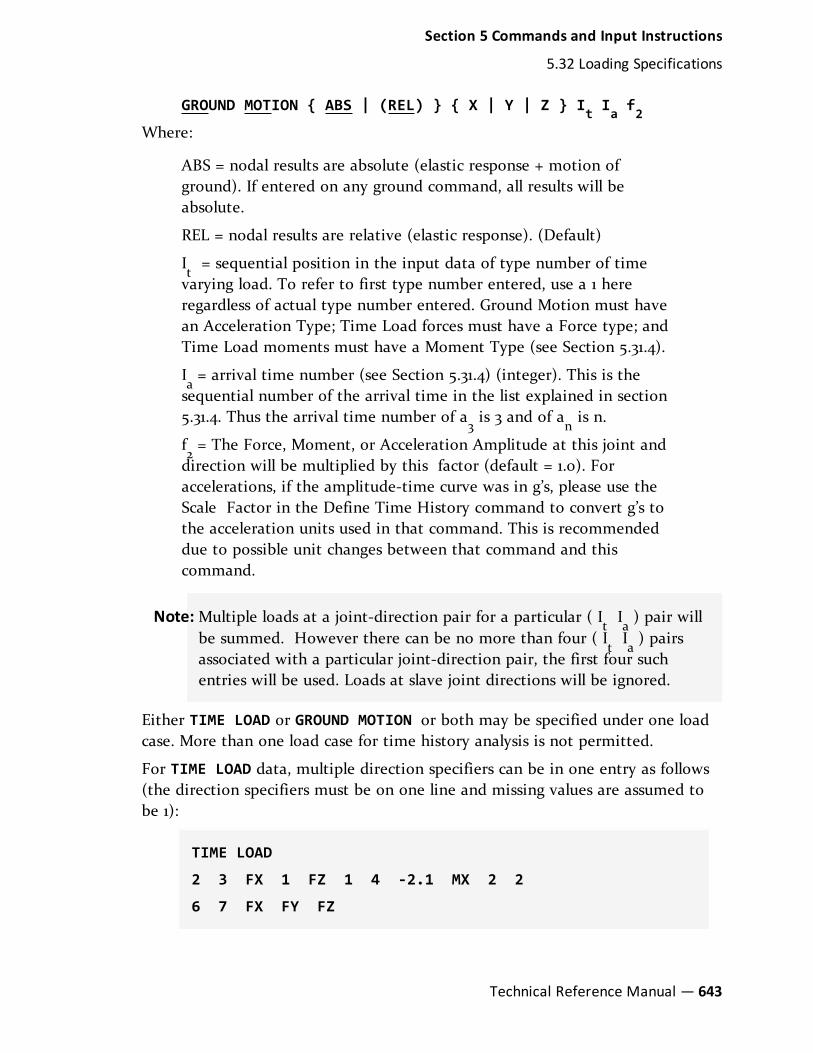
GROUND MOTION { ABS | (REL) } { X | Y | Z } It Ia f2Where:
ABS = nodal results are absolute (elastic response + motion ofground). If entered on any ground command, all results will beabsolute.
REL = nodal results are relative (elastic response). (Default)
It= sequential position in the input data of type number of time
varying load. To refer to first type number entered, use a 1 hereregardless of actual type number entered. Ground Motion must havean Acceleration Type; Time Load forces must have a Force type; andTime Load moments must have a Moment Type (see Section 5.31.4).
Ia= arrival time number (see Section 5.31.4) (integer). This is the
sequential number of the arrival time in the list explained in section5.31.4. Thus the arrival time number of a
3is 3 and of a
nis n.
f2= The Force, Moment, or Acceleration Amplitude at this joint and
direction will be multiplied by this factor (default = 1.0). Foraccelerations, if the amplitude-time curve was in g’s, please use theScale Factor in the Define Time History command to convert g’s tothe acceleration units used in that command. This is recommendeddue to possible unit changes between that command and thiscommand.
Note:Multiple loads at a joint-direction pair for a particular ( ItIa) pair will
be summed. However there can be no more than four ( ItIa) pairs
associated with a particular joint-direction pair, the first four suchentries will be used. Loads at slave joint directions will be ignored.
Either TIME LOAD or GROUND MOTION or both may be specified under one loadcase. More than one load case for time history analysis is not permitted.
For TIME LOAD data, multiple direction specifiers can be in one entry as follows(the direction specifiers must be on one line and missing values are assumed tobe 1):
TIME LOAD
2 3 FX 1 FZ 1 4 -2.1 MX 2 2
6 7 FX FY FZ
Section 5 Commands and Input Instructions
5.32 Loading Specifications
Technical Reference Manual — 643

Example
LOAD 1
SELFWEIGHT X 1.0
SELFWEIGHT Y 1.0
SELFWEIGHT Z 1.0
MEMBER LOADS
5 CON GX 7.5 10.0
5 CON GY 7.5 10.0
5 CON GZ 7.5 10.0
TIME LOAD
2 3 FX 1 3
5 7 FX 1 6
GROUND MOTION REL X 2 1
In the above example, the permanent masses in the structure are provided in theform of selfweight and member loads (see sections 5.32 and 1.18.3) for obtainingthe mode shapes and frequencies. The mass model can also be created using aReference Load case with the Loadtype of Mass (See "Mass Modeling UsingReference Loads" on page 533). The rest of the data is the input for application ofthe time varying loads on the structure. Forcing function type 1 is applied atjoints 2 and 3 starting at arrival time number 3. (Arrival time number 3 is 1.8seconds in example shown in section 5.31.4). Similarly, forcing function type 1 isapplied at joints 5 and 7 starting at arrival time number 6 (4.4 seconds). Aground motion (type 2) acts on the structure in the x-direction starting at arrivaltime number 1 (0.0 seconds).
5.32.10.3 Floor Spectrum Response
The following commands have been added in order to allow the responsespectrum of floors to be extracted from a time history analysis. The datagenerated consists of frequency versus acceleration pairs.
This command is used to specify the calculation of floor and/or joint spectra fromtime history results. The Floor Response Spectrum command must immediatelyfollow an analysis command. That analysis can only contain a single time historyload case.
644— STAAD.Pro V8i (SELECTseries 4)
Section 5 Commands and Input Instructions
5.32 Loading Specifications

General Format
The format of the Floor Spectrum command is such that 3 sets of data arerequired thus:
1. Initiate command
GENERATE FLOOR SPECTRUM
2. Specify Floor Groups
Next, identify the floors which will have spectrum curves generated eitherby referencing a NODE GROUP (see section 5.16) or explicitly listing the listof nodes that constitute the floor and the direction.
BEGIN FLOOR DIRECTION {GX | GY | GZ} (title)
{joint-group | joint-list}
Where:
GX, GY and GZ specify up to three global directions for whichfrequency versus acceleration spectrums will be generated for thisfloor.
title is an optional description of up to 50 characters, for thisfloor that will be displayed on the graphs in post processing.
The above can be repeated as many lines as necessary to specify all of thegroups and directions that are needed.
3. Specify Options
Next enter additional parameters used in the Floor Spectrum calculations.
OPTIONS { FLOW f1 | FHIGH f2 | FDELTA f3 | DAMP f4 |(RELATIVE) } (THPRINT i1) (SPRINT)
This command may be continued over a number of lines by ending eachline except the last with a hyphen.
Required parameters:
l f1 = Lowest frequency to be in the calculated spectrum. FLOW shouldbe greater than 0.01 Hz.
l f2 = Highest frequency to be in the calculated spectrum.
l f3 = The spectrum will be calculated at FDELTA intervals from FLOW toFHIGH
Section 5 Commands and Input Instructions
5.32 Loading Specifications
Technical Reference Manual — 645

l f4 = Up to 10 damping values may be entered. One spectrum will begenerated for each damping value for each global direction requestedfor each floor defined. The spectrum will be based on these modaldamping ratios. 3% damping should be entered as 0.03. The default is0.05.
l RELATIVE: If there is ground motion defined and you want the spec-trums to be based on the relative acceleration of the floor to theground acceleration, then include the RELATIVE parameter value.
Optional parameters:
l i1 = 0, no print; =2, Print the time history acceleration being used ineach spectrum calculation.
l SPRINT: Print the calculated spectrum.
4. End the command
Finally, the command is completed with the line:
END FLOOR SPECTURM
A successful analysis will result in the output file containing the base shearin the global X, Y and Z directions.
Example
DEFINE TIME HISTORY
TYPE 1 FORCE
0 -20 0.5 100 1 200 1.5 500 2 800 2.5 500 3 70 16 0
ARRIVAL TIME
0
DAMPING 0.075
*
LOAD 1 LOADTYPE SEISMIC TITLE TIME HISTORY LOAD CASE
* MASS MODEL REQUIRED
SELFWEIGHT X 1
SELFWEIGHT Y 1
SELFWEIGHT Z 1
JOINT LOAD
646— STAAD.Pro V8i (SELECTseries 4)
Section 5 Commands and Input Instructions
5.32 Loading Specifications

1 TO 6 FX 62.223 FY 62.223 FZ 62.223
* TIME LOADS
TIME LOAD
2 FX 1 1
PERFORM ANALYSIS
*
GENERATE FLOOR SPECTRUM
BEGIN FLOOR DIRECTION GX GZ GROUND MOTION
_FL1
_FL17
BEGIN FLOOR DIRECTION GX GZ FLOOR 18 A/C UNIT 36
_FL18
OPTIONS FLO 0.5 FHI 35.0 FDEL 0.1-
DAMP 0.03 0.05 0.07 –
RELATIVE
END FLOOR SPECTRUM
5.32.11 Repeat Load SpecificationThis command is used to create a primary load case using combinations ofpreviously defined primary load cases.
General Format
REPEAT LOAD
i1, f1, i2, f2 ... in, fnWhere:
i1, i2... i
n= primary load case numbers
f1, f2... f
n= corresponding factors
This command can be continued to additional lines by ending all but last with ahyphen. Limit of 550 prior cases may be factored. Prior cases to be factored mayalso contain the REPEAT LOAD command.
Section 5 Commands and Input Instructions
5.32 Loading Specifications
Technical Reference Manual — 647

Description
This command may be used to create a primary load case using combinations ofpreviously defined primary load case(s). The REPEAT LOAD differs from the loadCOMBINATION command (See "Load Combination Specification" on page 672) intwo ways:
1. A REPEAT LOAD is treated as a new primary load. Therefore, a P-Delta anal-ysis will reflect correct secondary effects. (LOAD COMBINATIONS, on theother hand, algebraically combine the results such as displacements,member forces, reactions and stresses of previously defined primary load-ings evaluated independently).
2. In addition to previously defined primary loads, you can also add new load-ing conditions within a load case in which the REPEAT LOAD is used.
3. The REPEAT LOAD option is available with load cases with JOINT LOADSand MEMBER LOADS. It can also be used on load cases with ELEMENTPRESSURE loads and FIXED END LOADS.
Modal dynamic analysis load cases (Response Spectrum, Time History,Steady State) should not be used in REPEAT LOAD. It is also not availablefor loads generated using some of the program’s load generation facilitiessuch as MOVING LOAD Generation. However load cases with WIND LOADmay be used in Repeat Load.
UBC cases may only be used in REPEAT LOAD if there is a PERFORMANALYSIS and CHANGE command after each UBC case. See notes with UBCLOAD command.
Prestress on a given member from 2 or more load cases cannot becombined.
Example:
LOAD 1 DL + LL
SELFWEIGHT Y -1.4
MEMBER LOAD
1 TO 7 UNIFORM Y -3.5
LOAD 2 DL + LL + WL
REPEAT LOAD
1 1.10
648— STAAD.Pro V8i (SELECTseries 4)
Section 5 Commands and Input Instructions
5.32 Loading Specifications

4. For a load case that is defined using the REPEAT LOAD attribute, theconstituent load cases themselves can also be REPEAT LOAD cases. See loadcase 4 below.
LOAD 1
SELFWEIGHT Y -1.0
LOAD 2
MEMBER LOAD
2 UNI GY -1.5
LOAD 3
REPEAT LOAD
1 1.5
LOAD 4
REPEAT LOAD
2 1.2 3 1.25
Notional Loads and Repeat Loads
Notional Loads (See "Notional Loads" on page 665 ) cannot be included in aREPEAT LOAD case. For example if the LOAD 2 is a notional load, you cannot useit in LOAD 3 using a REPEAT LOAD. The notional load will simply not be repeatedin such case.
Incorrect syntax:
LOAD 2 LOADTYPE NONE TITLE TEST-NOTIONAL
NOTIONAL LOAD
LOAD 3 LOADTYPE NONE TITLE TEST-COMBO
REPEAT LOAD
2 1.0
Or
LOAD 1 : DEAD
JOINT LOAD
Section 5 Commands and Input Instructions
5.32 Loading Specifications
Technical Reference Manual — 649

13 TO 16 29 TO 32 45 TO 48 61 TO 64 FY -100
NOTIONAL LOAD
1 X 0.002
LOAD 2 : IMPOSED
JOINT LOAD
13 TO 16 29 TO 32 45 TO 48 61 TO 64 FY -50
NOTIONAL LOAD
2 X 0.002
LOAD 3 : LOAD 1 + LOAD 2 + NOTIONAL LOADS
REPEAT LOAD
1 1.0 2 1.0
The correct syntax is:
LOAD 1 : DEAD
JOINT LOAD
13 TO 16 29 TO 32 45 TO 48 61 TO 64 FY -100
NOTIONAL LOAD
1 X 0.002
LOAD 2 : IMPOSED
JOINT LOAD
13 TO 16 29 TO 32 45 TO 48 61 TO 64 FY -50
NOTIONAL LOAD
2 X 0.002
LOAD 3 : LOAD 1 + LOAD 2 + NOTIONAL LOADS
REPEAT LOAD
1 1.0 2 1.0
NOTIONAL LOAD
650— STAAD.Pro V8i (SELECTseries 4)
Section 5 Commands and Input Instructions
5.32 Loading Specifications

1 X 0.002 2 X 0.002
5.32.12 Generation of LoadsThis command is used to generate Moving Loads, UBC Seismic loads and WindLoads using previously specified load definitions.
Primary load cases may be generated using previously defined load systems. Thefollowing sections describe generation of moving loads, UBC seismic loads andWind Loads.
5.32.12.1 Generation of Moving Loads
This command is used to generate Moving Loads using previously specified loaddefinitions.
Also see Sections 1.17 and 5.31.1
Pre-defined moving load system types may be used to generate the desirednumber of primary load cases, each representing a particular position of themoving load system on the structure. This procedure will simulate the movementof a vehicle in a specified direction on a specified plane on the structure.
General Format
LOAD GENERATION n (ADD LOAD i )
TYPE j x1 y1 z1 *{ XINC f1 | YINC f2 | ZINC f3 } ( { YRANGE| ZRANGE } r)
Where:
n = total no. of primary load cases to be generated.
i = load case no. for the previously defined load case to be added tothe generated loads.
j = type no. of previously defined load system.
x1, y1, z1= x, y and z coordinates (global) of the initial position of the
reference load.
f1, f2, f3= x, y or z (global) increments of position of load system to be
used for generation of subsequent load cases. Use only XINC & ZINC ifY up; Use only XINC & YINC if Z up.
Section 5 Commands and Input Instructions
5.32 Loading Specifications
Technical Reference Manual — 651

r = (Optional) defines section of the structure along global verticaldirection to carry moving load. This r value is added and subtractedto the reference vertical coordinate (y
1or z
1)in the global vertical
direction to form a range. The moving load will be externallydistributed among all members within the vertical range thusgenerated. r always should be a positive number. In other words, theprogram always looks for members lying in the range Y
1and Y
1+ABS
(r) or Z1and Z
1+ABS(r). The default r value is very small, so entering r
is recommended.
The ADD LOAD specification may be used to add a previously defined load caseto all the load cases generated by the LOAD GENERATION command. In theexample below, the SELFWEIGHT specified in load case 1 is added to all thegenerated load cases.
Sequential load case numbers will be assigned to the series of generated primaryload cases. Numbering will begin at one plus the immediate previous load casenumber. Allow for these when specifying load cases after load case generation.
Notes
a. Primary load cases can be generated from Moving Load systems for framemembers only. This feature does not work on finite elements.
b. This facility works best when the roadway, as well as the movement of thevehicle are along one of the global horizontal (X or Z) or (X or Y)directions. For bridge decks which are skewed with respect to the globalaxes, the load generation may not yield the most satisfactory results. Insuch cases, the STAAD.Beava program, which is an add-on module toSTAAD.Pro, is recommended. That program works on the influenceline/influence surface method, and is considerably superior to the movingload generator described in this section. It also has the advantage of beingable to calculate the critical load positions on decks modeled using plateelements, something which this facility cannot at present..
c. The x1, y1, z1values of the starting position of the reference wheel must be
provided bearing in mind that the reference wheel has to be at theelevation of the deck. An improper set of values of these parameters mayresult in the wheels being positioned incorrectly, and consequently, no loadmay be generated at all.
652— STAAD.Pro V8i (SELECTseries 4)
Section 5 Commands and Input Instructions
5.32 Loading Specifications

Example
LOAD 1 DL ONLY
SELFWEIGHT
LOAD GENERATION 20 ADD LOAD 1
TYPE 1 0. 5. 10. XI 10.
TYPE 2 0. 10. 10. ZI 15.
LOAD 22 LIVE LOAD ON PAVEMENT
MEMB LOAD
10 TO 20 30 TO 40 UNI GY -5.0
LOAD COMBINATION 31 10 0.75 22 0.75
PERFORM ANALYSIS
5.32.12.1.1 Generation of Seismic Loads
This command is used to generate UBC Seismic loads using previously specifiedload definitions.
5.32.12.1.2 Generation of UBC or IBC Seismic Loads
Built-in algorithms will automatically distribute the base shear amongappropriate levels and the roof per the relevant code specifications. The followinggeneral format should be used to generate loads in a particular direction.
General Format
LOAD i
code LOAD { X | Y | Z } (f1) (DEC f2) (ACC f3)
code = { UBC | IBC | 1893 | AIJ | COL | CFE | NTC | RPA }
Where:
i = load case number
f1= factor to be used to multiply the UBC Load (default = 1.0). May be
negative.
Section 5 Commands and Input Instructions
5.32 Loading Specifications
Technical Reference Manual — 653

f2= multiplying factor for Natural Torsion, arising due to static
eccentricity which is the difference between center of mass and centerof rigidity of a rigid floor diaphragm, to be used to multiply the UBC,IBC, 1893, etc. horizontal torsion load (default = 0.0). Must be apositive or zero.
f3= multiplying factor for Accidental Torsion, to be used to multiply
the UBC, IBC, 1893, etc. accidental torsion load (default = 1.0). May benegative (otherwise, the default sign for MY is used based on thedirection of the generated lateral forces).
Use only horizontal directions.
To include horizontal torsional moment arising due to static eccentricity for arigid floor diaphragm following conditions must be satisfied.
a. The floor must be modeled as a rigid diaphragm.
b. A positive value for DEC must be provided. If it is 0.0 (zero), then the onlyaccidental torsion will be considered for that particular seismic load case.
c. The ACC command must not be present in seismic definition (i.e., in theDEFINE code LOAD command). If present, the natural torsion factor will beignored and only the accidental torsion for all seismic loads will be con-sidered.
The design eccentricity for calculating horizontal torsion is the DEC + ACC values.When ACC is negative, it becomes DEC - ACC (i.e., the torsion magnitudes arealways additive).
Example
DEFINE UBC LOAD
ZONE 0.2 K 1.0 I 1.5 TS 0.5
SELFWEIGHT
JOINT WEIGHT
1 TO 100 WEIGHT 5.0
101 TO 200 WEIGHT 7.5
LOAD 1 UBC IN X-DIRECTION
UBC LOAD X DEC 1.0 ACC 0.05
JOINT LOAD
654— STAAD.Pro V8i (SELECTseries 4)
Section 5 Commands and Input Instructions
5.32 Loading Specifications

5 25 30 FY -17.5
PERFORM ANALYSIS
CHANGE
LOAD 2 UBC IN X-DIRECTION
UBC LOAD X DEC 1.0 ACC -0.05
JOINT LOAD
5 25 30 FY -17.5
PERFORM ANALYSIS
CHANGE
LOAD 3 UBC IN Z-DIRECTION
UBC LOAD Z DEC 0.0 ACC 0.05
PERFORM ANALYSIS
CHANGE
LOAD 3 DEAD LOAD
SELFWEIGHT
LOAD COMBINATION 4
1 0.75 2 0.75 3 1.0
In the above example, notice that the first three load cases are UBC load cases.They are specified before any other load cases.
Notes
a. The UBC load cases should be provided as the first set of load cases. Non-UBC primary load case specified before a UBC load case is not acceptable.Additional loads such as MEMBER LOADS and JOINT LOADS may bespecified along with the UBC load under the same load case.
Example of Incorrect Usage: The error here is that the UBC cases appear asthe 3rd and 4th cases, when they should be the 1st and 2nd cases.
LOAD 1
SELFWEIGHT Y -1
LOAD 2
Section 5 Commands and Input Instructions
5.32 Loading Specifications
Technical Reference Manual — 655

JOINT LOAD
3 FX 45
LOAD 3
UBC LOAD X 1.2
JOINT LOAD
3 FY -4.5
LOAD 4
UBC LOAD Z 1.2
MEMBER LOAD
3 UNI GY -4.5
PERFORM ANALYSIS
Example of Correct Usage
SET NL 10
LOAD 1
UBC LOAD X 1.2
JOINT LOAD
3 FY -4.5
PERFORM ANALYSIS
CHANGE
LOAD 2
UBC LOAD Z 1.2
MEMBER LOAD
3 UNI GY -4.5
PERFORM ANALYSIS
CHANGE
LOAD 3
SELFWEIGHT Y -1
LOAD 4
JOINT LOAD
656— STAAD.Pro V8i (SELECTseries 4)
Section 5 Commands and Input Instructions
5.32 Loading Specifications

3 FX 45
PERFORM ANALYSIS
LOAD LIST ALL
b. If the UBC cases are to be factored later in a Repeat Load command; or ifthe UBC case is to be used in a tension/compression analysis; or if Re-analysis (two analysis commands without a CHANGE or new load case inbetween); then each UBC case should be followed by PERFORM ANALYSISthen CHANGE commands as shown in the example above. Otherwise thePERFORM ANALYSIS then CHANGE can be omitted. Using the CHANGEcommand will require the SET NL command to define the maximumnumber of load cases being entered in the analysis. Also LOAD LIST ALLshould be entered after the last PERFORM ANALYSIS command.
Example of Incorrect Usage: The error here is that the CHANGE command ismissing before Load Case 2.
LOAD 1
UBC LOAD X 1.2
SELFWEIGHT Y -1
JOINT LOAD
3 FY -4.5
PDELTA ANALYSIS
LOAD 2
UBC LOAD Z 1.2
SELFWEIGHT Y -1
JOINT LOAD
3 FY -4.5
PDELTA ANALYSIS
Example of Correct Usage
LOAD 1
UBC LOAD X 1.2
SELFWEIGHT Y -1
Section 5 Commands and Input Instructions
5.32 Loading Specifications
Technical Reference Manual — 657
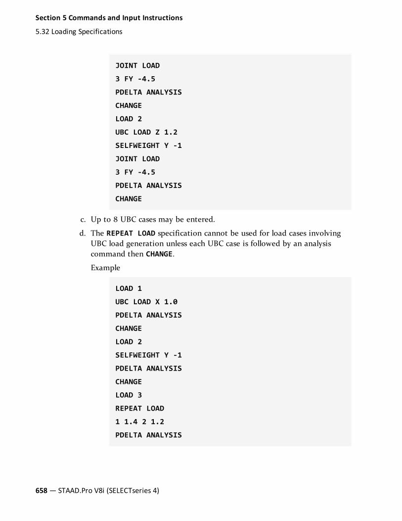
JOINT LOAD
3 FY -4.5
PDELTA ANALYSIS
CHANGE
LOAD 2
UBC LOAD Z 1.2
SELFWEIGHT Y -1
JOINT LOAD
3 FY -4.5
PDELTA ANALYSIS
CHANGE
c. Up to 8 UBC cases may be entered.
d. The REPEAT LOAD specification cannot be used for load cases involvingUBC load generation unless each UBC case is followed by an analysiscommand then CHANGE.
Example
LOAD 1
UBC LOAD X 1.0
PDELTA ANALYSIS
CHANGE
LOAD 2
SELFWEIGHT Y -1
PDELTA ANALYSIS
CHANGE
LOAD 3
REPEAT LOAD
1 1.4 2 1.2
PDELTA ANALYSIS
658— STAAD.Pro V8i (SELECTseries 4)
Section 5 Commands and Input Instructions
5.32 Loading Specifications

e. If UBC load generation is performed for the X and the Z (or Y if Z up) direc-tions, the command for the X direction must precede the command for theZ (or Y if Z up) direction.
5.32.12.1.3 Generation of IS:1893 Seismic Load
The following general format should be used to generate the IS 1893 load in aparticular direction.
General Format
LOAD i
1893 LOAD { X | Y | Z } (f1) (ACC f2)
where
i = load case number
f1= factor to be used to multiply the 1893 Load (default = 1.0)
f2= multiplying factor for Accidental Torsion, to be used to multiply
the UBC, IBC, 1893, etc. accidental torsion load (default = 1.0). May benegative (otherwise, the default sign for MY is used based on thedirection of the generated lateral forces).
Use only horizontal directions.
Example
In the above example, the first two load cases are the 1893 load cases. They arespecified before any other load case.
DEFINE 1893 LOAD
ZONE 0.05 RF 1.0 I 1.5 SS 1.0
SELFWEIGHT
JOINT WEIGHT
7 TO 12 WEIGHT 17.5
13 TO 20 WEIGHT 18.0
MEMBER WEIGHT
1 TO 20 UNI 2.0
Section 5 Commands and Input Instructions
5.32 Loading Specifications
Technical Reference Manual — 659

LOAD 1 1893 LOAD IN X-DIRECTION
1893 LOAD X
JOINT LOAD
5 25 30 FY -17.5
LOAD 2 1893 LOAD IN Z-DIRECTION
1893 LOAD Z
LOAD 3 DEAD LOAD
SELFWEIGHT
LOAD COMBINATION 4
1 0.75 2 0.75 3 10
5.32.12.2 Generation of Wind Loads
This command is used to generate Wind Loads using previously specified loaddefinitions.
The built-in wind load generation facility can be used to calculate the wind loadsbased on the parameters defined in Section 5.31.3. The following general formatshould be used to perform the wind load generation. See Section 1.17.3 for thetwo types of structures on which the load can be generated. For closed typestructures, the vertical panel areas bounded by beam members only (and ground),and exposed to the wind, are used to define loaded areas (plates and solids areignored). The loads generated are applied only at the joints at vertices of thebounded areas. For open type structures also, generation is done considering onlythe members in the model.
The automated load generator should only be used for vertical panels. Panels notparallel to the global Y axis (for Y UP) should be loaded separately.
General Format
LOAD i
WIND LOAD (-){ X | Y | Z } (f) TYPE j (OPEN) { XR f1 f2 | YRf1 f2 | ZR f1 f2 | LIST memb-list | ALL }
Where:
i = Load case number
660— STAAD.Pro V8i (SELECTseries 4)
Section 5 Commands and Input Instructions
5.32 Loading Specifications

X, -X, Z or -Z = Direction of wind in global axis system. Usehorizontal directions only.
j = Type number of previously defined systems;
f = The factor to be used to multiply the wind loads. Negative signsmay be used to indicate opposite direction of resulting load(default=1.0)
f1, f2= global coordinate values to specify X or Y or Z range for
member selection.
OPEN optional word to be used if loading is to be generated on open-type of structures. If this not specified, load will be generatedassuming the panels are “closed”.;
Using X, -X, Z or –Z and the f factor. With respect to the axis, a minus signindicates that suction occurs on the other side of the selected structure. If all ofthe members are selected and X (or Z) is used and the factor is positive, then theexposed surfaces facing in the –x (or –z) direction will be loaded in the positive x(or z) direction (normal wind in positive direction). See diagrams that follow. IfX and a negative factor is used, then the exposed surfaces facing in the +xdirection will be loaded in the negative x direction (normal wind in negativedirection). [If –X is entered and a negative factor, then the exposed surfacesfacing in the -x direction will be loaded in the negative x direction (suction). If –X is entered and a positive factor, then the exposed surfaces facing in the +xdirection will be loaded in the positive x direction (suction).]
Figure 5-53: Sign convention for internal and external pressure
Section 5 Commands and Input Instructions
5.32 Loading Specifications
Technical Reference Manual — 661

A member list or a range of coordinate values (in global system) may be used. Allmembers which have both end coordinates within the range are assumed to becandidates (for closed type structures) for defining a surface which may be loadedif the surface is exposed to the wind. The loading will be in the form of jointloads (not member loads). 1, 2 or 3 ranges can be entered to form a “layer”, “tube”or “box” for selecting members in the combined ranges. Use ranges to speed upthe calculations on larger models.
Example
DEFINE WIND LOAD
TYPE 1
INTENSITY 0.1 0.12 HEIGHT 100 200
EXP 0.6 JOI 1 TO 25 BY 7 29 TO 37 BY 4 22 23
TYPE 2
662— STAAD.Pro V8i (SELECTseries 4)
Section 5 Commands and Input Instructions
5.32 Loading Specifications

INT 0.1 0.12 HEIGHT 100 900
EXP 0.3 YR 0 500
LOAD 1
SELF Y -1.0
LOAD 2
WIND LOAD Z 1.2 TYPE 2 ZR 10 11
LOAD 3
WIND LOAD X TYPE 1 XR 7 8 ZR 14 16
LOAD 4 SUCTION ON LEEWARD SIDE
WIND LOAD -X 1.2 LIST 21 22 42
Example
For open structures
LOAD 1 WIND LOAD IN Z DIRECTION
WIND LOAD 2 -1.2 TYPE 1 OPEN
Notes
a. For closed type structures, panels or closed surfaces are generated by theprogram based on the members in the ranges specified and their end joints.The area within each closed surface is determined and the share of this area(influence area) for each node in the list is then calculated. The individualbounded areas must be planar surfaces, to a close tolerance, or they will notbe loaded.
Hence, one should make sure that the members/joints that are exposed tothe wind make up a closed surface (ground may form an edge of the closedsurface). Without a proper closed surface, the area calculated for the regionmay be indeterminate and the joint force values may be erroneous.Consequently, the number of exposed joints should be at least three.
b. Plates and solids are not considered for wind load generation. On suchentities, wind must be applied using pressure loading facilities for platesand solids.
Section 5 Commands and Input Instructions
5.32 Loading Specifications
Technical Reference Manual — 663

Figure 5-54: Load diagram for wind on open structures
5.32.13 Generation of Snow LoadsThis command is used to generate Snow Loads using previously specified Snowload definitions. This input should be a part of a load case.
General Format
SNOW LOAD
_flr_group TYPE j CS f1 { BALA | UNBA } { OBST | UNOB }{ MONO | HIP | GABLE }
Where:
_flr_group = The members that form the roof and that are to beloaded by snow load must be listed in a floor group (See section 5.16).
j = type no. of previously defined snow load system.
f1 = Roof Slope factor (CS). Default = 0.0. For sloped roofs, the roofslope factor is described in section 7.4 of the SEI/ASCE-7-02. A valueof 0 indicates that the roof is horizontal.
BALA or UNBA = Balanced or unbalanced snow load. Default isbalanced. These terms are described in section 7.6, and figures 7.3 and7.5 of ASCE 7-02.
664— STAAD.Pro V8i (SELECTseries 4)
Section 5 Commands and Input Instructions
5.32 Loading Specifications

OBST or UNOB = Obstructed or unobstructed. Default isunobstructed.
MONO or HIP or GABLE= Roof type. Default is MONO.
Use as many floor groups and types as necessary in each load case.
5.32.14 Notional LoadsA notional load is a lateral load (horizontal load) which is derived from anexisting vertical load case. This load type has been introduced to accommodate arequirement in design codes. The AISC 360-05 specification for example definesnotional loads as lateral loads that are applied at each framing level and arespecified in terms of gravity loads.
Description
Both Principal and Reference load cases can be selected and moved into theNotional Load Definition where the required factor and direction can bespecified. The notional loads are calculated and applied as joint loads.
Note: The actual values of the applied loading are not displayed in the UserInterface until after the analysis has been performed.
General Format
LOAD nLoad LOADTYPE type TITLE title
…
Load items
…
NOTIONAL LOAD
n { X | Z } (f1)
Where:
n = Load case number of the primary load case or reference load casewhich contains the vertical load items.
f1= factor by which the contents of LN are to be multiplied. Typically,
codes recommend 0.2 to 0.3 % (0.002 to 0.003). The default is 0.002or the factor specified in DIRECT ANALYSIS definition block. .
Section 5 Commands and Input Instructions
5.32 Loading Specifications
Technical Reference Manual — 665

Multiple load items can be specified under any NOTIONAL LOAD and there can beone or more blocks of NOTIONAL LOAD command(s) in any load case.
Note: Notional Loads can be derived from gravity load cases specified underthe DEFINE REFERENCE LOAD table which are described in section5.31.6
Example 1
LOAD 1 : DEAD
JOINT LOAD
13 TO 16 29 TO 32 45 TO 48 61 TO 64 FY -100
LOAD 2: DEAD NOTIONAL LOAD
NOTIONAL LOAD
1 X 0.002
…
LOAD 10: IMPOSED
JOINT LOAD
13 TO 16 29 TO 32 45 TO 48 61 TO 64 FY -50
LOAD 11:IMPOSED NOTIONAL LOAD
NOTIONAL LOAD
10 X 0.002
Example 2
If we want to combine the load cases in the example shown above, the correctsyntax would be
LOAD 3 : LOAD 1 + LOAD 2 + NOTIONAL LOADS
REPEAT LOAD
1 1.0 2 1.0
NOTIONAL LOAD
1 X 0.002 2 X 0.002
666— STAAD.Pro V8i (SELECTseries 4)
Section 5 Commands and Input Instructions
5.32 Loading Specifications

The following syntax would not include the contributions of Notional loads foreach component cases as Notional Loads are not going to be repeated.
LOAD 3 : LOAD 1 + LOAD 2 + NOTIONAL LOADS
REPEAT LOAD
1 1.0 2 1.0
Example 3
Similarly,
LOAD 1 LOADTYPE NONE TITLE TEST
SELFWEIGHT Y -1.15
MEMBER LOAD
143 145 CON GY -16
502 515 CON GY -95
LOAD 2 LOADTYPE NONE TITLE TEST-NOTIONAL
NOTIONAL LOAD
1 X 1.0
LOAD 3 LOADTYPE NONE TITLE TEST-COMBO
REPEAT LOAD
2 1.0
Load case 3 in the above example would produce no loads.
Example 4
Using Notional loads with REFERENCE loads
DEFINE REFERENCE LOADS
LOAD R1 LOADTYPE DEAD TITLE REF DEAD LOAD
SELFWEIGHT Y -1 LIST 1 TO 120
FLOOR LOAD
YRANGE 19 21 FLOAD -0.05 GY
YRANGE 39 41 FLOAD -0.05 GY
Section 5 Commands and Input Instructions
5.32 Loading Specifications
Technical Reference Manual — 667

LOAD R2 LOADTYPE LIVE TITLE REF LIVE LOAD
FLOOR LOAD
YRANGE 19 21 FLOAD -0.03 GY
YRANGE 39 41 FLOAD -0.03 GY
END DEFINE REFERENCE LOADS
**********************************************
* LOAD COMBINATIONS INCLUDING NOTIONAL LOADS *
**********************************************
*
*DEAD + LIVE +/- NOTIONAL LOAD
*
LOAD 1
REFERENCE LOAD
R1 1.2 R2 1.6
NOTIONAL LOAD
R1 X 0.0024 R2 X 0.0032
LOAD 2
REFERENCE LOAD
R1 1.2 R2 1.6
NOTIONAL LOAD
R1 X -0.0024 R2 X -0.0032
LOAD 3
REFERENCE LOAD
R1 1.2 R2 1.6
NOTIONAL LOAD
R1 Z 0.0024 R2 Z 0.0032
LOAD 4
REFERENCE LOAD
R1 1.2 R2 1.6
NOTIONAL LOAD
R1 Z -0.0024 R2 Z -0.0032
668— STAAD.Pro V8i (SELECTseries 4)
Section 5 Commands and Input Instructions
5.32 Loading Specifications

If a PRINT STATIC CHECK or PRINT LOAD DATA command is added with anyanalysis specification in the input file, the generated NOTIONAL LOADs wouldbe printed as in the following:
NOTIONAL LOAD - (POUN,FEET)
LOADING 4 DL+NDLX
JOINT DIRECTION LOAD
…
6117 X -0.00200 X 74124.266 = -148.249
6118 X -0.00200 X 115504.569 = -231.009
6119 X -0.00200 X 38397.157 = -76.794
6120 X -0.00200 X 15551.155 = -31.102
6121 X -0.00200 X 17347.718 = -34.695
6122 X -0.00200 X 29341.723 = -58.683
6123 X -0.00200 X 39771.147 = -79.542
6124 X -0.00200 X 39712.750 = -79.426
6125 X -0.00200 X 34006.254 = -68.013
==============================================
48554642.872 -97109.290
5.33 Reference Load Cases - ApplicationDescribes how you can call the data specified under those types in actual loadcases. Reference Load types are described in section 5.31.6 of this manual.
General FormatThe format of a reference to a Reference Load in a primary load (j) case is thus:
LOAD j LOADTYPE (type) load_title
REFERENCE LOAD
R(i) 1.0
…
Example
LOAD 1 LOADTYPE NONE TITLE D+L
REFERENCE LOAD
R1 1.0 R2 1.0
LOAD 2 LOADTYPE NONE TITLE DEAD+SNOW
REFERENCE LOAD
Section 5 Commands and Input Instructions
5.33 Reference Load Cases - Application
Technical Reference Manual — 669

R1 1.0 R3 1.0
LOAD 3 LOADTYPE NONE TITLE D+H
REFERENCE LOAD
R1 1.0 R4 1.0
ELEMENT LOAD
1212 1267 TRAP GY JT -0.54 -0.44 -0.44 -0.54.
5.34 Frequency CalculationThere are two methods available in STAAD for calculating the frequencies of astructure – 1) an approximate method called the Rayleigh method and 2) a moreexact method which involves the solution of an eigenvalue problem.
Both methods are explained in the following sections.
5.34.1 Rayleigh Frequency CalculationThis command may be used to calculate the Rayleigh method approximatefrequency of the structure for vibration corresponding to the general direction ofdeflection generated by the load case that precedes this command. Thus, thiscommand typically follows a load case.
General Format
CALCULATE RAYLEIGH (FREQUENCY)
Description
This command is specified after all other load specifications of any primary loadcase for which the Rayleigh frequency is calculated. This Rayleigh frequencycalculation is based on the Rayleigh iteration method using 1 iteration. If a moreaccurate, full-scale eigensolution is required, the MODAL CALCULATION command(see next section) may be used. A full eigensolution is automatically performed ifa RESPONSE SPECTRUM or TIME HISTORY is specified in any load case.
Example
LOADING 1
SELFWEIGHT X 1.0
670— STAAD.Pro V8i (SELECTseries 4)
Section 5 Commands and Input Instructions
5.34 Frequency Calculation

CALCULATE RAYLEIGH FREQUENCY
LOADING 2
SELFWEIGHT Z 1.0
CALCULATE RAYLEIGH FREQUENCY
LOADING 3 WIND LOAD
In this example, the Rayleigh frequency is calculated for the X direction mode ofvibration in load case 1, and the Z direction in case 2.
In case 1, the structure is being displaced by SELFWEIGHT applied statically alongglobal X. For most frames which are supported only at their base, this produces adeflected shape resembling the lowest mode shape along global X. Hence, thisfrequency will resemble that for the lowest X direction mode.
Similarly, the frequency calculated for load case 2 ought to be similar to that forthe lowest Z direction mode because the selfweight is applied statically alongglobal Z.
Hint: If you want a mode or frequency to be for lateral motion (X or Z), thenenter the loads in the X or Z directions. Entering loads in the verticaldirection when the lowest modes are in the lateral direction is acommon mistake.
The output will consist of the value of the frequency in cycles per second (cps),the maximum deflection along with that global direction and the joint numberwhere that maximum occurs.
Notes
This command is based on the Rayleigh method of iteration using 1 iteration.The frequency calculated estimates the frequency as if the structure wereconstrained to vibrate in the static deflected shape generated by the loads in theload case.
In many instances, the forces should be in one global direction to get the modeand frequency associated with that direction.
5.34.2 Modal Calculation CommandThis command may be used to obtain a full scale eigensolution to calculaterelevant frequencies and mode shapes. It should not be entered if this case or anyother case is a TIME LOAD or RESPONSE SPECTRUM case. For Steady
Section 5 Commands and Input Instructions
5.34 Frequency Calculation
Technical Reference Manual — 671

State/Harmonic analysis this command must be included in the load case thatdefines the weights and weight moment of inertias for eigensolutions (seesections 1.18.3 and 5.32).
General Format
MODAL (CALCULATION REQUESTED)
This command is typically used in a load case after all loads are specified. Theloads will be treated as weights and weight moment of inertias for eigensolutions(see sections 1.18.3 and 5.32). You are advised to specify the loads keeping this inmind.
This case will be independently solved statically and dynamically. Static resultsusing the loads will include joint displacements, member forces, supportreactions, and other outputs computed from a normal static analysis without anydynamic effects included.
STAAD.Pro can include the stress stiffening effect (geometric stiffness) based onthe axial member forces/plate in-plane stresses from a selected load case whencalculating the modes & frequencies of a structure.
In addition, the Dynamic results (using loads as masses) will include Mode Shapesand Frequencies.
Note: The MODAL CALCULATION command can be included in any of theprimary load cases, but only in one of them.
5.35 Load Combination SpecificationThis command may be used to combine the results of the analysis. The structurewill not be analyzed for the combined loading. The combination of results maybe algebraic, SRSS, a combination of both algebraic and SRSS, or Absolute.
Note: The LOAD COMBINATION specification is not appropriate for obtainingsecondary effects for combined loads. Refer to notes below.
General FormatLOAD COMBINATION ({ SRSS | ABS }) i a1i1 f1 i2 f2 … fsrss
Where:
672— STAAD.Pro V8i (SELECTseries 4)
Section 5 Commands and Input Instructions
5.35 Load Combination Specification

i = Load combination number. This can be any integer smaller than100,000 that is not the same as any previously defined primary loadcase or load combination number.
a1 = Any title for the load combination.
i1, i2... = represents the load case or load combination numbers which
are to be combined.
f1, f2... = represents corresponding factors to be applied to loadings. A
value of 0.0 is also allowed.
fSRSS
= optional factor to be applied as a multiplying factor on thecombined result of the SRSS load combination (see examples below).
A hyphen may be used at the end of a line to continue this command onto thenext line.
DescriptionIf the load combination option is left out (i.e., neither ABS or SRSS is included),then the results from analyses will be combined algebraically.
LOAD COMBINATION 6 DL+LL+WL
1 0.75 2 0.75 3 1.33
LOAD COMBINATION ABS
If the ABS load combination method is included, then the absolute value ofresults from the analyses will be combined.
LOAD COMBINATION ABS 7 DL+LL+WL
1 0.85 2 0.65 3 2.12
If the SRSS load combination method is included, then the results from analysesmay be combined both algebraically and using the SRSS (Square Root ofSummation of Squares) method. The combination scheme may be mixed ifrequired. For example, in the same load combination case, results from load casesmay be combined in the SRSS manner and then combined algebraically withother load cases.
Note: The case factor is not squared.
Section 5 Commands and Input Instructions
5.35 Load Combination Specification
Technical Reference Manual — 673

If some of the factors are negative, then the sum of the factored squares maybecome negative. If negative, the SQRT will be of the absolute value and theresult of the SQRT will be set negative.
Example of Simple SRSS CombinationSeveral combination examples are provided to illustrate the possible combinationschemes
LOAD COMBINATION SRSS 8 DL+SEISMIC
1 1.0 2 0.4 3 0.4
This (LOAD COMBINATION SRSS 8) illustrates a pure SRSS load combinationwith a default SRSS factor of one. The following combination scheme will beused:
v = 1.0⋅(1⋅L12 + 0.4⋅L22 + 0.4⋅L32)1/2
where
v = the combined value
L1, L2, and L3 = values from load cases 1, 2 and 3.
Since an SRSS factor is not provided, the default value of 1.0 is being used.
Notes
a. In the LOAD COMBINATION SRSS option, if the minus sign precedes anyload case no., then that load case will be combined algebraically with theSRSS combination of the rest.
b. If the secondary effects of combined load cases are to be obtained througha P-Delta, Member/Spring Tension/Compression, Multilinear Spring, orNonlinear Analysis, then the LOAD COMBINATION command isinappropriate for the purpose. See the REPEAT LOAD command (section5.32.11) for details.
c. In a load combination specification, a value of 0 (zero) as a load factor ispermitted. In other words, a specification such as
LOAD COMB 7
1 1.35 2 0.0 3 1.2 4 0.0 5 1.7
is permitted. This is the same as
LOAD COMB 7
674— STAAD.Pro V8i (SELECTseries 4)
Section 5 Commands and Input Instructions
5.35 Load Combination Specification

1 1.35 3 1.2 5 1.7
d. All combination load cases must be provided immediately after the lastprimary load case.
e. The total number of primary and combination load cases combined cannotexceed the limit described in section 5.2 of this manual.
f. A maximum of 550 load cases can be combined using a LOAD COMBINATIONcommand.
g. Load combinations can refer to previously defined load combinationnumbers.
Note: This feature requires build 20.07.07.30 or higher.
Examples of Algebraic & SRSS Combination in the Same LoadCombination Case
Example 1
LOAD COMBINATION SRSS 9
-1 0.75 2 1.3 3 2.42 0.75
The combination formula will be as follows:
v = 0.75⋅L1 + 0.75⋅(1.3⋅L22 + 2.42⋅L32)1/2
where
v = combined value
L2 & L3 = values from load cases 2 & 3.
In the above specification, a minus sign precedes load case 1. Thus, Load 1 iscombined algebraically with the result obtained from combining load cases 2 and3 in the SRSS manner. The SRSS factor of 0.75 is applied on the SRSScombination of 2 and 3.
Example 2
LOAD COMBINATION SRSS 10
-1 0.75 -2 0.572 3 1.2 4 1.7 0.63
Section 5 Commands and Input Instructions
5.35 Load Combination Specification
Technical Reference Manual — 675

Here, both load cases 1 and 2 are combined algebraically with the SRSScombination of load cases 3 and 4. Note the SRSS factor of 0.63. The combinationformula will be as follows:
v = 0.75⋅L1 + 0.572⋅L2 + 0.63⋅(1.2⋅L32 + 1.7⋅L42)1/2
5.36 Calculation of Problem StatisticsThis item has been removed. Please contact the Bentley Technical Support Groupfor further details.
5.37 Analysis SpecificationSTAAD analysis options include linear static analysis, P-Delta (or second orderanalysis), Nonlinear analysis, and several types of Dynamic analysis.
This command is used to specify the analysis request. In addition, this commandmay be used to request that various analysis related data, like load info, staticscheck info, etc. be printed.
5.37.1 Linear Elastic AnalysisUsed to perform a static, linear elastic analysis on the structure.
General Format
PERFORM ANALYSIS (PRINT { LOAD DATA | STATICS CHECK| STATICS LOAD | BOTH | ALL } )
Without one of these analysis commands, no analysis will be performed. TheseANALYSIS commands can be repeated if multiple analyses are needed at differentphases.
The following PRINT options are available:
l If the PRINT LOAD DATA command is specified, the program will print aninterpretation of all the load data.
l PRINT STATICS CHECK will provide a summation of the applied loads andsupport reactions as well as a summation of moments of the loads and reac-tions taken around the origin.
l PRINT STATICS LOAD prints everything that PRINT STATICS CHECKdoes, plus it prints a summation of all internal and external forces at eachjoint (generates voluminous output).
676— STAAD.Pro V8i (SELECTseries 4)
Section 5 Commands and Input Instructions
5.36 Calculation of Problem Statistics

l PRINT BOTH is equivalent to PRINT LOAD DATA plus PRINT STATICSCHECK.
l PRINT ALL is equivalent to PRINT LOAD DATA plus PRINT STATICS LOAD.
l The PRINT MODE SHAPES command may be added separately after theAnalysis command if mode shapes are desired. Refer to section 5.42 forusing additional Print specifications.
Notes
This command directs the program to perform the analysis that includes:
a. Checking whether all information is provided for the analysis;
b. Forming the joint stiffness matrix;
c. Checking the stability of the structure;
d. Solving simultaneous equations, and
e. Computing the member forces and displacements.
f. If a RESPONSE SPECTRUM, TIME LOAD, or GROUND MOTION is specifiedwithin a load case or the MODAL CALCULATION command is used, adynamic analysis is performed.
General Analysis Comments
STAAD allows multiple analyses in the same run. Multiple analyses may be usedfor the following purposes:
a. Successive analysis and design cycles in the same run result in optimizeddesign. STAAD automatically updates changes in member cross-sectionalsizes. Thus the entire process is automated.
Refer to Example 1 in the Getting Started & Examples manual for detailedillustration.
b. Multiple analyses may be used for load-dependent structures. For example,structures with bracing members are analyzed in several steps. The bracingmembers are assumed to take Tension load only. Thus, they need to beactivated and inactivated based on the direction of lateral loading.
The entire process can be modeled in one STAAD run using multiplePERFORM ANALYSIS commands. STAAD is capable of performing a designbased on the load combinations provided.
Section 5 Commands and Input Instructions
5.37 Analysis Specification
Technical Reference Manual — 677

Refer to Example 4 in the Getting Started & Examples manual for detailedillustration.
c. You may also use Multiple Analyses to model change in other characteristicslike supports, releases, section properties, etc.
d. Multiple Analyses may require use of additional commands like the SET NLcommand (section 5.5) and the CHANGE command.
e. Analysis and CHANGE are required after UBC cases if the case issubsequently referred to in a Repeat Load command or if the UBC case willbe re-solved after a Select command or after a Multiple analysis.
5.37.2 P-Delta Analysis OptionsUsed to perform a second-order analysis, considering either large- or small-deltaeffects—or both—on the structure.
General Format
The following options are available in STAAD.Pro when performing a P-Deltaanalysis:
Note: Options 1 and 2 in the present form are effective from STAAD.Pro 2007Build 06.
1. P-Delta analysis with Small & Large Delta effects or Large Delta effects only.With this option the global forces are adjusted with every iteration
PDELTA (n) ANALYSIS (CONVERGE (m)) ( { LARGEDELTA |SMALLDELTA } ) (PRINT print-options)
Where:
n = no. of iterations desired (default value of n = 1).
m = the maximum number of iterations used to checkconvergence, even if convergence has not been achieved. Do notuse CONVERGE when n is specified.
SMALLDELTA is the default
2. P-Delta analysis including stress stiffening effect of the KG matrix. With thisoption the global stiffness is adjusted with every iteration
PDELTA KG ANALYSIS (PRINT print-options)
678— STAAD.Pro V8i (SELECTseries 4)
Section 5 Commands and Input Instructions
5.37 Analysis Specification

print-options = { LOAD DATA | STATICS CHECK | STATICS LOAD| BOTH | ALL }
See section 5.37.1 for details.
Without one of these P-Delta analysis commands, no P-Delta analysis will beperformed.
These ANALYSIS commands can be repeated if multiple analyses are needed atdifferent phases.
A PDELTA ANALYSIS will correctly reflect the secondary effects of a combinationof load cases only if they are defined using the REPEAT LOAD specification(section 5.32.11). Secondary effects will not be evaluated correctly for loadcombinations.
P-Delta effects are computed for frame members and plate elements only. Theyare not calculated for solid elements or curved beams.
Notes for Small or Large Delta (Option 1)
a. This command directs the program to perform the analysis that includes:
1. Checking whether all information is provided for the analysis;
2. Forming the joint stiffness matrix
3. Checking the stability of the structure;
4. Solving simultaneous equations, and
5. Computing the member forces and displacements.
6. For P-Delta analysis, forces and displacements are recalculated, takinginto consideration the chosen P-Delta effect.
7. If a RESPONSE SPECTRUM, TIME LOAD, or GROUND MOTION is specifiedwithin a load case or the MODAL CALCULATION command is used, adynamic analysis is performed.
Note: Computing P-Delta effects for dynamic load cases is notrecommended since such effects are not considered.
8. In each of the iterations of the PDELTA ANALYSIS, the load vectorwill be modified to include the secondary effect generated by thedisplacements caused by the previous iterations.
b. The default procedure of option 1 is based on “P-small & large Delta” effects.(sometimes referred to as P-δ & P-Δ). Enter the LargeDelta parameter to
Section 5 Commands and Input Instructions
5.37 Analysis Specification
Technical Reference Manual — 679

only include the “PlargeDelta” effects (P-Δ only). SmallDelta isrecommended.
c. This PDELTA (n) ANALYSIS command (option 1) should specify 3 to 30iterations to properly incorporate the P-Delta effect. With this manyiterations, the PDELTA (n) ANALYSIS SMALLDELTA command results areas good as or better than the PDELTA KG (option 2) command results forstatic analysis. The advantage of this PDELTA (n) ANALYSIS commandcomes from not having to re-form and then triangular factorize the stiffnessmatrix for every iteration within every case. Also this command allowstension/compression.
d. Be aware that global buckling can occur in P-Delta analysis, resulting inlarge or infinite or NaN values for displacement. Do not use the results ofsuch a case. Sometimes the loads from Repeat Load combination cases aretoo large; sometimes partial moment releases rather than the full release isneeded, sometimes connectivity needs to be corrected. Always check themaximum displacements for P-Delta analyses.
e. When the CONVERGE command is not specified, the member end forces areevaluated by iterating n times (once, if n is not specified).
Warning: Do not enter n when CONVERGE is provided.
f. When the CONVERGE command is included, the member end forces areevaluated by performing a convergence check on the joint displacements. Ineach step, the displacements are compared with those of the previousiteration in order to check whether convergence is attained based on theconvergence displacement tolerance. In case m is specified, the analysis willstop after that iteration even if convergence has not been achieved. Ifconvergence is achieved in less than m iterations, the analysis is terminated.
Note: The convergence option is not recommended.
To set the convergence displacement tolerance, enter one of the following:
l SET DISPLACEMENT i2 command, where i2 = a target displacementvalue in current units. The default value is the maximum span of thestructure divided by 120.
l SET PDELTA TOL i9 command, where i9 = a displacement thresholdfor convergence in current units of length. The default value is 0.01
680— STAAD.Pro V8i (SELECTseries 4)
Section 5 Commands and Input Instructions
5.37 Analysis Specification

inch. If the maximum change in displacement from two consecutiveiterations is less than ftol, then that load case is converged.
Refer to section 5.5 for additional information.
Example
Following are some examples on use of the command for P-Delta analysis asdescribed in option 1.
PDELTA ANALYSIS
PDELTA 5 ANALYSIS
PDELTA ANALYSIS CONVERGE
PDELTA ANALYSIS CONVERGE 5
PDELTA 20 ANALYSIS SMALLDELTA PRINT STATICS CHECK
STAAD allows multiple P-Delta analyses in the same run (see the GeneralComments section of 5.37.1 for details).
Notes for Stress Stiffening Matrix (Option 2)
The P-Delta analysis also provides the option of including the stress stiffeningeffect of the Kg matrix into the member / plate stiffness.
a. A regular STAAD P-Delta Analysis (option 1) performs a first order linearanalysis and obtains a set of joint forces from member/plates based on bothlarge and small P-Delta effects. In contrast, the P-Delta KG Analysis (thatis, with the Kg option selected) includes the effect of the axial stress afterthe first analysis is used to modify the stiffness of the member/plates. A sec-ond analysis is then performed using the original load vector. Large & smallP-Delta effects are always included in this KG option.
b. This command directs the program to perform the analysis that includes:
1. Solving the static case.
2. Re-forming the global joint stiffness matrix to include the Kg matrixterms which are based on the computed tensile/compressive axialmember forces.
3. Solving simultaneous equations for displacements;
4. If a RESPONSE SPECTRUM, TIME LOAD, or GROUND MOTION is specified
Section 5 Commands and Input Instructions
5.37 Analysis Specification
Technical Reference Manual — 681

within a load case or the MODAL CALCULATION command is used, adynamic analysis is performed. The static cases solved for a PDELTAKG analysis command will be solved first then the dynamic analysiscases.
Note: The stiffness matrix used in the dynamic analysis will be theK+Kg matrix used in the last iteration for the last staticcase. This is a stress stiffened dynamic analysis, sometimesknown as a PDELTA Dynamic analysis .
c. A PDELTA KG ANALYSIS will correctly reflect the secondary effects of acombination of load cases only if they are defined using the REPEAT LOADspecification (section 5.32.11). Secondary effects will not be evaluated cor-rectly for load combinations since only final results are combined.
d. P-Delta KG effects are computed for frame members and plate elementsonly. They are not calculated for solid elements. The results are based on“P-large & small Delta” effects.
e. For static analysis, the other P-Delta command [ PDELTA (n) ANALYSIS(SMALL) ] with 20 or more iterations (option 1) is preferred.
f. Tension/compression only members are not allowed with this PDELTA KGcommand. You must use the PDELTA (n) ANALYSIS (SMALL) commandinstead.
g. Be aware that global buckling can occur in a PDELTA KG ANALYSIS. Thiscondition is usually detected by STAAD. A message is issued (in the basicsolver negative L-matrix diagonals may be reported) and the results for thatcase are set to zero. STAAD will continue with the next load case.
h. Global buckling may not be detected which could result in a solution withlarge or infinite or NaN values for displacement or negative L-matrix dia-gonals or stability errors. Do not use the results of such cases. This con-dition may require a nonlinear analysis. Sometimes the loads from RepeatLoad combination cases are too large; sometimes partial moment releasesrather than the full release is needed, sometimes connectivity needs to becorrected. Always check the maximum displacements for P-Delta analyses.
Example
PDELTA KG ANALYSIS PRINT BOTH
682— STAAD.Pro V8i (SELECTseries 4)
Section 5 Commands and Input Instructions
5.37 Analysis Specification

PDELTA KG 2 ANALYSIS
5.37.3 Nonlinear Cable Analysis
General Format
{ PERFORM CABLE } ANALYSIS ( { STEPS f1 | EQITERATIONS f2 |EQTOLERANCE f3 | SAGMINIMUM f4 | STABILITY f5 f6 | KSMALL f7} ) (print-options)
print-options = { LOAD DATA | STATICS CHECK | STATICS LOAD| BOTH | ALL }
See section 5.37.1 for details.
This command may be continued to the next line by ending with a hyphen.
Where:
f1 = Number of load steps. The applied loads will be applied graduallyin this many steps. Each step will be iterated to convergence. Defaultis 145. The f1 value, if entered, should be in the range 5 to 145.
f2 = Maximum number of iterations permitted in each load step.Default is 300. Should be in the range of 10 to 500.
f3 = The convergence tolerance for the above iterations. Default is0.0001.
f4 = Cables (not trusses) may sag when tension is low. This isaccounted for by reducing the E value. Sag minimum may be between1.0 (no sag E reduction) and 0.0 (full sag E reduction). Default is 0.0.As soon as SAGMIN becomes less than 0.95 the possibility exists thata converged solution will not be achieved without increasing the stepsto 145 or the pretension loads. The Eq iterations may need to be 300or more. The Eq tolerance may need to be greater or smaller.
f5 = A stiffness matrix value, f5, that is added to the global matrix ateach translational direction for joints connected to cables andnonlinear trusses for the first f6 load steps. The amount added linearlydecreases with each of the f6 load steps. If f5 entered, use 0.0 to1000.0. Default is 1.0. This parameter alters the stiffness of thestructure.
Section 5 Commands and Input Instructions
5.37 Analysis Specification
Technical Reference Manual — 683
f6 = The number of load steps over which f5 is gradually applied.Default is 1 (one) step.
f7 = A stiffness matrix value, f7, that is added to the global matrix ateach translational direction for joints connected to cables andnonlinear trusses for every load step. The range for f7 is between 0.0and 1.0. Default is 0.0 . This parameter alters the stiffness of thestructure.
Notes
a. STAAD allows multiple analyses in the same run (see the GeneralComments in section 5.37.1).
b. Multiple Analyses may require use of additional commands like the SET NLcommand and the CHANGE command.
c. Analysis and CHANGE are required between primary cases for PERFORMCABLE ANALYSIS.
5.37.4 Buckling Analysis
Note: This feature is available in STAAD.Pro 2007 Build 01 and higher.
General Format
PERFORM BUCKLING ANALYSIS (MAXSTEPS f1) (PRINT print-options)
print-options = { LOAD DATA | STATICS CHECK | STATICS LOAD| BOTH | ALL }
See section 5.37.1 for details.
Without this command (or any of the analysis commands described earlier), noanalysis will be performed. These ANALYSIS commands can be repeated ifmultiple analyses are needed at different phases.
Where:
f1 = maximum no. of iterations desired (default value of n = 10). 15 isrecommended. Used for Basic Solver, only.
There are two procedures available. One comes with the basic solver and theother with the advanced solver.
684— STAAD.Pro V8i (SELECTseries 4)
Section 5 Commands and Input Instructions
5.37 Analysis Specification

Basic Solver
This command directs the program to perform an analysis that includes:
a. Solving the static case.
b. Re-forming the global joint stiffness matrix to include the Kg matrix termswhich are based on the computed tensile/compressive axial member forcesand inplane plate stresses..
c. Solving simultaneous equations for displacements;
d. Repeat b) and c) for the number of required additional iterations; eitheruntil convergence or until MAXSTEPS is reached.
If the loads must be in the opposite direction, STAAD will stop solving that caseat 1 iteration. The results for the case will be outputted; then STAAD willcontinue with the next case.
Convergence occurs when two consecutive buckling factors in the iteration arewithin 0.1% of each other.
Results are based on the highest successful Buckling Factor estimate that wascalculated; as if the original applied loads times the buckling factor had beenentered.
Example with Basic Solver:
PERFORM BUCKLING ANALYSIS MAXSTEPS 15 –
PRINT LOAD DATA
Advanced Solver
Note:MAXSTEPS input is ignored when using the advanced solver.
This command directs the program to perform the analysis that includes:
a. Solving the static case.
b. Re-forming the global joint stiffness matrix to include the Kg matrix termswhich are based on the computed tensile/compressive axial member forces& inplane plate stresses..
c. Solving an eigenvalue problem for up to 4 buckling factors and bucklingshapes
Section 5 Commands and Input Instructions
5.37 Analysis Specification
Technical Reference Manual — 685

A Buckling Analysis will correctly reflect the secondary effects of a combinationof load cases only if they are defined using the REPEAT LOAD specification(Section 5.32.11). Buckling will not be performed for LOAD COMBINATIONScases.
Buckling Kg matrices are computed for frame members and plate elements only.They are not calculated for solid elements or curved members. The results arebased on “P-large & small Delta” effects (refer to Option 1 in section 5.37.2).
Buckling Analysis solves for Buckling Factors. These are the amounts by whichthe load case must be factored for the buckling shape to occur. Only the lastbuckling case will be presented in the post processing. However, the bucklingfactors of all buckling cases will be written to the output.
If the loads must be in the opposite direction, STAAD will compute negativebuckling factors.
Results are for the normalized buckling shape not as if the original applied loadstimes the buckling factor had been entered.
Example with Advanced Solver:
PERFORM BUCKLING ANALYSIS
5.37.5 Direct AnalysisThe Direct Analysis is available effective STAAD.Pro 2007 Build 03
General Format
PERFORM DIRECT ANALYSIS ( {LRFD or ASD} TAUTOL f1 DISPtol f2ITERDIRECT i3 (REDUCEDEI i4) (PDiter i5) PRINT print-options )
print-options = { LOAD DATA | STATICS CHECK | STATICS LOAD| BOTH | ALL }
See "Linear Elastic Analysis" on page 676 for details.
This command directs the program to perform the analysis that includes:
a. Reduce Axial & Flexure stiffness to 80% for members selected in the DefineDirect input. The 80% applies only to analysis.
b. Solving the static case which has notional loads included.
c. Perform iterations of the iterative PDelta with SmallDelta analysis
686— STAAD.Pro V8i (SELECTseries 4)
Section 5 Commands and Input Instructions
5.37 Analysis Specification

procedure (default 15 iterations).
d. Solving simultaneous equations for displacements;
e. Compute Tau-b of AISC 05 Direct Analysis Appendix 7 based on requiredstrength versus yield strength.
f. Re-forming the global joint stiffness matrix.
g. Solving simultaneous equations for displacements;
h. Repeat steps c) through g) until converged or ITERDIRECT iterations arereached.
A Direct Analysis will correctly reflect the secondary effects of a combination ofload cases only if they are defined using the REPEAT LOAD specification (Section5.32.11) and/or REFERENCE LOAD specification (Section 5.33). Direct analysis willnot be performed for LOAD COMBINATIONS cases.
Notional loads must be defined using a DEFINE NOTIONAL table.
A list of members which will have their initial Tau-b value set and/or have theirAxial stiffness reduced and/or their flexural stiffness reduced must be enteredusing a DEFINE DIRECT table.
For information on NOTIONAL LOADS, see sections 5.31.7 and 5.32.14.
PDELTA iterative load adjustments are computed for frame members only. Theyare not calculated for plate or solid elements. The results are based on “P-large&small Delta” effects (refer to Option 1 in section 5.37.2).
Convergence occurs when 2 consecutive iterations have all member tau-b valuesthe same within a tolerance, TAUTOL, and displacements & rotations the samewithin a tolerance, DISPTOL.
LRFD is the default (all generated loads are factored by 1.0). If ASD entered thenloads are factored by 1.6 for the Pdelta and Tau-b calculations. ASD final resultsare based on the final displacements divided by 1.6
If resulting displacements are diverging, then the P-Delta iterations will beterminated and the current iteration results will be used as the final results forthat load case.
Section 5 Commands and Input Instructions
5.37 Analysis Specification
Technical Reference Manual — 687

ParameterName
DefaultValue
Description
TAUTOL 0.01 Tau-b tolerance f1 is nor-mally 0.001 to 1.0.
DISPTOL 0.01 inch(displacement)
0.01 radians(rotation)
Displacement tolerance f2should not be too tight. Thevalue is in current lengthunits.
ITERDIRECT 1 Limits the number of iter-ations. A value for i3between 1 to 10 is typicallysufficient.
REDUCEDEI 1 Integer, i4, specifies whetherto use the reduced EI (Tau-b * 0.8 * EI) for membersection moment & sectiondisplacement.
= 1 - uses the reduced EI(Tau-b * 0.8 * EI) formember section moment §ion displacementcalculations
= 0 - uses the full EI formember section moment §ion displacementcalculations.
PDiter 15 The number of iterations,i5, used in the iterativePDelta with SmallDelta anal-ysis procedure within DirectAnalysis;5 to 25 iterations isthe normal range. Thedefault is recommended..
Table 5-32: Direct analysis parameters
688— STAAD.Pro V8i (SELECTseries 4)
Section 5 Commands and Input Instructions
5.37 Analysis Specification

Note: You can use the SET NOPRINT DIRECT command to turn off the tau-bdetails in the output file when running a Direct Analysis. This cangreatly reduce the volume of output content for models with many loadcases.
Example
PERFORM DIRECT ANALYSIS LRFD TAUTOL 0.01 -
DISPTOL 0.01 ITERDIRECT 2 -
PRINT LOAD DATA
5.37.6 Steady State and Harmonic AnalysisThe options available under steady state analysis in STAAD are described in thenext few sections.
5.37.6.1 Purpose
This analysis type is used to model steady, harmonically varying load on astructure to solve for the steady harmonic response after the initial transientresponse has damped out to zero. STAAD Steady State analysis options includeresults for one forcing frequency or for a set of frequencies. You may specifyground motion or a distributed joint loading in one load case. Damping isrequired either in this input or from the Modal Damp input or from theComposite Damping input.
This command is used to specify the analysis request, specify that the load casewith the MODAL CALCULATION command (which must be prior to this analysiscommand) be used as the definition of the mass distribution, and to begin ablock of data input describing the steady state forcing functions, the outputfrequencies, and the printing of the joint responses.
All of the input and output frequencies are in Hertz (Hz or CPS).
Related topics can be found in the following sections:
Section 5 Commands and Input Instructions
5.37 Analysis Specification
Technical Reference Manual — 689

Misc. Settings for Dynamics,Cutoff values, and mode selection
- 5.30
Frequency Calculation - 5.34
Modal & Composite Damping - 5.26.4,5.26.5
Analysis Specification - 5.37
Dynamic Analysis overview - 1.18.3
The Modal Calculation command is required in the weight/mass definition loadcase. See section 5.34.
General Format
PERFORM STEADY STATE ANALYSIS
This command directs the program to perform the analysis that includes:
a. Checking whether all information is provided for the analysis;
b. Forming the joint stiffness matrix;
c. Solving simultaneous equations;
d. Solving for modes and frequencies;
e. Computing for the steady state joint displacements, velocities &accelerations and phase angles;
f. Computing the above quantities versus frequency and displaying the resultsgraphically.
g. Member & element forces & stresses and support reactions are not currentlycomputed.
The first input after the Perform Steady State Analysis command is:
BEGIN ( { STEADY | HARMONIC } ) ( { FORCE | GROUND } )
Steady or Harmonic
Steady = the analysis is at one forcing frequency.
Harmonic = the analysis is at several frequencies.
690— STAAD.Pro V8i (SELECTseries 4)
Section 5 Commands and Input Instructions
5.37 Analysis Specification

Force or Ground
Choose whether the loading is a distributed joint force load or a groundmotion.
This command selects which of the 4 load/analysis types, that are available, willbe used in this analysis. These four are described in sections 5.37.6.4 through5.37.6.7.
This block of data should be terminated with the END STEADY command asmentioned in Section 5.37.6.9.
The steady state/harmonic analysis will calculate the maximum displacement andthe associated phase angle for each of 6 joint directions, relative to the groundmotion, for each frequency defined in the next section.
In PRINT JOINT DISP and in Post processor displayed results, the load casedisplacement for a given joint and direction will be the maximum value over allof the frequencies (without the phase angles) for a Steady State load case.
In post-processing for harmonic analysis, Log-Log graphs of any joint’s relativetranslational displacement or velocity or acceleration versus frequency may beselected.
See section 5.37.6.8 for printing displacements with phase angles by frequency.
5.37.6.2 Define Harmonic Output Frequencies
If Harmonic is requested above, then optionally include the next input.
FREQUENCY (FLO f1 FHI f2 NPTS f3 ( MODAL ) FLIST freqs )
Where:
f1= Lowest frequency to be included in Harmonic output. Default to
half the first natural frequency.
f2= Highest frequency to be included in Harmonic output. Default
to highest frequency plus largest difference between two consecutivenatural frequencies.
f3= Number of plot frequencies to be included between natural
frequencies. Defaults to 5 (7 if fewer than 10 modes) (3 if more than50 modes). These points are added to improve the graphic display ofresponses versus frequency.
The natural and forcing frequencies are automatically included in the plotfrequencies.
Section 5 Commands and Input Instructions
5.37 Analysis Specification
Technical Reference Manual — 691

MODAL
This option causes the natural frequencies between FLO and FHI to beadded to the list of forcing frequencies.
FLIST
freqs = List of forcing frequencies to be included in the Harmonic analysis. Continue freqs input to additional lines by ending each line except the lastwith a hyphen.
Only forcing frequencies will be used to create load case results and print results.
5.37.6.3 Define Load Case Number
The load case number is automatically the case with the MODAL CALC command(see Section 5.34.2)
5.37.6.4 Steady Ground Motion Loading
This set of commands may be used to specify steady ground motion loading onthe structure, the ground motion frequency, the modal damping, and the phaserelationship of ground motions in each of the global directions.
General Format
This command specifies the ground motion frequency and damping.
STEADY GROUND FREQ f1 { DAMP f2 | CDAMP | MDAMP } { ABSOLUTE| RELATIVE }
Where:
f1= value is the steady state frequency (Hz) at which the ground will
oscillate.
f2= Damping ratio for all modes when DAMP is selected. Default value
is 0.05 (5% damping if 0 or blank entered).
DAMP, MDAMP, and CDAMP Select source of damping input:
l DAMP indicates to use the f2value for all modes.
l MDAMP indicates to use the damping entered or computed with theDEFINE DAMP command if entered, otherwise default value of 0.05 will beused.
692— STAAD.Pro V8i (SELECTseries 4)
Section 5 Commands and Input Instructions
5.37 Analysis Specification

l CDAMP indicates to use the composite damping of the structure calculatedfor each mode. One must specify damping for different materials under theCONSTANT specification.
ABSOLUTE or RELATIVE. Ground motion results in output file will be relative tothe ground unless ABSOLUTE is specified. Graphical results are relative. Thisoption has no effect for the force loading cases.
General Format
Enter the direction of the ground motion, the acceleration magnitude, and thephase angle by which the motion in this direction lags (in degrees). One GroundMotion command can be entered for each global direction.
GROUND MOTION { X | Y | Z } { ACCEL | DISP } f3 PHASE f4Where:
f3= Ground acceleration in g’s or displacement in length units.
f4= Phase angle in degrees
5.37.6.5 Steady Force Loading
This set of commands may be used to specify JOINT loads on the structure, theforcing frequency, the modal damping, and the phase relationship of loads ineach of the global directions.
General Format
This command specifies the forcing frequency and damping for a case of steadyforces.
STEADY FORCE FREQ f1 { DAMP f2 | CDAMP | MDAMP }
Where:
f1= value is the steady state frequency at which the joint loads below
will oscillate.
f2= Damping ratio for all modes when DAMP is selected. Default
value is 0.05 (5% damping if 0 or blank entered).
DAMP, MDAMP, and CDAMP Select source of damping input:
Section 5 Commands and Input Instructions
5.37 Analysis Specification
Technical Reference Manual — 693

l DAMP indicates to use the f2value for all modes.
l MDAMP indicates to use the damping entered or computed with theDEFINE DAMP command if entered, otherwise default value of 0.05 will beused.
l CDAMP indicates to use the composite damping of the structure calculatedfor each mode. One must specify damping for different materials under theCONSTANT specification.
Joint Loads
Refer to Section 5.32.1 for additional information on Joint Loads
JOINT LOAD ( [ PHASE *{ X | Y | Z } f7] )
Where:
f7= Phase angle in degrees. One phase angle per global direction.
Bracketed data may be entered for each global direction on the same line. Allmoments specified below will be applied with a phase angle of 0.0. All forcesspecified below will be applied with the phase angle specified above, if any.Default is 0.0.
Next are the joint forces, if any. Repeat as many lines of joint force data asneeded.
joint-list *{ FX f1 | FY f2 | FZ f3 | MX f4 | MY f5 | MZ f6 }
Where:
f1, f2, f3= specify a force in the corresponding global direction.
f4, f5, f6= specify a moment in the corresponding global direction.
Notes
a. Joint numbers may be repeated where loads are meant to be additive in thejoint.
b. UNIT command may be on lines in between joint-list lines.
c. Forces applied at a slave DOF will be ignored.
694— STAAD.Pro V8i (SELECTseries 4)
Section 5 Commands and Input Instructions
5.37 Analysis Specification

Copy Loads
The next command, Copy Load, may optionally be placed here to use theequivalent joint loads from prior cases. This feature enables using the morecomplex loading commands like selfweight, floor load, wind load, etc. that arenot directly available here.
COPY LOAD
i1, f1, i2, f2 ... in, fnWhere:
i1, i2... i
n= prior primary load case numbers that are in this analysis
set.
f1, f2... f
n= corresponding factors
This command can be continued to additional lines by ending all but last with ahyphen. These cases must have been between the Perform Steady State Analysiscommand and the prior Analysis command (if any).
5.37.6.6 Harmonic Ground Motion Loading
This set of commands may be used to specify harmonic ground motion loadingon the structure, the modal damping, and the phase relationship of groundmotions in each of the global directions. Response at all of the frequenciesdefined in section 5.37.6.2 will be calculated.
General Format
HARMONIC GROUND { DAMP f1 | CDAMP | MDAMP } { ABSOLUTE| RELATIVE }
Where:
f1= Damping ratio for all modes when DAMP is selected. Default
value is 0.05 (5% damping if 0 or blank entered).
This command specifies the damping. The steady state response will becalculated for each specified output frequency entered or generated, see section5.37.6.2.
DAMP, MDAMP, and CDAMP Select source of damping input:
Section 5 Commands and Input Instructions
5.37 Analysis Specification
Technical Reference Manual — 695

l DAMP indicates to use the f2value for all modes.
l MDAMP indicates to use the damping entered or computed with theDEFINE DAMP command if entered, otherwise default value of 0.05 will beused.
l CDAMP indicates to use the composite damping of the structure calculatedfor each mode. One must specify damping for different materials under theCONSTANT specification.
ABSOLUTE or RELATIVE. Ground motion results in output file will be relative tothe ground unless ABSOLUTE is specified. Graphical results are relative. Thisoption has no effect for the force loading cases.
General Format
GROUND MOTION { X | Y | Z } { ACCEL | DISP } f3 PHASE f4Enter the direction of the ground motion, the acceleration and the phase angleby which the motion in this direction lags (in degrees). One Ground Motioncommand can be entered for each global direction.
Where:
f3= Ground acceleration in g’s or displacement in length units.
f4= Phase angle in degrees
Next is an optional amplitude versus frequency specification to be used when theground motion acceleration is a function of frequency. For any forcing frequencyan amplitude can be determined, from the data below, which will multiply theacceleration f
3entered above. If no amplitude data is entered for a direction
then the acceleration is f3for that direction.
AMPLITUDE ( A a B b C c )
Where:
Amplitude = a*ω2 + b*ω + c
ω = forcing frequency in rad/sec.
a, b, c = Constants. a and b default to 0.0 and c defaults to 1.0.
Or
AMPLITUDE
(f1 a1 f2 a2 … fn an)
696— STAAD.Pro V8i (SELECTseries 4)
Section 5 Commands and Input Instructions
5.37 Analysis Specification

f1a1f2a2 … f
nan= Frequency - Amplitude pairs are entered to describe the
variation of acceleration with frequency. Continue this data onto as many lines asneeded by ending each line except the last with a hyphen (-). These pairs mustbe in ascending order of frequency. Use up to 199 pairs. Linear interpolation isused.
One Ground Motion and Amplitude command set can be entered for each globaldirection.
5.37.6.7 Harmonic Force Loading
This set of commands may be used to specify JOINT loads on the structure, themodal damping, and the phase relationship of loads in each of the globaldirections. Response at all of the frequencies defined in section 5.37.6.2 will becalculated.
General Format
HARMONIC FORCE { DAMP f1 | CDAMP | MDAMP }
Where:
f1= Damping ratio for all modes. Default value is 0.05 (5% damping
if 0 or blank entered).
This command specifies the damping for a case of harmonic forces.
DAMP , MDAMP and CDAMP. Select source of damping input.
l DAMP indicates to use the f1value for all modes.
l MDAMP indicates to use the damping entered or computed with theDEFINE DAMP command if entered, otherwise default value of 0.05 will beused.
l CDAMP indicates to use the composite damping of the structure calculatedfor each mode. One must specify damping for different materials under theCONSTANT specification
Joint Loads
Refer to Section 5.32.1 for additional information on Joint Loads
JOINT LOAD ( [ PHASE *{ X | Y | Z } f7] )
Where:
Section 5 Commands and Input Instructions
5.37 Analysis Specification
Technical Reference Manual — 697

f7= Phase angle in degrees. One phase angle per global direction.
Bracketed data may be entered for each global direction on the same line. Allmoments specified below will be applied with a phase angle of 0.0. All forcesspecified below will be applied with the phase angle specified above, if any.Default is 0.0.
Next are the joint forces, if any. Repeat as many lines of joint force data asneeded.
joint-list *{ FX f1 | FY f2 | FZ f3 | MX f4 | MY f5 | MZ f6 }
Where:
f1, f2, f3= specify a force in the corresponding global direction.
f4, f5, f6= specify a moment in the corresponding global direction.
Notes
a. Joint numbers may be repeated where loads are meant to be additive in thejoint.
b. UNIT command may be on lines in between joint-list lines.
c. Forces applied at a slave DOF will be ignored.
Copy Loads
The next command, Copy Load, may optionally be placed here to use theequivalent joint loads from prior cases. This feature enables using the morecomplex loading commands like selfweight, floor load, wind load, etc. that arenot directly available here.
COPY LOAD
i1, f1, i2, f2 ... in, fnWhere:
i1, i2... i
n= prior primary load case numbers that are in this analysis
set.
f1, f2... f
n= corresponding factors
This command can be continued to additional lines by ending all but last with ahyphen. These cases must have been between the Perform Steady State Analysiscommand and the prior Analysis command (if any).
698— STAAD.Pro V8i (SELECTseries 4)
Section 5 Commands and Input Instructions
5.37 Analysis Specification

Next is an optional force multiplier (amplitude) versus frequency specification tobe used when the force loading is a function of frequency. For any forcingfrequency an amplitude can be determined, from the data below, which willmultiply the forcing loads entered above. If no amplitude data is entered thenthe forcing loads are as entered above.
AMPLITUDE ( A a B b C c )
Where:
Amplitude = a*ω2 + b*ω + c
ω = forcing frequency in rad/sec.
a, b, c = Constants. a and b default to 0.0 and c defaults to 1.0.
Or
AMPLITUDE
(f1 a1 f2 a2 … fn an)
f1a1f2a2 … f
nan= Frequency - Amplitude pairs are entered to describe the
variation of forces with frequency. Continue this data onto as many lines asneeded by ending each line except the last with a hyphen (-). These pairs mustbe in ascending order of frequency. Use up to 199 pairs. Linear interpolation isused.
Leaving the direction field blank or inserting ALL will use the same Frequencyversus Amplitude for all 6 force directions.
Enter amplitudes for up to three directions. For directions without amplitudeinput, including moment directions, the amplitude will be set to 1.0.
5.37.6.8 Print Steady State/Harmonic Results
General Format
PRINT HARMONIC DISPLACEMENTS list-spec
list-spec = { (ALL) | LIST list of items-joints }
This command must be after all steady state/harmonic loadings and before theEND STEADY command. For each harmonic frequency of section 5.37.6.2 thefollowing will be printed:
1. Modal responses.
2. Phase angles with 1 line per selected joint containing the phase angle for
Section 5 Commands and Input Instructions
5.37 Analysis Specification
Technical Reference Manual — 699

each of the 6 directions of motion.
3. Displacements table with 1 line per selected joint containing the maximumdisplacements for each of the 6 directions of motion.
4. Velocities.
5. Accelerations.
Steady State Examples
BEGIN STEADY GROUND
STEADY GROUND FREQ 22.4 DAMP .033 ABS
GROUND MOTION X ACC .11 PHASE 0.0
GROUND MOTION Y ACC .21 PHASE 10.0
GROUND MOTION Z ACC .15 PHASE 20.0
PRINT HARMONIC DISP ALL
END
BEGIN HARMONIC GROUND
FREQ FLO 3.5 FHI 33 NPTS 5 MODAL FLIST 4 5 10 -
17 21 30
HARMONIC GROUND DAMP .033 REL
GROUND MOTION X ACC .11 PHASE 0.0
AMPLIT A 0.10 B .21 C 0.03
GROUND MOTION Y DIS .21 PHASE 10.0
AMPLITUDE
3 5 5 4 10 6 -
35 3
GROUND MOTION Z ACC .15 PHASE 20.0
AMPLIT A 0.10 B .21 C 0.03
PRINT HARMONIC DISP ALL
END
BEGIN STEADY FORCE
700— STAAD.Pro V8i (SELECTseries 4)
Section 5 Commands and Input Instructions
5.37 Analysis Specification

STEADY FORCE FREQ 11.2 DAMP .033
JOINT LOAD PHASE X 0.0 PHASE Y 10.0 PHASE Z 15.0
UNIT KIP
10 5 TO 7 BY 2 88 FX 10.0 FY 5.0
UNIT POUND
10 5 TO 7 BY 2 -
88 FX 10.0 FY 5.0
COPY LOAD
1 1.5 2 0.8 -
3 1.0
PRINT HARMONIC DISP ALL
END
BEGIN HARMONIC FORCE
FREQ FLO 3.5 FHI 33 NPTS 5 MODAL FLIST 4 5 10 -
17 21 30
HARMONIC FORCE DAMP .033
JOINT LOAD PHASE X 0.0 PHASE Y 10.0 PHASE Z 15.0
UNIT KIP
10 5 TO 7 BY 2 88 FX 10.0 FY 5.0
UNIT POUND
10 5 TO 7 BY 2 -
88 FX 10.0 FY 5.0
COPY LOAD
1 1.5 2 0.8 -
3 1.0
AMPLIT X A 0.10 B .21
AMPLITUDE Y
3 5 5 4 10 6 -
35 3
AMPLIT Z A 0.10 C 0.03
Section 5 Commands and Input Instructions
5.37 Analysis Specification
Technical Reference Manual — 701

PRINT HARMONIC DISP ALL
END
BEGIN HARMONIC FORCE
FREQ FLO 3.5 FHI 33 NPTS 5 MODAL FLIST 4 5 10 -
17 21 30
HARMONIC FORCE DAMP .033
JOINT LOAD PHASE X 0.0 PHASE Y 10.0 PHASE Z 15.0
UNIT KIP
10 5 TO 7 BY 2 88 FX 10.0 FY 5.0
UNIT POUND
10 5 TO 7 BY 2 -
88 FX 10.0 FY 5.0
COPY LOAD
1 1.5 2 0.8 -
3 1.0
AMPLIT ALL A 0.10 B .21
PRINT HARMONIC DISP ALL
END
Note: For full examples, refer to the files SVM33.STD, SVM32.STD, SS-BEAM2.STD, SS-BEAM3.STD, EXAM07.STD, and EXAM14B.STD in thefolder …\SPROV8I\STAAD\EXAMP\STEADYSTATE\ , which is found inthe program folder where STAAD.Pro V8i was installed.
Stead State Notes
For members, the final results at the joints will be complete but the sectionresults will be as if the member loads were applied as statically equivalent loadsat the member ends.
5.37.6.9 Last Line of this Steady State/Harmonic Analysis
Used to end a Steady State or Harmonic Analysis.
702— STAAD.Pro V8i (SELECTseries 4)
Section 5 Commands and Input Instructions
5.37 Analysis Specification

General Format
END STEADY
5.37.7 Pushover AnalysisRefer to the STAAD.Pro Pushover Analysis Help for details of the implementationof pushover analysis.
Note: An advanced analysis module license is required to access this feature.
5.37.8 Geometric Nonlinear Analysis
Note: Effective from STAAD.Pro V8i (release 20.07.05).
General Format
PERFORM NONLINEAR ANALYSIS (ARC f1) (ITERATION i1)(TOLERANCE f2) (STEPS i2) (REBUILD i3) (KG (i4)) (JOINT_TARGET i5 (i6)) (DISPL_TARGET f3) (PRINT print-specs)
The first analysis step must be stable, otherwise use ARC control to preventinstability. The procedure does not use follower loads. Loads are evaluated at thejoints before the first step; then those loads translate with the joint but do notrotate with the joint. Equilibrium is computed in the displaced position.
Note: The nonlinear analysis command requires the Advanced Analysis Enginepackage.
The following table describes the parameters available for nonlinear analysis:
Section 5 Commands and Input Instructions
5.37 Analysis Specification
Technical Reference Manual — 703

ParameterName
DefaultValue
Description
f1
0.0 Displacement control. Valueis the absolute displacementlimit for the first analysisstep. If max. displacement isgreater than this limit, ARCwill calculate a new stepsize for the first step and anew value for STEPS. Valueshould be in current lengthunits.
ARC = 0 indicates nodisplacement control.
i1
100 Max. Number of iterationsto achieve equilibrium inthe deformed position tothe tolerance specified.
f2
0.0001 inch For convergence, two suc-cessive iteration resultsmust have all displacementsthe same within this tol-erance. Value entered is incurrent units.
i2
1 Number of load steps. Loadis applied in stages ifentered. One means that allof the load is applied in thefirst step.
Table 5-33: Geometric Nonlinear Analysis parameters
704— STAAD.Pro V8i (SELECTseries 4)
Section 5 Commands and Input Instructions
5.37 Analysis Specification

ParameterName
DefaultValue
Description
i3
1 Frequency of rebuilds of thetangent K matrix per loadstep & iteration.
0. = once per load step
1. = every load step &iteration
i4
KG This parameter controlswhether the geometric stiff-ness, KG, is added to thestiffness matrix, K.
l KG or KG 1 Use K+KGfor the stiffnessmatrix. (Default)
l KG 0 Do not use KG.
i5
none Joint being monitored in adisplacement target anal-ysis.
i6
1 Local DOF (1 through 6)
f3
none Displacement target valuein current length units.
print-spec
none Standard STAAD analysisprint options.
See section 5.37.1 for details.
If Joint target and Displacement target are entered and the STEPS parameter isgreater than two; then the analysis will proceed step by step until the targetedjoint degree of freedom has displaced DISPL_TARGET length units or more.
Nonlinear entities such as tension/compression members, multilinear springs,gaps, etc. are not supported when using a nonlinear analysis. Additionally,nonlinear analysis does not account for post-buckling stiffness of members.
Section 5 Commands and Input Instructions
5.37 Analysis Specification
Technical Reference Manual — 705

Warning: The deprecated NONLINEAR nn ANALYSIS command will adopt thenew procedure (unless a SET command is entered to invoke the oldprocedure for backward compatibility). The Simple parameter withiterations equal to nn will be used.
5.37.9 Imperfection AnalysisThis performs a modified linear elastic analysis using Member ImperfectionSpecifications (see section 5.26.6) defined on beam and column members.
An Imperfection analysis will reflect the secondary effects only if the camberand/or drift is specified in a DEFINE IMPERFECTIONS specification (Section5.26.6). For combination of load cases, with imperfection, use the Repeat Loadspecification rather than the Load Combination.
General Format
PERFORM IMPERFECTION ANALYSIS (PRINT { LOAD DATA | STATICSCHECK | STATICS LOAD | BOTH | ALL } )
See "Linear Elastic Analysis" on page 676 for details.
Without one of these analysis commands, no analysis will be performed. TheseANALYSIS commands can be repeated if multiple analyses are needed at differentphases.
5.37.10 Spectrum CommandThis command is used to specify the calculation of floor spectra from timehistory acceleration results. The Floor Response Spectrum command mustimmediately follow an analysis command associated with the time history loadcase. The acceleration used may be either the absolute acceleration or therelative to ground acceleration.
Note: This data should only be entered if there is a time history case beingsolved.
General Format
First line of this Floor Spectrum Data.
GENERATE FLOOR SPECTRUM
Specify Floor Groups
706— STAAD.Pro V8i (SELECTseries 4)
Section 5 Commands and Input Instructions
5.37 Analysis Specification
Each new floor definition starts with the next command:
BEGIN FLOOR DIRECTION { GX | GY | GZ } { TITLE }
GX, GY and GZ specify up to 3 global directions for which acceleration vsfrequency spectrums will be generated for this floor. Optionally enter aTitle/Description (up to 50 characters) for this floor that will be displayed on thegraphs in post processing.
The next one or more lines will identify the floors which will have spectrumcurves generated either by referencing a NODE GROUP (see section 5.16) orexplicitly listing the joints that constitute the floor. For multiple groups, entereach on a separate line.
{ _jointgroup | jointlist }
Enter as many lines as necessary to specify all of the groups needed to define thisfloor.
If more floors are to be defined, then repeat the Begin Floor –direction commandfollowed by the joint-_Group_Name data. Enter as many floors as desired.
Specify Options
After the last floor definition, enter the following parameters that will be used inall of the Floor Spectrum calculations.
OPTIONS ( { FLOW f1 | FHIGH f2 | FDELTA f3 | DAMP f4 (… fn)| RELATIVE } ) print-options
This command may be continued to the next line by ending the line with ahyphen.
Where:
f1= Lowest frequency to be in the calculated spectrum. The value for
FLOW should be at least 0.01 Hz.
f2= Highest frequency to be in the calculated spectrum.
f3= The spectrum will be calculated at FDELTA intervals from FLOW
to FHIGH.
f4… f
n= Up to 10 damping values may be entered. One spectrum will
be generated for each damping value for each global directionrequested for each floor defined. The spectrum will be based on thesemodal damping ratios.
3% damping should be entered as 0.03. The default is 0.05.
Section 5 Commands and Input Instructions
5.37 Analysis Specification
Technical Reference Manual — 707

RELATIVE= If there is ground motion defined and you want thespectrums to be based on the relative acceleration of the floor to theground acceleration, then enter the Relative parameter. Default isabsolute.
Optional print parameters.
Hint: Omitting these options is recommended.
THPRINT = 0, no print; =2, Print the time history acceleration beingused in each spectrum calculation.
SPRINT = Print the calculated spectrum.
Last line of the floor spectrum data:
END FLOOR SPECTRUM
Example
DEFINE TIME HISTORY
TYPE 1 FORCE
0 -20 0.5 100 1 200 1.5 500 2 800 2.5 500 3 70 16 0
ARRIVAL TIME
0
DAMPING 0.075
*
LOAD 1 LOADTYPE SEISMIC TITLE TIME HISTORY CASE
* MASS MODEL REQUIRED
SELFWEIGHT X 1
SELFWEIGHT Y 1
SELFWEIGHT Z 1
JOINT LOAD
1 TO 6 FX 62.223 FY 62.223 FZ 62.223
* TIME LOADS
TIME LOAD
2 FX 1 1
708— STAAD.Pro V8i (SELECTseries 4)
Section 5 Commands and Input Instructions
5.37 Analysis Specification

PERFORM ANALYSIS
GENERATE FLOOR SPECTRUM
BEGIN FLOOR DIRECTION GX GZ GROUND MOTION
_FL1
_FL17
BEGIN FLOOR DIRECTION GX GZ FLOOR 18 A/C UNIT 36
_FL18
OPTIONS FLO 0.5 FHI 35.0 FDEL 0.1 –
DAMP 0.03 0.05 0.07
END FLOOR SPECTRUM
5.38 Change SpecificationThis command is used to reset the stiffness matrix. Typically, this command isused when multiple analyses are required in the same run.
General FormatCHANGE
This command indicates that input, which will change the stiffness matrix, willfollow. This command should only be used when an analysis has already beenperformed. The CHANGE command does or requires the following:
l sets the stiffness matrix to zero
l makes members active if they had been made inactive by a previousINACTIVE command
l allows the re-specification of the supports with another SUPPORTcommand that causes the old supports to be ignored. The SUPPORTspecification must be such that the number of joint directions that are freeto move (DOF or "releases") before the CHANGE must be greater than orequal to the number of "releases" after the CHANGE.
l the supports must be specified in the same order before and after theCHANGE command. To accomplish this when some cases have moresupports than others do, you can enter unrestrained joints into theSUPPORT command list using FIXED BUT FX FY FZ MX MY MZ. It is bestto put every joint that will be supported in any case into every SUPPORT
Section 5 Commands and Input Instructions
5.38 Change Specification
Technical Reference Manual — 709

list.
l CHANGE, if used, should be after PERFORM ANALYSIS and before the nextset of SUPPORT, LOADS.
l Only active cases are solved after the CHANGE command.
l Analysis and CHANGE are required between primary cases for PERFORMCABLE ANALYSIS.
l Analysis and CHANGE are required after UBC cases if the case issubsequently referred to in a Repeat Load command or if the UBC case willbe re-solved after a Select command or after a Multiple analysis.
ExampleBefore CHANGE is specified:
1 PINNED
2 FIXED BUT FX MY MZ
3 FIXED BUT FX MX MY MZ
After CHANGEis specified:
1 PINNED
2 FIXED
3 FIXED BUT FX MZ
The CHANGE command is not necessary when only member properties are revisedto perform a new analysis. This is typically the case in which the user has askedfor a member selection and then uses the PERFORM ANALYSIS command toreanalyze the structure based on the new member properties.
Notes
a. If new load cases are specified after the CHANGE command such as in astructure where the INACTIVE MEMBER command is used, the user needsto define the total number of primary load cases using the SET NL option(see Section 5.5 and Example 4).
b. Multiple Analyses using the CHANGE command should not be performed ifthe input file contains load cases involving dynamic analysis or Moving
710— STAAD.Pro V8i (SELECTseries 4)
Section 5 Commands and Input Instructions
5.38 Change Specification

Load Generation.
c. Section forces and moments, stress and other results for postprocessing willuse the last entered data for supports and member properties regardless ofwhat was used to compute the displacements, end forces and reactions. Sobeware of changing member properties and releases after a CHANGEcommand.
5.39 Load List SpecificationThis command allows specification of a set of active load cases. All load casesmade active by this command remain active until a new load list is specified.
This command is used to activate the load cases listed in this command and, in asense, deactivate all other load cases not listed in this command. In other words,the loads listed are used for printing output and in design for performing thespecified calculations. When the PERFORM ANALYSIS command is used, theprogram internally uses all load cases, regardless of LOAD LIST command, exceptafter a CHANGE command. In these two cases, the LOAD LIST command allowsthe program to perform analysis only on those loads in the list. If the LOAD LISTcommand is never used, the program will assume all load cases to be active.
General FormatLOAD LIST { load-list | ALL }
Example
LOAD LIST ALL
PRINT MEMBER FORCES
LOAD LIST 1 3
PRINT SUPPORT REACTIONS
CHECK CODE ALL
In this example, member forces will be printed for all load cases, whereas loading1 and 3 will be used for printing support reactions and code-checking of allmembers.
Section 5 Commands and Input Instructions
5.39 Load List Specification
Technical Reference Manual — 711

Notes
a. The LOAD LIST command may be used for multiple analyses situationswhen an analysis needs to be performed with a selected set of load casesonly. All load cases are automatically active before a first CHANGE com-mand is used.
b. After a CHANGE command has been used anywhere in the data, it is goodpractice to specify the LOAD LIST command after an ANALYSIS commandand before the next command; otherwise only the last case analyzed maybe used in the design.
c. Do not enter this command within the loads data (from the first Load com-mand in an analysis set to the associated Analysis command).
5.40 Load EnvelopeLoad Envelopes are a means for clustering a set of load cases under a singlemoniker (number). If one or more tasks have to be performed for a set of loadcases, such as, serviceability checks under steel design for one set of load cases,strength checks under steel design for another set of cases, etc., this feature isconvenient.
It is an alternative to the LOAD LIST command described in Section 5.39.
The envelope can be tagged with optional key words to specify the qualitativenature of the load or load combination cases included in the envelop definition.
ExampleIn the example below, the keyword SERVICEABILITY is associated with envelop2. Keywords can be any single word (with no blank spaces) of the your choice.
DEFINE ENVELOPE
1 TO 8 ENVELOPE 1 TYPE CONNECTION
9 TO 15 ENVELOPE 2 TYPE SERVICEABILITY
16 TO 28 ENVELOPE 4 TYPE STRESS
END DEFINE ENVELOPE
The first line within the DEFINE ENVELOPE command means that load casesnumbered 1 to 8 make up the CONNECTION type load envelope 1. Similarly loadcases 9 to 15 define the SERVICEABILITY type load envelope 2.
712— STAAD.Pro V8i (SELECTseries 4)
Section 5 Commands and Input Instructions
5.40 Load Envelope

To print out the support reactions corresponding to load envelope 1, thefollowing commands should be provided in the input file
LOAD LIST ENV 1
PRINT SUPPORT REACTIONS
5.41 Section SpecificationThis command is used to specify sections along the length of frame member forwhich forces and moments are required.
This command specifies the sections, in terms of fractional member lengths, atwhich the forces and moments are considered for further processing.
General FormatSECTION f1( f2) ( f3) { MEMBER memb-list | (ALL) }
Where:
f1, f2, f3= Section (in terms of the fraction of the member length)
provided for the members. Maximum number of sections is 3, andonly values between 0.0 and 1.0 will be considered. In other words, nomore than three intermediate sections are permissible per SECTIONcommand.
Example
SECTION 0.17 0.48 0.72 MEMB 1 2
SECTION 0.25 0.75 MEMB 3 TO 7
SECTION 0.6 MEMB 8
In the above example, first, section locations of 0.17, 0.48, and 0.72 are set formembers 1 and 2. In the next SECTION command, sections 0.25 and 0.75 are setfor members 3 to 7. In the third SECTION command, member 8 has its sectionspecified at 0.6. The remainder of the members will have no sections providedfor them. As mentioned earlier, no more than three intermediate sections areallowed per SECTION command. However, if more than three intermediatesections are desired, they can be examined by repeating the SECTION commandafter completing the required calculations. The following example will clarify.
Section 5 Commands and Input Instructions
5.41 Section Specification
Technical Reference Manual — 713

Example
SECTION 0.2 0.4 0.5 ALL
PRINT SECTION FORCES
SECTION 0.6 0.75 0.9 ALL
PRINT SECTION FORCES
In this example, forces at three intermediate sections (namely 0.2, 0.4 and 0.5)are printed. Then forces at an additional 3 sections (namely 0.6, 0.75 and 0.9) areprinted. This gives the user the ability to obtain section forces at more thanthree intermediate sections.
Notes
a. The SECTION command just specifies the sections. Use the PRINT SECTIONFORCES command after this command to print out the forces and momentsat the specified sections.
b. This is a secondary analysis command. The analysis must be performedbefore this command may be used.
c. To obtain values at member ends (START and END), use the PRINT MEMBERFORCES command.
d. If this command is specified before a steel design operation, and if the BEAMparameter is set to zero, the section locations specified by this commandwill also be designed for, in addition to the BEAM ends.
5.42 Print SpecificationsThis command is used to direct the program to print various modelinginformation and analysis results. STAAD offers a number of versatile printcommands that can be used to customize the output.
General FormatData Related Print Commands
PRINT { JOINT COORDINATES | MEMBER PROPERTIES | ELEMENTINFORMATION (SOLID) | MEMBER PROPERTIES | SUPPORTINFORMATION | ALL } { (ALL) | LIST item/joint/member-list }
Print Location of CG
714— STAAD.Pro V8i (SELECTseries 4)
Section 5 Commands and Input Instructions
5.42 Print Specifications

PRINT CG (_group_name)
Print Analysis Results
PRINT { (JOINT) DISPLACEMENTS | MEMBER FORCES (GLOBAL) |ANALYSIS RESUTLS| MEMBER SECTION FORCES | MEMBER STRESSES| ELEMENT (JOINT) STRESSES (AT f1 f2) | ELEMENT FORCES |ELEMENT (JOINT) STRESSES SOLID | MODE SHAPES } list-spec
list-spec = { (ALL) | LIST joint/member/elements-list }
Print Support Reactions
PRINT SUPPORT REACTIONS
Print Story Drifts or Stiffness
PRINT STORY DRIFT (f3)
PRINT STORY STIFFNESS
Print Location of Center of Rigity at each Floor
PRINT DIAPHRAGM CR
DescriptionThe list of items is not applicable for PRINT ANALYSIS RESULTS and PRINTMODE SHAPES commands.
The PRINT JOINT COORDINATES command prints all interpreted coordinates ofjoints.
The PRINT MEMBER INFORMATION command prints all member information,including member length, member incidences, beta angles, whether or not amember is a truss member and the member release conditions at start and end ofthe member (1 = released, 0 = not released).
The PRINT ELEMENT INFORMATION command prints all incident joints, elementthicknesses, and Poisson ratios for Plate/Shell elements. The PRINT ELEMENTINFORMATION SOLID command prints similar information for Solid elements.
The PRINT MEMBER PROPERTIES command prints all member propertiesincluding cross sectional area, moments of inertia, and section moduli in bothaxes. Units for the properties are always INCH or CM (depending on FPS orMETRIC) regardless of the unit specified in UNIT command.
The following designation is used for member property names:
AX
Cross section area
Section 5 Commands and Input Instructions
5.42 Print Specifications
Technical Reference Manual — 715

AY
Area used to adjust shear/bending stiffness in local Y axis toaccount for pure shear in addition to the classical bending stiff-ness
AZ
Area used to adjust shear/bending stiffness in local Z axis toaccount for pure shear in addition to the classical bending stiff-ness.
IZ
Moment of Inertia about the local Z-axis
IY
Moment of Inertia about the local Y-axis
IX
Torsional constant
SY
Smallest section modulus about the local Y-axis
SZ
Smallest section modulus about the local Z-axis
The PRINT MATERIAL PROPERTIES command prints all material properties forthe members, including E (modulus of elasticity), G (shear modulus), weightdensity and coefficient of thermal expansion (alpha) for frame members. Thiscommand is available for members only. G may be listed as zero if command isbefore load cases and Poisson ratio was entered but G was not entered.
The PRINT SUPPORT INFORMATION command prints all support informationregarding their fixity, releases and spring constant values, if any. The LISToption is not available for this command.
The PRINT ALL command is equivalent to last five print commands combined.This command prints joint coordinates, member information, memberproperties, material properties and support information, in that order.
The PRINT CG command prints out the coordinates of the center of gravity andthe total weight of the structure or of a single group of member/elements. If theCG of a portion of the structure is desired, the members and elements of thatportion must be assigned using a group name (see section 5.16 for details onusing group-names). Only the selfweight of the structure is used to calculate the
716— STAAD.Pro V8i (SELECTseries 4)
Section 5 Commands and Input Instructions
5.42 Print Specifications

C.G. User defined joint loads, member loads etc. are not considered in thecalculation of C.G.
The PRINT (JOINT) DISPLACEMENTS command prints joint displacements in atabulated form. The displacements for all six directions will be printed for allspecified load cases. The length unit for the displacements is always INCH or CM(depending on FPS or METRIC unit) regardless of the unit specified in UNITcommand.
The PRINT (MEMBER) FORCES command prints member forces (i.e., Axial force(AXIAL), Shear force in local Y and Z axes (SHEAR-Y and SHEAR-Z), TorsionalMoment (TORSION), Moments about local Y and Z axes (MOM-Y and MOM-Z))in a tabulated form for the listed members, for all specified load cases. TheGLOBAL option will output forces in the global coordinate system rather than themember local coordinate system for each member.
The PRINT SUPPORT REACTIONS command prints global support reactions in atabulated form, by support, for all specified load cases. Use LIST option forselected joints.
The PRINT ANALYSIS RESULTS command is equivalent to the above threecommands combined. With this command, the joint displacements, supportreactions and member forces, in that order, are printed.
The PRINT (MEMBER) SECTION FORCES command prints shears & bendingmoments at the intermediate sections specified with a previously input SECTIONcommand. The printing is done in a tabulated form for all specified cases for thefirst requested member, then for the next member, etc.
The PRINT (MEMBER) STRESSES command tabulates member stresses at thestart joint, end joint and all specified intermediate sections. These stressesinclude axial (i.e., axial force over the area), bending-y (i.e., moment-y oversection modulus in local y-axis), bending-z (i.e., moment-z over section modulusin local z-axis), shear stresses in both local y and z directions (shear flow, q, overthe shear area), and combined (absolute combination of axial, bending-y andbending-z) stresses.
For PRISMATIC sections, if AY and/or AZ is not provided, the full cross-sectionalarea (AX) will be used.
For TAPERED sections, the values of AY and AZ are those for the location wherethe stress is printed. Hence at the location 0.0, the AY and AZ are based on thedimensions of the member at the start node.
The PRINT ELEMENT STRESSES command must be used to print plate stresses(SX, SY, SXY, SQX, SQY), moments per unit width (MX, MY, MXY) and principal
Section 5 Commands and Input Instructions
5.42 Print Specifications
Technical Reference Manual — 717

stresses (SMAX, SMIN, TMAX) for plate/shell elements. Typically, the stresses andmoments per unit width at the centroid will be printed. The Von Mises stresses(VONT, VONB) as well as the angle (ANGLE) defining the orientation of theprincipal planes are also printed.
The variables that appear in the output are the following. See "Sign Conventionof Plate Element Stresses and Moments" on page 28 for more informationregarding these variables.
SQX
Shear stress on the local X face in the Z direction
SQY
Shear stress on the local Y face in the Z direction
MX
Moment per unit width about the local X face
MY
Moment per unit width about the local Y face
MXY
Torsional Moment per unit width in the local X-Y plane
SX
Axial stress in the local X direction
SY
Axial stress in the local Y direction
SXY
Shear stress in the local XY plane
VONT
Von Mises stress on the top surface of the element
VONB
Von Mises stress on the bottom surface of the element
TrescaT
Tresca stress on the top surface of the element
TrescaB
Tresca stress on the bottom surface of the element
718— STAAD.Pro V8i (SELECTseries 4)
Section 5 Commands and Input Instructions
5.42 Print Specifications

SMAX
Maximum in-plane Principal stress
SMIN
Minimum in-plane Principal stress
TMAX
Maximum in-plane Shear stress
ANGLE
Angle which determines direction of maximum principal stresswith respect to local X axis
If the JOINT option is used, forces and moments at the nodal points are alsoprinted out in addition to the centroid of the element.
The AT option may be used to print element forces at any specified point withinthe element. The AT option must be accompanied by f
1and f
2. f1and f
2are local
X and Y coordinates (in current units) of the point where the stresses andmoments are required. For detailed description of the local coordinate system ofthe elements, refer to Section 1.6 of this manual.
The PRINT ELEMENT FORCES command enables printing of plate “corner forces”[ Fp = Kp • Dp ] in global axis directions.
The PRINT ELEMENT (JOINT) STRESS SOLID command enables printing ofstresses at the center of the SOLID elements. The variables that appear in theoutput are the following.
Normal Stresses
SXX, SYY and SZZ
Shear Stresses
SXY, SYZ and SZX
Principal Stresses
S1, S2 and S3.
Von Mises Stresses
SE
Direction cosines
Section 5 Commands and Input Instructions
5.42 Print Specifications
Technical Reference Manual — 719

Six direction cosines are printed following the expression DC,corresponding to the first two principal stress directions.
The JOINT option will print out the stresses at the nodes of the solid elements.
The PRINT MODE SHAPES command prints the relative joint motions of each ofthe modes that were calculated. The maximum motion is arbitrary and has nosignificance. Dynamic analysis will scale and combine the mode shapes to achievethe final dynamic results.
Example
PERFORM ANALYSIS
PRINT ELEMENT JOINT STRESS
PRINT ELEMENT STRESS AT 0.5 0.5 LIST 1 TO 10
PRINT SUPPORT REACTIONS
PRINT JOINT DISPLACEMENTS LIST 1 TO 50
PRINT MEMBER FORCES LIST 101 TO 124
ExamplePrinting the Center of Gravity (CG)
PRING CG
PRINT CG _RAFTERBEAMS
PRINT CG _RIDGEBEAMS
Notes
1. The output generated by these commands is based on the current unitsystem. The user may wish to verify the current unit system and change it ifnecessary.
2. Results may be printed for all joints/members/elements or based on aspecified list.
720— STAAD.Pro V8i (SELECTseries 4)
Section 5 Commands and Input Instructions
5.42 Print Specifications

Printing the Story Drift and StiffnessThe PRINT STORY DRIFT command may be used to obtain a print-out of theaverage lateral displacement of all joints at each horizontal level along the heightof the structure.
The procedure used in STAAD.Pro for calculating story drift is independent ofany code. For example, the story drift determination as explained in section12.8.6 of the ASCE 7-05 code is not implemented in STAAD.
The method implemented in STAAD involves:
a. Find all the distinct Y coordinates in the model. Those are what STAADcalls as stories.
b. For each of those distinct stories, find all the nodes at that story elevation.
c. For each story, find the average displacement along the horizontaldirections (X and Z) by adding up corresponding displacement for all thenodes at that storey, and dividing by the number of nodes for that story.Thus, even if there is only a single node representing a story, a drift iscalculated for that story too.
In STAAD.Pro if PRINT STORY DRIFT command is issued, the program prints theaverage of horizontal displacements of all the joints present at the particular floorlevel.
However, to check inter-story drift, the following commands needs to be issuedafter the PERFORM ANALYSIS command.
LOAD LIST i1PRINT STORY DRIFT f3
Where:
i1= the primary load number for which inter-story drift check is required
f3= The allowable drift factor, as per the code provision
The program will calculate the relative horizontal displacement between twoadjacent floors. This calculated value is checked against the allowable limit. Theresult is reported as either "PASS" or "FAIL" in the output.
There is only one exception to this format. For IS 1893: 2002 static seismic loadcase, even if this factor is not provided the program internally checks if theloading is IS 1893 static seismic loading or not. If yes, it automatically calculatesthe inter-story drift and checks against the code provisions.
Section 5 Commands and Input Instructions
5.42 Print Specifications
Technical Reference Manual — 721

For dynamic IS 1893: 2002 response spectrum analysis the above format for inter-story drift check does not hold true. The reason is that in response spectrumanalysis the joint displacements represents the maximum magnitude of theresponse quantity that is likely to occur during seismic loading. Any responsequantity like story drift should be calculated from actual displacements of eachmode considered during analysis. The inter-story drift from each mode iscombined using modal combination to get the maximum magnitude of thisresponse quantity. In order to compute story drift for IS 1893 response spectrumthe load case command format described in Section 5.32.10.1.2 must be used..
The PRINT STORY STIFFNESS command may be used to include the calculatedlateral stiffness of each story used in determining the drift. In STAAD.Pro lateralstiffness is calculated only when the floor is modeled as rigid floor diaphragmsince it functions as transferring story shears and torsional moments to lateralforce-resisting members during earthquake.
Printing the Center of Rigidity & Center of MassThe PRINT DIAPHRAGM CR command may be used to obtain a print-out of thecenter of rigidity and center of mass at each rigid diaphragm in the model. Thelateral force at each floor, as generated by earthquake and wind loading, acts atthe center of rigidity of each floor which is modeled as rigid floor diaphragm.The center of mass of each floor is defined as the mean location of the masssystem of each floor. The mass of the floor is assumed to be concentrated at thispoint when the floor is modeled as rigid diaphragm. The distance between thesetwo is the lever arm for the natural torsion moment for seismic loads when thatoption is used.
5.43 Stress/Force output printing for Surface EntitiesDefault locations for stress/force output, design, and design output for surfaceelements are set as follows:
SURFACE DIVISION X xd
SURFACE DIVISION Y yd
Where:
xd = number of divisions along X axis,
yd = number of divisions along Y axis.
xd and yd represent default numbers of divisions for each edge of the surfacewhere output is requested. The output is provided for sections located between
722— STAAD.Pro V8i (SELECTseries 4)
Section 5 Commands and Input Instructions
5.43 Stress/Force output printing for Surface Entities

division segments. For example, if the number of divisions = 2, then the outputwill be produced for only one section (at the center of the edge).
Values of internal forces may be printed out for any user-defined section of a wallmodeled using the Surface element.
General FormatPRINT SURFACE FORCE (ALONG {X | Y} ) (AT a)
(BETWEEN d1 d2) LIST s1 s2 … siWhere:
a = distance along the local axis from start of the member to the fullcross-section of the wall,
d1d2= coordinates in the direction orthogonal to ξ, delineating a
fragment of the full cross-section for which the output is desired.
s1s2… s
i= list of surfaces for output generation
ALONG specifies local axis of the surface element
Notes
a. If the keyword ALONG is omitted, direction Y (default) is assumed.
b. If command AT is omitted, output is provided for all sections along thespecified (or default) edge. Number of sections will be determined from theSURFACE DIVISION X or SURFACE DIVISION Y input values.
c. If the BETWEEN keyword is omitted, the output is generated based on fullcross-section width.
The attributes associated with the surface element, and the sections of thismanual where the information may be obtained, are listed below:
AttributesRelatedSections
Surfaces Incidences 5.13.3
Openings in surface 5.13.3
Section 5 Commands and Input Instructions
5.43 Stress/Force output printing for Surface Entities
Technical Reference Manual — 723

AttributesRelatedSections
Local Coordinates system forsurfaces
1.6.3
Specifying sections for stress/forceoutput
5.13.3
Property for surfaces 5.21.2
Material constants 5.26.3
Surface loading 5.32.3.4
Stress/Force output printing 5.42
Shear Wall Design 3.8.2, 5.55
5.44 Printing Section Displacements for MembersThis command is used to calculate and print displacements at sections(intermediate points) of frame members. This provides the user with deflectiondata between the joints.
General FormatPRINT SECTION (MAX) DISPLACEMENTS (NSECT i) (SAVE a) { NOPRINT | ALL | LIST memb-list }
Where:
i = number of sections to be taken. Defaults to 12 if NSECT is not usedand also if SAVE is used (max=24, min=2).
a = File name where displacement values can be stored and used bythe STAADPL graphics program. If the NOPRINT command is used inconjunction with the SAVE command, the program writes the data tofile only and does not print them in the output.
Note: This option is not necessary in STAAD.Pro.
724— STAAD.Pro V8i (SELECTseries 4)
Section 5 Commands and Input Instructions
5.44 Printing Section Displacements for Members

DescriptionThis command prints displacements at intermediate points between two joints ofa member. These displacements are in global coordinate directions (see figure). Ifthe MAX command is used, the program prints only the maximum localdisplacements among all load cases.
Figure 5-55: Displacements in the global coordinate directions
Example
PRINT SECTION DISPL SAVE
PRINT SECTION MAX DISP
SECTION DISPLACEMENTS are measured in GLOBAL COORDINATES. The valuesare measured from the original (undeflected) position to the deflected position.See figure above.
The maximum local displacement is also printed. First, the location is determinedand then the value is measured from this location to the line joining start andend joints of the deflected member.
Figure 5-56: Local deflection
Section 5 Commands and Input Instructions
5.44 Printing Section Displacements for Members
Technical Reference Manual — 725

Notes
a. The section displacement values are available in Global Coordinates. Theundeflected position is used as the datum for calculating the deflections.
b. This is a secondary analysis command. An analysis must be performedbefore this command may be used.
5.45 Printing the Force EnvelopeThis command is used to calculate and print force/moment envelopes for framemembers. This command is not available for finite elements.
General FormatPRINT { FORCE | MAXFORCE } ENVELOPE (NSECTION i) list-spec
list-spec = { LIST memb-list | (ALL) }
DescriptionWhere:
i = the number of equally spaced sections to be considered in printingmaximum and minimum force envelopes (where i is in the range 2through 96). If the NSECTION i command is omitted, i will default to12.
MAXFORCE command produces maximum/minimum force values only of allsections, whereas the FORCE command prints maximum/minimum force valuesat every section as well as the max/min force values of all sections. The force
726— STAAD.Pro V8i (SELECTseries 4)
Section 5 Commands and Input Instructions
5.45 Printing the Force Envelope

components include FY, MZ, FZ, and MY. The SECTION command (as describedin section 5.40) does not define the number of sections for force envelopes. Forthe sign convention of force values, refer to Section 1.19
Note: This is a secondary analysis command and should be used after analysisspecification.
Example
PRINT FORCE ENV
PRINT MAXF ENV NS 15
PRINT FORCE ENV NS 4 LIST 3 TO 15
5.46 Post Analysis Printer Plot SpecificationsThis command has been discontinued in STAAD.Pro. Please use the facilities ofthe Graphical User Interface (GUI) for screen and hard copy graphics.
5.47 Size SpecificationThis command provides an estimate for required section properties for a framemember based on certain analysis results and user requirements.
General FormatSIZE *{ WIDTH f1 | DEFLECTION f2 | LENGTH f3 | BSTRESS f4 |SSTRESS f5 } { MEMBER memb-list | ALL }
Where:
f1= allowable width
f2= Maximum allowable (Length/Maxm. local deflection) ratio
f3= Length for calculating the above ratio. The default value is the
actual member length.
f4= Maximum allowable bending stress.
f5= Maximum allowable shear stress.
The values must be provided in the current unit system.
Section 5 Commands and Input Instructions
5.46 Post Analysis Printer Plot Specifications
Technical Reference Manual — 727

DescriptionThis command may be used to calculate required section properties for amember based on analysis results and user specified criteria. The user specifiedcriteria may include Member width, Allowable (Length/Maxm. Deflection) Ratio,Maxm. allowable bending stress and Maximum allowable shear stress. Anynumber of these criteria may be used simultaneously. The output includesrequired Section Modulus (about major axis), required Shear Area (for shearparallel to minor axis), Maxm. moment capacity (about major axis), Maxm. shearcapacity (for shear parallel to minor axis) and Maxm. (Length/local maxm.deflection) ratio.
Example
SIZE WID 12 DEFL 300 LEN 240 BSTR 36 ALL
SIZE DEFL 450 BSTR 42 MEMB 16 TO 25
Note: It may be noted that sizing will be based on only the criteria specifiedby the user in the relevant SIZE command.
In the first example above, sizing will be based on user specified member widthof 12, Length/Deflection ratio of 300 (where Length= 240) and max. allowablebending stress of 36.
In the second example, sizing will be based on Length/Deflection ratio of 450(where Length= actual member length) and max. allowable bending stress of 42.
Note: This is a post-analysis facility and must be used after the analysisspecifications.
5.48 Steel and Aluminum Design SpecificationsThis section describes the specifications necessary for structural steel & aluminumdesign.
The specific details of the implementation of these codes may be found in thefollowing places:
l American AISC ASD & AISC LRFD - Section 2 of this manual
l AASHTO - Section 2 of this manual
l AISI (American Cold formed steel code) - Section 2 of this manual
728— STAAD.Pro V8i (SELECTseries 4)
Section 5 Commands and Input Instructions
5.48 Steel and Aluminum Design Specifications

l All other countries - International Codes Manual
l American Aluminum specifications - International Codes Manual
l ASCE 10-97 Transmission Tower code - International Codes Manual
Section 5.49.1 discusses specification of the parameters that may be used tocontrol the design. Sections 5.49.2 and 5.49.3 describe the CODE CHECKING andMEMBER SELECTION options respectively. Member Selection by optimization isdiscussed in 5.49.4.
STAAD also provides facilities for Weld Design per the American welding codes.Details may be found in sections 2.12 and 5.49.5 of this manual.
5.48.1 Parameter SpecificationsThis set of commands may be used to specify the parameters required for steeland aluminum design.
General Format
PARAMETER
CODE design-code
{ parameter-name f1 | PROFILE a1 (a2 a3) } { MEMBER memb-list| ALL | member-group-name | deck-name }
AASHTO
AISC
AISI
ALUMINUM
S136
AUSTRALIAN
BRITISH
CANADIAN
FRENCH
GERMAN
INDIA
JAPAN
LRFD
NORWAY
BS5400
RUSSIA
LRFD2
API
TIMBER
SPANISH
CHINA
EN1993
ASCE
DUTCH
NPD
DANISH
BSK94
FINNISH
IS801
IS802
MEXICAN
BAS59520 1990
Table 5-34:design-code =
Section 5 Commands and Input Instructions
5.48 Steel and Aluminum Design Specifications
Technical Reference Manual — 729

Please see section 5.16 for the definition of member group names. Deck namesare explained in section 5.20.7.
parameter-name = refers to the PARAMETER NAME (s) listed in theparameter table contained in the Steel and Aluminum Design section.
f1= Value of the parameter. Not all parameters require values.
Description
The details of the parameters available for specific codes may be found in thefollowing places:
l American AISC ASD & AISC LRFD - Section 2 of this manual
l AASHTO - Section 2 of this manual
l AISI (American Cold formed steel code) - Section 2 of this manual
l All other countries - International Codes Manual
l American Aluminum specifications - International Codes Manual
l ASCE72 Transmission Tower code - International Codes Manual
l API code - International Codes Manual
l ANSI/AISC N690 - International Codes Manual
l ASME NF 3000 - International Codes Manual
You can control the design through specification of proper parameters.
The PROFILE parameter is available for only a limited number of codes like theAISC ASD and AISC LRFD. You can specify up to three profiles (a1, a2 and a3).Profile is the first three letters of a section name from its steel table, like, W8X,W12, C10, L20 etc. The PROFILE parameter-name is used only for memberselection where members are selected from each of those profile names. ThePROFILE for a T-section is the corresponding W-shape. Also, the shape specifiedunder PROFILE has to be the same as that specified initially under MEMBERPROPERTIES.
The CODE parameter let you choose the type of steel or aluminum code to bechecked for design. The default steel code depends on the country of distribution.
Example
PARAMETERS
CODE AISC
730— STAAD.Pro V8i (SELECTseries 4)
Section 5 Commands and Input Instructions
5.48 Steel and Aluminum Design Specifications

KY 1.5 MEMB 3 7 TO 11
NSF 0.75 ALL
PROFILE W12 W14 MEMB 1 2 23
RATIO 0.9 ALL
Notes
a. All unit sensitive values should be in the current unit system.
b. For default values of the parameters, refer to the appropriate parametertable.
5.49 Code Checking SpecificationUsed to perform the CODE CHECKING operation for steel and aluminummembers.
This command checks the specified members against the specification of thedesired code. Refer to Section 2 of this manual for detailed information.
General FormatCHECK CODE { MEMBER memb-list | ALL | member-group-name| deck-name | PMEMB pmember-list }
Example
CODE CHECK MEMB 22 TO 35
CODE CHECK PMEMB 1 3
CODE CHECK _BEAMS
CODE CHECK ALL
CODE CHECK PMEMB ALL
Notes
a. The output of this command may be controlled using the TRACK parameter.Various codes support various levels of details. Refer to the appropriate sec-tion of the documentation, as explained in the table in section 5.48.1 formore information on the TRACK parameter.
Section 5 Commands and Input Instructions
5.49 Code Checking Specification
Technical Reference Manual — 731

b. Member group names and deck names are explained in section 5.16 and5.20.7 respectively.
c. The PMEMB list is explained in section 5.16.2.
5.49.1 Member Selection SpecificationThis command may be used to perform the MEMBER SELECTION operation.
This command instructs STAAD to select specified members based on theparameter value restrictions and specified code. The selection is done using theresults from the most recent analysis and iterating on sections until a least weightsize is obtained. Refer to Section 2 for more details.
General FormatSELECT { MEMBER memb-list | ALL | member-group-name | deck-name | PMEMB pmember-list }
It is important that the keywords MEMBER, ALL, or PMEMB be provided. Thus, thekeyword SELECT by itself is not sufficient.
Example
SELECT MEMB 22 TO 35
SELECT PMEMB 1 3
SELECT _COLUMNS
SELECT ALL
SELECT PMEMB ALL
Notes
a. The output of this command may be controlled using the TRACKparameter. Various codes support various levels of details. Refer to theappropriate section of the documentation, as explained in the table insection 5.48.1 for more information on the TRACK parameter.
b. Member selection can be done only after an analysis has been performed.Consequently, the command to perform the analysis has to be specifiedbefore the SELECT MEMBER command can be specified.
c. This command does not cause the program to re-analyze for results based
732— STAAD.Pro V8i (SELECTseries 4)
Section 5 Commands and Input Instructions
5.49 Code Checking Specification

on the selected member sizes. However, to maintain compatibility ofanalysis results with the final member sizes, you should enter a subsequentPERFORM ANALYSIS command. Otherwise the post processor will displaythe prior results with the revised member sizes.
d. Member group names and deck names are explained in section 5.16 and5.20.7 respectively.
e. The PMEMB list is explained in section 5.16.2.
5.49.2 Member Selection by OptimizationThis command performs member selection using an optimization techniquebased on multiple analysis/design iterations.
The program selects all members based on an optimization technique. Thismethod performs 2 analyses as well as iteration of sizes to reduce the overallstructure weight. This command should be used with caution since it will requirelonger processing time.
General FormatSELECT OPTIMIZED
Notes
a. The output of this command may be controlled using the TRACKparameter. Three levels of details are available. Refer to the appropriateSteel Design section for more information on the TRACK parameter.
b. This command will perform 1 additional analysis/design cycles and thereforemay be time consuming. Steps taken are: CHECK CODE ALL; then modifyratios; then SELECT ALL; then PERFORM ANALYSIS; then SELECT ALL. Seesection 5.49 Group Specification for other options used with this command.You may want to repeat this command for further optimization.
c. See section 5.48.3 note 3.
5.49.3 Weld Selection SpecificationThis command performs selection of weld sizes for specified members.
By this command, the program selects the weld sizes of the specified members atstart and end. The selections are tabulated with all the necessary information. Ifthe TRUSS command is used, the program will design welds for angle and double
Section 5 Commands and Input Instructions
5.49 Code Checking Specification
Technical Reference Manual — 733

angle members attached to gusset plates with the weld along the length ofmembers.
General Format
SELECT WELD (TRUSS) { MEMBER memb-list | ALL }
Notes
Currently, this feature is available only with the American welding specifications.Regardless of the code name specified prior to this command, design will beperformed according to US code specifications. Some information on theimplementation of these specifications is available in Section 2.12 of this manual.The parameters available for controlling weld sizes are listed in Table 2.1 inSection 2 of this manual.
Note: It is important that the keywords MEMBER or ALL be provided. Thus,the keyword SELECT by itself is not sufficient.
Example
SELECT WELD TRUSS MEMB 22 TO 35
SELECT WELD ALL
5.50 Group SpecificationThis command may be used to group members together for analysis and steeldesign.
General Format(FIXED GROUP)
GROUP prop-spec MEMBER memb-list (SAME AS i1)
prop-spec = { AX | SY | SZ }
Where:
i1 = member number used in the SAME AS command. If provided, theprogram will group the members based on the properties of i1.
734— STAAD.Pro V8i (SELECTseries 4)
Section 5 Commands and Input Instructions
5.50 Group Specification

DescriptionThis command enables the program to group specified members together foranalysis based on their largest property specification.
When FIXED GROUP is omitted, the GROUP command is usually entered after themember selection command, and the selected members will be groupedimmediately and the new member properties will be used in any furtheroperations. After the grouping is completed, the GROUP commands are discardedand will not be used again. Further grouping will be done only if a new GROUPcommand is encountered later.
If the FIXED GROUP option precedes the group data, the specified grouping willbe retained in memory by the program and will be used in subsequent SELECTcommands. No grouping will occur unless a SELECT (MEMBER or ALL orOPTIMIZED) command is performed. However, grouping will be performed withevery subsequent SELECT command.
Example 1
SELECT ALL
GROUP SZ MEMB 1 3 7 TO 12 15
GROUP MEMB 17 TO 23 27 SAME AS 30
In this example, the members 1, 3, 7 to 12, and 15 are assigned the same propertiesbased on which of these members has the largest section modulus. Members 17 to23 and 27 are assigned the same properties as member 30, regardless of whethermember 30 has a smaller or larger cross-sectional area. AX is the default propertyupon which grouping is based.
Example 2
FIXED GROUP
GROUP MEMB 1 TO 5
SELECT OPTIMIZED
In the above example, the usage of the FIXED GROUP command is illustrated. Inthis example, the SELECT OPTIMIZED command involves the six stage process of
Section 5 Commands and Input Instructions
5.50 Group Specification
Technical Reference Manual — 735

1. CHECK CODE ALL followed by modification of RATIO
2. SELECT ALL
3. GROUPING MEMBERS 1 TO 5
4. PERFORM ANALYSIS
5. SELECT ALL
6. GROUPING MEMBERS 1 TO 5
The FIXED GROUP command (and the GROUP commands that follow it) isrequired for execution of steps 3 and 6 in the cycle. You may want to repeat thisdata for further optimization.
Notes
The FIXED GROUP + GROUP commands are typically entered before the memberselection for further analysis and design. This facility may be effectively utilizedto develop a practically oriented design where several members need to be of thesame size.
All the members in a list for a specific GROUP command should have the samecross section type. Thus, if the command reads
GROUP MEMB 1 TO 10
and member 3 is a W shape and member 7 is a Channel, grouping will not bedone. The 10 members must be either all W shapes or all channels.
Also see section 5.48.3, note 3.
5.51 Steel and Aluminum Take Off SpecificationThis command may be used to obtain a summary of all steel sections andaluminum sections being used along with their lengths and weights (quantityestimates).
This command provides a listing of the different steel and aluminum tablesections used in the members selected. For each section name, the total lengthand total weight of all members which have been assigned that section will belisted in a tabular form. This can be helpful in estimating steel and aluminumquantities.
736— STAAD.Pro V8i (SELECTseries 4)
Section 5 Commands and Input Instructions
5.51 Steel and Aluminum Take Off Specification

General Format{ STEEL | ALUMINUM } (MEMBER) TAKE (OFF) ( { LIST memb-list| LIST membergroupname | ALL } )
If the MEMBER option is specified, the length and weight of each member and thesection name it is assigned will be reported.
Example
STEEL TAKE OFF LIST 71 TO 85
ALUMINUM TAKE OFF LIST_PLGNO3
5.52 Timber Design SpecificationsThis section describes the specifications required for timber design. Detaileddescription of the timber design procedures is available in Section 4.
5.52.1 Timber Design Parameter SpecificationsThis set of commands may be used for specification of parameters for timberdesign.
General FormatPARAMETER
CODE design-code
parameter-name f1 { MEMBER member-list | ALL }
Where:
f1= the value of the parameter.
TIMBER
AITC
AITC 1984
AITC 1994
TIMBER CANADIAN
TIMBER EC5
Table 5-35:design-code =
parameter-name= refers to the parameters described in Section 4.
Section 5 Commands and Input Instructions
5.52 Timber Design Specifications
Technical Reference Manual — 737

Notes
a. All values must be provided in the current unit system.
b. For default values of parameters, refer to Section 4.
5.52.2 Code Checking SpecificationThis command performs code checking operation on specified members based onthe American Institute of Timber Construction (AITC), Canadian StandardsAgency (CSA), or Eurocode (EC5) codes.
The results of the code checking are summarized in a tabular format. Examplesand detailed explanations of the tabular format are available in Section 4.
General FormatCHECK CODE { MEMBER member-list | ALL }
Note: The output of this command may be controlled by the TRACKparameter. Two levels of details are available. Refer to Section 4 fordetailed information on the TRACK parameter.
5.52.3 Member Selection SpecificationThis command performs member selection operation on specified membersbased on the American Institute of Timber Construction (AITC 1984) code.
This command may be used to perform member selection according to the AITC1984 code. The selection is based on the results of the latest analysis anditerations are performed until the least weight member satisfying all theapplicable code requirements is obtained. Parameters may be used to control thedesign and the results are available in a tabular format. Detailed explanations ofthe selection process and the output are available in Section 4.
General FormatSELECT { MEMBER memb-list | ALL }
Note: The output of this command may be controlled by the TRACKparameter. Two levels of details are available. Refer to Section 4 fordetailed information on the TRACK parameter.
738— STAAD.Pro V8i (SELECTseries 4)
Section 5 Commands and Input Instructions
5.52 Timber Design Specifications

5.53 Concrete Design SpecificationsThis section describes the specifications for concrete design for beams, columnsand individual plate elements. The concrete design procedure implemented inSTAAD consists of the following steps:
5.53.1 Design InitiationThis command is used to initiate concrete design for beams, columns andindividual plate elements.
This command initiates the concrete design specification. With this, the designparameters are automatically set to the default values (as shown on Table 3.1).Without this command, none of the following concrete design commands will berecognized.
Note: This command must be present before any concrete design command isused.
General FormatSTART CONCRETE DESIGN
5.53.2 Concrete Design-Parameter SpecificationThis set of commands may be used to specify parameters to control concretedesign for beams, columns and individual plate elements.
General Format
CODE design-code
parameter-name f1 { MEMBER member-list | ALL }
Section 5 Commands and Input Instructions
5.53 Concrete Design Specifications
Technical Reference Manual — 739

ACI
AUSTRALIAN
BRITISH
CANADIAN
CHINA
EUROPE
FRENCH
GERMAN
INDIA
JAPAN
MEXICO
NORWAY
Table 5-36:design-code =
Where:
f1= is the value of the parameter. Wherever applicable, this value is
input in the current units. The UNIT command is also accepted duringany phase of concrete design.
parameter-name = refers to the concrete parameters described in Table3.1 for the ACI code and in various corresponding concrete chapters ofthe International Design Codes Manual for all other codes.
Notes
a. All parameter values are provided in the current unit system.
b. For default values of parameters, refer to Section 3.4 for the ACI code. Forother codes, please see the International Codes manual.
5.53.3 Concrete Design CommandThis command may be used to specify the type of design required. Members maybe designed as BEAM, COLUMN or ELEMENT.
Members to be designed must be specified as BEAM, COLUMN, or ELEMENT.Members, once designed as a beam, cannot be redesigned as a column again, orvice versa.
740— STAAD.Pro V8i (SELECTseries 4)
Section 5 Commands and Input Instructions
5.53 Concrete Design Specifications

General FormatDESIGN { BEAM | COLUMN | ELEMENT } { memb-list | (ALL) }
Notes
a. Only plate elements may be designed as ELEMENT.
b. Enter this command after the parameters needed for this command havebeen entered.
c. The DESIGN ELEMENT command designs individual plate elements usingthe procedure explained in section 3.8.1 for the ACI code. For theoreticalinformation on designing individual plate elements per other design codes,please see the International Codes manual. For designing shear walls andslabs, see sections 3.8.2, 3.8.3 and 5.55 of this manual.
5.53.4 Concrete Take Off CommandThis command may be used to obtain an estimate of the total volume of theconcrete, reinforcement bars used and their respective weights.
This command can be issued to print the total volume of concrete and the barnumbers and their respective weight for the members designed.
General FormatCONCRETE TAKE OFF
Sample Output************** CONCRETE TAKE OFF **************
(FOR BEAMS, COLUMNS AND PLATES DESIGNED ABOVE)NOTE: CONCRETE QUANTITY REPRESENTS VOLUME OF CONCRETE IN BEAMS, COLUMNS, AND PLATES
DESIGNED ABOVE.REINFORCING STEEL QUANTITY REPRESENTS REINFORCING STEEL IN BEAMS AND COLUMNS
DESIGNED ABOVE.REINFORCING STEEL IN PLATES IS NOT INCLUDED IN THE REPORTED QUANTITY.TOTAL VOLUME OF CONCRETE = 4.4 CU. YARDBAR SIZE WEIGHTNUMBER (in lbs)-------- --------
4 2615 876 998 1619 272
------------*** TOTAL= 880
Section 5 Commands and Input Instructions
5.53 Concrete Design Specifications
Technical Reference Manual — 741

Note: This command may be used effectively for quick quantity estimates.
5.53.5 Concrete Design TerminatorThis command must be used to terminate the concrete design.
This command terminates the concrete design, after which normal STAADcommands resume.
Note:Without this command, further STAAD commands will not berecognized.
General Format
END CONCRETE DESIGN
Example
START CONCRETE DESIGN
CODE ACI
FYMAIN 40.0 ALL
FC 3.0 ALL
DESIGN BEAM 1 TO 4 7
DESIGN COLUMN 9 12 TO 16
DESIGN ELEMENT 20 TO 30
END
5.54 Footing Design SpecificationsThis feature has been removed from batch mode design. Please contact theTechnical Support department for further information.
Footing design may be performed using STAAD.foundation via the FoundationDesign mode in the graphical interface.
5.55 Shear Wall DesignSTAAD performs design of reinforced concrete shear walls per the followingcodes: ACI 318-02 (American), BS 8110 (British), and IS 456:2000 (Indian). In order
742— STAAD.Pro V8i (SELECTseries 4)
Section 5 Commands and Input Instructions
5.54 Footing Design Specifications

to design a shear wall, it must first be modeled using the Surface element.
The attributes associated with the surface element, and the sections of thismanual where the information may be obtained, are listed below:
AttributesRelatedSections
Surfaces Incidences 5.13.3
Openings in surface 5.13.3
Local Coordinates system forsurfaces
1.6.3
Specifying sections for stress/forceoutput
5.13.3
Property for surfaces 5.21.2
Material constants 5.26.3
Surface loading 5.32.3.4
Stress/Force output printing 5.42
Shear Wall Design 3.8.2, 5.55
Scope of the design is dependent on whether panel definition, as explained insection 5.55.1, precedes the shear wall design input block which is explained insection 5.55.2.
a. No panel definition.
Design is performed for the specified horizontal full cross-section, located ata distance c from the origin of the local coordinates system.
b. Panels have been defined.
Design is performed for all panels, for the cross-section located at a distancec from the start of the panel.
Shear Wall design is not available for dynamic load cases.
Section 5 Commands and Input Instructions
5.55 Shear Wall Design
Technical Reference Manual — 743
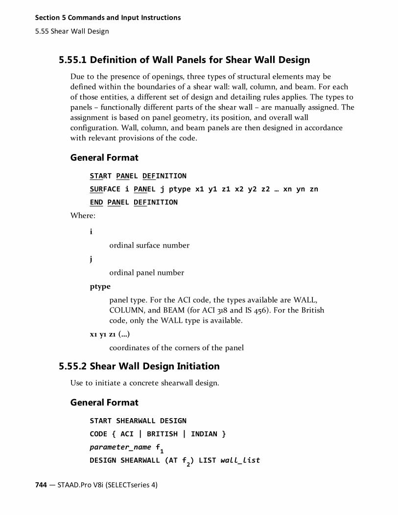
5.55.1 Definition of Wall Panels for Shear Wall DesignDue to the presence of openings, three types of structural elements may bedefined within the boundaries of a shear wall: wall, column, and beam. For eachof those entities, a different set of design and detailing rules applies. The types topanels – functionally different parts of the shear wall – are manually assigned. Theassignment is based on panel geometry, its position, and overall wallconfiguration. Wall, column, and beam panels are then designed in accordancewith relevant provisions of the code.
General Format
START PANEL DEFINITION
SURFACE i PANEL j ptype x1 y1 z1 x2 y2 z2 … xn yn zn
END PANEL DEFINITION
Where:
i
ordinal surface number
j
ordinal panel number
ptype
panel type. For the ACI code, the types available are WALL,COLUMN, and BEAM (for ACI 318 and IS 456). For the Britishcode, only the WALL type is available.
x1 y1 z1 (…)
coordinates of the corners of the panel
5.55.2 Shear Wall Design InitiationUse to initiate a concrete shearwall design.
General Format
START SHEARWALL DESIGN
CODE { ACI | BRITISH | INDIAN }
parameter_name f1DESIGN SHEARWALL (AT f2) LIST wall_list
744— STAAD.Pro V8i (SELECTseries 4)
Section 5 Commands and Input Instructions
5.55 Shear Wall Design

CREINF i1TRACK i2END SHEARWALL DESIGN
Codes choices are ACI (for ACI 318) or BRITISH (for BS 8110).
Where:
parameter-name = refers to the PARAMETER NAME (s)listed in atabular form in section 3.8.2 of this manual for the ACI code, and inthe International Codes manual for BS 8110 and IS 456:2000.
f1= Value of the parameter. Not all parameters require values.
f2= optional location at which design is to be performed
Note: If the command AT is omitted, the design proceeds for allcross sections of the wall or panels, as applicable, defined bythe SURFACE DIVISION X or SURFACE DIVISION Y inputvalues.
i1= column reinforcing parameter. Reinforcement distribution within
COLUMN panels is controlled by parameter CREINF, that may haveone of three possible values:
0. equal number of bars on all four faces of the column (default),
1. equal number of bars on two faces perpendicular to the plane ofthe wall,
2. equal number of bars on two faces parallel to the plane of thewall.
i2= output parameter TRACK specifies how detailed the design
output should be:
0. indicates a basic set of results data (default),
1. full design output will be generated.
5.56 End Run SpecificationThis command must be used to terminate the STAAD run.
This command should be provided as the last input command. This terminates aSTAAD run.
Section 5 Commands and Input Instructions
5.56 End Run Specification
Technical Reference Manual — 745

General FormatFINISH
746— STAAD.Pro V8i (SELECTseries 4)
Section 5 Commands and Input Instructions
5.56 End Run Specification

Technical Reference Manual — 747
Index
A
Accidental Torsion 606
ACI Beam Design 230
Advanced Solver 274
AIJ (Japanese) 446
AISC-ASD
Composite Beam Design 133
AISC 360
ASD 104
LRFD 103
Parameters 106
Algerian 469
Allowables per AISC Code 112
Aluminum
Take Off ReportSee Take OffSpecification
American LRFD 3rd edition code
Composite Beam Designper 146
Analysis
Buckling 684
Compression Only 77
Dynamic 80
Response Spectrum 82, 586
Secondary 92
Tension Only 77
Time History 84
Analysis Consideration 224
Analysis Facilities 63
Analysis Requirements 138
Anchorage 226
Design 226
Applying 363
Fireproofing 363
Area Load 55, 555
Assign 41, 350
Profile Specification 350
Assigning MaterialConstants 385

Index: Automatic Spring Support Generator – Concrete Take Off Command
Automatic Spring Support Gen-erator
Foundations 409
Axial Compression 139
Axial Tension 139
B
Beam Design 225, 227
Bending 112-113, 140
Stress 112
Boundary Condtions
Torsional 115
Buckling Analysis 73, 684
C
Cable Member
Linearized 47
Cable Members
Nonlinear 49
Cable SpecificationSee Member,Cable Specification
Castellated Beams 152
Center of GravitySee also PrintCG
Print 95
Center of Rigidity 606
Center of StiffnessSee Center ofRigidity
CFE 462
Change Specification 709
Code Checking 131, 145, 262
Specification 731
Colombian Seismic Load 444
Combined Axial Force 140
Combined Compression 113
Comision Federal De Elec-tricidad 462
Command Formats 276
Command Language
Separator 294
Command Language Con-ventions 275
Composite Beam Design
AISC-ASD 133
Composite Beam Designper 146
Composite Beams 45
Composite Damping 82, 401
Springs 401
Composite Decks 45, 351
Compression-OnlyAnalysisSee Analysis, Com-pression Only
Compression-OnlyMembersSee Member,Compression
Concrete Design 218
Section Types 218
Concrete Design Command 740
Concrete DesignSpecifications 739
Concrete DesignTerminator 742
Concrete Take OffCommand 741
748— STAAD.Pro

Index: Cracked Moment – Element Loads
Cracked Moment 230
Inertia 230
Cracked Section Properties 367
Curved Members 46, 355
Cut-Off Frequency 427
D
Damping
Composite 82
Modeling 82
Springs 401
Define Harmonic OutputFrequencies 691
Definition 386, 429, 433, 503,530
Load Systems 429
Material Constants 386
Moving Load System 429
Snow Load 530
Static Force Procedures 433
Time History Load 507
Wind Load 503
Deflection Check With SteelDesign 133
Delete Member 324
Deprecated Commands
Area Load 555
Design 116, 140, 225-226, 236,244
Anchorage 226
elements 236
Flexure 225
I-shaped beams per ACI-318 244
Shear 140, 225
Web Tapered Sections 116
Design Initiation 739
Design Operations 97, 217, 250
Design Parameters 117, 140, 220
Design per American ColdFormed Steel Code 209
Design Specifications 296
Direct Analysis 686
Member Definition 534
Discontinued Commands
Draw 427
Printer Plot 727
Problem Statistics 676
Displacements 92
Draw 427
Drift 721
Dynamic Analysis 80, 427
Miscellaneous Settings 427
Dynamic LoadingSpecification 586
E
Eccentricity 606
Eigenproblem 80
Solution 80
Element Design 236
Element Ignore Stiffness 374
Element Loads 59, 544
Joints 549
Technical Reference Manual — 749
Index: Element Mesh Generation – Inactive Member
Plates 544
Solids 547
Element Mesh Generation 310
Element Plane Stress 382
Element PropertySpecification 369
Element ReleaseSpecification 373
Element Releases 46, 370
Element/Surface Property Spec-ification 368
Elements 236, 275, 303
Designing 236
End Run 745
Examples 351
F
Finish 745
Finite Elements 21, 33
Fireproofing 363
Applying 363
Fixed-End LoadSpecification 579
Fixed End Member Load 57
Flexural Design Strength 140
Flexure 225
Design 225
Floor Load 562
Floor Spectrum Response 644
Force Envelopes 92
Foundations 409
Frequencies
Max. Number 282
G
Gamma Angle 357
General Comments 136
Generation 651
Loads 651
Geometric NonlinearAnalysis 75, 703
Global Coordinate System 10
Global SupportSpecification 405
Groups 318, 734
Specification 318
GUI 95
H
Harmonic Force Loading 697
Harmonic Ground Motion Load-ing 695
Harmonic Loading Function 84
Harmonic Response 85, 689
I
I-shaped beams per ACI-318 244
Design 244
Ignore Inplane Rotation Spec-ification 382
Ignore Specifications 296
Imperfection Analysis 76, 706
Imperfection Information 401
Inactive Member 324
750— STAAD.Pro

Index: Inactive Members – Local Coordinates
Inactive Members 93
Inclined
Joint Load Specification 540
Inclined SupportSpecification 408
Inertia 230
Cracked Moment 230
Input Generation 7
Input Specification 252
Input Wdith 284
Inter-Story DriftSee Drift
Intermediate Sections 92
Introduction 6, 273
IS 1893
Floor Level Definitions 454
Response Spectrum 598
Seismic Load 449
Soft Story 423, 452
Story Drift 599
J
Japanese Seismic Load 446
Joint
Element Load 549
Redefinition 317
Joint CoordinatesSpecification 296
Joint Load 53
Joint Load Specification 540
Joint Numbers
RenumberingSee Redefinition
Joints
Max Number 282
Joist Girders 42
L
Lamination
Orientation 263
Last Line 702
Limits 282
Linearized Cable Members 47
Listing
Members/Joints 318
Lists
Groups 318
Load
Selfweight 582, 584-585
Temperature 578
Load Cases
Max. Number 282
Load Combinations
Max. Number 282
Load Generator 60-61
Moving 61
Load List Specification 711
Load Systems 429
Definition 429
Loads 53, 651
Generation 651
Specifications 539
Local Coordinate System 11
Local Coordinates 15
Technical Reference Manual — 751

Index: LRFD Fundamentals – Modeling
LRFD Fundamentals 137
M
Mass Modeling 80
Reference Loads 533
Master-Slave Joints 53
Master/Slave Specification 420
Material Constants 52, 386
Definition 386
Member
Cable Specification 376
Camber Imperfection 402
Compression 47, 377
DeleteSee Delete Member
Dimensions 219
Displacements 92
Drift Imperfection 403
End ForcesSee Member EndForces
ForcesSee Member Forces
GroupsSee Groups
Imperfections 401
InactiveSee Inactive Member
Redefinition 317
RenumberingSee Member,Redefinition
Tension 47, 377
Member End Forces 87
Member Forces 92
Member Incidences Spec-ification 300
Member Load 54
Member Load Specification 541
Member OffsetSpecification 383
Member Offsets 50
Member Properties 98
Member PropertySpecification 339
Examples 351
Member ReleaseSpecification 370
Member Releases 46, 370
Member Selection 132, 145, 262,732-733
Member Stresses 92
Member Truss Specification 375
Member Truss/Cable/Ten-sion/Compression Spec-ification 375
Members 363
Max. Number 282
Miscellaneous Facilities 94
Miscellaneous Settings 427
Dynamic Analysis 427
Modal CalculationCommand 672
Modal DampingInformation 396
Mode Selection 428
Mode Shapes 427
Modeling
Damping 82
752— STAAD.Pro

Index: Modes – Print Section Displacement
Modes
Max. Number 282
Moving 61
Load Generator 61
Moving Load System 429
Definition 429
Multi-linear Spring Support 77
Multilinear Spring Support 414
Multiple Analyses 93
N
Natural Torsion 722
Node
Element Load 549
Non Linear Cable Members 49
Non Linear Cable/TrussAnalysis 78
Nonlinear Analysls
Geometric 75, 703
Notional Loads 665
O
Oneway Load 556
Optimization 132, 733
Orientation
Lamination 263
Output
Description 227
Output Width 284
P
P-Delta
Dynamic Analysis 71
KG 681
Large Delta 678
Small Delta 678
Stress Stiffening 70, 681
P-Delta Analysis 67-68, 678
Page Length/EjectCommand 295
Page New 295
Parameter Specifications 729
Partial Moment Release 372
Plate 303
Element Loads 544
Plate Element 21
Plate Girders 134
Plates
Max. Number 282
Plotting
Facilities 94
Post Analysis Plot 727
Post Processing 95
Poststress Member Load 57
Prestress 57
Prestress Load Specification 573
Print CG 714
Print Force Envelope Spec-ification 726
Print Section Displacement 724
Technical Reference Manual — 753

Index: Print Specifications – Seismic Load
Print Specifications 714
Print Steady State/HarmonicResults 699
Printer Plot 727
Printing
Facilities 94
Prismatic Properties 38
Prismatic PropertySpecification 346
Prismatic Tapered Tube 347
Property Specification 350
Purpose 689
R
Rayleigh FrequencyCalculation 670
RC Designer 244
Redefinition
Joint 317
Member 317
Reduced Section Properties 367
Reference Loads 531
Relationship
Global and LocalCoordinates 15
Repeat Load Specification 647
Response History Analysis 642
Time Varying Load 642
Response Spectrum 82, 586
Eurocode 8-1996 613
Eurocode 8-2004 621
Generic 587
IBC 2006 629
IS 1893-2002 (Indian) 598
SNiP (Russian) 636
Response Time History 83
Rigidity
Center ofSee Center of Rigid-ity
Rotation
Structure GeometrySee Struc-ture Geometry, Rota-tion
RPA (Algerian) 469
S
Second Order Analysis 67
Secondary AnalysisSee Redef-inition
Section Classification 138
Section Properties
Cracked 367
Reduced 367
Section Specification 713
Section Types 218
Concrete Design 218
Seismic Analysis 433
Seismic Load 462, 469
AIJ 446
Columbian 444
Japanese 446
UBC 1985 438
UBC 1994 438
UBC 1997 434
754— STAAD.Pro

Index: Select Member – Steel
Select Member 732
Selfweight 582, 584-585
SeparatorSee Command Lan-guage, Separator
Set 284
Shear 140, 225
Design 140, 225
Shear Stress 112
Shear Wall Design 238, 742
Initiation 744
Wall Panels 744
Shear walls 236
Shell Element 21
Shell Element Incidence Spec-ification 303
Singly Symmetric Sections 114
Size Specification 727
Slabs 236, 244
Slender CompressionElements 116
Slenderness Effects 224
SNiP II-7-81 636
Snow Load 530
Definition 530
Soft Story
ASCE 7-95 423
Check 423
IS 1893-2002 423, 452
Soil
Modeled as Springs 77
Solid Element 33
Solid Element Incidences Spec-ification 305
Solids
Element Loads 547
Max. Number 282
Solution
Eigenproblem 80
Specification 539
Loading 539
Specified Sections 92
Spring 401, 416
Composite Damping 401
Multilinear 414
Tension/Compression Spec-ification 416
Spring Support 77
Springs
Compression Only 47
Tension Only 47
Static Force Procedures 433
Definitions 433
Steady Force Loading 693
Steady Ground MotionLoading 692
Steady State 85, 689
Steady State/HarmonicAnalysis 702
Steel
Take Off ReportSee Take OffSpecification
Technical Reference Manual — 755

Index: Steel Design – The Commands
Steel Design 146
Tabulated Results 146
Steel Design per AISC/LRFDSpecification 136
Steel Design Specifications 728
Steel Joist 42
Steel Section Library 40, 98, 341
Steel Sections
Built-In Library 40, 98, 341
Stiffness
Center ofSee Center of Rigid-ity
Stiffness Analysis 63
Story Drift
IS 1893 599
Strain Load 59, 578
Stress 112
Bending 112
Stress Due To Compression 112
Stress Stiffening Matrix 681
Stress/Force output 722
Structure Geometry
Rotation 324
Structures
Types 7
Substitute 95
Support Displacement Load 59
Support Joint DisplacementSpecification 580
Support Specifications 405
Supports 52
Surface ConstantsSpecification 394
Surface Elements 36
as Shear Walls 238
Constants 394
Loads 551
Surface EntitiesSpecification 306
Surface Loads Specification 551
Surface PropertySpecification 369
Surfaces 303
T
Tabulated Results 146
Steel Design 146
Take Off Specification 736
Tapered MemberSpecification 349
Tapered Sections 41
Temperature 59
Temperature Load 578
Tension-Only AnalysisSee Anal-ysis, Tension Only
Tension-OnlyMembersSee Member, Ten-sion
Tension Stress 112
Tension/Compression Spec-ification 416
Spring 416
The Commands
Elements 275
756— STAAD.Pro

Index: Timber Code Checking – Wind Load Generator
Timber Code Checking 738
Timber Design Parameter Spec-ification 737
Timber DesignSpecification 737
Timber Member Selection 738
Time 427
Time History Analysis 84
Time History Load 507
Time History Response 83
Time Varying Load 642
Response HistoryAnalysis 642
Torsion
FIXED BUT Support 115
Torsion per Publication T114 114
Truss Members 47, 133
Types
Structures 7
U
UBC 1994 438
UBC 1997 Load Definition 434
UBC Seismic Load Generator 61
Units
Force 282
Length 282
Systems of 9
Unsymmetric Sections 133
User Provided Steel Table 41,326, 350
User Provided Table 350
User Steel Tabl 326
W
Wdith
Input 284
Web Tapered Sections 116
Design 116
Weld SelectionSpecification 733
Width
Output 284
Wind Load 503
Definition 503
Wind Load Generator 62
Technical Reference Manual — 757


Technical Reference Manual — 759
Index of
CommandsThis following is an alphabetic listof all STAAD.Pro commands in theTechnical Reference Manual.
A B C D E F G H I J K L M N OP Q R S T U V W Y X Z
A, BALUMINUM MEMBER TAKE OFF
AREA LOAD
CCALCULATE RAYLEIGH
CHANGE
CHECK CODE
CONCRETE TAKE OFF
CONSTANTS
CUT OFF
DDEFINE 1893
DEFINE AIJ
DEFINE CFE
DEFINE COLUMBIAN LOAD
DEFINE DAMPING
DEFINE DIRECT
DEFINE ENVELOPE
DEFINE IBC
2000 OR 2003
2006
DEFINE IMPERFECTION
DEFINE MATERIAL
DEFINE MESH
DEFINE MOVING LOAD
DEFINE NRC
1995
2005
DEFINE NTC
DEFINE PMEMBER
DEFINE REFERENCE LOAD
DEFINE RPA

Index: –
DEFINE SNOW LOAD
DEFINE TIME HISTORY
DEFINE UBC
1997
1994 or 1985
DEFINE WIND
DELETE
DESIGN
EELEMENT INCIDENCES
ELEMENT INCIDENCES SOLID
ELEMENT LOAD
JOINTS
PLATE
SOLID
ELEMENT PLANE STRESS
ELEMENT PROPERTY
ELEMENT RELEASES
END CONCRETE DESIGN
END PANEL DEFINITION
END SHEARWALL DESIGN
END STEADY
FFIXED END LOAD
FLOOR DIAPHRAGM
FLOOR LOAD
FREQUENCY
GGENERATE ELEMENT
GENERATE FLOOR SPECTRUM
GROUND MOTION
GROUP
HHARMONIC FORCE
HARMONIC GROUND
IIGNORE LIST
IGNORE STIFFNESS
INACTIVE
INPUT NODESIGN
INPUT WIDTH
J, KJOINT COORDINATES
JOINT LOAD
LLOAD COMBINATION
LOAD GENERATION
LOAD LIST
MMATERIAL
MEMBER CABLE
MEMBER COMPRESSION
MEMBER CRACKED
MEMBER CURVED
760— STAAD.Pro

Index: –
MEMBER FIREPROOFING
MEMBER INCIDENCES
MEMBER LOAD
MEMBER OFFSETS
MEMBER PRESTRESS LOAD
MEMBER PROPERTIES
MEMBER RELEASES
MEMBER TENSION
MEMBER TRUSS
MODAL CALCULATION
MODE SELECT
MULTILINEAR SPRINGS
NNOTIONAL LOAD
OONEWAY LOAD
OUTPUT WIDTH
P, QPAGE LENGTH
PAGE NEW
PARAMETER
STEEL & ALUMINUM
TIMBER
CONCRETE
PDELTA ANALYSIS
PERFORM ANALYSIS
PERFORM BUCKLING ANALYSIS
PERFORM CABLE ANALYSIS
PRINT DIAPHRAGM CR
PERFORM DIRECT ANALYSIS
PERFORM IMPERFECTIONANALYSIS
PERFORM NONLINEAR ANALYSIS
PERFORM ROTATION
PERFORM STEADY STATEANALYSIS
PRINT FORCE ENVELOPE
PRINT HARMONICDISPLACEMENTS
PRINT SECTION DISPLACEMENTS
PRINT STORY DRIFT
PRINT STORY STIFFNESS
PRINT SURFACE FORCE
RREFERENCE LOAD
REPEAT LOAD
SSECTION
SELECT (MEMBER)
SELECT OPTIMIZED
SELECT WELD
SELFWEIGHT
SEPARATOR
SET
SIZE
SLAVE
SNOW LAOD
SPECTRUM
Technical Reference Manual — 761

Index: –
1893 (Indian)
EURO, EURO 2004
IBC 2006
SPRING COMPRESSION
SPRING DAMPING
SPRING TENSION
STAAD
START DECK DEFINITION
START GROUP DEFINITION
START PANEL DEFINITION
START SHEARWALL DESIGN
START USER TABLE
STEADY FORCE FREQUENCY
STEADY GROUND FREQUENCY
STEEL MEMBER TAKE OFF
SUBSTITUTE
SUPPORTS
SURFACE CONSTANTS
SUPPORT DISPLACEMENT
SURFACE INCIDENCES
SURFACE LOAD
SURFACE PROPERTY
TTEMPERATURE LOAD
TIME LOAD
U, V, W, X, Y, ZUNIT
762— STAAD.Pro

Technical SupportThese resources are provided to help you answer support questions:
l Service Ticket Manager — http://www.bentley.com/serviceticketmanager —Create and track a service ticket using Bentley Systems' online site forreporting problems or suggesting new features. You do not need to be aBentley SELECT member to use Service Ticket Manager, however you doneed to register as a user.
l Knowledge Base — http://appsnet.bentley.com/kbase/ — Search the BentleySystems knowledge base for solutions for common problems.
l FAQs and TechNotes — http://-communities.bentley.com/Products/Structural/Structural_Analysis___Design/w/Structural_Analysis_and_Design__Wiki/structural-product-tech-notes-and-faqs.aspx — Here you can find detailed resolutions and answersto the most common questions posted to us by you.
l Ask Your Peers — http://-communities.bentley.com/forums/5932/ShowForum.aspx — Post questionsin the Be Community forums to receive help and advice from fellow users.
Technical Reference Manual — 763

764— STAAD.Pro V8i (SELECTseries 4)
Technical Support

Bentley Systems, Incorporated
685 Stockton Drive, Exton, PA 19341 USA
+1 (800) 236-8539
www.bentley.com