A simple and accurate Riemann solver for isothermal MHD

Journal of Computational Physics 225 (2007) 1427–1441

www.elsevier.com/locate/jcp

A simple and accurate Riemann solver for isothermal MHD

A. Mignone

Dipartimento di Fisica Generale ‘‘Amedeo Avogadro’’, Universita degli Studi di Torino, via Pietro Giuria 1, 10125 Torino, Italy

INAF/Osservatorio Astronomico di Torino, Strada Osservatorio 20, 10025 Pino Torinese, Italy

Received 14 November 2006; received in revised form 25 January 2007; accepted 30 January 2007Available online 9 February 2007

Abstract

A new approximate Riemann solver for the equations of magnetohydrodynamics (MHD) with an isothermal equationof state is presented. The proposed method of solution draws on the recent work of Miyoshi and Kusano, in the context ofadiabatic MHD, where an approximate solution to the Riemann problem is sought in terms of an average constant veloc-ity and total pressure across the Riemann fan. This allows the formation of four intermediate states enclosed by two out-ermost fast discontinuities and separated by two rotational waves and an entropy mode. In the present work, acorresponding derivation for the isothermal MHD equations is presented. It is found that the absence of the entropy modeleads to a different formulation which is based on a three-state representation rather than four. Numerical tests in one andtwo dimensions demonstrate that the new solver is robust and comparable in accuracy to the more expensive linearizedsolver of Roe, although considerably faster.� 2007 Elsevier Inc. All rights reserved.

Keywords: Magnetohydrodynamics; Approximate Riemann solver; HLL; HLLD; Isothermal

1. Introduction

The numerical solution of the magnetohydrodynamics (MHD) equations has received an increasingamount of attention over the last few decades motivated by the growing interests in modeling highly nonlinearflows. Numerical algorithms based on upwind differencing techniques have established stable and robustframeworks for their ability to capture the dynamics of strong discontinuities. This success owes to the propercomputation of numerical fluxes at cell boundaries, based on the solution of one-dimensional Riemann prob-lems between adjacent discontinuous states. The accuracy and strength of a Riemann solver is intrinsically tiedto the degree of approximation used in capturing the correct wave pattern solution.

In the case of adiabatic flows, an arbitrary initial discontinuity evolves into a pattern of constant states sep-arated by seven waves, two pairs of magneto-sonic waves (fast and slow), two Alfven discontinuities and onecontact or entropy mode. With the exception of the entropy mode, a wave separating two adjacent states maybe either a shock or a rarefaction wave. In the limit of efficient radiative cooling processes or highly conducting

0021-9991/$ - see front matter � 2007 Elsevier Inc. All rights reserved.

doi:10.1016/j.jcp.2007.01.033

E-mail address: [email protected]

mailto:[email protected]

1428 A. Mignone / Journal of Computational Physics 225 (2007) 1427–1441

plasma, on the other hand, the adiabatic assumption becomes inadequate and the approximation of an iso-thermal flow is better suited to describe the flow. In this case, the solution of the Riemann problem is similarto the adiabatic case, with the exception of the contact mode which is absent.

Although analytical solutions can be found with a high degree of accuracy using exact Riemann solvers, theresulting numerical codes are time-consuming and this has pushed researcher’s attention toward other moreefficient strategies of solution. From this perspective, a flourishing number of approaches has been developedin the context of adiabatic MHD, see for example [1–3,11] and references therein. Similar achievements havebeen obtained for the isothermal MHD equations, see [1,10].

Recently, Miyoshi and Kusano ([9], MK henceforth) proposed a multi-state Harten–Lax–van Leer (HLL,[8]) Riemann solver for adiabatic MHD. The proposed ‘‘HLLD’’ solver relies on the approximate assumptionof constant velocity and total pressure over the Riemann fan. This naturally leads to a four-state representa-tion of the solution where fast, rotational and entropy waves are allowed to form. The resulting scheme wasshown to be robust and accurate. The purpose of the present work is to extend the approach developed byMK to the equations of isothermal magnetohydrodynamics (IMHD henceforth). Although adiabatic codeswith specific heat ratios close to one may closely emulate the isothermal behavior, it is nevertheless advisableto develop codes specifically designed for IMHD, because of the greater ease of implementation and efficiencyover adiabatic ones.

The paper is structured as follows: in Section 2 the equations of IMHD are given; in Section 3 the new Rie-mann solver is derived. Numerical tests are presented in Section 4 and conclusions are drawn in Section 5.

2. Governing equations

The ideal MHD equations describing an electrically conducting perfect fluid are expressed by conservationof mass,

oqotþr � ðqvÞ ¼ 0; ð1Þ

momentum,

om

otþr � ðmv� BBþ IpTÞ ¼ 0; ð2Þ

and magnetic flux,

oB

ot�r� ðv� BÞ ¼ 0: ð3Þ

The system of equations is complemented by the additional solenoidal constraint r � B ¼ 0 and by an equa-tion of state relating pressure, internal energy and density. Here q, v and m ¼ qv are used to denote, respec-tively, density, velocity and momentum density. The total pressure, pT, includes thermal ðpÞ and magneticðjBj2=2Þ contributions (a factor of

ffiffiffiffiffiffi4pp

has been reabsorbed in the definition of B). No energy equation is pres-ent since I will consider the isothermal limit for which one has p ¼ a2q, where a is the (constant) isothermalspeed of sound. With this assumption the total pressure can be written as:

pT ¼ a2qþ jBj2

2: ð4Þ

Finite volume numerical schemes aimed to solved (1)–(3) rely on the solution of one-dimensional Riemannproblems between discontinuous left and right states at zone edges. Hence without loss of generality, I willfocus, in what follows, on the one-dimensional hyperbolic conservation law

oU

otþ oF

ox¼ 0; ð5Þ

where the vector of conservative variables U and the corresponding fluxes F are given by

A. Mignone / Journal of Computational Physics 225 (2007) 1427–1441 1429

U ¼

q

qu

qv

qw

By

Bz

0BBBBBBBB@

1CCCCCCCCA; F ¼

qu

qu2 þ pT � B2x

qvu� BxBy

qwu� BxBz

Byu� Bxv

Bzu� Bxw

0BBBBBBBB@

1CCCCCCCCA; ð6Þ

where u, v and w are the three components of velocity in the x, y and z directions, respectively. The solution ofEq. (5) may be achieved through the standard two-point finite difference scheme

Unþ1i ¼ Un

i �DtDx

Fiþ12� Fi�1

2

� �; ð7Þ

where Fi�12

is the numerical flux function, properly computed by solving a Riemann problem between Ui andUi±1.

As already mentioned, the solution to the Riemann problem in IMHD consists of a six wave pattern, withtwo pairs of magneto-sonic waves (fast and slow) and two Alfven (rotational) waves. These families of wavespropagate information with characteristic signal velocities given by the eigenvalues of the Jacobian oFðUÞ=oU:

kf� ¼ u� cf ; ks� ¼ u� cs; ka� ¼ u� ca; ð8Þ

where the fast, Alfven and slow velocity are defined as in adiabatic MHD:

cf ¼1ffiffiffi2p a2 þ b2 þ

ffiffiffiffiffiffiffiffiffiffiffiffiffiffiffiffiffiffiffiffiffiffiffiffiffiffiffiffiffiffiffiffiffiffiffiffiffiða2 þ b2Þ2 � 4a2b2

x

q� �1=2

; ð9Þ

ca ¼ jbxj; ð10Þ

cs ¼1ffiffiffi2p a2 þ b2 �

ffiffiffiffiffiffiffiffiffiffiffiffiffiffiffiffiffiffiffiffiffiffiffiffiffiffiffiffiffiffiffiffiffiffiffiffiffiða2 þ b2Þ2 � 4a2b2

x

q� �1=2

; ð11Þ

with b ¼ B=ffiffiffiqp

.The contact or entropy mode is absent. Fast and slow waves can be either shocks, where flow quantities

experience a discontinuous jump, or rarefaction waves, characterized by a smooth transition of the state vari-ables. Across the rotational waves, similarly to the adiabatic case, density and normal component of velocityare continuous, whereas tangential components are not. In virtue of the solenoidal constraint, the normalcomponent of the magnetic field is constant everywhere and should be regarded as a given parameter.

3. The HLLD approximate Riemann solver

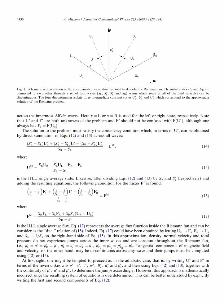
In what follows, I will assume that the solution to the isothermal MHD Riemann problem can be repre-sented in terms of three constant states, U�L; U�c and U�R, separated by four waves: two outermost fast mag-neto-sonic disturbances with speeds SL and SR ðSL < SRÞ and two innermost rotational discontinuities withvelocities S�L and S�R, see Fig. 1. Slow modes cannot be generated inside the solution. Since no entropy modeis present and rotational discontinuities carry jumps in the tangential components of vector fields only, it fol-lows that one can regard density, normal velocity and total pressure as constants over the fan. This assump-tion is essentially the same one suggested by MK but it leads, in the present context, to a representation interms of three states rather than four. Quantities ahead and behind each wave must be related by the jumpconditions

SaðU�a �UaÞ ¼ F�a � Fa; ð12Þ
across the outermost fast waves, and
S�aðU�c �U�aÞ ¼ F�c � F�a; ð13Þ

U

UU

x

t

R*

*c

L*

S

S

SR

R*

L

SL*

UL UR

Fig. 1. Schematic representation of the approximated wave structure used to describe the Riemann fan. The initial states UL and UR areconnected to each other through a set of four waves (SL, S�L, S�R and SR) across which some or all of the fluid variables can bediscontinuous. The four discontinuities isolate three intermediate constant states U �L, U �c and U �R which correspond to the approximatesolution of the Riemann problem.


across the innermost Alfven waves. Here a = L or a = R is used for the left or right state, respectively. Notethat U* and F* are both unknowns of the problem and F* should not be confused with FðU�Þ, although onealways has Fa ¼ FðUaÞ.

The solution to the problem must satisfy the consistency condition which, in terms of U*, can be obtainedby direct summation of Eqs. (12) and (13) across all waves:

ðS�L � SLÞU�L þ ðS�R � S�LÞU�c þ ðSR � S�RÞU

�R

SR � SL

¼ Uhll; ð14Þ

where

Uhll ¼ SRUR � SLUL � FR þ FL

SR � SL

ð15Þ

is the HLL single average state. Likewise, after dividing Eqs. (12) and (13) by Sa and S�a (respectively) andadding the resulting equations, the following condition for the fluxes F* is found:

1S�

L� 1

SL

� �F�L þ 1

S�R� 1

S�L

� �F�c þ 1

S�L� 1

S�R

� �F�R

1SR� 1

SL

¼ Fhll; ð16Þ

where

Fhll ¼ SRFL � SLFR þ SRSLðUR �ULÞSR � SL

ð17Þ

is the HLL single average flux. Eq. (17) represents the average flux function inside the Riemann fan and can beconsider as the ‘‘dual’’ relation of (15). Indeed, Eq. (17) could have been obtained by letting Ua ! Fa;Fa ! Ua

and Sa ! 1=Sa on the right-hand side of Eq. (15). In this approximation, density, normal velocity and totalpressure do not experience jumps across the inner waves and are constant throughout the Riemann fan,i.e., q�L ¼ q�c ¼ q�R � q�; u�L ¼ u�c ¼ u�R � u�; p�T L

¼ p�T c¼ p�T R

� p�T. Tangential components of magnetic fieldand velocity, on the other hand, may be discontinuous across any wave and their jumps must be computedusing (12) or (13).

At first sight, one might be tempted to proceed as in the adiabatic case, that is, by writing U* and F* interms of the seven unknowns q�; u�; v�; w�; B�y ; B�z and p�T, and then using Eqs. (12) and (13), together withthe continuity of q�; u� and p�T, to determine the jumps accordingly. However, this approach is mathematicallyincorrect since the resulting system of equations is overdetermined. This can be better understood by explicitlywriting the first and second components of Eq. (12):


Saðq� � qaÞ ¼ q�u� � qaua; ð18ÞSaðq�u� � qauaÞ ¼ q�ðu�Þ2 þ p�T � qaua � pT a

; ð19Þ

where I have used the fact the q�; u� and p�T are constants in each of the three states. Eqs. (18) and (19) providefour equations (two for a = L and two for a = R) in the three unknowns q�; u� and p�T and, as such, they can-not have a solution. Furthermore, the situation does not improve when the equations for the tangential com-ponents are included, since more unknowns are brought in.

The problem can be disentangled by writing density and momentum jump conditions in terms of fourunknowns rather than three. This is justified by the fact that, according to the chosen representation, densityand momentum components of U* and F* are continuous across the Riemann fan and, in line with the con-sistency condition, they should be represented by their HLL averages:

q� � q�L ¼ q�c ¼ q�R ¼ qhll; ð20Þm�x � m�xL

¼ m�xc¼ m�xR

¼ mhllx ; ð21Þ

F �½q� � F �½q�L ¼ F �½q�c ¼ F �½q�R ¼ F hll½q�; ð22Þ

F �½mx� � F �½mx �L ¼ F �½mx�c ¼ F �½mx�R ¼ F hll½mx�; ð23Þ

where qhll; mhll; F hll½q� and F hll

½mx� are given by the first two components of Eqs. (15) and (17).This set of relations obviously satisfies the jump conditions across all the four waves. The absence of the

entropy mode, however, leaves the velocity in the Riemann fan, u*, unspecified. This is not the case in the adi-abatic case, where one has m� ¼ F �½q� ¼ q�u� and from the analogous consistency condition the unique choiceqhllu� ¼ mhll

x . Still, in the isothermal case, one has the freedom to define u� ¼ F hll½q�=q

hll or u� ¼ mhllx =q

hll. The twochoices are not equivalent and one can show that only the first one has the correct physical interpretation of an‘‘advective’’ velocity. This statement becomes noticeably true in the limit of vanishing magnetic fields, wheretransverse velocities are passively advected and thus carry zero jump across the outermost sound waves.Indeed, by explicitly writing the jump conditions for the transverse momenta, one can see that the conditionsv�a ¼ va and w�a ¼ wa can be fulfilled only if q�u� ¼ F �½q�.

Thus one has, for variables and fluxes in the star region, the following representation:

U� ¼

q�

m�xq�v�

q�w�

B�yB�z

0BBBBBBBB@

1CCCCCCCCA; F� ¼

q�u�

F �mx

q�v�u� � BxB�yq�w�u� � BxB�z

B�y u� � Bxv�

B�z u� � Bxw�

0BBBBBBBB@

1CCCCCCCCA; ð24Þ

which gives eight variables per state and thus a total of 24 unknowns. The four continuity relations (20)–(23)together with the 12 jump conditions (12) across the outer waves can be used to completely specify U�a (fora = L and a = R) in terms of UL and UR. Note that the total pressure does not explicitly enter in the definitionof the momentum flux. The remaining four unknowns in the intermediate region (v�c ; w�c ; B�yc

and B�zc) may be

found using (13). However, one can see that

ðS�a � u�Þq�v�c þ BxB�yc¼ ðS�a � u�Þq�v�a þ BxB�ya

; ð25ÞðS�a � u�Þq�w�c þ BxB�zc

¼ ðS�a � u�Þq�w�a þ BxB�za; ð26Þ

ðS�a � u�ÞB�ycþ Bxv�c ¼ ðS�a � u�ÞB�ya

þ Bxv�a; ð27ÞðS�a � u�ÞB�zc

þ Bxw�c ¼ ðS�a � u�ÞB�zaþ Bxw�a ð28Þ

cannot be simultaneously satisfied for a = L and a = R for an arbitrary definition of S�a, unless the equationsare linearly dependent, in which case one finds


S�L ¼ u� � jBxjffiffiffiffiffiq�p ; S�R ¼ u� þ jBxjffiffiffiffiffi

q�p : ð29Þ

This choice uniquely specifies the speed of the rotational discontinuity in terms of the average Alfven velocityjBxj=

ffiffiffiffiffiq�p

. Thus only 4 (out of 8) equations can be regarded independent and one has at disposal a total of 24independent equations, consistently with a well-posed problem.

Proceeding in the derivation, direct substitution of (24) into Eqs. (12) together with (20), (29) and theassumption u� ¼ F hll

½q�=qhll yields

q�v�a ¼ q�va � BxBya

u� � ua

ðSa � S�LÞðSa � S�RÞ; ð30Þ

q�w�a ¼ q�wa � BxBza

u� � ua


B�ya¼ Bya

q�qaðSa � uaÞ2 � B2

x


B�za¼ Bza

q�qaðSa � uaÞ2 � B2

x


which clearly shows that ðv�a;w�aÞ ! ðva;waÞ when B! 0. As in the adiabatic case, the consistency conditionshould be used to find v�c , w�c , B�yc

and B�zc:

q�v�c ¼ðq�v�L þ q�v�RÞ

2þ

X ðB�yR� B�yL

Þ2

; ð34Þ

q�w�c ¼ðq�w�L þ q�w�RÞ

2þ

X ðB�zR� B�zL

Þ2

; ð35Þ

B�yc¼ðB�yLþ B�yR

Þ2

þ ðq�v�R � q�v�LÞ

2X; ð36Þ

B�zc¼ðB�zLþ B�zR

Þ2

þ ðq�w�R � q�w�LÞ

2X; ð37Þ

where X ¼ ffiffiffiffiffiq�p

signðBxÞ. The inter-cell numerical flux F required in Eq. (5) can now be computed by samplingthe solution on the x=t ¼ 0 axis:

F ¼

FL for SL > 0;

FL þ SLðU�L �ULÞ for SL < 0 < S�L;

F�c for S�L < 0 < S�R;

FR þ SRðU�R �URÞ for S�R < 0 < SR;

FR for SR < 0;

8>>>>>><>>>>>>:

ð38Þ

where F�c is computed from (24) using (34) through (37).To conclude, one needs an estimate for the upper and lower signal velocities SL and SR. I will adopt the

simple estimate given by [5], for which one has

SL ¼ minðkf�ðULÞ; kf�ðURÞÞ; SR ¼ minðkfþðULÞ; kfþðURÞÞ; ð39Þ
with kf�ðUÞ given by the first of (8). Other estimates have been proposed, see for example [6].
The degenerate cases are handled as follows:

for zero tangential components of the magnetic field and B2x > a2qa, a degeneracy occurs where S�a ! Sa and

the denominator in Eqs. (29)–(32) vanishes. In this case, one proceeds as in the adiabatic case by imposingtransverse components of velocity and magnetic field to have zero jump; the case Bx ! 0 does not poses any serious difficulty and only the states U�L and U�R have to be evaluated in

order to compute the fluxes. One should realize, however, that the final representation of the solution differsfrom the adiabatic counterpart. In the full solution, in fact, Alfven and slow modes all degenerate into a


single intermediate tangential discontinuity with speed u*. In the adiabatic case, this degeneracy can still bewell described by the presence of the middle wave, across which only normal velocity and total pressure arecontinuous. Although this property is recovered by the adiabatic HLLD solver, the same does not occur inour formulation because of the initial assumption of constant density through the Riemann fan. The unre-solved density jump, in fact, can be thought of as the limiting case of two slow shocks merging into a singlewave. Since slow shocks are not considered in the solution, density will still be given by the single HLL-averaged state. Tangential components of velocity and magnetic field, on the other hand, can yet be discon-tinuous across the middle wave. Thus, in this limit, the solver does not reduce to the single state HLLsolver.

This completes the description of the proposed isothermal HLLD Riemann solver. The suggested formu-lation satisfies the consistency conditions by construction and defines a well-posed problem, since the numberof unknowns is perfectly balanced by the number of available equations: 12 equations for the outermostwaves, 8 continuity conditions (for q�, u�, F �½q�, F �½mx� across the inner waves) and the four equations for the tan-

gential components. The positivity of the solver is trivial since no energy equation is present and the density isgiven by the HLL-averaged state (20).

4. Numerical tests

The performance of the new Riemann solver is now investigated through a series of selected numerical testsin one and two dimensions. One-dimensional shock tubes (in Section 4.1) consist in a decaying discontinuityinitially separating two constant states. The outcoming wave pattern comprises several waves and an analyt-ical or reference solution can usually be obtained with a high degree of accuracy. For this reason, one-dimen-sional tests are commonly used to check the ability of the code in reproducing the correct structure.

The decay of standing Alfven waves in two dimensions is consider in Section 4.2. The purpose of this test isto quantify the amount of intrinsic numerical dissipation inherent to a numerical scheme. A two-dimensionaltests involving the propagation of a blast wave in a strongly magnetized environment is investigated in Section4.3 and finally, in Section 4.4, the isothermal Orszag–Tang vortex system and its transition to supersonic tur-bulence is discussed.

Eq. (7) is used for the spatially and temporally first order scheme. Extension to second order is achievedwith the second order fully unsplit Runge–Kutta total variation diminishing (TVD) of [7] and the harmonicslope limiter of [14]. For the multidimensional tests, the magnetic field is evolved using the constrained trans-port method of [2], where staggered magnetic fields are updated, e.g. during the predictor step, according to

Bnþ1x;iþ1

2;j¼ Bn

x;iþ12;j� Dt

Dyj

Xziþ1

2;jþ12� Xz

iþ12;j�

12

� �; ð40Þ

Bnþ1y;i;jþ1

2¼ Bn

y;i;jþ12þ Dt

DxiXz

iþ12;jþ

12� Xz

i�12;jþ

12

� �: ð41Þ

The electric field Xziþ1

2;jþ12

is computed by a spatial average of the upwind fluxes available at zone interfaces dur-

ing the Riemann solver step:

Xziþ1

2;jþ12¼�F ½By �

iþ12;j� F ½By �

iþ12;jþ1þ F ½Bx�

i;jþ12

þ F ½Bx�iþ1;jþ1

2

4; ð42Þ

where F ½By � is the By component of the flux (38) available during the sweep along the x-direction. A similarprocedure applies to F ½Bx�.

4.1. One-dimensional shock tubes

An interface separating two constant states is placed in the middle of the domain ½0; 1� at x ¼ 0:5. Unlessotherwise stated, the isothermal speed of sound a is set to unity. States to the left and to the right of the dis-continuity together with the final integration time are given in Table 1. The reader may also refer to [10] for the

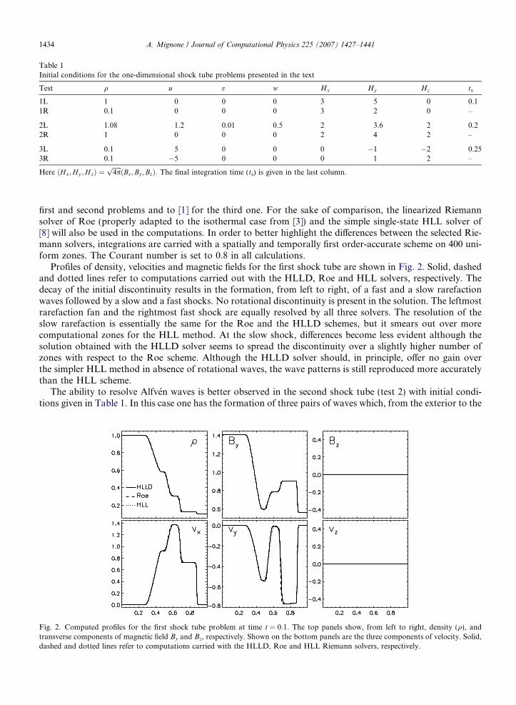
Table 1Initial conditions for the one-dimensional shock tube problems presented in the text

Test q u v w Hx Hy Hz ts

1L 1 0 0 0 3 5 0 0.11R 0.1 0 0 0 3 2 0 –

2L 1.08 1.2 0.01 0.5 2 3.6 2 0.22R 1 0 0 0 2 4 2 –

3L 0.1 5 0 0 0 �1 �2 0.253R 0.1 �5 0 0 0 1 2 –

Here ðH x;Hy ;H zÞ ¼ffiffiffiffiffiffi4ppðBx;By ;BzÞ. The final integration time (ts) is given in the last column.


first and second problems and to [1] for the third one. For the sake of comparison, the linearized Riemannsolver of Roe (properly adapted to the isothermal case from [3]) and the simple single-state HLL solver of[8] will also be used in the computations. In order to better highlight the differences between the selected Rie-mann solvers, integrations are carried with a spatially and temporally first order-accurate scheme on 400 uni-form zones. The Courant number is set to 0.8 in all calculations.

Profiles of density, velocities and magnetic fields for the first shock tube are shown in Fig. 2. Solid, dashedand dotted lines refer to computations carried out with the HLLD, Roe and HLL solvers, respectively. Thedecay of the initial discontinuity results in the formation, from left to right, of a fast and a slow rarefactionwaves followed by a slow and a fast shocks. No rotational discontinuity is present in the solution. The leftmostrarefaction fan and the rightmost fast shock are equally resolved by all three solvers. The resolution of theslow rarefaction is essentially the same for the Roe and the HLLD schemes, but it smears out over morecomputational zones for the HLL method. At the slow shock, differences become less evident although thesolution obtained with the HLLD solver seems to spread the discontinuity over a slightly higher number ofzones with respect to the Roe scheme. Although the HLLD solver should, in principle, offer no gain overthe simpler HLL method in absence of rotational waves, the wave patterns is still reproduced more accuratelythan the HLL scheme.

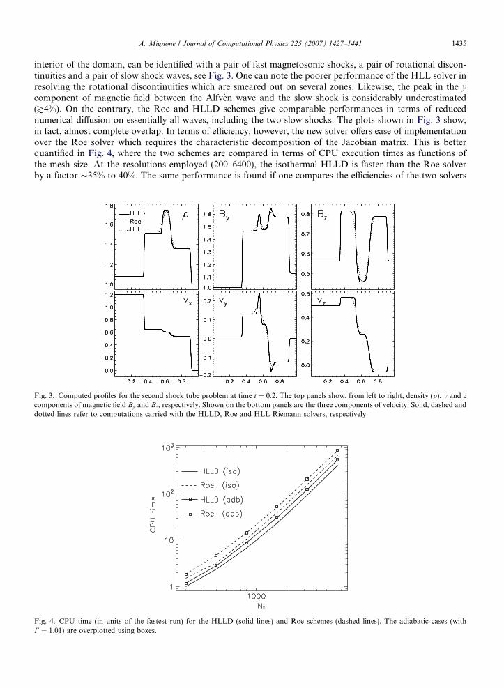
The ability to resolve Alfven waves is better observed in the second shock tube (test 2) with initial condi-tions given in Table 1. In this case one has the formation of three pairs of waves which, from the exterior to the

Fig. 2. Computed profiles for the first shock tube problem at time t ¼ 0:1. The top panels show, from left to right, density (q), andtransverse components of magnetic field By and Bz, respectively. Shown on the bottom panels are the three components of velocity. Solid,dashed and dotted lines refer to computations carried with the HLLD, Roe and HLL Riemann solvers, respectively.


interior of the domain, can be identified with a pair of fast magnetosonic shocks, a pair of rotational discon-tinuities and a pair of slow shock waves, see Fig. 3. One can note the poorer performance of the HLL solver inresolving the rotational discontinuities which are smeared out on several zones. Likewise, the peak in the y

component of magnetic field between the Alfven wave and the slow shock is considerably underestimated(J4%). On the contrary, the Roe and HLLD schemes give comparable performances in terms of reducednumerical diffusion on essentially all waves, including the two slow shocks. The plots shown in Fig. 3 show,in fact, almost complete overlap. In terms of efficiency, however, the new solver offers ease of implementationover the Roe solver which requires the characteristic decomposition of the Jacobian matrix. This is betterquantified in Fig. 4, where the two schemes are compared in terms of CPU execution times as functions ofthe mesh size. At the resolutions employed (200–6400), the isothermal HLLD is faster than the Roe solverby a factor 35% to 40%. The same performance is found if one compares the efficiencies of the two solvers

Fig. 3. Computed profiles for the second shock tube problem at time t ¼ 0:2. The top panels show, from left to right, density (q), y and z

components of magnetic field By and Bz, respectively. Shown on the bottom panels are the three components of velocity. Solid, dashed anddotted lines refer to computations carried with the HLLD, Roe and HLL Riemann solvers, respectively.

Fig. 4. CPU time (in units of the fastest run) for the HLLD (solid lines) and Roe schemes (dashed lines). The adiabatic cases (withC ¼ 1:01) are overplotted using boxes.


by running the same test with an adiabatic equation of state (by setting C ¼ 1:01). Furthermore, direct inspec-tion of Fig. 4 reveals that at lower resolution (i.e. [600) the CPU time ratio adiabatic/isothermal is 1.2,whereas it increases up to 1.35 at higher resolutions. This justifies the need for codes specifically designedfor IMHD, as already anticipated in Section 1.

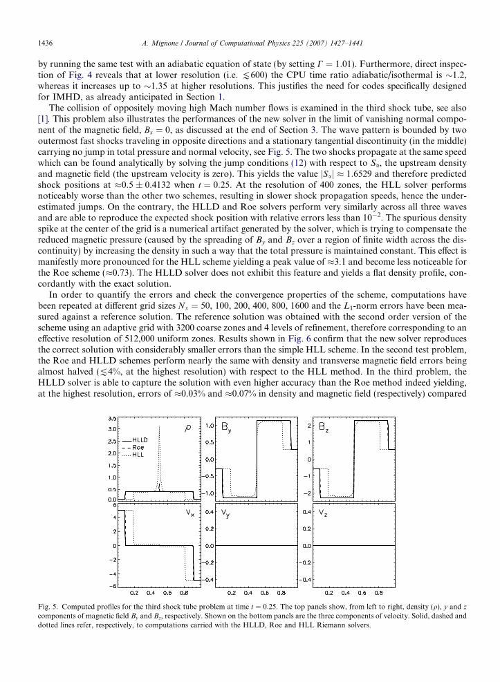
The collision of oppositely moving high Mach number flows is examined in the third shock tube, see also[1]. This problem also illustrates the performances of the new solver in the limit of vanishing normal compo-nent of the magnetic field, Bx ¼ 0, as discussed at the end of Section 3. The wave pattern is bounded by twooutermost fast shocks traveling in opposite directions and a stationary tangential discontinuity (in the middle)carrying no jump in total pressure and normal velocity, see Fig. 5. The two shocks propagate at the same speedwhich can be found analytically by solving the jump conditions (12) with respect to Sa, the upstream densityand magnetic field (the upstream velocity is zero). This yields the value jSaj � 1:6529 and therefore predictedshock positions at �0.5 ± 0.4132 when t ¼ 0:25. At the resolution of 400 zones, the HLL solver performsnoticeably worse than the other two schemes, resulting in slower shock propagation speeds, hence the under-estimated jumps. On the contrary, the HLLD and Roe solvers perform very similarly across all three wavesand are able to reproduce the expected shock position with relative errors less than 10�2. The spurious densityspike at the center of the grid is a numerical artifact generated by the solver, which is trying to compensate thereduced magnetic pressure (caused by the spreading of By and Bz over a region of finite width across the dis-continuity) by increasing the density in such a way that the total pressure is maintained constant. This effect ismanifestly more pronounced for the HLL scheme yielding a peak value of �3.1 and become less noticeable forthe Roe scheme (�0.73). The HLLD solver does not exhibit this feature and yields a flat density profile, con-cordantly with the exact solution.

In order to quantify the errors and check the convergence properties of the scheme, computations havebeen repeated at different grid sizes N x ¼ 50, 100, 200, 400, 800, 1600 and the L1-norm errors have been mea-sured against a reference solution. The reference solution was obtained with the second order version of thescheme using an adaptive grid with 3200 coarse zones and 4 levels of refinement, therefore corresponding to aneffective resolution of 512,000 uniform zones. Results shown in Fig. 6 confirm that the new solver reproducesthe correct solution with considerably smaller errors than the simple HLL scheme. In the second test problem,the Roe and HLLD schemes perform nearly the same with density and transverse magnetic field errors beingalmost halved ([4%, at the highest resolution) with respect to the HLL method. In the third problem, theHLLD solver is able to capture the solution with even higher accuracy than the Roe method indeed yielding,at the highest resolution, errors of �0.03% and �0.07% in density and magnetic field (respectively) compared

Fig. 5. Computed profiles for the third shock tube problem at time t ¼ 0:25. The top panels show, from left to right, density (q), y and z

components of magnetic field By and Bz, respectively. Shown on the bottom panels are the three components of velocity. Solid, dashed anddotted lines refer, respectively, to computations carried with the HLLD, Roe and HLL Riemann solvers.

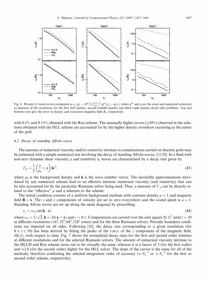
Fig. 6. Percent L1 norm errors (computed as �L1ðqÞ ¼ 102=Nx

Pi¼Nxi¼1 jqexðxiÞ � qðxiÞj where qex and q are the exact and numerical solutions)

as function of the resolution, for the first (left panels), second (middle panels) and third (right panels) shock tube problems. Top andbottom rows give the error in density and transverse magnetic field By, respectively.


with 0.1% and 0.13% obtained with the Roe scheme. The unusually higher errors (J10%) observed in the solu-tions obtained with the HLL scheme are accounted for by the higher density overshoot occurring at the centerof the grid.

4.2. Decay of standing Alfven waves

The amount of numerical viscosity and/or resistivity intrinsic to computations carried on discrete grids maybe estimated with a simple numerical test involving the decay of standing Alfven waves, [12,10]. In a fluid withnon-zero dynamic shear viscosity l and resistivity g, waves are characterized by a decay rate given by

CA ¼1

2

lq0

þ g

� �jkj2; ð43Þ

where q0 is the background density and k is the wave number vector. The inevitable approximations intro-duced by any numerical scheme lead to an effective intrinsic numerical viscosity (and resistivity) that canbe also accounted for by the particular Riemann solver being used. Thus, a measure of CA can be directly re-lated to the ‘‘effective’’ l and g inherent to the scheme.

The initial condition consists of a uniform background medium with constant density q ¼ 1 and magneticfield B ¼ x. The x and y components of velocity are set to zero everywhere and the sound speed is a ¼ 1.Standing Alfven waves are set up along the main diagonal by prescribing

vz ¼ �cA sinðk � xÞ; ð44Þ
where cA ¼ 1=
ffiffiffi2p

, k ¼ 2pðxþ yÞ and � ¼ 0:1. Computations are carried over the unit square ½0; 1�2 until t ¼ 10at different resolutions (162,322,642,1282 zones) and for the three Riemann solvers. Periodic boundary condi-tions are imposed on all sides. Following [10], the decay rate corresponding to a given resolution (for0 6 t 6 10) has been derived by fitting the peaks of the r.m.s. of the z component of the magnetic field,dBzðtÞ, with respect to time. Fig. 7 shows the normalized decay rates for the first and second order schemesat different resolutions and for the selected Riemann solvers. The amount of numerical viscosity intrinsic tothe HLLD and Roe scheme turns out to be virtually the same, whereas it is a factor of 3 (for the first order)and �2.6 (for the second order) higher for the HLL solver. The slope of the curves is the same for all of themethods, therefore confirming the selected integration order of accuracy (/ N�1

x or / N�2x for the first or

second order scheme, respectively).

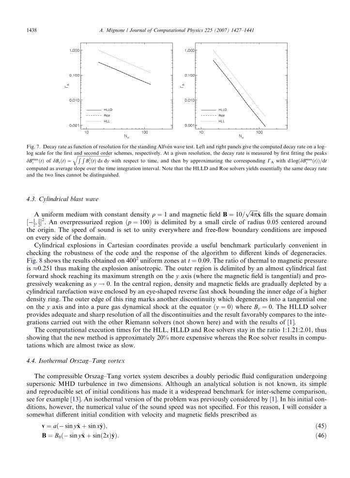
Fig. 7. Decay rate as function of resolution for the standing Alfven wave test. Left and right panels give the computed decay rate on a log–log scale for the first and second order schemes, respectively. At a given resolution, the decay rate is measured by first fitting the peaks

dBmaxz ðtÞ of dBzðtÞ ¼

ffiffiffiffiffiffiffiffiffiffiffiffiffiffiffiffiffiffiffiffiffiffiffiffiffiffiffiffiffiffiR RB2

z ðtÞ dx dyq

with respect to time, and then by approximating the corresponding CA with d logðdBmaxz ðtÞÞ=dt

computed as average slope over the time integration interval. Note that the HLLD and Roe solvers yields essentially the same decay rateand the two lines cannot be distinguished.


4.3. Cylindrical blast wave

A uniform medium with constant density q ¼ 1 and magnetic field B ¼ 10=ffiffiffiffiffiffi4pp

x fills the square domain½�1

2; 1

2�2. An overpressurized region ðp ¼ 100Þ is delimited by a small circle of radius 0.05 centered around

the origin. The speed of sound is set to unity everywhere and free-flow boundary conditions are imposedon every side of the domain.

Cylindrical explosions in Cartesian coordinates provide a useful benchmark particularly convenient inchecking the robustness of the code and the response of the algorithm to different kinds of degeneracies.Fig. 8 shows the results obtained on 4002 uniform zones at t = 0.09. The ratio of thermal to magnetic pressureis �0.251 thus making the explosion anisotropic. The outer region is delimited by an almost cylindrical fastforward shock reaching its maximum strength on the y axis (where the magnetic field is tangential) and pro-gressively weakening as y ! 0. In the central region, density and magnetic fields are gradually depleted by acylindrical rarefaction wave enclosed by an eye-shaped reverse fast shock bounding the inner edge of a higherdensity ring. The outer edge of this ring marks another discontinuity which degenerates into a tangential oneon the y axis and into a pure gas dynamical shock at the equator ðy ¼ 0Þ where By ¼ 0. The HLLD solverprovides adequate and sharp resolution of all the discontinuities and the result favorably compares to the inte-grations carried out with the other Riemann solvers (not shown here) and with the results of [1].

The computational execution times for the HLL, HLLD and Roe solvers stay in the ratio 1:1.21:2.01, thusshowing that the new method is approximately 20% more expensive whereas the Roe solver results in compu-tations which are almost twice as slow.

4.4. Isothermal Orszag–Tang vortex

The compressible Orszag–Tang vortex system describes a doubly periodic fluid configuration undergoingsupersonic MHD turbulence in two dimensions. Although an analytical solution is not known, its simpleand reproducible set of initial conditions has made it a widespread benchmark for inter-scheme comparison,see for example [13]. An isothermal version of the problem was previously considered by [1]. In his initial con-ditions, however, the numerical value of the sound speed was not specified. For this reason, I will consider asomewhat different initial condition with velocity and magnetic fields prescribed as

v ¼ að� sin yxþ sin xyÞ; ð45ÞB ¼ B0ð� sin yxþ sinð2xÞyÞ: ð46Þ

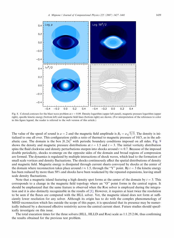
Fig. 8. Colored contours for the blast wave problem at t ¼ 0:09. Density logarithm (upper left panel), magnetic pressure logarithm (upperright), specific kinetic energy (bottom left) and magnetic field lines (bottom right) are shown. (For interpretation of the references to colorin this figure legend, the reader is referred to the web version of this article.)


The value of the speed of sound is a ¼ 2 and the magnetic field amplitude is B0 ¼ affiffiffiffiffiffiffiffi3=5

p. The density is ini-

tialized to one all over. This configuration yields a ratio of thermal to magnetic pressure of 10/3, as in the adi-abatic case. The domain is the box ½0; 2p�2 with periodic boundary conditions imposed on all sides. Fig. 9shows the density and magnetic pressure distributions at t ¼ 1:5 and t ¼ 3. The initial vorticity distributionspins the fluid clockwise and density perturbations steepen into shocks around t � 0:7. Because of the imposeddouble periodicity, shocks re-emerge on the opposite sides of the domain and broad regions of compressionare formed. The dynamics is regulated by multiple interactions of shock waves, which lead to the formation ofsmall scale vortices and density fluctuations. The shocks continuously affect the spatial distributions of densityand magnetic field. Magnetic energy is dissipated through current sheets convoyed by shocks at the center ofthe domain where reconnection takes place around t � 1:5, through the ‘‘Y’’ point. By t ¼ 3 the kinetic energyhas been reduced by more than 50% and shocks have been weakened by the repeated expansions, leaving smallscale density fluctuations.

Note that a magnetic island featuring a high density spot forms at the center of the domain by t ¼ 3. Thiscorresponds to a change in the magnetic field topology where an ‘‘O’’ point forms in the central region. Itshould be emphasized that the same feature is observed when the Roe solver is employed during the integra-tion and it is also distinctly recognizable in the results of [1]. However, it requires at least twice the resolutionto be seen if the fluxes are computed with the HLL solver. Yet, the magnetic island does not form at suffi-ciently lower resolution for any solver. Although its origin has to do with the complex phenomenology ofMHD reconnection which lies outside the scope of this paper, it is speculated that its presence may be numer-ically induced by a decreased effective resistivity across the central current sheet. Future studies should specif-ically investigate on this issue.

The total execution times for the three solvers (HLL, HLLD and Roe) scale as 1:1.25:2.06, thus confirmingthe results obtained for the previous test problem.

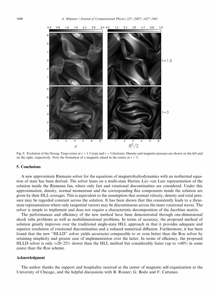
Fig. 9. Evolution of the Orszag–Tang vortex at t ¼ 1:5 (top) and t ¼ 3 (bottom). Density and magnetic pressure are shown on the left andon the right, respectively. Note the formation of a magnetic island in the center at t ¼ 3.


5. Conclusions

A new approximate Riemann solver for the equations of magnetohydrodynamics with an isothermal equa-tion of state has been derived. The solver leans on a multi-state Harten–Lav–van Leer representation of thesolution inside the Riemann fan, where only fast and rotational discontinuities are considered. Under thisapproximation, density, normal momentum and the corresponding flux components inside the solution aregiven by their HLL averages. This is equivalent to the assumption that normal velocity, density and total pres-sure may be regarded constant across the solution. It has been shown that this consistently leads to a three-state representation where only tangential vectors may be discontinuous across the inner rotational waves. Thesolver is simple to implement and does not require a characteristic decomposition of the Jacobian matrix.

The performances and efficiency of the new method have been demonstrated through one-dimensionalshock tube problems as well as multidimensional problems. In terms of accuracy, the proposed method ofsolution greatly improves over the traditional single-state HLL approach in that it provides adequate andsuperior resolution of rotational discontinuities and a reduced numerical diffusion. Furthermore, it has beenfound that the new ‘‘HLLD’’ solver yields accuracies comparable to or even better than the Roe solver byretaining simplicity and greater ease of implementation over the latter. In terms of efficiency, the proposedHLLD solver is only �20–25% slower than the HLL method but considerably faster (up to �60% in somecases) than the Roe scheme.

Acknowledgment

The author thanks the support and hospitality received at the center of magnetic self-organization at theUniversity of Chicago, and the helpful discussions with B. Rosner, G. Bodo and F. Cattaneo.


References

[1] (a) D.S. Balsara, Linearized formulation of the Riemann problem for adiabatic and isothermal magnetohydrodynamics, Astrophys.J.Suppl. 116 (1998) 119;

(b) D.S. Balsara, Total variation diminishing scheme for adiabatic and isothermal magnetohydrodynamics, Astrophys. J. Suppl. 116(1998) 133.

[2] D.S. Balsara, D.S. Spicer, A staggered mesh algorithm using high-order Godunov fluxes to ensure solenoidal magnetic fields inmagnetohydrodynamic simulations, J. Comput. Phys. 149 (1999) 270.

[3] P. Cargo, G. Gallice, Roe matrices for ideal MHD and systematic construction of Roe matrices for systems of conservation laws, J.Comput. Phys. 136 (1997) 446.

[2] (a) W. Dai, P.R. Woodward, Extension of the piecewise parabolic method to multidimensional ideal magnetohydrodynamics, J.Comput. Phys. 115 (1994) 485;

(b) W. Dai, P.R. Woodward, An approximate Riemann solver for ideal magnetohydrodynamics, J. Comput. Phys. 111 (1994) 354.[5] S.F. Davis, Simplified second-order Godunov-type methods, SIAM J. Sci. Statist. Comput. 9 (1988) 445.[6] B. Einfeldt, C.D. Munz, P.L. Roe, B. Sjogreen, On Godunov-type methods near low densities, J. Comput. Phys. 92 (1991) 273.[7] S. Gottlieb, C.W. Shu, Total variation diminishing Runge–Kutta schemes, Math. Comp. 67 (1998) 73–85.[8] A. Harten, P.D. Lax, B. van Leer, On upstream differencing and Godunov-type schemes for hyperbolic conservation laws, SIAM

Rev. 25 (1983) 35.[9] T. Miyoshi, K. Kusano, A multi-state HLL approximate Riemann solver for ideal magnetohydrodynamics, J. Comput. Phys. 208

(2005) 315.[10] J. Kim, D. Ryu, T.W. Jones, S.S. Hong, A multidimensional code for isothermal magnetohydrodynamic flows in astrophysics,

Astrophys. J. 514 (1999) 506.[11] D. Ryu, T.W. Jones, Numerical magnetohydrodynamics in astrophysics: algorithm and tests for one-dimensional flow, Astrophys. J.

442 (1995) 228.[12] D. Ryu, T.W. Jones, A. Frank, Astrophys. J. 452 (1995) 785.[13] G. Toth, The $ Æ B = 0 constraint in shock-capturing magnetohydrodynamics codes, J. Comput. Phys. 161 (2000) 605.[14] B. Van Leer, Towards the ultimate conservative difference scheme. II. Monotonicity and conservation combined in a second-order

scheme, J. Comput. Phys. 14 (1974) 361.

A simple and accurate Riemann solver for isothermal MHD

Documents

Transcript of A simple and accurate Riemann solver for isothermal MHD