Renormdynamics, multiparticle production, negative binomial distribution, and Riemann zeta function

Renormdynamics, multiparticle production, negative binomial distributionand Riemann zeta function

Nugzar Makhaldiani

Laboratory of Information TechnologiesJoint Institute for Nuclear ResearchDubna, Moscow Region, Russiae-mail address: [email protected]

Bogoliubov Readings,23 September 2010.

N.V.Makhaldiani (Laboratory of Information Technologies Joint Institute for Nuclear Research Dubna, Moscow Region, Russia e-mail address: [email protected] )Renormdynamics, multiparticle production, negative binomial distribution and Riemann zeta function23 September 2010 1 / 94

Introduction

In the Universe, matter has manly two geometric structures, homogeneous,[Weinberg,1972] and hierarchical, [Okun, 1982].

The homogeneous structures are naturally described by real numbers withan infinite number of digits in the fractional part and usual archimedeanmetrics. The hierarchical structures are described with p-adic numbers withan infinite number of digits in the integer part and non-archimedeanmetrics, [Koblitz, 1977].

A discrete, finite, regularized, version of the homogenous structures arehomogeneous lattices with constant steps and distance rising as arithmeticprogression. The discrete version of the hierarchical structures ishierarchical lattice-tree with scale rising in geometric progression.

There is an opinion that present day theoretical physics needs (almost) allmathematics, and the progress of modern mathematics is stimulated byfundamental problems of theoretical physics.


Quantum field theory and Fractal calculus -Universal language of fundamental physics

In QFT existence of a given theory means, that we can control its behaviorat some scales (short or large distances) by renormalization theory[Collins, 1984].If the theory exists, than we want to solve it, which means to determinewhat happens on other (large or short) scales. This is the problem (andcontent) of Renormdynamics.The result of the Renormdynamics, the solution of its discrete or continualmotion equations, is the effective QFT on a given scale (different from theinitial one).We can invent scale variable λ and consider QFT on D + 1+ 1 dimensionalspace-time-scale. For the scale variable λ ∈ (0, 1] it is natural to considerq-discretization, 0 < q < 1, λn = qn, n = 0, 1, 2, ... and p - adic,nonarchimedian metric, with q−1 = p - prime integer number.The field variable ϕ(x, t, λ) is complex function of the real, x, t, and p -adic, λ, variables. The solution of the UV renormdynamic problem means,to find evolution from finite to small scales with respect to the scale timeτ = lnλ/λ0 ∈ (0,−∞). Solution of the IR renormdynamic problem meansto find evolution from finite to the large scales, τ = lnλ/λ0 ∈ (0,∞).


This evolution is determined by Renormdynamic motion equations withrespect to the scale-time.As a concrete model, we take a relativistic scalar field model withlagrangian (see e.g. [Makhaldiani, 1980])

L =1

2∂µϕ∂

µϕ− m2

2ϕ2 − g

nϕn, µ = 0, 1, ...,D − 1 (1)

The mass dimension of the coupling constant is

[g] = dg = D − nD − 2

2= D + n− nD

2. (2)

In the case

n =2D

D − 2= 2 +

4

D − 2= 2 + ǫ(D)

D =2n

n− 2= 2 +

4

n− 2= 2 + ǫ(n) (3)

the coupling constant g is dimensionless, and the model is renormalizable.We take the euklidean form of the QFT which unifies quantum andstatistical physics problems. In the case of the QFT, we can return (in)tominkowsky space by transformation: pD = ip0, xD = −ix0.


The main objects of the theory are Green functions - correlation functions -correlators,

Gm(x1, x2, ..., xm) =< ϕ(x1)ϕ(x2)...ϕ(xm) >

= Z−10

∫

dϕ(x)ϕ(x1)ϕ(x2)...ϕ(xm)e−S(ϕ) (4)

where dϕ is an invariant measure,

d(ϕ+ a) = dϕ. (5)

For gaussian actions,

S = S2 =1

2

∫

dxdyφ(x)A(x, y)φ(y) = ϕ ·A · ϕ (6)

the QFT is solvable,

Gm(x1, ..., xm) =δm

δJ(x1)...J(xm)lnZJ |J=0,

ZJ =

∫

dϕe−S2+J ·ϕ = exp(1

2

∫

dxdyJ(x)A−1(x, y)J(y))

= exp(1

2J ·A−1 · J) (7)

Nontrivial problem is to calculate correlators for non gaussian QFT.N.V.Makhaldiani (Laboratory of Information Technologies Joint Institute for Nuclear Research Dubna, Moscow Region, Russia e-mail address: [email protected] )Renormdynamics, multiparticle production, negative binomial distribution and Riemann zeta function23 September 2010 5 / 94

p-adic convergence of perturbative series

Perturbative series have the following qualitative form

f(g) = f0 + f1g + ...+ fngn + ..., fn = n!P (n)

f(x) =∑

n≥0

P (n)n!xn = P (δ)Γ(1 + δ)1

1 − x, δ = x

d

dx(8)

In usual sense these series are divergent, but with proper nomalization ofthe expansion parametre g, the coefficients of the series are rationalnumbers and if experimental dates indicates for some rational value for g,e.g. in QED

g =e2

4π=

1

137.0...(9)

then we can take corresponding prime number and consider p-adicconvergence of the series. In the case of QED, we have

f(g) =∑

fnp−n, fn = n!P (n), p = 137,

|f |p ≤∑

|fn|ppn (10)


In the Youkava theory of strong interections (see e.g. [Bogoliubov,1959]),we take g = 13,

f(g) =∑

fnpn, fn = n!P (n), p = 13,

|f |p ≤∑

|fn|pp−n <1

1− p−1(11)

So, the series is convergent. If the limit is rational number, we consider itas an observable value of the corresponding physical quantity. Note also,that the inverse coupling expansions, e.g. in lattice(gauge) theories,

f(β) =∑

rnβn, (12)

are also p-adically convergent for β = pk. We can take the followingscenery. We fix coupling constants and masses, e.g in QED or QCD, in loworder perturbative expansions. Than put the models on lattice andcalculate observable quantities as inverse coupling expansions, e.g.

f(α) =∑

rnα−n,

αQED(0) = 1/137; αQCD(mZ) = 0.11... = 1/32 (13)


Renormdynamics of QCD

The RD equations play an important role in our understanding of QuantumChromodynamics and the strong interactions. The beta function and thequarks mass anomalous dimension are among the most prominent objectsfor QCD RD equations. The calculation of the one-loop β-function in QCDhas lead to the discovery of asymptotic freedom in this model and to theestablishment of QCD as the theory of strong interactions[Gross,Wilczek,1973, Politzer,1973, ’t Hooft,1972].The MS-scheme [’t Hooft,1972] belongs to the class of massless schemeswhere the β-function does not depend on masses of the theory and the firsttwo coefficients of the β-function are scheme-independent.


The Lagrangian of QCD with massive quarks in the covariant gauge

L = −1

4F aµνF

aµν + qn(iγD −mn)qn

− 1

2ξ(∂A) + ∂µca(∂µc

a + gfabcAbµc

c)

F aµν = ∂µA

aν − ∂νA

aµ + gfabcAb

µAcν

(Dµ)kl = δkl∂µ − igtaklAaµ, (14)

Aaµ, a = 1, ..., N2

c − 1 are gluon; qn, n = 1, ..., nf are quark; ca are ghostfields; ξ is gauge parameter; ta are generators of fundamentalrepresentation and fabc are structure constants of the Lie algebra

[ta, tb] = ifabctc, (15)

we will consider an arbitrary compact semi-simple Lie group G. For QCD,G = SU(Nc), Nc = 3.


The RD equation for the coupling constant is

a = β(a) = −β2a2 − β3a3 − β4a

4 − β5a5 +O(a6),

a = αs/π =g2

4π2, g(t), t = µ2,

∫ a

a0

da

β(a)= t− t0 = ln

µ

µ0, (16)

µ is the ’t Hooft unit of mass, the renormalization point in the MS-scheme.To calculate the β-function we need to calculate the renormalizationconstant Z of the coupling constant, ab = Za, where ab is the bare(unrenormalized) charge.


The expression of the β-function can be obtained in the following way

0 = d(abµ2ε)/dt = µ2ε(εZa+

∂(Za)

∂a

da

dt)

⇒ da

dt= β(a, ε) =

−εZa∂(Za)∂a

= −εa+ β(a),

β(a) = ad

da(aZ(1)) (17)

where

β(a, ε) =D − 4

2a+ β(a) (18)

is D−dimensional β−function and Z1 is the residue of the first pole in Zexpansion

Z(a, ε) = 1 + Z1ε−1 + ...+ Znε

−n + ... (19)

Since Z does not depend explicitly on µ, the β-function is the same in allMS-like schemes, i.e. within the class of renormalization schemes whichdiffer by the shift of the parameter µ.


For quark anomalous dimension, RD equation is

b = γ(a) = −γ1a− γ2a2 − γ3a

3 − γ4a4 +O(a5),

b = lnmq,

b(t) = b0 +

∫ t

t0

dtγ(a(t)) = b0 +

∫ a

a0

daγ(a)/β(a). (20)

To calculate the quark mass anomalous dimension γ(g) we need tocalculate the renormalization constant Zm of the quark massmb = Zmm, mb is the bare (unrenormalized) quark mass. Than we findthe function γ(g) in the following way

0 = mb = Zmm+ Zmm = Zmm((lnZm)· + (lnm)·)

⇒ γ(a) = −d lnZm

dt

= −d lnZm

da

da

dt= −d lnZm

da(−εa+ β(a)) = a

dZ(1)m

da, (21)

where RD equation in D−dimension is

a = −εa+ β(a) = β1a+ β2a2 + ... (22)


and Z(1)m is the coefficient of the first pole in the ε−expantion of the Zm in

MS-scheme

Zm(ε, g) = 1 +Z

(1)m (g)

ε+Z

(2)m (g)

ε2+ ... (23)

Since Zm does not depend explicitly on µ and m, the γm-function is thesame in all MS-like schemes, i.e. within the class of renormalizationschemes which differ by the shift of the parameter µ.


Reparametrization of the RD equation

RD equation,

a = β1a+ β2a2 + ... (24)

can be reparametrized,

a(t) = f(A(t)) = A+ f2A2 + ...+ fnA

n + ...

A = b1A+ b2A2 + ...,

(b1A+ b2A2 + ...)(1 + 2f2A+ ...+ nfnA

n−1 + ...)= β1(A+ f2A

2 + ...+ fnAn + ...)

+β2(A2 + 2f2A

3 + ...) + ...+ βn(An + nf2A

n+1 + ...) + ...= β1A+ (β2 + β1f2)A

2 + (β3 + 2β2f2 + β1f3)A3+

...+ (βn + (n− 1)βn−1f2 + ...+ β1fn)An + ... (25)

b1 = β1,b2 = β2 + f2β1 − 2f2b1 = β2 − f2β1,b3 = β3 + 2f2β2 + f3β1 − 2f2b2 − 3f3b1 = β3 + 2(f22 − f3)β1, ...bn = βn + ...+ β1fn − 2f2bn−1 − ...− nfnb1= βn + ...+ (1− n)β1fn − 2f2bn−1 − ...− (n− 1)fn−1b2 (26)

so, by reparametrization, beyond the critical dimension (β1 6= 0) we canchange any coefficient but β1.


We can fix any higher coefficient with zero value, if we take

f2 =β2β1, f3 =

β32β1

+ f22 , ... , fn =βn + ...

(n− 1)β1, ... (27)

In this case we have exact classical dynamics in the (external) space-timeand simple scale dynamics,

g = (µ/µ0)−2εg0 = e−2ετg0;

ϕ(τ, t, x) = e−(D−2)/2τϕ0(t, x),

ψ(τ, t, x) = e−(D−1)/2τψ0(t, x) (28)

We will consider in applications the case when only one of higher coefficientis nonzero.In the critical dimension of space-time, β1 = 0, and we can change byreparametrization any coefficient but β2 and β3. If we know somehow thecoefficients βn, e.g. for first several exact and for others asymptotic values(see e.g. [Kazakov,Shirkov,1980]) than we can construct reparametrizationfunction (25) and find the dynamics of the running coupling constant. Thisis similar to the action-angular canonical transformation of the analyticmechanics (see e.g. [Faddeev, Takhtajan, 1987]).


Nambu - Poisson formulation of Renormdynamics

In the case of several integrals of motion, Hn, 1 ≤ n ≤ N, we canformulate Renormdynamics as Nambu - Poisson dynamics (see e.g.[Makhaldiani,2007])

ϕ(x) = [ϕ(x),H1,H2, ...,HN ], (29)

where ϕ is an observable as a function of the coupling constantsxm, 1 ≤ m ≤M.In the case of Standard model [Weinberg,1995], we have three couplingconstants, M = 3.


Hamiltonian extension of the Renormdynamics

The renormdynamic motion equations

gn = βn(g), 1 ≤ n ≤ N (30)

where gn, 1 ≤ n ≤ N, are coupling constants, can be presented asnonlinear part of a hamiltonian system with linear part

Ψn = −∂βm∂gn

Ψm, (31)

hamiltonian and canonical Poisson bracket as

H =

N∑

n=1

β(g)nΨn, {gn,Ψm} = δnm (32)

In this extended version, we can define optimal control theory approach[Pontryagin, 1983] to the unified field theories. We can start from theunified value of the coupling constant, e.g. α−1(M) = 29.0... at the scaleof unification M, put the aim to reach the SM scale with values of thecoupling constants measured in experiments, and find optimal thresholdcorrections to the RD coefficients.


Finite temperature and density QCD

The fundamental quark and gluon degrees of freedom are the relevant onesat high temperatures and/or densities. Since these degrees of freedom areconfined in the low temperature and density regime there must be a quarkand/or gluon (de)confinement phase transition.It is difficult to describe the phase transition because there is not known alocal parameter which can be linked to confinement. We consider thefractal dimension of the hadronic/quark-gluon space as order parameter of(de)confinement phase transition. It has value less than 3 in the abelian,hadronic, phase, and more than 3, in nonabelian, quark-gluon, phase.


Renormdynamics of observable quantities in high energy physics

Let us consider l−particle semi-inclusive distribution

Fl(n, q) =dlσn

dq1...dql=

1

n!

∫ n∏

i=1

dq′iδ(p1 + p2 − Σli=1qi −Σn

i=1q′i)

·|Mn+l+2(p1, p2, q1, ..., ql, q′1, ..., q

′n; g(µ),m(µ)), µ)|2 ,

dp ≡ d3p

E(p), E(p) =

√

p2 +m2. (33)


Renormdynamics of observable quantities in high energy physics

From the renormdynamic equation

DMn+l+2 =γ

2(n+ l + 2)Mn+l+2, (34)

we obtain

DFl(n, q) = γ(n+ l + 2)Fl(n, q),DFl(q) = γ(< n > +l + 2)Fl(q),

D < nk(q) >= γ(< nk+1(q) > − < nk(q) >< n(q) >),DCk = γ < n(q) > (Ck+1 − Ck(1 + k(C2 − 1)))

Fl(q) ≡dlσ

dq1...dql=

∑

n

dlσn

dq1...dql, < nk(q) >=

∑

n nkdlσn/dq

l

∑

n dlσn/dql

Ck =< nk(q) >

< n(q) >k(35)


Scaling relations for multi particle cross sections

From dimensional considerations, the following combination of crosssections [Koba et al, 1972] must be universal function

< n >σnσ

= Ψ(n

< n >). (36)

Corresponding relation for the inclusive cross sections is[Matveev et al, 1976].

< n(p) >dσndp

/dσ

dp= Ψ(

n

< n(p) >). (37)

Indeed, let us define n−dimension of observables [Makhaldiani, 1980]

[n] = 1, [σn] = −1, σ = Σnσn, [σ] = 0, [< n >] = 1. (38)

The following expression does not depend on any dimensional quantitiesand must have a corresponding universal form

Pn =< n >σnσ

= Ψ(n

< n >). (39)

Let us find an explicit form of the universal functions using renormdynamicequations.


From the definition of the moments we have

Ck =

∫ ∞

0dxxkΨ(x), (40)

so they are universal parameters,

DCk = 0 ⇒ Ck+1 = (1 + k(C2 − 1))Ck ⇒Ck = (1 + (k − 1)(C2 − 1))...(1 + 2(C2 − 1))C2. (41)

Now we can invert momentum transform and find (see [Makhaldiani, 1980]and appendix ) universal functions [Ernst, Schmit, 1976],[Darbaidze et al, 1978].

Ψ(z) =1

2πi

∫ +i∞

−i∞dnz−n−1Cn =

cc

Γ(c)zc−1e−cz,

C2 = 1 +1

c(42)


1 2 3 4

0.2

0.4

0.6

0.8

Figure: KNO distribution (42), Ψ(z), with c = 2.8

The value of the parameter c can be measured from the dispersion low,

D =√

< n2 > − < n >2 =√

C2 − 1 < n >= A < n >,

A =1√c≃ 0.6, c = 2.8;

(c = 3, A = 5.8) (43)

which is in accordance with n−dimension counting.


1/ < n > correction to the scaling function

We can calculate also 1/ < n > correction to the scaling function (seeappendix)

< n >σnσ

= Ψ = Ψ0(n

< n >) +

1

< n >Ψ1(

n

< n >),

Ck = C0k +

1

< n >C1k ,

C0k =

∫ ∞

0dxxkΨ0(x), C

1k =

∫ ∞

0dxxkΨ1(x),

Ψ1(z) =1

2πi

∫ +i∞

−i∞dnz−n−1C1

n =C12c

2

2(z − 2 +

c− 1

cz)Ψ0 (44)


Characteristic function for KNO

The characteristic function we define as

Φ(t) =

∫ ∞

0dxetxΨ(x) = (1− t/c)−c, Re(t) < c (45)

For the moments of the distribution, we have

Φ(k)(0) = Ck = (−c)(−c − 1)...(−c − k + 1)(−1/c)k =Γ(c+ k)

Γ(c)ck(46)

Note that it is an infinitely divisible characteristic function, i.e.

Φ(t) = (Φn(t))n, Φn(t) = (1− t/c)−c/n (47)

If we calculate observable(mean) value of x, we find

< x >= Φ′(0) = nΦ(0)n′ = n < x >n,

< x >n=< x >

n(48)


For the second moment and dispersion, we have

< x2 >= Φ(2)(0) = n < x2 >n +n(n− 1) < x >2n,

D2 =< x2 > − < x >2= n(< x2 >n − < x >2n) = nD2

n

D2n =

D2

n=

D2

< x >< x >n (49)


Physical distributions

In a sense, any Hamiltonian quantum (and classical) system can bedescribed by infinitely divisible distributions, because in the functionalintegral formulation, we use the following step

U(t) = e−itH = (e−i tNH)N (50)


Physical distributions

In the case of our scalar field theory (1),

L(ϕ) =1

2∂µϕ∂

µϕ− m2

2ϕ2 − g

nϕn = g

22−n (

1

2∂µφ∂

µφ− m2

2φ2 − 1

nφn),(51)

so, to the constituent field φN corresponds higher value of the couplingconstant,

gN = gNn−22 (52)

For weak nonlinearity, n = 2 + 2ε, d = 2/ε+ 2, gN = g(1 + ε lnN +O(ε2))


Closed equation of renormdynamics for the generating function of theobservables

Let us consider a generating function of the topological crossections

F (h, g,m, µ) = Σn≥2hnσn,

σn =1

n!

dn

dhnF |h=0,

σ = F |h=1, < n >=d

dhlnF |h=1, ... (53)

It is natural that for the generating function we have closed renormdynamicequation [Makhaldiani, 1980]

(D− γ(h∂

∂h+ 2))F = 0,

F (h(µ), g(µ),m(µ), µ) = F (h(µ), g(µ),m(µ), µ) exp(2

∫ µ

µ

dρ

ργ(g(ρ))),

h = h(µ) = h(µ) exp(

∫ µ

µ

dρ

ργ(g(ρ))),

m = m(µ) = m(µ) exp(

∫ µ

µ

dρ

ρη(g(ρ))),

∫ g

g

dg

β(g)= ln

µ

µ(54)


Negative binomial distribution

Negative binomial distribution (NBD) is defined as

P (n) =Γ(n+ r)

n!Γ(r)pn(1− p)r,

∑

n≥0

P (n) = 1, (55)

5 10 15 20 25 30

0.02

0.04

0.06

0.08

0.10

Figure: P (n), (55), r = 2.8, p = 0.3, < n >= 6


NBD provides a very good parametrization for multiplicity distributions ine+e− annihilation; in deep inelastic lepton scattering; in proton-protoncollisions; in proton-nucleus scattering.

Hadronic collisions at high energies (LHC) lead to charged multiplicitydistributions whose shapes are well fitted by a single NBD in fixed intervalsof central (pseudo)rapidity η [ALICE,2010].

It is interesting to understand how NBD fits such a different reactions?


NBD and KNO scaling

Let us consider NBD for normed topological cross sections

σnσ

= P (n) =Γ(n+ k)

Γ(n+ 1)Γ(k)(

k

< n >)k(1 +

k

< n >)−(n+k)

=Γ(n+ k)

Γ(n+ 1)Γ(k)(1 +

k

< n >)−n(1 +

< n >

k)−k

=Γ(n+ k)

Γ(n+ 1)Γ(k)(

< n >

< n > +k)n(

k

k+ < n >)k,

=Γ(n+ k)

Γ(n+ 1)Γ(k)

( k<n>)

k

(1 + k<n>)

k+n,

r = k > 0, p =< n >

< n > +k. (56)

The generating function for NBD is

F (h) = (1 +< n >

k(1− h))−k = (1 +

< n >

k)−k(1− ah))−k,

a = p =< n >

< n > +k. (57)

Indeed,N.V.Makhaldiani (Laboratory of Information Technologies Joint Institute for Nuclear Research Dubna, Moscow Region, Russia e-mail address: [email protected] )Renormdynamics, multiparticle production, negative binomial distribution and Riemann zeta function23 September 2010 32 / 94

(1− ah))−k =1

Γ(k)

∫ ∞

0dttk−1e−t(1−ah)

=1

Γ(k)

∫ ∞

0dttk−1e−t

∞∑

0

(tah)n

n!

=∞∑

0

Γ(n+ k)an

Γ(k)n!hn,

P (n) = (1 +< n >

k)−kΓ(n+ k)

Γ(k)n!(< n >

< n > +k)n

=kkΓ(n+ k)

Γ(k)Γ(n+ 1)(< n > +k)−(n+k) < n >n

=Γ(n+ k)

Γ(n+ 1)Γ(k)(

k

< n >)k(1 +

k

< n >)−(n+k)

=Γ(n+ k)

Γ(n+ 1)Γ(k)(

k

< n >)k(1 +

k

< n >)−(n+k) (58)


Note that KNO characteristic function (45) coincides with the NBDgenerating function (57) when t =< n > (h− 1), c = k.The Bose-Einstein distribution is a special case of NBD with k = 1.

If k is negative, the NBD becomes a positive binomial distribution, narrowerthan Poisson (corresponding to negative correlations).For negative (integer) values of k = −N, we have Binomial GF

Fbd = (1 +< n >

N(h− 1))N = (a+ bh)N , a = 1− < n >

N, b =

< n >

N,

Pbd(n) = CnN (< n >

N)n(1− < n >

N)N−n (59)

(In a sense) we have a (quantum) spectrum for the parameter k, whichcontains any (positive) real values and (with finite number of states) thenegative integer values, (0 ≤ n ≤ N)


Dispersion low for NBD

From the generating function we have

< n2 >= (hd

dh)2F (h)|h=1 =

k + 1

k< n >2 + < n >, (60)

for dispersion we obtain

D =√

< n2 > − < n >2 =1√k< n > (1 +

k

< n >)1/2

=1√k< n > +

√k

2+O(1/ < n >), (61)

so the dispersion low for KNO and NBD distributions are the same, withc = k, for high values of the mean multiplicity.The factorial moments of NBD,

Fm = (d

dh)mF (h)|h=1 =

< n(n− 1)...(n −m+ 1) >

< n >m=

Γ(m+ k)

Γ(m)km, (62)

and usual normalized moments of KNO (46) coincides.


The KNO as asymptotic NBD

Let us show that NBD is a discrete distribution corresponding to the KNOscaling,

lim<n>→∞

< n > Pn| n<n>

=z = Ψ(z) (63)

Indeed, using the following asymptotic formula

Γ(x+ 1) = xxe−x√2πx(1 +

1

12x+O(x−2)), (64)

we find

< n > Pn =< n >(n + k − 1)n+k−1e−(n+k−1)

Γ(k)nne−n

kk

nk< n > zke−k n+k

<n>

=kk

Γ(k)zk−1e−kz +O(1/ < n >) (65)

We can calculate also 1/ < n > correction term to the KNO from theNBD. The answer is

Ψ =kk

Γ(k)zk−1e−kz(1 +

k2

2(z − 2 +

k − 1

kz)

1

< n >) (66)

This form coincides with the corrected KNO (44) for c = k and C12 = 1.


We have seen that KNO characteristic function (45) and NBD GF (57)have almost same form. This relation become in coincidence if

c = k, t = (h− 1)< n >

k(67)

Now the definition of the characteristic function (45) can be read as∫ ∞

0e−<n>z(1−h)Ψ(z)dz = (1 +

< n >

k(1− h))−k (68)

which means that Poisson GF weighted by KNO distribution gives NBD GF.Because of this, the NBD is the gamma-Poisson (mixture) distribution.


NBD, Poisson and Gauss distributions

Fore high values of x2 = k the NBD distribution reduces to the Poissondistribution

F (x1, x2, h) = (1 +x1x2

(1− h))−x2 ⇒ e−x1(1−h) = e−<n>eh<n>

=∑

P (n)hn,

P (n) = e−<n>< n >n

n!(69)

For the Poisson distribution

d2F (h)

dh2|h=1 =< n(n− 1) >=< n >2,

D2 =< n2 > − < n >2=< n > . (70)

In the case of NBD, we had the following dispersion low

D2 =1

k< n >2 + < n >, (71)

which coincides withe previous expression for high values of k.Poisson GF belongs to the class of the infinitely divisible distributions,

F (h,< n >) = (F (h,< n > /k))k (72)


For high values of < n >, the Poisson distribution reduces to the Gaussdistribution

P (n) = e−<n>< n >n

n!=

1√2π < n >

exp(−(n− < n >)2

2 < n >) (73)

For high values of k in the integral relation (68), in the KNO functiondominates the value zc = 1 and both sides of the relation reduce to thePoisson GF.


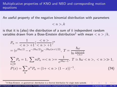
Multiplicative properties of KNO and NBD and corresponding motionequations

An useful property of the negative binomial distribution with parameters

< n >, k

is that it is (also) the distribution of a sum of k independent randomvariables drawn from a Bose-Einstein distribution1 with mean < n > /k,

Pn =1

< n > +1(< n >

< n > +1)n

= (eβ~ω/2 − e−β~ω/2)e−β~ω(n+1/2), T =~ω

ln <n>+1<n>

∑

n≥0

Pn = 1,∑

nPn =< n >=1

eβ~ω−1, T ≃ ~ω < n >, < n >≫ 1,

P (x) =∑

n

xnPn = (1+ < n > (1− x))−1. (74)

1A Bose-Einstein, or geometrical, distribution is a thermal distribution for single state systems.


This is easily seen from the generating function in (57), remembering thatthe generating function of a sum of independent random variables is theproduct of their generating functions.Indeed, for

n = n1 + n2 + ...+ nk, (75)

with ni independent of each other, the probability distribution of n is

Pn =∑

n1,...,nk

δ(n −∑

ni)pn1 ...pnk,

P (x) =∑

n

xnPn = p(x)k (76)

This has a consequence that an incoherent superposition of N emitters thathave a negative binomial distribution with parameters k,< n > produces anegative binomial distribution with parameters Nk,N < n >.


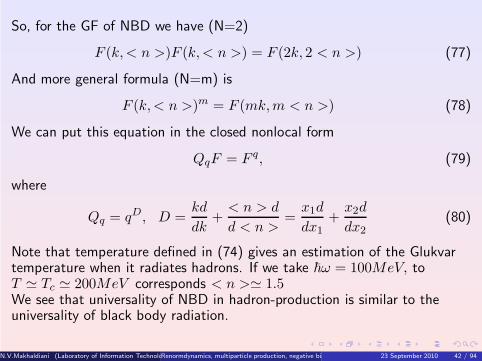
So, for the GF of NBD we have (N=2)

F (k,< n >)F (k,< n >) = F (2k, 2 < n >) (77)

And more general formula (N=m) is

F (k,< n >)m = F (mk,m < n >) (78)

We can put this equation in the closed nonlocal form

QqF = F q, (79)

where

Qq = qD, D =kd

dk+< n > d

d < n >=x1d

dx1+x2d

dx2(80)

Note that temperature defined in (74) gives an estimation of the Glukvartemperature when it radiates hadrons. If we take ~ω = 100MeV, toT ≃ Tc ≃ 200MeV corresponds < n >≃ 1.5We see that universality of NBD in hadron-production is similar to theuniversality of black body radiation.


p-adic string theory

p-adic string amplitudes can be obtained as tree amplitudes of the fieldtheory with the following lagrangian and motion equation (see e.g.[Brekke, Freund, 1993])

L =1

2ΦQpΦ− 1

p+ 1Φp+1,

QpΦ = Φp, Qp = pD (81)

D = −1

2△, △ = −∂2x0

+ ∂2x1+ ...+ ∂2xn−1

, (82)

Φ - is real scalar field on D-dimensional space-time with coordinatesx = (x0, x1, ..., xD−1). We have trivial, Φ = 0 and Φ = 1, and followingnontrivial solutions of the equation (81)

Φ(x0, x1, ..., xD−1) = pD

2(p−1) e1−p−1

2 lnp(x2

0−x21−x2

2−...−x2D−1) (83)


The equation (81) permits factorization of its solutionsΦ(x) = Φ(x0)Φ(x1)...Φ(xD−1), every factor of which fulfils onedimensional equation

pε∂2xΦ(x) = Φ(x)p, ε = ±1

2(84)

The trivial solution of the equations are Φ = 0 and Φ = 1. For nontrivialsolution of (84), we have

pε∂2xΦ(x) = ea∂

2Φ(x) =

1√4πa

∫ ∞

−∞

dye−14a

y2+y∂Φ(x)

=1√4πa

∫ ∞

−∞

dye−14a

y2Φ(x+ y) = Φ(x)p, a = ε ln p (85)

If we (de quantize) put, p = q, and take (classical) limit, q → 1, the motionequation reduce to

ε∂2xΦ = Φ lnΦ, (86)

with solution

Φ(x) = e12 e

x2

4ε . (87)


It is obvious that the anzac

Φ = Aebx2, (88)

can pass the equation (85). Indeed, the solution is

Φ(x) = p1

2(p−1) e1−p−1

4ε ln px2

,

Φ(x0, x1, ..., xD−1) = pD

2(p−1) e1−p−1

2 lnp(x2

0−x21−x2

2−...−x2D−1) (89)


Corresponding class of the motion equations

Now, we can define the following class of motion equations

QqF = F q, (90)

where

Qq = qD, D = D1(x1) + ...+Dl(xl), (91)

Dk(x) is some (differential) operator depending on x. In the case of theNBD GF,

Dk(x) =xd

dx. (92)

For this (Qlike) class of equations, we have factorization property

F = F (x1, ..., xl) = F1(x1)...Fl(xl),

qDk(x)Fk(x) = ckFk(x)q, 1 ≤ k ≤ l, c1c2...cl = 1. (93)


NBD motivated equations

For NBD distribution we have correspondingmultiplication(convolution)formulas

(P ⋆ P )n ≡n∑

m=0

Pm(k,< n >)Pn−m(k,< n >)

= Pn(2k, 2 < n >) = Q2Pn(k,< n >), ... (94)

So, we can say, that star-product on the distributions of NBD correspondsordinary product for GF.It will be nice to have similar things for string field theory(SFT)[Kaku,2000].SFT motion equation is

QΦ = Φ ⋆ Φ (95)

For stringfield GF F we may have

QF = F 2. (96)


By construction we know the solution of the nice equation (79) as GF ofNBD, F. We obtain corresponding differential equations, if we considerq = 1 + ε, for small ε,

(D(D − 1)...(D −m+ 1)− (lnF )m)Ψ = 0,

(Γ(D + 1)

Γ(D + 1−m)− (lnF )m)Ψ = 0,

(Dm − Φm)Ψ = 0,m = 1, 2, 3, ...

Dm =Γ(D + 1)

Γ(D + 1−m),Φ = lnF, (97)

with the solution Ψ = F = exp(Φ). In the case of the NBD and p-adicstring, we have correspondingly

D =x1d

dx1+x2d

dx2;

D = −1

2△, △ = −∂2x0

+ ∂2x1+ ...+ ∂2xn−1

. (98)

These equations have meaning not only for integer m.


For high mean multiplicities we have corresponding equations for KNO

Q2Ψ(z) = Ψ ⋆Ψ ≡∫ z

0Ψ(t)Ψ(z − t)dt (99)

Due to the explicit form of the operator D, these equations andcorresponding solutions have the symmetry under the change of thevariables

k → ak, < n >→ b < n > . (100)

When

a =< n >

k, b =

k

< n >, (101)

we obtain the symmetry with respect to the transformationsk ↔< n >, x1 ↔ x2.


Zeros of the Riemann zeta function

The Riemann zeta function ζ(s) is defined for complex s = σ + it andσ > 1 by the expansion

ζ(s) =∑

n≥1

n−s, Res > 1. (102)

All complex zeros, s = α+ iβ, of ζ(σ + it) function lie in the critical stripe0 < σ < 1, symmetrically with respect to the real axe and critical lineσ = 1/2. So it is enough to investigate zeros with α ≤ 1/2 and β > 0.These zeros are of three type, with small, intermediate and big ordinates.


Riemann hypothesis

The Riemann hypothesis [Titchmarsh,1986] states that the (non-trivial)complex zeros of ζ(s) lie on the critical line σ = 1/2.At the beginning of the XX century Polya and Hilbert made a conjecturethat the imaginary part of the Riemann zeros could be the oscillationfrequencies of a physical system (ζ - (mem)brane).After the advent of Quantum Mechanics, the Polya-Hilbert conjecture wasformulated as the existence of a self-adjoint operator whose spectrumcontains the imaginary part of the Riemann zeros.The Riemann hypothesis (RH) is a central problem in Pure Mathematicsdue to its connection with Number theory and other branches ofMathematics and Physics.


The functional equation for zeta function

The functional equation is (see e.g. [Titchmarsh,1986])

ζ(1− s) =2Γ(s)

(2π)scos(

πs

2)ζ(s) (103)

From this equation we see the real (trivial) zeros of zeta function:

ζ(−2n) = 0, n = 1, 2, ... (104)

Also, at s=1, zeta has pole with reside 1.From Field theory and statistical physics point of view, the functionalequation (103) is duality relation, with self dual (or critical) line in thecomplex plane, at s = 1/2 + iβ,

ζ(1

2− iβ) =

2Γ(s)

(2π)scos(

πs

2)ζ(

1

2+ iβ), (105)

we see that complex zeros lie symmetrically with respect to the real axe.On the critical line, (nontrivial) zeros of zeta corresponds to the infinitevalue of the free energy,

F = −T ln ζ. (106)


At the point with β = 14.134725... is located the first zero. In the interval10 < β < 100, zeta has 29 zeros. The first few million zeros have beencomputed and all lie on the critical line. It has been proved thatuncountably many zeros lie on critical line.The first relation of zeta function with prime numbers is given by thefollowing formula,

ζ(s) =∏

p

(1− p−s)−1, Res > 1. (107)

Another formula, which can be used on critical line, is

ζ(s) = (1− 21−s)−1∑

n≥1

(−1)n+1n−s, Res > 0. (108)


From Qlike to zeta equations

Let us consider the values q = n, n = 1, 2, 3, ... and take sum of thecorresponding equations (90), we find

ζ(−D)F =F

1− F(109)

In the case of the NBD we know the solutions of this equation.Now we invent a Hamiltonian H with spectrum corresponding to the set ofnontrivial zeros of the zeta function, in correspondence with Riemannhypothesis,

−Dn =n

2+ iHn, Hn = i(

n

2+Dn),

Dn = x1∂1 + x2∂2 + ...+ xn∂n, H+n = Hn =

n∑

m=1

H1(xm),

H1 = i(1

2+ x∂x) = −1

2(xp+ px), p = −i∂x (110)

The Hamiltonian H = Hn is hermitian, its spectrum is real. The casen = 1 corresponds to the Riemann hypothesis.


The case n = 2, corresponds to NBD,

ζ(1 + iH2)F =F

1− F, ζ(1 + iH2)|F =

1

1− F,

F (x1, x2;h) = (1 +x1x2

(1− h))−x2 (111)

Let us scale x2 → λx2 and take λ→ ∞ in (111), we obtain

ζ(1

2+ iH1(x))e

−(1−h)x =1

e(1−h)x − 1,

1

ζ(12 + iH(x))

1

eεx − 1= e−εx,

H(x) = i(1

2+ x∂x) = −1

2(xp+ px), H+ = H, ε = 1− h. (112)


Now we scale x→ xy, multiply the equation by ys−1 and integrate

1

ζ(12 + iH(x))

∫ ∞

0dy

ys−1

eεxy − 1=

∫ ∞

0dye−εxyys−1 =

1

(εx)sΓ(s),

1

ζ(12 + iH(x))

∫ ∞

0dy

ys−1

eεxy − 1

=1

ζ(12 + iH(x))x−sε−sΓ(s)ζ(s), (113)

so

ζ(1

2+ iH(x))x−s = ζ(s)x−s ⇒ H(x)ψE = EψE ,

ψE = cx−s, s =1

2+ iE, (114)


we have correct way and can return to the previous step (112) and take thefollowing transformation

1

eεxy − 1=

1

2π

∫ ∞+ic

−∞+icdEx−iE−1/2ϕ(E, εy),

ϕ(E, εy) =

∫ ∞

0dx

xiE− 12

eεxy − 1=

Γ(12 + iE)

(εy)iE+1/2ζ(

1

2+ iE),

1

2π

∫ ∞+ic

−∞+icdEx−iE−1/2ϕ(E, εy)

1

ζ(1/2 + iE)= e−εxy (115)


If we take the following formula

ζ(s) =1

Γ(s)

∫ ∞

0

ts−1dt

et − 1, (116)

which says that ζ function is the Mellin transformation, we can find

Γ(1 + iH2)F

1− F=

∫ ∞

0

dt/t

et − 1F 1/t, (117)

or

Γ(1 + iH2)Φ =

∫ ∞

0

dt/t

et − 1(

Φ

1 + Φ)1/t,

Φ =F

1− F=

1

(1 + x1x2(1− h))x2 − 1

(118)


We can obtain also the following equation with argument of ζN on criticalaxis

ζN (1

2+ iH1(x2))F (x1, x2, h) =

N∑

n=1

1

(1 + x1nx2

(1− h))nx2

=

N∑

n=1

F (x1, nx2, h),

ζN (1

2+ iH1(x2))F (λx1, x2, h) =

N∑

n=1

1

(1 + λx1nx2

(1− h))nx2

=

N∑

n=1

F (λx1, nx2, h) ≃ Ne−λ(1−h)x1 , N ≫ 1. (119)


Let us calculate next therm in the 1/λ expansion in the (111)

F (x1, λx2, h) = (1 +εx1λx2

)−λx2 = e−λx2 ln(1+ε

x1λx2

)

= e−εx1e(εx1)

2

2λx2+O(λ−2)

= e−εx1(1 +(εx1)

2

2λx2+O(λ−2)),

(F−1 − 1)−1 = (eλx2 ln(1+ε

x1λx2

) − 1)−1

=1

eεx1 − 1(1 +

eεx1

eεx1 − 1

(εx1)2

2λx2+O(λ−2)) (120)

The zero order term, λ0 we already considered. The next, λ−1 order termgives the following relations

ζ(−δ1 − δ2)x21x2e−εx1 =

1

x2ζ(1− δ1)x

21e

−εx1 =x21e

εx1

x2(eεx1 − 1)2,

ζ(1− δ)x2e−εx =x2eεx

(eεx − 1)2= x2e−εx +O(e−2εx)

ζ(1− δ)Ψ = EΨ +O(e−2εx),Ψ = x2e−εx, E = 1. (121)


There have been a number of approaches to understanding the Riemannhypothesis based on physics (for a comprehensive list see [Watkins])According to the idea of Berry and Keating, [Berry,Keating,1997] the realsolutions En of

ζ(1

2+ iEn) = 0, (122)

are energy levels, eigenvalues of a quantum Hermitian operator (theRiemann operator) associated with the one-dimensional classical hyperbolicHamiltonian

Hc = xp, (123)

where x and p are the conjugate coordinate and momentum.


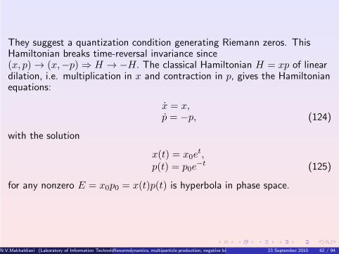
They suggest a quantization condition generating Riemann zeros. ThisHamiltonian breaks time-reversal invariance since(x, p) → (x,−p) ⇒ H → −H. The classical Hamiltonian H = xp of lineardilation, i.e. multiplication in x and contraction in p, gives the Hamiltonianequations:

x = x,p = −p, (124)

with the solution

x(t) = x0et,

p(t) = p0e−t (125)

for any nonzero E = x0p0 = x(t)p(t) is hyperbola in phase space.


The system is quantized by considering the dilation operator in the x space

H =1

2(xp+ px) = −i~(1

2+ x∂x), (126)

which is the simplest formally Hermitian operator corresponding to theclassical Hamiltonian. The eigenvalue equation

HψE = EψE , (127)

is satisfied by the eigenfunctions

ψE(x) = cx−12+ i

~E , (128)

where the complex constant c is arbitrary, since the solutions are notsquare-integrable. To the normalization

∫ ∞

0dxψE(x)

∗ψE′(x) = δ(E − E′), (129)

corresponds c = 1/√2π.


We have seen that

ζ(1

2+ iH)e−εx =

1

eεx − 1,

H = −i(12+ x∂x) = x1/2px1/2, p = −i∂x, (130)

than

e−εx =

∫

dEx−1/2+iEϕ(E, ε), ϕ(E, ε) =1

2π

∫ ∞

0dxx−1/2−iEe−εx

=ε−1/2+iE

2πΓ(1/2 + iE);

ζ(1

2+ iE)ϕ(E, ε) =

1

2π

∫ ∞

0dxx−1/2−iE

eεx − 1

=ε−1/2+iE

2πΓ(1/2 + iE)ζ(

1

2+ iE). (131)


Some calculations with zeta function values

From the equation (112) we have

ζ(1

2+ iH1(x))e

−εx =1

eεx − 1, H1 = i(

1

2+ x∂x),

ζ(−x∂x)(1− εx+(εx)2

2+ ...) =

1

εx(1− (

εx

2+

(εx)2

6+ ...)+

+(εx

2+ ...)2 + ...), (132)

so

ζ(0) = −1

2, ζ(−1) = − 1

12, ... (133)

Note that, a little calculation shows that, the (εx)2 terms cancels on ther.h.s, in accordance with ζ(−2) = 0.


More curious question concerns with the term 1/εx on the r.h.s. To itcorresponds the term with actual infinitesimal coefficient on the l.h.s.

1

ζ(1)

1

εx, (134)

in the spirit of the nonstandard analysis (see, e.g. [Davis,1977]), we canimagine that such a terms always present but on the r.h.s we may not notethem.For other values of zeta function we will use the following expansion

1

ex − 1=

1

x+ x2

2 + x3

3! + ...=

1

x− 1

2+

∑

k≥1

B2kx2k−1

(2k)!,

B2 =1

6, B4 = − 1

30, B6 =

1

42, ... (135)

and obtain

ζ(1− 2n) = −B2n

2n, n ≥ 1. (136)


Multiparticle production stochastic dynamics

Let us imagine space-time development of the the multiparticle process andtry to describe it by some (phenomenological) dynamical equation. Westart to find the equation for the Poisson distribution and than naturallyextend them for the NBD case.Let us define an integer valued variable n(t) as a number of events(produced particles) at the time t, n(0) = 0. The probability of eventn(t), P (t, n), is defined from the following motion equation

Pt ≡∂P (t, n)

∂t= r(P (t, n− 1)− P (t, n)), n ≥ 1

Pt(t, 0)) = −rP (t, 0),P (t, n) = 0, n < 0, (137)

so

P (t, 0) ≡ P0(t) = e−rt,P (t, n) = Q(t, n)P0(t),Qt(t, n) = rQ(t, n− 1), Q(t, 0) = 1. (138)


To solve the equation for Q, we invent its generating function

F (t, h) =∑

n≥0

hnQ(t, n), (139)

and solve corresponding equation

Ft = rhF, F (t, h) = erth =∑

hn(rt)n

n!, Q(t, n) =

(rt)n

n!, (140)

so

P (t, n) = e−rt (rt)n

n!(141)

is the Poisson distribution.If we compare this distribution with (73), we identify < n >= rt, as if wehave a free particle motion with velocity r and the distance is the meanmultiplicity. This way we have a connection between n-dimension of themultiplicity and the usual dimension of trajectory.


As the equation gives right solution, its generalization may give moregeneral distribution, so we will generalize the equation (137). For this, weput the equation in the closed form

Pt(t, n) = r(e−∂n − 1)P (t, n)

=∑

k≥1

Dk∂kP (t, n), Dk = (−1)k

r

k!, (142)

where the Dk, k ≥ 1, are generalized diffusion coefficients.For other values of the coefficients, we will have other distributions.


Fractal dimension of the multiparticle production trajectories

For mean square deviation of the trajectory we have

< (x− x)2 >=< x2 > − < x >2≡ D(x)2 ∼ t2/df , (143)

where df is fractal dimension. For smooth classical trajectory of particleswe have df = 1; for free stochastic, Brownian, trajectory, all diffusioncoefficients are zero but D2, we have df = 2. In the case of Poisson processwe have,

D(n)2 =< n2 > − < n >2∼ t, df = 2. (144)

In the case of the NBD and KNO distributions

D(n)2 ∼ t2, df = 1. (145)

As we have seen, rasing k, KNO reduce to the Poisson, so we have adimensional (phase) transition from the phase with dimension 1 to thephase with dimension 2. It is interesting, if somehow this phase transition isconnected to the other phase transitions in strong interaction processes.For the Poisson distribution GF is solution of the following equation,

F = −r(1− h)F, (146)


For the NBD corresponding equation is

F =−r(1− h)

1 + rtk (1− h)

F = −R(t)F, R(t) = r(1− h)

1 + rtk (1− h)

. (147)

If we change the time variable as t = T df , we reduce the dispersion lowfrom general fractal to the NBD like case. Corresponding transformation forthe evolution equation is

FT = −dfT df−1R(T dF )F, (148)

we ask that this equation coincides with NBD motion equation, and definerate function R(T )

dfTdf−1R(T dF ) =

r(1− h)

1 + rTk (1− h)

, (149)

now the following equation defines a production processes with fractaldimension dF

Ft = −R(t)F, R(t) = r(1− h)

dF tdF−1

dF (1 + rt1/dFk (1− h))

(150)


Spherical model of the multiparticle production

Now we would like to consider a model of multiparticle production based onthe d-dimensional sphere, and (try to) motivate the values of the NBDparameter k. The volum of the d-dimensional sphere with radius r, in unitsof hadron size rh is

v(d, r) =πd/2

Γ(d/2 + 1)(r

rh)d (151)

Note that,

v(0, r) = 1, v(1, r) = 2r

rh,

v(−1, r) =1

π

rhr

(152)

If we identify this dimensionless quantity with corresponding coulombenergy formula,

1

π=e2

4π, (153)

we find e = ±2.N.V.Makhaldiani (Laboratory of Information Technologies Joint Institute for Nuclear Research Dubna, Moscow Region, Russia e-mail address: [email protected] )Renormdynamics, multiparticle production, negative binomial distribution and Riemann zeta function23 September 2010 72 / 94

For less then -1 even integer values of d, and r 6= 0, v = 0. For negativeodd integer d = −2n+ 1

v(−2n + 1, r) =π−n+1/2

Γ(−n+ 3/2)(rhr)2n−1, n ≥ 1, (154)

v(−3, r) = − 1

2π2(rhr)3, v(−5, r) =

3

4π3(rhr)5 (155)

Note that,

v(2, r)v(3, r)v(−5, r) =1

π, v(1, r)v(2, r)v(−3, r) = − 1

π(156)

We postulate that after collision,it appear intermediate state with almostspherical form and constant energy density. Than the radius of the sphererise dimension decrease, volume remains constant. At the last moment ofthe expansion, when the crossection of the one dimensional sphere - stringbecome of order of hadron size, hadronic string divide in k independentsectors which start to radiate hadrons with geometric (Boze-Einstein)distribution, so all of the string final state radiate according to the NBDdistribution.


So, from the volume of the hadronic string,

v = π(r

rh)2l

rh= πk, (157)

we find the NBD parameter k,

k =πd/2−1

Γ(d/2 + 1)(r

rh)d (158)

Knowing, from experimental date, the parameter k, we can restrict theregion of the values of the parameters d and r of the primordial sphere (PS),

r(d) = (Γ(d/2 + 1)

πd/2−1k)1/drh,

r(3) = (3

4k)1/3rh, r(2) = k1/2rh, r(1) =

π

2krh (159)

If the value of r(d) will be a few rh, the matter in the PS will be in thehadronic phase. If the value of r will be of order 10rh, we can speak aboutdeconfined, quark-gluon, Glukvar, phase. From the formula (160), we see,that to have for the r, the value of order 10rh, in d = 3 dimension, we needthe value for k of order 1000, which is not realistic.


So in our model, we need to consider the lower than one, fractal,dimensions. It is consistent with the following intuitive picture. Confinedmatter have point-like geometry, withe dimension zero. Primordial sphereof Glukvar have nonzero fractal dimension, which is less than one,

k = 3, r(0.7395)/rh = 10.00,k = 4, r(0.8384)/rh = 10.00 (160)

From the experimental data we find the parameter k of the NBD as afunction of energy, k = k(s). Then, by our spherical model, we constructfractal dimension of the Glukvar as a function of k(s).If we suppose that radius of the primordial sphere r is of order (or less) ofrh. Than we will have higher dimensional PS, e.g.

d r/rh k3 1.3104 3.00024 1.1756 3.00036 1.1053 2.99948 1.1517 3.9990


Extra dimension effects at high energy and large scale Universe

With extra dimensions gravitation interactions may become strong at theLHC energies,

V (r) =m1m2

m2+d

1

r1+d(161)

If the extra dimensions are compactified with(in) size R, at r >> R,

V (r) ≃ m1m2

m2(mR)d1

r=m1m2

M2P l

1

r, (162)

where (4-dimensional) Planck mass is given by

M2P l = m2+dRd, (163)

so the scale of extra dimensions is given as

R =1

m(MP l

m)2d (164)


If we take m = 1TeV, (GeV −1 = 0.2fm)

R(d) = 2 · 10−17 · ( MP l

1TeV)2d · cm,

R(1) = 2 · 1015cm,R(2) = 0.2 cm !R(3) = 10−7cm !R(4) = 2 · 10−9cm,R(6) ∼ 10−11cm (165)

Note that lab measurements of GN (= 1/M2P l,MP l = 1.2 · 1019GeV ) have

been made only on scales of about 1 cm to 1 m; 1 astronomical unit(AU)(mean distance between Sun and Earth) is 1.5 · 1013cm; the scale of theperiodic structure of the Universe, L = 128Mps ≃ 4 · 1026cm. It is curiouswhich (small) value of the extra dimension corresponds to L?

d = 2ln MPl

m

ln(mL)= 0.74, m = 1TeV,

= 0.81, m = 100GeV,= 0.07, m = 1017GeV. (166)


Dynamical formulation of z - Scaling

Motion equations of physics (applied mathematics in general) connectdifferent observable quantities and reduce the number of independentlymeasurable quantities. More fundamental equation contains less number ofindependent quantities. When (before) we solve the equations, we inventdimensionless invariant variables, than one solution can describe all of theclass of phenomena.In the z - Scaling (zS) approach to the inclusive multiparticle distributions(MPD) (see, e.g. [Tokarev, Zborovsry, 2007a]), different inclusivedistributions depending on the variables x1, ...xn, are described by universalfunction Ψ(z) of fractal variable z,

z = x−α11 ...x−αn

n . (167)

It is interesting to find a dynamical system which generates thisdistributions and describes corresponding MPD.


We can find a good function if we know its derivative. Let us consider thefollowing RD like equation

zd

dzΨ = V (Ψ),

∫ Ψ(z)

Ψ(z0)

dx

V (x)= ln

z

z0(168)

In x−representation,

ln z = −n∑

k=1

αk lnxk, δz = zd

dz= −

∑

k

δknhαk

,

n∑

k=1

xknhαk

∂

∂xkΨ(x1, ..., xn) + V (Ψ) = 0, (169)

e.g.

z = δzz = −n∑

k=1

xknhαk

∂

∂xkx−α11 ...x−αn

n = z, nh = n. (170)


In the case of NBD GF (79), we have

n = 2, x1 = k, x2 =< n >, α1 = α2 = 1, nh = 1,Ψ = F, V (Ψ) = −Ψ lnΨ. (171)

In the case of the z−scaling, [Tokarev, Zborovsry, 2007a],

n = 4, x3 = ya, x4 = yb,α1 = δ1, α2 = δ2, α3 = εa, α4 = εb, nh = 4, (172)

for infinite resolution, αn = 1, n = 1, 2, 3, 4. In z variable the equation forΨ has universal form. In the case of n = 2, α1 = α2 = 1, nh = 1, we findthat V (Ψ) = −Ψ lnΨ, so if this form is applicable also in the case of n=4,

zd

dzΨ(z) = −Ψ lnΨ,

Ψ(z) = ec/z = (Ψ(z0)z0)

1z = Ψ(z0)

z0z ,

c = z0 lnΨ(z0) < 0, z ∈ (0,∞), Ψ(z) ∈ (0, 1). (173)

Note that the fundamental equation is invariant with respect to the scaletransformation z → λz, but the solution is not, the scale transformationtransforms one solution into another solution. This is an example of thespontaneous breaking of the (scale) symmetry by the states of the system.


Formal motivation (foundation) of the RD motion equation for Ψ

As a dimensionless physical quantity Ψ(z) may depend only on the runningcoupling constant g(τ), τ = ln z/z0

zd

dzΨ = Ψ =

dΨ

dgβ(g) = U(g) = U(f−1(Ψ)) = V (Ψ),

Ψ(τ) = f(g(τ)), g = f−1(Ψ(τ)) (174)


Realistic solution for Ψ

According to the paper [Tokarev, Zborovsry, 2007a], for high values ofz, Ψ(z) ∼ z−β ; for small z, Ψ(z) ∼ const.So, for high z,

zd

dzΨ = V (Ψ(z)) = −βΨ(z); (175)

for smaller values of z, Ψ(z) rise and we expect nonlinear terms in V (Ψ),

V (Ψ) = −βΨ+ γΨ2. (176)

With this function, we can solve the equation for Ψ(see appendix) and find

Ψ(z) =1

γβ + czβ

. (177)


Reparametrization of the RD equation

RD equation of the z-Scaling,

zd

dzΨ(z) = V (Ψ), V (Ψ) = V1Ψ+ V2Ψ

2 + ...+ VnΨn + ... (178)

can be reparametrized,

Ψ(z) = f(ψ(z)) = ψ(z) + f2ψ2 + ...+ fnψ

n + ...

zd

dzψ(z) = v(z) = v1ψ(z) + v2ψ

2 + ...+ vnψn + ...

(v1ψ(z) + v2ψ2 + ...+ vnψ

n + ...)(1 + 2f2ψ + ...+ nfnψn−1 + ...)

= V1(ψ + f2ψ2 + ...+ fnψ

n + ...)+V2(ψ

2 + 2f2ψ3 + ...) + ...+ Vn(ψ

n + nf2ψn+1 + ...) + ...

= V1ψ + (V2 + V1f2)ψ2 + (V3 + 2V2f2 + V1f3)ψ

3+...+ (Vn + (n− 1)Vn−1f2 + ...+ V1fn)ψ

n + ...v1 = V1,v2 = V2 − f2V1,v3 = V3 + 2V2f2 + V1f3 − 2f2v2 − 3f3v1 = V3 + 2(f22 − f3)V1, ...vn = Vn + (n− 1)Vn−1f2 + ...+ V1fn − 2f2vn−1 − ...− nfnv1, ...(179)

so, by reparametrization, we can change any coefficient of potential V butV1.


We can fix any higher coefficient with zero value, if we take

f2 =V2V1, f3 =

V32V1

+ f22 =V32V1

+ (V2V1

2

), ...

fn =Vn + (n− 1)Vn−1f2 + ...+ 2V2fn−1

(n− 1)V1, ... (180)

We will consider the case when only one of higher coefficient is nonzero andgive explicit form of the solution Ψ.


More general solution for Ψ

Let us consider more general potential V

zd

dzΨ = V (Ψ) = −βΨ(z) + γΨ(z)1+n (181)

Corresponding solution for Ψ is

Ψ(z) =1

(γβ + cznβ)1n

(182)


More general solution contains three parameters and may better describethe data of inclusive distributions.

0.5 1.0 1.5 2.0 2.5 3.0

0.2

0.4

0.6

0.8

1.0

Figure: z-scaling distribution (182), Ψ(z, 9, 9, 1, 1)

In the case of n = 1 we reproduce the previous solution.


Another ”natural” case is n = 1/β,

Ψ(z) =1

(γβ + cz)β(183)

In this case, we can absorb (interpret) the combined parameter by shift andscaling

z → 1

c(z − γ

β) (184)

Another interesting point of view is to predict the value of β

β =1

n= 0.5; 0.33; 0.25; 0.2; ..., n = 2, 3, 4, 5, ... (185)

For experimentally suggested value β ≃ 9, n = 0.11


In the case of n = −ε, β = γ = 1/ε, c = εk, we will have

V (Ψ) = −Ψ lnΨ, Ψ(z) = ekz (186)

This form of Ψ−function interpolates between asymptotic values of Ψ andpredicts its behavior in the intermediate region. These three parameterfunction is restricted by the normalization condition

∫ ∞

0Ψ(z)dz = 1,

B(β − 1

βn,1

βn) = (

β

γ)β−1βn

βn

cβn, (187)

so remains only two free parameter. When βn = 1, we have

c = (β − 1)(β

γ)β−1 (188)

If βn = 1 and β = γ, than c = β − 1.In general

cβn = (β

γ)β−1βn

βn

B(β−1βn ,

1βn)

(189)


Scaling properties of scaling functions and they equations

RD equation of the z-scaling (181), after substitution,

Ψ(z) = (ϕ(z))1n , (190)

reduce to the n = 1 case with scaled parameters,

ϕ = −βnϕ+ γnϕ2, (191)

this substitution could be motivated also by the structure of the solution(182),

Ψ(z, β, γ, n, c) = Ψ(z, βn, γn, 1, c)1n = Ψ(z, β, γ, βn, c)β . (192)

General RD equation takes form

ϕ = nv1ϕ+ nv2ϕ1+ 1

n + nv3ϕ1+ 2

n + ...+ nvnϕ2 + nvn+1ϕ

2+ 1n + ... (193)


Space-time dimension inside hadrons and nuclei

The dimension of the space(-time) is the model dependent concept. E.g.for the fundamental bosonic string model (in flat space-time) the dimensionis 26; for superstring model the dimension is 10 [Kaku,2000].Let us imagine that we have some action-functional formulation with thefundamental motion equation

zd

dzΨ = V (Ψ(z)) = V (Ψ) = −βΨ+ γΨ1+n. (194)

Than, the corresponding Lagrangian contains the following mass andinteraction parts

−β2Ψ2 +

γ

2 + nΨ2+n (195)

The action gives renormalizable (effective quantum field theory) modelwhen

d+ 2 =2N

N − 2=

2(2 + n)

n= 2 +

4

n= 2 + 4β, (196)

so, measuring the parameter β inside hadronic and nuclear matters, we findcorresponding (fractal) dimension.


Another action formulation of the Fundamental equation

From fundamental equation we obtain

(zd

dz)2Ψ ≡ Ψ = V ′(Ψ)V (Ψ) =

1

2(V 2)′

= β2Ψ− βγ(n+ 2)Ψn+1 + γ2(n + 1)Ψ2n+1 (197)

Corresponding action Lagrangian is

L =1

2Ψ2 + U(Ψ), U =

1

2V 2 =

1

2Ψ2(β − γΨn)2

=β2

2Ψ2 − βγΨ2+n +

γ2

2Ψ2+2n (198)

This potential, −U, has two maximums, when V = 0, and minimum, whenV ′ = 0, at Ψ = 0 and Ψ = (β/γ)1/n, and Ψ = (β/(n + 1)γ)1/n,correspondingly.


We define time-space-scale field Ψ(t, x, η), where η = ln z− is scalecoordinate variable, with corresponding action functional

A =

∫

dtddxdη(1

2gab∂aΨ∂bΨ+ U(Ψ)) (199)

The renormalization constraint for this action is

N = 2 + 2n =2(2 + d)

2 + d− 2= 2 +

4

d, dn = 2, d = 2/n = 2β. (200)

So we have two models for spase-time dimension, (196) and (200),

d1 = 4β; d2 = 2β (201)

The coordinate η characterise (multiparticle production) physical process atthe (external) space-time point (x,t). The dimension of the space-timeinside hadrons and nuclei, where multiparticle production takes place is

d+ 1 = 1 + 2β (202)

Note that this formula reminds the dimension of the spin s state,ds = 2s+ 1. If we take β(= s) = 0; 1/2; 1; 3/2; 2; ... We will haved+ 1 = 1; 2; 3; 4; 5; ...


Note that as we invent Ψ as a real field, we ought to take anothernormalization

∫

ddx|Ψ|2 = 1 (203)

for the solutions of the motion equation. This case extra values of theparameter β is possible, β > d/2.


Measurement of the space-time dimension inside hadrons

We can take a renormdynamic scheme were Ψ(g) is running couplingconstant. The variable z is a formation length and has dimension -1, RDequation for Ψ in ϕ3

D model is

zd

dzΨ =

6−D

2Ψ + γΨ2 (204)

β =D − 6

2(205)

For high values of z, β = 9, so D = 24. This value of D corresponds to thephysical (transverse) degrees of freedom of the relativistic string, to thedimension of the external space in which this relativistic string lives. This isalso the number of the quark - lepton matter degrees of freedom, 3 · 6 + 6.So, in these high energy reactions we measured the dimension of thespace-time and matter and find the values predicted by relativistic stringand SM. For lower energies, in this model, D monotonically decrees untilD = 6, than the model (may) change form on the ϕ4

D, β = D − 4. So wehave two scenarios of behavior. In one of them the dimension of thespace-time inside hadrons has value 6 and higher. In another the dimensionis 4 and higher.


Perturbative QCD indicates that we have a fixed point of RD in dimensionslightly higher than 4, and ordinary to hadron phase transition correspondsto the dimensional phase transition from slightly lower than 4, in QED, toslightly higher than 4 dimension in QCD. In general scalar field model ϕn

D,

β = −dg =nD

2− n−D. (206)

For ϕ3 model, β = 9 corresponds to D = 24. In tha case of theO(N)−sigma model

β = D − 2, (207)

For the experimental value of β = 9, we have the dimension of theM−theory, D = 11!


K. Aamodt et al. [ALICE collaboration] Eur. Phys. J. C65, 111 (2010); arXiv:1004.3034; arXiv:1004.3514.

M. Berry, Speculations on the Riemann operator, Symposium on Supersymmetry and Trace formulae, Cambridge, 1997.

N.N.Bogoliubov and D.V.Shirkov, Introduction to the Theory of Quantized Fields, New York, 1959.

L.Brekke, P.G.O.Freund, Phys. Rep. 233 1 (1993).

P.Carruthers, C.C.Shih, Int. J. Mod. Phys. A4 5587 (1989).

J.C.Collins, Renormalization, Cambrige Univ. Press, London, 1984.

Ya.Z.Darbaidze, N.V.Makhaldiani, A.N.Sisakian, L.A.Slepchenko, TMF 34 303 (1978).

M.Davis, Applied nonstandard analysis, New York, 1977.

W.Ernst, I.Schmitt, Nuovo Cim. A33 195 (1976).

L.D.Faddeev and L.A.Takhtajan, Hamiltonian methods in the theory of solitons, Springer, Berlin, 1987.

D.J. Gross, F. Wilczek, Phys. Rev. Lett. 30 (1973) 1343;

M.Kaku, Strings, Conformal Fields, and M - Theory, Springer, New York, 2000.

D.I.Kazakov, L.R.Lomidze, N.V.Makhaldiani, A.A.Vladimirov, Ultraviolet Asymptotics in Renormalizable Scalar Theories,

Communications of JINR, E2-8085, Dubna, 1974.

D.I.Kazakov, D.V.Shirkov, Fortschr. d. Phys. 28 447 (1980).

Z.Koba, H.B.Nielsen, P.Olesen, Nucl. Phys. B40 317 (1972).

Neal Koblitz, p-adic numbers, p-adic analysis, and Zeta-functions, Springer-Verlag, New York Heidelberg Berlin, 1977.


N.V.Makhaldiani, Approximate methods of the field theory and their applications in physics of high energy, condensed

matter, plasma and hydrodynamics, Dubna, 1980.

N.Makhaldiani, Nambu-Poisson dynamics of superintegrable systems, Atomic Nuclei, 70 564 (2007).

N. V. Makhaldiani, Renormdynamics and Scaling Functions, in Proc. of the XIX International Baldin Seminar on High

Energy Physics Problems eds. A.N.Sissakian, V.V.Burov, A.I.Malakhov, S.G.Bondartenko, E.B.Plekhanov, Dubna, 2008,Vol.II, p. 175.

V.A.Matveev, A.N.Sisakian, L.A.Slepchenko, Nucl. Phys. 23 432 (1976).

L.B.Okun, Leptons and Quarks, North Holland, 1982.

H.D. Politzer, Phys. Rev. Lett. 30 (1973) 1346;

L.S.Pontriagin et al., Mathematical Theory of Optimal Processes, Nauka, Moscow, 1983.

G. ’t Hooft, report at the Marseille Conference on Yang-Mills Fields, 1972.

G. ’t Hooft, Nucl.Phys. B 61 (1973) 455.

E.C. Titchmarsh, The Theory of the Riemann zeta-function (Clarendon Press, Oxford, 1986).

M.V.Tokarev, I.Zborovsky, Z-Scaling in the Proton-Proton Collisions at RHIC, in Investigations of Properties of Nuclear

Matter at High Temperature and Densities, Editid by A.N. Sisakian, F.A. Soifer, Dubna, 2007.

M.V.Tokarev, I.Zborovsky, T.G.Dedovich, Z-Scaling at RHIC and Tevatron, hep-ph, 0708.246, 2007.

M.Watkins at http://secamlocal.ex.ac.uk/∼ mwatkins/zeta/physics.htm.

S. Weinberg, Gravitation and Cosmology, New York, 1972.

S.Weinberg, The Quantum Theory of Fields, Volum I - Foundations, Cambridge Univ. Press, 1995.

S.Weinberg, The Quantum Theory of Fields, Volum II - Modern Applications, Cambridge Univ. Press, 1996.


S.Weinberg, The Quantum Theory of Fields, Volum III - Supersymmetry, Cambridge Univ. Press, 2000.

K.G.Wilson and J.Kogut, Phys. Rep. 12C 75 (1974).


Renormdynamics, multiparticle production, negative binomial distribution, and Riemann zeta function

Documents

Transcript of Renormdynamics, multiparticle production, negative binomial distribution, and Riemann zeta function