A new approach towards solving the Riemann hypothesis - OSF

A new approach towards solving the Riemann

hypothesis

Al-Mouid Mohammed Hasibul Haque

April 15, 2022

Abstract

In this paper, we create a new approach, using elementary tech-niques from complex analysis, by which we attempt to prove the Rie-mann hypothesis. We modify the gamma function and use that mod-ified form to reformulate the Riemann xi function. Then using someformulas that are similar to the Jacobi theta identity and analytic func-tion manipulation techniques from complex analysis, we show that allthe non-trivial zeros of the Riemann zeta function must lie on the crit-ical line. Then by recalling Hardy’s theorem we attempt to prove thatthe Riemann hypothesis is true.

Keywords: Complex analysis, Riemann hypothesis, Riemann’s Func-tional equation

1

1 Introduction

The Riemann hypothesis has been an unsolved mystery in the field of puremathematics for a long time.it is said to be the most daunting problem inall of pure mathematics. It is an essential part of analytic number theory.Hundreds of other theorems in analytic number theory depend on this hy-pothesis being true. The heart of the problem is simple to understand. Itsimply asks the question ‘Do all the non trivial zeros of the Riemann zetafunction lie on the critical line or are there some zeros that lie elsewherein the critical strip ?’ Or to put it in simple mathematical terms for all<(s) ∈ (0, 1) is

ζ(s) = 0

only for <(s) = 12 . The ζ(s) function is a meromorphic function with residue

1. It has many forms but its most fundamental form is the following

ζ(s) =

∞∑n=1

1

ns

Two functions that are very important in the study of this function are theGamma function and the xi function. These functions are the following

Γ(s) =

ˆ ∞o

xs−1e−xdx

and

ξ(s) =1

2s(s− 1)π−

s2 Γ(

s

2)ζ(s)

Euler was the first to notice that ζ(s) = 0 for s belonging to negative evenintegers. These zeros are called the trivial zeros of the zeta function. Sincethen many mathematicians have worked on this function and Riemann wasthe first to prove that all the non-trivial zero of the zeta function lie on the‘Critical strip’ which is the region where 0 < <(s) < 1. The distributionof these zeros as well as various properties of the Riemann zeta functionand some consequences of the Riemann hypothesis are well documented inE.C. Titchmarsh’s book[1]. Among the mathematicians who have provedvarious theorems related to the Riemann hypothesis G.H. Hardy stands outthe most in terms of finding where the non-trivial zeros lie. G.H. Hardy hasproved that there are infinitely many non-trivial zeros in the ‘Critical line’meaning the line where <(s) = 1

2 .

2

In order to prove that the hypothesis is true, many mathematicianshave tried various different approaches. The most common approach is touse analytic number theory to study the properties of the Riemann zetafunction and similar types of L-functions on the critical strip. From theseapproaches we now know that more than two-fifths of the non-trivial zerosof the zeta function lie on the critical line. This result can be found in J.B. Conrey’s paper[2]. Our approach also uses complex analysis to get ourdesired result. However the exact method that we use is different and hintstoward a more general condition by which we can test whether an L-functionhas a Riemann hypothesis or not.

Now for the proof we will mainly use the method of contradiction. Weuse the technique of contour integration on a function which is derived frommanipulating the definition of the ξ(s) function. Then we derive an inequal-ity by manipulating the parts of the contour integral using some formulasthat are similar to the Jacobi theta identity and the assumption that thevalue of ξ(s) is 0. By doing this we restrict ourselves to only the non-trivialzeros of the ζ function. From this inequality we arrive at a contradictionthat occurs only if any non-trivial zero lies on the critical strip but not thecritical line. By doing so we prove that all the non-trivial zeros of the zetafunction must lie on the critical line. But before jumping into the proof let’sprove two lemmas.

2 Preliminaries

These lemmas are as follows

Lemma 2.0.1. Let ξ(s) = 12s(s−1)π−

s2 Γ( s2)ζ(s) be the Riemann xi function

which is an entire function. Since it is an entire function ξ(s) and ξ(s) mustexist. Then the following holds true

|ξ(s)| = |ξ(s)|

Proof. We can easily see that∣∣∣ξ(s)∣∣∣ = |ξ(s)| because the output of ξ(s) is just

a complex number. So its complex conjugate must have the same modulus.Since ξ(s) is an entire function, it can be expressed as an analytic functionin any region within the complex plane and the center of the region wherethe function is analytic can be expressed as c, where c ∈ C or c ∈ R. For ourpurposes we say that the region is an open disc D where D ⊂ C and we willchoose c ∈ R (Since the function is entire, it doesn’t matter which region wechoose or where the center is, because the function is by definition analytic

3

in the entire complex plane. So if we choose a real number in D to be thecenter of our function then the function still remains analytic.) Now we canwrite

ξ(s) =

∞∑n=0

an(s− c)n

So

ξ(s) =

∞∑n=0

an(s− c)n

and ∣∣∣ξ(s)∣∣∣ =

∣∣∣∣∣∞∑n=0

an(s− c)n∣∣∣∣∣

≤∞∑n=0

|an| |(s− c)|n

Because zn = (z)n where z ∈ C . Similarly

|ξ(s)| =

∣∣∣∣∣∞∑n=0

an(s− c)n∣∣∣∣∣

≤∞∑n=0

|an||(s− c)|n

Now ∣∣∣ξ(s)∣∣∣− |ξ(s)| ≤ ∞∑n=0

|an| |(s− c)|n −∞∑n=0

|an||(s− c)|n

and |an| = |an| where an ∈ C. So∣∣∣ξ(s)∣∣∣− |ξ(s)| ≤ ∞∑n=0

|an| (|(s− c)|n − |(s− c)|n)

Recall that we chose c ∈ R so we have c = c . Thus∣∣∣ξ(s)∣∣∣− |ξ(s)| ≤ ∞∑n=0

|an| (|(s− c)|n − |(s− c)|n)

⇒∣∣∣ξ(s)∣∣∣− |ξ(s)| ≤ 0

∴∣∣∣ξ(s)∣∣∣ ≤ |ξ(s)|

4

Similarly if we take

|ξ(s)| −∣∣∣ξ(s)∣∣∣ ≤ ∞∑

n=0

|an||(s− c)|n −∞∑n=0

|an| |(s− c)|n

By a similar argument we arrive at

|ξ(s)| −∣∣∣ξ(s)∣∣∣ ≤ 0

∴ |ξ(s)| ≤∣∣∣ξ(s)∣∣∣

Now both of these inequalities must be true. And the only way both can be

true is if∣∣∣ξ(s)∣∣∣ = |ξ(s)|. And by using the fact that

∣∣∣ξ(s)∣∣∣ = |ξ(s)| we can

clearly state that |ξ(s)| = |ξ(s)|. �

Now let’s move on to the second lemma. The way this lemma is provedfollows a similar approach to the proof of the classical Jacobi theta functionidentity although with some modifications in the method (due to a slightlydifferent statement of the lemma). Now before we do this let’s define thefollowing two sets

C+ := {z ∈ C : =(z) > 0}

andC− := {z ∈ C : =(z) < 0}

Lemma 2.0.2. For x ∈ C− − I the following holds true

∑n∈Z

e−n2πx2i =

e−πi4

x

∑n∈Z

en2πi 1

x2

Proof. For x ∈ C− − I we can clearly see that both the series in the L.H.S.and R.H.S. converge. From Poisson’s summation formula we know∑

n∈Ze−n

2πx2i =∑k∈Z

ˆ ∞−∞

e−y2πx2ie−2πikydy

=∑k∈Z

ˆ ∞−∞

e−iπ[y2x2+2ky+( kx

)2−( kx

)2]dy

=∑k∈Z

ˆ ∞−∞

e−iπ[(xy+ kx

)2−( kx

)2]dy

5

=∑k∈Z

eiπk2

x2

ˆ ∞−∞

e−iπ[(xy+ kx

)2]dy

=∑k∈Z

eiπk2

x2

ˆ ∞−∞

e−iπx2(y+ k

x2 )2

dy

Let y +k

x2= z

dy = dz

then as y →∞, z →∞+ ic

and as y → −∞, z → −∞+ ic

Where c is a positive constant which depends on =(x),<(x) and k. Now

ˆ ∞+ic

−∞+ice−iπx

2z2dz =

ˆ ∞−∞

e−iπx2z2dz−

(ˆ −∞+ic

−∞e−iπx

2z2dz +

ˆ ∞∞+ic

e−iπx2z2dz

)And here the latter two integrals have the same lengths but have oppositeorientations and for this reason after adding the two their effect on the sumis nullified and thusˆ ∞+ic

−∞+ice−iπx

2z2dz =

ˆ ∞−∞

e−iπx2z2dz

We can also say that since the argument is the same thus we can just evaluatethe integral from −∞ to ∞ instead of −∞ + ic to ∞ + ic. Either way theabove equality remains the same. Then∑

n∈Ze−n

2πx2i =∑k∈Z

eiπk2

x2

ˆ ∞−∞

e−iπx2z2dz

=∑k∈Z

eiπk2

x2

√π

iπx2

=1

x√i

∑k∈Z

eiπk2

x2

=e−i

π4

x

∑k∈Z

eiπk2

x2

∴∑n∈Z

e−n2πx2i =

e−πi4

x

∑n∈Z

en2πi 1

x2

�

6

3 The Riemann hypothesis

The statement of the theorem is as follows

Theorem 3.1. Let ζ(s) =∑∞

n=11ns be a meromorphic function that is an-

alytically continued to the entire complex plane except s = 1. Then all thenon-trivial zeros of ζ(s) for s∈ C lie on the line where <(s) = 1

2 .

This statement is slightly different from what Riemann originally hypoth-esised and what Bombieri [4] stated in the description of this millenniumproblem. But the statements are equivalent. Since G.H. Hardy alreadyproved that their are infinitely many zeros in the critical line we have an ad-vantage here (A proof of Hardy’s theorem is found in [1, pp. 256-258]). Ifwe can simply prove that all the non-trivial zeros must lie on the line where<(s) = 1

2 then it will be equivalent to proving the Riemann hypothesis.In the proof we will use methods that are similar to the method first usedby Riemann [3] himself in order to define the Riemann xi function but ourmethod to define the xi function will be slightly different. Nonetheless theRiemann’s functional equation will still apply and the Riemann xi functionwill still be entire as we will see later on. Now let’s jump into the proof.

4 The Proof

Proof. Riemann’s functional equation states that

ξ(s) = ξ(1− s)

We will need this later on. From the definition of the Gamma function wehave

Γ(s

2) =

ˆ ∞0

ts2−1e−tdt

By substituting t = n2πx2 we get

Γ(s

2) =

ˆ ∞0

(n2πx2

) s2−1e−n

2πx22n2πxdx

⇒ Γ(s

2) = 2

ˆ ∞0

nsπs2xs−1e−n

2πx2dx

⇒ 1

2π−

s2n−sΓ(

s

2) =

ˆ ∞0

xs−1e−n2πx2

dx

7

By summing n from 1 to ∞ we get

1

2π−

s2

∞∑n=1

n−sΓ(s

2) =

∞∑n=1

ˆ ∞0

xs−1e−n2πx2

dx

The R.H.S. converges for <(s) > 1. So by convergence and using Fubini’stheorem we have

1

2π−

s2 ζ(s)Γ(

s

2) =

ˆ ∞0

xs−1∞∑n=1

e−n2πx2

dx

⇒ s(s− 1)

2π−

s2 ζ(s)Γ(

s

2) = s(s− 1)

ˆ ∞0

xs−1∞∑n=1

e−n2πx2

dx

∴ ξ(s) = s(s− 1)

ˆ ∞0

xs−1∞∑n=1

e−n2πx2

dx

Since the L.H.S. is holomorphic for s ∈ C(meaning the function is entire),sothe R.H.S. is also holomorphic for s ∈ C.1

By substituting s with s, where s is the complex conjugate of s, we get

ξ(s) = s(s− 1)

ˆ ∞0

xs−1∞∑n=1

e−n2πx2

dx

Since ξ(s) = ξ(1− s) from the functional equation we can write

s(s− 1)

ˆ ∞0

xs−1∞∑n=1

e−n2πx2

dx = s(s− 1)

ˆ ∞0

x−s∞∑n=1

e−n2πx2

dx (1)

Now we writeˆ ∞0

xs−1∞∑n=1

e−n2πx2

dx−ˆ ∞

0xs−1

∞∑n=1

e−n2πx2

dx =ξ(s)

s(s− 1)− ξ(s)

s(s− 1)(2)

Since ξ(s) and ξ(s) are entire and <(s) ∈ (0, 1), so the R.H.S. is holomorphic.Moreover both the integrals in the L.H.S. are also analytic for <(s) ∈ (0, 1).2

By using equation (1) we write equation (2) as

ˆ ∞0

x−s∞∑n=1

e−n2πx2

dx−ˆ ∞

0xs−1

∞∑n=1

e−n2πx2

dx =ξ(s)

s(s− 1)− ξ(s)

s(s− 1)

1By analytic continuation we can show that the R.H.S. is analytic for s ∈ C and furthermore we can show that if s ∈ (0, 1) then the integral itself is holomorphic without thes(s− 1) multiplicative factor. We will give a rigorous proof of this in the appendix.

2This is a trivial consequence of corollary A.1.1. in the appendix.

8

⇒ˆ ∞

0(x−s

∞∑n=1

e−n2πx2 − xs−1

∞∑n=1

e−n2πx2

)dx =1

2π−

s2 Γ(

s

2)ζ(s)− 1

2π−

s2 Γ(

s

2)ζ(s)

∴

∞

0

∞∑n=1

e−n2πx2

(x−s − xs−1)dx =1

2π−

s2 Γ(

s

2)ζ(s)− 1

2π−

s2 Γ(

s

2)ζ(s) (3)

Here we can do this because ,as we prove in a corollary in the appendix, theintegral in the L.H.S. of equation (3) can be analytic for <(s) ∈ (0, 1) viathe method of analytic continuation. So the above equation actually holdsfor <(s) ∈ (0,∞). Now let’s see what will happen to ζ(s) if ζ(s) = 0. Forthis we will go back to the ξ(s) function. From lemma 1 we can state that

|ξ(s)| = |ξ(s)|

⇒∣∣∣∣12s(s− 1)π−

s2 Γ(

s

2)ζ(s)

∣∣∣∣ =

∣∣∣∣12 s(s− 1)π−s2 Γ(

s

2)ζ(s)

∣∣∣∣Since <(s) ∈ (0, 1) and Γ(s) has no zeros for <(s) ∈ (0, 1) we can divide

both sides by

∣∣∣∣12 s(s− 1)π−s2 Γ(

s

2)

∣∣∣∣. Recalling that the absolute value of a

product is the product of the absolute value and switching sides we get

|ζ(s)| = |ζ(s)|∣∣∣∣Γ( s2)

Γ( s2)

∣∣∣∣Because

∣∣∣∣∣ 12s(s− 1)π−

s2

12 s(s− 1)π− s

2

∣∣∣∣∣ = 1, we ignored it in the expression above. Now

Γ( s2) 6= 0 for all <(s) ∈ (0, 1) and same goes for Γ( s2) for all <(s) ∈ (0, 1).So if ζ(s) = 0 then by the expression above ζ(s) = 0.

Now we assume ξ(s) = 0 and by doing this we consider ζ(s) = 0 onlywhen <(s) ∈ (0, 1).Then equation (3) becomes

ˆ ∞0

∞∑n=1

e−n2πx2

(x−s − xs−1)dx = 0 (4)

This expression is valid for <(s) ∈ (0, 1) 3and the L.H.S. of the above equa-tion becomes zero whenever ξ(s) = 0.

3Here each integral can be analytically continued by corollary A.1.1 in the appendix.And since the combination of analytic functions is analytic so equation (4) remains validfor <(s) ∈ (0, 1)

9

0<(s)

=(s)

c

Reiπ4

γ

B

RA

π4

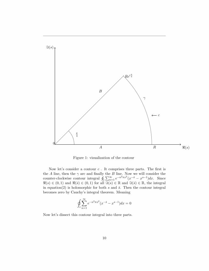
Figure 1: visualization of the contour

Now let’s consider a contour c . It comprises three parts. The first isthe A line, then the γ arc and finally the B line. Now we will consider thecounter-clockwise contour integral

¸c

∑∞n=1 e

−n2πx2(x−s − xs−1)dx. Since

<(s) ∈ (0, 1) and <(s) ∈ (0, 1) for all =(s) ∈ R and =(s) ∈ R, the integralin equation(2) is holomorphic for both s and s. Then the contour integralbecomes zero by Cauchy’s integral theorem. Meaning

˛c

∞∑n=1

e−n2πx2

(x−s − xs−1)dx = 0

Now let’s dissect this contour integral into three parts.

10

We can write˛c

∞∑n=1

e−n2πx2

(x−s−xs−1)dx =

ˆA

∞∑n=1

e−n2πx2

(x−s−xs−1)dx+

ˆγ

∞∑n=1

e−n2πx2

(x−s−xs−1)dx

+

ˆB

∞∑n=1

e−n2πx2

(x−s − xs−1)dx

We define the line A to start from 0 and go to R where R→∞ and defineB to start from Rei

π4 and go to 0 where R→∞. Now

˛c

∞∑n=1

e−n2πx2

(x−s − xs−1)dx = limR→∞

ˆ R

0

∞∑n=1

e−n2πx2

(x−s − xs−1)dx+

ˆB

∞∑n=1

e−n2πx2


ˆγ

∞∑n=1

e−n2πx2


∴ 0 = limR→∞

ˆ R

0

∞∑n=1

e−n2πx2


ˆB

∞∑n=1

e−n2πx2


ˆγ

∞∑n=1

e−n2πx2

(x−s − xs−1)dx (5)

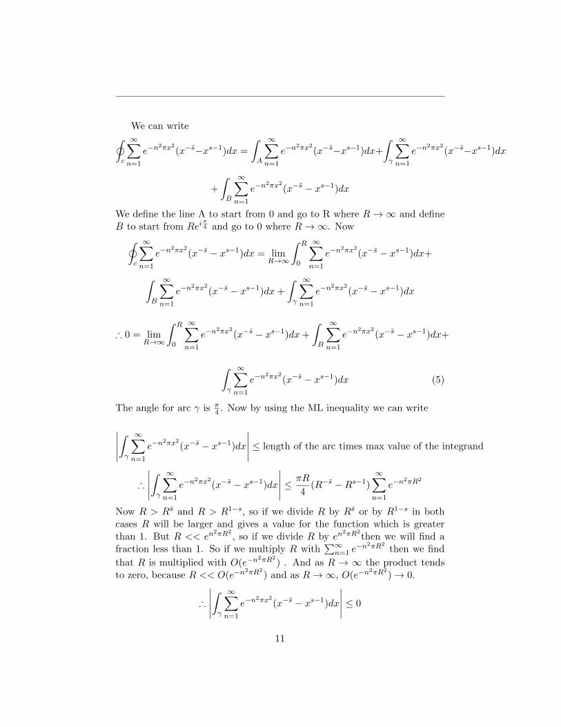
The angle for arc γ is π4 . Now by using the ML inequality we can write

∣∣∣∣∣ˆγ

∞∑n=1

e−n2πx2


∣∣∣∣∣ ≤ length of the arc times max value of the integrand

∴

∣∣∣∣∣ˆγ

∞∑n=1

e−n2πx2


∣∣∣∣∣ ≤ πR

4(R−s −Rs−1)

∞∑n=1

e−n2πR2

Now R > Rs and R > R1−s, so if we divide R by Rs or by R1−s in bothcases R will be larger and gives a value for the function which is greaterthan 1. But R << en

2πR2, so if we divide R by en

2πR2then we will find a

fraction less than 1. So if we multiply R with∑∞

n=1 e−n2πR2

then we find

that R is multiplied with O(e−n2πR2

) . And as R → ∞ the product tendsto zero, because R << O(e−n

2πR2) and as R→∞, O(e−n

2πR2)→ 0.

∴

∣∣∣∣∣ˆγ

∞∑n=1

e−n2πx2


∣∣∣∣∣ ≤ 0

11

∴ˆγ

∞∑n=1

e−n2πx2

(x−s − xs−1)dx = 0

Now we can write´B

∑∞n=1 e

−n2πx2(x−s − xs−1)dx as the following by sub-

stituting x with teiπ4 and integrating with respect to t

ˆB

∞∑n=1

e−n2πx2

(x−s−xs−1)dx =

ˆB

∞∑n=1

e−n2πx2

x−sdx−ˆB

∞∑n=1

e−n2πx2

xs−1dx

= limR→∞

ˆ 0

Reiπ4

∞∑n=1

e−n2πx2

x−sdx−ˆ 0

Reiπ4

∞∑n=1

e−n2πx2

xs−1dx

= eiπ4 limR→∞

ˆ 0

R

∞∑n=1

e−in2πt2t−se−is

π4 dt− lim

R→∞

ˆ 0

R

∞∑n=1

e−in2πt2ts−1eis

π4 dt

Since t is a dummy variable we can change it with x. Then the expressionbecomes

ˆB

∞∑n=1

e−n2πx2

(x−s − xs−1)dx = eiπ4 limR→∞

ˆ 0

R

∞∑n=1

e−in2πx2

x−se−isπ4 dx−

limR→∞

ˆ 0

R

∞∑n=1

e−in2πx2

xs−1eisπ4 dx

If we let x→ 0 but x 6= 0 then we can take a segment from B line that

goes from εeπia to 0 where ε → 0, then we find the integral in that small

segment to be

limε→0

ˆ 0

εeiπ4

∞∑n=1

e−n2πx2


We can then easily show that limε→0

´ 0

εeiπ4

∑∞n=1 e

−n2πx2(x−s−xs−1)dx = 0.4

So we can easily disregard that segment and let the B line go from Reiπ4 to

εeiπ4 , where R→∞ and ε→ 0. Then the above expression becomes

ˆB

∞∑n=1

e−n2πx2

(x−s−xs−1)dx = limR→∞ε→0

(eiπ4

(1−s)ˆ ε

R

∞∑n=1

e−n2πx2ix−sdx−

ˆ ε

Reis

π4

∞∑n=1

e−n2πx2ixs−1dx

)4This can be easily done using a length based argument. We will prove a theorem in

the appendix that will show that this is the case.

12

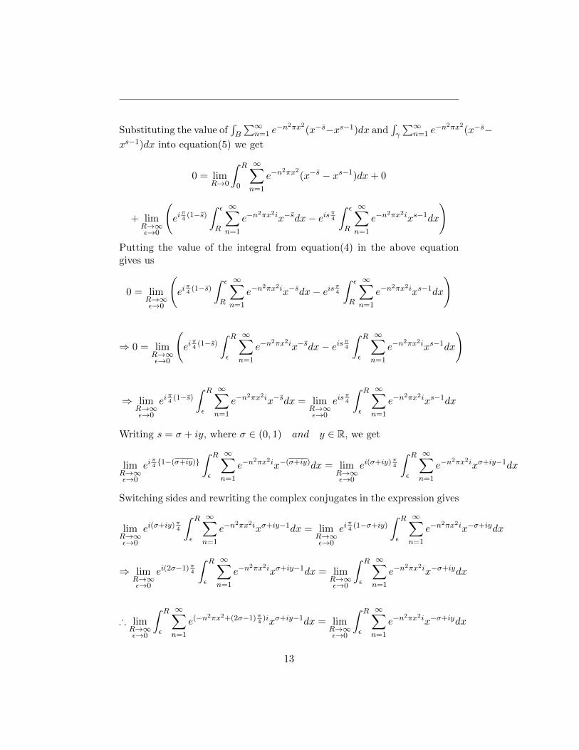
Substituting the value of´B

∑∞n=1 e

−n2πx2(x−s−xs−1)dx and

´γ

∑∞n=1 e

−n2πx2(x−s−

xs−1)dx into equation(5) we get

0 = limR→0

ˆ R

0

∞∑n=1

e−n2πx2

(x−s − xs−1)dx+ 0

+ limR→∞ε→0

(eiπ4

(1−s)ˆ ε

R

∞∑n=1

e−n2πx2ix−sdx− eis

π4

ˆ ε

R

∞∑n=1

e−n2πx2ixs−1dx

)Putting the value of the integral from equation(4) in the above equationgives us

0 = limR→∞ε→0

(eiπ4

(1−s)ˆ ε

R

∞∑n=1


π4

ˆ ε

R

∞∑n=1

e−n2πx2ixs−1dx

)

⇒ 0 = limR→∞ε→0

(eiπ4

(1−s)ˆ R

ε

∞∑n=1


π4

ˆ R

ε

∞∑n=1

e−n2πx2ixs−1dx

)

⇒ limR→∞ε→0

eiπ4

(1−s)ˆ R

ε

∞∑n=1

e−n2πx2ix−sdx = lim

R→∞ε→0

eisπ4

ˆ R

ε

∞∑n=1

e−n2πx2ixs−1dx

Writing s = σ + iy, where σ ∈ (0, 1) and y ∈ R, we get

limR→∞ε→0

eiπ4{1−(σ+iy)}

ˆ R

ε

∞∑n=1

e−n2πx2ix−(σ+iy)dx = lim

R→∞ε→0

ei(σ+iy)π4

ˆ R

ε

∞∑n=1

e−n2πx2ixσ+iy−1dx

Switching sides and rewriting the complex conjugates in the expression gives

limR→∞ε→0

ei(σ+iy)π4

ˆ R

ε

∞∑n=1

e−n2πx2ixσ+iy−1dx = lim

R→∞ε→0

eiπ4

(1−σ+iy)

ˆ R

ε

∞∑n=1

e−n2πx2ix−σ+iydx

⇒ limR→∞ε→0

ei(2σ−1)π4

ˆ R

ε

∞∑n=1

e−n2πx2ixσ+iy−1dx = lim

R→∞ε→0

ˆ R

ε

∞∑n=1


∴ limR→∞ε→0

ˆ R

ε

∞∑n=1

e(−n2πx2+(2σ−1)π4

)ixσ+iy−1dx = limR→∞ε→0

ˆ R

ε

∞∑n=1


13

(6)

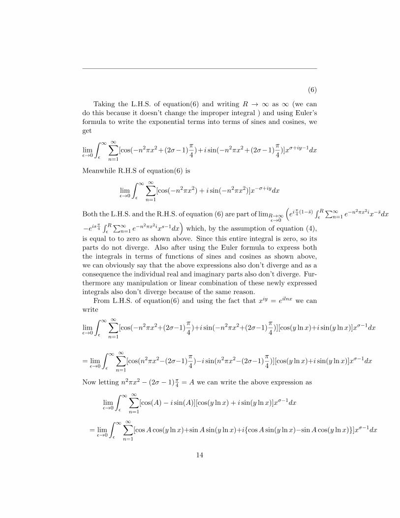
Taking the L.H.S. of equation(6) and writing R → ∞ as ∞ (we cando this because it doesn’t change the improper integral ) and using Euler’sformula to write the exponential terms into terms of sines and cosines, weget

limε→0

ˆ ∞ε

∞∑n=1

[cos(−n2πx2 +(2σ−1)π

4)+i sin(−n2πx2 +(2σ−1)

π

4)]xσ+iy−1dx

Meanwhile R.H.S of equation(6) is

limε→0

ˆ ∞ε

∞∑n=1

[cos(−n2πx2) + i sin(−n2πx2)]x−σ+iydx

Both the L.H.S. and the R.H.S. of equation (6) are part of limR→∞ε→0

(eiπ4

(1−s) ´ Rε

∑∞n=1 e

−n2πx2ix−sdx

−eisπ4

´ Rε

∑∞n=1 e

−n2πx2ixs−1dx)

which, by the assumption of equation (4),

is equal to to zero as shown above. Since this entire integral is zero, so itsparts do not diverge. Also after using the Euler formula to express boththe integrals in terms of functions of sines and cosines as shown above,we can obviously say that the above expressions also don’t diverge and as aconsequence the individual real and imaginary parts also don’t diverge. Fur-thermore any manipulation or linear combination of these newly expressedintegrals also don’t diverge because of the same reason.

From L.H.S. of equation(6) and using the fact that xiy = eilnx we canwrite

limε→0

ˆ ∞ε

∞∑n=1

[cos(−n2πx2+(2σ−1)π

4)+i sin(−n2πx2+(2σ−1)

π

4)][cos(y lnx)+i sin(y lnx)]xσ−1dx

= limε→0

ˆ ∞ε

∞∑n=1

[cos(n2πx2−(2σ−1)π

4)−i sin(n2πx2−(2σ−1)

π

4)][cos(y lnx)+i sin(y lnx)]xσ−1dx

Now letting n2πx2 − (2σ − 1)π4 = A we can write the above expression as

limε→0

ˆ ∞ε

∞∑n=1

[cos(A)− i sin(A)][cos(y lnx) + i sin(y lnx)]xσ−1dx

= limε→0

ˆ ∞ε

∞∑n=1

[cosA cos(y lnx)+sinA sin(y lnx)+i{cosA sin(y lnx)−sinA cos(y lnx)}]xσ−1dx

14

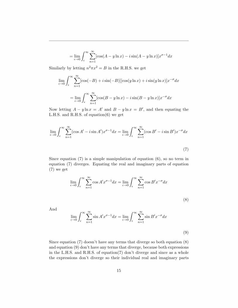
= limε→0

ˆ ∞ε

∞∑n=1

[cos(A− y lnx)− i sin(A− y lnx)]xσ−1dx

Similarly by letting n2πx2 = B in the R.H.S. we get

limε→0

ˆ ∞ε

∞∑n=1

[cos(−B) + i sin(−B)][cos(y lnx) + i sin(y lnx)]x−σdx

= limε→0

ˆ ∞ε

∞∑n=1

[cos(B − y lnx)− i sin(B − y lnx)]x−σdx

Now letting A − y lnx = A′ and B − y lnx = B′, and then equating theL.H.S. and R.H.S. of equation(6) we get

limε→0

ˆ ∞ε

∞∑n=1

(cosA′ − i sinA′)xσ−1dx = limε→0

ˆ ∞ε

∞∑n=1

(cosB′ − i sinB′)x−σdx

(7)

Since equation (7) is a simple manipulation of equation (6), so no term inequation (7) diverges. Equating the real and imaginary parts of equation(7) we get

limε→0

ˆ ∞ε

∞∑n=1

cosA′xσ−1dx = limε→0

ˆ ∞ε

∞∑n=1

cosB′x−σdx

(8)

And

limε→0

ˆ ∞ε

∞∑n=1

sinA′xσ−1dx = limε→0

ˆ ∞ε

∞∑n=1

sinB′x−σdx

(9)

Since equation (7) doesn’t have any terms that diverge so both equation (8)and equation (9) don’t have any terms that diverge, because both expressionsin the L.H.S. and R.H.S. of equation(7) don’t diverge and since as a wholethe expressions don’t diverge so their individual real and imaginary parts

15

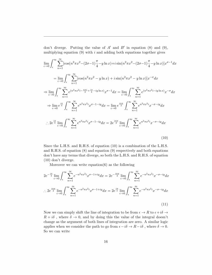
don’t diverge. Putting the value of A′ and B′ in equation (8) and (9),multiplying equation (9) with i and adding both equations together gives

limε→0

ˆ ∞ε

∞∑n=1

[cos(n2πx2−(2σ−1)π

4−y lnx)+i sin(n2πx2−(2σ−1)

π

4−y lnx)]xσ−1dx

= limε→0

ˆ ∞ε

∞∑n=1

[cos(n2πx2 − y lnx) + i sin(n2πx2 − y lnx)]x−σdx

⇒ limε→0

ˆ ∞ε

∞∑n=1

e(n2πx2i−πσi2

+ iπ4−iy lnx)xσ−1dx = lim

ε→0

ˆ ∞ε

∞∑n=1

e(n2πx2i−iy lnx)x−σdx

⇒ limε→0

eiπ4

ˆ ∞ε

∞∑n=1

en2πx2ixσ−1−iydx = lim

ε→0eiπσ2

ˆ ∞ε

∞∑n=1

en2πx2ix−σ−iydx

∴ 2eiπ4 limε→0

ˆ ∞ε

∞∑n=1

en2πx2ixσ−1−iydx = 2e

iπσ2 lim

ε→0

ˆ ∞ε

∞∑n=1


(10)

Since the L.H.S. and R.H.S. of equation (10) is a combination of the L.H.S.and R.H.S. of equation (8) and equation (9) respectively and both equationsdon’t have any terms that diverge, so both the L.H.S. and R.H.S. of equation(10) don’t diverge.

Moreover we can write equation(6) as the following

2e−iπ4 limε→0

ˆ ∞ε

∞∑n=1

e−n2πx2ixσ−1+iydx = 2e−

iπσ2 lim

ε→0

ˆ ∞ε

∞∑n=1

e−n2πx2ix−σ−iydx

∴ 2eiπσ2 lim

ε→0

ˆ ∞ε

∞∑n=1

e−n2πx2ixσ−1+iydx = 2e

iπ4 limε→0

ˆ ∞ε

∞∑n=1


(11)

Now we can simply shift the line of integration to be from ε→ R to ε+ iδ →R + iδ , where δ → 0, and by doing this the value of the integral doesn’tchange as the argument of both lines of integration are zero. A similar logicapplies when we consider the path to go from ε− iδ → R− iδ , where δ → 0.So we can write

16

limε→0

ˆ ∞ε

∞∑n=1

e−n2πx2ixσ−1+iydx = lim

δ→0ε→0

ˆ ∞−iδε−iδ

∞∑n=1

e−n2πx2ixσ−1+iydx

(12)

limε→0

ˆ ∞ε

∞∑n=1

e−n2πx2ix−σ−iydx = lim

δ→0ε→0


∞∑n=1


(13)

limε→0

ˆ ∞ε

∞∑n=1

en2πx2ix−σ−iydx = lim

δ→0ε→0

ˆ ∞+iδ

ε+iδ

∞∑n=1


(14)

and

limε→0

ˆ ∞ε

∞∑n=1

en2πx2ixσ−1−iydx = lim

δ→0ε→0

ˆ ∞+iδ

ε+iδ

∞∑n=1

en2πx2ixσ−1−iydx

(15)

So from equation (10) and equation (11) we can write

limδ→0ε→0


∞∑n=1

e−n2πx2ix−σ−iydx = lim

δ→0ε→0


∞∑n=1


(16)

and

limδ→0ε→0

ˆ ∞+iδ

ε+iδ

∞∑n=1

en2πx2ix−σ−iydx = lim

δ→0ε→0

ˆ ∞+iδ

ε+iδ

∞∑n=1

en2πx2ixσ−1−iydx

(17)

Now∑∞

n=1 en2πx2i and

∑∞n=1 e

−n2πx2i are part of the sums∑

n∈Z en2πx2i and∑

n∈Z e−n2πx2i respectively, both of which abide by the second lemma stated

17

in the preliminary. This is because here x ∈ C− − I so lemma 2.0.2 can beapplied to the R.H.S. of the above expression. So we can write the followingequations from lemma 2.0.2

∑n∈Z

e−n2πx2i =

e−iπ4

x

∑n∈Z

en2π 1

x2 i (18)

And ∑n∈Z

e−n2π 1

x2 i = e−iπ4 x∑n∈Z

en2πx2i (19)

where the last equation can be easily proved the same way lemma 2.0.2 wasproved which holds for x ∈ C+ − I.

From equation (18) we have

1 + 2∞∑n=1

e−n2πx2i =

e−iπ4

x

(2∞∑n=1

en2π 1

x2 i + 1

)

⇒ 2∞∑n=1

e−n2πx2i =

e−iπ4

x+ 2

e−iπ4

x

∞∑n=1

en2π 1

x2 i − 1

∴ 2eiπ4

∞∑n=1

e−n2πx2i =

1

x+

2

x

∞∑n=1

en2π 1

x2 i − eiπ4 (20)

From equation(19) we have

1 + 2

∞∑n=1

e−n2π 1

x2 i = −ieiπ4 x

(1 + 2

∞∑n=1

en2πx2i

)

⇒ 1

x(−ieiπ4 )

+ 2

∑∞n=1 e

−n2π 1x2 i

x(−ieiπ4 )

= 1 + 2

∞∑n=1

en2πx2i

⇒ i

x(eiπ4 )

+ 2i∑∞

n=1 e−n2π 1

x2 i

x(eiπ4 )

== 1 + 2

∞∑n=1

en2πx2i

⇒ i

x+ 2

i∑∞

n=1 e−n2π 1

x2 i

x= e

iπ4 + 2e

iπ4

∞∑n=1

en2πx2i

18

∴ 2eiπ4

∞∑n=1

en2πx2i =

i

x+ 2

i∑∞

n=1 e−n2π 1

x2 i

x− e

iπ4 (21)

Using equation (21) on the L.H.S. of equation (17) we get

L.H.S. = limδ→0ε→0

[ˆ ∞+iδ

ε+iδ

i

xxσ−1−iydx+ 2i

ˆ ∞+iδ

ε+iδ

∞∑n=1

e−n2π 1

x2 ixσ−2−iydx− eiπ4

ˆ ∞+iδ

ε+iδxσ−1−iydx

]

Writing limδ→0ε→0

´∞+iδε+iδ

ixx

σ−1−iydx = I,2i limδ→0ε→0

´∞+iδε+iδ

∑∞n=1 e

−n2π 1x2 ixσ−2−iydx =

E and limδ→0ε→0

eiπ4

´∞+iδε+iδ xσ−1−iydx = J we get,

L.H.S. = I + E − J (22)

Now

E = 2i limδ→0ε→0

ˆ ∞+iδ

ε+iδ

∞∑n=1

e−n2π 1

x2 ixσ−2−iydx

By substituting

x =1

t

dx = −t−2dt

While changing the limits we notice, as x→ ε+ iδ and ε→ 0, δ → 0 thent→ 1

ε+iδ and 1ε+iδ →∞− iδ

′ . And since δ is infinitesimally small so δ′ = δ

and thus 1ε+iδ →∞− iδ . By a similar argument as x→∞+ iδ t→ ε− iδ.

∴ E = −2i limδ→0ε→0

ˆ ε−iδ

∞−iδ

∞∑n=1

e−n2πt2it2−σ+iyt−2dt

= limδ→0ε→0

2i


∞∑n=1

e−n2πt2it−σ+iydt

Now since t is a dummy variable we can switch it with x

∴ E = 2i limδ→0ε→0


∞∑n=1


19

Now multiplying eiπ4 to both sides of equation (16) gives us

2eiπσ2

+ iπ4 limδ→0ε→0


∞∑n=1

e−n2πx2ixσ−1+iydx = 2e

πi2 limδ→0ε→0


∞∑n=1


∴ 2eiπσ2


ˆ ∞+iδ

ε+iδ

∞∑n=1

e−n2πx2ixσ−1+iydx = 2i lim

δ→0ε→0

ˆ ∞+iδ

ε+iδ

∞∑n=1


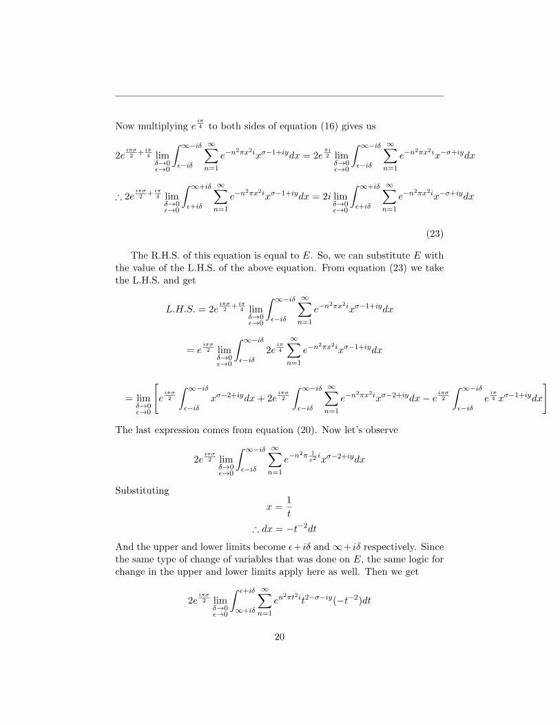
(23)

The R.H.S. of this equation is equal to E. So, we can substitute E withthe value of the L.H.S. of the above equation. From equation (23) we takethe L.H.S. and get

L.H.S. = 2eiπσ2



∞∑n=1


= eiπσ2 lim

δ→0ε→0


2eiπ4

∞∑n=1


= limδ→0ε→0

[eiπσ2


xσ−2+iydx+ 2eiπσ2


∞∑n=1

e−n2πx2ixσ−2+iydx− e

iπσ2


eiπ4 xσ−1+iydx

]

The last expression comes from equation (20). Now let’s observe

2eiπσ2 lim

δ→0ε→0


∞∑n=1

e−n2π 1

x2 ixσ−2+iydx

Substituting

x =1

t

∴ dx = −t−2dt

And the upper and lower limits become ε+ iδ and∞+ iδ respectively. Sincethe same type of change of variables that was done on E, the same logic forchange in the upper and lower limits apply here as well. Then we get

2eiπσ2 lim

δ→0ε→0

ˆ ε+iδ

∞+iδ

∞∑n=1

en2πt2it2−σ−iy(−t−2)dt

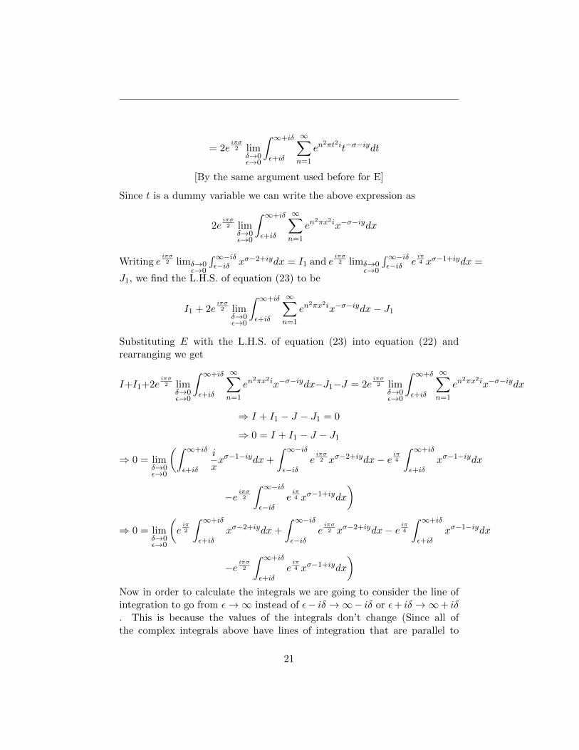
20

= 2eiπσ2 lim

δ→0ε→0

ˆ ∞+iδ

ε+iδ

∞∑n=1

en2πt2it−σ−iydt

[By the same argument used before for E]

Since t is a dummy variable we can write the above expression as

2eiπσ2 lim

δ→0ε→0

ˆ ∞+iδ

ε+iδ

∞∑n=1


Writing eiπσ2 limδ→0

ε→0

´∞−iδε−iδ xσ−2+iydx = I1 and e

iπσ2 limδ→0

ε→0

´∞−iδε−iδ e

iπ4 xσ−1+iydx =

J1, we find the L.H.S. of equation (23) to be

I1 + 2eiπσ2 lim

δ→0ε→0

ˆ ∞+iδ

ε+iδ

∞∑n=1

en2πx2ix−σ−iydx− J1

Substituting E with the L.H.S. of equation (23) into equation (22) andrearranging we get

I+I1+2eiπσ2 lim

δ→0ε→0

ˆ ∞+iδ

ε+iδ

∞∑n=1

en2πx2ix−σ−iydx−J1−J = 2e

iπσ2 lim

δ→0ε→0

ˆ ∞+δ

ε+iδ

∞∑n=1


⇒ I + I1 − J − J1 = 0

⇒ 0 = I + I1 − J − J1

⇒ 0 = limδ→0ε→0

(ˆ ∞+iδ

ε+iδ

i

xxσ−1−iydx+


eiπσ2 xσ−2+iydx− e

iπ4

ˆ ∞+iδ


−eiπσ2


eiπ4 xσ−1+iydx

)⇒ 0 = lim

δ→0ε→0

(eiπ2

ˆ ∞+iδ

ε+iδxσ−2+iydx+


eiπσ2 xσ−2+iydx− e

iπ4

ˆ ∞+iδ


−eiπσ2

ˆ ∞+iδ

ε+iδeiπ4 xσ−1+iydx

)Now in order to calculate the integrals we are going to consider the line ofintegration to go from ε→∞ instead of ε− iδ →∞− iδ or ε+ iδ →∞+ iδ. This is because the values of the integrals don’t change (Since all ofthe complex integrals above have lines of integration that are parallel to

21

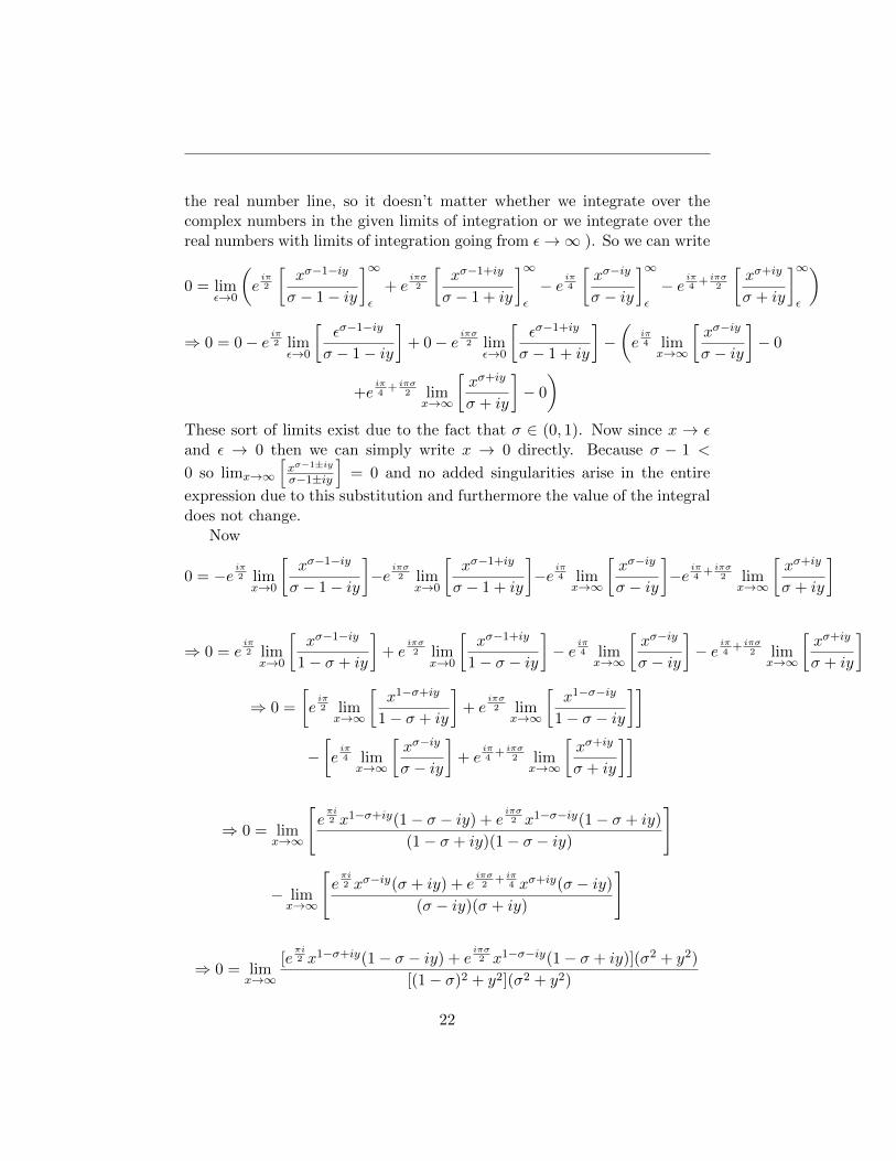
the real number line, so it doesn’t matter whether we integrate over thecomplex numbers in the given limits of integration or we integrate over thereal numbers with limits of integration going from ε→∞ ). So we can write

0 = limε→0

(eiπ2

[xσ−1−iy

σ − 1− iy

]∞ε

+ eiπσ2

[xσ−1+iy

σ − 1 + iy

]∞ε

− eiπ4

[xσ−iy

σ − iy

]∞ε

− eiπ4

+ iπσ2

[xσ+iy

σ + iy

]∞ε

)

⇒ 0 = 0− eiπ2 limε→0

[εσ−1−iy

σ − 1− iy

]+ 0− e

iπσ2 lim

ε→0

[εσ−1+iy

σ − 1 + iy

]−(eiπ4 limx→∞

[xσ−iy

σ − iy

]− 0

+eiπ4

+ iπσ2 lim

x→∞

[xσ+iy

σ + iy

]− 0

)These sort of limits exist due to the fact that σ ∈ (0, 1). Now since x → εand ε → 0 then we can simply write x → 0 directly. Because σ − 1 <

0 so limx→∞

[xσ−1±iy

σ−1±iy

]= 0 and no added singularities arise in the entire

expression due to this substitution and furthermore the value of the integraldoes not change.

Now

0 = −eiπ2 limx→0

[xσ−1−iy

σ − 1− iy

]−e

iπσ2 lim

x→0

[xσ−1+iy

σ − 1 + iy

]−e

iπ4 limx→∞

[xσ−iy

σ − iy

]−e

iπ4

+ iπσ2 lim

x→∞

[xσ+iy

σ + iy

]

⇒ 0 = eiπ2 limx→0

[xσ−1−iy

1− σ + iy

]+ e

iπσ2 lim

x→0

[xσ−1+iy

1− σ − iy

]− e

iπ4 limx→∞

[xσ−iy

σ − iy

]− e

iπ4

+ iπσ2 lim

x→∞

[xσ+iy

σ + iy

]

⇒ 0 =

[eiπ2 limx→∞

[x1−σ+iy

1− σ + iy

]+ e

iπσ2 lim

x→∞

[x1−σ−iy

1− σ − iy

]]−[eiπ4 limx→∞

[xσ−iy

σ − iy

]+ e

iπ4

+ iπσ2 lim

x→∞

[xσ+iy

σ + iy

]]

⇒ 0 = limx→∞

[eπi2 x1−σ+iy(1− σ − iy) + e

iπσ2 x1−σ−iy(1− σ + iy)

(1− σ + iy)(1− σ − iy)

]

− limx→∞

[eπi2 xσ−iy(σ + iy) + e

iπσ2

+ iπ4 xσ+iy(σ − iy)

(σ − iy)(σ + iy)

]

⇒ 0 = limx→∞

[eπi2 x1−σ+iy(1− σ − iy) + e

iπσ2 x1−σ−iy(1− σ + iy)](σ2 + y2)

[(1− σ)2 + y2](σ2 + y2)

22

− limx→∞

[eiπ4 xσ−iy(σ + iy) + e

iπσ2

+ iπ4 xσ+iy(σ − iy)]{(1− σ)2 + y2}

[(1− σ)2 + y2](σ2 + y2)

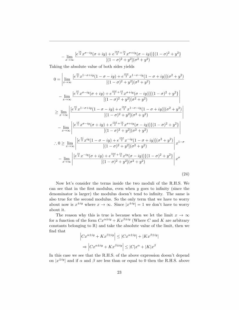
Taking the absolute value of both sides yields

0 =

∣∣∣∣∣ limx→∞

[eπi2 x1−σ+iy(1− σ − iy) + e

iπσ2 x1−σ−iy(1− σ + iy)](σ2 + y2)

[(1− σ)2 + y2](σ2 + y2)

− limx→∞

[eiπ4 xσ−iy(σ + iy) + e

iπσ2

+ iπ4 xσ+iy(σ − iy)]{(1− σ)2 + y2}

[(1− σ)2 + y2](σ2 + y2)

∣∣∣∣∣≥ lim

x→∞

∣∣∣∣∣ [eπi2 x1−σ+iy(1− σ − iy) + e

iπσ2 x1−σ−iy(1− σ + iy)](σ2 + y2)

[(1− σ)2 + y2](σ2 + y2)

∣∣∣∣∣− limx→∞

∣∣∣∣∣ [eiπ4 xσ−iy(σ + iy) + e

iπσ2

+ iπ4 xσ+iy(σ − iy)]{(1− σ)2 + y2}

[(1− σ)2 + y2](σ2 + y2)

∣∣∣∣∣∴ 0 ≥ lim

x→∞

∣∣∣∣∣ [eπi2 xiy(1− σ − iy) + e

iπσ2 x−iy(1− σ + iy)](σ2 + y2)

[(1− σ)2 + y2](σ2 + y2)

∣∣∣∣∣x1−σ

− limx→∞

∣∣∣∣∣ [eiπ4 x−iy(σ + iy) + e

iπσ2

+ iπ4 xiy(σ − iy)]{(1− σ)2 + y2}

[(1− σ)2 + y2](σ2 + y2)

∣∣∣∣∣xσ(24)

Now let’s consider the terms inside the two moduli of the R.H.S. Wecan see that in the first modulus, even when y goes to infinity (since thedenominator is larger) the modulus doesn’t tend to infinity. The same isalso true for the second modulus. So the only term that we have to worryabout now is x±iy where x → ∞. Since |x±iy| = 1 we don’t have to worryabout it.

The reason why this is true is because when we let the limit x → ∞for a function of the form Cxα±iy +Kxβ±iy (Where C and K are arbitraryconstants belonging to R) and take the absolute value of the limit, then wefind that ∣∣∣Cxα±iy +Kxβ±iy

∣∣∣ ≤ |Cxα±iy|+ |Kxβ±iy|⇒∣∣∣Cxα±iy +Kxβ±iy

∣∣∣ ≤ |C|xα + |K|xβ

In this case we see that the R.H.S. of the above expression doesn’t dependon |x±iy| and if α and β are less than or equal to 0 then the R.H.S. above

23

goes to zero and if and only if α and β are greater than 0 then the R.H.S.goes to infinity as x→∞.

So by the same reasoning, in inequality (24) x±iy doesn’t have any rel-evant impact on the value of the R.H.S. and we can thus replace the twoabsolute values with two positive (finite) constants that are fixed for specificvalues of σ and y and don’t depend on x.

Now, letting the R.H.S. of inequality (24) be S, we can write

S = limx→∞

C1x1−σ − C2x

σ

Where C1 and C2 are two positive constants belonging to R. Now

limx→∞

C1x1−σ − C2x

σ

= limx→∞

C1x− C2x2σ

xσ

Let limx→∞C1x−C2x2σ

xσ = L. Then there are two cases.Case− 1 : 0 < σ < 1

2then 2σ < 1So,L := limx→∞

C1x−C2x2σ

xσ → ∞ as C1x grows much faster than C2x2σ

and dividing by xσ doesn’t effect the result. Even if we only consider C1x1−σ

and C2xσ then we can still see that C1x

1−σ grows much faster then C2xσ for

all σ ∈ (0, 12) and the limit goes to infinity as x→∞. Then inequality (24)

doesn’t hold true. Since in the interval 0 < σ < 12 inequality (24) doesn’t

hold true then we can clearly see a contradiction and thus prove that thereare no zeros of ξ(s) for <(s) ∈ (0, 1

2) and thus there are no zeros of ζ(s) for<(s) ∈ (0, 1

2) . This applies for all =(s) ∈ R because we have already proventhat ζ(s) = 0 if ζ(s) = 0 and thus the positive or negative value of y doesn’teffect the final result.

Case− 2 : 12 < σ < 1

then 2σ > 1So, L := limx→∞

C1x−C2x2σ

xσ → −∞ because now C2x2σ grows much

faster than C1x and dividing by xσ doesn’t effect the result. Then inequality(24) holds and we find no apparent contradiction. Then based on this onemight assume that ζ(s) can have zero in the interval <(s) ∈ (1

2 , 1). But weknow from the identity ξ(s) = ξ(1 − s) that if ζ(s) = 0 then ζ(1 − s) = 0where s = σ + iy and 1 − s = 1 − σ − iy and as stated before, positive ornegative values of y doesn’t effect the result. Now σ ∈ (1

2 , 1) so 1−σ ∈ (0, 12)

and from Case-1 we have already shown that ζ(s) 6= 0 for <(s) ∈ (0, 12). We

24

find another clear contradiction here and thus we can say that Case-2 is alsonot true.

However, if we let <(s) = 12 then not only inequality (24) but also every

equation starting from equation(4) holds true. Thus we can conclude thatζ(s) can have a non-trivial zero if and only if <(s) = 1

2 . And by usingHardy’s theorem we can clearly state that all the non-trivial zeros of ζ(s),where s∈ C, lie on the line where <(s) = 1

2 and there are infinitely many ofthem. �

5 Remarks

The proof here has been done mostly based on methods from complex anal-ysis.Though this approach to prove the Riemann hypothesis is very elemen-tary but it should serve the cause.

According to the approach if any function has a Riemann hypothesis likethe zeta function then it must abide by an inequality similar to inequality(24), which would force the function to only have nontrivial zeros on thecritical line, for this approach to apply for that function. So cases such asthe Epstein series [5] do not apply for this approach because even thoughthese functions have functional equations similar to the Riemann functionalequation, but these functions don’t give us any inequality similar to inequal-ity (24) and thus our approach doesn’t apply. However, the approach doesnot guarantee that all L-functions have a Riemann hypothesis, because forthat to hold true we need to prove that there are finitely or (more likely)infinitely many nontrivial zeros that lie on the critical line and if some L-function does not give us an inequality similar to inequality (24) then itdoesn’t automatically say that the function doesn’t have a Riemann hy-pothesis but rather it would mean that our approach doesn’t apply for thatparticular L-function. So this approach might not apply for the generalizedRiemann hypothesis but further investigation is needed for that assertion.

The approach we have created is so elementary that even the Euler prod-uct was not explicitly used in our main theorem. However we see somethinginteresting when we examine the integral in equation (3). We know that theEuler product the zeta function is the following

ζ(s) =∏p

1

1− p−s

We know that the above expression leads to the usual series representationof the zeta function. Now the usual series representation of the zeta function

25

is linear. Not only that but each term in the Euler product representationis also linear. Because of this linearity we can derive the particular repre-sentation of ξ(s) that we have utilized in our proof and from this particularrepresentation of the ξ(s) and the identity ξ(s) = ξ(1− s) we derived equa-tion (3) which holds true for <(s) > 1. This was because both the seriesrepresentation and product representation of the zeta function converges ab-solutely in the region <(s) > 1. Then we analytically continued the integralin equation (3) to also hold for the region <(s) ∈ (0, 1). This same logicalso holds for other L-functions that have a Euler product. However it isnot clear whether our new approach holds true for proving the Riemannhypothesis in the general case (though it is most likely that if the approachactually works for the ordinary Riemann hypothesis then a similar approachwill also work for other Dirichlet L-functions).

Finally even if it is the case that the given proof above is inadequate toprove the Riemann hypothesis, the approach used in the proof is still worthinvestigating further as such approaches may help uncover some propertiesof L-functions which might not be apparent currently.

Data availability statement: The manuscript has no associated data

26

Appendix

A Proof of the convergence of the integral in theRiemann xi function

This theorem uses a modified version of the argument presented in [1] whichproves that the Riemann xi function is entire. Now let’s start by stating thetheorem

Theorem A.1. let the definition of the Riemann xi function be the followingξ(s) := s(s − 1)

´∞0 xs−1

∑∞n=1 e

−n2πx2dx . Then ξ(s) is analytic for all

s ∈ C.

Proof. We have

ξ(s) = s(s− 1)

ˆ ∞0

xs−1∞∑n=1

e−n2πx2

dx

Lets only consider the integral first. For simplicity we will consider∑∞

n=1 e−n2πx2

=ψ(x2). Then

ˆ ∞0

xs−1∞∑n=1

e−n2πx2

dx =

ˆ ∞0

xs−1ψ(x2)dx

=

ˆ ∞1

xs−1ψ(x2)dx+

ˆ 1

0xs−1ψ(x2)dx

=

ˆ ∞1

xs−1ψ(x2)dx+

ˆ 1

0ys−1ψ(y2)dy

Let y = 1x and dy = − 1

x2dx. Then the upper limit becomes 1 and the lowerlimit becomes ∞. Then the latter integral becomes the following

ˆ 1

∞x1−sψ(

1

x2)(− 1

x2)dx

=

ˆ ∞1

x−s−1ψ(1

x2)dx

We know that one of the Jacobi theta functions is

θ(x2) =∑n∈Z

e−n2πx2

27

= 2ψ(x2) + 1

And it abides by the following identity

1

xθ(

1

x2) = θ(x2)

⇒ θ(1

x2) = xθ(x2)

We can do this because x doesn’t approach 0 in the interval of the integralwe are concerned with. By using this identity we can write

2ψ(1

x2) = θ(

1

x2)− 1

= 2xψ(x2) + x− 1

∴ ψ(1

x2) =

x

2+ xψ(x2)− 1

2

Then we can writeˆ ∞1

x−s−1ψ(1

x2)dx =

ˆ ∞1

x−s−1(x

2+ xψ(x2)− 1

2)dx

=1

2

ˆ ∞1

x−sdx+

ˆ ∞1

x−sψ(x2)dx− 1

2

ˆ ∞1

x−s−1dx

= −1

2

ˆ ∞1

x−s−1dx+1

2

ˆ ∞1

x−sdx+

ˆ ∞1

x−sψ(x2)dx

= − 1

2s+

1

2(s− 1)+

ˆ ∞1

x−sψ(x2)dx

=1

2s(s− 1)+

ˆ ∞1

x−sψ(x2)dx

The above expression is always true for <(s) > 1. The integrand of thelast integral converges absolutely for all s ∈ C and x ∈ (1,∞), because

the integrand is of order O( e−πx2

xs ). So this expression can be analyticallycontinued for all s ∈ C. Then if we simply include this dissected form of theintegral into ξ(s), we find

ξ(s) = s(s− 1)

(ˆ ∞1

xs−1ψ(x2)dx+1

2s(s− 1)+

ˆ ∞1

x−sψ(x2)dx

)

⇒ ξ(s) = s(s− 1)

ˆ ∞1

xs−1ψ(x2)dx+1

2+ s(s− 1)

ˆ ∞1

x−sψ(x2)dx

28

Here the integrand of the first integral is analytic and the last integralconverges absolutely as stated above. So the R.H.S. is analytic for all of s ∈C. Thus we can clearly state that ξ(s) = s(s − 1)

´∞0 xs−1

∑∞n=1 e

−n2πx2dx

is analytic for all s ∈ C. �

Corollary A.1.1. For <(s) ∈ (0, 1) the integral´∞

0 xs−1∑∞

n=1 e−n2πx2

dxis analytic.

Proof. From the proof above we can write´∞

0 xs−1∑∞

n=1 e−n2πx2

dx as thefollowing

ˆ ∞0

xs−1∞∑n=1

e−n2πx2

dx =

ˆ ∞1

xs−1ψ(x2)dx+

ˆ ∞1

x−s−1ψ(1

x2)dx

and ˆ ∞1

x−s−1ψ(1

x2)dx =

1

2s(s− 1)+

ˆ ∞1

x−sψ(x2)dx

Where ψ(x2) =∑∞

n=1 e−n2πx2

. Here we can clearly see that the integralis analytic for s ∈ C − {0, 1} , so obviously for <(s) ∈ (0, 1) the integral´∞

1 x−s−1ψ( 1x2 )dx is analytic and as a result the integral

´∞0 xs−1

∑∞n=1 e

−n2πx2dx

is analytic. �

B An additional theorem

This additional theorem will suffice to show that not including the integrallimε→0

´ 0

εeiπ4

∑∞n=1 e

−n2πx2(x−s−xs−1)dx in the expansion of the B segment

was only logical because this integral goes to zero. Let’s now state and provethe theorem.

Theorem B.1. Let s ∈ C and let limε→0

´ 0

εeiπ4

∑∞n=1 e

−n2πx2(x−s−xs−1)dx

lie on a line segment on the complex plane that goes from εeπi4 to 0 where

ε→ 0. Then limε→0

´ 0

εeiπ4

∑∞n=1 e

−n2πx2(x−s − xs−1)dx = 0.

Proof. We recall from the corollary above that the integral´∞

0 xs−1∑∞

n=1 e−n2πx2

dxconverges for <(s) ∈ (0, 1). So the integrand converges and thus holomorphicin the complex plane if s ∈ C and <(s) ∈ (0, 1). So, if we take a semi-circlewithin the region enclosed by the set U then we will find the contour inte-gral along the boundary of the semicircle to be zero by Cauchy’s integraltheorem. Meaning

˛Λ

(x−s − xs−1)∞∑n=1

e−n2πx2

dx = 0

29

Here I have taken the semicircle over the set U ′ ⊂ U and I have taken thecontour in such a manner that the path along the contour goes clockwiseinstead of counter-clockwise. Meaning

˛Λ

∞∑n=1

e−n2πx2

(x−s − xs−1)dx =

Λ

∞∑n=1

e−n2πx2


Let’s dissect the contour integral

Λ

∞∑n=1

e−n2πx2

(x−s−xs−1)dx = limε→0

ˆ 0

εeiπ4

∞∑n=1

e−n2πx2

(x−s−xs−1)dx+

ˆλ

∞∑n=1

e−n2πx2

(x−s−xs−1)dx

⇒ limε→0

ˆ 0

εeiπ4

∞∑n=1

e−n2πx2

(x−s − xs−1)dx =

Λ

∞∑n=1

e−n2πx2

(x−s − xs−1)dx−

ˆλ

∞∑n=1

e−n2πx2


⇒ limε→0

ˆ 0

εeiπ4

∞∑n=1

e−n2πx2

(x−s − xs−1)dx = 0−ˆλ

∞∑n=1

e−n2πx2


∴ limε→0

ˆ 0

εeiπ4

∞∑n=1

e−n2πx2

(x−s − xs−1)dx = −ˆλ

∞∑n=1

e−n2πx2


. Now let’s use the ML inequality on the integral in the R.H.S.∣∣∣∣∣ˆλ

∞∑n=1

e−n2πx2


∣∣∣∣∣ ≤ Maximum value of the integrand in the interval

times the length of the semi-circle

⇒

∣∣∣∣∣ˆλ

∞∑n=1

e−n2πx2


∣∣∣∣∣ ≤ limε→0

maxx∈U ′

∞∑n=1

e−n2πx2

(x−s − xs−1)πε

2

Here the length of the semi-circle is such because the full length of theinterval is ε. So the radius of the semi-circle will be ε

2 . The max value of

the integrand is of order O(e−πε2ε−σ) where σ ∈ (0, 1). If we multiply this

with the length of the semi-circle then the function in the R.H.S. becomes

30

of order O(e−πε2ε1−σ). Here 1− σ is positive for σ ∈ (0, 1). So we can write

the R.H.S. as O(e−πε2εa), where a is a positive real number.

∴

∣∣∣∣∣ˆλ

∞∑n=1

e−n2πx2


∣∣∣∣∣ ≤ limε→0

O(e−πε2εa)

Here the power of ε is always positive. So as ε→ 0 the R.H.S. tends to zero.Then ∣∣∣∣∣

ˆλ

∞∑n=1

e−n2πx2


∣∣∣∣∣ ≤ 0

∴ˆλ

∞∑n=1

e−n2πx2

(x−s − xs−1)dx = 0

And thus

limε→0

ˆ 0

εeiπ4

∞∑n=1

e−n2πx2

(x−s − xs−1)dx = 0

�

31

References

[1] E.C. Titchmarsh. ‘The theory of the Riemann Zeta-function’ Second edi-tion. Edited with a preface by D.R. Heath-Brown, Clarendon Press Ox-ford University Press, New York ,1986.

[2] J. B. Conrey, ‘More than two fifths of the zeros of the zeros of the Rie-mann zeta function are on the critical line Journal fur die reine undangewandte Mathematik, 1989.

[3] B. Riemann, ‘Ueber die Anzahl der Primzahlen unter einer gegebenenGrosse ’.(German)[On the Number of Prime Numbers less than a givenQuantity. ] Monatsberichte der Berliner Akademie, November 1859. En-glish translation by D.R. Wilkins 1998.

[4] E. Bombieri, ‘Problems of the millennium: The Riemann Hypothesis,’Clay, 2000.

[5] H. Ki, ‘All but infinitely many non-trivial zeros of the approximationsof Epstein zeta function are simple and on the critical line’ LondonMathematical Society,2005.

e-mail: [email protected]

32

A new approach towards solving the Riemann hypothesis - OSF

Documents

Transcript of A new approach towards solving the Riemann hypothesis - OSF